IMBIBITION ASSISTED OIL RECOVERY

A Thesis

by

ORKHAN H. PASHAYEV

Submitted to the Office of Graduate Studies of Texas A&M University

in partial fulfillment of the requirements for the degree of

MASTER OF SCIENCE

August 2004

Major Subject: Petroleum Engineering

brought to you by COREView metadata, citation and similar papers at core.ac.uk

provided by Texas A&M University

IMBIBITION ASSISTED OIL RECOVERY

A Thesis

by

ORKHAN H. PASHAYEV

Submitted to Texas A&M University in partial fulfillment of the requirements

for the degree of

MASTER OF SCIENCE

Approved as to style and content by:

_______________________________ _______________________________

David S. Schechter J. Bryan Maggard (Chair of Committee) (Member)

_______________________________ _______________________________

Wayne M. Ahr Stephen Holditch (Member) (Head of Department)

August 2004

Major Subject: Petroleum Engineering

iii

ABSTRACT

Imbibition Assisted Oil Recovery. (August 2004)

Orkhan H. Pashayev, B.S., Azerbaijan State Oil Academy

Chair of Advisory Committee: Dr. David S. Schechter

Imbibition describes the rate of mass transfer between the rock and the fractures.

Therefore, understanding the imbibition process and the key parameters that control the

imbibition process is crucial. Capillary imbibition experiments usually take a long

time, especially when we need to vary some parameters to investigate their effects.

Therefore, this research presented the numerical studies with the matrix block

surrounded by the wetting phase for better understanding the characteristic of

spontaneous imbibition, and also evaluated dimensionless time for validating the scheme

of upscaling laboratory imbibition experiments to field dimensions.

Numerous parametric studies have been performed within the scope of this research. The

results were analyzed in detail to investigate oil recovery during spontaneous imbibition

with different types of boundary conditions. The results of these studies have been

upscaled to the field dimensions. The validity of the new definition of characteristic

length used in the modified scaling group has been evaluated. The new scaling group

used to correlate simulation results has been compared to the early upscaling technique.

The research revealed the individual effects of various parameters on imbibition oil

recovery. Also, the study showed that the characteristic length and the new scaling

technique significantly improved upscaling correlations.

iv

DEDICATION This thesis is dedicated to my daughter Emilia.

v

ACKNOWLEDGEMENTS I would like to take this opportunity to express my deepest gratitude and appreciation to

the people who have given me their assistance throughout my studies and during the

preparation of this thesis. I would especially like to thank my advisor and committee

chair, Dr. David S. Schechter, for his continuous encouragement and his academic and

creative guidance.

I would like to thank Dr. Wayne M. Ahr and Dr. Bryan J. Maggard for serving as

committee members, and I do very much acknowledge their friendliness, guidance, and

helpful comments while working towards my graduation.

I wish to take the opportunity to thank and acknowledge Dr. Erwinsyah Putra, who is my

mentor and who guided me in this research. I know that I would not be where I am today

without his guidance, friendliness, and patience throughout my graduate program.

I would also like to thank my friends in the naturally fractured reservoir group, Deepak,

Vivek, Babs, Emeline, Mirko, Prasanna, Kim, and especially Zuher Siyab, for their

support and guidance. I would also like to thank Kenan, Oktay, Anar and Rustam for

making my graduate years very pleasant and my special thanks go to Nasir Akilu for his

useful advice and support.

I am thankful to the BP Caspian Sea Ltd. for their financial support throughout my

study. A further note of appreciation goes to Ms. Violetta Cook, Associate Director of

Sponsored Student Programs, for her support and help.

vi

I am especially indebted to my family and my wife’s family for their love, care, and

encouragement without which this work could not been accomplished. My wife, Aygun,

deserves special thanks for being the grammar checker of my thesis and for preparing

delicious food at home. Most important, her confidence and encouragement kept me

going during my research. Her unwavering support was essential in bringing this

endeavor to success.

Finally, I thank Allah, by whose constant supply of grace I was able to labor.

vii

TABLE OF CONTENTS Page

ABSTRACT ......................................................................................................................iii

DEDICATION ..................................................................................................................iv

ACKNOWLEDGEMENTS ...............................................................................................v

TABLE OF CONTENTS .................................................................................................vii

LIST OF FIGURES...........................................................................................................ix

LIST OF TABLES ............................................................................................................xi

CHAPTER I INTRODUCTION ...................................................................................1

1.1 Naturally Fractured Reservoirs ......................................................1 1.2 Capillary Imbibition .......................................................................2 1.3 Research Problem...........................................................................5 1.4 Objectives.......................................................................................5 1.5 Methodology ..................................................................................6 1.6 Outline of Thesis ............................................................................6

CHAPTER II BACKGROUND AND LITERATURE REVIEW.................................8

2.1 Fluid Flow Modeling in Naturally Fractured Reservoirs ..............8 2.2 Imbibition Flooding.....................................................................11 2.3 Transfer Functions.......................................................................15 2.3.1 Scaling Transfer Functions..............................................15

CHAPTER III DESCRIPTION OF SPONTANEOUS IMBIBITION EXPERIMENT AND DATA ACQUISITION ..................................................................22

3.1 Materials.......................................................................................22 3.2 Experimental Procedures..............................................................22 3.2.1 Saturating the Core with Brine.........................................23 3.2.2 Establishing Initial Water Saturation ...............................23 3.2.3 Spontaneous Imbibition Test............................................24 3.3 Data Available..............................................................................26

viii

Page CHAPTER IV NUMERICAL MODELING AND PARAMETRIC STUDIES OF SPONTANEOUS IMBIBITION MECHANISM .................................29

4.1 Discretization of the Experiment and Grid Sensitivity Analysis .......................................................................................30 4.2 Matching Experimental Results ..................................................34 4.2.1 Relative Permeability and Capillary Pressure .................36 4.3 Boundary Conditions...................................................................42 4.3.1 All Faces Open (AFO) ....................................................42 4.3.2 Two Ends Open (TEO) ...................................................42 4.3.3 Two Ends Closed (TEC) .................................................42 4.3.4 One End Open (OEO) .....................................................43 4.4 The Effect of Gravity on Modeling of Imbibition Experiment ...45 4.5 Comparison of Time Rates of Imbibition for Different Types of Boundary Conditions ..............................................................47 4.6 The Effect of Heterogeneity on the Imbibition Oil Recovery.....50 4.6.1 Formulation of the Problem ............................................50 4.7 Parametric Study .........................................................................55 4.7.1 The Effect of Water-Oil Viscosity Ratio.........................56 4.7.2 The Effect of Capillary Pressure and Relative Permeability ....................................................................59 4.7.3 The Effect of Fracture Spacing .......................................64 4.8 Summary and Discussions ..........................................................66 CHAPTER V SCALING OF STATIC IMBIBITION MECHANISM .......................68

5.1 Scaling of Static Imbibition Data ................................................68 5.1.1 Scaling Spontaneous Imbibition Mechanism with Different Types of Boundary Conditions..........................70 5.1.2 Scaling Spontaneous Imbibition Mechanism with Varying Mobility Ratios....................................................72 5.2 Summary and Discussions ..........................................................75

CHAPTER VI SUMMARY AND CONCLUSIONS ..................................................77

NOMENCLATURE.........................................................................................................80

REFERENCES.................................................................................................................82

VITA ................................................................................................................................87

ix

LIST OF FIGURES

FIGURE Page 1.1 Schematic representation of the displacement process in fractured media ................3

2.1 Idealization of dual porosity reservoir .....................................................................10

2.2 Typical production curve for imbibition ..................................................................12

2.3 An example of Capillary Pressure Plot function......................................................13

3.1 Spontaneous imbibition cell .....................................................................................25

3.2 Oil recovery curve from static imbibition experiment .............................................28

4.1 Grid size effect on oil recovery from static imbibition experiment .........................32

4.2 Simulation times for different grid sizes ..................................................................33

4.3 Observed oil recovery vs. simulated before adjustment of reservoir data ...............37

4.4 Capillary pressure curve...........................................................................................39

4.5 Match of the simulated oil recovery with the observed oil recovery .......................40

4.6 Water distribution at different imbibition times from x-plane view ........................41

4.7 Schematic representation of imbibition in cores with different boundary conditions: A) One End Open, B) Two Ends Open, and C) Two Ends Closed types ................................................................................44

4.8 Effect of gravity on imbibition response..................................................................46

4.9 Oil recoveries for All Faces Open, Two Ends Closed, Two Ends Open, and One End Open types of boundary conditions...........................................................48

4.10 Absolute time for imbibition to reach Sor as a function of the faces available for imbibition............................................................................................................49

4.11 OEO imbibition model: first case-k1>k2>k3>k4 and second case- k1<k2<k3<k4..............................................................................................................51

4.12 Permeability profiles along the core: A) k1>k2>k3>k4, B) k1<k2<k3<k4 ..................52

4.13 J-function correlation of capillary of pressure data..................................................53

4.14 Oil recovery curves for different permeability profiles along the core....................54

4.15 Oil recovery curves with different oil viscosities.....................................................57

4.16 Water distribution at different oil viscosities ...........................................................58

x

FIGURE Page 4.17 Effect of different capillary pressure on oil recovery...............................................61

4.18 Effect of different oil relative permeabilities on oil recovery ..................................63

4.19 Effect of different water relative permeabilities on oil recovery .............................63

4.20 Effect of different fracture spacing on oil recovery .................................................65

4.21 Absolute time for imbibition to reach Sor as a function of the fracture spacing ......65

5.1 Correlation of the results for the systems with different boundary conditions, using the length of the core in the equation of dimensionless time .........................71

5.2 Correlation of the results for the systems with different boundary conditions, using the characteristic length in the equation of dimensionless time .....................71

5.3 Comparing correlation of the results for the systems with different mobility ratios using Eq. 5.4 and Eq. 5.5 – Two Ends Open..................................................73

5.4 Comparing correlation of the results for the systems with different mobility ratios using Eq. 5.4 and Eq. 5.5 – One End Open....................................................74

xi

LIST OF TABLES

TABLE Page 2.1 Types of Fractured Reservoirs ...................................................................................8

3.1 Physical Properties of the Core and Brine ...............................................................26

3.2 Oil Recovery from Static Imbibition Experiment ....................................................27

4.1 Table of Grid Sizes Investigated in the Grid Sensitivity Analyses ..........................31

4.2 Properties of the Core for Numerical Simulation.....................................................35

4.3 Table of Relative Permeabilities and Capillary Pressure .........................................38

4.4 Capillary Pressure Values ........................................................................................60

1

CHAPTER I

INTRODUCTION

1.1 Naturally Fractured Reservoirs

It has been estimated that 30% of the oil production of the world comes from

naturally fractured reservoirs. Naturally fractured reservoirs are typically

considered as a dual-porosity system, which is composed of two distinct media: the

matrix and the fractures. The matrix has high porosity but low permeability, and the

fractures have very high permeability and low porosity. This combination means

that most of oil and gas is stored in the matrix and the fractures system provides the

main channel for fluid flow. A successful recovery process is the one that recovers

hydrocarbon from the low-permeability high-porosity matrix. Because of the

interactions between the matrix and the fracture, the characteristics of the fluid

flow in the naturally fractured reservoirs are quite different from those of

conventional single-porosity reservoirs. Some of the tasks in the recent modeling

studies of naturally fractured reservoirs include the following main steps:

geological fracture characterization, hydraulic characterization of fractures,

upscaling of fractured reservoir properties, and fractured reservoir simulation.

During the past decades, the modeling of naturally fractured reservoirs has

advanced considerably because of the desire to increase recovery from naturally

fractured formations and to exploit the vast storage capacity of naturally fractured

oil reservoirs for the underground disposal of nuclear wastes. There are two

common modeling methods of naturally fractured reservoirs:

_______________ This thesis follows the style of the SPE Reservoir Evaluation & Engineering Journal.

2

• Numerical models with sufficiently refined grids to adequately represent

matrix/fracture geometry.

• Dual porosity models which assume fractures and rock matrix as two

superimposed continuous porous media.

In the dual porosity model, the fluid flow between the matrix blocks and the

surrounding fractures is characterized by the transfer functions. For the transfer

functions, it is a prerequisite that they accurately describe the multiphase flow

between the matrix and the surrounding fractures. The expulsion of oil from the

matrix blocks to the surrounding fractures by capillary imbibition of water is one of

the most important oil recovery mechanisms in naturally fractured reservoirs with

the low-permeability rock matrix, since in such reservoirs the conventional

methods of production, such as building a pressure difference across matrix blocks,

fail because of the high-permeability fracture network.

1.2 Capillary Imbibition

Capillary imbibition is described as a spontaneous penetration of a wetting phase

into a porous media while displacing a non-wetting phase by means of capillary

pressure, e.g., water imbibing into an oil-saturated rock. Imbibition plays an

important role in the recovery of oil from naturally fractured reservoirs. The

schematic representation of the imbibition process is presented in Fig 1.1.

3

Imbibition describes the rate of mass transfer between the rock and the fractures.

Therefore, understanding the imbibition process and the key parameters that control

the imbibition process is crucial.

Imbibition occurs when the porous solid containing a fluid comes into contact with

another fluid that more preferably wets the solid. If the porous solid is an oil

containing reservoir with oil saturation above the residual value, then water

imbibing into the pore space may displace a portion of this trapped oil out of the

matrix through a replacement mechanism. This imbibition mechanism may be

employed to produce oil from the porous reservoirs formed by the invasion of oil

into the pore matrix over geological time periods. Normally, these porous oil

reservoirs contain both oil and water (called connate water). If this type of reservoir

MATRIX BLOCK

MATRIX BLOCK

FRACTURE

OIL SATURATED

MATRIX

IMBIBED

WATER

CAPILLARY

IMBIBITION

VISCOUS

FLOW OIL

PRODUCED

Fig 1.1—Schematic representation of the displacement process in fractured media

4

is water wet, the trapped oil is a candidate for recovery by the imbibition water

soak process. Oil recovery by this imbibition process is accomplished by contacting

water with the porous solid. The water is then imbibed into the pore matrix, where

upon reaching regions of oil saturation, the water will encroach along the solid

surface causing a portion of trapped oil to be displaced. In the typical fractured

low- permeability reservoirs, most of the trapped oil is contained in the pore matrix

itself with remaining oil residing in the fractures. Primary oil production accounts

mainly for oil recovery from these fractures and the rock matrix very near the

fractures. Attempts to recover the substantial amount of trapped oil in the matrix by

the secondary production processes are generally inefficient, because injected fluid

tends to channel through the fracture network to the production site, bypassing

large amounts of oil trapped in the pore matrix.

Water imbibition is an alternative enhanced oil production strategy capable of

recovering a portion of this trapped oil through a replacement mechanism that

exchanges water for oil. The effectiveness of this process depends on several

parameters, including matrix block size, rock porosity and permeability, fluid

viscosities, interfacial tensions, and rock wettability. The process is also a function

of the contact area between the imbibing fluid and the rock matrix. For this reason,

fractured porous oil reservoirs are the best candidates for oil recovery by the water soak imbibition process because the natural fractures provide an extremely large

fluid to rock contact area. In this manner, the reservoir may be visualized as a

combination of many small oil production blocks separated by the fracture zones

rather than a single large oil production block.

Water imbibition is a primary component of fluid transfer from the matrix to the

fracture. Two approaches are generally used to describe the flow from the matrix

blocks to the fractures and within the matrix blocks themselves: numerical and

analytical. Numerical modeling requires intensive computer programming. The

5

relations among the model parameters are often obscured inside of complex non-

linear expressions. Analytical solutions may provide more necessary physical

insights about the effect of the model parameters and help better understand

imbibition mechanisms to predict and optimize oil recovery. In turn, this can help

to refine existing numerical models and/or develop better models in the future.

1.3 Research Problem

Different critical aspects of the capillary imbibition process have received a limited

treatment in the petroleum literature. None of the recent papers devoted to capillary

imbibition studies investigated the numerical scale-up of the process. Most authors

checked the validity of their numerical models against data from the imbibition

tests involving the same boundary conditions. Early scaling studies of spontaneous

imbibition mostly focused on the shape factor, while there is no emphasis on end-

point mobilities. Large discrepancies among the scaled curves brought up the effect

of sample heterogeneity, which is not well studied yet.

1.4 Objectives

The objectives of the present study are to conduct numerical studies with the matrix

block surrounded by the wetting phase for better understanding the characteristic of

spontaneous imbibition, and also evaluate dimensionless time for validating the

scheme of upscaling laboratory imbibition experiments to field dimensions. The

purpose here is to isolate the individual effects of various parameters on imbibition

recovery. This study addresses the importance of characterizing the imbibition

mechanism for analysis of reservoir performance.

6

1.5 Methodology

Capillary imbibition experiments usually take a long time, especially when we need

to vary some parameters to investigate their effects. Therefore, to achieve the

objectives of the present study, numerical modeling of the spontaneous imbibition

experiment was performed using a two-phase black-oil commercial simulator

(CMG™). The experimental results from water static imbibition experiments

performed by Yan Fidra1 have been acquired.

Numerous parametric studies were performed and the results were analyzed in

detail to investigate oil recovery during spontaneous imbibition with different types

of boundary conditions. These studies included the effect of varying mobility ratio,

different fracture spacing, different capillary pressure, different relative permeabilities, and

varying permeability profiles along the core.

The results of these studies were upscaled to the field dimensions. The validity of

the new definition of characteristic length used in the modified scaling group was

evaluated based on our model. The new scaling group used to correlate simulation

results was compared to early upscaling technique.

1.6 Outline of Thesis

In this report the study has been divided into chapters. Chapter II presents a

detailed literature review on various aspects of spontaneous imbibition and also

pertinent information on the upscaling of experimental results from a spontaneous

imbibition process.

Chapter III describes the spontaneous imbibition experiments conducted by Yan

Fidra and data available from his experimental work. Experimental procedures,

7

including core treatment and followed by spontaneous imbibition tests, are

explained in detail. Chapter IV describes numerical modeling of spontaneous

imbibition experiments using a two-phase black-oil commercial simulator

(CMGTM). This chapter includes grid sensitivity analysis, matching laboratory

experiment with numerical model, parametric studies, and detailed analysis of the

results to investigate oil recovery during spontaneous imbibition. Chapter V

presents the upscaling of static imbibition results to the field dimensions. The final

chapter concludes the thesis.

8

CHAPTER II

BACKGROUND AND LITERATURE REVIEW

This chapter presents a detailed literature review on various aspects of spontaneous

imbibition and also pertinent information on the upscaling of experimental results

from spontaneous imbibition process.

2.1 Fluid Flow Modeling in Naturally Fractured Reservoirs

Fractures are defined as “naturally occurring macroscopic planar discontinuities in

rock due to deformation or physical digenesis.2” Fractured reservoirs, according to

Nelson2 can be divided into four types, Table 2.1:

Reservoir

Type Definition Examples

Type 1 Fractures provide essential porosity and

permeability.

Amal, Libya Ellenburger fields, Texas

Edison, California PC Fields, Kansas

Type 2 Fractures provide essential permeability

Agha Jari, Iran Haft Kel, Iran Sooner

Trend, Oklahoma Spraberry Trend

Area, Texas

Type 3 Fractures provide a permeability

assistance

Kirkuk, Iraq Dukhan, Qatar

Cottonwood Creek, Wyoming Lacq,

France

Type 4

Fractures provide no additional porosity

or permeability, but create significant

reservoir anisotropy.

Pineview, Utah Beaver Creek, Alaska

Hugoton, Kansas

Table 2.1—Types of Fractured Reservoirs

9

The porous system of any reservoir can usually be divided into two parts:

• Primary Porosity, which is usually intergranular and controlled by lithification

and deposition processes.

• Secondary Porosity, which is caused by post-lithification processes, such as

fracturing, jointing, solution, recrystalization and dolomitization.

The void systems of sands, sandstones, and oolitic limestones are typical for

primary porosity. Typical for secondary porosity are vugs, joints, fissures, and

fractures. Naturally fractured reservoirs form a challenge to the engineers and

geologists due to their complexities. These reservoirs have millions of barrels of oil

left unrecovered due to the poor knowledge of the reservoirs. Therefore, the studies

of naturally fractured reservoirs have gained importance over the years. And the

substantial research studies have been accomplished in the area of geomechanics,

geology and reservoir engineering of fractured reservoirs.3-8

Warren and Root9 first introduced the concept of dual porosity medium and

presented an analytical solution for the single-phase, unsteady-state flow in a

naturally fractured reservoir. Their idealized dual model is widely used in today’s

commercial reservoir simulators to simulate the fluid flow in naturally fractured

reservoirs. In their model, the isolated cubes represent the matrix blocks and the

gaps between cubes represent well-connected fractures, as shown in Fig 2.1. The

fracture system is further assumed to be the primary flow paths, but it has

negligible storage capacity. Also, the matrix is assumed to be the storage medium

of the system with negligible flow capacity. The idealization made the following

assumptions:

• The primary porosity is homogeneous and isotropic, and is contained within a

systematic array of identical, rectangular parallelepipeds.

10

• All of the secondary porosity is contained within an orthogonal system of

continuous, uniform fractures, which are oriented parallel to the principal axes

of permeability.

• The flow can occur between the primary and secondary porosities, but the flow

through the primary-porosity elements can not occur.

The primary and secondary porosities are coupled by a factor called the transfer

function or the inter-porosity flow. Physically, this can be defined as the rate of the

fluid flow between the primary and secondary porosities. Since the secondary

porosity is the only fluid path and it lacks in fluid storage, the dual porosity

simulation method can be imagined as a system of the secondary porosity with the

primary porosity as the only source of fluids. Transfer functions assume that the

transfer or inter-porosity flow can be attributed to imbibition phenomenon.

VUGS MATRIX

FRACTURE

MATRIX FRACTURE

ACTUAL RESERVOIR MODEL RESERVOIR

VUGS MATRIX

FRACTURE

VUGS MATRIX

FRACTURE

MATRIX FRACTUREMATRIX FRACTURE

ACTUAL RESERVOIR MODEL RESERVOIR

Fig 2.1—Idealization of dual porosity reservoir

11

2.2 Imbibition Flooding

The importance of capillary imbibition was identified by the early investigators.

Brownscombe and Dyes suggested that imbibition flooding could contribute to oil

production from the Spraberry trend of West Texas.10 This study established that

for applying successful imbibition flood, the rock has to be preferentially water-wet

and the rock surface exposed to imbibition should be as large as possible. Kleppe

and Morse11 suggested a two-dimensional numerical model which was able to

simulate flow of water and oil in the matrix block as well as in the fractures. The

fractures were represented by horizontal and vertical flow channels surrounding the

matrix blocks.

The published studies have been concerned with different conditions under which

water imbibition occurs. Geometrical shape and size of the samples, boundary

conditions, effects of gravity, type of fluids, and flowing conditions of the fluid

surrounding the rock blocks are among the many factors that have been considered.

Oil recovery by water imbibition displacement has concentrated on evaluating the

relationship between time and oil production rate. Fig. 2.2 shows a typical curve of

time versus oil recovery by water imbibition.

12

0

10

20

30

40

50

0 100 200 300 400 500 600 700 800Time, minutes

Flui

d Im

bibe

d, %

Por

e Vo

lum

e

In dealing with imbibition, it is vital to consider capillary pressure. Capillary

pressure is a basic parameter that relates the pressures of the wetting and non-

wetting fluid in the porous media. Generally capillary pressure is expressed as the

pressure of a non-wetting phase minus the pressure of a wetting phase, and this

relation known as the Laplace equation is given by,

θσ cos2r

PPP wnwc =−= , …………………………………… (2.1)

where σ is the interfacial tension between a wetting and a non-wetting phase, r is

the pore radius, and θ is the contact angle measured through the wetting phase.

Thus, capillary pressure is a strong function of pore size. The rocks with large pore

size will exhibit lower capillary forces in contrast to the rocks with small pores that

can generate larger capillary forces. A pore size and pore size distribution influence

the capillary pressure curve shape.

Fig 2.2—Typical production curve for imbibition12

13

Capillary pressure is not a unique function of saturation as it depends on the

saturation history and the direction of saturation change.13 A primary drainage

curve is obtained when a porous medium begins from 100% water saturation and is

subsequently drained to a minimum value, Swi followed by the imbibition curve,

when water saturation increases again from Swi to a maximum value Snwr, residual

saturation. If the porous medium is drained again, a secondary drainage curve can

be obtained.

In Fig. 2.3 we observe that beyond the irreducible saturation Swi, a wetting phase is

no longer continuous, hence further pressure change does not result in additional

desaturation. Similarly, an imbibition curve terminates at a maximum saturation

Snwr, which is lower than 100%, due to the amount of the non-wetting fluid which

remains trapped in the form of isolated blobs. The remaining non-wetting fluid is

called a non-wetting phase residual saturation.

0

10

20

30

40

50

0 10 20 30 40 50 60 70 80 90 100Saturation, %

Cap

illar

y Pr

essu

re, c

m w

ater

Fig 2.3—An example of Capillary Pressure Plot function14

Drainage

Imbibition

Swi Snwr

14

Another characteristic value is the capillary pressure at the point of injection of a

drainage path, which is called the displacement pressure or the entry pressure. This

is the minimum pressure difference required for the non-wetting fluid to displace

the wetting one and is also called the threshold capillary pressure. Before this value

is reached, saturation remains constant, while the capillary pressure is increasing

and only when it is exceeded, does the actual desaturation take place. Several

empirical and semi-empirical expressions have been proposed to correlate the

capillary pressure, medium properties, and fluid properties to phase saturation.

Brooks and Corey15 arrived at one of such power expressions, which is given by,

ecc

ee PP

PP

S >⎟⎟⎠

⎞⎜⎜⎝

⎛= ,

λ

, ………………………………………… (2.2)

where Se is the effective water saturation, Pc is the capillary entry pressure, and λ is

a fit parameter.

Leverett16 came up with a function known as the Leverett J function, which is a

unique function of saturation. For several different water-wet unconsolidated sands,

he found a single characteristic curve. The Leverett J function is defined as:

( )φθσkP

SJ cw cos= , ………………………………………… (2.3)

where k is the absolute permeability of the medium, ф is the porosity, and the ratio

(k/ф)1/2 is interpreted as a characteristic mean pore or grain diameter.

15

2.3 Transfer Functions

As was mentioned earlier, the primary and secondary porosities are coupled by a

factor called transfer function or the inter-porosity flow.17 Transfer functions can

be broadly classified to be of four types:

• Material Balance Transfer Functions.

• Diffusivity Transfer Functions.

• Empirical Transfer Functions.

• Scaling Transfer Functions.

Material Balance Transfer functions assume that the transfer of fluids from the

matrix to the fracture can be adequately described by Darcy’s Law with an

appropriate geometric factor that accounts for the characteristic length and the flow

area between the matrix and the fracture. Diffusivity Transfer functions assume that

the inter-porosity flow can be approximated by “diffusion” phenomenon. These

functions are based on incompressible flow and assume that the diffusivity

equation18 is sufficient to model the inter-porosity flow between the matrix and the

fracture media. Empirical models assume the transfer or the inter-porosity flow can

be attributed to imbibition phenomenon. They assume an exponential decline

function to describe the time rate of exchange of oil and water for a single matrix

block, when surrounded by the fractures with high water saturation.19-26

2.3.1 Scaling Transfer Functions

Scaling transfer functions are used to predict recovery in field size cases with the

results from lab experiments. Rapoport27 proposed the “scaling laws” applicable in

case of oil/water flow. These laws are derived directly from Darcy’s Law for the

individual phases and the continuity equation. If the scaling conditions are met, the

results from a laboratory will simulate the reservoir prototype behavior. Rapoport’s

16

scaling laws require one type of relative permeability and similarly shaped capillary

pressure curves for all porous media, but are still general enough to be applied to

the imbibition process.

Using these laws, Graham and Richardson28 developed a theoretical model for a

system where capillary imbibition occurs only in one direction (1D). Their model

considered linear imbibition, where a length of homogenous porous rock is

assumed to be completely encapsulated, except for one surface designated the

imbibition face. The term linear imbibition refers to the fact that the imbibing water

advances only in one direction. If this rock is completely filled with oil and connate

water, then imbibing water will flow in through the imbibition face displacing oil

countercurrently out of the same imbibition face. This model used Darcy’s Law,

Leverett’s reduced capillary pressure function, and the fact that the flow rate of

water into the pore matrix, at any given point, is equal to the flow rate of oil in the

opposite direction. The following equation was derived and formulated as the

Graham/Richardson model for the flow of oil and water phases:

⎥⎦

⎤⎢⎣

⎡

∂∂

⎟⎟⎠

⎞⎜⎜⎝

⎛+

−=L

SSdSdJ

kkkk

fAktLq w

w

w

rworow

rorwo )(

)()(),(

µµθσφ . .. (2.4)

Their conclusions were as follows:

• The rate of water imbibition varies with the square root of absolute permeability

and interfacial tension between two liquids.

• The rate of water imbibition is a function of the viscosity of both oil and water.

• The rate of water imbibition is a complex function of relative permeability and

capillary pressure.

Graham and Richardson implied that laboratory data could be scaled up to reservoir

parameters to estimate oil recovery, which would probably eliminate the trouble of

17

finding precise values for many parameters in their model. In addition, Graham and

Richardson concluded that the initial rate of imbibition and the amount of oil

recovered were independent on the sample length and that at high flooding rates oil

is produced due to large applied pressure gradients, while low injection rates

produce oil through capillary pressure gradients, where imbibition is the dominant

production mechanism. Furthermore, at higher injection rates more water had to be

injected to produce a given amount of oil and the time required to produce that

amount of oil did not decrease proportionally with injection rate. From these

observations they concluded that for a given fracture width lower injection rates

yielded better oil recoveries per amount of injected water.

Encouraged by Graham and Richardson’s work, Mattax and Kyte29 developed the

following relationship, which can be used for scaling laboratory data to field

conditions:

blockmatrixreservoir

wlaboratoryw Lkt

Lkt ⎥

⎦

⎤⎢⎣

⎡=⎥

⎦

⎤⎢⎣

⎡22 µ

σφµ

σφ

, ………………. (2.5)

where L is core length. However, to use Mattax and Kyte’s scaling relation, the

following restrictions have to be satisfied:

• Gravity effects are negligible.

• The shape of a laboratory model is identical to that of the reservoir matrix

block.

• The laboratory model has the same oil/water viscosity ratio as that of the

reservoir.

• The laboratory model duplicates the initial fluid distributions in the reservoir

matrix block and the pattern of water movement in the surrounding fractures.

18

• Relative permeabilities as the functions of fluid saturation are the same for the

reservoir matrix block and the laboratory model.

• The capillary pressure of the reservoir matrix block and the laboratory model

are related by direct proportionality, such as Leverett’s dimensionless J-function.

Mattax and Kyte performed 1D and 3D imbibition experiments to examine their

scaling relations. They showed that the imbibition time could be normalized using a

dimensionless time:

2

1L

kttW

mD µ

σφ

= . ……………………………………… (2.6)

Mattax and Kyte’s scaling relation is not restricted to any dimensions and is

applicable to any arbitrary shape matrix block, provided that the shape of the

reservoir matrix block is duplicated in the laboratory model. It is a major difficulty

to duplicate the relative permeability and capillary pressure functions of a reservoir

matrix block in laboratory systems. Mattax and Kyte, however, claimed that these

functions would be automatically matched if rock samples from the reservoir itself

were used. The one unique advantage of Mattax and Kyte’s scaling relation is that

it can be used for both co-current and countercurrent imbibition, since it does not

put a restriction on the direction of flow.

Blair30 presented an analytical solution of the equations describing the effects of

water imbibition and oil displacement. The water imbibition studies were

conducted on both linear and radial systems. Changes in capillary pressure and

relative permeability curves, initial water saturation, and oil viscosity were

observed as a result of variation of imbibition rates. These parameters were

evaluated as the functions of time. The time required to imbibe a fixed amount of

water was approximately equal to the square root of the reservoir oil viscosity if oil

viscosity was greater than water viscosity.

19

Du Prey31 performed imbibition experiments on cores within centrifuges to account

for gravity effect on imbibition. In his work, he showed discrepancy among the

scaled recovery curves corresponding to different block sizes. Du Prey defined

three more dimensionless parameters:

• Dimensionless Shape factor.

• Dimensionless mobility.

• Capillary to gravity ratio.

The dimensionless time was defined for two cases: low capillary to gravity ratio

and for high capillary to gravity ratio

max

2

oct

oc kP

SHt

µφ∆= , …………………………………………. (2.7)

maxo

og gk

SHt

ρµφ

∆∆

= , ………………………………………….. (2.8)

where tc is dimensionless time factor for high capillary gravity ratio and tg is

dimensionless time factor for low capillary gravity ratio. Du Prey’s model can be

applied to any arbitrary shaped matrix block. However, experimental studies by Du

Prey did not verify the above scaling parameters.

Hamon and Vidal32 performed a set of laboratory imbibition tests. They showed

that use of conventional scaling laws could sometimes lead to errors in recovery

rate predictions because of heterogeneity of rock samples.

Bourblaux and Kalaidjian33 studied co-current and countercurrent imbibition. They

came up with the conclusion that the effects of heterogeneities of the porous

medium on the spatial distribution of the fluids should be taken into account in

20

modeling to separate the effects of viscous coupling from those of macroscopic

heterogeneities.

Kazemi et al.34 presented an improved version of Mattax and Kyte’s scaling

relation in terms of the matrix block shape factor:

tFktD⎥⎥⎦

⎤

⎢⎢⎣

⎡⎟⎟⎠

⎞⎜⎜⎝

⎛=

µσ

φ , …………………………………... (2.9)

where the shape factor, Fs is defined as

∑=ma

ma

ma dA

VF 1 , ………………………………….…….. (2.10)

and Vma is the volume of the matrix block, Ama is the area of a surface open to flow

in a given direction, and dma is defined by the shape and boundary conditions of the

matrix block.

Akin, Kovsek and Schembre35 and later Akin and Kovsek36 observed that both

water/air and oil/water imbibition results in diatomite can be correlated with a

single dimensionless function. Moreover, they noticed that imbibition fronts in the

absence of initial water saturation are sharp, suggesting that during spontaneous

imbibition pores of all sizes fill simultaneously.

Ma et al.37 studied the relationship between water wetness and oil recovery from

imbibition. They modified the dimensionless scaling parameter of Mattax and Kyte.

In their work, authors showed that for water/oil systems the imbibition rate is

proportional to the geometric mean of the water and oil viscosities:

owg µµµ = . ………………………………………….. (2.11)

21

Also Ma et al. introduced the idea of characteristic length into dimensionless

scaling parameter. A characteristic length can be defined for the systems with

different boundary conditions:

∑=

= n

i A

i

b

ilA

VLc

1

, …………………………………………. (2.12)

where lAi is the length defined by the shape and boundary conditions of the matrix

block, Vb is bulk volume of the matrix, and Ai is the area open to imbibition at the

ith direction. So, depending on all these factors, Ma et al. came up with the different

formulations for characteristic lengths.

22

CHAPTER III

DESCRIPTION OF SPONTANEOUS IMBIBITION EXPERIMENT

AND DATA ACQUISITION

This chapter describes the spontaneous imbibition experiments conducted by Yan

Fidra and data available from his experimental work. The experimental procedures,

including core treatment and followed by spontaneous imbibition tests, are

explained in detail.

3.1 Materials

The material used in the experimental work consisted of Berea outcrop and

synthetic brine. Berea sandstone was selected because it is widely used as a

standard porous rock for experimental work in the petroleum industry.

Before being used, the core sample was dried at an ambient temperature. Then the

sample was dried in an oven at 110 °C for at least 3 days and cooled in a vacuum

chamber.

3.2 Experimental Procedures

First, the cleaning process was performed. The objective of core cleaning was to

remove all organic compounds without altering the basic pore structure of the rock.

To clean very tight core sample traditional toluene Dean-Stark extraction, which

removes water and light components by boiling, was used. To insure the core

sample was really clean, the process was then followed by injecting chloroform

into the core sample. Then clean core was dried in an oven at 110 °C for 3 days.

23

3.2.1 Saturating the Core with Brine

Dry core sample was weighted on a balance after measurement of air permeability.

The core sample was then saturated with deaerated brine using a vacuum pump for

at least 12 hours. After saturating the core sample with brine, a period of about 3

days was allowed for the brine to achieve ionic equilibrium with the rock. The

porosity and pore volume of the core were determined from the dry and saturated

weights of core sample, bulk volume, and brine density. Then the core sample was

inserted into a Hassler core holder using a confining pressure of 500 psig to

measure the core absolute permeability to brine.

3.2.2 Establishing Initial Water Saturation

The core sample was saturated with oil by injecting oil through the core confined in

a Hassler core holder with a confining pressure of 500 psig to establish initial water

saturation.

The oil flooding pressure applied varied from a few psi to 50 psig with oil

throughput ranging from 2 to 10 pore volumes, depending on the initial water

saturation desired. In establishing initial water saturation, the direction of flooding

was reversed halfway through the oilflooding cycle to minimize unevenness in

saturation distribution. The lowest initial water saturation achieved was 30%.

For lower initial water saturations, high viscosity paraffin oil was injected into the

core sample, until initial water saturation was achieved. Then about 10 pore

volumes of oil were injected into the core to displace paraffin oil. The initial water

saturation achieved using this method was about 25%.

24

3.2.3 Spontaneous Imbibition Test

The spontaneous imbibition tests were performed using an imbibition apparatus

shown in Fig. 3.1. As can be seen from the figure, the apparatus is a simple glass

container equipped with a graduated glass cap. To perform an imbibition test, a

core sample was immersed in the glass container filled with preheated brine. The

container was then covered with a graduated cap. After filling the cap full with

brine, the container was then stored in an air bath that had been set at constant

temperature of 138 °F. Due to capillary imbibition action, oil was displaced from

the core sample by the imbibing brine. The displaced oil accumulated in the

graduated cap by gravity segregation. During the experiment, the volume of

produced oil was recorded against time. Before taking the oil volume reading, the

glass container was gently shaken to expel oil drops adhered to the core surface and

the lower part of the cap, so that all of the produced oil accumulated in the

graduated portion of the glass cap. At the early stage of the test, the oil volume was

recorded every ½ hour, while near the end of the test the oil volume was recorded

every 24 hours. Excluding the core preparation, the test was completed within 21

days.

25

BrineBrineCoreplugCoreplug

Glass funnelGlass funnel

Oil bubbleOil bubble

Oil recoveredOil recovered

Core

plug Brine

Glass funnel

Oil bubble

Oil recovered

Air Bath

Fig. 3.1—Spontaneous imbibition cell

26

3.3 Data Available

The physical properties of the core sample and synthetic brine are listed in Table 3.1.

Property Value Unit

Dimensions of the core 3.2 x 3.2 x 4.9 cm

Porosity 15.91 %

Permeability 74.7 md

Initial water saturation 41.61 %

Viscosity of oil 3.52 cp

Density of oil 0.8635 g/cm3

API 31 °

Viscosity of water 0.68 cp

Density of water 1 g/cm3

Table 3.2 shows the results of the spontaneous imbibition experiment performed in

the lab and Fig. 3.2 presents the cumulative oil production from the core sample as

a function of time. The portion of the oil recovery curve corresponding to the early

times represents maximum rate of imbibition and the deviation of the oil recovery

curve is caused by slowing down the imbibition rate. The imbibition rate slows

Table 3.1—Physical Properties of the Core and Brine

27

down, as all the major channels of flow are already filled. Later, the curve

completely bends over and the rate of imbibition is drastically reduced. At this

stage, a very slow change in water saturation within time is observed in the core.

The final water saturation in the core reached 55.32%.

Time, hours Volume of oil, cm3 Recovery, %IOIP

0 0 0

0.02 0.1 2.13

0.03 0.3 6.38

0.07 0.7 14.89

0.27 1.3 27.66

0.49 1.5 31.91

1.19 1.65 35.11

1.65 1.7 36.17

2.5 1.8 38.3

4.17 1.85 39.36

8.69 1.9 40.43

12.62 1.95 41.49

15.75 2 42.55

20.75 2 42.55

63.75 2.05 43.62

255.75 2.1 44.68

500 2.1 44.68

750 2.1 44.68

Table 3.2—Oil Recovery from Static Imbibition Experiment

28

0

5

10

15

20

25

30

35

40

45

50

0 5000 10000 15000 20000 25000 30000 35000 40000 45000 50000

Time, minute

Oil

Rec

over

y, %

IOIP

Fig 3.2—Oil recovery curve from static imbibition experiment

29

CHAPTER IV

NUMERICAL MODELING AND PARAMETRIC STUDIES OF

SPONTANEOUS IMBIBITION MECHANISM

This chapter describes a numerical modeling of spontaneous imbibition experiment

using a two-phase black-oil commercial simulator (CMGTM). The scope of this

chapter includes

• Grid sensitivity analyses to determine an optimal grid size of the model.

• Matching laboratory cumulative oil production with a numerical model, to

improve the agreement between model results and observed behavior from a

laboratory experiment.38-43 Investigation of oil recoveries of the numerical model

with different types of boundary conditions. These boundary conditions are as

follows:

One End Open.

Two Ends Closed.

Two Ends Open.

All Faces Open.

• Numerous parametric studies and detailed analysis of the results to investigate oil

recovery during the spontaneous imbibition with different types of boundary

conditions. These studies include the effect of varying mobility ratio, different

fracture spacing, different capillary pressure, different relative permeabilities, and

varying permeability profiles along the core.

30

4.1 Discretization of the Experiment and Grid Sensitivity Analysis

The core was completely surrounded by a wetting phase. Therefore, all faces of the

core were at a constant water saturation of 1.0. All the rest of the core, prior to the

experiment, was at constant initial water saturation, as was expressed by the initial

conditions. Hence, the boundary conditions for this experiment were:

( )( )( )( )( )( ) zw

yw

xw

w

w

w

LztzyxS

LytzyxSLxtzyxS

ztzyxSytzyxSxtzyxS

==

==========

,1,,,

,1,,,,1,,,

0,1,,,0,1,,,0,1,,,

, ……………………………………. (4.1)

To simulate the experiment numerically, the core was discretized into a grid model.

An extra gridblock of very small dimensions was added at the top, bottom, and all

over the sides of the core to account for the boundary condition. This gridblock was

assigned a water saturation value of 1.0. To keep this value constant at all times,

the pore volume of this gridblock was multiplied by a huge number.

Grid sensitivity analysis has been performed to determine an optimal grid size of

the model, to accurately represent fluid flow and yet maintain relatively fast

simulation run. To investigate the sensitivity to a grid size, the initial model has

been refined from coarse into fine grid. Table 4.1 shows five grid sizes, which has

been investigated in sensitivity analysis. The Cartesian grid system has been used.

31

Number of gridblocks in I, J, and K directions Number of

Simulation

Runs I-Direction J-Direction K-Direction

Total

number of

gridblocks

1 7 7 7 343

2 12 12 12 1,728

3 16 16 16 4,096

4 20 20 20 8,000

5 20 20 25 10,000

Decision on an optimal grid size has been made based on the analysis of oil

recovery curves and computer CPU times. The comparisons of results are shown in

Figs. 4.1 and 4.2. Fig. 4.1 represents oil recovery curves vs. time for five grid sizes.

From the figure it can be seen that although oil recoveries for the grid sizes 7×7×7

and 16×16×16 are different, as we refine the grid size the difference becomes very

little. So, the difference in oil recoveries between the case with 20×20×20 grid size

and the case with 20×20×25 grid size is almost negligible.

Table 4.1—Table of Grid Sizes Investigated in the Grid Sensitivity Analyses

32

0

5

10

15

20

25

30

35

40

45

50

0 5000 10000 15000 20000 25000 30000 35000 40000 45000 50000

Time, minutes

Oil

Rec

over

y, %

7x7x7 - 343

12x12x12 - 1728

16x16x16 - 4096

20x20x20 - 8000

20x20x25 - 10000

Fig. 4.1—Grid size effect on oil recovery from static imbibition experiment

Grid sizes:

33

0

20

40

60

80

100

120

140

160

180

200

0 2000 4000 6000 8000 10000 12000

Total No. of Gridblocks

CPU

Tim

e, s

ec

Fig. 4.2 has been developed to demonstrate the effect of the grid size refinement on

the total simulation time, and also to help us determine the optimal number of

gridblocks. According to the theory, the time for solving the pressure equation in

Grid size=20×20×20

Fig. 4.2—Simulation times for different grid sizes

34

gridblock simulation increases exponentially. At a certain number of gridblocks,

the exponential increase becomes more obvious. Our own analysis determined that

this point occurred at 8,000 gridblocks, which corresponds to the grid size of

20×20×20.

So, based on the grid sensitivity analysis, the decision was made to use the grid

size of 20×20×20. As can be seen from Fig. 4.2, it took around 90 seconds to

simulate this case. Properties of the core after the grid sensitivity analysis for the

further numerical simulation are represented in Table 4.2.

4.2 Matching Experimental Results

The primary objectives of matching were to improve and to validate the reservoir

simulation data. In general, the use of the initial simulation input data does not match the

historical reservoir performance to a level that is acceptable for making an accurate

future forecast. The final matched model is not unique. In other words, several different

matched models may provide equally acceptable matches to past reservoir performance,

but may yield significantly different future predictions.

35

Property Value Units

Number of grid blocks in X-Direction 20 -

Number of grid blocks in Y-Direction 20 -

Number of grid blocks in Z-Direction 20 -

Grid Block Dimension X-Direction 0.178 cm

Grid Block Dimension Y-Direction 0.178 cm

Grid Block Dimension Z-Direction 0.242 cm

Density of oil 0.8635 g/cm3

Density of water 1 g/cm3

Viscosity of oil 3.52 cp

Viscosity of water 0.68 cp

Permeability 74.7 Md

Porosity 0. 1591 -

Initial Water Saturation (2-19×2-19×2-19)*0.4161 -

Boundary Condition All Sides -

Table 4.2—Properties of the Core for Numerical Simulation

36

There is no way to avoid this problem, but matching as much production data as

available and adjusting only the least known reservoir data within the acceptable ranges

should yield a better match.44

In our own case, the only available data we had was the cumulative oil production

from the core sample as a function of time (Table 3.2). This data was matched by

trial and error estimates of relative permeability and capillary pressure. Fig. 4.3 is

a comparison of the observed oil recovery vs. simulated oil recovery. A very poor match

could be observed from this figure.

4.2.1 Relative Permeability and Capillary Pressure

Relative permeability was modeled using the power law correlations built in the

commercial simulator CMG™. The values of end-point permeabilities were varied

to obtain the best match. The capillary pressure was modeled by trial and error

solution.

Table 4.3 shows the relative permeabilities and the capillary pressure values

obtained for this match. Fig. 4.4 demonstrates the capillary pressure curve obtained

for the model. The match of the recovery is shown in Fig. 4.5.

37

0

5

10

15

20

25

30

35

40

45

50

0 5000 10000 15000 20000 25000 30000 35000 40000 45000 50000

Time, minutes

Oil

Rec

over

y, %

Simulation

Experiment

Fig. 4.3—Observed oil recovery vs. simulated before adjustment of reservoir data

38

Water

Saturation,

Fraction

Water Relative

Permeability

Oil Relative

Permeability

Capillary

Pressure,

psi

0.4161 0 0.9 1.7537

0.4338 0.0007 0.7787 1.555

0.4516 0.003 0.6331 1.445

0.4693 0.0067 0.5069 1.373

0.4871 0.0119 0.3987 1.273

0.5048 0.0186 0.3071 1.164

0.5226 0.0268 0.2307 1.078

0.5403 0.0365 0.1682 0.976

0.5581 0.0476 0.1181 0.922

0.5758 0.0603 0.0791 0.828

0.5935 0.0744 0.0498 0.733

0.6113 0.09 0.0288 0.651

0.6290 0.1071 0.0148 0.547

0.6468 0.1257 0.0062 0.345

0.6645 0.1458 0.00018 0.254

0.6823 0.1674 0.00015 0.134

0.7 0.2 0 0

Table 4.3—Table of Relative Permeabilities and Capillary Pressure

39

0

0.2

0.4

0.6

0.8

1

1.2

1.4

1.6

1.8

2

0 0.1 0.2 0.3 0.4 0.5 0.6 0.7 0.8 0.9 1Water Saturation, fraction

Cap

illar

y Pr

essu

re, p

si

Fig. 4.4—Capillary pressure curve

40

0

5

10

15

20

25

30

35

40

45

50

0 5000 10000 15000 20000 25000 30000 35000 40000 45000 50000

Time, minutes

Oil

Rec

over

y,%

Simulation

Experiment

Fig. 4.5—Match of the simulated oil recovery with the observed oil recovery

41

The distance of the water imbibed into the core plug is demonstrated by the water

saturation profile as shown in Fig. 4.6. As time increases, more water is imbibed

into the core plug and, in turn, more oil is recovered.

0.5

0.6

0.7

0.8

0.9

1

1.1

0 0.5 1 1.5 2 2.5 3 3.5

x-Plane, cm

Wat

er S

atur

atio

n, %

1 hr 2.5 hr 20 hr 750 hr

Fig. 4.6—Water distribution at different imbibition times from x-plane view

42

4.3 Boundary Conditions

Once the model has been satisfactorily built, different types of boundary conditions

have been studied. Oil recoveries have been investigated for All Faces Open, Two

Ends Open, Two Ends Closed, and One End Open types of spontaneous imbibition

model.

4.3.1 All Faces Open (AFO)

The base case had “All Faces Open” type of boundary condition. This meant that

all faces of the core were open to imbibition, i.e., a wetting phase imbibed into the

core from all sides.

4.3.2 Two Ends Open (TEO)

“Two Ends Open” type of boundary condition has been applied to the base case

model. This type of imbibition model refers to the matrix block with only two faces

at the top and bottom open to imbibition. The sides of the core were closed for a

wetting phase to imbibe. The boundary conditions for this model were as follows:

( )( )( )( ) yw

xw

w

w

LytzyxSLxtzyxS

ytzyxSxtzyxS

========

,1,,,,1,,,

0,1,,,0,1,,,

, ……………………………………. (4.2)

4.3.3 Two Ends Closed (TEC)

“Two Ends Closed” type of boundary condition refers to the imbibition model with

two impermeable faces at the top and the bottom. For this type of imbibition, the

flow occurs simultaneously through four faces of the matrix block. The boundary

conditions for this type of the model were as follows:

43

( )( ) ZZ

Z

LztzyxSztzyxS====

,1,,,0,1,,,

, ……………………………………. (4.3)

4.3.4 One End Open (OEO)

“One End Open” type of boundary condition assumed that the imbibition occurred

only through one face. In our case a wetting phase imbibed through the bottom of

the core. The boundary conditions for OEO type of the model were as follows:

( )( ) YY

XX

LytzyxSLxtzyxS

====

,1,,,,1,,,

, ……………………………………. (4.4)

The schematic representation of Two Ends Open, Two Ends Closed, and One End

Open types of boundary conditions is shown in Fig. 4.7. In all cases a wetting

phase was in contact with the core at all times. To account for this effect, a water

saturation value of 1.0 was assigned to a very small extra gridblock. The water

saturation of this gridblock was kept constant at all times. To achieve constant

water saturation, decision was made to multiply the pore volume of gridblock by a

big number.

44

A)

B)

C)

Fig 4.7— Schematic representation of imbibition in cores with different boundary

conditions: A) One End Open, B) Two Ends Open, and C) Two Ends Closed types

45

4.4 The Effect of Gravity on Modeling of Imbibition Experiment

Even though the gravity has an effect on imbibition, in the current study the gravity

effect was neglected, because the scope of the research covers only capillary imbibition,

where capillary forces are dominant and gravity forces are neglected.

To neglect the effect of the gravity, the Bond number had to be adjusted. Bond number

is the measure of the relative effect of the gravity forces to that of capillary forces. The

expression for Bond number is as follows:

( )σρρ 2

21 HgBO

−= , ……………………………….....….… (4.5

where g is gravitational acceleration, ρ1 and ρ2 are the densities of a wetting and a non-

wetting phase accordingly, H is the height of the core, and σ is surface tension. When Bo

>>1, capillarity is negligible, if Bo <<1, then gravity is negligible.

Although the height of the core was very small, it was decided to reduce the effect of the

gravity by making density difference equal to zero. The density of water has been

changed from 1 g/cm3 to 0.8635 g/cm3 and made equal to the density of oil. This way the

value of Bond number has been set to zero, which meant that the gravity effect has been

neglected.

Fig. 4.8 shows the effect of the gravity on oil recovery. From the figure it was observed

that the gravity effect wasn’t so prominent, and neglecting gravity didn’t significantly

affect the oil recovery.

46

0

5

10

15

20

25

30

35

40

45

50

0 5000 10000 15000 20000 25000 30000 35000 40000 45000 50000

Time, minutes

Oil

Rec

over

y, %

No gravity

Gravity

Fig 4.8—Effect of gravity on imbibition response

47

4.5 Comparison of Time Rates of Imbibition for Different Types of Boundary

Conditions

The comparative study of time rates of spontaneous imbibition of water for

different types of boundary conditions is presented here. The comparison was based

on the total surface area available for imbibition and corresponding times taken for

saturating a core until residual oil saturation. Fig. 4.9 shows oil recovery curves for

four types of boundary conditions: AFO, TEO, TEC, and OEO. As can be observed

from the figure, the model with OEO type of boundary condition exhibits the

smallest oil recovery, while the model with AFO type of boundary condition

exhibits the largest value of oil recovery. The former type of boundary condition

has only one face of the core available for imbibition, while the latter type of

boundary condition has six faces of the core open for imbibition.

Fig. 4.10 is a plot of absolute time of imbibition as a function of the number of

faces available for imbibition. It is observed from Fig. 4.10 that the time required

for saturating a core with water until residual oil saturation increases exponentially,

as the number of faces available for imbibition decreases. The comparison of all

four types of boundary conditions shows that a non-wetting recovery for the AFO

type of model is most efficient and fast, as compared with all other cases.

48

25

30

35

40

45

50

0 5000 10000 15000 20000 25000 30000 35000 40000 45000 50000

Time, minutes

Oil

Rec

over

y, % Recovery_AFO

Recovery_TEC

Recovery_TEO

Recovery_OEO

Fig 4.8—Oil recoveries for All Faces Open, Two Ends Closed, Two Ends Open,

and One End Open types of boundary conditions

Fig 4.8—Oil recoveries for All Faces Open, Two Ends Closed, Two Ends Open,

and One End Open types of boundary conditions

Fig 4.9—Oil recoveries for All Faces Open, Two Ends Closed, Two Ends Open,

and One End Open types of boundary conditions

49

0

200

400

600

800

1000

1200

0 1 2 3 4 5 6 7Number of Open Faces

Tota

l Tim

e of

Imbi

bitio

n un

til R

esid

ual O

il Sa

tura

tion,

m

inut

es

Fig 4.10—Absolute time for imbibition to reach Sor as a function of the faces

available for imbibition

50

4.6 The Effect of Heterogeneity on the Imbibition Oil Recovery

The effect of heterogeneities on oil recovery has received limited treatment in the

petroleum literature. The effect of varying permeability profiles along the core on

oil recovery was investigated here. It is well known that under the influence of the

capillary forces water imbibes from the more permeable zones of porous medium

into the less permeable zones and displaces oil. However, without experimental or

numerical studies it is difficult to determine oil displacement from the more

permeable zone into the less permeable. The same problem could be brought up

when water displaces oil from high permeable oil lenses into the less permeable

zones of porous medium. For further investigation of the problem, numerical

analyses have been performed.

4.6.1 Formulation of the Problem

To formulate the problem, a core with only one imbibing face open to fluid flow

was considered. The permeability has been varied along the core. Particularly, two

cases have been considered: the first case is when oil has been displaced by water

and the permeability of the core was decreasing from the bottom to the top of the

core; the second case is when permeability was increasing from the bottom to the

top. A schematic of both cases is shown in Fig. 4.11. The core on the scheme has

been conditionally divided into four parts for allowing a reader to understand the

permeability change along the core. For the computational ease the permeability

variance along the core was distributed linearly Fig. 4.12. This study was based on

the numerical simulation, using the previously matched model of the spontaneous

imbibition. The gravity effect was neglected.

The J–Function (Eq. 4.6) was used to scale capillary pressures to account for the

differences in block permeability. The J-function has the effect of normalizing all

51

curves to approach a single curve. Fig. 4.13 shows a J-curve, which was used a

master curve and represented the permeability variance of the core (Fig.4.11)

( )φθσkP

SJ cw cos= , ………………………………………… (4.6)

The results of numerical analyses are shown in Fig. 4.14. From the figure it was

observed that oil recovery curves for both cases have generally known shape, but

different oil recovery values. From the figure it is clear that capillary displacement

of oil by water is more efficient for a case when water imbibes into the core in the

direction of decreasing permeability.

Fig 4.11—OEO imbibition model: first case-k1>k2>k3>k4 and second case-

k1<k2<k3<k4

K4

K3

K2

K1

WATER

52

0

1

2

3

4

5

6

0 100 200 300 400 500 600 700 800 900 1000

Permeability, md

Cor

e H

eigh

t, cm

0

1

2

3

4

5

6

0 100 200 300 400 500 600 700 800 900 1000

Permeability, md

Cor

e H

eigh

t, cm

A)

B)

Fig 4.12—Permeability profiles along the core: A) k1>k2>k3>k4,

B) k1<k2<k3<k4

53

0

1

2

3

4

5

6

7

0 0.1 0.2 0.3 0.4 0.5 0.6 0.7 0.8 0.9 1

Water Saturation, fraction

J-Fu

nctio

n

Fig 4.13— J-function correlation of capillary pressure data

Direction of decreasing

permeability

54

0

5

10

15

20

25

30

35

40

45

50

0 5000 10000 15000 20000 25000 30000 35000 40000 45000 50000

Time, minutes

Oil

Rec

over

y, %

Case 1 - k1>k2>k3>k4

Case 2 - k1<k2<k3<k4

Fig 4.14— Oil recovery curves for different permeability profiles along the core

55

The explanation lies in understanding the mechanism of capillary displacement and

also realizing that capillary pressure is an inversely proportional function of

permeability, which means that when permeability decreasing the capillary pressure

is increasing or vice-versa. So when water imbibes in the direction of decreasing

permeability, it reaches the boundary of two different permeability zones and

without any difficulty moves into the next zone. This unhampered movement

occurs because water moves from the zones of low capillary forces into the zones

with high capillary forces.

The case is different when the permeability of a porous medium increases in the

direction of water imbibition. Water imbibed into the low permeable zone of the

core moves ahead under the influence of capillary forces and, finally, reaches the

boundary of the high permeable zone. At this point, the further movement of water

is getting hindered because water moves into the zone with low capillary forces.

So, the analyses indicated that oil displacement from a porous medium, consisting

of the sequential zones of different permeabilities, is more efficient, if imbibition

occurs in the direction of decreasing permeability than in the direction of increasing

permeability.

4.7 Parametric Study

Capillary imbibition experiments usually take a long time, especially when we need to

vary some parameters to investigate their effects. Therefore, a numerical modeling is

needed to simulate this process.

This parametric study was based on the numerical simulation, using the previously

matched model of the spontaneous imbibition. The gravity effect was neglected.

The first series of computer runs were conducted to study the change in imbibition

recovery, which was expected with the change in viscosities of the reservoir fluids.

56

The second series considered the changes caused by different capillary pressure and

relative permeability curves. The third set of computer runs was conducted to

examine oil recoveries for the models with different fracture spacing. Other

reservoir and fluid properties were held constant.

4.7.1 The Effect of Water-Oil Viscosity Ratio

Fluid viscosity can significantly affect the rate of imbibition. The effect of different

water-oil viscosity ratios, at which water imbibed into the core, was examined. The

original water-oil ratio used in the base case model was 0.68:3.52. To examine the

effect of oil viscosity on imbibition oil recovery, the simulation runs were made for

two different oil viscosities: 0.352 and 50 cp. The water viscosity was held constant

at 0.68 cp. The first case with 0.68:0.352 water-oil viscosity ratio simulated the

case with favorable fluid flow mobility. The second case with 0.68:50 water-oil

viscosity ratio simulated the case with unfavorable fluid flow mobility.

The effect of different oil viscosities on the oil recovery for AFO type of spontaneous

imbibition model is shown in Fig. 4.15. From the figure it can be observed that the

lower the oil viscosity, the bigger the volumes of oil produced from the core as a

function of time.

The distance of water imbibed into the core plug is demonstrated by the water

saturation profile in Fig. 4.16. As oil viscosity increases, less and less water is

imbibed into the core plug. Exactly the same picture has been observed with three

other types of imbibition models.

57

0

5

10

15

20

25

30

35

40

45

50

0 5000 10000 15000 20000 25000 30000 35000 40000 45000 50000Time, minutes

Oil

Rec

over

y, %

Oil Viscosity=0.352

Oil Viscosity=3.52

Oil Viscosity=50

Fig 4.15— Oil recovery curves with different oil viscosities

58

0.5

0.6

0.7

0.8

0.9

1

1.1

0 0.5 1 1.5 2 2.5 3 3.5

x-Plane, cm

Wat

er S

atur

atio

n, %

Oil viscosity=0.352 Oil viscosity=3.52 Oil viscosity=50

Fig 4.16— Water distribution at different oil viscosities

59

4.7.2 The Effect of Capillary Pressure and Relative Permeability

Capillary pressure is a function of pore sizes and the interfacial tension between the

fluids in the matrix and the driving force during spontaneous imbibition. In general,

the smaller the pore size or the higher the interfacial tension, the stronger the

capillary pressure.

To investigate the sensitivity of imbibition capillary pressure on the imbibition oil

recovery, two different capillary pressures were used with the multiplication in

order of 0.1 and 10 to the matching results of capillary pressure. In other words,

these series of simulation runs were made to determine the effect on imbibition of

changing capillary pressure. AFO type of the spontaneous imbibition model was

used. Other data used in the simulator remained unchanged.

Table 4.4 shows the capillary pressures for the Base Case and two test cases,

namely Case 1 and Case 2. Changes in the imbibition oil recovery for these cases

are clearly demonstrated in Fig. 4.17. It can be seen that the change from the Base

Case to Case 1 caused a decrease in the oil recovery. Also, the change of capillary

pressure from the Base Case to Case 2 caused an increase in spontaneous

imbibition oil recovery.

60

Base Case

Capillary Pressure,

Psi

Case 1

Base Case PC x 0.1,

psi

Case 2

Base Case PC x 10,

psi

1.7537 0.1754 17.537

1.555 0.1555 15.55

1.445 0.1445 14.45

1.373 0.1373 13.73

1.273 0.1273 12.73

1.164 0.1164 11.64

1.078 0.1078 10.78

0.976 0.0976 9.76

0.922 0.0922 9.22

0.828 0.0828 8.28

0.733 0.0733 7.33

0.651 0.0651 6.51

0.547 0.0547 5.47

0.345 0.0345 3.45

0.254 0.0254 2.54

0.134 0.0134 1.34

0 0 0

Table 4.4—Capillary Pressure Values

61

0

5

10

15

20

25

30

35

40

45

50

0 5000 10000 15000 20000 25000 30000 35000 40000 45000 50000

Time, minutes

Oil

Rec

over

y, %

Base CaseCase 2Case 1

Fig 4.17— Effect of different capillary pressure on oil recovery

62

Capillary pressure is assumed to be the only driving force in the spontaneous

imbibition process. Thus, increasing the capillary pressure increased the imbibition

recovery as shown in Fig 4.17. Likewise, the decrease of imbibition oil recovery

from the Base Case to Case 1 was also based on the fact that capillary pressure of

Case 1 was lower than that of the Base Case.

To investigate the sensitivity of relative permeability curves on the imbibition oil

recovery, two cases have been investigated. Relative permeabilities were multiplied

in order of 0.1 and 0.5 to the matching results of relative permeability.

The results in Fig. 4.18 and Fig. 4.19 show that oil recovery by imbibition is

sensitive to the oil relative permeability curves, while no significant effect was

observed in changing the water relative permeability curves. The imbibition oil

recovery was sensitive to the oil relative permeability. This can be explained by the

fact that a capillary diffusion coefficient is a function of the square of oil relative

permeability and, thus, affects the imbibition process much stronger.

63

0

5

10

15

20

25

30

35

40

45

50

0 5000 10000 15000 20000 25000 30000 35000 40000 45000 50000

Time, minutes

Oil

Rec

over

y, %

Original KroOriginal Kro x 0.1Original Kro x 0.5

0

5

10

15

20

25

30

35

40

45

50

0 5000 10000 15000 20000 25000 30000 35000 40000 45000 50000

Time, minutes

Oil

Rec

over

y, %

Original KrwOriginal Krw x 0.1Original Krw x 0.5

Fig 4.18— Effect of different oil relative permeabilities on oil recovery

Fig 4.19— Effect of different water relative permeabilities on oil recovery

64

4.7.3 The Effect of Fracture Spacing

Here the effect of different fracture spacing has been investigated on the Two Ends

Open type of model. Fracture spacing is the distance between parallel fracture

planes. The top and the bottom of the model, which were open to water imbibition,

have been assumed as fracture planes and the distance between the top and the

bottom of the model has been varied to study the effect on oil recovery. Different

fracture spacing has been obtained by multiplying original fracture spacing by 2, 4,

and 8.

Fig. 4.20 and Fig. 4.21 present a comparative study of time rates of spontaneous

imbibition of water for different fracture spacing. The comparison here was based

on the fracture spacing and the corresponding times taken to saturate the core until

residual oil saturation. Fig. 4.20 shows oil recovery curves for four different

fracture spacings.

Fig. 4.21, which is a plot of absolute time of imbibition as a function of the fracture

spacing, points out that the time required for saturating a core with water until

residual oil saturation increases linearly, as the fracture width increases.

65

0

5

10

15

20

25

30

35

40

45

50

0 5000 10000 15000 20000 25000 30000 35000 40000 45000 50000

Time, minutes

Oil

Rec

over

y, %

Base Case

Case 1

Case 2

Case 3

0

50

100

150

200

250

300

350

400

450

0 5 10 15 20 25 30 35 40 45

Fracture spacing, cm

Tim

e of

Imbi

bitio

n U

ntil

Res

idua

l Oil

Satu

ratio

n, h

ours

Fig 4.20— Effect of different fracture spacing on oil recovery

Fig 4.21— Absolute time for imbibition to reach Sor as a function of the fracture spacing

66

4.8 Summary and Discussions

In this chapter a numerical modeling of spontaneous imbibition experiment has

been performed. Grid sensitivity analysis revealed optimal grid size, which has

been used in the numerical studies. To improve the reservoir simulation data, the

simulated oil recovery has been matched with observed oil recovery. The match

was obtained by trial and error estimates of relative permeability and capillary

pressure. Once the model has been satisfactorily matched, four types of boundary

conditions have been investigated. They are All Faces Open, Two Ends Open, Two

Ends Closed, and One End Open types of spontaneous imbibition model. The

assumption that the gravity effect is negligible was made by setting the density of a

wetting phase equal to the density of a non-wetting phase.

Numerical studies have been conducted to understand the displacement of oil by

water. The comparative study of time rates of water spontaneous imbibition for

different types of boundary conditions revealed the fact that the time required for

saturating a core with water until residual oil saturation increases exponentially, as

the number of faces available for imbibition decreases. The comparison of all four

types of boundary conditions showed that oil recovery for the AFO type of a model

is most efficient and fast compared with all other cases. The effect of varying

permeability profiles along the core on oil recovery was investigated. Results

showed that when water imbibes in the direction of decreasing permeability, oil

recovery is higher than when water imbibes in the direction of increasing

permeability.

The study of the effect of different water-oil viscosity ratios, at which water

imbibed into the core, showed that the lower the oil viscosity, the bigger the

volumes of oil produced from the core as a function of time. The series of

simulation runs were made to determine the effect on imbibition of changing

capillary pressure and water/oil relative permeabilities. The results showed that

67

increasing the capillary pressure increased the imbibition recovery. Oil recovery by

imbibition was sensitive to the oil relative permeability curves, while no significant

effect was observed in changing the water relative permeability curves.

A comparative study of time rates of spontaneous imbibition of water for different

fracture spacing has been conducted. The results evinced the fact that the time required

for saturating a core with water until residual oil saturation increased linearly, as

the fracture width increased.

68

CHAPTER V

SCALING OF STATIC IMBIBITION MECHANISM

In this chapter, the static imbibition results from the previous chapter have been

upscaled to the field dimensions. The validity of the new definition of characteristic

length used in the modified scaling group has been evaluated. The new scaling

group used to correlate simulation results has been compared to the early upscaling

technique.

5.1 Scaling of Static Imbibition Data

Spontaneous imbibition is an important phenomenon in oil recovery from fractured

reservoirs, where the rate of mass transfer between the rock matrix and the

fractures determines the oil production. Imbibition is also important in evaluation

of wettability of fluid/liquid/porous media system. The rate of imbibition depends

primarily on the porous media, the fluids, and their interactions. These include

relative permeabilities, matrix shapes, boundary conditions, fluid viscosity,

interfacial tension (IFT), and wettability. Laboratory results need to be scaled to

estimate oil recovery from the reservoir matrix blocks that have shapes, sizes, and

boundary conditions different from those of the laboratory core samples. Upscaling

of imbibition oil recovery from the small reservoir core sample allows us to predict

field performance.

The basic requirements for scaling laboratory data to field conditions were

investigated by Rapoport. In scaling imbibition results for different oil/brine/rock

systems or in predicting field performance from laboratory measurements, Mattax

and Kyte proposed the following scaling group:

69

2

1L

kttW

mD µ

σφ

= , ……………………………..………… (5.1)

where tD is dimensionless time, t is imbibition time, km is matrix permeability, ф is

porosity, σ is IFT, µw is water viscosity, and L is core length. The assumptions

made in deriving this equation were that the sample shapes must be identical, the

oil/water viscosity ratio must be duplicated, the gravity effects must be neglected,

initial fluid distribution must be duplicated, the capillary pressure functions must

be related by direct proportionality, and the relative permeability functions must be

the same.

In oil production from fractured reservoirs, the systems with different matrix sizes,

shapes, and boundary conditions will give different mass transfer rates between the

fractures and the rock matrix. The smaller the ratio of a volume to open surface

area, the faster the imbibition rate. So, based on the work of Mattax and Kyte and

Kazemi et al. a characteristic length was proposed by Ma et al., which was defined

as follows:

∑=

= n

i Ai

iC

xA

VL

1

, ………………………………………….… (5.2)

where V is the bulk volume of the matrix, Ai is the area open to the imbibition at the

ith direction and xAi is the length defined by the shape and boundary conditions of

the matrix block. Because one of the assumptions in deriving Eq. 5.1 is that

viscosity ratios are identical, Ma et al. also proposed to use oil viscosity in Eq. 5.1,

provided that the viscosity ratio is constant, taking into consideration from the

recent studies that for water/oil systems imbibition rate is proportional to the

geometric mean of the water and oil phase viscosities,

WOg µµµ = . ………………………………………..….… (5.3)

70

So, to account for both the effect of viscosity ratio and boundary conditions, the

following modified scaling group was proposed by Ma et al.:

2

1

Cg

mD L

ktt

µσ

φ= . ……………………………..…...…… (5.4)

5.1.1 Scaling Spontaneous Imbibition Mechanism with Different Types of

Boundary Conditions In the present work, the applicability of Eq. 5.4 was tested through extensive

numerical study of the effect of boundary conditions. Two types of boundary

conditions have been examined: One End Open and Two Ends Open. Then the

results from numerical studies of spontaneous imbibition mechanism were used to

compare between Eq 5.1 and Eq. 5.4. The comparison has been performed on the

semi-log plot of oil recovery vs. dimensionless time.

Fig. 5.1 shows correlation of results for different boundary conditions using Eq. 5.1.

Fig. 5.2 shows correlation of results for different boundary conditions using

characteristic length in Eq. 5.4. Comparison of both figures revealed the fact that

points are more scattered in Fig. 5.1 than in Fig. 5.2. This fact proved that using

characteristic length in the equation of dimensionless time improves the correlation

for the models with different boundary conditions.

71

0.0

5.0

10.0

15.0

20.0

25.0

30.0

35.0

40.0

45.0

0.0 0.1 1.0 10.0 100.0 1000.0 10000.0 100000.0 1000000.0

Dimensionless time, td

Oil

Rec

over

y,%

TEO

OEO

0.0

5.0

10.0

15.0

20.0

25.0

30.0

35.0

40.0

45.0

0.0 0.1 1.0 10.0 100.0 1000.0 10000.0 100000.0

Dimensionless time, td

Oil

Rec

over

y, %

TEO

OEO

Fig 5.1— Correlation of the results for the systems with different boundary conditions, using the length of the core in the equation of dimensionless time

Fig 5.2— Correlation of the results for the systems with different boundary conditions, using the characteristic length in the equation of dimensionless time

72

5.1.2 Scaling Spontaneous Imbibition Mechanism with Varying Mobility Ratios

Here, the new scaling group proposed to correlate simulation results has been

compared to the early upscaling technique. The previous scaling studies of

spontaneous imbibition didn’t pay too much attention to the varying mobilities of

the fluids. Therefore, it was decided to study this effect and compare results from

the previous upscaling technique (Eq. 5.4) to the results from the newly developed

scaling equation.

The newly developed scaling technique has been proposed by Zhou et al.45 They

included characteristic mobilities of a wetting and a non-wetting phase into the

equation of dimensionless time. The equation is as follows:

MML

ktt NWW

C

mD 1

12

+= λλσ

φ, ………..….........… (5.5)

µ

λ k= , ………..…...........................................................… (5.6)

and,

NW

WMλλ

= , ………..….....................................................… (5.7)

where λ is a characteristic mobility for a wetting and a non-wetting phase, and M is

characteristic mobility ratio. Here, end-point relative permeabilities are used when

calculating λ and M. The mobility ratios also depend on the viscosity of fluids. The

above equation is valid, only if relative permeability and capillary pressure functions are

similar for all of the measurements. Fig. 5.3 and Fig. 5.4 show comparison between the

newly proposed upscaling method (Eq. 5.5) and previous upscaling technique (Eq. 5.4).

The comparison is shown for two types of boundary conditions: Two Ends Open, and

One End Open.

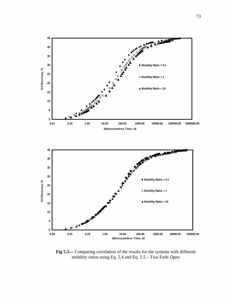
73

0

5

10

15

20

25

30

35

40

45

0.01 0.10 1.00 10.00 100.00 1000.00 10000.00 100000.00 1000000.00

Dimensionless Time, td

Oil

Rec

over

y, %

Mobility Ratio = 0.1

Mobility Ratio = 1

Mobility Ratio = 10

0

5

10

15

20

25

30

35

40

45

0.00 0.01 0.10 1.00 10.00 100.00 1000.00 10000.00 100000.00Dimensionless Time, td

Oil

Rec

over

y, %

Mobility Ratio = 0.1

Mobility Ratio = 1

Mobility Ratio = 10

Fig 5.3— Comparing correlation of the results for the systems with different mobility ratios using Eq. 5.4 and Eq. 5.5 – Two Ends Open

74

0

5

10

15

20

25

30

35

40

45

0.01 0.10 1.00 10.00 100.00 1000.00 10000.00 100000.00 1000000.00

Dimensionless Time, td

Oil

Rec

over

y, %

Mobility Ratio = 0.1

Mobility Ratio = 1

Mobility Ratio = 10

0

5

10

15

20

25

30

35

40

45

0.01 0.10 1.00 10.00 100.00 1000.00 10000.00 100000.00

Dimensionless Time, td

Oil

Rec

over

y, %

Mobility Ratio = 0.1

Mobility Ratio = 1

Mobility Ratio = 10

Fig 5.4— Comparing correlation of the results for the systems with different

mobility ratios using Eq. 5.4 and Eq. 5.5 – One End Open

75

Three mobility ratios have been considered. The first case was with favorable

mobility ratio, the second case was with unit mobility ratio, and the third case was

with unfavorable mobility ratio. In all cases, oil viscosity has been altered, and

water viscosity remained unchanged. From both figures it could be observed that

the curves fall into a narrow range, when we use the newly developed scaling

technique. The scaling is almost perfect with slight differences at late times. These

differences, probably, result from the influence of the boundary of the porous

medium on imbibition. When using a previous scaling equation, the data is more

scattered.

So, we observe a pretty good correlation for the results of spontaneous imbibition

with the new scaling technique. The recovery curves agree reasonably well for all

mobility ratios. The data are reduced to a single curve in spite of the fact that non-

wetting fluid viscosity varies by 3 orders of magnitude. The results indicate that the

new dimensionless time can significantly improve the scaling of spontaneous

imbibition.

5.2 Summary and Discussions

In this chapter, the spontaneous imbibition results from the previous chapter have

been upscaled to the field dimensions. The validity of the new definition of

characteristic length used in the modified scaling group has been evaluated. The

new scaling group used to correlate simulation results has been compared to the

early upscaling techniques.

The results revealed the fact that the characteristic length in the equation of

dimensionless time improves a correlation between data points for the models with

different boundary conditions. The new scaling technique, which was used for upscaling,

significantly improved correlations by taking end-point fluid phase mobilities and the

76

mobility ratios into account. The comparison between the new and the previous

dimensionless times proved that even if non-wetting fluid viscosity varies by 3 orders of

magnitude, the data could be reduced to a single curve, if we use new dimensionless

time definition.

77

CHAPTER VI

SUMMARY AND CONCLUSIONS

In the current work, the different aspects of spontaneous imbibition have been studied.

Spontaneous imbibition is a process, where capillary forces are dominant. Capillary

imbibition, in the petroleum literature, is described as a spontaneous penetration of

a wetting phase into a porous media, while displacing a non-wetting phase by

means of capillary pressure.

Capillary imbibition experiments usually take a long time, especially when we need

to vary some parameters to investigate their effects. Therefore, to achieve

objectives of the present study, numerical modeling of spontaneous imbibition

experiment was performed using a two-phase black-oil commercial simulator

(CMG™). The experimental results from water static imbibition experiments

performed in the laboratory have been obtained. Grid sensitivity analysis revealed

optimal grid size, which has been used in further numerical studies. To improve the

reservoir simulation data, the simulated oil recovery has been matched with

observed oil recovery. The match was obtained by trial and error estimates of

relative permeability and capillary pressure. Once the model has been satisfactorily

matched, four types of boundary conditions have been investigated. They are All

Faces Open, Two Ends Open, Two Ends Closed, and One End Open types of

spontaneous imbibition model. The assumption that the gravity effect is negligible

was made by setting the density of a wetting phase equal to the density of a non-

wetting phase. Numerous parametric studies have been performed and the results

were analyzed in detail to investigate oil recovery during spontaneous imbibition

with different types of boundary conditions. These studies included the effect of

78

varying mobility ratio, different fracture spacing, different capillary pressure,

different relative permeabilities, and varying permeability profiles along the core.

The results of these studies have been upscaled to the field dimensions. The

validity of the new definition of characteristic length used in the modified scaling

group has been evaluated. The new scaling group used to correlate simulation

results has been compared to the early upscaling techniques.

The following conclusions have been derived from this study:

• The comparative study of time rates of water spontaneous imbibition for

different types of boundary conditions revealed the fact that the time required

for capillary imbibition until residual oil saturation increases exponentially, as

the number of faces available for imbibition decreases.

• The comparison of all four types of boundary conditions showed that oil

recovery for the All Faces Open type of a model is most efficient and fast, as

compared with all other cases.

• The effect of varying permeability profiles along the core on oil recovery

showed that when water imbibes in the direction of decreasing permeability, oil

recovery is higher than when water imbibes in the direction of increasing

permeability.

• The study of the effect of different water-oil viscosity ratios, at which water

imbibed into the core, showed that the lower the oil viscosity, the greater the

volumes of oil produced from the core as a function of time.

• The results showed that increasing the capillary pressure increased imbibition

recovery. Oil recovery by imbibition was sensitive to oil relative permeability

curves, while no significant effect was observed in changing the water relative

permeability curves.

79

• A comparative study of time rates of spontaneous imbibition of water for

different fracture spacing showed that the time required for capillary imbibition

until residual oil saturation increased linearly, as the fracture space increased.

• The characteristic length described by Ma and co-workers37 in the equation of

dimensionless time improved a correlation between data points for the models

with different boundary conditions.

• The new technique used for upscaling, significantly improved correlations by

taking end-point fluid phase mobilities and the mobility ratios into account.

80

NOMENCLATURE

A = Total area, ft2

Bo = Bond Number

D = Diameter, ft

g = Gravitational acceleration, ft/sec2

H = Height, ft

J(Sw) = Leverett J-function

k = Permeability, md

kro = Oil relative permeability

krw = Water relative permeability

L = Length, ft

Lc = Characteristic length, ft

M = Mobility ratio

Pc = Capillary pressure, psi

Pnw = Pressure of non-wetting phase, psi

Pw = Pressure of wetting phase, psi

r = Pore radius, ft

R = Oil recovery, %

R∞ = Ultimate recovery, %

Rimb = Imbibition oil recovery, %

Sw = Water saturation, fraction

Swi = Irreducible water saturation, fraction

Snwr = Residual saturation, fraction

Se = Effective water saturation, fraction

t = Time, min

td = Dimensionless time

tc = Dimensionless time for high capillary gravity ratio

81

tg = Dimensionless time for low capillary gravity ratio

V = Volume, ft3

µo = Oil viscosity, cp

µw = Water viscosity, cp

µg = Geometric mean of the water and oil phase viscosities, cp

ρ = Density, ft/lb3

ф = Porosity, fraction

σ = Interfacial tension, dynes/cm

θ = Contact angle, degrees

λ = Phase mobility, md/cp

82

REFERENCES

1. Fidra, Y.: “A Study of Imbibition Mechanisms in the Naturally Fractured

Spraberry Trend Area,” MS thesis, New Mexico Institute of Mining and

Technology, Los Lunas, New Mexico (1998).

2. Nelson, R.A.: Geological Analysis of Naturally Fractured Reservoirs, second

edition, Gulf Professional Publishing, St. Louis (2001).

3. Jaeger, J.S. and Cook, N.G.W.: Fundamentals of Rock Mechanics, third edition,

Chapman and Hall Ltd., New York City (1979).

4. Aguilera, R.: Naturally Fractured Reservoirs, second edition, PennWell Pub. Co.,

Tulsa (1995).

5. Reiss, L.H.: The Reservoir Engineering Aspects of Fractured Reservoirs, Golf.

Pub. Co., Houston (1980).

6. Van Golf-Racht, T.D.: Fundamentals of Fractured Reservoir Engineering, Elsevier

Scientific Pub. Co., Amsterdam (1982).

7. Nelson, R.A.: Geologic Analysis of Naturally Fractured Reservoirs, Golf. Pub.

Co., Houston (1985).

8. Rock Fractures and Fluid Flow: Contemporary Understanding and Applications,

Committee on Fracture Characterization and Fluid Flow, National Academy Press,

Washington, D.C. (1996).

9. Warren, J.E. and Root, P.J.: “The Behavior of Naturally Fractured Reservoirs,”

SPEJ (September 1963) 245-255.

10. Brownscombe, E.R., and Dyes, A.B.: “Water-Imbibition Displacement… Can it

Release Reluctant Spraberry Oil?,” Oil and Gas J. (17 November 1952) 264-265.

11. Kleppe, J., and Morse, R.A.: “Oil Production from Fractured Reservoirs by Water

Displacement,” paper SPE 5084 presented at the SPE-AIME 49th Annual Fall

Meeting, Houston, Texas, 6-9 October.

12. Scheidegger, A.E.: The Physics of Flow Through Porous Media, The Macmillan

Co., New York, (1960).

83

13. Dullien, F.A.L.: Porous Media: Fluid Transport and Pore Structure, Academic

Press, New York (1979).

14. Cox, J.C.: “Surfactant Based Imbibition and Induced Solution Gas Drive Process:

Investigation by Nuclear Magnetic Resonance,” MS Thesis, Texas A&M

University, College Station, Texas, (1993).

15. Brooks, R.H. and Corey, A.T.: “Hydraulic Properties of Porous Media,”

Hydrology Papers No. 3, Colorado State University, Fort Collins, Colorado, March

1964.

16. Leverett, M.C.: “Flow of Oil-Water Mixtures through Unconsolidated Sands,”

Trans., AIME, 132, 149 (1939).

17. Barenblatt, G.I., Zheltov, I.P. and Kochina, I.N.: “Basic Concepts in the Theory of

Seepage of Homogenous Liquids in Fissured Rocks (Strata),” J. Appl. Math. Mech.

(1960) 24, 1286-1303.

18. Chen, J., Miller, M.A., and Sepehrnoori, K.: “Theoretical Investigation of

Countercurrent Imbibition in Fractured Reservoir Matrix Blocks,” paper SPE

29141 presented at 1995 SPE Symposium on Reservoir Simulation, San Antonio,

Texas, 12-15 February.

19. Aronofsky, J.S., Masse, L., and Natanson, S. G.: “A Model for the Mechanism of

Oil Recovery from the Porous Matrix Due to Water Invasion in Fractured

Reservoirs,” Trans., AIME (1958) 213, 17-19.

20. Handy, L.L.: “Determination of Effective Capillary Pressures for Porous Media

from Imbibition Data,” Trans., AIME (April 1960) 80.

21. Iffly, R., Rousselet, D.C., and Vermeulen, J. L.: “Fundamental Study of Imbibition

in Fissured Oil Fields,” paper SPE 4102 presented at the 1972 SPE Annual

Meeting, San-Antonio, Texas, 8-11 October.

22. Civan, F.: “Waterflooding of Naturally Fractured Reservoirs: An Efficient

Simulation Approach,” paper SPE 25449 presented at the 1993 Production

Operations Symposium, Oklahoma City, Oklahoma, 21-23 March.

84

23. Gupta, A., and Civan, F.: “An Improved Model for Laboratory Measurement of

Matrix to Fracture Transfer Function Parameters in Immiscible Displacement,”

paper SPE 28929 presented at the 1994 SPE Annual Technical Conference and

Exhibition, New Orleans, Louisiana, 25-28 September.

24. Civan, F.: “Quadrature Solution for Waterflooding of Naturally Fractured

Reservoirs,” SPEREE (April 1998) 141-147.

25. Civan, F., Wang, W., and Gupta, A.: “Effect of Wettability and Matrix to Fracture

Transfer on the Waterflooding in Fractured Reservoirs,” paper SPE 52197

presented at the 1999 SPE Mid-Continent Operations Symposium, Oklahoma City,

Oklahoma, 28-31 March.

26. Cil, M., Reis, J.C., Miller M.A., and Misra, D.: “An Examination of

Countercurrent Capillary Imbibition Recovery from Single Matrix Blocks and

Recovery Predictions by Analytical Matrix/Fracture Transfer Functions,” paper

SPE 49005 presented at the 1998 SPE Annual Technical Conference, New

Orleans, Louisiana, 27-30 September.

27. Rapoport, L.A.: “Scaling Laws for Use in Design and Operation of Water/Oil Flow

Models,” Trans., AIME (1955) 204, 143.

28. Graham, J.W., and Richardson, J.G.: “Theory and Application of Imbibition

Phenomena in Recovery of Oil,” Trans., AIME (1959) 216, Technical Note 2029.

29. Mattax, C.C., and Kyte, J.R.: “Imbibition Oil Recovery from Fractured, Water-

Drive Reservoirs,” SPEJ (June 1962) 177-184; Trans., AIME, 225.

30. Blair, P.M.: “Calculation of Oil Displacement by Countercurrent Water

Imbibition,” SPEJ (September 1964) 195-202.

31. Du Prey, E.L.: “Gravity and Capillary Effects on Imbibition in Porous Media,”

Soc. Pet. Eng. J. (June, 1978) 195-206.

32. Hamon, G., and Vidal, J.: “Scaling-Up the Capillary Imbibition Process from

Laboratory Experiments on Homogeneous and Heterogeneous Samples,” paper

SPE 15852 presented at the 1986 SPE European Petroleum Conference, London,

20-22 October.

85

33. Bourblaux, J., and Kalaidjian, F.J.: “Experimental Study of Co-current and

Countercurrent Flows in Naturally Porous Media,” paper SPE 18283 presented at

the 1988 SPE Annual Technical Conference and Exhibition, Houston, 2-5 October.

34. Kazemi, H., Gilman, J.R., and Elsharkawy, A.M.: “Analytical and Numerical

Solution of Oil Recovery from Fractured Reservoirs with Empirical Transfer

Functions,” paper SPE 6192 presented at the 1976 SPE Annual Technical

Conference and Exhibition, New-Orleans, Louisiana, 3-6 October.

35. Akin, S., Kovsek, A.R., and Schembre, J.M.: “Spontaneous Water Imbibition into

Diatomite,” paper SPE 46211 presented at the 1998 Western Regional Meeting,

Bakersfield, California, 10-13 May.

36. Akin, S., and Kovsek, A.R.: “Imbibition Studies of Low-Permeability Porous

Media,” paper SPE 54590 presented at the 1999 Western Regional Meeting,

Anchorage, Alaska, 26-27 May.

37. Ma, S., Zhang, X., and Morrow, N.R.: “Experimental Verification of a Modified

Scaling Group for Spontaneous Imbibition,” paper SPE 30762 presented at the

1995 SPE Annual Technical Conference and Exhibition, Dallas, Texas, 22-25

October.

38. Cuiec, L., Bourblaux, J., and Kalaidjian, F.: “Oil Recovery by Imbibition in Low-

Permeability Chalk,” paper SPE 20259 presented at the 1990 SPE/DOE

Symposium on Enhanced Oil Recovery, Tulsa, Oklahoma, 22-25 April.

39. Abbasov, M.T., Abbasov, V.A., and Mamedov, R.A.: Capillary Phenomenon and

Oil Recovery, Elm Publishing House, Baku, Azerbaijan (1987).

40. Kerimova, F.G.: “Studies of Effects of pH of Water on Oil Recovery during the

Imbibition,” Works of Institute of Deep Oilfield Problems, Baku, Azerbaijan

(1990).

41. Guo, B., Schechter D.S., and Baker, R.O.: “An Integrated Study of Imbibition

Waterflooding Trend Area Reservoirs in the Naturally Fractured Spraberry,” SPE

Permian Basin Oil and Gas Recovery Conference, Midland, Texas, 25-27 March

1998.

86

42. Putra, E., Fidra, Y. and Schechter, D.S.: “Study of Waterflooding Process in

Naturally Fractured Reservoirs from Static and Dynamic Imbibition Experiments”

Mexico PRRC, Socorro, New Mexico (1998).

43. Petroleum Engineering Handbook, H.B. Bradley (ed.), Third Printing, Society of

Petroleum Engineers, Richardson, Texas, (1992) 48-9.

44. Ertekin, T., Abou-Kassem, J.H., and King, G.R.: Basic Applied Reservoir

Simulation, SPE Textbook Series, SPE, Richardson, Texas (2001) 1, 350-351.

45. Zhou, D., Jia, L., Kamath, J., and Kovscek, A.R.: “An Investigation of Counter-

Current Imbibition Process in Diatomite,” paper SPE 68837 presented at the 2001

SPE Western Regional Meeting, Bakersfield, California, 26-30 March.

87

VITA

Name: Orkhan H. Pashayev

Born: 24 September 1980

Baku, Azerbaijan

Permanent Address: 102 Tabriz St, Apt#63

Baku, Azerbaijan

(opashayev@yahoo.co.uk)

Experience: KBR/Halliburton. July 2001 – July 2002. Title: Process

Engineer. Project: ACG Phase 1 – Design of the BP

Sangachal Terminal Expansion.

Education: Texas A&M University, College Station, Texas, USA

Master of Science Degree in petroleum engineering

August 2004

Azerbaijan State Oil Academy, Baku, Azerbaijan

Bachelor of Science Degree in petroleum engineering

July, 2001