NBER WORKING PAPER SERIES

INFORMATION AND THE ACQUISITION OF SOCIAL NETWORK CONNECTIONS

Toman BarsbaiVictoria LicuananAndreas Steinmayr

Erwin TiongsonDean Yang

Working Paper 27346http://www.nber.org/papers/w27346

NATIONAL BUREAU OF ECONOMIC RESEARCH1050 Massachusetts Avenue

Cambridge, MA 02138June 2020

For helpful discussions, we thank Christine Binzel, David McKenzie, David Miller, Sharon Maccini, John O’Sullivan, Christoph Trebesch, Justin Valasek, Tricia Yang, and Andy Zapechelnyuk, as well as seminar audiences at U. Illinois (Urbana-Champaign), U. Kiel, U. Paris 1 Panthéon-Sorbonne, U. St Andrews, LMU Munich, U. Hohenheim, Wharton, and UC Davis, and conference participants in Berlin, Edinburgh, Florence, Heidelberg, and Landeck. We received funding from the International Initiative for Impact Evaluation (3ie), grant number OW4/1171. The views expressed in this article are not necessarily those of 3ie or its members. IRB review was provided by the University of Michigan (HUM00087460). We are deeply indebted to CFO’s former Officer-in-Charge Regina Galias, Ivy Miravalles, former Secretary Imelda M. Nicolas, former Undersecretary Gertie A. Tirona, and the whole CFO team for their continuous support. We also thank the PDOS officers and all contributors to the new PDOS modules. We are grateful to Isabel Hernando for excellent project coordination and Alexander Jung, Franziska Paul, and Jennifer Umlas for superb research assistance. Last but not least we thank 3ie for funding, technical review, and support throughout the study. All remaining errors are our own. The views expressed herein are those of the authors and do not necessarily reflect the views of the National Bureau of Economic Research.

NBER working papers are circulated for discussion and comment purposes. They have not been peer-reviewed or been subject to the review by the NBER Board of Directors that accompanies official NBER publications.

© 2020 by Toman Barsbai, Victoria Licuanan, Andreas Steinmayr, Erwin Tiongson, and Dean Yang. All rights reserved. Short sections of text, not to exceed two paragraphs, may be quoted without explicit permission provided that full credit, including © notice, is given to the source.

Information and the Acquisition of Social Network ConnectionsToman Barsbai, Victoria Licuanan, Andreas Steinmayr, Erwin Tiongson, and Dean YangNBER Working Paper No. 27346June 2020JEL No. D83,D85,F22

ABSTRACT

How do information interventions affect individual efforts to expand social networks? We study a randomized controlled trial of a program providing information on settling in the U.S. for new immigrants from the Philippines. Improved information leads new immigrants to acquire fewer new social network connections. Treated immigrants make 16-28 percent fewer new friends and acquaintances and are 65 percent less likely to receive support from organizations of fellow immigrants. The treatment has no effect on employment, wellbeing, or other outcomes. Consistent with a simple model, the treatment reduces social network links more in places likely to have lower costs of acquiring network links (those with more prior fellow immigrants). Information and social network links appear to be substitutes in this context: better-informed immigrants invest less in expanding their social networks upon arrival. Our results suggest that endogenous reductions in acquisition of social network connections can reduce the effectiveness of information interventions.

Toman BarsbaiSchool of EconomicsPriory Road ComplexBristolUKtoman.barsbai@bristol.ac.uk

Victoria Licuanan123 Paseo de RoxasLegazpi VillageMakati1229 Metro ManilaPhilippinesvlicuanan.aim@gmail.com

Andreas SteinmayrDepartment of EconomicsUniversity of Munich (LMU)Ludwigstr. 33

Erwin TiongsonWalsh School of Foreign ServiceGeorgetown UniversityWashington, DC 20057ert@georgetown.edu

Dean YangUniversity of MichiganDepartment of Economics andGerald R. Ford School of Public Policy735 S. State Street, Room 3316Ann Arbor, MI 48109and NBERdeanyang@umich.edu

D-80539 MunichGermanyandreas.steinmayr@econ.lmu.de

A randomized controlled trials registry entry is available at https://www.socialscienceregistry.org/trials/1389

1 Introduction

Failures of the perfect information assumption – that agents are endowed with

full information relevant for the decisions they make – are a popular focus of

research in economics. Imperfect information takes center-stage in economic

studies of health (Dupas, 2011; Einav and Finkelstein, 2018), labor market

search (Calvo-Armengol, 2004), and financial literacy (Lusardi and Mitchell,

2014), among other areas. Programs to mitigate information imperfections

are ubiquitous, and are themselves a frequent subject for applied research in

economics.

Individuals and households also make their own efforts to fill information gaps.

A commonly-studied information source is social networks, which can channel

information from more- to less-informed network members and thus provide

information capital (Jackson, 2019). Social networks facilitate flows of in-

formation about new agricultural technologies (Foster and Rosenzweig, 2010;

Carter, Laajaj and Yang, forthcoming), health goods (Dupas, 2014), microfi-

nance products (Banerjee et al., 2013), employment opportunities (including

migration) (Munshi, 2003; Beaman, 2012; Beaman and Magruder, 2012; Dust-

mann et al., 2016; Blumenstock, Chi and Tan, 2019), and business opportuni-

ties (Cai and Szeidl, 2018).

To date, there has been scarce research on how interventions to improve in-

formation might interact with the acquisition of social network connections.

Immigrants who have just arrived in their country of destination are a fruitful

context in which to study this interaction. Immigrants typically have im-

perfect information about their new societies. At the same time, immigrants

usually have small social networks at arrival. They are hence likely to invest in

social networks to reduce information imperfections. Substantial past research

documents the important role of social networks for immigrants.1 Immigrants

frequently live and work with compatriots in ethnic enclaves, motivated in part

1 Key citations include Massey (1988); Borjas (1992); Carrington, Detragiache and Vish-wanath (1996); Orrenius et al. (1999); Munshi (2003); Calvo-Armengol and Jackson (2004);Orrenius and Zavodny (2005); Amuedo-Dorantes and Mundra (2007); Dolfin and Genicot(2010); Docquier, Peri and Ruyssen (2014); Mahajan and Yang (2020).

2

by eased sharing of information that comes with geographic proximity (Portes

and Jensen, 1989; Beaman, 2012).

We implemented a randomized controlled trial on the impact of reducing im-

perfect information problems among immigrants. In collaboration with the

Philippine government, we designed an information intervention for new immi-

grants to the U.S.: an enhanced “pre-departure orientation seminar” (PDOS)

and an accompanying paper handbook. We randomly assigned these to Fil-

ipinos about to depart for the U.S. as new legal permanent residents (“green

card” holders). A control group received the standard PDOS, which was sub-

stantially less informative in terms of both quantity and quality of information

provided. We surveyed treatment and control group participants after arrival

on their settlement in the U.S.,2 social networks, employment, and overall life

satisfaction. Our empirical analyses are guided by a pre-analysis plan and

account appropriately for multiple hypotheses.

We find that the treatment led to reductions in the number of social network

links in the U.S. As pre-specified, we measure social network size with an

index combining information on the number of new friends and acquaintances,

and support received from Filipino organizations. This effect is substantial

in magnitude, amounting to 0.14 to 0.17 standard deviations of the network

size index, and is stable across the short- and longer-run. The treatment

has negative effects on each component of the index, reducing the number

of friends and acquaintances by 16-28 percent, and reducing support received

from organizations by two-thirds. The treatment has no large or statistically

significant impacts on settlement, employment, or self-reported wellbeing.

Our finding of a negative effect on social network links was unanticipated.

Because the new PDOS explicitly encourages migrants to make new friends

and join Filipino associations in the U.S., in our pre-analysis plan we hy-

pothesized a positive treatment effect on social network connections. After

seeing the actual negative treatment effect, we wrote down a simple theoret-

ical model that can rationalize such an effect. We consider individuals with

2 We measure “settlement” as the fraction of the following items the immigrant hasacquired: bank account, Social Security number, health insurance, and driver’s license.

3

imperfect information deciding on the optimal number of first-degree network

links (“friends”).3 Friends are costly to acquire, but reduce information im-

perfections. We consider the impact of exogenously reducing information im-

perfections. Information and friends could be substitutes, meaning additional

information provided by the treatment reduces the marginal benefit of friends,

and correspondingly reduces friend acquisition. Alternately, information and

friends could be complements: the treatment could increase the marginal ben-

efit of friends, increasing friend acquisition. In the context of the model, our

empirical results are consistent with information and friends being substitutes:

improved information leads to offsetting reductions in acquisition of network

links.

In exploratory analyses, we examine the heterogeneity of the treatment effect

with respect to a proxy for the cost of finding friends, the size of the local

Filipino community. We test a theoretical prediction: the lower the cost of

acquiring friends, the more likely information and friends are to be substitutes

rather than complements. The heterogeneity in the treatment effect on the

social network size index indeed follows this pattern, as does heterogeneity in

the treatment effect on subjective wellbeing. While the treatment does not

affect labor market outcomes such as wages or employment, it does change

the way immigrants search for jobs. Immigrants who received employment-

related information in the new PDOS are less likely to have found their job

through social networks, which also suggests that information and networks

are substitutes.

Our work contributes to the economics literature on social networks (Sacer-

dote, 2014; Chuang and Schechter, 2015). Ours is the first study to examine the

causal impact of an exogenous reduction in information imperfections on so-

cial network links. Few studies examine factors influencing strategic network

formation. Comola and Mendola (2015) and Barr, Dekker and Fafchamps

(2015) examine correlates of new network connections. Very few studies mea-

3 The number of first-degree links is a measure of the expansiveness of the network.The literature on social networks has argued that network expansiveness is important forefficient information transmission (cf. Granovetter, 1973).

4

sure the causal impact of any kind of exogenous treatment on social networks.

We are aware of only five other randomized controlled trials where social net-

work connections are an outcome of interest, and in none of these does the

randomized treatment relate to information. Three studies examine the im-

pact of a microfinance treatment. Comola and Prina (forthcoming), Banerjee

et al. (2018) and Cecchi, Duchoslav and Bulte (2016) find that savings, credit,

and insurance interventions (respectively) reduce social network connections.

Heß, Jaimovich and Schundeln (forthcoming) find that a community-driven

development program in Gambia reduces social network connections. Caria,

Franklin and Witte (2018) show that a job-search assistance intervention in

Ethiopia reduces social interactions between treated and untreated individuals.

We also contribute to the literature on immigrant integration. A well-documented

finding is that the economic assimilation of immigrants takes time and is usu-

ally imperfect. Especially in the first years after arrival, immigrants typically

earn considerably less than natives (Borjas, 1985; Lubotsky, 2007). Identi-

fying policies that facilitate the arrival and settling-in process of immigrants

is therefore important and only few studies have rigorously evaluated policies

that aim to improve the early integration path of immigrants (Rinne, 2013;

National Academies of Sciences, Engineering, and Medicine, 2015).

In addition, we provide a new Stata command that adjusts p-values for mul-

tiple hypothesis testing. It modifies the List, Shaikh and Xu (2019) method

to be regression-based and allow for inclusion of control variables.

From a policy standpoint, the intervention we study – provision of information

to migrants about their destinations – is widespread.4 Many governments and

NGOs in developing countries implement trainings of migrants (IOM, 2011),

but prior to our study there has been no causally well-identified assessment

of their impacts (Rinne, 2013; McKenzie and Yang, 2015). More generally,

our results suggest that the effectiveness of information interventions might

be attenuated due to offsetting reductions in social network links.

4 Past research has also examined migrant integration programs carried out in destinationcountries (Joona and Nekby, 2012; Sarvimaki and Hamalainen, 2016; Shrestha and Yang,2019).

5

2 Theory

We are interested in the interplay between information imperfections and ef-

forts to increase first-degree social network links. In particular, we are inter-

ested in the impact of interventions alleviating information imperfections. We

wrote down the following simple model after learning that our treatment had

a negative impact on new social network connections, which is the opposite of

what we had anticipated. The model allows for either a positive or negative

treatment effect on efforts to acquire new social network connections.5

Individuals have imperfect information about a variety of things in life that

matter to them, such as jobs, financial services, and government services. Peo-

ple also have social network connections (“friends”, which includes acquain-

tances), which provide information, helping reduce information imperfections.

Network theory suggests that efficient information gathering typically requires

expansive networks with many short network paths (cf. Granovetter, 1973).

Thus, we use the number of first-degree friends as a proxy for network expan-

siveness. Because friends are valuable, people make efforts to acquire them,

but making friends is costly. Costs of friend acquisition may include effort and

monetary costs.

We focus on the benefits friends bring by reducing information imperfections.

We abstract away from other benefits of friends, which the network literature

typically refers to as cooperation capital, such as various forms of assistance

(transfers, informal insurance, and psychological support).6

Utility depends on baseline or starting-point information imperfections, θ, and

endogenous friend investment f ≥ 0. Individuals choose f to maximize the

benefits from friends B(θ, f) minus the cost of friend acquisition C(f):

U = B(θ, f)− C(f)

5 This is related to models where individuals endogenously form social contacts (Calvo-Armengol, 2004; Jackson and Wolinsky, 1996; Jackson and Rogers, 2007) and where social-izing takes effort (Cabrales, Calvo-Armengol and Zenou, 2011; Canen, Jackson and Trebbi,2019; Currarini, Jackson and Pin, 2009).

6 These other non-information benefits of friends could be thought of as entering the costterm in the maximization problem we write down below, reducing the net cost of friends.

6

People acquire friends only up to the point at which the marginal cost does

not exceed the marginal benefit of friends.

Simple assumptions and functional forms generate useful possibilities. In-

formation imperfections θ range from 0 to 1 (θ ∈ [0, 1]). Individuals have

both exogenous friends (those that are given at baseline without cost), e, and

endogenous friends, f , which they acquire at a cost. Let e ≥ 1.7 Let an in-

dividual’s amount of information I be a function of information imperfections

θ, exogenous friends e, and endogenous friends f as follows:

I = 1− θ

e+ f

One’s amount of information can range from 0 (no information) to 1 (full infor-

mation). If baseline information imperfections θ are 0, then one starts with full

information. A higher number of friends e+f reduces the importance of one’s

baseline information imperfections and raises one’s amount of information I.

For simplicity, let the cost of endogenous friends be linear with a per-friend

cost c, so the total cost of friend acquisition is cf .

We analyze three cases: constant, decreasing, and increasing returns to infor-

mation. Analysis of the different cases makes clear that reductions in infor-

mation imperfections have indeterminate impacts on friend acquisition.

When returns to information I (in utility) are either constant or decreasing, a

reduction in information imperfections θ (e.g., our information treatment for

new immigrants) always reduces friend acquisition. We flesh out this case in

Appendix A.

By contrast, when there are increasing returns to information (for example,

if better information allows one to search more efficiently for additional infor-

mation), the impact of information imperfections is ambiguous. We capture

increasing returns to information simply by letting the benefit function include

7 For new immigrants, the exogenous friend could be the individual who officially sponsorstheir immigration visa.

7

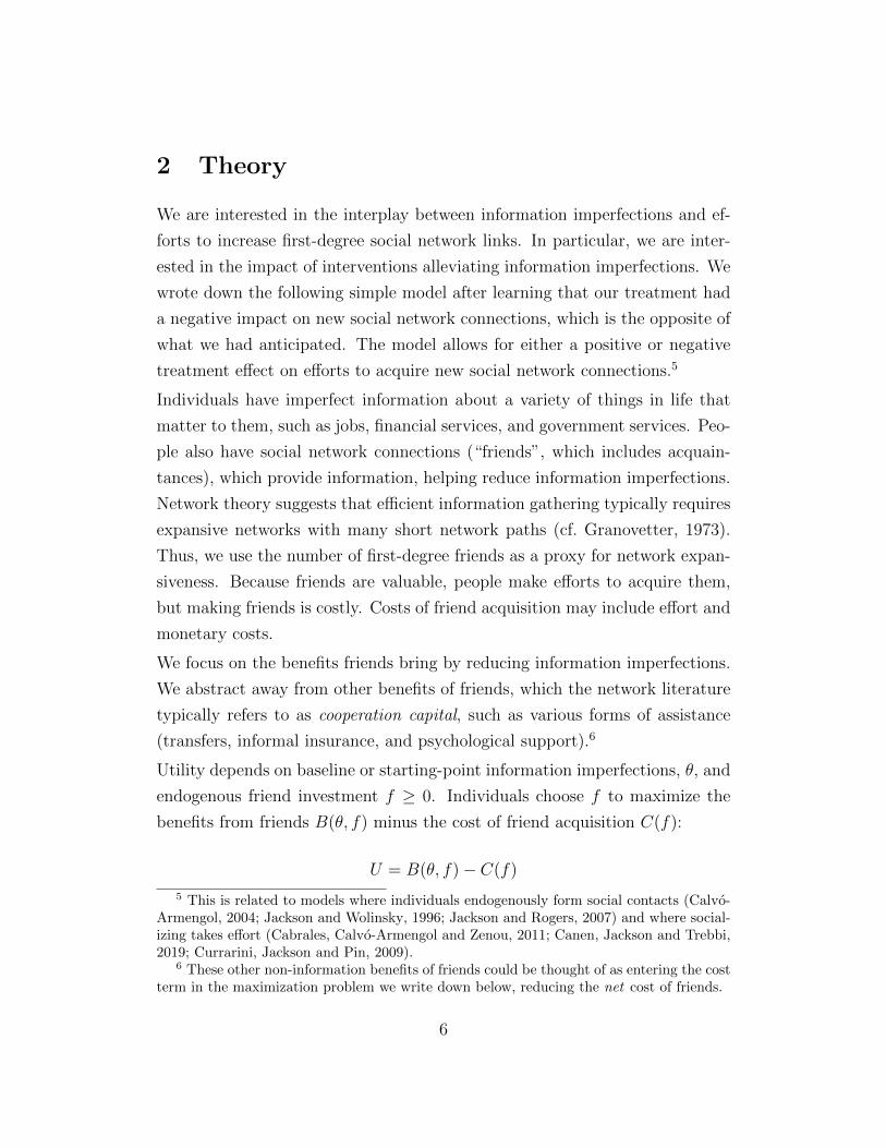
a quadratic term in information:

B(θ, f) = 1− θ

e+ f+ α(1− θ

e+ f)2

The parameter α measures the strength of increasing returns to information

(if α = 0, we have constant returns to information).

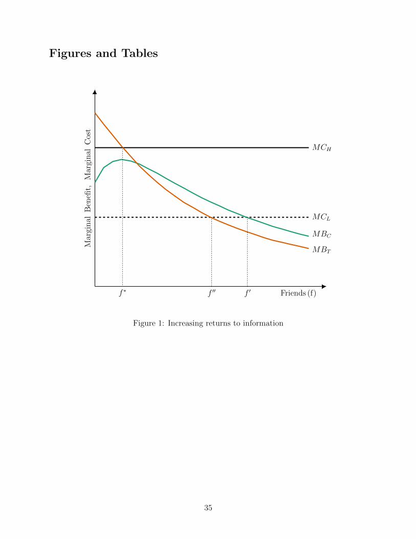
We analyze this case graphically in Figure 1. The parameter values used

in the figure are e = 1 and α = 5. The marginal benefit functions for the

control and treatment groups areMBC (green curve) andMBT (orange curve),

with θ = 0.9 and θ = 0.6 respectively. The marginal benefit functions can

have upward-sloping (increasing returns) and downward-sloping (decreasing

returns) sections.

Consider, first, optimal decisions when marginal costs are “high” (c = 2.4),

represented by the upper horizontal black line, MCH . The optimum is found

at the intersection of the marginal cost function and the downward-sloping

part of the relevant marginal benefit function.

When marginal costs are “high”, for the control group (blue curve, MBC) there

is no amount of friend investments for which the marginal benefit of friends

exceeds marginal costs. This is a corner solution with zero friend acquisition.

From this starting point, a reduction in θ (from 0.9 to 0.6) can lead the

marginal benefit function to shift so that there is an interior solution with

positive friend acquisition (f ∗ > 0), where MBT and MCH intersect. In this

case, an information treatment that lowers θ leads to more friend acquisition.

There is also the possibility, for lower values of the cost of friends c, that reduc-

tions in θ reduce friend acquisition. This would be the case if the marginal cost

of friends was lower, such as at MCL(assuming c = 1.2), so that the marginal

cost function (the horizontal dashed line) would intersect both the control

group and treatment group marginal benefit functions on their downward-

sloping portions. If this were the case, a reduction in θ would lead to a reduc-

tion in friend acquisition, from f ’ to f”.

Overall, therefore, it is possible for an intervention that reduces information

8

imperfections to either raise or lower efforts to build one’s social network.

(The prediction that the treatment effect on friends becomes more negative

as marginal costs fall also holds for the case where returns to information are

constant or decreasing.)

In Appendix A, we examine the impact of a treatment that reduces information

imperfections for a continuous range of marginal cost levels, from high to low.

Starting from the highest marginal costs, reductions in marginal costs make

the treatment effect on friend acquisition even more positive, because this

is the region where information and friends are complements. As we lower

marginal costs further, we enter the region where friends and information are

substitutes. The treatment effect on friends becomes negative, and becomes

even more negative as marginal costs fall further.

The treatment effect on utility follows a similar pattern. Starting from the

highest marginal costs, reductions in marginal costs make the treatment effect

on utility even more positive, as long as one remains in the region where

information and friends are complements. As we lower marginal costs further,

friends and information become substitutes, the treatment effect on utility

declines, and eventually can be even lower than when marginal costs were

very high.

In our empirical analyses, we ask whether a treatment that reduces information

imperfections reduces or increases friend acquisition. We also examine the

heterogeneity in the treatment effect with respect to a proxy for the marginal

cost of friend acquisition.

3 Context, Treatments, and Hypotheses

The Philippines is a major emigration country. In 2013, 4.8 million Filipino-

born individuals were permanent migrants, 4.2 million temporary migrants,

and 1.2 million undocumented migrants in other countries. By comparison, the

Philippine population was 98.5 million in that year (CFO, 2013; World Bank,

2019). The U.S. is by far their largest destination, accounting for 64.4% of

9

Filipino permanent migrants in 2015 (CFO, 2015). From the U.S. standpoint,

the Philippines is the fourth-largest immigrant origin, after Mexico, China and

India (Lopez, Ruiz and Patten, 2017).

The Philippine government implements a number of policies related to interna-

tional migration of its citizens. Our collaborator on this study, the Commission

on Filipinos Overseas (CFO), enacts policies related to permanent migrants.

Pre-departure orientation seminars (PDOS) are one of the government’s most

prominent migration policies. Filipinos intending to leave the country with a

permanent migration visa must register with CFO and attend a PDOS before

departure. Attendees already have their immigration visa and are about to

leave the Philippines. Individuals lacking proof of PDOS attendance may be

denied departure at airports. Seminar content is tailored to the destination.

We recruited our study participants among individuals attending the PDOS

for permanent migrants to the U.S., which were attended annually by roughly

40,000 individuals from 2005-2015 (CFO, 2015).

The migration policies of the Philippines are regarded as a model for other

migrant-sending countries that have PDOS in place or are considering intro-

ducing them (Testaverde et al., 2017). As a major destination country, Canada

also provides a PDOS for migrants moving to Canada known as Canadian Ori-

entation Abroad.

Treatments

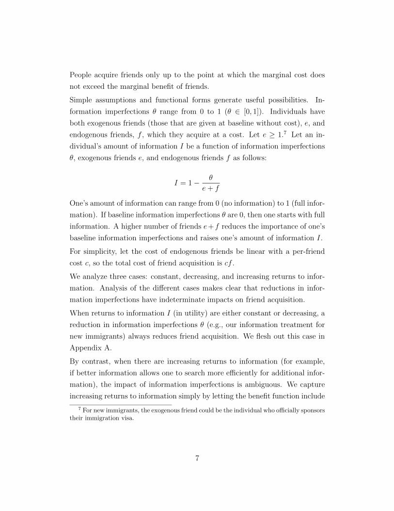
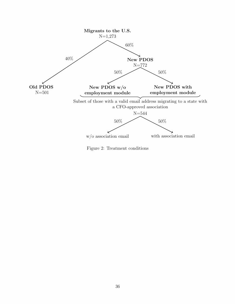
Figure 2 shows the treatment conditions. We randomly assign study partici-

pants to either a control group attending the original PDOS (“old PDOS”) or

to a treatment group attending the “new PDOS”. The old PDOS focused on

travel and immigration procedures, only briefly covering issues such as cultural

differences, settlement, and employment, and not covering financial literacy or

engagement with Filipino associations. An instructor conveyed the informa-

tion in a presentation lasting 1.5 hours on average. Participants took away

with them a short 30-page paper booklet with related but not very practical

information.

10

The new PDOS was developed collaboratively by the CFO and our research

team from scratch and goes significantly beyond the content of the old PDOS

in terms of both topics and depth of coverage. It comes with a much more

comprehensive and practical paper handbook. New PDOS development drew

upon interviews with past and prospective migrants, the International Organi-

zation for Migration’s Canadian Orientation Abroad program, and input from

TIGRA, a U.S. Filipino immigrant NGO. The new PDOS covered an extended

set of topics related to longer-term socio-economic integration: (i) preparing

for departure and entering the U.S., (ii) getting settled in the U.S., (iii) build-

ing a support network, (iv) finding a job, (v) managing one’s finances, and

(vi) maintaining and strengthening ties with the Philippines. Participants

attended a longer presentation (2.5 hours on average) and took away a com-

prehensive 116-page paper handbook, which covers the above topics in detail

and provides easy-to-follow checklists as well as links to online resources.

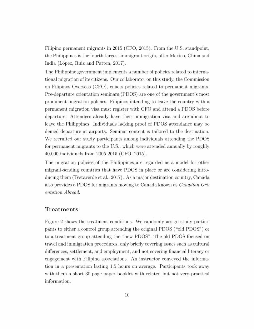
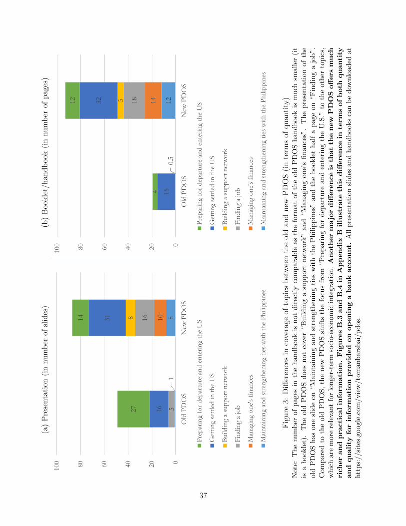
Compared to the old PDOS, the new PDOS shifts the focus from topic (i) to

topics (ii)-(vi). Figure 3 documents this shift in focus. It shows the number

of slides and handbook pages of the old and the new PDOS by topic. In ad-

dition, the delivery of the new PDOS centers around the handbook. During

the PDOS, the instructor provides an overview of the topics covered by the

handbook and shows migrants where to find which information. The primary

objective of the new PDOS is hence to improve migrants’ ability to find in-

formation, rather than their knowledge of different topics. This makes the

handbook an important part of the new PDOS as it gives migrants the possi-

bility to look up information when they actually need it. While the old PDOS

provides written information in the form of a booklet, the handbook of the

new PDOS offers much richer and practical information. Figures B.3 and B.4

in Appendix B illustrate this difference in terms of both quantity and quality

for information provided on opening a bank account.

Our primary analyses compare control group individuals to treatment group

individuals exposed to the new PDOS. We implemented the new PDOS in

two different versions. One version contained all components listed above

(henceforth “new PDOS with employment module”), another version omit-

11

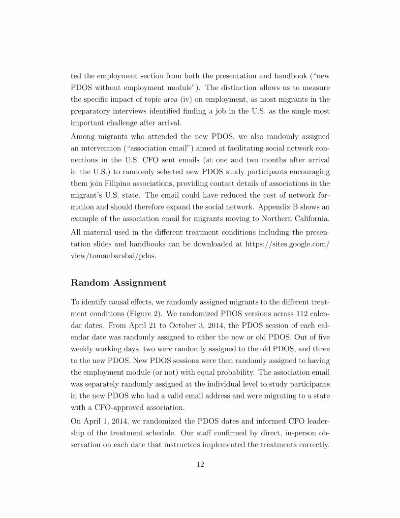
ted the employment section from both the presentation and handbook (“new

PDOS without employment module”). The distinction allows us to measure

the specific impact of topic area (iv) on employment, as most migrants in the

preparatory interviews identified finding a job in the U.S. as the single most

important challenge after arrival.

Among migrants who attended the new PDOS, we also randomly assigned

an intervention (“association email”) aimed at facilitating social network con-

nections in the U.S. CFO sent emails (at one and two months after arrival

in the U.S.) to randomly selected new PDOS study participants encouraging

them join Filipino associations, providing contact details of associations in the

migrant’s U.S. state. The email could have reduced the cost of network for-

mation and should therefore expand the social network. Appendix B shows an

example of the association email for migrants moving to Northern California.

All material used in the different treatment conditions including the presen-

tation slides and handbooks can be downloaded at https://sites.google.com/

view/tomanbarsbai/pdos.

Random Assignment

To identify causal effects, we randomly assigned migrants to the different treat-

ment conditions (Figure 2). We randomized PDOS versions across 112 calen-

dar dates. From April 21 to October 3, 2014, the PDOS session of each cal-

endar date was randomly assigned to either the new or old PDOS. Out of five

weekly working days, two were randomly assigned to the old PDOS, and three

to the new PDOS. New PDOS sessions were then randomly assigned to having

the employment module (or not) with equal probability. The association email

was separately randomly assigned at the individual level to study participants

in the new PDOS who had a valid email address and were migrating to a state

with a CFO-approved association.

On April 1, 2014, we randomized the PDOS dates and informed CFO leader-

ship of the treatment schedule. Our staff confirmed by direct, in-person ob-

servation on each date that instructors implemented the treatments correctly.

12

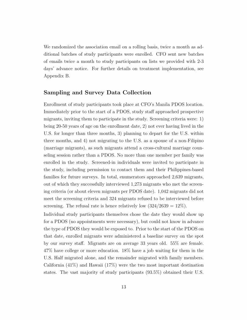
We randomized the association email on a rolling basis, twice a month as ad-

ditional batches of study participants were enrolled. CFO sent new batches

of emails twice a month to study participants on lists we provided with 2-3

days’ advance notice. For further details on treatment implementation, see

Appendix B.

Sampling and Survey Data Collection

Enrollment of study participants took place at CFO’s Manila PDOS location.

Immediately prior to the start of a PDOS, study staff approached prospective

migrants, inviting them to participate in the study. Screening criteria were: 1)

being 20-50 years of age on the enrollment date, 2) not ever having lived in the

U.S. for longer than three months, 3) planning to depart for the U.S. within

three months, and 4) not migrating to the U.S. as a spouse of a non-Filipino

(marriage migrants), as such migrants attend a cross-cultural marriage coun-

seling session rather than a PDOS. No more than one member per family was

enrolled in the study. Screened-in individuals were invited to participate in

the study, including permission to contact them and their Philippines-based

families for future surveys. In total, enumerators approached 2,639 migrants,

out of which they successfully interviewed 1,273 migrants who met the screen-

ing criteria (or about eleven migrants per PDOS date). 1,042 migrants did not

meet the screening criteria and 324 migrants refused to be interviewed before

screening. The refusal rate is hence relatively low (324/2639 = 12%).

Individual study participants themselves chose the date they would show up

for a PDOS (no appointments were necessary), but could not know in advance

the type of PDOS they would be exposed to. Prior to the start of the PDOS on

that date, enrolled migrants were administered a baseline survey on the spot

by our survey staff. Migrants are on average 33 years old. 55% are female.

47% have college or more education. 18% have a job waiting for them in the

U.S. Half migrated alone, and the remainder migrated with family members.

California (41%) and Hawaii (17%) were the two most important destination

states. The vast majority of study participants (93.5%) obtained their U.S.

13

green cards via family sponsorship, i.e. they have family already in the U.S.8

Balance checks reveal no major differences between observable characteris-

tics of study participants across treatment conditions. For balance tests and

summary statistics, see Appendix E, Tables E.1-E.3. Out of ten baseline vari-

ables, only one (indicator for female) is statistically significantly related to

treatment status. This is approximately what would be expected to occur

by chance. These baseline characteristics are also included as controls in all

regressions (as pre-specified).

Analyses of treatment effects use data from follow-up phone interviews of mi-

grants and direct interviews with their Philippine households at about seven,

15, and 30 months after arrival in the U.S. For further details on survey im-

plementation, see Appendix B.

Pre-Analysis Plan

This study is registered with the AEA RCT Registry.9 We submitted our

first pre-analysis plan (PAP) on September 17, 2014 before completion of the

baseline phase and availability of any post-treatment data. We submitted

subsequent PAPs to guide analysis of the mid-term survey data (submitted

July 19, 2015) and final survey data (submitted July 28, 2016). These lat-

ter two PAPs add additional hypotheses related to employment and network

characteristics.

For simplicity, all analysis in this paper will be based on the first PAP of

September 2014, the only PAP that was submitted before the collection of any

outcome data. Analyses based on subsequent PAPs are provided in Appendix

E. All conclusions are robust to estimating longer-run impacts using methods

from longer-run PAPs.

In a few ways, we deviate from the pre-analysis plan. Most importantly, we

correct test statistics to address multiple hypothesis concerns, following List,

8 Of the 6.5% of study participants not reporting family sponsorship, about two-thirdsreport obtaining their green cards through an employer, and the remainder do not clearlyspecify the nature of their sponsor.

9 https://www.socialscienceregistry.org/trials/1389/

14

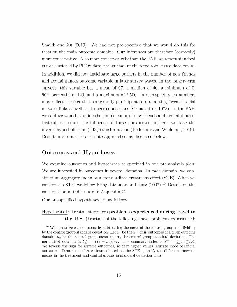
Shaikh and Xu (2019). We had not pre-specified that we would do this for

tests on the main outcome domains. Our inferences are therefore (correctly)

more conservative. Also more conservatively than the PAP, we report standard

errors clustered by PDOS date, rather than unclustered robust standard errors.

In addition, we did not anticipate large outliers in the number of new friends

and acquaintances outcome variable in later survey waves. In the longer-term

surveys, this variable has a mean of 67, a median of 40, a minimum of 0,

90th percentile of 120, and a maximum of 2,500. In retrospect, such numbers

may reflect the fact that some study participants are reporting “weak” social

network links as well as stronger connections (Granovetter, 1973). In the PAP,

we said we would examine the simple count of new friends and acquaintances.

Instead, to reduce the influence of these unexpected outliers, we take the

inverse hyperbolic sine (IHS) transformation (Bellemare and Wichman, 2019).

Results are robust to alternate approaches, as discussed below.

Outcomes and Hypotheses

We examine outcomes and hypotheses as specified in our pre-analysis plan.

We are interested in outcomes in several domains. In each domain, we con-

struct an aggregate index or a standardized treatment effect (STE). When we

construct a STE, we follow Kling, Liebman and Katz (2007).10 Details on the

construction of indices are in Appendix C.

Our pre-specified hypotheses are as follows.

Hypothesis 1: Treatment reduces problems experienced during travel to

the U.S. (Fraction of the following travel problems experienced:

10 We normalize each outcome by subtracting the mean of the control group and dividingby the control group standard deviation. Let Yk be the kth of K outcomes of a given outcomedomain, µk be the control group mean and σk the control group standard deviation. Thenormalized outcome is Y ∗

k = (Yk − µk)/σk. The summary index is Y ∗ =∑

K Y ∗k /K.

We reverse the sign for adverse outcomes, so that higher values indicate more beneficialoutcomes. Treatment effect estimates based on the STE quantify the difference betweenmeans in the treatment and control groups in standard deviation units.

15

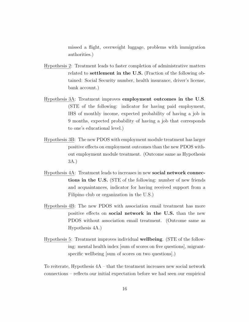
missed a flight, overweight luggage, problems with immigration

authorities.)

Hypothesis 2: Treatment leads to faster completion of administrative matters

related to settlement in the U.S. (Fraction of the following ob-

tained: Social Security number, health insurance, driver’s license,

bank account.)

Hypothesis 3A: Treatment improves employment outcomes in the U.S.

(STE of the following: indicator for having paid employment,

IHS of monthly income, expected probability of having a job in

9 months, expected probability of having a job that corresponds

to one’s educational level.)

Hypothesis 3B: The new PDOS with employment module treatment has larger

positive effects on employment outcomes than the new PDOS with-

out employment module treatment. (Outcome same as Hypothesis

3A.)

Hypothesis 4A: Treatment leads to increases in new social network connec-

tions in the U.S. (STE of the following: number of new friends

and acquaintances, indicator for having received support from a

Filipino club or organization in the U.S.)

Hypothesis 4B: The new PDOS with association email treatment has more

positive effects on social network in the U.S. than the new

PDOS without association email treatment. (Outcome same as

Hypothesis 4A.)

Hypothesis 5: Treatment improves individual wellbeing. (STE of the follow-

ing: mental health index [sum of scores on five questions], migrant-

specific wellbeing [sum of scores on two questions].)

To reiterate, Hypothesis 4A – that the treatment increases new social network

connections – reflects our initial expectation before we had seen our empirical

16

results. We originally expected the treatment to increase new social network

connections because the new PDOS explicitly encourages migrants to reach

out and build a support network in the U.S.

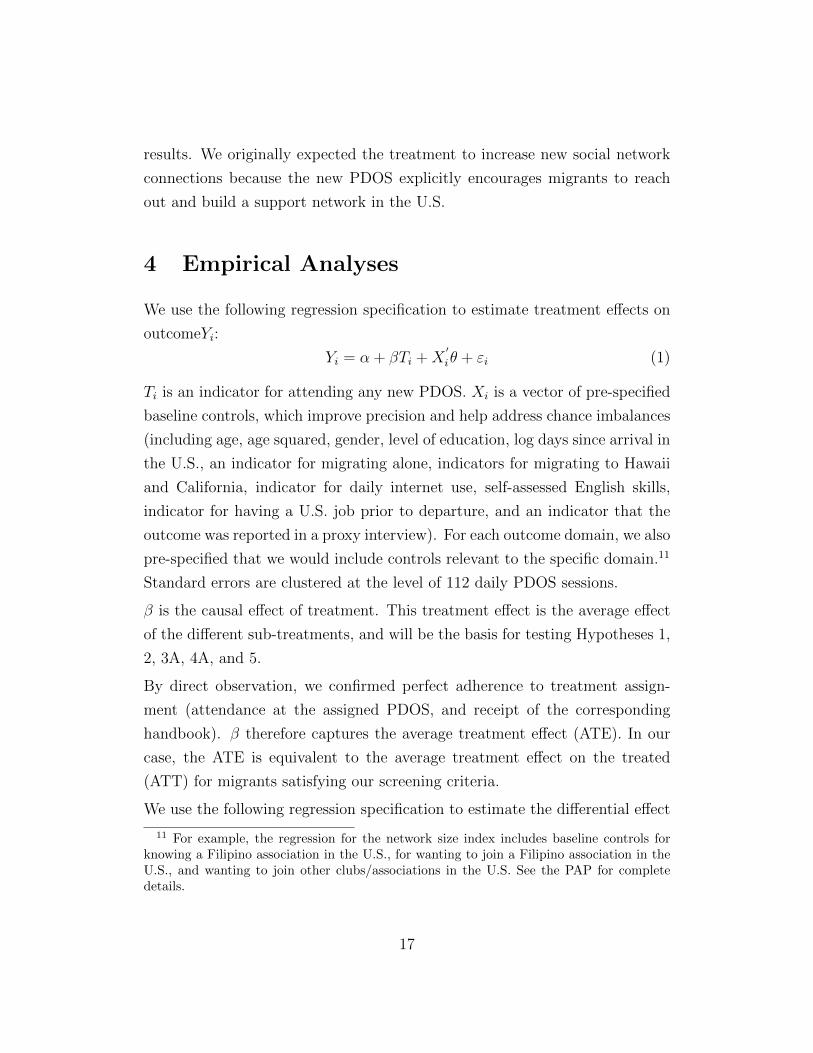
4 Empirical Analyses

We use the following regression specification to estimate treatment effects on

outcomeYi:

Yi = α + βTi +X′

iθ + εi (1)

Ti is an indicator for attending any new PDOS. Xi is a vector of pre-specified

baseline controls, which improve precision and help address chance imbalances

(including age, age squared, gender, level of education, log days since arrival in

the U.S., an indicator for migrating alone, indicators for migrating to Hawaii

and California, indicator for daily internet use, self-assessed English skills,

indicator for having a U.S. job prior to departure, and an indicator that the

outcome was reported in a proxy interview). For each outcome domain, we also

pre-specified that we would include controls relevant to the specific domain.11

Standard errors are clustered at the level of 112 daily PDOS sessions.

β is the causal effect of treatment. This treatment effect is the average effect

of the different sub-treatments, and will be the basis for testing Hypotheses 1,

2, 3A, 4A, and 5.

By direct observation, we confirmed perfect adherence to treatment assign-

ment (attendance at the assigned PDOS, and receipt of the corresponding

handbook). β therefore captures the average treatment effect (ATE). In our

case, the ATE is equivalent to the average treatment effect on the treated

(ATT) for migrants satisfying our screening criteria.

We use the following regression specification to estimate the differential effect

11 For example, the regression for the network size index includes baseline controls forknowing a Filipino association in the U.S., for wanting to join a Filipino association in theU.S., and wanting to join other clubs/associations in the U.S. See the PAP for completedetails.

17

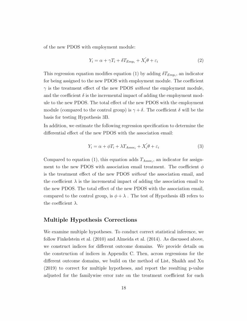
of the new PDOS with employment module:

Yi = α + γTi + δTEmpi +X′

iθ + εi (2)

This regression equation modifies equation (1) by adding δTEmpi , an indicator

for being assigned to the new PDOS with employment module. The coefficient

γ is the treatment effect of the new PDOS without the employment module,

and the coefficient δ is the incremental impact of adding the employment mod-

ule to the new PDOS. The total effect of the new PDOS with the employment

module (compared to the control group) is γ + δ. The coefficient δ will be the

basis for testing Hypothesis 3B.

In addition, we estimate the following regression specification to determine the

differential effect of the new PDOS with the association email:

Yi = α + φTi + λTAssoci +X′

iθ + εi (3)

Compared to equation (1), this equation adds TAssoci , an indicator for assign-

ment to the new PDOS with association email treatment. The coefficient φ

is the treatment effect of the new PDOS without the association email, and

the coefficient λ is the incremental impact of adding the association email to

the new PDOS. The total effect of the new PDOS with the association email,

compared to the control group, is φ+ λ . The test of Hypothesis 4B refers to

the coefficient λ.

Multiple Hypothesis Corrections

We examine multiple hypotheses. To conduct correct statistical inference, we

follow Finkelstein et al. (2010) and Almeida et al. (2014). As discussed above,

we construct indices for different outcome domains. We provide details on

the construction of indices in Appendix C. Then, across regressions for the

different outcome domains, we build on the method of List, Shaikh and Xu

(2019) to correct for multiple hypotheses, and report the resulting p-value

adjusted for the familywise error rate on the treatment coefficient for each

18

domain. We modified the List, Shaikh and Xu (2019) method to be regression-

based and allow for inclusion of control variables. We provide details on the

modifications of the procedure, simulations, and access to our Stata command

mhtreg in Appendix D.

Attrition

Attrition over time was a key challenge as the entire migrant sample moved

from the Philippines to the U.S. and changed their contact details between the

baseline and follow-up interviews. To minimize attrition, we asked study par-

ticipants to provide contact information for the household in the Philippines

they would remain most closely connected to after their departure, which we

then also surveyed. We also fully informed migrants of expectations of multi-

ple follow-up surveys at time of consent and provided financial incentives for

completed surveys. We regularly updated and intensively used contact data of

multiple types (phone, email, Skype, and social media) and solicited household

assistance in contacting migrants if necessary. We used Philippine-household

proxy reports on migrant outcomes if migrants could not be surveyed. Proxy

reports account for about 40 percent of the outcomes collected in the short-

term survey and 50 percent in the long-term survey.12

Our re-interview rates reach 87 percent in the short-term survey and 61 percent

in the long-term survey. These success rates are comparable to those of other

studies that survey and track migrants from their origin to their destination

countries. Ambler (2015) successfully tracked 73 percent of migrants from

El Salvador to Washington DC, Ashraf et al. (2015) 57 percent of migrants

from El Salvador to Washington DC, Shrestha and Yang (2019) 60 percent of

Filipino maids to Singapore, and Gibson et al. (2019) 64 percent of migrants

from Tonga to New Zealand.

We examine a range of potential attrition problems. A crucial question is

whether attrition from the follow-up survey sample is related to treatment

12 Our results hold when we restrict the analysis to directly reported data from migrants,which might be more reliable (Appendix Tables E.7 and E.17).

19

status. If so, concerns arise about selection bias in treatment effect estimates.

We do not find that attrition is related to treatment status in different sur-

vey rounds (Appendix Tables E.4 and E.14). Because attrition is specific to

given outcome measures, we also examine this outcome by outcome (Appendix

Tables E.5 and E.15).13 Again, this analysis raises no concerns. Likewise,

treatment status cannot explain whether an interview is conducted directly

with the migrant or indirectly with a family member in the Philippines via

a proxy survey (Appendix Tables E.6 and E.16). Across the large number of

tests where we check whether treatment predicts attrition, in only very few

cases are coefficients statistically significant at conventional levels, no more

than would be expected to occur by chance.

Throughout, baseline characteristics have little power to predict re-interview

status (attrition or proxy survey status). The R-squared of the corresponding

regressions is low (<0.03) suggesting that baseline characteristics do not sys-

tematically correlate with re-interview status. There is no indication that our

sample loses specific types of migrants over time.

5 Results

Table 1 presents regression results for our primary hypothesis tests, using data

from the short-term survey. Panel A presents coefficients from Equation (1) on

the indicator for receiving the new PDOS (either version) for the five outcome

indices, testing Hypotheses 1, 2, 3A, 4A, and 5. The treatment leads to sub-

stantial reductions in the number of travel related problems (column 1), with

multiple-hypothesis-corrected p-value 0.30. This result points to the impor-

13 Attrition varies across different outcomes, depending on a number of factors: (i) whetheran interview was conducted as a direct interview with the migrant or a proxy interviewwith a family member (as some outcomes could not be collected in proxy interviews), (ii)whether a family member was knowledgeable on a given outcome (as the share of “don’tknow”-responses was considerable higher in proxy interviews), (iii) the common number ofobservations for the individual indicators used to build aggregate indices, (iv) whether weanalyze the new PDOS with association email (as the email could only be randomized amongthe subset of those with a valid email address migrating to a state with a CFO-approvedassociation).

20

tance of the enhanced handbook as the new PDOS featured considerably less

travel-related content than the old PDOS. The treatment also leads to a lower

network size index (column 4). This is the sole outcome that is statistically

significant after multiple-hypothesis correction (p-value 0.03). The coefficients

on the treatment indicator in regressions for the other outcomes are small in

magnitude, and none are statistically significantly different from zero.

Panel B presents coefficients from estimating Equation (2) on the employment

index for receiving the new PDOS (either version) and the new PDOS with

employment module. The latter coefficient, testing Hypothesis 3B, is negative

but not statistically significant at conventional levels.

Panel C presents coefficients from estimating Equation (3) on the network size

index for receiving the new PDOS (either version) and the new PDOS with as-

sociation email. The latter coefficient, testing Hypothesis 4B, is not precisely

estimated. But the economically meaningful positive coefficient is consistent

with the email reducing the cost of acquiring social network connections. In

this regression, the coefficient on the indicator for new PDOS (either version)

is interpreted as the effect of receiving the new PDOS without the associa-

tion email. This coefficient is negative, large in magnitude, and statistically

significant after multiple-hypothesis correction (p-value 0.05).

Using data from the long-term survey, Table 2 presents similar regression re-

sults. (The travel-related problems regression is excluded; it was pre-specified

only as a short-term outcome.) As pre-specified in the long-term PAP, we

replace a missing long-term value with the mid-term or short-term value, in

that order. Because observations missing from the short-term survey may be

found in a later survey, the samples in Table 2 have higher sample sizes (lower

attrition) than Table 1.

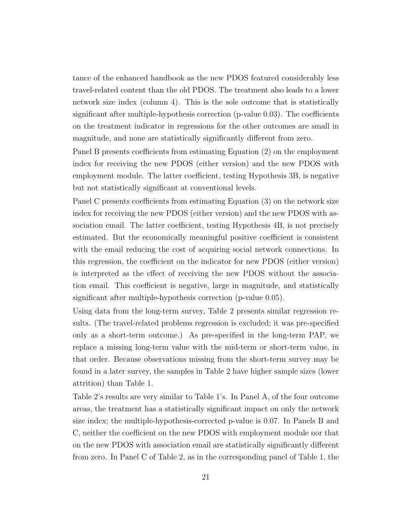
Table 2’s results are very similar to Table 1’s. In Panel A, of the four outcome

areas, the treatment has a statistically significant impact on only the network

size index; the multiple-hypothesis-corrected p-value is 0.07. In Panels B and

C, neither the coefficient on the new PDOS with employment module nor that

on the new PDOS with association email are statistically significantly different

from zero. In Panel C of Table 2, as in the corresponding panel of Table 1, the

21

coefficient on the indicator for new PDOS (either version) is negative, large

in magnitude, and statistically significant after multiple-hypothesis correction

(p-value 0.03).

The stability of the findings in Table 2’s expanded sample and longer time

frame provides an indication of the robustness of the empirical findings. In

Appendix Tables E.7 and E.17, we also show that our results hold when we

exclude proxy reports from household members and restrict the analysis to

directly reported data from migrants.

These results suggest that better-informed immigrants invest less in developing

social networks in their new societies, thus attenuating the overall gains from

the new information. From the perspective of our simple theoretical model,

information and social network links are substitutes. The suggestive evidence

in favor of fewer travel-related problems and no treatment effects on settle-

ment, employment, and wellbeing is consistent with this interpretation. The

new PDOS could affect migrants’ travel experience before they had formed

networks in the U.S. In contrast to post-arrival outcomes, endogenous reduc-

tions in social network connections could hence not attenuate the effects on

travel-related problems.

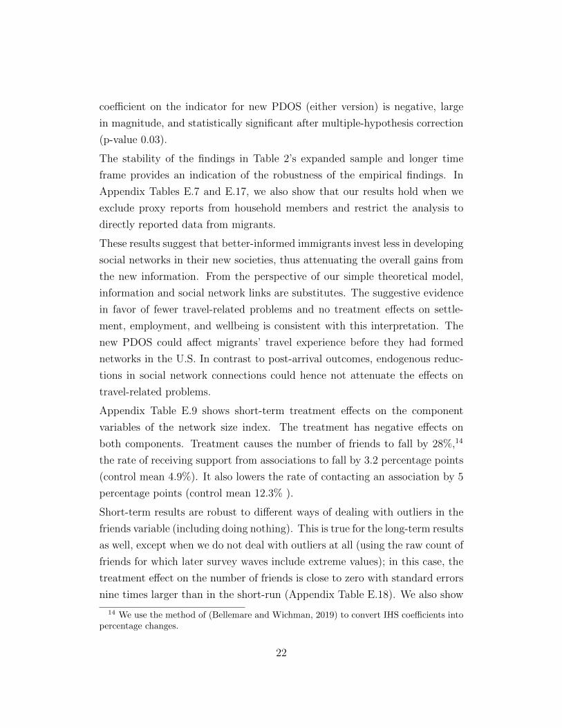
Appendix Table E.9 shows short-term treatment effects on the component

variables of the network size index. The treatment has negative effects on

both components. Treatment causes the number of friends to fall by 28%,14

the rate of receiving support from associations to fall by 3.2 percentage points

(control mean 4.9%). It also lowers the rate of contacting an association by 5

percentage points (control mean 12.3% ).

Short-term results are robust to different ways of dealing with outliers in the

friends variable (including doing nothing). This is true for the long-term results

as well, except when we do not deal with outliers at all (using the raw count of

friends for which later survey waves include extreme values); in this case, the

treatment effect on the number of friends is close to zero with standard errors

nine times larger than in the short-run (Appendix Table E.18). We also show

14 We use the method of (Bellemare and Wichman, 2019) to convert IHS coefficients intopercentage changes.

22

robustness to defining the network measure as specified in the long-term PAP

(Appendix Table E.22).

Density plots of the number of friends provide an alternate view of the treat-

ment effects. Figure 4 presents probability density functions of the number

of friends for the control group (old PDOS) and the treatment group (new

PDOS, any version). The PDF for the treatment group lies to the left of

the control group’s PDF. The PDF of the treatment group has substantially

greater probability mass under 30 friends, and less mass above 30 friends.

The treatment might induce migrants to invest in fewer, but different types

of social network connections. In the long-run PAP, we distinguish between

Filipino and non-Filipino friends and acquaintances as well as close friends (we

did not collect these outcomes in the short-term survey). Appendix Table E.23

shows that the new PDOS particularly reduces the number of Filipino friends

and acquaintances and close friends. The effect is negative for non-Filipino

friends, but not statistically significant. In addition, we do not find that the

new PDOS affects other network characteristics (Appendix Table E.24). The

corresponding index is defined as a STE that summarizes whether the two

closest new contacts in the U.S. have a college degree or higher and whether

they are of non-Filipino ethnicity, whether the migrant has visited people of

U.S. origin in their home, whether the migrant has received visitors of U.S.

origin, and how often the migrant has received everyday favors from non-

Filipino individuals. The new PDOS has no effect on the index or any of its

components. Overall, our results suggest a reduction in the number of network

links across the board with few changes in the type of links.

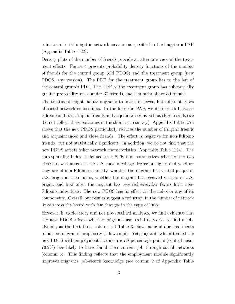
However, in exploratory and not pre-specified analyses, we find evidence that

the new PDOS affects whether migrants use social networks to find a job.

Overall, as the first three columns of Table 3 show, none of our treatments

influences migrants’ propensity to have a job. Yet, migrants who attended the

new PDOS with employment module are 7.8 percentage points (control mean

70.2%) less likely to have found their current job through social networks

(column 5). This finding reflects that the employment module significantly

improves migrants’ job-search knowledge (see column 2 of Appendix Table

23

E.13), which reduces their reliance on social networks. By contrast, migrants

who received the association email, which explicitly encourages them to expand

their social network to find a job, are 9.6 percentage points more likely to have

found a job through social networks (column 6). The opposing effects of the

sub-treatments explain why the overall treatment effect of the new PDOS on

having found a job through social networks is close to zero and not statistically

significant (column 4).

In additional exploratory and not pre-specified analyses, we test a theoreti-

cal possibility highlighted above in Section 2. When friend-acquisition costs

are lower, information and friends are more likely to be substitutes. In this

case, the treatment leads to greater reduction in friends and has a less posi-

tive impact on wellbeing because utility gains from better treatment-provided

information are offset by reductions in friend-provided information. When

friend-acquisition costs are higher, information and friends are more likely

to be complements. In this case, the treatment may lead to an increase in

friend acquisition, as well as an increase in well-being because utility gains

from friend-provided information are added to gains from treatment-provided

information.

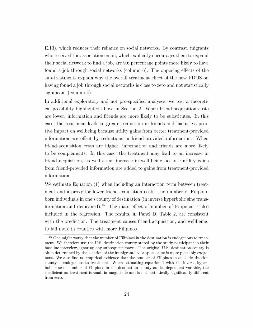
We estimate Equation (1) when including an interaction term between treat-

ment and a proxy for lower friend-acquisition costs: the number of Filipino-

born individuals in one’s county of destination (in inverse hyperbolic sine trans-

formation and demeaned).15 The main effect of number of Filipinos is also

included in the regression. The results, in Panel D, Table 2, are consistent

with the prediction. The treatment causes friend acquisition, and wellbeing,

to fall more in counties with more Filipinos.

15 One might worry that the number of Filipinos in the destination is endogenous to treat-ment. We therefore use the U.S. destination county stated by the study participant in theirbaseline interview, ignoring any subsequent moves. The original U.S. destination county isoften determined by the location of the immigrant’s visa sponsor, so is more plausibly exoge-nous. We also find no empirical evidence that the number of Filipinos in one’s destinationcounty is endogenous to treatment. When estimating equation 1 with the inverse hyper-bolic sine of number of Filipinos in the destination county as the dependent variable, thecoefficient on treatment is small in magnitude and is not statistically significantly differentfrom zero.

24

There is no corresponding heterogeneity in regressions for the settlement and

employment indices. This may reflect that there are factors important for over-

all wellbeing that are not related to, or well-measured by, our rather coarse

settlement or employment indices. For example, immigrants with better infor-

mation may have lower stress levels, perhaps because they feel more confident

in their ability to respond to unexpected future shocks or changes in circum-

stances.

These patterns also reveal themselves in the nonparametric estimation of Fig-

ure 5. In the figure we plot on the vertical axis a nonparametric regression

estimate of the treatment effect of the new PDOS (any version) for study

participants in destination counties with different-sized Filipino populations

(horizontal axis). The nonparametric estimate uses a Gaussian kernel. We

show 90% confidence intervals of the nonparametric regression estimate, based

on 200 bootstrap replications. To give a sense of ranges of the horizontal axis

accounting for more of our study population, we also present the density in

our study sample of the inverse hyperbolic sine of the number of Filipinos in

their destination county (the light gray solid line). The figure suggests that in

counties with the fewest Filipinos (those below the 15th percentile, or a value

on the horizontal axis of 6), the impact of the treatment on the social network

size index is zero, and the impact on wellbeing is positive.

6 Conclusion

We study an intervention that provides immigrants with information about

their new societies, with the aim of facilitating settlement and improving

their socioeconomic outcomes. We find that when new immigrants are better-

informed, they acquire fewer new social network connections. At the same

time, we find no evidence of positive impacts of the information intervention

on immigrant settlement, employment, or overall well-being. In the context

of a simple model, these findings suggest that information and social network

connections are substitutes. Exogenously-provided information (such as from

an information intervention) may be beneficial in itself, but its impact on over-

25

all well-being may be attenuated if beneficiaries respond to the information

provided by reducing their acquisition of information from social networks.

The intervention we study is widespread and important in and of itself. Many

national governments and NGOs seek to provide information to migrants and

other populations more broadly. Thus, the results may also be relevant for

understanding the impacts of other interventions that involve provision of

information, such as financial education or health information programs. The

empirical record of the effectiveness of such programs is mixed (Kaiser and

Menkhoff 2017, Fernandes, Lynch Jr and Netemeyer 2014). In future research,

it will be important to examine whether information interventions in other

contexts also lead to offsetting reductions in social networks, thus attenuating

the overall gains from these interventions.

We do find evidence that the impact of the information intervention we study

is heterogeneous in our study population. The intervention has less negative

effects on social network connections, and positive effects on well-being, for

those in localities with relatively few prior immigrant co-nationals. This could

be due to the fact that acquisition of social network connections is costlier in

such localities. From the standpoint of the theoretical model, the higher the

cost of acquiring social network connections, the less likely it is that informa-

tion and social network connections are substitutes, and the more positive can

be the impact of the information intervention on well-being. This finding has

a policy implication: information interventions may have the highest positive

impacts on the well-being of beneficiaries – and therefore should be considered

more seriously – in situations where beneficiaries have high costs of acquiring

new (or maintaining pre-existing) social network connections (e.g., immigrants

arriving in locations with relatively few prior immigrant compatriots).

26

References

Almeida, Rita, Sarojini Hirshleifer, David McKenzie, Cristobal

Ridao-Cano, and Ahmed Levent Yener. 2014. “The Impact of Voca-

tional Training for the Unemployed: Experimental Evidence from Turkey.”

Economic Journal, 126(597): 2115–2146.

Ambler, Kate. 2015. “Don’t Tell on Me: Experimental Evidence of Asym-

metric Information in Transnational Households.” Journal of Development

Economics, 113: 52–69.

Amuedo-Dorantes, Catalina, and Kusum Mundra. 2007. “Social Net-

works and Their Impact on the Earnings of Mexican Migrants.” Demogra-

phy, 44(4): 849–863.

Ashraf, Nava, Diego Aycinena, Claudia Martinez, and Dean Yang.

2015. “Savings in Transnational Households: A Field Experiment Among

Migrants from El Salvador.” Review of Economics and Statistics, 97: 332–

351.

Banerjee, Abhijit, Arun G Chandrasekhar, Esther Duflo, and

Matthew O Jackson. 2013. “The Diffusion of Microfinance.” Science,

341(6144).

Banerjee, Abhijit, Arun G Chandrasekhar, Esther Duflo, and

Matthew O Jackson. 2018. “Changes in Social Network Structure in Re-

sponse to Exposure to Formal Credit Markets.” Available at SSRN 3245656.

Barr, Abigail, Marleen Dekker, and Marcel Fafchamps. 2015. “The

Formation of Community-Based Organizations: An Analysis of a Quasi-

Experiment in Zimbabwe.” World Development, 66: 131–153.

Beaman, Lori A. 2012. “Social Networks and the Dynamics of Labour Mar-

ket Outcomes: Evidence from Refugees Resettled in the US.” Review of

Economic Studies, 128–161.

27

Beaman, Lori, and Jeremy Magruder. 2012. “Who Gets the Job Referral?

Evidence from a Social Networks Experiment.” American Economic Review,

102(7): 3574–3593.

Bellemare, Marc F, and Casey J Wichman. 2019. “Elasticities and the

Inverse Hyperbolic Sine Transformation.” Oxford Bulletin of Economics and

Statistics.

Blumenstock, Joshua, Guanghua Chi, and Xu Tan. 2019. “Migration

and the Value of Social Networks.” CEPR Discussion Papers 13611.

Bonferroni, Carlo E. 1935. Il Calcolo delle Assicurazioni su Gruppi di Teste.

Tipigrafia del Senato.

Borjas, George J. 1985. “Assimilation, Changes in Cohort Quality, and the

Earnings of Immigrants.” Journal of Labor Economics, 3(4): 463–489.

Borjas, George J. 1992. “Ethnic Capital and Intergenerational Mobility.”

Quarterly Journal of Economics, 107(1): 123–150.

Cabrales, Antonio, Antoni Calvo-Armengol, and Yves Zenou.

2011. “Social Interactions and Spillovers.” Games and Economic Behavior,

72(2): 339–360.

Cai, Jing, and Adam Szeidl. 2018. “Interfirm Relationships and Business

Performance.” Quarterly Journal of Economics, 133(3): 1229–1282.

Calvo-Armengol, Antoni. 2004. “Job Contact Networks.” Journal of Eco-

nomic Theory, 115(1): 191–206.

Calvo-Armengol, Antoni, and Matthew O Jackson. 2004. “The Effects

of Social Networks on Employment and Inequality.” American Economic

Review, 94(3): 426–454.

Canen, Nathan, Matthew O Jackson, and Francesco Trebbi. 2019.

“Endogenous Networks and Legislative Activity.” Available at SSRN

2823338. http://ssrn.com/abstract=2823338.

28

Caria, Stefano, Simon Franklin, and Marc Witte. 2018. “Searching with

Friends.” CSAE Working Paper Series 14.

Carrington, William J, Enrica Detragiache, and Tara Vishwanath.

1996. “Migration with Endogenous Moving Costs.” American Economic Re-

view, 909–930.

Carter, Michael, Rachid Laajaj, and Dean Yang. forthcoming. “Subsi-

dies and the African Green Revolution: Direct Effects and Social Network

Spillovers of Randomized Input Subsidies in Mozambique.” American Eco-

nomic Journal: Applied Economics.

Cecchi, Francesco, Jan Duchoslav, and Erwin Bulte. 2016. “Formal

Insurance and the Dynamics of Social Capital: Experimental Evidence from

Uganda.” Journal of African Economies, 25(3): 418–438.

CFO. 2013. “Stock Estimate of Overseas Filipinos.” Commission on Filipinos

Overseas. https://www.cfo.gov.ph/downloads/statistics/stock-estimates.

html, accessed 23.10.2019.

CFO. 2015. “CFO Statistics on Philippine International Migration.” Com-

mission on Filipinos Overseas. https://www.cfo.gov.ph/images/pdf/2017/

2015compendiumstats-insidepages-2017-06-29.pdf, accessed 23.10.2019.

Chuang, Yating, and Laura Schechter. 2015. “Social Networks in Devel-

oping Countries.” Annual Review of Resource Economics, 7(1): 451–472.

Comola, Margherita, and Mariapia Mendola. 2015. “Formation of Mi-

grant Networks.” Scandinavian Journal of Economics, 117(2): 592–618.

Comola, Margherita, and Silvia Prina. forthcoming. “Treatment Effect

Accounting for Network Changes: Evidence from a Randomized Interven-

tion.” Review of Economics and Statistics.

Currarini, Sergio, Matthew O Jackson, and Paolo Pin. 2009. “An

Economic Model of Friendship: Homophily, Minorities, and Segregation.”

Econometrica, 77(4): 1003–1045.

29

Docquier, Frederic, Giovanni Peri, and Ilse Ruyssen. 2014. “The Cross-

Country Determinants of Potential and Actual Migration.” International

Migration Review, 48(1 suppl): 37–99.

Dolfin, Sarah, and Garance Genicot. 2010. “What Do Networks Do? The

Role of Networks on Migration and ‘Coyote’ Use.” Review of Development

Economics, 14(2): 343–359.

Dupas, Pascaline. 2011. “Do Teenagers Respond to HIV Risk Information?

Evidence from a Field Experiment in Kenya.” American Economic Journal:

Applied Economics, 3(1): 1–34.

Dupas, Pascaline. 2014. “Short-Run Subsidies and Long-Run Adoption of

New Health Products: Evidence from a Field Experiment.” Econometrica,

82(1): 197–228.

Dustmann, Christian, Albrecht Glitz, Uta Schonberg, and Herbert

Brucker. 2016. “Referral-Based Job Search Networks.” Review of Economic

Studies, 83: 514–546.

Einav, Liran, and Amy Finkelstein. 2018. “Moral Hazard in Health In-

surance: What We Know and How We Know It.” Journal of the European

Economic Association, 16(4): 957–982.

Fernandes, Daniel, John G Lynch Jr, and Richard G Netemeyer.

2014. “Financial Literacy, Financial Education, and Downstream Financial

Behaviors.” Management Science.

Finkelstein, A, S Taubman, H Allen, J Gruber, JP Newhouse, B

Wright, and K Baicker. 2010. “The Short-Run Impact of Extending

Public Health Insurance to Low-Income Adults: Evidence from the First

Year of the Oregon Medicaid Experiment.” Analysis plan.

Foster, Andrew D, and Mark R Rosenzweig. 2010. “Microeconomics of

Technology Adoption.” Annual Review of Economics, 2(1): 395–424.

30

Gibson, John, David McKenzie, Halahingano Rohorua, and Steven

Stillman. 2019. “The Long-Term Impact of International Migration on Eco-

nomic Decision-Making: Evidence from a Migration Lottery and Lab-in-the-

Field Experiments.” Journal of Development Economics, 138: 99–115.

Granovetter, Mark. 1973. “The Strength of Weak Ties.” American Journal

of Sociology, 78(6): 1360–1380.

Heß, Simon H, Dany Jaimovich, and Matthias Schundeln. forthcom-

ing. “Development Projects and Economic Networks: Lessons From Rural

Gambia.” Review of Economic Studies.

Holm, Sture. 1979. “A Simple Sequentially Rejective Multiple Test Proce-

dure.” Scandinavian Journal of Statistics, 6: 65–70.

IOM. 2011. “IOM Migrant Training Programmes Overview 2010–

2011.” www.iom.int/jahia/webdav/shared/shared/mainsite/activities/

facilitating/IOM Migrant Training Programmes Overview 2010 2011.pdf,

accessed 23.10.2019.

Jackson, Matthew O. 2019. “A Typology of Social Capital and Associated

Network Measures.” Social Choice and Welfare, 1–26.

Jackson, Matthew O, and Asher Wolinsky. 1996. “A Strategic Model of

Social and Economic Networks.” Journal of Economic Theory, 71(1): 44–74.

Jackson, Matthew O, and Brian W Rogers. 2007. “Meeting Strangers

and Friends of Friends: How Random are Social Networks?” American

Economic Review, 97(3): 890–915.

Jones, Damon, David Molitor, and Julian Reif. 2019. “What do Work-

place Wellness Programs do? Evidence from the Illinois Workplace Wellness

Study.” Quarterly Journal of Economics, 134(4): 1747–1791.

Joona, Pernilla Andersson, and Lena Nekby. 2012. “Intensive Coaching

of New Immigrants: An Evaluation Based on Random Program Assign-

ment.” Scandinavian Journal of Economics, 114(2): 575–600.

31

Kaiser, Tim, and Lukas Menkhoff. 2017. “Does Financial Education Im-

pact Financial Literacy and Financial Behavior, and If So, When?” World

Bank Economic Review, 31(3): 611–630.

Kling, Jeffrey R, Jeffrey B Liebman, and Lawrence F Katz. 2007.

“Experimental Analysis of Neighborhood Effects.” Econometrica, 75(1): 83–

119.

List, John A, Azeem M Shaikh, and Yang Xu. 2019. “Multiple Hy-

pothesis Testing in Experimental Economics.” Experimental Economics,

22(4): 773–793.

Lopez, Gustavo, Neil G Ruiz, and Eileen Patten. 2017. “Key Facts

about Asian Americans, A Diverse and Growing Population.” Pew Research

Center.

Lubotsky, Darren. 2007. “Chutes or Ladders? A Longitudinal Analysis of

Immigrant Earnings.” Journal of Political Economy, 115(5): 820–867.

Lusardi, Annamaria, and Olivia S Mitchell. 2014. “The Economic Im-

portance of Financial Literacy: Theory and Evidence.” Journal of Economic

Literature, 52(1): 5–44.

Mahajan, Parag, and Dean Yang. 2020. “Taken by Storm: Hurricanes,

Migrant Networks, and US Immigration.” American Economic Journal: Ap-

plied Economics, 12(2): 250–277.

Massey, Douglas S. 1988. “Economic Development and International Mi-

gration in Comparative Perspective.” Population and Development Review,

383–413.

McKenzie, David, and Dean Yang. 2015. “Evidence on Policies to Increase

the Development Impacts of International Migration.” World Bank Research

Observer, 30(2): 155–192.

32

Munshi, Kaivan. 2003. “Networks in the Modern Economy: Mexican

Migrants in the US Labor Market.” Quarterly Journal of Economics,

118(2): 549–599.

National Academies of Sciences, Engineering, and Medicine. 2015.

The Integration of Immigrants into American Society. National Academies

Press, Washington, DC.

Orrenius, Pia M, and Madeline Zavodny. 2005. “Self-Selection Among

Undocumented Immigrants from Mexico.” Journal of Development Eco-

nomics, 78(1): 215–240.

Orrenius, Pia M, et al. 1999. “The Role of Family Networks, Coyote Prices

and the Rural Economy in Migration from Western Mexico: 1965-1994.”

Federal Reserve Bank of Dallas Research Paper, , (99–10): 2–11.

Portes, Pia, and Leif Jensen. 1989. “The Enclave and the Entrants: Pat-

terns of Ethnic Enterprise in Miami before and after Mariel.” American

Sociological Review, 54(6): 929–949.

Rinne, Ulf. 2013. “The Evaluation of Immigration Policies.” In International

Handbook on the Economics of Migration. Edward Elgar Publishing.

Romano, Joseph P, and Michael Wolf. 2010. “Balanced Control of Gen-

eralized Error Rates.” Annals of Statistics, 38(1): 598–633.

Sacerdote, Bruce. 2014. “Experimental and Quasi-Experimental Analysis of

Peer Effects: Two Steps Forward?” Annual Review of Economics, 6(1): 253–

272.

Sarvimaki, Matti, and Kari Hamalainen. 2016. “Integrating Immigrants:

The Impact of Restructuring Active Labor Market Programs.” Journal of

Labor Economics, 34(2): 479–508.

Shrestha, Slesh A, and Dean Yang. 2019. “Facilitating Worker Mobil-

ity: A Randomized Information Intervention among Migrant Workers in

Singapore.” Economic Development and Cultural Change, 68(1): 63–91.

33

Testaverde, Mauro, Harry Moroz, Claire H. Hollweg, and Achim

Schmillen. 2017. “Migration Policy in Sending Countries.” Migrating to

Opportunity: Overcoming Barriers to Labor Mobility in Southeast Asia,

Chapter 7, 203–246. Washington, DC:World Bank.

Westfall, Peter H, and S Stanley Young. 1993. Resampling-based Multiple

Testing: Examples and Methods for P-value Adjustment. Vol. 279, Hoboken,

NJ: John Wiley & Sons.

World Bank. 2019. World Development Indicators.

34

Figures and Tables

Friends (f)

Mar

ginal

Ben

efit,

Mar

ginal

Cos

t

MCH

MCL

MBC

MBT

f ∗ f ′f ′′

Figure 1: Increasing returns to information

35

Migrants to the U.S.N=1,273

40%

Old PDOSN=501

New PDOSN=772

60%

New PDOS w/oemployment module

50%

New PDOS withemployment module

50%

Subset of those with a valid email address migrating to a state witha CFO-approved association

N=544

with association email

50%

w/o association email

50%

Figure 2: Treatment conditions

36

(a)

Pre

senta

tion

(in

num

ber

ofsl

ides

)(b

)B

ook

let/

han

db

ook

(in

num

ber

ofpag

es)

SLID

ESHA

NDB

OO

KO

ld P

DOS

New

PDO

SO

ld P

DOS

New

PDO

SM

aint

aini

n

1

8M

aint

aini

n

0

12M

anag

ing

o

010

Man

agin

g o

0

14Fi

ndin

g a

jo5

16Fi

ndin

g a

jo0.

518

Build

ing

a s

0

8Bu

ildin

g a

s

05

Gett

ing

set

16

31Ge

ttin

g se

t

1532

Prep

arin

g f

27

14Pr

epar

ing

f

412

1810

5

168

16

31

27

14

020406080100

Old

PD

OS

New

PD

OS

Prep

arin

g fo

r dep

artu

re a

nd e

nter

ing

the

US

Get

ting

settl

ed in

the

US

Build

ing

a su

ppor

t net

wor

k

Find

ing

a jo

b

Man

agin

g on

e's fi

nanc

es

Main

tain

ing

and

stre

ngth

enin

g tie

s with

the

Phili

ppin

es

1214

0.5

185

15

32

4

12

020406080100

Old

PD

OS

New

PD

OS

Prep

arin

g fo

r dep

artu

re a

nd e

nter

ing

the

US

Get

ting

settl

ed in

the

US

Build

ing

a su

ppor

t net

wor

k

Find

ing

a jo

b

Man

agin

g on

e's fi

nanc

es

Main

tain

ing

and

stre

ngth

enin

g tie

s with

the

Phili

ppin

es

SLID

ESHA

NDB

OO

KO

ld P

DOS

New

PDO

SO

ld P

DOS

New

PDO

SM

aint

aini

n

1

8M

aint

aini

n

0

12M

anag

ing

o

010

Man

agin

g o

0

14Fi

ndin

g a

jo5

16Fi

ndin

g a

jo0.

518

Build

ing

a s

0

8Bu

ildin

g a

s

05

Gett

ing

set

16

31Ge

ttin

g se

t

1532

Prep

arin

g f

27

14Pr

epar

ing

f

412

1810

5

168

16

31

27

14

020406080100

Old

PD

OS

New

PD

OS

Prep

arin

g fo

r dep

artu

re a

nd e

nter

ing

the

US

Get

ting

settl

ed in

the

US

Build

ing

a su

ppor

t net

wor

k

Find

ing

a jo

b

Man

agin

g on

e's fi

nanc

es

Main

tain

ing

and

stre

ngth

enin

g tie

s with

the

Phili

ppin

es

1214

0.5

185

15

32

4

12

020406080100

Old

PD

OS

New

PD

OS

Prep

arin

g fo

r dep

artu

re a

nd e

nter

ing

the

US

Get

ting

settl

ed in

the

US

Build

ing

a su

ppor

t net

wor

k

Find

ing

a jo

b

Man

agin

g on

e's fi

nanc

es

Main

tain

ing

and

stre

ngth

enin

g tie

s with

the

Phili

ppin

es

Fig

ure

3:D

iffer

ence

sin

cove

rage

ofto

pic

sb

etw

een

the

old

and

new

PD

OS

(in

term

sof

quan

tity

)N

ote:

The

nu

mb

erof

page

sin

the

han

db

ook

isn

otd

irec

tly

com

par

able

asth

efo

rmat

ofth

eol

dP

DO

Sh

and

book

ism

uch

smal

ler

(it

isa

book

let)

.T

he

old

PD

OS

does

not

cove

r“B

uil

din

ga

sup

por

tn

etw

ork”

and

“Man

agin

gon

e’s

fin

ance

s”.

Th

ep

rese

nta

tion

ofth

eold

PD

OS

has

one

slid

eon

“M

ainta

inin

gan

dst

ren

gth

enin

gti

esw

ith

the

Ph

ilip

pin

es”

and

the

book

let

hal

fa

pag

eon

“Fin

din

ga

job

”.C

om

pare

dto

the

old

PD

OS

,th

en

ewP

DO

Ssh

ifts

the

focu

sfr

om“P

rep

arin

gfo

rd

epar

ture

and

ente

rin

gth

eU

.S.”

toth

eot

her

topic

s,w

hic

har

em

ore

rele

vant

for

lon

ger

-ter

mso

cio-

econ

omic

inte

grat

ion

.A

noth

er

majo

rd

iffere

nce

isth

at

the

new

PD

OS

off

ers

mu

chri

cher

an

dp

racti

cal

info

rmati

on

.F

igu

res

B.3

an

dB

.4in

Ap

pen

dix

Billu

stra

teth

isd

iffere

nce

inte

rms

of

both

qu

anti

tyan

dqu

ali

tyfo

rin

form

ati

on

pro

vid

ed

on

op

en

ing

ab

an

kaccou

nt.

All

pre

senta

tion

slid

esan

dh

and

book

sca

nb

ed

own

load

edat

htt

ps:

//si

tes.

googl

e.co

m/vie

w/t

omanb

arsb

ai/p

dos

.

37

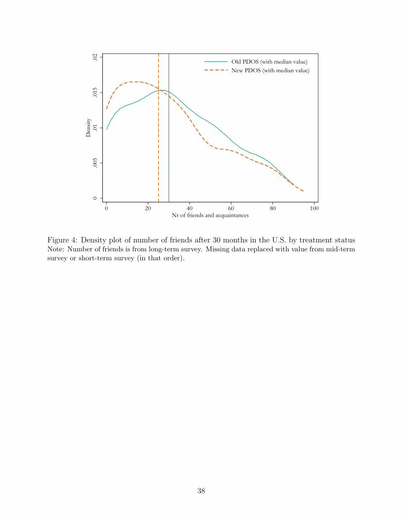
0.0

05.0

1.0

15.0

2D

ensit

y

0 20 40 60 80 100Nr of friends and acquaintances

Old PDOS (with median value)New PDOS (with median value)

Figure 4: Density plot of number of friends after 30 months in the U.S. by treatment statusNote: Number of friends is from long-term survey. Missing data replaced with value from mid-termsurvey or short-term survey (in that order).

38

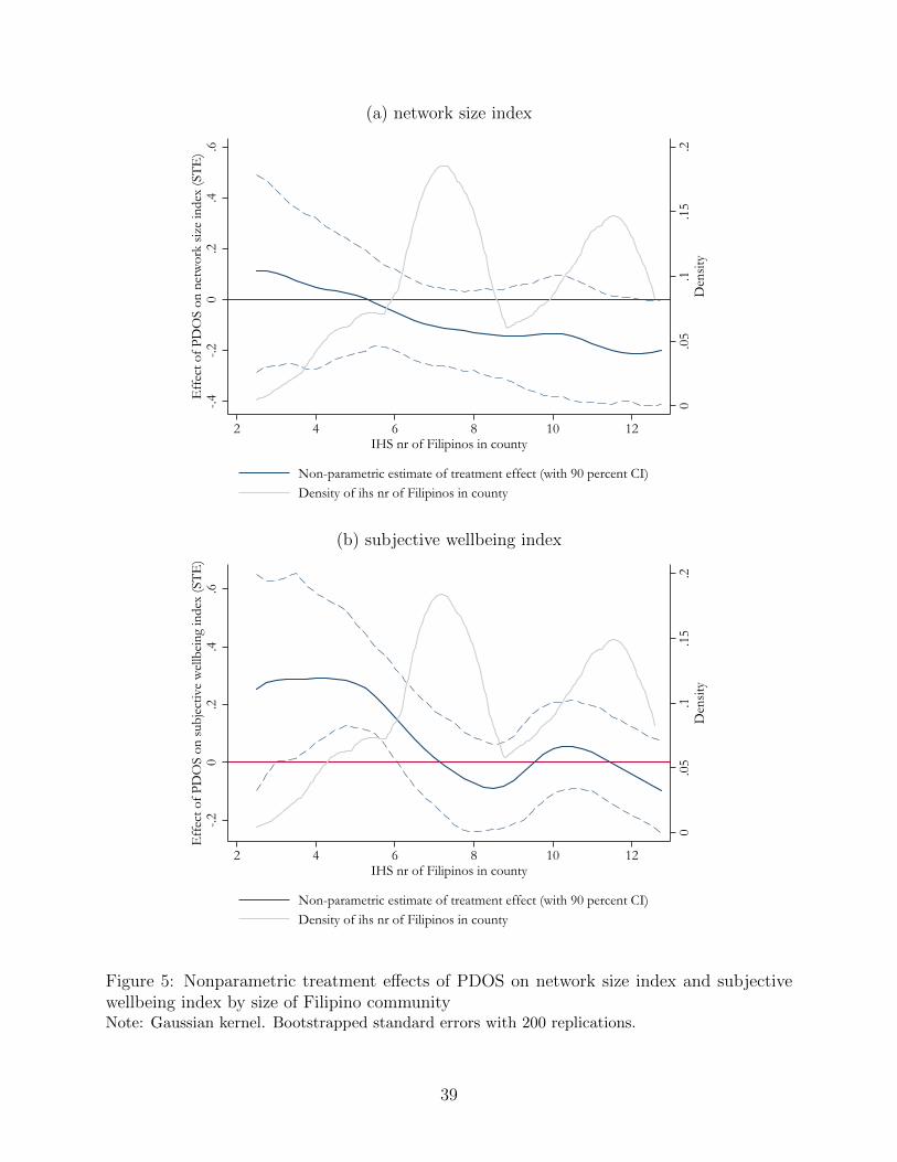
(a) network size index

-.4-.2

0.2

.4.6

Eff

ect o

f PD

OS

on n

etw

ork

size

inde

x (S

TE)

2 4 6 8 10 12IHS nr of Filipinos in county

Non-parametric estimate of treatment effect (with 90 percent CI)Density of ihs nr of Filipinos in county

0.0

5.1

.15

.2D

ensit

y

(b) subjective wellbeing index

-.20

.2.4

.6E

ffec

t of P

DO

S on

subj

ectiv

e w

ellb

eing

inde

x (S

TE)

2 4 6 8 10 12IHS nr of Filipinos in county

Non-parametric estimate of treatment effect (with 90 percent CI)Density of ihs nr of Filipinos in county

0.0

5.1

.15

.2D

ensit

y

Figure 5: Nonparametric treatment effects of PDOS on network size index and subjectivewellbeing index by size of Filipino communityNote: Gaussian kernel. Bootstrapped standard errors with 200 replications.

39

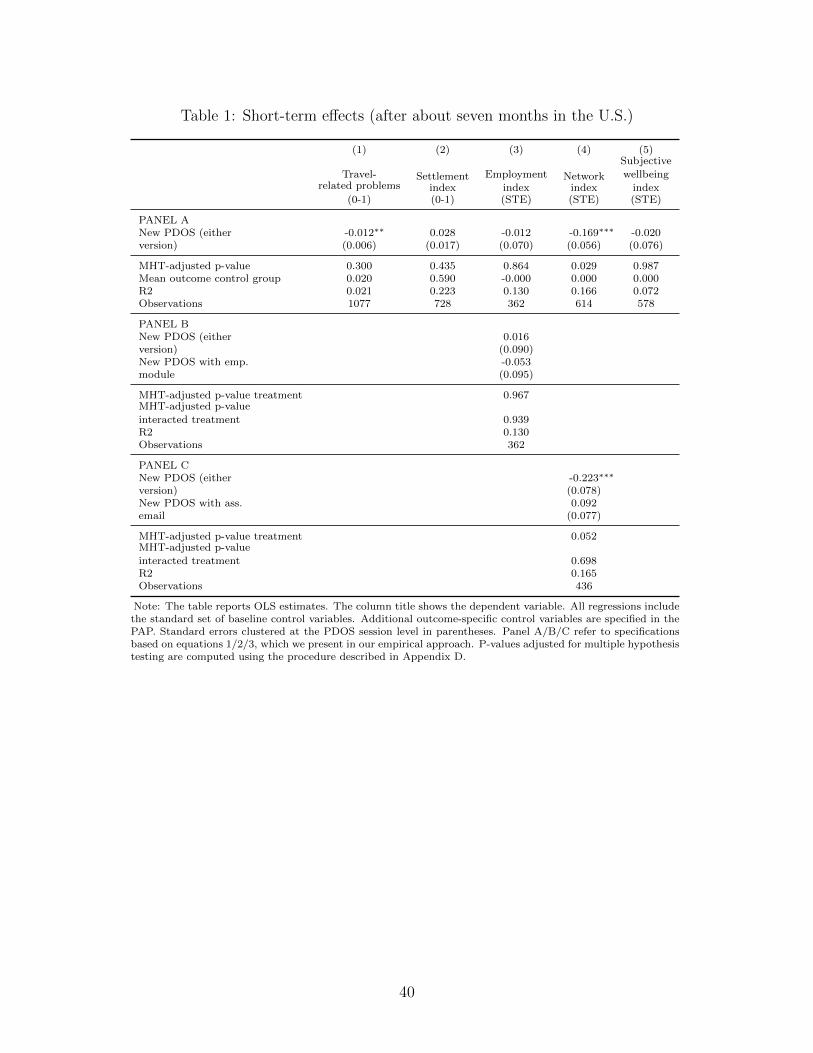
Table 1: Short-term effects (after about seven months in the U.S.)

(1) (2) (3) (4) (5)

Travel-related problems

(0-1)

Settlementindex(0-1)

Employment

index(STE)

Networkindex(STE)

Subjective

wellbeing

index(STE)

PANEL ANew PDOS (either -0.012∗∗ 0.028 -0.012 -0.169∗∗∗ -0.020version) (0.006) (0.017) (0.070) (0.056) (0.076)

MHT-adjusted p-value 0.300 0.435 0.864 0.029 0.987Mean outcome control group 0.020 0.590 -0.000 0.000 0.000R2 0.021 0.223 0.130 0.166 0.072Observations 1077 728 362 614 578

PANEL BNew PDOS (either 0.016version) (0.090)New PDOS with emp. -0.053module (0.095)

MHT-adjusted p-value treatment 0.967MHT-adjusted p-value

interacted treatment 0.939R2 0.130Observations 362

PANEL CNew PDOS (either -0.223∗∗∗

version) (0.078)New PDOS with ass. 0.092email (0.077)

MHT-adjusted p-value treatment 0.052MHT-adjusted p-value

interacted treatment 0.698R2 0.165Observations 436

Note: The table reports OLS estimates. The column title shows the dependent variable. All regressions includethe standard set of baseline control variables. Additional outcome-specific control variables are specified in thePAP. Standard errors clustered at the PDOS session level in parentheses. Panel A/B/C refer to specificationsbased on equations 1/2/3, which we present in our empirical approach. P-values adjusted for multiple hypothesistesting are computed using the procedure described in Appendix D.

40

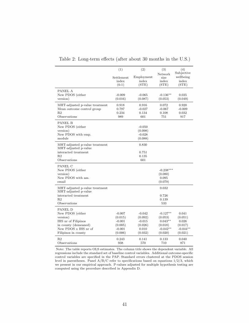
Table 2: Long-term effects (after about 30 months in the U.S.)

(1) (2) (3) (4)

Settlementindex(0-1)

Employment

index(STE)

Networksize

index(STE)

Subjective

wellbeing

index(STE)

PANEL ANew PDOS (either -0.009 -0.065 -0.136∗∗ 0.035version) (0.016) (0.087) (0.053) (0.049)

MHT-adjusted p-value treatment 0.918 0.916 0.072 0.920Mean outcome control group 0.797 -0.027 -0.067 -0.009R2 0.234 0.134 0.108 0.032Observations 989 601 751 917

PANEL BNew PDOS (either -0.050version) (0.098)New PDOS with emp. -0.028module (0.088)

MHT-adjusted p-value treatment 0.830MHT-adjusted p-value

interacted treatment 0.751R2 0.135Observations 601

PANEL CNew PDOS (either -0.238∗∗∗

version) (0.080)New PDOS with ass. 0.095email (0.079)

MHT-adjusted p-value treatment 0.032MHT-adjusted p-value

interacted treatment 0.726R2 0.139Observations 533

PANEL DNew PDOS (either -0.007 -0.042 -0.127∗∗ 0.041version) (0.015) (0.092) (0.053) (0.051)IHS nr of Filipinos -0.001 -0.015 0.043∗∗ 0.026in county (demeaned) (0.005) (0.026) (0.018) (0.017)New PDOS x IHS nr of -0.001 0.010 -0.042∗∗ -0.044∗∗

Filipinos in county (0.006) (0.032) (0.020) (0.021)

R2 0.243 0.141 0.133 0.040Observations 938 570 710 871

Note: The table reports OLS estimates. The column title shows the dependent variable. Allregressions include the standard set of baseline control variables. Additional outcome-specificcontrol variables are specified in the PAP. Standard errors clustered at the PDOS sessionlevel in parentheses. Panel A/B/C refer to specifications based on equations 1/2/3, whichwe present in our empirical approach. P-values adjusted for multiple hypothesis testing arecomputed using the procedure described in Appendix D.

41

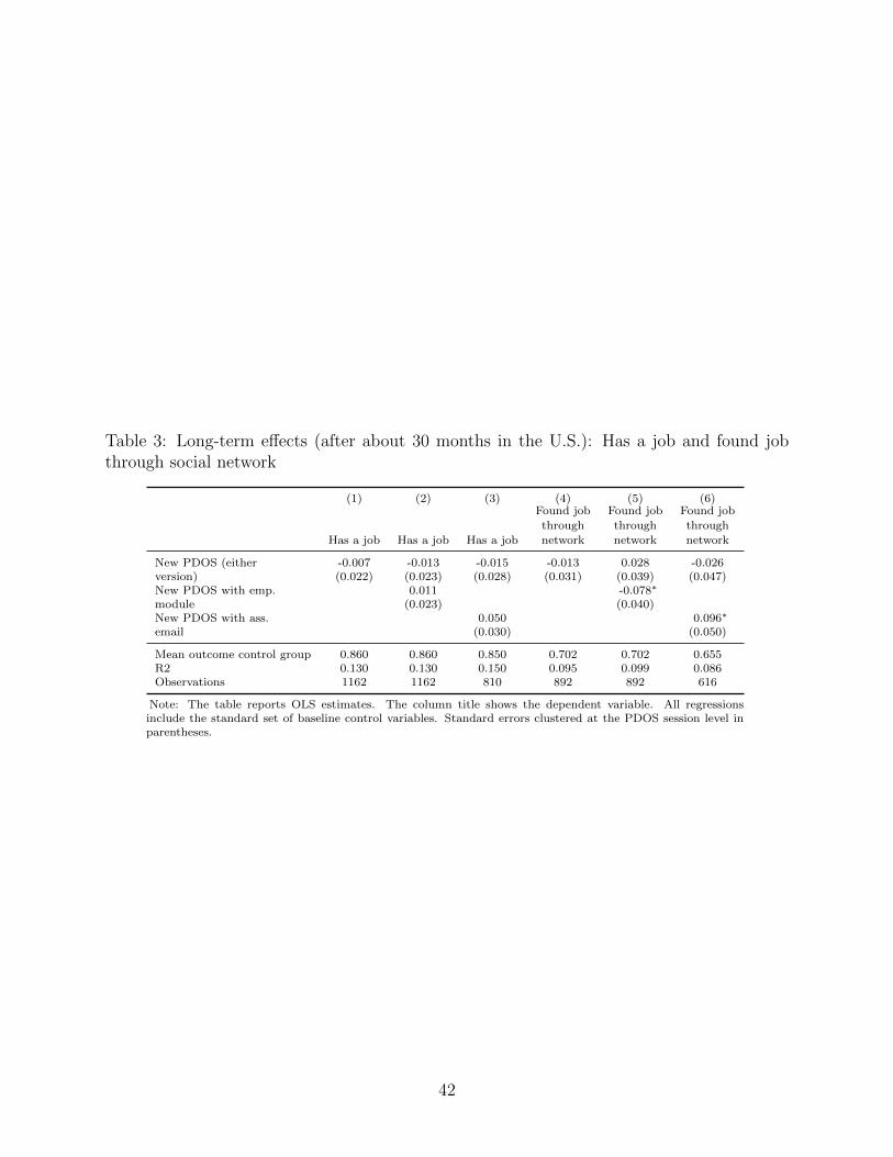
Table 3: Long-term effects (after about 30 months in the U.S.): Has a job and found jobthrough social network

(1) (2) (3) (4) (5) (6)

Has a job Has a job Has a job

Found job

through

network

Found job

through

network

Found job

through

network

New PDOS (either -0.007 -0.013 -0.015 -0.013 0.028 -0.026version) (0.022) (0.023) (0.028) (0.031) (0.039) (0.047)New PDOS with emp. 0.011 -0.078∗

module (0.023) (0.040)New PDOS with ass. 0.050 0.096∗

email (0.030) (0.050)

Mean outcome control group 0.860 0.860 0.850 0.702 0.702 0.655R2 0.130 0.130 0.150 0.095 0.099 0.086Observations 1162 1162 810 892 892 616

Note: The table reports OLS estimates. The column title shows the dependent variable. All regressionsinclude the standard set of baseline control variables. Standard errors clustered at the PDOS session level inparentheses.

42

APPENDIX (NOT FOR PRINT PUBLICATION)

Information and the Acquisition of Social Network Connections

Authors

Toman Barsbai (University of Bristol and IfW Kiel)

Victoria Licuanan (AIM Manila)

Andreas Steinmayr (LMU Munich, CESifo, IZA, IPL, and IfW Kiel)

Erwin Tiongson (Georgetown University)

Dean Yang (University of Michigan, NBER, and BREAD)

Appendices

Appendix A: A Simple Model of social network investment

Appendix B: Further details on treatment and survey implementation

Appendix C: Construction of indices

Appendix D: Multiple hypothesis testing

Appendix E: Further figures and tables

A A Simple Model of Social Network Investment

We present here a simple model of social network investment in the context of imperfect

information. We are interested in the interplay between information imperfections and indi-

vidual efforts to expand one’s social network. In particular, we are interested in the potential

impact of interventions to alleviate information imperfections. If an intervention reduces in-

formation imperfections, does this raise or reduce individual efforts to expand one’s social

network? We will see that it is theoretically possible for reductions in information imperfec-

tions to either raise or lower optimal choice of social network size.

Individuals have imperfect information about a variety of things in life that matter to them,

such as jobs (how to find them and what jobs are available), financial services, government

services, and the like. People also have social networks (“friends”), which provide infor-

mation, helping to reduce information imperfections. This can come about simply in the

process of friends conversing and sharing information with one another about topics relevant

to their lives. Network theory suggests that efficient information gathering typically requires

expansive networks with many short network paths (cf. Granovetter, 1973). Thus, we use

the number of first-degree friends as a proxy for network expansiveness.

Because friends are valuable, people make efforts to acquire them, but making friends is to

some degree costly. The costs of friend acquisition may include effort costs of socializing,

as well as monetary costs incurred to facilitate networking, such as travel costs to meetings

and social events, costs of membership in clubs or organizations, and the like.

We focus on the benefits friends bring by reducing information imperfections. We abstract

away from other benefits of friends that the network literature typically refers to as co-

operation capital, such as various forms of assistance (transfers, informal insurance, and

psychological support).1

We model individual utility as depending on baseline or starting-point information imperfec-

tions (prior to any reduction in information imperfections resulting from friend investments),

θ, and endogenous friend investment f ≥ 0. For simplicity, we abstract from other deter-

minants of utility that are independent of friends. Individuals choose f to maximize the

benefits from friends B(θ, f) net of the cost of friend investment C(f):

U = B(θ, f)− C(f)

People therefore acquire friends only up to the point at which the marginal cost does not

1These other non-information benefits of friends could be thought of as entering the cost term in themaximization problem we write down below, reducing the net cost of friends.

2

exceed the marginal benefit of friends. With reasonable assumptions on functional forms

one can obtain an interior solution for the optimal number of friends. A corner solution

is also possible of course, if the cost of friend investments is so high relative to benefits

that the optimal number of friends is zero. Once functional forms are posited, we can make

statements about the responsiveness of friend investments to changes in baseline information

imperfections θ.

Some simple assumptions and functional forms generate useful possibilities. Let information

imperfections θ range from 0 to 1 (θ ∈ [0, 1]), and allow individuals to have both exogenous

friends (those that are given at baseline without cost), e, and endogenous friends, f , which

they acquire at a cost. Let e ≥ 1.2 Let one’s amount of information I be a function of

information imperfections θ, exogenous friends e, and endogenous friends f as follows:

I = 1− θ

e+ f

In this setup, one’s amount of information can range from 0 (no information) to 1 (full infor-

mation). If baseline information imperfections θ are 0, then one starts with full information.

A higher number of friends e + f reduces the importance of one’s baseline information im-

perfections and raises one’s amount of information I.

For simplicity, let the cost of endogenous friends be linear with a per-friend cost c, so the

total cost of friend acquisition is cf .3 As mentioned, exogenous friends e, as part of one’s

endowment, are costless.

We now analyze three distinct cases: constant, decreasing, and increasing returns to infoma-

tion. Analysis of the different cases makes clear that reductions in information imperfections

(increases in information) have indeterminate impacts on friend investments.

Case 1: Constant Returns to Information

Let the benefit B(θ, f) be constant or linear in the amount of information I. The individual’s

maximization problem is as follows:

maxf

1− θ

e+ f− cf

The first order condition is:θ

(e+ f)2= c

2 In our empirical context, assuming that individuals start with at least one friend is reasonable. For newimmigrants to the U.S., the exogenous friend could be the individual who officially sponsors the immigrantfor their immigration visa.

3The main predictions of the model are robust to the assumption of increasing per-friend net cost, whichmight result from decreasing per-friend assistance benefits in larger networks.

3

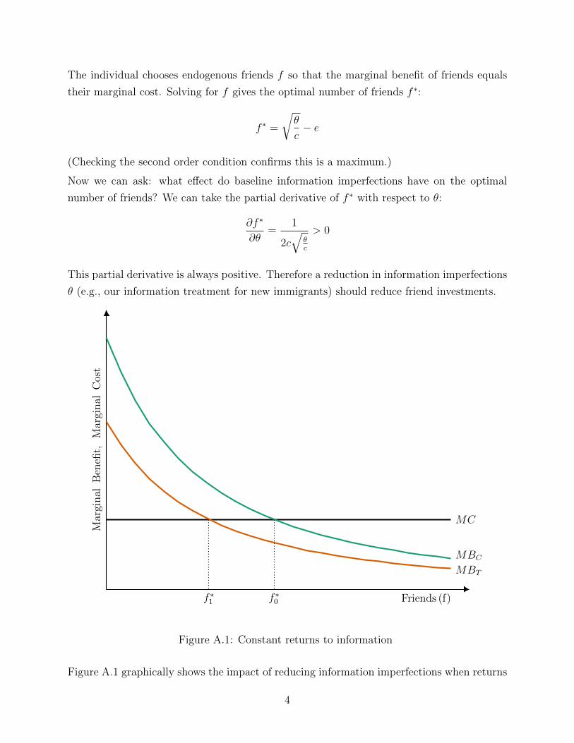
The individual chooses endogenous friends f so that the marginal benefit of friends equals

their marginal cost. Solving for f gives the optimal number of friends f ∗:

f ∗ =

√θ

c− e

(Checking the second order condition confirms this is a maximum.)

Now we can ask: what effect do baseline information imperfections have on the optimal

number of friends? We can take the partial derivative of f ∗ with respect to θ:

∂f ∗

∂θ=

1

2c√

θc

> 0

This partial derivative is always positive. Therefore a reduction in information imperfections

θ (e.g., our information treatment for new immigrants) should reduce friend investments.

Friends (f)

Mar

ginal

Ben

efit,

Mar

ginal

Cos

t

MC

MBC

f ∗0

MBT

f ∗1

Figure A.1: Constant returns to information

Figure A.1 graphically shows the impact of reducing information imperfections when returns

4

to information are constant. Parameter values used in the figure are: e = 1, c = 0.25.

The red line is the marginal cost function, which is horizontal because the cost of friends is

constant. The green curve is the marginal benefit function for the control group (without

the information treatment), with θ = 0.9. The orange curve is the marginal benefit function

for the information treatment group, which due to the treatment has lower information

imperfections (θ = 0.6). The reduction in information imperfections due to treatment lowers

the marginal benefit of friends (the orange curve is always lower than the green curve).

The optimal number of friends is given by the intersection of the marginal benefit and

marginal cost functions. In the control group, the optimal number of friends is f ∗0 . In the

treatment group, the optimal number of friends is f ∗1 , which is lower than f ∗0 . The reduction

in information imperfections due to treatment lowers the marginal benefit of friends, lowering

the optimal number of friends.

Case 2: Decreasing Returns to Information

The case of decreasing returns to information is very similar to the constant-returns case. We

modify the benefit function so that benefits are a function of the square root of information,

so the migrant’s optimization problem is:

maxf

(1− θ

e+ f)12 − cf

The first order condition is:θ

2(1− θe+f

)f 2= c

Aside from the change in the benefit function and thus the marginal benefit functions,

assumptions are otherwise the same as for the constant-returns case in Figure A.1. As in

Figure A.1, the reduction in information imperfections due to treatment lowers the marginal

benefit of friends (the orange curve is always lower than the green curve).

Case 3: Increasing Returns to Information

Assuming increasing returns to information leads to ambiguous predictions regarding the

impact of information imperfections on friend investments. We modify the benefit function

to add a quadratic term in information, allowing for increasing returns to information. So

the migrant’s optimization problem is:

maxf

1− θ

e+ f+ α(1− θ

e+ f)2 − cf

The parameter α measures the strength of increasing returns to information. The first order

5

condition is now:θ

(e+ f)2+

2αθ

(e+ f)2(1− θ

(e+ f)) = c

These marginal benefit and cost curves now allow an information treatment (that lowers θ)

to either raise or lower optimal friend investments.

We analyze this case graphically in Figure 1. The parameter values used in the figure are e =

1, c = 2.4, and α = 5. As in Figure A.1, the horizontal red line is the marginal cost function.

The green and orange curves are the marginal benefit functions for the control group and

treatment groups with, θ = 0.9 and θ = 0.6 respectively. The marginal benefit functions

can have upward-sloping (increasing returns to friends) and downward-sloping (decreasing

returns to friends) sections. The optimum is found at the intersection of the marginal cost

function and the downward-sloping part of the relevant marginal benefit function. (The

optimum would not be at the intersection with the upward-sloping part of the marginal

benefit function, because at that intersection the marginal benefit of friends is increasing, so

the individual could continue to increase utility by raising friend investments.)

The figure depicts the case where the cost of friend investments is high enough that for the

control group (blue marginal benefit curve), there is a corner solution where f ∗ = 0 (utility is

maximized with no friend investments.) For the control group, there is no amount of friend

investments for which the marginal benefit of friends is positive, so the individual makes no

friend investments.

From this starting point, a reduction in (in this figure, from 0.9 in the control group to 0.6

in the treatment group) can lead the marginal benefit function to shift so that there is an

interior solution with positive friend investments (f ∗ > 0).

There is also of course the possibility, for lower values of the cost of friends c, that reductions

in θ lead to reductions in the optimal number of friends. This would be the case if the

marginal cost of friends was lower, so that the marginal cost function (the horizontal red

line) would intersect both the control group and treatment group marginal benefit functions

on their downward-sloping portions. If this were the case, a reduction in θ would have effects

similar to those depicted in Figure A.1: a reduction in optimal friend investments.

Overall, therefore, depending on parameter values and functional forms, it is possible for an

information intervention, such as the one we implemented among new U.S. immigrants from

the Philippines, to either raise or lower investments made in building one’s social network.

This possibility arises when there are increasing returns to information (Case 2 above), but

not when returns to information are constant (Case 1 above).

6

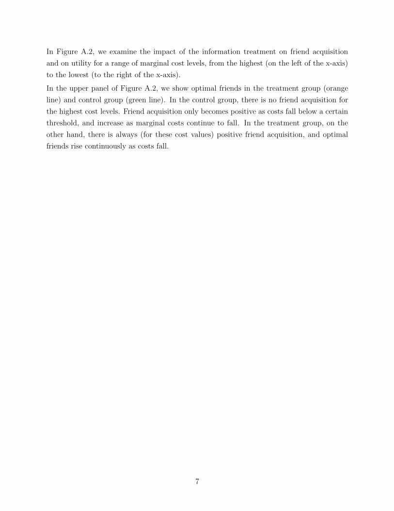
In Figure A.2, we examine the impact of the information treatment on friend acquisition

and on utility for a range of marginal cost levels, from the highest (on the left of the x-axis)

to the lowest (to the right of the x-axis).

In the upper panel of Figure A.2, we show optimal friends in the treatment group (orange

line) and control group (green line). In the control group, there is no friend acquisition for

the highest cost levels. Friend acquisition only becomes positive as costs fall below a certain

threshold, and increase as marginal costs continue to fall. In the treatment group, on the

other hand, there is always (for these cost values) positive friend acquisition, and optimal

friends rise continuously as costs fall.

7

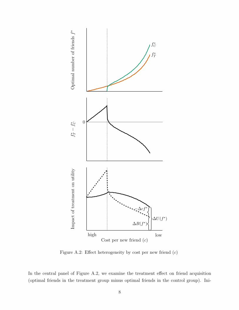
f ∗C

f ∗T

Opti

mal

num

ber

offr

iendsf∗

0

f∗ T−f∗ C

−∆cf∗

∆B(f∗)∆U(f∗)

Cost per new friend (c)

Impac

tof

trea

tmen

ton

uti

lity

high low

Figure A.2: Effect heterogeneity by cost per new friend (c)

In the central panel of Figure A.2, we examine the treatment effect on friend acquisition

(optimal friends in the treatment group minus optimal friends in the control group). Ini-

8

tially, reductions in marginal costs make the treatment effect on friend acquisition even more

positive, because we are in the region where information and friends are complements. As

we lower marginal costs further into the zone where there is now positive friend acquisition

in the control group, friends and information are now substitutes. The treatment effect on

friends becomes negative, and increasingly so as marginal costs fall more.

In the lower panel of Figure A.2, we examine the treatment effect on utility. The treatment

effect on utility (solid line) follows a pattern similar to the central panel. Starting from the

highest marginal costs, reductions in marginal costs make the treatment effect on utility

even more positive, as long as one remains in the region where information and friends are

complements. As we lower marginal costs further, friends and information become substi-

tutes, and the treatment effect on utility declines, and eventually can be even lower than

when marginal costs were very high.

All told then, the impact of the treatment on friend acquisition and on utility is not mono-

tonic. There is a range (when marginal costs start from a “high” level) where information

and friends are complements, during which the treatment effect on friends and on utility

rises as marginal costs fall. Then as marginal costs continue to fall, we transition to a region

where information and friends are substitutes. In this region, the treatment effect on friends

becomes negative, and the treatment effect on both friends and utility declines as marginal

costs continue to fall.

B Further Details on Treatments and Survey Imple-

mentation

Content of the New PDOS

The new PDOS and the corresponding handbook consist of the following components.

Travel – This short module helps migrants to prepare for the journey to the U.S.. It covers

travel-related issues such as travel documents, airport and immigration procedures, luggage,

and restricted items. The new module is considerably shorter than the previous module, but

the new expanded handbook provides comprehensive information on these matters.

Settlement – This is the broadest of all modules and covers issues related to migration

in general and migration to the U.S. in particular. The module addresses topics such as

cultural differences and culture shock, rights and obligations of U.S. permanent residents,

important things to take care of after arrival (such as obtaining a social security number,

health insurance, a driver’s license, etc.) as well as information about health care, education,

9

and housing.

Associations in the U.S. – Filipino associations, but also non-Filipino associations such

as neighborhood associations, may be an important provider of post-arrival support for

migrants. The module informs migrants about the potential benefits of associations for

expanding their social network. Such contacts may ultimately help migrants to integrate

into the U.S. and find a decent job.

Employment – This module aims to help migrants to find a decent job in the U.S., which

our preparatory interviews identified as the single most important challenge for Filipino

migrants. It informs about the U.S. labor market and addresses important issues such as

the recognition of certificates and diplomas, job search strategies, how to prepare a CV and

cover letter, and behave in a job interview. There are two versions of the new PDOS, one

with and one without employment module.

Financial literacy – This module is based on the fact that migrants often experience a

substantial increase in income when starting a job abroad. The module teaches basic rules

of thumb on opening a bank account, financial planning, savings, sending remittances, and

making a joint financial plan with the family in the Philippines on the amount and use of

remittances.

Diaspora engagement – This module aims to strengthen the links between Filipino mi-

grants and the Philippines. It covers Filipino culture and values, overseas voting rights, the

right to re-acquire Filipino citizenship and government programs such as BalinkBayan and

Linkapil, which help migrants to stay in touch with their home country and give them the

possibility to contribute to development causes in the Philippines.

The new PDOS provides each migrant with a comprehensive 116-page paper handbook,

which covers the above topics in detail and provides easy-to-follow checklists as well as

links to online resources. While the old PDOS provides written information in the form of

a booklet, the handbook of the new PDOS offers much richer and practical information.

Figures B.3 and B.4 below illustrate this difference in terms of both quantity and quality for

information provided on opening a bank account.

All material used in the different treatment conditions including the presentation slides and

handbooks can be downloaded at https://sites.google.com/view/tomanbarsbai/pdos.

10

32Ope

ning

a B

ank

Acco

unt

One

of y

our fi

rst s

teps

in th

e U

S sh

ould

be

open

ing

a U

S ba

nk

acco

unt.

Havi

ng a

n ac

coun

t allo

ws

you

to m

anag

e yo

ur d

ay-

to-d

ay fi

nanc

ial t

rans

acon

s, w

hich

may

invo

lve

buyi

ng d

aily

ne

cess

ies

, or r

enng

or p

urch

asin

g a

new

hom

e. M

oreo

ver,

with

an

acco

unt,

you

are

a st

ep c

lose

r to

fully

real

izing

you

r fin

anci

al g

oals

– m

ay it

be

shor

t, m

id-,

or lo

ng te

rm.

Belo

w a

re th

e ge

nera

l ste

ps to

be

take

n in

ope

ning

an

acco

unt: Do

you

r res

earc

h. S

ince

ban

ks c

ome

in v

ario

us ty

pes a

nd si

zes a

nd offe

r a d

iver

se

rang

e of

ser

vice

s an

d fe

es, i

t is

best

to d

o re

sear

ch o

n w

hich

ban

k is

suita

ble

to

your

goa

ls, n

eeds

, and

life

styl

e. Yo

u m

ay w

ant t

o as

k ar

ound

, rea

d on

line,

or s

peak

di

rect

ly to

a b

ank

repr

esen

tave

to h

ave

your

que

son

s ans

wer

ed.

Know

mor

e ab

out y

our p

rosp

ecve

ban

k. C

onsu

lt th

e w

ebsit

e of

you

r pre

ferr

ed

bank

or

call

a ba

nk r

epre

sent

ave

for

the

com

plet

e re

quire

men

ts.

Fact

or i

n co

nsid

era

ons s

uch

as b

anki

ng h

ours

, dist

ance

, fee

s, in

tere

st ra

tes,

etc

. Ask

abo

ut

ATM

rel

ated

ban

k se

rvic

es li

ke lo

caon

, cus

tom

er p

rote

con

, fee

s, w

ithdr

awin

g lim

it, e

tc.

For

you

it m

ight

be

of p

arcu

lar

impo

rtan

ce w

hat

the

fees

are

for

in

tern

aon

al t

rans

acon

s to

or

from

the

Phi

lippi

nes.

Som

e ba

nks

have

spe

cial

re

laon

ship

s w

ith fo

reig

n ba

nks

that

redu

ce fe

es fo

r int

erna

onal

tran

sac

ons—

this

will

be

liste

d on

thei

r web

sites

.

Dete

rmin

e w

hat t

ype

of a

ccou

nt y

ou w

ant.

Fam

iliar

ize y

ours

elf w

ith th

e va

rious

ty

pes

of a

ccou

nts

and

know

wha

t sui

ts y

our n

eeds

bes

t. Th

e tw

o co

mm

on k

inds

of

ban

k ac

coun

ts a

re:

Savi

ngs

Acco

unt

and

Chec

king

Acc

ount

. Co

mpa

re y

our

opon

s.

Gath

er th

e re

quire

men

ts. M

ake

sure

you

hav

e th

e co

mpl

ete

requ

irem

ents

with

yo

u be

fore

hea

ding

to th

e ba

nk. E

ach fin

anci

al in

stu

on h

as it

s ow

n re

quire

men

ts,

but t

he st

anda

rd re

quire

men

t inc

lude

s:

Soci

al S

ecur

ity N

umbe

r•

Iden

fica

on C

ard

with

Pho

to (P

assp

ort,

Driv

er’s

Lice

nse,

etc

.)•

Indi

vidu

al T

axpa

yer I

den

fica

on N

umbe

r (fo

r som

e ba

nks)

•

Not

e: B

anks

som

em

es re

quire

an

addi

onal

dep

osit.

Man

y ban

ks a

lso w

ave

the

fees

if y

ou k

eep

a m

inim

um b

alan

ce in

the

acco

unt.

Cons

ult y

our b

ank

for t

he e

xact

am

ount

.

Head

to

the

Bank

. Pr

esen

t ad

dion

al d

ocum

ents

and

fill

out

the

prov

ided

fo

rms.

Sch

edul

e an

app

oint

men

t, if

nece

ssar

y. C

heck

with

the

ban

k fo

r on

line

appl

ica

ons.

1 2 3 4 533

Find

ing

a Pl

ace

to L

ive

(Hou

sing

)

The d

ecisi

on w

heth

er to

rent

or b

uy a

hom

e is g

reat

ly influ

ence

d by

your

per

sona

l con

sider

aon

, fo

r ins

tanc

e yo

ur p

refe

renc

es, s

uita

bilit

y, an

d fin

anci

al si

tua

on.

The

US

Depa

rtm

ent o

f Hou

sing

and

Urb

an D

evel

opm

ent (

HUD)

web

site

(hp:

//po

rtal

.hud

.go

v/hu

dpor

tal/

HUD)

pro

vide

s an

exha

usve

list

of t

ools

that

can

gui

de y

ou in

you

r dec

ision

. Yo

u w

ill se

e va

st n

umbe

r of s

ervi

ces,

che

cklis

ts, a

nd in

form

aon

by

stat

e.

The fir

st d

ecisi

on t

o m

ake

is w

heth

er b

uyin

g a

hom

e or

ren

ng is

the

bes

t op

on fo

r yo

u.

Belo

w is

a g

uide

to h

elp

you

eval

uate

you

r op

ons.

19

Buyi

ng

Rentin

gIf y

ou p

lan t

o s

tay

in o

ne lo

catio

nIf y

ou p

lan t

o m

ove

aro

und a

nd d

on’t

want

to b

e t

ied in

one lo

catio

n

If y

ou h

ave

funds

for

a d

ow

n p

aym

ent

and c

losi

ng

cost

sIf y

ou d

on’t

have

the f

unds

for

a d

ow

n p

aym

ent

and

closi

ng c

ost

s

If y

ou c

an a

fford

the m

ain

tenance

cost

s of

ow

nin

g

(repairs,

law

n c

are

, etc

.)If y

ou c

an’t

affo

rd t

he p

ote

ntia

l main

tenance

cost

s of

ow

nin

g (

repairs,

law

n c

are

, etc

.)

If y

ou w

ant

to b

uild

equity

ove

r th

e lo

ng-t

erm

If y

ou a

re s

avi

ng f

or

the f

utu

re

If y

ou w

ant

the p

ote

ntia

l tax

adva

nta

ges

Pre

pare

your

quest

ions

in a

dva

nce

and d

o n

ot

hesi

tate

to a

sk t

hem

.•

Consu

lt w

ith a

bank

repre

senta

tive w

ho c

an w

alk

you t

hro

ugh t

he v

arious

• pro

duct

s, o

ffers

, and s

erv

ices

ava

ilable

. D

eci

de o

n w

hat

is c

onve

nie

nt

for

you –

tele

phone,

mobile

, or

onlin

e b

anki

ng.

• D

o n

ot

sign u

p f

or

a b

ank

acc

ount

with

out

com

paring s

eve

ral o

ptio

ns.

• D

o n

ot

sign t

he t

erm

s and a

gre

em

ents

unle

ss y

ou h

ave

read a

nd u

nders

tood

• th

e d

ocu

ment.

Rem

embe

r:

19.

Deci

de w

hat’s

rig

ht—

rent

or

buy?

(n.d

.).

Retr

ieve

d f

rom

Fannie

Mae K

now

YourO

ptio

ns:

http://k

now

youro

ptio

ns.

com

/rent/ove

rvie

w/d

eci

de-w

hats

-rig

ht-

rent-

or-

buy

Not

e: F

or jo

int b

ank

acco

unts

, con

sult

with

the

bank

if b

oth

signa

torie

s nee

d to

be

pres

ent w

hen

open

ing

the

acco

unt.

Fig

ure

B.3

:In

form

atio

non

how

toop

ena

ban

kac

count

pro

vid

edin

the

han

db

ook

ofth

enew

PD

OS

11

to present your social security number andother documents to confirm your identity.

Bank Account

Open a bank account to safe keep your money. It willalso help facilitate your financial transactions. Beforeopening bank accounts, compare the services, fees,working hours and location of banks so you can choosethe one that best meets your needs.

Taxes

As permanent residents, you will be taxed by the U.S.Government for your income inside and outside of theU.S. You must file your income tax statements at theInternal Revenue Service regardless of whether you areearning an income or not.

For more information, please visit the websitehttp:/ /www.irs.gov/ localcontacts/ index.html , orcall 1-800-829-1040.

U.S. Military Selective Service

All male permanent resident aliens aged 18 to 25 yearsmust register with the Selective Service System (SSS).Registration must be accomplished within 30 days beforeand after the 18th birthday. If the age upon arrival in theU.S. is between 18 and 25 years, registration must bedone within 30 days upon arrival. There are noexceptions to the said age bracket. Even mentally orphysically disabled persons must register.

12

Figure B.4: Information on how to open a bank account provided in the booklet of the oldPDOS

12

Association Email

Below is the template for the association email. Each email provides contact details of

Filipino associations in the migrant’s U.S. state. The email below is for migrants moving to

Northern California.

13

An invitation to get in touch with Filipino Association

Dear <<Salutation>> <<First Name>> <<Last Name>> ,

Greetings from the Commission on Filipinos Overseas

(CFO)!

Kamusta na po kayo? We hope you are doing well. By

now, you are most likely in the midst of preparing for your

new life in the US. We recognize that post-arrival support

for newly-settled migrants like you is very important to

help you in your adjustment period – from learning about

job opportunities, expanding social networks, accessing

government services including social security benefits, to

enrolling children in school.

The good news is that several Filipino associations in the

US have long been providing such support by linking

newly arrived Filipinos to other Filipinos in the area. These

contacts open great opportunities in getting guidance on

how to make the best of your new life in the US, find a job,

locate the best schools in the area and available

scholarships, or simply, discover new activities to try,

places to explore, and make new friends!

We therefore strongly encourage you and your

family to get in touch with Filipino associations to

find out about their programs and advocacies that

could potentially suit you.

To start your search, we invite you to

browse and contact the following

organizations in Northern

California:

Transnational Institute for

Grassroots Research and Action

(TIGRA)

900 Alice Street #400, Oakland, CA 94607

Contact person: Francis Calpotura

Email: tigra@transnationalaction.org

Website – Facebook

Phone: (510) 338-4915

Filipina Women’s Network

P.O Box 192143, San Francisco, CA 94119

Contact person: Marily Mondejar

Email: marilym@ffwn.org or

filipina@ffwn.org

Website – Facebook

Phone: (415) 935-4396

Filipino American Development

Development Foundation /

Bayanihan Community Center

1010 Mission St Ste. B, San Francisco, CA

94103 Bernadette Sy

Contact person: MC Canlas

Email: b_sy@att.net or

mccanlast@aol.com

Website

Phone: (415)348-8042 / (415) 974-0349

Subscribe Past IssuesShare Translate

Be part of the community. Join a Filipino association near you! http://us8.campaign-archive1.com/?u=2c07729e0394ce149dcca5c11&...

1 of 2 05.05.2016 20:26

may still want to get in touch with them through email or

phone. They have a large network and may recommend

you to another association close to your place of residence.

These associations are dedicated in helping migrants such

as yourself and may help you a great deal in transitioning

to your new home.

If you get to connect with a Filipino association in

your area, please do tell us how it went and how

else we can assist you. Feel free to reach us

through Filsupport@cfo.gov.ph.

Hangad namin na maiayos sa madaling panahon ang

inyong bagong buhay sa America. Sa pamamagitan ng

mga grupong ito, maaari kang makatanggap ng suporta

at tulong na iyong kinakailangan. Bukod dito, maaari ka

ding makatulong sa ibang migranteng Pilipino na tulad

mo.

Maraming salamat po!

Very truly yours,

Chairperson

Commission on Filipinos Overseas

Northern California

2195 Cobblehill Pl, San Mateo, CA 94402

Contact person: Marife Sevilla

Email: msevilla2195@hotmail.com

Website – Facebook

Phone: (650) 3020210 / 5788508

This map provides information on many

more Filipino organizations in the US.

Subscribe Past IssuesShare Translate

Be part of the community. Join a Filipino association near you! http://us8.campaign-archive1.com/?u=2c07729e0394ce149dcca5c11&...

2 of 2 05.05.2016 20:26

Treatment Implementation

Our protocols were designed to minimize spillover of information from treatment to control

study participants. Scheduling the new and old PDOS on different dates minimizes the

possibility of interaction between the two groups. The CFO leadership did not share the

full schedule or email list with instructors or other implementation staff. Instructors were

informed one week in advance of the PDOS version to be given on a particular day. Prospec-

tive PDOS participants were never informed that different PDOS versions were given on

different dates, and would have had great difficulty discovering the schedule in advance.

To avoid control group contamination through instructors, different groups of instructors

conducted the new and old PDOS. Instructors of the old PDOS were not informed about

the content of the new PDOS and had no access to the new training materials, including the

handbook. To assign instructors to the new or old PDOS and balance their characteristics,

we ranked them by instruction quality and used paired random assignment. Distribution of

the new, enhanced handbook was also tightly controlled. No new handbooks were available

on “old PDOS” dates, and only the matching version (with and without employment module)

for the corresponding new PDOS was available on each date. In addition, handbooks were

not available for download on the internet during the randomized implementation period.

CFO instructors gave the old and new PDOS presentations at a central location in Manila.

The delivery of both the new and the old PDOS was highly standardized. Written instruc-

tions specified the content to be delivered for each presentation slide, and we gave instructors

substantial advance training prior to study initiation.

Survey Data Collection

Due to the complexity of data collection involving face-to-face interviews across the Philip-

pines and phone interviews with migrants in the U.S., we hired the Philippine branch of

TNS, a large international survey firm, to conduct the fieldwork of the project. TNS could

provide field staff in all parts of the Philippines and the infrastructure needed for phone

interviews.

Preparation for fieldwork followed standard practice including pre-tests of the survey instru-

ment and extensive training of enumerators. In all survey rounds, training, data collection,

and monitoring were the same across treatment and control groups. In addition, field staff

was blind to both the treatment status of each respondent and the content of the inter-

ventions. All interviews were computer-assisted and administered on tablets. Computer

assistance facilitated tracking individuals over time and improved data quality through au-

16

tomated routing and error checks. To further improve data quality, a supervisor monitored

all phone interviews. Field supervisors audited ten percent of the interviews conducted with

household members in the Philippines. In addition, backchecks, with a focus on non-changing

information, were conducted on 20 percent of the interviews.

There was a modest compensation for participation in the survey. For completed baseline

interviews, migrant respondents received PHP 200 gift certificates and household respondents

bags worth PHP 110. For completed follow-up interviews, migrant respondents received

phone credit worth PHP 100 to be sent to a person of their choice in the Philippines.

Household respondents received phone credit worth PHP 200 and an additional PHP 100

for completed proxy interviews. To maximize response rate, we increased compensation

for migrant interviews in the endline survey. In this final round, migrants received a gift

certificate worth USD 10, which they could choose to keep or donate to the Red Cross. To

further increase response rates, we also experimented with higher tokens. In the very last

weeks of the endline survey, we offered PHP 1,000 for completed migrant and household

interviews. This strategy led to the completion of about three dozen additional interviews.

C Construction of Indices

We use indices for different outcomes domains to reduce the number of outcomes to examine.

Here we provide more details on how we construct the different indices (as pre-specified in

the first PAP). We also reprint the exact survey questions and answer options in italics.

Travel-related problems – Average of having (i) missed a flight, (ii) had luggage problems,

(iii) had customs problems, (iv) had problems with authorities in the Philippines, (v) had

problems with authorities in the U.S.. Ranges from 0 to 1.

Please think back to your travel from the Philippines to the U.S.. Did you experience the

following problems: (i) Missed flight from the Philippines or connecting flight, (ii) problems

with airline because of too much luggage or prohibited items in luggage, (iii) problems with

custom authorities because of prohibited items in luggage, (iv) problems with authorities in

the Philippines because of wrong/missing documents, (v) problems with authorities in the

U.S. because of wrong/missing documents? Yes / No

Settlement index – Average of having (i) a social security number, (ii) health insurance,

(iii) a driver’s license, (iv) a bank account. Ranges from 0 to 1.

Do you have a Social Security number in the United States? Yes / No, but I have already

applied / No, I have not applied yet

Do you have health insurance in the United States? Yes / No, but I have already applied /

17

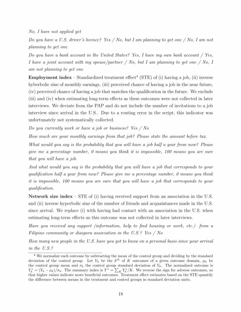
No, I have not applied yet

Do you have a U.S. driver’s licence? Yes / No, but I am planning to get one / No, I am not

planning to get one

Do you have a bank account in the United States? Yes, I have my own bank account / Yes,

I have a joint account with my spouse/partner / No, but I am planning to get one / No, I

am not planning to get one

Employment index – Standardized treatment effect4 (STE) of (i) having a job, (ii) inverse

hyberbolic sine of monthly earnings, (iii) perceived chance of having a job in the near future,

(iv) perceived chance of having a job that matches the qualification in the future. We exclude

(iii) and (iv) when estimating long-term effects as these outcomes were not collected in later

interviews. We deviate from the PAP and do not include the number of invitations to a job

interview since arrival in the U.S.. Due to a routing error in the script, this indicator was

unfortunately not systematically collected.

Do you currently work or have a job or business? Yes / No

How much are your monthly earnings from that job? Please state the amount before tax.

What would you say is the probability that you will have a job half a year from now? Please

give me a percentage number, 0 means you think it is impossible, 100 means you are sure

that you will have a job.

And what would you say is the probability that you will have a job that corresponds to your

qualification half a year from now? Please give me a percentage number, 0 means you think

it is impossible, 100 means you are sure that you will have a job that corresponds to your

qualification.

Network size index – STE of (i) having received support from an association in the U.S.

and (ii) inverse hyperbolic sine of the number of friends and acquaintances made in the U.S.

since arrival. We replace (i) with having had contact with an association in the U.S. when

estimating long-term effects as this outcome was not collected in later interviews.

Have you received any support (information, help to find housing or work, etc.) from a

Filipino community or diaspora association in the U.S.? Yes / No

How many new people in the U.S. have you got to know on a personal basis since your arrival

in the U.S.?

4 We normalize each outcome by subtracting the mean of the control group and dividing by the standarddeviation of the control group. Let Yk be the kth of K outcomes of a given outcome domain, µk bethe control group mean and σk the control group standard deviation of Yk. The normalized outcome isY ∗k = (Yk − µk)/σk. The summary index is Y ∗ =

∑K Y ∗

k /K. We reverse the sign for adverse outcomes, sothat higher values indicate more beneficial outcomes. Treatment effect estimates based on the STE quantifythe difference between means in the treatment and control groups in standard deviation units.

18

Subjective wellbeing index – STE of (i) mental wellbeing index and (ii) migrant wellbeing

index. The mental wellbeing index is the sum of five five-point items. It measures how often

during the past month the respondent (i) was happy, (ii) felt calm and peaceful, (iii) was

not very nervous, (iv) did not feel downhearted and blue, (v) did not feel so down in the

dumps that nothing could cheer her/him up. The migrant wellbeing index is the sum of two

five-point items. It measures how often during the past month the respondent did not feel

(i) homesick and (ii) overwhelmed by the challenges faced in the U.S..

During the past month, how much of the time (i) were you a happy person, (ii) did you feel

calm and peaceful, (iii) were you a very nervous person, (iv) did you feel down-hearted and

blue, (v) did you feel so down in the dumps that nothing could cheer you up, (vi) did you

feel homesick, (vii) did you feel overwhelmed by the challenges you face in the U.S.? None

of the time / A little of the time / Some of the time / Most of the time / All of the time

D Multiple Hypothesis Testing

We estimate treatment effects using variants of the following regression specification:

Yi,k = β0 + β1Di,1 + . . .+ βLDi,L + X′iθ + ui,k, (D.4)

where Yi,k denotes the kth outcome of interest for the ith unit, Di,1 . . . Di,L the independent

variables of interest (treatments), β1 . . . βL the parameters of interest and Xi a set of further

independent variables (baseline covariates). We might further estimate these parameters in

subgroups formed by the values of variables Zi. Note that the set of variables in Xi and Zi

might be overlapping. Testing multiple hypotheses simultaneously arises due to investigating

the effects on multiple outcomes of interest, the effects of multiple independent variables of

interest (in the same regression specification or in different ones), the effects in multiple

subgroups, or any combination thereof. In other words, we make simultaneous inference on

the elements of a parameter vector β = (β1, ..., βS) with individual null hypothesis of the

form HS : βs = 0. In these situations, we want to control for the familywise error rate

(FWER) – the probability of one or more false rejections.

List, Shaikh and Xu (2019) provide a bootstrap-based stepwise procedure for simultaneously

testing null hypotheses from settings with multiple outcomes, treatments, and subgroups.

The procedure is based on the results in Romano and Wolf (2010). It asymptotically con-

trols the FWER and is asymptotically balanced in that the marginal probabilities of rejecting

true null hypotheses are approximately equal in large samples. Information about the de-

pendence structure between hypotheses yields greater statistical power to reject truly false

19

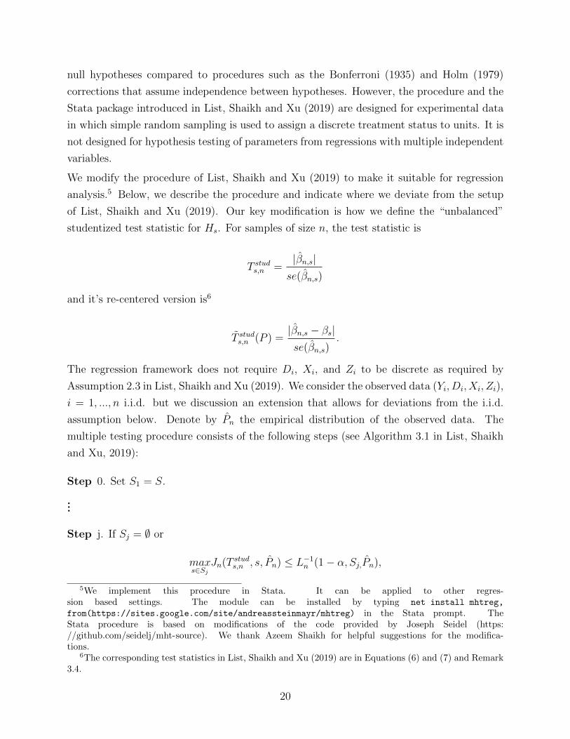
null hypotheses compared to procedures such as the Bonferroni (1935) and Holm (1979)

corrections that assume independence between hypotheses. However, the procedure and the

Stata package introduced in List, Shaikh and Xu (2019) are designed for experimental data

in which simple random sampling is used to assign a discrete treatment status to units. It is

not designed for hypothesis testing of parameters from regressions with multiple independent

variables.

We modify the procedure of List, Shaikh and Xu (2019) to make it suitable for regression

analysis.5 Below, we describe the procedure and indicate where we deviate from the setup

of List, Shaikh and Xu (2019). Our key modification is how we define the “unbalanced”

studentized test statistic for Hs. For samples of size n, the test statistic is

T studs,n =|βn,s|se(βn,s)

and it’s re-centered version is6

T studs,n (P ) =|βn,s − βs|se(βn,s)

.

The regression framework does not require Di, Xi, and Zi to be discrete as required by

Assumption 2.3 in List, Shaikh and Xu (2019). We consider the observed data (Yi, Di, Xi, Zi),

i = 1, ..., n i.i.d. but we discussion an extension that allows for deviations from the i.i.d.

assumption below. Denote by Pn the empirical distribution of the observed data. The

multiple testing procedure consists of the following steps (see Algorithm 3.1 in List, Shaikh

and Xu, 2019):

Step 0. Set S1 = S.

...

Step j. If Sj = ∅ or

maxs∈Sj

Jn(T studs,n , s, Pn) ≤ L−1n (1− α, Sj,Pn),

5We implement this procedure in Stata. It can be applied to other regres-sion based settings. The module can be installed by typing net install mhtreg,

from(https://sites.google.com/site/andreassteinmayr/mhtreg) in the Stata prompt. TheStata procedure is based on modifications of the code provided by Joseph Seidel (https://github.com/seidelj/mht-source). We thank Azeem Shaikh for helpful suggestions for the modifica-tions.

6The corresponding test statistics in List, Shaikh and Xu (2019) are in Equations (6) and (7) and Remark3.4.

20

then stop. Otherwise reject any Hs with Jn(T studs,n , s, Pn) > L−1n (1− α, Sj, Pn), set

Sj+1 = {s∈Sj : Jn(T studs,n , s, Pn) ≤ L−1n (1− α, Sj, Pn)},

and continue to the next step....

The adjusted p-value for HS, padjs,n can be computed as the smallest value of α for which HS

is rejected in Algorithm 3.1. Furthermore, the procedure allows calculating an unadjusted

bootstrap p-value for HS, ps,n = 1− Jn(Ts,n, s, Pn).

We use bootstrap resamples to approximates,n

J n(x, s, Pn) and Ln(x, S ′, Pn). For b = 1, ..., B

draw a sample of size n from Pn and denote by T ∗,b,studs,n (Pn) the quantity T studs,n (Pn) using the

bth resample and Pn as an estimate of P . In our modified version this is

T ∗,b,studs,n (Pn) =|β∗,bn,s − βn,s|se(β∗,bn,s)

We approximates,n

J n(x, s, Pn) as

Jn(x, s, Pn) =1

B

∑1≤b≤B

I{T ∗,b,studs,n (Pn) ≤ x}

and Ln(x, S ′, Pn) as

Ln(x, S ′, Pn) =1

B

∑1≤b≤B

I{maxs∈S′

Jn(T ∗,b,studs,n (Pn), s, Pn) ≤ x}.

Simulations

To evaluate the algorithm in terms of correct rejection rates and statistical power, we run

a set of simulations based on different data-generating processes (DGP).7 Let µ be a ten-

dimensional vector of zeros (0, 0, ..., 0)′. Let I be a 10×10 identity matrix. Let Σ be a 10×10

covariance matrix where all off-diagonal elements are equal to 0.9. Let D = 1[N (0, 1) > 0]

be a binary indicator equal to one with probability 0.5 for all scenarios except scenario five.

The data-generating processes for each simulations are:

1. Normal i.i.d errors (ten outcomes)

7We base the structure of these simulations on similar simulations for a multiple-hypothesis procedurebased on Westfall and Young (1993) in the Appendix C of Jones, Molitor and Reif (2019).

21

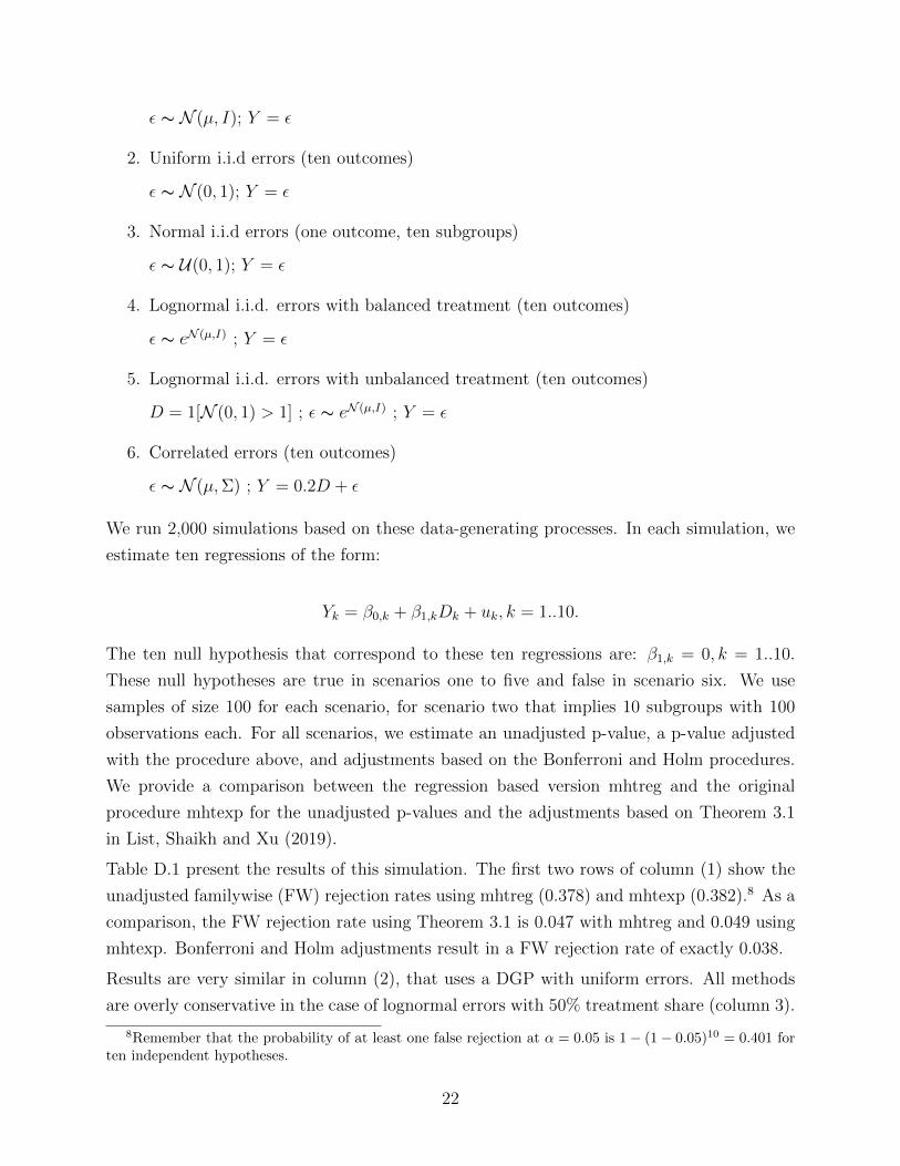
ε ∼ N (µ, I); Y = ε

2. Uniform i.i.d errors (ten outcomes)

ε ∼ N (0, 1); Y = ε

3. Normal i.i.d errors (one outcome, ten subgroups)

ε ∼ U(0, 1); Y = ε

4. Lognormal i.i.d. errors with balanced treatment (ten outcomes)

ε ∼ eN (µ,I) ; Y = ε

5. Lognormal i.i.d. errors with unbalanced treatment (ten outcomes)

D = 1[N (0, 1) > 1] ; ε ∼ eN (µ,I) ; Y = ε

6. Correlated errors (ten outcomes)

ε ∼ N (µ,Σ) ; Y = 0.2D + ε

We run 2,000 simulations based on these data-generating processes. In each simulation, we

estimate ten regressions of the form:

Yk = β0,k + β1,kDk + uk, k = 1..10.

The ten null hypothesis that correspond to these ten regressions are: β1,k = 0, k = 1..10.

These null hypotheses are true in scenarios one to five and false in scenario six. We use

samples of size 100 for each scenario, for scenario two that implies 10 subgroups with 100

observations each. For all scenarios, we estimate an unadjusted p-value, a p-value adjusted

with the procedure above, and adjustments based on the Bonferroni and Holm procedures.

We provide a comparison between the regression based version mhtreg and the original

procedure mhtexp for the unadjusted p-values and the adjustments based on Theorem 3.1

in List, Shaikh and Xu (2019).

Table D.1 present the results of this simulation. The first two rows of column (1) show the

unadjusted familywise (FW) rejection rates using mhtreg (0.378) and mhtexp (0.382).8 As a

comparison, the FW rejection rate using Theorem 3.1 is 0.047 with mhtreg and 0.049 using

mhtexp. Bonferroni and Holm adjustments result in a FW rejection rate of exactly 0.038.

Results are very similar in column (2), that uses a DGP with uniform errors. All methods

are overly conservative in the case of lognormal errors with 50% treatment share (column 3).

8Remember that the probability of at least one false rejection at α = 0.05 is 1− (1− 0.05)10 = 0.401 forten independent hypotheses.

22

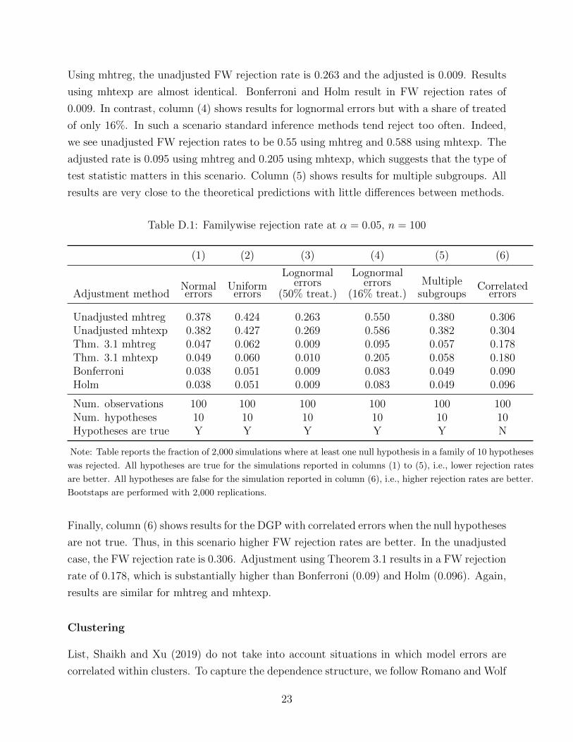
Using mhtreg, the unadjusted FW rejection rate is 0.263 and the adjusted is 0.009. Results

using mhtexp are almost identical. Bonferroni and Holm result in FW rejection rates of

0.009. In contrast, column (4) shows results for lognormal errors but with a share of treated

of only 16%. In such a scenario standard inference methods tend reject too often. Indeed,

we see unadjusted FW rejection rates to be 0.55 using mhtreg and 0.588 using mhtexp. The

adjusted rate is 0.095 using mhtreg and 0.205 using mhtexp, which suggests that the type of

test statistic matters in this scenario. Column (5) shows results for multiple subgroups. All

results are very close to the theoretical predictions with little differences between methods.

Table D.1: Familywise rejection rate at α = 0.05, n = 100

(1) (2) (3) (4) (5) (6)

Adjustment methodNormalerrors

Uniformerrors

Lognormalerrors

(50% treat.)

Lognormalerrors

(16% treat.)Multiple

subgroupsCorrelated

errors

Unadjusted mhtreg 0.378 0.424 0.263 0.550 0.380 0.306Unadjusted mhtexp 0.382 0.427 0.269 0.586 0.382 0.304Thm. 3.1 mhtreg 0.047 0.062 0.009 0.095 0.057 0.178Thm. 3.1 mhtexp 0.049 0.060 0.010 0.205 0.058 0.180Bonferroni 0.038 0.051 0.009 0.083 0.049 0.090Holm 0.038 0.051 0.009 0.083 0.049 0.096

Num. observations 100 100 100 100 100 100Num. hypotheses 10 10 10 10 10 10Hypotheses are true Y Y Y Y Y N

Note: Table reports the fraction of 2,000 simulations where at least one null hypothesis in a family of 10 hypotheses

was rejected. All hypotheses are true for the simulations reported in columns (1) to (5), i.e., lower rejection rates

are better. All hypotheses are false for the simulation reported in column (6), i.e., higher rejection rates are better.

Bootstaps are performed with 2,000 replications.

Finally, column (6) shows results for the DGP with correlated errors when the null hypotheses

are not true. Thus, in this scenario higher FW rejection rates are better. In the unadjusted

case, the FW rejection rate is 0.306. Adjustment using Theorem 3.1 results in a FW rejection

rate of 0.178, which is substantially higher than Bonferroni (0.09) and Holm (0.096). Again,

results are similar for mhtreg and mhtexp.

Clustering

List, Shaikh and Xu (2019) do not take into account situations in which model errors are

correlated within clusters. To capture the dependence structure, we follow Romano and Wolf

23

(2010) who suggest using a block bootstrap in such situations. In addition, we allow the test

statistics to be computed with cluster-robust standard errors. We also allow using a com-

bination of the two strategies. The option cluster(cluster id) of the mhtreg command

identifies the cluster variable. The option cltype(t) specifies the type of clustering. Value

t=0 specifies no clustering at all, t=1 specifies the use of a clustered bootstrap, t=2 specifies

the use of cluster-robust standard errors for the model, and t=3 specifies the use of both.

We run a simulation to evaluate the performance of the different types of clustering. Again,

let µ be a ten-dimensional zero vector (0, 0, ..., 0)′, and let I be a 10 × 10 identity matrix.

The data-generating process for this simulation scenario is

1. Errors correlated within clusters (ten outcomes)

c = 1...100 clusters

i = 1...10 observations within clusters

ηc ∼ N (µ, I)

εci ∼ N (µ, I)

Yci = ηc + εci

We again simulate 2,000 datasets. In each simulation, we estimated the following ten regres-

sions:

Yk,ci = β0,k + β1,kDc + uk,ci, k = 1..10.

where the dummy variable Dc = 1[N (µ, I) > 0] varies only at the level of clusters.

Column (1) of Table D.2 shows the results without accounting for clustering. In the unad-

justed case, at least one out of ten hypotheses is rejected almost every time (0.993). The

adjustment methods also result in rejection proportions of more than 90%. Column (2) shows

results when a clustered bootstrap is used but model standard errors are not adjusted. FW

rejection rates are close to the theoretical predictions, 0.416 in the unadjusted case, 0.065

with Theorem 3.1 adjustment, and 0.058 using Bonferroni or Holm. Column (3) uses a non-

clustered bootstrap but cluster-robust model standard errors. Again, results are close to the

theoretical predictions with slightly smaller FW rejections rates. Finally, column (4) uses a

clustered bootstrap and cluster-robust model standard errors, which again delivers results

close to the theoretical predictions.

While it does not seem to make a difference, we use the double-clustering as presented in

column (4) for results where clustering appears to be appropriate.

24

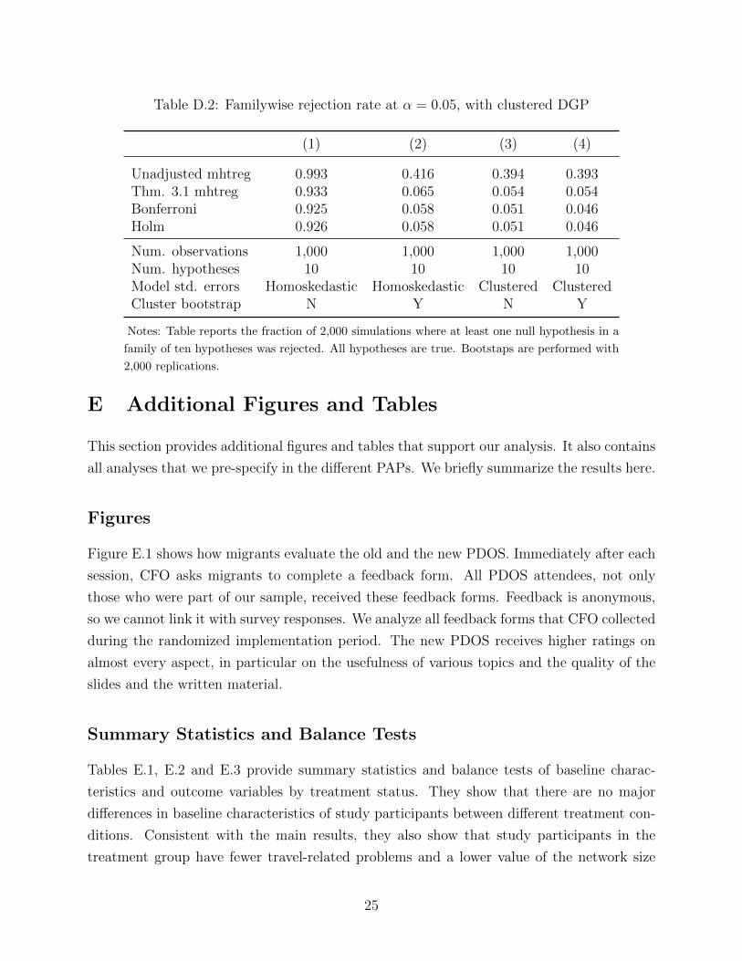
Table D.2: Familywise rejection rate at α = 0.05, with clustered DGP

(1) (2) (3) (4)

Unadjusted mhtreg 0.993 0.416 0.394 0.393Thm. 3.1 mhtreg 0.933 0.065 0.054 0.054Bonferroni 0.925 0.058 0.051 0.046Holm 0.926 0.058 0.051 0.046

Num. observations 1,000 1,000 1,000 1,000Num. hypotheses 10 10 10 10Model std. errors Homoskedastic Homoskedastic Clustered ClusteredCluster bootstrap N Y N Y

Notes: Table reports the fraction of 2,000 simulations where at least one null hypothesis in a

family of ten hypotheses was rejected. All hypotheses are true. Bootstaps are performed with

2,000 replications.

E Additional Figures and Tables

This section provides additional figures and tables that support our analysis. It also contains

all analyses that we pre-specify in the different PAPs. We briefly summarize the results here.

Figures

Figure E.1 shows how migrants evaluate the old and the new PDOS. Immediately after each

session, CFO asks migrants to complete a feedback form. All PDOS attendees, not only

those who were part of our sample, received these feedback forms. Feedback is anonymous,

so we cannot link it with survey responses. We analyze all feedback forms that CFO collected

during the randomized implementation period. The new PDOS receives higher ratings on

almost every aspect, in particular on the usefulness of various topics and the quality of the

slides and the written material.

Summary Statistics and Balance Tests

Tables E.1, E.2 and E.3 provide summary statistics and balance tests of baseline charac-

teristics and outcome variables by treatment status. They show that there are no major

differences in baseline characteristics of study participants between different treatment con-

ditions. Consistent with the main results, they also show that study participants in the

treatment group have fewer travel-related problems and a lower value of the network size

25

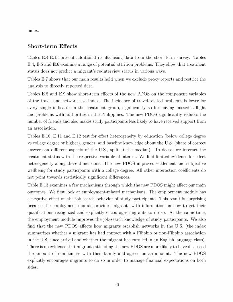
index.

Short-term Effects

Tables E.4-E.13 present additional results using data from the short-term survey. Tables

E.4, E.5 and E.6 examine a range of potential attrition problems. They show that treatment

status does not predict a migrant’s re-interview status in various ways.

Tables E.7 shows that our main results hold when we exclude proxy reports and restrict the

analysis to directly reported data.

Tables E.8 and E.9 show short-term effects of the new PDOS on the component variables

of the travel and network size index. The incidence of travel-related problems is lower for

every single indicator in the treatment group, significantly so for having missed a flight

and problems with authorities in the Philippines. The new PDOS significantly reduces the

number of friends and also makes study participants less likely to have received support from

an association.

Tables E.10, E.11 and E.12 test for effect heterogeneity by education (below college degree

vs college degree or higher), gender, and baseline knowledge about the U.S. (share of correct

answers on different aspects of the U.S., split at the median). To do so, we interact the

treatment status with the respective variable of interest. We find limited evidence for effect

heterogeneity along these dimensions. The new PDOS improves settlement and subjective

wellbeing for study participants with a college degree. All other interaction coefficients do

not point towards statistically significant differences.

Table E.13 examines a few mechanisms through which the new PDOS might affect our main

outcomes. We first look at employment-related mechanisms. The employment module has

a negative effect on the job-search behavior of study participants. This result is surprising

because the employment module provides migrants with information on how to get their

qualifications recognized and explicitly encourages migrants to do so. At the same time,

the employment module improves the job-search knowledge of study participants. We also

find that the new PDOS affects how migrants establish networks in the U.S. (the index

summarizes whether a migrant has had contact with a Filipino or non-Filipino association

in the U.S. since arrival and whether the migrant has enrolled in an English language class).

There is no evidence that migrants attending the new PDOS are more likely to have discussed

the amount of remittances with their family and agreed on an amount. The new PDOS

explicitly encourages migrants to do so in order to manage financial expectations on both

sides.

26

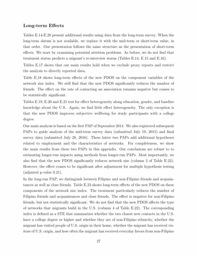
Long-term Effects

Tables E.14-E.28 present additional results using data from the long-term survey. When the

long-term datum is not available, we replace it with the mid-term or short-term value, in

that order. Our presentation follows the same structure as the presentation of short-term

effects. We start by examining potential attrition problems. As before, we do not find that

treatment status predicts a migrant’s re-interview status (Tables E.14, E.15 and E.16).

Tables E.17 shows that our main results hold when we exclude proxy reports and restrict

the analysis to directly reported data.

Table E.18 shows long-term effects of the new PDOS on the component variables of the

network size index. We still find that the new PDOS significantly reduces the number of

friends. The effect on the rate of contacting an association remains negative but ceases to

be statistically significant.

Tables E.19, E.20 and E.21 test for effect heterogeneity along education, gender, and baseline

knowledge about the U.S.. Again, we find little effect heterogeneity. The only exception is

that the new PDOS improves subjective wellbeing for study participants with a college

degree.

Our main analysis is based on the first PAP of September 2014. We also registered subsequent

PAPs to guide analysis of the mid-term survey data (submitted July 19, 2015) and final

survey data (submitted July 28, 2016). These latter two PAPs add additional hypotheses

related to employment and the characteristics of networks. For completeness, we show

the main results from these two PAPs in this appendix. Our conclusions are robust to to

estimating longer-run impacts using methods from longer-run PAPs. Most importantly, we

also find that the new PDOS significantly reduces network size (column 3 of Table E.22).

However, the effect ceases to be significant after adjustment for multiple hypothesis testing

(adjusted p-value 0.21).

In the long-run PAP, we distinguish between Filipino and non-Filipino friends and acquain-

tances as well as close friends. Table E.23 shows long-term effects of the new PDOS on these

components of the network size index. The treatment particularly reduces the number of

Filipino friends and acquaintances and close friends. The effect is negative for non-Filipino

friends, but not statistically significant. We do not find that the new PDOS affects the type

of networks that migrants build in the U.S. (column 4 of Table E.22). The corresponding

index is defined as a STE that summarizes whether the two closest new contacts in the U.S.

have a college degree or higher and whether they are of non-Filipino ethnicity, whether the

migrant has visited people of U.S. origin in their home, whether the migrant has received vis-

itors of U.S. origin, and how often the migrant has received everyday favors from non-Filipino

27

individuals. Similarly, the new PDOS has no effect on any other outcome domain.

Table E.25 tests for spillover effects on family members in the Philippines. We look at a range

of outcomes: (i) an index that summarizes the respondents’ perceived situation of the migrant

in the U.S. in terms of meeting new people, social life, language skills, employment, degree

recognition, adjusting to culture in the U.S., adjusting to weather in the U.S., dealing with

U.S. authorities, housing, and finances, (ii) family members’ intention to travel to the U.S.,

(iii) family members’ intention to emigrate to the U.S., (iv) respondents’ perception that it

would be good for young household members to live in the U.S., (v) respondents’ perceived

ease of living and finding a job in the U.S. her/himself, (vi) an index that summarizes

respondents’ perceived effect of migrant’s emigration on the household in terms of financial

security, standard of living, housing, health, education, family life, social life, and social

status, (vii) the inverse hyperbolic sine amount of remittances received by the household.

We find no evidence for spillover effects.

Table E.26 looks at secondary outcomes and mechanisms. It shows that the new PDOS, with

or without employment module, does not affect the use of welfare programs in the U.S. or

employment quality. There is also no evidence that the treatment helps migrants to initiate

and complete the process of having their qualifications recognized.

Finally, we present results using data from the mid-term survey, following the short-term

PAP (Table E.27) and the medium-term PAP (E.28). When the medium-term datum is

not available, we replace it with the mid-term value. As before, we find that the new

PDOS significantly reduces network size. However, the effect ceases to be significant after

adjustment for multiple hypothesis testing.

28

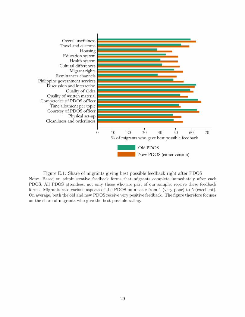
0 10 20 30 40 50 60 70% of migrants who gave best possible feedback

Cleanliness and orderlinessPhysical set-up

Courtesy of PDOS officerTime allotment per topic

Competence of PDOS officerQuality of written material

Quality of slidesDiscussion and interaction

Philippine government servicesRemittances channels

Migrant rightsCultural differences

Health systemEducation system

HousingTravel and customs

Overall usefulness

Old PDOSNew PDOS (either version)

Figure E.1: Share of migrants giving best possible feedback right after PDOSNote: Based on administrative feedback forms that migrants complete immediately after eachPDOS. All PDOS attendees, not only those who are part of our sample, receive these feedbackforms. Migrants rate various aspects of the PDOS on a scale from 1 (very poor) to 5 (excellent).On average, both the old and new PDOS receive very positive feedback. The figure therefore focuseson the share of migrants who give the best possible rating.

29

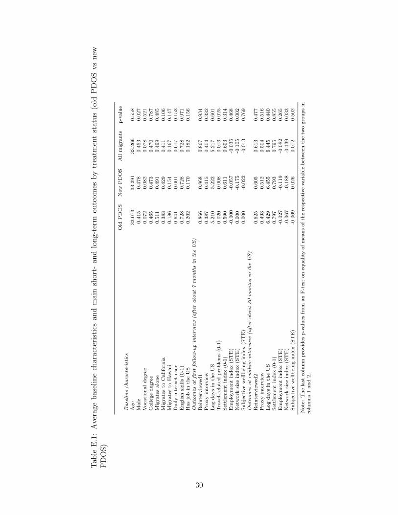
Tab

leE

.1:

Ave

rage

bas

elin

ech

arac

teri

stic

san

dm

ain

shor

t-an

dlo

ng-

term

outc

omes

by

trea

tmen

tst

atus

(old

PD

OS

vs

new

PD

OS)

Old

PD

OS

New

PD

OS

All

mig

rants

p-v

alu

eB

ase

lin

ech

ara

cter

isti

csA

ge

33.0

73

33.3

91

33.2

66

0.5

58

Male

0.4

15

0.4

78

0.4

53

0.0

27

Voca

tion

al

deg

ree

0.0

72

0.0

82

0.0

78

0.5

21

Colleg

ed

egre

e0.4

65

0.4

73

0.4

70

0.7

87

Mig

rate

salo

ne

0.5

11

0.4

91

0.4

99

0.4

85

Mig

rate

sto

Califo

rnia

0.3

83

0.4

29

0.4

11

0.1

06

Mig

rate

sto

Haw

aii

0.1

86

0.1

54

0.1

67

0.1

47

Daily

inte

rnet

use

r0.6

41

0.6

01

0.6

17

0.1

53

En

glish

skills

(0-1

)0.7

28

0.7

28

0.7

28

0.9

71

Has

job

inth

eU

S0.2

02

0.1

70

0.1

82

0.1

56

Ou

tco

mes

at

firs

tfo

llo

w-u

pin

terv

iew

(aft

era

bou

t7

mo

nth

sin

the

US

)R

einte

rvie

wed

10.8

66

0.8

68

0.8

67

0.9

34

Pro

xy

inte

rvie

w0.3

87

0.4

15

0.4

04

0.3

32

Log

days

inth

eU

S5.2

10

5.2

22

5.2

17

0.6

01

Tra

vel

-rel

ate

dp

rob

lem

s(0

-1)

0.0

20

0.0

08

0.0

13

0.0

25

Set

tlem

ent

ind

ex(0

-1)

0.5

90

0.6

11

0.6

03

0.3

14

Em

plo

ym

ent

ind

ex(S

TE

)-0

.000

-0.0

57

-0.0

35

0.4

68

Net

work

size

ind

ex(S

TE

)0.0

00

-0.1

75

-0.1

05

0.0

02

Su

bje

ctiv

ew

ellb

ein

gin

dex

(ST

E)

0.0

00

-0.0

22

-0.0

13

0.7

69

Ou

tco

mes

at

end

lin

ein

terv

iew

(aft

era

bou

t3

0m

on

ths

inth

eU

S)

Rei

nte

rvie

wed

20.6

25

0.6

05

0.6

13

0.4

77

Pro

xy

inte

rvie

w0.4

93

0.5

12

0.5

04

0.5

16

Log

days

inth

eU

S6.4

29

6.4

55

6.4

45

0.4

40

Set

tlem

ent

ind

ex(0

-1)

0.7

97

0.7

93

0.7

95

0.8

55

Em

plo

ym

ent

ind

ex(S

TE

)-0

.027

-0.1

19

-0.0

82

0.2

65

Net

work

size

ind

ex(S

TE

)-0

.067

-0.1

88

-0.1

39

0.0

33

Su

bje

ctiv

ew

ellb

ein

gin

dex

(ST

E)

-0.0

09

0.0

26

0.0

12

0.5

02

Note

:T

he

last

colu

mn

pro

vid

esp

-valu

esfr

om

an

F-t

est

on

equ

ality

of

mea

ns

of

the

resp

ecti

ve

vari

ab

leb

etw

een

the

two

gro

up

sin

colu

mn

s1

an

d2.

30

Tab

leE

.2:

Ave

rage

bas

elin

ech

arac

teri

stic

san

dm

ain

shor

t-te

rman

dlo

ng-

term

outc

omes

by

trea

tmen

tst

atus

(old

PD

OS

vs

new

PD

OS

wit

han

dw

ithou

tem

plo

ym

ent

module

)

Old

PD

OS

New

PD

OS

wit

hem

pm

odu

leN

ewP

DO

Sw

ith

ou

tem

pm

od

ule

All

mig

rants

p-v

alu

eB

ase

lin

ech

ara

cter

isti

csA

ge

33.0

73

33.1

93

33.6

20

33.2

66

0.7

04

Male

0.4

15

0.4

67

0.4

90

0.4

53

0.0

72

Voca

tion

al

deg

ree

0.0

72

0.0

70

0.0

95

0.0

78

0.4

08

Colleg

ed

egre

e0.4

65

0.5

04

0.4

37

0.4

70

0.1

77

Mig

rate

salo

ne

0.5

11

0.5

21

0.4

57

0.4

99

0.1

64

Mig

rate

sto

Califo

rnia

0.3

83

0.4

24

0.4

35

0.4

11

0.2

58

Mig

rate

sto

Haw

aii

0.1

86

0.1

43

0.1

67

0.1

67

0.2

16

Daily

inte

rnet

use

r0.6

41

0.6

03

0.5

99

0.6

17

0.3

59

En

glish

skills

(0-1

)0.7

28

0.7

36

0.7

19

0.7

28

0.3

64

Has

job

inth

eU

S0.2

02

0.1

74

0.1

64

0.1

82

0.3

39

Ou

tco

mes

at

firs

tfo

llo

w-u

pin

terv

iew

(aft

era

bou

t7

mo

nth

sin

the

US

)R

einte

rvie

wed

10.8

66

0.8

50

0.8

89

0.8

67

0.2

73

Pro

xy

inte

rvie

w0.3

87

0.3

97

0.4

35

0.4

04

0.3

62

Log

days

inth

eU

S5.2

10

5.2

06

5.2

38

5.2

17

0.4

22

Tra

vel

-rel

ate

dp

rob

lem

s(0

-1)

0.0

20

0.0

07

0.0

10

0.0

13

0.0

73

Set

tlem

ent

ind

ex(0

-1)

0.5

90

0.6

10

0.6

12

0.6

03

0.6

02

Em

plo

ym

ent

ind

ex(S

TE

)-0

.000

-0.0

96

-0.0

14

-0.0

35

0.5

27

Net

work

size

ind

ex(S

TE

)0.0

00

-0.1

50

-0.2

04

-0.1

05

0.0

04

Su

bje

ctiv

ew

ellb

ein

gin

dex

(ST

E)

0.0

00

-0.0

58

0.0

19

-0.0

13

0.6

97

Ou

tco

mes

at

end

lin

ein

terv

iew

(aft

era

bou

t3

0m

on

ths

inth

eU

S)

Rei

nte

rvie

wed

20.6

25

0.5

88

0.6

24

0.6

13

0.4

70

Pro

xy

inte

rvie

w0.4

93

0.5

08

0.5

15

0.5

04

0.7

96

Log

days

inth

eU

S6.4

29

6.4

39

6.4

73

6.4

45

0.5

21

Set

tlem

ent

ind

ex(0

-1)

0.7

97

0.8

03

0.7

82

0.7

95

0.6

54

Em

plo

ym

ent

ind

ex(S

TE

)-0

.027

-0.1

46

-0.0

90

-0.0

82

0.4

74

Net

work

size

ind

ex(S

TE

)-0

.067

-0.1

62

-0.2

18

-0.1

39

0.0

63

Su

bje

ctiv

ew

ellb

ein

gin

dex

(ST

E)

-0.0

09

0.0

30

0.0

22

0.0

12

0.7

88

Note

:T

he

last

colu

mn

pro

vid

esp

-valu

esfr

om

an

F-t

est

on

equ

ality

of

mea

ns

of

the

resp

ecti

ve

vari

ab

leb

etw

een

the

thre

egro

up

sin

colu

mn

s1-3

.

31

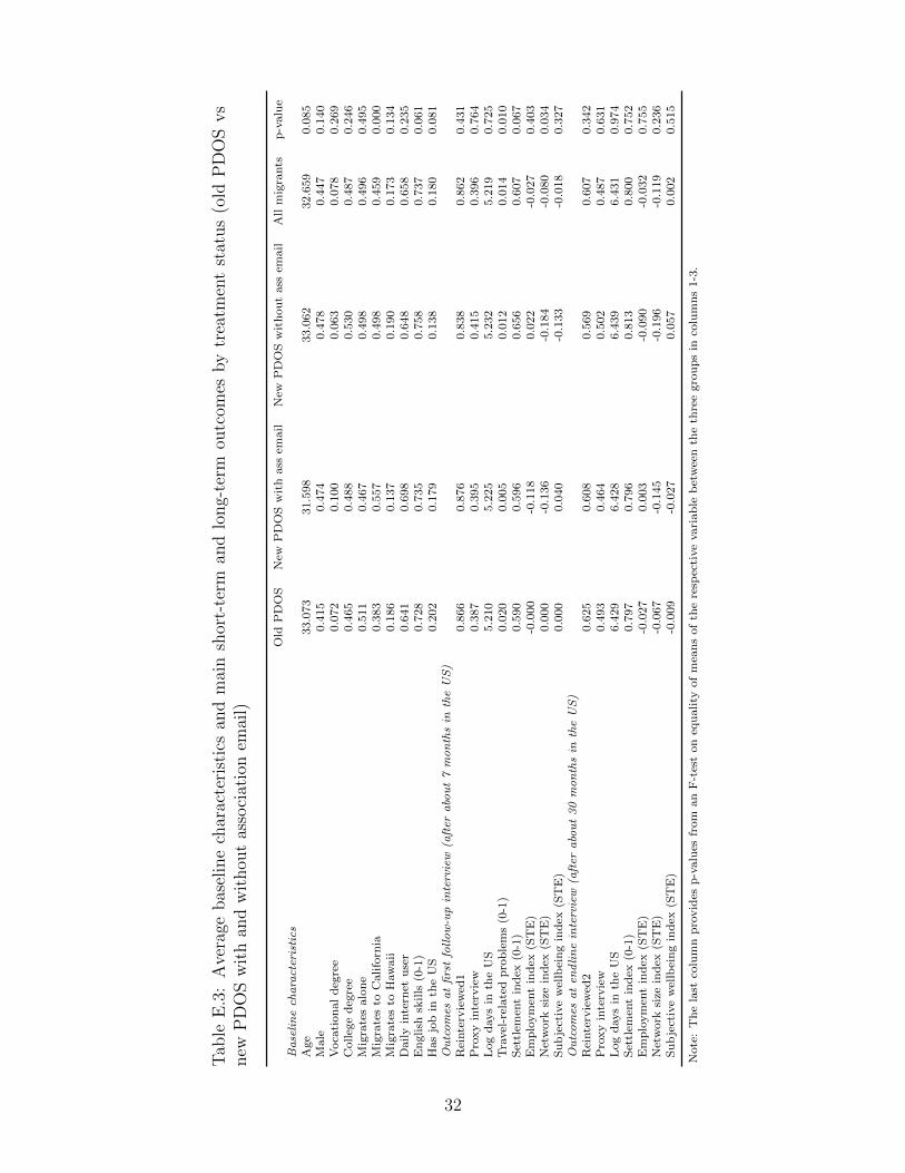
Tab

leE

.3:

Ave

rage

bas

elin

ech

arac

teri

stic

san

dm

ain

shor

t-te

rman

dlo

ng-

term

outc

omes

by

trea

tmen

tst

atus

(old

PD

OS

vs

new

PD

OS

wit

han

dw

ithou

tas

soci

atio

nem

ail)

Old

PD

OS

New

PD

OS

wit

hass

email

New

PD

OS

wit

hou

tass

email

All

mig

rants

p-v

alu

eB

ase

lin

ech

ara

cter

isti

csA

ge

33.0

73

31.5

98

33.0

62

32.6

59

0.0

85

Male

0.4

15

0.4

74

0.4

78

0.4

47

0.1

40

Voca

tion

al

deg

ree

0.0

72

0.1

00

0.0

63

0.0

78

0.2

69

Colleg

ed

egre

e0.4

65

0.4

88

0.5

30

0.4

87

0.2

46

Mig

rate

salo

ne

0.5

11

0.4

67

0.4

98

0.4

96

0.4

95

Mig

rate

sto

Califo

rnia

0.3

83

0.5

57

0.4

98

0.4

59

0.0

00

Mig

rate

sto

Haw

aii

0.1

86

0.1

37

0.1

90

0.1

73

0.1

34

Daily

inte

rnet

use

r0.6

41

0.6

98

0.6

48

0.6

58

0.2

35

En

glish

skills

(0-1

)0.7

28

0.7

35

0.7

58

0.7

37

0.0

61

Has

job

inth

eU

S0.2

02

0.1

79

0.1

38

0.1

80

0.0

81

Ou

tco

mes

at

firs

tfo

llo

w-u

pin

terv

iew

(aft

era

bou

t7

mo

nth

sin

the

US

)R

einte

rvie

wed

10.8

66

0.8

76

0.8

38

0.8

62

0.4

31

Pro

xy

inte

rvie

w0.3

87

0.3

95

0.4

15

0.3

96

0.7

64

Log

days

inth

eU

S5.2

10

5.2

25

5.2

32

5.2

19

0.7

25

Tra

vel

-rel

ate

dp

rob

lem

s(0

-1)

0.0

20

0.0

05

0.0

12

0.0

14

0.0

10

Set

tlem

ent

ind

ex(0

-1)

0.5

90

0.5

96

0.6

56

0.6

07

0.0

67

Em

plo

ym

ent

ind

ex(S

TE

)-0

.000

-0.1

18

0.0

22

-0.0

27

0.4

03

Net

work

size

ind

ex(S

TE

)0.0

00

-0.1

36

-0.1

84

-0.0

80

0.0

34

Su

bje

ctiv

ew

ellb

ein

gin

dex

(ST

E)

0.0

00

0.0

40

-0.1

33

-0.0

18

0.3

27

Ou

tco

mes

at

end

lin

ein

terv

iew

(aft

era

bou

t3

0m

on

ths

inth

eU

S)

Rei

nte

rvie

wed

20.6

25

0.6

08

0.5

69

0.6

07

0.3

42

Pro

xy

inte

rvie

w0.4

93

0.4

64

0.5

02

0.4

87

0.6

31

Log

days

inth

eU

S6.4

29

6.4

28

6.4

39

6.4

31

0.9

74

Set

tlem

ent

ind

ex(0

-1)

0.7

97

0.7

96

0.8

13

0.8

00

0.7

52

Em

plo

ym

ent

ind

ex(S

TE

)-0

.027

0.0

03

-0.0

90

-0.0

32

0.7

55

Net

work

size

ind

ex(S

TE

)-0

.067

-0.1

45

-0.1

96

-0.1

19

0.2

36

Su

bje

ctiv

ew

ellb

ein

gin

dex

(ST

E)

-0.0

09

-0.0

27

0.0

57

0.0

02

0.5

15

Note

:T

he

last

colu

mn

pro

vid

esp

-valu

esfr

om

an

F-t

est

on

equ

ality

of

mea

ns

of

the

resp

ecti

ve

vari

ab

leb

etw

een

the

thre

egro

up

sin

colu

mn

s1-3

.

32

Tab

leE

.4:

Fir

stfo

llow

-up

inte

rvie

w:

Att

riti

onan

dm

ode

ofre

-inte

rvie

w

(1)

(2)

(3)

(4)

(5)

(6)

(7)

(8)

(9)

Su

cces

sfu

lre

-inte

rvie

wS

ucc

essf

ul

re-i

nte

rvie

wS

ucc

essf

ul

re-i

nte

rvie

wD

irec

tre

-inte

rvie

wD

irec

tre

-inte

rvie

wD

irec

tre

-inte

rvie

wP

roxy

re-i

nte

rvie

wP

roxy

re-i

nte

rvie

wP

roxy

re-i

nte

rvie

w

New

PD

OS

(eit

her

0.0

01

0.0

19

-0.0

30

-0.0

25

-0.0

47

-0.0

34

0.0

25

0.0

47

0.0

34

ver

sion

)(0

.021)

(0.0

24)

(0.0

27)

(0.0

28)

(0.0

35)

(0.0

41)

(0.0

28)

(0.0

35)

(0.0

41)

New

PD

OS

wit

hem

p.

-0.0

34

0.0

42

-0.0

42

mod

ule

(0.0

29)

(0.0

39)

(0.0

39)

New

PD

OS

wit

hass

.0.0

33

0.0

28

-0.0

28

email

(0.0

27)

(0.0

37)

(0.0

37)

Age

-0.0

04

-0.0

04

-0.0

15

0.0

09

0.0

09

0.0

08

-0.0

09

-0.0

09

-0.0

08

(0.0

08)

(0.0

08)

(0.0

11)

(0.0

13)

(0.0

13)

(0.0

14)

(0.0

13)

(0.0

13)

(0.0

14)

Age

squ

are

d0.0

00

0.0

00

0.0

00

-0.0

00

-0.0

00

-0.0

00

0.0

00

0.0

00

0.0

00

(0.0

00)

(0.0

00)

(0.0

00)

(0.0

00)

(0.0

00)

(0.0

00)

(0.0

00)

(0.0

00)

(0.0

00)

Male

-0.0

02

-0.0

03

-0.0

02

0.0

01

0.0

02

-0.0

00

-0.0

01

-0.0

02

0.0

00

(0.0

18)

(0.0

18)

(0.0

22)

(0.0

29)

(0.0

29)

(0.0

33)

(0.0

29)

(0.0

29)

(0.0

33)

Voca

tion

al

edu

cati

on

0.0

61∗∗

0.0

60∗∗

0.1

19∗∗∗

-0.0

23

-0.0

21

-0.0

47

0.0

23

0.0

21

0.0

47

(0.0

29)

(0.0

29)

(0.0

26)

(0.0

55)

(0.0

55)

(0.0

61)

(0.0

55)

(0.0

55)

(0.0

61)

Colleg

eed

uca

tion

0.0

06

0.0

07

0.0

19

-0.0

08

-0.0

09

0.0

08

0.0

08

0.0

09

-0.0

08

(0.0

22)

(0.0

22)

(0.0

26)

(0.0

31)

(0.0

31)

(0.0

35)

(0.0

31)

(0.0

31)

(0.0

35)

Mig

rate

salo

ne

-0.0

15

-0.0

14

-0.0

22

-0.0

15

-0.0

16

-0.0

23

0.0

15

0.0

16

0.0

23

(0.0

18)

(0.0

18)

(0.0

23)

(0.0

25)

(0.0

25)

(0.0

31)

(0.0

25)

(0.0

25)

(0.0

31)

Califo

rnia

0.0

02

0.0

02

0.0

19

0.0

11

0.0

12

0.0

16

-0.0

11

-0.0

12

-0.0

16

(0.0

21)

(0.0

21)

(0.0

28)

(0.0

29)

(0.0

29)

(0.0

34)

(0.0

29)

(0.0

29)

(0.0

34)

Haw

aii

0.0

10

0.0

09

0.0

24

0.1

18∗∗∗

0.1

20∗∗∗

0.0

97∗∗

-0.1

18∗∗∗

-0.1

20∗∗∗

-0.0

97∗∗

(0.0

29)

(0.0

29)

(0.0

35)

(0.0

37)

(0.0

37)

(0.0

43)

(0.0

37)

(0.0

37)

(0.0

43)

Daily

inte

rnet

use

-0.0

00

-0.0

01

-0.0

04

0.0

13

0.0

13

0.0

28

-0.0

13

-0.0

13

-0.0

28

(0.0

19)

(0.0

19)

(0.0

24)

(0.0

36)

(0.0

36)

(0.0

42)

(0.0

36)

(0.0

36)

(0.0

42)

En

glish

skills

-0.0

10∗

-0.0

10∗

-0.0

10

0.0

01

0.0

00

-0.0

01

-0.0

01

-0.0

00

0.0

01

(0.0

05)

(0.0

05)

(0.0

07)

(0.0

08)

(0.0

08)

(0.0

09)

(0.0

08)

(0.0

08)

(0.0

09)

Has

job

inU

S0.0

33

0.0

33

0.0

37

-0.0

78∗

-0.0

79∗

-0.0

60

0.0

78∗

0.0

79∗

0.0

60

(0.0

27)

(0.0

27)

(0.0

34)

(0.0

40)

(0.0

40)

(0.0

50)

(0.0

40)

(0.0

40)

(0.0

50)

Con

stant

1.0

26∗∗∗

1.0

25∗∗∗

1.1

76∗∗∗

0.4

67∗∗

0.4

68∗∗

0.4

54∗

0.5

33∗∗

0.5

32∗∗

0.5

46∗∗

(0.1

50)

(0.1

50)

(0.1

93)

(0.2

16)

(0.2

15)

(0.2

53)

(0.2

16)

(0.2

15)

(0.2

53)

F-s

tati

stic

trea

tmen

tvari

ab

les=

00.0

01

0.7

58

0.9

42

0.7

54

0.9

63

0.3

96

0.7

54

0.9

63

0.3

96

p-v

alu

e0.9

75

0.4

71

0.3

93

0.3

87

0.3

85

0.6

74

0.3

87

0.3

85

0.6

74

R2

0.0

11

0.0

12

0.0

24

0.0

14

0.0

15

0.0

11

0.0

14

0.0

15

0.0

11

Ob

serv

ati

on

s1273

1273

902

1273

1273

902

1273

1273

902

Note

:T

he

tab

lere

port

sO

LS

esti

mate

s.T

he

colu

mn

titl

esh

ow

sth

ed

epen

den

tvari

ab

le.

Sta

nd

ard

erro

rscl

ust

ered

at

the

PD

OS

sess

ion

level

inp

are

nth

eses

.*/**/***

den

ote

stati

stic

al

sign

ifica

nce

at

the

10/5/1

per

cent

level

.

33

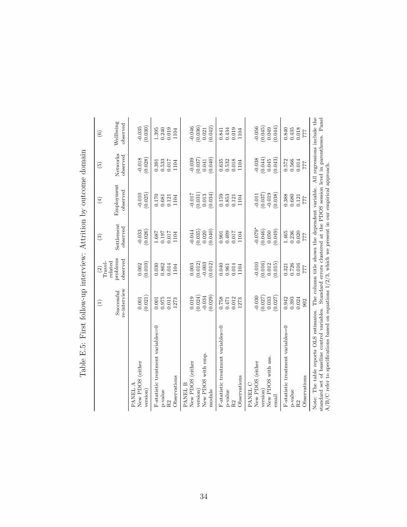
Tab

leE

.5:

Fir

stfo

llow

-up

inte

rvie

w:

Att

riti

onby

outc

ome

dom

ain

(1)

(2)

(3)

(4)

(5)

(6)

Su

cces

sfu

lre

-inte

rvie

w

Tra

vel

-re

late

dp

rob

lem

s

ob

serv

edS

ettl

emen

tob

serv

ed

Em

plo

ym

ent

ob

serv

edN

etw

ork

sob

serv

ed

Wel

lbei

ng

ob

serv

ed

PA

NE

LA

New

PD

OS

(eit

her

0.0

01

0.0

02

-0.0

33

-0.0

10

-0.0

18

-0.0

35

ver

sion

)(0

.021)

(0.0

10)

(0.0

26)

(0.0

25)

(0.0

28)

(0.0

30)

F-s

tati

stic

trea

tmen

tvari

ab

les=

00.0

01

0.0

30

1.6

87

0.1

70

0.3

91

1.3

95

p-v

alu

e0.9

75

0.8

62

0.1

97

0.6

81

0.5

33

0.2

40

R2

0.0

11

0.0

14

0.0

17

0.1

21

0.0

17

0.0

19

Ob

serv

ati

on

s1273

1104

1104

1104

1104

1104

PA

NE

LB

New

PD

OS

(eit

her

0.0

19

0.0

03

-0.0

44

-0.0

17

-0.0

39

-0.0

46

ver

sion

)(0

.024)

(0.0

12)

(0.0

35)

(0.0

31)

(0.0

37)

(0.0

36)

New

PD

OS

wit

hem

p.

-0.0

34

-0.0

03

0.0

20

0.0

13

0.0

41

0.0

21

mod

ule

(0.0

29)

(0.0

12)

(0.0

40)

(0.0

34)

(0.0

40)

(0.0

42)

F-s

tati

stic

trea

tmen

tvari

ab

les=

00.7

58

0.0

40

0.9

01

0.1

59

0.6

35

0.8

41

p-v

alu

e0.4

71

0.9

61

0.4

09

0.8

53

0.5

32

0.4

34

R2

0.0

12

0.0

14

0.0

17

0.1

21

0.0

18

0.0

19

Ob

serv

ati

on

s1273

1104

1104

1104

1104

1104

PA

NE

LC

New

PD

OS

(eit

her

-0.0

30

-0.0

10

-0.0

79∗

-0.0

11

-0.0

38

-0.0

56

ver

sion

)(0

.027)

(0.0

16)

(0.0

46)

(0.0

37)

(0.0

44)

(0.0

45)

New

PD

OS

wit

hass

.0.0

33

0.0

12

0.0

50

-0.0

19

0.0

45

0.0

49

email

(0.0

27)

(0.0

15)

(0.0

49)

(0.0

38)

(0.0

43)

(0.0

44)

F-s

tati

stic

trea

tmen

tvari

ab

les=

00.9

42

0.3

21

1.4

65

0.3

88

0.5

72

0.8

40

p-v

alu

e0.3

93

0.7

26

0.2

36

0.6

80

0.5

66

0.4

35

R2

0.0

24

0.0

16

0.0

20

0.1

21

0.0

14

0.0

18

Ob

serv

ati

on

s902

777

777

777

777

777

Note

:T

he

tab

lere

port

sO

LS

esti

mate

s.T

he

colu

mn

titl

esh

ow

sth

ed

epen

den

tvari

ab

le.

All

regre

ssio

ns

incl

ud

eth

est

an

dard

set

of

base

lin

eco

ntr

ol

vari

ab

les.

Sta

nd

ard

erro

rscl

ust

ered

at

the

PD

OS

sess

ion

level

inp

are

nth

eses

.P

an

elA

/B

/C

refe

rto

spec

ifica

tion

sb

ase

don

equ

ati

on

s1/2/3,

wh

ich

we

pre

sent

inou

rem

pir

ical

ap

pro

ach

.

34

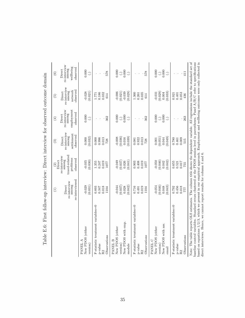
Tab

leE

.6:

Fir

stfo

llow

-up

inte

rvie

w:

Dir

ect

inte

rvie

wfo

rob

serv

edou

tcom

edom

ain

(1)

(2)

(3)

(4)

(5)

(6)

Dir

ect

re-i

nte

rvie

wam

on

g

re-i

nte

rvie

wed

Dir

ect

re-i

nte

rvie

wam

on

g

travel

-rel

ate

dp

rob

lem

s

ob

serv

ed

Dir

ect

re-i

nte

rvie

wam

on

g

sett

lem

ent

ob

serv

ed

Dir

ect

re-i

nte

rvie

wam

on

g

emp

loym

ent

ob

serv

ed

Dir

ect

re-i

nte

rvie

wam

on

g

net

work

ob

serv

ed

Dir

ect

re-i

nte

rvie

wam

on

g

wel

lbei

ng

ob

serv

ed

PA

NE

LA

New

PD

OS

(eit

her

-0.0

29

-0.0

35

0.0

00

0.0

00

-0.0

28

0.0

00

ver

sion

)(0

.031)

(0.0

30)

(0.0

32)

(.)

(0.0

21)

(.)

F-s

tati

stic

trea

tmen

tvari

ab

les=

00.8

93

1.3

55

0.0

00

.1.7

71

.p

-valu

e0.3

47

0.2

47

0.9

96

.0.1

86

.R

20.0

18

0.0

19

0.0

13

.0.0

32

.O

bse

rvati

on

s1104

1077

728

362

614

578

PA

NE

LB

New

PD

OS

(eit

her

-0.0

44

-0.0

49

-0.0

08

0.0

00

-0.0

06

0.0

00

ver

sion

)(0

.037)

(0.0

37)

(0.0

36)

(.)

(0.0

21)

(.)

New

PD

OS

wit

hem

p.

0.0

28

0.0

26

0.0

16

0.0

00

-0.0

39

0.0

00

mod

ule

(0.0

42)

(0.0

41)

(0.0

39)

(.)

(0.0

29)

(.)

F-s

tati

stic

trea

tmen

tvari

ab

les=

00.7

16

0.9

03

0.0

81

.1.3

60

.p

-valu

e0.4

91

0.4

08

0.9

22

.0.2

61

.R

20.0

19

0.0

19

0.0

13

.0.0

35

.O

bse

rvati

on

s1104

1077

728

362

614

578

PA

NE

LC

New

PD

OS

(eit

her

-0.0

54

-0.0

50

0.0

01

0.0

00

-0.0

31

0.0

00

ver

sion

)(0

.046)

(0.0

46)

(0.0

51)

(.)

(0.0

29)

(.)

New

PD

OS

wit

hass

.0.0

48

0.0

42

0.0

44

0.0

00

0.0

04

0.0

00

email

(0.0

43)

(0.0

42)

(0.0

49)

(.)

(0.0

33)

(.)

F-s

tati

stic

trea

tmen

tvari

ab

les=

00.7

92

0.6

55

0.7

80

.0.9

21

.p

-valu

e0.4

56

0.5

21

0.4

61

.0.4

01

.R

20.0

18

0.0

17

0.0

09

.0.0

53

.O

bse

rvati

on

s777

755

515

263

436

411

Note

:T

he

tab

lere

port

sO

LS

esti

mate

s.T

he

colu

mn

titl

esh

ow

sth

ed

epen

den

tvari

ab

le.

All

regre

ssio

ns

incl

ud

eth

est

an

dard

set

of

base

lin

eco

ntr

ol

vari

ab

les.

Sta

nd

ard

erro

rscl

ust

ered

at

the

PD

OS

sess

ion

level

inp

are

nth

eses

.P

an

elA

/B

/C

refe

rto

spec

ifica

tion

sb

ase

don

equ

ati

on

s1/2/3,

wh

ich

we

pre

sent

inou

rem

pir

ical

ap

pro

ach

.E

mp

loym

ent

an

dw

ellb

ein

gou

tcom

esw

ere

on

lyco

llec

ted

ind

irec

tin

terv

iew

s.H

ence

,w

eca

nn

ot

rep

ort

resu

lts

for

colu

mn

4an

d6.

35

36

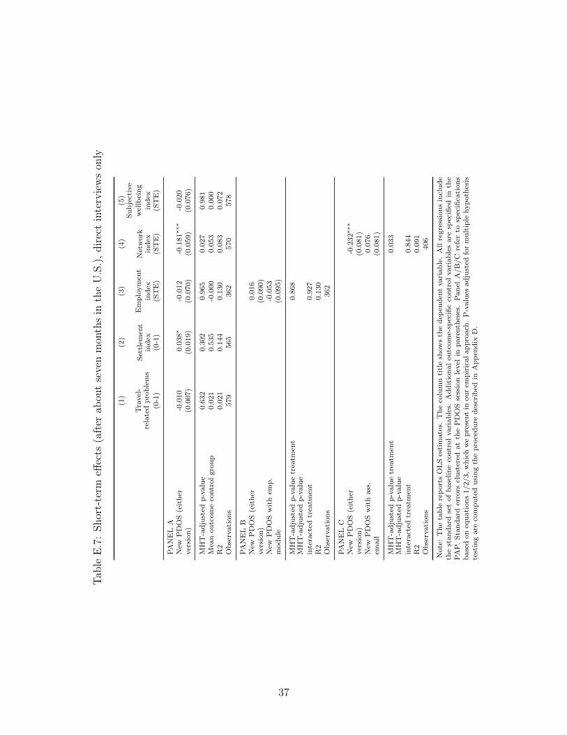
Tab

leE

.7:

Shor

t-te

rmeff

ects

(aft

erab

out

seve

nm

onth

sin

the

U.S

.),

dir

ect

inte

rvie

ws

only

(1)

(2)

(3)

(4)

(5)

Tra

vel

-re

late

dp

rob

lem

s

(0-1

)

Set

tlem

ent

ind

ex(0

-1)

Em

plo

ym

ent

ind

ex(S

TE

)

Net

work

ind

ex(S

TE

)

Su

bje

ctiv

e

wel

lbei

ng

ind

ex(S

TE

)

PA

NE

LA

New

PD

OS

(eit

her

-0.0

10

0.0

38∗

-0.0

12

-0.1

81∗∗∗

-0.0

20

ver

sion

)(0

.007)

(0.0

19)

(0.0

70)

(0.0

59)

(0.0

76)

MH

T-a

dju

sted

p-v

alu

e0.6

32

0.3

02

0.9

65

0.0

27

0.9

81

Mea

nou

tcom

eco

ntr

ol

gro

up

0.0

21

0.5

35

-0.0

00

0.0

53

0.0

00

R2

0.0

21

0.1

44

0.1

30

0.0

83

0.0

72

Ob

serv

ati

on

s579

565

362

570

578

PA

NE

LB

New

PD

OS

(eit

her

0.0

16

ver

sion

)(0

.090)

New

PD

OS

wit

hem

p.

-0.0

53

mod

ule

(0.0

95)

MH

T-a

dju

sted

p-v

alu

etr

eatm

ent

0.8

68

MH

T-a

dju

sted

p-v

alu

e

inte

ract

edtr

eatm

ent

0.9

27

R2

0.1

30

Ob

serv

ati

on

s362

PA

NE

LC

New

PD

OS

(eit

her

-0.2

32∗∗∗

ver

sion

)(0

.081)

New

PD

OS

wit

hass

.0.0

76

email

(0.0

81)

MH

T-a

dju

sted

p-v

alu

etr

eatm

ent

0.0

33

MH

T-a

dju

sted

p-v

alu

e

inte

ract

edtr

eatm

ent

0.8

44

R2

0.0

91

Ob

serv

ati

on

s406

Note

:T

he

tab

lere

port

sO

LS

esti

mate

s.T

he

colu

mn

titl

esh

ow

sth

ed

epen

den

tvari

ab

le.

All

regre

ssio

ns

incl

ud

eth

est

an

dard

set

of

base

lin

eco

ntr

ol

vari

ab

les.

Ad

dit

ion

al

ou

tcom

e-sp

ecifi

cco

ntr

ol

vari

ab

les

are

spec

ified

inth

eP

AP

.S

tan

dard

erro

rscl

ust

ered

at

the

PD

OS

sess

ion

level

inp

are

nth

eses

.P

an

elA

/B

/C

refe

rto

spec

ifica

tion

sb

ase

don

equ

ati

on

s1/2/3,

wh

ich

we

pre

sent

inou

rem

pir

icalap

pro

ach

.P

-valu

esad

just

edfo

rm

ult

iple

hyp

oth

esis

test

ing

are

com

pu

ted

usi

ng

the

pro

ced

ure

des

crib

edin

Ap

pen

dix

D.

37

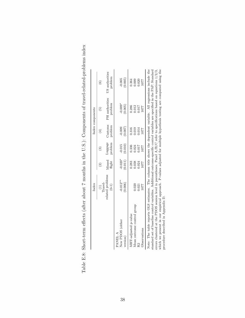
Tab

leE

.8:

Shor

t-te

rmeff

ects

(aft

erab

out

7m

onth

sin

the

U.S

.):

Com

pon

ents

oftr

avel

-rel

ated

-pro

ble

ms

index

Ind

exIn

dex

com

pon

ents

(1)

(2)

(3)

(4)

(5)

(6)

Tra

vel

-re

late

dp

rob

lem

s

(0-1

)M

isse

dfl

ight

Lu

ggage

pro

ble

mC

ust

om

sp

rob

lem

PH

au

thori

ties

pro

ble

mU

Sau

thori

ties

pro

ble

m

PA

NE

LA

New

PD

OS

(eit

her

-0.0

12∗∗

-0.0

20∗

-0.0

15

-0.0

09

-0.0

09∗

-0.0

05

ver

sion

)(0

.006)

(0.0

11)

(0.0

10)

(0.0

07)

(0.0

05)

(0.0

05)

MH

T-a

dju

sted

p-v

alu

e0.2

83

0.3

36

0.3

16

0.2

86

0.3

64

Mea

nou

tcom

eco

ntr

ol

gro

up

0.0

20

0.0

38

0.0

24

0.0

19

0.0

12

0.0

09

R2

0.0

21

0.0

24

0.0

17

0.0

14

0.0

17

0.0

20

Ob

serv

ati

on

s1077

1077

1077

1077

1077

1077

Note

:T

he

tab

lere

port

sO

LS

esti

mate

s.T

he

colu

mn

titl

esh

ow

sth

ed

epen

den

tvari

ab

le.

All

regre

ssio

ns

incl

ud

eth

est

an

dard

set

of

base

lin

eco

ntr

ol

vari

ab

les.

Ad

dit

ion

al

ou

tcom

e-sp

ecifi

cco

ntr

ol

vari

ab

les

are

spec

ified

inth

eP

AP

.S

tan

dard

erro

rscl

ust

ered

at

the

PD

OS

sess

ion

level

inp

are

nth

eses

.P

an

elA

/B

/C

refe

rto

spec

ifica

tion

sb

ase

don

equati

on

s1/2/3,

wh

ich

we

pre

sent

inou

rem

pir

ical

ap

pro

ach

.P

-valu

esad

just

edfo

rm

ult

iple

hyp

oth

esis

test

ing

are

com

pu

ted

usi

ng

the

pro

ced

ure

des

crib

edin

Ap

pen

dix

D.

38

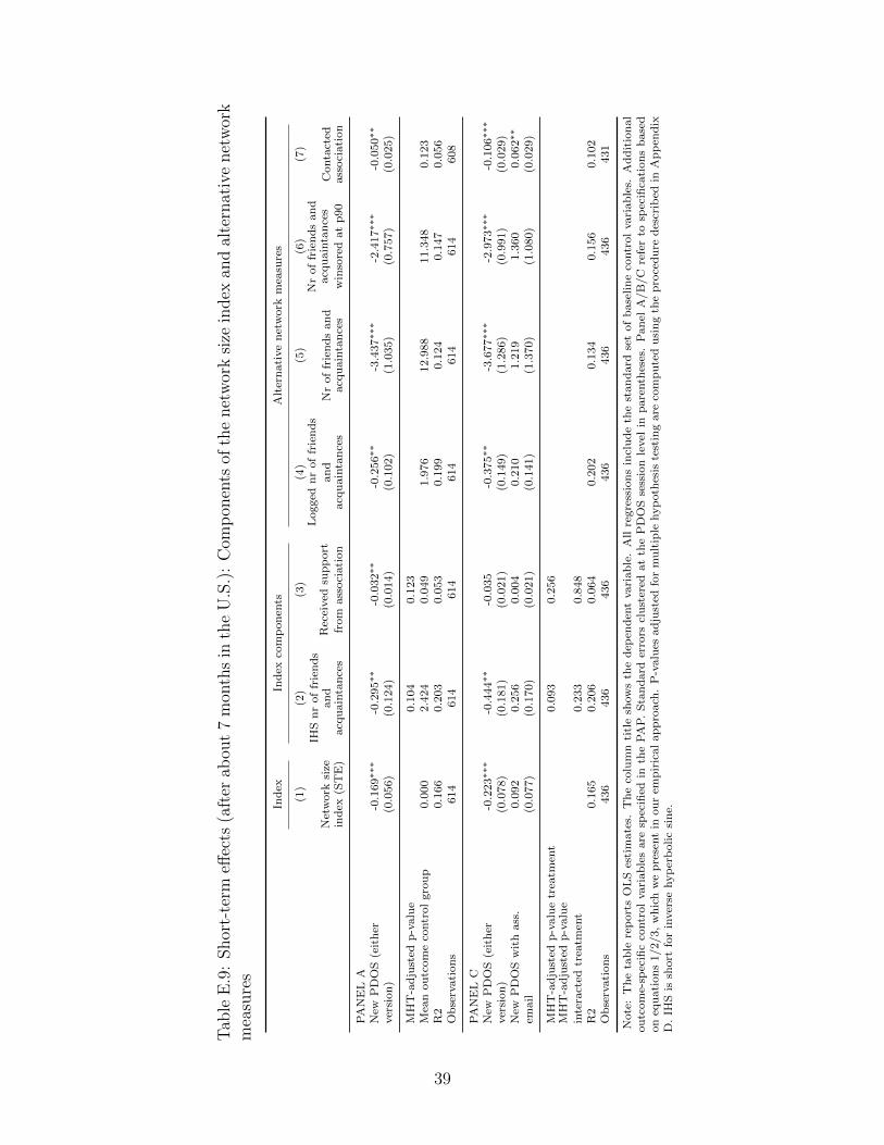
Tab

leE

.9:

Shor

t-te

rmeff

ects

(aft

erab

out

7m

onth

sin

the

U.S

.):

Com

pon

ents

ofth

enet

wor

ksi

zein

dex

and

alte

rnat

ive

net

wor

km

easu

res

Ind

exIn

dex

com

pon

ents

Alt

ern

ati

ve

net

work

mea

sure

s

(1)

(2)

(3)

(4)

(5)

(6)

(7)

Net

work

size

ind

ex(S

TE

)

IHS

nr

of

frie

nd

san

dacq

uain

tan

ces

Rec

eived

sup

port

from

ass

oci

ati

on

Logged

nr

of

frie

nd

s

an

dacq

uain

tan

ces

Nr

of

frie

nd

san

dacq

uain

tan

ces

Nr

of

frie

nd

san

dacq

uain

tan

ces

win

sore

dat

p90

Conta

cted

ass

oci

ati

on

PA

NE

LA

New

PD

OS

(eit

her

-0.1

69∗∗∗

-0.2

95∗∗

-0.0

32∗∗

-0.2

56∗∗

-3.4

37∗∗∗

-2.4

17∗∗∗

-0.0

50∗∗

ver

sion

)(0

.056)

(0.1

24)

(0.0

14)

(0.1

02)

(1.0

35)

(0.7

57)

(0.0

25)

MH

T-a

dju

sted

p-v

alu

e0.1

04

0.1

23

Mea

nou

tcom

eco

ntr

ol

gro

up

0.0

00

2.4

24

0.0

49

1.9

76

12.9

88

11.3

48

0.1

23

R2

0.1

66

0.2

03

0.0

53

0.1

99

0.1

24

0.1

47

0.0

56

Ob

serv

ati

on

s614

614

614

614

614

614

608

PA

NE

LC

New

PD

OS

(eit

her

-0.2

23∗∗∗

-0.4

44∗∗

-0.0

35

-0.3

75∗∗

-3.6

77∗∗∗

-2.9

73∗∗∗

-0.1

06∗∗∗

ver

sion

)(0

.078)

(0.1

81)

(0.0

21)

(0.1

49)

(1.2

86)

(0.9

91)

(0.0

29)

New

PD

OS

wit

hass

.0.0

92

0.2

56

0.0

04

0.2

10

1.2

19

1.3

60

0.0

62∗∗

email

(0.0

77)

(0.1

70)

(0.0

21)

(0.1

41)

(1.3

70)

(1.0

80)

(0.0

29)

MH

T-a

dju

sted

p-v

alu

etr

eatm

ent

0.0

93

0.2

56

MH

T-a

dju

sted

p-v

alu

e

inte

ract

edtr

eatm

ent

0.2

33

0.8

48

R2

0.1

65

0.2

06

0.0

64

0.2

02

0.1

34

0.1

56

0.1

02

Ob

serv

ati

on

s436

436

436

436

436

436

431

Note

:T

he

tab

lere

port

sO

LS

esti

mate

s.T

he

colu

mn

titl

esh

ow

sth

ed

epen

den

tvari

ab

le.

All

regre

ssio

ns

incl

ud

eth

est

an

dard

set

of

base

lin

eco

ntr

ol

vari

ab

les.

Ad

dit

ion

al

ou

tcom

e-sp

ecifi

cco

ntr

ol

vari

ab

les

are

spec

ified

inth

eP

AP

.S

tan

dard

erro

rscl

ust

ered

at

the

PD

OS

sess

ion

level

inp

are

nth

eses

.P

an

elA

/B

/C

refe

rto

spec

ifica

tion

sb

ase

don

equ

ati

on

s1/2/3,

wh

ich

we

pre

sent

inou

rem

pir

ical

ap

pro

ach

.P

-valu

esad

just

edfo

rm

ult

iple

hyp

oth

esis

test

ing

are

com

pu

ted

usi

ng

the

pro

ced

ure

des

crib

edin

Ap

pen

dix

D.

IHS

issh

ort

for

inver

sehyp

erb

oli

csi

ne.

39

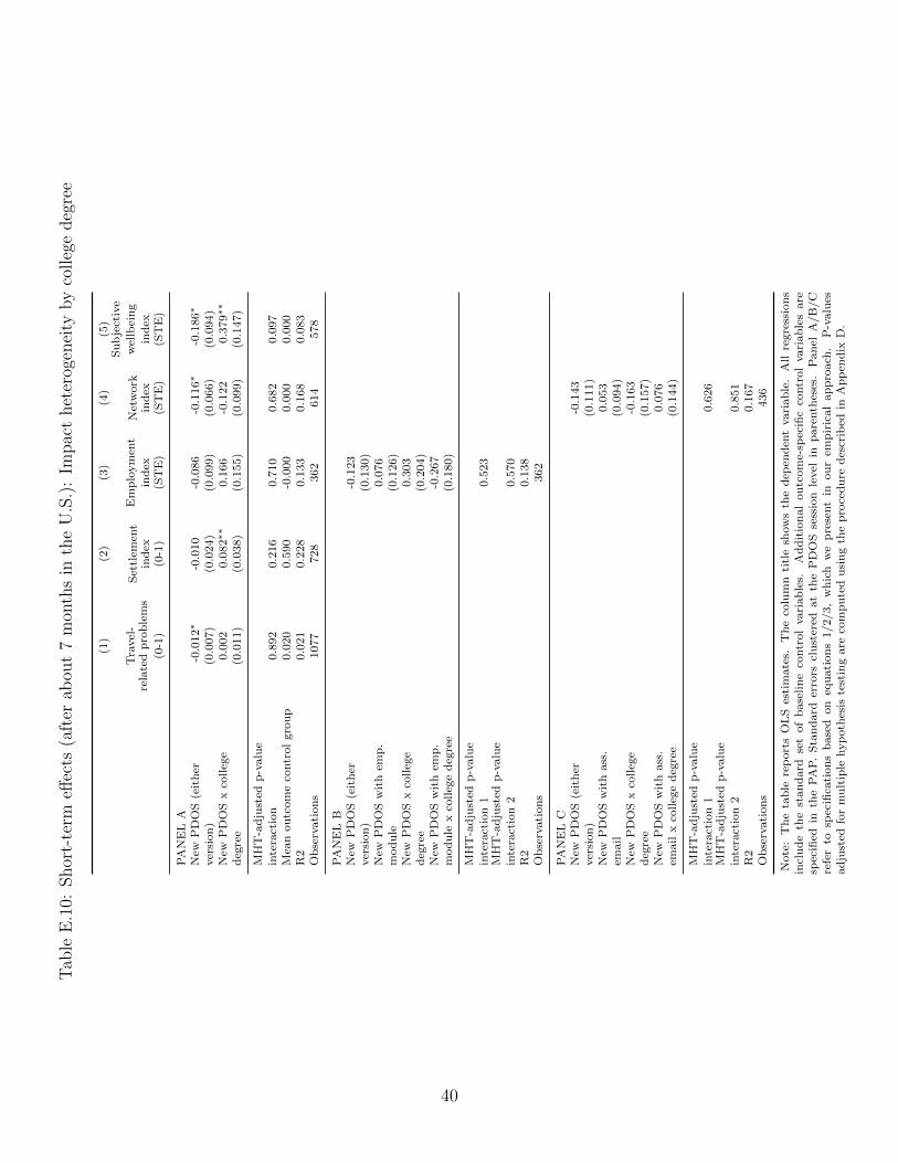
Tab

leE

.10:

Shor

t-te

rmeff

ects

(aft

erab

out

7m

onth

sin

the

U.S

.):

Impac

thet

erog

enei

tyby

colleg

edeg

ree

(1)

(2)

(3)

(4)

(5)

Tra

vel

-re

late

dp

rob

lem

s

(0-1

)

Set

tlem

ent

ind

ex(0

-1)

Em

plo

ym

ent

ind

ex(S

TE

)

Net

work

ind

ex(S

TE

)

Su

bje

ctiv

e

wel

lbei

ng

ind

ex(S

TE

)

PA

NE

LA

New

PD

OS

(eit

her

-0.0

12∗

-0.0

10

-0.0

86

-0.1

16∗

-0.1

86∗

ver

sion

)(0

.007)

(0.0

24)

(0.0

99)

(0.0

66)

(0.0

94)

New

PD

OS

xco

lleg

e0.0

02

0.0

82∗∗

0.1

66

-0.1

22

0.3

79∗∗

deg

ree

(0.0

11)

(0.0

38)

(0.1

55)

(0.0

99)

(0.1

47)

MH

T-a

dju

sted

p-v

alu

ein

tera

ctio

n0.8

92

0.2

16

0.7

10

0.6

82

0.0

97

Mea

nou

tcom

eco

ntr

ol

gro

up

0.0

20

0.5

90

-0.0

00

0.0

00

0.0

00

R2

0.0

21

0.2

28

0.1

33

0.1

68

0.0

83

Ob

serv

ati

on

s1077

728

362

614

578

PA

NE

LB

New

PD

OS

(eit

her

-0.1

23

ver

sion

)(0

.130)

New

PD

OS

wit

hem

p.

0.0

76

mod

ule

(0.1

26)

New

PD

OS

xco

lleg

e0.3

03

deg

ree

(0.2

04)

New

PD

OS

wit

hem

p.

-0.2

67

mod

ule

xco

lleg

ed

egre

e(0

.180)

MH

T-a

dju

sted

p-v

alu

ein

tera

ctio

n1

0.5

23

MH

T-a

dju

sted

p-v

alu

ein

tera

ctio

n2

0.5

70

R2

0.1

38

Ob

serv

ati

on

s362

PA

NE

LC

New

PD

OS

(eit

her

-0.1

43

ver

sion

)(0

.111)

New

PD

OS

wit

hass

.0.0

53

email

(0.0

94)

New

PD

OS

xco

lleg

e-0

.163

deg

ree

(0.1

57)

New

PD

OS

wit

hass

.0.0

76

email

xco

lleg

ed

egre

e(0

.144)

MH

T-a

dju

sted

p-v

alu

ein

tera

ctio

n1

0.6

26

MH

T-a

dju

sted

p-v

alu

ein

tera

ctio

n2

0.8

51

R2

0.1

67

Ob

serv

ati

on

s436

Note

:T

he

tab

lere

port

sO

LS

esti

mate

s.T

he

colu

mn

titl

esh

ow

sth

ed

epen

den

tvari

ab

le.

All

regre

ssio

ns

incl

ud

eth

est

an

dard

set

of

base

lin

eco

ntr

ol

vari

ab

les.

Ad

dit

ion

al

ou

tcom

e-sp

ecifi

cco

ntr

ol

vari

ab

les

are

spec

ified

inth

eP

AP

.S

tan

dard

erro

rscl

ust

ered

at

the

PD

OS

sess

ion

level

inp

are

nth

eses

.P

an

elA

/B

/C

refe

rto

spec

ifica

tion

sb

ase

don

equ

ati

on

s1/2/3,

wh

ich

we

pre

sent

inou

rem

pir

ical

ap

pro

ach

.P

-valu

esad

just

edfo

rm

ult

iple

hyp

oth

esis

test

ing

are

com

pu

ted

usi

ng

the

pro

ced

ure

des

crib

edin

Ap

pen

dix

D.

40

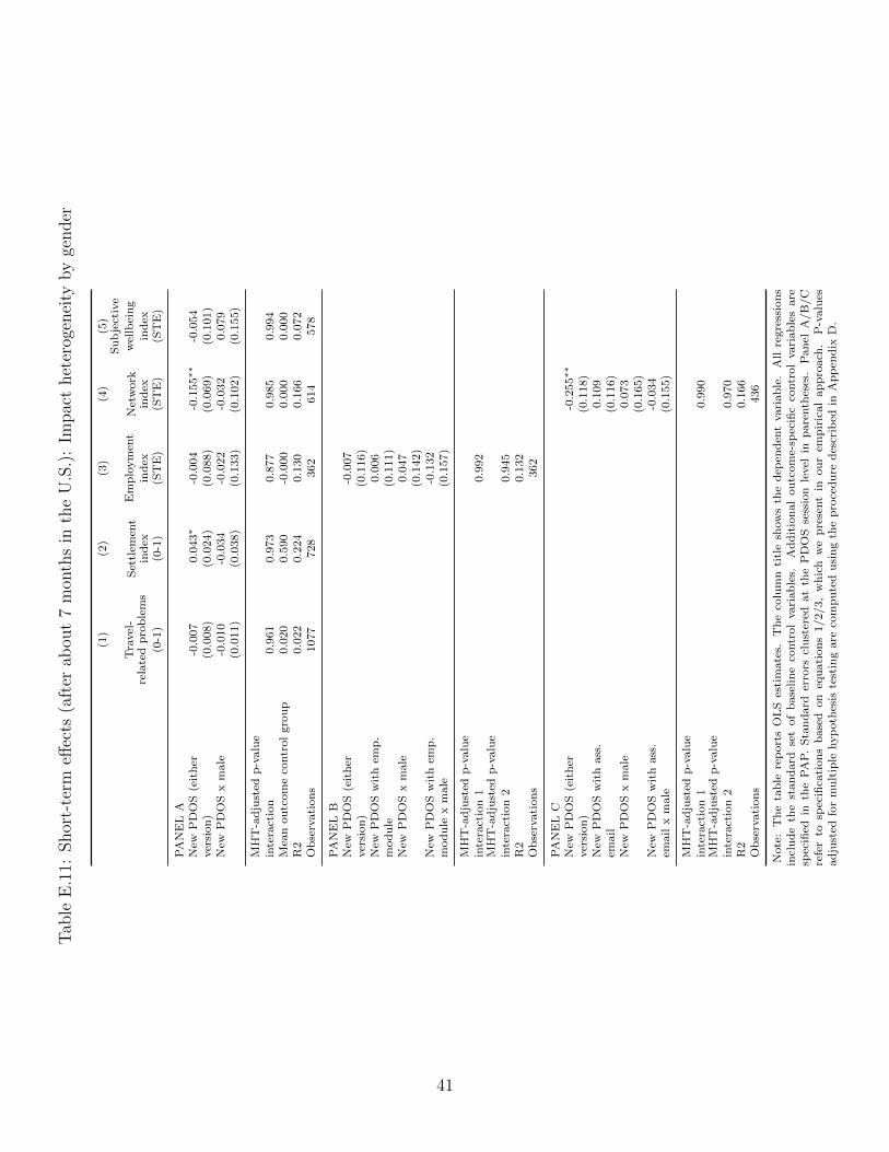
Tab

leE

.11:

Shor

t-te

rmeff

ects

(aft

erab

out

7m

onth

sin

the

U.S

.):

Impac

thet

erog

enei

tyby

gender

(1)

(2)

(3)

(4)

(5)

Tra

vel

-re

late

dp

rob

lem

s

(0-1

)

Set

tlem

ent

ind

ex(0

-1)

Em

plo

ym

ent

ind

ex(S

TE

)

Net

work

ind

ex(S

TE

)

Su

bje

ctiv

e

wel

lbei

ng

ind

ex(S

TE

)

PA

NE

LA

New

PD

OS

(eit

her

-0.0

07

0.0

43∗

-0.0

04

-0.1

55∗∗

-0.0

54

ver

sion

)(0

.008)

(0.0

24)

(0.0

88)

(0.0

69)

(0.1

01)

New

PD

OS

xm

ale

-0.0

10

-0.0

34

-0.0

22

-0.0

32

0.0

79

(0.0

11)

(0.0

38)

(0.1

33)

(0.1

02)

(0.1

55)

MH

T-a

dju

sted

p-v

alu

ein

tera

ctio

n0.9

61

0.9

73

0.8

77

0.9

85

0.9

94

Mea

nou

tcom

eco

ntr

ol

gro

up

0.0

20

0.5

90

-0.0

00

0.0

00

0.0

00

R2

0.0

22

0.2

24

0.1

30

0.1

66

0.0

72

Ob

serv

ati

on

s1077

728

362

614

578

PA

NE

LB

New

PD

OS

(eit

her

-0.0

07

ver

sion

)(0

.116)

New

PD

OS

wit

hem

p.

0.0

06

mod

ule

(0.1

11)

New

PD

OS

xm

ale

0.0

47

(0.1

42)

New

PD

OS

wit

hem

p.

-0.1

32

mod

ule

xm

ale

(0.1

57)

MH

T-a

dju

sted

p-v

alu

ein

tera

ctio

n1

0.9

92

MH

T-a

dju

sted

p-v

alu

ein

tera

ctio

n2

0.9

45

R2

0.1

32

Ob

serv

ati

on

s362

PA

NE

LC

New

PD

OS

(eit

her

-0.2

55∗∗

ver

sion

)(0

.118)

New

PD

OS

wit

hass

.0.1

09

email

(0.1

16)

New

PD

OS

xm

ale

0.0

73

(0.1

65)

New

PD

OS

wit

hass

.-0

.034

email

xm

ale

(0.1

55)

MH

T-a

dju

sted

p-v

alu

ein

tera

ctio

n1

0.9

90

MH

T-a

dju

sted

p-v

alu

ein

tera

ctio

n2

0.9

70

R2

0.1

66

Ob

serv

ati

on

s436

Note

:T

he

tab

lere

port

sO

LS

esti

mate

s.T

he

colu

mn

titl

esh

ow

sth

ed

epen

den

tvari

ab

le.

All

regre

ssio

ns

incl

ud

eth

est

an

dard

set

of

base

lin

eco

ntr

ol

vari

ab

les.

Ad

dit

ion

al

ou

tcom

e-sp

ecifi

cco

ntr

ol

vari

ab

les

are

spec

ified

inth

eP

AP

.S

tan

dard

erro

rscl

ust

ered

at

the

PD

OS

sess

ion

level

inp

are

nth

eses

.P

an

elA

/B

/C

refe

rto

spec

ifica

tion

sb

ase

don

equ

ati

on

s1/2/3,

wh

ich

we

pre

sent

inou

rem

pir

ical

ap

pro

ach

.P

-valu

esad

just

edfo

rm

ult

iple

hyp

oth

esis

test

ing

are

com

pu

ted

usi

ng

the

pro

ced

ure

des

crib

edin

Ap

pen

dix

D.

41

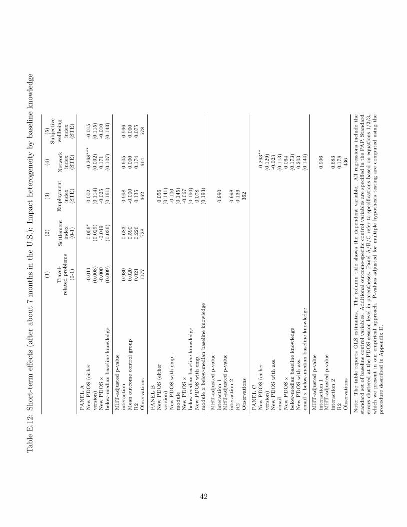
Tab

leE

.12:

Shor

t-te

rmeff

ects

(aft

erab

out

7m

onth

sin

the

U.S

.):

Impac

thet

erog

enei

tyby

bas

elin

eknow

ledge

(1)

(2)

(3)

(4)

(5)

Tra

vel

-re

late

dp

rob

lem

s

(0-1

)

Set

tlem

ent

ind

ex(0

-1)

Em

plo

ym

ent

ind

ex(S

TE

)

Net

work

ind

ex(S

TE

)

Su

bje

ctiv

e

wel

lbei

ng

ind

ex(S

TE

)

PA

NE

LA

New

PD

OS

(eit

her

-0.0

11

0.0

56∗

0.0

02

-0.2

68∗∗∗

-0.0

15

ver

sion

)(0

.008)

(0.0

29)

(0.1

14)

(0.0

92)

(0.1

15)

New

PD

OS

x-0

.000

-0.0

49

-0.0

25

0.1

71

-0.0

10

bel

ow

-med

ian

base

lin

ekn

ow

led

ge

(0.0

09)

(0.0

36)

(0.1

61)

(0.1

07)

(0.1

43)

MH

T-a

dju

sted

p-v

alu

ein

tera

ctio

n0.9

80

0.6

83

0.9

98

0.6

05

0.9

96

Mea

nou

tcom

eco

ntr

ol

gro

up

0.0

20

0.5

90

-0.0

00

0.0

00

0.0

00

R2

0.0

21

0.2

26

0.1

35

0.1

74

0.0

75

Ob

serv

ati

on

s1077

728

362

614

578

PA

NE

LB

New

PD

OS

(eit

her

0.0

56

ver

sion

)(0

.141)

New

PD

OS

wit

hem

p.

-0.1

00

mod

ule

(0.1

45)

New

PD

OS

x-0

.067

bel

ow

-med

ian

base

lin

ekn

ow

led

ge

(0.1

90)

New

PD

OS

wit

hem

p.

0.0

78

mod

ule

xb

elow

-med

ian

base

lin

ekn

ow

led

ge

(0.1

93)

MH

T-a

dju

sted

p-v

alu

ein

tera

ctio

n1

0.9

90

MH

T-a

dju

sted

p-v

alu

ein

tera

ctio

n2

0.9

98

R2

0.1

36

Ob

serv

ati

on

s362

PA

NE

LC

New

PD

OS

(eit

her

-0.2

63∗∗

ver

sion

)(0

.129)

New

PD

OS

wit

hass

.-0

.023

email

(0.1

13)

New

PD

OS

x0.0

64

bel

ow

-med

ian

base

lin

ekn

ow

led

ge

(0.1

73)

New

PD

OS

wit

hass

.0.2

03

email

xb

elow

-med

ian

base

lin

ekn

ow

led

ge

(0.1

44)

MH

T-a

dju

sted

p-v

alu

ein

tera

ctio

n1

0.9

96

MH

T-a

dju

sted

p-v

alu

ein

tera

ctio

n2

0.6

83

R2

0.1

78

Ob

serv

ati

on

s436

Note

:T

he

tab

lere

port

sO

LS

esti

mate

s.T

he

colu

mn

titl

esh

ow

sth

ed

epen

den

tvari

ab

le.

All

regre

ssio

ns

incl

ud

eth

est

an

dard

set

of

base

lin

eco

ntr

ol

vari

ab

les.

Ad

dit

ion

al

ou

tcom

e-sp

ecifi

cco

ntr

ol

vari

ab

les

are

spec

ified

inth

eP

AP

.S

tan

dard

erro

rscl

ust

ered

at

the

PD

OS

sess

ion

level

inp

are

nth

eses

.P

an

elA

/B

/C

refe

rto

spec

ifica

tion

sb

ase

don

equ

ati

on

s1/2/3,

wh

ich

we

pre

sent

inou

rem

pir

ical

ap

pro

ach

.P

-valu

esad

just

edfo

rm

ult

iple

hyp

oth

esis

test

ing

are

com

pu

ted

usi

ng

the

pro

ced

ure

des

crib

edin

Ap

pen

dix

D.

42

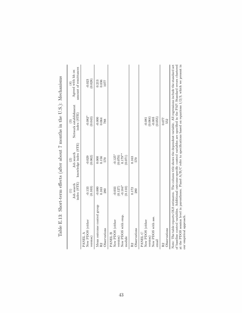
Tab

leE

.13:

Shor

t-te

rmeff

ects

(aft

erab

out

7m

onth

sin

the

U.S

.):

Mec

han

ism

s

(1)

(2)

(3)

(4)

Job

searc

hin

dex

(ST

E)

Job

searc

hkn

ow

led

ge

ind

ex(S

TE

)N

etw

ork

esta

blish

men

tin

dex

(ST

E)

Agre

edw

ith

hh

on

am

ou

nt

of

rem

itta

nce

s

PA

NE

LA

New

PD

OS

(eit

her

-0.1

33

-0.0

29

-0.0

82∗

-0.0

23

ver

sion

)(0

.103)

(0.0

62)

(0.0

43)

(0.0

28)

Mea

nou

tcom

eco

ntr

ol

gro

up

-0.0

00

0.0

00

-0.0

00

0.2

13

R2

0.1

63

0.1

56

0.0

64

0.0

36

Ob

serv

ati

on

s280

579

788

1077

PA

NE

LB

New

PD

OS

(eit

her

-0.0

33

-0.1

25∗

ver

sion

)(0

.127)

(0.0

70)

New

PD

OS

wit

hem

p.

-0.1

84∗

0.1

79∗∗

modu

le(0

.110)

(0.0

71)

R2

0.1

72

0.1

63

Ob

serv

ati

on

s280

579

PA

NE

LC

New

PD

OS

(eit

her

-0.0

81

ver

sion

)(0

.064)

New

PD

OS

wit

hass

.-0

.003

email

(0.0

55)

R2

0.0

77

Ob

serv

ati

on

s552

Note

:T

he

tab

lere

port

sO

LS

esti

mate

s.T

he

colu

mn

titl

esh

ow

sth

ed

epen

den

tvari

ab

le.

All

regre

ssio

ns

incl

ud

eth

est

an

dard

set

of

base

lin

eco

ntr

ol

vari

ab

les.

Ad

dit

ion

al

ou

tcom

e-sp

ecifi

cco

ntr

ol

vari

ab

les

are

spec

ified

inth

eP

AP

.S

tan

dard

erro

rscl

ust

ered

at

the

PD

OS

sess

ion

level

inp

are

nth

eses

.P

an

elA

/B

/C

refe

rto

spec

ifica

tion

sb

ase

don

equ

ati

on

s1/2/3,

wh

ich

we

pre

sent

inou

rem

pir

ical

ap

pro

ach

.

43

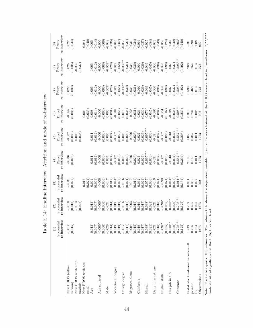
Tab

leE

.14:

Endline

inte

rvie

w:

Att

riti

onan

dm

ode

ofre

-inte

rvie

w

(1)

(2)

(3)

(4)

(5)

(6)

(7)

(8)

(9)

Su

cces

sfu

lre

-inte

rvie

wS

ucc

essf

ul

re-i

nte

rvie

wS

ucc

essf

ul

re-i

nte

rvie

wD

irec

tre

-inte

rvie

wD

irec

tre

-inte

rvie

wD

irec

tre

-inte

rvie

wP

roxy

re-i

nte

rvie

wP

roxy

re-i

nte

rvie

wP

roxy

re-i

nte

rvie

w

New

PD

OS

(eit

her

-0.0

17

-0.0

10

-0.0

31

-0.0

36

-0.0

37

-0.0

25

0.0

22

0.0

25

0.0

27

ver

sion

)(0

.015)

(0.0

18)

(0.0

22)

(0.0

25)

(0.0

33)

(0.0

36)

(0.0

30)

(0.0

35)

(0.0

44)

New

PD

OS

wit

hem

p.

-0.0

13

0.0

03

-0.0

05

mod

ule

(0.0

22)

(0.0

36)

(0.0

37)

New

PD

OS

wit

hass

.0.0

15

0.0

04

-0.0

41

email

(0.0

24)

(0.0

35)

(0.0

40)

Age

0.0

13∗

0.0

13∗

0.0

04

0.0

11

0.0

11

0.0

08

0.0

05

0.0

05

0.0

05

(0.0

07)

(0.0

07)

(0.0

09)

(0.0

12)

(0.0

12)

(0.0

14)

(0.0

12)

(0.0

12)

(0.0

14)

Age

squ

are

d-0

.000∗

-0.0

00∗

-0.0

00

-0.0

00

-0.0

00

-0.0

00

-0.0

00

-0.0

00

-0.0

00

(0.0

00)

(0.0

00)

(0.0

00)

(0.0

00)

(0.0

00)

(0.0

00)

(0.0

00)

(0.0

00)

(0.0

00)

Male

-0.0

20

-0.0

21

-0.0

17

0.0

04

0.0

04

0.0

03

-0.0

52∗

-0.0

52∗

-0.0

48

(0.0

14)

(0.0

14)

(0.0

19)

(0.0

27)

(0.0

27)

(0.0

31)

(0.0

28)

(0.0

28)

(0.0

35)

Voca

tion

al

deg

ree

0.0

19

0.0

19

0.0

44∗

-0.0

07

-0.0

07

-0.0

18

-0.0

12

-0.0

12

-0.0

13

(0.0

19)

(0.0

19)

(0.0

22)

(0.0

50)

(0.0

50)

(0.0

56)

(0.0

58)

(0.0

58)

(0.0

67)

Colleg

ed

egre

e-0

.017

-0.0

16

-0.0

16

0.0

08

0.0

08

0.0

15

-0.0

66∗∗

-0.0

66∗∗

-0.0

55

(0.0

17)

(0.0

17)

(0.0

21)

(0.0

29)

(0.0

29)

(0.0

35)

(0.0

30)

(0.0

31)

(0.0

37)

Mig

rate

salo

ne

-0.0

04

-0.0

03

-0.0

17

-0.0

26

-0.0

26

-0.0

28

0.0

34

0.0

34

0.0

31

(0.0

15)

(0.0

15)

(0.0

19)

(0.0

25)

(0.0

25)

(0.0

31)

(0.0

31)

(0.0

30)

(0.0

34)

Califo

rnia

0.0

19

0.0

19

0.0

32

0.0

27

0.0

27

0.0

26

-0.0

10

-0.0

10

-0.0

16

(0.0

17)

(0.0

17)

(0.0

24)

(0.0

25)

(0.0

25)

(0.0

30)

(0.0

29)

(0.0

29)

(0.0

37)

Haw

aii

0.0

38∗

0.0

38∗

0.0

55∗

0.0

95∗∗∗

0.0

95∗∗∗

0.0

76∗

-0.0

49

-0.0

49

-0.0

25

(0.0

21)

(0.0

21)

(0.0

30)

(0.0

36)

(0.0

36)

(0.0

45)

(0.0

45)

(0.0

45)

(0.0

54)

Daily

inte

rnet

use

-0.0

21

-0.0

21

-0.0

19

-0.0

21

-0.0

21

-0.0

20

-0.0

36

-0.0

36

-0.0

23

(0.0

16)

(0.0

16)

(0.0

21)

(0.0

32)

(0.0

32)

(0.0

37)

(0.0

36)

(0.0

36)

(0.0

43)

En

glish

skills

-0.0

97∗

-0.0

96∗

-0.0

93

-0.0

07

-0.0

07

-0.0

54

-0.0

95

-0.0

95

-0.0

58

(0.0

55)

(0.0

55)

(0.0

74)

(0.0

88)

(0.0

88)

(0.1

07)

(0.0

99)

(0.0

98)

(0.1

24)

Has

job

inU

S0.0

40∗∗

0.0

40∗∗

0.0

44∗

-0.0

43

-0.0

43

-0.0

19

0.0

37

0.0

37

0.0

34

(0.0

20)

(0.0

20)

(0.0

25)

(0.0

34)

(0.0

34)

(0.0

36)

(0.0

37)

(0.0

37)

(0.0

42)

Con

stant

0.7

98∗∗∗

0.7

98∗∗∗

0.9

11∗∗∗

0.5

57∗∗∗

0.5

57∗∗∗

0.5

98∗∗

0.5

25∗∗∗

0.5

25∗∗∗

0.5

03∗∗

(0.1

25)

(0.1

25)

(0.1

64)

(0.2

04)

(0.2

03)

(0.2

39)

(0.1

92)

(0.1

92)

(0.2

40)

F-s

tati

stic

trea

tmen

tvari

ab

les=

01.2

49

0.7

09

0.9

61

2.1

05

1.0

53

0.3

10

0.5

30

0.2

83

0.5

31

p-v

alu

e0.2

66

0.4

95

0.3

86

0.1

50

0.3

52

0.7

34

0.4

68

0.7

54

0.5

90

R2

0.0

24

0.0

25

0.0

27

0.0

11

0.0

11

0.0

08

0.0

13

0.0

13

0.0

08

Ob

serv

ati

on

s1273

1273

902

1273

1273

902

1273

1273

902

Note

:T

he

tab

lere

port

sO

LS

esti

mate

s.T

he

colu

mn

titl

esh

ow

sth

ed

epen

den

tvari

ab

le.

Sta

nd

ard

erro

rscl

ust

ered

at

the

PD

OS

sess

ion

level

inp

are

nth

eses

.*/**/***

den

ote

stati

stic

al

sign

ifica

nce

at

the

10/5/1

per

cent

level

.

44

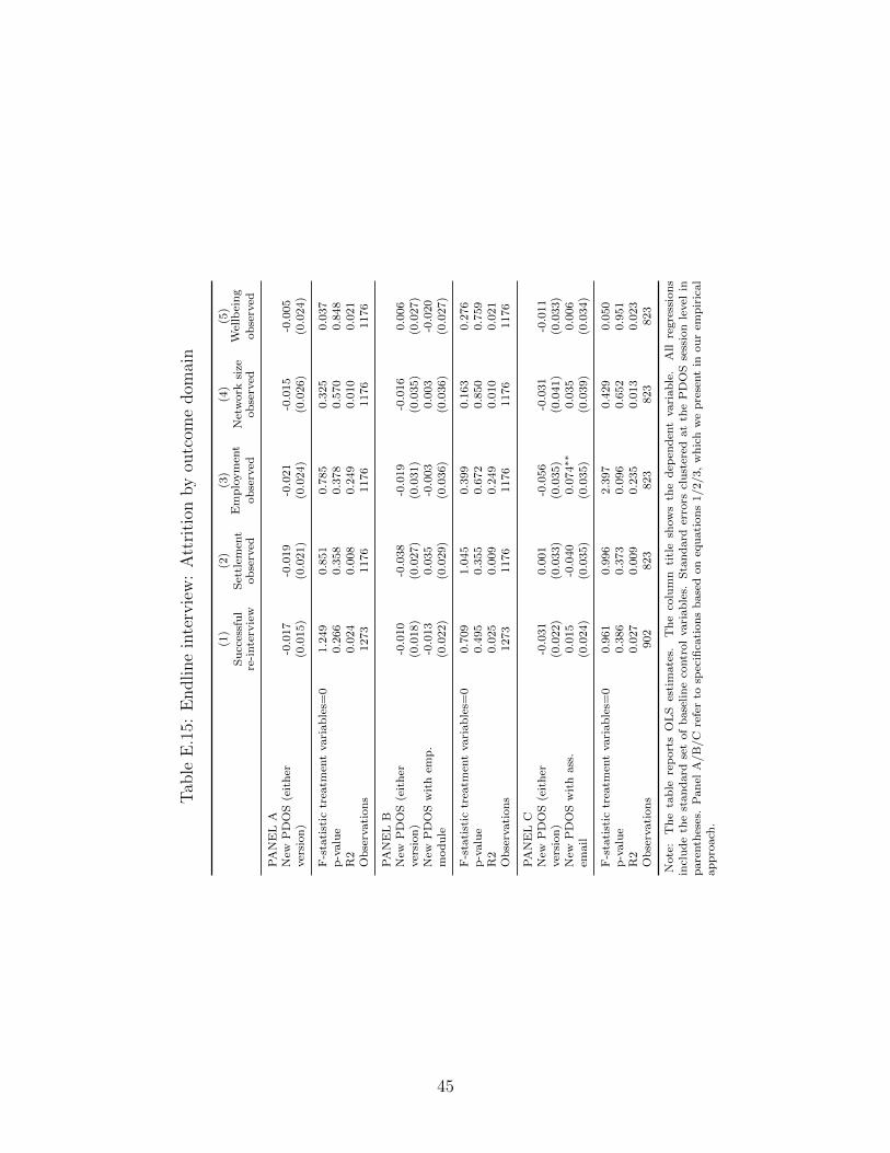
Tab

leE

.15:

Endline

inte

rvie

w:

Att

riti

onby

outc

ome

dom

ain

(1)

(2)

(3)

(4)

(5)

Su

cces

sfu

lre

-inte

rvie

wS

ettl

emen

tob

serv

ed

Em

plo

ym

ent

ob

serv

edN

etw

ork

size

ob

serv

ed

Wel

lbei

ng

ob

serv

ed

PA

NE

LA

New

PD

OS

(eit

her

-0.0

17

-0.0

19

-0.0

21

-0.0

15

-0.0

05

ver

sion

)(0

.015)

(0.0

21)

(0.0

24)

(0.0

26)

(0.0

24)

F-s

tati

stic

trea

tmen

tvari

ab

les=

01.2

49

0.8

51

0.7

85

0.3

25

0.0

37

p-v

alu

e0.2

66

0.3

58

0.3

78

0.5

70

0.8

48

R2

0.0

24

0.0

08

0.2

49

0.0

10

0.0

21

Ob

serv

ati

on

s1273

1176

1176

1176

1176

PA

NE

LB

New

PD

OS

(eit

her

-0.0

10

-0.0

38

-0.0

19

-0.0

16

0.0

06

ver

sion

)(0

.018)

(0.0

27)

(0.0

31)

(0.0

35)

(0.0

27)

New

PD

OS

wit

hem

p.

-0.0

13

0.0

35

-0.0

03

0.0

03

-0.0

20

mod

ule

(0.0

22)

(0.0

29)

(0.0

36)

(0.0

36)

(0.0

27)

F-s

tati

stic

trea

tmen

tvari

ab

les=

00.7

09

1.0

45

0.3

99

0.1

63

0.2

76

p-v

alu

e0.4

95

0.3

55

0.6

72

0.8

50

0.7

59

R2

0.0

25

0.0

09

0.2

49

0.0

10

0.0

21

Ob

serv

ati

on

s1273

1176

1176

1176

1176

PA

NE

LC

New

PD

OS

(eit

her

-0.0

31

0.0

01

-0.0

56

-0.0

31

-0.0

11

ver

sion

)(0

.022)

(0.0

33)

(0.0

35)

(0.0

41)

(0.0

33)

New

PD

OS

wit

hass

.0.0

15

-0.0

40

0.0

74∗∗

0.0

35

0.0

06

email

(0.0

24)

(0.0

35)

(0.0

35)

(0.0

39)

(0.0

34)

F-s

tati

stic

trea

tmen

tvari

ab

les=

00.9

61

0.9

96

2.3

97

0.4

29

0.0

50

p-v

alu

e0.3

86

0.3

73

0.0

96

0.6

52

0.9

51

R2

0.0

27

0.0

09

0.2

35

0.0

13

0.0

23

Ob

serv

ati

on

s902

823

823

823

823

Note

:T

he

tab

lere

port

sO

LS

esti

mate

s.T

he

colu

mn

titl

esh

ow

sth

ed

epen

den

tvari

ab

le.

All

regre

ssio

ns

incl

ud

eth

est

an

dard

set

of

base

lin

eco

ntr

ol

vari

ab

les.

Sta

nd

ard

erro

rscl

ust

ered

at

the

PD

OS

sess

ion

level

inp

are

nth

eses

.P

an

elA

/B

/C

refe

rto

spec

ifica

tion

sb

ase

don

equ

ati

on

s1/2/3,

wh

ich

we

pre

sent

inou

rem

pir

ical

ap

pro

ach

.

45

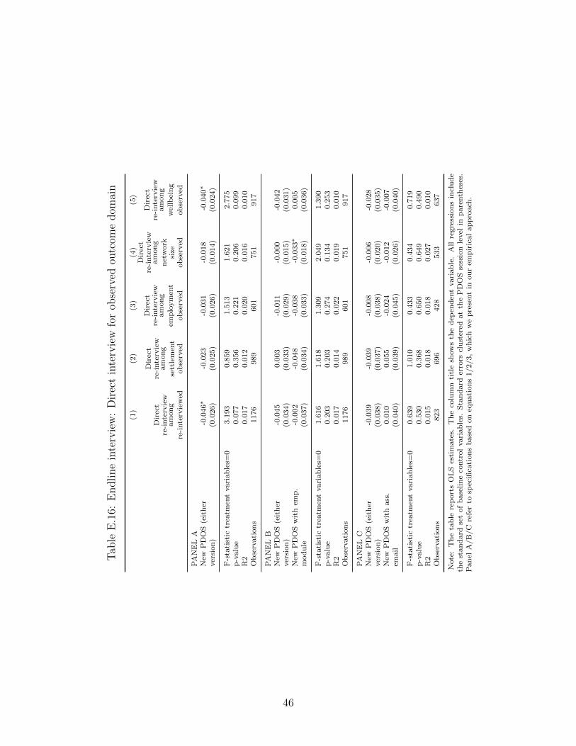
Tab

leE

.16:

Endline

inte

rvie

w:

Dir

ect

inte

rvie

wfo

rob

serv

edou

tcom

edom

ain

(1)

(2)

(3)

(4)

(5)

Dir

ect

re-i

nte

rvie

wam

on

g

re-i

nte

rvie

wed

Dir

ect

re-i

nte

rvie

wam

on

g

sett

lem

ent

ob

serv

ed

Dir

ect

re-i

nte

rvie

wam

on

g

emp

loym

ent

ob

serv

ed

Dir

ect

re-i

nte

rvie

wam

on

g

net

work

size

ob

serv

ed

Dir

ect

re-i

nte

rvie

wam

on

g

wel

lbei

ng

ob

serv

ed

PA

NE

LA

New

PD

OS

(eit

her

-0.0

46∗

-0.0

23

-0.0

31

-0.0

18

-0.0

40∗

ver

sion)

(0.0

26)

(0.0

25)

(0.0

26)

(0.0

14)

(0.0

24)

F-s

tati

stic

trea

tmen

tvari

ab

les=

03.1

93

0.8

59

1.5

13

1.6

21

2.7

75

p-v

alu

e0.0

77

0.3

56

0.2

21

0.2

06

0.0

99

R2

0.0

17

0.0

12

0.0

20

0.0

16

0.0

10

Ob

serv

ati

on

s1176

989

601

751

917

PA

NE

LB

New

PD

OS

(eit

her

-0.0

45

0.0

03

-0.0

11

-0.0

00

-0.0

42

ver

sion

)(0

.034)

(0.0

33)

(0.0

29)

(0.0

15)

(0.0

31)

New

PD

OS

wit

hem

p.

-0.0

02

-0.0

48

-0.0

38

-0.0

33∗

0.0

05

mod

ule

(0.0

37)

(0.0

34)

(0.0

33)

(0.0

18)

(0.0

36)

F-s

tati

stic

trea

tmen

tvari

ab

les=

01.6

16

1.6

18

1.3

09

2.0

49

1.3

90

p-v

alu

e0.2

03

0.2

03

0.2

74

0.1

34

0.2

53

R2

0.0

17

0.0

14

0.0

22

0.0

19

0.0

10

Ob

serv

ati

on

s1176

989

601

751

917

PA

NE

LC

New

PD

OS

(eit

her

-0.0

39

-0.0

39

-0.0

08

-0.0

06

-0.0

28

ver

sion

)(0

.038)

(0.0

37)

(0.0

38)

(0.0

20)

(0.0

35)

New

PD

OS

wit

hass

.0.0

10

0.0

55

-0.0

24

-0.0

12

-0.0

07

email

(0.0

40)

(0.0

39)

(0.0

45)

(0.0

26)

(0.0

40)

F-s

tati

stic

trea

tmen

tvari

ab

les=

00.6

39

1.0

10

0.4

33

0.4

34

0.7

19

p-v

alu

e0.5

30

0.3

68

0.6

50

0.6

49

0.4

90

R2

0.0

15

0.0

18

0.0

18

0.0

27

0.0

10

Ob

serv

ati

on

s823

696

428

533

637

Note

:T

he

tab

lere

port

sO

LS

esti

mate

s.T

he

colu

mn

titl

esh

ow

sth

ed

epen

den

tvari

ab

le.

All

regre

ssio

ns

incl

ud

eth

est

an

dard

set

of

base

lin

eco

ntr

ol

vari

ab

les.

Sta

nd

ard

erro

rscl

ust

ered

at

the

PD

OS

sess

ion

level

inp

are

nth

eses

.P

an

elA

/B

/C

refe

rto

spec

ifica

tion

sb

ase

don

equ

ati

on

s1/2/3,

wh

ich

we

pre

sent

inou

rem

pir

ical

ap

pro

ach

.

46

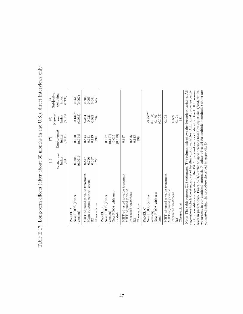
Tab

leE

.17:

Lon

g-te

rmeff

ects

(aft

erab

out

30m

onth

sin

the

U.S

.),

dir

ect

inte

rvie

ws

only

(1)

(2)

(3)

(4)

Set

tlem

ent

ind

ex(0

-1)

Em

plo

ym

ent

ind

ex(S

TE

)

Net

work

size

ind

ex(S

TE

)

Su

bje

ctiv

e

wel

lbei

ng

ind

ex(S

TE

)

PA

NE

LA

New

PD

OS

(eit

her

0.0

18

0.0

50

-0.1

34∗∗

0.0

51

ver

sion

)(0

.021)

(0.0

94)

(0.0

65)

(0.0

62)

MH

T-a

dju

sted

p-v

alu

etr

eatm

ent

0.8

77

0.8

44

0.2

64

0.8

05

Mea

nou

tcom

eco

ntr

ol

gro

up

0.7

50

0.0

31

-0.0

21

0.0

05

R2

0.3

37

0.1

13

0.0

92

0.0

44

Ob

serv

ati

on

s527

399

526

527

PA

NE

LB

New

PD

OS

(eit

her

0.0

57

ver

sion

)(0

.107)

New

PD

OS

wit

hem

p.

-0.0

15

mod

ule

(0.0

98)

MH

T-a

dju

sted

p-v

alu

etr

eatm

ent

0.8

47

MH

T-a

dju

sted

p-v

alu

e

inte

ract

edtr

eatm

ent

0.8

76

R2

0.1

13

Ob

serv

ati

on

s399

PA

NE

LC

New

PD

OS

(eit

her

-0.2

52∗∗

ver

sion

)(0

.103)

New

PD

OS

wit

hass

.0.1

39

email

(0.1

05)

MH

T-a

dju

sted

p-v

alu

etr

eatm

ent

0.1

05

MH

T-a

dju

sted

p-v

alu

e

inte

ract

edtr

eatm

ent

0.6

69

R2

0.1

21

Ob

serv

ati

on

s381

Note

:T

he

tab

lere

port

sO

LS

esti

mate

s.T

he

colu

mn

titl

esh

ow

sth

ed

epen

den

tvari

ab

le.

All

regre

ssio

ns

incl

ud

eth

est

an

dard

set

ofb

ase

lin

eco

ntr

olvari

ab

les.

Ad

dit

ion

alou

tcom

e-sp

ecifi

cco

ntr

ol

vari

ab

les

are

spec

ified

inth

eP

AP

.S

tan

dard

erro

rscl

ust

ered

at

the

PD

OS

sess

ion

level

inp

are

nth

eses

.P

anel

A/B

/C

refe

rto

spec

ifica

tion

sb

ase

don

equ

ati

on

s1/2/3,

wh

ich

we

pre

sent

inou

rem

pir

ical

ap

pro

ach

.P

-valu

esad

just

edfo

rm

ult

iple

hyp

oth

esis

test

ing

are

com

pu

ted

usi

ng

the

pro

ced

ure

des

crib

edin

Ap

pen

dix

D.

47

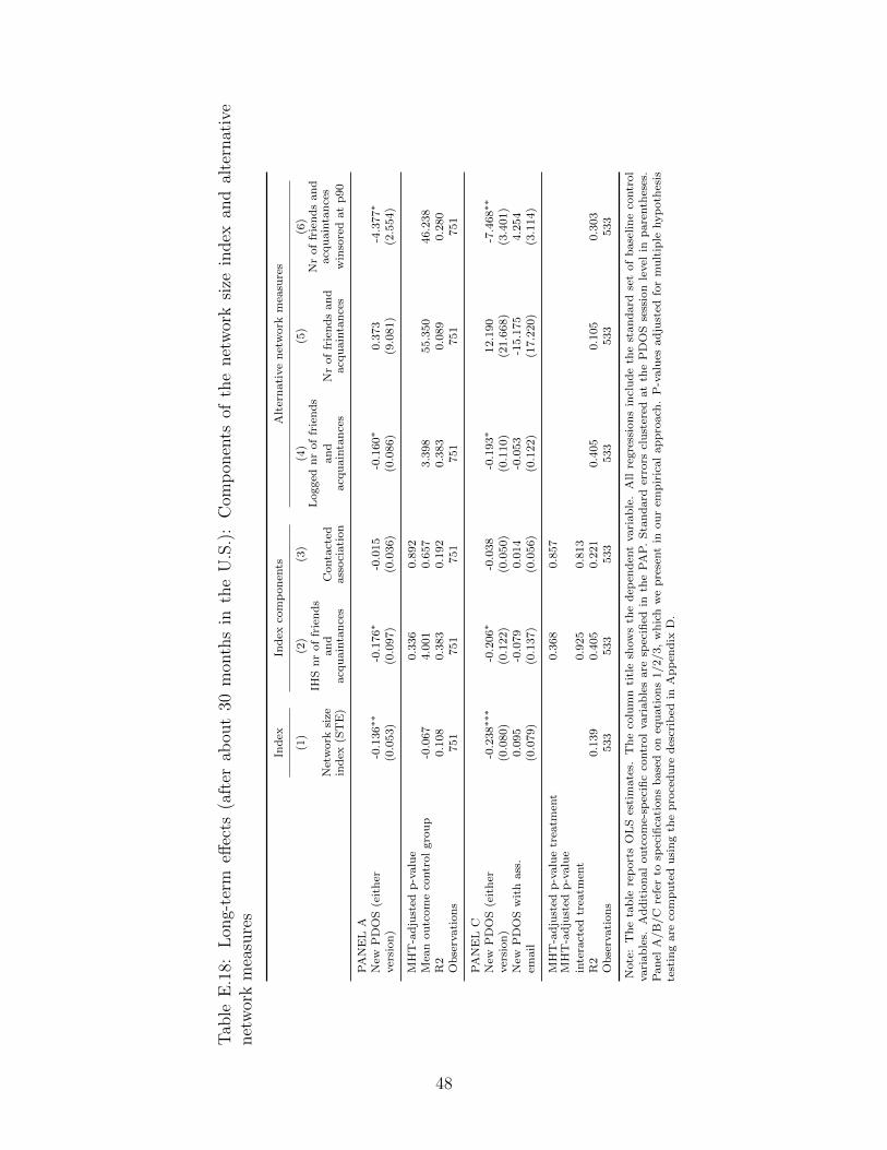
Tab

leE

.18:

Lon

g-te

rmeff

ects

(aft

erab

out

30m

onth

sin

the

U.S

.):

Com

pon

ents

ofth

enet

wor

ksi

zein

dex

and

alte

rnat

ive

net

wor

km

easu

res

Ind

exIn

dex

com

pon

ents

Alt

ern

ati

ve

net

work

mea

sure

s

(1)

(2)

(3)

(4)

(5)

(6)

Net

work

size

ind

ex(S

TE

)

IHS

nr

of

frie

nd

san

dacq

uain

tan

ces

Conta

cted

ass

oci

ati

on

Logged

nr

of

frie

nd

s

an

dacq

uain

tan

ces

Nr

of

frie

nd

san

dacq

uain

tan

ces

Nr

of

frie

nd

san

dacq

uain

tan

ces

win

sore

dat

p90

PA

NE

LA

New

PD

OS

(eit

her

-0.1

36∗∗

-0.1

76∗

-0.0

15

-0.1

60∗

0.3

73

-4.3

77∗

ver

sion

)(0

.053)

(0.0

97)

(0.0

36)

(0.0

86)

(9.0

81)

(2.5

54)

MH

T-a

dju

sted

p-v

alu

e0.3

36

0.8

92

Mea

nou

tcom

eco

ntr

ol

gro

up

-0.0

67

4.0

01

0.6

57

3.3

98

55.3

50

46.2

38

R2

0.1

08

0.3

83

0.1

92

0.3

83

0.0

89

0.2

80

Ob

serv

ati

on

s751

751

751

751

751

751

PA

NE

LC

New

PD

OS

(eit

her

-0.2

38∗∗∗

-0.2

06∗

-0.0

38

-0.1

93∗

12.1

90

-7.4

68∗∗

ver

sion

)(0

.080)

(0.1

22)

(0.0

50)

(0.1

10)

(21.6

68)

(3.4

01)

New

PD

OS

wit

hass

.0.0

95

-0.0

79

0.0

14

-0.0

53

-15.1

75

4.2

54

email

(0.0

79)

(0.1

37)

(0.0

56)

(0.1

22)

(17.2

20)

(3.1

14)

MH

T-a

dju

sted

p-v

alu

etr

eatm

ent

0.3

68

0.8

57

MH

T-a

dju

sted

p-v

alu

e

inte

ract

edtr

eatm

ent

0.9

25

0.8

13

R2

0.1

39

0.4

05

0.2

21

0.4

05

0.1

05

0.3

03

Ob

serv

ati

on

s533

533

533

533

533

533

Note

:T

he

tab

lere

port

sO

LS

esti

mate

s.T

he

colu

mn

titl

esh

ow

sth

ed

epen

den

tvari

ab

le.

All

regre

ssio

ns

incl

ud

eth

est

an

dard

set

of

base

lin

eco

ntr

ol

vari

ab

les.

Ad

dit

ion

al

ou

tcom

e-sp

ecifi

cco

ntr

ol

vari

ab

les

are

spec

ified

inth

eP

AP

.S

tan

dard

erro

rscl

ust

ered

at

the

PD

OS

sess

ion

level

inp

are

nth

eses

.P

an

elA

/B

/C

refe

rto

spec

ifica

tion

sb

ase

don

equ

ati

on

s1/2/3,

wh

ich

we

pre

sent

inou

rem

pir

ical

ap

pro

ach

.P

-valu

esad

just

edfo

rm

ult

iple

hyp

oth

esis

test

ing

are

com

pu

ted

usi

ng

the

pro

ced

ure

des

crib

edin

Ap

pen

dix

D.

48

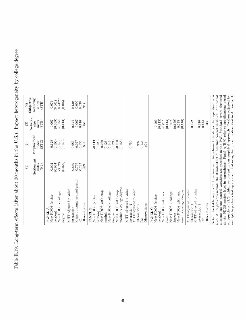
Tab

leE

.19:

Lon

g-te

rmeff

ects

(aft

erab

out

30m

onth

sin

the

U.S

.):

Impac

thet

erog

enei

tyby

colleg

edeg

ree

(1)

(2)

(3)

(4)

Set

tlem

ent

ind

ex(0

-1)

Em

plo

ym

ent

ind

ex(S

TE

)

Net

work

size

ind

ex(S

TE

)

Su

bje

ctiv

e

wel

lbei

ng

ind

ex(S

TE

)

PA

NE

LA

New

PD

OS

(eit

her

0.0

02

-0.1

28

-0.0

67

-0.0

74

ver

sion

)(0

.024)

(0.1

06)

(0.0

69)

(0.0

61)

New

PD

OS

xco

lleg

e-0

.023

0.1

48

-0.1

54

0.2

47∗∗

deg

ree

(0.0

29)

(0.1

46)

(0.1

13)

(0.1

05)

MH

T-a

dju

sted

p-v

alu

ein

tera

ctio

n0.6

69

0.6

83

0.6

44

0.1

39

Mea

nou

tcom

eco

ntr

ol

gro

up

0.7

97

-0.0

27

-0.0

67

-0.0

09

R2

0.2

35

0.1

36

0.1

10

0.0

38

Ob

serv

ati

on

s989

601

751

917

PA

NE

LB

New

PD

OS

(eit

her

-0.1

13

ver

sion

)(0

.123)

New

PD

OS

wit

hem

p.

-0.0

30

mod

ule

(0.1

23)

New

PD

OS

xco

lleg

e0.1

49

deg

ree

(0.1

71)

New

PD

OS

wit

hem

p.

-0.0

00

mod

ule

xco

lleg

ed

egre

e(0

.158)

MH

T-a

dju

sted

p-v

alu

ein

tera

ctio

n1

0.7

50

MH

T-a

dju

sted

p-v

alu

ein

tera

ctio

n2

0.9

97

R2

0.1

36

Ob

serv

ati

on

s601

PA

NE

LC

New

PD

OS

(eit

her

-0.1

03

ver

sion

)(0

.113)

New

PD

OS

wit

hass

.-0

.015

email

(0.1

14)

New

PD

OS

xco

lleg

e-0

.278

deg

ree

(0.1

69)

New

PD

OS

wit

hass

.0.2

25

email

xco

lleg

ed

egre

e(0

.176)

MH

T-a

dju

sted

p-v

alu

ein

tera

ctio

n1

0.4

72

MH

T-a

dju

sted

p-v

alu

ein

tera

ctio

n2

0.6

10

R2

0.1

44

Ob

serv

ati

on

s533

Note

:T

he

tab

lere

port

sO

LS

esti

mate

s.T

he

colu

mn

titl

esh

ow

sth

ed

epen

den

tvari

-ab

le.

All

regre

ssio

ns

incl

ud

eth

est

an

dard

set

of

base

lin

eco

ntr

ol

vari

ab

les.

Ad

dit

ion

al

ou

tcom

e-sp

ecifi

cco

ntr

ol

vari

ab

les

are

spec

ified

inth

eP

AP

.S

tan

dard

erro

rscl

ust

ered

at

the

PD

OS

sess

ion

level

inp

are

nth

eses

.P

an

elA

/B

/C

refe

rto

spec

ifica

tion

sb

ase

don

equ

ati

on

s1/2/3,

wh

ich

we

pre

sent

inou

rem

pir

ical

ap

pro

ach

.P

-valu

esad

just

edfo

rm

ult

iple

hyp

oth

esis

test

ing

are

com

pu

ted

usi

ng

the

pro

ced

ure

des

crib

edin

Ap

pen

dix

D.

49

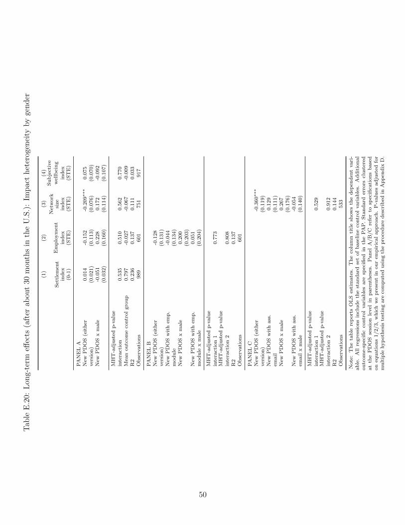
Tab

leE

.20:

Lon

g-te

rmeff

ects

(aft

erab

out

30m

onth

sin

the

U.S

.):

Impac

thet

erog

enei

tyby

gender

(1)

(2)

(3)

(4)

Set

tlem

ent

ind

ex(0

-1)

Em

plo

ym

ent

ind

ex(S

TE

)

Net

work

size

ind

ex(S

TE

)

Su

bje

ctiv

e

wel

lbei

ng

ind

ex(S

TE

)

PA

NE

LA

New

PD

OS

(eit

her

0.0

14

-0.1

52

-0.2

09∗∗∗

0.0

75

ver

sion

)(0

.021)

(0.1

13)

(0.0

76)

(0.0

70)

New

PD

OS

xm

ale

-0.0

51

0.2

28

0.1

72

-0.0

92

(0.0

32)

(0.1

60)

(0.1

14)

(0.1

07)

MH

T-a

dju

sted

p-v

alu

ein

tera

ctio

n0.5

35

0.5

10

0.5

62

0.7

70

Mea

nou

tcom

eco

ntr

ol

gro

up

0.7

97

-0.0

27

-0.0

67

-0.0

09

R2

0.2

36

0.1

37

0.1

11

0.0

33

Ob

serv

ati

on

s989

601

751

917

PA

NE

LB

New

PD

OS

(eit

her

-0.1

28

ver

sion

)(0

.131)

New

PD

OS

wit

hem

p.

-0.0

44

mod

ule

(0.1

34)

New

PD

OS

xm

ale

0.2

00

(0.2

03)

New

PD

OS

wit

hem

p.

0.0

51

mod

ule

xm

ale

(0.2

04)

MH

T-a

dju

sted

p-v

alu

ein

tera

ctio

n1

0.7

73

MH

T-a

dju

sted

p-v

alu

ein

tera

ctio

n2

0.8

08

R2

0.1

37

Ob

serv

ati

on

s601

PA

NE

LC

New

PD

OS

(eit

her

-0.3

60∗∗∗

ver

sion

)(0

.119)

New

PD

OS

wit

hass

.0.1

29

email

(0.1

11)

New

PD

OS

xm

ale

0.2

67

(0.1

76)

New

PD

OS

wit

hass

.-0

.054

email

xm

ale

(0.1

40)

MH

T-a

dju

sted

p-v

alu

ein

tera

ctio

n1

0.5

29

MH

T-a

dju

sted

p-v

alu

ein

tera

ctio

n2

0.9

12

R2

0.1

44

Ob

serv

ati

on

s533

Note

:T

he

tab

lere

port

sO

LS

esti

mate

s.T

he

colu

mn

titl

esh

ow

sth

ed

epen

den

tvari

-ab

le.

All

regre

ssio

ns

incl

ud

eth

est

an

dard

set

of

base

lin

eco

ntr

ol

vari

ab

les.

Ad

dit

ion

al

ou

tcom

e-sp

ecifi

cco

ntr

ol

vari

ab

les

are

spec

ified

inth

eP

AP

.S

tan

dard

erro

rscl

ust

ered

at

the

PD

OS

sess

ion

level

inp

are

nth

eses

.P

an

elA

/B

/C

refe

rto

spec

ifica

tion

sb

ase

don

equ

ati

on

s1/2/3,

wh

ich

we

pre

sent

inou

rem

pir

ical

ap

pro

ach

.P

-valu

esad

just

edfo

rm

ult

iple

hyp

oth

esis

test

ing

are

com

pu

ted

usi

ng

the

pro

ced

ure

des

crib

edin

Ap

pen

dix

D.

50

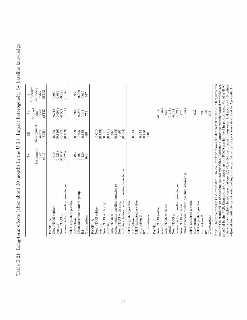
Tab

leE

.21:

Lon

g-te

rmeff

ects

(aft

erab

out

30m

onth

sin

the

U.S

.):

Impac

thet

erog

enei

tyby

bas

elin

eknow

ledge

(1)

(2)

(3)

(4)

Set

tlem

ent

ind

ex(0

-1)

Em

plo

ym

ent

ind

ex(S

TE

)

Net

work

size

ind

ex(S

TE

)

Su

bje

ctiv

e

wel

lbei

ng

ind

ex(S

TE

)

PA

NE

LA

New

PD

OS

(eit

her

0.0

19

0.0

05

-0.1

18

0.0

80

ver

sion

)(0

.021)

(0.1

36)

(0.0

93)

(0.0

83)

New

PD

OS

x-0

.048∗

-0.1

21

-0.0

33

-0.0

81

bel

ow

-med

ian

base

lin

ekn

ow

led

ge

(0.0

28)

(0.1

69)

(0.1

11)

(0.1

09)

MH

T-a

dju

sted

p-v

alu

ein

tera

ctio

n0.4

83

0.9

29

0.7

64

0.9

58

Mea

nou

tcom

eco

ntr

ol

gro

up

0.7

97

-0.0

27

-0.0

67

-0.0

09

R2

0.2

39

0.1

35

0.1

11

0.0

36

Ob

serv

ati

on

s989

601

751

917

PA

NE

LB

New

PD

OS

(eit

her

-0.0

10

ver

sion

)(0

.149)

New

PD

OS

wit

hem

p.

0.0

31

mod

ule

(0.1

31)

New

PD

OS

x-0

.066

bel

ow

-med

ian

base

lin

ekn

ow

led

ge

(0.1

95)

New

PD

OS

wit

hem

p.

-0.1

07

mod

ule

xb

elow

-med

ian

base

lin

ekn

ow

led

ge

(0.2

04)

MH

T-a

dju

sted

p-v

alu

ein

tera

ctio

n1

0.9

34

MH

T-a

dju

sted

p-v

alu

ein

tera

ctio

n2

0.9

74

R2

0.1

36

Ob

serv

ati

on

s601

PA

NE

LC

New

PD

OS

(eit

her

-0.1

60

ver

sion

)(0

.137)

New

PD

OS

wit

hass

.0.0

54

email

(0.1

18)

New

PD

OS

x-0

.144

bel

ow

-med

ian

base

lin

ekn

ow

led

ge

(0.1

71)

New

PD

OS

wit

hass

.0.0

75

email

xb

elow

-med

ian

base

lin

ekn

ow

led

ge

(0.1

47)

MH

T-a

dju

sted

p-v

alu

ein

tera

ctio

n1

0.9

37

MH

T-a

dju

sted

p-v

alu

ein

tera

ctio

n2

0.9

38

R2

0.1

44

Ob

serv

ati

on

s533

Note

:T

he

tab

lere

port

sO

LS

esti

mate

s.T

he

colu

mn

titl

esh

ow

sth

ed

epen

den

tvari

ab

le.

All

regre

ssio

ns

incl

ud

eth

est

an

dard

set

of

base

lin

eco

ntr

ol

vari

ab

les.

Ad

dit

ion

al

ou

tcom

e-sp

ecifi

cco

ntr

ol

vari

ab

les

are

spec

ified

inth

eP

AP

.S

tan

dard

erro

rscl

ust

ered

at

the

PD

OS

sess

ion

level

inp

are

nth

eses

.P

an

elA

/B

/C

refe

rto

spec

ifica

tion

sb

ase

don

equ

ati

on

s1/2/3,

wh

ich

we

pre

sent

inou

rem

pir

ical

ap

pro

ach

.P

-valu

esad

just

edfo

rm

ult

iple

hyp

oth

esis

test

ing

are

com

pu

ted

usi

ng

the

pro

ced

ure

des

crib

edin

Ap

pen

dix

D.

51

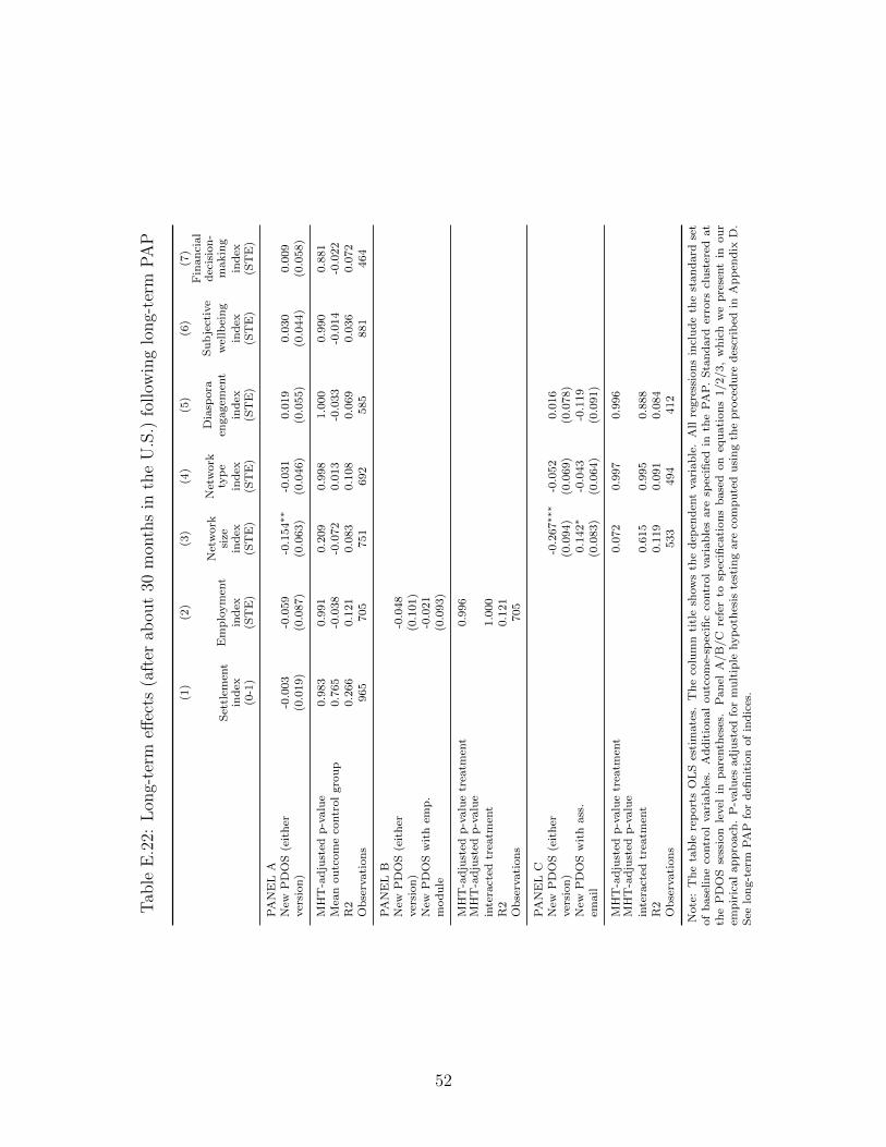
Tab

leE

.22:

Lon

g-te

rmeff

ects

(aft

erab

out

30m

onth

sin

the

U.S

.)fo

llow

ing

long-

term

PA

P

(1)

(2)

(3)

(4)

(5)

(6)

(7)

Set

tlem

ent

ind

ex(0

-1)

Em

plo

ym

ent

ind

ex(S

TE

)

Net

work

size

ind

ex(S

TE

)

Net

work

typ

e

ind

ex(S

TE

)

Dia

spora

engagem

ent

ind

ex(S

TE

)

Su

bje

ctiv

e

wel

lbei

ng

ind

ex(S

TE

)

Fin

an

cial

dec

isio

n-

makin

g

ind

ex(S

TE

)

PA

NE

LA

New

PD

OS

(eit

her

-0.0

03

-0.0

59

-0.1

54∗∗

-0.0

31

0.0

19

0.0

30

0.0

09

ver

sion

)(0

.019)

(0.0

87)

(0.0

63)

(0.0

46)

(0.0

55)

(0.0

44)

(0.0

58)

MH

T-a

dju

sted

p-v

alu

e0.9

83

0.9

91

0.2

09

0.9

98

1.0

00

0.9

90

0.8

81

Mea

nou

tcom

eco

ntr

ol

gro

up

0.7

65

-0.0

38

-0.0

72

0.0

13

-0.0

33

-0.0

14

-0.0

22

R2

0.2

66

0.1

21

0.0

83

0.1

08

0.0

69

0.0

36

0.0

72

Ob

serv

ati

on

s965

705

751

692

585

881

464

PA

NE

LB

New

PD

OS

(eit

her

-0.0

48

ver

sion

)(0

.101)

New

PD

OS

wit

hem

p.

-0.0

21

mod

ule

(0.0

93)

MH

T-a

dju

sted

p-v

alu

etr

eatm

ent

0.9

96

MH

T-a

dju

sted

p-v

alu

e

inte

ract

edtr

eatm

ent

1.0

00

R2

0.1

21

Ob

serv

ati

on

s705

PA

NE

LC

New

PD

OS

(eit

her

-0.2

67∗∗∗

-0.0

52

0.0

16

ver

sion

)(0

.094)

(0.0

69)

(0.0

78)

New

PD

OS

wit

hass

.0.1

42∗

-0.0

43

-0.1

19

email

(0.0

83)

(0.0

64)

(0.0

91)

MH

T-a

dju

sted

p-v

alu

etr

eatm

ent

0.0

72

0.9

97

0.9

96

MH

T-a

dju

sted

p-v

alu

e

inte

ract

edtr

eatm

ent

0.6

15

0.9

95

0.8

88

R2

0.1

19

0.0

91

0.0

84

Ob

serv

ati

on

s533

494

412

Note

:T

he

tab

lere

port

sO

LS

esti

mate

s.T

he

colu

mn

titl

esh

ow

sth

ed

epen

den

tvari

ab

le.

All

regre

ssio

ns

incl

ud

eth

est

an

dard

set

of

base

lin

eco

ntr

ol

vari

ab

les.

Ad

dit

ion

al

ou

tcom

e-sp

ecifi

cco

ntr

ol

vari

ab

les

are

spec

ified

inth

eP

AP

.S

tan

dard

erro

rscl

ust

ered

at

the

PD

OS

sess

ion

level

inp

are

nth

eses

.P

an

elA

/B

/C

refe

rto

spec

ifica

tion

sb

ase

don

equ

ati

on

s1/2/3,

wh

ich

we

pre

sent

inou

rem

pir

ical

ap

pro

ach

.P

-valu

esad

just

edfo

rm

ult

iple

hyp

oth

esis

test

ing

are

com

pu

ted

usi

ng

the

pro

ced

ure

des

crib

edin

Ap

pen

dix

D.

See

lon

g-t

erm

PA

Pfo

rd

efin

itio

nof

ind

ices

.

52

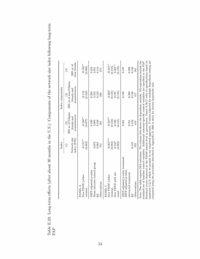
Tab

leE

.23:

Lon

g-te

rmeff

ects

(aft

erab

out

30m

onth

sin

the

U.S

.):

Com

pon

ents

ofth

enet

wor

ksi

zein

dex

follow

ing

long-

term

PA

P

Ind

exIn

dex

com

pon

ents

(1)

(2)

(3)

(4)

Net

work

size

ind

ex(S

TE

)

IHS

nr

of

Fil

ipin

o

frie

nd

san

dacq

uain

tan

ces

IHS

nr

of

non

-Filip

ino

frie

nd

san

dacq

uain

tan

ces

IHS

nr

of

close

frie

nd

s

PA

NE

LA

New

PD

OS

(eit

her

-0.1

54∗∗

-0.1

68∗∗

-0.1

10

-0.1

82∗∗

ver

sion

)(0

.063)

(0.0

77)

(0.1

02)

(0.0

90)

MH

T-a

dju

sted

p-v

alu

e0.1

99

0.2

95

0.2

24

Mea

nou

tcom

eco

ntr

ol

gro

up

-0.0

72

3.9

03

3.4

53

2.9

51

R2

0.0

83

0.1

09

0.1

23

0.1

13

Ob

serv

ati

on

s751

591

590

474

PA

NE

LC

New

PD

OS

(eit

her

-0.2

67∗∗∗

-0.2

57∗∗

-0.2

63∗

-0.3

15∗∗

ver

sion

)(0

.094)

(0.1

24)

(0.1

35)

(0.1

53)

New

PD

OS

wit

hass

.0.1

42∗

0.1

60

0.1

95

0.3

01∗∗

email

(0.0

83)

(0.1

21)

(0.1

45)

(0.1

35)

MH

T-a

dju

sted

p-v

alu

etr

eatm

ent

0.2

01

0.1

99

0.1

87

MH

T-a

dju

sted

p-v

alu

e

inte

ract

edtr

eatm

ent

0.3

51

0.4

60

0.2

09

R2

0.1

19

0.1

32

0.1

56

0.1

30

Ob

serv

ati

on

s533

419

417

341

Note

:T

he

tab

lere

port

sO

LS

esti

mate

s.T

he

colu

mn

titl

esh

ow

sth

ed

epen

den

tvari

ab

le.

All

regre

ssio

ns

incl

ud

eth

est

an

dard

set

of

base

lin

eco

ntr

ol

vari

ab

les.

Ad

dit

ion

al

ou

tcom

e-sp

ecifi

cco

ntr

ol

vari

ab

les

are

spec

ified

inth

eP

AP

.S

tan

dard

erro

rscl

ust

ered

at

the

PD

OS

sess

ion

level

inp

are

nth

eses

.P

an

elA

/B

/C

refe

rto

spec

ifica

tion

sb

ase

don

equ

ati

on

s1/2/3,

wh

ich

we

pre

sent

inou

rem

pir

ical

ap

pro

ach

.P

-valu

esad

just

edfo

rm

ult

iple

hyp

oth

esis

test

ing

are

com

pu

ted

usi

ng

the

pro

ced

ure

des

crib

edin

Ap

pen

dix

D.

IHS

issh

ort

for

inver

sehyp

erb

olic

sin

e.

53

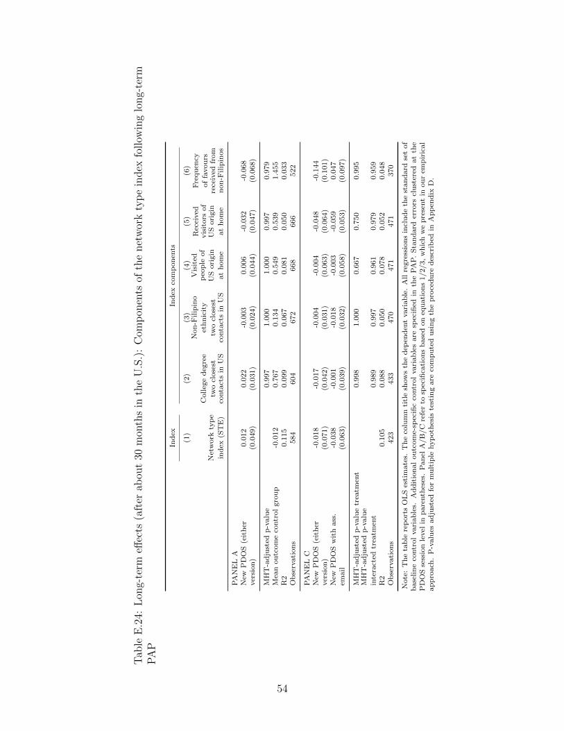
Tab

leE

.24:

Lon

g-te

rmeff

ects

(aft

erab

out

30m

onth

sin

the

U.S

.):

Com

pon

ents

ofth

enet

wor

kty

pe

index

follow

ing

long-

term

PA

P

Ind

exIn

dex

com

pon

ents

(1)

(2)

(3)

(4)

(5)

(6)

Net

work

typ

e

ind

ex(S

TE

)

Colleg

ed

egre

e

two

close

stco

nta

cts

inU

S

Non

-Filip

ino

eth

nic

ity

two

close

stco

nta

cts

inU

S

Vis

ited

peo

ple

of

US

ori

gin

at

hom

e

Rec

eived

vis

itors

of

US

ori

gin

at

hom

e

Fre

qu

ency

of

favou

rsre

ceiv

edfr

om

non

-Filip

inos

PA

NE

LA

New

PD

OS

(eit

her

0.0

12

0.0

22

-0.0

03

0.0

06

-0.0

32

-0.0

68

ver

sion

)(0

.049)

(0.0

31)

(0.0

24)

(0.0

44)

(0.0

47)

(0.0

68)

MH

T-a

dju

sted

p-v

alu

e0.9

97

1.0

00

1.0

00

0.9

97

0.9

79

Mea

nou

tcom

eco

ntr

ol

gro

up

-0.0

12

0.7

67

0.1

34

0.5

49

0.5

39

1.4

55

R2

0.1

15

0.0

99

0.0

67

0.0

81

0.0

50

0.0

33

Ob

serv

ati

on

s584

604

672

668

666

522

PA

NE

LC

New

PD

OS

(eit

her

-0.0

18

-0.0

17

-0.0

04

-0.0

04

-0.0

48

-0.1

44

ver

sion

)(0

.071)

(0.0

42)

(0.0

31)

(0.0

63)

(0.0

64)

(0.1

01)

New

PD

OS

wit

hass

.-0

.038

-0.0

01

-0.0

18

-0.0

03

-0.0

59

0.0

47

email

(0.0

63)

(0.0

39)

(0.0

32)

(0.0

58)

(0.0

53)

(0.0

97)

MH

T-a

dju

sted

p-v

alu

etr

eatm

ent

0.9

98

1.0

00

0.6

67

0.7

50

0.9

95

MH

T-a

dju

sted

p-v

alu

e

inte

ract

edtr

eatm

ent

0.9

89

0.9

97

0.9

61

0.9

79

0.9

59

R2

0.1

05

0.0

88

0.0

50

0.0

78

0.0

52

0.0

48

Ob

serv

ati

on

s423

433

470

471

471

370

Note

:T

he

tab

lere

port

sO

LS

esti

mate

s.T

he

colu

mn

titl

esh

ow

sth

ed

epen

den

tvari

ab

le.

All

regre

ssio

ns

incl

ud

eth

est

an

dard

set

of

base

lin

eco

ntr

ol

vari

ab

les.

Ad

dit

ion

al

ou

tcom

e-sp

ecifi

cco

ntr

ol

vari

ab

les

are

spec

ified

inth

eP

AP

.S

tan

dard

erro

rscl

ust

ered

at

the

PD

OS

sess

ion

level

inp

are

nth

eses

.P

an

elA

/B

/C

refe

rto

spec

ifica

tion

sb

ase

don

equ

ati

on

s1/2/3,

wh

ich

we

pre

sent

inou

rem

pir

ical

ap

pro

ach

.P

-valu

esad

just

edfo

rm

ult

iple

hyp

oth

esis

test

ing

are

com

pu

ted

usi

ng

the

pro

ced

ure

des

crib

edin

Ap

pen

dix

D.

54

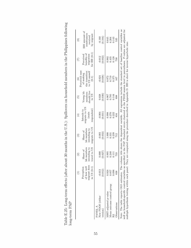
Tab

leE

.25:

Lon

g-te

rmeff

ects

(aft

erab

out

30m

onth

sin

the

U.S

.):

Spillo

vers

onhou

sehol

dm

emb

ers

inth

eP

hilip

pin

esfo

llow

ing

long-

term

PA

P

(1)

(2)

(3)

(4)

(5)

(6)

(7)

(8)

Per

cep

tion

of

how

wel

lm

igra

nt

does

inU

S(0

-1)

Sh

are

of

hh

mem

ber

sin

tend

ing

to

travel

toU

S

Sh

are

of

hh

mem

ber

sin

ten

din

gto

mig

rate

toU

S

Inte

nd

sto

mig

rate

toU

S

(main

resp

on

den

t)

You

ng

hh

mem

ber

ssh

ou

ldlive

inU

S

Per

ceiv

edea

seof

makin

g

the

tran

siti

on

toU

Son

esel

f(0

-1)

Per

ceiv

edb

enefi

tsof

mig

rati

on

for

HH

(0-1

)

IHS

am

ou

nt

of

rem

itta

nce

sre

ceiv

edby

mig

rant

PA

NE

LA

New

PD

OS

(eit

her

-0.0

13

0.0

00

-0.0

01

-0.0

04

0.0

28

-0.0

24

-0.0

12

-0.1

60

ver

sion)

(0.0

12)

(0.0

27)

(0.0

32)

(0.0

31)

(0.0

36)

(0.0

38)

(0.0

32)

(0.1

04)

MH

T-a

dju

sted

p-v

alu

e0.9

24

0.9

95

1.0

00

0.9

98

0.9

67

0.9

72

0.9

92

0.6

45

Mea

nou

tcom

eco

ntr

ol

gro

up

0.8

57

0.2

40

0.3

31

0.2

70

0.7

85

0.7

19

0.4

35

6.2

04

R2

0.0

98

0.1

11

0.2

39

0.2

22

0.1

44

0.3

75

0.1

28

0.1

43

Ob

serv

ati

on

s838

733

712

834

898

167

730

535

Note

:T

he

table

rep

ort

sO

LS

esti

mate

s.T

he

colu

mn

titl

esh

ow

sth

ed

epen

den

tvari

ab

le.

All

regre

ssio

ns

incl

ud

eth

est

an

dard

set

of

base

lin

eco

ntr

ol

vari

ab

les

as

wel

las

hou

seh

old

-sp

ecifi

cco

ntr

ol

vari

ab

les

as

spec

ified

inth

eP

AP

.S

tan

dard

erro

rscl

ust

ered

at

the

PD

OS

sess

ion

level

inp

are

nth

eses

.P

-valu

esare

ad

just

edfo

rm

ult

iple

hyp

oth

esis

test

ing

wit

hin

each

pan

el.

Th

eyare

com

pu

ted

usi

ng

the

pro

cedu

red

escr

ibed

inA

pp

end

ixD

.IH

Sis

short

for

inver

sehyp

erb

olic

sin

e.

55

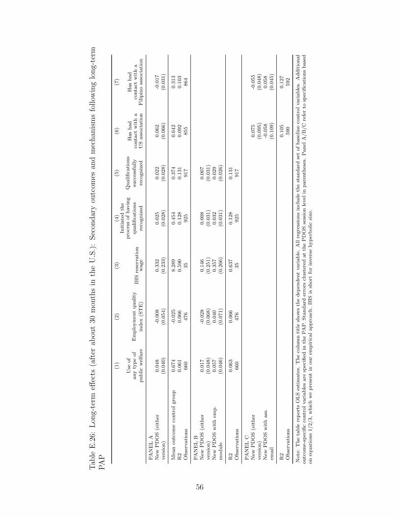
Tab

leE

.26:

Lon

g-te

rmeff

ects

(aft

erab

out

30m

onth

sin

the

U.S

.):

Sec

ondar

you

tcom

esan

dm

echan

ism

sfo

llow

ing

long-

term

PA

P

(1)

(2)

(3)

(4)

(5)

(6)

(7)

Use

of

any

typ

eof

pu

blic

wel

fare

Em

plo

ym

ent

qu

ality

ind

ex(S

TE

)IH

Sre

serv

ati

on

wage

Init

iate

dth

ep

roce

ssof

havin

g

qu

alifi

cati

on

s

reco

gn

ized

Qu

alifi

cati

on

s

succ

essf

ully

reco

gn

ized

Has

had

conta

ctw

ith

aU

Sass

oci

ati

on

Has

had

conta

ctw

ith

aF

ilip

ino

ass

oci

ati

on

PA

NE

LA

New

PD

OS

(eit

her

0.0

48

-0.0

08

0.3

32

0.0

25

0.0

22

0.0

62

-0.0

17

ver

sion

)(0

.040)

(0.0

54)

(0.2

33)

(0.0

28)

(0.0

28)

(0.0

66)

(0.0

31)

Mea

nou

tcom

eco

ntr

ol

gro

up

0.6

74

-0.0

25

8.2

89

0.4

54

0.3

74

0.6

42

0.3

13

R2

0.0

61

0.0

66

0.5

90

0.1

28

0.1

31

0.0

92

0.1

03

Ob

serv

ati

on

s660

476

35

925

917

855

864

PA

NE

LB

New

PD

OS

(eit

her

0.0

17

-0.0

28

0.1

46

0.0

08

0.0

07

ver

sion

)(0

.048)

(0.0

68)

(0.2

51)

(0.0

31)

(0.0

31)

New

PD

OS

wit

hem

p.

0.0

57

0.0

40

0.3

57

0.0

32

0.0

29

mod

ule

(0.0

46)

(0.0

71)

(0.2

66)

(0.0

31)

(0.0

26)

R2

0.0

63

0.0

66

0.6

37

0.1

28

0.1

31

Ob

serv

ati

on

s660

476

35

925

917

PA

NE

LC

New

PD

OS

(eit

her

0.0

75

-0.0

55

ver

sion

)(0

.095)

(0.0

48)

New

PD

OS

wit

hass

.-0

.058

0.0

58

email

(0.1

09)

(0.0

45)

R2

0.1

05

0.1

27

Ob

serv

ati

on

s590

592

Note

:T

he

tab

lere

port

sO

LS

esti

mate

s.T

he

colu

mn

titl

esh

ow

sth

ed

epen

den

tvari

ab

le.

All

regre

ssio

ns

incl

ud

eth

est

an

dard

set

of

base

lin

eco

ntr

ol

vari

ab

les.

Ad

dit

ion

al

ou

tcom

e-sp

ecifi

cco

ntr

ol

vari

ab

les

are

spec

ified

inth

eP

AP

.S

tan

dard

erro

rscl

ust

ered

at

the

PD

OS

sess

ion

level

inp

are

nth

eses

.P

an

elA

/B

/C

refe

rto

spec

ifica

tion

sb

ase

don

equ

ati

on

s1/2/3,

wh

ich

we

pre

sent

inou

rem

pir

ical

ap

pro

ach

.IH

Sis

short

for

inver

sehyp

erb

olic

sin

e.

56

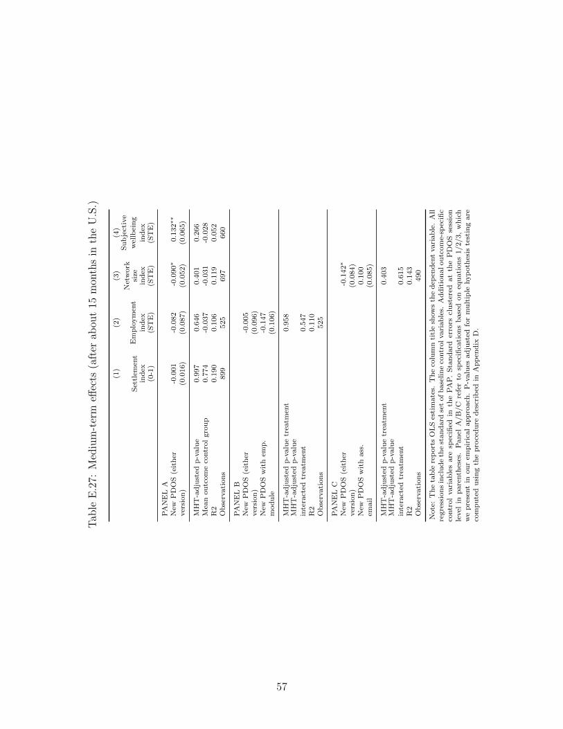
Tab

leE

.27:

Med

ium

-ter

meff

ects

(aft

erab

out

15m

onth

sin

the

U.S

.)

(1)

(2)

(3)

(4)

Set

tlem

ent

ind

ex(0

-1)

Em

plo

ym

ent

ind

ex(S

TE

)

Net

work

size

ind

ex(S

TE

)

Su

bje

ctiv

e

wel

lbei

ng

ind

ex(S

TE

)

PA

NE

LA

New

PD

OS

(eit

her

-0.0

01

-0.0

82

-0.0

90∗

0.1

32∗∗

ver

sion

)(0

.016)

(0.0

87)

(0.0

52)

(0.0

65)

MH

T-a

dju

sted

p-v

alu

e0.9

97

0.6

46

0.4

01

0.2

66

Mea

nou

tcom

eco

ntr

ol

gro

up

0.7

74

-0.0

37

-0.0

31

-0.0

28

R2

0.1

90

0.1

06

0.1

19

0.0

52

Ob

serv

ati

on

s899

525

697

660

PA

NE

LB

New

PD

OS

(eit

her

-0.0

05

ver

sion

)(0

.096)

New

PD

OS

wit

hem

p.

-0.1

47

mod

ule

(0.1

06)

MH

T-a

dju

sted

p-v

alu

etr

eatm

ent

0.9

58

MH

T-a

dju

sted

p-v

alu

e

inte

ract

edtr

eatm

ent

0.5

47

R2

0.1

10

Ob

serv

ati

on

s525

PA

NE

LC

New

PD

OS

(eit

her

-0.1

42∗

ver

sion

)(0

.084)

New

PD

OS

wit

hass

.0.1

00

email

(0.0

85)

MH

T-a

dju

sted

p-v

alu

etr

eatm

ent

0.4

03

MH

T-a

dju

sted

p-v

alu

e

inte

ract

edtr

eatm

ent

0.6

15

R2

0.1

43

Ob

serv

ati

on

s490

Note

:T

he

tab

lere

port

sO

LS

esti

mate

s.T

he

colu

mn

titl

esh

ow

sth

ed

epen

den

tvari

ab

le.

All

regre

ssio

ns

incl

ud

eth

est

an

dard

set

ofb

ase

lin

eco

ntr

olvari

ab

les.

Ad

dit

ion

alou

tcom

e-sp

ecifi

cco

ntr

ol

vari

ab

les

are

spec

ified

inth

eP

AP

.S

tan

dard

erro

rscl

ust

ered

at

the

PD

OS

sess

ion

level

inp

are

nth

eses

.P

anel

A/B

/C

refe

rto

spec

ifica

tion

sb

ase

don

equ

ati

on

s1/2/3,

wh

ich

we

pre

sent

inou

rem

pir

ical

ap

pro

ach

.P

-valu

esad

just

edfo

rm

ult

iple

hyp

oth

esis

test

ing

are

com

pu

ted

usi

ng

the

pro

ced

ure

des

crib

edin

Ap

pen

dix

D.

57

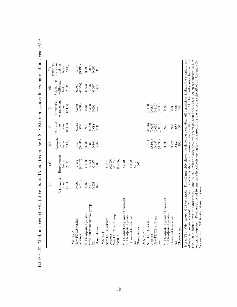
Tab

leE

.28:

Med

ium

-ter

meff

ects

(aft

erab

out

15m

onth

sin

the

U.S

.):

Mai

nou

tcom

esfo

llow

ing

med

ium

-ter

mP

AP

(1)

(2)

(3)

(4)

(5)

(6)

(7)

Set

tlem

ent

ind

ex(0

-1)

Em

plo

ym

ent

ind

ex(S

TE

)

Net

work

size

ind

ex(S

TE

)

Net

work

typ

e

ind

ex(S

TE

)

Dia

spora

engagem

ent

ind

ex(S

TE

)

Su

bje

ctiv

e

wel

lbei

ng

ind

ex(S

TE

)

Fin

an

cial

dec

isio

n-

makin

g

ind

ex(S

TE

)

PA

NE

LA

New

PD

OS

(eit

her

0.0

04

-0.0

87

-0.1

47∗∗

-0.0

32

-0.0

35

0.0

88

-0.1

07

ver

sion

)(0

.018)

(0.0

82)

(0.0

65)

(0.0

64)

(0.0

64)

(0.0

55)

(0.1

31)

MH

T-a

dju

sted

p-v

alu

e0.9

69

0.9

30

0.3

07

0.9

88

0.9

94

0.6

76

0.9

94

Mea

nou

tcom

eco

ntr

ol

gro

up

0.7

19

-0.0

31

-0.0

31

-0.0

00

-0.0

00

-0.0

27

-0.0

00

R2

0.2

21

0.1

17

0.1

01

0.0

88

0.0

96

0.0

47

0.0

52

Ob

serv

ati

on

s875

607

697

550

496

660

335

PA

NE

LB

New

PD

OS

(eit

her

0.0

07

ver

sion

)(0

.095)

New

PD

OS

wit

hem

p.

-0.1

79∗

mod

ule

(0.1

06)

MH

T-a

dju

sted

p-v

alu

etr

eatm

ent

0.9

42

MH

T-a

dju

sted

p-v

alu

e

inte

ract

edtr

eatm

ent

0.6

79

R2

0.1

21

Ob

serv

ati

on

s607

PA

NE

LC

New

PD

OS

(eit

her

-0.1

63

-0.0

46

-0.0

60

ver

sion

)(0

.101)

(0.0

98)

(0.0

87)

New

PD

OS

wit

hass

.0.0

37

0.0

55

0.1

40∗

email

(0.0

98)

(0.0

95)

(0.0

83)

MH

T-a

dju

sted

p-v

alu

etr

eatm

ent

0.6

97

0.9

79

0.9

88

MH

T-a

dju

sted

p-v

alu

e

inte

ract

edtr

eatm

ent

0.9

76

0.9

94

0.7

05

R2

0.1

33

0.0

88

0.1

04

Ob

serv

ati

on

s490

390

346

Note

:T

he

tab

lere

port

sO

LS

esti

mate

s.T

he

colu

mn

titl

esh

ow

sth

ed

epen

den

tvari

ab

le.

All

regre

ssio

ns

incl

ud

eth

est

an

dard

set

of

base

lin

eco

ntr

ol

vari

ab

les.

Ad

dit

ion

al

ou

tcom

e-sp

ecifi

cco

ntr

ol

vari

ab

les

are

spec

ified

inth

eP

AP

.S

tan

dard

erro

rscl

ust

ered

at

the

PD

OS

sess

ion

level

inp

are

nth

eses

.P

an

elA

/B

/C

refe

rto

spec

ifica

tion

sb

ase

don

equ

ati

on

s1/2/3,

wh

ich

we

pre

sent

inou

rem

pir

ical

ap

pro

ach

.P

-valu

esad

just

edfo

rm

ult

iple

hyp

oth

esis

test

ing

are

com

pu

ted

usi

ng

the

pro

ced

ure

des

crib

edin

Ap

pen

dix

D.

See

mid

-ter

mP

AP

for

defi

nit

ion

of

ind

ices

.

58