The Experiments, as the Irreducible Basis of All

Science, and the Observer, as the Probability

Space of All Experiments, Are Found Sufficient to

Entail All Physics

Alexandre Harvey-Tremblay†

†Independent scientist, aht@protonmail.chApril 19, 2022

Abstract

While there exists in the wild a process to derive the laws of physics—namely, the practice of science— such does not currently benefit froma purely formal construction. This lack necessarily leads to obscurities inthe development of physics. It is our present purpose to formalize the pro-cess within a purely mathematical background that will eliminate theseobscurities. The first step in the program will be to eliminate all ambigu-ities from our language. To do so, we will express arbitrary experimentsusing Turing complete languages and halting programs. A listing of suchexperiments is recursively enumerable and, if understood as an incremen-

tal contribution to knowledge, then serves as a formulation of mathematicsthat models the practice of science entirely. In turn this formulation leadsto a definition of the observer as the probability space over all experimentsin nature, and physics as the solution to an optimization problem on theproduction of a message from said space; interpreted, physics defines acircumscription on the participation of the observer in nature. Finally,we discuss our model of the observer and the relation to physics, in thecontext of a comprehensive theory of reality.

Contents

1 Introduction 3

2 The Formal System of Knowledge 62.1 Halting Programs as Knowledge . . . . . . . . . . . . . . . . . . . 102.2 Incremental Contributions . . . . . . . . . . . . . . . . . . . . . . 142.3 Connection to Formal Axiomatic Systems . . . . . . . . . . . . . 172.4 Discussion — The Mathematics of Knowledge . . . . . . . . . . . 182.5 Axiomatic Information . . . . . . . . . . . . . . . . . . . . . . . . 20

1

3 The Formal System of Science 213.1 Terminating Protocols as Knowledge about Nature . . . . . . . . 243.2 The Universal Experimenter . . . . . . . . . . . . . . . . . . . . . 263.3 Classification of Scientific Theories . . . . . . . . . . . . . . . . . 293.4 The Fundamental Theorem of Science . . . . . . . . . . . . . . . 29

4 A Formal Theory of the Observer 304.1 Nature . . . . . . . . . . . . . . . . . . . . . . . . . . . . . . . . . 314.2 Definition of the Observer . . . . . . . . . . . . . . . . . . . . . . 314.3 The Experience of the Observer . . . . . . . . . . . . . . . . . . . 32

5 Intermission 335.1 Science . . . . . . . . . . . . . . . . . . . . . . . . . . . . . . . . . 335.2 The Observer . . . . . . . . . . . . . . . . . . . . . . . . . . . . . 345.3 The Theories . . . . . . . . . . . . . . . . . . . . . . . . . . . . . 375.4 ”It from Bit” . . . . . . . . . . . . . . . . . . . . . . . . . . . . . 385.5 Origin of the Wave-Function . . . . . . . . . . . . . . . . . . . . . 395.6 A Random Walk in Algorithmic Space . . . . . . . . . . . . . . . 415.7 Dissolving the Measurements Problem . . . . . . . . . . . . . . . 435.8 Automatic Inclusion of Gravity . . . . . . . . . . . . . . . . . . . 455.9 Context . . . . . . . . . . . . . . . . . . . . . . . . . . . . . . . . 45

6 Main Result 466.1 Completing the Measure over Nature . . . . . . . . . . . . . . . . 48

6.1.1 Split to Amplitude / Probability Rule . . . . . . . . . . . 496.1.2 Tensor Product . . . . . . . . . . . . . . . . . . . . . . . . 496.1.3 Direct Sum . . . . . . . . . . . . . . . . . . . . . . . . . . 50

6.2 Discussion — Fock Spaces as Measures over Tuples . . . . . . . . 516.3 Connection to Computation . . . . . . . . . . . . . . . . . . . . . 51

7 Foundation of Physics 527.1 Matrix-Valued Vector and Transformations . . . . . . . . . . . . 537.2 Algebra of Observables, in 2D . . . . . . . . . . . . . . . . . . . . 53

7.2.1 Geometric Representation of 2× 2 matrices . . . . . . . . 537.2.2 Axiomatic Definition of the Algebra, in 2D . . . . . . . . 557.2.3 Observable, in 2D — Self-Adjoint Operator . . . . . . . . 567.2.4 Observable, in 2D — Eigenvalues / Spectral Theorem . . 57

7.3 Algebra of Observables, in 4D . . . . . . . . . . . . . . . . . . . . 587.3.1 Geometric Representation, in 4D . . . . . . . . . . . . . . 587.3.2 Axiomatic Definition of the Algebra, in 4D . . . . . . . . 59

7.4 Probability-Preserving Transformation . . . . . . . . . . . . . . . 607.4.1 Left Action, in 2D . . . . . . . . . . . . . . . . . . . . . . 607.4.2 Adjoint Action, in 2D . . . . . . . . . . . . . . . . . . . . 61

2

8 Applications 628.1 Familiar Grounds . . . . . . . . . . . . . . . . . . . . . . . . . . . 62

8.1.1 Dirac Current and the Bilinear Covariants . . . . . . . . . 628.1.2 Unitary Gauge Recap . . . . . . . . . . . . . . . . . . . . 64

8.2 New Contributions . . . . . . . . . . . . . . . . . . . . . . . . . . 648.2.1 General Linear Gauge Invariance . . . . . . . . . . . . . . 658.2.2 Physical Interpretation . . . . . . . . . . . . . . . . . . . . 658.2.3 A Step Towards Falsifiable Predictions . . . . . . . . . . . 67

9 Discussion 689.1 The Ontological Sufficiency of the Experience . . . . . . . . . . . 69

10 Conclusion 70

A Notation 71

B Lagrange equation 72B.1 Multiple constraints . . . . . . . . . . . . . . . . . . . . . . . . . 73B.2 Multiple constraints - General Case . . . . . . . . . . . . . . . . . 73

C Example of a Formal Proof 74

D A Step Towards Testable Predictions (Space-time interference) 75D.1 Geometric Algebra Dot Product . . . . . . . . . . . . . . . . . . 75D.2 Geometric Interference (General Form) . . . . . . . . . . . . . . . 77D.3 Complex Interference (Recall) . . . . . . . . . . . . . . . . . . . . 77D.4 Geometric Interference in 2D . . . . . . . . . . . . . . . . . . . . 77D.5 Geometric Interference in 4D . . . . . . . . . . . . . . . . . . . . 78D.6 Geometric Interference in 4D (Shallow Phase Rotation) . . . . . 79D.7 Geometric Interference in 4D (Deep Phase Rotation) . . . . . . . 79D.8 Geometric Interference in 4D (Deep Spinor Rotation) . . . . . . . 80

E The General Linear Probability Amplitude in Other Dimen-sions 81E.1 Zero-dimension case . . . . . . . . . . . . . . . . . . . . . . . . . 81E.2 Odd-dimension cases . . . . . . . . . . . . . . . . . . . . . . . . . 82E.3 Even-dimension cases . . . . . . . . . . . . . . . . . . . . . . . . . 82

1 Introduction

It is intuitive for many to describe the laws of physics as a circumscription onone’s own freedom of action. For instance, the following phrasing is commonlyheard: ”In nature, one can do anything except violate the laws of physics”, or”The laws of physics are what one cannot violate in nature”. This is in contrastto the modern formulation of the laws of physics as a characterization of the

3

behaviour of a substance external to oneself, such as the behaviour of the elec-tron or the photon, which has historically been more amenable to mathematicalformalization.

Our present purpose will be to derive physics consistently with this intuition,and then it will be to capitalize on the advantages of the new formulation.

To derive physics we must start at a level more fundamental than its axioms.Four systems will be introduced to support this. The first, second and thirdsystems formalizes knowledge, the practice of science and the observer, respec-tively, —and this is key— without reference to physics. Then, in the last system,physics is recovered as the solution to an optimization problem circumscribingthe observer’s participation in nature.

Essentially, the model that formalizes the practice of science by the observerin nature is both sufficiently sophisticated to entail physics, and sufficientlyfundamental to be prior to physics.

With this more fundamental starting point, results which previously eludedthe axiomatic formulation of physics will be manifest: the origin of the wave-function and the Born rule (section 5.5), the purpose and mechanism of wave-function collapses (section 5.4 and 5.6), a geometric theory of quantum physics(section 7 and 8), a plausible unification of general relativity with quantummechanics (section 8.2), and of course the recovery of familiar quantum fieldtheory (section 8.1).

The model therefore completes modern theoretical physics with many of itskey missing parts.

How does the model work in the technical sense?First, a sketch.The four systems are:

1. A Formal System of Knowledge

We define knowledge and we select the appropriate mathematical tools tomodel it. Specifically, a unit of knowledge will be modelled as a haltingprogram. Then, each discovery of a halting program will be taken asa contribution to the lexicon of knowledge. The lexicon, as it includesall halting programs, is Turing complete, and consequently will not bedecidable, but rather recursively enumerable. Furthermore, as it is Turing-complete, the lexicon is maximally expressive, and on par with any otherTuring complete language. Finally, we show that the lexicon satisfies theepistemological definition of knowledge.

2. A Formal System of Science (used to ”map” knowledge)

We connect halting programs to a description of reality. To do so, weintroduce the notion of an experiment as an initial preparation along witha protocol (i.e. a series of steps) to be performed on the preparationsuch that it terminates with a result. We then further introduce thenotion of a universal experimenter as a machine that can carry out anyexperiments in nature. We find that such admits equivalent mathematicaldefinitions to that of a halting program and that of a universal Turing

4

machine, respectively. Finally, we argue that any system can be describedequivalently, and without ambiguities, by a corresponding collection ofterminated experiments (in lieu of, say, dynamical equations).

From here, a scientific method will be defined as a function that recur-sively enumerates experiments. A specific listing of halting programs orexperiments produces an incremental contribution of mathematical or ex-perimental knowledge, respectively. Such can then be used to validate orinvalidate predictive models of knowledge.

This yields a formalization of the practice of science that is entirely freeof obscurities. Purely mathematical definitions for experimentations, pre-dictions, falsification and other scientific notions are also made available.

3. A Formal Theory of the Observer (used to practice science)

We define and model the object that practices science. We attack theproblem from this angle: If the observer deterministically produces a re-cursive enumeration of experiments, then it is merely a machine and thephysics it is subjected to is super-deterministic; if however, the observerprobabilistically produces a recursive enumeration of experiments, then itis a probability space of experiments.

As the later case involves the use of probabilities and since its domain is theset of all experiments, we qualify it as a model of observer participationunder the assumption of experimenter freedom (a term borrowed fromits use as an assumption to the Bell inequality), or interchangeably as;’freedom of action’, ’free participation’ or ’free practice of science’. Theterms ’free’ and ’freedom’ are in this context to be interpreted similarlyto the strict sense given by Conway and Kochen[1] as freedom from beingdetermined by past history, thus allowing a probabilistic enumeration inthe present; and that of the Bell inequality as having the freedom to pickthe experiment (or equivalently its parameters), also undetermined by pasthistory. It is not meant to be interpreted in the metaphysical sense of freewill commonly used in philosophy.

With the observer so defined, its ”experience” will be given in the form ofthe production or receipt of a message (in the sense of the theory of infor-mation of Claude Shannon) of experimental contributions. Furthermore,since the elements of the message are selected according to a probabilitymeasure, then a quantity of information will be associated to receiving orproducing it.

As we found, the unit of information associated with the message is, forarbitrary experiments, not representable by bits, but rather by ’clicks’ (aterm we borrowed from John A. Wheeler[2] regarding the recording of anincidence by an incidence counter). Thus, in our system, the fundamentalexperience of the observer corresponds to a specific sequence of recorded’clicks’ representing a specific a selection of completed experiments in na-ture. Essentially, these ’clicks’ define the ”path” the observer takes in thespace of all experiments.

5

The observer is then an object that is free, in this sense, to practice sci-ence in nature (rather than be compelled to act by a Turing machine ordeterministic algorithm), and as we found, it is in this context that thelaws of physics, in their familiar form, are manifest.

4. A Formal Model of Physics (derived by optimization as a circumscriptionon the freedom of action of the observer).

We found that fundamental physics is derivable by solving an optimiza-tion problem on the quantity of information associated with the receipt(or production) of a message of experimental contributions. Interpreted,physics defines the ’freest’ circumscription around observer participation.

Optimizing the information of the ’clicks’ will be sufficient to entail quan-tum physics. This is because, quite remarkably, these ’clicks’ behave sim-ilarly to wave-function measurement collapses. In fact, applying the tra-ditional machinery of statistical mechanics to an ensemble of clicks, thenmaximizing the entropy, yields very straightforwardly the wave-functionand the Born rule in lieu of the Gibbs measure, thereby providing an originfor these concepts that were previously postulated.

Furthermore, we found the machinery to be sufficiently powerful to derivequantum theory up to gravity in the form of a gauge-invariant generallinear wave-function. This is because the structure of the ’clicks’ that werecover is in fact slightly more general than the collapses that are manifestin standard quantum physics, and as it turned out, are exactly enough toadmit the Einstein field equations (EFE) as its equation of motion. Westress that the EFE does not need to be imported into the quantum theory,nor does it need to be reduced to its linearized form, and follows directlyfrom within.

If we interpret the production or receipt of a message of experimentalcontributions as the result of the free participation of the observer innature, then the resulting model of physics, as it is optimized, is merelyinterpreted as the maximally permissive model of said participation. Fromthis, the inviolability of the laws of physics automatically follows, simplybecause the observer logically cannot make a choice ’freer than freest’ andthat ’freest’ is used to define the laws of physics.

We pass now to the detailed and rigorous execution of the argument sketchedabove.

2 The Formal System of Knowledge

Mathematics tends to be formulated on the backbone of theories of truth, forinstance propositional logic or first order logic, and their aim are to correctlypropagate truth from statement to statement; whereas in the sciences, we tend tofind theories of knowledge whose aim are to produce incremental contributionsto validate (or invalidate) an ever more complete model thereof.

6

Knowledge is similar to truth in many ways. For instance, both quanti-tatively relate to a binary state: knowledge is either known (1) or unknown(0), and truth is either true (1) or false (0). But, theories of truth tend toview incompleteness as a weakness since it signals obscurities, whereas thoseof knowledge seek it as it signals an opportunity for progress. Furthermore,axiomatic theories formulated in terms of truth tend to clash with one another(incompatible premises entail contradictions), whereas those formulated basedon knowledge contribute to one another (knowledge is closed under union).

We have a plurality of theories of truth in mathematics, but so far we havenot captured these differences and intuitions into a formal system of knowledge.

Let us begin by stating that attempts to find a complete logical basis fortruth have been made ad nauseam in the past but they failed for primarily tworeasons. First, they were attempted before Godel-type theorems were knownand appreciated, and attempts were directed at constructing decidable logicalbases for truth. Second, instead of directing efforts to recursively enumerablebases following the discovery of said incompleteness theorems, efforts simply feltout of favour as it was understood that any sufficiently expressive system of truthwould contain obscurities, and this made them philosophically unattractive. Itis however possible to construct recursively enumerable bases (provided theyare not decidable), and further the limitations of recursive enumeration ought toinstead be seen as an opportunity; in this case, to create a formal system to mapout knowledge, such that it may serve as the foundation to a formalization ofscience. In this case, the theory challenges us to discover new knowledge, ratherthan to merely fix truth definitionally only to bail out at the first obscurity, andin this context we call it a theory of knowledge to distinguish it from a theoryof truth. Theories of knowledge, as recursively enumerable systems, are a moregeneral concept than theories of truth which are subsets thereof. Indeed, for allstatements that are either true (1) or false (0), it is the case that we can know(1) its truth value; but if a statement is such that it is undecidable, a binarystate of knowledge still applies to it: unknown (0).

To help appreciate the utility and to fix the intuition, consider the follow-ing ”amusing” construction which we will call rotting arithmetic. In logic weare allowed to inject any sentence as a new axiom, and to investigate its con-sequences. Rotting arithmetic will be defined as the union of the axioms ofPeano’s arithmetic and of the axiom of rot, which we define as follows:

Axiom of rot :=(22

82,589,933 − 1)

is a prime (1)

Rotting Arithmetic := Peano’s Arithmetic ∪ Axiom of rot (2)

The axiom of rot claims that a very large is number is a prime. If it’s true,then it has no effects on the system, but if it’s false, the system is inconsis-tent. Comparatively, the largest known prime (at the time of this writing) is282,589,933 − 1 which is orders of magnitude smaller than the number referencedin the axiom of rot. Since we have used randomness to generate the axiom ofrot, odds are minuscules that it is a prime... or perhaps we did hit the jackpot

7

and it is a prime. A theory of knowledge can assign the state unknown (0) tothe axiom of rot until such a time as we find out if the proposed number is orisn’t a prime; whereas a theory of truth expects true or false right now, as it’struth-value is fixed in principle.

It may be that it takes us a century until we find out if the axiom of rot is orisn’t true, as our computing capacities may need to improve before we can know.As time goes by, the ”freshness” of the theory slowly diminishes, until such atime as it is revealed to be rotten at which time it is discarded (or alternativelyit keeps perpetually fresh if we did hit the jackpot and the number is a prime).

Rotting arithmetic is ”threatened” by falsification, but contrary to what wemight expect for falsification to be possible, in this case the threat contains noreferences to nature. It is purely a mathematical effect due to the limits of ourcomputing power.

The example of rotten arithmetic may appear convoluted or unnatural —after-all why would we take the chance with an axiom of rot, when we can easilydo arithmetic without it —, but now consider what often happens in science.For nearly a century before Einstein produced the theory of special relativity(Einstein, 20th century), the union of both classical mechanics (Newton, 17thcentury) and electromagnetism (19th century) was ”fresh”:

Law of Inertia := F = ma (3)

Maxwells’ equation := ∇ ·E = ρ/ε0,∇ ·B = 0, ... (4)

Union := F = ma ∪ Maxwells’ equation (5)

The discovery of ”rot” in their union (Maxwell’s equations reports a constantspeed of light independently of the observer’s velocity, whereas velocities inF=ma are additive) had to wait for nearly a century to be noticed and corrected.In the mean time, most were happy to use both theories, and the problemremained unnoticed. Similarly to the case of rotten arithmetic, the state ofknowledge of ”rot” in the union had to go from unknown (0) to known (1),before a new model was to be produced.

Falsification in general can be manipulated in a similar fashion. Instead ofhaving two axiomatic theories, we have an empirical statement along with anaxiomatic theory:

Observation := Precession of Mercury’s orbit (6)

Law of Gravitation := F = GmM/r2 (7)

Falsification? := P[...] of Mercury’s orbit ∪ F = GmM/r2 (8)

The statement ”Precession of Mercury’s orbit” would plausibly indicate asequence of measurements, observations or experiments, and falsification occursif they are not solutions to the law of gravitation.

The next step is to develop the mathematical tools that are appropriate todescribe a theory of knowledge formally. To realize this we must be a bit more

8

technical. Let us look at the philosophical discipline that studies knowledge,epistemology, and distill it for usable insights.

Epistemology, at least historically and dating all the way back to Plato, hasconsidered knowledge to be that which is a justified true belief. For instance ”Iknow Bill is from Arkansas (as a justified true belief), because his driver’s licenseis from Arkansas (justification), and he is from Arkansas (true)”. However, theGettier problem[3] is a well known objection to this definition. Essentially, ifthe justification is not loophole free, there exists a case where one is right bypure luck, even if the claim were true and believed to be justified. For instance,if one glances at a field and sees a shape in the form of a dog, one might thinkhe or she is justified in the belief that there is a dog in the field. Now supposethere is a dog elsewhere in the field, but hidden from view. The belief ”there isa dog in the field” is justified and true, but it is a hard sale to call it knowledgebecause it is only true by pure luck.

Richard Kirkham[4] proposed to add the criteria of infallibility to the jus-tification. Knowledge, previously justified true belief, would now be infallibletrue belief. Merely seeing the shadow of a dog in a field would not be enough toqualify as infallible true belief, as all claims will have to be exactly proportionalto the evidence. This is generally understood to eliminate the loophole, but it isan unpopular solution because adding it is assumed to reduce knowledge to rad-ical skepticism in which almost nothing is knowledge, thus rendering knowledgenon-comprehensive.

Here, we will adopt the insight of Kirkham regarding the requirement ofinfallibility whilst resolving the non-comprehensiveness objection. To do so, wewill structure our statements such that they are each infallible, thus epistemi-cally certain, yet as a group will form a Turing complete language.

Our tool of choice to represent infallible true beliefs will be the halting pro-grams. They will act as the building blocks of knowledge in our system. Here,we understand halting programs as a descriptive language, similar in expressivepower to any other Turing complete language, such as say english. But unlikeenglish, using halting programs makes the description of each unit of knowl-edge completely free of ambiguities. And ambiguities are of course antitheticalto knowledge. General translations between all Turing languages exists, andso we do not lose any expressive power by using them, over any other choiceof language. For instance, any mathematical problem can be reformulated asa statement regarding the halting status of a program via the Curry–Howardcorrespondence. Other correspondences exist between all Turing-complete lan-guages.

The primary advantage in using a listing of halting programs over other can-didates is that it will allow us to union all new discoveries of knowledge witholder ones, without any risk of the new ones invalidating the previous ones; thusmaking old knowledge immutable under union with new knowledge. Indeed, ifa program is known to halt, then no other halting programs discovered after-wards can contradict that. Rather, it will be explanatory models of knowledgethat would or could be invalidated (falsified) by new knowledge, and not oldknowledge. Contributions of new knowledge to a lexicon will be incremental

9

and permanent by guarantee.Halting programs are of course subject to the halting problem and this will

entail our system to be a trial and error system. Consequently, acquiring newknowledge will be difficult, even arbitrarily difficulty, and may even containdead-ends (non-halting programs). These trial and error effects will in turnbecome the basis of a formal model of science that is entirely formalized, yetsufficiently sophisticated to be comprehensive.

Let us inform the reader that information regarding the connection be-tween mathematics, science and programs, is available in the works of GregoryChaitin[5, 6, 7] which constitute a major source of inspiration for our work. Afamiliarity with his work and ideas is assumed.

2.1 Halting Programs as Knowledge

How do we construct an epistemically certain statement, so that it qualifies asinfallible in the sense of Kirkham?

Let us take the example of a statement that may appear as an obvious truestatement such as ”1 + 1 = 2”, but is in fact not epistemically certain. Here,we will provide the definition of an epistemically certain statement, but equallyimportant, such that the set of all such statements is Turing complete, thusforming a language of maximum expressive power.

Specifically, the sentence ”1+1 = 2” halts on some Turing machine, but noton others and thus is not epistemically certain. Instead consider the sentencePA ⊢ [s(0)+s(0) = s(s(0))] to be read as ”Peano’s axioms proves that 1+1 = 2”.Such a statement embeds as a prefix the set of axioms in which it is provable.Without decorations, one can deny ”1 + 1 = 2” (for example, an adversarycould claim binary numbers, in which case 1 + 1 = 10), but if one specifiesthe exact axiomatic basis in which the claim is provable, said adversary wouldfind it harder to find a loophole to fail the claim. Nonetheless, even with thisimprovement, an adversary can fail the claim by providing a Turing machinefor which PA ⊢ [s(0) + s(0) = s(s(0))] does not halt.

The key is to structure the statement so that all context required to provethe statement is provided along with the statement itself; then it is the claimthat the context entails the statement that is epistemically certain. If we usethe tools of theoretical computer science we can produce statements free of allloopholes, thus ensuring they are epistemically certain. Those statements, whichare mathematical theorems, are also —via Curry–Howard correspondence— thehalting programs. The value in knowing that a specific programs halts correlateswith the complexity of running the program until termination, which dependingon the sophistication of the statement could be substantial. Let us now introducea few definitions.

Let Σ be a set of symbols, called an alphabet. A word is a sequence ofsymbols from Σ. The empty word is represented as ∅. The set of all finitewords is given as:

10

W :=

∞⋃

i=0

Σi (9)

Finally a language L is as a subset of W.As an example, the sentences of the binary alphabet Σ = 0, 1 are the

binary words ∅, 0, 1, 00, 01, 10, 11, 000, . . . .There exists multiple models of computation, such as Turing machines, µ-

recursive functions, Lambda calculus, etc. Here, to retain generality we will usecomputable functions without requiring a specific model.

Instead of a Turing machine, we will consider a Turing-computable functionand its definition is as follows:

A Turing machine Φ computes a partial function TM: W → W iff:

1. For each d ∈ Dom(TM), Φ(d) halts and equals TM(d).

2. For each d /∈ Dom(TM), Φ(d) never halts.

Then, TM is a Turing-computable function (or simply, a computable func-tion). We denote TM as the set of all computable partial functions fromW → W.

Likewise, and instead of a universal Turing machine as a specific implementa-tion, we will prefer to use a universal Turing-computable partial function of twoinputs DM: W×W → W. To use the elements of TM in this function, we mustintroduce a bijective function, which we call an interpreter, as: 〈·〉 : TM ↔ W

specific to the DM. Then, if for all TM ∈ TM and for all d ∈ Dom(TM), it isthe case that if DM(〈TM〉, d) ≃ TM(d), then DM is a universal function, andwe denote it as UTM.

Definition 1 (Halting Program). A halting program p is a pair TM×W:

p := (TM, d) (10)

such that TM(d) = r.

With this definition, d can be considered as the statement, TM is its context,and if TM(d) halts, then both are paired as a context-free halting claim:

p = (TM, d); UTM(〈TM〉, d) halts (11)

Since a translation exists between universal Turing machine, a claim thatd halts on TM, if known, entails ”p halts” is verifiable on all universal Turingmachines, and requires no specific context for this to be verified.

For instance, the following (trivial) program halts:

11

fn one_plus_one_equals_two()

if 1+1==2

return;

loop;

The claim ”p = (cargo run, one plus one equals two);UTM(p) halts” is aunit of knowledge, and I can contribute it to the lexicon.

A less trivial example is shown in Annex C which presents a formal proof ofthe commutativity of addition for natural numbers written in COQ[8]. Thus,the claim ”p = (COQ, plus comm); UTM(p) halts” would be another unit ofknowledge.

The second objection is that the epistemic certainty requirement is too de-manding, preventing knowledge from being comprehensive by making it ableat most to only tackle a handful of statements. However, the set of all halt-ing programs constitutes the entire domain of the universal Turing machine,and thus the expressive power of halting programs must be on par with anyTuring complete language. Since there exists no greater expressive power fora formal language than that of Turing completeness, then no reduction takesplace. The resulting construction is element-by-element epistemically certain,and comprehensive as a set:

Definition 2 (The Lexicon). The set of all programs TM ×W that halts con-stitutes the lexicon of epistemically certain knowledge, or simply the lexicon,K.

• K constitute the set of all epistemically certain statements.

• K is non-computable, but is recursively enumerable.

• K contains countably infinitely many elements.

• We can definite K, we can also contribute to it, but we cannot completeit.

• Unlike the hyperwebster[9] which includes all possible words from Σ re-gardless of halting status and is thus without knowledge, here each entryis a halting program and thus carries knowledge.

Definition 3 (Translation (of K)). A translation T of K is a map from TM×W

to W × W such that the interpreter function 〈·〉 is applied to each element ofTM. Each translation of K corresponds to the domain of a universal Turingmachine UTM.

TUTM := Dom(UTM) (12)

And contains all pairs W×W that halt on UTM.

12

Theorem 1 (Incompleteness Theorem). Since a translation of K is the domainof a UTM, then it is undecidable. The proof follows from the domain of auniversal Turing machine being undecidable. Finally, since 〈·〉 is bijective, itfollows that K is also undecidable.

The theorem implies that we will never run out of new knowledge to discover,and can thus perpetually contribute to the lexicon (job security is assured).

Theorem 2 (K is recursively enumerable). We will list K by dovetailing.

Proof. First, let us recursively enumerate the translation T of K. Consider adovetail program scheduler which works as follows.

1. Sort the columns of W×W in shortlex:

d1 d2 d3 . . .

〈TM1〉 (〈TM1〉, d1) (〈TM1〉, d2) (〈TM1〉, d3) . . . (13)

〈TM2〉 (〈TM2〉, d1) (〈TM2〉, d2) (〈TM2〉, d3) . . . (14)

〈TM3〉 (〈TM3〉, d1) (〈TM3〉, d2) (〈TM3〉, d3) . . . (15)

......

......

. . .

then trace a line across the pairs starting at (〈TM1〉, d1) then (〈TM2〉, d1),(〈TM1〉, d2), (〈TM2〉, d2), (〈TM3〉, d1) and so on. This produces an order-ing which grabs all pairs.

2. Take the first element of the sort, DM(〈TM1〉, d1), then run it for oneiteration.

3. Take the second element of the sort, DM(〈TM2〉, d1), then run it for oneiteration.

4. Go back to the first element, then run it for one more iteration.

5. Take the third element of the sort, DM(〈TM1〉, d2), then run it for oneiteration.

6. Continue with the pattern, performing iterations one by one, with eachcycle adding a new element of the sort.

7. Make note of any pair (〈TMi〉, dj) which halts.

Finally, use the interpreter function to convert W×W to TM× L, yieldingthe lexicon.

This scheduling strategy is called dovetailing and allows one to enumeratethe domain of a universal Turing machine recursively, without getting stuck byany particular program that may not halt. Progress will eventually be made onall programs, thus producing a recursive enumeration.

13

Definitionally, the domain of a recursively enumerable function is a set; how-ever in practice and implemented as an algorithm, a dovetailer and other im-plementations of recursive enumerations produces a sequence of incrementalcontributions to knowledge. Each new element that halts gets added to a list;the order of which depends on the implementation of the enumerating algorithm.

2.2 Incremental Contributions

We will now use the lexicon of knowledge and halting programs to redefine thefoundations of mathematics to be in terms of an incremental contribution toknowledge, rather than in terms of formal axiomatic systems.

In principle, one can use any Turing complete language to re-express math-ematics. The task is not particularly difficult. One generally has to build atranslator between the two formulations, whose existence is interpreted as aproof of equivalence. For instance, one can write all of mathematics using settheory with arbitrary set equipments, but also using the english language, orusing a computer language such as c++, or using arithmetic with multiplica-tion, etc. If the language is Turing complete, then it is as expressive as anyother Turing complete language, and translators are guaranteed to exist. Sowhy pick a particular system over another? This is often due to conveniencesand constraints other than pure expressive power. For instance, sets allow usto intuitively express a very large class of mathematical problems quite conve-niently. Typical selection criterions are; can we express the problem at handclearly?; elegantly?; are the solutions also clear and easier to formulate than inthe alternative system?

Here we will use and introduce the incremental contribution formulation ofmathematics, and, as we found its advantages regarding the capture, preserva-tion and accumulation of epistemically certain statements, as well as its upcom-ing role as the foundation of the formalized practice of science, are remarkable.

An incremental contribution comprises a group of programs known to halt,and this group of programs defines a specific instance of accumulated mathe-matical knowledge.

Definition 4 (Incremental Contribution (to Knowledge)). Let K be the lexiconof knowledge. An incremental contribution m of n halting program is an elementof the n-fold Cartesian product of K:

m ∈ Kn (16)

The tuple, in principle, can be empty m := (), finite n ∈ N or countablyinfinite n = ∞.

Note on the notation:

• We will designate pi = (TMi, di) as an halting program element of m,and proj1(pi) and proj2(pi) designate the first and second projection ofthe pair pi, respectively. Thus proj1(pi) is the TMi associated with pi,

14

and proj2(pi) is the input di associated with pi. If applied to a tuple orset of pairs, then proj1(m) returns the set of all TM in m and proj2(m)returns the set of all inputs d in m.

The programs comprising the incremental contribution adopt the normalrole of both axioms and theorems and form a single verifiable atomic conceptconstituting a unit of mathematical knowledge.

Let us explicitly point out the difference between the literature definition ofa formal axiomatic system and ours. In a formal axiomatic sytem, its theoremsare a subset of the sentences of L provable from the axioms — whereas in ours,a sequence of incremental contributions, its elements are pairs of TM×W whichhalts on a UTM.

Let us now explore some of the advantages of using incremental contributionsversus formal axiomatic systems.

Sequences of incremental contributions are more conductive to a descriptionof the scientific process, including the continued accumulation of knowledge,than formal axiomatic systems. Essentially, under an incremental contributionformulation, and unlike a formal axiomatic system, we will be able to perpet-ually accumulate new mathematical knowledge building up to the full lexicon(exclusively), without having to continuously readjust or expand some under-laying axiomatic basis to accommodate it.

Let us open a small parenthesis to explore this advantage more illustrativelyby comparing it to the tally mark numbering system, which admits a very similaradvantage, and then we will investigate it in greater detail.

Tally mark numbering systems are most useful in cases where intermediateresults do not have to be discarded, because one does not need to redraw thenumbers as the count is increased. Tally mark numbering system were likely thefirst numbering system used, and dates at least back to the Upper Palaeolithic.Remarkably, and although they are few and far in between, such systems stilladmit desirable use cases in modern time. For instance, consider the followingwarning sign posted at Hanakapiai Beach which utilizes such a numeral system:

15

[10]Here, the tally mark numbering system no doubt adds to the impact and

seriousness of the warning, and to the permanence of what is being recorded.When marking in stone, or using paint on a wood plank, a counting sys-

tem which necessitates erasure of the symbols to increase the count is highlyundesirable. For instance, if one uses Arabic numerals, one would start withthe symbol ”1”, then as the second incidence occurs, one has to erase the ”1”from the stone, and write a new symbol, in this case the symbol ”2”, and so on.But with a tally mark system, one only needs to add a new mark at the nextlocation to increase the count. No erasures are needed.

Now, going back to incremental contributions.The incremental contribution formulation is, essentially, a tally mark system

for knowledge and as such there exists a number of use cases for which it exceedsthe utility of formal axiomatic systems.

In the sciences, it is typical to produce a scientific theory as an axiomaticbasis, expand it into theorems, compare them to experimental data, then if amismatch is found, rewrite said axiomatic basis to accommodate the new knowl-edge. This is the prediction, falsification and refinement process characteristicof the Karl Popper method.

In mathematics, a similar process can also be manifest. We refer to in-completeness theorems such as the halting problem, Godel’s incompletenesstheorems, and to the limits induced on the completeness of formal axiomaticsystems. Suppose one would wish to represent in real-time and with live updates

16

the knowledge produced by all mathematicians and for an indefinite amount oftime into the future. Can a singular axiomatic system provide such a repre-sentation? Alas, since one can produce the Godel sentence of any (sufficientlyexpressive) axiomatic system, perpetual additions to the axioms of said systemwould be required to accommodate all possible new discoveries of knowledge.

But this is not the only ”annoyance” of formal axiomatic systems. One daya mathematician may wish to work with Euclid’s axiom, and on another day heor she may wish to work in ZFC set theory. How do we accumulate knowledgethat is discovered under different axiomatic basis? Or as another example,what if a mathematician finds a contradiction in some esoteric systems; findinga contradiction is still valuable knowledge and we may wish to record theirdiscoveries for posterity. Do we inject a wrapper of para-consistent logic aroundthem? Formal axiomatics systems, even with accommodations, ”crystallizes”into a particular form of knowledge; and this form excludes other forms.

Comparatively, using the incremental contribution formulation of mathe-matics, the task is much easier. One simply need to push each new discoveryat the end of the sequence whenever the discovery is made; no adjustment tothe methodology is ever required after insertion, we never run out of space, andhalting programs do not undermine each other even if some of them internallyrelates to a contradiction.

An incremental contribution is the equivalent of an empirical notebook ofraw mathematical knowledge and behaves similarly to a tally mark numberingsystem in the sense that ”erasing” then ”rewriting” a base set of axions is nolonger required to accommodate new knowledge.

In our formalization of the practice of science, an incremental contributionwill represent the base knowledge against which formal axiomatic systems maybe validated or invalidated, then refined as new knowledge is acquired. Itself isnot revised; only accumulated.

2.3 Connection to Formal Axiomatic Systems

We can connect our incremental contributions formulation of mathematics tothe standard formal axiomatic system (FAS) formulation:

Definition 5 (Enumerator (of a FAS)). Let FAS be a formal axiomatic systemand let s be a valid sentence of FAS. A function enumeratorFAS is an enumeratorfor FAS if it recursively enumerates the theorems of FAS:

enumeratorFAS(s) =

1 FAS ⊢ s

∄/ does-not-halt otherwise(17)

Definition 6 (Domain (of a FAS)). Let FAS be a formal axiomatic system andlet enumeratorFAS be a function which recursively enumerates the theorems ofFAS. Then the domain of FAS, denoted as Dom(FAS), is the set of all sentencess ∈ L which halts for enumeratorFAS.

17

Definition 7 (Formal Axiomatic Representation (of a sequence of incrementalcontributions)). Let FAS be a formal axiomatic system, let m be a sequence ofincremental contributions and let enumeratorFAS be a function which recursivelyenumerates the theorems of FAS. Then FAS is a formal axiomatic representa-tion of m iff:

Dom(FAS) = proj2(m) (18)

Definition 8 (Episto-morphism). Let FAS be the set of all formal axiomaticsystems; an episto-morphism is a map M : FAS → FAS such that ∀FAS ∈FAS : Dom(FAS) = Dom(M(FAS)). Two formal axiomatic systems FAS1 andFAS2 are said to be episto-morphic if and only if Dom(FAS1) = Dom(FAS2).

2.4 Discussion — The Mathematics of Knowledge

Each element of an incremental contribution is a program-input pair represent-ing an algorithm which is known to halt.

Let us see a few examples.How does one know how to tie one’s shoes? One knows the algorithm re-

quired to produce a knot in the laces of the shoe. How does one train for anew job? One learns the internal procedures of the shop, which are known toproduce the result expected by management. How does one impress manage-ment? One learns additional skills outside of work and applies them at workto produce results that exceed the expectation of management. How does onecreate a state in which there is milk in the fridge? One ties his shoes, walksto the store, pays for milk using the bonus from his or her job, then bringsthe milk back home and finally places it in the fridge. How does a baby learnabout object permanence? One plays peak-a-boo repeatedly with a baby, untilit ceases to amuse the baby — at which point the algorithm which hides theparent, then shows him or her again, is learned as knowledge. How does oneuntie his shoes? One simply pulls on the tip of the laces. How does one untiehis shoes if, after partial pulling, the knot accidentally tangles itself preventingfurther pulling? One uses his fingers or nails to untangle the knot, and thentries pulling again.

Knowledge can also be in more abstract form — for instance in the form ofa definition that holds for a special case. How does one know that a specificitem fits a given definition of a chair? One iterates through all properties refer-enced by the definition of the chair, each step confirming the item has the givenproperty — then if it does for all properties, it is known to be a chair accordingto the given definition.

In all cases, knowledge is an algorithm along with an input, such that thealgorithm halts for it, lest it is not knowledge. The set of all known pairs forman incremental contribution to knowledge.

Let us consider a few peculiar cases. What if a sequence contains both ”A”and ”not A” as theorems? For instance, consider:

18

m := ((TM1, A), (TM1,¬A)) (19)

Does such a contradiction create a problem? Should we vandalize our systemby adding a few restrictions to avoid this unfortunate scenario? Let us try anexperiment to see what happens — specifically, let me try to introduce A∧¬Ainto my personal knowledge, and then we will evaluate the damage I have beensubjected to by this insertion. Consider the following implementation of TM1:

fn main(input: String)

if p=="A"

return;

if p=="not A"

return;

loop();

It thus appears that I can have knowledge that the above program halts forboth ”A” and ”not A” and still survive to tell the tale. A-priori, the sentences”A” and ”not A” are just symbols. Our reflex to attribute the law of excludedmiddle to these sentences requires the adoption of a deductive system. Thisoccurs one step further at the selection of a specific formal axiomatic represen-tation of the sequence of incremental contributions, and not at the level of theincremental contribution itself.

The only inconsistency that would create problems for this framework wouldbe a proof that a given halting program both [HALTS] and [NOT HALTS] on aUTM. By definition of a UTM, this cannot happen lest the machine was not aUTM to begin with. Thus, we are expected to be safe from such contradictions.

Now, suppose one has a sizeable sequence of incremental contributions whichmay contain a plurality of pairs:

m := ((TM1, d1), (TM2,¬d1), (TM1, d2), (TM2, d1), (TM2,¬d3)) (20)

Here, the negation of some, but not all, is also present across the pairs: in thisinstance, the theorems d1 and d3 are negated but for different context. Whatinterpretation can we give to such elements of a sequence? For our example,let us call the sentences d1, d2, d3 the various flavours of ice cream. It could bethat the Italians define ice cream in a certain way, and the British define it ina slightly different way. The context contains the definition under which theflavour qualifies as real ice cream. A flavour with a large spread is consideredreal ice cream by most definitions (i.e. vanilla or chocolate ice cream), andone with a tiny spread would be considered real ice cream by only very fewdefinitions (i.e. tofu-based ice cream). Then, within this example, the presence

19

of p1 and its negation associated with another definition, simply means thattofu-based ice cream is ice cream according to one definition, but not accordingto another.

Reality is of a complexity such that a one-size-fits-all definition does notwork for all concepts, and further competing definitions might exist: a chairmay be a chair according to a certain definition, but not according to another.The existence of many definitions for one concept is a part of reality, and amathematical framework which correctly describes it ought to be sufficientlyflexible to handle this, without itself exploding into a contradiction.

Even in the case where both A and its negation ¬A were to be theoremsof m while also having the same premise, is still knowledge. It means one hasverified that said premise is inconsistent. One has to prove to oneself that agiven definition is inconsistent by trying it out against multiple instances of aconcept, and those trials are an incremental contribution.

2.5 Axiomatic Information

Let us now plant the seed and introduce axiomatic information. If any accountfor the elements of any particular incremental contribution is relegated to havingbeen ’randomly picked’, according to a probability measure ρ, from the set ofall possible halting programs, then we can quantify the information of the pickusing the entropy.

Definition 9 (Axiomatic Information). Let Q be a set of halting programs.Then, let ρ : Q → [0, 1] be a probability measure that assigns a real in [0, 1]to each program in Q. The axiomatic information of a single element of Q isquantified as the entropy of ρ:

S = −∑

p∈Q

ρ(p) ln ρ(p) (21)

For instance, a well-known (non-computable) probability measure regardinga sum of prefix-free programs is the Halting probability[11] of computer science:

Ω =∑

p∈Dom(UTM)

2−|p| =⇒ ρ(p) = 2−|p| (22)

The quantity of axiomatic information (and especially its optimization),rather than any particular set of axioms, will be the primary quantity of in-terest for the production of a meaningful theory in this framework. A strategyto gather mathematical knowledge which picks halting programs according tothe probability measure which maximizes the entropy will be interpreted as the”least encumbered” or ”freest” strategy.

20

3 The Formal System of Science

We now assign to our incremental contributions formulation of mathematics, theinterpretation of a purely mathematical system of science. As hinted previously,the primary motivation for constructing a system of science follows from the setof knowledge being recursively enumerable (as opposed to decidable) making itsenumeration subject to the non-halting problem. Notably, in the general case,halting programs can only be identified by trial and error and this makes theapproach irreducibly experimental.

At this point in the paper, I must now warn the reader that, based on myprevious experience, almost any of the definitions I choose to present next willlikely either quickly induce at least a feeling of uneasiness, or may even triggeran aversion in some readers. First and foremost, let me state that the definitionsare, we believe, mathematically correct, scientifically insightful and productive,and thus we elected to fight against this aversion, rather than to abandon theproject. This uneasiness would present itself to a similar intensity regardlessof which definition I now choose to present first, and so we might as well pickthe simplest one. For instance, let us take the relatively simple definition of thescientific method, which will be:

Definition 10 (Scientific method). A scientific method is any algorithm whichproduces an incremental contribution of knowledge.

Mathematically speaking, this is a very simple definition. We have pre-viously defined knowledge as halting programs (this made it comprehensible)and it’s domain as that of a universal Turing-function (this made it compre-hensive). Now we simply give a name, the scientific method, to any algorithmwhich recursively enumerates its domain, or part thereof. The notion of thescientific method, a previously informal construction, is now imported into puremathematics and as such we presume to have produced a net gain for science,compared to not having it.

The features of the scientific method are found implicitly in the definition.Indeed, implicit in said definition lies a requirement for the algorithm to verifythe input to be knowledge by running its corresponding program to completion,and reporting success once proven to halt. That it may or may not halt is thehypothesis, and the execution of the function is the ’experiment’ which verifiesthe hypothesis. If an input runs for an abnormally long time, one may try adifferent hypothesis hoping to reach the conclusion differently. Each terminatingexperiments are formally reproducible as many times as one needs to, to besatisfied of its validity. All of the tenets of the scientific method are implicit inthe definition, and its domain is that of knowledge itself, just as we would expectfrom the scientific method. Finally, the domain of knowledge is arbitrarilycomplex and countably infinite, therefore we never run out of new knowledgeallowing for a perpetual and never ending application of the scientific method.Mathematically, it is a remarkably simple definition for such an otherwise richconcept.

21

But outside of mathematical land, the tone gets a bit more grim. Somereaders may need a few more definitions before they start feeling the full weightinduced by a total commitment to formalization on their worldview, but formany this definition will mark that point. Let us give a few comments to illus-trate the type and intensity of the aversions that can plausibly be experienced:

1. Those who previously believed, or even nurtured the hope that, reality ad-mitted elements of knowledge that are outside the scientific method mustnow find a flaw, or correct their worldview. As scientific as most peopleclaim to be, a surprisingly large group seem to have an aversion to this.The unbiased response is, rather, to appreciate that what they thoughtwas knowledge was in fact fallible (and thus simply a guess), whereas thescientific method does not output guesses, it outputs knowledge (which isepistemically certain).

2. Those who nurture a worldview which is not ”reducible” to our definitionof knowledge in terms of halting program, must now argue that our defini-tion contains gaps of knowledge, lest they have to correct their worldview.But our definition is simply the unique logical construction of knowledgewith is both comprehensible and comprehensive. Thus, as comprehensive-ness implies no gaps, their worldview is revealed to necessarily contain atleast some elements that are incurably ambiguous, or it would be reducibleto our definition.

3. The elimination of all naive concepts or notions (no more ”magic” or”handwaving”) is now required. If one has a worldview that relies upona plurality of non-formalizable ambiguities, then one’s worldview will notsurvive this formalization. For many, this is interpreted as killing the”fun” or the ”imagination” from reality. It is unlikely that anyone’s pre-existing worldview survives without some changes to accommodate totalformalization.

Does one even stand a chance at maintaining an informal worldview againstsuch definitions? Many of our base definitions were carefully chosen to merelymatch and rebrand pre-existing and well respected mathematical definitions,and this was a strategic choice to make it incredibly unlikely to find fatal flaws.In our experience the battery of aversion we typically receive boils down to anequivalent formulation of ”I can’t find a specific error, but it must be wrongbecause [my worldview] requires [certain informal physical or metaphysical lan-guage], and here there is no support for that”. The other possibility, however,is that one could be simply wrong in assuming that the world needs such infor-mality to be defined for the purposes of physics. Furthermore, a fatal flaw hasso far not been identified otherwise we would either correct the source of theerror if possible, or immediately abandon the project altogether depending onthe nature of the error presented, and would clearly state so out of respect forother’s time.

22

Consider the alternative for a moment and let us try to be a crowd pleaser.How could we leave room for ambiguities so that people to not feel constrainedby formalism, while remaining mathematically precise? Should we define thescientific method as a function that recursively enumerates 95% of knowledge,leaving a sympathetic 5% out for love, beauty and poetry? How would wepossibly justify this mathematically. Functions which recursively enumerateone hundred percent of the domain do exists; should we just lie to ourselvesand pretend they don’t? Of course, we cannot. Whether a painting is or isn’tbeautiful, if not the result of an instantiation of epistemically certain knowledge,is merely a guess. The scientific method does not output guesses, it outputsknowledge.

Now, there is a way to discuss, for instance, beauty scientifically; if oneactually works out a precise definition of beauty, such as:

fn is_beautiful(painting: Object) -> bool

if (painting.colors.count()>=3)

return true;

return false;

Then congratulations, one now has a definition of beauty that is actuallycomprehensible for the scientific method! The function returns true if the paint-ing has 3 or more colours, otherwise it returns false. The scientific method cannow use this definition to output all objects which are ”beautiful” according tosaid definition.

Good luck getting everyone to agree to accept this definition as the be-all-end-all of beauty. However, all hope is not lost; the set of all halting programsincludes the totality of all possible comprehensible definitions of beauty andtherefore if a ’good-one’ does exists then by necessity of having them all itmust be in there, otherwise it simply means the concept is fundamentally non-comprehensible. Picking the ’good-one’ from the set of all comprehensible defi-nitions of beauty could merely be a social convention based on what everyone’sconcept of beauty coalesces into. Even under this more challenging description,which references a social convention, comprehensible definitions are still foundin the purview of the scientific method, as one can use a function such as this:

fn is_beautiful(painting: Object, people: Vec<Person>) -> bool

for person in people

if person.is_beautiful(painting)==true

return true;

return false;

This function returns true if at least one person thinks it’s beautiful. Inthis case, the scientific method ’polls’ every ’person’ in ’people’ and asks if

23

the painting is beautiful, and as soon as one says yes, then it returns true,otherwise it returns false at the end of the loop. In this case the definition ofbeauty is comprehensible provided that each ’person’ in ’people’ also produceda comprehensible implementation of the function is beautiful. The scientificmethod a-priori has no preference for which definition we end up agreeing (ordisagreeing) upon; it simply verifies that which can be verified comprehensibly.

The scientific method’s sole purpose is to convert comprehensible questionsor definitions into knowledge.

Let us return to our discussion on aversion. At the other end of the aver-sion spectrum, we find some readers (it would be overly optimistic to expect itfrom all readers, but hopefully some) that accept and understand that the pro-posed system induces what amounts to a checkmate position for informal (naive)worldview. Of those readers, most will then condition themselves to accept are-adjustment of their worldview such that it becomes conductive to completeformalization. For these readers, their desire for formalization is greater thantheir attachment to an informal worldview, and they are willing to make thenecessary sacrifices to work completely formally.

Let us now reprise our more neutral tonality to introduce and complete theformal system of science. Although the ”magic” is now gone, we hope that thereader can find the will to smile again by immersing himself or herself in thecheerful world of formal terminating protocols, in lieu of said ”magic”.

3.1 Terminating Protocols as Knowledge about Nature

Both Oxford Languages and the Collins dictionary defines a protocol as

[Protocol]: A procedure for carrying out a scientific experiment

Comparatively, Wikipedia, interestingly more insightful in this case, de-scribes it as follows:

[Protocol]: In natural and social science research, a protocol ismost commonly a predefined procedural method in the design andimplementation of an experiment. Protocols are written wheneverit is desirable to standardize a laboratory method to ensure suc-cessful replication of results by others in the same laboratory or byother laboratories. Additionally, and by extension, protocols havethe advantage of facilitating the assessment of experimental resultsthrough peer review.

The above description precisely hits all the right cords, making it especiallydelightful as an introduction of the concept. We will now make the case fora new description of nature, or natural processes, which is conductive to com-plete formalization. Of course, as we did for knowledge, we will require thisdescription of nature to also be comprehensible and comprehensive in the samemathematical sense.

24

The proposed description will essentially require that one describes naturevia the set of all protocols known to have terminated thus far. This type ofdescription has a similar connotation to our previous formulation of mathematicsin terms of halting programs. In fact, the tools introduced for the former willalso be usable for the later. The proposed description is further similar to arequirement well-known to peer-review, and should be already familiar to mostreaders. In the peer-reviewed literature, the typical requirement regarding thereproducibility of a protocol is that an expert of the field be able to reproduce theexperiment. This is of course a much lower standard than formal reproducibilitywhich is a mathematically precise definition, but nonetheless serves as a goodentry-level example.

Hinkelmann, Klaus and Kempthorne, Oscar in ’Design and Analysis of Ex-periments, Introduction to Experimental Design’[12] note the following:

If two observers appear to be following the same protocol of mea-surement and they get different results, then we conclude that thespecification of the protocol of measurement is incomplete and is sus-ceptible to different implementation by different observers. [...] If aprotocol of measurement cannot be specified so that two trained ob-servers cannot obtain essentially the same observation by followingthe written protocol of measurement, then the measurement processis not well-defined.

In practice it is tolerated to reference undefined, even informal, physical lan-guage, as long as ’experts in the field’ understand each other. For instance, onecan say ”take a photon-beam emitter” or one can reference an ”electric wire”,etc., without having to provide a formal definition of either of these concepts.Those definitions of physical objects ultimately tie to a specific product ID, asmade by a specific manufacturer, and said ID is often required to be mentionedin the research report explicitly. For the electric wire, a commonly used product,it is perhaps sufficient that the local hardware store sells them, and for morecomplex products, such as a specific laser or protein solutions, an exact ID fromthe manufacturer will likely be required for the paper to pass peer-review. If weattempted to explain to, say, an alien from another universe what an electricwire is, we would struggle unless our neighbourhood chain of hardware storesalso has a local office in its universe for it to buy the same type of wire.

Appeal to the concept of ’expert’ is a way for us to introduce and to tolerateinformality into a protocol without loosing face; as that which is understoodby ’experts’ does not need to be specified. In a formal system of science wewill require a much higher standard of protocol repeatability than merely beingcommunicable to a fellow expert. We aim for mathematically precise definitions.For a protocol to be completely well-defined, the protocol must specify all stepsof the experiment including the complete inner workings of any instrumentationused for the experiment. The protocol must be described as an effective methodequivalent to an abstract computer program.

Let us now produce a thought experiment to help us understand how thiswill be done.

25

3.2 The Universal Experimenter

Suppose that an industrialist, perhaps unsatisfied with the abysmal record ofirreproducible publications in the experimental sciences (i.e. replication crisis),or for other motivations, were to construct what we would call a universalexperimenter ; that is, a machine able to execute in nature the steps specifiedby any experimental protocol.

A universal experimenter shares features with the universal constructor ofVon-Neumann, as well as some hint of constructor theory concepts, but will beutilized from a different stand-point, making it particularly helpful as a toolto formalize the practice of science and to investigate its scope and limitationsself-reflectively. Von-Neumann was particularly interested in the self-replicatingfeatures of such a construction, but self-replication will here not be our primaryfocus of interest. Rather, the knowledge producible by such a machine will beour focus.

The universal constructor of Von-Neumann is a machine that is able toconstruct any physical item that can be constructed, including copies of itself.Whereas, a universal experimenter is a machine that can execute any scientificprotocol, and thus perform any scientific experiment. Of course, both machinesare subject to the halting problem, and thus a non-terminating protocols (oran attempt to construct the non-constructible in the case of the universal con-structor) will cause the machine to run forever.

Both the machine and the constructor can be seen as the equivalent of eachother. Indeed, it is the case that a universal constructor is also a universalexperimenter (as said constructor can build a laboratory in which an arbitraryprotocol is executed), and a universal experimenter is also a universal construc-tor (as a protocol could call for the construction of a universal constructor, oreven for a copy of itself, to experiment on).

Specifically, a universal experimenter produces a result if the protocol it isinstructed to follows terminates. A realization of such a machine would com-prise possibly wheels or legs for movement, robotic arms and fingers for objectmanipulation, a vision system and other robotic appendages suitable for bothmicroscopic and macroscopic manipulation. It must have memory in sufficientquantity to hold a copy of the protocol and a computing unit able to work outthe steps and direct the appendages so that the protocol is realized in nature.It must be able to construct a computer, or more abstractly a Turing machine,and run computer simulation or other numerical calculation as may be specifiedby the protocol. The machine can thus conduct computer simulations as well asphysical experiments. Finally, the machine must have the means to print out,or otherwise communicate electronically, the result (if any) of the experiment.Such result may be in the form of a numerical output, a series of measurementsor even binary data representing pictures.

Toy models are easily able to implement a universal experimenter; for in-stance Von Neumann, to define an implementation universal constructor, cre-ated a 2-D grid ’universe’, allocated a state to each element of the grid, thendefined various simple rules of state-transformations, and showed that said rule

26

applied on said grid allowed for various initial grid setups in which a constructorcreates copies of itself. Popular games, such as Conway’s Game of Life are ableto support self-replication and even the implementation of a universal Turingmachine, and thus would admit specific implementations of a universal experi-menter. In real life, the human body (along with its brain) is the closest machineI can think of that could act as a general experimenter.

How would a theoretical physicist work with such a machine?To put the machine to good use, a theoretical physicist must first write a

protocol as a series of steps the machine can understand. For instance, themachine can expose a move instruction, causing it to move its appendages incertain ways as well as a capture instruction to take snapshots of its environ-ment, etc. In any case, the physicist will produce a sequence of instructionsfor the machine to execute. The physicist would also specify an initial setup,known as the preparation, such that the protocol is applied to a well-definedinitial condition. The initial condition is specified in the list of instructions, assuch it is created by the machine making the full experiment completely repro-ducible. Finally, the physicist would then upload the protocol to the machine,and wait for the output to be produced.

The mathematical definition of the protocol is as follows:

Definition 11 (Protocol). A protocol is defined as a partial computable func-tion:

prot : W −→ W

prep 0−→ r (23)

• The domain of the protocol Dom(prot) includes the set of all preparationswhich terminates for it.

Let us now define the universal experimenter. A universal experimenter isable to construct any preparation and execute any protocol on it. If a protocoldoes not terminate, then the universal experimenter will run forever, hence it issubject to the non-halting problem.

Definition 12 (Universal Experimenter). Let 〈prot〉 be the description of aprotocol prot interpreted into the language of a universal experimenter UE, andprep, the preparation, both be sentences of a W, called the instructions. Then auniversal experimenter is defined as:

UE(〈prot〉, prep) ≃ prot(prep) (24)

for all protocols and all preparations.

Definition 13 (Experiment). Let PROT be the set of all protocols, and let Wbe the set all preparations. An experiment p is a pair PROT×W:

27

p := (prot, prep) (25)

that terminates, such that prot(prep) = r.

Definition 14 (Domain of Science). We note D as the domain of science. Thedomain of science is the set of all experiments.

Definition 15 (Experimental Contribution (to Knowledge)). An experimentalcontribution to knowledge is a tuple of n elements of D:

m := Dn (26)

• An experimental contribution to knowledge only contains protocol-preparationpairs that have terminated.

• An experimental contribution to knowledge corresponds, intuitively, to asequence of related or unrelated experiments, that have been verified by auniversal experimenter.

• An experimental contribution to knowledge corresponds to an instance ofnatural knowledge (knowledge about nature).

• Finally, as the set of knowledge is comprehensive, then all systems whichadmits knowledge, physical or otherwise, can be represented in the form ofa specific experimental contribution associated to a specific experimenter,and said contribution constitutes a complete representation of the knowl-edge the machine has produced thus far for its operator.

For a universal experimenter to execute a protocol, both the protocol andits preparation must be described without ambiguity. Physical language such asa camera cannot be referenced informally in the specifications of the protocol,otherwise the universal experimenter cannot construct it. If the protocol calls forthe usage of a camera, then the behaviour of the camera must also be specifiedwithout ambiguity in formal terms within the instructions. Consequently, allrules and/or physical laws which are required to be known, including any initialconditions, must be precisely provided in the description, so that the universalexperimenter can construct the experiment.

For some highly convoluted experiments, such as : ”is this a good recipe forapple pie?”... the aphorism from Carl Sagan ”If you wish to make an apple piefrom scratch, you must first invent the universe” is adopted quite literally bythe universal experimenter. The universal experimenter must create (or at leastsimulate) the universe, let interstellar matter accretes into stars, let biologicalevolution run its course, then finally conduct the experiment once the requiredactors are in play by feeding them apple pie. For a universal experimenter,certain protocols, due to their requirement for arbitrary complex contexts orgeneral protocol complexity, cannot be created more efficiently than from literalscratch and by going through the full sequence of events until the end of theexperiment.

28

3.3 Classification of Scientific Theories

Definition 16 (Scientific Theory). Let m be an experimental contribution byUE, and let ST be a formal axiomatic system. If

proj2(m) ∩Dom(ST) ∕= ∅ (27)

then ST is a scientific theory of m.

Definition 17 (Empirical Theory). Let m be an experimental contribution byUE and let ST be a scientific theory. If

proj2(m) = Dom(ST) (28)

then ST is an empirical theory of m.

Definition 18 (Scientific Field). Let m be an experimental contribution by UEand let ST be a scientific theory. If

Dom(ST) ⊂ proj2(m) (29)

then ST is a scientific field of m.

Definition 19 (Predictive Theory). Let m be an experimental contribution byUE and let ST be a scientific theory. If

proj2(m) ⊂ Dom(ST) (30)

then ST is a predictive theory of m.Specifically, the predictions of ST are given as follows:

S := Dom(ST) \ proj2(m) (31)

Scientific theories that are predictive theories are supported by experiments,but may diverge outside of this support.

3.4 The Fundamental Theorem of Science

With these definitions we can prove, from first principle, that the possibility offalsification is a necessary consequence of the scientific method.

Theorem 3 (The Fundamental Theorem of Science). Let m1 and m2 be twoexperimental contributions to knowledge, such that the premises of the formerare a subset of the later: proj2(m1) ⊂ proj2(m2). If ET2 is an empirical theoryof m2, then it follows that ET2 is a predictive theory of m1. Finally, up toepisto-morphism, Dom(ET2) has measure 0 over the set of all distinct domainsspawned by the predictive theories of m2.

Proof. Dom(ET2) is unique. Yet, the number of distinct domains spawned bythe set of all possible predictive theories of m1 is infinite. Finally, the measureof one element of an infinite set is 0.

29

Consequently, the fundamental theorem of science leads to the concept offalsification, as commonly understood in the philosophy of science and as givenin the sense of Popper. It is almost certain (measure of 1) that a predictivescientific theory will eventually be falsified.

Let us point out that there exists a plurality of strategies to tame the effectof this theorem. For instance, one can create scientific fields, whose aim areto prove only a subpart of the experimental contribution. This allows one toqualify the experimental contributions it is unable to prove as simply out ofscope, rather than to falsify the field.

4 A Formal Theory of the Observer

Biology has the organism, microbiology the cell and chemistry the molecule, butwhat about physics; what is its fundamental object of study? Is it the planets(∼16th century), is it mechanics (17th century), is it thermodynamics (18thcentury), is it electromagnetism (19th century), is it quantum mechanics andspecial relativity (early 20th century) or is it general relativity, quantum fieldtheory, the standard model and cosmology (20th century). Is it broadly whatwe haven’t figured out about nature yet? Or perhaps it is permissively anythingphysicists do?

In our model of physics, it will be the observer and its actions that will bethe fundamental object of study.

Let us first attempt to fix the intuition by taking the example of a generictheory of the electron. To understand the electron, one must experiment onthe electron. For instance, in a lab, one could power electricity into a wire,undertake spin measurements, perform double-slits experiments or magnetismexperiments, etc. All of these experiments build up the knowledge of the elec-tron’s behaviour and properties. Eventually with enough accumulated knowl-edge, one can formulate a theory of the electron, which describes its behaviourand properties. The theory of the electron is considered a physical theory byassociation, because it applies to the electron, which by definition is a physicalparticle.

At a first approximation, we now invite the reader to think of our theory ofthe observer along the same lines, except we replace the word ’electron’ withthe word ’observer’. Instead of experimenting on the electron, we experimenton the observer. Instead of a few targeted experiment in the lab, we target allpossible experiments this observer could do in nature. Instead of recovering,say, the Schrodinger equation which governs the behaviour of the electron, weget a comprehensive theory of fundamental physics which governs the completeparticipation of the observer in nature.

But where the electron only knows a few tricks, the scope of possible observerparticipation is a coalescence of three mathematically related but philosophicallydistinct concepts: the universal Turing machine, the universal constructor andthe universal experimenter, and thus is able to account for all construction andverification rules whether physical, simulated or mathematical and over any

30

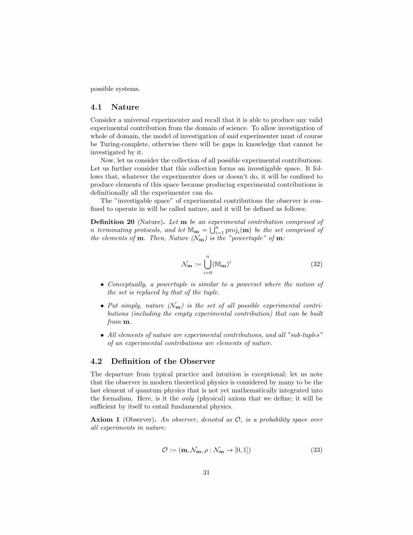
possible systems.

4.1 Nature

Consider a universal experimenter and recall that it is able to produce any validexperimental contribution from the domain of science. To allow investigation ofwhole of domain, the model of investigation of said experimenter must of coursebe Turing-complete, otherwise there will be gaps in knowledge that cannot beinvestigated by it.

Now, let us consider the collection of all possible experimental contributions.Let us further consider that this collection forms an investigable space. It fol-lows that, whatever the experimenter does or doesn’t do, it will be confined toproduce elements of this space because producing experimental contributions isdefinitionally all the experimenter can do.

The ”investigable space” of experimental contributions the observer is con-fined to operate in will be called nature, and it will be defined as follows:

Definition 20 (Nature). Let m be an experimental contribution comprised ofn terminating protocols, and let Mm =

⋃ni=1 proji(m) be the set comprised of

the elements of m. Then, Nature (Nm) is the ”powertuple” of m:

Nm :=

n⋃

i=0

(Mm)i (32)

• Conceptually, a powertuple is similar to a powerset where the notion ofthe set is replaced by that of the tuple.

• Put simply, nature (Nm) is the set of all possible experimental contri-butions (including the empty experimental contribution) that can be builtfrom m.

• All elements of nature are experimental contributions, and all ”sub-tuples”of an experimental contributions are elements of nature.

4.2 Definition of the Observer

The departure from typical practice and intuition is exceptional; let us notethat the observer in modern theoretical physics is considered by many to be thelast element of quantum physics that is not yet mathematically integrated intothe formalism. Here, is it the only (physical) axiom that we define; it will besufficient by itself to entail fundamental physics.

Axiom 1 (Observer). An observer, denoted as O, is a probability space overall experiments in nature:

O := (m,Nm, ρ : Nm → [0, 1]) (33)

31

where ρ is a probability measure, m is an experimental contribution, andNm, nature, is the space of all experimental contributions over m, and wherethe measure sums to one. We note that, unlike traditional measure theory inmathematics, here our definition of the measure is over tuples rather than sets.A recipe to tackle such a measure will be given in the main result section.

Just our minimalistic definition of the scientific method earlier recovered therichness of the concept, here a similar richness will be recovered for fundamentalphysics as a consequence of this definition of the observer.

4.3 The Experience of the Observer

For the familiar laws of physics to be recovered, we found that the model ofinvestigation must support a probability measure over the possible incrementalcontributions, rather than merely be a deterministic implementation of a partic-ular scientific method algorithm. In this case, we may qualify the experimenteras having the ”freedom” to investigate nature. This property is reminiscent of(and will ultimately connect to) the Bell inequality experimenter freedom infamiliar quantum mechanics, hence the name.

As stated in the sketch, the terms ’free’ and ’freedom’ are in this contextto be interpreted similarly to the strict sense given by Conway and Kochen[1]as freedom from being determined by past history, thus allowing a probabilisticenumeration in the present; and that of the Bell inequality as having the freedomto pick the experiment (or equivalently its parameters), also undetermined bypast history. It is not meant to be interpreted in the metaphysical sense of freewill commonly used in philosophy.

As a probability space over all experiments of nature, the observer will thenreceive or produce a message (in the sense of Claude Shannon’s theory of infor-mation) of completed experiments. The receipt (or production) of this messageconstitutes what we will call his or her experience, and represents the model ofinvestigation used by the observer to acquire knowledge in nature.

To obtain the laws of physics, the final step is to optimize the informationassociated with the receipt (or production) of this message. As the solutionto an optimization problem on experimenter freedom, the laws of physics willdefine a circumscription on the freedom of action of the observer.

Maximizing experimenter freedom will involve a similar methodology as thatused in ordinary statistical mechanics to maximize the entropy. The Lagrangemultiplier method will be utilized. The entropy will also be utilized and max-imized, but here we will not think of the entropy as a ’measure of disorder’,but rather as a quantification of information in the sense of Claude Shannon’stheory of information. The information acquired by the observer following ameasure will adopt the role of a message that fixes the acquired knowledge intoa new state.

Finally, maximizing the entropy of a measure over a power-tuple rather thana power-set requires modifications to the original recipe, and this will be givenin the main result.

32

Thesis 1 (Fundamental Physics). The probability measure that maximizes ex-perimenter freedom in nature constitutes the fundamental physics, or simply ’thelaws of physics’.

Our definition of fundamental physics is not given as a pre-formulated lawsuch as F = ma. That is not to say that laws do not come into play; but whenthey do they are derived from this measure, and not brutely postulated. Takingan example of statistical mechanics, the ideal gas law PV = nRT can be derivedfrom the Gibbs measure as an equation of state under the appropriate energyand volume constraint on entropy.

5 Intermission

5.1 Science

To introduce falsification within a formal system of science, the notion of knowl-edge being epistemically certain is critical. It is the reason why we can be certainthat acquiring new knowledge does in fact necessarily falsify any conflicting mod-els. If our knowledge was uncertain, we would simply be perpetually juggling theprobabilistic weights of various hypotheses and models, and no model could everbe falsified. With this in mind, let us correct a terminology error made by KarlPopper. A core tenet of Karl Popper’s philosophy is that scientific knowledgeis always transitory, and so a scientific theory would be subject to falsification.The correction is minor, but nonetheless leads to substantial clarifications. Thecorrection is on the usage of the term knowledge; knowledge is not transitoryrather it is the models that are. Models are entailed by knowledge, as such theydo not entail it in return. In fact, when acquiring new knowledge, if the modelconflicts with it, then the model always loses the tug of war because the formeris epistemically certain while the later isn’t. The correct terminology is thatscientific models (not knowledge) are transitory because knowledge (which isn’ttransitory) takes precedence over the conflicting model.

Karl Popper’s extended philosophy is correct in regards to scientific theories(e.g. biology, economic science, psychology, etc.), but physics as it would is adifferent beast altogether. The difference between the two stands out when weinvestigate their relationship to our newly formalized observer. For instance, ifan observer ”violates” a scientific theory, then said theory is simply falsified.This happens every once in a while, and other than perhaps a bruised ego, notmuch harm is done. Whereas, if an observer were to violate the laws of physics,presumably all hell would break loose. Why the difference? Of course, withouta formal system of science, we have historically derived and justified our lawsof physics the same way as any other scientific theory assuming they are ofthe same category, and thus the difference was unnoticed, but with a formalsystem of science we can pinpoint the difference. A scientific theory involvesa choice of formal axiomatic representation of an experimental contribution,and it is this choice that is falsified when facing conflicting knowledge. Incontrast, the observer cannot violate the fundamental physics without violating

33

its circumscription. The circumscription is unique to physics and is absentfrom mere scientific theories; this makes fundamental physics inviolable to theobserver, whereas a scientific theory is only falsifiable to the observer hence notinviolable.

Newfound clear-cut delimitations between previously overlapping conceptsis typically welcomed, especially when the overlap is caused by ambiguities. Forinstance, chemistry overlaps with physics significantly, and so does biology viabio-physics. What is the exact split, if any, or is everything ultimately physics?With our system, we now know the difference; scientific theories are entailedby knowledge, whereas fundamental physics is entailed by the definition of theobserver as the maximally permissive circumscription over its freedom of partic-ipation. A word of caution however; in practice one could always demand thatwe subject Axiom 1, and its predictions, to the falsification process, and thusphysics, via the technicality of the definition of the observer remains falsifiabledespite being of a different category; physics is the unique member of a specialcategory of falsifiable theories.

This difference carries over with respect to the techniques used to falsifyphysics. Physics, although falsifiable as we just said, is not subject to the fun-damental theorem of science which applies only to formal axiomatic represen-tations of experimental contributions and is responsible for a common scientifictheory being falsifiable. For physics, a special falsification theorem must becreated, and such must start with the definition of the observer rather thanwith the elements of the experimental contribution. The resulting falsificationtheorem will be more challenging than the first, simply because the observer isa probability space and this is a more challenging mathematical object to workwith than a mere enumeration. To falsify a common empirical theory via thefundamental theorem of science, it suffices to identify a halting program withinthe experimental contribution to knowledge that is not entailed by it. For in-stance, J.B.S. Haldane one of the founders of evolutionary biology reportedlystated that finding the fossils of a rabbit in the Precambrian would falsify thetheory of evolution. This is a binary yes/no type of falsification. Whereas, sincephysics is entailed by a probability space, falsifying physics will involve the useof probabilities. Specifically, we will find that repeat experiments over multi-ple copies of identical preparations, such that a probability distribution can beextracted from a plurality of similar measurements, will be required to test orfalsify physics by comparing it to the predicted expectation values.

5.2 The Observer

The reader will notice that Axiom 1 does not reference a plurality of observers,rather it postulates what amounts to a singleton observer. The system is in-tended to be formulated from the perspective of the observer. This should beless surprising than it tends to be as it avoids a battery of observer-related para-doxes, and captures the ontologically safest possible foundation, but we have tobe careful so that the intent is not misunderstood. Let us explain the term, andthen we will discuss its motivation and attempt to address the concerns. The

34

term singleton is imported from software engineering, where the singleton pat-tern refers to a design pattern of object-oriented programming in which a classcan only be instantiated once. Singleton does not mean that the program itselfcan only be ran once, it only means that each running copy has only one instan-tiation of its singleton variables within its memory. Our system supports theidea of ”running” multiple times in parallel, thus admitting multiple observers—or more precisely formulated; it allows other observers to claim singleton sta-tus from their perspective—, and the singleton observer axiom is not designedto prevent that; it simply means that for each execution, the theory is formu-lated from the perspective of its singleton observer. The singleton observer is”I” from my perspective, and ”you” from your perspective, and ”him” from hisperspective, etc. To be explicit, it is not a universal observer neither it is God— just you, him, her or I. The singleton observer is a mathematical descriptionof who ”I” am that also conveniently formalizes the set of tools ”I” have accessto in order to understand or participate in nature.

First, let us explain exactly how the theory is intended to support otherobservers from the perspective of the singleton observer. Their existence willbe evidence-derived rather than postulated. Other observers, if they exist, canand will be derived by the singleton observer the same way any other facts areinvestigated, by merely inspecting the experimental contributions and weightingthe evidence for them, and thus do not need to be postulated. Do we also needto postulate rocks, trees, or bees — or can we accept that their existence willbe derived conditional upon the scientific evidence, and if so why not demandthe same in regards to evidence for other observers? Indeed, psychologicallyand developmental-wise, this is what happens naturally as an infant maturesand over time develop a theory of the mind to assess the motivations and thedecision-making strategies of others — i.e. Infant solipsism (Piaget). Evidencefor other observers is identified by inspection of all available evidence and buildsover time and is the subject of the scientific method and to falsification. Toinclude other observers via postulation would be to erase said developmentalsteps from the domain of the scientific method, or at least eliminate the necessityof a laborious but insightful derivation thereof by virtue of having reduced themto mere postulation, and would result in a representation of reality missing thissophistication.

Let us further point out that if we find it reasonable to expect that physicsought to work for any number of observers between 1 and infinity; then physicsmust also work with just one — and just like Peano’s axiom posits only the firstnatural number and the others are derived by the successor function, here thesingleton observer is the base axiom and others are intended to be derived fromevidence.

Secondly, one must remember the role of axioms. Axioms are the logicalminimal required to derive a theory and are intended to be free of any redun-dancy. They are not a collection of desiratas, nor are they designed to make theworld a better place than it is. Not only do we not need a plurality thereof tocomplete the theory, if we made the world conditional upon multiple axiomaticobservers, the thesis becomes nonsensical: We would be claiming that at least

35

two observers are needed to entail the laws of physics... can an observer, whenworking alone, violate the laws of physics, but can’t if working as a team... ?Of course not.

Just like quantum theory should work for one or any number of particles, thelaws of physics should logically be definable against only one observer if needbe, or any other number, because they limit what each observer can individuallydo or cannot do. Team work, although perhaps socially beneficial, does not inthis case prevail against the laws of physics.

Let us now discuss the singleton observer within the context of a relevantphysics experiment. The Wigner’s friend experiment puts forward a paradoxin which two observers appears to witness the collapse of a wave-function atdifferent times. The Wigner’s friend experiment supposes that an observer Fmeasures a wave-function |ψ〉 = α |φ1〉+ β |φ2〉 to be in state |φ1〉 or |φ2〉, withprobability |α|2 and |β|2 respectively, that F notes the result somewhere in hislaboratory, but refrains from advising another observer W of the result. Thisother observer then understands the wave-function of the laboratory in whichF performed his measurement to retain the superposition. Whether the systemis or isn’t in a superposition appears to be resolved at different times for eachobserver; F sees the collapse at the instant of measure, but W sees it only af-ter F choose to share his notes with him. This difference in collapse timing isthe paradox. A commonly proposed resolution is that superposition does notoccur in macroscopic objects, and the reproduction of this experiment in a mi-croscopic system would appear less paradoxical. In actuality however, as soonas observer F notes then hides the result, F begins to act as a glorified hiddenvariable theory with respect to W and this is ruled out by Bell’s inequality; thusF cannot cause |ψ〉 to collapse at any time other than simultaneously for all ob-servers. In his original paper Wigner focused on another possible resolution:”All this is quite satisfactory: the theory of measurement, direct or indirect,is logically consistent so long as I maintain my privileged position as ultimateobserver”. Historically, this has not been the preferred interpretation because ofthe obvious resistance to the connotation associated with a privileged ultimateobserver. In our system, the observer is not assumed to be ”privileged ultimate”but merely to be formulated as a singleton, and other observers can proclaimthe same. Specifically, the wave-function will be formulated from the perspec-tive of a singleton observer; and since other observers are derived by inspectionof the evidence ”gathered” by said wave-function, they will obviously be unableto support a different wave-function behaviour than that reported by the sin-gleton. Furthermore, as we said, other observers can proclaim the same, andthus, symmetry oblige and as we found guaranteed by the laws of physics, allobservers, singleton and evidence-derived, will observe the same wave-functionbehaviour as each other.

Our feedback was that some find this last point hard to accept as they imag-ine we are implying the need for some prior non-local synchronization effect toguarantee agreement between observers whenever they meet to compare results.However, this is not necessary. Let us open a small parenthesis, grant ourselvesaccess to more lenient, illustrative and familiar physical language, and expand

36

on this statement, at the cost of dropping some of the generality. For the pur-poses of these examples, let us assume the concepts of matter, biological bodies,light cones and wave-function. Essentially, the picture is painted as follows.First, the singleton observer defines itself as the sole probability space over theexperiments of nature. What about the evidence-derived observers? In the wildthey simply appear to the singleton as biological bodies evolving in nature andthey are subject to the same physical laws as anything else made of matter.That they may or may not be more than that (i.e. are they also, from their ownperspectives, a probability space?) is private knowledge that is not availableto the singleton. Hence, the behaviour of biological bodies, as they are madeof ordinary matter, are solutions of the singleton’s wave-function, like otherother object made of matter. The second element that negates the need forprior non-logical synchronization is the incremental contribution formulation.Suppose observer A knowns halting program 1 and observer B knowns haltingprogram 2. The union of their knowledge is always a valid state of knowledge(i.e. knowledge is closed under union). No prior non-local synchronicity isrequired to ensure future compatibility of knowledge.

Finally, why did we present the singleton observer as an axiom, and not say,as a definition? An axiom implies one could claim it to be false, and technicallyspeaking this is indeed possible. For instance, one simply has to state they do notbelieve they exist as an observer, and as we would only have their proclamationof such to go by since the singleton observer is postulated, the scientific methodwould be powerless to prove the claim wrong. The question ”what if axiom 1 isfalse” is answered amicably with ”then you are not an observer”, and we moveon. The other, slightly more challenging, reformulation of the question is ”whatif axiom 1 is slightly-off ” (in the sense that our probability space definitionof the singleton observer is the wrong one to use, but the concepts we putforward might still otherwise be the correct overall approach). In this case wewould simply get, proportionally to a how wrong our definition is, the wronglaws of physics, which is why we claimed earlier that physics is also subjectto falsification. We do not exclude that, in principle, future experiments mayconfirm, or force us to adjust, the mathematical form of axiom 1 along with itsaccompanying entropy-maximization recipe. Consequently, our physical theoryof the observer is in principle falsifiable.

5.3 The Theories

We have previously stated that a scientific theory is entailed by knowledge, andthat it does not entail it in return. Phrasing it like this however makes it soundslike models are vacuous; this is not the case as they do provide value, but wedo not call this value knowledge, rather we call it insight.

For instance, it is the case that natural selection is an insightful model of bio-diversity, but does it give us knowledge of bio-diversity? — or, it is knowledgeof bio-diversity that gives us natural selection as the insight?

Consider these statements:

37

1. (The model of) natural selection entails knowledge of bio-diversity.

2. Knowledge of bio-diversity entails (the model of) natural selection.

In our system, the entailment is always as follows:

Knowledge =⇒ Model (34)

The entailment must be in this direction because knowledge is epistemi-cally certain, and the model, as it is only hypothetical, cannot entail epistemiccertainty.

Let us consider what is perhaps a more counter-intuitive example:

1. (The model of) gravity entails knowledge of objects falling.

2. Knowledge of objects falling entails (the model of) gravity.

It is common to hear that the first is true on the grounds that gravity causesobjects to fall. However, it is knowledge of objects falling that caused Newtonto produce the model of gravity. Gravity may appear as logically equivalentto the sum-total of all falling objects; but nature is not gravity, nature is thesum-total of all falling objects.

It is in regards to the formulation of quantum physics that adopting the cor-rect entailment will pay the most dividends. Consider the following statements;which one is true?

1. Measuring a wave-function |ψ〉 = α |φ1〉 + β |φ1〉 caused it to collapse to|φ1〉 or to |φ2〉.

2. Registering ’clicks’ such as |φ1〉 or |φ2〉 on an incidence counter causes usto derive |ψ〉 = α |φ1〉+ β |ψ1〉 as a statistical model of the clicks.

As always, the second is the correct entailment. But careful; this reversesthe typical formulation of quantum physics! — First, ’clicks’ are recorded thenthe wave-function is derived...

In the upcoming sections, we will investigate the consequences and advan-tages of this reversal.

5.4 ”It from Bit”

Let’s begin by explaining what we mean by a ’click’. We borrowed the term from”Information, Physics, Quantum; The Search for Links.” by John A. Wheeler[2].Wheeler states:

[The photon is one of many examples] that may illustrate thetheme of it from bit. [...] With polarizer over the distant source andanalyzer of polarization over the photodetector under watch, we askthe yes or no question, ”Did the counter register a click during the

38

specified second?” If yes, we often say, ”A photon did it.” We knowperfectly well that the photon existed neither before the emissionnor after the detection. However, we also have to recognize that anytalk of the photon ”existing” during the intermediate period is onlya blown-up version of the raw fact, a count

Wheeler explains the term ’it from bit’ as follows:

It from bit symbolizes the idea that every item of the physicalworld has at bottom — at a very deep bottom, in most instances— an immaterial source and explanation; that what we call real-ity arises in the last analysis from the posing of yes-no questionsand the registering of equipment-evoked responses; in short, thatall things physical are information-theoretic in origin and this is aparticipatory universe.

Essentially, ’clicks’ are wave-function collapses; they refer to what an instru-ment records when they occur.

By taking the ’click’ as the fundamental object, rather than the wave-function, the formulation of quantum mechanics will be in the opposite direction;our goal will be to start with a sequence of recorded ’clicks’ and to end up, viasome mathematical procedure, on the wave-function.

Having some familiarity with the work of John A. Wheeler on the partici-patory universe, we believe this may be where he hit the roadblock as he wasmissing said mathematical procedure.

The procedure will be presented in the following section.

5.5 Origin of the Wave-Function

Statistical mechanics derives the Gibbs measure under specific constraints onthe entropy. Using a similar methodology, we will appropriately constrain theentropy subject to recorded ’clicks’, and we will derive the wave-function alongwith the Born rule (together forming a measure), essentially as an extension ofstatistical mechanics.

First let us review statistical mechanics. In statistical mechanics, constraintson the entropy are associated to instruments acting on the system. For instance,an energy constraint on the entropy:

E =∑

q∈Q

ρ(q)E(q) (35)

is interpreted physically as an energy-meter measuring the system and pro-ducing a series of energy measurement E1, E2, . . . converging to an average valueE.

Another common constraint is that of the volume:

39

V =∑

q∈Q

ρ(q)V (q) (36)

associated to a volume-meter acting on the system and converging towardsan average volume value V , also by producing a sequence of measurements ofthe volume V1, V2, . . . .

With these two constraints, the typical system of statistical mechanics isobtained by maximizing the entropy using its corresponding Lagrange equation,and the method of the Lagrange multipliers:

L = −kB∑

q∈Q

ρ(q) ln ρ(q) + λ

1−

∑

q∈Q

ρ(q)

+ β

E −

∑

q∈Q

ρ(q)E(q)

+ γ

V −

∑

q∈Q

ρ(q)V (q)

(37)

and then solving ∂L∂ρ

= 0 for ρ, we get the Gibbs measure:

ρ(q,β, p) =1

Zexp(−βE(q) + γV (q)) (38)

=1

Zexp(−β(E(q) + pV (q))) (39)

Let us now recover the wave-function using a similar methodology.To do so, we will introduce a larger class of instruments into statistical

mechanics. Instead of an energy-meter or a volume-meter, consider a phase-invariant instrument, such that the constraint it induces on the entropy is givenas follows:

tr

(a −b

b a

)=

∑

q∈Q

ρ(q) tr

(a(q) −b(q)b(q) (a)

)(40)

where

(a(q) −b(q)b(q) a(q)

)∼= a(q) + ib(q) is the matrix representation of the

complex numbers.Here, the purpose of the trace is to enforce the phase-invariance of the instru-

ment. The entropy will be maximized, not under energy or volume constraintsthis time, but under the constraint of measurement-events (or ’clicks’) collectedby phase-invariant instruments (or ’click’ recorders), and this will yield thewave-function along with the Born rule automatically as the statistical modelof the ’clicks’.

The corresponding Lagrangian equation that maximizes the entropy will inthis case be:

40

L = −∑

q∈Q

ρ(q) ln(q) + α

1−

∑

q∈Q

ρ(q)

+ τ

tr

(a −b

b a

)−

∑

q∈Q

ρ(q) tr

(a(q) −b(q)b(q) a(q)

)

(41)

Maximizing the entropy under such constraints does produce the probabilitymeasure of the wave-function along with the Born rule. But here it is derivedusing the same technique as we would for any other system of statistical me-chanics, and thus we inherit its tools, interpretation and will be able to accountfor the origin of the measure. Indeed, solving ρ for ∂L

∂ρ(q) = 0 gives:

ρ(q) =1

Zexp tr τ

(a(q) −b(q)b(q) a(q)

)(42)

=1

Zdet exp τ

(a(q) −b(q)b(q) a(q)

)(43)

∼= exp 2τa(q)| exp iτb(q)|2 Born rule (44)

We hold this to be the true origin of the wave-function and the Born rule.This formulation yields what we call the minimal interpretation of quan-

tum mechanics: In nature, there exists instruments that record sequences ofmeasurements on systems, those instruments have a phase-invariance, and thewave-function along with the Born rule are the base measure constrained bythose measurements. This interpretation is completely factual and entirely freeof redundancies (many-worlds, etc.).

Let us expand further in the following section.

5.6 A Random Walk in Algorithmic Space

Starting with the definition of the observer, a probability space over all ex-periments of nature, the correspondence between our approach and statisticalmechanics can be improved further — and even be made complete. Specifically,the correspondence is as follows:

Statistical Mechanics Statistical System of ’clicks’

Entropy Boltzmann Shannon (45)

Measure Gibbs Born Rule (46)

Constraint Energy meter Phase-invariant instrument (47)

Micro-state Energy values Sub-Contributions (48)

Macro-state Equation of state Evolution of the wave-function (49)

Experience Ergodic Message (50)

We will now investigate the correspondence.

41

As stated previously, nature N is the power tuple of the incremental contri-bution m; it therefore comprises multiple elements. Let us now call the elementsof N the possible sub-contributions. These elements will be the micro-states ofour system. As for the macroscopic state, it will acquire the form of a wave-function and will describe the evolution of the possible micro-states. Finally,the message connects to the macro-state via a specific sequence of registered’clicks’, and this information is quantified by the Shannon entropy.

In statistical mechanics it is often assumed that the system, say the moleculesof air in a box, permute over the possible micro-states of the system (i.e. ergodichypothesis), whereas in our system as we use the Shannon entropy, there is nosuch permutation; how the observer experiences the system is in the form ofa message fixing the realized incremental contribution from the possible sub-contributions available in nature. And the information gained by the observerfrom this message is equal and opposite to that of the entropy of the system.Thus, our formulation contains no redundancies; there are no many-worlds —only a unique message of incremental contributions that the observer experiencesas reality.

Here, it is the experience that is considered real and fundamental. In oursystem, the experience is defined under the assumption of an observer withexperimenter freedom (Axiom 1) receiving or producing a message as an incre-mental contribution. The observer could have produced a different incrementalcontribution but it so happen to have produced this particular one, and thedifference between what is and what could have been constitutes the entropythat associates with experimenter freedom. The clicks represent the informa-tion required to fix the experience of the observer as a particular message fromnature.

As for the rest of the table, it simply follows from (maximizing the quan-tity of information/entropy of, or generally to optimize the information of) theexperience.

Finally, new contributions by the observer resulting from its continued par-ticipation in nature, will automatically trigger new ’clicks’ to be registered inthe system so as to preserve the general form of the experience as a messageand to do so consistently over the addition of those new contributions. Theclicks are therefore directly produced by observer participation in nature andserves as evidence of experimenter freedom, and this is more fundamental thanthe wave-function which is derived afterwards as a statistical model entailed bythe clicks that are registered.

An example to fix the intuition is that of a random walk in algorithmic space(in nature). As the observer collects halting programs (completed experiments),’clicks’ are registered to define the path it takes. Here, the ’clicks’ are theexperimental analog to the bits used to define the path of a one-dimensionalrandom walk.

Aspects of our model connects with insights by Conway and Kochen[1],where they describe ”new bits of information coming into existence in the uni-verse” as a result of experimenter freedom. They say:

42

...there will be a time t0 after x, y, z are chosen with the propertythat for each time t < t0 no such bit is available, but for every t > t0some such bit is available.

But in this case the universe has taken a free decision at timet0, because the information about it after t0 is, by definition, not afunction of the information available before t0!

In our work, we have taken it a step further and revealed that the unitof information of experimenter freedom is not the bit but actually the ’click’,and that unlike the bit, the ’click’ contains enough sophistication to encode theexperience of the observer such that its maximized freedom of action is preciselycircumscribed by the laws of physics as they are empirically familiar to us. Wewill see that in detail in the main result.

5.7 Dissolving the Measurements Problem

Starting with a sequence of ’clicks’ (wave-function collapses), our procedure de-rived the wave-function (which supports a plurality, or superposition, of possible’click’ results). We have traversed the measurement problem from the oppositedirection of the standard formulation:

Standard: Measurement(wave-function︸ ︷︷ ︸Axiomatic

) =⇒ ’click’︸ ︷︷ ︸collapse problem?

(51)

Ours: Max-Entropy( ’clicks’︸ ︷︷ ︸Axiomatic

) =⇒ wave-function︸ ︷︷ ︸derived

(52)

We note that the maximization of entropy operation is non-problematic,but the measurement operation introduces the problem of the wave-functioncollapse.

Let’s investigate the distinction in more details.Very broadly, all statistical systems, classical or quantum, admit two formu-

lations, sometimes referred to as a frequentist or a bayesian formulation.Our formulation of quantum mechanics from statistical mechanics is entirely

frequentist ; whereas the standard formulation mix and match elements of boththe bayesian and the frequentist schools. Specifically, the wave-function collapsein the standard formulation is treated using the bayesian school; it assumes aprior (the wave-function) and updates it with the result of each measurementas they occur. However, the bayesian update (the collapse) is not physicallyunderstood and constitute what is known as the wave-function collapse problem.

To better understand how the formulations differ and to illustrate the na-ture of problem, let’s consider the archetypical example of a fair coin toss with50%/50% probability of landing on either head or tail. We can produce theformulations by picking different points in the history of the system to definethe measure; either before or after the coin lands.

43

1. If formulated before the coin lands:

If we are to formulate the statistical model before the coin lands, we wouldfirst posit a probability measure 50% head /50% tail (bayesian prior), thenwe would find that sampling the system (throwing the coin) yields eitherhead or tail whenever it lands (this is the bayesian update). In this case,the probability measure, if it were proclaimed to be the complete physicaldescription of the system would be insufficient to support a physical mech-anism for the bayesian update. This is similar to how quantum mechanicsis typically formulated.

2. If formulated after the coin lands:

Now, consider the discovery of a coin on the floor with head facing up.To work with probabilities, we must first assume an appropriate historyfor this coin making the present result due to chance; and specificallythe choice will be that the coin landed as the result of fair coin toss.Unlike the previous case, we did not witness this history. We merely as-sumed it following the discovery of the coin on the floor, and theoreticallyspeaking, we could be wrong about our assumption (someone could havejust deposited it carefully on the ground face up). This is the post-factoformulation. Then, under the fair coin toss history assumption, we canconstruct a probability measure to account for the state the coin was dis-covered in. The probability measure assigns a 50/50 probability to eachoutcome: head or tail. We end up with the same statistical model as theprevious case, but no sampling of the probability measure has occurredand the probability interpretation is readily understood to merely be aplausible model of the history of the system. Since we model the past andthe past is fixed, no updates on the measure need occur.

In our system, the wave-function along with the Born rule are not fundamen-tal, but are derived following the registration of ’clicks’. It models the history ofthe system; it is not a physical object that is acted on by an observer; it holdsonly after the observer has acted.

That is not to say that the wave-function cannot be used predictively, butimplicit assumptions are required to do so; in all cases and while the experimentis carried out, the regularity of the environment must be assumed. However,this regularity is verifiable only after the experiment is completed. For instance,one typically assumes a meteor will not strike the lab. Or perhaps the lab willlose funding mid-experiment and will shutdown. That the environment is orisn’t regular until the end cannot be know, in the general case, until the end.Or said differently; a predictive wave-function is a gamble that the system will,at some point in the future, be in a state such that the system’s past is correctlymodelled by it.

The advantage of our interpretation is that it matches what actually occursin reality; it is indeed the case that we first register the ’clicks’ on a recorder,and only then do we derive the measure to be a wave-function. Likewise, if weregister no clicks, we assume no wave-function.

44

Finally, since we cannot have knowledge of the existence of a wave-function(the prior) before a click is registered (its update), it should now be clear thatthe bayesian interpretation demands that the update precedes its prior — andthis is nonsense.

Some may have the impression that this may be too simple to be the solution,but let us reassure the reader that this is not the case. This interpretation wasnot conductive before our main result relating statistical mechanics (and phase-invariant instruments) to the wave-function, as its origin was otherwise tooobscure to support this interpretation.

5.8 Automatic Inclusion of Gravity

In our main result we will actually obtain a generalization of quantum mechan-ics to support general linear transformations. In this case the interpretationof quantum mechanics takes its simplest and most visualizable interpretation.The phase-invariant instruments are upgraded from a complex phase to a gen-eral linear phase, and the geometry automatically follows. The probabilitywill then be associated with a sequence of ’clicks’ recorded in space-time asevents. The framework will describe reality as a sequence of space-time ’clicks’(or events) which, under entropy maximization, are associated to a general lin-ear wave-function in lieu of the Gibbs ensemble. As we note, general relativityis primarily a theory of events in space-time, and the extension to quantum the-ory assigns a probability and an entropy to said events, such that the measureover said events is a wave-function able to support the transformations requiredby general relativity while preserving the invariance of the probability measure.This generalization yields a gauge-invariant general linear wave-function whoseequations of motions are exactly the Einstein field equations. No other equationsof motion are supported (except as sub-cases).

5.9 Context

Finally, let us address a common concern:

Surely there is more to reality than simply ’clicks’ — what aboutobjects such as chairs or kitchen tables, what about colours or liter-ature?

Here we give a ”first-approximation answer”. It is not designed to be acomplete answer, but merely to guide the intuition.

This is where context sneaks in. Each halting program contains the contextto the claim it makes. An observer with a naturally-selected brain will beinfluenced by biological evolution and other environmental factors, and will picka preferred context to clarify the set of halting program it knows (this could becolours instead of wavelength, or set theory instead of quantum Turing machineprograms). The mind understands reality as a collection of scientific fields,which are choices of formal axiomatic bases, formulated in a matter it finds

45

efficient or convenient; each representing a falsifiable choice of context. Why wethink of a particular cloud of ’clicks’ as a chair, or another cloud as a wood clubwhich is a potential weapon, is simply the result of natural selection influencingthese contextual choices and committing them to the biological wiring of thebrain.

The laws of physics, however, are without specific context and this is re-quired for them to be universal. The lack of dependance upon a specific contextrelate the laws of physics to the ”fraction” of reality. Specifically, they relateto the transformations from arbitrary initial states to arbitrary final states a-contextually, and the ”rest” of reality is relegated to scientific theories whichare contextual.

6 Main Result

Let us now use the definition of the observer (Axiom 1) as our starting point toderive fundamental physics. We recall that our definition of the observer is:

O := (m,N , ρ : N → [0, 1]) (53)

where m is a n-tuple, N is a ”powertuple” and ρ is a (probability) measureover N .

In this main result, we will maximize the entropy of ρ using the method ofthe Lagrange multipliers. How?

First, note the similarity between our definition of the observer to that ofa measure space in mathematics. Comparatively, the definition of a measurespace is:

M := (X,Σ, µ(Σ)) (54)

where X is a set, Σ is (often) taken to be the powerset of X, and µ is ameasure over Σ.

The difference with our measure is simply that sets have been replaced bytuples. Consequently, we must adapt the standard definition of a measure spacefrom set to tuples. To do so, we will use the following recipe:

1. We assign a non-negative real number to each element of N (this numberrepresents the probability associated with the element).

2. We equip said numbers with the addition operation, converting the con-struction to a vector space.

3. We maximize the entropy of a single element under the effect of con-straints, by using the method of the Lagrange multipliers.

4. We use the tensor product n-times over said vector space to construct aprobability measure of n-tuples of halting programs.

46

5. We use the direct sum to complete the measure over the whole of tuple-space by combining the measures of different sizes as a single measure.

Explicitly, we maximize the entropy:

S = −∑

p∈m

ρ(p) ln ρ(p) (55)

subject to these constraints:

∑

p∈m

ρ(p) = 1 (56)

∑

p∈m

ρ(p) trM(p) = trM (57)

where the notation∑

p∈m designates a sum over the elements of the experi-mental contributionm, whereM(p) are a matrix-valued maps from the elementsof m to Cn×n representing the linear transformations of the vector space ontoitself, and where M is a element-by-element average matrix.

Let us note that maximizing the entropy under these constraints is the math-ematically explicit form of what we have previously called maximizing experi-menter freedom, or maximizing ’freedom of action’. The linear transformationsof this vector space will in turn be we found to associate to one of the stepsspecified by an experimental protocol. By maximizing the entropy here, we willtherefore look for the ’least encumbered’ probability measure consistent withthese transformations. After entropy-maximization, the resulting physics is acircumscription on experimenter freedom.

Usage of the trace of a matrix as a constraint imposes an invariance with re-spect to a similarity transformation, accounting for all possible linear reorderingof the elements of the tuples of the sum, thus allowing the creation of a measureof a tuple or group of tuples from within a space of tuples, invariantly withrespect to the order of the elements of the tuples. Similarity transformationinvariance on the trace is the result of this identity:

trM = trBMB−1 (58)

Furthermore, as the trace of a matrix corresponds to the expectation of itseigenvalues (times the dimension of the matrix), and the eigenvalues have ageometric interpretation the form of the ratio of the distortion of the length ofa geometric transformation, the probability measure will be inherently geomet-ric. The constraint of the entropy is to preserve this expectation value of saidgeometric transformation. We will further discuss the geometric implications insection 7 and 8.

47

We now use the Lagrange multiplier method to derive the expression for ρ

that maximizes the entropy, subject to the above mentioned constraints. Thecorresponding Lagrange equation is:

L = −kB∑

p∈m

ρ(p) ln(p) + α

(1−

∑

p∈m

ρ(p)

)+ τ

(trM−

∑

p∈m

ρ(p) trM(p)

)

(59)

where α and τ are the Lagrange multipliers. Except for the presence of thetrace and matrices, the method is standard and shown in most introductorytextbooks of statistical mechanics to derive the Gibbs measure. The explicitderivation is made available in Annex B.

With the trace and matrices, the resulting probability measure exceeds thesophistication of the Gibbs measure, and is:

ρ(p, τ) =1

Z(τ)det exp(−τM(p)) (60)

where

Z(τ) =∑

p∈m

det exp(−τM(p)) (61)

We finish up the probability measure by adding the prior. The prior, whichaccounts for an arbitrary preparation of the ensemble, ought to be —for purposesof preserving the scope of the theory— of the same kind as the elements of theprobability measure. Let us thus introduce the prior as the map P from theelements of m to Cn×n and inject it into the probability measure as well as intothe partition function:

ρ(p) =1

Zdet exp (P(p)) det exp (−τM(p)) (62)

where

Z =∑

p∈m

det exp (P(p)) det exp (−τM(p)) (63)

6.1 Completing the Measure over Nature

In the previous section, we have produced a measure over a tuple of singleexperiments. Whereas the measure we are after is a sum over the whole spaceof experiments spawned by an experimental contribution, which contains allsub-tuples of the experimental contribution (i.e. over the whole of nature).

48

Completing the measure over nature will require us to sum over differently-sized tuples. To do so, first, we will use the tensor product to produce measuressumming over multiple elements, and second, we will use the direct sum tocombine the differently-sized measures into a single final measure.

6.1.1 Split to Amplitude / Probability Rule

Before we are able to proceed with both the tensor product and the direct sum,we can capitalize on pre-existing familiarity by splitting the measure into twooperations.

We begin by splitting the probability measure into a first step, which islinear with respect to a ’probability amplitude’, and a second which connectsthe amplitude to the probability. We thus write the probability measure as:

ρ(p, τ) =1

Zdetψ(p, τ) (64)

where

ψ(p, τ) = exp(P(p)) exp(−τM(p)) (65)

Here, the determinant is interpreted as a generalization of the Born ruleand reduces to exactly it when M is the matrix representation of the complexnumbers. In the general case where M are arbitrary n×n matrices, ψ(p, τ) willbe called the general linear probability amplitude.

We can write ψ(p, τ) as a column vector:

|ψ〉 :=

ψ(p1, τ)ψ(p2, τ)

...ψ(pn, τ)

=

ψ1

ψ2

...ψn

(66)

6.1.2 Tensor Product

How do we extend the measure to experimental contributions containing mul-tiple experiments? We have to use a Cartesian product. For instance, let usconsider the following sets of experiments:

M1 = p1a, p1b (67)

M2 = p2a, p2b (68)

The Cartesian product produces a set of experimental contributions com-prised of two elements:

49

m ∈ M1 ×M2 = (p1a, p2a), (p1a, p2b), (p1b, p2a), (p1b, p2b) (69)

At the level of the probability amplitude, the Cartesian product of setstranslates to the tensor product. For instance, we start with a column vectorwhere each entry is one experiment;

|ψ1〉 =(expP(p1a)expP(p1b)

)(70)

Adding a program-step via a linear transformation produces:

T |ψ1〉 =(T00 expP(p1a) + T01 expP(p1b)T10 expP(p1a) + T11 expP(p1b)

)(71)

We then introduce another column vector:

|ψ2〉 =(expP(p2a)expP(p2b)

)(72)

along with a program-step:

T′ |ψ2〉 =(T ′

00 expP(p2a) + T ′

01 expP(p2b)T ′

10 expP(p2a) + T ′

11 expP(p2b)

)(73)

Then the tensor product of these states produces the probability measure ofan experimental contribution as follows:

T |ψ1〉 ⊗T′ |ψ2〉 =

(T00 expP(p1a) + T01 expP(p1b))(T′

00 expP(p2a) + T ′

01 expP(p2b))(T00 expP(p1a) + T01 expP(p1b))(T

′

10 expP(p2a) + T ′

11 expP(p2b))(T10 expP(p1a) + T11 expP(p1b))(T

′

00 expP(p2a) + T ′

01 expP(p2b))(T10 expP(p1a) + T11 expP(p1b))(T

′

10 expP(p2a) + T ′

11 expP(p2b))

(74)

Now, each element of the resulting vector is an experimental contributionof two programs, but its probability is a sum over a path. One can repeat theprocess n times.

6.1.3 Direct Sum

In the previous section, we have introduced a way to produce measures of fixedsizes n by using the tensor product. Here, we wish to produce a measure with el-ements of different sizes. Taking the direct sum of the measures of different sizes

50

(where each individual size is produced from the tensor product), accomplishesthe goal and yields an amplitude given has follows:

|ψ〉 = |ψ1〉 ⊕ (|ψ′

1〉 ⊗ |ψ′

2〉)⊗ (|ψ′′

1 〉 ⊗ |ψ′′

2 〉 ⊗ |ψ′′

3 〉)⊕ ... (75)

In quantum field theory, in the limiting case n → ∞ and when M(p) isreduced to the complex field, these are the states of a Fock Space, which wehave obtained here simply my maximizing the entropy of the measure associatedwith our simple definition of the observer (Axiom 1).

6.2 Discussion — Fock Spaces as Measures over Tuples

Some may consider our result purely using measure theory as the starting pointand neglect the model of the observer. An entropy-maximized measure over thetuples of a tuple-space (as an extension to typical measure theory defined for thesubsets of a set) induces a Fock Space, along with the appropriate probabilityrule (Born rule) for use in quantum mechanics. The measures used in quantummechanics would thus result quite intuitively from this simple extension of mea-sure theory, previously defined for sets, to tuples, and then simply maximizingthe entropy.

We should mention that, although tuples can represent anything, in oursystem Axiom 1 requires the tuples to represent experimental contributions (orhalted programs). But this is a minimal constraint, enforcing, while introducingno other constraints, that all experimental preparations or protocols must bedescribable using computable steps, and thus be comprehensible to the scientificmethod.

6.3 Connection to Computation

Previously, in the formal system of knowledge, we have stated that our defini-tions will reference the concept of the computable function, and that such willhold irrespectively of the underlaying model of computation. We can now claimmore. Here, we will see that having maximized the entropy of the measure spaceover tuples has automatically generated the underlaying model of computation.

Let us begin by reviewing the basics of quantum computation. One startswith a state vector:

|ψa〉 =

0...n

(76)

Which evolves unitarily to a final state:

|ψb〉 = U0U1 . . . Um |ψa〉 (77)

51

Clever use of the unitary transformations, often arranged as simple ’gates’,allows one to execute a program; but technically speaking any arrangementsof unitary transformations qualify abstractly as a program (without or withoutgates). The input to the program is the state |ψa〉 and the output is the state|ψb〉. One would note that, so defined and if the sequence of unitary transfor-mation is finite, such a program must always halt, and thus its complexity mustbe bounded. One can however get out of this predicament by taking the finalstate |ψb〉 to instead be an intermediary state, and then to add more gates inorder continue with a computation:

step 1 |ψb〉 = U0U1 . . . Up |ψa〉 (78)

step 2 |ψc〉 = U ′

0U′

1 . . . U′

q |ψb〉 (79)

...

step k |ψk′〉 = U ′

0U′

1 . . . U′

v |ψk〉 (80)

...

For a quantum computation to simulate a universal Turing machine it mustbe able to add more steps until a halting state is reached (or continue to addsteps indefinitely if the program never halts).

The linear transformationsT1,T2, . . . of our main result are here interpretedin the same manner as those used in quantum computations, but extended tothe general linear group. Protocols are executed by chaining transformationson a preparation:

|ψb〉︸︷︷︸final state

= T1T2 . . .Tn︸ ︷︷ ︸protocol

|ψa〉︸︷︷︸preparation

(81)

And a quantum computation involves a sequence of unitary transformationson the unit vectors of a complex Hilbert space:

|ψb〉︸︷︷︸final state

= U1U2 . . .Un︸ ︷︷ ︸computing steps

|ψa〉︸︷︷︸initial state

(82)

We are now ready to begin investigating the main result as a general linearquantum theory.

7 Foundation of Physics

We will now introduce the algebra of observables of the general linear wave-function.

52

7.1 Matrix-Valued Vector and Transformations

To work with the general linear wave-function, we will use vectors whose ele-ments are matrices. An example of such a vector is:

|ψ〉 =

M1

...Mm

(83)

Likewise a linear transformation of this space will expressed as a matrix ofmatrices:

T =

M00 . . . M0m

.... . .

...Mm0 . . . Mmm

(84)

Note: The scalar element of the vector space are given as:

a |ψ〉 =

aM1

...aMm

(85)

7.2 Algebra of Observables, in 2D

The notation of our upcoming definitions will be significantly improved if we usea geometric representation for matrices. Let us therefore introduce a geometricrepresentation of 2× 2 matrices.

7.2.1 Geometric Representation of 2× 2 matrices

Let G(2,R) be the two-dimensional geometric algebra over the reals. We canwrite a general multi-vector of G(2,R) as follows:

u = A+X+B (86)

where A is a scalar, X is a vector andB is a pseudo-scalar. Each multi-vectorhas a structure-preserving (addition/multiplication) matrix representation. Ex-plicitly, the multi-vectors of G(2,R) are represented as follows:

Definition 21 (Geometric representation of a matrix (2× 2)).

A+Xx+ Y y +Bx ∧ y ∼=(A+X −B + YB + Y A−X

)(87)

53

And the converse is also true, each 2 × 2 real matrix is represented as amulti-vector of G(2,R).

We can define the determinant solely using constructs of geometric algebra[13].

Definition 22 (Clifford conjugate (of a G(2,R) multi-vector)).

u‡ := 〈u〉0 − 〈u〉1 − 〈u〉2 (88)

Then the determinant of u is:

Definition 23 (Geometric representation of the determinant (of a 2 × 2 ma-trix)).

det : G(2,R) −→ R

u 0−→ u‡u (89)

For example:

detu = (A−X−B)(A+X+B) (90)

= A2 −X2 − Y 2 +B2 (91)

= det

(A+X −B + YB + Y A−X

)(92)

Finally, we define the Clifford transpose:

Definition 24 (Clifford transpose (of a matrix of 2× 2 matrix elements)). TheClifford transpose is the geometric analogue to the conjugate transpose. Like theconjugate transpose can be interpreted as a transpose followed by an element-by-element application of the complex conjugate, here the Clifford transpose isa transpose followed by an element-by-element application of the Clifford conju-gate:

u00 . . . u0n

.... . .

...um0 . . . umn

‡

=

u‡00 . . . u‡

m0...

. . ....

um0 . . . u‡nm

(93)

If applied to a vector, then:

v1

...vm

‡

=(v‡1 . . .v‡

m

)(94)

54

7.2.2 Axiomatic Definition of the Algebra, in 2D

Let V be an m-dimensional vector space over G(2,R). A subset of vectors in V

forms an algebra of observables A(V) iff the following holds:

1. ∀ψ ∈ A(V), the bilinear map:

2.

〈·, ·〉 : V× V −→ G(2,R)

〈u,v〉 0−→ u‡v (95)

is positive-definite:

〈ψ,ψ〉 ∈ R>0 (96)

3. ∀ψ ∈ A(V), then for each element ψ(q) ∈ ψ, the function:

ρ(ψ(q),ψ) =1

〈ψ,ψ〉ψ(q)‡ψ(q) (97)

is positive-definite:

ρ(ψ(q),ψ) ∈ R>0 (98)

We note the following comments and definitions:

• From (1) and (2) it follows that ∀ψ ∈ A(V), the probabilities sum tounity:

∑

ψ(q)∈ψ

ρ(ψ(q),ψ) = 1 (99)

• ψ is called a natural (or physical) state.

• 〈ψ,ψ〉 is called the partition function of ψ.

• ρ(q,ψ) is called the probability measure (or generalized Born rule) of ψ(q).

• The set of all matrices T acting on ψ, as Tψ → ψ′, which leaves the sumof probabilities normalized (invariant):

∑

ψ(q)∈ψ

ρ(ψ(q),Tψ) =∑

ψ(q)∈ψ

ρ(ψ(q),ψ) = 1 (100)

are the natural transformations of ψ.

• A matrix O such that ∀u∀v ∈ A(V) :

〈Ou,v〉 = 〈u,Ov〉 (101)

is called an observable.

• The expectation value of an observable O is:

〈O〉 = 1

〈ψ,ψ〉 〈Oψ,ψ〉 (102)

55

7.2.3 Observable, in 2D — Self-Adjoint Operator

Let us now investigate the general case of an observable is 2D. A matrix O isan observable iff it is a self-adjoint operator; defined as:

〈Oφ,ψ〉 = 〈φ,Oψ〉 (103)

∀u∀v ∈ V.

Setup: Let O =

(O00 O01

O10 O11

)be an observable. Let φ and ψ be 2 two-state

vectors φ =

(φ1

φ2

)and ψ =

(ψ1

ψ2

). Here, the components φ1, φ2, ψ1, ψ2, O00,

O01, O10, O11 are multi-vectors of G(2,R).

Derivation: 1. Let us now calculate 〈Oφ,ψ〉:

2〈Oφ,ψ〉 = (O00φ1 +O01φ2)‡ψ1 + ψ

‡1(O00φ1 +O01φ2)

+ (O10φ1 +O11φ2)‡ψ2 + ψ

‡2(O10φ1 +O11φ2) (104)

= φ‡1O

‡00ψ1 + φ

‡2O

‡01ψ1 + ψ

‡1O00φ1 + ψ

‡1O01φ2

+ φ‡1O

‡10ψ2 + φ

‡2O

‡11ψ2 + ψ

‡2O10φ1 + ψ

‡2O11φ2 (105)

2. Now, 〈φ,Oψ〉:

2〈φ,Oψ〉 = φ‡1(O00ψ1 +O01v2) + (O00ψ1 +O01ψ2)

‡φ1

+ φ‡2(O10ψ1 +O11ψ2) + (O10ψ1 +O11ψ2)

‡φ1 (106)

= φ‡1O00ψ1 + φ

‡1O01ψ2 + ψ

‡1O

‡00φ1 + ψ

‡2O

‡01φ1

+ φ‡2O10ψ1 + φ

‡2O11ψ2 + ψ

‡1O

‡10φ1 + ψ

‡2O

‡11φ1 (107)

For 〈Oφ,ψ〉 = 〈φ,Oψ〉 to be realized, it follows that these relations musthold:

O‡00 = O00 (108)

O‡01 = O10 (109)

O‡10 = O01 (110)

O‡11 = O11 (111)

Therefore, it follows that it must be the case that O must be equal to itsown Clifford transpose. Thus, O is an observable iff:

56

O‡ = O (112)

which is the equivalent of the self-adjoint operator O† = O of complexHilbert spaces.

7.2.4 Observable, in 2D — Eigenvalues / Spectral Theorem

Let us show how the spectral theorem applies to O‡ = O, such that its eigen-values are real. Consider:

O =

(a00 a− xe1 − ye2 − be12

a+ xe1 + ye2 + be12 a11

)(113)

In this case, it follows that O‡ = O:

O‡ =

(a00 a− xe1 − ye2 − be12

a+ xe1 + ye2 + be12 a11

)(114)

This example is the most general 2 × 2 matrix O such that O‡ = O. Theeigenvalues are obtained as follows:

0 = det(O− λI) = det

(a00 − λ a− xe1 − ye2 − be12

a+ xe1 + ye2 + be12 a11 − λ

)(115)

implies:

0 = (a00 − λ)(a11 − λ)− (a− xe1 − ye2 − be12)(a+ xe1 + ye2 + be12 + a11)(116)

0 = (a00 − λ)(a11 − λ)− (a2 − x2 − y2 + b2) (117)

finally:

λ = 1

2

(a00 + a11 −

√(a00 − a11)2 + 4(a2 − x2 − y2 + b2)

), (118)

1

2

(a00 + a11 +

√(a00 − a11)2 + 4(a2 − x2 − y2 + b2)

) (119)

We note that in the case where a00−a11 = 0, the roots would be complex iffa2−x2−y2+b2 < 0, but we already stated that the determinant of real matricesmust be greater than zero because the exponential maps to the orientation-preserving general linear group— therefore it is the case that a2−x2−y2+b2 ≥ 0,as this expression is the determinant of the multi-vector. Consequently, O‡ = O

57

— implies, for orientation-preserving1 transformations, that its roots are real-valued, and thus constitute a ’geometric’ observable in the traditional sense ofan observable whose eigenvalues are real-valued.

7.3 Algebra of Observables, in 4D

We will now consider the general case for a vector space over 4× 4 matrices.

7.3.1 Geometric Representation, in 4D

The notation will be significantly improved if we use a geometric representationof matrices. Let G(4,R) be the two-dimensional geometric algebra over thereals. We can write a general multi-vector of G(4,R) as follows:

u = A+X+ F+V +B (120)

where A is a scalar, X is a vector, F is a bivector, V is a pseudo-vector,and B is a pseudo-scalar. Each multi-vector has a structure-preserving (ad-dition/multiplication) matrix representation. Explicitly, the multi-vectors ofG(4,R) are represented as follows:

Definition 25 (Geometric representation of a matrix (4× 4)).

A+ Tγ0 +Xγ1 + Y γ2 + Zγ3

+ F01γ0 ∧ γ1 + F02γ0 ∧ γ2 + F03γ0 ∧ γ3 + F23γ2 ∧ γ3 + F13γ1 ∧ γ3 + F12γ1 ∧ γ2

+ Vtγ1 ∧ γ2 ∧ γ3 + Vxγ0 ∧ γ2 ∧ γ3 + Vyγ0 ∧ γ1 ∧ γ3 + Vzγ0 ∧ γ1 ∧ γ2

+Bγ0 ∧ γ1 ∧ γ2 ∧ γ3

∼=

A+X0 − iF12 − iV3 F13 − iF23 + V2 − iV1 −iB +X3 + F03 − iV0 X1 − iX2 + F01 − iF02

−F13 − iF23 − V2 − iV1 A+X0 + iF12 + iV3 X1 + iX2 + F01 + iF02 −iB −X3 − F03 − iV0

−iB −X3 + F03 + iV0 −X1 + iX2 + F01 − iF02 A−X0 − iF12 + iV3 F13 − iF23 − V2 + iV1

−X1 − iX2 + F01 + iF02 −iB +X3 − F03 + iV0 −F13 − iF23 + V2 + iV1 A−X0 + iF12 − iV3

(121)

And the converse is also true; each 4 × 4 real matrix is represented as amulti-vector of G(4,R).

In 4D as well we can define the determinant solely using constructs of geo-metric algebra[13].

Definition 26 (Clifford conjugate (of a G(4,R) multi-vector)).

u‡ := 〈u〉0 − 〈u〉1 − 〈u〉2 + 〈u〉3 + 〈u〉4 (122)

1We note the exception that a geometric observable may have real eigenvalues even in the

case of a transformation that reverses the orientation if the elements a00 − a11 are not zero

and up to a certain magnitude, whereas transformations in the natural orientation are not

bounded by a magnitude — thus creating an orientation-based asymmetry. We do not know

its physical consequences.

58

and ⌊m⌋3,4 as the blade-conjugate of degree 3 and 4 (flipping the plus sign toa minus sign for blade 3 and blade 4):

⌊u⌋3,4 := 〈u〉0 + 〈u〉1 + 〈u〉2 − 〈u〉3 − 〈u〉4 (123)

Then, the determinant of u is:

Definition 27 (Geometric representation of the determinant (of a 4 × 4 ma-trix)).

det : G(4,R) −→ R (124)

u 0−→ ⌊u‡u⌋3,4u‡u (125)

7.3.2 Axiomatic Definition of the Algebra, in 4D

Let V be a m-dimensional vector space over the 4 × 4 real matrices. A subsetof vectors in V forms an algebra of observables A(V) iff the following holds:

1. ∀ψ ∈ A(V), the quadri-linear form:

〈·, ·, ·, ·〉 : V× V× V× V −→ G(4,R)

〈u,v,w,x〉 0−→ ⌊u‡v⌋3,4w‡x (126)

is positive-definite:

〈ψ,ψ,ψ,ψ〉 ∈ R>0 (127)

2. ∀ψ ∈ A(V), then for each element ψ(q) ∈ ψ, the function:

ρ(ψ(q),ψ) =1

〈ψ,ψ,ψ,ψ〉⌊ψ(q)‡ψ(q)⌋3,4ψ(q)‡ψ(q) (128)

is positive-definite:

ρ(ψ(q),ψ) ∈ R>0 (129)

We note the following properties, features and comments:

• ψ is called a natural (or physical) state.

• 〈ψ,ψ,ψ,ψ〉 is called the partition function of ψ.

• ρ(ψ(q),ψ) is called the probability measure (or generalized Born rule) ofψ(q).

• The set of all matrices T acting on ψ such as Tψ → ψ′ which leaves thesum of probabilities normalized (invariant):

∑

ψ(q)∈ψ

ρ(ψ(q),Tψ) =∑

ψ(q)∈ψ

ρ(ψ(q),ψ) = 1 (130)

are the natural transformations of ψ.

59

• A matrix O such that ∀u∀v∀w∀x ∈ V :

〈Ou,v,w,x〉 = 〈u,Ov,w,x〉 = 〈u,v,Ow,x〉 = 〈u,v,w,Ox〉 (131)

is called an observable.

• The expectation value of an observable O is:

〈O〉 = 〈Oψ,ψ,ψ,ψ〉〈ψ,ψ,ψ,ψ〉 (132)

7.4 Probability-Preserving Transformation

7.4.1 Left Action, in 2D

A left action on a wave-function : T |ψ〉, connects to the bilinear form as follows:〈ψ|T‡T |ψ〉. The invariance requirement on T is as follows:

〈ψ|T‡T |ψ〉 = 〈ψ|ψ〉 (133)

We are thus interested in the group of matrices such that:

T‡T = I (134)

Let us consider a two-state system. A general transformation is:

T =

(u vw x

)(135)

where u, v, w, x are multi-vectors of 2 dimensions. The expression G‡G is:

T‡T =

(v‡ u‡

w‡ x‡

)(v wu x

)=

(v‡v + u‡u v‡w + u‡xw‡v + x‡u w‡w + x‡x

)(136)

For the results to be the identity, it must be the case that:

v‡v + u‡u = 1 (137)

v‡w + u‡x = 0 (138)

w‡v + x‡u = 0 (139)

w‡w + x‡x = 1 (140)

This is the case if

T =1√

v‡v + u‡u

(v u

−eϕu‡ eϕv‡

)(141)

60

where u, v are multi-vectors of 2 dimensions, and where eϕ is a unit multi-vector. Comparatively, the unitary case is obtained with X → 0, and is:

U =1√

|a|2 + |b|2

(a b

−eiθb† eiθa†

)(142)

We can show that G‡G = I as follows:

=⇒ T‡T =1

v‡v + u‡u

(v‡ −e−ϕuu‡ e−ϕv

)(v u

−eϕu‡ eϕv‡

)(143)

=1

v‡v + u‡u

(v‡v + u‡u v‡u− v‡uu‡v − u‡v u‡u+ v‡v

)(144)

= I (145)

In the case where T and |ψ〉 are n-dimensional, we can find an expressionfor it starting from a diagonal matrix:

D =

(ex1x+y1y+ib1 0

0 ex2x+y2y+ib2

)(146)

where T = PDP−1. It follows quite easily that D‡D = I, because eachdiagonal entry produces unity: e−x1x−y1y−ib1ex1x+y1y+ib1 = 1.

7.4.2 Adjoint Action, in 2D

The left action case can recover at most the special linear group. For the generallinear group itself, we require the adjoint action. Since the elements of |ψ〉 arematrices, in the general case, the transformation is given by adjoint action:

T |ψ〉T−1 (147)

The bilinear form is:

(T |ψ〉T−1)‡(T |ψ〉T−1) = (T−1)‡ 〈ψ|T‡T |ψ〉T−1 (148)

and the invariance requirement on T is as follows:

(T−1)‡ 〈ψ|T‡T |ψ〉T−1 = 〈ψ|ψ〉 (149)

With a diagonal matrix, this occurs for general linear transformations:

61

D =

ea1+x1x+y1y+ib1 0 0

0 ea2+x2x+y2y+ib2 0

0 0. . .

(150)

where T = PDP−1.Taking a single diagonal entry as an example, the reduction is:

e−a1+x1x+y1y+ib1ψ‡1e

a1−x1x−y1y−ib1ea1+x1x+y1y+ib1ψ1e−a1−x1x−y1y−ib1 (151)

= e−a1+x1x+y1y+ib1ψ‡1e

2a1ψ1e−a1−x1x−y1y−ib1 (152)

We note that ψ‡ψ is a scalar, therefore

= ψ‡1ψ1e

2a1e−a1+x1x+y1y+ib1e−a1−x1x−y1y−ib1 (153)

= ψ‡1ψ1e

2a1e−a1e−a1 = ψ‡1ψ1 (154)

8 Applications

8.1 Familiar Grounds

Before we propose new contributions, let us first recover familiar grounds.

8.1.1 Dirac Current and the Bilinear Covariants

For this application, we will impose a group reduction from the general lineargroup to the spinor group. As such we pose X → 0 and V → 0.

The general linear wave-function reduces from:

ψ = exp(A+X+ F+V +B) (155)

to:

(ψ|X→0,V→0 = exp(A+ F+B) (156)

We recall that in 4D, the probability associated with our wave-function isgiven as follows:

detψ = ⌊ψ‡ψ⌋3,4ψ‡ψ = exp 4A = ρ (157)

but, since we eliminated X → 0 and V → 0, we can drop the blade inversionof degree 3, and the rule reduces to:

62

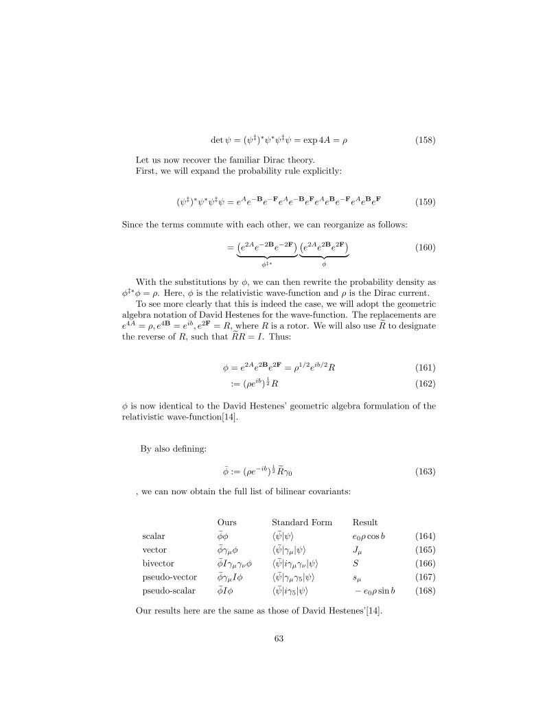
detψ = (ψ‡)∗ψ∗ψ‡ψ = exp 4A = ρ (158)

Let us now recover the familiar Dirac theory.First, we will expand the probability rule explicitly:

(ψ‡)∗ψ∗ψ‡ψ = eAe−Be−FeAe−BeFeAeBe−FeAeBeF (159)

Since the terms commute with each other, we can reorganize as follows:

=(e2Ae−2Be−2F

)︸ ︷︷ ︸

φ‡∗

(e2Ae2Be2F

)︸ ︷︷ ︸

φ

(160)

With the substitutions by φ, we can then rewrite the probability density asφ‡∗φ = ρ. Here, φ is the relativistic wave-function and ρ is the Dirac current.

To see more clearly that this is indeed the case, we will adopt the geometricalgebra notation of David Hestenes for the wave-function. The replacements aree4A = ρ, e4B = eib, e2F = R, where R is a rotor. We will also use R to designatethe reverse of R, such that RR = I. Thus:

φ = e2Ae2Be2F = ρ1/2eib/2R (161)

:= (ρeib)1

2R (162)

φ is now identical to the David Hestenes’ geometric algebra formulation of therelativistic wave-function[14].

By also defining:

φ := (ρe−ib)1

2 Rγ0 (163)

, we can now obtain the full list of bilinear covariants:

Ours Standard Form Result

scalar φφ 〈ψ|ψ〉 e0ρ cos b (164)

vector φγµφ 〈ψ|γµ|ψ〉 Jµ (165)

bivector φIγµγνφ 〈ψ|iγµγν |ψ〉 S (166)

pseudo-vector φγµIφ 〈ψ|γµγ5|ψ〉 sµ (167)

pseudo-scalar φIφ 〈ψ|iγ5|ψ〉 − e0ρ sin b (168)

Our results here are the same as those of David Hestenes’[14].

63

One might have been sceptical that our extension from the Born rule oncomplex-valued wave-functions to the determinant of matrices could yield anyrelevance for physics, but this result shows that it is equivalent to the full Diractheory, in 4D.

We would argue, however, that our approach conceptually much simpler; itessentially only involves applying the determinant to a sum of matrices and not-ing the emergence of the geometric elements manifest in the geometric algebrarepresentation of matrices. No import of physical language is required to getthe Dirac theory; the result follows directly from our recipe.

We even get the geometry of space-time (R and R) for free, again withoutrequiring insertions from outside the theory.

8.1.2 Unitary Gauge Recap

Quantum electrodynamics is obtained by gauging the wave-function with U(1).The U(1) invariance results from the usage of the complex norm in ordinaryquantum theory. A parametrization of ψ over a differentiable manifold is re-quired to support this derivation. Localizing the invariance group θ → θ(x) oversaid parametrization, yields the corresponding covariant derivative:

Dµ = ∂µ + iqAµ(x) (169)

where Aµ(x) is the gauge field.If one then applies a gauge transformation to ψ and Aµ:

ψ → e−iqθ(x)ψ and Aµ → Aµ + ∂µθ(x) (170)

The covariant derivative is:

Dµψ = ∂µψ + iqAµψ (171)

→ ∂µ(e−iqθ(x)ψ) + iq(Aµ + ∂µθ(x))(e

−iqθ(x)ψ) (172)

= e−iqθ(x)Dµψ (173)

Finally, the field is given as follows:

Fµν = [Dµ,Dν ] (174)

where Dµ is the covariant derivative with respect to the potential one-formAµ = A α

µ Tα, and where Tα are the generators of the lie algebra of U(1).

8.2 New Contributions

We are now ready to investigate new contributions of the general linear modelof quantum physics.

64

8.2.1 General Linear Gauge Invariance

The fundamental invariance group of the general linear wave-function is theorientation-preserving general linear group GL+(4,R). Like quantum electro-dynamics (via the U(1) gauge) is the archetypal example of QFT, here quantumgravity (via the GL+(4,R) gauge) will be the archetypal example of our system.

Gauging the GL+(4,R) group is known to produce the Einstein field equa-tions since the resulting GL+(4,R)-valued field can be viewed as the Christoffelsymbols Γ

µ, and the commutator of the covariant derivatives as the Riemanntensor. This is not a new result and dates back to 1956 by Utiyama[15], in1961 by Kibble[16]. The novelty here is that our wave-function is able to ac-commodate all transformations required by general relativity without violatingprobability conservation laws.

Due to our usage of the determinant, a general linear transformation:

ψ′(x) → gψ(x)g−1 (175)

will leave the probability measure of the wave-function invariant, because

det gψ(x)g−1 = detψ(x) (176)

The gauge-covariant derivative associated with this transformation is:

Dµψ = ∂µψ − [iqAµ,ψ] (177)

Finally, the field is given as follows:

Rµν = [Dµ, Dν ] (178)

where Rµν is the Riemann tensor.The resulting Lagrangian is of course the Einstein-Hilbert action which, up

to numerical constant, is:

S =

∫εabcdR

ab ∧ ec ∧ ed =

∫d4 x

√−gR (179)

Let us now discuss the physical interpretation of this quantum theory ofgravity.

8.2.2 Physical Interpretation

Typically to insert gravity into a quantum field theory, one would write themetric as follows: gµν = ηµν + hµν . Then after expansion in powers of h, theEinstein-Hilbert action becomes:

65

(S =

1

16πG

∫d4 x

√−gR

∣∣∣∣gµν→ηµν+hµν

→ 1

16πG

∫d4 x(∂h∂h+ h∂h∂h+ h2∂h∂h+ . . . )

(180)

where the indices on h have been dropped for brevity.The terms ∂h∂h are similar in role to those of an ordinary scalar field theory

∂φ∂φ, and the higher order terms are interaction terms. The linearized approx-imation of the full theory of quantum gravity is obtained by dropping the higherorder terms.

Comparatively in our theory, the Einstein field equations are automaticallyentailed by the theory as the equation of motion of the wave-function. They donot have to be imported from outside, nor to they have to be linearized.

Before we further explore the idea, let us first review the interpretationproposed by David Hestenes for the spinor case of the wave-function, whereX → 0,V → 0. The resulting wave-function is then parametrized as follows:

φ(x0, x1, x2, x3) = ρ(x0, x1, x2, x3)1/2 exp(2F(x0, x1, x2, x3) + 2B(x0, x1, x2, x3))

(181)

or, using David Hestenes’ notation it is equivalent to:

ψ(x0, x1, x2, x3) = (ρ(x0, x1, x2, x3) exp(ib(x0, x1, x2, x3)))1/2

R(x0, x1, x2, x3)(182)

The wave-function simply assigns a rotor R, a probability density ρ and acomplex phase exp(ib) to each point of R4. R, as a rotor, represents a Lorentz

rotation at each point: eµ = RγuR. As argued by David Hestenes[14], this de-scription is equivalent to other interpretations of quantum physics. It is framedin terms of a relativistic kinematic theory of the electron.

How does the general linear case compare? The wave-function would beparametrized as follows:

ψ(x0, x1, x2, x3) =

ρ(x0, x1, x2, x3)1/4 exp(X(x0, x1, x2, x3) + F(x0, x1, x2, x3) +V(x0, x1, x2, x3) +B(x0, x1, x2, x3))

(183)

where (x0, x1, x2, x3) ∈ M4.The general linear wave-function assigns an element of the GL+(4,R) group,

an instruction to transform the frame bundle, to each point on the manifold.The dynamics of this field, obtained by gauging the general linear group, arenow given by the complete Einstein field equations.

The general linear wave-function can further be extended to a Fock spacevia simple tensor products and direct sums, and consequently the formulation is

66

able to represent a superposition of general linear frame bundles transformationsat each point on M4.

Neither gravity nor quantum physics needed to be imported from outside thetheory; both are uniquely entailed by the recipe, and appear in a compatibleform. Finally, the recipe suggests that between general relativity and quantumphysics, it was quantum physics that required corrections (i.e. an extension toa larger group) to support the other; general relativity remained as-is.

8.2.3 A Step Towards Falsifiable Predictions

Annex D lists a number falsifiable predictions.The main idea is that a general linear wave-function would allow a larger

class of interference patterns than what is possible merely with complex inter-ference.

As a secondary idea, it is also plausible that an Aharonov–Bohm effect ex-periment on gravity could detect a general linear phase.

Let us now summarize the Annex.A general linear interference pattern between two arbitrary geometries will

be of the following form:

detψ1 + ψ2 = detψ1 + detψ2 + ψ1 · ψ2 (184)

= enA1 + enA2 + ψ1 · ψ2 (185)

where detψ1 + detψ2 is a sum of probabilities and where ψ1 · ψ2 is theinterference pattern, and where n is the number of dimensions of the matrixrepresentation of the geometric algebra.

The interference pattern is given by the dot product which we define asfollows:

• In 2D the dot product is equivalent to this form:

1

2(det(u+ v)− detu− detv) =

1

2

((u+ v)‡(u+ v)− u‡u− v‡v

)

(186)

= u‡u+ u‡v + v‡u+ v‡v − u‡u− v‡v(187)

= u‡v + v‡u (188)

• In 4D it is substantially more verbose:

67

1

2(det(u+ v)− detu− detv) (189)

=1

2

(⌊(u+ v)‡(u+ v)⌋3,4(u+ v)‡(u+ v)− ⌊u‡u⌋3,4u‡u− ⌊v‡v⌋3,4v‡v

)

(190)

=1

2

(⌊u‡u+ u‡v + v‡u+ v‡v⌋3,4(u‡u+ u‡v + v‡u+ v‡v)− . . .

)

(191)

= ⌊u‡u⌋3,4u‡u+ ⌊u‡u⌋3,4u‡v + ⌊u‡u⌋3,4v‡u+ ⌊u‡u⌋3,4v‡v

+ ⌊u‡v⌋3,4u‡u+ ⌊u‡v⌋3,4u‡v + ⌊u‡v⌋3,4v‡u+ ⌊u‡v⌋3,4v‡v

+ ⌊v‡u⌋3,4u‡u+ ⌊v‡u⌋3,4u‡v + ⌊v‡u⌋3,4v‡u+ ⌊v‡u⌋3,4v‡v

+ ⌊v‡v⌋3,4u‡u+ ⌊v‡v⌋3,4u‡v + ⌊v‡v⌋3,4v‡u+ ⌊v‡v⌋3,4v‡v − . . .(192)

= ⌊u‡u⌋3,4u‡v + ⌊u‡u⌋3,4v‡u+ ⌊u‡u⌋3,4v‡v

+ ⌊u‡v⌋3,4u‡u+ ⌊u‡v⌋3,4u‡v + ⌊u‡v⌋3,4v‡u+ ⌊u‡v⌋3,4v‡v

+ ⌊v‡u⌋3,4u‡u+ ⌊v‡u⌋3,4u‡v + ⌊v‡u⌋3,4v‡u+ ⌊v‡u⌋3,4v‡v

+ ⌊v‡v⌋3,4u‡u+ ⌊v‡v⌋3,4u‡v + ⌊v‡v⌋3,4v‡u (193)

Comparatively, complex interference is given as:

|ψ1 + ψ2|2 = |ψ1|

2 + |ψ2|2 + 2|ψ1||ψ2| cos (φ1 − φ2) (194)

More algebraically manageable special cases of the general linear interferencepattern are provided in the annex.

Finally, we stress that the general linear interference pattern can only betested within the context of quantum gravity, as ordinary quantum field theoryreduces to complex interference.

9 Discussion

Let us now attempt to tie everything together.Assume a formal theory of everything (ToE).This leads to a paradox.Godel showed that for a very wide range of formal systems – and arguably

any ToE - it is always possible to create a proposition that is true but notprovable within the system, which then added as a new axiom to the system,extends it. And this extendibility is possible into the transfinite, implying thatno ToE is ever finally finished, is ever really a ToE. As a consequence, a ToE mustbe redefined as dynamical in that it be able to accommodate new discoveries.Science and mathematics are examples of two systems that already work thisway – but neither claims to be a ToE.

68

Adding the observer makes possible such a system that does constitute aToE, as now newly defined, to be knowledgeable of physics. Four systems wererequired to derive physics from this approach:

1. A Formal System of Knowledge (used to represent knowledge)

2. A Formal System of Science (used to map out knowledge)

3. A Formal Theory of the Observer (used to practice science)

4. A Formal Model of Physics (as a circumscription on the free practice ofscience in nature by the observer).

Step 1 and 2 defined, as we required, a dynamical theory of knowledge ableto accommodate new discoveries thereof. Adding the observer as a probabilityspace (step 3) over halting programs entailed an experience defined as the re-ceipt (or production) of a message of halted programs. Finally, optimizing theinformation of the message (step 4) yielded an inviolable circumscription oversaid experience; it described a model of computation (main result - section 6),and it entailed the laws of physics in their empirically familiar form (applications- section 8).

The resulting model describes reality as the observer having an experiencein nature circumscribed by the laws of physics, and it is closed with respect toall that occurs within this experience. That is our ToE.

9.1 The Ontological Sufficiency of the Experience

What about ”physical” objects; observers in the wild report an observable uni-verse — why?

While our framework cannot explain why an observer exists nor why he orshe has freedom of participation —it is the logical primitive— we can providearguments that his or her experience is ontologically sufficient as a theory ofreality.

Let us warn the reader that some may be uneasy with what we are aboutto suggest, but just like the heliocentric model is a more elegant mathematicaldevice to model the solar system than the geocentric model, here the formalrepresentation of the experience of the observer in nature is also a mathematicaldevice that simplifies our theory of reality. Finally, let us state that even if onewere not to believe in the ontological sufficiency of the experience, one can stillappreciate the mathematical improvements provided by the device.

In the beginning of this manuscript we focused heavily on the notion ofepistemic certainty, and on its relation to knowledge. We will now use epistemiccertainty as a tool to produce ontological guarantees. The famous result alongthis line is the cogito ergo sum in which the epistemic certainty of ”I think” (i.e.if one doubts, one is certain to think) entails the ontological guarantee of one’sown existence. Epistemic certainty is the preferred foundation for philosophicalconstruction (because it makes it infallible), however it is believed only to apply

69

to a very limited range of beliefs (such as ”I exist”) making it unusable as acomprehensive framework.

But what if epistemic certainty constituted a Turing-complete language, andwe simply missed it; will the guarantees it provides be sufficient for ontologicalclosure over reality?

Let us begin by stating that the universe, in modern cosmology, is reasonablyexpected to be a computable solution of quantum gravity. Let us also state thatin our system, the ontological guarantees are provided by the epistemic certaintyof the elements of the message defining the experience of the observer; thatthese elements do halt is verified in our model also by a computable solutionof quantum gravity. Finally, as per the main result, we note that this solutiontakes the form of a long chain of unitary (and general linear) transformationsacting on a wave-function and consequently associates with the entire quantumhistory of the system.

From this, we may simply interpret the universe as the halting proof of theelements constituting the experience of the observer, and as said experience isepistemically certain, then the universe, as its proof, exists as the ontologicalguarantee provided by the experience.

10 Conclusion

We suggest that the primary aim of physics is not to explain, say, how theelectron or the planets behave, as these are incidental to its main objective; thatis, physics is not a theory extrinsic to the observer. Rather, physics is the theorythat circumscribes the experience of the observer in nature, and the mathematicsought to be completely consistent and coherent with this representation. Themathematics presented here-in are a realization of this representation.

References

[1] John Conway and Simon Kochen. The free will theorem. Foundations ofPhysics, 36(10):1441–1473, 2006.

[2] John A Wheeler. Information, physics, quantum: The search for links.Complexity, entropy, and the physics of information, 8, 1990.

[3] Edmund L Gettier. Is justified true belief knowledge? analysis, 23(6):121–123, 1963.

[4] Richard L Kirkham. Does the gettier problem rest on a mistake? Mind,93(372):501–513, 1984.

[5] Gregory J Chaitin. Meta math! the quest for omega. arXiv preprintmath/0404335, 2004.

[6] G. J. Chaitin. Foundations of Mathematics. ArXiv Mathematics e-prints,February 2002.

70

[7] Gregory Chaitin. Mathematics, complexity and philosophy.https://www.academia.edu/31320410/Mathematics_Complexity_

and_Philosophy_full_bilingual_text_, 2010.

[8] Wikipedia contributors. Curry–howard correspondence — Wikipedia, thefree encyclopedia, 2021. [Online; accessed 6-December-2021].

[9] Ian Stewart et al. From here to infinity. Oxford Paperbacks, 1996.

[10] Wikimedia Commons. File:hanakapiai beach warning sign only.jpg — wiki-media commons, the free media repository, 2021. [Online; accessed 18-March-2022].

[11] Gregory J. Chaitin. A theory of program size formally identical to infor-mation theory. J. ACM, 22(3):329–340, July 1975.

[12] Klaus Hinkelmann and Oscar Kempthorne. Design and analysis of exper-iments, volume 1: Introduction to experimental design, volume 592. JohnWiley & Sons, 2007.

[13] Douglas Lundholm and Lars Svensson. Clifford algebra, geometric algebra,and applications. arXiv preprint arXiv:0907.5356, 2009.

[14] David Hestenes. Spacetime physics with geometric algebra. AmericanJournal of Physics, 71(7):691–714, 2003.

[15] Ryoyu Utiyama. Invariant theoretical interpretation of interaction. PhysicalReview, 101(5):1597, 1956.

[16] Tom WB Kibble. Lorentz invariance and the gravitational field. Journalof mathematical physics, 2(2):212–221, 1961.

[17] Bohdan I Lev. Wave function as geometric entity. Journal of ModernPhysics, 3:709–713, 2012.

A Notation

Sets, unless a prior convention assigns it another symbol, will be written us-ing the blackboard bold typography (ex: L,W,Q, etc.). Matrices will be inbold upper case (ex: A,B), whereas tuples, vectors and multi-vectors will bein bold lower case (ex: u,v,g) and most other constructions (ex.: scalars,functions) will have plain typography (ex. a,A). The identity matrix is I,the unit pseudo-scalar (of geometric algebra) is I and the imaginary numberis i. The Dirac gamma matrices are γ0, γ1, γ2, γ3 and the Pauli matrices areσx,σy,σz. The basis elements of an arbitrary curvilinear geometric basis willbe denoted e0, e1, e2, . . . , en (such that eν · eµ = gµν) and if they are orthonor-mal as x0, x1, x2, . . . , xn (such that xµ · xν = ηµν). The asterisk z∗ denotesthe complex conjugate of z, and the dagger A† denotes the conjugate trans-pose of A. A geometric algebra of m dimensions over a field F is noted as

71

G(m,F). The grades of a multi-vector will be denoted as 〈v〉k. Specifically,〈v〉0 is a scalar, 〈v〉1 is a vector, 〈v〉2 is a bi-vector, 〈v〉n−1 is a pseudo-vectorand 〈v〉n is a pseudo-scalar. Furthermore, a scalar and a vector 〈v〉0 + 〈v〉1is a para-vector, and a combination of even grades (〈v〉0 + 〈v〉2 + 〈v〉4 + . . . )or odd grades (〈v〉1 + 〈v〉3 + . . . ) are even-multi-vectors or odd-multi-vectors,respectively. The commutator is defined as [A,B] := AB −BA and the anti-commutator as A,B := AB +BA. We use the symbol ∼= to relate two setsthat are related by a group isomorphism. We use the symbol ≃ to relate twoexpressions that are equal if defined, or both undefined otherwise. We denotethe Hadamard product, or element-wise multiplication, of two matrices using⊙, and is written for instance as M ⊙ P, and for a multivector as u ⊙ v; forinstance: (a0 + x0x+ y0y+ b0x∧ y)⊙ (a1 + x1x+ y1y+ b01x∧ y) would equala0a1 + x0x1x+ y0y1y + b0b1x ∧ y.

B Lagrange equation

The Lagrangian equation to maximize is:

L(ρ,α, τ) = −kB∑

q∈Q

ρ(q) ln ρ(q) + α

1−

∑

q∈Q

ρ(q)

+ τ tr

M−

∑

q∈Q

ρ(q)M(q)

(195)

where α and τ are the Lagrange multipliers. We note the usage of thetrace operator for the geometric constraint such that a scalar-valued equation ismaximized. Maximizing this equation for ρ by posing ∂L

∂ρ(p) = 0, where p ∈ Q,

we obtain:

∂L

∂ρ(p)= −kB ln ρ(p)− kB − α− τ trM(p) (196)

0 = kB ln ρ(p) + kB + α+ τ trM(p) (197)

=⇒ ln ρ(p) =1

kB(−kB − α− τ trM(p)) (198)

=⇒ ρ(p) = exp(−kB − α

kB) exp(− τ

kBtrM(p)) (199)

=1

Zdet exp(− τ

kBM(p)) (200)

where Z is obtained as follows:

72

1 =∑

q∈Q

exp(−kB − α

kB) exp(− τ

kBtrM(q)) (201)

=⇒(exp(

−kB − α

kB)

)−1

=∑

q∈Q

exp(− τ

kBtrM(q)) (202)

Z :=∑

q∈Q

det exp(− τ

kBM(q)) (203)

We note that the Trace in the exponential drops down to a determinant, viathe relation det expA ≡ exp trA.

B.1 Multiple constraints

Consider a set of constraints:

M1 =∑

q∈Q

ρ(q)M1(q) (204)

...

Mn =∑

q∈Q

ρ(q)Mn(q) (205)

Then the Lagrange equation becomes:

L = −kB∑

q∈Q

ρ(q) ln ρ(q) + α

1−

∑

q∈Q

ρ(q)

+ τ1 tr

M1 −

∑

q∈Q

ρ(q)M1(q)

+ . . .

+τn tr

Mn −

∑

q∈Q

ρ(q)Mn(q)

(206)

and the measure references all n constraints:

ρ(q) =1

Zdet exp(− τ1

kBM1(q)− · · ·− τn

kBMn(q)) (207)

B.2 Multiple constraints - General Case

In the general case of a multi-constraint system, each entry of the matrix cor-responds to a constraint:

73

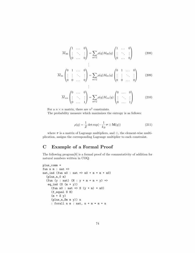
M00

1 . . . 0...

. . ....

0 . . . 0

=

∑

q∈Q

ρ(q)M00(q)

1 . . . 0...

. . ....

0 . . . 0

(208)

...

M01

0 1 . . . 0...

.... . .

...0 0 . . . 0

=

∑

q∈Q

ρ(q)M01(q)

0 1 . . . 0...

.... . .

...0 0 . . . 0

(209)

...

Mnn

0 . . . 0...

. . ....

0 . . . 1

=

∑

q∈Q

ρ(q)Mnn(q)

0 . . . 0...

. . ....

0 . . . 1

(210)

For a n× n matrix, there are n2 constraints.The probability measure which maximizes the entropy is as follows:

ρ(q) =1

Zdet exp(− 1

kBτ ⊙M(q)) (211)

where τ is a matrix of Lagrange multipliers, and ⊙, the element-wise multi-plication, assigns the corresponding Lagrange multiplier to each constraint.

C Example of a Formal Proof

The following program[8] is a formal proof of the commutativity of addition fornatural numbers written in COQ:

plus_comm =

fun n m : nat =>

nat_ind (fun n0 : nat => n0 + m = m + n0)

(plus_n_0 m)

(fun (y : nat) (H : y + m = m + y) =>

eq_ind (S (m + y))

(fun n0 : nat => S (y + m) = n0)

(f_equal S H)

(m + S y)

(plus_n_Sm m y)) n

: forall n m : nat, n + m = m + n

74

D A Step Towards Testable Predictions (Space-time interference)

Certain transformations of the wave-function in quantum gravity, under thegeneral linear group or some of its subgroups, would produce richer interferencepatterns than what is possible merely with complex interference in standardQFT. This offer a difference in predictions between ordinary QFT and oursystem, that can be used to test our system. The possibility of interferencepatterns resulting from geometric algebra representation of the wave-functionhas been proposed before; specifically, I note the work of B. I. Lev.[17] whichsuggests (theoretically) the possibility of an interference pattern associated withthe David Hestenes form of the relativistic wave-function and for the subset ofrotors.

Here we derive a number of these possible interference patterns.In the case of the general linear group, the interference pattern is much

more complicated than the simple cosine of the standard Born rule, but thatis to be expected as it comprises the full general linear group and not just theunitary group. It accounts for the group of all geometric transformations whichpreserves the probability distribution ρ for a two-state general linear system.

General linear interference can be understood as a generalization of complexinterference, which is recovered under a ”shallow” phase rotation in 4D andunder just a plain normal phase rotation in 2D. Furthermore, when all elementsof the odd-sub-algebra are eliminated (by posing X → 0, V → 0), then thewave-function reduces to the geometric algebra form of the relativistic wave-function identified by David Hestenes, in terms of a spinor field.

Such reductions entails a series of interference patterns of decreasing com-plexity, and as such they provide a method to experimentally identify whichgroup of geometric transformations physical reality allows in the most generalcase of quantum gravity, using interference experiments as the identificationtool. Identification of the full general linear interference pattern (with all the el-ements A,X,F,V,B) in a lab experiment would suggest a general linear gauge,whereas identification of a reduced interference pattern (produced by A,F,B)and subsequently showing a failure to observe the full general linear interfer-ence (X → 0,V → 0) would suggest the Lorentz gauge instead of full quantumgravity.

Let us start by introducing a notation for a dot product, then we will listthe various possible interference patterns.

D.1 Geometric Algebra Dot Product

Let us introduce a notation. We will define a bilinear form using the dot productnotation, as follows:

75

· : G(2n,R)×G(2n,R) −→ R (212)

u · v 0−→ 1

2(det(u+ v)− detu− detv) (213)

For example,

u = A1 +X1e1 + Y1e2 +B1e12 (214)

v = A2 +X2e1 + Y2e2 +B2e12 (215)

=⇒ u · v = A1A2 +B1B2 −X1X2 − Y1Y2 (216)

Iff detu > 0 and detv > 0 then u · v is always positive, and thereforequalifies as a positive inner product (over the positive determinant group), butno greater than either detu or detv, whichever is larger. This definition of thedot product extends to multi-vectors of 4 dimensions.

2D: In 2D the dot product is equivalent to this form:

1

2(det(u+ v)− detu− detv) =

1

2

((u+ v)‡(u+ v)− u‡u− v‡v

)(217)

= u‡u+ u‡v + v‡u+ v‡v − u‡u− v‡v (218)

= u‡v + v‡u (219)

4D: In 4D it is substantially more verbose:

1

2(det(u+ v)− detu− detv) (220)

=1

2

(⌊(u+ v)‡(u+ v)⌋3,4(u+ v)‡(u+ v)− ⌊u‡u⌋3,4u‡u− ⌊v‡v⌋3,4v‡v

)

(221)

=1

2

(⌊u‡u+ u‡v + v‡u+ v‡v⌋3,4(u‡u+ u‡v + v‡u+ v‡v)− . . .

)(222)

= ⌊u‡u⌋3,4u‡u+ ⌊u‡u⌋3,4u‡v + ⌊u‡u⌋3,4v‡u+ ⌊u‡u⌋3,4v‡v

+ ⌊u‡v⌋3,4u‡u+ ⌊u‡v⌋3,4u‡v + ⌊u‡v⌋3,4v‡u+ ⌊u‡v⌋3,4v‡v

+ ⌊v‡u⌋3,4u‡u+ ⌊v‡u⌋3,4u‡v + ⌊v‡u⌋3,4v‡u+ ⌊v‡u⌋3,4v‡v

+ ⌊v‡v⌋3,4u‡u+ ⌊v‡v⌋3,4u‡v + ⌊v‡v⌋3,4v‡u+ ⌊v‡v⌋3,4v‡v − . . . (223)

= ⌊u‡u⌋3,4u‡v + ⌊u‡u⌋3,4v‡u+ ⌊u‡u⌋3,4v‡v

+ ⌊u‡v⌋3,4u‡u+ ⌊u‡v⌋3,4u‡v + ⌊u‡v⌋3,4v‡u+ ⌊u‡v⌋3,4v‡v

+ ⌊v‡u⌋3,4u‡u+ ⌊v‡u⌋3,4u‡v + ⌊v‡u⌋3,4v‡u+ ⌊v‡u⌋3,4v‡v

+ ⌊v‡v⌋3,4u‡u+ ⌊v‡v⌋3,4u‡v + ⌊v‡v⌋3,4v‡u (224)

76

D.2 Geometric Interference (General Form)

A multi-vector can be written as u = a + s, where a is a scalar and s is themulti-vectorial part. In general, the exponential expu equals exp a exp s becausea commutes with s.

One can thus write a general two-state system as follows:

ψ = ψ1 + ψ2 = eA1eS1 + eA2eS2 (225)

(226)

The general interference pattern will be of the following form:

detψ1 + ψ2 = detψ1 + detψ2 + ψ1 · ψ2 (227)

= enA1 + enA2 + ψ1 · ψ2 (228)

where detψ1 + detψ2 is a sum of probabilities and where ψ1 · ψ2 is theinterference pattern, and where n is the number of dimensions of the geometricalgebra.

D.3 Complex Interference (Recall)

Consider a two-state wave-function:

ψ = ψ1 + ψ2 = eA1eB1 + eA2eB2 (229)

The interference pattern familiar to quantum mechanics is the result of thecomplex norm:

ψ†ψ = ψ†1ψ1 + ψ

†2ψ2 + ψ

†1ψ2 + ψ

†2ψ1 (230)

= eA1e−B1eA1eB1 + eA2e−B2eA2eB2 + eA1e−B1eA2eB2 + eA2e−B2eA1eB1

(231)

= e2A1 + e2A2 + eA1+A2(e−B1+B2 + e−(−B1+B2)) (232)

= e2A1 + e2A2

︸ ︷︷ ︸sum

+2eA1+A2 cos(B1 −B2)︸ ︷︷ ︸interference

(233)

D.4 Geometric Interference in 2D

Consider a two-state wave-function:

ψ = ψ1 + ψ2 = eA1eX1+B1 + eA2eX2+B2 (234)

77

To lighten the notation we will write it as follows:

ψ = ψ1 + ψ2 = eA1eS1 + eA2eS2 (235)

where

S = X+B (236)

The interference pattern for a full general linear transformation on a two-state wave-function in 2D is:

ψ†ψ = ψ†1ψ1 + ψ

†2ψ2 + ψ

†1ψ2 + ψ

†2ψ1 (237)

= eA1(eS1)‡eA1eS1 + eA2(eS2)‡eA2eS2 + eA1(eS1)‡eA2eS2 + eA2(eS2)‡eA1eS1

(238)

= e2A1 + e2A2 + eA1+A2((eS1)‡eS2 + (eS2)‡eS1) (239)

= e2A1 + e2A2

︸ ︷︷ ︸sum

+ eA1+A2(e−X1−B1eX2+B2 + e−X2−B2eX1+B1)︸ ︷︷ ︸interference

(240)

D.5 Geometric Interference in 4D

Consider a two-state wave-function:

ψ = ψ1 + ψ2 = eA1eX1+F1+V1+B1 + eA2eX2+F2+V2+B2 (241)

To lighten the notation we will write it as follows:

ψ = ψ1 + ψ2 = eA1eS1 + eA2eS2 (242)

where

S = X+ F+V +B (243)

The geometric interference patterns for a full general linear transformationin 4D is given by the product:

⌊ψ‡ψ⌋3,4ψ‡ψ = ⌊ψ‡1ψ1⌋3,4ψ‡

1ψ1 + ⌊ψ‡2ψ2⌋3,4ψ‡

2ψ2 + ψ1 · ψ2 (244)

= e4A1 + e4A2 +(eA1eS1

)·(eA2eS2

)(245)

In many cases of interest, the pattern simplifies. Let us see some of thesecases now.

78

D.6 Geometric Interference in 4D (Shallow Phase Rota-tion)

If we consider a sub-algebra in 4D comprised of even-multi-vector products ψ‡ψ,then a two-state system is given as:

ψ = ψ1 + ψ2 (246)

where

ψ1 = (eA1eF1eB1)‡(eA1eF1eB1) = e2A1e2B1 (247)

ψ2 = (eA2eF2eB2)‡(eA2eF2eB2) = e2A2e2B2 (248)

Thus

ψ = e2A1e2B1 + e2A2e2B2 (249)

The quadri-linear map becomes a bilinear map:

ψ†ψ = (e2A1e−2B1 + e2A2e−2B2)(e2A1e2B1 + e2A2e2B2) (250)

= e2A1e−2B1e2A1e2B1 + e2A1e−2B1e2A2e2B2 + e2A2e−2B2e2A1e2B1 + e2A2e−2B2e2A2e2B2

(251)

= e4A1 + e4A2

︸ ︷︷ ︸sum

+2e2A1+2A2 cos(2B1 − 2B2)︸ ︷︷ ︸complex interference

(252)

D.7 Geometric Interference in 4D (Deep Phase Rotation)

A phase rotation on the base algebra (rather than the sub-algebra) produces adifference interference pattern. Consider a two-state wave-function:

ψ = ψ1 + ψ2 = eA1eB1 + eA2eB2 (253)

The sub-product part is:

ψ‡ψ = (eA1eB1 + eA2eB2)(eA1eB1 + eA2eB2) (254)

= eA1eB1eA1eB1 + eA1eB1eA2eB2 + eA2eB2eA1eB1 + eA2eB2eA2eB2 (255)

= e2A1e2B1 + e2A2e2B2 + 2eA1+A2eB1+B2 (256)

The final product is:

79

⌊ψ‡ψ⌋3,4ψ‡ψ = (e2A1e−2B1 + e2A2e−2B2 + 2eA1+A2e−B1−B2)

× (e2A1e2B1 + e2A2e2B2 + 2eA1+A2eB1+B2) (257)

= e2A1e−2B1e2A1e2B1 + e2A1e−2B1e2A2e2B2 + e2A1e−2B12eA1+A2eB1+B2

+ e2A2e−2B2e2A1e2B1 + e2A2e−2B2e2A2e2B2 + e2A2e−2B22eA1+A2eB1+B2

+ 2eA1+A2e−B1−B2e2A1e2B1

+ 2eA1+A2e−B1−B2e2A2e2B2

+ 2eA1+A2e−B1−B22eA1+A2eB1+B2 (258)

= e4A1 + e4A2 + 2e2A1+2A2 cos(2B1 − 2B2)

+ e2A1e−2B12eA1+A2eB1+B2

+ e2A2e−2B22eA1+A2eB1+B2

+ 2eA1+A2e−B1−B2e2A1e2B1

+ 2eA1+A2e−B1−B2e2A2e2B2

+ 4e2A1+2A2 (259)

= e4A1 + e4A2

︸ ︷︷ ︸sum

+2e2A1+2A2 cos(2B1 − 2B2)︸ ︷︷ ︸complex interference

+2eA1+A2(e2A1 + e2A2) cos(B1 −B2) + 4e2A1+2A2

︸ ︷︷ ︸deep phase interference

(260)

D.8 Geometric Interference in 4D (Deep Spinor Rotation)

Consider a two-state wave-function (we note that [F,B] = 0):

ψ = ψ1 + ψ2 = eA1eF1eB1 + eA2eF2eB2 (261)

The geometric interference pattern for a full general linear transformationin 4D is given by the product:

⌊ψ‡ψ⌋3,4ψ‡ψ (262)

Let us start with the sub-product:

ψ‡ψ = (eA1e−F1eB1 + eA2e−F2eB2)(eA1eF1eB1 + eA2eF2eB2) (263)

= eA1e−F1eB1eA1eF1eB1 + eA1e−F1eB1eA2eF2eB2

+ eA2e−F2eB2eA1eF1eB1 + eA2e−F2eB2eA2eF2eB2 (264)

= e2A1e2B1 + e2A2e2B2 + eA1+A2eB1+B2(e−F1eF2 + e−F2eF1) (265)

= e2A1e2B1 + e2A2e2B2 + eA1+A2eB1+B2(R1R2 + R2R1) (266)

80

where R = eF, and where R = e−F.The full product is:

⌊ψ‡ψ⌋3,4ψ‡ψ =(e2A1e−2B1 + e2A2e−2B2 + eA1+A2e−B1−B2(R1R2 + R2R1)

)

×(e2A1e2B1 + e2A2e2B2 + eA1+A2eB1+B2(R1R2 + R2R1)

)

(267)

= e2A1e−2B1e2A1e2B1 + e2A1e−2B1e2A2e2B2 + e2A1e−2B1eA1+A2eB1+B2(R1R2 + R2R1)

+ e2A2e−2B2e2A1e2B1 + e2A2e−2B2e2A2e2B2 + e2A2e−2B2eA1+A2eB1+B2(R1R2 + R2R1)

+ eA1+A2e−B1−B2(R1R2 + R2R1)e2A1e2B1

+ eA1+A2e−B1−B2(R1R2 + R2R1)e2A2e2B2

+ eA1+A2e−B1−B2(R1R2 + R2R1)eA1+A2eB1+B2(R1R2 + R2R1)

(268)

= e4A1 + e4A2 + 2e2A1+2A2 cos(2B1 − 2B2) (269)

+ eA1+A2(R1R2 + R2R1)( (270)

e2A1(e−B1+B2 + eB1−B2) (271)

+ e2A2(eB1−B2 + e−B1+B2)) (272)

+ e2A1+2A2(R1R2 + R2R1)2 (273)

= e4A1 + e4A2

︸ ︷︷ ︸sum

+2e2A1+2A2 cos(2B1 − 2B2)︸ ︷︷ ︸complex interference

+ 2eA1+A2(e2A1 + e2A2)(R1R2 + R2R1)(cos(B1 −B2)) + e2A1+2A2(R1R2 + R2R1)2

︸ ︷︷ ︸deep spinor interference

(274)

E The General Linear Probability Amplitude inOther Dimensions

Let us investigate the application of this system to dimensions other than 4. Inthis section, we simply list various observations and do not reach any conclu-sions.

E.1 Zero-dimension case

0. In 0D, the ”geometric algebra” is: ψ = expA, where A is a scalar. In oursystem, this is equivalent to classical probabilities.

Obviously, there is no geometry in a 0D system.

81

E.2 Odd-dimension cases

1. In 1D, the geometric algebra is: ψ = expA + B, where A is a scalarand B = e0B = IB ∼= iB is a pseudo-scalar. In 1D, the multi-vectoris a 1 × 1 matrix. The probability measure is given as the determinantdet

(a+ ib

)= a + ib. This is not a real number, so naturally we flag the

1D case.

3. In 3D, the geometric algebra is ψ = expA + X + V + B, where A is ascalar, X is a vector, V is a pseudo-vector and B is a pseudo-scalar. Herethe multi-vector is a representation of the complex 2× 2 matrices. Takingthe determinant produces a complex value and not a real, so naturally weflag 3D for the same reason we flagged 1D.

2n+1 In (2n+1)D, the same here happens as the 1D and 3D cases. We flag allodd dimensions for the same reason: the determinant produces a complexvalue instead of a real.

For all odd-dimension cases, the probability in our system maps to a complexvalue instead of a real. We are not necessarily claiming that these are notrelevant for physics, but if they are then one needs an explanation to accountfor complex probabilities (two probably measures required to describe the wholespace... ?)

E.3 Even-dimension cases

2. In 2D, the geometric algebra is ψ = expA+X +B, where A is a scalar,X is a vector and B is a pseudo-scalar. The probability normalizes to areal value detψ = ψ‡ψ. As we did in the 4D case, let us now use spinors(X → 0). We get:

ψ‡xψ = eAe−BxeAeB = e2AeBxe−B (275)

It supports a particle kinematics as we get one rotor: eµ = eBxµe−B. The

2D theory also supports a gravity theory as it invariably admits the generallinear group. In 2D, since the determinant is a polynomial of degree 2of ψ then the QFT and the quantum gravity are the same as they areentailed from the same probability rule. This equivalence between QFTand quantum gravity is a feature unique to 2D.

4. In 4D, we have recovered in the previous section the kinematic relativistictheory of the electron that we are familiar with (or at least an interpre-tation –David Hestenes’ interpretation– equivalent to it). But unlike the2D case, the QFT is a sub-construction of the quantum gravity theory.Specifically, the familiar QFT comes out with these replacements:

φ = ρ1

2 e−ibRγ0 (276)

φ = ρ1

2 eibR (277)

82

Field theories over φ and φ do not capture the full invariance group ofthe determinant. Trying to make quantum gravity fit on a φ and φ frame,that is to say make quantum gravity a QFT, in 4D is bound to fail sincethe φ and φ frame is a sub-construction of quantum gravity. Quantumgravity requires the 4 degree polynomial ⌊ψ‡ψ⌋3,4ψ‡ψ to be defined in 4D.

6. In 6D, the wave-function is:

ψ = expA+X+ F+T+Q+V +B (278)

where A is a scalar, X is a vector, F is a bivector, T is a trivector, Qis a quadrivector, V is a pseudo-vector and finally B is a pseudo-scalar.Taking the even-sub-algebra, the spinor is:

ψ = expA+ F+Q+B (279)

The wave-function will produce a probability measure (after simplifica-tions), and the transformation of the comoving frame would be as follows:

e6Ae−Fe−Qe−BxµeFeQeB (280)

Here we have more than just the rotors eF as we also have the ”spin-rotors” eQ. A typical QFT is extended to more dimensions than 4 byadding the rotations instructions over the extra dimensions. However, in6D the pure geometric interpretation in terms of rotations is not complete,and the expected QFT construction requires the extra spin-rotation termseQ.

2n In even dimensions (2n > 6) the same happens as the 6D case, but witheven more extra terms for the spinors.

The constraints of our probability measure are such that the rotors requiredto produce a pure kinematical and geometric interpretation of the wave-functiononly show up by themselves in 2D and 4D, and this seems to suggest thata geometric interpretation purely in terms of a wave-function that assigns aninstruction to rotate at each point in space-time, is only appropriate for thesedimensions. In 6D or above, the formulation still admits structures that feelsimilar enough to a QFT; but such formulation contains additional terms thatare not purely Lorentz rotation, thus making any geometric interpretation above4D more challenging.

Even in 4D the geometric interpretation still contains the small increasedchallenge of a spin around the pseudo-scalar I with parameter B, whereas inthe 2D version it is purely a rotor. Only the 2D version is therefore purelygeometric and without spin.

83