An exploration of the current state-of-the-art in automatic musictranscription - with proposed improvements using machine

learning

October 17, 2018Lund University

Abstract

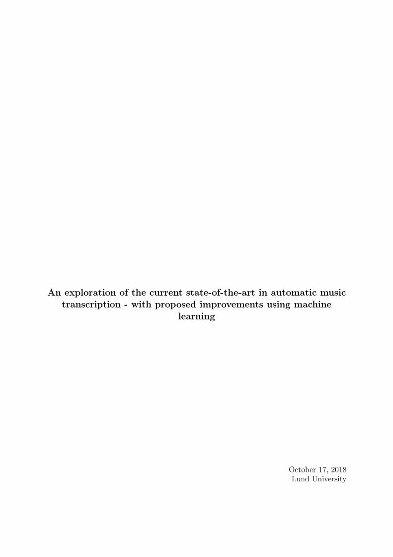
The research field of automatic music transcription has vastly grown during the 21st century,where the goal is to transcribe a polyphonic music signal into annotated sheet music. Withinthis field, the subproblem of fundamental frequency estimation in a piece of music is a difficultproblem, e.g., due to dissimilar structures in signals from different instruments playing the samenote. This becomes further convoluted in a polyphonic signal consisting of several notes, wherethe harmonic overtones of the notes interact. To solve this and other issues, machine learningtechniques have furthered the research in music transcription, which is the main focus of thisthesis. This is undertaken by comparing the best performing fundamental frequency estimatorsfrom recent years, mainly from MIREX competitions from 2015-2017. These are recreated andevaluated on a customized test set consisting of MIDI files of various instruments. The evaluationconsists both of typical music transcription measures such as precision, recall and accuracy, butalso by deeper analysis in order to find the large-scale structural biases. The evaluation of thetests herein shows that the best performing models are THK1 and CT1 from MIREX 2017 whichare based on CNN. This work has identified some structural errors in these methods pointing outpotential for further improvements. In addition, a novel approach of applying complex-valuedneural networks in music transcription is also examined, by modifying research in an existingdeep complex neural network model. The proposed and improved model finishes on third placein the evaluation, indicating that complex neural networks may develop the research area ofmusic transcription even further.

1

A special thanks to my supervisor, Dr. Ted Kronvall for all support and a commitment farbeyond what could be expected in finding solutions and improvements of this work. I also want tothank the system manager James Hakim for helping me out with daily computer related questions.Finally all researchers who kindly contributed with their models, receives my gratitude. Withoutany of you this thesis would not be the same.

2

Contents

1 Popular scientific summary (in Swedish) 5

2 Introduction 6

3 Theory 83.1 Introduction of Automatic Music Translation . . . . . . . . . . . . . . . . . . . . 8

3.1.1 Spectral Analysis . . . . . . . . . . . . . . . . . . . . . . . . . . . . . . . . 103.1.2 Musical- and Overtone Theory . . . . . . . . . . . . . . . . . . . . . . . . 133.1.3 Signal Processing . . . . . . . . . . . . . . . . . . . . . . . . . . . . . . . . 143.1.4 Technical Complications . . . . . . . . . . . . . . . . . . . . . . . . . . . . 15

3.2 Pitch Estimation . . . . . . . . . . . . . . . . . . . . . . . . . . . . . . . . . . . . 163.2.1 Subharmonic Summation . . . . . . . . . . . . . . . . . . . . . . . . . . . 163.2.2 Neural Networks . . . . . . . . . . . . . . . . . . . . . . . . . . . . . . . . 173.2.3 Types of Neural Network . . . . . . . . . . . . . . . . . . . . . . . . . . . 233.2.4 Complex Neural Network . . . . . . . . . . . . . . . . . . . . . . . . . . . 283.2.5 Postprocessing . . . . . . . . . . . . . . . . . . . . . . . . . . . . . . . . . 30

3.3 Available Datasets for Model Training . . . . . . . . . . . . . . . . . . . . . . . . 31

4 MIREX 334.1 MIREX Evaluation . . . . . . . . . . . . . . . . . . . . . . . . . . . . . . . . . . . 33

4.1.1 The MIREX Dataset . . . . . . . . . . . . . . . . . . . . . . . . . . . . . . 334.2 Multiple Fundamental Frequency Estimation . . . . . . . . . . . . . . . . . . . . 344.3 Note Tracking . . . . . . . . . . . . . . . . . . . . . . . . . . . . . . . . . . . . . . 37

5 Models of Multiple Fundamental Frequency Estimation and Tracking 405.1 Evaluated Models . . . . . . . . . . . . . . . . . . . . . . . . . . . . . . . . . . . . 405.2 MIREX 2015 Participating Models . . . . . . . . . . . . . . . . . . . . . . . . . . 41

5.2.1 BW . . . . . . . . . . . . . . . . . . . . . . . . . . . . . . . . . . . . . . . 415.2.2 CB/Silvet . . . . . . . . . . . . . . . . . . . . . . . . . . . . . . . . . . . . 415.2.3 SY/MPE . . . . . . . . . . . . . . . . . . . . . . . . . . . . . . . . . . . . 42

5.3 MIREX 2016 Participating Models . . . . . . . . . . . . . . . . . . . . . . . . . . 435.3.1 CB/Silvet . . . . . . . . . . . . . . . . . . . . . . . . . . . . . . . . . . . . 435.3.2 DT . . . . . . . . . . . . . . . . . . . . . . . . . . . . . . . . . . . . . . . . 435.3.3 MM . . . . . . . . . . . . . . . . . . . . . . . . . . . . . . . . . . . . . . . 44

5.4 MIREX Participating Models 2017 . . . . . . . . . . . . . . . . . . . . . . . . . . 455.4.1 CB/Silvet . . . . . . . . . . . . . . . . . . . . . . . . . . . . . . . . . . . . 455.4.2 CT . . . . . . . . . . . . . . . . . . . . . . . . . . . . . . . . . . . . . . . . 465.4.3 KD . . . . . . . . . . . . . . . . . . . . . . . . . . . . . . . . . . . . . . . . 465.4.4 MHMTM . . . . . . . . . . . . . . . . . . . . . . . . . . . . . . . . . . . . 475.4.5 PR . . . . . . . . . . . . . . . . . . . . . . . . . . . . . . . . . . . . . . . . 485.4.6 THK . . . . . . . . . . . . . . . . . . . . . . . . . . . . . . . . . . . . . . . 48

5.5 Result from MIREX 2015-2017 . . . . . . . . . . . . . . . . . . . . . . . . . . . . 495.6 Other models . . . . . . . . . . . . . . . . . . . . . . . . . . . . . . . . . . . . . . 50

5.6.1 DOPT . . . . . . . . . . . . . . . . . . . . . . . . . . . . . . . . . . . . . . 51

3

5.6.2 PEBSI-Lite . . . . . . . . . . . . . . . . . . . . . . . . . . . . . . . . . . . 525.6.3 ESACF . . . . . . . . . . . . . . . . . . . . . . . . . . . . . . . . . . . . . 535.6.4 Deep Complex model . . . . . . . . . . . . . . . . . . . . . . . . . . . . . . 53

5.7 Proposed models - Deep Complex model with LSTM and CQT/FFT . . . . . . 555.8 Summary and Trends about the models . . . . . . . . . . . . . . . . . . . . . . . 56

6 Tests 606.1 Dataset . . . . . . . . . . . . . . . . . . . . . . . . . . . . . . . . . . . . . . . . . 606.2 Translation between formats . . . . . . . . . . . . . . . . . . . . . . . . . . . . . . 616.3 Conversion to MIREX format . . . . . . . . . . . . . . . . . . . . . . . . . . . . . 636.4 MIREX Evaluation . . . . . . . . . . . . . . . . . . . . . . . . . . . . . . . . . . . 64

7 Results 677.1 Results of Multiple Fundamental Frequency Estimation . . . . . . . . . . . . . . 67

7.1.1 Averaged Multi-F0 Results . . . . . . . . . . . . . . . . . . . . . . . . . . . 677.1.2 Single Test Files Multi-F0 Results . . . . . . . . . . . . . . . . . . . . . . 68

7.2 Result of Note Track . . . . . . . . . . . . . . . . . . . . . . . . . . . . . . . . . . 697.2.1 Averaged Note Track Results . . . . . . . . . . . . . . . . . . . . . . . . . 697.2.2 Single Test Files Note Track Results . . . . . . . . . . . . . . . . . . . . . 707.2.3 Note Track Without Offset Criterion . . . . . . . . . . . . . . . . . . . . . 71

7.3 Plots of estimates . . . . . . . . . . . . . . . . . . . . . . . . . . . . . . . . . . . . 727.4 Analysis of Results . . . . . . . . . . . . . . . . . . . . . . . . . . . . . . . . . . . 85

8 Conclusions and Summary 928.1 Summary of the Test Results . . . . . . . . . . . . . . . . . . . . . . . . . . . . . 928.2 Discussion of Model Features . . . . . . . . . . . . . . . . . . . . . . . . . . . . . 928.3 Analysis of the Proposed Models . . . . . . . . . . . . . . . . . . . . . . . . . . . 948.4 Ideas for Future Research . . . . . . . . . . . . . . . . . . . . . . . . . . . . . . . 94

9 Bibliography 96

4

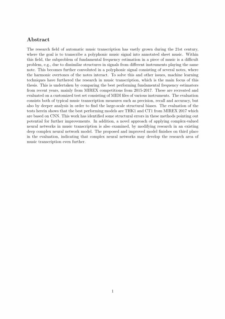
1 Popular scientific summary (in Swedish)

Forskning kring att utvinna information om musik direkt från en ljudinspelning har pågått sedanslutet av 1900-talet. Många nya upptäckter har gjorts de allra senaste åren, dels på grund avatt forskningsområdet har varit relativt outforskat men också då den tekniska utvecklingen hargått framåt väldigt kraftigt. Denna avhandling utforskar en gren inom forskningsområdet, kalladmultipel fundamentalfrekvensestimation, där målet är att få en dator att omvandla musik i formav en ljudinspelning av flera samtidigt spelande instrument, till ett notblad med korrekt tran-skriberade noter. En fundamentalfrekvens motsvarar ljudvågornas svängningshastighet för varjeton i notsystemet. Rent intuitivt kan detta låta som magi, och som man kan förvänta sig finnsdet heller inte någon enkel formel som felfritt löser problemet. De lösningsmetoder som finnsär snarare inriktade på att göra en så bra estimation av det korrekta notbladet som möjligt.Tillvägagångssätten består generellt sett av avancerade modeller som i flera steg omvandlar dataoch optimerar parametrar utifrån olika tekniska och musikteoretiska aspekter. Hur forskningenssenaste modeller fungerar och hur bra de presterar är två ämnen som denna avhandling utreder.

Tillämpningsmöjligheterna för forskningsområdet är stora, givet att en modell skulle fungera iprincip felfritt. En musiker skulle t.ex. kunna få ut noterna till vilken ljudinspelning som helst,vilket skulle vara uppskattat och praktiskt för musiker på alla nivåer.

Avhandlingen går inledningsvis igenom de tekniska och musikteoretiska delarna som de senasteforskningsmodellerna baseras på, samt vilka hinder man behöver få bukt med. En stor del avsvårigheten i multipel fundamentalfrekvens-estimation ligger i att ljudet från flera olika instru-ment går in i varandra och frekvenser kan på så vis både förstärkas eller ta ut varandra. Vidarevet datorn inte vilken uppsättning av instrument som ljudet kommer från, samt hur mångatoner som spelas samtidigt. Ett nyligen applicerat segment inom forskningsområdet är machinelearning genom så kallade neurala nätverk. Ett neuralt nätverk lärs upp till att automatisktidentifiera mönster i ett okänt dataset genom att anpassa parametrar på en stor mängd trän-ingsdata. Hur neurala nätverk fungerar rent praktiskt och hur de appliceras för att estimerafundamentalfrekvenser är något som också utreds i denna avhandling.

Ett avsnitt är tillägnat åt att implementera en egen modell som baserar sig på insikter frånexisterande modeller. Den presenterade modellen använder sig av en variant av neurala nätverksom tillåter komplexa värden, det vill säga roten ur negativa tal. Detta är en nyintroduceradvariant av neurala nätverk inom forskningsvärlden som inom bland annat bildigenkänning harvisat bättre resultat än likvärdiga realvärda neurala nätverk. I avhandlingen görs en omfattandeutvärdering där totalt 24 modeller testas på 12 musikstycken i olika stilar och instrumentkonstel-lationer. Den föreslagna modellen presterar väldigt väl och är enligt testerna den tredje bästamodellen.

Testerna används dels för att avgöra vilka modeller som presterar bäst, vilket ger ett mått påvad dagens forskning kan åstadkomma. Testerna används också för att analysera vilka frekvensermodellerna klarar av att estimera samt om det går att hitta några strukturella fel som de inteklarar av. Att grundligt utvärdera metoderna inom dagens forskning kan förhoppningsvis hjälpatill att vägleda framtidens forskning till att fortsätta göra nya framsteg.

5

2 Introduction

To automate music transcription would in many applications be appreciated and developing.Take for example a musician sitting next to the guitar writing a song. The melody which wasjust invented on the guitar turned out to be perfect and the musician starts to write down thenotes as good as it was remembered. Imagine the musician using an automatic music transcribingdevice, the melody would instead simply appear on a music sheet just as it was played. Anotherexample is a musician listening to a song which the musician wants to play himself. Instead oflistening to the song recording in slow motion in order to write down the tones one by one, anautomatic music transcriber would give the sheet music directly. The musician could insteadspend the time on practicing the song directly.

So why don’t everyone use an automatic music transcription device? The simple answer is thatit doesn’t exist, at least not a completely working one, at least not right now. The follow-upquestion is of course, when will it exist? This question can of course not be answered by a masterstudent in mathematical statistics. What a master student can answer, which this thesis will beabout, is how well the currently best music transcription devices perform statistically, how theywork and perhaps how far from perfect they currently are. To determine the directions of furtherresearch, this is an important question to answer. This question is actually answered every yearin a conference called MIREX where music transcription models are evaluated. But the MIREXevaluation is not optimal in order to lead the way of future research, which will be motivatedherein.

Every year researchers send their novel algorithmic solutions to MIREX and the best performingone is decided. The issue is that the question "why" it performs the best, is not further analyzed.In this thesis a broader selection of models, more corresponding to what currently is availablein the music transcription area, will be evaluated. Also, the results will be presented such thatdifferent features in the models may be analyzed. In order to limit this thesis, both models inMIREX which were participating 2014 and before as well as other models which haven’t par-ticipated in MIREX, have been omitted. It should be mentioned that even if more models areevaluated in this thesis than in one single MIREX conference, there are published models claim-ing to perform state-of-the-art which are not considered in this thesis.

The most recent music transcription models are based on machine learning, which can be de-scribed as methods where a large amount of data is used to train a network consisting of oftenseveral thousands of parameters. Machine learning has previously been proved to be successfulfor image analysis, but recently also for music transcription. This thesis will study the novelapproach of applying complex-valued neural networks to music transcription. Complex-valuedneural networks is a newly discovered area which has been showed to enrich other applicationssuch as image recognition [1]. This thesis will aim to answer if complex-valued neural networksmay enrich the area of music transcription as well.

Comparable studies as this thesis has been made, for example [2] where many types of musictranscription techniques are explained and compared, or [3] where the challenges for the auto-matic music transcription area are described and what needs to be developed in order to makefurther progress.

6

This thesis is aimed for two types of readers. The first is the dedicated researcher in the musictranscription subject, for whom the test results might be the most interesting. The second is thestudent who is new to the area and wants to get a thorough review of the current research and theunderlying theory. The thesis will be structured as follows: In chapter 3 the fundamental toolsfor music transcription will be described. Chapter 4 will describe what a music transcriptionmodel is supposed to perform and how it is evaluated. In chapter 5 all the considered musictranscription models are presented. In chapter 6 statistical testing of the models is described.In chapter 7 the test results are presented, and finally in chapter 8 conclusions of the results aremade.

7

3 Theory

In this section the basic theory behind music translation will be introduced: First a general reviewof what automatic music transcription is presented in Section 3.1. The steps are then furtherexplained by analyzing the music signal using different methodologies, such as spectral analysisin Section 3.1.1, musical theory in Section 3.1.2, signal processing in Section 3.1.3, and technicaldifficulties that may appear in Section 3.1.4. Then the theory behind the pitch estimation isexplained, which essentially amounts to different solutions to a signal processing classificationproblem. An approach called subharmonic summation is described in Section 3.2.1, whereafteran introduction to neural network in Section 3.2.2, followed by different types of neural networksin Section 3.2.3 and 3.2.4. The section ends with the translation of pitch probabilities to a musicsheet in Section 3.2.5.

3.1 Introduction of Automatic Music Translation

Transcribing music is complicated, therefore the solutions may be very advanced. The solutionsalso differ depending on who tries to solve the problem. There are a couple of steps on the pathto a complete music transcription model which the current research seems to have agreed on [2].The researchers’ attempts to optimize these steps will be explained in this section.

First of all, if one wants to understand music transcription, one needs to understand some theoryabout audio. The formal definition of audio, stated in [4], is vibrations which propagate througha transmission medium such as a gas, liquid or solid. As further explained, humans can only hearthese vibrations if the waves cycles in the specific range 20 Hz to 20 · 106 Hz (Hz = cycles persecond). Considering blowing in a whistle, the high whistling sound is simply the transmissionmaterial air which vibrates a high amount of Hz. A tone played by a musical instrument consistsof a duration, a loudness and a pitch, among other features [4]. The pitch is the part of thetone which is related to the amount of wave formed cycles per unit of time. Two tones with thesame duration and loudness but with different pitches will sound different and each tone can bejudged as either higher or lower.

Humans don’t perceive sound as wave formed signals, but a computer does. From a wave formedsignal one can find the amount of cycles per second the signal contains, also called the frequencyof the signal. There are a couple of technical ways to establish the frequency. The most famousand well known is the Fast Fourier Transform (FFT) [5], which computes the discrete Fouriertransform (DFT). The DFT is a complex-valued transformation describing the frequency contentof the signal. The original wave formed signal is transformed by the DFT to the frequencydomain. The formula of the DFT in [5] is:

Xk =

N−1∑n=0

xne−i2πknN k = 0, ..., N − 1 (1)

where X is the output sequence (the Fourier transformed signal), x is the wave formed signaland N is the length of the wave formed signal. The FFT computes the DFT with less op-erations than calculating the DFT directly from the sum in (1), according to [5], and that isthe reason why the FFT has become so famous. What practically happens in the DFT is thatthe data is divided into equally spaced frequency bins, and for each frequency bin a complex-value is calculated corresponding to a phase and amplitude of the frequency content in the signal.

8

The output of the DFT is complex-valued and its absolute value corresponds to the amplitude ofthe transformed signal. The absolute value gives an illustration of the signal’s frequency contentwhich is easier to interpret, and is called the amplitude spectrum. In Figure 1, a guitar playingthe tone A3 is visualized together with the amplitude spectrum1.

Figure 1: Top plot shows how the strike of the guitar string appears right after the time starts.One can also see how the power is decaying as the tone is fading out. The middle plot shows azoomed in version of the above plot which is highlighting the wave form of the signal. The bottomplot shows the absolute value of the discrete Fourier transform which has a high peak at 220 Hzand a smaller but distinct peak at 440 Hz. By looking closer to the bottom plot one can find somesmaller peaks at higher frequencies as well.

About the amplitude spectrum in Figure 1 some words must be said. The tone A3 correspondsto the pitch of 220 Hz, and a high power in the amplitude spectrum for that frequency can benoticed, corresponding to a high content of that frequency. Another distinct amplitude appearsat 440 Hz which would correspond to the pitch of tone A4. A medium high content of the fre-quency 440 Hz is found even if tone A4 was not played. The peak at 440 Hz in the spectrum hasappeared due to a property of musical instruments called overtones, as explained in [6]. Noticethat the second peak appears around 440 Hz which is 2× 220 Hz. This approximately multiplephenomena of the peaks is not a coincidence. By looking closer at the amplitude spectrum, onefinds the smaller peaks in higher frequencies to occur at approximately multiples of 220 Hz (660,

1In music transcription one is interested in describing the signal as much as possible by the frequency rep-resentation. In order to perfectly recreate the signal from its frequency representation, the signal needs to bestationary. Clearly the top figure is not stationary, because of the changes in the envelope of the curve. Ifone studies a shorter segment of the data, like the middle plot, the data can be considered as stationary. Theamplitude spectrum in the bottom plot is determined from 100 ms of data.

9

880, 1100 Hz and so on). All these multiples are called overtones. The frequency correspondingto the actual pitch is called the fundamental frequency. In many real-world sounds includingsignals from musical instrument, it is a common fact that overtones appear at approximatelymultiples of the fundamental frequency. The power in each overtone differs between instruments,as well as the envelope of a tone [6]2. This is closely related to the concept of timbre which willbe further discussed in this thesis.

One observation to notice from the amplitude spectrum in Figure 1 is that the fundamentalfrequency has more power than the overtones. The most powerful frequency is called the pre-dominant frequency and the fundamental frequency is by far the most common predominantfrequency. This discovery has contributed very much to the music transcription research [2].

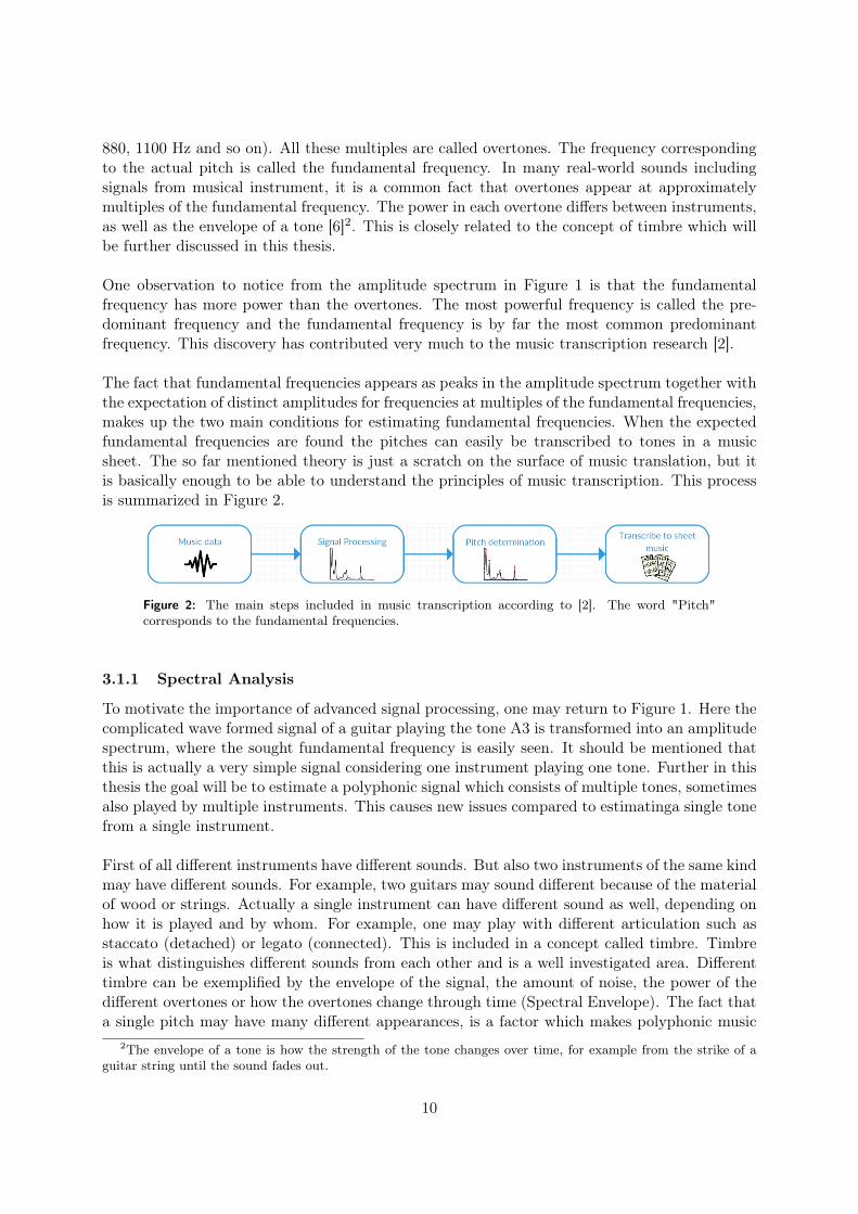
The fact that fundamental frequencies appears as peaks in the amplitude spectrum together withthe expectation of distinct amplitudes for frequencies at multiples of the fundamental frequencies,makes up the two main conditions for estimating fundamental frequencies. When the expectedfundamental frequencies are found the pitches can easily be transcribed to tones in a musicsheet. The so far mentioned theory is just a scratch on the surface of music translation, but itis basically enough to be able to understand the principles of music transcription. This processis summarized in Figure 2.

Figure 2: The main steps included in music transcription according to [2]. The word "Pitch"corresponds to the fundamental frequencies.

3.1.1 Spectral Analysis

To motivate the importance of advanced signal processing, one may return to Figure 1. Here thecomplicated wave formed signal of a guitar playing the tone A3 is transformed into an amplitudespectrum, where the sought fundamental frequency is easily seen. It should be mentioned thatthis is actually a very simple signal considering one instrument playing one tone. Further in thisthesis the goal will be to estimate a polyphonic signal which consists of multiple tones, sometimesalso played by multiple instruments. This causes new issues compared to estimatinga single tonefrom a single instrument.

First of all different instruments have different sounds. But also two instruments of the same kindmay have different sounds. For example, two guitars may sound different because of the materialof wood or strings. Actually a single instrument can have different sound as well, depending onhow it is played and by whom. For example, one may play with different articulation such asstaccato (detached) or legato (connected). This is included in a concept called timbre. Timbreis what distinguishes different sounds from each other and is a well investigated area. Differenttimbre can be exemplified by the envelope of the signal, the amount of noise, the power of thedifferent overtones or how the overtones change through time (Spectral Envelope). The fact thata single pitch may have many different appearances, is a factor which makes polyphonic music

2The envelope of a tone is how the strength of the tone changes over time, for example from the strike of aguitar string until the sound fades out.

10

transcription a complicated problem.

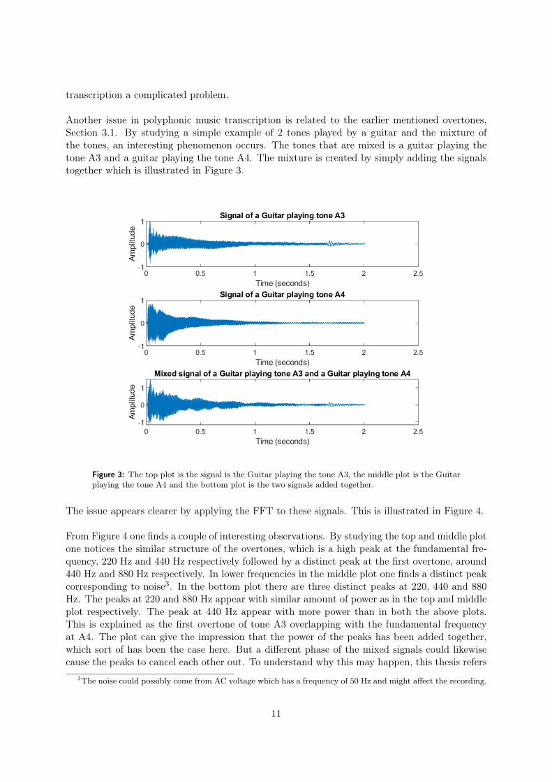
Another issue in polyphonic music transcription is related to the earlier mentioned overtones,Section 3.1. By studying a simple example of 2 tones played by a guitar and the mixture ofthe tones, an interesting phenomenon occurs. The tones that are mixed is a guitar playing thetone A3 and a guitar playing the tone A4. The mixture is created by simply adding the signalstogether which is illustrated in Figure 3.

Figure 3: The top plot is the signal is the Guitar playing the tone A3, the middle plot is the Guitarplaying the tone A4 and the bottom plot is the two signals added together.

The issue appears clearer by applying the FFT to these signals. This is illustrated in Figure 4.

From Figure 4 one finds a couple of interesting observations. By studying the top and middle plotone notices the similar structure of the overtones, which is a high peak at the fundamental fre-quency, 220 Hz and 440 Hz respectively followed by a distinct peak at the first overtone, around440 Hz and 880 Hz respectively. In lower frequencies in the middle plot one finds a distinct peakcorresponding to noise3. In the bottom plot there are three distinct peaks at 220, 440 and 880Hz. The peaks at 220 and 880 Hz appear with similar amount of power as in the top and middleplot respectively. The peak at 440 Hz appear with more power than in both the above plots.This is explained as the first overtone of tone A3 overlapping with the fundamental frequencyat A4. The plot can give the impression that the power of the peaks has been added together,which sort of has been the case here. But a different phase of the mixed signals could likewisecause the peaks to cancel each other out. To understand why this may happen, this thesis refers

3The noise could possibly come from AC voltage which has a frequency of 50 Hz and might affect the recording.

11

Figure 4: The top plot is the amplitude spectrum of a guitar playing the tone A3 (220 Hz), themiddle plot is the amplitude spectrum of a guitar playing the tone A4 (440 Hz) and the bottomplot is the amplitude spectrum of the two signals added together. All amplitude spectrums in theplot are of 100 ms of data.

to theory about of addition of complex numbers [7]. Whether two overlapping peaks from twosignals which are mixed together should be added together, take each other out, or anything inbetween, can in a real world scenario be considered as random. When dealing with polyphonicmusic signals, overlapping overtones will occur very frequently and as described, these overtonesmay not be easily identified or separated.

If one pretends to be given the bottom plot in Figure 4 and asked to determine the active pitches,one may think that it is an easy task just to pick out the two highest peaks. That would beeasy given the number of active pitches and what instrument that is used. But when these ques-tions should be answered automatically by a music transcription model, the number of pitchesand what instruments used, are unknown. One may realize that this turns out to be a morecomplicated task. Given the knowledge that the piano has an overtone structure where the firstovertone has about the same power as the fundamental frequency [6], the amplitude spectrumin the bottom plot in Figure 4, could likewise be estimated as a single tone played by a piano.

By adding more instrument signals to a mix, the number of overlapping overtones will justincrease and the music transcription will appear more complicated. In order to have optimalconditions at the pitch estimation part (Figure 2) one would like to use some kind of spectrumwhich contains as much and robust information as possible and as little noise as possible. Thisis further discussed in Section 3.1.3.

12

3.1.2 Musical- and Overtone Theory

In this section some basic concept of music theory will be explained a bit further. Knowledge inbasic musical theory is essential for a technically oriented music transcriber. In Section 3.1, itwas stated that a musical tone consisted of for example a duration, a loudness and a pitch. Inthis section the pitch of the tone will be focused.

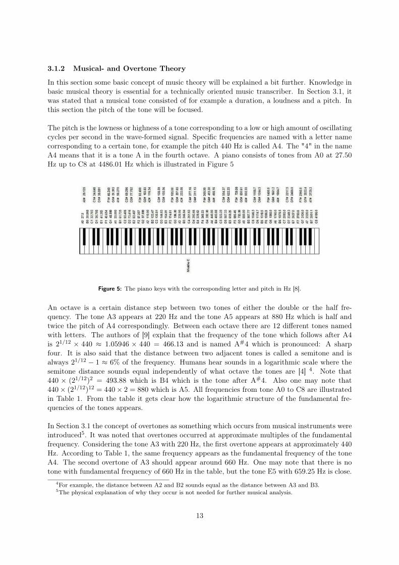
The pitch is the lowness or highness of a tone corresponding to a low or high amount of oscillatingcycles per second in the wave-formed signal. Specific frequencies are named with a letter namecorresponding to a certain tone, for example the pitch 440 Hz is called A4. The "4" in the nameA4 means that it is a tone A in the fourth octave. A piano consists of tones from A0 at 27.50Hz up to C8 at 4486.01 Hz which is illustrated in Figure 5

Figure 5: The piano keys with the corresponding letter and pitch in Hz [8].

An octave is a certain distance step between two tones of either the double or the half fre-quency. The tone A3 appears at 220 Hz and the tone A5 appears at 880 Hz which is half andtwice the pitch of A4 correspondingly. Between each octave there are 12 different tones namedwith letters. The authors of [9] explain that the frequency of the tone which follows after A4is 21/12 × 440 ≈ 1.05946 × 440 = 466.13 and is named A#4 which is pronounced: A sharpfour. It is also said that the distance between two adjacent tones is called a semitone and isalways 21/12 − 1 ≈ 6% of the frequency. Humans hear sounds in a logarithmic scale where thesemitone distance sounds equal independently of what octave the tones are [4] 4. Note that440 × (21/12)2 = 493.88 which is B4 which is the tone after A#4. Also one may note that440× (21/12)12 = 440× 2 = 880 which is A5. All frequencies from tone A0 to C8 are illustratedin Table 1. From the table it gets clear how the logarithmic structure of the fundamental fre-quencies of the tones appears.

In Section 3.1 the concept of overtones as something which occurs from musical instruments wereintroduced5. It was noted that overtones occurred at approximate multiples of the fundamentalfrequency. Considering the tone A3 with 220 Hz, the first overtone appears at approximately 440Hz. According to Table 1, the same frequency appears as the fundamental frequency of the toneA4. The second overtone of A3 should appear around 660 Hz. One may note that there is notone with fundamental frequency of 660 Hz in the table, but the tone E5 with 659.25 Hz is close.

4For example, the distance between A2 and B2 sounds equal as the distance between A3 and B3.5The physical explanation of why they occur is not needed for further musical analysis.

13

C C# D D# E F F# G G# A A# B0 27.50 29.14 30.871 32.70 34.65 36.71 38.89 41.20 43.65 46.25 49.00 51.91 55.00 58.27 61.742 65.41 69.30 73.42 77.78 82.41 87.31 92.50 98.00 103.83 110.00 116.54 123.473 130.81 138.59 146.83 155.56 164.81 174.61 185.00 196.00 207.65 220.00 233.08 246.944 261.63 277.18 293.66 311.13 329.63 349.23 369.99 392.00 415.30 440.00 466.16 493.885 523.25 554.37 587.33 622.25 659.25 698.46 739.99 783.99 830.61 880.00 932.33 987.776 1046.50 1108.73 1174.66 1244.51 1318.51 1396.91 1479.98 1567.98 1661.22 1760.00 1864.66 1975.537 2093.00 2217.46 2349.32 2489.02 2637.02 2793.83 2959.96 3135.96 3322.44 3520.00 3729.31 3951.078 4186.01

Table 1: Frequencies of musical notes in the range of a piano. The notes in a scale are in eachcolumn and the octaves are in each row. The table should be read as the frequency of tone C2 isfound in the C-column (1st column) on the 2-row (3rd row) as 65.41. The frequencies are roundedto 2 decimals.

Actually E5 is close enough in order to interact with the second overtone of A3 and one may saythat A3 and E5 have overlapping overtones at around 660 Hz (interaction between overlappingfrequencies were described in Section 3.1.1). Actually all tones in Table 1 with frequencies ≈ 660

nfor all n ∈ Z will have an overlapping overtone with A3 at 660 Hz. This similarly holds for allovertones of A3, also at the fundamental frequency. When describing all active frequencies in atone, both the fundamental frequency and the overtones, at once, the term harmonics is used.The first harmonic is the fundamental frequency, the second harmonic is the first overtone andso on.

One may note that all combination of two tones, given enough active overtones, will sooner orlater have two harmonics which will overlap6. For some combination of two tones this occursfor high frequencies while for others it occurs for lower frequencies. A mix of two tones wherethe first overlapping overtone appears at a high frequency are nicest from a music transcriptionperspective, since there are less interactions in the spectrum, which are hard to deal with.Unfortunately for the music transcriber, a mix of tones in music sound more pleasantly andsweetly from a psychological perspective if the tones are in harmony and the overtones becomemerged. This psychological feeling has been sought by music creators throughout time, and themusic humans listen to is mainly in harmonies. It would have been advantageously for a musictranscriber if the music humans listen to was out of harmony. But as the world look like, a userof a music transcription device would only be interested in transcribing harmonic music whichsounds good, so that is what the music transcription models should be able to handle. Thepsychological phenomenon of good and bad sound according to different combinations of tones,is called consonance and dissonance between tones.

3.1.3 Signal Processing

FFT is this far the only signal processing method mentioned in this thesis. However, the FFTis rarely used in common music transcription models. The reason why it has been used in theabove examples is partly because of its simplicity and its familiarity to technical skilled persons,but also since many of the other signal processing methods have similarities to the FFT.

6For two tones x and y, one can see that x×(21/12)m and y×(21/12)n, for some m,n ∈ Z, will be approximatelyequal.

14

One of the most frequently used signal processing methods in music transcription is the Constant-Q transform (CQT) [10]. To explain what it does it is often compared with the FFT, see (1).For the FFT, the frequency axis is linearly spaced, which means that the difference betweentwo neighbouring frequency bins is always the same. In the CQT, the frequency axis instead isgeometrically spaced. According to [10], its frequencies are

fk = f0 · 2kb k = 0, 1, ... (2)

where b is the number of frequency bins per octave and f0 is a chosen center frequency. The mo-tivation of geometrically spaced frequency bins is that is more similar to the human logarithmichearing. For example, the step difference between G3 (196 Hz) and A3 (220 Hz) does for a humansound the same as between G4 (392 Hz) and A4 (440 Hz) even if the step difference is twiceas big measured in absolute frequency. The frequency resolution of the CQT remain constantin different octaves while the frequency resolution of the FFT is higher for higher octaves thanlower octaves. This can also be considered as a downside of the CQT since the resolution of pri-marily higher frequencies are lost compared to the FFT. In the CQT, for each frequency fk, thecorresponding multiples (...14fk,

12fk, 2fk, 3fk, ...) will also get their frequency content evaluated,

which is convenient due to the importance of overtones in musical transcription. For the FFT,the frequency axis will in general not contain all exact multiples of fk.

About the parameters in (2), b is usually chosen to be a multiple of 12 since that is the numberof tones in each octave. f0 is usually chosen as the lowest tone which is expected in the signal(which for a piano would be A0 with 27.50 Hz). Because its better alignment to the humanaudio perception, the CQT (or versions of it) is considered to be a more robust transform thanthe FFT and is therefore more frequently used in music transcription models.

Other versions of the FFT where the frequency axis is differently scaled are commonly used inmusic transcription models. One variant is the Equivalent Rectangular Bandwidth where thefrequency axis is transformed by

ERB(f) = 6.23 · f2 + 93.39 · f + 28.52 (3)

which is a designed to approximate the bandwidth of human auditory filters [11].

Another scaling of the frequency axis is by the Mel scale. Frequencies are transformed to melsm, by

m = 2595log10(1 +f

700) (4)

which also is based on the human perception of sound [12].

3.1.4 Technical Complications

In a piano roll representation a tone is represented as a quarter note, a whole note or somethingsimilar given a rate of beats per minutes. Comparing a musician to a computer by playing amelody from a music sheet, the musician may hit all tones correctly, but due to tempo changes,different pronunciation or other timbre differences, they will not be identical. In order to createa dataset containing both a real music recording and a ground truth music sheet, the sheet musicneeds to be manually recreated from the recording. To create a such sheet music is not trivial.The music transcription models consider time bins of 10 ms, therefore the note sheet needs the

15

same accuracy. Considering a melody of 30 seconds, that is 3000 time bins which should be filledwith the correct frequencies. Creating a perfectly working dataset is complicated and takes lotsof time. This has caused a lack of established datasets, which is affecting the research.

The hardest part in manually recreating the sheet music is to determine where a tone ends, orspecifically where the offset occurs. Due to the envelope of for example a guitar tone, with sharpfluctuations in the beginning and high power in the spectrogram, both the fluctuations and thespectrogram power decays towards offset of the tone7. Thus it is not perfectly clear where thetone ends. Often some kind of threshold is used when transcribing to determine when a toneshould be considered active or inactive. By defining the onset and offset by a threshold usuallygives an accurate precision of where the onset appears but a quite vague precision of where theoffset appears.

Another issue when considering real recorded music is that the instrument must be tuned per-fectly. If not, the pitches of the tones will differ from the ground truth. By recording a melodyone needs to consider the choice of sampling frequency. The highest possible frequency whichcan be identified from a recording is the half sampling frequency, fs2 , and is called the Nyquistfrequency. The highest tone on a piano is the C8 which occurs at 4186.01 Hz. The samplingfrequency should reasonably be of at least 2 · 4186.01 = 8372.02. A final technical considerationneeds to be taken about the instruments which have a vibrating sound, like the flute or the violin,where the pitch tends oscillates around the true pitch. This is a feature which is not capturedby the piano roll representation but may affect an estimation.

3.2 Pitch Estimation

This section will describe the step in the music transcription algorithm where a set of givenspectrums are used to estimate the active pitches. One intuitive way of this would be to searchfor all the peaks is the spectrum, set a minimum threshold such that peaks caused by noise canbe excluded, then finally transcribe the frequencies corresponding to the acceptable peaks intoa music sheet. Using this method one would probably be able to find most of the correct tones,but since there will be peaks in the spectrums which correspond to overtones, a lot of incorrecttones will be estimated. Thus, a more sophisticated algorithm must be used.

By analyzing the models in the research field, there are in general three variants of pitch estima-tion methods: probabilistic, parametric and neural network-based methods. The probabilisticmethods are complicated to explain in a general form but is based on combined estimated proba-bilities about features in the signal. Further a parametric method and a couple of neural networkmethods will be explained in detail. In general the different variants of methods ends up in prob-abilities for each pitch candidate to be a fundamental frequency, which is the pitch estimationpart of the problem. Given those probabilities some optional method, called postprocessing, isused to choose which pitches should be the estimated fundamental frequencies, which completesthe pitch estimation part.

3.2.1 Subharmonic Summation

In order to not mistakenly estimate overtones as fundamental frequencies one way is to use thePair-Wise Subharmonic Summation [2]. This method compares all the peaks (potential pitches)

7Also called the onset of a tone.

16

in the spectrogram with each other. For each pair of the pitch candidates there will be one higherand one lower frequency which are notated by fhigh and flow. [2] divides the algorithm into twoparts, and first it is assumed that they are successive harmonics. If the ratio h = flow

fhigh−flow isclose to an integer then h can potentially be the harmonic number of flow and correspondinglyh+ 1 can be the harmonic number of fhigh. As in [2], similarly it is tested if the peaks have anodd harmonic relation by h = 2flow

fhigh−flow . If the ratio is close to an integer, h can potentially bethe harmonic number of flow and correspondingly h + 2 can be the harmonic number of fhigh.Following the algorithm in [2], after all possible pairs of peaks has been evaluated, fp, called thevirtual pitches, are calculated as fp = fi

hi. The virtual pitches correspond to weights which after

a few more steps in the algorithm in [2], are added to the peak candidates of the fundamentalfrequencies.

There are a couple of ways these candidates can be classified as pitches. The simplest way is bysetting a straight threshold which may have been achieved through training on data. The pitchcandidates who fulfill the threshold condition becomes the estimated fundamental frequencies.There are more advanced variants of thresholds which will be described in Section 3.2.5.

The subharmonic summation is a method which goes under the category of parametric methodssince the weights are threatened with trained parameters in order to form the pitch candidates.The subharmonic summation is built on the assumption that overtones always appear in musicsignals, which is most often true. But a weakness is that different instruments have differentamount of overtones which might favor or disadvantage different musical instruments. Thesubharmonic summation was in 2016 claimed by [2] to be the best and most current method ofpitch estimation.

3.2.2 Neural Networks

Neural networks have recently become immensely popular with an ever increasing number ofapplications. Before 2016, the use of neural networks in music transcription was very limited butnowadays the neural network methods are dominating the field8.

Neural networks are complicated systems loosely inspired by the human brain. By feeding thenetwork with a lot of training data one can explain a neural network as a system that learns itselfto find patterns and to solve problems. Classification problems are typical problems which neuralnetworks have been proven to be successful within. To reconnect this to music transcription,one can describe the pitch estimation as a classification problem where some input data of thespectrum form is given. Each of the potential pitches (for example the 88 tones for a piano fromA0 (27.5 HZ) to C8 (4186.01 Hz)), should be estimated as either active (1) or inactive (0).

There are many different types of neural networks, but a few are more popular in the musi-cal transcription area. The most common network types are the convolutional neural network(CNN) and different types of recurrent neural networks (RNN) such as the long-short term mem-ory (LSTM) network. This section describes how a standard neural network, called a Multilayerperceptron (MLP), works with theory based on [13], [14] and [15]. Further, in Section 3.2.3, areview of different types of networks will be presented.

8Both according to the participating models in the music transcription competition MIREX and other publi-cations in the area.

17

Every neural network consists of an input layer, one or more hidden layers and an output layer[14]. The input layer consists of neurons which is explained in [14] as a holder of a number whichis determined by what is fed into the network. In a typical neural networks, a vector of data is fedto the network which can be of various types, e.g., time series data, multidimensional biologicaldata or images. Not all of these seem naturally as a vector of numbers, but by stacking multiplecolumns or transforming colors by the RGB-scale for example, a vector can be created and usedas neurons in the input layer. The output layer does also consist of neurons and the amount ofneurons in the output layer is usually specified to the number of classes there are in the data[14]. For example, if one wants to classify images of hand written digits one naturally specifies10 classes each corresponding to the numbers 0-9. The hidden layers are described in [14] as theheart of the neural network. For an MLP there can be one or more hidden layers. The hiddenlayers do also consist of neurons, called hidden units. The numbers the hidden units consist ofare values in the input layer and some weights [14]. The MLP is a fully connected network, whichmeans that all neurons in the input layer are connected to each of the neurons in the first hiddenlayer, and each of these connections have an individual weight [13]. From the hidden units in thefirst hidden layer there are connections to the hidden units in the second hidden layer and so onsuch that all neurons are connected to all neurons in the other layers over the whole network9.The connections from the input layer to the first hidden layer is mathematically written in [13]as:

aj =D∑i=1

w(1)ji xi + b

(1)j , j = 1, ...,M (1) (5)

where aj is called the activation of the j’th hidden unit. The superscript, (1), indicates thatthe parameters correspond to the first hidden layer which consists of totally M hidden units10.x is the data in the input layer which consists of totally D neurons. w(1)

ji are the weights, eachcorresponds to the connection between a neuron in the input layer and a neuron in the hiddenlayer. b(1)j are called biases and can be seen as constant terms. The weights and biases can bothbe positive and negative, and initially they are randomly initialized for example by drawing froma Gaussian distribution [13].

The hidden units z are, as in [13], formed by a differentiable activation function h(·)

zj = h(aj) (6)

where aj are the activations from (5). The activation function can for example be chosen to bea sigmoidal function, such as the logistic sigmoid

zj =1

1 + e−aj(7)

which squeezes R onto [0, 1], as defined in [13], or the tanh function. Another popular activationfunction is the Rectified Linear Unit (ReLU), also defined in [13], which is determined as

zj = max(0, aj). (8)9Note that a neuron never is connected to another neuron in the same layer.

10That the parameters correspond to the first hidden layer means the connections from the input layer to thefirst hidden layer.

18

For the second hidden layer, in [13], the activations are formed similarly to the first hidden layer,by

ak =

M(1)∑j=1

w(2)kj zj + b

(2)k , k = 1, ...,M (2) (9)

Where the superscript, (2), indicates that the weights and biases correspond to the second hiddenlayer. The hidden units zj corresponds to the first hidden layer which was determined in (5) and(6). To achieve the hidden units of the second hidden layer an activation function as in (6), isapplied to (9).

This continues in the same way for all hidden layers until the output layer appears. For theoutput layer, the activation function often differs from the functions which are used for the otherlayers, and is denoted by σ instead of h. The output layer activation function is determinedby the purpose of the neural network. If the purpose is linear regression, then the activationfunction could simply be yk = σ(ak) = ak. If the purpose is classification, the softmax function

yk = σ(ak) =exp(ak)∑j exp(aj)

(10)

as defined in [13], could be used. If one has a neural network with a single hidden layer, theoutput can directly be written as a function of the input, i.e.,

yk(x,w) = σ

(M(1)∑j=1

w(2)kj h

(D∑i=1

w(1)ji xi + b

(1)j ,

)+ b

(2)k

), j = 1, ...,M (1), k = 1, ...,M (2) (11)

where w(2)kj and b

(2)k are the weights and bias between the hidden layer and the output layer.

M (2) is the number of neurons in the output layer. The MLP consists basically of input data,activation functions and weights. The format of the input data and the variants of activationfunctions are manually designed when creating the neural network. The weights have to bedetermined by training which is done by feeding the network with training data. For supervisedlearning the output is known and the weights are adapted by a computer to minimize an errorfunction. The error function may be chosen with regards to the purpose of the network. Formany common applications of a neural network, the error function, E(w), may have the form asin [14], which is

E(w) =1

2

N∑n=1

(y(xn, w)− tn)2 (12)

called squared loss error, where w are the weights, xn is the n’th input vector of totally Ntraining samples, y(xn, w) is the estimated output by the network (similar to (11)), and tn isthe expected output which is given in the training data, also called the ground truth. The errorfunction will for each training example achieve a cost and by taking the average cost of all thetraining samples one will get a score on how well the network is doing [14]. A low cost is desirableand by using gradient information, the optimizer may change the weights in order to find a lowercost value. It should be noted that this is a quite complicated procedure since this single errorscore should be used to optimize all the weights in the network, which for a reasonable simple

19

neural network structure, still can be tens of thousands of weights. It is described in [14] thatthis huge amount of weights makes the error function extremely multidimensional, which resultsin a large amount of minimum points. There are ways to analytically find a local minimum butnot a global one [15]. In order to find the optimal minimum of the error function, the globalminimum needs to be found, which is a complicated task. The strategy of finding the globalminimum is closely related to the way of finding local minimum points.

Local minimum points of a function in a multidimensional space can be found where the deriva-tive is equal to zero. For that assumption to hold it is of great importance that the function isdifferentiable over the whole space [13]. From (11), considering differentiable choices of activationfunctions, h and σ, one sees that neural networks are differentiable. A differentiable functionyk(xn, w) inserted into (12), the error function is also differentiable.

Given some starting point in the multidimensional space, there are different ways of finding localminimum points. In [15] Conjugate directions method, Newton’s method or Steepest descent arementioned as methods which are used for this kind of task, but with some differences in efficiencyand assumptions of once or twice differentiable functions. The algorithm of the steepest descent,described in [15], which assumes a once differentiable function method will further be explainedherein. The derivative at the starting point x is first calculated. Since Oy(x) indicates in whichdirection y has the largest growth, −Oy(x) indicates in which direction y has the steepest descent.Steepest descent then makes a one-dimensional search along this direction

d = −Oy(x) (13)

for the minimum point. The process is then repeated. This is thus an iterative method, wherethe next point is determined by

xk+1 = xk + λkdk (14)

where λk is chosen such that it satisfies, for example, the Wolfe conditions or the Barzilai-Borweinmethod [16], which guarantee that y(xk+1) < y(xk). By letting k →∞ the minimum value willbe found under certain conditions. In practice one will not do this infinitely many times. Instead[15] solves this by setting a threshold value close to zero, and if the derivative is below thatthreshold, a minimum value is assumed to be found. [15] claims that this method actually turnsout to be poor in relation to the other mentioned methods. Further it is explained that thesteepest descent especially has problems when the function’s curvature is of an elliptic shape.The reason why this example was used is because the other ones have similar structure but areless intuitive.

By the steepest descent method a local minimum can be found11. Considering an extremelymultidimensional function, as the error function of a neural network, a random local minimumwill not be a good choice of weights, since the probability that it would be the global minimumis extremely low, because of the large amount of local minimum points [14]. A very ineffectiveway would be to find thousands of local minimum points by randomizing starting points, andthen choose the best one. Anyhow, this approach would not necessarily give a good result [15].A cleverer way of updating the weights in a neural network is therefore needed. The regular wayof doing this is through a method called backpropagation.

11Even if another choice of method would be more appropriate.

20

In backpropagation the weights are being estimated by starting from the back of the network(the output layer) and then moving backward to end up with the weights from the input layer.In [14] this is described by zooming in on the cost of a single weight, wjk, between the k’thoutput neuron yk and the j’th neuron from the last hidden layer zj in a single training examplex0. The cost function from (12) appears as

Ck =1

2(yk(x0, wjk)− tk0)2 (15)

where tk0 is the ground truth of class k of a single training example, denoted by subscript 0. Ckis the cost of this specific example12. yk(x0, wjk) is the estimated class k output value of thenetwork. Note that this is a clear simplification since in a standard neural network yk woulddepend on wjk for all j and not just a single weight. In the optimal case Ck = 0. If Ck is largeit means that the system needs to put much effort in changing yk(x0, wjk). If Ck is close to zerothe system will not put as much effort in changing it. In [14] it is shown that yk(x0, wjk) can berewritten as a function of the earlier steps in the network by

yk(x0, wjk) = σ(w(L)jk z

(L−1)j + b

(L)j ) (16)

where wjk is the weight and bj is the bias. (L) indicates the last layer (the output layer) andthe w(L)

jk and b(L)j are connections between layer L − 1 and layer L. Here, σ is the activation

function and zj is the j’th hidden unit of layer L − 1. It is possible to rewrite this further asz(L−1)j = h(w

(L−1)ij z

(L−2)i + b

(L−1)i ) and so on where i is the i’th hidden unit of layer L − 2. In

order to keep this intuitive the form of (16) will be used. In backpropagation it is of interest tochange yk(x0, wjk) depending on how much error it causes [14]. This is determined by calculat-ing weights’ and biases’ impact on yk(x0, wjk), since the weights and biases is what indirectlyinfluence the cost of yk(x0, wjk). The impact of the weights is calculated by the derivative ∂Ck

∂w(L)jk

[14]. Recall that in backpropagation the training starts from the back, at layer L, which means,first estimate w(L)

jk (for all j and k), then w(L−1)ij (for all i and j) and so on.

By the chain rule the derivative may, as in [14], be rewritten as

∂Ck

∂w(L)jk

=∂a

(L)k

∂w(L)jk

∂yk

∂a(L)k

∂Ck∂yk

(17)

Where yk(x0, wjk) is shortened as yk and a(L)k = w(L)jk z

(L−1)j +b

(L)j which is the inner part of (16).

The derivatives of the right hand side of (17) can, as in [14], be calculated one by one as

∂Ck∂yk

= yk(x0, wjk)− tk0 (18)

∂yk

∂a(L)k

= σ′(a(L)k ) (19)

∂a(L)k

∂w(L)jk

= z(L−1)j (20)

12A more appropriate variable name would have been Ck0,x0,wjk but in order to simplify notation it is shortenedas Ck.

21

where a couple of constant terms has been cancelled. Combining (18), (19) and (20), as in [14],makes (17) to be rewritten as

∂Ck

∂w(L)jk

= yk(x0, wjk)− tk0)σ′(a(L)k )z

(L−1)j (21)

which may be evaluated directly. One interesting fact from this is that the impact of the weightsbetween layer L − 1 and L is directly related to neuron z(L−1)j in the hidden layer L − 1. This

means that a weight w(L)jk only can be influential if the neuron zj in hidden layer L− 1, is influ-

ential.

By going further in the backpropagation and examining ∂Ck

∂w(L−1)ij

, one needs to take into account

all the different paths each neuron can influence each output. For the neurons in layer L − 1,the term ∂Ck

∂yk, may as in [14], be replaced by

∂Ck

∂z(L−1)j

=

n(L)∑i=1

=∂a

(L)i

∂z(L−1)j

∂z(L)i

∂a(L)i

∂Ck

∂z(L)i

(22)

which looks a bit messier, but it’s actually just adding all connections together. The backprop-agation in [14], for the weights, continues like this all the way back to the input layer. The samething is done for the biases

∂Ck

∂b(L)j

=∂a

(L)k

∂b(L)j

∂yk

∂a(L)k

∂Ck∂yk

(23)

where ∂a(L)k

∂b(L)j

= 1, which gives the following cost derivative

∂Ck

∂b(L)j

= (yk(x0, wjk)− tk0)σ′(a(L)k ) (24)

which is found to be independent to other weights and biases in the L’th layer. The further stepsin the backpropagation for biases is calculated in the same way as for the weights. The totalcost of the whole network is in [14] defined by

C0 =1

2

N∑h=1

n(L)∑l=1

(yl(xh, w)− tlh)2 (25)

where N still is the number of training samples, n(L) is the number of neurons in the outputlayer, yl(xh) is the l’th neuron in the output layer (determined by wjl for all j), xh is the h’thinput, lh is the corresponding expected output, and w indicates all weights and biases in thenetwork. The cost derivative is calculated for all weights and biases and suggests how much eachof them should change to get a better estimation. Combining the cost derivatives one may, as in[14], form

OC0 = [∂C0

∂w(1),∂C0

∂b(1), ...,

∂C0

∂w(L),∂C0

∂b(L)] (26)

where

∂C0

∂w(1)= [

∂C0

∂w(1)11

, ...,∂C0

∂w(1)1n(1)

, ...,∂C0

∂w(1)n(2)1

, ...,∂C0

∂w(1)n(2)n(1)

] (27)

22

are the cost derivatives for each connection weight between the input layer and the first hiddenlayer. The bias derivatives

∂C0

∂b(1)= [

∂C0

∂b(1)1

, ...,∂C0

∂b(1)n(2)

] (28)

are similarly calculated as the weight derivatives. The cost derivative is calculated for all thetraining samples13. This gives suggested changes for each of the weights in order to minimizethe cost function by averaging the derivatives over for all the training data [14]. Then a localminimum point is search for around the suggested weights. This is done by one of the minimumsearching methods and then a new round of backpropagation is applied. These two alternatesan optional (preferably large) amount of times until a local minimum can be considered closeenough a global minimum [14].

The statement that the cost derivative was calculated for all the training samples needs to beclarified. However, calculating the derivative from all training samples is expensive, and typicallynot done in practice. Instead [14] says that all training data usually are divided into mini-batcheswhich each consists of a smaller amount of randomly chosen training data. The derivative of amini-batch only approximates the derivative of the whole training set, but it greatly reduces thecomputational complexity. [14] claims that letting the network train to the limit, it will convergeto the same answer but much faster.

3.2.3 Types of Neural Network

The MLP neural network described in Section 3.2.2 is the simplest version of a feed forwardneural network. Feed forward means that the connections between the nodes do only send in-formation forward in the network, which means that no cycle connections exists. A commonlyused variant of feed forward neural network is the convolutional neural network (CNN) which isintroduced in this section. Moreover, a neural network which is not categorized as feed forwardmay use recurrent layers. Such occur in recurrent neural networks (RNN) and its extension calledlong short-term memory (LSTM) networks which are mentioned later in this section.

The CNN is the most common architecture used for classifying objects in images. To this effect,[17] mentions classification of the MNIST-dataset, containing hand written digits, as an exam-ple where the CNN has been proved successful. The CNN is specifically designed to find localstructures and to combine them, or in other words it is said to be shift invariant, which meansthat it doesn’t matter where in the image the object is located [17].

The CNN has an input layer, an output layer and multiple hidden layers just as the standardMLP neural network and according to [17] the input is commonly an image with a certain size (itis important that this size is constant for all images). The output is commonly a couple of nodes,each corresponding to a probability of a certain classification. If a neural network consists of aconvolutional layer it is said to be a CNN which is what differs from an MLP [17]. A standardCNN commonly also consists of pooling layers and fully connected layers.

13Actually not all samples at the same time. This will be discussed further down.

23

An image is just pixels with numbers in different scales (for example RGB-scale or black andwhite scale) and these numbers of n×m× 3 (RGB-scale) or n×m (Black and white scale) arewhat the input neurons are filled with. The first layer in a CNN is generally a convolutional layer[17]. In the convolutional layer one starts by considering an optional small area in the top leftof the image, for example 5× 5 pixels. The convolution is made by multiplying each pixel in thearea with a specific weight, and then summing all these weights up, the area is estimated into onenumber which is inserted to a corresponding neuron. The next step is to move the area of 5× 5pixels a specified number of steps to the right (this number is called strides) and then repeatthe convolutional steps. This continues until one reaches the right border of the image14[17].When the top row is finished, the area of 5 × 5 pixels moves a specified number of steps downfrom the top left corner and continues in the same way until the bottom right corner is reached15 [17]. The layer which follows from a convolutional layer can be described as a new image,which now has a new size according to the specified settings of the pixel area, strides and padding.

A CNN or other neural networks consisting of many hidden layers are called deep networks.After a convolutional layer, a ReLU layer and some kind of pooling layer generally follows, [17].The ReLU layer is a non-linear activation function which truncates negative values to zero, as in(8). The pooling layer is a kind of non-linear down-sampling where a specified area of an imageis convolved by its max value or average value. It can be noted that the ReLU and pooling layerdon’t involve any weights. The pooling layer does only simplify the training of the networks,while the ReLU makes the communication in the network possible.

The network structure of a CNN does typically rotate by a convolutional layer, a ReLU layerand a pooling layer [17]. Typically, the last layer is fully connected and connects each pixel inthe second to last layer to each of the outputs, as explained in Section 3.2.2. Since the CNN isa feed forward network, it is trained through backpropagation, similarly as the MLP.

One may wonder why a CNN is considered in a thesis about music transcription, when CNNmainly is applied to image classification. By considering the participants in MIREX 2016-2017[18], CNN is actually a very commonly used method in the music transcription area. By stackingspectrums for consecutive time steps, a time-frequency representation with the power in the thirddimension is obtained, called the spectrogram, and is visualized in Figure 6. Analyzing a spec-trogram image means analyzing spectrums over time. This seems to be a reasonable approachsince a spectrum is highly dependent of the adjacent spectrums.

Another type of neural network layer is the recurrent layer, which in its simplest form occursin the RNN16. An RNN is similar to an MLP in the sense that the layers contribute to thefollowing layers through an activation function with weights. The difference is that an RNN usesthe fact that the input is formed as a sequence, where the next value in the sequence is relatedto the previous ones [19]. If the input is related to the previous inputs in the sequence, then theactivations must be related to the previous activations in the sequence. To use this relation, the

14The right side of the right boarder is padded, which means that zeros are added outside the image. Whenthe right boarder of the image is reached, there are two standard options, either to stop just as the padded zerosare reached, or one may continue until the 5 × 5 pixel area just contains the right boarder of the image. Whichone to use is optional but the following layer will have different size depending of the choice.

15The bottom side of the image is also padded and the same boarder options occurs for the bottom boarder asfor the right boarder.

16Recurrent neural network.

24

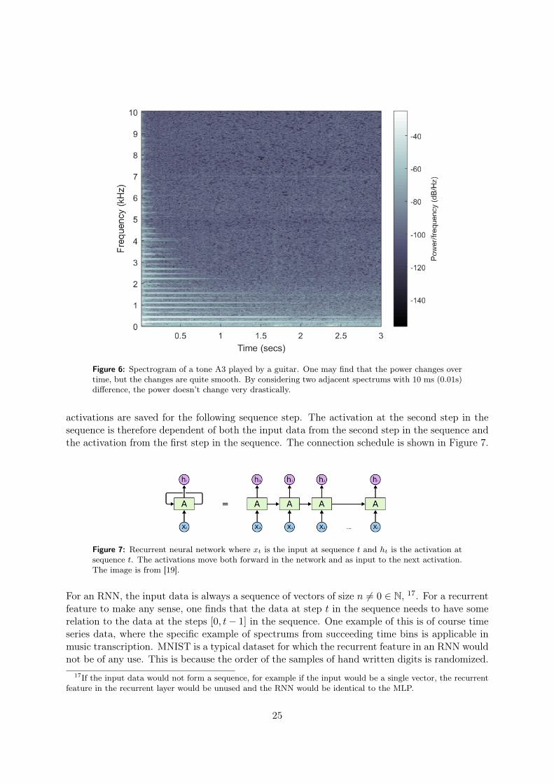
Figure 6: Spectrogram of a tone A3 played by a guitar. One may find that the power changes overtime, but the changes are quite smooth. By considering two adjacent spectrums with 10 ms (0.01s)difference, the power doesn’t change very drastically.

activations are saved for the following sequence step. The activation at the second step in thesequence is therefore dependent of both the input data from the second step in the sequence andthe activation from the first step in the sequence. The connection schedule is shown in Figure 7.

Figure 7: Recurrent neural network where xt is the input at sequence t and ht is the activation atsequence t. The activations move both forward in the network and as input to the next activation.The image is from [19].

For an RNN, the input data is always a sequence of vectors of size n 6= 0 ∈ N, 17. For a recurrentfeature to make any sense, one finds that the data at step t in the sequence needs to have somerelation to the data at the steps [0, t− 1] in the sequence. One example of this is of course timeseries data, where the specific example of spectrums from succeeding time bins is applicable inmusic transcription. MNIST is a typical dataset for which the recurrent feature in an RNN wouldnot be of any use. This is because the order of the samples of hand written digits is randomized.

17If the input data would not form a sequence, for example if the input would be a single vector, the recurrentfeature in the recurrent layer would be unused and the RNN would be identical to the MLP.

25

For an RNN the weights don’t change for different steps in the sequence. The algorithm describedin [19] for an RNN, is the following:18

ht = w1xn + w2ht−1 (29)

where w1 and w2 are two different weight matrices. x is the previous layer which for examplecould be the input, and h is the activations. This gives

h0 = w1x0, h1 = w1x1 + w2h0 = w1x1 + w2w1x0 (30)

and similarly

h2 = w1x2 + w2h1 = w1x2 + w2(w1x1 + w2w1x0) = w1x2 + w2w1x1 + w22w1x0. (31)

Estimating parameters for an RNN is typically quite complicated, [19]. For the RNN, a variantof backpropagation, called backpropagation through time, is used in [19]. The problem is thatbackpropagation through time needs to handle a structure of dependencies. Since backpropaga-tion through time is built on the derivatives of dependencies, the influence of x0 for the activationh100 will contribute with w100 · x0, which is critical. If w < 1 the contribution of x0 will be mul-tiplied with almost nothing (0.9100 = 0.00002656139) and if w > 1 the contribution of x0 willbe very significant (1.1100 = 13780.6123398). This relatively small change of 1.1− 0.9 = 0.2 forthe weights can make a considerably large difference for the output. Many local minimums willappear due to these large influence possibilities of the weights but the most of them will givevery bad estimates [19].

This issue is called the vanishing or exploding gradient, and in order to solve it, the RNN is oftenextended. One extension is the LSTM network, which builds on the idea that all informationfrom all previous sequences is not needed to be used, only the previous information which turnsout to be important should be used19. In a LSTM, the network learns which information thatcan be useful for later and the rest is thrown away. The structure of the LSTM network is shownin Figure 8.

The LSTM has an input layer and ends up by calculating an activation, just as the RNN. Also,the activation of the previous sequence is used as input for the next. The main difference de-scribed in [19], is that there is another input from the previous sequence as well, called the cellstate C. The cell state is visualized in Figure 9.

It is the cell state which holds the important information which will be saved for many sequencesin the network. Information in the cell state can be added or deleted through each sequence.What information that is added or deleted is determined through weights trained by the network.

In [19], a forget gate layer ft is created through ft = σ(Wf [ht−1, xt] + bf ) where Wf is thecorresponding weight matrix, bf is the corresponding bias, and σ is a sigmoid, (7), which forcesall values to be between [0, 1] 20. The forget gate layer is convolved with the previous cell state.The ft values which are close to 1 makes the cell state to remember its previous value while a ft

18The algorithm can be easier understood by studying Figure 7.19LSTM stands for Long short term memory.20Just as for other neural networks, the weights and biases are the only parameters which are trained by the

neural network.

26

Figure 8: The structure of a Long Short-Term Memory network. The image is from [19].

Figure 9: Close-up of the cell state, Ct, which is the long term memory part of the Long Short-TermMemory network. The image is from [19].

value close to 0 makes the cell state to forget its previous value.

The next step in [19] is to add new information to the cell state, which is done in two steps. Firstthe input gate layer it = σ(Wi[ht−1, xt] + bi) decides which values in the cell state that should beupdated, where Wi and bi are the weights and bias corresponding to the input gate layer. Thesecond part is to create new cell state candidates Ct = tanh(WC [ht−1, xt] + bC) [19]. WC andbC corresponds to weights and bias for the candidate values. Here the tanh activation functionmaps all values to [−1, 1]. The input gate values are then convolved with the candidate valuesand then added to the cell state. The cell state finally becomes

Ct = ft ∗ Ct−1 + it ∗ Ct (32)

and will be sent to the next sequence as well as it will be used for creating the activations of thecurrent sequence. The activations are created both through the activations from the previoussequence ht−1, the input layer xt and the current cell state Ct. How it’s done is illustrated inFigure 10.

27

Figure 10: Close-up at the output layer which is the short term part of the Long Short-Term Memorynetwork. The image is from [19].

The output layer ot = σ(Wi[ht−1, xt] + bi) in [19] corresponds to the short term memory part ofthe LSTM, with Wi and bi as corresponding weights and bias. The output layer is multipliedwith a filtered version of the cell state using the tanh activation. The final activation in [19]then becomes ht = ot ∗ tanh(Ct).

The weights and biases are determined from backpropagation through time. One may note thatthe issue of vanishing or exploding gradients have been stabilized since ht only do additive up-dates of Ct instead of multiplicative as for RNN. The parameter estimates for a LSTM thusbecome more stable [19]. This is one reason why the LSTM is more applicable than the RNN,both in music transcription and other areas.

3.2.4 Complex Neural Network

Neural networks are often described as a computer version of the human brain with millions ofneurons which communicates between themselves through connections. Often are these neuronsdescribed either as active 1 or inactive 0. This might be a reason why complex-valued neuralnetworks haven’t been a high topic area of the current neural network research. Recently it hasbeen found that complex-valued neural networks can contribute in many areas both for imageclassification, music transcription and speech recognition[1, 20]21.

All theory of neural networks described herein, are so far adapted for real-valued numbers. Howthese real-valued operations and representations should be adapted for complex values are notobvious and currently (spring 2018) none of the open source neural network libraries supportscomplex-valued numbers. In this section, complex-valued counterparts to the convolutions, theactivation functions and batch normalization are introduced with the theory based on [20].

First a short introduction to complex values is given. A complex number is written as z = a+ ib,21The autors of [1] very recently, July 2018, achieved 100% rate on the MNIST dataset using complex-valued

neural network. Another example is [20] who used Deep complex-valued neural networks on all these areas withimpressive results.

28

where a is the real part and b the imaginary part, where i2 = −1. In order to make it compatiblewith the non-supporting neural network libraries, z is in [20] represented as a n× 2-matrix witha and b in each column.

A complex-valued convolution of two complex-valued functions are comparable to the cross cor-relation between the functions. An example is when a complex filter matrix W = A + iB isconvolved with the complex vector z, where A and B are real matrices. The convolution ispresented in [20] as

W ∗ z = (A ∗ a−B ∗ b) + i(B ∗ a+A ∗ b) (33)

which in matrix notation this is represented as[Re(W ∗ z)Im(W ∗ Z)

]=

[A −BB A

]∗[ab

](34)

where Re(·) is the real part and Im(·) is the imaginary part.

The activation function ReLU, as defined in (8) is not compatible with complex numbers. Acouple of complex-valued versions are suggested in [20] where the best performing one was foundto be the naivest one, called the Complex ReLU, CReLU(·) which is defined as

CReLU(z) = ReLU(Re(z)) + iReLU(Im(z)) (35)

which is complex-valued with a, b ≥ 0, i.e., simply the ReLU for the real and complex partseparably.

Batch normalization is a common tool used in training of the neural network. When each ofthe batches in the training state is normalized, there will be less overfitting and faster trainingas described in [21]. For the first part of real-valued batch normalization in [21] the mean andstandard deviation is calculated from the values in the batch. The mean is then subtracted fromthe data and finally divided by the standard deviation.

x =x− E(x)√

V (x)(36)

where x is the real-valued data in the batch. In addition to this normalized data, x, a shiftparameter β and a scaling parameter µ is trained in the network to recreate normalized valuesclose to the original. The final result in [21] of a batch normalization have the form

y = µx+ β (37)

where y is real-valued. The standard batch normalization is defined for real values only. Tomake it compatible for complex values, first the normalization step needs to follow the complexnormal distribution. The way the complex-valued batch normalization is defined in [20], is thatthe normalization part from (36) becomes

z =

[a

b

]√V (z)

(38)

29

where[a

b

]is a 2 × n vector where the rows correspond to the real and imaginary part of the

complex-valued vector z − E(z). The denominator consists of

V (z) =

(Cov(Re(z), Re(z)) Cov(Re(z), Im(z))Cov(Im(z), Re(z)) Cov(Im(z), Im(z))

)(39)

which is a 2 × 2 matrix consisting of real values. Analogously with the real-valued batch nor-malization, the shift and scaling parameters are trained and y = µz + β is thus formed. Herethe scaling parameter is a 2 × 2-matrix (corresponding to the inverse of the square root of thecovariance matrix) formed as

µ =

(µrr µriµri µii

). (40)

The normalized vector z in (38) is centered at 0 but does not follow the complex normal distribu-tion. If the real or imaginary part have different variance, the normalized vector will be ellipticshaped rather than circular, which would have been the case for a complex normal distributedvector.

3.2.5 Postprocessing

In pitch estimation methods such as neural networks, probabilistic or parametric methods, theestimators typically yield approximative probabilities, or something similar, for the candidatepitches to be a fundamental frequency. Most often those probabilities are not simply 1 or 0. Inthat case the fundamental frequency extraction would be obvious.

In an MLP for a classification purpose, Section 3.2.2, a softmax, (10), was suggested as thefinal activation function. In order to achieve probability 1 for one of the classes, the activationsfor all other classes contributing to the softmax must be −∞. This is practically infeasible toachieve by numerical methods, and one must probably trust a system which says that a pitch issignificantly active, with probability > 0.95. But one would probably trust lower probabilitiesas well. To automatically choose which probabilities to accept, the simplest solution is to set abinary threshold. Output pitches with higher probabilities than the threshold are, by the binarythreshold method, set to 1 and pitches with lower probabilities are set to 0. The output afterthe binary threshold has been applied can easily be translated into a music sheet.

The binary threshold can be computed in different ways. One way is to train the threshold bymaximizing the MIREX accuracy, (43). By setting a binary threshold one is determining whereon the precision-recall scale to be placed. By choosing a high threshold, the precision will behigh since only pitches with a high probability will be chosen. By choosing a low threshold, therecall will be high since even the least salient fundamental frequencies will be captured. Thiscan be summarized in the precision-recall curve, Figure 11.

Other versions of postprocessing can also be considered. For example, due to the spectrumenvelope of a tone with high power at the onset which then is decaying, the pitches may appearwith a higher probability from a neural network or subharmonic summation close to the onset.One may therefore consider lower probabilities close to the offset. Different algorithms for thisexists and are explained further in [2].

30

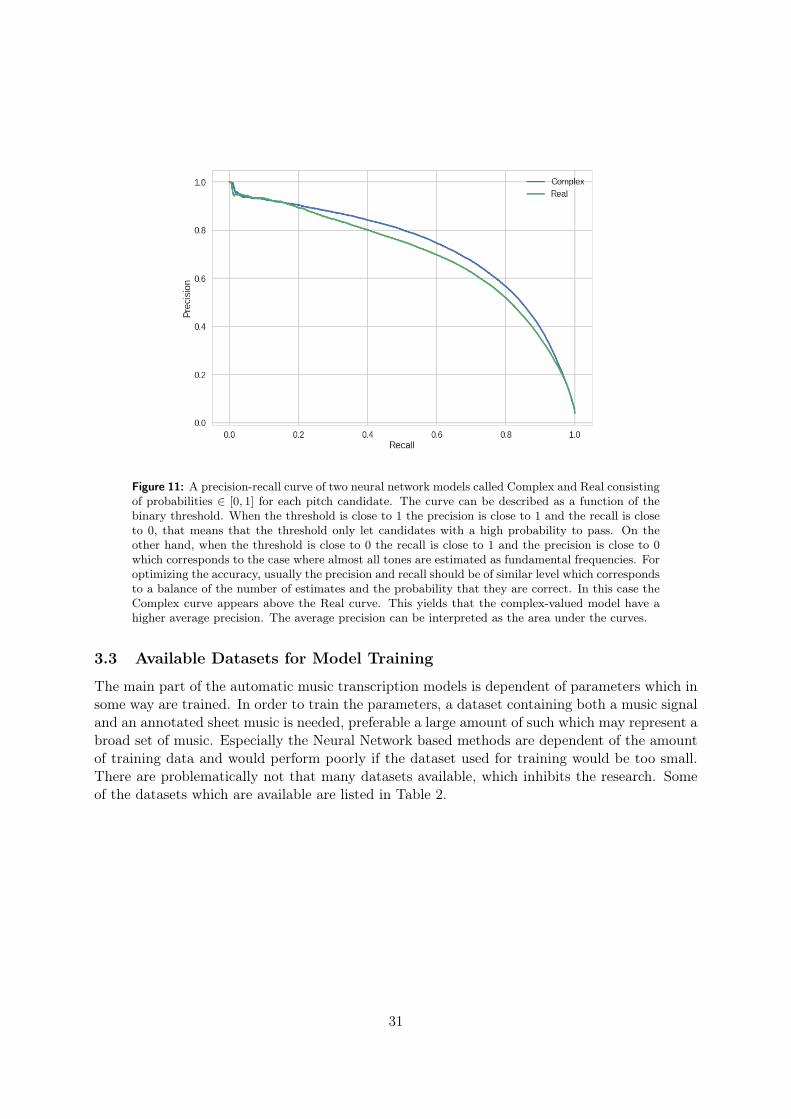
Figure 11: A precision-recall curve of two neural network models called Complex and Real consistingof probabilities ∈ [0, 1] for each pitch candidate. The curve can be described as a function of thebinary threshold. When the threshold is close to 1 the precision is close to 1 and the recall is closeto 0, that means that the threshold only let candidates with a high probability to pass. On theother hand, when the threshold is close to 0 the recall is close to 1 and the precision is close to 0which corresponds to the case where almost all tones are estimated as fundamental frequencies. Foroptimizing the accuracy, usually the precision and recall should be of similar level which correspondsto a balance of the number of estimates and the probability that they are correct. In this case theComplex curve appears above the Real curve. This yields that the complex-valued model have ahigher average precision. The average precision can be interpreted as the area under the curves.

3.3 Available Datasets for Model Training

The main part of the automatic music transcription models is dependent of parameters which insome way are trained. In order to train the parameters, a dataset containing both a music signaland an annotated sheet music is needed, preferable a large amount of such which may represent abroad set of music. Especially the Neural Network based methods are dependent of the amountof training data and would perform poorly if the dataset used for training would be too small.There are problematically not that many datasets available, which inhibits the research. Someof the datasets which are available are listed in Table 2.

31

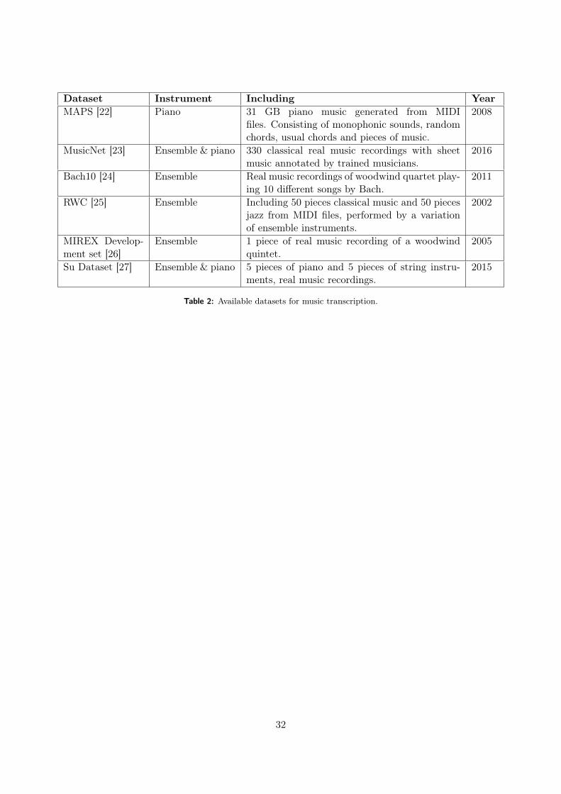
Dataset Instrument Including YearMAPS [22] Piano 31 GB piano music generated from MIDI

files. Consisting of monophonic sounds, randomchords, usual chords and pieces of music.

2008

MusicNet [23] Ensemble & piano 330 classical real music recordings with sheetmusic annotated by trained musicians.

2016

Bach10 [24] Ensemble Real music recordings of woodwind quartet play-ing 10 different songs by Bach.

2011

RWC [25] Ensemble Including 50 pieces classical music and 50 piecesjazz from MIDI files, performed by a variationof ensemble instruments.

2002

MIREX Develop-ment set [26]

Ensemble 1 piece of real music recording of a woodwindquintet.

2005

Su Dataset [27] Ensemble & piano 5 pieces of piano and 5 pieces of string instru-ments, real music recordings.

2015

Table 2: Available datasets for music transcription.

32

4 MIREX

MIREX stands for Music Information Retrieval Evaluation eXchange and started up 2000 ina small edition. This is an annual conference arranged by the International Society for MusicInformation Retrieval (ISMIR) where different researchers from all over the world presents theirsolutions to different tasks, or estimation problems, in music information retrieval (MIR). Theconference, has been growing since the start and for MIREX 2017 totally 22 different tasks whereincluded in the conference, such as Tempo Estimation, Chord Estimation, Classical ComposerIdentification, KPOP Genre Classification, Cover Song Identification and more [18]. The numberof tasks is changing from year to year since new areas of MIR are discovered as time goes by.This follows as the relatively small field of MIR is growing.

One of the tasks in Mirex is called Multiple Fundamental Frequency Estimation and Tracking,which mainly focuses on correctly finding the notes in a music piece. This task was the in-spiration to this thesis and it will be in focus. The goal of this task is to identify the activefundamental frequencies in a polyphonic music signal. Compared to other tasks, this one isquite straight forward. Multiple Fundamental Frequency Estimation and Tracking has been atask in the conference since 2007 where it replaced the closely related task Melody Extraction [18].

The task is divided into subtasks, which will be explained in detail in this section. How thesubtasks are organized is described in Section 4.1, the design of the test set is declared inSection 4.1.1, how the estimates are measured for Multi-F0 are explained in Section 4.2, and thecounterpart for Note Track is described in 4.3.

4.1 MIREX Evaluation

The competing researchers first send in their models a couple of weeks before the conference.For the Multiple Fundamental Frequency Estimation and Tracking task, the models are thenevaluated on two similar subtasks which gives different scores. Those two tasks can be readabout in [18] and are Multiple F0 Estimation, where each active fundamental frequencies shouldbe presented for each time frame, and Note Tracking where the result is presented as noteswith a certain duration, which is more similar to sheet music. Both subtasks are evaluated ontwo different datasets, the The so called MIREX and Su datasets, introduced 2009 and 2015,respectively, which both are real-world recordings. The MIREX Dataset is kept secret for thecompetitors while the Su Dataset is open for the public and available through [27]22. Further inthis thesis, when referring to the results, results on the MIREX Dataset are considered if nothingelse is claimed23.

4.1.1 The MIREX Dataset

The MIREX Dataset (used in task Multiple Fundamental Frequency Estimation and Tracking)consists of 40 clips of half minutes long polyphonic music of with 2-5 ensemble instruments [18].

22The confidentiality for the MIREX dataset is one of the reasons why the competing researchers needs to sendin their models instead of just evaluating and presenting the results themselves.

23Because of higher thrust in a secret dataset.

33

There is a total of 11 songs, each with different combinations of the instruments, resulting intotally 40 music files. Some of the music clips comes from a woodwind quintet transcription ofL. van Beethoven’s String Quartet Op. 18 No.524. The rest of the clips are RWC MIDI andMIDI samples including pieces from Classical to Jazz collections [18].

For the Note Tracking task, there is a total of 34 music files, where 24 came from polyphonicensembles of 2-5 instruments and 6 polyphonic piano files. For the Note Track piano subtask,only the 6 piano files are considered, generated using a disklavier playback piano [18].

4.2 Multiple Fundamental Frequency Estimation

The first subtask considered herein is the Multiple Fundamental Frequency Estimation, or Multi-F0 as it is shortened. In the submission format, as described in [18], for each time frame of 0.01seconds (10 ms), one is supposed to determine which fundamental frequencies are active25. Thegeneral form is

time F01 F02 F03time F01 F02 F03 F04time . . . . . . . . . . . .

and a model output might look like

0 .78 146 .83 220 .00 349 .230 .79 349 .23 146 .83 369 .99 220 .000 .80 . . . . . . . . . . . .

To measure how the different models are performing, the estimates are compared to the groundtruth fundamental frequencies. If an estimated pitch is within a quartertone (±3%) from theground truth it is assumed to be correct26. From this comparison one first finds the amounts oftrue and false positives (TP and FP) and true and false negatives (TN and FN). These measuresare understood simply by studying Figure 12.

From these measures one can, as in [29], calculate the two most standard classification measures,precision and recall, as

Precision =TP

TP + FP(41)

Recall =TP

TP + FN(42)

and in text, precision describes how probable an estimated pitch was to be correctly estimated,while recall describes how probable a true pitch is estimated active. Both measures are boundedby [0, 1] where a score close to 1 is considered good and a score close to 0 is considered bad.

Precision and recall are in some sense describing how good an estimate is. But, for example, ifone would estimate only one pitch to be active, and it turned out to be correct, the precision

24Even if the song is known, the woodwind quintet transcription is not known. Also, this specific music pieceis about 25 min, so it is not obvious which parts are included in the dataset.

25ms stands for Milliseconds and the fundamental frequencies are measured in Hz.26In the evaluation of an estimate in MIREX, only one true fundamental frequency can be associated with

one estimated pitch. That means, for example, that if two true pitches differ by a quarter tone and a pitch isestimated in between them, it can only be associated with one of the true pitches.

34

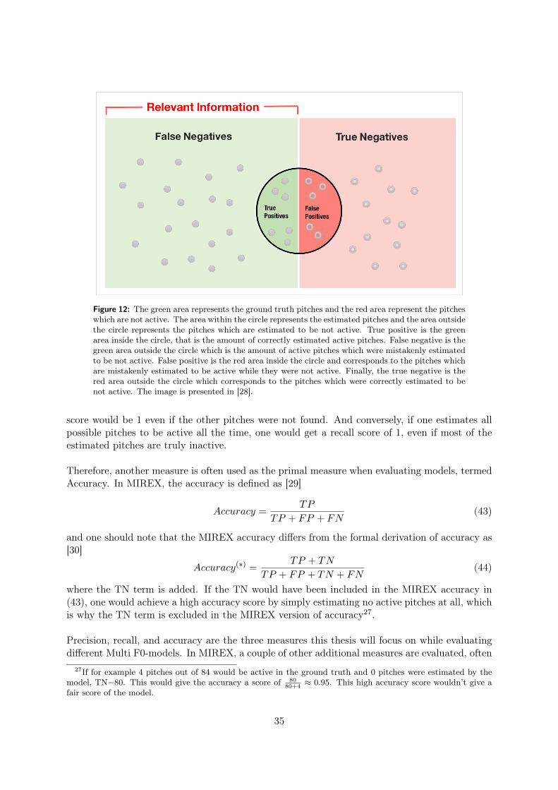
Figure 12: The green area represents the ground truth pitches and the red area represent the pitcheswhich are not active. The area within the circle represents the estimated pitches and the area outsidethe circle represents the pitches which are estimated to be not active. True positive is the greenarea inside the circle, that is the amount of correctly estimated active pitches. False negative is thegreen area outside the circle which is the amount of active pitches which were mistakenly estimatedto be not active. False positive is the red area inside the circle and corresponds to the pitches whichare mistakenly estimated to be active while they were not active. Finally, the true negative is thered area outside the circle which corresponds to the pitches which were correctly estimated to benot active. The image is presented in [28].

score would be 1 even if the other pitches were not found. And conversely, if one estimates allpossible pitches to be active all the time, one would get a recall score of 1, even if most of theestimated pitches are truly inactive.

Therefore, another measure is often used as the primal measure when evaluating models, termedAccuracy. In MIREX, the accuracy is defined as [29]

Accuracy =TP

TP + FP + FN(43)

and one should note that the MIREX accuracy differs from the formal derivation of accuracy as[30]

Accuracy(∗) =TP + TN

TP + FP + TN + FN(44)

where the TN term is added. If the TN would have been included in the MIREX accuracy in(43), one would achieve a high accuracy score by simply estimating no active pitches at all, whichis why the TN term is excluded in the MIREX version of accuracy27.

Precision, recall, and accuracy are the three measures this thesis will focus on while evaluatingdifferent Multi F0-models. In MIREX, a couple of other additional measures are evaluated, often

27If for example 4 pitches out of 84 would be active in the ground truth and 0 pitches were estimated by themodel, TN=80. This would give the accuracy a score of 80

80+4≈ 0.95. This high accuracy score wouldn’t give a

fair score of the model.

35

termed error scores. These are used mainly to describe what type of errors that appear in theestimates from the model. A perfect estimation will achieve an error score of 0. The error scoresmentioned in this section, are however, not used to analyze the models considered herein. First,ESub is defined as [31]

Esubs =

∑tmin(Nref (t), Nsys(t))−Ncorr(t)∑

tNref (t)

where Nref (t) = TP (t) + FN(t), which is the number of true pitches in frame t. Nsys(t) =TP (t) + FP (t) is the number of estimated pitches at frame t. Ncorr(t) = TP (t) is the correctlyestimated pitches at frame t. Esubs gives a measure similar to recall since it counts how manyof the ground truth pitches which are actually estimated, but it is less robust than recall sincean underestimating model (which estimates less pitches than the ground truth) can also get agood score. Actually one will get a perfect score of 0 if the model either estimates all pitches,no pitches at all or exactly the correct pitches. The measure is bounded by [0, 1] where a scoreclose to 0 is sought. The second error score is Emiss which is defined as [31]

Emiss =

∑tmax(0, Nref (t)−Nsys(t))∑

tNref (t)

which is indicating if the model estimates too few pitches. If a model estimates exactly the samenumber of pitches or more it will achieve an error score of 0. The measure is bounded by [0, 1].The Efa is defined as [31]

Efa =

∑tmax(0, Nsys(t)−Nref (t))∑

tNref (t)

and is the opposite of Emiss. Efa is a measure which indicates if a model estimates too manypitches. If the model estimates exactly the same amount of pitches or less, it will get a goodscore close to 0. The measure is non-negative but not upwards bounded. The final error scoreEtot is defined by [31]

Etot =

∑tmax(Nref (t), Nsys(t))−Ncorr(t)∑

tNref (t)

which is a shortened formula of the sum of all the other error scores together. One finds thismeasure to be the only robust of these error scores, since only the perfect model will get a scoreof 0. This score is non-negative but not upwards bounded.

For the Mulit-F0 task the 7 measures (precision, recall, accuracy, Etot, Esubs, Emiss, Efa) arealso evaluated for chroma results. This means that all estimated frequencies are mapped to asingle octave before the evaluation is done. The reason why this is done is since one of the mostcommon mistakes when estimating the fundamental frequency, fk, is to mistakenly estimate thehalf tone 1

2fk (also called the sub octave) or the first overtone 2fk28. In some areas one might

only be interested in the chroma tones. That gives two reasons why this transcription is exam-ined in MIREX. Historically in MIREX, one finds that the rankings in the chroma list of resultdon’t differ that much from the rankings in the standard list of result [18].

The final MIREX performing measure presented in the Multi-F0 task is the Friedman test, wheredifferences among the models’ performances are examined as significant or not. The performance

28See Section 3.1.2 and 3.1.3 for details about overtones.

36

is measured in accuracy, being considered as the most overall measure. The Friedman test mainlyconsists of a Tukey-Kramer HSD Multi-Comparison [32]. Pairwise, student T distributed-based,confidence bounds between each model’s accuracy measure are formed by

Ii,j = µi − µj ±qα,df√

2σε

√2

n

Where µk is the accuracy for model k, q is the student T value for the confidence rate α (typically0.95) with degrees of freedom df . The estimated standard deviation σε is calculated from allmodels (not just the two that are compared), and n is the number of test samples. If 0 is in theinterval Ii,j , then the model i and model j cannot be proven to perform statistically different [32].The spread of each model performance is considered by the test, which can be claimed to be themost correct way of comparing models. However, in the work of this thesis, the Friedman testwould be too complicated to apply because of its parameters being determined from all involvedmodels. The test will thus not be considered further in this thesis.

4.3 Note Tracking

The second subtask considered herein is Note Tracking. This format is more closely related to theway a person reads music from a music sheet. There are different ways to symbolically representa tone in a music sheet, but here the piano-roll convention is used. The piano-roll submissionformat in [18] for each estimated tone, consists of: An onset time, an offset time and a singleestimated frequency. That is when the tone starts, when the tone ends and what pitch. Thegeneral format [18], looks like

onset o f f s e t F01onset o f f s e t F02. . . . . . . . .

which may look like

0 .68 1 .20 349 .230 .72 1 .02 220 .00. . . . . . . . .

which appears easier to translate to a music sheet than the Multi-F0 format. To classify a toneto be correctly estimated, the estimated pitch first of all have to be within a quartertone (±3%)from the reference pitch. Also the estimated onset needs to be within ±50 ms from the referenceonset. Finally the offset needs to be within 20% range from the true tone offset (the percentageis depending on the length of the true tone)[18]. All these three conditions need to be fulfilledin order to classify an estimated tone as correct. Similarly as for the Multi-F0 task, only oneground truth tone can be associated with one estimated tone. For Note Tracking the measuresprecision and recall are calculated in the same way as for Multi-F0 in (41) and (42). Here onemay note that the number of correct and incorrect estimated tones, generally is less than thecorrect and incorrect estimated frequencies each time bin for Multi-F0, making the precision andrecall for Note Tracking more sensitive.

In Multi-F0, accuracy was used as the main measure. For Note Track, this is replaced by theF-measure. The F-measure is defined in [29] from the precision and recall by

37

F = 2 · Precision ·RecallPrecision+Recall

This measure is bounded by [0, 1] and gives a fair average of the precision and recall. It is robustagainst shortcuts such as maximizing only one of the precision or recall29. In order to maximizethe F-measure, the precision and recall should in general be of similar levels.

There is a fourth measure (in addition to precision, recall and F-measure) for Note Tracking calledAverage Overlap. This measure will only be mentioned here but not considered any further inthis thesis. The average overlap measures, for each ground truth tone, the ratio of how well theonset and offset matches the closest estimated tone’s onset and offset. The ratio is determinedby combining the reference and the estimated onset and offset. The Overlap Ratio is, as in [29],defined as

OR =min(refoffset, estoffset)−max(refonset, estonset)

max(refoffset, estoffset)−min(refonset, estonset)

where the inner interval of onset to offset is divided by the outer interval of onset to offset30. Toachieve a high Average Overlap score, the estimated onset and offset should be as identical asthe reference onset and offset as possible. The Overlap Ratio is bounded by [0, 1].

For the Note Tracking task, these 4 measures are evaluated for chroma results in the same way asfor Multi-F0 (Section 4.2). This will, in the same way as for Multi-F0, not be considered furtherin this thesis. In the Note Track task in MIREX one test is on ensemble music and one test ison piano music [18]. This is taken into consideration further when designing the test dataset,described in Section 6.1.

There are also results presented without considering the offset. Thus an estimated tone onlyneeds to fulfill the criterion of being within the quartertone and to have an onset within ±50ms. This is of interest because the definition of the offset definition is quite vague, Section 3.1.4,and in addition it is often the most crucial criterion. To illustrate the vague definition of anoffset one may again consider a Figure 1. Because of the shape of the signal it is not so easyto determine exactly where the tone ends and where the offset should appear. The way it isdetermined practically for the ground truth, is that a threshold is set and when the amplitudeof the tone is below this threshold, the tone is considered as inactive. From Figure 1 one finds apeak when the tone starts, making it quite easy to identify where the amplitude will be abovethe threshold and where the onset should appear. To find where the amplitude will fade belowthe threshold is not as obvious and therefore the offset is more complicated to determine.

Finding when a tone starts and what pitch the tone has may be considered being the most im-portant information. Along with the knowledge that those two criteria are the most trustworthyin the ground truth, one may in some cases consider the Note Track representation without theoffset to be the fairest one. Further in this thesis, both the standard result including the offsetcriterion and the result excluding the offset criterion will be considered.

29Ways of maximizing precision and recall one by one was mentioned in Section 4.2.30In MIREX there are some low-performing models which achieves negative average overlap which contradicts

this definition of the overlap ratio. Thus the MIREX version of the average overlap and the one in [29] may differ.Anyway, the MIREX version of overlap ratio is not expected to differ that much from this one.

38

In the same way as for Multi-F0, a Friedman test is evaluated for the models, using Tukey-Kramer HSD Multi-Comparison. Here the significance tests are based on th F-measure which isconsidered to be the most general measure. However, this measure is deemed to be of limitedinterest in this thesis and will not be considered in the evaluations.

39

5 Models of Multiple Fundamental Frequency Estimation andTracking

A main part of this thesis consisted of understanding and evaluating the most recent methodsused in the research area of polyphonic music transcription. This was done by finding interestingmodels, understanding how the models should be executed and then evaluating them on a cre-ated test set. Afterwards the models have been analyzed in order to explain different behavioursin the test results.

In this section, first a description of which models are considered in this thesis, Section 5.1, theneach of the considered models in MIREX will be introduced and shortly explained together witha summary of their result in MIREX along with technical details, Section 5.2-5.4, followed bya summary of MIREX 2015-2017 in Section 5.5, then a similar introduction to models whichhaven’t participated in MIREX in Section 5.6. Then two herein proposed models (which arevariants of the model in Section 5.6.4) are presented in Section 5.7, and finally in section 5.8the models are summarized and compared, in order to identify some trends of the models. Allresults from MIREX which the following sections will refer to, are found in [18].

5.1 Evaluated Models

Ever since the late 90’s, many different models has been suggested considering polyphonic mu-sic transcription. To consider them all would not be possible in the scope of this thesis. Aselection of models was therefore considered mainly based on models published in conjunctionwith MIREX conference. While aiming to get the most recent research, the models publishedin MIREX 2015-2017 were considered. All models aimed at solving the fundamental frequencyestimation problem are, however, not published in conjunction with MIREX and some effort wasdone to track these. Such methods considered herein were found from suggestions by researchersin the area.

The documentation one gets from the participating models in MIREX is a short report, referredas an abstract, for each submitted model. To be able to evaluate the models, the correspondingauthors were contacted through e-mail and asked to share their code of their model31. Most ofparticipants sent code for their trained models while some returned their model estimates bye-mail after receiving the test files32. The models which weren’t reached from MIREX was eitheravailable on the Internet or delivered through e-mail.

Some participants submitted more than one model. Examples of this could be one version forMulti-F0 and one for Note Track or one model trained on ensemble music and one model trainedon piano music. A third example is someone sending both a slow model, as well as a fast butless accurate model. All these versions will not be considered in the thesis, instead a selection

31Not all models from MIREX 2017 and 2016 are presented in this thesis. Time limited forced a selection ofmodels to be considered, thus 6 models were disregarded. The disregarded models were: PRGR1, PRGR2, WCS1,ZCY2, SL1 (MIREX 2017) and KB1 (MIREX 2016). The best performing models in MIREX 2017 which werenot considered in this thesis was WCS1 which came in 5th place in the Multi-F0 task and PRGR1 which came in3rd place in the Note Track task. For MIREX 2016 KB1 came in 5th place in Note Track (all positions are basedon the accuracy or F-measure depending on the Multi-F0 or Note Tracking task). All the disregarded modelswere in MIREX stated to be significantly lower performing than the best performing model the correspondingyear of participation. Thus, this thesis can be claimed consider the best performing models from MIREX.

32This was done for the authors who, for publishing reasons, could not send their complete models.

40

will be made, motivated in each specific subsection.

The models considered, do in general have a long name, referring to how it works. To keep no-tation simple, a long name for a model has been changed into the initials of its author. If therewere more than one author, the first letter in the surname of each author is used. If multiplemodels by the same authors are considered, the name of each model will be appended by differentnumbers.

5.2 MIREX 2015 Participating Models

MIREX 2015 had a quite thin lineup, with only 3 participating research teams (compared toMIREX 2014 which had 9 research teams). However, each team instead contributed with 2-4models, which resulted in a total of 9 participating models. In short, for the Multi-F0 task, theclear winner according to the accuracy measure was model BW1 followed by model MPE1. ForNote Tracking model BW2 performed the best on the mixed music dataset followed by BW3.On the subtask with piano music there was reversed rolls where the BW3 came 1st followed byBW2. These will now be briefly presented.

5.2.1 BW

Overall model BW can be seen as the winner of MIREX 2015, both in the Multi-F0 and the NoteTrack task. The model for MIREX 2015 was an improved version of their model 2014, whichended up in 3rd place for both tasks.

The BW model for MIREX 2015 consists of three similar versions [33]. BW1, which is trainedon ensemble music for Multi-F0, BW2, which is trained on ensemble and piano music for NoteTracking, and finally BW3, which is trained on piano music only for Note Tracking.

The model applies the Equivalent Rectangular Bandwidth to the input data, see (3). It is claimedthat the ERB gives a better temporal resolution while simultaneously keeping the frequency axiscompact [33]. The model then uses the probabilistic latent component analysis (PLCA), wherethe probability of a certain tone at a certain time step is calculated based on the sound state,pitch and instrument [33]. This can be understood clearer by considering a tone played by apiano. A piano tone has different evolutions through a tone, referred as attack, sustain, anddecay. Also it is probable that a tone in the middle register (somewhere between 110-880 Hz) isplayed. These unknown probabilities are updated for each time step until they converge, usingthe expectation-maximization (EM)-algorithm. These weighted probabilities are used when cal-culating the probabilities of a certain pitch at a certain time step. If the probability is higherthan a set threshold, the pitch is considered as active [33].

The model was written by Emmanouil Benetos and Tillman Weyde at Queen Mary University.The code of the model was written in Matlab. The training data came from the RWC database[25] for all instrument except piano where the MAPS dataset [22] was used.

5.2.2 CB/Silvet

CB, or Silvet as it is referred to in the literature, is one of the most recurrent models in theMIREX competition. This model submission is identical to their model submitted 2012, as well

41

as every year since. In MIREX 2015 it is performing averagely. Their top placement in MIREX2015 occurred at the Note Tracking for piano music task with a 2nd place. At Note Tracking forensemble music, the model came in 3rd place.

The model is superficially described in [34] and more in detail in [35] and is mainly created forNote Tracking, but the authors have also converted the model estimates to the Multi-F0 format.They also train the model on ensemble music and piano music separately, which equates a totalof 4 models. In this thesis, the Multi-F0 model for ensemble and piano music is analyzed aswell as the Note Track model for ensemble music (Note Track for piano music is disregarded).There also exists a so-called Silvet-live model, which is essentially faster than the default Silvetat the cost of results. Since the running speed of the models are not directly measured in thisevaluation, this model is not considered in the thesis.

Silvet is a multi-feature model which includes a couple of different music feature extractionssuch as onset/offset detection, beat/tempo estimation, instrument classification and key/chorddetection. Silvet uses these features together with CQT-transformed data for estimating tonesin Note Tracking using a probabilistic latent-variable estimation method, similar to the earlierdescribed model BW (Section 5.2.1) [34]. In the model a couple of thresholds are trained fromthe mentioned features which decides the note activations. The training is done on solo instru-ment recordings and source separation is performed on the input data in order to estimate thedifferent parts of the signal [35].

The Silvet model is created by a couple of researchers at Queen Mary, University of London.The researchers which are referred as the authors of the music transcription part of the modelare Chris Cannam and Emmanouil Benetos. 33. The code of the model is written in C+ +. Thetraining data is from the MAPS dataset [22] and MIDI files extraction from a Disklavier piano.Data from the RWC [25] database and the MIREX development set [26] are used for trainingfor the ensemble parts (which is criticized by the authors to be too small datasets).

5.2.3 SY/MPE

The SY model is in the literature also referred to as MPE. In MIREX 2015, 4 variants of theMPE model participated, where MPE1 was the one performing the best in both Multi-F0 andNote Tracking. MPE1 achieved the 2nd place both in Multi-F0 and in Note Tracking. It isn’tvery usual that a single model performs on such high level in both tasks. It is worth to mentionthat the MPE1 achieved 1st place in Multi-F0 for the Su dataset, but some criticism to theseresults are motivated since the authors of MPE are the same as those who created the Su dataset.

The model is considered robust due to its high performance in both the Multi-F0 and the NoteTracking. Concerning what differentiates the 4 different models, the available abstract [36]doesn’t indicate how. A guess is that they are either trained on different datasets or have differ-ent thresholds. In order to be prudent, all 4 models were considered in this thesis.

The model’s authors also propose a new approach to music transcription called combined fre-quency and periodicity. The model is based on the theoretical framework for single pitch estima-tion [37]. The spectral and a temporal representation is calculated both in form of a log-scaled

33It may be noted that Emmanouil Benetos also was involved in model BW in Section 5.2.1.

42

spectrum and the logarithm cepstrum. The log scaled spectrum is the logarithm of the absolutevalue of the DFT or similar. The power cepstrum is

|F−1{log(|F{xt}|2)}|2

where F is the Fourier transform and F−1 is the inverse Fourier transform. The formula describesthe squared inverse Fourier transform of the logarithm of the squared Fourier transform. Theauthors claim that the cepstrum directly yields the subharmonics or the fundamental frequency,and is robust against so called octave errors, i.e., nf0 for all n ∈ Z, where the fundamentalfrequency is denoted f0. The spectrum of a pitch signal consists of the fundamental frequencyand its overtones, and [36] claims it to be robust against sub-octave errors, i.e., 1

nf0 for all n ∈ Z.Combining the spectrum and the cepstrum in a smart way should thus be robust against bothsub-octave errors and octave errors. This assumption is applied to a multipitch scenario and apitch estimation function is applied34.

The MPE models are created by Li Su and Yi-Hsuan Yang at Research Center for InformationTechnology Innovation, Academia Sinica , Taipei, Taiwan. The code was written in Matlab. Thetraining data is unknown from the abstract, but it is not unrealistic to assume that parts of theSu Dataset was used, as it was also created by these authors.

5.3 MIREX 2016 Participating Models

MIREX 2016 had, just like the previous year, quite low participation. The competition wasbetween 4 participating research teams where the number of participating models was 5. Inshort, for the Multi-F0 task the model MM1 outperformed the other ones while the model DT1was the best performing model on the Note Track task both on the mixed dataset and the pianodataset, based on the F-measure [18]. The model KB1 was participating but was not consideredin this thesis due to its bad score35.

5.3.1 CB/Silvet

CB is essentially the same model as described in Section 5.2.2. It performs moderately well andachieves a 2nd place in the Multi-F0 task at MIREX 2016 and a 3rd place in Note Tracking forboth subtasks. Recalling MIREX 2015, Silvet was performing better in the Note Track tasksthan the Multi-F0 task, which suggests that Silvet is quite universal.

5.3.2 DT

The model DT achieved an impressive score on the Note Track task, resulting in a 1st place bothfor the ensemble and the piano music subtasks. On the Multi-F0 task it was placed 3rd.

The DT model described in [38], is one of many participating models this year which are basedon neural networks. This specific model uses CNN, as described in Section 3.2.3. The model usesa variant of the CQT where non-linear scaling is added together with some form of normaliza-tion. There was a whole number of frequency bins per note for a pooling layer to not mistakenlymerge frequencies of two different tones. The model then detects where onsets may appear in

34Further details about the model, such as exactly how the spectral and temporal representation should bedesigned or how the pitches are declared, are not available through the given available abstract [36].

35Which was partly due to bugs in their submitted code.

43

the signal. This is done by considering a spectrogram and identify where many frequency binsincreased in power in a short period of time. The spectrogram is then divided into rectangularwindows from one onset to the next. These sliced spectrograms were then used as input to theCNN [38].

The CNN architecture is based on a state-of-the-art image detection architecture [39]. The out-put layer in the CNN is an array of length 88 where each neuron represents a tone [38]. Adifference from the CNN described in Section 3.2.3 is that the sigmoid (7), was used as activa-tion function. This results in approximative probabilities (or independent probabilities)36. Inaddition to these probabilities, some filtering was made in order to detect separate notes. Allneurons which received a probability over a certain threshold were considered as fundamentalfrequency candidates, and the rest were set to 0. The probabilities appear as peaks at differentfrequencies which were ordered from most probable to least. From the empirical results in [38],one of the fundamental frequencies in the signal is typically likely to have the strongest peak.This peak is then selected to be considered as a fundamental frequency. All candidate frequenciesof a multiple of the selected frequency is disregarded of consideration of being a fundamentalfrequency. The next fundamental frequency is determined from the rest of the candidates, and soon, until no candidates were left. Finally the CNN output probabilities and the filter candidatesare combined to produce a final estimate. For each estimated fundamental frequency, the onsetwas estimated using onset detection and the offset was set to the time point where the next onsetwas estimated [38].

The DT model was created by Daylin Troxel at the company Lunaverus. The network was trainedto maximize the standard accuracy (44). The model was trained on 2.5 million of samples auto-generated from 3000 MIDI files. The samples in MIDI-format were translated to .wav-format.The code for the model was not open source. In order to receive the test results from DT1, thetest files were sent by e-mail to the author who then returned the estimates.

5.3.3 MM

The MM model performed very well at MIREX 2016. In the Multi-F0 task, it came on 1st place,and on both subtasks in Note Track it was placed 2nd.

The MM model stands out from the other models in a special way, even if it is one of manysubmissions this year which are using neural networks. The model is submitted in MIREX 2016but the article which it is referred to is published 2004. The model’s article [40] states that noprevious references to works that uses neural networks for music transcription was found. TheMM model was way ahead of the research back then and it was a pity that this work didn’tget more attention in order to inspire the research area to start elaborating more with neuralnetwork for music transcription.

From its paper, [40], it is quite clear that it is a couple of years old. Many tools which are usedin this model has not been seen in the other music transcription models in more recent years.Many concepts in this work needs some explanation and a lot of theoretical aspects should beadded to understand this model completely. This extra work is considered unnecessary for thescope of this thesis, therefore only some parts of this model are explained.

36Which sum could become above 1.

44

The model consists of the two main parts. In the first part the music signal is presented as aspectrogram on the time-frequency scale and the second part is where the notes are recognized.Both parts are using neural networks in different ways. The first part divids the signal intofrequency channels by so called gammatone filters and a hair cell model. In the second part,where a spectrogram is given from the frequency channels, a set of 76 different neural networksare introduced. Each network’s mission is to determine if a certain frequency is in the signal.The use of 76 networks and not 88 (which is the amount of tones on a piano, Section 3.1.2), ismotivated by the claim that the 10 ms of data considered in each spectrum makes it impossible todistinguish low frequencies. Therefore the lowest octave is disregarded37. This is a bit differentfrom the described neural network for music transcription in Section 3.2.2. In this case the finallayer consists of a single neuron where a high value indicates that the corresponding frequencyis in the signal and a low value that it is not.

It should be mentioned that this model is quite complicated in the sense that many featuresare added to the model. To determine the active frequencies by the 76 networks, first a partialtracker module is used in order to reduce octave errors [40]. Also an onset detector using theMLP is added to the networks. The neural network model which is used is a time-delay neuralnetwork which often is applied in speech recognition. Given the estimated active frequencies, adetector of repeated notes is added to the model. This is supposed to determine whether a pitchwhich is active for a long time sequence where multiple onsets are appearing, is one long toneor multiple repeated shorter tones. This detector consists of an MLP. Finally, the length andloudness of the tones are estimated, and the transcription is complete [40].

The MM model is created by Matja Marolt at University of Ljubljana. The model was trained ona dataset consisting of a set of 120 MIDI piano pieces of various styles including classical music,ragtime, jazz, blues and pop. To make the dataset able to recognize low and high tones whichdidn’t occur in the MIDI dataset, synthesized piano pieces with one to six tones played simulta-neously. Totally the final dataset contains 300’000 pairs of input-output patterns. Each of thenetworks were trained on a smaller amount where 1/3 of the datasets included its correspondingfrequency. The code was written in C++.

5.4 MIREX Participating Models 2017

MIREX 2017 had a total of 10 participating research teams with a total of 14 participatingmodels. The high number of participants increased the quality of the competition. In the Multi-F0 task model THK1 performed best, followed by KD2 on a second place, and MHMTM1 ona third place38. In the Note Track task for ensemble music model, CT1 achieved the 1st place,KD2 came 2nd and CB1 came on third. In the Note Track task for piano music CT1 still ended1st, CB1 came 2nd and PR1 ended 3rd.

5.4.1 CB/Silvet

The Silvet (CB) model is familiar from Section 5.2.2 and 5.3.1. The model is perhaps not thebest, but it is performing fairly good every year. This year the performance in Note Track was

37It is also mentioned in [40] that so low tones are very rare in general music.38KD1 got exactly equal score as KD2 on the Multi-F0 task but no result at all at the Note Track task, therefore

it is disregarded.

45

the best, and CB came on 3rd place in ensemble music and a 2nd place in piano music, which isimpressive.

5.4.2 CT

The model CT only participated in the Note Tracking task, in which it performed best of allmodels in both subtasks. In the piano subtask the superiority was clear while the ensemble musicwas not significantly better than the second placed model.

The CT model, as described in [41], is built on CNN but includes recurrent layers. As an inputto the network, the data is preprocessed by a variant of the CQT called sliCQ. The resultingspectrograms are log-scaled power spectrograms and finally stacked in the depth dimension39.The spectrograms are then used as input. There are two separate channels introduced, one calledarticulation and one sustain. The sustain channel is 1 whenever some kind of sound appears and0 whenever it is quiet. The articulation channel is 1 at the specific points where a note eventoccurs, i.e., when an onset appears. The neural network performs a succession of convolutionsand average pooling operations. They are followed by a LSTM layer with convolutions, calledConvLSTM. Layer normalizations are also applied. The final layer is a network-in-network layer,which is a variant of deep convolutional neural network. A sigmoid activation, i.e., (7), is appliedin the final layer. Finally the postprocessing consists of combining the estimated active frequen-cies with the articulation and sustain channels to identify the onset and offset of each tone [41].

The CT model is created by Carl Thomé and Sven Ahlbäck at DoReMIR Music Research AB.The dataset by which the model is trained is not specified in the abstract [41], neither is thesource code language. Similarly to the DT model in Section 5.3.2, the code was not open sourceand in a similar fashion, estimates on the test data were received through e-mail.

5.4.3 KD

The KD model performed very well in MIREX 2017. In the Multi-F0 task it came 2nd just asit did in the Note Track task. For the Note Track piano subtask it did not perform as well,achieving a 5th place.

KD is described in [2] and is a parametric pitch estimation model. A multi-resolution FFT isused as input, implemented by the model author in [2]. The multi-resolution FFT is the FFTwith adapting frequency and time resolution. When applying the standard FFT there is always aresolution issue whether one wants high frequency resolution or high time resolution. Since highfrequencies have higher resolution with regards to semitones, the loss of frequency resolution isnot very critical40. Therefore higher frequencies can be estimated with a higher time resolution.On the other hand, lower frequencies need higher frequency resolution, so the loss of time reso-lution is argued being a price worth paying. If one reasons that lower octaves are usually used toplay chords, the time resolution perhaps isn’t that essential. The multi-resolution FFT adaptsthe time-frequency resolution according to the frequency scale in the described way [2].

From the resulting spectrogram of the multi-resolution FFT, subharmonic summation is appliedfor pitch estimation, described in Section 3.2.1. For tones played by instruments, there is usually

39The power spectrogram denotes the squared amplitude spectrogram.40Higher frequencies have higher resolution due to the logarithmic behaviour of sound and music.

46

a strong emphasis in the beginning of the tone followed by a slow decline in the power. Thisexpected envelope is used to predict the onset and the offset of the tone in [2]. The envelope ofthe tone is estimated in combination with an onset detection for each pitch. The pitch candi-dates from the subharmonic summation are then used in an iterative process where first the pitchwhich is most probably a fundamental frequency is considered to be extended from the signal, asdescribed in [2]. Some further analysis is then made whereafter the second most probable pitchis considered and so on.

The KD model is created by Karin Dressler at Technische Universität Ilmenau, Germany. Themodel algorithm consists of many combined individual steps where parameters for each stepare trained on the MIREX development dataset from 2005 [26], less than 1 minute of audio.Nevertheless it is the most similar dataset to the test data which MIREX will evaluate themodel on, making it a good approach in order to get a high score in MIREX. The code of themodel was private, but the estimates were achieved by an executable file.

5.4.4 MHMTM

The MHMTM model consists of two submissions which perform quite similarly, but MHMTM1was slightly better and achieved the 3rd place in the Multi-F0 task. It was not participating inthe Note Track task.

The MHMTM model in [42] is based on a CNN. The difference between the two submitted mod-els is that MHMTM1 is trained on all types of music such as solo piano, piano together withother instruments and ensemble music, while MHMTM2 similarly is trained on different types ofmusic, but an estimator is categorizing which type of music the audio consists of, for which theappropriate network is used. When the code of the model was achieved from its author, only thecode for MHMTM1 was attached, so that is the only MHMTM model which will be evaluatedherein.

In this model, the audio first is preprocessed by the CQT, forming the spectrogram matrix. Thetime step between each centralization of the spectrums in the spectrogram is 0.02 seconds anddifferent overlap ratios between the spectrums were applied. The frequency axis reaches fromthe highest to the lowest tone on a piano, and each octave is divided into 36 frequency bins.The spectrum is then normalized and the logarithm of the spectrum calculated [42]. The CNNnetwork is based on the same CNN image detection architecture, see [39], as the DT model inSection 5.3.2. The input corresponds to 0.1 seconds of data, corresponding to 5 spectrums, whichwere stacked, and the output is an array of 88 neurons corresponding to a probability for eachpitch41. A binary threshold is set using the first approach in Section 3.2.5.

The MHMTM model was created by a research team consisting of Shinjiro Mita, Gaku Hatanaka,Alexis Meneses, Nattapong Thammasan and Daiki Miura at Osaka University. The sourcecode was written in Tensorflow. The training data consisted of a selection of 130’000 MIDIfiles consisting of pop, rock, jazz, classical music and videogame music. The MIDI files weretransformed by custom programs for the piano and ensemble music to sound more realistic.

41The stacking can be compared to an RGB image which has 3 color dimensions which are stacked, Section3.2.3.

47

5.4.5 PR

The PR model was performing with mixed results in MIREX 2017. In the Multi-F0 task it came10th, on the Note Track it came 5th for the ensemble music, and 3rd for the piano music.

Only one version of PR (PR1) was submitted to MIREX, but in this evaluation both a PR1 anda PR2 model are evaluated. The reason is that the model consists of two separate versions, onefor Multi-F0 and one for Note Track outputs. In this evaluation both outputs are calculated,and afterwards translated to the other format (this will be explained further in Section 6.2), suchthat both models will be evaluated in both tasks. In this evaluation PR1 is originally given onMulti-F0 format and PR2 originally on Note Track format.

The PR model is a technically advanced model [43]. The model consists of one signal process-ing part and one pitch tracking part. The authors propose a signal processing technique calledDynamic Mode Decomposition, which consists of transforming time segments of audio data to aspectrum form similar to the FFT. The technique is based on eigenvalue decompositions of linearautonomous systems and is considered outside the thesis’ scope. The peaks in the spectrum arethen identified and the salience of each pitch is calculated by taking both the spectrum, thetiming and the harmonics into account. The pitches are then sorted by the salience, if the pitchwith the highest salience is above a set threshold it is estimated as a fundamental frequency. Allother pitches which appear as overtones are penalized, after which the second highest salience isconsidered, and so on.

The PR model was created by Leonid Pogorelyuk and Clarence Rowley at Princeton University,USA. The source code was written in Python. The data on which the model was trained wasnot specified in the abstract [43].

5.4.6 THK

The THK model only participates in the Multi-F0 task where it performed very well and cameon 1st place by margin.

The THK model is briefly described in [44], and in more detail in [45]. The model is built onCNN, similarly to many other models. But there are a couple of things in the model which standout. First of all the audio data is transformed using a hand-crafted filter bank consisting of512 cosine-windowed filters. The audio data is transformed to a frequency representation withlogarithmic spaced frequency bins from 50 Hz to 6000Hz [44]. The handcrafted filter bank is mo-tivated by gained advantages in a CNN. Each filter considers 1/12 seconds of audio. The strideof the filters is 10 ms, and stacking 25 filters results in a spectrum of 25 dimensions coveringabout a 1/3 second of audio which is used as the input for the neural network [44].

The network architecture is interesting because it is not very deep, with only two hidden layers.The first layer is a convolutional layer using 128 hidden nodes with a stride of 2. The secondhidden layer is a fully connected layer with 4096 hidden multidimensional nodes. The resultingoutput is matrix of size 193 × 4096 [44]. This output is fed to a linear classifier for each pitch.This classifier is a linear regression model which is trained in order to minimize the square loss.If the classifier for a certain pitch is over a set threshold it is considered to be a fundamentalfrequency [45].

48

The THK model was created by John Thickstun, Zaid Harchaoui and Sham M. Kakade atUniversity of Washington, USA, together with Dean Foster at Amazon. The model is trained onthe MusicNet dataset [23] which is a dataset containing both ensemble music and piano musicconstructed by the same authors. To reduce overfitting, the audio was randomly stretched by upto 5 semitones when the model was trained. Also the speed was randomly raised and decreased.By changing the training data, each training sample would not appear exactly similarly twiceand the network would thus not overfit the model [44]. The code was written in Tensorflow.

5.5 Result from MIREX 2015-2017

In this section the results from MIREX 2015-2017 is summarized in Figure 13a, 13b and 14.The tables are extracted from the MIREX summarized evaluation results for each year [18]. Theresults for both the MIREX Dataset and the Su Dataset are presented. The measure which isconsidered for the Multi-F0 task is accuracy. For the two subtasks of Note Track, the resultwithout the offset criterion is presented with both the average F-measure and the average over-lap, and done so for both the MIREX Dataset and the Su dataset.

Among the results in MIREX 2016 and 2017 in Figure 13b and 14, the top row in each columnrepresents the overall best score in MIREX for the corresponding measure. This gives a guidelineof what the state-of-the-art can perform, which is what this thesis is supposed to answer. Theuse of this thesis can however be motivated by its content of thoroughgoing analysis of whycertain models get higher scores than others.

By studying Figure 14, the overall best scores are stated for all MIREX years. Apparently thebest Multi-F0 accuracy score was achieved 2014 and is therefore not presented in this thesis,which is unfortunate. But the THK1 model is only slightly behind with a score of 0.003 lessthan the model from 2014. For the Note Track mixed dataset, a model from 2014 has the highestF-measure, and the difference to the best model in 2017, CT1, is more significant. For the NoteTrack piano subtask, the best score was achieved 2016 by DT1, slightly better than CT1.

49

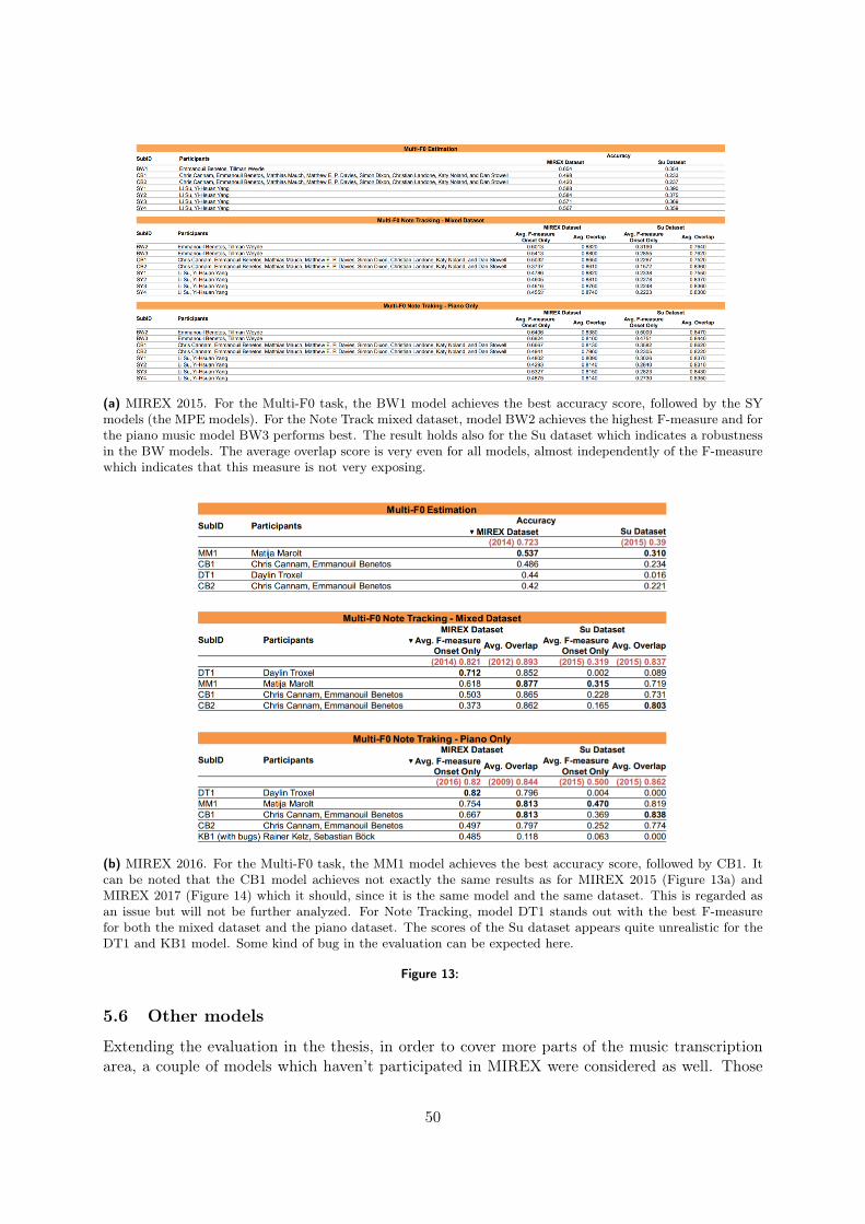
(a) MIREX 2015. For the Multi-F0 task, the BW1 model achieves the best accuracy score, followed by the SYmodels (the MPE models). For the Note Track mixed dataset, model BW2 achieves the highest F-measure and forthe piano music model BW3 performs best. The result holds also for the Su dataset which indicates a robustnessin the BW models. The average overlap score is very even for all models, almost independently of the F-measurewhich indicates that this measure is not very exposing.

(b) MIREX 2016. For the Multi-F0 task, the MM1 model achieves the best accuracy score, followed by CB1. Itcan be noted that the CB1 model achieves not exactly the same results as for MIREX 2015 (Figure 13a) andMIREX 2017 (Figure 14) which it should, since it is the same model and the same dataset. This is regarded asan issue but will not be further analyzed. For Note Tracking, model DT1 stands out with the best F-measurefor both the mixed dataset and the piano dataset. The scores of the Su dataset appears quite unrealistic for theDT1 and KB1 model. Some kind of bug in the evaluation can be expected here.

Figure 13:

5.6 Other models

Extending the evaluation in the thesis, in order to cover more parts of the music transcriptionarea, a couple of models which haven’t participated in MIREX were considered as well. Those

50

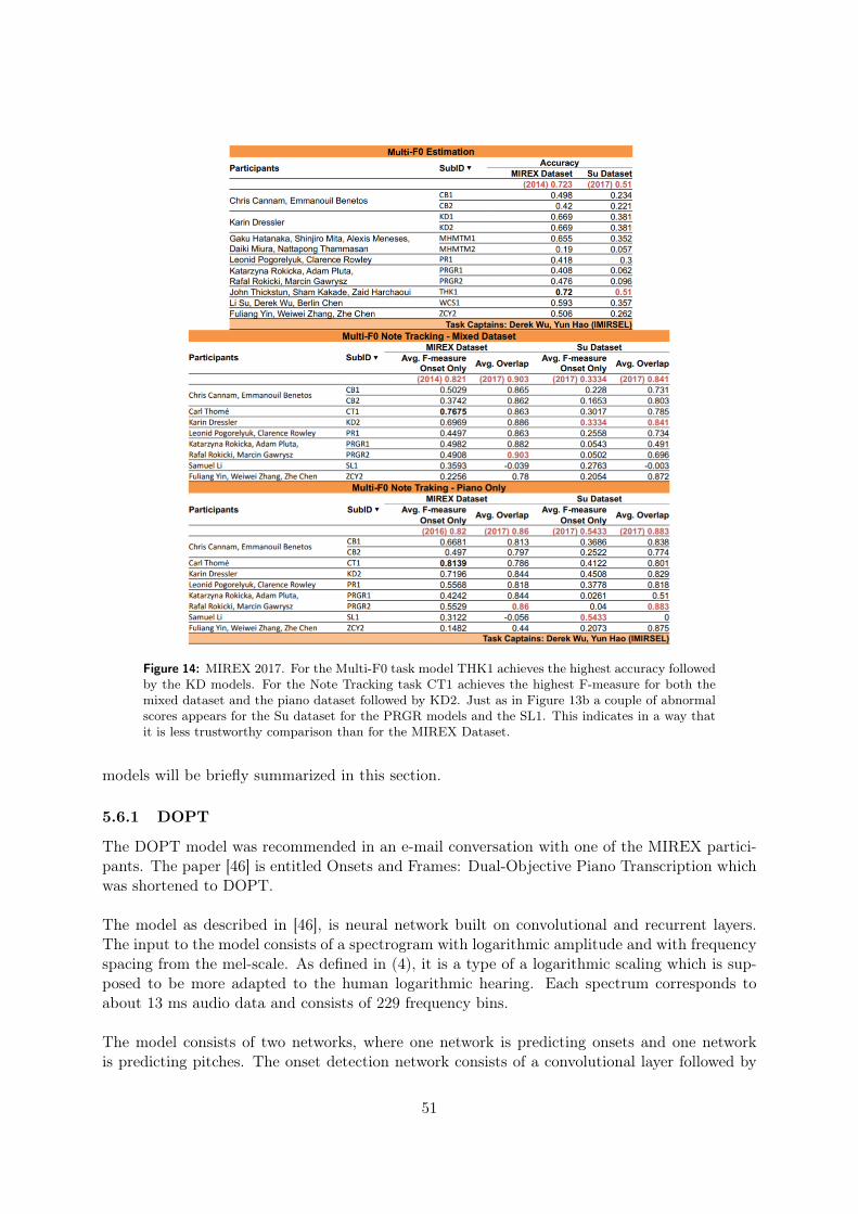
Figure 14: MIREX 2017. For the Multi-F0 task model THK1 achieves the highest accuracy followedby the KD models. For the Note Tracking task CT1 achieves the highest F-measure for both themixed dataset and the piano dataset followed by KD2. Just as in Figure 13b a couple of abnormalscores appears for the Su dataset for the PRGR models and the SL1. This indicates in a way thatit is less trustworthy comparison than for the MIREX Dataset.

models will be briefly summarized in this section.

5.6.1 DOPT

The DOPT model was recommended in an e-mail conversation with one of the MIREX partici-pants. The paper [46] is entitled Onsets and Frames: Dual-Objective Piano Transcription whichwas shortened to DOPT.

The model as described in [46], is neural network built on convolutional and recurrent layers.The input to the model consists of a spectrogram with logarithmic amplitude and with frequencyspacing from the mel-scale. As defined in (4), it is a type of a logarithmic scaling which is sup-posed to be more adapted to the human logarithmic hearing. Each spectrum corresponds toabout 13 ms audio data and consists of 229 frequency bins.

The model consists of two networks, where one network is predicting onsets and one networkis predicting pitches. The onset detection network consists of a convolutional layer followed by

51

a LSTM layer and finally a fully connected layer which outputs a vector of 88 neurons [46].Each neuron in the output layer corresponds to a probability that an onset has occurred forthat specific tone. The architecture for the pitch estimation network is similar as for the onsetdetection. A convolutional layer is followed by a fully connected layer, which together with theonset prediction output is fed into a LSTM layer. The final step is a fully connected layer whichoutputs a vector with 88 neurons, indicating the probability of an active pitch.

In addition, a velocity estimator is added. The velocity is used to capture the speed which a pianokey was depressed which is related to the loudness and articulation. As explained in [46], thisestimator is built with similar structure as the onset detector and pitch estimator, but doesn’taffect the note estimation more than making the resulting transcription sound more natural.

The DOPT model is created by a large group consisting of Curtis Hawthorne, Erich Elsen, JialinSong, Adam Roberts, Ian Simon, Colin Raffel, Jesse Engel, Sageev Oore and Douglas Eck atGoogle Brain Team, Mountain View, USA. The model is trained on the MAPS dataset [22] andis therefore supposed to only be applicable to piano data [46]. The code is written in Tensorflow.

5.6.2 PEBSI-Lite

PEBSI-Lite denotes Pitch Estimation using Block Sparsity, - Improved and Lighter.42. Themodel has not been participating in MIREX.

The model as described in [47] differs from all the other models in the sense that it is data-independent, i.e., that it doesn’t use any training data at all, except for 2 regularization param-eters that need to be manually set. Instead, it is built on the strong prior assumption that eachframe of data consists of a stationary sequence of harmonically related sinusoids, i.e.,

x(t) =

K∑k=1

Lk∑l=1

ak,leiωklt

where t = 1, ..., N is the time point, ωk is the frequency of the l’th harmonic in the k’th pitch andak,l is a complex-valued parameter denoting magnitude and phase. The fundamental frequenciesare estimated by estimating the ak,l-parameters for a grid of candidate fundamental frequencies.This is done in [47] by minimizing the convex optimization problem

C(Ψ) =1

2

N∑t=1

∣∣∣y(t)−P∑p=1

Lmax∑l=1

ap,leiωklt

∣∣∣2+λ1

P∑p=1

Lmax∑l=1

|ap,l|+λ2PLmax∑q=1

|aq+1e−ϕq+1−aqe−ϕq | (45)

where Ψ represent all parameters in the model, except for λ1 and λ2 which are regularizationparameters that are set manually or using cross-validation. The cost function consists of threeparts. The first is an error score which becomes as small as possible if the signal is perfectlymatched. The second part is a penalty on the amplitude parameters which push down ampli-tudes which only contribute marginally. The third part is built on the idea that the spectralenvelope is smooth. Thus, two amplitudes of adjacent overtones are penalized if the absolutedifference is large.

42Hence the model has nothing to do with any type of soft drink.

52

The model considers 10 ms audio data at each time. For each time sequence an ADMM optimizeris used on (45). This is made independently of the adjacent time sequences [47]. The model istypically not rounding of the fundamental frequency estimate to the closest tone, which mostpart of the other models does.

The model is created by Ted Kronvall, Filip Elvander, Stefan Ingi Adalbjornsson and AndreasJakobsson at Lund University. The regularization parameters were trained on Monte Carlosimulation of signals with different fundamental frequencies and different signal-to-noise ratios.The code was written in Matlab and it can be mentioned that it is very time consuming, due tothe need to solve an advanced optimization problem for every 10 ms data.

5.6.3 ESACF

ESACF denotes the Enhanced Summary Autocorrelation Function, and has not been participat-ing in MIREX.

ESACF is the oldest model considered in this thesis, as it was published in the year 2000 in [48].The model divides the signal into two channels, one being high pass filter for frequencies above1000 Hz, and a low pass filter for frequencies below 1000 Hz. The Fourier transform is then per-formed on the two filtered signals. The absolute value of the transforms is summed together andthe inverse Fourier transform is applied [48]. This yields the summary autocorrelation function(SACF). The next step in the model is to determine which of the resulting peaks correspond tofundamental frequencies. The number of active fundamental frequencies is manually fixed. Themodel finds the strongest peak which is most probable to correspond to a fundamental frequency.All frequencies which appear at multiples (up to a set parameter) of this frequency are extractedand then the highest of the remaining peaks are considered. This is repeated until the set numberof fundamental frequencies are found [48].

The ESACF model is written by Tero Tolonen and Matti Karjalainen at Helsinki University ofTechnology, Finland. The recommended parameter settings were found by testing on real data43.The code was written in Matlab and is very fast. In order to evaluate ESACF on the test dataset,the number of instrument sources were manually set individually for each test file. For the pianomusic files, that manually set number of tones was the maximum of the simultaneously playedtones.

5.6.4 Deep Complex model

This model differs in many ways from the above mentioned models. The model is presented ina paper [20] on complex-valued neural networks where the main focus is on the mathematicalframework of implementing operations on complex-valued numbers in neural networks. Thereare a couple of applications of complex-valued neural networks presented where automatic musictranscription is one of them. It can therefore be assumed that the authors haven’t put all theireffort in tweaking and optimizing the model.

In the paper, four different models are presented where the model called Deep Complex per-formed the best. Deep Complex is influenced by a deep neural network model originally created

43The data which was referred to in [48] could not be found, probably since the article has become a few yearsold.

53

for image recognition [49]. In the paper the model was compared to a real-valued deep neuralnetwork model with similar architecture. The result was that the complex-valued model out-performed the real-valued one. Until recently, complex-valued neural networks have been anunmentioned topic in the machine learning community. But recent research has shown thatcomplex-valued neural networks outperform the earlier real-valued state-of-the-art neural net-works in many fields, where one example is hand written digit classification [1]. This invites toinvestigate the potential of complex-valued neural networks in polyphonic music transcription aswell and compare it to the acknowledged models.

It is not unrealistic that a complex-valued neural network would outperform a real-valued coun-terpart. Transforming the music signal to any amplitude-frequency representation, by for exam-ple the Fourier transform, the transformation initially appears on comple-valued form consistingof both amplitude and phase. A complex-valued signal seems complicated for a human to in-terpret, and perhaps for this reason, the magnitude spectrum is considered in almost all musictranscription models44. But there is an information loss by applying the absolute value. Bykeeping the complex-valued representation, information might be gained. This gained informa-tion, which is much easier for a computer to deal with than for a human, could possibly improvethe estimates.

The Deep Complex model in [20] estimates active pitches at independent time segments. Theinput is the DFT from the FFT of a time segment of about 0.37 seconds, consisting of complex-valued data with 0.012 seconds overlap. According to the authors [20], the core of the DeepComplex model is its 6 convolutional networks in 1 dimension which convolve 3 − 6 adjacentcomplex values, as detailed in (34). A convolution is followed by a complex-valued batch nor-malization, a CReLU (35), as activation function and an average pooling. The dimensionalityis decreasing because of the convolution and the pooling but for each convolution the numberof filters is doubled, implying a high number of parameters45. The model ends with two fullyconnected layers where the last one uses a sigmoid function to get an output layer of size 84 (oneneuron for each possible note) with corresponding probabilities46 [20].

The model is trained using an optimizer called ADAM on the MusicNet dataset [23], which isresampled from 44100 Hz to 11000 Hz. The network is trained by dividing the data into batchesconsisting of 0.37 seconds segments from each of the 321 music files in the training set. In orderto cover the whole dataset, about 1000 batches are needed. A training section of 1000 batchesare called an epoch, and totally the model was trained on 200 epochs. The total training timewas about 12 hours47.

The model is claimed to be state-of-the-art [20]. This turned out to be incorrect since the onlycomparison that is made in the paper is with the real counterpart and an example model availablein [23]. In [50] the Deep Complex model is outperformed by a couple of models. The result ofthe Deep Complex model is only presented using the average precision metric which correspondsto the area under the precision-recall curve, see Figure 11. To make it comparable with the other

44All except PEBSI-Lite.45A similar structure will be shown for the extension of the Deep Complex model where the model architecture

is shown in Figure 15.46Note that a piano contains 88 notes but only 84 tones appeared in the training set. Thus the network would

not be able to train the weights for the last 4 output neurons and which thereby could be excluded.47On a PC with CUDA-programmable NVIDIA GPUs.

54

models, a binary threshold was trained, as described in Section 3.2.5.

5.7 Proposed models - Deep Complex model with LSTM and CQT/FFT

By analyzing the Deep Complex model, Section 5.6.4, a couple of remarkable features were foundwhich weresn’t clearly motivated from a music transcription perspective. The fact that the modelwas written by researchers who are more focused on machine learning than music automationmight explain this. In this thesis, a novel method is proposed, in which these features are changedto be more proper from a signal processing and music theoretical perspective. The features wereimplemented directly in the source code of the Deep Complex model, but the main part of thecode was left unchanged. The shortcomings of the Deep Complex model and the changes will bedescribed further. The parts which are not mentioned are also not changed.

First of all one may note that the resampling of the dataset is not done by a multiple of 2 since4410011000 ≈ 4.009. This makes it not obvious how the resampling was performed. In order to evaluatethe Deep Complex model fairly, the test data needed a similar resampling as for the data it wastrained with. The resampling was performed using the Python SciPy function signal.resamplewhich probably doesn’t differ markable from the resampling performed on the training data.Anyway, the same resampling ratio was kept for the proposed model to being able to train it onthe same dataset.

A second observation is that the input is the whole DFT from the Fourier transform of 4096complex data values. The Fourier transform is symmetric around zero for real-valued data whichmeans that the all the input values have a doublet. This is maybe not a very complicatedproblem for a neural network to learn, but the number of parameters can be reduced and thecalculation speed and the risk of overfitting can be reduced. To consider all 4096 Fourier valuesis therefore a bad choice. The Nyquist frequency at fs

2 = 110002 = 5500Hz is the highest possible

frequency the Fourier transform is able to identify, where fs is the sampling frequency. Theamount of data values which is reasonable to consider, could instead of all 4096 values be relatedto the Nyquist frequency, which in this case is 2048 data values. One may also note that thehighest note on a piano is C8 with fundamental frequency 4186.01 Hz, which is smaller than thesampling frequency. On the other hand, no overtones of C8 can be identified, which may not bea very big issue since such high pitches are rarely occurring48.

Considering the proposed models, the only difference between them is that one is built on theFourier transform (described in Section 3.1) and the other on the Constant-Q transform (Section3.1.3). The model based on the FFT has, for each 0.37s time sequence, 2048 input values cor-responding to a spectrum with equally spaced frequency steps from, but not including zero, upto the 5500Hz, i.e., the Nyquist frequency. The model based on the CQT has 504 input valuescorresponding to 84 pitches with 12 · 6 = 72 frequency bins in each octave. The lowest pitchwhich is possible to detect from the CQT is A0 at 27.50 Hz and the highest pitch is G#7 at3322.44 Hz. One could claim that the CQT should cover even higher frequencies since a pianogoes up to the tone C8. But the fact is that no such high pitches occurred in the training data,so the model would not be able to categorize those high tones correctly anyway.

Another observation about the Deep Complex model is that it has no recurrent layers. Since the48The first overtone f1 appears at 4186.01 · 2 = 8372.02 Hz.

55

model is originally built for image recognition [49], where the order of the images is randomized,recurrent layers would not be of any use49. But for music data, there is a string dependenceon previous and following data values, which almost all models in MIREX take into account.Therefore a recurrent LSTM layer may be added to the proposed models. This LSTM layer isplaced just before the final two fully connected layers. Where in the network the LSTM layershould be placed optimally was not analyzed.

For the recurrent layer to make any sense, the code of the training batches needed some correctionsince the Deep Complex model used one time segment from each music file in the training. Thecorrection meant that first a music file was randomized, then the start position in that music filewas randomized and the following 321 time segments were considered as one batch. By makingthis correction, the amount of training data was not changed but the number of music files usedin each epoch could be less since two music files can be randomized in the same epoch.

One final difference between the proposed models and the Deep Complex model is the numberof epochs performed. Because of the longer training time caused by the LSTM layer and theConstant-Q transform, the number of epochs for the proposed models was decreased to 100. Thetraining time for 100 epochs was about 15 hours and because of limited time, 200 epochs were notpossible to perform. This would of course give a fairer comparison to the Deep Complex modelsince more epochs would have improved the training. However, the first 100 epochs seemed togive an acceptable estimate.

The model architecture is similar for both models, but the different inputs change the dimen-sionality of the layers further in the network, due to different dimensionalities of the FFT andthe CQT. The complete architecture and the number of parameters is shown in Figure 15.

One aspect which would have been desirable to change is the loss the Deep Complex modelis trained to maximize the standard accuracy (44) instead of the MIREX accuracy (43). Thedifference is that under estimating models (which estimate too few pitches) can achieve goodscores using the standard accuracy measure, while the MIREX accuracy weights the estimatesmore reasonably. This change was however not applied to the proposed model50.

5.8 Summary and Trends about the models

There are some trends which can be seen in the models. To illustrate those, the models arecategorized in different methodical structures. This is presented in Table 3 where the methodsfor both signal processing, pitch estimation and potential feature detection are presented for thedifferent models.

For pitch estimation, the models have been categorized into probabilistic, parametric and neuralnetwork methods in Table 3. The probabilistic methods are those which are using probabilisticlatent component analysis. The parametric methods are using pitch estimation functions basedon parameters which either are set by training or manually. The parametric methods can alsobe rule-based algorithms, like iterative methods, which are dependent of parameters. NeuralNetwork methods are methods using some kind of machine learning (such as CNN or complex-valued neural networks). The feature detection column in Table 6 indicates whether there are

49They are randomized such that there is no relation to the previous or following images.50Also because of limited time.

56

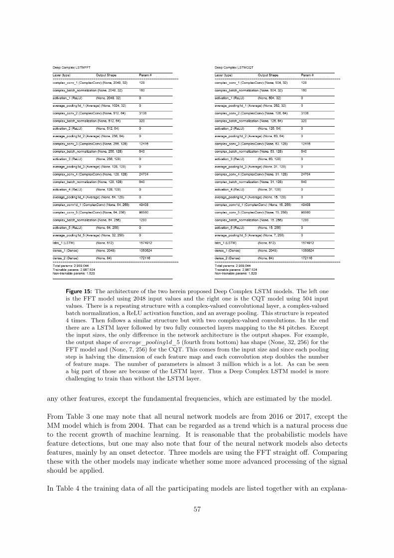
Figure 15: The architecture of the two herein proposed Deep Complex LSTM models. The left oneis the FFT model using 2048 input values and the right one is the CQT model using 504 inputvalues. There is a repeating structure with a complex-valued convolutional layer, a complex-valuedbatch normalization, a ReLU activation function, and an average pooling. This structure is repeated4 times. Then follows a similar structure but with two complex-valued convolutions. In the endthere are a LSTM layer followed by two fully connected layers mapping to the 84 pitches. Exceptthe input sizes, the only difference in the network architecture is the output shapes. For example,the output shape of average_pooling1d_5 (fourth from bottom) has shape (None, 32, 256) for theFFT model and (None, 7, 256) for the CQT. This comes from the input size and since each poolingstep is halving the dimension of each feature map and each convolution step doubles the numberof feature maps. The number of parameters is almost 3 million which is a lot. As can be seena big part of those are because of the LSTM layer. Thus a Deep Complex LSTM model is morechallenging to train than without the LSTM layer.

any other features, except the fundamental frequencies, which are estimated by the model.

From Table 3 one may note that all neural network models are from 2016 or 2017, except theMM model which is from 2004. That can be regarded as a trend which is a natural process dueto the recent growth of machine learning. It is reasonable that the probabilistic models havefeature detections, but one may also note that four of the neural network models also detectsfeatures, mainly by an onset detector. Three models are using the FFT straight off. Comparingthese with the other models may indicate whether some more advanced processing of the signalshould be applied.

In Table 4 the training data of all the participating models are listed together with an explana-

57

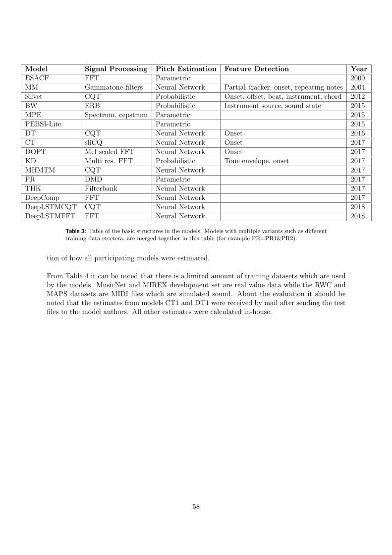
Model Signal Processing Pitch Estimation Feature Detection YearESACF FFT Parametric 2000MM Gammatone filters Neural Network Partial tracker, onset, repeating notes 2004Silvet CQT Probabilistic Onset, offset, beat, instrument, chord 2012BW ERB Probabilistic Instrument source, sound state 2015MPE Spectrum, cepstrum Parametric 2015PEBSI-Lite Parametric 2015DT CQT Neural Network Onset 2016CT sliCQ Neural Network Onset 2017DOPT Mel scaled FFT Neural Network Onset 2017KD Multi res. FFT Probabilistic Tone envelope, onset 2017MHMTM CQT Neural Network 2017PR DMD Parametric 2017THK Filterbank Neural Network 2017DeepComp FFT Neural Network 2017DeepLSTMCQT CQT Neural Network 2018DeepLSTMFFT FFT Neural Network 2018

Table 3: Table of the basic structures in the models. Models with multiple variants such as differenttraining data etcetera, are merged together in this table (for example PR=PR1&PR2).

tion of how all participating models were estimated.

From Table 4 it can be noted that there is a limited amount of training datasets which are usedby the models. MusicNet and MIREX development set are real value data while the RWC andMAPS datasets are MIDI files which are simulated sound. About the evaluation it should benoted that the estimates from models CT1 and DT1 were received by mail after sending the testfiles to the model authors. All other estimates were calculated in-house.

58

Model Training Data Evaluation Test filesBW1 RWC, orchestral MatlabBW2 RWC, orchestral MatlabBW3 MAPS, piano MatlabCT1 Unknown Achieved through mailDeepComp MusicNet, orchestral and piano Python, tensorflowDeepLSTMCQT MusicNet, orchestral and piano Python, tensorflowDeepLSTMFFT MusicNet, orchestral and piano Python, tensorflowDOPT MAPS, piano Python, tensorflowDT1 MIDI files, orchestral and piano Achieved through mailESACF Unknown MatlabKD1 MIREX development set, orchestral Executable fileMHMTM1 MIDI files, orchestral and piano Python, tensorflowMM1 MIDI files, piano Executable fileMPE1 Unknown MatlabMPE2 Unknown MatlabMPE3 Unknown MatlabMPE4 Unknown MatlabPEBSI-Lite None MatlabPR1 Unknown PythonPR2 Unknown PythonSilvetMF0 RWC, MAPS, Disklavier, orchestral and piano Executable fileSilvetMF0piano MAPS, Disklavier, piano Executable fileSilvetNT RWC, MAPS, Disklavier, orchestral and piano Executable fileTHK1 MusicNet, orchestral and piano Python, tensorflow

Table 4: The training data of each model together with a description of what program the test fileswere estimated with.

59

6 Tests

One of the most interesting questions this thesis is trying to answer is: Which model is state-of-the-art in music transcription right now? The reason why this answer is not readily found onthe Internet or even at MIREX, is because all music transcribing models are not evaluated atthe same time or at the same dataset51. This thesis gathers many of the last years recent modelsand compares them on the same dataset. One advantage with the tests in this thesis is that thedatasets afterwards will be available for the public and it will thus be possible to see exactly howeach model is performing for each tone in each song52.

In this section, the steps taken by going from estimates to a measure of the performance willbe explained. First by presenting the test dataset in 6.1, then explaining how an estimate ofNote Track form is converted to Multi-F0 form (and vice versa) in 6.2. Then, in Section 6.3, themethods are aligned to give outputs of the same format, and finally in Section 6.4 it is explainedhow the MIREX measures are calculated practically.

6.1 Dataset

There was a couple of things to consider while designing the test-dataset. The main idea wasto make it representative of the MIREX development dataset. The only comparable dataset isthe MIREX development dataset which consists of real instrument recordings in mono, sampledat 44, 1 kHz53. The MIREX development dataset consists of the fifth variation from L. vanBethoven Variations from String Quartet Op.18 N.5. The song is arranged for a woodwind quin-tet consisting of Bassoon, Clarinet, Flute, French Horn and Oboe. Each of the instruments areperformed and recorded by itself while the performer was listening to the other parts throughheadphones. Finally they are mixed together. The sheet music annotations are manually tran-scribed and are used as the ground truth for the model [18].

For the scope of this thesis, it was not possible to record a test dataset as realistically as theMIREX development dataset. A couple of real recordings with manually annotated sheet musicare available on the Internet, such as the MusicNet dataset and the Bach-10 dataset, summarizedin Table 2. But since these datasets are few, there is always a risk that one of the models hasused this dataset as its training set, which wouldn’t give fair evaluation. Instead, inspired of thepartly realistic MIDI-version of the real recording of the MIREX development dataset, MIDI filesfrom MuseScore [51] were used as the test set. Sheet music from famous composers arranged byprivate persons are being shared on the MuseScore homepage and can be downloaded for free.Only sheet music which was available for commercial use has been part of the test dataset. Byusing MuseScore, the sheet music could be transformed to wav-files with more realistic soundthan MIDI files. Also, the ground truth is completely known. Compared to sheet music annota-tions made manually by professionals, the MIDI file sheet music representation is actually moreprecise. For example, in the MusicNet dataset, there is an expected error rate of 4%. One could

51A model in MIREX is only compared with participating models of the same year and all other papers aboutmusic transcription which are not participating in MIREX are mainly evaluated on extracted parts of the trainingdataset.

52In Section 4.1 it was stated that the MIREX Dataset is needed to be kept secret.53The MIREX development dataset is available for research. A request form was filled in and accepted by the

MIREX organizers.

60

note that the play time of a wav-file and a MIDI file differs. By analyzing the music files, theplaytime of the MIDI file ends directly when the sound ends while the wav-file has some quiteseconds in the end. This indicates that the MIDI file is the true ground truth and therefore thisissue is disregarded.

The test dataset consists of 11 music files from MuseScore and 1 music file from the Bach-10dataset. The Bach-10 file was added to investigate how the models were performing on realrecorded music and not only simulated music. By a quick analysis of the evaluated models, noneof them seemed to have been trained on the Bach10 dataset which approves the use of it in thetestset54. The test dataset was chosen to be as wide and general as possible but still similar tothe MIREX test set. It needed to contain at least some ensemble music and some piano musicsince that is what the MIREX Dataset does. The test dataset is restricted to classical musicand hymns with no percussion or singing. There are woodwind compositions and piano musicsimilarly to the MIREX test set, but some other instruments are investigated here as well suchas the guitar, the violin and a string quartet. The pace of the tones varies from the differentmusic files as well as the number of tones played at the same time, so each of the music filesin the test set investigates how well each model manages a certain type of music for a certaininstrument. The test files were chosen to have a similar length of time and no replays55. Thetest dataset is stated in Table 5.

One thing to notice is that the wav-files from MuseScore were in stereo, while the wav-file fromBach-10 were mono. The majority of the models were able to handle multi-channel recordings,while some models (PEBSI-Lite, ESACF and THK1) could only cope with single-channel inputs.In those cases, the two channels were mixed together by summing the signals.

6.2 Translation between formats

The two different formats for Multi-F0 and Note Track, illustrated in Section 4.2 and 4.3, filldifferent purposes but are still similar. Each model either has an output similar to the Multi-F0format or the Note Track format56. To be able to evaluate each model for both the tasks atranslation between the different formats was needed to be implemented.

From Note Track to Multi-F0 is a straight-forward translation. In each row of the Note Trackoutput there is a tone represented by an onset, an offset, and a frequency. The translation al-gorithm does the following: For each tone, each of the time bins between the onset and offsetcreates a pair for that frequency. Finally, all frequencies which are paired with each time bin arestacked in a row, resulting in the active frequencies for that time bin such that each time bincorresponds to none, one, or multiple frequencies.

Going from Multi-F0 to Note Track is a bit complicated. In the Multi-F0 output there are timebins with corresponding active frequencies. The translation algorithm does the following: Start-

54Since the Bach10 dataset only consists of 10 music files, it would for example not be reasonable to use theBach10 to train a neural network. Therefore the risk that Bach10 would occur as training dataset for some of themodels is low.

55A similar time was needed such that they wouldn’t need a weighting when the results are added together. Noreplays should appear since two equal parts of a song would give a very similar estimation which would not addanything to the evaluation.

56except MPE which gave both output formats directly and the Deep Complex model (as well as the DeepComplex LSTMCQT and Deep Complex LSTMFFT) which gave another type of output.

61

Music piece name Composer Arranger Shortname

Instruments Numb.of in-stru-ments

Songlength

Songspeed andstyle

Nun bitten wir denheiligen Geist (fromBach10)

J.S. Bach - mix1 Violin, clar-inet, saxophone,bassoon

4 0:37 Hymn, longtones

"Graduale" from thRequiem in C MinorNo.2

L. Cheru-bini

Mike Maga-tagan

mix2 Flute, oboe, clar-inet, bassoon

4 01:13 Slow, longtones

Tochter Zion G. F.Händel

User:Oboeli95

mix3 Flute, oboe, Bb-clarinet, frenchhorn, bassoon

5 01:03 Medium,long &short tones

Prelude: "Helft mir,Gottes Güte preisen"

J.S. Bach Mike Maga-tagan

mix4 Flute, oboe, A-clarinet, bassoon

4 01:12 Fast, shorttones

Hark! The HeraldAngels sing

F.Mendels-sohn

User:dan.ricci.37

mix5 Violin × 2, viola,flute, Bb clarinet,bassoon, Bb trum-pet × 3, C tuba

10 0:39 Hymn, slow

B flat scale - User:Hersey1754

piano1 Piano 1 0:33 Monopho-nic, longtones

Lullaby J. Haydn Don Moss piano2 Piano 1 01:12 Slow, longtones,chords

Sonata No.2 4th

Movement Opus 35F. F.Chopin

User: Clas-sicMan

piano3 Piano 1 01:25 Fast, shorttones

Trepak (RussianDance) From theNutracker BalletSuite Op. 71A: II.C.

P. I.Tchaikov-sky

User:AlphonseGayloaSamson

piano4 Piano 1 01:08 Fast, shorttones,chords

Adantino Op.241No.20

F. Carulli User:Marieh

guitar1 Guitar 1 0:52 Medium,long &short tones

Divertimento in FK138 III. Presto

W. A.Mozart

User: AR-Boyes

violin1 Violin 1 0:22 Medium,long &short tones

Alla Rustica III. Al-legro

A. Vivaldi User:pribylova

strings1 Violin × 3, violin-cello

4 0:52 Monopho-nic, shorttones

Table 5: Summary of the test dataset. All music pieces are used as -wav format. The top dataset(short name mix1) is a real recording from Bach10 dataset [24]. The rest are simulated sound fromMuseScore files [51].

62

ing at the first time bin, the first frequency is considered as a part of the first tone. The onsetof this tone is the first time bin. In the following time bins, this frequency is searched for. Ifthe frequency is found, the tone is considered as still active and the next time bin is consideredand so on. If the frequency is not found, the previous time bin is considered as the offset of thetone. Then one goes back to the second frequency of the first time bin and repeat the process.This is repeated until for all frequencies of the first time bin. For the following time bin onesearches for frequencies which were not active in the previous time bin. For each new frequencythe procedure of finding an offset is done.

The described translation of Multi-F0 to Note Track does only work for a Multi-F0 representa-tion where frequencies has been truncated to the closest tone. For example, if a model estimatesa frequency of 225 Hz the closest tone is A3 with a pitch of 220 Hz (A#3 is the second closestwith tone with pitch 233.082 Hz). Most of the models do this truncation automatically, but somedon’t57. With the above algorithm, almost all tones appear only for one time bin for the modelswithout this automatic rounding. Since this is not a fair way of comparison, the translation con-siders all frequencies which are within ±3% from a tone to be rounded to the corresponding pitch.

6.3 Conversion to MIREX format

There are very strict rules in the MIREX format for evaluation. In order to evaluate the estimatesthey need to be given on a consistent fashion58. For most of the MIREX models, the output ofthe given source code was correctly, but some models needed minor modifications. This sectionwill describe which modifications were needed to evaluate the models. The modifications shouldnot affect the performance of the models, but to recreate the presented results, similar changesare needed.

Some methods yielded more accurate time or frequency estimates than a two decimal precision,which is the MIREX standard for both Multi-F0 and Note Track. In those cases, the values wererounded to two decimals59. Another case that was handled was when some models didn’t outputa text file. For the outputs in excel format, the estimates were just copied into a txt-file. Forthe models which gave a matrix or cell-array output in Matlab, the output was converted intoa text file. Two of the models gave MIDI files as output. Those cases were converted in Matlabwith [52] which transforms the MIDI file to a variant of Note Track format. The transformationincludes the onset and offset as well as the MIDI number, the velocity and instrument number.A MIDI number corresponds to a certain pitch and can be translated to a frequency as in [9] by

fn = 2n12 · 440Hz (46)

where n is the MIDI number and fn is the corresponding frequency. By extracting the onset,offset, and MIDI number, and transforming the MIDI number to frequency, the Note Track for-mat was obtained. This conversion was also used when transforming the MIDI files in the test

57It is common for music transcription models to automatically round to the closest tone since a piano rollrepresentation usually is what is wanted. Anyway, there are models like PEBSI-Lite and ESACF which justestimate active frequencies independently of what frequencies can be expected from musical instruments.

58One format for Multi-F0 and one for Note Track as described in Section 4.2 and 4.3.59In MIREX it is accepted to submit estimates with more than 2 decimals. But when various formatting files

were written for this thesis, this was not considered. In order to not rewrite all the formatting files the roundingsolution was the most efficient.

63

dataset to the ground truth Note Track and Multi-F0 format.

The most demanding conversion was for the Deep Complex models60. The output was a n× 84matrix with probabilities for each of the 84 possible tones in each of the n time bins61. Todetermine which tones to be considered as active, a binary threshold as in Section 3.2.5 wasimplemented. Probabilities which appeared higher than the threshold were considered as ac-tive tones. The threshold was trained for each of the Deep Complex models by maximizing theMIREX accuracy (43), for the Music net test set using Matlab to minimize the negative accuracy.Using the threshold the active tones were extracted for each time bin and then transformed topitches62. The output finally achieved the Multi-F0 format.

Presenting the output of the Deep Complex model as probabilities is not a bad idea, since theaverage accuracy could be calculated from the precision recall-curve using the probabilities, Sec-tion 3.2.5. However, a presentation with a Multi-F0 or Note Track format is more intuitive andcloser to a usable product. That is probably the reason why a probability based output is notconsidered in MIREX.

As summary of the output formats of the different models, consider Table 6. To get all modelsof both Multi-F0 and Note Track format, the above presented conversions and the presentedtranslations in Section 6.2, were applied for the models which didn’t output both formats directly.

6.4 MIREX Evaluation

The output as Multi-F0 or Note Track format from the models are evaluated with differentmeasures, as described in Section 4.2 and 4.3. The measures which are considered in this thesisare, for Multi-F0, the 3 measures precision, recall and accuracy and similarly for Note Track,the 6 measures precision, recall and F-measure both with and without the offset criterion63. Tocalculate these measures, the Python library mir_eval version 0.4 was used from [29].

One advantage with using an existing evaluation library is that the results can easily be recre-ated. Another is that this library is very user friendly. The library is also transparent such thatit is robust to a shift between the estimation and the ground truth64. The disadvantage is thatthe evaluation is not identical to how MIREX is evaluating the different measures. This wouldhave been possible to achieve by proposing a new evaluation program. Some disadvantages arethat bugs can be hard to identify and if any changes are made in the library by its authors, theexact same results might not be possible to recreate65.

For evaluating the Multi-F0 the multipitch function [29] was used, which doesn’t differ particu-larly from the MIREX evaluation. The number of matching frequencies for each time bin betweenthe estimated Multi-F0 output and the ground truth on Multi-F0 form is calculated and fromthis, precision, recall and accuracy are calculated. If the matching is not ideal (accuracy 6= 1 in

60Deep Complex model, Deep Complex LSTMCQT and Deep Complex FFT.61The size was motivated in Section 5.6.4.62Recall that this is a n × 84 matrix where 1 indicates an active tone and 0 indicates an inactive tone. The

transformation from this matrix was done with a similar formula as for the MIDI number, (46).63Accuracy is referred as the MIREX accuracy, (43).64To avoid implementing this, saved the author many hours of work.65Some bugs were identified in the library due to weird test results. These bugs were possible to work around

by adjusting the data, but there might be smaller bugs in the library which weren’t found in this thesis.

64

Model Multi-F0 Format Note Track Format MIDI Format OtherBW1 xBW2 xBW3 xCT1 Detailed version

of Note TrackDeepComp Note ProbabilitiesDeepLSTMCQT Note ProbabilitiesDeepLSTMFFT Note ProbabilitiesDOPT xDT1 Note Track in Ex-

cel (3 decimals)ESACF Multi-F0 in Mat-

lab MatrixKD1 Note Track (6

decimals)MHMTM1 xMM1 xMPE1 x xMPE2 x xMPE3 x xMPE4 x xPEBSI-Lite Multi-F0 in Mat-

lab cell arrayPR1 xPR2 xSilvetMF0 xSilvetMF0piano xSilvetNT xTHK1 x

Table 6: "x" corresponds to the format of the model output. There are 4 models (MPE 1-4) whichoutput was not modified at all by the author. The other models were modified by a translation orconversion (or both).

65

(43)), the time bins of the estimate are resampled using nearest neighbour to achieve the bestpossible match of the estimate and ground truth. The frequencies of the estimate, correspondingto the time bins which appear outside the ground truth time bins after the resampling, don’tcontribute to the evaluation.

The evaluation of the Note Track is done by the transcription function [29] which is not asintuitive as for Multi-F0. The evaluation method counts how many of the estimated notes whichmatch the ground truth and how many which don’t. Based on these counts, the precision, recall,and F-measure are calculated. The criteria for a tone to be considered correct is (from Section4.3) that the onset is within ±50 ms, the frequency is within ±3% (a quartertone), and the offsetneeds to be within a 20% range, from the ground truths66. In this evaluation library, the offsetcriteria is slightly changed to be within 20% range from the ground truths’ offset or within ±50ms, whichever is larger67. Another note to make is that the evaluation method uses a bipartitegraph matching to find the optimal paring68.

The library is used both to evaluate the Note Track estimation with the offset and without theoffset criterion69. Compared to the MIREX evaluation method, this library is expected to givea higher score of the precision, recall and accuracy by about 1% − 2%70. This is not perfectlydesirable but since the difference is not considerably large it will not make that big difference.Also, all models will be evaluated with the same conditions, thus this will not affect the result.

A couple of smaller modifications are necessary to address, in order for the functions in thelibrary to compile. Some of the estimates got negative time bins, which could for example looklike

−0.02−0.01 220 .000 .00 220 .00. . .

which were not accepted. In these cases, the time bins < 0 were deleted. Another error occurredfor some of the Note Track estimates when a tone only appeared for a single time bin (onset andoffset appeared on the same time bin). Since it is technically impossible for a tone to hold onfor less than 0.01 seconds, those tones were deleted from the Note Track estimates to make thelibrary function compile.

66The "within" is clarified as −50 ms ≥ f0 ≤ 50 ms for example. I.e., all "within" measures includes the limit.67There is contradictory information about the criterion for the offset on the MIREX homepage [18], that’s

why this confusion may have appeared.68This is done since each estimated tone can only be paired with one true tone.69The score without the offset criterion is always higher (≥) than the score with the offset criterion70According to tests by the authors of the library [29].

66

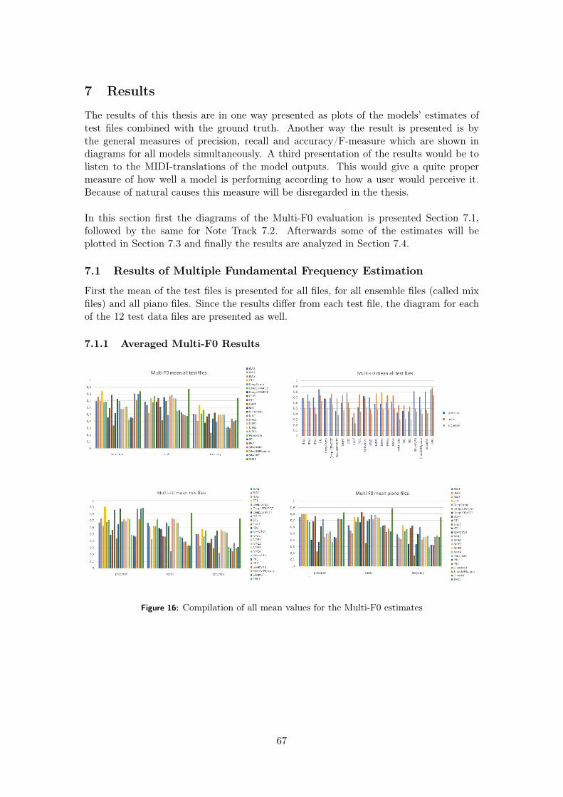
7 Results

The results of this thesis are in one way presented as plots of the models’ estimates oftest files combined with the ground truth. Another way the result is presented is bythe general measures of precision, recall and accuracy/F-measure which are shown indiagrams for all models simultaneously. A third presentation of the results would be tolisten to the MIDI-translations of the model outputs. This would give a quite propermeasure of how well a model is performing according to how a user would perceive it.Because of natural causes this measure will be disregarded in the thesis.

In this section first the diagrams of the Multi-F0 evaluation is presented Section 7.1,followed by the same for Note Track 7.2. Afterwards some of the estimates will beplotted in Section 7.3 and finally the results are analyzed in Section 7.4.

7.1 Results of Multiple Fundamental Frequency Estimation

First the mean of the test files is presented for all files, for all ensemble files (called mixfiles) and all piano files. Since the results differ from each test file, the diagram for eachof the 12 test data files are presented as well.

7.1.1 Averaged Multi-F0 Results

Figure 16: Compilation of all mean values for the Multi-F0 estimates

67

7.1.2 Single Test Files Multi-F0 Results

Figure 17: Compilation of all Multi-F0 estimates on the ensemble files in the testdataset

Figure 18: Compilation of all Multi-F0 estimates on the piano files in the test dataset

68

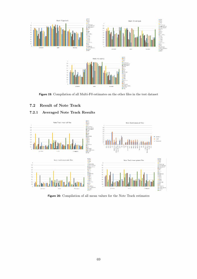
Figure 19: Compilation of all Multi-F0 estimates on the other files in the test dataset

7.2 Result of Note Track

7.2.1 Averaged Note Track Results

Figure 20: Compilation of all mean values for the Note Track estimates

69

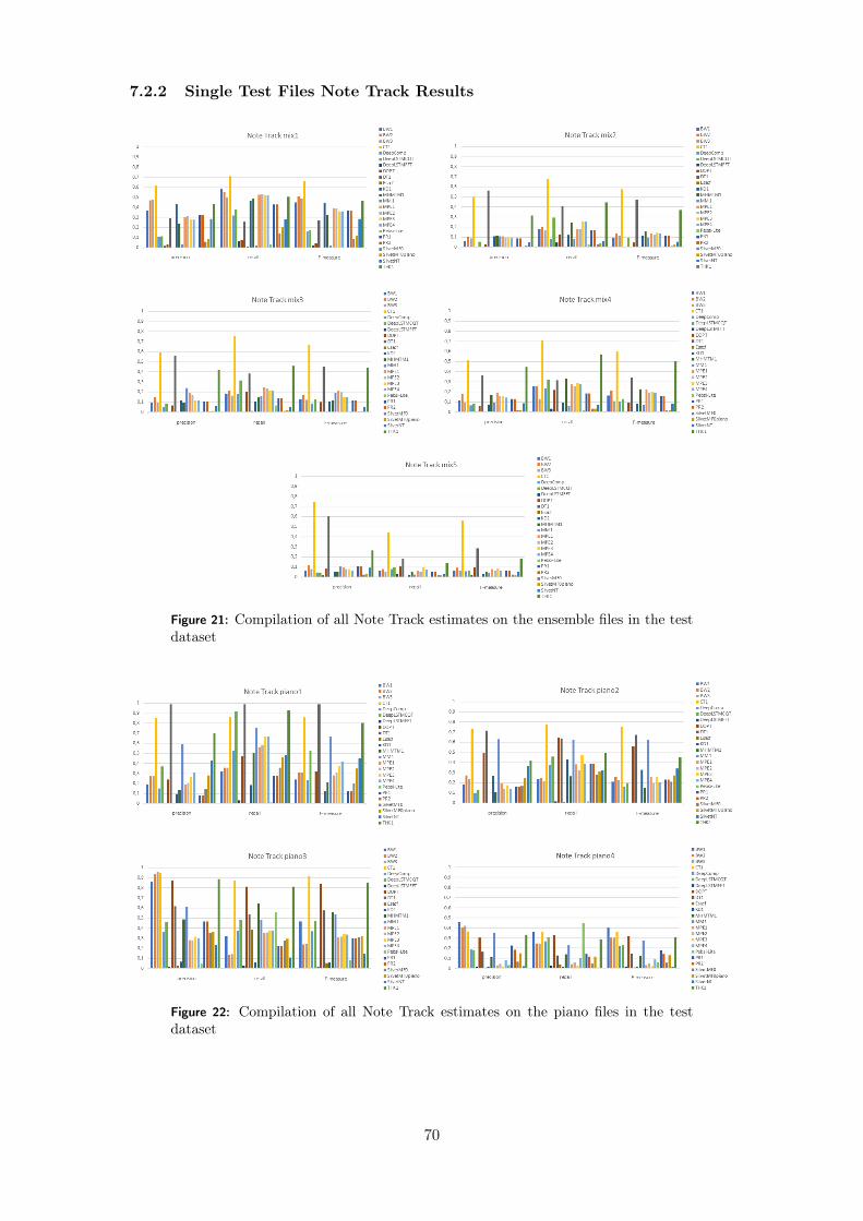
7.2.2 Single Test Files Note Track Results

Figure 21: Compilation of all Note Track estimates on the ensemble files in the testdataset

Figure 22: Compilation of all Note Track estimates on the piano files in the testdataset

70

Figure 23: Compilation of all Note Track estimates on the other files in the testdataset

7.2.3 Note Track Without Offset Criterion

Figure 24: Compilation of all mean values for the Note Track without offset criterionestimates

71

7.3 Plots of estimates

The results presented in the figures in Section 7.1 and 7.2 are the main results of this thesis. Inorder to analyze the results and to find out the types of errors behind the performance metrics, asubset of results will be visualized in time-fundamental frequency plots. Visual inspection makesit possible to connect the different methodical structures in the models to their performance.Because of the large number of test files (12) and models (24), the results of all test files of allmodels (12 · 24 = 288) cannot be presented. Instead, a selection of these, where specific resultsare of more interest, will be included.

In this section a lot of plots will be presented. Each plot will include the ground truth of thewhole part of one test file (a whole song) and the estimate from a single model. The plots are ofthe Multi-F0 representation, where the estimated pitches for each time bin of 10 ms (100 samplesper second) are visualized. For each estimation, the plot will indicate a true positive pitch (acorrectly estimated pitch within a quartertone from the ground truth) by a large black dot. Afalse positive pitch (incorrectly estimated pitch) will be indicated by a pink cross. Since a tone ingeneral lasts longer than 10 ms, the dots will be stacked such that they will look like a line. Theground truth is a thin colored dot where the color indicates which instrument that was playingthat pitch71.

The representation will give a fairer indication of the Multi-F0 score than the Note Track score.To include some indications of the Note Track score, each pitch which is incorrectly estimated butwithin the time interval of ±50 ms of a ground truth pitch, will be indicated by a yellow square.Those incorrect frequencies may in the Note Track representation, be included in a correctlyestimated tone. A final indicator is if an estimated pitch appears between a quartertone anda semitone from a ground truth pitch. Those pitches will be marked by an orange star andindicates that the signal processing has failed. Thus, the incorrect tones marked by a pink crosswill mainly indicate where the pitch estimation has failed, that is a false positive. Another typeof error is when a ground truth tone is not estimated, indicated by a colored line which has noblack line behind, i.e., a false negative. The plots which follow are analyzed further in Section7.4.

71Note that the models only estimate pitches and not which instrument playing each pitch. However, the groundtruth information about the instrument can be used for analyzing the result.

72

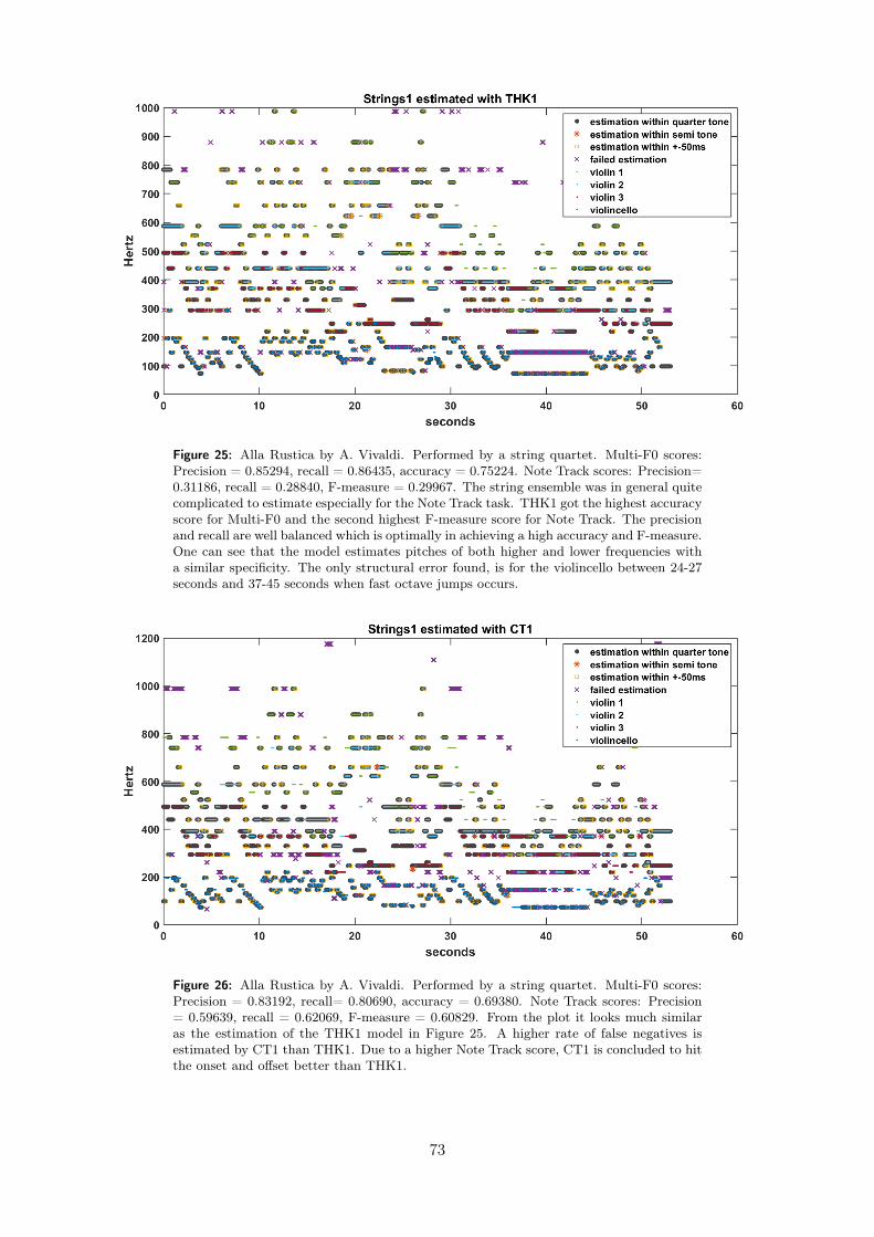
Figure 25: Alla Rustica by A. Vivaldi. Performed by a string quartet. Multi-F0 scores:Precision = 0.85294, recall = 0.86435, accuracy = 0.75224. Note Track scores: Precision=0.31186, recall = 0.28840, F-measure = 0.29967. The string ensemble was in general quitecomplicated to estimate especially for the Note Track task. THK1 got the highest accuracyscore for Multi-F0 and the second highest F-measure score for Note Track. The precisionand recall are well balanced which is optimally in achieving a high accuracy and F-measure.One can see that the model estimates pitches of both higher and lower frequencies witha similar specificity. The only structural error found, is for the violincello between 24-27seconds and 37-45 seconds when fast octave jumps occurs.

Figure 26: Alla Rustica by A. Vivaldi. Performed by a string quartet. Multi-F0 scores:Precision = 0.83192, recall= 0.80690, accuracy = 0.69380. Note Track scores: Precision= 0.59639, recall = 0.62069, F-measure = 0.60829. From the plot it looks much similaras the estimation of the THK1 model in Figure 25. A higher rate of false negatives isestimated by CT1 than THK1. Due to a higher Note Track score, CT1 is concluded to hitthe onset and offset better than THK1.

73

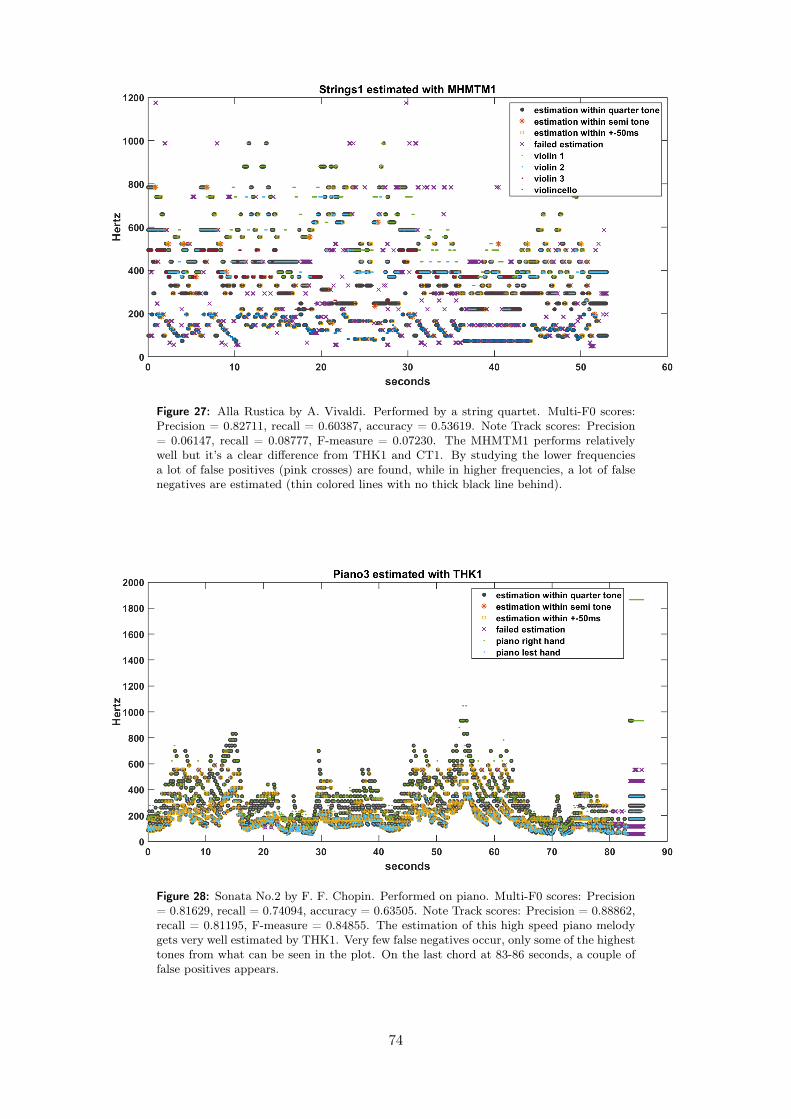
Figure 27: Alla Rustica by A. Vivaldi. Performed by a string quartet. Multi-F0 scores:Precision = 0.82711, recall = 0.60387, accuracy = 0.53619. Note Track scores: Precision= 0.06147, recall = 0.08777, F-measure = 0.07230. The MHMTM1 performs relativelywell but it’s a clear difference from THK1 and CT1. By studying the lower frequenciesa lot of false positives (pink crosses) are found, while in higher frequencies, a lot of falsenegatives are estimated (thin colored lines with no thick black line behind).

Figure 28: Sonata No.2 by F. F. Chopin. Performed on piano. Multi-F0 scores: Precision= 0.81629, recall = 0.74094, accuracy = 0.63505. Note Track scores: Precision = 0.88862,recall = 0.81195, F-measure = 0.84855. The estimation of this high speed piano melodygets very well estimated by THK1. Very few false negatives occur, only some of the highesttones from what can be seen in the plot. On the last chord at 83-86 seconds, a couple offalse positives appears.

74

Figure 29: Sonata No.2 by F. F. Chopin. Performed on piano. Multi-F0 scores: Precision= 0.89047, recall = 0.79800, accuracy = 0.72667. Note Track scores: Precision = 0.95129,recall = 0.87500, F-measure = 0.91155. Also a well performed estimation by CT1. Alot of yellow squares, similar as Figure 28, indicating a minor time resolution error whichdoesn’t affect the Note Track score. Also similarly, the final chord consists of a couple oferrors.

Figure 30: Lullaby by J. Haydn. Performed on piano. Multi-F0 scores: Precision =0.78113, recall = 0.95356, accuracy = 0.75251. Note Track scores: Precision = 0.49533,recall = 0.64898, F-measure = 0.56184. A well performed estimation with a very highrecall in the Multi-F0 task. A couple of tones seem to be estimated as false positivesaround 80 Hz, this is odd since they don’t seem to appear at the half frequency of anyground truth, 1

2fk. Most probable, they are related to 1

3fk which would be quite easy to

prevent by tweaking the model. Other failed estimates seem to appear after the offset ofthe true tone.

75

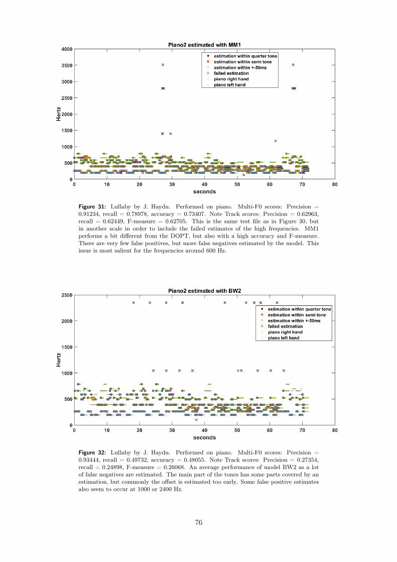
Figure 31: Lullaby by J. Haydn. Performed on piano. Multi-F0 scores: Precision =0.91234, recall = 0.78978, accuracy = 0.73407. Note Track scores: Precision = 0.62963,recall = 0.62449, F-measure = 0.62705. This is the same test file as in Figure 30, butin another scale in order to include the failed estimates of the high frequencies. MM1performs a bit different from the DOPT, but also with a high accuracy and F-measure.There are very few false positives, but more false negatives estimated by the model. Thisissue is most salient for the frequencies around 600 Hz.

Figure 32: Lullaby by J. Haydn. Performed on piano. Multi-F0 scores: Precision =0.93444, recall = 0.49732, accuracy = 0.48055. Note Track scores: Precision = 0.27354,recall = 0.24898, F-measure = 0.26068. An average performance of model BW2 as a lotof false negatives are estimated. The main part of the tones has some parts covered by anestimation, but commonly the offset is estimated too early. Some false positive estimatesalso seem to occur at 1000 or 2400 Hz.

76

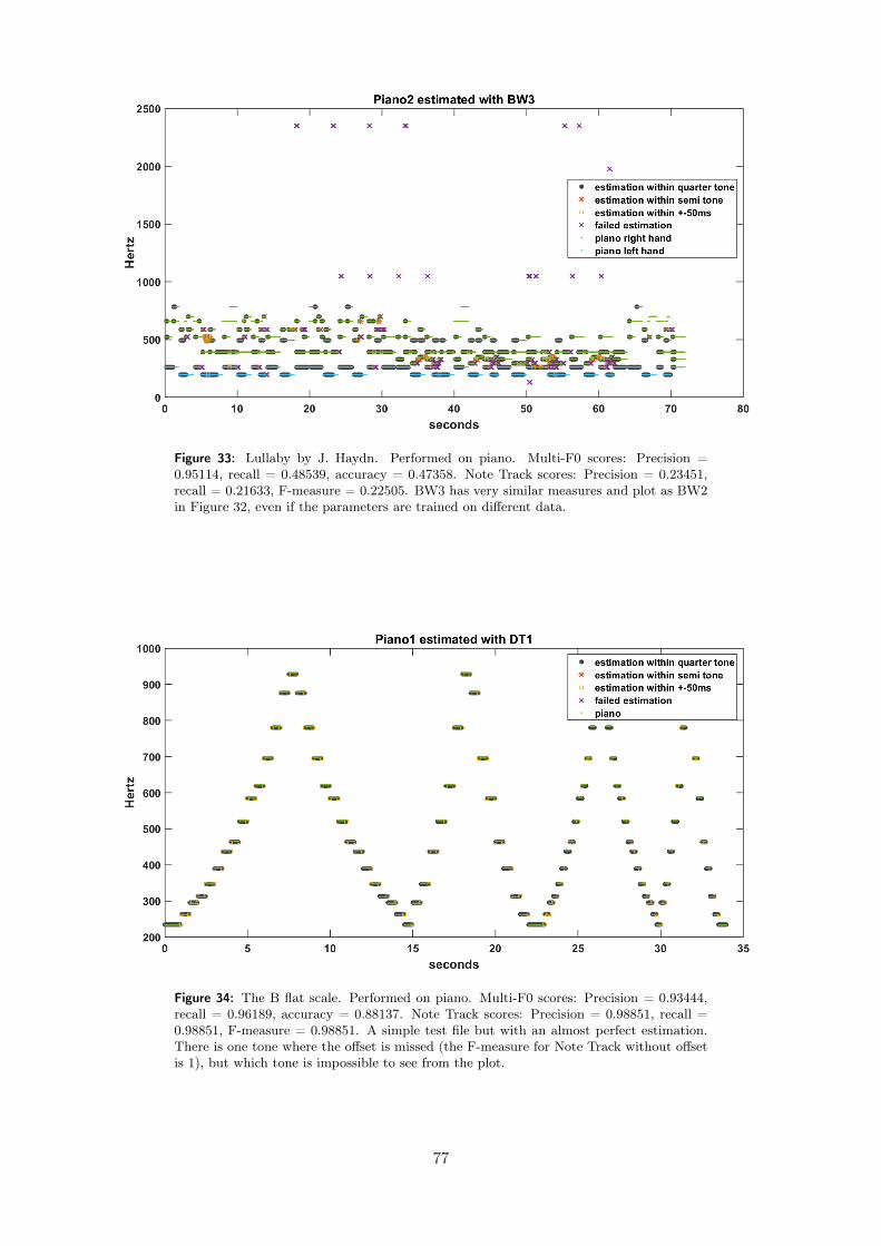
Figure 33: Lullaby by J. Haydn. Performed on piano. Multi-F0 scores: Precision =0.95114, recall = 0.48539, accuracy = 0.47358. Note Track scores: Precision = 0.23451,recall = 0.21633, F-measure = 0.22505. BW3 has very similar measures and plot as BW2in Figure 32, even if the parameters are trained on different data.

Figure 34: The B flat scale. Performed on piano. Multi-F0 scores: Precision = 0.93444,recall = 0.96189, accuracy = 0.88137. Note Track scores: Precision = 0.98851, recall =0.98851, F-measure = 0.98851. A simple test file but with an almost perfect estimation.There is one tone where the offset is missed (the F-measure for Note Track without offsetis 1), but which tone is impossible to see from the plot.

77

Figure 35: Trepak by P. I. Tchaikovsky. Performed on piano. Multi-F0 scores: Precision= 0.58251, recall = 0.75757, accuracy = 0.49098. Note Track scores: Precision = 0.16349,recall = 0.12794, F-measure = 0.14355. A well performed estimation by DT1 on thiscomplicated test file with many short tones and chords. Few false negatives are estimated,resulting in a high recall. The performance in the high frequencies appears similar as in thelower frequencies. The false positive estimates do mainly appear between two repeatingtones. This is seen at 150 Hz from 3-26 and 48-66 seconds where two tones are repeatingat two different frequencies. At 150 Hz again but from 26-45 seconds the tones are notrepeating and the failed estimates are much fewer.

Figure 36: Trepak by P. I. Tchaikovsky. Performed on piano. Multi-F0 scores: Precision= 0.59000, recall = 0.47999, accuracy = 0.35993. Note Track scores: Precision = 0.14879,recall = 0.11538, F-measure = 0.12997. Compared to Figure 35, the same type of errorwith repeating tones occur, but only in the lower register. In general there are many falsenegatives estimated resulting in low recall. But there are many true positives, that is thetones which are estimated are in general correct, especially for the frequencies > 200 Hz,resulting in a relatively good precision.

78

Figure 37: The Divertimento by W. A. Mozart. Performed on violin. Multi-F0 scores:Precision = 0.40795, recall = 0.98256, accuracy = 0.40502. Note Track scores: Precision= 0.05983, recall = 0.10687, F-measure = 0.07671. DOPT does as in Figure 30, estimatefew false negatives and receives a high recall score. Differently from the piano2 estimation,the failed estimates appear in the higher frequency region and can commonly be mappedas the first overtone of a ground truth fundamental frequency.

Figure 38: Hark! The Herald Angels sing by F. Mendelssohn. Performed on violin. Multi-F0 scores: Precision = 0.97401, recall = 0.53655, accuracy = 0.52898. Note Track scores:Precision = 0.26357, recall = 0.14011, F-measure = 0.18296. There are lots of tones tokeep track of in this test file, but the THK1 estimation performs very well. The onlytones which seem problematic is the clarinet at 700-900 Hz where many false negatives areestimated, that means quite few ground truth tones are estimated.

79

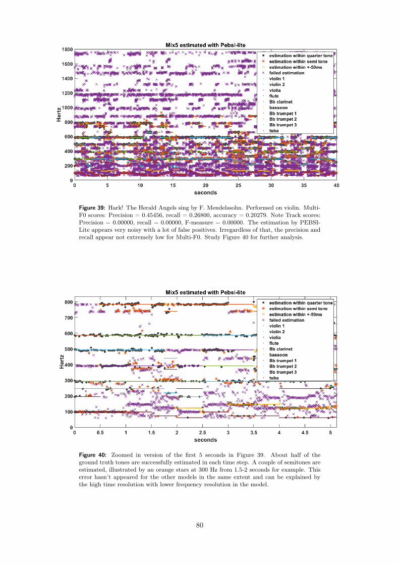
Figure 39: Hark! The Herald Angels sing by F. Mendelssohn. Performed on violin. Multi-F0 scores: Precision = 0.45456, recall = 0.26800, accuracy = 0.20279. Note Track scores:Precision = 0.00000, recall = 0.00000, F-measure = 0.00000. The estimation by PEBSI-Lite appears very noisy with a lot of false positives. Irregardless of that, the precision andrecall appear not extremely low for Multi-F0. Study Figure 40 for further analysis.

Figure 40: Zoomed in version of the first 5 seconds in Figure 39. About half of theground truth tones are successfully estimated in each time step. A couple of semitones areestimated, illustrated by an orange stars at 300 Hz from 1.5-2 seconds for example. Thiserror hasn’t appeared for the other models in the same extent and can be explained bythe high time resolution with lower frequency resolution in the model.

80

Figure 41: Nun bitten wir den heiligen Geist by J.S. Bach. Performed on violin, clarinet,saxophone and bassoon. Multi-F0 scores: Precision = 0.75322, recall = 0.85980, accu-racy = 0.67083. Note Track scores: Precision = 0.43548, recall = 0.46154, F-measure =0.44813. A good estimation of KD1. The balance between precision and recall is quitegood, especially for the Note Track task, resulting in a high accuracy and F-measure. Itis noticeable how the failed estimates seem to be perfectly spread over the frequency (andtime) axis. Errors can be identified, but no structural errors. Similarities has only beenidentified for neural network models with a very low error rate.

Figure 42: Tochter Zion by G. F. Händel. Performed on flute, oboe, Bb-clarinet, frenchhorn, bassoon. Multi-F0 scores: Precision = 0.60421, recall = 0.73074, accuracy = 0.49418.Note Track scores: Precision = 0.11211, recall = 0.10482, F-measure = 0.10834. Comparedto Figure 41, there are lots of structural errors such as the flute is estimated as falsenegatives, that is the true tones of the flute is not estimated. Also the tones of the oboeare estimated to be much longer than the ground truth. The french horn and the clarinetin the middle frequency register seem to be the only instruments which are well estimated.

81

Figure 43: "Graduale" from th Requiem by L. Cherubini. Performed on flute, oboe,clarinet, bassoon. Multi-F0 scores: Precision = 0.30622, recall = 0.52641, accuracy =0.24008. Note Track scores: Precision = 0.00493, recall = 0.08333, F-measure = 0.00930.A quite bad estimation by the Deep Complex model with lots of false positives and lots offalse negatives. It is a bit noisy to see, but the bassoon is in a large extent missed.

Figure 44: "Graduale" from th Requiem by L. Cherubini. Performed on flute, oboe,clarinet, bassoon. Multi-F0 scores: Precision = 0.67075, recall = 0.80831, accuracy =0.57870. Note Track scores: Precision = 0.05652, recall = 0.29333, F-measure = 0.09478.Compared to the 43, there are much less false positives. The failed estimates which occurscan often be mapped as the first overtone of the true fundamental frequencies, for exampleat 300 Hz for 30-75 seconds, the ground truth bassoon has similar frequency movementson half the frequencies. Similarly at 800 Hz, which has similar frequency movements asthe oboe at 400 Hz.

82

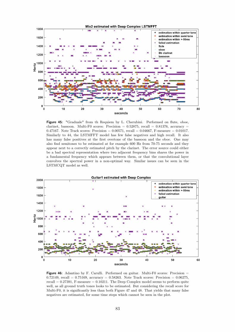
Figure 45: "Graduale" from th Requiem by L. Cherubini. Performed on flute, oboe,clarinet, bassoon. Multi-F0 scores: Precision = 0.52875, recall = 0.81376, accuracy =0.47167. Note Track scores: Precision = 0.00571, recall = 0.04667, F-measure = 0.01017.Similarly to 44, the LSTMFFT model has few false negatives and high recall. It alsohas many false positives at the first overtone of the bassoon and the oboe. One mayalso find semitones to be estimated at for example 600 Hz from 70-75 seconds and theyappear next to a correctly estimated pitch by the clarinet. The error source could eitherbe a bad spectral representation where two adjacent frequency bins shares the power ina fundamental frequency which appears between them, or that the convolutional layerconvolves the spectral power in a non-optimal way. Similar issues can be seen in theLSTMCQT model as well.

Figure 46: Adantino by F. Carulli. Performed on guitar. Multi-F0 scores: Precision =0.72149, recall = 0.75169, accuracy = 0.58263. Note Track scores: Precision = 0.06275,recall = 0.27391, F-measure = 0.10211. The Deep Complex model seems to perform quitewell, as all ground truth tones looks to be estimated. But considering the recall score forMulti-F0, it is significantly less than both Figure 47 and 48. That yields that many falsenegatives are estimated, for some time steps which cannot be seen in the plot.

83

Figure 47: Adantino by F. Carulli. Performed on guitar. Multi-F0 scores: Precision =0.67649, recall = 0.87181, accuracy = 0.61529. Note Track scores: Precision = 0.09581,recall = 0.37826, F-measure = 0.15290. The LSTMCQT performs slightly better than theDeep Complex model does. The same failed estimates appear at around 1000 Hz but alsosome more in connection to a ground truth tone where the onset or offset is missed.

Figure 48: Adantino by F. Carulli. Performed on guitar. Multi-F0 scores: Precision =0.45502, recall = 0.86302, accuracy = 0.42437. Note Track scores: Precision = 0.00232,recall = 0.01739, F-measure = 0.00410. The similar structures as could be seen in theFigure 46 and 47. Similar recall as the LSTMCQT model but lower precision, resulting inthe lowest accuracy of the Deep Complex models.

84

7.4 Analysis of Results

First, the average scores for the Multi-F0 and Note Track tasks will be considered for analysis,and the best performing models will be discussed. Thereafter, some interesting models or specifictest files will be considered.

The model THK1 can be concluded to perform significantly better than all the other models inthe Multi-F0 task, since it achieves the highest averaged accuracy scores in Figure 1672. Themodel CT1 clearly has the 2nd best accuracy, followed by the herein proposed model Deep Com-plex LSTMCQT. The significance for the THK1 model is clear both for the ensemble test filesand the piano test files. Considering each individual test file in Section 7.2.2, one may note thatthe models THK1 and CT1 are very robust and achieves high accuracy scores for all types of files,while for example the models MM1 and DOPT performs better on piano music than ensemblemusic. THK1 has more equal scores of precision and recall than the rest of the models, whileCT1 has a higher precision than recall for the Multi-F0 task.

Furthermore, considering the Note Track task, average scores are presented in Figure 20. CT1performs significantly better than the other models and achieves the highest F-measure for boththe ensemble test files and the piano test files with a margin. The models THK1 and DT1perform significantly better than the fourth best model. Again the models DOPT and MM1perform well on the piano test files but worse on the rest. The proposed model performs rela-tively bad on the Note Track task compared to the Multi-F0 task. The CT1 model is found tohave a more equal score of precision and recall which was not the case for the Multi-F0 task.Considering Note Track with no offset criterion in Figure 24, CT1 might be one of the modelswhich F-measure increases the least, but it is still the best model considering all test files. Forthe averaged piano test files, the models DOPT and MM1 performs better and achieves shared2nd best accuracy with DT1.

Overall it can be said that the THK1 and CT1 are the best performing models in the evaluations.The models’ estimates of the test file strings1 are plotted in Figure 25 and 26. Both models per-form very well on this test file and receives the two highest accuracy scores and F-measure scoresin both the Multi-F0 and the Note Track task. The models are performing very similarly andsucceed to estimate both high and low frequencies very well. Both models also have problemswith the octave jumps of the violincello as described in the figure texts. One thing that canbe seen is that the CT1 model estimates more false negatives than THK1, resulting in a lowerrecall score for the Multi-F073. But for Note Track, the recall score is higher for CT1. This isperhaps not obvious from the plots, but THK1 seems to be trained to find as many frequenciesas possible, while CT1 seems to be trained to find as many complete tones as possible. One maysee in the plots that THK1 has more pink crosses that are sparsely spread, while CT1 obtainssuch errors in clusters. In Note Track, a cluster of failed estimates are as bad as a lonely failedestimation, while each time bin for a failed estimation counts equally in the Multi-F0 task. Also,in Note Track, a couple of correctly estimated frequencies may count as failed estimates if thelength of the estimated tone is not enough. The different models are thus optimized for differentpurposes and may therefore achieve different scores in the two tasks, even if the plots indicatesimilar performance.

72No tests has been made to statistically prove that the results are significant. The term significant indicatesa large difference, at least > 5% better than the second best model.

73For specification of TP, FP, TN, and FN, see Section 4.2

85

In order to explain how well THK1 and CT1 are performing compared to other models, theestimation of MHMTM1 on the test file strings1 is plotted in Figure 27. MHMTM1 performsrelatively well on strings1, achieving the 4th best accuracy score in the Multi-F0 task. Struc-tural errors can moreover be found, such as overestimating lower frequencies, i.e., a lot of falsepositives, giving a high recall but low precision in the region of frequencies below 200 Hz. On theother hand, many ground truth frequencies above 400 Hz tend to not be estimated by the model,i.e., many false negatives, which results in high precision but low recall. In order to optimizethe accuracy, the precision and recall should be similar, which is clearly not the case. This is anissue that doesn’t appear in THK1 and CT1, which indicates a structural advantage for thosemodels.

Another impressive result for THK1 and CT1 is shown in Figure 28 and 29, for an advancedpiano test file with many fast and short tones. From the plots it can be seen that almost alltrue pitches are estimated, i.e., with few false negatives. However, many yellow squares appear,indicating that the estimates are slightly off in the time domain but correct in the frequencydomain. This error does only affect the Multi-F0 score negatively. That is probably the reasonwhy the Note Track scores appear higher than the Multi-F0 scores. Interestingly, the only ob-viously error in the estimates is made in the end, where six long tones are played. One couldotherwise guess that long tones would be easier to estimate since a high time resolution is notneeded. Probably the uncommonly high tone at 1900 Hz is confusing the models.

Two other models that are performing well and worth discussing further are DOPT and MM1.The models achieve high scores for all piano test files, Figure 18 and 22. They also have thesecond best F-measures for Note Track without offset criterion considering the piano test files,Figure 24. For almost all other test files, these models perform averagely. This may be explainedby the fact that the models are built on neural networks trained on piano music only. The modelsseem to learn very well how to estimate piano music, but no other instruments. The estimates onpiano2 for the two models are shown in Figure 30 and 31. The two models perform similarly inthe accuracy and F-measure, but quite differently when it comes to precision and recall. DOPTtends to get high recall and lower precision, and MM1 tends to get high precision and lowerrecall. From the plots this becomes clear, as DOPT has almost no false negatives but has plentyof false positives. The MM1 model has very few false positives but quite many false negatives.One may also note that both models are very accurate in finding the onsets. However, for theoffset, a structural error seems to appear for the two models, where MM1 tends to put the offsettoo early while DOPT tends to put the offset too late. Another structural error seems to be thatDOPT mistakenly estimates low frequencies while MM1 mistakenly estimates high frequencies.

The results of MM1 are also interesting since it performs better than DT1 in MIREX 2016 forthe Multi-F0 task on ensemble music and DT1 performed better than MM1 on Note Track onpiano music. The comparisons herein show that DT1 scores higher in both Multi-F0 and NoteTrack. Since DT1 is trained on both ensemble and piano music, these new Multi-F0 results are amore expected. An interesting comment about the DOPT and MM1 models is their performanceon the guitar1 test file. In the Note Track task, see Figure 23, it can be seen that they mayperform well for other instruments than piano. This can be explained by the fact that the soundof a guitar and a piano are similar as they both are stringed. Also their overtone structures arevery similar, as explained in Section 3.1.1.

86

Considering another test file, the plot of estimates by BW2 and BW3 on piano2 is illustratedin Figure 32 and 33. In this case BW2 is trained on ensemble and piano music while BW3 istrained on piano music only. Both models are trained for Note Tracking. Interestingly, the modeltrained on ensemble and piano music gets a higher score in both accuracy and F-measure for thepiano2 test file. By comparing the plots of the estimates, one notices that they are very similar.They almost have the same tones estimated correctly and incorrectly and the small differenceswhich occurs may just as well be random. By studying the Note Track results for all the pianofiles, Figure 22, one may note that BW2 and BW3 tend to perform similarly, while in Figure 21BW2 seems to perform better than BW3. One may question the idea of focusing a BW modelon piano music by training it on piano music only, since that didn’t seem to improve the model.This is contrary to the conclusion about DOPT and MM1 where their high performance on thepiano test files was explained by the fact that they were trained on piano music74. One differencebetween DOPT & MM1 and BW2 & BW3 is that DOPT and MM1 are neural network modelswhile BW2 and BW3 are probabilistic models. The probabilistic models seem to be more robustto the type of training data. This is confirmed by studying SilvetMF0 and SilvetMF0piano inFigure 17, where the model trained on piano performs almost as well as the model trained onensemble and piano music.

By this discussion, the training data seems extra important for the neural network models. Thosemodels trained on the MAPS dataset or MIDI files have a natural advantage in the tests hereinsince the main part of the test files comes from MIDI files. If the best performing models wouldhave been trained on MIDI files, the results of this evaluation could be questioned. Perhaps DT1would not achieve the third best F-measure in the Note Track task if it hadn’t been trained onMIDI files. The THK1 and Deep Complex LSTMCQT models are trained on MusicNet which isa real recorded music dataset. Unfortunately, the dataset which CT1 is trained by is not publicor detailed. MusicNet may be considered a very powerful dataset, since it can be used to out-perform models trained on MIDI files for test files constructed by MIDI files. Interestingly, thenetwork architecture of THK1 is quite shallow which might indicate that a music transcriptionmodel is more dependent of a good training dataset than adding more advanced architecture ofthe network or more feature detections. On the other hand, CT1 has more advanced architectureand feature detections. Whether a perfectly working model is achieved by improving the trainingdataset or by changing the architecture and adding more features, or both, is an unresolved inthis thesis. This question should be further investigated.

The test file piano1 is quite special and was included in the test set to be the simplest possiblemelody to estimate. It consists of a single pitch melody, or more specifically a chromatic scale, ona piano. Since the models are able to estimate quite advanced polyphonic melodies, this simplemelody was expected to achieve full score of almost all models. However, most models actuallystruggled with it, as can be seen in Figure 18 and 22. One model lived up to the expectations andachieved an almost full score in the Note Track task. That was model DT1 and its correspondingestimates for piano1 are shown in Figure 34. A couple of yellow squares in the plot indicatessmall misses in the time dimension, reducing the Multi-F0 score but not the Note Track score.The Multi-F0 score is interesting in the sense that a perfectly estimated melody according tothe Note Track accuracy, only receives a Multi-F0 accuracy of 0.88137. The source of the errors

74While many other models which used ensemble music as training data did not perform as well on the pianotest files.

87

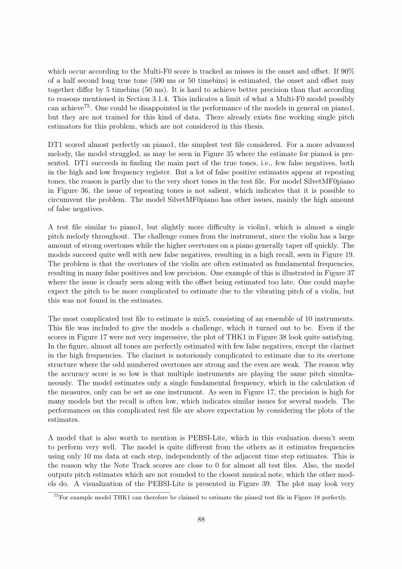
which occur according to the Multi-F0 score is tracked as misses in the onset and offset. If 90%of a half second long true tone (500 ms or 50 timebins) is estimated, the onset and offset maytogether differ by 5 timebins (50 ms). It is hard to achieve better precision than that accordingto reasons mentioned in Section 3.1.4. This indicates a limit of what a Multi-F0 model possiblycan achieve75. One could be disappointed in the performance of the models in general on piano1,but they are not trained for this kind of data. There already exists fine working single pitchestimators for this problem, which are not considered in this thesis.

DT1 scored almost perfectly on piano1, the simplest test file considered. For a more advancedmelody, the model struggled, as may be seen in Figure 35 where the estimate for piano4 is pre-sented. DT1 succeeds in finding the main part of the true tones, i.e., few false negatives, bothin the high and low frequency register. But a lot of false positive estimates appear at repeatingtones, the reason is partly due to the very short tones in the test file. For model SilvetMF0pianoin Figure 36, the issue of repeating tones is not salient, which indicates that it is possible tocircumvent the problem. The model SilvetMF0piano has other issues, mainly the high amountof false negatives.

A test file similar to piano1, but slightly more difficulty is violin1, which is almost a singlepitch melody throughout. The challenge comes from the instrument, since the violin has a largeamount of strong overtones while the higher overtones on a piano generally taper off quickly. Themodels succeed quite well with new false negatives, resulting in a high recall, seen in Figure 19.The problem is that the overtones of the violin are often estimated as fundamental frequencies,resulting in many false positives and low precision. One example of this is illustrated in Figure 37where the issue is clearly seen along with the offset being estimated too late. One could maybeexpect the pitch to be more complicated to estimate due to the vibrating pitch of a violin, butthis was not found in the estimates.

The most complicated test file to estimate is mix5, consisting of an ensemble of 10 instruments.This file was included to give the models a challenge, which it turned out to be. Even if thescores in Figure 17 were not very impressive, the plot of THK1 in Figure 38 look quite satisfying.In the figure, almost all tones are perfectly estimated with few false negatives, except the clarinetin the high frequencies. The clarinet is notoriously complicated to estimate due to its overtonestructure where the odd numbered overtones are strong and the even are weak. The reason whythe accuracy score is so low is that multiple instruments are playing the same pitch simulta-neously. The model estimates only a single fundamental frequency, which in the calculation ofthe measures, only can be set as one instrument. As seen in Figure 17, the precision is high formany models but the recall is often low, which indicates similar issues for several models. Theperformances on this complicated test file are above expectation by considering the plots of theestimates.

A model that is also worth to mention is PEBSI-Lite, which in this evaluation doesn’t seemto perform very well. The model is quite different from the others as it estimates frequenciesusing only 10 ms data at each step, independently of the adjacent time step estimates. This isthe reason why the Note Track scores are close to 0 for almost all test files. Also, the modeloutputs pitch estimates which are not rounded to the closest musical note, which the other mod-els do. A visualization of the PEBSI-Lite is presented in Figure 39. The plot may look very

75For example model THK1 can therefore be claimed to estimate the piano2 test file in Figure 18 perfectly.

88

nasty as there is a very large amount of false positives, but considering a zoomed version of thefirst 5 seconds, as in Figure 40, the model doesn’t seem to perform catastrophically bad. Thereare a lot of false positives, resulting in a bad accuracy, but it has a precision and recall whichis about half of the THK1 model, which in turn was considered as a very well performing model76.

A model which was expected to perform a little bit better was KD1. In MIREX 2017 it achievedthe second place both in the Multi-F0 task and the Note Track task for ensemble music. Butfor the tests herein, the model is quite far from the top performing models. There is one testfile it performs much better on, namely mix1. A plot of the KD1 estimate of mix1 is shown inFigure 41. In the plot the instruments in the middle register, the saxophone and the clarinet, areideally estimated. At the same time, a couple of true tones from the bassoon are missed and theoffset of the violin quite often appears too late, as well as a couple of false positives in the highand middle register. But in general KD1 performs very well on this test file, unlike the rest ofthe test files. The reason is probably that the model is using parameters trained on the MIREXdevelopment set, which is a real recorded music file just like mix1. Studying Figure 17 and 21,the KD1 estimates for the other ensemble files, which consists of simulated sound, achieves lowerscores for the than mix1. In Figure 42, the KD1 estimate of mix3, which is a test file consistingof simulated sound, is plotted. The estimate appears distinctly different to the estimate of thereal recorded music test file mix1. Lots of false positive estimates appears where the failed esti-mates form long continuous tones. Also big parts of the flute appear as false negatives. Thus,the training data seems to be crucial for what type of music the KD1 model succeeds to estimate.

Other models which perform much better on the real recorded music test file mix1 than the rest,are BW1, BW2, and BW3. On both the Multi-F0 and the Note Track task, these models achievethe highest accuracy and F-measure after THK1 and CT1 respectively for mix1, Figure 17 and21. Both BW1, BW2, BW3, and KD1 were performing very well in MIREX, but they seem tobe focused on only the type of data which appears in MIREX, real recorded music. The test filesgenerated from MIDI files in this thesis seem to not be in favor of these models. Consideringa real life application of a music transcription model, one would almost always consider realrecorded music, which they work quite well in. Neither BW1, BW2, BW3, or KD1 are neuralnetwork-based models. Also, the parametric model PR performs better on the real sound testfile than the simulated sound test files. From Figure 17 and 21, the neural network model THK1,trained on real sound, and DT1, trained on MIDI files, both seem to be able to deal with bothsimulated and real sound, independently of what kind of data the model has been trained on.This is a sign of robustness for the neural network models. There are exceptions of non-neuralnetwork models which may handle both types of data, such as the MPE models, Figure 17, butthe trend is quite clear that the neural network models is better of dealing with different typesof data.

A general observation from the models’ performances is that false positive estimates are mostcommon in either very high frequencies, far from the ground truth tones, or at the end of thetones where the offset is estimated too late. The false positives which occur far from the groundtruth are usually octave errors or other multiples of a fundamental frequency, where an over-tone is mistakenly estimated as a fundamental frequency. This is probably the most common

76Some of the failed estimates by PEBSI-Lite are semitones which are estimated due to the high time resolutionand low frequency resolution. Exclusively most false positives can be linked as overtones which mistakenly areestimated as fundamental frequencies.

89

error. The failed estimates corresponding to the missed offsets were expected, due to issues withthe offset determination described in Section 3.1.4. False positive errors which don’t occur ascommonly as expected are estimates occurring between a quartertone and a semitone, whichwould occur due to bad frequency resolution. The errors which are indicated as such in theplots are mainly due to late offsets and that the following ground truth tone jump is a semitone.The reason why this type of error doesn’t appear that frequently is possibly due to the perfectlytuned simulated instrument sounds from the MIDI files or that the models are using well workingspectral representations.

Finally the Deep Complex models will be discussed. The models are designed for the Multi-F0task, which will be in focus. First, considering Figure 16, it can initially be noted that the DeepComplex LSTMCQT achieves the 3rd highest accuracy based on the average of all models. Thisis a very pleasing result. Comparing the different Deep Complex models one may note that theDeep Complex LSTMCQT has a slightly higher average accuracy than Deep Complex which inturn has slightly higher than the Deep Complex LSTMFFT. The proportions are almost equalconsidering only the averaged ensemble or piano test files. This suggests a structural improve-ment of the LSTMCQT model and a structural degradation of the LSTMFFT model comparedto the Deep Complex model. The three models are very similar in their structure, but the fewdifferences seem to have a quite large impact. The small differences in the model structures givequite large differences in the estimates, which is illustrated in Figure 43, 44, and 45, where theestimates of the test file mix2 are shown. For this test file, the Deep Complex model performspoorly and a large amount of false positive estimates are apparent both in the high and the lowfrequency region. The estimates from the LSTMCQT model are cleaner as there are not as manyfalse positive estimates even if there clearly are some. However, the number of false negativesis low. The false positives seem to appear at frequencies which can be linked as overtones ofthe true fundamental frequencies. For example, the false positives around 800 Hz have a similarform as the oboe playing around 400 Hz. The same is true for the false positives around 300 Hzbetween 30-75 seconds, where a similar form as the tones from the bassoon appear around 150Hz. The plot of the LSTMFFT model have similar look as the LSTMCQT where the overtonesseem to be mistakenly estimated as fundamental frequencies. The LSTMFFT also has more falsepositives than LSTMCQT. The optimized threshold for the LSTMFFT model was a bit lowerthan the LSTMCQT, which might be a reason why its number of false positives is higher.

Also, the Deep Complex models are considered for the test file guitar1 in Figure 46, 47, and 48.For this test file the standard Deep Complex model performs better and achieving the highestprecision of the three models while the LSTMCQT and LSTMFFT models achieve a higher re-call. The reason is probably that the estimates of the Deep Complex model have limited relationto the adjacent time steps. Studying Figure 46, it looks like almost all true frequencies are esti-mated, but from the recall score it says that about 25% was false negative estimates. Since theDeep Complex model estimates each time bin independently, it fails to estimate the frequencyfor all time bins of the tone. A disadvantage of using a relation of the adjacent time bins can beseen for the LSTMCQT and LSTMFFT in Figure 47 and 48 where some tones are estimated tobe longer than the ground truth, i.e., the offset is estimated to late. Another issue is that a falsepositive estimate may affect the following estimates to also become a false positive estimation.This makes the false positives of the Deep Complex model to last for shorter periods than thefalse positives do for LSTMCQT and LSTMFFT. This is most clearly seen for the LSTMFFT.In general, the Deep Complex model achieves a precision close to the Deep Complex LSTMCQT,

90

but a lower recall resulting in an overall better accuracy for the LSTMCQT model.

Finally it needs to be stated that it is much easier to point out structural errors than it is tosolve them. The music transcription research is based on both scientific discoveries and empiricaltests. Thus, it is not always simple to point out exactly what is needed to correct an error. Thebest approach is probably to add a feature which could correct the error and then empiricallytest if it worked. The goal of this thesis is not to solve the structural errors which occurs in thedifferent models. Instead this thesis reveals what can be improved and presents differences inthe approaches of the models wherein the solution might exist.

91

8 Conclusions and Summary

The problem formulations in the outset of the thesis were: How well does the best current musictranscription model performs. How does it work and why does it work so well? Can complex-valued neural networks enrich the music transcription research area? These questions will beanswered in this Section 8.1-8.3 followed by some further elaborations in Section 8.4.

8.1 Summary of the Test Results

The results on the test files show that there is one model, THK1, which is clearly superiorin Multiple fundamental frequency estimation, and that there is another model, CT1, whichis clearly superior in Note Tracking. This is the same result achieved in MIREX 2017, whichstrengthens the credibility of both the evaluation made in this thesis and the MIREX evaluation.This thesis also illustrates how well the models perform by visualizing the estimates against theground truth for different models. Even if the accuracy score was not perfect for the best models,the plots of the estimates showed a satisfying result where only minor structural errors couldbe found. This indicates that the respective researchers have come far in the process towardsautomatic music transcription. But even if the structural errors barely exist, there are thingswhich may be fine tuned in order to make the models even more accurate, perhaps the missingcomponent is already existing as a part of another model.

8.2 Discussion of Model Features

To find the most valuable features it is natural to start studying the two best performing models,THK1 and CT1. Both models are neural network based models using CNN. Both models usea logarithmically spectral representation, one using the sliced CQT and one using hand-craftedfilter banks. The outputs of the networks are then postprocessed to output the final estimates,one uses a linear classifier and one uses estimated features such as the onset and offset. Themodels are concluded to be quite similar, but there are a couple of differences.

In THK1, much effort is put into training the network such that no overfitting should occur.This is very reasonable since for example the spectrum of the piano tone E3 activates differentparameters in the network than the piano tone F3, but the spectrums of the two tones are verysimilar, just a shift in the frequency. Randomly shifting the training data makes the model learnthe structure of a piano tone and not only the structure of the piano tone E3. The THK1 modelhas a surprisingly shallow neural network model, only consisting of one convolutional layer andone fully connected layer. This indicates that the deeper models are perhaps too complicatedto be trained correctly with the amount of available data. Finally, it should be mentioned thatthe model is trained on the new dataset MusicNet, which can be motivated to be the best oneavailable, due to its size and all its combinations of instruments.

CT1 has a more advanced and deeper network structure. It uses a succession of convolutionallayers and a convolutional LSTM layer in two different channels where one channel is estimatingthe onsets and is used as input to the pitch estimation channel. The onset approach is mo-tivated by its appearance in other successful models, such as MM1 and DOPT. These modelswere solely trained on piano data, which makes them perform well on the piano test files only.THK1 includes temporal dependence, but only for 1/3 of a second. Due to the convolutionalLSTM layer in CT1, the model may use longer time dependencies as well. It is not clear from the

92

results herein whether a longer time dependence is important. Some time dependence betweenthe estimates can nevertheless be motivated by the weaker performance of the Deep Complexmodel and PEBSI-Lite, which don’t use any time dependence at all.

By considering the average results of both Multi-F0 and Note Track, Figure 16 and 20, at leastthe three best performing models are neural network based. This clearly indicates that neuralnetworks are the state-of-the-art in music transcription. One could argue that all the parametricand probabilistic models should be forgotten and all focus for further research should be onoptimizing the architecture of the neural networks, but there are features used in the old modelswhich could probably also be used in the neural network models. One example is postprocess-ing, where the output of the neural network is very similar to many of the probabilistic andparametric pitch estimators, in which the postprocessing is usually more advanced than a binarythreshold, which is used in some neural network models. Another example is the onset detector,which is already used in a couple of neural network models and seems to give effective results.But other feature detectors could probably also be added to the networks such as beat or chordestimator. It can be argued that feeding as much valuable information for music transcriptionas possible into the neural network, only improves the network. The network could then be ableto learn by itself in what extent these features should be used.

Herein, complex-valued neural networks are proposed. It has been shown in this thesis that acomplex-valued neural network, even if the structure is very simple, can match the best per-forming real-valued models. It is true that the Deep Complex LSTMCQT model was quite farfrom both THK1 and CT1, but considering the simple structure of the model consisting of aneural network and a binary threshold, the result is quite impressive. One part of its success isprobably that it has been trained on a solid dataset, and compared to THK1, which is the onlymodel which has been trained on the same dataset, it performs badly77. A couple of potentialimprovements of the Deep Complex model are suggested in Section 8.3. The use of complexvalues in neural networks for music transcription is theoretically motivated by that a neural net-work performs better if it is given more usable information. The complex-valued representationof a signal which keeps both phase and amplitude intact, is herein claimed to be more usefulthan only the absolute value.

The THK1 and CT1 may be the best performing models right now, but the research is changingfast. It can be expected that the few structural errors identified herein being overcome in a fewyears, perhaps using some of the improvements suggested herein. Right now one might be ableto fine-tune the estimates to look perfectly in a plot. Further, the goal will be to achieve theperfect precision and recall scores78.

77Almost the same dataset. THK1 add some actions to avoid overfitting to the dataset which are not consideredfor Deep Complex LSMTCQT.

78An example of a research field which has come a step further than the music transcription field, is theresearch about hand written digits. Models for the MNIST dataset are optimized to achieve the perfect precision.Currently, year 2018, the error is 0.21%. It should be noted that this level of fine tuning not is possible in themusic transcription field at the moment, for example due to an approximate 4% error in the annotation of theMusicNet training dataset.

93

8.3 Analysis of the Proposed Models

The herein proposed models were inspired by the original Deep Complex model and by modelsparticipating in MIREX, where the latter provided inspiration to add a recurrent layer to thenetwork, and to use the CQT. It is interesting how the LSTM layer by itself (by keeping theFFT representation) worsened the model while adding the CQT together with the LSTM layerimproved it. One reason could be that the LSTM layer increased the number of parameters andthe amount of 100 epochs in the training section was not enough for the FFT model in orderto find the optimal weights. 100 epochs seemed to be enough for the CQT model which can beexplained by the CQT consisted of 1/4 the input data as the FFT model used. The reason whythe CQT did improve over the Deep Complex model is probably because of the convolutionallayer, in which it is advantageous to convolve the same number of frequency bins between eachmusical note. A convolution of an FFT representation with linearly spaced frequency bins mightconvolve frequencies corresponding to two different musical notes, which would then not be pos-sible to distinguish.

The Deep Complex LSTMCQT model achieved the 3rd best accuracy score in the Multi-F0task. Despite that, a couple of possible improvements are possible. First of all, the model wastrained to optimize the accuracy, (44), where the true negatives were counted in the score. In-stead, the MIREX accuracy in (43) should be used. The second suggested improvement is aboutpostprocessing, where a more advanced method than the binary threshold should probably beused. From the plots of the estimates it was clear that the model often estimated the secondharmonic as a separate fundamental frequency. Using a more specialized algorithm could prob-ably reduce the amount of false positives. For future work it would also be of interest to changethe architecture of the neural network and change some of the convolutional layers79. Somefeature detectors could be added to the model, such as, for example, an onset detector and abeat detector. Finally, the training data may be randomly shifted in the frequency domain, inorder to reduce overfitting.

8.4 Ideas for Future Research

A couple of ideas emerged while typing this thesis. One was about the recurrent layers in aneural network which are dependent of the previous data. Unlike other application areas of therecurrent layers, the input data for the next time bins is known. Therefore the future input datacould be used for predicting the frequencies in the previous time step, as a reversed recurrentlayer. A version of this exists in convolutional neural network where spectrums from previousand future time bins are convolved, but the idea is that there might be even longer dependenciesin the future as well as the past. A combination of a neural network and a Hidden Markov modelmight be used for this purpose.

Another idea was about a big issue in the music transcription research area, namely the lack ofavailable datasets consisting of instrumental music and its annotated sheet music. This thesisshows that some models, mainly parametric and probabilistic, are performing differently on realrecorded music and simulated music. For those models, which generally are older, the type ofdata is crucial both for training and testing. This thesis also shows that other models, mainlyneural network models, perform equally on real and simulated music. If a study would considerthe same test files in two versions, both real and simulated music, in order to investigate if one

79As the THK1 performed very well on fewer amount of hidden layers.

94

can prove that the neural network based methods are performing equally on the different typesof datasets, thousands of datasets with perfectly annotated sheet music will be available verycheaply. Also, the sheet music annotations would be perfectly aligned with the sound files, whichis currently not possible to achieve manually. This would break a lot of limitations which theresearch field has been struggling with for a long time.

95

9 Bibliography

References

[1] I. Aizenberg and A. Gonzalez, "Image Recognition using MLMVN and Frequency DomainFeatures," 2018 IEEE International Joint Conference on Neural Networks (IJCNN), July,2018 pp. 1550-1557. USA, July 2018. [Online]. Available: https://drive.google.com/file/d/1CR6ijceulhdPqrQa5yrii6V9MIU3FKlM/view. [Accessed August 16, 2018].

[2] K. Dressler, "Automatic Transcription of the Melody from Polyphonic Music," Ph.D.dissertation, Fak. für Elekt. und Infor. der Techn. Univ. Ilmenau, 2016. [On-line]. Available: https://www.db-thueringen.de/servlets/MCRFileNodeServlet/dbt_derivate_00038847/ilm1-2017000136.pdf. [Accessed August 16, 2018].

[3] E. Benetos, S. Dixon, D. Giannoulis et al. "Automatic music transcription: challenges andfuture directions," J Intell Inf Syst 41: 407, 2013. [Online]. Available: https://doi.org/10.1007/s10844-013-0258-3. [Accessed August 16, 2018].

[4] "Sound," Wikipedia. [Online]. Available: https://en.wikipedia.org/wiki/Sound. [Ac-cessed August 16, 2018].

[5] "Fast Fourier transform," Wikipedia. [Online]. Available: https://en.wikipedia.org/wiki/Fast_Fourier_transform. [Accessed August 16, 2018].

[6] J. Florén and J. Torby, "Musical Instrument Categorization using Spectral- and CepstralAnalysis," B.S. thesis, Center of Math. Scien. Lund Univ., 2016. [Online]. Available: http://lup.lub.lu.se/student-papers/record/8891409. [Accessed August 16, 2018].

[7] "Complex number," Wikipedia. [Online]. Available: https://en.wikipedia.org/wiki/Complex_number. [Accessed September 1, 2018].

[8] F. Galletta, "Do the 88 keys of a piano cover the full range of frequencies that thehuman ear can perceive?," 2017. [Online forum image] Available: https://www.quora.com/Do-the-88-keys-of-a-piano-cover-the-full-range-of-frequencies-that-the-human-ear-can-perceive. [Accessed August 16, 2018].

[9] "Musical note," Wikipedia. [Online]. Available: https://en.wikipedia.org/wiki/Musical_note. [Accessed September 1, 2018].

[10] J.C. Brown, "Calculation of a Constant Q spectral transform," Journal of the AcousticalSociety of America, vol. 144, no. 1, pp. 425-434, Jan. 1991. [Online]. Available: https://doi.org/10.1121/1.400476. [Accessed August 16, 2018].

[11] B.C.J. Moore and B.R. Glasberg, "Suggested formulae for calculating auditory-filter band-widths and excitation patterns," Journal of the Acoustical Society of America, vol. 74, no. 3,pp. 750-753, 1983.

[12] D. O’Shaughnessy, "Speech communication: human and machine", Addison-Wesley, 1987, pp. 150. [Online]. Available: https://books.google.se/books?ei=rhFfSpa-BJOCNsTT4IUG&id=mHFQAAAAMAAJ&dq=Speech+Communications:+Human+and+Machine&q=2595&redir_esc=y#search_anchor. [Accessed August 16, 2018].

96

[13] C.M. Bishop. Pattern Recognition and Machine Learning. Springer-Verlag Berlin, Heidel-berg, 2006.

[14] G. Sanderson. "Neural Networks," 2017-2018 [Online video playlist]. Available: https://www.youtube.com/playlist?list=PLZHQObOWTQDNU6R1_67000Dx_ZCJB-3pi. [Accessed Au-gust 16, 2018].

[15] L-C. Böiers. Lectures on Optimization, 3rd ed. KFS AB. 2009.

[16] "Gradient descent," Wikipedia. [Online]. Available: https://en.wikipedia.org/wiki/Gradient_descent. [Accessed October 4, 2018].

[17] A. Karpathy, "Convolutional Neural Networks for Visual Recognition," Lectureat Stanford Univ, spring 2018. [Online]. Available: http://cs231n.github.io/convolutional-networks/ [Accessed August 16, 2018].

[18] "MIREX HOME," Mirex. [Online]. Available: http://www.music-ir.org/mirex/wiki/MIREX_HOME. [Accessed August 16, 2018].

[19] C. Olah, "Understanding LSTM Networks," [Online]. Available: http://colah.github.io/posts/2015-08-Understanding-LSTMs/. [Accessed August 16, 2018].

[20] C. Trabelsi, O. Bilaniuk, D. Serdyuk, S. Subramian and J.F. Santos et al. "Deep ComplexNetworks," ICLR, 2018.[Online]. Available: https://arxiv.org/abs/1705.09792. [AccessedAugust 16, 2018].

[21] S. Ioffe and C. Szegedy. "Batch Normalization: Accelerating Deep Network Training byReducing Internal Covariate Shift," Google Inc. 2015. [Online]. Available: https://arxiv.org/abs/1502.03167. [Accessed September 9, 2018].

[22] V. Emiya, MAPS Database – A piano database for multipitch esti-mation and automatic transcription of music, 2008. [Online]. Availableby request: http://www.tsi.telecom-paristech.fr/aao/en/2010/07/08/maps-database-a-piano-database-for-multipitch-estimation-and-automatic-transcription-of-music/. [Accessed August 16, 2018].

[23] J. Thickstun, Z. Harchaoui and S. Kakade, MusicNet, 2016. [Online]. Available: https://homes.cs.washington.edu/~thickstn/musicnet.html. [Accessed August 16, 2018].

[24] Z. Duan, B. Pardo and C. Zhang, Bach10 Dataset, “Multiple fundamental frequency es-timation by modeling spectral peaks and non-peak regions,” IEEE Trans. Audio SpeechLang. Process. vol. 18, no. 8, pp. 2121-2133, 2010. [Online]. Available by request: http://music.cs.northwestern.edu/data/Bach10.html. [Accessed August 16, 2018].

[25] RWC Music Database, 2002. [Online]. Available by request: https://staff.aist.go.jp/m.goto/RWC-MDB/. [Accessed August 16, 2018].

[26] MIREX Development Dataset, 2005. Available by request: http://www.music-ir.org/mirex/wiki/2017:Multiple_Fundamental_Frequency_Estimation_%26_Tracking.[Accessed August 16, 2018].

97

[27] L. Su and Y. H. Yang, "Escaping from the Abyss of Manual Annotation: NewMethodology of Building Polyphonic Datasets for Automatic Music Transcrip-tion," Int. Symp. Computer Music Multidisciplinary Research (CMMR), June2015. [Online]. Available: https://sites.google.com/site/lisupage/research/new-methodology-of-building-polyphonic-datasets-for-amt. [Accessed August16, 2018].

[28] C. Focacci, "False Negatives: A Serious Danger in Your AML Program",April, 2016. [Online image]. Available: https://transparint.com/blog/2016/04/01/false-negatives-a-serious-danger-in-your-aml-program/. [Accessed August 16, 2018].

[29] Raffel, B. McFee, E. J. Humphrey, J. Salamon, O. Nieto, D. Liang and D. P. W. Ellis,"mir_eval: A Transparent Implementation of Common MIRMetrics", Proceedings of the 15thInternational Conference on Music Information Retrieval, 2014. [Online]. Available: http://colinraffel.com/publications/ismir2014mir_eval.pdf. [Accessed August 16, 2018].

[30] "Precision and recall," Wikipedia. [Online]. Available: https://en.wikipedia.org/wiki/Precision_and_recall. [Accessed August 16, 2018].

[31] A. Berg and S. Blomstrand. "Pitch Perfect: Building a MIREX Evaluation System," Projectin Stationary and Non-Stationary Spectral Analysis, Lund Univ.

[32] "Tukey’s range test," Wikipedia. [Online]. Available: https://en.wikipedia.org/wiki/Tukey%27s_range_test. [Accessed August 16, 2018].

[33] E. Benetos and T. Weyde, "Multiple-F0 Estimation and Note Tracking for MIREX 2015Using a Sound State-Based Spectrogram Factorization Model," MIREX 2015. [Online]. Avail-able: http://www.music-ir.org/mirex/abstracts/2015/BW1.pdf. [Accessed August 16,2018].

[34] C. Cannam, E. Benetos, M. Mauch, M. E. P. Davies, S. Dixon, C. Landone, K. Noland andDan Stowell, "MIREX 2015: Vamp Plugins from the Centre for Digital Music,"MIREX 2015.[Online]. Available: http://www.music-ir.org/mirex/abstracts/2015/CB1.pdf. [AccessedAugust 16, 2018].

[35] E. Benetos and S. Dixon, "A Shift-Invariant Latent Variable Model for Automatic MusicTranscription," Computer Music Journal, 36(4), pp. 81-94. [Online]. Available: http://dx.doi.org/10.1162/COMJ_a_00146. [Accessed August 16, 2018].

[36] L. Su and Y. H. Yang, "Multiple-F0 Estimation for MIREX 2015," MIREX 2015. [Online].Available: http://www.music-ir.org/mirex/abstracts/2015/SY1.pdf. [Accessed August16, 2018].

[37] G. Peeters, "Music pitch representation by periodicity measures based on combined tem-poral and spectral representations," 2006 IEEE Inter. Conf. on Acoustics Speech and Sig-nal Processing Proceedings, 2006. [Online]. Availible: http://recherche.ircam.fr/anasyn/peeters/ARTICLES/Peeters_2006_ICASSP_Periodicity.pdf. [Accessed August 16, 2018].

[38] D. Troxel, "Music Transcription with a Convolutional Neural Network 2016," MIREX 2016.[Online]. Available: http://www.music-ir.org/mirex/abstracts/2016/DT1.pdf. [AccessedAugust 16, 2018].

98

[39] K. He, X. Zhang, S.Ren, J. Sun, "Deep Residual Learning for Image Recognition," MicrosoftResearch, 2015. [Online]. Available: https://arxiv.org/abs/1512.03385. [Accessed August16, 2018].

[40] M. Marolt, "A Connectionist Approach to Automatic Transcription of Polyphonic PianoMusic," Fac. of Comp. and Info. Sci. at Univ. of Ljubljana, 2004. [Online]. Available: http://lgm.fri.uni-lj.si/wp-content/uploads/2016/09/4203860.pdf. [Accessed August 16,2018].

[41] C. Thomé and S. Ahlbäck "Polyphonic Pitch Detection with Convolutional RecurrentNeural Networks," MIREX 2017. [Online]. Available: http://www.music-ir.org/mirex/abstracts/2017/CT1.pdf. [Accessed August 16, 2018].

[42] S. Mita, G. Hatanaka, A. Meneses, N. Thammasan and D. Miura, "MIREX 2017 : Multi-instrumental End-to-End Convolutional Neural Network for Multiple F0 estimation,"MIREX2017. [Online]. Available: http://www.music-ir.org/mirex/abstracts/2017/MHMTM1.pdf.[Accessed August 16, 2018].

[43] L. Pogorelyuk and C. Rowley, "Melody Extraction for MIREX 2016 Using Dynamic ModeDecomposition," MIREX 2017. [Online]. Available: http://www.music-ir.org/mirex/abstracts/2017/PR1.pdf. [Accessed August 16, 2018].

[44] J. Thickstun, Z. Harchaoui, D. Foster and S. M. Kakade, "MIREX 2017: Frequency DomainConvolutions for Multiple F0 Estimation," MIREX 2017. [Online]. Available: http://www.music-ir.org/mirex/abstracts/2017/THK1.pdf. [Accessed August 16, 2018].

[45] J. Thickstun, Z. Harchaoui and S. M. Kakade, "Learning Features of Music From Scratch,"ICLR 2017. [Online]. Available: https://arxiv.org/pdf/1611.09827.pdf. [Accessed Au-gust 16, 2018].

[46] C. Hawthorne, E. Elsen, J. Song, A. Roberts, I. Simon, C. Raffel, J. Engel, S. Oore andD. Eck, "Onsets and Frames: Dual-Objective Piano Transcription," Google Brain Team,Mountain View, CA, USA, 2017. [Online]. Available: https://arxiv.org/abs/1710.11153.[Accessed August 16, 2018].

[47] T. Kronvall, F. Elvander, S. Ingi Adalbjörnsson and Andreas Jakobsson, "An AdaptivePenalty Approach to Multi-Pitch Estimation," EUSIPCO 2015. [Online]. Available: https://www.eurasip.org/Proceedings/Eusipco/Eusipco2015/papers/1570103397.pdf. [Ac-cessed August 16, 2018].

[48] T. Tolonen and M. Karjalainen, "A Computationally Efficient MultipitchnAnalysisModel," IEEE Transactions on Speech and Audio Processing, vol. 8, Issue 6, pp. 708- 716, Nov 2000. http://citeseerx.ist.psu.edu/viewdoc/download?doi=10.1.1.334.1573&rep=rep1&type=pdf. [Accessed August 16, 2018].

[49] K. Simonyan and A. Zisserman, "Very Deep Convolutional Networks for Large-Scale ImageRecognition," ICLR, April 2015. [Online]. Available: https://arxiv.org/abs/1409.1556.[Accessed August 16, 2018].

[50] J. Thickstun, Z, Harchaoui, D. Foster, S. M. Kakade,"Invariances and Data Augmentationfor Supervised Music Transcription," 2017. [Online]. Available: https://arxiv.org/abs/1711.04845. [Accessed August 16, 2018].

99

[51] MuseScore. [Online]. Available: https://musescore.org/en. [Accessed August 16, 2018].

[52] readmidi, Matlab function. [Online]. Available: http://kenschutte.com/midi. [AccessedAugust 16, 2018].

100