Wisconsin Department of Natural Resources - WI.gov

Wisconsin 2020 Consolidated Assessment

and Listing Methodology (WisCALM)

Clean Water Act Section 303(d) and

305(b) Integrated Reporting

Wisconsin Department of Natural Resources

April 2019


101 S. Webster Street ∙ PO Box 7921 ∙ Madison, Wisconsin 53707-7921

608-266-2621

I have reviewed this guidance document or proposed guidance document and I certify that it complies with sections 227.10 and 227.11 of the Wisconsin Statutes. I further certify that the guidance document or proposed guidance document contains no standard, requirement, or threshold that is not explicitly required or explicitly permitted by a statute or a rule that has been lawfully promulgated. I further certify that the guidance document or proposed guidance document contains no standard, requirement, or threshold that is more restrictive than a standard, requirement, or threshold contained in the Wisconsin Statutes.

A · Stocks, Director Water Quality Bureau

Statutory Authority

State

• Sections 281.11 and 281.12, Wis. Stats., grant necessary powers and establish a comprehensive

program under the WDNR to enhance quality management and protection of all waters of the state. It

grants the WDNR general supervision and control to carry out the planning, management and

regulatory programs necessary for prevention/reduction of water pollution and for improvement of

water quality.

• Section 281.13, Wis. Stats., grants the department authority to research and evaluation the quality and

condition of the state’s natural water sources.

• Section 281.15, Wis. Stats. mandates that the department promulgate water quality standards,

including water quality criteria and designated uses. It recognizes that different use categories and

criteria are appropriate for different types of waterbodies, and that the department shall establish

criteria which are not more stringent than reasonably necessary to assure attainment of the designated

use for the water bodies in question.

• Section 281.65(4)(c) and (cd), Wis. Stats., directs the department to prepare a list of waters impaired

by nonpoint source pollution.

• Section 283.83, Wis. Stats., mandates the departments establish a continuing water quality

management planning process, part of which is identifying water quality status.

Federal

• Sec. 303 (d)(1)(A) of the Federal Water Pollution Control Act (Clean Water Act) requires states to

develop an impaired waters list that identifies waters that are not meeting any water quality standard.

• Sec. 305(b)(1) of the Federal Water Pollution Control Act (Clean Water Act) requires states to

prepare a biennial report documenting which waterbodies are attaining their designated uses.

• 40 CFR s. 130. 4 Water Quality Monitoring. This section requires water quality monitoring and

assessments of state waters.

• 40 CFR s. 130.7 Total maximum daily loads (TMDLs) and individual water quality-based effluent

limitations. This section provides additional information related to requirements for developing the

impaired waters list.

• 40 CFR s. 130.8 Water Quality Reports. States must submit water quality reports to EPA that include

a water quality assessment of state waters.

• 40 CFR s. 130.3. Water quality standards. This section defines water quality standards as setting

water quality goals for a waterbody that will protect its designated uses (such as protection of fish,

wildlife, recreation, and public health and welfare). Criteria will be set to protect those uses.

• 40 CFR s. 131.11 Criteria. States must adopt those water quality criteria that protect the designated

use. Such criteria must be based on sound scientific rationale and must contain sufficient parameters

or constituents to protect the designated use. For waters with multiple use designations, the criteria

shall support the most sensitive use.

Wisconsin Department of Natural Resources Page ii

Governor

• Tony Evers

Natural Resources Board

• Terry N. Hilgenberg, Chair

• Dr. Frederick Prehn, Vice-Chair

• Julie Anderson, Secretary

• William Bruins

• Gregory Kazmierski

• Gary Zimmer


• Preston D. Cole, Secretary

• Elizabeth Kluesner, Deputy Secretary

• Todd Ambs, Assistant Deputy Secretary

• Darsi Foss, Division Administrator

• Jim Zellmer, Deputy Administrator, Division of Environmental Management

• Adrian Stocks, Director, Water Quality Bureau

Cover photo: Brule River Flowage in Florence County, Photo by Luke Ernster.

The Wisconsin Department of Natural Resources provides equal opportunity in its employment, programs, services,

and functions under an Affirmative Action Plan. If you have any questions, please write to Equal Opportunity

Office, Department of the Interior, Washington, D.C. 20240.

This publication is available in alternate format (large print, Braille, audio tape, etc.) upon request. Please call 608-

267-7694 for more information.

Wisconsin Department of Natural Resources Page iii

Acknowledgements

This guidance document was prepared and built upon by the coordinated efforts of many people. Many

thanks are extended to those who provided information and assistance in updating this guidance

document.

Editor

Ashley Beranek

Major Contributors

Tim Asplund, Ashley Beranek, Nicki Clayton, Matt Diebel, Mark Hazuga, Lisa Helmuth, Katie Hein,

Dan Helsel, Jim Kreitlow, Gina LaLiberte, Aaron Larson, Mary Anne Lowndes, John Lyons, Robert

Masnado, Molli MacDonald, Michael Miller, Kristi Minahan, Amanda Perdzock, Ruth Person, Kurt

Rasmussen, Mike Shupryt, Alex Smith, Brian Weigel

Additional Contributors

Jim Baumann, Donalea Dinsmore, Jennifer Filbert, Toni Glymph, Dave Heath, Linnea Rock, Russ

Rasmussen, Candy Schrank, Ken Schreiber, Greg Searle, Tim Simonson, Mike Wenholz, Scott Van

Egeren, Valerie Villeneuve, Sarah Yang

Wisconsin Department of Natural Resources Page iv

TABLE OF CONTENTS

BACKGROUND ............................................................................................................................................................ 8 1.0 WATER QUALITY STANDARDS: THREE ELEMENTS .............................................................................................. 9 2.0 WISCONSIN’S MONITORING PROGRAM AND DATA MANAGEMENT ................................................................... 11

2.1 Water Quality Monitoring ............................................................................................................................ 11 2.2 Use of Monitoring Data from Other Sources ............................................................................................... 12 2.3 Quality Assurance and Laboratory Analysis ............................................................................................... 12 2.4 Data Management ........................................................................................................................................ 13 2.5 Data Requirements....................................................................................................................................... 14 2.6 Assessment Unit Delineation and Grouping ................................................................................................ 16

3.0 THE ASSESSMENT PROCESS: AN OVERVIEW ...................................................................................................... 17 3.1 General Condition Assessment ..................................................................................................................... 17 3.2 Impairment Assessment ................................................................................................................................ 17 3.3 Water Quality Condition Categories and Lists ............................................................................................ 18

4.0 LAKE CLASSIFICATION AND ASSESSMENT METHODS ........................................................................................ 21 4.1 Lake Classification....................................................................................................................................... 21 4.2 Selecting Representative Stations ................................................................................................................. 24 4.3 Lake General Condition Assessment ............................................................................................................ 27 4.4 Lake Impairment Condition Assessment ...................................................................................................... 31 4.5 Lake Impairment Condition Assessment: Aquatic Life (AL) Use ................................................................ 32 4.6 Lake Impairment Condition Assessment: Recreation Use .......................................................................... 43 4.7 Lake Impairment Condition Assessment: Public Health and Welfare Uses ................................................ 47 4.8 Lake Impairment Condition Assessment: Wildlife Use ................................................................................ 47

5.0 STREAM & RIVER CLASSIFICATION AND ASSESSMENT METHODS ..................................................................... 48 5.1 Stream and River Classifications ................................................................................................................. 48 5.2 Selecting Representative Stations ................................................................................................................. 50 5.3 Stream and River General Condition Assessment ........................................................................................ 51 5.4 Stream and River Impairment Condition Assessment: Aquatic Life Use ..................................................... 55 5.4 Stream and River Impairment Condition Assessment: Recreation Use ....................................................... 59 5.5 Stream and River Impairment Condition Assessment: Wildlife Use ............................................................ 59

6.0 PUBLIC HEALTH AND WELFARE USES – APPLICABLE TO ALL WATERBODY TYPES ........................................... 60 6.1 Fish Consumption Use Assessment .............................................................................................................. 60 6.2 Contaminated Sediment Assessment ............................................................................................................ 61 6.3 Public Water Supply Use Assessment .......................................................................................................... 61

7.0 MAKING A DECISION TO LIST OR DELIST WATERBODIES .................................................................................. 63 7.1 Independent Applicability & Tools to Resolve Data Conflicts ..................................................................... 63 7.2 Professional Judgment ................................................................................................................................. 65 7.3 Threatened Waters ....................................................................................................................................... 65 7.4 Watch Waters ............................................................................................................................................... 66 7.5 Identifying Sources of Impairment ............................................................................................................... 66 7.6 Pollutant-Impairment Combinations ............................................................................................................ 67 7.7 Delisting Impaired Waters ........................................................................................................................... 70 7.8 Decision Documentation .............................................................................................................................. 70

8.0 INTEGRATED REPORT LISTING CATEGORIES ...................................................................................................... 72 8.1 Priority Ranking for TMDL Development .................................................................................................... 73

9.0 PUBLIC PARTICIPATION ..................................................................................................................................... 74 9.1 Requests for Data from the Public ............................................................................................................... 75 9.2 Submittal of Wisconsin’s Integrated Report to U.S. EPA ............................................................................ 75

10.0 QUICK LINK GUIDE .......................................................................................................................................... 76 11.0 REFERENCES CITED ......................................................................................................................................... 79 APPENDIX A. QUICK REFERENCE SECTION .......................................................................................................... 82

Acronyms and Terminology ................................................................................................................................ 83 Water Quality Criteria & Assessment Quick-Reference Tables ......................................................................... 88 EPA Five-Part Categorization ............................................................................................................................ 91

APPENDIX B. 2018 IMPAIRED WATERS ASSESSMENT DOCUMENTATION FORM ................................................... 93 APPENDIX C. SUMMARY OF FISH TISSUE CRITERIA FOR FISH CONSUMPTION ADVICE ........................................ 96

Wisconsin Department of Natural Resources Page v

APPENDIX D. METHODOLOGY FOR USING FIELD DATA TO IDENTIFY AND CORRECT WISCONSIN STREAM

“NATURAL COMMUNITY” MISCLASSIFICATIONS (VERSION 4) ................................................................................. 98 APPENDIX E. CONSENSUS-BASED SEDIMENT QUALITY GUIDELINES RECOMMENDATIONS FOR USE &

APPLICATION ......................................................................................................................................................... 116

Wisconsin Department of Natural Resources Page vi

LIST OF FIGURES

Figure 1. Wisconsin's integrated reporting process. ................................................................................... 11 Figure 2. SWIMS database sign in screen. ................................................................................................. 13 Figure 3. Categorization of waterbodies based on water quality assessments. Categories 1 – 5 align with

EPA’s CWA 305(b) reporting categories. Impaired waters are defined as those in category 5, which is

consistent with all states. Wisconsin defines category 4 waters as its Restoration Waters List and waters in

categories 1 and 2 as its Healthy Waters List. ............................................................................................ 19 Figure 4. Illustrations of (A) a shallow, mixed lake and (B) a deep, stratified. lake. ................................ 22 Figure 5. Distribution of Shallow and Deep lake types (for lakes greater than 10 acres). .......................... 23 Figure 6. Hydrology of a seepage lake versus a drainage lake. ................................................................. 23 Figure 7. Selection of representative stations in WATERS under ‘Monitoring and Listing’. Access to

WATERS is only available to DNR staff. .................................................................................................. 24 Figure 8. Large Lakes: Select well-spaced stations throughout lake. Example: Lake Winnebago ........... 25 Figure 9. Reservoir/Flowages: Select stations along the deepest channel. Example: Lake Petenwell,

Juneau County ............................................................................................................................................. 25 Figure 10. Lobed Lakes with multiple deep holes: One station per deep hole. Example: Two Sisters Lake,

Oneida County ............................................................................................................................................ 26 Figure 11. Lobed Lakes with one deep hole: Use Deep Hole station and another station representative of

shallower area. Example: Fox Lake, Dodge County ................................................................................... 26 Figure 12. Continuum of lake trophic status in relation to Carlson Trophic State Index. ......................... 27 Figure 13. Comparison of the Upper and Lower Confidence Limit values and Mean/Median (M) to the

criteria. ........................................................................................................................................................ 36 Figure 14. Station selection in WATERS for a river or stream segment. WATERS access is available to

DNR staff only. ........................................................................................................................................... 51 Figure 15. Independent Application Matrix. ............................................................................................... 63 Figure 16. Example of assessing a stream for multiple uses with multiple parameters, to determine the

overall waterbody listing. ............................................................................................................................ 68 Figure 17. Example of assessing a lake for multiple uses with multiple parameters, to determine the

overall waterbody listing. ............................................................................................................................ 69

LIST OF TABLES

Table 1. Date range for data used each assessment cycle. This 10-year pattern is consistent back to the

1998 list. ...................................................................................................................................................... 14 Table 2. Description of category 4 subcategories. These subcategories are based on those outlined by the

EPA. Waters in category 4 are on Wisconsin’s Restoration Waters List because a TMDL or alternative

restoration plan has been created and approved by the EPA. ..................................................................... 20 Table 3. Descriptions of category 5 subcategories. These subcategories are loosely based on ones outlined

by EPA but are specific to Wisconsin. All waters in category 5 are part of the state’s Impaired Waters

List, also known as the CWA 303(d) List. .................................................................................................. 20 Table 4. Lake and reservoir natural communities and defining characteristics. ......................................... 21 Table 5. Trophic Status Index (TSI) thresholds – general assessment of lake Natural Communities. ....... 29 Table 6. Mean and median inferred TP values calculated from top and bottom segments of sediment cores

from 87 Wisconsin lakes (Garrison, unpublished data). ............................................................................. 30 Table 7. General water condition assessment decisions based on biological and water quality metrics. ... 31 Table 8. Assessing phosphorus and biology in combination to determine impairment status and pollutant.

.................................................................................................................................................................... 38 Table 9. Lake assessment decisions based on ambiguous phosphorus results and associated chlorophyll-a

results. Chlorophyll-a results can be assessed without TP if there are 6 samples, meeting minimum data

requirements. A listing decision will be made after more monitoring and at least 3 years of data are

available. ..................................................................................................................................................... 38

Wisconsin Department of Natural Resources Page vii

Table 10. Aquatic Life Use impairment thresholds for lake natural communities. ................................... 42 Table 11. Recreation impairment thresholds for lake natural communities. .............................................. 45 Table 12. World Health Organization indicator thresholds of high health risk associated with potential

exposure to cyanotoxins. ............................................................................................................................. 47 Table 13. Wildlife Criteria from NR105.07. ............................................................................................... 47 Table 14. Fish Indices of Biological Integrity for Wisconsin streams and rivers. ...................................... 52 Table 15. Modeled water temperature and flow criteria used to predict Natural Communities in healthy

Wisconsin streams and fish index of biotic integrity (IBI) for bioassessment associated with each Natural

Community. ................................................................................................................................................ 53 Table 16. Condition category thresholds for applicable fish indices of biotic integrity (IBI). ................... 54 Table 17. Condition category thresholds for wadeable stream macroinvertebrate index of biotic integrity.

.................................................................................................................................................................... 54 Table 18. Condition category thresholds for nonwadeable river macroinvertebrate index of biotic

integrity. ...................................................................................................................................................... 55 Table 19. Additional parameters for river & stream impairment assessments. .......................................... 56 Table 20. Aquatic Life use impairment thresholds for rivers/streams ........................................................ 58 Table 21. Aquatic Life use aquatic toxicity impairment thresholds for rivers/streams. ............................. 59 Table 22. Resulting pollutant and/or impairment from an exceedance of each parameter. These are not all

the possible parameters assessed, but some of the most common. ............................................................. 67 Table 23. Integrated Report (IR) Listing Categories and associated lists. .................................................. 72 Table 24. Example of a waterbody assessment with multiple pollutant listings and how that translates

into the overall waterbody category listing. ................................................................................................ 73

Wisconsin Department of Natural Resources Page 8

Background

Over 15,000 lakes and 84,000 miles of streams and rivers in Wisconsin are managed to ensure that their

water quality condition meets state and federal standards. Water quality standards (WQS) are the

foundation of Wisconsin’s water quality management program and serve to define goals for a waterbody

by designating its uses, setting criteria to protect those uses, and establishing provisions to protect water

quality from pollutants.

Waters are monitored to collect water quality data to determine, or assess, its current status or condition.

Water quality monitoring results and assessment data are stored in state and federal databases and the

majority of data are available online to agencies and the public. General assessments are known as

“305(b) assessments” in the Federal CWA (CWA). Waters with available data are reviewed by Wisconsin

Department of Natural Resources (WDNR) biologists and placed in one three categories: attaining, not

attaining, or insufficient information. If biological data is available the water will further be placed in one

of four categories: excellent, good, fair and poor, as defined in section 3.1 of this document.

Specific assessments are conducted to determine if a waterbody is “impaired” or not meeting WQS.

Waters that do not meet WQS are placed on Wisconsin’s Impaired Waters List—also known as the

303(d) list—under Section 303(d) of the CWA. Wisconsin is required to submit list updates every 2 years

to the United States Environmental Protection Agency (EPA) for approval. WDNR has submitted

Impaired Waters Lists, as required1, every other year since 1996.

Water quality assessments aid Department staff in determining management actions that are needed to

meet WQS, including anti-degradation, or maintenance, of existing water quality condition, as well as

restoration of impaired waters.

Each state must document the methodology used to assess waters, including how the state makes

decisions to add or delete waters from the existing Impaired Waters List. Waters may be removed from

the list (delisted) when water quality data identifies that the designated use has been restored (i.e., the

water is meeting WQS). The methodology for conducting general and specific assessments is outlined,

and updated for 2020, in this WisCALM guidance document.

1 EPA did not require and WDNR did not submit an Impaired Waters List in FFY 2000.


1.0 Water Quality Standards: Three Elements Wisconsin’s assessment process begins with water quality standards (WQS). WDNR is authorized to

establish WQS that are consistent with the CWA (Public Law 92-500) through Chapter 281 of the

Wisconsin Statutes. These WQS are explained in detail in chs. NR 102, 103, 104, 105, and 207 of the

Wisconsin Administrative Code (Wis. Adm. Code).

The WQS described in the Wis. Adm. Code rely on three elements to collectively meet the goal of

protecting and enhancing the state’s surface waters:

• Use designations, which define the goals for a waterbody by designating its uses,

• Water quality criteria, which are set to protect the water body’s designated uses, and

• Anti-degradation provisions to protect water quality from declining.

Waters not meeting one or more of these water quality elements are to be included on the Impaired

Waters List.

Designated Uses Designated uses are goals or intended uses for surface waterbodies in Wisconsin which are classified into

the categories of: Aquatic Life, Recreation, Public Health and Welfare, and Wildlife. The following

designated uses are described in ch. NR 102, Wis. Adm. Code:

Aquatic Life2: All surface waters are considered appropriate for the protection of

fish and other aquatic life. Surface waters vary naturally with respect to factors like

temperature, flow, habitat, and water chemistry. This variation allows different

types of fish and aquatic life communities to be supported.

Recreation: All surface waters are considered appropriate for Recreation use

unless a sanitary survey has been completed to show that humans are unlikely to

participate in activities requiring full body immersion.

Public Health and Welfare: All surface waters are considered appropriate to

protect for incidental contact and ingestion by humans and human consumption of

fish. All waters of the Great Lakes as well as a small number of inland water

bodies are also identified as public water supplies and have associated water

quality criteria to account for human consumption3.

Wildlife: All surface waters are considered appropriate for the protection of

wildlife that relies directly on the water to exist or rely on it to provide food for

existence.

Use Designations for Aquatic Life (AL) are separated into the following sub-

categories: Coldwater (Cold), Warmwater Sport Fish (WWSF), Warmwater Forage

Fish (WWFF), Limited Forage Fish (LFF) and Limited Aquatic Life (LAL). More detail on these

subcategories is in the Streams and River Classification chapter of this report.

2 Aquatic Life use was formerly called ‘Fish and Aquatic Life’. The word ‘Fish’ was removed because it was redundant. 3 Distinct water quality criteria are specified for public water supply and non-public water supply waters.

http://docs.legis.wisconsin.gov/code/toc/nr

http://docs.legis.wisconsin.gov/code/admin_code/nr/100/102/


Water Quality Criteria – Numeric and Narrative Each designated use has its own set of water quality criteria, either numeric or narrative requirements that

must be met to protect the intended use. Some of these requirements relate to the amount of the physical

(e.g., water temperature) or chemical (e.g., ammonia concentrations) conditions that must be met to avoid

causing harm. Wisconsin’s water quality criteria may be either numeric (quantitative) or narrative

(qualitative) and are authorized by state statutes and enumerated in chs. NR 102, 104, and 105, Wis. Adm.

Code.

Numeric criteria: Numeric criteria are quantitative and are expressed as a particular concentration of a

substance or an acceptable range for a substance. For example, the pH value shall be from 6-9 standard

units. Numeric surface water quality criteria have been established for conventional parameters (e.g.,

dissolved oxygen, pH, and temperature), toxics (e.g., metals, organics, and ammonia), and pathogens

(e.g., E. coli and fecal coliform bacteria). These numeric criteria are established for each designated use.

Narrative criteria: All waterbodies must meet a set of narrative criteria which qualitatively describe the

conditions that should be achieved. A narrative water quality criterion is a statement that prohibits

unacceptable conditions in or upon the water, such as floating solids, scum, or nuisance algae blooms that

interfere with public rights. These standards protect surface waters and aquatic biota from eutrophication,

algae blooms, and turbidity, among other things. The association between a narrative criterion and a

waterbody’s designated use is less well defined than it is for numeric criteria; however, most narrative

standards protect aesthetic or Aquatic Life designated uses. Wisconsin’s narrative criteria are found in s.

NR 102.04(1), Wis. Adm. Code.

Anti-degradation Wisconsin’s anti-degradation policy is intended to maintain and protect existing uses and high-quality

waters. This part of a waterbody quality standard is intended to prevent water quality from lowering,

especially when reasonable control measures are available. The anti-degradation policy in Wisconsin is

stated in s. NR 102.05(1) of the Wis. Adm. Code:

“No waters of the state shall be lowered in quality unless it has been affirmatively demonstrated to

WDNR that such a change is justified as a result of necessary economic and social development,

provided that no new or increased effluent interferes with or becomes injurious to any assigned uses

made of or presently possible in such waters.”

One component of Wisconsin’s anti-degradation policy is the designation of Outstanding Resource

Waters (ORW) and Exceptional Resource Waters (ERW). These are surface waters which provide

outstanding recreational opportunities, support

valuable fisheries and wildlife habitat, have good water

quality, and are not significantly impacted by human

activities. ORWs typically do not have any

dischargers, while ERW designation offers limited

exceptions for dischargers if human health would

otherwise be compromised (e.g., expansion of

wastewater treatment facilities to protect public

health).

Inherent in the assessment and impaired waters listing

process is the application of anti-degradation

provisions. Anti-degradation is an important aspect of

pollution control because preventing deterioration of

surface waters is less costly to society than attempting

to restore waters once they have become degraded.

How is a water designated ORW or

ERW?

ORWs are listed in NR 102.10 and

include national and state wild and

scenic rivers. ERWs are listed in

NR102.11. Surface waters, or portions

thereof, may be added to, or deleted

from, the outstanding resource waters

and exceptional resources waters

designations through the rule making

process. This process may be changed

in the future.

http://docs.legis.wisconsin.gov/document/administrativecode/NR%20102.04



Wisconsin DNR’s Water Division

Monitoring Strategy is available on

WDNR’s website at: https://dnr.wi.gov/topic/SurfaceWater/m

onitoring/strategy/Strategy_2015_2020

2.0 Wisconsin’s Monitoring Program and Data Management

2.1 Water Quality Monitoring

WDNR’s Surface Water Monitoring Strategy directs

monitoring efforts in a manner that efficiently addresses

the wide variety of information needs, while providing

adequate depth of surface water knowledge to support

decision making. A stratified monitoring approach to

gathering information ensures that the status of

Wisconsin’s water resources can be determined in a

comprehensive manner, without depleting the capacity to conduct in-depth analyses and problem-solving

where needed. Monitoring activities are grouped into three types, baseline, prescribed, and local needs,

which form the basis of the integrated reporting process (Figure 1).

Baseline Monitoring – Statewide

• Trends sites (Lakes, Rivers)

• Probabilistic surveys (streams, Aquatic Invasive Species (AIS), National Aquatic Resource Surveys

(NARS) (coastal condition and wetlands))

• Reference sites (wadeable streams, macrophytes, large river macroinvertebrates)

Prescribed Monitoring – Statewide and District

• Targeted Watershed Approach

• Directed Lake Assessment (including Aquatic Plant Management (APM) and Critical Habitat)

• 319 (non-point) Project Evaluation

• Follow-up for Impaired Waters

Local Needs Monitoring – District Initiated

• Cross program support

• Unique stressors, projects

Figure 1. Wisconsin's integrated reporting process.

https://dnr.wi.gov/topic/SurfaceWater/monitoring/strategy/Strategy_2015_2020.pdf



2.2 Use of Monitoring Data from Other Sources

In addition to Department-generated data, WDNR biennially seeks information from partners and the

public to use in its assessment of waterbodies. Partners include: the U.S. Geological Survey, EPA, U.S.

Fish and Wildlife Service, other state agencies, universities, regional planning commissions and major

municipal sewerage districts. Guidance is provided on how to submit third party data on the WDNR

assessment website [https://dnr.wi.gov/topic/SurfaceWater/assessments.html]. GovDelivery, a web-based

service used by WDNR, is also used to solicit data from citizens. This service offers the public real-time

updates on topics of interest via email or text messages and is also used to provide information regarding

the Integrated Reporting Process and Wisconsin’s Impaired Waters Program. Any one is able to sign up

for GovDelivery emails for a number of topics on WDNR’s website:

https://public.govdelivery.com/accounts/WIDNR/subscriber/new.

As datasets are submitted, WDNR reviews the data and the procedures used to collect and analyze the

data. WDNR will review information provided by any individual or group at any time; however, the data

used for listing purposes must have been obtained using documented quality assurance procedures that

meet WDNR procedures. Data submitters outside of WDNR are referred to EPA’s site for questions on

quality assurance project plans at https://www.epa.gov/quality.

Agencies and individuals submitting data for assessment purposes must: meet minimum data

requirements, demonstrate that sample collection occurred at appropriate sites, during appropriate periods,

and use certified laboratories for sample analysis. If the quality assurance procedures are not adequate,

staff may use this data to initiate further investigations by Department staff. If quality assurance

procedures are adequate, WDNR may use this data to assess the water for possible impairment listing.

WDNR may assist outside groups in the design and implementation of data quality procedures necessary

for data to be used for assessments. Department staff will consult with EPA water quality criteria

guidance, state WQS, and use professional judgment to interpret the results of field sampling to determine

whether or not WQS are achieved. Groups outside of WDNR who regularly collect and submit data to

WDNR may work with staff at Central Office to upload data into the SWIMS database to be considered

as part of our evaluation and assessment process.

WDNR also supports Citizen Based Monitoring Programs for rivers, streams and lakes. As stated in

the WDNR's Water Resources Monitoring Strategy for Wisconsin, “If citizens follow defined

methodology and quality assurance procedures, their data will be stored in a Department database and

used in the same manner as any Department-collected data for status and trends monitoring defined in the

Strategy.” Citizen data are currently used for general water quality assessments, including broad-scale

statewide assessments. If these data indicate a potential water quality problem at a specific site, additional

data may be collected by Department staff to verify the extent of the problem and determine if a

waterbody should be placed on the Impaired Waters List.

2.3 Quality Assurance and Laboratory Analysis

Information used for assessments must be consistent with the WDNR Quality Management Plan or have

been obtained using comparable quality assurance procedures. For all baseline monitoring supporting

general and statewide assessments, quality assurance measures are described within each applicable

chapter of the Wisconsin DNR Water Division Monitoring Strategy. WDNR uses only certified

laboratories sample analysis, primarily the State Lab of Hygiene and the University of Wisconsin Stevens

Point Aquatic Entomology Laboratory. For targeted, or special, monitoring studies which are frequently

used to discern impairment prior to listing a waterbody, quality assurance protocols, such as field blanks,

duplicates or spikes, are incorporated as funds allow.

https://dnr.wi.gov/topic/SurfaceWater/assessments.html

https://public.govdelivery.com/accounts/WIDNR/subscriber/new

https://www.epa.gov/quality


2.4 Data Management

Well organized and readily accessible data is fundamental to a smooth functioning, scientifically

grounded water quality monitoring and assessment program. The WDNR has invested many resources

into building and maintaining monitoring and assessment databases.

Monitoring Data – SWIMS The Surface Water Integrated Monitoring

System (SWIMS) (Figure 2) is a WDNR

information system that holds chemistry

(water, sediment), physical (flow), and

biological (macroinvertebrate, aquatic

invasive) data.

SWIMS is the state’s repository for water

and sediment monitoring data collected for

CWA work and is the source of data sharing

through the federal Water Quality Exchange

Network, which is an online federal

repository for all states’ water monitoring

data. WDNR Fisheries and Water Quality

Biologists use the system to document

monitoring stations for both Water Quality

and Fisheries Program datasets, providing a

gateway to fisheries management datasets

housed at the U.S. Geological Survey.

The SWIMS database supports Citizen Based Stream Monitoring (CBSM) Level 2 Program volunteers.

Level 2 volunteers come into the program with previous water monitoring experience, most volunteers

having participated in the CBSM Level 1 Program (Water Action Volunteers or WAV Program). The

Level 2 training focuses on the proper use of WDNR field methods and specialized equipment, such as

transparency tubes, DO and pH meters. The Level 2 Program Coordinator trains volunteers to properly

calibrate the instruments, use and store the equipment, record the data, etc. Volunteers chose monitoring

locations on nearby streams with input from WDNR staff. The data collected by Level 2 volunteers are

entered into the SWIMS database and quality assured by WDNR staff. SWIMS also supports the Citizen

Lake Monitoring Network (CLMN) datasets, which are collected by citizen volunteers and used directly

for lake general assessment work.

Assessment Data – WATERS The Water Assessment, Tracking and Electronic Reporting System (WATERS) is an internal WDNR data

system that includes the following water program items:

• Water Division Objectives, Goals, Performance Measures, and Success Stories;

• CWA Use Designations and Classifications (chs. NR 102 and 104, Wis. Adm. Code);

• Outstanding and Exceptional Resource Waters Designations (ch. NR 102, Wis. Adm. Code);

• CWA assessment data, including decisions about whether a waterbody is meeting its designated

use or is considered "impaired”;

• Impaired waters tracking information, including the methodology used for listing, the status of

the Total Maximum Daily Load (TMDL) creation, and restoration implementation work;

• Fisheries Trout Classifications [s. NR1.02(7), Wis. Adm. Code];

• Watershed planning recommendations, decisions, and related documents.

Figure 2. SWIMS database sign in screen.

https://dnr.wi.gov/topic/surfacewater/swims/


https://www.epa.gov/waterdata/storage-and-retrieval-and-water-quality-exchange

https://www.epa.gov/waterdata/storage-and-retrieval-and-water-quality-exchange

https://dnr.wi.gov/topic/surfacewater/monitoring/cbsm.html

https://dnr.wi.gov/lakes/CLMN/





2.5 Data Requirements

By establishing data requirements, WDNR staff collect representative data as efficiently as possible with

limited staff and fiscal resources and use those data in a manner that minimizes the chance of incorrectly

characterizing the attainment status of a particular water. Extremely large datasets are neither available

nor necessary for many water bodies in the state. Minimum data requirements have been established for

indicators including:

Period of Record: Generally, data from the most recent 10-year period may be considered when

assessing waters to ensure that the data are representative of a wide range of factors that affect water

quality (i.e., weather, flow) 4. If staff determine that older data within the 10-year period are no longer

representative of recent conditions, the period may be shortened to the most recent 5 years. To make such

a determination department staff will consider whether significant changes at the watershed or local scale

have occurred, such as changes in land use, nonpoint source controls, or the amount of pollutants

discharged from point sources.

Table 1. Date range for data used each assessment cycle. This 10-year pattern is consistent back to the

1998 list.

Assessment

Cycle

Period of Record

(Data Date Range)

Assessment

Cycle

Period of Record

(Data Date Range)

2024 2013 – 2022 2010 1999 – 2008

2022 2011 – 2020 2008 1997 – 2006

2020 2009 – 2018 2006 1995 – 2004

2018 2007 – 2016 2004 1993 – 2002

2016 2005 – 2014 2002 1991 – 2000

2014 2003 – 2012 2000 1989 – 1998

2012 2001 – 2010 1998 1987 – 1996

Sampling Period: The WisCALM guidance document identifies the appropriate sampling period for

each parameter and waterbody type. The determination of appropriate sampling period is based on

seasonal variability in pollutant levels and corresponding ecological responses. Data from two sampling

seasons will be needed for some assessments to account for sampling error or annual variation. Further

parameter and waterbody specific details on sampling periods are included in sections 4.0 Lake

Classification and Assessment Methods, 5.0 Stream & River Classification and Assessment Methods, and

6.0 Public Health and Welfare Uses Applicable to all Waterbody Types.

Representative Data:

• Sampling Protocol: Individual data points must have been collected according to parameter-

specific protocols. Prescheduled sampling designs are often used for 305(b)/303(d)-related

monitoring in order to randomly capture the range of conditions. In these cases, targeted samples

that are collected for other purposes (e.g. monitoring targeted during runoff events) should not be

incorporated into the 305(b)/303(d) assessment datasets. In other cases, weather and hydrologic

conditions must match intended conditions specified in the sampling protocols. For example,

biological samples should be collected during base flow, not following a runoff or scouring flow

event, to ensure the sample is representative of normal conditions.

4 Total phosphorus and biological data (chlorophyll-a, macroinvertebrates and fish) from the most recent 5-year

period are used to make impairment decisions. However, if insufficient data are available from the most recent 5-

year period, data collected within the past ten years may be used.


• Extreme Weather Years: Chemical and biological parameters are likely to be affected by

extreme weather conditions. If a prescribed sampling schedule falls during an extreme weather

year, exhibiting unusual average air temperature, precipitation, stream flow or water levels, a

determination should be made as to whether that year was an extreme weather year that resulted

in unrepresentative conditions. As a very general guideline, an extreme weather year may be

defined as a year where precipitation, flow, stage/elevation, and/or temperature are above the 90th

or below the 10th percentile of the annual averages within the period of record. Staff may use a

combination of the following sources to document their determination of whether data were

collected from a particular waterbody during an extreme weather year:

o Climate data from nearest regional weather station(s);

o Regional stream stage/flow gage(s);

o Indices of drought severity (e.g., Palmer Drought Severity Index, U.S. Drought Monitor).

If it is determined that a year was an extreme weather year resulting in unrepresentative

conditions, that year’s data points should not be excluded, but rather should be supplemented with

data from an additional year of monitoring. In this case, combined data from a minimum of two

years should be used for assessments to account for variability between years. Gaps in assessment

datasets left when samples are determined to be unrepresentative should be filled by either

collecting additional data or considering data from outside the standard period of record.

Best professional judgment may be used to determine whether data were collected from an

extreme weather year and are considered unrepresentative of normal conditions. For instance, a

region may be experiencing drought, but stream flow may not be impacted significantly for those

streams that are dominated by groundwater flows.

• “Evaluated” Information: Information that is not considered representative of current

conditions or was not collected according to WDNR’s Quality Management Plan cannot be used

in preparation of the Impaired Waters List. WDNR classifies these types of data as “evaluated”

information, which may include:

o Information provided by groups, other agencies or individuals where collection methods

are not documented and thus the data quality cannot be assured;

o Projected surface water conditions based on changes in land use with no corresponding

in-water data (i.e., desktop analyses or models);

o Visual observations that are not part of a structured evaluation;

o Anecdotal reports.

Though not used directly to update the impaired waters list, “evaluated” data may potentially

be used to identify areas where further monitoring may be needed for future assessment

cycles.

• Sample Type: The indicator being evaluated will dictate what type of samples should be used

for an assessment decision. In some cases, samples may be collected as instantaneous

measurements vs. continuous measurements. In other cases, the choice may be between a grab

sample and a composite sample. In either case, the selection of the values should result in using

the most representative data available.

• Sample Size: This document outlines sample sizes that appropriately and efficiently represent

existing and relevant conditions. Sample size requirements differ by water body type and

parameter. The number of samples required is commensurate with the inherent sampling error

and annual variation of the parameter measured. Available representative data should be reviewed

to ensure that the minimum data requirements are met. However, a waterbody may be listed as

https://waterdata.usgs.gov/nwis/sw

https://www.ncdc.noaa.gov/temp-and-precip/drought/historical-palmers/

https://www.drought.gov/drought/data-gallery/us-drought-monitor


impaired despite minimum sample size not being achieved if overwhelming evidence of

impairment exists (see Ch. 7.2, Professional Judgment).

2.6 Assessment Unit Delineation and Grouping

Assessment units (AUs) represent the spatial area that data can be associated with for the purpose of

categorizing a waterbody or developing management goals. Data collected within an assessment unit’s

boundaries may be compared when determining the health of a waterbody. When working on a project for

a specific waterbody, such as assessing its monitoring data or developing a TMDL, it may be necessary to

split an existing AU or beneficial to group multiple AUs for efficiency and practicality.

The following are guidelines for DNR staff to consider when determining breakpoints between AUs and

AU groupings:

Existing TMDL breakpoints

Before grouping AUs, check to see if there is an existing TMDL in place. If so, try to match the

breakpoints used in the TMDL, if feasible. This will avoid future difficulties with TMDL implementation

on these segments.

Change in Natural Community classification and/or codified designated uses

Natural Communities (NCs) are assemblages of specific plant and animal species within a specific

habitat. A waterbody’s NC determines the type of assessment done. Stream NCs are based on temperature

and flow, which are important grouping factors. However, the modeled NCs and codified designated uses

are not continuously updated, so be sure to use any additional data or professional judgment when

combining AUs. Other pertinent classifications may also be considered, such as trout fishery

classifications.

• EXAMPLE: As appropriate, combine all adjacent AUs with a common NC classification; but if

the NC has not been verified and is suspected to be incorrect, then take that into account in the

decision to combine the AUs.

• EXAMPLE: NC verification shows a current AU has two different NCs, which means one

portion is not representative of the other. This AU is a candidate for splitting.

Change in flow or assimilative capacity of waterbody

Flow is important because it impacts assimilative capacity, a waterbody’s ability to carry pollutants

without adverse impacts. Compliance points are also often determined just upstream of major changes in

flow or assimilative capacity.

• EXAMPLE: Where a significant tributary joins a stream; or where a permittee’s discharge

significantly changes the flow or the concentration of the pollutant of concern.

Change in criteria

Consider establishing a breakpoint if the assessed pollutant’s criteria changes.

• EXAMPLE: A stream’s Total Phosphorus (TP) criterion changes from 75 µg/l to 100 µg/L; a

stream flows into a lake with a lower criterion; a site specific criterion has been established; or

there are variances to water quality criteria (such as listed in Ch. NR 104 Wis. Adm. Code).

Major Land Use changes

Using best professional judgment, consider land use changes that may alter the pollutant load or habitat

being assessed.

• EXAMPLE: Major change in farming practices; rural to urban changes.

Avoid splitting existing multipart segmentation of the WDNR’s 1:24,000 scale geospatial dataset

In determining where an AU grouping should end, try to match the breakpoint to the existing extent of a

geodatabase hydrolayer segment, if possible. Hydrolayers can be viewed on the Surface Water Viewer.

https://dnr.wi.gov/topic/rivers/naturalcommunities.html

https://dnr.wi.gov/topic/Fishing/trout/streamclassification.html


https://docs.legis.wisconsin.gov/code/admin_code/nr/100/104


Best Professional Judgment

Use professional judgment to account for other natural habitat changes or anthropogenic modifications

that might be unique to the water being assessed.

• EXAMPLE: Major stream bed changes (e.g., from gravel to silt, or natural to concrete)

3.0 The Assessment Process: An Overview

3.1 General Condition Assessment

Data collected under WDNR’s stratified monitoring strategy are used to begin assessing whether a

waterbody is attaining its assigned designated uses. A general condition assessment can be done with

biological and water quality metrics but is only considered a general assessment because there is

insufficient data for a full impairment assessment. Minimum data requirements for each assessment type

are available throughout this document.

WDNR uses four levels of biological conditions to represent water’s placement in the overall water

quality continuum:

• Excellent- Waters are considered to be fully supporting their assessed designated uses.

• Good or Fair- Waters are considered to be supporting their assessed designated uses.

• Poor- Waters may not support assessed designated use(s) but have insufficient information for a

decision at the impairment assessment level.

Waters meeting criteria for water quality metrics, which include temperature, total phosphorus, and

chloride, are considered attaining their assessed designated uses. Waters where a water quality metric

exceeds criteria are potentially not meeting their assessed designated uses, but there is insufficient

information for an attainment decision.

Waters determined to be in poor condition or exceeding criteria based on a limited amount of monitoring

data are further evaluated and may be selected for additional monitoring or, if the limited dataset includes

overwhelming evidence of impairment (e.g. large magnitude of exceedance), might be considered for

Wisconsin’s Impaired Waters List based on best professional judgment (see section 7.2).

3.2 Impairment Assessment

The assessment of whether a waterbody is meeting designated uses requires comparison to applicable

water quality criteria, or, when numeric criteria do not exist, a well-defined reference condition or listing

thresholds as a benchmark for comparison to narrative standards.

This section briefly outlines the concepts of indicators and associated thresholds to measure attainment

status of Wisconsin lakes, rivers, and streams. For purposes of this guidance, the term “indicator” is used

to describe the various measures of water quality, including those that represent physical, chemical,

biological, habitat, and toxicity data. The term “threshold” is used when referring to the numeric value or

narrative description that distinguishes attainment of the WQS versus values that indicate impairment. In

the simplest sense, a waterbody is defined as “impaired” when it is not meeting WQS, including its

assigned designated uses.

Key Indicators for Assessments Detailed assessments are tailored to the specific characteristics of a waterbody. Some assessments will

focus upon one key indicator only, whereas others use multiple indicators. Furthermore, a stepwise

process of indicator selection may be employed. For example, for assessment of total phosphorus impacts

in cases of moderate enrichment, available biological information will be used to determine aquatic life


use impairment and place the water in the proper reporting category. However, if phosphorus levels are

exceedingly high, biological indicator data are not needed to determine impairment (i.e., the biological

impairment is assumed). Assessment indicators are sub-divided into the following categories:

• Conventional physical-chemical

• Toxicity

• Biological

Impairment Thresholds Impairment thresholds are applied to determine whether waterbodies should be placed on the Impaired

Waters List. These thresholds are usually expressed as ambient water concentrations of various

substances based on numeric water quality criteria included in chs. NR 102-105, Wis. Adm. Code,

WDNR technical documents, and federal guidance (document links found in 10.0 Quick Link Guide). In

some cases, qualitative thresholds based upon narrative standards may be used to make impairment

decisions. In those cases, a thoroughly documented analysis of the contextual information should be used

in conjunction with professional judgment to collectively support a decision. Impairment thresholds

outlined in WisCALM guidance must be in line with the intent of the water quality criteria in code. In

some cases, WisCALM lists impairment thresholds for parameters for which water quality criteria have

not been promulgated (e.g., macroinvertebrate and fish indices of biotic integrity and chlorophyll

concentration) that may also be used as guidance for impairment listing decisions.

For some assessments methods, a single criterion or threshold may not be applicable across all the

different waterbody types. For assessments of waters against the statewide total phosphorus criteria, for

example, an initial waterbody classification analysis is required to ensure the assessment process applies

the correct criteria. For other assessment methods, the WDNR applies the same water quality criterion or

threshold across all resource types. An example is the use of the same fish tissue mercury concentration

for all our lakes and rivers in the assessment of Fish Consumption Advisories as part of the Public Health

and Welfare Use (Chapter 6.1).

Exceedance Frequency In the context of numeric water quality criteria, exceedance frequency refers to the number of times a

criterion may be exceeded over a period of time before the water is no longer attaining the criterion and is

considered impaired. Allowable exceedance frequencies for criteria contained in Wis. Adm. Code, are

outlined in this WisCALM document in the assessment requirements for each parameter. In addition,

allowable exceedance frequencies for some water quality or biological thresholds that are not included in

Wis. Adm. Code are provided in the Lakes and Rivers/Streams chapters.

3.3 Water Quality Condition Categories and Lists

An assessed waterbody is placed into one of 5 condition categories, also known as integrated report

(CWA 305(b)) categories (Figure 3). Waterbodies with insufficient data for a full assessment or

ambiguous assessment results where a determination cannot be made are placed in Category 3.

Waterbodies where all designated uses have been assessed and found to be supporting are placed in

Category 1. Waterbodies where at least one designated use is attained, and no use is impaired, are placed

in Category 2. Waterbodies can be placed in categories 2 or 3 based on general or impairment

assessments.

Waters with impairments are placed in either category 4 or 5 depending on whether a cleanup plan

(TMDL or alternative) has been approved by the EPA. Each of these categories has subcategories to

further define the type of listing. Category 4 waters, also referred to as Wisconsin’s Restoration Waters

List, are subcategorized by cleanup plan (Table 2). Waters on the Impaired Waters List are those in

category 5 and are subcategorized by pollutant, source, or cleanup plans (Table 3). Further description of

these categories and listings can be found in 8.0 Integrated Report Listing Categories.


Figure 3. Categorization of waterbodies based on water quality assessments. Categories 1 – 5 align with

EPA’s CWA 305(b) reporting categories. Impaired waters are defined as those in category 5, which is

consistent with all states. Wisconsin defines category 4 waters as its Restoration Waters List and waters in

categories 1 and 2 as its Healthy Waters List.

1

2

3

4

5


Table 2. Description of category 4 subcategories. These subcategories are based on those outlined by the

EPA. Waters in category 4 are on Wisconsin’s Restoration Waters List because a TMDL or alternative

restoration plan has been created and approved by the EPA.

Table 3. Descriptions of category 5 subcategories. These subcategories are loosely based on ones outlined

by EPA but are specific to Wisconsin. All waters in category 5 are part of the state’s Impaired Waters

List, also known as the CWA 303(d) List.

Sub-

category Description

Key Defining

Factor

4A A State developed TMDL has been approved by EPA or a TMDL has

been established by EPA for any segment-pollutant combination.

TMDL approved

by EPA.

4B Other required control measures are expected to result in the attainment

of an applicable water quality standard in a reasonable period of time.

Alternative to

TMDL approved

by EPA.

4C The non-attainment of any applicable water quality standard for the

segment is the result of pollution and is not caused by a pollutant. No pollutant.

Sub-

category Description

Key Defining

Factor

5A

Available information indicates that at least one designated use is not

met or is threatened, and/or the anti-degradation policy is not

supported, and one or more TMDLs are still needed. This is the

default category for impaired waters.

TMDL needed.

Default

subcategory.

5B Available information indicates that atmospheric deposition of

mercury has caused the impairment and no other sources have been

identified.

Mercury only.

5C Available information indicates that non-attainment of water quality

standards may be caused by naturally occurring or irreversible human-

induced conditions.

Natural or

irreversible

conditions.

5P

Available information indicates that the applicable total phosphorus

criteria are exceeded; however, biological impairment has not been

demonstrated (either because bioassessment shows no impairment or

because data are not available).

Phosphorus only.

5W

Pollutant/impairment a low priority for a TMDL because the impaired

water is included in a watershed area addressed by at least one of the

following WDNR-approved watershed plans: adaptive management

plan, adaptive management pilot project, lake management plan, or

Clean Water Act Section 319-funded watershed plan (i.e., nine key

elements plan).

Alternative

cleanup plan.


4.0 Lake Classification and Assessment Methods

4.1 Lake Classification

WDNR classifies or groups similar lake types based upon physical data. Specifically, lake size,

stratification characteristics, hydrology and watershed size are identified as the primary influences on a

lake and, to a large degree, these characteristics determine the natural biological communities each lake

type supports. Using this information, lakes should fall into one of ten natural community types (Table 4).

Table 4. Lake and reservoir natural communities and defining characteristics.

Natural Community Stratification

Status Hydrology

Lakes/Reservoirs <10 acres

• Small Variable Any

Lakes/Reservoirs >10 acres

• Shallow Seepage

Mixed

Seepage

• Shallow Headwater Headwater Drainage

• Shallow Lowland Lowland Drainage

• Deep Seepage

Stratified

Seepage

• Deep Headwater Headwater Drainage

• Deep Lowland Lowland Drainage

Other Classification (any size)

• Spring Ponds Variable Spring Hydrology

• Two-Story Fishery Lakes Stratified Any

• Impounded Flowing Waters Variable Headwater or Lowland Drainage

The WDNR recognizes that lakes may vary geographically. Spatial data are available for each of the

lakes. Regional differences in soils, climate and land use may explain additional variation in the bio-

indicator metrics used in the classification of lakes5. However, WDNR has determined that lake size,

hydrology and depth are more critical factors for initial classification of lakes, and that regional

differences are secondary.

For most lakes, the WDNR’s automated data packages determine which natural community and which

impairment thresholds are appropriate based on the parameters described below. However, if the biologist

has information to suggest that a lake’s automatically assigned natural community is inaccurate or not

representative of the lake, a change to the natural community may be made if reasons for the change are

documented. If a Partial Lake Listing is being considered, a different Natural Community may be

assigned to the portion of the lake being considered for a Partial Lake Listing, based on site characteristics

that are significantly different from those in the rest of the lake.

Reservoirs – Reservoirs are classified using the same classification schema as lakes, described below,

though biologists may employ multiple sampling stations on reservoirs to provide more representative

data. NR 102.06(2)(f) of Wis. Admin. Code defines a reservoir as “a waterbody with a constructed outlet

structure intended to impound water and raise the depth of the water by more than two times relative to

the conditions prior to construction of the dam, and that has a mean water residence time of 14 days or

5 Past Wisconsin studies have used eco-regions to explain landscape variability and EPA has proposed using this

framework for assessment (Omernik 1987).

http://docs.legis.wisconsin.gov/document/administrativecode/NR%20102.06(2)(f)


more under summer mean flow conditions using information collected over or derived for a 30 year

period.”

Size: Small vs. Large – Lake classification begins by first separating lakes into those 10 acres and greater

and those less than 10 acres.

Small Lakes – Lakes less than 10 acres are classified into the Small Lake community. These lakes are

uniquely different from communities in larger lakes but there is limited monitoring data available in

Wisconsin. Because data for lakes less than 10 acres is so limited, it is difficult to set quality thresholds

for assessment. Currently, there are very few thresholds set for water quality, fisheries, or aquatic plants

for lakes less than 10 acres6. To address these small lakes in the future, Wisconsin may look to emerging

wetland assessment tools for guidance.

Large Lakes – Lakes 10 acres or more are classified as Large Lakes. Large Lakes are further subdivided,

by stratification status, hydrology, and watershed size, as shown below.

Stratification Status: Shallow (Unstratified or Mixed) vs. Deep (Stratified) – Lakes that are 10 acres

or greater may be further characterized by their tendency to mix or stratify thermally. Stratification is an

important factor in determining overall lake water quality and availability of suitable habitat for fish and

aquatic life. An equation developed by WDNR Researchers (Lathrop and Lillie, 1980) is used by WDNR

to identify whether a lake is categorized as Deep (Stratified) or Shallow (Unstratified or Mixed)7.

Although this model is used to automatically generate lake classifications from the WDNR database, use

of field data on depth, area, residence time, and temperature profiles to refine the model-based lake

classifications is encouraged.

The Lathrop/Lillie equation is represented by a ratio calculated as follows:

Maximum Depth (meters) – 0.1

Log 10 Lake Area (hectares) or

Maximum Depth (feet)*0.3048 – 0.1

Log 10 (Lake Area (acres)*0.40469)

Shallow (Unstratified or Mixed) – When using the Lathrop/Lillie Equation, any value less than or equal to

3.8 predicts a mixed lake, which is placed in the Shallow category (Figure 4A). Mixed lakes (Figure 4B)

tend to be shallow, well-oxygenated, and may be impacted by sediment re-suspension. In addition,

shallow lakes have the potential to support rooted aquatic plants across the entire bottom of the lake

(Figure 4A).

6 Total Phosphorus criteria apply to lakes of five acres and larger. 7 WDNR’s decision to use the Lillie/Lathrop equation to determine stratification status also examined several other

models for predicting lake stratification based on depth and area. These included work by Emmons et al. (1999), the

Osgood Index (Osgood 1988), a Minnesota “lake geometry ratio” (Heiskary and Wilson 2005) and a model by

WDNR Researchers (Lathrop and Lillie, 1980). The Lathrop/Lillie Equation was selected because it better

distinguishes between clearly stratified and mixed lakes.

Figure 4. Illustrations of (A) a shallow, mixed lake and (B) a deep, stratified.

lake. A B


Deep (Stratified) –When using the Lathrop/Lillie Equation, any value greater than 3.8 predicts a stratified

lake, which is placed in the Deep category. Stratified lakes tend to be deep, with a cold-water refuge for

fish, and the potential for anoxic conditions (without oxygen) in the bottom layer which may release

nutrients from sediments into the water column. Aquatic plants are typically confined to shallow (littoral)

waters around the perimeter of the lake (Figure 4B). Stratified lakes exhibit thermal layering throughout

the summer or they undergo intermittent stratification.

Figure 5. Distribution of Shallow and Deep lake types (for lakes greater than 10 acres).

*For unknown lake types a piece of information, like watershed size, is missing.

Hydrology and Watershed Size – Lake hydrology is the measure of the relative inflow/outflow of

surface water compared to direct precipitation and groundwater inputs. Lake hydrology and lake

watershed size are two other critical factors in lake classification. Both Deep and Shallow Lakes are

further divided based on hydrology. The terms “seepage” or “drainage” are best used to describe the

appropriate hydrologic category for lakes.

Seepage Lakes – A lake with no surface water inflow or outflow is considered a seepage lake (Figure 6).

A seepage lake receives water from two sources: primarily from precipitation, both as overland sheet flow

to the lake and directly onto the lake and seepage into the lake from groundwater. Seepage lakes tend to

have lower nutrient concentrations, due to relatively small catchment areas, and may be poorly buffered

against acid deposition.

Drainage Lakes – A lake with surface water inflow/ outflow from a river or stream is classified as a

drainage lake (Figure 6). Drainage lakes tend to have more variable water quality and nutrient levels,

depending upon the amount of land area drained by the lake’s watershed. For this reason, watershed size

also plays a key role in the classification of Drainage Lakes (Emmons, et al, 1999). Drainage lakes are

subdivided by watershed size as follows:

• Headwater Drainage Lakes: If the watershed draining to the lake is less than 4 square miles, the

lake is classified as a Headwater Drainage Lake.

Figure 6. Hydrology of a seepage lake versus a drainage lake.

Drainage Lake Seepage Lake


• Lowland Drainage Lakes: If the watershed draining to the lake is greater than or equal to 4

square miles, the lake is classified as a Lowland Drainage Lake.

Other Classifications (any size) – Three other classes representing unique natural communities are

recognized in this classification scheme: Spring Ponds, Two Story Lakes, and Impounded Flowing

Waters.

Spring Ponds –Spring ponds typically contain cold surface water and support coldwater fish species and

are most often shallow headwater lakes. In order to be included in this category there should be

documentation of a current or historical cold-water fishery (e.g., stream trout) and evidence of spring

hydrology.

Two Story Fishery Lakes – Two-story fishery lakes are often more than 50 feet deep and are always

stratified in the summer. They have the potential for an oxygenated hypolimnion during summer

stratification and therefore the potential to support coldwater fish species in the hypolimnion. In order to

be included in this category, a lake should meet the definition of “stratified” (Lathrop/Lillie equation

value >3.8), be greater than five acres, and support a coldwater fishery. Supporting a coldwater fishery

may either be demonstrated through documentation of a current or historical native cold-water fishery

(e.g., cisco, lake trout), or verification with DNR fisheries biologists that the lake is on a long-term

stocking plan for coldwater species, where the individuals have good year-to-year survival.

Impounded Flowing Waters—Rivers or streams that are impounded but do not meet the definition of

reservoir above are considered to be “impounded flowing waters.” Impounded flowing waters are lotic in

nature and should be evaluated using the river and stream criteria that apply to the primary stream or river

entering the impounded water. Biological response metrics may also include metrics that are typically

used for lakes, such as chlorophyll-a, as deemed appropriate based on professional judgment.

4.2 Selecting Representative Stations

Station Locations: Selecting representative stations for assessment Station selection is determined by the regional DNR biologist. For the majority of lakes a single “Deepest

Spot” station has been selected for use in the automated assessment packages. If more than one station is

designated in SWIMS as “Deepest Spot,” the packages will use both. Biologists can change which

stations the package utilizes by using the checkbox in WATERS under “Use for Assessment Pkgs?”

(Figure 7). They can select and unselect stations as needed to appropriately characterize the site.

Figure 7. Selection of representative stations in WATERS under ‘Monitoring and Listing’. Access to

WATERS is only available to DNR staff.


Lakes with multiple stations: Reservoirs, multi-lobed lakes, and very large lakes may not have a Deepest

Spot station and/or may need more than one sampling station to accurately characterize the lake’s

morphology and to assess the lake. In these cases, to determine which stations should be selected to use

for assessments, use the following guidelines:

• Typically, between two and five stations would be chosen to be representative of lake conditions,

depending on the size and character of the lake.

• Select only ‘active’ stations that have data from within the past ten years.

• If there are stations that seem to be duplicative of the same location, contact SWIMS/WATERS

support staff to determine whether those stations should be consolidated.

• For very large lakes (Figure 8), select well-spaced stations representative of the entire lake.

• For reservoirs/flowages (Figure 9), select stations that are roughly equally spaced along the

thalweg (the deepest channel along the river line). Stations in flowing portions near the upstream

entry point of the river may be eliminated.

• For lobed lakes,

o if there are multiple deepest spots (Figure 10), select a station for each deep spot.

o if there is one deepest spot but it is not representative of the entire lake (Figure 11) select

the deep spot as well as other stations to represent the other portions of the lake. It may

be more difficult in these situations to determine which stations provide the best

representation of the lake.

Once the biologist has selected which stations will be used to assess the lake, the additional stations

should be indicated in WATERS. To do this, check the checkbox to the right of each station you wish to

select8. These stations are then automatically represented in the TP and chlorophyll-a Package results.

For lakes with multiple stations selected, the assessment results for each station will be shown

individually.

Note: The maps below are for illustrative purposes only; the stations shown may not be the most representative

stations available.

Figure 9. Reservoir/Flowages: Select

stations along the deepest channel.

Example: Lake Petenwell, Juneau

County

8 Data packages are updated every Friday evening. If new stations are selected, the biologist will need to re-run the packages the

following week to incorporate the new information.

Figure 8. Large Lakes: Select well-

spaced stations throughout lake.

Example: Lake Winnebago


Whole Lake vs. Partial Lake Assessment

As a rule, a lake is a mixed system that functions as a single, contiguous unit. Therefore, in the vast

majority of situations where there are multiple stations used for assessments, if one station is impaired on

the lake, the whole lake would be listed as impaired. However, in cases where a known or suspected

localized pollution source is believed to cause impairment in only one portion of a lake (such as an

isolated bay or well-defined lobe), biologists may consider assessing and listing that portion as impaired

separate from the larger lake.

In cases where Partial Lake Assessments and/or Partial Lake Impairment Listing are warranted, the

portion of the lake under consideration should be delineated as a separate Assessment Unit to differentiate

it from the larger part of the lake. This is typically warranted when the geography of the lake is such that

there is a physical barrier separating most of one portion of the lake from the main portion. In such cases,

the partial lake area will typically be assigned its own Natural Community, which may differ from the

greater lake.

For Partial-Lake assessments, a sampling station should be added that is representative of the partial-lake

area. Such a station should be situated in open water, so that samples are not taken near-shore or in an

effluent plume but in ambient lake water within the vicinity of the suspected source of the problem.

Partial Lake Impairment Listings

In cases where a localized pollution source is believed to cause impairment in only one portion of a lake,

as evidenced by a station’s exceedance of an impairment threshold in only one area of a lake, biologists

may consider listing only that portion of the lake as impaired using the appropriate Natural Community

threshold. However, if, for instance, one area of a lake is experiencing high algae concentrations due to

algae that are being produced throughout the lake but are blown by the wind to a particular area, this

would be considered a whole lake problem and partial lake listing would not be appropriate.

Figure 11. Lobed Lakes with one deep hole: Use Deep

Hole station and another station representative of shallower

area.

Example: Fox Lake, Dodge County

Figure 10. Lobed Lakes with multiple deep

holes: One station per deep hole.

Example: Two Sisters Lake, Oneida County


4.3 Lake General Condition Assessment

The WDNR focuses on in-lake water quality metrics to assess a specific lake’s Aquatic Life designated

use. These in-lake parameters correlate strongly with fish and other aquatic life communities (e.g.,

macroinvertebrates, aquatic plants, etc.) within a lake.

Wisconsin bases its General

Condition Assessment for

lakes on the multiple metrics

including the Carlson Trophic

State Index (TSI) (Carlson,

1977), water chemistry, and

physical measures.

Carlson Trophic State Index (TSI) The Carlson TSI is the most

commonly used index of lake

productivity. It provides

separate, but relatively

equivalent, TSI calculations

based on either chlorophyll-a

concentration (chlorophyll-a,

or CHL in the equation below) or Secchi depth (SD, for which Wisconsin also uses satellite clarity data as

a surrogate)9. Because TSI is a prediction of algal biomass, typically the chlorophyll-a value is a better

predictor than Secchi or satellite data. Water clarity as measured by Secchi depth or satellite is a practical

measure of algal production and water color. Algal production is known to be highly correlated with

nutrient levels (especially phosphorus). High levels of nutrients can lead to eutrophication and blue-green

algae blooms. This limits the amount of available light to macrophytes and adversely affects other aquatic

organisms. Information from each of these parameters is valuable because the interrelationships between

them can be used to identify other environmental factors that may influence algal biomass.

TSI values range from low (less than 30), representing very clear, nutrient-poor lakes, to high (greater

than 70) for extremely productive, nutrient-rich lakes (Figure 12). Very few lakes in Wisconsin would fall

into the category of “very clear, nutrient poor lakes.” The cutoff for excellent TSI values would certainly

include these lakes (Table 5) but also includes some lakes in the mesotrophic category, based on sediment

core data which indicates that some lakes are naturally more productive than others.

Data requirements

TSI is automatically calculated using a programming package (TSI Package) that draws from Department

data in SWIMS. The rules used by the TSI Package are described below. These requirements are set to

provide enough data to account for the average lake condition during the summer index period (when the

lake responds to nutrient inputs and achieves maximum aquatic plant growth) over several years to

account for unusual weather (dry, wet, hot, cold).

a) Seasonal Range and Sampling Frequency.

• For chlorophyll-a and Secchi data, the TSI Package requires 2 samples per year in each

of 3 different years. Samples should be collected between July 15 – September 15.

9 Carlson also provides an equation to convert total phosphorus concentration to TSI, but WDNR is not using that

equation for purposes of water quality assessments or 303(d) Impaired Waters Listing.

Figure 12. Continuum of lake trophic status in relation to Carlson

Trophic State Index.


• For satellite clarity data, at least one satellite inferred clarity reading is required in each of

3 years (3 values minimum). Samples should be collected between July 1 – September

30.

b) Sampling Depth. Chlorophyll-a samples taken from the top 2 meters of the lake will be used

to calculate TSI (excluding grab samples collected at 0 m). Samples can be grab samples or

integrated samples.

c) Year Range. Sampling data are used from within the most recent 5 years (2008-2012).

d) Sampling and Analytical Methods. Field collection, preservation and storage should follow

procedures outlined in the WDNR Field Procedures Manual and the Citizen Lake Monitoring

Manual (http://dnr.wi.gov/lakes/CLMN/manuals/). Laboratory analysis should follow standard

methods (WSLH 1993). Data collected using different protocols may be considered, with

limitations, based upon professional evaluation.

Calculations

a) For each year with sufficient data, first all values are converted to TSI using the calculations

below (calculate TSI separately for chlorophyll-a, Secchi, and satellite data)10. (Note: Satellite

readings are automatically converted to clarity values (equivalent to Secchi depth) in SWIMS.)

TSICHL = 9.81 ln (CHL) + 30.6

TSISD = 60 – 14.41 ln (SD) (satellite inferred clarity data can also be used in lieu of Secchi data

in this equation)

Where:

b) For each year of data, an Annual Average is calculated from the data points within that year

(Annual Averages are calculated separately for each parameter).

c) All available Annual Averages from the last 5 years are averaged together, to produce a Multi-

Year Average (Multi-year Averages are calculated separately for each parameter).

d) The TSI Package automatically prioritizes which TSI Multi-Year Average to use in

comparison against the General Condition Assessment Thresholds. Historically, there has been a

tendency to average the three TSI values, but research suggests that this generally is not a good

practice (Carlson and Simpson 1996). Therefore, Wisconsin has instituted a prioritization system

for selecting which TSI score to use. When more than one Multi-Year Average TSI score is

available, whichever TSI score is based on the most direct measure of algal biomass will be used,

as follows:

• TSI based on chlorophyll-a will be used if available, since this is the most direct measure of

trophic state.

• TSI based on measured Secchi data is the second preference; Secchi depth readings measures

clarity as a surrogate for trophic state.

• TSI based on satellite data is the third preference, as it infers water clarity rather than

measuring water clarity directly.

e) The final step in the General Assessment is to compare the lake-specific Multi-year Average

TSI value to the lake general condition assessment thresholds shown in Table 5. As described

10 Although Carlson’s Trophic State Index also provides a calculation for TSI based on total phosphorus (TP),

Wisconsin does not calculate TSI based on phosphorus for General Condition Assessments. TP concentrations are

used to determine whether a waterbody exceeds thresholds for 303(d) listing as a pollutant.

TSI = Trophic Status Index CHL = Chlorophyll-a concentration (µg/L)

SD = Secchi depth (meters) Ln = natural log

http://dnr.wi.gov/lakes/CLMN/manuals/


previously, the lake condition assessment thresholds establish four categories for each Lake

Natural Community: Excellent, Good, Fair, and Poor.

Table 5. Trophic Status Index (TSI) thresholds – general assessment of lake Natural Communities.

Condition

Level

Shallow Deep

Headwater Lowland Seepage Headwater Lowland Seepage Two-Story

Excellent < 53 < 53 < 45 < 48 < 47 < 43 < 43

Good 53 – 61 53 – 61 45 – 57 48 – 55 47 – 54 43 – 52 43 – 47

Fair 62 – 70 62 – 70 58 – 70 56 – 62 55 – 62 53 – 62 48 – 52

Poor > 71 > 71 > 71 > 63 > 63 > 63 > 53

Note: Although TSI thresholds are not yet available for three natural communities: 1) Small Lakes; 2) Spring

Ponds; and 3) Impounded Flowing Waters, by default assessments are completed for the most similar natural

community for which thresholds are currently available.

Derivation of TSI General Condition Thresholds TSI thresholds are used to place a lake into one of four general condition categories of excellent, good,

fair, and poor. These thresholds are not codified as water quality standards and are not used for

impairment assessments (i.e. to determine a use is not supported). However, TSI data may be used to

determine that the Aquatic Life use is supported, and the lake may be assigned to integrated reporting

Category 2 when the lake’s general condition is fair or better and no other information is available to

assess. The following describes the derivation of the TSI condition thresholds.

Excellent Condition

To establish the excellent range for TSI conditions, WDNR uses excellent or “reference” conditions

inferred from total phosphorus (TP) values based upon preserved diatom communities from pre-

settlement times found in lake bottom sediment cores.

Sediment cores measure fossilized diatom communities allowing a comparison of historical (pre-

settlement) conditions and recent water condition. This allows the comparison of current water clarity

measurements to historical conditions with changes represented by the changes in algae conditions over

time. Diatoms are a type of algae containing siliceous cell walls that fossilize in lake sediments. Diatom

taxa are known to prefer narrow ranges of water quality. Therefore, inferences about historical water

condition can be made from fossilized diatom communities at the bottom of the sediment core. These

inferred concentrations, when converted to TSI values using the Carlson equations, can be used as

reference values. This approach will not work for most reservoirs, impounded flowing waters, or raised

wetland lakes since these lakes are artificial and pre-settlement conditions do not exist. WDNR has not

yet developed criteria specific to these artificially created waterbodies.

WDNR has sediment core data spanning each of the 6 natural lake community types (Table 6) and derives

excellent TSI thresholds from these data (Garrison et al. 2008). The transition between excellent and good

for each natural community is based on the 75th percentile of the TSI values calculated from sediment

core bottom inferred phosphorus concentrations. The bottom sediment core values represent reference

lake conditions and using the 75th percentile gives some margin for lakes to have changed since the

bottom of the sediment core accumulated (Table 6).

Sediment cores are not available for small lakes or spring ponds and are not appropriate for impounded

flowing waters. Since adequate sediment core data from two-story lakes is not available, the 75th

percentile value for deep seepage lakes was used for the threshold between excellent and good condition

(Table 5). Ideally, sediment core data should be collected whenever monitoring is conducted on two-story

lakes.


Table 6. Mean and median inferred TP values calculated from top and bottom segments of sediment

cores from 87 Wisconsin lakes (Garrison, unpublished data).

Lake

Class Natural Community N

Mean TP (µg/L) Median TP (µg/L) 75th

Percentile

(µg/L)

(Bottom)

TSI

Threshold Top Bottom Top Bottom

1 Shallow Headwater 17 27 24 26 19 30.3 53

2 Deep Headwater 19 24 18 21 14 20.5 48

3 Shallow Lowland 11 28 25 28 24 30.5 53

4 Deep Lowland 43 25 19 20 15 20.0 47

5 Shallow Seepage 15 17 16 16 14 17.0 45

6 Deep Seepage 29 15 13 12 11 15.3 43

Poor Condition

Setting the threshold for Poor Condition was approached differently for each lake type, as most

appropriate for the specific conditions exhibited by those lakes:

Shallow Lakes: The transition between a fair and poor condition for shallow lakes was set at a

TSI of 71 (corresponding to TP concentration of 100 µg/L) because this approximates TP

concentrations that lead to a switch from aquatic plant dominated to algal dominated ecosystems

in shallow lakes (Jeppesen et al. 1990). This represents a major ecosystem change and once it

occurs, it is very difficult to restore to the aquatic plant dominated state.

Deep Lakes: The fair to poor transition threshold for deep lakes was set using a TSI value known

to cause increased frequency of algal blooms, high amounts of blue-green algae and/or

hypolimnetic oxygen depletion. A TSI of 63 (corresponding to TP of 60 µg/L) was chosen

because it represents the threshold between eutrophic and hyper-eutrophic lakes (Carlson 1977).

Two-Story Lakes: TSI values that cause significant hypolimnetic oxygen depletion should be used

as the threshold for two-story lakes since this habitat component is critical for maintaining

coldwater fisheries. This value will be highly dependent upon the lake’s morphometry.

Hypolimnetic oxygen demand is largely from the sediment; therefore, the greater the ratio of

sediment area to hypolimnetic water volume the higher the hypolimnetic oxygen demand. That

makes setting this threshold very difficult. A conservative TSI value of 53 (corresponding to a TP

of 30 µg/L) is recommended. Further research on these relationships is needed to derive accurate

values for two-story lakes.

Good and Fair Condition

The transition value between the condition of “fair” and “good” for each natural community was selected

as a mid-point between the excellent and poor TSI values (Table 5).

Other Parameters Any of the chemical, physical, and biological parameters assessed to determine lake impairment can also

be used for a general condition assessment. Full impairment assessments require a minimum amount of

data, but assessment methods can be applied to datasets that do not meet that threshold; results from these

assessments are used for general assessments. An assessment resulting in attainment is considered

attaining one or more uses. A general assessment that results in a parameter exceeding criteria is

considered potentially not attaining (Table 7). Minimum data requirements for each parameter type and

designated use assessment for lakes are outlined in the rest of section 4.


Table 7. General water condition assessment decisions based on biological and water quality metrics.

General Assessment Categorization Waters assessed at the general level are placed onto the Healthy Waters List or into Category 3

(insufficient information) (Figure 3). General assessments do not result in impairment listings unless a

biologist demonstrates a reason for listing using their best professional judgment (Chapter 7.2

Professional Judgment). General condition assessments of ‘May Not Support Use’ (Table 7) result in the

water being placed in Category 3 and are potential follow-up monitoring priorities. If all metrics support

the use assessed then the water is placed in Category 1 or 2, also called the Healthy Waters List.

Waters that started in Category 2 but have a new general assessment metric that may not support the

designated use will remain in Category 2 until an impairment condition assessment can be done or a

decision is made based on best professional judgment.

4.4 Lake Impairment Condition Assessment

Not all waters categorized as Poor or Exceeding Criteria in the General Condition Assessment should be

considered Impaired or warrant 303(d) listing. Whether or not a waterbody should be listed as impaired is

dependent on the strength of the data used to make the assessment. To submit a lake for the 303(d) List, it

should exceed certain numeric listing thresholds or meet narrative listing criteria. A General Condition

Assessment status of “Poor” or “Fair” based on TSI score serves as a flag that TSI values and other

parameters such as TP, temperature, DO, and pH should be evaluated against the additional impairment

thresholds outlined in Table 10. In addition, best professional judgment may be needed for certain

parameters (such as TSS and turbidity), or unique natural communities (such as two-story lakes or

impounded flowing waters) for which there are currently no thresholds or criteria for certain parameters.

It is important to determine the relationship between the impairment and pollutant when placing a

waterbody on Wisconsin’s Impaired Waters List. There are a number of field-measurements that can be

taken to more clearly define the condition of a lake and determine what specific impairments and

pollutants may be present. Selecting the correct indicators is an important part of understanding the

underlying causes of water quality problems. Collectively, the type of data collected and the frequency of

sampling is critical for accurate listing and the development of a successful management strategy.

Guidance on how to make attainment decisions for some of the more common pollutants or stressors

observed in Wisconsin lakes is provided below.

Metric Assessment

Biological Metrics

(TSI*, mIBI, fIBI)

Water Quality Metrics

(TP, Temp., Chloride, etc.)

Designated Use

Support Attainment Decision

Excellent

Meets Criteria

Fully Supports Use

Attaining Good Supports Use

Fair

Poor** Exceeds Criteria** May Not Support Use Insufficient Information

*Secchi, chlorophyll, and satellite-based values.

**Not enough data to do a full impairment assessment.


4.5 Lake Impairment Condition Assessment: Aquatic Life (AL) Use11

Minimum data requirements and calculations for Pollutant and Impairment indicators

For all of the Lake Pollutant and Impairment Indicators, the following guidance on minimum data

requirements apply for Station Location, Year Range, Sampling and Analytical Methods, and Data

Quality. Guidance for frequency, seasonality, sampling depth, and any specific data quality notes are

specific to different parameters and are provided under each Pollutant or Impairment Indicator. Some of

the more common Pollutants and Impairments are described in the text below; these and others are also

documented in Table 10.

Station Location. See section 4.2 Selecting Representative Stations.

Sampling and Analytical Methods. Field collection, preservation and storage should follow procedures

outlined in the most recent version of the WDNR Lake Sampling Procedure document which can be

found by searching in WDNR’s guidance library (https://dnr.wi.gov/water/egadSearch.aspx, search term

“lake sampling procedure”) and the Citizen Lake Monitoring Manual

(http://dnr.wi.gov/lakes/CLMN/manuals/). Laboratory analysis should follow standard methods (WSLH

1993). Data collected using different protocols may be considered, with limitations, based upon

professional evaluation of data.

Data Quality. Sample points may be excluded if there are quality control concerns or if the data were

collected for specific studies that are not representative of overall lake conditions. Quality concerns are

determined by consulting the sampling methods used and/or the Quality Assurance Plan associated with

the data.

Total Phosphorus (TP) and Chlorophyll-a 12 Phosphorus is one of Wisconsin’s most common pollutants for lakes. In 2010, Wisconsin developed

numeric criteria for TP and corresponding protocols for listing waterbodies for TP as a pollutant. Algal

biomass, as measured by chlorophyll-a concentrations, is one of the most common response metrics to

increased phosphorus concentrations. For the purpose of assessing water quality against impairment

thresholds, in-lake TP values and chlorophyll-a concentrations are calculated using automated

programming packages that draw from Department data in SWIMS (these packages are referred to as the

TP Package and Chlorophyll Package). The rules used by these packages are described below. Results

from the packages are provided to biologists to use in their assessments; biologists may use professional

judgment in assessing package results.

Any qualifying data from the period of record in the SWIMS database will be used, and the automated

assessment package will provide statistical summary output whether or not the quantity of data points

meets the assessment requirements. Including lake datasets that do not meet minimum requirements will

allow biologists to review the available data and determine future monitoring needs. However, the

automated assessment packages will indicate which stations do or do not meet the minimum data

requirements for impairment assessment, and only those that do meet assessment requirements will be

used for assessment reporting. Chlorophyll has separate thresholds for Recreation (REC) impairments and

for Aquatic Life (AL) impairments. The REC TP thresholds, which are codified in ch. NR 102, Wis.

Adm. Code, are used for both REC and AL. There are three, distinct packages that are run to report the

needed calculations: TP REC & AL, CHL REC, and CHL AL. The calculations used are almost identical

11 Aquatic Life Use was previously referred to as “Fish and Aquatic Life (FAL)”. This was only a terminology

change; no changes to the use definition were made.

12 Heiskary, S, and C. B. Wilson, 2005. Minnesota Lake Water Quality Assessment Report: Developing Nutrient

Criteria, Third Edition. Minnesota Pollution Control Agency, September 2005.

https://dnr.wi.gov/water/egadSearch.aspx





for TP REC & AL and CHL AL. These protocols are described below. The protocols for CHL REC are

slightly different and are described in the Chapter 4.6. Once the package results are available, the TP and

Chlorophyll results are assessed separately and in combination with one another to determine whether a

lake should be listed as impaired, and if so, in what category. Because algae and aquatic plants are

biological metrics that respond to phosphorus, they are used as biological confirmation of impairment

related to phosphorus concentrations.

1. Select data to use

Period of record (for both TP & Chlorophyll-a)

Data from the most recent 10-year period may be used, but data from the most recent 5 years is given

preference, as it is more representative of current conditions. See “Select appropriate year range to use”

(below) for more detail.

Seasonal range and frequency

For official assessment purposes, the goal of the DNR’s lake monitoring program will be to have 3

samples per year for both TP and chlorophyll-a that meet the data requirements outlined below.

• One sample per month should be taken during the designated sampling season. They should be

taken as close as possible to the middle of the month.

• Samples must be spaced at least 15 days apart, to evenly represent the season.

• For TP, the allowable date range is June 1 – Sept. 15, allowing for four monthly samples (June,

July, August, Sept.). Only three samples are needed for the calculations, but more samples will be

used if available. For Deep (stratified) Lakes, samples from May and/or late September may be

manually added if it can be demonstrated that the lake is thermally stratified during that time

period.

• For chlorophyll-a, the target date range is July 15-Sept. 1513, which should result in one sample

for each of July, August, and September. However, if sampling within that window is not

possible, data will be accepted if it is collected within one week of the sample season (i.e. July 8-

Sept. 22).

Sampling protocols

• Sampling and analytical methods: Field collection, preservation and storage should follow

procedures outlined in the WDNR Field Procedures Manual which is stored in the SWIMS

system and the Citizen Lake Monitoring Manual. Laboratory analysis should follow standard

methods (WSLH 1993). Data collected using different protocols may be considered, with

limitations, based upon professional evaluation of data.

• Sampling depth: Only surface samples taken from the top 2 meters of the lake will be used

(excluding grab samples collected at 0 m because these may contain a scum layer). Samples can

be grab samples or depth-integrated samples. (If samples were taken from more than one depth

within this zone at a single station on a single day, average the samples for that station for that

day to produce the station’s daily average.)

• Data quality: Sample points may be excluded if there are quality control concerns or if the data

were collected for specific studies that are not representative of overall lake conditions. See

Chapter 2.5 in WisCALM on Data Requirements.

• Units: Both TP and chlorophyll-a values should be expressed in µg/L. This is consistent with

phosphorus water quality criteria in ch. NR 102, Wis. Adm. Code.

13 The sampling periods for TP and chlorophyll-a are not identical. June samples are not used for chlorophyll-a

assessments because many lakes have a clear water phase in June due to food web dynamics. Therefore, June

samples do not appropriately represent lakes’ summer chlorophyll-a conditions. However, for TP, June samples are

included to reflect the range of summer conditions.



Aggregating samples and determining “qualifying years”

• Calculate Daily Mean: Most lakes will have only one sample per day within the correct depth

zone (0-2 m or 0-6 ft); in these cases that single sample serves as the daily mean. If there is more

than one sample from a single station on a single day from within the correct depth zone, then

these samples should be averaged into one, and flagged. Samples with no depth or wrong depth

should be excluded.

• Determine “Qualifying Years”14: A “qualifying year” is one that has at least 2 daily means that

are in different months of the appropriate date range and that are at least 15 days apart. Whether

or not a year is a qualifying year is indicated by the assessment package output.

• Calculate Monthly Mean: For all years, regardless of whether they are qualifying years, calculate

the monthly mean from the daily means. Most lakes will have only one daily mean per month; in

these cases that single value serves as the monthly mean. If more than one daily mean are

available for a given month, average them into a monthly mean.

Number of samples required to meet assessment requirements

• For TP, a minimum of 6 monthly means over at least two qualifying years are required.

• For chlorophyll-a, the minimum number of monthly means and years required depends on

whether the assessment is being used as a ‘biology only’ (i.e., standalone) impairment listing for

chlorophyll-a, or whether it is being used in conjunction with TP for an impairment listing.

o For a listing based on biology only (chlorophyll-a) exceedances, a minimum of 6 monthly

means over at least two qualifying years are required.

o For listing based on chlorophyll-a and TP exceedances, a minimum of 3 chlorophyll-a

monthly means from at least one qualifying year is required.

• If three monthly means during a year are not available, multiple years may be used to assemble

the minimum number of data points.

Select appropriate year range to assess

• All data (that meets requirements for depth/dates/etc.) from the most recent 5 years will be used.

If there are enough monthly means within the most recent 5 years to meet minimum data

requirements (6 monthly means over at least 2 qualifying years), then only the most recent 5

years will be used.

• If there are not enough monthly means within the most recent 5 years to meet minimum data

requirements, then the data package will go back year by year (up to 10 years) to include more

months until the minimum data requirement is met, and then stop (i.e. will not use any additional

months from the 5-10 year range once minimum data requirement is met).

• If there are not enough months with data from the whole 10-year period to meet the minimum

data requirements, the package will still run the formulas and provide statistical summary output

using the months available from that 10-year period, for informational purposes. However, the

station will be flagged as not meeting assessment requirements.

2. Compute confidence intervals and exceedance frequencies

The assessment packages run the following calculations on all stations that have any monthly data,

regardless of whether they have enough data to meet the minimum data requirements for assessment

14 At this stage, biologists may also determine whether any years should be considered “Extreme Weather Years”, as

described in Chapter 2.5 in WisCALM on Data Requirements. If so, and if the biologist feels the extreme weather

year resulted in data that would make the assessment result unrepresentative, the biologist may manually check to

determine that at least one “normal year” was included in the assessment before making impairment decisions.

Gaps in assessment datasets left when samples are determined to be unrepresentative should be filled by either

collecting additional data or considering data from outside the standard period of record.


purposes. However, stations that do not meet the minimum data requirements for an assessment are

flagged. Years that did not have at least 2 monthly means are also flagged.

Along with the automated assessment packages, an Excel spreadsheet template is also available for

performing the calculations described below manually. Manual calculations of the statistical values may

be required to assess data that is not in the SWIMS database.

Calculate the grand mean and related statistics

Take the average of monthly means across years to calculate each station’s grand mean. Use monthly

means from the ‘appropriate year range’ as described above. The grand mean is used for TP REC & AL,

and CHL AL (not for CHL REC). The list of statistical values needed for this calculation and other values

useful for assessment and reporting are:

• Applicable impairment thresholds for the lake type

• Grand Mean

• Min

• Max

• Lower Confidence Limit (LCL) (see formula below)

• Upper Confidence Limit (UCL) (see formula below)

• Standard Deviation

• # of data points used

• Period of Record (the most recent 10-year period, starting with the most recent even numbered

year)

• Year range used from within the period of record

• Number of years used

• Number of monthly means used

Calculate confidence intervals for TP REC & AL, & Chlorophyll AL

The following statistical method applies to the Lakes TP package for both AL and REC. For the Lakes

chlorophyll-a package, it applies for the AL impairment assessment, but not REC.

The confidence interval (CI) around the mean is:

𝐶𝐼 = 𝑒𝑥𝑝 (�̅� ± 𝑡1−

𝛼2,𝑁−1

𝑆

√𝑁)

where �̅� and S are the mean and standard deviation, respectively, of the natural logarithms of the

measured values, N is the sample size, α is the desired significance level, and t1-α/2, N-1 is the 100(1-α/2)

percentile of the t distribution with N – 1 degrees of freedom.

3. Compare formula results to the applicable criteria/thresholds

For each of the formula runs above (TP REC & AL, and CHLOROPHYLL AL), as well as the

CHLOROPHYLL REC described in the next chapter, compare the resulting mean to the applicable TP

criteria and CHLOROPHYLL thresholds for the lake type. The impairment criteria/thresholds are shown

in Table 10 for AL and in Table 11 for REC. If the criterion is within the confidence interval the Upper

and Lower Confidence Limits are used to compare to the criterion.

Relation of mean/median to criteria (visualized in Figure 13):

• If LCL > criteria = the lake “Clearly Exceeds” the criteria.

• If UCL < criteria = the lake “Clearly Meets” the criteria.

• If mean/median > criteria, AND LCL < criteria, AND UCL > criteria = the lake “May Exceed”

the criteria.


• If mean/median < criteria, AND LCL < criteria, AND UCL > criteria = the lake “May Meet” the

criteria.

Regardless of whether the decision was a “Clear” decision, the package will report the decision based

upon the data points used to meet the minimum data requirements, rather than including older data that

may be less representative15.

4. Indicate whether the package results meet the assessment requirements

For TP results, indicate the following:

• Did the data meet the minimum data requirements for assessments? (Need at least 6 monthly

means, from at least 2 qualifying years.)

For Chlorophyll results (both REC & AL), indicate the following:

• Do the results qualify for an assessment based on TP and chlorophyll? (Need at least 3 monthly

means, from at least 1 qualifying year.)

• Do the results qualify for a “biology-only” assessment? (Need at least 6 monthly means from at

least 2 qualifying years).

15 The Integrated Reporting workgroup discussed whether to include more data from earlier years to try to reach a more “Clear”

decision, but decided against this. If the lake is trending better or worse over time, it is most appropriate to use the most recent

data and recommend future monitoring to reach a more “Clear” decision rather than using older data. However, biologists may

incorporate less recent data, as appropriate.

Figure 13. Comparison of the Upper and Lower Confidence Limit values and Mean/Median (M) to the criteria.


5. Determine listing categories: Hierarchy of Indicators

Once it has been determined that one or more metrics (TP and/or biological metrics such as chlorophyll or

macrophytes) have exceeded an impairment threshold, the department looks at the results of both the TP

and biological response indicators in combination to determine which listing category the lake should be

placed into. There are several assessment paths that can lead to listing a lake as impaired for TP,

chlorophyll-a, or a combination of both.

• TP Only—based on “Overwhelming TP exceedance”: If a lake’s lower 90% confidence interval

exceeds its phosphorus criterion by 1.5 times16, it is considered to have an ‘overwhelming

exceedance’ of the phosphorus criteria, and the lake can be listed as impaired based on

phosphorus alone, in Category 5A. In this case, only one year of overwhelming exceedance is

required if that year is not an extreme weather year (see Chapter 2.5 on page 7 on Data

Requirements for a definition of extreme weather year), and biological confirmation is not

required (though can be included if available).

• Biology Only—based on impairment of uses: If a lake’s phosphorus concentration does not

exceed the criteria, but at least one biological metric is exhibiting impairment over two years, the

lake can be listed for biology only. In these cases, the lake would be listed as having an impaired

Aquatic Life or Recreation Use under Category 5A, but the pollutant associated with this

impairment may be listed as “Unknown” instead of as “Phosphorus”. If it is believed that

phosphorus is the causal factor in the biological impairment, the lake may be a good candidate for

a more stringent site-specific phosphorus criterion.

• TP & biology in combination—based on TP and chlorophyll exceedance: If TP exceeds the

criteria but not by 1.5 times, biological confirmation will be used to determine what listing

category is appropriate.

o If at least one of the biological response metrics is poor for at least one year, the lake

should be listed as impaired for Aquatic Life and/or Recreation uses under Category 5A,

with phosphorus listed as the pollutant.

o If either insufficient biological data are available to conduct an assessment or biological

data are available and do not indicate an impairment, the lake will be placed in Category

5P17. This category is a special category on the impaired waters list for waters exceeding

TP criteria but without biological information indicating an impairment. More monitoring

is needed, and/or other metrics may need to be considered. Category 5P lakes may be

good candidates for site-specific phosphorus criteria.

Assessment scenarios incorporating TP and biological data are listed in Table 8. Lake specific listing

decisions based on ambiguous TP results are listed in

Table 9.

16 For lakes an “overwhelming exceedance” is defined as 1.5 times the phosphorus criteria; for rivers/streams, an “overwhelming

exceedance” is defined as 2 times the phosphorus criteria. 17 All Category 5P waters require TMDLs, but will be given a low priority for TMDL development.


Table 8. Assessing phosphorus and biology in combination to determine impairment status and pollutant.

Biological Response

Indicators

Overall Assessment Result

& EPA Listing Category Pollutant

Meets TP criteria

None indicate

impairment

Not Impaired

Category 2 NA

One or more indicate

impairment

Impaired – Biology Only

Category 5A Unknown

Exceeds TP criteria

(not an overwhelming

exceedance)


impairment

Impaired – TP & Biology

Category 5A TP

None indicate

impairment

Impaired – Exceeds TP but has

insufficient or conflicting

biological data

Category 5P

TP

Exceeds TP criteria

by an overwhelming

amount

None needed

Impaired – TP Only (i.e.

Overwhelming exceedance)

Category 5A

TP

Table 9. Lake assessment decisions based on ambiguous phosphorus results and associated chlorophyll-a

results. Chlorophyll-a results can be assessed without TP if there are 6 samples, meeting minimum data

requirements. A listing decision will be made after more monitoring and at least 3 years of data are

available.

TP Chl-a (3 or 6 samples) Assessment Decision Category Decision

May Meet

Clearly Exceeds (3) Not Impaired – Monitoring Priority

Category 3 May Exceed (3 or 6)

Clearly Meets (3) Not Impaired – Monitoring Recommended

May Meet (3 or 6)

Clearly Meets (6) Not Impaired Category 2

May Exceed

Clearly Exceeds (3)

Not Impaired – Monitoring Priority Category 3

May Exceed (3 or 6)

May Meet (3 or 6)

Clearly Meets (3)

Clearly Meets (6) Category 2

Delisting Total Phosphorus

Because the TP assessment method involves the comparison of confidence interval ranges to the

applicable thresholds, the calculated value that is compared against the water quality standard is different

for listing versus delisting. The lower confidence limit value is compared against the applicable criterion

for listing decisions and the upper confidence limit value is compared against the applicable criterion for

delisting decisions. This method increases confidence in listing and delisting decisions and, for waters


with ambient concentrations that hover around the applicable criterion, reduces the potential variability in

attainment status and to avoid multiple changes to listing status for the same water due to natural

variability in TP concentrations.

Dissolved Oxygen (DO)

Low DO in lakes occurs when oxygen consuming processes such as microbial respiration of organic

matter exceed oxygen producing processes, such as aeration and photosynthesis. A lake is impaired for

DO when the primary cause of low DO is related to human influence, such as eutrophication or discharge

of materials that exert biochemical oxygen demand (BOD).

Data Requirements

a) Period of record. Data from the most recent 10-year period may be used, but data from the most

recent 5 years is given preference, as it is more representative of current conditions.

b) Seasonal Range and Frequency. A minimum of 10 discrete values, measured on separate

calendar days during the ice-free period.

c) Measurement Depth. DO should be measured in the epilimnion18 of a lake, either at a discrete

depth or over a vertical profile. With vertical profiles, the minimum DO in the epilimnion is used

in calculations.

d) Units. DO values should be expressed in mg/L.

e) Data Quality. Data should only be used from DO meters where calibration records are available,

or from titration methods.

Calculations and Exceedance Frequencies

a) Calculations. Calculate the percentage of all DO values that meet the data requirements described

above.

b) Exceedance Frequency. If more than 10% of the qualifying DO values are less than 5 mg/L, the

lake is impaired for DO.

Macrophytes (aquatic plant metrics)

Aquatic plants respond to human disturbance (Lacoul & Freedman 2006, Wilcox 1995). Certain plant

species are lost when nearshore areas are developed or when non-point source pollution, especially

phosphorus, impacts water chemistry, triggering a response from aquatic plant communities. Plants can be

used as a metric to signify ecological impairment, for example, due to eutrophication. The department has

employed a standardized point-intercept sampling method beginning in 2005 to make data more

comparable across lakes and to gain lake-wide coverage of the entire aquatic plant community (Hauxwell

et al. 2010, Mikulyuk et al. 2010). Methodological standardization has resulted in high among-lake

comparability and robust estimations of species richness and frequency of occurrence.

Multivariate community analysis can be used to compare aquatic plant communities in assessment lakes

to those in undisturbed reference sites. Lakes that have substantially different plant communities from

reference lakes can be flagged for further investigation. The aquatic plant data from flagged systems can

then be used to calculate a number of metrics that indicate human perturbation. Individual metrics can be

18 Two-Story Lake measurements should be taken where coldwater fish species are found, which may include the

metalimnion. Updated assessment protocols for Two-Story lakes have been drafted and will be added once DO

criteria are updated in Wisconsin Administrative Code.


combined into a comprehensive index score. One of these indices, called the Aquatic Macrophyte

Community Index, or AMCI, decreases with increasing human disturbance. This multi-metric aquatic

plant index was created by Nichols, Weber, and Shaw (2000) using data from transect-based plant

surveys of Wisconsin lakes. Current analysis is underway to evaluate the component metrics of the AMCI

and consider additional or alternative plant metrics that are most informative at identifying impaired

lakes.

Because a waterbody’s overall AMCI score reflects a wide range of stressors, WDNR researchers have

determined that for purposes of impairment [303(d)] listing related to individual stressors such as

phosphorus, it is more appropriate to use a combination of plant community information and individual

plant metrics correlated to that stressor, instead of the overall AMCI score. WDNR has developed

protocols for assessing the following variables and metrics that correlate to elevated phosphorus levels

and eutrophication impairments in Wisconsin lakes:

• Plant species abundance

• Plant community composition

• Relative % littoral area vegetated

• Relative % tolerant species

• Maximum depth of plant growth

Biological impairment will be analyzed using a reference condition approach. We selected a pool of

reference lakes representing regional least-impacted conditions as defined by land-use at the watershed

and local scale (100m shoreline buffer). The reference plant communities serve as benchmarks against

which other plant communities may be compared. However, environmental factors not related to humans

influence aquatic plant communities and also must be accounted for before making comparisons

(Mikulyuk et al. 2011). Thus, we grouped reference lakes according to plant community composition.

Lakes fell into three major groups that were best explained by latitude and substrate type (soft vs. sandy).

The assessment procedure involves assigning category membership to new assessment lakes (based on

latitude and substrate), and then comparing the test community to those communities in the appropriate

reference group using multivariate methods (Reynoldson et al. 1995). If plant communities in comparison

lakes are found to be significantly different, then an investigation into the possible sources of impairment

proceeds first by evaluating the scores of individual impairment metrics.

The impairment indicated by different aspects of an aquatic plant community will vary. For example,

maximum depth of plant growth (MDC) and relative frequency of tolerant species (TOL) both indicate an

eutrophication impairment, while frequency of floating-leaf plants (FLOAT) signifies a habitat

degradation impairment. The metrics that appear to be most strongly related to land-use disturbance are

frequency of floating-leaf plants (buffer zone urban disturbance) and relative frequency of tolerant species

(watershed agriculture disturbance).

An aquatic botanist review team will review plant metrics and make a determination based on their

established protocols and best professional judgment as to whether Aquatic Life uses are impaired due to

aquatic plants. Such a determination may also be used to corroborate total phosphorus exceedance.

Chloride

Chloride is a concern for Wisconsin waters in part because of road salt used in the winter months. In

surface waters chloride can be toxic to many forms of aquatic life. The chloride standards are set to

protect aquatic life from chronic (long-term) and acute (short-term) toxicity. The criterion for chronic

toxicity is 395 mg/L and for acute toxicity it is 757 mg/L. These criteria apply to AL use of streams,

rivers, lakes, reservoirs, and impoundments. Chloride levels may be assessed at any time during the year

because the aquatic community may be detrimentally impacted regardless of season; however, levels tend

to be highest after snow melts.


For lakes, reservoirs, and impoundments samples can come from any depth and are not averaged across

depths if a profile is taken. The highest chloride value at any depth is considered the daily maximum. A

waterbody is considered impaired for chronic toxicity if a 4-day average of the daily maximum values

taken from 4 consecutive days exceeds the chronic criterion more than once in a three-year period19. For

acute toxicity, a waterbody is considered impaired if the daily maximum exceeds the acute criterion more

than once in a three-year period (Table 5). Chloride has been assessed on a systematic statewide basis

since the 2014 assessment cycle.

19 A chronic value determination for a water can be made if a single data point is available over a 4-day period. To assess whether the chronic

criterion is being attained, 2 values would need to exceed the chronic criterion within a 3-year period, as identified in table 15.


Table 10. Aquatic Life Use impairment thresholds for lake natural communities.

Indicators Min. Data

Requirement(4)

Exceedance Frequency

(see text for details)

Impairment Threshold – LAKES – Aquatic Life Use

Shallow Deep

Headwater

Drainage

Lake

Lowland

Drainage

Lake

Seepage

Lake

Headwater

Drainage

Lake

Lowland

Drainage

Lake

Seepage

Lake

Two-story

fishery lake

Biological indicators

Chlorophyll-a

3 monthly values

from each of two

years(3) from the

period July 15 –

Sept. 15

Lower bound 90%CI of the

mean exceeds threshold

≥27 µg/L(6)

(≥63 TSI)

≥27 µg/L

(≥63 TSI)

≥10 µg/L

(≥53 TSI)

Aquatic plant

metrics

Baseline aquatic

plant survey NA (1 survey) (Data will be reviewed by DNR’s Aquatic Botanist Review Team for impairment assessments)

Conventional physical-chemical indicators

Total phosphorus

(TP)

3 monthly values

from the period

June 1 –Sept. 15

Lower bound 90%CI of the

mean exceeds threshold ≥40 µg/L(7) ≥30 µg/L(7)

≥20

µg/L(7) ≥15 µg/L

Dissolved oxygen

(DO)

10 discrete(1)

epilimnetic values

(ice free period,

epilimnetic

samples)

Greater than 10% of values < 5 mg/L < 5 mg/L(8)

Temperature

20 discrete(1) values

collected within a

given calendar

month

Greater than 10% of daily

maximum or any weekly

average temperature values(5)

in a calendar month

See Table 4 of NR 102.25(4) of Wis. Admin. Code for acute and sub-lethal temperature criteria by

calendar month for non-specific waters

pH 10 discrete(1) values Vary (see thresholds) - Outside the range of 6.0-9.0

- Change 0.5 units outside natural seasonal maximum (mean) & minimum (mean) (2)

Aquatic Toxicity-based indicators

Acute aquatic

toxicity 2 values within a 3-

year period

Maximum daily concentration

not exceeded more than once

every 3 years

Criteria in NR 105.05 Wis. Adm. Code

Chronic aquatic

toxicity

Maximum 4-day

concentration not exceeded

more than once every 3 years

Criteria in NR 105.06 Wis. Adm. Code

(1) Discrete values refer to samples collected on separate calendar days. DO, temperature, and pH criteria are taken from s. NR 102.04, Wis. Adm. Code, Water Quality Standards for

Wisconsin Surface Waters.

(2) Based on historical data or reference site.

(3) When used in combination with TP criteria exceedance to assess impairment, chlorophyll data from only one year is required.

(4) Smaller datasets may be considered in certain cases, such as a high magnitude of exceedance.

(5) Weekly average temperature values are calculated using the daily max values when comparing data against applicable sub-lethal criterion.

(6) The chlorophyll-a threshold in shallow lakes changed from 60 µg/L (used from 2012 – 2016) to 27 µg/L. The new criterion of 27 µg/L represents expected chlorophyll-a values at

lakes that have a tropic status at the high end of eutrophic but that have not yet become hyper-eutrophic (Trophic State Index (TSI) of 63, Figure 12). At this stage, the lake still

may be restored to a clear water state.

(7) Lake total phosphorus thresholds for Aquatic Life use were changed to match the thresholds for Recreation use. These are the thresholds codified in Chapter NR 102 of Wis.

Admin. Code.

(8) Minimum data requirements and assessment methods slightly different for Two-Story Fishery lakes. Refer to pages 28 – 29 for details.

http://docs.legis.wisconsin.gov/code/admin_code/nr/100/105/05



4.6 Lake Impairment Condition Assessment: Recreation Use

Recreation Use impairments for lakes are based primarily on both phosphorus and chlorophyll-a

(Chlorophyll-a) levels, as Chlorophyll-a is a measure of algal concentrations. The protocols for assessing

both phosphorus and chlorophyll were revised significantly in 2014 from those used in 2012. The

assessments now utilize a more sophisticated statistical approach that more appropriately accounts for the

variability of water quality samples. As with Aquatic Life listings, once individual metrics for

eutrophication are assessed, phosphorus results should be reviewed in combination with biological

response indicators such as chlorophyll to make a determination as to which listing category the lake

should be placed into. This is described in Chapter 4.5 Lakes Aquatic Life, under the subheading

“Determine listing categories”.

Total Phosphorus (TP)

For Recreation uses, TP data are assessed in the same way as described in Chapter 4.5 Lake Impairment

Condition Assessment: Aquatic Life (AL) Use.

Algal blooms (chlorophyll-a)

Algae, including blue-green algae, are naturally occurring organisms found throughout the state and are

an important part of Wisconsin’s freshwater ecosystem. However, excessive nutrient loading (particularly

phosphorus) can cause algae populations to grow rapidly under certain environmental conditions and

form “blooms” that can impact water quality and pose health risks to people, pets, and livestock. Blue-

green algae pose the greatest nuisance and risk to those recreating. Most blue-green algae are buoyant and

when populations reach bloom densities, they float to the surface where they form scum layers or floating

mats. In Wisconsin, blue-green algae blooms generally occur between mid-June and late September,

although in rare instances, blooms have been observed in winter, even under the ice.

Algae blooms can cause many water quality problems including: a) reduced light penetration affecting the

ability of macrophytes to thrive; b) discoloration of water; c) taste and odor concerns, and d) reduced DO

concentrations due to massive decomposition of the cells when they die-off. Another important

consequence of blue-green algae is their ability to produce naturally-occurring toxins. Effects of algal

toxicity and related thresholds are discussed further in the Public Health and Welfare Uses Chapter.

Calculating percent days with moderate algal levels20 and confidence intervals for Chlorophyll-a

The assessment protocol for determining if Chlorophyll-a is exceeding a Recreation use threshold is

significantly different from that used prior to the 2014 assessment cycle. Initially, the threshold was a

concentration threshold, similar to that used for TP. The protocol was changed in 2014 to better reflect

actual impairments of Recreation uses, and to better capture the variability of chlorophyll in lakes. The

protocol now uses the percent of days during the sampling season that a lake experiences moderate algal

levels as its benchmark for assessments. Moderate algal levels are defined as exceeding 20 µg/L

chlorophyll-a. This was defined based on user perception surveys conducted in Minnesota. For deep

lakes, the impairment threshold is 5% of days of moderate algal levels during the sampling season. For

20 The term “moderate algae level” is replacing the term “nuisance algal bloom” that was used in the 2018

WisCALM guidance. Through discussions with stakeholders, it became apparent that “nuisance algal bloom” led

people to envision worse conditions than are actually present at 20 µg/L chlorophyll-a. Based on Wisconsin lake

user perception surveys, at 20 µg/L, half of lake users perceive some impairment to their enjoyment and recreation

due to algae, but over 90% would still swim. It was determined that “moderate algae level” better described this

condition. As algae levels rise higher than 20 µg/L chl-a, the number of lake users that would swim decreases

rapidly.


shallow lakes, the impairment threshold is 30% of days of moderate algal levels during the sampling

season.

For Chlorophyll-a Recreation use assessments, the same protocols apply for data selection and calculating

a grand mean as those described in Chapter 4.5 Lake Impairment Condition Assessment: Aquatic Life

(AL) Use. However, the following statistical formula replaces that found under the sub header “Calculate

confidence intervals for TP REC & AL, & Chlorophyll AL.”

The statistical formula for Chlorophyll-a Recreation assessments determines the frequency that a lake

exceeds a specific chlorophyll threshold, and also calculates the 90% confidence interval. This formula is

difficult to run manually but can be done through use of a programming package such as “R”

(http://www.r-project.org/). Use the following procedure to calculate the percent of days a lake is

exceeding 20 µg/L chlorophyll-a (P):

1. Using the chlorophyll sample values, calculate =20−�̅�

𝜎 , where �̅� is the sample mean and σ is the

sample standard deviation.

2. Using the T table provided by the department21, for each confidence level (lower 90%, Tlow; median,

Tmed; and upper 90%, Thigh), and for the appropriate value of n (number of samples), find the value

of T that is closest to the one calculated in step 1.

3. Report the value of P that is associated with the value of T that was selected in step 2.

In the absence of meeting minimum data requirements (for instance, nearshore data are available but not

from the deep station), the professional judgment of the District Biologist should be used to consider

listing any waterbody that experiences frequent and severe algal blooms where there is strong reason to

believe that designated uses are impaired and nutrient levels may be contributing to such blooms.

Information such as taste and odor complaints, documentation of toxin-producing blue-green algae

genera, and algal cell counts can be used as justification for impairment determinations based on best

professional judgment.

21 The department can provide the appropriate T table file upon request as a CSV file (Ttable.csv).

http://www.r-project.org/


Table 11. Recreation impairment thresholds for lake natural communities.

Macrophytes (aquatic plants)

Although healthy aquatic plant communities are necessary for a good quality lake system, impacted lakes

that receive high nutrient inputs may respond not with excessive algal blooms (and the associated high

chlorophyll-a values), but instead may exhibit very high macrophyte growth that is matted and densely

topped out across the lake surface. This can impact recreational boating and swimming if it becomes a

severe problem.

The department has developed listing protocols based on macrophyte metrics for use in determining

Aquatic Life use impairments, as described in Chapter 4.5 Lakes Aquatic Life on page 43. However,

more research is needed to define how to appropriately conduct Recreation use assessments based on

macrophytes. WDNR recognizes the importance of developing such a protocol and hopes to further

investigate this issue through additional research and data review, for use in future listing cycles. Such

research may investigate correlations between density of macrophytes or frequency of species occurrence

with impacts such as inhibited Recreation uses or increased issuance of Aquatic Plant Management

permits.

Invasive species such as Eurasian Water Milfoil and Curly Leaf Pondweed often contribute to high

macrophyte levels. However, Wisconsin does not list waters as impaired due to invasive species, as no

guidance is yet available from EPA on how to do so.

Inland and Great Lakes Beaches Many, but not all, beaches are evaluated for Recreation Uses in Wisconsin. Federal criteria for

Escherichia coli (E. coli) are applicable to the open waters of the Great Lakes – including beaches. In

Wisconsin, inland beaches follow the same monitoring and assessment protocol as the Great Lakes

beaches. E. coli is a species of bacteria that serves as an indicator of the presence of fecal matter in the

Note: For all parameters, the assessment period is the most recent 10-year period. For TP and chlorophyll-a, data from within the most recent

5-year period are prioritized for impairment assessments.

Indicators

Min. Data

Requirement

(see text for

details)

Exceedance

Frequency

(see text for

details)

Impairment Threshold – LAKES – Recreation Use

Shallow Deep

Headwater

Drainage

Lake

Lowland

Drainage

Lake

Seepage

Lake

Headwater

Drainage

Lake

Lowland

Drainage

Lake

Seepage

Lake

Two-story

fishery

lake

Conventional physical-chemical indicators

Total phosphorus

(TP)

3 monthly values

from each of two

years from the

period June 1 –

Sept. 15

Lower bound

90%CI of the

mean exceeds

threshold

≥40 µg/L ≥30 µg/L ≥20

µg/L ≥15 µg/L


Chlorophyll-a (1)

3 monthly values

from each of two

years(2) from the

period July 15 –

Sept. 15

Lower bound

90%CI of the

mean exceeds

threshold

> 30% of days in sampling season have

moderate algal levels (> 20 µg/L)

> 5% of days in sampling season have moderate algal

levels (> 20 µg/L)

Aquatic plant

metrics

Baseline aquatic

plant survey

N/A (one

survey) (reserved until guidance available)

(1) While the TP impairment thresholds for the Recreation Use are based on codified criteria, the chlorophyll-a thresholds for impairment and plant metrics

assessments protocols are not codified.

(2) When used in combination with a TP dataset for impairment assessments, chlorophyll data from only one year is required.


water – suggesting that there may be harmful bacteria, viruses, or protozoans present that elevate risk to

humans.

Monitoring for E. coli at many public beaches along the shorelines of Lake Michigan and Lake Superior

is conducted in accordance with the Beach Environmental Assessment and Coastal Health Act of 2000

(the BEACH Act). As of the 2015 beach season, approximately 100 monitoring sites22 at public beaches

in Wisconsin are sampled for E. coli for implementation of the BEACH Act. Beaches included in the

monitoring program get sampled between 1 and 4 times per week depending on the tier or priority given

to the beach and local resources. Established monitoring frequency considers beach usage, historic water

quality or impairment status, potential contaminant sources, and available resources. For more

information on Wisconsin’s Beach Program please visit: http://dnr.wi.gov/topic/beaches/ and

www.wibeaches.us.

Although E. coli may not be representative of the pathogen strains that result in illness to humans, its

presence suggests that fecal matter may be in the water and that other pathogens may be present. It is

often these and other pathogens that result in water borne illnesses in humans. Data from this effort are

used to make decisions on which beaches are impaired – namely due to chronic closure problems due to

the presence of high counts of E. coli bacteria.

EPA has established two different water quality criteria for E. coli – a single sample maximum of 235

colony forming units (cfu) /100 mL and a long-term geometric mean23 maximum of 126 cfu/100 mL.

Beach closure decisions are routinely made considering the single sample maximum value. However,

when evaluating E. coli data to determine if a beach should be included on the Impaired Waters List,

WDNR relies on long-term data sets.

To assess the attainment of Recreation uses at Wisconsin beaches, WDNR aggregates by month all data

collected from beaches during the “beach season” (defined as May 1 through September 30) over the past

five years24. The data is aggregated by month because it more closely approximates the “five samples per

month” requirement of the geometric mean criterion and recognizes that typical sampling frequencies are

often less than five times per month. For example, Monthly aggregate data sets with fewer than five data

points are considered insufficient for assessing Recreation use support. If one or more of the monthly-

aggregated geometric means exceeds the criterion of 126 cfu/100 ml, the beach will be identified as not

supporting its recreation use and placed on the Impaired Waters List. When a beach is included on the

proposed Impaired Waters List, the pollutant is listed as E. coli and the impairment is identified as

“Recreational Restrictions – Pathogens.” WDNR will propose to remove a beach from the Impaired

Waters List when the monthly-aggregated geometric means of data collected during the previous five

years meet the criterion of 126 cfu/100 ml. WDNR believes this is an appropriate way of recognizing

chronic risk to human health associated with recreational activities in water with long-term elevated levels

of E. coli.

Delisting a beach

For delisting a beach new E. coli data used in the calculation need to show that no monthly-aggregated

geometric mean exceeds the criterion of 126 cfu/100 ml. Even if a beach shows no exceedance of the 126

cfu/100 ml local biologists and project managers can consider the frequency of beach closures and other

factors in whether the beach should be delisted.

22 A few large beaches require multiple sites to reflect condition. In these cases, samples from multiple sites on one

beach are often combined to make up a composite sample. 23 A geometric mean is a measure of central tendency calculated by multiplying a series of numbers and taking the

nth root of the product, where n is the number of items in the series 24 For example, a five-year lake assessment period for the 2018 Impaired Waters List is January 1, 2012 through

December 31, 2016.

https://www.epa.gov/beach-tech/about-beach-act

http://dnr.wi.gov/topic/beaches/

http://www.wibeaches.us/

http://www.businessdictionary.com/definition/measure.html

http://www.businessdictionary.com/definition/central-tendency.html

http://www.investorwords.com/4497/series.html

http://www.investorwords.com/3874/product.html

http://www.businessdictionary.com/definition/item.html


4.7 Lake Impairment Condition Assessment: Public Health and Welfare Uses

Harmful Algal Blooms- Blue-green Algal Toxin Health Risks

Algal toxins can be harmful to humans and animals alike through skin contact, inhalation, or ingestion.

Some of the species commonly found in Wisconsin that produce algal toxins include Anabaena spp.,

Aphanizomenon spp., Cylindrospermopsis raciborskii, Dolichospermum spp., Microcystis spp., and

Planktothrix spp. Illnesses related to blue-green algae can occur in both humans and animals. People may

be exposed to these toxins through contact with the skin (e.g., when swimming), through inhalation (e.g.,

when motor boating or water skiing), or by swallowing algal cells or toxins in water. Where monitoring

of blue-green algae occurs, notices are provided to local public health agencies when concentrations are

presumed to exceed 100,000 cells/mL. The World Health Organization (WHO) reports exceeding a

density of 100,000 cyanobacterial cells per ml (which is equivalent to approximately 50 μg/L of

chlorophyll-a, if cyanobacteria dominate) as a guideline for a high illness risk in recreational waters

(WHO 2003). At this density, 20 μg/L of microcystins are likely. This toxin concentration is equivalent to

20 times the WHO provisional guideline value for microcystin-LR in drinking water, but would result in

consumption of an amount close to the tolerable daily intake for an adult of 60 kg consuming 100 ml of

water while swimming (rather than 2 liters of drinking water) (Table 12).

Table 12. World Health Organization indicator thresholds of high health risk associated with potential

exposure to cyanotoxins.

Indicator (units) Thresholds

Chlorophyll-a (μg/L) ≥50

Cyanobacteria cell counts (cells/mL) ≥ 100,000

Microcystin (μg/L) >20

Best professional judgment will be used to determine whether a waterbody exceeds the thresholds in

Table 12 at a frequency that prevents attainment of the Public Health and Welfare use. When a waterbody

is proposed to be included on the impaired waters list due to frequent and elevated blue-green algal cell

counts or toxins, the impairment indicator in the WATERS database should be identified as “Recreational

Restrictions – Blue-green Algae.” If the cause of impairment can be identified (e.g., total phosphorus

concentrations), then the pollutant should also be listed. In the absence of meeting minimum data

requirements to assess pollutant data (for instance, nearshore TP data is available but not deep station

data), professional judgment should be used to consider listing any waterbody that experiences frequent

and severe blue-green algal blooms or elevated levels of toxins where there is strong reason to believe

that nutrient levels may be contributing to such blooms.

4.8 Lake Impairment Condition Assessment: Wildlife Use

Wildlife criteria protect wildlife that consume surface water and aquatic organisms. Table 13 shows the

wildlife criteria in NR 105.07(1), Wis. Adm. Code.

Table 13. Wildlife Criteria from NR105.07.

Substance Criteria (ng/L, except

where indicated)

Minimum Data

Requirement Exceedance Frequency

DDT & Metabolites 0.011

2 values within a

3-year period

Criteria not exceeded more

than once every 3 years

Mercury 1.3

PCBs 0.12

2,3,7,8 – TCDD 0.003 (pg/L)

http://www.who.int/

http://docs.legis.wisconsin.gov/document/administrativecode/NR%20105.07(1)


5.0 Stream & River Classification and Assessment Methods

5.1 Stream and River Classifications

The condition of streams and rivers in Wisconsin are currently assessed for the following use

designations: Aquatic Life, Recreation Use, Public Health and Welfare (Fish Consumption) and General

Uses. The following provides details on the classifications and water quality goals against which waters

are assessed.

Aquatic Life: Stream and River Classifications Assignment of designated uses for the protection of fish and aquatic life has been an iterative process

dating back to the late 1960’s. Many of the designated uses that are included in the Wis. Adm. Code date

back to the 1980’s. While efforts are underway to revise AL use subcategories, the current codified AL

use designation subcategories in ch. NR 102, Wis. Adm. Code will be used for evaluating WQS

attainment status. as defined in s. NR 102.04(3), Wis. Adm. Code, Wisconsin’s Aquatic Life (AL) use

designations for streams and rivers are categorized into the following subcategories:

• Coldwater (Cold) Community: Streams capable of supporting a cold-water sport fishery or serving

as a spawning area for salmonids and other cold-water fish species. Representative aquatic life

communities associated with these waters generally require cold temperatures and concentrations of

DO that remain above 6 mg/L. Since these waters are capable of supporting natural reproduction, a

minimum DO concentration of 7 mg/L is required during times of active spawning and support of

early life stages of newly-hatched fish.

• Warmwater Sport Fish (WWSF) Community: Streams capable of supporting a warm water-

dependent sport fishery. Representative aquatic life communities associated with these waters

generally require cool or warm temperatures and concentrations of DO that do not drop below 5

mg/L.

• Warmwater Forage Fish (WWFF) Community: Streams capable of supporting a warm water-

dependent forage fishery. Representative aquatic life communities associated with these waters

generally require cool or warm temperatures and concentrations of DO that do not drop below 5

mg/L.

• Limited Forage Fish (LFF) Community: Streams capable of supporting small populations of

forage fish or tolerant macroinvertebrates that are tolerant of organic pollution. Typically limited due

to naturally poor water quality or habitat deficiencies. Representative aquatic life communities

associated with these waters generally require warm temperatures and concentrations of DO that

remain above 3 mg/L.

• Limited Aquatic Life (LAL) Community: Streams capable of supporting macroinvertebrates and/or

occasionally fish that can tolerate organic pollution. Typically, this category includes small streams

with very low-flow and very limited habitat. Certain marshy ditches, concrete line-drainage channels,

and other intermittent streams. Representative aquatic life communities associated with these waters

are tolerant of many extreme conditions, and require concentrations of DO that remain above 1 mg/L.

Aquatic Life use designations for individual waters are defined in chs. NR 102 or 104, Wis. Adm. Code.

In some cases, coldwater fish communities referenced in the 1980 Trout Book (Wisconsin Trout Streams

– Publication 6-3600(80)) may be codified by reference. Waters that are not referenced in code are

considered default AL waters and are assumed to support either a coldwater community or warmwater

community depending on water temperature and habitat.



http://dnr.wi.gov/water/wsSWIMSDocument.ashx?documentSeqNo=170337231



Natural Communities

Streams and rivers are evaluated for placement in a revised Aquatic Life use classification system, in

which the Aquatic Life use subclasses are referred to as Natural Communities. Natural Communities are

defined for streams and rivers using model-predicted flow and temperature ranges associated with

specific fish and/or macroinvertebrate communities. This model, developed by the USGS and WDNR

Science Services research staff, generated proposed stream natural communities based on a variety of

base data layers at various scales. The Natural Communities data layer for Wisconsin rivers and streams

identifies which fish index of biological integrity (F-IBI) to apply when assessing our waters. The

following Natural Communities have been defined:

Macroinvertebrate – very small, almost always intermittent streams (i.e., cease flow for part of the

year, although water may remain in the channel) with a wide range of summer temperatures. No or

few fish (< 25 per 100 m of wetted length) are present, but a variety of aquatic invertebrates may be

common, at least seasonally.

Coldwater – small to large perennial streams with cold summer water temperatures. Coldwater fish

range from common to dominant (25-100% of individuals), transitional fish from absent to abundant

(up to 75% of individuals), and warmwater fish from absent to rare (0-5% of individuals). Small-

stream, medium-stream, and large-river fish range from absent to dominant (0-100% of individuals).

Cool-Cold Headwater – small, usually perennial streams with cool to cold summer water

temperatures. Coldwater fish range from absent to abundant, transitional fish from common to

dominant, and warmwater fish from absent to common. Small-stream fish range from very common

to dominant (50-100% of individuals), medium-stream fish from absent to very common (0-50% of

individuals), and large-river fish from absent to uncommon (0-10% of individuals).

Cool-Cold Mainstem – moderate to large but still wadeable perennial streams with cool to cold

summer water temperatures. Coldwater fish range from absent to abundant, transitional fish from

common to dominant, and warmwater fish from absent to common. Small-stream fish range from

absent to very common, medium-stream fish from very common to dominant, and large-river fish

from absent to very common.

Cool-Warm Headwater – small, sometimes intermittent streams with cool to warm summer

temperatures. Coldwater fish range from absent to common, transitional fish from common to

dominant, and warmwater fish from absent to abundant. Small-stream fish range from very common

to dominant, medium-stream fish from absent to very common, and large-river fish from absent to

uncommon.

Cool-Warm Mainstem – moderate to large but still wadeable perennial streams with cool to warm

summer temperatures. Coldwater fish range from absent to common, transitional fish from common

to dominant, and warmwater fish from absent to abundant. Small-stream fish range from absent to

very common, medium-stream fish from very common to dominant, and large-river fish from absent

to very common.

Warm Headwater – small, usually intermittent streams with warm summer temperatures. Coldwater

fish range from absent to rare, transitional fish from absent to common, and warmwater fish from

abundant to dominant. Small-stream fish range from very common to dominant, medium-stream fish

from absent to very common, and large-river fish from absent to uncommon.

Warm Mainstem – moderate to large but still wadeable perennial streams with warm summer

temperatures. Coldwater fish range from absent to rare, transitional fish from absent to common, and

warmwater fish from abundant to dominant. Small-stream fish range from absent to very common,


medium-stream fish from very common to dominant, and large-river fish from absent to very

common.

Large Rivers – non-wadeable large to very-large rivers. Summer water temperatures are almost

always cool-warm or warm, although reaches are identified based strictly on flow. Coldwater fish

range from absent to rare, transitional fish from absent to common, and warmwater fish from

abundant to dominant. Small-stream fish range from absent to uncommon, medium-stream fish from

absent to common, and large-river fish from abundant to dominant.

Relatively few of the modeled stream segments have data on flow, water temperature, or fish

communities. Thus, segments are initially classified into Natural Communities based on landscape-scale

statistical models that predict long-term flows and temperatures from watershed characteristics such as

watershed size, surficial and bedrock geology, topography, climate, and land cover. These predictions

represent the realistic potential Natural Community of the segment under current land-cover and climate

conditions in the absence of significant site-specific human impacts, such as local riparian degradation.

The Natural Community model is occasionally updated, and the most current model is used to classify

streams that do not have monitored data.

In independent validation tests, the models were found to be largely unbiased and to predict the correct

Natural Community for about 70-75% of test segments. However, for some test segments the predicted

Natural Community was different from the Natural Community that actually occurred. Errors in Natural

Community classification will reduce the accuracy of bioassessment. Misclassified streams will be

assessed with the wrong IBI, and their environmental condition may be misjudged. Misclassified

segments can only be detected through collection of appropriate field data. A separate guidance document

(Lyons, 2013) was developed to provide guidelines on validating or correcting a modeled Natural

Community Classification, including the types of data that should be collected, how the data should be

interpreted, and how new classifications should be determined. This guidance document is included in

Appendix D.

5.2 Selecting Representative Stations

Station Locations: Selecting representative stations for assessment Station selection is determined by the regional DNR biologist. In general, most river and stream stations

are used for water quality assessments, so long as they are representative of the river or stream segment as

a whole. Biologists can change which stations are selected by the package by using the checkbox in

WATERS under “Use for Assessment Pkgs?” (Figure 14).

The following are reasons a river or stream site may not be representative. Station is:

• Near a discharger outfall;

• Within a half mile of lake or reservoir outlet;

• Not an appropriate station type (Beach, Boat Launch, Facility).

Station selection is based on best professional judgment of the biologists; more information on

professional judgment is available in section 7.2 Professional Judgment.

http://www.dnr.wi.gov/water/wsSWIMSDocument.ashx?documentSeqNo=85476081


Figure 14. Station selection in WATERS for a river or stream segment. WATERS access is available to

DNR staff only.

5.3 Stream and River General Condition Assessment

Aquatic Life General Assessments WDNR uses biological indices, including fish indices of biological integrity (F-IBI) and the

macroinvertebrate index of biological integrity (M-IBI), to determine whether current water quality

conditions support the Aquatic Life designated use.

Fish Indices of Biological Integrity Multiple, peer-reviewed F-IBIs have been developed by WDNR research staff and are used to assess the

biological health and quality of fish assemblages of streams and rivers (Lyons, Wang, and Simonson

1996; Lyons 1992, 2001, 2006, and 2012). F-IBIs have been customized to account for differences in

stream morphology, water temperature and fish species associated with rivers and streams. The IBIs

“…explicitly formulate an expected condition for the biota in the absence of substantial environmental

degradation and take into account inherent natural sources of variation in community characteristics.

Based on empirical data, the relationship between the biological community and the amount of

environmental degradation is estimated” (Lyons et al., 2001). An objective procedure was used to select

and score the metrics that compose the various F-IBIs, choosing metrics that represent a variety of the

structural, compositional, and functional attributes of fish assemblages (Table 14).


Table 14. Fish Indices of Biological Integrity for Wisconsin streams and rivers.

Macroinvertebrate Indices of Biological Integrity Data derived from aquatic macroinvertebrate samples, combined with stream habitat and fish

assemblages, provide valuable information on the physical, chemical and biological condition of streams.

Most aquatic macroinvertebrates live for one or more years in streams, reflecting various environmental

stressors over time. Since the majority of aquatic invertebrates are limited in mobility, they are good

indicators of localized conditions, upstream land use impacts and water quality degradation.

WDNR uses the M-IBI developed by Weigel (2003) to assess wadeable streams. The M-IBI is composed

of various metrics used to interpret macroinvertebrate sample data. The M-IBI was developed and

validated for cold and warm water wadeable streams and cannot be used as an assessment tool for non-

wadeable rivers or ephemeral streams. The following metrics are included in the M-IBI:

o Species richness o Proportion of Shredders (Shr)

o Ephemeroptera–Plecoptera– Trichoptera (EPT) o Proportion of Scrapers (Scr)

o Mean Pollution Tolerance Value o Proportion of Gatherers (Gath)

o Proportion of Depositional Taxa o Proportion of Isopoda (Isop)

o Proportion of Diptera (Dipt) o Proportion of Amphipoda

o Proportion of Chironomidae (Chir) o Proportion of Shredders (Shr)

A macroinvertebrate IBI has been developed, validated, and applied to assess nonwadeable rivers (Weigel

and Dimick 2011). Hester–Dendy artificial substrates were used to conduct a standardized

macroinvertebrate survey at 100 sites on 38 nonwadeable rivers in Wisconsin. Ten metrics that represent

macroinvertebrate assemblage structure, composition, and function constitute the IBI:

o Number of Insecta taxa o Proportion of gatherer individuals

o Number of EPT taxa o Proportion of scraper individuals

o Proportion of Insecta individuals o Proportion of individuals from the dominant 3 taxa

Cold F-IBI

(Lyons et al., 1996)

Warm F-IBI

(Lyons, 1992)

Small F-IBI

(Lyons, 2006)

Large River F-IBI

(Lyons et al., 2001)

Cool-Warm F-IBI

(Lyons, 2012) Cool-Cold F-IBI

(Lyons, 2012)

Temperature Maximum daily mean

<22° C

Maximum daily mean

>22° C

Maximum daily

mean >22° C

N/A Maximum daily

mean 22.6–24.6 °C

Maximum daily

mean 20.7–22.5 °C

Applicable

Stream Size

& Location

Streams of any size or

watershed area

Wadeable streams of

a width between

2.5m and 50m, and

depth of at least

~1.25m

Streams with

watershed areas that

are 4km2 to 41km2

Rivers with at least 3km

of contiguous, non-

wadeable channel

Scoring criteria

depend on the

watershed area

(“large” is > 200 km2

and “small” is ≤ 200

km2) and latitude

(“north” > 44.6◦N

and “south” is ≤

44.6◦N)

Scoring criteria

depend on the

watershed area

(“large” is > 200 km2

and “small” is ≤ 200

km2) and latitude

(“north” > 44.6◦N

and “south” is ≤

44.6◦N)

Individual

Metrics

a) # intolerant species

b) % tolerant species

c) % top carnivore

species

d) % native or exotic

stenothermal

coldwater or coolwater

species,

e) % salmonid

individuals that are

brook trout

a) # native species

b) # darter species

c) # sucker species

d) # sunfish species

e) # intolerant species

f) % tolerant species

g) Percent omnivores

h) % insectivores

i) % top carnivores

j) % simple

Hthophils

k) # of individuals

per 300m2

l) % diseased fish

a) # native species

b) # intolerant

species

c) # minnow species

d) # headwater

species

e) Total catch per

100m, excluding

tolerant species

f) Catch per 100 m of

brook stickleback

g) % diseased fish

a) Weight Biomass PUE

b) # native species

c) # sucker species

d) # intolerant species

e) # riverine species

f) % diseased fish

g) % riverine

h) % lithophils

i) % insectivore

j) % round suckers

a) # native minnow

species

b) # intolerant

species

c) % tolerants

d) # benthic

invertivore species

e) % omnivores

a) # darter, madtom

and sculpin species

b) # coolwater

species

c) # intolerant species

d) % tolerant species

e) % generalist

feeders


o Proportion of intolerant EPT individuals o Mean Pollution Tolerance Value

o Proportion of tolerant Chironomidae

individuals

o Number of unique functional trait niches

Fish and macroinvertebrate data are used to calculate the appropriate F-IBI and M-IBI scores. Biological

data collected within the last ten years are assessed. General biological condition assessments require at

least one F-IBI value or one M-IBI value, whereas at least two values of a particular index are required

for impairment assessments. Due to strong temporal variations in biological assemblage characteristics at

degraded sites, more samples and a longer time frame are needed to determine biotic integrity at sites with

human impacts than is needed at least-impacted sites (Lyons et al., 2001). Natural Community

classifications are used to determine which biological index to apply (Table 15).

Table 15. Modeled water temperature and flow criteria used to predict Natural Communities in healthy

Wisconsin streams and fish index of biotic integrity (IBI) for bioassessment associated with each Natural

Community.

Natural Community Maximum Daily Mean

Water Temperature (˚F)

Annual 90%

Exceedance Flow

(ft3/s)

Index of Biotic Integrity

Macroinvertebrate Any 0.0 – 0.03 Macroinvertebrate

Coldwater < 69.3 0.03 – 150 Coldwater Fish

Cool-Cold Headwater 69.3 – 72.5 0.03 – 3.0 Small-Stream (Intermittent)

Fish

Cool-Cold Mainstem 69.3 – 72.5 3.0 – 150 Cool-Cold Transition

(Coolwater) Fish

Cool-Warm

Headwater 72.6 – 76.3 0.03 – 3.0

Small-Stream (Intermittent)

Fish

Cool-Warm

Mainstem 72.6 – 76.3 3.0 – 150

Cool-Warm Transition

(Coolwater) Fish

Warm Headwater > 76.3 0.03 – 3.0 Small-Stream (Intermittent)

Fish

Warm Mainstem > 76.3 3.0 – 150 Warmwater Fish

Large River Any > 150 River Fish

The biological indices respond to watershed scale impacts of agricultural and urban land uses, local

riparian stressors, nutrient enrichment, and instream habitat degradation including sedimentation and

scouring. In general, as the rate of stream degradation increases, a corresponding decrease in the number

of environmentally-sensitive species and an increase in environmentally tolerant species are observed.

These changes in aquatic community composition are scored relative to a reference or “least-impacted”

condition, and are placed in a condition category based on the resulting score. The condition categories

(excellent, good, fair, poor) and corresponding F-IBI scores are shown in Table 16, and the wadeable M-

IBI and nonwadeable river M-IBI thresholds are given in Tables 15 and 16, respectively. To determine

the biological condition of streams and rivers for assessments, the F-IBI or M-IBI values should be

compared against thresholds established for each natural community class.


For general condition assessments, all waters scoring in the excellent, good, or fair categories are

considered supporting the AL use, unless corroborating physical or chemical data exceed impairment

thresholds. Waters scoring in the poor condition category based on general assessments using one

bioassessment result are flagged for follow-up monitoring.

Table 16. Condition category thresholds for applicable fish indices of biotic integrity (IBI).

Natural Community Fish IBI Type Fish IBI Condition Category

Coldwater Coldwater Fish

81-100 Excellent

51-80 Good

21-50 Fair

0-20 Poor

Cool-Cold or Cool-

Warm Headwater

Small-Stream (Intermittent)

Fish

91-100 Excellent

61-90 Good

31-60 Fair

0-30 Poor

Cool-Cold Mainstem Cool-Cold Transition Fish

61-100 Excellent

41-60 Good

21-40 Fair

0-20 Poor

Cool-Warm Mainstem Cool-Warm Transition Fish

61-100 Excellent

41-60 Good

21-40 Fair

0-20 Poor

Warm Headwater Small-Stream (Intermittent)

Fish

91-100 Excellent

61-90 Good

31-60 Fair

0-30 Poor

Warm Mainstem Warmwater Fish

66-100 Excellent

51-65 Good

31-50 Fair

0-30 Poor

Large River River Fish

81-100 Excellent

61-80 Good

41-60 Fair

0-40 Poor

Table 17. Condition category thresholds for wadeable stream macroinvertebrate index of biotic integrity.

Wadeable Stream

M-IBI Thresholds

Condition Category

> 7.5 Excellent

5.0-7.4 Good

2.5-4.9 Fair

< 2.5 Poor


Table 18. Condition category thresholds for nonwadeable river macroinvertebrate index of biotic

integrity.

River M-IBI Thresholds Condition Category

>75 Excellent

50-75 Good

25-49 Fair

<25 Poor

Other Parameters Any of the chemical, physical, and biological parameters assessed to determine lake impairment can also

be used for a general condition assessment. Full impairment assessments require a minimum amount of

data, but assessment methods can be applied to datasets that do not meet that threshold; results from these

assessments are used for general assessments. An assessment resulting in attainment is considered

attaining one or more uses. A general assessment that results in a parameter exceeding criteria is

considered potentially not attaining (Table 7). Minimum data requirements for each parameter type and

designated use for full impairment assessment are outlined in the rest of section 5.

5.4 Stream and River Impairment Condition Assessment: Aquatic Life Use25

To make an impairment assessment, all available data over the last 10-year period are reviewed.

If a stream or river general assessment category is ‘poor’, an impairment assessment is conducted. Data

up to the past decade, preferably from within the past five years, can be used when conditions are

confirmed to be stable throughout the assessment time period. Biological data alone can be used to list a

water as impaired, as long as minimum data requirements are met. At least two samples of one biological

assemblage (fish or macroinvertebrates) collected in different calendar years are required to assess

biological condition for impairment listings. However, if corroborating water quality or physical habitat

data exists, one fish survey or one macroinvertebrate sample may be sufficient for impairment listing

decisions. For example, if the biological condition category is ‘poor’ based on the IBI value, and

minimum total phosphorous sampling requirements are met, and the TP concentrations exceed the

impairment threshold, the water would be listed for “degraded biological community” impairment with

the pollutant “total phosphorus” listed as the “cause” of the impairment.

Additional targeted monitoring may be needed to identify a particular pollutant/impairment combination

and could include supplemental physical and chemical data, as well as biological data, at additional

monitoring sites to obtain adequate coverage of extent of impairment (Table 19). WDNR Biologists have

knowledge of the factors that influence community response in rivers and streams. Those insights should

be considered when selecting indicators to collect or when scheduling supplemental monitoring. Potential

stressors and habitat surveys can help choose the appropriate parameters to be monitored and evaluated to

confirm the impairment and to define the associated pollutant. Field collection, preservation and storage

should follow procedures outlined in the WDNR Trend Reference Sites manuals and laboratory analysis

should follow standard methods (Wisconsin State Lab of Hygiene, 1993).

25 Aquatic Life Use was previously referred to as “Fish and Aquatic Life (FAL)”. This was only a terminology

change; no changes to the use definition were made.

https://dnr.wi.gov/water/wsSWIMSDocument.ashx?documentSeqNo=114118785


Table 19. Additional parameters for river & stream impairment assessments.

* = Numeric Water Quality Criteria are available in chs. NR 102 or 105, Wis. Adm. Code

Specific Protocols and Indicator Thresholds for Impairment Decisions

Biological Indicators

As in general condition assessments, biological indicators are also used to assess attainment of WQS and

determine whether Aquatic Life uses are supported. Section NR 102.01(2) of Wis. Adm. Code explains

the goal of WQS is to “protect the use of water resource for all lawful purposes… which includes the

protection of public health and welfare and the present and prospective uses of all waters of the state for

public and private water supplies, propagation of fish and other aquatic life and wild and domestic

animals, domestic and recreational purposes, and agricultural, commercial, industrial, and other legitimate

uses.” Chapter 102.04(1)d Wis. Adm. Code provides narrative standards for the protection of fish and

other aquatic life in surface waters, stating “Substances in concentrations or combinations which are toxic

or harmful to humans shall not be present in amounts found to be of public health significance, nor shall

substances be present in amounts which are acutely harmful to animal, plant or aquatic life.” For streams

and rivers, attainment of the narrative biological standards is assessed using the fish and macro-

invertebrate indices described in the previous section. Biological indicator data collected from two or

more sampling visits for a particular assessment unit (i.e. stream segment) are considered sufficient data

to assess attainment of the narrative biological standards. The general condition category threshold for

“poor” condition is used as the benchmark for evaluating attainment of WQS.

Total Phosphorus

For streams and rivers, TP can be linked as a pollutant causing biological impairment using WDNR’s

sampling protocol, which has been developed consistent with considerations of seasonality, timing and

frequency of sample collection used by USGS for development of the TP criteria [s. NR 102.06(3) Wis.

Adm. Code]. Waters should be sampled monthly over a 6-month period from May through October,

ideally within the same year. Each sample should be collected approximately 30 days apart, with no

samples collected within 15 days of one another. If more than one sample is available per month, the

sample closest to mid-month should be used in the analysis. If one or more monthly samples are missed

within a year, additional samples may be collected in subsequent years corresponding with the missed

months (e.g., if July and August samples were not collected in the first year, they could be collected in the

second year to make a complete data set). If multiple years of data are available, the three most recent

years of data should be used. TP data collected for study-specific purposes as part of a targeted

monitoring design (e.g., storm event sampling or targeted flow regimes) are not appropriate for

assessment of attainment of the applicable TP water quality criterion.

A parametric statistical approach is employed to assess stream TP data against the applicable water

quality criterion found in s. NR 102.06 of Wis. Adm. Code. This approach involves the calculation of an

80% confidence limit around the median of a TP sample dataset. A confidence limit is calculated using

Parameters

• Alkalinity • Hardness • Sediment Chemistry

• Ammonia* • Heavy Metals* • Solids – Total Suspended

• Biochemical Oxygen Demand • Land Use • Solids – Settleable

• Chloride* • Nitrogen – Total Kjeldahl • Specific Conductivity

• Dissolved Oxygen* • Nitrogen – (Nitrate & Nitrite) • Temperature%

• Exotic Species – Abundance • Organic Compounds* • Toxicity – Ambient*

• Exotic Species – Presence/Absence • Periphyton • Toxicity – Sediment

• Flow • pH* • Transparency

• Habitat – Qualitative • Phosphorus – Ortho

• Habitat – Quantitative • Phosphorus – Total*


http://docs.legis.wisconsin.gov/document/administrativecode/NR%20102.04(1)(d)





measures of sample size and variation to suggest with a specified level of certainty that the true

population statistic (e.g., median) falls within a specified range of values. When sample values are

normally distributed, the confidence interval around the median is identical to the confidence interval

around the mean. Because phosphorus concentrations are usually log-normally distributed, the raw

concentrations are log-transformed for the confidence interval calculation. The formula for the calculation

is identical to the one shown in section 4.4 for lake phosphorus assessment.

WDNR uses automated database assessment packages to perform the calculations for sampling stations

that meet the minimum data requirements for assessment purposes. Along with the automated assessment

packages, an Excel spreadsheet template is also available for performing the calculations manually.

Manual calculations of the statistical values may be required to assess data that was submitted during data

solicitation (section 9.1 Requests for Data from the Public) but is not yet in the SWIMS database.

If the lower confidence limit (LCL) of the phosphorus dataset from a particular stream site exceeds the

applicable criterion, and those data were representative of normal weather and hydrology, then the

corresponding stream segment is considered to be exceeding the TP criteria. Two assessment paths lead to

listing a stream or river for the pollutant TP in the standard impaired waters category, Category 5A. If the

LCL exceeds the applicable TP criterion by two-fold (i.e., “overwhelming exceedance”), then biological

confirmation of impairment is not required. However, if the LCL exceeds the criterion less than two-fold

(under normal weather and hydrologic conditions), an F-IBI or M-IBI score indicating ‘poor’ biological

condition sufficiently corroborates the AL use impairment. Waters that exceed TP criteria, but biological

data are not available, or the biological assessment does not indicate impairment, will be placed in an

impaired waters subcategory, Category 5P. These waters are assigned a high priority for biological data

collection to determine appropriate future management actions. All Category 5P waters require TMDLs

but will be given a low priority for TMDL development. These TP-related impairment listing scenarios

are summarized in Table 8.

Delisting protocols for Total Phosphorus can be found in section 4.5 Lake Impairment Condition

Assessment: Aquatic Life (AL) Use.

Chloride

Chloride is a concern for Wisconsin waters in part because of road salt used in the winter months. In

surface waters chloride can be toxic to many forms of aquatic life. The chloride standards are set to

protect aquatic life from chronic (long-term) and acute (short-term) toxicity. The criterion for chronic

toxicity is 395 mg/L and for acute toxicity it is 757 mg/L. These criteria apply to AL use of streams,

rivers, lakes, reservoirs, and impoundments. Chloride levels may be assessed at any time during the year

because the aquatic community may be detrimentally impacted regardless of season; however, levels tend

to be highest after snow melts. A waterbody is considered impaired for chronic toxicity if a 4-day average

of the daily maximum values taken from 4 consecutive days exceeds the chronic criterion more than once

in a three-year period26. For acute toxicity, a waterbody is considered impaired if the daily maximum

exceeds the acute criterion more than once in a three-year period (Table 15). These criteria also apply to

AL use of lakes, reservoirs, and impoundments. Chloride has been assessed on a systematic statewide

basis since the 2014 assessment cycle and an automated assessment package was created in 2018.

Other physical/chemical indicators

For other physical/chemical parameters listed in Table 19 monitoring data are evaluated against minimum

data requirements, specific thresholds and allowable exceedance frequencies as indicated in the table. If

readily available data for the parameters listed are evaluated and determined to be insufficient (i.e., does

not meet minimum data quantity requirements), but the limited data indicates a potential use impairment,

26 A chronic value determination for a water can be made if a single data point is available over a 4-day period. To assess whether the chronic

criterion is being attained, 2 values would need to exceed the chronic criterion within a 3-year period, as identified in table 15.


the waterbody may be a designated as a “Watch Water,” and assigned a higher priority for monitoring in

the near future.

Table 20. Aquatic Life use impairment thresholds for rivers/streams

Note: Data are evaluated from within the most recent 10-year period for all parameters.

27 Smaller datasets may be considered in certain cases, such as a high magnitude of exceedance. 28 Discrete values refer to samples collected on separate calendar days. 29 One ‘poor’ F-IBI or one ‘poor’ M-IBI is also required to corroborate the impairment of the FAL use for standard impaired waters Category 5A

listings. Streams exceeding TP criteria alone will be placed in an impaired waters subcategory, Category 5P.

Parameters Minimum Data

Requirement27 Exceedance Frequency Cold Waters

Warm

Waters

Limited

Forage Fish

Limited

Aquatic Life

Conventional physical and chemical indicators

Dissolved

Oxygen

3 days of continuous

measurements (no less

than 1 sample per hour)

in July or August

collected from each of 2

separate calendar years.

Greater than 10% of

values

<6.0 mg/L and

<7.0 mg/L

during

spawning

season

<5.0 mg/L <3.0 mg/L <1.0 mg/L

Temperature

10 discrete daily values28

or days of continuous

temperature data

collected within a given

calendar month to assess

against acute and sub-

lethal criteria,

respectively.

Greater than 10% of daily

maximum values or any

weekly average

temperature value in a

calendar month exceeds

acute criteria or sub-lethal

criteria, respectively.

See Table 2 of NR 102.25(2) of Wis. Admin. Code for acute and

sub-lethal temperature criteria by calendar month for non-specific

waters

pH 10 discrete daily values

Greater than 10% of

values within a continuous

sampling period or for

instantaneous w/in season

Outside the range of 6.0 to 9.0 standard units (SU), or change is

0.5 SU outside natural seasonal maximum (mean) and minimum

(mean)

Total

Phosphorus29

6 samples monthly from

May through October

Lower 90% confidence

interval of the sample

median exceeds threshold

≥0.100 mg/l for rivers;

≥0.075 mg/l for streams


Fish IBI

1 value when used in

combination with TP

data. For a standalone

bio-assessment, 1 value

from each of 2 years

within 5 years


combination with TP data.

For a standalone AL

listing, average value from

2 samples across 2 years

See “poor” condition thresholds in Table 16

Macroinverte

brate IBI


combination with TP

data. For standalone bio-

assessment, 1 value from

each of 2 years within 5

years


combination with TP data.

For standalone AL listing,

average value from 2

samples across 2 years

See “poor” condition thresholds in Table 17 and Table 18



Table 21. Aquatic Life use aquatic toxicity impairment thresholds for rivers/streams.

*total recoverable form

5.4 Stream and River Impairment Condition Assessment: Recreation Use

Federal criteria for E. coli were developed after consideration of risk to the swimming public. All of the

data used to establish the federal criteria were collected from swimming beaches. In general, flowing

rivers and streams in Wisconsin do not provide comparable recreational activities for full body

immersion. For those water bodies, WDNR utilizes the long-standing water quality criterion for fecal

coliform that is reflected in s. NR 102.04(5), Wis. Adm. Code. That section reads:

(a) Bacteriological guidelines. The membrane filter fecal coliform count may not exceed 200 per 100 ml as

a geometric mean based on not less than 5 samples per month, nor exceed 400 per 100 ml in more than

10% of all samples during any month.

When a flowing stretch of a river or stream is included on the proposed Impaired Waters List, the

pollutant is listed as fecal coliform and the impairment is identified as “Recreational Restrictions –

Pathogens.” In many instances where fecal coliform counts are high, E. coli data or other pathogen data

are also collected for streams and rivers and may be used in lieu of or supplementary to fecal coliform

data to make best professional judgment decisions to list or not list the waterbody as impaired.

5.5 Stream and River Impairment Condition Assessment: Wildlife Use

Wildlife criteria protect wildlife that consume surface water and aquatic organisms. Table 13 shows the

wildlife criteria in NR 105.07(1), Wis. Adm. Code.

Aquatic Toxicity-Based indicators

Acute aquatic toxicity indicators

Minimum

Data

Requirement

Exceedance

Frequency

Criteria Table

Reference

Cadmium*, Chromium(3+)*, Copper*,

Lead*, Nickel*, Zinc*,

Pentachlorophenol, Selenium, and

Ammonia 2 values within

a 3-year period

Maximum

daily

concentration

not exceeded

more than once

every 3 years

Criteria in NR 105.05

Wis. Adm. Code Arsenic(+3)*, Chromium(+6)*,

Mercury(+2)*, free Cyanide, Chloride,

Chlorine (total residual), Gamma –

BHC, Dieldrin, Endrin, Toxaphene,

Chlorpyrifos, and Parathion

Chronic aquatic toxicity indicators

Cadmium*, Chromium(3+) *, Copper*,

Lead*, Nickel*, Zinc*, Selenium,

Ammonia and Pentachlorophenol 2 values within

a 3-year period

Maximum 4-

day average

concentration

not exceeded

more than once

every 3 years

Criteria in NR 105.06

Wis. Adm. Code Arsenic(+3)*, Chromium(+6)*,

Mercury(+2)*, free Cyanide, Chloride,

Chlorine (total residual), Dieldrin,

Endrin, and Parathion








6.0 Public Health and Welfare Uses – Applicable to all Waterbody Types Wisconsin’s water quality standards specify that all surface waters shall be suitable for supporting the

Public Health and Welfare designated use. To protect the Public Health and Welfare use of waters of the

state, water quality criteria were established, including temperature, taste and odor criteria, as well as

human health criteria in ss. NR 105.08 and 105.09, Wis. Adm. Code, to protect humans from adverse

effects resulting from contact with or ingestion of surface waters and from ingestion of aquatic organisms

taken from surface waters. The human threshold criteria (HTC) were derived for those toxic substances

for which a threshold dosage or concentration can be estimated below which no adverse effect or response

is likely to occur. The human cancer criteria (HCC) are the maximum concentrations of substances

established to protect humans from an unreasonable incremental risk of cancer resulting from contact with

or ingestion of surface waters and from ingestion of aquatic organisms taken from surface waters.

Waters for which available datasets meet minimum data requirements are assessed against the applicable

criteria, which may vary depending on the assigned Aquatic Life use and whether the waterbody is a

public water supply. Waters with two or more discrete values within a consecutive 3-year period (within

the current 10-year assessment period) will be assessed against the applicable criteria. Discrete values

refer to samples collected at least 30 days apart. One exceedance within a 3-year period is allowed, while

waters with two or more HTC or HCC criteria excursions within a 3-year period fail to meet the criteria

and the Public Health and Welfare use is deemed not supported.

6.1 Fish Consumption Use Assessment

Waterbodies may be designated as impaired on the 303(d) list based on the level of fish consumption

advice, which, in Wisconsin, is due primarily to mercury, PCBs, dioxin and furan congeners, and

Perfluorooctane sulfonate (PFOS). In 1998, 241 waters were added to the 303(d) list in Category 5B30,

“Waters Impaired by Atmospheric Deposition of Mercury,” because mercury-based fish consumption

advisories had been issued for these specific waterbodies based on advisory protocols then used by

Wisconsin (1985 and 1986 Mercury Protocols).

In 2001, Wisconsin adopted a statewide general advisory that applies to all (non-Great Lakes) waters of

the state based on statewide distribution of mercury in fish and species differences in mercury

concentrations. The statewide general advisory eliminated the need for many of the pre-2001 advisories

because the equivalent of more stringent advice now applied through the general advisory. Exceptions to

the general statewide advice apply to some species of fish from specific waters where higher

concentrations of mercury, PCBs or other chemicals require advice more stringent than the general

advisory. Since 2002, the 303(d) list has been updated based on changes made to the list of specific

advisory waters.

Since the 2012 impaired waters update, a waterbody is proposed for removal from the 303(d) list when

the most recent advisory update indicates that only the statewide general advisory is necessary for

concentrations of bioaccumulating chemicals that are of concern in Wisconsin fish. The waters defined as

impaired waters are those with specific contaminant data for game and panfish species that require advice

more stringent than the statewide general advice based on examination of data in conjunction with

WDNR of Health Services. Appendix C lists the fish tissue contaminant thresholds that are used when

developing fish consumption advisories.

Specific waters are proposed for de-listing where fish samples are collected and tested for the appropriate

chemicals and where the general statewide advisory is determined to be adequate and exceptions are not

30 See Chapter 8 on page 59 for an explanation of Integrated Report Assessment Categories.


https://www.epa.gov/sites/production/files/2017-12/documents/ffrrofactsheet_contaminants_pfos_pfoa_11-20-17_508_0.pdf


necessary based on an evaluation of the concentrations of mercury, PCBs, dioxin/furans, or other

chemicals using Wisconsin’s fish advisory protocols. The general fish consumption advisory will still

apply to these waters, but they will no longer be included on the 303(d) list.

Wisconsin Departments of Natural Resources and Health Services jointly manage the fish contaminant

monitoring and advisory programs. The monitoring strategy for fish contaminants varies by the pollutant

and the waterbody (see Wisconsin’s Water Division Monitoring Strategy). WDNR fisheries staff

conducts the fish sampling supported by a variety of fisheries funds. The Wisconsin State Laboratory of

Hygiene supports most chemical analyses through general revenue and an agreement with the WDNR.

Some EPA funds are used for supplies, lab and freezer rentals, advisory publications, and special

analyses.

More information about the specific consumption advisory can be found in the publication: Choose

Wisely, A Healthy Guide for Eating Fish in Wisconsin (PUB-FH-824 2016 or subsequent years.) It is

available on line at http://dnr.wi.gov/topic/fishing/consumption/.

6.2 Contaminated Sediment Assessment

Waterbodies that have sediment deposits that are known to have toxic substances that exceed state water

quality criteria for ambient water (as specified in ch. NR 105, Wis. Adm. Code) will be included on the

Impaired Waters List. These waters may be identified through various monitoring activities, including

routine water quality monitoring, sediment analysis, and collection of fish tissue. In addition to a

comparison to the water quality criteria found in ch. NR 105, Wis. Adm. Code, WDNR compares the

concentrations of commonly found, in place contaminants to the values outlined in a sediment quality

guidance document Consensus-Based Sediment Quality Guidelines, WT PUB- 732, 2003 (See Appendix

E; https://dnr.wi.gov/files/PDF/pubs/rr/RR088.pdf). The guidance was developed through an assimilation

of results from multiple published effects-based toxicity testing to freshwater benthos, and serves as part

of a tiered approach to evaluating potential ecological and human health risks at sites under evaluation for

various reasons.

6.3 Public Water Supply Use Assessment

The Public Health and Welfare designated use found at s. NR 102.04 (7), Wis. Adm. Code, contains a

designation for public drinking water supply. The public water supply use is a subcategory under the

Public Health and Welfare designated use. Chapter NR 104, Wis. Adm. Code, contains the listing of

specific waterbodies that are to meet “the public water supply standard.” Of the waters assigned the

public water supply use, Lakes Winnebago, Superior and Michigan (including Green Bay) are the surface

waters currently used as a source for a public water supply.

Surface water quality standards were established to protect public water supply (PWS) source waters to

the extent that the PWS can meet the Safe Drinking Water Act (SDWA) standards using only

conventional treatment technologies as defined by the SDWA. The PWS use will be assessed, where data

that meet minimum data quantity and quality requirements are readily available, by comparing ambient

source (i.e., raw) water data or PWS facility intake data against applicable human health surface water

quality standards in ch. NR 105, Wis. Adm. Code, and additional water quality indicators for which

surface water quality standards are not yet established. Assessment indicators and methods are described

below.

Cyanobacteria (Blue-green Algae) Toxins – There are no federal or state regulatory standards for

cyanobacteria toxins (cyanotoxins) in drinking water. However, the World Health Organization (WHO)

adopted a provisional drinking water guideline value of 1.0 µg/L for microcystin-LR (WHO 1998). Since

the cyanobacteria thresholds are based on acute exposures, assessment methods will be based on a

maximum concentration not to be exceeded. Source waters with finished water samples showing two or

more excursions in a 3-year period above the WHO guideline for microcystin-LR (1.0 µg/L) will be

http://dnr.wi.gov/topic/fishing/consumption/



https://dnr.wi.gov/files/PDF/pubs/rr/RR088.pdf


http://docs.legis.wisconsin.gov/code/admin_code/nr/100/104

https://www.epa.gov/dwstandardsregulations?_sm_au_=iqV0tPqsTS4S3J1r



identified as impaired and not supporting the PWS use. The assessment will also consider whether the

dataset is representative of the current conditions of the source water. Quality assured sample data from

ambient (raw) water or PWS intakes will be evaluated from the most recent 10-year period of record; two

or more discrete values within a consecutive 3-year period are required to assess against the applicable

criteria. Discrete samples are those collected at least 30 days apart; multiple samples collected within a

30-day period will be averaged.

Nitrate – Elevated levels of nitrate can cause acute health effects. The SDWA finished water standard of

10 mg/L will be applied as a maximum concentration not to be exceeded. Using this indicator, the PWS

use is not supported when two or more discrete samples exceed the SDWA Maximum Contaminant Level

(MCL) standard within a 3-year period. Quality assured sample data from ambient (raw) water or PWS

finished water will be evaluated from the most recent 10-year period of record; two or more discrete

values within a consecutive 3-year period are required to assess against nitrate standard. Discrete samples

are those collected at least 30-days apart; multiple samples collected within a 30-day period will be

averaged. Source waters with nitrate sample datasets showing concentrations exceeding 5 mg/L will be

identified as “watch waters” and prioritized for additional monitoring to evaluate nitrate concentration

trends.

Cryptosporidium – Public water systems are required to collect Cryptosporidium raw water samples at a

minimum frequency of monthly over a two-year period at their point of intake in order to fulfill SDWA

regulations. The maximum rolling annual average Cryptosporidium concentration is used to place the

public water system in SDWA Bin classifications of 1 through 4. Concentrations of Cryptosporidium

greater than or equal to 1.0 oocysts/L place the system in Bin 3 or 4 and require additional treatment

beyond conventional or source water controls in the watershed. Therefore, the PWS use will be deemed as

not supported for source waters when one or more public water supply systems fall in Bins 3 or 4.

Pollutants with Human Health-based Water Quality Criteria – Human health criteria in ss. NR

105.08 and NR 105.09, Wis. Adm. Code, are established to protect humans from adverse effects resulting

from ingestion of surface waters of the state and from ingestion of aquatic organisms taken from surface

waters of the state. The human threshold criteria (HTC) are derived for toxic substances that have a

threshold dosage or concentration below which no adverse effects or responses are likely to occur. The

human cancer criteria (HCC) are the maximum concentrations of substances established to protect

humans from an unreasonable incremental risk of cancer resulting from contact with or ingestion of

surface waters of the state and from ingestion of aquatic organisms taken from surface waters of the state.

The applicable HTC and HCC are determined both by a waterbody’s Aquatic Life use subcategory and

whether the waterbody is a public water supply.

Source waters having readily available pollutant datasets containing two or more discrete sample values

within a consecutive 3-year period (from the current 10-year assessment period) will be assessed against

the applicable HTC or HCC criteria. Discrete samples are those collected at least 30-days apart; multiple

samples collected within a 30-day period will be averaged. Source waters with two or more excursions in

a 3-year period may be identified as impaired and not supporting the PWS use.

Taste and Odor-producing Substances – Available information regarding non-natural substances

producing taste and odor will be assessed against the taste and odor criteria found in NR 102.04(8)(b),

Wis. Adm. Code. In addition, the public water supply use will be deemed not supported when taste and

odor substances are present in quantities requiring additional treatment by the public water supply to

prevent taste and odor problems.




https://docs.legis.wisconsin.gov/document/administrativecode/NR%20102.04(8)(b)


7.0 Making a Decision to List or Delist Waterbodies Once data have been assessed to determine whether any parameters indicate impairment of a waterbody, a

decision to list a waterbody as impaired or to delist a waterbody should be made. There are several

nuances to this decision that are discussed in this chapter. These include resolution of conflicting results

from different parameters on a waterbody, identification of which Use Designations are impaired,

determination of the appropriate EPA category, and identification of “Causes” and “Sources” of

impairment.

When minimum data requirements are met, an attainment decision should be made and documented.

When a decision is made to not list a waterbody due to insufficient data, where limited data show criteria

excursions, the water is identified as a “Watch Water,” as defined in section 7.4 Watch Waters, and

prioritized for future monitoring to collect sufficient data for future assessment. All assessment results

and impaired waters listing details are documented in the WATERS database.

7.1 Independent Applicability & Tools to Resolve Data Conflicts

Under Federal guidance, a water shall be listed on the Impaired Waters List if data is reflective of current

conditions, data has met minimum data requirements, and the water does not meet WQS, including water

quality criteria, designated uses, and/or antidegradation. This decision philosophy is referred to as

independent applicability, consistent with the CWA that protects biological, chemical, and physical

integrity of surface waters. However, EPA recognizes that there are certain situations in which factors

beyond a strict interpretation of Independent Applicability should be considered to make the most

appropriate listing decision. When assessing whether a water is attaining narrative WQS, for example, a

suite of indicators are often used. Accordingly, EPA allows states to formulate specific decision rules

pertaining to circumstances under which one type of parameter should be given a greater ‘weight’ than

others.

Figure 15.

Independent

Application

Matrix.

Wisconsin has developed decision rules that use a hierarchy of indicators for certain parameters, which

are described within the Lakes and Rivers & Streams chapters of this guidance document.


If one of the WQS are not met, but multiple data sets produce conflicting results (some indicating

impairment and some not), WDNR staff should review all available data to assist in making an attainment

decision. There are several factors biologists may use to resolve these differences to arrive at a listing

decision. A decision matrix describes the process for not making attainment decisions using independent

application (Figure 15). Cases where this process is used will be rare and should be well documented for

that water in the WATERS database.

Data quality differences

If one parameter indicates impairment but another does not, differences between the two data sets in data

quality, data quantity, analytical methods, sampling technique or statistical confidence may provide

reason to weight one set of data more heavily than another.

Site-specific factors

Natural background levels of a pollutant may be higher than impairment thresholds or uncontrollable

factors may cause an exceedance of WQS. In these circumstances, WDNR will determine whether criteria

exceedance are reasonably expected to be due to natural or uncontrollable causes, as defined in the “Six

Factors” of Use Attainability Analysis [40 CFR 131.10(g)]. If assessment documentation supports that

impairment is due to natural or uncontrollable factors, a Use Attainability Analysis (UAA) should be

pursued to modify the Designated Use and/or associated criteria. However, a water with suspected

naturally occurring pollutant levels that exceed applicable water quality criteria should be placed on the

Impaired Waters List under Category 5C, until the appropriate designated use and/or site-specific water

quality criteria have been approved by WDNR and EPA. Category 5C waters are those that are identified

as impaired, but the cause of the impairment may be attributed to natural or uncontrollable source(s).

Weight of Evidence

In certain cases where data sets conflict with one another, states may apply a “weight of evidence”

approach. This approach helps define the extent of the problem based on how it impacts the Designated

Use and allows biologists to consider aspects of the data that might indicate whether one data set should

be weighted more greatly than another.

In all cases, Department staff will look for corroborating information, such as the various habitat and

biological indices and water chemistry data. If the suite of available data does not suggest an evident

impairment, then the water will not be listed, but will be recommended for additional monitoring as

resources allow. WDNR will provide a rationale for those cases where data are available that show that a

water quality criterion has been exceeded, but the water has not been recommended for the impaired

waters list. In those cases, the indicator has not reached the magnitude, duration or frequency to warrant

placing a waterbody on the list or the available data from a particular indicator are not representative of

current conditions.

Hierarchy of Indicators

In some situations, a hierarchy of the indicators may be appropriate. For example, biological indicators

(e.g., fish or macroinvertebrate IBI) for assessment of the Aquatic Life use may have precedence over

physical or chemical indicators in the impairment decision process, because they are direct measures of

health of aquatic life. However, this hierarchical approach should be used with caution, knowing that

exceedance of chemical indicators may correspond to a more recent event that was not reflected in the

biological community data due to differences in collection periods or delays in community response. In

such a case, a decision to rely on a hierarchical approach would be inappropriate.

When assessing waters against the applicable phosphorus criteria, biological data are used in combination

with phosphorus data to determine whether the Aquatic Life use is currently impaired. If biological

impairment is observed, the water is placed in the standard impaired waters category (5A). If the water

http://www.ecfr.gov/cgi-bin/text-idx?tpl=/ecfrbrowse/Title40/40cfr131_main_02.tpl

https://www.epa.gov/wqs-tech/use-attainability-analysis-uaa


exceeds phosphorus criteria but biological impairment is not observed, the water is placed in an impaired

water subcategory (5P) that is given a lower priority for management actions, until biological impairment

is confirmed.

7.2 Professional Judgment

WDNR staff most familiar with a waterbody should be directly involved in the assessment decision. Staff

knowledge and experience along with the factors that influence water quality should be considered when

reviewing and interpreting available data. Professional staff should explore a myriad of issues to

determine the most relevant and appropriate data to use for attainment decisions, including: data quality,

frequency and magnitude of exceedances, weather and flow conditions during sample collection,

anthropogenic or natural influences on water quality in the watershed, etc. If any available data is not

used because of professional judgment, clear documentation of the reasons for doing so should be

included in the final attainment decision. Again, whether a waterbody is listed as impaired, or the decision

has been made not to list a waterbody, all decisions should be well documented within the database and

future management recommendations will be noted on waters that were not listed (for example, a formal

use designation change is needed in order to list the water as impaired, and a recommendation would be

made in WATERS to reflect this need).

Two specific review stages occur during the assessment process when regional water resource biologists

review the preliminary assessment results. The first review is a data review of the automated database

assessment packages. The package results include a series of downloadable reports and spreadsheet

outputs for some assessment parameters, which are provided to biologists for review. At that time,

reviewers may document justification for a different assessment result based on data quality, additional

data and/or waterbody classification errors. After incorporating all assessment and listing modifications

from the data review, a Professional Judgment Team will review the draft assessment results and make

recommendations for any needed modifications. The following questions may be considered during the

professional judgment review stage:

• Are the data from appropriate weather and flow conditions, or are they limited to critical hydrological

regimes (low and high flows)? If data are available only from extreme weather years (as defined in

Section 2.5), should that dataset be supplemented with data from current conditions before making an

assessment decision?

• Are data representative of current water quality conditions?

• Have land uses or point sources changed substantially since the data were collected?

• If the minimum data requirements are not met, do the limited data provide overwhelming evidence of

impairment (e.g., phosphorus dataset does not meet minimum data requirements, but biological

impairment has been documented, or the phosphorus criterion is exceeded by double)?

7.3 Threatened Waters

Wisconsin recognizes threatened waters as defined by the United States Environmental Protection

Agency (EPA):

Any waterbody of the United States that currently attains water quality standards, but for which

existing and readily available data and information on adverse declining trends indicate that

water quality standards will likely be exceeded by the time the next list of impaired or threatened

waterbodies is required to be submitted to EPA.

Waters identified as threatened waters become a formal part of the Impaired Waters List, with all of the

ramifications associated with impaired waters. Currently no guidance exists on how to formally list

threatened waters as impaired, however, waters that fall into this category may be evaluated on a case-by-

case basis. A biologist would have to provide sufficient data and information (e.g., 5-10 years of data and


multiple samples per year to run a regression analysis) that clearly shows a “declining trend” to predict

that the water would be impaired by the next listing cycle. If such significant data exists, the water could

be considered for listing as threatened on the Impaired Waters List.

7.4 Watch Waters

Watch Waters are those for which limited data indicate potential impairment, but insufficient data are

available to make a final impairment decision, and, therefore, are identified for further monitoring. These

waters are not included on the Impaired Waters List due of circumstances warranting further observation

or evaluation.

For example, a water may be designated as a Watch Water if water quality data indicating impairment

were collected from unrepresentative “extreme weather” periods, as defined in Section 2.5, resulting in

insufficient data to assess. Watch Water status is also designated when phosphorus data are assessed for a

particular water but a “clear” decision cannot be made (i.e., 90th percent confidence interval of the

phosphorus sample concentration data overlaps the criterion). WisCALM guidance defines a “clear”

exceedance of the phosphorus criteria as the lower 90th percent confidence interval of a phosphorus

sample concentration dataset that exceeds the applicable criterion. Conversely, the phosphorus criteria are

“clearly met” when the upper 90th percent confidence interval of the phosphorus sample concentration

data is below the applicable criterion.

7.5 Identifying Sources of Impairment

When a water is deemed impaired, the potential source(s) causing the impairment should be identified.

Impairment sources affect which parameters are monitored, what model should be used for analysis and

what type of restoration activities would be best on that individual water. In the WATERS database under

the “WDNR Impaired Waters Category,” sources may be entered. Some possible sources of impairment

include:

Atmospheric Deposition: This source category includes waters with fish consumption advisories (FCAs)

caused by atmospheric deposition of mercury. Atmospheric deposition is currently only applicable to

mercury and PCBs but could be identified as a source for other in the future.

Contaminated Sediment: Waters identified through various monitoring activities, sediment core

analysis, and collection of fish tissue that exceed ambient water quality criteria for toxics as specified in

ch. NR 105, Wis. Adm. Code. In addition, this may include waters where contaminated sediments contain

pollutant concentrations that will cause “probable effects” in biological organisms based on guidelines

outlined in the “Consensus-Based Sediment Quality Guidelines: Recommendations for Use and

Application” (Appendix E).

Physical Habitat: Waters where designated uses are not being met due to a physical habitat degradation,

including anthropogenic stream channel alterations, such as a dam installation, stream channelization,

bank erosion, and riparian zones disturbance.

Point Source Dominated: Waters are categorized as point source dominated when the impairment is a

result of a current discharge from an existing point source. The Wisconsin Pollutant Discharge

Elimination System (WPDES) Permit Program issues and evaluates permits for point sources to assure

the attainment of standards at the time of permit issuance. Existing laws and administrative rules

including the WQS and WPDES permit rules preclude the issuance of a permit if it will not attain WQS.

Waters in this category are likely between permit cycles or may have obtained a variance to the WQS

under current law.

Nonpoint Source (NPS) Dominated: Waters in which the impairment is a result of nonpoint source

runoff, including urban stormwater runoff.



Nonpoint Source/Point Source Blend: Waters are placed in this category when impairments exist due to

both point source contributions and nonpoint source runoff. Listing a waterbody which is impacted by a

point source does not imply that the source is not meeting all the requirements in its discharge permit, but

only indicates that a TMDL is needed to determine relative contributions by each of the sources and what

additional requirements may be needed.

7.6 Pollutant-Impairment Combinations

Pollutant and impairment listings are derived from the parameter assessed for each waterbody type. There

are several pollutant-impairment combinations that have been in common use since the 2012 assessment

cycle. Table 22 shows the common parameters assessed and the resulting pollutant and/or impairments

associated with an exceedance. Figure 16 and Figure 17 are examples of an entire waterbody assessment.

Table 22. Resulting pollutant and/or impairment from an exceedance of each parameter. These are not all

the possible parameters assessed, but some of the most common.

Parameter Pollutant Aquatic Life Use Impairment Recreation Use Impairment

Total Phosphorus Total Phosphorus Impairment Unknown Impairment Unknown

Total Phosphorus

(Overwhelming

Exceedance)

Total Phosphorus High Phosphorus Levels* High Phosphorus Levels *

Chlorophyll-a -- Eutrophication Excess Algal Growth

mIBI -- Degraded Biological Community --

fIBI -- Degraded Biological Community --

Chloride Chloride Chronic Aquatic Toxicity;

Acute Aquatic Toxicity --

Temperature -- Elevated Water Temperature --

E. coli E. coli -- Recreational Use Restrictions

*The term “High Phosphorus Levels” was previously called “Water Quality Use Restrictions” which was used from

cycles 2012 – 2018 to indicate an overwhelming exceedance of the total phosphorus criteria.


Figure 16. Example of assessing a stream for multiple uses with multiple parameters, to determine the

overall waterbody listing.

---

---

---

---

Leafy Creek

Recreation Public Health Aquatic Life

Total Phosphorus

mIBI

fIBI

Temperature

--- Meets Criteria

Meets Criteria

Meets Criteria

Meets Criteria

Chloride

E. coli

Meets Criteria

Meets Criteria ---

Mercury --- Exceeds Criteria ---

PCBs --- Meets Criteria

---

Wate

rbod

y

Use

s

Pa

ram

eter

s

Use Attainment Attaining Not Attaining

Attaining

Overall

Waterbody Status Impaired for Mercury in fish tissue (Category 5B).

Ass

essm

ent

---

---

---

---

---

---


Figure 17. Example of assessing a lake for multiple uses with multiple parameters, to determine the

overall waterbody listing.

---

Exceeds Criteria

---

Mud Lake

Recreation Public Health Aquatic Life

Total Phosphorus

Chlorophyll-a

Temperature

Exceeds Criteria

Exceeds Criteria

Exceeds Criteria

Meets Criteria

Chloride

E. coli

Meets Criteria

Meets Criteria

---

Mercury --- Meets Criteria

---

PCBs --- Meets Criteria

---

Wate

rbod

y

Use

s

Pa

ram

eter

s

Use Attainment Not Attaining

Attaining

Not Attaining

Overall

Waterbody Status

Impaired for Total Phosphorus, Excess Algal Growth, and

Eutrophication (Category 5A).

Ass

essm

ent

---

---

---

---

---


7.7 Delisting Impaired Waters

Waters and/or associated pollutants and impairments are delisted from the state’s impaired waters list

when the state determines, and the EPA approves, that the waters are no longer impaired, or a particular

pollutant impairment combination should be removed. A water will not be delisted until all previously

listed pollutant/impairment combinations have been removed because applicable WQS are attained.

WDNR proposes to de-list a waterbody and/or associated pollutants and impairments from the Impaired

Waters List when contemporary, representative, and high-quality data warrant delisting. However, when a

change to a water quality standard (e.g., site-specific criteria) has been approved by EPA and the

waterbody now meets the revised criterion, WDNR may propose to remove the water and/or associated

pollutants and impairments from future lists.

Water No Longer Impaired WDNR delists waters that have been restored. New monitoring data will be collected to evaluate the

response of the waterbody to some sort of implementation or restoration strategy. Waters will be assessed

through the same process identified as listing a waterbody on the 303(d) Impaired Waters List and must

meet WQS to be removed from the list.

If a portion of a previously listed water is later determined to be no longer impaired, while other portions

remain impaired, the originally listed water may be subdivided into multiple assessment units to account

for these differences in attainment status. Guidance on delineating, subdividing and aggregating

assessment units is provided in Section 2.6 on page 16.

Water Listing Validation Found No Impairment WDNR has identified some waters on historical Impaired Waters Lists that may be inappropriately listed.

Common reasons include improper documentation of a past assessment, misidentification of a waterbody,

and/or incorrect description of the reach and its specific location within a watershed. In those cases,

contemporary information will be documented and WDNR may propose to delist those waters if the most

recent assessment indicates all designated uses are achieved.

EPA Approved TMDL or Alternative Restoration Plan When EPA approves a TMDL or alternative restoration plan, the water pollutants covered by the TMDL

or plan are proposed for removal from EPA-approved list of impaired waters that require a TMDL

(Category 5 waters). However, the water is still considered impaired until applicable WQS have been met.

Waterbodies having completed TMDLs are moved to Category 4A and ones with alternative plans are

moved to Category 4B (Table 23). These Category 4 waters are considered the Restoration Waters List.

Once the water is restored and meets applicable water quality criteria, it may be moved to Category 2 and

the Healthy Waters List.

7.8 Decision Documentation

A primary goal of the WDNR is to document all impaired waters decisions, verify the current impaired

waters list, and make this information accessible to the public. It is critical that WDNR staff fully

document their impaired waters listing recommendations, supporting materials, and justification of their

decisions, including any professional judgment used to support those decisions. As a part of this process,

it is also important to document assessment decisions for waterbodies that were evaluated but deemed

fully supporting assessed uses. The WATERS data system for monitoring and assessment data provides

WDNR staff with a systematic location and process for documenting assessment decisions.

Data contained in these data systems are available for the public via the WDNR Surface Water Data

Viewer. Information such as monitoring stations, Impaired Waters, WPDES permits, etc. can be accessed

from this site. WDNR also maintains dynamic webpages created for Impaired Waters where the public

can find water quality monitoring data, pollutants/impairments of concern, TMDL status, and possible

http://dnr.wi.gov/topic/surfacewater/swdv/

http://dnr.wi.gov/topic/surfacewater/swdv/


management solutions for improving the waterbody. The Impaired Waters Search Tool may be accessed

at the following website: http://dnr.wi.gov/water/impairedSearch.aspx.

Assessments of non-conventional parameters or those that deviate from standard WisCALM guidance

should be documented in the WATERS database or on the standardized documentation form (Appendix

B) and include a justification or case-specific reason for diverging from the assessment guidance. An

electronic documentation form is available on request; please send requests to

[email protected].

http://dnr.wi.gov/water/impairedSearch.aspx

mailto:[email protected]


8.0 Integrated Report Listing Categories One of the elements of the Integrated Report (IR) is defining IR listing categories (Table 23) for each

waterbody or assessment unit to communicate work conducted under the use designation, assessment and

restoration elements of the WQS program. Wisconsin’s IR listing categories loosely follow federal

categories identified in the 2008 EPA Integrated Reporting Guidance document. These are the same

categories as described in Section 3.3 and in APPENDIX A. Quick Reference Section.

Table 23. Integrated Report (IR) Listing Categories and associated lists.

List IR Category How Categories Are Used in Wisconsin

Hea

lth

y W

ate

rs

Category 1

All designated uses are met, no use is threatened, and the anti-degradation policy is

supported. This category requires that all designated uses have been assessed for a given

water.

Category 2

Available information indicates one or more designated uses are met. This category is

applied to waters that have been assessed and considered fully meeting one or more

designated uses and is also applied in Wisconsin to waters that have been restored and

removed from the impaired waters list.

Category 3

There is insufficient available data and/or information to assess whether a specific

designated use is being met or if the anti-degradation policy is supported. This category is

also used for situations where the state has not yet had time or resources to analyze

available data.

Res

tora

tion

Wate

rs Category 4: Waters where a Total Maximum Daily Load (TMDL) is approved by EPA or not required.

Category 4A

All TMDLs needed for attainment of water quality standards have been approved or

established by EPA. This does not mean that all other designated uses have been

evaluated and found to be meeting their designated use.

Category 4B

Required control measures are expected to achieve attainment of water quality standards

in a reasonable period of time. Environmental Accountability Projects or 9-Key Element

Plans may be proposed as an alternative to TMDL development.

Category 4C

A waterbody where the impairment is not caused by a pollutant. Pollution is defined by

EPA as the human-made or human-induced alteration of the chemical, physical,

biological, and radiological integrity of water [Section 502(19)].

Imp

air

ed

Wate

rs

Category 5: Waters where a TMDL is required.

Category 5A

Available information indicates that at least one designated use is not met or is threatened,

and/or the anti-degradation policy is not supported, and one or more TMDLs are still

needed.

Category 5B

Available information indicates that atmospheric deposition of mercury has caused the

impairment of the water. The water is listed for a specific advisory and no in-water source

is known other than atmospheric deposition.

Category 5C Available information indicates that non-attainment of water quality standards may be

caused by naturally occurring or irreversible human-induced conditions.

Category 5P

Available information indicates that the applicable total phosphorus criteria are exceeded;

however, biological impairment has not been demonstrated (either because bioassessment

shows no impairment or because bioassessment data are not available).

Category 5W

Available information indicates that water quality standards are not met; however, the

development of a TMDL for the pollutant of concern is a low priority because the

impaired water is included in a watershed area addressed by at least one of the following

WDNR-approved watershed plans: adaptive management plan, adaptive management

pilot project, lake management plan, or CWA Section 319-funded watershed plan (i.e.,

nine key elements plan).


Placing Assessment Units in Categories Evaluated waters are placed in Category 3 unless sufficient data or information is available to move the

water from a Category 3 to a different group. Waters that meet one or more designated uses -- and have

no uses impaired will be included in Category 2. For example, if a waterbody was previously listed as

impaired, but, subsequently restored and removed from the impaired waters list, it may then be placed in

Category 2. This category cannot be used for situations in which one or more use designations have been

restored but other use designations remain impaired. Waters will be placed in Category 2 after WisCALM

guidance has been applied and the water has been fully assessed through an impaired waters de-listing

process and determined to be meeting applicable WQS.

Moving Assessment Units between Categories Waters are moved from one category to another during updates to the assessment database by water

quality biologists and program coordinators. Once an assessment has been conducted the water will be

moved from Category 3, to the updated category. This process usually occurs once a year during the

update of the state’s water assessments during basin plan updates.

Assessment Units with multiple pollutant/impairment listings Wisconsin uses one category per water, as well as a category for each pollutant/impairment listing

combination. Because of this, the waterbody is placed in the more protective or restrictive category

available. For example, if a waterbody is listed for two use impairments (e.g., Recreation and Aquatic

Life) and one of the two remain impaired while the other is restored, the waterbody will remain in an

impaired water category (i.e., Category 5).

Table 24. Example of a waterbody assessment with multiple pollutant listings and how that translates

into the overall waterbody category listing.

Use Pollutant Pollutant-Category Overall Waterbody

Category

Aquatic Life Total Phosphorus Category 4A

Category 5A Recreation E. coli Category 5A

Fish Consumption Mercury Category 5B

Impaired Waters List Listings determined to be in Category 5 are part of the Impaired Waters List. Listings covered by a

TMDL or an alternative plan, ones in Category 4, are part of the Restoration Waters List. Category 4

waters were considered part of the impaired waters list prior to the 2020 assessment cycle. While

Category 4 waters are not yet restored they are already addressed by an EPA-approved plan. Waters in

Categories 1 or 2 are part of the Healthy Waters List. These lists were distinguished to better convey the

status of assessments, listing, and restoration.

8.1 Priority Ranking for TMDL Development

Waters on the Impaired Waters List will be ranked by priority for Total Maximum Daily Load (TMDL)

development. A TMDL is an analysis that determines how much of a pollutant a waterbody can assimilate

before it exceeds Water Quality Standards. Federal law requires that TMDLs be developed for impaired

waters.

TMDL prioritization is based on Wisconsin’s Water Quality Restoration and Protection Prioritization

Framework [PDF] document. Prioritization currently focuses on two pollutants, total phosphorus (TP) and

total suspended solids (TSS) as these are two of the most commonly identified pollutants on the impaired

waters list. Priority areas are identified through systematic and objective modeling analysis that identified

parts of the state experiencing the most ecological degradation and vulnerability to future degradation.




On the impaired waters list the ‘TMDL Status’ is labeled high, medium, or low for a pollutant in

Category 5. The categorization for the TMDL Status is defined as follows:

• High: A TMDL is currently in development. This could be for any pollutant, but with the current

priority framework is most likely addressing TP or TSS. This status is associated with Level 1

Priority in the prioritization framework document.

• Medium: These are waters with TP or TSS listings that are in geographic areas identified as

vulnerable based on the Healthy Waters Assessment (HWA). These areas have poor predicted

ecological health or high phosphorus yields and instream concentrations. Additional waters

labeled medium priority are those in the top phosphorus priority areas identified in Wisconsin’s

Nutrient Strategy. Medium priority is associated with Level 2 Priority in the prioritization

framework document.

• Low: These are waters with listings that do not fall into High or Medium priority. These listings

are likely pollutants other than TP or TSS, but some 5P TP listings may also be in this category if

outside the areas identified in the HWA or Nutrient Strategy.

For more information on the prioritization process please refer to the prioritization document.

9-Key Element Plans Alternatives to a TMDL can be prepared for waters on the 303(d) list. A 9-Key Element Plan covers any

plan that includes these nine minimum elements:

A. Identify the causes and sources;

B. Estimate pollutant loading into the watershed and the expected load reductions;

C. Describe management measures that will achieve load reductions and targeted critical areas;

D. Estimate the amounts of technical and financial assistance and the relevant authorities needed to

implement the plan;

E. Develop an information/education component;

F. Develop a project schedule;

G. Develop the interim, measurable milestones;

H. Identify indicators to measure progress and make adjustments;

I. Develop a monitoring component.

These nine elements can provide the structure for land and water resource management plans, lake

management and protection plans, river protection plans, CWA Section 319-funded watershed plans, and

other watershed-based plans. These plans are approved by the EPA. Impairment listings addressed by an

EPA approved 9-Key Element plan will be moved to Category 4B (Table 23).

Environmental Accountability Projects (EAPs) Environmental Accountability Projects or EAPs are another alternative to a TMDL. These are any

planned implementation actions on the impaired water that will result in that water meeting WQS. EAPs

are commonly used when the source of an impairment and the appropriate management action are readily

identifiable. EAP listings are designated when the sources and pathways of pollutants do not require a

TMDL analysis to identify management actions. Wisconsin currently has several projects that may have

an EAP analysis prepared to address specific pollutants and impairments.

9.0 Public Participation WDNR recognizes the importance of public involvement in the assessment, restoration and protection of

the state’s water resources. Public involvement in the development of the state’s Impaired Waters List is

also required by the CWA. Several opportunities are provided for public comment on the water quality

https://dnr.wi.gov/topic/watersheds/hwa.html

https://dnr.wi.gov/topic/surfacewater/nutrientstrategy.html

https://dnr.wi.gov/topic/surfacewater/nutrientstrategy.html

http://dnr.wi.gov/topic/ImpairedWaters/documents/EAPFactSheet.pdf


assessments related to the development of the Impaired Waters List and Integrated Report as it is

developed, including the following:

▪ Calls for data as public noticed by WDNR.

▪ Statewide public informational meetings to discuss the draft list of impaired waters and the

WisCALM document used to determine impairments.

▪ Informal meetings, as resources allow, with interested parties.

▪ Draft 305(b) report and 303(d) list as public noticed by WDNR with request for comments.

▪ Supporting assessment documentation provided upon request.

▪ Public comments must be sent to WDNR during the formal comment period to be considered in

the listing decision submittal. However, comments may be sent to WDNR or directly to EPA

about WDNR’s Integrated Report at any time during the process.

9.1 Requests for Data from the Public

The WDNR provides an opportunity for the public, partners and stakeholders to submit water quality

datasets for inclusion in assessment of waters against water quality standards for the Integrated Report of

Water Quality. Submittals of quality-assured datasets meeting minimum requirements for assessment will

be used in the development of the Integrated Report.

9.2 Submittal of Wisconsin’s Integrated Report to U.S. EPA

Wisconsin will provide the EPA with an integrated dataset, a narrative report, associated spatial data files,

and a list of updates to the state’s 2020 Impaired Waters List on or before April 1, 2020. When this

occurs, the WDNR will post the final submittal package on the agency’s website

(https://dnr.wi.gov/topic/SurfaceWater/assessments.html) for public informational purposes.

https://dnr.wi.gov/topic/SurfaceWater/assessments.html


10.0 Quick Link Guide

Federal Clean Water Act & EPA Guidance How US EPA Manages the Quality of its Environmental Data:


Drinking Water Contaminants- Standards and Regulations:

https://www.epa.gov/dwstandardsregulations?_sm_au_=iVVMN2W4PQ7jM2QN

Beaches Environmental Assessment and Coastal Health Act (BEACH Act):


Electronic Code of Federal Regulations, Title 40, Ch. I, Subchapter D, Part 131- Water Quality Standards:

https://www.ecfr.gov/cgi-bin/text-

idx?tpl=/ecfrbrowse/Title40/40cfr131_main_02.tpl&_sm_au_=iVVW3452QBmB6LmN

Use Attainability Analysis:


Wisconsin State Administrative Codes Chapter NR1.02(7), Trout Stream Classification:


Chapter NR102, Water Quality Standards for Wisconsin Surface Waters:


Chapter NR 103, Water Quality Standards for Wetlands:


Chapter NR 104, Uses and Designated Standards:


Chapter NR 105, Surface Water Quality Criteria and Secondary Values for Toxic Substances:


Chapter NR 107, Aquatic Plant Management:


Chapter NR 207, Antidegradation and Antibacksliding:


Chapter NR 281, Paint and Ink Formulation:


Monitoring Strategies and Protocols Wisconsin’s Water Monitoring Strategy 2015 - 2020, June 2015. Wisconsin Department of Natural

Resources, Madison, WI:



https://www.epa.gov/dwstandardsregulations?_sm_au_=iVVMN2W4PQ7jM2QN


https://www.ecfr.gov/cgi-bin/text-idx?tpl=/ecfrbrowse/Title40/40cfr131_main_02.tpl&_sm_au_=iVVW3452QBmB6LmN

https://www.ecfr.gov/cgi-bin/text-idx?tpl=/ecfrbrowse/Title40/40cfr131_main_02.tpl&_sm_au_=iVVW3452QBmB6LmN












Citizen Lake Monitoring Network:



Citizen Based Stream Monitoring:


Consensus-Based Sediment Quality Guidelines, WT PUB- 732, 2003 (See Appendix E);

https://dnr.wi.gov/files/PDF/pubs/rr/RR088.pdf).

WDNR Topic Pages Wisconsin’s Riverine and Lake Natural Communities:


Trout Stream Classifications:


Water Quality Management Planning:

https://dnr.wi.gov/topic/SurfaceWater/wqmplan/index.html

Total Maximum Daily Loads (TMDLs):

https://dnr.wi.gov/topic/tmdls/

Nine Key Element Watershed Plans:

https://dnr.wi.gov/topic/Nonpoint/9keyElementPlans.html

Wisconsin Beaches:


Data Resources and Tools Surface Water Integrated Monitoring System (SWIMS):


US Drought Monitor


Federal Water Quality Exchange Network:

https://www.epa.gov/waterdata/water-quality-data-wqx

Palmer Drought Severity Index:


USGS Surface-Water Data for the Nation:


The R Project for Statistical Computing:


Wisconsin Beach Health:

www.wibeaches.us

The Impaired Waters Search:




https://dnr.wi.gov/files/PDF/pubs/rr/RR088.pdf



https://dnr.wi.gov/topic/SurfaceWater/wqmplan/index.html

https://dnr.wi.gov/topic/tmdls/

https://dnr.wi.gov/topic/Nonpoint/9keyElementPlans.html




https://www.epa.gov/waterdata/water-quality-data-wqx




http://www.wibeaches.us/



1980 Trout Book (Wisconsin Trout Streams – Publication 6-3600(80)

Assessment Package Documentation

WisCALM 2018 - E. coli Beach Assessment Parameter Documentation:


WisCALM 2018 - Chloride Assessment Parameter Documentation:


WisCALM 2018 - Lake Chlorophyll a Assessment Parameter Documentation:


WisCALM 2018 - Lake Total Phosphorus Assessment Parameter Documentation:


WisCALM 2018 - Large River mIBI R Assessment Parameter Documentation:


WisCALM 2018 - River and Stream Total Phosphorus Assessment Parameter Documentation:


WisCALM 2018 - Wadeable mIBI Assessment Parameter Documentation:


WisCALM 2018 - Lake Trophic State Index (TSI) Assessment Parameter Documentation:


WisCALM 2018 - Temperature Assessment Parameter Documentation:


WisCALM 2018 - Nonwadeable fIBI Assessment Parameter Documentation:


WisCALM 2018 - Wadeable fIBI Assessment Parameter Documentation:


Additional Resources World Health Organization:

http://www.who.int/

Choose Wisely, A Healthy Guide for Eating Fish in Wisconsin (PUB-FH-824 2016):


Technical Fact Sheet- Perfluorooctane Sulfonate (PFOS) and Perfluorooctanoic Acid (PFOA):

https://www.epa.gov/sites/production/files/2017-

12/documents/ffrrofactsheet_contaminants_pfos_pfoa_11-20-17_508_0.pdf














http://www.who.int/





11.0 References Cited Carlson. R.E. 1977. A trophic state index for lakes. Limnology and Oceanography. 22(2):361-369.

Carlson. R.E., and J. Simpson. 1996. A coordinator’s guide to volunteer lake monitoring needs. North

American Lake Management Society, Madison, Wisconsin, USA.

Emmons, E.E., M.J. Jennings, and C. Edwards. 1999. An alternative classification method for northern

Wisconsin lakes. Canadian Journal of Fisheries and Aquatic Sciences. 56(4):661-669.

Garrison, P., M. Jennings, A. Mikulyuk, J. Lyons, P. Rasmussen, J. Hauxwell, D. Wong, J. Brandt, and G.

Hatzenbeler. 2008. Implementation and Interpretation of Lakes Assessment Data for the Upper Midwest.

Wisconsin DNR Publication PUB-SS-1044 2008. https://dnr.wi.gov/files/PDF/pubs/ss/SS1044.pdf

Hauxwell, J., S. Knight, K. Wagner, A. Mikulyuk, M. Nault, M. Porzky, and S. Chase. 2010.

Recommended baseline monitoring of aquatic plants in Wisconsin: sampling design, field and laboratory

procedures, data entry and analysis, and applications. Available from Wisconsin Department of Natural

Resources, PUB-SS-1068 2010. Madison, WI.

Heiskary, S, and C. B. Wilson, 2005. Minnesota Lake Water Quality Assessment Report: Developing

Nutrient Criteria, Third Edition. Minnesota Pollution Control Agency, September 2005.

Jeppesen E., J. P. Jensen, P. Kristensen, M. Søndergaard, E. Mortensen, O. Sortkjær, K. Olrik. 1990. Fish

manipulation as a lake restoration tool in shallow, eutrophic, temperate lakes 2: threshold levels, long-

term stability and conclusions. Biomanipulation Tool for Water Management. Developments in

Hydrobiology 61:219-227.

Lacoul, P. and B. Freedman. 2006. Environmental influences on aquatic plants in freshwater ecosystems.

Environmental Reviews. 14:89-136.

Lathrop, R.C. and Lillie., R.A. 1980. Thermal stratification of Wisconsin lakes. Wisconsin Academy of

Sciences, Arts, and Letters, 68: 90–96.

Lyons, J., L. Wang, and T. D. Simonson. 1996. Development and validation of an Index of Biotic

Integrity for coldwater streams in Wisconsin, North American Journal of Fisheries Management 16:2,

241-256.

Lyons, J. 1992. Using the index of biotic integrity (IBI) to measure environmental quality in warmwater

streams of Wisconsin. General Technical Report NC-149, U.S. Forest Service, North Central Forest

Experiment Station, St. Paul, Minnesota.

Lyons, J., R.R. Piette, and K.W. Niermeyer. 2001. Development, validation, and application of a fish-

based index of biotic integrity for Wisconsin’s large warmwater rivers. Transactions of the American

Fisheries Society 130:1077-1094.

Lyons, J. 2006. A fish-based index of biotic integrity to assess intermittent headwater streams in

Wisconsin, USA. Environmental Monitoring and Assessment 122:239-258.

Lyons, J. 2012. Development and validation of two fish-based indices of biotic integrity for assessing

perennial coolwater streams in Wisconsin, USA. Ecological Indicators 23:402-412.

https://dnr.wi.gov/files/PDF/pubs/ss/SS1044.pdf


Lyons, J. 2013. Methodology for using field data to identify and correct Wisconsin stream “natural

community” misclassifications. Version 4. Bureau of Science Services, Wisconsin Department of Natural

Resources, Madison, WI.

Mikulyuk, A., J. Hauxwell, P. Rasmussen, S. Knight, K. I. Wagner, M. E. Nault, and D. Ridgely. 2010.

Testing a methodology for assessing plant communities in temperate inland lakes. Lake and Reservoir

Management 26:54-62.

Mikulyuk, A., S. Sharma, S. Van Egeren, E. Erdmann, M.E. Nault, and J. Hauxwell. 2011. The relative

role of environmental, spatial, and land-use patterns in explaining aquatic macrophyte community

composition. Canadian Journal of Fisheries and Aquatic Sciences 68:1778-1789.

Moore, I. and K. Thornton. 1988. USEPA Lake and Reservoir Restoration Guidance Manual.

Nichols, S., S. Weber, and B. Shaw. 2000. A proposed aquatic plant community biotic index for

Wisconsin lakes. Environmental Management 26(5):491-502.

Omernik, J.M. 1987. Ecoregions of the Conterminous United States. Annals of the Association of

American Geographers 77: 118-125.

Osgood, R.A. 1988. Lake mixes and internal phosphorus dynamics. Archiv fur Hydrobiologie, 113:629–

638.

Reynoldson, T. B., R. C. Bailey, K. E. Day, and R. H. Norris. 1995. Biological guidelines for freshwater

sediment based on BEnthic Assessment of SedimenT (the BEAST) using a multivariate approach for

predicting biological state. Australian Journal of Ecology 20:198-219.

U. S. Environmental Protection Agency. 2005. Guidance for 2006 Assessment, Listing, and Reporting

Requirements Pursuant to Sections 303(d), 305(b) and 314 of the CWA; United States Environmental

Protection Agency. Washington, DC.

U. S. Environmental Protection Agency. 2006. Memorandum to Regions 1-10 Water Division Directors

Regarding Information Concerning 2008 CWA Sections 303(d), 305(b), and 314 Integrated Reporting

and Listing Decisions. Washington, D.C.

Weigel, B.M. 2003. Development of stream macroinvertebrate models that predict watershed and local

stressors in Wisconsin. Journal of the North American Benthological Society 22:123–142.

Weigel, B.M., and J.J. Dimick. 2011. Development, validation, and application of a macroinvertebrate-

based index of biotic integrity for nonwadeable rivers of Wisconsin. Journal of the North American

Benthological Society 30:665-679.

Wilcox, D. A. 1995. Wetland and aquatic macrophytes as indicators of anthropogenic hydrologic

disturbance. Natural Areas Journal. 15:240-248.

Wisconsin Department of Natural Resources.1980. Wisconsin trout streams. WDNR, Publication

6-3600(80). Madison.

Wisconsin State Laboratory of Hygiene. 1993. Manual of Analytical Methods Inorganic Chemistry Unit.

Environmental Sciences Section, Laboratory of Hygiene. University of Wisconsin, Madison, WI.

Wisconsin State Legislature. 2000. Wisconsin State Statutes Chapter NR 107, aquatic plant management.


Wisconsin State Legislature. 2004. Wisconsin State Statutes Chapter NR 104, uses and designated

standards.

Wisconsin State Legislature. 2010. Wisconsin State Statutes Chapter NR102, water quality standards for

Wisconsin surface waters.

Wisconsin State Legislature. 2010. Wisconsin State Statutes Chapter NR105, surface water quality

criteria and secondary values for toxic substances.

Wisconsin State Legislature. 2015. Wisconsin State Statutes Chapter NR 103, water quality standards for

wetlands.

Wisconsin State Legislature. 2018. Wisconsin State Statutes Chapter NR207, antidegradation and

antibacksliding.

State Legislature. 2018. Wisconsin State Statutes Chapter NR281, paint and ink formulation.

World Health Organization. 1998. Guidelines for Drinking-Water Quality- Second Edition- Volume 2-

Health Criteria and Other Supporting Information- Addendum. World Health Organization. Geneva.

Accessed 07/18 http://www.who.int/water_sanitation_health/dwq/2edaddvol2a.pdf

World Health Organization. 2003. Guidelines for Safe Recreational Water Environments. Volume 1,

Coastal and Fresh Waters. World Health Organization, Geneva.

http://www.who.int/water_sanitation_health/dwq/2edaddvol2a.pdf


APPENDIX A. Quick Reference Section


Acronyms and Terminology

AL: Aquatic Life Use. Designated use category used to indicate whether waters are appropriate for the

protection of fish and other aquatic life.

AMCI: Aquatic Macrophyte Community Index. Multi-metric aquatic plant index which decreases

with increasing human disturbance. Used to assess aquatic macrophyte communities in lakes.

AU: Assessment Unit.

BPJ: Best Professional Judgement.

CBSM: Citizen Based Stream Monitoring. Programs that utilize citizen volunteers to collect data to

characterize a stream’s biology, chemistry, or physical state.

cfu: colony-forming unit. A unit of measurement depicting the number of viable bacterial or fungal cells

in a sample. Results are expressed in the form of cfu/mL for liquids and cfu/g for solids.

Chl-a: Chlorophyll A (aka CHL). A green pigment, present in all green plants and cyanobacteria,

responsible for the absorption of light to provide energy for photosynthesis, measured to assess

productivity in lake systems.

CI: Confidence Interval.

Cold: Coldwater. Sub-category in the Aquatic Life Use Designation for streams. Streams classified at

“cold” are capable of supporting a cold-water sport fishery, or serving as a spawning area for salmonids

and other cold-water fish species.

CWA: Clean Water Act (aka Federal Water Pollution Control Act). Primary United States federal

law governing water pollution and quality.

DO: Dissolved Oxygen. The amount of gaseous oxygen dissolved in water, measured in units of

milligrams per liter (mg/L).

EAP: Environmental Accountability Project. Any planned implementation actions on an impaired

water that will result in that water meeting water quality standards. Environmental Accountability

Projects can be utilized as an alternative to TMDLs when the sources and pathways of pollutants do not

require a TMDL analysis to identify management actions.

E. coli: Escherichia coli. Coliform bacterium commonly found in the lower intestine of warm-blooded

organisms. Some strains of E. coli pose a human health risk and result in conditions such as

gastroenteritis, infection, neonatal meningitis, hemorrhagic colitis, and Crohn’s disease.

EPA: Environmental Protection Agency. Independent agency of the United States federal government

which oversees the maintenance and enforcement of national standards under a variety of environmental

laws.

EPT: Ephemeroptera-Plecoptera-Trichoptera. Common stream invertebrates: mayfly, stonefly,

caddisfly. One of several metrics used to determine M-IBI for streams.


ERW: Exceptional Resource Water. Wisconsin’s designation under state water quality standards to

waters with exceptional quality and which may be provided a higher level of protection through various

programs and processes.

FCA: Fish Consumption Advisory. Recommendations issued to notify the public that certain species of

fish or shellfish caught from a specific water body or type of water body should not be eaten or should be

limited for consumption due to chemical contamination.

F-IBI: Fish Index of biological integrity (Fish IBI). An Index of Biological Integrity (IBI) is a

scientific tool used to identify and classify water pollution problems. An IBI associates anthropogenic

influences on a water body with biological activity in the water and is formulated using data developed

from biosurveys. In Wisconsin, Fish IBIs are created for each type of natural community in the state’s

stream system.

g: gram.

HCC: Human Cancer Criteria. Maximum concentrations of substances established to protect humans

from an unreasonable incremental risk of cancer resulting from contact with or ingestion of surface waters

and from ingestion of aquatic organisms taken from surface waters.

HTC: Human Threshold Criteria. A threshold dosage or concentration of a toxic substance below

which it is estimated that no adverse effect or response is likely to occur.

IBI: Index of Biological Integrity. A scientific tool used to identify and classify water pollution

problems. Utilizes biological data to analyze anthropogenic influence on a waterbody.

IR: Integrated Report.

Kg: Kilogram.

LAL: Limited Aquatic Life. Sub-category in the Aquatic Life Use Designation

LCL: Lower Confidence Limit.

LFF: Limited Forage Fish. Sub-category in the Aquatic Life Use Designation for streams. Streams

designated as “LFF” are capable of supporting small populations of forage fish or tolerant

macroinvertebrates that are tolerant of organic pollution.

M-IBI: Macroinvertebrate Index of biological integrity. In Wisconsin, the MIBI, or

macroinvertebrate Index of biological integrity, was developed specifically to assess Wisconsin’s

macroinvertebrate community (see also Fish IBI).

Meeting Criteria: When comparing to a water quality criterion this means that the value is not exceeding

the criteria. Meeting criteria indicates attainment.

µg/L: micrograms per liter.

NC: Natural Community. A system of categorizing water based on inherent physical, hydrologic, and

biological assemblages. Streams and lakes are categorized using an array of “natural community” types.

ng: nanogram.


NPS: Nonpoint Source. Pollution derived from diffuse sources, generally caused by rainfall or

snowmelt moving over and through the ground. As the rainfall or snowmelt moves it picks up pollutants

and deposits them into lakes, rivers, wetlands, coastal waters, and groundwater.

ORW: Outstanding Resource Water- Wisconsin’s designation under state water quality standards to

waters with outstanding quality and which may be provided a higher level of protection through various

programs and processes.

PCBs: Polychlorinated Biphenyls. A group of man-made organic chemicals commercially produced in

the United States from 1929 to 1979. They can have effects on the immune system, reproductive system,

nervous system, endocrine system and other health effects, such as increased risk of cancer. They do not

readily break down in the environment, so can remain for long periods of time.

PFOS: Perfluorooctane sulfonate. Man-made fluorinated compounds that repel oil and water. PFOS

are used in a variety of industrial and consumer products, such as carpet and clothing treatments, and

firefighting foams. Toxicological studies on animals indicate potential developmental, reproductive and

systemic effects.

PPM: Parts Per Million. A measurement of a substance’s concentration in water or soil. One part per

million is equivalent to one milligram of a substance per liter of water.

PPT: Parts Per Trillion. A measurement of a substance’s concentration in water or soil. One part per

trillion is equivalent to one nanogram of a substance per kilogram of water.

PWS: Public Water Supply. This is a surface water used to supply public drinking water. Currently

there are only three lakes used for this purpose: Lake Superior, Lake Michigan, and Lake Winnebago.

REC: Recreation Use: Designated use category used to indicate whether waters are appropriate for

recreational use. Waters will fail this designated use if a sanitary survey has been completed to show that

humans are unlikely to participate in activities requiring full body immersion on the waterbody.

SD: Secchi Depth. A measurement of light transparency in lakes collected using a 20-cm (8-inch)

diameter disc painted white and black in alternating quadrants. Depth measurements give a general

picture of a lake’s water clarity and can help determine if changes occur in a waterbody’s clarity over

time.

SDWA: Safe Drinking Water Act. Federal law that protects public drinking water supplies throughout

the United States. Under the SDWA, EPA sets standards for drinking water quality and with its partners

implements various technical and financial programs to ensure drinking water safety.

SU: Standard Unit.

SWIMS: Surface Water Integrated Monitoring System. A WDNR information system that holds

chemistry (water, sediment), physical (flow), and biological (macroinvertebrate, aquatic invasive) data.

SWIMS ID: Surface Water Integrated Monitoring System (SWIMS) Identification Code. The

unique monitoring station identification number for the location where monitoring data was gathered.

TCDD: Tetrachlorodibenzodioxin. In this document it is specifically 2,3,7,8-Tetrachlorodibenzo-P-

Dioxin. This is a carcinogenic chemical that was a byproduct of producing certain herbicides. This

chemical is also formed from metal production and from burning waste, fossil fuels, and wood. It is a

developmental toxicant in animals and is linked to several types of human cancer.


TMDL: Total Maximum Daily Load. A technical report required for impaired waters Clean Water Act.

TMDLs identify sources, sinks and impairments associated with the pollutant causing documented

impairments.

TP: Total Phosphorus. An analyzed chemical parameter collected in aquatic systems frequently

positively correlated with excess productivity and eutrophication in many of Wisconsin’s waters.

TSI: Trophic Status Index. Commonly used index of lake productivity published by Carlson in 1977. It

provides separate, but relatively equivalent, calculations based on either chlorophyll-a concentration or

Secchi depth to predict algal biomass in a waterbody.

TSS: Total Suspended Solids. An analyzed physical parameter collected in aquatic systems that is

frequently positively correlated with excess productivity, reduced water clarity, reduced dissolved oxygen

and degraded biological communities.

WATERS: Waterbody Assessment, Tracking and Electronic Reporting System. A WDNR

information system that holds decisions and information regarding the status of rivers, streams, and lakes,

as well as

Great Lakes shoreline miles including a variety of use designation, assessment, management uses, and

linkages to documents or reports supporting decisions about a waterbody.

WATERS ID: The Waterbody Assessment, Tracking and Electronic Reporting System

Identification Code. A unique numerical sequence number assigned by the WATERS system, also

known as “Assessment Unit ID code”.

WAV: Water Action Volunteer. Statewide program which utilizes individual citizens, environmental

groups, students and other volunteer groups to collect data to characterize a stream’s biology, chemistry,

or physical state.

WBIC: Water Body Identification Code. WDNR’s unique identification codes assigned to water

features in the state. The lines and information allow the user to execute spatial and tabular queries about

the data, make maps, and perform flow analysis and network traces.

WDNR: Wisconsin Department of Natural Resources. Wisconsin Department of Natural Resources is

an agency of the State of Wisconsin created to preserve, protect, manage, and maintain natural resources.

WHO: World Health Organization. Specialized agency of the United Nations concerned with

international public health.

WisCALM: Wisconsin Consolidated Assessment and Listing Methodology. Developed by WDNR,

provides guidance on assessment of water quality data against surface water quality standards and for

Clean Water Act reporting on surface water quality status and trends. WisCALM is updated for each

biennial surface water assessment cycle.

WPDES: Wisconsin Pollutant Discharge Elimination System.

WQS: Water Quality Standards.

WSLH: Wisconsin State Laboratory of Hygiene (aka WSLOH). the state’s certified laboratory that

provides a wide range of analytical services including toxicology, chemistry, and data sharing.


WWFF: Warmwater Forage Fish. Sub-category in the Aquatic Life Use Designation for streams.

Streams designated as “WWFF” are capable of supporting a warm water-dependent forage fishery.

WWSF: Warmwater Sport Fish. Sub-category in the Aquatic Life Use Designation for streams.

Streams designated as “WWSF” are capable of supporting a warm water-dependent sport fishery.


Water Quality Criteria & Assessment Quick-Reference Tables

The tables displayed here are meant for quick reference of the most commonly used numeric water

quality criteria and do not include detailed assessment methodologies. All numbers outlined in this

section are the maximum levels permitted in a waterbody before it is listed as impaired. Please refer to the

main body of this document for more information like minimum data requirements and exceedance

thresholds; relevant portions are linked in each table’s notes.

Lakes: Total Phosphorus & Chlorophyll-a

Total Phosphorus

Criteria

(µg/L)

Chlorophyll-a Criteria

(AL: µg/L; REC: % days where

Chl-a > 20 µg/L)

Stratification1 Lake Natural Community1 AL2 & REC3 AL2 REC3

Unstratified

(Shallow)

Headwater Drainage

40 27 30% Lowland Drainage

Seepage

Stratified

(Deep)

Headwater Drainage 30

27 5%

Lowland Drainage

Seepage 20

Two-Story Fishery 15 10

1. Natural Community and Stratification definitions can be found in section 4.0 Lake Classification and Assessment

Methods.

2. Fish and Aquatic Life Use (AL). Sampling, data selection, and assessment methods for AL TP are found in

section 4.5 Lake Impairment Condition Assessment: Aquatic Life (AL) Uses.

3. Recreation Use (REC). Assessment methods for REC TP are the same as AL. Chl-a REC assessment methods

are found in section 4.6 Lake Impairment Condition Assessment: Recreational Uses.

Rivers & Streams (Aquatic Life Use4): Total Phosphorus

Waterbody Type Total Phosphorus Criteria (µg/L) 3

River1 100

Stream 75

Impounded Flowing Water2 Criteria of the river or stream associated with

the impounded flowing water.

1. A list of waters that have the criteria of 100 µg/L is available in Wisconsin Administrative Code Chapter NR

102.06(3).

2. Impounded Flowing Waters are impoundments that have a water residence time of < 14 days.

3. Assessment protocols can be found in section 5.3 Stream and River Impairment Condition Assessment: Aquatic

Life Uses.

4. There currently are no Total Phosphorus criteria for Recreation Use.

All Surface Waters: Chloride Protection Level Criteria (mg/L)1

Chronic Aquatic Toxicity 395

Acute Aquatic Toxicity 757

1. Assessment protocols can be found in section 5.3 Stream and River Impairment Condition Assessment: Aquatic

Life Uses and Table 21.


All Surface Waters (Aquatic Life Use): Temperature

Acute Temperature Criteria in Fahrenheit for each month by Water Type1

Month

Rivers & Streams2 Lakes

3

Cold Warm Large Warm Small LFF Northern Lake4 Southern Lake

4

Jan 68 76 76 78 76 77

Feb 68 76 76 79 76 78

Mar 69 76 77 80 76 78

Apr 70 79 79 81 78 80

May 72 82 82 84 81 82

Jun 72 85 84 85 85 86

Jul 73 86 85 86 86 87

Aug 73 86 84 86 86 87

Sep 72 84 82 85 84 85

Oct 70 80 80 83 80 81

Nov 69 77 77 80 78 78

Dec 69 76 76 79 76 77

1. This table is a combination of Acute Temperature Criteria found in Wisc. Admin. Code Chapter NR 102 Tables

2 and 4.

2. River and Stream assessment protocols can be found in Table 20.

3. Lake assessment protocols can be found in Table 10.

4. Northern means North of State Highway 10 and Southern means South of State Highway 10.

Acute Temperature Criteria in Fahrenheit for each month for specific waters1

Month Mississippi River Rock River2

Wisconsin River3

Lower Fox River Upper Lower

Jan 75 76 76 75 76

Feb 76 76 76 75 76

Mar 76 77 76 77 77

Apr 79 79 78 79 80

May 82 84 82 83 83

Jun 85 85 85 85 85

Jul 86 86 86 86 87

Aug 86 85 85 86 86

Sep 84 84 84 84 85

Oct 81 81 80 80 80

Nov 77 77 77 77 78

Dec 76 76 76 76 76

1. This table was created from Wisc. Admin. Code Chapter NR 102 Tables 2 and 4.

2. Applies to portions of the Rock River downstream of Lake Koshkonong.

3. “Upper” means any part of the Wisconsin River upstream of Petenwell Dam and “Lower” means any part of the

Wisconsin River downstream of Petenwell Dam. This does not include impoundments along the Wisconsin

River.


All Surface Waters (Aquatic Life Use): Dissolved Oxygen

1. Assessment protocols can be found in section 4.5 Lake Impairment Condition Assessment: Aquatic

Life (AL) Use and 5.4 Stream and River Impairment Condition Assessment: Aquatic Life Use.

Waterbody Type Waterbody Designation Criteria (mg/L)

Streams, Rivers

Cold Waters

6.0

and

7.0 during spawning season

Warm Waters 5.0

Limited Forage Fish 3.0

Limited Aquatic Life 1.0

Lakes ---- 5.0


EPA Five-Part Categorization

The EPA encourages States/Tribes to use a five-category system for classifying all water bodies (or

segments) within its boundaries. This classification system is built around designated uses and

categorizes waters based on their status in meeting the State’s/Tribe’s water quality standards. Each

waterbody and designated use combination is assigned a condition/reporting category as listed in the table

below. More information can be found in section 3.3 Water Quality Condition Categories and Lists.

List Category/

Subcategory Description

Hea

lth

y

Wate

rs Category 1 All designated uses are supported, no use is threatened.

Category 2 Available data and/or information indicate that some, but not all, designated

uses are supported.

Category 3

There is insufficient available data and/or information to make a use support

determination.

Res

tora

tio

n W

ate

rs

Category 4 Available data and/or information indicate that at least one designated use is not

being supported or is threatened, but a TMDL is not needed.

Category 4a A State developed TMDL has been approved by EPA or a TMDL has been

established by EPA for any segment-pollutant combination.

Category 4b Other required control measures are expected to result in the attainment of an

applicable water quality standard in a reasonable period of time.

Category 4c The non-attainment of any applicable water quality standard for the segment is

the result of pollution and is not caused by a pollutant.

Category 5

Available data and/or information indicate that at least one designated use is not

being supported or is threatened, and a TMDL is needed.

WDNR has further refined Category 5 (waters not meeting water quality standards and a TMDL is

needed) waters into subcategories to distinguish among differing types of impaired waters and TMDL

priorities.

Subcategory Definition

Imp

air

ed W

ate

rs L

ist

Category 5A

Available information indicates that at least one designated use is not met or is

threatened, and/or the anti-degradation policy is not supported, and one or more

TMDLs are still needed. This is the default category for impaired waters.

Category 5B Available information indicates that atmospheric deposition of mercury has

caused the impairment and no other sources have been identified.

Category 5C Available information indicates that non-attainment of water quality standards may

be caused by naturally occurring or irreversible human-induced conditions.

Category 5P

Available information indicates that the applicable total phosphorus criteria are

exceeded; however, biological impairment has not been demonstrated (either

because bioassessment shows no impairment or because bioassessment data are not

available).

Category

5W

Available information indicates that water quality standards are not met; however,

the development of a TMDL for the pollutant of concern is a low priority because

the impaired water is included in a watershed area addressed by at least one of the

following WDNR-approved watershed plans: adaptive management plan,

adaptive management pilot project, lake management plan, or Clean Water Act

Section 319-funded watershed plan (i.e., nine key elements plan).


Listing Combinations

Assessing phosphorus and biology in combination to determine impairment status and pollutant.

Biological Response

Indicators

Overall Assessment Result

& EPA Listing Category Pollutant

Meets TP criteria

None indicate

impairment

Not Impaired

Category 2 NA


impairment

Impaired – Biology Only

Category 5A Unknown

Exceeds TP criteria

(not an overwhelming

exceedance)


impairment

Impaired – TP & Biology

Category 5A TP

None indicate

impairment

Impaired – Exceeds TP but has

insufficient or conflicting

biological data

Category 5P

TP

Exceeds TP criteria

by an overwhelming

amount

None needed

Impaired – TP Only (i.e.

Overwhelming exceedance)

Category 5A

TP

Resulting pollutant and/or impairment from an exceedance of each parameter. These are not all the

possible parameters assessed, but some of the most common.

Parameter Pollutant Aquatic Life Use Impairment Recreation Use Impairment

Total Phosphorus Total Phosphorus Impairment Unknown Impairment Unknown

Total Phosphorus

(Overwhelming

Exceedance)

Total Phosphorus High Phosphorus Levels* High Phosphorus Levels *

Chlorophyll-a -- Eutrophication Excess Algal Growth

mIBI -- Degraded Biological Community --

fIBI -- Degraded Biological Community --

Chloride Chloride Chronic Aquatic Toxicity;

Acute Aquatic Toxicity

Chronic Aquatic Toxicity;

Acute Aquatic Toxicity

Temperature -- Elevated Water Temperature Elevated Water Temperature

E. coli E. coli -- Recreational Use Restrictions

*The term “High Phosphorus Levels” was previously called “Water Quality Use Restrictions” which was used from

cycles 2012 – 2018 to indicate an overwhelming exceedance of the total phosphorus criteria.


APPENDIX B. 2018 Impaired Waters Assessment Documentation Form


APPENDIX C. Summary of Fish Tissue Criteria for Fish Consumption Advice


Wisconsin fish consumption advisory protocols. (Duplicated from Wisconsin’s Fish Contaminant Monitoring and Advisory Program:

1970-2012 article by Candy S. Shrank in Wisconsin’s Contaminant Monitoring Program of January 2014).

Contaminant Population Concentration Range Meal Frequency Recommendation

PCBs All ≤0.05 ppm Unlimited consumption

0.05 – 0.22 ppm 1 meal/week or 52 meals/year

0.22 – 1.0 ppm 1 meal/month or 12 meals/year

1.0 -1.9 ppm 6 meals/year

≥ 2 ppm Do Not Eat

Mercury: General Sensitive Groups ≤0.05 ppm Unlimited consumption



> 0.95 ppm Do Not Eat

Others ≤0.16 ppm Unlimited consumption


> 0.65 ppm 1 meal/month or 12 meals/year

Mercury: Site-Specific All Species-site panfish average > 0.22 ppm

(n > 4), max > 0.33 ppm

Sensitive group: 1 meal/month of

panfish, Do Not Eat gamefish

Species-site gamefish average > 0.65

ppm, max > 0.95 ppm

General group: 1 meal/week of panfish,

1 meal/month of gamefish

Dioxin All < 10 ppt No advice given

> 10 ppt Do Not Eat

Chlordane All ≤0.16 ppm No advice given



2.83 – 5.62 ppm 6 meals/year

> 5.62 ppm Do Not Eat

PFOS All < 388 ng/g Unlimited consumption

38 – 160 ng/g 1 meal/week or 52 meals/year

160 – 700 ng/g 1 meal/month or 12 meals/year

> 700 ng/g Do Not Eat 1PCBs - Species-site specific advisories are provided to protect against reproductive health effects and other potential health effects such as immune suppression and

cancer. The same advice is given for women, children, and men. The following values were used in deriving the fish tissue criteria for PCBs:

- Health Protection Value of 0.05 µg PCB/kg/day. Average Meal size = 227 g uncooked fish. Consumer = 70 kg adult for others, meal size is assumed

proportional to body size). Meal rates defined in the advisory ranging from unrestricted (>225/yr) to none. Skinning/trimming/cooking reduction factor = 50%.

The Health Protection Value is from the “Protocol for a Uniform Great Lakes Sport Fish Consumption Advisory. Great Lakes Sport Fish Task Force. September

1993. Since 2000, only specific PCB-based advice is listed for species-sites more stringent than the general statewide advisory.

2Mercury - Sensitive group includes pregnant women, women of childbearing age, and children under age 15. Others are women beyond childbearing age and men. The

HPV for the sensitive group is 0.1 μg/kg/day (EPA RfD) and for others it is 0.3 μg/kg/day (Iraq 1990 RfD). A Protocol for Mercury-based Fish Consumption Advice.

Anderson et al., May 2007. Average Meal size = 227 g uncooked fish. Consumer = 70 kg adult (for others, meal size is assumed proportional to body size). Meal rates

defined in the advisory ranging from unrestricted (>225/yr) to none. No reduction factor is applied.

- For the statewide general advisory, species were placed in a meal-category considering the distribution of concentrations for each species in the tissue criteria for

each meal category, angler harvest, bag and size limitations, and other factors pertinent to consumption.

- In addition to the general advisory, mercury-based special advice is provided for species-sites where higher mercury concentrations have been documented. For

special mercury advisories, a number of factors are examined including: maximum and average concentrations for a species in a waterbody or reach,

concentration-size relationships, size range of the species expected to be harvested, angler harvest information, and other factors.

3Sum of total dioxin equivalence expressed as 2,3,7,8 TCDD based on dioxin and furan congeners and WHO 2005 human health TEFs

4Sum of chlordane isomers. Hornshaw 1999 HPV = 0.15 μg/kg/day

5MN Rfd (Seacat et al. 2002 Tox Sci 68:249-264) 0.075 μg/kg/day


APPENDIX D. Methodology for Using Field Data to Identify and Correct Wisconsin Stream “Natural Community” Misclassifications (Version 4)


Methodology for Using Field Data to Identify and Correct Wisconsin Stream “Natural

Community” Misclassifications

Version 4, May16, 2013

John Lyons

Bureau of Science Services, Wisconsin Department of Natural Resources, Madison

[email protected]

Summary

All stream and river segments within Wisconsin are classified into one of nine fish-based Natural

Communities for bioassessment based on long-term summer maximum water temperature and minimum

flow patterns. Temperature and flow values are estimated from landscape-scale, GIS-based, predictive

statistical models. These models perform quite well but nonetheless yield inaccurate values for many

segments, leading to Natural Community misclassifications. The methodology described here uses actual

fish data from bioassessment samples to determine if the predicted Natural Community of a stream

segment is appropriate and, if it is not, to assign the segment to the correct Natural Community. The

methodology has up to four steps. First, the proportions of the fish catch in different thermal and stream-

size guilds are calculated and compared with expectations for the predicted Natural Community. If

catches are within the expected ranges, then the predicted Natural Community is retained. If they fall

outside these ranges, the second step occurs. In this second step, the proportions of intolerant and tolerant

individuals in the fish catch are compared with expected values for the Natural Community. If both

proportions are outside expected ranges, then differences between observed and expected thermal and

stream-size guilds are likely due to degradation, in which case the predicted Natural Community is

retained. If fish catches do not suggest degradation, the third step takes place. In this third step, air

temperature and precipitation data are compiled from the nearest weather station. If the mean air

temperature in the month before sampling or the total precipitation in the 12 months before sampling were

in the top or bottom 10% of values over the last 25 or more years and the nature of the weather was

consistent with the mismatch between observed and expected fish catches (e.g., coldwater fish less than

expected in an unusually warm period), then weather conditions may have modified fish community

characteristics temporarily, and the validity of the predicted Natural Community cannot be determined. A

second fish community sample from a non-extreme weather period must be analyzed beginning at step

one to determine the appropriate Natural Community for the reach. However, if weather conditions prior

to sampling were not extreme or the extreme weather could not explain fish community patterns, the

fourth and final step occurs. In this step, best professional judgment is employed to determine if other

segment- or sample-specific factors could account for differences between expected and observed

proportions of fish thermal and stream-size guilds. If these other factors are judged to be sufficiently

important, the predicted Natural Community should be retained. However, if they are judged not

sufficiently important, then the Natural Community designation should be changed to match the observed

proportions of the fish thermal and stream-size guilds.

Background

Wisconsin streams are highly diverse and contain a wide range of biological communities. This natural

diversity must be considered when conducting bioassessments. Presently, inherent variation in fish

communities among streams is accounted for through the “Natural Community” classification system.

Each of the many stream segments in the state is grouped into one of nine Natural Communities based on

estimates of long-term average stream low flow (annual 90% exceedance flow) and summer maximum

water temperature (maximum daily mean water temperature) (Table 1), environmental factors that are

particularly important in determining stream fish communities. Analyses indicate that stream fish

communities from relatively undegraded streams within a particular Natural Community are more similar

mailto:[email protected]


to each other than they are to fish communities from relatively undegraded streams in other Natural

Communities. Each of the Natural Communities has a specific Index of Biotic Integrity (IBI) that is

optimized for use in bioassessment.

Wisconsin has over 160,000 discrete stream segments, and relatively few of these have data on flow,

water temperature, or fish communities. Thus, segments are initially classified into Natural Communities

based on landscape-scale statistical models that predict long-term flows and temperatures from watershed

characteristics such as watershed size, surficial and bedrock geology, topography, climate, and land cover.

These predictions represent the realistic potential Natural Community of the segment under current land-

cover and climate conditions in the absence of significant site-specific human impacts, such as local

riparian degradation. In independent validation tests, the models were found to be largely unbiased and to

predict the correct Natural Community for about 70-75% of test segments. However, for some test

segments the predicted Natural Community was different from the Natural Community that actually

occurred.

Errors in Natural Community classification will reduce the accuracy of bioassessment. Misclassified

streams will be assessed with the wrong IBI, and their environmental condition may be misjudged. This

could lead to some segments being rated as in good condition when in fact they were in poor condition, in

which case they would not receive appropriate regulatory and restoration attention. Alternatively, other

segments could be scored as poor when they were actually good, and effort could be wasted in trying to

restore them unnecessarily. Misclassified segments can only be detected through collection of appropriate

field data. However, there are no guidelines on what types of data should be collected, how the data

should be interpreted, and how new classifications should be determined. This white paper proposes

protocols for using field data to identify misclassified stream segments and to determine their appropriate

Natural Community classification.

The Issue

Since the statistical models of flow and water temperature misclassify some stream segments into

the wrong Natural Communities, when and how should field data be used to assign individual stream

segments into different and more appropriate Natural Communities?

Proposed Methodology

Detection:

A potentially misclassified stream segment can be detected either during a field survey or via a review of

existing field data. Conceptually, misclassification could be indicated by discrepancies between predicted

and actual measurements of flow, water temperature, or the fish community. However, for several

reasons, the most reliable and cost-effective indicator of misclassification will be fish community data.

The Natural Community classification is based on predicted average summer maximum temperature and

annual low flow over a 20-year period. Neither value can be measured directly without an expensive

long-term monitoring program, impractical in nearly all cases. Short-term approximations are possible,

but they require multiple site visits, and the estimated values are highly variable and particularly sensitive

to short-term variations in weather (e.g., droughts and floods, heat-waves and cold-spells). Fish data, on

the other hand, require only a single site visit, utilize the same information as the actual bioassessment,

and are relatively more stable and less influenced by weather extremes than water temperature and stream

flow measures.

Fish data can provide insight into both the thermal and flow (stream-size) attributes of stream segments.

In the absence of major environmental degradation, each Natural Community has a characteristic fish


community, with expected ranges of coldwater, transitional, and warmwater individuals (Table 2), and

small-stream, medium-stream, and large-river individuals (Table 3). The observed relative abundances of

fish thermal and stream-size guilds can indicate whether the designated Natural Community is correct.

However, not all mismatches between expected and observed fish community characteristics represent a

Natural Community misclassification. Often, fish communities have been modified by environmental

degradation of the stream segment. Or fish may display temporary distribution and abundance shifts in

response to unusual weather conditions. The predicted Natural Community classification represents the

potential of the segment in the absence of major site-specific environmental impacts and under average

climate conditions, whereas the observed conditions will incorporate the effects of weather extremes and

local human activities in and along the stream. The segment may have fish community values outside the

range of its predicted Natural Community because it has poor environmental quality or because of

atypical weather, not because it has been misclassified. Thus, when predicted and observed values do not

agree, the challenge is determining whether this disagreement occurs because the predictions are wrong or

because the predictions are correct but the segment has been environmentally degraded or has recently

experienced extreme precipitation or air temperatures.

It is important to note that the process of determining whether the designated Natural Community of a

stream segment is accurate is separate and different from the process of bioassessment of that segment

with the IBI, even though both processes use the same fish catch data. The Natural Community process

takes place first and must be completed before the IBI process can begin. The IBI process relies on an

accurate Natural Community classification to determine which IBI should be employed. The fish metrics

used to determine the appropriate Natural Community are largely different from those used in the IBI

bioassessment; only the percentage tolerant fish metric occurs in both. The determination of segment

degradation in the Natural Community process is not a substitute for bioassessment, and the ultimate

determination of the ecological health of the segment should rely on the IBI analysis.

Data Interpretation:

Two types of data are necessary to assess the accuracy of the designated Natural Community

classification of a stream segment: fish community data and weather and climate information.

Fish Community: Standard fish bioassessment procedures can be used to determine the relative

abundances of fish individuals within each of the thermal and stream-size guilds at a stream segment.

These abundances can then be compared with expectations for the predicted Natural Community from

Tables 2 and 3. If the observed abundances differ from the expected abundances (e.g., the sample yields a

high percentage of coldwater individuals but the expectation is that coldwater individuals should be rare),

then the segment may be misclassified. However, before a final determination can be made, the

environmental quality of the segments and the recent weather it has experienced need to be considered.

Environmental quality can be inferred from the fish community data. Environmental degradation tends to

eliminate intolerant species and elevate the relative abundance of tolerant individuals. If a site has both no

intolerant species and more tolerant individuals than expected (Table 4), then the fish community may be

reflecting human impacts rather than an inappropriate Natural Community classification. If abundances of

either intolerant or tolerant individuals or both are within appropriate ranges, then weather and climate

information needs to be examined.

Weather and Climate: Weather extremes complicate determination of the appropriate Natural Community

because fish may shift locations and increase or decrease in abundance in response to unusual air

temperatures and amounts of precipitation. Local data on recent weather and long-term climate patterns

are available statewide from weather stations. Long-term climate information provides the average

monthly air temperature and total annual precipitation for a stream segment, whereas recent weather

reveals the actual air temperatures and precipitation the segment experienced just before the fish

community was sampled. If air temperatures during the month before sampling or total precipitation

during the 12 months previous to sampling are not extreme – not in the top or bottom 10% of values over


the last 25 or more years – then unusual weather probably does not explain differences between observed

and expected fish relative abundances, and a Natural Community misclassification is likely. Conversely,

if air temperatures or precipitation are extreme, then unusual weather may account for the differences, in

which case the direction of those differences becomes important. Differences in fish communities

consistent with the weather extremes, such as more coldwater and large-river species than expected

during unusually cold and wet periods or fewer coldwater and large-river species during unusually hot

and dry periods, could merely reflect atypical weather and not indicate a Natural Community

misclassification. The fish community would need to be re-sampled when air temperatures and

precipitation were closer to average to determine the appropriate classification. However, differences

inconsistent with weather extremes, such as fewer coldwater and large-river species than expected during

unusually cold and wet periods or more coldwater and large-river species during unusually hot and dry

periods, would be evidence that the segment was misclassified.

Determining the Appropriate Natural Community:

The use of field data to determine the appropriate Natural Community classification of a stream segment

involves a process of answering up to four questions:

Question 1: Does the actual catch of fish in the three thermal and three stream-size guilds match the

expectations for the designated Natural Community of the segment? Fish data should be collected

from the study segment following standardized bioassessment procedures. All fish collected (excluding

those that appeared to have been stocked or released/escaped from a bait bucket or ornamental pond or

tank within the last 90 days) should be classified into the appropriate thermal and stream-size guilds based

on Table 5. Percentages of the fish catch in each of the three thermal guilds (based on numbers of

individuals) should be compared with the expected range for that thermal guild from Table 2 for the

designated Natural Community of the segment. If all the observed percentages are within the expected

ranges, then the designated thermal Natural Community is probably appropriate and should be retained.

However, if one or more of the observed thermal guild percentages falls outside the expected range then

the designated thermal Natural Community may be inappropriate and the analysis should continue to

Question 2. Similarly, percentages of the fish catch in each of the three stream-size guilds (based on

numbers of individuals) should be compared with the expected range for that stream-size guild from

Table 3 for the designated Natural Community of the segment. If all the observed percentages are within

the expected ranges, then the designated Natural Community is probably appropriate and should be

retained. However, if one or more of the observed stream-size guild percentages falls outside the expected

range then the designated stream-size Natural Community may be inappropriate and the analysis should

continue to Question 2.

Question 2: Can environmental degradation at the segment explain differences between observed

and expected percentages for the thermal or stream-size guilds? Fish should be classified into the

appropriate tolerance guilds based on Table 5 and then the percentages of the fish catch in the intolerant

and tolerant tolerance guilds (based on numbers of individuals) should be compared with the expected

range from Table 4 for the designated Natural Community of the segment. If intolerant species are absent

and the percentage of tolerant individuals is higher than expected (both must be true) then the segment is

likely degraded, and deviations from expected ranges for the thermal or stream-size guilds could have

been caused by the degradation rather than a Natural Community misclassification. In such a case the

designated Natural Community is probably appropriate and should be retained. However, if intolerant

species are present or the percentage of tolerant species is within the expected range, or both, then the

segment is unlikely to be degraded, and therefore degradation cannot explain deviations from expected

ranges for the thermal or stream-size guilds. In that case, the analysis should continue to Question 3.

Question 3: Can recent weather extremes at the segment explain differences between observed and

expected percentages for the thermal or stream-size guilds? Long-term (> 25 year period) data on

mean air temperatures for the month before sampling and total annual precipitation for the 12 months


before sampling should be obtained from the weather station nearest to the segment, and the mean

monthly air temperature for the month prior to the sampling and the total precipitation for the 12 months

prior to sampling should be calculated. Values for monthly mean air temperature and total annual

precipitation should be compared with the values from previous years to determine if weather conditions

just before sampling were extreme for that segment, that is, in the bottom 10% or top 90% of values

across all years. If the weather was not extreme, then the analysis should continue to Question 4. If the

weather was extreme, then the nature of the weather extremes should be examined. Unusually cold

conditions could lead to relatively more coldwater or transitional individuals and fewer warmwater

individuals but would be unlikely to lead to fewer coldwater or transitional individuals and more

warmwater individuals. Unusually wet conditions could lead to relatively more medium-stream or large-

river individuals and fewer small-stream individuals but would be unlikely to lead to fewer medium-

stream or large-river individuals and more small-stream individuals. The opposite expectations would be

likely for unusually warm or dry conditions. If extreme weather conditions just before sampling were

consistent with differences between observed and expected fish communities, then the recent weather

conditions might account for these differences, and fish sampling would need to be repeated during a non-

extreme year and the resulting data analyzed beginning with Question 1 in order to determine if the

designated Natural Community was appropriate. However if the extreme weather conditions just prior to

sampling were inconsistent with the differences between observed and expected fish communities, then

recent weather conditions would be unlikely to account for the differences, and the analysis should

continue to Question 4.

Question 4: Considering other available information on fish, weather, and segment characteristics

and location, and employing Best Professional Judgment (BPJ), is there sufficient justification for

changing the Natural Community classification of the segment? The determination of whether to

change the Natural Community classification cannot be a completely automated process and must

consider other relevant information, sometimes qualitative or anecdotal in nature, which could influence

which fish were actually captured from a stream segment. Even if the answers to the previous three

questions support a change in the Natural Community designation for a segment, a biologist familiar with

the segment and more generally the streams and rivers of the region should review all available

information and use BPJ to decide whether a change is actually warranted. Consideration should be given

to factors besides degradation and unusual weather that might account for differences between observed

and expected fish abundances. These could include factors that call into question the representativeness of

the fish sample (e.g., difficult sampling conditions because of high water or bad weather, or equipment

problems that reduced effectiveness) and suggest that a new sample should be collected and analyzed, and

factors related to unique characteristics of the segment that might account for differences between

observed and expected fish percentages (e.g., a cool-cold headwater segment that emptied directly into a

large warmwater river might have more warmwater and large-river fish than expected because of strays

from the river) and suggest that the existing Natural Community classification should be retained.

However, if the sample thought to be representative, and the segment is judged to not have unique

characteristics, then a new Natural Community classification should be assigned based on the observed

relative abundances of fish thermal and stream-size guilds using the criteria in Tables 2 and 3. The new

classification, along with supporting data and analyses, should be documented in a standardized format

(See Appendix) and made available for incorporation into the statewide stream Natural Community

database.

Example Calculation:

Little Scarboro Creek, Kewaunee County; October 29, 2008; 100 m backpack sample

Designated Natural Community – Cool-Cold Transition Headwater

Fish catch


American Brook Lamprey N=2 (Transitional, Medium-Stream, Intolerant)

Western Blacknose Dace N=1 (Transitional, Small-Steam, Tolerant)

Creek Chub N=25 (Transitional, Small-Stream, Tolerant)

Central Mudminnow N =1 (Transitional, Small-Stream, Tolerant)

Coho Salmon N=7 (Coldwater, Medium-Stream, Intermediate)

Rainbow Trout N=15 (Coldwater, Medium-Stream, Intermediate)

Brook Trout N = 61 (Coldwater, Small-Stream, Intolerant)

Mottled Sculpin N=46 (Coldwater, Small-Stream, Intolerant)

Total Fish = 158 individuals

Observed Guild Percentages

Thermal: Coldwater = 82% (129/158); Transitional = 18% (29/158); Warmwater = 0% (0/158)

Stream-Size: Small-Stream = 85% (135/158); Medium-Stream =15% (23/158); Large-River = 0% (0/158)

Tolerance: Intolerant = 69% (109/158); Intermediate = 14% (22/158); Tolerant = 18% (27/158)

Expected Guild Percentages for Cool-Cold Transitional Headwater (from Tables 2-4)

Thermal: Coldwater 0-75%; Transitional 25-100%; Warmwater 0-25%

Stream-Size: Small-Stream 50-100%; Medium-Stream 0-50%; Large-River 0-10%

Tolerance: Intolerant – > 0% (i.e., Present); Intermediate – Not applicable; Tolerant 0-75%

Question 1: Does the actual percentages of fish in the three thermal and three stream-size guilds match

the expectations for the designated Natural Community of the segment?

Thermal: Higher percentage of coldwater individuals than expected (0-75% < 82% [observed values in

bold]), lower percentage of transitional individuals than expected (18% < 25-100%), within expected

range of warmwater individuals (0% < 0% < 25%). Conclusion: Possible Thermal Natural

Community Misclassification (Cool-Cold Transition expectations not met; observed fish match

expectations for Coldwater).

Stream-Size: Percentages of small-stream (50% < 85% < 100%); medium-stream (0% < 15% < 50%),

and large-river individuals (0% < 0% < 10%) all within expectations. Conclusion: Stream-Size Natural

Community Appropriate (Headwater).

Question 2: Can environmental degradation at the segment explain differences between observed and

expected percentages for the thermal or stream-size guilds?

Intolerant individuals are present (0% < 69%) and the percentage of tolerant individuals (0% < 18% <

75%) are within expectations for a non-degraded cool-cold transition headwater stream.

Conclusion: Segment likely NOT degraded.

Question 3: Can recent weather extremes at the segment explain differences between observed and

expected percentages for the thermal or stream-size guilds?

Data from the nearest weather station at Kewaunee (station 474195) from 1977-2008:

Mean September Air Temperature range: 55.2 F (1993) – 64.5 F (1998); 2008 @ 60.8 F. Of the 30 years

with data, 2008 had the 19th coldest and 11th warmest mean air temperature for the month of September.

The 10th percentile mean September air temperature was 57.1 F and the 90th was 63.6 F. Therefore, 2008

@ 60.8 F was within the 10th to 90th percentile range.

Total Annual (October – September) Precipitation range: 19.94 inches (1994-1996) – 42.12 inches (1985-

1986); October 2007- September 2008 @ 28.07 inches; Of the 21 years with complete precipitation data,

2007-2008 was the 7th driest and 14th wettest year. The 10th percentile total annual precipitation was 24.80

inches and the 90th was 38.84 inches. Therefore, 2007-2008 @ 28.07 inches was within the 10th to 90th

percentile range.

Conclusion: September 2008 was NOT an unusually hot or cold month and October 2007-

September 2008 was NOT an unusually wet or dry period. Therefore, there was no extreme

weather just before sampling.


Question 4: Considering other available information on fish, weather, and segment characteristics and

location, and employing Best Professional Judgment (BPJ), is there sufficient justification for changing

the Natural Community classification of the segment?

Observed thermal guild percentages were distinctly different from expectations and outside the realm of

normal sampling variation. No flow, weather, or equipment issues affected sampling effectiveness. The

segment was not close to a very different Natural Community where strays would have potentially

influenced fish thermal guild percentages. In 2008, the fish community sample was collected outside of

the standard May-September sampling time frame. However, fish collections in 2007, 2009, and 2010

yielded similar results to 2008, indicating that the discrepancies between observations and expectations

were real and not merely the result of a sampling date later in the fall. There were no unusual features of

the sampling or the segment or of the 2007-08 weather patterns that could explain the discrepancies

between expected and observed fish thermal-guild percentages.

Conclusion: Based on existing data and my knowledge of Little Scarboro Creek and similar nearby

streams, a thermal Natural Community misclassification of the segment seems likely.

Overall Conclusion: Change Thermal Classification from Cool-Cold Transition to Coldwater.

Retain Stream-Size Classification as Headwater

(Note: the Coldwater Natural Community does not have separate Headwater and Mainstem Stream-Size

classifications, so the overall new Natural Community becomes Coldwater)

Table 1 – Modeled water temperature and flow criteria used to predict Natural Communities in healthy

Wisconsin streams and the primary index of biotic integrity (IBI) for bioassessment associated with each

Natural Community.

Natural Community

Long-Term Average Maximum Daily Mean

Water Temperature (˚F)

Long-Term Average Annual 90% Exceedance

Flow (ft3/s)

Primary Index of Biotic Integrity

Macroinvertebrate Any < 0.03 Macroinvertebrate

Coldwater < 69.3 0.03-150 Coldwater Fish

Cool-Cold Headwater

69.3 - 72.5 0.03-3.0 Small-Stream

(Intermittent) Fish

Cool-Cold Mainstem

69.3 - 72.5 3.0-150 Cool-Cold Transition

(Coolwater) Fish

Cool-Warm Headwater

72.6 - 76.3 0.03 - 3.0 Small-Stream

(Intermittent) Fish

Cool-Warm Mainstem

72.6 - 76.3 3.0-150 Cool-Warm Transition

(Coolwater) Fish

Warm Headwater > 76.3 0.03 - 3.0 Small-Stream

(Intermittent) Fish

Warm Mainstem > 76.3 3.0 - 110.0 Warmwater Fish

Nonwadeable Warm River

> 76.3 > 150.0 Large River Fish


Table 2 – Fish thermal guild expectations (percentage of total individuals collected) for Natural

Communities in non-degraded Wisconsin streams. See Table 5 for fish species thermal guild assignments.

Species that belong to the “lake” stream-size guild in Table 5 should be excluded from calculations. At

least 25 total fish must be collected from the stream segment to apply these criteria. Fish that are known

or thought to have been stocked (including bait bucket and ornamental pond/tank escapees/releases)

within 90 days of the sampling should be excluded from all calculations.

Natural Community

Coldwater Individuals

Transitional Individuals

Warmwater Individuals

Macroinvertebrate Not applicable Not applicable Not applicable

Coldwater 25-100% 0-75% 0-5%

Cool-Cold Headwater

0-75% 25-100% 0-25%

Cool-Cold Mainstem

0-75% 25-100% 0-25%

Cool-Warm Headwater

0-25% 25-100% 0-75%

Cool-Warm Mainstem

0-25% 25-100% 0-75%

Warm Headwater 0-5% 0-25% 75-100%

Warm Mainstem 0-5% 0-25% 75-100%


0-5% 0-25% 75-100%


Table 3 – Fish stream-size guild expectations (percentage of total individuals collected) for Natural

Communities in non-degraded Wisconsin streams. See Table 5 for fish stream-size guild assignments.

Species that belong to the lake guild should be excluded from calculations. At least 25 total fish must be

collected from the segment to apply any of the percentage criteria. Fish that are known or thought to have

been stocked (including bait bucket and ornamental pond/tank escapees/releases) within 90 days of the

sampling should be excluded from calculations.

Natural Community

Small-Stream Individuals

Medium-Stream Individuals

Large-River Individuals

Macroinvertebrate Total catch of fish (all size guilds combined) less than 25

individuals in at least 100 m wetted stream length sampled Absent

Coldwater 0-100% 0-100% 0-100%

Cool-Cold Headwater

50-100% 0-50% 0-10%

Cool-Cold Mainstem

0-50% 50-100% 0-50%

Cool-Warm Headwater

50-100% 0-50% 0-10%

Cool-Warm Mainstem

0-50% 50-100% 0-50%

Warm Headwater 50-100% 0-50% 0-10%

Warm Mainstem 0-50% 50-100% 0-50%


0-10% 0-25% 75-100%


Table 4 – Fish tolerance guild expectations (percentage of total individuals collected) for Natural

Communities in non-degraded Wisconsin streams. See Table 5 for fish species tolerance guild

assignments. Species that belong to the “lake” stream-size guild in Table 5 should be excluded from

calculations. Fish that are known or thought to have been stocked (including bait bucket or ornamental

pond/tank escapees/releases) within 90 days of the sampling should be excluded from all calculations.

Note: For purposes of Natural Community verification, the percentage of intermediate individuals is not

used to determine degradation status.

Natural Community

Intolerant Individuals

Intermediate Individuals

Tolerant Individuals

Macroinvertebrate Not applicable Not applicable Not applicable

Coldwater > 0%

(i.e., Present) Not applicable 0-25%

Cool-Cold Headwater

> 0% (i.e., Present)

Not applicable 0-75%

Cool-Cold Mainstem



Cool-Warm Headwater



Cool-Warm Mainstem



Warm Headwater > 0%


Warm Mainstem > 0%






Table 5 – Thermal, stream-size, and tolerance guilds of Wisconsin fishes. Lake indicates a species that

primarily inhabits lakes in Wisconsin. Such species may occasionally be collected in the lower reaches of

tributaries, especially during their spawning seasons, but they are not regular stream or river inhabitants

and should be excluding from thermal-, stream-size-, and tolerance-guild percentage calculations. __________________________________________________________________________________________ Common Name Scientific Name Thermal Stream-Size Tolerance __________________________________________________________________________________________ LAMPREYS PETROMYZONTIDAE Chestnut Lamprey Ichthyomyzon castaneus Warmwater Large Intolerant Northern Brook Lamprey Ichthyomyzon fossor Transitional Medium Intolerant Southern Brook Lamprey Ichthyomyzon gagei Transitional Medium Intolerant Silver Lamprey Ichthyomyzon unicuspis Warmwater Large Intolerant American Brook Lamprey Lampetra appendix Transitional Medium Intolerant Sea Lamprey Petromyzon marinus Transitional Medium Intolerant STURGEONS ACIPENSERIDAE Lake Sturgeon Acipenser fulvescens Transitional Large Intermediate Shovelnose Sturgeon Scaphirhynchus platorynchus Warmwater Large Intermediate PADDLEFISHES POLYODONTIDAE Paddlefish Polyodon spathula Warmwater Large Intermediate GARS LEPISOSTEIDAE Longnose Gar Lepisosteus osseus Warmwater Large Intermediate Shortnose Gar Lepisosteus platostomus Warmwater Large Intermediate BOWFINS AMIIDAE Bowfin Amia calva Warmwater Large Intermediate MOONEYES HIODONTIDAE Goldeye Hiodon alosoides Warmwater Large Intermediate Mooneye Hiodon tergisus Warmwater Large Intermediate FRESHWATER EELS ANGUILLIDAE American Eel Anguilla rostrata Warmwater Large Intermediate HERRINGS CLUPEIDAE Skipjack Herring Alosa chrysochloris Warmwater Large Intermediate Alewife Alosa pseudoharengus Transitional Lake Intermediate Gizzard Shad Dorosoma cepedianum Warmwater Large Intermediate MINNOWS CYPRINIDAE Central Stoneroller Campostoma anomalum Warmwater Small Intermediate Largescale Stoneroller Campostoma oligolepis Warmwater Small Intermediate Goldfish Carassius auratus Warmwater Medium Tolerant Redside Dace Clinostomus elongatus Transitional Small Intolerant Lake Chub Couesius plumbeus Transitional Lake Intermediate Spotfin Shiner Cyprinella spiloptera Warmwater Large Intermediate Common Carp Cyprinus carpio Warmwater Large Tolerant Gravel Chub Erimystax x-punctatus Warmwater Large Intolerant Brassy Minnow Hybognathus hankinsoni Transitional Small Intermediate Mississippi Silvery Minnow Hybognathus nuchalis Warmwater Large Intolerant Pallid Shiner Hybopsis amnis Warmwater Large Intolerant Striped Shiner Luxilus chrysocephalus Warmwater Medium Intermediate Common Shiner Luxilus cornutus Warmwater Medium Intermediate Redfin Shiner Lythrurus umbratilis Warmwater Medium Intermediate Shoal (Speckled) Chub Macrhybopsis hyostoma Warmwater Large Intolerant Silver Chub Macrhybopsis storeriana Warmwater Large Intermediate Pearl Dace Margariscus margarita Transitional Small Intermediate Hornyhead Chub Nocomis biguttatus Warmwater Medium Intermediate Golden Shiner Notemigonus crysoleucas Warmwater Medium Tolerant Pugnose Shiner Notropis anogenus Transitional Medium Intolerant Emerald Shiner Notropis atherinoides Warmwater Large Intermediate


River Shiner Notropis blennius Warmwater Large Intermediate Ghost Shiner Notropis buchanani Warmwater Large Intolerant Ironcolor Shiner Notropis chalybaeus Warmwater Medium Intermediate Bigmouth Shiner Notropis dorsalis Warmwater Medium Intermediate Blackchin Shiner Notropis heterodon Transitional Medium Intolerant Blacknose Shiner Notropis heterolepis Transitional Medium Intolerant Spottail Shiner Notropis hudsonius Warmwater Large Intolerant Ozark Minnow Notropis nubilus Warmwater Medium Intolerant Carmine Shiner Notropis percobromus Warmwater Medium Intolerant Rosyface Shiner Notropis rubellus Warmwater Medium Intolerant Sand Shiner Notropis stramineus Warmwater Large Intermediate Weed Shiner Notropis texanus Warmwater Large Intolerant Mimic Shiner Notropis volucellus Warmwater Large Intermediate Channel Shiner Notropis wickliffi Warmwater Large Intermediate Pugnose Minnow Opsopoeodus emiliae Warmwater Large Intermediate Suckermouth Minnow Phenacobius mirabilis Warmwater Medium Intermediate Northern Redbelly Dace Phoxinus eos Transitional Small Intermediate Southern Redbelly Dace Phoxinus erythrogaster Warmwater Small Intermediate Finescale Dace Phoxinus neogaeus Transitional Small Intermediate Bluntnose Minnow Pimephales notatus Warmwater Medium Tolerant Fathead Minnow Pimephales promelas Warmwater Small Tolerant Bullhead Minnow Pimephales vigilax Warmwater Large Intermediate Longnose Dace Rhinichthys cataractae Transitional Medium Intermediate Western Blacknose Dace Rhinichthys obtusus Transitional Small Tolerant Creek Chub Semotilus atromaculatus Transitional Small Tolerant SUCKERS CATOSTOMIDAE River Carpsucker Carpiodes carpio Warmwater Large Intermediate Quillback Carpiodes cyprinus Warmwater Large Intermediate Highfin Carpsucker Carpiodes velifer Warmwater Large Intolerant Longnose Sucker Catostomus Coldwater Medium Intolerant White Sucker Catostomus commersonii Transitional Medium Tolerant Blue Sucker Cycleptus elongatus Warmwater Large Intolerant Creek Chubsucker Erimyzon oblongus Warmwater Medium Intermediate Lake Chubsucker Erimyzon sucetta Warmwater Medium Intermediate Northern Hog Sucker Hypentelium nigricans Transitional Medium Intolerant Smallmouth Buffalo Ictiobus bubalus Warmwater Large Intermediate Bigmouth Buffalo Ictiobus cyprinellus Warmwater Large Intermediate Black Buffalo Ictiobus niger Warmwater Large Intolerant Spotted Sucker Minytrema melanops Warmwater Large Intolerant Silver Redhorse Moxostoma anisurum Warmwater Large Intermediate River Redhorse Moxostoma carinatum Warmwater Large Intermediate Black Redhorse Moxostoma duquesnei Warmwater Large Intolerant Golden Redhorse Moxostoma erythrurum Warmwater Medium Intermediate Shorthead Redhorse Moxostoma macrolepidotum Warmwater Large Intermediate Greater Redhorse Moxostoma valenciennesi Warmwater Large Intolerant BULLHEAD CATFISHES ICTALURIDAE Black Bullhead Ameiurus melas Warmwater Medium Tolerant Yellow Bullhead Ameiurus natalis Warmwater Medium Tolerant Brown Bullhead Ameiurus nebulosus Warmwater Large Intermediate Channel Catfish Ictalurus punctatus Warmwater Large Intermediate Slender Madtom Noturus exilis Warmwater Medium Intolerant Stonecat Noturus flavus Warmwater Medium Intermediate Tadpole Madtom Noturus gyrinus Warmwater Large Intermediate Flathead Catfish Pylodictis olivaris Warmwater Large Intermediate PIKES ESOCIDAE Grass Pickerel Esox americanus vermiculatus Warmwater Medium Intermediate Northern Pike Esox lucius Transitional Small Intermediate Muskellunge Esox masquinongy Transitional Large Intolerant MUDMINNOWS UMBRIDAE Central Mudminnow Umbra limi Transitional Small Tolerant SMELTS OSMERIDAE


Rainbow Smelt Osmerus mordax Coldwater Lake Intermediate TROUTS SALMONIDAE Cisco/Lake Herring Coregonus artedi Coldwater Lake Intolerant Lake Whitefish Coregonus clupeaformis Coldwater Lake Unclassified Bloater Coregonus hoyi Coldwater Lake Unclassified Deepwater Cisco Coregonus johannae Coldwater Lake Unclassified Kiyi Coregonus kiyi Coldwater Lake Unclassified Blackfin Cisco Coregonus nigripinnis Coldwater Lake Unclassified Shortnose Cisco Coregonus reighardi Coldwater Lake Unclassified Shortjaw Cisco Coregonus zenithicus Coldwater Lake Intolerant Pink Salmon Oncorhynchus gorbuscha Coldwater Medium Intermediate Coho Salmon Oncorhynchus kisutch Coldwater Medium Intermediate Rainbow Trout Oncorhynchus mykiss Coldwater Medium Intermediate Kokanee/Sockeye Salmon Oncorhynchus nerka Coldwater Lake Unclassified Chinook Salmon Oncorhynchus tshawytscha Coldwater Medium Intermediate Pygmy Whitefish Prosopium coulteri Coldwater Lake Unclassified Round Whitefish Prosopium cylindraceum Coldwater Lake Unclassified Brown Trout Salmo trutta Coldwater Medium Intermediate Brook Trout Salvelinus fontinalis Coldwater Small Intolerant Lake Trout Salvelinus namaycush Coldwater Lake Intolerant TROUT-PERCHES PERCOPSIDAE Trout-perch Percopsis omiscomaycus Transitional Large Intermediate PIRATE PERCHES APHREDODERIDAE Pirate Perch Aphredoderus sayanus Warmwater Medium Intermediate CODFISHES GADIDAE Burbot Lota lota Transitional Large Intermediate TOPMINNOWS FUNDULIDAE Banded Killifish Fundulus diaphanus Warmwater Medium Intermediate Starhead Topminnow Fundulus dispar Warmwater Large Intermediate Blackstripe Topminnow Fundulus notatus Warmwater Large Intermediate LIVEBEARERS POECILIIDAE Western mosquitofish Gambusia affinis Warmwater Medium Tolerant NEW WORLD SILVERSIDES ATHERINOPSIDAE Brook Silverside Labidesthes sicculus Warmwater Large Intermediate STICKLEBACKS GASTEROSTEIDAE Brook Stickleback Culaea inconstans Transitional Small Tolerant Threespine Stickleback Gasterosteus aculeatus Transitional Lake Unclassified Ninespine Stickleback Pungitius pungitius Coldwater Lake Unclassified SCULPINS COTTIDAE Mottled Sculpin Cottus bairdii Coldwater Small Intolerant Slimy Sculpin Cottus cognatus Coldwater Small Intolerant Spoonhead Sculpin Cottus ricei Coldwater Lake Intolerant Deepwater Sculpin Myoxocephalus thompsonii Coldwater Lake Intolerant TEMPERATE BASSES MORONIDAE White Perch Morone americana Warmwater Large Intermediate White Bass Morone chrysops Warmwater Large Intermediate Yellow Bass Morone mississippiensis Warmwater Large Intermediate SUNFISHES CENTRARCHIDAE Rock Bass Ambloplites rupestris Warmwater Large Intolerant Green Sunfish Lepomis cyanellus Warmwater Small Tolerant Pumpkinseed Lepomis gibbosus Warmwater Medium Intermediate Warmouth Lepomis gulosus Warmwater Large Intermediate Orangespotted Sunfish Lepomis humilis Warmwater Large Intermediate Bluegill Lepomis macrochirus Warmwater Large Intermediate Longear Sunfish Lepomis megalotis Warmwater Medium Intolerant Smallmouth Bass Micropterus dolomieu Warmwater Large Intolerant Largemouth Bass Micropterus salmoides Warmwater Large Intermediate


White Crappie Pomoxis annularis Warmwater Large Intermediate Black Crappie Pomoxis nigromaculatus Warmwater Large Intermediate PERCHES PERCIDAE Western Sand Darter Ammocrypta clara Warmwater Large Intolerant Crystal Darter Crystallaria asprella Warmwater Large Intolerant Mud Darter Etheostoma asprigene Warmwater Large Intermediate Rainbow Darter Etheostoma caeruleum Warmwater Medium Intolerant Bluntnose Darter Etheostoma chlorosoma Warmwater Large Intolerant Iowa Darter Etheostoma exile Warmwater Small Intolerant Fantail Darter Etheostoma flabellare Warmwater Small Intermediate Least Darter Etheostoma microperca Warmwater Medium Intolerant Johnny Darter Etheostoma nigrum Transitional Medium Intermediate Banded Darter Etheostoma zonale Warmwater Large Intolerant Ruffe Gymnocephalus cernuus Transitional Medium Intermediate Yellow Perch Perca flavescens Transitional Large Intermediate Logperch Percina caprodes Warmwater Large Intermediate Gilt Darter Percina evides Warmwater Large Intolerant Blackside Darter Percina maculata Warmwater Large Intermediate Slenderhead Darter Percina phoxocephala Warmwater Large Intolerant River Darter Percina shumardi Warmwater Large Intermediate Sauger Sander canadensis Warmwater Large Intermediate Walleye Sander vitreus Transitional Large Intermediate DRUMS SCIAENIDAE Freshwater Drum Aplodinotus grunniens Warmwater Large Intermediate GOBIES GOBIIDAE Round Goby Neogobius melanostomus Warmwater Large Intermediate Tubenose Goby Proterorhinus marmoratus Warmwater Lake Intermediate


Appendix: Worksheet to Document Natural Community Verification Process

Stream Name: ___________________________________________________

WBIC: _______________ County: _________________ Sample Date: __________

Sample Location: _________________________________________________________

________________________________________________________________________

SWIMS Station ID: _________________ SWIMS Sample ID: __________________

Predicted Natural Community (NC): _________________________________________

FINAL NATURAL COMMUNITY: _________________________________________

Question 1: Do observed and expected percentages for fish thermal and stream-size guilds

agree?

Thermal Guild Percentages:

Expected: Coldwater: ________ Transitional: ________ Warmwater: ________

Observed: Coldwater: ________ Transitional: ________ Warmwater: ________

If Observed Percentages all within Expected Ranges, retain Predicted Thermal NC as Final

Thermal NC.

If Observed Percentage NOT all within Expected Ranges, go to Question 2.

Stream-Size Guild Percentages:

Expected: Small: ________ Medium: ________ Large: ________

Observed: Small: ________ Medium: ________ Large: ________

If Observed Percentages all within Expected Ranges, retain Predicted Stream-Size NC as Final

Stream-Size NC.

If Observed Percentage NOT all within Expected Ranges, go to Question 2.

Question 2: Is Segment degraded?


Tolerance Guild Percentages:

Expected: Intolerant: > 0% Tolerant: ________

Observed: Intolerant: ________ Tolerant: ________

If EITHER of the Observed Percentages is within Expected Ranges, segment is unlikely to

be degraded. Go to Question 3.

If BOTH of the Observed Percentages are NOT within Expected Ranges, segment is likely

to be degraded. Retain Predicted NC as Final NC.

Question 3: Could weather extremes have affected fish guild percentages?

Nearest Weather Station (ID Number): ________________________________________

Month Before Fish Sample: _______ 12 Months Before Fish Sample: _____________

Mean Monthly Air Temperature:

Start Year: ________ End Year: ________ Years of Data: _______

Minimum Monthly Mean: _________ Maximum Monthly Mean: _________

Mean for Month before Sample: _______ Rank: _____ Warmest _____ Coldest

10th Percentile Monthly Mean: _______ 90th Percentile Monthly Mean: _______

If Mean Air Temperature for the Month before is in top or bottom 10% of Long-Term

Monthly Mean Air Temperature, and the temperature extreme prior to sampling is

consistent with the direction of the difference between observed and expected fish thermal

guilds, then EXTREME WEATHER may confound the Natural Community Verification.

Collect a new fish sample when extreme weather is not a factor and redo the analysis

beginning with Question 1.

If Air Temperature was NOT EXTREME before sampling or if the extreme was NOT

CONSISTENT with the fish community differences, go to analysis of whether Total Annual

Precipitation before sampling was extreme.

Total Annual (12months before sample) Precipitation:

Start Year: _______ End Year: _______ Years of Data: _____


Minimum 12-Month Total: _________ Maximum 12-Month Total: _________

Total for Year before Sample: _______ Rank: _____ Wettest _____ Driest

10th Percentile 12-Month Total: _______ 90th Percentile 12-Month Total: _______

If Total Precipitation for the year before the sample is in top or bottom 10% of Long-Term

Total Annual Precipitation, and the precipitation extreme prior to sampling is consistent

with the direction of the difference between observed and expected fish stream-size guilds,

then EXTREME WEATHER may confound the Natural Community verification. Collect a

new fish sample when extreme weather is not a factor and redo the analysis beginning with

Question 1.

If Precipitation was NOT EXTREME before sampling, or if the extreme was NOT

CONSISTENT with fish community differences, go to Question 4.

Question 4: Based on Best Professional Judgment, can other factors account for the

differences between observed and expected fish thermal and stream-size guild percentages?

Do other factors support either retaining the Predicted Natural Community or collecting new fish

data and repeating the analysis? Yes: ____ No: ____

If “Yes”, describe why: ____________________________________________________

________________________________________________________________________

________________________________________________________________________

________________________________________________________________________

If “Yes”, retain Predicted NC as the Final NC or collect a new fish sample and repeat

analysis beginning with Question 1, as appropriate.

If “No”, designate a new Final NC based on observed percentages of fish thermal and

stream-size guilds.


APPENDIX E. Consensus-Based Sediment Quality Guidelines Recommendations for Use & Application

Consensus-Based Sediment QualityGuidelines

Recommendations for Use & Application

Interim Guidance

Developed by theContaminated Sediment Standing Team

December 2003

WT-732 2003

II

GOVERNORJim Doyle

NATURAL RESOURCES BOARD

Trygve Solberg, ChairJames Tiefenthaler Jr., Vice Chair

Gerald O'Brien, SecretaryHerbert F. BehnkeHoward D. Poulson

Jonathan P. ElaStephen D. Willett

Wisconsin Department of Natural ResourcesBox 7921

Madison, WI 53707

Scott Hassett, SecretaryWilliam H. Smith, Deputy Secretary

Elizabeth Kluesner, Executive Assistant

The Wisconsin Department of Natural Resources provides equal opportunity in its employmentprograms, services, and functions under an Affirmative Action Plan. If you have any questions,please write to Equal Opportunity Office, Department of Interior, Washington, D.C. 20240.

This publication is available in alternative format (large print, Braille, audio tape, etc.) upon request.Please call 608-267-3543 for more information.

PDF Version III

III

Acknowledgments

Preparation of this guidance, Consensus - Based Sediment Quality Guidelines; Recommendations forUse & Application, was a joint effort of Regional and Central Office staff that are members of theDepartment of Natural Resource's Contaminated Sediment Standing Team.

The Contaminated Sediment Standing Team is sponsored by:

Bureau of Remediation and Redevelopment, Air and Waste Division

Bureau of Watershed Management, Water Division

Contaminated Sediment Standing Team Members:

Tom Aartilla Jim Hosch Liesa NiestaJim Amrhein Tom Janisch Kelly O'ConnorMargaret Brunette Jim Killian Jennie PelczarBill Fitzpatrick Ed Lynch Candy SchrankSteve Galarneau Paul Luebke Linda TalbotBob Grefe Al Nass Xiaochun Zhang

Guidance Status

This guidance will be updated as needed. Comments and concerns may be sent to “GuidanceRevisions” – RR/3, WDNR, P.O. Box 7921, Madison, WI, 53707

Notice

This document is intended solely as guidance and does not contain any mandatoryrequirements except where requirements found in statute or administrative rule arereferenced. This guidance does not establish legal rights or obligations and is not finallydeterminative of any of the issues addressed. This guidance does not create any rightsenforceable by any party in litigation with the State of Wisconsin or the Department of NaturalResources. Any regulatory decisions made by the Department of Natural Resources will bemade by applying the governing statutes and administrative rules to the relevant facts.

IV

Consensus - Based Sediment Quality Guidelines; Recommendations for Use &Application

Table of Contents

1. Overview …………………………………………………………………………………………….12. Introduction…………………………………………………………………………………………..33. Recommendations on the Type of Sediment Quality Guidelines to be Used………………...44. The Uses of Sediment Quality Guidelines………………………………………………………..45. Considerations and Advantages of Using Consensus-Based Sediment Quality

Guidelines…………………………………………………………………….. …………………….66. Interpreting Guidelines Concentrations That Fall Between the Lower TEC and

Upper PEC Consensus-Based Effect Guideline Values………………………………………..87. Recommended Guidelines and Values to be Used in Sediment Quality Assessments …….98. Additional Considerations for Some Contaminants…………………………………………….109. Background or Reference Site Concentration Considerations in Using the

Effect-Based Sediment Quality Guidelines……………………………………………………...119.1 Metals and Silt/Clay Fraction Relationships………………………………………………..139.2 Nonpolar Organic Compound and Total Organic Carbon Relationships………………..14

10. Point of Application of the CBSQGs in the Bed Sediment…………………………………….1511. Other Approaches Being Used to Develop SQGs …………………………………………….16

Tables

Table 1. Recommended Sediment Quality Guideline Values for Metals and Associated Levels of Concern to be Used in Doing Assessments of Sediment Quality……………………17

Table 2. Recommended Sediment Quality Guideline Values for Polycyclic AromaticHydrocarbons (PAHs) and Associated Levels of Concern to be Used in Doing Assessmentsof Sediment Quality……………………………………………………………………………………18

Table 3. Recommended Sediment Quality Guideline Values for Polychlorinated Biphenyls(PCBs) and Chlorinated and Other Pesticides and Associated Levels of Concern to be Usedin Doing Assessments of Sediment Quality………………………………………………………..19

Table 4. Recommended Sediment Quality Guideline Values for Assorted Contaminantsand Associated Levels of Concern to be Used in Doing Assessments of SedimentQuality………………………………………………………………………………………………….20

References …………………………………………………………………………………………..21

V

Appendixes

Appendix A. Recommended Procedure for Calculating Mean Probable EffectQuotients (PEC Quotients) for Mixtures of Chemicals found at ContaminatedSediment Sites and Their Reliability of Predicting the Presence or Absence ofToxicity……………………………………………………………………………………………..25

Appendix B. Recommended Procedure for Calculating the Maximum ProbableBackground Concentration (MPBC) For a Metal or Organic Compound at Referenceor Background Sites…………………………………………………………………………….. 29

Appendix C. Notes On Dioxins and Furans…………………………………………………. 32

Appendix D. Calculation Table. Dry Weight Sediment Concentrations of OrganicCompounds Normalized to 1% TOC for Comparison with CBSQGs and Grain SizeNormalizations of Metals for Site-to-Site Comparisons ………………………………...……33

Appendix E. Identification of Contamination that Leads to Adverse Effects………………. 35

1

Consensus - Based Sediment Quality Guidelines; Recommendations for Use &Application

1. Overview

• Wisconsin DNR needs effects-based (i.e., empirical) sediment quality guidelines (SQGs) forcommonly found, in place contaminants to serve as benchmark values for making comparisons tothe concentrations of contaminant levels in sediments at sites under evaluation for variousreasons (e.g., NR 347 dredging projects, degree and extent studies, screening level ecologicalrisk assessments). There is a need for these values on lower assessment tiers and on a screeninglevel basis and for other objectives during different phases of a site assessment.

• In the last few years, a number of entities have generated effects-based SQGs for some of themore widely measured contaminant metal and organic chemical compounds. Most of theguidelines have focused on effects to benthic-dwelling species. Watershed program staff haveused some of the guidelines for evaluating sediment quality at initial or lower tiers in theassessment process for the sediment quality at sites.

• The most recent development in sediment quality guidelines is where the effect-levelconcentrations from several guidelines of similar narrative intent are combined through averagingto yield consensus-based lower and upper effect values for contaminants of concern (e.g.,MacDonald et al. 2000a). The consensus-based values have been evaluated for their reliability inpredicting toxicity in sediments by using matching sediment chemistry and toxicity data from fieldstudies. The results of the reliability evaluation showed that most of the consensus-based valuesfor individual contaminants provide an accurate basis for predicting the presence or absence oftoxicity (MacDonald et al. 2000a). To predict the toxicity for mixtures of various contaminants insediments, the concentration of each contaminant is divided by its corresponding probable effectconcentration (PEC). The resulting values are called PEC-Quotients (PEC-Q). The individualPEC-Qs are summed and divided by the number of PEC-Qs to yield a mean PEC-Q. Usingrelationships derived from existing databases, the mean PEC-Q value can be used to predict thetoxicity of a mixture of contaminants in a sediment sample. The appendix provides furtherexplanation and examples of calculating and combining PEC-Q values.

• The CBSQGs as developed only involve effects to benthic macroinvertebrate species. A largeamount of databases from toxicological research have established the cause and effect orcorrelations of sediment contaminants to benthic organism and benthic community assessmentendpoints. The guidelines do not consider the potential for bioaccumulation in aquatic organismsand subsequent food chain transfers and effects to humans or wildlife that consume the upperfood chain organisms. For the most part where noncarcinogenic or nonbioaccumulative organicchemicals are involved, the guidelines should be protective of human health and wildlifeconcerns. Where bioaccumulative compounds such as PCBs and methyl mercury are involved,protection of human health or wildlife-based endpoints could result in more restrictive sedimentconcentrations than contained in the CBSQGs. Where these bioaccumulative compounds areinvolved, the CBSQGs need to be used in conjunction with other tools, such as human health andecological risk assessments, bioaccumulation-based guidelines, bioaccumulation studies, and

2

tissue residue guidelines to evaluate the direct toxicity and upper food chain effects of thesecompounds. Food chain models will need to be used to estimate safe levels of contaminants insediments that will not result in accumulated levels in upper food chain organisms that exceedtoxicity and tissue reference values.

• There are a number of program needs and uses for sediment quality guidelines during a tieredassessment process for a site under investigation related to further investigative and managementdecisions. For consistency sake, we recommend that the consensus-based SQGs (CBSQGs) ascurrently developed by MacDonald et al. (2000a) be utilized in appropriate situations by allDepartment programs for screening sediment quality data to help estimate the likelihood oftoxicity, as staff evaluate the available information in order to make case-by-case investigative andmanagement decisions for a site. For chemicals for which CBSQGs are not available, werecommend utilizing the most reliable of other effects-based freshwater SQGs that have beenpublished in the scientific literature or developed by WDNR or other regulatory entities. In theSQG tables that follow, these latter values are included and identified as to source. In most cases,the guidelines will need to be backed by additional sampling and field studies at sites underinvestigation to support the guideline-predicted biological effects.

• The MacDonald et al. (2000a) CBSQGs have a lower (threshold effect concentration - TEC) andupper (probable effect concentration - PEC) effect level at which toxicity to benthic-dwellingorganisms are predicted to be unlikely and probable, respectively. There is an incrementalincrease in toxicity as the contaminant concentrations increase between the TEC and PECconcentrations, although specific numerical values relating to the degree of toxicity can't bederived. Based on the ranges of concentration related to the TEC and PEC values, we havedeveloped a qualitative descriptor system to be used to provide a common basis of expressingrelative levels of concern with increasing contaminant concentrations. The resulting levels ofconcern can be used to rank and prioritize sites for additional investigation phases. The midpointeffect concentration (MEC) is a concentration midway between the TEC and PEC concentrations.

Level ofConcern

ThresholdEffect

Concentration(TEC)

Level ofConcern

MidpointEffect

Concentration(MEC)

Level ofConcern

ProbableEffect

Concentration(PEC)

Level ofConcern

Level 1 Level 2 Level 3 Level 4≤ TEC

FromCBSQGs > TEC ≤ MEC

TEC + PEC / 2= MEC > MEC ≤ PEC

FromCBSQGs > PEC

• Development of sediment quality guidelines is an evolving science. As additional SQGs withapplicability to Wisconsin sites and reliability in predicting toxicity are developed, they in turnshould be evaluated for possible replacement of the CBSQGs as appropriate. There is a need tocontinually reexamine the appropriate use of SQGs as management tools and to refine uses ofSQGs to better predict toxicity and/or biological community impairment (Fairey et al. 2001).Given the 1) variable environmental and site-specific factors that control the sequestering,release, and bioavailability of contaminants in sediments, 2) the effects of varying mixtures ofsediment contaminants, and 3) the variable sensitivities and exposure and uptake routes ofbenthic macroinvertebrates to contaminants, there is a continued need for guidelines to besupported by site-specific field studies. Along with numerical guidelines, biological criteria basedon specific toxicity tests and identified endpoints (e.g., mortality, growth, and reproduction to thetest organisms) and benthic community study metrics should be established and used, as

3

appropriate, in evaluating sediment quality. Levels of acceptable reductions in the endpoints(e.g., no more than 20% reduction [p < 0.05] in endpoint response compared to the reference siteor control site results in toxicity tests) that can be extrapolated to have ecological relevance forthe survival of populations in the field should be established (Lawrence, 1999; Michelsen, 1999;Chapman et al. 1997; Suter, 1996; and Suter and Tsao, 1996) and used in the evaluation andmanagement decisions for a contaminated sediment site.

2. Introduction

Over the past several years, different entities including several states, Canadian provinces, U.S. EPA,and various researchers have each developed sets of effects-based SQGs. The guidelines weregenerally developed using empirical approaches that established databases that related a range ofeffects (e.g. reduced survival, growth, or reproduction of benthic macroinvertebrate organisms) to arange of increasing concentrations of individual sediment-associated contaminants. The guidelinesgenerally established two concentration levels based on effects - a lower effect level at which no orminimal effects are predicted and an upper effect concentration level at which adverse effects arehighly probable or will frequently be seen. The focus for all the sets of guidelines was primarily ondeveloping concentrations that would be protective of the majority of bottom dwelling species thatreside on or in the sediments and sediment pore water. The developed guidelines generally do notconsider the food chain aspects of such bioaccumulative compounds as methyl mercury and thenonpolar organic compounds (e.g., PCBs) in terms of effects to humans or wildlife.

During the early-1990’s, the sediment staff within the Water Quality Standards Section of the Bureauof Watershed Management had initially used effects-based guidelines developed by the province ofOntario in Canada (Persaud et al.1993) and NOAA (1991) in doing screening level assessments ofsediment quality for various sediment projects (e.g., NR 347 assessments and in relationship to siteinvestigations conducted at a number of sites). In 1996, based on the studies of contaminatedsediments in the Great Lakes, U.S. EPA (Ingersoll et al. 1996a, 1996b) produced a set of sedimentquality guidelines that Water Program staff incorporated into doing assessments along with the abovetwo sets of guidelines. The Ontario and U.S. EPA guidelines are relevant because they weredeveloped based on databases from studies involving benthic macroinvertebrate species and sitesfrom the Great Lakes region. Since the U.S. EPA guidelines were published, several other sets ofguidelines have been developed and published (MacDonald and MacFarlane, 1999 and CCME,1999).

The most recent development in SQGs is the consensus-based SQGs (CBSQGs) in which thegeometric mean of several sets of SQGs of similar narrative intent have been integrated to yield"consensus based" lower (threshold effect concentration - TEC) and upper (probable effectconcentration - PEC) effect levels (MacDonald et al. 2000a, 2000b ; Swartz, 1999). The CBSQGs ofMacDonald et al. (2000a) have been adopted for use as sediment quality targets in the St. LouisRiver Area of concern (Crane et al. 2000). Prior to publication of the above consensus-basedguidelines in the literature, Water Program staff used the consensus-based approach to developsediment quality guidelines for a number of metals based on averaging the effect levels from severalsets of guidelines. The latter sediment quality objectives are now being superceded by ourrecommendation that the CBSQGs of MacDonald et al. (2000a) be used for all future sediment qualityassessments.

4

3. Recommendations On the Type of Sediment Quality Guidelines To Be Used

For the sake of consistency on a statewide basis in doing initial screenings of sediment quality in thelower tiers of a site assessment and for other uses, it is recommended that:1) The CBSQGs as developed by MacDonald et al. (2000a) for the protection of benthic organisms

should be considered for use by all evaluators;2) Reliable effect-based freshwater sediment quality guidelines published in the scientific literature

or in Water Quality Standards Section development memos should be used for contaminants forwhich CBSQGs are not available; and

3) Because points 1 and 2 above principally involve protective levels for benthic organisms, otherapproaches such as food chain modeling and back calculating from acceptable fish tissue levelsshould be used to establish protective levels of bioaccumulative contaminants in sediments forecological receptors and humans. Water Quality Standards Section staff tentatively plan todevelop a separate technical paper that lists the approaches available and calculation methods ofeach approach to derive concentrations of contaminants in sediments that would be protective ofhumans and ecological receptors such as birds and wildlife.

4. The Uses of Sediment Quality Guidelines

As discussed above, there is a need for effects-based sediment SQGs for commonly foundcontaminants in order to compare to the concentrations that may be in the sediments of a site understudy. There is a need for these values on a screening level basis and for other needs duringdifferent phases of a site assessment. The uses for CBSQGs include:

1) To assess the quality of prospective dredged materials (NR 347 dredging projects) related topotential effects both in place, during removal activities, and at the completion of removalactivities. The possible impacts of residual contaminant levels left exposed at the projectdepth and/or in the side walls at the project boundaries also need to be evaluated.

2) To screen study site contaminant concentrations to evaluate the relative degree of potentialrisks and impacts to sediment dwelling species.

3) To identify and to help prioritize sites for additional studies based on the relative degree andextent of contamination, size of contaminated deposits, and potential risks to benthicreceptors. These steps can allow for a systematic basis for prioritorizing sites for allocation ofavailable funding and resources for further monitoring.

4) To evaluate the need to collect additional sediment chemistry data, based on initial screeningresults, and determine the need to do a concurrent collection of biological data (e.g., toxicitytesting and macroinvertebrate community studies) in a second study phase to moreadequately characterize the degree and extent of contamination. The biological studies wouldattempt to validate if the CBSQGs are accurate predictors of toxicity and impacts to the benthiccommunity related to the contaminant concentrations found at a site.

5) As toxicity benchmarks in the staged processes associated with screening level ecological riskassessments and the problem formulation stage of baseline ecological risk assessments(Crane et al. 2000; Ingersoll et al. 1997; U.S. EPA, 1997; WDNR, 1992). Use of the CBSQGs

5

as benchmarks for toxicity screening serves to 1) estimate the likelihood that a particularecological risk exists, 2) helps identify the need for site-specific data collection efforts, and 3)helps to focus site-specific baseline ecological risk assessments.

6) As one line of evidence where multiple lines of evidence are used to support decision-makingactivities for a site in a weight-of-evidence approach. No single line of evidence would be usedto drive decision-making. Each line of evidence should be evaluated for the 1) adequacy andquality of the data, 2) degree and type of uncertainty associated with the evidence, and 3)relationship of the evidence to the potential degree of impact being estimated. All of the linesof evidence will be integrated to characterize risk based on: 1) concurrence of all line ofevidence results 2) preponderance, 3) magnitude, 4) extent, and 5) strength of relationshipsbetween the exposure and the effects data.

7) The process for assessing sediment quality as it relates to identifying surface water issues will be based on the tiered assessment framework established by the Department’s Contaminated

Sediment Standing Team (WDNR, 2001). The tiered framework utilizes numerical CBSQGs inthe lower tiers and moves to more comprehensive, structured risk-based assessments in thehigher tiers. The diversity of different types of sediment assessments and objectives calls forthe need for a flexible framework with options for assessing sediment quality. Moreinformation is developed in successive tiers until it can be determined that enough informationis available to adequately assess the sediment quality related to biological effects. Reasonsfor conducting risk-based studies at higher assessment tiers may include 1) the complexity ofthe interactions of the aquatic ecosystem and the contaminant stressors, 2) diverse mixtures ofcontaminants may be present at a site, 3) outstanding exposure issues where a riskassessment will allow realistic use of information about the natural history of a species such asforaging areas, breeding times, and migration patterns (Moore et al. 1998), and/or 4) there areunresolved issues with regard to potential human or ecological exposures. A formal riskassessment is not something that needs to be conducted at every sediment site underassessment. The appropriate risk-based studies may need to be designed and carried out athigher assessment tiers. As needed, site-specific studies can progress to effects-basedtesting and risk-based studies of various designs and scope. Guidance for carrying out suchrisk-based studies are contained in WDNR guidance documents (1992a; 1992b) and a numberof U.S. EPA guidance documents (e.g. U.S. EPA, 1998).

8) The CBSQGs should not be used on a stand-alone basis to establish cleanup levels or forsediment management decision making. However, in certain situations, with the agreement ofall parties involved in overseeing remediation and those responsible for remediating acontaminated sediment site, the CBSQG values deemed to be protective of the site receptorscan be used as the remediation objective for a site (at or approaching the lower effect orthreshold effect levels for the contaminant of concern). An example of the latter applicationwas at Gruber's Grove Bay on the Wisconsin River, which was contaminated by dischargescontaining metals from the Badger Army Ammunition Plant. The Army agreed to clean up thesediments based on the greater of the CBSQG TEC for mercury or the backgroundconcentration, in lieu of doing any additional biological assessments or studies for the site.Since the background concentration for mercury was found to be greater than the TEC value,background was used as the remediation objective. Using CBSQGs to drive cleanup of somesites may be preferable under certain conditions (based on considerations of size of site anddefined boundaries of contamination) rather than spending a large amount of time and

6

resources for additional studies and risk assessments that may lead to considerable costs withlittle benefit. At larger, more complex sites, the costs associated with detailed studies may bewarranted to reduce uncertainties and focus resources on the remedial actions that provide thegreatest benefits (MacDonald et al. 1999).

9) It should be noted that there may be contaminated sediment sites and situations where anumerical chemical concentration related to effects may not be the primary driver in asediment cleanup. Based on a number of balancing factors (e.g., technical feasibility ofremediation methods, considerations of natural attenuation factors specific to the site, remedialimplementability, human health and ecological risks, stakeholder input, and costs)performance-based standards based on the removal of an established mass of contaminant orremoval of visual contamination (applicable to coal tars and petroleum oils) from a site may bethe remediation action objective rather than a numerical concentration. There may besituations where the above balancing factors will also be considered to derive a factoredcleanup concentration that will not initially achieve the science-based protective sedimentconcentration but may after an established time period (e.g., when factors such as naturalattenuation are considered).

5. Considerations and Advantages of Using Consensus-Based Sediment Quality Guidelines

Given the number of guidelines available, selection of any one as the most appropriate and mostreliable for ability to predict toxicity and impacts to benthic species at a study site is difficult. Eachguideline set was generally developed using a different methodology (e.g. Ontario [Persaud et al.1993] used the screening level concentration approach and Ingersoll et al.[1996a] used the effectlevel approach). Each approach for developing guidelines has inherent advantages, limitations,levels of acceptance, different extent of field validation, and differing degree of environmentalapplicability (EPA, 1992). Selecting one set of guidelines is further complicated by uncertaintiesregarding the bioavailability of contaminants in sediments, the effects of co-varying chemicals andchemical mixtures, the ecological relevance of the guidelines, and correlative versus causal relationsbetween chemistry and biological effects (MacDonald et al. 2000a). Given these problems, muchdiscussion has taken place over the use of guidelines as a tool for use in doing sediment qualityassessments (Peddicord et al. 1998). Cautions are often placed on the use of any one set ofguidelines as stand alone decision tools in the assessment and remediation decision making processwithout additional supporting data from toxicity testing and in-field studies. However, recentevaluations based on combining several sets of guidelines into one to yield "consensus-based"guidelines have shown that such guidelines can substantially increase the reliability, predictive ability,and level of confidence in using and applying the guidelines (Crane et al. 2000; MacDonald et al.2000 a, 2000 b; Ingersoll et al. 2000). The agreement of guidelines derived from a variety oftheoretical and empirical approaches helps to establish the validity of the consensus-based values.Use of values from multiple guidelines that are similar for a contaminant provides a weight-of-evidence for relating to actual biological effects.

A series of papers were produced (Swartz, 1999; Macdonald et al. 2000a, 2000b;) that addressedsome of the difficulties associated with the assessment of sediment quality conditions using variousnumerical sediment quality guidelines. The results of these investigations demonstrated thatcombining and integrating the effect levels from several sets of guidelines to result in consensus-based sediment quality guidelines provide a unifying synthesis of the existing guidelines, reflectcausal rather than correlative effects, and can account for the effects of contaminant mixtures in

7

sediment (Swartz, 1999). Additionally, MacDonald et al. (2000a) have evaluated the consensus-based effect levels for reliability in predicting toxicity in sediments by using matching sedimentchemistry and toxicity data from field studies conducted throughout the United States. The results oftheir evaluation showed that most of the consensus-based threshold effect concentrations (TEC -lower effect level) and probable effect concentrations (PEC - upper effect level) for individualcontaminants provide an accurate basis for predicting the absence or presence, respectively, ofsediment toxicity.

Ingersoll et al. (2000, 2001), MacDonald et al. (2000a), and Fairey et al. (2001) evaluated thereliability of using mean quotient concentration-related values to predict the toxicity in sediments of amixture of different contaminants. For example, mean PEC quotients were calculated to evaluate thecombined effects of multiple contaminants in sediments (Ingersoll et al. 2000, 2001; MacDonald et al.2000a). A PEC quotient is calculated for each contaminant in each sample by dividing theconcentration of a contaminant in sediment by the PEC concentration for that chemical. A meanquotient was calculated for each sample by summing the individual quotient for each contaminant andthen dividing this sum by the number of PECs evaluated. Dividing by the number of PEC quotientsnormalizes the value to provide comparable indices of contamination among samples for whichdifferent numbers of contaminants were analyzed. Results of the evaluation showed that the meanPEC quotients that represent mixtures of contaminants were highly correlated to the incidences oftoxicity in the same sediments. See Appendix A for calculation methods and ranges of PEC quotientvalues that are potentially associated with toxicity.

Based on MacDonald et al. (2000a), the consensus-based SQGs can be used for or considered forthe following:• To provide a reliable basis for assessing sediment quality conditions in freshwater ecosystems.

• To identify hot spots with respect to sediment contamination.

• To determine the potential for and spatial extent of injury to sediment-dwelling organisms.

• To evaluate the need for sediment remediation.

• To support the development of monitoring programs to further assess the extent of contaminationand the effects of contaminated sediment on sediment-dwelling organisms.

The above applications are strengthened when the consensus-based values are used in combinationwith other sediment quality assessment tools including effects-based testing (i.e., sediment toxicitytests, bioaccumulation assessments, benthic invertebrate community assessments, and morecomprehensive designed risk-based studies).

The consensus-based SQGs as developed only involve effects to benthic macroinvertebrate species.The guidelines do not consider the potential for bioaccumulation in aquatic organisms andsubsequent food chain transfers to humans or wildlife. Where bioaccumulative compoundsare involved, the consensus-based SQGs need to be used in conjunction with other tools, such asbioaccumulation-based guidelines, bioaccumulation studies, food chain modeling, and tissue residueguidelines to evaluate the direct toxicity and upper food chain effects of these compounds.

8

The MacDonald et al. (2000a) consensus-based sediment quality guidelines have been adopted bythe Minnesota Pollution Control Agency (Crane et al. 2000) for use as sediment quality targets in theSt. Louis River Area of Concern (AOC) on Lake Superior. Following the recommendation in thisguidance for the use of the MacDonald et al. (2000a) consensus-based SQGs, which would involvetheir use on the Wisconsin side of the AOC, would be somewhat consistent with their planned use byMinnesota for making assessment and management decisions for contaminated sediment sites onthe Duluth side of the AOC.

6. Interpreting Sediment Concentrations That Fall Between the Lower TEC and Upper PECConsensus-Based Effect Guideline Concentrations

The greatest certainty in predicting the absence or presence of sediment toxicity occurs at sedimentcontaminant concentrations that are lower than the TEC or greater than the PEC values, respectively.The development of consensus-based SQGs does not include determining the predictability of toxicityrelated to specific contaminant concentrations in the gradient between the TEC and PEC values.Generally, a consensus-based value for a contaminant cannot be set within the range between theTEC and PEC that would have a low frequency of both false negatives and false positives (Swartz,1999). Toxicity does occur at contaminant concentrations between the TEC and PEC values with theamount of toxicity dependent on the particular contaminant and with the incidence of toxicity greaterthan that which occurs at the TEC concentration but less than that which occurs at the PECconcentration (MacDonald et al. 2000a). The TEC and PEC concentrations in the consensus-basedSQGs define three ranges of concentrations for each contaminant (i.e. < TEC ; > TEC but < PEC ;and > PEC. In assessing the degree of concordance that exists between the chemicalconcentrations in the three ranges and the incidence of toxicity, it has been demonstrated that formost reliable consensus-based SQG contaminants, there is a consistent and incremental increase inthe incidence of toxicity to sediment-dwelling organisms with increasing chemical concentrations(MacDonald et al. 2000a, 2000b).

The databases for some individual sets of guidelines, such as the Ontario guidelines (Persaud et al.1993) that have been combined with other guidelines to produce the consensus-based SQGs can beinterpolated to yield predictions of the percent of benthic species that may be affected at specificconcentrations between the lower and upper effect levels. A somewhat conservative but still realisticinterpretation that can be applied to contaminant concentrations that fall in the gradient ofconcentrations between the consensus-based TEC and PEC concentrations is that as theconcentrations of a contaminant increase, toxicity and effects to benthic macroinvertebrate speciesrelated to reductions in survival, reproduction, and growth, bioaccumulation, and benthic communityalterations correspondingly increase and/or are increasingly more probable. An identified limitationof this relationship is that the threshold and nature of this trend can be controlled by factors in specificsediments due to their characteristics (Peddicord et al.1998). Site specific effects-based testing canbe performed to determine the reliability of the prediction of adverse effects based on the use of theCBSQGs on the lower tiers of the assessment.

It is recommended that for the purposes of interpreting the potential impacts of concentrations ofcontaminants between the TEC and PEC values of the CBSQGs or other guidelines, that a midpointeffect concentration (MEC) be derived and qualitative descriptors be applied to the four possibleranges of concentration that will be created. The qualitative descriptors would be termed "ConcernLevels" and would be used as a relative gauge of the potential impacts to the benthic species at thatlevel of contaminant and could be used to prioritize sites for additional studies. A prioritization scheme

9

for ranking sites will, in most cases, depend on professional judgment of staff given the fact thatsampling data for sites will generally be variable for the number of samples and the number ofparameters analyzed for. The descriptive “Concern Level” scheme is shown in the following table forarsenic concentrations and is applied below in Tables 1 – 4 of the CBSQGs for the various groupedcontaminants.

Level ofConcern

ThresholdEffect

Concentration(TEC)

Level ofConcern

MidpointEffect

Concentration(MEC)

Level ofConcern

ProbableEffect

Concentration(PEC)

Level ofConcern

Level 1 Level 2 Level 3 Level 4≤ TEC

CBSQGValue > TEC ≤ MEC

TEC + PEC / 2= MEC > MEC ≤ PEC

CBSQGValue > PEC

Example For CBSQG Values for Arsenic (mg/kg)≤ 9.8 9.8 > 9.8 ≤ 21.4 21.4 > 21.4 ≤ 33 33 > 33

7. Recommended Guidelines and Values to be Used in Sediment Quality Assessments

The consensus-based SQG parameters and related effect concentrations in the tables below are fromMacDonald et al. (2000a) and are indicated in the source column as CBSQGs. Effect-based sediment qualityguideline values for some contaminants from other published sources for which CBSQGs were not availableare also included in the following tables and identified as such in the source column. These values alsorepresent useful tools for assessing sediment quality. However, their ability to predict toxicity and reliabilitymay not be as great as that for the CBSQGs for a number of reasons including incomplete validation from fieldtesting. This uncertainty has to be weighed in using the values in the assessment process. In cases wheremore than one set of guidelines have effect-based concentrations for contaminants for which CBSQGs are notavailable, the effect-based values from that set of guidelines that were the lowest were generally used in theguideline tables that follow. The narrative terminology for effect levels for the latter guidelines may be differentfrom the TEC and PEC terminology from the CBSQGs but the narrative intent is generally the same inestablishing a lower and a higher effect level. Also, the emphasis is on those guidelines developed fromstudies done in freshwater rather than marine or estuarine habitats.

The individual sets of guidelines that were combined and integrated by MacDonald et al. (2000a) to yield theCBSQGs are as follows:

Type of SQG Acronym Approach ReferenceDerivation of Threshold Effect Concentration (TEC) CBSQG by MacDonald et al. (2000a) from the following

Lowest Effect Level LEL Screening Level Concentration Approach Persaud et al. 1993Threshold Effect Level TEL Effect Level Approach Smith et al. 1996.Effect Range - Low ERL Effect Level Approach Long and Morgan, 1991Threshold Effect Level forHyalella azteca in 28-day tests TEL-HA28 Effect Level Approach Ingersoll et al. 1996a and

1996bMinimal Effect Threshold MET Screening Level Concentration Approach EC and MENVIQ, 1992Chronic Equilibrium PartitioningThreshold

SQAL(Sediment Quality

Advisory Level)Equilibrium Partitioning Approach Bolton et al. (1985); Zarba,

(1992); U.S. EPA, 1997

Derivation of Probable Effect Concentration (PEC) CBSQG by MacDonald et al. (2000a) from the followingSevere Effect level SEL Screening Level Concentration Approach Persaud et al. 1993Probable Effect level PEL Effect Level Approach Smith et al. 1996.Effect Range - Median ERM Effect Level Approach Long and Morgan, 1991Probable Effect Level forHyalella azteca in 28-day tests PEL-HA28 Effect Level Approach Ingersoll et al. 1996a and

1996bToxic Effect Threshold TET Effect Level Approach EC and MENVIQ, 1992Acute Equilibrium PartitioningThreshold

No guidelinedeveloped ----- -----

10

8. Additional Considerations For Some Contaminants

PAHs

Some sources of the parent or unsubstituted PAHs that are in Table 2, such as creosote, coal tars,and petroleum oils, can have co-occurring compounds such as substituted PAHs and heterocyclicaromatic compounds (carbozoles, indoles, acridines, and quinolines) that can be equally or moretoxic and more soluble than the listed parent PAH compounds.

Additionally, photoactivation of certain unsubstituted and substituted PAHs, which enhances theirtoxicity to aquatic organisms that have bioaccumulated these compounds, has been demonstratedboth in the laboratory and in the field. The latter may have implications in certain types of habitats(Ankley et al. 2002).

The possible presence of co-occurring toxic compounds where petroleum oils and coal tars areinvolved and photoactivation of PAHs at sites may need to be considered or toxicity may beunderestimated by looking only at the sediment guidelines for the listed parent PAHs in Table 2.

Dioxins and Furans

Polychlorinated dibenzo dioxins (PCDDs) and Polychlorinated dibenzo furans ( PCDFs) are unwantedby products of various chemical manufacturing and combustion processes. They are generallyubiquitous in soils and sediments in urban and rural areas. The potential for greatest levels to befound in environmental media are where chlorinated organic compounds such as certain pesticidesand pentachlorophenol were either manufactured or used. Pentachlorophenol use at wood treatmentoperations (railroad ties, utility poles, or lumber) at some sites in Wisconsin sites has led to dioxin andfuran compound contamination in floodplain soils and stream sediments. Another source of PCDDsand PCDFs is from the production of paper products from chlorine-bleached wood pulp.

There are 210 polychlorinated dibenzo-p-dioxins (PCDDs) and dibenzofurans (PCDFs) which arebased on the points of attachment or substitution of chlorine atoms on the aromatic rings. Of these,17 (7 dioxins and 10 furans) which have chlorine substituted in the 2,3,7,8 positions are thought topose the greatest risks to receptor organisms. In order to account for the differing toxicities of the 172,3,7,8-substituted isomers, each has been given a toxic equivalency factor (TEF) related to the mosttoxic form, 2,3,7,8-TCDD (TEF = 1.0). In terms of risk assessments, those PCDDs and PCDFs notsubstituted in the 2,3,7,8 positions can be ignored. The summed concentration of the TEF of each2,3,7,8-substituted isomer times its concentration equals the toxic equivalent concentration to 2,3,7,8-TCDD or TCDD-EQ concentration. Appendix C provides a table to calculate a summed TCDD-EQconcentration based on the TEF value and reported concentration for each of the 17 2,3,7,8-substituted isomers found in sediments and floodplain soils.

Cyanide

Cyanide as measured and reported as total cyanides in sediments can include hydrogen cyanide(HCN), cyanide ion (CN-), simple cyanides, and metallo- and organo-cyanide complexes. HCN andCN- are grouped as free cyanides and are the most toxic forms of cyanide and the forms of concern.

11

Most complexed cyanides are relatively nontoxic and total cyanide determinations are not very usefulmeasures of either water or sediment quality. Factors that affect the release or dissociation of freecyanides from complexed cyanide forms include pH, redox potential, photodecomposition of thecomplex and release of free cyanide, relative strength of the metallo- and organo-cyanide complexes,and possible presence of bacteria responsible for degradation of ferrocyanide complexes. Insediments, the cyanide in the free form present in the pore water is more relatable to toxicity tobenthic organisms than the total cyanide measured in the solid phase. However, given the abovefactors, it is difficult to predict or model the dissociation and release of the free toxic forms of cyanideto the pore water from the less toxic total cyanide form associated with and normally measured in thesolid phase sediments. A general idea of the concentrations of free cyanide in pore water that wouldbe toxic to benthic invertebrates can be drawn from the acute and chronic toxicity criteria for freecyanides in surface waters classified as supporting Warm Water Sport Fish (NR 105, Wis. Admin.Code) which are 45.8 ug/L and 11.47 ug/L, respectively. Free cyanides as HCN, in general, are notvery persistent in the environment due to their volatility, have low adsorption to sediment particles,high water solubility, and inability to substantially bioaccumulate. Where any significant levels of totalcyanide are detected in sediments, additional analysis may need to be done to also determine whatfractions of the total cyanide are in dissociable forms (amenable to chlorination or weak aciddissociable forms) to give an indication of the potential to release free cyanide with its attendanttoxicity..

9. Background or Reference Site Concentration Considerations In Using the Effect-BasedSQGs

In designing and collecting sediment samples at any phase of a site assessment, consideration mayneed to be given to sampling and analyzing for the same potential chemical stressors, biological data,and/or physical data that are being analyzed for within the study site area at a representativebackground/reference site to be used as benchmarks for comparison purposes. Establishingrepresentative reference sites is critical because if reference sites are not highly similar to the areasunder study, misleading or inappropriate conclusions may be drawn when making data comparisons(Apitz et al. 2002). The background/reference site selected needs to have all the characteristics of thestudy site sediments as close as practical, which includes similar particle size fractions, total organiccarbon content, depositional attributes, and relative positioning (e.g., water depth and stream crosssection) in the water body as the study site location, but needs to be out of the influence of the studysite and the factors responsible for contaminating the study site. Contributions of contaminants (seeAppendix E for a discussion of contamination/contaminant and relation to adverse effects) at thereference site can come from two sources: 1) natural sources based on the soils and geologicalfeatures in the watershed, and 2) anthropogenic sources such as urban runoff. The reference siteshould be relatively unaffected by anthropogenic inputs. In urban areas, sediment sites outside of thefactors that may be influencing the study site may themselves be influenced by ubiquitous urbansources. The sediment quality of reference sites should be reflective of the land uses and land coverof the watershed that the study site is in. Alternatively, suitable background values may be derivedthrough sediment profiles by examining concentrations at depth with the assumption that the lowestconcentration at depth represents the pre-industrial or pre-development sediment horizon (Persaudet al. 1993).

It has to be recognized that in diverse geographical and geological areas, the natural levels of metalsand ubiquitous source anthropogenic organic compounds will vary. Given this variation, dependence

12

should be put on site-specific samples for establishing reference site concentrations rather thandepending on data compiled from other unrelated sites. In areas and at sites where thebackground/reference site concentrations are greater than the CBSQG TEC values, the localbackground/reference site concentrations should be used as the practical lower limit for doingsediment evaluations and making management decisions for additional sediment assessments.

The particle size fractions (for metals) and total organic carbon (TOC) content (for nonpolar organiccompounds) of all samples should be used to normalize concentrations in order to do relevant andappropriate site-to-site comparisons of contaminant concentrations.

TOC can have its origin either from organic matter from natural sources such as plant materialsdeposited on sediments or anthropogenic inputs to aquatic systems. In the latter case, elevated TOCsources in sediments can be from such sources as residual petroleum oils, coal tars, or creosote.The controlling importance of the amount of natural organic matter as a TOC source for determiningthe fate and bioavailability of organic chemicals, especially nonpolar or neutral compounds, has beenestablished (U.S. EPA, 1993). A chemically-unique partitioning coefficient (KOC) for a nonpolarorganic compound is used to estimate the pore water concentration based on its partitioning fromnatural TOC in the sediment. The partitioning coefficient for a compound is assumed to be relativelyconstant and predictable across various types of natural organic matter. The KOC values for organiccompounds can be found in chemical reference books. Nonpolar organic compounds associated withresidual oils of anthropogenic origin as a partition media will have different partitioning coefficientscompared to natural organic matter (Boyd and Sun, 1990 and Sun and Boyd, 1991) due to the qualityof organic carbon. The latter situation may need to be addressed when estimating the bioavailabilityof nonpolar organic compounds where the TOC is predominantly contributed by some sources ofanthropogenic origin.

For metals and particle size, comparing the concentrations of a contaminant in a sample dominatedby a fine fraction with one dominated by a sand fraction would be inappropriate and would not yielduseful information. Metals and anthropogenic organic compounds will tend to sorb and concentrate inor on finer grained sediments and TOC, respectively.

The intensity of sampling for establishing representative background/reference site concentrations ofcontaminants should increase at upper tiers in the sediment evaluation process. For example, forcomparisons done in the lower tiers of an assessment when initially investigating the site, one tothree sediment samples from the reference site, either analyzed individually or composited for oneanalysis may be appropriate. Where the reference site concentration comparisons may play a moreimportant role in evaluation and management decisions for a site at upper tiers of an assessment, thesampling intensity should generally increase, with at least 10 or more samples taken at the referencesite and analyzed individually. Data sets with fewer than 10 samples generally provide for poorestimates of mean concentrations (i.e., there is a large difference between the sample mean and the95% upper confidence limit). In most cases, a maximum probable background concentration (MPBC)should be calculated for the contaminant(s) derived from the upper 95% confidence level of the mean(EPA, 1992b) after consideration of the distribution of the sample concentrations as showing either anormal or log normal distribution (see Appendix B for example calculations).

Sample results for a metal or organic compound of concern at the background/reference site may bereported out as a censored value i.e. less than a detection level based on the analytical method thatmeets the data quality objectives established for the sampling and analysis. There are various

13

methods to handle the censored data to derive values that can be used with the uncensored values inthe data set to derive a mean and standard deviation to be used in the calculation of a maximumprobable background concentration. Analyses of methods to handle censored data show that, inmost cases, sophisticated statistical techniques recommended for estimation problems involvingcensored data are unnecessary or even inappropriate for statistical comparisons where the number ofcensored data samples in a data set are generally small. In general, the simple substitution methodswork best to maintain power and control type I error rate in statistical comparisons (Clarke, 1995).The simple substitution method includes either 1) substitution of the detection limit as the quantifiedconcentration, or 2) substitution of one-half the detection limit as the quantified concentration. Clarke(1995) recommends steps in selecting the substitution method. At its simplest, substitution method 1)above should generally be used where the number of censored data results are less than 40% of thedata set, and method 2) where the censored data is greater than 40%.

9.1 Metals and Silt/Clay Fraction Relationships

There is a strong correlation between decreasing grain size and increasing metal concentrations.Sand-sized material, which is typically low in trace metal concentrations, may serve as a diluent ofmetal-rich finer grained particles. Larger fractions of sand can hide significant trace metalconcentrations and dispersion patterns (Horowitz, 1991). Adjusting for particle grain size effects isimportant for 1) determining natural background levels of trace elements associated with sediments toserve as a baseline for comparison purposes with other sites, 2) for distinguishing and determiningthe degree of anthropogenic enrichment, 3) for comparing metal data from site-to-site on astandardized basis, and 4) providing a means for tracing the extent of metal transport and dispersionby eliminating the diluent effects of large particle size contributions.

Two methods are used to address grain size effects. One is to separate out the sand, silt, and claysized particles from a sample by sieving and analyzing the separate fractions. The other method is toassume that the majority of the metals in a sample are associated with the fine fraction (silt + clay)and then mathematically normalize the metal data to this fraction by dividing the bulk concentration bythe fine fraction percentage expressed as a decimal fraction to yield mg of a metal / kg of fines.Particle size analysis of a sediment sample is usually reported as percent sand, silt, and clayfractions. An example of normalizing a bulk sediment concentration for a metal to the fine fraction fora sample with 84 mg/kg of lead and 60% fines (40% silt + 20% clay) is 84 mg Pb/kg ÷ 0.60 kgfines /kg sediment = 140 mg lead / kg of fines. The assumption may not always hold true that all ormost of the metals are associated with the fine fraction. Also, when the fine fraction falls below 50%of the total combined fractions, the mathematical normalization may not represent the true metalconcentration in the fines (Horowitz, 1991). The normalization to the fine fractions should at aminimum be done at least qualitatively to compare on a relative basis the fine fraction contentsbetween the sediment samples where the metal concentrations are being compared. Besides grainsize, other normalizing factors have been used and include iron, aluminum, and total organic carbon(Daskalakis et al. 1995).

It should be noted that for the CBSQGs for the metals, MacDonald et al. (2000a) do not indicate whatthe relative percentage of the mineral particle size fractions (% sand, silt, and clay) were assumed tobe associated with the expressed values. TOC may play some role in the chemical form of the metaland thus its release from the sediments and its bioavailability. TOC may serve as a secondarybinding phase of metals with acid volatile sulfates (AVS) serving as the primary binding phase. It isdifficult to predict or measure the role of TOC as it relates to metals. For this reason, the study site

14

bulk sediment metal concentrations need to be directly compared with the CBSQG concentrations inTable 1 without any adjustments for TOC or fine fraction content. The process above for adjustingmetal concentrations based on the percent fines is an additional assessment tool for comparing theconcentrations between the unimpacted reference site and the study site and between study sites ona fine content-normalized basis and does not play a role in SQG application.

Normalizing contaminant concentrations to the mineral fine content or TOC content is not to be donefor assessing toxicity under TSCA or determining hazardous waste characteristics under the ToxicityCharacteristic Leaching Procedure (TCLP) test. The sample dry weight bulk concentrations asreported by the analytical laboratory are to be used for comparison with the applicable criteria underthese regulations.

9.2 Nonpolar Organic Compound and Total Organic Carbon Relationships

In the case of nonpolar organic compounds such as PAHs, PCBs, dioxins/furans, and chlorinatedpesticides, the bulk sediment concentrations can be normalized to the TOC content for site-to-sitecomparison purposes by dividing the dry weight sediment concentration by the percent TOC in thesediment expressed as a decimal fraction. For example the TOC normalized PCB concentration for asediment concentration of 7 mg/kg with 3.5% TOC is 200 mg PCB / kg TOC (i.e., 7 mg PCBs/kg ÷0.035 kg TOC/kg = 200 mg PCB/kg TOC). Normalization of nonpolar organic compounds to TOCcontent is valid only if the TOC content in the sediments is greater than 0.2%. At TOC concentrationsless than 0.2%, other factors that influence partitioning to the sediment pore waters (e.g., particle sizeand sorption to nonorganic mineral fractions) become relatively more important (Di Toro et al.1991).

MacDonald et al. (2000a) indicate that some individual sets of guidelines that were used in theirconsensus-based approach were originally expressed on an organic carbon-normalized basis. Theyconverted the values in these sets of to dry weight-normalized values at 1% organic carbon to beaveraged with the other sets of guideline values to yield the CBSQGs. The final MacDonald et al.(2000a) CBSQG values are expressed on a dry weight basis without regard to organic carboncontent. It should be noted that the consensus-based SQG values in Tables 2, 3, and 4 below areexpressed on an assumed dry weight normalized basis at 1% organic carbon. It has beenestablished that the organic carbon content of sediment is an important factor influencing themovement and bioavailability of nonpolar organic compounds (e.g., PAHs, PCBs, and chlorinatedpesticides) between the organic carbon content in bulk sediments and the sediment pore water andoverlying surface water. Biological responses of benthic organisms to nonionic organic chemical insediments are different across sediments when the sediment concentrations are expressed on a dryweight basis, but similar when expressed on an organic carbon normalized basis (ug chemical / gorganic carbon basis) (U.S. EPA, 2000).

To appropriately compare the CBSQG dry weight-normalized to 1% TOC values with the dry weightconcentrations in the study sediments of variable TOC content, the study sediment contaminantconcentrations also need to be converted to a dry weight-normalized to 1% TOC basis.Appendix D provides a spread sheet for calculating dry weight sediment concentrations for nonpolarorganic compounds normalized to 1% TOC. The concentrations given are for an example sediment.Appendix D also contains a spreadsheet for calculating the concentrations of metals normalized tothe fine fraction in a sediment sample. An Excel spreadsheet is available for doing the calculations.

15

An example showing the necessity of doing this conversion to a common 1% TOC basis for organiccompounds is shown as follows:

• The threshold effect concentration (TEC) for total PAHs (TPAHs) is 1,610 ug/kg at 1% TOC.• The example site under assessment has a TPAH concentration of 7,300 ug/kg at 5% TOC.• Comparing the dry weight concentrations between the guideline value and the example site

concentration without consideration of the TOC content differences would appear to show thatthe study site concentrations are greater than the TEC guideline value (7,300 study site vs.1,610 TEC).

• To convert the study site TPAH concentration to a dry weight concentration normalized to 1%,divide the 7,300 ug/kg value by 5 (5% TOC content) = 1,460 ug TPAH/kg at 1% TOC. On thecommon basis of 1% TOC, the study site TPAH concentration is less than the TECconcentration (1,460 ug/kg study site vs. 1,610 ug/kg TEC).

• In the case above, another approach for converting the concentrations to a commonnormalized basis is to multiply the TEC concentration by 5 that is the percent TOC of the studysite sample. The common basis here are dry weight-normalized concentrations at 5% TOC(7,300 ug/kg study site vs. 8,050 ug/kg TEC).

10. Point of Application of the CBSQGs in the Bed Sediment

The numerical CBSQGs apply to the biologically active zone associated with deposited sediments inflowing (streams and rivers) and static (lakes and ponds) water bodies and wetland soils andsediments. The biologically active zone is inhabited by infaunal organisms including microbes,meiofauna, and macroinvertebrates and other organisms (e.g., egg and larval stage of fish) thatspend all or part of their life cycles associated either within (infaunal) or on (epibenthic) the bottomsediments. The community of organisms present will generally depend on the physical and chemicalcharacteristics of the waterbody and bottom sediments as determined by the watershed location andecoregion within the State. The depth of the biologically-active zone varies between sites dependingon the substrate characteristics present (including particle size fractions, organic matter content,compaction, pore-water geochemistry, and water content) which influence the composition ofsediment-associated organisms present. The biologically active zone typically encompasses the top20 to 40 cm. of sediment in freshwater environments (Clarke et al. 2001). The majority of benthicorganisms will usually be associated with the upper strata (e.g., 15 cm) related to these depth ranges.Certain invertebrate and/or amphibian species can utilize habitats deeper in bed sediments during aportion of their life history (e.g., down to 100 cm below the sediment surface) (MacDonald et al.2000a). The best available knowledge about the local composition of sediment-associated biota andthe bioactive depth zone they occupy should supplement the generic depth assumptions above(Clarke et al. 2001) where possible. Contaminants in sediments at depths below the biologicallyactive zone can be of concern because of their potential to move to the upper sediment strata throughvarious mechanisms that include diffusion and being transported on groundwater flows that dischargeto the surface water body. The groundwater-sediment-surface water zone is a zone of transitions inwhich various environmental factors can affect contaminant fate and transport.

The CBSQGs should be considered when assessing contaminated soils and sediments deposited onupper bank areas and floodplain areas that have the potential to be eroded or scoured andtransported to and deposited in a nearby surface water body.

16

11. Other Approaches Being Used to Develop SQGs

U.S. EPA has developed national equilibrium partitioning sediment guidelines (ESGs) for a broadrange of sediment types. They have finalized the methodologies for deriving ESGs for nonionicorganic chemicals (2000a) and mixtures of certain metals (cadmium, copper, lead, nickel, zinc, andsilver (U.S.EPA, 2000b). U.S. EPA is planning to publish final guidance (EPA, 2000c) for developingSQGs based on a combination of the equilibrium partitioning (EqP) approach, quantitative structureactivity relationships, narcosis theory, and concentration addition models for mixtures of PAH found atspecific sites. The EqP-based summed PAH toxicity model provides a method to address causality,account for bioavaliability, consider mixtures, and predict toxicity and ecological effects (U.S. EPA,2000). The U.S. EPA guidance indicates that the total number of PAHs that need to be considered inSQG development is 34 (18 parent and 16 with alkylated groups). Use of fewer than 34 may greatlyunderestimate the total toxicological contribution of PAH mixtures. The guidance requires the use ofconservative uncertainty factors to be applied when fewer than the 34 are being used to estimate site-specific toxicity of PAH mixtures.

When guidance has been published in final for the use and application of the ESGs for metals, PAHmixtures, and other nonionic organic compounds, the Water Quality Standards section plans toproduce additional guidance on the use of the ESGs to be used in addition to or instead of theCBSQGs. U.S. EPA’s apparent intent is not to use the ESG numeric values as stand alone criteriafor application as part of a States water quality standards under Section 3 (c) of the Clean Water Act,but to use them as a screening tool in conjunction with other assessment tools such as toxicity testingin evaluating and prioritizing sites under various programs (e.g., developing Total Maximum DailyLoads (TMDLs) s and WPDES permit limitations, Superfund, RCRA).

17

Table 1. Recommended Sediment Quality Guideline Values For Metals and Associated Levels ofConcern To Be Used In Doing Assessments of Sediment Quality.

mg/kg dry wt.++

Metal

Level 1Concern

≤ TECTEC

Level 2Concern

> TEC≤ MEC

MEC

Level 3Concern

> MEC≤ PEC

PEC

Level 4Concern

> PEC

Source of SQGEffect-Based

Concentrations

Antimony ⇦⇦⇦⇦ 2 ⇔⇔⇔⇔ 13.5 ⇔⇔⇔⇔ 25 ⇨⇨⇨⇨ NOAA (1991) 1.

Arsenic ⇦⇦⇦⇦ 9.8 ⇔⇔⇔⇔ 21.4 ⇔⇔⇔⇔ 33 ⇨⇨⇨⇨ CBSQG (2000a)2

Cadmium ⇦⇦⇦⇦ 0.99 ⇔⇔⇔⇔ 3.0 ⇔⇔⇔⇔ 5.0 ⇨⇨⇨⇨ CBSQG (2000a)Chromium ⇦⇦⇦⇦ 43 ⇔⇔⇔⇔ 76.5 ⇔⇔⇔⇔ 110 ⇨⇨⇨⇨ CBSQG (2000a)Copper ⇦⇦⇦⇦ 32 ⇔⇔⇔⇔ 91 ⇔⇔⇔⇔ 150 ⇨⇨⇨⇨ CBSQG (2000a)Iron ⇦⇦⇦⇦ 20,000 ⇔⇔⇔⇔ 30,000 ⇔⇔⇔⇔ 40,000 ⇨⇨⇨⇨ Ontario (1993) 3

Lead ⇦⇦⇦⇦ 36 ⇔⇔⇔⇔ 83 ⇔⇔⇔⇔ 130 ⇨⇨⇨⇨ CBSQG (2000a)Manganese ⇦⇦⇦⇦ 460 ⇔⇔⇔⇔ 780 ⇔⇔⇔⇔ 1,100 ⇨⇨⇨⇨ Ontario (1993)Mercury ⇦⇦⇦⇦ 0.18 ⇔⇔⇔⇔ 0.64 ⇔⇔⇔⇔ 1.1 ⇨⇨⇨⇨ CBSQG (2000a)Nickel ⇦⇦⇦⇦ 23 ⇔⇔⇔⇔ 36 ⇔⇔⇔⇔ 49 ⇨⇨⇨⇨ CBSQG (2000a)Silver ⇦⇦⇦⇦ 1.6 ⇔⇔⇔⇔ 1.9 ⇔⇔⇔⇔ 2.2 ⇨⇨⇨⇨ BC (1999) 4.

Zinc ⇦⇦⇦⇦ 120 ⇔⇔⇔⇔ 290 ⇔⇔⇔⇔ 460 ⇨⇨⇨⇨ CBSQG (2000a) ++ The CBSQGs for organic compounds are expressed on a dry weight concentration at 1% TOC in sediments. However, unlike the organic compounds, the CBSQG and study site metals concentrations can be compared on a bulk chemistry basis and do not need to be adjusted to a 1% TOC basis to do the comparison. TOC does not play the same role in determining metals availability as it does in determining organic compound availability.

1. NOAA (1991) = Long, E.R. and L.G. Morgan. 1991. The potential for biological effects of sediment-sorbed contaminants tested in the National Status and Trends Program. NOAA Technical Memorandum NOS OMA 52. National Oceanic and Atmospheric Administration. Seattle, Washington.

2. CBSQG (2000a) = MacDonald, D.D., C.G. Ingersoll, and T.A. Berger. 2000a. Development and evaluation of consensus-based sediment quality guidelines for freshwater ecosystems. Arch. Environ. Contam. Toxicol. 39:20-31.

3. Ontario (1993) = Persaud, D.R., R. Jaagumagi, and A. Hayton. 1993. Guidelines for the protection and management of aquatic sediments in Ontario. Standards Development Branch. Ontario Ministry of Environment and Energy. Toronto, Canada.

4. MacDonald, D.D. and M. MacFarlane. 1999. (Draft). Criteria for managing contaminated sediment in British Columbia. British Columbia Ministry of Environment, Lands, and Parks. Victoria, British Columbia.

18

Table 2. Recommended Sediment Quality Guideline Values For Polycyclic Aromatic Hydrocarbons(PAHs) and Associated Levels of Concern To Be Used In Doing Assessments of Sediment Quality.

ug/kg dry wt. at 1% TOC ++

PAHLevel 1Concern

≤ TECTEC

Level 2Concern

> TEC≤ MEC

MEC

Level 3Concern

> MEC≤ PEC

PEC

Level 4Concern

> PEC


Concentrations

Low Molecular Weight PAHs ( 3 or less benzene rings)Acenapthene ⇦⇦⇦⇦ 6.7 ⇔⇔⇔⇔ 48 ⇔⇔⇔⇔ 89 ⇨⇨⇨⇨ CCME (1999) 1.

Acenaphthylene ⇦⇦⇦⇦ 5.9 ⇔⇔⇔⇔ 67 ⇔⇔⇔⇔ 128 ⇨⇨⇨⇨ CCME (1999)Anthracene ⇦⇦⇦⇦ 57.2 ⇔⇔⇔⇔ 451 ⇔⇔⇔⇔ 845 ⇨⇨⇨⇨ CBSQG (2000a) 2.

Fluorene ⇦⇦⇦⇦ 77.4 ⇔⇔⇔⇔ 307 ⇔⇔⇔⇔ 536 ⇨⇨⇨⇨ CBSQG (2000a)Naphthalene ⇦⇦⇦⇦ 176 ⇔⇔⇔⇔ 369 ⇔⇔⇔⇔ 561 ⇨⇨⇨⇨ CBSQG (2000a)2-methylnapthalene ⇦⇦⇦⇦ 20.2 ⇔⇔⇔⇔ 111 ⇔⇔⇔⇔ 201 ⇨⇨⇨⇨ CCME (1999)Phenanthrene ⇦⇦⇦⇦ 204 ⇔⇔⇔⇔ 687 ⇔⇔⇔⇔ 1,170 ⇨⇨⇨⇨ CBSQG (2000a)

High Molecular Weight PAHs ( 4 or more benzene rings)Benz(a)anthracene ⇦⇦⇦⇦ 108 ⇔⇔⇔⇔ 579 ⇔⇔⇔⇔ 1,050 ⇨⇨⇨⇨ CBSQG (2000a)Benzo(a)pyrene ⇦⇦⇦⇦ 150 ⇔⇔⇔⇔ 800 ⇔⇔⇔⇔ 1,450 ⇨⇨⇨⇨ CBSQG (2000a)Benzo(e)pyrene ⇦⇦⇦⇦ 150 ⇔⇔⇔⇔ 800 ⇔⇔⇔⇔ 1,450 ⇨⇨⇨⇨ Similar as above 3.

Benzo(b)fluoranthene ⇦⇦⇦⇦ 240 ⇔⇔⇔⇔ 6,820 ⇔⇔⇔⇔ 13,400 ⇨⇨⇨⇨ Similar as below 4.

Benzo(k)fluoranthene ⇦⇦⇦⇦ 240 ⇔⇔⇔⇔ 6,820 ⇔⇔⇔⇔ 13,400 ⇨⇨⇨⇨ Persaud et al. 1993 5

Benzo(g,h,I)perylene ⇦⇦⇦⇦ 170 ⇔⇔⇔⇔ 1,685 ⇔⇔⇔⇔ 3,200 ⇨⇨⇨⇨ Persaud et al. 1993Chrysene ⇦⇦⇦⇦ 166 ⇔⇔⇔⇔ 728 ⇔⇔⇔⇔ 1,290 ⇨⇨⇨⇨ CBSQG (2000a)Dibenz(a,h)anthracene ⇦⇦⇦⇦ 33 ⇔⇔⇔⇔ 84 ⇔⇔⇔⇔ 135 ⇨⇨⇨⇨ CBSQG (2000a)Fluoranthene ⇦⇦⇦⇦ 423 ⇔⇔⇔⇔ 1,327 ⇔⇔⇔⇔ 2,230 ⇨⇨⇨⇨ CBSQG (2000a)Indeno(1,2,3-cd)pyrene ⇦⇦⇦⇦ 200 ⇔⇔⇔⇔ 1,700 ⇔⇔⇔⇔ 3,200 ⇨⇨⇨⇨ CBSQG (2000a)Pyrene ⇦⇦⇦⇦ 195 ⇔⇔⇔⇔ 858 ⇔⇔⇔⇔ 1,520 ⇨⇨⇨⇨ CBSQG (2000a)

Total PAHsTotal PAHs ⇦⇦⇦⇦ 1,610 ⇔⇔⇔⇔ 12,205 ⇔⇔⇔⇔ 22,800 ⇨⇨⇨⇨ CBSQG (2000a) ++ To compare the study site concentrations with the Table 2 concentrations on a common basis, divide the study site concentrations by the %TOC at the study site to yield a dry wt. normalized value at 1% TOC. If no site TOC information is available, assume a 1% TOC content.

1. CCME (1999) = Canadian Council of Ministers of the Environment (CCME). 1999. Canadian sediment quality guidelines for the protection of aquatic life: Summary tables. In: Canadian environmental quality guidelines. 1999. Canadian Council of Ministers of the Environment, Winnipeg.2. CBSQG (2000a) = MacDonald, D.D., C.G. Ingersoll, and T.A. Berger. 2000a. Development and evaluation of consensus-based sediment quality guidelines for freshwater ecosystems. Arch. Environ. Contam. Toxicol. 39:20-31.3. There are no guideline values for Benzo(e)pyrene. "Similar as above" assumes the similarity of the chemical structure of Benzo(e)pyrene with Benzo(a)pyrene would yield similar quantitative structure activity relationships (QSARs) as it relates to toxicity, therefore the effect level concentrations that were derived for Benzo(a)pyrene would also apply to Benzo(e)pyrene.4. There are no guideline values for Benzo(b)fluoranthene. "Similar as below" assumes the similarity of the chemical structure of Benzo(b)fluoranthene with Benzo(k)fluoranthene would yield similar quantitative structure activity relationships (QSARs) as it Relates to toxicity, therefore the effect level concentrations that were derived for Benzo(k)fluoranthene would also apply to Benzo(b)fluoranthene.5. Ontario (1993) = Persaud, D.R., R. Jaagumagi, and A. Hayton. 1993. Guidelines for the protection and management of aquatic sediments in Ontario. Standards Development Branch. Ontario Ministry of Environment and Energy. Toronto, Canada.

19

Table 3. Recommended Sediment Quality Guideline Values For Polychlorinated Biphenyls (PCBs)And Chlorinated and Other Pesticides and Associated Levels of Concern To Be Used In DoingAssessments of Sediment Quality.


PCB and Pesticides

Level 1Concern

≤ TECTEC

Level 2Concern

> TEC≤ MEC

MEC

Level 3Concern

> MEC≤ PEC

PEC

Level 4Concern

> PEC


Concentrations

PCBsTotal PCBs ⇦⇦⇦⇦ 60 ⇔⇔⇔⇔ 368 ⇔⇔⇔⇔ 676 ⇨⇨⇨⇨ CBSQG (2000a) 1.

PesticidesAldrin ⇦⇦⇦⇦ 2 ⇔⇔⇔⇔ 41 ⇔⇔⇔⇔ 80 ⇨⇨⇨⇨ Ontario (1993) 2.

BHC ⇦⇦⇦⇦ 3 ⇔⇔⇔⇔ 62 ⇔⇔⇔⇔ 120 ⇨⇨⇨⇨ Ontario (1993)alpha-BHCalpha-BHCalpha-BHCalpha-BHC ⇦⇦⇦⇦ 6 ⇔⇔⇔⇔ 53 ⇔⇔⇔⇔ 100 ⇨⇨⇨⇨ Ontario (1993)beta-BHCbeta-BHCbeta-BHCbeta-BHC ⇦⇦⇦⇦ 5 ⇔⇔⇔⇔ 108 ⇔⇔⇔⇔ 210 ⇨⇨⇨⇨ Ontario (1993)gamma-BHCgamma-BHCgamma-BHCgamma-BHC(lindane)(lindane)(lindane)(lindane) ⇦⇦⇦⇦ 3 ⇔⇔⇔⇔ 4 ⇔⇔⇔⇔ 5 ⇨⇨⇨⇨ CBSQG (2000a)Chlordane ⇦⇦⇦⇦ 3.2 ⇔⇔⇔⇔ 10.6 ⇔⇔⇔⇔ 18 ⇨⇨⇨⇨ CBSQG (2000a)Dieldrin ⇦⇦⇦⇦ 1.9 ⇔⇔⇔⇔ 32 ⇔⇔⇔⇔ 62 ⇨⇨⇨⇨ CBSQG (2000a)Sum DDD ⇦⇦⇦⇦ 4.9 ⇔⇔⇔⇔ 16.5 ⇔⇔⇔⇔ 28 ⇨⇨⇨⇨ CBSQG (2000a)Sum DDE ⇦⇦⇦⇦ 3.2 ⇔⇔⇔⇔ 17 ⇔⇔⇔⇔ 31 ⇨⇨⇨⇨ CBSQG (2000a)Sum o,p’ + p,p’DDT

⇦⇦⇦⇦ 4.2 ⇔⇔⇔⇔ 33.6 ⇔⇔⇔⇔ 63 ⇨⇨⇨⇨ CBSQG (2000a)

Sum of DDT +DDD+ DDE

⇦⇦⇦⇦ 5.3 ⇔⇔⇔⇔ 289 ⇔⇔⇔⇔ 572 ⇨⇨⇨⇨ CBSQG (2000a)

Endrin ⇦⇦⇦⇦ 2.2 ⇔⇔⇔⇔ 104.6 ⇔⇔⇔⇔ 207 ⇨⇨⇨⇨ CBSQG (2000a)Heptachlor Epoxide ⇦⇦⇦⇦ 2.5 ⇔⇔⇔⇔ 9.3 ⇔⇔⇔⇔ 16 ⇨⇨⇨⇨ CBSQG (2000a)Mirex ⇦⇦⇦⇦ 7 ⇔⇔⇔⇔ 10.5 ⇔⇔⇔⇔ 14 ⇨⇨⇨⇨ BC (1999) 3.

Toxaphene ⇦⇦⇦⇦ 1 ⇔⇔⇔⇔ 1.5 ⇔⇔⇔⇔ 2 ⇨⇨⇨⇨ BC (1999)++ To compare the study site concentrations with the Table 3 concentrations on a common basis, divide the study site concentrations by the %TOC at the study site to yield a dry wt. - normalized value at 1% TOC. If no site TOC information is available, assume a 1% TOC content.

1. CBSQG (2000a) = MacDonald, D.D., C.G. Ingersoll, and T.A. Berger. 2000a. Development and evaluation of consensus-based sediment quality guidelines for freshwater ecosystems. Arch. Environ. Contam. Toxicol. 39:20-31.

2. Ontario (1993) = Persaud, D.R., R. Jaagumagi, and A. Hayton. 1993. Guidelines for the protection and management of aquatic sediments in Ontario. Standards Development Branch. Ontario Ministry of Environment and Energy. Toronto, Canada.

3. MacDonald, D.D. and M. MacFarlane. 1999. (Draft). Criteria for managing contaminated sediment in British Columbia. BritishColumbia Ministry of Environment, Lands, and Parks. Victoria, British Columbia.

20

Table 4. Recommended Sediment Quality Guideline Values For Assorted Contaminants andAssociated Levels of Concern To Be Used In Doing Assessments of Sediment Quality.


Sediment Contaminant

Level 1Concern

≤ TECTEC

Level 2Concern

> TEC≤ MEC

MEC

Level 3Concern

> MEC≤ PEC

PEC

Level 4Concern

> PEC


Concentrations

Benzene ⇦⇦⇦⇦ 57 ⇔⇔⇔⇔ 83.5 ⇔⇔⇔⇔ 110 ⇨⇨⇨⇨ BC (1999) 1.

Toluene ⇦⇦⇦⇦ 890 ⇔⇔⇔⇔ 1,345 ⇔⇔⇔⇔ 1,800 ⇨⇨⇨⇨ BC (1999)Xylene ⇦⇦⇦⇦ 25 ⇔⇔⇔⇔ 37.5 ⇔⇔⇔⇔ 50 ⇨⇨⇨⇨ BC (1999)2,3,7,8-TCDD (pgTEQ/g) ⇦⇦⇦⇦ 0.85 ⇔⇔⇔⇔ 11.2 ⇔⇔⇔⇔ 21.5 ⇨⇨⇨⇨ Canada (2002) 2.

Pentachlorophenol ⇦⇦⇦⇦ 150 ⇔⇔⇔⇔ 175 ⇔⇔⇔⇔ 200 ⇨⇨⇨⇨ Janisch (1990) 3.

Tributyltin ⇦⇦⇦⇦ 0.52 ⇔⇔⇔⇔ 1.73 ⇔⇔⇔⇔ 2.94 ⇨⇨⇨⇨ Janisch (1994) 4.

1,2-Dichlorobenzene ⇦⇦⇦⇦ 23 ⇔⇔⇔⇔ ----- ⇔⇔⇔⇔ 23 ⇨⇨⇨⇨ Washington (1991) 5.

1,4-Dichlorebenzene ⇦⇦⇦⇦ 31 ⇔⇔⇔⇔ 60.5 ⇔⇔⇔⇔ 90 ⇨⇨⇨⇨ Washington (1991)1,2,4-Trichlorobenzene ⇦⇦⇦⇦ 8 ⇔⇔⇔⇔ 13 ⇔⇔⇔⇔ 18 ⇨⇨⇨⇨ Washington (1991)Dimethyl Phthalate ⇦⇦⇦⇦ 530 ⇔⇔⇔⇔ ----- ⇔⇔⇔⇔ 530 ⇨⇨⇨⇨ Washington (1991)Diethyl Phthalate ⇦⇦⇦⇦ 610 ⇔⇔⇔⇔ 855 ⇔⇔⇔⇔ 1,100 ⇨⇨⇨⇨ Washington (1991)Di-N-Butyl Phthalate ⇦⇦⇦⇦ 2,200 ⇔⇔⇔⇔ 9,600 ⇔⇔⇔⇔ 17,000 ⇨⇨⇨⇨ Washington (1991)Di-N-Octyl Phthalate ⇦⇦⇦⇦ 580 ⇔⇔⇔⇔ 22,790 ⇔⇔⇔⇔ 45,000 ⇨⇨⇨⇨ Washington (1991)Dibenzofuran ⇦⇦⇦⇦ 150 ⇔⇔⇔⇔ 365 ⇔⇔⇔⇔ 580 ⇨⇨⇨⇨ Washington (1991)Phenol ⇦⇦⇦⇦ 4,200 ⇔⇔⇔⇔ 8,100 ⇔⇔⇔⇔ 12,000 ⇨⇨⇨⇨ Washington (1991)2-Methylphenol ⇦⇦⇦⇦ 6,700 ⇔⇔⇔⇔ ----- ⇔⇔⇔⇔ 6,700 ⇨⇨⇨⇨ Washington (1991)2,4-Dimethyl Phenol ⇦⇦⇦⇦ 290 ⇔⇔⇔⇔ ----- ⇔⇔⇔⇔ 290 ⇨⇨⇨⇨ Washington (1991)Benzyl Alcohol ⇦⇦⇦⇦ 570 ⇔⇔⇔⇔ 650 ⇔⇔⇔⇔ 730 ⇨⇨⇨⇨ Washington (1991)Benzoic Acid ⇦⇦⇦⇦ 6,500 ⇔⇔⇔⇔ ----- ⇔⇔⇔⇔ 6,500 ⇨⇨⇨⇨ Washington (1991)++ To compare the study site concentrations with the Table 4 concentrations on a common basis, divide the study site concentrations by the %TOC at the study site to yield a dry wt. - normalized value at 1% TOC. If no site TOC informatio is available, assume a 1% TOC content.

1. MacDonald, D.D. and M. MacFarlane. 1999. (Draft). Criteria for managing contaminated sediment in British Columbia. BritishColumbia Ministry of Environment, Lands, and Parks. Victoria, British Columbia.

2. Canadian Sediment Quality Guidelines for the Protection of Aquatic Life. Summary Table. Update 2002. Canadian Council of Ministers of the Environment.3. Janisch (1990) = Memo of February 7, 1990 prepared to Maltbey of NCD entitled Sediment Quality Criteria for Pentachlorophenol related to the Semling-Menke Company Contaminated Groundwater Inflow to the Wisconsin River. Sediment guidelines for Developed for pentachlorophenol in sediment based on the water quality criteria in NR 105. Considerations made for pH of of water and organic carbon partitioning coefficient of pentachlorophenol. The pH determines the dissociated / undissociated forms of pentachlorophenol and its partitioning coefficient. The pH used to calculate the above sediment values was 7.0. The Koc value used was 3.226 or 1,821 L/kg OC. The organic carbon content of the sediment was assumed to be 1%. The TEC and PEC values above for PCP were based on the chronic and acute water quality criteria in NR 105, respectively.4. Janisch (1994) = Memo of November 14, 1994 prepared to LaValley of NWD entitled Preliminary Ecological Risk Assessment for the Contaminated Sediments Associated with the Fraser Shipyard Site, Superior, Wisconsin. Sediment guidelines for tributyltin derived based on the proposed water quality criteria for tributyltin at the time (EPA, 1988). The organic carbon partitioning coefficient used was 1,970 L/kg OC and an assumed organic carbon content of 1% in sediment. The TEC and PEC values above for tributyltin were based on the chronic and acute water quality values as proposed by EPA, respectively.5. Washington (1991) = Sediment Management Standards, Chapter 173-204 WAC, Washington State Department of Ecology. April 1991. The Standards were developed using the Apparent Effects Threshold Approach. The TEC and PEC values above for the compounds are based on no effect and minimal effect standards, respectively, from the Washington Standards and are intended to apply to Puget Sound, an estuarine habitat. The values were calculated based on an assumed TOC content in sediment of 1%.

21

References

Ankley, G.T., L.P. Burkhard, P.M. Cook, S.A. Diamond, R.J. Erickson, and D.R. Mount. 2002.Assessing risks from photoactivated toxicity of polycyclic aromatic hydrocarbons to aquaticorganisms. Mid-Continent Ecology Division. National Health and Environmental Effects ResearchLaboratory. U.S. EPA. Duluth, MN.

Apitz, S.E. et al. 2000. Critical issues for contaminated sediment management. Marine EnvironmentalSupport Office. U.S. Navy. Chapter 7. Evaluating reference area conditions in sediment assessments.MESO-02-TM-01.

Bolton, S.H., Breteler, R.J., B.W. Vigon, J.A. Scanlon, and S.L. Clark. 1985. National perspective onsediment quality. Prepared for U.S. EPA, Washington, DC. 194 pgs.

Boyd, S.A. and S. Sun. 1990. Residual petroleum and polychlobiphenyl oils as sorptive phases fororganic contaminants in soils. Environ. Sci. Technol. 24:142-144.

British Columbia. Ministry of Environment, Lands and Parks. 1999. Criteria for managingcontaminated sediment in British Columbia (Draft). Prepared pursuant to Section 26(1) of the WasteManagement Act.

Canadian Council of Ministers of the Environment (CCME). 1999. Canadian sediment qualityguidelines for the protection of aquatic life: Summary tables. In: Canadian environmental qualityguidelines. 1999. Canadian Council of Ministers of the Environment, Winnipeg.

Chapman, P.M., M. Cano, A.T. Fritz, C. Gaudet, C.A. Menzie, M. Sprenger, and W.A. Stubblefield.1997. Critical issues in methodological uncertainty. Session 4. Contaminated site cleanup decisions.Chapter 7. Workgroup summary report on contaminated site cleanup decisions. Proceedings of thePellston Workgroup on Sediment Ecological Risk Assessment. April 23-28, 1995. Pacific Grove, CA.Edited by C.G. Ingersoll, T. Dillon, and G.R Biddinger. Society of Environmental Toxicology andChemistry. (SETAC Press).

Clarke, D.G., Palermo, M.R., and T.C. Sturgis. 2001. Subaqueous cap design: Selection ofbioturbation profiles, depths, and rates. DOER Technical Notes Collection. ERDC TN-DOER-C21.U.S. Army Engineers Research and Development Center, Vicksburg, MS.

Clarke, J.U. 1995. Guidelines for statistical treatment of less than detection limit data in dredgedsediment evaluations. U.S. Army Engineer Waterways Experiment Station. Vicksburg, MS. EEDP-04-23.

Crane, J.L., D.D. MacDonald, C.G. Ingersoll, D.E. Smorong, R.A. Lindskoog, C.G. Severn, T.A.Berger, and L.J. Field. 2000. Development of a framework for evaluating numerical sediment qualitytargets and sediment contamination in the St. Louis River Area of Concern. U.S. EnvironmentalProtection Agency, Great Lakes National Program Office, Chicago, IL. EPA-905-R-00-008.

Daskalakis, K.D. and T.P. O'Connor. 1995. Normalization and elemental sediment contamination inthe coastal United States. Environ. Sci. Technol. 29:4470-477.

22

Di Toro, D.M., C.S. Zarba, D.J. Hansen, W.J. Berry, R.C. Swartz, C.E. Cowan, S.P. Pavlou, H.E.Allen, N.A. Thomas, and P.R. Paquin. 1991. Annual Review. Technical basis for establishingsediment quality criteria for nonionic organic chemicals using equilibrium partitioning. Environ.Toxicol. Chem. 10:1541-1583.

EC, MENVIQ (Environment Canada and Ministere de l'Environnement du Quebec. 1992. Interimcriteria for quality assessment of St. Lawrence River sediment. Environment Canada, Ottawa.

Fairey, R., E.R. Long, C.A. Roberts, B.S. Anderson, B.M. Phillips, J.W. Hunt, H.R. Puckett, and C.J.Wilson. 2001. An evaluation of methods for calculating mean sediment quality guideline quotients asindicators of contamination and acute toxicity to amphipods by chemical mixtures. Environ. Toxicol.Chem. 20:2276-2286.

Gilbert, R.O. 1987. Statistical Methods for Environmental Pollution Monitoring. Von NostrandReinhold. New York, N.Y.

Horowitz, A.J. 1991. A primer on sediment-trace element chemistry. Lewis Publishers.

Ingersoll, C.G., P.S. Haverland, E.L. Brunson, T.J. Canfield, F.J. Dwyer, C.E. Henke, N.E. Kemble,and D.R. Mount. 1996a. Calculation and evaluation of sediment effect concentrations for theamphipod Hyalella azteca and the midge Chironomus riparius. Assessment and Remediation ofContaminated Sediments (ARCS) Program. U.S. EPA Great Lakes National Program Office. Region5. EPA 905-R96-008.

Ingersoll, C.G., P.S. Haverland, E.L. Brunson, T.J. Canfield, F.J. Dwyer, C.E. Henke, N.E. Kemble,D.R. Mount, and R.G. Fox. 1996b. Calculation and evaluation of sediment effect concentrations forthe amphipod Hyalella azteca and the midge Chironomus riparius. J. Great Lakes Res. 22(3)602-623.

Ingersoll, C.G., T. Dillon, and G.R. Biddinger. 1997. Ecological risk assessments of contaminatedsediments. Proceedings of the Pellston workshop on sediment ecological risk assessment. SpecialPublication of the Society of Environmental Toxicology and Chemistry (SETAC). Pensacola, FL.

Ingersoll, C.G., D.D. MacDonald, N. Wang, J.L. Crane, L.J. Field, P.S. Haverland, N.E. Kemble, R.A.Lindskoog, C. Severn, and D.E. Smorong. 2000. Prediction of toxicity using consensus-basedfreshwater sediment quality guidelines. U.S. EPA Great Lakes National Program Office. EPA-905/R-00/007.

Ingersoll, C.G., D.D. MacDonald, N. Wang, J.L. Crane, L.J. Field, P.S. Haverland, N.E. Kemble, R.A.Lindskoog, C. Severn, and D.E. Smorong. 2001. Predictions of sediment toxicity using consensus-based freshwater sediment quality guidelines. Arch. Environ. Contam. Toxicol. 41:8-21.

Lawrence, G. 1999. EC20 determinations for toxicity tests in aquatic risk assessments. SETAC News.July 1999.

Long, E.R. and L.G. Morgan. 1991. The potential for biological effects of sediment-sorbedcontaminants tested in the National Status and Trends Program. NOAA Technical MemorandumNOS OMA 52. National Oceanic and Atmospheric Administration. Seattle, Washington.

23

MacDonald, D.D. and M. MacFarlane. 1999 (draft). Criteria for managing contaminated sediment inBritish Columbia. British Columbia Ministry of Environment, Lands, and Parks. Victoria, BritishColumbia.

MacDonald, D.D., C.G. Ingersoll, and T.A. Berger. 2000a. Development and evaluation of consensus-based sediment quality guidelines for freshwater ecosystems. Arch. Environ. Contam. Toxicol. 39:20-31.

MacDonald, D.D., L.M. Dipinto, J. Field, C.G. Ingersoll, and E.R. Long. 2000b. Development andevaluation of consensus-based sediment effect concentrations for polychlorinated biphenyls. Environ.Toxicol. Chem. 19:1403-1413.

Michelsen, T. 1999. Contaminated sediments: When is cleanup required? The Washington StateApproach. Pgs. 74-77. In: Deciding when to intervene. Data interpretation tools for making sedimentmanagement decisions beyond source control. Sediment Priority Action Committee. Great LakesWater Quality Board. Report to the International Joint Commission. Based on a workshop at theGreat Lakes Institute for Environmental Research in Windsor, Ontario. December 1-2, 1998.

Moore, D.W., T.S. Bridges, and J. Cora. 1998. Use of risk assessment in dredging and dredgedmaterials management. Technical Note DOER-RI. U.S. Army Engineer Waterways ExperimentStation. Vicksburg, MS.

Peddicord, R.K, C.R. Lee, and R.M Engler. 1998. Use of sediment quality Guidelines (SQGs) indredged material management. Dredge Research Technical Note EEDP-04-29. Long-Term Effectsof Dredging Operations Program. U.S. Army Engineer Waterways Experiment Station, Vicksburg,MS.

Persaud, D.R., R. Jaagumagi, and A. Hayton. 1993. Guidelines for the protection and management ofaquatic sediments in Ontario. Standards Development Branch. Ontario Ministry of Environment andEnergy. Toronto, Canada.

Smith, S.L., D.D. MacDonald, K.A. Keenleyside, C.G. Ingersoll, and L.J. Field. 1996. A preliminaryevaluation of sediment quality assessment values for freshwater ecosystems. J. Great Lakes Res.22(3):624-638.

Sun, S., and S.A. Boyd. 1991. Sorption of polychlorobiphenyls (PCB) congeners by residual PCB-oilphase in soils. J. Environ. Qual. 20:557-561.

Suter, G.W. II. 1996. Risk characterization for ecological risk assessment of contaminated sites. OakRidge National Laboratory. Oak Ridge, TN. ES/ER/TM-200.

Suter, G.W. II and C.L. Tsao. 1996. Toxicological benchmarks for screening potential contaminants ofconcern for effects on aquatic biota: 1996 revision. Oak Ridge National Laboratory, Oak Ridge, TN.ES/ER/TM-96/R2.

Swartz, R.C. 1999. Consensus sediment quality guidelines for polycyclic aromatic hydrocarbonmixtures. Environ. Toxicol. Chem. 18:780-787.

24

U.S. EPA. 1988 (Draft). Ambient water quality criteria for tributyltin - 1988. Prepared for U.S. EPA.Office of Research and Development. Environmental Research Laboratories, Duluth, MN.

U.S. EPA. 1992a. Sediment classification methods compendium. Office of Water. EPA 823-R-92-006.

U.S. EPA. 1992b. Supplemental Guidance to RAGS: Calculating the Concentration Term. Publication9285.7-081. May 1992.

U.S. EPA. 1993. Technical basis for deriving sediment quality criteria for nonionic organiccontaminants for the protection of benthic organisms by using equilibrium partitioning. EPA 822-R-93-011. U.S. Environmental Protection Agency. Office of Water, Washington D.C.

U.S. EPA. 1997. The incidence and severity of sediment contamination in surface waters of theUnited States. Volume 1: National sediment quality survey. EPA 823-R-97-006. Office of Science andTechnology. Washington, D.C.

U.S. EPA. 1997. Ecological risk assessment guidance for Superfund: Process for designing andconducting ecological risk assessments. Interim Final. EPA 540-R-97-006.

U.S. EPA. 2000a. Technical basis for the derivation of equilibrium partitioning sediment guidelines(ESGs) for the protection of benthic organisms: Nonionic organics. U.S. EPA Office of Science andTechnology. Washington, D.C.

U.S. EPA. 2000b. Equilibrium partitioning sediment guidelines (ESGs) for the protection of benthicorganisms: Metal mixtures (cadmium, copper, lead, nickel, silver, and zinc). U.S. EPA. Office ofScience and Technology. Washington, D.C.

U.S. EPA. 2000c. (Final Draft). Equilibrium partitioning sediment guidelines (ESGs) for the protectionof benthic organisms: PAH mixtures. Office of Science and Technology and Office of Research andDevelopment.

WDNR. 1992a. Background document on assessing ecological impacts and threats fromcontaminated sediments. PUBL-WR-322-93.

WDNR. 1992b. Guidance for assessing ecological impacts and threats from contaminated sediments.PUBL-WR-321-93.

WDNR. 2001. Figure Showing: Process Steps for Assessing Sediment Quality Objectives Protectiveof Human Health, Aquatic Organisms, and Aquatic Dependent Wildlife. Developed by theContaminated Sediment Standing Team. February 27, 2001.

U.S. EPA. Guidelines for ecological risk assessment. EPA/630/R95/002F. April 1998. RiskAssessment Forum.

Zarba, C.S. 1992. Equilibrium partitioning approach. In: Sediment classification methodscompendium. EPA 823-R-92-006. Office of Water. U.S. EPA. Washington, D.C.

25

Appendix A

Recommended Procedure for Calculating Mean Probable Effect Quotients (Mean PECQuotients) for Mixtures of Chemicals found at Contaminated Sediment Sites and TheirReliability of Predicting the Presence or Absence of Toxicity (Adopted from Ingersoll et al.2000, 2001).

Step 1. Based on existing databases, the reliability to predict toxicity is greatest for the organiccompound groups of total PAHs and total PCBs and the metals arsenic, cadmium,chromium, copper, lead, nickel, and zinc. Inclusion of other compounds or metals thathave a PEC value, where there is insufficient data available to evaluate its predictivereliability (e.g., mercury, dieldrin, DDD, DDT, endrin, and lindane) into the overallPEC-Q calculation may result in an overall PEC-Q value with lower predictive ability.

Step 2. Calculate the individual PEC Quotients (PEC-Qs) for chemicals with reliable PECswithin each of the chemical classes. Since the PECs for PAH and PCB chemicalclasses are based on total concentrations, individual PEC-Qs for individual compoundsin these classes do not need to be calculated.

Individual Chemical PEC-Q = Chemical concentration in Study Site Sediments (in dry wt.) PEC SQG Concentration for Chemical (in dry wt.)

For the nonpolar organic compounds (total PCBs and total PAHs), the PEC SQG is expressedon a dry weight basis normalized to 1% organic carbon. The concentration for these groups ofnonpolar compounds in the study site sediments also needs to be expressed on this samebasis. To do this, divide the concentration in the study site sediments by the percent TOC inthe sediments expressed as a whole number (e.g., 7,300 ug/kg PCB at 5% TOC is 7,300 ÷ 5 =1,460 mg/kg dry weight normalized to 1% TOC).

Step 3. In the case of metals, a mean PEC-Qmetals for the metals involved needs to becalculated based on summing the PEC-Q for the individual metals and dividing by thenumber of metals.

Mean PEC-Qmetals = Σ individual metal PEC-Qs Number of metals for which individual PEC-Qs calculated

Step 4. Calculate the overall mean PEC-Q for the three main classes of chemicals.

Mean PEC-Qoverall = (mean PEC-Qmetals + PEC-Qtotal PAHs + PEC-Qtotal PCBs) nWhere n = number of classes of chemicals for which sediment chemistry available (e.g., in this case,there are three classes – metals, PAHs and PCBs. In other cases, metals and PAHsmay be the only chemicals of concern at a site and therefore PEC-Qs may only be calculated forthese two groups and therefore n = 2.

26

Appendix A (continued)

The database used by Ingersoll et al. (2001) to determine the ability of the PEC-Qs to predict toxicityis based on testing freshwater sediments from a number of sites using 10- to 42-day toxicity tests withthe amphipod Hyalella azteca or the 10- to 14-day toxicity tests with the midges Chironomus tentansor C. riparius. Toxicity of samples was determined as a significant reduction in survival or growthof the test organisms relative to a control or reference sediment. A relative idea of the predictiveability of the overall mean PEC-Qs and individual PEC-Qs for each group of chemicals is shown inthe table below from Ingersoll et al. (2001). Mean PEC quotients were calculated to provide anoverall measure of chemical contamination and to support an evaluation of the combined effects ofmultiple contaminants in sediments.

Incidence of Toxicity (% of samples where toxicity observed versus notoxicity) Based on the Mean PEC Quotients

(Number of Samples in Parentheses)Range of Mean PEC Quotients

Test Species and TestDuration

< 0.1 0.1 to < 0.5 0.5 to < 1.0 1.0 to < 5.0 > 5.0

TotalNumber ofSamples

Hyalella azteca10- to 14-day testsMean Overall PEC-Q 1. 19 (79) 26 (89) 38 (34) 49 (35) 86 (29) 266Qmetals

2. 23 (40) 24 (139) 33 (45) 81 (31) 100 (11) 266PEC-Qtotal PAHs

3. 25 (123) 33 (76) 35 (20) 49 (33) 100 (14) 266PEC-QtotalPCBs

4. 20 (98) 25 (61) 47 (43) 47 (34) 73 (30) 266Hyalella azteca28- to 42-day tests > 1.0

Mean Overall PEC-Q 4 (45) 6 (18) 50 (18) NC 5. 100 (28) 109PEC-Qmetals 5 (40) 25 (24) 60 (33) NC 100 (12) 109PEC-Qtotal PAHs 8 (57) 64 (37) 55 (9) NC 100 (6) 109PEC-Qtotal PCBs 4 (26) 6 (35) 17 (12) NC 97 (36) 109Chironomus spp.10- to 14-day tests > 5.0

Mean Overall PEC-Q 29 (21) 35 (78) 35 (26) 50 (34) 78 (18) 177PEC-Qmetals 8 (12) 43 (107) 22 (36) 75 (12) 90 (10) 177PEC-Qtotal PAHs 26 (64) 33 (73) 77 (13) 85 (20) 71 (7) 177PEC-Qtotal PCBs 48 (58) 23 (31) 34 (32) 35 (34) 68 (22) 177

1. Mean Overall PEC-Q = Based on samples where average metal quotient, total PAH quotient, and PCB quotient summed and divided by 3.

In samples where the metals, total PAHs, and total PCBs were all measured, each of the three PEC-Qs were evaluated individually to determine their predictive ability, yielding the individual PEC-Qvalues below.

2. PEC-Qmetals = Average PEC quotient for the number of metals involved calculated .3. PEC-Qtotal PAHs = Based on the samples where individual PAHs measured in samples which were

summed to yield a total PAHs value.4. PEC-Qtotal PCBs = Based on samples where total PCBs measured in samples.

5. NC = Not calculated.

27

Appendix A (continued)

Observations from Ingersoll et al. (2001):• There was an overall increase in the incidence of toxicity with an increase in the mean quotients in

toxicity tests involving all three test organisms.• A consistent increase in the toxicity in all three tests occurred at a mean quotient of > 0.5. However, the

overall incidence of toxicity was greater in the Hyalella azteca 28-day test compared to shorter term tests.The longer term tests, in which survival and growth are measured, tend to be more sensitive than theshorter term tests, with the acute to chronic ratios on the order of six indicated for Hyalella azteca.

• The use of chronic laboratory toxicity tests better identified chemical contamination in sediments comparedto many of the commonly used measures of benthic invertebrate community structure. The use of longer-term toxicity tests in combination with SQGs may provide a more sensitive and protective measure ofpotential toxic effects of sediment contamination on benthic communities compared to use of the 10-daytoxicity tests.

• There appears to be different patterns of toxicity when the PEC-Qs for the chemical classes are used aloneor combined. The different patterns in toxicity may be the result of unique chemical signals associated withindividual contaminants in samples. While the combined mean PEC quotient value from the chemicalclasses can be used to classify samples as toxic or nontoxic, individual PEC quotients of each chemicalclass might be useful in helping identify substances that may be causing or substantially contributing to theobserved toxicity.

• The results of the evaluation indicate that the consensus-based PECs can be used to reliably predicttoxicity of sediments on both a regional and national basis.

Example Calculation

The analytical results for a sediment sample and the steps to derive a mean overall PEC-Q for all thecontaminants are as follows:

mg/kg dry wt.Sample Bulk Sediment Concentrations

Metals OrganicsArsenic Cadmium Copper Chromium Lead Nickel Zinc Total

PAHsTotalPCBs

TOC

75 9 170 90 270 65 320 108 9.2 2.5%Since TOC does not play a major role in the partitioning of metals from the sediments to the sediment porewater and its subsequent bioavailability, it is not necessary to convert metals concentrations to a dry weightnormalized concentration at 1% TOC. Use the bulk sediment concentration as reported on the lab sheetsto compare directly with the PEC SQGs. Normalization of metals concentrations to the fine fraction is donefor the purposes of comparing the study site metal concentrations with the reference site concentrations ona common basis and is not related to the SQGs.

Convert the PAH and PCBconcentrations dry wt. normalizedconcentrations at 1% TOC. Divideconcentrations by 2.5. Step 2 above.

75 9 170 90 270 65 320 43.2 3.68Determine the PEC concentrations for each contaminant (from Tables 1, 2, and 3 above).

33 5 150 110 130 49 460 22.8 0.68Calculate the PEC-Q for each contaminant. Step 2 above.

2.27 1.8 1.13 0.82 2.08 1.33 0.70 1.89 5.41Calculate a mean PEC-Q for the metals. Step 3 above.

1.45 1.89 5.41Calculate an overall mean PEC-Q value from the 3 chemical classes (metals, PAHs, and PCBs). Step 4 above.

Mean PEC-Q = 2.92Compare the 2.92 value with the ranges of PEC-Q values in the table above. For the shorter-term toxicity tests with Hyalella aztecaand Chironomus spp., a value of 2.92 is in a range where 50% of the samples were toxic. For the longer-term tests with H. azteca, allof the samples were toxic at the PEC-Q value of 2.92. It appears based on these results, H. azteca or benthic organisms of similarsensitivity in the field populations may be significantly impacted by the concentrations of contaminants present. If these resultsrepresented an actual site, further assessments of the site is warranted.

28

Observations From MacDonald et al. (2000)

MacDonald et al. (2000) also looked at the predictive ability of the CBSQGs. To examine therelationships between the degree of chemical contamination and probability of observing toxicity infreshwater sediments, the incidence of toxicity within various ranges of mean PEC quotients wascalculated from an existing database. The data were plotted in a graph (Table 1, MacDonald et al.2000). The interpolated data from this graph is in the table below. MacDonald et al. found thatsubsequent curve-fitting indicated that the mean PEC-quotient is highly correlated with incidence oftoxicity (r2 = 0.98), with the relationship being an exponential function. The resulting equation (Y =101.48 (1-0.36X) can be used to estimate the probability of observing sediment toxicity at any meanPEC quotient.

Relationship between Mean PEC Quotient and Incidence of Toxicity in FreshwaterSediments

(Derived and Interpolated from MacDonald et al. 2000a)Mean PEC Quotient Average Incidence of Toxicity (%)

0 00.25 200.50 400.75 541.00 641.25 701.50 771.75 842.00 872.25 902.50 922.75 953.00 963.25 983.50 993.75 99.5≥ 4.00 100

Utilizing the mean PEC-Quotient of 2.92 calculated in the example above yields a predicted averageincidence of toxicity of approximately 95% based on the table immediately above. The chances arelikely that if a sampled site yields a mean PEC-Q of 2.92, significant toxicity to infaunal species will bepresent.

29

Appendix B

Recommended Procedure for Calculating the Maximum Probable Background Concentration(MPBC) For a Metal or Organic Compound at Reference or Background Sites

Calculating the 95% upper confidence limit (UCL) of the mean of a data set of backgroundconcentrations for a parameter. Use of the UCL as the maximum probable background concentration(MPBC) for comparison purposes with the study site concentrations (Adapted from EPA, 1992b).

Statistical confidence limits are a tool for addressing uncertainties of a distribution average.The 95% UCL of the arithmetic mean concentration is used as the average concentrationbecause it is not possible to know the true mean. The 95% UCL therefore accounts foruncertainties due to limited sampling data. As sample numbers increase, uncertaintiesdecrease as the UCL moves closer to the true mean. Sampling data sets with fewer than 10samples may provide a poor estimate of the mean concentration (i.e., there is a largedifference between the sample mean and the 95% UCL). Data sets with 10 to 20 samplesmay provide a somewhat better estimate of the mean (i.e., the 95% UCL is close to the samplemean). In general, the UCL approaches the true mean as more samples are included in thecalculation.

Transformation of the Data

The data set for the background concentrations should be looked at to determine if the data islognormally or normally distributed. A statistical test should be used to identify the bestdistributional assumption for the data set. The W-test (Gilbert, 1987) is one statistical methodthat can be used to determine if a data set is consistent with a normal or lognormal distribution.In all cases, it is useful to plot the data to better understand the parameter distribution in thebackground or reference site area.

Assuming the data set for the background concentrations is normally distributed, the 95% UCL iscalculated by the following four steps:

1) Calculate the arithmetic mean of the untransformed data.2) Calculate the standard deviation of the untransformed data.3) Determine the one-tailed t-statistic (see a statistical text for the Student t Distribution table).4) Calculate the UCL using the following equation:

UCL = x + t (s / square root of n)

Where;UCL = Upper Confidence Level of the Mean to be used as the maximum probable backgroundconcentration (MPBC).x = Mean of the datas = Standard deviation of the datat = Student-t statistic from statistical textbookn = number of samples

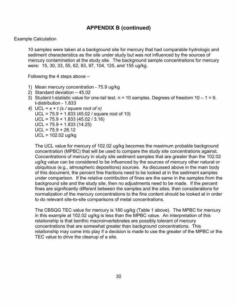
30

APPENDIX B (continued)

Example Calculation

10 samples were taken at a background site for mercury that had comparable hydrologic andsediment characteristics as the site under study but was not influenced by the sources ofmercury contamination at the study site. The background sample concentrations for mercurywere: 15, 30, 33, 55, 62, 83, 97, 104, 125, and 155 ug/kg.

Following the 4 steps above –

1) Mean mercury concentration - 75.9 ug/kg2) Standard deviation – 45.023) Student t-statistic value for one-tail test. n = 10 samples. Degrees of freedom 10 – 1 = 9.

t-distribution - 1.8334) UCL = x + t (s / square root of n)

UCL = 75.9 + 1.833 (45.02 / square root of 10)UCL = 75.9 + 1.833 (45.02 / 3.16)UCL = 75.9 + 1.833 (14.25)UCL = 75.9 + 26.12UCL = 102.02 ug/kg

The UCL value for mercury of 102.02 ug/kg becomes the maximum probable backgroundconcentration (MPBC) that will be used to compare the study site concentrations against.Concentrations of mercury in study site sediment samples that are greater than the 102.02ug/kg value can be considered to be influenced by the sources of mercury other natural orubiquitous (e.g., atmospheric depositions) sources. As discussed above in the main bodyof this document, the percent fine fractions need to be looked at in the sediment samplesunder comparison. If the relative contribution of fines are the same in the samples from thebackground site and the study site, then no adjustments need to be made. If the percentfines are significantly different between the samples and the sites, then considerations fornormalization of the mercury concentrations to the fine content should be looked at in orderto do relevant site-to-site comparisons of metal concentrations.

The CBSQG TEC value for mercury is 180 ug/kg (Table 1 above). The MPBC for mercuryin this example at 102.02 ug/kg is less than the MPBC value. An interpretation of thisrelationship is that benthic macroinvertebrates are possibly tolerant of mercuryconcentrations that are somewhat greater than background concentrations. Thisrelationship may come into play if a decision is made to use the greater of the MPBC or theTEC value to drive the cleanup of a site.

31

An example of what fewer background samples would mean to the resulting MPBC valuecan be seen by the following example using only 4 of the sample results for mercury –30. 62, 104, and 155 ug/kg.

1) Mean mercury concentration – 87.8ug/kg2) Standard deviation – 54.113) Student t-statistic value for one-tail test for n = 4 samples. Degrees of freedom 4 – 1 = 3

t-distribution – 2.353 UCL = x + t (s / square root of n)

UCL = 87.8 + 2.353 (54.11 / square root of 4)UCL = 87.8 + 2.353 (54.11 / 2)UCL = 87.8 + 2.353 (27.06)UCL = 87.8 + 63.7UCL = 151.5 ug/kg

32

APPENDIX CNotes on Dioxins and Furans

• Polychlorinated dibenzo-p-dioxins and dibenzofurans are ubiquitous contaminants, primarily from combustionsources. Background concentrations are normally in the range 0.15 - 2.5 pg TCDD-EQ/g Sediment.

• There are concerns with the other 2,3,7,8-substituted congeners beside 2,3,7,8-TCDD and TCDF. There is a need torequest that all 17 - 2,3,7,8 substituted congeners be analyzed for. Analytical costs are high. To do an adequateenvironmental assessment, detection levels for 2,3,7,8-TCDD need to be at the single digit pg/g level.

• Dioxins and furans are not produced commercially but are unintended by-products from various chemicalmanufacturing and other sources.

• Dioxins and furans are found in discharges from wood treatment facilities that use pentachlorophenol, kraft pulp mills,and chemical manufacturing plants that produced pentachlorophenol, trichlorophenol, and the pesticides 2,4-D and2,4,5-T. Also, if a water body has a history of aquatic applications of the herbicide Silvex, residual dioxins and furansmay be present

• For some perspective, the department's landspreading program for paper mill sludges sets limits for spreading basedon land uses - Silviculture - 10 pg/g; Agriculture - 1.2 pg/g; Grazing - 0.5 pg/g.

• Examples of high levels of dioxins/furans at Wisconsin sediment sites include - Crawford Creek - discharge from woodtreatment facility that used pentachlorophenol - 5,500 pg TCDD-EQ/g; Military Creek-discharge from wood treatmentfacility that used pentachlorophenol– 2,500 pgTCDD-EQ/g; Fox River - paper mill discharges - 21 - 441 pg TCDD-EQ/ g; and Wisconsin River - paper mill discharges - 31 - 78 pg TCDD-EQ / g.

• The recommendation is that dioxin and furan analysis only be done where there is a demonstrated need given theidentification of possible historical sources at a site.

• The different 2,3,7,8 – substituted dioxins and furans have toxic equivalency factors (TEF) assigned to them relativeto their toxicity compared to 2,3,7,8-TCDD. The table below provides a method to calculate the summed TCDDequivalent concentration for all the substituted forms in a sample.

2,3,7,8 - Substituted Dioxin and Furan Congeners

Worksheet For Calculating2,3,7,8-TCDD Equivalent

Concentrations

SedimentConcentration

pg/g (ppt) dry weight

ToxicEquivalency Factors

(TEF)(Equivalency to2,3,7,8-TCDD)

pg/g x TEF =Toxic Equivalency

to 2,3,7,8-TCDDOr TCDD-EQ

Dioxins2,3,7,8-TetraCDD 1.01,2,3,7,8-PentaCDD 0.51,2,3,4,7,8-HexaCDD 0.11,2,3,6,7,8-HexaCDD 0.11,2,3,7,8,9-HexaCDD 0.11,2,3,4,6,7,8-HeptaCDD 0.01OctaCDD 0.001

Furans2,3,7,8-TetraCDF 0.12,3,4,7,8-PentaCDF 0.51,2,3,7,8-PentaCDF 0.051,2,3,4,7,8-HexaCDF 0.11,2,3,6,7,8-HexaCDF 0.12,3,4,6,7,8-HexaCDF 0.11,2,3,7,8,9-HexaCDF 0.11,2,3,4,6,7,8-HeptaCDF 0.011,2,3,4,7,8,9-HeptaCDF 0.01OctaCDF 0.001

Sum of TCDD-EQ of Individual Substituted Dioxin and Furan Congeners(___pg TCDD-EQ / kg sediment) =

33

APPENDIX D

Dry Weight Sediment Concentrations of Organic Compounds Normalized to 1%TOC for Comparison with CBSQGs and Grain Size Normalizations of Metals for

Site-to-Site ComparisonsSample Site: Example Calculations

(Request a copy of Excel Spreadsheet)

Sample Description:Date:

ug/g = ppm = mg/kgng/g = ppb = ug/kg

TOC reported as mg/kg ÷ 10,000 = % TOCBulk Chemistry

Parameter Concen-tration Units % TOC in

SampleTOC 25,000 mg/kg 2.5%

Dry Wt. Concentration ÷ TOC expressed as a % = Concentration Normalized to 1% TOC

PAHs Dry WeightConcentration

Normalized to 1% TOC forComparison With CBSQG Values

Acenapthene 3.2 ug/kg 1.3 ug/kg @ 1% TOCAcenaphthylene 5.9 ug/kg 2.4 ug/kg @ 1% TOC

Anthracene 57.2 ug/kg 22.9 ug/kg @ 1% TOCFluorene 77.4 ug/kg 30.9 ug/kg @ 1% TOC

Napthalene 176 ug/kg 70.4 ug/kg @ 1% TOC2-Methylnapthalene 20.2 ug/kg 8.1 ug/kg @ 1% TOC

Phenanthrene 204 ug/kg 81.6 ug/kg @ 1% TOCBenzo(a)anthracene 108 ug/kg 43.2 ug/kg @ 1% TOC

Benzo(a)pyrene 150 ug/kg 60 ug/kg @ 1% TOCBenzo(e)pyrene 150 ug/kg 60 ug/kg @ 1% TOC

Benzo(b)fluoranthene 240 ug/kg 96 ug/kg @ 1% TOCBenzo(k)fluoranthene 240 ug/kg 96 ug/kg @ 1% TOCBenzo(g,h,i)perylene 170 ug/kg 68 ug/kg @ 1% TOC

Chrysene 166 ug/kg 66.4 ug/kg @ 1% TOCDibenz(a,h)anthracene 33 ug/kg 13.2 ug/kg @ 1% TOC

Fluoranthene 423 ug/kg 169.2 ug/kg @ 1% TOCIndeno(1,2,3-c,d)pyrene 200 ug/kg 80 ug/kg @ 1% TOC

Pyrene 195 ug/kg 78 ug/kg @ 1% TOC

Total PAHs(sum of 18 PAHs listed above)

2618.9 ug/kg 1,047.6 ug/kg @ 1% TOC

34

PCB and Pesticides Concen-tration Units

Normalized to 1% TOC forComparison With CBSQG Values

PCBs (total) 60 ug/kg 21 ug/kg @ 1% TOCAldrin 2 ug/kg 0.8 ug/kg @ 1% TOCBHC 3 ug/kg 1.2 ug/kg @ 1% TOC

a-BHC 6 ug/kg 2.4 ug/kg @ 1% TOCB-BHC 5 ug/kg 2 ug/kg @ 1% TOC

Y-BHC (lindane) 3 ug/kg 1.2 ug/kg @ 1% TOCChlordane 3.2 ug/kg 1.3 ug/kg @ 1% TOC

Dieldrin 1.9 ug/kg 0.8 ug/kg @ 1% TOCSum pp DDD 4.9 ug/kg 1.9 ug/kg @ 1% TOCSum pp DDE 3.2 ug/kg 1.3 ug/kg @ 1% TOC

Sum op + pp DDT 4.2 ug/kg 1.7 ug/kg @ 1% TOCSum of DDT and metabolites 5.3 ug/kg 2.1 ug/kg @ 1% TOC

Endrin 3 ug/kg 1.2 ug/kg @ 1% TOCHeptachlor Epoxide 2.5 ug/kg 1.0 ug/kg @ 1% TOC

Mirex 7 ug/kg 2.8 ug/kg @ 1% TOCToxaphene 1 ug/kg 0.4 ug/kg @ 1% TOC

Metals % sand 50 %

% silt 25 %Particle Size% clay 25 %

Fine FractionSilt + Clay = 50% or 0.50

Dry Wt. Concentration ÷ Fines expressed as decimal fraction = Normalized to Fine Concentration

MetalsDry Weight

Concentration (Compare with CBSQGs

Normalized to Fine Concentration forSite-to-site Comparisons( Not for

Comparison with CBSQGs)Antimony 2 mg/kg 4 mg/kg finesArsenic 9.8 mg/kg 19.6 mg/kg fines

Cadmium 0.99 mg/kg 1.98 mg/kg finesChromium 43 mg/kg 86 mg/kg fines

Copper 32 mg/kg 64 mg/kg finesIron 20,000 mg/kg 40,000 mg/kg finesLead 36 mg/kg 72 mg/kg fines

Manganese 460 mg/kg 920 mg/kg finesMercury 0.18 mg/kg 0.36 mg/kg finesNickel 23 mg/kg 46 mg/kg finesSilver 1.6 mg/kg 3.2 mg/kg finesZinc 120 mg/kg 240 mg/kg fines

35

Appendix E

Identification of Contamination that Leads to Adverse Effects

Contamination of a chemical nature (i.e., a contaminant) is a substance or substances (either organicor inorganic) that are present in environmental media such as sediments or surface waters that arefound above levels that would normally occur. What is normal or background for metals or nutrients(e.g., nitrogen, phosphorus) would be those metals and nutrients at levels that originate from thenatural soil types and the geochemical components of the watershed. What is normal for naturalorganic compounds would generally be those compounds that originate from natural watershed-source vegetative or animal matter that are deposited on the bottoms of lakes, streams, andwetlands. Organic chemicals manufactured by humans and released to the environment by variousmechanisms generally do not have counterparts found in nature and therefore any levels found inenvironmental media would be considered potential contamination. Many manufactured organiccompounds may be found ubiquitously at low levels in sediments especially in urban areas. ,

Environmental concerns arise when the level of contamination (concentration of contaminants) insurface waters and sediments leads to observed and measurable effects to biological receptors, suchas 1) chronic and/or acute toxicity (the contaminant becomes a toxicant) to aquatic receptors (forexample directly to aquatic life such as bottom inhabiting macroinvertebrates), and/or 2) concernsabout humans and wildlife that are upper food chain organisms who may become exposed to harmfullevels of contaminants principally through consumption of aquatic organisms that havebioaccumulated the contaminants. For the toxicity to aquatic organisms to be realized and/orunacceptable levels of bioaccumulation to occur, the aquatic organism has to (a) be exposed to thepotential toxicant in its habitat, (b) the potential toxicant has to be in a form available for uptake, and(c) the uptake or dose of the contaminant has to be at a level that causes toxicity to the particularexposed receptor or results in levels of bioaccumulation that may pose risks to humans and/or wildlifewho consume the exposed receptor as food.

Elevated levels of nutrients can lead to eutrophication of water bodies and production and depositionplant materials in sediments that deplete oxygen levels in the water body when they decompose.Addition and decomposition of natural organic matter and anthropogenic-added organic matter insediments can lead to production of hydrogen sulfide and ammonia levels that may be detrimental tobenthic organisms.

Wisconsin Department of Natural Resources - WI.gov

Documents

Transcript of Wisconsin Department of Natural Resources - WI.gov