Centre for Research and Analysis of Migration Department of Economics, University College London Drayton House, 30 Gordon Street, London WC1H 0AX

Discussion Paper Series

CDP No 15/07

What Explains the Wealth Gap Between Immigrants and the New Zealand Born?

John Gibson, Trinh Le, Steven Stillman

Centre for Research and Analysis of Migration Department of Economics, Drayton House, 30 Gordon Street, London WC1H 0AX

Telephone Number: +44 (0)20 7679 5888 Facsimile Number: +44 (0)20 7916 2775

CReAM Discussion Paper No 15/07

What Explains the Wealth Gap Between Immigrants and the New Zealand Born?

John Gibson, Trinh Le, Steven Stillman *

* Motu Economic and Public Policy Research

New Zealand.

Non-Technical Abstract

Immigrants are typically found to have less wealth and hold it in different forms than the native born. These differences may affect both the economic assimilation of immigrants and overall portfolio allocation when immigrants are a large share of the population, as in New Zealand. In this paper, data from the 2001 Household Savings Survey are used to examine wealth differences between immigrants and the New Zealand-born. Differences in the allocation of portfolios between housing and other forms of wealth are described. Unconditional and conditional wealth quantiles are examined using parametric models. Semiparametric methods are used to decompose differences in net worth at different parts of the wealth distribution into the part due to differences in characteristics and the part due to differences in the returns to characteristics. Keywords: Immigration, Portfolios, Semiparametric Decomposition, Wealth JEL-Code: D31, G11, J15

i

Author contact details John Gibson University of Waikato and Motu Economic and Public Policy Research Email: jkgibson@mngt.waikato.ac.nz Trinh Le New Zealand Institute of Economic ResearchEmail: Trinh.Le@nzier.org.nz Steven Stillman Motu Economic and Public Policy Research Email: stillman@motu.org.nz

Acknowledgements We are grateful to participants at the NZAE session on migration and especially Deborah Cobb-Clark for helpful comments, and to Grant Scobie who has helped develop the broad research program on household wealth of which this paper is a part. The financial support and logistical support of the Office of the Retirement Commissioner and the New Zealand Treasury is gratefully acknowledged. Access to the data used in this study was provided by Statistics New Zealand in a secure environment designed to give effect to the confidentiality provisions of the Statistics Act, 1975. The results in this study and any errors contained therein are those of the authors, not Statistics New Zealand.

Motu Economic and Public Policy Research PO Box 24390 Wellington New Zealand Email info@motu.org.nz Telephone +64-4-939-4250 Website www.motu.org.nz

© 2007 Motu Economic and Public Policy Research Trust. All rights reserved. No portion of this paper may be reproduced without permission of the authors. Motu Working Papers are research materials circulated by their authors for purposes of information and discussion. They have not necessarily undergone formal peer review or editorial treatment. ISSN 1176-2667 (print) ISSN 1177-9047 (Online)

1

I) Introduction

New Zealand has a large foreign-born population with almost one quarter of residents born

abroad. In other countries, immigrants are often found to have less wealth and to hold it in

different forms than the native born (Cobb-Clark and Hildebrand 2006a). These differences

can affect the economic assimilation of immigrants and aggregate portfolio allocation,

especially when immigrants are a large share of the population, as in New Zealand. The

wealth holdings of immigrants should be especially of interest in New Zealand, where even

the Reserve Bank has suggested a need to change the management of immigration because of

the apparent impact of immigration on house price inflation.1

A number of recent papers have examined labour market outcomes and incomes for

immigrants compared with those of the New Zealand-born (Boyd 2003; Hartog and

Winkelmann 2003; Macpherson et al 2000; New Zealand Immigration Service 2003; Poot

1993; Winkelmann and Winkelmann 1998; Winkelmann 2000). However, there has been no

such analysis of how the wealth of immigrants compares to the wealth of other New

Zealanders.2 In this paper, we use data from the 2001 Household Savings Survey to examine

wealth differences between different nativity groups.

We explore three related questions. First, how large are the differences in wealth

between immigrants and the NZ-born? Second, to what factors might any differences be

attributed? Third, if immigrants and non-immigrants were to be assigned the same personal

characteristics (age, education, income, etc.) would there be any remaining “unexplained”

differences in wealth which might be attributed to nativity? To answer these questions, we

1 “Reserve Bank suggests house-sales tax” The New Zealand Herald June 18, 2007 quotes from the Reserve Bank’s submission to a parliamentary inquiry on housing affordability that “the management of immigration … may need to be tempered in future in light of migration’s apparent sustained impact on the level of house prices”. 2 This lack of analysis includes the comprehensive report by Statistics New Zealand (2002a and b) on the Household Savings Survey, which considered how net worth varied with age, gender, ethnicity, occupation and employment status, and income level and sources, but not by nativity or immigrant status.

2

use two techniques, quantile regression and a semi-parametric decomposition, that allow us to

examine differences across the entire wealth distribution, rather than at just a single point like

the mean. We use quantile regression to gauge the extent to which several covariates related

to individual and locational characteristics explain nativity differences at various wealth

quantiles. We use a semi-parametric decomposition to explore the contribution of age,

education, inheritances and incomes to wealth differences by nativity status with few

parametric assumptions.

There are at least two reasons why differences in wealth are of interest. First, wealth may

be distributed quite differently from income, so an over-emphasis on studies of income may

disguise some of the other differences that exist. Wealth is an important measure of economic

well-being whose effects are not necessarily captured by studies that focus on earnings or

income. As Gittleman and Wolff (2004) point out:

“Two families with the same incomes but widely different wealth levels are not identical. The wealthier family is likely to be able to better provide for the educational and health needs of its children, to be living in a neighbourhood characterised by more amenities and lower levels of crime, to have greater resources that can be called upon in times of economic hardship, and to have more influence in political life.” (p.194).

The second reason why wealth is of interest is that differences in wealth may contribute

to the intergenerational transmission of disadvantage and to a slowing of immigrant

assimilation. Differences in wealth are likely to be key determinants of educational

investments. Imperfect capital markets could cause this, with children from less wealthy

families facing higher discount rates and leaving school when marginal investments are still

highly productive (Gibson 1998).

The variety of immigrant selection policies used around the world mean that findings

from other countries may have little applicability to New Zealand, providing further

motivation for examining wealth differences between immigrants and the New Zealand-born.

For example, in Canada which, similar to New Zealand, has skill-selective immigration,

3

Zhang (2003) finds that among married families (single individuals), immigrants have higher

wealth than their Canadian-born counterparts from the 40th to 90th (55th to 95th) percentiles

of the distribution. But in the United States, which has much more open immigration, Cobb-

Clark and Hildebrand (2006b) find that the median wealth level of US-born couples (singles)

is 2.5 (3) times the median wealth level of foreign-born couples, placing the median foreign-

born couple between the 30-35th percentile of the native-born wealth distribution. As Bauer

et al. (2007) note, there appears to be substantial cross-national disparity in the economic

well-being of immigrant and native families that is largely consistent with domestic labor

markets and the selection policies used to shape the nature of the immigration flow.

II) Data

Household Saving Survey

We use data from the Household Saving Survey (HSS) to examine wealth differences

between different nativity groups. This survey of the assets, liabilities, personal

characteristics and income of New Zealand residents was conducted in 2001 by Statistics NZ

for the Office of the Retirement Commissioner (Statistics New Zealand 2002a and 2002b). In

terms of surveys fielded in other countries, it is most comparable in coverage and

methodology to the Canadian Survey of Financial Security (Statistics Canada 2001).

The HSS covered individuals age 18 and above living in private dwellings and usually

resident in New Zealand. The survey population covered about 98% of the resident adult

population. A stratified sample of 6,600 households (in 675 primary sampling units (PSUs))

and a Maori booster sample were combined to give a total achieved sample size of 5,374

households.3 The overall response rate was 74%.4 One person from those qualifying in a

3 The stratification scheme used location, ethnicity, education and employment characteristics. The 675 PSUs are out of the 19,000 in all of New Zealand. On average, PSUs in New Zealand contain about 70 dwellings. 4 The analyses reported below use sampling weights to adjust for different sampling probabilities and where possible take account of the multi-stage sample selection when calculating standard errors and hypothesis tests.

4

selected household was chosen at random and information was collected from and about that

individual. In the case where they had a partner, information was collected for the couple,

i.e., where the respondent and his/her partner were living in the same household the couple

was interviewed as a single unit. Thus, we have data on uncoupled individuals (n=2,392) and

on couples (n=2,982), but not for households or families. We refer to uncoupled individuals

as ‘singles’ throughout the remainder of the paper. We present all results separately for

singles and couples, because previous work has shown that the data restrictions needed to

pool these two samples are statistically rejected (Gibson and Scobie 2003).

We restrict our analysis to the sample of singles between age 25 and 75 (n=1,682) and

couples where both partners are in this age range (n=2,565).5 The reason for excluding the

very young and the very old is that selective household formation among the young and both

selective mortality and selective mobility into supported care among the old may bias wealth

estimates since one needed to be living in an independent household to be selected into the

HSS sample.

All individuals in the HSS were asked whether they were born in New Zealand, and if

they were not, the number of years that they had lived in New Zealand. We use this

information to classify singles as being either NZ-born (n=1,498) or migrants (n=184) and

couples as being either both NZ-born (n=1,915), both migrants (n=262) or mixed nativity

(n=388). The distinction between the both-migrant and mixed nativity group may enable us to

better understand the role of marriage and cohabitation in immigrant assimilation.

Throughout the remainder of the paper we refer to these groups as ‘nativity groups’.

5 We also drop 69 singles and 52 couples who either have negative or zero total income or whose main income source is investment income. A major aim of the analysis in this paper is to examine the effect of income on wealth and negative incomes are clearly not good proxies for permanent income. For incomes that are mainly from investment, the causality goes from wealth to income rather than the reverse.

5

Our main outcome variable throughout the paper is total net worth (also referred to as

wealth below), which is defined as the difference between total asset and liabilities. The

assets covered by the survey include residential, investment and overseas property, farms,

businesses, life insurance, bank deposits, positive credit card balances, shares and managed

funds, money owed, motor vehicles, cash, collectibles, and holdings in personal

superannuation and defined contribution schemes. The liabilities include property mortgages,

student loans, negative credit card balances and other bank debt.

Descriptive Results

We begin by examining the raw differences in net worth between nativity groups for singles

and couples in the HSS. These results are presented in Table 1. Panel A displays the mean

and median wealth for each nativity group for both singles and couples and Panel B displays

the difference in mean and median wealth between migrants and the NZ-born. Among

singles, migrants actually have both higher mean and median wealth than the NZ-born,

although neither difference is statistically significant. On the other hand, couples where both

partners are migrants have significantly lower mean and median wealth than couples where

both partners are NZ-born. This gap is fairly large, with migrant couples having $141,500

lower mean wealth and $74,000 lower median wealth than NZ-born couples. Mixed nativity

couples have slightly lower mean wealth than NZ-born couples, but this difference is not

statistically significant, and have almost identical median wealth.

We next examine how the different components of wealth vary across nativity groups. In

particular, we examine differences in homeownership, equity in one’s primary dwelling,

equity in overseas properties, total property equity, net assets in trusts, total value of farms,

total value of businesses, total bank assets, total bank debts, total financial assets and

superannuation. These results are presented in Table 2. For singles, consistent with the

evidence on total net worth, migrants are more likely to own their home than the NZ-born

6

(51% versus 41%), have greater equity in their primary dwelling and in all properties.

Migrants have slightly more wealth in trusts and in businesses, but substantially less wealth

in farms. Both nativity groups have similar low levels of superannuation and migrants have

less net bank assets and financial assets. Overall, on average, single migrants hold nearly

two-thirds of their wealth in property compared to less than one-half for the NZ-born.

Turning to couples, NZ-born and mixed nativity couples are more likely to own their

home than migrant couples, with 67% of NZ-born, 71% of mixed nativity couples and only

56% of migrant couples owning their own home. However, average primary home and total

property equity are similar across the groups. Interestingly, nearly 8% of migrant couples’

property equity is from overseas properties. Migrant couples have much less wealth in trusts,

farms and businesses than either mixed or NZ-born couples and mixed couples have less

wealth in farms and businesses than NZ-born couples. Migrant couples have much lower

superannuation savings than mixed nativity and NZ-born couples and less financial assets,

but greater net bank assets. Overall, on average, NZ-born couples hold one-third of their

wealth in property, compared with 40% for mixed nativity couples, and nearly one-half for

migrant couples.

It is also useful to examine how wealth differences between nativity groups vary at

particular points in the wealth distribution. We use two approaches to do this: non-parametric

kernel density estimation and quantile regressions. Figures 1 and 2 present non-parametric

kernel density estimates of the wealth distribution by nativity, for singles and couples,

respectively. These estimated densities are from an Epanechnikov kernel in the adaptive

kernel density procedure of Van Kerm (2003):

7

∑ ⎟⎟⎠

⎞⎜⎜⎝

⎛ −

∑=

=

=

n

i i

i

i

in

ii

hxx

Khw

wxf

1

1

)(1)(ˆ (1)

Unlike kernel densities with fixed bandwidths, h, the adaptive kernel, allows the

bandwidth, hi to vary inversely with the square root of the underlying density function at the

sample points: ( ) .)(; 5.0iiii xfGhh == λλ This varying bandwidth is particularly useful for

long-tailed distributions because a fixed bandwidth may undersmooth (i.e. put too much

weight on individual data points) in areas with only sparse observations. In contrast, the

variable bandwidth gives greater precision in areas where data are abundant and greater

smoothness in areas where data are sparse.

Examining Figure 1, we see that single migrants are more likely than NZ-born singles to

have wealth between −$35,000 and −$15,000 and between $15,000 and $160,000. Above

$160,000, migrants and the NZ-born have a similar wealth distribution. Overall, the most

noticeable difference in these distributions is that fewer migrants have wealth between

−$8,000 and $10,000, which is the amount of wealth that the majority of NZ-born single

have. Turning to Figure 2, migrant couples are more likely to have wealth below $60,000

than NZ-born couples and are less likely to have wealth above that amount. Mixed nativity

couples have a wealth distribution that looks similar to the distribution for NZ-born couples,

but instead of having a density that peaks sharply around $25,000, mixed nativity couples

have a density that plateaus at between $25,000 and $150,000.

Another way of comparing these two distributions is to calculate quantile regressions at

various points of the wealth distribution. The advantages of this approach are discussed by

Zhang (2003) and include: (1) a wealth gap can be generated at any point of the distribution,

not just a single measure such as the mean wealth gap; (2) the method is semi-parametric so

that no distributional assumptions on the dependent variable are needed; (3) the estimator is

less sensitive to outliers; and (4) tests of the statistical significance of the gaps can easily be

8

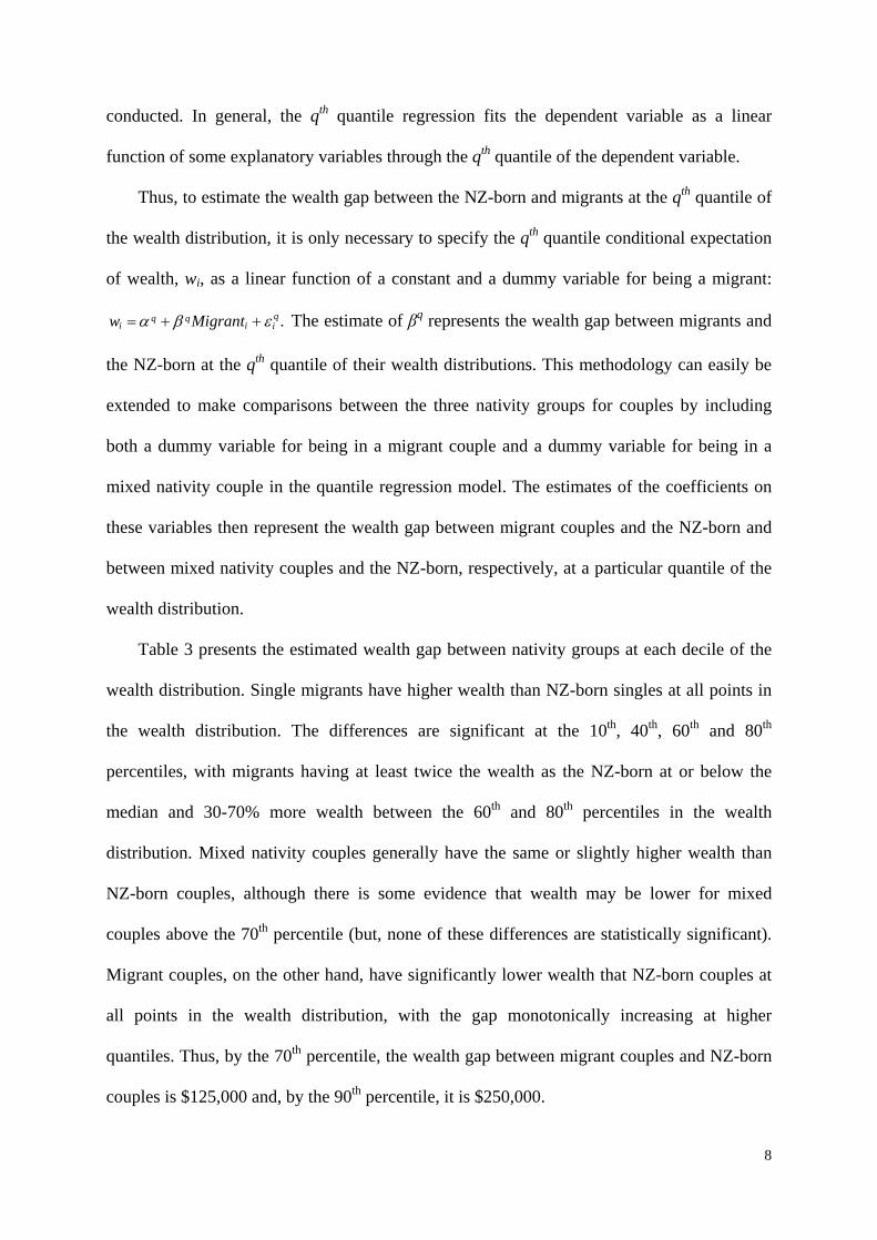
conducted. In general, the qth quantile regression fits the dependent variable as a linear

function of some explanatory variables through the qth quantile of the dependent variable.

Thus, to estimate the wealth gap between the NZ-born and migrants at the qth quantile of

the wealth distribution, it is only necessary to specify the qth quantile conditional expectation

of wealth, wi, as a linear function of a constant and a dummy variable for being a migrant:

.qq qi i iw Migrantα β ε= + + The estimate of βq represents the wealth gap between migrants and

the NZ-born at the qth quantile of their wealth distributions. This methodology can easily be

extended to make comparisons between the three nativity groups for couples by including

both a dummy variable for being in a migrant couple and a dummy variable for being in a

mixed nativity couple in the quantile regression model. The estimates of the coefficients on

these variables then represent the wealth gap between migrant couples and the NZ-born and

between mixed nativity couples and the NZ-born, respectively, at a particular quantile of the

wealth distribution.

Table 3 presents the estimated wealth gap between nativity groups at each decile of the

wealth distribution. Single migrants have higher wealth than NZ-born singles at all points in

the wealth distribution. The differences are significant at the 10th, 40th, 60th and 80th

percentiles, with migrants having at least twice the wealth as the NZ-born at or below the

median and 30-70% more wealth between the 60th and 80th percentiles in the wealth

distribution. Mixed nativity couples generally have the same or slightly higher wealth than

NZ-born couples, although there is some evidence that wealth may be lower for mixed

couples above the 70th percentile (but, none of these differences are statistically significant).

Migrant couples, on the other hand, have significantly lower wealth that NZ-born couples at

all points in the wealth distribution, with the gap monotonically increasing at higher

quantiles. Thus, by the 70th percentile, the wealth gap between migrant couples and NZ-born

couples is $125,000 and, by the 90th percentile, it is $250,000.

9

These wealth gaps can be contrasted with more widely studied income gaps. In Table 4,

we present the estimated income gap between nativity groups at each decile of the income

distributions estimated using the HSS data. Singles migrants have similar incomes as NZ-

born singles at all points in the income distribution. Combined with the above evidence, this

may suggest that, given a particular level of income, single migrants save more than NZ-born

singles. Interestingly, migrant couples only have lower incomes than NZ-born couples in the

bottom half of the income distribution. So, in contrast to the singles, this suggests that, given

a particular level of income, higher income NZ-born couples may save more than migrant

couples.6 As with the wealth distribution, the income distribution for mixed nativity couples

is statistically indistinguishable from that for NZ-born couples.

The results in the previous tables do not control for differences between the groups in

characteristics, such as age, education and income. As can be seen in Table 5, single migrants

are older and more educated than NZ-born singles. Migrant and mixed nativity couples are of

similar ages as NZ-born couples, but like singles, are more educated. Migrant couples are

also significantly less likely to have ever received a large inheritance than both NZ-born and

mixed nativity couples. Since these characteristics are related to the accumulation of wealth,

if we do not control for these factors, we are unable to isolate the effect of nativity on wealth

accumulation. In the next section, we use two methods to control for other factors that may

explain nativity wealth differences in an attempt to isolate the unexplained portion of the

wealth gap between nativity groups.

6 The available data do not allow either the timing or form of any saving differences to be examined. However, if immigration does raise house prices it would enable “passive” savings by the NZ-born who were more likely to be incumbent homeowners while more recently arrived immigrants may face higher entry prices into the housing market.

10

III) Multivariate Estimates

Parametric Models

As indicated in Table 3, we find some evidence that migrants and the NZ-born have different

levels of wealth and that these differences are more pronounced than the observed differences

in the income distribution for these groups. However, income is only one factor which might

explain the pattern of wealth accumulation. A snapshot of wealth, such as that provided by

the HSS, is an encapsulation of many forces that have shaped peoples lives and the policies

that have influenced their decisions up to the time of the survey. Ideally, we would like to

measure all of these factors. While that is not possible, the HSS does contain a rich set of

information on which we can draw.

We begin by estimating quantile regression models that allow us to describe how

particular covariates are correlated with wealth and to gauge the extent to which these

covariates explain nativity wealth differences at various wealth quantiles. These models

control for many factors that might reasonably be considered as influencing the level of net

wealth, including demographic characteristics, education, location, inheritances and income.

While some of these variables may be chosen with lifetime wealth objectives in mind, we

ignore any modelling of their endogeneity and treat them as predetermined, at least by the

time the HSS observed respondents. Thus, these are purely descriptive regression models.

However, the results show whether differences in wealth across nativity groups persist once

we control for the relationship between other covariates and the wealth distribution.

Semi-Parametric Decomposition

We next use a semi-parametric approach proposed by DiNardo, Fortin and Lemieux (1996)

for wage decompositions to examine what the distribution of wealth for migrants would be if

11

they had the characteristics of the NZ-born.7 This approach requires fewer parametric

assumptions than the quantile regression approach, but with a few trade-offs that we discuss

below. Given the joint distribution of wealth, w, and characteristics, x, the marginal

distribution of wealth for an observation with characteristics x can be written as

∫= dxxhxwfwg )()|()( .8 The observed density of wealth for an observation that is a migrant

(m=1) is:

( | 1) ( | ) ( | 1)mg w m f w x h x m dx= = =∫ (2)

The counterfactual density of wealth for a migrant observation, if it were given the

characteristics of the NZ-born (m=0) can be defined as:

( ) ( | ) ( | 0)( | ) ( | 1) ( )

m mCF

mg w f w x h x m dx

f w x h x m x dxψ= == =∫∫

(3)

which is based on the density of “re-weighted” observations for migrants.

The re-weighting factor is the ratio of two conditional densities:

( | 0)( ) .( | 1)

h x mxh x m

ψ ==

= (4)

By using Bayes rule (for the jth nativity group):

( | ) ( )( | )( )

prob m j x h xh x m jprob m j

== =

= (5)

the re-weighting factor can be expressed as:

7 This approach is also used by Zhang (2003) to examine nativity wealth gaps in Canada and by Bauer et al. (2007) to compare the nativity wealth gap in the US, Australia, and Germany, and by Cobb-Clark and Hildebrand (2006b) to examine ethnic wealth gaps in the US. 8 To translate this to the more familiar parametric approach of Oaxaca and Ransom (1994), intuitively, the conditional expectation, f( ) is similar to an estimated regression line and the marginal density of x, h( ) is analogous to the vector of characteristics.

12

( 1) ( 0 | )( ) .( 0) ( 1| )

prob m prob m xxprob m prob m x

ψ = ==

= = (6)

The first part of the re-weighting factor is the ratio of migrants to NZ-born in the population.9

The second part is the ratio of two conditional probabilities, each of which can come from a

(survey-weighted) logit regression of nativity status on explanatory variables, x.

With the counterfactual density from equation (3), one decomposition of the migrant-

NZ-born wealth gap is based on:

unexplained explained

( ) ( ) ( ) ( ) ( ) ( ).m mnz m nz mCF CFg w g w g w g w g w g w− = − + −

1442443 1442443 (7)

However, it is also possible to construct another counterfactual density, by giving the NZ-

born the characteristics of migrants:

1( ) ( | ) ( | 1)

( | ) ( | 0) ( )nz nzCF

nzg w f w x h x m dx

f w x h x m x dxψ −= == =∫∫

(8)

This alternative counterfactual density gives the decomposition:

explained unexplained

( ) ( ) ( ) ( ) ( ) ( ).nz nznz m nz mCF CFg w g w g w g w g w g w− = − + −

1442443 1442443 (9)

It is sometimes argued that equation (9), which uses the counterfactual density of wealth

for the majority group given the characteristics of the minority group, is the more reliable

decomposition (Barsky et al. 2002). For example, Cobb-Clark and Hildebrand (2006b)

examine the wealth gap between Mexican-Americans and Whites in the US, where Mexican-

Americans have a much narrower observed earnings distribution than Whites. Hence, re-

weighting the wealth distribution of Mexican-Americans would involve extrapolating the

conditional expected wealth function for this group into regions of the White earnings

distribution where these group members are virtually nonexistent. Bauer et al. (2007) use a

9 This is calculated using the survey weights. Note, that when estimating the counterfactual density, the product of the original survey weight and the re-weighting factor is used.

13

similar argument to justify focusing on counterfactual distributions of immigrant wealth

created by reweighting the wealth distribution of native households.

However, in the current data there is less reason to favour one decomposition over the

other. Figures 3 and 4 present non-parametric kernel density estimates of the income

distribution by nativity for singles and couples, respectively. Figure 3 shows that the income

distribution for singles is nearly identical for migrants and the NZ-born, while Figure 4 shows

that, while the density of migrant couple incomes is somewhat to the left of that for the NZ-

born, there is a very considerable overlap for all three nativity groups among couples. There

is also considerable overlap in other factors, such as age. Thus, as in Zhang (2003), we

present results from both versions of the decomposition.

This methodology can easily be extended to decompose the wealth gap between the

three nativity groups defined for couples (NZ-born, both-migrant, mixed), by estimating the

conditional probabilities using a (survey-weighted) multinomial logit regression model of

nativity status on the explanatory variables, x. For both singles and couples, we decompose

the nativity wealth gap into four separate vectors of wealth determinants: 1) a quadratic in the

age of the respondent and partner (if a couple); 2) the number of years of school and post-

school education of the respondent and partner (if a couple); 3) whether the single person or

either member of the couple has ever received an inheritance of $10,000 or more and the

amount of the inheritance;10 and 4) a quadratic in the income of the single person or couple.

One trade-off with using this semi-parametric approach is that only a limited set of separate

vectors of wealth determinants can be considered because the number of unique orderings of

10 Previous papers on the immigrant wealth gap in other countries have not examined the role that inheritances play in explaining wealth differences. Yet, this may emerge as an important factor because bequests, especially of parental dwellings, may be more conveniently transferred when the parents and adult children live in the same country. Inheritances are certainly important for explaining other wealth gaps; for example, Menchik and Jianakoplos (1997) find that differences in inheritances explain a significant part of Black-White wealth gap in the US. Thus, we examine whether differences in the availability of inheritances or how these are used by different nativity groups explain differences in wealth across nativity groups.

14

these vectors increases at a squared rate whenever a new vector is added.11 We choose these

four vectors because our descriptive results suggest that they are the most important factors

influencing an individuals or couples position in the wealth distribution.

In addition to the questions of which decomposition to use and which characteristics to

control for, the other important modelling question concerns the order in which each

explanatory factor is considered. For example, the measured effect of age differences by

nativity in shifting the counterfactual wealth distribution for migrants will depend on which

factors had already been accounted for before age was considered. To deal with this issue we

follow Shorrocks (1999), Hyslop and Maré (2003), Cobb-Clark and Hildebrand (2006b) and

Bauer et al. (2007) and use all possible orderings of the factors, presenting results averaged

across all orderings. For example, consider a three factor decomposition using age, education

and inheritances. We would initially consider age alone. We would then use age and

inheritances and calculate the change in the explained wealth gap due to age by comparing

this with a decomposition with just inheritances. We would then use age and education, once

again comparing with a decomposition that uses only education. Finally, we would use age,

inheritances and education and find the marginal effect of age by comparing with a

decomposition that uses just inheritances and education. The reported impact of age

differences on the nativity wealth gap would be the average across these four sets of results.

Results

We present in Table 6 (singles) and Table 7 (couples) the results from estimating quantile

regression models for the 10th, 25th, 50th (median), 75th and 90th percentile pooling nativity

groups and controlling for all of the variables in these tables. Comparing the coefficients on

the nativity groups in each table with the coefficients in Table 3 for models that had no other

11 For example, a 3-factor decomposition has nine unique orderings, while a 4-factor decomposition has 16 unique orderings.

15

covariates shows the extent to which wealth difference are explained by differences in the

included characteristics across nativity groups. For example, the gap between New Zealand-

born singles and single migrants at the 90th percentile of the wealth distribution rises from

$37,000 when no covariates are used to $150,000 once controlling for individual

characteristics and location differences. In other words, the unexplained wealth advantage of

single migrants at the upper-end of the wealth distribution is even larger once adjusting for

differences in their age, education, income, inheritances and location compared to NZ-born

singles.

Turning to the results for couples, the wealth gap between migrant couples and the NZ-

born is generally unaltered by the inclusion of control variables, and hence remains

unexplained, except at the 90th percentile where roughly half of the $250,000 gap is

explained by differences in covariates. On the other hand, once controlling for differences in

covariates, mixed nativity couples appear to have lower levels of wealth than NZ-born

couples at the median and above, even though no wealth gap was apparent for this group at

these quantiles when we do not control for covariates. This occurs because mixed nativity

couples relative to NZ-born couples have characteristics that are associated with having

higher levels of wealth, so the fact that there is no raw wealth gap for this group creates an

unexplained gap when we condition on these characteristics.

Of particular interest, we control for a quadratic in years in New Zealand for migrants in

the quantile regressions, allowing us to judge how wealth accumulation changes with

assimilation (or for different cohorts of migrants since it is not possible to separate these

factors in cross-sectional data). Examining the results for singles, wealth at the 10th (25th)

percentile is increasing in years in NZ until 18 (27) years and then decreasing. On the other

hand, wealth at the 75th (90th) percentile is decreasing in years in NZ until 22 (33) years and

then increasing. There is no relationship between years in NZ and median wealth among

16

single migrants. Interestingly, years in NZ is not significantly related to the wealth of migrant

or mixed nativity couples at any point in the wealth distribution. This may occur because we

have constrained the relationship between years in NZ and wealth to be the same for migrant

couples and mixed nativity couples.

We next turn to the results from the DiNardo, Fortin and Lemieux decomposition. Table

8 presents the results for singles using both counterfactual distributions.12 Once controlling

semi-parametrically for age, education, inheritances and income, there is little evidence that

single migrants have different wealth than comparable NZ-born singles. The only exceptions

are found when we use the characteristics of the NZ-born to generate counterfactual wealth

distributions for migrants. Here, we find a significantly positive residual component at the

10th and 80th percentiles, i.e. controlling for characteristics, migrants still have higher wealth

than the NZ-born at these points in the distribution. We find consistent evidence that the

positive wealth gap for single migrants is almost entirely explained by differences in the age

distribution between these groups. This is true at all points in the wealth distribution and

using either weighting scheme. None of the other covariates explain a significant proportion

of the wealth gap. Overall, these results indicate that the higher wealth observed for single

migrants compared to NZ-born singles occurs because the migrants are more concentrated at

ages where individuals have higher levels of wealth, which is consistent with the descriptive

evidence presented in Table 5. This age effect is less apparent when using the more

parametric quantile regression approach, which shows significant positive wealth gaps at the

75th and 90th percentiles, even when controlling for age.

12 The approach outlined in the previous section allows us to estimate the entire counterfactual wealth distribution. We present results for the decomposition of the estimated wealth gaps between nativity groups at each decile of the wealth distributions. Bootstrapping methods using a normal approximation with 1,000 replications that account for the complex sample design are used to calculate standard errors.

17

Tables 9 and 10 present similar results for migrant couples and mixed nativity couples,

respectively. Now there are three possible decompositions since the characteristics of any of

the three nativity groups can be used to generate counterfactual wealth distributions for the

other two groups. We present all three sets of results. First, in Table 9, we examine the

findings for couples where both partners are migrants. Recall that migrant couples have less

wealth than NZ-born couples at all points in the wealth distribution and these gaps persist

(except at the 10th percentile) even after conditioning on the set of variables in Table 7 when

using the quantile regression approach. However, the semi-parametric approach provides

more nuanced results; most of this gap is unexplained by the different distribution of age,

education, inheritances and income across these groups at the 10-30th percentiles, as well as,

at the 90th percentile, whereas one-half to two-thirds of the gap is generally explained in the

remainder of the wealth distribution. In this part of the distribution (e.g. between the 40th and

80th percentiles), differences in inheritances and in incomes are responsible for about an

equal share of the explained gap. Lesser receipt of inheritances and lower incomes actually

explain most of the wealth gap between migrant couples and NZ-born couples between the

30th and 80th percentiles of the wealth distribution, but age (and to a lesser extent education)

differences between these groups suggest that migrant couples should have higher levels of

wealth, and thus decrease the overall proportion of the wealth gap that is explained at these

points in the distribution.

Next, in Table 10, we examine the findings for mixed nativity couples. Recall that these

couples have a similar unconditional wealth distribution as the NZ-born and this similarity

occurs even after controlling for the variables in Table 7 using the quantile regression

approach, except perhaps at the top-end of the distribution. Using the more flexible, semi-

parametric approach to control for age, education, income and inheritances, there is still little

evidence that mixed nativity couples have different wealth than comparable NZ-born couples.

18

Mixed couples have a negative residual component at the 80th percentile of the wealth

distribution using the first re-weighting scheme and a negative residual at mean of the wealth

distribution using the third re-weighting scheme, meaning that, once counterfactual

characteristics are assigned to a particular group, their wealth is predicted to be higher than it

is actually. We find some evidence, depending on the weighting scheme used, that

differences in education between mixed couples and NZ-born couples contribute to higher

levels of wealth for mixed couples in most points in wealth distribution. Below the median,

these differences explain one-third to two-thirds of the small positive wealth gap for mixed

nativity couples, while at the median and above, these differences suggest that these couples

should have even higher relative wealth than what is actually observed (this is consistent with

the negative, albeit insignificant, residual components found at the median and above).

Robustness

Ideally, we would like to know whether the relationship between permanent income and

wealth differs by nativity, but all we observe in our data is a cross-sectional estimate of

income at different ages for different individuals. If the life-cycle relationship between

income and wealth accumulation differs for migrants and the NZ-born, then controlling for

income will potentially bias the estimates of the relationship between the other characteristics

and wealth. In unreported results, we re-estimate the semi-parametric decomposition model

excluding income as an explanatory factor. It appears that excluding income from the

decomposition has a limited effect on our main findings for singles with the difference in age

distributions still explaining almost the entire positive wealth gap found for single migrants.

For couples, we find that excluding income leads to a higher proportion of the wealth gap

between migrants and the NZ-born being unexplained. This is consistent with income

differences, controling for other characteristics, being an important explanation for

differences in wealth. Otherwise, the results remain substantively unchanged. This is also true

19

for the results for mixed nativity couples, where excluding income from the decomposition

has little impact on our main findings.

IV) Conclusions

The economic assimilation of immigrants is an important area for study and policy, especially

in countries, such as New Zealand, where nearly one in four individuals is foreign-born, with

forty per cent of immigrants having arrived within the past ten years. This large and recent

immigration may have effects on the overall income and wealth distribution, on portfolio

allocation and on prices in asset markets, most especially for housing. It is therefore of

interest to ask the following question: How large is the wealth gap between immigrants and

the New Zealand-born and what explains any gaps that exist? In this study, we use data from

the 2001 Household Saving Survey to estimate quantile regression models and to use a semi-

parametric decomposition technique that allow us to answer these questions by examining

differences across the entire wealth distribution, rather than at just a single point like the

mean. We also distinguish between immigrants who are single, immigrants whose spouse or

partner is New Zealand-born and immigrant couples where both individuals are foreign-born.

We find that single migrants have higher wealth than NZ-born singles at all points in the

unconditional wealth distribution, but that this positive wealth gap is almost entirely

explained by differences in the age distribution between these groups. Once controlling semi-

parametrically for age, education, inheritances and income, there is little evidence that single

migrants have different wealth than comparable NZ-born singles. Mixed nativity couples

have similar unconditional wealth as NZ-born couples, but migrant couples have significantly

lower unconditional wealth that NZ-born couples at all points in the wealth distribution, with

the gap monotonically increasing at higher quantiles. Controling semi-parametrically for age,

education, income and inheritances, there is still little evidence that mixed nativity couples

have different wealth than comparable NZ-born couples. However, for migrant couples, we

20

find evidence that while most of the wealth gap is unexplained at the 10-30th percentiles, as

well as, at the 90th percentile, one-half to two-thirds of the gap is generally explained in the

remainder of the wealth distribution, where differences in inheritances and in incomes are

responsible for about an equal share of the explained gap.

Although we may have answered some questions about immigrant wealth there are

several others that deserve future examination. For example, New Zealand admits immigrants

both from countries that are wealthier than New Zealand and from those that are poorer.

Thus, it would be interesting to see how wealth gaps and assimilation differ between

immigrants from these two groups of countries; unfortunately, country of birth is not

collected in the HSS. Similarly, most immigrants come through channels that select on skills,

but many also come through family reunification or humanitarian streams. Wealth gaps and

the rate of assimilation may depend on these details of immigration policy; again which are

not measured in the HSS. Since assimilation is difficult to observe with cross-sectional data,

where cohort and time effects are conflated, future analyses will benefit most from using the

Survey of Family Income and Employment (SoFIE) which will soon provide biannual

longitudinal data on wealth and also measures nativity, years in New Zealand and country of

birth.

21

References

Barsky, Robert, John Bound, Kerwin Kofi, Charles Lupton, Joseph P Lupton (2002)

“Accounting for the Black-White Wealth Gap: A Nonparametric Approach”. Journal of

the American Statistical Association 97(459): 663-673.

Bauer, Thomas, Deborah Cobb-Clark, Vincent Hildebrand and Mathias Sinning (2007) “A

Comparative Analysis of the Nativity Wealth Gap.” IZA Discussion Paper 2772 (May).

Boyd, Caroline. 2006. “Migrants in New Zealand: An Analysis of Labour Market Outcomes

for Working Aged Migrants Using 1996 and 2001 Census Data.” New Zealand

Department of Labour Report available online at www.dol.govt.nz.

Bowles, Samuel and Herbert Gintis (2002) “Inter-generational inequality” Journal of

Economic Perspectives 16(3): 1-28.

Cobb-Clark, Deborah A. and Vincent A. Hildebrand (2006a) “The Wealth And Asset

Holdings Of U.S.-Born And Foreign-Born Households: Evidence From SIPP Data.”

Review of Income and Wealth 52(1): 17-42.

Cobb-Clark, Deborah A. and Vincent A. Hildebrand (2006b) “The Wealth of Mexican

Americans.” Journal of Human Resources 41(4): 841-868.

DiNardo, John, Nicole M. Fortin and Thomas Lemieux (1996) “Labor Market Institutions

and the Distribution of Wages”. Econometrica 64(5): 1001-1044.

Easton, B. (1980). Social Policy and the Welfare State in New Zealand, Allen and Unwin,

Auckland.

Gibson, J. (1998) Ethnicity and Schooling In New Zealand: An Economic Analysis Using a

Survey of Twins, Institute of Policy Studies, Wellington.

Gibson, J. (2000). “Sheepskin effects in the returns to education in New Zealand: do they

differ by ethnic groups?” New Zealand Economic Papers 34(2): 201-220.

22

Gibson, J. and Scobie, G. M. (2003) “Net wealth of New Zealand households: an analysis

based on the Household Savings Survey” Office of the Retirement Commissioner,

Wellington. http://www.retirement.org.nz/symposia_2003_papers.html

Gittleman, M. and Wolff, E. (2004). “Racial differences in patterns of wealth accumulation.”

Journal of Human Resources 49(1):193-227.

Hartog, Joop and Rainer Winkelmann (2003) “Comparing Migrants to Non-Migrants: The

case of Dutch migration to New Zealand.” Journal of Population Economics 16: 683-

705.

Hyslop, D. and Maré, D. (2001) “Understanding Changes in the Distribution of Household

Incomes in New Zealand Between 1983-86 and 1995-98”. New Zealand Treasury

Working Paper 01/21.

Jianakoplos, N. A. and Menchik, P. L. (1997) “Wealth mobility”. The Review of Economics

and Statistics 79(1): 18-31.

Macpherson, C., Richard D. Bedford and Paul Spoonley. 2000. “Fact or Fable? The

Consequences of Migration for Educational Achievement and Labour Market

Participation.” Contemporary Pacific 12(1): 57-82.

Menchik, P. L. and Jianakoplos, N. A. (1997) “Black-White Wealth Inequality: Is Inheritance

the Reason?” Economic Inquiry 35(2): 428-442

New Zealand Immigration Service. 2003. “Migrants in New Zealand: An Analysis of 2001

Census Data.” New Zealand Immigration Service Immigration Research Programme

(March).

Oaxaca, Ronald L. and Michael R. Ransom (1994) “On Discrimination and the

Decomposition of Wage Differentials” Journal of Econometrics (March).

Poot, Jacques. 1993. “Adaptation of Migrants in the New Zealand Labour Market.”

International Migration Review 27. no. 1: 121-39.

23

Shorrocks, A. (1999) “Decomposition procedures for distributional analysis: a united

framework based on the Shapley Value” unpublished working paper, University of

Essex, June.

Statistics New Zealand (2002a) “The net worth of New Zealanders: A report on their assets

and debts.” Wellington, Statistics New Zealand. <http://sorted.org.nz/survey_index.php>

Statistics New Zealand (2002b) "The net worth of New Zealanders: Data from the 2001

household savings survey: Standard tables and technical notes." Wellington, Statistics

New Zealand, August. <http://sorted.org.nz/survey_index.php>

Van Kerm, P. (2003) “Adaptive kernel density estimation.” The Stata Journal 3(2): 148-156.

Winkelmann, Rainer. (2000) “The Labor Market Performance of European Immigrants in

New Zealand in the 1980s and 1990s.” International Migration Review 34(1): 33-58.

Zhang, X. (2003) “The wealth position of immigrant families in Canada.” Statistics Canada

Analytical Studies Branch Research Paper 197.

Mean Median Mean Median

NZ-Born 116,628 24,178 352,703 190,879(9,245) (4,343) (19,529) (12,167)

Migrant 127,715 57,000 211,248 116,710(16,332) (20,447) (16,986) (19,277)

Mixed 318,773 191,334(24,083) (11,710)

Migrant - NZ-Born 11,087 32,822 -141,455 -74,169(18,488) (19,710) (24,971) (17,595)

Mixed - NZ-Born -33,929 455(29,609) (15,673)

ObservationsNote: All standard errors account for the complex sample design. Those for the median arecalculated by bootstrapping using a normal approximation with 1,000 replications.

Nativity Group

Table 1 – Net Worth by Nativity Group of Respondent

Singles Couples

1,682 2,565

Panel A: Mean/Median (Standard Error) of Net Worth

Panel B: Difference Between Migrants and NZ-Born in Mean/Median (Standard Error)

NZ-Born Migrant NZ-Born Migrant MixedOwn Home 0.411 0.509 0.666 0.562 0.709

(0.017) (0.051) (0.014) (0.031) (0.029)Total Net Worth 116,628 127,715 352,703 211,248 318,773

(9,245) (16,332) (19,529) (16,986) (24,083)Equity in Primary Residence 41,426 70,288 92,381 81,456 104,974

(2,992) (10,673) (4,131) (7,218) (8,124)Overseas Property Equity 573 749 558 7,540 2,221

(273) (484) (520) (3,722) (1,533)Total Property Equity 53,078 81,379 110,834 100,321 123,620

(4,926) (11,608) (4,920) (8,791) (9,069)Net Assets in Trusts 18,241 21,710 89,552 48,811 96,157

(5,359) (14,960) (15,832) (14,088) (25,990)Total Value of Farms 9,511 839 47,620 10,083 29,002

(3,574) (842) (7,648) (5,002) (12,550)Total Value of Businesses 9,251 10,343 51,265 15,367 36,735

(2,358) (5,769) (10,371) (5,006) (7,830)Total Bank Assets 11,064 8,013 16,339 24,671 19,724

(1,715) (1,587) (1,379) (5,721) (3,151)Total Bank Debts 2,541 3,201 7,353 4,435 4,034

(621) (1,618) (2,040) (1,771) (1,295)Total Financial Assets 7,302 6,915 27,461 15,636 20,286

(1,410) (2,348) (4,076) (3,629) (6,162)Superannuation 9,349 9,775 28,707 13,108 23,575

(1,831) (4,157) (2,439) (2,956) (3,753)Observations 1,498 184 1,915 262 388Note: All standard errors account for the complex sample design.

Nativity Group

Table 2 – Net Worth Components by Nativity Group of Respondent - Mean (Standard Deviation)

Singles Couples

Wealth Quantile 10th 20th 30th 40th 50th 60th 70th 80th 90th

NZ-Born -4,500 0 1,943 9,600 24,178 60,884 110,493 180,696 321,800Migrant 0 500 8,029 29,250 57,000 105,000 139,697 246,000 358,430Migrant - NZ-Born 4,500* 500 6,086 19,650* 32,822 44,116* 29,204 65,304* 36,630

(962) (1,135) (5,034) (9,118) (19,710) (18,790) (29,847) (32,224) (69,223)

NZ-Born 6,500 40,500 81,700 128,944 190,879 266,450 369,667 509,000 817,508Migrant -20 9,348 39,295 64,335 116,710 183,086 245,551 368,810 564,035Mixed 12,796 57,850 104,100 146,108 191,334 280,310 360,000 466,600 691,354Migrant - NZ-Born -6,520* -31,152* -42,405* -64,609* -74,169* -83,364* -124,116* -140,190* -253,473*

(1,970) (4,881) (9,772) (15,269) (17,595) (20,964) (31,636) (36,830) (58,583)Mixed - NZ-Born 6,296 17,350* 22,400 17,164 455 13,860 -9,667 -42,400 -126,154

(6,728) (8,670) (11,598) (11,958) (15,673) (23,959) (30,635) (30,788) (86,570)Note: Wealth gaps that are statistically significant at the 5% level are indicated by *. The standard errors are calculated by bootstrapping using anormal approximation with 1,000 replications that account for the complex sample design.

Table 3 – Net Worth Quantiles for Immigrants and the New Zealand-Born

Panel A: Singles

Panel B: Couples

Wealth Quantile 10th 20th 30th 40th 50th 60th 70th 80th 90th

NZ-Born 9,500 13,127 15,000 17,474 21,000 27,698 32,000 41,471 60,000Migrant 10,119 13,282 15,529 19,200 24,255 29,529 35,000 42,500 56,000Migrant - NZ-Born 619 155 529 1,726 3,255 1,831 3,000 1,029 -4,000

(2,352) (794) (824) (1,870) (2,668) (2,874) (4,882) (4,765) (7,027)

NZ-Born 22,976 33,000 41,300 50,000 58,250 67,500 78,500 90,588 120,000Migrant 14,765 22,000 26,022 34,000 42,500 58,258 72,000 88,000 110,000Mixed 25,588 38,300 45,000 50,925 57,566 66,588 76,000 90,000 116,925Migrant - NZ-Born -8,211* -11,000* -15,278* -16,000* -15,750* -9,242 -6,500 -2,588 -10,000

(2,127) (1,470) (2,158) (3,117) (6,837) (7,164) (6,756) (6,152) (10,808)Mixed - NZ-Born 2,612 5,300 3,700 925 -684 -912 -2,500 -588 -3,075

(2,005) (2,746) (1,872) (1,691) (1,627) (2,531) (4,128) (3,001) (15,421)Note: Wealth gaps that are statistically significant at the 5% level are indicated by *. The standard errors are calculated by bootstrapping using anormal approximation with 1,000 replications that account for the complex sample design.

Table 4 – Household Income Quantiles for Immigrants and the New Zealand-Born

Panel A: Singles

Panel B: Couples

NZ-Born Migrant NZ-Born Migrant MixedAge 43.9 47.7 45.9 47.2 46.2

(0.5) (1.3) (0.4) (0.9) (0.7)Partner's Age 46.0 47.2 45.7

(0.4) (0.9) (0.7)Years of Secondary School 3.36 3.67 3.48 3.90 3.70

(0.05) (0.16) (0.04) (0.13) (0.08)Partner's Years of Secondary School 3.41 3.82 3.75

(0.04) (0.14) (0.07)Years of Post-Secondary School 1.81 2.43 1.78 2.64 2.38

(0.08) (0.24) (0.06) (0.21) (0.13)Partner's Years of Post-Secondary School 1.74 2.69 2.18

(0.06) (0.19) (0.13)Ever Inherit > $10,000 0.169 0.169 0.295 0.157 0.326

(0.013) (0.034) (0.014) (0.026) (0.029)Amount of Inheritance 11,772 21,664 24,062 13,921 27,474

(1,815) (9,155) (3,062) (4,195) (5,273)Total Individual/Couple Income 31,089 29,586 69,599 60,508 74,091

(1,203) (2,391) (1,692) (4,141) (4,306)Years in New Zealand 25.1 17.6 31.8

(1.6) (1.1) (1.1)Partner's Years in New Zealand 16.7

(1.1)Observations 1,498 184 1,915 262 388Note: All standard errors account for sample weights.

Nativity Group

Table 5 – Sociodemographic Characteristics by Nativity Group - Mean (Standard Deviation)

Singles Couples

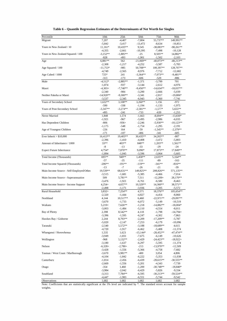
Percentile 10th 25th 50th 75th 90thMigrant 7,207 -4,407 -7,804 55,737** 149,991**

-5,842 -3,417 -13,472 -8,634 -10,851Years in New Zealand / 10 11,161* 10,435** 9,545 -38,083** -98,261**

-4,355 -2,661 -10,395 -7,498 -10,128Years in New Zealand Squared / 100 -3,152** -1,885** -25 8,505** 14,882**

-828 -493 -1,901 -1,502 -2,103Age 6,881** 562 -21,069** -40,073** -48,213**

-2,308 -1,217 -4,252 -3,587 -5,783Age Squared / 100 -11,753* -985 50,708** 100,397** 128,707**

-4,749 -2,565 -8,976 -7,712 -12,682Age Cubed / 1000 725* 241 -3,364** -7,073** -9,481**

-313 -173 -606 -529 -886Male -4,512* -2,885** -1,371 -3,799 701

-1,874 -937 -3,144 -2,612 -4,976Maori -4,303+ -7,740** -9,450** -14,634** -18,037**

-2,340 -984 -3,290 -2,666 -5,039Neither Pakeha or Maori -14,920** -9,300** -3,341 -2,817 -19,806*

-3,537 -2,345 -6,943 -5,360 -7,741Years of Secondary School 1,632** 3,108** 3,260** 1,156 -972

-590 -338 -1,194 -1,133 -1,975Years of Post-Secondary School -3,347** -3,274** -2,581** -1,577* 5,655**

-495 -241 -733 -639 -1,255Never Married 1,848 1,574 -1,663 -8,694** -13,830*

-1,921 -967 -3,495 -2,986 -6,035Has Dependent Children -806 -936+ -2,246 -5,930** -10,123**

-1,175 -548 -1,754 -1,295 -2,191Age of Youngest Children -226 164 -59 -1,545** -2,379**

-171 -107 -406 -341 -605Ever Inherit > $10,000 16,413** 19,403** 30,435** 34,265** -807

-2,396 -1,410 -4,408 -3,472 -5,803Amount of Inheritance / 1000 33** 403** 848** 1,203** 1,561**

-8 -13 -33 -29 -24Expect Future Inheritance 4,754* 7,870** 9,090* 17,873** 17,849**

-1,894 -1,045 -3,596 -3,064 -5,605Total Income (Thousands) 695** 949** 1,458** 2,635** 5,164**

-57 -35 -111 -89 -163Total Income Squared (Thousands) -206** -191** -119** -341** -816**

-13 -7 -26 -21 -39Main Income Source - Self-Employed/Other 19,539** 68,631** 149,825** 208,826** 571,135**

-3,515 -1,681 -5,385 -4,466 -7,014Main Income Source - Superannuation 509 5,781** 7,511 -12,209+ 28,170**

-3,476 -1,921 -6,761 -6,580 -8,463Main Income Source - Income Support 4,254+ 4,657** 10,329** 14,360** 38,571**

-2,498 -1,171 -3,936 -3,205 -5,572Rural Household 3,832+ 7,254** 4,571 18,376** 105,654**

-2,320 -1,444 -4,827 -4,454 -8,860Northland 4,144 10,517** 6,460 -22,971** -29,097**

-3,670 -1,733 -6,072 -5,149 -10,519Waikato 5,219+ 7,626** -1,218 -14,882** -18,004*

-3,003 -1,484 -5,110 -4,554 -8,011Bay of Plenty 2,398 8,542** 4,118 -1,798 -14,794+

-3,396 -1,595 -6,247 -4,302 -7,863Hawkes Bay / Gisborne 2,244 8,793** -2,209 -17,209** -5,787

-5,020 -2,147 -7,253 -6,179 -10,096Taranaki -2,540 5,572** -3,188 -18,689** 4,615

-4,720 -1,917 -6,462 -5,408 -11,574Whanganui / Horewhenua 1,535 1,623 -15,144* -28,452** -47,474**

-3,949 -1,831 -7,675 -6,149 -10,626Wellington -968 5,132** -2,429 -24,423** -18,922+

-3,180 -1,637 -6,297 -5,595 -11,374Nelson -6,328+ -2,780+ -213 -13,970** -12,509

-3,428 -1,556 -5,366 -4,758 -7,682Tasman / West Coast / Marlborough -3,670 5,981** -400 3,054 4,806

-4,104 -1,842 -6,222 -5,353 -11,038Canterbury -1,814 -2,456 -6,439 -28,615** -30,555**

-2,669 -1,556 -5,201 -4,343 -7,739Otago -354 1,460 -1,200 -30,748** -18,840*

-3,984 -2,042 -6,429 -5,826 -9,334Southland -3,313 7,784** -6,595 -30,213** -59,524**

-4,447 -1,983 -6,551 -5,744 -9,542Observations 1,682 1,682 1,682 1,682 1,682Note: Coefficients that are statistically significant at the 5% level are indicated by *. The standard errors account for sampleweights.

Table 6 – Quantile Regression Estimates of the Determinants of Net Worth for Singles

Percentile 10th 25th 50th 75th 90thMigrant Couple -1,663 -47,144** -69,867** -154,353** -129,851*

-16,506 -15,194 -24,378 -45,931 -54,323Mixed Nativity Couple 377 -15,412 -38,229* -63,727* -77,844*

-10,463 -10,257 -16,506 -31,677 -39,215Years in New Zealand / 10 -17,383+ -2,253 -4,228 26,352 -44,382

-10,298 -9,528 -15,609 -28,355 -27,619Years in New Zealand Squared / 100 3,478 -666 1,724 -3,768 9,040

-2,176 -2,118 -3,437 -6,044 -5,775Partner's Years in New Zealand / 10 -2,081 -10 19,520 43,308 35,753

-10,158 -10,086 -16,343 -31,453 -36,392Partner's Years in New Zealand Squared / 100 1,452 1,134 -1,949 -7,419 -3,867

-2,205 -2,327 -3,677 -6,898 -7,769Age 6,404 -5,334 -1,246 -40,873 -60,481+

-8,340 -9,366 -15,006 -28,005 -34,334Age Squared / 100 -8,145 17,081 13,216 98,685 165,733*

-17,853 -19,533 -31,694 -60,222 -73,787Age Cubed / 1000 406 -1,178 -990 -6,430 -12,214*

-1,209 -1,302 -2,145 -4,137 -5,056Partner's Age -18,087* -11,761 -11,584 2,583 17,485

-8,377 -8,991 -14,754 -27,478 -31,880Partner's Age Squared / 100 42,053* 31,392+ 32,688 1,009 -41,534

-17,989 -18,902 -31,092 -58,276 -67,784Partner's Age Cubed / 1000 -2,929* -2,216+ -2,318 -53 4,003

-1,216 -1,264 -2,096 -3,945 -4,605Both Maori Couple -43,152** -54,195** -56,826** -91,308** -74,963**

-9,502 -8,938 -12,816 -23,821 -26,938Mixed Maori Couple -24,774** -32,285** -52,339** -56,489* 20,297

-8,272 -7,008 -11,725 -22,074 -29,204Other Couple -7,245 4,824 -5,736 22,935 846

-10,269 -9,506 -15,018 -28,595 -36,436Years of Secondary School 4,679* 10,366** 16,232** 27,285** 31,287**

-2,034 -2,111 -3,533 -6,748 -8,406Years of Post-Secondary School -2,070 -1,275 -1,381 426 -419

-1,369 -1,179 -1,879 -3,579 -3,865Partner's Years of Secondary School 2,844 2,783 3,007 -549 21,732*

-2,118 -2,139 -3,533 -6,894 -9,189Partner's Years of Post-Secondary School 1,107 10 -2,030 3,456 -4,714

-1,142 -1,176 -1,895 -3,674 -4,261Married Couple 17,521** 15,075* 29,174** 35,061+ 55,980**

-6,439 -6,504 -10,172 -18,956 -19,972Has Dependent Children 1,742 1,661 9,143* 16,826* 26,124**

-2,582 -2,486 -3,823 -7,507 -9,331Age of Youngest Children 71 778 -11 1,093 776

-554 -536 -927 -1,874 -2,251Ever Inherit > $10,000 29,201** 32,221** 48,718** 38,510* 8,483

-6,689 -6,030 -9,780 -18,800 -23,654Amount of Inheritance / 1000 185** 583** 782** 1,149** 2,488**

-43 -36 -65 -116 -115Expect Future Inheritance 24,128** 15,810** 17,821* 12,252 51,184**

-5,049 -5,054 -8,201 -16,310 -19,837Total Income (Thousands) 444** 1,205** 1,963** 3,473** 3,069**

-92 -85 -150 -299 -382Total Income Squared (Thousands) 73** -3 22 -66 660**

-15 -14 -32 -51 -59Main Income Source - Self-Employed/Other 29,004** 59,195** 125,817** 189,012** 319,237**

-6,275 -6,309 -9,795 -18,407 -21,552Main Income Source - Superannuation -28,979* -26,601* -73,337** -109,169** -192,291**

-12,796 -12,299 -19,518 -41,399 -47,835Main Income Source - Income Support -25,152* -30,188** -29,316+ -19,701 -3,104

-11,346 -11,152 -16,614 -29,570 -35,585Rural Household -547 -8,542 46,047** 135,688** 305,114**

-7,293 -7,141 -11,034 -20,893 -24,024Northland 30,011** 35,839** 14,462 -70,123+ -154,249**

-11,412 -11,111 -19,489 -39,180 -43,668Waikato 12,887 6,545 -7,295 -44,444 1,455

-9,643 -9,633 -15,216 -29,779 -37,667Bay of Plenty 25,168** 4,489 16,263 -14,462 -8,549

-9,495 -10,343 -16,354 -31,348 -35,980Gisborne 31,961* 30,749* 20,232 50,667 38,426

-13,249 -13,595 -22,741 -48,290 -69,820Hawkes Bay 4,009 -8,986 -20,899 -59,884+ -96,568*

-11,539 -11,151 -17,028 -33,884 -41,562Taranaki 23,908* 20,020+ 7,353 -19,566 60,228

-10,193 -10,550 -17,273 -35,461 -47,795Manawatu / Whanganui 1,772 -8,115 -22,575 -49,631 -24,565

-9,583 -9,486 -15,805 -32,309 -38,822Wellington -12,521 -12,650 -18,534 -77,818** -97,174**

-8,570 -7,979 -12,985 -25,543 -30,291Marlborough / Nelson / Tasman / West Coast 14,634 10,932 18,714 -45,638 -75,479+

-9,739 -9,164 -15,155 -31,093 -42,661Canterbury 2,365 4,291 -4,659 -58,738* -59,500+

-7,901 -7,921 -12,885 -25,176 -32,215Otago -4,863 -12,823 -65,264** -132,969** -177,073**

-9,907 -9,654 -15,691 -31,122 -38,303Southland -2,243 -10,518 -26,225 -62,327+ -21,247

-11,709 -11,043 -17,896 -35,052 -43,019Observations 2,560 2,560 2,560 2,560 2,560Note: Coefficients that are statistically significant at the 5% level are indicated by *. The standard errors account for sample weights.

Table 7 – Quantile Regression Estimates of the Determinants of Net Worth for Couples

Migrant - NZ-BornWealth Gap Raw Gap Age Education Inheritences Income Residual Age Education Inheritences Income Residual10th Percentile 4,500* 0 0 0 0 4,500* 3,254 -2,446 -105 -613 4,410

(962) (1,599) (533) (181) (276) (2,028) (7,365) (14,800) (3,242) (34,457) (41,322)20th Percentile 500 464 -32 -6 -352 426 517 -144 -40 -240 407

(1,135) (698) (433) (165) (332) (579) (7,360) (15,182) (5,005) (34,488) (41,970)30th Percentile 6,086 4,701 681 -155 -999 1,858 3,950 995 -149 -1,227 2,517

(5,034) (3,056) (2,065) (1,034) (1,920) (4,180) (6,650) (17,254) (7,848) (35,399) (46,134)40th Percentile 19,650* 15,290* -360 -812 -1,170 6,703 11,115 2,837 -192 -2,930 8,820

(9,118) (6,255) (4,148) (2,421) (3,952) (8,208) (8,075) (19,990) (5,174) (36,598) (48,910)Median 32,822 30,258* -6,603 -2,637 -8,048 19,852 30,860* 6,207 521 -6,265 1,499

(19,710) (13,793) (8,094) (4,285) (6,973) (14,389) (11,913) (20,072) (4,711) (36,466) (52,272)60th Percentile 44,116* 28,591* -11,382 -2,834 -7,135 36,876 40,899* 3,923 1,161 -7,183 5,316

(18,790) (10,961) (10,728) (5,241) (8,385) (20,706) (10,565) (19,041) (6,061) (35,096) (48,378)70th Percentile 29,204 29,711 -28,339 -612 -6,809 35,253 39,272* 8,235 708 -10,360 -8,651

(29,847) (16,237) (15,896) (8,134) (9,107) (30,333) (11,198) (18,405) (6,739) (33,721) (51,733)80th Percentile 65,304* 36,728* -36,079 -1,088 -11,838 77,580* 42,056* 19,906 5,475 -15,201 13,069

(32,224) (16,718) (19,259) (11,743) (12,343) (37,470) (12,704) (17,941) (11,206) (33,165) (52,393)90th Percentile 36,630 39,796 -54,938 10,680 -43,450 84,541 66,965* 39,890 18,720 -32,486 -56,460

(69,223) (27,141) (39,170) (36,654) (31,982) (72,396) (20,102) (21,932) (22,224) (37,018) (84,073)Mean 11,087 16,056* -13,501 -2,173 -9,895 20,600 27,617* 3,672 5,948 -11,260 -14,890

(15,364) (6,165) (7,674) (7,029) (7,944) (18,229) (8,564) (15,013) (7,768) (32,228) (41,620)

Table 8 – Semi-Parametric Decomposition of Differences in Net Worth for Immigrants and the New Zealand-Born Singles

Note: Components for the wealth gap that are statistically significant at the 5% level are indicated by *. The standard errors are calculated by bootstrapping using a normalapproximation with 1,000 replications that account for the complex sample design.

Counterfactuals Generated for Migrants Counterfactuals Generated for the New Zealand-Born

Migrant Couple - NZ-BornWealth Gap Raw Gap Age Educ Inherit Income Residual Age Educ Inherit Income Residual Age Educ Inherit Income Residual10th Percentile -6,520* 1,636 -541 -1,014* -2,069 -4,532 5,938* 3,341 -2,780* -5,789* -7,230 3,398 2,009 -685 -3,287* -7,954*

(1,970) (944) (940) (482) (1,348) (2,651) (2,468) (1,914) (800) (1,496) (3,838) (1,779) (1,295) (822) (1,516) (3,522)20th Percentile -31,152* 7,191* 2,266 -4,143 -10,357 -26,110* 14,780* 9,868* -7,981* -12,589* -35,231* 12,971* 5,252 -3,933 -13,347* -32,094*

(4,881) (3,597) (3,364) (2,694) (5,631) (7,390) (4,590) (2,869) (1,608) (3,106) (6,926) (4,845) (3,120) (3,906) (6,509) (9,843)30th Percentile -42,405* 18,702* 6,239 -13,191* -25,484* -28,671 20,341* 13,967* -11,678* -18,424* -46,611* 19,493* 7,576 -13,706* -27,726* -28,042

(9,772) (6,380) (8,301) (5,357) (9,313) (17,852) (6,607) (4,091) (2,526) (4,291) (10,557) (7,378) (5,941) (6,892) (8,702) (16,200)40th Percentile -64,609* 17,625 4,203 -21,165* -36,276* -28,995 24,227* 14,536* -15,618* -21,072* -66,682* 20,593* 4,438 -22,182* -32,531* -34,926

(15,269) (9,047) (11,125) (7,654) (11,623) (21,297) (7,641) (4,770) (3,596) (5,484) (15,066) (9,804) (7,825) (9,532) (11,369) (20,012)Median -74,169* 25,723* 2,207 -27,588* -39,530* -34,982 28,149* 16,707* -24,039* -32,415* -62,571* 29,925* 5,724 -30,143* -41,520* -38,156

(17,595) (10,699) (14,177) (11,146) (17,048) (32,547) (9,119) (6,489) (5,356) (7,671) (17,718) (12,023) (10,717) (14,655) (16,408) (31,268)60th Percentile -83,364* 28,652* 4,758 -35,906 -48,816 -32,051 30,436* 20,286* -31,651* -41,660* -60,777* 34,985* 6,777 -43,752 -49,314* -32,059

(20,964) (11,361) (20,604) (21,160) (24,932) (56,631) (10,716) (8,726) (7,858) (11,075) (21,315) (13,567) (15,316) (23,896) (24,191) (48,869)70th Percentile -124,116* 25,795 7,871 -79,671* -70,591 -7,520 38,594* 31,619* -36,707* -61,453* -96,169* 37,943* 13,836 -80,458* -70,230 -25,207

(31,636) (14,967) (29,217) (28,603) (37,968) (75,561) (12,778) (11,902) (11,173) (17,346) (33,377) (18,647) (24,141) (35,228) (38,850) (70,329)80th Percentile -140,190* 27,293 2,002 -86,688* -84,684* 1,888 33,776* 31,699 -37,690* -63,750* -104,224* 29,238 10,272 -79,746 -80,908 -19,046

(36,830) (18,676) (30,843) (35,035) (42,372) (69,170) (14,637) (19,831) (15,643) (27,132) (47,178) (21,846) (39,416) (42,424) (63,203) (105,220)90th Percentile -253,473* 17,730 6,258 -40,863 -44,573 -192,025* 49,085 64,056 -54,358 -96,595 -215,661 18,823 41,180 -28,706 -6,977 -277,794*

(58,583) (24,536) (29,248) (35,781) (36,292) (61,525) (27,791) (53,324) (48,868) (98,897) (129,538) (31,655) (45,835) (48,988) (98,908) (133,734)Mean -141,455* 20,941* 6,974 -33,944* -42,139* -93,288* 29,180* 34,334* -24,556* -46,365 -134,048* 26,497* 23,236 -32,317* -30,910 -127,961*

(21,614) (9,042) (12,442) (12,098) (15,361) (29,321) (10,491) (16,175) (10,692) (27,816) (37,598) (11,658) (13,563) (15,794) (27,261) (39,996)

Counterfactuals for NZ-Born and Migrant Couples

Note: Components for the wealth gap that are statistically significant at the 5% level are indicated by *. The standard errors are calculated by bootstrapping using a normal approximation with 1,000 replicationsthat account for the complex sample design.

Table 9 – Semi-Parametric Decomposition of Differences in Net Worth for Migrant Couples and the New Zealand-Born Couples

Counterfactuals for NZ-Born and Mixed NativityCounterfactuals for Migrants and Mixed Nativity

Mixed Couple - NZ-BornWealth Gap Raw Gap Age Educ Inherit Income Residual Age Educ Inherit Income Residual Age Educ Inherit Income Residual10th Percentile 6,296 900 1,521 178 -29 3,727 -378 367 1,854 -2,665 7,118 2,194 2,127 624 -1,655 3,007

(6,728) (2,656) (2,802) (1,092) (840) (5,234) (4,178) (3,236) (2,489) (2,311) (7,986) (1,769) (1,108) (731) (1,203) (6,763)20th Percentile 17,350* 6,888 10,647* 1,432 -329 -1,287 6,947 2,293 1,871 -7,135* 13,374 5,482 4,547* 1,385 -2,615 8,551

(8,670) (4,610) (4,876) (1,749) (1,529) (9,071) (5,961) (4,633) (3,795) (3,589) (10,467) (3,997) (1,730) (1,608) (2,477) (8,605)30th Percentile 22,400 5,120 11,558* 2,047 216 3,460 12,489 2,740 4,382 -13,090* 15,879 7,303 7,173* 2,416 -3,700 9,208

(11,598) (5,275) (5,389) (2,832) (1,740) (12,209) (6,975) (6,037) (5,458) (4,859) (13,338) (5,560) (2,648) (2,668) (3,826) (11,257)40th Percentile 17,164 4,155 8,521 2,490 -1,380 3,378 17,726* 1,599 -254 -13,267* 11,360 9,029 7,011* 3,105 -4,136 2,155

(11,958) (5,549) (5,722) (2,655) (2,285) (14,061) (7,616) (6,708) (6,210) (5,872) (15,000) (7,007) (3,308) (3,891) (5,412) (13,444)Median 455 1,001 13,943* 892 -317 -15,065 19,897* 245 -7,520 -21,828* 9,661 13,089 8,840 3,946 -5,590 -19,829

(15,673) (6,320) (6,642) (3,092) (3,095) (14,712) (9,923) (11,339) (8,507) (8,329) (20,335) (8,435) (4,526) (5,767) (7,855) (17,822)60th Percentile 13,860 9,988 36,213* 6,619 -3,020 -35,940 19,037 -8,528 6,508 -20,438 17,282 14,264 10,506 4,434 -4,708 -10,636

(23,959) (11,927) (13,878) (6,441) (6,830) (28,865) (13,423) (15,850) (13,670) (13,717) (31,955) (9,020) (6,347) (6,586) (11,439) (25,638)70th Percentile -9,667 -286 22,129* 2,042 -5,626 -27,925 29,265 3,885 -22,314 -33,033 12,529 18,774 15,822 5,047 -3,404 -45,906

(30,635) (10,258) (10,838) (4,364) (7,434) (29,528) (15,711) (17,694) (13,711) (19,431) (40,378) (12,952) (13,800) (11,109) (22,798) (39,540)80th Percentile -42,400 13,922 35,633* 305 -10,221 -82,039* 33,680 -2,274 -33,544 -30,637 -9,626 17,059 18,583 5,824 -2,068 -81,799

(30,788) (11,629) (15,628) (5,723) (10,783) (31,277) (18,697) (24,931) (18,743) (30,259) (53,735) (14,596) (33,329) (13,447) (50,990) (85,307)90th Percentile -126,154 24,229 8,912 578 -3,317 -156,556 71,646* 34,068 -48,027 -29,284 -154,557 9,334 39,582 6,848 33,141 -215,059

(86,570) (22,603) (39,356) (11,376) (37,653) (89,298) (35,259) (59,542) (57,787) (105,112) (139,280) (23,588) (41,009) (23,714) (90,581) (129,030)Mean -33,929 5,496 7,549 3,650 -1,479 -49,145 22,983* 17,022 -1,468 -17,370 -55,097 10,231 20,397 3,584 7,016 -75,158*

(26,858) (6,743) (13,976) (5,820) (11,492) (32,090) (10,705) (16,256) (13,984) (26,823) (39,418) (9,443) (11,127) (7,488) (24,686) (36,028)

Counterfactuals for NZ-Born and Migrant Couples

Note: Components for the wealth gap that are statistically significant at the 5% level are indicated by *. The standard errors are calculated by bootstrapping using a normal approximation with 1,000 replicationsthat account for the complex sample design.

Table 10 – Semi-Parametric Decomposition of Differences in Net Worth for Mixed Nativity Couples and the New Zealand-Born Couples

Counterfactuals for NZ-Born and Mixed NativityCounterfactuals for Migrants and Mixed Nativity

Figure 1 – Estimated Wealth Distributions by Nativity for Singles

Figure 2 – Estimated Wealth Distributions by Nativity for Couples

Figure 3 – Estimated Income Distributions by Nativity for Singles

Figure 4 – Estimated Income Distributions by Nativity for Couples

Motu Working Paper Series

All papers are available online at http://www.motu.org.nz/motu_wp_series.htm or by contacting Motu Economic and Public Policy Research. 07-10 Grimes, Arthur; David C. Maré and Melanie Morten, “Adjustment in Local Labour and

Housing Markets.”

07-09 Grimes, Arthur and Yun Liang, “Spatial Determinants of Land Prices in Auckland: Does the Metropolitan Urban Limit Have an Effect?”

07-08 Kerr, Suzi; Kit Rutherford and Kelly Lock, “Nutrient Trading in Lake Rotorua: Goals and Trading Caps”.

07-07 Hendy, Joanna; Suzi Kerr and Troy Baisden, “The Land Use in Rural New Zealand Model Version 1 (LURNZ v1): Model Description”.

07-06 Lock, Kelly and Suzi Kerr, “Nutrient Trading in Lake Rotorua: Where Are We Now?”

07-05 Stillman, Steven and David C. Maré, “The Impact of Immigration on the Geographic Mobility of New Zealanders”.

07-04 Grimes, Arthur and Yun Liang, “An Auckland Land Value Annual Database”.

07-03 Kerr, Suzi; Glen Lauder and David Fairman, “Towards Design for a Nutrient Trading Programme to Improve Water Quality in Lake Rotorua”.

07-02 Lock, Kelly and Stefan Leslie, “New Zealand’s Quota Management System: A History of the First 20 Years”.

07-01 Grimes, Arthur and Andrew Aitken, “House Prices and Rents: Socio-Economic Impacts and Prospects”.

06-09 Maani, Sholeh A.; Rhema Vaithianathan and Barbara Wolf, “Inequality and Health: Is House Crowding the Link?”

06-08 Maré, David C. and Jason Timmins, “Geographic Concentration and Firm Productivity”.

06-07 Grimes, Arthur; David C. Maré and Melanie Morten, “Defining Areas Linking Geographic Data in New Zealand”.

06-06 Maré, David C. and Yun Liang, “Labour Market Outcomes for Young Graduates”.

06-05 Hendy, Joanna and Suzi Kerr, “Land-Use Intensity Module: Land Use in Rural New Zealand Version 1”.

06-04 Hendy, Joanna; Suzi Kerr and Troy Baisden, “Greenhouse Gas Emissions Charges and Credits on Agricultural Land: What Can a Model Tell Us?”

06-03 Hall, Viv B.; C. John McDermott and James Tremewan, “The Ups and Downs of New Zealand House Prices”.

06-02 McKenzie, David; John Gibson and Steven Stillman, “How Important is Selection? Experimental vs Non-Experimental Measures of the Income Gains from Migration”.

06-01 Grimes, Arthur and Andrew Aitken, “Housing Supply and Price Adjustment”.

05-14 Timmins, Jason, “Is Infrastructure Productive? Evaluating the Effects of Specific Infrastructure Projects on Firm Productivity within New Zealand”.

05-13 Coleman, Andrew; Sylvia Dixon and David C. Maré, “Māori Economic Development—Glimpses from Statistical Sources”.

05-12 Maré, David C., “Concentration, Specialisation and Agglomeration of Firms in New Zealand”.

05-11 Holmes, Mark J. and Arthur Grimes, “Is There Long-Run Convergence of Regional House Prices in the UK?”

05-10 Hendy, Joanna and Suzi Kerr, “Greenhouse Gas Emission Factor Module: Land Use in Rural New Zealand—Climate Version 1”.

05-09 Poland, Michelle and David C. Maré, “Defining Geographic Communities”.

05-08 Kerr, Suzi; Joanna Hendy, Emma Brunton and Isabelle Sin, “The Likely Regional Impacts of an Agricultural Emissions Policy in New Zealand: Preliminary Analysis”.

05-07 Stillman, Steven, “Examining Changes in the Value of Rural Land in New Zealand between 1989 and 2003”.

05-06 Dixon, Sylvia and David C. Maré, “Changes in the Māori Income Distribution: Evidence from the Population Census”.

05-05 Sin, Isabelle and Steven Stillman, “The Geographical Mobility of Māori in New Zealand”.

05-04 Grimes, Arthur, “Regional and Industry Cycles in Australasia: Implications for a Common Currency”.

05-03 Grimes, Arthur, “Intra and Inter-Regional Industry Shocks: A New Metric with an Application to Australasian Currency Union”.

05-02 Grimes, Arthur; Robert Sourell and Andrew Aitken, “Regional Variation in Rental Costs for Larger Households”.

05-01 Maré, David C., “Indirect Effects of Active Labour Market Policies”.

04-12 Dixon, Sylvia and David C. Maré, “Understanding Changes in Māori Incomes and Income Inequality 1997–2003”.

04-11 Grimes, Arthur, “New Zealand: A Typical Australasian Economy?”

04-10 Hall, Viv and C. John McDermott, “Regional Business Cycles in New Zealand: Do They Exist? What Might Drive Them?”

04-09 Grimes, Arthur; Suzi Kerr and Andrew Aitken, “Bi-Directional Impacts of Economic, Social and Environmental Changes and the New Zealand Housing Market”.

04-08 Grimes, Arthur and Andrew Aitken, “What’s the Beef with House Prices? Economic Shocks and Local Housing Markets”.

04-07 McMillan, John, “Quantifying Creative Destruction: Entrepreneurship and Productivity in New Zealand”.

04-06 Maré, David C. and Isabelle Sin, “Māori Incomes: Investigating Differences Between Iwi”.

04-05 Kerr, Suzi; Emma Brunton and Ralph Chapman, “Policy to Encourage Carbon Sequestration in Plantation Forests”.

04-04 Maré, David C., “What do Endogenous Growth Models Contribute?”

04-03 Kerr, Suzi; Joanna Hendy, Shuguang Liu and Alexander S. P. Pfaff, “Uncertainty and Carbon Policy Integrity”.

04-02 Grimes, Arthur; Andrew Aitken and Suzi Kerr, “House Price Efficiency: Expectations, Sales, Symmetry”.

04-01 Kerr, Suzi; Andrew Aitken and Arthur Grimes, “Land Taxes and Revenue Needs as Communities Grow and Decline: Evidence from New Zealand”.

03-19 Maré, David C., “Ideas for Growth?”

03-18 Fabling, Richard and Arthur Grimes, “Insolvency and Economic Development: Regional Variation and Adjustment”.

03-17 Kerr, Suzi; Susana Cardenas and Joanna Hendy, “Migration and the Environment in the Galapagos: An Analysis of Economic and Policy Incentives Driving Migration, Potential Impacts from Migration Control, and Potential Policies to Reduce Migration Pressure”.

03-16 Hyslop, Dean R. and David C. Maré, “Understanding New Zealand’s Changing Income Distribution 1983–98: A Semiparametric Analysis”.

03-15 Kerr, Suzi, “Indigenous Forests and Forest Sink Policy in New Zealand”.

03-14 Hall, Viv and Angela Huang, “Would Adopting the US Dollar Have Led to Improved Inflation, Output and Trade Balances for New Zealand in the 1990s?”

03-13 Ballantyne, Suzie; Simon Chapple, David C. Maré and Jason Timmins, “Movement into and out of Child Poverty in New Zealand: Results from the Linked Income Supplement”.

03-12 Kerr, Suzi, “Efficient Contracts for Carbon Credits from Reforestation Projects”.

03-11 Lattimore, Ralph, “Long Run Trends in New Zealand Industry Assistance”.

03-10 Grimes, Arthur, “Economic Growth and the Size & Structure of Government: Implications for New Zealand”.

03-09 Grimes, Arthur; Suzi Kerr and Andrew Aitken, “Housing and Economic Adjustment”.

03-07 Maré, David C. and Jason Timmins, “Moving to Jobs”.

03-06 Kerr, Suzi; Shuguang Liu, Alexander S. P. Pfaff and R. Flint Hughes, “Carbon Dynamics and Land-Use Choices: Building a Regional-Scale Multidisciplinary Model”.

03-05 Kerr, Suzi, “Motu, Excellence in Economic Research and the Challenges of ‘Human Dimensions’ Research”.

03-04 Kerr, Suzi and Catherine Leining, “Joint Implementation in Climate Change Policy”.

03-03 Gibson, John, “Do Lower Expected Wage Benefits Explain Ethnic Gaps in Job-Related Training? Evidence from New Zealand”.

03-02 Kerr, Suzi; Richard G. Newell and James N. Sanchirico, “Evaluating the New Zealand Individual Transferable Quota Market for Fisheries Management”.

03-01 Kerr, Suzi, “Allocating Risks in a Domestic Greenhouse Gas Trading System”.