WhatEveryEngineerShouldKnowaboutExcel

WhatEveryEngineerShouldKnow:ASeries

SeriesEditor*PhillipA.Laplante

PennsylvaniaStateUniversity

1.WhatEveryEngineerShouldKnowaboutPatentsWilliamG.Konold,BruceTittel,DonaldF.Frei,andDavidS.Stallard

2.WhatEveryEngineerShouldKnowaboutProductLiabilityJamesF.ThorpeandWilliamH.Middendorf

3.WhatEveryEngineerShouldKnowaboutMicrocomputers:Hardware/SoftwareDesign,AStep-by-StepExample

WilliamS.BennettandCarlF.Evert,Jr.

4.WhatEveryEngineerShouldKnowaboutEconomicDecisionAnalysisDeanS.Shupe

5.WhatEveryEngineerShouldKnowaboutHumanResourcesManagementDesmondD.MartinandRichardL.Shell

6.WhatEveryEngineerShouldKnowaboutManufacturingCostEstimatingEricM.Malstrom

7.WhatEveryEngineerShouldKnowaboutInventingWilliamH.Middendorf

8.WhatEveryEngineerShouldKnowaboutTechnologyTransferandInnovationLouisN.MogaveroandRobertS.Shane

9.WhatEveryEngineerShouldKnowaboutProjectManagementArnoldM.RuskinandW.EugeneEstes

10.WhatEveryEngineerShouldKnowaboutComputer-AidedDesignandComputer-AidedManufacturing:TheCAD/CAMRevolution

JohnK.Krouse

11.WhatEveryEngineerShouldKnowaboutRobotsMauriceI.Zeldman

12.WhatEveryEngineerShouldKnowaboutMicrocomputerSystemsDesignandDebuggingBillWrayandBillCrawford

13.WhatEveryEngineerShouldKnowaboutEngineeringInformationResourcesMargaretT.SchenkandJamesK.Webster

14.WhatEveryEngineerShouldKnowaboutMicrocomputerProgramDesignKeithR.Wehmeyer

15.WhatEveryEngineerShouldKnowaboutComputerModelingandSimulationDonM.Ingels

16.WhatEveryEngineerShouldKnowaboutEngineeringWorkstationsJustinE.HarlowIII

17.WhatEveryEngineerShouldKnowaboutPracticalCAD/CAMApplicationsJohnStark

18.WhatEveryEngineerShouldKnowaboutThreadedFasteners:MaterialsandDesignAlexanderBlake

19.WhatEveryEngineerShouldKnowaboutDataCommunicationsCarlStephenClifton

20.WhatEveryEngineerShouldKnowaboutMaterialandComponentFailure,FailureAnalysis,andLitigation

LawrenceE.Murr

21.WhatEveryEngineerShouldKnowaboutCorrosionPhilipSchweitzer

22.WhatEveryEngineerShouldKnowaboutLasersD.C.Winburn

23.WhatEveryEngineerShouldKnowaboutFiniteElementAnalysisJohnR.Brauer

24.WhatEveryEngineerShouldKnowaboutPatents:SecondEditionWilliamG.Konold,BruceTittel,DonaldF.Frei,andDavidS.Stallard

25.WhatEveryEngineerShouldKnowaboutElectronicCommunicationsSystemsL.R.McKay

26.WhatEveryEngineerShouldKnowaboutQualityControlThomasPyzdek

27.WhatEveryEngineerShouldKnowaboutMicrocomputers:Hardware/SoftwareDesign,AStep-by-StepExample,SecondEdition,RevisedandExpandedWilliamS.Bennett,CarlF.Evert,andLeslieC.Lander

28.WhatEveryEngineerShouldKnowaboutCeramicsSolomonMusikant

29.WhatEveryEngineerShouldKnowaboutDevelopingPlasticsProductsBruceC.Wendle

30.WhatEveryEngineerShouldKnowaboutReliabilityandRiskAnalysisM.Modarres

31.WhatEveryEngineerShouldKnowaboutFiniteElementAnalysis:SecondEdition,RevisedandExpanded

JohnR.Brauer

32.WhatEveryEngineerShouldKnowaboutAccountingandFinanceJaeK.ShimandNormanHenteleff

33.WhatEveryEngineerShouldKnowaboutProjectManagement:SecondEdition,RevisedandExpanded

ArnoldM.RuskinandW.EugeneEstes

34.WhatEveryEngineerShouldKnowaboutConcurrentEngineeringThomasA.Salomone

35.WhatEveryEngineerShouldKnowaboutEthicsKennethK.Humphreys

36.WhatEveryEngineerShouldKnowaboutRiskEngineeringandManagementJohnX.WangandMarvinL.Roush

37.WhatEveryEngineerShouldKnowaboutDecisionMakingUnderUncertaintyJohnX.Wang

38.WhatEveryEngineerShouldKnowaboutComputationalTechniquesofFiniteElementAnalysisLouisKomzsik

39.WhatEveryEngineerShouldKnowaboutExcelJackP.Holman

40.WhatEveryEngineerShouldKnowaboutSoftwareEngineeringPhillipA.Laplante

41.WhatEveryEngineerShouldKnowaboutDevelopingReal-TimeEmbeddedProductsKimR.Fowler

42.WhatEveryEngineerShouldKnowaboutBusinessCommunicationJohnX.Wang

43.WhatEveryEngineerShouldKnowaboutCareerManagementMikeFicco

44.WhatEveryEngineerShouldKnowaboutStartingaHigh-TechBusinessVentureEricKoester

45.WhatEveryEngineerShouldKnowaboutMATLAB®andSimulink®AdrianB.BiranwithcontributionsbyMosheBreiner

46.GreenEntrepreneurHandbook:TheGuidetoBuildingandGrowingaGreenandCleanBusinessEricKoester

47.TechnicalWriting:APracticalGuideforEngineersandScientistsPhillipA.Laplante

48.WhatEveryEngineerShouldKnowaboutCyberSecurityandDigitalForensicsJoannaF.DeFranco

49.WhatEveryEngineerShouldKnowaboutModelingandSimulationRaymondJosephMadachy

50.WhatEveryEngineerShouldKnowaboutExcel,SecondEditionJackP.HolmanandBlakeK.Holman

*FoundingSeriesEditor:WilliamH.Middendorf.

WhatEveryEngineerShouldKnowAboutExcelSecondEdition

JackP.HolmanandBlakeK.Holman

CRCPressTaylor&FrancisGroup6000BrokenSoundParkwayNW,Suite300BocaRaton,FL33487-2742

©2018byTaylor&FrancisGroup,LLCCRCPressisanimprintofTaylor&FrancisGroup,anInformabusiness

NoclaimtooriginalU.S.Governmentworks

Printedonacid-freepaper

InternationalStandardBookNumber-13:978-1-138-30614-1(Hardback)InternationalStandardBookNumber-13:978-1-138-03530-0(Paperback)

Thisbookcontains informationobtainedfromauthenticandhighlyregardedsources.Reasonableeffortshavebeenmade topublish reliabledataandinformation,buttheauthorandpublishercannotassumeresponsibilityforthevalidityofallmaterialsortheconsequencesoftheiruse.The authors and publishers have attempted to trace the copyright holders of all material reproduced in this publication and apologize tocopyrightholdersifpermissiontopublishinthisformhasnotbeenobtained.Ifanycopyrightmaterialhasnotbeenacknowledged,pleasewriteandletusknowsowemayrectifyinanyfuturereprint.

ExceptaspermittedunderU.S.CopyrightLaw,nopartofthisbookmaybereprinted,reproduced,transmitted,orutilizedinanyformbyanyelectronic, mechanical, or other means, now known or hereafter invented, including photocopying, microfilming, and recording, or in anyinformationstorageorretrievalsystem,withoutwrittenpermissionfromthepublishers.

Forpermissiontophotocopyorusematerialelectronicallyfromthiswork,pleaseaccesswww.copyright.com(http://www.copyright.com/)orcontact the Copyright Clearance Center, Inc. (CCC), 222 Rosewood Drive, Danvers, MA 01923, 978-750-8400. CCC is a not-for-profitorganizationthatprovideslicensesandregistrationforavarietyofusers.FororganizationsthathavebeengrantedaphotocopylicensebytheCCC,aseparatesystemofpaymenthasbeenarranged.

TrademarkNotice: Product or corporate names may be trademarks or registered trademarks, and are used only for identification andexplanationwithoutintenttoinfringe.

LibraryofCongressCataloging-in-PublicationData

Names:Holman,J.P.(JackPhilip),author.Title:WhateveryengineershouldknowaboutExcel/J.P.HolmanandBlakeK.Holman.Description:Secondedition.|BocaRaton:Taylor&Francis,CRCPress,2018.|Series:Whateveryengineershouldknowseries|Includesbibliographicalreferencesandindex.Identifiers:LCCN2017035509|ISBN9781138035300(pbk.)|ISBN9781138306141(hardback)|ISBN9781315268583(ebook)Subjects:LCSH:MicrosoftExcel(Computerfile)|Engineering--Computerprograms.Classification:LCCTA345.H652018|DDC005.54--dc23LCrecordavailableathttps://lccn.loc.gov/2017035509

VisittheTaylor&FrancisWebsiteathttp://www.taylorandfrancis.com

andtheCRCPressWebsiteathttp://www.crcpress.com

Contents

PrefacetotheFirstEditionPrefacetotheSecondEditionAbouttheAuthors

1.Introduction1.1GettingtheMostfromMicrosoftExcel1.2Conventions1.3IntroductiontotheMicrosoftOfficeRibbonBar1.4OutlineofContents

2.MiscellaneousOperationsinExcelandWord2.1Introduction2.2GeneratingaScreenshot2.3CustomKeyboardSetupforSymbolsinWordorExcel2.4ViewingorPrintingColumnandRowHeadingsandGridlinesinExcel2.5MiscellaneousUsefulTipsandShortcuts2.6MovingObjectsinSmallIncrements(Nudging)2.7FormattingObjectsinWord,IncludingWrapping2.8FormattingObjectsinExcel2.9CopyingFormulasbyDraggingtheFillHandle2.10CopyingCellFormulas:EffectofRelativeandAbsoluteAddresses2.11ShortcutforChangingtheStatusofCellAddresses2.12 Switching andCopyingColumnsorRows, andChangingRows toColumnsorColumns to

Rows2.13Built-InFunctionsinExcel2.14CreatingSingle-VariableTables2.15CreatingTwo-VariableTables

Problems

3.ChartsandGraphs3.1Introduction3.2MovingDialogWindows3.3ExcelChoicesofx–yScatterCharts3.4SelectingandAddingDataforx–yScatterCharts3.5Changing/ReplacingDataforCharts3.6AddingDatatoCharts3.7AddingTrendLinesandCorrelationEquationstoScatterCharts3.8EquationforR23.9CorrelationofExperimentalDatawithPowerRelation3.10UseofLogarithmicScales

3.11CorrelationwithExponentialFunctions3.12UseofDifferentScatterGraphsfortheSameData

3.12.1Observations3.13PlotofaFunctionofTwoVariableswithDifferentChartTypes

3.13.1ChangesinGapWidthon3-DDisplays3.14PlotsofTwoVariableswithandwithoutSeparateScales3.15ChartsUsedforCalculationPurposesorG&AFormat

3.15.1G&AChart3.16StretchingOutaChart3.17CalculationandGraphingofMovingAverages

3.17.1StandardError3.18BarandColumnCharts3.19ChartFormatandCosmetics3.20SurfaceCharts3.21AnExercisein3-DVisualization

Problems

4.LineDrawings,EmbeddedObjects,Equations,andSymbolsinExcel4.1Introduction4.2Constructing,Moving,andInsertingStraightLineDrawings

4.2.1DrawingLineSegmentsinPreciseAngularIncrements4.3InsertingEquationTemplatesandSymbolsUsingExcelandWord

4.3.1SymbolInsertion4.3.2EquationTemplateInsertion

4.4InsertingEquationsandSymbolsinExcelUsingEquationEditor4.5ConstructionofLineDrawingsfromPlottedCoordinates

Problems

5.SolutionofEquations5.1Introduction5.2SolutionstoNonlinearEquationsUsingGoalSeek5.3SolutionstoNonlinearEquationsUsingSolver5.4IterativeSolutionstoSimultaneousLinearEquations5.5SolutionsofSimultaneousLinearEquationsUsingMatrixInversion

5.5.1ErrorMessages5.6SolutionsofSimultaneousNonlinearEquationsUsingSolver5.7SolverResultsDialogBox5.8ComparisonofMethodsforSolutionofSimultaneousLinearEquations5.9CopyingCellEquationsforRepetitiveCalculations5.10CreatingandRunningMacros

Problems

6.OtherOperations6.1Introduction

6.2NumericalEvaluationofIntegrals6.3UseofLogicalIFStatement6.4HistogramsandCumulativeFrequencyDistributions6.5NormalErrorDistributions6.6CalculationofUncertaintyPropagationinExperimentalResults6.7FractionalUncertaintiesforProductFunctionsofPrimaryVariables6.8MultivariableLinearRegression6.9MultivariableExponentialRegression

Problems

7.FinancialFunctionsandCalculations7.1Introduction7.2Nomenclature7.3CompoundInterestFormulas7.4InvestmentAccumulationwithIncreasingAnnualPayments7.5PayoutatVariableRatesfromanInitialInvestment

Problems

8.OptimizationProblems8.1Introduction8.2GraphicalExamplesofLinearandNonlinearOptimizationProblems8.3SolutionsUsingSolver8.4SolverAnswerReportsforExamples8.5NomenclatureforSensitivityReports8.6NomenclatureforAnswerReports8.7NomenclatureforLimitsReports

Problems

9.PivotTables9.1Introduction9.2OtherSummaryFunctionsforDataFields9.3RestrictionsonPivotTableFormulas9.4CalculatingandChartingSingleorMultipleFunctions∂(x)vs.xUsingPivotTables

9.4.1WorkingaroundChartingLimitationsofExcel2016—ScatterCharts9.5CalculatingandPlottingFunctionsofTwoVariables

Problems

10.DataManagementResourcesinExcel10.1Introduction10.2OrganizingDatainExcelWorksheetsandTables10.3Filtering,Sorting,andUsingSubtotals

10.3.1Filtering10.3.2Sorting10.3.3Subtotals

10.4UsefulDataFunctionsinExcel10.5ConnectingExceltoExternalData

10.5.1GeneralConcepts10.5.2ConnectingtoMSAccess10.5.3ConnectingtoMSSQLServer10.5.4ConnectingtoMySQL10.5.5ConnectingtoOtherDataSources

10.6MicrosoftPowerQueryProblems

11.Office365andIntegrationwithCloudResources11.1Introduction11.2WhatIsOffice365?11.3LeveragingMSExcelonPremiseandintheCloud11.4IntegratingMSExcelwithCloudResources

11.4.1MicrosoftAzure11.4.2AmazonWebServices

11.5ExcelandMicrosoftPowerBI

References

Index

PrefacetotheFirstEdition

ThiscollectionofmaterialsinvolvingoperationsinMicrosoftExcelisintendedprimarilyforengineers,althoughmanyofthedisplaysandtopicswillbeofinteresttootherreadersaswell.Theprocedureshavebeengenerated randomly as individual segments,whichweredistributed to classes as theneed arose.Theydonottaketheplaceofthemanyexcellentbooksonthesubjectsofnumericalmethods,statistics,engineering analysis, or the information that is available through the Help features of the softwarepackages.Someofthesuggestionsofferedwillbeobvioustoanexperiencedsoftwareuserbutwillbelessapparentoreveneye-openingtoothers.Itisthislattergroupforwhomthecollectionwasassembled.

Some of the materials were written for use in classes in engineering laboratory and heat-transfersubjects, so several of the examples are slanted in thedirectionof these applications.Even so, topicssuch as solutions to simultaneous linear and nonlinear equations and uses of graphing techniques arepervasiveandeasilyextendedtootherapplications.

Thereaderwillnotice thatabasic familiaritywithspreadsheets, the formats forenteringequations,and a basic knowledge of graphs are assumed. A basic acquaintance with Microsoft Word is alsoexpected,includingsimpleeditingoperations.

TheTableofContentsfurnishesafairlystraightforwardguideforselectingtopicsfromthebook.Thetopicsarepresentedas stand-alone items inmanycases,whichdonotnecessarilydependonprevioussections.Whereprevioustopicsarerelevant,theyarenotedinthatsection.Thereaderwillfindthatsometopics are repeated—such as instructions for formatting graphs and charts—where it was judgedbeneficial.

In Chapter 1, the convention employed for sequential sets of operations is noted along with thebackgroundexpectedofthereader.TheuserwillfindthesuggestedcustomkeyboardsetupinSection2.3tobeveryusefulfortypingequationsandmathsymbols.Whilepossiblyofinfrequentuse,theapplicationofphotoinsertsisdiscussedinSection2.9.Increaseduseofscannersanddigitalcamerasmayaddtotheutilityofthesesections.

Most engineering graphs are of the x–y scatter variety, and the combination of the informationpresented in Section 3.3 and the suggested default settings in Section 3.22 should be quite helpful inapplyingthesegraphs.MostpeopledonotthinkofusingExceltogeneratelinedrawings.ThediscussioninSection4.2 illustrates therelativesimplicityofmakingsuchdrawingsandembedding theminExceland Word documents. Sections 4.3 and 4.5 illustrate methods for inserting and combining symbols,equations,andgraphicsinbothExcelandWord.

Chapter5presentsmethods for solvingsingleor simultaneoussetsof linearornonlinearequations.Section5.4presentsan iterativemethod that isparticularlyuseful forsolving linearnodalequations inapplicationswithsparsecoefficientmatrices.Histograms,cumulativefrequencydistributions,andnormalprobabilityfunctionsarediscussedinChapter6alongwithseveralregressionmethods.Threeregressiontechniquesareappliedtoanexamplethatanalyzestheperformanceofacommercialair-conditioningunit.

Because financial analysis is frequently a part of engineering design, Chapter 7 presents anabbreviatedviewofthebuilt-inExcelfinancialfunctions.Severalexamplesoftheuseofthesefunctionsarealsogiven.Optimizationtechniquesareapartofengineeringdesign;Chapter8givesabriefviewoftheuseoftheSolverfeatureofExcelforanalyzingsuchproblems.

Pivottablesareemployedforarrangingandcategorizingsmallorlargedatasetsintodifferentformats.InChapter9,theapproachhasbeentoemploytheirusenotonlyforrearrangingtabularinformationbutalsofor insertingcalculatedresultsof interest.Thispresentation thenbecomesavehicle tosupplementthecreationofdatatablesandchartsbyothermeans.

JackP.Holman

PrefacetotheSecondEdition

Thefirsteditionofthisbookwaswrittenbymyfather,Dr.JackP.Holman,notedengineeringprofessorandauthor.Hiscommitmenttoeducationwasunequaledinhisprofession.Dr.Holmanlivedhislifewithhigh standards, high expectations, and a focus on continuous learning.This second edition extendsDr.Holman’sinitialwork,updatingittothecurrentversionofMicrosoftExcel(2016),andexpandsitsscopeto includedatamanagement, connectivity toexternaldata sources, and integrationwith“thecloud” foroptimaluseoftheMicrosoftExcelproduct.

TheadvancementofMicrosoftExcelsincethefirsteditionmadeseveralthingseithernon-applicableorobsolete.TheseincludethefollowingthatDr.Holmancalledoutinhisprefacetothefirstedition:

–Section2.9isnolongerpresent,asMicrosofthasasimpleInsertPicturemenuoptionavailable.Usingthebuilt-inHelpfunctionprovidessufficientinformationonthisoperation.

–Section3.22ofthefirsteditionisnolongerpresentinprovidingsuggesteddefaultsettingsforlineandscattercharts.

–Inthefirstedition,thereweresignificantdifferencesbetweenExcelandWordintheircapabilitiesforuseofsymbolsandequations.SincetheintroductionoftheribbonbarintotheMicrosoftOfficeproducts,Microsofthasmadetheirproductsmuchmoreconsistentincapability,includingtheuseofsymbolsandequations.Forthisreason,thissecondeditionhasfarlessemphasisthanthefirsteditiononcreatingsymbolorequationelementsinWordandthentransferringthemtoExcel.

Withregardtotheexpandedscopeofthisedition,Chapter10providesseveralwaysinwhichExcelcanbe interfaced to or integrated with external data sources for data management purposes. Chapter 11providesabriefintroductionto“cloud”servicesandcapabilitieswhereExcelcanbeveryuseful.

BlakeK.Holman

AbouttheAuthors

JackP.HolmanreceivedaPhDinmechanicalengineeringfromOklahomaStateUniversity(OSU).AfterresearchexperienceattheAirForceAerospaceResearchLaboratories,hejoinedthefacultyofSouthernMethodistUniversity,Dallas,Texas.

Dr.Holmanhaspublishedover30papersinseveralareasofheattransferandwastheauthorofthreewidely used books: Heat Transfer (10th edition, 2009), Thermodynamics (4th edition, 1988), andExperimentalMethodsforEngineers(8thedition,2012).ThesebookshavebeentranslatedintoSpanish,Chinese,Japanese,Korean,Portuguese,Thai,andIndonesianandaredistributedworldwide.

AfellowofASME,Dr.Holman receivednumerousawards forhiscontributions toengineeringandengineeringeducation.Hewasawarded theWorcesterReedWarnerGoldMedal and the JamesHarryPotterGoldMedalfromASMEfordistinguishedcontributionstothepermanentliteratureofengineering.He received theAmericanSociety forEngineeringEducation’sGeorgeWestinghouse andRalphCoatsRoeAwards for distinguished contributions tomechanical engineering education. In 1993,Dr.Holmanwas awarded the Melvin R. Lohmann Medal from OSU and was posthumously inducted into OSU’sEngineeringHallofFamein2015.

BlakeK.Holman received his bachelor’s degree inmechanical engineering fromSouthernMethodistUniversityandbeganhiscareerininformationtechnologyasamanagementconsultantinDallas,Texas.

In2005,Mr.HolmanbecamechiefinformationofficerofRyan,LLC,theworld’slargestindependenttax consulting firm, based in Dallas, Texas. During his tenure at Ryan, InformationWeek magazinerecognized his accomplishments, ranking Ryan number 130 on the InformationWeek 500 in 2011 andranking Ryan number 98 on the InformationWeek 500 in 2012. In 2013, ComputerWorld magazinerecognizedMr.HolmanasoneoftheirPremier100ITLeaders,arecognitionthathonorsindividualswhohavehadapositiveimpactontheirorganizationsthroughtechnology.

Mr.HolmaniscurrentlythechiefinformationofficerofSt.David’sFoundationinAustin,TexasandwasrecognizedintheFallof2016asafinalistforAustinITExecutiveoftheYear.

1Introduction

1.1GettingtheMostfromMicrosoftExcelMicrosoftExcel isadeceptivesoftwarepackagein that itofferscomputationandgraphicscapabilitiesfar beyond what one would expect in a spreadsheet tool. Its capabilities remain unknown to manyengineersandtechnicalpersons,althoughmoreengineersareadoptingitsuse.ThisbookiswrittenforthepersonwhoiscasuallyfamiliarwithExcelbutisunawareofitsbroadpotential.Althoughanovicewillfindthematerialuseful,itwillbemostattractivetothosewhohavethefollowing:

1. AbasicknowledgeofbothExcelandMicrosoftWord,includingproceduresforenteringequationsinExcel,editingfundamentals,andsomeexperiencewithcreatinggraphs

2. Abasicknowledgeofdifferentialandintegralcalculus3. Forsomesections,afamiliaritywithsolutiontechniquesforsingleandsimultaneousequations4. For somesections,a familiaritywithbasic statistics, including theconceptsof standarddeviation

andprobability

Manyofthesectionsinthisbookresultedfromsmallinstructionalsetsthatwerewrittenasstand-alonepackagesforengineeringstudentsenrolledinamechanicalengineeringcurriculum.Inaddition,someofthe sets and example problems are related to applications in the thermal and fluids sciences areas ofmechanicalengineering.Althoughtheseapplicationexamplesareretained,theyarepresentedaspartofmoregeneralproceduresthatareapplicabletootherengineeringandtechnicaldisciplines.

UnlessapersonworkswithasoftwarepackagesuchasExcelonacontinualbasis,itiseasytoforgetsome of the shortcuts and nuances of operation that accomplish calculation or presentation objectives,namelyprocedures forviewingall equationsonaworksheet, inserting symbols inequations, etc.Suchhintsarepresentedincompactformforthereader’sconvenience.

The title of this book refers to Excel, but the reader will find several applications that call for acombinationoffeaturesofWordinconjunctionwiththecapabilitiesofExcel.MicrosoftPowerPointisalsoapowerfultoolforpresentationsbutisnotcoveredinthisbook.

The Help features of both Excel and Word are of obvious practical utility in working with thesoftware.Whenappropriate,thereader’sattentionisdirectedtotheHelpfacilityforfurtherinformation.ManybookswrittenonExcelandmanyspecializedreferencespertaintoparticularengineeringexamples.A list of all references for this book is given in the appendix, and callouts to this list are made atappropriatetimesinthebook.Separatereferencelistsarenotprovidedattheconclusionofeachchapter.

Many worked examples are presented throughout the book. For the reader’s convenience, eachexample is given a title. In some cases, the example title also specifies the calculation principle ortechnique that is being demonstrated.The bookmakes extensive use of graphs and figures, aswell asprintoutsofspecificspreadsheetsegmentsemployed in theexamples.Screenshots that showworksheetanddialogwindowcontentsinperspectivearealsodisplayed.

Thereaderwillfindthatmanysectionsinthebookcanbeusedindependently.Thisstand-alonenatureresults from the manner in which many of the topics were initially generated, as well as from anexpectationthatmanyreaderswantinformationinacompactself-containedformwithouthavingtomove

backandforthfromsectiontosection.Tofurtherachieveacompactpresentation,explanatorynotesaresometimesdisplayedasembeddedtextonthepertinentworksheet.Whenatopicrelatestoothersections,appropriatenotesandreferencesaregiven.

1.2ConventionsAsdescribedearlier,manyofthepresentationsareinacompactform,whichallowsformorerapidorconvenientuse.AllreferencestoExcelorWordinthisbookrefertothe2016versionsoftheseproducts.

Whenspecifyingaprocedurethatconsistsofasequenceofmenuorribbonbaroperations,wewillusethefollowingconvention

VIEW/SHOW/Gridlines

insteadofthemorecumbersomesetofinstructions:

1. ClicktheViewtaboftheribbonbar2. GototheShowsectionoftheribbon3. ClickGridlines

AnotherexampleinExcelis

INSERT/ILLUSTRATIONS/Pictures

whichisequivalenttothefollowing:

1. ClickontheInserttaboftheribbonbar2. GototheIllustrationssectionoftheribbon3. ClickonPictures

EmbeddingoftextboxesanddescriptivestatementsintheexampleExcelworksheetsisfreelyemployedtoexpresstheinstructionsinacompactform.Inmanycases,thisresultsinafontsizesmallerthanthatinthemainbodyofthetext,butisusuallynotobjectionable.

1.3IntroductiontotheMicrosoftOfficeRibbonBarBeginningwithOffice2007,releasedin2006,Microsoftintroducedtheribbonbarfornavigationwithineach Office application. In addition to being a new user interface, Microsoft introduced a level ofconsistencyacrosstheOfficeapplicationsthatwasnotpreviouslyseen.

Theribbonbaroccupiesamaterialamountofspaceonthetopofthescreen,butaffordstheusertheopportunitytohavemanyusefuloptionsavailableattheclickofabutton.Theribbonbarisorganizedintotabs,andeachtabhasseveralsectionsthatpresentthevariouschoicesavailableunderthattab.Toinsertapictureintoadocument,whetheritbeWordorExcel,theusermustonlyclickontheInserttabofthe

ribbonbar,gototheIllustrationssectionoftheribbonandclickonPicturestoaccomplishtheirtask.AsnotedinSection1.2,wewouldnotethisoperationasINSERT/ILLUSTRATIONS/Pictures.

If the readerhasbeenusingOfficeversions later than2007, the ribbonbar shouldbe familiar.ForthosewhomightstillbeusingOffice2003orearlier,theyareencouragedtouseanInternetsearchenginetoobtainamoreextensiveintroductiontotheOfficeribbonbarthatallowsthemtonavigatewithintheMicrosoftOfficeapplications.

1.4OutlineofContentsChapter2presentsapotpourriofmiscellaneoustopicsinWordandExcelthatareapplicabletotheotherchapters. Chapter 3 describes several graphing techniques that may be employed in engineeringapplications.Chapter4discussestheuseoflinedrawingsandothergraphicsinWordandExcel.Chapter5 presents a variety ofExcel techniques for solving single andmultiple linear or nonlinear equations,along with numerical examples of each technique. Chapter 6 presents other numerical applications,including histograms and multivariable regression analysis, whereas Chapter 7 is devoted to thediscussionanduseoffinancialfunctionsbuiltintoExcel.Chapter8presentsoptimizationtechniquesthatmay be exploitedwith Excel Solver. Chapter 9 presents some basic, but very useful, operationswithpivot tables.Chapter10presents techniques for interfacingExcelwithexternaldata sourcesandusingsuchdatainvariousoperations.Finally,Chapter11presentsan introduction to theuseofExcel in“thecloud”aswellas integrationwithothercloudapplicationsthat theengineeror technologyprofessionalmightfinduseful.

2MiscellaneousOperationsinExcelandWord

2.1IntroductionThischaptercontainsacollectionofusefuloperationsforeditingorformatting,orsimplyashortcut todoingsomething.ThereadershouldtakeparticularnoteofSection2.3,whichoffersdetailedsuggestionsfor customizing the keyboard for direct typing ofmath andGreek symbols.Using these shortcutswillgreatlysimplifytypingmanyequationsandmathematicalexpressions,particularlyiftypingsymbolsandequations isa frequent task.For those that requiresignificantentryofequations,ExcelandWordhaveadvancedequation-editingcapabilitieseasilyaccessiblefromtheInserttaboftheribbonbar.Section4.3providesmorein-depthexplanationofthiscapability.

Someoftheformattingandeditinginstructionsarerepeatedfromtimetotimewhentheyareneededinaparticularexampleordiscussion.

2.2GeneratingaScreenshotItisoftenveryusefultogenerateapictureofthecontents(oraportionofthecontents)ofthecomputerscreenataparticularmomentintime.Thiscaninvolvecontentsoftheentirescreen,asinglewindowonthescreen,orasubsetofawindow(orwindows)onthescreen.

Microsoftoperatingsystemscontinue tosupport full screencaptureandcurrentwindowcaptureviathePrintScreenandALT+PrintScreenkeysequences.UsingtheScreenClippingcapabilityinExcelorWord, however, the user can get a full screen capture, a single window capture, or a large or smallportionofthescreenoftheuser’schoice.

Beforebeginningthescreencaptureprocess,haveatargetdocumentopenandreadyforinsertionofthescreencapture.ThefollowingaretheinstructionsonusingtheScreenClippingoptionandinsertingthescreenclippingintothetargetdocument,foreachofthefollowingthreescenarios:

Capturingtheentirescreen

1. To generate a screenshot of the currently selected window on the screen, press the ALT+ PrintScreenkeys.

2. Navigatetothedocumentlocationwherethescreencapturewillbeinserted.3. (a)RightclickatthelocationandselectfromthePasteoptionsavailable,or(b)presstheCTRL+V

keystopastethescreencaptureatthecurrentlocation.

FIGURE2.1

Capturingasinglewindowonthescreen

1. Togenerateascreenshotoftheentirescreen,pressthePrintScreenkey.

Capturingaportionofthescreennotboundbyawindow

1. To generate a screenshot of an unbounded portion of the screen, use theINSERT/ILLUSTRATIONS/ScreenshotmenuoptionandclickScreenClipping.Doingsowill thenminimize theprograminwhich theuser is inserting thescreenclippingandwill returnhim/her towhatthescreenlookedlikerightbeforehe/shestartedtoperformtheinsertoperation.

2. Selectanareaofthescreenwiththemouse—clicktostarttheselectionandthendragthemouseuntilthedesiredareaishighlighted.Uponreleasingthemousebutton,theselectedareawillbeinsertedintothedocumentattheactivecursorlocationwhentheinsertoperationwasinitiated.

Figure2.1showstheresultofascreenclippingthatcrossesmultiplewindowsonthescreen.

2.3CustomKeyboardSetupforSymbolsinWordorExcelThefollowingproceduremaybeusedineitherWordorExceltocustomizeindividualkeyboardkeysforfrequentlyusedsymbols:

1. Opennewdocument.2. ClickINSERT/SYMBOLS/Symbol/MoreSymbols.3. SelectFont:Symboloranyotherdesiredstyle.4. Clickonthedesiredsymbol.5. ClickShortcutkey.6. Pressalternativekeysoracombinationofkeys.7. ClickASSIGN.8. ClickCLOSE.9. Repeatthisproceduretoinsertasmanysymbolsandcharactersasdesired.10. ClickClosetoreturntothedocument.

FIGURE2.2

NewshortcutsaresavedinthedefaultdocumenttemplateforWordorExcelsothattheyareavailableforall documents. For reference, the symbol font is shown in Figure 2.2, and a sample custom setup forshortcutkeysisshowninFigure2.3.

2.4ViewingorPrintingColumnandRowHeadingsandGridlinesinExcel

Tovieworprintcolumnandrowheadingsandgridlines:

1. ClickPAGELAYOUT/SHEETOPTIONS/GridlinesandcheckPrintforprintingofgridlines(Figure2.4).

2. ClickPAGELAYOUT/SHEETOPTIONS/HeadingsandcheckPrintforprintingofheadings(Figure2.5).

2.5MiscellaneousUsefulTipsandShortcuts

Through years of using Excel,many useful capabilities have emerged time and time again. The itemslisteddownare a short list of thesemiscellaneoususeful items—the reader is encouraged to discoverhis/her own shortcuts and add to them.Where seemingly appropriate, some of these are repeated inexamplesthroughoutthisbook.

FIGURE2.3SuggestedcustomshortcutkeysetupforMicrosoftWordsymbols:TypeALT+firstsymboltogetthesymbolafterthecomma.

FIGURE2.4

FIGURE2.5

ListingrecentlyusedExcelfiles

FILE/OPTIONS/Advanced/Displayandthenchoosethenumberofrecentworkbookstolist.

Movingandsizingchartsandtextboxesonaworksheet

Tomove the entire chart or text box, activate the chart by clicking on theCHARTAREA, not thePLOTAREA,anddraggingittothenewlocation.

Toresizethechart,activatethechart,clickonthecornersorsidehandlesoftheCHARTAREAuntiladoublearrowappears,thendragtothedesiredproportions.

Addingorremovingfilltocellsortextboxes

Activate the object or area, click on theHOME/FONT/FillColor icon, and select the desired fillcolor,pattern,orNoFill.

Addingorremovingalineborderonatextbox

Activatetheobject,clickonDRAW/PENS/Colortoselectavisiblelinecolorforthetextbox.

Changingborderordrawinglineweights

Activatetheobject,clickonDRAW/PENS/Thickness,andmakeaselection.

Editingchartelements

Activate thechart.Clickthe+iconto therightof thechartandselectfromTitles,Axes,Gridlines,Legend,ErrorBars,DataTable,andDataLabels.

Displayingformulasincells

Press theCTRL+`keysequence to togglebackandforthbetweendisplayingcell formulasandcellvalues.

Adding(ordeleting)sheetandpagenumbers

ClickonPAGELAYOUT/PAGESETUP/FullpagesetupoptionsandselecttheHeader/Footertabofthedialogbox.Setupyourdesiredheaderandfooter.

Printingportraitorlandscapepageorientation

Select PAGE LAYOUT/PAGE SETUP/Orientation and choose the desired format: Portrait orLandscape.

DeletinginWord

Todeletethewordbehindthecursor:pressCTRL+Backspace.Todeletethewordafterthecursor:pressCTRL+Delete.

SubscriptsandsuperscriptsinWord

Subscript:CTRL+theequalsign(=)Reversesubscript:CTRL+theequalsign(=)Superscript:CTRL+theplussign(+)(usingtheShiftkey)Reversesuperscript:CTRL+theplussign(+)(usingtheShiftkey)

Protectingworksheets

Topreventaccidental typingoverformulasorobjects inaworksheet, lockthematerial inplacebyclickingFILE/PROTECTWORKBOOK/ProtectCurrent Sheet orHOME/CELLS/Format/ProtectSheetandselectthedesiredprotectionsfortheworkbookorworksheet.

To reverse the protection action, clickFILE, and on the PROTECTWORKBOOK selection, clickUnprotect in the lower right corner of the selection. Alternatively, you can selectHOME/CELLS/Format/UnprotectSheet.

2.6MovingObjectsinSmallIncrements(Nudging)Tomoveanobjectbysmallincrements:

1. Selecttheobjectbyclickingit.2. Pressthearrowkeystomoveobjectinthedesireddirection.3. HolddowntheCTRLkeywhilepressingthearrowkeystomovetheobjectinone-pixelincrements.

2.7FormattingObjectsinWord,IncludingWrappingCharts,graphs,drawingobjects,pictures,andtextboxesmayallbecopiedtoWordfromothersources,namely, Excel, and then adjusted in size or position, orwrappedwith text. The procedure formakingtheseadjustmentsisasfollows:

1. Activateanobject,achart,adrawing,orapicturebyclickingit.2. ClickLAYOUT/ARRANGE/WrapText/MoreLayoutOptions.Thedialogwindowwillappearasin

Figure2.6.3. Selectthetabofinterest.InFigure2.7,theSizetabisshown,whichmaybeusedtoadjustthesizeof

theobject.

2.8FormattingObjectsinExcelDrawingobjectsandpicturesmaybealteredinsizeinExcelbydraggingtheedgestothedesiredsizeorbyfirstactivatingtheobjectandthenusingthePictureToolsFORMATtaboftheribbonbar.Forpictures,thetabofFigure2.8willappear,whichallowsmodificationofthepicturesize(farrightendoftheribbon

bar) and a variety of other adjustments including Corrections, Color, Artistic Effects, Borders, OtherEffects, and even Cropping. Recent versions of Excel have incorporated many functions that werepreviouslypresentonlyindigital-photo-editingsoftware.

FIGURE2.6

FIGURE2.7

FIGURE2.8

2.9CopyingFormulasbyDraggingtheFillHandleMany engineering situations arise in which tabulations or plots of a function are needed for uniformincrementsintheargumentofthefunction.ThisoperationisveryeasytoperforminExcelbyusingtheFillHandleanddraggingit.InFigures2.9through2.11,weshowhowthisisaccomplishedforthesimplefunctiony=x2inincrementsofΔx=0.1overtherange1<x<2.

ThestartoftherangeforxisenteredincellA4as1.Then,thenextvalueofxisenteredincellA5as1.1.CellsA4andA5areactivated,producingwhatisshowninFigure2.9(notethatCTRL+`wasusedtodisplay the formulas). Then, the Fill Handle is clicked and dragged down for the desired number ofincrements,producingtheresultshowninFigure2.10.

FIGURE2.9

FIGURE2.10

The formula forx2 is entered in cellB4as shown inFigure2.9.This cell is activated and theFillHandle is dragged down to copy the formula as shown in Figure 2.10. Toggling the formula view bypressingCTRL+`producesthefinalnumericalresultsasshowninFigure2.11.Displayoftheformulasisnotnecessaryinthedragprocess,andtheresultinFigure2.11canbeproducedbydrag-copyingcellB4whileinthenumericaldisplaymode.

Copyingofcellformulascouldalsobeaccomplishedbyactivatingthecell,clickingEDIT/COPY,andthendraggingthemouseforthenumberofcellsdesired.UsingtheFillHandlecanbeeasier,thoughitisoftenamatterofpersonalpreference.

2.10 Copying Cell Formulas: Effect of Relative and AbsoluteAddresses

Copyingacellformulacanproducedifferentresultsdependingonwhetherabsolutecellreferencesareusedornot.IncellB4ofFigure2.12,theformulacallsforthesquareofthevalueincellF1.Thesame

resultiscalledforintheformulaofcellC4.Usingthecellreference$F$1isanabsolutecellreferencetothevalueincellF1,whereasusingthecellreferenceF1iscalledarelativecellreference.Theresultsofcopyingthesetwoformulasareshownontheworksheet.WhenB4iscopiedtoC8,theformuladoesnotchangebecauseoftheabsolutecellreference$F$1.WhenC4iscopied,anentirelydifferentsetofresultscanbeobtainedasshownbelow:

FIGURE2.11

1. WhenC4iscopiedtoD8,F1becomesG5(onecolumntotheright—thus,FbecomesG,andfourrowsdown—thus,row1becomesrow5).

FIGURE2.12

2. WhenC4iscopiedtoE8,F1becomesH5(twocolumnstotheright—thus,FbecomesH;andfourrowsdown—thus,row1becomesrow5).

3. WhenC4iscopiedtoE4,F1becomesH1(twocolumnstoright—thus,FbecomesH;andtherowremainsthesame,sotherownumberremains1).

4. AformulamaybecopiedforsuccessiverowsorcolumnsasshownincolumnA.ThisisdonebydraggingtheFillHandleofaselectedformulacell,aprocedureoutlinedinSection2.9.Notehowtheformularetainstheabsolutereferencebutchangestherelativecelllocations.

Notethatmovingaformuladoesnotchangethecelladdressesintheformula.See“MovingFormulas”inExcelHelpfordetails.

2.11ShortcutforChangingtheStatusofCellAddressesTheF4keymaybeusedtoquicklychangetheabsoluteorrelativestatusofacelladdress.TheprocedureasappliedtotheformulaincellB4ofFigure2.9isasfollows:

1. ActivatethecellB4containingtheformula.2. HighlighttheA4cellreferenceintheformula.3. PresstheF4keyuntilthedesiredtypeofcellreferenceisobtained.RepeatedpressingoftheF4key

willcyclethroughthefourpossiblecellreferencesasA4,$A4,A$4,and$A$4.4. PressEnter.

2.12SwitchingandCopyingColumnsorRows,andChangingRowstoColumnsorColumnstoRows

Sometimes the position of data in a column or row needs to be switched in order to provide for adifferentorientationonachart.Whenusingx–yscattergraphs(Section3.3),Exceltreatstheleftcolumnorthetoprowofdataasthexorabscissacoordinate.Thepositionofthecolumnontheworksheetmaybechangedbycopyingoneofthecolumns(orrows)toanewlocationbythefollowingprocedure:

1. Select(activate)thecolumnsorrowsofcellstobecopied.2. ClickHOME/CLIPBOARD/CopyorpressCTRL+C.3. Clickthecellthatwillbethetopcellofthenewcolumnortheleftcellofthenewrow.4. ClickHOME/CLIPBOARD/Paste.ThemenushowninFigure2.13willappear.UnderPaste,choose

oneoftheValuesoptionsifnewformulasarenottobecreated.Seetheearlierdiscussiononrelativeandabsolutecelllocations.

5. Ifacolumnistobeswitchedtoaroworifarowistobeswitchedtoacolumn,clickTranspose.6. ClickOK.

FIGURE2.13

FIGURE2.14

2.13Built-InFunctionsinExcelExcelhashundredsofbuilt-infunctionsthatmaybeaccessedbythefunctionnamefollowedbythesyntaxthatapplies to that function.Thereaderwhoneeds toapply thesefunctions inworksheet formulaswillusuallybeawareoftheabbreviationsassignedtothefunctions.

Foralistingoffunctions,thereadermayconsultExcelHelpbypressingF1foradditionaldetailsbyenteringsearchtermssuchasthefollowing:

EngineeringfunctionsMathandtrigonometryfunctionsStatisticalfunctionsFinancialfunctions(forbusinessusers)

Alternatively,thereadermayclickonthefunctionsymbolontheformulabar(Figure2.14),whichwillraise thedialogboxshowninFigure2.15.Selectingacategoryof functions from thedrop-downmenuwillprovidedetailsonthefunctionsavailableinthatcategory.

Forlaterreference,theusermaywishtoprintoutthelistoffunctions.Acompletedescriptionofeachfunctioncanbecalledupby thefunctionnameusingHelp,whichwilldisplayallsyntaxrequirements.SomeexamplesaregiveninTable2.1.FinancialfunctionsarediscussedinChapter7.

2.14CreatingSingle-VariableTablesCopyingformulasinsuccessivecells isonewaytocreateadatatableasdescribedinSection2.9.Analternative,andsometimessimpler,procedureusestheDATA/FORECAST/What-If-Analysis/DataTablecommandaccordingtothefollowingsteps:

1. Setasiderowsorcolumnsinaworksheetforlabelingvariables.

FIGURE2.15

2. Chooseacolumn tocontain thenumericalvaluesof the inputvariables. Insert inputvalues in thiscolumn.IncrementsmaybesetasdescribedinSection2.9orbydirectentry.

3. Type the formula tobe calculated in the column to the rightof the column in step2 andone rowabove.Theformulashouldbewrittenintermsofaninputcellthatislocatedapartfromthebodyofcells that will house the final table. Selection of the input cell is rather arbitrary. The onlyrequirementisthatitmustbelocatedoutsidethecellrangeassignedforthetable.

4. Select(activate)cellscontainingvaluesoftheinputvariable,formulatobeevaluated,andcellsthatwillcontaintheresults.

5. ClickDATA/FORECAST/What-If-Analysis/DataTable.6. Entertheinputcelllocationforacolumntableinthedialogwindow.7. ClickOK.Thetablewillappear.8. Ifadditionalresultfunctionsneedtobeevaluated,entertheformulasforeachinthecellsadjacentto

theformulasinstep3,andrepeatsteps4through7.9. Theproceduremayalsobeexecutedusingrowsfordatainput.Inthiscase,theformulasaretypedin

thecolumntotheleftoftheinitialvalueandonecellbelow.

TABLE2.1AbbreviatedListofExcelBuilt-InFunctions

FIGURE2.16

Example2.1:ConstructijonofaTableforSimpleFunctionsofaSingleVariable

We will construct a table for the following three functions of x over the range 0 < x < 5 inincrementsof1.0:

TheworksheetisshowninFigure2.16.CellA2isusedforthexlabel.ThethreeformulasforthefunctionsarelistedincellsB2,C2,andD2,respectively,andthecellrangetohousethetableisA2:D7.AninputcellapartfromthisregionischosenasF2andtheformulaswrittenintermsofthis cell are shown inFigure2.16.Note that theCTRL+` key sequencewas used to switch toformulaviewing.

Thetableareaisselected,theDATA/FORECAST/What-If-Analysis/DataTablemenuoptionisclicked and Input column cell F2 is inserted in this dialog box, producing the result shown inFigure 2.17. OK is clicked. The result (formula view) is shown in Figure 2.18 while thenumericalresultisshowninFigure2.19.

2.15CreatingTwo-VariableTablesTwo-variable tables may be constructed using a procedure similar to that employed for one-variabletables.Twoexamplesofformulasinvolvingtwoinputvariablesare:

and

FIGURE2.17

FIGURE2.18

Theprocedureforcreatingthetwo-variabledatatableisasfollows:

1. Selecttwoinputcellsapartfromtheblockofcellsthatwillhousethedatatable.Thesecellswillserveasthevariablesintheformulas.

2. Chooseacellontheworksheetandentertheformulaforthefunctionintermsofthetwoinputcells.

FIGURE2.19

3. Enter a list of input values for one variable in the same column as the formula, but below theformula.

4. Enteralistofinputvaluesforthesecondvariableinthesamerowcontainingtheformula,buttotherightoftheformula.

5. Select (click and drag) the range of cells that are to contain the formula, input values of bothvariables,anddatatable.

6. ClickDATA/FORECAST/What-If-Analysis/DataTable.7. Thedialogwindowwillappear.Entertherowandcolumninputcellsusedinwritingtheformulain

step2andthosecorrespondingtotheinputvaluesenteredinsteps3and4.8. ClickOK.Thetablewillappear.

Example2.2:Two-VariableDataTable

Toillustratethismethod,wewillconstructadatatableforthefunction:

Incrementsofxandyarechosenas1.0.TheworksheetissetupsothatcellsH2andI2arechosenas inputcells forxandy, respectively,and the formula forz iswritten incellA2as shown inFigure2.20.TheAcolumnischosenforx,withthefiveinputvaluesentered.Likewise,row2ischosenfory,withfivecorrespondinginputvalues.SmallerorlargerincrementsinxandycouldbechosenandenteredeitherdirectlyorasdescribedinSection2.9.

Next, the table range A2:F7 is selected by click-dragging. DATA/FORECAST/What-If-Analysis/DataTable is clickedand I2 enteredas the input cell fory alongwithcellH2as theinputcellforx.TheentriesareshowninthewindowofFigure2.21.OKisclickedandthedatatableappearsasshowninFigure2.22,withtheformulasdisplayed.RemovingtheformulasgivesthefinaltableshowninFigure2.23.

FIGURE2.20

FIGURE2.21

FIGURE2.22

FIGURE2.23

Problems2.1InExcel,clickFILE/OPTIONS.CopyaportionoftheOptionswindowusingtheScreenclipping

capabilities.Adjustthesizeoftheinsertedscreenclipping.Movethewindowtonewpositionsbypressingthecursorarrowsorbydraggingtheimage.

2.2 Customize the keyboard in Word or Excel as shown in Section 2.3 and type the followingequations:

2.3 Open a new Excel worksheet. Type a few comments or equations. Change the font for theworksheettoadifferenttypeandsizetosuityourpersonalinterests.

2.4Performthedrag-copyingprocessasdescribedinSections2.9and2.10.

2.5OpenanExcelworksheetandevaluatethefollowingfunctions:

e−0.5

cosh(2.3)

Tanh−1(0.5)

Numericalvalueofπ

2.6UsingtheDATA/FORECAST/What-If-Analysis/DataTablecommand,constructatableofvaluesofthefunctionsin(nx)forn=1,2,and3andx=1to1.5.Chooseappropriateincrementsinxforthecalculations.

2.7 Using the DATA/FORECAST/What-If-Analysis/Data Table command, construct a table of thethreefunctions:

overtherange0<x<5.

2.8 Using the DATA/FORECAST/What-If-Analysis/Data Table command, construct a table of theBesselfunctionJ(n,x)forn=1,2,and3and0<x<3.Chooseincrementsinxasdesired.

2.9UsingtheHOME/CLIPBOARD/Copycommand,transposethex–ycolumndataincolumnsAandBintotherowdatashown:

2.10EnterthefollowingvaluesinanExcelworksheet:

1,1.2,1.1,1.05,0.96,0.95,1.06,1.15,1.21,0.94,1.01

andusingbuilt-infunctions,evaluate:

where

2.11Compare the resultofProblem2.10and theapplicationof theworksheet functionsSTDEVandSTDEVPtothedatapoints.

3ChartsandGraphs

3.1IntroductionThe preparation, publication, and presentation of graphs and charts represent a significant portion ofengineeringpractice.InExcel,amajorityofsuchdisplaysaregiventhedesignationofx–yscattergraphs.Forthisreason,wewillconcentrateourdiscussiononthattypeofgraphicalpresentation.Bargraphsandcolumngraphsarediscussedbriefly inSection3.18,andsurface(3-D)chartsarediscussed inSection3.20.Obviously,theinterestedreadermayexploreothergraphicalpossibilities.

The display and discussion in Section 3.3 categorize the five types of scatter graphs available inExcel, alongwith a general statement of an application for each type. Examples of data presentationsusing scatter charts are given in this chapter as well as in the application sections of other chapters.TreatmentofmathandothersymbolsingraphicaldisplaysisdiscussedinthischapterandinsectionsofChapter 4 connected with embedded drawing objects. An important part of the present chapter isconcernedwiththedisplayandcorrelationofdatausingtrendlinesandthebuilt-inleast-squaresanalysisfeatures of Excel. Examples are given for correlation equations using linear, power, and exponentialfunctions.Section3.19discusses formattingandcosmeticadjustments thatareavailable for thevariousgraphs.

Asinotherchaptersinthisbook,manyofthesectionsofthischapterareessentiallyself-containedandcanbestudiedonastand-alonebasis.Toprovideforthiscapability,chartsinsomesectionshavebeenembeddedwith text alongwith a reduction in type size.As appropriate, cross-references aremade torelatedsectionsofthisandotherchapters.

3.2MovingDialogWindowsAsmalldatasetisshowninFigure3.1a.INSERT/CHART/Lineisclicked,producingtheChartinsertionshowninFigure3.1b.Ifneeded,thechartmaybemovedbyclickingonthechartborderanddraggingittoanewpositionasshowninFigure3.1c.

FIGURE3.1

3.3ExcelChoicesofx–yScatterChartsExceloffersseveralvariationsofx–yscattercharts.Figure3.2showstheseoptionsasaresultofclickingon the INSERT/CHART/Scatter/More Scatter Charts…menu option. Each chart is discussed brieflybelow.

1. Scatter: Data plotted using data markers but no connecting line segments. This type of plot isemployedforexperimentaldatawithconsiderablescatterbutmaybefittedwithacomputedtrendline.

2. Scatterwith SmoothLines andMarkers:Data plotted using datamarkers connected by smoothedlinesasdeterminedby thecomputer.This typeofplot isemployed foreithercalculatedpointsorexperimentaldatawithrathersmoothvariationsfrompointtopoint.

3. ScatterwithSmoothLines:Dataplottedasinitem2butwithoutdatamarkers.Thistypeofplotismostfrequentlyemployedforcalculatedcurvesandisalmostneverusedforpresentingexperimentaldatabecausethedatapointsarenotdisplayed.

FIGURE3.2

4. Scatter with Straight Lines and Markers: Data points plotted with markers and with pointsconnectedbystraightlinesegments.Thistypeofplotissometimesemployedforcalibrationcurvesinwhichlinearinterpolationbetweendatapointsisassumed.

5. ScatterwithStraightLines:Datapointsplottedasinitem4,butwithoutdatamarkers.Thistypeofplot is frequently used when points are obtained from a numerical analysis that assumes linearbehaviorbetweencalculatedpoints.

6. Bubble:Datapointsplottedaslargecircles,or“bubbles.”Thistypeofplotisusefulwhenthereisaneedtoshowtherelativesizeofaplottedvalueinrelationtootherplottedvalues.

7. 3-DBubble:Datapointsplottedaslargespheres,or3-D“bubbles.”Thistypeofplotissimilartoabubbleplotwhenonlytheplottedpointsappearinthreedimensionsinsteadoftwo.

3.4SelectingandAddingDataforx–yScatterCharts

Insettingupscattercharts,thex-axiswillbeeithertheleftcolumnorthetoprowofdata,dependingonwhether columnsor rows are chosen for the data series.They-axiswill be the remaining columnsorrows. After the chart is established, the addition of data will be as a new y-axis regardless of theirlocationrelativetothecolumnorrowtakenasthex-axis.Thedataselectionprocedureisasfollows:

1. Click-dragcellsforthex-axisandreleasethemousebuttonwhenthex-axisselectioniscomplete.2. PresstheCTRLkeyandmovethepointertothestartofthefirsty-axisdata.Click-dragcellsforthe

firsty-axisdatawhileholdingdowntheCTRLkey.3. Continuethisprocedureforsuccessivey-axisdata,stillholdingdowntheCTRLkey.

3.5Changing/ReplacingDataforChartsThedataforchartscanbechangedorreplacedasfollows:

1. Activatethechart.TheChartToolsmenuoptionswillappearontheRibbonBar.2. Click CHART TOOLS/DESIGN/DATA/Select Data. A Select Data Source popup window will

appearasinFigure3.3,allowingyoutoexpandoredittheexistingdataseries.3. IntheChartDataRangeselection,eithertypeorselectanewrangeofdataforthechart.Thenew

rangecanincludetheolddatarange,oritcanbeacompletelynewdataselection.

a. Forselectingnewdata,clickthecollapsebuttonattherightendoftheChartDataRangefield,andthenproceedtoselecttheworksheetdatadesired.

FIGURE3.3

b. Selectthereplacementdatacells tobeaddedasdescribedinSection3.4.Thesereplacementcellsmaybechosentoincludeoromittheolddatacells.Toaddadataserieswhileretainingtheolddata,seeSection3.6.

4. Clickthecollapse(expand)buttonagainandtheSelectDataSourcedialogboxwillreappear.5. ClickOK,whichwillredrawthechartwiththenewreplacementdata.6. Makecosmeticandotheradjustmentstothechartasneeded.

3.6AddingDatatoChartsDatacanbeaddedtochartsasfollows:

1. Activatethechart.TheChartToolsmenuoptionswillappearontheRibbonBar.2. Click CHART TOOLS/DESIGN/DATA/Select Data. A Select Data Source popup window will

appearasinFigure3.3.ThelowerleftareaoftheSelectDataSourcepopupwindowiswhereyouwillclickAddtoaddanotherdataseriesusingtheEditSeriesdialogboxthatappearsasshowninFigure3.4.

3. In theEditSeriesdialogbox, selectaname for thedata series.Use thecollapse/expandbutton ifneeded.

4. After selecting a name for the data series, select the Series X and Y values, again, using thecollapse/expandbuttonasneeded.

FIGURE3.4

FIGURE3.5

5. After completing the selections, clickOK.TheSelectData Source popupwill reappearwith theadditionaldataserieslisted,andthechartwillbeupdatedwiththeadditionaldataseriesplottedinthechartasshowninFigure3.5.

6. Makecosmeticandotheradjustmentstothechartasneeded.

3.7AddingTrendLinesandCorrelationEquationstoScatterChartsToaddatrendline,firstclickonthecharttoactivateit.Intheupper-rightcornerofthechart,clickthe“+”signtoaddachartelement.Inthepopup,selectTrendlineforastandardlineartrendline,orselecttherightarrowtopickatypeoftrendline(Linear,Exponential,LinearForecast,orTwoPeriodMovingAverage). Upon selecting the type, a prompt for additional information will appear. In the case of asimplex–ylineartrendline,thepromptasksforthedesiredaxisforthetrendline—xory.

When a trend line is added to a chart, Excel automatically calculates its R2 value. To display anequationforthetrendlineanditsR2value,doubleclickthetrendlineonthecharttobringupaFormatTrendlinewindow.Towardthebottomofthatwindow,therearetwochoices:DisplayEquationonchart

andDisplayR-squaredvalueonchart.Selectfromthosetwochoicestodisplaytheitems.SeeSections3.9and3.10forspecificexamples.

3.8EquationforR2

TheequationemployedbyExcelforcalculatingR2inthetrendlinefitsisgivenby

R2 is called the coefficient of determination, whereas R is called the correlation coefficient. Thisequation expresses what is called the Pearson correlation coefficient, which is demonstrated by thePEARSONworksheetfunction.AcalculationofR2separatefromthetrendlinedeterminationsmayalsobeobtainedbycallingeithertheworksheetfunctionRSQorPEARSON.UsetheExcelHelpfacilityforthe proper syntax of these functions. The R2 displayed with the graphical trend line is expressed asfollows:

whereSSEisthesumofthesquaresoftheerrorfromthecorrelatingtrendline,or

and SST is the sum of squares of deviations from the arithmetic mean, ymean = (∑yi)/n, and may beexpressedintheform:

whereyicrepresentsthevalueofyonthelineartrendlinefit.Foraperfectmatchbetweenthedatapointsyi and the trend line, R2 = 1.0. For exponential, power, and polynomial trend lines, Excel uses atransformedregressionmodel.Notethatthesecalculationsareequivalenttousingapopulationstandarddeviationinsteadofasamplestandarddeviation.Still,aperfectfitwillbeobtainedwhenyi=yic.SSTmay also be calculated in terms of the population standard deviation function STDEVP through therelation:

3.9CorrelationofExperimentalDatawithPowerRelationSeveralphysicalphenomenafollowapowerlawrelationbetweenvariables.Examplesareasfollows:

forforcedconvectionand

forfreeconvectionheattransfer.Thegeneralpowerlawrelationhastheform

Takingthelogarithmofbothsidesoftheequationgives

whichisalinearrelationbetweenlogyandlogx.Whenxandyareplottedonalog–loggraph,bwillbetheslopeofthelineandlogawillbetheinterceptatx=1.0(seeSection3.10).Whentryingtofit theexperimentaldatawiththepowerlawrelation,scatterinthedatawillnormallyoccurandaleast-squaresanalysisshouldbeemployedtodeterminethebestfit.Acorrelationcoefficientmayalsobecalculatedtoindicatethegoodnessoffit.

Excelmaybeusedto(1)displaythedataonalog–logplot,(2)calculatethevaluesoftheconstantsaandbusingaleast-squaresanalysis,(3)displaytheresultantcorrelationtrendline,and(4)displaythecorrelationequationsontheplot.

PerformingthesestepsinExcel,theprocedureisasfollows:

1. Listthedataintwocolumns.Labelcolumnsasappropriate.Considerdiscardinganydatapointsthatappeartobeingrosserror.Thisstepmaybedeferreduntilafterthedataplotisobtained.Seestep7.

2. Selectthedatatobeplotted.3. Click INSERT/CHARTS/Scatter and select the scatter chartwithout connecting the line segments

(type1chart).4. Clickthecharttobeedited.Doubleclickeitherthex-ory-valueaxis—aFORMATAXISwindow

willappearontherightsideoftheExcelworksheet.UnderAXISOPTIONS,selecttheupperandlowerboundsfortheaxisaswellasthemajorandminorunitsontheaxisscale.ClickLogarithmicScaleand thedesiredbase (10 isdefault).Repeat for theothervalueaxis. Ifdesired, expand theTICKMARKS,LABELS,andNUMBERoptionsandselectthedesiredoptionsforeachaxis.

5. Once step 4 is completed, click the chart again. Then, click CHART TOOLS/DESIGN/CHARTLAYOUTS/AddChartElement/Trendline/MoreTrendlineOptions.UnderTrendlineOptions,selectPower,andclickDisplayEquationonthechartandDisplayR-squaredvalueonthechart.Thechartwillautomaticallyupdatewiththetrendline,theequation,andtheR2value.

6. Inspectthefinalgraph.Doesthetrendlineappeartorepresent thedata?Ifnot, thepowerrelationmay not be correct for the physical application. This step is important!A correlation equationshould neverbeacceptedwithout visual confirmationof agreementwith the experimental datapoints.Thecomputerwillperformthetrendlineanalysisasinstructed,butitcannotassurethatthefunctionalformselectediscorrect.

7. Examine the individualdatapoints in the finalplot. If somepoints appear tobewidely scatteredfromthemainbodyofdata,consulttheoriginaldatasheetsforpossibleerrorsorerraticbehaviorintheexperiment.Considereliminatingsuspiciouspoints.

8. Ifadecisionismadetoeliminatepointsasdiscussedinstep7,deletetherespectiveentriesinthedatacells.Thedeletionswillappearonthechart,andanewtrendlineandcorrelationequationwillbedisplayed,basedontheremainingdatapoints.

9. Makefinaladjustmentstothecosmeticsofthechart,fonts,titles,etc.Ifalargenumberofdatapointsareinvolved,someadjustmentsinthesizeofdatamarkersorinthelinewidthforthetrendlinemaybeinorder.

TwoexamplesofpowerlawcorrelationplotsareshowninFigure3.6.Onehasarathergoodfit,whereastheotherhasa lotofscatter. In the lattercase,oneshouldsuspect thateither thedataarebador thatapowerlawrelationdoesnotfitthephysicalsituation.

FIGURE3.6

3.10UseofLogarithmicScalesThedataarefirstplottedonalineargraphasshowninFigure3.7a,indicatingadecayingexponentialorinversepower relation.Logarithmic scales are then selectedbydouble clickingoneachvalueaxis.AFORMATAXISwindowwillappearontherightsideoftheExcelworksheet.UnderAXISOPTIONS,select theupperand lowerbounds for theaxisaswellas themajorandminorunitson theaxis scale.ClickLogarithmicScaleandthedesiredbase(10isdefault).Remembertorepeatfortheothervalueaxis.

For the y-axis, in theFORMATAXIS section labeled “Horizontal axis crosses,” set the “Axis value”field to0.1 (the loweredgeof thegraph),and the result is shown inFigure3.7b.Next, a trend line isadded by clicking on the chart. Then, click CHART TOOLS/DESIGN/CHART LAYOUTS/Add ChartElement/Trendline/MoreTrendlineOptions.UnderTrendlineOptions, select Power, and clickDisplayEquationonthechartandDisplayR-squaredvalueonthechart.Thechartwillautomaticallyupdatewiththe trend line, the equation, and the R2 value. The result is shown in Figure 3.7c. Visual inspectionindicatesthatapowerrelationdoesindeedfitthedata.

FIGURE3.7

3.11CorrelationwithExponentialFunctionsTheexponentialfunctiony=e−0.1x(y=EXP(−0.01x)asanExcelfunction)istabulatedandisshownfirstasalinearplotinFigure3.8awithalineartrendlinefit,whichobviouslydoesnotfit.Second,alinearplotwithanexponentialtrendlinefitisshowninFigure3.8bwithperfectcorrelation.Third,thefunctionis plotted on a semi-log graph that displays the function as a straight line in Figure 3.8c. Again, anexponential trend line is fitted with perfect correlation. Inspection of the visual display is needed toevaluatethetrendlinefit.Forcomparison,thefinaltwoplotsofFigure3.8dandeshowfitsofsecond-andthird-degreepolynomials.Thethird-degreepolynomialshowsaperfectcorrelation.Polynomialsmayfrequentlybeemployedtoobtainagoodfitwhenthefunctionalformisuncertain.

FIGURE3.8

3.12UseofDifferentScatterGraphsfortheSameDataFigure3.9showssixscatterplotsofasetofhypotheticalexperimentaldatadisplayedin theupper-leftcornerofthesheet.Figure3.9aisatype1scattergraph,Figure3.9bisatype4chart,andFigure3.9cisatype3chart—allplottedwithlinearscalesonbothaxes(seeSection3.3).Figure3.9dthroughfarethesametypesofplots,butwithlogarithmicscalesontheaxes(seeSection3.10).ThegraphinFigure3.9dshows that thedata fall approximatelyona straight line soapower law relationmightbeanticipated.InsertingatrendlineandthecorrelationequationandvalueofR2(seeSection3.9)providesconfirmationofsuch.

FIGURE3.9

Inspecting thedataplot inFigure3.10a, fivedatapoints seemoutofplace andare,hence, suspect.FourofthosedatapointsarecircledinFigure3.10aandoneiscircledinFigure3.10d.Figure3.10bandcaretype4andtype3scatterchartsrespectivelyforthedatainFigure3.10a.Figure3.10eandfarealsotype4andtype3scattercharts,butwithlogarithmicscalesontheaxes.IfthesepointsareeliminatedasshowninFigure3.11,abettercorrelationresults.SimilartoFigures3.9and3.10,Figure3.11providestype1,type4andtype3scatterchartsinFigure3.11athroughcrespectively,andtype1,type4andtype3scatterchartsplottedonalogarithmicscaleforFigure3.11dthroughfrespectively.

3.12.1ObservationsThechartsinFigure3.9candfdonotconveymuchinformationaboutthedataanddonotgivethereaderanyhintofwhatmightbegoingonwiththeexperiment.Lookingat theotherchartswouldcertainlynotgiveonetheimpressionofasmoothvariationofyasafunctionofx.ThechartsinFigure3.9bandearebetter,butthoseinFigure3.9aanddgivethebestimpressionofthescatterofdata.ThechartinFigure

3.9d,becauseitindicatesthatthedataareapproximatelyonastraightlineinalog–logplot,givesthecluethatapowerrelationmayapplyifonedeletesthefirstdatapoint,whichappearscompletelyskewed.Aswehavestatedbefore,oneshouldneverleaveoutthedatamarkerswhenplottingexperimentalresults.Inotherchartexamples,involvingplotsofcalculatedpoints,wewillseethattheuseofsmoothcurvesasinFigure3.11candfwillbeappropriate.

FIGURE3.10

3.13PlotofaFunctionofTwoVariableswithDifferentChartTypesThisexampleillustrateshowitispossibletopresenttheplotofafunctionordataindifferentcharttypesto convey different impressions of the function. The Bessel function Jn(x) is chosen for presentation

because of its attractive appearance as a damped sine wave. The function is callable in Excel asBESSELJ(x,n).TheworksheetissetupasshowninFigure3.12,withcolumnAlistingthevaluesoftheargumentxtobeincrementedusingtheDxvalueincellH3.Theseincrementsmaybeselectedascoarseorasfineasdesired.ColumnsBthroughFcomputetheBesselfunctionsasafunctionoftheargumentxandordersn=0–4.Theformulasarecopiedforasmanyrowsasneededfortheplot.InFigure3.12,thetwoviewsofabriefworksheetareshown,onewithformulasdisplayed(usingCTRL+`)andonewithvaluesdisplayed.

FIGURE3.11

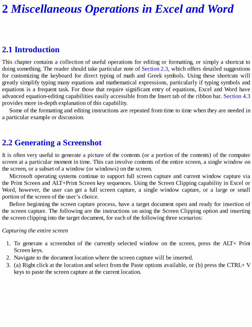
ThedifferenttypesofchartsselectedforpresentationoftheBesselfunctionareshowninFigure3.13athroughf.ThechartinFigure3.13a isa typical type3scattergraphwithsmoothcurvesconnecting the

pointsandnodatamarkers.ThechartinFigure3.13bisanareachartshowingthecurvesasoverlappingwithashadingeffect.ThechartinFigure3.13cisasurfacechartwithawireframe3-Dsurface.

ThechartsinFigure3.13dthroughfareallvariationsofthechartinFigure3.13b.Startingwith thatchart,changethecharttypeviatheCHARTTOOLS/DESIGN/TYPE/ChangeChartTypemenuandselectArea/3-DArea.Torotatethechartplotarea,doubleclicktheplotareaforthechartandgotothePlotAreaOptions.Under3-DRotation,enteravalueforX-Rotation. In thecaseofFigure3.13d throughf,rotationvaluesof289°,329°,and239°arechosen.TheresultsareshowninFigure3.13dthroughf.Thispresentationenablesonetolookatthe“front”or“back”offunctionsordata.Othereffects,suchasy-axisrotationandperspective,arealsoavailablefromthePlotAreaOptionspanel.

FIGURE3.12

3.13.1ChangesinGapWidthon3-DDisplaysThewidthoftheseparationgapbetweentheplotteddataseriesina3-Dchartmaybeadjustedusingthefollowingprocedure:

1. Activatethedataseriesbyclickingonit.2. ClickCHARTTOOLS/FORMAT/CURRENTDATASELECTION/FormatSelectiontobringupand

makechangesingapwidthasdesired.Ifmultipleseriesaredisplayed,adjustthegapwidthforeachdataseriesinthechart.

FIGURE3.13

3.14PlotsofTwoVariableswithandwithoutSeparateScalesTwosetsofdata(curves)witheithermarkedlydifferentrangesorunitsmaybeplottedastwodataserieson the same scatter graph. Both the abscissas (x-coordinate) and ordinates (y-coordinate) may havedifferentscalesorunits.TheprocedureshowninFigure3.14isasfollows:

1. Plotbothsetsofpointsusingthenormalprocedureforscattergraphs,asshowninFigure3.14a.

FIGURE3.14

2. Double click on theY2data series to cause theFormatDataSerieswindow to appear.ClickonSecondaryAxistocreateasecondaryordinateaxisforY2.Thescaleofthegraphforthatserieswillbeexpandedorcontractedandthedatawillbereplottedaccordingly,asshowninFigure3.14b.

3. Attachtitles(labels)ofindicatedvariablesandunits,tickmarks,titles,etc.,asappropriate.Thedatasetsmaybemarkedortitledusingaseparatelegendbox,differentcolorlines,orboxlabelsinserteddirectlyonthechartitself.

Othercosmeticfeaturesmaybeaddedasnecessary.

3.15ChartsUsedforCalculationPurposesorG&AFormatFigure3.15showsa type3x–yscatterchart fordisplayingcomputedvaluesofR, thecapital recoveryfactorusedinfinancialcalculations.TheExceltableofvaluesisshownintheupperpartoftheworksheet,followedbyanequationforR.Theuseofsmoothedcurveswithoutdatamarkersisanexcellentchoiceforthepresentationinthisexample.

3.15.1G&AChartInFigure3.16,thesameinformationisplottedinwhatwechoosetocallaG&AChart(forGeneralsandAdmirals).Still, a type3 scatter chart is employed,but larger fonts areused for axis andchart labelswhere possible.Minor gridlines are deleted, and a light pattern is added to the body of the chart forcosmeticeffects.Thismightbecalleda“broadbrush”chartasitshowsmaintrends.Itshouldnotbeusedforcalculationpurposes.ThechartinFigure3.15canbeusedtoreadratherprecisevaluesofR.

FIGURE3.15

FIGURE3.16

3.16StretchingOutaChartAchartthatneedstoextendbroadlyfromtoptobottomorsidetoside,butwhichappearscompressedonasinglepage,canbestretchedoutorexpandedasfollows:

1. Clickthecharttoactivateit.2. Ifthechartisneededonapagebyitself,openanewworksheetinthecurrentExcelworkbook.3. Clicktheupper-leftcornercell(A1)ofthenewworksheetorthecellatwhichtheupper-leftcorner

ofthechartshouldbelocated.4. ClickEDIT/PASTEorCTRL+V.5. Thechartcanberesizedbyusingoneofthefollowingtechniques:

a. Toresizethechartwithoutmaintainingtheaspectratio(ratiooflengthtowidth),clickonasideoracornerofthechartandusethemousetomovethatsideorcornertothedesireddimension.

b. Toresizethechartwhilemaintainingtheaspectratio(ratiooflengthtowidth),clickonacornerwhile holding down the SHIFT key and drag the corner to the desired size of the chart. Thelengthandwidthwillautomaticallyadjusttomaintaintheaspectratio.

3.17CalculationandGraphingofMovingAveragesMovingaveragesareemployedasforecastingtoolsinapplicationsrangingfromstockmarketpredictionstoestimationsofsalesandinventorytrends.Thecalculationassumesthataforecastvalueofthevariableunderconsiderationmaybemadeasasimplearithmeticaverageof theprecedingactualvaluesoveraselected number of time periods. The number of periods is chosen to fit the situation. Inmany cases,moving averages are charted using several calculation intervals to gain comparative insights into thespecifictrends.

Theformulaforthemovingaveragecalculationis:

or

whereFt=forecastvalueofthevariableattimetn=numberofprevioustimeperiodsoverwhichtheaverageistobecomputed(Excelusesadefault

valueofthreeperiodsifsomeothernumberisnotspecified)At=actualvalueofthevariableattimetThus,forn=4timeintervals,wewouldhaveforecastvaluesattimest=6and7ofF6=(A5+A4+A3+A2)/4F7=(A6+A5+A4+A3)/4Excelperforms thecalculation for a setof specifiedAt values andpresents a graphof the forecast

valuesFtalongwiththeactualvaluesforcomparison.Itiseasytochangethenumberofperiodsforthemovingaveragecalculationtoexaminetheinfluenceofthisselectionontheforecastingtrends.

Example3.1:WeatherTemperatureTrends

Figure3.17displaysthreetypesofweathertemperaturedataasindicatedinthenomenclatureforthefigure:(1)TVfifth-dayfutureforecastsforhighandlowtemperatures,(2)actualhighandlowtemperatures,and(3)long-termaverageornormalhighandlowtemperatures.Wewillpresenttheresultsofmovingaveragecalculationsfor10-,30-,and60-dayintervalsovera220-daytotaltimeperiod.Thecalculationswillbemadeforthefollowing:

1. TheTVfifth-dayfutureforecastfordailyhightemperaturein°F2. Thelong-termaveragehightemperaturein°F

InExcel2016,plottingamovingaverageonachart forasetofdata isassimpleasplottingatrendline,suchaslinear,power,andpolynomialtrendlinespreviouslydiscussed.

Beginning with a chart containing a plot of the TV fifth-day future forecast for daily hightemperatures, a moving average trend line is added by clicking on CHARTTOOLS/DESIGN/CHARTLAYOUTS/AddChartElement/MoreTrendlineOptions. TheFormatTrendlineOptionswindow appears on the right side of theworksheet. From thiswindow,weselectMovingaveragewithaPeriodvalueof10,indicatinga10-daymovingaverage.TheresultofthisadditionisshowninFigure3.18.

Followingthesamesteps,weadda30-daymovingaverageanda60-daymovingaveragetothesamechart,whichresultsinthechartshowninFigure3.19.

FIGURE3.17

FIGURE3.18

FIGURE3.19

FIGURE3.20

3.17.1StandardErrorThestandarderrorforthemovingaveragefunctionisdefinedby:

Thisfunctionhasthesameformasapopulationstandarddeviation.The standard error for the 10-day moving average of Figure 3.18 is plotted in Figure 3.20. The

decreasing trendwith the approach of summer indicates less volatility in temperature as the calendarprogresses.Asonemightexpect,thissimplymeansthatTexasispredictablyhotinthesummer—dayafterday.

3.18BarandColumnChartsAlthoughnotaswidelyusedas scattercharts,barandcolumnchartshaveanumberofapplications inengineering and are rather straightforward to create inExcel. The data are simply highlighted and theappropriate bar or column chart is created using INSERT/CHARTS/Bar Chart orINSERT/CHARTS/Column Chart. Editing with choices of fonts, fill patterns, line widths, etc., isessentiallythesameaswithanyotherchart,buttheeditingofgapwidthsandoverlapbetweencolumnsdeservessomespecialmention.Toperformthisediting, ineither2-Dor3-Dbarorcolumncharts, thedataseriesarefirstactivatedbydouble-clickingonthechart.TheFormatDataSerieswindowwillthenappearasshowninFigure3.21fora2-DchartorFigure3.22fora3-Dchart.

Fora2-Dbarorcolumnchart,gapwidthisthespacingbetweenthebarsrepresentingeachdatapoint.Overlap indicates the spacing between the adjacent data points. Negative Overlap indicates a spacebetween thecolumns.Figure3.23 illustrates the results of changing both parameters for a simple datasystem.

Similarly,ina3-Dbarorcolumnchart,theparametersofgapdepth,gapwidth,andchartdepthmaybevariedtochangetheappearanceofthefinalchartpresentation.

FIGURE3.21

FIGURE3.22

3.19ChartFormatandCosmeticsMostchartsprepared forengineeringpurposeswillhaveasimple format involvingminimalartisticorcosmetic effects. For visual presentations, color is certainly used to advantage. Excel offers theopportunitytoadjustchartfills,fonts,colors,linesize,andothereffects.

FIGURE3.23

The purpose of this section is to illustrate the format windows that may be called up to makeadjustments invariouschart layoutsandappearance.Figure3.24 showsavery simple type4 (Section3.3)scatterchart.ThemainelementsofthechartlayoutsthatmaybevariedareChartArea,PlotArea,EitherAxis,DataSeries,Title,andGridlines.Theformatprocessisinitiatedbydouble-clickingoneoftheseelementsand therebycallingup the formatwindowas shown inFigure3.25.Note that theChartOptionsdrop-downmenuhasbeenselectedtoshowallthechartelementsthatareeditablethroughthiswindow.For theChartArea selection, there areChartOptions and there areTextOptions that canbeedited.ForChartOptions,thereareoptionsforFill&Line( ),Effects( ),andSize&Properties( ).

Clickingoneachoftheserespectiveiconswillpresentalltheoptionsfromwhichtochoose.Thereaderisencouragedtoselecteachoptionareaandbecomefamiliarwithallavailableoptions.

FIGURE3.24

FIGURE3.25

FIGURE3.26

3.20SurfaceChartsSurfacechartsofthewiremeshorcolorvariationtypemaybeplottedbyselectingaSurfaceChartfromthe INSERT/CHARTS/InsertSurfaceorRadarChartmenuoption.Theadjustmentof thechartdepth isproblematic,butmaybeaccomplishedusingthefollowingprocedure:

1. Select(activate)thedata.2. OntheChartWizard,chooseAreaChart,3-Deffect.3. DoubleclickachartelementtobringuptheFormatwindow.OntheChartOptionsdrop-downmenu,

selectSideWallandclickontheEffectsIcon.Scrolldownandexpandthe3-DRotationoptionsandincreasethevalueoftheDepth(%ofbase)from100to520.

4. ChangethecharttypetoSurfaceandresizethechartforbetterviewing.

Figure3.26showstheresultofthisprocedureappliedtotheBesselfunctionsdescribedinSection3.13.

3.21AnExercisein3-DVisualizationThis example gives the reader an opportunity to exercise his or her space visualization capabilities.Considerthesetof3-DviewsoftheobjectshowninFigure3.13.

Figure3.27displaystheobjectinFigure3.13eatseveraldifferentelevationandrotationparameters.Before going further, the reader may want to examine each of these views and try to visualize theirrelativepositions.

FIGURE3.27

Whenconsideringtherotationof3-Dcharts,notethatcertainanglesrepresentcertainviews.Notethatarotationangleof0°or360°representsaviewhead-onorstraightintothepage.Anelevationangleof0°representsthesameviewingposition.Anelevationangleof+90°representsaviewstraightdownonthetopof theobject,whereasanelevationangleof−90° representsaviewstraight into thebottomof theobject.ThedisplayoftheviewspresentedinFigure3.27notes thedesignationsof theircorrespondingrotationandelevationangles.

VisualizingthedifferentobjectpositionsofFigure3.27withouttheelevationandrotationinformationisnotaneasytaskandrepresentssomedifficultyformostreaders.ThisexampleillustratesonceagaintheincredibledisplaycapabilitiesofExcelandtheeasewithwhichtheycanbeaccomplished.

Problems3.1Thefollowingdataarecollectedinacertainexperiment:

Plot thedataas types1,2,and4scatterchartsusing linear, semi-log,and log–logcoordinates.Basedon theseplots,obtainasuitablecorrelationfor thedata. Include thecorrelationequationandvalueofR2ineachplot.

3.2ThefollowingadditionaldataarecollectedfortheexperimentofProblem3.1.Addtotheoriginaldataandobtainanewcorrelationforthecompletesetofdata.

3.3Plot the followingdata in a suitable scatter chart andobtaina trend line thatbest fits thedata.Includethetrendline,correlationequation,andvalueofR2inthechart.

3.4InterchangethecolumnsinProblems3.1through3.3andreplotthedatausingyastheabscissa.Subsequently,obtainnewcorrelationandtrendlineequations.

3.5Twosetsofvariablesaremeasuredasfunctionsofxandaretabulatedasfollows:

Plotthedataonatype4scattergraphusing(1)thesamescalefory1andy2,(2)anexpandedscalefory1,and(3)anexpandedandinvertedscalefory1.

3.6PlotthedataofProblem3.5as(1)acolumnchartand(2)abarchart.

3.7PlotthedataofProblem3.5asasurfacechartwith(1)variablesurfacecolorand(2)asawiremeshchart.

3.8Constructatableofthefunction:

forn=1,2,and3and0<x<π.Selecttheincrementsinxasappropriate.Plotthefunctionas(1)anareachartwith3-D,(2)asurfacechartwithvariablecolors,and(3)a3-Dwiremeshchart.

3.9Thefollowingdataarecollectedinanexperiment:

Plotthesedataastypes1,2,and4scattergraphsonlinearcoordinates.Whatdoyouconclude?Select the most appropriate of these plots and obtain linear, exponential, second-orderpolynomial,andpowercorrelationsof thedata.Displaythetrendline, thecorrelationequation,andvalueofR2foreachcorrelation.Dependingontheresultsofthesecorrelations,replotthedataonsemi-logorlog–logcoordinatestoimprovethedatadisplay.

3.10ReconstructthedataofFigure3.15.Plot theresultsas(1)anareachartwith3-D,(2)asurfacechartwithvariablecolor,and(3)a3-Dwiremeshchart.

3.11For colorful results, add the following fill effects to anyof the charts obtained in the previousproblems:

a. Fill the chart area with a colorful gradient of your choice by double clicking on the chart,selecting Fill from the Format Chart Area popupwindow, and then selecting the backgroundpatternandcolorsthatyoulike.

b. Filltheplotareawithacolorfulgradientofyourchoicebydoubleclickingontheplotareaofthe chart, selecting Fill from the Format Chart Area popup window, and then selecting thebackgroundpatternandcolorsthatyoulike.

3.12Acertaincommoninvestmentstockhasthefollowingpricehistory:

Plotthestockpriceasafunctionofperiod.Subsequently,constructthemovingaveragesforthestockpricehaving intervals ranging from two to fourperiods.Also,plot the standarderror foreachofthemovingaverages.Commentontheresults.

3.13Thefollowingresultsarecalculatedfromaknownanalyticalrelationship:

Choosean appropriate scattergraph forplottingy as a functionofx.Then, replotusingy as afunctionof1/x.Selectthecoordinatesystemsappropriatetothetabularvalues.

3.14PlotthestockpricedataofProblem3.12asacolumnchart.Repeatfordifferentgapwidthsandoverlaps.

3.15The followingdataare expected to followaquadratic relationship. Investigate this expectationusinganappropriatescatterchartandsecond-degreepolynomialtrendlinefit.

Aquadraticfunctionwillplotasastraightlineonlinearcoordinateswhentheratio(y–y1)/(x–x1)isplottedagainstx.Takingtheseconddataset(1,3.724)forthex1andy1coordinates,makesuchaplotandobtainalineartrendlinefit tothedata.Howdoesthisresultcomparewiththatobtainedusingthesecond-degreepolynomialfitfortheoriginaldataset?

4Line Drawings, EmbeddedObjects, Equations,andSymbolsinExcel

4.1IntroductionInChapter3,wesawhowitispossibletogenerateavarietyofgraphicaldisplaysinExcel,whichmaybe employed for data presentation or calculation of results. The drawing capabilities of Excel offerfurtheropportunitiesfordisplayingrelatedschematicdrawingsorotherinformationalongwithworksheetresults and datamanipulations. Although the drawing capabilities in Excel are not as extensive as inComputerAidedDesignsoftwareor tools suchasMicrosoftVisioProfessional, theyareversatileandoffertheconvenienceofcreatingdrawingsinotherMicrosoftOfficedocuments.ForthosereaderswhouseMicrosoftPowerPoint,thedrawingcapabilitiesareevenmoreuseful.

EngineeringschematicsordrawingsfrequentlyinvolvetheuseofGreekormathsymbols.Theuseofthese symbols ismuch improved in recent versions of Excel. Examples and exercises in applying thevarious drawing capabilitieswill be given so that the reader can achieve some familiaritywith theseelements.Thereadercanthenexpandtheuseashisorherneeddictates.

4.2Constructing,Moving,andInsertingStraightLineDrawings1. Open a new worksheet. Navigate to the Insert tab of the ribbon bar and focus attention on the

Illustrationssection.2. ClickShapesandthenclick toselect theFreeformline typeunder theLinessectionof theShapes

menu.Figure4.1showstheFreeformlinetypeicon.3. HoldingdowntheShiftkey,clickthecrosshairatapointtostartdrawingwithstraightlines,quickly

release-click, thenmove thecrosshair to thenextpointandclickagain; repeatuntil theendof thedrawingisreachedandthendouble-click.If theendisataclosedfigure,rightclick.Several lineelements may be drawn separately to form the final drawing object, in which case multiplerepetitions of this process must be performed. Line weight or style (including shading) may beadjustedbychoosingtheappropriateoptionsfromtheShapeStylessectionoftheFormattabontheribbonbar.

FIGURE4.1

TheExcelworksheetgridmaybeused toguide thedrawingprocess.Dependingon thesizeofdrawingneeded,itmaybeadvantageoustoworkwithareducedorcompressedworksheetgridbyadjustingthezoomlevelusingtheVIEW/ZOOM/ZoomorVIEW/ZOOM/ZoomtoSelectionoptions.Reducing the column width with HOME/CELLS/Format menu choices may also help drawingprecision.Therowheightmayalsobereducedtoprovideafinerdrawinggrid.Drawingpiecesmaybeconstructedseparatelyandthendraggedtogethertoassembleanoveralldrawingobject.PressF1forExcelHelpandenter the search term“Grouping” formore information in this regard.Precisemovements of objectsmay be accomplished by selecting the object and pressing arrow keys formovementinthedesireddirection.

4. INSERT/SHAPES/Calloutsmaybeusedtoaddnomenclature,ascanINSERT/TEXT/TextBox,withor without arrows. Line borders of callouts may be removed by clicking the FORMAT/SHAPESTYLES/Shape Outline and then selecting No Outline. To avoid overlap of worksheet or graphgridlines,calloutsortextboxesmaybefilledwithwhitecolor.

5. Drawingobjectswithallannotationsmaybemoved,copied,orinsertedelsewherebyhighlighting(selecting/dragging)thecellscontainingtheobjectandthenclickingHOME/CLIPBOARD/CopyorbyusingthekeyboardshortcutCTRL+C.Thetargetdocumentisthenopened,thedesiredlocationisclicked/selected (see upper-left cell for the location on an Excel worksheet). ClickHOME/CLIPBOARD/Pasteandselect theappropriateoperation to insert theobject into the targetdocument. CTRL+V is a keyboard shortcut that can be used in the place ofHOME/CLIPBOARD/Paste.

4.2.1DrawingLineSegmentsinPreciseAngularIncrementsTodrawanunwaveringstraight-linesegment(notafreeformobject)inanangularincrementof15°(orprecisely horizontal or vertical), click on the straight line icon (see Figure 4.1) from theINSERT/SHAPES/Linesmenu.Then,whileholdingdowntheShiftkey,clickandholdthemousebuttonatthe starting point andmove themouse to the end location to draw the line.When the Shift key is notdepressed,thelinemaybedrawninanydirection.Thisisveryusefulfordrawingprecisehorizontalorverticallines.

Example4.1:AssortmentofDrawingShapes

Figure 4.2 shows a collection of different drawing shapes that may be constructed using theINSERT/SHAPEScapabilitiesofExcel.Thefollowingremarksrefer totheobjectsat thenotedcell locations for items in which the construction is not obvious or already noted on theworksheet.

FIGURE4.2

H2:P13—Thedonutshapeischangedtoahollowcylinderusingthe3-Deffectstool,whichallowsvariationinlength.Agradientpatternfillisthenadded.

Q2:R25—A resistor shape is first drawn using the AutoShapes/Freeform lines tool (seediscussion in Section 4.2, step 3) and then is copied several times using assorted lineweights(asnoted).Itisalsocompressedbydragging.

B24:L37—Arectangleshapeisdrawnfirst.3-Deffectsareadded,andthenafillpatternwithgradienteffectisused.

Q26:R37—Twocirclesaredrawnand then filledwithgradientpatterns frominner-to-outerandouter-to-inner.

H24:L37—A rectangle is drawn with 3-D, and light fill is applied. A resistor element isaddedalongwitharrowsandstraightlines.Theelementsaregrouped(combinedtoformoneobject)andthenrotated.

M24:P37—If needed, a digitized photo can be added. This digital photo is taken using adigitalcameraandcopiedtotheworksheet.Editingofbrightness,contrast,cropping,andimage size may be accomplished before transfer to the worksheet. Editing can also be

performedaftertransfertotheworksheetbyrightclickingthephotoandselectingFormatPicturefromthepopupmenu.

Of course, the figuremayalsobepresentedwithout thepresenceofgridlines, andcolumnand rowheadings.

Example4.2:Construction,Assembly,andLabelingofaLineDrawing

An illustrationof themechanismsofanassemblyof linedrawings inExcel is shown inFigure4.3:

1. InFigure4.3a,ashellofasolarabsorberisdrawnwithINSERT/SHAPES/Lines/Freeformasdescribedpreviously.

2. Next, the innerboundary isdrawn inFigure4.3bandadded toFigure4.3a toproduce thecombinationshowninFigure4.3c.Inpractice,thetwoelementswouldnotbemovedaroundasshownhere.Thedrawingsarecopiedtoshowthestepsastheyprogress.

3. A5%patternfillisaddedtotheinnerboundaryasshowninFigure4.3d.Thisrepresentstheairinsidethecollector.

4. A long, thin rectangle is drawn in Figure 4.3e and filled with a 25% pattern fill. Thedimensions of the rectangle are squeezed, adjusted, andmoved to the top of the shell asshowninFigure4.3f.Thiselementrepresentstheglasscoverofthesolarcollector.

5. A 4.5-pt black line is added in Figure4.3g to indicate the black absorbing surface at thebottomofthesolarcollector.

6. The elements of the assembled drawing are then grouped by (1) holding down Shift, (2)clicking on the elements in sequence, and (3) clickingFORMAT/ARRANGE/GROUP/Group.Theassembledobjectmaynowbemovedorcopiedas a single object. In Figure 4.3i, the solar absorber has been rotated by either clickingFORMAT/ARRANGE/RotateorclickingtheRotateiconanddraggingittothedesiredangle.

FIGURE4.3

7. Theassembleddrawingcan thenbecopied toaWorddocument inwhichnomenclature isaddedwithsubscriptsandappropriatesymbols.Similarly,nomenclaturecanbeaddedwithinExcel.ThefinaldiagramisshowninFigure4.3h.Theoutputshownhereiswithoutgridlinesorcolumnandrowheadings,althoughgridlinesareveryusefulwhenconstructingdrawingelements.

Example4.3:PracticeExerciseswiththeINSERTandFORMATTabs

Gaining familiaritywith the INSERT (Figure4.4a) and FORMAT (Figure 4.4b) tabs shown inFigure 4.4 may be accomplished by carrying out the following exercises, which refer to thedrawingobjects shown inFigures4.2 and4.3.The solar absorber inFigure 4.3 is consideredfirst.

ForFigure4.3a, click INSERT/SHAPES; then in theLines section, click theFreeform icon(seeFigure4.1).HolddowntheShiftkey,movethecrosshairtothedesiredstartingpoint(a corner of a cell, for example), click quickly, and release the mouse button. While

continuing to hold down the Shift key, move the crosshair to the next corner, click andrelease quickly, and continue until five segments (two top lips, two sides, and a bottomsegment)areinplace.Doubleclicktocompletetheobject.

ForFigure4.3b, perform the sameoperation as that shown inFigure4.3a, except that onlythreelinesegmentsarerequired.LineupthedrawingusingaworksheetgridtoobtainthedimensionsinFigure4.3b.

ForFigure4.3c,activatethedrawinginFigure4.3banddrag-movetomatchwithFigure4.3a,as shown in Figure4.3c.Once the drawings are assembled, activate Figure 4.3b—clickuntil boundary handles appear. Then, click the FORMAT/SHAPE STYLES/Shape Fillmenutoselectafillcolorandstyle.FromthisShapeFillmenu,youcanselectGradientsandthenMoreGradientstoobtainavarietyofFilloptions.Inthisexample,thePatternfilloption isusedand the5%filloption is selected.Selecting thiswill fill theobject as inFigure4.3d.

For Figure 4.3e, create a rectangle using the INSERT/SHAPES/Basic Shapes menu andselectingtheappropriaterectangle.Clickthemousebuttontostart therectangleanddragthe mouse to draw the rectangle. Release the mouse button when the desired shape isattained.Donotworryiftherectangleisnottheexactsizeorproportionneeded.Next,usethe FORMAT/SHAPE STYLES/Shape Fill menu. Like above, select Gradients, MoreGradients,andthenPatternfilltoselecttheappropriatefillpattern.Thefourthboxonthetop row of the pattern fill options will provide a 25% fill pattern. Click OK, and therectanglewillappearasinFigure4.3e.

FIGURE4.4

Drag the filled rectangle to a position on top of the drawing in Figure 4.3d. Then, drag,squeeze, or stretch the object to the dimensions shown. This is done by positioning thedouble-arrowpointeronthesidehandlesofthefilledrectanglebyholdingdownthemousebutton and dragging until the two figures line up.Nudge it into exact position using thearrowkeys.

Next, draw a straight line at the inside bottom of the collector usingINSERT/SHAPES/Lines/FreeformasinFigure4.3aandb.Tocreatethicknessforthisline,usetheFormatShapetaskpanetodoso.ToopentheFormatShapetaskpane,clickinthelower right corner of the FORMAT/SHAPE STYLES section (see Figure 4.4b). In theFormatShapetaskpane,underLine,adjusttheWidthbyselectingthe4.5-ptlinewidth.

Group the drawing elements created earlier by holding down the Shift key and clicking insequence the four elements (a, b, e, and the 4.5-pt line). ClickFORMAT/ARRANGE/GROUP/Group to connect these elements as one object. Thecompositeobjectmaynowbemovedasasingleentity.

At this point, the composite figuremaybe copied to anotherMicrosoftOfficedocumentbyactivating the object and then clicking HOME/CLIPBOARD/COPY. Open a Word orPowerPointdocumentandclickHOME/CLIPBOARD/PASTEtopastethecompositefigureattheappropriatelocationwithinthedocument.

Thenomenclatureelementsareaddedbyusingeithertextboxesorcalloutarrows(asforT1andT2).These elements canbe addeddirectly fromwithinExcel, or they canbe addedfromwithinWordorPowerPoint.Arrowsaresimplyanotherobject typefromwithintheINSERT/SHAPESchoices.SubscriptsorsuperscriptsareformattingappliedtotextviatheFont Settings menu and math symbols are inserted via the INSERT/SYMBOLS/Symbolmenuoption.SeeSection2.3formoredetailinthisregard.

Afterthenomenclatureisadded,groupthenomenclatureandtheoriginalcompositedrawingtogether via the FORMAT/ARRANGE/GROUP/Groupmenu option so that it appears asshowninFigure4.3h.

Rotation of the object may be performed by activating the object and either clickingFORMAT/ARRANGE/Rotate or the Rotate icon (third from the left on the Drawingtoolbar).

ThefollowingexercisesrefertosomeofthedrawingobjectsshowninFigure4.2:

1. Create circles as shown in the figure at Q26:R37 using theINSERT/ILLUSTRATIONS/Shapesandpickingacircle.HoldingdowntheShiftkey,createa circle by moving the crosshair until the desired size is accomplished. Excel shouldautomaticallychangetotheDrawingToolsFORMATtabontheribbonbar.Whilethecircleis still activated, click the FORMAT/SHAPE STYLES/Shape Fill menu item. Click theGradient option that best matches the top circle. Repeat these steps to mimic the bottomcircle.

2. CreatedonutshapeslikethoseatJ4andK4.UseINSERT/ILLUSTRATIONS/Shapes/BasicShapes/Donut.Dragtheyellowdottoachievethedesiredthicknessofthedonutwall.

3. Create the hollow cylinder, as shown at N5, by first creating a donut. Then, click theFORMAT/SHAPE STYLES/Shape Effects/Bevel/3-D Options. Choose a top and bottombevel,andthenincreasetheDepthsettingtorepresentthedesiredlengthofthecylinder.

4. Create arcs like those at B17:G22 using INSERT/ILLUSTRATIONS/Shapes/BasicShapes/Arc. Then, repeat while holding down the Shift key. Note that circular arcs arecreated.Notetheeffectofdraggingtheyellowdot.

5. The resistor elements at Q2:R25 are created by (1) usingINSERT/ILLUSTRATIONS/Shapes/Lines/Freeformtoconstructasingleresistor,(2)copyingthe resistor toother rows, (3)changing the linewidthofeachcopied resistor, (4)copying

andcompressingtheresistor,and(5)subsequentlycopyingthecompressedresistortoothercellsandmodifyingtheirrespectivelineweights.

Performing these exercises enables a person to achieve a reasonable level of proficiency indrawingandformattingobjectsinExcel.Ofcourse,furtherexperimentationisencouraged.

4.3InsertingEquationTemplatesandSymbolsUsingExcelandWordInsertingsymbolsorequations inExcel,Word,orPowerPointdocuments isgreatlysimplifiedbyusingthe INSERT/SYMBOLS/Equation or INSERT/SYMBOLS/Symbol menu options. Word supportsadditionalequationtypesbeyondthosesupportedinExcelthatthereadercanexplore.

4.3.1SymbolInsertionForinsertingsymbolsinExceldocuments,usethefollowingprocedure:

1. Designatethelocationforasymbolinsertion.2. ClickINSERT/SYMBOLS/SymboltobringupthedialogboxshowninFigure4.5.Fromthisdialog

box, choose the font and then choose the symbol set to display the symbol options in the mainwindow.

3. SelectthedesiredsymbolandpresstheInsertbutton.

Excel 2016 has 38 sets of symbols from which to choose using the dialog box mentioned in step 2.Additionally,Excel2016supports27specialcharactersfromtheSpecialcharacterstabofthedialogboxinstep2.

4.3.2EquationTemplateInsertionForinsertingequationsinExcelorWorddocuments,usethefollowingprocedure:

1. Designatethelocationforanequationinsertion.2. Click the down arrow on the INSERT/SYMBOLS/EQUATIONmenu to bring up the dialog box

shown in Figure 4.6. From this dialog box, choose an equation template, which will insert aneditableequationintothedocument.CustomequationscanbecreatedusingtheInkEquationmenuoptionfromINSERT/SYMBOLS/EQUATION.

FIGURE4.5

3. Edittheequationtemplatetosuityourneeds.

4.4InsertingEquationsandSymbolsinExcelUsingEquationEditorInsertingequationsandsymbolsinExcelusingtheEquationEditorcanbeaccomplishedbyfollowingthisprocedure:

1. Selectacellforthelocationoftheequation.2. ClickINSERT/TEXT/OBJECT/Object,selectMicrosoftEquation3.0andclickOK.3. Beforestartingtoconstructanequationorsymbol,setthesizeofthetypebyclickingSIZE/OTHER,

andthenenterthedesiredfinalpointsize.ClickOK.4. ConstructtheequationorsymbolsusingfeaturesofEquationEditor.5. Whenanequationorsymbolhasbeenconstructed,double-clicktheobjectuntilitishighlightedor

activated.6. ClickEDIT/CUT.7. Clickthecellorchartlocationfortheinsertion.8. Click HOME/PASTE and select the appropriate paste operation. The object will appear at the

designatedcellorattheupper-leftcornerofthechart.9. Activatetheobjectanddragittothefinaldesiredlocation.Aboxmayenclosetheobject.Remove

the line enclosing the box, if desired, by activating the object and clicking FORMAT/SHAPESTYLES/ShapeOutlineandclickingNooutline.

FIGURE4.6

10. Anemptyboxwillappearatthecellchoseninstep1.Deleteit.11. Toedittheobjectequationorsymbol,double-clicktoactivateit,andtheEquationEditortoolbar

willappear.Editasappropriate.

Example4.4:Graphics,Symbols,andTextCombinations

AnexampleoftheuseofinsertionsandgraphicscomposedandcopiedbetweenWordandExcelisshowninFigure4.7.Inthisfigure,theassemblyofitemsisprintedasaworksheetwithcolumnandrowheadings.Ofcourse,thegridlinesandrowandcolumnheadingscouldhavebeenleftoutto give a more appealing final presentation. Some elements of the assembly are shown in thefollowingcelllocations:

FIGURE4.7

FIGURE4.8

A1:F12—This is the Excel calculation of the equation at H12. The equation at H12 wascreatedusingtheINSERT/SYMBOLS/Symboloperation.

H2:K10—This is the cavity drawing assembly.The cavity and semitransparent coverweredrawn in Excel, grouped, and copied to Word. The labels using subscripts and Greeksymbolswere thenadded inWord, and the total assemblywascopiedback to theExcelworksheet. The labels, Greek symbols, and subscripts could equally have been createddirectlyinExcel.

A14:L43—ThegraphwasplottedfromtheExcelcalculationsusingChartWizardwithatype3x–yscattergraphchosenforthepresentation(seeSection3.3).Thex-andy-axislabelswerecomposedwithintheChartWizard.

A44:H62—This descriptive write-up was composed in a text box within Excel, includingsymbolinsertionandusingsubscripts.

Figure4.8showsanetworkschematicusedtoderivetheequationsfor theillustrationinFigure4.7.

Example4.5:ProgramwithEmbeddedTextDocumentation

Figure4.9illustratesaconvenientapproachtoproducingoutputinExcel.AprogramispresentedatA2:D3withvariablesandnomenclatureatE2:F15.Thedocumentationanddescriptionoftheprogram can be written in a text box, including the use of Greek symbols, subscripts, andsuperscripts.Thisapproachresultsinacompactpresentationonasinglepage(ifonecantoleratethe small type size). A reader studying the program will find it much easier to follow thandocumentationoccupyingseveralpages.

FIGURE4.9

FIGURE4.10

4.5ConstructionofLineDrawingsfromPlottedCoordinatesAclosedfiguremaybeconstructedinExcelbyplottingasequenceofdatapointsthatreturnstotheinitialcoordinateset.AninitialsketchonordinarygraphpapermayformthebasisforgeneratingasmoothedlinedrawingwhencombinedwiththeeditingfeaturesofExcelgraphs.Weillustratethistechniquewithan airfoil shape. The airfoil shape has been hand-sketched on a sheet of graph paper graduated inincrementsof0.1in.Thex-andy-coordinatesoftheshapearethentabulatedinsequence,startingwiththetrailingedgeoftheairfoil,proceedingalongthebottomsurfaceofthesection,andthenaroundthetopsurfacebacktothetrailingedge.TheresultingdataareshownincolumnsAandBofFigure4.10,withthe dimensions given in inches. A type 3 scatter chart is plotted and appears in Figure 4.10, withouteditingofthechartproportions.Notethatthefittedcomputercurveforthetabulateddataisnotassmoothas onewould expect for an airfoil section. This unevenness results from either a poor sketch (by theauthor)orinaccuratereadingsofthecoordinatesofthesketch.

TheunevennessmaybesmoothedbyfirstadjustingthechartproportionstothedistortedformshowninFigure4.11,whichemphasizestheimperfectionsintheplot.Next,thedataseriesisactivatedandthedatapointsaredouble-clickedatpointsalongthecurvethatappeartoneedadjustment.Thesepointsarethen

gentlydraggedtonewpositionstosmoothoutthecurve.TwoovercorrectionsareshowninFigure4.12toillustratetheaction.TheresultsofgentlesmoothingareshowninFigure4.13.Notethattheresultsofthesmoothing(orovercorrecting)alsoappearinthetabulatedvaluesforxandy.

FIGURE4.11

Once the surface curve has been smoothed, the chart proportions are adjusted by dragging the sidehandlesuntil the increments inx-andy-coordinateshave thesamechartmeasurements.TheresultsareshowninFigure4.14.

FIGURE4.12

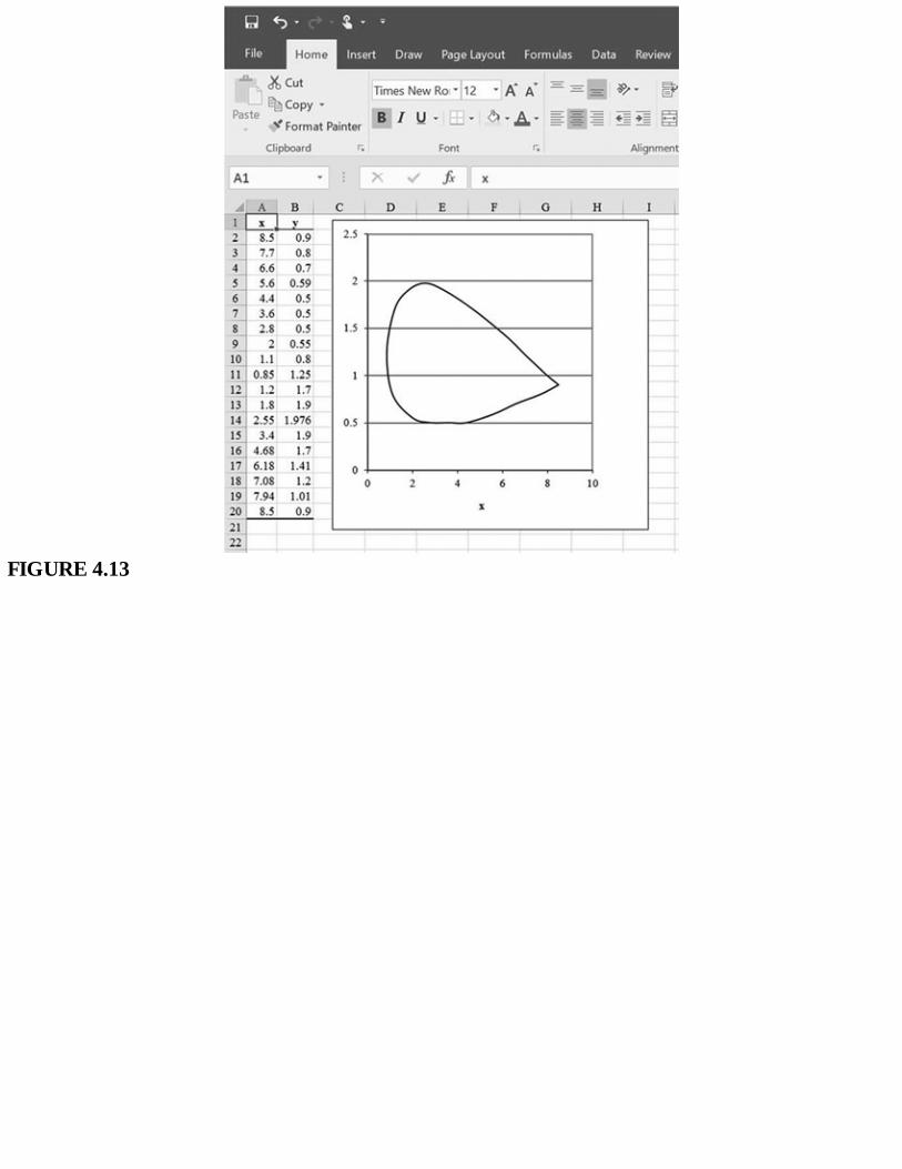
FIGURE4.13

FIGURE4.14

Problems4.1Plotthefunctiony=3.25xe−0.1xovertherange0<x<5usingatype3scatterchart(Section3.3).

Create appropriate labels for the axes using the INSERT/SYMBOLS/Symbolmenu Include thefunctionontheappropriateaxislabel.

4.2Constructtheasymmetriccirclesshown.Then,filltheareasasindicated(orwithafillpatternofyourchoice),andengagethe3-Deffectsshown.

4.3Createthetextboxshownwithaninsertedequation.Then,modifywiththefillandshadoweffectsindicated.NotethatactivatingthetextboxfollowedbyFORMAT/ARRANGE/Rotatewillallowyoutoorientthetextboxvertically.

4.4CreateFigure4.8byfirstcreatingtheresistorelementsasdescribedinSection4.3.Then,createthesmallcircles.TheresistorelementsmayberotatedbyclickingFORMAT/ARRANGE/Rotate.AssemblethedrawinginExcelandgroupwithFORMAT/ARRANGE/GROUP/Group.Createandinsert all the labels using text boxeswithout line borders.Also, construct the equations in textboxesbelowthediagramandpositionthemappropriatelywithrespecttothedrawing.

4.5Ifyouhavenotalreadydoneso,workthroughtheexercisesinSection4.3.

5SolutionofEquations

5.1IntroductionInthischapter,wewillexaminethefeaturesofExcelthatprovideforsolutionsofsingleorsimultaneouslinearandnonlinearequations.Fourmethodswillbedescribed:(1)useoftheGoalSeekfeature,(2)useof the Solver feature, (3) iterative techniques, and (4) matrix inversion with the associated matrixoperations.Exampleswillbegivenforeachmethodandcommentswillbeofferedontheselectionofthebestmethod for a particular problem. Finally, a brief discussionwill be presented on the creation ofmacros,alongwithanexample.

5.2SolutionstoNonlinearEquationsUsingGoalSeekNonlinearequationsmaybeeasilysolvedforrealrootsbyusingtheGoalSeekfeature,whichiscalledbyclickingDATA/FORECAST/What-If-Analysis/GoalSeek.First,theequationiswrittenintheform

Keeping inmind that nonlinear equationsmay havemultiple roots, including complex ones, itmay beadvantageoustoplotthefunctiontogetanideaofthelocationofthepossibleroots.GoalSeekusesaniterativeschemetosolvetheequation,andaninitialguessmustbeprovidedtostartthecomputation.Agraphicaldisplaymaybeusefulinchoosingtheinitialguess.

Weconsidertwoexamples—atranscendentalequation

andacubicpolynomial

ThetranscendentalequationisplottedinFigure5.1usingincrementsinxof0.05overtherange−2<x<+2.Avisualsurveyofthegraphindicatesthatthereisarootatx≈1.0.

FIGURE5.1

FIGURE5.2

TheworksheetinFigure5.2issetupwithaninitialguessforxinsertedincellB4andtheformulafor∂(x) in cell B6. The guess of x = 1.0 was chosen by consulting the plot in Figure 5.1. Next,DATA/FORECAST/What-If-Analysis/GoalSeek is clicked,whichproduces thewindow inFigure 5.4.WesetcellB6=0bychanging(iterating)thevaluesofxincellB4.WhenOKisclicked,thewindowinFigure5.5appearsalongwiththesolutionontheworksheetshowninFigure5.3.Becauseofsymmetry,thereisalsoarootatx=−1.076845.

Thesameprocedureisfollowedwiththecubicpolynomial.AgraphofthefunctionisshowninFigure5.6,indicatingarootataboutx≈2(itturnsoutthattherootisexactly2.0).TheworksheetissetupasshowninFigure5.7withaninitialguesstakenasx=0.(Wecouldhavechosenx=2.0,butthatwouldnot

beas interesting.)Again,DATA/FORECAST/What-If-Analysis/GoalSeek iscalled,and thesolution isshowninFigure5.8havingavalueofx=1.999998558≈2.0.

FIGURE5.3

FIGURE5.4

FIGURE5.5

FIGURE5.6

FIGURE5.7

FIGURE5.8

Thegraphforthecubicpolynomialindicatesthatweshouldnotexpectanyotherrealroots.Dividingthecubicpolynomialby(x−2)toextracttherealrootyieldsaquadraticfunction:

Therootsofthisquadraticfunctionarecomplexandhavethevaluesx=2/3±1.5986i.

5.3SolutionstoNonlinearEquationsUsingSolverSolverandGoalSeekofferalternatewaystosolvenonlinearequations,althoughbothemployiterativemethods.Agraphofthefunctionishelpfulinbothinstancesbecauseitindicatesareasonablevaluetouseastheinitialguessintheiterativeprocess.

ForSolverexamples,weusethesamenonlinearequationsasusedintheGoalSeekexamples.InthetopportionofFigure5.9,wehavetheworksheetsetupforthetranscendentalequation:

DATA/ANALYSIS/Solverisclicked,andtheSolverParameterswindowisdisplayed,targetingcellB4toapproachzerobychangingthevalueofcellB3.Aninitialguessislistedasx=1.0,andthesolutionisgivenintherightsideof thetopportionofFigure5.9asx=1.076874witharesidualvalueof∂(x)=4.29E-7.

FIGURE5.9

Figure5.10givestheworksheetforthecubicequation:

ThetargetfunctionisincellB4,whichistoapproachzerobychangingthexvaluesincellB3.Aninitialguessofx=1istaken,andtheresultisgivenasx=2.00000001witharesidualvalueof∂(x)=4.227E-6.

FIGURE5.10

5.4IterativeSolutionstoSimultaneousLinearEquations

The following procedure may be used as an alternative to Gauss–Seidel or matrix solutions ofsimultaneouslinearequations.Itisparticularlyapplicabletosteady-statenodalequationsinproblemsinwhichsparsecoefficientmatricesareinvolved.

1. OpenanewExcelworksheet.2. ClickonFORMULAS/CALCULATION/CalculationOptionsandselectManual.Thisisnecessaryas

youwillbeenteringformulasthatcreatecyclicalreferences,whichExceldoesnotlikewhensettoauto-calculate.

FIGURE5.11

3. ToggletheworksheetintothemodeofviewingformulasbyclickingtheCTRL+`keysequence.4. Enterequationsintheworksheetusingthefollowingformat:

Forexample,theequations

wouldappearasshowninFigure5.11.5. Equationswillnowbeinviewontheworksheet.Checkcarefullytoensuretherearenomistakes.

Donotadvancetothenextstepunlesstheequationsarecorrect.6. Press theCTRL+`key sequence to return to the numerical viewon theworksheet. Solutionswill

nowappear,inaccordancewiththenumberofiterationsselected.Thedefaultvalueis100iterationswithadeviationof0.001.Thesevaluesmaybechangedtoobtaingreateraccuracy.

Example5.1:SolutionofNineNodalEquations

The following set of equations is obtained from a nodal analysis of a combined convection–conductionheat-transferproblem.Ninenodeswereinvolved,sonineequationsmustbesolvedtoobtain the temperature distribution in the solid. We have already written the equations in theformatforaniterativesolution.

T1=(15.625+1.15T2+1.15T4)/5.425T2=(1.15T1+1.15T3+31.25+2.3T5)/10.85T3=(1.15T2+115+31.25+2.3T6)/10.85T4=(1.15T1+2.3T5+1.15T7)/4.6

FIGURE5.12

FIGURE5.13

T5=(T2+T4+T6+T8)/4T6=(T3+T5+T9+100)/4T7=(1.15T4+115+2.3T8)/4.6T8=(T5+T7+T9+100)/4T9=(T6+T8+200)/4

Thesetofequationsforanine-nodeanalysisoftheproblemisshownascolumnsAandBoftheaccompanyingworksheet(Figure5.12).AmatrixofthenineequationswouldbesparsebecauseeachTdoesnotconnectwithalloftheotherT’s.Theequations/solutionsaredisplayedasagroupbytogglingCTRL+`.ThesolutionsforthevaluesofeachTareshowninFigure5.13.

5.5 Solutions of Simultaneous Linear Equations Using MatrixInversion

WenotedinsolvingthesetofnineequationsinExample5.1thatamatrixsolutiontotheproblemwouldrequireentryofmanymoreconstantsthantheiterativesolution,becausethatparticularprobleminvolvedavery sparsematrix.Fornonsparsematrices (or ifoneprefers, for sparseones too),matrix inversionmaybeanattractivesolutionmethod.Excelprovidesaneasyprocedureforobtainingsuchsolutions.

Thesetoflinearequationsmaybewrittenintheform

where[A]isthecoefficientmatrix,[X]isthesetofunknownvariables,and[C]istheconstantmatrix.Thesetoftwoequations

willhave

astherespectivecoefficientandconstantmatrices.Thesolutionisexpressedas

where[A]−1 is the inverse of the coefficientmatrix, and [A]−1[C] is the product of the two indicatedmatrices.

Excelprovidestwoworksheetfunctionstoperformthematrixinversionandproductoperations.Thefunction

MINVERSE(squarearray)

returnstheinverseofthesquarearraydesignatedintheparentheses.NotethatasquarearrayisrequiredfortheMINVERSE()function.Thefunction

MMULT(matrix1,matrix2)

returnstheproductofthetwomatricesintheparentheses.UnliketheMINVERSE()function,thematrixargumentstotheMMULT()functionneednotbesquarearrays.Oncetheargumentsareentered,pressingCTRL+Shift+Enteractivateseitherof thematrixworksheet functions. Ifonlya singlevalue is returnedinsteadofamatrix,youhavefailedtoexecutetheCTRL+Shift+Enterinput.

Theprocedureforobtainingmatrixsolutionstosimultaneouslinearequationsisasfollows:

1. Enterthecoefficientmatrixinaworksheetasasquarearray.2. DeterminetheinverseofthisarrayusingtheMINVERSEworksheetfunction.3. Entertheconstantmatrixintheworksheet.4. Multiplytheresultsofstep2bythearrayinstep3toobtainthesolution.

Example5.2:NineNodalEquationsSolutionUsingMatrixInversion

Themethodmaybeillustratedbysolvingthenine-equationprobleminExample5.1usingmatrixinversion.TheworksheetisshowninFigure5.14.First,the9×9arrayforthecoefficientmatrixisenteredas [A] in the81cellsB2:J10,whereas theconstantmatrix [C] isentered in theninecellsofB23:B31.

Theinverse[A]−1isobtainedbythefollowing:

1. ActivatingcellsB12:J20toreservespacefor[A]−1.2. Enteringtheformula=MINVERSE(B2:J10)incellB12atthetop-leftcornerofthearray.3. PressingCTRL+Shift+Entertoexecutetheinversefunction.

Thecoefficientsof[A]−1willappearincellsB12:J20asshown.Next,ninecellsareactivatedatE23:E31toreservespaceforthesolutionmatrix[T].

Theformula

=MMULT(B12:J20,B23:B31)

isenteredinthetopcellE23,anduponpressingCTRL+Shift+Enter,thesolutionappearsincellsE23:E31.ItisunderstoodthatT1=E23,T2=E24,etc.

Finally,ifoneisinterested,acheckonthecalculationsmaybemadebyexecutingtheproduct[A][T]inthecellsH23:H31.Thisisperformedbyactivatingthesecellsandenteringtheformula

=MMULT(B2:J10,E23:E31)

inthecellH23.TheresultsincolumnH23:H31shouldagreewiththoseincolumnB23:B31.Notetheagreement,althoughifyoudisplayenoughprecisionontheresult,cellsH26andH27arenotquiteequaltozerobecauseoftheroundingerrorsinthecalculationprocess.

Althoughwe have shownboth thematrix [A] and its inverse [A]−1 inFigure 5.14, it is notnecessarytocalculateanddisplaythecoefficientsoftheinversefunction[A]−1asanintermediatestepinthesolutionprocess.Instead,onemaygodirectlytothesolutionasshowninFigure5.15.Inthiscase,theinverseandmatrixmultiplicationoperationsareperformedbyactivatingtheninecells E12:E20 to reserve space for the solution (Ts) and entering the following combinationformulaincellE12:

=MMULT(MINVERSE(B2:J10,B12:B20)

wherethecellsB12:B20representtheconstantmatrix[C].

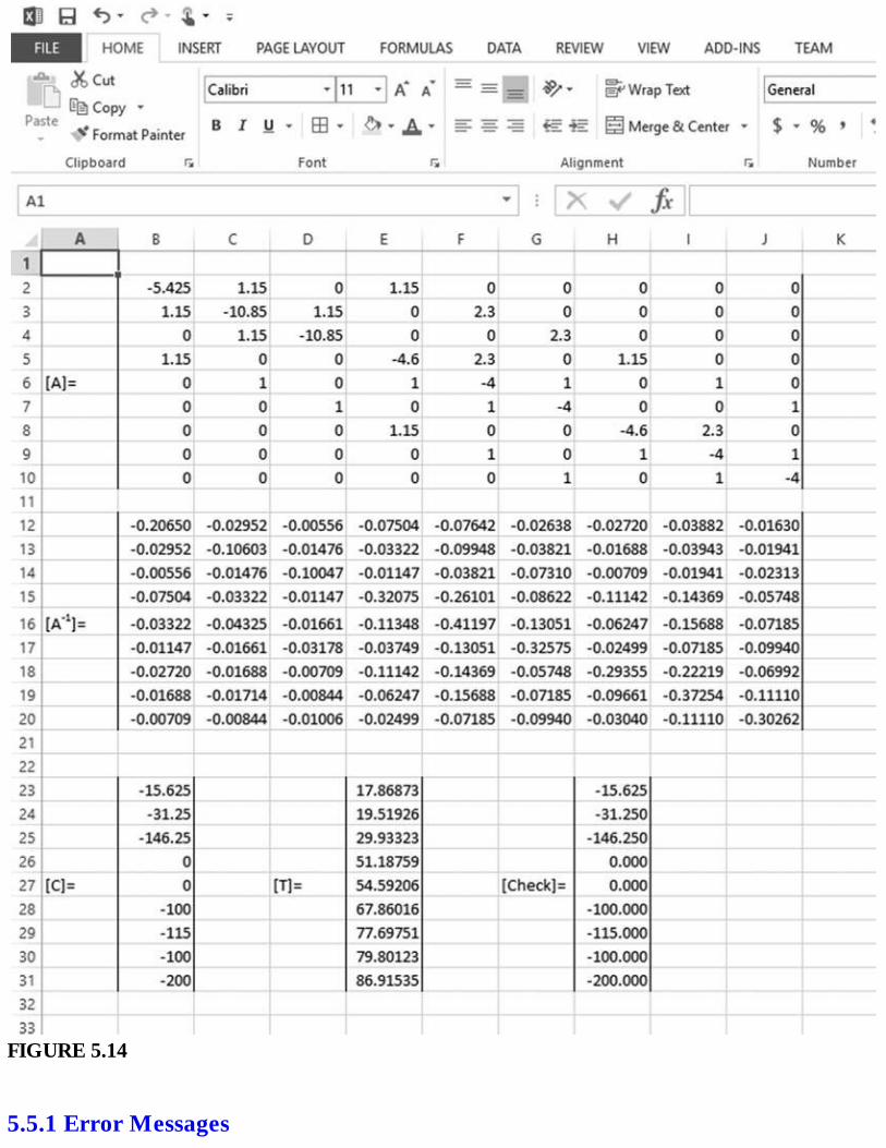
FIGURE5.14

5.5.1ErrorMessages

Ifanyofthecellsin[A]areleftopen,MINVERSE()willreturnthe#VALUE!errorvalue.Itwillalsoreturnthissameerrornoticeifthearraydoesnothaveanequalnumberofrowsandcolumns,i.e.,ifitisnotasquarearray.Ifthedeterminantof[A]iszero,itisnoninvertibleandwillreturnthe#NUM!errorvalue.

FIGURE5.15

5.6SolutionsofSimultaneousNonlinearEquationsUsingSolverExcelSolvermaybeused to solve simultaneous linear or nonlinear equations.The equations are firstwrittenintheform:

Intheequationset(Equation5.5),therewillbenequationsinnunknowns.Asnoted,theequationsmaybelinearornonlinear.Anewfunctiong(x1,x2,…,xn)isformedsuchthat

ThesolutiontechniqueistoallowExcelSolvertoiterateonvaluesofx1,x2,etc.,tocausethefunctiongtoapproachzero.Becauseof thesquares in thef functions, they toowillapproachzeroandresult inasolutionforthesetofequations.Analternateformulationwouldbetoexpressgasasumoftheabsolutevaluesoftheffunctionthroughg=∑ABS(fi(xi)).Fornonlinearequations,multiplesetsofsolutionsmayresult(includingcomplexsolutions);hence,restrictionsmustbeplacedontheiterativeprocesstomatchthe physical problem represented by the equations. For example, a solution to a heat-transfer probleminvolving absolute temperatureswould require that all the temperatures bepositive.These restrictionsmustbeinsertedwhenformulatingtheproblem.

ThefollowingisasuggestedprocedureforsettinguptheExcelworksheettoaccomplishthesolution:

1. IncolumnA,typex1=,x2=,etc.,fornrows.2. IncolumnB,adjacenttocolumnAofstep1,insertinitialestimatesforvaluesofx1,x2,etc., forn

rows.These guesses should bemade in accordancewith the best estimate of the solution for thephysicalproblemrepresentedbytheequations.

3. Skiparow,thenincolumnA,typef1=,f2=,etc.,fornrows,wherethef’sareintheformofasetofequations(Equation5.5).

4. IncolumnB,adjacent tocolumnAof step3, type functions (=…)according to theequation set(Equation5.5).Usecelllocationsfromstep2fordesignatingthevariables.

5. Skipafewrows,thenincolumnA,typeg=.6. IncolumnA,typeg=.7. IncolumnBandthesamerowasstep6,type(=…)functionaccordingtoEquation5.6.Usecell

designationsforthefunctionsfromstep4.8. ClickDATA/ANALYSIS/Solver.Thetargetcellisthatofthefunctioninstep7.Setthistargetcell

equaltozerobychangingthecellsincolumnBofstep2.Constraintsaresetaccordingtophysicalproblems.Asnoted,ifabsolutetemperatureswerethevariablesinathermalproblem,≤0mightbesetastheconstraint.

9. ClickSolve.Asolutionmayormaynotbeobtained.Ifnot,repeatSolve.Often,thiswillproduceasolution.Or, alternate initial estimates for the variables in step 2may be selected and the Solveproceduremayberepeated.Asolutionusuallyresults.Iftoohigha“precision”isspecified,Solvermay state that a solution is not foundwhen, in fact, one has been found but not to the precisionselected.Thepersonformulatingthephysicalproblemmustmakeajudgmentcallinsuchcases.Oneshouldnotaskforunreasonablelimitsofprecisionwhentheuncertaintiesofthephysicalproblemdonotjustifythem.

Example5.3:SolutionofaSetofAlgebraicEquations

TheworksheetandSolverwindowsareshowninFigure5.16forsolutionsofthefollowingsetofnonlinearequations:

FIGURE5.16

The resultingvaluesof the f andg functions are alsogiven.For thisproblem, the constraintofB3:B5≤0(positivevalues)wasselected.Theexactsolutionsarex1=1,x2=2,andx3=3.Asaninterestingexercise,tryadjustingthedesiredprecisionofthisexampleundertheOptionsbuttonoftheSolverwindowandnotethedifferenceinsolutionsandvaluesofthefandgfunctions.

Example5.4:RadiationandConvectionHeatTransferbetweenTwoPlates

Asystemschematicofaheat transferproblemisshowninFigure5.17.The temperatureon theoutsideoftheleftplateisTa,andthetemperatureontheoutsideoftherightplateisTb.Theplateshavedifferentthicknessandconductivities.Heatisconductedthrougheachplateandisdissipatedto fluid flowing between the plates. A fluid moves through the space between the plates attemperatureTf, and the inner surfaces of the plates exchange heatwith each other by radiationenergy, which is proportional to the absolute temperature to the fourth power. In addition, theplates lose heat by convection to the fluid. The convection coefficients are proportional to thetemperaturedifferencetothe0.25power.

The energybalanceon each inside surface is given inEquations5.7 and5.8 alongwith thetemperaturedependenceofEb1,Eb2,h1,andh2inEquations5.9through5.12.Ourobjectiveistodeterminethetemperaturesoftheinsidesurfacesofthewalls,T1andT2.

FIGURE5.17

The purpose of this example is to illustrate the solution of nonlinear equations, sowe ask thereader to accept the format of the equations as given. Detailed information on heat-transferformulationsisavailableinReference3.

The Excel worksheet is set up as shown in Figure 5.18, with the six variables located atB4:B9. The outsidewall temperatures and fluid temperature are entered in columnEwith thevalues that are assigned for this particular case.Other valuesmaybe selected if the effects ofdifferentboundaryconditionsaretobeexamined.Equations5.7and5.8arealreadyinthecorrectformat[∂(…)=0],sotheyareenteredintheworksheetatcellsB11andB12.Thegfunction

isenteredincellB14.ThisisthetargetcellthatwewanttoiteratetozerobychangingthevaluesofT1andT2incellsB4andB5.

Examining Equations 5.7 through 5.12, we see that the formulas in B6:B9 could have beenincorporatedintheformulasforf1andf2.Wechoosetolistthemseparatelysothatthecalculatedvalues of these quantities will become part of the solution presentation. The boundarytemperatures in E4:E6 could also be inserted in the formulas; however, by using this type ofdisplay,theyalsobecomepartofthesolutionpresentation.

The formula displays are removed from the screen and the Solver window called byDATA/ANALYSIS/Solver.ThiswindowisshowninFigure5.19.Fromthephysicalnatureoftheproblem,itcanbeinferredthattheminimumtemperatureinthetwowallsmustalwaysbegreaterthanthefluidtemperatureTf=300K;hence,theconstraintsareasshownintheSolverwindow.Theinitialguessesof301and302forT1andT2areshownatB4andB5oftheformulawindowin Figure 5.18. All temperatures are expressed in absolute (degrees kelvin) because of theradiationterms.

FIGURE5.18

AftersettingthetargetcellasB14=0,Solveisclicked,andtheresultsareshowninFigure5.19.Notethesmallvalueofg,i.e.,0.00005≈0.

Example5.5:SolutionofSimultaneousLinearEquationsUsingSolver

TheprocedureforsolvingasetoflinearequationswithSolveristhesameasthatfornonlinearequations.First,theequationsmustbewrittenintheform∂(x1,…,xn)=0.Forthisexample,wechoosethesamesetofequationsthatweresolvedbyiterationinExample5.1.

Thelistingof theTvariablesfromB1throughB9isshownin theworksheet inFigure5.20.Theequationsforthe∂functionsarelistedfromB12throughB20inthisworksheet.Finally,thegfunctionislistedasthesumofthesquaresofthe∂functionsincellB22.TheinitialguessesfortheTvariablesarealltakenaszeroincellsB1throughB9.

FIGURE5.19

SolveristhencalledbyclickingDATA/ANALYSIS/Solver.TheSolverwindowappearsasinFigure5.20.ThetargetcellthatcontainsthegfunctionisB22,whichissettozero.Thecellstobechanged for the iteration process are those of the variables in B1:B9. The constraint that thesolutionsbegreaterthanorequaltozeroisadded.Solveristhenclickedandasolutionisfoundthat appears as in Figure 5.21. All the ∂ functions and the g function have small values. ThesolutionsfortheTvariablesagreewiththevaluesobtainedpreviously.

Although the use of Solver to obtain a solution to simultaneous linear equations is quitesatisfactory,itismorecumbersometousethantheiterativetechniquedescribedinSection5.4.

5.7SolverResultsDialogBox

TheSolverResultsdialogboxoffersadditionaloptionsbeyondkeepingorrejectingasolution.Whenasolution is found,Solveralsoprovides theuser three typesof reports:Answer,Sensitivity, andLimitsreports. If Answer is checked, a summary answer report is generated and will appear as a separateAnswerReportsheetintheworkbook.Similarly,clickingSensitivityand/orLimitswillproduceseparateSensitivityand/orLimitsreportsheetsintheworkbook.Thesereportsarepreformattedinastylesuitableforpresentationor transfer tootherdocumentsorpresentations.TheAnswerreport forExample5.4 isshown in Figure 5.22. Further information regarding this feature is available via Excel Help. Thesereportsarequiteusefulwhenpresentingtheresultsofoptimizationproblems,aswewillseeinChapter8.

FIGURE5.20

5.8 Comparison of Methods for Solution of Simultaneous LinearEquations

Three methods have been demonstrated for solving simultaneous linear equations: (1) an iterativetechnique particularly applicable to sets of equations with sparse coefficient matrices, described inSection5.4, (2)an iterative techniqueusingExcelSolver,described inSection5.6, and (3)a solutionusing matrix inversion as described in Section 5.5. In physical problems, the constants in [C] oftenrepresentboundaryconditionsimposedontheproblem,whichmaybevariedtoinvestigatetheireffectson the final solution. Their display in the separate matrix offers the advantage of somewhat more

convenientadjustmentsthanwhentheyareembeddedintheequationsforaniterativesolution.Elementsoftheconstantmatrixmaybeexpressedintermsofothercelladdressesthatmay,inturn,bevariedwhenexaminingdifferentphysicalboundaryconditions.

FIGURE5.21

For an abundance of equations with sparse coefficient matrices, a large number of zeros must beentered.Overhalftheentriesarezerointhenine-equationprobleminExample5.2.Anerrorofjustoneentry will result in an incorrect solution. In these cases, the iterative technique is probably the most

convenient solutionmethod. Although not as visible as in thematrixmethod, the boundary conditionsrepresentedasconstanttermsintheequationsmaystillbereferredtovariablecelllocationsandchangedasneededinthephysicalproblem.

FIGURE5.22

5.9CopyingCellEquationsforRepetitiveCalculationsThedrag-copy feature ofExcel is very useful in applications inwhich repetitive calculationsmust beperformed sequentially based on a previous result. One application is that of transient-heat-transferanalysis using finite-difference equations. Problems are usually formulated using the following nodalequation:

where Tp represents temperatures at the beginning of a time increment, and Tp+ represents nodaltemperaturesafteratimeincrementΔτ.Acalculationofthetransienttemperatureresponseoftheobjectisperformedbyapplyingthisequationsequentiallytoeverynodeinthesolidforasmanytimeincrementsasdesired. If the calculation is carried forward to a large number of time increments, the steady-statetemperaturedistributionwillbeobtained.Differentinitialconditionsmaybeexaminedeasilybychangingthetemperaturesthatstartthecalculationattimezero.

Excel’s reference address feature is leveraged tomake formula creation easier bywriting the cell(temperaturenode)formulasinreferenceaddressformandthencopyingthemforasmanytimeincrementsas needed. In thisway, the p + 1 node is always specified in terms of the p node preceding it in theworksheet.Theprocedureforthisapproachisasfollows:

1. Select the number of time increments for the solution of the problem and set the number of rowsrequired for setup equal to the number of time increments minus one. For example, 20 timeincrementswillrequire21rows.

2. Entertheinitialtemperatureconditionsinthefirstrow.3. Enterthenodalequationsintheworksheetintherequiredformat,startingwithrow2.Displaythe

formulasinthebodyoftheworksheetusingtheCTRL+`keysequence,whichwhenusedagainwilltogglebacktodisplayingtheworksheetvalues.Checkcarefullytoseethattheformulasarecorrect.

4. Copythecellformulasdownforthenumberofrowsselectedinstep1byusingthemethodoutlinedinsection2.9(copyingcellsbydraggingtheFillHandle).

5. PresstheCTRL+`keysequencetodisplaythetemperaturedistributionontheworksheet.6. Theproblemmaybere-workedforotherinitialconditionsbyreturningtostep2andenteringnew

values.Thenewsolutionswillappearimmediately.

A simple numerical example of this method is given below. The reader unfamiliar with heat-transfernomenclatureshouldnotbeconcernedwiththeformulasused,butinsteadshouldobservethebehaviorofthesolutionandthewaythedrag-copyoperationisperformed.

Example5.6:TransientTemperatureDistributionina1-DSolid

A1-Dslab is initiallyatauniformtemperature.The temperatureof the leftsurface issuddenlychanged to100°C,while that of the right surface is suddenly changed to200°C.Determine thetemperaturedistributionatfourpositionsinthesolidusing(Δx)2/αΔτ=2andasufficientnumberoftimeincrementstoachievesteadystate.Obtainsolutionsforinitialtemperaturesof0°C,200°C,300°C,and1000°C.

SolutionWhenthetransientparameterisselectedasgiven,thenodalequationsbecome(seeReference3foranexplanationofthisparameter):

wherem+1andm−1refertothetemperaturestotherightandleftofnodem,respectively.Or,forrowtwooftheworksheet,wehave

TheequationsareshowninFigure5.23,andthenumericalresultsaregiveninFigure5.24intheaccompanying printouts for 40 time increments (41 rows), which are sufficient in all cases toachievethesteady-statevaluesof120°,140°,160°,and180°C.Notethatwiththeuseofthedrag-copy, the relative address feature expresses the temperatures in each row in terms of thetemperaturesinthepreviousrow.Eachrowrepresentsatimeincrement.ThespecificvalueofthetimeincrementwoulddependontheparametersΔxandα,whicharenotdefinedintheproblemstatement.

5.10CreatingandRunningMacrosAmacroisasequenceofoperationswithkeystrokesandmouseactionsthatmayberecordedandstoredforrepeateduse.TheprocedureforcreatingmacrosinExcelismosteasilydemonstratedwithaspecificexample.

Example5.7:MacrotoSolvef(x)=0

Createamacro toobtain the roots to f(x)=0,where f(x)appears incellB4of theworksheet.ObtainthesolutionusingGoalSeek,iteratingthevaluesofxcontainedincellB3.Oncethemacroiscreated,different functionsmaybeentered inB4anda solutionobtainedwitha singleclickaction.

Theprocedureisasfollows:

1. Setupaworksheetforthewayitwillbeused—inthiscase,setupaworksheetforaGoalSeeksolutionofthefunctionincellB4,withvariablexincellB3.

2. Thisstepconsistsofthefollowingactions:

a. Click VIEW/MACROS/Macros/Record New Macro. The Record Macro dialog boxwillappearasshowninFigure5.25.Assignanametothemacro(Macro1,inthiscase).Thefirstcharacterofthemacronamemustbealetter,followedbyyourchoiceofotherletters,numbers,orsymbols.Spacesarenotpermitted,butanunderscoremaybeusedinsteadofaspacebetweenwords.

b. Ifdesired,ashortcutkeymaybeassignedforthemacroatthistime.ThekeymusttaketheformofCTRL+letter.Numbersarenotpermitted.

c. Specifythestorageplaceofthemacro.“ThisWorkbook”ischosenforthisexample.d. Enteradescriptionofthemacro.

3. ClickOK.Tostoprecordingthemacro,clickVIEW/MACROS/Macros/StopRecording.Notethatbydefault,therecordingofamacrowillbebasedonabsolutecellreferences.Tochangethisbehaviortorelativecellreferences,clickVIEW/MACROS/Macros/UseRelativeReferences.

4. Executetheproceduretoobtaintheroots.Inthiscase,thesolutiontoB4=0isperformedasshown in thediscussionofGoalSeeksolutions.Obviously, thesolution to thisexample isvery simple (B3 = 6). When the procedure execution is completed, clickVIEW/MACROS/Macros/StopRecording.

FIGURE5.23

FIGURE5.24

a. If therecordingisdoneonanabsolutecellbasis(relativecellbuttonnotclicked), thesolutionwillbeobtainedforB4=0bychangingthevaluesofB3.ThesolutionappearsinB3andtheresidualvalueoff(x)appearsinB4.

b. If the macro is recorded on a relative cell basis (relative cell button activated), thefunctioncellmustbeactivated(clicked)beforestarting themacro.Forexample, if thefunction is entered in cell M9, that cell should be activated. The solution will thenappear in the cell just above (or M8); therefore, that cell should be reserved fordisplayingthesolutionorinitialguessesfortheiterativeGoalSeekcalculation.

5. Themacroisexecutedbypressingtheshortcutkeyassigned(CTRL+letter)orbyclickingVIEW/MACROS/Macros/View Macros, selecting Macro1, and then clicking Run. In

addition,themacromaybeattachedtoanobjectorbuttonontheworksheetthatwillrunthemacrowhenclicked.TwoexamplesareshowninFigure5.26forthismacro.

FIGURE5.25

a. ArectangledrawingobjectiscreatedandthemacronameMacro1istypedinside.Themacroisassignedbyactivatingtherectangle,rightclicking,followedbyAssignMacrowithMacro1selectedinthedialogbox.

b. A special button is created by clicking DEVELOPER/INSERT/Button. The AssignMacroboxwillappear.MaketheassignmentandthenclickOK.Thebuttonwillremain

activated;ifnot,activatebypressingCTRLwhileclickingontheperipheryofthebutton.Typethetitleofthemacrointhebuttonusingadesiredstyleandfont.

Note that for this special button procedure, the usermust enable theDEVELOPERtoolbar.ThisisaccomplishedbyselectingFILE/OPTIONS/CustomizeRibbonandthencheckingtheDeveloperoptionontheright-handsideoftheCustomizeRibbonwindow.

FIGURE5.26

Problems5.1SolvethefollowingequationsusingbothGoalSeekandSolver:

a. x=0.09[1−(1+x)n]forn=5,10,15,and20

b. 4x3−3x2+2x−87=0c. xsinx−1=0d. xe−0.1x=1e. x3−(0.647)2[(1−x)2(2+x)]=0f. 3.587(1+0.04x2/3)=0.0668xg. 8.3(302−x)=5.102×10−8(x4−278)h. 4.74(300−x)1/4+5.102×10−8(5004−x4)=0

5.2 Solve the following sets of linear equations using both the iterative technique and matrixinversion:

a.

b.

c.

d.

e.

5.3SolvethefollowingsetsofnonlinearequationsusingSolver:

a.

b.

c.

d.

e.

5.4 The following set of equations describes the performance of a crossflow finned-tube heatexchanger:

Determinethevaluesofthesixvariables.Allvaluesmustbepositive.

5.5Thetemperatureratioinapinfinisdescribedbythefollowingequation:

wherem=(hP/kA)1/2;P=πd;A=πd2/4

Ina finwithd=0.01mandL=0.1m, the temperature ratiosaremeasuredat twox locationsgiving

UsingSolver,determinethevaluesofhandk.

5.6Theamplituderesponseforaseismicinstrumentisdescribedbythefollowingequation:

wherex=ω/ωn,C=c/cc,cc=(4mk)1/2,andωn=(k/m)1/2

Threeamplitudemeasurementsaretakengiving

UsingthesedataandSolver,determinevaluesofmandk.

6OtherOperations

6.1IntroductionInthischapter,wegathersomeoperationsthatdonotfalleasilyintothetopicscoveredinotherchapters.Theseitemsareasfollows:

1. Numericalintegration2. UseofthelogicalIFfunction3. Histograms4. Normalerror(probability)distributions5. Calculationofuncertaintypropagationinexperiments6. Multivariable linear and exponential regression analysis with LINEST and LOGEST worksheet

functions7. Examplesandcomparisonofregressionmethods

Examples are given for each topic, and some coordination between the use of histograms, cumulativefrequencydistributions,andthenormalerrordistributionsispresented.

6.2NumericalEvaluationofIntegralsNumerical evaluation of integrals may be performed in Excel by using either the trapezoidal rule orSimpson’srule.First,theareaunderthecurvey=∂(x)isdividedintoincrementsofΔx.Inthetrapezoidalrule, thecurveisreplacedbyaseriesofstraight linesegments,andtheareaofeachelementunder thecurveiscalculatedasaproductofthemeanheightandthewidthΔx.Thus,

Takingthevariablesasrangingfrom1toninindices,thetotalareaunderthecurvewillbe

wherethesumiscarriedoutfromi=2toi=n−1.Iftheincrementsinxarenotuniform,theelementalareasare

Thetotalareaunderthecurveisthenobtainedbysummingalltheelementalareas.Simpson’srulefitsaseriesofparabolastoconsecutivesetsofthreepointsonthecurvesuchthatthe

areamaybecalculatedfrom

foruniformincrementsinx.IftheareaunderthecurveisdividedintoanevennumberofequallyspacedvaluesofΔx,theintegralbecomes

wherethesummationisperformedfromi=2toi=n−1.ForanevennumberofincrementsinΔx,thenumberofdatapointswillbeodd.

Thelargerthenumberofincrementsinx,thebetterwillbetheapproximationoftheintegral.

EXAMPLE6.1:IntegrationoftheSineFunction

TheworksheetsshowninFigures6.1through6.3aresetuptocalculatetheintegralofsin(x)overtheintervalof0<x<π.Theexactvalueoftheintegralisequalto−cos(x)evaluatedfrom0toπradians,whichgives−(−1−1),oranexactvalueof2.0.TheworksheetisarrangedtoallowfordifferentvaluesoftheincrementΔx,whichisassignedincellI4.Wewillpresenttheresultsfortwo Δx increments: π/10 and π/22. In both cases, we have an even number of increments, soEquation6.4isusedforevaluationwithSimpson’srule.InFigure6.1,valuesofxarelistedforthe26-incrementcaseincolumnA,startingwithzeroandsteppingupbyincrementsspecifiedincellI4.ColumnBcalculatesthecorrespondingvaluesofsin(x).

FIGURE6.1

FIGURE6.2

Thefirstarea(orintegral)calculationismadeusingthetrapezoidalruleofEquation6.1.Halfthevaluesofy1andynareenteredincellsC4andC26,respectively,whereastheothery-valuesare copied in cells C5:C25 from cells B5:B25. Cell C29 then calculates the sum of the cellsC4:C26 multiplied by the Δx increment to yield an area of 1.9966002 (0.016999% error) asshowninFigure6.3.

For the calculation using Simpson’s rule, the “i” index is created in column E and theargumentsofthesummationofEquation6.4arecomputedincellsF4:F26.CellC29thensumstheentriesofcolumnFandmultipliesbyΔx/3 inaccordancewithEquation6.4.The result for thecalculatedareais2.000004631(0.000231%error).

Thesamecalculation ismadefor10 increments inx,and theresultsaredisplayed inFigure6.2. Use of fewer increments gives an area of 1.983523538 (−0.823825% error) for thetrapezoidal rule and 2.000109517 (0.005476% error)when Simpson’s rule is applied. In bothcases,Simpson’sruleismoreaccuratethanthetrapezoidalrule.

FIGURE6.3

EXAMPLE6.2:NumericalIntegrationofExperimentalData

WenowexamineahypotheticalsetofexperimentaldatashownasthevariablesxandyatthetopleftoftheworksheetofFigure6.4.Thedataareexpectedtofollowalinearvariationandhenceareplottedonalinearx–yscattergraphasshowninFigure6.4athroughd.ThegraphinFigure6.4a is a type 5 scatter graphwith straight line segments joining the data points, the graph inFigure6.4bisatype3scattergraphwithacomputer-smoothedcurvejoiningthepoints,andthegraph inFigure6.4c is a type 1 scatter graph.The graph in Figure6.4d is the same as that inFigure6.4cbutwiththeadditionofalineartrendlinefitforthedata.

Ifalinearplotisexpectedfromeitherphysicalreasoningorpreviousexperience,thenFigure6.4d may be the preferred vehicle for presentation of the data. It is interesting to perform anumericalintegrationofthedataovertherange0<x<5withincrementsΔx=0.5,thesameasusedforthedataincrements.

The integration is performed similar to that of the sine function inFigure6.1 using both thetrapezoidalruleandSimpson’srule.InFigure6.5,theformulasaredisplayed,whereasinFigure6.6,thecomputedvaluesoftheintegralincellC19forthetrapezoidalintegrationandincellF19forSimpson’sruleareshown.Thecomputedvaluesare24.15and23.8666667,respectively.Itisinteresting to compare these numberswith those obtained by integrating over the trend line ofFigure6.4d.

Thetrendlineisrepresentedby

andtheareaunderthecurveby

FIGURE6.4

FIGURE6.5

This value compares favorably with the results obtained in the numerical integration shownearlier,andmaybethebestrepresentationofthedatabecauseitisdeterminedbythetrendlinefit.ThesmoothedcurveinFigure6.4bisprobablyunrealistic,andthescatterofthedataisbesttakenintoaccountbytheleast-squarestrendlinefitinFigure6.4d.

6.3UseofLogicalIFStatementTheIFstatementwillplaceavalueinthecellitoccupiesbasedonatrueorfalseresultofalogicaltest.Thefunctiontakestheform:

IF(logicaltest,placevalueof_____inthecurrentcelliftestistrue;otherwise,placevalueof_____inthecurrentcelliftestisfalse)

EXAMPLE6.3:NestedIFStatementsandEmbeddedDocumentation

Figure6.7showstheworksheetforacalculationthatusestwonestedIFfunctions(upto64arepermitted, although not advised) to choose the proper calculation equation for flat-plate heat-transfer coefficients. The three equations are listed in mathematical format in the block at the

bottom of the sheet, alongwith restrictions on their range of applicability in terms of theReLparameter.TheequationsarewritteninExcelformatincellsC14,C15,andC16.ThevalueoftheReparameter(Reynoldsnumber)thatdetermineswhichequationistobeusediscalculatedincellC11.AwrittendescriptionoftheactionscalledbythenestedIFstatementsincellC17isgivenasfollows:

FIGURE6.6

Thefirst(outer)IFstatementis

IfthevalueinC11is<5E5(truetestresult),gotocellC14forthecalculation.

IfthevalueinC11isnot<5E5(falsetestresult),gotothenext(inner)IFstatement.

FIGURE6.7

Thesecond(inner)IFstatementis

IfthevalueofC11is<1E7(truetestresult)[andalso>5E5fromthefirstIFstatement],gotocellC15forthecalculation.

IfthevalueinC11isnot<1E7(falsetestresult),gotocellC16forthecalculation.

EXAMPLE6.4:UseofIFStatementtoReturnComments

ThelogicalIFstatementmaybeusedtoreturnawrittencommentinsteadofacalculationactionasdescribedinExample6.3.InFigure6.8,thenumericalvalueincellA3istested.Ifthevalueis>3,thecommentYESisdisplayedincellA4.IfthevalueincellA3is<3(i.e.,thelogicaltestisfalse),thecommentNOisdisplayedincellA4.TheIFstatementformulaisshownalongwithtwospecificcases—forA3=2(<3, false result),NOisdisplayed inA4;andforA3=4(>3, trueresult),YESisdisplayedinA4.Iflongcommentsaretobedisplayed,itisprobablybettertohaveashortreferencecomment,suchas“Seetextboxnumber1,”etc.,astheoutputoftheIFstatement.

FIGURE6.8

6.4HistogramsandCumulativeFrequencyDistributionsHistogramsare,verysimply,awayofcompartmentalizingvarioussetsofdata.Thus,wemightconstructa histogram that listed new cars in bins, or compartments according to their base Manufacturer’sSuggestedRetailPrice(MSRP)prices,ortheirweight,ortheirenginedisplacement.Ahistogramforadigitalcameraprovidesavisualdisplaythatshowsthedistributionof lightacrossthevisualspectrum.Excelprovidesameansforarrangingdatainsuchhistograms.

EXAMPLE6.5:StudentTestScores

TheuseofExcelforproducinghistogramsandcumulativefrequencydistributionsforasetofdatawillbedemonstratedbyanalyzingahypotheticalsetofstudentscores.ThesescoresareshownincolumnBofFigure6.9,alongwithastudent-identifyingnumberincolumnA.Wewishtodisplaythedistributionofgrades in10-pointranges(orbins)of90–100,80–90,70–80,60–70,50–60,and below50.We specify the upper bound of each range (bin) as shown in cellsD3:D7.Theselectionof79.9,89.9,etc.forcesgradessuchas80or90tofallinthenexthigherbin.

InExcel2016,creatingahistogramisaseasyascreatinganyotherchartorgraph.Usingthedata incolumnBofFigure6.9, select thescoresand insertahistogramchart in theworksheet.Excel will automatically create bins based on the data. The result of this default behavior isdisplayedinFigure6.10.

Toedit thebinsdisplayedon theHistogram, rightclickon thehorizontalaxisandselect theFormatAxismenuoption.Adjust thebinparameters in theformattingwindowdisplayedon therightsideofthescreen.Figure6.11displaysthebinsadjustedforthedatainFigure6.9alongwithanupdatedHistogram.

FIGURE6.9

FIGURE6.10

FIGURE6.11

Cumulativefrequencyinformationisusefulinthisexample,asareotherstatisticalcalculations.Cumulative frequency information ispresented incellsF3:H9,andother statistical calculationsarepresentedincellsJ4:K9.StandardExcelfunctionswereemployedformostofthesestatisticalcalculationsasshowninthedisplayoftheformulasinFigure6.12.STDEVcalculatesthesamplestandard deviation, whereas STDEVP calculates the population standard deviation. They arenearlyequalfor38datapoints.AnalternativewaytocalculatethearithmeticmeanistousetheExcelAVERAGEfunction.CellK4wouldthenbecome=AVERAGE(B3:B40).

Inthisexample,thescoresareweightedtowardthehighergrades.Itmustbeagoodclass!

FIGURE6.12

6.5NormalErrorDistributionsTheGaussianornormalerrordistributionisdefinedby

where

x=valueforevaluationoffunctionxm=arithmeticmeanofthedistribution=SUM(xi)/norcalculatedwiththefunctionAVERAGE(x1,x2,

…,xn)n=numberofx-valuesσ=standarddeviationforthesetofx-values

and∂iscalledtheprobabilitydensityfunction.Thefunctionisnormalizedsothat

Thecumulativefrequencyisdefinedby

Thenormaldistributionfunctioniscalledwith

where“mean”isthearithmeticmeanofthesetofdata,and“standarddev”isthestandarddeviationforthe data. For “cumulative,” the word “true” is entered for a calculation of the cumulative frequencyaccordingtoEquation6.7,whereastheword“false”isenteredtoreturnacomputationoftheprobability

densityaccording toEquation6.5.For thespecialcaseofxm=0andstandarddev=1.0, the functionreturns the value of the standard normal distribution. That same distribution may be called with thefunction

Theinversefunction

returnsthevalueofxcorrespondingtotheargumentsinthefunctionsyntax.

FIGURE6.13

EXAMPLE6.6:ApplicationofNormalDistributionandInverseFunctions

For practice purposes, some quick examples of applying the normal distribution and inversefunctionsaregivenas

Thecalculationsandgraphs inFigures6.13and6.14 show thedensity functionandcumulativefrequency for an arithmetic mean xm = 0 and standard deviations of 1, 3, and 5. The densityfunctionsexhibitthefamiliarbellcurvedistributionthatresultswhenalargenumberofsamplesare taken.The tabulation andplots aremade for the range−20<x<+20.Thedensity functionreachesanearzerovaluebyx=±15.

FIGURE6.14

ThechartinFigure6.14showingthecumulativefrequencyplotindicatesthat,forallstandarddeviation values, half the values lie above and half lie below the arithmetic mean. For asufficientlylargevalueofx,allcumulativefrequencydistributioncurvesapproachavalueof1.0,i.e.,allofthevaluesofxareincluded.

The next example compares the cumulative frequency of the student scores examined inExample 6.5 with that of a normal distribution having the same mean and standard deviationvalues.

EXAMPLE6.7:ComparisonofActualandNormalCumulativeFrequencies

We have seen how a cumulative frequency plot for a set of data may be viewed in differentperspectivesbychangingtheboundariesofthebinsonahistogram.Theresultinghistogramsmayormaynotresembleanormaldistribution.Comparisonwithanormaldistributionmaybemadeby takinguniform increments inxandacomputationof thenormaldistributionhaving thesamemeanandstandarddeviationvaluesasthoseofthedata.Forthiscomparison,wewillusethesetofstudentscoresdiscussedpreviously.

TheworksheetshowninFigure6.13liststhescaleforthestudentscoresshowninExample6.5incolumnAusingtwo-pointincrements.ThenumberofstudentscoresuptoeachpointislistedincolumnD.ThecumulativefrequencyforthestudentscoresiscalculatedincolumnBwith=D3/38because the total number of scores is 38. These entries stopwhen the score reaches 100. ThecumulativefrequencyforanormaldistributionwiththesamemeanandstandarddeviationvaluesiscomputedincolumnCusingmean=77.868andstandarddeviation=16.409.Thefunctionisthen

where x is the student score in columnA.The functions are dragged-copied for the number ofrowsneeded.Forthestudentscores,thecalculationisstoppedwhenascoreof100isreached,whereas thecalculationfor thenormaldistributioniscarriedpastascoreof100toapproachamaximum frequency of 1.0. A type 5 scatter chart is employed for the graphical presentationshowninFigure6.15.Thecomparisonisnotbad.

6.6CalculationofUncertaintyPropagationinExperimentalResultsAcommoncalculationintheanalysisofexperimentaldatainvolvesthepropagationofuncertaintiesfromthebasicmeasuredparametersintoaresultcalculatedfromthesevariables.Theexperimentalistmustsetthe values of the uncertainties in the primary measurements based on calibration information,manufacturer’sspecificationsfortheinstruments,andtheoveralllaboratoryexperience.Anexperimentalvariablewillthenbeexpressedas

wherewx1istheuncertaintyinx1.Thecalculatedresultyisexpressedintermsofmeasuredparametersthroughaknownfunction∂.(It

mustbeknowntocalculatearesult!)Thus,

If the uncertainties in the experimental x-values are all expressed with the same probabilities, theuncertaintyinymaybecalculatedwith

Analternative to performing thepartial differentiations is a calculationof thederivatives using finite-differenceapproximations.Thus,thepartialderivativesareapproximatedby

FIGURE6.15

whereΔx1≈0.01x1orsomesmallincrementinx1.

EXAMPLE6.8:UncertaintyCalculationforThreeVariables

TheExcelprocedureformakingthiscalculationwillbedemonstratedbyapplicationtoarathersimple∂function.Theprocedureiseasilyextendedtomorecomplicatedfunctions.

Weassumethatyisafunctionofthreeexperimentalvariablesthroughtherelation

TheworksheetissetupasshowninFigure6.16,withthenumericalvaluesofxtobeenteredatB1:B3andtheiruncertaintiesatD1:D3.Iftheprobleminvolvesmoreparameters,therewouldbecorrespondinglymorerowstolisttheexperimentalvaluesandassociateduncertainties.

FIGURE6.16

TheformulafortheyfunctioniswrittenatB6accordingtoEquation6.11,usingabsolutecellreferences.TheformulaisthencopiedtoB8:B10,and$B$1isreplacedby1.01*B1inthefirstformula,$B$2isreplacedby1.01*B2inthesecondformula,and$B$3isreplacedby1.01*B3inthe third formula.Note that Δx is taken as 0.01x in all cases. This increment should be smallenoughtogivesatisfactoryresults.

Thevalues of the ∂f/∂x are calculated atD8:D10usingEquation6.10.Again, the equationsmaybedragged-copiedforcomplicatedfunctionswithmanyvariables.

Thevalues of the ∂f/∂x are copied toE1:E3 for display and convenience purposes, and thevaluesofthe(∂f/∂x)2wx

2arecomputedatF1:F3.Again,dragging-copyingoftheformulasmaybeusedwhenmanyvariablesareinvolved.

Finally,wyiscomputedwithEquation6.9atD13,andthepercentageuncertaintyiscalculatedatcellE13.

Theresultsfornumericalvaluesof

and

areshowninFigure6.17.

Comment

ByobservingtherelativevaluesoftheentriesatF1:F3,theexperimentalistcanusuallyobtainanideaofthevariablesthatcausethegreatestuncertaintyinthecalculatedresult.Inthisexample,

FIGURE6.17

Clearly,variablex1causesthegreatestcontributiontotheuncertaintyoftheresult.Notonlydoesithavethegreatestpercentageuncertaintytostartwith,butitalsoinfluencesthecalculationoftheresult throughasquare term.Fromthestandpointofexperimentplanning, the instrumentationorexperimentaltechniqueassociatedwithx1shouldbeimprovedfirsttoeffectthegreatestreductionin uncertainty of the results. In contrast, variable x2 contributes little to the uncertainty of theresult.

EXAMPLE6.9:UncertaintyinMeasurementofHeat-TransferCoefficient

Forced-convectionheat-transfercoefficientsmaybemeasuredbyobservingthetemperatureriseofafluidasitpassesthroughtheconvectionchannel.Theheattransfermaybeexpressedby

where

q=heat-transferrate,Wm=mass-flowrateoffluid,kg/sc=specificheatofthefluid,J/kg°CT1=enteringfluidtemperatureT2=exitingfluidtemperature

Thisheattransfermayalsobeexpressedintermsoftheconvectionheat-transfercoefficienthwith

where

h=heat-transfercoefficient,W/m2°C

A=surfacearea,m2

Tw=wallorsurfacetemperatureincontactwiththefluid

Theaveragefluidtemperaturemaybetakenasthemeanbetweentheenteringandexitingfluidtemperatures.Settingthetwoexpressionsforheattransferequal,hmaybeexpressedas

Wenowexamineanexperimental situation inwhich theuncertainties in thearea, specificheat,and mass flow are assumed to be small in relation to the uncertainties in the temperaturemeasurements.Accordingly,wewillset theiruncertainties tozero in theanalysisof theoveralluncertaintyofthedeterminationofh,theheat-transfercoefficient.

TheworksheetissetupasshowninFigure6.18,withA=1,m=1,c=4180(thevalueforwater), T1 = 55°C, T2 = 65°C, and Tw = 85°C. The uncertainties in each of the temperaturedeterminations are assumed to be ±1.0°C (<2%). In this example, we will see how thetemperature levels greatly influence the uncertainty in h even when the uncertainties in theindividualtemperaturesremainconstant.

FIGURE6.18

FIGURE6.19

AsinExample6.8,wetakethefinite-differencechangeineachvariableas0.01ofthevariableforapproximatingthepartialderivativesincellsB11:B13andD11:D13.Foursetsofresultsareshown as follows. For the given set of temperature data, the results are shown inFigure 6.19,havinganuncertaintyinhof15.1%ofthecalculatedvalueof1672W/m2°C.InFigure6.20 thevalueofT1isreducedto40°C,whilekeepingtheothertwotemperaturesthesame.Theresultinguncertaintyinhisnowonly6.8%,orlessthanhalf thepreviousresult.InFigure6.21, the inletandexittemperaturesarereturnedtotheiroriginalvalues,butthewalltemperatureisloweredto70°C.Theuncertainty in h increases to 18.8%.Finally, inFigure6.22, the inlet temperature isincreasedto60°Cfrom55°C,whileT2andTw remainat theiroriginalvalues. In thiscase, theuncertainty in h increases to the large value of 29.2%. Note that the uncertainty in eachtemperaturehasremainedthesameforallfourcalculations,i.e.,±1°C.

The reason there is so much variation in the four results is that the uncertainties in theindividual temperatures produce larger or smaller uncertainties in the temperature differencecalculationsof(T2−T1)and(Tw−Tavgfluid) thatappear in theformulaforh,dependingon thevaluesof the temperatures themselves. If a fifth calculationweremadewithT1 raised to 63°C

while retainingT2 = 65°CandTw= 85°C, the resulting uncertainty in hwould be awhopping72%.

UncertaintiesinA,c,andmcouldalsobeincludedinthecalculation,butitshouldbeobviousfrom the aforementioned results that they would have relatively less influence on the finaluncertaintyinh.

FIGURE6.20

FIGURE6.21

FIGURE6.22

6.7 Fractional Uncertainties for Product Functions of PrimaryVariables

Consider thecase inwhich the resulty isexpressedasaproduct functionof theprimarymeasurementvariablesxi,eachraisedtoapowerai.Thus,

EvaluatingthepartialderivativesinEquation6.9anddividingbyyfromEquation6.15gives

When sums or differences of variables are involved in the result along with power variables, somevariablesubstitutionsmaybemadetofittheresultfunctionintotheformofEquation6.15.Forexample,therelation

couldberewrittenwithavariablesubstitutionΔT=T1−T2toread

TheuncertaintyinΔTcouldbeevaluatedseparatelyandthenEquation6.18couldbetreatedasapowerrelationwithaq=1,aA=−1,andaΔT=−1.TheuncertaintyintheresultcouldthenbeevaluatedusingEquation6.16.

Fortheproductfunctioncases,anExcelworksheetmaybearrangedtoeithercalculatethefractionaluncertainty in the result directly from Equation 6.16 or compute the influence coefficients (aiwxi/xi)2

separately before the individual influence coefficients are used in the final result. Although the lattercalculation is abit longer, it offers theopportunity to examine the relativemagnitudesof the influencecoefficientsand,thus,toobtainadditionalinsightintothebehavioroftheexperimentalresults.Notethatacalculation using Equation 6.16 does not involve any finite-difference approximations for the partialderivatives. Depending on the complexity of the experiment and the form of the result function, somecombinationofmethodsmaybechosenforthecalculation,asdescribedinExample6.10.

EXAMPLE6.10:ModificationofExample6.9forUncertaintiesinmandc

Example6.9assumedexactdeterminationofthemassflowmandspecificheatc.NotethatbothvariablesappearasaproductfunctioninEquation6.14.Now,letusexaminethecaseinwhichmandcarenotexactbuthaveassociateduncertaintiesofwmandwc.Inaddition,weassumethatthemass-flowrateisdeterminedfromaflowmeasurementinwhich

whereCDisaflowcoefficientwithaknownuncertaintywCd,Afisanareaknownalmostexactly,p isapressuremeasurement,andΔp isadifferentialpressuremeasurement.Equation6.19 isaproductfunction,andwm/mcanbecalculatedusingEquation6.16,alongwithadeterminationofwc/c.Avariablef(T)maybedefinedby

andaseparatedeterminationofwf(T)/f(T)madeusingthemethodofExample6.9.Then,Equation6.14isexpressedasaproductresultfunction

with

Adirect applicationofEquation6.16 can bemade to calculate the fractional uncertaintywh/h.Extensionofthistechniquetomorecomplexresultfunctionsisstraightforwardbutmaybetediousinexecution.Adiscussionof the importanceofuncertaintydeterminations inexperimentdesignandvarioustypesofdataanalysesisgiveninReference2.

EXAMPLE6.11:ApplicationofProductMethodtoExample6.8

TheyfunctiongiveninEquation6.11isaproductfunctionwithax1=2,ax2=1,andax3=1.FromExample6.8,wehave

Theresultforyis

ApplicationofEquation6.16givesthefractionaluncertaintyforyas

ThisvaluemaybecomparedwiththeresultgiveninExample6.8as0.17522.The0.17448valueis the correct one because it does not rely on a finite-difference approximation to the partialderivatives. Even so, the two results for fractional uncertainty agree within 0.5%. Clearly, aworksheetcouldbeconstructedtoexaminetherelativeeffectsoftheinfluencecoefficientsontheresult,similartothatinExample6.8.

6.8MultivariableLinearRegressionLinearregressionanalysiswithasingleindependentvariablemaybeperformedusingagraphicaldisplayandthetrendlineandR2featuresdiscussedinSections3.7and3.8.

Excelmayalsobeused toperforma least-squares regressioncalculation for a linear functionwithmultipleindependentvariables.

Considerthevariableyexpressedasthelinearfunction:

whichbecomesthefamiliarlinearequationforastraightline,

whenonlyasingleindependentvariableisinvolved.Excelexecutestheleast-squareslinearregressioncalculationusingtheworksheetfunctionLINEST,whichrequiresthefollowingsyntax:

where

nisthenumberofindependentvariablesinEquation6.21y-valuesisaknownarrayofnumericaly-valuesthatmayequalorexceedn+1

xn-valuesisaknownarrayofnumericalvaluesfortheindependentvariablesthatmayequalorexceedn+1foreachvariable

constant(true/false) isa logicalstatement;TRUEisentered if the regressionanalysis is to includeadeterminationoftheconstantbinEquation6.21;FALSEisenteredifthevalueofbistobetakenaszero

statistics(true/false)isalogicalstatement;TRUEreturnsacalculationofcertainstatisticalfunctionsasdescribedinthefollowingtext;entryofFALSEreturnsnostatisticalcalculations

TheLINEST functionmustbeenteredasanarray.Ablockof cells is first selected (activated), thefunction is typed in the upper-left corner of the block, and the key combination Ctrl+Shift+Enter ispressed.Theformatoftheresultsarrayisasfollows:

Thus,anarrayof5rowsandn+1columnsshouldbeselectedforthepresentationoftheresults.Nootherinformationmayappearinthisblockofcells.

The m and b values displayed are used in Equation 6.21, R2 is the coefficient of determinationdescribed in Section 3.8, these terms are the standard errors for the various quantities, ssreg is theregressionsumofsquares,ssresidualistheresidualsumofsquares,dfisthenumberofdegreesoffreedom,and F is a statistical function. The reader should consult Excel Help under the LINEST function and“standarderrors” for adescriptionof the standarderror and statistical functions.Ourprimaryconcernhereistodeterminethemnandbconstantsfortheprocedure.

EXAMPLE6.12:LinearRegressionforThreeVariables

Numerical values for y as a function of the three variables x1, x2, and x3 are shown in theworksheetofFigure6.23,witheightnumericalvaluesforeachvariable.AblockofcellsfortheoutputresultsoftheLINESTfunctionisselectedasA12:D16.TheLINESTfunctionisthentypedincellA12asshowninFigure6.24,inaccordancewiththesyntaxofEquation6.23.Thearraycontainingthenumericaly-valuesisD2:D9,andthearraycontainingallofthenumericalxnvaluesisA2:C9.EntryofthefirstTRUEcallsforadeterminationoftheconstantb,whereasentryofthesecond TRUE calls for display of the statistical results. Ctrl+Shift+Enter is then pressed toexecutethefunction.

FIGURE6.23

FIGURE6.24

The results are shown inFigure6.25 alongwith the original numerical data. In accordancewiththeoutputformatdescribedinSection6.8,wehave

FIGURE6.25

andthefinalregressionformulaforyis

Notethatthevaluesofthemnappearinreverseordertothecolumnsforthenumericalvaluesofthexn.

ItisinterestingtocompareEquation6.24withtheoriginalnumericaldata.Forthex-valuesinrow2,wemaycalculate

Forthex-valuesinrow9,weobtain

ThevalueofR2=0.991indicatesafairlygoodregressionresult.

EXAMPLE6.13:ModelingPerformanceofanAir-ConditioningUnit

Thecoolingperformanceofacommercialair-conditioningunitdependsontheindoorandoutdoortemperatures.Theappropriateindoortemperaturethatgovernsthecoolingprocessisthewetbulbtemperature,whichwedesignateasTew (°F).Theoutdoor temperature thatgoverns thecoolingprocess is thedrybulb temperature that enters the conditioningunit,whichwedesignate asTc(°F).ThecoolingperformanceoftheunitisstatedinunitsofthousandsofBtu/handisdesignatedasQew.

TheupperportionofFigure6.26givestheperformancedataforanactualair-conditioningunitasspecifiedby themanufacturer.Thesedataarebasedon theactualmeasurementsof theunit’scooling capacity and are fitted to standard temperature ranges agreed to by the manufacturer.Althoughthesedataareusefulastheystandforunit-sizingactivities,ananalyticalexpressionofthedatamaybedesired formodeling studies inconjunctionwithperformanceofotherdevicesassociatedwithaparticularapplication,suchaspumpsandfans.TheLINESTworksheetfunctionisasuitablewaytoobtainsucharelation.

Thedependentvariableor“y-function”isQew,whereastheindependentvariablesareTewandTc.Agroupofcells(A21:C25)isactivatedasshowninFigure6.26,andtheLINESTfunctionisenteredincellA21.Thearrayforthey-variableisC4:C19,whereasthearraycontainingthex-variables isA4:B19.TRUE is entered toobtaina fitwithaconstantvalueb,withTRUEalsoentered to obtain values of the statistical parameters. Ctrl+Shift+Enter is pressed, and theregressionparametersarelistedincellsA21:C21asshowninFigure6.27withthevalues

FIGURE6.26

TheresultinglinearregressionformulatobeusedforcalculatingQewis,therefore,

withR2=0.943Valuescalculatedfromthisformulamaybecomparedwith theoriginaldatabycalculatinga

two-variable table using the DATA/FORECAST/What-If-Analysis/Data Table commanddescribedinSection2.15.

6.9MultivariableExponentialRegressionInadditiontothelinearregressionanalysiswiththeLINESTworksheetfunctiondescribedinSection6.8,Excel also provides an exponential regression operation, which employs the LOGEST worksheetfunction.This functionmaybe used to obtain a least-squares regression to fit exponential functions ofsingleormultipleindependentvariables,althoughsingle-variableregressionismoreeasilyaccomplishedasdescribedinSections3.10and3.11.Thegeneralformofequationusedforthefitis

FIGURE6.27

Forasinglevariable,theequationbecomes

Execution of the least-squares regression is accomplished in the same manner as that for the linearanalysisdescribedinSection6.8.Now,theLOGESTworksheetfunctionisexecutedwiththefollowing

syntax:

where thenomenclature is the sameas that forEquation6.23.AswithLINEST, theLOGEST functionmustbeenteredasanarrayby(1)selectingcellsfortheoutputarray(sameformatasinSection6.8),(2)enteringtheequationfortheLOGESTfunctionintheupper-leftcellofthearrayselected,and(3)pressingCtrl+Shift+Enter.Useofthemethodisdescribedinthefollowingexample.

EXAMPLE6.14:MultivariableExponentialRegression

Asamatterofinterest,wewillperformamultivariableexponentialregressiononthesamedatasetusedinExample6.13foralinearanalysis.ThedataaredisplayedasbeforeinFigure6.28.Ablockofcellsisselectedfortheoutputarrayasshownintheright-sideinsertofthisfigure,andtheLOGEST function is entered in cellA21.Ctrl+Shift+Enter is pressed, producing the outputshownincellsA21:C25inFigure6.29.Wehavethefollowingresults:

FIGURE6.28

FIGURE6.29

whichproducethefinalequationforQewas

EXAMPLE6.15:CombinedRegressionAnalysis

Aninspectionof thedata inFigure6.26suggestsa linearvariationof thecoolingcapacityQewwiththecondensertemperatureTc.ThevariationwithTewappears tobenonlinear.ThesefactssuggestthatacombinationregressionanalysisusinganonlinearvariationwithTewmayproduceabetterfittothedatapointsthanthelinearregressiondevelopedinExample6.13.

First,wereconstructthedatatableofFigure6.26intheformatshowninFigure6.30.Next,achartisconstructedforthesedatawithTewasabscissa,andisdisplayedwiththeoriginaldatainFigure6.31. The curves are obtained for each value of Tc. For each of these lines, a second-degreepolynomial(quadratic) is fittedusing themethoddescribed inSection3.7.Theresultingtrendlinesareplotted,andthetrendlineequationsaredisplayedalongsidethegraph.Theaveragevalueofthecoefficientofx2(Tew2)is0.034,andtheaveragevalueofthecoefficientofx(Tew)is−3.925.Theapparent linearvariationofQewwithTc suggests thatanewvariableQew′maybedefinedas

wheremandbareconstants tobedeterminedusinga linearregressionanalysisofQew′vs.Tc.ThevaluesofQew′ are computedbyusing theDATA/FORECAST/What-If-Analysis/DataTablecommanddescribedinSection2.15,andtheresultsareshowninFigure6.32.

TheresultingvaluesofQew′ are thenplottedasa functionofTcasshowninFigure6.33.Alineartrendlineisplottedthroughthedatapoints,andtheresultingtrendlineequationisdisplayed(withTcsubstitutedforx)as:

Equations6.32and6.33arecombinedtogivethefinalcorrelationforQewas:

FIGURE6.30

FIGURE6.31

TheDATA/FORECAST/What-If-Analysis/DataTablecommandisusedalongwithEquation6.34toconstructatableofresultsforthecombinedregressionanalysis,andisshowninFigure6.34.

Itshouldbenotedthatacertainamountofart is involvedineffectingacombinedregressionanalysis.Inmostcases,thestartingpointisaconstructionofgraphsoftheresultyasfunctionsofeachindependentvariable.Theappearanceofthecurvesobtainedwillsuggestthefunctionalformofthecorrelationtobetried.

EXAMPLE6.16:ComparisonofResultsofExamples6.13through6.15

Examples 6.13 through 6.15 presented three methods for obtaining a regression analysis orcorrelationfitforthedatashowninFigure6.26.Inthissection,wewillcomparetheregressionresultsonthebasisofacalculatedroot-mean-squaredeviationfromtheoriginaldata.Thus,wewillperformthefollowingcalculationforeachofthethreeregressionresults:

FIGURE6.32

FIGURE6.33

FIGURE6.34

where the summation is taken over the 16 original data points of Figure6.26 and n = 16. Theworksheet for the calculation is setup initially as shown inFigure6.35,with theoriginal dataenteredincolumnsA,B,andCandrows5through20.TheformulaforthelinearregressionofQewwasgiven inEquation6.28 and is entered in theworksheet in cellD5.The result for theexponential regression given in Equation 6.31 is entered in cell E5, and the formula for the

combinedregression,Equation6.34,isenteredincellF5.Intheseformulas,A5andB5refertotheTewandTcdatavalues,respectively.

FIGURE6.35

The formulas inD5:F5aredragged-copied for another15 rows toD20:F20.Thedisplay isswitched from formulaview tovalueview (via theCTRL+`key sequence), and the calculatedvaluesforthethreeQew,regressaredisplayedinD5:F20,asshowninFigure6.36.Inaddition,thesquaresofQew,regress−Qew,dataarecomputedanddisplayedincolumnsG,H,andIofthisfigure.

Finally,Equation6.35forthelinear,exponential,andcombinedregressionsisenteredincellsN5,N7, andN9, respectively, as shown inFigure6.37. In these formulas, the SUMworksheetfunctionsumsthesquaresofthedeviationscomputedincolumnsG,H,andI.Whentheformulasareremovedfromview,theresultsaredisplayedincellsN5,N7,andN9showninFigure6.38andarerepeatedas

Fromtheseresults,wecanconcludethatthecombinationregressionprocedureofExample6.15providesthebestfittotheoriginaldata.Notethatthecombinationregressionismorecomplicatedandrequiresmoreartandinsightonthepartofthepersonperformingtheanalysis.

FIGURE6.36

FIGURE6.37

FIGURE6.38

Problems6.1Planck’sblackbodyradiationformulais

where

C1=3.743×108andC2=14387andλisinμmandTinK

Performanumericalintegrationofthisformulafrom0to10μmfortemperaturesof1000and2000K,i.e.,evaluate∫Ebλdλoverthespecifiedrange.Repeatfor0<λ<20μm.

6.2Asetofexperimentaldataisexpectedtofollowtherelationship

withthevaluesofCandngiveninthefollowingtable.UsingappropriateIFstatements,deviseaworksheettocalculatethevaluesofyovertherangeof4<x<400,000.Then,plotyvs.xonalog–logscattergraph.

X C n4–40 0.911 0.38540–4,000 0.683 0.4664,000–40,000 0.193 0.61840,000–400,000 0.0266 0.805

6.3Another set of experimental data is expected to follow the same functional relation asgiven inProblem 6.2. The values of C and n for these data are given in the following table.Devise aworksheet tocalculateyas a functionofxusing IF statements.Then,plot the relationover therange0.01<x<1012.

x C n0.01–100 1.02 0.148100–10,000 0.85 0.18810,000–1.0E7 0.48 0.251.0E7–1.0E12 0.125 0.3333

6.4Onascaleof0–100,studenttestscoreshavethevalues:

87,73,90,75,96,76,84,57,58,20,76,56,82,95,94,52,82,89,56,77,20,98,68,98,38,47,93,59,69,68,49,80

Following the procedure of Example 6.5, arrange the scores in 10-point bins from scoresranging from49.9 to 99.9, and construct an appropriate histogramof the scores.Determine themean, median, maximum, andminimum scores as well as the sample and population standarddeviations.Usinghistogramsandvariablebinwidths,deviseasystemforsettinglettergradesofAthroughFforthesescores.Consideratleastthreealternatives.

6.5CompareacumulativefrequencydistributionofthestudentscoresinProblem6.4withthatofanormaldistributionhavingthesamemeanandstandarddeviationvalues.Whatdoyouconclude?

6.6Acertainexperimentalresultyisafunctionofthreemeasuredvariablesthroughtherelation:

Themeasuredvariableshaveuncertaintiesofwx1=±1.0,wx2=±0.5, andwx3=±0.2, and thevariablesaremeasuredoverthefollowingranges:

Deviseaworksheettocalculatethevaluesofyandtheirpercentageuncertainties.Then,performthesecalculationsattheupperandlowerlimitsofthemeasurementrangesandtwointermediatepoints.

6.7Anexperimentalresultyhasthefunctionalformof

intermsofthethreemeasuredvariables.Theuncertaintiesinallthreevariablesare±1.0,andthevariablesaremeasuredoverrangesof10–100.Deviseaworksheettocalculatevaluesofyandtheir percentage uncertainty. Perform the calculations for the lower and upper limits of themeasuredvariablesandtwointermediatepoints.

6.8ForthestudenttestscoresinProblem6.4,plotthenormalprobabilitydensityfunctionforoneandtwostandarddeviations.

6.9 The manufacturer’s performance data for an air-conditioning unit similar to that discussed inExample6.13aregiveninthefollowingtable.NotethattheelectricworkinputW,expressedinkW,isfurnishedinadditiontothecoolingperformanceQewinkBtu/h.FollowingthemethodsofExamples6.13and6.14,obtainlinearandexponentialregressionsforbothQewandW.Plot theresults of the analysis compared with the data table. Compare the results of the regressionanalysesusingRMSDevdefinedinEquation6.32.

7FinancialFunctionsandCalculations

7.1IntroductionInengineeringdesignapplications,differenteconomicalternativesmustfrequentlybeinvestigated.Exceloffersover50built-in financial functions thatmaybe employed for such investigations.We shall nowgive examples of calculations based on some of these functions. First, we define the nomenclatureemployed in the syntax statements of the Excel functions and see how they relate to some elementarycompoundinterestformulas.

7.2Nomenclature

fv Thisisthefuturevalueaninvestmentmayhaveafterallpaymentshavebeenmadeoraccrued,includinganinitialpayment.

nper Thisisthenumberofperiodsthatinvestmentpaymentsaremade.Theperiodsmaybeuniformornonuniformintimeandmaybespecifiedintermsofdays,months,years,orthetimebetweenspecificdates.Thistermisoftendesignatedbythesymboln.

pmt Thisistheperiodicpaymenttoorfromaninvestmentmedium.Thepaymentmaybeconstantorvariablewithtime.

pv Thisisthepresentvalueofasetoffuturepaymentsorthecurrentvalueofaloan.Rate Thisistheinterestrateordiscountrateofaloanorinvestmentspecifiedforaparticularperiod,

suchasannuallyormonthly.ItisusuallydesignatedbythesymbolI.WhenenteringtheinterestordiscountrateasanargumentinExcelfunctions,itmustbeexpressedasapercentageoradecimalfraction.Twelvepercentwouldbeenteredas12%or0.12,butnotas12.If12%isstatedastheannualrate,themonthlyratewouldbe12%/12=1%unlessmonthlycompoundingisspecified.

Type Thisisthetypeofintervalforwhichinvestmentsaremade,i.e.,whetheratthebeginningorendoftheperiod.Setthetypeas0(oromittheparameter)forpaymentsattheendoftheperiodorsetthetypeas1forpaymentsatthebeginningoftheperiod.

Dates Thisistheentryofaspecificdatesuchas4/15/2017forApril15,2017.PressF1forHelpwithinExcel,andthensearchfortheterm“dateformat”forafulldiscussionofExceldateformatting.

7.3CompoundInterestFormulasTheExcelfinancialfunctionsarerelatedtoelementarycompoundinterestformulas:

1. Amounttowhich$1willaccumulateatinterestrateIperperiodfornperiods:

2. PaymentperperiodatinterestrateIperperiodfornperiodstorepayaloanhavingapresentvalueof$1:

3. Presentvalueof$1contributedperperiodfornperiodsatinterestrateIperperiod:

4. Amount towhich$1perperiodwillaccumulatewhen investedfornperiodsat interest rate Iperperiod:

All of these equationsmay be evaluated easily with a calculator for single-use computations, but theappropriate Excel function will be preferable for use in larger programs. In most cases, the Excelfunctionsallowformorevariablesandflexibilitythanthesimpleformulas.

Table7.1givesasummaryofthefunctionswewilldiscuss,thesyntaxandparametersforevaluationofeachfunction,andadescriptionofthecomputationperformedbythefunction.Parametersenclosedinsquare brackets ([]) are considered optional. At least one specific example will be given for eachfunction,and,whereneeded,acopyoftheappropriateworksheetdisplayswillbeprovided.

Example7.1:AccumulationofUniformMonthlyPayments

Towhatfuturevaluewillauniformseriesofmonthlypaymentsof$250accumulateovera3-yearperiodwithanannualinterestrateof9%?

ThecalculationcanbemadewitheitherEquation7.4ortheFVfunction.Thenumberofmonthlyperiodsis3×12=36andthemonthlyinterestrateis9%/12=0.75%.

UsingEquation7.4andmultiplyingbythe$250monthlypaymentgives

TheFVfunctionyields

wherethepresentvalueisassumedtobezero.

TABLE7.1FinancialFunctionsandOperationalSyntax

Example7.2:AccumulationofUniformPaymentswithPresentCashValue

RepeatExample7.1 forapresentcashvalueof$5000 thataccumulatesalongwith themonthlycashpayments.

TheFVfunctioninthiscasebecomes

Equation7.1maybeusedtocalculatethefuturevalueforthe$5000as

When this value is added to that of Equation 7.5 of Example 7.1, we obtain $6543.23 +$10288.18=$16831.41,avalueinagreementwiththecalculationusingtheFVfunction.

Example7.3:TimePeriodforDefinedAccumulation

Apersonwishestoaccumulateasumof$200,000startingwithaninitialinvestmentof$5000andthenmakingmonthlypaymentsof$1500.Sheassumesaninterestrateof12%peryear.Howmanymonthswillbeneededtoaccumulate$200,000?

Inthiscase,weapplytheNPERfunctionwiththefollowingarguments:Rate=9%/12=0.75%,pmt=$1500permonth, pv=$5000, fv=$200,000, and type=0

(indicatingpaymentattheendoftheperiods).Thus,

Notethatwecouldalsohavetakenrate=0.0075.

Example7.4:RateofReturnforDiscountBonds

An investor buys a $250,000 bondwith a coupon rate of 3% paid semiannually. The bond ispurchasedata20%discount($200,000fora$250,000bond),andthebondmaturesin7years.Whatistheinternalrateofreturnforthisinvestment?

ThisexampleisanapplicationoftheIRRfunction.Wefirstlistallthepaymentspaidoutoftheinvestment in columnBof theworksheet inFigure7.1. There are 14 semiannual payments out(positive values) of $3750 ((3%/2)×$250,000) plus the $250,000paid atmaturity. In addition,thereisanegativepaymentatthestartof-$200,000,whichrepresentsthepurchasepriceofthebond.Thelastpaymentistherefore$250,000+$3750=$253,750.TheIRRfunctionisenteredincellB22as

FIGURE7.1Rateofreturnfordiscountbonds

This is thesemiannualrate; thus, theannualratewouldbe3.3078923×2=6.6157846%.Notethatnoguesswasenteredfortherate,sothefunctionassumedavalueof10%.Ifthecalculationweremadewithaguessof2%,thesameanswerwouldresult.

TheanswermaybecheckedbycalculatingtheNPVfunctionusingarateof3.3078923%andusingthesamepaymentsintheIRRcalculation.ThiscomputationisalsolistedontheworksheetatcellB24,anditgivestheresult

which,ofcourse,isthepurchasepriceofthebondatthestartofthefirstperiod.

Example7.5:RateofReturnwithReinvestmentofBondInterest

AssumethatthefundsreceivedbythebondinvestorinExample7.4maybereinvestedatarateof5%peryear.Theinterestrateforfinancingtheoriginalinvestmentof$200,000is3%peryear.Calculatethemodifiedrateofreturnforthisfinancingarrangement.

ThecalculationisperformedbycallinguptheMIRRfunctionincellB26ofFigure7.1.Forthesemiannualperiod,thefinancingrateisenteredas0.015(3%/2),whereasthereinvestmentrateisenteredas0.025(5%/2).Wehavetheresult

oranannualrateof2×3.2260364=6.4520728%.

Example7.6:RateofReturnofZero-CouponBond

The investor inExample7.4 decides to buy another 7-year bond, 3months after the first bondpurchase.Thenewbondisa“zero-coupon”instrument,whichsellsatadeepdiscountbutdoesnotreturnanyfundstotheinvestoruntilmaturity.Thepurchasepriceforthisbondis$68,000foravalue atmaturity of $100,0005years later.Calculate the internal annual rate of return for thisbond.

Forthiscalculation,wecanusethecompoundinterestformulaofEquation7.1andsolveforI,theinterestrate.Wehave:

UsingthelogarithmsinEquation7.1resultsinanequationfortheinterestrateas

The8.018%isanannualratebecausen=5isthenumberofannualperiods.

Example7.7:RateofReturnofMultipleBondInvestment

ThebondpurchasesinExamples7.4and7.6maybeconsideredasoneinvestmentwithvariablepayoutsover theperiodof7years3months. (Thesecondbondispurchased3monthsafter thefirstbond.)Calculatetheinternalrateofreturnforthisoverallinvestment.

This problem involves nonequal payments at nonuniform periods. We list the payments incolumnDofFigure7.2,withtheircorrespondingdates listedincolumnE.Basedona365-dayyear,thecomputerconvertsthedateforeachpaymenttoanumberofdaysbeginningwithazerodaystartingonJanuary1,1900.Thefirstbondpurchaseislistedas−$200,000incellD3,andthe secondbondpurchase is listed as−$68,000 in cellD4.The couponpayments for the first

investmentarelistedincellsD5:D17.ThematuritypaymentforthefirstbondistheentryincellD18,whereas thematuritypayment for the secondbond is listedas$100,000 incellD19.TheXIRRfunctionisemployedforthecalculationwithaguessof4%andisenteredincellE22as

FIGURE7.2Rateofreturnofmultiplebondinvestments

with a result of 6.43974% on an annual basis. The 4% entry is the guess to start the iterativecalculation.TheresultmaybecheckedwiththeXNPVfunctionenteredincellE24as

whichisnearly0(comparedto100,000).Inotherwords,thepresentvalueofallthepaymentsiszerountiltheinitialinvestmentsaremade.

7.4InvestmentAccumulationwithIncreasingAnnualPaymentsThe first case we will consider is the accumulation problem. The nomenclature for this case is asfollows:

APresentaccumulationatbeginningofperiodNNumberofperiodsthatpaymentsaretobemadeintoinvestmentSAmounttobeinvestedatthebeginningofinitialperiodR Rate of increase in S in subsequent years (R = 0.05 for 5%) (rate may be either positive or

negative)IAssumedrateofreturn(interest)oninvestment(I=0.05for5%)fortheperiodA(n)Accumulationofinvestmentafternperiods

Bywritingoutthesequenceofpaymentsfornperiods,itispossibletoexpresstherelationforA(n)inacompactformulaas:

7.5PayoutatVariableRatesfromanInitialInvestmentThesecondcase is just the reverseof theaccumulationproblem. In this instance,we startoutwithaninvestmentsumandthenmakeapayoutthatincreasesineachperiodforaspecifiednumberofperiods.Thenomenclatureemployedforthiscaseis:

BAccumulationatstartofpayoutNNumberofperiodspayoutistobemadePAmountoffirstpaymentatendoffirstperiodCRateofincreaseinPofeachperiod(C=0.05for5%)IAssumedrateofreturn(interest)oninvestmentforeachperiod(I=0.05for5%)B(n)Capital(funds)remainingatendofnyears

TherelationforB(n)is:

TherearetwolimitingcasesofEquation7.11thatexpressthefractionP/Bfor(a)noreductionincapital,i.e.,B(n)=Band(b)completeconsumptionofcapital,i.e.,B(n)=0.Forthesecases,wehave:

forB(n)=Band

forB(n)=0AmoregeneralrelationfortheretentionofafractionFofthecapitalusesF=B(n)/B.Thisresultsin:

Example7.8:AccumulationofRetirementContributionswithIncreasingRate

Thepurposeofthisexampleistoshowtheeffectofincreasingcontributionstoaninvestmenteachyearatsomeassumedrateofincrease.Theresultscanberatherdramatic.Supposethatapersonhasaccumulated$25,000insavingstowardretirementatage35andisnowstartingacontributionplan inwhichhewill be able to contribute $5000 the first year.Because of anticipated salaryincreases,heestimates thathewillbeable to increasehiscontributionsby3%eachyear (R=0.03).Heestimatesthathewillbeabletoachieveanaveragereturnoninvestmentof7%overtheyears(I=0.07).Hewishestoestimatetheaccumulationthatwillbeachievedatage65(n=30years)usingEquation7.15.WehavealreadynotedthevaluesofRandIearlier.ObservethatthepresentaccumulationAis$25,000,whereastheinitialannualcontributionisS=$5000.InsertingallthesevaluesinEquation7.15givestheaccumulationA(n)after30years:

which is a rather substantial amount. This sum might be entered into Equation 7.16 withappropriateassumptionstoestimateretirementbenefitsoveranextendedperiodoftime.

Example7.9:PayoutofRetirementBenefitThatIncreaseswithCostofLiving

Inthisexample,westartwithanassumedaccumulationandexaminetheeffectsofdrawingdownthesumwithincreasingpayoutstomatchananticipatedriseinthecostofliving.Forthiscase,weassumethataninvestmentisavailablethatwillyieldatax-freereturnof5%(I=0.05)aftertaxesandthatthecostoflivingwillincrease3%peryear(C=0.03).Theprospective retiree has accumulated a sum of $1,500,000 and has determined that sheneedsabout$50,000peryearforacomfortableretirement.WeuseEquation7.16for thecalculation, taking I andC as given alongwith B = $1,500,000 and P = $50,000. Theprospectiveretireewishes toknowwhatwill remainofheroriginal investmentafter20years(n=20).WeinserttheaforementionedvaluesinEquation7.16andobtain:

i.e., her investment has actually grown over this period of time by the amount of$361,980.38. Please note that this calculation assumes that the $1,500,000 initialinvestmenthasbeenaccumulatedaftertaxes.

Example7.10:PayouttoExhaustRetirementFund

The individual inExample7.9wishes todetermine themaximuminitialpayment for thegivenconditionsthatwilljustexhaustthefundafter20years.Equation7.17bapplies,withI=0.05,C=0.03,andn=20,togive

WithB=$1,500,000,thisgivesafirst-yearpaymentof0.062638×$1,500,000or

AworksheetisshowninFigure7.3listingtheinputparametersandformulasnecessaryforthe solution of the previous examples. To use the program, the formula display can beremovedby clickingCTRL+`,which toggles viewing of formulas on and offwithin theworksheet.Thevaluesof theparameters are enteredatB4:B8,B13:B17, andB20.TheresultsaredisplayedatB10,B18,orB21.DonotenternumericalvaluesinB10,B18,orB21asdoingsowilloverwritetheformulasinthosecells.

FIGURE7.3Accumulationandpayoutofinvestments.

Problems7.1Three$1500monthlypaymentsaremadeintoanaccountwithaninitialbalanceof$15,000.Three

withdrawals of $2000 permonth and six deposits of $1600 permonth follow these payments.Calculatethepresentandfuturevaluesofthesepaymentsforaninterestrateof8%peryear.

7.2Aninvestorplanstomake12annualdepositsof$6000intoaninvestmentwithapresentvalueof$30,000.What rate of interest is required for the investment to accumulate to $250,000 in 12years?

7.3UsingtheresultsofProblem7.2,applythePMTfunctiontoverifythe$6000annualpayment.

7.4A bond thatmatures in 5 years has a presentmarket value of $10,000 and amaturity value of$12,000.Semiannual couponpayments aremadeat an annual rateof5%of thematurityvalue.Assumingthecashpaymentsmaybereinvestedatarateof5%,calculatethepresentvalueoftheinvestmentandthevalueatmaturity.

7.5Aninvestmentgrouphasafundwithapresentcashvalueof$75,000.Monthlypaymentsaretobeadded to the fund in the amount of $6000 per month. The anticipated rate of return on theinvestmentsis8%peryear.Howlongwillittaketoaccumulate$350,000?

7.6 An investment group provides a cash outlay of $500,000 by borrowing the sum at an annualinterestrateof4.5%withmonthlypayback.Thefundsareinvestedinareal-estateventurewithananticipatedreturnof11%peryearinsemiannualpayments.Calculatetheaccumulatedvalueattheendof8yearsandthepresentvalueoftheinvestmentreturns.Stateanyassumptions.

7.7Ahousingproject requiresan initial cashoutlayof$600,000 followedbymonthlypaymentsof$30,000 for 24 months. The project will provide quarterly income payments (8 payments) of$200,000each.Whatistheinternalrateofreturnofthisinvestment?

7.8Financialadvisorssometimesrecommend“laddering”offixedincomeinvestments.Thefollowingthreeinvestmentsaresuggested:

$135,000inabondmaturingto$200,000in5yearswithanannualpayoutof6%ofthematurityvalue$50,0001year later in another5-yearbondyielding5.75%and selling for80%ofmaturityvalue$65,000ayearlaterina5-yearbondyielding6.25%andsellingfor87%ofmaturityvalue

–Calculateanetpresentvalueofallthepaymentsassumingarateof5%.–Calculatetheinternalrateofreturnoftheinvestmentsoverthe8-yearperiod.

7.9IfthefinancingcostofthebondinvestmentsinProblem7.8is5.25%andthereinvestmentrateis6%,calculatethemodifiedrateofreturn.

7.10A construction project is to be financedwith a cash payment of $200,000 and a bank loan of$1,500,000at7%,paidbackin24equalmonthlyinstallments.Incomefromtheprojectisassumedto start at month 25 at the rate of $80,000 per month for 12 months followed by income of

$120,000permonthfor24months.Calculatetheinternalrateofreturnofallthepaymentsoverthe5-yearperiod.

7.11AssumingthepaymentsfromtheprojectinProblem7.10areinvestedatarateof5.75%,whatwillbetheaccumulationattheendofthe5-yearperiod?Whatpresentvalue,investedat5.75%,wouldproducethesameaccumulation?

7.12Comparethefollowinginvestmentsonanappropriatebasis.Stateanyassumptions.

a. Atax-freezero-couponbondyielding4%tomaturityin10years.b. Atax-freecouponbondyielding4%paidsemiannuallyovera10-yearperiod.c. Thesamepresentvalueas(a)investedinatax-shelteredaccountthataccumulatesat6.15%for

10years.Thegainovertheinitialinvestmentistaxableatarateof33%attheendofthe10-yearperiod.

d. Thesamepresentvalueas(a)investedinataxablebondyielding5.75%.Theincomeistaxedatarateof33%.

e. Thesamepresentvalueas(a)investedinarealestateventure,whichaccumulatesattherateof7%,withtheprofit(gain)taxedatarateof20%attheendof10years.

7.13 A sum of $500,000 is available for payout with an investment return of 5% with the payoutincreased2%eachyearoveraperiodof15years.Whatinitialpaymentisallowedifthefundistobeexhaustedafter15years?

7.14Atrustfundistobecreated,whichwillaccumulateto$500,000overa15-yearperiodassumingareturnon investmentof5%.Annualpaymentswillbemade into the fund,which increaseat therateof2.5%peryear.Whatinitialpaymentisrequired?Fora5%interestrate,whatisthepresentvalueofallpayments?

7.15Adedicatedfundof$500,000isprovidedformaintenanceofafacilityovera20-yearperiod.Thefacilitywillbe torndownat theendof20years. It isestimatedthat themaintenancecostswillincreaseattherateof3.1%peryearandthefundswillearnarateofreturnof5.7%.Basedontheseassumptions,whatinitialannualpaymentshouldbemadetoexhaustthefund?Whatwillbethelastpayment?

7.16Aprojectistobefinancedovera20-yearperiod.Theassumptionismadethatincomewillriseeach year such that the net cash input requiredwill decrease by 3%per year.A 6% return oninvestment is assumed. The initial annual payment is $150,000 from an investment fund of$750,000.Whatwillbethevalueofthefundafter20years?

7.17SupposetheinvestorsfortheprojectinProblem7.16desiretoretainalloftheinitialcapitalof$750,000 after 20 years.What first-year paymentwould be permitted?Repeat for retention of50%oftheoriginalcapital.

7.18A trust fund has an initial cash value of $250,000 available for investment.Additional annualpaymentsintothefundwillbemadestartingwith$25,000.Theannualpaymentswillincreaseby4% per year and the return on investment is assumed to be 6% per year. Compare twoalternatives:

a. Theinvestmentsaremadeintoataxshelterinwhichthetotalinterestgainistaxedat33%after10years.

b. Theinterestgainistaxedannuallyatarateof33%thatreducestheeffectiveafter-taxreturnoninvestmentto(1−0.33)×6%=4.02%.

8OptimizationProblems

8.1IntroductionWe have seen how Solver and Goal Seek may be employed to solve single nonlinear equations orsimultaneous linear or nonlinear equations through an iteration process. That process iterates on thevaluesofthevariablestocauseatargetfunctiontoapproachzero.Now,wewillseehowSolvercanbeusedtomaximizeorminimizeafunctionsubjecttoasetofconstraintsthattaketheformofinequalities.Thefunctionthatissetasthetargetisusuallycalledtheobjectivefunction.Othertitlesfortheobjectivefunctionmaybeuseddependingon the situation they represent, suchascost function (minimizecosts),weight function (minimizeweight), profit function (maximize profits), etc.The optimization process isnormally treated as a subject in operations research, and the mathematical techniques are part of thesubjectofmathematicalprogramming.

Specific applications of the optimization processes are beyond the scope of this text; however,wedirectthereadertoReferences1,4,and5foradditionalinformation.

Theobjectivefunctionisdefinedas

whichisexpressedasafunctionofthexivariables.Theconstraintsonthegfunctionarealsoexpressedintermsofthexivariablesthroughadditionalfunctionalrelations,suchas

The number of ∂i functions may be small or large, and are generally not equal to the number of xivariables.Notethatbothequalitiesandinequalitiesmaybepartoftheconstraints.Forsimpleproblems,thenumberofvariablesmaynumberonlytwoorthree;forcomplicatedproblems,theymaynumberinthehundredsorthousands.Foronlytwovariables,i.e.,x1andx2,theoptimizationprocessmaybedepictedgraphically; for largernumbersofvariables, sucha representation isnotpossible (unlessapersonhasextraordinaryvisualizationcapabilities!).

If both the g and ∂ functions are linear in xi,we say that the problem is linear, and the solution isobtained by linear programming. If one or more of the g or ∂ functions is nonlinear, the problem isnonlinearandbecomesmorecomplicated.Weshallconsidertwooptimizationproblems,eachwithtwovariables (one linear and one nonlinear). As mentioned earlier, such problems may be representedgraphically.Wewillsolve theseproblemsgraphically to illustrate theconcepts.Then,wewillemploySolvertoobtainthesamesolutions,independentofanygraphicaldisplay.

8.2 Graphical Examples of Linear and Nonlinear OptimizationProblems

Wefirstconsiderthelinearproblem:Maximizeorminimize

subjecttotheconstraints

Inmostpracticalproblems,thevariablesxiarepositivebecausetheyrepresentcostperitem,numberofboltsornutsproduced,quantityofaningredientinafoodprocess,etc.

ThegraphicaldisplayforthisproblemisshowninFigure8.1.First,thelinex1+x2=5isplottedasshown.Theacceptablevaluesofymustlieabovethislinebecauseofthe≤5specification.Next,theline2x1+x2=12 isplottedas indicated in the figure.Theacceptablevaluesofymust liebelowthis linebecauseofthe≤12specificationonthefunction.Finally,thelinesrepresentingx1=0andx2=0arethecoordinateaxesofthefigure,andthe≤0specificationindicatesthatonlypositivevaluesareacceptable.Asaresultofthesefourconstraints,wefindthattheacceptablevaluesofymustliewithinthefour-sidedfigureindicatedbytheshadedlines.Thisareaiscalledthefeasibleregion.

Straightlinesarethenplottedonthechartfordifferentvaluesofy=constant=2x2+3x1.Theselinesallhaveaslopeof−1.5anday-interceptofy/2.Allpointson the liney=30 lieoutside the feasibleregion,soy=30isanunacceptablesolution.Theliney=24hasonepointthatliesjustinthefeasibleregionandintersectsthisregionattheuppermostcorner.Thereisnolargervalueofythatwilllieinthefeasibleregion,soy=24isthemaximumvalueforthestatedconstraints.

FIGURE8.1

Theliney=8liesentirelybelowthefeasibleregionandthus,cannotrepresentanacceptablesolution.Theliney=10justintersectsthefeasibleregionatx1=0andx2=5.Thereisnosmallervalueofythatwillensurethelinehasapointinsidethefeasibleregion;so,y=10istheminimumvaluethatwillsatisfythegivenconstraints.

It can be shown that for linear problems, acceptableminimumormaximumvalues of the objectivefunctionmustalwayscorrespondtooneoftheverticesofthefeasibleregion(seeReference4).Wecan,therefore,stateourfinalanswersas:

Later,wewillseehowthisproblemcanbeworkedusingSolver.Thesecondoptimizationproblemweconsiderhasanobjectivefunctionof

andtheconstraints

Becauseofthenatureof∂2,thisisanonlinearproblem.ThegraphicaldisplayforthisproblemisshowninFigure8.2.First,theline2x2+3x1=30isplottedasshown.Acceptablesolutionsmustliebelowthislinebecauseofthe≤30constraint.Thenonlinear(circle)constraintisplottedasaquartercircle,andthesolutionmustlietothetopandrightbecauseofthe∂2≤36specification.Thelinex2=12isdrawnatthetopofthefigure,andacceptablesolutionsmustliebelowthisline.Finally,thecoordinateaxeslinesx1=0andx2=0aredrawn,andtheacceptablesolutionsarerestrictedtopositivevalues.Thefeasibleregionisthefive-sidedfigureenclosedbytheshadedlines.

Valuesoftheobjectivefunctiony=g=x1+x2fory=constantarenowdrawnasstraightlineswithaslopeof−1anday-interceptofy.Theliney=15liesentirelyoutsidethefeasibleregion;so,y=15isanunacceptablesolution.Theliney=14justintersectsthefeasibleregionattheupper-rightcornerlocatedatx1=2andx2=12.Thisisthelargestvalueofythatwilllieinthefeasibleregion.Forsmallervaluesofy,wenotethattheliney=6justintersectsthefeasibleregionattwopoints:x1=6,x2=0andx1=0,x2=6.Anysmallervalueofywillplotthelineoutsidethefeasibleregion.Thus,wehavetwominimums.Ourfinalresultsareasfollows:

FIGURE8.2

8.3SolutionsUsingSolverToobtainsolutionstotheexampleoptimizationproblems,theSolverworksheetisorganizedinafashionsimilar to that used for the solution of simultaneous equations. For the linear example, Figure 8.3a(displayingcellformulas)andFigure8.3b(displayingcellvalues)demonstrate theproblemsetup.Thevariablesx1andx2areenteredincellsB1andB2.Solverwilliterateonthesevaluestoobtainasolution.

The constraint function formulas are entered in cellsB5 throughB8without the inequality conditions.Theywillbeaddedinthedialogboxlater.Finally,theobjective(target)gfunctionformulaisenteredincellB11.Atthispoint,theformulaentriesshouldbecheckedtoensurethattheyarecorrect.

FIGURE8.3

Solver is now called up by clicking DATA/ANALYZE/Solver. The Solver parameters windowappearsasshowninFigure8.4a.The targetcell issetas thegfunction incellB11,and the inequalityconstraintsareenteredinaccordancewithEquation8.4.Forthemaximizationpartoftheproblem,“Max”isclickedinreferencetothetargetfunction.The“ByChangingVariableCells”entriesarethevariablecells B1 and B2. Next, make sure that the Simplex LP option is selected under the Select a SolvingMethoddrop-downmenu,asthisproblemislinear.Zerovaluesareenteredastheinitialguessesforthevariable cellsB1 andB2.ClickSolve and theSolverResultswindowwill appear (Figure 8.4b).Aswell, the solution to the problemwill appear in cellsB1,B2, andB11 as shown inFigure 8.3b. Theoperationisrepeatedfortheminimizationcondition.Thesolutionstothemaximizationproblemmaybetaken as the initial guess for the minimization problem. The procedure is the same as that for themaximizationproblemexceptforclickingMininsteadofMax.Again,thesolutionswillappearincellsB1,B2, andB11as shown inFigure8.3c.The answers are the same as thoseobtainedgraphically inFigure8.1.

FIGURE8.4

The solution for the nonlinear problem is obtained in the sameway as that for the linear problem,exceptthattheGRGNonlinearoptionisselectedintheSelectaSolvingMethoddrop-downmenu.Inthiscase, there are five constraint functions that are entered in cells B5 through B9. The formula for theobjectivegfunctionisenteredincellB12.

The formulas for themaximization condition alongwith initial guessesof zero are shown inFigure8.5a.TheresultantsolutionforthemaximizationconditionisshowninFigure8.5b,andthevaluesagreewith the graphic solution obtained previously. The Solver Parameters window for the maximizationcondition,withentriesof therespectiveconstraints, isshowninFigure8.6a.The twosolutionsfor theminimization condition are shown in Figure 8.6b. The left-hand side solution is obtained with initialguessesofzeroforcellsB1andB2.Theright-hand(RH)sidesolutionisobtainedwithguessestakenasthesolutions to themaximizationproblem, i.e.,x1=2andx2=12.Theseresults illustrate thefact thattheremaybemore thanoneoptimumsolutionwhennonlinearconstraintsare involved.Wesee that thespecific minimum point attained by Solver depends on the direction from which the solution isapproached. For a real-life physical problem, the best answermay be selected on the basis of otherfactors.

Inthenonlinearexamplejustdescribed,bothminimumvaluesoftheobjectivefunctionhadthesamevalue:y=6.Supposetheconstraintx2≤0ischangedtox2≤1.0andtheinitialguessesarex1=10andx2=6.Nowtheminimumvalueofywillbedisplayedasy=6.91608atthepointx1=5.91608andx2=1.0.ConsultingFigure8.2,weseethatthisisjusttheintersectionofx2=1andx12+x22=36,i.e.,(36−1)1/2

=5.91608.

FIGURE8.5

FIGURE8.6

Ifthesolutionisapproachedusingx1=0andx2=0,theobjectivefunctionisasbefore,whichis6.0.Wesaythatthefirstpointaty=6.91608representsalocalminimum,whereasthesecondpointrepresentsan absolute minimum. The minimum points depend on the way the values are approached in themathematicalprocess.Forthisproblem,wehaveagraphicalpicturetoguideusinassigningthenamesoflocal or absoluteminimum values. The solutionmay not be so easy in problemswithmore than two

variables.Fornonlinearproblems,thecorrectsolutionmayhingeuponthephysicalinsightbroughttotheanalysisbyanastuteengineer.

8.4SolverAnswerReportsforExamplesUpon deciding that a satisfactory solution has been obtained, we click Save Scenario in the SolverResults dialog window. At the same time, we may call for the Answer Report, which will then beavailable as a separate titled sheet in theworkbook. TheAnswer Reports for the linear optimizationproblemareshowninFigures8.7and8.8.Wenotethatthetarget(objectivefunction)andadjustablecellvaluesaredisplayedforthestartofiteration(initialguesses),andthefinalvaluesafteralltheconstraintshave been satisfied. The final ∂ function values are displayed in theConstraints box alongwith theirrespective constraint formulas.Under Status, the termbindingmeans that the constraint applies to thefinalsolution.The termnotbindingmeans there isacertainslackbetween theconstraintand the finalsolution.These slack values are also displayed. In themaximization example (Figure8.7), two of theconstraintsarebindingandtwoarenotbinding.Azeroslackresultswhenaconstraintisbinding.

FIGURE8.7

FIGURE8.8

TheAnswerReportfortheminimizationexampleisshowninFigure8.8.Thisreportshowsaninitialvalueof thegfunctionas24—thefinal resultof themaximizationproblem.Theoriginalvaluesfor theadjustablecellsarealsotakenasthefinalvaluesforthemaximizationproblem.Asinthemaximizationproblem,twooftheconstraintsarebindingandtwoarenotbinding.

TheAnswerReportsforthenonlinearoptimizationproblemareshowninFigures8.9and8.10.Theoriginalguessesaretakenaszeroforthemaximizationproblem(Figure8.9),andthefinalvaluesofthetargetandadjustablecellvaluesareindicated.Forthiscase,twooftheconstraintsarebindingandthree

are not binding.Again,when a constraint is binding,we note that its slack is zero. Theminimizationproblem(Figure8.10) startswith initial guesses taken as the answers from themaximizationproblem.Therearetwobindingconstraintsforthiscaseandthreenot-bindingconstraints.

FIGURE8.9

TheAnswerReport sheets arepreformatted in a style suitable for reportpresentationor transfer toanotherdocument.

FIGURE8.10

8.5NomenclatureforSensitivityReports

Reducedgradient Thisindicatestherateofchangeofthetargetcellperunitchangeinthechangingcell.Lagrangemultiplier

Thisindicatestherateofchangeofthetargetcellperunitincreaseintherespectiveconstraint.

If theAssumeLinearModelbox ischecked, the followingadditional information isprovided foreachchangingcell:

Reducedcost

Thisreplacesthereducedgradient.

Objectivecoefficient

Thisindicatestherelativerelationshipbetweenachangingcellandthetargetcell.

Allowableincrease

Thisindicatesthechangethatmustbepresentintheobjectivecoefficientuntilthereisacorrespondingincreaseintheoptimalvalueofanyofthechangingcells.

Allowabledecrease

Thisindicatesthechangethatmustbepresentintheobjectivecoefficientbeforethereisacorrespondingdecreaseintheoptimalvalueofanyofthechangingcells.

Theinformationprovidedforeachconstraintcellisasfollows:

Shadowprice

ThisreplacestheLagrangemultiplierandindicatestheincreaseofthetargetperunitincreaseintheRHsideoftheconstraintequation.

ConstraintRHside

Thisindicatestheconstraintvaluesspecifiedintheproblem.

Allowableincrease

ThisindicatesthechangethatmaybepresentintheconstraintRHsidevaluebeforethereisanincreaseintheoptimalvalueofanyofthechangingcells.

Allowabledecrease

ThisindicatesthechangethatmaybepresentintheconstraintRHsidevaluebeforethereisadecreaseintheoptimalvalueofanyofthechangingcells.

8.6NomenclatureforAnswerReports

Targetcell ThisisgivenasenteredintheSolverdialogbox.Statuscolumn,binding

Thisindicatesthatthefinalcellvalueequalstheconstraintvalue.

Statuscolumn,notbinding

Thisindicatesthatthefinalcellvalueisdifferentfromtheconstraintvaluebutthattheconstraintconditionismet.

Slackcolumn Thisindicatesthedifferencebetweenthefinalcellvalueatsolutionandtheconstraintvalue.Forallbindingcells,theslackiszero.

8.7NomenclatureforLimitsReports

Lowerlimit

Thisindicatesthesmallestvaluethatachangingcellmayhavewhileholdingalltheotherchangingcellsconstant,stillsatisfyingalltheconstraints.

Upperlimit

Thisindicatesthelargestvaluethatachangingcellmayhavewhileholdingalltheotherchangingcellsconstant,stillsatisfyingtheconstraints.

Targetresult

Thisindicatesthevalueofthetargetcellwhenthechangingcelltakesonitslowerorupperlimit.

Problems8.1MaximizeorminimizethefollowingyfunctionsusingExcelSolver:

a.

b.

c.

d.

e.

8.2 Using Excel Solver, maximize or minimize the following y functions subject to the givenconstraints:

a.

b.

c.

d.

e.

8.3Minimize:

Whatdoyouconcludefromthesecalculations?

8.4Maximizethefunction:

whereKisaconstantthattakesonthevalues0.001,0.005,0.007,0.015,and0.02.

Whatdoyouconcludefromthesecalculations?

9PivotTables

9.1IntroductionPivot tables aremost frequently employed to rearrange, regroup,modify, or analyze data appearing inlistsortables.Thenamepivotcomesfromthefactthatthetablesaredevicesfor“twisting”or“pivoting”dataaroundacentralcoreofinformation.Examplesoftheiruseincluderearrangingandpresentingsalesor manufacturing data by region or product groups and subgroups, profit and supply schedules fordifferent items,orotherapplicationsprimarilyconcernedwithbusiness situations.Becauseof thewaytheyoperate,pivottablesmayalsobeusedeffectivelytoarrange,modify,andpresentengineeringdatafromdifferentperspectives.Theyalsooffergraphingandchartingfeaturesthatcanbequiteuseful.

Aswithsomeothertopicswehavediscussed,wewillnotpresentageneraldiscussionofpivottablesbut will rely on specific examples to illustrate their utility and capabilities. Important terms will bedefined and differentWindowsoptionswill be explained as the examples progress or as the situationwarrants.Readersmayexpand theirknowledgeof the topicbyconsulting theHelp featureofExcelorsearchingatopicusingtheirfavoriteInternetsearchengine,bothofwhichwemaysuggestfromtimetotime.

CreatingapivottableinthelatestversionofExcelisavailablefromtheINSERTribbonbar,similartocreatingaChart.Theexamplesbelowhighlightanumberoffeaturesofpivottablesanddemonstratehoweasytheyaretocreateandhowusefultheycanbe.

EXAMPLE9.1:AnalysisofPerformanceofAir-ConditioningUnit

Theperformancedataoftheair-conditioningunitofExample6.13aredisplayedincolumnsA,B,andCofFigure9.1.ColumnDhasbeenaddedtofurnishdatafortheelectricworkinputW(inunitsofkW)fortheunit.Thetermsinthetablearethusdefinedas

Tew=insidewetbulbtemperature,°FTc=outsideairtemperatureforunit,°FQew=coolingperformanceoftheunit,kBtu/hW=electricpowerinput,kW

Inaddition,twootherparametersareimportant:

WewillusethepivottablefeatureofExceltoanalyzetheseparameters.First,wewillexaminejustTew,Tc, andQew (somewhat repeating Example 6.13) to show the pivot table operationalfeatureswhilekeepingthepresentationverysimple.

Apivottableiscreatedusingthefollowingprocedure:

1. CreateaspreadsheetwiththedatashowninFigure9.1.ColumnsA,B,andCwillbeusedforinitialcreationofthepivottable.

2. CreateapivottableusingtheINSERT/TABLES/PivotTable.TheCreatePivotTableWizardwindow will appear as shown in Figure 9.2. Note that the data range selected is cellsA3:C19.Forthisexample,wechoosetocreatethepivottableinaseparateworksheet.

3. ClickOK.AnewworksheetisaddedtotheworkbookandthescreennowappearsasshowninFigure9.3.At the right side of thewindow appear the three data fields (Tew, Tc, andQew)thatwewishtoanalyzeorarrange.Later,wewilladdW,EER,andQhasdatafieldsforanalysis.

4. Wechoose todisplay the respective fieldsbydraggingTew to the row location,Tc to thecolumnlocation,andQewtothebodyofthetable(DataField).ThesechoicesareshowninFigure9.4.NotethatthetermSumofQewappears.Bydefault,ExceldisplaysthesumofallvaluesofQewforasetofTewandTcvalues.ThereisonlyonevalueofQewforeachsetinthedata, so thisdefault is thesameas listing thevaluesofQew.Fornow, ignore theSumnomenclature.Later,wewillseethatitispossibletoperformotherfunctionalmanipulationsofthedata.

FIGURE9.1

FIGURE9.2

FIGURE9.3

FIGURE9.4

NotethatTewappearsgenericallyasRowLabelsandTcappeargenericallyasColumnLabels.Torenamethesecellsmoredescriptively,doubleclickontheRowLabelsandtypeinanewlabel.Similarly,performthesamestepforColumnLabelsandtypeinanewlabel.

NotealsotheappearanceoftheGrandTotalfield,whichsumstherowandcolumnvaluesofQew.Thesesumsareofno interestandcanbe removedby rightclickingon theGrandTotalandselectingRemoveGrandTotal.TherevisedversionofthepivottableappearsasinFigure9.5withrowsandcolumnslabeledandGrandTotalsremoved.

Atthispoint,wenotethattheplacementoftheTew,Tc,andQewfieldsmaybealteredtochangethewaythedataaredisplayed.

Inadditiontoapivottable,thereadermaywanttodisplaythedatainachartnexttothetable.Figure9.6isobtainedbythefollowing:

1. Clicktheupper-leftcornerofpivottable(SumofQew).Thisactivatesthedatatable.2. SelectINSERT/CHARTS/LineChart/StackedLinewithMarkers.SeeChapter3forinformationon

formatandcosmeticadjustmentsforCharts.

An alternate display of the pivot table data is shown in Figure 9.7 as an area chart with 3-D visualeffects.Again,seeChapter3forformatandcosmeticinstructions.

Although onewould normally treat Tew andTc as the entry variables to obtain a value ofQew, asituationmight arise inwhichvaluesofTewandTc thatwill produce a specificperformance coolingvalueofQewaresought.Thepivottablecanaccommodatethistypeofrequest.

First,thepivottableofFigure9.4isactivated.Then,thePivotTableWizardisengagedtoreassignthefields,withQewassignedtotherowfield,Tewassignedtothecolumnfield,andTcassignedtothebodyofthetable.TheresultingpivottableisshowninFigure9.8.Notethatthereareseveralemptycellsinthebodyofthetable.

FIGURE9.5

FIGURE9.6

FIGURE9.7

FIGURE9.8

EXAMPLE9.2:IntroducingCalculatedDataFieldsinPivotTables

Inthisexample,weseehowtoentertheadditionaldatafieldsW,EER,andQhintothepivottableofExample9.1.EERandQhare“calculated”fromthevaluesofQewandW.Thecalculationscouldbeperformedontheworksheet,butwewillseehowtheymaybeexecutedinthepivottabletoillustratethatparticularfeature.

First,allfourcolumnsofFigure9.3areactivatedandthenthePivotTableWizardisengagedtoproduceanewworksheetforthepivottable.Thedataelementsaredraggedtotheirappropriatelocationsresulting in thedisplayofFigure9.9.Note thatbothQewandWaredisplayed in thebodyofthetableasfunctionsofTewandTc.

To insert the calculated values of EER and Qh as data fields, you must first create thecalculatedfieldsforthosevalues.Todothis,performthefollowingsteps:

1. Activate thePivotTable todisplaytwonewmenusontheribbonbarunder theheadingofPIVOTTABLETOOLS.

2. Navigate toPIVOTTABLETOOLS/ANALYZE/CALCULATIONS/Fields, Items&SetsandclickonCalculatedField.EnterEERunderNameandentertheformula=Qew/W,producingtheresultinFigure9.10.

3. ClickAddandrepeatstep2foraddingQhwiththeformula=Qew+3.413×W.4. AllfourdatafieldsareinthePivotTableWizardtoproducetheresultshowninFigure9.11.

Thefieldsmaybemovedinandoutofthepivottableasdesired.

EXAMPLE9.3:AdditionofRegressionResultstoPivotTable

It is a simplematter to add the resultsof the linear regressionanalysisofExample6.13 to thepivottablesforQewpresentedintheprecedingtext.TheresultsoftheregressionforQewasafunctionofTewandTcandwritteninformatforentryinthepivottablebecome:

FIGURE9.9

FIGURE9.10

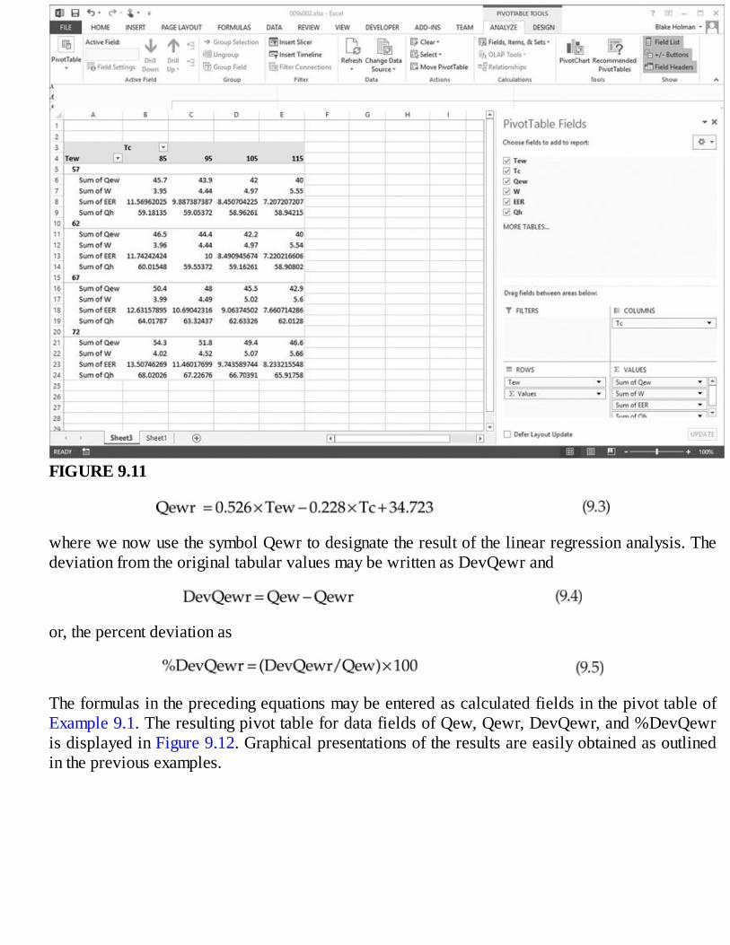
FIGURE9.11

wherewenowusethesymbolQewrtodesignatetheresultofthelinearregressionanalysis.ThedeviationfromtheoriginaltabularvaluesmaybewrittenasDevQewrand

or,thepercentdeviationas

TheformulasintheprecedingequationsmaybeenteredascalculatedfieldsinthepivottableofExample9.1.TheresultingpivottablefordatafieldsofQew,Qewr,DevQewr,and%DevQewrisdisplayedinFigure9.12.Graphicalpresentationsoftheresultsareeasilyobtainedasoutlinedinthepreviousexamples.

FIGURE9.12

9.2OtherSummaryFunctionsforDataFieldsAsnotedinExample9.1,theExceldefaultpivottabledisplayssumsofthedataitemsforeachsetofrowandcolumnvalues.Whenthereisonlyonevalueforeachset,asinthepreviousexamples,thesumactionisofnoconsequence.Ifmultiplevaluesarepresentinthedata,Excelprovidesotherchoicesforthedatapresentation in addition to the sum function.These choicesmaybedisplayed and set by the followingprocedure:

1. BeginwiththePivotTablecreatedasshowninFigure9.4.2. RightclicktheSumofQewfieldinthePivotTable,andselectValueFieldSettingsfromthemenu.

The result appears as shown inFigure9.13.The function choices for summaryof thedata are asfollows:

SumCountAverageMaxMin

ProductCountnumbersStdDev

FIGURE9.13

StdDevpVarVarp

3. Rowandcolumnfieldsmayalsobemanipulated indifferentwaysby rightclickingononeof theroworcolumnvaluestoselecttheFieldSettingsmenuitemandthenselectingfromasimilarsetofchoices.TheresultofsuchactionfortheTewrowsisshowninFigure9.14.Inthecaseofrowsandcolumns, the Subtotals are obtained in contrast to the Grand Totals described previously. TheseSubtotalsmaybedeletedfromthepivot tablepresentationbyclickingNoneasachoice inFigure9.14.SelectionofAutomaticdisplaystheSubtotals.

EXAMPLE9.4:PivotTableforBasicFinancialFunctions

Asanotherexample,wenowshowhowpivottablesmaybeemployedtocalculateandpresentthebasicfinancialfunctionsofSection7.3.Theformulasarerepeatedbelowforconvenience:

FIGURE9.14

wherewenowusethesymbolfvptodesignatethefuturevalueofuniformperiodicpayments.TheformulasmayalternatelybeexpressedintermsoffvcalculatedfromEquation9.6as

Atableissetup,asshowninFigure9.15,forIvaluesof3%,4%,5%,and6%andnvaluesof5,10,15,20,25,and30periodsincolumnsAandB.ThevaluesoffvarecalculatedincolumnCusingEquation9.6.ThetableisthenactivatedandthePivotTableWizardisengagedtoproducethe initial pivot table as shown in Figure 9.16. Subsequently, the other functions are added ascalculateddatafields,usingtheprocedureoutlinedinSection9.1.ThepivottabledisplayingalltheresultingdataisshowninFigure9.17.Pivottablesforthefvandfvpfunctionsareshownin

Figures9.18and9.19,respectively,withlinegraphs(nodatamarkers)displayed.Inbothcases,thegraphsarepresentedalternatelywithnandIastheabscissa.

FIGURE9.15

FIGURE9.16

FIGURE9.17

Although the financial functions could have been calculated directly on a worksheet andsubsequentlydisplayedintherespectivegraphs,theuseofpivottablesoffersincreasedflexibilityofpresentationpossibilities,withmuchlessfussaboutswitchingcolumnsandrows,clickinganddraggingtoselectdataforcharts,etc.

FIGURE9.18

FIGURE9.19

9.3RestrictionsonPivotTableFormulasSeveral restrictions are placed on theway formulas are constructed to enter calculated data fields inpivot tables. For engineeringwork, perhaps themost restrictive requirement is the fact thatworksheetfunctions(EXP,SQRT,etc.)maynotdisplayacellreferenceordefinednamesasparametersinthesyntaxstatements for the functions. Array references as used in the function BESSELJ(n, x) are also notpermitted.Inmanycases,therestrictionscanbecircumventedbysettinguptheformulasintermsofthedatafieldsofthepivottableaswasdoneinExamples9.2through9.4.ThereadershouldconsultExcelHelpunder“Syntaxforcalculatedfieldanditemformulasinpivottables”foradditionalinformation.

9.4CalculatingandChartingSingleorMultipleFunctions∂(x)vs.xUsingPivotTables

Inaccordancewithourpreviousdiscussion,aprocedureforcalculatingfunctions∂(x)maybedescribedasfollows:

1. OpenanExcelworkbook.ColumnAwillbeusedforvaluesofx.TheinitialvalueofxisassignedincellC1.Theincrementinx,Dx,isassignedincellE1.Entertheformula=C1incellA2.Enterthe formula = A2+$E$1 in cell A3. Drag-copy cell A3 for as many rows as desired for thecalculations:Severalhundredrowsaresuggestedtoaccommodatesmallincrementsinx.Theupper-leftportionofsheet1willappearasshowninFigure9.20forx1=0andDx=0.2.

2. Assignthedesiredvaluesofx1andDxforthecalculations.3. Insertanewpivot tableatcellG1(in theexistingworksheet),where thedata forx is inboth the

rowsandthebodyofthepivottable.Removethegrandtotals.4. Thesimpledataforf(x)=xinthepivottableareactivatedandplottedinalinegraphatC16:J30.

TheresultingworksheetisshowninFigure9.21.

Additionalfunctionsofxarenowenteredinthepivottablebythefollowingprocedure:

1. Activatethepivottablebyclickingtheupper-leftcorner.2. Add calculated fields to the data set by navigating to PIVOTTABLE

TOOLS/ANALYZE/CALCULATIONS/Fields,Items&SetsandclickingonCalculatedField.Namenew functions under Name: and insert the associated formula for the name in the line provided.SeveralfunctionsareshowninFigure9.22astypicaladditions.Forexample,theformulaforsin2xwouldbeenteredas=SIN(2 * x).ClickAdd.Insertasmanyfunctionsasdesired,andthenclickOK.Aseachnewfieldisadded,thepivottablewillbeupdated(Figure9.23).

3. FunctionsmaybegraphedsinglyorinmultiplesbyactivatingthepivottableandusingChartWizard.Multiple function chartsmay become rather cluttered, and discretion is advised.A line graph forsin(nx)forn=1–5isshowninFigure9.24.Notethatthecurvesarenotatallsmoothasonewouldexpectofaplotofasinecurve.ThisraisesasignificantlimitationofpivottablesinExcel2016asdescribedinSection9.4.1.

FIGURE9.20

FIGURE9.21

FIGURE9.22

FIGURE9.23

9.4.1WorkingaroundChartingLimitationsofExcel2016—ScatterChartsUnfortunately,Excel2016hasasignificantlimitationinthatitwillnotallowtheusertocreateascatterchartofdatacreatedusingapivot table.Attempting todoso results in theerrormessagedisplayed inFigure9.25.Thisisalimitationforreasonsrelatedtodatamismatchbetweenwhatapivottableprovidesandwhatascatterchartrequires.

FIGURE9.24

FIGURE9.25

Likemanythingsinlife,though,thereisanalternativeapproachtocreatingascatterchartfrompivottabledata.ConsiderthelinegraphofFigure9.24.Asimplemethodforcreatingascatterchartfromdatainapivottableistocopythedatatoanotherareaoftheworksheetortoadifferentworksheetandthencreatethescatterchartfromthecopieddata.ToaccomplishthiswiththedatainFigure9.24,performthefollowing:

1. HighlightthedatainthepivottablebyselectingcellsG1:L14inFigure9.24.2. CopytheselecteddatausingtheCTRL+Ckeysequence.3. SelectcellG17andrightclicktopastethevaluescopiedfromthepivottable.4. Selectthecopiedcells(G17:L30)andtheninsertatype3scatterchart.

FIGURE9.26

TheresultingworksheetisshowninFigure9.26.ThereareothermethodsforworkingaroundthislimitationinExcel2016,oneofwhichistheuseof

PowerQuery,whichisdiscussedinSection10.6ofthistext.

9.5CalculatingandPlottingFunctionsofTwoVariablesWe have already seen in Example 9.4 the calculations for functions of two variables; in this case,financial functions are functions of I and n.Because pivot tables cannot accept array formulas, itmaysometimes be preferable to use the DATA/FORECAST/What-If-Analysis/Table command for suchcalculations, as described inSection2.15.However, pivot tables offer the advantage of easy entry ofseveralfunctionsintothetableandquicksubsequentmanipulationofthesefunctions.Takingthetwoentryvariables as x and y, we wish to calculate the ∂(x, y) values. Again, because of the non-array entryrequirements,allcombinationsofthevariablesxandymustbepresentintheentryfields.NoteinFigure

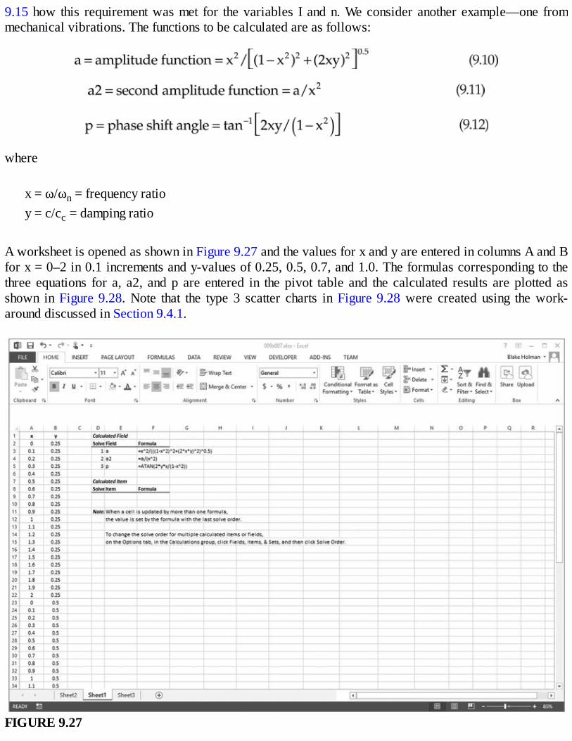
9.15howthis requirementwasmet for thevariables I andn.Weconsideranotherexample—one frommechanicalvibrations.Thefunctionstobecalculatedareasfollows:

where

x=ω/ωn=frequencyratioy=c/cc=dampingratio

AworksheetisopenedasshowninFigure9.27andthevaluesforxandyareenteredincolumnsAandBforx=0–2in0.1incrementsandy-valuesof0.25,0.5,0.7,and1.0.Theformulascorrespondingtothethree equations for a, a2, andp are entered in thepivot table and the calculated results areplotted asshown inFigure9.28.Note that the type 3 scatter charts in Figure9.28were created using thework-arounddiscussedinSection9.4.1.

FIGURE9.27

FIGURE9.28

Problems9.1Thefollowingfunctionoccursinanengineeringdesignapplication:

where

SetupapivottabletocalculatevaluesofeasafunctionofNandCfortheranges:

Then,provideagraphforseveralvaluesofthesevariables.Plotase=∂(N)fordifferentvaluesofCandalsoase=∂(C)forselectedvaluesofN.

9.2SetupapivottablesimilartothatinExample9.3butfortheexponentialregressionofExample6.14.

9.3SetupapivottablesimilartothatofExample9.3butbasedonthecombinedregressionanalysisofExample6.15.

9.4SetupapivottabletocalculateP/BfromEquation7.17bforI=3%,5%,7%,9%,and12%withvaluesofn=5,10,15,20,and25periods.SelectvaluesofCasappropriate.NotethatvaluesofC=Iwillresultindivisionbyzero,butselectingI=3andC=2.99willnotproduceanerror.ProvideagraphofP/Bforonevalueofn.

9.5Performasecond-orderpolynomialfitfortheW(kW)dataofExample9.1usingasinglevalueofTew=57°FalongwiththefourgivenvaluesofTc.Obtainthefollowing:

OnahotsummerdayinAustin,Texas,thetemperatureTcvariesaccordingto

wheretisthetimemeasuredinhoursfrommidnight.UsingthecombinationregressionobtainedforQewinExample6.15,constructapivottablethatwill

a. PresentvaluesofQew(kBtu/h)asafunctionoftb. PresentvaluesofW(kW)asafunctionoftc. SumthetotalcoolingQew(kBtu)andenergyinputW(kWh)overa24-hperiodd. DisplayvaluesofTcasafunctionoft

Usingthisinformation,plotQew(kBtu/h),W(kW),andTcasfunctionsoftinhours.

9.6Thecoolingloadthattheair-conditioningunitinProblem9.5mustaccommodatevariationwithTcaccordingtotherelation:

Assume that theunit is oversized such that it candeliver10%more cooling than themaximumneeded under the most severe temperature conditions, i.e., for Tc = 102° F at 5 pm. Deviseadditions to the pivot table of Problem 9.5 thatwill calculate and display a duty cycle factordefinedby

PlotthevaluesofFasafunctionoft.

9.7Astheair-conditioningunitinProblems9.5and9.6isoversized,aproposalismadetostoretheexcess capacity by suitablemeans, namely, by storing chilledwater ormaking it available forotherapplications.ProvideadditionstothepivottablethatwilldisplaythehourlyBtuofexcesscapacitythatwillbeavailable.

9.8 The particle displacement amplitude for a “standing” sound wave may be described by therelation:

where

x=spatiallocation,mλ=wavelengthofthesound,mc=acousticvelocity,m/sect=time,sec

Deviseapivottabletodisplayandgraphasuitablerangeofvaluesoftheamplitudefunctionforλ=0.2mandc=344m/s.

9.9Thesteady-stateamplituderesponseofafirst-ordersystemtoanimpressedfrequencyωisgivenby

whereϕisthephaseshiftangledefinedby

Deviseapivottabletodisplaythisresponse.Plottheresultsonasuitablegraph.

9.10Thetime-delaybehaviorofalow-frequency(≈1cycleper24h)thermalwaveinalargesolidisdescribedbytheamplituderesponseequation:

where

xisthedepthinthesolidmaterial,mωisthefrequencyofthethermalwaveatx=0,incycles/stisthetime,sα=constant=7×10−7m2/s

Constructapivottableandappropriatechartstodisplaythebehaviorofa(x,t)overatleasttwocyclesoftheimpressedwaveatx=0.Also,examinethebehaviorofatime-delayfunction:

9.11Atransientcoolingprobleminvolvestheequation:

where

X=(x2/4αt)0.5α,h,k=constantsx=spacecoordinatet=timecoordinate

Devise a pivot table to display values of θ in the range from 0.01 to 1.0 for ranges of thevariables:

10DataManagementResourcesinExcel

10.1IntroductionAs we have seen in several examples throughout this volume, Excel can hold tables of data forcalculations, analysis, and charting purposes. Excel can also hold data for reference and processingpurposes.Whenthereisaneedtokeepdata,calculations,analyses,andchartstogether,worksheetsandtableswithinanExcelworkbookmakeanexcellentchoice.Thereare,however,timeswhenthedatamaynotbeavailablefor inclusion inanExcelworkbookormaybebetter referencedfromanexternaldatasource.

In addition to supporting various methods for storing and accessing data, Excel has numerouscapabilities for managing and processing data, over and above the analyses and charting capabilitiesdiscussedthusfar.Thischapteraimstooutlinemanyofthesecapabilitiesandmethods,whichthereaderisthenencouragedtoemployinhis/herday-to-daywork.

10.2OrganizingDatainExcelWorksheetsandTablesThesimplestway toorganizedata inExcel is inworksheet rowsandcolumns.Consideracontact listwherenamesandaddressesarestoredinaworksheetforeasyreference.ThismaylooklikethedatainFigure10.1.

In this format, thedata isveryworkable—easy toview,andcaneasilybe referencedbyadditionalcolumns, or by cells in other worksheets whether they are in the same workbook or in other Excelworkbooks.

Excelalsohastheabilitytocreateatablereferencebyname,ratherthanrelyingonworksheetnameandrow/columninformation.TocreateatablenamedContactsforthesamedata,performthefollowingsteps:

1. Highlight the column headings and all the rows of the data which will become the table namedContacts.

2. PressthekeysequenceCTRL+torclickonHOME/STYLES/FormatAsTableandpickastyle.3. Uponperformingstep2,adialogboxwillappearasinFigure10.2.Verifytheinformationandclick

OK.

FIGURE10.1

FIGURE10.2

4. Theresultingtablewillhaveeitherthedefaultcoloring(bypressingCTRL+t)orthecoloringchosen(clickingonHOME/STYLES/FormatAsTable),anditwillhaveauto-filteringenabledsothat the

usercansortandfilterthecolumnsofthetable(Figure10.3).

FIGURE10.3

FIGURE10.4

5. Togive the table the customnameContacts, place the cursorona cell in the table and theTableToolsmenuwillappearon the ribbonbar.Navigate to theTableToolsDesignmenuandnote theupper-leftcornerof the ribbonbar. It shouldappearas inFigure10.3.Tochange thenameof thetabletoContacts,typeoverthetermTable1withthetermContacts.Navigateawayfromthetableandbacktoittoensurethatthenameispreserved(Figure10.4).

10.3Filtering,Sorting,andUsingSubtotals

10.3.1Filtering

Filteringofdataisanextremelyusefulfeature,particularlywhenworkingwithlargenumbersofrowsofdata.Inthesituationofacontactlist,imaginewantingtofilternamesbyzipcodeorcountry.Abruteforcemethodforperformingsuchcouldbetosortthedatabyeitherzipcodeorcountryandthenhidetherowsthat don’t fit with what you seek. Alternatively, using Excel’s built-in filtering capabilities canautomaticallyaccomplishthesesteps.

Thesimplestwaytoengagefilteringis tousetheAuto-FilterfacilityofExcel.Highlight thecolumnheadingsanddatayouwanttofilterandnavigatetoDATA/SORT&FILTERandclickonFilter.Excelwill enable a drop-down filter on each column from which you can perform several actions. Thesepotentialactionsincludethefollowing:

–SortAtoZ(ascendingorder)–SortZtoA(descendingorder)–SortbyColor(ifcolorsareenabledandused)–ClearFilterfrom{columnname}–FilterbyColor–ASearchboxforvaluesinthatcolumn–Aboxthatallowstheusertoselectwhichvaluestoshoworhide

Consider the data in Figure10.1. Enabling filtering on that data set and then selecting the drop-downmenuontheStreetAddressfieldwouldappearasinFigure10.5.

ByuncheckingtheSelectAllvalueandthencheckingthe12345NorthMainStreetvalue,thetableofdatawillbereducedtoonlytworowswith12345NorthMainStreetasavaluefortheStreetAddresscolumn.

FIGURE10.5

10.3.2SortingAsseenfromthemenuchoicesabove,sortingcanbeaccomplishedusingthefilteringdrop-downmenuson each column. If, however, nested sorting (sortingbyvalueA, thenvalueBwithinvalueA, etc.) isneeded,analternativeapproachisneeded.

ConsiderthedatainFigure10.6.ImaginethatthesedataneedtobesortedfirstbyLastName,thenbyFirstName,andthenbyMiddleInitial.Tocreateanestedsortforthesedata,performthefollowingsteps:

1. Highlightthedatatobesorted.2. ClickDATA/SORT&FILTER/SorttobringupthedialogboxinFigure10.7.3. ClickontheMydatahasheaderscheckboxintheupper-rightcorner.4. ClicktheSortbydrop-downboxandpickLastNameasthefirstsortitem.KeeptheSortonValues

choiceandkeeptheOrderofAtoZ.5. ClickonAddLeveltoaddanextlevelsort.Anadditionalrowwillappearinthedialogbox.For

that new row, select FirstName from the Sort by drop-down box leaving the Sort on andOrderoptionsattheirdefaultvalues.

6. ClickonAddLevelagain,thistimepickingMiddleInitialfromtheSortbydrop-downmenu,againleavingSortonandOrderastheirdefaultvalues,resultinginthedialogboxinFigure10.8.

7. ClickonOKandthedatawillrearrangeasshowninFigure10.9.

FIGURE10.6

FIGURE10.7

FIGURE10.8

10.3.3SubtotalsSubtotals can be used inExcel to perform several operations on subgroups of data. The datamust besortedbyavalueonwhichthedataaregrouped,andthensubtotalscanbeemployedonvariousotherdataelements. The operations that can be performed on a subgroup of data are Sum, Count, Average,Minimum,Maximum,andProduct.Productisamultiplicationoperation,minimumistheidentificationoftheminimumvalueofasubgroup,andmaximumistheidentificationofamaximumvalueinasubgroup.

ConsiderthedatainFigure10.10.Thedataconsistofalistofsparepartsthatmightbeonhandwithapresent-day ITgroup forquick repairofproblematicdevices.Let’s say, for example, thatmanagementwouldliketoknowhowmanydevicesareheldpercategoryaswellasthedollarvalueofthatinventory.Usingsubtotalsforsummingthenumberof itemsonhandaswellas thevalueof thoseitemswouldbeveryhandy.

Toperformsuchanoperationonthissampledata,performthefollowingsteps:

1. Startbyhighlightingthedataandcolumnheadingsforwhichsubtotalswillbecreated.

FIGURE10.9

2. Sort thedatabycategorytoensurethat thelineitemsaregroupedtogetherbythatcolumn.ThisisaccomplishedusingtheDATA/SORT&FILTER/Sortmenuitem.MakesurethatMydatahasheadersisselectedandpicktheCategorycolumnnamefortheSortbyfield.

3. EngagethesubtotalingfacilityviatheDATA/OUTLINE/Subtotalmenuchoice,andthedialogboxinFigure10.11willappear.

4. ChangetheAteachchangein:drop-downvaluetobeCategory,andchecktheboxforNumberonHandintheAddSubtotalto:window.BothNumberonHandandExt.Costshouldbecheckedforsubtotals.

5. ClickOK to see the result inFigure10.12.Notice thatExcel has inserted subtotal lines for eachcategoryandhasprovidedasubtotalofitemsonhandinthatcategoryaswellasthevaluesofthoseitems.Inaddition,aGrandTotalisprovidedatthebottomofthesheet.

6. Note that there are three columns numbered 1, 2, and 3 to the left of the row numbers of theworksheet.Thesedesignate the levelsof information in thedataset.Clickingon thenumber threeshowsalldetailsof thedata set.Clickingon thenumber twowill show just thesubtotalsand theGrandTotal,andclickingonthenumberonewillshowonlytheGrandTotal.Figure10.13showstheresultofclickingonthenumbertwo.

FIGURE10.10

FIGURE10.11

FIGURE10.12

FIGURE10.13

10.4UsefulDataFunctionsinExcelThrough many years of using Excel for data processing and manipulation, numerous Text andLookup/Reference Excel functions show their use and versatility on nearly a daily basis. These veryusefulfunctionsareshowninTable10.1.RefertotheExcelHelpfunction(pressF1fromwithinExcel)formoreinformationoneachfunction.

TABLE10.1UsefulDataProcessingandManipulationFunctions

EXAMPLE10.1:StringManipulationUsingSeveralFunctionsinTable10.1

ConsiderthedatasetinFigure10.14.Notethatthereareseveralholesinthedataset,whichthefunctionsinTable10.1caneasilyhelpusfill.Forexample,

–TheIDfieldisintendedtobethefirstthreelettersofthelastnamewiththeindexappendedtoit.

–TheFullNameisintendedtobethepiecingtogetheroftheFirstName,MiddleInitial,andLastNamewithappropriatespacing.

–TheSimpleZipisintendedtobethefirstfivecharactersoftheZip+4field.–ThePlus4isintendedtobethelastfourcharactersoftheZip+4field.–TheAreaCodeisintendedtobethefirstthreecharactersoftheTelephonefield.

FIGURE10.14

FIGURE10.15

FIGURE10.16

The worksheet in Figure 10.14 is put into formula display mode, which you will recall frompreviouschaptersisaccomplishedviatheCTRL+`keysequence.UsingseveralofthefunctionsfromTable10.1,Figure10.15showshowthesefunctionscanbeusedintheopencolumnsofdatatoaccomplishtheintentionsnotedabove.Figure10.16showsthefinalresultsbyswitchingbacktodisplayingvaluesfromformulasusingtheCTRL+`togglekeysequence.

Thereaderislefttoaddacolumnforcleaningupthemiddleinitials,makingthemuppercase,andcopyingandpasting themback into theproperplace.Observehow theFullNamechangeswhenthiscleanupiscomplete.

10.5ConnectingExceltoExternalDataWhenadatasourceisavailableforanalysisoutsideofExcel,itisconvenienttobeabletoreferencethatdatasourcewithouthavingtotypethedataintoaworksheetorrebuildthedataotherwise.Anexampleofan external data source might be anMS Access database to which a data logging tool has recordedexperimental data.Similarly, aCentralPlantmanagement systemmay storenumerousdata readingsontemperaturesandwaterflowthroughoutthesystem,whichwarrantanalysis.Excelprovidesquiteabitofflexibilityinconnectingtosuchdatasourcesandaccessingthedataforanalysis,charting,orprocessingpurposes.

10.5.1GeneralConceptsExcelhasthecapabilityofconnectingtodataoutsideofthecurrentworkbookandmaintainingareferencethatsuchdataareexternalandmayneedtoberefreshedperiodically.Theexternaldatacanbeinmanyforms:anExcelworkbook,anMSAccessdatabase,anMSSQLServerdatabase,aMySQLdatabase,oroneofmanyothers.

The idea is toconfigureanExcelworksheet to lookoutside itself fordataandshowthedata in thecurrentworksheetforanalysisormanipulationpurposes.Inthediscussionsthatfollow,itisassumedthatthereaderhasabasicunderstandingofdatabasesandtables in thecontextof typicaldatabasesystems.For an in-depth understanding of databases, the reader is encouraged to explore any number of othersourcesincludingMicrosoft.comandmysql.com.

10.5.2ConnectingtoMSAccessConsiderabuildingsecuritysystemthatisloggingbadgeswipesofemployeebadgesasemployeesenterand exit the doors of their employer’s building. Let’s say that the logging system has extremely poorreportingcapabilitiesandthecompany’sexecutivemanagementwouldlikeareportofthelast100peopletoenterthefacility.TheloggingsystemstoresitsdatainanMSAccessdatabase.

SaythatthenameoftheMSAccessdatabaseisSecuritySystem.accdbandthetableinthedatabasethatishometo thebadgeswipes isnamedBadgeSwipes.ToconfigureMSExcel toconnect to thissampledatabase,performthefollowingsteps:

1. OpenanewExcelworkbooktoSheet1.2. ClickonDATA/GETEXTERNALDATA/FromMSAccess.3. Locate the file system path to the MS Access database file SecuritySystem.accdb, highlight that

filename,andclickOpen.

FIGURE10.17

FIGURE10.18

4. ThedialogboxinFigure10.17willappear.Thefouroptionsenabletheuserto

a. CreateatablewithintheworkbookthathasacopyofthedatafromtheAccessdatabase(andplaceitinthecurrentoranewworksheet)

b. ProceeddirectlytocreateaPivotTableassociatedwiththedata(andplaceitinthecurrentoranewworksheet)

c. ProceeddirectlytocreateaPivotChartassociatedwiththedata(andplaceitinthecurrentoranewworksheet)

d. Simplyconnecttothedatawithoutanyotheroperation

5. Inourcase,acceptthesettingsastheyareinFigure10.17andclickOK.Theresultappearsas inFigure10.18.

10.5.3ConnectingtoMSSQLServer

Consider the situation in Figure 3.6b, except the data are stored in the cloud on anMS SQL ServerrunningatMicrosoft(Azure).Assumethat thereaderhasa loginandpasswordcapableof loggingintoand reading data from this SQL Server and that the SQL Server firewall has been set up properly toacceptconnectionsfromthereader’scomputer.Chapter11coversmore informationaboutcloud-basedservices.

FIGURE10.19

SaythatthehostnameoftheSQLServerissecsys.database.windows.net.Additionally,thedatabaseontheserverthatholdsthedataiscalledExpDataandthetableinthedatabasethatishometothedataisnamedExperiment1.ToconfigureMSExceltoconnecttothistable,performthefollowingsteps:

1. OpenanewExcelworkbooktoSheet1.2. ClickonDATA/GETEXTERNALDATA/FromOtherSources/FromSQLServer.3. AdialogboxlikethatshowninFigure10.19willappear.4. EntertheSQLServername,indicatethelogincredentialsbeingusedandclickNext.5. TheDataConnectionWizard dialog boxwill appear.Under Select the database that contains the

datayouwant,selectExpDatafromthedrop-downchoices.DoingsowilldisplaytheExperiment1tableinthelistasshowninFigure10.20.

6. HighlighttheExperiment1tablenameandclickNext;then,clickFinishontheSaveDataConnectionFileandFinishscreen.

7. AdialogboxsimilartothatinFigure10.17willappear.ClickOKandtheresultwilllooksimilartoFigure10.21.

10.5.4ConnectingtoMySQL

ConsiderthedatainProblem3.1,exceptthedataarestoredinthecloudonaMySQLServerrunningatAmazonWebServices.Assume that the reader has a login and password capable of logging into andreadingdata from thisMySQLServerand that theMySQLServer firewallhasbeensetupproperly toacceptconnectionsfromthereader’scomputer(seeChapter11formoreinformationaboutcloud-basedservices).

BeforeconnectingtoanMySQLdatabase,onemustfirstinstallMySQLOpenDataBaseConnectivity(ODBC)driverstoallowExceltoconnect.Then,onemustsetupaconnectiondefinitionsothatwecanmakeaconnectiontothedatabaseserverandpulldatafromatableinthedatabase.

FIGURE10.20

FIGURE10.21

InformationaboutdownloadingandinstallingtheMySQLODBCdrivercanbefoundontheInternetathttps://dev.mysql.com/downloads/connector/odbc.ThiswebsiteprovidesexcellentinstructionsonhowtodownloadandinstalltheMySQLdriver.

Oncethedriverisinstalled,anODBCconnectiondefinitionneedstobesetupfortheMySQLserverusingthenewlyinstalleddriver.AsimplesearchonGoogleorBingusingtheterm“ODBCsetup”willprovideampleinstructionsonhowtoconfiguretheODBCconnectionforyourMySQLserver.

NowthattheMySQLODBCconnectionisconfigured,it istimetoconfigureExceltoconnecttotheMySQLserverthatholdsthedatainquestion.Inthiscase,thedatafromProblem3.1arestoredinatablenamedExperiment2 in anMySQLdatabasenamedExpData.To configureMSExcel to connect to thistable,performthefollowingsteps:

1. OpenanewExcelworkbooktoSheet1.2. ClickonDATA/GETEXTERNALDATA/FromOtherSources/FromDataConnectionWizard.3. AdialogboxlikethatshowninFigure10.22willappear.SelectODBCDSNandclickNext.4. ClickonthenameoftheODBCDSNfortheMySQLServerthatwassetupabove.Inthecaseofthis

example,thenameissimplyMySQL.ClickNextoncethenameisselected.5. TheDataConnectionWizarddialogboxwillappearasinFigure10.23.BecausetheMySQLODBC

connectionalreadyspecifiedthedatabaseExpData, thedialogboxalreadyhas thatdatabasenameindicated.Assuch,thedialogboxdisplaysthetablenameExperiment2.

6. Make sure theExperiment2 table name is selected and clickNext; then, clickFinish on theSaveDataConnectionFileandFinishscreen.

7. AdialogboxsimilartothatinFigure10.17willappear.ClickOKandtheresultwilllooksimilartoFigure10.24.

FIGURE10.22

FIGURE10.23

FIGURE10.24

10.5.5ConnectingtoOtherDataSourcesAbove,we have outlined connecting to several common data sources. Excel, however, supportsmanymoreoptionsthatwillhavebuilt-insupport(likeMSAccessorMSSQLServer),thatwillbeaccessibleviaanODBCconnection,orthatwillrepresentnon-databasesources(FromWeb,FromText,etc.).Thereaderisencouragedtoexploretheseoptionsforfunandgainingfamiliarity.

10.6MicrosoftPowerQueryMicrosoftPowerQuery is simply theDATA/GET&TRANFORMsetofmenuoptions inExcel2016.Using this facility, we replicate obtaining badge swipe data from the Access database as outlined inSection10.5.2.

StartingwiththeMSAccessdatabasefilereferencedinSection10.5.2,wewillgetthedatafromthedatabaseusingthisalternatefacility.Todoso,performthefollowingsteps:

1. OpenanewExcelworkbook.2. Click on DATA/GET & TRANSFORM/New Query/From Database/From Microsoft Access

Database.Noticethenumberandvarietyofstandarddatabasesourcesfromwhichyoucanquery.3. AdialogboxappearstoselecttheappropriateMSAccessdatabasefilefromthefilesystem.Find

andselectSecuritySystem.accdbasinthepreviousprocedure.AnavigatorwindowwillappearasinFigure10.25.SelecttheBadgeSwipesobjecttoviewthetabledata.ClickonLoad.

4. ThedatawillloadintoanotherworksheetasshowninFigure10.26.

Aswith aMicrosoftAccess data source, PowerQuery can be used to get and transform data from avariety of sources: files, databases, Microsoft Azure, Online Sources, and Other data sources. Thebulleted list below provides a listing of the categories and options available from theDATA/GET&TRANSFORM/NewQuery source options. The reader is encouraged to explore these options to gainexperienceandfamiliaritywiththeirapplicability.

FIGURE10.25

FIGURE10.26

–Files:Workbook,CSV,XML,Text,JSON,Folder,MSSharePointFolder–Databases:MSSQLServer,MSAccess,MSSQLServerAnalysisServices,Oracle, IBMDB2,

MySQL,PostgreSQL,Sybase,Terradata,SAPHana–MSAzure:MSAzureSQLDatabase,MSAzureSQLDataWarehouse,MSAzureMarketplace,MS

AzureHDInsight,MSAzureBlobStorage,MSAzureTableStorage–OnlineServices:MSSharePointOnlineList,MSExchangeOnline,MSDynamicsCRMOnline,

Facebook,SalesforceObjects,SalesforceReports– Other Sources:Web,MS SharePoint List, OData feed, Hadoop File,MSActive Directory,MS

Exchange,ODBC,BlankQuery

Problems10.1Consider the data set used in Example10.1. Instead of constructing the FullName to be First

NameMiddle Initial Last Name, modify the string concatenation formula to construct the FullNameasLastName,FirstNameMiddleInitial.

10.2 Consider the Total Number of Winners data available at the websitewww.powerball.com/powerball/pb_totalwinners.asp. Construct a worksheet in Excel thatretrievesthedataandinsertsthedataintoaworksheet.Forfun,usingthetechniquesinChapter3,plotaverticalbarchartoftotalwinnersbyUSState.

10.3CreateanMSAccessdatabasewiththedatafromProblem3.1init.CreateanExcelworkbookthatqueriesthedatausingPowerQuery.

10.4UsingthesameAccessdatabasefromProblem10.3,createanExcelworkbookthat imports thedata using the DATA/GET EXTERNAL DATA/From Access menu option. Comment on thedifferencebetweenthismethodandthatusedinProblem10.3.

10.5CreatealistofstudentIDs(columnA)andstudentfirstnames(columnB)andstudentlastnames(columnC) in aworksheet (Sheet1). In a separateworksheet (Sheet2), create a random list ofstudentIDsincolumnA.IncolumnBofSheet2,createaformulausingVLOOKUPthatobtainsthestudentfirstnamesandlastnamesandconcatenatesthemtogetherintheformatoflastname,firstname.EnvisionhowthismightworkwithrowsandtheHLOOKUPfunctioninstead.

11 Office 365 and Integration with CloudResources

11.1Introduction“TheCloud” is a term that has come about in the last 5 or so years to represent a broadening of theconceptofservicebureaucomputingthatputElectronicDataSystems(EDS)onthemapinthelatterpartof the20thcentury.Whileservicebureaucomputingfocusedonmainframecomputingresources,Cloudcomputingisfocusedonseveraldimensionsofcomputingforbothcommercialandconsumeruse,mostlyinthecontextofmidrangeandminicomputerplatforms.Cloudcomputing,sometimesreferredtoasgridcomputing,caninvolvemanyvariations.Forpurposesof this text,wewillfocusonflexiblecomputingservices likeOffice365,MicrosoftAzure,andAmazonWebServices(AWS)as theirbusinessmodelsallowcustomerstoadjusttheirresourceneedsasdemandfluctuates.

11.2WhatIsOffice365?Microsoft’sOffice365product is a collectionof software capabilities ranging fromsimpleuseof theMicrosoftOfficesuiteoftoolstoanEnterprisesetoftoolsthatincludecorporateE-mail(MSExchangeOnline),SocialEnterprise(MSYammerandDelve),Collaborationtools(MSSharePoint),andseveralothers.Customerspayamonthly fee for access to the softwareand services,which includeautomatedupdatesandfeatureenhancements.FulldetailscanbeobtainedviaMicrosoft’swebsiteoraMicrosoftaccount representative. Note that nonprofit and educational organizations can qualify for a significantpricereductionduetotheirnonprofitoreducationalstatus.

11.3LeveragingMSExcelonPremiseandintheCloudOffice365supportsbotha locally installedversionofMSExcelaswell asanonline instanceofMSExcelcalled,oddlyenough,ExcelOnline.Imaginevisitingacolleagueandwantingtodemonstrateanewwhiz-bang Excel spreadsheet that you crafted that shows groundbreaking results from an experimentalanalysis.But,youdon’thaveyourcomputerwithyouandtheydon’thaveMSExcel(strangeas itmaysound).TheadvantageofOffice365andExcelOnlineisthatyoucanlogintotheMicrosoftOffice365portalanduseExcelOnlinetoviewyourspreadsheetandsharetheexcitementwithyourcolleague.

11.4IntegratingMSExcelwithCloudResourcesThanks to the power of internetworking, Excel is no longer limited to data containedwithin anExcelspreadsheetoronalocalornetworkdiskdriveclosetoyourcomputer.WithvalidInternetconnectivity,

thepossibilitiesarenearlyendlessforconnectingtodataandbeingabletomanipulateit.AsdemonstratedwithseveralscenariosinChapter10,Excelcanobtaindatafromotherworksheets,

workbooks,datafiles,databases,websites,andevenonlineserviceslikeFacebook.Dataareeverywhereand Excel can get to the data either through the DATA/GET EXTERNALDATAmenu options or thePowerQueryfacility,notedastheDATA/GET&TRANFORMmenuoptions.

ThereaderisencouragedtoexploretheservicesthatExcelsupports toseehowthedatalookwhenbrought into an Excel workbook. Chapter 10 provides a great start to this exploration process. Forexample,Problem10.2pointstodataonthePowerBallwebsite.

11.4.1MicrosoftAzureInadditiontoOffice365,Microsofthasacloudserviceofferingforserver-basedcomputingcapabilities.CalledMicrosoftAzure,itisaconstantlyevolvingMicrosoftserviceoffering.MoreinformationcanbefoundattheMicrosoftAzurewebsiteathttp://azure.microsoft.com.Thereaderisencouragedtoconsidersigning up for a free account to evaluate and explore cloud-based Microsoft SQL Server databaseservicesonAzure.

11.4.2AmazonWebServicesSimilar to Microsoft, Amazon has a cloud service offering for server-based computing capabilities,offered under the AWS product family. AWS is a constantly evolving product offering fromAmazon.More information about AWS can be found at http://aws.amazon.com. The reader is encouraged toconsidersigningupforafreetieraccountwithAWSandexplorecloud-basedMySQLdatabaseservicesatAWS.

11.5ExcelandMicrosoftPowerBIThis entire text has focused on Excel as an excellent toolset for analyzing data, processing data, andchartingtheresultsofdataanalyses.MicrosoftPowerBIisaproductthatcomplementsExcelwithregardto charting data and presenting the data to users in a Dashboard format. Excel worksheets make anexcellentdatasourceforMicrosoftPowerBIasdodatabasesources.

Figures11.1and11.2showsampledatasourcesinExcelworkbookformasinputstoMicrosoftPowerBI. They represent data regarding a cash room operation and show dashboard data regarding theiroperation. Figure 11.3 shows a sample dashboard created in Microsoft Power BI in under an hour,demonstratingthespeedwithwhichdatadashboardscanbecreated.

FIGURE11.1

FIGURE11.2

FIGURE11.3

Thereader isencouragedtosignupforafreeaccountatwww.powerbi.comandexplore theuseofthistoolsetinconjunctionwithExcel.

References

1.Hillier,F.S.andLieberman,G.J.,IntroductiontoMathematicalProgramming,2nded.,McGraw-Hill,NewYork,1995.

2.Holman,J.P.,ExperimentalMethodsforEngineers,7thed.,McGraw-Hill,NewYork,2000.3.Holman,J.P.,HeatTransfer,9thed.,McGraw-Hill,NewYork,2002.4.Winston,W.L.,OperationsResearch, Applications, andAlgorithms, 3rd ed., PWS-Kent,Boston,MA,1994.

5.Wu,N.andCoppins,R.,LinearProgramming,McGraw-Hill,NewYork,1981.

Index

AAbsoluteaddress,13–16Access,connectingto,209,210–211Address,cellseeCelladdressAmazonWebServices,212,220Area/3-DArea,41Averages,moving,46–49AWS,212,220Axis,format,36Azure,Microsoft,211,220

BBarcharts,49–50Besselfunction,40,41Binding,166Bonds

discount,rateofreturn,150–151interest,reinvestmentof,rateofreturn,151–152multipleinvestments,rateofreturn,152–153zero-coupon,rateofreturn,152

Bordersadding,9editing,9removing,9

Bubblecharts,29

CCallouts,60Celladdress

absolute,13–16changingstatusof,15–16relative,13–16

Cellsequationsin,copyingof,95–97fillin,9formulasin,copying,13–15

ChartArea,51Chartdepth,49ChartOptions,51Charts,27–54;seealsoScattercharts;seealso3-Dcharts

bar,49–50calculation,for,45column,49–50editingelementsof,9formatting,50–53movingaverages,graphing,46–49movingonworksheet,8–9pivottables,using,189–195resizing,46sizingonworksheet,8–9stretching,46surface,53

Cloudintegrationwith,219–222Office365,useof,219–220

Coefficientofdetermination,33Columncharts,49–50Columns,199

headings,printing,7switchingtorows,16–17

Combinedregression,138–139,142Comments,IFstatementtoreturn,112Compoundinterestformulas,148–153Conventions,2Copying

cellequations,95–97cellformulas,13–15FillHandlefor,12–13,15formulas,12–13

Correlationcoefficient,33Correlationequations,32–33

exponentialdatawithpowerrelation,33–35

exponentialfunctions,37–38powerrelationwithexponentialdata,33–35

Costfunction,159Cumulativefrequencydistribution,113–116,117,119–120

DDatafields

inpivottables,181summaryfunctionsfor,184–188

Datamanagement,199–217externaldata,connectingto,209–215filteringdata,201–202functionsfor,207–209organizingdata,199–201sortingdata,203–204subtotals,204–207

DataSeries,51Data-Table,17,22Deletions,inWord,9Depth,in3-Dcharts,49Deviation,standard,33Dialogwindows,moving,27Drawings,seeLinedrawings;seeShapes

EEitherAxis,51Embeddedtextasdocumentation,69–70EquationEditor,66–70Equations, see also Linear equations; see also Nonlinear equations; see also Simultaneous linear

equationscopying,forrepetitivecalculations,95–97correlation,32–35,37–38cubicpolynomial,75,76,79,80insertingEquationEditor,66–70template,65–66

transcendental,75–76,79Error,standard,formovingaverages,49Errordistributions,117–120

Errormessages,86–87ExcelOnline,219–220Exponentialfunction,37–38Exponentialregression,multivariable,134–137,142

FFeasibleregion,160–161Files,recentlyused,8Fill,9FillHandle,12–13,15Financialfunctions,147–158

compoundinterestformulas,148–153investmentaccumulationwithincreasingannualpayments,153–154listingof,149–150nomenclature,147payoutatvariableratesfrominitialinvestment,154–156pivottablefor,185–188

Format,63–65FormattinginWord

charts,50–53objects,10pictures,10

Formulascellcopying,13–15displaying,9

copying,12–13displaying,9

Freeformlinetype,59Functions,Excel,seealsoFinancialfunctions

built-in,17,19Calculating,withpivottable,189–195fordatamanagement,207–209restrictionsinpivottables,189

GGapwidth,42,49Gauss–Seidelsolutions,81

GeneralsandAdmiralscharts,45GoalSeek,75–79Gradients,63–64Graphs,seeChartsGridlines,51Gridlines,printing,7Group,64

HHeadings,printing,7Heattransfer,radiationandconvection,89–91Heattransfercoefficient,uncertaintyanalysisof,123–127Histograms,113–116

IIFstatement,110–112Illustrations,59,64–65Insert,63–65,175Integrals,numericalevaluationof,105–110Interest,compound,148–153Investmentpayoutatvariablerates,154–156

KKeyboard,setupforsymbols,6–7

LLandscapeorientation,9Linearequations,seealsoSimultaneouslinearequations

iterativesolutions,81–83,93matrixinversion,84–87,93

Linearoptimizationproblems,160–162Linearregression,multivariable,129–134,142Linedrawings

constructionof,59–65

fromcoordinates,71–73lineweight,59preciseangular,60–65smoothing,71–72

LINESTfunctions,130,133,134Logarithmicscales,36–37LOGESTfunction,134–136Log–logplots,34

MMacros,97–101Matrixinversion,84–87,93Matrixsolutions,81Maximization,inoptimizationproblems,159,163–164MicrosoftPowerBI,220–222Minimization,inoptimizationproblems,159,164MINVERSEfunction,84,85MMULTfunction,84,85Movingaverages,46–49Multivariableexponentialregression,134–137,142Multivariablelinearregression,129–134,142MySQLServer,connectingto,212–215

NNegativeOverlap,49NestedIFstatements,110–112Nonlinearequations

GoalSeek,solutionsusing,75–79simultaneous,87–92Solver,solutionsusing,79–81,87–92

Nonlinearoptimizationproblems,160–162Normaldistributionfunction,117,118–119Normalerrordistribution,117–120Notbinding,166Nudging,10

O

Objectivefunction,159Objects,formatting

formattinginExcel,10–12inWord,10

moving,10Office365,219–220Optimizationproblems,159–173

feasibleregion,160–161linear,160–162nonlinear,160–162Solver,solutionusing,162–170

Orientation,9Overlap,49

PPagenumbers,9Payments

increasingannual,accumulationof,153–154uniformmonthly,accumulationof,148,150

Payoutatvariablerates,investment,154–156PEARSONworksheetfunction,33PictureTools,10Pivottables,175–198

chartinglimitationsof,191–193multiplefunctions,189–193singlefunctions,189–193

creationof,175,176–180datafieldsin,181,184–188forfinancialfunctions,185–188functionrestrictionsin,189multiplefunctions,calculatingandcharting,189–193regressionresultsin,181–183singlefunctions,calculatingandcharting,189–193Wizard,176,178,186

PlotArea,51Portraitorientation,9Powerlawrelations,33–35PowerQuery,216–217Presentcashvalue,accumulationofuniformpayments,150

PrintScreen,5Probabilitydensityfunction,117Profitfunction,159Protectingworksheets,10ProtectWorkbook,10

RRadarChart,53Regression

combined,138–139,142comparisonofmethods,139–144exponential,multivariable,134–137,142linear,multivariable,129–134,142

Relativeaddress,13–16Retirementpayouts

costofliving,increaseswith,155fundexhaustion,155–166increasingrate,accumulationofcontributions,155

Ribbonbar,3Rotate,63,64Rows,199

headings,printing,7switchingtocolumns,16–17

R-squared,equationfor,33RSQworksheetfunction,33

SScattercharts

bubble,29correlationequations,32–33dataadding,29–30,31–32changing,30–31replacing,30–31selecting,29–30,34

differenteffectswith,38–43GeneralsandAdmirals,45pivottables,from,191–193

smoothlines,with,28smoothlinesandmarkers,with,28straightlines,with,29straightlinesandmarkers,with,293-D,41–42gapwidthin,42–43rotationin,41–42,54

3-Dbubble,29trendlinesin,32–33,34twovariables,44–45typesof,28–29

Scattergraphs,seeScatterchartsScreenClipping,5–6Screenshot,5–6Shapes,59,60,63–64

moving,64typesof,60–61

Sheetnumbers,9Shortcuts,7–10,15–16,60Simpson’srule,105,106,107,109Simultaneouslinearequations

comparisonofsolutionmethods,93–95iterativesolutions,81–83,93matrixinversion,solutionusing,84–87,93nine-nodal,82–83,85Solver,solutionsusing,91–92,93

Single-variabletables,17–20Solver

AnswerReports,93,166–169,170LimitsReports,93,170Resultsdialogbox,92–93SensitivityReports,93,169–170solutionsusingmaximization,159,163–164minimization,159,164nonlinearequations,79–81optimizationproblems,162,170simultaneouslinearequations,91–92,93simultaneousnonlinearequations,87–92

Specialcharacters,65SQLServer,Microsoft,211–212,220Standarderror,formovingaverages,49STDEVP,33,116

Subscripts,inWord,9Superscripts,inWord,9SurfaceChart,53Symbols,59

combinedwithtextandgraphics,67–69inserting,65,66–70keyboardsetup,customizing,6–7

TTables

creatingusingData-Tablecommand,17–20,22single-variable,17–20two-variable,20–24,40–45

Textdeleting,inWord,9embeddeddocumentation,69–70

Textboxesborderson,9fillin,9moving,8–9

TextOptions,51Textwrapping,103-Dbubblecharts,293-Dcharts,41–42

gapwidthin,42–43rotationin,41–42,54visualizationwith,53–54

Timeperiodfordefinedaccumulation,150Title,51Transpose,16Trapezoidalrule,105,109Trendline,32–33,34Two-variabletables,20–24,40–45

UUncertaintyanalysis

fractional,127–129heat-transfercoefficient,123–127

threevariable,121–123

WWeathertemperaturetrends,47–48Weightfunction,159Worksheets,protecting,10Wrappingtext,10

Xx-yscattergraphs,seeScattercharts