What are households willing to pay for improved water

access? Results from a meta-analysis

GEORGE L. VAN HOUTVEN∗ SUBHRENDU K. PATTANAYAK†

FARAZ USMANI‡ JUI-CHEN YANG§

January 4, 2017

Abstract

Although several factors contribute to low rates of access to improved water and sani-tation in the developing world, it is especially important to understand and measurehousehold demand for these services. One valuable source of information regardingdemand is the growing empirical literature that has applied stated preference methodsto estimate households’ willingness to pay (WTP). Because it is difficult to generalizeand support planning based on this scattered literature, we conduct a meta-analysis totake stock of the worldwide sample of household WTP for improved drinking waterservices. Using 171 WTP estimates drawn from sixty studies, we first describe thissample and then examine the potential factors that explain variation in WTP estimates.Our results suggest that households are willing to pay between approximately $3 and$30 per month for improvements in water access. Specifically, in line with economictheory and intuition, WTP is sensitive to scope (the size of the change in drinking waterservices), as well as household income, and stated-preference elicitation method. Wedemonstrate how our results can be used to predict household-level WTP for selectedimprovements in drinking water access in regions with low coverage, and find thatprivate benefits exceed the cost of provision.

Keywords: Meta-analysis, water, sanitation, contingent valuation, willingness to payJEL classification: Q21, Q25, Q51, Q56∗RTI International, Research Triangle Park, NC, USA. gvh@rti.org†Corresponding author. Sanford School of Public Policy & Global Health Institute, Duke University,

Durham, NC 27708, USA. subhrendu.pattanayak@duke.edu‡Duke University, Durham, NC, USA. faraz.usmani@duke.edu§RTI International, Research Triangle Park, NC, USA. Present address: Pacific Economic Research, LLC,

Bellevue, WA, USA. yangjuichen@gmail.com

PUBLISHED AS: Van Houtven, G., Pattanayak, S., Usmani, F., & Yang, J.-C. (2017). What are householdswilling to pay for improved water access? Results from a meta-analysis. Ecological Economics, 136, 125-135.doi:10.1016/j.ecolecon.2017.01.023

c© 2017. This manuscript version is made available under the CC-BY-NC-ND 4.0 license.

1 Introduction

For decades, the international community has recognized the widespread problems asso-ciated with inadequate water and sanitation. Yet, nearly 700 million people lack accessto improved water supplies and almost 2.5 billion people lack adequate sanitation eventoday (WHO/UNICEF, 2015). The burden of disease imposed by inadequate water sup-ply and sanitation services (WSS) largely falls on the developing countries of Asia, andcentral and southern Africa (Figure 1), and these health impacts are likely to worsen withglobal warming and climate change (Confalonieri et al., 2007; Haines et al., 2006). Theinternational community initially responded to this problem by pledging to reduce thepercentage of people living without basic water and sanitation services by half as partof the Millennium Development Goals (MDGs) (United Nations, 2007). A commitmentto ensure universal and equitable access to safe and affordable drinking water has beenupheld in the recently-adopted Sustainable Development Goals (SDGs) (United Nations,2014). However, appraisals show that very few WSS are resilient to climate change andthat the threat of climate change itself may become a major driver for improving servicequality and adapting to changing conditions (Howard et al., 2010).

Unfortunately, regions that struggle with a lack of access to improved water servicesalso face a host of other socioeconomic challenges, such as low income, energy poverty,poor education, and high rates of respiratory illness due to poor air quality. Because thereare so many margins for improvement, the opportunity costs of sector-specific interventions(such as WSS delivery) can be especially high. Without a meaningful understanding of thenature and scale of the benefits of WSS, policy-makers cannot determine the optimal levelof support for this sector. The planning and delivery of water and sanitation interventionsmust rely on economic principles of demand (Gunatilake et al., 2007; Whittington andPattanayak, 2015). Therefore, we review and synthesize the evidence base for householddemand and willingness to pay (WTP). As the global agenda refocuses on achieving theSDGs and WSS remain front and center, our analysis of household demand is timely.

Although several socioeconomic, political, and demographic factors contribute to lowrates of access to WSS in the developing world, it is important to understand and measurethe economic benefits associated with improved access to drinking water. One valuablesource of information regarding these benefits is the extensive empirical literature thathas applied stated preference (SP) methods to estimate households’ WTP for improvedaccess (Gunatilake et al., 2007). Another potential source of WTP information is from

2

Figure 1: Diarrheal disability-adjusted life years (DALYs) as percentage of all-cause DALYs

(4.88,12.82](1.23,4.88](0.50,1.23][0.15,0.50]

Note. This figure presents country-level diarrheal diseases DALYs as a fraction of all-cause DALYs for the year2012. Data on DALYs obtained from the World Health Organization (2014).

revealed preferences (RP) studies on averting and preventive behaviors. However, thereare at least two concerns with relying on RP studies. First, as shown by Pattanayak et al.(2010), there are simply too few RP studies from developing countries to develop any broadunderstanding of global demand for WSS. In addition, where there is no historical data,RP methods may not inform policies for improved supply of safe, reliable, and sufficientwater in low-coverage regions. By definition, new government policies and new productsare beyond the range of historical experience, setting up the case for SP studies (Whiteheadet al., 2008). Second, unlike SP studies, RP studies do not provide estimates of total WTPfor improved WSS because they fail to capture potentially important subcomponents ofvalue, such as avoided pain and suffering due to illness, and nonuse values. Furthermore,concerns relating to biases in SP data can be directly examined by evaluating how studydesign features influence WTP estimates, e.g., multivariate regression analysis of multipleWTP estimates from multiple SP studies.

This study uses meta-analysis to first describe and then summarize results from sixty SPWTP studies conducted in different parts of the world. As prefaced, such a meta-analysisallows us to take stock of the literature on household demand for improved WSS. Meta-regression analysis allows us to accomplish two other goals (Smith and Pattanayak, 2002):(1) examine a range of potential factors that explain variation in WTP estimates, includingtesting basic theory; and (2) predict household-level WTP for selected improvements in

3

drinking water access and services. In this capacity—and, specifically, by comparing ourWTP estimates to current costs of supply in different parts of the world—we comment onthe prospects for implementing water and sanitation policies in line with the SDGs.

This paper proceeds as follows: Section 2 offers a brief background of meta-analysisand its application to nonmarket valuation of water and sanitation services; Section 3presents an overview of our study-screening procedure and dataset; Section 4 describesour meta-regression models; Section 5 presents results; Section 6 presents estimates of costsand benefits of enhancing access to water services; and Section 7 concludes.

2 Background

Meta-analysis represents a set of methods that are now widely used to synthesize andintegrate results from collections of individual studies. Although it originally evolvedand has primarily been applied in the fields of health sciences and medical research, ithas become increasingly popular in social science applications. In economics, the mostwidespread application of the meta-analytic approach is meta-regression analysis, where acommon summary statistic from a set of studies investigating an empirical relationship isregressed on study-specific characteristics (such as study design or sample size) (Nelsonand Kennedy, 2009). Such an exercise sheds light on what drives heterogeneity acrossdifferent study sites and contexts, and is motivated in large part by the need for relativelylow-cost and transferable benefit estimates to support economic analyses of a wide rangeof public programs and policies (Bergstrom and Taylor, 2006). Prominent applicationsinclude evaluations of gender-based wage discrimination (Stanley and Jarrell, 1998), therelationship between institutions and economic performance (Efendic et al., 2011), and theimpact of environmental regulation on firms (Horvathova, 2010). Unsurprisingly, meta-analysis of nonmarket valuation and WTP studies has been a particularly active area ofresearch (Boyle et al., 2013; Brander et al., 2006; Smith and Pattanayak, 2002; Van Houtven,2008).

Although the empirical literature measuring households’ WTP for improvements indrinking water services and access is now extensive, going back over two decades andincluding studies from all over the world, to our knowledge there is no peer-reviewed,published meta-analysis of this literature.1 As such, a critical need exists to take stock of

1In an unpublished Ph.D. thesis, Ukoli-Onodipe (2003) analyzed results from twenty studies on WTP for

4

and summarize results from a large and sometimes disparate group of studies to guide ourunderstanding of the perceived benefits of access to improved water services.

3 Data

Data for meta-analysis must be primarily drawn from information reported in existingstudies and publications (Whitehead et al., 2008). Therefore, the first step was to identifyand screen candidate studies for inclusion in the analysis. We initially identified andacquired nearly 100 potential candidate publications using Internet searches of the scholarlyliterature using key words such as “WTP,” “willingness to pay,” “contingent valuation,”“sanitation,” and “drinking water.” Following the established protocol in the meta-analysisliterature, we also used citation and reference lists linked to these studies to identifyadditional candidates.

As we acquired the studies, we screened them more thoroughly and selected theones that met the following two main criteria: (1) they applied contingent valuation (CV)methods in low- or middle-income countries to measure individuals’ or households’ valuesfor improved drinking water services; and (2) they reported at least one average WTPestimate for a specific sample population and defined improvement in water services. Weincluded both peer-reviewed and “grey literature” publications to minimize publicationbias.

Using information from the selected studies, we then created a database of WTPestimates. Each observation in the database corresponds to a single average WTP estimatereported in the literature. To characterize each observation, we created fields to capture thefollowing information:

• bibliographic data for the source study/publication;• WTP estimate, including information about the units, currency, year, frequency, and

duration of payments;• valuation method, including information about the value elicitation format;• survey method;• baseline drinking water conditions for survey respondents, including payments;

improved water services (including both drinking water and sanitation improvements). Although the studyprovides a basis for synthesizing WTP estimates, it is limited by a relatively small sample size, and does notinvestigate the robustness of results using alternative regression model specifications as we do.

5

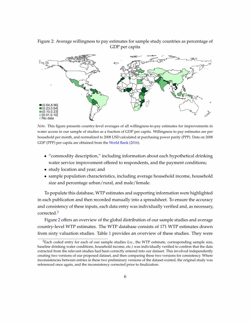
Figure 2: Average willingness to pay estimates for sample study countries as percentage ofGDP per capita

(0.64,8.96](0.23,0.64](0.10,0.23][0.01,0.10]No data

Note. This figure presents country-level averages of all willingness-to-pay estimates for improvements inwater access in our sample of studies as a fraction of GDP per capita. Willingness to pay estimates are perhousehold per month, and normalized to 2008 USD calculated at purchasing power parity (PPP). Data on 2008GDP (PPP) per capita are obtained from the World Bank (2016).

• “commodity description,” including information about each hypothetical drinkingwater service improvement offered to respondents, and the payment conditions;

• study location and year; and• sample population characteristics, including average household income, household

size and percentage urban/rural, and male/female.

To populate this database, WTP estimates and supporting information were highlightedin each publication and then recorded manually into a spreadsheet. To ensure the accuracyand consistency of these inputs, each data entry was individually verified and, as necessary,corrected.2

Figure 2 offers an overview of the global distribution of our sample studies and averagecountry-level WTP estimates. The WTP database consists of 171 WTP estimates drawnfrom sixty valuation studies. Table 1 provides an overview of these studies. They were

2Each coded entry for each of our sample studies (i.e., the WTP estimate, corresponding sample size,baseline drinking water conditions, household income, etc.) was individually verified to confirm that the dataextracted from the relevant studies had been correctly entered into our dataset. This involved independentlycreating two versions of our proposed dataset, and then comparing these two versions for consistency. Whereinconsistencies between entries in these two preliminary versions of the dataset existed, the original study wasreferenced once again, and the inconsistency corrected prior to finalization.

6

Table 1: Summary of drinking water valuation studies included in the meta-analysis

Publication Country Study Year WTP estimates

1 Aguilar and Sterner (1995) Costa Rica 1993 32 Akram and Olmstead (2011) Pakistan 2007 53 Al-Ghuraiz and Enshassi (2005) Gaza (Israel) 2001 54 Altaf et al. (1992) Pakistan 1988 175 Altaf (1994) Pakistan 1990 26 Arouna and Dabbert (2012) Benin 2007 17 Bilgic (2010) Turkey 2007 28 Boadu (1992) Ghana 1989 129 Bohm et al. (1993) Philipinnes 1987 510 Briscoe et al. (1990) Brazil 1987 611 Casey et al. (2006) Brazil 2001 412 Choe and Varley (1997) India 1995 213 Chowdhury (1999) Bangladesh 1998 414 Davis (2004) Ukraine 1996 415 del Saz-Salazar et al. (2015) Bolivia 2011 116 Dutta (2005) India 2004 117 Egziabher and Adnew (2007) Ethiopia 2006 218 Fissha (2006) Ethiopia 2006 219 Fujita et al. (2005) Peru 2003 220 Genius and Tsagarakis (2006) Greece 2004 121 Genius et al. (2008) Greece 2004 122 Goldblatt (1999) South Africa 1994 123 Gunatilake and Tachiiri (2012) Bangladesh 2009 124 Hoehn and Krieger (2000) Egypt 1995 225 Hopkins et al. (2004) Rwanda 2000 126 Kadisa (2013) Botswana 2013 227 Kaliba et al. (2003) Tanzania 2001 128 Kanyoka et al. (2008) South Africa 2005 329 Katuwal and Bohara (2007) Nepal 2005 230 Lauria et al. (1995) Venezuela 1995 131 McPhail (1993) Morocco 1990 532 McPhail (1994) Tunisia 1990 133 Nam and Son (2005) Vietnam 2003 234 Pattanayak et al. (2001) Nepal 2001 335 Pattanayak et al. (2004) Sri Lanka 2003 436 Perez-Pineda and Quintanilla-Armijo (2013) El Salvador 1999 137 Peters and Mohamed (2010) Guyana 2010 138 Pinheiro and Whittington (1995) Mozambique 1994 439 Reddy (1999) India 1993 640 Rosado (1998) Brazil 1996 141 Shah (2003) Tanzania 2003 142 Singh et al. (1993) India 1988 143 de Oca and Bateman (2006) Mexico 2001 244 Stoveland and Bassey (2000) Nigeria 1997 145 Tussupova et al. (2015) Kazakhstan 2012 446 Vaidya (1996) India 1994 147 Vasquez et al. (2009) Mexico 2008 248 Vasquez et al. (2012) Nicaragua 2009 149 Vasquez and Franceschi (2013) Nicaragua 2009 250 Vasquez (2014) Guatemala 2012 151 Virjee (2006) Trinidad and Tobago 2003 252 Wang et al. (2010) China 2006 153 Wasike and Hanley (1998) Kenya 1995 454 Whittington et al. (1989) Tanzania 1988 1255 Whittington et al. (1990a) Haiti 1986 256 Whittington et al. (1990b) Nigeria 1989 657 Whittington et al. (1991) Nigeria 1987 158 Whittington et al. (1992) Ghana 1989 159 Widiyati (2011) Indonesia 2011 160 Wright et al. (2014) Uganda 2011 1

7

conducted in a total of 41 different countries between 1986 and 2013. The number of WTPestimates drawn from each publication ranges from one to seventeen, with an average(median) of 2.85 (2) estimates per study. Multiple WTP estimates from a single study wereonly included in the database if they were (1) estimated for different changes in drinkingwater services, or (2) based on distinct, nonoverlapping subsamples of households (e.g.,households living in separate geographic parts of the study area). If these conditionswere not fulfilled, multiple estimates covering same subsample of households were eitherdropped or averaged into one estimate.

4 Meta-regression models

As mentioned earlier, using meta-regression methods, it is possible to summarize andsynthesize a large number of WTP results from several studies. More importantly, it allowsus to explore the sources of variation in these WTP estimates. Specifically, meta-regressioncan be used to address the following questions:

• To what extent is the variation in WTP estimates systematically and significantlyrelated to observable factors?

• Do these factors affect WTP in ways that are consistent with expectations and eco-nomic theory?

If meta-regression reveals a strong systematic and consistent pattern underlying WTPestimates, then the results can also provide a useful framework for predicting averageWTP under alternative conditions for planning purposes.

To establish a consistent definition for the variables expressed in monetary terms—WTPand household income—these estimates were converted to average monthly values inUSD using the purchasing power parity (PPP) rate for the currency and year reported inthe study. All USD values from previous years were then updated to 2008 USD using theUS consumer price index (CPI). Generally speaking, the PPP is preferable to the officialcurrency exchange rate for international price comparisons and benefit transfers because itis specifically designed to measure relative purchasing power of the currency (Pattanayaket al., 2002).3

3The meta-regression results in this application are very similar when an exchange rate conversion is usedsince the PPP and exchange rate are highly correlated for the years and countries included in the analysis.

8

Table 2 describes the variables created from the WTP database and used in the meta-analysis, while Table 3 reports summary statistics for these variables. The variable WT-PINCR represents the average incremental monthly WTP for improving drinking waterservices from baseline conditions to the service level proposed in the SP scenario. Somestudies elicit and primarily report the total WTP for the final service level. For thesestudies, WTPINCR was constructed by deducting the baseline payment levels reportedin the studies. The resulting WTPINCR variable ranges in value from $0.02 to over $154,with an average (median) value of $19 ($10.50). Partly because of its rightward skewness,we used the natural log of this variable, LNWTPINCR, as the dependent variable in ourregression analyses.

The explanatory variables used in the analysis include a dummy variable (PRIVTAP)that equals one if the elicited improvement in drinking water services corresponding toeach WTP estimate refers to the provision of private, in-home tap water; if, on the otherhand, a particular WTP estimate has been recovered using a CV question that looks atWTP for improved public drinking water sources, its corresponding value for PRIVTAP iscoded as zero.

We also include controls for households’ baseline access to water services. The mainobjective of this to test for scope effects. If—as theory would predict—average WTP forimproved drinking water services is positively related to the magnitude of the elicitedwater-services improvement, including these allows us to control for differences in themarginal value of service improvements associated with differences in reference conditions.Thus, three additional dummy variables (BASELINE1, BASELINE2, and BASELINE3)capture the three main levels of existing water services described in the studies, respectively:(1) unimproved drinking water source; (2) public tap; and (3) private water connection.4

Specifically, BASELINE1 equals one if the primary source of water for a majority of thesample is unimproved; BASELINE2 equals one if a majority has access to public drinkingwater sources; and BASELINE3 equals one if a majority has access to a private drinkingwater connection. Approximately 25 percent of the WTP estimates in our database areelicited from households with no access to improved water sources, 45 percent are fromthose with some access to a public water source, and thirty percent are from those with

4In our specifications in Table 4, we drop BASELINE1 to avoid perfect multicollinearity. Thus, the coeffi-cients on BASELINE2 and BASELINE3 may be interpreted as the impact on average willingness to pay ofhouseholds’ access to public and private water sources, respectively, relative to access to only unimprovedsources.

9

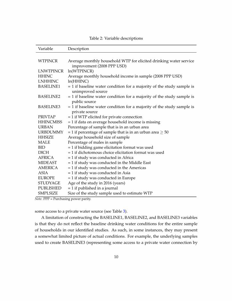
Table 2: Variable descriptions

Variable Description

WTPINCR Average monthly household WTP for elicited drinking water serviceimprovement (2008 PPP USD)

LNWTPINCR ln(WTPINCR)HHINC Average monthly household income in sample (2008 PPP USD)LNHHINC ln(HHINC)BASELINE1 = 1 if baseline water condition for a majority of the study sample is

unimproved sourceBASELINE2 = 1 if baseline water condition for a majority of the study sample is

public sourceBASELINE3 = 1 if baseline water condition for a majority of the study sample is

private sourcePRIVTAP = 1 if WTP elicited for private connectionHHINCMISS = 1 if data on average household income is missingURBAN Percentage of sample that is in an urban areaURBDUMMY = 1 if percentage of sample that is in an urban area ≥ 50HHSIZE Average household size of sampleMALE Percentage of males in sampleBID = 1 if bidding game elicitation format was usedDICH = 1 if dichotomous choice elicitation format was usedAFRICA = 1 if study was conducted in AfricaMIDEAST = 1 if study was conducted in the Middle EastAMERICA = 1 if study was conducted in the AmericasASIA = 1 if study was conducted in AsiaEUROPE = 1 if study was conducted in EuropeSTUDYAGE Age of the study in 2016 (years)PUBLISHED = 1 if published in a journalSMPLSIZE Size of the study sample used to estimate WTP

Note. PPP = Purchasing power parity.

some access to a private water source (see Table 3).A limitation of constructing the BASELINE1, BASELINE2, and BASELINE3 variables

is that they do not reflect the baseline drinking water conditions for the entire sampleof households in our identified studies. As such, in some instances, they may presenta somewhat limited picture of actual conditions. For example, the underlying samplesused to create BASELINE3 (representing some access to a private water connection by

10

Table 3: Descriptive statistics

VARIABLES MEAN P5 P25 P50 P75 P95 SD MIN MAX

WTPINCR 19.0 1.50 5.52 10.5 21.3 72.6 23.8 0.015 154.9LNWTPINCR 2.35 0.41 1.71 2.35 3.06 4.28 1.19 -4.20 5.04HHINC 781.3 31.2 296.5 727.8 999.2 2086.1 680.8 31.2 3584.8LNHHINC 6.15 3.44 5.69 6.59 6.91 7.64 1.22 3.44 8.18BASELINE1 0.25 0 0 0 1 1 0.44 0 1BASELINE2 0.45 0 0 0 1 1 0.50 0 1BASELINE3 0.30 0 0 0 1 1 0.46 0 1PRIVTAP 0.74 0 0 1 1 1 0.44 0 1HHINCMISS 0.14 0 0 0 0 1 0.35 0 1URBAN 47.0 0 0 40.1 100 100 48.0 0 100URBDUMMY 0.47 0 0 0 1 1 0.50 0 1HHSIZE 6.21 3.90 4.95 5.89 7.20 9.50 1.81 2.90 12.0MALE 0.53 0.29 0.50 0.50 0.59 0.75 0.14 0.051 0.91BID 0.59 0 0 1 1 1 0.49 0 1DICH 0.25 0 0 0 1 1 0.44 0 1AFRICA 0.33 0 0 0 1 1 0.47 0 1MIDEAST 0.088 0 0 0 0 1 0.28 0 1AMERICA 0.18 0 0 0 0 1 0.39 0 1ASIA 0.37 0 0 0 1 1 0.48 0 1EUROPE 0.036 0 0 0 0 0 0.19 0 1STUDYAGE 19.8 5 13 22 27 29 8.06 3 30PUBLISHED 0.58 0 0 1 1 1 0.49 0 1SMPLSIZE 284.3 18 89 150 324 997 395.4 2 3677

Observations 171

a majority of the sample) range from about 55 percent for a sample of households inShoshong, Botswana as documented by Kadisa (2013), to full connectivity to a privatewater system for one in Matiguas, Nicaragua as documented by Vasquez et al. (2012).5

Moreover, these variables cannot fully capture differences in baseline quality—such as

5This underlying variability helps explain why a particular study may be coded as having BASELINE3= 1 and PRIVTAP = 0, i.e., investigating WTP for enhancing access to public drinking water sources forhouseholds that largely have some private water access. Enhanced access to public services need not beperceived as a “reduction” in services for such communities; households facing unreliable private access, orthose in communities with significant heterogeneity in access may indeed perceive benefits from improvedaccess to alternate sources of drinking water, as we show in Table 5.

11

water reliability, pressure, color, or taste—that may also be important determinants of thebenefits that accrue to households from enhanced access (Jeuland et al., 2015; Yang et al.,2006). We note, however, that a majority of the studies we identify report multiple WTPestimates for distinct subsamples (such as households with or without a private waterconnection). In instances where the water access characteristics of the subsample are clearlydefined, we are able to assign more accurate baseline drinking water conditions to thecorresponding WTP estimate. Thus, while admittedly somewhat limited, our approachto specifying baseline drinking water conditions allows us to balance statistical powerconcerns with our aim of gaining new insights from the literature on demand for improveddrinking water access.

Four main sample characteristic variables (HHINC, URBDUMMY, HHSIZE, and MALE)are also included as explanatory variables.6 Assuming drinking water services are a normalgood, average household income is expected to have a positive effect on WTP. The mean(median) value of average monthly household income across study samples is $781 ($728)after 24 observations with missing data on household income are replaced with the samplemean of non-missing observations. A dummy variable (HHINCMISS) is included toaccount for the potential effect of these missing data. The expectations regarding HHSIZE,URBDUMMY, and MALE are less clear-cut than for household income.

Further, two CV elicitation method variables (BID and DICH) are included, with theomitted category being open-ended elicitation.7 Finally, four regional dummy variables(AFRICA, MIDEAST, ASIA, and AMERICA) and two general publication descriptors(STUDYAGE and PUBLISHED) are also included.8

5 Results

We summarize our meta-regression results in Table 4. We estimate the regressions usingweighted least squares where each WTP data point is weighted according to the sizeof the underlying sample used (SMPLSIZE). In essence, this approach assumes that the

6URBDUMMY is coded as a dummy variable that equals one if at least half of the relevant subsample ofhouseholds for each WTP estimate is located in an urban area (i.e., URBAN ≥ 50).

7The stated preference elicitation approaches we observe in our collected studies (bidding game, dichoto-mous choice, and open-ended elicitation formats) map on to the stated preference nomenclature proposed byCarson and Louviere (2011)—namely, bidding game, binary/multinomial choice question, and direct question,respectively. We point readers to this work for additional insights.

8The EUROPE regional dummy variable is omitted in our meta-regression.

12

variance of the WTP estimates is inversely proportional to the magnitude of the underlyingsample sizes.9 In addition, to account for the panel structure of the data (i.e., multiple WTPestimates from individual studies), the standard errors are clustered by “study” using aHuber-White method. These are well-established methods for meta-regression analyses ofWTP data (Nelson and Kennedy, 2009; Van Houtven et al., 2007).

Table 4 reports results for the full sample (N = 171) and for six different modelspecifications. Model (1) is our most parsimonious specification, only including the log ofhousehold income (LNHHINC) and a dummy variable for whether the elicited offer forthe relevant estimate asks about access to a private or public source (PRIVTAP). The effectof income is positive and highly statistically significant. While the coefficient on PRIVTAPin model (1) is positive—suggesting a willingness to pay a price premium for access to aprivate connection—the result is not statistically significant. It is only when we controlfor households’ baseline water access level by including the BASELINE2 and BASELINE3dummy variables in model (2) do we see a clear, statistically significant pattern emerge. Wefind that households are more willing to pay for private water connections than public ones.In addition, our results strongly suggest that households’ WTP for proposed improvementsin water access declines as their baseline water availability improves. Thus, WTP estimatesappear to be sensitive to scope; they are systematically larger for larger improvements indrinking water services.

To further examine the robustness of the regression results to model specification, inmodels (3)-(6) we sequentially introduce a variety of additional controls related to demo-graphic characteristics; survey elicitation methods; global regions; and, finally, publicationcharacteristics. Our results are consistent across all further model specifications and robustto the addition of these controls. We also find that the coefficient on the DICH dummyvariable is positive and highly statistically significant in each of the specifications in whichit is included. As noted by Carson et al. (2001), dichotomous choice questions attemptingto elicit willingness to pay for private or quasi-public public goods face a high rate of“yes” responses since such responses increase the likelihood that the good will be providedwhile allowing for purchase decisions to be delayed until later, effectively enhancing thechoice set at no cost. Our results are consistent with this hypothesis and prior empiricalresults, suggesting that dichotomous choice formats do indeed induce “yea-saying” byrespondents and, thus, yield relatively high WTP values, and that open-ended formats

9Very few of the studies report variance or standard error estimates for the estimated WTP values; therefore,weighting according to sample size was used as a second-best approximation.

13

Table 4: Willingness to pay meta-regression results

VARIABLES (1) (2) (3) (4) (5) (6)

LNHHINC 0.321** 0.347** 0.329** 0.246* 0.248* 0.272*(0.153) (0.137) (0.149) (0.143) (0.145) (0.157)

PRIVTAP 0.177 0.859** 0.797** 0.890*** 0.886** 0.949**(0.504) (0.360) (0.315) (0.332) (0.338) (0.363)

BASELINE2 -1.133*** -0.971*** -1.088*** -1.075*** -1.118***(0.324) (0.327) (0.339) (0.356) (0.341)

BASELINE3 -1.418*** -1.315*** -1.384*** -1.397*** -1.455***(0.337) (0.347) (0.399) (0.435) (0.441)

HHINCMISS -0.168 0.205 0.196 0.156(0.388) (0.307) (0.322) (0.343)

URBDUMMY 0.328 0.209 0.251 0.116(0.228) (0.265) (0.249) (0.236)

HHSIZE 0.0478 0.0637 0.0696 0.0732(0.0710) (0.0690) (0.0764) (0.0780)

MALE -0.390 -0.168 0.256 0.315(0.793) (0.822) (0.907) (1.114)

BID 0.450 0.440 0.605(0.422) (0.424) (0.414)

DICH 0.933*** 0.931*** 0.965***(0.310) (0.323) (0.334)

AFRICA -0.0541 -0.262(0.531) (0.549)

MIDEAST -0.131 -0.213(0.425) (0.495)

AMERICA 0.164 -0.0399(0.453) (0.499)

ASIA -0.154 -0.418(0.546) (0.587)

STUDYAGE -0.0214(0.0208)

PUBLISHED -0.184(0.269)

Constant 0.332 0.679 0.454 0.237 -0.00566 0.461(0.934) (0.773) (1.075) (1.114) (1.299) (1.202)

Observations 171 171 171 171 171 171R-squared 0.084 0.219 0.240 0.310 0.318 0.332

Note. This table presents weighted least squares regression results for the full sample of willingness to pay(WTP) estimates; each estimate is weighted by its underlying sample size. The dependent variable for eachmodel is LNWTPINCR. Standard errors are clustered at the study level and shown in parentheses. *** p<0.01,** p<0.05, * p<0.1

14

induce respondents to understate their true maximum WTP (Carson, 2000; Holmes andKramer, 1995).

We find no statistically significant differences in WTP across regions per se (that is,controlling for other socio-demographics that differentiate the regions). The estimatedeffect of household size is positive but also not statistically significant. Nevertheless, whenevaluated at the mean value of the household size variable, the magnitude of the coefficientestimates suggests that WTP increases roughly in proportion to household size.

6 So what? Costs and (model-predicted) benefits of plans to im-prove drinking water supply

Beyond synthesizing results and testing hypotheses related to WTP estimates, the meta-regression functions in Table 4 provide models that can be used to predict WTP for alter-native conditions and changes. We illustrate this application of the meta-regressions inTable 5, which uses the sixth model specification from Table 4 to predict average monthlyhousehold WTP for different combinations of BASELINE1, BASELINE2, BASELINE3, andPRIVTAP.10 For all of these predictions, the other explanatory variables in the model areset at their sample mean values (see Table 3). The predicted WTP values range fromapproximately $3 per month (with a ninety percent confidence interval of $1.1 to $6.1)to $33.5 per month ($17.9 to $66.0). As expected, larger improvements in drinking wateraccess and services (i.e., private connections versus public sources) lead to higher predictedWTP values, and higher baseline levels have the opposite effect. To avoid the assumptionsregarding baselines and to obtain general estimates for WTP, we can use model (1) in Table4, which does not specify BASELINE2 and BASELINE3 as explanatory variables, to alsopredict monthly household WTP. These values range from $9.2 ($3.4 to $16.1) for access topublic water sources to $11 ($8.8 to $15.4) for access to private water services. As expectedthese estimates fall in the mid-range of the values in Table 5.

Next, we wish to demonstrate how predictions of household WTP, one of the twogoals of meta-analysis (Smith and Pattanayak, 2002), could allow policy-makers to targetWSS delivery, for example, by mapping spatial heterogeneity in demand. Using estimatesfrom model (1) of Table 4, we calculate household-level WTP for private water sources

10To appropriately transform the model prediction of mean ln(WTP) to mean WTP, we applied a smearingfactor to the exponentiated model predictions of LNWTPINCR (Duan, 1983). This factor is equal to the averageof the exponentiated residuals for the 171 observations in the estimation sample.

15

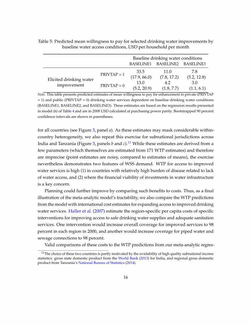
Table 5: Predicted mean willingness to pay for selected drinking water improvements bybaseline water access conditions, USD per household per month

Baseline drinking water conditionsBASELINE1 BASELINE2 BASELINE3

Elicited drinking waterimprovement

PRIVTAP = 133.5 11.0 7.8

(17.9, 66.0) (7.8, 17.2) (5.2, 12.8)

PRIVTAP = 013.0 4.2 3.0

(5.2, 20.9) (1.8, 7.7) (1.1, 6.1)Note. This table presents predicted estimates of mean willingness to pay for enhancement in private (PRIVTAP= 1) and public (PRIVTAP = 0) drinking water services dependent on baseline drinking water conditions(BASELINE1, BASELINE2, and BASELINE3). These estimates are based on the regression results presentedin model (6) of Table 4 and are in 2008 USD calculated at purchasing power parity. Bootstrapped 90 percentconfidence intervals are shown in parentheses.

for all countries (see Figure 3, panel a). As these estimates may mask considerable within-country heterogeneity, we also repeat this exercise for subnational jurisdictions acrossIndia and Tanzania (Figure 3, panels b and c).11 While these estimates are derived from afew parameters (which themselves are estimated from 171 WTP estimates) and thereforeare imprecise (point estimates are noisy, compared to estimates of means), the exercisenevertheless demonstrates two features of WSS demand. WTP for access to improvedwater services is high (1) in countries with relatively high burden of disease related to lackof water access, and (2) where the financial viability of investments in water infrastructureis a key concern.

Planning could further improve by comparing such benefits to costs. Thus, as a finalillustration of the meta-analytic model’s tractability, we also compare the WTP predictionsfrom the model with international cost estimates for expanding access to improved drinkingwater services. Haller et al. (2007) estimate the region-specific per capita costs of specificinterventions for improving access to safe drinking water supplies and adequate sanitationservices. One intervention would increase overall coverage for improved services to 98percent in each region in 2000, and another would increase coverage for piped water andsewage connections to 98 percent.

Valid comparisons of these costs to the WTP predictions from our meta-analytic regres-

11The choice of these two countries is partly motivated by the availability of high quality subnational incomestatistics: gross state domestic product from the World Bank (2013) for India, and regional gross domesticproduct from Tanzania’s National Bureau of Statistics (2014).

16

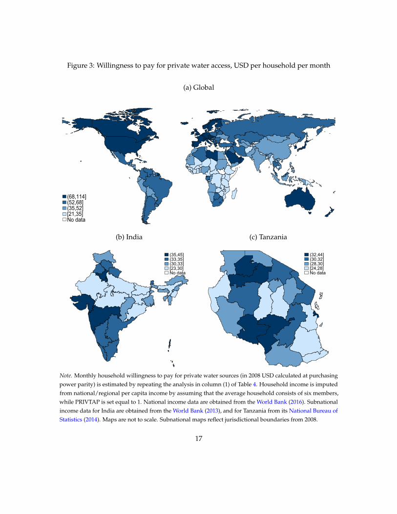
Figure 3: Willingness to pay for private water access, USD per household per month

(a) Global

(68,114](52,68](35,52][21,35]No data

(b) India

(35,45](33,35](30,33][23,30]No data

(c) Tanzania

(32,44](30,32](28,30][24,28]No data

Note. Monthly household willingness to pay for private water sources (in 2008 USD calculated at purchasingpower parity) is estimated by repeating the analysis in column (1) of Table 4. Household income is imputedfrom national/regional per capita income by assuming that the average household consists of six members,while PRIVTAP is set equal to 1. National income data are obtained from the World Bank (2016). Subnationalincome data for India are obtained from the World Bank (2013), and for Tanzania from its National Bureau ofStatistics (2014). Maps are not to scale. Subnational maps reflect jurisdictional boundaries from 2008.

17

sion model require several adjustments. First, to approximate costs for only improvingdrinking water services (not sanitation), we multiply the ratio of (1) the population withoutaccess to drinking water by (2) the combined population without access to improvedwater or sanitation. Country-level coverage estimates for 2000 were taken from the WorldHealth Organization and United Nations Children’s Fund Joint Monitoring Programmefor Water Supply and Sanitation (WHO/UNICEF, 2010). Second, to estimate per capitacosts averaged over the non-covered population rather than the total population, we dividedby the percent of the population without drinking water coverage. Third, we convertedfrom annual to monthly costs by dividing by twelve and from 2000 USD to 2008 USD bymultiplying by the CPI inflation factor (see Pattanayak et al., 2010). Fourth, we convertedfrom per capita to per household values by multiplying by six (rough estimate of personsper household).

To estimate average per-household WTP for these interventions and regions, we againapplied meta-regression model (6) from Table 4 using the following specifications:

• For the first intervention (improved drinking water) we set baseline water conditionsat unimproved (BASELINE1 = 1) and assumed an increase in access to public watersources (PRIVTAP = 0).

• For the second intervention (piped water) we assumed an increase in access to privatewater connections (PRIVTAP = 1) from the same baseline (BASELINE1 = 1).

• For household income, we used 2000 GDP per capita in each region (converted toper household per month figures in 2008 USD).

• For URBAN, we used the percent of the region’s total non-covered population in2000 that lived in urban areas (WHO/UNICEF, 2010).12

• For the region, we set the corresponding dummy variable equal to 1.• Finally, we set STUDYAGE = 9, PUBLISHED = 1, HHINCMISS = 0, and all other

variables at their study sample means.

Table 6 reports the resulting benefit-cost comparisons for three regions included byHaller et al. (2007) with relatively low levels of drinking water coverage—Africa, Asia,and the high mortality stratum of the Americas (AMR-D).13 The estimated per-household

12To obtain the appropriate coefficient, we reran the regression in model (6) with URBAN instead ofURBDUMMY.

13Asia includes Indonesia, Sri Lanka, Thailand, Bangladesh, Bhutan, Democratic People’s Republic of Korea,India, Maldives, Myanmar, and Nepal. The Americas (high mortality stratum, AMR-D) include Bolivia,Ecuador, Guatemala, Haiti, Nicaragua, and Peru.

18

Table 6: Benefit-cost comparison for improved drinking water services, USD perhousehold per month

RegionImproved water coverage (98%) Piped water supply (98%)

BASELINE1 = 1, PRIVTAP = 0 BASELINE1 = 1, PRIVTAP = 1WTP Costs WTP Costs

Africa 10.17 2.03 26.32 9.87Asia 9.74 2.68 25.20 12.61

Americas 18.81 3.10 48.69 13.45Note. This table presents regional estimates of benefits and cost of enhancing access to improved drinkingwater services (in 2008 USD calculated at purchasing power parity).

benefits of providing 98 percent access to improved drinking water services are greater thanthe estimated costs in all three regions. The difference is greatest in the Americas, wherethe estimated benefits are over six times the magnitude of costs. In addition, estimatedbenefits of access to private water connections also exceed costs in all regions, despite afourfold increase in the cost of increasing piped water access relative to simply increasingimproved water coverage.

It should be noted that the WTP estimates reported in Table 6 may overstate the benefitsof improving drinking water access because they are based on mean household incomelevels for each region. The average income level in the non-covered population is likely tobe below this mean. This may be of particular concern to policy-makers looking to expandaccess to improved water sources for low-income households in remote, rural regions,where the ratio of benefits to costs is likely to be the lowest (Whittington and Pattanayak,2015). That said, our calculations suggest that income levels would need to be substantiallybelow the mean—for instance, more than ninety percent below the mean in the Africaregion—before the estimated costs of improving water coverage exceed its benefits.

7 Conclusion

We use meta-analysis in this study to synthesize results from a worldwide sample of sixtystated preference (SP) studies estimating household willingness to pay (WTP) for improvedaccess to or quality of drinking water services. Using 171 WTP estimates drawn fromthese studies and applying regression analysis, we examine a range of potential factorsthat explain variation in WTP estimates. We find that households’ WTP are sensitive to

19

scope (i.e., the size of the change in drinking water services), average household income,and SP elicitation method. Critically, the influence of these factors follows theoreticalpredictions and intuition. We then demonstrate how these regression models can be usedto predict household-level WTP for selected improvements in drinking water access andservices. This use of the regression model provides a useful framework for estimatingthe benefits of policies that improve households’ access to these services. For example, inselected regions with currently low levels of coverage, we find that WTP for improveddrinking water access greatly exceeds the cost of provision. However, the models alsosuggest that if considerable income disparities exist, the perceived private benefits ofinterventions that enhance access to piped water services may fail to exceed their costs. Insuch settings, policy-makers looking to promote increases in piped water coverage on thebasis of merit-good or equity arguments may need to rely on external sources of finance(such as international aid) to cover the gap between benefits and costs. As global leadersmove forward with policies in line with the water and sanitation Sustainable DevelopmentGoals (SDGs), our meta-analysis and the resulting first-order estimates of benefits forimproved water access illustrate how one might distinguish settings where local financecould be sufficient from those where external financial assistance will be vital.

Acknowledgments

This research was partially supported by the US Environmental Protection Agency undercontract EP-W-07-069. We thank two anonymous reviewers for their helpful comments.

References

AGUILAR, M. AND T. STERNER (1995): “Willingness to pay for improved communal waterservices,” Environmental Economics Unit Working Paper, Department of Economics,Gothenburg University.

AKRAM, A. A. AND S. M. OLMSTEAD (2011): “The Value of Household Water ServiceQuality in Lahore, Pakistan,” Environmental and Resource Economics, 49, 173–198.

AL-GHURAIZ, Y. AND A. ENSHASSI (2005): “Ability and willingness to pay for watersupply service in the Gaza Strip,” Building and Environment, 40, 1093–1102.

20

ALTAF, M. A. (1994): “Household demand for improved water and sanitation in a largesecondary city,” Habitat International, 18, 45–55.

ALTAF, M. A., H. JAMAL, AND D. WHITTINGTON (1992): “Willingness to pay for water inrural Punjab, Pakistan,” Tech. rep., World Bank, Washington, DC, prepared for the UNDP-World Bank Water and Sanitation Program, Water and Sanitation Division, Infrastructureand Urban Development Department.

AROUNA, A. AND S. DABBERT (2012): “Estimating rural households’ willingness to pay forwater supply improvements: a Benin case study using a semi-nonparametric bivariateprobit approach,” Water International, 37, 293–304.

BERGSTROM, J. C. AND L. O. TAYLOR (2006): “Using meta-analysis for benefits transfer:Theory and practice,” Ecological Economics, 60, 351–360.

BILGIC, A. (2010): “Measuring willingness to pay to improve municipal water in southeastAnatolia, Turkey,” Water Resources Research, 46.

BOADU, F. O. (1992): “Contingent Valuation for Household Water in Rural Ghana,” Journalof Agricultural Economics, 43, 458–465.

BOHM, R. A., T. J. ESSENBURG, AND W. F. FOX (1993): “Sustainability of potable waterservices in the Philippines,” Water Resources Research, 29, 1955–1963.

BOYLE, K. J., C. F. PARMETER, B. B. BOEHLERT, AND R. W. PATERSON (2013): “DueDiligence in Meta-analyses to Support Benefit Transfers,” Environmental and ResourceEconomics, 55, 357–386.

BRANDER, L. M., R. J. G. M. FLORAX, AND J. E. VERMAAT (2006): “The Empirics ofWetland Valuation: A Comprehensive Summary and a Meta-Analysis of the Literature,”Environmental & Resource Economics, 33, 223–250.

BRISCOE, J., P. F. DE CASTRO, C. GRIFFIN, J. NORTH, AND O. OLSEN (1990): “TowardEquitable and Sustainable Rural Water Supplies: A Contingent Valuation Study in Brazil,”The World Bank Economic Review, 4, 115–134.

CARSON, R. T. (2000): “Contingent Valuation: A User’s Guide,” Environmental Science &Technology, 34, 1413–1418.

CARSON, R. T., N. E. FLORES, AND N. F. MEADE (2001): “Contingent Valuation: Contro-versies and Evidence,” Environmental and Resource Economics, 19, 173–210.

CARSON, R. T. AND J. J. LOUVIERE (2011): “A Common Nomenclature for Stated Prefer-ence Elicitation Approaches,” Environmental and Resource Economics, 49, 539–559.

CASEY, J. F., J. R. KAHN, AND A. RIVAS (2006): “Willingness to pay for improved waterservice in Manaus, Amazonas, Brazil,” Ecological Economics, 58, 365–372.

21

CHOE, K. AND R. VARLEY (1997): “Conservation and pricing-does raising tariffs to aneconomic price for water make the people worse off,” Prepared for the Best ManagementPractice for Water Conservation Workshop, South Africa.

CHOWDHURY, N. T. (1999): “Willingness to pay for water in Dhaka slums: A ContingentValuation Study,” in The Economic Value of the Environment: Cases from South Asia, ed. byJ. E. Hecht, Kathmandu, Nepal: IUCN.

CONFALONIERI, U., B. MENNE, R. AKHTAR, K. EBI, M. HAUENGUE, R. KOVATS, B. RE-VICH, AND A. WOODWARD (2007): “Human health,” in Climate Change 2007: Impacts,Adaptation and Vulnerability. Contribution of Working Group II to the Fourth AssessmentReport of the Intergovernmental Panel on Climate Change, ed. by M. Parry, O. Canziani,J. Palutikof, P. van der Linden, and C. Hanson, Cambridge, UK: Cambridge UniversityPress, 391–431.

DAVIS, J. (2004): “Assessing Community Preferences for Development Projects: AreWillingness-to-Pay Studies Robust to Mode Effects?” World Development, 32, 655–672.

DE OCA, G. S. M. AND I. J. BATEMAN (2006): “Scope sensitivity in households’ willingnessto pay for maintained and improved water supplies in a developing world urban area:Investigating the influence of baseline supply quality and income distribution uponstated preferences in Mexico City,” Water Resources Research, 42.

DEL SAZ-SALAZAR, S., F. GONZALEZ-GOMEZ, AND J. GUARDIOLA (2015): “Willingnessto pay to improve urban water supply: the case of Sucre, Bolivia,” Water Policy, 17, 112.

DUAN, N. (1983): “Smearing Estimate: A Nonparametric Retransformation Method,”Journal of the American Statistical Association, 78, 605–610.

DUTTA, V. (2005): “Public Support for Water Supply Improvements: Empirical EvidenceFrom Unplanned Settlements of Delhi, India,” The Journal of Environment & Development,14, 439–462.

EFENDIC, A., G. PUGH, AND N. ADNETT (2011): “Institutions and economic performance:A meta-regression analysis,” European Journal of Political Economy, 27, 586–599.

EGZIABHER, K. AND B. ADNEW (2007): “Valuing Water Supply Service Improvements InAddis Ababa,” Ethiopian Journal of Economics, 16.

FISSHA, M. (2006): “Household demand for improved water service in urban areas: thecase of Addis Ababa, Ethiopia,” Master’s thesis, Addis Ababa University.

FUJITA, Y., A. FUJII, S. FURUKAWA, AND T. OGAWA (2005): “Estimation of willingness-to-pay (WTP) for water and sanitation services through contingent valuation method(CVM): A case study in Iquitos City, The Republic of Peru,” JBICI Review, 11, 59–87.

22

GENIUS, M., E. HATZAKI, E. M. KOUROMICHELAKI, G. KOUVAKIS, S. NIKIFORAKI, AND

K. P. TSAGARAKIS (2008): “Evaluating Consumers’ Willingness to Pay for ImprovedPotable Water Quality and Quantity,” Water Resour Manage, 22, 1825–1834.

GENIUS, M. AND K. P. TSAGARAKIS (2006): “Water shortages and implied water quality:A contingent valuation study,” Water Resources Research, 42.

GOLDBLATT, M. (1999): “Assessing the effective demand for improved water suppliesin informal settlements: a willingness to pay survey in Vlakfontein and Finetown,Johannesburg,” Geoforum, 30, 27–41.

GUNATILAKE, H. AND M. TACHIIRI (2012): “Willingness to pay and inclusive tariff designsfor improved water supply services in Khulna, Bangladesh,” Asian Development BankSouth Asia Working Paper Series.

GUNATILAKE, H., J.-C. YANG, S. K. PATTANAYAK, AND K. A. CHOE (2007): “Good prac-tices for estimating reliable willingness-to-pay values in the water supply and sanitationsector,” Tech. rep., Asian Development Bank, http://hdl.handle.net/11540/2354.

HAINES, A., R. KOVATS, D. CAMPBELL-LENDRUM, AND C. CORVALAN (2006): “Climatechange and human health: impacts, vulnerability, and mitigation,” The Lancet, 367,2101–2109.

HALLER, L., G. HUTTON, AND J. BARTRAM (2007): “Estimating the costs and healthbenefits of water and sanitation improvements at global level,” Journal of Water andHealth, 5, 467.

HOEHN, J. P. AND D. J. KRIEGER (2000): “An Economic Analysis of Water and WastewaterInvestments in Cairo, Egypt,” Evaluation Review, 24, 579–608.

HOLMES, T. P. AND R. A. KRAMER (1995): “An Independent Sample Test of Yea-Sayingand Starting Point Bias in Dichotomous-Choice Contingent Valuation,” Journal of Envi-ronmental Economics and Management, 29, 121–132.

HOPKINS, O. S., D. T. LAURIA, AND A. KOLB (2004): “Demand-Based Planning of RuralWater Systems in Developing Countries,” J. Water Resour. Plann. Manage., 130, 44–52.

HORVATHOVA, E. (2010): “Does environmental performance affect financial performance?A meta-analysis,” Ecological Economics, 70, 52–59.

HOWARD, G., K. CHARLES, K. POND, A. BROOKSHAW, R. HOSSAIN, AND J. BARTRAM

(2010): “Securing 2020 vision for 2030: climate change and ensuring resilience in waterand sanitation services,” Journal of Water and Climate Change, 01, 2.

JEULAND, M., J. ORGILL, A. SHAHEED, G. REVELL, AND J. BROWN (2015): “A matter

23

of good taste: investigating preferences for in-house water treatment in peri-urbancommunities in Cambodia,” Envir. Dev. Econ., 21, 291–317.

KADISA, K. (2013): “Willingness to pay for improved water supply services in Shoshong,Phaleng ward, Botswana: application of Contingent Valuation Method (CVM),” Master’sthesis, University of Zimbabwe.

KALIBA, A., D. NORMAN, AND Y.-M. CHANG (2003): “Willingness to pay to improvedomestic water supply in rural areas of Central Tanzania: Implications for policy,”International Journal of Sustainable Development & World Ecology, 10, 119–132.

KANYOKA, P., S. FAROLFI, AND S. MORARDET (2008): “Households’ preferences andwillingness to pay for multiple use water services in rural areas of South Africa: ananalysis based on choice modelling,” Water SA, 34, 715 – 723.

KATUWAL, H. AND A. BOHARA (2007): “Coping with unreliable water supplies andwillingness to pay for improved water supplies in Kathmandu,” Presented at the SecondAnnual Himalayan Policy Research Conference, Nepal Study Center.

LAURIA, D., J. DAVIS, AND E. MCCLELLAND (1995): “Final Report on Households’Willingness to Pay for Improved Water Supply and Sanitation in Maturin, Venezuela,”Tech. rep., CVM, Inc., Chapel Hill, NC.

MCPHAIL, A. A. (1993): “The “five percent rule” for improved water service: Can house-holds afford more?” World Development, 21, 963–973.

——— (1994): “Why Don’t Households Connect to the Piped Water System? Observationsfrom Tunis, Tunisia,” Land Economics, 70, 189.

NAM, P. AND T. SON (2005): “Households Demand for Improved Water Services in Ho ChiMinh City: A Comparison of Contingent Valuation and Choice Modelling Estimates,”Tech. rep., Economy and Environment Program for Southeast Asia, Singapore.

NATIONAL BUREAU OF STATISTICS (2014): “National Accounts of Tan-zania Mainland,” Retrieved from http://www.nbs.go.tz/nbstz/index.

php/english/statistics-by-subject/national-accounts-statistics/

340-national-accounts-of-tanzania-mainland-2001-2013.NELSON, J. P. AND P. E. KENNEDY (2009): “The Use (and Abuse) of Meta-Analysis in

Environmental and Natural Resource Economics: An Assessment,” Environmental andResource Economics, 42, 345–377.

PATTANAYAK, S. K., C. POULOS, J.-C. YANG, AND S. PATIL (2010): “How valuable areenvironmental health interventions? Evaluation of water and sanitation programmes inIndia,” Bulletin of the World Health Organization, 88, 535–542.

24

PATTANAYAK, S. K., J. M. WING, B. M. DEPRO, G. L. VAN HOUTVEN, P. DE CIVITA, D. M.STIEB, AND B. HUBBELL (2002): “International health benefits transfer application tool:the use of PPP and inflation indices,” Tech. rep., RTI International, Research TrianglePark, NC, prepared for the Economic Analysis and Evaluation Division, Health Canada.

PATTANAYAK, S. K., J.-C. YANG, C. AGARWAL, H. M. GUNATILAKE, H. M. S. J. H.BANDARA, AND T. RANASINGHE (2004): “Water, Sanitation, and Poverty in SouthwestSri Lanka,” Tech. rep., RTI International, Research Triangle Park, NC, prepared for theWorld Bank.

PATTANAYAK, S. K., J.-C. YANG, D. WHITTINGTON, K. C. BAL KUMAR, G. SUBEDI, Y. B.GURUNG, K. P. ADHIKARI, D. V. SHAKYA, L. S. KUNWAR, AND B. K. MABUHANG

(2001): “Willingness to Pay for Improved Water Supply in Kathmandu Valley, Nepal,”Tech. rep., RTI International, Research Triangle Park, NC, prepared for the World Bank.

PEREZ-PINEDA, F. AND C. QUINTANILLA-ARMIJO (2013): “Estimating willingness-to-pay and financial feasibility in small water projects in El Salvador,” Journal of BusinessResearch, 66, 1750–1758.

PETERS, E. J. AND Z. MOHAMED (2010): “Willingness to pay for water on the Guyana eastcoast,” Proceedings of the ICE - Water Management, 163, 315–323.

PINHEIRO, A. AND D. WHITTINGTON (1995): “Introducing a Demand-Side Approach toRural Water Investment in Mozambique: A Rapid Appraisal of Household Demand forImproved Water Services in Marracuene,” Tech. rep., National Rural Water Program(PRONAR), Maputo, Mozambique.

REDDY, V. R. (1999): “Quenching the Thirst: The Cost of Water in Fragile Environments,”Development and Change, 30, 79–113.

ROSADO, M. (1998): “Willingness to pay for drinking water in urban areas of developingcountries,” 1998 Annual meeting, August 2-5, Salt Lake City, UT 20821, American Agri-cultural Economics Association (New Name 2008: Agricultural and Applied EconomicsAssociation).

SHAH, A. S. (2003): “Value of Improvements in Water Supply Reliability in ZanzibarTown,” Master’s thesis, Yale School of Forestry and Environmental Studies.

SINGH, B., R. RAMASUBBAN, R. BHATIA, J. BRISCOE, C. C. GRIFFIN, AND C. KIM (1993):“Rural water supply in Kerala, India: How to emerge from a low-level equilibrium trap,”Water Resources Research, 29, 1931–1942.

SMITH, V. K. AND S. K. PATTANAYAK (2002): “Is Meta-Analysis a Noah’s Ark for Non-Market Valuation?” Environmental and Resource Economics, 22, 271–296.

25

STANLEY, T. AND S. B. JARRELL (1998): “Gender Wage Discrimination Bias? A Meta-Regression Analysis,” The Journal of Human Resources, 33, 947.

STOVELAND, S. AND B. BASSEY (2000): “Status of water supply and sanitation in 37 smalltowns in Nigeria,” Paper Presented at the Donor Conference in Abuja, February 2-4,2000.

TUSSUPOVA, K., R. BERNDTSSON, T. BRAMRYD, AND R. BEISENOVA (2015): “Investigat-ing Willingness to Pay to Improve Water Supply Services: Application of ContingentValuation Method,” Water, 7, 3024–3039.

UKOLI-ONODIPE, G. O. (2003): “Designing optimal water supply systems for developingcountries,” Ph.D. thesis, The Ohio State University.

UNITED NATIONS (2007): “Millenium Development Goals,” Tech. rep., United Nations,New York.

——— (2014): “Open Working Group proposal for Sustainable Development Goals,” Tech.rep., United Nations, New York.

VAIDYA, C. (1996): “Demand and willingness to pay for urban water and sanitationservices in Baroda,” Journal of Indian Water Works Association, 28, 87–92.

VAN HOUTVEN, G. L. (2008): “Methods for the Meta-Analysis of Willingness-to-Pay Data,”PharmacoEconomics, 26, 901–910.

VAN HOUTVEN, G. L., J. POWERS, AND S. K. PATTANAYAK (2007): “Valuing water qualityimprovements in the United States using meta-analysis: Is the glass half-full or half-empty for national policy analysis?” Resource and Energy Economics, 29, 206–228.

VASQUEZ, W. F. (2014): “Willingness to pay and willingness to work for improvementsof municipal and community-managed water services,” Water Resources Research, 50,8002–8014.

VASQUEZ, W. F. AND D. FRANCESCHI (2013): “System Reliability and Water ServiceDecentralization: Investigating Household Preferences in Nicaragua,” Water ResourManage, 27, 4913–4926.

VASQUEZ, W. F., D. FRANCESCHI, AND G. T. V. HECKEN (2012): “Household preferencesfor municipal water services in Nicaragua,” Envir. Dev. Econ., 17, 105–126.

VASQUEZ, W. F., P. MOZUMDER, J. HERNANDEZ-ARCE, AND R. P. BERRENS (2009):“Willingness to pay for safe drinking water: Evidence from Parral, Mexico,” Journal ofEnvironmental Management, 90, 3391–3400.

VIRJEE, K. (2006): “The Willingness to Pay for Changes in Water, Wastewater and Electricity

26

Services in Trinidad and Tobago,” Working Paper, Department of Civil Engineering,McGill University.

WANG, H., J. XIE, AND H. LI (2010): “Water pricing with household surveys: A study ofacceptability and willingness to pay in Chongqing, China,” China Economic Review, 21,136–149.

WASIKE, W. S. K. AND N. HANLEY (1998): “The Pricing of Domestic Water Services inDeveloping Countries: A Contingent Valuation Application to Kenya,” InternationalJournal of Water Resources Development, 14, 41–54.

WHITEHEAD, J. C., S. K. PATTANAYAK, G. L. VAN HOUTVEN, AND B. R. GELSO (2008):“Combining Revealed and Stated Preference Data to Estimate the Nonmarket Valueof Ecological Services: An Assessment of the State of the Science,” Journal of EconomicSurveys, 22, 872–908.

WHITTINGTON, D., J. BRISCOE, X. MU, AND W. BARRON (1990a): “Estimating the Will-ingness to Pay for Water Services in Developing Countries: A Case Study of the Use ofContingent Valuation Surveys in Southern Haiti,” Economic Development and CulturalChange, 38, 293–311.

WHITTINGTON, D., D. T. LAURIA, AND X. MU (1991): “A study of water vending andwillingness to pay for water in Onitsha, Nigeria,” World Development, 19, 179–198.

WHITTINGTON, D., D. T. LAURIA, A. M. WRIGHT, K. CHOE, J. HUGHES, AND V. SWARNA

(1992): “Household demand for improved sanitation services; a case study of Kumasi,Ghana,” Tech. rep., World Bank, Washington, DC, prepared for the UNDP-World BankWater and Sanitation Program, Water and Sanitation Division, Infrastructure and UrbanDevelopment Department.

WHITTINGTON, D., M. R. MUJWAHUZI, G. MCMAHON, AND K. CHOE (1989): “Willing-ness to pay for water in Newala district, Tanzania: strategies for cost recovery,” Tech.Rep. WASH Field Report No. 246, USAID, Washington, DC, prepared for the USAIDMission to Tanzania and UNICEF/Tanzania WASH Activity No. 445.

WHITTINGTON, D., A. OKORAFOR, A. OKORE, AND A. MCPHAIL (1990b): “Strategy forcost recovery in the rural water sector: A case study of Nsukka District, Anambra State,Nigeria,” Water Resources Research, 26, 1899–1913.

WHITTINGTON, D. AND S. K. PATTANAYAK (2015): “Water and sanitation economics:reflections on application to developing economies,” in Handbook of Water Economics, ed.by A. Dinar and K. Schwabe, Edward Elgar Publishing, chap. 24, 469–499.

27

WHO/UNICEF (2010): “Progress on Sanitation and Drinking-water: 2010 Update,” Tech.rep., WHO/UNICEF Joint Monitoring Programme for Water Supply and Sanitation.

——— (2015): “Progress on Sanitation and Drinking Water: 2015 Update and MDGAssessment,” Tech. rep., WHO/UNICEF Joint Monitoring Programme for Water Supplyand Sanitation.

WIDIYATI, N. (2011): “Willingness to Pay to Avoid the Cost of Intermittent Water Supply:A case study of Bandung, Indonesia,” Master’s thesis, University of Gothenburg.

WORLD BANK (2013): “India - Country partnership strategy for the period FY13-FY17,”Retrieved from http://data.worldbank.org/data-catalog/india-cps.

——— (2016): “World Development Indicators 2016,” Retrieved from http://hdl.handle.

net/10986/23969.WORLD HEALTH ORGANIZATION (2014): “Global Health Estimates 2000–2012,” Retrieved

from http://www.who.int/healthinfo/global_burden_disease/estimates/en/.WRIGHT, S. G., D. MURALIDHARAN, A. S. MAYER, AND W. S. BREFFLE (2014): “Willing-

ness to pay for improved water supplies in rural Ugandan villages,” Journal of Water,Sanitation and Hygiene for Development, 4, 490.

YANG, J.-C., S. K. PATTANAYAK, F. R. JONSON, C. MANSFIELD, C. VAN DEN BERG, AND

K. JONES (2006): “Unpackaging Demand For Water Service Quality: Evidence FromConjoint Surveys In Sri Lanka,” Tech. rep., The World Bank.

28