
Changes in the interannual SST-forced signals on West African rainfall. AGCM intercomparison
Upload
khangminh22Category
view
0download
0
ISSN: 2276-9129
West African Journal of Industrial & academic research
August 31, 2012 Vol. 4 No.1
West African Journal of Industrial & Academic Research
www.wajiaredu. com email: info@ wajiaredu.com Evaluation And Comparison Of The Principal Component Analysis (PCA) and Isometric Feature Mapping (Isomap) Techniques On Gas Turbine Engine Data Uduak A.Umoh, Imoh J.Eyoh and Jeremiah E. Eyoh 3
On the Probability Density Functions of Forster-Greer-Thorbecke (FGT) Poverty Indices Osowole, O. I., Bamiduro, T.A 10 Comparison of Three Criteria for Discriminant Analysis Procedure Nwosu, Felix D., Onuoha, Desmond O. and Eke Charles N. 17 A Computational Analysis of the Negative Impact of Cigarette Smoking on Human Population In Imo State Ekwonwune E, Osuagwu O.E, Edebatu D 30
An Application of Path Sharing To Routing For Mobile Sinks In Wireless Sensor Networks Okafor Friday Onyema, Fagbohunmi Griffin Siji 42
Expert System for Diagnosis of Hepatitis B Ibrahim Mailafiya, Fatima Isiaka 57 A Comparative Performance Analysis of Popular Internet Browsers in Current Web Applications Boukari Souley, Amina S. Sambo 69 Adjusting for the Incidence of Measurement Errors in Multilevel Models Using Bootstrapping and Gibbs Sampling Techniques Imande, M.T and Bamiduro, T.A 79
Design and Implementation of an M/M/1 Queuing Model Algorithm and its Applicability in Remote Medical Monitoring
Ifeoma Oji and Osuagwu O.E. 94 Classification of Implemented Foreign Assisted Projects into Sustainable And Non-sustainable Groups: A Discriminant Analysis Approach: Iwuagwu Carmelius Chibuzo 110 A Study on the Evaluation of Industrial Solid Waste Management Approaches in Some Industries in Aba, South Eastern Nigeria Ajero, C.M.U and Chigbo,U.N 114 Deploying Electronic Roadside Vehicle Identification Technology to Intercept Small Arms and Ammunition on Nigeria Roads Akaenyi, I.W, Osuagwu O.E 126 Statistical Analysis of Deviance among Children in Makurdi Metropolis Kembe, M.M and Kembe, E.M 143 A Profile Analysis on the Effectiveness of Two kinds of Feeds on Poultry Birds. Onuoha, Desmond O. and Opara Pius N 155 Information and Communication Technology (Ict) Integration Into Science, Technology, Engineering And Mathematic (Stem) In Nigeria A.A. Ojugo., A. Osika., I.J.B. Iyawa and R.O. Yerokun (Mrs.) 169 Comparative Analysis of the Functions 2n, n! and nn Ogheneovo, E. E.; Ejiofor, C. and Asagba, P. O 179 Implementation of A Collaborative E-Learning Environment On A Linux Thin-Client System Onyejegbu L. N. and Ugwu C. 185 An assessment of Internet Abuse in Nigeria M.E Ezema, H.C. Inyama 191
Editor-in-Chief: Prof. O. E. Osuagwu, FNCS, FBCS
IISTRD

West African Journal of Industrial and Academic Research Vol.4 No. 1 August 2012 2
West African Journal of Industrial & academic research
V V V Vol.ol.ol.ol.4444 No.1. No.1. No.1. No.1. AugustAugustAugustAugust 2012 2012 2012 2012
West African Journal of Industrial West African Journal of Industrial West African Journal of Industrial West African Journal of Industrial & Academic Research& Academic Research& Academic Research& Academic Research
Publications Office: International office:::: 9-14 mbonu Ojike Street 255 North D Street
Ikenegbu, Owerri, Nigeria San Bernardino, CA 92401
Tel: 234 81219 41139 909.884.9000 www.wajiaredu.com
Editor-in-Chief: Prof. Oliver E. Osuagwu, PhD, FNCS, FBCS CITP, MIEEE, MACM
Editorial Board: Prof Tony B.E. Ogiemien, PhD, BL, (USA), Engr. Prof E. Anyanwu, Ph.D, FNSE, Prof. G. Nworuh, PhD, Dr. B. C. Ashiegbu, PhD, Prof. C.O.E. Onwuliri, PhD, FAS , Prof .E. Emenyionu, PhD, (Connecticut USA,) Prof. E.P. Akpan, Ph.D, Engr. Prof. C.D. Okereke, Ph.D, Prof. B.E.B. Nwoko, Ph.D, Prof. N.N. Onu, PhD, Prof M.O. Iwuala, PhD, Prof C.E.Akujo, PhD, Prof. G. Okoroafor, PhD, Prof Leah Ojinna, Ph.D (USA), Prof. O. Ibidapo-Obe, PhD, FAS., Prof. E. Adagunodo, PhD, Prof. J.C .Ododo, PhD, Dan C. Amadi, PhD(English), Prof.(Mrs) S.C. Chiemeke, PhD, Prof (Mrs) G. Chukwudebe,PhD, FNSE, Dr. E.N.C. Okafor, PhD, Dr (Mrs) I. Achumba, Dr. T. Obiringa, PhD, Dr. S. Inyama, PhD, Prof. C. Akiyoku, PhD, Prof. John Ododo, PhD, Prof. E. Nwachukwu, Ph.D, FNCS, Dr. S. Anigbogu, PhD,FNCS, Prof. H. Inyama, PhD, FNSE .Prof. B.N.. Onwuagba, PhD, Prof J.N. Ogbulie, PhD
Published by:
Olliverson Industrial Publishing House The Research & Publications Division of Hi-Technology Concepts (WA) Ltd For The International Institute for Science, Technology Research & Development, Owerri, Nigeria & USA All rights of publication and translation reserved. Permission for the reproduction of text and illustration
should be directed to the Editor-in-Chief @ OIPH, 9-14 Mbonu Ojike Street, Ikenegbu, Owerri, Nigeria or
via our email address or the international office for those outside Nigeria
© International Institute for Science, Technology Research & Development, Owerri, Nigeria

West African Journal of Industrial and Academic Research Vol.4 No. 1 August 2012 3
Evaluation and Comparison of the Principal Component Analysis (PCA) and Isometric Feature Mapping (Isomap) Techniques on Gas Turbine Engine Data
Uduak A.Umoh+, Imoh J.Eyoh+ and Jeremiah E. Eyoh*
+Department of Computer Science,
University of Uyo, Uyo, Akwa Ibom State, Nigeria
*Department of Turbo Machinery (Reliability and Maintenance), Exxon Mobile, QIT, Eket, Akwa Ibom State, Nigeria
Abstract
This paper performs a comparative analysis of the results of PCA and ISOMAP for the purpose of reducing or eliminating erratic failure of the Gas Turbine Engine (GTE) system. We employ Nearest-neighbour classification for GTE fault diagnosis and M-fold cross validation to test the performance of our models. Comparison evaluation of performance indicates that, with PCA, 80% of good GTE is classified as good GTE, 77% of the average GTE is classified as average GTE and 67.6% of bad GTE is classified as bad GTE. With ISOMAP, 67% of good GTE is classified as good GTE, 70.8% of the average GTE is classified as average GTE and 81% of bad GTE is classified as bad GTE. PCA produces 26% error rate with nearest neighbour classification and 17% error rate with M-fold cross validation. While ISOMAP produces 35% error rate with nearest neighbour classification, and 26.5% error rate with M-fold cross validation. Results indicate that PCA is more effective in analyzing the GTE data set, giving the best classification for fault diagnosis. This enhances the reliability of the turbine engine during wear out phase, through predictive maintenance strategies. _______________________________________________________________________________ 1.0 Introduction
Maintenance of complex engineering systems such as GTE has posed a serious challenge to systems engineers, as this affects the GTE subsystems and entire system reliability and performance. Monitoring the health of a system is part of the predictive maintenance approach that seeks to extend the reliability and life of the system. Principal Component Analysis (PCA) and Isomeric Feature Mapping (ISOMAP) are dimensionality reduction techniques employed to transform a high-dimensional data space to a low-dimensional space with information and local structure of the data set being preserved as much as possible. Principal Components Analysis, PCA has been proven to be good in transforming high dimensional linear data set to lower dimensional space, with much lose of information contained in the original data. Applying linear techniques of dimensionality reduction to a nonlinear data such as GTE data set is sure not going to give a much success story as when linear techniques are applied to a linear data set. Isometric Feature Mapping, ISOMAP is a
nonlinear dimensionality reduction method that maps from the high dimensional space to a low-dimensional Euclidean feature space. Also, the projected observation with reduced dimensions preserves as much as possible the intrinsic metric structure of the observation [9]. In this work, we evaluate and compare analyzed signal characteristics and extracted features based on PCA and ISOMAP data-based analysis techniques. We explore Matlab and C++ programming tools for the implementation. . 2.0 Literature Review Gas turbine engines have proven to be very efficient and are widely used in many industrial and engineering systems. They are used in systems such as Aircrafts, Electrical power generation Systems, Trains, Marine vessels, as drivers to industrial equipment such as high capacity compressors and pumps. In most cases, areas of application of gas turbine engines are safety critical which require very high reliability and availability of these systems. To maintain high system reliability and availability, critical system parameter variables

West African Journal of Industrial and Academic Research Vol.4 No. 1 August 2012 4
such as engine vibration, bearing temperature, lube oil pressure, etc, must be continuously monitored for prompt detection of deviation from normal operation values. To design a system for high reliability means, increasing the cost of the system and its complexity [4]. More so, monitoring, control and protection subsystems of the Gas Turbine Engines further add more cost and complexity to the overall system. The application of a classical maintenance approaches has been proven over the years, to be unsuitable for engineering systems such as Gas turbine engines [7] [6]. The health state of a GTE is determined by its functional state or characteristics of the parameter variables. Depending on the characteristics of these parameter variables, the GTE health state can be in a particular state [7]. In PCA, data can be transformed to a new set of coordinates or variables that are a linear combination of the original variables [8]. Researchers have developed various systems’ health condition monitoring strategies in which the state of the system is expected to operate under designed operating conditions. Thus, condition based predictive maintenance has significant cost reduction implications [7]. The health state of a GTE is determined by its functional state or characteristics of the parameter variables. Depending on the characteristics of these parameter variables, the GTE health state can be in any of the following states [7]. Basic fault models are due [6] [7] [1] [10]. Most of the turbine engine diagnostic and prognostic systems are based on model-based and, or knowledge-based approaches, in which artificial neural networks techniques are used. Some of the disadvantages of this approach are that it adds more cost to the system life cycle and further physical and architectural structure of this complex system greatly reduces the reliability of the entire system [5]. 3. Research Methodology Data-based health condition monitoring of GTE employs dimensionality reduction techniques to analyze the systems parameter variable data in order to extract hidden features which are useful in fault detection and diagnosis. This is achieved by exploring different data classification techniques for fault diagnosis. We first applied PCA to the EngData training set to project the high dimensional nonlinear data to a low-dimensional
subspace [2]. The low dimensional data obtained shows that over 90 % of the information contained in the original high dimensional data is found in just the first ten principal component of the analysis. The ISOMAP technique, which is nonlinear method, is also applied to the data and the reduced dimensional data is further analyzed [3]. We evaluate, and compare the results of PCA and ISOMAP on the training data, using nearest-neighbour classification and cross validation techniques. 4.0 Performance Evaluation of PCA and
ISOMAP a. PCA Though many techniques are available to test the performance of the data model developed using PCA, its performance is in a way, dependent on the nature of the data set being analyzed. PCA will perform much better analysis if the data set is normally distributed around the median. Before the PCA is applied on the data, it is first of all pre-processed to standardize the data for better results. The data was standardized to have zero mean, unit standard deviation and unity variance [2]. The analysis of the GTE training data set produces 15 PCs, Eigen values as shown on Table 1. The low-dimensional basis based on the principal components minimizes the reconstruction error, which is given by: = x - x (1) This error e can be rewritten as; = (2)
Where N = 98; K = 10, 11, 12, 13, 14, 15. Throughout the analysis of this work, K is chosen to be 12. Calculating error when k = 10 is as follows; = ½ (98 – 88.8294) = 4.5853 For K = 12; = ½ (98 –90.8989) = 3.551 The residual error is relatively small as can be seen from the calculation when K = 12, as used in this analysis. This also indicates that PCA has been able to analyze the data comparatively well, though the GTE data is nonlinear and the distribution of the data is not perfectly around the median.

West African Journal of Industrial and Academic Research Vol.4 No. 1 August 2012 5
The classification of GTE classes is shown in Table 2. Here 80% of good GTE are classified as good GTE, 77% of the average GTE was classified as average GTE and 67.6% of bad GTE are classified as bad GTE. No bad GTE are classified as good GTE and no good GTE are classified as
bad GTE. This achievement by PCA is vey commendable as it is very paramount in safety critical systems such as GTE. We employ cross validation method to test the performance of the data-based model developed using PCA.
Table 1 showing 15 PCs, Eigen values
Principal Components (PCs)
Rival (latent) Camus of Rival
Colum of Rival (%)
PC#1 36.6533 36.6533 37.4013 PC#2 13.9509 50.6042 51.6369 PC#3 8.5086 59.1128 60.3191 PC#4 7.2647 66.3774 67.7321 PC#5 6.4723 72.8498 74.3365 PC#6 4.8586 77.7083 79.2942 PC#7 3.7902 81.4985 83.1617 PC#8 3.2723 84.7708 86.5008 PC#9 2.3949 87.1657 88.9445 PC#10 1.6638 88.8294 90.6423 PC#11 1.2393 90.0688 91.9069 PC#12 0.9210 90.9898 92.8467 PC#13 0.8787 91.8685 93.7434 PC#14 0.7817 92.6502 94.5410 PC#15 0.7240 93.3743 95.2799
Table 2 Percentage of classification result with PCA
PREDICTED CLASSIFICATION Good GTE
(class 1) Average GTE (class 2)
Bad GTE (class 3)
Good GTE (class 1)
12 (80%) 3 0
Average GTE (class 2)
11 37 (77%) 0
KNOWN CLASSIFICATION
Bad GTE (class 3)
0 12 25 (67.6%)
Total number of test cases = 100 Total number of Good GTE = 15; percentage of good GTE classification = 80% Total number of Average GTE = 48; percentage of average GTE classification = 77% Total number of Bad GTE = 37; percentage of bad GTE classification = 67.6%
Table 2 shows that 12 good GTE out of 15 were classified as good GTE, 3 good GTE out of 15 were classified as average GTE and no good GTE was classified as bad GTE. Also, from the table, it can be seen that no bad GTE was classified as good GTE. This is very reasonable for safety critical system such as GTE. Despite the fact that the GTE data set is noisy and nonlinear, the result from PCA is very impressive because of the following achievements: The residual error is reasonably small. The high dimensional data space is projected to low-
dimensional subspace without much lost of information contained in the original data. 80% of good GTE was classified as good GTE, 77% of the average GTE is classified as average GTE and 67.6% of bad GTE is classified as bad GTE. No bad GTE is classified as good GTE and no good GTE was classified as bad GTE. This achievement by PCA is vey commendable as it is very paramount in safety critical systems such as GTE. The cross validation of the training model of the data base also recorded an impressive result; that is 83% of the training data model is classified while only 17%

West African Journal of Industrial and Academic Research Vol.4 No. 1 August 2012 6
of the training data model is misclassified. Therefore PCA has been able to detect 80% of the good GTE, 77% of the average GTE and 67.6% of the bad GTE, though PCA is not always an optimal dimensionality reduction procedure for classification purposes. b. ISOMAP As stated in the case of PCA, the effectiveness or performance of ISOMAP depends on the nature of the data set. ISOMAP give a better result for manifolds of moderate dimensionality, since the estimates of manifold distance for a given graph size degrades as the dimensionality increases. The data set whose classes or features are sparsely distributed without defined uniformity, such as engineering data obtained from practical systems, may not give a better result when analyzed using ISOMAP.
The performance of ISOMAP can be evaluated using nearest neighbour classification of the test data set and cross validation of the training data set. In this project work, the performance of ISOMAP is seriously affected by the choice of neighbourhood factor, k for the algorithm. This may be due to the nature of the data set. The neighbourhood factor above 8 gives a comparatively bad result while a value of k below 7 leads to discontinuity and the Y.index (which contains the indices of the points embedded), produced is less than 98 indices. When k = 6 or 5 was used, the Y.index was 35 and k = 3 gave much lower indices. This made the ISOMAP analysis limited to only neighbourhood factor values. That is 7 or 8. Table 3 presents percentage of classification result with ISOMAP when k = 7. Table 4 shows percentage of classification result with ISOMAP when K = 8
Table 3 Percentage of classification result with ISOMAP when K = 7
PREDICTED CLASSIFICATION Good GTE
(class 1) Average GTE (class 2)
Bad GTE (class 3)
Good GTE (class 1)
0 (0%) 14 1
Average GTE (class 2)
0 33(68.75%) 15
KNOWN CLASSIFICATION
Bad GTE (class 3)
0 5 32 (86%)
Total number of test cases = 100 Total number of Good GTE = 15; percentage of good GTE classification = 0% Total number of Average GTE = 48; percentage of average GTE classification = 68.75% Total number of Bad GTE = 37; percentage of bad GTE classification = 86%
Table 4 Percentage of classification result with ISOMAP when K = 8 PREDICTED CLASSIFICATION
Good GTE (class 1)
Average GTE (class 2)
Bad GTE (class 3)
Good GTE (class 1)
1 (6.7%) 14 0
Average GTE (class 2)
3 34 (70.8%) 11
KNOWN CLASSIFICATION
Bad GTE (class 3)
0 7 30 (81%)
Total number of test cases = 100 Total number of Good GTE = 15; percentage of good GTE classification = 6.7% Total number of Average GTE = 48; percentage of average GTE classification = 70.8% Total number of Bad GTE = 37; percentage of bad GTE classification = 81%

With K = 8, ( though, even number is not a good choice for K), the classification gives a slightly good result as no good GTE was classified as bad GTE and no bad GTE is classified as good GTE. It is still not generally good approach because 14 out of 15 good GTE are classified as average GTE.
Figure 1 presents Residual Variance vs Isomap dimensionality with K = 7. ISOMAP technique applied to GTE data set is able to correctly recognize its intrinsic three-dimensionality as indicated by the arrow in Figure 1.
0 2 4 6 8 10 12
0
0.05
0.1
0.15
0.2
0.25
0.3
0.35
Res
idua
l var
ianc
e
Isomap dimensionality
plot of variance vs dimensionswhen k = 7
The knee point
Fig. 1: Residual Variance vs Isomap dimensionality with K = 7
Other achievement by ISOMAP of the GTE data set includes the following: ISOMAP generated a two-dimensional embedding with a neighbourhood graph which gives a visual information or characteristic of the data set. This is helpful in studying the geometrical structure of the GTE data. Also, the ISOMAP analysis preserves information contained in the data and the local structure of the data. With k = 8, ISOMAP is achieve 6.7% of good GTE is classified as good GTE, 70.8% of the average GTE is classified as average GTE and 81% of bad GTE is classified as bad GTE. No bad GTE is classified as good GTE and no good GTE is classified as bad GTE. This achievement is reasonably good as no it is important in safety critical systems such as GTE. But the system availability and productivity is affected as over 93% of good GTE is classified as average GTE. The cross validation of the training model of the data base using ISOMAP also recorded an impressive result; that is 73.5% of the training data model was classified while only 26.5% of the training data model was misclassified. 5. Comparison of PCA and ISOMAP Analysis Results. PCA and ISOMAP are dimensionality reduction techniques employed to transform a high-dimensional data space to a low-dimensional space
with information and local structure of the data set being preserved as much as possible. Both techniques use the number of significant Eigen values to estimate the dimensionality. ISOMAP is a graph-based, spectral, nonlinear method of dimensionality reduction approach with no local optima. It is parametric, non-iterative, polynomial time procedure which guarantees global optimality. PCA is non-parametric, linear method in which the direction of the greatest variance is the eigenvector corresponding to the largest Eigen values of the data set. PCA is guarantee to recover the correct or true structure of the linear manifolds while ISOMAP is guaranteed to recover the correct or true dimensionality and geometrical structure of a large class of non linear manifolds as shown in Figures 4 and 5. The knee point in the Figure 4 indicates the true dimensionality of the manifold, while in Figure 5; the PCA cannot recover the correct dimensionality. In this work, when the two methods are applied on the GTE data set, the results show that PCA best analyzed the data than ISOMAP. Table 5 compares the results obtained from both methods. Thus PCA performance for this analysis is better than ISOMAP. Figure 5 shows comparison evaluation of PCA and ISOMAP performance of the training data using nearest-neighbour classification and cross validation. PCA produced 26% error rate with nearest neighbour classification, and 17% error rate with M-fold cross

West African Journal of Industrial and Academic Research Vol.4 No. 1 August 2012 8
validation. ISOMAP produced 35% error rate with nearest neighbour classification, and 26.5% error
rate with M-fold cross validation.
0 2 4 6 8 10 12
0
0.05
0.1
0.15
0.2
0.25
0.3
0.35
Res
idua
l var
ianc
e
Isomap dimensionality
plot of variance vs dimensionswhen k = 7
The knee point
Fig. 4: ISOMAP Plot of variance (Eigen values) vs dimensionality:
0 10 20 30 40 50 60 70 80 90 100
0
5
10
15
20
25
30
35
40
Eigenvalue index - k
Eig
enva
lue
Scree Plot Test
Knee Point = 12 PCs
Fig. 5: PCA Plot of variance (Eigen values) vs dimensionality:
Table 5 comparison of PCA and ISOMAP Performance
PCA Analysis ISOMAP Analysis Classified Misclassified Classified Misclassified NN Classify 74% 26% 65% 35% M-Fold CV 83% 17% 73.5% 26.5%
6.0 Conclusions
Data-based techniques are simple and cost effective method of monitoring the health condition of a system, as part of the predictive maintenance strategy that seeks to improve and extend the
reliability and life of the system. ISOMAP and PCA are employed to project the high-dimensional data space to the lower dimensional subspace. The low dimensional data set was analyzed to extract changes in the feature for fault detection and

West African Journal of Industrial and Academic Research Vol.4 No. 1 August 2012 9
diagnosis. Data classification and visualization are very effective means of discovering characteristics or features encoded in a given data set. The GTE data set was visualized in two-dimension using scatter plot. The data-based model performance evaluation results indicate that PCA is very suitable and more effective in analyzing high-dimensional data such as GTE dataset than ISOMAP, giving the best classification for fault diagnosis. Thus PCA
data based technique for health condition monitoring is an effective predictive maintenance strategy which can easily extract unknown or hidden features or geometrical structures of the system parameter variables. These features can be used to detect and diagnose system fault. The weakness of ISOMAP in this project may be due to the sparse nature of the GTE data set.
________________________________________________________________________
References [1] Chiang, L. H., E.L. Russell, and R.D. Braatz. (2001). Fault Detection and Diagnosis in Industrial Systems. Springer-Verlag, [2] Eyoh, J. E., Eyoh, I. J., Umoh, U. A. and Udoh, E. N. (2011a), Health Monitoring of Gas Turbine
Engine using Principal Component Analysis Approach. Journal of Emerging Trends in Engineering and Applied Sciences (JETEAS) 2 (4): 717-723
[3] Eyoh, J. E., Eyoh, I. J., Umoh, U. A. and Umoeka, I. J. (2011b), Health Monitoring of Dimensional Gas Turbine Engine (EngData) using ISOMAP Data-Based Analysis Approach. World Journal of Applied Sciences and Technology (WOJAST) 3(2), 112-119.
[4] Ghoshal, S., Roshan Shrestha, Anindya Ghoshal, Venkatsh Malepati, Somnath Deb, Krishna pattipati and David Kleinman, (1999)“An Integrated Process For System Maintenance, Fault Diagnosis and Support”, Invited Paper in Proc. IEEE Aerospace Conf., Aspen, Colorado.
[5] Greitzer, F. L., Lars J. Kangas, Kristine M. Terrones, Melody A. Maynard, Bary W. Wilson, Ronald A. Pawlowski, Daniel R. Sisk and Newton B. Brown, (1999). “Gas Turbine Engine Health Monitoring and Prognostics”, Paper presented at the International Society of Logistics (SOLE) 1999 Symposium, Las Vegas, Nevada, August 30 – September 2.
[6] Isermann, R. (2006). “Fault-Diagnosis Systems – An Introduction from Fault Detection to Fault Tolerance”, " Springer, Berlin. [7] Kadirkamanathan, V., (2008) “ACS 6304 – Health Care Monitoring”, Department of Automatic Control & Systems Engineering, University of Sheffield, 21 – 25 January. [8] Martinez, W. L. and Angel R. Martinez, (2004) “Exploratory Data Analysis with MATLAB”, (Computer Science and Data Analysis), Chapman & Hall/CRC, 2004 ...CRC Press. [9] Tenenbaum, J. B. (1998). “Mapping a Manifold of Perceptual Observations”, Department of Brain and Cognitive Sciences, Massachusetts Institute of Technology, Cambridge, MA 02139. [10] Yang, P., Sui-sheng Liu, (2005)“Fault Diagnosis System for Turbo-Generator Set Based on Fuzzy
Network”, International Journal of Information Technology, Vol. 11 No. 12, 2005, pp. 76-84.

West African Journal of Industrial and Academic Research Vol.4 No. 1 August 2012 10
On the Probability Density Functions of Forster-Greer-Thorbecke (FGT) Poverty Indices
Osowole, O. I.+, Bamiduro, T.A+
Department of Statistics, University of Ibadan [email protected]
Abstract Distributional properties of poverty indices are generally unknown due to the fact that statistical inference for poverty measures are mostly ignored in the field of poverty analysis where attention is usually based on identification and aggregation problems. This study considers the possibility of using Pearson system of distributions to approximate the probability density functions of Forster-Greer-Thorbecke (FGT) poverty indices. The application of the Pearson system reveals the potentials of normal and four parameter distributions in poverty analysis.
Keywords: Distributional properties, Pearson system of distributions, FGT poverty indices, Normal distribution, Four parameter beta distribution. _______________________________________________________________________________ 1.0 Introduction The poverty situation in Nigeria presents a paradox, because despite the fact that the nation is rich in natural resources, the people are poor. [1] referred to this situation as poverty in the midst of plenty. In 1992, for instance, 34.7 million Nigerians (one-third of the population) were reported to be poor, while 13.9 million people were extremely poor [1]. The incidence of poverty increased from 28.1 percent in 1980 to 46.3 percent in 1985. The poverty problem grew so worse in the 1990s that in 1996, about 65.6 percent of the population was poor, while the rural areas accounted for 69.3 percent [2]. Recent data showed that in 2004, 54.4 percent of Nigerians were poor [3]. Also, more than 70 percent of the people are poor, living on less than $1 a day. Similarly, Nigeria’s Human Development Index (HDI) of 0.448 ranks 159th among 177 nations in 2006, portraying the country as one of the poorest in the world [4-5]. This paradox was further highlighted in (Soludo, 2006). He noted that Nigeria is a country abundantly blessed with natural and human resources but the potential remain largely untapped and even mismanaged. With a population estimated at about 140 million, Nigeria is the largest country in Africa and one sixth of the black population in the world. It is the eight largest oil producers and has the sixth
largest deposit of natural gas in the world. The growth in per capita income in the 1990s was zero while the incidence of poverty in 1999 was 70% [6]. Traditional approaches to measurement usually start with the specification of poverty line and the value of basic needs considered adequate for meeting minimum levels of decent living in the affected society. Poverty can also be measured using the head count ratio which is based on the ratio or percentage of the number of individuals or households having incomes not equal to the poverty line to the total number of individuals or households [7-9]. Another method of measuring intensity of poverty is the “income-gap” ratio. Here the deviation of the incomes of the poor from the poverty line is averaged and divided by the poverty line [10]. These are the convectional approaches to poverty analysis where the population is classified into two dichotomous groups of poor and non-poor, defined in relation to some chosen poverty line based on household income/expenditure [11]. In the last few years, poverty analyses made substantial improvements by gradually moving from the conventional one-dimensional approach to multidimensional approach [12-14].

West African Journal of Industrial and Academic Research Vol.4 No. 1 August 2012 11
Statistical inference for poverty and inequality measures are widely ignored in the field of poverty analysis where attention is usually based on identification and aggregation problems [15] . The implication of this is that distributional properties of poverty and inequality indices are generally unknown. This study therefore intends to demonstrate how moments and cumulants of Forster-Greer-Thorbecke (FGT) poverty indices could be obtained from knowledge of their probability density functions from the Pearson system of distributions. 2.0 FORSTER-GREER THORBECKE (FGT)
POVERTY INDICES In analyzing poverty, it has become customary to use the so called FGT P-Alpha poverty measures proposed by [11]. These FGT P-Alpha measures are usually used to measure the poverty level. This is a family of poverty indexes, based on a single formula, capable of incorporating any degree of concern about poverty through the “poverty aversion” parameter, α. This measure is given as
1
1( ) ( , )
n ii
z yP I z y
n zα
α−= ∑ (1)
where z is the poverty line; n is the total number of individuals in the reference population; is the expenditure/income of the household in which individual lives, α takes on values, 0, 1, and 2. The quantity in parentheses is the proportionate shortfall of expenditure/income below the poverty line. This quantity is raised to a power α. By increasing the value of α, the aversion to poverty as measured by the index is also increased [16]. The P-alpha measure of poverty becomes head count, poverty gap and square poverty gap indices respectively when α = 0, 1, and 2 in that order. 3.0 The Pearson System of Distributions Several well known distributions like Gaussian, Gamma, Beta and Student’s t -distributions belong to the Pearson family. The system was introduced by [17] who worked out a set of four-parameter probability density functions as solutions to the differential equation
20 1 2
( ) ( )
( ) ( )
f x P x x a
f x Q x b b x b x
′ −= =+ +
.(2)
where f is a density function and a , b0 , b 1 and b 2 are the parameters of the distribution. What m a k e s the Pearson’s four-parameter s ys t e m par t icu lar l y appealing i s the direct co r res p o n d en c e between the parameters and the central moments 1 2 3 4( , , )andµ µ µ µ of the
distribution [18]. The parameters are defined as
23 4 2
1
22 2 4 3
0
2 32 4 3 2
2
( 3 )
(4 3 )
(2 3 6 )
b aA
bA
bA
µ µ µ
µ µ µ µ
µ µ µ µ
+= = −
− = − − −= −
(3)
The scaling parameter A is obtained from 3 2
4 2 2 310 18 12A µ µ µ µ= − − (4)
When the theoretical central moments are replaced by their sample estimates, the above equations define the moment estimators for the Pearson parameters a , b0 ,b1 and b2 . As alternatives to the basic four-parameter systems, various extensions have been proposed with the use of higher-order polynomials or restrictions on the parameters. Typical extension modifies (2) by setting P (x) = aO +a1 x so that
0 12
0 1 2
( ) ( )
( ) ( )
a a xf x P x
f x Q x b b x b x
′ += =+ +
(5)
This parameterization characterizes t h e same distributions b u t has the advantage t h a t a1 can be zero and the values of the parameters are bound when the fourth cumulant exists [19]. Several attempts to parameterize t h e model using cubic and quadratic curves have been made already by Pearson and o t h e r s , but these systems proved too cumbersome for general use. Instead the simpler scheme with linear numerator and quadratic d e n o m i n a t o r are more acceptable. 3.1 Classification and Selection of
Distributions in the Pearson System There are different ways to classify the
distributions generated by the roots of the polynomials in (2) and (5). Pearson himself organized the solution to his equation i n a system of twelve classes identified by a number. The numbering c r i t e r i o n has no systematic

West African Journal of Industrial and Academic Research Vol.4 No. 1 August 2012 12
b a s i s and it has varied depending on the source. An alternative approach suggested by [20] for distribution selection based on two statistics t h a t are functions of the four Pearson parameters will be adopted. The scheme is presented i n Tables 1 and 2 where D and λ denote the selection criteria. D and λ are defined
as
20 2 1
21
0 2
D b b b
b
b bλ
= −=
(6)
Table 1: Pearson Distributions The table provides a classification of the Pearson Distributions, f(x) satisfying the differential equation
( )( ) 0 11( ) 2( ) ( )0 1 2
a a xdf P xf dx Q x b b x b x
+= =
+ + . The signs and values for selection criteria, 2
0 2 1D b b b= − and2
1
0 2
b
b bλ = , are
given in columns three and four. Table 1: Person Distributions
P(x) = a0 , Q(x) = 1 Restrictions D λ Support Density 1. a0 < 0 0 0/0 +R
, 0xe γγ γ− >
P(x) = a0 , 2( ) ( )Q x b x x α= +
Restrictions D λ Support Density 2(a). α > 0 < 0 ∞ [ - α , 0]
1
1( ) , 1m
m
mx mα
α +
+ + < −
2(b).
α > 0 < 0 ∞ [ - α , 0] 1
1( ) , 1 0m
m
mx mα
α +
+ + − < <
P(x) = a0 , 2
0 1( ) 2 ( )( ),Q x b b x x x xα β α β= + + = − − <
Restrictions D λ Support Density 3(a). 0 0
0
a
α β≠
< <
< 0 >1 [ β, ∞] ( 1)( )( ) ( )
( 1, 1)
1, 1, 0, 0,
m nm nx x
B m n n
m n m n m n
β α α β− + +− − −
− − − +> − > − ≠ ≠ = −
3(b).
0 0
0
a
α β≠< <
< 0 >1 [ -∞,α] ( 1)( )
( ) ( )( 1, 1)
1, 1, 0, 0,
m nm nx x
B m n m
m n m n m n
β α α β− + +− − −
− − − +> − > − ≠ ≠ = −
4. 0 0
0
a
α β≠< <
< 0 < 0 [ α, β] 2 2
1( ) ( )
( ) ( 1, 1)
1, 1, 0, 0,
m nm n
m nx x
B m n
m n m n m n
α β α βα β + + − −
+ + +> − > − ≠ ≠ = −
0 1( ) , ( ) 1P x a a x Q x= + =
Restrictions D λ Support Density 5.
1 0a ≠ 0 0/0 R 2
2
( )
21
2
x
eµ
σ
πσ
−−

West African Journal of Industrial and Academic Research Vol.4 No. 1 August 2012 13
Table 2: Pearson Distributions (Continued)
0 1( ) , ( )P x a a x Q x x α= + = −
Restrictions D λ Support Density 6.
1 0a ≠ < 0 ∞ [α,∞]
1( )( ) , 0
( 1)
mm k xk
x e km
αα+
− − −− >Γ +
20 1 0 1( ) , ( ) 2 ( )( ),P x a a x Q x b b x x x xα β α β= + = + + = − − ≠
Restrictions D λ Support Density 7(a).
1 0
0
a
α β≠
< <
< 0 >1 [ β, ∞] ( 1)( )( ) ( )
( 1, 1)
1, 1, 0, 0,
m nm nx x
B m n n
m n m n m n
β α α β− + +− − −
− − − +> − > − ≠ ≠ ≠ −
7(b).
1 0
0
a
α β≠< <
< 0 >1 [ -∞,α] ( 1)( )
( ) ( )( 1, 1)
1, 1, 0, 0,
m nm nx x
B m n m
m n m n m n
β α α β− + +− − −
− − − +> − > − ≠ ≠ ≠ −
8. 1 0
0
a
α β≠< <
< 0 < 0 [ α, β] 2 2
1( ) ( )
( ) ( 1, 1)
1, 1, 0, 0,
m nm n
m nx x
B m n
m n m n m n
α β α βα β + + − −
+ + +> − > − ≠ ≠ ≠ −
2
0 1 0 1( ) , ( ) 2 ( )( ),P x a a x Q x b b x x x xα β α β= + = + + = − − =
9. 1 0a
α β>=
0 1 [ α, ∞] 1
( ) , 0, 1( 1)
mm xx e m
m
γγ α γ−
−−− > >Γ −
20 1 0 1( ) , ( ) 2 ,P x a a x Q x b b x x= + = + + complex roots
Restrictions D λ Support Density 10.
0 1
21 0
0, 0
0,
0
a a
b b ββ
= <
= =≠
>0 0 R 2 12 2 1
( ) ,1 1 2( , )2 2
mmx m
B m
α β−
−+ >−
11. 0 1
01
1
0, 0a a
ab
a
≠ <
≠
>0 0> <1
R 1( )var tan( )20 1
20 1
( 2 )
1,
2
x bcmc b b x x e
m b b
β
β
+−−+ +
> = −
The advantage of this approach in statistical modeling in the Pearson framework i s its simplicity. Implementation is done in accordance with the following steps: (1) Estimate m o m e n t s from data. (2) Calculate the Pearson parameters a , b 0 , b1 and b 2 using (3) and (4). (3) Use the e s t i m a t e s o f t h e
parameters to compute the selection criteria
D and λ as given in (6).
(4) Select an appropriate distribution from Tables (1) and (2) based on the s i g n s o f t h e v a l u e s o f t h e s e l e c t i o n c r i t e r i a .
4.0 Bootstrapping Poverty indices are complex in nature and this makes direct analytic solutions very tedious and complex. Alternative numerical solutions are possible through simulation Bootstrapping. Bootstrapping is essentially a re-sampling method. That is, re-sampling is a Monte-Carlo method of

West African Journal of Industrial and Academic Research Vol.4 No. 1 August 2012 14
simulating data set from an existing data set, without any assumption on the underlying population. Bootstrapping was invented by [21-22] and further developed by [23]. It is based on re-sampling with replacement from the original sample. Thus each bootstrap sample is an independent random sample of size n from the empirical distribution. The elements of bootstrap samples are the same as those of the original data set. Bootstrapping, like other asymptotic methods, is an approximate method, which attempts to get results for small samples (unlike other asymptotic methods). The estimates of the parameters of the selection criteria for the purpose of selecting appropriate probability distributions from the Pearson system for head count, poverty gap and square poverty gap indices were obtained through bootstrap simulation method. The bootstrap sample size was 10,000 and the number of iterations was 5,000. 5.0 Results and Discussion The methods presented are applied to The Nigerian Living Standard Survey (NLSS, 2004) data. The survey was designed to give estimates at National, Zonal and State levels. The first stage was a cluster of housing units called numeration Area (EA), while the second stage was the housing units. One hundred and twenty EAs were selected and sensitized in each state, while sixty were selected in the Federal Capital Territory. Ten EAs with five housing units were studied per month. Thus a total of fifty housing units were canvassed per month in each state and twenty-five in Abuja. Data were collected on the following key elements: demographic characteristics, educational skill and training, employment and time use, housing and housing conditions, social capital, agriculture, income, consumption expenditure and non-farm enterprise. The total number of households in the survey was 19,158. The estimates of the selection criteria for the selection of probability distributions from the Pearson system were obtained as shown in Table 3. Based on the values and signs of these criteria, the normal and four parameter beta distributions were selected for the poverty indices based on the classifications in Tables 1 and 2. The normal distribution was selected for the head count index while, the four parameter beta distribution was
selected for both poverty gap and square poverty gap indices respectively. The estimates of the parameters of these selected distributions were equally estimated as shown in Tables 4, 5 and 6. Table 3: Estimates of Selection Criteria
( 20 2 1D b b b= − and
21
0 2
b
b bλ = ) for FGT Poverty
Indices P0
Poverty Head Count Index
P1
Poverty Gap Index
P2
Square Poverty Gap Index
b0 -1.13687 X 10⁻⁵ -3.40804 X 10⁻⁶ -1.62081 X 10⁻⁶
b1= a -4.91928 X 10⁻⁵ -3.84213 X 10⁻⁵ -1.33289 X 10⁻⁵
b2 -1.45081 X 10⁻² 6.80230 X 10⁻³ 6.40434 X 10⁻³
D 1.62518 X 10⁻⁷ -2.46587 X 10⁻⁸ -1.05579 X 10⁻⁸
λ 3.08817 X 10⁻⁶ 6.36771 X 10⁻² -1.71151 X 10⁻²
A 2.17318 X10⁻¹⁴ 4.32546 X 10⁻¹⁶ 4.67674 X 10⁻¹⁷
Table 4: Parameter Estimates of the Normal Distribution for Head Count Poverty Index
Parameter Estimate µ 0.52096 σ 0.00345
Table 5: Parameter Estimates of the Four Parameter Beta Distribution for Poverty Gap Index
Parameter Estimate α1 224.73 α2 388.02 a 0.17752 b 0.27147
Table 6: Parameter Estimates of the Four Parameter Beta Distribution for Square Poverty Gap Index
Parameter Estimate α1 47.953 α2 48.085 a 0.10164 b 0.12648

West African Journal of Industrial and Academic Research Vol.4 No. 1 August 2012 15
6.0 Conclusion The probability distributions of head count, poverty gap and square poverty gap indices have been determined. The distributions appropriate for the indices obtained using the procedure given by Andreev for the selection of probability distributions from the Pearson system of distributions were the normal distribution for head count index and the four parameter beta distribution for both poverty gap and square poverty gap
indices. The normality confirms the applicability of laws of large numbers and the consequent validity of the central limit theorem. Hence, study on poverty indices should involve large samples. The selection of the beta distribution for the two indices may be due to the fact that the Beta distribution is often used to mimic other distributions when a vector of random variables is suitably transformed and normalized.
_______________________________________________________________________________
References [1]. World Bank (1996) “Poverty in the Midst of Plenty: The challenge of growth with
inclusion in Nigeria” A World Bank Poverty Assessment, May 31, World Bank, Washington, D.C.
[2]. Federal Office of Statistic (FOS) (1999), Poverty and Agricultural sector in Nigeria FOS, Abuja, Nigeria. [3]. Federal Republic of Nigeria (FRN) (2006). Poverty Profile for Nigeria. National Bureau of Statistics (NBS) FRN. [4]. United Nations Development Program (UNDP) (2006). Beyond scarcity: Power, poverty and the global water crisis. Human Development Report 2006. [5]. IMF (2005). Nigeria: Poverty Reduction Strategy Paper— National Economic Empowerment and Development Strategy. IMF Country Report No. 05/433. [6]. Soludo (2006) ‘’Potential Impacts of the New Global Financial Architecture on Poor
Countries’’: Edited by Charles Soludo, Monsuru Rao, ISBN 9782869781580, 2006, CODERSIA, Senegal, paperback. 80 pgs.
[7]. Bardhan, P. K. (1973) “On the Incidence of Poverty in Rural India”. Economic and Political Weekly,. March [8]. Ahluwalia, M.S. (1978) “Inequality, Poverty and Development”. Macmillan Press U.K. [9]. Ginneken, W. V.(1980), “Some Methods of Poverty Analysis: An Application to Iranian Date,” World Development, Vol. 8 [10]. World Bank (1980), Poverty and Basic Needs Development Policy Staff Paper, Washington D.C. [11]. Foster, James, J. Greer and Eric Thorbecke.(1984) . “A Class of Decomposable Poverty
Measures,”Econometrica, 52(3): 761-765. [12]. Hagenaars A.J.M. (1986), The Perception of Poverty, North Holland, Amsterdam. [13]. Dagum C. (1989), “Poverty as Perceived by the Leyden Evaluation Project. A Survey of Hagenaars’ Contribution on the Perception of Poverty”, Economic Notes, 1, 99-110. [14]. Sen A.K. (1992), Inequality Reexamined, Harvard University Press, Cambridge (MA). [15]. Sen, A. (1976) “An Ordinal Approach to Measurement”, Econometrica, 44, 219- 232. [16]. Boateng, E.O., Ewusi, K., Kanbur, R., and McKay, A. 1990. A Poverty Profile for Ghana,
1987-1988 in Social Dimensions of Adjustment in Sub-Saharan Africa, Working Paper 5. The World Bank: Washington D.C.
[17]. Pearson, K.1895. Memoir on Skew Variation in Homogeneous Material. Philosophical Transactions of the Royal Society. A186: 323-414 [18]. Stuart, A. and Ord. J.1994. Kendall’s Advanced Theory of Statistics, Vol. I: Distribution Theory. London: Edward Arnold. [19]. Karvanen, J.2002. Adaptive Methods for Score Function Modeling in Blind Source

West African Journal of Industrial and Academic Research Vol.4 No. 1 August 2012 16
Separation. Unpublished Ph.D. Thesis, Helsinki University of Technology. [20]. Andreev, A., Kanto, A., and Malo, P.2005. Simple Approach for Distribution Selection in
the Pearson System. Helsinki School of Economics Working Papers: W-388. [21]. Efron, B.1982. The Jacknife, the Bootstrap, and Other Resampling Plans. Philadelphia: SIAM. [22]. Efron, B. 1983. Bootstrap Methods; Another Look at the Jacknife. The Annals of Statistics. 7: 1-26. [23]. Efron, B. and R.J. Tibshirani.1993. An Introduction to the Bootstrap. London: Chapman
and Hall.

West African Journal of Industrial and Academic Research Vol.4 No. 1 August 2012 17
Comparison of Three Criteria for Discriminant Analy sis Procedure
Nwosu, Felix D., Onuoha, Desmond O. and Eke Charles N. Department of Mathematics and Statistics
Federal Polytechnic Nekede, Owerri, Imo State. E-mail: [email protected]
Abstract
This paper presents a fisher’s criterion, Welch’s criterion, and Bayes criterion for performing a discriminant analysis. These criteria estimates a linear discriminant analysis on two groups (or regions) of contrived observations. The discriminant functions and classification rules for these criteria are also discussed. A linear discriminant analysis is performed in order to determine the best criteria among Fisher’s criterion, Welch’s criterion and Bayes criterion by comparing their apparent error rate (APER). Any of these criteria with the least error rate is assumed to be the best criterion. After comparing their apparent error rate (APER), we observed that, the three criteria have the same confusion matrix and the same apparent error rate. Therefore we conclude that none of the three criteria is better than each other. Kay Words: Fisher’s criterion, Welch’s criterion, Bayes criterion and Apparent Error rate ___________________________________________________________________________________ 1. Introduction: Discriminant Analysis is concerned with the problem of classification. This problem of classification arises when an investigator makes a number of measurements on an individual and wishes to classify the individual into one of several categories or population groups on the basis of these measurements. This implies that the basic problem of discriminant analysis is to assign an observation X, of more distinct groups on the basis of the value of the observation. In some problems, fairly complete information is available about the distribution of X in the two groups. In this case we may use this information and treat the problem as if the distributions are known. In most cases, however information about the distribution of X comes from a relatively small sample from the groups and therefore, slightly different procedures are used. The Objectives of Discriminant Analysis includes: To classify cases into groups using a discriminant prediction equation; to test theory by observing whether cases are classified as predicted; to investigate differences between or among groups; to determine the most parsimonious way to distinguish among groups; to determine the percent of variance in the dependent variable explained by the independents; to assess the relative importance of the independent variables in classifying the dependent variable and to discard variables which has little relevance in relation to group distinctions.
In this study, we wish to determine the best criterion among the three criteria namely; Fisher’s criterion, Welch’s criterion and Bayes criterion for good discriminant functions, by comparing their apparent error rate (APER) while the significance is for detecting the variables that allow the researcher to discriminate between different groups and for classifying cases into different groups with a better than chance accuracy. 2. Related Literature: Anderson[1] viewed the problem of classification as a problem of “statistical decision functions”. We have a number of hypotheses which proposes is that the distribution of the observation is a given one. If only two populations are admitted, we have an elementary problem of testing one hypothesis of a specified distribution against another. Lachenbruch (1975) viewed the problem of discriminant analysis as that of assigning an unknown observation to a group with a low error rate. The function or functions used for the assignment may be identical to those used in the multivariate analysis of variance. Johnson and Wichern (1992) defined discriminant analysis and classification as multivariate techniques concerned with separately distinct set of observations (or objects) and with

West African Journal of Industrial and Academic Research Vol.4 No. 1 August 2012 18
allocating new observation (or object) to previously defined groups. They defined two goals namely: Goal 1: To describe either graphically (in at most three dimensions) or algebraically the differential features of objects (or observations) from several known collections (or populations) and Goal 2: To sort observations (or objects) into two or more labeled classes. The emphasis is on deriving a rule that can be used to optimally assign a new observation to the labeled classes. They used the term discrimination to refer to Goal 1 and used the term classification or allocation to refer to Goal 2. A more descriptive term for goal 1 is separation. They also explained that a function that separates may sometimes serve as an allocator or classificatory and conversely an allocation rule may suggest a discriminator procedure. Also that goal 1 and 2 frequently overlap and the distinction between separation and allocation becomes blurred. According to Bartlett M.S. (1951); Discriminant function analysis is used to determine which variables discriminate between two or more naturally occurring groups. Costanza W.J. and Afifi A.A. (1979) computationally stated that discriminant function analysis is very similar to analysis of variance (ANOVA). Theoretical Basis by Lachenbruch P.A. [6] elaborated that the basic problem in discriminant analysis is to assign an unknown subject to one of two or more groups on the basis of a multivariate observation. It is important to consider the costs of assignment, the a priori probabilities of belonging to one of the groups and the number of groups involved. The allocation rule is selected to optimize some function of the costs of making an error and the a priori probabilities of belonging to one of the groups. Then the problem of minimizing the cost of assignment is to minimize the following equation
Min ∑ ∑ P (Dj/∏i) Pi Cji
3.0 The Criterion: 3.1 Fishers Criterion: Fisher (1936) suggested using a linear combination of the observations and choosing the coefficients so that the ratio of the differences of the means of the linear combination in the two groups to its variance is maximized. For classifying observation into one of two population groups, fisher considered the linear discriminant function
у=λ1X. Let the mean of у in population I (∏1) be λ1µ1, and the mean of у in ∏2 be λ1µ2, its variance is λ1∑λ in either population where ∑ = ∑1 = ∑2. Then he chooses λ to
Maximize ( )
λλµλµλ
Σ−
=Φ1
2
21
11
(3.1.1)
Differentiating (3.1.1) with respect to λ, we have
( )21
22
11
11212
11
1 )(2))((2
λλµλµλλλλµµµλµλ
λ Σ
−Σ−Σ−−=Φ
d
d
(3.1.2) Equating (3.1.2) to zero, we have 2(λ1µ1– λ1µ2)(µ1– µ2) λ1Σλ = 2λΣ (λ1µ1 – λ1µ2)
2
µ1–µ = λλ
µλµλλΣ−Σ
12
11
1 )( (3.1.3)
Since λ is used only to separate the populations, we may multiply λ by any constant we desire. Thus λ is proportional to ).( 21
1 µµ −Σ− The assignment procedure is to assign an individual to ∏1, If Y =
(µ1– µ2)1 Σ-1X is closer to 1Y = (µ1– µ2)
1 Σ-1µ1 than
to 2Y = (µ1– µ2)1Σ-1µ2 and an individual is assigned
to Π2 if Y = (µ1– µ2)1 Σ-1 X is closer to 2Y = (µ1–
µ2)1 Σ-1 µ1 than to 1Y . Then midpoint of the interval
between 1Y and 2Y is
2
21 yy + = ½ (µ1 + µ2)
1 Σ-1 (µ1 – µ2).
This is used as the cut off point for the assignment.
The difference between 1Y and
2Y is
1Y – 2Y = (µ1 – µ2) 1∑ -1µ 1 (µ1 – µ2)
1∑-1 µ 2 = (µ1 –
µ2)1∑- 1(µ1 – µ2)
= δ2 δ2 is called the Mahalanobi’s (squared) distance for known parameters. If the parameters are not known,
it is the usual practice to estimate them by 1X , 2X
and S where 1X is the mean of a sample from ∏1,
2X is the mean of a sample from ∏2 and S is the pooled sample variance-covariance matrix from the two groups. The assignment procedure is to assign

West African Journal of Industrial and Academic Research Vol.4 No. 1 August 2012 19
an individual to ∏1 if Y = ( 1X – 2X )1S-1X is closer
to 1Y = ( 1X – 2X )1S-11X than to 2Y = ( 1X –
2X )1S-12X
while an individual is assigned to ∏2 if Y = ( 1X –
2X )1S-1X is closer to 211
212 )( XSXXY −−= than
to 1Y = ( 1X – 2X )1S-11X
The midpoint of the interval between 1Y and 2Y is
221 yy +
= ½ ( 1X + 2X )1S-1( 1X – 2X ).
Y is closer to 1Y if |Y – 1Y | < |Y – 2Y | which
occurs if Y > ½ ( 1Y + 2Y ) since 1Y > 2Y , The
difference between 1Y and 2Y is 1Y – 2Y = ( 1X –
2X )1S-11X – ( 1X – 2X )1S-1
2X
= ( 1X – 2X )1S-1( 1X – 2X ) = D2 which is called the Mahalanobis (squared) distance for unknown parameters. The distribution of D2 can be used to test if there are significant differences between the two groups (or Regions). We consider the two independent random samples (Xij, j = 1, 2, . . . n1) and (X2j, j = 1, 2, . . . n2) from Nk(µ1, ∑) and Nk(µ2, ∑) respectively. We test the hypothesis that both samples came from the same normal distribution, that is,
H0: µ 1= µ 2 versus H1: µ 1≠ µ 2.
Let A1 = ( )( )∑=
−−1
1
11111 ;
n
jjj xxxx A2 =
( )( )∑=
−−2
1
12222
n
jjj xxxx
The pooled estimator S of ∑ is ( ) ( )
2
11
2 21
2211
21
21
−+−+−=
−++=
nn
SnSn
nn
AAS and is
unbiased for ∑ It is the property of the Wishart Distribution that if X ij ~ iidNk(N, ∑) 1 < j < n then
A = ( )( )∑=
−−n
jijij xxxx
1
111 ~ Wk (∑, n-1); therefore
( )Snn 221 −+ ~ Wk(∑, ( )221 −+ nn and is
independent of ( 1X – 2X ) which is
Σ
+
21
11,0
nnNk when the null hypothesis is
true.
( )Σ+
+,0~
11
21
21kN
nn
xxand is Independent of S.
Therefore, T2 = V X1 D-1X, V > k is the Hotelling’s T2 based on V degrees of freedoms where X and D are independent.
Here we have X = 1X – 2X and D = ( )Snn 221 −+ ;
( ) ( )( ) ( )( )2211
21211
21
1
21
1
21
2 −+−−+−
+= −
−
nnxxSnnxxnn
T
= ( ) ( )2111
2121
21 xxSxxnn
nn−−
+−
(3.1.4) If X 2 ~ Nk(0, ∑) and D ~Wk (∑, V), D, X is
independent, then 1,1
~2 +−+−
knFkn
kvT k
Therefore,
=2T ( ) ( )2111
2121
21 xxSxxnn
nn−−
+−
1,1
~ +−+−
knFkn
kvk
=F
( ) ( )2111
212121
2121
)2(
)1(xxSxx
knnnn
knnnn−−
−++−−+ −
=F 2
2121
2121
)2(
)1(D
knnnn
knnnn
−++−−+
(3.1.5)
The variable =F 2
2121
2121
)2(
)1(D
knnnn
knnnn
−++−−+
where n1 and n2 are the sample sizes in ∏1 and ∏2 respectively and K is the number of variables, has an F-distribution with F and 121 −−+ knn degrees
of freedom. The use of 2
21 yy + as a cut off point
can be improved upon if the apriori probabilities of ∏1 and ∏2 are not equal.

West African Journal of Industrial and Academic Research Vol.4 No. 1 August 2012 20
3.2 Welch’s Criterion An alternative way to determine the discriminant
function is due to Welch (1939). Let the density functions of ∏1 and ∏2 be denoted by F1(X) and F2(X) respectively. Let q1 be the proportion of ∏1 in the population and q2 = (1 – q1) be the proportion of ∏2 in the population. Suppose we assign X to ∏1 if X is in some region R1 and to ∏2 if X is in some region R2. We assume that R1 and R2 are mutually exclusive and their union includes the entire space R. The total probability of misclassification is,
∫ ∫+=R R
dxxfqdxxfqFRT )()(),( 2211
∫ ∫+−=R R
dxxfqdxxfq )())(1( 2211
∫ −+=R
dxxfqxfqq ))()(( 11221 (3.2.1)
This quantity is minimized if R1 is chosen such that q2f2(x) = q1f1(x) < O for all points in R1 Thus the classification rule is:
Assign X to ∏1 if 1
2
2
1
)(
)(
q
q
xf
xf> (3.2.2)
And to ∏2 if otherwise; it is pertinent to note that this rule minimizes the total probability of misclassification. An important special case is when ∏1 and ∏2 are multivariate normal with means µ1 and µ2 and common covariance matrix ∑. The density in population ∏1 is
)()(2/1exp||)2(
1)( 11
2/12/ iipi xxxf µµπ
−Σ−−Σ
=
(3.2.3) The ratio of the densities is
)()(2/1exp
)()(2/1exp
)(
)(
211
2
111
1
2
1
µµµµ
−Σ−−−Σ−−
=xx
xx
xf
xf
= )]()()()(2/1exp[ 2
1121
111 µµµµ −Σ−−−Σ−− xxxx
[ ] 211
211
2211
111
111
1111
21exp µµµµµµµµ −−−−−− Σ−Σ+Σ+Σ+Σ−Σ−−= xxxx
( )[ ] ( ) 2111
2121exp µµµµ −Σ+−= −X (3.2.4)
The optimal rule is to assign the unit X to ∏1 if
= ( )[ ] ( )1
221
11
2121)(
q
qinXXDT >−Σ+−= − µµµµ
(3.2.5)
The quantity on the left of equation 3.2.5 is called the true discriminant function DT(X). Its sample analogue is
( )[ ] ( )211
1
2121)( XXSXXXXDT −+−= − (3.2.6)
The coefficient of X is seen to be identical with Fishers result for the linear discriminant function. The function DT(X) is a linear transformation of X and knowing its distribution will make it possible to calculate the error rates that will occur if DT(x) is used to assign observation to ∏1 and ∏2. Since X is multivariate normal, DT(x) being a linear combination of X is normal. The means of DT(x) if X comes form ∏1 is
( )[ ] ( )2111
2111 2
1)( µµµµµ −Σ+−=
Π−xDE T
[ ] ( )2111
212 21
21 µµµµµ −Σ−−= −
( ) ( )2111
2121 µµµµ −Σ−−= −
= 2
21 δ
Where δ2 = (µ1 - µ2)
1∑-1 (µ1 - µ2) In ∏2, the mean of DT(x) is
( )[ ] ( )2111
2111 2
1)( µµµµµ −Σ+−=
Π−xDE T
[ ] ( )2111
212 21
21 µµµµµ −Σ−−= −
( ) ( )2111
2121 µµµµ −Σ−−= −
= 2
21 δ
In either population the variance is
( ) ( )( ) ( )211111
212)()( µµµµµµµ −∑−−∑−=− −−
iiiTT xxEDxED
( ) ( )( ) ( )211111
21 µµµµµµ −∑−−∑−= −−ii xxE
( ) ( ) 221
1121 δµµµµ =−∑−= −
The quantity δ2 is the population Mahalanobis (squared) distance. 3.3 Bayes Criterion A Bayesian criterion for classification is one that assigns an observation to a population with the greatest posterior probability. A Bayesian criterion

West African Journal of Industrial and Academic Research Vol.4 No. 1 August 2012 21
for classification is to place the observation in ∏1 if p (∏1/x) > p (∏2/x).
By Bayes theorem )():(
xpxp
xp i Π=
Π
)()(
)(
2211
1
xfqxfq
xfq i
+= ;
Hence the observation X is assigned to ∏1 if
)()(
)(
)()(
)(
2211
22
2211
11
xfqxfq
xfq
xfqxfq
xfq
+>
+ (3.3.1)
The above rule reduces to assigning the observation
to ∏1 if 1
2
2
1
)(
)(
q
q
xf
xf> (3.3.2)
and to ∏2 otherwise. Where
( )[ ] ( ) 2111
212
1
21exp
)(
)( µµµµ −Σ+−= −Xxf
xf
q1 = the proportion of ∏1 in the population. q2= (1-q1) = the proportion of ∏2 in the population. 3.4 Probabilities of Misclassification In constructing a procedure of classification, it is desired to minimize the probability of misclassification or more specifically, it is desired to minimize on the average the bad effects of misclassification. Suppose we have an observation from either population ∏1 or population ∏2 the classification of the observation depends on the vector of measurements. X1= (X1, X2, . . . , Xk)
1 on the observation. We set up a rule that if an observation is characterized by
certain sets of values of X1, X2,. . .,Xk, we classify it as from ∏1, if it has other values, we classify it as from ∏2. We think of an observation as a point in a K-dimensional space. We divide the space into two regions or groups. If the observation falls in R1, we classify it as coming from population ∏1, and if it falls in R2, we classify it as coming from population ∏2. In following a given classification procedure, the statistician can make two kinds of errors in classification. If the observation is actually from ∏1, the statistician or researcher can classify it as coming from ∏2; or if it is from ∏2, the statistician may classify it as from ∏1. We need to know the relative undesirability of these two kinds of misclassification. Let the probability that an observation comes from population ∏1 be q1 and from population ∏2 be q2. Let the density function of population ∏1 be f1(x) and that of population ∏2 be f2(x). Let the regions of classification from ∏1
be R1 and from ∏2 be R2. Then the probability of correctly classifying an observation that is actually drawn from ∏1 is
∫1
)(R
dxxf where dx = dx1, dx2, . . , dxk and the
probability of misclassifying an observation from
∏1 is ∫=2
1 )(R
dxxfP
Similarly the probability of correctly classifying an observation from ∏2 is ∫f2(x) dx and the probability of misclassifying such an observation is
∫=2
2 )(R
dxxfP ; then the total probability of
misclassification is
∫∫ +=1
22
2
11 )()();(RR
dxxfqdxxfqfRT (3.4.1)
Table 3.4.1: confusion matrix
Statisticians’ decision
1Π 2Π Correct Classification P1
Population 1Π
2Π P2 Correct Classification
Probabilities of misclassification can be computed for the discriminant function. Two cases have been considered. (i) When the population parameter are know.
(ii) When the population parameter are not known but estimated from samples drawn from the two populations.

West African Journal of Industrial and Academic Research Vol.4 No. 1 August 2012 22
3.5 Apparent Error Rates (APER) One of the objectives of evaluating a discriminant function is to determine its performance in the classification of future observations. When the (APER) is
∫∫ +=1
22
2
11 )()();(RR
dxxfqdxxfqfRT
If f1(x) is multivariate normal with mean µ1 and covariance ∑, we can easily calculate these rates. When the parameters are not known a number of error rates may be defined. The function T(R,F) defines the error rates (APER). The first argument is the presumed distribution of the observation that will be classified.
4.0 Data Analysis Consider to carry out a linear discriminant analysis on two groups (or regions) of contrived observations.
A B X1 6 7 9 8 8 10 X2 7 5 10 8 9 9 4.1: Using Fishers Criterion For A
−Σ−Σ−Σ−Σ
=22
221212
212121
21
µµµµµµ
NxNxx
NxxNxA =
=
169
910A
For A
6,8,8,393,400,394,48,48 22112122
2121 ======Σ=Σ=Σ=Σ=Σ NXXXXXXXX µµ
For B
6,15,15,1409,1398,1432,90,90 22112122
2121 ======Σ=Σ=Σ=Σ=Σ NXXXXXXXX µµ
−Σ−Σ−Σ−Σ= 2
2221212
2121
21
21
xNxxxNxx
xxNxxxNxB =>
=
4859
5982B
221 −++=nn
BAS =
4.68.6
8.62.9
( ) XSxxY 11
21−−=
Y = 0.2212X1 - 1.3293X2 which is the discriminant function.
( ) 111
211 XSxxY −−= => 1Y = (0.2212 – 1.3293)
8
8 = -8.8648
2Y = (0.2212 – 1.3293)
15
15 = -16.6215
Cut off point 2
21 YY += and this is also referred to as the mid point and it’s equal to -12.74315.
X1 11 15 22 17 12 13 X2 13 16 20 16 11 14

West African Journal of Industrial and Academic Research Vol.4 No. 1 August 2012 23
Assignment procedure:
Assign observation with measurement X to ∏1 if 2
21 YYY
+> and assign to ∏2 if 2
21 YYY
+≤
Discriminant scores Y = 0.2212X1 -1.3293X2 A -7.9779 -5.0981 -11.3022 -8.8648 -10.1941 -9.7517 B -14.8477 -17.9508 -21.7196 -18.8356 -17.5084 -15.7346 For Group A For Group B -7.9779 – (-12.74315) = 4.7653 > ∏1 -14.8477 – (-12.74315) = -2.1046 < ∏2 -5.0981 – (-12.74315) = 7.6451 > ∏1 -16.9508 – (-12.74315) = -5.2077 < ∏2
-11.3022 – (-12.74315)= 1.4410 > ∏1 -21.7196 – (-12.74315) = -6.0925 < ∏2
-8.8648 – (-12.74315) = 2.5491 > ∏1 -18.8356- (-12.74315) = -6.0925 < ∏2
-10.1941 – (-12.74315)= 2.5491 > ∏1 -17.5084 – (-12.74315) = 0.7753 > ∏1
-9.7517 – (-12.74315) = 2.9915 > ∏1 -15.7346 – (-12.74315) = -2.9915 < ∏2
Tables 4.1.1. Confusion matrix
Statistician decision ∏1 ∏2 Population ∏1 6 0 Population ∏2 1 5
The probability of misclassification P(2/1) = 0/6 = 0 P (1/2) = 1/6
Apparent error rate (APER)
Error rate 12
12
1
1
2
21
=Π+Π
+
=TotalTotal
nn
; hence the APER 12
1=
4.2 : Using Welch’s Criterion The classification rule is:
Assign X to ∏1 if 1
2
2
1
)(
)(
q
q
xf
xf> and to ∏2 if otherwise.
)(
)(
2
1
xf
xf ( )[ ] ( ) 2111
2121exp µµµµ −Σ+−= −X
1
2
q
q>
Taking the Lim of both sides; we have ( )[ ] ( ) 2111
2121 µµµµ −Σ+− −X
1
2
q
qIn> therefore; DT(x) =
( )[ ] ( ) 2111
2121 µµµµ −Σ+− −X
1
2
q
qIn>
Where

West African Journal of Industrial and Academic Research Vol.4 No. 1 August 2012 24
DT(x) is called the true discriminant function and q1 = q2 since they have equal sample size. The optimal rule is to assign the unit X to ∏1 if
DT(x) = ( )[ ] ( ) 2111
2121 µµµµ −Σ+− −X
1
2
q
qIn> and to ∏2 if otherwise.
But n
nq 1
1 = where 126621 =+=+= nnn and n
nq 2
2 = where 126621 =+=+= nnn , hence; 2
121 == qq
DT(x) = ( )[ ] ( ) 2111
2121 XXSXXX −+− − while the
−−
=−
7278.05379.0
5379.05063.01S
DT(x) = ( )[ ] ( ) 2111
2121 XXSXXX −+− − 0)1(
5.0
5.0 >=>> InIn
A B
X1 6 7 9 8 8 10 X2 7 5 10 8 9 9
Table 4.2.1: Confusion Matrix Statistician Decision
∏1 ∏2 Population ∏1 6 0 Population ∏2 1 5
The probability of misclassification P(2/1) = 0/6 = 0 P (1/2) = 1/6
Error rate 12
12
1
1
2
21
=Π+Π
+
=TotalTotal
nn
4.3: Using Bayes Criterion The classification rule:
Observation X is assigned to ∏1 if 1
2
2
1
)(
)(
q
q
xf
xf> and to ∏2 if otherwise.
)(
)(
2
1
xf
xf ( )[ ] ( ) 2111
2121exp µµµµ −Σ+−= −X
1
2
q
q>
Note that 2
121 == qq which means that 1
1
2 =q
q
( )[ ] ( ) 2111
2121exp µµµµ −Σ+−= −X
1
2
q
q>
−−
=∑= −−
7278.05379.0
5379.05063.011S
Therefore, observation X is assigned to ∏1 if exp ( )[ ] ( ) 2111
2121 XXSXXX −+− − 1> and to ∏2 if otherwise.
X1 11 15 22 17 12 13 X2 13 16 20 16 11 14

West African Journal of Industrial and Academic Research Vol.4 No. 1 August 2012 25
Table 4.3.1 Confusion Matrix Statistician Decision
∏1 ∏2 Population ∏1 6 0 Population ∏2 1 5
The probability of misclassification P(2/1) = 0/6 = 0 P (1/2) = 1/6
Error rate 12
12
1
1
2
21
=Π+Π
+
=TotalTotal
nn
= 0.0833
5.0 Summary, Conclusion and
Recommendation 5.1: Summary Discriminant Analysis and Classification is defined by Johnson and Wichern (1992) as multivariate techniques concerned with separating district set of objects and with allocating new objects to previously defined groups. In fisher’s criterion, object X is assigned to
population ∏1 if 2
21 YYY
+> and to ∏2 if
otherwise; and in Welch’s criterion, the optimal rule is to assign the unit X to ∏1 if DT(x) =
( )[ ] ( ) 2111
2121 µµµµ −Σ+− −X
1
2
q
qIn> and to ∏2
if otherwise while in Bayes theorem, the object X is
assigned to ∏1 if 1
2
2
1
)(
)(
q
q
xf
xf> and to ∏2 if
otherwise. 5.2: Conclusion In other to know the best criteria among fisher’s criterion, Welch’s criterion, and Bayes criterion, we carried out a linear discriminant analysis on two groups (or regions) of contrived object (or observations). After the analysis, we discovered that the three criteria (Fisher’s criterion, Welch’s criterion, and Bayes criterion) had equal error rate, that is, none of them is better than each other in linear discriminant analysis. 5.3: Recommendation We recommend for further studies with enlarged sample size to ascertain if the conclusion can be validated.
_________________________________________________________________________________

West African Journal of Industrial and Academic Research Vol.4 No. 1 August 2012 26
References [1]Anderson T.W (1973) “Asymptotic evaluation of the probabilities of misclassification by linear discriminant
functions” In Discriminant analysis and applications, T.Cacoullos edition New York Academic press page 17-35.
[2]Bartlelt M.S. (1951) “An inverse matrix adjustment arising in discriminant analysis” Annals of Mathematical Statistics, 22 page 107-111.
[3]Costanza W.J. and Afifi A.A. (1979)”Comparison of stopping rules in forward stepwise discriminant analysis” Journal of American Statistical Association, 74, page 777-785.
[4]Lachenbruch P.A. (1968) “On the expected values of probabilities of misclassification in discriminant analysis, necessary size and a relation with the multiple correlation coefficient” Biometrics 24, page 823.
[5]Lachenbruch P.A. (1975) Discriminant Analysis. Hafner press New York. [6] Lachenbruch P.A. and Mickey M.R. (1968) “Estimation of Error Rates in Discriminant Analysis”
Technometrics, 10, page 1. [7] Onyeagu S.I. and Adeboye O.S. (1996) “Some methods of Estimating the probability of misclassification in
Discriminant Analysis” Journal of the mathematical Association of Nigeria ABACUS vol 24 no 2 page 104-112.
[8] Onyeagu Sidney I. (2003): “A first Course in Multivariate Statistical Analysis”, A Profession in Nigeria Statistical Association, Mega concept Publishers, Awka, Page. 208-221.
[9] Smith C.A.B. (1947) “Some examples of discrimination” Annals of Eugenics, 18 page 272-283.

West African Journal of Industrial and Academic Research Vol.4 No. 1 August 2012 27
A Computational Analysis of the Negative Impact of Cigarette Smoking on Human Population In Imo State
Ekwonwune E+, Osuagwu O.E.++, Edebatu D*
+Department of Computer Science, Imo State University, Owerri. Nigeria ++Department of Information Mgt Technology, Federal University of Technology, Owerri, Nigeria
*Department of Computer Science, Nnamdi Azikiwe University, Awka, Anambra State, Nigeria
Abstract
Smoking is a practice in which a substance most commonly called Tobacco or Cannabis is burnt and the smoke tasted or inhaled. Recognition of the consequences of cigarette smoking and abuse on physical and mental health as well as socio-occupational life are necessary steps for initiating appropriate action to reduce the harm or dangers resulting from smoking. This work was motivated by the observed and anticipated negative health burden with its concomitant socio-economic consequences which the nation is bound to face if systematic efforts are not made now to control the growing problem of cigarette smoking. Three methodologies have been combined in the execution of this research. The first methodology involved conducting the clinical test to determine the independent assessment of impact of smoking using Digital Display Nicotine Tester (DDNT). Secondly, sample populations of people treated at the Imo State University Teaching Hospital from diseases emanating from smoking were collected, statistically analyzed using Statistical Packages for Social Sciences (SPSS).Relevant coefficients were extracted and deployed for the coding of the simulation model. Thirdly, simulation software was developed using the indices collected from the statistical software to assess the impact of smoking on t population in the next 50 years. This is to assist policy formlators and decision makers on what public policy should be in place to stem possible health catastrophe that may occur as a result of uncontrolled consumption. The software simulation follows a stochastic model. ________________________________________________________________________ Introduction The issue of smoking and associated health risks in human beings have become a crucial matter for discussion. Most people today engage in one type of Tobacco smoking or the other without knowing its negative impact on human beings. The inhalation of products of tobacco may cause serious respiratory complications. According to WHO [12] as many as one-third of patients admitted to burn treatment unit have pulmonary injury from smoke inhalation. Morbidity and deaths due to smoke inhalation exceed those attributed to the burns themselves. This same report also shows that the death rate of patients with both severe body burns and smoke inhalation exceeds 50%. In 1612, six years after the settlement of Jamestown, John Rolfe was credited as the first settler to successfully raise tobacco as a cash
crop. The demand quickly grew as tobacco, referred to as "golden weed", reviving the Virginia join stock company from its failed gold expeditions [7]. In order to meet .demands from the old world, tobacco was grown in succession, quickly depleting the land. This became a motivator to settle west into the unknown continent, and likewise an expansion of tobacco production [3]. Indentured servitude became the primary labor force up until Bacon's Rebellion, from which the focus turned to slavery. This trend abated following the American Revolution as slavery became regarded as unprofitable. However the practice was revived in 1794 with the invention of the cotton gin [7]. A Frenchman named Jean Nicot (from whose name the word Nicotine was derived) introduced tobacco to France in 1560. From France tobacco spread to England. The first report of a smoking Englishman was a sailor in Bristol in 1556, seen "emitting smoke from his

West African Journal of Industrial and Academic Research Vol.4 No. 1 August 2012 28
nostrils” [11]. Like tea, coffee and opium, tobacco was just one of many intoxicants that were originally used as a form of medicine [5]. Tobacco was introduced around 1600 by French merchants in what today is modern-day Gambia and Senegal. At the same time caravans from Morocco brought tobacco to the areas around Timbuktu and the Portuguese brought the commodity (and the plant) to southern Africa, establishing the popularity of tobacco throughout all of Africa by the 1650s. Soon after its introduction to the Old World, tobacco came under frequent criticism from state and religious leaders. Murad IV, sultan of the Ottoman Empire 1623-40 was among the first to attempt a smoking ban by claiming it was a threat to public moral and health [5]. The Chinese emperor Chongzhen issued an edict banning smoking two years before his death and the overthrow of the Ming dynasty. Later, the Manchu of the Qing dynasty, who were originally a tribe of nomadic horse warriors, would proclaim smoking "a more heinous crime than that even of neglecting archery". In Edo period Japan, some of the earliest tobacco plantations were scorned by the shogunate as being a threat to the military economy by letting valuable farmland go to waste for the use of a recreational drug instead of being used to plant food crops [8].
The most common method of smoking today is through cigarettes, primarily industrially manufactured but also hand-rolled from loose tobacco and rolling paper. Other smoking tools include pipes, cigars, bidis, hookahs and bongs. It has been suggested that smoking related disease kills one half of all long term smokers but these diseases may also be contracted by non-smokers. A 2007 report states that about 4.9 million people worldwide each year die as a result of smoking.[16]
Fig 1: An elaborately decorated pipe. Source: Proctor R. N., (2000).
Smoking is one of the most common forms of recreational drug use. Tobacco smoking is today by far the most popular form of smoking and is practiced by over one billion people in the majority of all human societies. Less common drugs for smoking include cannabis and opium [7].
The history of smoking can be dated to as early as 5000 BC, and has been recorded in many different cultures across the world. Early smoking evolved in association with religious ceremonies; as offerings to deities, in cleansing rituals or to allow shamans and priests to alter their minds for purposes of divination or spiritual enlightenment. After the European exploration and conquest of the Americans, the practice of smoking tobacco quickly spread to the rest of the world. In regions like India and sub-Saharan Africa, it merged with existing practices of smoking (mostly of cannabis) [6]. In Europe, it introduced a new type of social activity and a form of drug intake which previously had been unknown. Perception surrounding smoking has varied over time and from one place to another; holy and sinful, sophisticated and vulgar, a panacea and deadly health hazard. Only relatively recently, and primarily in industrialized Western countries-, has smoking come to be viewed in a decidedly negative light. Today medical studies have proven that smoking tobacco is among the leading causes of many diseases such as lung cancer, heart attacks, and erectile dysfunction and can also lead to birth defects. The inherent health hazards of smoking have caused many countries to institute high taxes on tobacco products and anti-smoking campaigns are launched every year in an attempt to curb tobacco smoking [6].
Many ancient civilizations such as the Babylonians, Indians and Chinese burnt incense as a part of religious rituals, as did the Israelites and the later Catholic and Orthodox Christian churches. Smoking in the Americas probably had its origins in the incense-burning ceremonies of shamans but was later adopted for pleasure or as a social tool. The smoking of tobacco and various other hallucinogenic drugs was used to achieve trances and to come into contact with the spirit world. Substances such as Cannabis, clarified butter (ghee), fish offal, dried snake skins and various pastes molded around incense slicks dates back at least 2000 years. Fumigation (dhupa) and fire offerings (homa) are prescribed in the Ayurveda for medical purposes and have been practiced for at least 3,000 years while

West African Journal of Industrial and Academic Research Vol.4 No. 1 August 2012 29
smoking, dhumrapana (literally "drinking smoke"), has been practiced for at least 2,000 years. Before modern times, these substances have been consumed through pipes, with stems of various lengths or chillums [3].
Cannabis smoking was common in the Middle East before the arrival of tobacco, and was early on a common social activity that centered on the type of water pipe called a hookah. Smoking, especially after the introduction of tobacco, was an essential component of Muslim society and culture and became integrated with important traditions such as weddings, funerals and was expressed in architecture, clothing, literature and poetry [5].
Cannabis smoking was introduced to Sub-Saharan Africa through Ethiopia and the east African coast by either Indian or Arab traders in the 13th century or earlier or spread on the same trade routes as those that carried coffee, which originated in the highlands of Ethiopia [13]. It was smoked in calabash water pipes with terra cotta smoking bowls, apparently an Ethiopian invention which was later conveyed to eastern, southern and central Africa. At the time of the arrivals of Reports from the first European explorers and conquistadors to reach the Americas tell of rituals where native priests smoked themselves into such high degrees of intoxication that it is unlikely that the rituals were limited to just tobacco [17]. Religious leaders have often been prominent
among those who considered smoking immoral or outright blasphemous. In 1634 the Patriarch of Moscow forbade the sale of tobacco and sentenced men and women who flaunted the ban to have their nostrils slit and their backs whipped until skin came off their backs. The Western church leader Urban VII likewise condemned smoking in a papal bull of 1590. Despite many concerted efforts, restrictions and bans were almost universally ignored. When James I of England, a staunch anti-smoker and the author of A Counterblast to Tobacco, tried to curb the new trend by enforcing a whopping 4000% tax increase on tobacco in 1604, it proved a failure, as London had some 7.000 tobacco sellers by the early 17th century. Later, scrupulous rulers would realize the futility of smoking bans and instead turned tobacco trade and cultivation into lucrative government monopolies [10].
Fig.2 A graph that shows the efficiency of smoking as a way to absorb any different one.
Source: Proctor R. N., (2000)

West African Journal of Industrial and Academic Research Vol.4 No. 1 August 2012 30
TABLE 1.1:
Increased Risks for Cigarette Smokers
Source: Burns, (1985.)
Methodology Three types of methods are adopted in this work: The first methodology involved conducting the clinical test to determine the independent assessment of impact of smoking. This was carried out with Digital Display Nicotine Tester (DDNT). Secondly, a sample population of people treated at the Imo State University Teaching Hospital from diseases emanating from smoking were collected, statistically analyzed and relevant coefficient were deployed for the coding of the simulation model. The third methodology which is the development of a simulation model to predict the negative impact of Cigarette Smoking will be discussed in a follow-up paper to be published in the next edition of this journal.
Steps Involved In Using Digital Display Nicotine Tester To use the Digital Display Nicotine test the following steps are involved: Step1: Warm Up Step
1: Press the power button; the tester is turned on with one beep sound.
2: The tester starts the 'countdown timer from 20 to 00 on the display and finally the LCD displays 0.00. At this point it is ready for Blood Nicotine Level (BNL) test.
Step 2: Test 1: Near and blow into the breath
inhaler for seconds 2: Read the test result on the LCD
(the level of Nicotine in the consumer's blood in mg/L)
Cardiovascular Disease
Coronary artery disease
Peripheral vascular disease
Aortic aneurysm
Stroke (at younger ages)
Cancer
Lung
Larynx, oral cavity, esophagus
Bladder, kidney
Pancreas, stomach
Lung Disorders
Cancer (as noted above)
Chronic bronchitis with airflow obstruction
Emphysema
Complications of Pregnancy
Infants—small for gestations age, higher perinatal mortality
Maternal complications— placenta previa, abruptio placenta
Gastrointestinal Complications
Peptic ulcer
Esophageal reflux

West African Journal of Industrial and Academic Research Vol.4 No. 1 August 2012 31
3: The buzzer continuously sounds alarm quickly if the Nicotine concentration or level is up to the level:
• Over and equal to 0.05% BNC • Over and equal to 0.08% BNC • Over and equal to 0,25mg/L • Over and equal to 0.50mg/L
Step 3: Power Off 1: Press the power button to turn off
the tester
2: The "OFF" is displayed on the LSD if the device is idle for 100 seconds. At that point the power button is pressed to turn off the equipment.
Recording Format For Experimental Result
The table of comparison for Nicotine in the blood between the mg/l and BNC is shown below;
Table: 2 Comparison of Experimental Result With Actual BNC Values
The level of Nicotine display in mg/l
mg/L
The level of Nicotine display in BNC
0.05
0.01
0.10
1.02
0.20
0.04
0.25
0.05S
0.30
0.06
0.40
0.08
0.55
0.11
0.60
0.12
0.70
0.14
0.80
0.16
0.90
0.18
1.00
0.20
Source: IMSUTH, ORLU
The blood Nicotine level as recorded on the LCD display is in mg/L. The actual Blood Nicotine Concentration (BNC) is obtained by dividing the value on the LCD display by five (5). The second methodology is guided by the Structured System Analysis and Design Methodology (SSADM). This enables the researcher to study the existing methodology of Nicotine testing for purposes of identifying gaps and weaknesses in order to deploy the improved methodology using the DDNT Clinical testing tool. The SSADM study enables the acquisition of data that will enhance the development of a computer simulated solution of cigarette smoking addiction model. To change the current system used in determining the Blood Nicotine Concentration (BNC) using blood serum test, to a better method
using a device called Digital Display Nicotine Tester (Fig. 2). It is pertinent to carry out an in-depth system's investigation and analysis of the old system. A High Level Model was developed from the study of the present system to solve the problems identified at the analysis stage. The Structured Systems Analysis And Design Methodology (SSADN) Steps The methodology adopted here in the second phase of the study is the Structured Systems Analysis and Design Methodology (SSADM). The SSADM is the standard information system development method. It takes a top-down approach to system development, in which a high level picture of system requirements is built and then

West African Journal of Industrial and Academic Research Vol.4 No. 1 August 2012 32
gradually refined into a detailed and rigorous system design. Its steps include: i. Problem identification ii. Feasibility study iii. Analysis iv. Design v. Implementation vi. Post implementation maintenance Discussion of Findings This section deals with the analysis of the collected (secondary) data from the Imo State University Teaching Hospital, IMUSTH, Orlu. Regression model was developed to estimate the death rates resulting from the tobacco smoking in the society. The descriptive statistics of each of the variables was calculated. These include: the mean,
the standard deviation and the correlation between the various consumption of Tobacco impact Data Source The source of the data for the work is Imo State University Teaching Hospital, IMUSTH, Orlu. Data was collected on the following variable over a period of 24 months, from the records of patients suffering from cigarette smoking-related killer diseases. • Liver disease • Lung disease • Hepatitis • Brain damage From the records, the total number of deaths resulting from these diseases was also recorded. Under the period, about 363 patients were found to be suffering from these diseases. Information was also collected on age of these patients
Data Arrangement The Data Collected Are Rearranged In Table 3
Table 3: Number Of Deaths From Four Killer Diseases
S/no Month No of death
Liver x1
Lung disease x2 Hepatitis x3 Brain damage x4
Total No of patients
1 Jan. 1 1 0 0 0 19
2 Feb. 2 1 0 1 0 18
3 March 2007 5 4 0 1 0 18
4 April 4 2 2 0 0 23
5 May 1 1 0 0 0 22
6 June 0 0 0 0 0 11
7 July 1 1 0 0 0 19
8 August 2 1 0 1 0 18
9 Sep. 4 1 0 2 1 16
10 Oct. 3 2 0 1 0 20
11 Nov. 3 0 3 0 0 18
12 Dec. 2 0 2 0 0 19
13 Jan. 2008 0 0 0 0 0 24
14 Feb 4 4 0 0 0 10
15 March 10 0 4 0 6 17
16 April 1 0 1 0 0 16
17 May 1 1 0 0 0 19
18 June 3 1 0 1 1 19
19 July 5 4 1 0 0 17
20 August 8 6 1 1 0 28
21 Sept. 5 5 0 0 0 12
22 Oct. 3 2 1 0 0 7
23 Nov 2 1 1 0 0 6
24 Dec. 1 0 1 0 0 5
Source: IMSUTH Orlu

West African Journal of Industrial and Academic Research Vol.4 No. 1 August 2012 33
Descriptive Statistics A preliminary descriptive statistics were done on the data collected for the period of 24 months. The mean number of deaths, their correlation as well as standard deviations were identified. The four
identified diseases caused by cigarette smoking were analyzed separately. Below are the computational formula used:
Y = aβx1 4Βx2 +… βxn
n
Mean (X) = 2 (1.1) X-number of deaths in each month Standard deviation (SD) = … (1.2)
And Correlation (r) =
(1.3) Where X = no of deaths from one disease Y = no of deaths from another disease Using the software “statistical packages for scientific studies (SPSS)”, the following results were obtained.
Mean Standard Deviation Liver = x1 = 1.6818 SD1 = 1.78316 Lung disease =x2 = 0.8636 SD2 = 1.20694 Hepatitis =x3 = 0.3182 SD3 = 0.56790 Brain Damage =x4 = 0.0909 SD4 = 0.29424 Total number of patients x = 16.5455 SD = 5.90179
Regression Analysis A regression model proposed is a non-intercept multiple regression model. This model will help to explain the proportion of deaths that can be
attributed to liver disease, lung disease, hepatitis and Brain damage, out of the total number of patients. The proposed non-intercept model is of the form:
Y = β1 X1 + β2X2+β3X3 +β4X4 + e (1.4)
Where Y = Total number of patients X1 = number of expected deaths from liver disease X2 = number of expected deaths from lung disease X3 = number of expected death from hepatitis
n n
n n

West African Journal of Industrial and Academic Research Vol.4 No. 1 August 2012 34
X4 = number of expected death from Brain E = error term.
β1 β2 β3 and β4 are the model parameters that will be estimated using the following formulas:
Y = βX+e, y=β1x1 +β2x2+ β3x3+β4x4+e (1.5) Putting this in matrix form we have Where Y=Xβ+e
y1 X11 X12 X13 X14 Y = X21 X22 X23 X24
y2 , X = X31 X32 X33 X34 : . ……………………….
yn Xn1 Xn2 Xn3 … Xn4
ei e2 e2
: . en (1.6) Using method of least squares, we can derive the estimate of β1 as follows: e = Y –βX (1.7) It is intended to minimize the sum of squares of the error term. SSe – e1e = (Y - X β)1 (Y-X β)
= Y1Y-Y1Xβ -β1X1Y -β1X1Xβ SSe = y1y-2β1x1y+β1x1xβ (1.8) Differentiating (4.6) wrt β and equating to zero, we obtain dSSe = 2x 1y-2β1x1x=0 dβ 2β1= 2 X 1Y
β= X1Y = (X1X)-1 (X1Y) (1.9) X1X The fitted model will be tested for its adequacy using an ANOVA table.
e =

.
West African Journal of Industrial and Academic Research Vol.4 No. 1 August 2012
The hypothesis of interest is: H0: B1= B2= B3= B4=0 Ha: B1≠ B2≠ B3≠ B4≠0
Table 4: Anova Table to Test Model Adequacy Source of variation
Df
Sum of square
Mean sum of square
F-ratio
Regression K SSR MSR MSR/MSe Error N-K-1 SSe MSe Total N-1 SST
Where K = number of parameters in the model N = number of observations per variable Λ
SSR = β1X1Y-NY2. (1.10a) Λ
SSe = Y1Y-βX1Y (1.10b) SST = Y1Y-NY2 (1.10c) MSR = SSR/K (1.10d) MSe = SSe/ (N-K-1) (1.10e)
The model is significant if F-ratio > F table at N-K-1, N-1 degrees of freedom and 5% level of significance or if the P-value given by the computer is less than 5%., If the model is significant it does not mean that all the parameters are significantly different from zero. So, we still need to test for each individual parameter significance using t-test given by
t = βi = βi (4.9) Se (β) δ2Cii
Where
βi = Coefficient of intercept
δ2 = MSe Cii = Diagonal element of
(X1X)1 The whole analyses were done using SPSS. The results are hereby presented.
Y = 3.095X1+4.782X2+8.329X3+1.911X4 (4.10) This model was tested for significance using the Anova table below.

.
West African Journal of Industrial and Academic Research Vol.4 No. 1 August 2012
Table 5: Anova table presented from SPSS. Model
Sum of square
Df
Mean sum of squares
F
P-value
Regression
4558.205
4
1139.551
9.341
0.000 Error 2195.795 18. 121.989
Total 6754.000 22 Using a significance level of 5%, the computed model is significant. That is, we reject Ho and accept Ha saying that at least one of the parameters
is significantly different from zero. To know which of these Bi is significantly different from zero, we have the following t-test results:
.
Table 6: T- Test table for test of significance Coefficient t-value P-value Remark B1 =3.095 2.556 0.020 Significant B2 =4.782 2.856 0.010 Significant B3 =8.329 1.337 0.198 Not significant B4 =1.911 0.163 0.872 Not significant
CORRELATION
Table 7: Correlation Table
R2 P-value Remark
Liver Vs Lung disease 0.257 0.124 Not significant
Liver Vs. Hepatitis 0.470 0.014 Significant
Liver Vs. Brain damage 0.125 0.290 Not significant
Lung disease Vs Hepatitis 0.049 0.415 Not significant
Hepatitis Vs Brain Damage 0.000 0.5 Not significant
Hepatitis Vs Brain Damage 0.707 0.000 Significant
Discussion of Results The above result shows that during the period under study, an average of 1.6818 person die monthly as a result of tobacco smoking-related liver disease, while an average of 0.8636 person die monthly from lung disease with standard deviations of 1.78316 and 1.20694 respectively. The average
numbers of persons dying from hepatitis and Brain Damage monthly with their standard deviations are 0.3182 with SD of 0.5680 and 0.0909 with SD of 0.294 respectively. This shows that more deaths are recorded from liver disease than any other disease. This may be due to the fact that tobacco smoking

.
West African Journal of Industrial and Academic Research Vol.4 No. 1 August 2012
directly has an impact on the liver since it makes the liver to over work. On the total number of patients suffering from the four killer diseases monthly, an average of 16.5455 with standard deviation of 5.9079, this figure is alarming since it may lead to more deaths being recorded monthly if not checked. Correlation shows the degree of linear (one on one) relationship between two variables. Thus, when a correlation value is recorded, it simply shows the strength of linear relationship between a pair [14 ]. There may be other strong or more powerful relationship between the pair that is not linear. Our analysis is purely on linear relationship. From the above correlation table, a correlation value of 0.257 was computed between the number of deaths recorded from liver disease and lung disease. This value was not significant at 5% level of significance, but shows a positive weak correlation between the pair. This value further shows that the number of deaths recorded from both diseases either increases or decreases together over the period under study. A very significant value of correlation was recorded between liver disease and Hepatitis. The figure of 0.470 with a P-value of 0.014 which shows that it is significant at 5% indicates that there is a moderate positive correlation, between the number of deaths recorded from liver disease and that recorded from hepatitis. Both diseases are moving in the same pattern. Deaths recorded from liver and Brain damage had no significant relationship as a value of 0.125 and a P-value of 0.290 were recorded. Lung disease and Hepatitis also recorded a poor relationship as well as Hypertension and Brain damage which recorded correlation values of 0.049 and 0.000 respectively. The highly significant pair is between Hepatitis and Brain damage which recorded a correlation value of
0.707 with a P-value of 0.000. This shows that there is a strong positive correlation between Hepatitis and Brain damage. Coefficient Of Multiple Determination (R2) The R2, tells us about the amount of variation in Y (total number of patients) that is accounted for by the number of death from liver, lung diseases, Hepatitis, and Brain damage. Thus for our model, the R2 computed is 0.603, which shows that about 60.3% of the variation in y can be accounted for by X1,X2,X3 and X4. Interpretation of Results The model Y = 3.095X1 + 4.782X2 + 8.329X3 + 1.911X4 shows that for every unit death as a result of liver disease, about 3.095 persons are patients suffering from any of the four diseases. Also for every unit death as a result of lung disease, about 4.782 patients are suffering from any of the four diseases. Also, for every unit death in hepatitis, 8.329 patients are suffering from the four diseases. In a similar manner, for every unit death as a result of brain damage, about 1.911 persons will be suffering from the four diseases as a result of a unit of death from brain damage. The test for the parameter significance shows that only death from liver disease and lung disease are significant at 5%. The number of deaths from hepatitis and brain damage are not significant at 5%. This does not mean that there are no deaths recorded in these diseases, but that the number of deaths recorded as a result of these diseases is not significant. This shows that B1 and B2 can be used for future predictions with certainty, but the prediction to be made with B3 and B4 may not be accurate.
___________________________________________________________________

.
West African Journal of Industrial and Academic Research Vol.4 No. 1 August 2012
References
[1] Doll R. and Hilly A., (1950). Smoking and carcinoma of the lung. Preliminary report. British Medical Journal 2 (4682)
[2] Doll R. and Hilly A., (1954). The mortality of doctors in relation to their smoking habits: A preliminary report. British Medical Journal
[3] Gay and Freud, (1988). A Life for Our Time. New York: W:W. Norton and Company. Pp. 650-651. [4] Geyelin M., (1998). Forty-six state agree to accept and 206 billion tobacco settlement. Wall Street Journal. [5] Harris J. R., (1998). The nurture assumption: Why children
turn out the way they do. Free Press New York. High Versus Low Fidelity Simulations: Does the Type of Format Affect Candidates Performance or Perceptions?
[6] Hilton M., (2000). “Smoking in British popular culture, 1800-2000: perfect pleasures”. Manchester University Press, p. 229-241.
[7] Iverson L, (2004). why do We smoke?: The physiology of smoking. in smoke. p 318-320.
[8] Pollard T, (2006). The pleasures and perils of smoking in Early Modern England. In smoke, p. 38. [9] Rock VJ, Malarcher A., Kahende JW, Asman K., Husten
C., Caraballo R., et al (2007). Cigarette Smoking Among Adults United State, 2006. United States Centers for Diseases Control and Prevention. http//www.cdc.gov/mmwr/preview/mmwrhtml/htm.
[9] Timon Screech, (2004). Tobacco in Edo Period Japan in smoke. [10] Trugar J, (1994). The people’s Chronology. [11] West R. and Shiffman S., (2007). Fast fact: smoking cessation. [12] World Health Organization Regional Office for the
Western Pacific (2007). WHO/WPRO-Tobacco Fact sheet. Retrieved 2009-01-01. [13] Yule, G.U and Kendall, M.G. (1950), “An introduction to
the Theory of Statistics”, 14th Edition (5th Impression 1968). Charles Griffin & Co. pp258-270

.
West African Journal of Industrial and Academic Research Vol.4 No. 1 August 2012
An Application of Path Sharing To Routing For Mobile Sinks In Wireless Sensor Networks
Okafor Friday Onyema+, Fagbohunmi Griffin Siji*
+Department of Computer Science
Michael Okpara University of Agriculture, Umudike T el:+234-803-7172374 Email: [email protected] *Department of Computer Science, Abia State Polytechnic, Aba Tel:+234-706-4808382. email: [email protected]
Abstract
Power Conservation is one of the most important challenges in wireless sensor networks. In this paper, we present a minimum-energy routing algorithm. Our main goal is to reduce power consumed and prolong the lifespan of the network. The protocol, named CODEXT: Coordination-based Data dissemination for Sensor Networks eXTension, addresses the sensor networks consisting of mobile sinks. CODEXT which is an improvement over CODE protocol Coordination-based Data dissemination for sensor networks considers energy conservation not only in communication but also in idle-to-sleep state. Better informed routing decisions can often be made by sharing information among neighbouring nodes. To this end, we describe the CODEXT protocol, a generic outline for Wireless Sensor Network (WSN) protocols that focuses on locally sharing feedback with little or no overhead. This paper describes one instantiation of it, CODEXT protocol for optimizing routing to multiple sinks through reinforcement learning. Such a routing situation arises in WSNs with multiple, possibly mobile sinks, such as WSNs with actuators deployed in parallel to sensors. This protocol is based on GAF protocol and grid structure to reduce energy consumed. Our simulation results show that CODEXT gain energy efficiency and prolong the network lifetime. Keywords: Source, Sink, Coordination-based Data dissemination protocol, WSNs ________________________________________________________________________________ 1.0 Introduction A wireless sensor network is randomly deployed by hundreds or thousands of unattended and constrained sensor nodes in an area of interest. These networking sensors collaborate among themselves to collect, process, analyze and disseminate data. In the sensor networks, a data source is defined as a sensor node that either detects the stimulus or is in charge of sensing requested information. The sources are usually located where environment activities of interest
take place. A sink is defined as a user’s equipment such as PDA, laptop, etc. which gathers data from the sensor network. Limitations of sensors in terms of memory, energy, and computation capacities give rise to many research issues in the wireless sensor networks. In recent years, a bundle of data dissemination protocols have been proposed [3]. Most of these efforts focus on energy conservation due to the energy limitation and the difficulty of

.
West African Journal of Industrial and Academic Research Vol.4 No. 1 August 2012
recharging batteries of thousands of sensors in hostile or remote environment. Generally, the power consumption of sensors can be used for three functionalities - the power consumed for the: (a) transmission of packets (b) reception of packets and (c) the power consumed when the network is idle. Besides, recent studies have shown that radio communication dominates energy consumption in the sensor networks, rather than computation [7]; therefore, power conservation is an especially important challenge at the communication layers. Each sensor network possesses its own characteristics to cater for different applications. An example of such applications is the monitoring and control of safety-critical military, environmental, or domestic infrastructure systems. Depending on each application, the sinks may be mobile while the sensors are stationary. On the other hand, the number of sinks may be large since many users may simultaneously access the sensor networks. In this paper, we propose an energy-efficient data dissemination approaches which have been built as an improvement over the CODE protocol. These protocols individually address the sensor networks consisting of mobile sinks and the sensor networks consisting of a large number of sinks. The algorithm, Coordination-based Data Dissemination Protocol Extension (or CODEXT for short), addresses mobile sinks. The authors are motivated by the fact that handling mobile sinks is a challenge of large-scale sensor network research. Though many researches have been published to provide efficient data dissemination protocols to mobile sinks [9]; they have proposed how to minimize energy consumed for network communication, regardless of idling energy consumption. In fact, energy consumed for nodes while idling cannot be ignored [10], show that energy consumption for idle:receive:send ratios are
1:1.05:1.4, respectively. Consequently, they suggest that energy optimizations must turn off the radio. Doing this not only simply reduces number of packets transmitted but also conserves energy both in overhead due to data transfer, and in idle state energy dissipation when no traffic exists, especially in sensor networks with high node density. In CODEXT, we take into account the energy for both communication and idle states. CODEXT provides an energy efficient data dissemination path to mobile sinks for coordination sensor networks. CODEXT is based on grid structure and coordination protocol GAF [13]. The key observation driving the CODEXT notion is that wireless communication between neighbouring nodes is not a private, point-to-point exchange between them, but rather it is broadcast, implying that it can be received by all nodes within range. Extensive amounts of local data exist on the single nodes in a wireless network, which, if shared, could improve the performance of the routing and or application levels. This data is usually small, such as residual energy, available routes to sinks, route costs to specific sinks, application role assigned to the node, link quality information, etc. When shared with neighbours, this information could be used for adjusting existing routes and taking routing decisions to minimize costs. To better understand the rest of the paper, the authors first describe the general protocol design goals of sensor networks in Section 2. Then in section 3 and 4, we present the protocol and its performance evaluation.. The discussion about benefit of the proposed approach is given right after its evaluation. Section 5 concludes the paper. 1.1 Protocol Design Goals The wireless sensor network has its own constraint that differs from adhoc networks. Such

.
West African Journal of Industrial and Academic Research Vol.4 No. 1 August 2012
constraints make designing routing protocol for sensor networks very challenging [1]. Firstly, sensor nodes are limited in power, processing capacities and memory. These require careful resource management. Secondly, sensor nodes may not have global identifications (IDs). Therefore, classical IP-based protocol can not be applied to the sensor networks. Thirdly, sensor nodes might be deployed densely in the sensor networks. Unnecessary nodes should turn off its radio while guaranteeing connectivity of the entire sensor field. Fourthly, generated data traffic has significant redundancy in it since multiple sensors may generate same data within the vicinity of a phenomenon. Such redundancy needs to be exploited (through compression techniques) by the routing protocols to improve energy and bandwidth utilization. This will be addressed in the clustering algorithm to be proposed later. In order to design a good protocol for the sensor networks, such constraints should be managed in an efficient manner. In this paper, emphases was placed on three major design goals in data dissemination protocol for wireless sensor networks. 1.1.1 Energy Efficiency/Network Lifetime Energy efficiency is the most important consideration due to the power constraint of sensor nodes. Recent studies have shown that radio communication is the dominant consumer of energy in the sensor networks. Most of recent publications mainly focus on how to minimize energy consumption for sensor networks. Besides, multi-hop routing will consume less energy than direct communication, since the transmission power of a wireless radio is proportional to the distance squared or even higher order in the presence of obstacle. However, multi-hop routing introduces
significant overhead for topology management and medium access control [1]. Another characteristic of the common sensor networks is that sensor nodes usually generate significant redundant data. Therefore similar packets from multiple nodes should be aggregated so that the number of packets transmitted would be reduced [8]. Several work, [7], [11], suggest that unnecessary nodes should be turned off to conserve energy and reduce collision. 1.1.2 Latency The user is interested in knowing about the phenomena within a given delay. Therefore, it is important to receive the data in a timely manner [5], [7]. 1.1.3 Scalability Scalability is also critical factor. For a large scale sensor network, it is likely that localizing interactions through hierarchical and aggregation will be critical to ensure scalability [5]. Keeping these design goals in mind, in this paper we propose a data dissemination protocols for large-scale sensor networks to achieve energy efficiency while guaranteeing a comparable latency with existing approaches. 1.2 CODEXT: A Coordination-Based Data
Dissemination Protocols To Mobile Sink CODEXT addresses the sensor networks consisting of mobile sinks. In CODEXT, we rely on the assumptions that all sensor nodes are stationary. Each sensor is aware of its residual energy and geographical location. Once a stimulus appears, the sensors surrounding it collectively process the signal and one of them becomes the source to generate data report. The sink and the source are not supposed to know any a-priori knowledge of potential position of each other. To make

.
West African Journal of Industrial and Academic Research Vol.4 No. 1 August 2012
unnecessary nodes stay in the sleeping mode, CODEXT is deployed above GAF-basic protocol [10]. Fig.1 depicts CODE general model where the routing algorithm is implemented above the GAF
protocol. In this paper, we only focus on CODEXT routing algorithm. Details of GAF algorithm can be referred in [13].
Fig.1.CODEXT System Model The basic idea of CODEXT is to divide sensor field into grids. Grids are indexed based on its geographical location. According to GAF, each grid contains one coordinator which acts as an intermediate node to cache and relay data. CODEXT consists of three phases: data announcement, query transfer and data dissemination. As a stimulus is detected, a source generates a data-announcement message and sends to all coordinators using simply flooding mechanism. Each coordinator is supposed to maintain a piece of information of the source including the stimulus and the source’s location. As a mobile sink joins in the network, it selects a coordinator in the same grid to act as its Agent. When it needs data, it sends a query to this Agent. The Agent is in charge of forwarding the query to the source based on the target’s location and grid IDs. An efficient data dissemination path is established while the query traverses to the source. Receiving a query, the source sends the data to the sink along the data dissemination path. The Agent helps the sink to continuously keep receiving data from the source when the sink moves around.
Periodically, the sink checks its location. If the sink moves to another grid, it first sends cache-removal message to clear out the previous data dissemination path and then re-sends a query to establish a new route. 1.3 CODEXT Theory A. Grid Indexing We assume that we have partitioned the network plane in virtual MxN grids (for example in Fig.2 that is 3x2 grids). Each grid ID which has a typed [CX.CY] is assigned as follows: at the first row, from left to right, the grid IDs are [0.0], [1.0], and [2.0]. Likewise, at the second row, grid IDs are [0.1], [1.1], and [2.1] and so forth. To do this, based on the coordinate (x, y), each node computed itself CX and CY:
(1)

.
West African Journal of Industrial and Academic Research Vol.4 No. 1 August 2012
where r is the grid size and [x] is largest integer less than x.
Fig.2.Grid Indexing
B. CODEXT Algorithms a) Data Announcement When a stimulus is detected, the source propagates a data-announcement message to all coordinators using simply flooding mechanism. Every coordinator stores a few piece of information for the data dissemination path discovery, including the information of the stimulus and the source location. In this approach, the source location does not mean the precise location of the source, but its grid ID. Since the coordinator role might be changed every time, the grid ID is the best solution for nodes to know the target it should relay the query to. To avoid keeping data-announcement message at each coordinator indefinitely, a source includes a timeout parameter in data-announcement
message. If this timeout expires and a coordinator does not receive any further data-announcement message, it clears the information of the stimulus and the target’s location to release the cache. b) Query Transfer Every node is supposed to maintain a Query INformation Table (hereafter called QINT) in its cache. Each entry is identified by a tuple of (query, sink, uplink) (sink is the node which originally sends the query; uplink is the last hop from which the node receives the query). By definition, two entries in QINT are identical if all their corresponding elements are identical. For example in Fig.3, node n1 and node n2 receive a query from sink1 and sink2, therefore it maintains a QINT as Fig.4.
Fig.3.Query Transfer And Data Dissemination Path Setup
Fig.4.Query Information Table Maintained At Nodes n1 and n2

.
West African Journal of Industrial and Academic Research Vol.4 No. 1 August 2012
Receiving a query from an uplink node, a node first checks if the query exists in its QINT. If so, the node simply discards the query. Otherwise, it caches the query in the QINT. Then, based on target’s location stored in each coordinator, it computes the ID of next grid to forward the query. This algorithm is described in Fig.5. In this figure, NODE is the current node handling the query packet and src_addr contains the target’s location. If NODE is the source, it starts sending data along the data dissemination path. Otherwise, it finds the next grid which is closest to the target to relay the query. In case the next grid contains no node (so-called void grid) or the next grid’s coordinator is unreachable, it tries to find a round path. To do this, it first calculates the disparity, δCX, δCY_..
The next grid will be NextGrid.CX = NODE.CX δCX
NextGrid.CY = NODE.CY δCY
Fig.5.Pseudo-Code Of Finding Next Grid ID Algorithm
Each node is supposed to maintain a one-hop-neighbour table. (i.e. information about its one-hop neighbours). If a node can not find the next grid’s
coordinator in this table, it considers that grid as a void grid
.

.
West African Journal of Industrial and Academic Research Vol.4 No. 1 August 2012
Fig.6.Multi-Hop Routing Through Coordinators
For example in Fig.6, the sink1 sends query to the source src along the path [4.1], [3.2], [2.3], [1.3], [0.3]. However, with the sink2, the grid [3.0]’s coordinator can not find grid [2.1]’s neighbour (due to void grid) and grid [3.1]’s coordinator also can not find grid [2.2]’s neighbor (due to unreachable node) in its one-hop-neighbour table. Therefore, it finds the round path as [3.1], [3.2], [2.3], [1.3], [0.3]. A data dissemination path is discovered by maintaining a QINT at each intermediate node. A query from a sink is re-transmitted when the sink moves to another grid. The path length of each neighbour for each sink are stored in a Neighbour Table, e.g., 1: init: 2: CODEXT.init(); 3: routeData(DATA): 4: CODEXT.updateFitness(DATA.Routing,
DATA.Feedback); 5: if (myAddr in Routing) 6: if (explore) 7: possRoutes =
PST.getAllRoutes(DATA.Routing.sinks); 8: route = explore.select(possRoutes); 9: else 10: route =
CODEXT.getBestRoute(DATA.Routing.sinks);
11: DATA.Feedback.value = CODEXT.getBestCost(DATA.Routing.sinks);
12: DATA.Routing = route; 13: sendBroadcast(DATA); Fig. 7. CODEXT Pseudo Code Initialization And Processing Of One DATA Packet
. c) Data Dissemination
A source starts generating and transmits data to a sink as it receives a query. Upon receiving data from another node, a node on the dissemination path (including the source) first checks its QINT if the data matches to any query to which uplinks it has to forward. If it finds that the data
matches several queries but with the same uplink node, it forwards only one copy of data. Doing this reduces considerable amount of data transmitted throughout the sensor network. For example in Fig.4, node n1 receives the same query A of sink1 and sink2 from the same uplink node (n2).

.
West African Journal of Industrial and Academic Research Vol.4 No. 1 August 2012
Therefore, when n1 receives data, it sends only one copy of data to n2. Node n2 also receives the same query A of sink 1 and sink 2 but from different uplink nodes (n3, n4). Thus, it must send two copies of data to n3 and n4. Likewise, the data is relayed finally to the sinks. 2.0 Handling Sink Mobility CODEXT is designed for mobile sinks. In this section, the authors describe how a sink keeps continuously receiving updated data from a source while it moves around within the sensor field. Periodically, a sink checks its current location to know which grid it is located. The grid ID is computed by the formula (1). If it is still in the same grid of the last check, the sink does nothing. Otherwise, it first sends a cache-removal message to its old Agent. The cache-removal message contains the query’s information, the sink’s identification and the target’s location. The old
Agent is in charge of forwarding the message along the old dissemination path as depicted in Fig.8. After receiving a cache-removal message, a node checks its QINT and removes the matched query. When this message reaches the source, the whole dissemination path is cleared out, i.e. each intermediate node on the path no longer maintains that query in its cache. Consequently, the source stops sending data to the sink along this dissemination path. After the old dissemination path is removed, the sink re-sends a query to the target location. A new dissemination path is established as described in section (b) above. By doing this, the number of queries which is needed to be re-sent is reduced significantly compared with other approaches. Hence, collision and energy consumption is reduced. Also, the number of lost data packet is decreased. In case the sink moves into a void grid, it selects the closest coordinator to act as its Agent.
Fig.8.Handling Sink Mobility
2.1 CODEXT Performance A. Simulation Model Here, the authors developed a simulator based on OMNET++ simulator to evaluate and compare
CODEXT to other approaches such as Directed Diffusion (DD) and CODE. To facilitate comparisons with CODE and DD, we use the same energy model used in n2 that requires about 0.66W,

.
West African Journal of Industrial and Academic Research Vol.4 No. 1 August 2012
0.359W and 0.035W for transmitting, receiving and idling respectively. The simulation uses MAC IEEE 802.11 DCF that OMNET++ implements. The nominal transmission range of each node is 250m, [13]. Our goal in simulating CODEXT is to examine how well it actually conserves power, especially in dense sensor networks. In the simulation, we take into account the total energy consumed for not only transmitting, receiving but also idling. The sensor network consists of 400 sensor nodes, which are randomly deployed in a 2000mx2000m field (i.e. one sensor node per 100mx100m grid). Two-ray ground is used as the radio propagation model and an omni-directional antenna having unity gain in the simulation. Each data packet has 64 bytes, query packet and the others are 36 bytes long. The default number of sinks is 8 moving with speed 10 m/sec (i.e. the fastest human speed) according to random way-point model (David B, J and David A.M 1996). Two sources generate different packets at an average interval of 1 second. Initially, the sources send a data-announcement to all coordinators using flooding method. When a sink needs data, it sends a query to its Agent. As a source receives a query, it starts generating and sends data to the sink along the data dissemination path. The simulation lasts for 200 seconds. Four metrics are used to evaluate the performance of CODEXT. The energy consumption is defined as the total energy network consumed. The success rate is the ratio of the number of successfully received packets at a sink to the total number of packets generated by a source, averaged over all source-sink pairs. The delay is defined as the average time between the time a source transmits a packet and the time a sink receives the packet, also averaged over all source-sink pairs. We define the
network lifetime as the number of nodes alive over time. 2.2 Performance Results a) Impact of Sink Number The impact of the sink number on CODEXT is first of all studied. In the default simulation, we set the number of sink varying from 1 to 8 with the max speed 10m/s and a 5-second pause time.
Fig.8.Energy Consumption For Different
Numbers Of Sinks
Fig.8 shows total energy consumption of CODEXT. It demonstrates that CODEXT is more energy efficient than other source protocols. This is because of three reasons. Firstly, CODEXT uses QINT to efficiently aggregate query and data along data dissemination path. This path is established based on grid structure. Hence CODEXT can find a nearly straight route between a source and a sink. Secondly, CODEXT exploits GAF protocol, so that nodes in each grid negotiate among themselves to turn off its radio. Thirdly CODEXT uses the concept of SHARING TREE. The goal in CODEXT is to route the data to multiple sinks. Because standard routing tables show single sink routes, we need a new data structure to manage options for routing data through different
CODEX
T CODE

.
West African Journal of Industrial and Academic Research Vol.4 No. 1 August 2012
combinations of neighbours to reach different combinations of multiple sinks. For this, we use the CODEXT Sharing Tree, a data structure that allows for easy selection of the next hop(s) for a given set of sinks. The name CODEXT sharing tree derives from the tree shape of the data structure, as well as our goal to allow a single packet to share a path as it travels to multiple sinks. This section outlines the key properties of the CODEXT [5].
Figure 9: The Neighbour Table For A Sample “Home Node” And Part Of Its Corresponding CODEXT Sharing Tree
2.2.1 Functionality Of The CODEXT Sharing Tree The CODEXT sharing tree is maintained at each node to keep all possible routes to all sinks through all combinations of neighbours. It is worth noting that each node, referred to as the home node in its CODEXT sharing tree, maintains only one sharing tree, independent of the number of sources, sinks, and neighbours. Here we explore the CODEXT sharing tree through its interface. init(): The CODEXT sharing tree is initialized with data contained in the Neighbour Table. Here, we illustrate the CODEXT sharing tree contents through the small example in Figure 9 where the home node has 2 neighbours, N1 and N2, and the system has 3 sinks, A, B, and C. The intention is to use the CODEXT sharing tree to select the neighbours to serve as the next hop(s) for each of
the destination sinks. As the goal is to share the routes as much as possible, the options of using a single neighbour to serve multiple sinks are considered. To illustrate the routing choices available, we observe that N1 can route packets toward any of the following neighbour combinations: A, B, C, A,B, A,C, B,C, A,B,C. The same subsets can be reached through N2. To select the next hops for all sinks, we must choose sets of these neighbour combinations, such that their union includes all desired sinks exactly once. For example, to route a packet to all three sinks, we could select A,BN1 and CN2, where the subscript indicates the neighbour to which the combination belongs. Alternately, A,B,CN1 is sufficient. The set of all possible routes for all three sinks is the brute force combination of all neighbour combinations. To structure these choices, a tree is constructed where each node is a neighbour combination. In this tree, a path from any leaf to the root represents a routing option to reach all of the sinks. For example, in Figure 9, the path from the first leaf to the home node (the tree’s root) corresponds to the first selection above. The final initialization step annotates each node of the CODEXT sharing tree with it fitness value, update Fitness(route, f). As previously observed, fitness values are initial estimates which are updated as the system receives new fitness values through the feedback mechanism of the CODEXT FRAMEWORK. Therefore, whenever a packet is overheard, its feedback values are used to update the corresponding neighbour combinations, the node(s) in the CODEXT sharing tree. update Tree(): Each time the Neighbour Table changes due to the insertion or deletion of a neighbour or sink, the CODEXT sharing tree must be updated. Since the fitness values are calculated only at initialization

.
West African Journal of Industrial and Academic Research Vol.4 No. 1 August 2012
and updated later through feedback, it is important not to lose them during an update. Therefore, rather than rebuild the CODEXT sharing tree from scratch, an update function that makes only the required changes is provided. GetAllRoutes(sinkSet) Every packet carries the subset of sinks that it should be routed to by the receiving node. The CODEXT sharing tree has the responsibility to take this subset and enumerate the possible options for the next hop(s). These options can be visualized as a set of partial paths in the CODEXT sharing tree starting at the home node. Each path must include PST nodes, which union includes exactly the destination sinks. getBestRoute(sinkSet): During the stable phase of our CODEXT protocol, we rotate among all available best routes for a specified sink subset. For convenience, we place the responsibility for balancing the selection among multiple options inside the CODEXT sharing tree, providing a single function that returns only one route. Therefore, it reduces significantly energy consumption. In contrast, DD (Direct Diffusion) always propagates the new location of sinks throughout the sensor field in order for all sensor nodes to get the sink’s location. In CODE, the new multi-hop path between the sink and the grid is rebuilt. Also, data dissemination path of CODE is along two sides of a right triangle. Fig.10 demonstrates the average end-to-end delay of CODEXT. As shown in this figure, the delay of CODEXT is shorter than CODE and slightly longer than DD. In Fig.10, it shows that the success rate of CODEXT is always above 90 percent. It means that CODEXT delivers most of data successfully to the multiple sinks.
Fig.10 .Delay For Different Numbers Of Sinks
Fig.11. Success Rate For Different Numbers Of
Sinks
CODEXT
CODE
CODEXT
CODE
DD
DD

.
West African Journal of Industrial and Academic Research Vol.4 No. 1 August 2012
2.2.2 Impact of Sink Mobility In order to examine the impact of sink mobility, CODEXT is measured for different sink speeds (0 to 30 m/sec). In this experiment, the network consists of 8 mobile sinks and 400 sensor nodes.
Fig.13. Delay For Different Sink Speeds
Fig.14. Success Rate For Different Sink Speeds
Fig.12 demonstrates total energy consumed as the sink speed changes. In both low and high speeds of the sinks, CODEXT shows the total energy consumed is better than other protocols, about twice less than CODE and three times less than DD. The reason is that, aside from above explanations, the mobile sink contact with the coordinator to receive data while it is moving. Thus, the query only needs to resend as it moves to another grid. Fig.13 shows the delay of CODEXT which is comparable with CODE and longer than DD. In Fig.14, the success
rate is also above 90 percent. These results show that CODEXT handles mobile sinks efficiently. 2.2.3 Impact Of Node Density To evaluate the impact of node density on CODEXT, we vary the number of nodes from 300 (1 node/cell on average) to 600 nodes (2 nodes/cell). Eight sinks move with speed 10m/sec as default. Fig.15 shows the energy consumption at different node densities. In this figure, CODEXT demonstrates better energy consumption than other protocols. As the number of nodes increase, the total energy consumption slightly increases. This is because of turning off node’s radio most of the time. Therefore, energy is consumed mostly by the coordinators. While in CODE and DD, nodes which don’t participate in communication still consume energy in sleeping mode.
Fig.15 .Energy Consumption For Different Node
Density 2.2.4 Network Lifetime In this experiment, the number of sinks is 8 moving with speed 10 m/sec. The number of sensor nodes is 400. A node is considered as a dead node if its energy is not enough to send or receive a packet. Fig.15 shows that number of nodes alive of CODEXT is about 60 percent higher than CODE at the time 600sec. This is due to two reasons: The first is that CODEXT focuses on energy efficiency. The second is that rotating coordinators distribute energy consumption to other nodes, thus nodes will
CODE CODEXT
CODEXT CODE
CODE

.
West African Journal of Industrial and Academic Research Vol.4 No. 1 August 2012
not quickly deplete its energy like other approaches. CODEXT concentrates on dissemination nodes to deliver data, therefore such nodes will run out of energy quickly. We do believe that when the node density is higher, the lifetime of CODEXT will be prolonged much more than other approaches.
Fig.16. Number Of Node Alive Over Time
2.3 Conclusion Many sensor network protocols have been developed in recent years. [2], [4], [12]. One of the earliest work, SPIN [3] addresses efficient dissemination of an individual sensor’s observation to all the sensors in the network. SPIN uses meta-data negotiations to eliminate the transmission of redundant data. Directed Diffusion [3] and DRP [7] are similar in that they both take the data-centric naming approach to enable in-network data aggregation. In Directed Diffusion, all nodes are application-aware. This enables diffusion to achieve energy saving by selecting empirically good paths and by caching and processing data in-network. DRP exploits application-supplied data descriptions to control network routing and resource allocation in such a way as to enhance energy efficiency and scalability. GRAB [14] targets at robust data delivery in an extremely large sensor network made
of highly unreliable nodes. It uses a forwarding mesh instead of a single path, where the mesh’s width can be adjusted on the fly for each data packet. GEAR [14], uses energy aware neighbour selection to route a packet towards the target region. It uses Recursive Geographic Forwarding or Restricted Flooding algorithm to disseminate the packet inside the destination regions. While such previous work only addresses the issue of delivering data to stationary sinks, other work such as CODE [6], SEAD [2] and SAFE [9], [3] target at efficient data dissemination to mobile sinks. CODE exploits local flooding within a local cell of a grid which sources build proactively. Each source disseminates data along the nodes on the grid line to the sink. However, it does not optimize the path from the source to the sinks. When a source communicated with a sink, the restriction of grid structure may multiply the length of a straight line path by 2. Also, CODE frequently renews the entire path to the sinks. It therefore increases energy consumption and the connection loss ratio. SAFE uses flooding that is geographically limited to forward the query to nodes along the direction of the source. SAFE uses geographically limited flooding to find the gate connecting itself to the tree. Considering the large number of nodes in a sensor networks, the network-wide flooding may introduce considerable traffic. Another data dissemination protocol, SEAD, considers the distance and the packet traffic rate among nodes to create near-optimal dissemination trees. SEAD strikes a balance between end-to-end delay and power consumption that favors power savings over delay minimization. SEAD is therefore only useful for applications with less strict delay requirements. CODEXT differs from such protocols in three fundamental ways. First, CODEXT exploits GAF protocol [13] to reduce energy consumption and
CODEXT CODE

.
West African Journal of Industrial and Academic Research Vol.4 No. 1 August 2012
data collision while the nodes make decision to fall into sleeping mode. Second, based on grid structure, CODEXT can control the number of transmitted hops and disseminates data along a path shorter than others such as CODE. Third, the number of re-transmitted queries is reduced by
maintaining an Agent to relay data to the sink when it moves within a grid. In addition, CODEXT takes into account of query and data aggregation [5], [6] to reduce the amount of data transmitted from multiple sensor nodes to sinks like other approaches.
___________________________________________________________________________ References
[1] Fan Ye et al (2002) “Sensor Networks: A Two-Tier Data Dissemination Model For Large- Scale Wireless Sensor Networks” Proceedings of the Eighth Annual ACM/IEEE International Conference on Mobile Computing and Networks (MobiCOM 2002), Atlanta, GA.
[2] Hyung Seok Kim et al (2003) “Dissemination: Minimum-Energy Asynchronous Dissemination To Mobile Sinks In Wireless Sensor Networks” Proceedings of the first international conference on Embedded networked sensor systems.
[3] Intanagonwiwat C et al (2003: 2-16) “Directed Diffusion For Wireless Sensor Networking” Networking, IEEE/ACM Transactions Vol 11 Issue.1. [4] Joanna Kulik et al (2002), “Negotiation-Based Protocols For Disseminating Information In Wireless Sensor Networks” ACM Transaction on Vol 8 , Issue 2. [5] Krishnamachari B, Estrin D, and Wicker S . (2002) “The Impact Of Data Aggregation In
Wireless Sensor Networks”. Proceedings of the 22nd International Conference on Distributed Computing Systems Workshops.
[6] Maddes S et al (2002) “Supporting Aggregate Queries Over Ad-Hoc Wireless Sensor Network”. IEEE Workshop on Mobile Computing Systems and Applcation. . [7] Nirupama B et al (2000:28-34), “Gps-Less Low Cost Outdoor Localization For Very Small Devices”. IEEE Personal Communications Magazine, Vol 7. [8] Pottie G J and Kaiser W J (2000:51-58). “Embedding The Internet: Wireless Integrated Network Sensors”. Communications of the ACM, Vol 43. [9] Sooyeon Kim et al (2003:228-234); “A Data Dissemination Protocol For Periodic Updates In
Sensor Networks” Workshops, Proceedings. 23rd International Conference on Distributed Computing Systems. [10] Stemm M and Katz R H. (1997) “Measuring And Reducing Energy Consumption Of Network Interfaces In Hand-Held Devices”. IEICE Transaction and communication. [11] Wendi B et al (1995) “An Application-Specific Protocol Architecture For Wireless Microsensor Networks” IEEE transactions on wireless communications. [12] Wensheng Zhang et al (2003:305-314) ”Data Dissemination With Ring-Based Index For
Wireless Sensor Networks” Proceedings. 11th IEEE International Conference on Wireless Netwoking. [13] Xu Y et al (2001), “Geography-Informed Energy Conservation For Ad Hoc Routing”.
Proceedings . of the Seventh Annual ACM/IEEE International Conference on Mobile Computing and Networking (MobiCom 2001), Rome, Italy.
[14] Yan Yu et al ,(2001) “Geographical And Energy Aware Routing: A Recursive Data Dissemination Protocol For Wireless Sensor Networks”, UCLA Computer Science Department.

.
West African Journal of Industrial and Academic Research Vol.4 No. 1 August 2012
Expert System for Diagnosis of Hepatitis B
Ibrahim Mailafiya, Fatima Isiaka
Department of Computer Science, Nasarawa State University, Keffi
Abstract This paper is a preview of the work so far concluded on Expert Systems implementation for the diagnosis of hepatitis B, which is one of the most common of all hepatitis ravaging mankind today. A user friendly application programme has been developed which can diagnose and prescribe solutions to the treatment of hepatitis B virus. The applications software has the capacity to monitor patients. The programme is limited to diagnosis and treatment of hepatitis B virus in Nigeria and the general terms in hepatitis B are considered under clinical study, general considerations, mechanisms regulation, virology, diagnosis and treatment. Key Words: Expert Systems, diagnosis, treatment, clinical study, patients _______________________________________________________________________________ 1.0 Introduction The use of computers has brought tremendous development to the world thereby making things a lot easier for people to handle. In recent times, only a few parts of the world are not making good use of computers to the full. It is only in these parts of the world that may not apply this software due to high cost of automation and low IT illiteracy level.
In the health sector two or more doctors cannot prescribe the same drug to a patient on a particular illness. Thus, the computer also at the end of the day will be making a routine decision for every patient. So far, there has been little success in achieving transfers of technology between medical computing research and the real application in medical science environment. In most cases new researches tend to be more
interesting to the medical professionals compared to the implementation of an already existing system. This project will require the involvement of two professionals which are the medical doctors and the computer scientist. They can help in providing a software application package that the medical specialist will need using information the medical specialist provides. Thus, the computer scientist is involved in tedious humanitarian services as well as working under stringent conditions such as budget and many unappreciative clients. Despite all these draw backs, it presents an opportunity for hepatitis patent to get diagnosed and treated with the help of a computer. In a paper presented by Shikhar, he proposed an architectural framework of an Expert System in the area of agriculture and describes the design and development of the Rule-based Expert System, using the Shell ESTA (Expert System for Text Animation). The designed system is intended for the diagnosis of common diseases occurring in the rice plant [2].

.
West African Journal of Industrial and Academic Research Vol.4 No. 1 August 2012
An Expert System is a computer program normally composed of a knowledge base, inference engine and user-interface [3]. The proposed expert system facilitates different components including decision support module with interactive user interfaces for diagnosis on the basis of response(s) of the user made against the queries related to particular disease symptoms. ESTA programming is based on logic programming approach. The system integrates a structured knowledge base that contains knowledge about symptoms and remedies of diseases in the rice plant appearing during their life span [1]. Ali (2010 ) had designed a Fuzzy Expert System for heart disease diagnosis. The designed system was based on the V.A. Medical Center, Long Beach and Cleveland Clinic Foundation data base. The system has 13 input fields and one output field. Input fields are chest pain type, blood pressure, cholesterol, fasting blood sugar, maximum heart rate, resting electrocardiography (ECG), exercise, old peak (ST depression induced by exercise relative to rest), thallium scan, sex and age. The output field refers to the presence of heart disease in the patient. It is integer valued from 0 (no presence) to 4 (distinguish presence (values 1, 2, 3, 4)). This system uses Mamdani inference method [4]. The results obtained from designed system are compared with the data in the database and observed results of designed system are correct in 94% of cases. The system was designed in Matlab software. The system can be viewed as an alternative for existing method. The use of computer technology in the fields of medicine area diagnosis, treatment of illnesses and patient pursuit has highly increased [6].Despite the fact that these fields, in which the computers are used, have very high complexity and uncertainty and the use of intelligent systems such as fuzzy
logic, artificial neural network and genetic algorithm have been developed [5]. In the domain fields of heart disease risk, smoke, cholesterol, blood pressure, diabetes, sex and age are main risk factors that affect heart disease risk [4]. Detecting diseases at early stage can enable a patient to have early treatment which can lead to effective control. Identifying the treatment accurately depends on the method that is used in diagnosing the diseases [7]. A Diagnosis expert system (DExS) can help a great deal in identifying those diseases and describing methods of treatment to be carried out taking into account the user capability in order to deal and interact with expert system easily and clearly. Present expert system uses inference rules and plays an important role that will provide certain methods of diagnosis for treatment [8]. Expert System can also be applied in Car failure detection. It is a complicated process and requires high level of expertise. Any attempt of developing an expert system dealing with car failure detection has to overcome various difficulties. The paper in the journal describes a proposed knowledge-based system for car failure detection [9]. A web-based expert system for wheat crop was
also developed in Pakistan. Wheat is one of the
major grain crops in Pakistan. It is cultivated in vast
areas of Punjab followed by Sindh and ranked first
as a cereal crop in the country[11]. Rule-based
expert system covers two main classes of problems
namely diseases and pests, normally encountered
in wheat crop. The expert system is intended to
help the farmers, researchers and students and
provides an efficient and goal-oriented approach
for solving common problems of wheat. The
system gives results that are correct and consistent
[10].

.
West African Journal of Industrial and Academic Research Vol.4 No. 1 August 2012
This paper is based on Hepatitis B, which is one of the most common of all hepatitis in Nigeria. Hepatitis B is irritation and swelling of the liver due to infection with the hepatitis B virus - HBV. Hepatitis B may be acute or chronic, the acute hepatitis B last less than six months, and it may lead to various infections that affect the liver. The chronic hepatitis B is at the risk of a lasting liver disease. It continues after and may persist beyond six months. Most of the damages from hepatitis B virus occur because of the way the body responds to the infection, when the body’s immune system detects the infection it sends out special cells to fight it off, however, these disease fighting cells can lead to liver inflammation. Hepatitis B is also known as Serum hepatitis. It has been in existence for over a thousand years. T disease has been recorded to have had a large number of deaths in most developed countries. The liver being the second largest organ in the body plays an important role in regulating the composition of various chemical cells in the body, this is the reason why special attention should be given to the liver. The computer which has already stored the relevant information needed by the physician and may be referred to as the stethoscope that assists the medical doctors do a very good job. Doctors can direct questions to the computer and receive answers on what they need to judge the diseases on the screen of the computer. This helps the doctor draw up an effective treatment chart thereby improving his efficiency on time, number of patients attended to and save more lives. 1.0.1 Types of Hepatitis B There are three types of hepatitis B
• Healthy chronic carrier of hepatitis B: these carriers are not infectious to other people
although they may slightly have a higher risk of cirrhosis and liver cancer. The virus becomes reactivated when the immune system becomes suppressed. • Chronic infectious hepatitis B: here the person is highly infectious to people around, they have very inflamed and damaged liver even when the person has few or no symptoms. • Chronic mutant hepatitis B: here the person has a mutant strain. A permanent alteration of HBV genetic make. They have the potential to be infectious to other and it is thought to be more resistant to treatment than the other types.
1.0.2 Mode of Transmission of HBV Hepatitis B infection can be spread through having contact with the blood, semen, virginal fluids and other body fluids of someone who already has hepatitis B infection. Infection can be spread by these modes
• Blood transfusions • Direct contact with blood in health care
settings • Sexual contact with an infected person. • Tattoo and acupuncture with unclean
needles or instruments. • Sharing needles during drug use. • Sharing personal items such as
toothbrush, razors and nail clippers with the infected person.
• Pains on the right side of the abdomen. It can also be passed from mother to child during child birth. 1.0.3 Symptoms of HBV If the body is able to fight off the hepatitis B virus, any symptoms should go away over a period of weeks to 6 months. Many people with chronic hepatitis have few or no symptoms. They may not

.
West African Journal of Industrial and Academic Research Vol.4 No. 1 August 2012
even look sick; as a result they may not know they are infectious. Some symptoms may not appear for up to 6 months after the infection. Early symptoms may include
• Appetite loss. • Fatigue. • Fever, low-grade. • Muscle and joint aches. • Nausea and vomiting. • Yellowish skin, dark yellow urine due to
jaundice. 1.0.4 Diagnosis and Test for HBV The following test are done to identify and monitor liver damage from hepatitis B;
• Albumin level. • Liver function test.
• Prothrombin time. The following test are done to help diagnose and monitor people with hepatitis B,
• Antibody to HBsAg (anti-HBs): a positive result means the body has either had hepatitis B in the past or has received a hepatitis B vaccine.
• Anti body to hepatitis B core antigen (anti-HBc): a positive result means the body has recently been infected or in the past.
• Hepatitis B surface antigen (HBsAg): a positive result means that the body has an acute infection.
• Hepatitis E surface antigen (HBe Ag): a positive result means the body has hepatitis B infection and is more likely to spread the infection to others through sexual contact or sharing needles.
Patients with chronic hepatitis will need ongoing blood test to monitor their status.
1.0.5 Treatment of HBV Acute hepatitis needs no treatment other than careful monitoring of the liver and other body functions with blood test. Therefore the patient should get the following.
• Plenty of bed rest. • Plenty of fluids to drink. • Eating healthy foods. • Treatment with alpha inferno and steroids
given by injjection. This stimulates the body’s immune system and is administered for 16 weeks; it has no serious side effect.
• Treatment with lamuvudine, a drug taken orally for 52 weeks. Side effects are not serious.
• It is in rare cases that may need liver transplant due to liver failure.
Patients with chronic hepatitis b should avoid alcohol and should always check with the doctor before taking over the counter medication or herbal supplements. This even includes medication such as acetaminophen, aspirin and ibuprofen.
1.0 Objectives The process of diagnosing and treating hepatitis B virus with this software is not easy but with mutual bridge between the doctors, patients and the computer will make things faster and more efficient. Patients are to be under careful supervision for a long period of time.
The key objective here is to develop an application programme that is user friendly and can diagnose and treat hepatitis B virus both the control forms logically and functionally will be related within the system and is available to monitor patients and should be consistent.

.
West African Journal of Industrial and Academic Research Vol.4 No. 1 August 2012
2.0 Design Methodology: The steps that has been adopted in the diagnosis and treatment of hepatitis B are as follows: analysis of current system, problem of the current system, analysis of the proposed system, system design, which are classified under Structured Systems Analysis and Design Methodology (SSADM). The inference engine uses problem-solving knowledge or methods that interacts with the user and processes the result from the collection of rules and data in the knowledge base. An expert-system
shell provides customizable inference engines and knowledge base that contains rules that are of the form “IF condition THEN action”. The condition portion of the rule is usually a fact inputted by the user, the action portion of the rule can include actions that affect the outside world, activate another rule or add a new fact to the database. It has the capacity to acquire, store, retrieve, communicate, process and use knowledge for the purpose of solving problem. Figure 1 shows the Rule-based Expert System of the proposed system.
.
Figure 1: structure of the rule based expert system and developmental process
The methods to be taken are indicated in the following steps:

West African Journal of Industrial and Academic Research Vol.4 No. 1 August 2012 1
Step I A feasibility study will be carried out to acquire knowledge about the activities of the physicians. This study also investigates the project and can either justify the development of the project or shows reasons why the project should not be continued. Step II Investigation and fact finding, which is a detailed study, will be conducted so as to identify the basic information requirements. It also involves contributions from the end users (asthmatics and experts) as well. They can easily pin-point the flaws in the old manual system and suggest improvements. Step III Analysis - this gives a full description of the old (manual) system and its objective. The manual system in this context refers to the traditional approach to diagnosis which involves direct contact
with the medical doctor or personnel as the case may be. Step IV Design is based on analysis carried out in the previous step and information gathered in previous steps. Interface will be created taken cognizance of the recommendations given in the previous stages. Coding comes in after the interface design; errors will be debugged and then the project can be implemented. Step V Training: in a situation where the project is to be adopted, there is a need to perform some training on the would-be users. The flowchart in figure (2) below, shows how the various subsystems or modules operate. The three (3) modules (subsystems) of the system are:
i. Patient information ii. Diagnosis iii. Result and medication
Figure 2 Patient information and diagnosis flowchart

.
West African Journal of Industrial and Academic Research Vol.4 No. 1 August 2012
Figure (3) indicates the system flow diagram, in which the database that will be used is MySQL because it is the world’s most free and open source software (FOSS) database. MySQL is a relational database management system which was drawn from the need to quickly and efficiently deploy a data base application. Java is the programming Language adopted for coding the application. The data base:
• Stores users (patients) information
• Retrieves patient’s information • Updates records.
Single table will be designed to handle the various records of the patient that needed to be stored (such as gender, age, answers to the diagnostic questions, recommendation e.t.c ) so as to enable the doctor retrieve the existing patient previous records. Also, the table will be properly decomposed so as to avoid repeating values.
Figure 3: System Flow Diagram.
3.0 Results and Discussion. The program has several windows (frames) each performing some certain tasks. In registering the patient, the first window is the patient information window which takes the information of the patient and performs some validity check on them. It is a separate class with only one constructor as:
public Frame1() initComponents(); When the information provided by the patient is authenticated, it is sent to another window called

.
West African Journal of Industrial and Academic Research Vol.4 No. 1 August 2012
the diagnostic test window. A separate class is also created for this task. The class has one constructor thus: public Frame2() initComponents();
public void setInformation(String name, String state, String town, String age, String gender, String marital, String regNo) nameField.setText(name.toUpperCase()); noField.setText(regNo.toUpperCase()); stateField.setText(state.toUpperCase()); townField.setText(town.toUpperCase()); ageField.setText(age); genderField.setText(gender.toUpperCase()); maritalField.setText(marital.toUpperCase()); Diagnosis test questions are asked as follows: and shown the interface in figure 5. 1. Do u have fever? 2. Do you have loss of appetite? 3. Do you have nausea and vomiting? 4. Do you have fatigue? 5. Do you have dark yellow urine? 6. Have you received any blood transfusion in the last 3-6 months? 7. Do you feel pains on the right hand
side of your abdomen? 8. Does anyone in your house or family have or have been treated of hepatitis? 9. Have you nursed a patient with hepatitis recently? 10. Do you live in overcrowded environment? 11. Do you share formite (cloths) or any
personal item like (toothbrush, razor e.t.c)? 12. Have you ever received injection
using any unsterilized needle or tattoo with unsterilized instrument?
13. Have you had unprotected sex with someone you suspect to have hepatitis.? And fields for providing answer to each of these questions are provided. When the user clicks the submit button, the answers are passed to another class called Test to diagnose hepatitis thus: 1. HBs Ag test 2. HBe Ag test 3. Anti-Hbc test 4. LFT( liver function test) 5. Urinalysis 6. Abdominal scan
Also a separate class is created for this which has one constructor and no main method. public ProgramLogic() The function of this class is to analyze the answers supplied by the user in order to determine whether the patient has hepatitis B or not. If–else if – else statements are constructed in some amazing order to make correct decision. If test 1,2,3,5 are positive, patient should be placed on regular check up, treated and advised. If any of test 4 and 6 are positive, patient should be placed on constant check up, treated with stronger medication, monitored and advised. If test 6 is severely damaged, patient may need a liver transplant.

.
West African Journal of Industrial and Academic Research Vol.4 No. 1 August 2012
Figure 4 Information Interface.
A separate class is also created for this and it is also frame-based. It has only one constructor and several methods. There is a method that accepts the hepatitis B test result. The frame has several panels. These include the panel containing the patient information (i.e. name,
reg. No, age etc), the panel containing the diagnostic question, responses of the patient, displaying the test result and the panel containing the appropriate recommendation, shown in figure (5), the other interfaces are shown later in this paper.

West African Journal of Industrial and Academic Research Vol.4 No. 1 August 2012 1
Figure 5: Interface for the test questions
The method that receives the hepatitis B test result displays the result of the test on the result panel. The recommendations are based on the hepatitis B level as described in later in this paper.. These recommendations are read from an external text file so that it can be updated easily by updating the text file which resides in the user home directory. Conclusion: A feasibility study was carried out through interviews with medical experts so as to extract expertise about hepatitis B. Doctors were interviewed to gain insight into their expectation as they would be part of the end-users. After taking into consideration the facts gained from the interviews and the questioners the output of this investigation was analyzed and the design was made which was successfully implemented. This project explains and shows how possible expert systems for the diagnosis of hepatitis B can be implemented. Below are some benefits:
a. It makes diagnosis faster and less prone to errors
b. The operation proved to be more consistent and accurate compared to the existing system
The project provides adequate solutions to the problems mentioned. It integrates expert systems into healthcare services via the creation of an expert system for hepatitis B diagnosis and management. If this project is fully implemented it will greatly aid the distribution of primary health care services around Nigeria, Africa and the globe. The result of this project has shown that an expert system for diagnosis and management of hepatitis B would be of immense help to hepatitis, non-hepatitis, medical experts and all who are interested in gaining information about hepatitis B and its symptoms. This system is not meant to replace doctors but to assist them in the quality service they render to humanity. The diagnostic capacity of a medical expert using this System improves only slightly compared with his/her capacity without the aid of the system.

West African Journal of Industrial and Academic Research Vol.4 No. 1 August 2012 1
________________________________________________________________________________
References [1] Rajkishore Prasad, Kumar Rajeev Ranjan, and A.K. Sinha, (2006) “AMRAPALIKA: An
Expert system for the diagnosis of pests, diseases, disorders in Indian mango,” Knowl.-Based Syst. 19(1): 9-21 (2006).
[2] Shikhar Kr. Sarma, Kh. Robindro Singh, An Expert System for diagnosis of diseases in Rice Plant, Department of Computer Science, Gauhati University Guwahati 781014: Assam, India
[3] Ganesan V., “Decision Support System “Crop-9-DSS” for Identified Crops”, Proceedings of World Academy of Science, Engineering and Technology Volume 12 March 2006 ISSN 1307-6884 PWASET Volume.
[4] Ali.Adeli (2010), A Fuzzy Expert System for Heart Disease Diagnosis, Proceedings of International Multiconference of Engineers and Computer Scientists, 2010 Vol I, IMECS 2010, March 17-19, 2010, Hongkong.
[4] Mehdi.Neshat, A Fuzzy Expert System for Heart Disease Diagnosis, Proceedings of International Multiconference of Engineers and Computer Scientists, 2010 Vol I, IMECS 2010, March 17-19, 2010, Hongkong.
[5] Ahmed Rafea, “Expert System Applications: Agriculture,” Central Laboratory for Agricultural Expert Systems, P.O.Box 100 Dokki Giza, Egypt. [6] P.Santosh Kumar Patra, An Expert System for Diagnosis of Human diseases, 2010 International Journal of Computer Applications (0975 – 8887) Volume 1 – No. 13. [7] Russell, S. and P. Norvig, 2002. Artificial Intelligence: A Modern Approach, Prentice Hall, Second Edition. [8] Ahmad T. Al-Taani, An Expert System for Car Failure Diagnosis, World Academy of Science, Engineering and Technology 12, 2005. [9] Fahad Shahbaz Khan, Dr. Wheat: A Web-based Expert System for Diagnosis of Diseases
and Pests in Pakistani Wheat, Proceedings of the World Congress on Engineering 2008 Vol I , WCE 2008, July 2 - 4, 2008, London, U.K.
[10] Duan, Y., Edwards, J.S., and Xu, (2005) M.X. Web-based expert systems: Benefits and
challenges. Information & Management, 42 (2005), 799-811.
.
West African Journal of Industrial and Academic Research Vol.4 No. 1 August 2012
A Comparative Performance Analysis of Popular Internet Browsers in Current Web
Applications
Boukari Souley, Amina S. Sambo Mathematical Sciences Programme, Abubakar Tafawa Balewa University(ATBU), Bauchi, Nigeria
[email protected] +2348069667696 +2348033512019
Abstract As more and more services become available on the Internet, the issue of fast and secured access to online resources gains more importance. The growth of the internet has encouraged a high number of people to explore and take advantage of the World Wide Web (www). The window to the World Wide Web is a web browser, hence the development of various web browsers in the market today. A comparative study of four web browsers namely Internet Explorer, Mozilla Firefox, Opera and Netscape was carried out. A web portal developed and fully tested was used to evaluate the performance of the four browsers. The results revealed that Mozilla Firefox and Netscape perform best in down load time, Internet Explorer performs best in memory usage, privacy and security, Mozilla Firefox and Netscape performs best in Page Layout, and Opera performs best in speed and performance. Key words: World Wide Web, Internet Browser, W3C, APIs, Milnet Introduction The World Wide Web (WWW) is one of the most accessible parts of the Internet. Its ease of use allows people to perform tasks quickly and easily. But the creation of online shopping, banking, search engines, corporate websites and other personal services leads many users to pass information that should be kept private in an environment to which potentially everyone could have access. Web browsers attempt to present to user the best presentation they can offer and other options to facilitate better services on the web. Similarly, browsers also attempt to notify the user when applications are downloaded and try to
execute on the user’s machine. However, the result of various browsers based on some useful characteristics differs. Though Web standards do exist, different browsers behave differently (in fact, the same browser may behave differently depending on the platform). Many browsers, such as Internet Explorer, also support pre-W3C APIs and have never added extensive support for the W3C-compliant ones[11]. Examples of web browsers include Netscape Navigator, Mozilla Firefox, Internet Explorer, Opera, Lynx, Enigma and so on. For browser compatibility, there are basic ways one can make a

.
West African Journal of Industrial and Academic Research Vol.4 No. 1 August 2012
Web application extensible in order to add new browser support later. In developing web applications, consideration must be given to possible browser differences; hence the developer should be informed about them. Following those guidelines not only allow your web applications to work in other browsers, but also on other platforms. Web browsers are now an essential part of our daily lives. Many people use them to access e-mail, perform research, buy products and do other errands. Because web browsers are used for so many tasks, there are built- in functions to perform those tasks as well as to protect users from malicious content on the World Wide Web. Generally, browsers react and display information differently and cross browser compatibility should be considered during web design. The World Wide Web contains millions of web pages with a variety of different types of content. The lack of awareness of available web browser and their characteristics, discourages many Nigerians from having access and enjoy faster access to vast mount of free information available on the internet. A high volume of commercial activities occur on the internet not to mention free online resources that will enable research and empowering us with knowledge. Internet access and awareness are currently available in most part of Nigeria. Though bandwidth is restricted, Surfers should be aware of the browser options they have and select them based on their most important criteria. For developers, the availability of a tool that performs the comparison helps to speed up the development time, assists them to become aware of
the short comings, features and capabilities of each of the four web browsers. This reduces the time it takes to track down bugs in the web applications hence improves development time and application performance. This study of web browsers becomes imperative to help serve as a educational and decision making tool for users. This study exploits on and explains the web browser characteristics of four web browsers from the various available web browsers. Related Work Brief history of the internet The internet started as a project called the Advanced Research Projects Administration Network (ARPANET). It was meant to be both, an experiment in reliable networking and to link the American Department of Defense (DOD) with military contractors and universities doing military funded research. It was launched in 1969 and started connecting three supercomputers in California, U.S.A and one in Utah, USA. The success of ARPANET caused many universities to desire to be connected to the network [1] This caused its growth and eventually it became hard to manage. It then split into two parts. MILNET, which catered for military sites only, and a new smaller ARPANET for non-military sites. Around 1980, the American National Sciences Foundation (NSF) decided to create five supercomputing centers for research use. The NSF created its own network NSFNET. By, 1990 almost all ARPANET traffic had been moved to NSFNET. In 1994, several large, commercial networks had been created within what is now called the internet. These networks grew beyond the borders of the United State and are today

.
West African Journal of Industrial and Academic Research Vol.4 No. 1 August 2012
connected to almost all countries of the world. Other networks in other countries also linked up to create the internet, as it is known today [2]. In [3] internet is defined as a sprawling collection of computer networks that span the globe, connecting government, military educational and commercial institutions, as well as private citizens to a wide range of computer services, resources and information. A set of network conventions and common tools are employed to give the appearance of a single large network even though the computers that are linked together use many different hardware and software platforms. A non technical definition of the internet as seen by an average internet user would be, “A virtual world assessed through computers and other devices. This virtual world modeled after the real world. This world now informally called ‘cyberspace’, has been evolving over the years and has continued to evolve.. Internet Services.
The internet offers many services to its users. The most popular services include E-mail, World Wide Web (WWW) and File Transfer protocol (FTP). Other less popular services offer access to other types of internet resources. These include Telnet, Finger and so on. E-Mail E-mail is the most popular internet service and it provides reliable means of communication worldwide. It consists of information, usually text that is electronically transferred over telephone lines, fiber optic cables and satellite links, from a single sender to one or more recipients. Two pieces of information are needed to send e-mail messages
over the internet - the recipients’ user identification and the computer name to which the mail is to be sent. Simple Mail Transfer Protocol (SMTP) and Post Office Protocol (POP) are used to standardize the transmission format [7]. File Transfer Protocol (FTP): This is a means of accessing files on a remote computer system, also called an ftp site. These files are stored in a tree like structures of directories. A connection is established with the computer system, the desired files are located and copied or downloaded onto the Users’ hard disk. This allows information to be populated to the internet [9]. World Wide Web: The WWW is the fastest growing internet service and it is treated as the future of internet navigational tools. It is a multimedia and hypertext system that allows pictures, video clips and sound to be included in text pages. The pages also have links to other pages that are displayed when the links are selected using a pointing device or keyboard. The WWW consists of documents called web pages and a collection of web pages on a particular subject matter stored on a single system from a website. The WWW uses the Hypertext Transfer Protocol (HTTP) to transmit web pages. Documents are viewed using software applications called web browsers[5]. Internet Browser and Characteristics Mozilla Firefox : Mozilla Firefox (originally known as "Phoenix" and briefly as "Mozilla Firebird") is a free, cross-platform, graphical web browser developed by the Mozilla Foundation and hundreds of volunteers.

.
West African Journal of Industrial and Academic Research Vol.4 No. 1 August 2012
The features of Mozilla Firefox distinguish it from other web browsers such as Internet Explorer, and are subject to both rave reviews and harsh criticisms. It lacks many features found in other browsers, in an effort to combat interface bloat and to allow the browser to be shipped as a small, pared-down core easily customizable to meet individual users' needs. Instead of providing all features in the standard distribution, Mozilla Firefox relies on the extension system to allow users to modify the browser according to their requirements. Internet Explorer: Internet Explorer (IE) is the popular Web browser created and distributed by Microsoft. IE was first released in 1995, and IE has been the most popular Web browser since 1999 [6]. Internet Explorer has been designed to view the broadest range of web pages without major problems. During the heydays of the historic browser wars, Internet Explorer embraced Netscape by supporting many of the progressive features of the time. For a long period after the introduction of version six, there was no further development on the browser. Major development on the browser restarted in 2004 for Windows XP SP2 and continues in IE7 [4]. Netscape Browser: Netscape Browser is the name of a proprietary Windows web browser published by American Online, but developed by Mercurial Communications. It is a continuation in name of the Netscape series of browsers, originally produced by the defunct Netscape Communications Corporation[10]. While Netscape Browser's version numbers start at 8, it is based on Mozilla Firefox, whereas
Netscape 6 and 7 were based on Mozilla Application Suite, itself a complete rewrite of the codebase developed in versions 1 through 4 - Netscape Navigator and Netscape Communicator. As with other recent versions, it incorporates support for AOL Instant Messenger, and other AOL-related features [3]. Perhaps the most noteworthy feature introduced in Netscape Browser is the ability to use either of two layout engines to render websites — either Internet Explorer's Trident or the Gecko engine used by Mozilla and its derivatives. This is used as part of the browser's "Site Controls" system, which allows security settings to be altered on a per-site basis, and is also touted as a defense against phishing and similar attacks, with both blacklists and white lists built in and automatically updated regularly. This system decides whether a site is "trusted" or "suspect", while only white listed sites use the Trident engine by default [8]. Other features highlighted by AOL's publicity include improved tabbed browsing capabilities, a toolbar system called the "MultiBar," which includes up to ten toolbars in the space of one, and extra support for "Live Content", such as RSS feeds. In keeping with the security emphasis, a new secure form information and password management system, known as a "PassCard," which saves usernames and passwords for individual sites, is also included[11]. Opera: Opera is a cross-platform web browser and Internet suite which handles common internet-related tasks including visiting web sites, sending and receiving e-mail messages, managing contacts, chatting online and displaying Widgets. Opera's lightweight mobile web browser Opera Mini and

.
West African Journal of Industrial and Academic Research Vol.4 No. 1 August 2012
most current versions of its desktop application are offered free of charge[12]. Opera is proprietary software developed by Opera Software based in Oslo, Norway. It runs on a variety of operating systems including many versions of Microsoft Windows, Mac OS X, Linux, FreeBSD and Solaris. It is also used in mobile phones, smartphones, Personal Digital Assistants, game consoles and interactive televisions. Technology from Opera is also licensed by other companies for use in such products as Adobe Creative Suite[4]. Methodology To successfully carry out an analytical comparison on these major web browsers, three major points have to be brought into consideration, namely - Performance, Usability and Security Putting into consideration these three points, the comparison will be based on the following Criteria.
• Download time: How long it takes to load a web page
• Memory usage: The amount of memory each web browsers use
• Page Layout/Image Display: How each handle / displays a web page
• Accessibility: How each complies to the international accessibility Standards
• Privacy and Security1 • Speed And Performance: These includes:
o Rendering Cascading Style Sheet (CSS)
o Rendering table
o Script speedEase of Setup: How easy it is to install on a users computer
Another step is determining what others tried doing to get around the issue of unusable user interfaces. Studies of existing browser reveal that while the user may really want to use the most popular internet browser other browsers have better features but lack of awareness is restricting them[9]. A website that will allow for the comparison to be carried out was designed using the concept of web portal, JavaScript and Macromedia Dreamweaver as the development tool and HTML for the front end user interface. Download Time
To make a proper comparison between both browers of how long it takes to download a specified web page. Memory Usage To effectively compare how much memory each web browser uses could cover two aspects. a. How much memory is used when
multiple windows are opened b. How much memory is used when
multiple tabs are opened To achieve each, the windows task manager would be used. The Task Manager calculates and displays how much memory each currently running applications is consuming. Page Layout / Image Display To achieve this test, a web page is created that contains common HTML elements that are common to websites. The web page would also contain all the various image file formats in the

.
West African Journal of Industrial and Academic Research Vol.4 No. 1 August 2012
industry today. This page is now viewed using the various web browsers and a comparison is made against each other. The key points here would be: a. How each layout and displays the web
page b. How each is able to handle, support
and display the various image file formats in the industry today.
The results are compared and analysis made based on the outcome. Accessibility Web accessibility means that people with disabilities can perceive, understand, navigate, and interact with the Web, and that they can contribute to the Web. Web accessibility also benefits others, including older people with changing abilities due to aging[8] This section would be based on already concluded test carried out by international communities that major on accessibility issue. The objective here is to determine to what extent each web browser implements the accessibility standards set by the international community. The process would be as follows: 1. List out the major associability standards set by the international community 2. Determine to what extent each web Browser implements each. Privacy and Security
This would be to determine how secure each web browser is. To achieve this, a web page would be created that contains the following elements.
a. Applets, Scripts and ActiveX Object b. A link to download an external document c. A link to execute an external program.
The essence of this test is to see how each of these web browsers secures the users from external third party programs from running on the host system. Speed and Performance The goal of this test is to determine how fast each of these web browses handles and executes various programs or instructions. The test would be carried out on individual web browser premises. 1. Rendering Cascading Style Sheets
(CSS) CSS which stands for Cascading Style Sheets, is the technology that make web pages look the way they look. It is a set of instructions given to a web browser to tell it how the web page is to be displayed, e.g. colors, font sizes, backgrounds etc. The essence of this test is to find out how effectively the web browser executes sets of this instruction within each web browser[12] Rendering table and Script Speed Tables are a common feature in most web pages. This test procedure is similar to the earlier mentioned process. We load a web page that contains lots of table elements and determine how well and how long it takes each web browser to render the tables, then we compare results.

.
West African Journal of Industrial and Academic Research Vol.4 No. 1 August 2012
This test would determine the length of time it take for each web browser to successfully complete the execution of a certain set(s) of commands. Scripts are a vital part of the functionality and interactivity of many web pages. The essence of this test is to see how reliable each web browsers in the execution of scripts. Ease Of Setup This test would require the installation of each of the web browsers in questions and determine how difficult or easy it was to successfully install the software on the user’s machine. Results can be taken from already carried out studies to save the user (supervisor) the hassles of having to uninstall and reinstall the web browser.
Results and Findings A web browser analysis tool was designed, fully implemented and tested to enable users make informed decisions about the use, installation and recommendation of the major web browsers considered in work. The tool was designed and implemented using industry standard technologies such as:
1. JavaScript Scripting Language 2. Hypertext Markup language (HTML) 3. Document Object Model (DOM) 4. Cascading Style Sheet (CSS)
The major Criteria used for comparison are: Download Time,Memory Usage, Page/Image Layout, Accessibility, Privacy and Security, Speed and Performance
Run Tests. Table 1: Scoring and Rating
Test Score Test Score Browser Info 5 Points ActiveXObject 1 Point CSS 1 3 points (1
each) Executable 1 Point
CSS 2 4 points (1 each)
Download 1 Point
CSS 3 2 Points (1 each)
Accessibility 3 Points(1 each)
Graphics 4 Points (1 each)
Card Layout 5 Points
The RunTests first set the result display area to a default value of 0 (Zero), it then proceeds to call 8
(eight) other functions (TryCatch fucntion, Layer Movement, Random number engine, Math Engine, Dom Speed, Array Functions, String Function, Ajax Declaration)

.
West African Journal of Industrial and Academic Research Vol.4 No. 1 August 2012
Results After testing on the various platforms, the Results obtained were summarized in Table 2 below:
Table 2: Result of each browser based on the criteria
Internet Explorer
Mozilla Firefox
Opera
Netscape
Download Time
17 seconds 4 seconds 15 seconds 4 seconds
Memory Usage
6kb 523kb 726kb 233kb
Page Layout 12 points 16 points 15 points 16 points
Privacy / Security
3 points 2 points 2 points 2 points
Accessibility 1 point 3 points 3 points 3 points
Speed And Performance
CSS – 80 ms SCRIPT – 3876ms
CSS – 241 ms SCRIPT – 4917 MS
CSS – 60 ms SCRIPT – 2233 ms
CSS – 150 ms SCRIPT – 0 (* )
Discussion Based on the results in the test run as shown in Table 2 above, the following observations have been made: Download Time: Internet Explorer performs best, followed by Opera, Netscape and Mozilla Firefox presents the same performance. Memory Usage: Opera uses the highest amount of memory available to the system, followed by Mozilla Firefox, Internet Explorer, in this test preformed best in the utilization of memory Page Layout: Mozilla Mozilla Firefox preformed best in the presentation and implementation of graphics and CSS style definitions followed by
Netscape, then Opera. Internet Explorer performed the least in this tests. Privacy and Security: Internet Explorer gave the highest notification alerts to third party activities within the web browser. Others performed the same. Accessibility: All the web browsers tested performed equally on this test except for Internet Explorer, scoring only a point. Speed and Performance: The speed test was carried out on two premises.

.
West African Journal of Industrial and Academic Research Vol.4 No. 1 August 2012
1. CSS Speed Test: In this category, Opera showed a higher performance in executing CSS definitions, followed closely by Internet Explorer. Mozilla Firefox and Netscape, performed slower. 2. Script Speed Test: Opera also, in this test, performed better in executing the various JavaScript commands that where sent to the scripting engine. It is followed by Internet Explorer in performance then Mozilla Firefox. Netscape could not successfully execute the process, hence failed in the test. Conclusion A study of four internet browsers was carried out. A portal was designed that serves as a decision
or intelligent tool for analyzing different web browsers. Depending on the browser on your system, the capacity of the system in terms of memory, speed and brand, results will be obtained for the criteria of comparison of browsers. This intelligent decision analysis tool will enlighten people on browser technology, possibility and finally will enable people to know which web browsers to use based on their various purposes. From the test results of the four internet browsers, a researcher would find internet explorer best because of its speed of download and security feature while a graphic programmer will find Mozilla Firefox more favorable because of its high performance of page layout
. __________________________________________________________________________
References [1] Vigil,B. (2002), Tech Target Security Media website. www.searchsecurity.techtarget.com [2] Oppliger, R., (2000) Security Technologies for the World Wide Web. Artech House, Boston [3] Raskin, J. (2000) The Humane Interface: New Directions for Designing Interactive
Systems. Addison Wesley Longman, Inc, London [4]. Tiwana, A..(1999) Web Security. Digital Press, Boston. [5] Brian B.. (2004)Browser Showdown Mozilla Firefox vs. Internet Explorer [6]. Rankin, (1997) Web browsers Addison Wesley Longman, Inc, London [7] http://www.agnitum.com/news/securityinsight/december2005issue.php [8] http://www.rnib.org.uk/xpedio/groups/public/documents/PublicWebsite [9] http://www.aadmm.de/en/month.htm [10] http://www.agnitum.com/news/securityinsight/december2005issue.php [11] http://www.us-cert.gov/cas/tips [12] http://en.wikipedia.org/wiki/Comparison_of_web_browsers

.
West African Journal of Industrial and Academic Research Vol.4 No. 1 August 2012
Adjusting for the Incidence of Measurement Errors in Multilevel Models Using Bootstrapping and Gibbs Sampling Techniques
Imande, M.T* and Bamiduro, T.A+
*Department of Mathematics and Computer Science, E-mail: [email protected]
Benue State University, P.M.B. 102119, Makurdi , Nigeria. + Department of Statistics, University of Ibadan, Nigeria.
Abstract
In the face of seeming dearth of objective methods of estimating measurement error variance and realistically adjusting for the incidence of measurement errors in multilevel models, researchers often indulge in the traditional approach of arbitrary choice of measurement error variance and this has the potential of giving misleading inferences. This paper employs bootstrapping and Gibbs Sampling techniques to systematically estimate measurement error variance of selected error-prone predictor variables and adjusts for measurement errors in 2 and 4 level model frameworks. Five illustrative data sets, partly supplemented through simulation, were drawn from an educational environment giving rise to the multilevel structures needed. Adjusting for the incidence of measurement errors using these techniques generally revealed coefficient estimates of error-prone predictors to have increased numerical value, increased standard error, reduced overall model deviance and reduced coefficient of variation. The techniques, however, performed better for error-prone predictor(s) having random coefficients. It is opined that the bootstrapping and Gibbs Sampling techniques for adjusting for the incidence of measurement errors in multilevel models is systematic and realistic enough to employ in respect of error-prone predictors that have random coefficients and adjustments that are meaningful should be appraised taking into cognizance changes in the coefficient of variation alongside other traditionally expected changes that should follow measurement error adjustments. Key words: Multilevel models, Measurement error adjustment, Coefficient of variation, Predictor variables, Bootstrapping, Gibbs sampling. _______________________________________________________________________________ 1.0 Introduction In many of the variables used in the physical, biological, social and medical science, measurement errors are found. The errors are essentially random or systematic. Both types of errors could be problematic in statistical inference. In fixed effects models such as linear and
generalized linear models, the incidence and effects of measurement errors on the response and explanatory variables has been well documented in the literature [4], [9], [2], [8], [1], [12], [4]. Generally, the consequences of ignoring measurement errors for independent observations

.
West African Journal of Industrial and Academic Research Vol.4 No. 1 August 2012
and response values are well understood in linear models. The efficacy of mixed models such as multilevel linear models is also adversely affected by a failure to properly account for measurement errors in their formulation and estimation. In particular, the behaviour of biases associated with measurement error in covariates or the response for multilevel hierarchical linear models is, up to date, not well known and can be complex [7]. In handling the incidence of measurement errors in multilevel modeling methodology, one of the daunting challenges that often confront researchers is that of estimating realistically measurement error variances and reliabilities of error-prone variables in a multilevel model. Most of the current techniques for estimating measurement error variance are, in general deficient; there is inability to sufficiently justify independence of measurement errors and the so called unidimensionality assumption as required in educational mental testing; accuracy and consistency of the estimates of the measurement error variance could not be guaranteed [3]. The method of instrumental variables strongly recommended for certain situations as in mental testing (see [3] ) requires, however, that several different instrumental variables be considered for comparison. There is also often the difficulty of establishing that measurement errors are independent of instrumental variables [11]. Some other researchers often simply assume measurement error variance and reliability values for error-prone variables in the multilevel models at the risk of obtaining unrealistic estimates. This paper employs bootstrapping and Gibbs sampling techniques to realistically estimate measurement error variances
of selected error-prone explanatory variables and adjusts for the incidence of these errors giving rise to more adequate multilevel models. 2.0 Methodology 2.1 Data Structure
The illustrative data employed was drawn from an educational environment. There were five data sets( Data 1-5) utilized. Data 1-3 were derived from 50 randomly selected secondary schools in Benue State of Nigeria while Data 4 and 5 included data supplemented by simulated values. Data 1 constituted a 4-level data structure in which there were 9,999 level 1 units (here students), 450 level 2 units (here subjects or subject groups), 150 level 3 units (here classes) and 50 level 4 units (here schools). The clustering was such that for any original sample nj ( 20 ≤ nj ≤ 30) of the students from each school j, the nj was “replicated” into 9 clusters giving rise to 9nj level 1 units for school j (j = 1,2, …,50). In other words, the same nj students in school j were mirrored in 9 clusters or groups and, in particular, for each school j, we had 9nj level 1 units nested in 9 level 2 units that were further nested in 3 level 3 units . Data 2 also constituted a 4-level data structure but here there were 6,666 level 1 units(students), 300 level 2 units( subjects or subject groups), 150 level 3 units( classes) and 50 level 4 units( schools); in this dataset, the seeming confounding characteristics in Data 1 were reduced by removing the level 2 unit or cluster relating to Common Entrance (CE) and variables based on it. Data 3 is a 2-level data structure with students nested in schools; any sample drawn in a school constituted a “statistical cohort” of students from whom Mathematics (M) and Science and Technology (ST) scores in JSS1,

.
West African Journal of Industrial and Academic Research Vol.4 No. 1 August 2012
JSSCE and SSCE/WAEC between 2002 and 2008 were captured. Data 3 had 1,111 level 1 units and 50 level 2 units. Additional levels 1 and 2 units were further generated via simulation to supplement
needed data for further exploration. These gave rise to Data 4 (having 2,222 level 1 units with same 50 level 2 units) and Data 5( having 4022 level 1 units and 110 level 2 units).
2.2 Description of Variables
Variable name Description of Variable Data set where used
Navgstemij Student’s Final STM score ; a level 1 response variable.
1, 2
Ncescoreij Student’s entrance score; a level 1 predictor variable 1 Normscoreij JSS1 school STM score student’s subject score per
class; a level 1 predictor variable. 1, 2
Navg1steml Final School STM score; a level 4 predictor variable 1, 2 Navgcel School common entrance score; a level 4 predictor
variable. 1
Navg2steml JSSCE school STM score ; a level 4 predictor variable.
1, 2
Navg3stemj Final School STM score; a level 4 predictor variable 1, 2 Navgsubj Score per subject; a level 2 predictor variable. 1, 2 Navginclsk Score in class ; a level 3 predictor variable. 1, 2 Navgscoreij STM score per student in all classes; a level 1
response variable. 3-5
NJS1avgij STM score per student in JSS1 subjects; a level 1 predictor variable
3-5
NJCEavgij
STM score per student in JSSCE subjects; a level 1 predictor variable.
3-5
Schstatusl school status(i.e whether school is owned as private or public); a categorical predictor variable.
3-5
Schsysteml school system; it is a categorical predictor variable with the systems categorized into “Boardsytem”, “ Daysystem” or “Bothsystem”.
1-5
Schgenderl School gender ; it is categorical predictor variable with school gender categorized into Boys school(Boysch), Girls school (Girlsch) or Mixed( Mixedsch).
1-5

.
West African Journal of Industrial and Academic Research Vol.4 No. 1 August 2012
Nrsqindexl School staff quality index (an indication of academic staff quality or strength in any particular school. This is estimated by dividing the total number of qualified academic staff by the entire estimated student population in the school; it is a predictor variable.
1-5
PSStatusl An indication of Electric Power Supply status in a school ; it is a categorical predictor variable categorized into school generator, PHCN, Both or one.
3, 4
Labavl An indication of the availability of Science Laboratories in a school; it is a categorical predictor variable categorized into “no science lab”, “ one science lab “ or “ two or more science labs” .
3
3 Multilevel Models and Measurement Errors A k-level model may be expressed in the compact form: Y = Xγ + ZU + Z(1)e (2.1) where, Y is a column vector of true unobservable responses each assumed continuous. Z = [Z(k) , Z(k-1), …, Z(2)] and U′ = [u(k) u(k-1) ,…,u(2)] . The Z(k)’s are block diagonal matrices having diagonal elements as Zj
(k) ( j= 1,2,…,mk) while u(k), X and γ are column matrices with elements, respectively, uj
(k) , Xj (j=1,2,…,mk),and γh0
(h=0,1,…,p). We assume that Z(1)e and U are normally distributed with zero mean and we, symbolically, write: Z(1)e = r ~ N (O, σ2 Ï*) … (2.2) and U ~ N (O, T*) … (2.3)
where Ï* and T* are appropriate block diagonal matrices comprising, respectively, the blocks of unit matrices and blocks of variance-covariance matrices of the residual vectors associated with the k-level model (that is the residual contributions from the levels 2, 3, …, k in the k-level model). We infer from (2.1),(2.2) and (2.3) that Y is normally distributed with E(Y) = Xγ and variance-
covariance matrix, Vk = V =E[E~
E~ ’] = )(∑
llkV
,where E~
= ZU + Z(1)e . The notation Vk here referring to the covariance( or variance-covariance) matrix associated with the response vector for the k-level model and Vk(l)( l = 1,2,…k), respectively, denote the contributions to the covariance matrix of the response vector from levels k, k-1,…,1 in a k-level model. The level 1 residuals are assumed to be independent across level 1 units. Similarly, levels 2, 3,…,k residuals are assumed to be independent across levels 2 ,3,…, k units respectively. It should be noted also that Vk is a block diagonal matrix

.
West African Journal of Industrial and Academic Research Vol.4 No. 1 August 2012
with block diagonal elements Vk(l)( l = 1,2,…k) and each of these elements is also block diagonal comprising blocks in their composition. If the collection or measurement of explanatory or response variables incorporated in (2.1) are susceptible to errors then the estimated coefficient parameters will be asymptotically biased and consequently incorrect inferences can result in
respect of the relevance or otherwise of some model variables. In practice explanatory or response variables utilized to fit models in social or educational environments are subject to some degree of measurement error. A basic model for measurement errors in a 2-level continuous response linear model for p
explanatory variables and responses takes the form. Y~
= y~ + q~ (2.4)
Y~
= [Y11 Y21...Yn1…Y1j Y2j...Ynjj…Y1J Y2J… YnJJ]' y~ = [y11 y21...yn1…y1j y2j...ynjj…y1J y2J… ynJJ]' q~ = [q11 q21...qn1…q1j q2j...qnjj…q1J q2J… qnJJ]' X ij = [x0ij x1ij… xhij.. xpij] and x0ij=1 In respect of the explanatory variables or predictors, we have
X~
= x~ + m~ (2.5) where
X~
= [X1 X2,.. XJ]' x~ =[x0 x1… xh.. xp]', x0 = a column of ones. m~ = [m1 m2 …mh…mp]' With xh =[xh11 xh21...xhn11…xh1j xh2j1,...,xh2jJ… xhnJJ]' mh =[mh11 mh21...mhn11…mh1j mh2j1,...,mh2jJ… mhnJJ]' and for each j we can write mhj =[mh1j mh2j...mhnjj]' xhj =[xh1j xh2j...xhnjj]' The measurement error vectors m~ and q~ are assumed independent and normally distributed with zero mean vectors. The measurement error models reflected by (2.4) and (2,5) can be analogously expressed in matrix form for any k-level model. The concern of researchers and statisticians is to seek ways of adjusting for the incidence of these measurement errors and to do this entails a an
estimation of ( or the use of known value(s) of ) measurement error variances of perceived error-prone variables and there after use the estimated values to modify the affected model and estimate same. Assuming the variables measured with error do not have random coefficients, then following

.
West African Journal of Industrial and Academic Research Vol.4 No. 1 August 2012
Goldstein( 2003), the ME corrected fixed coefficients estimate for any k- level model is
- - . . . - (2.6)
where = ∑
α( ,
k = 1,2,… are correction matrices for measurement errors,
mkαΩ is the covariance matrix of measurement
errors for the thα level k block, Vα is the thα block of V, the variance-covariance matrix of residuals in the k-level model. For the random components, based upon the model with observed variables, we write the residual for a unit in a level k as
ij..l =)(k
lZ )(klu + ... +
)3(kZ )3(
ku + )2(
jZ )2(ju +
)1(..lijkZ eijk..l +qij..l - m'β (2.7)
. The estimation of the variance or variance-covariance components(i.e the random components) are all estimated iteratively and, for a k-level model, the measurement error corrected estimate of these components, assuming the coefficients of the variables measured with error do
not have random coefficients, is obtained at each iteration as
+ T1 + T2 + … Tk ] (2.8)
Where T1= )ˆ'ˆ 1 ββ ijmij
Ω⊕ and Tk
= α⊕ for k ≥ 2.
We note that ij1Ω is the covariance of
measurement errors for the ij th measurements of level 1 while lqij ..
2σ is the measurement error variance for the ij..l th response measurement. If the coefficients of the variables measured with error have random coefficients then the formulae in (2.6) and (2.8) do not apply and in particular m~ ' V-
1m~ has measurement errors in all its components and, following the suggestions made by Woodhouse [13], Moment-based techniques are not appropriate but rather the Bayesian technique of Gibbs sampling( an MCMC technique) is employed. Some of the selected predictor variables perceived error-prone in this paper have random coefficients and so Gibbs sampling technique rather than moment-based technique shall be employed to adjust for the incidence of these errors and, for the estimation of measurement error variances and reliabilities of the error-prone variables, the bootstrapping technique shall be employed.

.
West African Journal of Industrial and Academic Research Vol.4 No. 1 August 2012
2.4 The Multilevel Models Examined The multilevel models formulated in respect of each of the data sets (1-5) are respectively given by (2.9), (2.10), (2.11), (2.12) and (2.13) below.
( ) ( )ijklll
llijkllijkljiijkl
eBothSystemDaySystem
gmNavgcegmstemNavgSubjectmNcescoreSubjectmNormscoreNavgstem
+++++
+−+−+−+−+=
l9l8l765
43210
gm)-(NrsqindexMixedschGirlsch
)()3( )()(
βββββ
βββββ
=ΩΩ
+=
+=+=
2202
20
2
0
222
11
000
:),0(~ff
f
ffl
l
ll
jklij
ll
Nf
f
f
u
f
σσ
σ
ββββββ
( )( )2
200
,0~
,0~
eijkl
ujkl
Ne
Nu
σ
σ
(2.9)
ijklllll
lijklllijkl
eSchstatusBothsystmDaysystmgmstemNavg
gmNrsqindexSubjectmNormscoreNavgstem
++++−+
−+−+=
1_)3(
)())((
6543
210
βββββββ
=ΩΩ
2101
20
1
0 :),0(~ff
f
ffl
l Nf
f
σσ
σ
( )2,0~ eijkl Ne σ
(2.10)
ll
ll
f
f
111
000
+=+=
ββββ

.
West African Journal of Industrial and Academic Research Vol.4 No. 1 August 2012
ijjj
jjjj
jjjij
ijjijjjij
eBothsystmDaysytm
gmNrsqindexPsstatusPsstatusPsstatus
LabavMixedschGirlschSchstatusgmstemNavg
SchoolmNJCEavgSchoolmavgNJSNavgscore
+++
−++++
++++−+
−+−+=
1312
111098
76543
210
)(4_3_2_
1_1_)3(
)(()(1(
ββββββ
ββββββββ
with
jj
jj
jj
u
u
u
222
111
000
+=
+=
+=
ββββββ
and
. )N(0,~ e
: ) N(0,~
2eij
22122
211
2
uu
2
1
0
σ
σσσσσ
σ
=ΩΩ
uuuo
uuo
uo
j
j
j
u
u
u
(2.11)
ijjjjjjj
tjjjijj
ijjtijjjij
ePsstatusPsstatusPsstatusBothsystmDaysystmLabav
gmNrsqindexMixedschGirlschSchstatusgmstemNavg
SCHOOLmNJCEavgSCHOOLmavgNJSNavgscore
++++++
+−++++−+
−+−+=
4_3_2_1_
)(1_)3(
))(())(1(
1312111098
76543
210
βββββββββββ
βββ
jj
jj
jj
u
u
u
222
111
000
+=
+=
+=
ββββββ
. )N(0,~ e
: ) N(0,~
2eij
22122
211
2
uu
2
1
0
σ
σσσσσ
σ
=ΩΩ
uuuo
uuo
uo
j
j
j
u
u
u
( 2.12)

.
West African Journal of Industrial and Academic Research Vol.4 No. 1 August 2012
ijjij
j
ijjjjij
egmNrsqindexBothsystmSCHOOLmavgNJS
Daysytm
SCHOOLmNJCEavgNavgscore
+−+−+
++++
−++=
)()).(1(
.Daysystmm(SCHOOL))-(NJS1avgBothsystmgm)-(Navg3stem
))((m(SCHOOL))-(NJS1avg
87
ij6j54j3
2ij10
ββββββ
βββ
jj
jj
jj
u
u
u
222
111
000
+=
+=
+=
ββββββ
[ ] )N(0,~ e
: ) N(0,~
0ij
22122
211
2
uu
2
1
0
e
uuuo
uuo
uo
j
j
j
u
u
u
Ω
=ΩΩ
σσσσσ
σ
(2.13)
2.5.1 The Measurement Error AdjustmentApproach Using Bootstrapping and Gibbs Sampling Techniques.
The approach essentially entails re-sampling repeatedly from each of the clusters or subgroups in a data structure to estimate the variance of the error-prone predictor variable, its measurement error variance, reliability and ultimately adjusting for the incidence of measurement errors and re-estimating the k-level model accordingly. The steps are: (i) From each group (or subgroup) of the multilevel model obtain an estimate of the
Explanatory variable mean ,•X j , based on sample sizes of at least 30 in each group.
(ii) Average these •X j’s (using arithmetic mean)
across the entire groups to obtain a value, say ∗X . (iii) Estimate the measurement error (ME) variance, σ2
hm, as the mean of the squares of
deviations of •X j’s from ∗X . (iv) Estimate σ2
hX as in the first paradigm approach. Estimate Rh accordingly. (v) Use the values σ2
hm and σ2hX to adjust for
measurement error in the variable (s) of interest and hence re-estimate the k-level model accordingly via Gibbs sampling ; a Markov Chain Monte Carlo(MCMC) method. (vi) Check for possible attenuation and/or
inconsistency of the estimated multilevel parameters
(vii) If there is attenuation (reduced or no

.
West African Journal of Industrial and Academic Research Vol.4 No. 1 August 2012
increase in predictive power of corresponding predictor) and/or inconsistency of the estimated multilevel parameters then repeat steps (i) to (vi) , possibly increasing re-sampling size per cluster and/or increasing number of samples.
3.0 Analysis and Discussion Four issues were addressed in the analysis of the multilevel models associated with each of the five data sets: (a) estimation of the measurement error
variances and reliabilities of STM score per student in JSS1 subjects( NJS1avg) or its proxies( such as Normscore variable for Data 1 and 2) as well as the School staff quality index(Nrsqindex) predictor variables.
(b) coefficient estimates of the perceived error-prone predictors ( and their standard errors) prior to adjustments in measurement error.
(c) coefficient estimates of the perceived error-prone predictors ( and their standard errors) following adjustments in measurement error.
(d) examination of coefficient of variation values of coefficient estimates of the error-prone predictors.
Bootstrapping with a minimum of 2000 replicates for each of the NJS1avg and Nrsqindex variables in each of the data sets and following steps (i) to (iv) we obtain measurement error variance and reliability values as reflected in table 1 below.
Table 1: Estimated Variances, Measurement Error (M.E) Variances and Reliabilities in respect of the
‘student’s subject score per class’ Predictor Variable or their proxies in various datasets.
Table 1: Estimated Variances, Measurement Error
Data Variable Variance M.E Variance Reliability 1 NJS1avg** 0.44393 0.222942 0.666872 2 NJS1avg* 0.541682 0.250571 0.683724 3 NJS1avg 0.735439 0.255298 0.742315 4 NJS1avg 0.674021 0.253647 0.726576 5 NJS1avg 0.822923 0.635357 0.564311
NJS1avg** and NJS1avg* actually refer to the Normscore variables used for Data 1 and 2 and are realistic proxies of the NJS1avg variable as they are already associated with the JSS1 scores. We find that for Data 2, 3 and 4 the variable
NJS1avg indicates a reasonably constant measurement error variance; an average of 0.25. In Data 1, the NJS1avg variable gave measurement error variance estimate slightly lower (i.e 0.22) than what obtained in Data 2, 3 and 4 but the

.
West African Journal of Industrial and Academic Research Vol.4 No. 1 August 2012
average for the Data 1-4 measurement error variance of the NJS1avg variable is still 0.25. The rather high measurement error variance estimate for the NJS1avg variable (here 0.64) for Data 5 may be attributable to weaknesses associated with the normal probability distribution model and the accompanying assumptions that were employed to simulate additional units for levels 1 and 2. The near-absence within group variation in respect of School staff quality index (Nrsqindex) predictor variable may have probably accounted for the high measurement error variance estimate of 0.85 associated with it. Using iterative generalized least squares(IGRLS) that is implemented in MLWiN package 2.20 [10] to estimating models (2.9) -
(2.13) prior to measurement error adjustments, we obtain coefficient estimates( with standard errors) of the NJS1avg variable or its proxy along with coefficient of variation(CV) of these estimates as reflected in Table 2 below. Table 2: Coefficient Estimates of Student’s STM score in JSS1(NJS1avg) and School staff quality Index(Nrsqindex), their standard errors, coefficients of variation(CV) and model deviance(D) for the measurement error unadjusted scenarios.
Table 2: Coefficients of Student STM
Data Variable Coefficient estimate
Standard error
Coefficient of variation (CV)
Model deviance (D)
NJS1avg ** 0.273 0.020 0.073 1 Nrsqindex -0.014 0.009 -0.643
21967
NJS1avg* 0.314 0.033 0.105 2
Nrsqindex -0.053 0.032 -0.604
15206
NJS1avg 0.680 0.017 0.025 3 Nrsqindex 0.010 0.062 6.20
808
NJS1avg 0.671 0.020 0.030 4 Nrsqindex 0.011 0.06 1 5.54
1188
NJS1avg 0.744 0.018 0.024 5 Nrsqindex 0.030 0.082 2.73
3456
Employing Gibbs Sampling technique implemented in MLWiN package 2.20 [10], we adjust for the incidence of measurement errors to obtain estimate results of the two predictor variables under investigation as in Table 3 below.
Table 3: Coefficient Estimates of Student’s STM score in JSS1 (NJS1avg) and School Staff quality Index (Nrsqindex), their standard errors, coefficients of variation (CV) and model deviance (D) for the measurement error adjusted scenarios.

.
West African Journal of Industrial and Academic Research Vol.4 No. 1 August 2012
Table 3: Predictor Variables
Data Variable M.E Variance
Coefficient estimate
Standard error
Coefficient of variation
(CV)
Model deviance (D)
NJS1avg ** 0.22 0.394 0.029 0.074 1
Nrsqindex 0.85 -0.101 0.074 -0.732
20023
NJS1avg ** 0.25 0.416 0.029 0.070 1 Nrsqindex None -0.015 0.009 -0.600
19904
NJS1avg ** 0.22 0.398 0.028 0.070 1 Nrsqindex None -0.015 0.009 -0.600
20068
NJS1avg* 0.25 0.468 0.10 0.218 2
Nrsqindex 0.85 -0.260 0.156 -0.600
12732
NJS1avg* 0.25 0.480 0.094 0.196 2
Nrsqindex None -0.039 0.027 -0.692
12928
NJS1avg 0.25 0.871 0.029 0.033 3 Nrsqindex 0.85 0.035 0.070 2.00
-4476
NJS1avg 0.25 0.860 0.019 0.022 3 Nrsqindex None 0.043 0.050 1.163
-4406
NJS1avg 0.25 0.828 0.021 0.025 4
Nrsqindex 0.85 -0.007 0.041 -5.86
-9170
NJS1avg 0.25 0.869 0.038 0.044 4 Nrsqindex None -0.003 0.044 14.67
-9325
NJS1avg 0.64 0.893 0.017 0.019 5 Nrsqindex 0.85 -0.029 0.030 -1.03
-16900
NJS1avg 0.25 0.901 0.016 0.018 5 Nrsqindex 0.85 -0.025 0.028 -1.12
-17433
NJS1avg 0.25 0.909 0.014 0.015 5 Nrsqindex None 0.005 0.012 2.40
-18359
NJS1avg 0.064 0.899 0.014 0.016 5 Nrsqindex None 0.002 0.013 6.50
-17855
Following measurement error adjustments, Data 1, 3, 4 and 5 all reflected an average CV of the coefficient estimate of NJS1avg to be equal to or less than what obtained in the measurement error unadjusted scenarios. In the case of the Nrsqindex variable, the measurement error adjustment did not seem as impressive as what obtains in the NJS1avg
variable; Data 1 and 2 did not reveal a drop in the numerical value of the CV of the coefficient estimate of the Nrsqindex variable. Data 2, 3 and 5 however reflected numerical CV values of the coefficient estimates of Nrsqindex for the measurement error adjusted cases to be, on average, less than or equal to what obtained in the

.
West African Journal of Industrial and Academic Research Vol.4 No. 1 August 2012
measurement error unadjusted cases. We observe that , apart from the near-absence between cluster variations in so far as the Nrsqindex variable was concerned, the variable also has a fixed coefficient. It is discernable that, in general, measurement error adjustments done gave rise to increase in numerical size of perceived error-prone predictors, increased standard error and reduced model deviance as expected. It is also found that, in the measurement error adjustments where measurement error variance values were assumed( rather than estimated) , coefficients tended to have been inaccurately determined with exaggerated estimates and lower standard errors. Ignoring the likelihood of measurement errors in some predictors and adjusting for error in some other predictors tend to also yield much higher coefficient estimate values with the overall model deviance not necessarily being lower. Deviations from expected post-measurement error adjustment effects are also discernable for variables with low reliability (i.e high measurement error variance); thus assuming a low measurement error variance value (i.e. high reliability) for a variable is likely to result in a coefficient estimate value indicating a higher predictive power than what obtains when we assume a higher measurement error variance (i.e. low reliability) for such a variable. Regardless of some inadequacies arising from supplementary data generation approaches that gave rise to Data 4 and 5 above and hence seeming unimpressive results in some measurement error adjustments done, the hypothesis that using estimated measurement error variance as input into model estimation process, as done here using bootstrapping and Gibbs sampling, is more
objective, more logical and realistic than using an assumed value. 4.0 Conclusion Although the incidence and effects of measurement errors on the response and explanatory variables in fixed effects models such as linear and generalized linear models , has been well documented in the literature(see, for example,[4],[9], [[2], [[8], [1], [12], [5]), studies on the behaviour of biases associated with measurement error in covariates or the response for mixed models such as multilevel hierarchical linear models is, up to date, not well known and can be complex [7]. One of the daunting challenges that often confront researchers is that of realistically estimating measurement error variances and reliabilities of error-prone variables in a multilevel model to enable realistic measurement error adjustment. An iterative measurement error adjustment technique entailing bootstrapping and Gibbs Sampling is applied on an educational illustrative data (i.e Data 1-5) to which levels two or four models are associated. Employing the iterative measurement error adjustment technique on the STM score per student in JSS1 subjects (NJS1avg) variable generally indicated numerical increase in the coefficient estimate, increased standard error of the coefficient estimate, decreased overall model deviance, decreased estimate of the coefficient of variation(CV) of the coefficient estimate. The near-absence between cluster variance coupled with possible weaknesses in the supplementary data generating simulation method employed in respect of predictors with fixed coefficients(such as Nrsqindex) and some data sets however revealed slightly differing trends. It is opined in this paper that the bootstrapping and Gibbs Sampling measurement error adjustment approach for addressing incidence of measurement errors in multilevel models is more efficacious in a situation where the error-prone predictor variables under consideration have random coefficients. It is a suggested that a realistic appraisal of the effectiveness or otherwise

.
West African Journal of Industrial and Academic Research Vol.4 No. 1 August 2012
of a measurement error variance estimation and measurement error adjustment approach should, apart from examining the general expectations of increase in numerical value of coefficient estimate, increased standard error, reduced level 1 residual and reduced over
all model deviance, also take into cognizance the coefficient of variation(CV) values of the coefficient estimates associated with the perceived error-prone predictors.
References [1] Carroll, R. I., Ruppert, D., Stefanski, L.A. (1995) Measurement error in Nonlinear
Models. Chapman and Hall. [2] Degracie, J.S. and Fuller, W. A. (1972) Estimation of the slopes and analysis of variance
when the concomitant variable is measured with error. Journal of American Statistical Association, 67, 930-937 .
[3] Ecob, E. and Goldstein, H.(1983).Instrumental variable methods for the estimation of test score reliability. Journal of Educational Statistics, Vol. 8, No. 3, 223-24.
[4] Fuller, W.A.(1987). Measurement Error Models. Wiley, New York [5] Fuller, W. A. (2006). Measurement Error Models. New York, Wiley [6] Goldstein, H. (2003). Multilevel Statistical Models, 4rd edn. London; Edward Arnold: New York, Wiley. [7] Goldstein,H.,Kounali,D,.andRobinson,A.(2008). Modeling measurement errors and
category misclassifications in multilevel models. Statistical Modeling, Vol. 8, No. 3, 243-261 [8] Joreskog, K. G. (1970) A general method for analysis of covariance structures. Biometrika,
57, 239-251. [9] Plewis, I. (1985). Analyzing change: Measurement and explanation using longitudinal data
. NewYork, Wiley [10] Rasbash,J.,Browne,W.,Healy,M.,Cameron,B. and Charlton,C.(2010). The MLwiN
Command Interface version 2.20. Centre for Multilevel Modelling,University of Bristol, Bristol.
[11] Sargan,J.D.(1958). The estimation of economic relationships using instrumental variables. Econometrica, 26,393-415.
[12] Skrondal, A. and Rabe-Hesketh, S. (2004) Diet and heart disease: A covariate measurement error model In Generalized latent variable modeling: Multilevel and structural equation models,Chapman and Hall.
[13] Woodhouse,G.(1998). Adjusment for Measurement Error in Multilevel Analysis. London,Institute of Education,University of London.

.
West African Journal of Industrial and Academic Research Vol.4 No. 1 August 2012
Design and Implementation of an M/M/1 Queuing Model Algorithm and its Applicability in Remote Medical Monitoring
Ifeoma Oji+ Osuagwu O.E. *
+Petroleum Training Institute, Effurum, Delta State *Department of Information Mgt Technology, Federal University of Technology, Owerri
Abstract
Remote Medical Monitoring is a component of telemedicine capable of monitoring the vital signs of patients in a remote location and sending the results directly to a monitoring station. Vital signs are collected by sensors attached to the human body and sent automatically to the server in the hospital. This paper focuses on the design and implementation of an M/M/1 queuing model capable of queuing the readings of the vital signs in the server according to how they arrive on a First In First Out (FIFO) basis and sending them in turn to the medical personnel when the need arises. The queuing model follows a Poisson distribution with parameter (β)t and a probability function called the negative exponential distribution. The obtained output is based on a simulation using the Queuing Model Simulator (QMS), simulation software which computes the mean, variance and the total cost of running the queue. Keywords: M/M/1 queuing model, FIFO, QMS, simulator, mean, variance, total cost ________________________________________________________________________________
1.0 Introduction With the advancement of wireless technologies, wireless sensor networks can greatly expand our ability to monitor and track conditions of patients in the healthcare area [8]. A medical monitor or physiological monitor or display, is an electronic medical device that measures a patient's vital signs and displays the data so obtained, which may or may not be transmitted on a monitoring network. Physiological data are displayed continuously on a CRT or LCD screen as data channels along the time axis. They may be accompanied by numerical readouts of computed parameters on the original data, such as maximum, minimum
and average values, pulse and respiratory frequencies, and so on [5].
In critical care units of hospitals, bedside units allow continuous monitoring of a patient, with medical staff being continuously informed of the changes in the general condition of a patient [1]. Some monitors can even warn of pending fatal cardiac conditions before visible signs are noticeable to clinical staff, such as arterial fibrillation or premature ventricular contraction (PVC). Old analog patient monitors were based on oscilloscopes, and had one channel only, usually reserved for electrocardiographic monitoring (ECG). So, medical monitors tended to be highly specialized [8]. One monitor would track a patient's
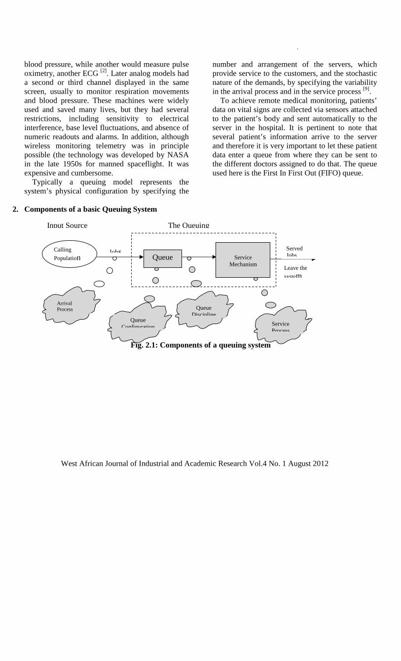
.
West African Journal of Industrial and Academic Research Vol.4 No. 1 August 2012
blood pressure, while another would measure pulse oximetry, another ECG [2]. Later analog models had a second or third channel displayed in the same screen, usually to monitor respiration movements and blood pressure. These machines were widely used and saved many lives, but they had several restrictions, including sensitivity to electrical interference, base level fluctuations, and absence of numeric readouts and alarms. In addition, although wireless monitoring telemetry was in principle possible (the technology was developed by NASA in the late 1950s for manned spaceflight. It was expensive and cumbersome. Typically a queuing model represents the system’s physical configuration by specifying the
number and arrangement of the servers, which provide service to the customers, and the stochastic nature of the demands, by specifying the variability in the arrival process and in the service process [9]. To achieve remote medical monitoring, patients’ data on vital signs are collected via sensors attached to the patient’s body and sent automatically to the server in the hospital. It is pertinent to note that several patient’s information arrive to the server and therefore it is very important to let these patient data enter a queue from where they can be sent to the different doctors assigned to do that. The queue used here is the First In First Out (FIFO) queue.
2. Components of a basic Queuing System
Fig. 2.1: Components of a queuing system
Calling
Population Queue
Service Mechanism
Jobs
Leave the system
Served Jobs
Arrival Process
Service Process
Queue Discipline
Queue Configuration
Input Source The Queuing

.
West African Journal of Industrial and Academic Research Vol.4 No. 1 August 2012
2.2 The Queuing Model for distribution of Patient data
Fig. 2.2: The Queuing Model Architecture
PID 1 Patient ID 1: This can be from Pid 1 to Pid n. SP 1 Specialist 1: This can also be form Sp 1 to Sp n.
Patient
WBAN
12
Bluetooth
IPDA Route
r WiFi
Doctor contacts patient through SMS for advice
PID 1
Hub
Doctor receiving patient’s data
Doctor SP 1
Doctor SP 2
Doctor SP 3
PID 2 PID 3

.
West African Journal of Industrial and Academic Research Vol.4 No. 1 August 2012
Fig. 2.3: Block diagram of the queuing model The M/M/1 queue consists of a server which provides service for the packets of data from the patients who arrive at the system and depart. It is a single-server queuing system with exponential
interarrival times, exponential service times and first-in-first-out queue discipline [4]. If a packet of data from a patient arrives when the server is busy, it joins the queue (the waiting line). There are two
Patient
SP 1
Doctor receiving patient’s data
Hub The Queuing System (FIFO)
SP 3 SP 2
IPDA
Router
Doctor contacts patient through SMS

.
West African Journal of Industrial and Academic Research Vol.4 No. 1 August 2012
types of events: arrival events (A) and departure events (D). The following quantities are used in representing the model:
AT = arrival time DT = departure time
Fig 2.4: M/M/1 Queue
Poisson Arrivals Departure
Server Queue
STA
INITIALIZE VARIABLES
AT<DT
DEPARTURE EVENT ARRIVAL EVENT
COMPUTE MEAN VALUES OF OUTPUT
STOP
STOP
YES
B
YES
NO
NO
D
C A
Fig 2.5: Flowchart of the queue simulation

.
West African Journal of Industrial and Academic Research Vol.4 No. 1 August 2012
Fig. 2.6: The first few events in simulation In the queuing model, vital signs are collected by the sensor on the patients’ body, sent through the Bluetooth (this data is simulated in the IPDA) to the IPDA which transmits this data by WiFi to the router which further transmits the data wirelessly to the hub which is in the server. The hub acts as a data repository where these data are stored and sent to the doctor when there is an abnormal situation. 2.1.2 The Queuing Model Queuing models can be represented using Kendall’s notation. A/B/S/K/N/D [3]. where A is the interarrival time distribution B is the service time distribution
S is the number of servers K is the system capacity N is the calling population D is the service discipline assumed
• The Arrival Rate The data arrive as packets of data from different patients wearing the sensors into the hub. Let Ci be the interarrival time between the arrivals of the (i – 1)th and the ith patients, the mean(or expected) inter-arrival time is denoted by E(C) and is called β; = 1/E(C) the arrival frequency. • Service Mechanism This is specified by the number of servers (denoted by S) each server having its own queue or a common queue and the probability distribution of the patient’s service time [7].
0
Interarrival time
T0
First arrival Next arrival
T1
Simulated time
Scheduled departure time
First departure

.
West African Journal of Industrial and Academic Research Vol.4 No. 1 August 2012
Let Si be the service time of the ith patient, the mean service time of a customer is denoted by E(S)
= the service rate of a server.
• Queue Discipline Discipline of a queuing system means the rule that a server uses to choose the next patient from the queue (if any) when the server completes the service of the current patient [6]. The queue discipline for this system is Single Server- (FIFO) First In First Out i.e. patient’s data are worked on according to when they came to the queue. • Measures of Performance for the Queuing System Let Di be the delay in queue of the ith patient Wi be the waiting time in the system of the ith patient F(t) be the number of patients in queue at time t G(t) be the number of patients in the system at time t = F(t) + No of patients served at t. Then the measures,
D = and
W =
are called the steady state average delay and the steady state average waiting time in the system. Also the measures,
F = and
G =
are called the steady state time average number in queue and the steady state
time average number in the system. • Single Channel Queue [M/M/1] : FCFS or FIFO Queue System
• Arrival Time Distribution This model assumes that the number of arrivals occurring within a given interval of time t, follows a poisson distribution with parameter This
parameter is the average number of arrivals in time t which is also the variance of the distribution. If n denotes the number of arrivals within a time interval t, then the probability function p(n) is given by
P(n) = n = 0,1,2…. (1)
The arrival process is called poisson input The probability of no(zero) arrival in the interval [0,t] is,
Pr (zero arrival in [0,t]) = = p(0) Also P(zero arrival in [0,t]) = P(next arrival occurs after
t) = P(time between two successive arrivals exceeds t) Therefore the probability density function of the inter- arrival times is given by,
for t > 0 This is called the negative exponential distribution with parameter or simply exponential distribution. The mean inter-arrival time and standard deviation of this distribution are both 1/ where, is the arrival time.

.
West African Journal of Industrial and Academic Research Vol.4 No. 1 August 2012
3.0Analysis of the Queuing System The state of the queuing system can be completely described by the number of units in the system. Thus the state of the process can assume values 0,1,2… (0 means none in the queue and the service is idle).
Let the steady state probabilities be denoted by Pn, n = 0,1,2,3,… where n refers to the number in the system. Pn is the probability that there are n units in the system. By considering a very small interval of time h, the transition diagram for this system can be seen as:
Fig. 4.18: The Transition Diagram If h is sufficiently small, no more than one arrival can occur and no more than one service completion can occur in that time. Also the probability of observing a service completion and an arrival time in h is .h2 which is very small (approximately zero) and is neglected. Thus the following four events are possible:
1. There are n units and 1 arrival occurs in h 2. There are n units and 1 service is completed
in h 3. There are n-1 units and 1 arrival occurs in h 4. There are n+1 units and 1 service is
completed in h For n > 1, (because of steady state and condition)
Pr (being in state n and leaving it) = Pr(being in other states and entering state n) = Pr(being in state n-1 or n+1 and entering state n). Thus Pn
(2) This is the steady state balance equation. For n = 0, only events 1 and 4 are possible, Po 1 * Therefore
P1= P0 Pn = Pn-1 Pn =( )n P0 (3)
0 1 n-1 n+1
n 2
βh βh βh βh
βh βh
Ph Ph Ph Ph

.
West African Journal of Industrial and Academic Research Vol.4 No. 1 August 2012
This can be determined by using the fact that the sum of the steady state probabilities must be 1. Therefore,
P0+P1+P2+…+Pn+Pn+1+…= 1
P0 + P0[ + P0[2+…+P0[
n+P0[n+1+ …= 1
P0[1+P + P2 + … + Pn + Pn+1 +…] = 1 P =
This is the sum of a geometric series. Therefore,
P0 = 1 as n
Since P< 1,
P0 = (1 – P) =
The term P = is equal to the probability that the
service is busy, referred to as Pr (busy period). 4.0 Performance Measures The average number of units in the system G can be found from G = sum of [n*Pn] for n = 1 to
G = = where P =
The average number in the queue is F = (G – (1 – P0) Sum of [(n-1)*Pn] for n = 1 to
F = =
The average waiting time in the system (time in the system) can be obtained from
W = = and
D = W - = .
The traffic intensity P (sometimes called occupancy) is defined as the average arrival rate (lambda) divided by the average service rate (mu). P is the probability that the server is busy.
P =
The mean number of customers in the system (N) can be found using the following equation:
You can see from the above equation that as p approaches 1 number of customers would become very large. This can be easily justified intuitively. p will approach 1 when the average arrival rate starts approaching the average service rate. In this situation, the server would always be busy hence leading to a queue build up (large N). Lastly we obtain the total waiting time (including the service time):
T =
In a queuing system with the inter arrival time of 25 seconds and the service time of 10 seconds, the parameters are calculated thus:

.
West African Journal of Industrial and Academic Research Vol.4 No. 1 August 2012
Table 1
Ci E( C ) = 1/Ci
β Si E(S) = 1/Si
µ P = β/ µ N = P/1-P T = 1/( µ - β ) 25 0.04 10 0.1 0.4 0.666667 16.66667 50 0.02 20 0.05 0.4 0.666667 33.33333 75 0.013333 30 0.033333 0.4 0.666667 50 100 0.01 40 0.025 0.4 0.666667 66.66667 125 0.008 50 0.02 0.4 0.666667 83.33333 150 0.006667 60 0.016667 0.4 0.666667 100 175 0.005714 70 0.014286 0.4 0.666667 116.6667 200 0.005 80 0.0125 0.4 0.666667 133.3333 225 0.004444 90 0.011111 0.4 0.666667 150 250 0.004 100 0.01 0.4 0.666667 166.6667
This is illustrated in the line chart and column chart below:
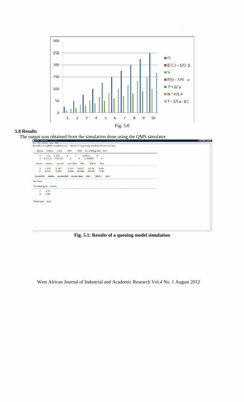
.
West African Journal of Industrial and Academic Research Vol.4 No. 1 August 2012
Fig. 5.0
5.0 Results The output was obtained from the simulation done using the QMS simulator.
Fig. 5.1: Results of a queuing model simulation

.
West African Journal of Industrial and Academic Research Vol.4 No. 1 August 2012
Fig. 5.2: Variance for the queue
Fig. 5.3: Average for the queue

.
West African Journal of Industrial and Academic Research Vol.4 No. 1 August 2012
Fig. 5.4: Max, Min for the queue
Fig. 5.5: Confidence Interval for the queue
6.0 Conclusion
A queuing model has been designed and simulated. The result of the simulation has been shown. It has been established that the packets of data from a patient’s body arrives to the hospital’s server and enter the queue from
where they are kept according to the order in which they arrive and any data with abnormal readings are sent to the doctor for immediate medical intervention.

.
West African Journal of Industrial and Academic Research Vol.4 No. 1 August 2012
References [1] Gao, T. (2005) “Vital Signs Monitoring and Patient Tracking Over a Wireless Network,” IEEE-
EMBS 27th Annual Int. Conference of the Eng. in Medicine and Biology. [2] Jurik, A.D.; Weaver, A.C. (2008). Remote health care monitoring devices Computer 41(4). [3] Kendall, D. (1953). "Stochastic Processes Occurring in the Theory of Queues and their Analysis
By the Method of the Imbedded Markov Chain". Annals of Mathematical Statistics 24 (3). [4] Lee, A., Miller D. (1966). "A Problem of Standards of Service ". Applied Queueing Theory. New
York: MacMillan. [5] Obrenovic, Z., Starcevic, D., Jovanov, E., & Radivojevic, V. (2002). An Agent Based
Framework Medical Devices. Autonomous Agents & Multi-Agent Systems, Bologna, Italy. McGraw Hill Company.
[6] Sen, R.(2010). Operations Research: Algorithms and Applications. Prentice-Hall. [7] Tijms, H.(2003), Algorithmic Analysis of Queues, A First Course in Stochastic Models, Wiley, Chichester,. [8] Varshney U. (2008), “Improving Wireless Health Monitoring Using Incentive-Based Router Cooperation,” Computer, 41(3). [9] Zhou, Y., Gans, N.(1999). A Single-Server Queue with Markov Modulated Service Times".
Financial Institutions Center, Wharton, UPenn. Retrieved from http://fic.wharton.upenn.edu/fic/papers/99/p9940.html. Retrieved 2011-01-11.

.
West African Journal of Industrial and Academic Research Vol.4 No. 1 August 2012
Classification of Implemented Foreign Assisted Projects into Sustainable And Non-sustainable Groups: A Discriminant Analysis Approach
Iwuagwu Carmelius Chibuzo
E-mail [email protected] Tel +2348033306938 Department of Planning, Research and Statistics. Ministry of Education,
Owerri, Nigeria.
Abstract Four variables of factors affecting the sustainability of foreign assisted projects at the end of implementation were extracted from literature review and informal interview of project management professionals. The managers of these projects were asked to rank these variables according to their relevance and importance in enhancing the sustainability and non sustainability of foreign assisted projects in Nigeria. Discriminant function analysis was applied in carrying out detailed analysis of these factors. Two factors were found to be the most discriminating factors among the four factors. The two factors are delivery of service or benefits and long term institutional capacity. The study also further revealed that continued delivery of services or benefits is the most discriminating factor. Key Words: Economic transformation, discriminant analysis, foreign assisted projects, delivery of service, long term institutional capacity 1.0 Introduction Rapid economic transformation in developing countries is often constrained by shortage of capital resources due to poor savings, inadequate foreign exchange earnings and low investment capacities. There is therefore, the tendency for developing countries to use more resources than those available to them. It is this “resource gap” that has given rise to the need for external development assistance from developed world. Nigeria has been a major beneficiary of development assistance in the form of concessionary and non-concessionary loans, outright grants and technical assistance. In Nigeria, most of this assistance comes from UNDP and
UNICEF. These grants are used in financing and implementing some development projects and they are termed foreign assisted projects.
Many of these projects cannot be sustained at the end of their successful implementation and handing over to the beneficiaries. Many of these projects survive for less than two years at the end of implementation and stop functioning.[7] Many reasons like bad implementation method, frequent change in government, inadequate funding, lack of beneficiaries support and other environmental factors have been advanced for this ugly trend[4],[10].

.
West African Journal of Industrial and Academic Research Vol.4 No. 1 August 2012
The study is concerned with building a model which can be used to classify implemented foreign assisted projects into one of two categories sustainable and non-sustainable group. Although the discriminant analysis which is used can be generalized for classification into a number of categories, the present study is limited to two categories. 2.0 Applications The discriminant analysis has been applied in a variety of investigations. These applications vary from parent selection in plant breeding to the classification of application for bank loan into good and bad creditors.[2][9][11][8][5] Discriminant analysis used to discriminate between two expenditures groups using the percentages of total household expenditure going to five major budget items as criterion variables.[14] As shown in the study, giving a household’s percentage expenditure on each of the five categories of commodities – accommodation, food, transport, household goods and clothing it is possible to use the household discriminant score to determine the household’s expenditure class – lower or middle.[14] Many of the standard applications of the techniques are found in the biological sciences, but it is also potentially fruitful in the social sciences. The technique was applied in an attempt to identify underdeveloped countries with good development potential. In their analysis, 73 underdeveloped countries were classified into three groups according to their past economic performance and a linear discriminant function estimated from a number of social, political and economic variable.[1] Once such a function has been estimated the values of these variables for a new
country can be fed into the discriminant function and the country assigned to one of the three groups, for development potential.[1] The discriminant analysis was used to classify household in Ile-ife into higher and “Lower” income brackets. A linear compound of five criterion variables namely, type of dwelling, rent status, availability of possession of selected household goods, size of household and highest educational level was formed.[8] Education level was found to have the highest weight in the discriminant function. This study was found useful where there are difficulties as directly obtaining authentic information on household incomes.[8] Discriminant analysis as a predictive tool for corporate technical failure and bankruptcy, his work provided answer to which ratios are important in detecting corporate financial failure potentials.[3] He utilizes a comprehensive list of financial ratios in assessing a firms failure potential[3]. 3.0. Sources of Data The data were obtained from foreign assisted projects UNDP and UNICEF located in six states representing the six geopolitical zones of Nigeria. The states are Imo, Rivers, Oyo, Borno, Kano and Plateau. The set of data was extracted from Questionnaire administered to the various projects establishments responsible for the day to day maintenance and sustainability of this foreign assisted project when they are handed over to the beneficiaries. Seventy-one (71) implemented foreign assisted projects of UNDP and UNICEF made up of 40 sustainable and 31 non-sustainable were used in the analysis. Four criterion variables were used in classifying implemented foreign assisted projects

.
West African Journal of Industrial and Academic Research Vol.4 No. 1 August 2012
into sustainable and Non-sustainable groups. These criterion variables were:
U1 = Delivery of service or benefits U2 = Political support U3 = Long term institutional capacity U4 = Maintenance of physical infrastructures
4.0. Discriminant Analysis The problem that is addressed with discriminant function analysis is how well it is possible to separate two or more groups of individual given measurements for these individuals on several variables.[6] Two methods of discriminant function analysis namely the Mahalanobis distance (independent variable) and stepwise methods were used. 4.1 Mahalanobis Distance Method Let 1X = 1i 2i pi (X , X ...X ) denote the vector of
mean value for the sample from the its group calculate using the
n
ijj=1
= X /njX ∑
(1)
1X
=
p
X
X
• • •
(2)
Let Ci denote the covariance matrix for the same sample calculated using the sample variance given by
( )2n
2ij j
i=1
= X -X / 1jS n−∑ (3)
In addition, the sample covariance between variable j and k defined as
Cjk = ( )( )1
/ 1n
ij j ik ki
x x X X n=
− − −∑ (4)
This being a measure of the extent to which the two variables are linearly related. The matrix of variance and covariance are given by
11 12 1p
21 22 2p
p1 p2 pp
C C ... C
C C C
C C ... C
C
=
(5)
Let C denote the pooled sample covariance matrix determined using
( ) ( )m
ii=1 1
= n -1 1n
i ii
C C n=
−∑ ∑ (6)
Then the Mahalanobis distance from an observation X’ = (X 1, X2, …Xp) to the centre of group is estimated as
( ) 12 -11 i i = X-X C (X-X ) D
− (7)
or
( ) ( )p
2i
r-1 1
D = p
r rsri s si
s
X X C X X−
− −∑∑ (8)
Where Crs is the element in the rth row and Sth column of C-1. The observation X is allocated to the group for which 2
iD has the smallest value.

.
West African Journal of Industrial and Academic Research Vol.4 No. 1 August 2012
Specifically for this study, a total of three canonical discriminant function were obtained. For the sustainable and non-sustinable implemented foreign assisted projects in Nigeria we have Z = a1U1 + a2U2 + a3U3 + a4U4 (9) And Z1 = a11U1 + a12U2 +a13U3+a14U4 (10) Z2= a21U1+a22U2+a23U3+a24U4 (11) Where Z denote the grouping that is for project sustainability and project non sustainability and Z1 for project sustainability and Z2 for project non-sustainability. The ai and aij – values are the canonical coefficients/variables. Therefore it is possible to determine several linear combinations for separating group.[6] Finding the coefficient of the canonical discriminant functions turns out to be an eign value problem. The within-sample matrix of sum of squares and cross products is calculated using.
( ) ( )n
j=1 1
= in
rc i jr jr ijc jci
W X X X X=
− −∑ ∑ (12)
. And Wrc is the element in the rth row and cth column of W The total sample matrix of sum of squares and cross product T is calculated using
trc= ( ) ( )1 1
jnm
ijr r ijc cj i
X X X X= =
− −∑ ∑
(13) The in between group matrix is given by B = T – W (14)
Which can be determined.
The matrix W-1B is found. If the eigen value are
A1>A2>A3…>Ai the Ai is the ratio of the in between group of sum of squares to the within group of sum of squares for the ith linear combination, Zi, while the element of the corresponding eigenvector ai = (ai1, ai2 – aip) are the coefficient of Zi.
5.2 Stepwise Method In this method, variables are added to the discriminant function one by one until it is found that adding extra variable does not give significant better discrimination. There are many different criteria that can be used for deciding on which variables to include in the analysis and which to miss out.[13] The order in which the repressors are introduced may be determined in several ways, two of the commonest are:
(a) The researcher may specify a prior the order in which he wants the repressor to be introduced
(b) The researcher may want to let the data determine the order.
For this study the WILK’s Lambda criterion was used as the criterion for entering the equation.
The Wilk’s Lambda (λ ) is defined as
= e
T
s
S (15)
where the matrix Se is the error of squares and cross product matrix ST is the within sum of square and cross product. (SSCP) matrix for the r samples.

.
West African Journal of Industrial and Academic Research Vol.4 No. 1 August 2012
Similarly the matrix ST is the total SSCP matrix. This is the matrix of sets of squares and cross products of our entire combined samples regardless of which population give rise to the sample items. As in ANOVA we have the relation
ST = Sλ + Se (16)
Where Sλ is the among SSCP matrix. The SSCP matrix is defined
S =
21 1 2 1 k
22 1 2 2 k
21 k 2
W W . . . W W
W . . . W W
W W . . . W kk
W
W W
W W
∑ ∑ ∑∑ ∑ ∑∑ ∑ ∑
.(17) Major statistical packages generally have a discriminant function for the application of the methods as described in Equation 1-17. The data were analyzed using the SPSS Program Discriminant Version 10. Two methods of selecting discriminating variables are available in this software packages namely, the independent (Mahalanobis) method and stepwise procedures. However analysis here was carried out using step wise procedures. 5.2.1 Evaluation of The Performance Of The
Model The evaluation of the performance of the classification of the discriminant model was based on some statistical criteria, validation and out of sample results. The statistical criteria employed included F-value, Eigen value, Wilk’s Lambda, Chi-square and canonical correlation.[13] The validation (that is in sample or resubstitution) test utilized the same set of sample observation while the out of sample was based on completely
independent set of sample from the ones used in the model estimation.[12]
In each case, we obtained the error rates associated with the model in addition to the overall error rates and overall correct classification rates.
5.3 Cutting Scores
The cutting score is zero. Discriminant scores greater than zero (ie the scores) indicated a predicated membership in the sustainable group. The dependent variable which was continuous scaled took the value zero and 1 for the non-sustainable group and sustainable group respectively.
5.3.1 Relative Discriminatory Power Of The
Variables The magnitude of the discriminant coefficient in the model reveals to some extent the importance of the discriminatory variable. However a major objective procedure of evaluating the contribution of each discriminating variable to the model is based on the relative discriminating power of the coefficient in the canonical discriminant function.[9] The measure of the relative discriminatory power of the variable is given by bi ( X i1- ioX ), the scalar vector i ibσ is used to
measure how the variables are correlated. Here bi = the discriminant function coefficient for the ith variable.
iδ = The square root of appropriate value
in the variance – covariance matrix (standard deviation)
1iX = ith variables mean for the
Successful project
0iX = ith variables mean for t failed project.

.
West African Journal of Industrial and Academic Research Vol.4 No. 1 August 2012
7.0 Model Estimation And Interpretation
The data described above was used to estimate the canonical discriminant function. Thus we used
stepwise procedure and the result of the discriminant analysis is presented in table 1.
(i) Canonical Discriminant function (W) W = -11.259+0.449U1+0.278U3 (18)
Table 1: Sustainable and Non-sustinable Foreign Assisted Projects Eigenvalue Wilkslambda Chi-square Significance F-value Canonical
correlation 9.688 0.094 161.100 0.000 7.520 0.952
(ii) Classification Function coefficients
Variable Sustainable Projects Non-sustainable projects U1 5.348 2.571 U2 5.299 3.581 Constant -102.319 -35.091
(iii) Group Centriods
W Function 0.00 -3.485 1.00 2.701
Based on the summary statistics presented in table 1,we found that only two variables out of four variables considered were adequate for discriminating implemented foreign assisted projects into sustainable and non sustainable categories. The ratio in order of importance based on the magnitude of their coefficients was (a) U1 (b) U3. However a more objective procedure of
evaluating the contributions of each discriminatory variable to the model is based on the relative discriminatory power of the coefficients in the canonical discriminant functions. The relative discriminatory power of the variables of this model is shown in table 2.

.
West African Journal of Industrial and Academic Research Vol.4 No. 1 August 2012
Table 2: Relative discriminatory power of the variables equation (18) W = -11.259+0.449U1+0.278U3
Variable ai iσ i1U i0U ai iσ
1 0( )i ia Ui U− %
U1 0.449 5.244 19.625 9.774 2.354 4.423 71.45% U3 0.278 3.634 18.550 12.194 1.010 1.767 28.55% Total 6.190 100%
Table 2 showed that variable U1 explained about 71.45% of the average discriminant score separation between sustinable and non-sustainable implemented foreign assisted projects while U3 contributed 28.55% in explaining the average discriminant score separation between foreign assisted project sustainability categories. The scalar vector showed that the variables used in constructing the discriminant model exhibit little or no correlation among them. 7.0 Evaluation of The Classification
Ability of The Discriminant Model In table 1, we present the discriminant model denoted as equation (18) with the associated statistics. The eigen value for the model is 9.688 while the Wilk’’s Lambda was 0.94 which is little low and the canonical correlation is 0.952. In order to test the statistical significance of the model (DF), the Wilk’s Lambda was converted into chi-square distribution and the model was found to be significant at 100% level.
The canonical correlation value (CCV) of 0.952 implied a very high degree of association between the discriminant function and the discriminating variables U1 and U3. The results of the validation test based on the original samples for the discriminant model denoted as W are presented in table 3. This table contains actual and predicted discriminant scores sustainable and non sustainable groups of implemented foreign assisted projects. Based on table 3, only one implemented foreign assisted projects was misclassified in the sustainable group. The project is number 12. The out of sample result are presented in table 4. Based on table 4, only three (3) out of eleven (11) implemented foreign assisted projects were wrongly negatively classified as non sustainable projects and one (1) out of seven (7) non-sustainable foreign assisted projects was also wrongly positively classified as sustainable project.

.
West African Journal of Industrial and Academic Research Vol.4 No. 1 August 2012
Table 3: Classification of Implemented Foreign Assisted Projects based on validation sample (41
sustainable vs 30 non-sustainable) Project No Group Discriminant scores 1 1 2.5457 2 1 3.3788 3 1 3.8922 4 1 1.3703 5 1 4.7253 6 1 1.0926 7 1 2.0968 8 1 2.2680 9 1 2.9945 10 1 2.5457 11 1 2.5457 12 1 -0.2539 13 1 1.8191 14 1 0.5371 15 1 4.1699 16 1 0.6437 17 1 3.1656 18 1 4.1699 19 1 2.7168 20 1 2.2680 21 1 3.6145 22 1 1.8191 23 1 2.8234 24 1 2.9945 25 1 2.8234 26 1 3.1656 27 1 3.8922 28 1 2.2680 29 3.4433 30 1 2.7168 31 1 3.4433 32 1 3.8922 33 1 3.3732 34 1 2.2680 35 1 2.7168 36 1 2.2680 37 1 3.4433 38 1 2.7168 39 1 1.9902 40 1 -0.0914

.
West African Journal of Industrial and Academic Research Vol.4 No. 1 August 2012
41 0 3.3958 42 0 -2.2625 43 0 -3.2247 44 0 -3.6735 45 0 -3.7801 46 0 2.6468 47 0 -4.5066 48 0 -3.3313 49 0 -3.3203 50 0 -3.4127 51 0 -3.8867 52 0 -4.3355 53 0 -3.1601 54 0 -3.7801 55 0 -1.9848 56 0 -3.7156 57 0 -3.9933 58 0 -3.5445 59 0 -3.9933 60 0 -3.7156 61 0 -3.9933 62 0 -3.2667 63 0 -3.4379 64 0 -4.8910 65 0 -3.9933 66 0 -4.4421 67 0 -4.4421 68 0 -3.9933 69 0 -4.4421 70 0 -1.6004 71 0 -3.7156

.
West African Journal of Industrial and Academic Research Vol.4 No. 1 August 2012
Table 4: Classification of Foreign Assisted Projects Based on out of sample Data (11 Sustainable Vs 7 unsustainable Projects)
Project No Group Discriminant Scores 1 1 2.383 2 1 3.623 3 1 -.0632** 4 1 2.832 5 1 3.623 6 1 -1.359** 7 1 2.447 8 1 1.827 9 1 -0.354** 10 1 0.202 11 1 2.554 12 0 3.901 13 0 -2.086 14 0 -2.237 15 0 0.651* 16 0 -3.433 17 0 -3.540 18 0 -4.438
Source: Using the Developed model
W = -11.259+0.449U1+0.278U3 **………………wrong classification
In table 5 we present various error and classification efficiency rates associated with the discriminant model equation (18). the validation sample method was extremely accurate in classifying about 98.59% of the total sample correctly. type 1 error proved to be only about 2.5% while type ii error was about 0%. The predictive ability of the model based on the out of sample data showed that type i error associated with the model was 25.99%. This implied that about 25% of the sustainable implemented foreign assisted projects were
wrongly classified as sustainable projects. however the overall classification efficiency of the model based on the out of sample data was high since 77.78% of the implemented foreign assisted projects were correctly classified while only about 22.22% represented the overall error rate. The high overall classification efficiency rate of 98.59% and 77.78% for validation and out of sample procedures suggested that the model may be useful as early warning device for predicting and classifying implemented foreign assisted project into different risk categories

West African Journal of Industrial and Academic Research Vol.4 No. 1 August 2012 1
. Table 5: Classification Result for the Discriminant Model Count Implemented foreign assisted projects Predicted group members
1.00 0.00 Total Out of sample count
Sustainable (1.00) Non-sustainable (0.00) 1.00 0.00 total
9 1 75.00% 83.33% 66.78%
3 5 25.55% 16.67% 22.22%
12 6 100% 100% 100%
(b) Validation count
Sustainable (1.00) Non sustainable (0.00)
39 0 97.50% 100% 98.59%
1 31 2.50% 0% 1.43%
30 31 100% 100% 100%

.
West African Journal of Industrial and Academic Research Vol.4 No. 1 August 2012
8.0 Conclusion and Recommendation In this study, the discriminant function analysis was used to classify implemented foreign assisted projects in Nigeria into “Sustainable” and non-sustainable groups. A linear compound of two variables namely, Delivery of services or benefits and long term institutional capacity was formed for the sustainable and non-sustainable group. They were found to be the most important factors that
discriminate between the sustainable and non-sustainable group. Delivery of services or benefits was found to have the highest weight in the discriminate function. All the coefficients of the variables have the expected sign and the overall discrimininating abilities of the function was found to be quite high as indicated by the various tests of the performance of the model.
8.2 Recommendations Based on the above, the following recommendations are offered on the basis of the research funding. 1. For continued delivery of service which is the most discriminating factor for foreign assisted project sustainability government should provide enough budgetary allocation for the maintenance of facilities that ensured continued delivery of service. Part of this budget should be made available to the benefiting communities to enable them manage these projects located in their place effectively. In the case of water projects, the community leaders should be allowed to sell the water at a reduced rate so as to have money to effect necessary repairs without waiting for the government. However, this should be monitored by the government to avoid abuse by these community leaders.
2. Project sustainability will frequently require an active involvement of local and community organization at all the stages of project planning, implementation and operations. The results of the virtual exclusion of beneficiaries often become apparent during the operational phase when beneficiaries only prove unwilling to pay for services or when they refuse to cooperate in project maintenance. Hence the government should promote beneficiaries participation which will have the positive result of ensuring project sustainability. 3. The role of donor agencies is crucial to project sustainability. They should established long term institutional capacity that ensure sustenance when they handover the project. Long term institutional capacity was found to be a very important discriminating factor of sustainability in this research. They should also offer advisory role from time to time to ensure project sustainability
References [1] Adelman & L. T Morris (1968) “Performance Criteria for Evaluating

.
West African Journal of Industrial and Academic Research Vol.4 No. 1 August 2012
Economi9c Development Potentials – An Operational Approach” Quart J. Economics, 82 p. 268-280.
[2] Aja Nwachukwu (2001) “A Discriminant Analysis of Commercial Banks Failure: The Case Study of Nigeria” Journal of Business & Finance – Imo State Vol. No. 4 2001 pp 26-35.
[3] Altman – E. (1968) “Financial Ratios Discriminant Analysis and the Prediction of Corporate Bankruptcy” The Journal of Finance Vol. 23, September.
[4] Cleland D.I. and Kerzner, H. (1985) A Project Management Dictionary of Terms, Van Nostrand Reinhold, New York.
[5] Deakin E. (1972): “A Discriminant Analysis of Predictor of Corporate Failure” Journals of Accounting Research Vol. 10 Spring.
[6] Hope Keith (1968) Method of Multivariate Analysis, University of London. [7] Iwuagwu C.C. (1994): “The Evaluation of the Effect of the Ten Critical
Success Factors on the Performance of ADP Projects”, Owerri, Unpublished M.Sc. Thesis, FUTO Nigeria.
[8] Iyaniwuru J.O. (1984) “Discriminant Analysis as a Technique for a Dichotomous Classification of Urban Income Earners in Ile Ife Nigeria” Journal of the Nigerian Statistical Association Vol. 2 No.1, 1984 Pp. 17-26
[9] Joy M.O. and Tollefson J.O. (1997) “On the Financial Application of Discriminant Analysis” Journal of Financial & Quantitative Analysis (December). Pp 723-739.
[10] Kayoed, M.O. (1978) The Art of Project Evaluation Ibadan University Press, Ibadan. [11] Keleck, W.R. (1980) Discriminant Analysis Services Quantitative
Application in the Social Sciences. No 19 Suga University Paper. [12] Laucherbanch P.A. (1967) “An Almost Unbiased Method of Obtaining
Confidence intervals for the Probability of Misclassification in Discrimination Analysis” Biometrics (December) pp. 639-645.
[13] Lewis, Beek (1980): Applied Regression: An Introduction to Quantitative Application in the Social Sciences 22 Beverly Calif; Saga.
[14] Olayemi, J.K. & Olayide, S.O. (1977) “Expenditure Pattern in Selected Area of Western Nigeria: A Discriminant Analysis” Journals of Statistical Research Vol. 11 1977.

.
West African Journal of Industrial and Academic Research Vol.4 No. 1 August 2012
A Study on the Evaluation of Industrial Solid Waste Management Approaches in Some Industries in Aba, South Eastern Nigeria
Ajero, C.M.U and Chigbo,U.N
Department of Environmental Biology Imo State University, Owerri Imo State Nigeria. [email protected]
Abstract Industrial solid waste is a serious health concern in Aba, South East Nigeria. This study was undertaken to assess the approaches of some industries toward some aspects of waste management in Aba. Interviews, observation and questionnaires administered to industry executives and waste managers were used to generate data for the study. The result from the field research showed that majority(47.39%) of the solid wastes stream were compostable while far less (4.69-9.90%) recyclable waste were generated. The result revealed that open ground was the most prominent storage facility used and only 42.50% of the industries undertake some form of treatment of waste before storage. The industries studied employ more than one method of waste disposal and it was mostly carried out with open trunk and wheel barrows. Waste contractors were engaged by 52.50% of the industries and wastes were equally deposited in dump sites (45.00%), rivers (12.50%), composited (20.00%)or incinerated(25.00%). There was inadequate provision of protective measure in most of the industry. The respondents acknowledged enjoying medical check which was however not regular and in some cases in poorly equipped health centers and drug stores. The awareness of respondents on the consequences of improper waste management was high (75.50%) while the level of attendance of health and safety treatment training was average (46.25%), however, none of the industries had health policy plan. It is recommended for the improvement of the function of the waste management regulatory body, Abia State Environmental Protection Agency(ASEPA) and commitment of the industries and the general public toward industrial solid waste management. Key words: Solid waste, Industries, Management processes, Aba, Nigeria _____________________________________________________________________________ 1.0 Introduction
In industrial production, many materials are employed to manufacture products and because of the scale of the production, a lot of waste is generally produced. The component categories
usually include: compostable (includes food, yard, and wood wastes); Paper; Plastic; Glass; Metal; and other (includes ceramics, textiles, leather, rubber, bones, inerts, ashes, coconut husks, bulky wastes, household goods).[1][2][3]

.
West African Journal of Industrial and Academic Research Vol.4 No. 1 August 2012
The improper management of solid waste poses health hazards to the residents causing diseases such as bronchitis and cancer.[4] High level of industrial discharge has effect of upsetting the ecological balance of nature. The microbial degradation of waste in water bodies lead to depletion of oxygen and fishes and other aquatic organisms which require oxygen for survival are thus affected.[5] In the extreme cases there is dislocation of socio-economic system of an area. As a result of the size of the problem, industrial companies employ waste managers to focus solely on the issue of proper and effective disposal of waste. Industrial waste management involves collection, transport, processing or disposal, management and monitoring of industrial waste material. Management of non –hazardous, residential and institutional waste in Nigeria is usually the responsibility of local/state government authorities while management of hazardous commercial and industrial waste is usually the responsibility of the generator.[ 6][7,][8]
The problems relating to management of industrial solid waste is associated with lack of infrastructural facilities and negligence of industries and environmental regulatory body to take proper control..[9] Most major cities in Africa have an established municipal waste collection system. Collection is carried out by human- and animal-drawn carts (wheelbarrows, pushcarts), open-back trucks, compactor trucks, and trailers. Collection rates across the continent range from 20 to 80%. Common feature of the municipalities is that they are ineffective, underequipped and poorly maintained (often vehicle immobilization rates reach as high as 70%), inadequately funded and poorly staffed.[3] The large industries (industries
with huge infrastructure, high man-power requirement and influx of capital asset) located in identified industrial areas respond to industrial compulsion as imposed by the pollution control laws by having some arrangement to dispose their solid waste. However, the problems persist with small industries. They find it easy to dispose waste here and there, thereby mixing industrial, residential and commercial waste and making it difficult for local bodies to collect such waste though it is not their responsibility.[11] The situation is disturbing since it is estimated that small scale units put together generate as much waste as the large industries [9] overwhelming majority of landfills in Africa are open dumps..[3] These facilities are generally located at the perimeter of major urban centers in open lots, wetland areas, or next to surface water sources. Though many municipalities have statutory requirements for the construction and maintenance of landfills these are generally not enforced. In most instances the landfills are owned and operated by the same public agency that is charged with enforcing the standards. Often a lack of financial and human resources, coupled with absent enabling policies, limit the extent to which landfills can be built, operated, and maintained at minimum standards for sanitary practice. There is no significant waste recovery and reuse activities in Nigerian cities. In most cases, scavenging plays an important role on the economic survival of a number of industries (e.g., steel, pulp and paper).
[2] Waste pickers work on dumps and even landfills, while some build squatter colonies on the edges of dumps, sometimes with disastrous consequences. Waste pickers are involved in a small-scale recovery and reuse operation.

.
West African Journal of Industrial and Academic Research Vol.4 No. 1 August 2012
The assessment of industrial waste management problems greatly varies depending on the nature of industry, their location and mode of disposal of waste.[12] Sound waste management cycle helps in reducing the adverse impacts on the human health and environment, while enhancing the lifestyle and developing the economic state of the country. In order to offer an appropriate solution for better management of industrial solid waste in industrial town like Aba in South- East of Nigeria, assessment of the approaches of industrial waste management is essential. This study aims to evaluate some industrial waste management approaches of some industries in Aba. 2.0 Study Area The study was carried out in Aba in Abia State of Nigeria. Aba is located at longitude 7°19¹E and latitude 5°10¹N. It has a population of 839,000 and accounting for four of the seventeen Local Government Areas in Abia State.[13]
Aba known as ‘Japan of Africa’ is the commercial and industrial center South East of Nigeria, situated at the bank of river Aba. There are many large and scale industries and four major markets. The solid waste management is carried out by private establishments and Abia State Environmental Agency. The landfill is situated at the outskirts of the town; however there are numerous dump sites. Most roads are filled with
refuse which leads to flooding especially during the rainy seasons. The waste provides breeding ground for vectors of human diseases and source of unpleasant odour. There are many private and government owned hospital and healthy centers. There is very ineffective public pipe borne water supply system. 3.0 Methodology The researcher adopted several instruments in data collection for this study in 2009. Planned questionnaires (including questions on nature of waste, storage of waste, collection, and method of disposal, treatment and waste manager’s welfare) were administered to waste managers, personnel and managers of industries. Furthermore additional data and information were collection from direct observation, interview with responsible persons. Secondary data were obtained from literature on the subject. A total of 192 respondents were sampled from twenty five small scale and fifteen large scale industries made up of 8(20,00%) extracting,9(22.50%) hospitality, 15(37,50%) manufacturing 4(10.00%) construction and 4 processing industries. Ethical considerations such as informed consent and confidentiality of personal information in the interview were observed. The percentage volume of the waste generated by the companies is shown in Table 1.

.
West African Journal of Industrial and Academic Research Vol.4 No. 1 August 2012
Table 1: Types of the solid waste generated Type of waste Volume(%) Plastics 12(6.25) Papers 19(9.90) Glass 9(4.69 ) Aluminum scraps 19(9.90) Metal scraps 20(10.41) Compostable(eg.food and wood) 91(47.39) Water sachets and cellophane packages 22(11.45 )
Wastes that can be readily composited had the highest volume of 47.39% while 4.69% was recorded for glass. Other percentage volume encountered were metal scraps 10.41%,paper and
aluminum 9.90%,cellophone containers 11.45% and plastic 6.25%. The response on the storage facilities used by the industries is shown in Table 2.
Table 2: Types of storage
Types of storage Small scale Large scale Total Industry industry N=40 N=25 (%) N=15 (%) (%) Uncovered drum 6(24.00) 3(20.00) 9(22.50) Open ground 14(56.00) 8(53.33) 22(55.00) Concrete bays 0(0.0) 0(0.00) 0(0.00) Pilled against a wall 2(8.00) 1(6.66) 3(7.50) Covered bin 3(12.00) 3(20.00) 6(15.00)
Open ground was the most prominent(55.00%) storage facility used by the industries followed by uncovered drums(22.50%).The result revealed that higher percentage of small scale industries employed both facilities. None of the industries stored their refuse in concrete bays. Covered bin
and pilling against a wall accounted for 7.50% and 15.00% of the storage facilities used.
The result of interview and questionnaires on the preliminary treatment of waste before disposal by the industries is illustrated in Table 3.
Table 3: Preliminary treatment of waste before disposal Questions Types of industry Total Small scale(%) Large scale(%) (%) Any waste treatment No Yes No Yes No Yes 18(72.00) 7(28.00) 5(33.33) 10(66.66) 23(57.50) 17(42.50) Types of treatment N=7 N=10 N=17 Segregation 7(100) 10(100) 17(100) Recycle/Reuse 2(28.57) 3(30.00) 5(29.410

.
West African Journal of Industrial and Academic Research Vol.4 No. 1 August 2012
The result revealed that 42.50% of the industries undertake some form of treatment with 28.00% of large and 66.66% of small scale industries involved. All the industries that reported treatment
of waste carry out segregation while only 29.41% recycle or reuse their waste. The methods of disposal of waste by the industries sampled are displaced in Table 4.
Table 4: Method of disposal of waste
Disposal method Types of industry Small scale Large scale Total N=25 (%) N=15 (%) N=40(%) Waste collection contractor 11(44.00) 10(66.00) 21(52.50) Deposited at waste dump 8(32.00) 5(33.33) 18(45.00) Solid to other industries 2(8.00) 6(40.00) 8(20.00) Deposited in the river 5(20.00) 0(0.00) 5(12.50) Compositing 5(20.00) 3(20.00) 8(20.00) Incinerating 8(32.00) 2(13.33) 10(25.00)
The industries studied employ more than one method for waste disposal(Table 4). Twenty one (52.50%) of the industries(10 large scale(66.00%) and 11(44.00%) small scale) employ contractors for waste disposal. Eight(32.50%) industries deposite their waste at the municipal dump while 20.00% of
the industries either sale or composite their industrial waste. Only 5(12.50%) small industries deposite their waste in river while 10(25.00%) carry out on-site incineration in make-shift incinerators
Table 5: Preventive measures available to waste managers
Number of respondents Measures Small scale N=110(%) Large scale N=82(%)
Total N=192(%)
Handkerchief 80(72.72) 17(20.73) 97(50.52) Respirator 0(0.00) 10(12.19) 10(5.20) Nose guard 30(27.27) 65(79.26) 95(49.47) Overall clothing 12(10.90) 55(67.07) 67(34.89) Jungle boot 17(15.45) 63(76.82) 80(41.66) Hand gloves 23(20.90) 74(91.24) 97(50.52)

.
West African Journal of Industrial and Academic Research Vol.4 No. 1 August 2012
Table 5 shows the preventive measures available to waste managers. From the result, 97(50.52%)of the respondents acknowledge the use of hand kerchief and handgloves.Jungle boot and nose guard were provided to 41.66% and 49.47% of the respondents respectively, while only 34.89% of the respondents had overall clothing. Incidentally, only 10(5.20%) of the respondents from large scale
industries acknowledge the use of respirator. Generally, large scale industries performed better in the provision of preventive measures except in the provision of unconventional handkerchief (72.72%) by small scale industries. The respondents’ response on prophylative measures available in the industries in shown in Table 6
Table 6: Prophylative measures available to waste managers
Variable Number of respondents Total Small scale Large scale N=110 N=82
Regular medical checkup Once a week Once a month Once a quarter Occasionally Not at all
O(0.00) 0(0.00) 0(0.00) 0(0.00) 17(20.73) 17(8.85) 14(12.72) 35(42.68) 49(25.52) 25(22.72) 21(25.60) 46(23.95) 41(37.27) 6(7.31) 47(24.47) 30(27.27) 3(3.65) 33(17.18)
Percentage in parenthesis None of the waste managers had regular medical checkup while 17(8.85%) from large scale industries had weekly check up(Table 6). Forty six(23.95%) and 49(25.52%) had quarterly and monthly medical check up respectively. Respondents who reported occasionally check were 47(24.47%) of which respondents from small scale industries accounted for
87.23%(41/47).Unfortunately,33(17.18%) of the respondents of which majority, 90.90%(30/33) are from small scale industries have not had any formal medical check up. The table 7 refers to the response of respondents on the availability of referral for medical check up to waste managers.
Table 7: Response on referral available by the industries to the waste managers
Variable Frequency(%) Small scale Large scale Total N=80 N=79 N=159 Company clinic 7(8.75) 53(67.08) 60(37.73) General hospital 18(22.50) 18(22.78) 36(22.64) Health center 8(10.00) 8(10.12) 16(10.06) Near by drug store 6(7.50) 0(0.00) 6(3.77) Not available 41(51.25) 0(0.00) 41(25.78)

.
West African Journal of Industrial and Academic Research Vol.4 No. 1 August 2012
Sixty (37.73%) of the respondents were referred to company clinic of which 89.33%(53/60) are workers of large scale industries. The result showed that 22.64% respondents attended government general hospital while 10.06% attended of the health centers .Only 6(7.50%) of respondents and
from small scale industries workers were referred to drug stores .Similarly, 41(25.78%) who reported no referral to health facility were worker from small scale industries. Table 8: Response on the awareness of health consequences of industrial solid waste and attendance of waste and attendance of health/safety training on waste management
Table 8
Variable Number of respondents from the industries Total Small scale N=110 Large scale N=82 N=192 Awareness of health 71(64.54) 73(89.02) 144(75.00) Consequences of waste Attendance of health 30(27.27) 59(71.95) 89(46.35) And safety training Health policy 0(0.00) 0(0.00) 0(0.00)
Percent in parenthesis The result illustrated in table 8 shows that 75% of the respondents were aware of the health impact of improper waste management, however only 46.35% of the respondents had attended health and safety training on waste management. Unfortunately, only 27.27% of worker from small scale industries had opportunity for the training. Discussion The industrialization of Aba has assisted in building self reliant population and also in uplifting of Nigerian economy. However, the huge waste generated has caused serious problems relating to environmental pollution. The problems relating to the disposal of industrial solid waste are associated with lack of infrastructural facilities, negligence of
industries and lack of commitment to take proper safeguards. The Abia State Environmental Protection Agency has not been able to enforce the legal provision and make industries legally responsible for safety of all concerned. The component category of the waste is semilar to other reports from several authors in different cities.[1][10][11][14][15] The result shows that compostables recorded the highest volume of 45.75%. The high organic content suggests possible value as composting material. Composting is mainly practiced by the hotels and eateries. This process converts waste to manue for agricultural purposes. However, the benefits are mostly not achieved as segregation is mostly not practiced to remove the non-degradable materials thereby producing low quality compose

.
West African Journal of Industrial and Academic Research Vol.4 No. 1 August 2012
.As a result, the viability of this scheme is hampered by poor demand of the end markets for their products. The waste stream indicates limited potential commercial value for the recovery of metals, glass, and plastic. This limitation does not deter the uncoordinated and unhygienic scavenging of waste in Aba. The analysis of the type of storage for industrial waste showed that little attention was paid to proper storage as the wastes were mostly exposed in uncovered container. The result in the study is similar to the observations of other authors.[6][16][17][18][19] The hazardous and non-hazardous waste are mixed and are expected to produce health problems among the workers and handlers of waste and the general population.[4]. The waste storage sites constitute foci for vectors of diseases, source of our pollution and possibly avenue for poisonous leacheates to contaminate underground water.[21][22]. Equally, the unrestricted access to dumpsites by unauthorized persons pose health risk. [23][24] Unfortunately, the hygienic covered bins were used by only 15% of the Industries. This trend was observed in the large and small scale industries revealing an institutionalized disregard for the regulation on the use of covered containers for waste storage. Preliminary treatment of waste is necessary in reducing the volume of hazardous waste and the key to achieving sound industrial waste management thereby encouraging source recovery, possible reuse and health risk reduction. [27] The 57.5% prevalence recorded in this study among industries without any form of pretreatment is noteworthy, with 66.6% of them being large scale as against only 16.0% small scale industries. It is estimated that scale units put together generate as
much waste as large units [9] as most of the small scale industries do not reduce their waste thereby contributing enormously to the waste problem. Investigations revealed that the recycling plants engaged by 5% of the industries were purely for paper recycling only. This limitation means that the small recyclable waste is not recovered and the concept of waste to health is completely neglected. In Aba, the approach is to dispose waste as cheaply as possible, without much concern as to what happens once the waste leaves the production premises. The industries surveyed in this study employ more than one means for disposal of waste. The waste collection contractors used by 5% of the industries are in most cases engaged with disregard to their capability. The wastes are manually handled. There are few mechanical aids for waste management. Stored waste is shoveled by hand into open trucks or lorries encouraging fly-tipping and often waste are taken to disposal sites impropriate for the type of waste concerned. These unhygienic practices are common in other cities in Nigeria.[23] [6][11][8] The reasons attributed to these include financial limitations, corruption and illiteracy. The result revealed that in 32.5% of the industries, industrial solid waste are intermingled with domestic waste making it difficult for waste disposal agency to manage. The health implication of this practice is magnified by the fact that non-hazardous waste assumes toxic nature once mixed with hazardous materials. [23][24] Five (20%) of small scale industries acknowledged deposition of waste in the river side thereby causing pollution and ecological disruption.[5][25] Fortunately, the large scale industries which naturally produce most of the hazardous waste do not deposite their solid waste in

.
West African Journal of Industrial and Academic Research Vol.4 No. 1 August 2012
the river. The small scale industries may have been lacking in action to dispose off it’s waste and upload it’s statutory responsibility due to lack of education, awareness and trained personnel to manage the waste in the industries, as well as paucity of fund available to create a proper waste management system. It is a common knowledge that in Aba, small scale industries do not seek the consent of the regulatory body, Abia State Environmental Protection Agency on waste disposal and equally their un-wholesome activities are ignored to the detriment of the inhabitants. It was clear from the survey and interviews that it is likely that the volume of solid waste will steadily increase as the owners are not accountable to higher authorities nor are the workers adequately informed. The results of this study are similar to those of other studies conducted in other countries.[26]. The government should monitor these industries so that they can be responsible with their waste management. In the ten industries that carry out incineration, the process is carried out in make-shift on site incinerators operating at temperature below 800oC, consequently inhabitants that live near the industries are exposed to dioxin, and furan or other toxic pollutants. [27]. The result further revealed that the industrial waste mangers use several protective measures. The large scale industries faired better with 10 (12.1%) of the respondents acknowledging to have used recommended air respirator. However, the use of handkerchief in the light of availability of hygienic and cheap nose guard is embarrassing. The companies’ executives need to be educated on the benefits of adequate protective measures for their workers. The improvement of the workers welfare will have
direct and positive relationship with their productivity. Medically, it is advised that waste mangers or handlers subject themselves to prophylactic measures to amenoriate unnecessary health problems [28]. Even though most of the respondents in this study acknowledged undertaking some form of prophylactic measures, none had regular medical check-up and as much as 17.1% mostly from small scale industries have not had any form of medical check. Respondents from large scale industries (37.7%) are mostly referred to the company clinic while the less financially buoyant small scale industries refer a sizeable (22.5%) number of their workers to the government general hospitals. Fortunately, the medical bills are settled partially or in full by the companies depending on the amount. The high percentage of referal available may be a reflection of 75% awareness of health consequences of industrial solid waste. On the frequency of attendance of health and safety training programme, respondents from large scale (71.1%) were better exposed to contemporary health and safety regulations and guideline even though the industries have no health policy plan. Conclusion The results from the present study have indicated that waste management from the industries studied is inadequate. The situation is worst among small scale industries. Companies need to be responsible for their industrial waste management. The small and large scale industries should be required to seek authorization from Abia State Environmental Protection agency under relevant rules; equally the agency should be committed in enforcing the

.
West African Journal of Industrial and Academic Research Vol.4 No. 1 August 2012
relevant rules. Towards this, law should be promulgated to tax the industries. The tax will help offset the environmental damage by going towards environmental restoration, protection and spreading information to increase knowledge on these issues. It is possible that through the efforts of ASEPA and industries, a mechanism could be evolved for better management. The industries should be made to undertake the detailed risk assessment of the waste. A policy should be formulated based on reduce, reuse, recover and dispose by the industries. Companies are expected to improve their waste and environmental performance and efficiency on a regular basis. Segregation should be done at the point of waste generation and can be achieved through proper training, cleaning standard and tough enforcement. Industrial waste should be collected and transported in safe containers. The open dump site should be closed and municipal should work in conjunction with the industrial sector towards development of specific sanitary landfill for the treatment and disposal of waste. Facility should be installed to
extract gas which can be burnt to generate the needed electricity in Aba. Personnel handling wastes of the industries should be made to wear appropriate protective clothing. Mechanical methods for handling waste should be adopted where possible and people should be educated about the dangers of manual handling of hazardous waste. Recycling plants as in developed countries should be built to convert some of the waste to useable materials and become a source of employment and income to the industries and the society [29]. The uncontrolled incineration should be discouraged, rather hygienic and well structured incinerators should be established outside the city to take care of the combustibles. Generally the government should promote environmental management system in all industries through awareness programmes training and demonstration projects which should cover all stakeholders concerned. There should proper budget allocation for waste management activities and most importantly industries should be encouraged to employ professionals.
________________________________________________________________________________
References
[1] PDE, (1994). Project in Development and the Environment. Comparing Environmental Health Risks in Cairo, Vol. 2. [2] Olanrewaju, A.O., (2000). Refuse: Tinubu’s Victory. P.M. News (Lagos), March [3] Palczynski ,R. J(2002) Study on Solid Waste Management Options for Poverty
Africa.Project report African Development Bank Sustainable Development & Reduction Unit [4] Adekoya, N and Bishop C (1992). Failure of environmental health programme in Nigeria: A

.
West African Journal of Industrial and Academic Research Vol.4 No. 1 August 2012
concern for health planners in developing nation. International Journal of Environmental Health Research 2: 167-170.
[5] Ajero,C.M.U. and Ukaga,C.N. (2006). Development, Global Change and Public Health. Mwgasoft Owerri [6]Ayotamuno, M.J., Godo, A.E. (2000). Municipal solid waste management in Port Harcourt,
Nigeria, obstacles and prospects. Management of environmental quality. African International Journal 15(4):389-398
[7] Kalu, C, Modugu, W.W. and Ubochi, I. (2009). Evaluation of solid waste management policy in Benin Metropolis, Edo State Nigeria. African Scientist 10 (1) 1595. [8] Oyeniyi, B.A. (2011) Waste Management in Contemporary Nigeria. The Abuja Example. International Journal of Politics and Good Governance 2 (2.2) Quarter 11 2011. [9] Assessment on industrial waste management and it’s impact on environment
http://www.wisegcek.com what is-industrial- waste management. htm) retrived 12/2/2012 [10] Afon, A (2007). Analysis of solid waste generation in a traditional African city: the example of
Ogbomoso, Nigeria. http//eau.Sagepub.com/coutent/19/2/527.refs.html.Retrived 18/1/2012. [11 ]Nabegu, A.B. (2010). Analysis of Municipal Solid Waste in Kano, Metropolis, Nigeria. Journal of Human Ecology 31 (2): 111-119 [12] Federal Environmental Protection Agency(1991).Guidelines and Standard for Industrial Effluents,Gaseous emission and Harzardous waste Management in nigeria. [13] NPC (1992). National Population Commision, Surulere Lagos Nigeria. [14] JICA (1998). The Study on Solid Waste Management in Nairobi City in The Republic of Kenya. JICA Final Report, Nairobi City Council, August [15] Diaz, L.(1999). An Overview of Solid Waste Management in Economically Developing Countries.A Regional Conference on Integrated Solid Waste Management. CapeTown, South Africa, October 25. [16] Odochu,J.N.K.(1994) Waste Generation and Management in a Depressed Economy. 2nd Edition, Geirge G.London [17] United Nations Environmental Programme, UNEP (1991) Technical Report Series No. 7.
Audit and Reduction Manual for industrial Emissions and Wastes UNEP, Nairobi, Kenya. Pp.26-32.
[18] United Nations environmental Programmers, UNEP (1995) Technical Support document on residential and industrial (solid) waste disposal. UNEP, Nairobi ,Kenya [19] Zurbrugg,C (1999).The chanllenge of solid waste disposal in developing countries, SANDEC
NEWS EAWAG No 4,1999. [20] Cunningham, W.P., Cunningham,M.A. and Saigo, B.W.,(2003). Environmental Science: A global concern. Mc-Graw Hill Book Companies, America.7th edition . [21] Longe, C.O. Kehinde, M.O (2005). Investigation of Potential Groundwater Impacts on an

.
West African Journal of Industrial and Academic Research Vol.4 No. 1 August 2012
unlined Waste disposal site in Agege, Lagos, Nigeria. Proc. 3rd Faculty of Engineering International Conference. University of Lagos Nigeria
[22] Hoornweg, B, Arnold, K and Smith, H (1999). Landfill gases as pollutant. A preliminary report from Mamilla MAB Technical Paper No 14 Paris UNESCO.
[23] Agunwamba,J.C.(1998).Solid waste management in Nigeria-Problems and issues. Environmental Management 22(6):849-856 [24] Agunwamba, J.C (2003). Analysis of scavengers’ activities and recycling in some cities of Nigeria. Environmental Management 32 (1): 116-127 [25] NCC(2000). African Development Bank, Solid Waste Management Questionnaire, Nairobi City Council. Nairobi, Kenya. [26] B a k u A (2010) . Working environment in some establishments in the UAE rural areas .International Journal of Academic Research Vol. 2. No. 6. Part I [27] Ec (1998). Proposal for a Council Directive on the Incineration of waste. Brussels 07.10.1998 Com(1999) 558 final.98/0289 (SYN). [28] Banjo A.D, Adebanibo, A.A.R and Dairo, O.S. (2011). Perception and operational habit of the
waste managers of domestic waste disposed in Ijebu ode, South East Nigeria. African journal of Basic and Applied Science 3 (4): 131-135
[29] Dhussa, A.K and Varshney, A.K (2000). Energy Recovery from Municipal Solid Waste- Potential and possibility. Bioenergy News, UNDP, 4 (1): 18-21

.
West African Journal of Industrial and Academic Research Vol.4 No. 1 August 2012
Deploying Electronic Roadside Vehicle Identification Technology to Intercept Small
Arms and Ammunition on Nigeria Roads
Akaenyi, I.W+, Osuagwu O.E.*
+Computer Education Department, Federal College Of Education (Tech.) Umunze, Anambra State. [email protected] +2347032022241
*Department of Information Mgt. Technology, Federal University of Technology, Owerri. [email protected] +23480371017932
Abstract The challenge of insecurity of life and property in Nigeria has assumed a frightening dimension. The security situation keeps degenerating daily in spite of government’s acclaimed effort to contain the situation. This implies that Nigeria of today has a complex security management challenges to handle in order to liberate her citizens from the bondage of insecurity of lives and property, ranging from kidnapping, armed robbery, militancy, suicide bombing, ritual murders and human parts selling. The arms being used in perpetuating some of these criminal acts are conveyed by the criminals using our roads. These security lapses are still possible in spite of huge security personnel presence on Nigeria road checkpoints. This implies that the present system of “ stop and search” operation is defective and inefficient to handle current security dynamics. To ensure effectiveness of roadside policing, there is need to carry out this “stop and search” operation using electronic security system. The objective of this paper, therefore, is to present a model archetype that would be capable of sweeping through commercial and private vehicles on the move automatically using Wireless Sensor Networks, Vehicular Ad Hoc Networks (VANETS), OCR, transponders linking all sensitive security observatories to a central data base for verifications, security alerts to the security agencies for prompt action and national security control. The paper presents a data base network and communications architecture from a roadside observatory through to the computer control room and then security personnel on duty. The present practice of stop and search fails to capture most vehicles conveying sensitive and dangerous security exhibits such as chemical, small and light arms. Moreover the present system is cumbersome, stressful, time consuming thus reducing the desired reliability, accuracy of roadside policing. Key Words: small arms and ammunitions, transponder, scanners. Sensors. RFID ______________________________________________________________________________

.
West African Journal of Industrial and Academic Research Vol.4 No. 1 August 2012
Introduction Security is the degree of protection against danger, damage, loss and criminal activities. It is the state of being free from danger. It is the measure taken as a precaution against theft, espionage or sabotage [1]. In other words, security must take into account the actions of people attempting to cause destruction. Security as a form of protection is a structure and processes that provide or improve security as a condition. It involves freedom from risk, or danger, doubt, anxiety or fear. More so, security provides safety and confidence in the people of any nation as well as foreigners. However, perception of security by criminals will deter malicious behaviour especially with visual signs of security protections such as video surveillance, alarm systems, closed circuit television (CCTV) and other automated Roadside Vehicle monitoring. This is physical security that describes measures that prevent or deter criminal attackers from accessing a facility illegally. These monitoring technologies assist in fortifying national security. However, it is very important to be secured and so all security policies must be enforced by mechanisms that are strong enough with sense of commitment. There are organized methodologies and risk assessment strategies to assure completeness of security policies and ensuring that they are completely enforced. Hence, security enforcement is very vital for the economic development of any nation like Nigeria. It is when this is assured that humans and goods can be easily transported from one location to another. To have effective security in the nation, there is need to check physically the content of any vehicle on transit. The present “stop and search” operation
done manually to track arms and ammunition on Nigeria roads has not achieved the desired security objective. It is then necessary to use electronic means to do actualize this goal. This will help in tracking down small arms and ammunition being conveyed by vehicle since road is the major means of transportation in Nigeria. Arms Small arms is a term used by arms forces to denote infantry weapon an individual soldier may carry [2]. The description is usually limited to revolvers, pistols, sub-machine guns, carbines assault rifles, rifles, sniper rifles, squad automatic weapons, high machine guns, and sometimes hand grenades. Short guns, general purpose machine guns, medium machine guns, and grenade launchers may be considered small arms or as support weapons, depending on the branch of the armed forces. Small arms typically do not include infantry support weapons. In the U.S military, small arms refer to hand guns or other firearms less than 20mm in caliber, and including machine guns [3]. The North Atlantic Treaty Organization (NATO) definition in [4], extends to “all crew-portable direct fire weapons of a caliber less than 50mm and will include a secondary capability to defeat light armour and helicopters”. Though there is no civilian definition of small arms, but the term encompasses both small arms and light weapons. Ammunition Ammunition is a generic term derived from the French Language La munitions which embraced all material used for war, but which in time came to refer specifically to gun powder and artillery. The collective term for all types of ammunition is

.
West African Journal of Industrial and Academic Research Vol.4 No. 1 August 2012
munitions [5]. In the widest sense of the word it covers anything that can be used in combat that includes bombs, missiles, warheads and mines. The purpose of ammunition is predominantly to project force against a selected target. However, since the design of the cartridge, the meaning has been transferred to the assembly of a projectile and its propellant in a single package. Current Security Scenario in Nigeria For some time now, the issue of insecurity of life and property in Nigeria has assumed a frightening dimension. The security situation keeps degenerating day by day and getting sophisticated with every Sunday bombing. This implies that Nigeria of today has a complex security management challenge to handle in order to liberate her citizens and foreigners alike from the bondage of insecurity of lives and property, ranging from kidnapping, religious disturbances, political gangsters, armed robbery, militancy, suicide bombing, arms proliferation and movement. Nigeria is a developing democratic country in West Africa and the most populous black nation in the world. It has the largest population on the continent of Africa. The population is estimated at 149 million people. However, the country has experienced a number of crimes, political, religious and cultural instabilities. This usually involves violence, destruction of properties and human life using arms and ammunition. One tends to wonder how these weapons of mass destruction reach the civilians in the village that enable them to use it at the slightest provocation. This demonstates that the security situation of this great country is in poor management state and therefore requires retooling.
Radio Nigeria reported on Wednesday, 18th August, 2010 [6] in its seven o’clock network news in the morning, that fire arms were discovered in a 504 Peugeot saloon car, traveling from Maiduguri to Kaduna and that these fire arms were neatly parked beneath the car’s seats. This was discovered at a police checkpoint. It is only a case out of many cars having such arms passing through the checkpoints in Nigeria undetected. It further highlights that most of such arms and ammunition are transported through road using vehicles which is the major means of transportation in Nigeria. On 15th June, 2010, the Department of State of USA, [7] warned U.S. citizens through a document titled “Travel Warning for Nigeria” circulated through the net that it is highly risky to travel to Nigeria. The Department of State recommended that while in the country the US citizens should avoid all but essential travel to some states of Nigeria. This shows how the international communities are seeing the security situation in the country. Furthermore, the document came up because of high rate of crime in the country carried out with arms and ammunition. The crimes includes kidnapping, armed robbery, suicide bombing and other armed attacks. Crimes in Nigeria are done by individual criminals and gangs, as well as some persons wearing police and military uniforms. In Nigeria, the citizens and foreigners have experienced armed muggings, assaults, burglary, carjacking, rape, kidnapping and extortions involving violence. Home invasions remain a serious threat, with armed robbers accessing even guarded compounds by scaling perimeter walls, following or tailgating residents or visitors arriving by car into the compound, subdoing guards and gaining entry into homes or apartments. However,

.
West African Journal of Industrial and Academic Research Vol.4 No. 1 August 2012
Nigerians and expatriates have been victims of armed robbery at banks, gas stations, grocery stores and on airport roads during daylight or evening hours. These criminal acts are performed by people carrying arms and ammunition in their vehicles passing law enforcement checkpoints unnoticed and undetected of the arms and ammunition. This is a big security problem throughout the country. It gives a sense of insecurity which casts an aspersion on the Nigeria security system. Present System of Tracking Arms and Ammunition on Nigeria Roads Presently, the detection and tracking of arms and ammunition on Nigeria roads is done manually, through what t Nigeria Police call “stop and search” operation. In most cases the police and other law enforcement officers will block the road thereby forcing motorists to stop at the check points. The officers will then approach the stopped vehicle and ask the drivers what they are carrying in their vehicle boots and then peep into the vehicle to observe contents. The officer may ask the driver to come down and open the boot to enable him see the content of the boot. When opened, the officer will usually look into the boot without searching and then may ask the vehicle to go. In some situations, proper searching of the vehicle will be done while some will not be searched at all. Government vehicles, politicians’ vehicles and rich men’s vehicles are not usually stopped for searching. Motorists who give, the law enforcement officers money are sometimes not searched. Motorists having any arms or ammunition usually never stop at checkpoints. Sometimes they wait until the law enforcement officers have left the checkpoints to pass since the law enforcement
officers do not render twenty fours service. This is a serious breach on security system of this country. However, the advantages in this present system are that: • It is cheaper since no special instrument is acquired in carrying out the operations apart from the usual gun. • It does not involve special training of security personnel apart from the usual training given to them at the Police College. Weaknesses of Present System of Tracking Arms and Ammunition on Nigeria Roads From the analysis of present system of tracking arms and ammunition on Nigeria roads, it is very obvious that the security operations at Nigeria checkpoint is very porous and ineffective in tracking arms and ammunitions. The “stop and search” operations carried out on vehicles at checkpoint is done manually. This approach isly it is very stressful, cumbersome, and involves tiredness on the part of the security agents and road users. It also creates traffic jams and makes travelling very uncomfortable. At this stage, the security agents usually allow some vehicle to pass unchecked. This implies that some vehicles with dangerous arms and ammunitions can be allowed to pass safely undetected. On the part of the road users, they become unnecessary aggressive to the security agents and some will start disobeying the security agents. Some military officers, police officers, politicians etc pass the checkpoint without being stopped to be searched. How are we sure that they are not having illegal arms or ammunition with them? When the “stop and search” operation is being done, most of the road users are impatient with

.
West African Journal of Industrial and Academic Research Vol.4 No. 1 August 2012
security agents. They will start to drive recklessly which usually end up with avoidable motor accidents leading to some deaths of people. However, the stop and search” operation goes with traffic jam which is usually not acceptable to the road users. At times the operation of “stop and search” is not properly done due to bribery and corruption or not done at all at the checkpoints. Some security agents at checkpoint collect money from motorists and other road users without searching their vehicles which has negative implications to the security of the nation. Refusal to offer bribery may lead to killing of innocent citizens by the security operatives. This was the case on Saturday, 13th August 2011 at Nwagu Junction, Agulu, Anambra State, where a 26-year old man was shut dead by a police man because he refused to offer bribe of twenty naira [8]. These weaknesses are very dangerous to the security of the entire nation. Although there are cases of getting these arms and ammunition at checkpoints, the number passed undetected is believed to be higher since road is the major means of transportation in Nigeria. These problems and more can be avoided if automated road side vehicle identification system is deployed at the road sides. This will track down any arms or ammunition being transported through our roads. Proposed Technology Solution In the new system, introducing the use of electronic road side vehicle identification system, for tracking small arms and ammunition movement at the checkpoint, will contribute positively to the security of the nation. The “stop and search” operation that is done manually by security agents will be carried out automatically by this device. The
device will be mounted at the checkpoint having a transponder fixed overhead. It will use the overhead transponder to scan the approaching vehicle which will also have transponder fixed on it. On reaching the checkpoint the vehicle will slow down, while the transponder connected with the electronic road side vehicle identification system (RSVIS) will scan the vehicle. The image and vehicle content will be transmitted to the computer monitoring screen kept beside the road in a house. If the vehicles has no metallic arms the vehicles continues his movement with green light showing. But if the vehicle is having any arms or ammunition the image of the arm will be shown on the monitoring screen and at the same time blow alarm with red light blinking or showing. The security officers at the checkpoint will then park the vehicle and properly search the vehicle now. The vehicle particulars, driver’s personal data, the vehicle owner’s data, description of the weapon will be obtained and typed into the database through the computer system attached with the RSVIS. After taking these data the security officer hands over the vehicle, driver etc to the police for further investigation and prosecution. In-dept analysis of Nigeria road transportation system have shown that it is possible to deploy electronic RSVIS for tracking small arms and ammunition movement on Nigeria roads. This system will remove or minimize human inadequacies affecting negatively the manual searching of vehicles at checkpoints. It will ensure and introduce fairness, fastness, objectivity and accuracy up to eighty percent in checkpoint searching thereby reducing violent crime through proactive measures.

West African Journal of Industrial and Academic Research Vol.4 No. 1 August 2012 9
Overall Data Flow Diagram of the New System: The overall data flow diagram (ODFD) of the Proposed new system is shown below:
Figure 1.1: ODFD of the new system
Vehicle moving towards the scanning point
OCR/Scanner screening
Vehicle content identified
If weapon If no weapon
Vehicle continues
RVIS show the content on
Security officer stops
Raise alert to draw attention
Security officer takes data using
Security officer hands
over the vehicle
Nigeria Police
Further Investigation
Prosecute in Court Judgment Imprisonment
Discharge and
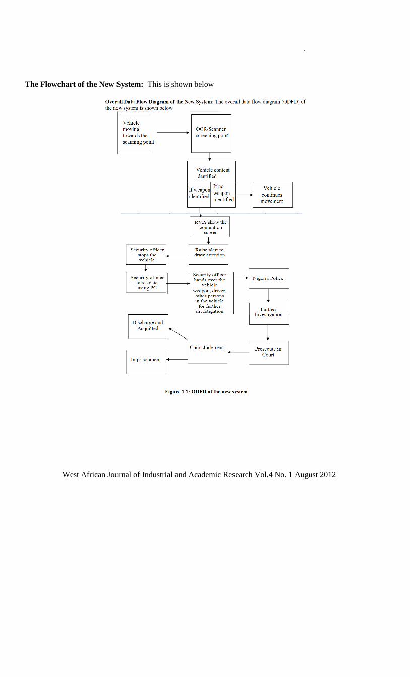
.
West African Journal of Industrial and Academic Research Vol.4 No. 1 August 2012
The Flowchart of the New System: This is shown below

West African Journal of Industrial and Academic Research Vol.4 No. 1 August 2012 1
We propose here for adaptation a hybrid ITS safety architecture that combines vehicle-to-vehicle communication and vehicle-to-roadside sensor communication [9]. Opposed to dedicated roadside units, which require major investments for purchase, installation and maintenance, roadside wireless sensor and networking technology represents a cost-effective solution and can leverage the deployment of the system as a whole. Among the various services of the hybrid communication system proposed here include accident prevention and post-accident investigation. Presented here also is a system and protocol architecture with a fully
distributed concept for efficient and secure storage of sensor data. For deployment, this architecture will likely be combined with an alternative approach using dedicated road-side units as a centralized network element for communication and data storage. For the proposed system, we describe the main components (radio, networking and services, security). Finally, we describe our prototype implementation and experimental tested featuring hardware and software platforms for vehicle on-board units and sensor nodes. Figure 1.3 presents the proposed WSN architecture with distributed and centralized data storage
.
Fig. 1.3: Systems architecture with distributed and centralized Data Storage[9][11]
The proposed Main technology components of the architecture are: (i) radio interfacesIEEE 802.11p and IEEE 802.15.4, (ii) routing protocols Geocast and tinyLUNAR, (iii) middleware for VANETs and tiny PEDS for WSNs, and (iv) Applications.
The components are well adapted to the specific requirements of VANETs and WSN, respectively. VANET = Vehicular Ad hoc Networks WSN = Wireless Sensor Networks

.
West African Journal of Industrial and Academic Research Vol.4 No. 1 August 2012
Table 1.1: Prototype Platforms For VANET And WSN Nodes [11]
Technology Integration Components. These are technological equipment needed or to be used in carrying out the tracking of metal arms in vehicles which will work with RVIS. ( i)Transponder This is a wireless communication, monitoring and control device that picks up and automatically responds to an incoming signal. It is a contraction of the words transmitter and responder. Simply put, transponder is an electric device used to wirelessly receive and transmit electrical signals [9]. It is an electronic device that can be used to send and receive signals wirelessly.
Transponders were developed to be attached to objects which needed to be located. A transponder functions by receiving a signal, called an “interrogator” because it is effectively “asking” for information, then automatically conveying a radio wave at predetermined frequency. In order to broadcast a signal on a different frequency than the
one received, a frequency converter is built in. By receiving and transmitting on different frequencies, the interrogator and transponder signals can be detected simultaneously. In a real situation, transponder will be attached to vehicles for easy location and searching. This can be mounted on the windshield or dashboard.
Transponders can be classified as active and passive transponders. Active transponder is a type of transponder employed in location, identification, and navigation systems for commercial and private vehicles. It transmits a coded signal when it receives a request from a monitoring or control point. The transponder output signal is tracked, so the position of the transponder (on the vehicle) can be constantly monitored. It will operate over a kilometre distance and an example of this is Radio Frequency Identification (RFID). Passive transponder is a type of transponder that allows a computer or robot to identify an object. It must be used with an active sensor that decodes and

.
West African Journal of Industrial and Academic Research Vol.4 No. 1 August 2012
transcribes the data the transponder contains. Magnetic labels, such as those on credit cards, and. store items are common examples. This is the one to be employed in this work
Figure 1.4: Transponder over a truck [Source: 9]
(ii) RFID This acronym stands for Radio Frequency Identification. It is the use of a wireless non-contact system that uses radio frequency electromagnetic fields to transfer data from a tag attached to an object, for the purposes of automatic identification and tracking. It is a technology that incorporates the use of electromagnetic or electrostatic compiling in
the radio frequency portion of the electromagnetic spectrum to uniquely identify an object, animal or person. It does not require direct contact or line-of-signal scanning. A RFID system uses tags, or labels attached to the objects to be identified. Two way radio transmitter-receivers called interrogators or readers send a signal to the tag and read its response. The readers generally transmit their observations to a computer system running RFID software or RFID middle ware. The tag’s information is stored electronically in a non-volatile memory. An RFID reader transmits an encoded radio signal to interrogate the tag. The tag receives the message and responds with its identification information. This may be only a unique tag serial number, or may be product related information such as stock number, lot or batch number, production date, or other specific information. Note that RFID tags can be either passive, active, or battery assisted passive. However, RFID system consists of these three components, antenna, transceiver (often combined into one reader) and a transponder [9].
Figure 1.5: RFID [source: 2]

.
West African Journal of Industrial and Academic Research Vol.4 No. 1 August 2012
(iii) Optical Character Recognition
This is often abbreviated as OCR, it refers to the branch of computer science that involves reading text from paper and translating the images into a form that the computer can manipulate. It is the recognition of printed or written text and characters by a computer system or OCR reader/OCR machine. It involves photo scanning of the text character-by-character, analysis of the scanned-in-image, to identify each alphabetic letter or numeric digit, and then the translation of the character image
into character codes such as ASCII, commonly used in data processing. Special software is used to compare the pattern of the signal sent from the machine or OCR reader to patterns already stored in the memory. When the match has been made, a respond signal will be sent to the machine accepting or rejecting the pattern. OCR is used in reading vehicles number plates. However, OCR systems include an optical scanner for reading text, and sophisticated software for analyzing images, and software to recognize characters.
Figure 1.6: OCR[9] (iv) Sensor A sensor is a converter that measures a physical quantity and converts it into a signal which can be read by an observer or by an instrument which are mostly now electronic. Generally, sensor is a device that receives signal and converts it into electrical form which can be further used for electronic
devices. For accuracy, most sensors are calibrated against known standards. In this work we are concerned with image sensor which is a device that converts an optical image into an electronic signal. It is used mostly in digital cameras and other imaging devices. Most currently used sensors are digital charge-coupled device

.
West African Journal of Industrial and Academic Research Vol.4 No. 1 August 2012
(CCD) or complementary metal-oxide-semiconductor which is active pixel sensors (CMOS APS). Both types of sensors accomplish the same task of capturing light and converting it into electrical signals. An active-pixel sensor (APS) is an image sensor consisting of an integrated circuit containing an array of pixel sensors, each pixel containing a photodetector and an active amplifier. There are many types of active pixel sensors including the CMOS APS used most commonly in cell phones cameras, web cameras. Such an image sensor is produced by a CMOS process (and is hence also known as a CMOS sensor) and has emerged as an alternative to charge couple device (CCD) image sensors.
Figure 1.7: Image sensor [2]
(v) GPS: This is Global Positioning System which is a spaced based satellite navigation system that provides location and time information in all weather, anywhere or near the Earth, where there is an unobstructed line of sight to four or more GPS
satellites. It is freely accessible to anyone with a GPS receiver. Modern vehicle tracking system commonly uses technology for locating vehicle. It can locate a vehicle anywhere on earth if it has vehicle tracking system. It also allows drivers of car and trucks to ascertain their location anywhere on earth. Mores, vehicle information can be viewed on electronic maps via the internet or specialized software. (vi) Simulation: This is the imitation of the operation of a real word processor system over time. The act of simulating something first requires that a model be developed; this model represents the key characteristics or behaviours of the selected physical or abstract system or process. The model represents the system itself, whereas the simulation represents the operation of the system over time. Simulation is used in many contexts, such as simulation of technology for performance optimization and for scientific modeling of natural systems or human systems to gain insight into their functioning. It can also be used to show the eventual real effects of alternative conditions and courses of action. Simulation is also used when the real system cannot be engaged or it is being designed but not yet built like in this thesis. In this thesis we are concerned with computer simulation. Computer simulation is a computer program that attempts to simulate an abstract model of a particular system. Simulation of a system is represented as the running of the system’s model. It can be used to explore and gain new insights into new technology and to estimate the performance of systems too complex for analytical solutions. Computer simulations vary from computer programs that run for a few minutes, to network

.
West African Journal of Industrial and Academic Research Vol.4 No. 1 August 2012
based groups of computers running for hours, to ongoing simulations that run for days. (vii) Computer System: A complete, working computer is known as computer system. It includes the computer along with any software and peripheral devices that are necessary to make the computer function. Every computer system requires an operating system. But a computer is programmable machine. The two principal characteristics of a computer are; • It responds to a specific set of instructions in a
well defined manner. • It can execute a pre-recorded list of instructions
that is program (viii) Image Scanner: In computing, an image scanner often abbreviated to just scanner, is a device that optically scans images, print text, handwriting, or an object, and coverts it to a digital image. Hand held scanners have evolved from text to three dimensional (3D) scanners. A 3D scanner is a device that analyses a real world object or environment to collect data on its shape and possibly its appearance. It is being used in different areas of life including inspection. The purpose of 3D scanner is usually to create a point cloud of geometric samples on the surface of the subject. It is analogous to cameras. Like cameras, they have a cone-like field of view and can only collect information about surfaces that are not obscured. A 3D scanner collects distance information about surfaces within its field of view. The “picture” produced by 3D scanner describes the distance to a surface at each point in the picture. This allows the three dimensional position of each point in the picture to be identified.
However, for most situations, a single scan will not produce a complete mode to the subject. Multiple scans, even hundreds, from many different directions are usually required to obtain information about all sides of the object. These scans have to be brought in a common reference system, a process that is usually called alignment or registration and then merged to create a complete model. This whole process, going from the single range map to the whole model, is usually known as the 3D scanning pipeline. There are varieties of technologies for digitally acquiring the shape of 3D object. A well establishment classification divides them into two types: contact and non-contact 3D scanners. Non contact 3D scanners can be further divided into two main categories, active and passive scanners. In this thesis, we are concerned with non contact 3D scanners. Active scanners emit some kind of radiation or light and detect its reflection in order to probe an object or environment. The possible types of emissions used include light, ultrasound or x-ray. But passive scanners do not emit any kind of radiation themselves, instead rely on detecting reflected ambient radiation. Most scanners of this type detect visible light because it is a readily available ambient radiation. Other types of radiation, such as infrared could also be used. Passive methods can be very cheap, because in most cases they do not need particular hardware but simple digital cameras. However, the anticipated roadside Vehicle Identification Technology for implementation is shown below but not drawn to to scale.

.
West African Journal of Industrial and Academic Research Vol.4 No. 1 August 2012
Figure 1.8: Proposed Roadside Vehicle identification layout [9].
How e-screen works
• As a participating vehicle approaches an enforcement station, the vehicle’s transponder is read by a roadside reader.
• A computer in the enforcement station looks up the transponder in a database to make sure the vehicle is in good standing with regard to
registration, safety record, and is not carrying any weapon.
• If everything checks out, the truck is given a green light on the transponder, indicating that the truck may proceed on down the road. Enforcement personnel are then free to focus their attention on high-risk carriers.
Figure 1.9: Proposed Electronic Screening Software[9]

.
West African Journal of Industrial and Academic Research Vol.4 No. 1 August 2012
Justification of the new system The new system ensures equity, fairness, fastness, reliability, objectivity and accuracy up to eighty percent than the “stop and search” operation at Nigeria road checkpoints. It will completely take care of the weaknesses observed in the present manual system. The system will automatically generate report or information on vehicles with arms or ammunition and then draw the attention of security operatives on duty. Moreover, every vehicle must be screened automatically. There would no further incidence of allowing vehicles to pass without being searched due to human inadequacies such as tiredness. If the new technology is properly implemented, it will reduce the rate of violent crimes, riot, agitation, etc in Nigeria involving the use of arms and ammunition. This will improve the security situation of this great country. Anticipated Benefits of the Proposed System
• For government: o More effective and
efficient screening. o Make better use of
security personnel. o Focus enforcement
resources on the high-risk carriers.
o More consistent and ubiquitous enforcement coverage
o Monitor more routes at more times
o More difficult for non-
Compliant carriers to avoid enforcement.
o Improved safety o Improved homeland
security
• For industry: o Creates a more level playing field o More difficult for anyone to short-
cut the requirements. o Everyone must play by the same
rules. o Better revenue base – everyone
paying their fair share o Streamlined operations at
enforcement locations o Safe and legal trucks avoid stops and
delays. o Fuel and time savings. o Improved safety o Unsafe operators taken off the road. o Less need to stop trucks on shoulder
to perform checks. Conclusion This paper has identified the emerging complex security scenario in Nigeria as being capable of disintegrating the Nigerian state if not urgently addressed. We have proposed a technology solution via the deployment of Electronic Roadside Vehicle Monitoring Technology using Wireless Sensor Networks, Transponders, OCR and dynamic camera and automated vehicle checkpoints to track incidence of small arms movement in Nigeria. The objective is to arrest the unbridled proliferation of small arms used in perpetuating murder, robbery

.
West African Journal of Industrial and Academic Research Vol.4 No. 1 August 2012
and bombings around Nigeria. The authors strongly believe that urgent implementation of this new tool by the Federal Government will go a long way in staving Nigeria away from the threat of sovereign collapse. Recommendations In line with the foregoing observations about the emerging complexity of the security scenario in Nigeria, we recommend thus:.
• That comprehensive automation of databases for vehicle registration throughout the country is initiated as a matter of urgency.
• That issuance of vehicle number plate should be comprehensively done with automated database system.
• Driving license issuance should be automated with a distributed or centralized database and security and access controlled from a central point.
• Vehicle registration database, vehicle number plate database and driving license issuance database must be linked and connected to the RSVIS when implemented for analysis.
• Database for offenders should be developed so, that reports can be generated at regular intervals when implemented.
• That there be established Emergency Security Response where all reports of identified arm movement on the road is reported for immediate security action.
.
________________________________________________________________________________
References [1] Merriam-Webster, (2010). Online Dictionary. Retrieved from http: //www.merriam-
webster.com/dictionary/ security on 22nd August, 2010. [2] Wikipedia, (2010) Small Arms Free Encyclopedia retrieved online from http://en.wikipedia.org/wiki/small_arms on 25th October, 2010. [3] Merchant-Smith, C.J & Haslam,, P.R (1982). Small Arms and Cannons. London: Brassey’s Publishers. [4] Dikshif, P (1994) Proliferation of Small Arms and Minor Weapons, strategic Analysis Journal of Proliferation of Arms and Weapons Volume 1 (2) [5] Chisholm, H. (ed) (2000). Ammunition. Encyclopedia Britisannia, USA: Cambridge University Press. [6] Radio Nigeria (2010). Seven O’clock Network Morning News of 18th August, 2010. [7] USA (2010) Travel Warning for Nigeria. Retrieved online from

.
West African Journal of Industrial and Academic Research Vol.4 No. 1 August 2012
http://travel.state.gov/travel on 22nd August, 2010. Published by Department of State of USS on 15th June 2010.
[8] Radio Nigeria (2011) Seven O’clock Network Morning News of 1st September, 2012. [9] Osuagwu, O.E.(2010) Deploying Electronic Roadside Vehicle Identification to Track
Transit Ammunition Movements: A Tool for Enhancing the Security of Nigerian State. A paper Delivered at the International Conference of the Nigeria Computer Society, held at Asaba from 26th to 30th July, 2010.
[10] Dellaporta, J. (2010) What is Transponder? Retrieved online from “http://www.wisegeek.com/” On 29th September, 2010. [11] http://www.vanet.info/

.
West African Journal of Industrial and Academic Research Vol.4 No. 1 August 2012
Statistical Analysis of Deviance among Children in Makurdi Metropolis
Kembe, M.M* and Kembe, E.M+
*Department of Mathematics, Benue State University, Makurdi + Department of Home Science and Management, University of Agriculture, Makurdi
Abstract This study sampled a total of four hundred and three individuals from designated households in Makurdi metropolis, Benue State. The study respondents responded to a self-report survey which gathered information on three deviant acts: alcoholism, smoking and dropping out of school. Criteria for deviant acts were defined, and each of the three acts was analyzed against the criteria of the type of family. Propensities toward deviance were identified against three normative dimensions – single parent (mother), single parent (father), both parents. The most prevalent deviance among children from single parents is children dropping out of school while that of children from two parents is alcoholism. It is the conclusion of this study that home background and family type has a correlation with deviant behavior. Based on this, there is need for youth employment, government intervention and awareness education on parental responsibility. Keywords: Households, deviance, drooping out of school, smoking and alcoholism 1.0 Introduction Deviance is behaving contrary to acceptable norms and expectation of a society. Deviant behavior is common with young children and adolescent especially in their formative years when character is formed and reformed to suit the expectation of the family and the community. Every society has specific behavioral standards and ways in which people are supposed to act; sometimes these are the paradigms for predictable behavior in the society. Deviance is a departure of certain types of behavior from the norms of a particular society at a particular time and place. In Nigeria, deviance is
described as a violation of culturally acceptable norms and or a failure to conform to set rules and ways of doing something that is traditionally prescribed.
According to Santrock [10], many parents and teachers often wonder about the rebelliousness (truancy, anti–social behavior, disrespect for constituted authority, sexual harassment, rape, arson, destruction, adolescents delinquency) that are portrayed by children and adolescent. A behavior considered as deviant in one society may be seen as non-deviant in another society. For example, the traditional African social custom appreciates chastity, modest dressing, good morals,

.
West African Journal of Industrial and Academic Research Vol.4 No. 1 August 2012
decent behavior, and respect for elders, hard work and integrity and frowns at premarital and extra marital sexual relationship. It also prohibits marriage between same sex such as homosexuality and consanguine sexual relationship. The Nigerian society frowns at alternative marriage styles and parenthood, for example, single parenthood and cohabitation. In some other societies, these unacceptable behaviors are acceptable. That is why; deviance is relative to time and place. Studies conducted by Mallum [9] and Kembe [7] shows that the home background plays an important role in the child’s personality development. The home is often critical to the type of behavior displayed in the society. The traditional family as reported by Shindi [11] is made up of family members who would normally contribute to the upbringing of the child. The extended family system provided a wide range of stimulating interactions that positively nurture the child, particularly in the psychosocial terms. In the absence of parental support provided by both parents and the social support network provided by the extended family, there are bound to be problems in child rearing and upbringing. According to Karst [6], a Single parent is a parent who cares for children without the assistance of the other parent in the home. Child birth and child rearing is a task that involves the responsibility of both parents. The number of one parent families has increased substantially. According to the United States Census Bureau [9], about 20 million children live in household which are single-headed. In the 1970s, divorce was a common reason for single parenting, and during this period the number of families headed by one parent increased rapidly. The
number peaked in the 1980s and the declined slightly in the 1990s. By 1996, 31 percent of children lived in single parent families. Apart from divorce, single teenage parenting is also reported among adolescent. This occurs as a result of teenage unwanted pregnancy leading to school dropout and other health consequences [4]. Furthermore, it has been proved that single headed families are not economically stable. Children from economic dependent homes are likely prey to social vices like stealing and school truancy. Indeed, the incidences of child abuse (street hawking, house maid, bus conductors, mine, factory worker, child prostitution) are as a result of poverty. Poverty has also forced some parents to abandon their primary responsibility of child care and nurturance. This in turn has resulted in all kinds of delinquent behavior such as compulsive television viewing, drug addiction, cultism and alcoholism. Farrington [3] reports that 90% of adolescent boys and girls in intact families were within the normal range on behavioral problems.10% had serious problems that we would generally require some type of professional help. The percentages for divorced families’ were 74% of the boys and 66% of the girls in the normal range and 26% of the boys and 34% of the girls were in the problematic range. It should be noted that reasons for single parenthood can be as a result of death of spouse. Spousal death of either the mother or the father can result in child rearing by only one parent. Normally, the family suffers set back especially if it is the bread winner of the family. Deviance behavior can result from the psychosocial loss of the loved one. So, there may be levels of deviance depending on the causal- effect relationship.

.
West African Journal of Industrial and Academic Research Vol.4 No. 1 August 2012
Recently, research in social science has attracted attention on the effects of mass media on violent and aggressive behavior. According to Anderson, Berkowitz, Donnerstein, Huesman, Johnson, Linz, Malamuth and Wartella [1] provided converging evidence linking frequent exposure to violent media in childhood with aggression later in life, including physical assault, alcoholism and other forms of abusive behavior. 2.0 Statement of the Problem Deviance has been reported variously as behavior that is contrary to acceptable cultural norms of a society. In Benue state recently, there is a ban on the consumption of illicit gin especially by the youths. The reason for the ban on drinking is not far from the deviant behavior that is exhibited by the youths as seen in hooliganism, illicit sexual activities, rape and other forms of abusive and anti-social behavior.
It is also a deviant behavior to see teenage girls who are supposed to be in school to be engaged in pregnancy and child rearing. Teenage pregnancy is often the reason for school dropout among
adolescent girls [10], [4] . 40% of teenage mothers drop out of school to rear their children as single parents. Single parenting places the burden and responsibility of intact families only on one parent. This raises doubts on the psycho social behavior of these children. Society is not oblivious of the fact that home background affects the behavior of children, [9],[1]. It is in view of this discourse, that this study intends to look at the deviant behavior exhibited by children from single parenthood and see whether there is a relationship between these behavior and those of children from intact families. Methods The research work was carried out in Makurdi, the capital of Benue State. A structured questionnaire was developed and given to our targeted respondents. A survey was sent to a randomly selected 500 Households. Of the 500 Households, 403 returned the questionnaire (81%). Analyses for this study include descriptive statistics and non parametric methods and the level of significance was set at 0.05.
Results and Discussions What are the different family status in Makurdi Metropolis?
Table 1. Percentage response on types of Family status in Makurdi Family status Responses
(f) (%) Single parent(mother) 220 54.6 Single parent (father) 102 25.3 Two parents(mother and father) 81 20.1 Total 403 100
Result from Table 1 shows that majority of families in Makurdi metropolis are composed of single
parents who are women (55%), other types of

.
West African Journal of Industrial and Academic Research Vol.4 No. 1 August 2012
family status include single parents made up of men(25%) and two parents(20%).
What are the prevalent deviances in Makurdi Metropolis
Table 2. Prevalence of deviance in Makurdi Metropolis
Deviances Responses (f) (%)
Alcoholics 100 24.8 Smoking 68 16.9 Dropping out of School/runaway 65 16.1 Teen parents 43 10.7 Cultism 55 13.6 Political thuggery 52 12.9 Robbery(petty robbery, armed robbery and house breaking)
18 4.5
Commit Suicide 2 0.5 Total 403 100
The result in Table 2 shows that 24.8% indicated that the most prevalent deviance amongst children in Makurdi town is alcohol. This is closely followed by smoking which is represented by 16.9%. Dropping out of school and run away from home is another deviance that is on the rise representing 16.1%. Cultism is also an emerging problem on the list of deviance in Makurdi town representing 13.6%.
Cumulative Deviance of Children from Single Parents Figure 1 depicts the cumulative sums of deviances in children from single parents. A plot of these cumulative deviances is presented in figure 1 below. It shows that the number of drop outs from school was highest followed by those taking alcohol.

.
West African Journal of Industrial and Academic Research Vol.4 No. 1 August 2012
Figure1. Cumulative sums of the three components of deviance in children of single parents. Cumulative Deviances of Children from Two Parent Families Figure 2 depicts the cumulative sums of deviances in children from two parents. A plot of these cumulative deviances presented in the figure
below shows that the number engaged in alcohol was highest and this is closely followed by the number of smokers and those dropping out of school the least.
Figure 2. Cumulative sums of the three components of deviance in children of two parents.

.
West African Journal of Industrial and Academic Research Vol.4 No. 1 August 2012
Comparison of deviance of children from single parents with those from two parents Figure 3 depicts cumulative deviance from children brought up from single parents compared
with those brought from two parents. It clearly shows that the highest deviance is exhibited by children from single parents than children from two parents.
Figure 3. Cumulative deviances from two types of family background
Hypothesis H0: There is no significant difference between family status and deviant behavior of children. The
Chi- Square ( ) statistics was used in the test of independence.
Table 3. The relationship between the family type and the observed defiant behavior of children. Parent status Alcoholics Smokers School
dropouts Single Parent(Mother)
20 19 18
Single Parent(Father)
48 70 68
Parents(Mother and Father)
54 76 20
Total 122 165 116 The null hypothesis: i=1,2…I;
j=1,2,…,J
Alternate Hypothesis:
Test Statistic;

.
West African Journal of Industrial and Academic Research Vol.4 No. 1 August 2012
Where the proportion of individuals in the
population who belong in category I of factor 1 and category j of factor 2 = P (a randomly selected individual falls in both category i of factor 1 and category j of factor 2
= P( a randomly selected individual
falls in category i of factor 1) = P( a randomly selected individual
falls in category j of factor 2)
Rejection region:
Thus But
Since ,
We therefore reject hypothesis of independence. We conclude that the status of parents of children does give information about the deviant behaviour of children. In particular Children who are alcoholics appear more likely to come from a single parent that is a mother. Discussions Results from analysis show that there are more single parents who are mothers in Makurdi metropolis. The vulnerability of women to poverty and the imbalances in education and employment coupled with the responsibility of housekeeping and child rearing affects the family. Recently single- headed families have become rampant either from the male-headed or female-headed households, leaving the burden of housekeeping and child-rearing a challenge. There have been various
reasons given for the types of family status, ranging from divorce, death of spouse, lifestyle and other social circumstances including out of wedlock births. According to Kandel [5], Social scientists have found that children growing up in single-parent families are disadvantaged in other ways when compared to a two parent families. Many of these problems are directly related to the poor economic condition of single-parent families, not just to parenting style. These children are at risk for the following: lower levels of educational achievement likely from irregular school attendance
i. likely to drop out of school resulting from unmet needs
ii. likely to become teen parents and face other social hazards of teenage pregnancy
iii. likely to become thugs and be involved in “boko haram”
iv. frequently abuse drugs and alcohol
v. high-risk sexual behavior vi. likely to engage in cultism vii. likely to commit suicide
According to Kembe (2005), a child is an ambassador of a home, thus whatever behavior the child exhibits both in the school and in the larger society is a direct function of how the child was brought up with some few exceptions though. Conger and Mussen [2] stated that children behave differently according to their home type. Home background plays a significant and critical role in the overall personality output of individuals. Children life adjustment is influenced from the home background, for example, children who have

.
West African Journal of Industrial and Academic Research Vol.4 No. 1 August 2012
lived in deprived and or abusive environment are most likely to exhibit negative societal behaviours. Also, children from two-parent structured homes are less likely to be engaged in deviances like dropping out of school, smoking, alcoholism compared to the children who are from unconventional homes. Conclusion and Recommendations The overall result of this study suggests that children from single parents homes, on average, are more engaged in deviances than children in two parent families. The common forms of deviant behaviors are school dropout, alcoholism and smoking. This has implication for later life adjustments. It is the conclusion of this study that home background and family type has a correlation with deviant behavior. Based on this, there is need for youth employment, government intervention and parental responsibility. In the light of t foregoing findings of this research, the following recommendations are made. Youth development
Youth unemployment resulting from lack of appropriate skills for work will continue to constitute a problem unless skill centres and programmes are developed to engage youths and impart skills especially for immediate small scale business. This recommendation, if implemented, will also improve the economic base of most homes. Government intervention Government can place policies and laws that will prosecute certain repeated cases of youth deviant behavior such as housebreaking, cultism, smoking of illicit drugs and alcoholism. The present law in the Benue State prohibiting the sale and drinking of alcohol in social events should be enforced and not made a mockery of. Parental Responsibility Parents are responsible for the upkeep of their families and to ensure that children grow up into acceptable personalities for the society. Quality family time, discipline and positive parenting style have implication for controlling deviant behavior.
References
[1] Anderson, C.A., et al (2003). The infulence of Media Violence on Youth Psychological Science in the Public Interest, 4, 81-110.
[2] Conger, J.J and Mussen, P.H (1997). Child Development and Personality. Harper & Row, publishers, New York
[3] Farrington, D.P. (1995). The Development of Offending and Antisocial Behavior from Childhood: Key Findings from the Cambridge Study in Delinquent Development. Journal of Child Psycho Psychiatry 36, 29-64
[4] Gipson, J. D., Koenig, M. A. and Hindin, M. J. (2008), The Effects of Unintended Pregnancy on Infant, Child, and Parental Health: Studies in Family Planning. Vol 39(1), 18-38

.
West African Journal of Industrial and Academic Research Vol.4 No. 1 August 2012
[5] Kandel , D. B. (1990). Parenting Styles, Drug Use, and Children’s Adjustment. .Journal of Marriage and family. Vol.52,(1),183-196 [6] Karst,P.(2000). The Single Mother's Survival Guide. Freedom, CA: Crossing Press [7] Kembe, M.M.(2005). Influence of Family Background on Pattern of Child Misbehavior in Makurdi Metropolis. Journal of Home Economics Research, Vol. 6(10), 166-170. [8] Kembe, M.M.(2008). Verbal Abuse: Causes and effects on Adolescent personality. The
Journal of Family Development Vol 3(1), 14-21 [9] Mallum, J.O. (2002). The Home Environment and the Educational development of the child. Journal of the Nigerian society for educational Psychologists Vol 1(1), 40-48 [10] Santrock, J.W. (2005). Adolescence. Boston: Mc Graw Hill [11] Shindi, J.(1989). The Nigerian Child. An Introduction to Child Care. Plateau state: welfare committee [12] United States Census Bureau (2002). APPENDIX A Cumulative sums of the three components of deviance in children of single parents.
S/N alcoholics
Cm smokers
Cm school dropouts Cm
1 1 1 0 0 4 4 2 2 3 1 1 5 9 3 1 4 0 1 2 11 4 1 5 4 5 1 12 5 2 7 0 5 0 12 6 1 8 3 8 2 14 7 3 11 2 10 4 18 8 0 11 0 10 1 19 9 0 11 0 10 1 19 10 2 13 3 13 2 21 11 3 16 0 13 2 23 12 0 16 2 15 3 26 13 1 17 1 16 5 31 14 3 20 2 18 3 34 15 1 21 0 18 3 37 16 2 23 1 19 2 39 17 2 24 0 19 2 41 18 5 29 1 20 1 42 19 3 32 2 22 1 43 20 2 34 1 23 2 45

.
West African Journal of Industrial and Academic Research Vol.4 No. 1 August 2012
Appendix B Cumulative sums of the three components of deviance in children of two parent families

.
West African Journal of Industrial and Academic Research Vol.4 No. 1 August 2012
Appendix B Cumulative sums of the three components of deviance in children of two parent families
S/N Alcoholics
C Smokers
C School dropouts C
1 2 2 0 0 0 0 2 3 5 1 1 0 0 3 2 7 0 1 2 2 4 0 7 0 1 0 2 5 4 11 1 2 1 3 6 2 13 2 4 1 4 7 2 15 1 5 1 4 8 4 19 3 8 1 6 9 3 22 1 9 0 6 10 2 24 2 11 0 6 11 3 27 1 12 2 8 12 1 28 2 14 0 8 13 0 28 3 17 1 9 14 2 30 0 17 1 10 15 4 34 1 18 0 10 16 0 34 0 18 0 10 17 1 35 3 21 O 10 18 3 38 1 22 1 11 19 3 41 3 25 1 12 20 2 43 1 26 0 12

.
West African Journal of Industrial and Academic Research Vol.4 No. 1 August 2012
Appendix C
Cumulative deviances from children brought up from single parents compared with those brought from two parents
S/No Cumulative deviance from single parents Cumulative deviances from two parents
1 5 2
2 13 6
3 16 10
4 22 10
5 24 16
6 30 21
7 39 25
8 40 33
9 41 37
10 48 41
11 53 47
12 58 50
13 65 54
14 73 57
15 77 62
16 82 62
17 86 66
18 93 72
19 99 79
20 104 82

.
West African Journal of Industrial and Academic Research Vol.4 No. 1 August 2012
A Profile Analysis on the Effectiveness of Two kinds of Feeds on Poultry Birds.
Onuoha, Desmond O+. and Opara Pius N*.
+Department of Mathematics and Statistics, Federal Polytechnic Nekede, Owerri, Imo State.
E-mail: [email protected] *Department of Statistics,Imo State University Owerri
Abstract:
This study was carried out to find the effect of two types of poultry feeds on the weight of poultry birds using chicken from Michika Farm in Igwuruta in Port Harcourt, Rivers State as a case study. The data was collected for a period of eight weeks, where a sample size of sixty chickens was divided into two equal populations. The data for the analysis was collected as a primary data through the method of direct observation and measurement. The data were analyzed using hostelling T2 distribution, F-distribution to Test for parallel profile. At the end of the analysis, it was found that the profile was not parallel. This shows that the levels of the treatment on feeds are not the same. Key words: poultry feeds, poultry birds, primary data, direct observation, hostelling T2 distribution,
F-distribution _______________________________________________________________________________ 1.0 Introduction
Poultry farming is one of most lucrative business ventures one can embark upon if properly managed. The management of poultry could be attributed to the production of healthy and weighty birds in order to maximize profit. To actualize this, one has to adopt the best poultry feed on the birds. This work is aimed at using Profile analysis to select the best feeds needed for the poultry birds. In this case, profile analysis could be described as a situation where a number of treatments are administered to two or more populations. [22] ,[15]
stated that the responses must be expressed in similar unit and are assumed to be independent of one another, for different populations.
Furthermore, in comparing two or more populations, we might be faced with questions such as; Is the population’s mean-vector the same? That is µ1 = µ2. By applying profile analysis to test for the effectiveness of two different types of feeds on poultry birds, the questions are formulated in a stage-wise approach: 1. Are the profiles parallel?

.
West African Journal of Industrial and Academic Research Vol.4 No. 1 August 2012
Or Equivalent: H01: µ1i - µ1(i-1) = µ2i - µ2(i-1) = µ3i - µ3(i-1) . . . = µgi - µg(i-1);
i = 1, 2, …,p 2. Assuming the profiles are parallel, are they
coincident? Or Equivalent: H02: µ1i = µ2i = µ3i = . . . = µgi ; i = 1, 2, …,p
3. Assuming the profiles are coincident, are they level? That is, are all means equal to the same constant? Or Equivalent: H03: µ11 = µ12 . . . = µ1p = µ21 = µ22 . . . = µ2p . . . = µ2p = . . . = µg1 = µg2 . . . = µgp If the two profiles are parallel it shows that the mean of the feeds are the same considering all the treatments applied together.
Sources and Method of Data Collection The data for the analysis is a primary data collected through the method of direct observation. The method of direct observation entails observing and recording events as it is happening. The data was collected from an experiment conducted for a period of eight (8) weeks and two days, with sixty (60) chickens divided into two (2) equal parts. The first two days of the measurements were not used to get the real effect of feed. It has been observed by Johnson et al (1986) that when a new diet formulation is introduced or a new type of feed is presented, birds will often refuse to eat for a period of time or intake is reduced. Group A made up of thirty (30) chickens, were subjected to FEED A (vital grower) while group B comprising of thirty (30) chickens that were also subjected to FEED B (top grower). Their weights were measured in kg at the end of each week. Scope and Limitations of the Study
This study is aimed at establishing the effects of two types of poultry feeds on the weight of poultry birds, using chicken as a case study. It involves an experiment conducted for a period of eight weeks where a sample size of sixty chickens was divided
into two equal populations, each subjected to a particular feed. Their responses were measured in kilogram (kg) using weighing balance. The variables x1, x2, x3, x4, x5, x6, x7, x8 stands for the weights of chickens at the end of each week. Review of Some Related Literature There are several different multivariate test statistics available for the test of parallel profile, all of which will generally yield equivalent results. Amongst the four commonly test statistics – namely Wilks Lambda, Pillai’s Trace, Hotelling-Lawley Trace and Roy’s Greatest Root; Wilks Lambda ( )λ is the most desirable because it can be converted exactly to an F-statistics [18],[8] Johnson and Wichern (2001) presented in their text a detailed approach of this conversion and the exact distribution of λ . Bartlett (2001) in his work presented a modification of λ for cases where the number of groups is more than three (g > 3), as well as when large sample sizes are involved. It is worthy to note that (p – 1) would replace p. Leboeur (1992) noted in his work – “Profile analysis”, that experiment is conducted in a way of

.
West African Journal of Industrial and Academic Research Vol.4 No. 1 August 2012
observing two responses for a given population; the same population is exposed to p-treatment at successive times. And that we can formulate successive times to enable us develop the question of equality of means in a step wise procedure. Hence, H01, µ1 = µ2 = … µn implies treatments which have the same effect on the population; hence, we test for coincident profile. Profile analysis, according to Ott (1999), is a specific style of Multivariate Analysis of Variance. Tabacknick and Fidell (2006) stated that Profile Analysis is equivalent to repeated measures, because of its multiple responses taken into sequence on the same subject(s). Ohaegbulen E.U and Nwobi F.N [17] stated that in poultry farming, the production of high quality birds is always desired as this boosts the revenue of the poultry farmer and showed how profile analysis can be used to determine the feed with better nutritive value to the poultry birds. Croyle (2007) conducted a profile analysis on self-harm experience among Hispanic and white young adults. He compared the self-reported rates of self-harm in 255 Non - Hispanic white (NHW) and 187 Hispanic (predominantly Mexican American). He observed that self-harm is relatively common with about 31 % of the sample reporting some history of self-harm. Rates and specific types of self-harm did not significantly differ between the Non-Hispanic and Hispanic groups. Abdu, P.A., Mera, U.M. and Saidu, L. [1] had a study on chicken mortality in Zaria and observed that the use of profile analysis to conduct a chicken mortality research is recommended. Jensen and Dolberg [13],[6],[7] advocated for using poultry as a tool in poverty alleviation. An enabling environment must be established by
providing access to feed, vaccine, vaccinations services, micro-finance, marketing and other inputs and services. A village group, composed of members of socially equal status, is an excellent entity to disseminate improved technology, a cost-effective entity to disseminate extension messages, and a secure entity for disbursement of loans. Rahman and Hossain, [19] showed that an intervention with poultry production created a relatively small decline in the overall poverty with the proportion of extreme poor declining from 31 to 23% and the moderate poor stagnating around 29%. Todd, [21] and Dolberg,[6] opined that poultry activity is to be considered as a learning process for the beneficiaries, but it has to be realised that one activity alone is not sufficient to lift a family out of poverty. The opportunities called as the enabling environment must be available for the beneficiaries to establish a small poultry enterprise, to minimize the risks and to take up other income generating activities. Jensen [13] observed that about 70 % of the rural landless women are directly or indirectly involved in poultry rearing activities. He found that homestead poultry rearing is economically viable. Mack et al [16] opined that in order to increase egg and poultry meat production there is a need for increased investment guided by policies and institutions that promote equitable, sustainable, and environmentally friendly long-term outcomes as backyard poultry make an important contribution to poverty mitigation, it should be considered as any strategy to improve rural livelihoods. Right policies and investment, well designed and participative development programmers can overcome the constraints faced by the smallholder poultry producers.

.
West African Journal of Industrial and Academic Research Vol.4 No. 1 August 2012
Karlan [14] opined that an enabling environment would give all the villagers access to poultry farm input supplies and services; pave the way for disbursement of micro-credits in a cost-effective way; facilitate easier formation of associations through formalized village livestock groups; help people acquire the skills that are required for a business set-up. Dolberg [7] reviewed poultry as a tool in poverty alleviation focusing on experiences from Bangladesh but survey and project work that has been undertaken in India. Animal husbandry and agricultural departments’ extension programmes are hardly known or used by most poor people for whom the poultry work is relevant. Gondwe et al (2003) found that rural poultry is raised and utilized by about 80 percent of the human population, primarily situated in rural areas and occupied by subsistence agriculture.
Bujarbaruah and Gupta [3] reported that a flock size ranging from 25-250 birds are reared across the country under the village poultry system. They have low production potential with only 40-80 eggs per year but are less susceptible to most of the common diseases requiring less veterinary care. In order to meet the deficiency gap in poultry meat and egg sectors, adequate and sustained efforts will have to be made to improve the production efficiency of the rural poultry which has been responsible to produce 40% of meat and 44% of egg requirement in the country. Krishna Rao [20] recorded that poultry are inseparable from mankind and in the rural scenario they do not need any land, are easy to manage, regularly lay eggs, disease resistant and well adapted to the harsh environment.
Research Methodology
Profile Analysis pertains to situations where a number of treatments are administered to two or more populations where all the responses must be expressed in
similar units and the responses for the different populations are assumed to be independent of one another. Suppose birds on diet one are observed weekly for eight weeks, we can calculate the mean using the formula below:
; Where the first subscript represents feed and the second subscript represents weeks. We plot the
mean 1X weights against the number of weeks.
=
18
12
11
1
.
.
.
X
X
X
X

.
West African Journal of Industrial and Academic Research Vol.4 No. 1 August 2012
Parallel Profile:
We assume that nxxx 11211 ,...,, is a random
sample from Np(µ1, Σ ) and nxxx 22221 ,...,, is
also a random sample from Np(µ2, Σ ).
( ) =− xPPC 1
−
−−
=
−111
1213
1112
1
.
.
.
pp
C
µµ
µµµµ
µ , where 1µC = 1*)1( −p
We can write Ho1 as Ho1: 1µC = 2µC Vs Ha1: 1µC ≠ 2µC . Instead of basing our test on the observations nxxx 11211 ,...,, , nxxx 22221 ,...,,
we should use CXij; i = 1, 2 while j = 1, . . ., n. To test Ho1; we calculate the Hotelling’s T2 [11].[12] as
( ) ( )BApooledBA XXCCSCnn
CXXT −
′
+′′
−=−1
21
2 11
with critical region T2 > ( )
[ ] 05.0,12
21121
21 =−+
−−+= −+− ααpnnPF
pnn
pnnt , if we
reject Ho1, we stop and conclude that the profile are not parallel and 1µ ≠ 2µ , but if Ho1 is not rejected, we test for coincident profiles given that the profiles are parallel. 3.2 Coincident profiles. If the profiles are parallel, they can only be coincident if the total of element in 1µ is equal to
the total element in 2µ .

.
West African Journal of Industrial and Academic Research Vol.4 No. 1 August 2012
The test statistic
( ) ( ) ( )BApooledBA XXISnn
XXT −
′
+
′−′=
−
1111
1
1
21
2
with critical region T2 > α,2, 211 −+ nnF If we reject Ho2, stop 3.3 Level Profiles If the profiles are coincident the Xij, j = 1, 2, …,n1 and X2j, j = 1, 2, …,n2 are sample space of size n1 + n2 from Np(µ1, Σ ) where µ = µ1 = µ2.
The test statistic is given as
( ) ( ) XCCSCCXnnT pooled1
212 −′′+= with critical
region
α,,)(
)1)(2(211
21
212 pnnFpnn
pnnT P −+
−+−−+
> −
3.4 Mean and Pooled Covariance Matrix
The mean n
xx
n
ii∑
== 1
Then for the respective group,
n
xx
n
xx
n
iiB
B
n
iAi
A
∑∑== == 11 ,
The pooled venue is given by
Pooled 221 −+
+=NN
BA
Analysis A sample size of sixty chickens is involved in this study. The chickens were divided into two equal parts of thirty chickens each. The chickens were labelled 1 to 30 for each of the groups. The weights of each of the groups classified as A and B are taken using a weighting balance for a period of eight weeks labelled x1 x2, x3, x4, x5, x6, x7 and x8. The weights over the weeks are shown in appendix A. The term profile is said to have been observed by Hotelling (1936) to come from the practice in applied works in which score on a test battery are plotted in terms of graph or profile. Profile analysis provides three types of information, level, dispersion and the shape Figure 1: A graph of sample means of Responses per week Sample profile for two types of poultry feeds on the weights of poultry birds Let A stand for feed A and B for feed B such that the means AX and BX are the respective means for the eight weeks under study.
4.2 Calculations For The Analysis. N = 30, n1 = n2 Mean of Means for feed A and B is given as;

.
West African Journal of Industrial and Academic Research Vol.4 No. 1 August 2012
x = =
The mean deviation of the two sample means are given by
( )BA XX − =
While the sum of squares and cross products of each of groups are given by the symmetric matrix below For feed A
A =

.
West African Journal of Industrial and Academic Research Vol.4 No. 1 August 2012
For feed B
B =
The Spooled (pooled covariance) matrices is given by
Spooled = 221 −+
+nn
BA
where n1 = n2 = 30 such that n1 + n2 – 2 = 58
Spooled approximated to 3 decimal places
I 1SpooledI = [ Sum of elements in Spooled] = 0.667
( )BA XX −1I = [Sum of elements in( )BA XX − ] = -1.64

.
West African Journal of Industrial and Academic Research Vol.4 No. 1 August 2012
C( )BA XX − = =
Where c is a contrast matrix.
( )1BA XX − C1 =
1X
C1 = )26.217.255.141.127.105.185.066.0(
−−
−−
−−
−
1000000
1100000
0110000
0011000
0001100
0000110
0000011
0000001
Therefore; 1
X C1 = )45.062.014.014.022.02.019.0( CSpooledC
1=

.
West African Journal of Industrial and Academic Research Vol.4 No. 1 August 2012
| CSpooledC
1| =
= (CSpooled C
1)-1 =

.
West African Journal of Industrial and Academic Research Vol.4 No. 1 August 2012
=
−−
−−
−−−−
70.9097.408.4019.2892.3479.3255.1
46.438.9897.2250.926.1457.507.6
00.3869.2372.13770.6500.5471.2382.9
94.2864.935.6704.8476.4955.1702.9
30.3510.1500.5862.4837.10555.5804.5
54.3306.497.3051.1564.5899.10566.3
49.112.653.908.911.577.357.74
Since N is large, it is assumed that the two sampled population are normal and the Hotelling’s T2 statistic can be used to carry out the various test, similarly note that,
A ∼ ( )111, CCCN Σµ while B ∼ ( )1
22 , CCCN Σµ
Where µ and Σ are the multivariate mean and variance.
Test For Parallel Profiles Hypothesis: Reject tabcal TTifCCHo 22
211 : >= µµ accept if otherwise.
Where ( ) ( )BApooledBA XXCCSCnn
CXXT −
′
+′′
−=−1
21
2 11
T2
−−
−−
−−−−
70.9097.408.4019.2892.3479.3255.1
46.438.9897.2250.926.1457.507.6
00.3869.2372.13770.6500.5471.2382.9
94.2864.935.6704.8476.4955.1702.9
30.3510.1500.5862.4837.10555.5804.5
54.3306.497.3051.1564.5899.10566.3
49.112.653.908.911.577.357.74

.
West African Journal of Industrial and Academic Research Vol.4 No. 1 August 2012
= T2
cal = 140.217
( )[ ] 05.0
12211
2
21
212 beLetTpnn
pnnT pnnPtabtab αα−+−
−+−−+=
T2
tab = 17.709 Conclusion Since T2cal > T tab, we reject the hypothesis that the profile are not parallel meaning that the mean weight of chicken A is not the same with the mean weight of chickens in group B considering all the treatments applied together. This also implies that feed A and feed B have different effect on the chickens. Tests For Coincident Profile Hypothesis
Reject tabcal TTifIIHo 22212 : >′=′ µµ accept if
otherwise
where
( ) ( ) ( )BApooledBAcal XXIISInn
XXIT −
′
+
′−′=
−1
21
2 11
and α,2, 21122 −+= nnTT tabtab
Let 05.0=α Hence
T2cal = ( ) 485757.60667.0
30
1
30
164.1
12 =
+−−
T2 tab. = 4.016
Conclusion We reject Ho2, since T2cal > T2
tab and conclude that there is no coincident profile. This means that the response of chickens on feed A is not the same with those of chickens on feed B. 4.5 Test For Level Of Profile Hypothesis: Reject Ho3: Cµ = 0 if T2
cal > T2tab accept if
otherwise
where ( ) ( ) XCCSCCXnnT pooledcal ′′+= 212
and the critical region is
α,,)(
)1)(2(211
21
212 pnnFpnn
pnnT Ptab −+
−+−−+
= −
Such that
05.0=αLet

.
West African Journal of Industrial and Academic Research Vol.4 No. 1 August 2012
T2 =
*
−−
−−
−−−−
70.9097.408.4019.2892.3479.3255.1
46.438.9897.2250.926.1457.507.6
00.3869.2372.13770.6500.5471.2382.9
94.2864.935.6704.8476.4955.1702.9
30.3510.1500.5862.4837.10555.5804.5
54.3306.497.3051.1564.5899.10566.3
49.112.653.908.911.577.357.74
* = 7364.4291
Hence T2cal = while the critical region is
α,,)(
)1)(2(211
21
212 pnnFpnn
pnnT Ptab −+
−+−−+
= −
T2
tab = 17. 709 ________________________________________
Decision: We reject the hypothesis that the profile level since the T2cal > T2
tab. The rejection of the level profile hypothesis means that the chicken on feed A and chicken on feed B do not have the same level of response or that the average response of the chicken to the respective feeds A and B are not leveled. Conclusion.
The analysis showed that the profile was not paralleled and there is significant difference between the two feeds A and B performance on the weights of the chicken. The Average profile
of feed A was greater than that of feed B, therefore, we select feed A as better than feed B. Recommendation.
This method of analysis is recommended for researchers trying to compare effects of an input on the yielded results. It is also important for researcher to note that time is of essence in this form of research. This is to allow for proper measurement of the weights as the chickens are being feed with the respective feeds. This analysis should be extended to more than two independent populations.
References [1] Adbu P. A and Mera U. M and Saidu L. (1992). A study on chicken mortality in
Zaria, Nigeria. In Proceedings. 19th World Poultry Congress, Amsterdam, Netherlands, 2, 151.

.
West African Journal of Industrial and Academic Research Vol.4 No. 1 August 2012
[2] Bartlett, M. S. (2001). Further aspect of the theory of multiple regressions. Proc. Cmb. Phil. Soc., 34: 33 – 34.
[3] `Bujarbaruah K.M. and Gupta J.J. (2005). Family poultry for the development of NEH region ICAR Research Complex Umiam, Barapani, Meghalaya IPSACON-2005
[4] Croyles J. (2007 ). Some issues in the design of agricultural decision support systems. Agricultural systems, 52(2/3): 355–381.
[5] Del Ninno, C., Dorosh, P. A., Smith, L.C. and Roy, D.K (2001). The 1998 Floods in Bangladesh. Disaster Impacts, Household Coping Strategies, and Response. International Food Policy Research Institute, Washington.
[6] Dolberg, F. (2001). A livestock development approach for Rural Development: Review of Household Poultry Production with Focus on Bangladesh and India Pro- Poor Livestock Policy Initiative.
[7] Dolberg Frands (2003). The Review of Household Poultry Production as a Tool in Poverty Reduction with Focus on Bangladesh and India Pro- Poor Livestock Policy Initiative (PPLPI)Website:
[8] Everitt, B. S. and Dunn G. (2001). Applied Multivariate Data Analysis. 2nd Edn, Edward Arnold, London.
[9] Gondwe Timothy N.P., Clemens B.A. Wollny, A.C.L. Safalaoh, F.C. Chilera and Mizeck G.G. Chagunda (2003) Community-Based Promotion of Rural Poultry Diversity,
[10] Management, Utilization and Research in Malawi. [11] Hotelling H. (1935) The Most Predictable Criterion” Journal of Educaitonal Psychology, 26, 139-142. [12] Hotelling H. (1936) “Relations between two sets of variables” Biometrika 28, page 321- 377. [13] Jensen, H. Askov (2000). Paradigm and Visions: Network for Poultry Production
in Developing Countries. [14] Karlan, D. S. (2002). Social Capital and Group Banking. Downloaded from ` http://web.mit.edu/spencer/www/soccappaper.pdf [15] Leboeur, Y and Carlotte D.C., (2000). Body Weight and Low Back Pain Systematic Review of the Epidemiologic Literature. [16] Mack, D. Hoffmann and J. Otte (2000). The contribution of poultry to rural
development Organization of the United Nations, Viale delle Terme di Caracalla, 00100 Rome, Italy. [17] Ohaegbulen E.U and Nwobi F.N (2009) Poultry Feed brands solution using profile Analysis surreal of Applied Science [18] Ott, P., (1999). Multivariate Analysis of Variance: Profile analysis – an example
using SAS, biometric information pamphlet 60 [19] Rahman, H. Z and Hossain. M (1995). Rethinking Rural Poverty: Bangladesh as a case study. UPL, Dhaka. Sage
publications New Delhi. Journal Article [20] Rao C. Krishna (2005). A rural poultry revolution for poverty alleviation in rural
India Former Animal Husbandry Commissioner, Govt. of India, Jaya Nagar , New Bowenpally, Secunderabad [21] Todd, H. (1999). Women in Agriculture and Modern Communication Technology. Proceedings of a workshop, March 30-April 3, 1998, Tune Landboskole, Denmark. [22] Wald A. (1944) “On a Statistical Problem arising in the Classification of an Individual into One of Two Groups” Annals of Mathematical Statistics 15 page 145-162 .

.
West African Journal of Industrial and Academic Research Vol.4 No. 1 August 2012
Information and Communication Technology (Ict) Integration Into Science, Technology, Engineering And Mathematic (Stem) In Nigeria
A.A. Ojugo.+, A. Osika++., I.J.B. Iyawa* and R.O. Yerokun (Mrs.)**
+Department of Mathematics/Computer Science, Federal University of Petroleum Resources Effurun,
Delta State (+234)8034072248, [email protected], [email protected] ++Computer Science Education Department, Delta State College of Physical Education, Mosogar,
Delta State. +2348060328840 ([email protected]) ** Computer science Education Department, Federal College of Education (Technical), Asaba,
Delta State. [email protected], [email protected]
Abstract As Nigeria aspires for technological growth, positive changes need be made by placing proper educational values towards Science, Technology, Engineering and Mathematics (STEM) education. Some problems faced by STEM include lack of qualified teachers, curriculum, the misconception that STEM education is reserved for the less intelligent in the society, amongst others. Need thus arises, to develop alternative strategies to alleviate such problems. Bridging ICT and constructivism will exponentially change educational processes of both teachers and students to succeed as well as present new forms of learning environment. It will also unveil the power shift in educational structures; equip students to become knowledge producers rather than consumers. Thus, an ICT-Constructivist rich class will help teachers enfranchise, emancipate students academically with a framework that measures quality of engaged student’s learning. This paper aims to reveal links between effective use of ICT and the long neglected theory of constructivism in the area of STEM Education. Keywords: Constructivism, Rationale, informatics, productivity, meida literacy, lifelong.
___________________________________________________________________________________________
1.0 Introduction STEM has now become an integral part of our culture – in that actualizing our current societal goals and those of our generations ahead will be a mirage unless we have excellent understanding of STEM. [1] points that STEM has become our heritage and mankind’s hope. Thus, the mission of today’s education must ensure students are scientifically literate to cope with technological
changes of the data age. [2] notes STEM goals as: (a) provides preparation for training in science and mathematics, (b) provides basic mathematics and science literacy for everyday living, (c) provide basic skills, attitude to prepare us for technological developments and (d) help stimulate and enhances creativity. Education is the art of transferring knowledge from a teacher to learner within a physical environment (called school with classroom) and

.
West African Journal of Industrial and Academic Research Vol.4 No. 1 August 2012
interrelationship that [3] calls a system of factors, which jointly affect learning individuals of cultural differences. The classroom provides the structure in which learning is organized and the school has three major components namely: learner, teacher and administrator. There are basically two styles of education delivery namely Traditional (a teacher employs face-to-face, oral method in which the teachers pass knowledge to a learner), and
Alternative Delivery (learners can construct new knowledge and meaning from previous concepts and beliefs with methods and strategies that involves media literacy. The latter is more concerned with what a learner does and understands rather than teacher’s input. Thus, the use of equipments becomes focus of study (technology education) and educational support (educational technology) as in figure 1 [2,4].
[5] laments that STEM education is not given serious attention as it is misunderstood by educators and stakeholders in Nigeria, who believe that STEM education are for those who cannot pursue academic programmes. Thus, proper values must be placed on its need to help attain the desired growth as today’s industrialized nations employed the skills of both the educated and less educated in their growth toward ICT. Technological advancement in Nigeria today, is a sad reflection of the poor quality of STEM education that still receives stigmatization in our educational system, hindering our expected technological progress. 1.1. Objective of Study The study objective is: (1) seek alternative exemplary educational practices, (2) showcase outcome that describes individual/group adoption patterns of technology in learning as well as (3) show evidences linking technology integration, quality students learning and staff development.
1.2. Statement of Problem This study investigates learning in technology rich class (constructivist) versus the traditional class (non-constructivist) via creaction of a constructivist and non-constructivist groups. Will constructivism make a difference via meaningful, engaged-learning and transferable knowledge by students, in their own context? It will also seek the extent of the success in constructivist learning as effective method to boost student’s learning, performance and achievement. 1.3. Research Question The study aims to determine:
a. Extent of student’s achievement and attitude in a constructivist and non-constructivist groups as reflected in their learning of STEM.
b. Impact of ICT on various learning processes. c. What is the rationale behind ICT integration.
2. 0 ICT Framework In Education The provision of modern technological equipment at all school levels varies due to their various levels of preparedness – both by teachers and students. A look at students’ ability in obtaining the necessary flexibility in the world of information closely correlates amongst others, level of information setting of schools as this will help provide schools with various expanse of data in
Figure 1 shows a constructivist-class model
Traditional Classroom
Students
Teachers
Non-Interactive Technology
Computer System
Hardware/Software
Physical Features
of a Classroom
Curriculum

.
West African Journal of Industrial and Academic Research Vol.4 No. 1 August 2012
printed and electronic format via regular updates and networks as well as those directed by experts in the informatics field. ICT integration into education results in great reforms to the learning process; and educators who advocate such reforms, opines that such learning is informed by constructivism [6] which pleads the need for students to develop high thinking skill and the failure of the current schooling methods to provide such opportunities [7-8]. Thus, a critical factor to ICT integration is constructivism, so that learning takes place as the learner completes tasks for which media support is required and used to maintain such learning environment and learners [9].
Technology creates ideal learning. Thus, [10] notes it has been ignored or its past implementation has failed widely – as it creates a learner-centered, learning environment with a belief that they learn more from what they do or think rather than the teacher’s input. But we must take care not to allow the dynamic nature of technology overshadow the enduring nature of learning and or the ever-increasing knowledge base about learning [7, 4].
[11] notes the concept of constructivism as one in which a learner has the ability to actively construct knowledge as he learns. It also emphasizes knowledge as a construction of reality in the learner’s mind because knowledge is a dynamic adaptation towards an interpretation of experience. It supports many interpretations to reality based on knowledge constructed from experience and media-rich class. It focuses on knowledge construction rather than consumption – as the learner constructs data from experiences and mental beliefs, interpreting events accomplished outside the mind. We thus see the world we describe rather than describing the world we see. When integrated across curriculum, it provides appropriate level of difficulty due to its tasks that are of real world relevance with engaged-learning and teachers becoming knowledge guides [12] as seen in figure 2.
2.1. Constructivism Today’s education is transformed by new technologies that provides large amount of data to learners, coupled with the fact that knowledge doubles at increasing speed requiring a transformative method to education. Its challenge is that educators and learners are suspicious of the educational practices as it differs from what they are used – as constructivism removes statewide assessment, which traditional model promotes by aligning tests. The issues of fund shortage, unclear vision to keep the change from occurring rapidly as well as teachers not having a good understanding of how ICT works as they are charged with the duty of emancipating students, are in continual resolution. This paradigm shift will require teachers’ retraining, role redefinition as well as acculturation to put this systemic change in place – even though it be slow [13].
[14] notes some of the known principles of the constructivist learning as thus: 1. Learning is active and consists of meaning construction and constructing system for meanings. 2. Knowledge construction is mental – since it happens in the mind of the learner. 3. Language influences greatly what we learn. 4. Learning is a social activity associated with connections the learner makes with others. 5. Learning is contextual – as learner cannot learn isolated facts or theories in abstract ethereal land, separate from real world situations. 6. Motivation is a key in learning to help us know how the acquired knowledge can be put to use. 7. Knowledge is important – as we cannot comprehend new ideas without some structure developed from prior knowledge to build on. 8. Learning is not instantaneous but takes time – as the learners must revisit principles, reflect on them and using them as often as possible. 2.2. New Paradigms: A Constructivism Class Education, transformed by new technologies yields the following paradigms, when adopted:

.
West African Journal of Industrial and Academic Research Vol.4 No. 1 August 2012
a. Shift from whole class to smaller groups b. Teachers coach weaker students rather than focus on all as with traditional settings. Coaching occurs rather than lecture and recitation. c. Students become actively engaged, cooperative and less competitive d. Students learn differently than simultaneously. e. Integrate visual/verbal thinking rather than primacy of verbal thinking as in traditional class. Thus, educators, parents and learners will become suspicious of the educational practices as it differs from what they are used. This is becasue such constructivist learning removes statewide, aligned assessment – unlike traditional model. Thus, learners will take standardized tests, which does not assess what they are learning but what new meaning they derive of concept. Class structure will become more fragmented and problems will abound due to lack of funds and unclear vision to keep this systematic change from occurring as rapid as possible. Teachers charged with the duty of emancipating students, may not have adequate understanding of how these technologies work and the amount of data available as such paradigm shift requires staff retraining, their roles re-defined to inform them to think about why they do what they do as well as funding [15-20]. 2.3. Challenges of Constructivism The common challenges of constructivism as: 1. Nativism: Cultural constructivism promotes nativism and language, which primarily distorts the fundamental unity in education generally. It thus denotes knowledge as meanings conveyed by learners in different tongues – though referring to same state. Meanings, applied are inseperable of linguistics; though, science views meaning as an objective states that transcends such linguistic boundaries. It thus proposes to recreate nature to suit cultural and linguistic boundaries. But, the nativism and empiricism of science are too parallel and may never meet at internationalization and globalization [21].
2. Knowledge Territorialism : A concept of false belief that Africans who live enclosed cannot yield scientific discourse. Knowledge transcends the idea of cultural boundaries – such that ideas from varied ccultural perspectives must converge a conventional consensus due to similarities over their differences – though, such similarities by virtue of their many appearances, imprints itself upon the mind; while individual differences that changes between cases, fails. Faraday, Newton amongst other scientific inventors made their ideas to transcend ethnic boundary. Thus, we must deterritorialize our seminars to hold global focus; instead of its localized viewpoint [5].
7.1 Globalization: Poor globalization in STEM is often misconstrued as nativism. Scientist must ensure unity via interaction and exchange of concepts, innovations and skills among experts world over. This will urge individuals and research organizations not to be localized and restricted by culture. Competition must be encouraged, with knowledge circulation a rule. Thus, cultural constructivism in education is faced with the challenge of capacity building and establishment of research networks with Africans in Diasporas and with other worlds [21]. 3. 0 Method And Materials This will be discussed under the following heading: 3.1 and 3.2 respectively. 3.1. Researchable Model: The researchers will adopt [22] researchable model as redesigned by [5] for STEM education. Teaching method will be divided into constructivist (via laboratory, Internet to allow online interaction) and non-constructivist (normal classroom) groups. Curriculum content in focus: Mathematics (Geometry), Biology (Reproduction), Physics (Pendulum) and Chemistry (Titration). Feats to be measured include teachers’/students’ attitude and involvement.

.
West African Journal of Industrial and Academic Research Vol.4 No. 1 August 2012
3.2. Population Nigeria, is today divided into 6 geo-political zones: South East (SE), South-South (SS), South-West (SW), North-North (NN), North-East (NE) and North-West (NW). The scope of the study is limited to tertiary institutions in the 6 geo-political regions. Two schools were chosen from each geo-political zones: Federal University of Petroleum Resources Effurun and University of Port-Harcourt (SS zone), University of Nigeria Nsukka and Imo State University Owerri (SE zone), Osun State University and University of Ibadan (SW zone), University of Agriculture Maiduguri and University of Jos (NW zone), Ahmadu Bello University Zaria and Nigerian Defence Academy Kaduna (NN zone) and lastly, Idah Polytechnic Idah and University of Illorin (NE zone). From these, 15 samples each were selected for the constructivist and non-constructivist
groups (i.e. 30 students and 30 teachers) – and the sstratified sampling method adopted, in the selection criteria to alleviate falsehood of results obtained as well as give a fair representation of population. 4. 0 Data Analysis And Findings
Pedagogical practice and extent of involvement will determine if a group exhibits characteristics of a constructivist class or not. Its outcome is measured via assessment of student’s performance as seen in figure 3. For analysis, mean (X) and standard dev. (SD) are used with results discussed below in:
4.1. Research Question 1: ICT integration impact on
students and what extent their achievement is reflected in their attitude?
Table 1a. Mean score of student acheivement in two gruops
Pre-Test Post-Test
Groups No. Mean SD Mean SD
Experimen-tal/Constructivist
720
13.84 64
3.1 24
21.43 33
4.1 50
Control/Non construc- tivist
720
10.62 5
2.5 61
19.40 27
3.4 84
Table 1b: Student’s attitude towards STEM in two groups
Groups No. Male Female
Experimental or Constructivist 720 10.1663 9.9823
Control or Non-Constructivist 720 11.0001 10.0011
Table 1a shows the differences in students’mean score achievement. At post-test, students in the constructivist group had a higher mean scores than their counterpart in non-constructivist group. This is attributed to the
exposure they had in the use of ICT in learning. While table 1b shows a significant difference as male students in the non-constructivist group exhibited higher attitude to STEM than their counterpart in constructivist group.

.
West African Journal of Industrial and Academic Research Vol.4 No. 1 August 2012
This can be a result of technophobia as they were introduced to a completely, new-pedagogical learning pattern and scenario. Thus, ICT supports learning with technology literacy, high academic emancipation from teachers, increased motivation for learning, improves their achievement in core subjects as measured by tests, increases their engaged learning and interdependence that allows them develop skills that are associated with time and resource management, concentration, self-discipline, attention to defined task and ability to follow instructions. Any change in role and requirement for new sets of skills to be introduced/supported, must be carefully done with consideration for learners with opposing perception and poor past experiences. It is also discovered that students use ICT in different ways because more access requires greater personal responsibility that is lacking in some students. 4.2. Research Question 2: ICT integration impact on
teachers and attitude reflection? Table 2. Teachers attitude towards STEM in two groups
Table 2 Groups No. Male Female
Experimental or Constructivist
720 14.663 9.660
Control or Non-Constructivist
720 11.001 8.912
Table 2 shows significant difference in the experimental group as teachers are more at home with the idea that such courses must and should be taught in technology-rich classes. ICT integration requires a complex change, as teachers must remain instructional leaders to aid human interaction, motivation and to retain their established influence over directing class activities. Teachers must reflect on ICT’s impact on their roles and on the learner. Teachers seeking to employ ICT note the issue of curriculum, learning materials, ICT usage in classroom, student roles and behaviour – as they must be provided with information access that leads to increased interest in teaching and experimentation. Such learning
requires more collaboration from administrators, parents and students with proper planning, energy, skills development and knowledge of ICT. This will lead to greater productivity via more engaged time for learners and presents a pedagogy with strategies that are: (1) learner-centered and active, (2) more cooperative and collaborative, (3) learning based on great information access and source, and (4) create in learners, the need for interdependence. 4.3. Research Question 3: ICT impact on Learning and
Its Environment. ICT offers new learning methods, allow teachers to rely on educational theory and past knowledge of educational situation to aid better decisions about what/how the learning environment will look like as well as improve overall effectiveness of learning environment. Its positive impacts are: (a) class-size reduction, (b) increased learning time, (c) better performance via the use of cost effective computer aided instruction (CAI) programs, and (d) significant gains in learning as ICT learning is mediated via components like curriculum, teachers and pedagogy. ICT allows proper investigation of real world applications with vast amount of data access, and tools to analyze and interpret data as well as broaden and deepen knowledge. It also allows active participation and proper assessment of class activities. Students’ engagement with curriculum will increase and afford them opportunities to create their own data and represent their own ideas. Simulation programs will help provide learners with learning experiences as they interact offline (with computers) or online (with others). Thus in all cases, students has more influence on learning as activities becomes more responsive to learners’ need to better facilitate development of theoretical framework and assist in deeper levels of learning. 4.4. Research Question 4: ICT integration impact on
school Curriculum.

.
West African Journal of Industrial and Academic Research Vol.4 No. 1 August 2012
Curriculum is a two-way rrelationship – in that ICT is used to cconvey curriculum and vice versa, change the contents of curriculum. Report shows that effective use of ICT to support learning is a function of the curriculum content and instructional strategy such that when appropriate, contents are addressed using appropriate strategies that students and teachers will benefit from. The impact of ICT to curriculum can be viewed in terms of (a) declarative knowledge that describes events by specifying properties that characterizes them, and (b) procedural knowledge that focuses on the processes needed to obtain a result or knowing how. This model is dynamic with interactive multimedia that provides visualization and analytic tools that are currently, changing the nature and inquiry into STEM. These changes affect the kind of phenomena considered and the nature of argumentation and acceptance of evidence. Thus, curriculum must remain relevant to societal needs so that while at school, it forms the learner’s foundation that helps them connect in meaningful and motivating ways as they apply it to their workplace – since at some stage, it becomes a trajectory needs to connect them with non-school discourses. 4.5. Research Question 5: ICT integration impact on
the Education System. Schools must provide infrastructure and support for learning to help maintain ICT integration and constructivist learning. [17] highlights seven requirements for ICT as: (1) Suiting technology to educational goals and standards, (2) vision for technology use to support curriculum, (3) provide in-service and pre-service training, (4) provide teachers time to plan and learn how to integrate the technologies, (5) ensure access to the appropriate technology, (6) provide administrative support for technology use, and (7) provide technical support for technology use. These falls into 5 areas as noted by [5]: (a) Provision of infrastructure, hardware and software, (b) Schooling, (c)
Curriculum, (d) School design, organisation, policies and practices, and (e) Ttechnical support for teachers. 4.6. Discussion Of Findings The study results show that there is significant difference exhibited by mean scores of students and of teachers in constructivist group over their counterparts in non-constructivist group. This confirms the view [5], that learning via the constructivist model paves way for meaningful, engaged learning and active participation and serves as motivational factor in learning. 4.7. Rationale For ICT Integration The rationale is whether in practice, it has positive impact and must lead to a system that decides what students, teachers and the school, aims to achieve.
[23-24] notes that 3 main rationales are thus:
1. Education Productivity: Ratio of output over input is the quantity/quality of learning demonstrated by the student over cost. With the proper selection of input, learning is optimized to increased outcome. Productivity cannot be based on the fact that ICT media are expensive to install – as cases may arise in where ttechnology becomes the solution to a problem. If part of the curriculum is not completed for lack of technology, its associated outcome and productivity becomes zero.
2. Technological Literacy – ICT helps to address problems in curriculum. Education technology is selected on the basis that it has best feats for implementing the curriculum, as there is always a two-way relationship between curriculum and educational technology. Firstly, policy makers decide what to learn (curriculum), after which technology and the method to be used is determined by the intended curriculum. Secondly, new technologyy adds new feats to curriculum contents; while making some contents obsolete.
3. Student’s Learning Support – There are much potential for the use of computers in learning but whatever the rationale, requires a critical evaluation on

.
West African Journal of Industrial and Academic Research Vol.4 No. 1 August 2012
the part of students. We must bear in mind these criteria to be met on the learner’s part: (a) managing high quality educational programmers requires large amount of data, which teachers must effectively help students manage, (b) Access to resource materials linked to teaching and learning (online and offline), and (c) computer literacy. 5. 0 Summary And Conclusion This study contributes in four ways: (1) its outcome gives a description of individual and group adoption of technology for teaching and learning across the various educational levels, (2) images exemplary practices for teaching, learning and research; and (3) it links ICT integration, engaged students learning as well as staff professional development. Teachers and aadministrators having gained insight, must rise and equip themselves to make decision that will avert these problems, as they hold the keys to students success in this new education plan.
Its significance is both theoretical and practical as it highlights the folowing:
a. Increases awareness/application of ICT theories – naming issue and cchallenges with widespread adoption of ICT in education and outcome of curricular across subject areas in schools.
b. Hhighlights an adoption mode documentation and feats of administrators/teachers willing to integrate ICT with the support of network facilities. Our results shows, use of shared data instrument for widespread access by both teachers and students, based on engaged learning and the stages of technology adoption, will form the basis for the next step in the planning and implementation processes at each school. A useful information to all stakeholders in educations. c. Education mode will provides the efficacious, much-needed images of integration for engaged learning – as such knowledge is useful, at organizational and individual level for staff development and ffurther research in such areas. 6. 0 Recommendation a. Government must fund the integration and provide infrastructural support – as reform is not just the provision of ICT equipments. b. Curricular reforms must be made to reflect ICT integration with reviews presented to the government for proper assessment and /implementation. c. Staff development schemes organized by school administrators to equip and redirect teachers’ focus to emancipatee students. This scheme and retraining, will aid teachers to better understand their new and expected role as well as will help them navigate a fully ICT integrated curricular.
References [1] H.A. Rowe., “Learning with personal computers,” 1993, Hawthorn: Australian Council for Educational Research. [2] A.A. Ojugo., F.O. Aghware and E.O. Okonta, “Re-engineering Nigerian education via ICT” EBSU Sci. Edu Jour., ISSN: 0189-9015, 2005, pp. 15-21.

.
West African Journal of Industrial and Academic Research Vol.4 No. 1 August 2012
[3] G. Salomon., “Differences in pattern: studying in computer enhanced learning environments,” 1994, Heidelberg, Springer Verlag. [4] A.A. Ojugo, F.O. Aghware and A.O. Eboka., “Role of ICT and CAI in Nigerian education,” 2006, IRDI, ISSN: 1597-8028, Vol. 2, 25-31. [5] A.A. Ojugo, F.O Aghware., E.O. Okonta., R.O Igbunu and C. Onochie., “Constructivism: Aid to
teaching/learning of computer science in Delta State, Nigeria,” 2008, ASSEQEN, ISSN: 0331-4790, Vol. 5(2), pp. 122-127
[6] R.W. Clouse and H.E. Nelson, “School reforms, constructed learning and educational technology, 2000, J. Edu. Tech. Sys., Vol 28 (4), 2000, pp. 289 – 303. [7] J. Campione, A.L. Brown and M. Jay, “Computers in the community of learners, 1990, Springer-Verlag, Berlin. [8] D. Loader and L. Nevile., “Educational computing: resourcing the future,” 1991, Incorp. Asso. of registered teachers of Victoria, VC. [9] L.S. Vygotsky., “Mind in society, development of higher psychological processes, 1978, Harvard press,
Cambridge. [10] C. Glickman. “Pretending not to know what we know, 1991, J. Edu. Leadership, Vol. 48(8), pp. 4–10. [11] J. Dewey, “Democracy and education,” 1966, Free press, New York. [12] R.H. Strommen and G.A. Lincoln. “Role of constructivism in the changing state of education,
application at Montgomery school for children. 1992, J. Edu. Tech, Vol. 32, 1 –18. [13] E. Vosniadou, “Implementing new education technologies, 2004, Princeton, New Jersey. [14] BECTA, “Impact of Information and communication technologies on pupil learning and attainment,” 2002, ICT in school research and evaluation series – No. 7, DfES. [15] Committee on Development of Science Learning (Ed.), “How people learn: Brain, mind, experience and School. 2000, National Academy press, Washington DC. [16] E. Decortes, “Learning with new information technologies in schools: perspectives from the psychology of learning and instruction,” 1990, J. Comp. Aided Instru., Vol 6, pg 69 – 87. [17] A.L. Brown, “Advancement of learning,” 1994, J. Edu. Researcher, Vol. 23(4), pp. 4 – 12. [18] B. Collis, “Using information technology to create a new educational situation,” 1989, UNESCO Congress on Edu. and Info., pp. 19. [19] T. Laferriere and R. Bracewell., “Benefits of using ICT for teaching and learning in K-12/13 classrooms,” 1999, SchoolNet Canada [online] www.schoolnet.ca/snab/e/reports/research.asp. [20] C. Lankshear and I. Snyder., “Teachers and technoliteracy,” 2000, Allen and Unwin, St. Leonards, NSW. [21] O. Abonyi, “Cultural constructivism in science education: issues of 21st century In Nigeria,” 2005, NERDC: Lagos, Vol.12(2), p. 172 – 183. [22] R.A. Yager., “Constructivism: an instructional strategy to reposition teaching and learning of mathematics in secondary schools,” 1991, New York: Free press. [23] P.C. Newhouse., “Impact of ICT on learning and teaching,” 2006, McGraw Hill publication, New York.
Y.U. Ilo, “New media for education and training”, 2004, Ferlam publishers, Geneva, 31-38.
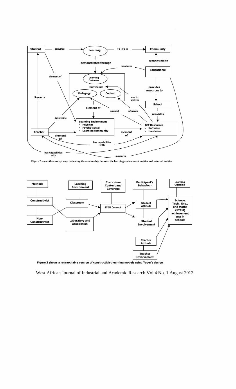
.
West African Journal of Industrial and Academic Research Vol.4 No. 1 August 2012
Student
Teacher
Learning
Curriculum
Learning
Outcome
Content Pedagogy
Learning Environment • Physical • Psycho-social • Learning community
element of
demonstrated through
ICT Resources
• Software • Hardware
Community
responsible to
School
provides
Educational
provides resources to
element of
To live in acquires
mandates
support influence
use to deliver
determine
element of
Supports
element of
has capabilities with
has capabilities with
supports
Figure 2 shows the concept map indicating the relationship between the learning environment entities and external entities
Figure 3 shows a researchable version of constructivist learning models using Yager’s design
Methods
Constructivist
Non-
Constructivist
Learning
Environment
Classroom
Laboratory and Association
Curriculum Content and Coverage
STEM Concept
Participant’s Behaviour
Student Attitude
Student Involvement
Teacher Attitude
Teacher
Involvement
Learning Outcome
Science,
Tech., Eng., and Maths
(STEM) achievement
test in schools

.
West African Journal of Industrial and Academic Research Vol.4 No. 1 August 2012
Comparative Analysis of the Functions 2n, n! and nn
Ogheneovo, E. E.; Ejiofor, C. and Asagba, P. O.
Department of Computer Science, University of Port Harcourt, Port Harcourt, Nigeria. [email protected], [email protected], [email protected]
Abstract In this paper, we have attempted to do comparative analysis of the following functions: 2n, n! and nn. We analyzed these functions, discussed how the functions can be computed and also studied how their computational time can be derived. The paper also discussed how to evaluate a given algorithm and determine its time complexity and memory complexity using graphical representation of the various functions, displaying how the function behaves graphically. However, it was noticed that when data are inputted into these functions, they gave cumbersome outputs that make it impossible to determine the execution (computational) time for the functions. We plotted a graph by taking a snapshot of the integer values n = 1 to 10 to compute the functions of 2n, n!, nn. From the graph, we noticed that 2n function had lower growth value; nn had the largest growth value and n! had slightly greater increase in growth than the 2n function. From our result, the execution time cannot be computed due to the largeness of the outputs. However, we were able to determine the function with the highest computing time and discovered that the time growth for the functions differs from one to the other. Keywords Algorithm, Pseudo code, Exponential functions, Recursion, Complexity. _________________________________________________________________________________ 1.0 Introduction Functions pervade all areas of mathematics and its applications. A function is a relation which associates any given number with another number [5]. Functions can be defined in several ways. We define a function from the set X into the set Y as a set of ordered pairs(x, y) where x is an element of x and y is an element of Y such that for X in x there is only one ordered pair (X, Y) in the function P. the notation used is f : X → Y or Y = f(x)Y or X → f(x)
or Y = f(X)
A function is a mapping or transformation of x into y or f(x). The variable x represents elements of the domain and is called the independent variable. The variable y representing elements of the range and is called the dependent variable (Clarke, 1996). The function y = f(x) is often called single valued function since there is a unique y in the range for each specified x. the converse may not necessarily be true, y = f(x) is the image of x. Often, a function depends on several independent variables. If there are n independent variables x1, x2,

.
West African Journal of Industrial and Academic Research Vol.4 No. 1 August 2012
x3, …, xn and the range is the set of all possible values of corresponding to the domain of (x1, x2, x3,
…, xn). We say that y is a function of xi’s, y = f(x1,
x2, x3, …, xn). Letters other than f may be used to represent a function [3] 2.0 Exponential Functions (2n And Nn) Exponential functions are perhaps the most important class of functions in mathematics. We use this type of function to calculate interest on investments, growth and decline rates of populations, forensic investigations as well as in many other applications (Constatinescu, 2004). The application of this function to a value x is written as exp(x). Equivalently, this can be written in the form of ex, where e is a mathematical constant, the base of the natural logarithm, which equals approximately 2.718281828, and is also known as Euler’s number (Schmidt and Makalic, 2009). As a function of the real variable x, the graph of y=ex is always positive (above the x axis) and increasing (viewed left-to-right). It never touches the x axis, although it gets arbitrarily close to it (thus, the x axis is a horizontal asymptote to the graph). It’s an inverse function [2]. Exponential growth is "bigger" and "faster" than polynomial growth. This means that, no matter what the degree is on a given polynomial, a given exponential function will eventually be bigger than the polynomial. Even though the exponential function may start out really, really small, it will eventually overtake the growth of the polynomial, since it doubles all the time [1]
2.1 Factorial The number of sequences that can exist with a set
of items, derived by multiplying the number of items by the next lowest number until 1 is reached. In Mathematics, product of all whole numbers up to 0 is considered. The special case zero factorial is defined to have value 0! = 1, consistent with the combinatorial interpretation of their being exactly on way to arrange zero objects. The factorial of all non-negative integers less than or equal to n.
n! = n(n-1)(n-2) … 3 x 2 x 1. where n! represents n factorial n = number of sets (items) For instance, the factorial operation is encountered in many different areas of mathematics, notably in combinatory, algebra, and mathematical analysis [13]. Its most basic occurrence is the fact that the definition of the factorial function can also be extended to non-integer arguments, while retrieving its most important properties [4]. 3.0 Computing Times Of Some Growing Functions. The time for different functions differs from one to the other. Some functions have a greater time growth than others. For example, we consider the figures 6 and 7 (the graphs) below; it shows how the computing times for 6 of the typical functions on the table grow with a constant equal to 1. You will notice how the times 0(n) and 0(nlogn) grow much more slowly than the others[9]. For large data set, algorithms with a complexity greater than 0(nlogn) are often impractical [14], [8]. An algorithm which is exponential will only be practical for very small values of n and even if we

.
West African Journal of Industrial and Academic Research Vol.4 No. 1 August 2012
decrease the leading constant, say by a factor of 2 or 3, we will not improve the amount of data we can handle significantly [7].
To see more precisely why a change in the constant, rather than to the order of an algorithm produces very little improvement in running time, we will consider the figure below:
Fig 6: Graphical representation of the functions 2n,n3, n2.
Fig 7: Graphical Representation of the functions nlog2n, n, log2n.

West African Journal of Industrial and Academic Research Vol.4 No. 1 August 2012 14
3.1 Comparing the Growth of Functions 2n, N!, Nn
Due to the fact that the execution time of function 2n, n!, nn is unreliable, and even though we had to give extra computing load to these functions, we still could not have a visible execution time. However, we decided to compare the growth of the functions in terms of the magnitude of the values they compute. We implemented these algorithms by using a program in the form of Turbo C++ program. When we entered the consecutive values for n from 1 – 150, the program generated growing output values for the various functions. We noticed that the program could not generate an output for the function when n is greater than 150. We decided to change the type of the value returned by the type of the value assigned to the local variable temp. The program was rerun and we noticed that although it
generated values for n > 200, there were some errors (problems) with the results of some of the functions. We noticed that the result generated by n! and nn started to generate negative integer values from n >= 20. In addition, we also discovered that after some time, n! started generating 0 as output. In other words, it stopped generating results as we continued increasing the integer values for n. 4.0 Discussion Of Results In this section, we are going to make a certain assertion about the behaviours for the growing functions of 2n, n!, nn and we also use a graph plotted of the functions against the values of n to discuss our findings. • With the graph of the growing function of 2n, n!, nn depicted in figure 8
Figure 8: Graphical representation of 2n, n!, nn
We plotted a graph by taking a snapshot of the integer values n= 1 to 10 to compute the growing functions of 2n, n!, nn. In this graph, we discovered that the 2n function had a lower growth of value than the n! and nn functions. We also noticed that the nn had the largest growth of values than the functions 2n and n! We observed also that n! had a slightly greater increase in growth than the 2n function.
5.0 Conclusion The execution time of functions cannot be calculated due to the largeness of the outputs when a value is inputted. However, we were able to determine the function with the highest computing time from the altitude of the curves in the graphs plotted. The time growth for functions differs from one to the other. Some grow much slowly than others while others are immensely fast. However,

.
West African Journal of Industrial and Academic Research Vol.4 No. 1 August 2012
the execution time could not be computed for the functions 2n, n!, and nn. ______________________________________________________________________________
References [1] Abramowitz and Stegun, (1972), Exponential Functions, In Handbook of Mathematical Functions with
Formulas, Graphs, and Mathematical Tables, New York, Dover, pp. 69 – 71. [2] Ahlfors, L. V. (1953), Complex Analysis, McGraw-Hill book Company Inc., U.S.A., pp. 56 – 80. [3] Anyanwu, S. A. C. (2002), Elementary Modern Algebra and trigonometry, Markowitz, Centre for Research and Development, Port Harcourt, pp. 203. [4] Borwein, P. (1985), Complexity of Calculating Factorials, Journal of Algorithm, Vol. 6, pp. 376 – 380. [5] Clark, G. D. (1996), Basic Calculus and co-ordinate Geometry for First Year University Students
, GODSONS Books, Port Harcourt, pp. 1 – 3. [6] Constantinescu, E. (2004), Inequalities for Logarithmic and Exponential Functions, General Mathematics, Vol. 12, No. 2, pp. 47 – 52. [7] Gerety, C. and Cull, P. (1986), Time Complexity of the Towers of Hanoi Problem, ACM SIGACT News, Vol. 18, No. 1, pp. 80 – 87. [8] Heileman, G. L. (1996), Data Structures, Algorithms and Object-Oriented Programming, Mo- Hill Book Co., Singapore, pp. 23 – 46. [9] Horowitz, E. and Sahni, S. (1978), Fundamentals of Computer Algorithms, Library of Congress Cataloguing, pp. 20 – 39. [10] Kruse, R. C. (1994), Data Structures and Program Design, Prentice-Hall, New Jersey, pp. 34 – 56. [11] Sahni, S. (1998), Data Structure, Algorithms and Application in C++, Mc-Hill Book Co., Singapore, pp. 15 – 39. [12] Schmids, D. F. and Makalic, E. (2009), Universal Models for the Exponential Distribution, IEEE Transactions on Information Theory, Vol. 55, No. 7, pp. 3087 – 3090. [13] Wikipedia, the Free Encyclopaedia, Factorials. [14] Wirth, N. (1976), Algorithms and Data structures, prentice-Hall, New Jersey, pp. 20 – 47.

.
West African Journal of Industrial and Academic Research Vol.4 No. 1 August 2012
Appendix A: Program Codes #include <iostream.h> #include <math.h> #include <time.h> #include <stdio.h> #define size 1000 double factorial(long); int main() long number, fact; double expon[size], factn[size], npowern[size]; cout<<" \n Enter the value of n: "; cin>>number; if(number < 0 ) cout<<" You have entered a wrong input!"<<"\n"; cout<<"\n Program stops!"; return 0; for(int i = 1; i <= number; i++) expon[i] = pow(2, i); factn[i]=factorial(i); npowern[i]= pow(i, i); cout<<"\tn 2 ^ n n! n ^ n \n"; cout<<"\t=== ===== === ===== \n"; for(int k = 1; k <= number; k++) cout<<"\t"<<k<<" "<<expon[k]<<" " <<factn[k]<<" "<< npowern[k]<<"\n"; getchar(); return 0; double factorial(long n) double temp; if(n == 1)return 1; if(n > 1)temp=n * factorial(n - 1); return temp;

.
West African Journal of Industrial and Academic Research Vol.4 No. 1 August 2012
Implementation of A Collaborative E-Learning Environment On A Linux Thin-Client
System
Onyejegbu L. N. and Ugwu C. Computer Science Department, University of Port-Harcourt, Rivers State, Nigeria.
[email protected], [email protected]
Abstract The advances in electronic technology have created opportunities for new instructional designs to be developed. Since Knowledge is expanding at a tremendous rate, these designs make it easy to impact the necessary knowledge (both practical) on people to enable them survive in a competitive environment. The Collaborative E-Learning Environment as an important group learning mode sets a goal of convenience and an adaptation into our technologically advanced society. It emphasizes the communication and information sharing among group members. Implementing this collaborative e-learning environment on a Linux thin-client system makes it possible for this environment to be available in most schools and companies because the Linux thin-clients are less expensive than other conventional computing systems. Developing a Collaborative E-Learning Environment on a Linux Thin-Client System provides a means of delivering an improved quality of education in our society. This paper involves the setting-up of Linux Thin-Client system, installing the appropriate applications necessary for this environment, and developing the interactive portal that will enable registered users to have access to the appropriate collaborative tools. Keywords: Bandwidth, Collaborative learning, E-learning, Linux, Thin-client
1.0 Introduction
Students learn best when they are actively involved in the process. Researchers report that, regardless of the subject matter, students working in small groups tend to learn more of what is taught and retain it longer than when the same content is presented in other instructional formats. Students who work in collaborative groups also appear more satisfied with their classes. Learning is enhanced when it is more like a team effort than a solo race. Good learning, like
good work, is collaborative and social, not competitive and isolated. Working with others often increases involvement in learning. Sharing one’s ideas and responding to other peoples ides, improves thinking and deepen understanding [3].
The term collaborative learning has been used in two different senses. In one sense, some have treated collaborative learning as a distinctive form of socially based learning that is fundamentally different from prevailing

.
West African Journal of Industrial and Academic Research Vol.4 No. 1 August 2012
psychological formulations. Another way to think about collaborative learning is not as a type of learning at all, but rather as a theory of instruction [4].
[2] defined collaborative learning as "a re-acculturative process that helps students become members of knowledge communities whose common property is different from the common property of the knowledge communities they already belong to ".Collaborative E-Learning Environment” is a collaborative, convenient, adaptive, and productive learning environment which allows different participants to communicate and coordinate with each other in a productive manner. Productivity and efficiency is obtained through synchronized communication between the different coordinating partners [8]. Within this process of synchronized communication, coordination can be accomplished by voice communication through video/voice conferencing, chat tools, share desktop and share applications [6]. Consequently, understanding the ideas and the techniques behind synchronized communication can be of great significance in the development of a Collaborative E-Learning Environment.
In this paper, a collaborative e-learning environment was developed on a Linux thin-client system, to allow communication between students and tutor(s). The operating system used is Fedora Core Linux. 2xThinClientServer software was installed on all the systems, and it was configured as a master server. A username and password was supplied to enable connection from the master server to MySQL database. After which the software that contains all the tools needed in the collaborative environment was installed. This
software is the Global Communications Network (GCN) software.
The Mozilla Firefox web browser was set on the server to popup with the URL to the portal services. This was achieved by writing a bash shell script that ran at systems start-up. A user must log in to the portal before he/she can have access to the lectures going on, lecture notes, and interact with other students that are equally logged on to the collaborative e-learning environment. 2.0 Review Of Relevant Concept The Linux thin-client technology is the system upon which collaborative e-learning environment is developed. Linux thin-clients have proven to be extremely reliable because tampering with settings are virtually non-existent, and in addition, an educational institution will also gain more control over how their students are using computing resources and access to data. Linux thin-client is distributed under the General Public License (GPL), meaning it is free. A thin-client (sometimes also called a lean or slim client) is a client computer or client software in client-server architecture networks which depends primarily on the central server for processing activities, and mainly focuses on conveying input and output between the user and the remote server. Thin-client can also be said to be a generic name for client machines on networks that deliver applications and data via a centralised computing model with the majority of processing carried out by the server(s). This is also known as server-based computing [1]. Typically, the thin-client terminal sends key strokes and mouse clicks to the server and the server sends screen updates to the terminal device Because of its flexibility and

.
West African Journal of Industrial and Academic Research Vol.4 No. 1 August 2012
cost effectiveness, thin client has been empowering schools, businesses, and organizations all over the world. Thin-client technology has high data security, low-maintenance, and terminals are less likely to be affected by virus because by default users are unable to tamper with settings [5]. Moreover, the entire system is simpler and easier to install and to operate. Linux Terminal Server Project (LTSP) is a free and open source add-on package for Linux that allow many people to simultaneously use the same computer. Applications are run on the server with a terminal known as a thin-client (also known as an X terminal) handling input and output. Generally, they are low-powered, absence of a hard disk; produce less noise than standard PCs, less prone to problems because they have fewer moving parts and no installed applications, as such producing a pleasant learning environment.
Server-Based Computing (SBC) is a technology whereby applications are deployed, managed, supported and executed on the server and not on the client. Only the screen information is transmitted between the server and client. This architecture
solves the many fundamental problems that occur when executing the applications on the client itself. SBC environments hardware and software upgrades, application deployment, technical support, data storage and backup are simplified because only the servers need to be managed. Data and applications reside on a few servers rather than on hundreds or thousands of clients [7]. 3.0 Problem Definition It is important to note that the economic survival and development of a nation depends on the productive capacity of the citizens, which depends on the kind of training and education the individuals receive from the educational sector in a nation. The problem of poverty has been used in most societies as an excuse and a reason why quality training and education is not given to students in most schools and organizations. This paper provides a way of providing information, bridge communication gap between people, and also training at a cheaper and less expensive rate.
4.0 Design For The Collaborative E- Learning Environment
Figure 1: Design for Collaborative E-Learning Environment
Figure 1 illustrates a design for this Collaborative E-Learning Environment.
The control computers (servers) consist of the following: mail server, print server, Domain Name

.
West African Journal of Industrial and Academic Research Vol.4 No. 1 August 2012
System (DNS) server, Dynamic Host Configuration Protocol (DHCP), Network-Attached Storage (NAS), and the server that serves the thin-clients with the user applications. Client: These are the students, administrative staffs, and academic staffs. Also the tutor can be an e-tutor. DHCP Sever: This is the Dynamic Host Configuration Protocol sever. It is used basically to dynamically allocate IP addresses to systems whose IP addresses are not statically configured. It is used mainly for fat clients that will be attached to the network, that is, in cases where some students or staff come with a laptop. DNS Sever: The Domain Name Service/System (DNS) sever is used to translate domain names into IP addresses. Print Server: This server manages the shared printers. Network Attached Storage (NAS): This is the file server, and it is dedicated to file storage. This is mainly where the electronic books and research materials will be stored.
Domain and Cooperate Mail Server: This server manages the domain and cooperate mail of staffs. Firewall and Router: This server is the gateway which controls asses to and from the network. 5.0 Developing The Collaborative
E-Learning Environment After choosing the server hardware (the control computer), the Fedora Core Linux OS distribution was installed. After which the 2x ThinClientServer software was installed. The 2X ThinCientServer is configured before starting up its services. This is done by opening the terminal as root (super user) and running the following commands: 2Xthinclientserver_conf.sh In the first part, the configuration script detects whether all necessary tools are present on the system. Then it ‘backs up’ the current configuration files for safe keeping. The license agreement is then reviewed and accepted to continue. Next, the network and security setup is probed. The total number of network interfaces installed on the machine is shown.

.
West African Journal of Industrial and Academic Research Vol.4 No. 1 August 2012
Figure 2: Master or Slave Menu Since our server was configured as a master server, there was a prompt for a username and password to connect to the local MySQL database. The following information was also asked for: Master server host name or IP: This is used by the slave servers, to communicate with the master server. Please note that hostnames are resolvable by all slaves. Internal IP address, as seen by the thin clients: This IP is used by the thin clients to communicate with the server. After entering all the information, the details were reviewed before proceeding with the configuration. After this phase, individual services were configured. The Apache and MySQL services, including all other services are started and the script exits. These lead to the configuration of the consoles and settings for direct connection to the terminal server. Settings were applied to individual thin client, by username, by group (effectively capturing all the members of the group). The next step was installing the software that was used in the collaborative environment. This software is the Global Communications Network (GCN) software. It contained all the tools that were needed in the environment. These tools consist of: E-mail, Chat Rooms, Private Messages, Games, a Web Browser, Popup-blocker, Profiles, Message Boards, Desktop Sharing, MSN, Yahoo, Voice Chat Rooms, Video Conferencing, Language Translation, File Transferring, Whiteboards and a Media Player.
The interactive portal was created using the Hyper Text Markup Language (HTML). This portal
enabled the users of the collaborative e-learning environment to have access to the needed tools.
1 6.0 Implementation, Methodology and
Updates After 2X ThinClientOS has booted from the client’s hard disk, it obtains the IP address of 2X ThinClientServer from the network settings returned by the 2X DHCP Helper Service.
Figure 3: 2X ThinClientOS booting up It now prompts for the username and password.
Figure 4:Log on screen
Acknowledgement We wish to acknowledge the contributions of Miss Enemugwem J. Silverline of Department of Computer Science, University of Port-Harcourt.

.
West African Journal of Industrial and Academic Research Vol.4 No. 1 August 2012
References
[1] Becta, 2007. http://www.becta.org.uk/publications (Accessed November 2010) [2] Brufee, K. 1993. Collaborative Learning. Baltimore, Johns Hopkins University Press
. UK. Pp24-32 [3] Chickering, A. W., and Gamson, Z. F. 1987. Seven Principles for Good Practice in Undergraduate Education, Wingspread Journal, vol, 9. No, 2. Pp 232-241. [4] Dillenbourg, P. 1999. Collaborative Learning, Cognitive and Computational Approaches, Oxford, Pergamon UK. Pp 53-57 [5] Richards, D. 2007. Linux Thin Client Networks, Design and Deployment, Packet Publishing, Birmingham. Pp 33-41 [6] Roschelle, J., and Teasley, S. 1995. The Construction of Shared Knowledge in
Collaborative Problem Solving in Computer Supported Collaborative Learning, Claire O'Malley, Berlin, Springer-Verlag USA. Pp 42-54.
[7] Server based computing, 2005. Retrieved from http://www.2x.com/whitepapers/WPserverbasedcomputing.pdf (Accessed April 2010)
[8] Tessmer, M., and Harris, D. 1992. Analyzing the instructional setting, Kogan publishers, London. Pp 67-73

.
West African Journal of Industrial and Academic Research Vol.4 No. 1 August 2012
An assessment of Internet Abuse in Nigeria
M.E Ezema*, H.C. Inyama+
Computer Science Department, University Nigeria Nsukka Email: [email protected]
+Department of Computer and Electronics Engineering, Nnamdi Azikiwe University Awka Anambra State Nigeria, Email : [email protected] Phone: 08034701121
Abstract As Internet use has proliferated worldwide, there has been debate whether some users develop disturbed patterns of Internet use (i.e., Internet abuse). This article highlights relevant literature on Internet abuse in Nigeria. Is the addiction paradigm appropriate for Internet use? Is behavior that has been labeled Internet abuse symptomatic of other problems such as depression, sexual disorders, or loneliness in Nigeria? What are alternative explanations for this phenomenon? Is there adequate research to support Internet abuse as a distinct disorder? Key words: Internet, Packet Switching, World Wide Web, Computer Crime, Cyber-bullying Malware Introduction The Internet was the result of some visionary thinking by people in the early 1960s that saw great potential value in allowing computers to share information on research and development in scientific and military fields. J.C.R. Licklider of MIT first proposed a global network of computers in 1962, and moved over to the Defense Advanced Research Projects Agency (DARPA) in late 1962 to head the work to develop it. Leonard Kleinrock of MIT and later UCLA developed the theory of packet switching, which was to form the basis of Internet connections. Lawrence Roberts of MIT connected a Massachusetts computer with a California computer in 1965 over dial-up telephone lines. It showed the feasibility of wide area networking, but also showed that the telephone
line's circuit switching was inadequate. Kleinrock's packet switching theory was confirmed. Roberts moved over to DARPA in 1966 and developed his plan for ARPANET. These visionaries and many more left unnamed here are the real founders of the Internet What is Internet Abuse? Defining Internet abuse is the first challenge, and creating an organization wide acceptable use policy (AUP) is the first step in the definition. Internet abuse refers to improper use of the internet and may include: computer crime, cyber bullying, spam and malwares. An acceptable use policy defines what constitutes Internet abuse in an organization. Acceptable Internet behaviour in one organization may be unacceptable in another, so the

.
West African Journal of Industrial and Academic Research Vol.4 No. 1 August 2012
acceptable use policy is a highly customized policy, based on the organizational mission. The organization determines what lines will be drawn when it comes to Internet abuse. The amount of resources and information the Internet contains is astounding. With the help of information collected on the net, people gain vast knowledge. Parents and children together can work to make the Internet a positive experience. However, some people can
misuse this wonderful knowledge bank and with no rules or regulations, can discover surreptitiously how to commit crimes, see things they ought not to see and chat with people of questionable character[1]. Thus parents ought to take precautions to see that their children do not abuse the internet access. On the other hand there are people who use the internet for nefarious activities and they strike to win converts among the unwary.
.
Fig 1: Review of the internet abuse in Nigeria Close monitoring and forbidden access The location of a computer may make a huge difference in the type of Web content one reads and surfs. If possible, computers should be in the office, living room, family room or some high traffic area so that one can always monitor the internet access. This will restrict abuse of the internet access at any given moment since someone may approach the computer while internet abuse is on going, hence people will be more cautious and careful of their online activities. On the other hand the cases of night browsing, parents should not allow their children to go to places they do not have adequate
trust on what their child may be doing or likely to be doing there at night. The highest of all is disciplined parents have to tell their children the implications of certain actions like watching bad films, discussing online with people you do not know their family background very well so that even if their parents are not at home with them they will be limited with what they do with the internet. Standard Internet Safety Another important thing that one needs to know is standard internet safety [3]. The key to a
INTERNET ABUSE
At home In the a cyber cafe
In a friends house
In the cafeteria At the market place

.
West African Journal of Industrial and Academic Research Vol.4 No. 1 August 2012
successful acceptable use policy (AUP) implementation in most organizations is similar to other policy development issues in the workplace. There must be “buy-in” from the “top-down”, in other words, the leaders of the organization must agree to the principles of the AUP and endeavour to push that policy down to the directors, managers and supervisors within the organization. The most critical stage of AUP development is dependent on upper management “buy-in” and their willingness to demonstrate the importance of this policy to the rest of the organization. It is very essential for one to know about computers and be familiar with the World Wide Web. Nothing can be more intimidating than a child knowing more about computers and internet than their parents, and often this is what happens with today's parents who probably know very little about internet compared to their children. Thus consider this aspect no one can know if something is amiss with a child while being totally repugnant if you do not know or understand the child's online activities
The Internet has become an invaluable resource in the workplace, the world's biggest reference library, social media centre, and pornography outlet is now only a click away. This availability presents a significant risk factor for employer liability and costs employers thousands of hours in productivity each day. Monitoring employee Internet use is one way to reduce employer liability, and whether or not you agree with the principles behind Internet monitoring, many employers agree that it is a necessary evil [2]. Internet abusers range from upper management employees in private offices viewing hardcore pornography, to the department
assistant in a cubicle that spends 3 hours a day using Facebook, doing online shopping, making travel arrangements, and paying bills through the company Internet. Internet abuse is endemic in the workplace and organizations are being forced to face the problem head on, or suffer the consequences. Among the many consequences of Internet abuse is a loss of productivity and scores of litigation issues such as sexual harassment, hostile work environment and discrimination. Monitoring Employee Internet access is one way that an organization can limit its liability. Holding a series of Internet workshops with employees of an organization is one way to introduce new acceptable use policy. As an educational session, an Internet workshop can address the sensitive issues surrounding Internet abuse in an open forum where employees can ask questions and provide input in a non-confrontational setting. During the Internet workshop, the organization can begin to educate the employees about Internet abuse and give them a chance to re-evaluate their Internet habits at work. It is important to be as open as possible with employees regarding chosen methodology for enforcing the AUP For example, if the organization has decided to employ Internet blocking technologies, the AUP should define the specific types of websites that will be blocked, for example, many organizations block pornography, “gross depictions” and “hate” websites. Discussing the types of websites the organization has decided to block and answering questions regarding the reasons for blocking will reinforce the organizational mission, and

.
West African Journal of Industrial and Academic Research Vol.4 No. 1 August 2012
demonstrate the types of websites that are inappropriate within an organization. If an organization is going to monitor and report on employee Internet access, the workshop will give one a chance to show the employees what the Internet reports look like, and discuss the circumstances in which they will be used. Taking the mystery out of what the organization is planning in regards to Internet monitoring and blocking will reduce employee speculation and set new expectations throughout the organization Problems with Internet Monitoring The technical aspects of blocking website access and monitoring employee Internet access are not without problems. The software for blocking websites has advanced tremendously over the past 5 years; however, there are still problems with blocking “all” inappropriate websites and blocking websites that you did not intend to block. No system is perfect and one will need assistance from a selected software or hardware vendor in addition to information systems department. If possible, it is always better to meet, in person, with the vendor representatives prior to the purchase of any Internet monitoring software. Voice your concerns with the vendor and secure “after sale” support with the vendor help desk. If you have an information systems department, one should make sure they are involved from the start of the project to help address any technical problems that the new system could bring. Monitoring Employee Internet Access - The People Side
Outside of the technical issues that will occur, the people side of Internet monitoring can be the most problematic of all. Even with the dissemination of information given at the Internet workshop and taking great care during policy development, some employees will, inevitably feel that Internet monitoring is unfair. Given this fact, it is of the utmost importance that the Internet reports are accurate, beyond question. Even if they are correct, there are still issues to consider. The scenarios listed below are examples of how employees could react if they are confronted with the accusation of Internet abuse. Moreover, the excuses below may be completely accurate and good explanation by the accused. "It wasn't me!" It is always possible that some other person was on the accused employee’s computer surfing the Internet. Once a user steps away from the computer, anything can happen. Another person sits down and starts using the computer logged in as the accused, everything they do on the Internet is recorded under somebody else's name. One suggestion is to have the user lock their computer before leaving for an extended period of time; this will reduce the chances of misidentification of the Internet abuser. "They have my password" This is a similar situation to the one mentioned above. If I have a user's password, I could log-in as the user and all of my Internet access would be attributed to them. How they got the password is another issue entirely, however the user makes a good point and has a potentially valid excuse for an Internet report that shows abuse.

.
West African Journal of Industrial and Academic Research Vol.4 No. 1 August 2012
"The Internet Report is Wrong" This can occur if the monitoring software is setup incorrectly or if there are network issues causing identification problems. This is another reason why one will want information systems department involved from the start and technical support from the vendor who sold the Internet monitoring solution. Defending an Internet report that shows abuse is difficult when you do not understand how the technical aspects of Internet monitoring work. Internet reporting is not an exact science, the reports could be wrong, and the person accused of Internet abuse may be completely innocent. The key is to research the potential offender and look into their history. People who abuse the Internet usually have a history of doing so, so look into their past Internet use first and then look at the Internet records on their computer. In short, do a “reality check”. Too often we take technology for its word and fail to look on the human side for insight that may confirm or make us question our suspicions. This practice will help reduce the number of errors that could be made during the investigation of Internet abuse, and help the employer maintain their credibility. Internet abuse is a fact of life in most large organizations today. Monitoring employee Internet use and employing blocking technologies can be
helpful in reducing employer liability and improving employee productivity. Developing an acceptable use policy to outline acceptable Internet behaviour in an organization is the first step in the process. To implement this policy successfully, the policy must be supported by upper, mid, and line level managers. The organization should endeavour, with enthusiasm, to educate the employees of the organization about Internet abuse and share the organizations plans to monitoring use and block inappropriate websites. Prior to purchasing a software or hardware solution for Internet monitoring and blocking, a vendor should be selected and invited into the organization to explain the technical problems that can occur with Internet monitoring and blocking technologies. During this vendor selection process, it is very important to include information systems department and other technical staff. Arranging after-sale support with the vendor of choice is highly recommended. Finally, there is the people side of the problem. Internet monitoring and blocking are only as good as the software and hardware solutions that are developed. There are many ways that these solutions can fail, so doing a thorough investigation prior to accusing an employee of Internet abuse is also highly recommended.
___________________________________________________________________________________
References [1] Acier, Didier and Laurence Kern. “Problematic Internet use: Perceptions of Addiction
Counselors.” Computers and Education. May 2011, Vol. 56: 983-989. [2] Block, Jerald. “Issues for DSM-V: Internet Addiction.” American Journal of Psychiatry. 2008, Vol. 165 No. 3: 306-307. [3] Internet Abuse, www.buzzle.com/editorials/1-13-2005-64163.

.
West African Journal of Industrial and Academic Research Vol.4 No. 1 August 2012
Instructions for Authors
WAJIAR provides a multidisciplinary forum for the publication of original research and technical papers, short communications, state-of-the-art developments in Information and communications technology, bio-medical informatics, computers, mathematics, control and information technology, physics, industrial electronics and engineering, Industrial chemistry, general technology, rocketry, space and astronomy, earth science, oceanography and the environment with special emphasis on the application of communications and information technology to these fields of importance in our modern civilization. The journal will review papers on advances, techniques, practice and application of information and communications technology in these areas. • Economics, Statistics and Mathematic • Information Technology & Applications • Electronics and Computer Engineering • Computer networks, Satellite & communications Engineering Research • Industrial Computer applications Today • Computer and Electro-Mechanical Maintenance • GPRS and Remote Sensing • Robotics ,Telemedicine & Remote Medical Monitoring • Artificial Intelligence & Expert Systems Development & Applications • Developments in Forensic Science Research • Information Assurance & Network Security: The African Dilemma • Space Information Systems & Rockery : which way for Africa • Video and Teleconferencing Innovations for Deployment in Africa • Telecommunications Technology & 4G Applications • Biotechnology • Agriculture , Food Technology & Processing Environmental Technology & Impact Analysis • E-Waste Management & Environmental Protection • Management Science & Operations Research • Wireless Technology, GSM and 4G Applications • Alternative ,Grid and Green Energy Solutions for Africa • Converting Academic Research in Tertiary Institutions for Industrial Production
WAJIAR is an international Journal of Science and Technology and is published quarterly in February, May, August and December.

.
West African Journal of Industrial and Academic Research Vol.4 No. 1 August 2012
Key Objectives: provide avenue for the advancement, dissemination of scientific and technology research in the fields of science and technology with special emphasis on the deployment of Information & Communications Technology as an enabler and solution tool.
Versions: Two versions of the journal will be published quarterly (electronic version posted in the web and hardcopy version. Submission
2 Typescript and soft copy in MS-word format should be submitted by email to: [email protected]. Typescripts should be written in English, double-spaced and single-sided on either Quarto or A4-sizeed sheets, and should be numbered beginning with the title page. The first page of an article should contain:
i) The title of the paper, the name(s) and address(s) of the author(s) ii) A short title not exceeding 45 letters with space
An abstract of 50-200 words should follow the title page on a separate sheet.
2.1 Text Headings and subheadings for different sections of the paper (e.g. Introduction, Methods, Results, and Discussions) should be clearly indicated. Units of measurement, abbreviations and symbols should follow the international system of units (SI), Equations and formulae should be typewritten or word-processed. Equations should be numbered consecutively with Arabic numerals in parentheses on the right-hand side of the page. Special symbols should be identified in the margin.
Tables and Figures Tables should be given short informative titles and should be numbered consecutively in Arabic numerals. Tables will be reproduced directly from the typed or word-processed softcopy. Figures in a form suitable for reproduction should be submitted separately from the text as original drawings in Indian ink, or as high contrast sharp photographs on glossy paper. Lettering on figures should be proportional to the size of the figure to ensure legibility after reduction. On the back of each figure, the orientation of the figure and the author and figure number should be cited consecutively in the text and a list of short descriptive captions should be provided at the end of the paper.
2.2 References References should be cited in the text using a number in square brackets in order of appearance. The references are listed at the end of the paper in numerical order.
General Information Proofs: Proofs will be sent to the nominated author to check typesetting accuracy. No changes to the original manuscript are accepted at this stage. Proofs should be returned within seven days of receipt.

.
West African Journal of Industrial and Academic Research Vol.4 No. 1 August 2012
Reprints: reprints may be ordered (pre-paid) at prices shown on the reprint order form which will be sent to the author together with the proofs. Page Charge: Please note that there will be a page charge of N20,000 or $100 (Twenty thousand naira or One Hundred American Dollars only) for each article accepted for publication in the journal. Annual Subscription is pegged at N20,000 or $125 per annum for four volumes. Electronic copies will be free access at our website. Subscription for the printed version will be completed via our Website www.wajiaredu.com. Subscriptions can also be sent via the journal’s email address: www.wajiaredu.com/webmail / [email protected] .ISSN: 2276-9129

.
West African Journal of Industrial and Academic Research Vol.4 No. 1 August 2012
West African Journal of Industrial & academic research
West African Journal of IndustrialWest African Journal of IndustrialWest African Journal of IndustrialWest African Journal of Industrial
& Academic Research& Academic Research& Academic Research& Academic Research Publications Office: International office::::
9-14 mbonu ojike Street 255 North D Stree
Ikenegbu, Owerri, Nigeria San Bernardino, CA 92401
Tel: 234 81219 41139 909.884.9000 www.wajiaredu.com
Editor-in-Chief: Prof. Oliver E. Osuagwu, PhD, FNCS, FBCS CITP, MIEEE, MACM Editorial Board: Prof Tony B.E. Ogiemien, PhD, BL, (USA), Engr. Prof E. Anyanwu, Ph.D, FNSE, Prof. G. Nworuh, PhD, Dr. B. C. Ashiegbu, PhD, Prof. C.O.E. Onwuliri, PhD, FAS ,
Prof .E. Emenyionu, PhD, (Connecticut USA,) Prof. E.P. Akpan, Ph.D, Engr. Prof. C.D. Okereke, Ph.D, Prof. B.E.B. Nwoko, Ph.D, Prof. N.N. Onu, PhD, Prof M.O. Iwuala, PhD, Prof C.E.Akujo, PhD, Prof. G. Okoroafor, PhD, Prof Leah Ojinna, Ph.D (USA), Prof. O. Ibidapo-Obe, PhD, FAS., Prof. E. Adagunodo, PhD, Prof. J.C .Ododo, PhD, Dan C. Amadi, PhD(English), Prof.(Mrs) S.C. Chiemeke, PhD, Prof (Mrs) G. Chukwudebe,PhD, FNSE, Dr. E.N.C. Okafor, PhD, Dr (Mrs) I. Achumba, Dr. T. Obiringa, PhD, Dr. S. Inyama, PhD, Prof. C. Akiyoku, PhD, Prof. John Ododo, PhD, Prof. E. Nwachukwu, Ph.D, FNCS, Dr. S. Anigbogu, PhD,FNCS, Prof. H. Inyama, PhD, FNSE .Prof. B.N.. Onwuagba, PhD, Prof J.N. Ogbulie, PhD
______________________________________________________________________________________________________________________________
Subscription Application Form Name of Subscriber:_____________________________________________________________ Institutional affiliation:___________________________________________________________ Mailing Address to send copies of journals __________________________________________ _____________________________________________________________________________ Email Address:_____________________________Tel:_________________________________ Version of Journal requested: (a) hard copy N20,000 or $125
(b) electronic N10000 or $63* Method of payment: Wire Transfer Visa Card Master Card Direct payment into our Diamond Bank
Account No:. 0024189096 Douglas Rd branch, Owerri Bank Draft Tick
All subscription Application should be forwarded to: [email protected] Subscribers Signature: _______________________ Date: DD/MM/YYYY___/____/___ *WWW.WAJIAREdu.com is free access. Electronic copies in form of e-book requested is what is mean here by “electronic”.
Copyright © 2022 FDOKUMEN