Welcome to ETABS

ISO ETA032913M1 Rev. 0 Berkeley, California, USA March 2013

Welcome to ETABS® 2013

Integrated Building Design Software

Copyright

Copyright Computers & Structures, Inc., 1978-2013 All rights reserved.

The CSI Logo®, SAP2000®, ETABS®, and SAFE® are registered trademarks of Computers & Structures, Inc. Watch & LearnTM is a trademark of Computers & Structures, Inc. Windows® is a registered trademark of the Microsoft Corporation. Adobe® and Acrobat® are registered trademarks of Adobe Systems Incorporated.

The computer programs SAP2000® and ETABS® and all associated documentation are proprietary and copyrighted products. Worldwide rights of ownership rest with Computers & Structures, Inc. Unlicensed use of these programs or reproduction of documentation in any form, without prior written authorization from Computers & Structures, Inc., is explicitly prohibited.

No part of this publication may be reproduced or distributed in any form or by any means, or stored in a database or retrieval system, without the prior explicit written permission of the publisher.

Further information and copies of this documentation may be obtained from:

Computers & Structures, Inc. www.csiberkeley.com

info@csiberkeley.com (for general information) support@csiberkeley.com (for technical support)

DISCLAIMER

CONSIDERABLE TIME, EFFORT AND EXPENSE HAVE GONE INTO THE

DEVELOPMENT AND TESTING OF THIS SOFTWARE. HOWEVER, THE USER

ACCEPTS AND UNDERSTANDS THAT NO WARRANTY IS EXPRESSED OR

IMPLIED BY THE DEVELOPERS OR THE DISTRIBUTORS ON THE ACCURACY

OR THE RELIABILITY OF THIS PRODUCT.

THIS PRODUCT IS A PRACTICAL AND POWERFUL TOOL FOR STRUCTURAL

DESIGN. HOWEVER, THE USER MUST EXPLICITLY UNDERSTAND THE BASIC

ASSUMPTIONS OF THE SOFTWARE MODELING, ANALYSIS, AND DESIGN

ALGORITHMS AND COMPENSATE FOR THE ASPECTS THAT ARE NOT

ADDRESSED.

THE INFORMATION PRODUCED BY THE SOFTWARE MUST BE CHECKED BY

A QUALIFIED AND EXPERIENCED ENGINEER. THE ENGINEER MUST

INDEPENDENTLY VERIFY THE RESULTS AND TAKE PROFESSIONAL

RESPONSIBILITY FOR THE INFORMATION THAT IS USED.

i

Contents

Welcome to ETABS

1 Introduction

History and Advantages of ETABS 1-1

What ETABS can do! 1-3

An Integrated Approach 1-4

Modeling Features 1-6

Analysis Features 1-7

Design Features 1-8

Detailing Features 1-8

2 Getting Started

Installing ETABS 2-1

If You Are Upgrading 2-1

About the Manuals 2-2

“Watch & Learn” Movies 2-2

CSi Wiki Technical Knowledgebase 2-3

Technical Support 2-3

Help Us to Help You 2-3

Telephone Support 2-4

Online Support 2-4

Welcome to ETABS

ii

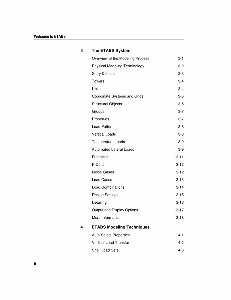
3 The ETABS System

Overview of the Modeling Process 3-1

Physical Modeling Terminology 3-2

Story Definition 3-3

Towers 3-4

Units 3-4

Coordinate Systems and Grids 3-5

Structural Objects 3-5

Groups 3-7

Properties 3-7

Load Patterns 3-8

Vertical Loads 3-8

Temperature Loads 3-9

Automated Lateral Loads 3-9

Functions 3-11

P-Delta 3-12

Modal Cases 3-12

Load Cases 3-13

Load Combinations 3-14

Design Settings 3-15

Detailing 3-16

Output and Display Options 3-17

More Information 3-18

4 ETABS Modeling Techniques

Auto-Select Properties 4-1

Vertical Load Transfer 4-2

Shell Load Sets 4-3

Contents

iii

Wind and Seismic Lateral Loads 4-4

Panel Zone Modeling 4-4

Wall Stacks 4-5

Live Load Reduction 4-5

Rigid and Semi-Rigid Floor Models 4-6

Edge Constraints 4-7

Cladding 4-8

Modifiers 4-8

Construction Sequence Loading 4-8

Design and Drift Optimization 4-9

Section Designer 4-10

More Information 4-10

5 ETABS Analysis Techniques

Linear Static Analysis 5-1

P-Delta Analysis 5-2

Nonlinear Static Analysis 5-3

Modal Analysis 5-3

Mass Source 5-4

Eigenvector Analysis 5-4

Ritz-Vector Analysis 5-5

Response Spectrum Analysis 5-6

Linear Time History Analysis 5-6

Nonlinear Time History Analysis 5-7

Buckling 5-8

More Information 5-8

History and Advantages of ETABS 1 - 1

Chapter 1

Introduction

ETABS is a sophisticated, yet easy to use, special purpose analysis and

design program developed specifically for building systems. ETABS

2013 features an intuitive and powerful graphical interface coupled with

unmatched modeling, analytical, design, and detailing procedures, all in-

tegrated using a common database. Although quick and easy for simple

structures, ETABS can also handle the largest and most complex build-

ing models, including a wide range of nonlinear behaviors, making it the

tool of choice for structural engineers in the building industry.

History and Advantages of ETABS

Dating back more than 40 years to the original development of TABS,

the predecessor of ETABS, it was clearly recognized that buildings con-

stituted a very special class of structures. Early releases of ETABS pro-

vided input, output and numerical solution techniques that took into con-

sideration the characteristics unique to building type structures, provid-

ing a tool that offered significant savings in time and increased accuracy

over general purpose programs.

Welcome to ETABS

1 - 2 History and Advantages of ETABS

As computers and computer interfaces evolved, ETABS added computa-

tionally complex analytical options such as dynamic nonlinear behavior,

and powerful CAD-like drawing tools in a graphical and object-based in-

terface. Although ETABS 2013 looks radically different from its prede-

cessors of 40 years ago, its mission remains the same: to provide the pro-

fession with the most efficient and comprehensive software for the

analysis and design of buildings. To that end, the current release follows

the same philosophical approach put forward by the original programs,

namely:

� Most buildings are of straightforward geometry with horizontal

beams and vertical columns. Although any building configura-

tion is possible with ETABS, in most cases, a simple grid system

defined by horizontal floors and vertical column lines can estab-

lish building geometry with minimal effort.

� Many of the floor levels in buildings are similar. This common-

ality can be used to dramatically reduce modeling and design

time.

� The input and output conventions used correspond to common

building terminology. With ETABS, the models are defined

logically floor-by-floor, column-by-column, bay-by-bay and

wall-by-wall and not as a stream of non-descript nodes and ele-

ments as in general purpose programs. Thus the structural defini-

tion is simple, concise and meaningful.

� In most buildings, the dimensions of the members are large in re-

lation to the bay widths and story heights. Those dimensions

have a significant effect on the stiffness of the frame. ETABS

corrects for such effects in the formulation of the member stiff-

ness, unlike most general-purpose programs that work on center-

line-to-centerline dimensions.

� The results produced by the programs should be in a form di-

rectly usable by the engineer. General-purpose computer pro-

grams produce results in a general form that may need additional

processing before they are usable in structural design.

Chapter 1 - Introduction

What ETABS Can Do! 1 - 3

What ETABS Can Do!

ETABS offers the widest assortment of analysis and design tools avail-

able for the structural engineer working on building structures. The fol-

lowing list represents just a portion of the types of systems and analyses

that ETABS can handle easily:

� Multi-story commercial, government and health care facilities

� Parking garages with circular and linear ramps

� Buildings with curved beams, walls and floor edges

� Buildings with steel, concrete, composite or joist floor framing

� Projects with multiple towers

� Complex shear walls and cores with arbitrary openings

� Buildings based on multiple rectangular and/or cylindrical grid

systems

� Flat and waffle slab concrete buildings

� Buildings subjected to any number of vertical and lateral load

cases and combinations, including automated wind and seismic

loads

� Multiple response spectrum load cases, with built-in input curves

� Automated transfer of vertical loads on floors to beams and walls

� Capacity check of beam-to-column and beam-to-beam steel con-

nections

� P-Delta analysis with static or dynamic analysis

� Explicit panel-zone deformations

� Construction sequence loading analysis

� Multiple linear and nonlinear time history load cases in any di-

rection

Welcome to ETABS

1 - 4 An Integrated Approach

� Foundation/support settlement

� Large displacement analyses

� Nonlinear static pushover

� Buildings with base isolators and dampers

� Design optimization for steel and concrete frames

� Design capacity check of steel column base plates

� Floor modeling with rigid or semi-rigid diaphragms

� Automated vertical live load reductions

And much, much more!

An Integrated Approach

ETABS is a completely integrated system. Embedded beneath the sim-

ple, intuitive user interface are very powerful numerical methods, design

procedures and international design codes, all working from a single

comprehensive database. This integration means that you create only one

model of the floor systems and the vertical and lateral framing systems to

analyze, design, and detail the entire building.

Everything you need is integrated into one versatile analysis and design

package with one Windows-based graphical user interface. No external

modules are required. The effects on one part of the structure from

changes in another part are instantaneous and automatic. The integrated

components include:

� Drafting for model generation

� Seismic and wind load generation

� Gravity load distribution for the distribution of vertical loads to

columns and beams when plate bending floor elements are not

provided as a part of the floor system

Chapter 1 - Introduction

An Integrated Approach 1 - 5

� Finite element-based linear static and dynamic analysis

� Finite element-based nonlinear static and dynamic analysis

(available in ETABS Nonlinear & Ultimate versions only)

� Output display and report generation

� Steel frame design (column, beam and brace)

� Concrete frame design (column and beam)

� Composite beam design

� Composite column design

� Steel joist design

� Shear wall design

� Steel connection design including column base plates

� Detail schematic drawing generation

ETABS 2013 is available in three different levels that all share the same

graphical user interface:

� ETABS 2013 Plus. Includes all available capabilities except for

certain nonlinear and dynamic analyses (p-delta and ten-

sion/compression only frame members are provided in all ver-

sions). Features include unmatched solution capacity with 64-bit

optimized solvers, shear wall modeling, multiple response spec-

trum analyses, linear modal time histories, numerous import and

export options, and comprehensive report generation. The steel

frame design, concrete frame design, composite beam design,

composite column design, steel joist design, shear wall design,

steel connection design and steel base plate design components

are all present.

� ETABS 2013 Nonlinear. Includes all of the features of ETABS

2013 Plus, with additional nonlinear static and dynamic capabili-

ties such as pushover, base isolation, dampers, Fast Nonlinear

Welcome to ETABS

1 - 6 Modeling Features

Analysis (FNA), Staged Construction, and multi-linear P-y

springs.

� ETABS 2013 Ultimate. Includes all of the features of ETABS

2013 Nonlinear with additional features such as nonlinear lay-

ered shell elements, linear and nonlinear direct integration time

history analysis, buckling, and the modeling of creep and shrink-

age behavior.

Modeling Features

The ETABS building is idealized as an assemblage of shell, frame, link

and joint objects. Those objects are used to represent wall, floor, column,

beam, brace and link/spring physical members. The basic frame geome-

try is defined with reference to a simple three-dimensional grid system.

With relatively simple modeling techniques, very complex framing situa-

tions may be considered.

The buildings may be unsymmetrical and non-rectangular in plan. Tor-

sional behavior of the floors and interstory compatibility of the floors are

accurately reflected in the results. The solution enforces complete three-

dimensional displacement compatibility, making it possible to capture

tubular effects associated with the behavior of tall structures having rela-

tively closely spaced columns.

Semi-rigid floor diaphragms may be modeled to capture the effects of in-

plane floor deformations. Floor objects may span between adjacent levels

to create sloped floors (ramps), which can be useful for modeling parking

garage structures.

Modeling of partial diaphragms, such as in mezzanines, setbacks, atriums

and floor openings, is possible without the use of artificial (“dummy”)

floors and column lines. It is also possible to model situations with mul-

tiple independent diaphragms at each level, allowing the modeling of

buildings consisting of several towers rising from a common base.

The column, beam and brace elements may be non-prismatic, and they

may have partial fixity at their end connections. They also may have uni-

form, partial uniform and trapezoidal load patterns, and they may have

Chapter 1 - Introduction

Analysis Features 1 - 7

temperature loads. The effects of the finite dimensions of the beams and

columns on the stiffness of a frame system are included using end offsets

that can be automatically calculated.

The floors and walls can be modeled as membrane elements with in-

plane stiffness only, plate bending elements with out-of-plane stiffness

only or full shell-type elements, which combine both in-plane and out-of-

plane stiffness. Floor and wall members may have uniform load patterns

in-plane or out-of-plane, and they may have temperature loads. The col-

umn, beam, brace, floor and wall members are all compatible with one

another.

Analysis Features

Static analyses for user specified vertical and lateral floor or story loads

are possible. If floors with plate bending capability are modeled, vertical

uniform loads on the floor are transferred to the beams and columns

through bending of the floor elements. Otherwise, vertical uniform loads

on the floor are automatically converted to span loads on adjoining

beams, or point loads on adjacent columns, thereby automating the tedi-

ous task of transferring floor tributary loads to the floor beams without

explicit modeling of the secondary framing.

The program can automatically generate lateral wind and seismic load

patterns to meet the requirements of various building codes. Three-

dimensional mode shapes and frequencies, modal participation factors,

direction factors and participating mass percentages are evaluated using

eigenvector or ritz-vector analysis. P-Delta effects may be included with

static or dynamic analysis.

Response spectrum analysis, linear time history analysis, nonlinear time

history analysis, and static nonlinear (pushover) analysis are all possible.

The static nonlinear capabilities also allow you to perform incremental

construction analysis so that forces that arise as a result of the construc-

tion sequence are included.

Results from the various static load cases may be combined with each

other or with the results from the dynamic response spectrum or time his-

tory analyses.

Welcome to ETABS

1 - 8 Design Features

Output may be viewed graphically, displayed in tabular output, compiled

in a report, exported to a database file, or saved in an ASCII file. Types

of output include reactions and member forces, mode shapes and partici-

pation factors, static and dynamic story displacements and story shears,

inter-story drifts and joint displacements, time history traces, and more.

Import and export of data may occur between third-party applications

such as Revit and AutoCAD from Autodesk, or with other programs that

support the CIS/2 or IFC data models.

ETABS uses the SAPFire™ analysis engine, the state-of-the-art equation

solver that powers all of CSI's software. This proprietary solver exploits

the latest in numerical technology to provide incredibly rapid solution

times and virtually limitless model capacity.

Design Features

Design of steel frames, concrete frames, concrete shear walls, composite

beams, composite columns, and steel joists can be performed based on a

variety of US and International design codes. Flexural, shear and deflec-

tion checks may all be performed depending upon the material and

member type. Steel and concrete frame members may be optimized from

autoselect lists, and concrete sections are designed using reinforcing bar

sizes chosen from US or International standards. Steel connection design

automates the review of beam-beam and beam-column connections

based on user specified bolt and shear plate preferences. Steel base plate

design verifies the size, thickness, and anchorage of the connection.

Detailing Features

Schematic construction drawings showing floor framing, column sched-

ules, beam elevations and sections, steel connection schedules, and con-

crete shear wall reinforcing may be produced. Concrete reinforcement of

beams, columns, and walls may be selected based on user-defined rules.

Any number of drawings may be created, containing general notes, plan

views, sections, elevations, tables, and schedules. Drawings may be

printed directly from ETABS or exported to DXF or DWG files for fur-

ther refinement.

Installing ETABS 2 - 1

Chapter 2

Getting Started

ETABS is an easy to use, yet extremely powerful, special purpose pro-

gram developed expressly for building systems. This chapter will help

you get started using the program.

Installing ETABS

Please follow the installation instructions provided in the separate instal-

lation document included in your ETABS Package, or ask your system

administrator to install the program and give you access to it.

If You are Upgrading

If you are upgrading from an early version of ETABS, be aware that the

model is now defined in terms of objects, which are automatically and

internally meshed into elements during analysis.

Welcome to ETABS

2 - 2 About the Manuals

This significant change drastically improves the capability of the pro-

gram, and we recommend that you read the remainder of this manual to

familiarize yourself with this and the many other new features.

About the Manuals

This volume is designed to help you quickly become productive with

ETABS. It provides this Welcome to ETABS manual, a User’s Guide and

an Introductory Tutorial. The next chapter of this Welcome to ETABS

manual provides a synopsis of the terminology used in ETABS, and

Chapters 4 and 5 describe modeling and analysis techniques, respec-

tively. The 15 chapters of the User’s Guide provide an introduction to

the steps and menu items used to create, analyze, design and detail a

model. The Introductory Tutorial describes the model creation, analysis,

and design processes for an example model.

It is strongly recommended that you read this manual and view the tuto-

rial movies (see “Watch & Learn” Movies) before attempting to com-

plete a project using ETABS.

Additional information can be found in the on-line Help facility available

within the ETABS graphical user interface, including Technical Notes

that describe code-specific design algorithms. Those documents are

available in Adobe Acrobat PDF format on the ETABS DVD, and can be

accessed from within the program using the Help menu.

“Watch & Learn” Movies

One of the best resources available for learning about the ETABS pro-

gram is the “Watch & Learn” movies series, which may be accessed on

the ETABS DVD or via the CSI web site at http://www.csiberkeley.com.

Those movies contain a wealth of information for both the first-time user

and the experienced expert, covering a wide range of topics, from basic

operation to complex modeling. The movies range from a few minutes to

nearly a half hour in length.

Chapter 2 - Getting Started

CSi Wiki Technical Knowledgebase 2 - 3

CSi Wiki Technical Knowledgebase

CSi maintains a Wiki page containing answers to frequently asked sup-

port questions as well as additional insights on program operation. This

is a good first stop before contacting technical support because many of

the most common, as well as some esoteric, questions are answered here.

This page is fully indexed and searchable, and may be found at

https://wiki.csiberkeley.com.

Technical Support

Free technical support is available from Computers and Structures, Inc.

(CSI) via telephone and e-mail for 90 days after the software has been

purchased. After 90 days, priority technical support is available only to

those with a yearly Support, Upgrade and Maintenance plan (SUM).

Customers who do not have a current SUM subscription can obtain tech-

nical support, but via e-mail only and at the non-priority level. Please

contact CSI or your dealer to inquire about purchasing a yearly SUM

subscription.

If you have questions regarding use of the software, please:

� Consult the documentation and printed information included

with your product.

� Check the on-line Help facility in the program.

� Visit the ETABS Wiki page.

If you cannot find an answer, then contact us as described in the sections

that follow.

Help Us to Help You

Whenever you contact us with a technical support question, please pro-

vide us with the following information to help us help you:

Welcome to ETABS

2 - 4 Telephone Support

� The program level (PLUS, Nonlinear or Ultimate) and version

number that you are using. This can be obtained from inside the

program using the Help menu > About ETABS command.

� A description of your model, including a picture, if possible.

� A description of what happened and what you were doing when

the problem occurred.

� The exact wording of any error messages that appeared on your

screen.

� A description of how you tried to solve the problem.

� The computer configuration (make and model, processor, oper-

ating system, hard disk size, and RAM size).

� Your name, your company’s name, and how we may contact

you.

Telephone Support

Priority telephone support is available to those with a current SUM sub-

scription via a toll call between 8:30 A.M. and 5:00 P.M., Pacific time,

Monday through Friday, excluding U.S. holidays. You may contact

CSI’s office via phone at (510) 649-2200.

When you call, please be at your computer and have the program manu-

als displayed.

Online Support

Online support can be obtained as follows:

• Send an e-mail and your model file to support@csiberkeley.com

• Visit CSI’s web site at http://www.csiberkeley.com.

If you send us e-mail, be sure to include all of the information requested

in the previous “Help Us to Help You” section.

Overview of the Modeling Process 3 - 1

Chapter 3

The ETABS System

ETABS analyzes, designs and details your building structure using a

model that you create using the graphical user interface. The key to suc-

cessfully implementing ETABS is to understand the unique and powerful

approach the program takes in modeling building systems. This chapter

will provide an overview of some of the key components and their asso-

ciated terminology.

Overview of the Modeling Process

A model developed using this program is different from models pro-

duced in many other structural analysis programs for two main reasons:

� This program is optimized for modeling building systems. Thus,

the modeling procedures and design capabilities are all tailored

to buildings.

� This program’s model is object-based. It consists of joint, frame,

link and shell objects. You make assignments to those objects to

define structural members such as beams, columns, braces,

Welcome to ETABS

3 - 2 Physical Modeling Terminology

floors, walls, ramps and springs. You also make assignments to

those same objects to define loads.

In its simplest form, developing a model requires three basic steps:

� Draw a series of joint, frame, link and shell objects that represent

your building using the various drawing tools available within

the graphical interface.

� Assign structural properties (sections and materials) and loads to

objects using the Assign menu options. Note that the assignment

of structural properties may be completed concurrently with the

drawing of the object using the Properties of Object form that

displays when Draw commands are used.

� Verify meshing parameters for floor (if they are not membrane

slab/deck/plank sections) and wall shell objects. Maximum mesh

size may be set independently for floors and walls.

When the model is complete, the analysis may be run. At that time, the

program automatically converts the object-based model into an element-

based model–this is known as the analysis model–that is used for the

analysis. The analysis model consists of joints, frame elements, link ele-

ments and shell (membrane and plate) elements that mathematically rep-

resent the structural members, i.e., columns, beams, braces, walls, floors,

etc. The conversion to the analysis model is internal to the program and

essentially transparent to the user.

Physical Modeling Terminology

In ETABS, we often refer to Objects, Members, and Elements. Objects

represent the physical structural members in the model. Elements, on the

other hand, refer to the finite elements used internally by the program to

generate the stiffness matrices. In many cases, objects and physical

members will have a one-to-one correspondence, and it is these objects

that the user “draws” in the ETABS interface. Objects are intended to be

an accurate representation of the physical members. Users typically do

not need to concern themselves with the meshing of those objects into

the elements required for the mathematical or analysis model. For in-

Chapter 3 - The ETABS System

Story Definition 3 - 3

stance, a single frame object can model a complete beam, regardless of

how many other members frame into it, and regardless of the loading.

With ETABS, model creation and the reporting of results are accom-

plished at the object level.

This differs from a traditional analysis program, where the user is re-

quired to define a sub-assemblage of finite elements that comprise the

larger physical members. In ETABS, the objects, or physical members

drawn by the user, are typically subdivided internally into the greater

number of finite elements needed for the analysis model, without user

input. Because the user is working only with the physical member based

objects, less time is needed to create the model and to interpret the re-

sults, with the added benefit that analysis results are generally more ap-

propriate for the design work that follows.

The concept of objects in a structural model may be new to you. It is ex-

tremely important that you grasp this concept because it is the basis for

creating a model in ETABS. After you understand the concept and have

worked with it for a while, you should recognize the simplicity of physi-

cal object-based modeling, the ease with which you can create models

using objects, and the power of the concept when editing and creating

complex models.

Story Definition

One of the most powerful features that ETABS offers is the recognition

of story levels, allowing for the input of building data in a logical and

convenient manner. Users may define their models on a floor-by-floor,

story-by-story basis, analogous to the way a designer works when laying

out building drawings. Story levels help identify, locate and view spe-

cific areas and objects of your model; column and beam objects are eas-

ily located using their plan location and story level labels.

In ETABS terminology, a story level represents a horizontal plane cut

through a building at a specified elevation, and all of the objects below

this plane down to the next story level. Because ETABS inherently un-

derstands the geometry of building systems, a user can specify that an

object being drawn be replicated at all stories, or at all similar stories as

Welcome to ETABS

3 - 4 Towers

identified by the user. This option works not only for repetitive floor

framing, but also for columns and walls. Story labeling, the height of

each story level, as well as the ability to mark a story as similar, are all

under the control of the user.

Towers

ETABS allows multiple towers to be defined, each with their own grid

system and story data. This allows for the modeling of multiple buildings

on a common podium. Views may be set to display one tower, all towers,

or any combination thereof.

Units

ETABS works with four basic units: force, length, temperature, and time.

Any units may be used at any time while working on the model, e.g.,

inch units for beam sections and feet units for grid layout. Time is always

measured in seconds.

Angular measure always uses the following units:

� Geometry, such as axis orientation, is always measured in de-

grees.

� Rotational displacements are always measured in radians.

� Frequency is always measured in cycles/second (Hz).

An important distinction is made between mass and weight. Mass is used

for calculating dynamic inertia and for loads caused by ground accelera-

tion only. Weight is a force that can be applied like any other force load.

Be sure to use force units when specifying weight values, and mass units

(force-sec2/length) when specifying mass values.

When you start a new model, you will be asked to initialize with either

"U.S." or "Metric" base units. This option sets the default units for the

model and controls which units are used internally to save the model -

input and output are always converted to and from the internal base units.

Chapter 3 - The ETABS System

3 - 5

Coordinate Systems and Grids

All locations in the model are ultimately defined with respect to a single

global coordinate system. This is a three-dimensional, right-handed, Car-

tesian (rectangular) coordinate system. The three axes, denoted X, Y, and

Z, are mutually perpendicular, and satisfy the right-hand rule.

ETABS always considers the +Z direction as upward. By default, gravity

acts in the –Z direction.

Additional coordinate systems can be defined to aid in developing and

viewing the model. For each coordinate system, a three-dimensional grid

system would be defined consisting of “construction” lines that are used

for locating objects in the model. Each coordinate/grid system may be of

Cartesian (rectangular) or cylindrical definition, and is positioned rela-

tive to the global system. When you move a grid line, specify whether

the objects in the model move with it.

Drawing operations tend to “snap” to gridline intersections (default)

unless you turn this feature off. Numerous other snaps are available, in-

cluding snap to line ends and midpoints, snap to intersections, and so

forth. Use these powerful tools whenever possible to ensure the accurate

construction of your model. Not using the snaps may result in “gaps” be-

tween objects, causing errors in the model’s connectivity.

Each object in the model has its own local coordinate system used to de-

fine properties, loads, and responses. The axes of each local coordinate

system are denoted 1 (red), 2 (green), and 3 (blue). Local coordinate sys-

tems do not have an associated grid.

Structural Objects

As stated previously, ETABS uses objects to represent physical structural

members. When creating a model, the user starts by drawing the geome-

try of the object, and then assigning properties and loads to completely

define the building structure.

The following object types are available, listed in order of geometrical

dimension:

Welcome to ETABS

3 - 6 Structural Objects

� Joint objects of two types:

o Joint objects are automatically created at the corners or

ends of all other types of objects, and they can be explic-

itly added anywhere in the model.

o Spring or Grounded (one joint) link objects are used

to model external springs and special support behavior,

such as isolators, dampers, gaps, multi-linear springs and

more.

� Frame objects are used to model beams, columns, braces and

trusses.

• Link (connecting two-joint) objects are used to model special

member behavior, such as isolators, dampers, gaps, multi-linear

springs, and more. Unlike frame objects, connecting link objects

can have zero length.

� Shell objects are used to model walls, slabs, decks, planks, and

other thin-walled members. Shell objects will be meshed auto-

matically into the elements needed for analysis. Walls and floors

with both membrane and plate behavior (e.g., cast-in-place solid,

waffle, & ribbed slabs) are meshed using a rectangular mesh

with a maximum size set by the user. If horizontal objects with

only membrane definition are included in the model (e.g., decks

and planks), the objects are meshed in a manner such that the

vertical loads will be properly distributed to supporting mem-

bers.

As a general rule, the geometry of the object should correspond to that of

the physical member. This simplifies the visualization of the model and

helps with the design process.

When you run an analysis, ETABS automatically converts your object-

based model into an element-based model that is used for analysis. This

element-based model is called the analysis model, and it consists of tradi-

tional finite elements and joints. After running the analysis, your object-

based model still has the same number of objects in it as it did before the

analysis was run.

Chapter 3 - The ETABS System

Groups 3 - 7

Although the majority of the object meshing is performed automatically,

you do have control over how the meshing is completed, such as the de-

gree of refinement and how to handle the connections at intersecting ob-

jects. An option is also available to manually subdivide the model, which

divides an object based on a physical member into multiple objects that

correspond in size and number to the analysis elements.

Groups

A group is a named collection of objects. It may contain any number of

objects of any number of types. Groups have many uses, including:

� Quick selection of objects for editing and assigning.

� Defining section cuts across the model.

� Grouping objects that are to share the same design.

� Selective output.

Define as many groups as needed. Using groups is a powerful way to

manage larger models.

Properties

Properties are “assigned” to each object to define the structural behavior

of that object in the model. Some properties, such as materials and sec-

tion properties, are named entities that must be specified before assigning

them to objects. For example, a model may have:

� A material property named CONCRETE.

� A rectangular frame section property named RECTANGLE, and

a circular frame section named CIRCULAR, both using material

property CONCRETE.

� A slab section property named SLAB that also uses material

property CONCRETE.

Welcome to ETABS

3 - 8 Load Patterns

If you assign frame section property RECTANGLE to a frame object,

any changes to the definition of section RECTANGLE or material CON-

CRETE will automatically apply to that object. A named property has no

effect on the model unless it is assigned to an object.

Other properties, such as frame releases or joint restraints, are assigned

directly to objects. Those properties can be changed only by making an-

other assignment of that same property to the object; they are not named

entities and they do not exist independently of the objects.

Load Patterns

Loads represent actions upon the structure, such as force, pressure, sup-

port displacement, thermal effects, and others. A spatial distribution of

loads upon the structure is called a load pattern.

As many named load patterns as needed can be defined. Typically, sepa-

rate load patterns would be defined for dead load, live load, static earth-

quake load, wind load, snow load, thermal load, and so on. Loads that

need to vary independently, for design purposes or because of how they

are applied to the building, should be defined as separate load patterns.

After defining a load pattern name, you must assign specific load values

to the objects as part of that load pattern, or define an automated lateral

load if the case is for seismic or wind. The load values you assign to an

object specify the type of load (e.g., force, displacement, temperature),

its magnitude, and direction (if applicable). Different loads can be as-

signed to different objects as part of a single load pattern, along with the

automated lateral load, if so desired. Each object can be subjected to

multiple load patterns.

Vertical Loads

Vertical loads may be applied to joint, frame and shell objects. Vertical

loads are typically input in the gravity, or -Z direction. Joint objects can

accept concentrated forces or moments. Frame objects may have any

number of point loads (forces or moments) or distributed loads (uniform

Chapter 3 - The ETABS System

Temperature Loads 3 - 9

or trapezoidal) applied. Uniform loads can be applied to Shell objects.

Vertical load cases may also include element self-weight.

Some typical vertical load cases used for building structures might in-

clude:

� Dead load

� Superimposed dead load

� Live load

� Reduced live load

� Snow load

If the vertical loads applied are assigned to a reducible live load pattern,

ETABS provides you with an option to reduce the live loads used in the

design phase. Many different types of code-dependent load reduction

formulations are available.

Temperature Loads

Temperature loads on frame and shell objects can be generated in

ETABS by specifying temperature changes. Those temperature changes

may be specified directly as a uniform temperature change on the object,

or they may be based on previously specified point object temperature

changes, or on a combination of both.

If the point object temperature change option is selected, the program as-

sumes that the temperature change varies linearly over the object length

for frames, and linearly over the object surface for shells. Although you

can specify a temperature change for a joint object, temperature loads act

only on frame and shell objects.

Automated Lateral Loads

ETABS allows for the automated generation of static lateral loads for

earthquake (seismic) and wind load cases based on numerous code speci-

Welcome to ETABS

3 - 10 Automated Lateral Loads

fications, including, but not limited to, ASCE, BOCA, UBC, NBCC, AS,

BS, NZS, Chinese, Italian, Mexican, Turkish and EUROCODE. Two

automatic static lateral loads can not be in the same load pattern. Thus,

define each automatic static lateral load in a separate load pattern. How-

ever, additional user-defined loads can be added to a load pattern that in-

cludes an auto lateral load.

When seismic has been selected as the load type, various auto lateral

load codes are available. Upon selection of a code, the Seismic Load Pat-

tern form is populated with default values and settings that may be re-

viewed and edited by the user. The program uses those values to generate

lateral loads in the specified direction based on the weight defined by the

masses assigned or calculated from the property definitions. After

ETABS has calculated a story level force for an automatic seismic load,

that force is apportioned to each joint at the story level elevation in pro-

portion to its mass. Seismic auto lateral loads should not be used with

models that contain more than one tower as an incorrect distribution of

lateral loads may occur.

If wind has been selected as the load type, various auto lateral load codes

are available. Upon selection of a code, the Wind Load Pattern form is

populated with default values and settings, which may be reviewed and

edited by the user. In ETABS, automatically calculated wind loads may

be applied to diaphragms (rigid or semi-rigid), or to walls and frames, in-

cluding non-structural walls such as cladding that are created using shell

objects, and to frames in open structures. If the rigid diaphragm option is

selected, a separate load is calculated for each rigid diaphragm present at

a story level. The wind loads calculated at any story level are based on

the story level elevation, the story height above and below the level, the

assumed exposure width for the rigid diaphragm(s) at that level and the

various code-dependent wind coefficients. The load is applied to a rigid

diaphragm at what ETABS calculates to be the geometric center.

Wind loads applied to semi-rigid diaphragms are calculated at each story

level in a manner similar to that for the rigid diaphragms, but are then

applied to every joint throughout the diaphragm. Although every joint in

the diaphragm receives some load, the distribution of the forces is done

in such a way that the resultant of the applied wind load passes through

the diaphragm’s geometric center.

Chapter 3 - The ETABS System

Functions 3 - 11

If the option has been selected whereby wind loads are calculated and

applied via shell objects defining walls, a wind pressure coefficient must

be assigned to each shell object that has exposure, and it must be speci-

fied as windward or leeward. On the basis of the various code factors and

user defined coefficients and exposures, ETABS calculates the wind

loads for each shell (wall) object and applies the loads as point forces at

the corners of the object. In addition, some codes allow wind loads to be

generated for exposed frame members (i.e., lattice or open structures), in

which case the program calculates joint forces based on the code selected

and the solid to gross area ratio specified. Wind auto lateral loads should

not be used with models that contain more than one tower as an incorrect

distribution of lateral loads may occur.

Functions

Functions are defined to describe how a load varies as a function of pe-

riod, time or frequency. Functions are only needed for certain types of

analysis; they are not used for static analysis. A function is a series of

digitized abscissa-ordinate data pairs.

There are two types of functions:

� Response spectrum functions are psuedo-spectral acceleration

versus period functions for use in response spectrum analysis. In

this program, the acceleration values in the function are assumed

to be normalized; that is, the functions themselves are not as-

sumed to have units. Instead, the units are associated with a scale

factor that multiplies the function and is specified when you de-

fine the response spectrum case.

� Time history functions are loading magnitude versus time func-

tions for use in time history analysis. The loading values in a

time history function may be ground acceleration values or they

may be multipliers for specified (force or displacement) load pat-

terns.

Define as many named functions as necessary. They are not assigned to

objects, but are used in the definition of Response Spectrum and Time

History cases.

Welcome to ETABS

3 - 12 P-Delta

P-Delta

P-Delta options are set to determine the type of P-Delta to use. P-Delta

refers to the nonlinear geometric effect that gravity loads have upon the

lateral stiffness of buildings. There are three options:

� None: No P-Delta is included in the analysis.

� Non-iterative: An efficient (but approximate) P-Delta technique

computed automatically from story mass.

� Iterative: A computationally robust approach based on a user

specified combination of loads.

P-Delta may also be specified using a static nonlinear load case.

Modal Cases

A modal case defines the type and number of modes to be extracted from

the model. An unlimited number of modal cases may be defined, al-

though for most purposes a single case is enough. Each modal case re-

sults in a set of modes, and each mode consists of a mode shape (normal-

ized deflected shape) and a set of modal properties, such as period and

cyclic frequency. The dynamic modes of the structure are calculated us-

ing either eigenvector or Ritz-vector methods:

� Eigenvector Analysis: Determines the undamped free-vibration

mode shapes and frequencies of the system, which provide an

excellent insight into the behavior of the building.

� Ritz-vector Analysis: Modes are generated by taking into ac-

count the spatial distribution of the dynamic loading, which

yields more accurate results than the use of the same number of

natural mode shapes. Ritz-vector modes do not represent the in-

trinsic characteristics of the structure in the same way the natural

(eigenvector) modes do.

A modal case is required in order to run either a response-spectrum or a

modal time-history load case.

Chapter 3 - The ETABS System

Load Cases 3 - 13

Load Cases

A load case defines how loads are to be applied to the structure, and how

the structural response is to be calculated. Many types of load cases are

available. Most broadly, load cases are classified as linear or nonlinear,

depending on how the structure responds to the loading.

The results of linear analyses may be superposed, i.e., added together, af-

ter analysis. The following types of load cases are available:

� Static: The most common type of analysis. Loads are applied

without dynamical effects.

� Response-Spectrum: Statistical calculation of the response

caused by acceleration loads. Requires response-spectrum func-

tions.

� Time-History: Time-varying loads are applied. Requires time-

history functions. The solution may be by modal superposition or

direct integration methods.

� Buckling: Calculation of buckling modes under the application

of loads.

The results of nonlinear load cases normally should not be superposed.

Instead, all loads acting together on the structure should be combined di-

rectly within the specific nonlinear load case. Nonlinear load cases may

be chained together to represent complex loading sequences. The follow-

ing types of nonlinear load cases are available:

� Nonlinear Static: Loads are applied without dynamical effects.

May be used for pushover analysis.

� Nonlinear Staged Construction: Loads are applied without dy-

namical effects, with portions of the structure being added or

removed. Time-dependent effects can be included, such as creep,

shrinkage, and aging.

Welcome to ETABS

3 - 14 Load Combinations

� Nonlinear Time-History: Time-varying loads are applied. Re-

quires time-history functions. The solution may be by modal su-

perposition or direct integration methods.

Any number of named load cases of any type may be defined. When the

model is analyzed, the load cases to be run must be selected. Results for

any load case may be selectively deleted.

Analysis results, when available, can be considered to be part of the

model. They are needed to perform design.

Load Combinations

ETABS allows for the named combination of the results from one or

more load cases and/or other combinations. When a combination is de-

fined, it applies to the results for every object in the model.

The five types of combinations are as follows:

� Linear Add: Results from the included load cases and combina-

tions are added.

� Envelope: Results from the included load cases and combina-

tions are enveloped to find the maximum and minimum values.

� Absolute Add: The absolute values of the results from the in-

cluded load cases and combinations are added.

� SRSS: The square root of the sum of the squares of the results

from the included load cases and combinations is computed.

� Range Add: Positive values are added to the maximum and

negative values are added to the minimum for the included load

cases and combos.

Except for the Envelope type, combinations should usually be applied

only to linear load cases, because nonlinear results are not generally su-

perposable.

Chapter 3 - The ETABS System

Design Settings 3 - 15

Design is always based on combinations, not directly on load cases. A

combination can be created that contains only a single load case. Each

design algorithm creates its own default combinations; supplement them

with your own design combinations if needed.

Design Settings

ETABS offers the following integrated design postprocessors:

� Steel Frame Design

� Concrete Frame Design

� Composite Beam Design

� Composite Column Design

� Steel Joist Design

� Shear Wall Design

� Steel Connection Design

The first five design procedures are applicable to frame objects, and the

program determines the appropriate design procedure for a frame object

when the analysis is run. The design procedure selected is based on the

line object’s orientation, section property, material type and connectivity.

Shear wall design is available for objects that have previously been iden-

tified as piers or spandrels, and both piers and spandrels may consist of

both shell and frame objects.

Steel connection design will identify which beam-to-beam and beam-to-

column locations have adequate load transfer capacity using the standard

connections specified in the connection preferences. Steel connection de-

sign also includes sizing and design capacity checks for column base

plates.

For each of the first five design postprocessors, several settings can be

adjusted to affect the design of the model:

Welcome to ETABS

3 - 16 Detailing

� The specific design code to be used for each type of object, e.g.,

AISC 360-10 for steel frames, EUROCODE 2-2004 for concrete

frames, and BS8110 97 for shear walls.

� Preferences for how these codes should be applied to a model.

� Combinations for which the design should be checked.

� Groups of objects that should share the same design.

� Optional “overwrite” values for each object that supersede the

default coefficients and parameters used in the design code for-

mulas selected by the program.

For steel and concrete frames, composite beam, composite column, and

steel joist design, ETABS can automatically select an optimum section

from a list you define. The section also can be changed manually during

the design process. As a result, each frame object can have two different

section properties associated with it:

� An “analysis section” used in the previous analysis

� A “design section” resulting from the current design

The design section becomes the analysis section for the next analysis,

and the iterative analysis and design cycle should be continued until the

two sections become the same.

Design results for the design section, when available, as well as all of the

settings described herein, can be considered to be part of the model.

Detailing

ETABS offers the ability to produce schematic construction documents

for buildings. Preferences may be set for the size and layout of draw-

ings; dimensioning units and label prefixes; and reinforcing bar sizes for

beams, columns and shear walls. Generated drawings, accessible on the

Detailing tab of the Model Explorer window, can include:

� Cover Sheets

Chapter 3 - The ETABS System

Output and Display Options 3 - 17

� General Notes

� Beam & Column Sections

� Floor Framing Plans

� Column Schedules

� Beam Schedules

� Connection Schedules

� Column Layout

� Wall Layout

� Wall Reinforcement Plans & Elevations

Output and Display Options

The ETABS model and the results of the analysis and design can be

viewed and saved in many different ways, including:

� Two- and three-dimensional views of the model

� Customizable user defined reports

� Input/output data values in plain text, spreadsheet, or database

format

� Function plots of analysis results

� Design sheets

� Story data for import into SAFE®

� Export to other drafting and design programs

Named definitions of display views and function plots can be saved as

part of a model. Combined with the use of groups, this can significantly

speed up the process of getting results as the modeling is being devel-

oped.

Welcome to ETABS

3 - 18 More Information

More Information

This chapter presents just a brief overview of some of the basic compo-

nents of the ETABS model. Additional information can be found in the

on-line Help facility available within the ETABS graphical user inter-

face, including Technical Notes that describe code-specific design algo-

rithms. Those documents are available in Adobe Acrobat PDF format on

the ETABS DVD, and can be accessed from within the program using

the Help menu.

Auto-Select Properties 4 - 1

Chapter 4

ETABS Modeling Techniques

ETABS offers an extensive and diverse range of tools to help you model

a wide range of building systems and behaviors. This chapter illustrates a

few of the techniques that you can use with ETABS to make many mun-

dane or complex tasks quick and easy.

Auto-Select Properties

When creating an ETABS model containing steel or concrete frame ob-

jects (frames, composite beams, and joists), determining explicit prelimi-

nary member sizes for analysis is not necessary. Instead, apply an auto-

select section property to any or all of the frame objects. An auto-select

property is a list of section sizes rather than a single size. The list con-

tains all of the section sizes to be considered as possible candidates for

the physical member, and multiple lists can be defined. For example, one

auto-select list may be for steel columns, another list may be used for

floor joists, and a third list may be used for steel beams and girders.

Welcome to ETABS

4 - 2 Vertical Load Transfer

For the initial analysis, the program will select the median section in the

auto-select list. After the analysis has been completed, run the design op-

timization process for a particular object where only the section sizes

available in the auto-select section list will be considered, and the pro-

gram will automatically select the most economical, adequate section

from this list. After the design optimization phase has selected a section,

the analysis model should be re-run if the design section differs from the

previous analysis section. This cycle should be repeated until the analysis

and design sections are identical.

Effective use of auto-select section properties can save many hours asso-

ciated with establishing preliminary member sizes.

Vertical Load Transfer

ETABS offers powerful algorithms for the calculation of vertical load

transfer. The vertical loads may be applied as dead loads, live loads, su-

perimposed dead loads, and reducible live loads, with the self-weight of

the objects included in the dead load pattern, if so desired.

The main issue for vertical load transfer is the distribution of surface

loads that lie on the shell object representing the floor plate in the analy-

sis model. ETABS analysis for vertical load transfer differs depending

upon whether the floor-type object has membrane only behavior or plate

bending behavior. The following bullets describe analysis for floor-type

objects:

� Out-of-plane load transformation for floor-type shell objects

with deck or plank section properties: In this case, in the

analysis model, loads are transformed to beams along the edges

of membrane elements or to the corner points of the membrane

elements using a significant number of rules and conditions (see

the Technical Notes accessed using the Help menu for a detailed

description). The load transfer takes into account that the deck or

plank spans in only one direction.

� Out-of-plane load transformation for floor-type shell objects

with slab section properties that have membrane behavior

only: In this case, in the analysis model, loads are transformed

Chapter 4 - ETABS Modeling Techniques

Shell Load Sets 4 - 3

either to beams along the edges of membrane elements or to the

corner points of the membrane elements using a significant

number of rules and conditions (see the Technical Notes ac-

cessed using the Help menu for a detailed description). The load

transformation takes into account that the slab spans in two di-

rections.

� Out-of-plane load transformation for floor-type shell objects

with slab (solid, waffle, & ribbed) section properties that

have plate bending behavior: In this case, the floor object is

automatically meshed using rectangular finite elements into an

analysis model based on a user-defined maximum element size.

Additional meshing lines are automatically introduced at all lo-

cations of objects, object boundaries, and gridlines. Meshing

lines can be introduced at specified locations by adding gridlines

or frame objects with NONE properties and then assigning them

to be included in the analysis mesh. For floor objects that have

plate bending behavior, ETABS uses a bilinear interpolation

function to transfer loads on the floor to the corner points of the

shell/plate elements in the analysis model.

The internal meshing for both membrane only and plate bending shell

sections does not alter the number or size of the objects, which allows for

simple revisions and modifications to be executed at the object level.

For the load transfers described herein, the program will automatically

calculate the tributary area being carried by each member so that live

load reduction factors may be applied. Various code-dependent formula-

tions are available for those calculations; however, the values can always

be overwritten with user specified values.

Shell Load Sets

Occasionally it is desirable to assign loads based on the type of occu-

pancy, e.g., hallway or office. ETABS provides Shell Uniform Load Sets

to accommodate occupancy loads that consist of several different load

patterns, i.e., the load set may contain loads from both dead and live pat-

terns. Shell load sets are assigned in the same manner as any other uni-

Welcome to ETABS

4 - 4 Wind and Seismic Lateral Loads

form shell load, and are additive to other assigned loads. Shell objects

may be assigned only one shell uniform load set.

Wind and Seismic Lateral Loads

The lateral loads can be in the form of wind or seismic loads. The loads

are automatically calculated from the dimensions and properties of the

structure based on built-in options for a wide variety of building codes.

For rigid diaphragm systems, the wind loads are applied at the geometric

centers of each rigid floor diaphragm. For semi-rigid diaphragms, wind

loads are applied to every joint in the diaphragm. For modeling multi-

tower systems, more than one rigid or semi-rigid floor diaphragm may be

applied at any one story.

The seismic loads are calculated from the story mass distribution over

the structure using code-dependent coefficients and fundamental periods

of vibration. For semi-rigid floor systems where there are numerous mass

points, ETABS has a special load dependent Ritz-vector algorithm for

fast automatic calculation of the predominant time periods. The seismic

loads are applied at the locations where the inertia forces are generated

and do not have to be at story levels only. Additionally, for semi-rigid

floor systems, the inertia loads are spatially distributed across the hori-

zontal extent of the floor in proportion to the mass distribution, thereby

accurately capturing the shear forces generated across the floor dia-

phragms.

ETABS also has a very wide variety of Dynamic Analysis options, vary-

ing from basic response spectrum analysis to nonlinear time history

analysis. Code-dependent response spectrum curves are built into the

system, and transitioning to a dynamic analysis is usually trivial after the

basic model has been created.

Panel Zone Modeling

Studies have shown that not accounting for the deformation within a

beam-column panel zone in a model may cause a significant discrepancy

between the analytical results and the physical behavior of the building.

Chapter 4 - ETABS Modeling Techniques

Wall Stacks 4 - 5

ETABS allows for the explicit incorporation of panel zone shear behav-

ior any time it is believed to have an appreciable impact on the deforma-

tion at the beam-to-column connection.

Mathematically, panel zone deformation is modeled using springs at-

tached to rigid bodies geometrically the size of the panel zone. ETABS

allows the assignment of a panel zone “property” to a point object at the

beam-column intersection. The properties of the panel zone may be de-

termined in one of the following four ways:

� Automatically by the program from the elastic properties of the

column.

� Automatically by the program from the elastic properties of the

column in combination with any doubler plates that are present.

� User-specified spring values.

� Users-specified link properties, in which case it is possible to

have inelastic panel zone behavior if performing a nonlinear time

history analysis. Link properties may also be used to specify

panel zone behavior for beam to brace and brace to column con-

nections.

Wall Stacks

ETABS offers a drawing option that allows for the quick placement of

predefined wall stacks. Wall stacks are assemblages of shell objects that

in plan can resemble the letters C, L, I, E, or F; single- or multi-cell

boxes; or user-defined general shapes. These assemblages may include

openings for doors. The thickness and length of each wall section may be

set independently, and the stack may be assigned to a single story, to a

range of stories, or to the entire building height.

Live Load Reduction

Certain design codes allow for live loads to be reduced based on the area

supported by a particular member. ETABS allows the live loads used in

the design postprocessors (not in the analysis) to be reduced for frame

Welcome to ETABS

4 - 6 Rigid and Semi-Rigid Floor Models

objects (columns, beams, braces, and so forth) and for wall-type objects

(shell objects with a wall property definition). The program does not al-

low the reduction of live loads for floor-type shell objects.

ETABS offers a number of options for live load reductions, and some of

the methods can have their reduced live load factors (RLLF) subject to

two minimums. One minimum applies to members receiving load from

one story level only, while the other applies to members receiving load

from multiple levels. The program provides default values for those

minimums, but the user can overwrite them. It is important to note that

the live loads are reduced only in the design postprocessors; live loads

are never reduced in the basic analysis output.

Rigid and Semi-Rigid Floor Models

ETABS offers three basic options for modeling various types of floor

systems. Floor diaphragms can be rigid or semi-rigid (flexible), or the

user may specify no diaphragm at all.

In the case of rigid diaphragm models, each floor plate is assumed to

translate in plan and rotate about a vertical axis as a rigid body, the basic

assumption being that there are no in-plane deformations in the floor

plate. The concept of rigid floor diaphragms for buildings has been in use

many years as a means to lend computational efficiency to the solution

process. Because of the reduced number of degrees of freedom associ-

ated with a rigid diaphragm, this technique proved to be very effective,

especially for analyses involving structural dynamics. However, the dis-

advantage of such an approach is that the solution will not produce any

information on the diaphragm shear stresses or recover any axial forces

in horizontal members that lie in the plane of the floors.

These limitations can have a significant effect on the results reported for

braced frame structures and buildings with diaphragm flexibility issues,

among others. Under the influence of lateral loads, significant shear

stresses can be generated in the floor systems, and thus it is important

that the floor plates be modeled as semi-rigid diaphragms so that the dia-

phragm deformations are included in the analysis, and axial forces are

recovered in the beams/struts supporting the floors.

Chapter 4 - ETABS Modeling Techniques

Edge Constraints 4 - 7

Luckily, with ETABS it is an easy process to model semi-rigid dia-

phragm behavior, and trivial to switch between rigid and semi-rigid be-

havior for parametric studies. In fact, ETABS, with its efficient numeri-

cal solver techniques and physical member-based object approach,

makes many of the reasons that originally justified using a rigid dia-

phragm no longer pertinent.

The object-based approach of ETABS allows for the automatic modeling

of semi-rigid floor diaphragms, each floor plate essentially being a floor

object. Objects with opening properties may be placed over floor objects

to “punch” holes in the floor system. The conversion of the floor objects

and their respective openings into the finite elements for the analysis

model is automatic for the most common types of floor systems, namely

concrete slabs, metal deck systems and concrete planks, which use in-

plane membrane behavior (see the previous Vertical Load Transfer sec-

tion). For other types of floor systems, the user may easily assign mesh-

ing parameters to the floor objects, keeping in mind that for diaphragm

deformation effects to be accurately captured, the mesh does not need to

be too refined.

Edge Constraints

Part of what makes traditional finite element modeling so time consum-

ing is creating an appropriate mesh in the transition zones of adjacent ob-

jects whose meshes do not match. This is a very common occurrence,

and almost always happens at the interface between walls and floors.

General purpose programs historically have had difficulties with the

meshing transitions between curved walls and floors, and between walls

and sloping ramps.

However, in ETABS, element mesh compatibility between adjacent ob-

jects is enforced automatically via edge constraints that eliminate the

need for the user to worry about mesh transitions. These displacement in-

terpolating edge constraints are automatically created as part of the finite

element analytical model (completed internally by the program) at inter-

sections of objects where mismatched mesh geometries are discovered.

Thus, similar to the creation of the finite elements as a whole, users of

ETABS do not need to worry about mesh compatibilities.

Welcome to ETABS

4 - 8 Cladding

Cladding

It is often necessary to apply wind loading to the exterior surface of a

building. ETABS offers a drawing option that allows for the automated

creation of exterior non-structural cladding to which wind loads may be

applied. The layout of the cladding may be defined using floor outlines,

perimeter beams, or perimeter columns. This cladding adds neither mass,

weight, nor stiffness to the building.

Modifiers

ETABS allows for modification factors to be assigned to both frame and

shell objects. For frame objects, frame property modifiers are multiplied

times the specified section properties to obtain the final analysis section

properties used for the frame elements. For shell objects, shell stiffness

modifiers are multiplied times the shell element analysis stiffnesses cal-

culated from the specified section property. Both of those modifiers af-

fect only the analysis properties. They do not affect any design proper-

ties.

The modifiers can be used to limit the way in which the analysis ele-

ments behave. For instance, assume that you have a concrete slab sup-

ported by a steel truss, but do not want the slab to act as a flange for the

truss; all flange forces should be carried by the top chord of the truss.

Using an shell object modifier, you can force the concrete slab to act

only in shear, thereby removing the in-plane “axial” behavior of the con-

crete so that it does not contribute any strength or stiffness in the vertical

direction of the truss. Other examples when the use of modifiers is bene-

ficial is in modeling concrete sections where it is necessary to reduce the

section properties because of cracking, or when modeling lateral dia-

phragm behavior so that the floor objects carry only shear, with the sub-

sequent bending forces carried directly by the diaphragm chords.

Construction Sequence Loading

Implicit in most analysis programs is the assumption that the structure is

not subjected to any load until it is completely built. This is probably a

reasonable assumption for live, wind and seismic loads and other super-

Chapter 4 - ETABS Modeling Techniques

Design and Drift Optimization 4 - 9

imposed loads. However, in reality the dead load of the structure is con-

tinuously being applied as the structure is being built. In other words, the

lower floors of a building are already stressed with the dead load of the

lower floors before the upper floors are constructed. Engineers have long

been aware of the inaccurate analytical results in the form of large unre-

alistic beam moments in the upper floors of buildings because of the as-

sumption of the instantaneous appearance of the dead load after the

structure is built.

In many cases, especially for taller buildings because the effect is cumu-

lative, the analytical results of the final structure can be significantly al-

tered by the construction sequence of the building. Situations that are

sensitive to the effects of the construction sequence include, among oth-

ers, buildings with differential axial deformations, transfer girders in-

volving temporary shoring, and trussed structures where segments of the

truss are built and loaded while other segments are still being installed.

ETABS has an option whereby the user can activate an automated se-

quential construction load case. This procedure allows the structure to be

loaded as it is built, story by story. Typically, you would do this for the

dead load pattern and use the analytical results from the sequential con-

struction load case in combination with the other load cases for the de-

sign phase.

Design and Drift Optimization

The various design code algorithms for member selection, stress check-

ing and drift optimization involve the calculation of member axial and

bi-axial bending capacities, definition of code-dependent design load

combination, evaluation of K-factors, unsupported lengths and second

order effects, moment magnifications, and utilization factors to deter-

mine acceptability.

Energy diagrams that demonstrate the distribution of energy per unit vol-

ume for the members throughout the structure can be generated and dis-

played. Those displays help in identifying the members that contribute

the largest to drift resistance under the influence of lateral loads. For drift

Welcome to ETABS

4 - 10 Section Designer

control, increasing the sizes of those members will produce the most ef-

ficient use of added material.

Along the same lines, ETABS offers an automatic member size optimi-

zation process for lateral drift control based on lateral drift targets that

the user specifies for any series of points at various floors. The drift op-

timization is based on the energy method described herein, whereby the

program increases the size of the members proportionately to the amount

of energy per unit volume calculated for a particular load case.

Section Designer

Section Designer is a built-in utility for defining frame and wall sections

graphically. Section Designer allows sections to be built of arbitrary ge-

ometry using a combination of steel and concrete materials. Section De-

signer then calculates the section properties (e.g., areas, moments of iner-

tia, torsional constant, section moduli) for use in analysis and design. In-

teraction surface and moment curvature diagrams for concrete sections

may be displayed from within Section Designer.

More Information

This chapter was intended to illustrate some of the many techniques

ETABS provides for the efficient modeling of systems and behaviors

typically associated with building structures. Additional information can

be found in the on-line Help facility available within the ETABS graphi-

cal user interface, including Technical Notes that describe code-specific

design algorithms. Those documents are available in Adobe Acrobat

PDF format on the ETABS DVD, and can be accessed from within the

program using the Help menu. In addition, the “Watch & Learn” movie

series is available from CSI’s web site at www.csiberkeley.com.

Linear Static Analysis 5 - 1

Chapter 5

ETABS Analysis Techniques

This chapter provides an overview of some of the analysis techniques

available within ETABS. The types of analyses described are P-Delta

analysis, linear static analysis, modal analysis, response-spectrum analy-

sis, time-history analysis, linear buckling analysis and nonlinear analysis.

In a given analysis run, you may request a P-Delta analysis, and multiple

cases of linear static, modal, response spectrum, time history, and buck-

ling analyses. Multiple nonlinear static and time history analysis cases

may also be defined.

Linear Static Analysis

A linear static load case is automatically created for each load pattern

that is defined. The results of different load cases can be combined with

each other and with other linear load cases, such as response spectrum

analyses.

Geometric and material nonlinearity, except for the P-Delta effect, are

not considered in a linear static analysis.

Welcome to ETABS

5 - 2 P-Delta Analysis

P-Delta Analysis

The P-Delta option accounts for the effect of a large compressive or ten-

sile load upon the transverse stiffness of members in the structure. Com-

pression reduces lateral stiffness, and tension increases it. This type of

geometric nonlinearity is known as the P-Delta effect. This option is par-

ticularly useful for considering the effect of gravity loads upon the lateral

stiffness of building structures.

The P-Delta analysis in ETABS 2013 considers the P-Delta effect of a

single loaded state upon the structure. This effect can be computed in one

of two ways:

� Iterative - Based on Loads: As a specified combination of static

load patterns. For example, this may be the sum of a dead load

pattern plus a fraction of a live load pattern. This approach re-

quires an iterative solution to determine the P-Delta effect upon

the structure.

� Non-iterative - Based on Mass: As a story-by-story load upon

the structure computed automatically from the mass at each

level. This approach is approximate, but does not require an it-

erative solution.

When you select a P-Delta option, it is performed before all linear analy-

ses in the same analysis run. The P-Delta analysis essentially modifies

the characteristics of the structure, affecting the results of all subsequent

analyses performed. Because the load causing the P-Delta effect is the

same for all linear analysis cases, their results may be superposed in load

combinations.

Finally, building codes typically recognize two types of P-Delta effects:

the first due to the overall sway of the structure and the second due to the

deformation of the member between its ends. ETABS 2013 can model

both of those behaviors. It is recommended that the former effect be ac-

counted for in the analysis by using the initial P-Delta option, and that

the latter effect be accounted for in design by using the applicable build-

ing code moment-magnification factors. The design components in

ETABS 2013 operate in this manner.

Chapter 5 - ETABS Analysis Techniques

Nonlinear Static Analysis 5 - 3

Nonlinear Static Analysis

Nonlinear static analysis can be used for a wide variety of purposes, in-

cluding : to analyze a building for material and geometric nonlinearity; to

form the P-delta stiffness for subsequent linear analyses; to perform

static pushover analysis; to investigate staged construction; and more.

Multiple nonlinear static analysis cases can be defined. Each analysis

case considers a single pattern of loading, specified as a linear combina-

tion of static load cases, acceleration loads, and vibration mode shapes.

� P-Delta: The P-Delta analysis option accounts for the effect of a

large compressive or tensile load upon the transverse stiffness of

members in the structure. A nonlinear static load case subjected

to gravity loads with P-delta is often an appropriate choice for

determining the initial conditions for other linear and nonlinear

load cases.

� Large Displacements: Large displacements analysis considers

the equilibrium equations in the deformed configuration of the

structure. This means that if the position or orientation of an

element changes, its effect upon the structure is accounted for.

� Static Pushover: Monitors nonlinear hinge formation as build-

ing is pushed using displacement control.

� Staged Construction: Staged construction allows you to define

a sequence of stages wherein you can add or remove portions of

the structure, selectively apply load to portions of the building,

and to consider time-dependent material behavior.

Modal Analysis

Modal analysis calculates vibration modes for the structure based on the

stiffnesses of the elements and the masses present. Those modes can be

used to investigate the behavior of a structure, and are required as a basis

for subsequent response spectrum and time history analyses.

Welcome to ETABS

5 - 4 Modal Analysis

Two types of modal analysis are available: eigenvector analysis and Ritz-

vector analysis. Only one type can be used in a single load case. Modal

analysis is always linear. A modal load case may be based on the stiff-

ness of the full unstressed structure, or upon the stiffness at the end of a

nonlinear load case. By using the stiffness at the end of a nonlinear case,

you can evaluate the modes under P-delta conditions.

Mass Source

To calculate modes of vibration, a model must contain mass. Mass may

be determined and assigned in ETABS using any of the following ap-

proaches:

� ETABS determines the building mass on the basis of object self

masses (defined in the properties assignment) and any additional

masses that the user specifies. This is the default approach.

� ETABS determines the mass from a load case that the user speci-

fies.

� ETABS determines the mass on the basis of self masses, any ad-

ditional masses the user assigns, and any load case that the user

specifies, which is a combination of the first two approaches.

Typically, masses are defined in all six degrees of freedom. However,

ETABS has an option that allows only assigned translational mass in the

global X and Y axes directions and assigned rotational mass moments of

inertia about the global Z axis to be considered in the analysis. This op-

tion is useful when vertical dynamics are not to be considered in a model.

In addition, an option exists for all lateral masses that do not occur at a

story level to be lumped together at the story level above and the story

level below the mass location. That approach is used primarily to elimi-

nate the unintended dynamic out-of-plane behavior of walls spanning be-

tween story levels.

Eigenvector Analysis

Eigenvector/eigenvalue analysis determines the undamped free-vibration

mode shapes and frequencies of the system. Those natural modes provide

Chapter 5 - ETABS Analysis Techniques

Modal Analysis 5 - 5

an excellent insight into the behavior of the structure. They can also be

used as the basis for response spectrum or time history analyses, al-

though Ritz vectors are strongly recommended for those purposes.

The eigenvector modes are identified by numbers from 1 to n in the order

the modes are found by the program. Specify the number of modes, N, to

be found, and the program will seek the N-lowest frequency (longest pe-

riod) modes.

The eigenvalue is the square of the circular frequency. The user specifies

a cyclic frequency (circular frequency/(2π)) range in which to seek the

modes. Modes are found in order of increasing frequency, and although

starting from the default value of zero is appropriate for most dynamic

analyses, ETABS does allow the user to specify a starting “shift fre-

quency”; this can be helpful when your building is subjected to higher

frequency input, such as vibrating machinery.

ETABS also offers an option for calculating residual-mass (missing-

mass) modes for eigen-analyses. In this way, ETABS tries to approxi-

mate high-frequency behavior when the mass participation ratio for a

given direction of acceleration load is less than 100%.

Ritz-Vector Analysis

ETABS offers the ability to use the sophisticated Ritz-vector technique

for modal analysis. Research has indicated that the natural free-vibration

mode shapes are not the best basis for a mode-superposition analysis of

structures subjected to dynamic loads. It has been demonstrated that dy-

namic analyses based on load-dependent Ritz vectors yield more accu-

rate results than the use of the same number of eigenvalue/eigenvector

mode shapes.

Ritz vectors yield excellent results because they are generated consider-

ing the spatial distribution of the dynamic loading. The direct use of the

natural mode shapes neglects this important information.

Each Ritz-vector mode consists of a mode shape and frequency. When a

sufficient number of Ritz-vector modes have been found, some of them

may closely approximate natural mode shapes and frequencies. In gen-

eral, however, Ritz-vector modes do not represent the intrinsic character-

Welcome to ETABS

5 - 6 Response Spectrum Analysis

istics of the structure in the same way the natural modes do because they

are biased by the starting load vectors.

Similar to the natural modes, specify the number of Ritz modes to be

found. In addition, specify the starting load vectors, which may be accel-

eration loads, static load cases, or nonlinear deformation loads.

Response Spectrum Analysis

For response spectrum analyses, earthquake ground acceleration in each

direction is given as a digitized response spectrum curve of pseudo-

spectral acceleration response versus period of the structure. This ap-

proach seeks to determine the likely maximum response rather than the

full time history.

ETABS performs response spectrum analysis using mode superposition,

and eigenvector or Ritz vectors may be used. Ritz vectors are typically

recommended because they give more accurate results for the same

number of modes.

Even though input response spectrum curves may be specified in three

directions, only a single, positive result is produced for each response

quantity. The response quantities may be displacements, forces, or

stresses. Each computed result represents a statistical measure of the

likely maximum magnitude for that response quantity. Although all re-

sults are reported as positive, actual response can be expected to vary

within a range from this positive value to its corresponding negative

value.

Linear Time History Analysis

Time history analysis is used to determine the dynamic response of a

structure to arbitrary loading. ETABS can complete any number of lin-

ear time history cases in a single execution of the program. Each case can

differ in the load applied and in the type of analysis to be performed.

Two types of linear time history analyses are available:

Chapter 5 - ETABS Analysis Techniques

5 - 7

� Modal: The standard mode superposition method of response

analysis is used by the program to solve the dynamic equilibrium

equations of motion for the complete structure. The modes used

can be the eigenvector or the load dependent Ritz vector modes,

and the damping in the structure is modeled using modal damp-

ing, also known as proportional or classical damping. The Ritz

vector algorithm is faster than the eigenvector algorithm, and is

therefore recommended for time history analyses.

� Direct Integration: This technique uses the direct integration of

the full equations of motion. Although modal superposition is of-

ten more accurate and efficient than direct integration, direct in-

tegration provides better response when modes are coupled or

blast/impact type loads are involved.

Nonlinear Time History Analysis

As with the linear time history analysis, two types of nonlinear analyses

are available:

� Modal: The method of nonlinear modal time-history analysis

used in ETABS is an extension of the Fast Nonlinear Analysis

(FNA) method. This method is extremely efficient and is in-

tended for use with structural systems that are primarily linear

elastic, but which have a limited number of predefined nonlinear

elements, such as buildings with base isolators and/or dampers.

� Direct Integration: Nonlinear direct integration provides the

same costs and benefits as the linear procedure. Direct integra-

tion results are extremely sensitive to time-step size in a way that

is not true for modal superposition..

The FNA method is highly accurate when used with appropriate Ritz

vector modes, and has advantages over traditional time-stepping methods

in terms of speed, and control over damping and higher mode effects.

Welcome to ETABS

5 - 8

Buckling

Linear buckling analysis seeks the instability modes of a structure due to

the P-delta effect under a specified set of loads. Each eigenvalue-

eigenvector pair is called a buckling mode of the structure. The eigen-

value is called the buckling factor. It is the scale factor that loads must be

multiplied by to cause buckling in the given mode.

More Information

This chapter provides a general introduction to the primary analytical

techniques ETABS offers for linear and nonlinear analysis of buildings.

Additional information can be found in the on-line Help facility available

within the ETABS graphical user interface, including Technical Notes

that describe code-specific design algorithms. Those documents are

available in Adobe Acrobat PDF format on the ETABS DVD, and can be

accessed from within the program using the Help menu. In addition, the

“Watch & Learn” movie series is available from CSI’s web site at

www.csiberkeley.com.