IFUP-TH/2010-24 CERN-PH-TH/2010-179

Weak Corrections are Relevant forDark Matter Indirect Detection

Paolo Ciafaloni(a), Denis Comelli(b), Antonio Riotto(c,d),Filippo Sala(e,f), Alessandro Strumia(c,e,g), Alfredo Urbano(h)

a INFN - Sezione di Lecce, Via per Arnesano, I-73100 Lecce, Italyb INFN - Sezione di Ferrara, Via Saragat 3, I-44100 Ferrara, Italy

c CERN, PH-TH, CH-1211, Geneva 23, Switzerlandd INFN, Sezione di Padova, Via Marzolo 8, I-35131, Padova, Italye Dipartimento di Fisica dell’Universita di Pisa and INFN, Italy

f Scuola Normale Superiore, Piazza dei Cavalieri 7, I-56126 Pisa, Italyg National Institute of Chemical Physics and Biophysics, Ravala 10, Tallin, Estonia

h Dipartimento di Fisica, Universita di Lecce and INFN - Sezione di Lecce,

Via per Arnesano, I-73100 Lecce, Italy

Abstract

The computation of the energy spectra of Standard Model particles originated from

the annihilation/decay of dark matter particles is of primary importance in indirect

searches of dark matter. We compute how the inclusion of electroweak corrections

significantly alter such spectra when the mass M of dark matter particles is larger

than the electroweak scale: soft electroweak gauge bosons are copiously radiated

opening new channels in the final states which otherwise would be forbidden if

such corrections are neglected. All stable particles are therefore present in the final

spectrum, independently of the primary channel of dark matter annihilation/decay.

Such corrections are model-independent.

1

arX

iv:1

009.

0224

v1 [

hep-

ph]

1 S

ep 2

010

Contents

1 Introduction 2

2 Qualitative discussion 4

3 Quantitative computation 7

3.1 Including EW corrections . . . . . . . . . . . . . . . . . . . . . . . . . . . . . . 9

3.2 Computing the EW parton distributions . . . . . . . . . . . . . . . . . . . . . . 9

3.3 Splitting functions . . . . . . . . . . . . . . . . . . . . . . . . . . . . . . . . . . 10

3.4 Splitting functions for massive partons . . . . . . . . . . . . . . . . . . . . . . . 12

4 Results 14

5 Conclusions 18

A Evolution Equations 19

B Eikonal approximation and the improved splitting functions 23

B.1 The eikonal amplitude . . . . . . . . . . . . . . . . . . . . . . . . . . . . . . . . 23

B.2 The Sudakov parametrization . . . . . . . . . . . . . . . . . . . . . . . . . . . . 24

B.2.1 Parton masses and the lower limit of integration . . . . . . . . . . . . . . 26

B.3 The exact parametrization . . . . . . . . . . . . . . . . . . . . . . . . . . . . . . 27

B.4 The Collinear Approximation . . . . . . . . . . . . . . . . . . . . . . . . . . . . 28

B.5 Full computation in the Minimal Dark Matter model . . . . . . . . . . . . . . . 31

C One loop Electroweak Fragmentation Functions 34

C.1 Splitting of fermions . . . . . . . . . . . . . . . . . . . . . . . . . . . . . . . . . 34

C.2 Splitting of Higgses . . . . . . . . . . . . . . . . . . . . . . . . . . . . . . . . . . 35

C.3 Splitting of vectors . . . . . . . . . . . . . . . . . . . . . . . . . . . . . . . . . . 36

1 Introduction

There are overwhelming cosmological and astrophysical evidences that our universe contains a

sizable amount of Dark Matter (DM), i.e. a component which clusters at small scales. While its

abundance is known rather well in terms of the critical energy density, ΩDMh2 = 0.110±0.005 [1],

its nature is still a mistery. Various considerations point towards the possibility that DM is

made of neutral particles. If DM is composed by particles whose mass and interactions are

dictated by physics in the electroweak energy range, its abundance is likely to be fixed by the

thermal freeze-out phenomenon within the standard Big-Bang theory. DM particles, if present

2

in thermal abundances in the early universe, annihilate with one another so that a predictable

number of them remain today. The relic density of these particles comes out to be:

ΩDMh2

0.110≈ 3× 10−26cm3/sec

〈σv〉ann

, (1)

where 〈σv〉ann is the (thermally-averaged) cross annihilation cross sections. A weak interaction

strength provides the abundance in the right range. This numerical coincidence represents the

main reason why it is generically believed that DM is made of weakly-interacting particles with

a mass in the range (102− 104) GeV. There are several ways to search for such DM candidates.

If they are light enough, they might reveal themselves in particle colliders, such as the LHC,

as missing energy in an event. In that case one knows that the particles live long enough to

escape the detector, but it will still be unclear whether they are long-lived enough to be the

DM [2]. Thus complementary experiments are needed. In direct detection experiments, the

DM particles elastically scatter off of a nucleus in the detector, and a number of experimental

signatures of the interaction can be detected [3]. In indirect searches DM annihilations or decays

around the Milky Way can produce Standard Model (SM) particles that decay into e±, p, p, γ

and d , producing an excess in their cosmic ray fluxes. Present observations are approaching

the sensitivity needed to probe the annihilation cross section suggested by cosmology, eq. (1).

Furthermore, this topic recently attracted interest because the PAMELA experiment [4]

observed an unexpected rise with energy of the e+/(e+ +e−) fraction in cosmic rays, suggesting

the existence of a new positron component. The sharp rise might suggest that the new com-

ponent may be visible also in the (e+ + e−) spectrum: although the peak hinted by previous

ATIC data [5] is not confirmed, the FERMI [6] and HESS [7] observations still demonstrate a

deviation from the naive power-law spectrum, indicating an excess compared to conventional

background predictions of cosmic ray fluxes at the Earth. While the current excesses might be

either due to a new astrophysical component, such as a nearby pulsar [8], or to some experi-

mental problem, it could be produced by DM with a cross section a few orders of magnitude

larger than in eq. (1), maybe thanks to a Sommerfeld enhancement [9, 10].

In any case, it is undeniable that nowadays indirect search of DM is a fundamental topic in

astroparticle physics, both from the theoretical and experimental point of view. Computing the

energy spectra of the stable SM particles that are present in cosmic rays and might originate

from DM annihilation/decay is therefore of primary importance.

The key point of this paper is to show that electroweak radiative corrections have a siz-

able impact on the energy spectra of SM particles originated from the annihilation/decay of

DM particles with mass M somehow larger than the electroweak scale. The reason is in fact

simple and should be familiar to readers working in collider physics: at energies much higher

than the weak scale (in our case the mass M of the DM) soft electroweak gauge bosons are

copiously radiated from highly energetic objects (in our case the initial products of the DM

annihilation/decay). This emission is enhanced by lnM2/M2W when collinear divergences are

3

present and ln2M2/M2W when both collinear and infrared divergences are present [11]. These

logarithmically enhanced terms can be computed in a model-independent way through the well

known partonic techniques based on the Collinear Approximation (CA). Our work will involve

generalizing the partonic splitting functions to massive partons, because our ‘partons’ include

the W,Z bosons.

Putting these technical details aside, what is important is that the emission of gauge bosons

changes significantly some final energy spectra. Indeed, suppose that DM annihilates into a

pair of leptons. The emitted gauge bosons give hadrons (resulting in a p flux) and mesons

(giving a significant extra amount of photons via π0 → γγ). The total energy gets distributed

among a large number of lower energy particles, thus enhancing the signal in the lower energy

region (say, (10− 100) GeV), that is measured by present-day experiments, like PAMELA.

This paper will be inevitably rather technical and therefore we have decided to defer as

many as possible technicalities to the various Appendices. To diminish the burden, we present

qualitative considerations in Section 2 and outline the quantitative computation in Section 3.

The reader interested in the final results may jump directly to Section 4 where our findings are

presented. Conclusions are presented in Section 5. In Appendix A we discuss EW evolution

equations, in Appendix B we derive parton splitting functions for massive partons, and in

Appendix C we list all splittings among SM particles, including the effect of the top Yukawa

coupling.

2 Qualitative discussion

As mentioned in the Introduction, the presence of DM is probed indirectly by detecting the

energy spectra of stable particles (p±, e±, ν, γ, d). At a first sight, since electroweak radiative

corrections are expected to be small — weak interactions are weak, after all — they might

seem to play no role in the DM indirect searches. At the typical weak scale of O(100) GeV,

radiative corrections produce relative effects of O(0.1)%. For instance, this was the case for

experiments that took place at the LEP collider. However at energies of the order of the TeV

scale, like those probed at the LHC, things are different: electroweak radiative corrections can

reach the O(30)% level [12] and they grow with energy, eventually calling for a resummation

of higher order effects [13]. In a nutshell, what happens at energies much higher than the

weak scale is that soft electroweak gauge bosons are copiously radiated from highly energetic

objects that undergo a scattering with high invariant mass. This is much the same as photon,

or gluon, radiation whenever the hard scale is such that the W,Z masses can be safely taken

to be very small. Important differences with respect to unbroken gauge theories like QCD and

QCD arise in the case of a (spontaneously) broken theory like the EW sector of the SM. It was

found [14] that in hard processes with at least two relativistic non abelian charges, effective

infrared divergencies that are manifest as double log corrections (α2 ln2M2/M2W ) appear. They

4

DM

Z p

0

+

µµ

e

e+

e+

e

µ+

Figure 1: DM annihilation/decay initially produces a hard positron-electron pair. The spectrum

of the hard objects is altered by electroweak virtual corrections (green photon line) and real Z

emission. The Z decays hadronically through a qq pair and produces a great number of much

softer objects, among which an antiproton and two pions; the latter cascade decay to softer γs

and leptons.

are not present in QED and QCD and this effect has been baptized “Bloch-Nordsieck Theorem

Violation” [14]. We refer the reader to the relevant literature [14, 15, 16] for details. In the case

at hand, since the initial DM particles are nonrelativistic, radiation related to the initial legs

does not produce log-enhanced terms. Therefore, we only need to examine soft EW radiation

related to the final state particles.

The hard scale in the case we examine here is provided by the DM mass M >∼ 1 TeV while the

soft scale is the typical energy where the spectra of the final products of DM decay/annihilation

are measured, E <∼ 100 GeV. Even bearing in mind that weak interactions are not so weak

at the TeV scale, one might wonder whether such “strong” electroweak effects are relevant

for measurements with uncertainties very far from the precision reachable by ground-based

experiments at colliders. In this context, and in view of our ignorance about the physics

responsible for DM cross sections, it might seem that even a O(30)% relative effect should

have a minor impact. This is by no means the case: including electroweak corrections has a

huge impact on the measured energy spectra from DM decay/annihilation. There are two basic

reasons for this rather surprising result.

• In the first place, since energy is conserved, but the total number of particles is not,

because of electroweak radiation a small number of highly energetic particles is converted

into a great number of low energy particles, thus enhancing the low energy (<∼ 100 GeV)

part of the spectrum, which is the one of relevance from the experimental point of view.

5

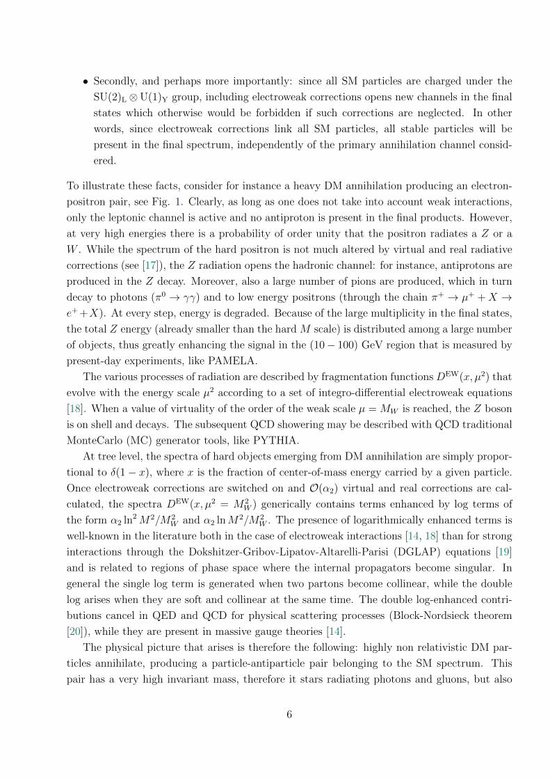
• Secondly, and perhaps more importantly: since all SM particles are charged under the

SU(2)L ⊗U(1)Y group, including electroweak corrections opens new channels in the final

states which otherwise would be forbidden if such corrections are neglected. In other

words, since electroweak corrections link all SM particles, all stable particles will be

present in the final spectrum, independently of the primary annihilation channel consid-

ered.

To illustrate these facts, consider for instance a heavy DM annihilation producing an electron-

positron pair, see Fig. 1. Clearly, as long as one does not take into account weak interactions,

only the leptonic channel is active and no antiproton is present in the final products. However,

at very high energies there is a probability of order unity that the positron radiates a Z or a

W . While the spectrum of the hard positron is not much altered by virtual and real radiative

corrections (see [17]), the Z radiation opens the hadronic channel: for instance, antiprotons are

produced in the Z decay. Moreover, also a large number of pions are produced, which in turn

decay to photons (π0 → γγ) and to low energy positrons (through the chain π+ → µ+ +X →e+ +X). At every step, energy is degraded. Because of the large multiplicity in the final states,

the total Z energy (already smaller than the hard M scale) is distributed among a large number

of objects, thus greatly enhancing the signal in the (10− 100) GeV region that is measured by

present-day experiments, like PAMELA.

The various processes of radiation are described by fragmentation functions DEW(x, µ2) that

evolve with the energy scale µ2 according to a set of integro-differential electroweak equations

[18]. When a value of virtuality of the order of the weak scale µ = MW is reached, the Z boson

is on shell and decays. The subsequent QCD showering may be described with QCD traditional

MonteCarlo (MC) generator tools, like PYTHIA.

At tree level, the spectra of hard objects emerging from DM annihilation are simply propor-

tional to δ(1− x), where x is the fraction of center-of-mass energy carried by a given particle.

Once electroweak corrections are switched on and O(α2) virtual and real corrections are cal-

culated, the spectra DEW(x, µ2 = M2W ) generically contains terms enhanced by log terms of

the form α2 ln2M2/M2W and α2 lnM2/M2

W . The presence of logarithmically enhanced terms is

well-known in the literature both in the case of electroweak interactions [14, 18] than for strong

interactions through the Dokshitzer-Gribov-Lipatov-Altarelli-Parisi (DGLAP) equations [19]

and is related to regions of phase space where the internal propagators become singular. In

general the single log term is generated when two partons become collinear, while the double

log arises when they are soft and collinear at the same time. The double log-enhanced contri-

butions cancel in QED and QCD for physical scattering processes (Block-Nordsieck theorem

[20]), while they are present in massive gauge theories [14].

The physical picture that arises is therefore the following: highly non relativistic DM par-

ticles annihilate, producing a particle-antiparticle pair belonging to the SM spectrum. This

pair has a very high invariant mass, therefore it stars radiating photons and gluons, but also

6

weak gauge bosons. The presence of collinear and/or infrared singularities allows to factor-

ize leading logarithmic electroweak corrections with a probabilistic interpretation very similar

to DGLAP equations, see Sec. 3. The exchange of virtual and emission of real electroweak

bosons lead to the appearance in the final spectrum of all the stable SM particles, not only the

ones initially emitted by the DM annihilation. Indeed, the higher is the mass of the DM, the

more democratically distributed the final spectrum of DM particles is. Therefore, including

electroweak corrections alters significantly the final spectrum of particles stemming from DM

decay/annihilation and this has a large impact on indirect searches of DM.

Let us close this Section by recalling that, while in this paper we only consider DM anni-

hilation/decay to two body final states, our approach is more general and model independent.

Indeed, the only assumptions we make are that the physics up to the DM mass scale M is

described by the SM and that the SM may be eventually extended by interactions that pre-

serve SU(2)L ⊗ U(1)Y gauge invariance. While these assumptions exclude cases like the ones

considered in Refs. [10] and [21] where gauge non invariant interactions where considered1, a

large number of models can be examined with the techniques we describe here. For instance,

let us extend the SM by adding a very heavy scalar S that interacts with the SM Higgs (H) and

leptons (L,E), through an effective operator SLEH. Then, the dominant decay of the scalar

is a three body decay, since the two body decay S → LE is suppressed by a relative factor

M2W/M

2. The framework described here applies as well, albeit with the additional complica-

tion that the three body decay with respect to which one factorizes electroweak interactions

provides a distribution rather than a simple δ function. In this sense, provided assumptions

specified above are fulfilled, our approach is completely model independent.

3 Quantitative computation

We now discuss in more technical terms the inclusion of EW gauge boson emission through the

evolution equations. We start from a first principle definition of the energy spectrum for emitted

particles and then we define the fragmentation functions as statistical objects describing the

probability of a particle to be transformed into another with a certain momentum fraction. The

full evolution equations for the fragmentation functions, containing EW and QCD interactions,

are analyzed. We provide an expression that can be used to match the outcome of Monte Carlo

codes adding EW corrections at leading order O(α2). Our approach is similar in spirit to the

one used, in a different context, in [23], with important differences.

The relevant quantity for indirect signals of DM is the energy spectrum dNf/dx of stable SM

particles f = e+, e−, γ, p, p, ν, ν, d produced per DM decay/annihilation, where x = 2Ef/√s

(0 ≤ x ≤ 1) is the fraction of center of mass energy carried by a stable particle f with energy

1The analysis of the Infrared virtual corrections to gauge non invariant amplitudes, i.e. amplitudes propor-

tionals to the higgs vev, has been recently performed in [22].

7

Ef . For clarity we will sometimes specify the formulæ assuming the case of non-relativistic

DM annihilations, for which√s = 2M such that x = Ef/M ; it is immediate to obtain the

corresponding formulæ for DM decays, where√s = M .

We assume that DM initially produces two primary back-to-back SM particles, and we

consider all relevant cases:

I = e+L,Re

−L,R, µ

+L,Rµ

−L,R, τ

+L,Rτ

−L,R, νeνe, νµνµ, ντ ντ ,

qq, cc, bb, tt, γγ, gg, W−T,LW

+T,L, ZT,LZT,L, hh

, (2)

where q = u, d, s denotes a light quark; h is the Higgs boson; Left or Right are the possible

fermion polarizations, and T ransverse or Longitudinal are the possible polarizations of massive

vectors, that correspond to different EW interactions. Then, the spectrum can be written as:

dNf

dx≡ 1

σDM DM→I

dσDM DM→I→f+X

dx, f = e+, e−, γ, p, p, ν, ν, d, (3)

with a similar formula for the case of DM decay. The “X” in this equation reminds of the

inclusivity already discussed in Section 2.

In each one of the possible cases I, MonteCarlo generators like PYTHIA allow to compute

the inclusive spectrum dNMCI→f (M,x)/dx by generating events starting from the pair I of initial

SM particles with back-to-back momentum and energy E = M , and letting the MC to simulate

the subsequent particle-physics evolution, taking into account decays of SM particles and their

hadronization, as well as QCD radiation and (partially) QED radiation.

Then, the spectra for a generic DM model that produce combinations of the two-body states

I can be obtained combining the various channels:

dNf

dx=∑I

BRI

dNMCI→f

dx. (4)

In some DM models, primary multi-body states can be important: one can obtain the final

spectra without running a dedicated MC code by computing the model-dependent energy spec-

tra DI(z) of each primary pair I (each one has energy E = zM with 0 ≤ z ≤ 1) and convoluting

them with the basic MC spectra:

dNf

d lnx(M,x) =

∑J

∫ 1

x

dz DJ(z)dNMC

J→f

d lnx

(zM,

x

z

). (5)

Notice that we combine particle-antiparticle pairs because we assume that they have the same

spectra, which is true whenever the cosmological DM abundance does not carry a CP asym-

metry. Otherwise, hadronization can be significantly affected and dedicated MC runs would

be necessary. The indices I, J = p + p denotes a primary particle p together with its anti-

particle p, with the same energy spectrum. Factors of two are such that for complex particles

one has dNp/dz = dNp/dz = DI , while for real particles (the Z, the γ, the Higgs h) one has

dNDM→p/dz = 2 DI .

8

3.1 Including EW corrections

We now come back to the basic case of DM that annihilates or decays in one primary channel I

and discuss how to achieve the goal of this paper: obtaining a set of basic functions dNI→f/dx

that take into account EW radiation, replacing the functions dNMCI→f/dx computed via Monte-

Carlo simulations. EW radiation is a model-independent subset of the higher order corrections

discussed above, and gives rise to specific spectra of initial SM particles, such that its effect

can be included in the primary basic spectra by a formula similar to eq. (5):

dNI→f

d lnx(M,x) =

∑J

∫ 1

x

dz ;DEWI→J(z)

dNMCJ→f

d lnx

(zM,

x

z

), (6)

where DEWI→J(z) is the EW I → J EW parton distribution: the J spectrum produced by initial

I. Our normalization is such that we have the uniform normalization DEWI→J(z) = δIJδ(1 − z)

at tree level for both real and complex particles. Some comments are in order:

i) When including higher order effects, one must avoid overcounting and take into account

that MC codes already include some particularly relevant higher-order effects: showering pro-

duced by strong (QCD) and electromagnetic (QED) interactions, up to details.2

ii) For initial particles that do have strong interactions, eq. (6) misses the interplay between

EW and QCD radiation; this limitation is not a problem because, as expected, in such cases

EW radiation will turn out to be subdominant with respect to QCD radiation.

iii) For initial particles that do not have strong interactions, eq. (6) holds at leading order in

the weak couplings: first they must do an EW splitting, and next one can add QCD splittings

neglecting EW radiation. We emphasize an important different between e.g. a Z → qq splitting

and the same Z → qq decay: in the decay the invariant mass of the qq pair is equal to the Z

mass (such that Z → tt is forbidden by the heaviness of the top t); in the splitting the invariant

mass can be much higher, and we approximate it as zM . This higher invariant mass strongly

affects the subsequent QCD radiation from quarks, which is more abundant in the splitting

case, leading to a higher multiplicity of p and γ.

In Appendix A we give a detailed discussion of the interplay between EW and QCD radiation

and of the level of approximation introduced by using eq. (6).

3.2 Computing the EW parton distributions

We define DEWI→J(z, µ2) as the probability for a given parent particle I with virtuality of the

order of µ to become a particle J with a fraction z of the parent particle’s energy mediated by

2We must include via eq. (6) only all those effects not included in MC codes. Existing MC codes have their

own peculiarities, e.g. Phytia automatically includes γ radiation from charged particles but not from the W±.

Of course, an alternative more precise approach, that we do not purse, would be implementing the missing EW

radiation effects into some existing MC code.

9

EW interactions. At large virtuality, they take the tree level values:

DEWI→J(z, µ2 = s) = δIJ δ(1− z); (7)

At low virtuality µ2 ∼ M2W , they are the functions we need: DEW

I→J(z) = DEWI→J(z, µ2 = M2

W ).

The evolution in the virtuality is described by integro-differential equations, that involve a set

of kernels3 PEWI→J(x, µ2) that have been derived in [18]:

∂DEWI→J(z, µ2)

∂ lnµ2= −α2

2π

∑k

∫ 1

x

dy

yPEWI→K(y, µ2) DEW

K→J(z/y, µ2). (8)

Since we work at leading order in the EW couplings, eq. (8) with the boundary conditions of

eq. (7) is solved by:

DEWI→J(z) = δIJδ(1− z) +

α2

2π

∫ s

M2W

dµ2

µ2PEWI→J(z, µ2). (9)

Differently from QED and QCD, the EW kernels feature infrared singular terms proportional

to lnµ2, so that the solutions (9) also include double logs beside the customary single logs of

collinear origin:

DEWI→J(z) = D2(z) ln2 M

MW

+D1(z) lnM

MW

+D0(z). (10)

Our goal is to include the model-independent logarithmically enhanced terms. Electroweak

radiation from the initial DM state is of course model-dependent: since DM is non-relativistic

this effect only contributes to the non-enhanced terms D0, that we neglect. Notice however

that for our purposes we need to include terms of the form (ln x)/x that are relevant in the

region x→ 0; this is discussed in detail in subsection 3.4.

3.3 Splitting functions

The leading-order parton distributions DI→J(z) can be computed by using the partonic splitting

functions P summing over all possible SM splittings [18]; the relevant splitting functions are

here collected in table 1.

A concrete simple example allows to clarify the procedure and the normalization factors: we

consider DM producing an initial generic F ermion-antiF ermion pair with FF invariant mass√s mF . We assume that F has charge qF under a generic vector V with mass MV

√s

and gauge coupling α. (In the SM the vector could e.g. be a Z and the fermion a neutrino).

The splitting process F → FV gives rise to:

DF→F (z) = δ(1− z)

[1 +

α q2F

2πP virF→F

]+α q2

F

2πPF→F (z), DF→V (z) =

α q2F

2πPF→V (z). (11)

3In this work we indicate with P (x, µ2) the unintegrated kernels, while the splitting functions P (x), obtained

by integrating in µ2, depend only on the energy fraction x; a list of the relevant splitting functions is given in

Table 1.

10

splitting 1→ x+ x′ splitting function: real and virtual

F0,M → F0,M + VM PF→F =1 + x2

1− xL(1− x) P vir

F→F =3`

2− `2

2

F0,M → VM + F0,M PF→V =1 + (1− x)2

xL(x) P vir

F→V =3`

2− `2

2

V → F + F PV→F = [x2 + (1− x)2]` P virV→F = −2`

3

SM → SM + VM PS→S = 2x

1− xL(1− x) P vir

S→S = 2`− `2

2

SM → VM + SM PS→V = 21− xx

L(x) P virS→V = 2`− `2

2

V → S + S ′ PV→S = x(1− x)` P virV→S = − `

6

VM → VM + VM PV→V = 2

[x

1− xL(1− x) +

1− xx

L(x) + x(1− x)`

]VM → VM + V0 P ′V→V = 2

[x

1− x`+

1− xx

L(x) + x(1− x)`

]VM → V0 + VM PV→γ = 2

[x

1− xL(1− x) +

1− xx

`+ x(1− x)`

]F → F + S PYuk

F→F = (1− x)` PYuk,virF→F = − `

2

F → S + F PYukF→S = x` PYuk,vir

F→S = − `2

S → F + F PYukS→F = ` PYuk,vir

S→F = −`

Table 1: Generalized splitting functions for massive partons. V denotes a vector, F a fermion

and S a scalar; VM denotes a vector with mass MV , V0 a massless vector, etc. The function

L(x) is defined in eq. (18) and ` = ln s/M2V .

By replacing F → S one obtains the corresponding result for a pair for Scalars, and so on.

The first term describes virtual corrections arising from one-loop diagrams, and the second

term describes real emission corrections. We define:

P virI→J ≡ −

∫ 1

0

dz PI→J(z), (12)

for any I and J ; e.g. from PV→V in table 1 we have:

P virV→V =

11

3`− `2 where ` = ln

s

M2V

. (13)

While both virtual corrections, related to P virI→J , and real corrections, related to PI→J , are listed

in table 1, the simple relation (12) holds between them. The relationship between real and

virtual contributions is dictated by the unitarity of the theory (see e.g. [17] for a more detailed

discussion). Intuitively, this just amounts to say that when an F radiates, it disappears from

the initial state.

11

One can verify that the partonic distributions DI→J satisfy a set of conservations laws (with

corresponding identities for the splitting functions P )

• The conservation of splitting probability:

1

2

∑J

∫ 1

0

dx DrealI→J +

∫ 1

0

dx DvirI→I = 0, (14)

where the factor 1/2 accounts for the fact that one particle splits in two.

• The conservation of total momentum:∑J

∫ 1

0

dx x DI→J = 1. (15)

• The conservation of electrical charge:∑J

∫ 1

0

dx QJ DI→J = QI . (16)

By combining these splitting functions with the appropriate electroweak couplings (including

the top quark Yukawa coupling) we get the electroweak splittings among SM particles, described

by the DI→J functions, explicitly listed in Appendix C. It is a simple exercise to verify that

conservation laws are satisfied. For completeness, we also list the splittings involving photons

(to be dropped if already included by MC codes), assuming for simplicity a photon with mass

MW ; sending it to zero gives infrared divergences that can be regulated and dealt with using

well known techniques that we do not need to discuss here.

3.4 Splitting functions for massive partons

We see from table 1 that P virI→J is explicitly given by linear or quadratic polynomials in ln s/M2

V :

the vector mass provides an infra-red regulator. This is unlike in the standard application of

partonic techniques, where all partons are massless and some infra-red regularization is needed.

In this subsection we briefly describe how we generalized partonic functions to massive

partons (such as the W,Z, t in the SM), and why particle masses modify the kinematics affecting

the log-enhanced terms, as encoded in a non trivial universal function L.

Let us consider the splitting process i → f + f ′ of a particle i into massive partons f, f ′:

the corresponding splitting functions can be non zero only in the kinematically allowed ranges:

mf

Ei< x < 1− mf ′

Ei, (17)

where x = Ef/Ei, and similarly for x′ = 1 − x = Ef ′/Ei. The modification due to nonzero

masses in the kinematical range is power suppressed and thereby mostly negligible; however

12

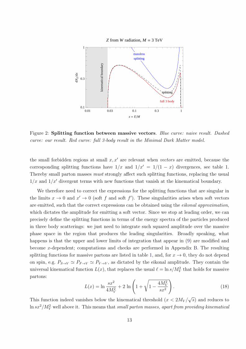
0.01 0.1 10.03 0.30.1

1

0.3

x = EM

dNZ

dx

Z from W radiation, M = 3 TeV

full 3 body

splittingkine

mat

ical

boun

dary

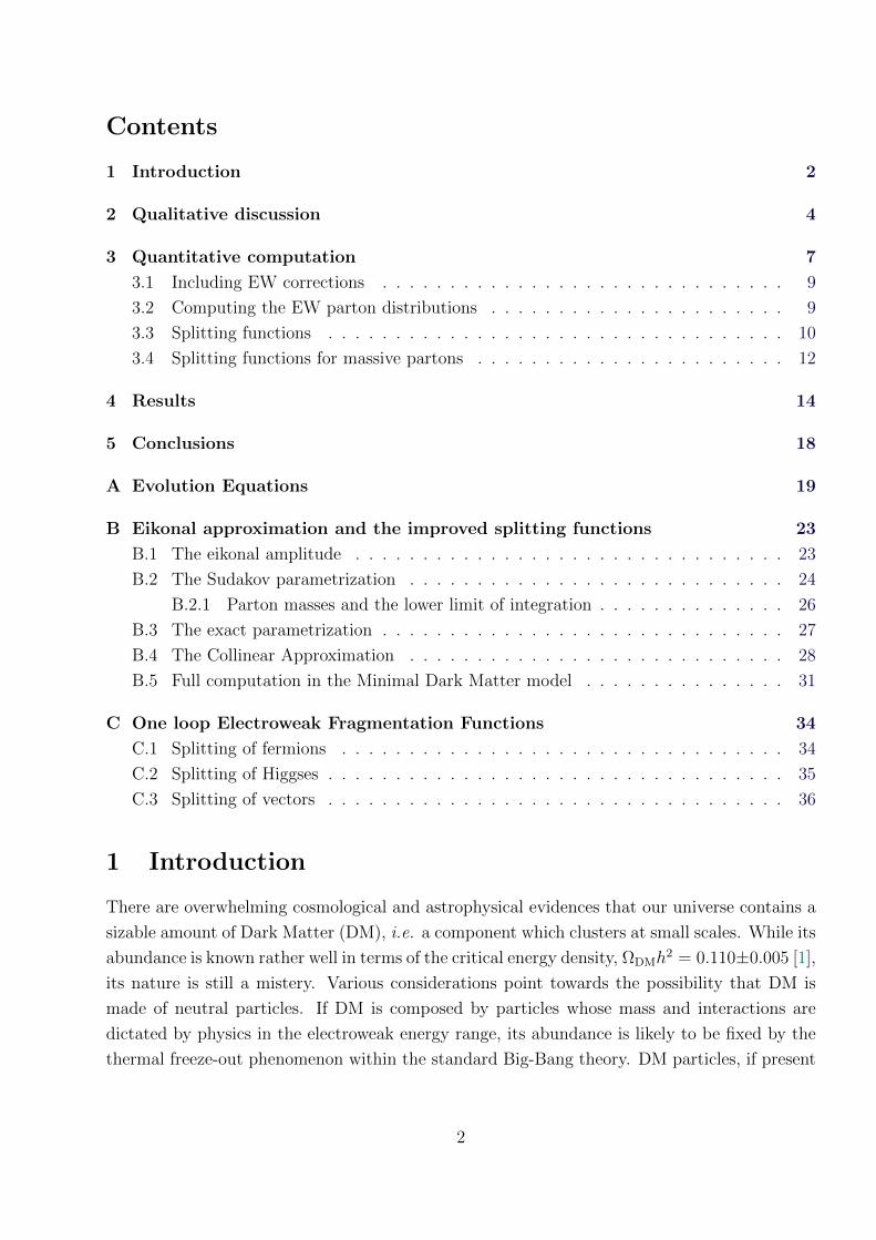
masslesssplitting

Figure 2: Splitting function between massive vectors. Blue curve: naive result. Dashed

curve: our result. Red curve: full 3-body result in the Minimal Dark Matter model.

the small forbidden regions at small x, x′ are relevant when vectors are emitted, because the

corresponding splitting functions have 1/x and 1/x′ = 1/(1 − x) divergences, see table 1.

Thereby small parton masses must strongly affect such splitting functions, replacing the usual

1/x and 1/x′ divergent terms with new functions that vanish at the kinematical boundary.

We therefore need to correct the expressions for the splitting functions that are singular in

the limits x → 0 and x′ → 0 (soft f and soft f ′). These singularities arises when soft vectors

are emitted, such that the correct expressions can be obtained using the eikonal approximation,

which dictates the amplitude for emitting a soft vector. Since we stop at leading order, we can

precisely define the splitting functions in terms of the energy spectra of the particles produced

in three body scatterings: we just need to integrate such squared amplitude over the massive

phase space in the region that produces the leading singularities. Broadly speaking, what

happens is that the upper and lower limits of integration that appear in (9) are modified and

become x-dependent; computations and checks are performed in Appendix B. The resulting

splitting functions for massive partons are listed in table 1, and, for x→ 0, they do not depend

on spin, e.g. PS→V ' PF→V ' PV→V , as dictated by the eikonal amplitude. They contain the

universal kinematical function L(x), that replaces the usual ` = ln s/M2V that holds for massive

partons:

L(x) = lnsx2

4M2V

+ 2 ln

(1 +

√1− 4M2

V

sx2

). (18)

This function indeed vanishes below the kinematical threshold (x < 2MV /√s) and reduces to

ln sx2/M2V well above it. This means that small parton masses, apart from providing kinematical

13

Ne Nγ, x > 10−5 Np

DM mass in TeV 0.3 1 3 0.3 1 3 0.3 1 3

DM DM→ e−Le+L 1.07 1.47 2.02 1.09 2.08 3.39 0.0148 0.0574 0.118

DM DM→ µ−Lµ+L 1.17 1.56 2.11 1.07 2.06 3.37 0.0147 0.0572 0.118

DM DM→ τ−L τ+L 1.48 1.86 2.40 3.15 4.09 5.34 0.0147 0.0572 0.118

DM DM→ W−T W

+T 15.1 18.9 24.8 31.3 39.8 53.2 1.50 1.92 2.62

DM DM→ W−LW

+L 15.5 19.6 25.8 32.3 41.6 55.9 1.52 1.94 2.66

DM DM→ hh 27.3 30.5 35.5 59.9 67.1 78.6 2.22 2.60 3.26

DM DM→ qq 22.6 34.6 48.9 47.5 73.9 107. 2.47 3.89 5.71

Table 2: Total number of e+, γ, p for a few DM annihilation channels.

thresholds, give rise to extra lnx factors with respect to the standard case of massless partons,

which become numerically relevant at small x, x′.

This was not noticed before, and Fig. 2 exemplifies its relevance. The dashed curve in Fig.

2 shows the splitting function between massive vectors (e.g. relevant for Z radiation from W±):

it significantly differs from the massless splitting function (upper curve) even away from the

kinematical boundaries, and it closely agrees with the full result of a 3-body computation in a

specific model, which also includes not log-enhanced terms. These terms are subleading in the

present example, where we here considered DM DM→ W+T W

−T annihilations with M = 3 TeV.

4 Results

Our main results are the energy spectra of all stable final SM particles f from any two-body

DM non-relativistic annihilations or decays. We will make the code freely available in [24], and

show here some examples.

In table 2 we show the total number of e+, p and γ, including EW radiation, for a few values

of the DM mass M . Without EW radiation, increasing M would just boost all particles, such

that dN/dx and consequently N does not depend on M . With EW radiation, the total number

of particles increases with the DM mass: the typical effect is about a factor of 2 going from 0.3

to 3 TeV. Of course, such dependence on M is similar to the one already present in the quark

channels (bottom row), due to QCD radiation.

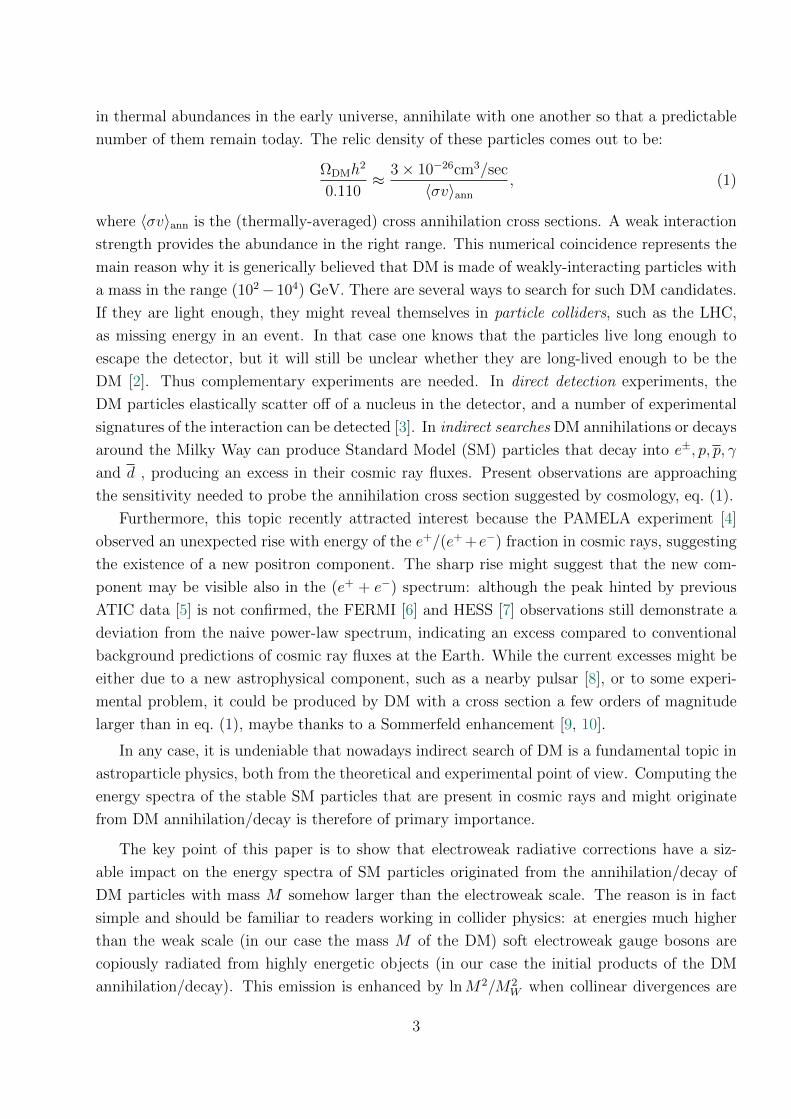
Coming to the energy spectra, these new particles appear at low energy. In Fig. 3 we

consider annihilations of DM with mass M = 3 TeV and compare the spectra with (continuous

curves) and without (dashed curves) EW corrections.

• In the top row we consider DM annihilations into W+W− with transverse (left) or longitu-

dinal (right) polarization. The final spectra do not significantly depend on the polarization

of the W , but this is an accident: a T ransverse W splits into all quarks as demanded

14

10-1 1 10 102 10310-2

10-1

1

10

102

E in GeV

dNd

lnE

WT at M = 3000 GeV

10-1 1 10 102 10310-2

10-1

1

10

102

E in GeV

dNd

lnE

WL at M = 3000 GeV

10-1 1 10 102 10310-3

10-2

10-1

1

10

E in GeV

dNd

lnE

eL at M = 3000 GeV

10-1 1 10 102 10310-3

10-2

10-1

1

10

E in GeV

dNd

lnE

ΜL at M = 3000 GeV

10-1 1 10 102 10310-3

10-2

10-1

1

10

E in GeV

dNd

lnE

Νe at M = 3000 GeV

10-1 1 10 102 10310-3

10-2

10-1

1

10

E in GeV

dNd

lnE

Γ at M = 3000 GeV

Figure 3: Comparison between spectra with (continuous lines) and without EW corrections

(dashed). We show the following final states: e+ (green), p (blue), γ (red), ν = (νe+νµ+ντ )/3

(black).

15

æ

æ

æ

ææ

ææ

ææ

æ

æ

æ

æææ

æ

æ

àà

à

à

à

à

à

à

à

ì

ì

ì

ì

ì

ì

ì

ì

ì

ò

ò

ò

ò

ò

ò

ò

ò

ò

ô

ô

ô

ô

10 102 103 104

1%

10%

3%

30%

Positron energy in GeV

Posi

tron

frac

tion

background?

PAMELA

ææ

ææ

ææ

ææææ

æ

æ

æææ æ

æ

1 10 102 103 104

10-5

10-4

10-3

10-2

p kinetic energy in GeV

pp

background?

PAMELA

DM DM ® WT+WT

- with M = 10 TeV, MIN, NFW

æ

æ

æ

ææ

ææ

ææ

æ

æ

æ

æææ

æ

æ

àà

à

à

à

à

à

à

à

ì

ì

ì

ì

ì

ì

ì

ì

ì

ò

ò

ò

ò

ò

ò

ò

ò

ò

ô

ô

ô

ô

10 102 103 104

1%

10%

3%

30%

Positron energy in GeV

Posi

tron

frac

tion

background?

PAMELA

æ

æ

ææ

ææ

ææææ

æ

æ

ææ

æ æ

æ

1 10 102 103 104

10-5

10-4

10-3

p kinetic energy in GeV

pp

background?

PAMELA

DM DM ® ΜL+ ΜL

- with M = 2. TeV, MED, NFW

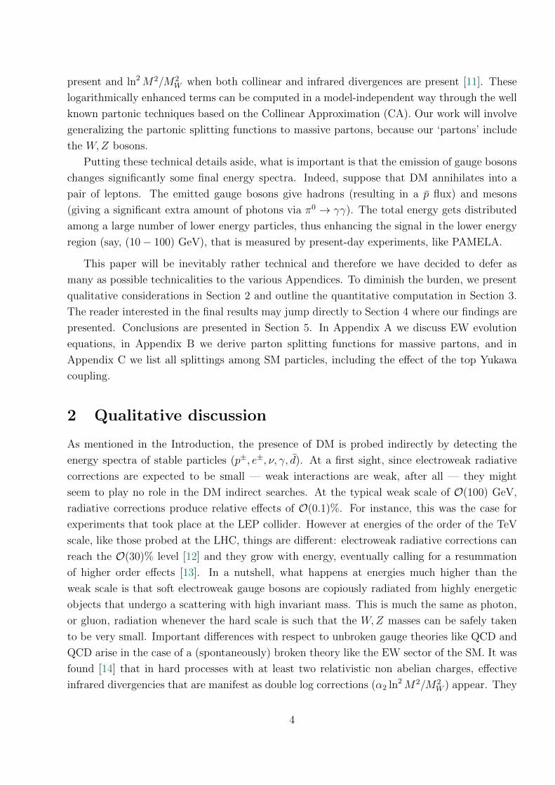
Figure 4: DM signals in the e+ (left) and p (right) fraction, with (dashed) and without (dot-

dashed) electroweak corrections for two DM models that can fit the PAMELA e+ excess: Minimal

Dark Matter (upper) or a muonic channel (lower). The gray area is the predicted astrophysical

background and the red area is the prediction adding the full DM contribution.

by their weak interactions, while a Longitudinal W (being the charged Goldstone in the

Higgs doublet) mainly splits into t and b quarks, as demanded by the top quark Yukawa

interaction. In both cases EW splittings increase the total number of final particles (e+, p,

γ, ν) increases by a factor of almost 2. The biggest effect is in the p spectra: without EW

corrections they are strongly suppressed below Ep < mp · (M/MW ) ∼ 100 GeV, because

of the boost factor M/MW of the W . Adding EW corrections, a W splits into quarks

with lower energy, producing p also at lower energy. This is important for interpreta-

tions of the PAMELA e+ excess in terms of annihilations of very heavy DM particles,

e.g. M = 10 TeV as predicted by Minimal Dark Matter [25]. EW corrections make more

16

difficult to avoid unseen effects in p by having all the DM effects above 100 GeV where

we do not have data yet. As illustrated in Fig. 4, in view of EW corrections there is some

tension with data, even assuming the MIN model of diffusion of charged particles in the

galaxy [26] (which gives the minimal amount of p compatibly with cosmic rays data and

theory).

• We do not plot our result for DM annihilations into the Higgs boson, because its mass

and decay modes are not yet known. The Higgs channel is similarly affected by EW

corrections as the WL and ZL channels (because they are the Goldstone components of

the Higgs doublet), and the main effect is again the h → t splitting induced by the top

Yukawa coupling.

• In the middle row of Fig. 3 we consider DM annihilations into charged leptons: e−Le+L

(left) and µ−Lµ+L (right). The spectra are significantly affected by EW corrections, because

leptons split into W,Z bosons, finally producing quarks, and consequently a copious tail

of e+, γ, p at lower energy. The main new qualitative feature is the appearance of p

from leptons, and in Fig. 4 (lower row) we show that DM annihilations into µ+Lµ−L with

M = 2 TeV (a scenario motivated by the PAMELA e+ and FERMI e+ + e− anomalies)

also gives a possibly detectable excess of p. We here assumed the favored MED model

of propagation of charged particles in the Milky Way [26]; p can be suppressed down to

a negligible by considering the MIN model and/or DM annihilations into µ+Rµ−R. Indeed

EW effects are more significant for left-handed leptons which have SU(2)L interactions

than for right-handed leptons which only have U(1)Y interactions.

• The bottom left panel of Fig. 3 shows that, in view of EW interactions, DM annihilations

into neutrinos also induce a significant spectrum of γ and some e+, p.

• The bottom right panel of Fig. 3 shows how EW corrections affect DM annihilations into

γγ: an hypothetical γ line at high energy Eγ = M ∼ few TeV must be accompanied by a

comparable flux of γ with lower energy Eγ ∼ (10− 100) GeV, where we have more data.4

• Finally, DM annihilations and decays into quarks are negligibly affected, so that we do

not show our results.

The same results hold for DM decays. EW corrections are irrelevant in models where DM

decays or annihilates into hypothetical ‘dark’ particles, lighter than the weak scale, that finally

decay back to SM particles.

There is a striking difference between the two examples of e+ fraction in Fig. 4: EW

corrections are relevant in the upper case (WT channel) and negligible in the lower case (µL

channel). At first sight, this is surprising, because Fig. 3 shows that in both cases EW

4This effect, already partly present in QED, seems to be not implemented into MonteCarlo codes.

17

corrections induce significant low energy tails to the e+ spectra at production. The qualitative

difference is due to e+ energy losses in the Milky Way that also gives a tail of e+ at low energy:

we explain how to understand which effect is dominant. The e+ flux can be approximatively

computed neglecting galactic diffusion and taking into account only energy losses, with the

resultdne−

dE=dne+

dE=

3m2e

4σTu⊕

1

E2

σv

2

(ρ⊕M

)2∫ M

E

dE ′dNe

dE ′(19)

where σT is the Thompson cross section, u⊕ is the energy density in radiation and magnetic

fields and ρ⊕ is the DM density, both at the location of the solar system. This means that

the e+ flux at a given energy E < M is proportional to the number of e+ produced with

energy between E and M . In the case of DM annihilations into leptonic channels, the tail of

e± at lower energy produced by EW radiation contains a number or e± at most comparable to

the amount of e± already present at E ∼ M : therefore EW corrections negligibly affect the

positron fraction. This is not the case for DM annihilations into W±, where instead the tail at

low energy is the dominant component of the total e± number, such that EW corrections more

significantly affect the e+ fraction.

5 Conclusions

In this paper we computed the energy spectrum of SM particles stemming out from DM annihi-

lation/decay. We have shown that EW corrections have a relevant impact on such spectra when

the mass M of the DM particles is larger than the EW scale MW . Soft EW boson emission is

enhanced in the collinear and infrared regime and this leads to ln2M2/M2W enhancement fac-

tors. The result of the inclusion of EW corrections is that all stable particles are present in the

final spectrum, independently of the primary annihilation/decay channel. For instance, even if

the DM particles annihilate/decay into light neutrinos, EW corrections cause the appearance

of hadrons and photons in the very final spectrum. The inclusion of EW corrections is therefore

an essential ingredient in order to have a physical picture of the correlated energy spectra of

final stable particles. Our quantitative results may be inferred from Fig. 3 where the energy

spectra dN/dE of stable SM particles are presented with and without EW corrections. These

spectra are the necessary ingredients to predict the flux for indirect searches once the effect

of diffusion and galactic energy loss are included. As a rule of thumb we may say that EW

corrections are important in determining the final flux of stable particles whenever

• the final flux of stable particles is dominated by the low energy tail of the dN/dE. One

example is the case of DM annihilation/decay into gauge bosons and e± final states (see

fig. 3). This point becomes more relevant in the present experimental situation, where

we mostly observe particles below 100 GeV, possibly much below the DM mass.

18

• the final flux of stable particles is absent when EW corrections are not taken into account.

One example is the case of DM annihilation/decay into leptons and antiprotons p final

states (see fig. 4). This point is important also for neutrino fluxes from DM annihilations

in the sun or in the earth, because all SM particles, even those that loose energy in

matter before decaying into neutrinos, can radiate a W or a Z that promptly decays into

neutrinos.

EW corrections may also significantly affect the fluxes of particles generated from heavy grav-

itino decays in supersymmetric theories. The computation of these energy fluxes is crucial in

studying the dissociation of the light element abundances generated during a period primordial

nucleosynthesis.

We expect that EW radiative corrections have a minor effect on the freeze-out cosmological

DM abundance, because it is determined by just the total non-relativistic annihilation DM cross

section. In the case of energy spectra instead, as explained in this paper, the low energy tails

can be enhanced by orders of magnitude, while the high energy part of the spectrum is mildly

depleted. The net effect on the total number of final particles typically is an enhancement by a

factor of 2. We conclude that, when DM is around or above the TeV scale, one must take into

account radiative EW corrections.

We computed EW corrections at leading order. Although we cannot give a sharp answer,

we argued that it is not necessary to resum higher order EW corrections as long as DM is

not too heavy: α2 ln2(M2/M2W )/2π 1 at M 100 TeV. Indeed, higher order corrections

are expected to give small effects for total cross sections at the TeV scale: a one loop effect

of the order of 30% means that one expects higher order effects to be at the 1% level. It is

more difficult to guess how low-energy tails might be affected without performing a dedicated

computation, which could be done implementing EW corrections in a MonteCarlo: we provided

splitting functions for massive partons and all ingredients.

Acknowledgments: D.C. during this work was partially supported by the EU FP6 Marie Curie

Research & Training Network ”UniverseNet” (MRTN-CT-2006-035863). P.C. wishes to thank Luigi

Lanzolla for many useful contacts and discussions, without which his work would have been much

more difficult. We also thank G.F. Giudice for useful conversations. We used the high-statistics

Pythia spectra computed on the Baltic Grid by Mario Kadastik, to appear in [24]; this work was

supported by the ESF Grant 8499 and by the MTT8 project.

A Evolution Equations

At present the energy spectrum dNMCI→f/dx are computed with MC generators like PYTHIA by gener-

ating events starting from the pair I of initial SM particles with back-to-back momentum and energy

E = M , and letting the MC to simulate the subsequent particle-physics evolution, taking into account

decays of SM particles and their hadronization, as well as QED and QCD radiation. As it is evident

19

the MC output are nothing else that the full QCD+QED fragmentation functions DQCD+QEDI→f (x) that

can be identified with dNMCI→f/dx. The fragmentation functions are related to a nonperturbative as-

pect of QCD, so that they cannot be precisely calculated by theoretical methods at this stage. The

situation is similar to the determination of the PDFs, where high-energy experimental data are used

for their determination instead of theoretical calculations. The µ2 evolution for the fragmentation

functions is calculated in the same way as the one for the PDFs by using the timelike DGLAP evo-

lution equations. The splitting functions are the same in the Leading Order (LO) evolution of the

PDFs; however, they are different in the Next-to-Leading Order (NLO). Explicit forms of the splitting

functions are provided in [18]. The evolution equations are then essentially the same as the PDF case.

The correct determination of the energy spectrum dNI→f/dx of the final stable particle f , ob-

tained through the particle-physical evolution of the initial pair I of SM particles with back-to-back

momentum and energy E = M , needs the solution of a full set of evolution equations, including both

strong and electroweak interactions.

In previous works the QCD DGLAP formalism has been extended to EW interactions [18]. The anal-

ysis of mass singularities in a spontaneously broken gauge theory like the electroweak sector of the

Standard Model has many interesting features. To begin with, initial states like electrons and protons

carry nonabelian (isospin) charges; this feature causes the very existence of double logs, i.e. the lack

of cancellations of virtual corrections with real emission in inclusive observables [14]. Secondly, initial

states that are mass eigenstates are not necessarily gauge eigenstates; this causes some interesting

mixing phenomena analyzed in [16].

On a general setting, the mathematical structure of the full system of EW and QCD evolution

is provided by the following set of integral differential equations with kernels PQCD/EW for different

gauge boson exchange (we omit for the moment the explicit QED evolution equations included in the

EW part of the SM and the various index parametrizing the flavour and quantum numbers): 5

µ2 ∂

∂µ2D(x, µ2) =

αs2π

D ⊗ PQCD θ(Λ < µ < M) +α2

2πD ⊗ PEW θ(MW < µ < M)

= D ⊗(αs

2πPQCD +

α2

2πPEW

)θ(MW < µ < M)

+αs2π

D ⊗ PQCD θ(ΛQCD < µ < MW ), (A.1)

where we have made explicit the running range: for the EW interactions from M to MW where the

gauge boson mass is freezing the running and for QCD corrections from M to ΛQCD where the non-

perturbative effects generate an effective cutoff to gluon exchanges. In practice, from ΛQCD to MW

the running is purely dictated by QCD (remember that QED interactions are not shown for simplicity,

in this case the running scale for photons is until the electron mass me) while the EW-QCD interplay

starts only above the MW scale. Note also that forgetting the underlying index structure can bring

to the wrong conclusion that, simply due to the fact that αs > α2, the EW part is just a correction to

the QCD dominant part. This would be a mistake as in many interesting annihilation channels (like

all the leptonic ones or the W±, Z or h) the QCD part is simple zero.

5 The precise index (flavour) structure is given in the Appendix C, the generic index structure is of the

form µ2 ∂∂µ2DI→J = α

2π

∑K DI→K ⊗ PK→J while the ⊗-operator means (f ⊗ g)(x) ≡ f(z) ⊗ g(x/z) =∫ 1

xdz/zf(z)g (x/z) =

∫ 1

0dz∫ 1

0dyf(y)g(z)δ(x− zy).

20

A numerical solution to the full (EW+QCD) problem is of course out of reach. Nevertheless,

we can find some reasonable approximation taking advantage of the fact that we can simulate the

pure QCD evolution also in the non perturbative regime with MC codes and that EW theory is in

the perturbative regime. Technically specking, the evolution equations are Schrodinger-like equations

with a time dependent Hamiltonian, where time is replaced by the µ2 variable and the Hamiltonian

by the P - kernel. A formal solution can be parametrized with the evolution operator:

D(x, µ21, µ

22) ≡ U(z, µ2

1, µ22)⊗ I δ

(1− x

z

)=

(Pµ2 e

∫ µ21µ22

dµ2

µ2(αs2π PQCD+

α22π

PEW))⊗ I, (A.2)

where Pµ2 is the µ2-ordering operator and I the identity in the flavour space. Due to the linearity of

the Eqs. (A.1) 6 we can then formally write the full solution as:

D(x,M2,Λ2QCD) = U(z,M2,M2

W ) ⊗ DQCD(xz,M2

W ,Λ2QCD

), (A.3)

where we have separated the running from M to MW inside the evolution operator U (that can be

perturbatively expanded as soon as αs lnM2/M2W and α2 ln2M2/M2

W are smaller than unity) and the

purely QCD piece DQCD(x,M2W ,Λ

2QCD) encoding also the non-perturbative low energy physics. In

order to keep under control further simplifications we need also to know the matrix flavour structure.

We display it under the form of a simplified four-dimensional space spanned by l=leptons, W =

(W±, Z, γ), q=quarks and g=gluons, for the EW and QCD kernels, PQCD and PEW:

PQCD =

0 0 0 0

0 0 0 0

0 0 PQCDqq PQCD

qg

0 0 PQCDgq PQCD

gg

, PEW =

PEWll PEW

lW 0 0

PEWWl PEW

WW PEWWq 0

0 PEWqW PEW

qq 0

0 0 0 0

. (A.4)

The above matrices do not commute; the EW and QCD sectors are connected through the channels

W → q, q → W and q → q, furthermore the leptonic and hadronic sectors are connected through

the mixed W → q, l, l, q → W channels. Reasonable approximate solutions are related both to

the possibility to expand perturbatively the general solution (B.15), and to the outcome from MC

generators which take automatically into account the full QCD plus QED evolution from M to ΛQCD

scales (me for QED).

One way of proceeding is to define pure EW (DEW) and QCD (DQCD) fragmentation functions

that evolve with their respective kernels, see eq. (A.4), for the energy range M2W < µ2 < M2:

µ2 ∂

∂µ2DQCD(x, µ2) =

αs2π

DQCD ⊗ PQCD and µ2 ∂

∂µ2DEW(x, µ2) =

α2

2πDEW ⊗ PEW, (A.5)

whose formal solutions are:

DEW/QCD(x,M2,M2W ) = Pµ2 e

∫M2

M2W

dµ2

µ2

(α2/s2π

PEW/QCD)⊗ I. (A.6)

6It might be useful to remember the property D(z,M2,M2W )⊗D(x/z,M2

W ,Λ2QCD) = D(x,M2,Λ2

QCD).

21

Then we introduce a new factorized EW ⊗ QCD fragmentation function:

D(x, µ2) ≡ (DEW ⊗DQCD)(x, µ2) with θ(MW < µ < M). (A.7)

This is clearly not a solution of the true evolution equations (A.1) but can be a useful approximate

solution. In order to relate the true solution D of eq. (A.3) with the new function D satisfying eq.

(A.7)), we can use the fact that in the M2W < µ2 < M2 interval we are in perturbative regime also for

the QCD side. Knowing that for two generic non-commuting operators A and B:

eA+B =

(I− 1

2[A,B] + ...

)eA eB, (A.8)

and identifying A =∫M2

M2W

dµ2

µ2

(α22π P

EW)

and B =∫M2

M2W

dµ2

µ2

(αs2π P

QCD), we can approximate the evo-

lution operator U at any order in αs,2. In particular at second order in O(α2s,2, αsα2) we have:

U(x,M2,M2W ) =

[(I +

αsα2

8π2

∫ M2

M2W

dµ2

µ2

∫dµ2

µ2[PEW, PQCD] + · · ·

)

⊗ DEW ⊗DQCD︸ ︷︷ ︸D

(x,M2,M2W ), (A.9)

where:

[PQCD, PEW]⊗ ≡(PQCD ⊗ PEW − PEW ⊗ PQCD

), (A.10)

and the · · · stand for the fact that there is an infinite series of commutators with coefficients of order

αm+12 αn+1

s with m + n ≥ 1. Starting from this expression we can write the perturbative relation

between the exact solution D and the present outcome of the MC codes DQCD:

D =

(I +

αsα2

8π2

∫ M2

M2W

dµ2

µ2

∫dµ2

µ2[PEW, PQCD] + ...

)⊗ DEW ⊗ dNMC

dx. (A.11)

The first order corrections to such a formula are obtained expanding also DEW at one loop:

DEW(x, µ2) = δ(1− x) I +α2

2π

∫ s

µ2PEW(x, µ′2)

dµ′2

µ′2, (A.12)

where we have explicitly shown the arguments x and µ of the matrix PEW.

At order O(α2 ln2M2/M2W , αs lnM2/M2

W ) we find that the energy spectrum for the process I → f+X

can be therefore written as in eq. (6):

dNI→fdx

=∑J

(IIJ +

α2

2π

∫ s

M2W

PEWI→J(x, µ′2)

dµ′2

µ′2

)⊗DQCD

J→f

(xfxI,M2,Λ2

)

≡∑J

(IIJ +

α2

2π

∫ s

µ2PEW′I→J (x, µ′2)

dµ′2

µ′2

)⊗dNMC

J→fdx

, (A.13)

where in the last passage, to be consistent, we have written EW′ in order to stress that only massive

W± and Z are included while QED is already encoded in the MC.

Through this expression one can match the MC code with the first order EW corrections.

22

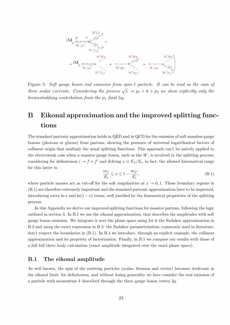
Figure 5: Soft gauge boson real emission from spin-1 particle. It can be read as the sum of

three scalar currents. Considering the process√s → p1 + k + p2 we show explicitly only the

bremsstrahlung contribution from the p1 final leg.

B Eikonal approximation and the improved splitting func-

tions

The standard partonic approximation holds in QED and in QCD for the emission of soft massless gauge

bosons (photons or gluons) from partons, showing the presence of universal logarithmical factors of

collinear origin that multiply the usual splitting functions. This approach can’t be naıvely applied to

the electroweak case when a massive gauge boson, such as the W , is involved in the splitting process;

considering for definiteness i→ f + f ′ and defying x ≡ Ef/Ei, in fact, the allowed kinematical range

for this latter is:mf

Ei≤ x ≤ 1−

mf ′

Ei, (B.1)

where particle masses act as cut-off for the soft singularities at x → 0, 1. These boundary regions in

(B.1) are therefore extremely important and the standard partonic approximation have to be improved,

introducing extra lnx and ln(1−x) terms, well justified by the kinematical proprieties of the splitting

process.

In this Appendix we derive our improved splitting functions for massive partons, following the logic

outlined in section 3. In B.1 we use the eikonal approximation, that describes the amplitudes with soft

gauge boson emission. We integrate it over the phase space using for it the Sudakov approximation in

B.2 and using the exact expression in B.3: the Sudakov parametrization, commonly used in literature,

don’t respect the boundaries in (B.1). In B.4 we introduce, through an explicit example, the collinear

approximation and its propriety of factorization. Finally, in B.5 we compare our results with those of

a full full three body calculation (exact amplitude integrated over the exact phase space).

B.1 The eikonal amplitude

As well known, the spin of the emitting particles (scalar, fermion and vector) becomes irrelevant in

the eikonal limit: for definiteness, and without losing generality we here consider the real emission of

a particle with momentum k described through the three gauge boson vertex 3g.

23

Considering Fig. 5 and using the conservation of momenta in the splitting vertex p = p1 + k we

can write:

iMρ

−g

2p1 · k[ε∗(k) · ε∗(p1)(k − p1)ρ + ε∗ρ(p1)2p1 · ε∗(k)− ε∗ρ(k)2k · ε∗(p1)

], (B.2)

where we have indicated with iMρ the remaining part of the amplitude and taken for simplicity k2 = 0.

Roughly speaking using the eikonal approximation it is possible to neglect the soft momenta in the

numerator in front of the hard one and in this example we can discuss the two opposite situation in

which either p1 or k are soft.

Considering Ward identities the first term in (B.2) vanishes in the case of transverse gauge bosons,

while for longitudinal degrees of freedom we refer the interested reader to [27] for an analysis of the

electroweak symmetry breaking effects; therefore for our purpose we have:

iMρ

− g

p1 · k[ε∗ρ(p1)p1 · ε∗(k)− ε∗ρ(k)k · ε∗(p1)

], (B.3)

where:

• the first term reconstructs the hard scattering amplitude iMρε∗ρ(p1) and it survives when k is

soft;

• the second term reconstructs the hard scattering amplitude iMρε∗ρ(k) and it survives when p1

is soft.

Squaring the amplitude (B.3), we sum over polarizations using the axial gauge [28]:∑εµ(k)ε∗ ν(k) = −gµν +

kµpν2 + kνpµ2p2 · k

, (B.4)

and as a result the eikonal limit leads to the factorization of the process in the product of the hard

cross section times an emission factor integrated over the allowed phase space of the soft particle:

I(p1) = g2 2k · p2

(p1 · k)(p2 · p1)

d4p1

(2π)3δ(p2

1)∣∣p01>0

p1 soft, (B.5)

I(k) = g2 2p1 · p2

(p1 · k)(p2 · k)

d4k

(2π)3δ(k2)

∣∣k0>0

k soft. (B.6)

The two integrals can be obtained through the exchange p1 ↔ k.

B.2 The Sudakov parametrization

We consider now the explicit evaluation of the eikonal integral in (B.5), and in order to perform this

calculation we choose a convenient parametrization of the external momenta; fixing two basis vectors:

P = (E, 0, 0, E), P = (E, 0, 0,−E), with: s = 4E2 ' 4M2, (B.7)

the Sudakov parametrization consists in the following decomposition for the soft momentum p1:

p1 = xP + xP − k⊥ = (E(x+ x),−kt, 0, E(x− x)) , (B.8)

24

where, without losing generality, we have taken the spatial component of k⊥ along the x direction.

In order to highlight in a simple way the logarithmical behavior of the eikonal integral we choose

to work considering as first step the massless case and approximating the two hard momenta k ' P

and p2 ' P , such that

d4p1 =sπ

2dk2

t dx dx. (B.9)

The eikonal integral takes the form:

I(p1) = dk2t dx dx δ

(sxx− k2

t

) α2

π

1

xx, (B.10)

and logarithmical singularities clearly arise in two opposite kinematical regions:

• x x: the soft gauge boson p1 is emitted along the k direction; integrating over x using

x = k2t /sx, the condition x x becomes an upper bound for the transverse momentum k2

t sx2

and therefore in terms of fragmentation functions in the p1 soft limit x→ 0 we obtain:

Dx→0 =

∫ sx2

M2W

dk2t

α2

2π

2

x

1

k2t

=α2

2π

2

xlnsx2

M2W

, (B.11)

that vanishes when x = MW /√s.

• x x: integrating over x using the relation x = k2t /sx, the eikonal integral gives exactly the

same logarithmical result previously discussed but in an opposite kinematical configuration since

the soft gauge boson p1 is emitted now along p2 direction.

In order to clarify the consequences of the symmetry p1 ↔ k between the two eikonal integrals, we

can now discuss in more details the Sudakov parametrization in the region x x. First we generalize

eq. (B.8) writing for k and p2:

k = zP + zP + k⊥ = (E(z + z), kt, 0, E(z − z)) , p2 = yP = (yE, 0, 0,−yE), (B.12)

and using the on-shell conditions in order to eliminate z, x writing z = k2t /sz, x = k2

t /sx. The

conservation of energy and spatial momentum gives the following relations between the kinematical

variables x, y, z:

y = 1− k2t

4E2z(1− z), x = 1− z, (B.13)

and we can therefore generalize the result for k soft just considering the substitution p1 → k =⇒x → z = 1 − x, and as a consequence the kinematical end-points for the x variable in the Sudakov

parametrization are:MW√s≤ x ≤ 1− MW√

s. (B.14)

Comparing eq. (B.11) with:

D =α2

2π

∫dk2

t

k2t

P (x, k2t ), (B.15)

25

where P (x, k2t ) is the usual unintegrated splitting function, we obtain its leading behavior in corre-

spondence of the two kinematical limit in the Sudakov parametrization:

x→ MW√s

: PSud ∼ 2

xL(x)|Sud , (B.16)

x→ 1− MW√s

: PSud ∼ 2

1− xL(1− x)|Sud , (B.17)

with:

L(x)|Sud = lnsx2

M2W

. (B.18)

B.2.1 Parton masses and the lower limit of integration

The upper bound on the integration over k2t is dictated by the kinematical proprieties of the collinear

emission, and can be studied even working in the massless case; parton masses, contrarily, affect in

a relevant way the lower bound of integration. To discuss this point, we need first to generalize the

Sudakov parametrization in eq. (B.12): it’s straightforward to verify that one can take into account

of the on-shell conditions k2 = m2k and p2

1 = m21 just redefining k2

t → k2t +m2

k for k and k2t → k2

t +m21

for p1. Then from the propagator of the collinear emission p→ p1 + k we have:

1

(p1 + k)2 −m2p

=x(1− x)

k2t +m2

1 + x(m2k −m2

1)−m2px(1− x)

. (B.19)

Depending on which particles are massive, three different situations arise.

1. Only the emitted vector is massive. This happens e.g. in EW interactions of the W,Z vectors.

Assuming m2k = M2

W , m2p = m2

1 = 0, eq. (B.19) becomes:

1

(p1 + k)2=

x(1− x)

k2t + xM2

W

≈ x(1− x)

k2t

ϑ(k2t − xM2

W ), (B.20)

where the latter passage holds in logarithmical accuracy. Integrating over k2t we have for the

x→ 1 singularity of the EW splitting function PF→F :

PF→F ∼2

1− xlns(1− x)2

xM2W

' 2

1− xL(1− x)|Sud , (B.21)

and therefore the lower x-dependence don’t affect the soft limit x→ 1.

2. Two particles are massive. This happens e.g. in the electromagnetic coupling of the W : m2p =

m2k = M2

W , m21 = 0; eq. (B.19) becomes:

1

(p1 + k)2 −M2W

≈ x(1− x)

k2t

ϑ(k2t − x2M2

W ). (B.22)

Integrating over k2t we have for the x→ 0, 1 singularities of the splitting function PV→γ :

PV→γ ∼2

1− xlns(1− x)2

x2M2W

+2

xln

sx2

x2M2W

' 2

1− xL(1− x)|Sud +

2

xln

s

M2W

, (B.23)

and the lower x-dependence affects the x→ 0 singularity for the soft photon.

26

3. All three particles are massive. This happens in the massive three gauge boson vertex, m2p =

m2k = m2

1 = M2W ; eq. (B.19) becomes:

1

(p1 + k)2 −M2W

≈ x(1− x)

k2t

ϑ[k2t − (1− x+ x2)M2

W ]. (B.24)

Integrating over k2t we have for the x→ 0, 1 singularities of the splitting function PV→V :

PV→V ∼2

1− xln

s(1− x)2

(1− x+ x2)M2W

+2

xln

sx2

(1− x+ x2)M2W

' 2

1− xL(1− x)|Sud +

2

xL(x)|Sud ,

(B.25)

and therefore the lower x-dependence don’t affect the soft limits x→ 0, 1.

B.3 The exact parametrization

The Sudakov parametrization, as we will discuss in B.5 comparing our results with a full three body

calculation, shows a bad behavior approaching x→ 0, namely when p1 is soft.

This because in (B.8) x cannot be considered exactly the variable describing the fraction of energy

of the particle after the splitting process respect to its initial value. In order to correct this point, we

need to introduce a different parametrization. Referring to the eikonal integral (B.5) we write:

k =

(zE, kt, 0,

√z2E2 − k2

t

), (B.26)

p1 =

(xE,−kt, 0,

√x2E2 − k2

t

), (B.27)

p2 = (yE, 0, 0− yE) ; (B.28)

and from energy and spatial momentum conservation we have:x+ y + z = 2,√

z2E2 − k2t +

√x2E2 − k2

t − yE = 0,(B.29)

together with the conditions:

x2E2 ≥ k2t , z2E2 ≥ k2

t , 0 ≤ x, y, z ≤ 1. (B.30)

In this parametrization x can be considered exactly as the variable describing the fraction of energy,

resolving the ambiguity noticed in the Sudakov parametrization.

The scalar products appearing in (B.5) can be explicitly rewritten as:

p1 · k = xzE2 + k2t −

√z2E2 − k2

t

√x2E2 − k2

t , (B.31)

p2 · k = yE

[zE +

√z2E2 − k2

t

], (B.32)

p1 · p2 = yE

[xE +

√x2E2 − k2

t

], (B.33)

while for the phase space of the emitted soft particle we have:

d3−→p 1

(2π)32p01

=dxdk2

t

16π2

E√x2E2 − k2

t

. (B.34)

In order to simplify the integration we note that:

27

• in the soft limit x→ 0 from (B.29) it follows that z ≈ y ≈ 1,

• since x2E2 ≥ k2t and 0 ≤ x ≤ 1 it is possible to approximate xE2 + k2

t ≈ xE2.

As a consequence the scalar products in (B.31,B.32,B.33) are simplified:

p1 · k|x→0 = E

[xE −

√x2E2 − k2

t

], (B.35)

p2 · p1|x→0 = E

[xE +

√x2E2 − k2

t

], (B.36)

k · p2|x→0 = 2E2, (B.37)

and the eikonal integral, considering (B.30) and introducing the mass MW as a physical cutoff for the

k2t → 0 singularity, reduces to:

Dx→0 =

∫ sx2/4

M2W

dk2t

16π2

g2√x2E2 − k2

t

4E

k2t

=α2

2π

2

x

[ln

sx2

4M2W

+ 2 ln

(1 +

√1−

4M2W

sx2

)], (B.38)

that shows the behavior:

Dx→0 ∼2

xln

sx2

4M2W

, (B.39)

when sx2/4 ≈M2W , vanishing correctly when x = 2MW /

√s.

The symmetry propriety of the eikonal integral allow us to generalize this result for k soft just

considering the substitution x→ z ≈ 1−x and therefore the kinematical end-points on the x variable

for the exact parametrization are:

2MW√s≤ x ≤ 1− 2MW√

s. (B.40)

As a conclusion we obtain the leading behavior of integrated splitting functions in correspondence of

the two kinematical limit in the exact parametrization:

x→ 2MW√s

: Pexact ∼2

xL(x), (B.41)

x→ 1− 2MW√s

: Pexact ∼2

1− xL(1− x), (B.42)

with L(x) given in eq. (18).

B.4 The Collinear Approximation

The eikonal approximation allows to highlight the singular behavior of the improved splitting functions

in the soft regions x→ 0, 1, as shown e.g. in Eqs. (B.41,B.42). In order to extract the entire structure

of the splitting functions and to show the factorization proprieties of our model independent approach,

we need to go one step further, introducing the CA; we discuss now its main features, having in mind an

illustrative explicit example. Following [17] we add to the SM Lagrangian a vector boson Z ′ with mass

M MW belonging to an extra U(1)′ gauge symmetry and singlet under SU(3)C ⊗ SU(2)L ⊗U(1)Y.

28

In order to simplify our discussion, let us suppose that the Z ′ couples only with left electron and

neutrino

Lint = fLZ′µLγ

µL, with: L = (νL, eL)T . (B.43)

At tree level we have two possible leptonic decay channel Γee ≡ Γ2(Z ′ → e+Le−L ) and Γνν ≡ Γ2(Z ′ →

νLνL), related through total isospin conservation Γνν = Γee ≡ ΓB. Considering the process Z ′ → νLνL,

labeling with P = (E, 0, 0, E) and P = (E, 0, 0,−E) the two back-to-back momenta of the two

neutrinos (with E = M/2), and indicating with Γ2(Z ′ → νLνL) the corresponding two-body decay

width for the amplitude squared we have at Born level:

|MBorn|2 = f2LTr

(/Pγµ /Pγν

)ε∗µ(Q)εν(Q). (B.44)

We calculate now the effect of adding one weak gauge boson emission, focusing on the three-body

decay width Γ3 related to the process Z ′(Q)→ νL(p1)νL(p2)ZT (k) and using the CA.

The key point of this approximation is the following: in the high energy regime M MW the

leading contributions to the three-body decay are produced by the region of phase space where the

emitted boson is collinear either to the final fermion or to the final antifermion, and in this region the

three-body decay width is factorized with respect to the two-body one.

Introducing:

dΓ3 =1

2M|M3|2 (2π)4δ(Q− p1 − p2 − k)

d3−→p 1

(2π)32p01

d3−→p 2

(2π)32p02

d3−→k(2π)32k0

, (B.45)

it’s possible to show in a simple way how the CA works both considering the factorization of the

amplitude squared and of the phase space related to the final state.

Considering for definiteness the case in which the weak gauge boson k is emitted along p1 direction,

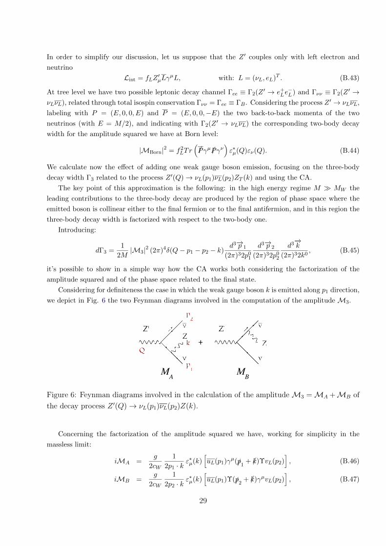
we depict in Fig. 6 the two Feynman diagrams involved in the computation of the amplitude M3.

MA MB

Figure 6: Feynman diagrams involved in the calculation of the amplitudeM3 =MA +MB of

the decay process Z ′(Q)→ νL(p1)νL(p2)Z(k).

Concerning the factorization of the amplitude squared we have, working for simplicity in the

massless limit:

iMA =g

2cW

1

2p1 · kε∗µ(k)

[uL(p1)γµ(/p1

+ /k)ΥvL(p2)], (B.46)

iMB =g

2cW

1

2p2 · kε∗µ(k)

[uL(p1)Υ(/p2

+ /k)γµvL(p2)], (B.47)

29

where Υ ≡ ifLγµεµ(Q); therefore when the gauge boson is emitted along the p1 direction p1 · k → 0,

and the first diagrams diverges while the second one is finite; as a consequence squaring the amplitude

M3 =MA+MB and using Feynman gauge divergences appear in the square |MA|2 and in the inter-

ference term MAM∗B +M∗AMB. Using the Sudakov parametrization B.2 for the external momenta

it’s straightforward to verify that:

|MA|2 =g2

2c2W

1

2p1 · kTr(

Υ/p2Υ∗/k

); (B.48)

now we use the only technical point of CA; writing:

2p1 · k =k2t

x(1− x), (B.49)

we simply observe that |MA|2 diverges as k2t → 0; in the trace we can therefore approximate k ≈

(1− x)P and p2 ≈ P : all the terms excluded by these approximations, in fact, softens the divergence

and can be neglected. As a consequence we have:

|MA|2 ≈g2

2c2W

1

k2t

x(1− x)2Tr(

Υ/PΥ∗ /P), (B.50)

and the remaining trace is exactly the one obtained in eq. (B.44) related to the process with no gauge

boson emission, showing our first step towards the factorization of the amplitude squared.

Considering the interference term MAM∗B +M∗AMB it’s possible to use the same trick writing:

MAM∗B ≈g2

2c2W

x2

k2t

Tr(

Υ/PΥ∗ /P), (B.51)

and as a result we obtain the factorization of the amplitude squared for the three-body decay in the

CA respect to the two-body one:

|M3|2 ≈g2

2c2W

x(1 + x2)

k2t

|MBorn|2. (B.52)

Referring to the eikonal approximation in eq. (B.3), we see that using CA it’s possible to factorize

the amplitude only respect to its squared.

We can apply the CA also considering the three-body phase space of Γ3 in eq. (B.45). Following

[17] we therefore obtain a complete factorization: the three-body decay width can be expressed as the

product of the two-body one times a collinear factor:

dΓ3

(Z ′ → νLνLZ

)≈ dΓ2

(Z ′ → νLνL

) α2

2π

1

4(1− s2W )

1 + x2

1− xdxdk2

t

k2t

. (B.53)

Integrating over the final phase space we finally find:

dΓ3(x) = Γ2α2

2π

1

4(1− s2W )

1 + x2

1− xL(1− x)|Sud dx (B.54)

with s = M2.

30

As commonly done in parton models, we interpret the factor multiplying the two-body decay width

as the parton distribution for finding a “neutrino parton” in the neutrino:

DνL→νL(x) =1

Γ2

dΓ3

dx=α2

2π

1

4(1− s2W )

1 + x2

1− xL(1− x)|Sud , (B.55)

where up to this point this expression take into account just the effects related to the real gauge boson

emission. Adding a tree level delta term to account the process without electroweak emission and

introducing virtual corrections at the same perturbative order of the real ones we obtain:

DνL→νL(x) =α2

2π

1

4(1− 2s2W )

PF→F + δ(1− x)

1 +

α2

2π

[3− 2s2

W

4(1− s2W )

]P virF→F

, (B.56)

where:

PF→F =1 + x2

1− xL(1− x)|Sud , P vir

F→F =3

2ln

s

M2W

− 1

2ln2 s

M2W

. (B.57)

A complete set of integrated splitting functions is collected in Table 1. eq. (B.56) represents a

concrete one-loop example, obtained through a direct calculation, of the logarithmical structure of the

electroweak fragmentation function DI→J . At this point one might be skeptical about the effective

validity of the CA. In order to remove all doubt, we compare in B.5 our improved CA with the full

result of a complete three-body calculation done in the context of the Minimal Dark Matter model [25],

finding an excellent agreement. The one-loop fragmentation functions for the entire SM are discussed

into Appendix C, in the more general context of the electroweak evolution equations [18].

At this point we are ready to evaluate in this example the energy spectrum of stable SM particles

produced by the Z ′ decay and for definiteness we consider the case of the neutrino. We get:

dNDM→νLdx

=1

Γtot

dΓ3(Z ′ → νLνLZ)

dx+dΓ3(Z ′ → νLe

+LW

−)

dx

, (B.58)

where Γtot = Γee + Γνν = 2ΓB. From eq. (B.55) we have:

dΓ3(Z ′ → νLνLZ)

dx= Γ2(Z ′ → νLνL)DνL→νL(x) = ΓBDνL→νL(x), (B.59)

and, in a similar way:

dΓ3(Z ′ → νLe+LW

−)

dx= Γ2(Z ′ → e+

Le−L )De−L→νL

(x) = ΓBDe−L→νL(x), (B.60)

with De−L→νLas in (C.2); finally we obtain the neutrino spectrum at perturbative order α2:

dNDM→νLdx

=1

2

DνL→νL(x) +De−L→νL

(x). (B.61)

B.5 Full computation in the Minimal Dark Matter model

In order to validate the eikonal and collinear approximations, we compare its results with a full compu-

tation performed in a specific predictive model. We consider the weak corrections to DM annihilations

into W+W− as predicted by “Minimal Dark Matter” models, where DM only has electroweak inter-

actions [25]. This generic situation is realized in the region of the MSSM parameter space where DM

31

could be the neutral component of the fermionic wino weak triplet with a value of the mass M ∼ 3 TeV

dictated by the cosmological DM relic density [25, 29]. The same situation can be realized with scalar

DM and/or with DM lying in different representations of the weak group. Particularly interesting are

two cases — a fermionic 5plet and a scalar 7plet with zero hypercharge — where DM is automati-

cally stable because SM particles do not have the quantum numbers that could couple to such DM

multiplets. Our computation applies in all such cases: at leading order we have the process DM DM

→ W+W−, and at NLO the three-body annihilation channels DM DM → W+W−Z and DM DM

→W+W−γ open up. The full expressions for the spectra for the emitted γ and Z are quite lengthy,

and therefore, we write them approximating MW ≈ MZ and defining ε ≡ MW /M 1, neglecting

terms of O(ε2):7

dNDM→γdx

=αem

π

[4(1− x+ x2

)2(1− x)x

ln2

ε+

2(4− 12x+ 19x2 − 22x3 + 20x4 − 10x5 + 2x6

)(x− 2)2(x− 1)x

+

+−6x5 + 32x4 − 74x3 + 84x2 − 48x+ 16

(x− 2)3(x− 1)xln(1− x)

], (B.62a)

dNDM→Zdx

=α2

πc2W

[9x4 − 18x3 + 25x2 − 16x+ 8

2x(1− x)ln

(2x/ε√

1− x+ x2

)+

2(−3x5 + 16x4 − 37x3 + 42x2 − 24x+ 8

)(2− x)3(1− x)x

ln(1− x) +

−(52− 176x+ 271x2 − 247x3 + 150x4 − 55x5 + 9x6

)x

2(2− x)2(1− x)(1− x+ x2)

], (B.62b)

dNDM→Wdx

= δ(1− x) +α2

πc2W

[9x4 − 18x3 + 25x2 − 16x+ 8

4x(1− x)ln

(2x/ε√

1− x+ x2

)+

(−5− 4/x2 + 5/x) ln(1− x) +

−80− 224x+ 425x2 − 473x3 + 341x4 − 140x5 + 36x6

16x(1− x)(1− x+ x2)

]+ (B.62c)

αem

π

[2(1− x+ x2

)2x(1− x)

ln

(2x

ε

)− 30− 54x+ 71x2 − 36x3 + 12x4

6(1− x)x+

−4− 7x+ 6x2 + x3 − 4x4 + 2x5

(1− x)x2ln(1− x)

]In the W spectra the first term is the leading order annihilation, the second one arises from 3-body

processes with an additional Z, and the third term from processes with an additional γ. Eq. (B.62a)

agrees with the result computed for fermionic DM in [30].8

We now compare the full result with its collinear approximation, where the same quantities in

Eqs. (B.62a,B.62b) are described through electroweak fragmentation functions. In the previous

7Incidentally we find that at this order the result is the same for both scalar and fermionic DM. Notice that

this Taylor expansion in ε is only valid at x ε, and consequently, like the Sudakov approximation, does not

correctly describe the kinematical boundaries.8Note that the diagram there called “QED Internal Bremsstrahlung” in our language is ordinary EW

bremsstrahlung from the initial DM and it does not give any log-enhanced effect because DM is non-relativistic.

We also agree with [30] with the terms suppressed by ∆M/MW , that we do not show because a ∆M would

need a DM coupling to the Higgs, and consequently extra 2 body annihilations.

32

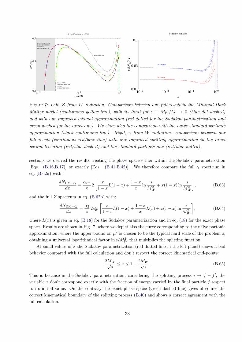
NAIVE SPLITTING

FULL 3 BODY, !" 0 andIMPROVED SPLITTING (SUDAKOV PARAMETRIZATION)

FULL 3 BODY + IMPROVED SPLITTING (EXACT PARAMETRIZATION)

10#2 10#1 1000.1

0.3

0.7

x $E!M

dNZ!dx

Z from W radiation, M $ 3 TeV

M = 10 TeV

M = 1 TeV

10!3 10!2 10!1 1000.01

0.03

0.1

x

xdN"!dx

" from W radiation

Figure 7: Left, Z from W radiation: Comparison between our full result in the Minimal Dark

Matter model (continuous yellow line), with its limit for ε ≡ MW/M → 0 (blue dot dashed)

and with our improved eikonal approximation (red dotted for the Sudakov parametrization and

green dashed for the exact one). We show also the comparison with the naıve standard partonic

approximation (black continuous line). Right, γ from W radiation: comparison between our

full result (continuous red/blue line) with our improved splitting approximation in the exact

parametrization (red/blue dashed) and the standard partonic one (red/blue dotted).

sections we derived the results treating the phase space either within the Sudakov parametrization

[Eqs. (B.16,B.17)] or exactly [Eqs. (B.41,B.42)]. We therefore compare the full γ spectrum in

eq. (B.62a) with:

dNDM→γdx

=αem

π2

[x

1− xL(1− x) +

1− xx

lns

M2W

+ x(1− x) lns

M2W

], (B.63)

and the full Z spectrum in eq. (B.62b) with:

dNDM→Zdx

=α2

π2c2W

[x

1− xL(1− x) +

1− xx

L(x) + x(1− x) lns

M2W

], (B.64)

where L(x) is given in eq. (B.18) for the Sudakov parametrization and in eq. (18) for the exact phase

space. Results are shown in Fig. 7, where we depict also the curve corresponding to the naıve partonic

approximation, where the upper bound on µ2 is chosen to be the typical hard scale of the problem s,

obtaining a universal logarithmical factor ln s/M2W that multiplies the splitting function.

At small values of x the Sudakov parametrization (red dotted line in the left panel) shows a bad

behavior compared with the full calculation and don’t respect the correct kinematical end-points:

2MW√s≤ x ≤ 1− 2MW√

s. (B.65)

This is because in the Sudakov parametrization, considering the splitting process i → f + f ′, the

variable x don’t correspond exactly with the fraction of energy carried by the final particle f respect

to its initial value. On the contrary the exact phase space (green dashed line) gives of course the

correct kinematical boundary of the splitting process (B.40) and shows a correct agreement with the

full calculation.

33

C One loop Electroweak Fragmentation Functions

In the following we collect one loop EW fragmentation functions obtained solving the EW evolution

equations in [18] for the entire Standard Model particle spectrum.

EW evolution equations have been already constructed in [18], exploiting the SU(2)L symmetry,

and classifying the states looking to their total isospin quantum numbers; consequently one have to

apply a projection technique (explained in details in [18]) in order to convert them to their QCD-like

formulation, i.e. labeling splittings with particle names: Di→j is the single leg fragmentation functions

that encode the probability for a single initial particle i to become a final particle j.

Since DM gives particle-antiparticle pairs, to reduce the combinatorics, we combine them into

pairs of primary back-to-back SM particles I instead of a single particle i. A simple formula allows us

to switch from the ‘single leg’ to the ‘double leg’ convention:

DI→J = c(Di→j +Di→j +Di→j +Di→j

), (C.1)

where c = 1/2 for complex final particles (such as the W or the ν) while c = 1/4 for real ones (such

as the Z or the γ).

C.1 Splitting of fermions

We start considering DM that produces two back-to-back fermions, ff with center-of-mass energy√s,

and compute the resulting partonic spectrum of other SM particles A, Df→A(z), with z ≡ EA/2√s.

As the ff pair produces A and A with the same energy spectrum, we always average over particle

and its anti-particle both in the initial and in the final state, even for real particles such as the Z.

The initial fermion can be f = eR, eL, νL, uL, dL, uR, dR and is identified by its T3 = −1/2, 0, 1/2,its electric charge Q, its generation number. We define the usual coupling to the Z, gf = T3 − s2

WQ

and to the photon, αem = s2Wα2. We define the top Yukawa coupling yt = mt/v with v ≈ 174 GeV

and αt = y2t /4π. Neglecting all other fermion masses we get:

Df→f (x) = δ(1− x)

[1 +

α2

2π(2T 2

3 +g2f

c2W

+Q2 s2W )P vir

F→F

]+ (C.2a)

+α2

2π(g2f

c2W

+Q2s2W ) PF→F (x), (C.2b)

Df→ZT (x) =α2 g

2f

2πc2W

PF→V (x), (C.2c)

Df→γ(x) =αem

2πQ2 PF→V (x), (C.2d)

Df→f ′(x) =α2

2π2 T 2

3 PF→F (x), (C.2e)

Df→WT(x) =

α2

2π2 T 2

3 PF→V (x), (C.2 f )

where f ′ is the SU(2)L partner of f (e.g. f ′ = eL for f = νL and viceversa). The virtual term in the

first line means that a fraction of the initial f with x = 1 disappears into f or other particles with

x < 1.

34

All splittings of quarks are negligible with respect to the QCD splittings (not written). For the t and

b quarks there are extra splittings (to be summed to the ones listed above due to gauge interactions)

due to the top quark Yukawa interaction, which also have minor effects. Again these splittings depend

on the quark polarization; for simplicity, we write them for average unpolarized t, b quarks:

DYukt→t(x) = δ(1− x)

3αt8π

PYuk,virF→F +

αt4π

PYukF→F (x) (C.3a)

DYukt→b(x) = DYuk

b→t(x) =αt8π

PYukF→F (x) (C.3b)

DYukt→ZL(x) = DYuk

t→h = DYukt→WL

= DYukb→WL

=αt8π

PYukF→S(x) (C.3c)

DYukb→b(x) = δ(1− x)

αt8π

PYuk,virF→F . (C.3d)

C.2 Splitting of Higgses

The Higgs doublet H contains the physical Higgs h, as well as the goldstone components that describe

the longitudinal polarizations WL and ZL of the SM massive vectors. Splittings induced by the top

quark Yukawa coupling have a significant effect; we describe them without specifying the polarizations

of the t, b quarks, which make a negligible difference.

For the physical Higgs h we have:

Dh→h(x) = δ(1− x)

[1 +

3 α2 + αY2π · 4

P virS→S

]+

3 αt4π

P vir,YukS→F , (C.4a)

Dh→WT(x) =

α2

2π

1

2PS→V (x) = 2 c2

W Dh→ZT (x), (C.4b)

Dh→WL(x) =

α2

2π

1

2PS→S(x) = 2 c2

W Dh→ZL(x), (C.4c)

Dh→t(x) =3 αt2π

PYukS→F (x). (C.4d)

The same expressions hold for an initial ZL. For the longitudinal WL we have:

DWL→WL(x) = δ(1− x)

[1 +

3 α2 + αY2π · 4

P virS→S

]+α2 + αY

2π · 4PS→S(x) +

3 αt4π

P vir,YukS→F , (C.5a)

= δ(1− x)

[1 +

αem

2πP virS→S

]+αem

2πPS→S(x) + · · · , (C.5b)

DWL→h(x) =α2

2π

1

4PS→S(x) = DWL→ZL(x), (C.5c)

DWL→ZT (x) =α2

2π

g2eL

c2W

PS→V (x), (C.5d)

DWL→γ(x) =αem

2πPS→V (x), (C.5e)

DWL→t(x) = DWL→b(x) =3 αt4π

PYukS→F (x). (C.5 f )

Eq. (C.5b) shows the QED corrections only, in case one needs to subtract them.

35

C.3 Splitting of vectors

For the transverse W± we find:

DWT→WT(x) = δ(1− x)

[1 +

α2

2π2 P vir

SU(2)

]+α2

2πPV→V (x), (C.6a)

DWT→ZT (x) =α2

2πc2W PV→V (x), (C.6b)

DWT→γ(x) =α2

2πs2W PV→V (x), (C.6c)

DWT→fL(x) =α2

2π

1

2Nc PV→F (x), f = e, νe, d, u;µ, νµ, s, c; τ, ντ , b, t, (C.6d)

DWT→h(x) =α2

2π

1

4PV→S(x) = DWT→ZL(x), (C.6e)

DWT→WL(x) =

α2

2π

1

2PV→S(x), (C.6 f )

and for the transverse Z we find:

DZT→ZT (x) = δ(1− x)

[1 +

α2

2π

(2 c2

W P virSU(2) +

s4W

c2W

P virU(1)

)], (C.7a)

DZT→WT(x) =

α2

2π2 c2

W PV→V (x), (C.7b)

DZT→f (x) =α2g

2f

2πc2W

2 Nc PV→F (x), f = νe, eL, eR, uL, uR, dL, dR, . . ., (C.7c)

DZT→h(x) =α2 g

2ν

2πc2W

PV→S(x) = DZT→ZL(x), (C.7d)

DZT→WL(x) =

α2

2π

2 g2eL

c2W

PV→S(x), (C.7e)

where we defined Nc = 1 (3) if f is a lepton (a quark) doublet; Ngen = 3, and:

P virSU(2) =

1

2P virV→V +

1

4P virV→S +Ngen P

virV→F , (C.8a)

P virU(1) = Ngen (2Y 2

L + Y 2E + 6Y 2

Q + 3Y 2U + 3Y 2

D) P virV→F + 2 Y 2

L PvirV→S . (C.8b)

The γ contributes to PWT→WTand can be excluded by dropping 1 = c2

W +s2W → c2

W in front of PV→V ,

both real and virtual. (Notice that PYTHIA does not include QED radiation from W±).

Finally for the photon we have:

Dγ→γ(x) = δ(1− x)

[1 +

αem

2π

(2 P vir

SU(2) + P virU(1)

)], (C.9a)

Dγ→WT(x) =

αem

2π2 PV→V (x), (C.9b)

Dγ→WL(x) =

αem

2π2 PV→S(x), (C.9c)

Dγ→f (x) =αem

2π2Q2 Nc PV→F (x), f = eL, eR, uL, uR, dL, dR, . . .. (C.9d)

References

[1] D. N. Spergel et al. [WMAP Collaboration], Astrophys. J. Suppl. 170 (2007) 377 [arXiv:astro-

ph/0603449].

36

[2] See, for instance, E. A. Baltz, M. Battaglia, M. E. Peskin and T. Wizansky, Phys. Rev. D 74,

103521 (2006).

[3] For a review, see E. Aprile, PoS E PS-HEP2009 (2009) 009.

[4] WMAP collaboration, arXiv:astro-ph/0603449.

[5] ATIC collaboration, Nature 456 (2008) 362.

[6] FERMI/LAT collaboration, arXiv:0905.0025.

[7] H.E.S.S. Collaboration, arXiv:0811.3894. H.E.S.S. Collaboration, arXiv:0905.0105.

[8] D. Hooper, P. Blasi and P. D. Serpico, JCAP 0901, 025 (2009) [arXiv:0810.1527].

[9] M. Cirelli, M. Kadastik, M. Raidal and A. Strumia, Nucl. Phys. B 813 (2009) 1.

[10] N. Arkani-Hamed, D. P. Finkbeiner, T. R. Slatyer and N. Weiner, Phys. Rev. D 79 (2009) 015014.

[11] P. Ciafaloni, D. Comelli, Phys. Lett. B 446, 278 (1999).

[12] A. Denner, S. Dittmaier and T. Hahn, Phys. Rev. D 56, 117 (1997); A. Denner and T. Hahn, Nucl.

Phys. B 525, 27 (1998); M. Beccaria, G. Montagna, F. Piccinini, F. M. Renard and C. Verzeg-

nassi, Phys. Rev. D 58 (1998) 093014; P. Ciafaloni and D. Comelli, Phys. Lett. B 446, 278

(1999); V. S. Fadin, L. N. Lipatov, A. D. Martin and M. Melles, Phys. Rev. D 61 (2000) 094002;

P. Ciafaloni, D. Comelli, Phys. Lett. B 476 (2000) 49; J. H. Kuhn, A. A. Penin and V. A. Smirnov,

Eur. Phys. J. C 17, 97 (2000); J. H. Kuhn, S. Moch, A. A. Penin, V. A. Smirnov, Nucl. Phys.

B 616, 286 (2001) [Erratum-ibid. B 648, 455 (2003)]; M. Melles, Phys. Rept. 375, 219 (2003);

J. H. Kuhn, A. Kulesza, S. Pozzorini and M. Schulze, Phys. Lett. B 609 (2005) 277 A. Denner,

B. Jantzen and S. Pozzorini, Nucl. Phys. B 761 (2007) 1; J. H. Kuhn, A. Kulesza, S. Pozzorini

and M. Schulze, E. Accomando, A. Denner and S. Pozzorini, JHEP 0703 (2007) 078; Nucl. Phys.

B 797 (2008) 27; J. y. Chiu,F. Golf, R. Kelley and A. V. Manohar, Phys. Rev. D 77 (2008) 053004;

J. y. Chiu, R. Kelley and A. V. Manohar, Phys. Rev. D 78 (2008) 073006; A. Denner, B. Jantzen

and S. Pozzorini, JHEP 0811 (2008) 062.

[13] V. S. Fadin, L. N. Lipatov, A. D. Martin and M. Melles, Phys. Rev. D 61 (2000) 094002;

P. Ciafaloni, D. Comelli, Phys. Lett. B 476 (2000) 49; J. H. Kuhn, A. A. Penin and V. A. Smirnov,

Eur. Phys. J. C 17, 97 (2000); J. H. Kuhn, S. Moch, A. A. Penin, V. A. Smirnov, Nucl. Phys.

B 616, 286 (2001) [Erratum-ibid. B 648, 455 (2003)]; M. Melles, Phys. Rept. 375, 219 (2003);

J. y. Chiu, F. Golf, R. Kelley and A. V. Manohar, Phys. Rev. D 77 (2008) 053004.

[14] M. Ciafaloni, P. Ciafaloni and D. Comelli, Phys. Rev. Lett. 84, 4810 (2000); Nucl.Phys. B 589 359

(2000); Phys. Lett. B 501, 216 (2001); Phys. Rev. Lett. 87 (2001) 211802; Nucl. Phys. B 613 (2001)

382; Phys. Rev. Lett. 88, 102001 (2002); JHEP 0805 (2008) 039; P. Ciafaloni, D. Comelli and

A. Vergine, JHEP 0407, 039 (2004); M. Ciafaloni, Lect. Notes Phys. 737 (2008) 151; P. Ciafaloni

and D. Comelli, JHEP 0511 (2005) 022; JHEP 0609, 055 (2006).

37

[15] M. Ciafaloni, P. Ciafaloni and D. Comelli, Nucl. Phys. B 613 (2001) 382.

[16] M. Ciafaloni, P. Ciafaloni, D. Comelli, Nucl.Phys. B 589 (2000) 359; M. Ciafaloni, P. Ciafaloni

and D. Comelli, Phys. Rev.Lett 87 , 211802 (2001); M. Ciafaloni, P. Ciafaloni and D. Comelli,

Phys. Lett. B 501, 216 (2001); P. Ciafaloni, D. Comelli and A. Vergine, JHEP 0407, 039 (2004);

[17] P. Ciafaloni and A. Urbano, Phys. Rev. D 82, 043512 (2010) [arXiv:1001.3950 [hep-ph]].

[18] M. Ciafaloni, P. Ciafaloni and D. Comelli, Phys. Rev. Lett. 88, 102001 (2002); P. Ciafaloni and

D. Comelli, JHEP 0511 (2005) 022.

[19] V. Gribov, L. Lipatov, Sov. J. Nucl. Phys 15, 438 (1972); L. Lipatov, Sov. J. Nucl. Phys 20, 94

(1972); G. Altarelli, G. Parisi, Nucl. Phys. B 126, 298 (1977); Y. Dokshitzer, Sov. Phys. JETP

46, 641 (1977).

[20] F. Bloch and A. Nordsieck, Phys. Rev. 52 (1937) 54. V. V. Sudakov, Sov. Phys. JETP 3, 65

(1956) [Zh. Eksp. Teor. Fiz. 30, 87 (1956)]. D. R. Yennie, S. C. Frautschi and H. Suura, Annals

Phys. 13 (1961) 379.

[21] N. F. Bell, J. B. Dent, T. D. Jacques and T. J. Weiler, Phys. Rev. D 78 (2008) 083540 J. B. Dent,

R. J. Scherrer and T. J. Weiler, Phys. Rev. D 78 (2008) 063509 M. Kachelriess, P. D. Serpico

and M. A. Solberg, Phys. Rev. D 80 (2009) 123533. M. Kachelriess and P. D. Serpico, Phys. Rev.

D 76 (2007) 063516. See also section 2.3 of M. Papucci and A. Strumia, JCAP 1003 (2010) 014

[arXiv:0912.0742].

[22] M. Ciafaloni, P. Ciafaloni and D. Comelli, JHEP 1003 (2010) 072.

[23] C. Barbot and M. Drees, Phys. Lett. B 533 (2002) 107 [arXiv:hep-ph/0202072].

[24] Our results are available at http://www.pi.infn.it/~astrumia/DMEW.html and will be included

in http://www.marcocirelli.net/PPPC4DMID.html together with the results of a paper by M.

Cirelli et al., to appear.

[25] M. Cirelli, N. Fornengo, A. Strumia, Nucl. Phys. B753 (2006) 178 [arXiv:hep-ph/0512090].

M. Cirelli, R. Franceschini, A. Strumia, Nucl. Phys. B800 (2008) 204 [arXiv:0802.3378].

[26] F. Donato, N. Fornengo, D. Maurin and P. Salati, Phys. Rev. D 69, 063501 (2004) [arXiv:astro-

ph/0306207].

[27] M. Ciafaloni, P. Ciafaloni and D. Comelli, Nucl. Phys. B 613 (2001) 382.

[28] R. Brock et al. [CTEQ Collaboration], Rev. Mod. Phys. 67, 157 (1995).

[29] J. Hisano, S. Matsumoto, M. Nagai, O. Saito and M. Senami, Phys. Lett. B 646 (2007) 34.

[30] L. Bergstrom, T. Bringmann, M. Eriksson and M. Gustafsson, Phys. Rev. Lett. 95 (2005) 241301.

38