WAVELET BASED IMAGE COMPRESSION ON THE TEXAS INSTRUMENT VIDEO PROCESSING BOARD TMS320DM6437

Riken Shah B.E., Gujarat University, India, 2007

PROJECT

Submitted in partial satisfaction of the requirements for the degree of

MASTER OF SCIENCE

in

ELECTRICAL AND ELECTRONIC ENGINEERING

at

CALIFORNIA STATE UNIVERSITY, SACRAMENTO

SPRING 2011

ii

WAVELET BASED IMAGE COMPRESSION ON THE TEXAS INSTRUMENT VIDEO PROCESSING BOARD TMS320DM6437

A Project

by

Riken Shah

Approved by: __________________________________, Committee Chair Jing Pang, Ph.D. __________________________________, Second Reader Fethi Belkhouche, Ph.D. ____________________________ Date

iii

Student:

Riken Shah

I certify that this student has met the requirements for format contained in the University

format manual, and that this project is suitable for shelving in the Library and credit is to

be awarded for the Project.

__________________________, Graduate Coordinator ________________ Preetham Kumar, Ph.D. Date Department of Electrical and Electronic Engineering

iv

Abstract

of

WAVELET BASED IMAGE COMPRESSION THE TEXAS INSTRUMENT VIDEO PROCESSING BOARD TMS320DM6437

by

Riken Shah

Time has become a crucial issue in today’s lifestyle and to keep up the pace with

the world we need to come up with technologies that can process things faster. With high

speed technology in image processing industry, the demand of good quality data is

increasing rapidly. The usage of image and streaming of video on internet have increased

exponentially. In addition, more storage capacity and more bandwidth as HD (High

Density) image and video have become more and more popular. In this project, mainly I

demonstrated two different methods of image compression DCT based image

compression and WAVELET based image compression on JPEG2000 image standard. I

designed DCT based image compression and WAVELET based image compression

codes in matlab and compared their results. After that, I implemented the wavelet

algorithm using C and C# in visual studio to verify the design. Finally I implemented the

same algorithm on TI’s digital signal processing board EVM320DM6437, based on C

language.

In addition, for implementing discrete wavelet transform on EVM320DM6437

board, I captured the image frame from a video signal. Then, I extracted the Y

v

components of the image. Then I used Code Composer Studio software to implement the

code written in C language to successful display the compression result on Television.

_______________________, Committee Chair Jing Pang, Ph.D. _______________________ Date

vi

ACKNOWLEDGEMENTS

As I am starting discussing the project, the first thing I would love to do is really

thank and say something to all the people who have contributed also motivated me for

completing this project successfully. I would like to thank Dr. Jing Pang for providing me

such a nice opportunity to work on this project, which was a great exposure to the field of

digital processing. I must say she has a very good knowledge in this field. I must say that

I would not have been possible for me to finish this project without her help throughout

the research.

I would like to thank Shetul Saksena, who also worked with me on this project.

Without his help, it would have been impossible for me to finish this project. His

experience and knowledge have played vital roles in this project.

I would like to thank Dr. Fethi Belkhouche for reviewing my report. His

experience was also a great help for me to understand this project. He showed me many

areas where I can improve my presentation of report work. Last but not the least I would

like to thank all of my family members for providing me strength and immense support.

Also, thanks to all the faculty members of Department of Electrical and Electronics

Engineering at California State University, Sacramento for the help and support to

complete my graduation successfully.

vii

TABLE OF CONTENTS

Page

Acknowledgements……………………………………………………………….……...vi

List of Figures...…………………………………………………………………………..ix

Chapter

1. INTRODUCTION……………………………………………………………………1

1.1 Introduction to image processing…….………………………………………1

1.2 Organization of report………………………………………………………..2

2. BASIC CONCEPT OF IMAGE PROCESSING AND TWO DIFFERENT TYPES OF FORMAT JPEG AND JPEG2000……….………………………………………4

2.1 Introduction to image compression and decompression...……………………4

2.2 Types of image compression techquniques….……………………………….4

2.2.1 Lossy image compression………………………………………………4

2.2.2 Lossless image compression……………………………………………5

2.3 Two different formats JPEG and JPEG 2000………………………………...6

2.3.1 Introduction to image standard JPEG…………………………………..6

2.3.2 Introduction to image standard JPEG 2000…………………………….7

2.4 Two algorithms DCT and Wavelets used in JPEG and JPEG 2000………….. respectively…………...…………...………………………………...………. 8

2.4.1 Wavelet based image processing………………………………………8

2.4.2 DCT based image processing………………………………………...11

2.4.2.1 Quantization in DCT………………………………………...12

viii

2.4.2.2 Zigzag scanning……………………………………………...13

3. MATLAB MODEL OF DCT AND WAVELET IMAGE PROCESSING………...14

3.1 Matlab representation of DCT based signal processing………………………...14

3.2 Wavelet based signal processing……………………………………………….19

4. WAVELET IMPLEMENTATION USING C LANGUAGE…….………………..22

4.1 Components on hardware and interface………...…………………………..23

4.2 Wavelet based image processing using C and C#....………………………..23

5. CONCLUSION AND FUTURE WORK........………................................................29

Appendix A Matlab model for DCT based processing…………….........………...…….30

Appendix B C model for wavelet based image compression on hardware…………......34

REFEREENCES...………………………………………………………………………35

ix

LIST OF FIGURES

1. Figure 1.1.1: Different steps of image compression and decompression..………..1 2. Figure 2.4.1(a): Steps involved in wavelet based image compression...………….9 3. Figure 2.4.1(b): DWT on each tile in an image………………..……………….....9 4. Figure 2.4.1(c): Wavelet transform on an image at different level…….……...…10

5. Figure 2.4.2(a): Equation to calculate DCT in 2D…………….….……………...11 6. Figure 2.4.2.1(a): Quantization matrix for DCT……………...………………….12 7. Figure 2.4.2.2(a): Path followed in zigzag scan…….……………………………13 8. Figure 3.1.1: Original test image of sunview……….……………………………14 9. Figure 3.1.2: YCbCr image result……………………………………………......15

10. Figure 3.1.3: Y component extraction of an image………..…………………….15

11. Figure 3.1.4: Quantized Y component of an image..…………………...…...…...16

12. Figure 3.1.5: Reconstructed YCbCr image…………………..…...……..……….17

13. Figure 3.1.6: Reconstructed RGB image……………………………..……….…17

14. Figure: 3.1.7: Error image………………………..………………………………18

15. Figure 3.2.1: Input image for wavelet based image compression.……………….19

26. Figure 3.2.2: Processed image……………….…………………………………..19

17. Figure 3.2.3: Reconstructed image………..……………………………………..20

18. Figure 3.2.4: Matrix for wavelet based image compression…………………..…20

19. Figure 4.1.1: TI DAVINCI signal processing board…………………………….22

20. Figure 4.1.2: Block diagram for TI DAVINCI signal processing board.………..23

x

21. Figure 4.2.1: Image used to do wavelet processing using C#...............................24

22. Figure 4.2.2: Wavelet based image processing 2 level………….……………….25

23. Figure 4.2.3: Wavelet based image processing 3 level………….………..……...26

1

Chapter 1

INTRODUCTION

1.1 Introduction to image processing

Image compression is getting more and more attention day by day as high speed

compression and good quality of image are in high demand. One advantage of an Image

compression is to reduce the time taken for transmission of an image [1]. For example, an

image has 512 rows and 512 columns. Without compression, totally 512x512x8 =

2,097,152 bits data needed to be stored [1]. And, each pixel is represented by 8-bit data

format. Now to compress it means to reduce the number of bits needed to store those bits

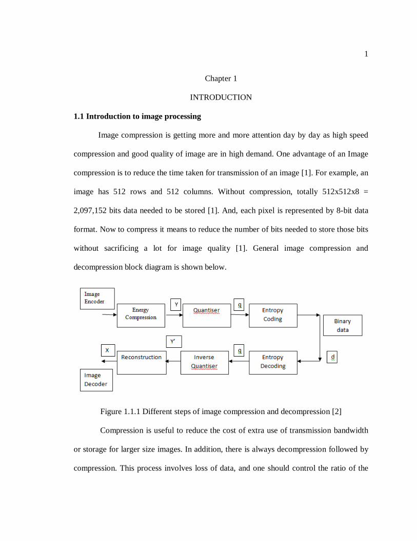
without sacrificing a lot for image quality [1]. General image compression and

decompression block diagram is shown below.

Figure 1.1.1 Different steps of image compression and decompression [2]

Compression is useful to reduce the cost of extra use of transmission bandwidth

or storage for larger size images. In addition, there is always decompression followed by

compression. This process involves loss of data, and one should control the ratio of the

2

information being lost, as images should not be compressed to a level that one cannot

even recover them with minimal loss.

What is JPEG2000? JPEG 2000 can give significant increase in performance as

compared to JPEG [2]. It is an extension to JPEG. It was introduced in 2000, so it is

called JPEG2000. The biggest advantage of it is flexibility. One can get compressed

images scalable in nature. The compression technique can be truncated at any point in

time, now the resolution and signal to noise ratio depend on the point they are truncated

[2]. In addition, it is possible to achieve variable compression rate due to its flexibility

and adaptability. With JPEG, compression algorithm is applied before encoding while

with JPEG2000 it is done in a single step. Wavelet is the algorithm name used to do

processing of JPEG2000 format. From the research, it has been found that compression

achieved by this method is 20% more as compared to JPEG [2]. Wavelet algorithm works

on a pixel value. It can vary from values 0 (black) to 256 (white). In wavelet based

compression, average and difference of two adjacent pixels are taken. Then the value

close to 0 is discarded. This is a method to reduce the number of bits. Because of its

effectiveness in edge detection, it is used in medical images as well as in military images.

Police department use it for finger print detection. DMV follows this algorithm for car

plate detection.

1.2 Organization of report

Chapter 2 consists of basic information of what compression and decompression.

In addition, the difference between two industry standards JPEG and JPEG 2000 I

3

described. Different components of these two standards are explained with lots of

figures. It makes this report easy to understand.

Chapter 3 has the entire information about Matlab model implemented for both

DCT based and Wavelet based image processing. Again, the results generated by those

matlab codes are included in the report. It is making the report easy for readers to

understand the difference between both of them.

Chapter 4 consists of C language based model of wavelet-based algorithm. This

algorithm was implemented on Texas Instruments’ digital signal processing board

provided by Dr. Jing Pang. All the result images generated by that algorithm to prove the

reliability of the code are included in this report.

Chapter 5 shows how Wavelet is better than DCT based algorithm along with

results to support it. In addition, the implementation of the code on hardware is also

shown.

4

CHAPTER 2

BASIC CONCEPT OF IMAGE PROCESSING AND TWO DIFFERENT TYPES OF FORMAT JPEG AND JPEG2000

2.1 Introduction to image compression and decompression

Any image taken from a camera is stored in a computer in form of a matrix. Each

pixel is represented by a value from 0 to 255. More pixels in an image means that more

memory is needed to store that image. Therefore, digital image processing concept is

concentrated on reduction of memory consumption. It has been found that general

1024X1024-color image occupies 3 MB of memory for storage [3]. Digital image

transmission is also a major area, where data compression and decompression methods

are required. Since most communication channels are noisy, Robustness of these

techniques is equally important [3].

2.2 Types of image compression techniques

Digital image compression can be divided mainly in two large categories: lossless

and lossy compression. Lossless compression is used for artificial images. They use low

bits rate. There is a possibility of loss some of the data during this process. While lossless

compression is preferred in medical images and military images.

2.2.1 Lossy image compression

In lossy compression and decompression methods, accuracy is so important.

There will be a data loss but it should be under the limit of tolerance. It should be good

enough for application of image processing. This kind of compression is used for

transmitting or storing multimedia data, where compromise with the loss is allowed. In

5

contrast to lossless data processing, lossy signal processing repeatedly does compression

and decompression on file. That eventually will affect the quality of data. The concept of

lossy compression is supported by rate distortion theory. CPC, JPEG, Fractal

compression are some examples of lossy signal processing methods. To conclude, on the

receiver side, when there is a human eye the signal allows lossy compression as human

eye can tolerate some imperfection [3].

2.2.2 Lossless image compression

In this type of compression, after decompression the images are almost the same

as output images. It can allow the difference between the original image and the

reconstructed image up to the certain predefined value. Lossless compression can be a

valuable solution where we have strict constrains on the reconstruction. In addition, this

method is useful where little information on each pixel is very important. We call wavelet

a loss less technique. In wavelet algorithm, we do successive re-construction. This makes

it possible to receive all the information without a data loss. RLE, LZW, Entropy coding

are some examples of lossless data compression.

Following are some basic steps involved in compressing and decompressing

image.

Step 1: Give specifications like what are the bits we have available and what the

error tolerance on the receiver side.

Step 2: Separate data into different categories depending on their importance.

Step 3: Quantize each category using all the information we have available.

Step 4: Encode all the information with help of entropy coder.

6

Step 5: On receiver side read data that is quantized. This process is usually faster

than transmitter side.

Step 6: Decode that data using entropy decoder.

Step 7: Dequantization of the data received after step 6.

Step 8: Reconstruct the image [4]

2.3 Two different formats JPEG and JPEG 2000

In this section, two different image standards JPEG and JPEG 2000 are discussed.

2.3.1 Introduction to image standard JPEG

JPEG (Joint Photographic Experts Group) comes from the committee name that

introduced this standard. This is a lossy type of image compression. It is effectively used

on still images. On the other hand, MPEG is used for moving image standards. JPEG is

called lossy because the reconstructed image on the receiver side is not the same as the

transmitter side. The advantage is that one can achieve much higher compression with

this standard but at the cost of some data. The small difference in color is invisible to

human eye and JPEG standard works on that concept. If detail analysis of the image

pixel-by-pixel is done, it would be realized that the amount of data being lost is high.

Although the data is lost, it can be controlled by setting parameters. One can keep

decreasing size of the file, by reducing the number of bits until it is not affecting the

quality of image. The image should be recognized well on the receiver side.

There is one mode called progressive mode, which handles real time image

transmission. In multiple scans, DCT co-efficients are sent. Depending on each scan, we

can get more compressed image. This mode is a hierarchical mode, which is used for an

7

image at multi resolution. Images with resolution like 1024X1024 and 2048X2048, are

stored as a difference with next small size images. There were many extensions

introduced to JPEG. Quantization is one of them. This method is most popular these days

for image compression. It is easy to separate most important and less important parts of

the image with this method. To code them, it is necessary to pay high attention to

important part and less attention to less important parts. [5]

2.3.2 Introduction to image standard JPEG 2000

JPEG 2000 is a result of extended study performed on JPEG standard for

improvements. Although studies are being done since 1996, the first paper on JPEG 2000

was published in December 2000. The Committee’s initial aim was to introduce these

concepts of high bit rate and better quality. Later scalability and Region of interest

concept were introduced. This makes it even more powerful. It can compress data with

low bit rate but without losing and the data image can be recovered. That is the reason it

is called the lossless compression [6].

Following are the steps involved in JPEG 2000:

• Better efficiency in compression of data can be achieved.

• There are more chances of lossless compression.

• Different output with different resolution can be decoded.

• Desired bit rate with this method can be achieved.

• Division of image in to different steps so that we can take use of all of them.

• Region of interest extraction.

8

• Very high noise resilience improvement.

• We can achieve access to any bit rate to get access of that particular image. File

format is more flexible.

This standard enables reuse of image created once in many other applications.

The biggest advantage is that one does not need to recompress it. It has the same stream

of bits. If a server leaves some data for a use to its consumers, then they can customize

same image differently [7].

2.4 Two algorithms DCT and Wavelets used in JPEG and JPEG 2000 respectively

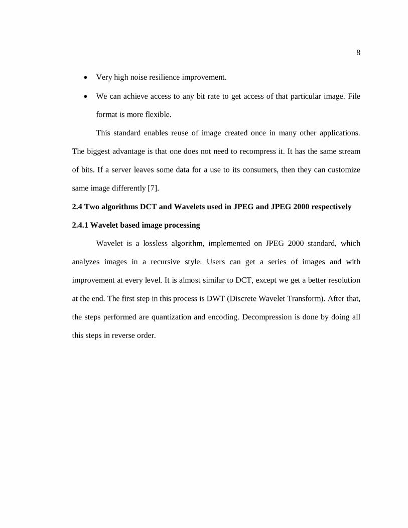
2.4.1 Wavelet based image processing

Wavelet is a lossless algorithm, implemented on JPEG 2000 standard, which

analyzes images in a recursive style. Users can get a series of images and with

improvement at every level. It is almost similar to DCT, except we get a better resolution

at the end. The first step in this process is DWT (Discrete Wavelet Transform). After that,

the steps performed are quantization and encoding. Decompression is done by doing all

this steps in reverse order.

9

Figure 2.4.1(a) Steps involved in Wavelet based compression [8]

Another advantage of this type of image processing is that we can view image at

different resolution level.

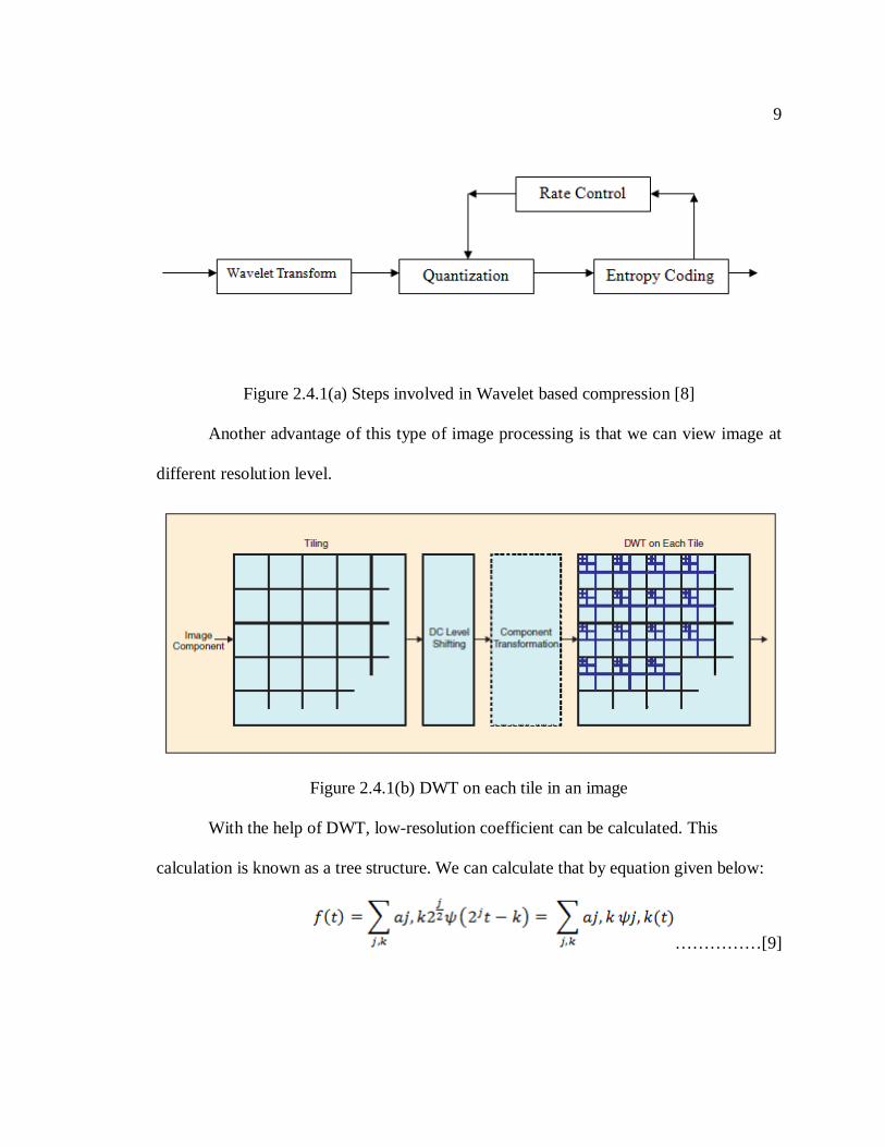
Figure 2.4.1(b) DWT on each tile in an image

With the help of DWT, low-resolution coefficient can be calculated. This

calculation is known as a tree structure. We can calculate that by equation given below:

……………[9]

10

Where aj,k is discrete wavelet transform of f(t). Scaling of the image

depends on variable k and shape of the wavelet is dependent of variable j.

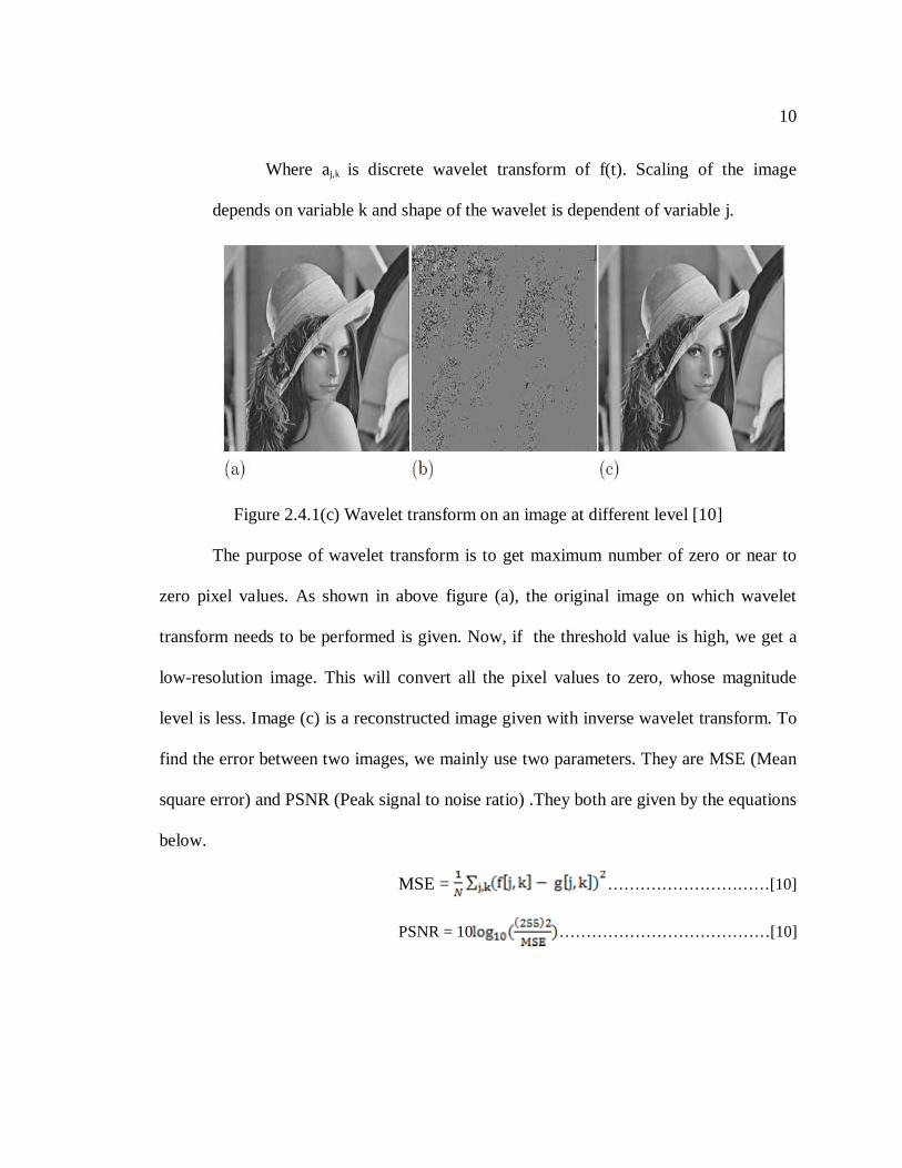
Figure 2.4.1(c) Wavelet transform on an image at different level [10]

The purpose of wavelet transform is to get maximum number of zero or near to

zero pixel values. As shown in above figure (a), the original image on which wavelet

transform needs to be performed is given. Now, if the threshold value is high, we get a

low-resolution image. This will convert all the pixel values to zero, whose magnitude

level is less. Image (c) is a reconstructed image given with inverse wavelet transform. To

find the error between two images, we mainly use two parameters. They are MSE (Mean

square error) and PSNR (Peak signal to noise ratio) .They both are given by the equations

below.

MSE = …………………………[10]

PSNR = 10 …………………………………[10]

11

Then Mean Square error (MSE) is one of the different ways to find the value of

difference between two things with estimation. So, in general MSE of an estimator A’

with respect to the estimated parameter A is defined as

MSE (A’) = E ((A’-A) 2)……………………………[8]

In addition, PSNR (Pick Signal to Noise Ratio) is a ratio between maximum

power of a signal and power of corrupted noise. These signals generally have a very long

range, hence a logarithmic scale is used. It is widely used standard for checking image

quality in image processing.

2.4.2 DCT based image processing

This technique is widely used in image processing. Even though it is lossy it

provides very high compression rate. It uses the ideas from Discrete Fourier Transform

(DFT) and Fast Fourier Transform (FFT). The main idea behind this algorithm is to

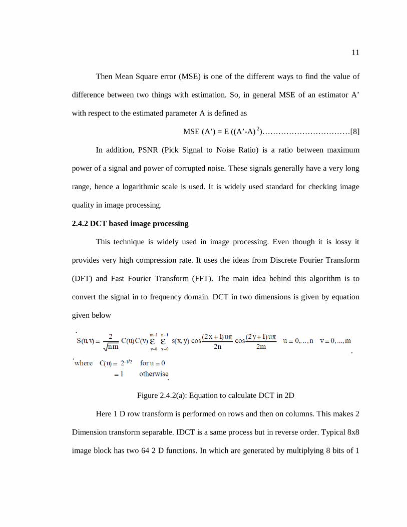
convert the signal in to frequency domain. DCT in two dimensions is given by equation

given below

Figure 2.4.2(a): Equation to calculate DCT in 2D

Here 1 D row transform is performed on rows and then on columns. This makes 2

Dimension transform separable. IDCT is a same process but in reverse order. Typical 8x8

image block has two 64 2 D functions. In which are generated by multiplying 8 bits of 1

12

D array to another. Each sets represent, horizontal and vertical frequencies respectively.

From both of the dimensions, coefficient with frequency value zero is called DC

coefficient. Others are known as AC coefficient. It is needed to make the value of the

coefficients of lower frequency near DC component. They can be removed, as they are

not important as high frequency values. The human eye is less sensitive to high frequency

value [4].

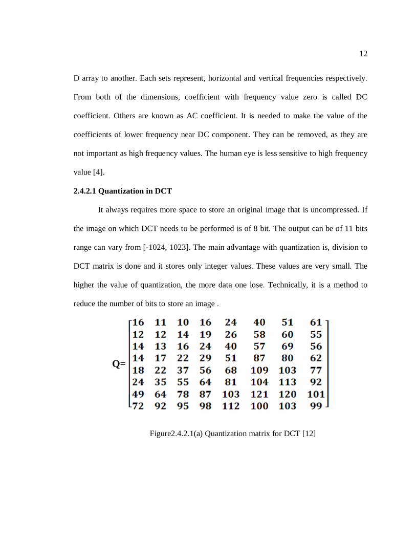
2.4.2.1 Quantization in DCT

It always requires more space to store an original image that is uncompressed. If

the image on which DCT needs to be performed is of 8 bit. The output can be of 11 bits

range can vary from [-1024, 1023]. The main advantage with quantization is, division to

DCT matrix is done and it stores only integer values. These values are very small. The

higher the value of quantization, the more data one lose. Technically, it is a method to

reduce the number of bits to store an image .

Q=

Figure2.4.2.1(a) Quantization matrix for DCT [12]

13

This matrix is designed in such a way that it has corresponding value for each

element of the image matrix. One should encrypt the essential data with low value of step

size and less important value with big step size.

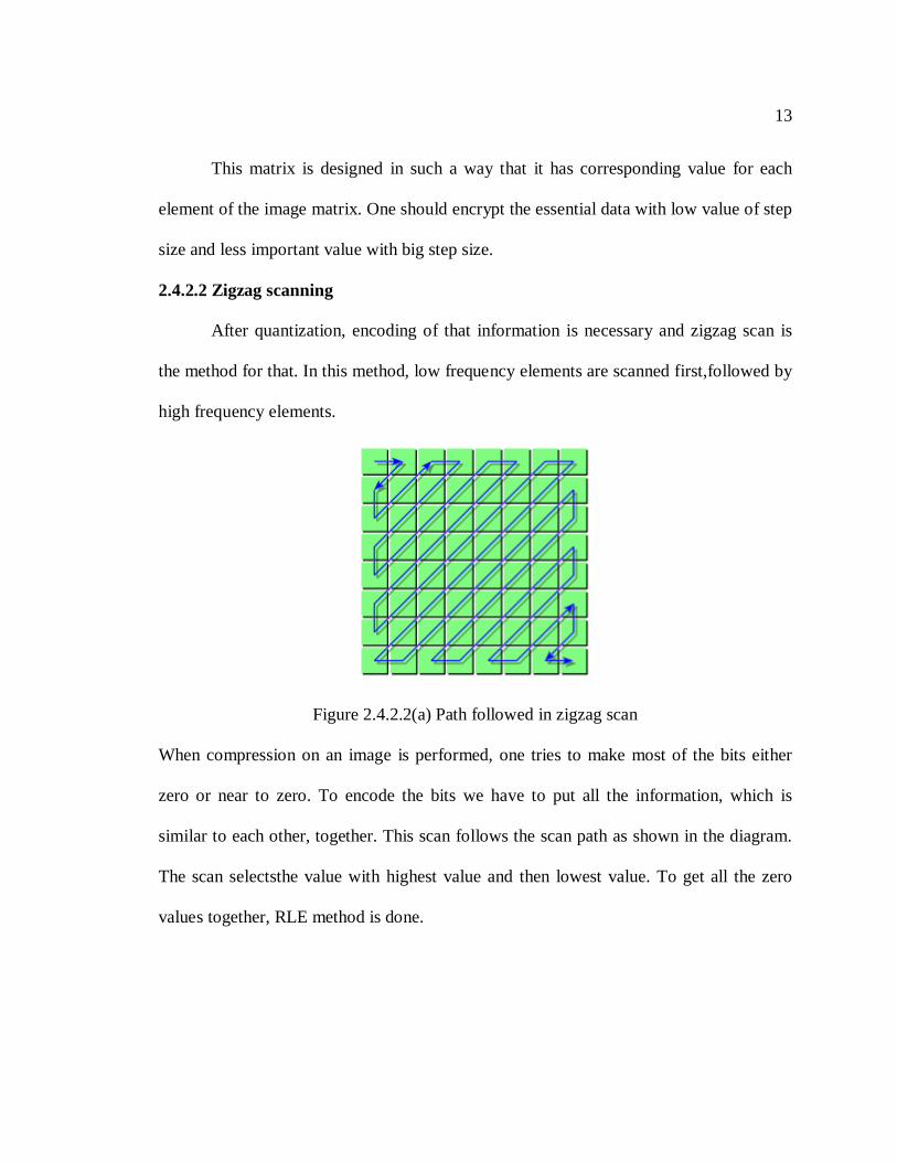
2.4.2.2 Zigzag scanning

After quantization, encoding of that information is necessary and zigzag scan is

the method for that. In this method, low frequency elements are scanned first,followed by

high frequency elements.

Figure 2.4.2.2(a) Path followed in zigzag scan

When compression on an image is performed, one tries to make most of the bits either

zero or near to zero. To encode the bits we have to put all the information, which is

similar to each other, together. This scan follows the scan path as shown in the diagram.

The scan selectsthe value with highest value and then lowest value. To get all the zero

values together, RLE method is done.

14

Chapter 3

MATLAB MODEL OF DCT AND WAVELET IMAGE PROCESSING

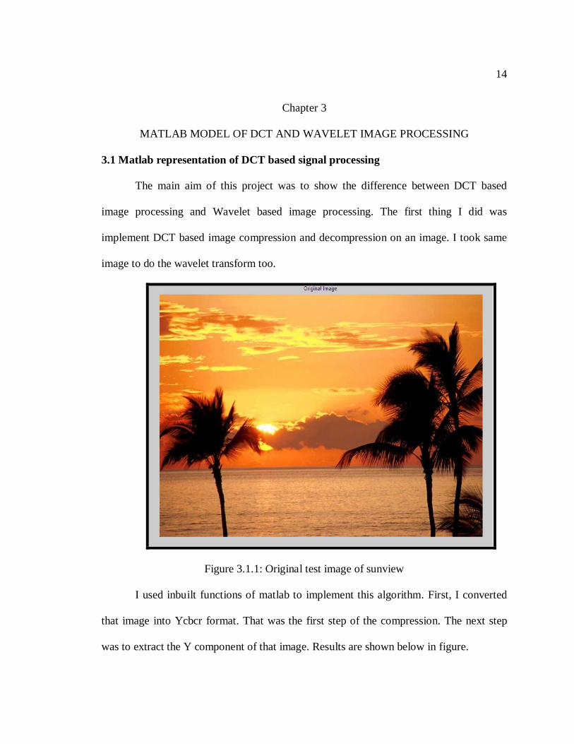
3.1 Matlab representation of DCT based signal processing

The main aim of this project was to show the difference between DCT based

image processing and Wavelet based image processing. The first thing I did was

implement DCT based image compression and decompression on an image. I took same

image to do the wavelet transform too.

Figure 3.1.1: Original test image of sunview

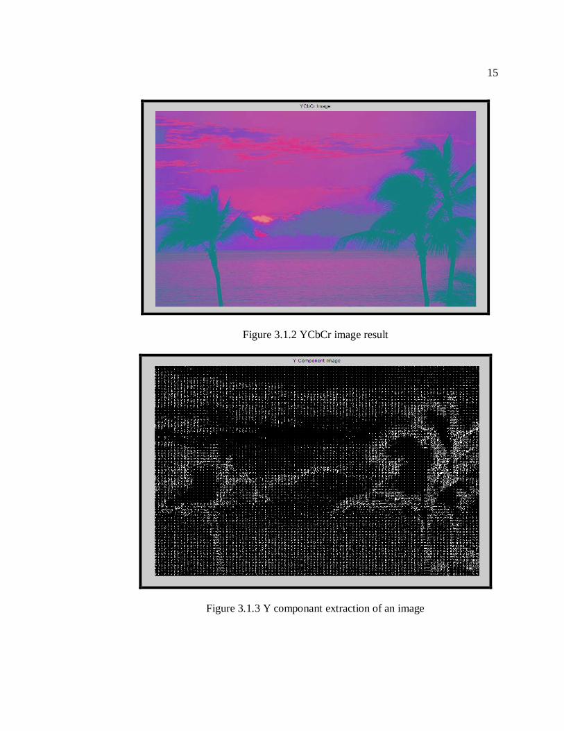
I used inbuilt functions of matlab to implement this algorithm. First, I converted

that image into Ycbcr format. That was the first step of the compression. The next step

was to extract the Y component of that image. Results are shown below in figure.

15

Figure 3.1.2 YCbCr image result

Figure 3.1.3 Y componant extraction of an image

16

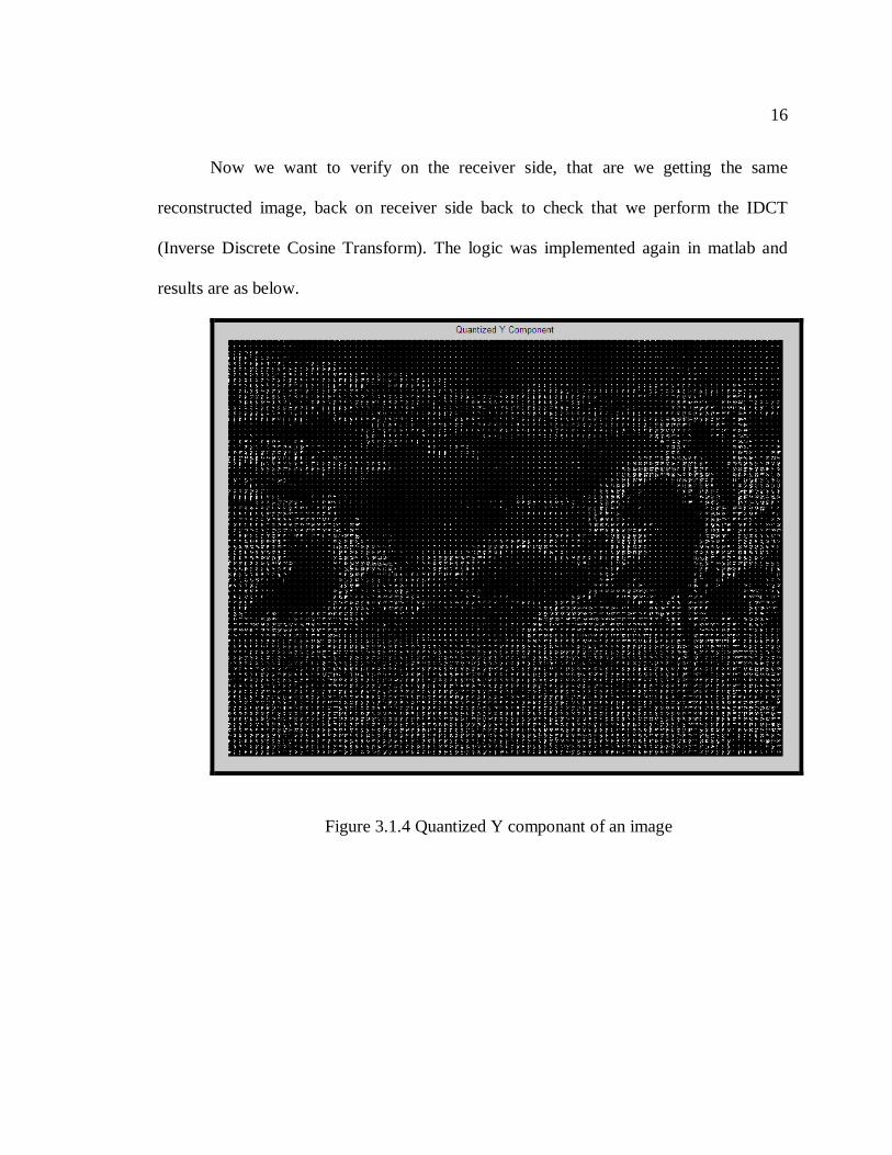
Now we want to verify on the receiver side, that are we getting the same

reconstructed image, back on receiver side back to check that we perform the IDCT

(Inverse Discrete Cosine Transform). The logic was implemented again in matlab and

results are as below.

Figure 3.1.4 Quantized Y componant of an image

17

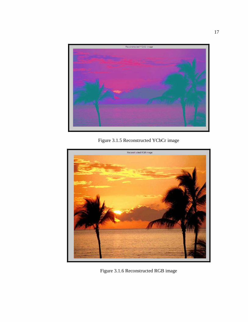
Figure 3.1.5 Reconstructed YCbCr image

Figure 3.1.6 Reconstructed RGB image

18

If we see this image from our eye we may not see the difference between original

image and reconstructed image. If you see the difference image given above you can

clearly see the amount of data we are loosing. This is the main advantage of the

compression using this meathod we are loosing some amount of data here, but we can

achieve high compression ratio.

Figure 3.1.7 Error image

19

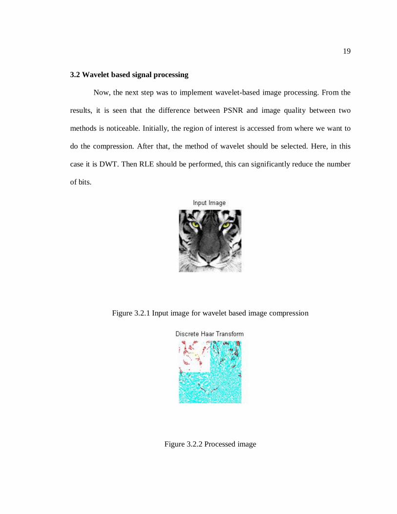
3.2 Wavelet based signal processing

Now, the next step was to implement wavelet-based image processing. From the

results, it is seen that the difference between PSNR and image quality between two

methods is noticeable. Initially, the region of interest is accessed from where we want to

do the compression. After that, the method of wavelet should be selected. Here, in this

case it is DWT. Then RLE should be performed, this can significantly reduce the number

of bits.

Figure 3.2.1 Input image for wavelet based image compression

Figure 3.2.2 Processed image

20

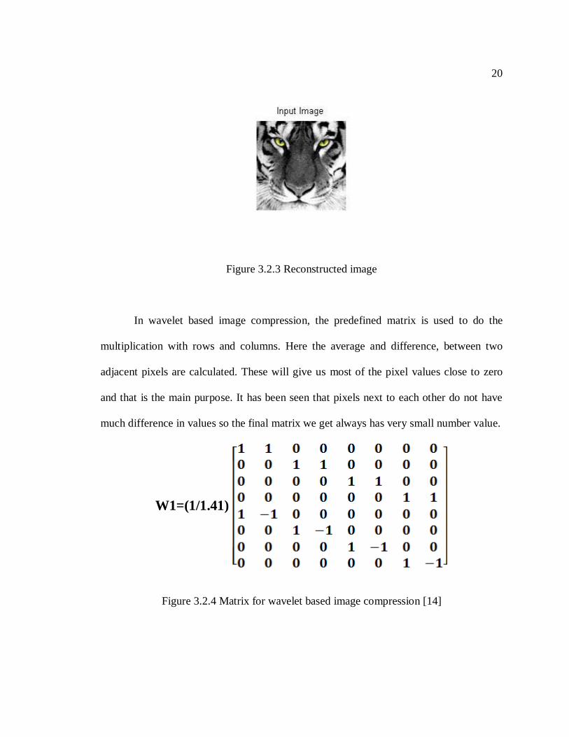
Figure 3.2.3 Reconstructed image

In wavelet based image compression, the predefined matrix is used to do the

multiplication with rows and columns. Here the average and difference, between two

adjacent pixels are calculated. These will give us most of the pixel values close to zero

and that is the main purpose. It has been seen that pixels next to each other do not have

much difference in values so the final matrix we get always has very small number value.

W1=(1/1.41)

Figure 3.2.4 Matrix for wavelet based image compression [14]

21

The concept of averaging and differencing explains the concept of filter. When

we do averaging that means we are doing filtering of high frequency data. It acts as a low

pass filter when it is used to smoothen the data [14]. In the same way, differencing

represents high pass filter that stops low frequency signals. It can be best method to find

noise from the signal because the noise is a high frequency signal [14]. Combining both,

we call it filter bank. Different features of signals as background, noise, edges correspond

to different frequencies. This is the main idea behind the wavelet based image-processing

concept.

22

Chapter 4

WAVELET IMPLEMENTATION USING C LANGUAGE

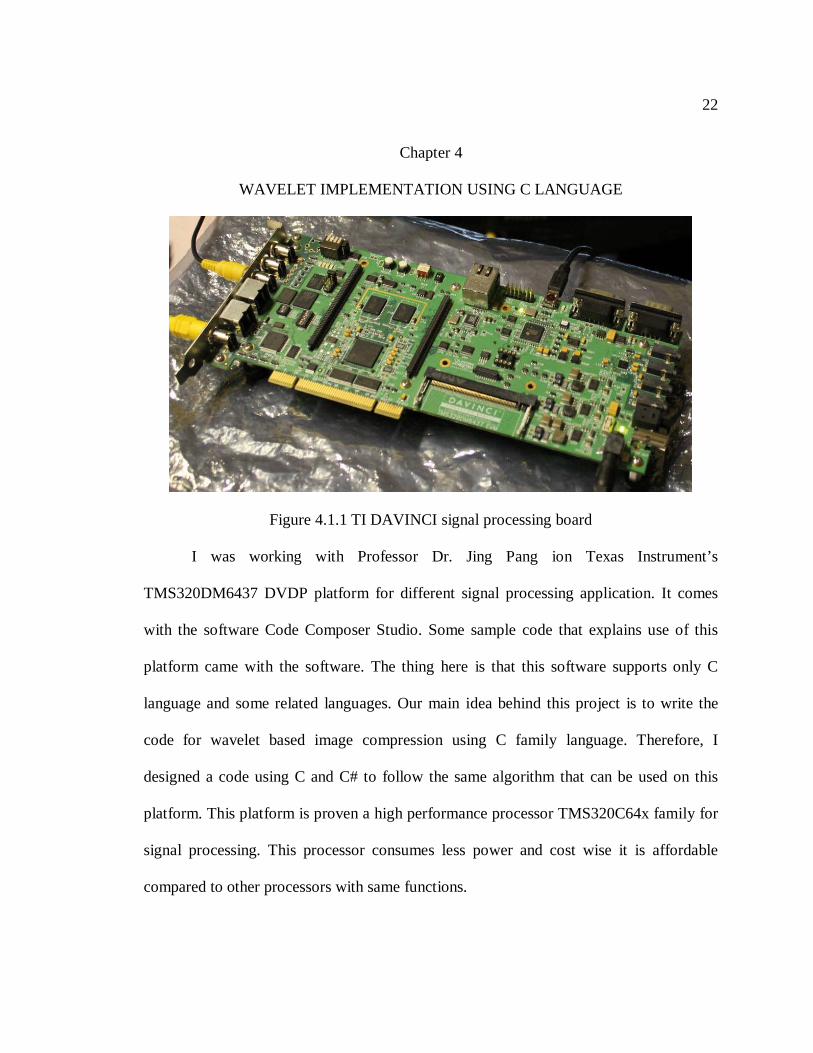
Figure 4.1.1 TI DAVINCI signal processing board

I was working with Professor Dr. Jing Pang ion Texas Instrument’s

TMS320DM6437 DVDP platform for different signal processing application. It comes

with the software Code Composer Studio. Some sample code that explains use of this

platform came with the software. The thing here is that this software supports only C

language and some related languages. Our main idea behind this project is to write the

code for wavelet based image compression using C family language. Therefore, I

designed a code using C and C# to follow the same algorithm that can be used on this

platform. This platform is proven a high performance processor TMS320C64x family for

signal processing. This processor consumes less power and cost wise it is affordable

compared to other processors with same functions.

23

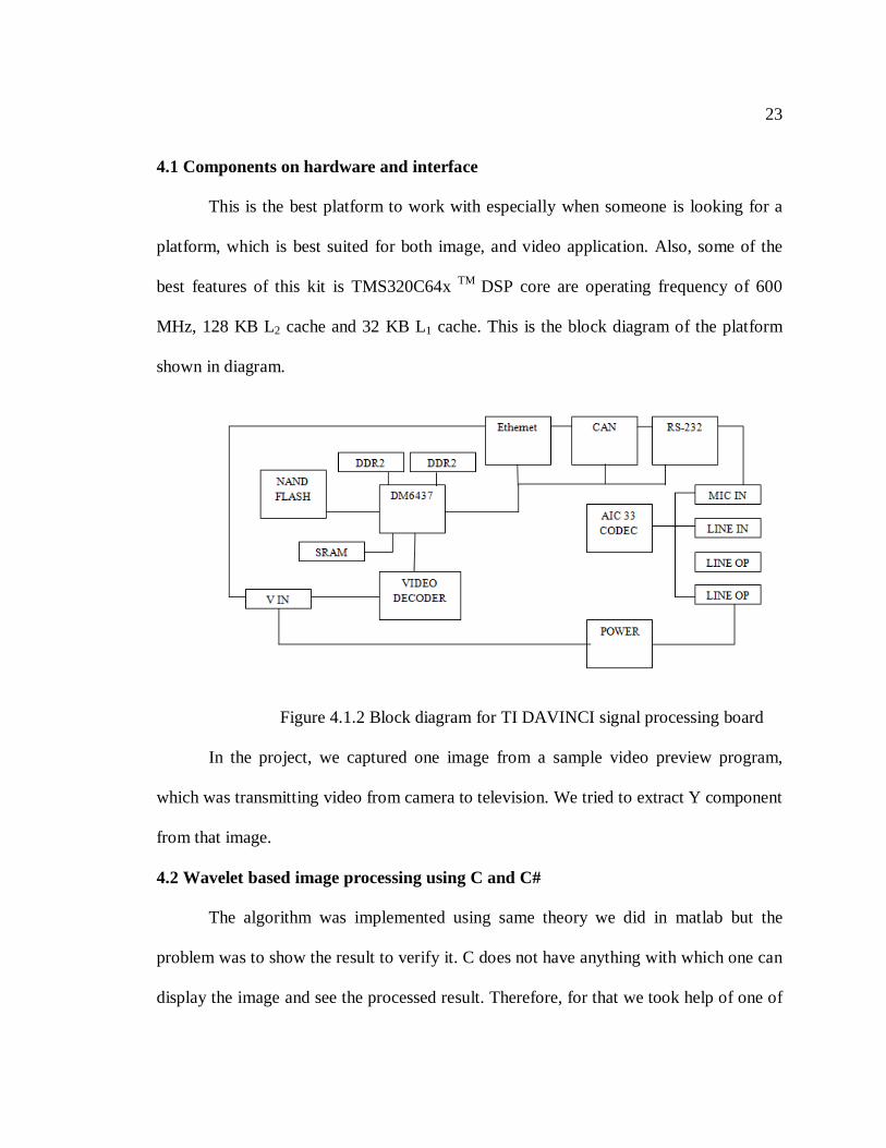
4.1 Components on hardware and interface

This is the best platform to work with especially when someone is looking for a

platform, which is best suited for both image, and video application. Also, some of the

best features of this kit is TMS320C64x TM DSP core are operating frequency of 600

MHz, 128 KB L2 cache and 32 KB L1 cache. This is the block diagram of the platform

shown in diagram.

Figure 4.1.2 Block diagram for TI DAVINCI signal processing board

In the project, we captured one image from a sample video preview program,

which was transmitting video from camera to television. We tried to extract Y component

from that image.

4.2 Wavelet based image processing using C and C#

The algorithm was implemented using same theory we did in matlab but the

problem was to show the result to verify it. C does not have anything with which one can

display the image and see the processed result. Therefore, for that we took help of one of

24

my friend who is in computer science department he knows C#. He help us developed

some forms to open an image. We implement that algorithm on image and saw the result

using C# to verify that. The implementation was so perfect we achieved the very good

ratio using that algorithm. We also have included the functions like how many level of

compression we want and what should be the threshold level entered by user. That gave

this code good flexibility and range I can show to others. We calculated SNR same way

we have calculated in Matlab.

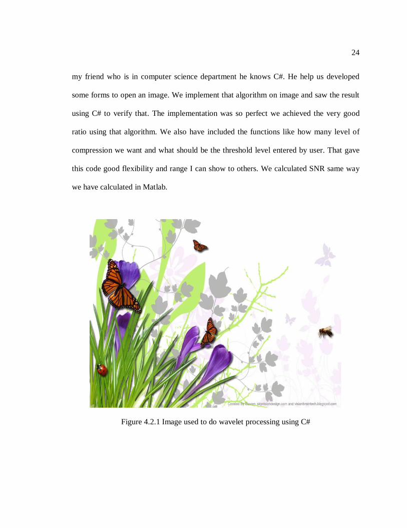
Figure 4.2.1 Image used to do wavelet processing using C#

25

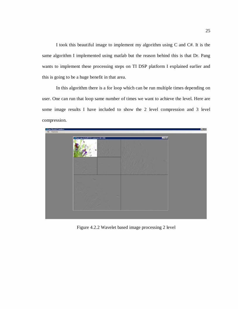
I took this beautiful image to implement my algorithm using C and C#. It is the

same algorithm I implemented using matlab but the reason behind this is that Dr. Pang

wants to implement these processing steps on TI DSP platform I explained earlier and

this is going to be a huge benefit in that area.

In this algorithm there is a for loop which can be run multiple times depending on

user. One can run that loop same number of times we want to achieve the level. Here are

some image results I have included to show the 2 level compression and 3 level

compression.

Figure 4.2.2 Wavelet based image processing 2 level

26

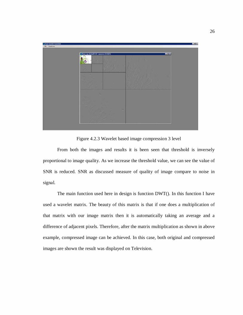
Figure 4.2.3 Wavelet based image compression 3 level

From both the images and results it is been seen that threshold is inversely

proportional to image quality. As we increase the threshold value, we can see the value of

SNR is reduced. SNR as discussed measure of quality of image compare to noise in

signal.

The main function used here in design is function DWT(). In this function I have

used a wavelet matrix. The beauty of this matrix is that if one does a multiplication of

that matrix with our image matrix then it is automatically taking an average and a

difference of adjacent pixels. Therefore, after the matrix multiplication as shown in above

example, compressed image can be achieved. In this case, both original and compressed

images are shown the result was displayed on Television.

27

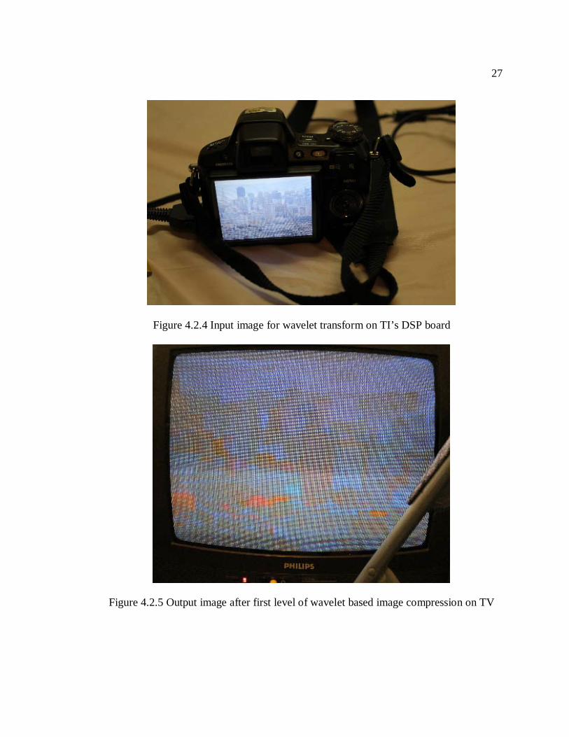
Figure 4.2.4 Input image for wavelet transform on TI’s DSP board

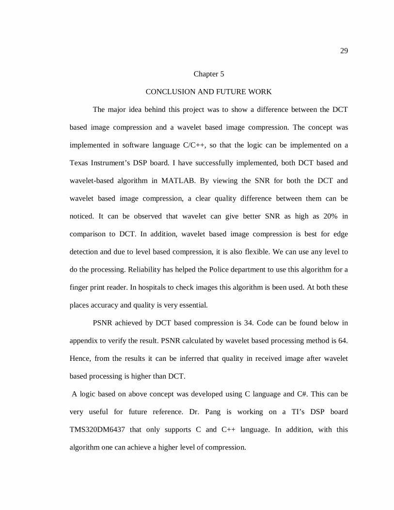
Figure 4.2.5 Output image after first level of wavelet based image compression on TV

28

From the output result, the first level of wavelet compression was achieved on

TI’s board and output can clearly see with the edges in the result image. The edge

detection is an essential part of a wavelet based image compression and it is been proved

by the results shown here.

29

Chapter 5

CONCLUSION AND FUTURE WORK

The major idea behind this project was to show a difference between the DCT

based image compression and a wavelet based image compression. The concept was

implemented in software language C/C++, so that the logic can be implemented on a

Texas Instrument’s DSP board. I have successfully implemented, both DCT based and

wavelet-based algorithm in MATLAB. By viewing the SNR for both the DCT and

wavelet based image compression, a clear quality difference between them can be

noticed. It can be observed that wavelet can give better SNR as high as 20% in

comparison to DCT. In addition, wavelet based image compression is best for edge

detection and due to level based compression, it is also flexible. We can use any level to

do the processing. Reliability has helped the Police department to use this algorithm for a

finger print reader. In hospitals to check images this algorithm is been used. At both these

places accuracy and quality is very essential.

PSNR achieved by DCT based compression is 34. Code can be found below in

appendix to verify the result. PSNR calculated by wavelet based processing method is 64.

Hence, from the results it can be inferred that quality in received image after wavelet

based processing is higher than DCT.

A logic based on above concept was developed using C language and C#. This can be

very useful for future reference. Dr. Pang is working on a TI’s DSP board

TMS320DM6437 that only supports C and C++ language. In addition, with this

algorithm one can achieve a higher level of compression.

30

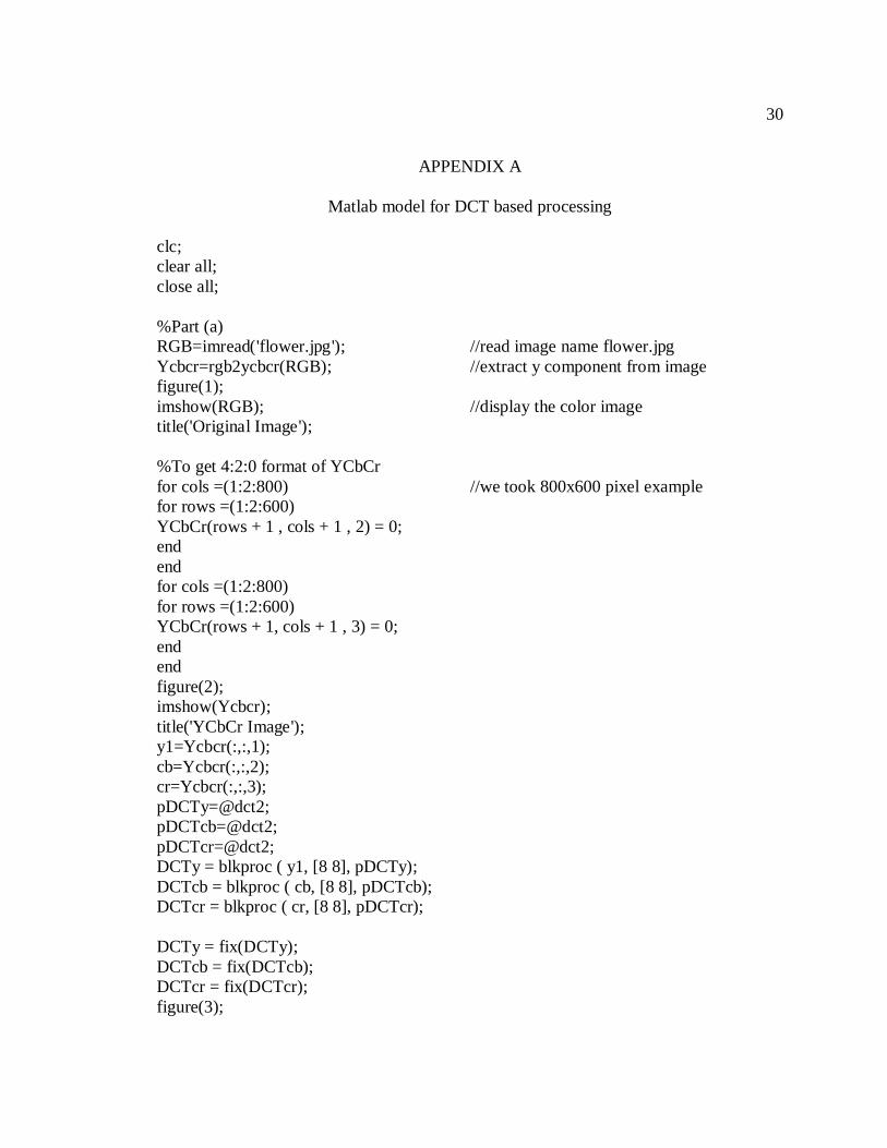
APPENDIX A

Matlab model for DCT based processing

clc; clear all; close all; %Part (a) RGB=imread('flower.jpg'); //read image name flower.jpg Ycbcr=rgb2ycbcr(RGB); //extract y component from image figure(1); imshow(RGB); //display the color image title('Original Image'); %To get 4:2:0 format of YCbCr for cols =(1:2:800) //we took 800x600 pixel example for rows =(1:2:600) YCbCr(rows + 1 , cols + 1 , 2) = 0; end end for cols =(1:2:800) for rows =(1:2:600) YCbCr(rows + 1, cols + 1 , 3) = 0; end end figure(2); imshow(Ycbcr); title('YCbCr Image'); y1=Ycbcr(:,:,1); cb=Ycbcr(:,:,2); cr=Ycbcr(:,:,3); pDCTy=@dct2; pDCTcb=@dct2; pDCTcr=@dct2; DCTy = blkproc ( y1, [8 8], pDCTy); DCTcb = blkproc ( cb, [8 8], pDCTcb); DCTcr = blkproc ( cr, [8 8], pDCTcr); DCTy = fix(DCTy); DCTcb = fix(DCTcb); DCTcr = fix(DCTcr); figure(3);

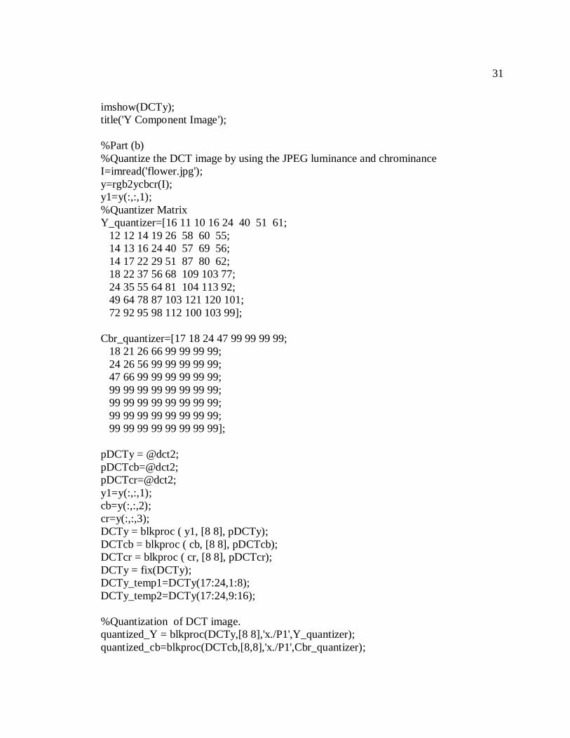
31

imshow(DCTy); title('Y Component Image'); %Part (b) %Quantize the DCT image by using the JPEG luminance and chrominance I=imread('flower.jpg'); y=rgb2ycbcr(I); y1=y(:,:,1); %Quantizer Matrix Y_quantizer=[16 11 10 16 24 40 51 61; 12 12 14 19 26 58 60 55; 14 13 16 24 40 57 69 56; 14 17 22 29 51 87 80 62; 18 22 37 56 68 109 103 77; 24 35 55 64 81 104 113 92; 49 64 78 87 103 121 120 101; 72 92 95 98 112 100 103 99]; Cbr_quantizer=[17 18 24 47 99 99 99 99; 18 21 26 66 99 99 99 99; 24 26 56 99 99 99 99 99; 47 66 99 99 99 99 99 99; 99 99 99 99 99 99 99 99; 99 99 99 99 99 99 99 99; 99 99 99 99 99 99 99 99; 99 99 99 99 99 99 99 99]; pDCTy = @dct2; pDCTcb=@dct2; pDCTcr=@dct2; y1=y(:,:,1); cb=y(:,:,2); cr=y(:,:,3); DCTy = blkproc ( y1, [8 8], pDCTy); DCTcb = blkproc ( cb, [8 8], pDCTcb); DCTcr = blkproc ( cr, [8 8], pDCTcr); DCTy = fix(DCTy); DCTy_temp1=DCTy(17:24,1:8); DCTy_temp2=DCTy(17:24,9:16); %Quantization of DCT image. quantized_Y = blkproc(DCTy,[8 8],'x./P1',Y_quantizer); quantized_cb=blkproc(DCTcb,[8,8],'x./P1',Cbr_quantizer);

32

quantized_cr=blkproc(DCTcr,[8,8],'x./P1',Cbr_quantizer); %Rounding the values. quantized_Y=round(quantized_Y); quantized_Y1=round(quantized_Y); quantized_cb=round(quantized_cb); quantized_cr=round(quantized_cr); quantized_Y_temp=quantized_Y1(17:24,1:16); %Display 1st two blocks of 3rd Row quantized_Y_temp1=quantized_Y1(17:24,1:8) quantized_Y_temp2=quantized_Y1(17:24,9:16) figure(4); imshow(quantized_Y1); title('Quantized Y Component'); figure(5); subplot(1,2,1), subimage(quantized_Y_temp1); title('1st Block of the 3rd Row'); subplot(1,2,2), subimage(quantized_Y_temp2); title('2nd Block of the 3rd Row'); dcy=[]; for i=1:8:600 for j=1:8:800 dcy=[dcy quantized_Y(i,j)]; end; end; fun3=zigzac(quantized_Y_temp) ; % zigzac function call. fun2=fun3(1:63) figure(6); imshow(fun2); %Inverse quantisation y_invq = blkproc(quantized_Y,[8 8],'x.*P1',Y_quantizer); cb_invq = blkproc(quantized_cb,[8 8],'x.*P1',Cbr_quantizer); cr_invq = blkproc(quantized_cr,[8 8],'x.*P1',Cbr_quantizer); y_invq_temp=y_invq(17:24,1:16); % Inverse DCT transform idc=@idct2; Invdct_y=blkproc(y_invq,[8,8],idc);

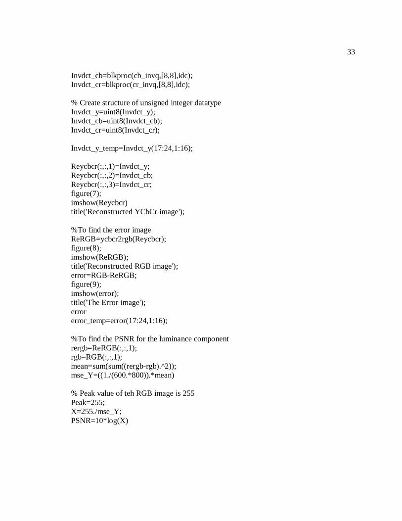
33

Invdct_cb=blkproc(cb_invq,[8,8],idc); Invdct_cr=blkproc(cr_invq,[8,8],idc); % Create structure of unsigned integer datatype Invdct_y=uint8(Invdct_y); Invdct_cb=uint8(Invdct_cb); Invdct_cr=uint8(Invdct_cr); Invdct_y_temp=Invdct_y(17:24,1:16); Reycbcr(:,:,1)=Invdct_y; Reycbcr(:,:,2)=Invdct_cb; Reycbcr(:,:,3)=Invdct_cr; figure(7); imshow(Reycbcr) title('Reconstructed YCbCr image'); %To find the error image ReRGB=ycbcr2rgb(Reycbcr); figure(8); imshow(ReRGB); title('Reconstructed RGB image'); error=RGB-ReRGB; figure(9); imshow(error); title('The Error image'); error error_temp=error(17:24,1:16); %To find the PSNR for the luminance component rergb=ReRGB(:,:,1); rgb=RGB(:,:,1); mean=sum(sum((rergb-rgb).^2)); mse_Y=((1./(600.*800)).*mean) % Peak value of teh RGB image is 255 Peak=255; X=255./mse_Y; PSNR=10*log(X)

34

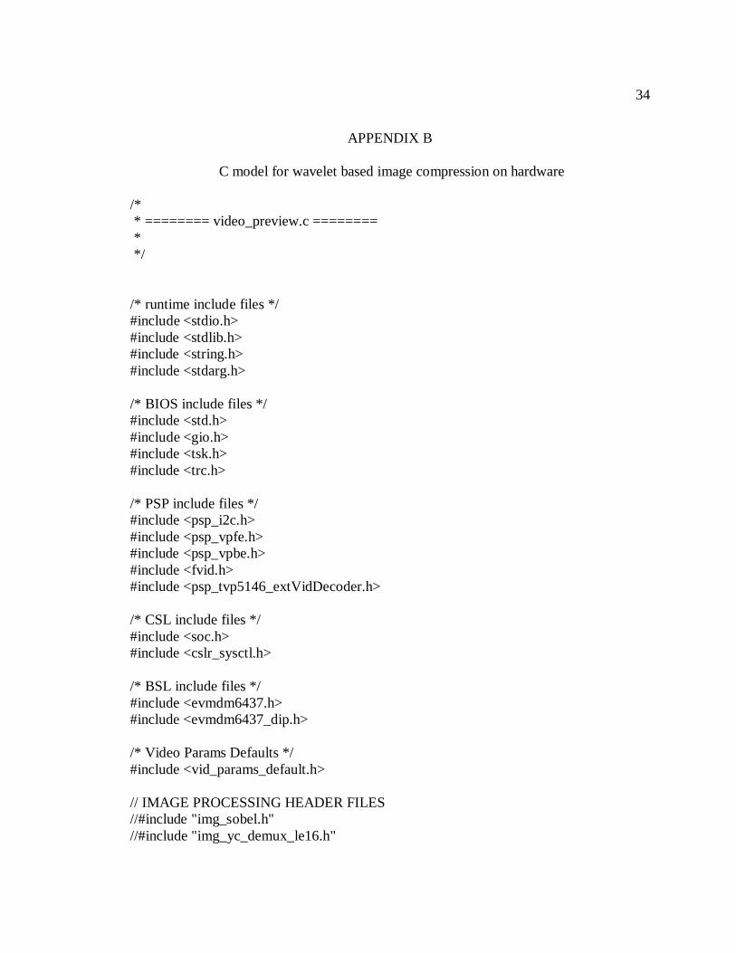
APPENDIX B

C model for wavelet based image compression on hardware

/* * ======== video_preview.c ======== * */ /* runtime include files */ #include <stdio.h> #include <stdlib.h> #include <string.h> #include <stdarg.h> /* BIOS include files */ #include <std.h> #include <gio.h> #include <tsk.h> #include <trc.h> /* PSP include files */ #include <psp_i2c.h> #include <psp_vpfe.h> #include <psp_vpbe.h> #include <fvid.h> #include <psp_tvp5146_extVidDecoder.h> /* CSL include files */ #include <soc.h> #include <cslr_sysctl.h> /* BSL include files */ #include <evmdm6437.h> #include <evmdm6437_dip.h> /* Video Params Defaults */ #include <vid_params_default.h> // IMAGE PROCESSING HEADER FILES //#include "img_sobel.h" //#include "img_yc_demux_le16.h"

35

/* This example supports either PAL or NTSC depending on position of JP1 */ #define STANDARD_PAL 0 #define STANDARD_NTSC 1 #define FRAME_BUFF_CNT 6 static int read_JP1(void); static CSL_SysctlRegsOvly sysModuleRegs = (CSL_SysctlRegsOvly )CSL_SYS_0_REGS; // User Defined Function void display (void * currentFrame); void haar (void * currentFrame); void dwt(); //float y[720 * 480]; //float z[720 * 480]; //float my_image[480][720]; float I_temp[480][720]; float O_temp[480][720]; //float a[720]; float w[480][480]; float wa[480][480]; float wt[480][480]; /* * ======== main ======== */ void main() { printf("Video Preview Application\n"); fflush(stdout); /* Initialize BSL library to read jumper switches: */ EVMDM6437_DIP_init(); /* VPSS PinMuxing */ /* CI10SEL - No CI[1:0] */ /* CI32SEL - No CI[3:2] */

36

/* CI54SEL - No CI[5:4] */ /* CI76SEL - No CI[7:6] */ /* CFLDSEL - No C_FIELD */ /* CWENSEL - No C_WEN */ /* HDVSEL - CCDC HD and VD enabled */ /* CCDCSEL - CCDC PCLK, YI[7:0] enabled */ /* AEAW - EMIFA full address mode */ /* VPBECKEN - VPBECLK enabled */ /* RGBSEL - No digital outputs */ /* CS3SEL - LCD_OE/EM_CS3 disabled */ /* CS4SEL - CS4/VSYNC enabled */ /* CS5SEL - CS5/HSYNC enabled */ /* VENCSEL - VCLK,YOUT[7:0],COUT[7:0] enabled */ /* AEM - 8bEMIF + 8bCCDC + 8 to 16bVENC */ sysModuleRegs -> PINMUX0 &= (0x005482A3u); sysModuleRegs -> PINMUX0 |= (0x005482A3u); /* PCIEN = 0: PINMUX1 - Bit 0 */ sysModuleRegs -> PINMUX1 &= (0xFFFFFFFEu); sysModuleRegs -> VPSSCLKCTL = (0x18u); return; } /* * ======== video_preview ======== */ void video_preview(void) { FVID_Frame *frameBuffTable[FRAME_BUFF_CNT]; FVID_Frame *frameBuffPtr; GIO_Handle hGioVpfeCcdc; GIO_Handle hGioVpbeVid0; GIO_Handle hGioVpbeVenc; int status = 0; int result; int i; int standard; int width; int height; /* Set video display/capture driver params to defaults */ PSP_VPFE_TVP5146_ConfigParams tvp5146Params =

37

VID_PARAMS_TVP5146_DEFAULT; PSP_VPFECcdcConfigParams vpfeCcdcConfigParams = VID_PARAMS_CCDC_DEFAULT_D1; PSP_VPBEOsdConfigParams vpbeOsdConfigParams = VID_PARAMS_OSD_DEFAULT_D1; PSP_VPBEVencConfigParams vpbeVencConfigParams; standard = read_JP1(); /* Update display/capture params based on video standard (PAL/NTSC) */ if (standard == STANDARD_PAL) { width = 720; height = 576; vpbeVencConfigParams.displayStandard = PSP_VPBE_DISPLAY_PAL_INTERLACED_COMPOSITE; } else { width = 720; height = 480; vpbeVencConfigParams.displayStandard = PSP_VPBE_DISPLAY_NTSC_INTERLACED_COMPOSITE; } vpfeCcdcConfigParams.height = vpbeOsdConfigParams.height = height; vpfeCcdcConfigParams.width = vpbeOsdConfigParams.width = width; vpfeCcdcConfigParams.pitch = vpbeOsdConfigParams.pitch = width * 2; /* init the frame buffer table */ for (i=0; i<FRAME_BUFF_CNT; i++) { frameBuffTable[i] = NULL; } /* create video input channel */ if (status == 0) { PSP_VPFEChannelParams vpfeChannelParams; vpfeChannelParams.id = PSP_VPFE_CCDC; vpfeChannelParams.params = (PSP_VPFECcdcConfigParams*)&vpfeCcdcConfigParams; hGioVpfeCcdc = FVID_create("/VPFE0",IOM_INOUT,NULL,&vpfeChannelParams,NULL); status = (hGioVpfeCcdc == NULL ? -1 : 0); } /* create video output channel, plane 0 */

38

if (status == 0) { PSP_VPBEChannelParams vpbeChannelParams; vpbeChannelParams.id = PSP_VPBE_VIDEO_0; vpbeChannelParams.params = (PSP_VPBEOsdConfigParams*)&vpbeOsdConfigParams; hGioVpbeVid0 = FVID_create("/VPBE0",IOM_INOUT,NULL,&vpbeChannelParams,NULL); status = (hGioVpbeVid0 == NULL ? -1 : 0); } /* create video output channel, venc */ if (status == 0) { PSP_VPBEChannelParams vpbeChannelParams; vpbeChannelParams.id = PSP_VPBE_VENC; vpbeChannelParams.params = (PSP_VPBEVencConfigParams *)&vpbeVencConfigParams; hGioVpbeVenc = FVID_create("/VPBE0",IOM_INOUT,NULL,&vpbeChannelParams,NULL); status = (hGioVpbeVenc == NULL ? -1 : 0); } /* configure the TVP5146 video decoder */ if (status == 0) { result = FVID_control(hGioVpfeCcdc, VPFE_ExtVD_BASE+PSP_VPSS_EXT_VIDEO_DECODER_CONFIG, &tvp5146Params); status = (result == IOM_COMPLETED ? 0 : -1); } /* allocate some frame buffers */ if (status == 0) { for (i=0; i<FRAME_BUFF_CNT && status == 0; i++) { result = FVID_allocBuffer(hGioVpfeCcdc, &frameBuffTable[i]); status = (result == IOM_COMPLETED && frameBuffTable[i] != NULL ? 0 : -1); } } /* prime up the video capture channel */ if (status == 0) { FVID_queue(hGioVpfeCcdc, frameBuffTable[0]); FVID_queue(hGioVpfeCcdc, frameBuffTable[1]); FVID_queue(hGioVpfeCcdc, frameBuffTable[2]); }

39

/* prime up the video display channel */ if (status == 0) { FVID_queue(hGioVpbeVid0, frameBuffTable[3]); FVID_queue(hGioVpbeVid0, frameBuffTable[4]); FVID_queue(hGioVpbeVid0, frameBuffTable[5]); } /* grab first buffer from input queue */ if (status == 0) { FVID_dequeue(hGioVpfeCcdc, &frameBuffPtr); } /* loop forever performing video capture and display */ while (status == 0 ) { /* grab a fresh video input frame */ FVID_exchange(hGioVpfeCcdc, &frameBuffPtr); haar ((frameBuffPtr->frame.frameBufferPtr)); dwt(); display((frameBuffPtr->frame.frameBufferPtr)); /* display the video frame */ FVID_exchange(hGioVpbeVid0, &frameBuffPtr); } } void haar (void * currentFrame) { int r,c; int offset; offset = 1; for(r = 0; r < 480; r++) { for(c = 0; c < 720; c++) { I_temp[r][c] = * (((unsigned char * )currentFrame + offset) ); offset = offset + 2; }

40

} } void dwt () { int i,j,k; for (i=0;i<480;i++) { for (j=0;j<240;j++) { if (j==(i+1)*2 -1 || j==(i+1)*2) w[i][j]=0.5; else w[i][j]=0; } for(j=240;j<480;j++) { if (j==((i+1)-240)*2 -1) w[i][j]=-(0.5); else if (j==((i+1)-240)*2) w[i][j]=0.5; else w[i][j]=0; } /* for(j=0;j<480;j++) wt[j][i]=w[i][j];*/ } for (i=0;i<480;i++) { for(j=0;j<480;j++) { wa[i][j]=0; for(k=0;k<480;k++) wa[i][j]+=1.41*w[i][k]*w[k][j]; } } } /* for (i=0;i<480;i++) {

41

for(j=0;j<480;j++) { I_temp[i][j]=0; for(k=0;k<480;k++) I_temp[i][j]+=2*wa[i][k]*wt[k][j]; } }*/ //********************************************************************** void display (void * currentFrame) { int r,c; int offset; offset = 1; for(r = 0; r < 480; r++) { for(c = 0; c < 480; c++) { * (((unsigned char * )currentFrame + offset) ) = wa[r][c]; offset = offset + 2; * (((unsigned char * )currentFrame)+ offset) = 0x80; offset = offset + 2; } } for(r = 0; r < 480; r++) { for(c = 480; c < 720; c++) { * (((unsigned char * )currentFrame + offset) ) = 0; offset = offset + 2; * (((unsigned char * )currentFrame)+ offset) = 0x80; offset = offset + 2;; } } } /* * ======== read_JP1 ======== * Read the PAL/NTSC jumper. * * Retry, as I2C sometimes fails: */

42

static int read_JP1(void) { int jp1 = -1; while (jp1 == -1) { jp1 = EVMDM6437_DIP_get(JP1_JUMPER); TSK_sleep(1); } return(jp1); }

43

REFERENCES

[1]. Van, Fleet Patrick J. Discrete Wavelet Transformations: An Elementary Approach

with Applications. Hobroken, N. J.: John Wiley and Sons, 2008. Print.

[2]. Kingsbury, Nick. “A Basic image Compression Example.” Connexions. Ed.

Elizabeth Gregory. 8 June. 2005. < http://cnx.org/content/m11086/latest/>

[3] Pitas, I. Digital Image Processing Algorithms and Applications. New York:

Wiley, 2000. Print.

[4] Kumar, Satish. “An Introduction to Image Compression.” Debugmode. Ed. Satish

Kumar. 22 Oct. 2001. < http://www.debugmode.com/imagecmp/>

[5] Faqs.org. 2011. 4 Feb 2011 <http://www.faqs.org/faqs/compression-

faq/part2/section-6.html >

[6] jpeg.org. 2011. Elysium Ltd. 1 May 2011

<http://www.jpeg.org/.demo/FAQJpeg2k/introduction.htm >

[7] Sharpe, Louis. "An Introduction to JPEG 2000." AIIM - Your Information

Management and Collaboration Resource. Web. 02 May 2011.

<http://www.aiim.org/Resources/Archive/Magazine/2002-Sep-Oct/25500 >.

[8] Al-Shaykh, Osama K., Iole Moccagatta, and Homer Chen. "JPEG-2000: A New

Still Image Compression Standard." IEEE 1.1-4 Nov 1998 (1998): 99-

103. Ieeexplore.ieee.org. 4 Nov. 1998. Web. 20 Apr. 2011.

<http://ieeexplore.ieee.org/Xplore/login.jsp?url=http%3A%2F%2Fieeexplore.ieee

.org%2Fiel4%2F6069%2F16210%2F00750835.pdf%3Farnumber%3D750835&a

uthDecision=-203 >.

44

[9] Betz, Sarah, Nirav Bhagat, Paul Murphy, and Maureen Stengler. WAVELET-

BASED IMAGE COMPRESSION. Rep. Web. 20 Apr. 2011.

http://www.clear.rice.edu/elec301/Projects00/wavelet_image_comp/index.html

[10] Walker, James S. Wavelet-based Image Compression. Working paper. CRC Press

Book: Transforms and Data Compression. Web. 20 Apr. 2011.

<http://www.uwec.edu/walkerjs/media/imagecompchap.pdf>.

[11] Watson, Andrew B. "Image Compression Using the Discrete Cosine

Transform." Mathematica 4.1 (1994): 81-88. Vision.arc.nasa.gov. Jan.-Feb. 1994.

Web. 20 Apr. 2011. <http://vision.arc.nasa.gov/publications/mathjournal94.pdf>

[12] "JPEG." Wikipedia, the Free Encyclopedia. Web. 02 May 2011.

<http://en.wikipedia.org/wiki/JPEG>

[13] Sandberg, Kristian. "The Haar Wavelet Transform." Applied Math Website -

Welcome to the Department of Applied Mathematics. Web. 02 May 2011.

<http://amath.colorado.edu/courses/5720/2000Spr/Labs/Haar/haar.html>