Wave simulation for the design of an innovative quay-wall

1

Wave simulation for the design of an innovative quay-wall: the case of Vlora’s harbour Alessandro Antonini1,2, Renata Archetti2, Alberto Lamberti2 1CIRI Edilizia e Costruzioni, University of Bologna, Bologna, 40100, Italy 2DICAM, University of Bologna, Bologna, 40136, Italy 5

Correspondence to: R. Archetti ([email protected])

Abstract. The sea state and environmental sea conditions are basic data for the design of marine structures. Hindcasted wave

data have been here applied for the definition of proper environmental conditions at sea, with the aim to estimate the design

condition of an innovative quay wall concept, for a more efficient dock design. 10

In this paper the results of a Computational Fluid Dynamic model is used to optimize the design of a non-reflective quay

wall of Vlora’s harbour and define design loads under the action of extreme conditions. The design wave conditions at the

harbour entrance have been estimated analysing 31 years hindcasted waves data simulated through the application of

WaveWatch III. Due to the particular geography and topography of the Vlora’s Bay wave conditions generated from

northwest are transferred to the harbour entrance with application of a 2D spectral wave model. Southern wave states, which 15

are also the most critical for the port structures, are defined by means of a wave generation model, according the available

wind measurements. In general hindcasted sea data, after the application of wave models at a proper scale, are the basic data

in support of the maritime works through the propagation of design wave condition from off-shore to harbour entrance. The

results show that the proposed method based on the numerical modelling allows the identification of the best site specific

solution also for a location devoid of any wave measurement. 20

1 Introduction

The development of global trade and ship transportation often requires that the existing docks must be upgraded,

consolidated or enlarged, in order to face effectively the increasing demand of people and freight traffic. With such aims,

quays over piles with absorbing rubble mound slopes can be used to enlarge or rebuild structures in the existing docks.

Generally the rubble mound assures low reflection in the port basins, very important for mooring and manoeuvring but they 25

lead to the construction of very wide superstructures that are not always possible due to the available spaces and economic

sources. The use of vertical walls as berthing structures is an alternative quite used in port areas: in fact this kind of solution

represents a compromise between the simplicity of construction and the small covered area. Nevertheless vertical quay walls

present the drawback of undesirable high wave reflection into the port areas. Low reflecting quays sort out the reflection in

port areas by means of porous or open structures that dissipate a part of the incident wave energy. Thereby several different 30

vertical dissipative solutions have been proposed during the last decades as result of research studies from all over the world.

Nat. Hazards Earth Syst. Sci. Discuss., doi:10.5194/nhess-2016-168, 2016Manuscript under review for journal Nat. Hazards Earth Syst. Sci.Published: 13 June 2016c© Author(s) 2016. CC-BY 3.0 License.

2

The availability of wave data is a necessary condition to pursue the design of innovative harbour parts, as the quays and

docks. At several locations direct measurements are not always available and series of hindcasted waves are necessary for

defining the proper condition at harbour entrance. The most common operative wave generation models are WaveWatch III,

WAM (WAMDI, 1988, Monbaliu et al., 2000), SWAN (Booij, 1999). WaveWatchIII model

(http://polar.ncep.noaa.gov/waves/wavewatch/wavewatch.shtml), developed by the National Weather Service (NWS) and 5

National Oceanic and Atmospheric Administration (NOAA) is operational at DICCA, University of Genoa. The model

covers the whole Mediterranean basin with a resolution equal to 0.1° (Sartini et al., 2014, Sartini et al. 2015). The model

chain is forced with the National Centers for Environmental Prediction (NCEP) Climate Forecast System Reanalysis (CFSR)

data at 0.5° resolution. Validation of the model has been extensively performed (Mentaschi et al., 2015). On the basis of such

numerical results, the design wave conditions are estimated through extreme wave analysis. Extreme events analysis can be 10

based on a widely number of methodology (Mazas et al., 2014, Masina et al, 2015) while the historic coastal structures

design practice leads to the use of Peak Over Threshold technique to select samples data (Mathiesen et al., 1994, Garcia-

Espinel et al., 2015).

To attenuate wave reflection various structures have been designed, being Jarlan-type structures (Jarlan, 1961) the most

widely used. However, all the existing antireflective solutions for vertical maritime structures have the drawback of their 15

exiguous efficacy to reduce the reflection of low frequency waves (i.e. wave periods larger than 25 s). To overcome this

technical problem, the design of a vertical structure can be based on a multi-cell circuit concept which is considered to be

especially effective to reduce the wave reflection of wind waves and oscillations associated with intense storms, resonance

waves in port basins, (Medina et al., 2010, Garrido et al 2014). Altomare and Gironella (2014), Matteotti (1991) and Faraci

et al. (2012) investigated, by means of physical model tests, quay walls consisting in prefabricated caissons with frontal 20

openings and internal rubble mounds. In cases where the sheet piling is allowed, when great retaining heights have to be

achieved a combined quay wall structure is normally preferred for its structural lightness.

In this work we present an application on the use of hindcasted data for defining the proper design condition at the entrance

of a new harbour in the Vlora’s bay; the results of extreme analysis is fundamental input for the optimisation of a new

concept of quay wall. The quay wall is investigated, by means of CFD simulations CD-ADAPCO (2013), Lamberti et al., 25

(2015). The structure is consisting of a sheet-pile quay-wall, a relieving platform, an anchors and piles foundation system

and an antireflective wave chamber filled with a rock-armoured slope.

Aim of the paper is twofold, i) showing application of sea situation estimation, through the use of wave hindcasted data, in

order to properly define the design wave conditions for a new harbour, ii) presenting new approach for investigating

innovative non-reflective quay-wall. 30

2 Site description

The city of Vlora, Republic of Albania, is located on a coastal plain in the North East part of the Bay. The Bay is

approximately 17 km long and 10 km wide with a depth that reaches 55 m. It is open to the Adriatic through North-West


3

side, while is bordered by tall and craggy mountain peaks to the south and west. The bay is also partially protected from the

swells coming from north-west by the presence of Sazan Island, located at the mouth of the bay, and from the shallow water

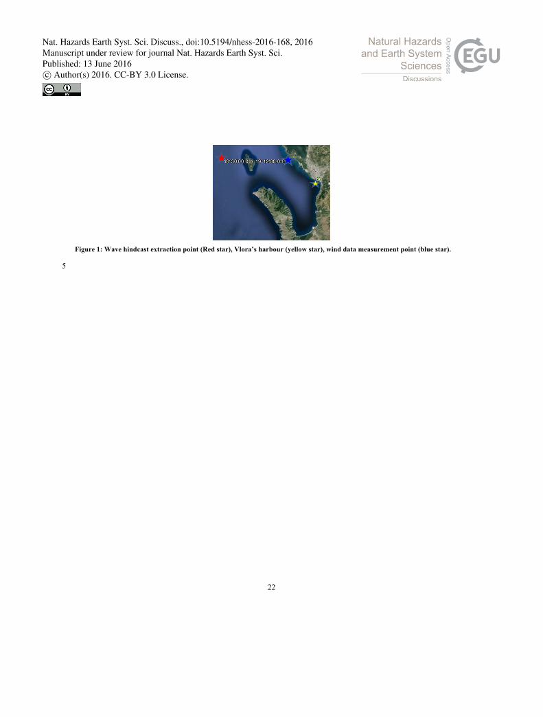
next to the mouth of the river Voiussa. The investigated port is located in the small northern stretch of the coast in the inner

part of the Bay. The location of the new harbour is presented on Fig. 1 by the yellow star.

In the surrounding area there are already some port infrastructures, some of them are still working and other are disused. 5

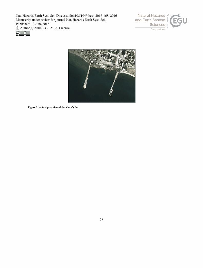
Such facilities include an offshore berth for tankers called New Port and the historical Old Port of Vlora. The harbour under

investigation presents two piers as shown in Fig.2, west wharf and east pier. The first is primarily intended for docking ferry

passengers while the second is used for berthing cargo vessels.

2 Design wave conditions

No measured wave data are available for Vlora’s bay, therefore wave climate was defined by means of 31 years (1999 - 10

2010) of hindcasted wave data supplied by the University of Genova, (Sartini, 2015, Mentaschi et al., 2015). The extraction

point (red star in Fig. 1) was selected on a grid point, representative of the wave climate outside the gulf. The wave rose at

the extraction point is presented in Fig. 3.

Two main directional sectors are evident: 240°N - 40°N, associated with Adriatic axis direction, and 160°N –200°N,

providing information on southern waves. Dominant wave conditions, characterized by the highest wave heights, are related 15

to the sector between 155°N -170°N whereas the maximum frequency of northern events, is related to 300 ° N and is equal

to 15%. Maximum northerly wave height is equal to 5.75 m, with 10 s peak period.

Due to the particular geography and topography of the Bay, southern wave data are not representative of the actual

conditions in the vicinity of the port. Consequently, definition of southern wave states (S-SW) requires another source of

information like wind measurements that are partially available inside the Bay. 20

In order to estimate the design wave conditions reaching the harbor entrance, two different approaches have been undertaken

for waves propagating from the Northern sectors and for waves generated by the S-SW wind. For both main directions, two

years (TR=2) and one hundred years (TR=100) return period wave states were estimated. Two years return period, event is

considered the limit of ordinary operation, that is, the limit condition for which there should not be any malfunction of the

harbor infrastructure, while 100 years return period, event is the design condition of the structures, namely, the event for 25

which the structures should only resist.

The northern wave conditions are established by the extreme wave analysis, performed on the hindcast wave data. The

southern design wave conditions have been estimated by applying the wave generation module of Mike21-SW on the

Vlora’s bay, by imposing as a main input the local wind intensity with TR= 2 years and TR= 100 years.

2.1 Design Waves from NW 30

The peak over threshold (POT) method has been applied to the northern storms time series (N-NW) in order to select

independent storm peaks. The technique is a well-established statistic approach, based on the following steps: i) application


4

of a proper threshold; ii) selection of homogeneous independent events and peaks which exceeding the selected threshold;

iii) identification of the probability model that best represents the exceedances; iv) determination of values within a given

return period. The great advantage of POT method is the utilization of an adequate number of independent extreme data,

achievable also with a relatively short time series.

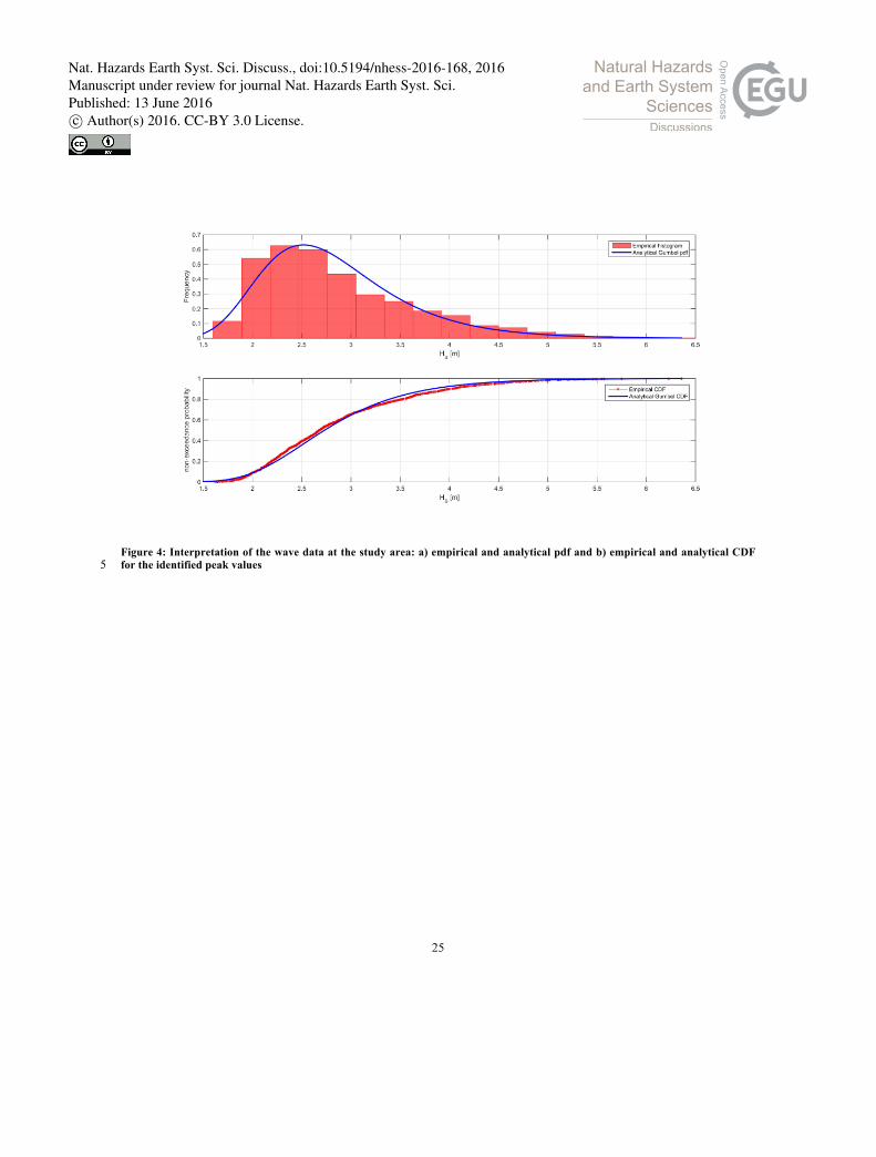
The POT analysis has been applied to the wave data providing the results illustrated in Fig. 4, where the empirical frequency 5

histogram and cumulative distribution function (pdf and CDF) are given along with the corresponding Gumbel distribution,

with best fit scale parameter (σ) and location parameter (µ) equal to 0.58 (95% lower and upper bounds parameter fitting:

0.55 – 0.61), 2.51 (95% lower and upper bounds parameter fitting: 2.48 – 2.55), respectively. The threshold used to define

individual storm has been established according to Boccotti’s method, (Boccotti, 2000). The method is based on a

preliminary identification of a wave height threshold, namely 1.5 times the annual average HSy, that is 0.5 m for the available 10

wave data: the chosen threshold value is therefore equal to 1.50 m. The application of the described approach led to the

detection of 355 independent events from the direction -120°N +40°N.

The analyses have provided the significant wave height (Hs) and the mean peak period (Tp), whose values are given in Table

1 with reference to a return period of 2 years and 100 years. The mean peak periods associated with the predicted extreme

significant wave heights have been estimated using a scatter plot of measured peak period versus significant wave height as 15

proposed by Viselli, (2015) and Schweizer et al. (2016). The parameters a and b in eq. 1. turn out to be equal to 2.36 (0.30,

4.42) and 0.72 (0.43, 1.01), respectively, values in parentheses indicate the lower and upper bounds of the 95% confidence

interval.

Tp = a ⋅Hsb (1)

20

Not exceedance probability distribution which best fits the extreme events data is the Gumbel distribution, the resulting

values of HS for the selected wave height are listed in Tab. 1. It is worst to remark that the estimated thirty years return

periods (TR=30 years) significant wave height (HTR30) is equal to 5.8 m, in accordance with the maximum hindcast wave

height equal to 5.75 m.

2.1.1 Propagation of design waves at the harbor entrance 25

Numerical model Mike 21-SW was applied to propagate the conditions from the offshore location to the entrance of the port.

The spectral wave module simulates the growth, decay and transformation of wind-generated waves. MIKE21-SW is third-

generation spectral wave models, as it doesn’t require any parameterization on either the spectral or the directional

distribution of power (or action density). The physical processes modelled comprise: (a) energy source/dissipation processes

(wind driven interactions with atmosphere, dissipation through wave breaking / whitecapping / wave-blocking due to strong 30

opposing currents, bottom friction-induced dissipation), (b) non-linear energy transfer conservative processes (resonant

quadruplet interactions, triad interactions), and (c) wave 20 propagation-related processes (wave propagation due to the wave

group / current velocity, depth-/current- induced refraction, shoaling, interactions with unsteady currents). The models


5

compute the evolution of wave action density by solving the action balance equation as described by Booij et al., (1999).

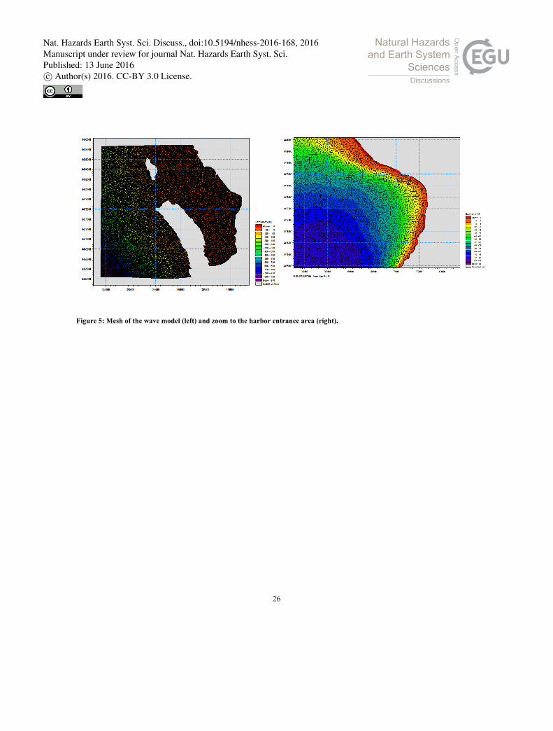
MIKE21 modelling suites discretize the computational domain by unstructured triangular meshes (flexible mesh).

Recent applications of MIKE 21-SW with a flexible mesh are described in Samaras et al, (2016) and Gaeta et al., (2016).

The bathymetric and shoreline data used in this work resulted from the digitization of nautical charts acquired from the

Italian National Hydrographic Military Service (“Istituto Idrografico della Marina Militare”). The triangular mesh dimension 5

is homogenous over the entire domain, resulting in a mesh forming 102995 elements with dimension of approx. 600 m2. The

grid for the entire domain, and harbor entrance is shown in Fig.5.

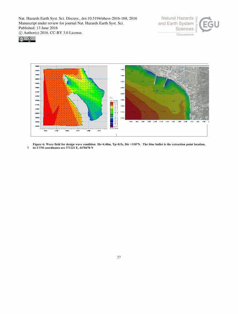
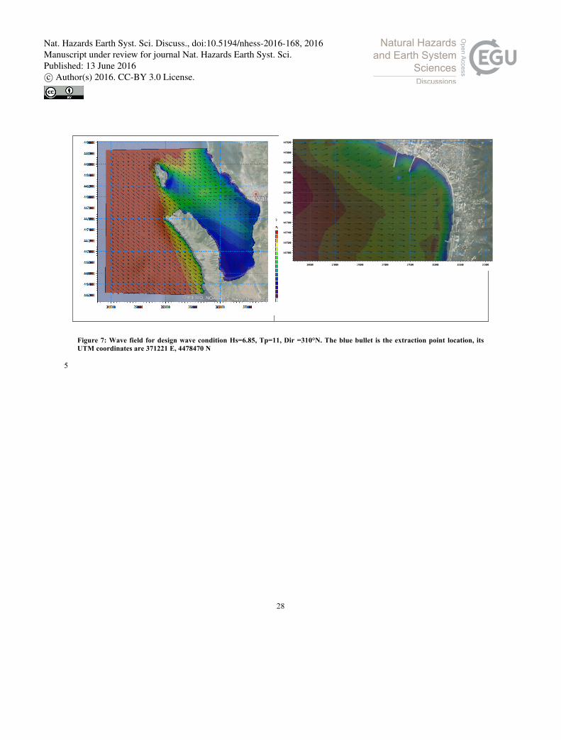
Wave field of HTR2 and HTR100 are presented in Fig. 6 and Fig. 7. In which reduction of the wave height due to the shoaling is shown. The design conditions at the harbor entrance, on a -13.5 m depth (UTM coord. 371221 E, 4478470 N, Fig. 4) are presented in 10


6

Table 2.

2.2. Design Waves from S

Southern design wave conditions were not easily estimated, as direct measures of waves inside the Vlora’s bay are not

available and also wind data are relatively scarce. Such conditions, which are also the most critical for the port structures, are

defined by means wave generation model of MIKE21-SW. 5

The approach is well known and here shortly summarised: Wind-wave generation is the process by which the wind transfers

energy into the water body for generating waves. The wind input is based on Janssen’s (1989, 1991) quasi linear theory of

wind–wave generation, where the momentum transfer from the wind to the sea not only depends on the wind stress, but also

to the sea state itself. The non-linear energy transfer is approximated by the DIA approach Hasselmann et al.

(1985). The source function describing the dissipation due to white capping is based on the theory of Hasselmann et al. 10

(1985) and Janssen (1989). The source function describing the bottom induced wave breaking is based on the well proven

approach of Battjes and Janssen (1978) and Eldeberky and Battjes (1996). A detail description of the various source

functions is available in Komen et al. (1994) and Sorensen et al. (2003). The default source of wind for the modelling of

waves is similar to the source functions implemented in the WAM Cycle 4 model, Komen et al. (1994). More details on the

wave generation module are provided in the DHI Manual (2011). The wave generation model was forced by the wind 15

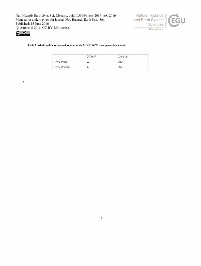
conditions with TR2 and TR100 (see Tab. 3, Lamberti et al., (2015)) with Charnock parameter equal to 0.1 and default input in

the model.

Wind data measurements were supplied by SIAP-MICROS s.r.l., the anemometer was installed on the Albania coast at point

of coordinate 40°30’51,98” N, 19°23’36,69” E, presented in Fig. 1 with a blue star. The measurement protocol followed the

standard, measuring every 10 minutes, the instrument measured for 2 years (July 2006-August 2008). The statistical analysis 20

of the data was preceded by a quality control check of all data to remove the outliers and to interpolate over small data gaps

that may be present. Overall, the corrected data were of sufficient quality, with less than 3% of the data removed as outliers

or unacceptable data, Belu and Koraicn (2009). Highest measured value is equal to 22.8 m/s, while a gust reduction factor

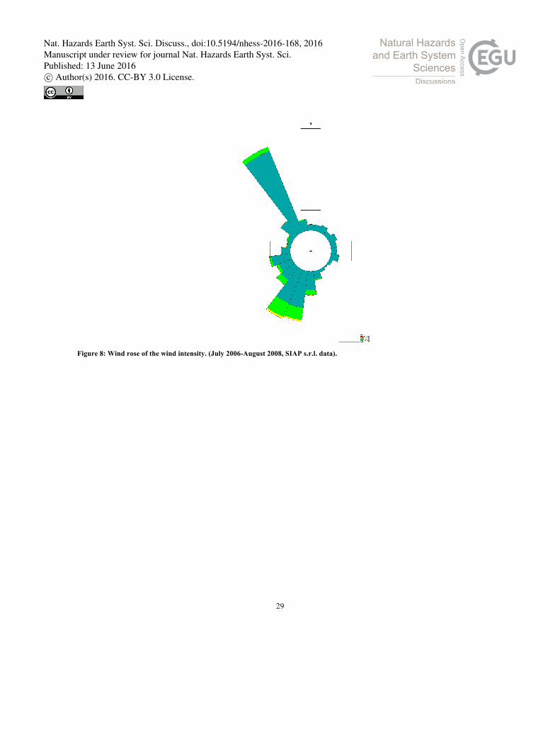
equal to 0.96 is applied in order to define the effective wind velocity, El-Hawary (2000). Fig.8 shows the wind rose based on

2 years data. 25

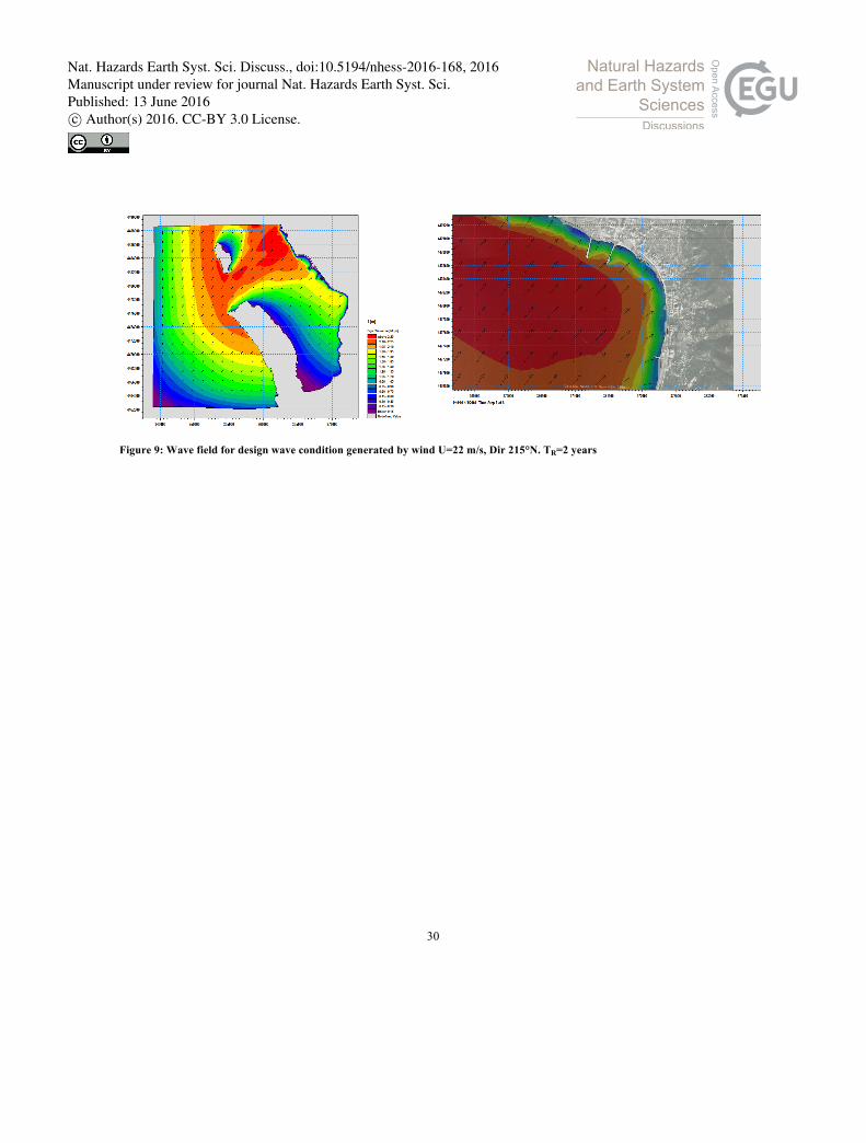
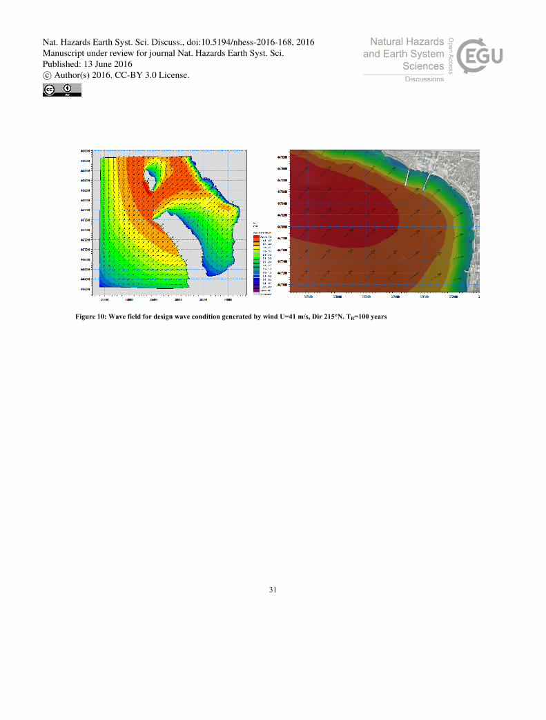
The wave fields generated by the wind conditions in Tab. 3 are presented in Fig. 9 and Fig. 10, while the extracted waves

conditions at the harbor entrance are presented in Tab. 4. Final result of the design wave characterization is a set of four

wave states, accounting two different directions (i.e. north-west and south-west) and two return periods (i.e. 2 and 100

years), Table 4.

3. Optimisation of the quay wall design 30

Quay-wall structure, consisting of steel piles foundation system and antireflective rock armoured wave chamber is

investigated through CFD model by means of commercial code STAR-CCM+ whose has been widely used for practical


7

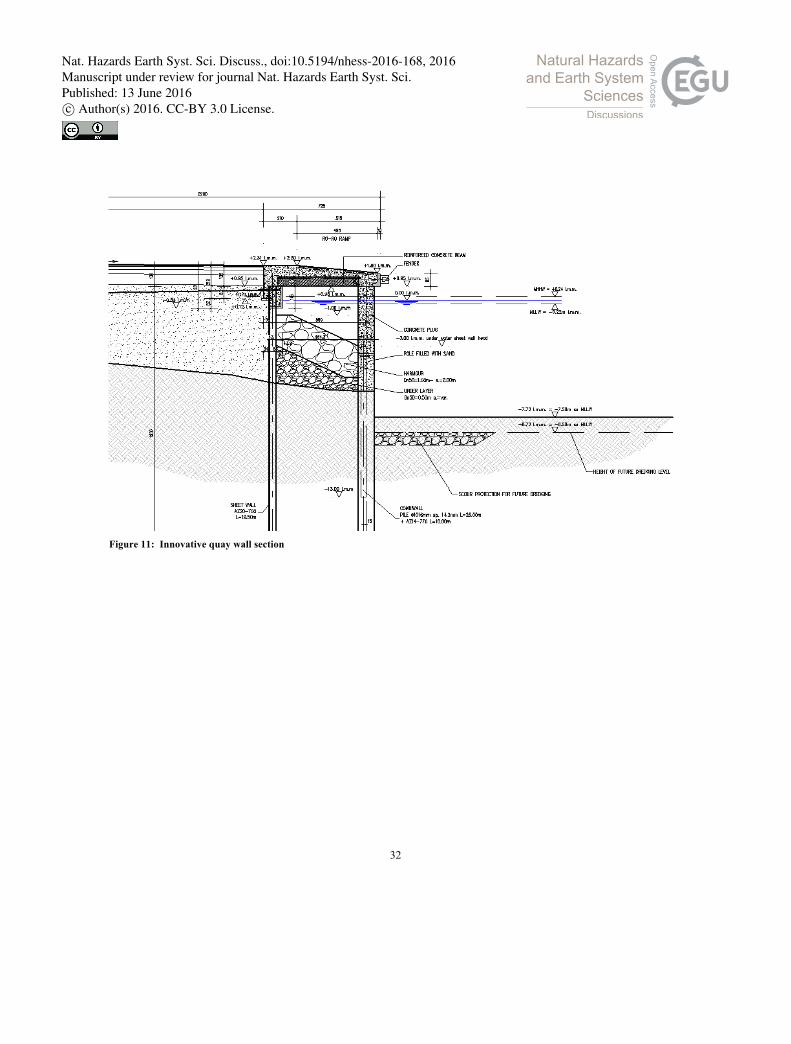
design approach, i.e. see Antonini et al. (2016a) validated with data in Antonini et al., (2015). An example of this innovative

design is presented in Fig. 11. Optimum site-specific geometry is defined through the comparison of three geometries. The

changes made during the analysis are related to:

1. length of the absorbing cell;

2. extension of the gap between front reflective surface and free surface; 5

3. arrangement of the armour slope inside the cell.

Aim of site-specific absorbing quay-wall design phase is the maximization of incident wave energy dissipation according the

exercise wave condition (described in Tab.4). The goal is reached considering a cell geometry with reflective surfaces far as

close as possible to the quarter of the wavelength, therefore only a single wave state (i.e. southern exercise condition) is

selected to optimize the geometry of the cell. In this light, for the analysis that follow the optimization of the absorbing cell 10

was carried out based on the characteristics of the wave climate recognized as ordinary storm from the South-West, i.e. wave

n° 3, (Hs = 1.80 m, Hmax = 3.2 m, Tp = 4.5 sec, Ts = 4.2 sec), while for waves n° 1 and 4 the performances of the optimized

cell are investigated.

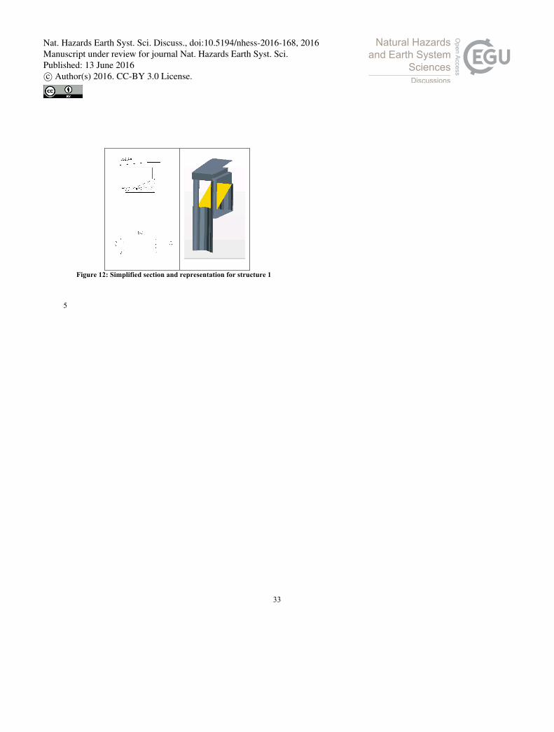
Geometry of structure 1 has a cell length equal to 5.47 m and the front reflective surface extends from -7.5 m to -2.5 m.

Armor slope extends from the front sheet pile up to the rear bean installed on top of back sheet pile, with a the nominal 15

diameter (DN50) equal to 1.00 m (Fig. 12).

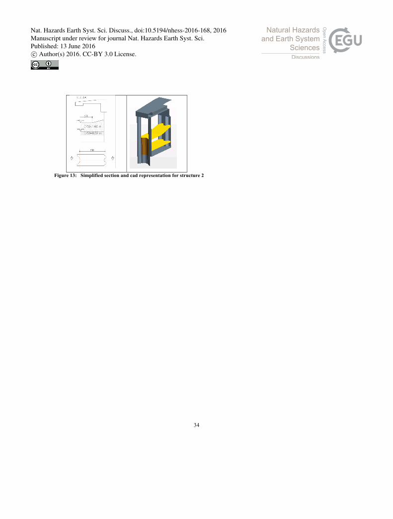
Structure 2 has cell length equal to 5.80 m, and the front reflective surface extends from -7.5 to -3.0 m. Armor slope extends

horizontally from the front sheet pile up to 2.70 m inside the cell where a slope of 1:4 reach the back sheet pile, nominal

diameter is 1.00 m. An under layer is designed in order to separate the rocks and the bottom sand. Its nominal diameter is

0.50 m (Fig. 13). 20

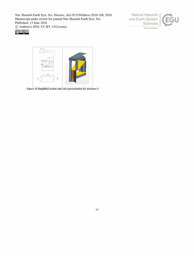
Structure 3 presents the same geometrical characteristics of structure 2 in terms of length and depth of the cell but some

differences in the arrangement of the armor slope which extends from the front sheet pile up to the back sheet pile with a

slope equal to 1:2, nominal diameter is 1.00 m (Fig. 14).

3.1 CFD numerical model set-up

A k–ω SST turbulence model (Menter, 1994) is applied with a two-layer all y+ wall treatment model, and a second order 25

implicit scheme was utilized for time marching. The transient SIMPLE algorithm is applied to linearize the equations and to

achieve pressure–velocity coupling. A volume of fluid method (VOF) is applied to describe the free surface. The calculation

is performed on a fixed grid and free surface interface orientation and shape are calculated as a function of the volume

fraction of the respective fluid within a control volume, Antonini et al., (2016b).

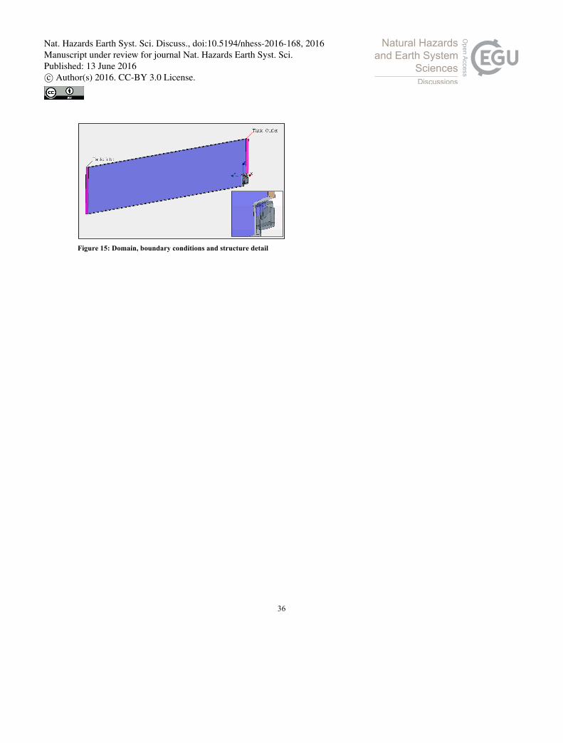
A right-handed Cartesian coordinate system is located at the intersection between frontal structure surface, the undisturbed 30

water surface and the medium vertical section of the domain. The longitudinal x-axis is pointing towards the outlet

boundary, the z-axis is vertical and points upwards, and the undisturbed free surface is the plane z=0 (Figure 15:).


8

The domain region is 2.62 m wide (-1.31 m ≤ y ≤ 1.31 m, i.e. structure pile center to pile center distance), 38.75 m high (-

7.75 m ≤ z ≤ 31.0 m) and its length varies according to the simulated wave group length (λg), (i.e. - 3/4λg ≤ x ≤ 6). The

seabed is given 7.5 m below the mean water surface, and a superposition of linear waves velocity profile is specified at the

up-wave boundary in order to generate an extreme focused wave group at the structure location according the design wave

climate defined above. The pressure outlet is implemented at the down-wave domain boundary. Four boundary conditions 5

have been used to describe the fluid field at the domain bounds. They involve: no-slip wall, velocity inlet, pressure outlet and

symmetry plane condition. No-slip wall boundary condition represents an impenetrable, no-slip condition for viscous flow,

such a boundary is used to describe the structure surface and the bottom (z=-7.5 m). Velocity inlet boundary represents the

inlet of the domain at which the flow velocity is known according to the required wave profile, this condition is used to

model the up-wave boundary at x =-3/4·∙λg and the top (z=31.0 m) of the domain, while lateral boundaries (y=-1.31 and 10

y=1.31 m) are discretized by means of symmetry plane. The pressure outlet boundary is a flow outlet boundary for which the

pressure is specified, in this model we used condition of calm water surface, outlet boundary is imposed at the boundary over

the structure (x =6 m) only for the air phase.

3.2 Modelling of the armor slope

The armor slopes proposed, within the absorbing cell, are modelled through the insertion of two solid communicating with 15

the fluid field. By means of these volumes, dissipation due to the inertial and viscous forces are imposed. These two terms

are subject of a long-time study as demonstrated by several authors (Burcharth and Andersen, 1995, Cruz et al., 1997,

Engelund, 1953) who proposed different methods to calculate them according the size and type of the modelled rocks.

According the Burcharth’s method and considering a nominal diameter of the armour rocks equal to 1.0 m the adopted

values in this study are 6.4 kg/m3/s for viscous dissipation coefficient and 1221 kg/m4 for the inertial coefficient, while for 20

the under layer characterized by a nominal diameter equal to 0.5 m the adopted values are 26 kg/m3/s for viscous dissipation

coefficient and 2440 kg/m4 for the inertial one, adopted porosity value is equal to 0.38 and is kept constant for both the

porous domains.

3.3 Simulated wave conditions

Three different wave conditions have been simulated, two characteristics of operating conditions, (wave n°1 and wave n°3 in 25

Tab. 4) and one dealing with extreme conditions (wave n°4 in Tab. 4). We assume that the modelling of extreme condition

from North-West (i.e. wave n° 2) is not necessary as the wave state is significantly less intense than southern one, as

highlighted in the wave climate study. In order to reduce the computation time, wave groups according to a Jonswap

spectrum are imposed at the inlet boundary. The wave groups are generated by a superposition of eight linear components,

each of them characterized by its own amplitude, period and phase. The input signal is calculated according the Boccotti’s 30

theory, (Boccotti,1983 and Boccotti et al. 1993). The procedure allows defining an extreme focused wave group coherent

with real sea state described by a spectral distribution. In this study a Jonswap spectral shape equal to 3.3 is adopted, while


9

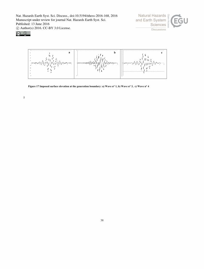
the maximum wave height at the focusing point is identified through the Goda’s method, Goda, (2000), (i.e. wave n° 1

Hmax=1.80 m; wave n° 3 Hmax=3.24 m; wave n° 4 Hmax=5.40 m, Fig. 17).

3.4 Grid generation

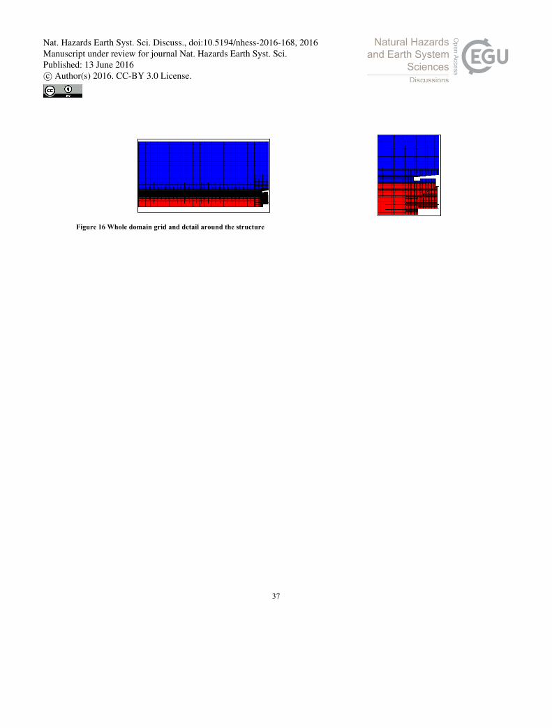
The domain mesh and prism layer grids are generated using the mesh generator in STAR-CCM+. Grid resolution is finer

near the free surface and around the quay-wall structure to capture both the wave dynamics and the details of the flow 5

around the structure, Fig. 16. Prism-layer cells are generated along the structure’s surface, the height of the first layer is set

so that the value of y+ (10 to 400) satisfies the turbulence model requirement by solving the velocity distribution outside the

viscous sub-layer, i.e. buffer layer and log-law regions are solved, Demirel et al. (2014), Schultz and Swain (2000). Regular

hexahedral cells discretize whole domain, while four thinner areas are used to capture free surface movements and the

interaction between the wave group and the structure, (Vw1, Vw2, VS1, VS2). The grid refinements across the water surface are 10

realized by the volumetric controls VW1 and VW2 proposed along the whole domain. VW2’s height is equal to the maximum

simulated wave height while VW1’s height is 50% more (see longitudinal section in Fig. 16). VW2’s horizontal grid size is

determined by the wavelength of the shortest linear incident component (λi1), i.e. ∆x=∆y=λi1/60, while vertical grid size is

adjusted according to the wave height of smallest linear incident component (Hi1), ∆z=Hi1/20, VW1’s grid sizes are 50 %

larger than VW2’s ones. Volumetric controls used for the refinements around the structure present the same grid dimension of 15

those used to discretized the water surface but their dimension are set in order to include a gap between the structure surface

and volumetric control edges equal to 1.0 m for VS1, and 5.0 m for VS2. These mesh characteristics contribute to generate a

grid of variable cell numbers from 2.0·106 to 3.5·106 according to the incident wave condition. To assure the numerical

stability and respect the requested Courant number, a time step equal to Tp/400 is adopted in the study. All the RANS

simulations are carried out on the work-station at the hydraulic laboratory of the University of Bologna, double compute 20

node consisting of hexa-core 2.00 GHz Intel Xeon E5. For a mesh with 2.0·106 elements, it takes about 36 h on 12 cores to

complete the entire wave group attack.


10

4. CFD results

Results are presented in terms of mean values of reflection coefficient (cr), and pressures acting on the most significant parts

of the structure. Pressures are analysed only with respect to the extreme conditions. Surface elevation is measured through 6

wave gauges placed at the domain axis (y = 0) and at different distances from the quay-wall, (x = -18; -16; -14; -12; -10; - 8

m). The selected range of distance values are chosen in order to be at least far from the quay wall for 1/4 of the incident peak 5

wavelength in order to exclude the effects of stationary oscillations which cannot be explained through the adopted reflection

analysis method, Zelt & Skjelbreia, (1992).

4.1 Reflection coefficients results

Wave reflection induced by the quay-wall is quantified by the reflection coefficient, defined as follows:

r

i

r

ir H

Hmm

c ==0

0 ; (2) 10

∫ ⋅⋅=p

p

f

ff dffSm

5.1

5.0

0)(0

(3)

where Hr and Hi are the reflected and incident wave heights, respectively, and m0r and m0i are the related zero-order spectral

moment calculated between 0.5 and 1.5 times the peak frequency.

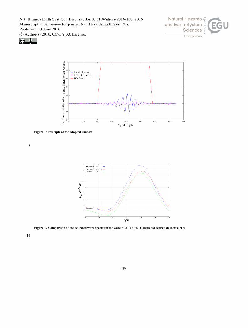
Calculation of the reflection coefficient is carried through spectral analysis of a non-stationary signal, since the generated

wave group is represented by a short time series coherently defined according the above identified wave states. The approach 15

implies the use of a time fixed window (i.e. fixed position along the time series vector) centred on both incident and reflected

wave group. A trapezoidal shaped window is used to reach this scope. Its length is defined according the signals shape, i.e.

the window begins with the first value above 0.05 m identified within the incident wave and closes after the last value above

0.05 m identified within the reflected signal. Two linear slopes between 0 and 1 characterize the window shape. The slopes

length is equal to 5% of the groups envelope (Fig. 18). According to this approach the reflection phenomenon is assumed to 20

be linear, thus reflected and incident spectral shape will not change except for the reduction of energy that is the investigated

parameter.

Comparison of the results enables to identify the optimal geometry as the structure 3, proposed in Fig. 19. It can be noted

that there is a generalized reduction of the reflected wave energy for whole range of analysed frequencies.

With regard to the lower frequencies, i.e. incident wave periods longer than 4.5 s, the required wave attenuation cannot be 25

guaranteed only by the resonance phenomenon of the cell, in this light the presence of the rocks inside the cell become more

important. The arrangement of the geometry with the smaller amour slope (structure 2, red line in Fig. 19), does not induce

the expected general improvement, whereas it is important for structure 3.


11

With regard to the higher frequencies, i.e. incident wave periods shorter than 4.5 s, the significant improvement associated

with the structure 3 is due to the variable length of the absorbing cell, generated by the inner slope that faces to the incoming

waves. With regard to the central frequencies, i.e. incident wave periods around 4.5 s, the largest improvement happens

between structures 1 and 2 because of the increased characteristic length of the absorbing cell. Structure 1 presents a ratio

between incident wave length and its own length equal to 0.18 while for structure 2 is 0.195, facilitating the establishing of 5

the resonance condition inside the cell.

A synthesis of the reflection coefficients is presented in Tab.5. It can be considered satisfactory the averaged reflection

coefficient determined for the structure 3. Therefore, structures 3, (presented in Fig. 11), can guarantee the required internal

agitation levels and it has been selected as the optimum structure for the future quay-wall of Vlora's harbour.

4.2 Pressures results 10

This section shows the pressures acting on different parts of the structure. In order to validate pressures and forces acting on

the quay-wall, numerical results are compared with the values calculated by means of empirical formulas based on physical

model tests carried out by McConnell et al. (2004), see Fig. 20. a/b/c, whereas the pressures distribution on the front sheet

pile is compared with the distribution calculated by means of Goda's method, (Goda, 2010), see Fig. 20. d. Four design

pressures are identified according the selected structure main parts. Eight virtual wave gauges are used to measure the uplift 15

pressure acting on the frontal beam, Fig. 20.a; twenty virtual wave gauges are used to measure the uplift pressure acting on

the internal beam, Fig. 20.b; four wave gauges are used to measure the horizontal unitary force acting on the frontal beam,

Fig. 20.c and finally sixteen wave gauges are used to measure the pressure distribution on the frontal sheet-pile, Fig. 20.d.

Two main activities have been carried out in order to reduce the effect of high frequency loads, and at the same time

consider all wave gauges positioned on the single investigated structure area. Firstly, the average pressure signal is 20

calculated except frontal sheet-pile pressure distribution, which is defined through the single gauge signal. Secondly, low-

band filter is applied considering a cutting frequency equal to 2 Hz, which is roughly the natural period of the structures

analysed. The considered design pressure values are the maximum value of each filtered signal, while pressure distribution

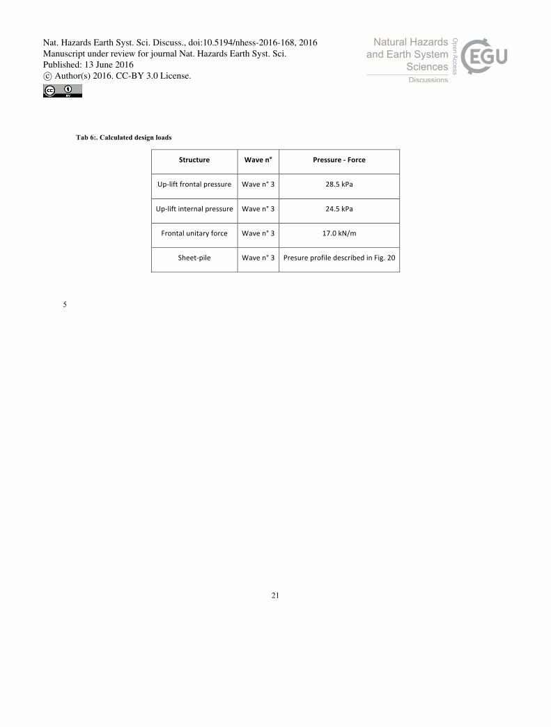
on the sheet-pile is calculated according the maximum value of each single pressure signal, (Tab. 6).

Each value arises from the analysis completed on all wave gauges positioned on the single investigated structure area. 25

The average signal obtained from the different probes has been filtered in order to exclude effect of high frequency loads.

The adopted design pressure values are the maximum value of the filtered signal (Table 6).


12

5. Conclusion

Hindcasted wave data have been here applied for the definition of environmental conditions at sea, with the aim to estimate

the proper design conditions for an efficient dock design based on an innovative quay-wall concept.

Design wave conditions are identified on the basis of the wind and wave data hindcasted outside and through the bay of

Vlora. Because of the different directions and periods, the identified waves conditions are distinguished in southerly and 5

northerly waves. According to this classification two limit conditions were assessed: the limit of the ordinary conditions for

which the service condition has to be ensured, and the extreme limit for which the only requirement is the resistance of the

structures. Once the wave conditions have been identified the analysis of the structures performance in terms of reflection

coefficients is carried out by means of CFD code. The optimization of the absorbing cell is carried out only for the ordinary

conditions, while the complete reflection analysis is completed through the other two identified wave states. The resulting 10

structure is a quay-wall with a non-reflective cell characterized by a ratio between wavelength and cell length equal to 0.195

with a 1:2 armor slope realized on the entire absorbing cell extension. The main findings are three values of reflection

coefficients cr 0.56, 0.33 and 0.4 for wave n° 1, 3 and 4 respectively. With the same code the pressures acting on the main

structural parts of the quay-wall are evaluated under the southern extreme conditions. Furthermore, a comparison of the

numerical results with empirical formulas is proposed in order to validate the calculated pressure values. A general good 15

agreement for the results is recognized through the compared pressure values. In conclusion sea data strongly supported a

correct optimisation of engineering design at Vlora’s harbor.

Acknowledgements

The authors gratefully acknowledge Prof. Giovanni Besio, Carlo Zumaglini, SIAP-MICROS s.r.l., for providing respectively

waves and wind data, Piacentini S.p.A. for the discussion on the quay design and Andrea Pedroncini DHI Italia for the useful 20

discussion on the MIKE21.

References

Altomare, C., Gironella, X., An experimental study on scale effects in wave reflection of low reflective quay walls with

internal rubble mound for regular and random waves. Coastal Engineering 90, 51–63. 2014. doi:

10.1016/j.coastaleng.2014.04.002. 25

Antonini A., Lamberti A. and Archetti R. OXYFLUX, an innovative wave-driven device for the oxygenation of deep layers

in coastal areas: A physical investigation. Coastal Engineering, 104, (54-68). 2015.

doi:10.1016/j.coastaleng.2015.07.005.

Antonini, A., Lamberti, A., Archetti, R., Miquel, A.M. 2016. CFD investigations of OXYFLUX device, an innovative

wave-driven device for the oxygenation of deep sea layers. Paper in press on Applied Ocean Research. 30


13

Antonini, A., Tedesco, G., Lamberti, A., Archetti, R., Ciabattoni, S., Piacentini, L.,. 2016. Innovative combiwall quay-wall

with internal rubble mound chamber: numerical tools supporting design activities. The case of Vlora’s harbor. Proceeding

of 26th International Ocean and Polar Engineering Conference, ISOPE 2016, Rhodos.

Arns A., T. Wahl, I.D. Haigh, J. Jensen, C. Pattiaratchi. Estimating extreme water level probabilities: A comparison of the

direct methods and recommendations for best practise. Coastal Engineering, 81, 51-66. 2013. doi: 5

10.1016/j.coastaleng.2013.07.003

Belu, R. and Koracin, D. Wind characteristics and wind energy potential in western Nevada. Renewable Energy, 34, (10),

2246–2251, 2009. doi: 10.1016/j.renene.2009.02.024

Boccotti, P. Some new results on statistical properties of wind waves. Applied Ocean Research, 1983, Vol. 5, No. 3. 1983.

doi:10.1016/0141-1187(83)90067-6 10

Boccotti, P., G. Barbaro, L. Mannino, A. Field experiment on the mechanics of irregular gravity waves, Journal of Fluid

Mechanics, 252 173-186. 1993. doi: http://dx.doi.org/10.1017/S0022112093003714

Boccotti, P., (2000) Design waves and risk analysis. In: Elsevier Oceanography Series, Volume 64: Wave mechanics for ocean

engineering, p 207-247. Doi: http://dx.doi.org/10.1017/S0022112093003714

Booij, N., Ris, R. C., and Holthuijsen, L. H.: A third-generation wave model for coastal Regions 2: Verification, J. Geophys. 15

Res.-Oceans, 104(C4), 7667–7682, doi:10.1029/1998JC900123, 1999.

Burharth, H., & Andersen, O.,. On the one dimensional steady and unsteady porous flow equations. Coastal engineering,24,

233-257. 1995. doi:10.1016/0378-3839(94)00025-S

CD-Adapco, "USER GUIDE STAR-CCM+ Version 10.02," London, 2013.

Cruz, E., Isobe, M., & Watanabe, A.. Boussinesq equations for wave transformation on porous flow equations. Coastal 20

Engineering.30, 125-154. 1997. doi:10.1016/S0378-3839(96)00039-7

Demirel, Y.K., Khorasanchi, M., Turan, O., Incecik, A., Schultz, M.P.. A CFD model for the frictional resistance prediction of

antifouling coatings. Ocean Eng. 89, 21–31. 2014.

Department of the army, US Army corps of engineers. (1984). Shore protection manual. Washington DC.

DHI, (2011). MIKE 21 SW. Spectral Wave Module. Scientific documentation. . Hørsholm: DHI Water & Environment. 25

Engelund, F. On the laminar and turbulent flows of ground water through homogeneous sand. Danish academy of Technical

sciences. 1953

El-Hawary, F., The Ocean Engineering Handbook, 2000. CRC Press, Taylor & Francis Group. ISBN 9780849385988 -

CAT# 8598

Faraci, C., Cammaroto, B., Cavallaro, L., Foti, E.. Wave reflection generated by caissons with internal rubble mound of variable 30

slope. Proc. of 33rd International Conference on Coastal Engineering. 2012.

Gaeta, M. G., Samaras, A. G., Federico, I., and Archetti, R.: A coupled wave-3D hydrodynamics model of the Taranto Sea

(Italy): a multiple-nesting approach, Nat. Hazards Earth Syst. Sci. Discuss., doi:10.5194/nhess-2016-95, in review, 2016.


14

Garcia-Espinel J.D., R. Alvarez-Garcia-Luben, J.M. Gonzalez-Herrero, D. Castro-Fresno. Glass fiber-reinforced polymer

caissons used for construction of mooring dolphins in Puerto del Rosario harbor (Fuerteventura, Canary Islands). Coastal

Engineering 98 16–25. 2015. doi:10.1016/j.coastaleng.2015.01.003.

Goda, Y. Random Seas and Design of Maritime Structures. 2nd edition. World Scientifc Publishing Co. Singapore. 2000. ISBN:

978-981-4282-39-0 5

Hirt, C.., Nichols, B. Volume of fluid (VOF) method for the dynamics of free boundaries. J. Comput. Phys. 39, 201–225. 1981.

doi:10.1016/0021-9991(81)90145-5

Jarlan, G. E., A perforated vertical breakwater. The Dock and Harbour Authority, Vol. 21, 486, 394-398. 1961.

Joaquín M. G., D. Ponce de León, A. Berruguete, S. Martínez, J. M., Lisardo Fort, D. Yagüe, J.A. González Escrivá and J.R.

Medina. Study of reflection of new low-reflectivity quay wall caisson, Proc of 34rd International Conference on Coastal 10

Engineering. 2014.

Lamberti A., Antonini A., Ceccarelli G. What could happen if the parbuckling of Costa Concordia had failed: Analytical and

CFD-based investigation of possible generated wave. Proc of 34rd International Conference on Coastal Engineering. 2014.

Lamberti A., Antonini A., Archetti, R., 2015. New Vlora's harbour, analysis of the internal wave agitation. Internal report

Masina M., Lamberti A., Archetti R., Coastal flooding: A copula based approach for estimating the joint probability of water 15

levels and waves. Coastal Engineering, (97) , 37-52. 2015. doi:10.1016/j.coastaleng.2014.12.010

Mathiesen, M., Goda Y. , Hawkes P. J., Mansard E., Martín M. J., Peltier E., Thompson E. F. and Van Vledder G

Recommended practice for extreme wave analysis, Journal of Hydraulic Research, 32:6, 803-814, DOI:

10.1080/00221689409498691. 1994.

Matteotti, G.. The reflection coefficient of a wave dissipating quay wall. Dock and Harbour Authority, 71(825), 285-291. 1991. 20

Mazas F., Kergadallan X., Garat P., Hamm L. Applying POT methods to the Revised Joint Probability Method for

determining extreme sea levels. Coastal Engineering, (91), 140-150. 2014.

Medina, J.R., J.A. Gonzalez-Escriva, L. Fort, S. Martinez, D. Ponce de Leon, J. Manuel, D. Yagüe, J. Garrido and A.

Berruguete., 2010. Vertical Maritime Structure with Multiple Chambers for Attenuation of Wave Reflection, International

PCT/EP2010/068000, EPO, The Hague, 23 pp. 2010. 25

Mentaschi L., Besio G., Cassola F. & Mazzino A. Performance evaluation of WavewatchIII in the Mediterranean Sea. Ocean

Modelling, 90, 82-94 doi:10.1016/j.ocemod.2015.04.003. 2015.

Mentaschi L., Perez J., Besio G., Mendez F. & Menendez M., 2015. Parameterization of unresolved obstacles in wave

modeling: a source term approach. Ocean Modelling, doi:10.1016/j.ocemod.2015.05.004

Mentaschi, L., Vousdoukas, M., Voukouvalas, E., Sartini, L., Feyen, L., Besio, G. & Alfieri, L. 2016. Non-stationary Extreme 30

Value Analysis: a simplified approach for Earth science applications, Hydrology and Earth System Sciences Discussions 65,

pp. 1-38, doi:10.5194/hess-2016-65 HESS 65.

Menter, F.R.. Two Equation Eddy Viscosity Turbulence Models For Engineering Applications. Aiaa 32, 1598–1605. 1994.


15

Monbaliu, J., Padilla-Hernández, R., Hargreaves, J.C., Carretero-Albiach, J.C., Luo, W., Sclavo, M., Günther, H.. The spectral

wave model WAM adapted for applications with high spatial resolution. Coastal Engineering, 41(1-3), 41-62. 2000.

doi:10.1016/S0378-3839(00)00026-0.

Muzaferija, S., Perić, M. Computation of free surface flows using interface-tracking and interface- capturing methods, in: WIT

Press (Ed.), Nonlinear Water Wave Interaction. Southampton, pp. 59–100. 1999. 5

Samaras, A. G., Gaeta, M. G., Moreno Miquel, A., and Archetti, R.: High resolution wave and hydrodynamics modelling in

coastal areas: operational applications for coastal planning, decision support and assessment, Nat. Hazards Earth Syst. Sci.

Discuss., doi:10.5194/nhess-2016-63, in review, 2016.

Sartini L., Cassola F. & Besio G.. Extreme waves seasonality analysis: an application in the Mediterranean Sea. Journal of

Geophysical Research – Oceans, 120 (9), 6266-6288. doi:10.1002/2015JC011061 120. 2015. 10

Sartini, L., Mentaschi, L. & Besio, G.. How an optimized meteocean modelling chain provided 30 years of wave hindcast

statistics: the case of the Ligurian Sea. In: Proc. of the 23rd International Conference on Coastal Engineering, Seoul, South

Korea 2014

Sartini L., Mentaschi L., Besio G. Comparing different extreme wave analysis models for wave climate assessment along the

Italian coast. Coastal Engineering, 100 (37), 1-10. doi: 10.1016/j.coastaleng.2015.03.006. 2015. 15

Schultz, M.P., Swain, G.W.,. The influence of biofilms on skin friction drag. Biofouling 15, 129–139. 2000

Schweizer, J., Antonini, A., Govoni, L., Gottardi, G., Archetti, R., Supino, E., Berretta, C., Casadei, C., Ozzi, C.

Investigating the potential and feasibility of an offshore wind farm in the Northern Adriatic Sea. Applied Energy 2016,

177, 449-463. doi:10.1016/j.apenergy.2016.05.114

Tezdogan, T., Demirel, Y.K., Kellett, P., Khorasanchi, M., Incecik, A., Turan, O. Full-scale unsteady RANS CFD 20

simulations of ship behaviour and performance in head seas due to slow steaming. Ocean Eng. 97, 186–206. 2015.

The WAMDI Group, 1988. The WAM Model. A Third Generation Ocean Wave Prediction Model. Journal of Physical

Oceanography, 18, 1775-1810. doi:10.1016/j.oceaneng.2015.01.011.

U.S. Army. Shore Protection Manual, U.S. Army Engineering Waterways Experiment Station, U.S. Government Printing

Office, Fourth Edition – No. 20402, Washington (DC). 2003. 25

Viselli, A.M., Forristall, G.Z., Pearce, B.R., Dagher, H.J. Estimation of extreme wave and wind design parameters for offshore

wind turbines in the Gulf of Maine using a POT method. Ocean Engineering, Volume 104 (15), pp. 649–658, 2015.

doi:10.1016/j.oceaneng.2015.04.086.

Zelt, J., & Skjelbreia, E. Estimating incident and reflected wave fields using an arbitrary number of wave gauges. Proc of 23rd

International Conference on Coastal Engineering, 1992. 30


16

Table 1: Extreme events interpretation of the northern wave data hindcasted at the selected location off the Vlora’s bay

Hs [m] Tp [s] Dir [°N]

Tr=2 years 4.40 8.5 310

Tr=100 years 6.85 11.0 310


17

Table 2: Wave conditions extracted at the harbor entrance (UTM coord. 371221 E, 4478470 N)

Hs [m] Tp [s] Dir

[°N]

Tr=2 years 1.00 8.5 260

Tr=100 years 1.70 11.0 265


18

Table 3: Wind conditions imposed as input to the MIKE21-SW wave generation module.

U [m/s] Dir [°N]

Tr=2 years 22 215

Tr=100 years 41 215

5


19

Table 4: Selected wave states

Wave

n° TR (years) Hs (m) Tp (s)

Lenght

(m) Dir (°N)

1 2 1.0 8.5 85.5 260

2 100 1.70 11.0 117.0 265

3 2 1.8 4.5 31.3 215

4 100 3.8 6.1 53.4 215


20

Tab 5: Calculated reflection coefficients

Structure Wave n° Reflection Coeff. (cr)

Structure 1 Wave n° 3 0.38





5


21

Tab 6:. Calculated design loads

Structure Wave n° Pressure -‐ Force

Up-‐lift frontal pressure Wave n° 3 28.5 kPa

Up-‐lift internal pressure Wave n° 3 24.5 kPa

Frontal unitary force Wave n° 3 17.0 kN/m

Sheet-‐pile Wave n° 3 Presure profile described in Fig. 20

5


22

Figure 1: Wave hindcast extraction point (Red star), Vlora’s harbour (yellow star), wind data measurement point (blue star).

5


23

Figure 2: Actual plan view of the Vlora’s Port


24

Figure 3: Wave rose of the significant wave heights HS at the entrance of Vlora’s bay (coord. 40°30’ N, 19°12’ E) with hindcasted data

5


25

Figure 4: Interpretation of the wave data at the study area: a) empirical and analytical pdf and b) empirical and analytical CDF for the identified peak values 5


26

Figure 5: Mesh of the wave model (left) and zoom to the harbor entrance area (right).


27

Figure 6: Wave field for design wave condition Hs=4.40m, Tp=8.5s, Dir =310°N. The blue bullet is the extraction point location, its UTM coordinates are 371221 E, 4478470 N 5


28

Figure 7: Wave field for design wave condition Hs=6.85, Tp=11, Dir =310°N. The blue bullet is the extraction point location, its UTM coordinates are 371221 E, 4478470 N

5


29

Figure 8: Wind rose of the wind intensity. (July 2006-August 2008, SIAP s.r.l. data).


30

Figure 9: Wave field for design wave condition generated by wind U=22 m/s, Dir 215°N. TR=2 years


31

Figure 10: Wave field for design wave condition generated by wind U=41 m/s, Dir 215°N. TR=100 years


32

Figure 11: Innovative quay wall section


33

Figure 12: Simplified section and representation for structure 1

5


34

Figure 13: Simplified section and cad representation for structure 2


35

Figure 14 Simplified section and cad representation for structure 3


36

Figure 15: Domain, boundary conditions and structure detail


37

Figure 16 Whole domain grid and detail around the structure


38

Figure 17 Imposed surface elevation at the generation boundary: a) Wave n° 1, b) Wave n° 3, c) Wave n° 4

5

a b c


39

Figure 18 Example of the adopted window

5

Figure 19 Comparison of the reflected wave spectrum for wave n° 3 Tab 7:. . Calculated reflection coefficients

10


40

a) b)

c) d)

Figure 20 Pressure gauges locations and measured time series


Wave simulation for the design of an innovative quay-wall

Documents

Transcript of Wave simulation for the design of an innovative quay-wall