ADP-10-20-T716

Wave Functions of the Proton Ground State in the Presence of a UniformBackground Magnetic Field in Lattice QCD

Dale S. Roberts,1 Patrick O. Bowman,2 Waseem Kamleh,1 and Derek B. Leinweber1

1Special Research Centre for the Subatomic Structure of Matterand Department of Physics, University of Adelaide 5005, Australia.

2Centre for Theoretical Chemistry and Physics and Institute of Natural Sciences,Massey University (Albany), Private Bag 102904, North Shore City 0745, New Zealand

We calculate the probability distributions of quarks in the ground state of the proton, and howthey are affected in the presence of a constant background magnetic field. We focus on wave functionsin the Landau and Coulomb gauges. We observe the formation of a scalar u-d diquark clustering.The overall distortion of the quark probability distribution under a very large magnetic field, asdemanded by the quantisation conditions on the field, is quite small. The effect is to elongate thedistributions along the external field axis while localizing the remainder of the distribution.

PACS numbers: 12.38.Gc,12.38.Aw,14.20.Dh

I. INTRODUCTION

The wave function of a baryon on the lattice providesinsight into the shape and properties of the particle. Fur-ther to this, the wave function also provides a diagnostictool for the lattice, being able to determine how well aparticular state fits on the lattice volume. The earliestwork on wave functions on the lattice was carried out onsmall lattices, for the pion and rho, initially in SU(2)[1]. Further progress was made in the early nineties,where gauge invariant Bethe-Salpeter amplitudes wereconstructed for the pion and rho [2, 3] by choosing apath ordered set of links between the quarks. This wasthen used to qualitatively show Lorentz contraction in amoving pion. Hecht and DeGrand [4] conducted an inves-tigation on the wave functions of the pion, rho, nucleonand Delta using a gauge dependent form of the Bethe-Salpeter amplitude, primarily focusing on the Coulombgauge.

The background field method [5] for placing an ex-ternal electromagnetic field on the lattice has been usedextensively in lattice QCD to determine the magneticmoments of hadrons. Early studies on very small latticeswith only a few configurations [6, 7] showed remarkableagreement with the experimental values of the magneticmoments of the proton and neutron. More recent stud-ies on magnetic moments [9] have shown good agreementwith experimental values of the magnetic moments of thebaryon octet and decuplet. This method has also beenextended to the calculation of magnetic and electric po-larisabilities [8, 10]. Here we use the wave function todetermine the effect of the background magnetic fieldson the shape of the proton.

As background field methods have become more widelyused, it is apparent that the large fields demanded by thequantisation conditions should cause some concern withregards to the calculation of moments and polarisabili-ties. It is entirely possible that the distortion caused bythese fields could be so dramatic that the particle un-der investigation bears little resemblance to its zero-field

form. For this reason, we will use the wave function asa tool to investigate the deformation caused by a back-ground field on a particle.

II. WAVE FUNCTION OPERATORS

The wave function of a baryon on the lattice is definedto be proportional to the two-point correlation functionat zero momentum in position space. The two-point cor-relation function in position space for a proton can bewritten as,

G(~x, t) = 〈Ω|TχP (x)χP (0)|Ω〉, (1)

where the Dirac indices have been suppressed. The op-erators χP and χP create and annihilate the proton re-spectively. χP is given by,

χP (~x) = εabc(uTa (~x)Cγ5db(~x))uc(~x), (2)

where u and d are the Dirac spinors for the up quark anddown quark respectively and C = γ2γ4 is the charge con-jugation matrix in the Pauli representation, with Diracindices suppressed and colour indices present. This in-terpolating field is chosen as it couples strongly to theground state of the proton. From this, we construct theadjoint spinor that will create the proton,

χP (~x) = χ†P γ0

= εabcua(~x)(db(~x)Cγ5uTc (~x)). (3)

In order to construct the wave function across the entirelattice, we need to modify the definition of the annihila-tion operator to be able to annihilate each of the quarksat different points on the lattice with respect to somecentral point or origin. In this case, we wish to have twoquarks annihilate some distance in one dimension from~x and have the remaining quark annihilate at any otherpoint on the lattice with respect to ~x. This gives

χP (~x, ~y, ~z, ~w) = εabc(uTa (~x+ ~y)Cγ5db(~x+ ~z))uc(~x+ ~w).(4)

arX

iv:1

011.

1975

v1 [

hep-

lat]

9 N

ov 2

010

For the case of a d quark wave function, we select ~w =(d1, 0, 0) and ~y = (d2, 0, 0). For separations of the uquarks across even numbers of lattice sites, d1 = −d2,and for odd separations, d1 + 1 = −d2. We considereight values for the separation of the quarks in Eq (5),between 0 and 7 lattice spacings, or 0 fm to 0.896 fm.

Wave functions of the u quarks are explored in a similarmanner. By inserting this into the definition of the two-point correlation function in Eq. (1) and restoring Diracindices, we arrive at the definition of the wave functionoperator

Gγδ(~x, ~y, ~z, ~w, t) =εabcεa′b′c′(Cγ5)αβ(Cγ5)µν〈Ω|uaα(~x+ ~y)d bβ(~x+ ~z)ucγ(~x+ ~w)ua

′

δ (0)d b′

µ (0)uc′

ν (0)|Ω〉

=− εabcεa′b′c′Scc

′

uγδ(~x+ ~w, 0)(Tr(Saa

′

u (~x+ ~y, 0)(Cγ5Sbb′

d (~x+ ~z, 0)Cγ5)T

+ (Cγ5Sbb′

d (~x+ ~z, 0)Cγ5)TγαSaa′

uαδ(~x+ ~y, 0)γδ), (5)

where the required Wick contractions have been takenover the quark spinors, and Su(~x, 0) and Sd(~x, 0) rep-resent propagators for the u and d quarks respectivelypropagating from 0 to ~x. A sum over ~x is used to isolatethe zero momentum state. Note that this definition ofthe wave function is not gauge invariant, and as such,gauge fixing is required. For large Euclidean times,∑

~x

Gγδ(~x, ~y, ~z, ~w, t) = λ0λ(~y, ~z, ~w)e−Mt(1 + γ0

2

)γδ,

(6)where λ0 is the coupling of the source interpolator to

the ground state of mass M (or energy E in the externalfield case) and λ(~y, ~z, ~w) encapsulates information on theground state wave function. Thus, G is directly propor-tional to the wave function. Through our use of gaugeinvariant Gaussian smearing at the source, the standardtwo point function as in Eq. (1) and the wave functionat the source are gauge invariant.

III. SIMULATION DETAILS

As this is the first investigation of the effects of a mag-netic field on the wave function of the nucleon, we usean ensemble of 200 quenched configurations with a lat-tice volume of 163 × 32, generated using the Luscher-Weisz O(a2) improved gauge action [11]. The O(a) im-proved FLIC fermion action [12] is used to generate thequark propagators with fixed boundary conditions in thetime direction. Four sweeps of stout link smearing [13]with smearing parameter ρ = 0.1 are applied to thegauge links in the irrelevant operators of the FLIC ac-tion. We use β = 4.53, corresponding to a lattice spacingof a = 0.128 fm, determined by the Sommer parameter,r0 = 0.49 fm [14]. We employ 50 sweeps of gauge invari-ant Gaussian smearing [15] to the fermion source at timeslice 8. Two values for the hopping parameter are con-sidered, κ = 0.12885 and 0.12990, corresponding to pionmasses of 0.697 GeV and 0.532 GeV. The gauge fieldsgenerated are fixed to the Landau gauge using the conju-

gate gradient Fourier acceleration method for improvedactions [16], to an accuracy of 1 part in 1012.

The normalisation chosen for the wave function is toscale the raw correlation function data such that the sum(over ~x and the parameter associated with the quark wavefunction coordinate) of the square of the correlation func-tion is 1 for each Euclidean time, t. For the d quark, thisis given by

ξ2(t)1

V

∑~z,~x

G?γδ(~x, 0, ~z, 0, t)Gγδ(~x, 0, ~z, 0, t) = 1, (7)

and similarly for the u quarks, with no sum over γ or δ.Here, V is the spatial volume of the lattice. Note thatthe quark separation parameters d1 and d2 are zero here.The wave functions of other quark separations are thenscaled by the same factor, ξ(t). In reporting our results,we focus on the probability distribution,

ργδ = ξ2(t)1

V

∑~x

G?γδ(~x, ~y, ~z, ~w, t)Gγδ(~x, ~y, ~z, ~w, t). (8)

For the zero field case, we report the probability distri-bution from the average of spin-up, (γ, δ) = (1, 1) and

spin down, (γ, δ) = (2, 2) correlators. For finite ~B, spinup and spin down probability distributions are reportedindividually. The time t is selected to lie well within theground state dominant regime as identified by a standardcovariance-matrix analysis of the local two-point func-tion.

IV. ZERO-FIELD RESULTS

We begin by looking at the probability distributionof the d quark with the aforementioned u quark separa-tions in the Landau gauge. Immediately we notice thatthe probability distribution is not symmetric around thecentre of mass of the proton. We note that in Fig. 1, thepeak is centred around the u quark that resides in thescalar pairing with the d quark in Eq. (4). This leads us

2

FIG. 1: (Colour Online) The Landau gauge probability distribution for the d quark of the proton from Eqs. (5) and (8), in theplane of the u quarks separated by zero lattice units (left), and by seven lattice units (right). The d quark is seen to prefer toreside near the u quark which is placed in the scalar pair in the interpolating field of Eq. (4).

to believe that the u and d quarks tend to form a scalarpair within the proton. At this point, we choose to sym-metrise the u quarks around the centre of the lattice,changing our annihilation operator from Eq. (4) to

χP (~x, ~y, ~z, ~w) = εabc(uTa (~x+ ~y)Cγ5db(~x+ ~z))uc(~x+ ~w)

+ εabc(uTa (~x+ ~w)Cγ5db(~x+ ~z))uc(~x+ ~y).(9)

This choice is motivated by the fact that the interpolat-ing field places one of the u quarks permanently withinthe scalar pair, however, physically, this would not bethe case, as the u quarks within the proton should beindistinguishable.

Upon implementing this symmetrisation, we see no ev-idence that diquark clustering is occurring at small u-quark separations. Rather, the probability distributionbroadens and flattens around the centre of mass of thesystem. However, when we move to a separation of fiveor more lattice units, or 0.640 fm, we see the formation oftwo distinct as illustrated in Fig. 2. At this stage, the uquarks are separated further than was considered in [4].

In the Coulomb gauge, diquark clustering is present asevidenced in the unsymmetrised wave function, however,the support in the centralized region hides the diquarkclustering upon symmetrisation. Fig. 2 illustrates resultsfor u quarks separated by 7 lattice units. Such a dif-ference in the probability distribution between the twogauges is a remarkable result.

In both the Landau and Coulomb gauges, the mass de-

pendence of the probability distributions is almost negli-gible, as there are no significant differences in the shapeof the probability distribution when the quark mass ischanged. This was also noted in Refs. [1, 2]

When we look at the probability distribution of thescalar u quark (i.e. the u quark in the scalar pair withthe d quark in Eq. 4) diquark clustering becomes morepronounced in the Landau gauge, as well as becomingapparent in the Coulomb gauge as illustrated in Fig. 3.

The probability distribution of the vector u quark(i.e. the u quark that carries the spinor index of χP inEq. (4)) in the Landau gauge also exhibits diquark clus-tering without a direct spin correlation in the interpolat-ing field. Such a clustering is anticipated in constituentquark models with hyperfine interactions. Clustering isalso observed in the Coulomb gauge. However, much likethe d quark, the probability distribution is more towardsthe centre of mass of the system (Fig 4).

We note that there are several reasons that we areable to see diquark clustering in the Landau gauge whereRef. [4] did not. Our use of a large smeared source, theaveraging over ~x in Eq. (5), using improved actions forboth the quarks and the gauge fields and the consider-ation of hundreds of gauge fields provides better statis-tics, allowing access to further u quark separations witha high signal-to-noise ratio, as well as the ability to in-vestigate lighter quark masses. Furthermore, our latticesextend twice as far in the temporal direction and usefixed boundary conditions, thus reducing the chance ofany contamination associated with the boundary condi-

3

FIG. 2: (Colour Online) The probability distribution for the d quark of the proton in the plane of the u quarks separated by7 lattice units, in the Landau gauge (left), and the Coulomb gauge (right). Two distinct peaks have formed over the locationof the u quarks in the Landau gauge probability distribution, whereas a single, broad peak is visible over the centre of massof the system in the Coulomb gauge. Note: as discussed following Eq. (7) the scale is such that the largest value of all of thefixed quark separations will sit at the top of the grid, with all other points of the probability distribution scaled accordingly.

tions.Although models featuring diquarks within hadrons

have been used extensively for many years [17], there hasbeen little, if any, direct evidence for the existence of sucha cluster within a particle. Earlier lattice studies thathave paired two light quarks with a static quark [18, 19]have shown a large diquark (O(1) fm) can form inside ofa baryon, though with limited effect on the structure ofthe particle. More recently, light quarks have been pairedwith various diquark correlators [20] which suggest thatdiquarks are not a significant factor in light baryons. Tothe best of our knowledge, this is the first time that sucha diquark configuration has been shown in a baryon com-posed of three light quarks.

V. BACKGROUND FIELDS ON THE LATTICE

A background electromagnetic field can be added tothe lattice in the form of a phase that multiplies theSU(3) links across the entire lattice. In this case, we wishto place a constant background magnetic field in the z

direction, or ~B = (0, 0, B). In order to accomplish thiswe note that in the continuum Bz = ∂xA

EMy − ∂yAEMx ,

where AEM is a U(1) vector potential [5]. As such weneed to modify this vector potential such that the mag-netic field can remain constant across the periodic bound-ary conditions of the lattice. The definition of the pla-

quette in the xy plane at some point x is given by

WEMµν (x) = UEMµ (x)UEMν (x+aµ)U†EMµ (x+aν)U†EMν (x),

(10)where UEMµ (x) = eiaeAµ(x), where a is the lattice spacing,and e is the electromagnetic coupling constant. Usinga finite difference approximation to the derivative, thisbecomes

WEMµν (x) = eia

2eFµν(x). (11)

Using the above definition for the magnetic field strength,our focus is on

WEM (x) ≡WEMxy (x) = −WEM

yx (x) = eia2eB . (12)

There are multiple vector potentials that allow such afield, two of which will be considered here. In the first ofthe two, we set Uy(x, y, z, t) = eiaeBx and Ux(x, y, z, t) =1. Away from the boundary of the lattice, this gives

WEM (x, y, z, t) = eiaeB(x+a)−iaeBx

= eia2eB , (13)

as required. On the boundary in the x direction, theperiodic boundary conditions come into effect and thevector potential has to be modified in order that thefield remains constant. This is accomplished by settingUx(Nx, y, z, t) = e−iaeNxBy, where Nx is the extent of

4

FIG. 3: (Colour Online) The probability distribution for the scalar u quark of the proton in the plane of the u and d quarksseparated by seven lattice units, in the Landau gauge (left), and the Coulomb gauge (right). In both gauges, the u quark isseen to prefer to be nearer the d quark. However, in the Coulomb gauge, the scalar u quark is closer to the centre of the latticethan in the Landau gauge probability distribution. The scale is as described in Fig. 2

FIG. 4: (Colour Online) The probability distribution for the vector u quark of the proton in the plane of the u and d quarksseparated by seven lattice units, in the Landau gauge (left), and the Coulomb gauge (right). The probability distributionpresents similarly to the d quark probability distribution in that strong clustering is seen in the Landau gauge. The Coulombgauge results here reveal a small amount of preferred clustering with the d quark. Also of note is that these probabilitydistributions show less structure than the others, as can be seen by the height of the smallest values, with the scale as describedin Fig. 2

5

the lattice in the x direction, i.e. only on the boundary.The plaquette then becomes

WEM (Nx, y, z, t) = eiae(−NxBy+Ba+NxB(y+a)−BNxa)

= eia2eB , (14)

as required. On the corner of the xy plane, quantisationconditions for the field emerge

WEM (Nx, Ny, z, t) = eia2B(−NxNy+1+Nx−Nx)

= eia2eBe−ia

2eNxNyB , (15)

where Ny is the extent of the lattice in the y direction.Hence, for the field to be constant at the corner of thelattice, it must be quantised such that

eB =2πn

NxNya2, (16)

where n is a non-zero integer. The second method ofplacing a constant magnetic field on the lattice used hereis to set Uy = 1 and Ux = e−iaeBy away from the bound-ary and setting Uy = eiaeNyBx for x = (x,Ny, z, t). Thisimplementation has the same quantisation conditions asin Eq. (16).

There are several points to note about placing a back-ground field on the lattice, the first of which is thatadding any constant to the potential will not affect theresultant field. It can also be shown that there is a gaugetransformation that links both of the above implementa-tions of the background field, given by,

G(x, y) = eieBxy, (17)

where x, y denote lattice sites 1, 2, . . . , Nx, Ny in units ofthe lattice spacing a and

Uµ(x)→ G(x)Uµ(x)G†(x+ µ). (18)

These implementations of the background field are ap-plied to both the Landau and Coulomb-fixed configura-tions.

We expect that this magentic field will cause a dis-tortion of the probability distribution, as the proton re-sponds to the presence of the field. Since the magneticfield is in the z direction, we expect that physical distor-tion will be symmetric about this direction, and all othereffects will be a result of the choice of the gauge potential~A.

A particle on the lattice in the presence of a back-ground magnetic field will undergo a mass shift given by

m( ~B) = m(0) +|e ~B|2m

+ µ · ~B +1

2βmB

2, (19)

where µ is the magnetic moment of the particle and βmis the magnetic polarisability [6]. Due to the quantisa-tion imposed by the periodic boundary conditions, themagnetic field will be very large. For n = 3, required to

accommodate the fractional charges, the value of the fieldon our lattices is eB = 0.175 GeV2, which implies thatthe first order response of a proton to the field would beµB = 260 MeV in the continuum. On the lattice how-ever, the mass of the ground state of the proton is largerand the moment itself is smaller[9], and as such the re-sponse will be smaller at approximately 150 MeV at ourlighter mass.

VI. BACKGROUND MAGNETIC FIELDRESULTS

The first notable result from the use of the aforemen-tioned method of placing a background field on the lat-tice is that an asymmetry is produced in the directionof the changing vector potential as illustrated in Fig. 5.This asymmetry occurs in both the Landau gauge andCoulomb gauge to a similar extent. This is an unphys-ical result of the gauge-dependent method in which weplace the field on the lattice, which can be shown byusing the second implementation described in Section V.Upon doing this, the asymmetry in the probability distri-bution can be seen to move to the direction of the vectorpotential once again as shown in Fig. 5. In order to min-imise the effect of the choice of gauge potential on theprobability distribution, we choose an average over fourimplementations of the background field. The two im-plementations described above and two in which a gaugetransformation is applied such that the magnitude of thevector potential decreases across the lattice. For the firstimplementation

G(x, y) = eiaeBNxy, (20)

and similarly for the second of the two implementations.Once averaging over the four vector potentials has beenapplied, symmetry around the z-axis is obtained. Thus,we look at the probability distribution in the xz-plane.

In spite of the very large magnetic field strength im-posed by the boundary conditions, the change in theprobability distribution is quite small for the case wherethe remaining quarks are both located in the centre ofthe lattice, (Fig. 6). This subtle result is consistentwith that expected from the polarisablilty as the cur-rent experimental value for the proton polarisability isβM = 1.9(5) × 10−4 fm3 which gives the second orderresponse to the field of around, 1

2βMe2B2 = 0.4 MeV.

Very little spin dependence can be seen in the proba-bility distributions themselves, the probability distribu-tions of the spin up proton quarks are largely the same asthe probability distributions of the spin down proton. Asubtle difference appears in the vector u quark probabil-ity distributions in the Coulomb gauge, as illustrated inFig. 7. A more prominent difference is visible in the Lan-dau gauge (Fig. 8). The probability distribution appearsmore spherical and localized when the spin is aligned withthe field, and a very subtle asymmetry is present in the

6

FIG. 5: (Colour online) The probability distribution for the d quark cut in the x− y plane of the u quarks, in the presence ofa background magnetic field in the Landau gauge, with the first implementation (left), and the second implementation (right)

of the vector potential described in Section V. In this image, the field, ~B, is pointing into the page. The red sphere denotes thelocation of the remaining quarks. There is a clear asymmetry perpendicular to the field that changes with the vector potential,Aµ, in spite of the background magnetic field not changing.

FIG. 6: (Colour online) The probability distribution for the d quark cut in the x− z plane of the u quarks, after symmetrisingthe vector potential, Aµ in the presence of the field in the Landau gauge (left) and Coulomb gauge (right). In this image, the

field, ~B, is pointing to the top of the page, and the u quarks are both in the centre of the lattice, denoted by the red sphere.In spite of the magnitude of the field, a fairly small deviation from spherical symmetry is seen in both gauges.

7

direction of the field. Spin dependence also manifests it-self in the energy of the proton, as can be seen in TableI, where the energy of the proton when its spin is anti-aligned to the field is lower than the zero-field energy,indicating that Landau levels are not having a dominanteffect on the particle energy. The spin aligned protonreceives a larger energy, due to the sign on the momentterm.

TABLE I: The dependence of the spin up and spin down massof the proton on the background magnetic field. When thespin is aligned with the field (up), the mass of the protonincreases, whereas when the spin is anti-aligned with the field(down), we see a mass decrease.

κ spin B Mass (GeV) m2π (GeV2) window χ2/dof

0.12885 averaged 0 1.492(10) 0.486 10-18 1.001down -3 1.366(11) 10-14 0.879

up -3 1.688(11) 10-18 0.9910.12990 averaged 0 1.327(11) 0.283 10-18 0.954

down -3 1.197(13) 10-14 1.061up -3 1.528(13) 10-15 0.983

The localization of the spin aligned probability dis-tribution can be understood in terms of a constituentquark mass effect in a simple potential model. The effectof the increased proton energy is to cause an increase inthe constituent quark mass, hence causing the probabil-ity distribution to sit lower in the potential. This makesthe spin aligned probability distribution smaller than thespin anti-aligned probability distribution.

As the quarks are separated, the probability distribu-tions in the background field tend to be more localizedthan the same probability distributions without a back-ground field. Some stretching along the field orientationat the centre of the distribution is apparent, making thedistribution more spherical (Fig. 9). This is consistentwith the effect of raising the constituent quark mass. Inthe Landau gauge, the diquark clustering is removed fromthe d quark probability distribution by the presence ofthe field (Fig. 10).

In contrast, diquark clustering is still apparent in thescalar u quark probability distribution in the presenceof the field, with a preference towards the centre of thelattice appearing on application of the magentic field(Figs. 11 and 12). The scalar u quark probability dis-tribution also shows more localization than either thevector u quark or d quark probability distributions. TheLandau gauge probability distribution is still larger thanthe Coulomb gauge probability distribution.

As illustrated in Figs. 13 and 14 for the Coulomb andLandau gauges respectively, the effect of the field on theprobability distribution of the vector u quark is more pro-nounced than the d quark and scalar u quark probabilitydistributions.

The spin orientation dependence as the quarks are sep-arated remains largely the same as in the case where thequarks are at the origin, with the vector u quark prob-ability distribution changing the most between the spin

aligned and anti-aligned cases. In the case where the spinis aligned with the field and the mass increases, the prob-ability distribution becomes more localized perpendicularto the field relative to when the spin is anti-aligned withthe field. This is in keeping with the constituent quarkmodel, where the field causes the constituent quark massto increase, and as such, the proton sits lower in the po-tential.

Very little spin dependence is visible in the d quark andscalar u quark probability distributions. However, theeffect on the probability distribution due to the magneticfield is more prominent when the remaining quarks areseparated, compared to when the quarks are at the origin.

VII. CONCLUSION

In this study, we have performed the first examinationof the probability distribution of quarks in the proton inthe presence of a background magnetic field in both theLandau and Coulomb gauges.

We have shown that there is a distinct difference be-tween the d quark probability distributions in the Landauand Coulomb gauge, with the Landau gauge exhibitingclear diquark clustering. The probability distributions inthe Coulomb gauge did not. The scalar u quark and vec-tor u quark probability distributions show clear diquarkclustering in both the Landau and Coulomb gauge, withthe scalar u quark being more tightly bound to the dquark than the vector u quark probability distribution.This is the first direct evidence of the ability of a scalardiquark pair to form in a baryon. Also, the probabilitydistributions in the Landau gauge were larger than thosein the Coulomb gauge.

On the application of the background field, we found agauge dependence in the probability distribution in thedirection of the vector potential. A symmetrisation wasperformed to rectify this.

In spite of the very large magnetic field required bythe quantisation conditions, the change in the probabil-ity distribution is small, being most prominent in thevector u quark. The effect is to elongate the distributionalong the axis of the field while generally localizing thedistribution. The vector u quark exhibits the most spindependence, with the probability distribution being morelocalized when the spin is aligned with the magnetic field.This effect can be understood in terms of a constituentquark model where the constituent quark mass increasesin the presence of the magnetic field.

More notable spin dependence appeared in the energyof the proton itself, largely associated with the magneticmoment, as opposed to higher order effects impactingthe structure of the proton. As the nucleon is rather stiffand only slightly more localized in a magnetic field, weanticipate the background field approach to determiningthe magnetic moment of baryons to be effective, even ina strong background field.

8

FIG. 7: (Colour online) The probability distribution for the vector u quark in the presence of the background field, cut in thex− z plane of the remaining quarks in the Coulomb gauge with the spin aligned (left) and anti-aligned (right) to the field. Thedirection of the field is down the page, and the red sphere denotes the remaining quarks. The probability distribution appearsmore spherical and localized when aligned with the field, and a very subtle asymmetry is present in the direction of the field.The smallest value shown for both probability distributions is 10% of the peak value.

FIG. 8: (Colour online) The probability distribution of the vector u quark in the presence of the background field, cut in thex− z plane of the remaining quarks in the Landau gauge with the spin aligned (left) and anti-aligned (right) to the field, andthe red sphere denotes the remaining quarks. The direction of the field is down the page. Much like in the Coulomb gauge, theprobability distribution appears more spherical and localized when aligned with the field. The smallest value shown for bothprobability distributions is 10% of the peak value.

9

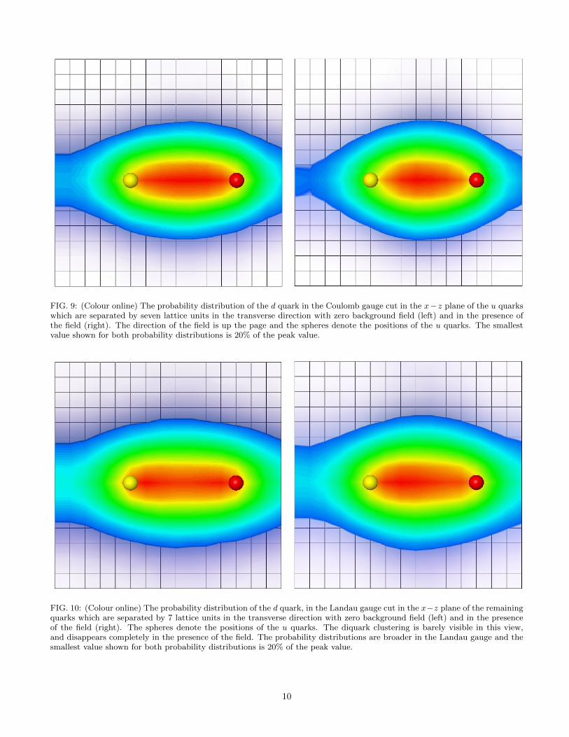
FIG. 9: (Colour online) The probability distribution of the d quark in the Coulomb gauge cut in the x−z plane of the u quarkswhich are separated by seven lattice units in the transverse direction with zero background field (left) and in the presence ofthe field (right). The direction of the field is up the page and the spheres denote the positions of the u quarks. The smallestvalue shown for both probability distributions is 20% of the peak value.

FIG. 10: (Colour online) The probability distribution of the d quark, in the Landau gauge cut in the x−z plane of the remainingquarks which are separated by 7 lattice units in the transverse direction with zero background field (left) and in the presenceof the field (right). The spheres denote the positions of the u quarks. The diquark clustering is barely visible in this view,and disappears completely in the presence of the field. The probability distributions are broader in the Landau gauge and thesmallest value shown for both probability distributions is 20% of the peak value.

10

FIG. 11: (Colour online) The probability distribution of the scalar u quark in the Coulomb gauge cut in the x − z plane ofthe remaining quarks which are separated by seven lattice units in the transverse direction with zero background field (left)and in the presence of the field (right). The direction of the field is up the page and the d quark is on the right, denoted bythe red sphere. In contrast to the d quark probability distribution, there is still a distinct preference for the formation of ascalar diquark. When the field is applied, the probability distribution can be seen to move toward the centre of the lattice.The smallest value shown for both probability distributions is 20% of the peak value.

FIG. 12: (Colour online) The probability distribution of the scalar u quark, in the Landau gauge which are separated by 7lattice units in the transverse direction with zero background field (left) and in the presence of the field (right). The directionof the field is up the page and the d quark is on the right, denoted by the red sphere. Preference towards the centre of thelattice is also visible in the Landau gauge, but is more subtle than in the Coulomb gauge. The probability distributions arebroader in the Landau gauge and the smallest value shown for both probability distributions is 20% of the peak value.

11

FIG. 13: (Colour online) The probability distribution of the vector u quark in the Coulomb gauge cut in the x− z plane of theremaining quarks which are separated by seven lattice units in the transverse direction with zero background field (left) and inthe presence of the field (right). The direction of the field is up the page and the d quark is on the right, denoted by the redsphere. The effect of the field on the vector u quark probability distribution is more pronounced than the d quark and scalaru quark probability distributions. The smallest value shown for both probability distributions is 20% of the peak value.

FIG. 14: (Colour online) The probability distribution of the vector u quark, in the Landau gauge cut in the x − z plane ofthe remaining quarks which are separated by 7 lattice units in the transverse direction with zero background field (left) and inthe presence of the field (right). The direction of the field is up the page and the d quark is on the right, denoted by the redsphere. The smallest value shown for both probability distributions is 20% of the peak value.

12

Acknowledgments

This research was undertaken on the NCI NationalFacility in Canberra, Australia, which is supported by

the Australian Commonwealth Government. We alsothank eResearch SA for generous grants of supercomput-ing time which have enabled this project. This researchis supported by the Australian Research Council.

[1] B. Velikson and D. Weingarten, Nucl. Phys. B 249, 433(1985).

[2] M. C. Chu, M. Lissia and J. W. Negele, Nucl. Phys. B360, 31 (1991).

[3] R. Gupta, D. Daniel and J. Grandy, Phys. Rev. D 48(1993) 3330 [arXiv:hep-lat/9304009].

[4] M. W. Hecht and T. A. DeGrand, Phys. Rev. D 46, 2155(1992).

[5] J. Smit and J. C. Vink, Nucl. Phys. B 286, 485 (1987).[6] G. Martinelli, G. Parisi, R. Petronzio and F. Rapuano,

Phys. Lett. B 116, 434 (1982).[7] C. W. Bernard, T. Draper, K. Olynyk and M. Rushton,

Phys. Rev. Lett. 49, 1076 (1982).[8] M. Burkardt, D. B. Leinweber and X. m. Jin, Phys. Lett.

B 385 (1996) 52 [arXiv:hep-ph/9604450].[9] F. X. Lee, R. Kelly, L. Zhou and W. Wilcox, Phys. Lett.

B 627, 71 (2005) [arXiv:hep-lat/0509067].[10] F. X. Lee, L. Zhou, W. Wilcox and J. C. Christensen,

Phys. Rev. D 73, 034503 (2006) [arXiv:hep-lat/0509065].[11] M. Luscher and P. Weisz, Commun. Math. Phys. 97, 59

(1985) [Erratum-ibid. 98, 433 (1985)].[12] J. M. Zanotti, D. B. Leinweber, W. Melnitchouk,

A. G. Williams and J. B. Zhang, Lect. Notes Phys. 663,199 (2005) [arXiv:hep-lat/0407039].

[13] C. Morningstar and M. J. Peardon, Phys. Rev. D 69,054501 (2004) [arXiv:hep-lat/0311018].

[14] R. Sommer, Nucl. Phys. B 411, 839 (1994) [arXiv:hep-lat/9310022].

[15] S. Gusken, Nucl. Phys. Proc. Suppl. 17, 361 (1990).[16] C. T. H. Davies et al., Phys. Rev. D 37, 1581 (1988).[17] M. Anselmino, E. Predazzi, S. Ekelin, S. Fredriksson and

D. B. Lichtenberg, Rev. Mod. Phys. 65, 1199 (1993).[18] C. Alexandrou, P. de Forcrand and B. Lucini, PoS

LAT2005, 053 (2006) [arXiv:hep-lat/0509113].[19] C. Alexandrou, Ph. de Forcrand and B. Lucini, Phys.

Rev. Lett. 97, 222002 (2006) [arXiv:hep-lat/0609004].[20] T. DeGrand, Z. Liu and S. Schaefer, Phys. Rev. D 77,

034505 (2008) [arXiv:0712.0254 [hep-ph]].

13