
Water Resources Systems Planning - Internet Archive
368
K A WATER RESOURCES SYSTEMS PLANNING Some Case Studies for India R N A T A K A Edited by Xrl *-Basin boundary AHESH C CHATURVED! t v * -—•—State boundary PETER ROGERS /0° V INDIAN ACADEMY OF SCIENCES Bangalore 560 080
-
Upload
khangminh22 -
Category
Documents
-
view
0 -
download
0
Transcript of Water Resources Systems Planning - Internet Archive
K A
WATER RESOURCES SYSTEMS PLANNING
Some Case Studies for India
R N A T A K A
Edited by Xrl *-Basin boundary
AHESH C CHATURVED! t v * -—•—State boundary
PETER ROGERS /0° V
INDIAN ACADEMY OF SCIENCES Bangalore 560 080

Digitized by the Internet Archive in 2018 with funding from
Public.Resource.Org
https://archive.org/details/waterresourcessyOOunse


WATER RESOURCES SYSTEMS PLANNING
Some Case Studies for India
Edited by MAHESH C CHATURVEDI
Indian Institute of Technology, New Delhi
PETER ROGERS Harvard University, U.S.A.
19 8 5
INDIAN ACADEMY OF SCIENCES
BANGALORE 560 080

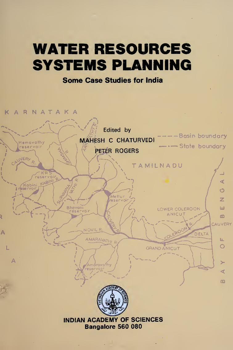
cover shows the plan of the Cauvery basin, from the paper by S. Vedula
Reprinted from
Edited by M.
© 1985 by the Indian Academy of Sciences
Sadharia-Academy Proceedings in Engineering Sciences Volume 8, pp. 1-350, 1985
Chaturvedi and P. Rogers and printed for the Indian Academy of Sciences by Macmillan India Press
Madras 600 041, India

CONTENTS
Foreword i
M C CHATURVEDI and PETER ROGERS: Introduction 1
M C CHATURVEDI: Water resources of India - an overview 13
M C CHATURVEDI: Water in India’s development: Issues, developmental policy and programmes, and planning approach 39
M C CHATURVEDI: The Ganga-Brahmaputra-Barak Basin 73
M C CHATURVEDI, PETER ROGERS and SHYANG-LAI KUNG: The coordinating model of the Ganga basin 93
PETER ROGERS and SHYANG-LAI KUNG: Decentralized planning for the Ganga basin: Decomposition by river basins 123
GEORGE KARADY and PETER ROGERS: Decentralized planning for the Ganga basin: Decomposition by political units 135
ROGER REVELLE and V LAKSHMINARAYANA: An unconventional approach to integrated ground and surface water development 147
M C CHATURVEDI and V K SRIVASTAVA: Storage of surface flows through groundwater recharge 159
P S RAO and S RAMASESHAN: Study of Bhakra reservoir operation 179
P S RAO and S RAMASESHAN: Integrated operation of the Beas-Sutlej system 207
S VEDULA: Optimal irrigation planning in river basin development: The case of the Upper Cauvery river basin 223
RAMESHWAR D VARMA: A case study of the Rajasthan canal 253
BASAWAN SINHA and P RAMAKRISHNA RAO : A study for optimum utilisation of the Damodar water resources 273
BASAWAN SINHA, RAMESH BHATIA and SUPRIYA LAHIRI: Planning for the Subemarekha river system in Eastern India 291
M C CHATURVEDI and D K SRIVASTAVA: Study of a complex water resources system with screening and simulation models 311
M C CHATURVEDI and PETER ROGERS: Overview and reflections 329
Author Index 351
Subject Index 355

..
' 1
.
. .

Foreword
Development of natural resources is, in many countries, a prerequisite for economic development. Two of these natural resources—land and water—play a key role in the
earlier stages of development in view of the primacy of the agricultural sector in the
overall economy. The development of water resources is particularly important in
India in view of its arid-monsoon climate. This fact has been realized since time immemorial. Since Independence great emphasis has been laid on water resources
development with almost 25 % of the current development budget being invested in this sector.
Ambitious plans have been drawn up by Government for rapid development of
water resources within the next 25 years. The first step in achieving this task is
Institutional modernization and development of well trained cadres of professionals
who have the appropriate concepts, attitudes and capabilities. With the development
of a systems approach to water management, it is now considered mandatory that
modern development should be planned on these lines.
Realizing these needs, the Ford Foundation has been supporting the development of
man-power in this sector. In view of the pioneering work done at Harvard University in
this area, a programme was started there and Indian faculty and senior officials were
invited to work with the Harvard faculty. We believe that the work done under that
project should be made available and widely disseminated as this would be helpful in the ongoing efforts of development of manpower in systems planning. Hence this volume.
The importance of systems planning has also been emphasized independently by the
Government of India. It was decided as far back as 1968 that a systems study of Ganga
basin be undertaken. The decision was taken by the then Union Minister of Irrigation,
Dr K L Rao, and a preliminary study of the Ganga basin was completed by one of the
authors (Chaturvedi). In this context a short term programme of three months was
organized at the Indian Institute of Technology (iit)-Delhi with the support of the Ministry of Irrigation in March 1972, to train prospective engineering officers for the
Ganga basin studies. Efforts have continued since then to train personnel in the systems approach of
water resources development. In the fourth five-year plan it was decided that the
systems study of two river basins be carried out so that capability in the studies in this
area could be developed. The Indian author was invited to carry out these studies in
systems planning for the state of Punjab and for a project in Maharashtra under the
auspices of the Planning Commission and the respective states. This effort was also
supported by the Ford Foundation. Some of the relevant studies carried out by the
Indian author independently of the Harvard-Ford Foundation programme have also
been accordingly included in the volume. The authors realize the shortcomings of the volume. It does not represent a single
coordinated or integrated study to illustrate the application of systems approach to
one river basin, but in totality several aspects of regional water resources development have been covered and we consider that it will be useful in the task of human
ii
resources development required for the challenges facing India. We also believe that
these studies will be helpful for other countries, both in the developing and the
developed part of the world, and will also contribute to the art and science of large scale
engineering-economic systems planning. The work is essentially a collaborative activity of all the participants whose studies
have been reported in the various papers. The work became possible only through the
support of the Ford Foundation which is gratefully acknowledged. The support of the
officers of the Ford Foundation, particularly Dr Sadik Toksaz and Dr Roberto R
Lenton, who have been directly responsible for the project not only as Ford
Foundation Administrators, but also as distinguished systems analysts is also gratefully
acknowledged.
The work was carried out at Harvard in the Centre for Population Studies. Prof
Roger Revelle, then Director of the Centre for Population Studies was an enthusiastic
supporter and collaborator and thanks are specially due to him. Thanks are also due to
other Harvard faculty who were involved in the programme. Some of the faculty who
deserve special mention are Professors Joseph J Harrington, Myron Fiering, Harold
Thomas Jr, Drs James Gavan, Richard Tabors and Samuel Liberman. Thanks are also
due to the many undergraduate and graduate students who worked as research
assistants and many of whom have moved on to distinguished careers in the area of
resources management. Dr John Brisco was particularly helpful in this category
Thanks are also due to the secretaries who provided office support so necessary for the
completion of such a project, particularly Ms. Elizabeth Gibson and Ms. Kathie
Macagy. On the Indian side, the Indian Institute of Technology, Delhi has been generously
supporting the work of the Indian author in this area. The work of two of his graduate
students, Dr V K Srivastava and Dr D K Srivastava has also been reported and thanks
are due to them for this collaboration. Thanks are also due to Mr B N Asthana,
Executive Engineer, Irrigation Department, up, currently leading the group working on
the up-Ford Foundation Project for helping the Indian author in the editing of these
studies. Without his help these studies could not have seen the light of the day.
While we express our thanks to the people and institutions mentioned above we wish
to make it absolutely clear that the views expressed in these papers are solely those of
the authors and do not necessarily reflect the views of any of the people or institutions who supported our research.
MAHESH C CHATURVEDI
PETER ROGERS

Introduction
MAHESH C CHATURVEDI* and PETER ROGERS t
* Applied Mechanics Department, Indian Institute of Technology, New Delhi 110016, India
t Department of Environmental Engineering, Pierce Hall, Harvard University, 121, Cambridge, MA 02138, USA
1. Background
Water, though a crucial component of the physical environment, is generally not
available as and when required, and attempts have been made since time immemorial to
make it available for man’s varied use. Indeed, in view of the importance of water, its
development has occupied a leading place in any society’s efforts. The ancient
civilizations of Egypt, Mesopotamia, India and China, show that making water
available for domestic use, harnessing it for irrigation and controlling it for flood protection against floods were basic preoccupatons in these societies. Interestingly, the
history of science and technology for quite some time was the history of mechanics,
hydraulics and water resources development (Rouse & Ince 1957). Continued emphasis
has been laid on this area, and in modern times, many impressive technological
achievements have become possible.
Water development in India has occupied the highest importance in view of the arid
monsoon climate and agrarian economy. There is evidence of canals, dams and
dugwells from prehistoric times. Large canals were being constructed as early as
16 A.D. Many canals with a capacity of the order of 300 cumecs were constructed as far
back as the middle of the 19th century. These developments attracted the attention of
scientists from the United States, and engineers from us Bureau of Reclamation visited these works for guidance in their later works (Maddock T III 1977 personal
communication). The Indian irrigation systems were one of the technological wonders
of the world and, indeed, still are.
As increasing technological capability is developed, it is becoming clear to perceptive
thinkers that technological activity, unless carefully planned can become a source of
societal and environmental damage. Techno-economic-environmental-social interac¬
tion is extremely complex, but what is crucial is that technology be developed creatively
and critically. Recent developments in several areas such as operations research, welfare
economics and computer science and technology have led to the development of the
new art and science of systems analysis to aid scientific technological planning. Concern
with the scientific development of technology, increasingly careful analysis of its
economic-social consequences and emphasis on the environmental-ecological impli¬
cations of technological activity have become the leading concerns of post-industrial
society. As water is a crucial component of the resource-environmental vector, systems
analysis has found extensive application in water resources planning. The origin of the
activity may be said to be in the late 1950s in the United States, when the us Bureau of
1
2 Mahesh C Chaturvedi and Peter Rogers
the Budget (now Office of Management and Budget, omb) asked the major us
governmental agency dealing with water projects, the us Army Corps of Engineers, to
provide better estimates of the social and economic consequences of the water projects
presented to the Budget Office for funding. In order to carry out this charge, the Corps
of Engineers approached various academic institutions for help. One such group of
engineers, economists and political scientists was at Harvard University. Pioneering
work was done by this group and is reported in Maass et al (1962). Since then, the
importance of systems planning has been increasingly recognized and continuous
advances are being made. Systems planning of the Ganga Basin was proposed to be
taken up by the Government of India at iit Delhi in 1968, but the international dispute
of the Ganga river led to the shelving of the proposal. In the Fourth Five Year Plan
(1969-74) systems planning of water resources was stipulated to be required for future
developments. Systems planning of Punjab was accordingly carried out by the Indian
author.
In 1972 the Ford Foundation, New Delhi, approached the Harvard University to
explore a collaborative venture in which the Harvard faculty would work with
practising Indian academics and professionals in the field of Water Resources Planning
to pursue the applicability of these new approaches to the Indian situation. The Indian
author was particularly invited by the Harvard group to collaborate on this project.
The papers contained in this volume are one result of this programme. Since 1973,
several Indian academics, government employees and private consultants have
participated in the programme. The participants in the programme worked alone or in
groups on various projects, some of which are outlined here. Simultaneously, certain
other studies have been carried out at iit Delhi, and Harvard, some of which are also
included. Basically, we believe that these new techniques are of substantial interest and
use in the Indian context, and may contribute to this field in general.
2. Systems analysis: some general observations
Systems analysis embraces a body of concepts, approaches and mathematical
techniques, aimed at assisting in the scientific and creative development of technology.
Technological planning, basically, is a complex decision process, involving develop¬
ment of the optimal scheme for the transformation of environment, resources, energy,
and information according to a society’s or an individual’s needs. The transformation
has to satisfy two considerations. First, the physical laws must be satisfied. This gives
the technological transformation or the production function. Second, the technological
transformation has to be evaluated in the context of a set of interrelated evaluation
criteria which may be classified as environmental, economic, political and social. Both
these tasks have to be carried out in an integrated and hierarchical fashion.
Technological planning is a very complex creative activity. Many of the issues or
objectives are non-quantifiable. There are no set answers, and infinite alternatives or
novel approaches are possible. The systems approach is an aid, typically using
mathematical modelling, to examine the various issues over a wide and yet manageable
range in a systematic manner. The models can be considered as ‘thought experiments’.
Systems planning is only an aid to and not a substitute for sound judgement.
Systems planning is particularly important for water resources, because of the
complex interlinkages and socio-economic interactions involved. Water resources
Introduction 3
development transforms the spatial and temporal availability of waer, through a
number of specific technological activities or projects, which are interrelated by
hydrologic continuity and other technological interlinkages. For their optimal specification, capacity and location, and the operating policy, these technological
interlinkages must be taken into account. Similarly, the complex socio¬
economic evaluation of the system and correspondingly of each project has to be carried
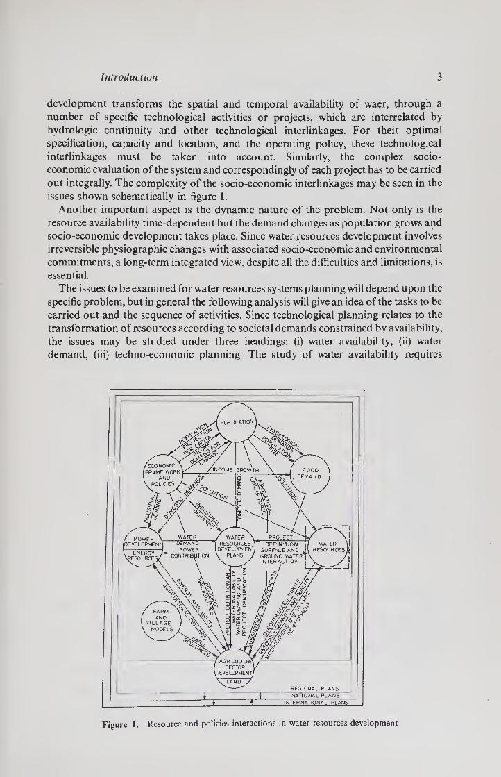
out integrally. The complexity of the socio-economic interlinkages may be seen in the
issues shown schematically in figure 1.
Another important aspect is the dynamic nature of the problem. Not only is the
resource availability time-dependent but the demand changes as population grows and
socio-economic development takes place. Since water resources development involves
irreversible physiographic changes with associated socio-economic and environmental
commitments, a long-term integrated view, despite all the difficulties and limitations, is
essential.
The issues to be examined for water resources systems planning will depend upon the
specific problem, but in general the following analysis will give an idea of the tasks to be
carried out and the sequence of activities. Since technological planning relates to the
transformation of resources according to societal demands constrained by availability,
the issues may be studied under three headings: (i) water availability, (ii) water
demand, (iii) techno-economic planning. The study of water availability requires
Figure 1. Resource and policies interactions in water resources development

4 Mahesh C Chaturvedi and Peter Rogers
sophisticated analysis of physical phenomena. The demand analysis similarly requires
refined engineering-economic analysis, such as developmental strategies, resources
availability and social evaluation of key resources, loss function and risk criteria, and
project selection criteria. Techno-economic systems studies start by assessing supply
and demand and then developing policies of optimal allocation of water resources over
planning regions leading to optimal development. It is a hierarchial-iterative activity,
which has to be carried out creatively on the basis of judgement with the help of models
depicting a large number of complex issues involving physical processes,
environmental-economic-social evaluation and analysis of technological activity.
Some of the issues under the above three headings and the appropriate models are
listed in table 1. A design morphology has to be suitably developed for the specific
study. For physical and technological systems studies the likely sequence is shown in
figures 2 and 3. The scope of the models and the state-of-art have been discussed
elsewhere (Chaturvedi 1984) and the approach may be only briefly mentioned here.
Starting with the estimate of water availability and water demand, a developmental
policy is outlined and a systems investigation model, termed the first coordination
model, is developed. The objectives of this model are to (i) scan the total system
Table 1. Relevant issues and models
Issues
Socio-economic studies Water and allied resources studies
General and related System studies Analysis of
sector planning physical
studies phenomena
1. Development strategies
2. Social evaluation of key
resources
3. Resources availabilities
4. Evaluation of loss function and
risk criteria
5. Project selection criteria
1. Regional optimal allocation
of water resources
2. Optimal development con¬
strained by economic and
physical resources
3. Project evaluation and
selection
1. Description of physical
phenomena
2. Analysis and simulation of
physical phenomena
Models
1. Intersectoral resource allocation
model
2. Population studies
3. Food demand models
4. Agricultural sectoral model
5. Technology-efficiency-equity
models
1. Preliminary system formu¬
lation model
2. Subsystem and system analy¬
sis (deterministic model)
3. Subsystem and system analy¬
sis (stochasic model)
4. System simulation models
5. Simulation of crop activities
6. Power sector models
7. Space structuring models
8. System environmental
models
1. Hydrologic models
2. Hydrogeologic exploration
models
3. Surface-ground water simu¬
lation model
4. Ground water recharge
models
5. Crop-water fertiliser res¬
ponse models
6. Water quality models

Introduction 5
INPUT - GENERAL SYSTEM STUOCS -4<-WATER RESOURCES SYSTEM STUOCS -M STUDES I 1 '
ITERATE THROUGH SENSITIVITY ANALYSIS TO REQUISITE DEGREE/REFINEMENT AND BALANCE
Figure 2. Water resources systems analysis modelling morphology
performance and then to determine the limits of interlinkage of various systems
elements which may be examined in greater detail, (ii) identify the sensitivity of the
decision to physical processes and parameters in terms of which data collection and
physical processes modelling may be carried out and (iii) identify the socio-economic
evaluation studies for a correspondingly more refined analysis. Progressively and
Figure 3. Water-resource system (after Ackermann 1969)

6 Mahesh C Chaturvedi and Peter Rogers
integrally each of these three activities may be refined. For instance, watershed
modelling coupled with groundwater simulation may be carried out to quantify surface
and groundwater availability and their dynamical interlinkage as man-made engineer¬
ing activities are proposed. In this, both quantity and quality analyses are involved.
Stream-flow synthesis studies may be carried out to arrive at a better understanding of
regional temporal availability, with consequent refinement of the capacity and
operating policy of the individual projects. Several other studies may be mentioned.
On the socio-economic side, the problem may be that instead of being limited to
partial equilibrium analysis, a general equilibrium analysis may have to be carried out
because of the large investments that go into water resources development in India.
Appropriate economic-environmental objectives may have to be developed and
quantified. For example, according to latest policies, employment generation is an
important objective in Indian developmental planning. An appropriate cropping
pattern for the project, embedded in a dynamic cropping pattern policy for the country
may have to be determined. It is not necessary that optimum water to meet physiologic crop-requirements be provided. A lower amount, according to optimal marginal
contribution to production may be more advisable. Further, the differential impact of
irrigation on farms of different sizes creates problems. Issues of institutional,
organizational and technological planning in terms of the multiobjectives of economic
efficiency and equity, and expected value and risk may have to be examined. Several
other issues may be mentioned.
As these studies of physical processes and evaluation continue, technological systems
studies get refined. Each subsystem may be studied for short time intervals to determine
the optimal capacity and operating policy. After deterministic analysis, stochastic
studies may be carried out. Algebraic technologic functions for each subsystem may be
developed and finally through the coordinating model, an optimal system plan may be
developed. In the final analysis, simulation of the system may be carried out.
Water resources development is so basic to India that its planning may involve
simultaneous consideration of systems planning in other areas, such as land, energy, or
transportation. Although difficulties are introduced when such an integrated planning
is envisaged, the interactions may make it mandatory in planning for many large river
basins. For example, at present, about 50 % of electric power in the Ganges Basin is
hydro-electric and its future potential is at least as important as other modes of energy.
Or canals may be developed as inland waterways and thereby integrated planning with
the transportation system may be advisable. Or, since transportation crossings are
economic sites for diversion works, it may be desirable to have integrated planning of
the two areas.
Systems planning involves the collection of data and techno-economic analysis. Any
systems analysis is only as good as the data: hydrologic, economic and technological.
However, there are two basic issues. First, systems studies shed valuable light on the
sensitivity of the decision to various parameters and at all stages of study, through
sensitivity analysis, are mandatory for data collection and techno-economic analysis.
Secondly, at each stage, the central issue is judicious balance in the level of
sophistication of the techno-economic analysis, study of physical phenomena and
analysis of techno-economic-environmental evaluation, in terms of the value of their
contribution to decision issues. Indeed, it is on this principle that continuous
progress in refinement is made and studies are iterated and finally terminated.
Large-scale water resources systems planning is thus an integrated-hierarchial-

Introduction 7
sequential activity. It calls for creative macro-modelling supported by adequate micro
studies. It is far removed from professional adhoc project-by-project analysis or
academic systems-analysis exercises Even the recent examples of modelling or
integrated planning, though contributing significantly in this area, fall short of the task,
particularly in developing countries because of undeveloped economic and tech¬ nological systems. What is needed is continued application of recent systems-analysis
approaches and techniques to real-life problems, leading to generalizations from the
experience thus gained. The studies presented in this and other papers in this volume seek to contribute to this end.
3. Overview
The present studies were carried out independently and cover a wide field of subjects
relating to a number of river basins. For convenience, these have been grouped into two
parts, one relating to the Ganga Basin and the second, relating to other river basins. The
river basins of India and those studied are shown in figure 4 and table 2 respectively.
After giving a background of the studies in this paper, the water resources of India
are briefly reviewed in another paper in this volume (Chaturvedi 1985a). Following it in
another article, the issues, developmental policy and programmes, and the planning
approach are discussed (Chaturvedi 1985b). It will be seen that much of the development
has taken place without any systematic policy analysis and the continued adhoc project-
by-project development that is taking place may lead to the most serious resource
depletion and environmental degradation. As the first step in systems analysis, the
issues, objectives and planning approach for the development of water resources have
to be decided. It may be necessary to have an all-India overview and to identify a policy
and trajectory of development, according to which hierarchial-iterative macro- and
micro-systems planning may be carried out.
The planning approach for the Ganga Basin, which is typical of a very large
basin is illustrated through a series of eight studies. First, the salient features of
Table 2. River basin and study area
River basin Study
area
River basin Study
area
Ganga Basin B5* Narmada B8
Brahmaputra
Barak and other rivers
A Tapi including Kim
Godavari
East flowing rivers between
Ganga and Mahanadi
Mahanadi
East flowing rivers between
B6 Krishna
Pennar and other east flowing
rivers between Krishna and
Cauvery
Mahanadi and Godavari Cauvery B3
Indus Bl+2
B4
East flowing rivers
below Cauvery
Luni and others of Saurashtra
and Kutch
Sabarmati and Mahi
B7 West flowing rivers
below Tapi
* Covers only Damodar river basin
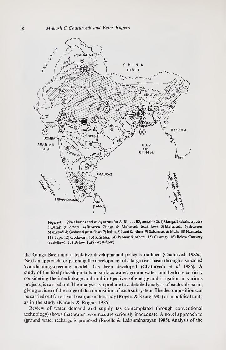
8 Mahesh C Chaturvedi and Peter Rogers
Figure 4. River basins and study areas (for A, B1 ... B8, see table 2). 1) Ganga, 2) Brahmaputra
3) Barak & others, 4) Between Ganga & Mahanadi (east-flow), 5) Mahanadi, 6) Between
Mahanadi & Godavari (east-flow), 7) Indus, 8) Luni & others, 9) Sabarmati & Mahi, 10) Narmada,
11) Tapi, 12) Godavari, 13) Krishna, 14) Pennar & others, 15) Cauvery, 16) Below Cauvery
(east-flow), 17) Below Tapi (west-flow)
the Ganga Basin and a tentative developmental policy is outlined (Chaturvedi 1985c).
Next an approach for planning the development of a large river basin through a so-called
‘coordinating-screening model’, has been developed (Chaturvedi et al 1985). A
study of the likely developments in surface water, groundwater, and hydro-electricity
considering the interlinkage and multi-objectives of energy and irrigation in various
projects, is carried out.The analysis is a prelude to a detailed analysis of each sub-basin,
giving an idea of the range of decomposition of each subsystem. The decomposition can
be carried out for a river basin, as in the study (Rogers & Kung 1985) or in political units
as in the study (Karady & Rogers 1985).
Review of water demand and supply (as contemplated through conventional
technology) shows that water resources are seriously inadequate. A novel approach to
(ground water recharge is proposed (Revelle & Lakshminarayan 1985). Analysis of the
Introduction 9
problem requires that numerical-techniques be used. Groundwater-stream interaction
through finite-difference approach has been developed and three schemes of ground-
water recharge-surface development have been examined (Chaturvedi & Srivastava 1985b).
Several other related issues have been examined in the following studies. In one of the
earliest papers on the subject, Rogers applies the game theory to demonstrate the use of
analytical tools to analyse problems of conflict. The paper was referred to Chaturvedi,
for independent study by the Indian Government as far back as 1968, and forms the
beginning of the collaborative project between the two authors.
Regional water resources development usually focusses attention on the land region,
neglecting the river-ocean interaction particularly as upstream developments take
place. It is important that the implications of these developments are studied
conjunctively. The implications of upstream development on flooding and saline
penetration have been carried out by Rogers (unpublished).
It must be reiterated that systems planning is an adjunct to real-life planning
demanding detailed technological and engineering-economic data and analysis. These
studies are only concerned with an approach to analysis and the results are only
indicative. We hope these studies will lead to detailed real-life systems planning of the
water resources of India, which is long overdue. Systems planning of one large region,
the Uttar Pradesh part of the Ganga Basin, is being carried out by Chaturvedi, but
much requires to be done.
Further, systems studies of several river basins which also cover various other aspects
of water resources planning, are presented. In the first of two studies, some problems of
the Indus Basin are studied (Rao & Ramaseshan 1985a). The operation of Bhakra has
been studied. It is shown that through multi-objective analysis and planning for
conjunctive surface and groundwater development through a linear programming
model, substantive improvements in returns and reliability could be obtained, both for
energy and irrigation. The studies are extended for the operation of the Sutlej and the
Beas (Rao & Ramaseshan 1985b) instead of only the Sutlej, in the second study.
The problem of optional operation of a number of reservoirs taking into account the
varying storage in flow characteristics of each and the possibility of obtaining the
optimum cropping pattern, is studied by Vedula (1985). The study relates specifically to
the Cauvery Basin. The issue of cropping patterns is extended by Verma (1985) by
studying, in addition and conjunctively, (i) the issues of the level of technology (high,
medium, and low crop yields), and (ii) levels of irrigation technology (sprinkler and
furrow irrigations). The area of interest is Rajasthan, a very arid region of the country,
and the project studied is the Rajasthan Canal, having a capacity of 530 cumecs, one of
the biggest canals in the world. Several policy issues are examined and significant
modification in existing policy are suggested by Verma (1985).
Techno-economic systems planning of two river basins in the eastern parts of
India—the Damodar Valley and the Subernarekha river is undertaken in two studies
by Sinha & Rao (1985), and Sinha et al (1985) respectively. Both deal with complex
large-scale systems and through mathematical modelling, incorporating multi¬
objective analysis and considering the possibility of optimal cropping patterns, an
optimal development policy is attempted.
The study of the issue of irrigation policy, particularly important in arid areas with
scarce water resources such as Rajasthan studied by Verma earlier is continued for an ad¬
joining arid area of Gujarat by Basu D N, Gopinath C & Karady G (unpublished). One
10 Mahesh C Chaturvedi and Peter Rogers
of the major issues in planning for investment of irrigation water is its allocation
amongst crops and regions. Some of the issues are (i) inter-seasonal allocation (ii) inter¬
regional allocation, (iii) extensive versus intensive irrigation and (iv) implications of
reliability of irrigation. Investigating (i) economic efficiency, (ii) calorific value and
(iii) employment generation objectives, the policies of allocation among the different
crops, seasons, regions and technologies have been examined through multi-objective
analysis.
Additional technological systems planning issues with application to another major
river basin are examined by Chaturvedi & Srivastava (1985a). The focus of interest is
the Narmada river, in central India, significant from many considerations. The basin
provides one of the most economical development options, perhaps in the world, and is
yet almost totally undeveloped. According to the policy analysis carried out earlier, it
can be an integral component in the national policy of water resources development.
The issues examined in the paper are naturally limited. A procedure of analysis has
been developed and has been applied to the Narmada system. It is proposed that for a
complex system, a screening model has to be used in the first stage to identify the range
of interlinkage for detailed subsystem analysis through decomposition. It is proposed
that a programming—simulation approach could be used for examining the stochastic
nonlinear nature of the problem.
The studies reported are isolated studies and are not related to the totality of real-life
systems. While they do contribute to the science of planning, and in certain cases to
specific issues, much remains to be done to apply them to real life problems. The issue of
systems planning of river basins, with insights obtained from the foregoing studies is
discussed in the concluding Overview and Reflections by the authors.
Systems planning of technology requires capability in design as well as in planning.
Very often, scientists working in these two activity areas work in isolation, the
professionals concentrating more on detailed design and project planning often from
narrow techno-economic considerations and the academics concentrating on sophisti¬
cations of systems analysis. There is a correlation between resolution level of data,
engineering-economic analysis and systems analysis in terms of value in decision¬
making. Both for real-life utility and advances in the science of systems analysis, it is
necessary that academics and professionals work together on real-life problems.
Unfortunately, as the review of water resources development in the usa reveals,
scientific planning though accepted as important, has generally not been followed
(Schwarz 1979). One of the impediments is the lack of appreciation for the need and
value of systems planning. We hope we have been able to make some contribution
towards understanding and appreciating this need.
References
Ackerman W C1969 Scientific hydrology in the United States, The progress of hydrology, II Int. Seminar for
Hydrology, Professors, University of Illinois, Champaign
Chaturvedi M C 1984 Water resources and environmental systems planning (New Delhi: Tata-McGraw Hill)
(in press)
Chaturvedi M C 1985a Sadhana 8: 13-38
Chaturvedi M C 1985b Sadhana 8: 39-72
Chaturvedi M C 1985c Sadhana 8: 73-92
Chaturvedi M C, Rogers P and Kung S L 1985 Sadhana 8: 93-121

Introduction 11
Chaturvedi M C, Srivastava D K 1985a Sadhana 8: 311-328
Chaturvedi M C, Srivastava V K 1985b Sadhana 8: 159-177
Karady G, Rogers P 1985 Sadhana 8: 135-145
Maass M M, Hufschmidt A, Dorfman R, Thomas H A, Marglin S A, Fair G M 1962 Design of water resources
systems (Cambridge, Massachusetts: Harvard University Press)
Rao P S, Ramaseshan S 1985a Sadhana 8: 179-206
Rao P S, Ramaseshan S 1985b Sadhana 8: 206-222
Revelle R, Lakshminarayana V 1985 Sadhana 8: 147-157
Rogers P, Kung S L 1985 Sadhana 8: 123-134
Rouse H, Ince S 1957 in History of hydraulics (Iowa: Institute of Hydraulics Res.)
Schwarz H E 1979 ASCE J. Water Resources Planning and Mgt. Div. WR1.
Sinha B, Bhatia R, Lahiri S 1985 Sadhana 8: 291-310
Sinha B, Rao P R 1985 Sadhana 8: 273-290
Vedula S 1985 Sadhana 8: 223-252
Verma R D 1985 Sadhana 8: 253-271

'

Water resources of India—an overview
M C CHATURVEDI,
Applied Mechanics Department, Indian Institute of Technology, New Delhi 110016, India
1. Introduction
Specific physiographic, climatic and hydrologic characteristics along with economic
and demographic features of a region determine the development of water resources. These are briefly described in the case of India as a prelude to the systems studies
described later. A historical and quantitative perspective of developments is also given
briefly. For details reference may be made to Rao (1976), Irrigation Commission
Reports (1972), Chaturvedi (1976) and National Commission on Agriculture Reports (1976).
2. Physiographic features
The land mass which forms the subcontinent of India is a large peninsula, covering an area of 328 million hectares (mha), and supporting a population of 658 million (1981). It
lies between 8° 4' and 37° 6' North latitude and 68° 7' and 97° 25' East longitude. With a land frontier of 15,200 km, much of which is bordered by very high mountains and a
coastline 5,700 km long, it is the seventh largest country in the world. The location and the characteristics—a large peninsula with high mountains on the North—create a
unique hydrologic-climatic environment.
Physiographically, India can be divided into seven divisions and twenty subdivisions
(figure 1): (a) the Northern Mountains (b) the Great Plains (c) the Central Highlands
(d) the Peninsular Plateau (e) the East Coast Belt (f) the West Coast Belt and (g) the
Islands. We shall only confine ourselves to the coterminous subcontinent.
The northern Himalayan mountains stretch in a virtually unbroken chain, 2,500 km
in length and 250 to 400 km in width, as a series of more or less parallel, though
sometimes converging, ranges from the Indus in the west to the Brahmaputra in the
east. In the north, there are three distinct ranges known as the Greater and the Middle
Himalayas and the Lower Siwaliks. The average heights of these ranges are 6,000,
4,000 and 1,000 m respectively. They have some of the highest peaks of the world, and
large areas above 5,000 m elevation are permanently snowclad. They contribute an
annual snow melt of 5 million hectare metres (m ha m). They are geologically very young
and, being formed of sedimentary rocks with steep slopes, contribute to high sediment
charge to surface runoff. This is fpitigated only by the fact that they are heavily covered
with forests. As human and livestbck populations grow, increasing soil erosion poses a
serious problem.
Stretching at their feet and built up from the rivers flowing from the Himalayas, are
the great Indo-Gangetic Plains. The alluvium forming the plains was laid down in
13

14 M C Chaturvedi
Figure 1. India physiographic map. international boundary-- regional boundary-.
(source: Chaturvedi 1976)
successive geological eras and have depths of thousands of metres. The plains, with an area of 652,000 km2, account for about 25 % of the total land area of India. The surface
of the great plains is at tide level near the sea but is well over 200 m above sea level in the
Punjab plains.
Further south, are the Central Highlands, consisting of a compact block of mountains, hills and plateaus intersected by valleys and basins covered by forests,
accounting for one-sixth of the total land area.
The triangular peninsula plateau, ranging in elevation from 300 to 900 m constitutes
about 35 % of the land. The surface sometimes consists of extensive plains. It is well-
drained by a number of rivers flowing from west to east.

Water resources of India—an overview 15
Of the two coast belts, the eastern is wider with a width of 100-300 km with a number of river deltas. The western belt is only 10-25 km wide between the Western Ghats and the sea.
The land is served by a number of large rivers. They can be divided into two groups; viz the perennial rivers of the Himalayan region which are snow fed, and the peninsular rivers. The maximum monthly discharge variation of the former is of the order of 50:1 while that of the latter is of the order of 1000:1. These can also be classified in three groups in terms of their catchment areas, as discussed later.
India can be divided into 17 river basins as shown in figure 2. The Ganga basin is the
Figure 2. India—: river basins 1) Ganga, 2) Brahmaputra, 3) Barak & others 4) Between Ganga & Mahanadi (east-flow), 5) Mahanadi, 6) Between Mahanadi & Godavari (east-flow), 7) Indus, 8) Luni & others, 9) Sabarmati & Mahi, 10) Narmada, 11) Tapi, 12) Godavari, 13) Krishna, 14) Pennar & others, 15) Cauvery, 16) Below Cauvery (east-flow), 17) Below Tapi (west-flow). International boundary-—, river basin boundary-(source: Chaturvedi 1976)

16 M C Chaturvedi
Table 1. Salient water, land and population statistics
Land Water
Utilizable
V
Cat
chm
ent
area
(i
nsid
e In
dia)
Cult
ura
ble
are
a
(% o
f 1)
Net s
own
area
(% o
f 2)
Cro
ppin
g i
nten
si
Pre
cip
itat
ion
Ev
apo
rati
on
Ann
ual
runoff
Ann
ual
gro
und \
re
char
ge
Sur
face
ru
no
ff
(%o
f 7)
Uti
liza
ble
grou
m
wat
er (
% o
f 7
Cl
m.ha °/ /o °/ /o % cm cm mhm mhm °/ /o °/ /o
No. River basin 1 2 3 4 5 6 7 8 9 10
1 Ganga 8615 70-0 76-5 125 116 212 55-01 14-62 33-6 18 9
2 Brahmaputra 18-71 64-9 22.7 118 122 125 42-2 3-97 2-1 4-5
3 Barak and others 7-82 14 3 66-5 124 286 150 17-5 1 60 2-12 3-7
4 Between Ganga and 8 10 63-0 65 1 114 147 175 4-35 1-63 94-0 16 0 Manahadi (East flow)
5 Mahanadi 1416 56-5 70-3 125 146 200 7-07 2-13 93-7 15 0
6 Between Mahanadi and 4-97 54-4 66-7 124 111 200 1-72 0-73 93-5 23-6 Godavari (East flow)
7 Indus 3213 30-0 72-3 133 56 200 7-69 2-90 64-2 14-8
8 Luni and others 32-18 72-8 60-3 105 38 305 1-23 0-80 74-0 48-2
9 Sabarmati and Mahi 5 93 62-8 77-6 111-5 159 320 1-55 0-62 73-35 21 0
10 Narmada 9-88 59-8 76-2 106 121 245 4-01 1-24 73-0 17-8
11 Tapi 669 66-0 88-6 104 78 305 1-97 0-61 71-0 20 1
12 Godavari 31-28 60-5 76-5 107 110 235 11-54 3-31 73-8 17-2
13 Krishna 25-90 78-4 76-6 105 81 290 6-28 2-65 83-5 315
14 Pennar and others 14-49 650 59-5 116 82 230 2-53 1-82 73-3 41-5
15 Cauvery 8-79 66-0 64-5 115 99 225 1 86 1-23 96-4 26-0
16 Below Cauvery East 3 51 75-0 62-8 111 91 270 0-95 0-54 36-9 12 2 flowing
17 West flowing below Tapi 11-21 56-0 69-0 119 279 200 2-79 2-01 13-2 50
Total 321-87 59-7 67-7 115-4 124-8 228 188-8 42-41 35-4 13-8

Water resources of India—an overview 17
People Unit figures
Utilized % of utilizable
Sur
face
Gro
un
d w
ater
To
tal
util
ized
% o
f ut
iliz
able
1
Popula
tion
% o
f to
tal
po
pu
lati
on
C4
6 £ >>
*CO c <L>
Q Cult
ura
ble
lan
d/c
apit
a
Wat
er/c
apit
a
Wat
er/c
ult
ura
ble
lan
d
% g
ross
sow
n ar
ea
irri
gate
d
°/ /o °/ /o
y /o m °/ /o persons/km 2 ha cu.m cms °/
/o
11 12 13 14 15 16 17 18 19 20
710 39-4 59 1 221-19 41.20 256 0.32 3140 116 28-3
700 1-1 23-6 17-65 3-28 94 0-69 25700 375 21-3
270 11-3 10-0 5-33 0-99 68 0-21 36000 171 13-0
15-18 3-1 13-3 13-70 2-55 169 0-37 4370 117.2 16 8
3360 2-8 27-1 17-80 3-39 126 0-45 5160 1151 18-3
54-60 5-0 45-0 9-44 1-76 190 0-29 2600 90-6 35 4
9340 71-2 90-0 24-63 4-58 77 0-39 4300 110 50-6
41-70 41-8 42-1 21-82 4-25 68 1-08 930 8-64 8-23
50-2 31-5 40-0 10-38 1-96 184-5 0-76 4060 54-5 11-6
9-46 19-8 111 10-60 1-97 107 0-56 4950 89 4-48
37-0 400 37-4 9 14 1-76 137 0-49 2820 58-4 6.10
38-4 28-2 37-5 35-46 6-69 113 0-29 2600 90-6 13 0
90-5 36-9 77-3 38-50 7-16 149 0-53 2190 41-6 12 9
810 450 71-6 30-28 5-18 209 0 31 1435 46-3 37-6
86-9 52-0 80-0 21-60 4-02 246 0-27 1430 53-3 36 5
82-1 10-4 83-1 9-48 1-77 270 0-28 1570 56-6 42-10
44-15 7-7 34-6 40-55 7-55 362 0-16 5850 379-0 17-0
47-1 30-0 50-1 537-55 100-06 166-2 0-43 4280 116-0 20-6
\

18 M C Chaturvedi
largest, covering almost one-fourth of the total geographical area. It has considerable
variations in physiography, climate and allied characteristics and is, therefore, sub¬
divided into eight sub-basins. Some vital statistics, regarding water, land and people of
the seventeen river basins are given in Table 1.
While our description of the system is primarily in terms of physical characteristics,
the States are the administrative units and reference may have to be made to them. The
country is divided into 22 states and 9 centrally administered union territories as shown
in figure 3.
3. Climate and rainfall
The distinguishing characteristics of India are a tropical climate and the monsoons.
Literally, the word monsoon means a wind system which undergoes a seasonal 180°
reversal of direction. Many regions of the world experience the monsoons, but in India,
two factors make them unique. One is the continuous and high mountain mass in the
north which forms an effective barrier to the air movement across them and also
contributes to the formation of a low pressure zone favourable to the monsoon across
Figure 3. India—political map (source: Chaturvedi 1976)

Water resources of India—an overview 19
India. The second is the peninsular shape of the subcontinent with the close proximity
of the land to the ocean, thereby providing a rich source of moisture. India has a
diversity and variety of climate and an even greater variety of weather conditions. The
climate varies from continental to oceanic, from extremes of heat to extremes of cold,
from extreme aridity and negligible rainfall to excessive humidity and torrential
rainfall. Thus, generalizations cannot be made, but for convenience, it is possible to
demarcate five broad regions with more or less similar patterns of climate and weather:
(a) north-west India comprising West Rajasthan, Punjab and Kashmir, (b) central India
comprising East Rajasthan, Gujarat, the northern districts of Madhya Pradesh, Uttar
Pradesh and Bihar (c) the plateau region (d) Eastern India comprising West Bengal,
Orissa and Assam and (e) the peninsular coastal lands and plains.
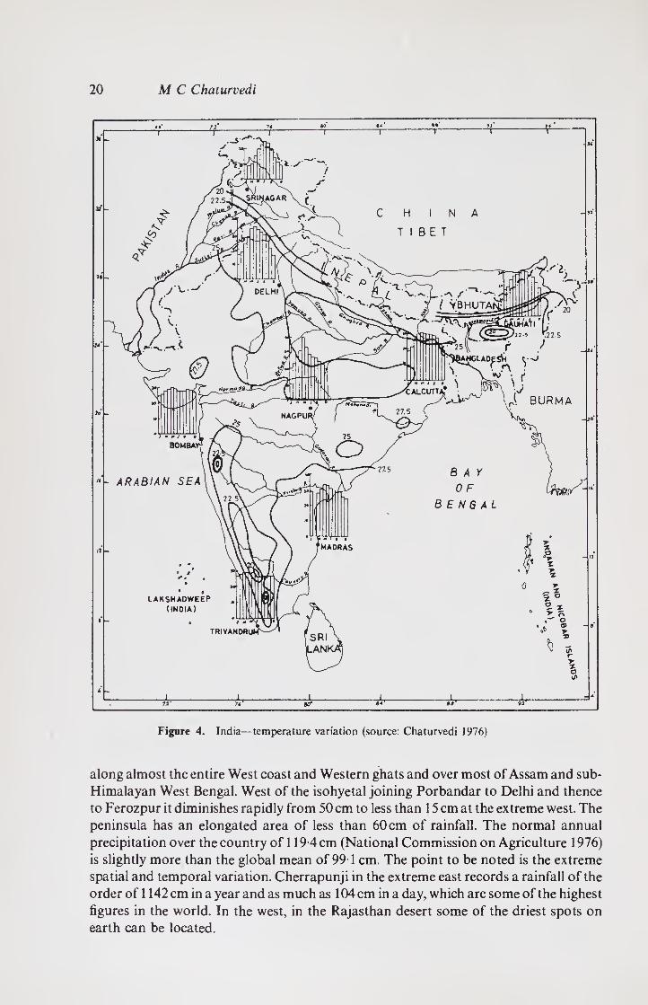
The average temperature with seasonal patterns is shown in figure 4. During the
winter season, from November to February, the temperature decreases from the south
to the north from about 24-29°C in the south to about 5-18°C in the north. From
March to May the temperature rises sharply in northern India and the maximum may
be above 40°C. Evaporation closely follows the march of the monsoon (figure 5). The
potential evapo-transpiration (pe) which may be assumed to be the same as the evaporation, ranges between 140 and 350 cm.
Rainfall is primarily dependent on the monsoons and to a certain extent on
shallow cyclonic depressions and disturbances. Only a fraction of the more than
3-87 x 108 mham of atmosphere moisture moving over India reaches the ground as
rain or snow. Evaporation from the oceans provides about 80 percent of this
precipitation. The summer monsoon, coming from the southwest, bursts on the
Malabar coast in the first week of June and establishes itself over most of the country by
the end of the month. Coming from over the sea, it provides about 80-90 % of the total
annual rainfall. In view of the orographical features, the monsoons travel up via the
Indus plain on the Arabian side and up the Gangetic plain on the Bay of Bengal side.
The strength of the monsoon current increases from June to July, remains more or less
steady in August and begins to weaken in north India in September, when there is a
rapid decrease in rainfall towards the end of that month. Prior to the monsoons in the early part of the year, disturbances continue to enter India, bringing some rain to
the north-west part of the country and a reasonable amount in West Bengal and Assam.
By the middle of October, the low pressure is transferred to the centre of the Bay of
Bengal and the direction of the winds becomes north-easterly. They cause occasional
showers on the mid east coast. Cyclonic storms from the Bay of Bengal, during October
and November, are mainly responsible for the rainfall in the Deccan Plateau and Tamil
Nadu. In the winter, from December to February, a shallow but extensive low pressure
system moves across northern India from west to east. There is heavy precipitation in
the form of snow in the higher ranges of the Himalayan system and moderate rain over
the lower and outer ranges. It has been estimated that during the four rainy months of June through September,
the Arabian sea branch of the monsoon carries moisture amounting to about
770 m ha m and the Bay of Bengal branch about 340 m ha m of the monsoon moisture,
25 to 30% precipitating in the form of natural rainfall. During the remaining eight
months also, there is a substantial amount of moisture over the country and it
constitutes a precipitation of the order of 100 m ha m, a small portion of it being in the
form of snowfall. The annual rainfall and its seasonal distribution is shown in figure 6. It is upto 250 cm
20 M C Chaturvedi
Figure 4. India—temperature variation (source: Chaturvedi 1976)
along almost the entire West coast and Western ghats and over most of Assam and sub-
Himalayan West Bengal. West of the isohyetal joining Porbandar to Delhi and thence
to Ferozpur it diminishes rapidly from 50 cm to less than 15 cm at the extreme west. The
peninsula has an elongated area of less than 60cm of rainfall. The normal annual
precipitation over the country of 119*4 cm (National Commission on Agriculture 1976)
is slightly more than the global mean of 99T cm. The point to be noted is the extreme
spatial and temporal variation. Cherrapunji in the extreme east records a rainfall of the
order of 1142 cm in a year and as much as 104 cm in a day, which are some of the highest
figures in the world. In the west, in the Rajasthan desert some of the driest spots on
earth can be located.
Water resources of India—an overview 21
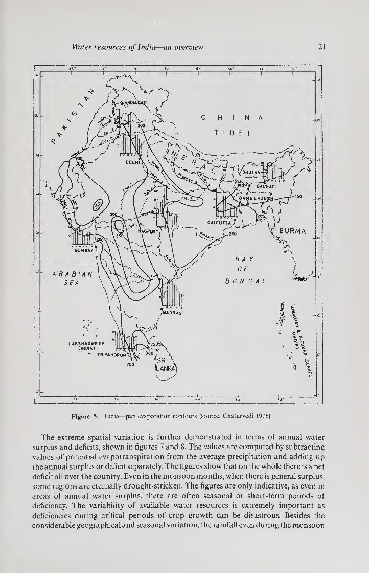
Figure 5. India—pan evaporation contours (source: Chaturvedi 1976)
The extreme spatial variation is further demonstrated in terms of annual water
surplus and deficits, shown in figures 7 and 8. The values are computed by subtracting
values of potential evapotranspiration from the average precipitation and adding up
the annual surplus or deficit separately. The figures show that on the whole there is a net
deficit all over the country. Even in the monsoon months, when there is general surplus,
some regions are eternally drought-stricken. The figures are only indicative, as even in
areas of annual water surplus, there are often seasonal or short-term periods of
deficiency. The variability of available water resources is extremely important as
deficiencies during critical periods of crop growth can be disastrous. Besides the
considerable geographical and seasonal variation, the rainfall even during the monsoon

22 M C Chaturvedi
Figure 6. India—Isohyetes (source: Chaturvedi 1976)
is most uncertain. There are alternating periods of heavy to moderate rains and partial
and general breaks when there are no rains.
The annual variation is, however, much less. The annual coefficients of variations are
shown in figure 9. These present the percent plus or minus variation from the mean for
70% of the year. It generally varies between 15 to 30 taking the year as a whole. Along
the West Coast near Mangalore, the coefficient of variation is less than 15%. The
isoline of 30% runs through Bengal, Orissa, the Bihar Plateau and Assam, the north¬
eastern part of Assam having less than 15 % variability. Over Gujarat and Rajasthan
this coefficient is higher than 40%.

Water resources of India—an overview 23
Figure 7, India—water surplus regions (source: Chaturvedi 1976)
4, Hydrological cycle and water balance
A correct assessment of the surface runoff is not possible as yet, as long-term and
reliable discharge measurements have not been carried out at sufficient locations. The
earliest attempt at estimating these was based on an empirical correlation with rainfall
and temperature. Later, studies were made by several agencies on the basis of actual
measurements and empirical studies. The figures currently in common use are given in

24 M C Chaturvedi
Figure 8. India—water deficit regions (source: Chaturvedi 1976)
table 1. These give the total runoff. Mean monthly and maximum monthly runoffs of
some major rivers at some measuring sites are shown in figure 10.
Natural runoff is the annual flow of water that would appear in surface streams if
there were no upstream development. In areas of surface water-groundwater con¬ tinuity, the natural runoff' includes the perennial recharge yield of groundwater
aquifers. According to the Irrigation Commission Reports (1972). some estimates are as
follows.
The mean annual natural runoff which leads to surface flows and groundwater
recharge is estimated to be 188T2mham. Of this, 42-41 mharn is estimated to be the

Water resources of India—an overview 25
mean annua! groundwater recharge. The total surface flows which are considered to be
utilisabie are estimated to be 66-6 m ham. In addition, 26T m ham of groundwater is
expected to be utilisabie leading to a total utilisabie resource of 92-7 m ha m. These
figures are still tentative and approximate. There are vast disparities from river basin to
river basin. For instance, the total utilisabie water resource per unit of land is 116 cm in
the Ganga basin, while the corresponding figure in the Cauvery basin is only 43 3 cm.
Assessment of groundwater is even more difficult and incomplete. Measurements of
water balance, annual recharge and groundwater levels have to be made. The
distribution of precipitation into surface runoff and groundwater recharge depends
upon site conditions. The potential for groundwater is shown in figure 11 and the

26 M C Chaturvedi
Figure 10. India—maximum and monthly mean river discharges in cumecs (source: Chaturvedi 1976)
pertinent data on annual ground-water recharge is given in table 1. The figures
although not accurate are the best estimate on the basis of currently available data. As
estimated earlier, out of the total of 42 41 m ha m, 26-1 m ha m are considered utilisable.
The availability is even more nonuniform spatially as brought out in figure 11, as about
70% of the land surface is covered by hard rocks. Besides the annual recharge, a vast
amount of nonrenewable groundwater resources are available which could be mined.
This, however, creates many problems. As the groundwater table is lowered, a new
equilibrium between surface runoff and annual recharge is established and contri-

Water resources of India—an overview 27
A R A B I A N S E A
LAKSHADWEEP
(iNDfA)
° TRIVANDRUM
REFERENCES Fresh groundwater aquifers
Extensive beyond 150 m L_J Limited between 100-150 m n Restricted upto 100 m r n Restricted variable I_I
Saline / Brakish
At all levels E53 At all levels with local EZ3 fresh water
Upto a depth of 100 m from LcJ the surface
I*
2- o
% \
cP
Figure 11. India—depth of aquifers and quality of groundwater (source: Chaturvedi 1976)
bution to surface runoff from groundwater will be reduced. There would be in-
perpetuity costs of pumping from the reduced levels, and the resources developed
would be nonrenewable.
Recently, water balance has again been estimated by the National Commission on
Agriculture (1976). The water balance as estimated in 1975 and the likely position in the
years 2000 and 2025 is shown in figure 12. The country’s average annual rainfall is about
119-4 cm and the country’s total average annual precipitation is estimated to be
394 m ha m. This may be rounded off to 400 m ha m including snowfall which is not yet

tota
l p
recip
itati
on
4
00
(F
OU
R
MO
NS
OO
N
MO
NT
HS ♦
EIG
HT
RE
MA
ININ
G
MO
NT
HS
) 28 M C Chaturvedi
if)
< £
’ L±J " O < Ll cr 3 LO
O U1
2 o cl
2 o h- < cl
.go
I" Ll)
LU H- < O UJ 2: 2
O if)
o h- 2
in “2^
O »■— <
O u cr lu CL
< Ll.
£ r§o.
if)
2 O CL Ll.
g
fin
LO
£ o
LU cr »— LO J5 S
< Q 2
O o o
Tn 2
cr LU
■s
< LU LO
$ o -i £ u_ <“
g tt “3-ocr
LJ ♦ i_ CL Ll
£ O
2 O CL Ll
1 2 oo 3 « O CL in O '
O
2 O CL
CL
CL CD
O in CL “ Ll
O < ^ CL oo 3 CD
’ LO
< O 1— 00 O'-
o ID
;CL
O Q m j z: ld Ll <*“
if) cr o > cr LU LO LU CL
Ul $ ro -
oo^n
Sis <U_ Jg UIO £ 00 — n5o Pose
o »— in < vj
.LO'-
CT)
t-- 2 f) <
CL LU
2 o
r—
iuo Q 0O
L0 2 jZ Q °L>
g Sogslg.
o 2 ^ 2;T o o cc cc 0- L_
r™ -J < f— O
L0
^z W UJO [Em
i“S5 ^ cc cc Z
-£^cruj£- XpQ (/) D3 LU h— Ll 3 £2
II'
cc <*- u> o cc S uj ^ cu -J <£ • <r O CD > Z Ll <r ct> UJ<o t-
sr pGo 3 m ^
^ o' ^ 4 in
Q in ^ l~ rs< ID < ^ CM
•L0 LD
h-O 3 r“
|
CL .—. Or- CL — < in
LU
O UJ
UJ CL 3 h- L0 O 2..
O L0
o
LU
Z § O (— h- L0 C
< o c Oin^r T , ccX < ^cc-=1 ; - co- 2 cn C0 c
° ] I £ <
2 o 10
r—^ 00 cr in o — CL O < LD > LU
2 § Q? To O g o Li
.cr cr cr _ Ll a ft 52
in co
O
: in akj CL
< rz ■P' O " 0. < > UJ
’ll a ; o UJ t— < o
Z a Q_ — O
CC _ ^ U. O o
O CC Osi
UJ ^ LO X p h- (— < L0 O ►- ,o
2 UJ UJ 1/0 * o CL QO 1/1 cr o ^ lu U_ Ll < >
-cr oo-, UJ' ' X ’ h- o o c—
o -in-
in CM
LOCJ CL 3- CE^
2 O f- < Or-
CL ro ~~ LD
<< CO
2 Old h_.cn
2 O
L0(
3 in c—
<!« p-co
pCN crX cr — D
CO
uj:
o
Fig
ure
12.
Ind
ia
app
rox
imat
e dis
trib
uti
on o
f av
erag
e an
nu
al w
ater
res
ourc
es a
s in 1
974,
2000, an
d 2
025 a
d (
m h
am). T
he
num
bers i
n br
acke
ts a
re t
hose
for
the
yea
r 2000 (
sour
ce:
Nat
ion
al C
omm
issi
on o
n A
gric
ultu
re)
Water resources of India—an overview 29
fully recorded. Out of the 400 m ha m, about 70 m ha m is estimated to be lost to the
atmosphere by evaporation. Of the remaining 330 m ha m, about 115 m ha m becomes
surface runoff and the remaining 215 m ha m soaks into the ground as soil moisture and
groundwater recharge. Of this, about 45mham regenerates as surface flows. An
additional 20 m ha m is brought in by streams and rivers from catchments lying outside
the country in Nepal and Tibet, and thus the total surface flows have been estimated to
be 180m ham. Of the total surface water of 180mham available in the country in an
average year, about 15 m ha m is stored in various reservoirs and tanks of which about
5mham is lost by evaporation. A considerable portion of the storage is in tanks
constructed over long periods in the past. With future construction of projects, storage
is ultimately expected to be about 35mham and the loss about 10mham. Of the
165mham of water that flows in the river annually at present without any storage
facility, the utilization through diversion works and direct pumping aggregates to 15 m ha m, which is more than that from the storage works. The remaining river flow of
150 m ha m goes to the sea and some adjoining countries. On full development, the use
of water through diversion works or direct pumping is expected to increase to
45 m ha m. The balance of 105 m ha m would continue to flow to the sea and outside the
country.
Of the 215 m ha m percolating into soil, about 50 m ha m, i.e. about 12-5% of the total
precipitation is estimated to percolate as groundwater and the rest is retained in the soil
as soil moisture. No significant change is expected in this according to present thinking
and policy, although as we will argue later, the groundwater recharge has to be and can
be substantially increased. Infiltration and contribution to groundwater also takes
place from the irrigation works themselves. In the alluvial plain of north India, about
45 % of the water that i§ let in at the head of an unlined canal system is lost from
channels through seepage. Of the remaining 55 % which reaches the field, another 30%
is lost. Thus, it is estimated that only about 40% of the water let into an unlined canal
system is actually utilised. It is estimated that at present about 5 m ha m is retained in
the soil as soil-moisture and about 12mham is added to the groundwater. On full
development of irrigation in the country, the contribution to soil moisture and
groundwater is expected to be about 15 m ha m and 25 m ha m respectively. Similarly,
contribution to groundwater from streams is estimated to be 5 m ha m currently and is
expected to be increased to 10 m ha m by developing schemes of induced groundwater.
With the addition of 5mham from flood flows and 12mham from the irrigation system to the 50mham from precipitation, the total groundwater, excluding soil
moisture comes to 67 m ha m. It is estimated that at present, of the total groundwater
amounting to 67 m ha m replenished on an average annually, 13 m ha m is extracted for
various uses, about 45 m ha m regenerates into rivers and the remaining 9 m ha m is
accounted for by evapotranspiration and raising of the water table. On the near full-
development of water resources, the extraction is estimated to rise to 35mham,
evapotranspiration reduced to 5 m ha m, and the remaining 45 m ha m regenerates to
rivers as at present.
Currently, the transpiration is estimated to be about 110mham, 13mham from
irrigated crops, 42 m ha m from unirrigated crops, and 55 m ha m from forests and
other vegetation. On full development, the total transpiration is estimated to become
125mham, the component figures being 35, 35 and 55mham, respectively.
Evaporation is a major item of the hydrological cycle. Of the total precipitation of
400mham, 70mham is lost directly. Of the 215mham percolating into the soil,

30 M C Chaturvedi
another 10mham is estimated to be non-beneficial evaporation. These figures are
estimated to change only marginally with development. In terms of estimated utilisable resources and their development, it is seen that
180 m ham of surface flows (which includes 45 m ham of contribution from ground-
water) is available. After almost complete development, these figures are estimated to
change to 185mham, the groundwater contribution to surface runoff remaining the
same. Currently, 13 m ha m of groundwater and 25 m ha m of surface water have been
developed, totalling 38mham. These figures are estimated to change to 35, 70 and
105mham at almost full utilisation—almost a three-fold increase. It is estimated that
currently 150 m ha m of natural runoff, mostly in the form of surface runoff is flowing to
the sea or out of India. This figure is anticipated to change to 105mham.
5. Floods
The extreme seasonal and spatial variability of water resources in India is dramatically yet catastrophically exemplified by the occurrence of droughts and floods in different
parts of the country almost at the same time every monsoon. The damage by floods
depends upon the use characteristics and land shapes of the flood plains. All river basins
are prone to floods in view of the extreme variability of the monsoons but the
Brahmaputra and the lower Ganga river basins are subject to serious floods every year.
(National Commission on Floods, 1980).
A total area of 40 m ha is estimated to be prone to floods of which 32 m ha can be
protected though by 1980 only 10 m ha had been protected. During the period 1970 to 1978, the flood affected area worked out to 11-9 m ha in respect of total area
affected and 5-4 m ha for cropped area. The former constituted 3-9% of the reporting
area in the country while the cropped area affected constituted 7-8 % of the total net
sown area. For major flood-prone states, relevant figures for the seventies are much
higher e.g. 12 % and 10% for Bihar, 10% each for UP and 15 and 9 % for West Bengal.
Besides crop losses, floods cause considerable damage to houses and property as also
loss of human and cattle lives. On an average 0-93 million houses were damaged every
year during the last 25 years, and 1240 human lives and 77,000 head of cattle were lost.
Railways, roads, communication lines, public utilities etc. also suffer considerable
damage during high floods.
Average figures, however, conceal large year-to-year variations. For instance, in the
case of the total area, while in 1965 only a million hectares were affected, the spread was
many times more during the three years 1976 to 1978 being over 17 m ha. About 3,500
people lost their lives in 1968 as against only 34 in 1953. The picture would be similar in
the case of other losses also. Besides the direct losses floods destabilize economic
activity. For instance, the annual rate of agricultural activity during the period 1962-63
to 1970-73 was 1.94% for the country as a whole. The rates recorded for most of the
flood-prone districts of eastern UP was only in the range of 0T to 0-9%.
6. Drought
Droughts are extended periods of subnormal precipitation. The effect of drought,
however, depends on climate and man’s adaptation to his environment. Thus in arid
areas where man customarily depends on surface and ground water for irrigation and

31 Water resources of India—an overview
/ supply, the lack of rainfall for a few months may not be noted, but in humid areas where
man relies more on water from current rainfall, lack of rain for a few months could be disasterous.
Agricultural drought occurs when the soil moisture is so depleted that the normal
yields are reduced resulting in substantial economic loss. Water supply drought, on the
other hand, is related to general nonavailability of water. While the definition of
drought is thus arbitrary we define drought areas as follows. We first define arid and
semi-arid zones as those where the difference between precipitation received and potential evapotranspiration is, less than 33 cm, and between 33 and 66 cm, respectively.
The drought areas are those which have an adverse water balance and 20 % probability of rainfall departure of more than 25 % from normal. If this probability is 40 % then the
area is called a chronically affected drought area. The drought areas are shown in figure 13. In order that the area may tide over the drought, 30 % or more of the area should be
irrigated. The total drought prone area comprises about 16 % of the total geographical area of the country and directly affects about 11 % of the population.
7. Water quality
Water quality is defined by a variety of physical and chemical parameters and pertains to suitability for a particular use. It is determined by the geological and hydrological
influences present in a basin and also by such man-made influences as regulation of flow, discharge of waters and accelerated soil erosion. Studies of water quality in India
are very scarce and we may analyse the basic factors to come to a general assessment. Sedimentary rocks contribute much more suspended material than igneous rocks.
Significant concentrations of dissolved materials, such as sodium, calcium, magnesium,
chloride and sulphate ions are commonly associated with sedimentary rocks retaining
brine from former marine environments. Areas of heavy precipitation and runoff, in otherwise similar situations, reduce dissolved chemical content but have little effect on
sediment loads and concentrations. Groundwater is usually more mineralized than
surface water owing to its longer and more intimate contact with weathered rocks and
soils. The management of watershed land has profound effects on the quality, and
considerable improvement could occur with the use of proper practices. By the above
considerations, the quality of natural water can be judged from the geohydrological
map of figure 11. Pollution problems start when water is withdrawn from its natural place of
occurrence, put to domestic, agricultural or industrial use, and this impaired water
returned to a water course. With proposed large scale diversion of water for irrigation,
and simultaneous increase in population and industrial activity, the problem is
particularly serious, as discussed later.
8. Related land resources
The total geographical area of the country is 328 m ha. Of this, only 305-5 m ha are
accounted for in land use statistics (1967-68). The difference of 22-5 m ha largely
consists of mountains, deserts and forests in inaccessible areas. Regionwise details of
land resources are given in table 1. The overall position is shown in table 2.

32 M C Chaturvedi
\ /
s J A M M I
AND I K A S H M I H.
05
, -v* ,> \HIMACHAJ.
^-v ^RADES^L O - , /~V’\ >j!_S^JN'^bCHANDI<;AflH
H N
SIKKIM. _
/** ^ h /-ArunachAc- r PRAD^Sfcb (
s ^ —c
^'NMJALAND
-rj'/ rpl v^. BHUTAN^ _ _
^EGHAL^A^
Cbangl^Va. ^man,p^ ( TRIPUI$aA j
Q4f OF
BENGAL
i 33 LEGEND
Drought areas (where probability of rainfall shortages of more than 25°/..
'from normal 15-20 °/» or more). [ i rrri Areas identified as draught affected 11 I I II by the commission.
are moisture indices .
Index values of more than-66
indicate aridity conditions and PONDICHERRY those between -33 and -66
indicate semi aridity conditions.
Figure 13. India—drought prone areas (source: Chaturvedi 1976)
According to the latest estimates (1972-73), the total arable area is estimated to be
175 m ha, of which 142 m ha would be under cultivation by the end of the Fourth
Plan. The gross cropped area would be 169 m ha. According to present estimates
97 m ha of land or 55 % of the gross cropped area can be ultimately irrigated both by
surface and groundwater sources, their contribution being 72 and 25 m ha respect¬
ively. The concept of irrigation in these estimates, is, however, that of the marginal
irrigation being provided as at present.
The percentage of the total land under cultivation in India is one of the highest in the
world amongst the large countries. The percentage figures are: World 11 *3; USSR 10-8;
USA 16-2; China 11-5; India 49-7; Pakistan 30; Japan 15-5.
Water resources of India—an overview 33
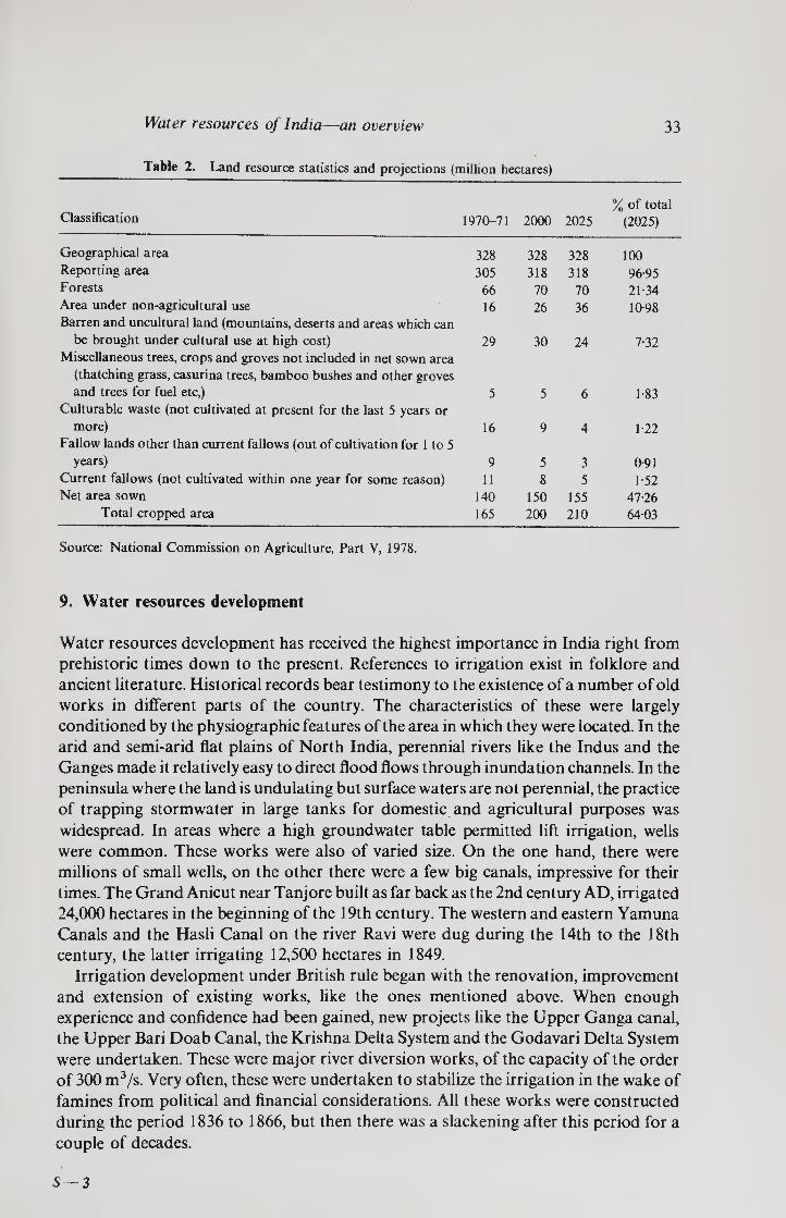
Table 2. Land resource statistics and projections (million hectares)
Classification 1970-71 2000 2025 % of total
(2025)
Geographical area 328 328 328 100 Reporting area 305 318 318 96-95 Forests 66 70 70 21-34 Area under non-agricultural use Barren and uncultural land (mountains, deserts and areas which can
16 26 36 10-98
be brought under cultural use at high cost) Miscellaneous trees, crops and groves not included in net sown area
(thatching grass, casurina trees, bamboo bushes and other groves
29 30 24 7-32
and trees for fuel etc,) Culturable waste (not cultivated at present for the last 5 years or
5 5 6 1-83
more) Fallow lands other than current fallows (out of cultivation for 1 to 5
16 9 4 1-22
years) 9 5 3 0-91 Current fallows (not cultivated within one year for some reason) 11 8 5 1-52 Net area sown 140 150 155 47-26
Total cropped area 165 200 210 64-03
Source: National Commission on Agriculture, Part V, 1978.
9. Water resources development
Water resources development has received the highest importance in India right from
prehistoric times down to the present. References to irrigation exist in folklore and
ancient literature. Historical records bear testimony to the existence of a number of old
works in different parts of the country. The characteristics of these were largely
conditioned by the physiographic features of the area in which they were located. In the
arid and semi-arid flat plains of North India, perennial rivers like the Indus and the
Ganges made it relatively easy to direct flood flows through inundation channels. In the
peninsula where the land is undulating but surface waters are not perennial, the practice
of trapping stormwater in large tanks for domestic and agricultural purposes was
widespread. In areas where a high groundwater table permitted lift irrigation, wells
were common. These works were also of varied size. On the one hand, there were
millions of small wells, on the other there were a few big canals, impressive for their
times. The Grand Anicut near Tanjore built as far back as the 2nd century AD, irrigated
24,000 hectares in the beginning of the 19th century. The western and eastern Yamuna
Canals and the Hash Canal on the river Ravi were dug during the 14th to the 18th century, the latter irrigating 12,500 hectares in 1849.
Irrigation development under British rule began with the renovation, improvement
and extension of existing works, like the ones mentioned above. When enough
experience and confidence had been gained, new projects like the Upper Ganga canal,
the Upper Bari Doab Canal, the Krishna Delta System and the Godavari Delta System
were undertaken. These were major river diversion works, of the capacity of the order
of 300 m3/s. Very often, these were undertaken to stabilize the irrigation in the wake of
famines from political and financial considerations. All these works were constructed
during the period 1836 to 1866, but then there was a slackening after this period for a
couple of decades.

34 M C Chaturvedi
Attracted by the profitability of these schemes, two private companies planned
grandiose schemes to construct transcountry link canals, but they failed. All that was
achieved was a series of disconnected waterways. However, two decisions followed
from these activities. It was decided that in future, irrigation development would be
undertaken exclusively by the government. Second, in accordance with the policy of
private companies, finances were developed by public loans and works were undertaken
only if they promised a minimum net return.
Not much activity was witnessed in the second half of the 19th century. However,
following the great famine of 1876-78, the Famine Commission of 1880 recommended
emphasis on irrigation, though no action was taken. The two great famines of 1897-98
and 1899-1900 however led to the appointment of an Irrigation Commission in 1901.
Policy recommendations about financial criteria were developed and several schemes
were proposed for public irrigation works. Emphasis was also laid on development of
private irrigation works like wells and tanks, through higher outlays on comparatively
easier terms. Much activity ensued, particularly on productive w'orks and particularly in
the area of Punjab in the context of the colonization of First World War soldiers. By
1920-21, the total irrigated area in undivided India (India and Pakistan) was
22-6 m ha.
Much of the irrigation development upto 1930 was in terms of diversion canals.
There was little development in groundwater or even wells. The area irrigated by wells
in British India was 4-68 m ha in 1902-03 and only 4-73 m ha in 1925-26. In 1930,
hydroelectric development was undertaken in Uttar Pradesh by tapping the falls in the
Ganga Canal and tubewell construction was started. By the time of Independence, about 28-2 m ha of land, almost 24% of the cultivated
land, was under irrigation. Source-wise, 54% of the area was irrigated by
canals (mostly Government-owned), 23% by wells, 12% by tanks and the remaining
11 % by miscellaneous sources. Much of the canal-irrigated area was, however, in what
constitutes Pakistan now, and after independence, the irrigated area in India was
reduced to 19 7 % of the net sown-area against the earlier figure of 24-1 % of undivided
India.
Table 3. Irrigation potential (in m ha) (gross)
Major and
medium
Minor irrigation Total
irrigation
Percentage of ultimate potential Period Ground Surface Total
1. Pre-Plan (1950-51) 9-70 6-50 . 6 40 12-90 22-60 19-9
2. End of 1st Plan (1956-58) 12-19 7-63 6-43 14-06 26-25 23-3 3. End of 2nd Plan (1960-61) 14-33 8-30 6-45 14-75 29-08 25-7
4. End of 3rd Plan (1965-66) 16-56 10-52 6-48 17-00 33-56 29-6 5. End of Annual Plans (1968-69) 1810 12-50 6-50 1900 37-10 32-7 6. End of 4th Plan (1973-74) 20-70 16-50 7-00 23-50 44-20 38 9 7. End of 5th Plan (1974-78) 24-77 19-80 7-50 27-30 52-25 46-0 8. Addl. target (1978-79) 26-12 20-85 7-75 28-60 54-90 48-4 9. Addl. target (1979-80) 27-22 22-10 8-00 30-10 57-50 50-7
10. Target 6th Plan (1980-85) 33-72 29-10 9-50 38-60 72-60 64-0 11. Ultimate feasible by conventional 58-60 40-00 15 00 55 00 113-50 100-0 12. Additional through national
prospectives 25-00 10 00 1000 148-00

Water resources of India—an overview 35
Water resources development received the highest importance after Independence.
Many impressive storage works, like the Bhakra Dam, the Rihand Dam, and the Earth
and Rockfill Ramganga Dam to name a few, were constructed to augment irrigation
facilities and hydropower generation. Equally important is the groundwater develop¬
ment particularly through private tubewells. This has unfortunately been limited to the
arid areas of northwest India, particularly in Punjab.
The development of irrigation is shown in tables 3 and 4 and figure 14. Table 3 gives
the development of irrigation source-wise and table 4 gives the net area sown, net area
irrigated and the percentage of net area sown. The growth of irrigation is also shown in
figure 14. The area irrigated crop-wise is given in table 5. The achievements vary from State to State. Rainfall irrigation and sources of
irrigation state-wise are given in figure 15.
Tabie 4. Development and future of irrigation in India
Net area Net area % of net sown irrigated sown area
Year (m ha) (m ha) irrigated
1950-51 110-75 20-85 17-56
1955-56 12916 22-76 17-62
1960-61 133-20 24-66 18-51
1967-68 139-70 27-52 19-70
1973-74 142-71 32-60 22-85
1977-78 149-93 4000 26-68
1982-83 15517 52-40 33-77
Source: Irrigation Commission Report (1972), Sixth Five Year Plan. Figures for 1982-83 are estimates
90
5 6
Figure 14. India—development of irrigation (source: Singh 1980)
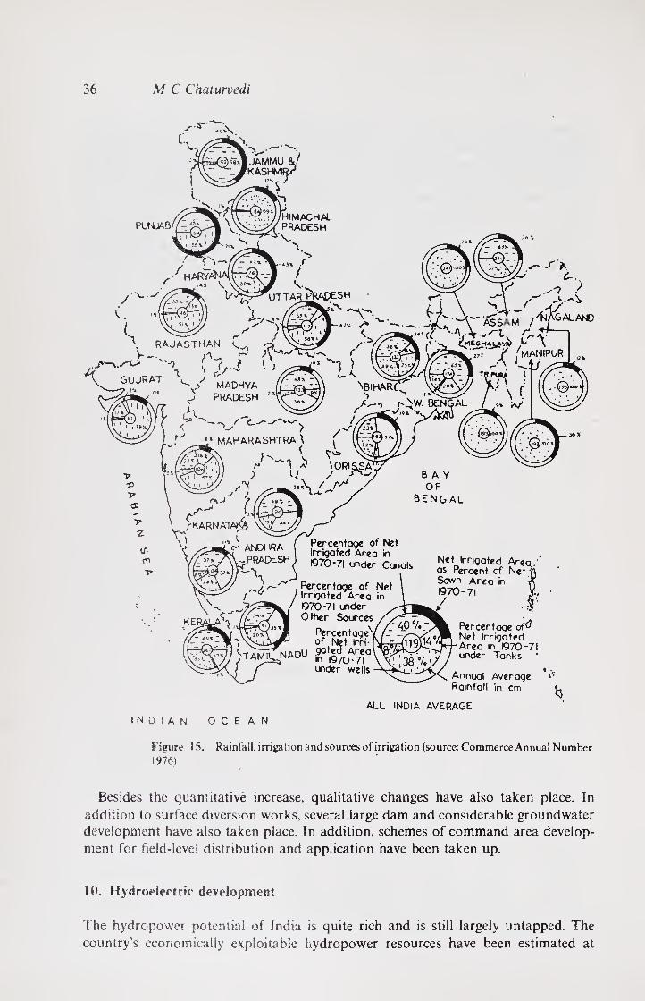
36 M C Chaturvedi
s
•■V.
JAMMU &/ KASHMIR r1
'tC //HIMACHAL PRADESH
N
T ARPRAPE S H '.-v.
\ RAJASTHAN L.
A T>
NeiHAR
./V-J r'^W. BENGAL
r~ T
\f,s GUJRAT V / MADHYA
PRADESH
LAX < s-' > W/i
MAHARASHTRA \ f
/* )ORI^SA
/ A ./ 1
^ \,U
/KARNATAb^
"0 andhrT f of Net ooAnrcu Irrigated Area n
.PRADESH^ ,970.7, un<jer Canals
X Percentage of Net Irrigated Area in
VV 1970-71 crder X X. '
jj ASS^M /Tl^GALAND
<c — ^ -. CMESHAJ^yi C \
' ' '' 'MANIPUR
Net Irrigated Area os Percent of Net A Sown Area in ft 1970-71 M.
.. v .?■ Other Sources / >,
D . \f /_ 4P Percentage of^ PercentageV/- -A1 Ne, ,rr^ted
«tS AreoNft^^A^fArea •" ©70-71 9° Af.ca \ ^r.. A / under Tank* * )tami^nadu ^,|d70Ar7« ,
under wells -\jkh i Annual Average Rainfall in cm
ALL INDIA AVERAGE *3
INDIAN OCEAN
Figure 15. Rainfall, irrigation and sources of irrigation (source: Commerce Annual Number 1976)
Besides the quantitative increase, qualitative changes have also taken place. In
addition to surface diversion works, several large dam and considerable groundwater development have also taken place. In addition, schemes of command area develop¬
ment for field-level distribution and application have been taken up.
10. Hydroelectric development
The hydropower potential of India is quite rich and is still largely untapped. The
country’s economically exploitable hydropower resources have been estimated at

Water resources of India—an overview 37
Table 5. Irrigated area under principal crops
Crops 1970-71 1985 2000 AD
Rice 14-93 21-50 24-00 Wheat 9-84 14-00 14-90 Other cereals 3-80 5-76 6-99
Total cereals 28-57 41-26 45-89
Pulses 1-99 4-30 5-37
Total foodgrains 30-56 45-56 51-26
Oilseeds 1-02 2-80 5-10 Cotton 1-29 4-00 7-50 Sugarcane 1-90 3-25 5-00 Tobacco 0-10 0-25 0-40 Other crops 3 63 5-14 14-74
Total non-foodgrains 7-94 15-44 32-74 Total irrigated area 38-50 61-00 84-00
Table 6. Basin-wise abstract of hydropower potential and development in India (MW)
Name of river basin
Power potential*
Installed capacity
Effective capacity
Balance to be exploited
Indus 7,000 3,039 2,370 4,630 Ganga 5,000 1,899 1,127 3,873 Brahmaputra 12,000 276 152 11,848 Sabarmati Nil Nil — —
Mahi 100 Nil — 100 Narmada 1,000 Nil — 1,000 Tapi 300 300 115 185 Subarnarekha 100 130 26 74 Brahmani 1,000 Nil Nil 1,000 Mahanadi 1,000 270 200 800 Godavari 6,000 1,355 662 5,338 Krishna 1,500 1,893 1,096 404 Pennar Nil Nil — —
Cauvery 1,000 940 586 414 Medium and Minor Basins 5,000 3,881 2,987 2,013
Source: Rao (1976) * These are earlier figures. The present potential is estimated to be 75,400 W.
41,000 MW at about 60% load factor of which only about 10% is utilised at present
(Sixth Five Year Plan 1980). In addition, the potential of Nepal is 85,000 MW of which none has been exploited. It is further considered that these estimates are on the low side
and the actual potential may be almost twice as much. For instance according to a more
recent estimate, the potential in India has been put at about 75,400 MW.

38 M C Chaturvedi
2
< o — _ tn Q < < 2 — > < < Z cr <
2 X ID
a:
2 < X <
< 2
x < < t cc <
IX UJ > 3 <
CL <
z cc < UJI CD OUJ
X <
cr < 2 2 LxJ
2S 3 cr QO LU z CD CD o *— tS)CC 2 CL 2 Z
Figure 16. Hydropower potential and development in India (source: Rao 1976)
A basin-wise abstract of the hydropower potential and development in India is
shown in table 6 and figure 16.
11. Conclusion
India is rich in natural resources, land and water, which however, have to be developed
to improve their productivity. With the rising population and efforts on economic
development, the problem is extremely important and urgent.
Development of water resources is central in this context as water is generally not
available where and when required. India’s arid-monsoon climate and geographical
features lead to extreme seasonal and spatial variations. Efforts in this direction have
been made since time immemorial, but as the overview shows, we have a long way to go.
References
Rao K L 1976 India's water wealth (New Delhi: Orient Longmans) Chaturvedi M C 1976 Water—Second India studies (New Delhi: Macmillans) Irrigation Commission Reports 1972 Government of India, New Delhi Reports of the National Commission on Agriculture 1976 Government of India, Ministry of Agriculture and
Irrigation, New Delhi
Water in India’s development: Issues, developmental policy and programmes, and planning approach
MAHESH C CHATURVEDI
Applied Mechanics Department, Indian Institute of Technology, New Delhi 110016, India
Abstract. The importance of water resources development for sustaining life and the agrarian economy under the conditions prevalent in India is brought out. The inadequacy of drinking water and irrigation facilities inspite of large investments under the various Plans is very disappointing, as also the poor development of the hydroelectric potential. Despite the rich environmental and natural resources of India, there has been very little developmental work due to various reasons, chief of them being non-involvement by specialized technologists in the areas where they matter most. The need for a scientific policy and a planned approach is emphasized so that higher employment generation and rapid economic growth can be achieved.
Keywords. Water resources development; developmental policy; technological planning.
1. Introduction
From legendary accounts down to latest planning documents, development of water
resources has been considered to be of the greatest importance in India. This is
understandable in view of its crucial importance for sustaining life and the agrarian economy under the characteristic climatic and hydrologic conditions of India. Yet even
till the beginning of the Sixth Five Year Plan (1981) this development could not be
described as satisfactory. For instance only 10% of the rural population had been
supplied with safe drinking water and only about 30 % of the cultivated land had been
irrigated (Sixth Five Year Plan 1981). The reliability and quantity of water supplied for
irrigation is also inadequate and is reflected in low yields. As stated in the Sixth Plan
Document, “Inspite of the large investment made in the irrigation sector and the
phenomenal growth of irrigation during the past 30 years, the returns for the
investment both in terms of yield as well as finance are very disappointing”. Against this
achievement one may note, to give an example, the achievement of 67-7 % of irrigated
land in China even by 1968 and correspondingly a much more stable agricultural base
(Leeden 1975; Swamy 1973).
A review of other sectors reveals a similar picture. Out of the hydroelectric potential
of 75,400 mw, only 10 % had been developed and out of 40 mha of the flood-prone area,
only 10 mha had been provided with protection till 1981 (Sixth Five Year Plan 1981).
This sad state is particularly poignant in view of the fact that India is rich in
environmental and natural resources—land, water and sunshine, as can be seen from
some salient statistics given in table 1. These are only indicative figures and have to be
interpreted with care. For instance, in large parts of the world, unlike India, only one
crop can be had per year, while on the other water resources may be available such that,
again unlike India or China, that these could be readily used without much human
39

40 Mahesh C Chaturvedi
Table 1. Some salient statistics of land, water and population
Region
Cultivable land/ total geographical
area (%)
Utilizable water/unit land (m)
Population density
(/km2)
India 43 0-3 166 China 11 017 75 Northwestern Europe 26 0-49 91 Southern Europe 64 0-2 81 U.S.A. 19 1-4 22
Source: Calculated from Leeden (1975) and de Mare (1977)
intervention. For instance, only 6-8 % of the total cultivated area in Europe and 9-6 % in usa have to be irrigated.
To a large extent, our colonial history may be said to be responsible for this sorry state of affairs. For instance, the net irrigation intensity (net irrigated area/net cultivated area) was only about 17 % in 1947 at the time of Independence. Impressive technological achievements can be noted since then and the irrigation intensity has been almost doubled. Yet a critical study of the policy documents indicates that it has not been possible to break from the past heritage of colonial concepts, policies and institutional framework. An ad hoc, technologically-oriented planning and bureaucratically-managed development by officers rather than by specialised profes¬ sional engineers continues. It will be argued that all this needs to be changed as otherwise it will not be possible to break the crawling agricultural growth rate of about 213% of the past. Besides, a serious resource depletion and environmental dilemma will also be encountered very soon. It will be shown that much higher employment generation, rapid economic growth with regional and local equity can be achieved and the spectre of resource depravation and environmental destruction can be avoided if a scientific policy and planned approach is adopted. This will require, first and foremost, institutional modernization, which is also briefly discussed.
2. Developmental policy
For the sake of convenience the developmental policy may be divided into two phases: (a) pre-Independence and (b) post-Independence phase. The reason for this is the scale of development and technology rather than, as will be emphasised later, modernisation of policy.
2.1 Pre-Independence phase
Efforts have been made in India since time immemorial, consistent with the techno- economic capability of the people, to develop tanks, wells and small canals for the development of water resources for drinking water and irrigation. It is important to note that a considerable portion of the current water resources development is due to these historical efforts. The reliability of water supply from these historic sources was inadequate and naturally these could not lift the population out of sustenance

Water in India's development 41
agriculture or even meet the demands of the growing population triggered off in the last century.
During the early British period, little heed was paid to the development of water
resources. Detailed studies of policy have not been carried out but it appears reasonable
to conclude that the foreign government was primarily interested in maintaining law
and order and undertaking only financially remunerative activities (Irrigation
Commission 1972; Cautley 1860; Lieftink et al 1969). As Cobden stated in the British
Parliament in 1855 “The single city of Manchester in the supply of its inhabitants with
the single article of water has spent a larger sum of money than the East India Company
has spent in the 14 years from 1834 to 1848 in public works of every kind throughout
the whole of its vast dominions” (Clairmonte 1961).
The increasing population and exploitary policy of the foreign government created
increasing strain on the economy and famines became more frequent and intense
(Bhatia 1967). Irrigation had, therefore, to be developed to avoid politically disturbing
phenomena. It is significant to note that many important irrigation works, such as the
Eastern Yamuna Canal in 1820, the Eastern Yamuna and Upper Ganga Canal during
1830-1854, the Upper Bari Doab Canal in 1851, the Godavari and Krishna anicuts in
1850, the Agra Canal in 1873, to name a few, were constructed for increasing revenue
and averting famines. It may be noted that irrigation activities were undertaken not
where there are easily developable facilities, such as eastern Uttar Pradesh (up) and
Bihar but in the arid western and border areas. The reason was that these were more
famine-prone and politically sensitive. The socio-political objective of irrigation was
thus only to stabilize the sustenance agriculture for which extensive irrigation became
the logical policy (Irrigation Commission 1972). Technological, economic and financial
considerations also supported this policy. Groundwater control was not known at that
time, the only technology known being surface diversion which cannot provide
dependable and adequate water supplies. Fear of water-logging indicated extensive
irrigation through diversion of the low flows. The poor paying capacity of the farmers
and lack of technological capability to give assured supplies also pointed in the same
direction. Similarly nonavailability of modern agricultural inputs also did not put
pressure for dependable and adequate supplies.
Besides irrigation, other uses of water resources viz., navigation, flood control,
drainage, hydroelectric development or even water supply for drinking purposes did
not get any importance. Even irrigation got low priority compared to railways as the
latter were considered essential for the maintenance of law and order. It may be noted
that navigation canals were an outstanding financial investment for transport purposes
in the growing economy of Europe at the beginning of the industrial revolution
(Lansing 1966). The financial attraction encouraged water resources development for
this purpose and even led to some private ventures in India, but it turned out to be a
failure because corresponding industrial development was not taking place. Even for
irrigation, the colonial government was content with supplying water up to canal
outlets, leaving the rest of the task of conveyance and distribution to the farmers
themselves. Activities such as land-levelling, drainage, lining of water courses etc.,
which demanded public participation were also not considered possible by a foreign
government. These were not within the capability of the poor peasantry and were,
therefore, neglected. Thus, in short, a policy of inefficient extensive irrigation through
low flow diversions to stabilize the sustenance agriculture evolved from a convergence
of social, political, economic, technological and financial considerations. It is significant

42 Mahesh C Chaturvedi
YEAR
Figure 1. Population and food dilemma of India (based on data in National Agricultural
Commission Report 1976)
to note that the per capita food availability continued to drop sharply till
Independence, as brought out in figure 1.
2.2 Post-Independence phase
After Independence, although the highest priority has been laid on irrigation
development and impressive developments have indeed taken place e.g. attainment of
58 mha of irrigated area and large projects, it has continued on a technologically-
oriented ad hoc project-by-project basis without any integrated policy analysis. In fact
the colonial policy of extensive irrigation has continued to be followed uncritically.
Developments have also been concentrated in those areas where developments had
taken place earlier without much concern for regional equity. Study of several projects,
shows that even when such technologies as storage dams and groundwater develop¬
ment are available, the old approach of inadequate and unreliable water supplies has
continued and little attention has been given to the package of associated develop¬
mental activities at the field level. A high technology bias is also distinctly evident. Ever
higher dams and larger canals have been the sole preoccupation of all concerned.
Projects continue to be taken up on an ad hoc basis without detailed coordinated
regional planning. Completion periods of projects get extended on various grounds
and irrigation adaptation follows a leisurely pace. Conceptual awareness that
integrated river basin planning and conjunctive surface and groundwater development
should be undertaken are often stated in Government announcements or Commission
Reports, but neither are these planned nor implemented.
Of late, increasing attention has been laid on field-level developments, incorporating
them with integrated rural development through command area development (cad)
and water management. The cad proposes a systematic programme of land consolid¬
ation, scientific land-shaping, construction of water courses and field channels to carry water to individual fields, field drains development, and a system of roads which will

Water in India's development 43
enable farmers to carry the produce to the market. Besides the above measures,
adequate and timely supply of inputs is proposed to be ensured and marketing and
other infrastructural facilities created so that the farmers are able to derive optimum
benefits from available land and water. By the end of March 1980, 76 cad projects had
been undertaken which covered an ultimate irrigation potential of 15-3 mha in 16 states
and Union Territories. The area covered under the field channels and land levelling to
the end of March 1980 was 30,82,570 ha and 9,36,970 ha respectively. But achievements
are poor and the machinery is neither adequately motivated nor appropriately educated.
Similarly soil and water conservation programmes were initiated during the First
Plan period and they have progressively intensified over the successive Plan periods.
Till 1979-80, an area of 23-40 mha was treated by various soil conservation measures.
Considering the magnitude of the problem of land degradation, its regional and
interstate ramifications and the high national priority accorded to tackle it, the Sixth
Plan aims at an additional target of 71 mha on the base of 23-4 mha. However, the same comment as for cad applies here.
Mention may also be made of the proposed modernisation programme. It has been
realised that there are a number of old irrigation projects and even those constructed
recently which are not able to meet the irrigation requirements. These are planned to be modernised but details and targets have yet to be developed.
A policy analysis was attempted only by the Second Irrigation Commission in 1972.
However, as a perusal of the Irrigation Commission Report (1972) or National
Commission on Agriculture (1976) will indicate, it is generally an assemblage of facts or
an ad hoc enunciation of some policy issues without consistency and the critical analysis
needed for the scientific formulation of a water resources developmental policy.
Similarly other documents of Government or senior Government policy makers give
no idea of the scientific policy (Rao 1976; Murthy 1975; U N Country Paper 1977).
There is mention of a strategy consisting of (a) expeditious completion of ongoing
projects, (b) action on a few selected projects to set the tempo of future development,
(c) modernisation of irrigation, (d) optimisation of benefits through better operation
of existing systems and conjunctive use of surface and groundwaters and adoption of
warabandi and (e) efficient water management in the Sixth Plan. The need for detailed project formulation has been noted. It is further noted that
“project consultancy and design engineering organisations would need considerable strengthening in such disciplines and types of projects where such consultancy
organisations do not exist .... The requisite expertise where it is not available in the
country could be drawn from amongst highly experienced and motivated Indians
abroad”. It is even stipulated that all project reports shall be completed in a phased
manner by 1989-90.
It has been stated that “Stress is laid on dealing with interrelated problems through a
system approach rather than in separate compartments, on greater management
efficiency and intensive monitoring in all sections and active involvement of the people
in formulating specific schemes of development at the local level and in securing their
speedy and effective implementation”.
Further, “The maximisation of production and income from every available litre of
water will be one of the important objectives of the Plan. This will call for detailed
attention to on-farm management of water jointly by the farmers in the command area
of an irrigation project and the project authorities. Command area management in

44 Mahesh C Chaturvedi
unirrigated areas and catchment area management in the catchment areas of major
river systems will all have to be designed in such a manner that the people concerned
and the administration can work together as partners in elevating and stabilising yields
without damage to the ecosystem”. The targets, pronouncements, and strategies sound very impressive. Much has also
been achieved. But when one reviews the efficiency of achievement, one is disappointed,
as the Sixth Plan itself notes. The reason is not far to seek. If one examines the details of
the plans and projects one finds a lack of scientific policy, detailed planning and design.
Construction and management is also not efficient. There are also serious institutional
and personnel deficiencies. In short, modernisation has not taken place as yet.
3. Developmental targets and implications
Between 1950-51 and 1978-79 the underlying trend rate of growth of national income
was 3-5%, of agricultural production 2-7% and of industrial production 61 %. In per
capita terms, income has grown at a trend rate of 1-3 %, which after allowing for the
rising share of investment in national income, has meant a modest IT % per annum rise in per capita consumption. The actual growth rates have generally been much lower
than the targeted growth rate (Sixth Five Year Plan 1981).
In the Sixth Plan a growth rate of 5-2 and 5-5 % in the subsequent ten year periods has been envisaged. An annual growth rate of 5-20 in the value of output during the plan
and 3-75 in the subsequent decade in agriculture has been postulated.
This is planned to be achieved by a rapid and long-term growth rate of irrigation of
4-2% so that the ultimate gross irrigation potential of 113 mha is achieved by 2000 ad
against the 1978-79 figure of 58 mha. It may be noted that the ultimate potential of
113 mha was proposed to be achieved by 2025 ad by the National Agriculture
Commission and the rate of achievement over the same period in the past has only been
about 28 mha in contrast to postulated additional 55 mha. It is not spelled out as to how
this dramatic doubling of the rate of achievement will take place particularly when it is
noted that the past achievements have been extremely disappointing.
The aforesaid plans are based on utilizing the currently estimated utilizable potential
of 105 mhm out of which 77 mhm shall be for irrigation. The components of development are given in figure 2 on the basis of the National Agricultural Commission
(1976).
In addition, a national perspective for water resources development has also been
developed for storage and interbasin transfer. It envisages the construction of
18-49 mham of storage capacity to enable additional utilisation of 2096 mham of water
for irrigating an additional 35 mha and generation of 40 million kW of hydropower
capacity. The particulars are given later on the basis of the Government of India
document, but these are extremely flimsy (National Perspectives 1980). The develop¬
ment is proposed to be completed by the turn of the century.
Several contradictions are easily noted in these targets. First, the proposed
development is ad hoc and conjectural. It is not based on any scientific policy or
integrated regional development techno-economic plan. There is no evidence that the
inefficiently developed irrigation plan will not continue. Second, the environmental
issues have not been examined. The current policy of development envisages almost
total low-flow diversion. This will be totally unacceptable from environmental
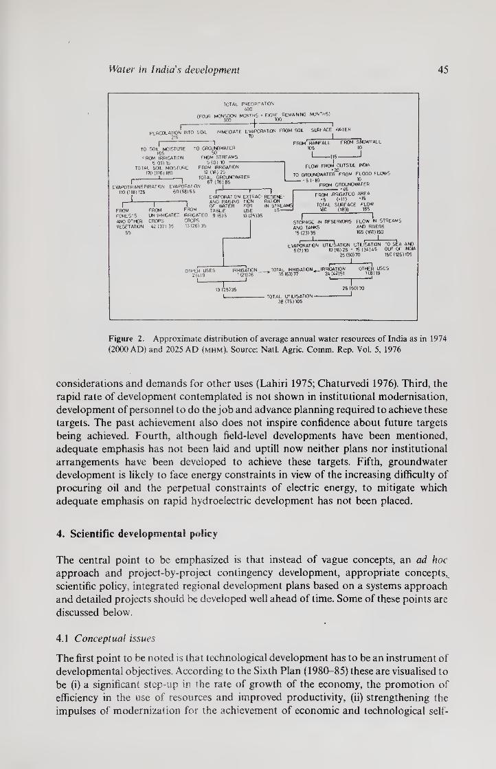
Water in India's development 45
TOTAL precipitation 400
(FOUR MONSOON MONTHS 300 |
* EIGHT REMAINING MONTHS) 100
PERCOLATION INTO SOIL 215
IMMEDIATE EVAPORATION FROM SOIL 70
1
I TO SOIL MOISTURE
165 FROM IRRIGATION
5 (11) 15 TOTAL SOIL MOISTURE
170 (176) 180
I-—^-1
-,
TO GROUNDWATER 50
FROM STREAMS
5 (8) 10
SURFACE WATER
FROM' RAINFALL FROM SNOWFALL
105
EVAPOTRANSPIRATION EVAPORATION
110 (118)125 60(58)55
J-,
FROM IRRIGATION
12 (18) 25 TOTAL GROUNDWATER
67 ( 76 ) 85
r1-T
—115 — I
1
FLOW FROM OUTSIOE INDIA
TO GROUNDWATER FROM FLOOD FLOWS
- -5 (-8) '10 FROM GROUNDWATER
45
r FROM FROM
EVAPORATION EXTRAC- REGENE- AND RAISING TION RATION OF WATER FOR IN STREAMS TABLE USE 45
FORESTS UN IRRIGATED IRRIGATED 9(6)5 13(25)35
FROM IRRIGATED AREA
• 5 (‘ID TOTAL SURFACE FLOW
180 (183) 185
ANO OTHER CROPS VEGETATION 42 (37) 35
55
CROPS
13(26) 35 STORAGE IN RESERVOIRS FLOW N STREAMS
AND TANKS ANO RIVERS
15 (23)35 165 (160)150
EVAPORATION UTILISATION UTILISATION TO SEA AMD 5(7)10 10 06)25 - 15 (34)45 OUT OF INDIA
25(50)70 150(126)105
OTHER USES 2(4)9
1_ IRRIGATION _
1(21)26 _l „TOTAL IRRIGATION, *■ 35 (63) 77
l- _ IRRIGATION
24 (42)51 OTHER USES
1(8)19 J
13 (25)35
I_ -TOTAL UTILISATION-
38 (75)105
25(50)70
_I
Figure 2, Approximate distribution of average annual water resources of India as in 1974
(2000 AD) and 2025 AD (mhm). Source: Natl. Agric. Comm. Rep. Vol. 5, 1976
considerations and demands for other uses (Lahiri 1975; Chaturvedi 1976). Third, the
rapid rate of development contemplated is not shown in institutional modernisation,
development of personnel to do the job and advance planning required to achieve these
targets. The past achievement also does not inspire confidence about future targets
being achieved. Fourth, although field-level developments have been mentioned,
adequate emphasis has not been laid and uptill now neither plans nor institutional
arrangements have been developed to achieve these targets. Fifth, groundwater
development is likely to face energy constraints in view of the increasing difficulty of
procuring oil and the perpetual constraints of electric energy, to mitigate which
adequate emphasis on rapid hydroelectric development has not been placed.
4. Scientific developmental policy
The central point to be emphasized is that instead of vague concepts, an ad hoc
approach and project-by-project contingency development, appropriate concepts,,
scientific policy, integrated regional development plans based on a systems approach
and detailed projects should be developed well ahead of time. Some of these points are
discussed below.
4.1 Conceptual issues
The first point to be noted is that technological development has to be an instrument of
developmental objectives. According to the Sixth Plan (1980-85) these are visualised to
be (i) a significant step-up in the rate of growth of the economy, the promotion of
efficiency in the use of resources and improved productivity, (ii) strengthening the
impulses of modernization for the achievement of economic and technological self-

46 Mahesh C Chaturvedi
reliance, (iii) a progressive reduction in the incidence of poverty and unemployment,
(iv) a speedy development of indigenous sources of energy with proper emphasis on
conservation and efficiency in energy use, (v) improving the quality of life in general
with special reference to the economically and socially handicapped population,
through a minimum needs programme whose coverage is so designed as to ensure that
all parts of the country attain nationally accepted standards within a prescribed period,
(vi) strengthening the redistributive bias of public policies and services in favour of the
poor, contributing to a reduction in inequalities of income and wealth, (vii) a
progressive reduction in regional inequalities in the pace of development and in the
diffusion of technological benefits, (viii) promoting policies for controlling the growth
of population through voluntary acceptance of small family norms, (ix) bringing about
harmony between the short and long-term goals of development by promoting the
protection and improvement of the ecological and environmental assets, and
(x) promoting the active involvement of all sections of the people in the process of
development through appropriate education, communication and institutional stra¬
tegies (Sixth Five Year Plan 1981).
Water resources have to be developed in the context of these objectives. For this
purpose, first, certain basic concepts of modern water resources and environmental
systems planning should be followed in future, in contrast to the ad hoc approach
of the past. It must be emphasised that technology in the present context of
development of water resources has to be an instrument to attain these objectives,
embedded in the socio-economic development and not an elitist activity visualised
merely in terms of certain grand projects. Tremendous possibilities for economic
development and employment generation through development of water resources
exist. For instance it is well-known that the yields in Indian agriculture are extremely
poor. The basic reason for this is the nonavailability of adequate and reliable water,
because of which other inputs of modern agriculture cannot be used. Yield and other
relevant statistics given in tables 2 and 3 bring out the immense potential for increasing
production and employment if water and corresponding inputs could be made
available (World Bank Operations 1972).
Table 2. Comparative yields of some important crops (1969)
Country
Yield (kg per hectare)
Paddy Wheat . Cotton
Japan 5,550 — —
UAR 5,110 — 790
USSR — — 770
France — 3,580 —
USA 4,790 2,060 490
Taiwan 3,510 — —
Thailand 1,840 — —
Pakistan 1,820 1,070 310
India 1,610 1,170 120
Source: Chaturvedi (1976)

Tab
le
3.
Develo
pm
enta
l p
ote
nti
al
in a
gri
cu
ltu
re
Water in India's development 47
IS & B
-0 3 0.
a S s & o
^ <L>
a-s 3 c3 O
15 2 -*-• TO 3 I
•C -*= 00 Uh
< S.
o T3
3 b e =5
JS o
aj <i> Q* ^
"g 2 8 «» 3 U. T3
- ° § O u 5
.3 5 3= 2
fc 8
_ V 2 !« U. TO
2 8 u .2 u -g U) U TO
% & 53 , i/) u_ O U °
. ^ O fe
-3 *0 b i- c 3 o
3 U; « « g /»v X*
2 «*
c *-< C« <l>
*
00 ^-5
O (-i cO
§ J3
O ^ * S3 S =3
3 £
.2 w. o
00 O-
r: 3 O U
to r- r- —h m a\ n m <N m 8 5?
•/i xt on •ri *n in r- on ’—« <N <
3 O Tf r- oo
r- oo *-h »o o w~) r** vo o *-h •n On M *h 3 2 2 3
r- m on »-* h f*l n o 8
cb 00 J O t 2 n ob On Com
m
0»oo0oor4wpmm t^^cfemmm<N<Nr4 OO <N »—' O *-4
<N
*-h r- os <n © m © m in m <6 © <s © ©
soosr-io©mr-© r-mu^T*—<r"-r'-oo ^OOOfNOOO
** ^ Os ** m rn 6 *h ’i' m —< m
NO'OoOTtNO'AMMO
w^j O <N ^ 0> OO Q ON NO
oc o m m
^'OOONOOfSHTfrf nOM/)«N(NOOOO^On m m <n <n <n <^h
CX 3 o X.
rO
a c •r u o
_ C r- O <-> 0) (L> § © '* g S? §< 2 « ^ < 4 o s
Cx 3 O x. o
> >vi2
*-* a> W5 P.JMJ O o, «* o rS 2.2 >> b 2P S ~ oo o 3 c ca a
W h > Cfl H On
c/3 <L>
.S -o Q. S
.& 3 ^ ^ cd
£liS
Os <N
00 <N
Os m
T" Os ©
Os <N CN
0> oo ctf Im <D > < S
ourc
e:
Changes
in a
gri
cu
ltu
re i
n 2
6 D
evelo
pin
g N
ati
on
s,
1948-1
968 (
U.S
. D
epart
ment
of A
gri
cult
ure
, F
ore
ign A
gri
cult
ura
l E
co
no
mic
Report
No.
29,
1965), a
s quote
d i
n W
orl
d O
pera
tio
ns,
Johns H
op
kin
s P
ress
, 1
97
2.
48 Mahesh C Chaturvedi
The second point to be emphasized is that water is a crucial vector of the geophysical-
biological environment and an important resource of the environmental-ecological
system. Its development has thus to be in the context of socio-economic development
consistent with environmental enhancement. A long-term view of the environmental
state and dynamics has also to be maintained. Thus, for instance, it is necessary that
certain minimum flows and water quality of surface flows is maintained, groundwater
quality is constantly watched, and soil erosion is reduced.
The third point to be emphasised is the need for a creative approach. One can develop
a number of technological options and one must choose critically instead of being
conditioned by certain techno-economic myths. For instance there is need for
conjunctive surface-groundwater and energy planning but this is more than what is
meant in the Government document. Again there is need for integrating traditional
technological solutions of surface diversions and conventional groundwater develop¬
ment with watershed development to alter land-water dynamics itself. These points are
elaborated later.
In this context it may be emphasised that technology includes, besides constructed
structural products, development of appropriate organisation and incentive systems.
One must, therefore, think of total technological systems development. For instance
when we think of dams and canals, or public or private tubewells, each has an
appropriate organisation and the totality of the technological system has to be
developed. One set may be better than another from the point of view of appropriate¬
ness of organisation rather than technological structure.
The fourth point to be emphasised is that water is an environmental-resource vector
which has a dynamics explained through the hydrological cycle in terms of state and
processes. The technological activity seeks to modify this cycle in terms of varied
demands. There is thus a spatial and dynamic interlinkage of the various projects from
hydrologic, economic and environmental considerations. Thus regional dynamic long¬
term planning is mandatory even though activity has to be initiated through individual
projects.
Thus water resources development has to be undertaken in terms of individual
projects developed creatively and with sensitivity in accordance with a long-term
dynamic developmental policy in the context of socio-economic environmental
multiobjective policies to satisfy the multipurposes. Although development has to be
undertaken in terms of projects, to identify the optimum portfolio of projects long¬
term policy and systems planning is mandatory. Some of the policy issues with focus on
various multipurposes are discussed below but it must be emphasised that the
developmental policy has to consider all the purposes integrally and should be region-
specific.
4.2 Policy issues with focus on habitat requirements
Water supply for human settlements for drinking and other domestic purposes may be
considered to be the most important demand. These requirements are a small portion
of the total demand. It is considered that adequate resources and technology are
available in all parts of the country to meet this demand and this could be adequately
met if there is the political will.
In this context, we have also to have a policy for habitat. As tubewells and canals are
developed for irrigation these can be easily used for supplying habitat demands not
only of sustenance but also of environmental enhancement and recreation.

Water in India's development 49
4.3 Policy issues with focus on irrigation
Agricultural needs account for about 90% of resource development and are crucial for
socio-economic development. Water is also important for electrical energy and
navigation. Water resources development for agriculture should be integrated with
energy system planning and transportation system planning for several reasons as
discussed later. For developing the policy, we however concentrate on water resources
development for irrigation in the first instance, but also integrate the policy with
electrical energy development and flood mitigation.
The possible important technological options for multipurpose water resources
development are given in figure 3. Additional programme and policies for modifying
the susceptibility to flood damage and modifying the loss burden are given in figure 4.
All these options are interlinked and not necessarily exclusive i.e. they are open-
interactive sets. A portfolio has to be chosen so that, consistent with conservation of
resources and environmental improvement, the planning objectives generation of
employment generation, economic efficiency and equity are optimally obtained
temporally and spatially, taking into account the regional, hydrologic, agro-climatic
and demographic potential and the developmental scenario over a period of time. The
alternative configurations, scale, operating policies and timing can be identified
through systems planning as discussed later. Further, as stated earlier, technological
planning does not mean only optimum capacity and timing of the projects, but also
Figure 3. Technological options for water resources development
5-4

50 Mahesh C Chaturvedi
Figure 4. Programmes and policies for modifying the susceptibility to flow damage and
modification of the loss burden. Source: Natl. Comm, on Floods (1980) l
development of an appropriate organisation and incentive system. For instance, better
economies in ground-water technological options may be obtained if cooperatives are
developed at the field level. This is a difficult task requiring social management and,
therefore, while it may be attempted in the long run, less efficient technology of
individually-developed small-scale tubewells may be encouraged, if necessary.
Let us examine each set starting with watershed management. Traditionally, water
resources developmental activities have centred around spatial and temporal trans¬
formation through structural techniques of diversion works, dams and tubewells after
certain land-water interactions have taken place. It may be worth considering altering
land-water dynamics through organic and non organic/structural techniques as shown
in figures 3 and 4 for flood mitigation, erosion control and water resources
development through additional groundwater recharge. Certain areas like the alluvial
plains of the Ganga basin offer attractive opportunities (Indo-U.S. Scientists
Workshop 1981). The scheme of watershed management is particularly important in
conjunction with groundwater recharge as discussed later and for development of
runoff from the entire land area. The issue is that the hydro-geological interaction,
particularly from the resource point of view is as shown in figure 5. By technological
intervention, the natural state can be altered at any level of interaction.
Groundwater development, particularly in the alluvial Indo-Gangetic plains and
Eastern coastal regions is of particular importance and priority as it can be developed
fast. There are several policy issues such as what should be the scale—small or large;
what should be the organisation—private or public; whether it should be diesel or
electric and whether there should be mining or whether development should be
confined to safe yield. Each can be considered a different technology and tested through
systems models. Some aspects may be noted.
Groundwater development through private low capacity pumps has the advantage
of mobilising local initiative, generating fast development, employment through simple

Water in India's development 51
Figure 5. Hydrogeological interaction. P: precipitation, E: evaporation, T: transpiration,
Q0: surface runoff, F: infiltration, Qt: groundwater seepage, M: water of volcanic origin, RN:
percolation
construction techniques and assurance of more dependable supplies. Public tubewells
provide economies of scale. It is debatable which contributes more to social justice. It
can be argued that private development be through low-capacity diesel tubewells and
public development be through high-capacity ones. Studies in one river basin indicate
that large-scale tubewells give only 5 % additional benefits while posing management
problems (Chaturvedi & Khepar 1981). These results are based only on one study and
more studies are required. An optimum development has to be worked out for each
planning unit (village, block, district) through a systems study.
In certain situations it may be possible to develop groundwater in conjunction with
surface water by storing the latter through groundwater recharge. Three technological
options have been suggested. One is storage of monsoon flows through induced
groundwater recharge by heavy pumping prior to monsoons along perennial and non¬
perennial rivers. The scheme has been termed Ganga Water Machine (Revelle &
Herman 1972; Chaturvedi et al 1975; Revelle & Lakshminarayan 1975; Chaturvedi
1981 a). The second option is by heavy irrigation during monsoons through leaky canals
with conjunctive prior groundwater development and its lowering (Chaturvedi &
Srivastava 1978). This has been termed as Kharif Channel Conjunctive Development
and has been shown to be more economical than the first one. However, one or both can
be used as found suitable.
The third alternative could be to pump down the excess rainfall at the field level itself
and thereby have additional resources and reduce floods. The conventional tubewells
could be used for this purpose through suitable provision of ordinary valves.
Alternatively, a low-capacity low-head reversible pump would be required for this
purpose. Preliminary studies have indicated its techno-economic feasibility (Sohoni
1976). It may be noted that for pumping down the water, no additional energy would be

52 Mahesh C Chaturvedi
required, except may be at the start of the operations or for achieving high rates of
recharge. The scheme is termed micro water machine. It may be noted that at this time
considerable secondary energy would be available.
Certain constricting myths have arbitrarily been imposed by technologists and these
have lead to a priori rejection of some of the basic options. For instance, groundwater
development is often restricted to the so-called safe yield, equivalent to annual recharge.
There is no reason why secular reserves could not be developed, of course, subject to a
policy that in the long run a steady optimum level of groundwater and recharge is
obtained from considerations of economic growth taking into account possible
recharge from surface water resources or interbasin transfer. For instance, after surface
water resources have been developed groundwater availability will be enhanced and
therefore mining may be done in the first instance. There may be the problem, however,
that in this process the performance of the shallow well may be affected but an
appropriate policy can be developed.
Surface resources have been developed for a long time but here too several issues
have been neglected. For surface development, the two basic options are diversions
with and without storage. Storage projects are very attractive and mandatory from an
electricity generation point of view and even more so when planned from consider¬
ations of conjunctive surface, groundwater and energy development point of view.
Figure 6 clearly shows the substantial advantages in additional water and power
supplies. The issue of induced groundwater has also to be added, and the problem has
to be considered in the context of spatial availability of the resources and demands
(Chaturvedi 1979). It may be emphasized that current storage developments do not
generally consider this integrated development and, therefore, do not represent optimal
development.
It is also mandatory that catchment area development such as watershed manage¬
ment and upstream construction work is completed before the storage works are
undertaken so that sedimentation does not jeopardise their economic life.
Surface diversions being economical and quick to construct have been the first
priority in water resources development so far. The benefit/cost ratio is particularly
attractive if capacity is limited to low flows. From environmental considerations,
unlimited low-flow diversions are, however, unacceptable. Perhaps limited low-flow
diversions may be tolerated, but the needless mass-scale diversions have created an
extremely precarious position. In the long run, minimum flows will have to be restored
by substituting with other technological options and the issue of navigation has to be
considered. Surface diversions of monsoon flows, that are known as kharif channels, on the other
hand, are extremely attractive, particularly if developed conjunctively with ground-
water development, as discussed earlier. The groundwater table may be developed
such that groundwater recharge during monsoons from kharif channels plus ground-
water development from long-term policy considerations plus permissible low-flow
diversions or release if there are storage works to meet the non-monsoon requirements
are adequate to meet winter (rabi) and summer requirements. Correspondingly, the
capacity of kharif channels can be finalised. Monsoon flows can also be used, and have been used, through local lift schemes. This
is attractive when the diversion canal may interfere with drainage and floods, as in the
lower parts of the Ganga basin and Bangladesh. Lift schemes are, however, important
for interbasin transfer and conservation, as discussed later.

Water in India’s development 53
Figure 6. Conjunctive surface and groundwater development and integrated water and
energy plan
The focus of attention so far has understandably been on major schemes, as they
yield better benefit/cost ratio and even more important, are technologically more
glamorous. It is important that total water resources development is considered
integrally. It is considered that the resource availability and developmental attractive¬
ness of the small or even non perennial schemes can be considerably improved by
storing monsoon waters through appropriate technology and their development
should be part of an integrated development with a portfolio of projects of appropriate
capacity and with identified timing.
Besides the direct approaches of water resources development the supplies can be
increased by more efficient conveyance and utilisation of water. This can be divided into
two parts, the main distribution system, consisting of main canals, branches,
distributaries and minors. Secondly, increased efficiency at the field level which includes
increasing the efficiency of the conveyance from the main distribution system to fields
and application at the field. The division has been made because the first was in
the Government Sector and had received some attention but the second had, with the

54 Mahesh C Chaturvedi
organisation of command area development activities, been left completely to the
farmers till recently. Even in the first, many works are old and there is considerable
scope for improvement and modernisation. The second has been termed field-level
development. It is considered that it may be the most economical, easy to undertake and
has large employment-generation potential. There is a choice of several alternatives,
and sophisticated analysis is required to decide optimal strategies (Chaturvedi &
Khepar 1981). In view of its importance we shall refer to it again later.
4.4 Hydroelectric development
The hydropower potential of India is quite rich and is still largely untapped. The
country’s economically exploitable hydropower resources have been estimated at
75,400 mw of which only about 10% of the potential is utilised at present (Sixth Five
Year Plan 1981).
In addition, the potential of Nepal is 85,000 mw, of which almost none has been
exploited. It is further considered that these estimates are on the low side and the
potential is almost the double of these estimates.
At present hydroelectric development is being undertaken on an ad hoc project-by-
project basis with capacity fixed on the basis of 90 % availability of water resources
annually with water availability estimated on a 10-day period on the basis of 90%
availability. This is a gross under-utilisation of these resources for the following
reasons.
First, we have to consider 90% reliability of the system and not of the individual
project. Through complementarity of the different modal choices viz (i) thermal (coal
and nuclear), (ii) run-of-river hydro and (iii) storage hydro, individual project capa¬
cities would be much larger through a systems approach.
Second, besides systems planning of production, integrated systems planning of
supply and demand has to be considered which will lead to further optimal
development of the potential. Reference has already been made to conjunctive surface
groundwater and energy planning. The approach has been applied in a real-life study
(Chaturvedi 1979).
With the increasing crunch on liquid energy fuel, the groundwater development
tempo, which is crucial to agricultural development and consequently to national
development, is in a serious state of jeopardy. Alternative sources of energy have to be
developed fast and hydro-electric development has also to be accelerated.
In irrigation and hydro-projects, capacity and operation are planned on the
assumption that irrigation supplies have to be met first. A nominal allocation is made,
as a power cushion on an ad hoc basis. This is wrong. Alternatively optimal capacities
and operation schedule have to be carefully worked out through multiobjective
analysis with integrated surface-groundwater and energy planning. Often planning
from energy considerations will be dominant (Chaturvedi & Rogers 1985).
4.5 Policy issues with focus on flood mitigation
A unique characteristic of water resources in India is extreme temporal variation. A
drought can very soon be followed by serious flood followed by a long period of water
scarcity. Flood and drought are not only extreme stress characteristics for the water
component of the physical environment, but for human and other biosystems as well.
A study of the flood problem has been carried out by the National Commission on

Water in India's development 55
Floods (ncf 1980) recently. It has been estimated that about 40 mha of area may be
considered as ‘flood-prone’ of which 10 mha have already been provided with
reasonable protection. It is considered that 80% of the flood-prone area could be
provided with reasonable protection, and that at the present level of prices, these activities will cost Rs. 51,000 crores.
Technological options for flood mitigation and programmes and policies for
modifying the susceptibility to flood damage and modification of the loss burden are
given in figure 4. Prevention of floods through organic activity such as afforestation
and agronomic practices, appear to be important. Precipitation conservation at field
level by bunding and forced groundwater recharge, storage, kharif channels and
embankments, planned integrally appear to be feasible leading to flood mitigation and
water resources development (Chaturvedi 1981a). The matter is not discussed further as
it has to be developed in concrete terms for each river basin. We would only like to
emphasize that the problem of flood management has so far been neglected in planning
water resources development in India. Flood mitigation is also necessary for
modernised agriculture and employment generation.
4.6 Policy issues with focus on navigation
Somehow navigation has been completely omitted from water resources development
in India. Several reasons appear to be responsible for this omission. One, in the colonial
policy, navigation was not found to be economical. Second, flow diversions for
irrigation conflict with navigation requirements and apparently the latter have been
summarily overlooked. Third, Indian rivers have large inter-seasonal variability and
this may have posed some problems for navigation.
It appears, however, that overriding all these factors is the fact that integrated
planning has not been carried out and navigation has been dropped on an ad hoc basis
as water resources development is carried out on the basis of the functional orientation
of planning agencies. It is not often realised that 2-3 m depth and 30-40 m width is
enough for large-size navigation requirements. These dimensions would be provided
even by many canals and rivers if environmental considerations were developed.
4.7 Policy issues with focus on environment
The natural land-water state is one level of the environment-resources vector. With
development, it gets changed to another state. Any perturbation has ecological-
biological-physical besides socio-economic implications which are extremely complex.
It is difficult to say what are the minimum surface flows and groundwater development
from environmental considerations but it would be logical to argue that there must be a
limit to physical development and any large-scale perturbation must be carried out only
after careful study of the environmental implications.
4.8 Drought policy
Drought is difficult to define as it relates to water availability as well as techno-
economic capability of development under a given environment. Israel is a semi desert
with an annual rainfall of 500 mm with wide spatial and temporal variation. Yet it has
the most highly modernized irrigation and agriculture development. In India according
to the Irrigation Commission, 16% of the total geographical area accounting for over
56 Mahesh C Chalurvedi
11 % of the population has been classified as drought-prone. The strategy of
development would be to emphasize efficient use of local water resources supplemented
by imports. Priority has to be given first to drinking and other domestic uses of water,
then for industry and then for appropriate agriculture, including animal husbandry.
The matter is one of detailed analysis and does not alter basic policy options.
It will follow from the above that an integrated water resources development taking
into consideration all demands and resources availability on a long-term basis on a
regional and interregional basis has to be carried out. The above discussion is only a
background for detailed system studies as discussed later.
5. Field level water management
Much of the foregoing discussion was in terms of technological schemes for water
resources development in the context of agricultural demands with some environ¬
mental constraints. Demand is not constant, but is a function of techno-economic
capability of the users. For instance, in India, while on the one hand, water availability is
inadequate, on the other hand, application is most inefficient and wasteful. It has been
estimated that only 40 % of water released at the canal head is made available to crops.
Thus, if more efficient water management were practised, much larger areas could be
irrigated or more water could be made available to the same farmers.
The technological solutions are lining of distribution systems, land levelling and
adoption of appropriate water management at the field level. An integrated field-level
water management can be worked out to identify optimal investment in each of these
three components and to determine the shadow prices so that the relative advantage of
field-level and macro-level development can be established (Chaturvedi & Khepar 1981). We do not visualize a complete change to sprinkler system or trickle irrigation.
The gravity flow system will remain the predominant technology but unit water
requirements should be reduced over the course of time. In long-term planning of water
resources, the urgency of the gradual improvement in efficiency has to be emphasized.
Field-level development has been neglected in the past in view of certain political-
organisational reasons. From economic, employment generation, and environmental
considerations, field-level management has the highest priority.
Water management at the watershed level, which we have emphasized is, however,
not a mere technological issue, but is a problem of adult education, formation of
cooperatives, etc., or in short, a problem of social change as a component of integrated
rural development.
6. Interbasin transfer
Temporal and spatial variability are usual features of water resources but the condition
in India is acute. Figure 7 brings out these characteristics, suggesting the need for large-
scale interbasin transfer. The possibility of interbasin transfer has implications for the
planning of all regional developmental projects in ensuring that important possible
benefits are not pre-empted and the possibility of providing flexibility in the projects
without undue extra commitment of investments is explored at the outset.
Two schemes have been proposed in this context and are worthy of examination.
One is the National Water Grid proposed by Rao (1976). The other is the National
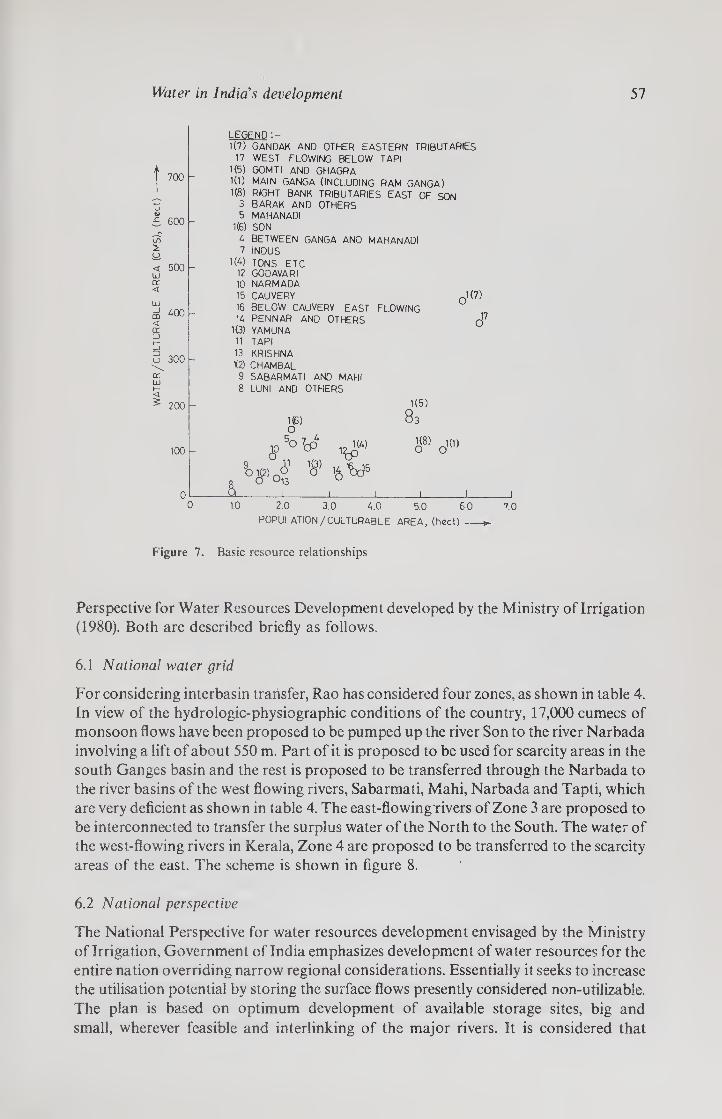
Water in India's development 57
TOO
600
in 5 y < UJ cr <
500 -
m < cc 3 t— j 5 o cr UJ ►- < 5
400
300
200
100
LEGEND
1(7) GANDAK AND OTHER EASTERN TRIBUTARIES
17 WEST FLOWING BELOW TAPI
1(5) GOMTI AND GHAGRA
1(1) MAIN GANGA (INCLUDING RAM GANGA)
1(8) RIGHT BANK TRIBUTARIES EAST OF SON 3 BARAK AND OTHERS 5 MAHANADI
1(6) SON
4 BETWEEN GANGA AND MAHANADI
7 INDUS
1W TONS ETC 12 GODAVARI 10 NARMADA
15 CAUVERY
16 BELOW CAUVERY EAST FLOWING 14 PENNAR AND OTHERS
1(3) YAMUNA
11 TAPI
13 KRISHNA
1(2) CHAMBAL
9 SABARMATI AND MAHI
8 LUNI AND OTHERS
O .1(7)
1(6) O
50
901C2) A’ 1S) O o13 l
i° 19 U4)
^P % ’fed5
1(5)
83
^ oK1)
L
1.0 2.0 3.0 4.0 5.0 6.0
POPULATION/CULTURABLE AREA, (hect) -».
70
Figure 7. Basic resource relationships
Perspective for Water Resources Development developed by the Ministry of Irrigation
(1980). Both are described briefly as follows.
6.1 National water grid
For considering interbasin transfer, Rao has considered four zones, as shown in table 4.
In view of the hydrologic-physiographic conditions of the country, 17,000 cumecs of
monsoon flows have been proposed to be pumped up the river Son to the river Narbada
involving a lift of about 550 m. Part of it is proposed to be used for scarcity areas in the
south Ganges basin and the rest is proposed to be transferred through the Narbada to
the river basins of the west flowing rivers, Sabarmati, Mahi, Narbada and Tapti, which
are very deficient as shown in table 4. The east-flowingtivers of Zone 3 are proposed to
be interconnected to transfer the surplus water of the North to the South. The water of
the west-flowing rivers in Kerala, Zone 4 are proposed to be transferred to the scarcity
areas of the east. The scheme is shown in figure 8.
6.2 National perspective
The National Perspective for water resources development envisaged by the Ministry
of Irrigation, Government of India emphasizes development of water resources for the
entire nation overriding narrow regional considerations. Essentially it seeks to increase
the utilisation potential by storing the surface flows presently considered non-utilizable.
The plan is based on optimum development of available storage sites, big and
small, wherever feasible and interlinking of the major rivers. It is considered that

58 Mahesh C Chaturvedi
Table 4. Zonal distribution of land-water resources
Zone No.
Total water
(annual
discharge
(x 109 m3)
Percentage of
land cultivated
Water potential
(% of total) Proposed interbasin links
1. Indus, Brahmaputra
and Ganga (North
Zone)
1045 44 77 Brahmaputra-Ganga,
Ganga-Narbada
2. Sabarmati, Mahi,
Narmada and Tapti
(West-flowing)
70 19 5 Ganga to Narbada and
to others
3. Subarnarekha,
Brahmani, Baitami,
Mahanadi,
Godavari,
and Cauveri
(East-flowing)
195 35 14 From northern rivers of
the region to southern
rivers
4. West-flowing rivers in
kerala
40 2 3 To be transferred to the
East
Total 1350 100 99
Source: Rao 1978
besides the currently estimated utilizable potential of 105 mhm, an additional
20-96 mhm of water, an additional 35 mha of irrigation and 40,000 MW hydroelectric
energy, perennial inland navigation and extensive flood mitigation shall be provided.
The perspective comprises two main components viz., (i) The Himalayan rivers
development; and (ii) peninsular rivers development. These are briefly outlined below.
6.2a Himalayan rivers development The Himalayan rivers development scheme en¬
visages construction of storage reservoirs on the main Ganga and the Brahmaputra and
their principal tributaries in India and Nepal along with inter-linking canal systems to
transfer surplus flows of the eastern tributaries of the Ganga to the West apart from the
linking of the main Brahmaputra with the Ganga. Apart from providing irrigation to an
additional area of about 22 mha and the generation of about 30 million kW of hydro-
power, it will provide substantial flood control in the Ganga-Brahmaputra basin. It
would provide 1332 cumecs (40,000 cusecs) to Calcutta Port and would provide
navigation facilities across the country. The scheme will benefit not only the States in
the Ganga-Brahmaputra Basin, but also our neighbours—Nepal and Bangladesh—as
well as the northern and western states in our country. Implementation of this scheme
will however largely depend on the cooperation of neighbouring countries.
6.2b Peninsular rivers development Amongst the peninsular rivers, the Mahanadi and
the Godavari are likely to have sizeable surpluses. It is, therefore, possible to divert the
surplus of the Mahanadi and the Godavari to the water-short rivers viz., the Krishna,
the Pennar and the Cauvery. The Mahanadi will also be linked on the north with Bura-
Balang, and 7-4 mhm of Mahanadi waters will be utilised for irrigating the coastal areas
in Orissa and interlinking the rivers to even out the hydrological variations.
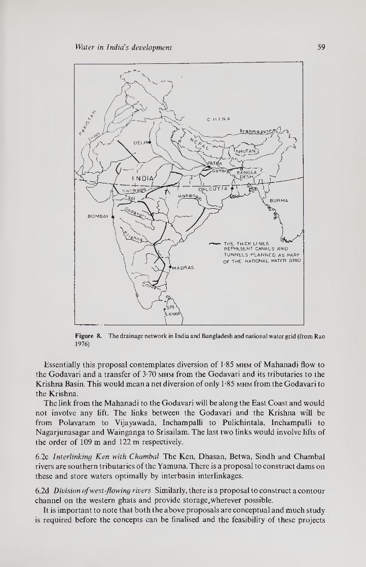
Water in India's development 59
Figure 8. The drainage network in India and Bangladesh and national water grid (from Rao
1976)
Essentially this proposal contemplates diversion of 1-85 mhm of Mahanadi flow to
the Godavari and a transfer of 3-70 mhm from the Godavari and its tributaries to the
Krishna Basin. This would mean a net diversion of only 1 -85 mhm from the Godavari to
the Krishna. The link from the Mahanadi to the Godavari will be along the East Coast and would
not involve any lift. The links between the Godavari and the Krishna will be
from Polavaram to Vijayawada, Inchampalli to Pulichintala, Inchampalli to
Nagarjunasagar and Wainganga to Srisailam. The last two links would involve lifts of
the order of 109 m and 122 m respectively.
6.2c Interlinking Ken with Chambal The Ken, Dhasan, Betwa, Sindh and Chambal
rivers are southern tributaries of the Yamuna. There is a proposal to construct dams on
these and store waters optimally by interbasin interlinkages.
6.2d Division of west-flowing rivers Similarly, there is a proposal to construct a contour
channel on the western ghats and provide storage,wherever possible.
It is important to note that both the above proposals are conceptual and much study
is required before the concepts can be finalised and the feasibility of these projects

60 Mahesh C Chaturvedi
determined. There are many other possibilities and optimal schemes have to be worked
out. Furthermore, these are not necessarily contradictory and an optimal scheme may
have elements of both or several others.
Some improvements are as follows. Rao’s scheme is complemented and improved by
visualising both mass and energy conservation and transfer as proposed by Chaturvedi
(1973). Consider the interlinkage of Zones I and II, which is crucial. The surplus water
flowing down the Himalayas which is proposed to be transferred is also capable of
producing energy in the Himalayas which at present is not planned to be utilised
beyond 90-95 % assured supplies round the year. Thus, much of the monsoon flows
and possible secondary energy is wasted. Since the marginal cost of extra energy
generation in the Himalayan run-of-river scheme is small, the installed capacity of these
developments should be planned from a consideration of the production of this
secondary energy also. This can be stored and transferred by pumping the Ganga water
and storing it in the Narbada, which has tremendous and economical storage potential.
This can be later released as firm energy which is almost three times more valuable than
the secondary energy and particularly as peak energy which is further almost three
times more valuable.
The National Water Perspective has also to be related to detailed basin planning and
preceded by it. The results of a study of integrated agricultural development in the light
of the current and ultimate potential without taking into account interbasin water
transfer but taking into account the variable cost of surface and groundwater
development in river basins is given in table 5. The variation in shadow price of water in
Table 5. Costs of surface water and ground water in various basins (1976-77)
(Rupees/hectare meter)
Surface water Ground water
River basins
Develop¬
ment
cost
Operation
and mainten¬
ance cost Total
Develop¬
ment
cost
Operation
and mainten¬
ance cost Total
Basin 1 183 121 304 189 435 624
Basin 2 318 180 498 429 645 1074
Basin 3 289 235 524 333 668 1001
Basin 4 136 85 221 316 835 1151
Basin 5 117 50 167 186 379 565
Basin 6 177 126 303 250 467 717
Basin 7 353 185 538 320 115 1435
Basin 8 154 99 253 424 785 1209
Basin 9 563 264 827 387 671 1058
Basin 10 156 96 252 241 690 931
Basin 11 1166 517 1683 397 2015 2412
Basin 12 220 91 311 361 893 1254
Basin 13 134 66 200 404 700 1104
Basin 14 166 77 243 199 1164 1363
Basin 15 370 160 530 269 1224 1493
Basin 16 269 119 388 339 892 1231
Basin 17 744 313 1057 364 1229 1593
Basin 18 814 322 1136 421 1065 1486
Basin 19 1374 503 1877 416 896 1312
Basin 20 396 170 566 238 1670 1908
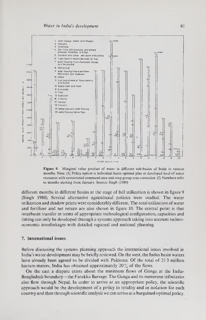
Water in India's development 61
1 main Ganga Gomti and Ghagra
2 Yamuna
3 Chambal
4 Son Tons Karamnosa and others between Chambal and Son
5 Gandak and other left bank tributaries
6 right bank tributaries east of Son
“□*
east flowing rlver9 between Ganga and Mahanadi
8 Mahanadi
9 east flowing rivers between
Mahanadi and Godavari
10 Indus
11 Luni and others of Saurashtra and Kutch
12 Sabarmati and Mahi
13 Narmada
14 Tapi
15 Godavari
16 Krishna
17 Pennar
18 Cauveri
19 below Cauveri east flowing
20 west flowing below Tapi
1-5 10-12
4,6 %i<yi
6J0
1,11,12
9
2,3
RIVER BASINS -
Figure 9. Marginal value product of water in different sub-basins of India in various
months. Note: (1) Policy option is individual basin optimal plan at developed level of water
resources with unrestricted command area and crop group area constraint. (2) Numbers refer
to months starting from January. Source: Singh (1980)
different months in different basins at the stage of full utilization is shown in figure 9
(Singh 1980). Several alternative agricultural policies were studied. The water
utilization and shadow prices were considerably different. The total utilization of water
and fertilizer and net return are also shown in figure 10. The central point is that
interbasin transfer in terms of appropriate technological configuration, capacities and
timing can only be developed through a systems approach taking into account techno-
economic interlinkages with detailed regional and national planning.
7. International issues
Before discussing the systems planning approach the international issues involved in
India’s water development may be briefly reviewed. On the west, the Indus basin waters
have already been agreed to be divided with Pakistan. Of the total of 21-3 million
hectare-meters, India has obtained approximately 20 % of the flows.
On the east a dispute exists about the minimum flows of Ganga at the India-
Bangladesh boundary—the Farakka Barrage. The Ganga and its numerous tributaries
also flow through Nepal. In order to arrive at an appropriate policy, the scientific
approach would be the development of a policy in totality and in isolation for each
country and then through scientific analysis we can arrive at a bargained optimal policy.

62 Mahesh C Chaturvedi
10000-
8000-
£ ° 6000-
n 4000-
2000-
40000
32000
E 24000
o S
16000
8000 I
a Utilized Groundwater
ggg Utilized SurtaceWater
Utilized Fertilizer
Net Returns
i
Cr Cr Cu Ar Aj Br Ai
80000 0
640000 S.
480000
320000
160000
<v z
Optimal Plans
Figure 10. Utilisation of water and fertilizer and net returns under various optimal plans for
the country as a whole (Source: Singh 1980)
Bangladesh and part of West Bengal constitute the largest delta of the world. Out of
the total area of 204,000 sq. km of Bangladesh, 85,000 is in the delta. The average annual
discharge from the Ganga, Brahmaputra and Meghana of 18-69, 19-82 and 5-10
thousand cumecs with a total of 43-61 thousand cumecs is second only to the Amazon
(Leeden 1975). These carry the world’s highest sediment load, with 1451 x 106 and 726
x 106 metric tons in the Ganga and the Brahmaputra respectively. To give a
quantitative idea, the estimated 2177 x 106 metric tonnes of average annual suspended
load in the Ganga and the Brahmaputra is larger than that in the dreaded Yellow river,
almost four times greater than the next highest sediment laden river Yangtze and
twenty times the silt load of Nile (Leeden 1975). The flows are extremely variable over
time. The Ganga draining an area of 1,098,600 sq. km above Goalundo has an average
annual flow of 11468-3 cumecs (405,000 cfs) with a maximum and a minimum of
70933-6 and 1161 cumecs (2,505,000 and 41,000 cfs). The Brahmaputra draining an area
of 580,000 sq. km above Goalundo (including catchment areas outside India and
Bangladesh) has an average annual flow of 19340-4 cumecs (680,000 cfs) with a
maximum and minimum of 71330 and 3115 cumecs (2,519,000 and 110,000 cfs). The
Brahmaputra flows are much more uniform and the high flows start in May while in the
Ganga they start in July.
The Ganga and the Brahmaputra unite at Aricha, the combined flow being known as
the Padma river. The drainage area of the Padma between Goalundo and its confluence
with Meghana is 12960 sq.km most of which is flooded during the high-flow season.
The maximum observed flow of the Padma at Goalundo is 91180 cumecs.
The Meghana river, with a catchment of 80200 sq. km constitutes one of the highest
rainfall areas of the world. It joins the Padma at Chandpur dumping another
5,100 cumecs into this tremendous water mass. The numerous channels in the delta
have developed the configuration in the context of the geophysical-hydraulic charac¬
teristics of the land water mass.
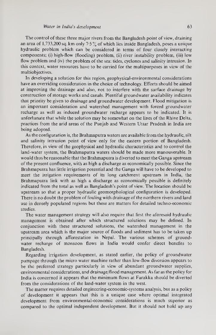
Water in India's development 63
The control of these three major rivers from the Bangladesh point of view, draining
an area of 1,733,200 sq. km only 7-5 % of which lies inside Bangladesh, poses a unique
hydraulic problem which can be considered in terms of four closely interacting
components; (i) high-flow (flooding) problem, (ii) river instability problem, (iii) low
flow problem and (iv) the problem of the sea: tides, cyclones and salinity intrusion. In
this context, water resources have to be carried for the multipurposes in view of the multiobjectives.
In developing a solution for this region, geophysical-environmental considerations
have an overriding consideration in the choice of technology. Efforts should be aimed
at improving the drainage and also, not to interfere with the surface drainage by
construction of storage works and canals. Plentiful groundwater availability indicates
that priority be given to drainage and groundwater development. Flood mitigation is
an important consideration and watershed management with forced groundwater
recharge as well as induced groundwater recharge appears to be indicated. It is
unfortunate that while the solution may be somewhat on the lines of the Rhine Delta,
practices from the arid areas of the Punjab and Western Uttar Pradesh in India are
being adopted.
As the configuration is, the Brahmaputra waters are available from the hydraulic, silt
and salinity intrusion point of view only for the eastern portion of Bangladesh.
Therefore, in view of the geophysical and hydraulic characteristics and to control the
land-water system, the Brahmaputra waters should be made more manouverable. It
would thus be reasonable that the Brahmaputra is diverted to meet the Ganga upstream
of the present confluence, with as high a discharge as economically possible. Since the
Brahmaputra has little irrigation potential and the Ganga will have to be developed to
meet the irrigation requirements of its long catchment upstream in India, the
Brahmaputra link with as high a discharge as economically possible is definitely
indicated from the total as well as Bangladesh’s point of view. The location should be
upstream so that a proper hydraulic geomorphological configuration is developed.
There is no doubt the problem of fouling with drainage of the northern rivers and land
use in densely populated regions but these are matters for detailed techno-economic
studies. The water management strategy will also require that first the aforesaid hydraulic
management is obtained after which structured solutions may be defined. In
conjunction with these structured solutions, the watershed management in the
upstream area which is the major source of floods and sediment has to be taken up
principally through afforestation in Nepal. The various schemes of ground-
water recharge of monsoon flows in India would confer direct benefits to
Bangladesh.
Regarding irrigation development, as stated earlier, the policy of groundwater
pumpage through the micro water machine rather than low-flow diversion appears to
be the preferred strategy particularly in view of abundant groundwater supplies,
environmental considerations, and drainage/flood management. As far as the policy for
India is concerned it appears that the minimum flows at Farakka should be diverted
from the considerations of the land-water system in the west.
The matter requires detailed engineering-economic-systems analysis, but as a policy
of development it appears that this is a unique case where optimal integrated
development from environmental-economic considerations is much superior as
compared to the optimal independent development. But it should not hold up any

64 Mahesh C Chaturvedi
upstream developments as the case is more of excess of water than shortage of water in
Bangladesh.
Unfortunately, in the dispute with Bangladesh the issue of the development of the
water resources of Nepal has been neglected. Nepal has very rich water resources
development potential and for India, development in Nepal is of utmost importance.
These should be taken up integrally with the development in India and with the highest
priority. It is interesting and important to note that from hydroelectric considerations
there is a remarkable analogy between the potential development of Sweden and Nepal.
Unfortunately while almost 60 % of the potential of 25 MkW has been developed in the
former, not even 1 % of the potential of 85 MkW has been developed in the latter.
8. Technological policy
We have discussed some issues of developmental policy and technological strategies for
water resources development in the foregoing. A package of technologies with some
indication of the pros and cons subject to detailed determination of production
function was indicated. Their selection, capacity, location and scheduling has to be
determined from detailed systems planning for which an approach is indicated in terms
of local, regional and national planning subject to detailed analysis. Likely tech¬
nological activities are indicated in table 6. While regional planning has to be in terms of
the river basins, we have developed a coarse spatial-temporal matrix for developing a
technological matrix as a first step for systems analysis. The country is divided into five
regions. The time is divided into three units, short run, medium run and long run. Each
technology is envisaged to be started at the optimal time so that each phase is optimally
completed.
According to the Sixth Plan complete utilization is scheduled in over 20 years. In our
judgement, technological, organisational and institutional capabilities do not warrant
such a schedule, but with the utmost efforts for modernization on these fronts, a
schedule of 30 years is feasible. However, if the present approach continues water
resources cannot be developed even over a much longer period and then too the
development will be suboptimal.
The policy on which the recommendation of table 6 is based is that (i) a tempo for
completing development over this period is built up and (ii) schemes are taken up on
priority which have comparatively higher attractive marginal productivity. It hardly
need be stated that table 6 is a tentative policy approach and an integrated regional and
temporal trajectory of development has to be worked out as shown in figure 11 with
regional focus in the Ganga Basin for illustration.
9. Planning approach
It is not as yet adequately appreciated in the engineering profession that water
resources development is not a mere technological problem, but is integrally related to
total socio-economic-technological developmental planning. Accordingly in the sys¬
tems planning approach, for convenience, the issues may be grouped under three
interacting heads (i) analysis of the physical phenomenon, (ii) socio-economic evalu¬
ation criteria, and (iii) systems planning. A typical set of issues and models required to
develop water resources at a regional level is shown in table 7. Planning studies and
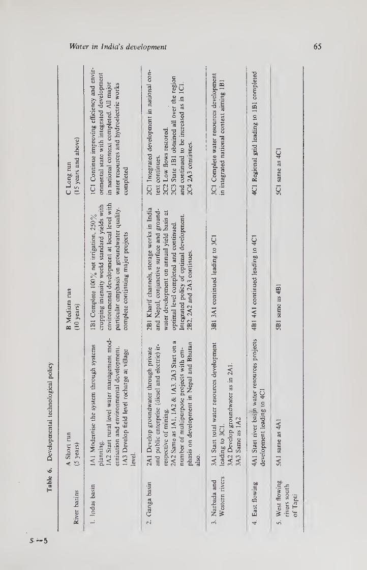
Tab
le
6.
Dev
elo
pm
en
tal
tech
no
log
ical
po
licy
Water in India's development 65
> O X G
*o G C G G
►3 £
G G Ut
s ^
.2 2 T3 G
^ o
G G
O oj ,G D C/3 ^
G X
Wh D
_>
5
c c G d
" s 'O a S o * « >> > D D G X> 2 -r-t * ^
2s
I? < c
G
O £ D
> .£ 2 6 a. .-a E is
« 2 3 3
•S
^ £
J3 o
g-3 G O X
g § r* ^ G <y O f > D
G *3 O
r ) G
SI
\o ^
o ^
S !§ « >>
I 'S
G 'O .SP c
t~< G
_ G o3 O -O G ft D OD +~*
V—i D
G Q-
- E § o > o
G G cr
fc 2 1 8
Is* § ^ o
d 2
c o ^ *
GO
CL ■
6 o U '
£
H D
x GO G O
E D
G D
£ a- c o o 1j &
'i
— CL
e D
o G1 E GO G
-a o £
G D
s D GO cd G G
6
G O cJ
2 2 13 ^ .2 CL
s s S o Gh (J
G ^ § 2? E ^ CL ■£ O >
S s D D
X) GO
G
oj £
c/5 _
is > tn jg
D —2 oo 03
'G *-• E 13 *—I 1_4 D
| % i ^ 'r t/l
-< C n < i3 < —i Cl ’—i
G X) 05 G
'O G
G X
G ft £ 2 s j: G V
s s E 2 D D
"O G CL a3 O
C 1> .2 S 3 0 on ,—;
•G CO D c < >
G O o
G .2 3 G
§ 6 CL O D > D
T3
TD 2 8 03 G feb.S
G O HH (J
Fj ?3 & 2
G O go rt D U Lh
D c x .5
D > o
G3 o3
TD D G G w X) O
2 D
3 53
T3 D Vh O C/5 D Ui C/5
o CG
o —1 (N CO u u (N <N
TD D G G
D G C
c o D
G co
O < o <N
T3 G U 03 <N
.2 -5
^ *2 c o3
= 3
aj !- u. G O 00
D G G G G
X3 O o 5
*3 «3 2 a
«-G D Li z
oa "§ (N cd
8 *9 •° S 2 c •g.| "3 “
c c C "* G
G 2 O D
G "S- D S G O g o Cl O d
y s
E CL 2 D > D
-o
S
§ CL ^ O
& S ° o L_ d O ^ >> < 2 <N
O T3 CL G
T3 ^ D <N
< . <N GO . D (N
G « -h (N
o3
D . G
I S
D
CL O
X ^ GO
o c G
3 =3 £ w
T3
§ 'C o £• ob Z
a fi o u u .2
S -9 Q o.
< c rs o3
2 55 CO <
CO <
<N
GO ^ G
is" L-. 05 O Oj D <L> > E « c« ^ C« CL 0-1 D ^ (-h 04
G i G
E 3 D X
43 « ■C ”0 * 5 05 ^
D G D CL o' 2
<^1 a G D •- W5 _
2 c p- D G E CL CL
■a o G 13
E I TD <Lh O G u O
X .55 Ego G X ^ C CL a3
G X G GO G G a
G D
E CO CL 2 GO D G > ' G
■S .1
X D
G O D
Uh G D G 3 .2 * 3 D G D ~0 U 2 6 2 O GO U 2
G
U c CO .5
U CO
GO _G
"3 G
-2
T3 D G C
G O (J
< CO
£ CO
E CL o
"d > D
XJ
G O
G £
2 6
< 04
G
< CO
GO G
*3 G D
2 < GO
Cl eg O
"d ^
s I Q t« fN m < < cn m
-o 53 S 2 03 ■-
OS _
3 £ G D
•e 3
z ^
"9 D
a E o o
£
GO
.5 tS G D
06
u
CJ
GO G X G D
G _G
G O D
< ’G’
£
G O
D U
£ o
,.G GO w G G X X
G u> -2 D >
*c G D
U 6 G CL
55 _o
<
13 > D
G’ T3
GO G
? O
CG
(3
S—5
io> ;.
Wes
t fl
ow
ing
5A1
sam
e as
4A
1 5B
1 sa
me
as 4
B1
5C1
sam
e as
4C
1
river
s so
uth
of
Tapti

66 Mahesh C Chaturvedi
Figure 11. Technological set of options and hierarchy of planning (with focus on the Ganga
basin)
Table 7. Relevant issues and models
Socio-economic studies Water and applied resources studies
General and related
sector planning
studies
System studies Analysis of
physical phenomena
1. Development strategies
2. Social evaluation of key
resources
3. Resources availabilities
4. Evaluation of loss function and
risk criteria
5. Project selection criteria
1. Regional optimal allocation
of water resources
2. Optimal development con¬
strained by economic and
physical resources
3. Project evaluation and
selection
1. Description of physical
phenomena
2. Analysis and simulation of
physical phenomena
Issues
Models
1. Intersectoral resource allocation
model
2. Population studies
3. Food demand models
4. Agricultural sectoral model
5. Technology-efficiency-equity
models
1. Preliminary system formu¬
lation model
2. System analysis-deterministic
model
3. System analysis-stochastic
model
4. System simulation models
5. Simulation of crop activities
6. Power sector models
7. Space structuring models
8. System environmental
models
1. Hydrologic models
2. Hydrogeological exploration
models
3. Surface-ground water simu¬
lation model
4. Ground water recharge
model
5. Crop-water fertilizer res¬
ponse models
6. Water quality models

Water in India's development 67
their progression are shown in figure 12. We start with (i) regional water availability,
(ii) water demand, and develop (iii) technological solutions. Each of these three is
progressively refined. Reference may be made to the set of case studies to appreciate the
details of the aforesaid component studies (Chaturvedi & Rogers 1985) and to standard
texts for the approaches to carry out the study. Systems planning of the water resources
of Uttar Pradesh is currently being carried out on these lines and the set of component
studies shown in figure 13, gives an idea of the approach (Chaturvedi 1981b).
Regional planning is interrelated to national policy planning at one end and project
planning at the other as shown in figure 14. We shall briefly discuss the planning at two
levels, as related to integrated rural development and in the context of national planning.
As we have emphasized water resources development or any technological activity
should be subordinated to socio-economic environmental development. The starting
issue is what the rural needs are and how the set of technological activities can be
planned so as to generate employment through agriculture and allied activities. For
example, as discussed earlier, diesel-operated tubewells were considered to be the first
choice in the Ganga basin with other sets of technologies on a bigger scale
supplementing it. Activity can be developed at village, block, and district level for the
related technological activities. Thus, teams can be developed for manufacturing screens (ferrous or plastic) at block or district level. Industries can be developed for
manufacture of pumps and motors at suitable levels from demand and corresponding
| Issues
Figure 12. Issues and systems analysis modelling morphology

EN
GIN
EE
RIN
G-E
CO
NO
MIC
ST
UD
IES
68 Mahesh C Chaturvedi
SOCIO ECONOMIC ANALYSIS
WATER RESOURCES SYSTEMS ANALYSIS Physical syst- EM AN AY SIS
U.P ECONOMIC-
DEMOGRAPH¬ IC FRAME
STUDY
1
ECONOMIC T-vu
NATIONAL AGRICULTUR¬ AL POLICY
ANALYSIS
SINGH-80
UP CROPPING
POLICY ANALYSIS
ECONCMST-H
“1
L. J L.
GANGA BASIN POLICY
ANALYSIS
CHAU0E-8O i
UP WATER RESOU¬ RCES PaiCY
ANALYSIS
ZSTHATJA-3!
wate/Z'Sesou-
3E
ROES SYSTEMS ANALYSIS
ZSTi^NA-fll
UP WATER RESOURCES
SYSTEMS ANALYSIS
3d
nr
YAMUNA SUB-SYSTEM
SYSTEM
GANGA SUB- SYSTEM
SYSTEM
GHAGRA
SUB-SYSTEM SYSTEM
*
ASTHANA-81 GUPTA-81 SRfVASTVA-81
MIC RO LEVEL
ll 1
SYSTEMS ANALYSIS
4- ll
CUAIf/KMHTy-fr 11 kHEPAR-fll 1
L_ ll
1 II
U.P FLOOD
MODELLING
STREAM FL¬ OW SYNTHE- SIS AND ON L INE ANALYSIS 1
H BHATIA-62 i PBHATIA-81 -==> 1
'WATER SHED SYSTEMS AN A LYSIS (RAIN¬ FALL RUNOFF
R-BiHATlA -ST
STREAM AOUIEER
INTERACTION
KHAN-81
JL UP WATER RESOURCES
■ DEVELOPMENT POLICY AND PROGRAMME
Figure 13. Water resources systems development planning scheme
Figure 14. Regional systems analysis modelling morphology

Water in India's development 69
economies of scale of supply. The central issue is to develop employment, technological
culture and resources for appropriate development in which the local people are
committed and take the lead in active development.
Development of water resources on such a large scale has national and international
interlinkage. With the development at the proposed scale, partial equilibrium analysis is
no longer valid and general equilibrium analysis is called for. The detailed approach
developed for market economies may not be applicable, and therefore, a more heuristic
multilevel analysis to study the interaction at national, regional and farm level has to be
developed. At the national level, the policy objective may be said to be to develop
irrigation in different regions consistent with balanced regional growth and self-
sufficiency (in view of non-market economy and transportation problems), the multi¬
objective of optimal productions of the major crops, optimal employment generation
and optimal nutrient production is obtained at minimum costs and with optimal
environmental enhancement. Taking into account regional agro-climatic and techno-
hydrological environmental attributes and budgetary allocations, the trajectory of
water resources developmental policy can be worked out. The trade-off between the
three objectives or more as may be visualised can be studied. At the regional level, the
objective is that, given the cropping pattern and targets, what the options and
scheduling policy of the projects should be. At the farmers’ level, the objective is that
given the projects and corresponding potential of pattern and quantities of water, what
the optimum cropping pattern from considerations of financial returns is. An iterative
solution satisfying the three-level decision follows (Chaturvedi & Duggal 1978). As
another example of the implication of national interlinkage in view of the changing
cropping pattern as development of water resources in different parts of the country
takes place, reference may be made to the work of Singh (1980). Optimal water
development was studied for nine policy options for the country, divided into 20 river
basins.
For the above it may be concluded that there are three factors which lead to the
necessity of a long-term national policy planning for water development. One is the
circular causatory interlinkage of demand and supply through the technological
activity. Second is the possibility of interbasin water transfer and correspondingly
optimal interrelated development at the regional and national level. And, the third is the
interlinkage due to the development taking place over a period of time. National policy
analysis is important not only to determine balanced growth, but even to determine
optimum individual project timing, capacity and technological design in view of
varying project characteristics and possibility of integrated water transfer viewed as
resource and energy. It is considered that most of the projects currently planned or
under execution and the management of existing projects is inefficient, and the
proposed systems studies at national, regional and village levels should be carried out
immediately so that currently proposed developments do not irreversibly and
inefficiently commit the valuable natural resources. It could be possible that the
technological options are provided with sufficient flexibility for possibility of increasing
the capacity, optimally, over a period of time. For instance, the capacity of the series of
storage dams due to be constructed over the Narbada or run-of-river hydroelectric
development in the Himalayas must be decided from the consideration of the feasibility
of the National Water Programme at the appropriate time.
It is important to emphasize that in water resources development, as in all activities, it
is not only the end product or the decision that is important, but more so the process of

70 Mahesh C Chaturvedi
decision making that is to be emphasised. Technology is a creative art and science and
not merely a routine activity as it often becomes.
10. Institutional and technological modernization
Models are an important part of systems analysis. They are valuable as they enable us to
perform so to say, “thought experiments”. But they do not replace judgement and
creativity as real-life issues are much too complicated. They complement judgement by
allowing analysis and creativity over a much wider range. It would be clear from the
above that water resources development for the new India can no longer be on the
currently adopted ad hoc project-by-project basis on outdated colonial policy concepts
and technological perceptions, but will have to be on a scientific and long-term basis
with concern for the people and the environment. The first pre-requisite for the new
approach is Institutional and Educational modernization of the profession.
Governmental agencies have to get rid of the bureaucratic-colonial heritage and have to
reorient themselves as agents of modernization. The engineers have to be educated to
develop proper concepts, attitudes and skills. They have to become specialists and
engineers rather than officers. This modernization is required in all phases of
technological activity-planning, design, construction, management and research.
We do not elaborate on the institutional change and technological modernization for
the new task except to underline that it is most urgent and it involves a complete
conceptual and organizational modernization. An integral issue is a colossal pro¬
gramme of long-term continuing education. It is a sad fact that least capability in terms
of higher education and research has taken place in water resources sector. The
educational programmes must be developed in collaboration with the major edu¬
cational institutions of the country for this task. These should be specifically designed
in collaboration with professional bodies for continuous updating at all levels.
Furthermore, institutional change and education at the users' level are also important
components of the modernization task. Village cooperatives have to be developed and
provided with extension services. In short a complete individual and organizational
revolution is called for. It is interesting to note that the Sixth Plan has identified these
issues as part of the objectives for achieving development.
One issue may be specifically mentioned. The first step in this revolution is
intellectual freedom. Even after 30 years of political independence, mental slavery and a
sense of inferiority to the West continues in India. Foreign experts are often invited for
instant development recipes. Some Indian techno-bureaucrats hanker after foreign
trips or instant education courses without ever realising that development must in the
last analysis be indigenous. Collaboration is no doubt valuable, but it must be on equal
terms and indigenous development is the first pre-requisite for meaningful collabor¬
ation. Unless there is intellectual freedom and commitment to the development of the
poor, appropriate technological development is a distant goal.
11. Conclusion
As stated at the outset, our effort has been to demonstrate that a revolution in concepts
and approach, and institutional and technological modernization is needed to meet the
Water in India’s development 71
tremendous challenge of water resources development in India. The first step is a break
from the colonial hangover, and attainment of intellectual freedom.
A scientific approach to planning leads to (a) scientific policy and programme at the
national level and (b) scientific policy and activities at project level.
A scientific planning approach is indicated. It is necessary to implement it
immediately, otherwise the individual projects will be inefficient and wasteful of
developmental potential and development would not be attained in due time.
References
Bhatia B M 1967 Famines in India (Bombay: Asia Publishing House)
Cautley P T 1860 Completion report Ganges Canal (London: Smith, Elder & Co.)
Chaturvedi M C 1973 Indian National Water Plan and Grid, First World Congress, Int. Water Resources
Assn, Chicago
Chaturvedi M C 1976 Water: Second India Studies (New Delhi: Macmillans)
Chaturvedi M C 1979 Integrated water and energy planning with interbasin transfer in Indian Indus basin,
XVIII Congress, Int. Assn for Hydraulic Research, Cagliari, Italy
Chaturvedi M C 1981a Ground water development and flood mitigation—systems planning, Indo-US
Workshop on Flood Mitigation and Water Resources Dev., Indian Institute of Technology, New Delhi
Chaturvedi M C (ed.) 1981b Water and power systems planning for UP, 1st Annual Report, Indian Institute
of Technology, New Delhi
Chaturvedi M C 1984 Systems approach to Water Resources Planning (New Delhi: Tata McGraw Hill)
Chaturvedi M C, Revelle R, Srivastava 1975 Ganga water machine II—Induced groundwater recharge, II
World Congress, Int. Water Resources Assn, New Delhi
Chaturvedi M C, Srivastava V K 1979 Water Resources Res. 15: 1156-1166
Chaturvedi M C, Duggal K. N 1978 Multilevel-multiobjective systems analysis in agriculture and irrigation,
II Int. Symp. on large engineering systems, University of Waterloo, Waterloo, Ontario, Canada
Chaturvedi M C, Khepar S D 1981 J. Water Resources Planning and Management, ASCE (Submitted)
Chaturvedi M C, Rogers P 1985 Sadhana 8: 329—350
Clairmonte F 1961 The economic liberalism and under-development (Bombay: Asia Pub. House)
de Mare L 1977 An assessment of the World Water situation by 2000, Water Int. 2: 7-19
Indo-US Scientists Workshop, Proc. 1981, Flood mitigation and water resources development, Indian
Institute of Technology, New Delhi
Irrigation Commission Report, 1972 Volume 1, Government of India, New Delhi
Lahiri A 1975 Commerce Annu. Number 131. 19-27
Lansing J B 1966 Transportation and economic policy (New York: The Free Press)
Leeden F 1975 Water resources of the world (New York. Port Washington)
Lieftink P, Sadove A R, Creyke T 1969 Water and power resources of West Pakistan (Baltimore and
London: Johns Hopkins Press)
Murthy Y K 1975 Commerce Annu. Number 131: 9-12.
National Commission on Agriculture 1976 Part V, Government of India, Ministry of Agriculture and
Irrigation, New Delhi
National Commission on Floods 1980 Government of India, Ministry of Energy and Irrigation, New Delhi
National Perspectives for Water Resources Development 1980 Government of India, Ministry of Irrigation,
New Delhi
Rao K L 1976 India's water wealth (New Delhi: Orient Longmans)
Rao K L 1978 River interlinks for irrigation in India, Hindustan Times, April 8
Revelle R, Herman T 1972 Some possibilities for international development of the Ganga-Brahmaputra
basin, Research Report, Harvard University, Centre for Population Studies, Massachusetts, USA
Revelle R, Lakshminarayanan V 1975 Science 188
Singh R 1980 Study of some aspects of water resources and agricultural policy of India, Ph D. thesis,
Indian Institute of Technology, New Delhi
Sixth Five Year Plan (1980-85) 1981 Government of India, New Delhi

72 Mahesh C Chaturvedi
Sohoni V M 1976 Design of Ion capacity reversible pumps for irrigation, M.Tech. Thesis, Indian Institute of
Technology, New Delhi
Swamy S 1973 Economic growth in China and India, 1952-70 (The University of Chicago Press)
Water Resources Development in India, 1977 Indian National Committee for the UN Water Conference,
Government of India, New Delhi
World Bank Operations 1972 Sectoral programmes and policies (Baltimore and London: The Johns Hopkins
Press)

The Ganga-Brahmaputra-Barak Basin
M C CHATURVED1
Applied Mechanics Department, Indian Institute of Technology, New Delhi 110016, India
Abstract. The physiographic-hydrologic-agroclimatic characteristics of the Greater Ganga Basin, one of the biggest river basins of the world and supporting the largest human population are described. A brief historical background of the development of the basin and the reasons for the desperately poor conditions are also discussed. The various issues involved in the planning of the water resources of this basin are outlined and a scenario of technological choices for the development at macro and micro levels has been developed. It has been brought out that interlinked competing issues, multipurpose and multiobjective considerations, spatial and temporal variations in the availability, and the large number of possible technological choices have made the application of a systems approach mandatory for integrated planning for future economic development of the basin.
Keywords. Ganga Basin; systems approach
1. IntrodMCfion
The river Ganga and its tributaries, and the flat and fertile plain through which they
flow, are one of the earth’s great natural resources. For thousands of years, abundant
water and generous land have provided the foundation for a highly developed
civilization based on agriculture and for one of the world’s largest concentrations of
human populations. But the farming is mainly traditional and at a subsistence level,
with little surplus, and as a result the population has remained overwhelmingly rural
and desperately poor. Although irrigation from canals and wells has been practised for
millennia, chiefly to protect against uncertainties of the monsoon rains, the water
resources are largely untapped; the small fraction of water used for irrigation is poorly
managed, its productivity is low, and the people continue to be exposed to the vagaries
of nature—droughts and floods.
Deeply-embedded cultural, social and economic practices inhibit modernization of
agricultuie and fuller utilization of water resources. Capital investment and tech¬
nological changes on a large scale are also required. As experience elsewhere shows, the
introduction of technological changes on the required scale might break the chains of
tradition that now bind the people in misery and poverty.
The development of such a large and complex system is a tremendous technological
challenge. It is a typical systems problem as the various elements are interlinked in a
variety of ways. Several studies have been undertaken by Chaturvedi & Rogers (1985)
to explore essentially, an approach to analysis. As a prelude to systems studies, the
salient characteristics of the system, a brief historical background of the development
and the possible future approaches to it are given. The data is based on published
material and papers from various sources, particularly background material presented
at a Workshop on Integrated Development of the Ganga-Brahmaputra-Barak Basin
(1978) held at the Gandhi Peace Foundation, New Delhi. This data, however, must be
73

74 M C Chaturvedi
considered tentative, and the studies demonstrate only the applicability of a systems
approach.
2. System characteristics
The system comprises the drainage basins of three international rivers, the Ganga, the
Brahmaputra, and the Barak or Meghna. This is also called the Greater Ganga Basin
and is shown in figure 1, with a schematic developmental sketch in figure 2 showing the
projects and the schemes. It covers parts of four countries: India, Nepal, Tibet and
Bangladesh, although primarily the system is focussed on India. In area as well as in
population and development opportunities the Ganga again has the central focus. The
Ganga basin itself is usually divided into eight or nine sub-basins (i) the Main Ganga
(including Ramganga), (ii) the Yamuna, (iii) the Chambal, (iv) the Tons, Karmnasa and
others between the Chambal and the Son; (v) the Son; (vi) the right-bank tributaries east
of the Son; (vi) the Gomti, the Ghagra and others between them; (vii) the Gandak and
other left-bank tributaries. Sometimes the Ramganga is treated separately.
The Greater Ganga system, next to the Amazon in South America, is the second
largest international river basin in the world so far as runoff is concerned. It drains an
area of 1.38 million sq km. With 326 million (1971), nearly a twelfth of the world’s total
population, the basin is the most populous in the world. The system carries a peak flow
of over 1,41,000 cumec at its estuary and empties annually about 127.61 mham of
water into the Bay of Bengal of which 80% is in the monsoon.
The physiographic characteristics of the system are the steep and geologically young
Himalayas in the north and east and the Vindhyas in the south. On the west a low
unnoticeable watershed separates this basin from the Indus basin. The Brahmaputra
and the Barak/Meghna meet the Ganga at its tail end. The extensive alluvial plains of
the Ganga and its tributaries and the Brahmaputra valley as they meet the Bay of
Bengal form a vast delta comprising most of Bangladesh and West Bengal in India.
More than half of the territory of Bangladesh is less than 7 m above sea level.
The system has a monsoon climate. The annual precipitation in the region is shown
in figure 3. The problems of land and water development in the Greater Ganga Basin
arise from the highly seasonal flow of the river and its tributaries. This can be observed
in figure 4. These figures represent the average seasonal flows in the river Ganga alone.
Further, there is considerable yearly variation leading to the most severe floods and
droughts. The flows of three of the major rivers are shown in figure 5.
2.1 The Ganga
The great river of the north Indian plains is officially as well as popularly known as the
Ganga, although internationally it is known by its anglicized name, Ganges. From
time immemorial it has been the holy river of the Hindus. For most of its course it is a
wide and sluggish stream, flowing through one of the most fertile and densely
populated tracts of territory in the world. Despite its importance, its length of 2506 km
makes it the 15th longest river in Asia and the 39th longest river in the world
(Encyclopaedia Britannica 1978).
Rising in the Himalayas and emptying into the Bay of Bengal it drains a quarter of
the territory of India, while its basin supports a concentration of about 300 millions, a
population larger than any state or even continent, except China and India.

The Ganga-Brahmaputra-Barak basin 75
Fig
ure
1.
The
Gan
ga-B
rah
map
utr
a-M
eg
hn
a r
iver
syst
em
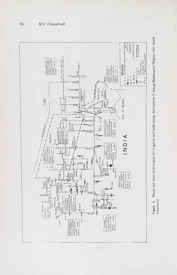
76 M C Chaturvedi
Fig
ure
2.
Mac
ro a
nd m
icro
lev
el p
roje
cts
for
irri
gati
on a
nd h
yd
el e
ner
gy d
evel
opm
ent
in G
anga-B
rahm
aputa
-Meghna r
iver
sy
stem
(sch
emat
ic)

The Ganga-Brahmaputra-Barak basin 77
Figure 3. Annual isohyetes (cm)
The Ganga rises in the southern Himalayas on the Indian side of the Tibet border. Its
five head streams—the Bhagirathi, the Alakhnanda, the Mandakini, the Dhauli Ganga
and the Pindar—all rise in the Uttarakhand division of the state of Uttar Pradesh (up).
Of these, the two main head streams are the Alakhnanda (the longer of the two) and the
Bhagirathi. The Bhagirathi, which is traditionally known as the source of the Ganga,
rises in India from the Gangotri glacier in the Himalayas at an elevation of about
7,010 m above mean sea level. After its confluence with the Alakhnanda at Dev Prayag,
the river assumes the name Ganga. After draining the middle ranges of the Himalayas
the river debouches into the plains at Hardwar. From Hardwar down to Allahabad
where the Yamuna joins it on the right bank, a distance of about 720 km, it generally
flows in a south/south-easterly direction. Lower down, the river flows eastwards and
past Varanasi, in up the Ganga is joined by a number of tributaries on both banks. Of
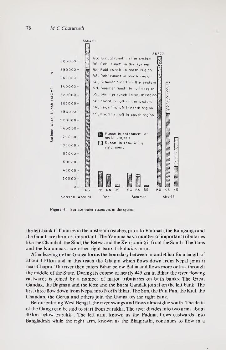
78 M C Chaturvedi
440430
2 CJ
X
o £
3 000 00
280000
260000
240000
220000
200000
180000
1 60000
140000
12 00 00
100000
800 00
600 00
400 00
200 00
0
‘I
1
368771
AG: Annual runoff in the system
RG Rabi runoff in the system
RN Rabi runoff in north region
RS: Rabi runoff in south region
SG : Summer runoff in the system
SN Summer runoff in north region
SS : Summer runoff in south region
KG Kharif runoff in the system
KN; Kharif runoff innorth region
KS ; Kharif runoff in south region
Runoff in catchment of major projects
Runoff in remaining
catchmen t
...IB
!■
AG
Season: Annual
RG RN RS
Rabi
SG SN SS
Sum mer
KG K N
Khari
KS
Figure 4. Surface water resources in the system
the left-bank tributaries in the upstream reaches, prior to Varanasi, the Ramganga and
the Gomti are the most important. The Yamuna has a number of important tributaries
like the Chambal, the Sind, the Betwa and the Ken joining it from the South. The Tons
and the Karamnasa are other right-bank tributaries in up.
After leaving up the Ganga forms the boundary between up and Bihar for a length of
about 110 km and in this reach the Ghagra which flows down from Nepal joins it
near Chapra. The river then enters Bihar below Ballia and flows more or less through
the middle of the State. During its course of nearly 445 km in Bihar the river flowing
eastwards is joined by a number of major tributaries on both banks. The Great
Gandak, the Bagmati and the Kosi and the Burhi Gandak join it on the left bank. The
first three flow down from Nepal into North Bihar. The Son, the Pun Pun, the Kiul, the
Chandan, the Gerua and others join the Ganga on the right bank.
Before entering West Bengal, the river swings and flows almost due south. The delta
of the Ganga can be said to start from Farakka. The river divides into two arms about
40 km below Farakka. The left arm, known as the Padma, flows eastwards into
Bangladesh while the right arm, known as the Bhagirathi, continues to flow in a

The Ganga-Brahmaputra-Barak basin 79
JAN FEB MAR APR MAY JUNE JULY AUG SEPT OCT NOV DEC
MONTHS
Figure 5. Monthly mean flows of some major rivers at their tail ends
southerly direction in West Bengal. Till some three hundred years ago, the Bhagirathi-
Hooghly constituted the main arm of the Ganga carrying the bulk of the flow.
Thereafter the Padma arm opened up more and more leaving Bhagirathi a mere spill
channel of the Ganga flowing mostly during high stages of flow. The river ultimately
flows into the Bay of Bengal about 145 km downstream of Calcutta. The length of the
river (measured along the Bhagirathi and the Hooghly) during its course in West Bengal
is about 520 km. Several tributaries join the Bhagirathi-Hooghly in West Bengal. The
Ganges in Bangladesh flows past Kushtia and Pabna till the Brahmaputra (locally
called Jamuna) joins it at Goalundo.
The united stream of the Brahmaputra and the Ganga beyond Goalunda continues
to flow south-east under the name Padma. At Chandpur, 105 km below Goalunda, the
Padma is again joined on the left bank by the Meghna, whose source is in the high
80 M C Chaturvedi
mountains, which are subjected to intense rainfall. From this confluence downwards,
the river, known as the lower Meghna becomes a very broad estuary making its exit into
the Bay of Bengal.
The precipitation over the Ganga basin is brought about by the south-west monsoon
as well as by cyclones originating over the Bay of Bengal. The average annual rainfall in
India varies from 35 cm on the western end of the basin to about 200 cm near the delta.
The river drains an area of 106.96 mha (excluding Tibet) and the average annual flow of
the Ganga at Farakka is about 55.01 mham.
2.21 The Brahmaputra
The Brahmaputra rises in the great glacier in the northern-most chain of the
Himalayas in the Kailash range just south of a lake called Konggyu Tsho. The river
under its Tibetan name of Tsangpo flows eastwards through southern Tibet for about
1700 km keeping a course roughly parallel to the main range of the Himalayas. In this
long journey it meets a number of tributaries. After turning south or southeast it enters
Arunachal Pradesh in India as the Dihang river. At the town of Sadiya, India, the
Dihang turns to the southwest and is joined by the two mountain streams of Luhit and
Dihang. After the confluence, about 1500 km from the Bay of Bengal, the river is known
as the Brahmaputra (the son of Brahma, the creator). The river then rolls down the Assam valley from east to west for about 720 km with
its channels meandering from side to side forming many islands. In Assam the river is
mighty even in the dry season and during the rains its banks are more than 10 km apart.
The largest island Majuli covers an area of 1250 sq km. As the river follows its braided
700 km course through the valley, it receives several rapid Himalyan streams, including
the Subansiri, the Kaneng, the Dhansiri, the Manas, the Champamati, the Saralbhanga
and the Sankosh. On the south bank, the main tributaries are the Noa Dihing, the Buri
Dihing, the Disang, the Dikhu and the Kopili. The Brahmaputra also has some
important tributaries flowing through North Bengal. They are the Tista, the Jaldhaka,
the Torsa, the Kaljani and the Raidok. Emerging swiftly from narrow gorges with steep
slopes, these rivers widen out considerably in the plains.
Swinging round the western spurs of the Garo Hills, near Goalpara, the river enters
the alluvial plains of Bangladesh, through which it flows southwards for another
270 km until it joins the Ganga at Goalundo. Below the confluence of the Tista, the old
channel of Brahmaputra branches off the left bank. From here to Goalunda the river is
called the Jamuna.
In Tibet the precipitation is in the form of snow which begins to melt in March
following the intrusion of warm air. Coming down the central basin in India, the annual
rainfall, brought by the southwest monsoon, is about 250 cm. Further down in
Bangladesh the rainfall over the basin averages about 240 cm. The river drains a total
catchment area of 23-41 mha (excluding Tibet and Bhutan) at Bahadurabad
(Bangladesh) and the average annual runoff at this site is 61-5 mham.
2.3 The Barak/Meghna
The Barak river, the head stream of the Meghna rises in the hills in Manipur (India) at
an elevation of about 2900 m. It flows south-westerly winding its way along hill ranges
for about 250 km. Thereafter it takes a sharp reflex bend and flows north. It changes

The Ganga-Brahmaputra-Barak basin 81
direction to west when emerging from the hills and follows a meandering course till it
enters Bangladesh. Many tributaries join the Barak. Near the border, the Barak
bifurcates into two rivers, the Surma and the Krishiyara which again join and flow in a
southerly direction under the name of Kalii. It takes the name Meghna before it meets
the Padma, which carries the combined flow of the Ganga and the Brahmaputra, at
Chandpur.
Below Chandpur the combined river, also known as the Lower Meghna, becomes a
very wide and deep estuary. It enters the Bay of Bengal through four principal channels.
The distance between Chandpur and the sea is about 130 km. The Meghna is thus
about 950 km long, of which 550 km including the estuary from Chandpur to the sea
lies in Bangladsh.
The river has a steep slope while flowing in the hills in India. After entering
Bangladesh it travels through the low-lying alluvial basin. When the Meghna flood
meets that of the Padma at Chandpur, its floods are backed and its basin acts as a
gigantic detention reservoir, without which the area between Goalundo and Chandpur
would be under much deeper water. At flood stages, the slope of the Meghna
downstream of Bhairab Bazar, where it meets the old Brahmaputra, is only about
1:88,000 which reflects the influence of back-water from the Ganga-Padma.
There is copious rainfall in the watershed of the Meghna and the Barak rivers.
Around the foothills in Assam, the rainfall reaches 500 cm on the windward side. At and
near Cherrapunji, where rainfall is amongst the highest in the world, the average annual
precipitation is about 1100 cm. In the plains of Bangladesh the rainfall varies from 200
to 300 cm. The drainage area of the Meghna at Bhairab Bazar is about 8 02 m ha and
average annual runoff is 11 1 mham.
2.4 Some systems characteristics
Despite the wide physiographic-geographical diversities some characteristics of the
system may be mentioned.
The Ganges-Jamuna area was once densely forested; historical writings indicate that
in the 16th and 17th centuries, wild elephants, buffaloes, bison, rhinoceroses, lions and
tigers were hunted there. Most of the original natural vegetation has disappeared from
the Gangetic basin as a whole and the land is intensely cultivated to meet the needs of an
ever-growing population. Hence, irrigation is increasingly depleting the low flows.
In ancient times the Ganga and some of its tributaries in the east were navigable. The
Ganga was navigable upto Agra. It has almost disappeared now and is practical
only in West Bengal and Bangladesh.
The Ganga as well as its tributaries and distributaries, are constantly vulnerable to
changes in their course in the delta region. Such changes have occurred in compara¬
tively recent times, specially since 1750; the most spectacular of these changes was the
eastward diversion of the Tista river and the ensuing development of the new channel of
the Jamuna, which occurred in 1787 with an exceptionally high flood in the Tista.
The delta of the Greater Ganga system is one of the biggest in the world covering an
area of 56,700 km2. The salient statistics of the region are shown in table 1. Some important
characteristics of the region are summarised in table 2. The salient pieces of information
about the entire Ganga basin and relevant statistics for India are given in table 3. The
details for the Ganga Basin in terms of eight sub-basins are given in table 4.
5 -6

82 M C Chaturvedi
Table 1. Salient characteristics of the Greater Ganga basin
Ganga Brahmaputra
No Item Unit India Nepal Bangladesh figure for basin India Bangladesh
1 2 3 4 5 6 7 8 9
A. Land
1. Geographical area Mha 86 14 14-08 6-74 106-96* 18-71 4-7
2. Cultivable area at Mha 60-30 398 3-64 67-92 12-15 3-0
present cultivation
B. Population
1. 1971 Census Million 221-19 11-29 27-03 259-51 17-65 24-83
2. Population density per sq km 257-00 8000 401-00 243 94 528
3. Agr. population Million 149-74 10-34 1906 179-14 1193 17 5
4. Agr. population % 67-6 91-6 70-5 69-03 67-6 70-5
C. Water
1. Mean annual rainfall cm/yr 60-200 100-250 150-212 120 212 200
2. Total annual runoff mhm 55-01*** — Neg 55-01 51-25 10-25
3. Irrigation potential Mha 17-81 1-202 295 21-96 2-3 1 46
(present)
D. Energy
1. Hydropower potential Mkw 13-274 85-00 Neg 98-27 13-43 Neg
2. Hydropower installed Mkw 1 83 0-41 Neg 2-24 00-18 Neg
3. Hydropower installed % 13-79 0-49 Neg 2-33 1 34 0-0
E. Unit figures
1. Land per capita Ha 0-39 1-25 0-25 0-4 1-06 0 189
2. Utilizable water/unit m3 116-00 — — — . 171-0 —
cultivable land
3. Cropping intensity % 125 — — — 118-0 —
4. Irrigation intensity % 23 — — — 21-3 —
5. Utilizable and utilized
water resource
a. Surface mhm 18-5/70-4 — — — 0-61/70 —
b. Ground mhm 10-64/39-4 — — — 0-02/1 1 —
c. Total mhm 29.14/59.4 — — — 2-68/23-5 —
Note: A. (i) *** Inclusive of runoff of Nepal; (ii) ** 29-3 Mha in Tibet and 529 Mha in Bhutan not included in this figure;
(iii) * 2-9 Mha in Tibet not included in this figure; (iv) Neg = Negligible; Agr. = Agricultural; (v) These figures are
derived from Irrigation Commission Report.
B. The figures have been taken from various published sources and are only indicative.
3. Developmental issues
Although technological activities for water resources development have been under¬
taken in the past, the region still provides unique opportunities for the development of
the huge unutilised potential. The best way would be to have an integrated approach,
treating the entire river basin as one. This may not be possible from political
considerations, but at least developmental planning may be carried out in totality, as
well as from each country’s point of view and then a bargained developmental plan for
each country may be developed.
The development in the Ganga basin in the pre- and post-Independence period has
been ad hoc and of the project-oriented technological type. The policy in the pre-
Independence period was one to support sustenance agriculture. It is now necessary to
develop an appropriate integrated future developmental policy. The approach has
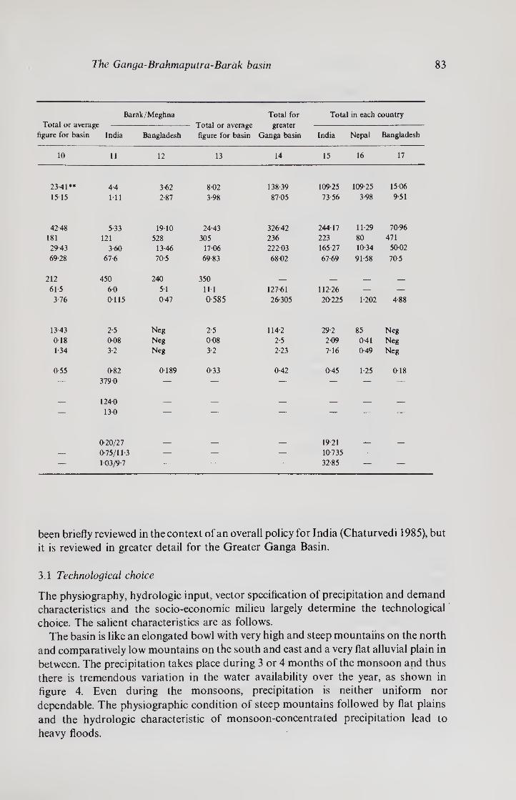
The Ganga-Brahmaputra-Barak basin 83
Barak/Meghna Total for Total in each country Total or average -- Total or average greater -
figure for basin India Bangladesh figure for basin Ganga basin India Nepal Bangladesh
10 11 12 13 14 15 16 17
23-41** 4.4 362 802 138 39 109 25 109 25 15-06
1515 111 2-87 3-98 87-05 73-56 3-98 9 51
42-48 5-33 19 10 24-43 326-42 244-17 11 29 70-96 181 121 528 305 236 223 80 471
29-43 3-60 13 46 17-06 222-03 165-27 10 34 50-02
69-28 67-6 70-5 6983 68-02 67-69 91 58 70-5
212 450 240 350 _ _ _ _ 615 6-0 5-1 111 127-61 112-26 — —
3-76 0-115 0-47 0-585 26-305 20-225 1-202 4-88
1343 2-5 Neg 2-5 114-2 29-2 85 Neg 0 18 0-08 Neg 0-08 2-5 209 041 Neg 1 34 3-2 Neg 3-2 2-23 7 16 049 Neg
0-55 0-82 379-0
124-0
0 189 0-33 0-42 0-45 1 25 018
13-0
0-20/27 1921 — 0-75/11 3 — — — 10-735 — — — 1-03/9-7 — — — 32-85 — —
been briefly reviewed in the context of an overall policy for India (Chaturvedi 1985), but
it is reviewed in greater detail for the Greater Ganga Basin.
3.1 Technological choice
The physiography, hydrologic input, vector specification of precipitation and demand
characteristics and the socio-economic milieu largely determine the technological
choice. The salient characteristics are as follows.
The basin is like an elongated bowl with very high and steep mountains on the north
and comparatively low mountains on the south and east and a very flat alluvial plain in
between. The precipitation takes place during 3 or 4 months of the monsoon and thus
there is tremendous variation in the water availability over the year, as shown in
figure 4. Even during the monsoons, precipitation is neither uniform nor
dependable. The physiographic condition of steep mountains followed by flat plains
and the hydrologic characteristic of monsoon-concentrated precipitation lead to
heavy floods.

84 M C Chaturvedi
Table 2. Summary of salient features of the Greater Ganga Basin
Item
Total for
Greater
Ganga basin
Share for
India
Land
Geographical area (106 ha) 138 39 109-25
Cultivable area (106 ha) 8705 73-56
Population
1971 Census (million) 326-42 244-17
Population density (per km2) 80—645 with an 223-0
Agricultural population (million)
average of 240
22203 165-27
Agricultural population (% of total) 68-02 67-69
Water
Mean annual rainfall (cm/yr) 60-450 with an —
Total annual runofT (mham)
average of 350
12761 112-26
Irrigation potential (mha) 26-3 20-2
Energy
Hydropower potential (MW) 114-2 29-2
Hydropower installed 2-5 209
Unit figures
Land per capita 0-42 0-45
Utilizable water/unit culturable land (m3) 116-379 —
Cropping intensity — 118-125
Irrigation intensity — 13-23
Utilizable water (mham)
(a) surface 19-21
(b) groundwater — 10-735
The Himalayas, which form a considerable portion of the catchment area of the
Greater Ganga Basin, are very young, erodible and have very steep slopes leading to
high flows and very heavy sediment loads—the highest in the world during the
monsoons (Leeden 1975). While the storage potential is large, it is a very small
proportion of the total water resources of the region—only about 8% (Rao 1976).
Most of the storage and hydroelectric potential of the Himalayan region is in Nepal.
Increasing population in Nepal is going to exacerbate the erosion, sedimentation and
flood problem due to cutting of forests for agriculture and energy demands. Thus, it is
both in India’s and Nepal’s interest to collaborate in the rapid development of the
watershed, social forestry, storage and hydroelectric energy, in the Himalayan region for
utilising the valuable water resources and hydroelectric potential and reducing the
hazards of erosion and floods. Water for this region is like oil for the middle east
countries with the further advantage of non-depletability. It can be said that gravity is
the biggest asset of this region. The economy of this region can be built around the
development of water, light industry and tourism rather than food crop-oriented
agriculture as necessity demanded in the past. Of course, these transitions will take
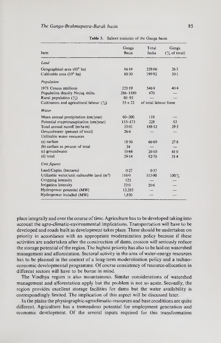
The Ganga-Brahmaputra-Barak basin 85
Table 3. Salient statistics of the Ganga basin
Item
Ganga
Basin
Total
India
Ganga
(% of total)
Land
Geographical area (106 ha) 86 14 32806 26-3
Cultivable area (106 ha) 60-30 19992 30-1
Population
1971 Census (million) 22119 546-9 40-4
Population density No/sq. miles 286-1180 470 —
Rural population (%) 80-93 — —
Cultivators and agricultural labour (%) 55 + 22 of total labour force
Water
Mean annual precipitation (cm/year) 60-200 118 —
Potential evapotranspiration (cm/year) 155-175 228 93
Total annual runoff (mham) 5501 18812 29-3
Groundwater (percent of total)
Utilizable water resources
26-6 — —
(a) surface 18-50 66-60 27-8 (b) surface as percent of total 34 — —
(c) groundwater 10-64 26-10 41-0 (d) total 29-14 92-70 314
Unit figures
Land/Capita (hectares) 0-27 0-37
Utilizable water/unit culturable land (m3) 116-0 115 00 100% Cropping intensity 125 — —
Irrigation intensity 23-0 20-6 —
Hydropower potential (MW) 13,285 — —
Hydropower installed (MW) 1,830 — —
place integrally and over the course of time. Agriculture has to be developed taking into
account the agro-climatic-environmental implications. Transportation will have to be
developed and roads built as development takes place. These should be undertaken on
priority in accordance with an appropriate modernization policy because if these
activities are undertaken after the construction of dams, erosion will seriously reduce
the storage potential of the region. The highest priority has also to be laid on watershed
management and afforestation. Sectoral activity in the area of water-energy resources
has to be planned in the context of a long-term modernization policy and a techno-
economic developmental programme. Of course consistency of resource-allocation in
different sectors will have to be borne in mind. The Vindhya region is also mountainous. Similar considerations of watershed
management and afforestation apply but the problem is not so acute. Secondly, the
region provides excellent storage facilities for dams but the water availability is
correspondingly limited. The implication of this aspect will be discussed later.
In the plains the physiographic-agroclimatic-resources and base conditions are quite
different. Agriculture has a tremendous potential for employment generation and
economic development. Of the several inputs required for this transformation
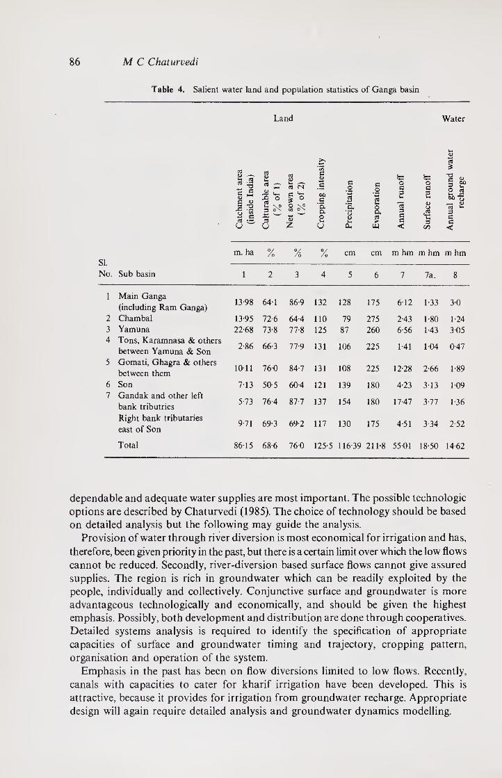
86 M C Chaturvedi
Table 4. Salient water land and population statistics of Ganga basin
Land Water
Is 3 2 "3 a e o
6
a <u ^ 1 ° in VO ^ ox
3 O
03 <N
P ^
d> z
>*
’S3
<D «-»
£ c <u Ss fa “O
g
g
c o
B
a o ■*—»
o G 3 t-4
O G 3 t-
3 O
'Ck Q, O
a
|
u
a 03 *>
1 G C3
8 <B u*
1 G
u a w < 3
C/5 G <
o3 -C o
si.
No.
m. ha °/ /o °/ /o °/ /o cm cm m hm m hm m hm
Sub basin 1 2 3 4 5 6 7 7a. 8
1 Main Ganga
(including Ram Ganga) 13 98 64 1 86-9 132 128 175 6 12 1-33 3-0
2 Chambal 13 95 72-6 64-4 110 79 275 2-43 1 80 1 24 3 Yamuna 22-68 73 8 77-8 125 87 260 6-56 1 43 3-05 4 Tons, Karamnasa & others
between Yamuna & Son 2-86 66-3 77-9 131 106 225 1 41 104 0-47
5 Gomati, Ghagra & others
between them 1011 76-0 84-7 131 108 225 12-28 2-66 1 89
6 Son 7 13 50-5 60-4 121 139 180 4-23 3-13 1-09 7 Gandak and other left
bank tributries 5-73 76-4 87-7 137 154 180 17-47 3-77 1 36
Right bank tributaries
east of Son 9-71 69-3 69-2 117 130 175 4 51 3-34 2-52
Total 8615 68-6 76-0 125-5 116-39 211-8 55-01 18-50 14-62
dependable and adequate water supplies are most important. The possible technologic
options are described by Chaturvedi (1985). The choice of technology should be based on detailed analysis but the following may guide the analysis.
Provision of water through river diversion is most economical for irrigation and has,
therefore, been given priority in the past, but there is a certain limit over which the low flows
cannot be reduced. Secondly, river-diversion based surface flows cannot give assured
supplies. The region is rich in groundwater which can be readily exploited by the people, individually and collectively. Conjunctive surface and groundwater is more
advantageous technologically and economically, and should be given the highest
emphasis. Possibly, both development and distribution are done through cooperatives.
Detailed systems analysis is required to identify the specification of appropriate
capacities of surface and groundwater timing and trajectory, cropping pattern,
organisation and operation of the system.
Emphasis in the past has been on flow diversions limited to low flows. Recently,
canals with capacities to cater for kharif irrigation have been developed. This is
attractive, because it provides for irrigation from groundwater recharge. Appropriate
design will again require detailed analysis and groundwater dynamics modelling.

The Ganga-Brahmaputra-Barak basin 87
People Unit figures
Utilizable
Utilized
% of utilizable
c o
*4-»
£ g
~o G eg
Sur
face
runoff
(% o
f 7)
Gro
und w
ater
(% o
f 7)
Sur
face
(% °
f 9)
Gro
un
d w
ater
(“/.
of
10)
To
tal
util
ized
%
of
util
izab
le
Popula
tion
o. a s O
<4-. o
rs
a M
'c/3 c a C
ult
ura
ble
ar
ea/c
apit
a
Wat
er/c
apit
a
Wat
er/c
ultu
rafc
% g
ross
sow
n ar
ea i
rrig
ated
°/ /o °/ /o <y /o °/ /o 7 /o m 7 /o No/km2 ha m3 7 /o
9 10 11 12 13 14 15 16 17 18 19 20
21-7 351 800 37-2 74-0 49-69 9-25 353 018 1830 101-80 18 3
74-2 35-8 46 1 64-0 52-0 15-35 2 91 110 0-66 2400 36-15 13 3 21 8 33-7 109.2 43-0 70-0 45-66 8-60 201 0-37 2100 57-25 23-6
73-8 26-5 36 5 29-5 35-10 6-83 1 37 239 0-28 2750 99-0 250
21 9 120 800 89-5 80-9 36-29 6 35 259 0-21 3910 184-3 26 1
740 18 9 32-85 10-0 29-5 7-88 1-57 111 0-45 6750 1480 15-7
21 5 5-9 6904 11-0 56-6 26-22 4-85 457 0-17 7200 4310 9-0
74-3 38-7 85-0 9-2 60-0 33-27 6-30 342 0-20 2100 104-60 37-1
33-6 19 3 71-0 39-4 59 1 221-29 41-20 259 0-32 3630 145-26 21-0
We have emphasized conjunctive surface and groundwater development, but since
surface water resources have already been considerably developed the focus will be on
groundwater development along with modernization of the existing systems.
Groundwater development represents the so-called ‘divisible technology’ and is very
attractive for the development and diffusion of the culture of technology. It could
provide employment in construction as well as through intensive irrigation, leading to
the most productive agriculture and the highest possible cropping intensity.
There is a serious problem of energy scarcity as electrical energy supplies have not
been developed adequately and diesel is going to be in increasingly short supply. There
is thus a case for urgently resolving the energy problem through a scientific energy
policy. On an ad hoc basis we may plan on development through diesel tubewells.
Groundwater is a major user of energy and surface water is a rich source of energy
through hydroelectric generation. There is thus a strong case for conjunctive surface-
groundwater and energy development.
In surface water resources development, the focus has been entirely on diversion of
the low flows of the major rivers. Mostly, the diversion site has been the mountain
foothills and the diverted flows basically represent the low flows of the Himalayan

88 M C Chaturvedi
Table 5. Developmental programme
Phase Alluvial plains
Himalayan
region
Vindhyan
region
A. 1st five
years
1. Intensive
groundwater
development through
energised/diesel pump
sets for 100% irrigation
intensity
2. Development and
modernisation of
existing systems for
conjunctive water
energy development
with kharif channels
3. Development and
modernization of water
distribution and field
management such as
efficient water use, land
levelling and
environmental
development.
4. Watershed
development for flood
mitigation, groundwater
recharge and soil
conservation with
development of minor
rivers and streams.
1. Complete road
network
2. Intensive water-shed
development
3. Start storage
projects, hopefully in
Nepal as well
1. Start development of
storage projects with
provision for additional
storage from annual
pumped storage
schemes and develop
surface and
groundwater irrigation
2. Start modernization
as in 2 of plains
3. Environmental
management
B. 2nd five 1. Increasingly energise 1. Continue A. 2 1. Continue A. 1
years A.l 2. Continue A. 3 2. Continue A. 2
2. Complete A. 2 3. Continue A. 3
3. Continue A. 3
4. Continue A. 4
C. 3rd five
years
1. Complete B. 1 and
continue B. 3 and B. 4
1. Complete A. 2
2. Continue A. 3
1. Complete A. 2 and
A. 3
2. Continue A. 1
3. Start transfer part of
annual pump storage
projects
D. Next 15 1. Continue increasing 1. Complete all 1. Complete C. 3 and
years efficiency of water use development and continue increasing
and environmental continue increasing environmental and
management ie B. 3
and B. 4
environmental efficiency resources efficiency

The Ganga-Brahmaputra-Barak basin 89
catchment region. The flows of the vast catchment of the plains are carried down in the
numerous minor streams. Some, which may even be quite large according to
international standards, like the Gomti, have been neglected. The runoff from the plain
area, which is a major component of the total runoff, thus causes floods and is wasted.
The focus should be on land-water dynamics, attempting to develop the land by
organic as well as structured means, so that floods and soil erosion are mitigated and
water resources are developed through groundwater recharge and storage. Possible
technologies are bunding, appropriate watershed management through cropping
practices and afforestation, storage through check dams to prevent submergence, and
to increase water detention, additional groundwater recharge by heavy pumping before
monsoons. The approach is so far conceptual, but its feasibility warrants detailed study.
In this connection the concept of the Ganges-Water Machine along perennial and non¬
perennial rivers and forced groundwater recharge may also be mentioned (Chaturvedi
1981a). For convenience, we may consider the above issue under two heads
(a) development of minor rivers and streams for flood mitigation, groundwater
recharge and irrigation and (b) watershed development for flood mitigation, groun¬
dwater recharge and soil conservation.
In groundwater development the question arises about the annual quantum to be
developed. Under the natural land-water dynamics a certain utilizable potential known
as safe yield is estimated. With the increasing perturbation of land water, a long-term
groundwater developmental policy has to be developed, which may lead to mining in
the short run. Mining may have repercussions on the yield of shallow wells and surface
discharge and, therefore, land-water dynamics has to be modelled to identify an
appropriate dynamics policy of groundwater development.
The foregoing discussion relates to macrolevel development and distribution. An
equally important aspect is field-level distribution and use. In the past, due to certain
colonial-bureaucratic reasons, use of water and development of land was left almost
entirely to the farmers. It is well known that our water use is most wasteful, and integral
lining of water courses, land levelling and associated technological activities at the field
level have to be carried out. Technology is, however, more than development of
projects. It is a process of social change and has to embrace adequate institutional and
motivational mechanisms. Field-level development has to be integrated with rural
development and can be a major source of employment generation and promotion of
modernization. Workshops can be developed in mofussil towns for the construction of
pumpsets and strainers. Drilling of tubewells and canal lining can be developed through
rural entrepreneurship. Command area development and water management activities
have been started but they have to be considerably extended and strengthened.
Our concern is primarily the development of water resources for irrigation. To a
certain extent, this will contribute to flow reduction although specific conventional and
non-conventional technological alternatives will have to be developed as flood damage
is a serious matter in this region. Besides loss of life and property, agricultural
development is seriously affected by floods in these regions.
We have developed five conceptual interacting technological sets: (i) development of
resources in the mountain zones, (ii) modernization of existing systems for conjunctive
water-energy development with kharif channels, (iii) development of minor rivers and
streams for flood mitigation, groundwater recharge and irrigation, (iv) watershed
development for flood mitigation, groundwater recharge and soil conservation and
(v) field level modernisation. A long-term regional water resources system plan has to
90 M C Chaturvedi
be developed to identify the optimal portfolio of projects so that land-water development is obtained over optimal time. This exercise has to be carried out for each planning region to arrive at the optimal plan for the Ganges basin. Water resources availability continuously increases from west to east, but it is almost equally unreliable all over. There should thus be increasing emphasis on groundwater development as we move eastward. In fact, the problem increasingly becomes one of managing excess monsoon water through groundwater recharge and drainage without disrupting the local terrain. To this extent, the problem in Bangladesh is essentially hydraulic rather than hydrologic, as discussed later.
The north-east, the Barak and the deltaic regions have certain specific physiographic- hydrologic characteristics although as discussed earlier their development is integrally linked with the rest of the region. The problems of the north-east region are similar to the Himalayan region, but increasing attention has to be paid to integrated flood management along with hydroelectric generation. The problem of the Barak region is essentially a problem of flood management. The problem of the deltaic region is essentially a hydraulic problem as mentioned earlier.
One of the important aspects of water resources development is the generation of electricity. Although this is generally accepted, several policy issues and outstanding potential technological options have been completely missed in the development activities so far, as discussed below.
The storage-hydroelectric potential in the Himalayas is large and very economical. There is also a very large run-of-river hydroelectric potential in the Himalayan region. The Vindhya region also provides considerable potential, which is also exceedingly economical for two reasons—the storage/height ratio is one of the highest in the world and the foundation conditions are faultless.
The point to be emphasized is that first, the storage and run-of-river plants have to be developed jointly so that, through suitable operating policies, optimal capacities in each plant and in the system are obtained. Implicit is integrated planning of the total power sector (Chaturvedi 1981b, 1985). Even then, if there is surplus potential of secondary energy, it can be converted into primary energy, by using the secondary energy to pump the large monsoon surface flows for storage in the Vindhya region, either in the Ganga basin or in the adjoining Narmada basin. In principle, this is a novel annual pumped- storage scheme for both hydro-energy and resource conservation.
Implicit in these suggestions is integrated water sector and power sector planning. Besides the interlinkage of water and energy sector for supply, there is an important supply-demand interlinkage. Groundwater development may account for a major portion of electric energy demand (as much as 20 to 60% at different stages of development) while water supplies may be met either from surface or groundwater sources. An integrated surface-groundwater-energy planning as discussed under systems planning can contribute to significant economics.
Further issues relate to environment and navigation. From both considerations, minimum flows have to be maintained. It is again a matter of economic analysis, but it can definitely be said that the largescale low-flow diversions of the past may be unacceptable both economically and environmentally. It is interesting to note that when the first major canal of the region, the Ganga Canal, was contemplated it was considered mandatory to ensure that navigation did not suffer and therefore the canal was joined again with the Ganga at Kanpur (Cautley 1860). The importance of navigation diminished not only because more attractive technological options like the

The Ganga-Brahmaputra-Barak basin 91
railways or the roads developed, but also because economic development did not take
place. River transport would be the most attractive means of transportation for the
increasing agricultural and other bulky commodities that constitute about 80-90 % of
the goods traffic. It is often not realized that only about 4 meters of draft is needed for
river transport and even 2 m would be enough. River transport should be complemen¬
tary to other modal choices instead of being competitive, and integrated water, energy
and transportation systems planning can lead to significant economies.
To consider the complex, interlinked as well as competing issues, involving large
variations in technological choices and capacities—spatially and temporally, for
multipurpose use, integrated systems planning is mandatory. Before identifying a
programme of development, it is necessary to consider the international issues involved
in the development of the Greater Ganga Basin. These have been discussed elsewhere
(Chaturvedi 1985).
In the dispute with Bangladesh, the simple fact that the development of Nepal is
crucial for the development of the Ganga basin and is in the interest of both countries
has been lost sight of. Highest priority has to be given to the integrated development of water resources in the region irrespective of whether the sites are located in Nepal or
India.
3.3 Development programme
The developmental policy for the water resources of the basin may now be summarised
and a tentative schedule may be postulated, as shown in table 5. In the schedule, our
concern has been mainly development of water supply for irrigation. We have
concentrated on the three main physiographic regions. Similar policy schedules can be
drawn up for energy and navigation and then integrated-hierarchial systems planning
can be carried out as discussed later. It will be seen that the schedule depends primarily
on management potential, the internal and international political and financial policy
of giving credit for development rather than on technological considerations. We have
postulated a time schedule from our experience of developing the water resources of
this region over the last 30 years, considering only management and technological
factors and not considering the financial or political factors as a constraint. If the latter
are uncongenial, it can only slow down the development and make it slightly less
economical. We believe that if earnest efforts are made, in 5 years almost complete and
dependable irrigation can be provided in almost the entire region. It can be made more
and more economical with full development in 30 years of irrigation, flood control,
hydroelectric energy and the environment. This may be contrasted with the con¬
templated attainment of about an additional 5 % irrigation at a crawling rate. Of course
the proposed schedule, will require a revolution in technological management and
institutions, and a high order of political and social commitment.
The conceptual policy issues developed so far have to be quantified through systems
studies.
4. Conclusion
As stated at the outset, the Greater Ganga basin is one of the world’s great natural
resources with an outstanding potential for hydroelectric energy and agricultural
production. Neglect over the last few centuries has led to serious environmental

92 M C Chaturvedi
degradation and human depravation, leading to one of the most intense concentrations
of population. The natural resources and environmental development offers an
outstanding opportunity for economic development and employment generation. It is
a very complex problem, making a systems approach mandatory.
For the successful application of technology, institutional modernization is a
precondition. Concepts and approaches developed in colonial days still reign supreme;
these have to be jettisoned first and foremost.
References
Cautley P T 1860 Completion report Ganges Canal (London: Smith Elder) Chaturvedi M C 1981a Groundwater development and flood mitigation, Indo-US Workshop on Flood
Mitigation and Water Resources Development, Indian Institute of Technology, New Delhi Chaturvedi M C 1981b First Annual Report, U. P. Water Resources Systems Study, Indian Institute of
Technology, New Delhi
Chaturvedi M C 1985 Sadhana 8: 39-72 Chaturvedi M C, Rogers P 1985 Sadhana 8: 329-350 Encylopaedia Britanniea 1978 Ganges river (Chicago: Encyclopaedia Britannica Inc.) Vol. 7 Leeden F 1975 Water resources of the world (New York: Port Washington) Rao K L 1976 India's water wealth (New Delhi: Orient Longmans) Workshop on Integrated Development of the Ganga-Brahmaputra-Barak-Basin 1978, Gandhi Peace
Foundation, New Delhi
The coordinating model of the Ganga Basin
M C CHATURVEDI, PETER ROGERS* and SHYANG-LAI KUNG**
Applied Mechanics Department and Centre for Systems Engineering and Policy Studies, Indian Institute of Technology, New Delhi 110016, India
* Department of Environmental Engineering, Harvard University, Pierce Hall, 121 Cambridge, Massachusetts 02138, USA
** Argonne National Laboratory, 9700, S Case Avenue, Argonne, Illinois 60439, usa
Abstract. A scheme of model studies required to analyse a complex large scale system through decomposition approach is outlined. First, the total system is proposed to be modelled to
identify interlinkages of the subsystems. Then the subsystems are analysed in detail to develop response functions. Finally the optimal system functioning is obtained by modelling the entire system in terms of response functions of the components.
A linear programming model is developed for modelling the total system to identify the interlinkages. Its application is demonstrated in the Greater Ganga Basin using published data. Trade-off is developed between power generation and irrigated area in various seasons.
Keywords. Large scale systems; multilevel hierarchical approach; co-ordinating screening model; linear programming model
1. Introduction
Systems analysis of large systems is an integrated-hierarchial multilevel and multistage
activity because of the complexity, scale and dynamic nature of the problem. Multilevel
hierarchial analysis may be carried out in several ways (Lasdon 1970; Haimes 1977;
Chaturvedi 1974). In the first instance, the total system may be modelled to identify the
order of interlinkage of the sub-systems. In the second study, the sub-systems may be
examined in detail and their response expressed as a function of the interlinkage over
the likely range as anticipated from the first study. Finally, the optimal system
functioning may be obtained by modelling the entire system in terms of the response
functions of each of the sub-systems as obtained from the second study. The type of model depends upon the characteristics, scale and complexity of the
system, as well as on the objectives of the analysis. The first study carried out through a
model called the coordinating-screening model is for coarse screening and de¬
terministic modelling dividing the year into two or three time periods. A linear-
programming approach may be used. Further, by adapting the inflows over a range to
cover the likely variability of inflows, the implications of the stochastic nature of inputs
may be studied (Jacoby & Loucks 1972; Chaturvedi & Srivastava 1981). For the second
series of models for sub-systems analysis, any appropriate systems analysis approach
using deterministic and stochastic models may be used (Hall & Dracup 1970; Biswas
1976; Chaturvedi 1984). And finally for the third-stage analysis, mathematical
programming models and simulation models, singly or hierarchially, may be used. For
studying the Ganga basin, the hierarchial modelling scheme shown in figure 1 was
A list of symbols is given at the end of the paper.
93
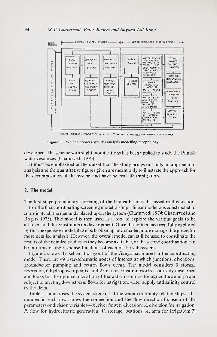
94 M C Chaturvedi, Peter Rogers and Shyang-Lai Kung
INPUT STUDIES
GENERAL SYSTEM STUDIES WATER RESOURCES SYSTEM STUDIES
ITERATE THROUGH SENSITIVITY ANALYSIS TO REQUISITE DEGREE /REFINEMENT AND BALANCE
Figure 1 Water resources systems analysis modelling morphology
developed. The scheme with slight modifications has been applied to study the Punjab
water resources (Chaturvedi 1979).
It must be emphasised at the outset that the study brings out only an approach to
analysis and the quantitative figures given are meant only to illustrate the approach for
the decomposition of the system and have no real life implication.
2. The model
The first stage preliminary screening of the Ganga basin is discussed in this section.
For the first coordinating-screening model, a simple linear model was constructed to
coordinate all the demands placed upon the system (Chaturvedi 1974; Chaturvedi and
Rogers 1975). This model is then used as a tool to explore the various goals to be
attained and the constraints on development. Once the system has been fully explored
by this inexpensive model, it can be broken up into smaller, more manageable pieces for
more detailed analysis. However, the overall model can still be used to coordinate the
results of the detailed studies as they become available, or the second coordination can
be in terms of the response functions of each of the sub-systems.
Figure 2 shows the schematic layout of the Ganga basin used in the coordinating
model. There are 49 river-schematic nodes of interest at which junctions, diversions,
groundwater pumping and return flows occur. The model considers 5 storage
reservoirs, 6 hydropower plants, and 25 major irrigation works as already developed
and looks for the optimal allocation of the water resources for agriculture and power
subject to meeting downstream flows for navigation, water supply and salinity control
in the delta.
Table 1 summarises the system sketch and the water continuity relationships. The
number in each row shows the connection and the flow direction for each of the
parameters or division variables—X, river flow; Y, diversion; Z, diversion for irrigation;
P, flow for hydroelectric generation; V, storage locations; A, area for irrigation; T,
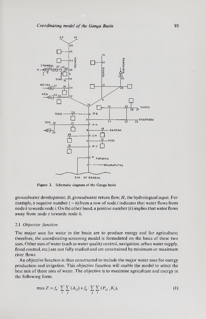
Coordinating model of the Ganga Basin 95
4 8 47
Figure 2. Schematic diagram of the Ganga basin
groundwater development; D, groundwater return flow; H, the hydrological input. For
example, a negative number (— k) from a row of node i indicates that water flows from
node k towards node i. On the other hand, a positive number (k) implies that water flows
away from node i towards node k.
2.1 Objective function
The major uses for water in the basin are to produce energy and for agriculture;
therefore, the coordinating-screening model is formulated on the basis of these two
uses. Other uses of water (such as water quality control, navigation, urban water supply,
flood control, etc.) are not fully studied and are constrained by minimum or maximum
river flows.
An objective function is thus constructed to include the major water uses for energy
production and irrigation. This objective function will enable the model to select the
best mix of these uses of water. The objective is to maximise agriculture and energy in
the following form.
max Z =/, • £ £ My) +/„'££ (*y U) * j j ‘
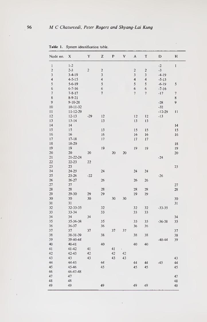
96 M C Chaturvedi, Peter Rogers and Shyang-Lai Kung
Table 1. System identification table.
Node no. X Y Z P V A T D H
1 1-2 -2 1
2 2-3 2 2 2 2 -3
3 3-4-19 3 3 3 -4-19
4 4-5-15 4 4 4 -5-15
5 5-6-19 5 5 5 -6-19 5
6 6-7-16 6 6 6 -7-16
7 7-8-17 7 7 7 -17 7
8 8-9-21 8
9 9-10-28 -28 9
10 10-11-32 -32
11 11-12-29 -12-29 11
12 12-13 -29 12 12 12 -13
13 13-14 13 13 13
14 14 14
15 15 15 15 15 15
16 16 16 16 16 16
17 17-18 17 17 17
18 18-20 18
19 19 19 19 19 19
20 20 20 20 20 20
21 21-22-24 -24
22 22-23 22
23 23 23 24 24-25 24 24 24
25 25-26 -22 -26
26 26-27 26 26 26
27 27 27
28 28 28 28 28 28
29 29-30 29 29 29 29
30 30 30 30 30 30
31 31 31
32 32-33-35 32 32 32 -33-35
33 33-34 33 33 33
34 34 34 34
35 35-36-38 35 35 35 -36-38 35
36 36-37 36 36 36
37 37 37 37 37 37
38 38-31-39 38 38 38 38
39 39-40-44 -40-44 39
40 40-41 40 40 40
41 41-42 41 41
42 42-43 42 42 42
43 43 43 43 43 43
44 44-45 44 44 44 -45 44
45 45-46 45 45 45 45
46 46-47-48
47 47 47
48 48 48
49 49 49 49 49 49

Coordinating model of the Ganga Basin 97
where fa is the net benefit of agriculture due to irrigation and fp is the net benefit of energy production.
2.2 The constraints
The constraints of the coordinating model are formulated according to system
identification in table 1 and the schematic layout in figure 2. There are six major types
of constraints, (i) hydrological constraints, (ii) agricultural constraints, (iii) capacity
constraints, (iv) municipal water supply, (v) economic constraints, (vi) environmental
constraints, and others. A complete description of the constraint set for each node is given in appendix A.
2.2a Hydrological constraints (i) Continuity constraints—a typical constraint of this
kind will be
Xij + Zij — Hij + Xi+l j; + Di + 1 j. (2)
The amount of water that flows away from node i (river flow Xijf irrigation diversion
Zy) equals the amount of water that flows towards node i (river flow Xi+i j,
groundwater return Di+l tJ and hydrological input Hy). (ii) Groundwater returns—a certain fraction of the unpumped groundwater is
returned to the river at a downstream node,
Dij = Zj 9: AG: 1TU (3)
For example, at node i, the groundwater pumped in a year is Zjfj and the amount of
groundwater left is 9iAGi — 'LjTij, of which <y portion is returned to the river at a
downstream node during the y'th period.
2.2b Agricultural constraints (i) Field irrigation requirements for each crop are
provided by surface water and groundwater irrigation,
Tij+Zij = a,jAlJ. (4)
It is assumed for simplicity that the irrigation water is lost to the river system. This
water is either evapotranspirated or percolated into the aquifer.
(ii) Culturable land and current irrigation level: irrigation cannot exceed the cul-
turable land at each district and it should reach at least the current irrigation level,
ALt ^ Atj ^ AH,, (5)
(iii) An artificial constraint is imposed in the model to make the summer season a land
preparation season for the following kharif season (i.e., irrigated acreage at any district
during the summer season equals that of the kharif season):
Z-i 2 — ^13, (6)
where An, Ai2, Ai3 are areas irrigated in rabi, summer and kharif seasons respectively.
2.2c Capacity constraints (i) Irrigation channel: new capacity for irrigation channels
at each agricultural district is provided in order to divert more surface water for
irrigation. The increased channel capacity at node i becomes ZHt + Z new,,
Ztj ^ mj ■ (ZH{ + Znew,),
where mj is the number of months during the jth period.
5 -7
(7)

98 M C Chaturvedi, Peter Rogers and Shyang-Lai Kung
(ii) Groundwater storage: annual groundwater irrigation at any agricultural district
cannot exceed the available groundwater storage at that district,
I (8) j
(iii) Diversion channel: the amount of water diverted cannot exceed the capacity of the
channel,
Yij ^ mj' YH{. (9)
(iv) Reservoir live storage: The reservoir cannot store more water than its live storage
capacity during any period of time,
Kj < VHt. (10)
(v) Hydropower plant capacity: The water that drives the turbine cannot exceed the
generating capacity. New turbines can be installed for necessary expansion of the power
plant,
PtJ ^ mJ(PHi + Pnew,). (11)
2.2d Municipal water supply Water is diverted from the Ganga to meet the municipal
water demand at Calcutta,
Ytj ^ rrij YL{. (12)
2.2e Economic constraint Power demand distribution: the energy generated during
each period must satisfy the distributional demand (rjj),
ZiPij-K^rijZZiPij-Ki). (13) « j >
2.2f Environmental and other constraints In order to maintain river flows for
navigation, water quality control, irrigation requirements downstream and other
purposes, several minimum flows are provided,
Xij^mj-XLi. (14)
3. Data used
Input data of the coordinating-screening model contains hydrological inputs (H(J),
field irrigation requirement given in appendix B (a^), culturable land (AHt), low flow
requirement (XL(), groundwater availability (0,/lG,), fractions of groundwater return (£j), reservoir live storage (FH,), hydropower plant capacity (PH,), power conversion
factor (K,), and power demand distribution t]j).
3.1 Hydrological input
Since the model is deterministic, the hydrology of a typical single year is required. For
flood protection and other purposes, a hydrology of extreme events which would have a
chance of realization of one year out of every 50 or 100 years may be more appropriate.
The hydrological inputs (HtJ) at various nodes are given in table 2. This table is
constructed according to the estimated average monthly flows in the sub-basins of the
Ganga by Briscoe (1974).

Coordinating model of the Ganga Basin 99
Table 2. Hydrological inputs (m cu m/season)
Node no Rabi Summer Kharif
1 80561 43891 346812
5 680 12925
7 773 14694
8 1814 34474
9 421 7995
11 636 12092
35 188 3580
38 188 3580
39 188 3580
44 471 8949
45 471 8949
14 3823 3330 22806
15 6501 8030 37461
16 1052 350 14838
18 8338 7229 53410
19 259 57 931
20 688 229 9697
23 5551 4785 32928
27 5551 4785 32928
28 370 123 5217
30 764 654 4489
31 575 194 8236
34 575 194 8236
37 575 194 8236
43 2506 777 32984
47 936 809 5569
48 936 809 5569
49 259 57 931
Total:
(1) Include Brahmaputra (node)
Rabi Summer Kharif
119620 182327 742096
1044043 m cu m/year.
(2) Exclude Brahamaputra (node)
Rabi Summer Kharif
39059 38436 395284
472779 m cu m/year.
3.2 Field irrigation requirements
Monthly field irrigation requirements (a0) are estimated as per crop, rainfall,
temperature, wind, humidity, sunshine, solar radiation and other factors at each
agricultural district. These monthly requirements are then aggregated into three
seasons for the simplified three-season model: (a) rabi season (November, December,
January, February and March); (b) summer season (April, May and June); and
(c) kharif season (July, August, September and October). Field irrigation requirements
for different seasons at various agricultural districts are presented in table 3.

100 M C Chaturvedi, Peter Rogers and Shyang-Lai Kung
Table 3. Field irrigation requirements at various districts (Seasonal)-(meter/unit area)
Node no A ^max ^min Rabi Summer Kharif
2 6600 660 0-5860 0-0510 0-3300 3 6600 660 0-6200 0-1310 0-3800 4 1900 190 0-6200 01310 0-3800 5 1900 190 0-6200 01310 0-3800 6 2600 260 0-6200 01310 0-3800 7 3000 300 0-6200 0-1310 0-3800
12 24000 2400 0-5490 0-2730 0-5720 13 20000 2000 0-5210 0-2150 0-5340 15 19000 1900 0-6200 0-1310 0-3800 16 19000 1900 0-6200 0-1310 0-3800 17 33000 3300 0-6340 0-1430 0-3700 19 26100 2610 0-6610 01390 0-3950 24 40000 4000 0-6140 0-1990 0-5020 26 36800 3680 0-6140 0-1990 0-5020 28 19000 1900 0-6490 0-1400 0-3750 29 20800 2080 0-4920 0-2250 0-4820 32 20000 2000 0-6220 0-1960 0-5140 33 3100 310 0-6450 0-1610 0-4560 35 20000 2000 0-6220 0-1960 0-5140 36 4700 470 0-6450 01610 0-4560 38 20000 2000 0-6220 01960 0-5140 40 100000 5000 0-6360 0-2280 0-7240 44 50000 2000 0-5320 0-2690 1-039 45 50000 2000 0-5100 0-2440 0-7800 49 26100 2610 0-6610 0-1390 0-3950
Total A max
Am- min
57-42 m ha 4 64 m ha
3.3 Culturable land and current irrigation level
Information about culturable land at each agriculture district is reported by the
Irrigation Commission (1972). Table 3 also gives the culturable land districtwise. The
current irrigation level has been assumed at 10 % of the culturable land in most districts.
3.4 Current irrigation capacity
Table 4 lists some capacities of irrigation channels as recorded in the Irrigation
Commission (1972). New capacity (Znew;) is constructed in the coordinating model to
allow more surface water diversion for irrigation.
3.5 Groundwater storage
Groundwater storage at an agriculture district is the product of annual groundwater
availability (0,) and area (AGt) over which groundwater is available. Aquifer is assumed
to be fully recharged annually. These groundwater storages are given in table 5
3.6 Reservoir live storage, hydro-power plant capacity, and power conversion factor
Figures of reservoir live storages, current power plant capacities, and power conversion
factors are presented in table 6. Although preliminary study indicates that there is a

Coordinating model of the Ganga Basin 101
Table 4. Current channel capacities
Node no m cu m/mon Node no mcu m/mon
2-7 _ 29 5-7 12 155-7 32 —
13 297-5 33 56-6 15 283-2 35 —
16 311-5 36 85-0 17 283-2 38 —
19 28-3 40 260-5 24 283-2 44 90-6 26 396-4 45 424-8 28 28-3 49 28-3
Table 5. Groundwater availability
Node no mcum Node no mcum Node no mcum
2, 3 2255 15 6462 32, 35, 38 2987 4, 5 677 16 4454 33 579
6 902 17 11659 36 877 7 621 19 11277 40 23816
12 7467 24 8960 44, 45 2987 13 2987 26 4480 49 10600
28 2838 29 3734
Total groundwater capacity: 122512mcum.
Table 6. Power conversion factors, power plant capacities and reservoir live storages.
Node no. MW
PH (MW) VH (mcum) mcu m/month
20 01816 195 10608 30 0-2270 130 2220 37 0 0454 13 780 41 0-0272 64 42 0-0908 111 1567 43 01090 75 6920
reservoir and a power plant at node 34 (ken), they are removed from the model because
they are not reported in the Irrigation Commission (1972). Appropriate new power
plant capacity (Pnew,) may be installed in order to attain higher energy production.
Power production factor (/(,) is calculated by using a head of one half dam height.
3.7 Power demand distribution
Distributional constraints may be imposed on the energy production so that the energy
output meets the monthly or seasonal demand (rjj). Initial values of the demand

102 M C Chaturvedi, Peter Rogers and Shyang-Lai Kung
distribution are taken at 0.0955, 0.0797, 0.0762, 0.0515, 0.0630, 0.0784, 0.0797, 0.0797,
0.0938,0.1233,0.1039, and 0.0753 for the respective twelve months. These distributions
should be reevaluated according to the power requirements for groundwater pumping
and other irrigation facilities.
3.8 Other water demands
Water uses such as water quality control, navigation, and other purposes are not well
developed. These water uses are considered in the model as minimum river flows and
are presented in table 7.
4. Matrix Generation
The coordinating-screening model described above is a form of linear program and can
be solved by ibm/mpsx. The matrix preparation for this ibm/mpsx used in Italy on the
Tiber River Basin by Rogers & Chi (1973) is employed to generate the matrix of the
Ganga Basin in the mpsx input format. The Ganga Basin linear program for a simplified
three-season model consists of 490 constraint rows of which most are continuity
equations, about 1050 decision variables and 3500 non-zero matrix elements.
5. Solutions
In this simplified three-season model solutions using various assumptions have been
obtained. In each solution the summer season (June irrigation) is assumed to be land
preparation and the model is constrained so that the area under irrigation during the
summer season at each district must also be irrigated in the kharif season. In most
solutions energy is maximized subject to different constraint sets.
5.1 Solution 1
Maximizing energy under current power plant capacity,
ma xZ=fP-Zt'Z(Pij-Ki). (15) j ‘
In this solution, energy production is unrestricted by the distributional constraints. The maximum energy under the current generating capacity is 55,863 GWh
Table 7. Low flow requirements.
Node no. XL (mcum/month)
2 100 5 50 7 240 9 285
10 255 44 38 45 180
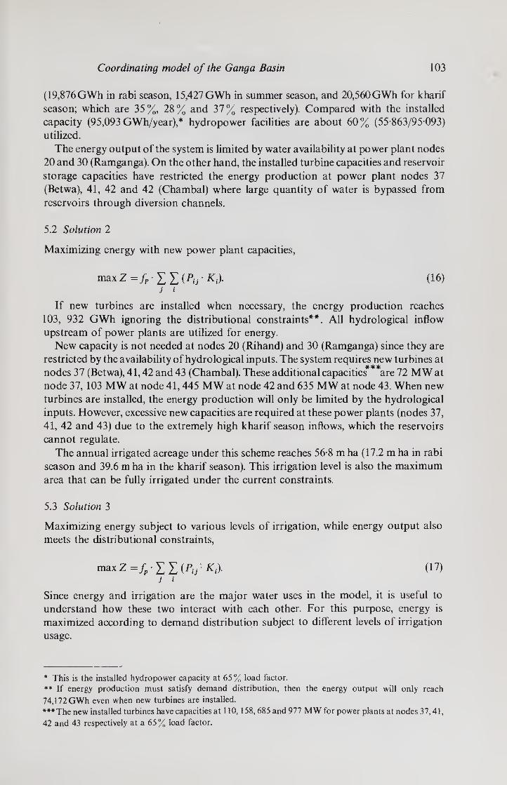
Coordinating model of the Ganga Basin 103
(19,876 GWh in rabi season, 15,427 GWh in summer season, and 20,560 GWh for kharif
season; which are 35%, 28% and 37% respectively). Compared with the installed
capacity (95,093 GWh/year),* hydropower facilities are about 60% (55-863/95 093)
utilized.
The energy output of the system is limited by water availability at power plant nodes
20 and 30 (Ramganga). On the other hand, the installed turbine capacities and reservoir
storage capacities have restricted the energy production at power plant nodes 37
(Betwa), 41, 42 and 42 (Chambal) where large quantity of water is bypassed from
reservoirs through diversion channels.
5.2 Solution 2
Maximizing energy with new power plant capacities,
ma xZ=fP-ZYJ(Pij-Ki). (16) j i
If new turbines are installed when necessary, the energy production reaches
103, 932 GWh ignoring the distributional constraints** ***. All hydrological inflow upstream of power plants are utilized for energy.
New capacity is not needed at nodes 20 (Rihand) and 30 (Ramganga) since they are
restricted by the availability of hydrological inputs. The system requires new turbines at
nodes 37 (Betwa), 41,42 and 43 (Chambal). These additional capacities are 72 MW at
node 37,103 MW at node 41,445 MW at node 42 and 635 MW at node 43. When new
turbines are installed, the energy production will only be limited by the hydrological
inputs. However, excessive new capacities are required at these power plants (nodes 37,
41, 42 and 43) due to the extremely high kharif season inflows, which the reservoirs
cannot regulate.
The annual irrigated acreage under this scheme reaches 56-8 m ha (17.2 m ha in rabi
season and 39.6 m ha in the kharif season). This irrigation level is also the maximum
area that can be fully irrigated under the current constraints.
5.3 Solution 3
Maximizing energy subject to various levels of irrigation, while energy output also
meets the distributional constraints,
ma xZ^-IK^-K,.). (17) j ‘
Since energy and irrigation are the major water uses in the model, it is useful to
understand how these two interact with each other. For this purpose, energy is
maximized according to demand distribution subject to different levels of irrigation
usage.
* This is the installed hydropower capacity at 65 % load factor. ** If energy production must satisfy demand distribution, then the energy output will only reach 74,172 GWh even when new turbines are installed. ***The new installed turbines have capacities at 110,158, 685 and 977 MW for power plants at nodes 37,41, 42 and 43 respectively at a 65 % load factor.

104 M C Chaturvedi, Peter Rogers and Shyang-Lai Kung
To facilitate the solution, the power distributional constraints are formulated in the
following form:
<«) > j >
where distribution values of tjj are subject to adjustment to simulate real demands.
With an irrigation level lower than 55 m ha (15.9 m ha in the rabi season, 39-1 m ha in
the kharif season) the energy output reaches a maximum level at 54,254 GWh
(23,362 GWh in rabi, 10,465 GWh in summer and 20,427 GWh in kharif.) On the other
hand, when energy production is less than 36,461 GWh (15,700 GWh in rabi,
7,033 GWh in summer and 13,728 GWh in kharif), the irrigation level is maximized at
56.8 m ha (17.2 m ha in rabi and 39.6 m ha in kharif). It is not possible to generate energy
higher than 54,254 GWh by sacrificing irrigation and it is not feasible to insist on an
irrigation level higher than 56.8 m ha by giving up energy production. For any level of
irrigation between these two extremes (55 and 56.8 m ha), there is a corresponding
energy production (between 36,461 and 54,254 GWh). No further parametric study on
energy and irrigation in these ranges is made since the difference between the two
irrigation levels is relatively small. Solutions of these two extremes are shown in figure 3. Any point inside the boundary ABCD is feasible but not efficient. Furthermore,
points between A and B are not efficient because the irrigation level can be increased
from zero to 55 m ha without any loss of energy. Similarly, points between C and D are
not efficient. Points that fall on the line BC denote the production frontier. Point C
represents operating the system for agricultural maximization and treating energy as a
residual. The marginal rate of transformation of energy for agriculture at any point on
the line BC is the gradient of the line segment BC. This rate is estimated at
-C
2 cn
t_) ZD □ O cr CL
O cr UJ z: LU
A
A (0,54254) B(55, 54254)
■>C (56.767, 36461)
1
1 ( |
1 1
(
1 1 ID (56.767,0) ,
IRRIGATED AREA (m ha)
2 (An * Al3) l
Figure 3. Trade-ofT between energy and total irrigation

Coordinating model of the Ganga Basin 105
— 10,070 GWh/m ha (i.e., to gain lmha of irrigation between points B and C
10,070 GWh energy is sacrificed).
The range of irrigated acreage is only 1.8 m ha (56.8 — 55) while energy production
has a relatively wide range (from 36,461 to 54,254 GWh) of variation. No substantial
irrigation can be gained by giving up energy production (at a rate of 10,070 GWh for only 1 m ha).
Irrigated acreage is at capacity level at most downstream districts where water is
available through accumulation of inflows. Reservoirs are full in the kharif season to regulate the excessive monsoon water for irrigation in the following rabi season.
5.4 Solution 4
Trade-off between rabi irrigation and kharif irrigation,
maxZ = ]T Ai3, subject to various levels of ]T An. (19) i i
Since the reservoirs and groundwater storage can regulate the water for irrigation from
one season to the next, there is a definite trade-off between rabi irrigation and kharif
irrigation. Solutions (points B, C, D, E, F, G and H) shown in figure 4 illustrate the
Figure 4. Trade-ofT between kharif and rabi irrigations

106 M C Chaturvedi, Peter Rogers and Shyang-Lai Kung
corresponding irrigation level in the kharif season for each irrigation level in the rabi
season. It is not feasible to irrigate in the rabi season at a level higher than 27.4 m ha.
The maximum level of irrigation in kharif can be achieved at a higher level (43.6 m ha).
Point D (at which rabi irrigation is 17.2 m ha and kharif irrigation is 39.6 m ha)
represents operating the system for maximum annual total irrigation. Steeper gradients
(— 2.96, — 3.73) at points E, G in figure 4 indicate that 2.96 and 3.73 units of irrigation
acreage in kharif season would be given up for every unit increment of irrigation in the
rabi season. This is because the June irrigation (summer season) binds the irrigation level of the kharif season (Ai2 = Ai3); therefore, a large quantity of river flow in the
kharif season is wasted.
5.5 Solution 5
Maximizing energy subject to different levels of rabi and kharif irrigations,
ma xZ=/,-£I(PyK,X (20) J ‘
this solution is obtained assuming that no new power capacity is provided and energy
production must satisfy the demand distributional constraints. For every rabi
irrigation level (according to §5.4) the energy is maximized while increasing kharif
irrigation level until infeasibility. To obtain solutions among rabi irrigation, kharif
irrigation and the corresponding energy production, the parametric procedure of linear
programming is adopted.
6. Results
Solutions (rabi irrigation, kharif irrigation and energy production) are presented in
table 8 and figure 5. The convex plane DGHIJKLN'E represents the operating
production frontier. Any point that falls on or inside the feasible region but not on this
plane (DGHIJKLN'E)* is not efficient and is dominated by that plane. Point / in
figure 5 represents operating the system for agricultural maximization and treating
energy production as a residual. Points that fall on the line DE represent operating the
system for energy maximization. The rates of marginal transformation are calculated
between energy and kharif irrigation for each given rabi irrigation as shown in figure 6.
The range of variation for energy production as defined in figure 6 is 17,793 GWh
(54,254 — 36,461 GWh) and irrigation acreage has a variation of 15.3 m ha
(56.8 — 41.5 GWh). The range of these variations is relatively narrow and no substantial
amount of energy will be sacrificed for further agricultural development and vice versa.
Basrur (1975) discussed the difficulties of identifying a trade-off between energy and
irrigation under the system described in this paper.
At some agricultural districts, June irrigation has bound the following kharif
irrigation because less water is available during the summer season.
Reservoirs are used to store the excessive monsoon water to their storage capacities
for the irrigation of the following rabi season.
* Point N' in figure 5 is a linear extrapolation point on the line EN to prevent the production frontier from going to points M and N where the rates of marginal transformation are negligible.
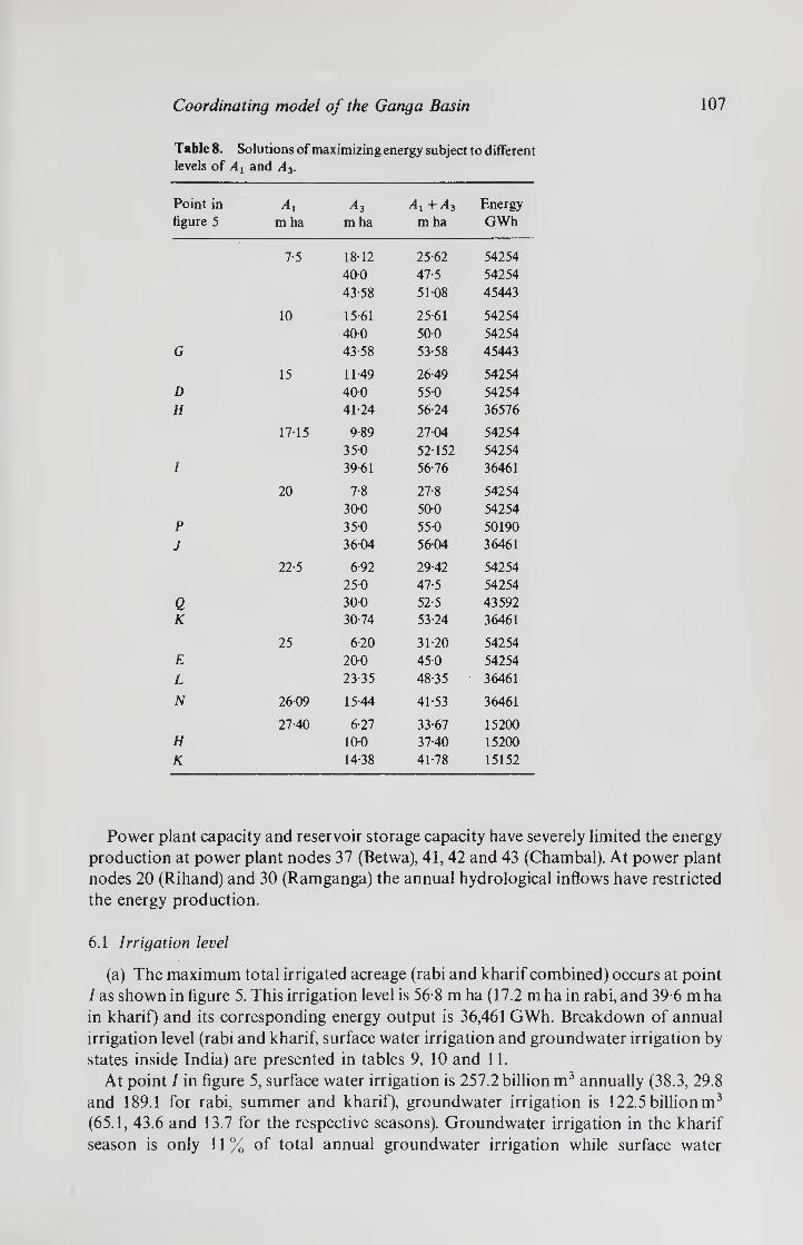
Coordinating model of the Ganga Basin 107
Table 8. Solutions of maximizing energy subject to different levels of A, and A3.
Point in
figure 5 ^1
m ha ^3
m ha
Ai +A3 m ha
Energy
GWh
7-5 18-12 25-62 54254
40-0 47-5 54254
43-58 51-08 45443
10 15-61 25-61 54254
40-0 500 54254
G 43-58 53-58 45443
15 11-49 26-49 54254
D 40-0 55-0 54254
H 41-24 56-24 36576
17-15 9-89 2704 54254
35-0 52152 54254
I 39-61 56-76 36461
20 7-8 27-8 54254
30-0 50-0 54254
P 35-0 55-0 50190
J 3604 56-04 36461
22-5 6-92 29-42 54254
25-0 47-5 54254
Q 30-0 52-5 43592
K 30-74 53-24 36461
25 620 31-20 54254
E 20-0 450 54254
L 23-35 48-35 36461
N 2609 15-44 41-53 36461
27-40 6-27 33-67 15200 H 10-0 37-40 15200
K 14-38 41-78 15152
Power plant capacity and reservoir storage capacity have severely limited the energy
production at power plant nodes 37 (Betwa), 41, 42 and 43 (Chambal). At power plant
nodes 20 (Rihand) and 30 (Ramganga) the annual hydrological inflows have restricted
the energy production.
6.1 Irrigation level
(a) The maximum total irrigated acreage (rabi and kharif combined) occurs at point
/ as shown in figure 5. This irrigation level is 56-8 m ha (17.2 m ha in rabi, and 39 6 m ha
in kharif) and its corresponding energy output is 36,461 GWh. Breakdown of annual
irrigation level (rabi and kharif, surface water irrigation and groundwater irrigation by
states inside India) are presented in tables 9, 10 and 11.
At point / in figure 5, surface water irrigation is 257.2 billion m3 annually (38.3, 29.8
and 189.1 for rabi, summer and kharif), groundwater irrigation is 122.5 billion m3
(65.1, 43.6 and 13.7 for the respective seasons). Groundwater irrigation in the kharif
season is only 11 % of total annual groundwater irrigation while surface water

108 M C Chaturvedi, Peter Rogers and Shyang-Lai Kung
Energy
103 GWH
Figure 5. Trade-off among energy, kharif irrigation and rabi irrigation. At point I, A, = 17152, A, = 39-615 and energy = 36,461, where A, + A3 = 56,167 is the maximum irrigated acreage that can be achieved
irrigation is nearly 74% of the total surface water irrigation. This is because of the
monsoon water availability in the kharif season. Surface water and groundwater irrigation relationship is presented in table 12.
lb) Maximum energy production that satisfies the distributional constraints occurs
on the line DE as shown in figure 5. This energy output is 54,254 GWh and the
corresponding irrigation levels are between 45 m ha and 55 m ha.
6.2 Cropping intensity
The Irrigation Commission (1972) reported that the agricultural level in the Ganges
Basin had a net sown area of 43.824 m ha, a gross sown area of 54.757 m ha, a net irrigated area of 10.817 m ha and a gross irrigated area of 12.544 m ha. Thus, the
cropping intensity in 1972 was 125% and the irrigation intensity was 23%.
The cropping and irrigation intensities in the future according to the above solutions
are as follows* (a) The cropping intensity is improved to 148 % when rabi irrigation is
* In order to calculate these intensities, it is assumed that all culturable land is cultivated in the kharif season with or without irrigation and only the area that is irrigated in the rabi season is cultivated in that season.

Coordinating model of the Ganga Basin 109
maximized (point M in figure 5). (b) The cropping intensity is 130% when the total
irrigation is maximized (point / in figure 5).
All the interesting cropping intensities and irrigation intensities from the solutions
obtained in this paper can be found in table 13.
6.3 Degree of complementarity
It is possible to assess the degree of complementarity of the three-season model by
assuming net benefits of energy and irrigation. When these net benefits are absent,
ranges of degree of complementarity are obtained.
When the system is operated as a single-purpose one for energy the annual energy
production is 54,254 GWh; and when the system is operated for agriculture maximiz¬
ation, the annual irrigation level is 56 8 m ha. Therefore, if the full potential of the

110 M C Chaturvedi, Peter Rogers and Shyang-Lai Kung
Table 9. Breakdown of irrigation level between states and seasons
Sub-basin HP. Haryana Delhi Rajasthan UP. M.P. Bihar W.B. Total
by basin
Chambal Ax
a3
1-428 1-908
0-017 0-022
1-087 1 453
2- 532 3- 383
Yamuna 0018 0106
0-296 1-780
0-010 0-061
0-243 1-463
0-558 3 359
0-526 3 163
1-651 9-932
Ramganga 1-283 0-471
1-283 0-471
Tons & others
0-071 0-529
0-081 0-607
0-038 0-284
0-190 1 420
Gomati & Ghaghara
2-260 6-777
0-078 0-233
2-338 7-010
Son 0-115 0-296
0-918 2-279
0-417 1-035
1-450 3-600
Gandak & others
0-083 0-083
3-471 3-471
0-696 0-696
4-250 4-250
Right bank tributaries
1-195 3-191
0-837 2-237
2-032 5-428
Main Ganga 1-427 4-120
1-427 4-120
Total by State
0018 0106
0-296 1-780
0-010 0061
1-671 3'71
5-814 15-647
2612 7-502
5 199 8214
1- 533 2- 933
17-153 39614
Table 10. Annual surface irrigation (109 m3/year)
Sub-basin HP. Haryana Delhi Rajasthan U P. M.P. Bihar W.B. Total by
basin
Chambal 13-814 0-162 10-521 24497
Yamuna 0-823 13-781 0-469 11-328 26-008 24493 76-902
Ramganga 5-907 5-907
Tons and others 2-128 2-441 1-141 5-710
Gomati and Ghaghara 48-393 1-667 50-060
Son 1-219 9-707 4406 15-332
Gandak and others 0-697 29 049 5-827 35-573
Right bank tributaries
1
7-821 5-482 13-303
Main Ganga 29-959 29-959
Total by State 0-823 13-781 0-469 25-142 114 473 76-211 20-862 5-482 257-243

Coordinating model of the Ganga Basin 111
Table 11. Annual groundwater irrigation (109 m3/year)
Sub-basin HP. Haryana Delhi Rajasthan UP. M.P. Bihar W.B. Total by
basin
Chambal 13-430 0157 10-229 23-816
Yamuna 0175 2-937 0-100 2-414 5-543 5-221 16-390
Ramganga 3-734 3-734
Tons & others 1-058 1-213 0-567 2-838
Gomati & Ghaghara Son
12-992 0-976 7-774
0-448 3-529
13-440 12-280
Gandak & others 0-245 10-203 2-047 12495
Right bank tributaries 15911 11-153 27-064
Main Ganga 10-454 10-454
Total by State 0 175 2-937 0-100 15-844 35-159 24-437 30-658 13-200 122-510
Table 12. Water utilisation of various solutions
Point
Surface water
109 m3 % by
season
Ground- water
109 m3 % by
season
Water Irrigated total acreage
109 m3 m ha Energy GWh
1 rabi 38-6 15-0 649 53-0 103-5 17-2 15-70 summer 29-5 11-5 43-9 35-8 73-4 — 7-03 kharif 189-1 73-5 13 7 11-2 202-8 396 13-73 total 257-2 1000 122-5 100-0 379-6 56-8 36-46
D rabi 37-5 24-0 114-5 95-3 152-0 25-0 23-36 summer 280 17-9 5-4 4-5 33-4 — 10-47 kharif 90-8 58-1 0-2 0-2 91-0 20-0 20-43 total 156-3 1000 1201 100-0 276-4 45-0 54-26
E rabi 42-7 161 48-4 45 1 91-0 15-0 23-36 summer 33-1 12-5 41 2 38-4 74-3 — 10-47 kharif 188-9 71-4 17-7 16 5 206-6 40-0 20-43 total 264-7 1000 107-3 100-0 371-9 55-0 54-26
N rabi 45-3 42-4 121-1 98-8 166-4 27-4 6-55 summer 15-3 14 3 1-2 1-0 16 5 — 2-93 kharif 46-4 43-3 0-2 0-2 46-6 6-3 5-72 total 107-0 100-0 122-5 100-0 229-5 33-7 15-20
N' rabi 44-0 23-7 84-7 73-8 128-7 261 15-70 summer 24-2 13 0 21-2 18-6 45-4 — 7-03 kharif 117-6 63-3 90 7-6 126-6 15 4 13-73 total 185-8 100-0 114 9 100-0 300-7 41 5 36-46
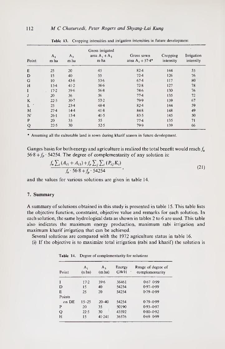
112 M C Chaturvedi, Peter Rogers and Shyang-Lai Kung
Table 13. Cropping intensities and irrigation intensities in future development
Point Aj
m ha a3
m ha
Gross irrigated area A, + A3
m ha Gross sown
area A, + 57-4* Cropping intensity
Irrigation intensity
E 25 20 45 82-4 144 55 D 15 40 55 72-4 126 76 G 10 43-6 53-6 67-4 117 80 H 15 4 41-2 56-6 72-8 127 78 I . 17-2 39-6 56-8 74-6 130 76 J 20 36 56 77-4 135 72 K 22-5 30-7 53-2 79-9 139 67 L ' 25 23-4 48-4 82-4 144 59 M 27-4 14-4 41-8 84-8 148 49 N' 26 1 15 4 41-5 83-5 145 50 P 20 35 55 77-4 135 71
Q 22-5 30 52-5 79-9 139 66
* Assuming all the culturable land is sown during kharif season in future development.
Ganges basin for both energy and agriculture is realized the total benefit would reach fa
56-8 + fP ■ 54254. The degree of complementarity of any solution is:
/.iMn + AiJ+filjlAW fa ■ 56-8 +/p- 54254
(21)
and the values for various solutions are given in table 14.
7. Summary
A summary of solutions obtained in this study is presented in table 15. This table lists
the objective function, constraint, objective value and remarks for each solution. In
each solution, the same hydrological data as shown in tables 2 to 6 are used. This table
also indicates the maximum energy production, maximum rabi irrigation and
maximum kharif irrigation that can be achieved.
Several solutions are compared with the 1972 agriculture status in table 16.
(i) If the objective is to maximize total irrigation (rabi and kharif) the solution is
Table 14. Degree of complementarity for solutions
Point A,
(n ha) a3
(m ha) Energy GWH
Range of degree of complementarity
I 17-2 39-6 36461 0-67-0-99 D 15 40 54254 0-97-0-99 E Points
25 20 54254 0-79-0-99
on DE 15-25 20-40 54254 0-79-0-99 P 20 35 50190 0-93-0-97
Q 22-5 30 43592 0-80-0-92 H 15 41-241 36576 0-69-0-99

Coordinating model of the Ganga Basin 113
Table 15. Summary of solutions
Objective function Constraints Objective value Remarks
1. Maximizing energy
II (Py;K.)
2. Maximizing energy
II(JV*|>
3. Maximizing energy
III Pij.K,)
4. Maximizing kharif irrigation
1^3 i
1. Basic constraints (hydrological inputs. . . .)
2. Minimum water supply, navigation etc.
3. Minimum flow at Farakka 4. No new power capacity 5. No power distributional
constraint.
1. Basic constraints 2. Minimum water supply,
navigation etc. 3. Minimum flow at Farakka 4. New power capacity 5. No power distribution.
1. Basic constraints 2. Minimum water supply,
navigation, etc. 3. Minimum flow at Farakka 4. No new power capacity 5. Power distribution 6. Various levels of
irrigation (418 to 56-8 m ha)
1. Basic constraints 2. Minimum water supply,
navigation, etc. 3. Minimum flow at Farakka 4. Various levels of
rabi irrigation (10 to 27-4 m ha)
55,863 GWh
B
NB B
103,932 GWh NB
NB
from 36,461 to B
54,254 GWh
B in rabi season B B B
from 14-4 to 43 6 m ha B
B in rabi season
B
Table 16. Present (1972) Irrigation and future irrigation (m ha)
(1) (2) (3) (4) (5) (6)
Rabi 57-42 17-15 40-27 57-42 Summer 57-42 39-62 17-80 57-42 Kharif 57-42 39-62 17-80 57-42
Total* 12-54 102-30 114-84 56-77 58-07 114-84
* Total equals rabi plus kharif. (1) Present (1972) gross irrigated area; (2) Present (1972) gross non- irrigated area; (3) Total = (1) + (2); (4) Future area under irrigation; (5) Future area not under irrigation; (6) Total = (4) + (5)

114 M C Chaturvedi, Peter Rogers and Shyang-Lai Kung
point / in figure 5. The total irrigation level is 56.8 m ha which is an improvement of
44-2 mha over the 1972 gross irrigation level (12.5 mha) or 2.5 times better.
(ii) If the objective is to maximize rabi irrigation, then point M in figure 5 dominates
the other solutions. The total irrigation level is 41.8 mha (27-4 in rabi, 14-4 in kharif)
which is a 29.3 mha improvement over 1972 level.
(iii) In order to avoid substantial energy sacrifice when rabi irrigation is maximized,
a compromise solution point N' in figure 5 is obtained. The total irrigation level is
41-5 mha (26-1 in rabi, 15 4 in kharif). This is a 29 mha improvement over the 1972
level. In this case, the reduction of rabi irrigation is only 1.3 m ha from that of case (ii)
while the energy output is increased from 15,200 GWh to 36,461 GWh.
Since this model of the Ganga basin considers only the benefit to the Indian states it is
necessary to understand the water availability when the Ganga enters Bangladesh
downstream; River flows at Farakka (which enter Bangladesh) are given in table 17.
Values shown in this table are under the maximum irrigation level (56 8 m ha) in Indian
states. Table 18 summarizes the results for each of the 9 sub-basins and compares them
with the Irrigation Commission (1972) estimates for resource use in 1968-69.
8. Conclusion
The objective of this model is to maximize the net benefit of energy and irrigation:
/.• 1(41+4,7)+/,'EI (PijK,)- i j i
This objective function has been replaced by a single-purpose objective (either
agriculture or energy) in every solution. It either maximizes energy subject to various
irrigation levels or vice versa. However, if the net benefits of energy and irrigation are
estimated and the objective function
/.E(4i+43)+/fEE(fljK,) * j ‘
is adopted, the solution should fall upon the plane DGHIJKLN'E&s shown in figure 5.
Solutions obtained by a comprehensive parametric study on values fa and fp will cover
points on the same plane DGHIJKLN'E in figure 5. The model presented in this paper aims to achieve ultimate development for Indian
states within the Ganga basin. It is equally important to provide necessary water
downstream of the Ganga for optimal development in Bangladesh. This is expressed in
the model in the form of minimum irrigation requirements in Bangladesh (XL2). It is
found that the rabi season river flow at Farakka is critical. River flow in this season
Table 17. River flows at Farakka, in Bangladesh, and diversion to Calcutta (million cubic metres)
River flows at Farakka
Water available after Brahmaputra joins Ganga
Diversion to Calcutta
Rabi 500 81,061 14,680 Summer 6,580 150,471 8,808 Kharif 173,226 520,038 11,744
Total 180,306 751,570 11,744

Coordinating model of the Ganga Basin 115
Table 18. Ganga basin water use and irrigation
Average
annual Surface Ground Irrigated
runoff water water areas
Basin (m cu m) (mcum) (mcu m) (ha x 106)
I 24,312 24,497 23,816 K 3-383 (0-886)
(8,305) (5,562) R 2-532
II 65,621 76,902 16,390 9-932 (3-054)
(15,523) (9,513) 1-651
III 18,626 5,907 3,734 0-471 (0-382)
(7,144) (1,446) 1-283
IV 14,123 5,710 2,838 1-420 (0-394)
(3,819) (U26) 0190
V 122,793 50,060 13,440 7-101 (2-143)
(21,280) (13,186) 2-338
VI 42,308 15,332 12,280 3-600 (0-336)
(10,335) (838) 1-450
VII 134,277 35,573 12,495 4-250 (0-374)
(26,006) (1,068) 4-250
VIII 45,145 13,303 27,064 5-428 (1-872)
(28,366) (1,552) 2-032
IX 42,533 29,959 10,454 4-120 (1-914)
(11,643) (6,604) 1-427
Total 509,738 257,243 122,510 39-614 (11-36)
(132,421) (40.895) 17-153
Figures in parentheses represent Irrigation Commission estimates of 1968-69 resource use.
(A^i) is binding at the minimum level. It is important to study the relation between the minimum flow requirement at Farakka and the irrigation level in Indian states.
There are few trade-off points found between energy and irrigation in this tljree- season model. This is because under the assumed system no water is diverted for irrigation upstream of a hydropower plant. The same water that drives the turbine can be used to irrigate an agricultural district downstream as discussed by Basrur (1975). The model in its present form considers the Ganga basin within Indian states as a unit despite possible different local interests. If various targets are required by different states in the basin, then more trade-off points can be expected.
Finally, the power conversion factor is estimated according to one half of the dam height. The real energy production will be less than the solutions obtained in this paper. Although seasonal average height of water surface in the reservoir is more appropriate, it is not used in this present study.
It must be clarified as emphasized at the outset that the study brings out only an approach to analysis and the quantitative figures given above are meant only to illustrate the approach for the decomposition of the system and have no real-life implication. However, it must also be added that the systems approach is a powerful tool for planning and if the currently available data with the various governmental agencies were made available, significant improvements in real-life water resources development could be made. This model is only the starting point for a detailed study.
9
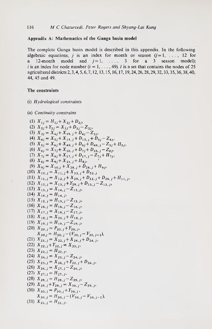
116 M C Chaturvedi, Peter Rogers and Shyang-Lai Kung
Appendix A: Mathematics of the Ganga basin model
The complete Ganga basin model is described in this appendix. In the following
algebraic equations, j is an index for month or season (/= 1, 12 for
a 12-month model and 7=1, .... 3 for a 3 season model);
i is an index for node number (i = 1,. . ., 49). / is a set that contains the nodes of 25 agricultural districts 2,3,4,5,6,7,12,13,15,16,17,19,24,26,28,29,32,33,35,36,38,40,
44, 45 and 49.
The constraints
(i) Hydrological constraints
(a) Continuity constrains
(1) Xlj = Hlj+X2j + D2j,
(2) X2j + Y2J = X3j + D3j-Z2j
(3) *3, = *4 j + *19, ,'+ 7^4j ~ Z3j,
(4) *4,= *5,+ *15,j + 7>15,j + 7757 ~ *4 J)
(5) *5,= *6,’ + *49, j + 7^6, + 7^49, j — Z5j + HSj,
(6) *6,= *7,' + *16.,- + 7>7j + T)i6.7 ~ *6j >
(7) *7,= *8,' + *i7,, + D11,j-Zij + 77?J,
(8) *8,= *97 + *21,, + 778j,
(9) *9,= *10,,' + *28,j + 7>28,j+ 77 9,’
(10) *10,,-
(ID *n,, (12) *12lj (13) X13,j
(14) X^j
(15) *15.,- (16) *16>i
(17) *i7,; (18) XlS'j (19) X19J
(20) X20,j
*20 J
(21) *2 ,, j (22) X22tj
(23) *23>, (24) A24>,
(25) *25>,
(26) X26tJ
(27) *27>j
(28) X28'j
(29) X29ij
(30) X30, ;
*30, J (31) *31
= *11,, + *32,, 4~D32,j
= *12, j+*29, j+^12,, + ^29,, + ^11,^
= *13, j + 1^29, , + 1^1 3, ,' *12, j’
= *14, j *13, jJ
7714, j,
= 7715 'j — Zl5j,
= 77l6., — *16,,»
= *18, j~~ *17, j>
= *20. j + 7718,
= 77i9 j — Zl9 j,
— 7*20, j + 1^20, j’
= 7720, j — ( f^O, ,• ~ ^20, , + 1 )>
= *22, j + *24, ,' + 7724> j,
+ ^22, j = *23 = 7723.,,
= *25, ,' *24, ,'»
= *26, , + *22,, +7*26,
= *27, ,' *26, j>
= T727,y»
= T728 j — Z2g'j,
+ *29, ,' = *30, , *29, j >
= 7*30, ,■ + *30, j, = 7730i j — (F30 j — ^30,,- i )>
= 7731> j,

Coordinating model of the Ganga Basin 117
(32) *32,2
(33) X33,;
(34) *34.j
(35) *35,;
(36) *36,,-
(37) *37. J
Xii.j
(38) *38.,-
(39) *39, j
(40) *40,;
(41) *41. j
X*i,j (42) *42,;
3^42, j
(43) *43, j
3^43, j (44) *44ij
(45) *45ij
(46) *46.,.
(47) *47,,-
(48) *48, j
(49) *49. j
= 3^35, j + *33, j+ ^33, j + D35 j — Z32,,.,
= 3^34,7 ~ j,
— H34, 2>
= 3636*38,2 4" ^36, j + ^38, j + ^35, j — Z35, j’
= 3^37,j — Z36,2>
= ^37, j+ ^37, j’
= ^31,j~(^31,j~ 1*37,2’—l)’
~ 3^31,2 + *39, j+ H36 j — Z36 j, *40,2 "1" 3^44,, *1“ Z)40, j 4“ D44, j + 7/30 j,
= *41,2 ~~ ^"40, j’
= ^41,2 4" *41,2’
~ 3^42, 2’ ’
= ^42, j 4" I42, 2 ’
= 3^43, j —(f/42,2—' 142,2'- 1)’
= ^43,2 + 143,2)
~ ^43,2 ( I43,2 l43,2'-l)’
3645, j + H45, j + HA4 j *44,
3^46, j + 1^46, 2 *45,2’
= 3^47,2 + *48, 2’
= H47, j ’
= ^48,2’
— 7i49 j — Z49 j.
(b) Groundwater returns
»ij = Zj
(ii) Agricultural constraints
(a) Field irrigation requirements
Tij+Zij — iel, Yj
(b) Culturable land and current irrigation level
4L, s$ < >4if„ ie/,
(c) Artificial constraints
^i2 = ^i3, ief
(iii) Capacity constraints
(a) Irrigation channels
Z„- ^ mfZHi + Znew,), ie/
(b) Groundwater storage
IX^M^ie/.

118 M C Chaturvedi, Peter Rogers and Shyang-Lai Kung
(c) Diversion channels
Yij^mJYHhielYJ.
(d) Reservoir live storages
Vtj ^ VHh i = 20, 30, 37, 42, 43, V ■
(e) Hydropower plant capacity
Pij mj(PHi + Pnew,), i = 20, 30, 37, 41, 42, 43, Y}.
(iv) Municipal water supply
Yu ^ nijYLid = 2, Yj.
Diversion to Calcutta for municipal water supply.
(v) Economic constraints
I (JW 11 (P«K|)
i = 20, 30, 37, 4J1, 42, 43, Y.
This is the power demand distributional constraint.
(vi) Environmental and other constraints
Minimum river flow
Xtj ^ mjX Lh i = 2, 5, 7, 10, 44, 45 Yj
The objective function
The objective of this model is to maximize the net benefit
max Z =/(/„, AtJ,fp, Pu, K,;f„fr, i,j),
or =/„ I [A„ + Ai3] +/p 11 [P,jK,]. i j ‘
Appendix B. Field irrigation requirements
In this appendix field irrigation requirements (a;j) in the Ganga basin are examined.
Only the Chambal sub-basin (node 40) is illustrated because the procedure for
obtaining these requirements is similar. The monthly or seasonal field irrigation
requirement is a function of (i) evaporation; (ii) cropping pattern; (iii) rainfall and
(iv) soil type, conveyance, storage and operational losses.
Evaporation
Christiansen et al (1966) have developed an empirical formula for estimation of a class
A pan evaporation:
Ep = 0-459 RC,C„ChCsCe,

Coordinating model of the Ganga Basin 119
where Ep is class A pan evaporation, R is extraterrestrial radiation; C,,Cw,Ch,Cs and Ce
are coefficients of temperature, wind velocity, relative humidity, sunshine percentage
and elevation. These coefficients for node 40 are presented in table B.l.
Cropping pattern
Evapotranspiration (consumptive use) of a crop is the product of evaporation (Ep) and
the consumptive use coefficients (k) of each crop. Consumptive use coefficients of the
kharif crop (mainly rice) and the rabi crop (mainly wheat) are taken from Ministry of
Agriculture (1971) estimates.
The consumptive use coefficients of rice are 0-97, 1-21, 1-24 and 0-80 for the four
months of the kharif season July to October respectively. The consumptive use
coefficients of wheat are 0-26, 0-75, 6-90, 0-81 and 0-61 for the months November to
March respectively. During the summer season the consumptive use coefficient of 08 is
assigned to June irrigation for land preparation. There is no irrigation requirement in
the months of April and May.
Rainfall
Net irigation requirements (nir) are the differences of evapotranspiration and effective
rainfall. Effective rainfall depends on the normal rainfall and the consumptive use.
These effective rainfalls (Re) in table B.l are estimated from Ministry of Agriculture
(1971) data.
Table B.l. Field irrigation requirements in Chambal sub-basin (node 40)
Month R Tc CT EP E, Rainfall nir (mm) FIR (mm)
Jan. 304 15 0-839 119 107 10-47 7-54 99 132
Feb. 321 19 0-965 145 117 7-46 5-50 111 148
Mar. 422 24 1-135 224 137 5-83 4-60 132 176
Apr. 464 27-5 1-250 272 — 3-74 — — —
May 513 29 1-305 313 — 9-08 — — —
Jun. 507 31 1-370 325 260 91 42 88-68 171 228
Jul. 520 32-5 1-425 347 337 283-42 280-00 57 76
Aug. 496 31 1-370 318 385 252-65 252-00 133 177
Sep. 434 29 1-305 265 329 137-26 137-00 192 256
Oct. 381 27-5 1-250 223 178 19-73 17-00 161 215
Nov. 309 25 1-167 169 44 9-30 6-00 38 51
Dec. 289 20 1-000 135 101 5-42 4-00 97 129
Total 4959 25-88 2855 1995 835-78 802-32 1191 1588
mean
R radiation in mm at latitude of 26° N; Tc monthly average temperature in °C; CT temperature coefficient in
Christiansen formula; Ep class A pan evaporation (assuming CwChCs = 1) in mm; £, evapotranspiration
(consumption use) in mm, E, — kEp. Rainfall: monthly rainfall in mm (weighted average 58% of East Rajasthan and 42% of West Madhya
Pradesh); Re effective rainfall in mm; a40 , = 636 mm, a40 2 = 228 mm, a4o,3 = 724 mm.
Node 40—Latitude 26°N, Elevation 500 m. Mean temperature 25-88°C, Annual rainfall 835-78 mm
120 M C Chaturvedi, Peter Rogers and Shyang-Lai Kung
Monthly rainfall of the Chambal sub-basin is a weighted average of East Rajasthan
(about 58 %) and West Madhya Pradesh (42 %). Rainfall statistics of Chambal and
other sub-basins are obtained from the Ministry of Irrigation and Power (1972) report.
Losses
Due to the unavoidable water losses through soil percolation, conveyance, storage and
operation, more irrigation water than the estimated net irrigation requirement (nir) is required. This field irrigation requirement (fir) is determined by nir and the field
application efficiency (fac). The efficiency is assumed to include all the losses for
simplicity.
fir = nir/fac.
An fac of 75 % is assumed for the Ganga basin model. The field irrigation requirements
of Chambal sub-basin are given in the last column (fir) in table B.l. Thus the firs at
node 40 for a three-season model are 0-636, 0-228 and 0-724 meters per unit area for
the rabi, summer and kharif seasons respectively.
References
Basrur V 1975 In the search of a trade-off, Harvard University
Biswas A K 1976 Systems approach to water management (New York: McGraw Hill)
Briscoe J 1974 Estimated average monthly flows in sub-basin of Ganges basin. Harvard University
Chaturvedi M C 1974 Ganges basin integrated system studies: Water resources development, Harvard
University
Chaturvedi M C 1978 Integrated systems planning for water and energy resources of the Greater Ganga basin
(New Delhi: Gandhi Peace Foundation Workshop)
Chaturvedi M C 1979 Regional water resources systems planning—A case study for Punjab (India), III
World Congress, IWRA, Mexico City
Chaturvedi M C 1984 Water resources systems planning (New Delhi: Tata McGraw Hill) in press
Chaturvedi M C, Rogers P 1975 Large scale water resources systems planning with reference to Ganges basin,
Proc. II World Congress (New Delhi: IWRA)
Chaturvedi M C, Srivastava D K 1981 Water Resources Res. 17: 783-795.
Christiansen J E (1968) J. of irrigation and drainage 94: 243-265.
Hall W A, Dracup J A 1970 Water resource systems engineering (New York: McGraw Hill)
Heimes Y Y 1977 Hierarchial analysis of water resources systems: Modelling and optimisation of large scale
systems (New York: McGraw Hill)
Jacoby R D, Loucke D P 1972 Water Resources Res. 8: 1401-1414
Lasdon L 1970 Optimization theory of large systems (London: Macmillan)
Ministry of Agriculture 1971 A guide for estimating irrigation water requirements, Tech. Ser. 2, Water
Management Division, Ministry of Agriculture, New Delhi
Ministry of Irrigation and Power 1972 Report of the Irrigation Commission, Government of India,
New Delhi
Rogers P & Chi T V 1973 A coordinating model for the Tiber river basin, Consiglio Nazionale Delli Richerch,
Institute di Ricerca Sulla Aque, Reports No. 1 and 6
List of symbols
AGj area (106 m2) at node i over which groundwater is available
AHj culturable land (106 m2) at district i

Coordinating model of the Ganga Basin 121
A Li minimum irrigation level (current irrigation level) at district i
Du quantity of water (m cu m) left from upstream river node i that returns to the
river node downstream
Hij hydrological inputs (mcum) at river node i during jth period
K, power converson factor (MW/mcum/mon) at power plant i
mj parameter specifying use constraint of a system capacity
PHi capacity of water (m cu m/mon) driving the turbine at power plant i
Pij quantity of water (m cu m) driving the turbine at power plant i
Pnew, new capacity (mcum/mon) to be added at power plant i fj quantity of groundwater (mcum) pumped for irrigation district i during yth
period
VH{ capacity (live storage in m cu m) at reservoir i Vij storage (mcum) at reservoir / during;th period
Xij quantity of water in 106 m3 (m cu m) flowing through a river away from node i downstream during ;th period
XLi minimum monthly flow (mcum) at node i
Yij quantity of water (m cu m) diverted from node i in ;'th period
YHi capacity of diversion channel from node i
YLi minimum water diversion requirement from node i Zu quantity of water (m cu m) diverted for irrigation from node i during jth period
ZHt capacity of diversion channel (irrigation) from node i Znew, new capacity of diversion channel to be added to irrigation
ctfj field irrigation requirement (mcum/106 x m2) at district i t]j power demand distribution for /th period
6i quantity of annual groundwater availability (mcum/106 x m2) at district i
the fraction of total unpumped groundwater returns to river system in ;'th
period

.

Decentralized planning for the Ganga basin: Decomposition by river basins
PETER ROGERS and SHYANG-LAI KUNG*
Department of Environmental Engineering, Harvard University, Pierce Hall, 121 Cambridge, Massachusetts 02138, USA
* Argonne National Laboratory, 9700, S. Case Avenue, Argonne, Illinois 60439, USA
Abstract. Ths use of the decomposition principle in analysing large and complex systems is demonstrated through its application to the Greater Ganga Basin. The decomposition principle consists of three models (i) the consistency model, (ii) the sub-problem model and (iii) the master problem model. The consistency model tries to identify a feasible solution and sends this information to all the sub-basins. In the sub-problem model each sub-basin optimises the water use according to local conditions subject to meeting the mandatory releases in the Ganga and/or energy targets. After gathering information from the two models the master problem model adjusts the water release requirements and energy targets according to shadow prices. The iterative process is carried out between the sub-problem model and the master problem model to obtain the best solution. The difficulties in getting convergence in the iterative process and the drawbacks of this approach are also highlighted.
Keywords. Decomposition; large scale system; decentralized planning; consistency model; sub-problem model; master problem.
1. Introduction
In this paper a case study of the Ganga Basin is taken up to explore some possible
approaches that a river basin authority could use to ensure more efficient use of the
water resources and also meet requirements at various downstream points, at such
specific locations as tributary nodal points, state frontiers and international bound¬
aries. The underlying data and the basic models are the same as those by Chaturvedi
et al (1985) but they are now rearranged in various ways to decentralize the decision¬ making. The actual numerical results are slightly different from those reported by
Chaturvedi et al (1985) and these differences are due to changes made to simplify the
computational procedure. The approach taken is to assume that there is some central agency responsible for
water resources planning in the Ganga basin. We call this the Ganga Basin Authority
(gba). The structure of the assumed authority is not relevant at present. The studies by
Chaturvedi et al (1985) were carried out as though the gba had the authority to make
water allocations as it liked in all parts of the Ganga Basin. We now modify this in two
ways. The first modification assumes that detailed planning decisions will be made by
separate river basin authorities for each of the major tributaries. These authorities
could all be from one state or could be interstate management boards where more than
one state is involved. The role and the responsibility of the central agency, the gba, is to
coordinate all of these independent river basins in such a way as to meet the upstream-
downstream requirements. This is to be implemented by the gba authorizing the
minimum seasonal flows out of each of the river basins. In other words the individual
123

124 Peter Rogers and Shyang-Lai Kung
basins can do what they like with the water within their own basin provided they meet
the outflow requirements.
The second approach dealt with by Karady & Rogers (1985) takes the political unit of the State as the basis of the decentralized decision-making. Under this approach a
variety of different algorithms for allocating water use are explored. Essentially, they
deal with the total inflows and outflows of the water to and from a State set as targets by
the gba.
This paper is an extension of the coordinating-screening model for the Ganga river
basin in which the water resources allocations are made using the decomposition
principle of large scale economic optimization models. A different approach has been
taken by Chaturvedi (1974). The coordinating-screening model is decomposed into
smaller mathematical programs by solving sub-basin problems. A hypothetical gba is
assumed as a central agency who will govern the main Ganga Basin and regulate the
river flows to the sub-basins subject to meeting the low-flow requirements down-stream
at Farakka for water supply, salinity control, navigation, irrigation, etc.
Several assumptions in constructing the decomposition model are described as
follows:
(i) Main basin and sub-basins The Ganga Basin is divided geographically into nine
basins: the main Ganga Basin and 8 sub-basins. Each sub-basin is a major tributary or a
set of smaller streams that join the main Ganga. These sub-basins including the main
Ganga Basin (shown in figure 1 and in more detail in figure 2) are:
BASIN 8 BASIN 9
BASIN 5
SON f5i -Kj 7
6CK—^ BASIN 4
GANDAK
BASIN 3
KIUL -XJ5
4 (V In
BASIN 1 Fi --*5 3
OTHER RIGHT BANK
TRIBUTARIES
} TO CALCUTTA TO BANGLADESH
BASIN 2
KOSI
Figure 1. Decentralization of Ganga basin into 9 sub-basins

Decentralized planning for Ganga basin 125
S -10

126 Peter Rogers and Shyang-Lai Kung
(a) Right bank tributaries east of Kiul; (b) Kosi; (c) Kiul; (d) Gandak; (e) Son;
(f) Ghaghara and Sarda; (g) Tons; (h) Yamuna, Chambal, Betwa and Ken, (i) Ganga
and Ramganga.
There is irrigation in each sub-basin. Hydropower plants and storage reservoirs are located in Son, Yamuna-Chambal, Ken, Betwa and Ganga-Ramganga sub-basins.
(ii) Hydrology A deterministic hydrology of average monthly flows of a typical single
year in the past is used. For flood protection and other purposes, a hydrology of
extreme events which would have a chance of realization in one year out of every 50 or
100 years would be more appropriate. This has not been considered at present. For the
groundwater hydrology it has been assumed, as in Chaturvedi et al (1985), that the
annual recharge is a proportion of the cultivable area, and that a fraction of the
unpumped groundwater becomes available as surface flow.
(iii) Time periods The year is divided into three seasons; rabi: November-March,
summer: April-June, kharif: July-October. (iv) Crops Two major cropping systems can be used annually, one each in the rabi and
the kharif season. Irrigation in summer is restricted to June irrigation for land
preparation for the following kharif season.
(v) Assumptions on decomposition principle (a) The decomposition principle presented
in this paper is composed of three models: the consistency model; the sub-problem
model; and the master problem model. A feasible solution is identified in the
consistency model and is used as a starting point in the sub-problem and the master
problem models. The decomposition model iterates between the two models of the sub¬
problem and the master problem until a convergent solution or a stopping rule is
reached. In each iteration, the gba sends the minimum water releases and/or energy
production targets to each sub-basin; and the sub-basins, after optimizing their own
sub-problems, feed back to the central authority the shadow prices and ranges on the
minimum water releases and/or energy production, (b) Each sub-basin adopts similar
technology in constructing its sub-problem model (its constraints and objective
function). The objective function in the sub-basins is to maximize the irrigation level of
the total of rabi and kharif seasons, (c) Each sub-basin makes its best efforts to utilize
the available water for agricultural developments and/or energy production. Each sub¬
basin maintains at least the minimum river flows (water releases required by gba) and
keeps perfect communication with the Authority.
2. The decomposition model
The three components of the decomposition model are described in detail as follows:
2.1 Consistency model
The gba tries to identify a feasible solution and sends this information to all the sub¬
basins (see figure 3). This model has the three major constraint sets described below.
2.1a. Continuity equation: The amount of water that flows into a river node equals the
amount of water that flows away from the node:
f(X, Y,D,F) = H. (1)
2.1b Irrigation constraints: These are: (a) The amount of water from surface
irrigation( Y) and tubewell irrigation (T) equals the product of the irrigation acreage (A)

Decentralized planning for Ganga basin 127
Figure 3. Information flows in river basin decentralisation
and the local field irrigation requirements (a), (b) The irrigation level of the summer
season equals the level of the following kharif season, (c) Annual groundwater pumping
(YT) is less than the groundwater storage (9AG), and groundwater recharges its storage
annually, (d) The unpumped groundwater returns to the river at a downstream node according to a seasonal distribution (£)
I(Y, T, D, Aj, a, 6AG, £) = 0. 12)
2.1c Capacity constraints: Surface diversion (Y) groundwater pumping (T), and
irrigation acreage must be less than their respective capacities (Y, Y, and A). In
addition, the irrigation acreage must exceed the current irrigation level (A) and the river
flows at Farakka (X2) and must meet the low flow requirements (F2).
(X, Y, T, A; F2) ^ (X, Y, T, A) < (X, T, T, A) (3)
where X, river flows with lower limit X and upper limit X; X2, river flows at Farakka; Y,
canal diversions for irrigation (Y, F); T, tubewell irrigation (T, T); D, groundwater and
drainage returned to the river; F, water releases from sub-basin; F2, minimum river
flows at Farakka; H, hydrological inputs. A, irrigation acreage (A, ~A), <x, field irrigation
requirements, 6AG, groundwater storage and £ groundwater return distribution.
To attain a feasible solution of the above constraint set, a linear program that
maximizes the irrigation level Atj\ can be used*. The water releases from each basin
are called F(0) (where (0) denotes the initial point).
2.2 Sub-problem model
In the sub-problem model, each sub-basin optimizes the water uses for local
agricultural development within each sub-basin subject to meeting the command
* In fact a consistent solution is easily found by assuming several feasible releases (F) and computing the
remaining releases.

128 Peter Rogers and Shyang-Lai Kung
water releases to the main Ganga, and/or energy target levels issued by the gba.
The objective functions of the sub-problem model takes the following form: /
Objective function maxZ, = £(Akl + Ak3), ¥;. (4) k
The constraints are:
(a) Continuity equations,
f'(X, Y, D, P, V) = H\ ¥,; (5)
(b) Irrigation constraints,
P{Y, T, D, A; a, 6AG, £) = 0; (6)
(c) Capacity constraint,
(X, Y, T, A, P, V; Fh Et) < (X, Y, T, A, P, V) < (X,Y,T, A, P, V), V, (7)
In this capacity constraint, the river flows from each sub-basin to the main Ganga must
exceed the requirements ^ F^)and/or the energy production must meet the issued
target levels (km Pmj ^ Emj), where, i is sub-basin number,;' is season number, km is the
conversion factor for flow through turbines to energy for sub-basin m, m is the sub¬
basin with energy production, Fu is water release requirements from sub-basin i during
season Emj is the energy production target in sub-basin during season ;.
After the optimization is reached each sub-basin reports the shadow prices (defined
as the reduction of irrigation acreage for every unit of increment of water releases
and/or of energy target levels) and their effective ranges on Fu and/or Emj, irrigation
acreage, and/or energy production to the central organization.
2.3 Master-problem model
With the information gathered from the sub-basins and from the consistency model,
the gba adjusts the water release requirements and energy target levels for the sub¬
basins according to the shadow prices. Sub-basins that have more important shadow
prices (i.e. larger negative shadow prices) will have reduction in the water release
requirements and vice versa. This is also true in adjusting the energy target levels.
To facilitate this adjustment process, a linear program is constructed to maximize the
incremental irrigation acreage, while honouring the minimum flow at Farakka and the
energy constraints.
The objective function of maximising the incremental irrigation acreage takes the
following form,
max Awik) = X ~~ AFy + X + IAAU- i.jUrij • l,j
(8)
Several simple constraints are constructed to ensure that the low flow requirements,
increasing irrigation level and distribution of energy production are met.
(a) Low flow requirements at Farakka (F2): The changes in increases (or decreases) of
water releases from sub-basins and the changes in Main Ganga irrigation must not
violate the minimum flow requirements at Farakka,
ZAFu-£(auA/l,;) i /
(9)

Decentralized planning for Ganga basin 129
(b) Energy production should maintain its seasonal distribution and improve over the
previous level if possible.
Y„ (10)* m k
IAE„>0, Vj. (11)** m
(c) Upper and lower bounds on the changes (AF, AE, AT),
AFU ^ A Fij ^ AFfj,
AEmj ^ AEmj ^ AEmj, Yj m>u, (12)
AAij ^ AAjj ^ AAU,
and AFU, AEmj and AT(J- are unrestricted as to sign, where A^\ is the objective function
of the incremental irrigation acreage in the kih iteration; dZJdFij} the shadow price of
water release requirement in sub-basin / in the season j; dZm/dEmj, the shadow price of
energy target level in sub-basin m in season j; AFtj, the change of water release in sub¬
basin i in season AEmj, the change of energy target level in sub-basin m in season j;
AA^, the change of irrigation level in main basin at node / in season j; t]j the seasonal
energy production distributions; AF, AE, AA, are the upper bounds on changes
determined by the smaller value of upper bounds over which the shadow prices are
effective and logical upper bounds; A F, A E, A A, are the lower bounds on changes determined by the larger value of lower bounds over which the shadow prices are
effective and logical lower bounds.
These upper bounds (AF, A E, A A) and lower bounds (A F, A E, AT) are deduced from
two sources: ranges reported from sub-basins, over which the shadow prices are
effective and logical constraints. For example, when the upper bound of a shadow price
is larger than the water that can be regulated from the surface, groundwater and
reservoirs, then the upper bound should only consider the amount of water that the
surface, groundwater and reservoir can regulate. Another example is when the lower
bound is negative infinity, it has to be set at zero to avoid negative river flows.
The solution of this master problem model in the kth stage is the adjustment of the
new water releases and energy target levels:
_ r(k-D i AT 1 ij 1 i j ' 1 i j y
fiffi-££r1,+A£.j, in) Alj’ = Afi-V + AA,,.
* Because the initial solution has enforced this seasonal distribution (tjj), and if the changes in energy
production also satisfy the seasonal distribution, then the new energy production will satisfy the
seasonal distribution automatically.
** This constraint should not be enforced when the trade-off between agriculture and energy is very obvious
(i.e., irrigation gains a lot by sacrificing a little energy).

130 Peter Rogers and Shyang-Lai Kung
3. Iterative decomposition process
The iterative process of the decomposition model takes place as shown in figure 3 by
repeating the sub-problem model and the master problem model. This iterative process
is described below:
(i) The initial feasible solution is attained by solving the consistency model. The gba
then issues the initial water releases and/or energy target levels to all the sub-basins.
(ii) Each sub-basin solves the sub-problem model by optimizing the irrigation level
under the given water releases and/or energy target levels. Each sub-basin then reports
to the central organization its optimal irrigation level, and/or energy production,
shadow prices and their effective ranges on the water releases and energy target levels.
(iii) The central organization solves the master problem based on the information
reported from the sub-basins by:
(a) Evaluating the appropriate upper and lower bounds on A F, A E and A A, (b) solving
the optimization equations (8) to (12), (c) adjusting the water releases and/or energy
target levels and issuing them to the corresponding sub-basins, (d) computing the new
total irrigation level and the energy production of the whole basin.
(iv) Stopping rule: This iteration procedure is checked to see whether it should go to
step (v) or repeat steps (ii) and (iii) by; (a) Going to step (v) if the water releases have
stabilized from iteration to iteration, or the total irrigation level no longer improves (i.e.
all shadow prices are zero or both their upper or lower bounds are equal); (b) Going to
step (v) if the iteration number has reached a pre-specified allowable number
(presumably a large number), (c) Going to step (ii) and repeating the iteration if neither
(a) nor (b) occurs.
(v) Stop iteration and report current values as the best solution.
It is possible that no feasible solution can be reached in step (ii) when a sub-basin
tries to solve the sub-problem model while honouring the new increased water releases
and energy target levels because the ranges are estimated on the basis of individual
constraints. When this happens parametric programming is adopted reducing the
energy target levels (according to seasonal distribution rjj) successively, until a feasible
zone appears. This parametric programming will reduce the energy production but
maintain the seasonal energy production distribution.
4. Solutions
Two solutions under conditions similar to those specified by Chaturvedi ei al (1985)
were made: (i) to maximize the irrigation and generate hydropower with available
water; and (ii) to maximize the irrigation and insist on the maximum achievable power
(with both distributional and power plant capacity constraints). The initial feasible
solution obtained from the consistency model for both the examples given above is
presented in table 1. In the first example, the decomposition process gives the solution (total irrigation
57-69 m ha) after the third iteration. The increments and decrements of each sub-basin
and the main basin are shown in tables 2 to 4 and the centrally administered low flows
are shown in table 5.

Decentralized planning for Ganga basin 131
Table 1. Feasible solution to consistency model
Seasonal releases
Sub-basin Rabi Fi, Summer Fi2 Kharif Fi3
1 50 _ _
2 1,500 5500 —
3 50 — —
4 1,500 4500 —
5 1,000 — —
6 10,000 1500 —
7 70 — —
8 1,000 100 1000 9 3,500 2000 —
In the second example, the iterative decomposition process reaches an irrigation level
of 54 m ha in the fourth iteration and stops because the improvement on irrigation from
the third iteration is slightly negative (see table 6). The energy generated is
26,479 GWh/year (see tables 6 and 7).
5. Conclusions
The decomposition principle presented in this chapter is very powerful in reducing the
size of the computational problem to smaller sub-problems of manageable size that can
be solved by a time-sharing computer system. Necessary changes from iteration to
iteration are easy to arrange. However, it is not clear from the particular cases that we
have solved whether it would always achieve such rapid convergence. The choice of our
feasible solution (table 1) was conditioned by the previous solutions made by
Chaturvedi et al (1985). Hence we started with a very good solution to the
problem and converged quickly to near optimal solutions. This is not really a fair test of
the methodology.
There are a few serious drawbacks associated with this approach. The first is that for
the method to converge towards the optimum the river basins have to report their
shadow prices and ranges over which they are applicable correctly. If the basins
misrepresent their requirements for some reason or the other there is no guarantee that
the planning approach is efficient. Unfortunately, there is a large incentive for
misrepresentation in this administrative set-up and, hence, some additional method to
control it may be needed. The second major drawback is that the individual sub-basins
cross state lines and, hence, there is little reason to believe that the sub-basins would
themselves be able to agree upon the “best” solutions given the flow requirements. This
issue is dealt by Karady & Rogers (1985).

132 Peter Rogers and Shyang-Lai Kung
C o
I s
■o 4> 05 00
c o
1 s $ 2
z as H
£ o O O O o © o o O <
u. o o O O o o o o o CO
u~> *C
cd X2 m
rf o
§ t"~ <N
o o NO
<N o
3 On <N o' VC
rn ro
m m Tf <N
m o o o o o o O o £
r- oo
N 1
< M o o o 5
o 8 o 8 m
£ <N vy rN < +
1 i
I
o o O o O o
<N ''T +
On 1
W-l <u § £ 3 3 o o o
§ to VO
m o NO m
NO
C/0 u. r- OO p—H ro © <N <N Tf ro
o o o O ON o oo On ’'t in
(N NO 8 Os
l/'N r^P —
N 1 i 1
o o o oo SO ON o oo On •pm »/-> oo 8 W r^ NO On
1 1 ''t TT i ON <N <
1 1 I
+ 1
i +
m
1
o r- o ON o o o r ^ »—. p—( r- NT) On
m o rH NO ON
15 «d
1 VO »n fN
On <N Ov 00 8 pH o oo 00 3 *n O »/0 rr) oo NO r- OO U, <N vr> (N e*~) r- p—i NO r-
NO oo O* o' NO NO
r^i m m m r- ON <N OO On r- r~ <N Tf 8 p—i
3 o© NO oo VO *0 NO ON On
1 1 1 1 I | I i |
N
G *55 «S
<N m *T) NO r" oo On
cd -C
'O o
X r- o NO »/-> s u ed
3 o f-

Table
3.
Max
imiz
atio
n o
f ir
rigate
d a
rea-s
eco
nd i
tera
tio
n
Decentralized planning for Ganga basin 133
<
*4 k,
d -C
* k.
k<
N
<
k (N
u< U e
i = C/3 k
<N
k
N
k <
k
X> d OJ 3
k
tin
N
|| CD ^
OOOOOOOOO
ooooooooo
o o OO <N O SO Os (N O <N
<N r—< SO cn
O" so" <N r-" rs
OOOOOOOOO
ooooooor-r- oo oo r- r-
OOOOOOOOfN
O^OOOOroO/N *T) rf <N 0\| —< *r> r~~ rn n 'O
rt —<
OOOOOOOoo<N O ON SO
o o o o o o o o o <N rs|
Or-OoiOOOOON to so r- so «r> m
<N
onoN^h --« o os <n OO ^ -h 0\ o rH n O M ^ SO <N '—I T-H r- o
r- r- <n Tt q m OO O O ON O OO
fNlfOrf-^'OhOOO
c _o
s <D
"O lx
3 T s «s
■S •*-* d oo
*C
d .c o
X
NO k »/->
3 d
*d O
Jt IS d H
k <3
k^ co
5
m
k
N
k <
k <N lx 4> s i =
c/3 k <N
k
N
k <1
k
Xi d C* 3
k
k \.
N
OOOOOOOOO
ooooooooo
O’—'OOoofNO'OO Tt OnMO fN —< <N —i O cn m
o' so"^ fO Tf (N
OOOOOOOOO
ooooooooo
OOOOOOOOFN
O^OOOO^OstN Tt <N ^ »0 r- ’-h oo Tf
OOOOOOOoom O r- no oo
OOOOOOOOO
or-'0<NOOOsoso so <N «—<
sO */*> CT) rf
o<NTf-*r^’-'Ooo*-< oo on wi r- os « M O M T) so
r- wn so <n
OOf^mhOsfNOOn h- »h n Q OO NO ^ NO Os NO oo
I I I I I
^<Nr^Tt«nsOr^OOOs
Tota
l are
a 5
7-69
x 1
06 h
a.

134 Peter Rogers and Shyang-Lai Kung
Table 5. Centrally administered low
flows during rabi (Fij) without power
targets.
Basin Start
After 1
iteration
After 2
iteration
1 50 0 0
2 1,500 1183 1183
3 50 0 0
4 1,500 1012 1012
5 1,000 2666 2666
6 10,000 5551 5551
7 70 0 0
8 1,000 1968 2469
9 3,500 201 0
Table 6. Maximizing irrigation with power targets
Iteration
Iteration 1 2 3 4
Total area irrigated (mha)
Total energy produced
(GWh)
51,048
20,889
53,854
23,134
54,052
24,468
54,000
26,479
Table 7. Maximizing irrigation with power targets (MW)
Basin iteration Son Yamuna Ganga-Ramgamga
power targets 1 2 3 4 1 2 3 4 1 2 3 4
Ei i 753 931 1134 1222 1722 1776 1776 1776 430 491 444 633
Eh 337 327 558 704 722 774 774 774 193 332 193 148
Eh 658 0 0 0 1506 2544 2976 3303 376 252 0 0
References
Chaturvedi M C 1974 Ganges basin water resources systems analysis. Harvard University
Chaturvedi M C, Rogers P, Kung S L 1985 Sadhana 8: 93-121
Karady G, Rogers P 1985 Sadhana 8: 135-145 Rogers P, Shapiro M 1975 Planning for coastal zone management: A multi-level framework, Meta Systems
Inc., Cambridge, Massachusetts
Decentralized planning for the Ganga Basin. Decomposition by
political units
GEORGE KARADY and PETER ROGERS*
Temple, Barker and Sloane Inc., 33, Hayden Avenue, Lexington, Massachusetts 02173, USA
•Department of Environmental Engineering and City Planning, Harvard University, Pierce Hall, 121, Cambridge, Massachusetts 02138, USA
Abstract. In this study the greater Ganga Basin is decomposed by political units for analysis instead of by hydraulic sub-basins. This method is more logical because water-resources-use planning is under the individual state jurisdiction but the Central Government is responsible for meeting the low flow requirement at Farakka. Maximisation of national benefits is taken in terms of total area irrigated. The solution technique proposed is an iterative procedure.
The problem is analysed under two schemes (i) flow quota scheme and (ii) resource allocation scheme. These schemes are worked out by three algorithms. The first algorithm requires that minimum flow at any point in the Ganga should be greater than the sum of the minimum quota fixed by the central Government for all the states above that point. Under algorithm two, water that leaves an upstream state may be used by a downstream neighbour provided that this neighbour allows a flow greater or equal to the sum of its and all the upstream states quota to pass into the next state. In algorithm three the restriction of algorithm two has been lifted. The merits and demerits of each algorithm are discussed.
Keywords. Large scale systems; decomposition; decentralized planning; flow quota scheme; resource allocation scheme.
1. Introduction
The purpose of this study is to apply a decentralized planning solution technique to the
coordinating-screening Ganga river basin model developed by Chaturvedi et al (1985).
Their large, deterministic linear programming model, which describes in detail the
water in the Ganga basin, was solved in its entirety. Later, a decomposition by river
basin solution was proposed by Rogers & Kung (1985). This latter approach assumes the existence of river basin authorities, which solve their own, much smaller resource
allocation problems and whose action is coordinated by some central planning agency.
The method presented here addresses the more complicated but realistic issue of
decomposition by provinces or states. The motivation for such a scheme is as follows.
Water resources use planning is under the jurisdiction of individual states, but it is the
central government which is responsible for meeting the low flow requirements at
Farakka. The central government’s (cg) objective is presumably to meet this above
constraint while coordinating the state governments’ (sg) work in such a way that the
total national benefits, in our case rabi and kharif season irrigation of agricultural land,
are maximized.
The technique proposed is an iterative one, in which the cg decrees some initial
allocation of water for each state so that the low flow constraints are met at Farakka.
The states solve their own, pertinent water allocations and report back to the cg some
shadow price on the initial allocation. The cg then reallocates in such a way that there is
135

136 George Karady and Peter Rogers
a net increase of total area irrigated in the states. This back and forth exchange of
information goes on until the cg cannot engineer a further improvement in its
objective. Hopefully, as was the case in the basin-wise decomposition, the iterative
process will terminate in a few steps. These iterations are equivalent to “rounds of
discussions” between the cg and the sg , each of which has conflicting goals and is trying
to secure the best possible solution for itself.
One of the broad schemes proposed calls for the cg to ask each sg to contribute a
certain amount of water to the national and international cause of satisfying the low
flow requirements at the Bangladesh border. Apart from this intervention the cg allows
the states to use their water resources in the most efficient way possible. The states do
this by solving their water allocations subject to the cg imposed quota and to other minimum flow requirements negotiated among themselves.
A second scheme, which will henceforth be referred to as the “resource allocation
scheme” requires that the cg tell the states how much water they can divert for
irrigation in each season. Under this proposal the cg must be aware of the hydrological
inputs to each of the states, so that it can check that the states do not misrepresent the
quantity of water they use. The advantages and disadvantages of this latter
decomposition method will be further expounded below. The major assumptions and simplifications made to the coordinating-screening
model are restated as follows: (i) The objectives are to maximize rabi and kharif season
irrigation subject to the constraint that during one month of the summer season, the
same area be irrigated as during the kharif season (this summer irrigation is to prepare
the soil for sowing), (ii) no consideration is given to power generation.
Other simplifications and their justifications are presented in § 4. A simplified view of
the Basin considered as 6 states plus Bangladesh is shown in figure 1.
2. Description of the decomposition algorithms
Each of the algorithms considered is of the primal feasible type, for it was deemed
important to be able to stop the process, if necessary, before the optimal solution was
found and still end up with a feasible set of operating rules. A further requirement was
that the operating policy be relatively easily implemented and enforced.
The greatest difficulty in connection with the decomposition by state scheme was
dealing with the serially-coupled nature of the problem. If a state decides to use less
water, i.e. allow more to pass into the downstream states, the question arises as to what
the optimal strategy is for the use of the extra water by these states. The algorithms
presented attempt more or less successfully to decouple the states from each other. The
situation is further complicated by the fact that the model considers not one, but three,
seasons among which there is also considerable coupling. For this reason at each
iterative step only one parameter of one season is changed.
3. Flow quota scheme
Under this scheme, each state contributes a certain amount of water, set by the cg, to
the quantity required at Farakka. The cg communicates an initial quota, F^J, (where N
refers to one of the states,j refers to the season) to each of the state governments. The sg
solves its problem, and returns shadow prices on its input and output constraints, as

Planning for the Ganga Basin 137
Figure 1. Line diagram of the Ganga basin
well as the range of the relevant right hand sides, over which the shadow prices are
unchanged, to the cg. The cg reassesses the data and changes the F(f], where k is the
iteration number, in such a way that the sum total of the irrigated area in the states
increases. This usually means that states with a high shadow price for water are required
to contribute less, while states with a low shadow price for water are to contribute more
to the common cause. The iterations are carried out until one of the following criteria is
met: (i) all shadow prices are equal; (ii) further increase or decrease of some of the F(‘j
would result in system infeasibilities.
A block diagram of this scheme is shown in figure 2 along with arrows depicting the
information flow between cg and sg. The cg sets the and enforces or at least checks
them by occasionally measuring the actual flow of water across the states’ borders. The sg
relays information concerning the shadow prices on its input and output of water and
the right hand side ranges over which these shadow prices are constant. Information as to

138 George Karady and Peter Rogers
Where is the central gov’s
allocation of water use to the
Nth. state.
rT|n 8. T70ut are the shadow
prices on incoming and outgoing water.
Figure 2. Schematic diagram and information flow between Central Government and State
Government.
each state’s optimal irrigation for a given F^jis also released to the cg. This is the extent
to which information is exchanged among the different hierarchies of government.
Unfortunately, the algorithms considered below are very much subject to mis¬
representation by the sgs. While the cg can ascertain, by direct measurement, that each
state allows at least F(*j amount of water to leave its territory, it cannot be sure whether
the shadow prices or ranges on their right hand sides have been falsified or not. In the
analysis that follows, it is assumed that the state governments do not misrepresent these
data. The problem of the cg in finding the optimal F(*j when misrepresenting is
considered should be investigated at a future date, for it may represent a more realistic
situation than the one considered here. It should be noted that the cg possesses no
direct mechanism by which it could force the states to comply with the required F(*j,
should their output fall short of this targeted value.
3.1 Algorithm I
Complete decoupling of the states, if not of the seasons, may be achieved by requiring
that the minimum flow anywhere in the main stream of the Ganga be greater than the
sum of the FNJs of all of the upstream states. See figure 3a for illustration. This is a
very restrictive constraint, for under this scheme downriver states can in no way utilize
the water released upstream. The system is effectively separated into one similar to that

Planning for the Ganga Basin 139
X>FRMP x^fRMP*fUP xsfrmp*fup*fbih
(Q)
15 tflO
9108 12144
XR?-FRAJ xUP3FRAJ •FuP XBIHSFRAJ *fup *fbih
xLsfRAJ *fUP*FBIH *fwb
(b)
RAJ UP BIHAR w. BENGAL
XR ^XUP XUP^XBIH XBIH^XL
XU* 115180
9108 12144
(C)
RAJ 8. MP UP BIHAR W. BENGAL
S Xri = 2 Hr, - Z Gr : j 1 j 1 i
Z XUP| = ST Hup, - ZGuPj + s Xr,
^ XBIHj= ? HBIHj _ ^ GBIH j + ^ XUPj
Z Xl j = Z HWj - Z Gwj + ^ x BIH j
(d)
XR j ^ xUPj
xUPj 4 x BIH j
XBIH j 4 x L j
Figure 3. a. Outflow quota scheme, algorithm I. b. Outflow quota scheme, algorithm II.
c. Low flow quota scheme, algorithm III. d. Resource allocation algorithm.
considered by Rogers & Kung (1985) in their basinwise decomposition. They showed
that convergence was rapid; only three iterations were required. From a practical,
implementational point of view, algorithm I is infeasible, for it requires that the flow of
water be regularly checked at each main stem node, and the final solution may be
socially inefficient, since it could allow a situation in which Northern up is
underirrigated, but Southern up has too much water. If the above constraint were
relaxed within up and were only enforced at its border with Bihar, up may be able to
increase its irrigated areas considerably. These considerations bring us to a second,
more realistic algorithm.
3.2 Algorithm II
Under this algorithm, water that leaves an upstream state may be used by its down¬
stream neighbour provided that this neighbour allows a flow greater or equal to the

140 George Karady and Peter Rogers
sum of its and all the up-stream states’ FNj to pass into the next state. The situation is
illustrated in figure 3b. While the algorithm may lead to higher overall irrigation levels,
it also poses some major computational difficulties. Monotonic convergence to the
global optimum is not assured anymore. It also becomes difficult to ascertain whether
after a seemingly last iteration a global optimum has in fact been attained. At the heart
of these difficulties lies the fact that the ranges on the right hand sides are computed
assuming that only that this side is changed. This means, for example, that one either
changes the inflow or the outflow constraints of a state. Changing both or changing one in
more than one season may lead to erratic results because a shift in one of the constraint’s
right hand side may lead to a changed shadow price or range for another constraint. With
all this in mind, consider the situation encountered in the first computational example after
the ninth iteration. The status of the model after this iteration is shown in figure 4a.
Briefly then, the shadow prices indicate that it would be beneficial to increase either the
input to up and/or to reduce its output to Bihar. Neither of these possibilities is open to
the cg, for up’s output already equals Rajasthan’s quota with FVPj = 0 in the first
season. Is one at an optimum? In a sense a local optimum has been reached, but can a
still higher optimum be reached by first increasing up’s output (a sub-optimal move)
and then increasing the input to it from Rajasthan? Will such a move lead to a better
solution, and if yes, by how much should one increase up’s output? These questions may
only be answered by actually performing the calculations. It is because of consider¬ ations like these that the convergence is not monotonic and is heavily dependent on the
‘path’ or decisions that were taken by the cg to get to the ‘local maxima’. At each
iteration the cg chooses from among a number of decisions, all of which will improve the overall solution. It does not know a priori which of the choices will take it the
“farthest”, along the decision tree. It may have to decide to “skip from one branch to
another” in a sub-optimal iterative step in order to progress further towards the global
optimum. The fifth iterative step was such a ‘skipping’ move. See figure 5 for further
details.
ITERATION
2 4 6 8 ITERATION
(b)
4 6 8 ITERATION
Figure 4. Shadow prices for Uttar Pradesh, a. Algorithm II. b. Algorithm III.

Planning for the Ganga Basin 141
In defence of the algorithm, it must be pointed out that there was very little
improvement to the objective function value after the fourth iteration. Familiarity with
the system would also tend to make one doubt that the solution after the ninth iteration
may be significantly improved. Nevertheless, it is entirely plausible that the relative
success of algorithm II on the Ganga basin problem is due to the insensitivity of the
model to changes in the input and output parameters. In the light of these difficulties,
one ought to exercise great caution when applying the algorithm to an unknown
general system.
3.3 Algorithm III
In the second algorithm, Rajasthan’s quota, for example, could be used by up but had to
be accounted for at its border with Bihar. In the algorithm considered here, this
restriction is lifted. The FN 's are no longer the Nth state’s contribution to the quota to
be met at Farakka, but it is the actual amount of water the Nth state is required to
release to its neighbour. In effect the cg is not only seeking the best solution subject
to the Farakka constraint, it also takes upon itself to redistribute the water of the
Ganges among the six states in such a way as to maximize the sum of the areas irrigated
in all of the states. Because this algorithm is less restrictive than algorithms I and II, one
expects it to yield the highest solution of the three. Figure 3c illustrates the situation.
While this method suffers from fewer computational difficulties than the second
algorithm, one wonders whether or not it constitutes a grave infraction on the part of
the cg on the states’ sovereignity, to dictate the redistribution of their resources in such
a manner.
This third algorithm converges monotonically to what is believed to be the global
maximum for the system. As yet, this statement has not been proved. The path to the
maximum does not seem to be unique, just as the solution, as far as the decision
variables are concerned, is not unique.
In summary then, algorithms were presented for the decomposition by state of the
Ganges basin. All the three are susceptible to misrepresentation by the sgs. Algorithm I,
which is the least difficult to solve, is almost impossible to implement in practice. Algorithm II, while most palatable in a political sense (contributions to a national
cause) has difficulties in converging to a global optimum. Algorithm III performs well
mathematically, but may promote animosity between the states and the cg.
4. Resource allocation schemes
Instead of prescribing the low flow requirement FNj, the cg allocates a certain
amount of water G(^j to be used by the Nth state in thejth period. The explicit form
this constraint takes is
I Z,J = G« (1) ij
where Z0 is the amount of water diverted for irrigation at node i in period j. The sum
over i runs over all the nodes in state N. Apart from minor modifications, the cg’s
strategy is as before. An initial feasible solution is chosen, which is improved upon by
adjusting the G%] with contributions from the respective shadow prices.
If the scheme of algorithm II is used, this problem is even harder to solve than
s-ii
142 George Karady and Peter Rogers
algorithm II. If the method adopted in algorithm III is the basis of the cg’s actions, then
complete decoupling may be achieved among the states. This happens because there is
now only one constraint for each state. The input and output constraints that plagued
the ‘low flow quota’ methods have been eliminated in favour of (1). If, for example, GRAJ
is reduced; but none of the other states’ G’s is changed, the extra water released by
Rajasthan will manifest itself as increased flow at Farakka. This seems to be the most
desirable feature of this method.
In order to minimize the chance of changing a G in such a way that infeasibilities
occur, the initial G’s should be set high enough such that no water flows out from any
one of the states. The situation is summarized in figure 3d.
The algorithm requires that the cg know the hydrological inputs to all the states. It
can then ascertain that the states are not misrepresenting the amount of water they
use by evaluating the following relationships;
I«« = ZfW + ICW-IXw. (2) ij J J J
where £ H is the annual hydrological input to the Nth state, £ FXj is the amount of ij j
water flowing out of the state and £ XNj is the input of water to the Nth state from its j
upstream neighbour.
After the cg chooses an initial allocation of GNJ's such that the constraints are met at
Farakka, the sgs solve their problems and relay back to the cg their shadow prices on
the GNj, the ranges and their output FNj. The reason for the cg’s inability to determine
the FNj a priori is because of the season-to-season coupling by groundwater pumping
and the operating of reservoirs. This is precisely where the shortcomings of the
algorithm lie. The cg is unable to determine, short of having the states do the
calculations, how the seasonal output of up, for example, will change if both GRAJ and
Gup are changed. Because of this seemingly insurmountable difficulty it was decided not
to investigate the method any further. It is conceivable, however, that because of the
general stiffness of the Ganga model, the season-to-season coupling would not be
strong enough to seriously interfere with the workings of the algorithm.
From a political point of view, the algorithm may not be a favourite of the sgs, as it
may be construed to infringe on state autonomy.
5. Computational experience
5.1 General remarks
Calculations were made using the Harvard Business School’s dec 1070 system. The
linear programming sub-problems were solved by the highly convenient and adaptable
hpslp subroutine available on this computer. Because of software, hardware, time and
fiscal limitations, it was necessary to make a few simplifications in the original model to
reduce the sizes of the sub-problems to solvable ones by the hbslp program. Even so, the
largest of the linear programs, that for up, had 121 variables and 123 constraints.
Admittedly, the input matrix was sparse, but such a large problem is still just about as
big as the existing time-shared software can handle. The cg’s master program was
solved by hand.

Planning for the Ganga Basin 143
5.2 Assumptions and simplifications
Since in both the solutions presented by Rogers & Kung (1985), the groundwater
reserves were completely exploited at the end of the third season, it was decided to set
the Df s to be identically zero {Di} is the quantity of groundwater and irrigation
drainage at node i that is returned to the river at a downstream node). Further
reductions in the size of up’s sub-problem were achieved by fixing the irrigation levels of
nodes 13, 24, 33, 44 and 45 at the levels calculated by the previous two methods. The
particular areas were chosen because their abundant water supplies assure their being
irrigated at a constant level for not too drastic changes in FRAJ and Fup.
Node 40 irrigates roughly equal areas in Madhya Pradesh and Rajasthan. Since
power generation was not considered in the objectives of the states, it was assumed that
the reservoirs at nodes 42 and 43 were operated in unison to derive the maximum
irrigation benefits for both states.
Because of similar considerations up’s reservoir at node 20 was operated in such a
fashion as to aid the irrigation of Bihar. Of course if power generation were one of the
objectives, operating policies would be drastically different.
5.3 Notes on iterations
Figure 5 represents the progress of the iterations for algorithms II and III.
5.3a Algorithm II: It proceeded smoothly until iteration four, at which point it was
realized that a ‘skip to another branch’ was necessary if one was not to get stuck at a
sub-optimal solution. This was done by increasing the first season output of up from
3000 to 6500-8 m cum, which was the limit dictated by the range of Bihar’s shadow price
for incoming water. This skip resulted in a slight decrease in the total area irrigated, but
permitted a yet higher level to be reached in subsequent iterations. A similar
procedure would have been performed after the ninth iteration, but as already pointed
out earlier, the value of such a procedure at this stage would have been questionable.
The optimization procedure was thus terminated at what is no doubt a sub-optimal
solution. The value of the primal feasible feature of the algorithm is thus amply
demonstrated. Figure 5 and table 1 summarize the status of the model after each
iteration and indicate what changes were made from iteration to iteration.
Table 1. Algorithm II: Gross area irrigated (million hectares)
Iteration Rajasthan and M.P. UP Bihar West Bengal Total
1 7-42 28-96 18-90 Ml 56-39 2 7-37 2908 19-11 Ml 56-67 3 7-38 29-22 19-12 Ml 56-83 4 7-18 29-46 19-12 Ml 56-87 5 7-18 28-89 19-68 Ml 56-86 6 7-02 29-07 19-68 Ml 56-88 7 6-53 29-58 19-68 Ml 56-90 8 6-36 29-83 19-68 Ml 56-98 9 6-33 29-87 19-68 Ml 56-99

144 George Karady and Peter Rogers
Figure 5. Iteration results of different algorithms.
5.3b Algorithm III It proceeded slowly and uneventfully. An effort was made at the
eighth iteration to speed up convergence by increasing the third season input to up by
2000mcu m rather than the 679 tncum that was indicated by the range on the shadow
price. The attempt was a failure. The value of 2000 was promptly reduced to 679 in the
ninth iteration. The progress of the algorithm and final results are summarised in
table 2 and figure 5.
6. Conclusions and discussions
The foregoing discussion should illuminate the complications encountered when a

Planning for the Ganga Basin 145
Table 2. Algorithm III: Gross area irrigated (million hectares)
Iteration Rajasthan and M.P. UP. Bihar West Bengal Total
1 7-26 29-53 18-96 Ml 56-86 2 7-26 29-53 18-76 1-32 56-87
3 7-26 29-62 18-67 1 32 56-87 4 7-18 29-72 18-67 1 32 56-89 5 6-87 30-05 18-67 1 32 56-91 6 6-73 30-26 18-67 1-32 56-98 7 6-56 30-43 18-67 1-32 56-98 8 6-51 30-52 18-67 1-32 57-02 9 5-71 30-33 19-67 1-32 57-03
10 5-71 30-31 19-68 1-32 57-02
large river basin is decomposed into sub-problems that are serially coupled to each
other. Both of the algorithms that were tested on the Ganga basin model seemed to
work adequately, but their limitations, as discussed in § 3, must never be lost sight of. It
is not at all certain, for example, that algorithm II would lead to satisfactory solutions
within a reasonable number of steps were it applied to a more flexible model than the
one used here for the Ganga basin. As has been already suggested, a game-theoretical
approach may be applicable here. Future studies should cover the behaviour of the
resource allocation algorithm of §4, and should refine the model by including power
generation in the objective functions. The effects of misrepresentation and how it
may be precluded by the cg or how the cg can actually force the states to release a
certain quantity of water to be used at Farakka should also be studied in detail.
One wonders whether algorithm II or algorithm III is the more socially equitable
one. Were they equivalent computationally, the decision to use one or the other should
be arrived at jointly by the central and state governments. As Kornai (1973) pointed out,
it is unreasonable to expect real world planning processes to follow the confined ways
and means of an elegant mathematical algorithm. While the results presented in this
paper are numerically correct, the way in which they were arrived at, the iterative
process between the cg and sgs, should not be taken too literally. There is so much that
the algorithms ignore. Economic and political pressures, corruption, bribery, behind-
the-scenes negotiations are all vastly more powerful forces in choosing what the actual
allocations will be, than the naive decisions taken by our hypothetical cg based entirely
on the computed shadow prices.
References
Chaturvedi M C, Rogers P, Kung S L 1985 Sadhana 8: 93-121 Kornai J 1973 Multilevel planning case studies in Mexico (eds) L M Goreux & A S Manne (New York:
North Holland) Chap. 5.3 Rogers P, Kung S L 1985 Sadhana 8: 123—134

.

An unconventional approach to integrated ground and surface water
development
ROGER REVELLE and V LAKSHMINARAYANA*
Department of Political Science, University of California, San Diego, California 92093, USA
‘Department of Civil Engineering, Indian Institute of Technology, Kanpur 208 016, India
Abstract. The conjunctive use of surface water with groundwater development in the Ganga Basin is considered more desirable due to unacceptable environmental conditions created by using all the low flows and the limited possibilities of surface storages. There are several ways to increase infiltration during the monsoon season. One method is to create groundwater storage by pumping during the non-monsoon period. A procedure for estimating the extent
and the rate of pumping such that it is replenished in 120 days of the monsoon season and equilibrium is achieved, is outlined in this study. The areas in the Ganga Basin suitable for such groundwater storage schemes have been marked out and the economic aspects of the scheme have also been studied. It is concluded that with this scheme of underground storage of flood water the total potential irrigation in the Ganga Basin may be limited by the area of irrigable land rather than the water supply.
It is suggested that this potentially advantageous scheme should be systematically studied and investigated in detail and factors like sediment transportation which may reduce the infiltration rate, the possible hazards of subsidence due to lowering of the water table, the possible ecological effects, and other relevant issues should also be considered.
Keywords. Groundwater; conjunctive use; surface water; underground water storage.
1. Introduction
The various Ganga models have suggested that large increases in irrigated area are only
obtained at the expense of good low flow conditions. Deteriorating low flow conditions would be unacceptable from environmental considerations and are not likely to be
accepted by downstream users of the Ganga.
One approach to the problem of the low flow of the Ganga grew out of the work of Revelle & Herman (1972) and Lakshminarayana & Revelle (1975) which has been
labelled “The Ganges Machine”. It is an approach based on groundwater development
in the Ganga basin in conjunction with surface water.
Besides the limited possibilities of surface storage, there are at least five ways in which
a portion of the monsoon flow could be stored underground. Infiltration into the water
table in the monsoon season could be increased by (i) water spreading in the piedmont
deposit north of the Terai belt of the springs and marshes; (ii) constructing bunds at
right angles to the flow lines in uncultivated fields to slow down run-off and increase
infiltration; (iii) pumping out the underground aquifers during the dry season in the
neighbourhood of nullahs (natural drains) which carry water during the monsoon
(Rama 1971); (iv) pumping out groundwater during the dry season along certain
tributaries of the Ganga to provide space for groundwater; and (v) increasing seepage
from irrigation canals during the monsoon season by extending the network of canals,
distributaries, and water courses for kharif irrigation and pumping out this seepage
147

148 Roger Revelle and V Lakshminarayana
water during the dry season. In addition, evaporation losses from the water table might
be reduced by lowering it below the level of appreciable evaporation. Finally, it may be
beneficial to export some monsoon water from the Basin to areas in the south and the
west where irrigation could be extended if firm water supplies were available.
In table 1 we have estimated the likely increase in irrigation water supplies produced
by some of these devices. A large increase could be obtained by constructing barrages
and “leaky” canal systems for surface irrigation of a large part of the cultivated area,
including an increased area of rice cultivation during the kharif season, and wells to
recover the underground seepage during the rabi season. Recharge of aquifers along
certain Ganga tributaries could provide an equally large increase of rabi irrigation
supplies.
There is good reason to believe that in many places the underground aquifers are
well-connected to the rivers and are highly permeable. For example, in one region
where a groundwater survey was made (Pathak 1969) the seasonal contours of the
water table on both sides of a large tributary show that this river is a drain which carries
off perhaps 0T2 x 106 ham of water that seeps into it during the dry months from the
underground aquifers. If these contours could be reversed by large-scale pumping of
the underground waters in the dry season, the aquifers could receive and store a large
Table i. Possible future water budget for the Ganga plain
Volume (x 106ham) during
Low flow High flow
season season
(November (July to
Source or sink to June) October)
Supplies
Present average river flow at Bangladesh boundary 7-3 28-9
Evapotranspiration from present surface storage and river diversion
(1968-1969) 1-8 1-8
Evapotranspiration from present well irrigation (1968-1969) 1-3 0-7
Additional surface storage (under construction or potential) 1-5 -15
Reduction of groundwater evaporation by pumping down watertable 0-8
Increased infiltration of rainfall by bunding in uncultivated areas 0-7 -0-7
Potential additional underground storage 60$ -60$
Transfers out of basin (such as “Ganga-Cauvery Link”) -1-8
Total supplies 19 4 21-4
Uses and excess flows
Consumptive use in present irrigation (1968-1969) 31 2-5
Consumptive use in potential additional irrigation 90 60
Diversion to Hooghly River at Farakka Barrage for 2-3$
Calcutta maintenance
Needs for irrigation in Bangladesh 1'8$
River navigation and waste disposal 3-2$
Monsoon flow at Bangladesh boundary 12-9*
Total uses and excess flows 19-4 214
+ See text. * Estimated by difference.

Integrated groundwater development 149
part of the monsoon flow of the river. We believe that similar underground storage of
river floodwater could be carried out along many tributaries of the Ganges.
It would be necessary to lower the water table at the beginning of the monsoon
season to a greater depth than that required simply to produce the storage volume.
Moreover, the aquifer directly under the river would need to be pumped down close to
the average depth. In the rivers of the western part of the plain, where the dry season
flow comes largely from groundwater seeping out of the river banks, the low flow
discharge during the first year would be removed by the pumping, and thereafter the
river would be virtually dry from November to June. Several years would be required to
obtain the full storage potential. Each year the water table at the beginning of the
monsoon season would be pumped deeper than the year before, until an equilibrium is
ultimately reached.
2. Pumping out groundwater during the low flow season
For a rough estimate we may assume that along 3200 km of the system of the larger
tributaries of the Ganga (about a quarter of the total length) large well fields could be
constructed which would produce storage space by pumping out the groundwater
during the low flow season. With well fields 6 km wide on either side of the river, the
area covered would be 3-8 x 10⁶ha. If we assume that the well field capacity is
2-25 cumecs/km (that is, 112 cumecs/km of length on each side of the river) and the
storage coefficient of the aquifer is 0-25, then the water table will be lowered, on the
average, about 12 m at the end of 8 months of continuous pumping. All the wells need
not be of the same capacity. It is necessary only to design the well spacings and
discharges in such a way that we pump out a trough of 12 m below the river bed. The
method used for finding the depressions of the water table is given below.
The drawdown due to pumping in an aquifer is given by
(1)
where the drawdown s = ht — h (m), /i, is the initial saturated thickness of the aquifer
(m), h is the height of the water table during pumping (m), Q is the discharge (m3/day), T
is the coefficient of transmissibility (m2/day,) S is the storage coefficient (dimensionless),
t is time since pumping started (days), and r is the distance from the pumping well (m).
Equation (1) holds strictly only for a confined aquifer which is isotropic and
homogenous. However, it can be used for an unconfined water table aquifer (as in the
present case) provided drawdown is small compared with the original saturated
thickness of the aquifer. In the Ganga plain the aquifers are quite thick, and the
drawdown of the water table will be small compared to the initial saturated thickness of
the aquifer; consequently, we can apply (1), which also has other assumptions involved
in its derivation. Revelle & Herman (1972) showed that although these assumptions are
not strictly valid in the present case, the equation can still be used to give a fairly good
solution.
Equation (1) is the solution of the differential equation
d2h 1 dh S dh
dr2 + r dr T dt' (2)

150 Roger Revelle and V Lakshminarayana
OO
t
BB — —O
t t I I
—17.6 km-
r1 -0*0
i t
RIVER - BB O-O t ? I I
-o 1 I
oo
Figure 1. Location of real and image well groups. BB, barrier boundary; R, real well group
centre; I, image well group centre
subject to certain simple boundary conditions. Since (2) is linear, the superposition
principle can be used to find the solution when more than one well is being pumped in
the aquifer. Equation (1) is obtained assuming that the aquifer is really infinite. If we
have boundaries, we must use the method of images
In the present calculation we have assumed that there is a natural groundwater divide
at a distance of 8 km on either side of the river. This is approximately true for many of
the tributaries that feed the main tributaries of the Ganga. The natural groundwater
divide acts as an impervious barrier. The presence of the river itself can be ignored in the
computations, since during the dry season the quantity of flow in many Ganga
tributaries will be small compared to the quantity of pumping. Grouping the wells in
pumping centres, we will have the real and image wells shown in figure 1. Because of the
assumed existence of an impervious boundary on either side of the river, there will be an
infinite number of images. However, only a few need to be considered, since the effect of
image wells very far off will be small near the river.
Equation (1) is applied repeatedly for all the real and image wells, and we obtain a
lowering of the water table, on the average, of about 12 m at the real wells.
3. Recharge of groundwater mound by monsoon flow
When pumping stops at the end of the dry season there is some flow into the trough
from the sides. It is, therefore, assumed that we have a net trough with an average depth
of 10 m to be partly filled by monsoon flow in the river.
The growth of the groundwater mound resulting from infiltration of the monsoon
flow in the river is computed by using the following equations given by Hantush (1967),
WT h2 = h\ + —— f {2 — 4i2 Erfc (L — x)(ATt/S) 1/2
/Co
- 4i2 Erfc (L + x) (ATt/S)~l 12} for x < L, (3)
WT h2 = h* + t{ *i2 Erfc (x-L) (4Tt/S)~112
- 4 i2 Erfc (L + x) (4Tt /S)~112 } for x > L, (4)

Integrated groundwater development 151
where the symbols other than the ones already used are: W, recharge rate through the
bed of the river (m/day); K, coefficient of the permeability in the aquifer (m/day); t, time
during which recharge takes place (days); L, half width of river (m); x, distance from
centre of river (m); and
Erf (*) = -T/2 f exp (- £2) df, 71 Jo
Erfc(x) — 1 —Erf(x); 4i2 Erfefx) = Erfc (x) — IxiErfc (x).
Since (3) and (4) are implicit, a trial and error procedure or a graphical method has
to be adopted for the solution. For example, assume t = 15 days. Then, using
T = 4650m2/day, L = 150 m, W = 0-61 m/day, K = 15-2 m/day, S = 0-25, /i, = 300 m,
and t = 15 days, we get (4Tt/Sf = 1055 m and L/(4Tt/S)$ — 0T44. From (3) we find
h2 = (300)2 + x x 15^ (0-56) = 96,270 m2,
Therefore, h = 310 m and h — /i, = 10 m.
Thus the time for the water to rise 10 m at the centre of the recharging strip is 15 days.
The height of the groundwater at a distance of 600 m from the centre of the river can
be computed as follows:
(x - L){4Tt/Sy1/2 = 450/1055 = 043,
(x + L)(4Tt/Sy112 = 750/1055 = 0-72.
Using (4) we obtain
h2 = (30°)2 + (^x^x 15) (0-35 — 0-14) = 92,350m2.
Therefore, h = 303-5 m and h — hi = 3-5 m. Similarly at 1500 m, we obtain
h2 = (30°)2 + (^x^x 15) (0-016-0-005) - 90,123m2,
h = 300-2 m and h — hj =0-2m.
Thus, assuming that the rate of recharge is 0-61 m/day, which is rather conservative,
the height of the water mound at the end of 15 days will be 3-5 m at a distance of 600 m
and 0-2 m at a distance of 1500 m. From this we can compute the quantity of monsoon
water abstracted as 1 x 10⁶ ha m. After 15 days there will still be some recharge, because
some of the bank flow from the river will continue to fill the trough. Thus, during the
first year of operation a little more than 1 x 10⁶ham will be extracted from the
monsoon flow. When this is spread over the groundwater basin 17-5 km wide, it will
raise the water table by 0-75 m. To this we may add a rise of the water table by 0-6 m
caused by 15 cm of net rainfall infiltrating to the water table. Thus, at the beginning of

152 Roger Revelle and V Lakshminarayana
the second year of operation the water table will be about 8-6 m below the level at the
beginning of the first year.
During the second year of operation, the water table will be lowered by 10 m to a
depth of about 18-6m before the monsoon flow begins. The time taken to raise the
water table 18-6m at the centre of the river bed during the monsoon works out to 33
days. At this time the height of the groundwater mound will be 7-5 m at a distance of
600 m and 1 -5 m at a distance of 1500 m. The total quantity of monsoon water extracted
will be about 2 x 10⁶ ha m, again ignoring the contribution from bank flow. This will
raise the water table by about 1 -5 m. Adding about 0-6 m due to infiltration of rainfall,
the depth of the water table at the beginning of the dry season in the following year will
be 16-5 m below the initial level.
During the third year of operation, this will again be lowered by 10 m, leaving the
water table at a depth of about 26-5 m at the beginning of the monsoon. The time taken
for the water table under the river to rise 26-5 m is about 70 days. At this time the height
of the groundwater mound will be 15 m at a distance of 600 m, 5 m at a distance of
1500 m, and 0 m at a distance of 3000 m. Thus, the amount of water extracted from the
monsoon flow, ignoring the contribution from bank flow, will be about 6 x 10⁶ ha m. At
the end of the monsoon the water table will be at an average depth of about 22 m over
the cross section of 17-5 km.
By similar computation, we can show that during the fourth year of operation the
depth of the water table at the end of the pumping season will be 32 m, and in the
120 days of the monsoon season we will extract from the monsoon about 9 x 10⁶ham.
The depth of the water table at the end of the monsoon will be about 25 m below the
initial level 4 years earlier.
From the following year onwards, the water table will be stabilized at these levels by
pumping out a quantity equal to consumptive use, surface drainage and return
infiltration to the groundwater table.
Figure 2 shows the growth of the groundwater mound under uniform recharge from
the river for the stated values of the parameters. Because different scales have been used
in the horizontal and vertical directions, the slope of the water table appears to be steep.
DISTANCE FROM RIVER CENTER (m)
4000 3000 2000 1000 0
Figure 2. Growth of groundwater mound under uniform recharge from river.

Integrated groundwater development 153
Actually its profile will be very flat. For instance, at the end of the first monsoon period
the slope will be approximately 1 to 170; at the end of the fourth monsoon period it will
be approximately 1 to 140. We can therefore use the bank storage equations given by
Cooper & Rorabaugh (1963) for a horizontal water table, as shown in the next section.
With any particular set of assumed parameters, equilibrium will be reached in the
number of years required to lower the water table to a depth such that 120 days (the
length of the monsoon season) will be required for the inflitration mound to reach the
bed of the river. For example, assuming a storage coefficient of 0-15, a transmissibility of
2800 m2/day, and a pumping rate of 1-35 cumecs km “ \ an equilibrium depth of 35 m at the end of the monsoon season will be reached in about 12 years. From that time
onward, 6 x 10⁶ ham will be stored each year.
During the monsoon season the rivers in northern India always carry some water,
with flood peaks occurring after every heavy storm. Thus, even if the duration of the
flood wave is short, say 6 to 12 hr in the smaller streams (longer in bigger tributaries), recharge will continue under the lesser flow that prevails before and after its passage.
Hence we can assume that about 120 days are always available for recharge during the
monsoon season.
4. Advantages of aquifer storage
4.1 Flood amelioration
During the flood wave there will be much more bank storage than there is now along
the tributaries where the water table has been lowered by pumping. This will
supplement the aquifer storage described above in reducing downstream flooding. The
amount of bank storage can be computed from the equations of Cooper & Rorabaugh
(1963).
Assuming a flood duration of 3 days, a flood crest of 3 m, aquifer transmissibility of
4650 m2/day, and a storage coefficient of 0-25, the amount of bank storage 2 days after
the beginning of the flood will be 2-3 x 10⁵ m3/km. This temporary bank storage is 50 %
of the water entering the aquifer during the same 2-day period; 75 % of the bank storage
will return to the river during the following 7 days.
4.2 Use of stored monsoon waters in irrigation
The area to be irrigated with the pumped waters would be larger than that of the well
fields. Assuming 6x 10⁶ham of storage from the monsoon flow, and adding the
rainfall infiltration of 015 m, the gross irrigated area would be 17-5 to 19 m ha. Here we
assume that an amount of water equal to 10% of consumptive use by evapotranspir-
ation is allowed for drainage to maintain a salt balance, or alternatively the original dry
season flow of the river is returned downstream of the well fields in order to maintain
the low flow. If the irrigated areas, including the zone of intense pumping, were located
in strips along both sides of the rivers used in the scheme, the average width on each side
of the rivers would be roughly 27 to 30 km.
Allowing for 20% return infiltration of the pumped water, the total pumping from
the irrigated area during the dry season is about 10-5 x 10⁶ ham, requiring a total well
capacity of around 5000 cumecs. If the well fields are 6 km wide on either side of the
river, more than half the net volume pumped would need to be transported to the outer

154 Roger Revelle and V Lakshminarayana
21- to 24-km strip in surface conveyance channels. Since unlined channels inevitably
leak into the ground a considerable fraction of the water they carry, this surface
distribution system could, with proper management, also be used as a groundwater
storage mechanism. For example, if the channels extended to the river, they could be
used as inundation canals for irrigation during the monsoon season, and 30-50 % of the
water carried in them would be expected to seep downward to the aquifer.
5. Possible tributaries for monsoon storage
Table 2 shows possible river reaches along which the underground storage scheme for
the monsoon waters might be used, and table 1 shows a possible future water budget
for the Ganga plain. It will be seen that in the western tributaries the initial dry-season
flow would be about 25 % of the water coming from the rivers into the aquifer. A
portion of pumped water would be needed for water supply and waste disposal for
cities and towns along these rivers; return flows from irrigation could also be used for
waste disposal. In either case, conveyance channels or pipes for the pumped water
would be required. In the central and eastern plain, the dry-season flow probably comes
largely from the Himalayas and equals 42 to 77 % of the quantity of stored monsoon
water. For economy in pumping and ease in maintaining the low flow water supplies for
cities and towns, it would probably be desirable to construct diversion barrages
upstream of the well fields and lined channels to carry the diverted water downstream of
these fields.
Table 2. Possible river reaches for underground storage of monsoon flows
River
Length
of well
fields
(km)
Monsoon flow (
Stored
under¬
ground
x106 ham)
Remain-
ing in
river
Dry-
season
flow
(x 106
ham)
Ratio of
dry-
season
to stored
flow (%)
Ganga to Yamuna 720 1-3 01 0-3 23
Ramganga 560 10 01 0-2 20
Yamuna system 1440 2-6 0-3 0-7 27
Gomti and Sai 610 11 01 0-3 27
Gagra, Sarda, and Rapti 1280 2-3 3-2 1-2 52
Son 640 1-2 10 0-5 42
Buhri, Gandak and
Baghmati 720 1-3 3-2 10 77
Below the Kosi, including
Mahananda 400 0-7 11 0-4 57
Totals 6370 115 91 4-6 42
Sum of 1 to 4 3330 60 0-6 1-5 25
Sum of 5 to 8 3040 5-5 8-5 31 56
Note:—Estimated monsoon and dry-season flows are based on UN data.

Integrated groundwater development 155
6. Costs and benefits of the storage scheme
6.1 Power requirements for pumping stored monsoon waters.
Assuming an average pumping lift of 30 m, the net electrical energy required to pump
10-5 x 10⁶ ham would be 8-75 x 109 kWh. With an overall efficiency of 67% including
transmission losses, the energy required at the generating plant would be 13
x 109 kWh, corresponding to an installed power capacity of 3000 MW at 50 % load factor.
The electrical power requirement could be supplied by pit head electric generating
plants in the Raniganj-Jharia coal fields in Bihar, or by utilizing a small fraction
(possibly less than 15 %) of the enormous potential hydroelectric capacity of Nepal.
All the methods we have described for underground storage of monsoon waters
would involve use of electric or diesel power for pumping. Because of the greater depth
of pumping, the energy requirements for the river storage scheme would be larger than
for other methods, but the ratio of benefits to costs would still be high.
6.2 Annual costs and benefits of the storage scheme
At $0 02 per kWh, the annual power cost would be $260 million, or about $14-50 per
gross irrigated hectare. At $0 005 per kWh, the power cost would be $3-65 per gross
irrigated hectare.
Construction costs of tube wells per unit of capacity diminish with increasing well
capacity. Compared with larger wells, the maximum cost should be for wells pumping
0 03 cumecs. Assuming that the cost is $ 10,000 per well, the total cost for 170,000 wells would be $1-7 billion. Amortized over 10 years at 8%, the annual costs of well
construction would be roughly $14 00 per gross irrigated hectare. To these fuel and
capital costs should be added the cost of land for the tube wells and the drainage
conveyance channels, the cost of constructing these channels, and the labour costs for
maintenance and operation of the system. With our present information we are unable
to estimate these costs, but we believe they should be less than $ 15 per year per gross
irrigated hectare.
The total annual costs would thus be about $40 to $45 per gross irrigated hectare.
With adequate water management and proper use of fertilizers and other inputs, it
would be possible to obtain high productivity from high-yielding crop varieties on the
irrigated fields in contrast to the present yields from traditional varieties, which must be
used on unirrigated lands. The gross value of cereal crops would be of the order of $ 500
per hectare, ten times the annual costs of irrigation water supplies.
Of equal importance would be the increased food production from the newly
irrigated lands. For the entire Ganga plain, the storage of monsoon waters along
tributaries by the pumping scheme we have proposed would provide a basis for an
increase in production of 55 x 109 kg per year. All storage methods combined, together
with increased kharif irrigation from canals, would give more than 110 x 109 kg above
present production, enough by itself to provide a greatly improved diet for 400 million
people.
In table 1 we estimate that 6 x 10⁶ ha m would be used for irrigation during the kharif
season of monsoon rainfall and high river flows. The necessity for irrigation in this
season is due both to the large variation from year to year in total monsoon rainfall and
156 Roger Revelle and V Lakshminarayana
to the intraseasonal irregularity of the rainfall. In many areas, water supplies for
monsoon irrigation could be obtained by construction of barrages across the Ganga
tributaries, which will divert waters into systems of canals, distributaries, and water
courses. About 35 to 50% of this water will seep into the ground and can be used for
well irrigation during the dry season. Thus, the possibilities for total underground
storage are much larger than our estimates of the storage than can be obtained by
pumping out the aquifers along tributaries. The total potential irrigation in the Ganga
plain may be limited by the area of irrigable land rather than the water supply.
7. Need for further investigation
The choice between systems for storage of underground water will vary from region to
region, and possibly with the stage of development of the integrated system of surface
and groundwater irrigation. Further detailed field investigations and systematic
analysis are required to determine the choice and sequence of investments for
irrigation. Among the factors which should be considered are: the effects of sediment
transportation and deposition which might reduce infiltration rates from the rivers, the
possible hazards of subsidence resulting from lowering the water table, and possible
ecojogical effects. Special attention should be paid to design and construction of
irrigation projects that are compatible with the long-range objectives of storing
monsoon waters and maintaining the present volume of flow during the dry season.
Projects that are incompatible with these objectives should not be initiated.
Appendix. A Consumptive use of irrigation water
The consumptive uses of irrigation water as of 1968-69 are computed as follows: 4-15
x 106ha are irrigated from storage reservoirs and canal systems, 1-55 x 106ha from
tanks and other minor surface storage, and 4-41 x 106 ha from wells. This gives a total
net irrigated area of 10-1 x 10⁶ ha. Assuming that the depth of water consumed in field
evapotranspiration and drainage is 45 cm, 20% of water diverted for irrigation from
large reservoirs and canal systems is lost by evaporation, mainly in the reservoirs, and
90% is lost from tanks, the total consumptive use is 3 6 x 10⁶ ha m for surface irrigation
and 2 x 10⁶ ha m from wells. The allocation of irrigation waters between kharif and rabi
seasons is our best estimate based on irrigation practices in the Ganga plain. It is
generally recognized that present irrigation supplies are inadequate. In considering
modification of present systems and future irrigation, we have assumed that average
field evapotranspiration and drainage will be 50cm, including nonbeneficial uses. For
37-5 x 10⁶ gross irrigated hectares, consumptive use plus other evaporation losses
would be about 20-6 x 10⁶ham. The average amount of water evaporating from the water table is probably between 2
and 3 cm. A reduction of 2 cm over an area of 40 x 106ha might be obtained if the
average depth to the water table were lowered by a few metres. This should not
seriously interfere with the seepage of groundwaters into the rivers, which is the source
of much of the river flows during the dry season. We estimate that construction of a
sufficient number of low bunds at right angles to the flow lines in uncultivated areas
might increase rainfall infiltration by 10% or 0-7 x 10⁶ham.

Integrated groundwater development 157
References
Cooper H H, Rorabaugh M J 1963 U.S. Geological Survey, Water Supply Paper 1536-1, p. 343
Economic Commission for Asia and the Far East 1966 A Compendium of major international rivers in the
ECAFE regions, Water Resources Series No. 29, United Nations, New York
Hantush M S 1967 Water Resources Res. 3:227
Irrigation Commission of India 1972, Report of the Irrigation Commission, Ministry of Irrigation and
Power, New Delhi, Vol 1-3.
Lakshminarayana V, Revelle R 1975 Science 188: 541-549
Pathak B D 1969 in Groundwater studies in arid and semi-arid regions, Proc. Symp. Roorkee, India, p. 55
Rama 1971 Science Today, September
Revelle R, Herman T 1972 Some possibilities for international development of the Ganges-Brahmaputra
basin. Res. Report, Harvard University Centre for Population Studies, Cambridge, Mass, USA
5 12 N

Storage of surface flows through groundwater recharge
M C CHATURVEDI* and V K SRIVASTAVA
•Applied Mechanics Department, Indian Institute of Technology, Hauz Khas, New Delhi 110016, India. tRaipur Engineering college, Raipur, India.
Abstract. The Ganga basin in India has a serious problem of water availability. The basin, which is only one twelfth of the United States in area, has a population greater than the total us population, and is increasing at a rate of 2-5% per annum. About 77% of the population is engaged in agriculture which is totally dependent on irrigation, as almost 85 % of the rainfall comes down in 2-3 monsoon months. Surface storage possibility is extremely limited, but groundwater recharge appears feasible, since sedimentary alluvial formations extend to depths of thousands of metres. Three alternative schemes of groundwater recharge have been proposed. One involves pumping heavily along perennial rivers prior to the monsoon so as to lower the water-table and promote induced groundwater recharge. The second proposes a similar approach along nonperennial rivers. The third involves irrigation during the monsoon with groundwater lowered adequately in the non-monsoon period so that enough induced groundwater recharge takes place to provide adequate supplies for non-monsoon months. A simulation-optimization model has been developed to study the surface flow-groundwater interaction and has been applied to study comparative cost effectiveness of the three alternate approaches. Sensitivity analysis has also been carried out. It is shown that the third scheme is the most attractive.
Keywords. Surface flows; induced groundwater recharge; groundwater simulation; sensitivity analysis; simulation-optimization model.
1. Introduction
The Ganga basin has a serious problem of water availability. Surface storage
possibilities are extremely limited but groundwater recharge appears feasible as
sedimentary alluvial formations extend to thousands of meters depth.
Of the several ways of groundwater recharge, three schemes of groundwater recharge
appear to be particularly promising. The first involves pumping heavily along perennial
rivers prior to the monsoons so as to lower the groundwater level to promote induced
groundwater recharge. The second proposes a similar approach along non-perennial
rivers. The third involves irrigation during monsoons with groundwater lowered
adequately in the non-monsoon period so that enough induced groundwater recharge
takes place to provide adequate supplies for non-monsoon month requirements.
A simulation-optimization model has been developed to study the surface flow-
groundwater interaction and has been applied to study the feasibility and comparative
cost-effectiveness of the three alternatives. Sensitivity analysis has also been carried out and the third scheme appears to be the most attractive.
This paper has been reprinted with permission from the American Geophysical Union: Chaturvedi M C and
Srivastava V K Water Resources Res. 15: 1156-1166 (1979), (g) AGU
159
160 M C Chaturvedi and V K Srivastava
2. The issue
The water availability in the Ganga basin in India is acute from several considerations.
It covers an area about one-twelfth of, and has a population almost that of the U.S.A. or
roughly one-tenth of the world’s population. The population growth rate of about
20 % is one of the highest in the world and the gnp per capita of about $ 100 is one of the
lowest. About 77 % of the population is engaged in agriculture. The average foodgrain
yields of 1000 kg/hectare are low, comparing unfavourably even with yields of
2500 kg/hectare in neighbouring regions of Punjab in India itself or 1800 kg/hectare in
China, or 5000 kg/hectare in Japan (Chaturvedi 1976).
Irrigation is crucial for scientific agriculture as over the years there is a long arid
period, punctuated by a short monsoon period of heavy rains and floods, when nearly
84 % of the rainfall takes place. Storage of monsoon waters is essential but surface
storage possibilities are very limited. The plains have, however, alluvial deposits
thousands of meters deep. Thus storage of the monsoon waters through induced
groundwater recharge is quite feasible. The physiographic and hydrologic features of
the basin are shown in figure 1 and figure 2 respectively.
i, . b:i'A&whnix •;!•< '• >' { bn-. artf iswol
2.1 Possible alternatives for surface water storage
Revelle & Herman (1973) Suggested storing of monsoon flows of the perennial rivers
through induced groundwater recharge by lowering of the groundwater table in the
adjoining areas by heavy pumping for irrigation prior to monsoons. A schematic layout
of tube wells is shown in figure 3. This has been designated scheme I for induced
groundwater recharge along perennial rivers (pr). It may be noted that there is no
pumping during the monsoon period. Independently, Rama (1971) had also suggested a similar scheme along non-perennial rivers. This has been designated as scheme II for
induced groundwater recharge along non-perennial rivers (nr). A third possibility,
suggested by Chaturvedi (Srivastava 1976), is through conjunctive surface irrigation
during monsoons and pumped groundwater irrigation during arid winter and summer
months. The monsoon irrigation is proposed through unlined canals with the capacity
to carry the demanded monsoon irrigation (called kharif) plus surplus water designed
to recharge the groundwater. The groundwater pumping in the previous arid months is
designed so that the natural rainfall recharge and induced monsoon flow recharge
equals the irrigation demand during this period (called rabi). The groundwater level is
also a decision variable to be suitably designed to obtain satisfactory induced
groundwater quantity and optimal pumped quantity. The monsoon irrigation
channels shall be unlined while the non-monsoon channels shall be lined as shown in
figure 4. This has been designated scheme III and is called kharif channel conjunctive
use (kc). This study relates to the development of a mathematical simulation-
optimization model and a comparative cost effectiveness study of the three schemes.
3. The model
Analytically, the problem is of modelling the stream-aquifer response given the stream
dimensions, flow specification and pumpage capacities. Next, for several pumpage
configurations, the optimal pumping policy has to be determined. On this basis,
preliminary selection can be carried out between the three alternative schemes. Having

161 Storage of surface flows through groundwater recharge
O
£ N~ O IT)
4_ r~ C O 01
i £
? CL o O O ci
©
o Q)
73
01 X
D CD
Cl O
c 0)
E 73 £ 0) 01
X E 0)
a o <b
73 u
XL
£ 3 <u 0 (!)
o c 0 X)
<o !w
0) > 0) <u o 3 C
a o (X Q_ D
-5 « <f> "O ^ ° I
a o E
^ a £ ■*-* ^
t*- r-
o ° ~ > § o a> .b: ><-0 0 cn v 3 ' ~ <ti
CO £ c C- ^ ^
R a l. 3^0
<L j- > 0^3 tfl J LO
aj X)
a G
o
3 06
JUG ddciP/v- /. ; u v,:
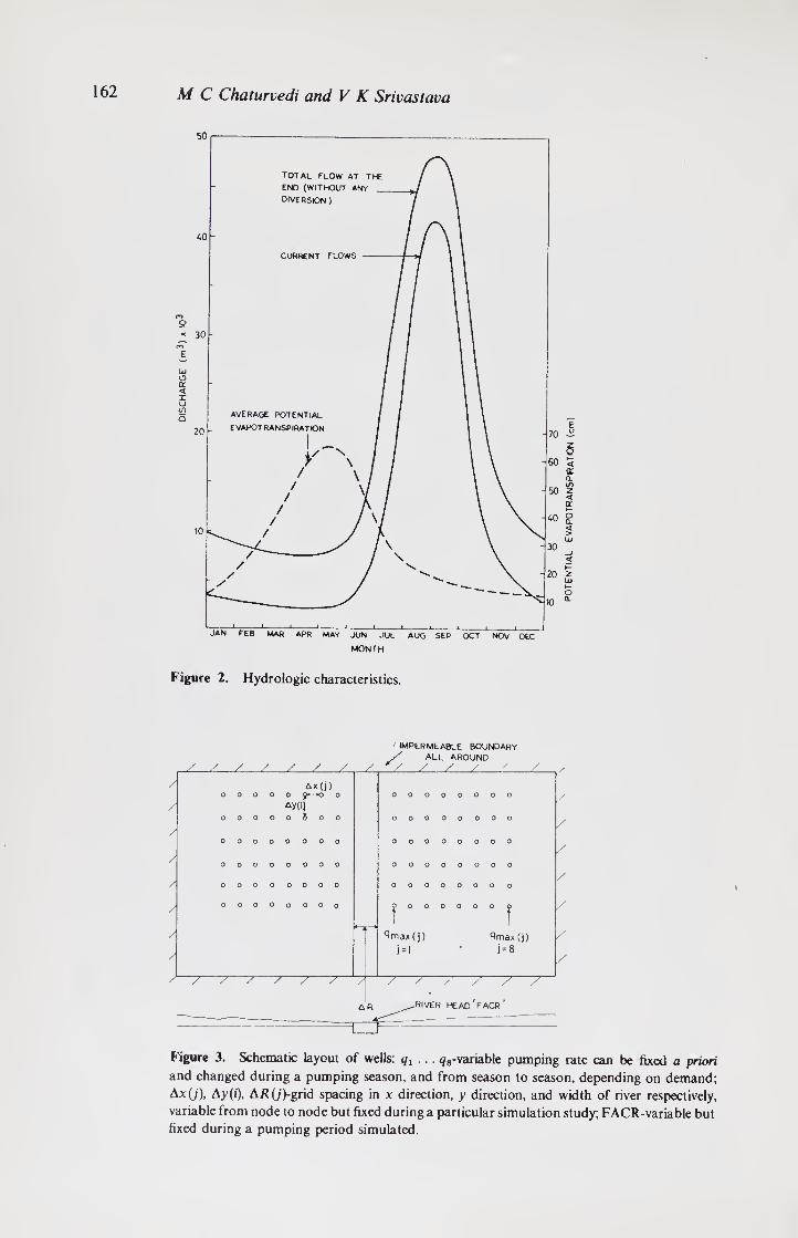
162 M C Chaturvedi and V K Srivastava
Figure 2. Hydrologic characteristics.
IMPERMEABLE BOUNDARY
Figure 3. Schematic layout of wells: qt ... q8-variable pumping rate can be fixed a priori
and changed during a pumping season, and from season to season, depending on demand;
Ax(j), Ay(i), spacing in x direction, y direction, and width of river respectively,
variable from node to node but fixed during a particular simulation study; FACR-variable but
fixed during a pumping period simulated.
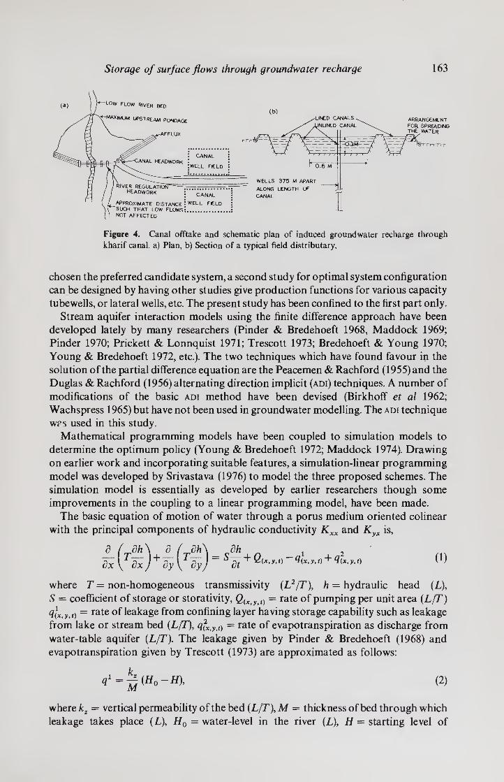
Storage of surface flows through groundwater recharge 163
Figure 4. Canal offtake and schematic plan of induced groundwater recharge through
kharif canal, a) Plan, b) Section of a typical field distributary.
chosen the preferred candidate system, a second study for optimal system configuration
can be designed by having other studies give production functions for various capacity
tubewells, or lateral wells, etc. The present study has been confined to the first part only.
Stream aquifer interaction models using the finite difference approach have been
developed lately by many researchers (Pinder & Bredehoeft 1968, Maddock 1969;
Pinder 1970; Prickett & Lonnquist 1971; Trescott 1973; Bredehoeft & Young 1970;
Young & Bredehoeft 1972, etc.). The two techniques which have found favour in the
solution of the partial difference equation are the Peacemen & Rachford (1955) and the
Duglas & Rachford (1956) alternating direction implicit (adi) techniques. A number of
modifications of the basic adi method have been devised (Birkhoff et al 1962;
Wachspress 1965) but have not been used in groundwater modelling. The adi technique
w?s used in this study.
Mathematical programming models have been coupled to simulation models to
determine the optimum policy (Young & Bredehoeft 1972; Maddock 1974). Drawing
on earlier work and incorporating suitable features, a simulation-linear programming
model was developed by Srivastava (1976) to model the three proposed schemes. The
simulation model is essentially as developed by earlier researchers though some
improvements in the coupling to a linear programming model, have been made.
The basic equation of motion of water through a porus medium oriented colinear
with the principal components of hydraulic conductivity Kxx and Kyx is,
_d_/ <tt\ l_ 3x \ 8x J 8y 3t - S^ + Q(x,y,t) t) + Q(x,y,t) (1)
where T = non-homogeneous transmissivity (L2/T), h = hydraulic head (L),
S = coefficient of storage or storativity, Q{Xiyyt) — rate of pumping per unit area (L/T)
q\x,y,t) — rate of leakage from confining layer having storage capability such as leakage
from lake or stream bed (L/T), q2xy<() = rate of evapotranspiration as discharge from
water-table aquifer (L/T). The leakage given by Pinder & Bredehoeft (1968) and
evapotranspiration given by Trescott (1973) are approximated as follows:
ql=^(Ho~H), (2)
where kz = vertical permeability of the bed (L/T), M = thickness of bed through which
leakage takes place (L), H0 = water-level in the river (L), H = starting level of

164 M C Chaturvedi and V K Srivastava
groundwater table held fixed (L), and
q2 = ^f(Hy-HL) (3)
where kE = maximum evapotranspiration rate (L/T), Hy = depth below top of the land
surface at which evapotranspiration ceases {L),HL = depth of water table below the top of the land surface (L). The finite difference equations and solution methodology is
given in appendix A. The grid is shown in figure 5.
A simple linear programming model has been formulated with an objective function
which optimises the pumping schedule and computes the overall cost of pumping
which consists of simulation of the cost of pumping at each individual well. The goal of
the basin management authority is the minimisation of the average annual cost of
pumping to meet the demand for water. Alternative development solutions to the
problems are therefore ranked according to the criteria
1 t = T N
min Q = r £ Z (fy>' W(n) At, (4)
in which t is the total pumping period broken up into several parts of At over which the
objective function is evaluated, N, the number of pumps which exist in a row, qwU), the
pumping rate of pump at yth column node across the direction of flow of the river with
the pump nearest to the river being qw{1), hj, the total pumping head or lift at column
node j determined from the aquifer model, and Q, the measure of the average annual net
operating cost of pumps.
The objective function is minimized subject to the following constraints:
q»{J)> 0 (j = 1, 2, .... , N), (5)
in which qw(j) is the pumping rate of the well at column node j in each row, and N is the
total number of installed pumps in a row and is the number of independent variables to
each of which q(j) as the pumping capacity is assigned. In the cases studied N takes a
maximum value of up to 8 pumps in a row.
Figure 5, Nodal array for digital model.

Storage of surface flows through groundwater recharge 165
Equation 5 has the non-negativity restrictions or constraints
<I»U) ^ ^maxO) ’ or
Smax®) ~ 4(j) =
in which <?max(;) is the maximum installed capacity of the pump at column node j, which
means that the pumping capacity assigned by the linear program solution cannot
exceed the installed pumping capacity at that node. Also
in which gtotal is the maximum pumping rate permitted of producing water, with the
combined capacity of all pumps not to produce more than this water for each row of
wells being the same for all rows.
Constraints of the type
gW(j) ^ ^min(y') ’
or (8)
*/min(j/) — Qj = °> .
in which qmm(J) is the minimum pumping capacity which must be assigned to each
group at column node j, have not been considered. The reason for not including such
constraints is that a pump which is uneconomical to operate can be shut down or
assumed to be non-existent to find the optimal well field geometry. Such constraints
can, however, be included by a simple modification of the program to include such a
condition when the situation requires it.
It may be noted that the objective ranking function is not an economic function in the
usual sense as the monetary value term and discounting function have not been
incorporated in it. It is, however, quite adequate for ranking purposes. The generalised
flow chart is given in figure 6. The computer listing is given by Srivastava (1976).
4. Analysis
As a preliminary estimate Revelle & Herman (1973) had proposed installing a battery of
tubewells of capacity 0 0285 cumecs each at 0-4 km distance, at right angles and parallel
to the river. Eight wells on either side were proposed to give the requisite discharge.
Considering the river as 0-8 km wide and the nearest point where the wells can be placed
as also 0-8 km away from the river bank, we get the total width of 0-8 km on either side
with a discharge of 2-25 cumecs per km length of river. The schematic representation of
the well field is given in figure 7.
For non-perennial rivers the same scheme (river dimensions) and geo-hydrologic
parameter were adopted. Only the water availability time was assumed as 120 or 240
days for two hydrologic conditions. This is not entirely representative as the
dimensions will be smaller and flow will not be constant for the entire period.
Alternatively, these time periods could be obtained through small storage works. For
the perennial river also discharge was assumed constant over the year although flow
would vary with time. These alternative details could be modelled but at this stage the
objective was only to develop an analytical tool and to get an idea of the comparative
and general order of magnitude under the three possible schemes, and their sensitivity
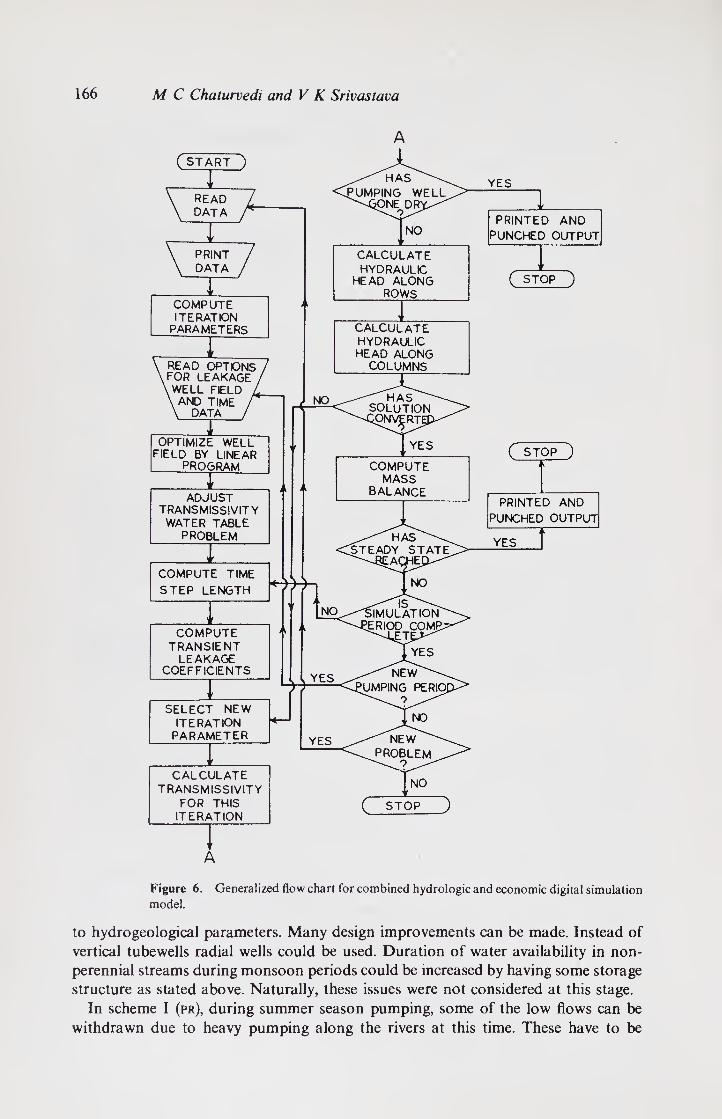
166 M C Chaturvedi and V K Srivastava
('start-')
_z_ READ /
\ DATA
PRINT DATA
CALCULATE HYDRAULIC
HEAD ALONG
READ OPTIONS ^ FOR LEAKAGE
v WELL FELD , AND TIME
DATA
- r~ OPTIMIZE WELL
FIELD BY LINEAR PROGRAM
~TT~ ADJUST
TRANSMISSIVITY WATER TABLE
PROBLEM
COMPUTE TIME
STEP LENGTH
COMPUTE TRANSIENT
LEAKAGE COEFFICIENTS
SELECT NEW ITERATION
PARAMETER
CALCULATE TRANSMISSIVITY
FOR THIS ITERATION
HYDRAULIC HEAD ALONG
COLUMNS
YES
' t_ PRINTED AND
PUNCHED OUTPUT
( STOP )
COMPUTE i l
ITERATION 1 ’ PARAMETERS CALCULATE
( STOP )
PRINTED AND
PUNCHED OUTPUT
YES
Figure 6. Generalized flow chart for combined hydrologic and economic digital simulation
model.
to hydrogeological parameters. Many design improvements can be made. Instead of
vertical tubewells radial wells could be used. Duration of water availability in non¬
perennial streams during monsoon periods could be increased by having some storage
structure as stated above. Naturally, these issues were not considered at this stage.
In scheme I (pr), during summer season pumping, some of the low flows can be
withdrawn due to heavy pumping along the rivers at this time. These have to be
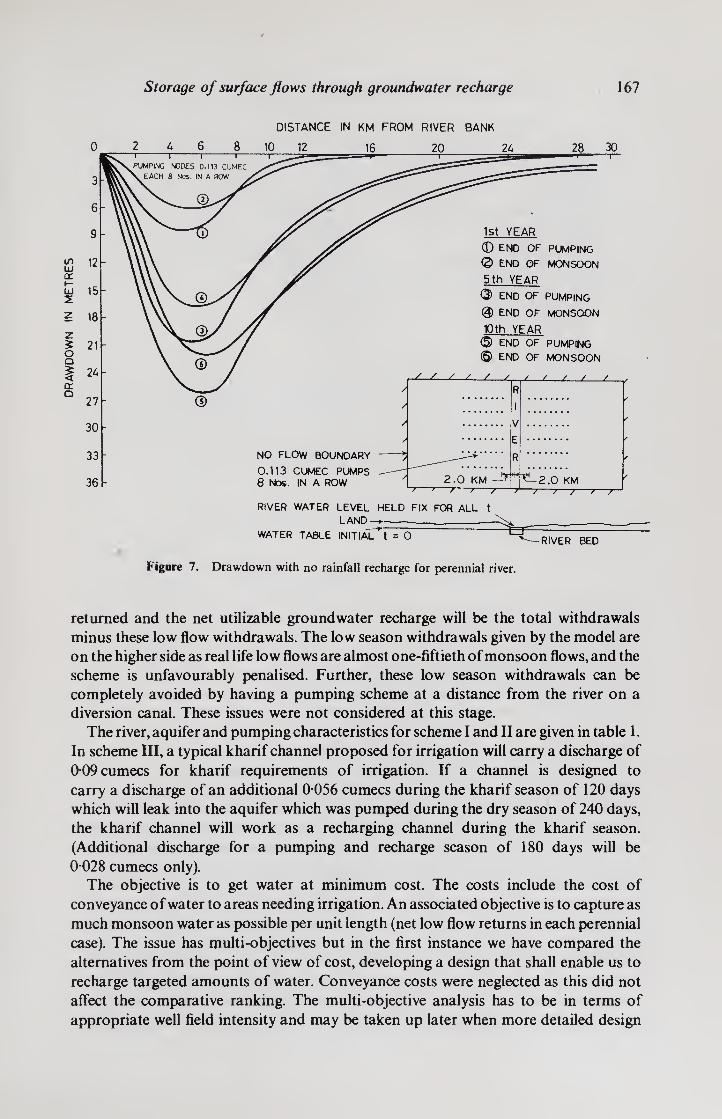
Storage of surface flows through groundwater recharge 167
DISTANCE IN KM FROM RIVER BANK
RIVER WATER LEVEL HELD FIX FOR ALL t LAND ___
WATER TABLE INITIAL t = O RIVER BED
Figure 7. Drawdown with no rainfall recharge for perennial river.
returned and the net utilizable groundwater recharge will be the total withdrawals
minus these low flow withdrawals. The low season withdrawals given by the model are
on the higher side as real life low flows are almost one-fiftieth of monsoon flows, and the
scheme is unfavourably penalised. Further, these low season withdrawals can be
completely avoided by having a pumping scheme at a distance from the river on a
diversion canal. These issues were not considered at this stage.
The river, aquifer and pumping characteristics for scheme I and II are given in table 1.
In scheme III, a typical kharif channel proposed for irrigation will carry a discharge of
O09cumecs for kharif requirements of irrigation. If a channel is designed to
carry a discharge of an additional 0 056 cumecs during the kharif season of 120 days
which will leak into the aquifer which was pumped during the dry season of 240 days,
the kharif channel will work as a recharging channel during the kharif season.
(Additional discharge for a pumping and recharge season of 180 days will be
0 028 cumecs only). The objective is to get water at minimum cost. The costs include the cost of
conveyance of water to areas needing irrigation. An associated objective is to capture as
much monsoon water as possible per unit length (net low flow returns in each perennial
case). The issue has multi-objectives but in the first instance we have compared the
alternatives from the point of view of cost, developing a design that shall enable us to
recharge targeted amounts of water. Conveyance costs were neglected as this did not
affect the comparative ranking. The multi-objective analysis has to be in terms of
appropriate well field intensity and may be taken up later when more detailed design
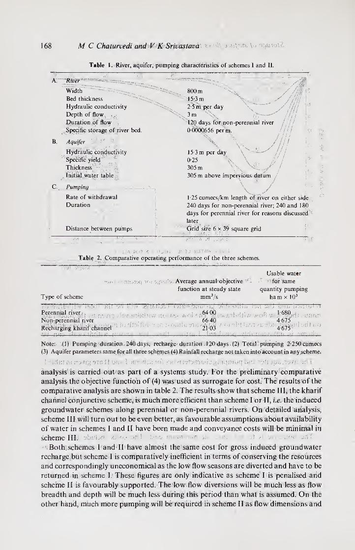
168 M C Chaturvedi and V K Srivastava / \\ s'iiftywv, \o
Table 1. River, aquifer, pumping characteristics of schemes I and II.
> A.
Width
Bed thickness
Hydraulic conductivity
Depth of flow
Duration of flow
Specific storage of river bed.
B. Aquifer
Hydraulic conductivity
Specific yield
Thickness
Initial water table
C. Pumping
Rate of withdrawal
Duration
Distance between pumps
800 m
15-3 m
2 5m per day
3 m ' \ ,-y;- 120 days for non-perennial river
0 0000656 per m.
vv
//MA\ i r ia
////
Hu l
X ' h ! / 8f
15 3 m per day
0-25
305 m I.. . /
305 m above impervious datum \ 13 j /
V~'/ 1-25 cumecs/km length of river on either side
240 days for non-perennial river; 240 and 180
days for perennial river for reasons discussed
later
Grid size 6 x 39 square grid
+.;rx\ i\ >4| .,. •/< i:
J J.JA XI3 0J3H J3V3J H3TAW S3Vlfl
Table 2. Comparative operating performance of the three schemes.
>.130 £3Vlfl- *
Type of scheme
Average annual objective
function at steady state
mm3/s
Usable water
for same
quantity pumping
ham x 103
Perennial river
Non-perennial river
Recharging kharif channel
“Sf.ft1 ;!!■: ;'L'
64 00
66-40
2103
1-680
4-675
4-675
Note: (1) Pumping duration 240days, recharge duration 120days (2) Total pumping 2-250cumecs
(3) Aquifer parameters same for all three schemes (4) Rainfall recharge not taken into account in any scheme.
i S id lit fit b/Ii 1 ..»! <0: • M i ■ : T'Jtn&iw'n UjfiSUQ b/’ • "vtiljpit. i
analysis is carried out as part of a systems study. For the preliminary comparative
analysis the objective function of (4) was used as surrogate for cost. The results of the
comparative analysis are shown in table 2. The results show that scheme III, the kharif
channel conjunctive scheme, is much more efficient than scheme I or II, i.e. the induced
groundwater schemes along perennial or non-perennial rivers. On detailed analysis,
scheme III will turn out to be even better, as favourable assumptions about availability
of water in schemes I and II have been made and conveyance costs will be minimal in
scheme III.
Both schemes I and II have almost the same cost for gross induced groundwater
recharge but scheme I is comparatively inefficient in terms of conserving the resources
and correspondingly uneconomical as the low flow seasons are diverted and have to be
returned in scheme I. These figures are only indicative as scheme I is penalised and
scheme II is favourably supported. The low flow diversions will be much less as flow
breadth and depth will be much less during this period than what is assumed. On the
other hand, much more pumping will be required in scheme II as flow dimensions and

Storage of surface flows through groundwater recharge 169
availability period corresponding to scheme I during monsoons shall not be available
unless storage structures are constructed which will naturally increase the unit cost.
Creative solutions for scheme I are also possible for increasing the efficiency by
pumping along diversions. Therefore, for taking decisions more detailed hydrologic,
hydraulic and engineering-economic analyses are needed. Furthermore, these schemes
are not mutually exclusive.
The important issue of long-term salt-balance has not been analysed in this case and
must be studied in any further study. Reference may therefore be made to the classic
study of the Indus basin by the Harvard group (Thomas & Burden 1965). ' CS* H* 9s & ST §T C f sa. a. S a a X ^ ra., 'a. \ rf
P O w _ O U C <7 ; g i
5. Sensitivity analysis , f.' U. O iXi v" -J) u y (i 17 |
Analysis has been carried out for a range of configurations and parameters in each of
these three cases to get an idea of the dynamics of the system. Some of the results for
scheme I are given in table 3. First, keeping the capacity constant, what is the effect of
the location of the wells? It is seen that the optimal case has two tubewells near the river.
Based on this result, radial wells appear to be attractive. Secondly, for the perennial case
net usable groundwater recharge increases, but at increased unit cost for a spread out
field. The implication is that if pumps are proposed to be spread out along the length of
the river to reduce groundwater lowering, there is a corresponding penalty in the
increased lateral dimension to maintain unit availability per unit length of river.
Thirdly, increased pumping time increases unit costs as drawdown increases while
groundwater recharge decreases, as proportionately larger amounts of water have to be
returned during the low flow season. Similar studies have also been carried out for the
other two schemes. i - I ■ ■ o- 1 !C ! a.
The sensitivity of the objective function to change in the aquifer parameters was also
carried out for each of these three cases. For one case, viz the non-perennial case, the
results are shown in table 4.
The changes for other cases are of the same order of magnitude. It will be seen that
the objective function is most sensitive to changes in aquifer hydraulic conductivity,
next to the specific yield, and comparatively insensitive to river bed hydraulic
conductivity; ; ; ... f
The drawdown, yearly recharge and pumped withdrawal per kilometre length of
river for some of the configuration and aquifer parameters are shown in figure 13.
Figure 7 shows that drawdown varies spatially and temporarily for a given
configuration. No rainfall recharge was assumed. The specific yield value adopted was
0.25. If a different value of specific yield or additional rainfall recharge is adopted
general characteristics remain the same and only the drawdowns vary.
Fora specific yield of 0-1 the drawdown at the end of the tenth year changed from 26
to 35 metres while with normal rainfall recharge of 15 cm annually, the drawdown at the
tenth year was changed only marginally to 23 from 26 metres. The yearly recharge and
pumped withdrawal per kilometer length of river is shown in figure 8. It will be seen that
a steady state is not reached even after 10 years. The drawdown will go down further
and objective function worsen, apparently asymptotically. Even if normal rainfall
recharge is taken into account, although the yearly recharge is increased, a steady state
is not reached after 10 years. However, if the value of the specific yield was 0-25, steady
state would be reached with normal rainfall recharge in about 10 years.
The effect of well configuration has also been studied by replacing eight wells by only
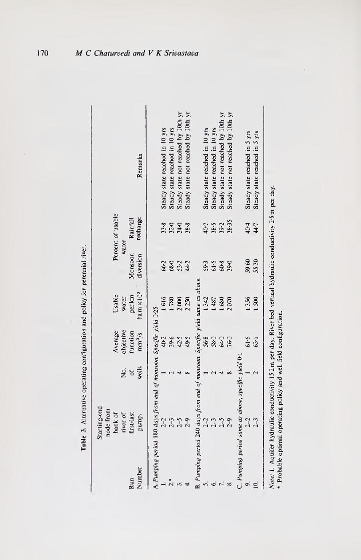
Tab
le
3.
Alt
ernat
ive
op
era
tin
g c
onfi
gura
tion a
nd p
oli
cy f
or
per
ennia
l ri
ver
.
170 M C Chaturvedi and V K Srivastava
eO E <L)
CC
<D x 3 3
—: o> 3 £ 13
CO o |V ay k-
8 S <u Oh
5 .5 2 -o
« .. e ° •S is -5 ~ D * 8. B
CO X
<d g e M cO -rj ro
a .8 g B ^ .o' § E
o <— — z ° g
"O c e u- u_ «—• u
1 o u. O o co
cO d 00 c
kx
c*-x
1) “O
LZ kx c « CO X
i co i-
6 3 Cl
$ C/3
o c
X »- X
JS c I 3 5
e£ Z
kx t- >- >V >> X X X X
1/5 kx
S o S 5 co k- —< C/5
V_ C/5 t-i i C/5 CO
>v «^i >> >% u. kx o O X X o O X X *►>
TD ~o T3 ■8
CO
c a Q <D c 3 ay c c X X X X
-a ~o a a i “O a a T3 ~o <D 0 s s <u 3 ay ay ay
X u. V- X X u- X X y cy o CJ y o
s s o o 3 3 o O c0 ay s
i— k- c c u. k* c c u- u. ay ay ay (U a> ay ay ay ay ay cO 5 S s S 5 S S S S to C/5 C/5 (A CO C/5 C/5 C/5 CO CO >> >v >> >v >> C0
"O ID -o "O “O "O *o •o TD T3 ~o cO cO CO cO CO co cO CO c0 «3 kx o 4> ay 0) w a5 ay ay ay
8, 55 55 55 <55 55 55 55 55 55 55
E *o
IZ5 <N oo o p oo r- <N fp Tf r- ro <N TJ- oo
$ oo 6s OO
i ? m m ro cn m m m *>
ty 3
~o c o
s
cy <N p <N CN m oo o o
m o X X
do X
rO *0 5
6s c/~l X s
d On CO »o
3 c0 kx
TD >v
o X -c *—X Q 8
X O Q O CO <N o o X 8 *—
T—1 oo o ^t oo oo ay > X r- o <N fp ■'O’ X o fp CO
«o <N
<N <N 5 C3
rs — ■o © CO
J5
.cu X
^2 kx ay >
CJ CJ £
Cj <N x CO OO o O o X O d <N d CJ X oo
3 X X <o
•8 L Ci,
ro Tf Tf CL Ci.
»Z5 CO r- X X
03 on kx
c c O 8. © ©
o o E
eg K ©
T—H <N OO CO c o <N 00 '^v i-H <N
<N CO
s S ay
ay >v
■§ cu
s
“3 c CL
5
cu cl co
<aT a
’>
O 3
TD © o O 3
X) 3
O cy
«o m
1 •O
1 On
1
CO >> (N
1 m X
i Os
1 co 3 <N
1 ro
1 cy
"3 o
(N <N <N <N O
(N <N (N <N Oy 5
CN <N 3 co kx
oo 3 *o r~i CO >v
^3 *3 X
©
©.
O
cx
•2 £ <0> CL
kx c£x 3
35 c
^5 •S
35 «
CD" <
s. s. 5. 5 S 5 3
ft. * 3 3
ft. CL
< <N ro Tf
CQ »zS X r-‘ OO
u 6 O
Pro
bab
le o
pti
mal
op
era
tin
g p
oli
cy a
nd w
ell
fiel
d c
on
fig
ura
tio
n.
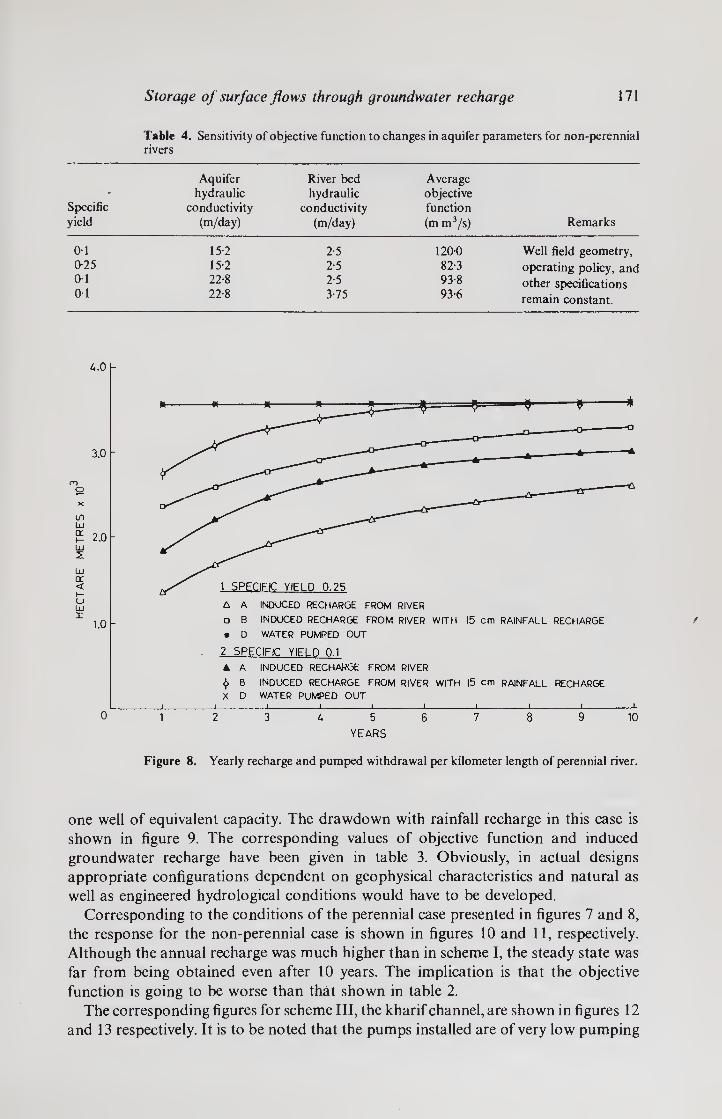
Storage of surface flows through groundwater recharge 171
Table 4. Sensitivity of objective function to changes in aquifer parameters for non-perennial rivers
Specific yield
Aquifer hydraulic
conductivity (m/day)
River bed hydraulic
conductivity (m/day)
Average objective function
(m m3/s) Remarks
01 15 2 2-5 1200 Well field geometry. 0-25 15 2 2-5 82-3 operating policy, and 01 22-8 2-5 93-8 other specifications 01 22-8 3-75 93-6 remain constant.
YEARS
Figure 8. Yearly recharge and pumped withdrawal per kilometer length of perennial river.
one well of equivalent capacity. The drawdown with rainfall recharge in this case is
shown in figure 9. The corresponding values of objective function and induced
groundwater recharge have been given in table 3. Obviously, in actual designs
appropriate configurations dependent on geophysical characteristics and natural as
well as engineered hydrological conditions would have to be developed.
Corresponding to the conditions of the perennial case presented in figures 7 and 8,
the response for the non-perennial case is shown in figures 10 and 11, respectively.
Although the annual recharge was much higher than in scheme I, the steady state was
far from being obtained even after 10 years. The implication is that the objective
function is going to be worse than that shown in table 2.
The corresponding figures for scheme III, the kharif channel, are shown in figures 12
and 13 respectively. It is to be noted that the pumps installed are of very low pumping

172 M C Chaturvedi and V K Srivastava
DISTANCE FROM RIVER IN km
32
21 -
Figure 9. Drawdown with rainfall recharge for perennial river.
DISTANCE FROM RIVER IN km
12 16 20
1st YEAR
© END OF
0 END OF
5th i YEAR
0 END OF
@ END OF
10th YEAR
© END OF
© END OF
PUMPING
MONSOON
PUMPING
MONSOON
PUMPING MONSOON
Figure 10. Non-perennial river drawdown with no rainfall recharge.
capacity and uniformly spread over the whole area and therefore the water table goes
down uniformly all over the aquifer due to the pumping stress. The drawdown,
therefore, is a horizontal line in all cases at the end of both pumping and the recharge
cycle. Steady state is reached, in contrast to the earlier two schemes, within five years.
6. Conclusion
The study is exploratory. An aquifer-stream flow interaction simulation-linear
programming model has been developed. Order of magnitude behaviour for three
schemes designed to conserve the monsoon flows in the Ganges basin by induced
groundwater recharge and the sensitivity to engineering decisions, hydrogeological
parameters and hydrological conditions has been quantified. Technical feasibility of
storage of large monsoon flows has been demonstrated.

Storage of surface flows through groundwater recharge 173
4.0
3.0
u) LU CL t— UJ X
a 2.0 <
o LU X
CO O
1.0
©© X-$-X-<1-*-1}—*-If—-<>—*—4-*-4—*-$—X—$-*
© ®
1- ®
®
1 SPECIFIC YIELD 0.25 A LEAKAGE WITH NO RAINFALL RECHARGE A LEAKAGE WITH 15 cm RAINFALL RECHARGE X WATER PUMPED OUT
2 SPECIFIC YIELD 0-1 © a LEAKAGE WITH NO RAINFALL RECHARGE
© o LEAKAGE WITH 15 cm RAINFALL RECHARGE
© ff WATER PUMPED OUT
5 6 YEARS -►
8 10
Figure 11. Yearly recharge and pumped withdrawal per kilometre length of non-perennial river.
100 80 60
DISTANCE FROM CHANNEL IN MT
40 20_0_20_40 60 80 1 1 -,-1-1-1— A
CHANNEL
I t
f ©
- ©
©l©
- ©»®
1
-
if) LU CL
LU 2
Z £ o o i CL Q
1st YEAR © END OF RABI SEASON
® END OF KHARIF SEASON
5th YEAR ® END OF RABI SEASON
© END OF KHARIF SEASON
10th YEAR
© END OF RABI SEASON
© END OF KHARIF SEASON
0.0071 CUMEC PUMPS 375 MT APART. 180 DAYS PUMPING
SPECIFICATIONS
CHANNEL WIDTH = 0-6 MT BED THICKNESS = 3 MT
PERMEABILITY =2.5 MT PER DAY
WATER LEVEL = 0.3 MT
AQUIFER
PERMEABLITY = I5.3 MT PER DAY
SPECIFIC YIELD =0.25
DEPTH =305 MT
GRID SIZE VARIABLE
0-3 MT KLo.e MT
— LAND
"INITIAL WATER TABLE t =0
CANAL WATER LEVEL HELD FIXED FOR ALL t
Figure 12. Drawdown with recharge during kharif season and pumping during rabi season.
s li

174 M C Chaturvedi and V K Srivastava
NON PERENNIAL CHANNEL
RECHARGE DURING SIX MONTHS KHARIF SEASON
WITHDRAWAL DURING SIX MONTHS RABI SEASON
PER 100 MT LENGTH OF CHANNEL
1 U1 UJ oc UJ 2 2.0
UJ cr < F— o UJ X
1.0
1 SPECIFIC YIELD = 0.25
(A) A LEAKAGE WITH NO RAINFALL RECHARGE
© X WATER PUMPED OUT
2 SPECIFIC YIELD =0.1
o LEAKAGE WITH NO RAINFALL RECHARGE □ WATER PUMPED OUT
__I_1_I_I_1_I_I-J-1-L_
0 1 23456789 10
YEARS -►
Figure 13. Yearly recharge and pumped withdrawal per kilometre length of non-perennial
river.
Economic feasibility is a matter of detailed systems planning and design. Of the three
schemes, the third, viz kharif channel conjunctive groundwater development appears to
be very attractive. The schemes are not mutually exclusive and their choice depends
upon general hydrologic-physiographic situations. For instance, in the three continu¬
ous areas of the Indo-Gangetic basin, each has some advantage over the other. In
Punjab, at the western end where all the perennial river flows have been stored, scheme
II is being explored. In Uttar Pradesh and Bihar, viz., the western and central Ganges
basin, where even after conserving all possible monsoon flows considerable excess
supplies shall be left over, scheme III or I is being proposed for adoption. In Haryana, in
the south-west, where groundwaters are saline, scheme II is being proposed.
References
Bredehoeft J D, Young R A 1970 Water Resources Res. 6: 3-21
Birkoff G, Virga R S, Young DM Jr 1962 Advances in Computers (New York: Academic Press) Vol 3
Chaturvedi M C 1976 Second India Studies—Water (New Delhi: MacMillan)
Duglas J Jr, Rachford H H Jr 1956 Trans. Am. Math. Soc. 82: 421-439
Peaceman D W, Rachford H H Jr 1955 J. Soc. Ind. App. Maths 3: 28-44
Pinder G F, Bredehoeft J D 1968 Water Resources Res. 4: 1069-1093
Pinder G F 1970 An iterative digital model for aquifer evaluation, Open file report US Geol. Survey, 65 pp
Prickett T A, Lonnquist C G 1971 Selected digital computer technique for groundwater resource evaluation,
Bulletin No. 55, Illinois State Water Survey, Urbana, 62 pp.
Rama 1971 An alternative to Ganga-Cauvery link, Sci. Today, Times of India Publication, Bombay,
September
Revelle R, Herman T 1973 Some possibilities for international development of the Ganges-Brahmaputra
Basin, First World Congress on Water Resources, International Water Resources Association, Chicago
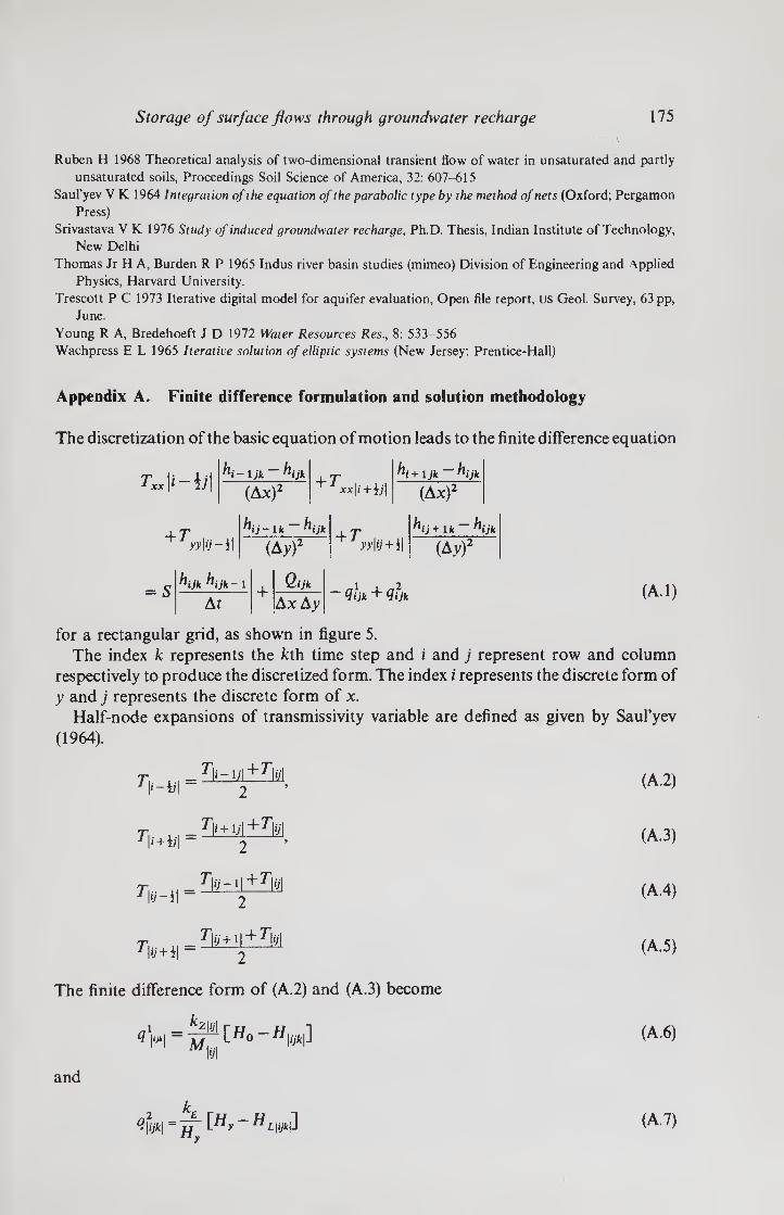
Storage of surface flows through groundwater recharge 175
Ruben H 1968 Theoretical analysis of two-dimensional transient flow of water in unsaturated and partly
unsaturated soils, Proceedings Soil Science of America, 32: 607-615
Saul’yev V K 1964 Integration of the equation of the parabolic type by the method of nets (Oxford; Pergamon
Press)
Srivastava V K 1976 Study of induced groundwater recharge, Ph.D. Thesis, Indian Institute of Technology,
New Delhi
Thomas Jr H A, Burden R P 1965 Indus river basin studies (mimeo) Division of Engineering and Applied
Physics, Harvard University.
Trescott P C 1973 Iterative digital model for aquifer evaluation, Open file report, us Geol. Survey, 63 pp,
June.
Young R A, Bredehoeft J D 1972 Water Resources Res., 8: 533-556
Wachpress E L 1965 Iterative solution of elliptic systems (New Jersey: Prentice-Hall)
Appendix A. Finite difference formulation and solution methodology
The discretization of the basic equation of motion leads to the finite difference equation
Txx\i-\j\
+r
ht. -* •j
-sT i •—> 1 i T hi+ljk hi jit
(Ax)2 + ixx|» + i/| (Ax)2
j - Ik hijjj hij +ut hijk
-il (Ay)2 ' - wii/'+il (Ay)2
hijk hijk-1 i Qijk
At Ax Ay -1ihk+qfjk (A.l)
for a rectangular grid, as shown in figure 5.
The index k represents the kth time step and i and j represent row and column
respectively to produce the discretized form. The index i represents the discrete form of
y and j represents the discrete form of x. Half-node expansions of transmissivity variable are defined as given by Saul’yev
(1964).
7’|i_I/|+7|i;1
T\i-ij\ ~ —2— ’ (A.2)
r, r\j+U\±I\fA v|i+b| 2 (A.3)
T,. ■■ = ^Ig- lilZjgl (A.4)
T. rll>' + 1l + 7J1>:l (A.5)
The finite difference form of (A.2) and (A.3) become
kz\ij\ q\ik\ Mu,
and
qiik\ H Ih,-hlwj
(A. 6)
(A.7)

176 M C Chaturvedi and V K Srivastava
An adi procedure is used to solve the equation after substituting the discretized values
of the various terms of (A.4). An iterative procedure used by Ruben (1968) is used to
increase the accuracy of the method. Application of these techniques to (A.4) leads to
two new equations.
Txx\ i-
(Ax)2
Tvv\u
T*x\i-lj\ , Txx\i + \j\ , S
(Ax)2 (Ax)2 At ./(«) Un+i) I *xx\i + {\ Un+l)
111 + (Ax)2
_ 1yy\ii-i\ l(h) , - (Ay)2 +
• yy\‘j-l\ , 2 y>’li/+ll _nn> (Ay)2 (Ay)2 At M
Kll~ i
Tvv\i, yyli/ + ll (Ay)2
Qijk ij+lk- 1
Ax Ay ' Qijk T Qijk (A.8)
and
(Ax) Un+l) Ixx\ij-^\ 2xx|i/ + j| - r(n)
\2 nij-lk ■■ '■> "r + • 1 (Ax)2 (Ax)2 At \ij\ Un+D nijk
I T*x\'j + l\ L(n + 1) _ Tyy\i-ij\un) ,
+ (Ax)2 h“+'k~ (Ay)2 +
Tyy\i-{j\ . Tyy\i + \\ S
(Ay)2 (Ay)2 _ r(n)
At 7M h\fk - i
Tyy\' + hi\ (Ay)2
h\"+ i jk- i + Qijk
Ax Ay - Qijk + Qijk
(A.9)
In (A.8) and (A.9) Iff denotes the iteration parameter at the ith and jth node point and is
defined by Pinder & Bredehoeft (1970) as
Iff = I\]0) exp L 2X„
n (A- 1)
where k is the number of iteration parameters desired. Xm is the larger of the total
number of rows and columns in the grid and
,2 ;(i) =
n 1
2X1 14<a*)2 - hi+ T\i+hi+ri<t - i|+T\ij+i|]’
(Ay)2
where Ax is maximum grid spacing and Ay is minimum grid spacing given by Trescott
(1973).
Known values are on the right side of (A.8) and (A.9). For the imposed grid, (A.8) and
(A.9) form two systems of linear equations. The first set represents the row values with
column values held fixed and the second set represents the column values with row
values held fixed. The values of hffk_ j and h{"jk are compared for all i's and/s. If the
absolute value of their difference is less than some convergence factor e the time-
increment counter k is advanced to k+ 1; if not, the iterative parameter index n is
advanced and k remains fixed, until convergence is achieved. The time duration At may
be large with iterative procedure. The program has two options on the time either to
simulate a given number of time steps or to simulate a given pumping period.
The transmissivity is computed at each iteration as product of saturated thickness
and hydraulic conductivity at each node. The program is set up to terminate

Storage of surface flows through groundwater recharge 111
computations when a pumping well “goes dry”. For nodes that go dry other than
pumping nodes a saturated thickness of 0305 m (on an empirical basis) is maintained so
that a saturated layer is maintained at the top and the unsaturated region is not
introduced. The program also has the facility of multiple pumping periods.
The program is set up to terminate computations to save computer time when the
solution approaches steady state long before the end of the pumping period. Withdrawal from a well node is assumed to occur over the area of influence of the well
node. Drawdown at a pumping node, therefore, is considerably less than would be
observed in a real well. The real well drawdown can be predicted by plotting drawdown
versus the log of distance for nodes near the pumping node (excluding those directions
in which other wells are within two nodes) and extrapolating to the radius of a real well.
Alternatively, these data can be used in the Theim equation to calculate the additional
drawdown in a fully penetrating real well.
Two major assumptions are made in treating the leakage from the multiple pumping
periods. Dimensionless time for the previous pumping period is assumed to be so large
that storage in the confining bed has a negligible effect on the leakage from this period. For a real problem involving pumping periods of months to years in length this is a
reasonable assumption. Rainfall infiltration recharge is treated as pumping into the
aquifer. A check is provided that the water table does not rise above the top of the
aquifer during computation. If very high recharge rate from rainfall is assumed the
program will not allow the water-table to rise above the top of the aquifer in such cases.
The water level in the source, from which leakage takes place, can be changed over
various pumping periods to simulate the real situations over long pumping periods and
the effect of leakage is included implicitly.
The grid spacing in the two directions can be different and quite large. However,
smaller grid spacing and shorter time periods will give better results.

.
.

Study of Bhakra reservoir operation
P S RAO* and S RAMASESHANt
* Indian Institute of Management, Bannerghatta Road, Bangalore 560076, India
t Civil Engineering Department, Indian Institute of Technology, Kanpur 208 016, India.
Abstract. The study outlines the methodology for working out a multiobjective reservoir operation with conjunctive utilization of surface and groundwater. Irrigation and power have been considered the two objectives for operation of the reservoir. The results of this study are compared with those achieved with conventional operation in the past and show that there is an increase in irrigation by 7 to 8 % due to conjunctive use of surface and groundwater. The trade-off between irrigation and power has been developed and discussed. The transformation surface between three objectives viz., power, irrigation and carry-over storage has been developed and the merits of carry-over storage have been discussed.
Keywords. Reservoir operation; multiobjective analysis; conjunctive use of water.
1. Introduction
Irrigation and power are two of the most important purposes for which surface and
groundwater resources are used. The integrated operation of a complex system is
necessary for efficient management of limited resources to meet irrigation and power
demands. The importance of the conjunctive utilization of surface and groundwater in
an integrated framework has been realised (Irrigation Commission 1972) but has not
been put into practice perhaps due to institutional constraints and lack of coordination.
However, using a systems analysis procedure it seems possible to study the integrated
operation of a multiobjective reservoir system with conjunctive utilization of surface
and groundwater. A case study of the Bhakra reservoir, which has been in operation
since 1966 is described in this paper. The object of this study is to analyse the past
operation of the reservoir within a multiobjective framework to evaluate the trade-offs
between irrigation and power demands in the past. The study also demonstrates the
methodology and procedures in multiobjective analysis within an integrated
framework.
2. System description
2.1 The Bhakra
The Bhakra system in Punjab constitutes one of India’s biggest projects (figure 1). The
Bhakra dam is a 225-55 m high concrete gravity dam built on the river Sutlej. The river,
the largest tributary of the river Indus, begins in Tibet and enters the Indo-Gangetic
plains near Bhakra. The total catchment area upstream of Bhakra is 56,980 km2. The
rainfall in the catchment varies over the basin with an annual average of around
875 mm. Govindsagar, the reservoir formed by the Bhakra dam, has a gross capacity of
179

180 P S Rao and S Ramaseshan
Figure 1. Interconnected system of the rivers Ravi, Beas and Sutlej.
9876 mcum and a live storage capacity of 7814mcum above a dead storage level of
445-62 m. It covers an area of 168-35 km2 when full. The total run-off at Bhakra for a
dependable year works out to 13,723 mcu m and that for a mean year to 16,441 m cu m.
A dependable year has been adopted by the planners as a hypothetical year in which the
mean discharge of any 10-day period is equalled or exceeded by the corresponding 10-
day mean discharges in 67 % of the years for which data are considered.
The river flows are high for the four months from June to September due to
snowmelt and monsoon rains. Almost 47% of the river flow of a dependable year
occurs during these four months. Water from Govindsagar (Bhakra reservoir) can be
passed through the turbines of two power houses, one on the right bank and the other
on the left bank at the foot of the Bhakra dam. Both the power houses have 5 turbines
each. Each of the generators in the right-bank power house has a maximum capacity of
120 mw when the head is 116 m or more, whereas each of the left-bank generators has a
maximum capacity of 90 mw when the head is 110 m or more. These capacities fall
respectively to 70 mw and 53 mw when the head falls to about 80 m. Thus the power¬
generating capacity varies from a maximum of 1050 mw to a minimum of 615 mw.
About 11 km downstream of the Bhakra dam is the Nangal reservoir formed by the
28-95 m high Nangal dam. It serves as a head regulator for control of irrigation releases.
Part of the water from Nangal is released to the Nangal hydel channel which is 64-48 km
long and has a carrying capacity of 353-75 cumecs. The remaining water is released to
the Sutlej. The Nangal hydel channel supplies water to two power houses in its path at
Ganguwal and Kotla with a total installed capacity of 154 mw. Water from the Nangal
hydel channel is then divided between the Bhakra main canal and the Sirhind canal. The
Bhakra main canal serves some of the canals of the old western Jamuna canal system
which were merged with the Bhakra system and so receives some supplies from the
western Jamuna canal.
Downstream of Nangal, there are headworks at two places on the river Sutlej at
Ropar and Harike. At Ropar, water is diverted to the Bist Doab and Sirhind canals. The
Beas river joins the Sutlej at Harike. Water is diverted at Harike to the Rajasthan feeder

Study of Bhakra reservoir operation 181
and the Ferozepur feeder for the Eastern and Bikaner canals and the Sirhind feeder.
Water from all these canals is distributed through the network of the branch canals of
the irrigation distribution system. The details of the system are given in figure 1.
Punjab possesses large resources of groundwater which are generally suitable for
irrigation. Due to the presence of alluvium, a large-scale programme to install tubewells
has been undertaken. The State in 1974 had about 126,000 tubewells and another
75,000 were proposed under the fifth plan (1973-1978). An area of 0-6 to 0-8 m ha suffers
from waterlogging. The installation of tubewells would also solve the waterlogging
problem to some extent.
2.2 Irrigation demands
Bhakra was primarily designed to improve irrigation over an area of 1-42 m ha and
irrigate an additional 2-43 million hectares. The area served consists of parts of Punjab,
Haryana and Rajasthan. The main crops grown in this region are bajra, cotton, maize,
rice, jowar, sugarcane, oilseeds, pulses and fodder during the monsoon (kharif) season;
and wheat, gram, oilseeds, barley, potatoes and fodder during the winter (rabi) season.
Irrigation requirements given in table 1 were assessed when the project was planned
Table 1. Irrigation requirements of the Bhakra system
Month Period
No.
of
days
Daily
irrigation
requirements
(in cumec days)
Total irrigation
requirements
(in cumec days)
Filling period (from 1st of June to 20th of September)
June 1-30 30 715-71 21471
July 1-31 31 56113 17395
August 1-31 31 561-13 17395
September 1-20 20 711-63 14233
70494 or 6100 m cu m
Depletion period (from 21st September to 31st of May)
September 21-30 10 711.63 7116
October 1-15 15 727-71 10916
16-31 16 654-63 10474
November 1-30 30 654-64 19639
December 1-10 10 611-76 6118
11-15 5 363-67 1818
16-31 16 345-80 5533
January 1-15 15 345-80 5187
16-31 16 363-67 5819
February 1-10 10 390-46 3905
11-28 18 545-52 9819
March 1-31 31 545-52 16911
April 1-15 15 345-80 5187
16-30 15 418-89 6283
May 1-31 31 703-50 21809
136534 or 11800 mcum
Total 6100+11800 = 17900 m cum
(Mehndiratta & Hoon 1973)
182 P S Rao and S Ramaseshan
and were modified only slightly since, although the irrigation demands have changed
due to the introduction of high-yielding varieties of crops which require more water.
The need to reassess irrigation requirements and revise the demands has been well
recognised.
Irrigation requirements are high from September to November owing to the water
required for the maturing of the kharif crops and the preparation and sowing of the
rabi crops. The requirements are low from December to April, except in the latter half
of February and in March when water is required for the maturing of the rabi crops.
The rabi crop requirements are smaller than the kharif crop requirements. In May and
June, the requirements are again high due to the preparation and sowing of the kharif
crops. During the monsoon season also the requirements are quite high as the areas
where such water is to be utilized have low rainfall.
2.3 Power demands
The releases from the reservoir were originally planned mainly for irrigation. Only
987mcum (revised upwards to 1360 mcum recently) was earmarked for releases for
power generation. These releases were in addition to those made for irrigation. It was
assessed that the releases for power made would yield a firm power of 282 mw from the
Bhakra power houses during an empirically-defined dry year.
2.4 Current operating policy
Each year the Bhakra Management Board (bmb) conducts operational planning
studies, referred to as water power studies, of the system as part of the planning to
regulate the supplies from the Bhakra reservoir. The water year from 1 June to 31 May
is divided into two periods. June 1 to 20 September is the ‘filling period’ when supplies
are generally available due to snowmelt and the monsoons and the reservoir fills up.
September 21 to 31 May is the ‘depletion period’ when water is released from reservoir
storage to meet the demands of irrigation and power.
During the filling period, irrigation demands are met in full subject to the constraint
that the reservoir is not allowed to deplete. This means that demands are not fully met if
they exceed inflows. This could happen because of the delayed arrival of monsoon,
during breaks in monsoon and also in relatively dry years.
Water power studies are conducted for the depletion period using the available
utilizable stored volume of water in the reservoir and dependable year or dry year
inflows for the depletion period. Although on the basis of 10-day inflows any particular
inflow figure of a river in a dependable year would have a probable availability of 67 %,
the total yearly inflow of a river at any particular site, corresponding to the dependable
year has a probable availability of about 85 %. A dry year is taken as the driest year on
record. It is not possible to meet the full irrigation requirements of the depletion period
every year. The ratio of deliveries to demands is called the reservoir factor (rf) defined
as
rf — (Total storage available in reservoir + expected inflow during de¬
pletion period ± gains or losses upto the point of offtake of canals.)/(Total canal requirements during the depletion period.)
The water power studies of bmb indicate that the firm power level is not a constant
throughout the depletion period. The firm power level is 15-30% higher from 21
Study of Bhakra reservoir operation 183
September to 10 December than from 10 December to 31 May. These studies include
the possibility of carryover storage from a good year to the subsequent year. Based on
water power studies a decision is taken on 21 September regarding regulation of
supplies from the reservoir during the depletion period. The decision implies choice of
(i) rf (ii) firm power level, and (iii) minimum reservoir drawndown level to be reached
on 31 May (this determines the carryover storage, if any).
3. Review of earlier studies
The Bhakra system has been studied and reported by economists (Raj 1960; Ansari
1968; Minhas et al 1972; Reidinger 1974) and by engineers (Singh 1964; Mehndiratta &
Hoon 1973). Raj concerned himself with some economic aspects of the Bhakra Nangal
project and a preliminary analysis of selected investment criteria. Ansari studied the
economics of irrigation rates and examined the basic arguments for incurring financial
deficits on irrigation supplies. Reidinger studied the institutional rationing of canal
water in an area in Hissar district which is served by one of the Bhakra canals.
Minhas et al (1972) made extensive simulation studies of the operations of the
Bhakra system (i) to determine for the depletion period the efficient combinations of
firm power with certainty and irrigation supplied with a given confidence level, (ii) to
evaluate the increase in availability of both irrigation and firm power due to conjunctive
utilization of surface and groundwater and to compare the economics of this scheme
with that of a thermal back-up. They observed that “in the absence of a satisfactory
economic measure of the relative worth of irrigation and power, one cannot determine
an ideal operating policy”. But the important question of devising such a satisfactory
economic measure has been left unanswered in the study. As such the trade-off
possibilities delineated in a probabilistic sense cannot be used by decision-makers in
choosing the point of operation of the reservoir at the end of the filling period.
Singh (1964) put forward the idea of using seasonally available secondary power for
lifting groundwater by tubewells in the general framework of conjunctive utilization of
surface and ground waters. Minhas et al (1972) noted that the tubewells, when operated
solely to augment irrigation supplies, can utilize power which would otherwise go waste and which therefore is ‘free’ in the economic sense of the term (since the economic value
of goods is based on their alternative uses). Operated solely to increase the level of firm
power output, tubewells can convert useless secondary power to valuable firm power.
Singh also pointed out the role of groundwater development as an antiwaterlogging
measure.
Mehndiratta & Hoon (1973) report the methodology adopted by bmb to regulate
supplies from the Bhakra reservoir from 1966 to 1972. This report greatly helped in
understanding the system and serves as the source material for the present study. Water
power studies of bmb, given in tables 2 and 3, reveal that according to the planning
studies for the operation of the reservoir in 1969-70 and 1970-71, considerable
secondary or dump power was generated during the early part of the depletion period.
From the studies reviewed, it is clear that (i) the sudden peak in the irrigation
demands during the rabi sowing season, which is the early part of the depletion period
of the reservoir, necessitates the release of water with high potential for power
generation for irrigation; (ii) consumers of power who get used to the higher level of
firm power supplied during this period find it difficult to reduce their consumption of
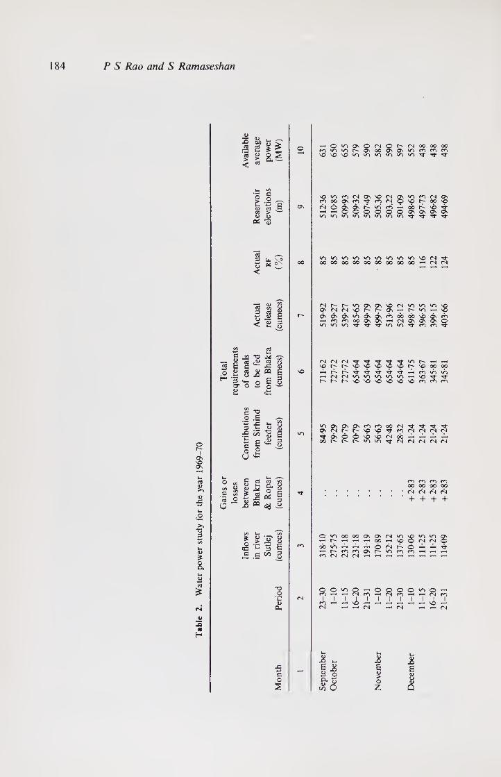
184 P S Rao and S Ramaseshan
X) 1) 00
u, o Sf o VS On O 04 O' 04 OO oo oo
u. £ OS vs VS Os OO On vs OS OS OS
> <D > a
£ so X SO vs vs vs vs vs vs Tt
<
C/5
~o c
SO VS os 04 os so 04 ft
vs OS 04 Os i> /—v os oo Os os os 04 SO O' oo so
CD E Os 04 © ft ft
O' V) os ob O' so *-H 1—< o o o O Os os o- Os
CD V) VS VS vs VS vs vs VS X 13
3 vs V) ITS VS VS vs VS VS vs so 04 Tf o\ oo oo OO OO OO OO oo oo OO 00 04 04
CD y—l •—1 i—i <
<D 04 r- vs Os OS so 04 */s vs vs so 3 <d Os 04 04 so O' O' OS y-* r- vs »—1 4^
8 E 0- 6s 6s 6s c/S 6s 6s OS OO ob SO 6s OS *—< ro OS OO Os On 1—< 04 os OS On
< u- IT) vs vs tT vs vs OS OS
CS)
3
G <L)
e
c/5
c
"O cd
X!
1/T O 4>
<N SO
<N r-
04 o> 3 3 3 3 3
vs O'
o^ so 00 OO
o V si J8
03 E SO T-H r- rh 'f Tf Tf rt •-H OS vs »OS
H . M i—H 04 04 VS vs VS vs vs »—1 so 3 <*- E r- r- O' so SO SO SO so so OS OS OS cr O ■*—> o <D
C/5 G -o O a v.
•*—> x: c- VS Os Os Os OS OS 00 04 -b c/5 T3
CD E VS
On rr
04 Os ©
r-
©
so so
so SO 04
OS
do 04 04 04 04
o ■+~*
£ £ 3 O
00 O' r- r- vs vs 04 04 04 04 04
O' o o ’ '
Os u c: so Os
u, „_s o c/5
<D
cS a o
<S3 OS OS OS OS <u >> C/3
c <D
Uh <D e rf
oo 04
oo 04
00 04
OO 04
<d x
a 1
x CQ
cc 3 + + + +
o
>s "O 3 C/5 C/5 o VS oo oo Os os 04 vs VO vs vs
ft > 4) r- *—• *—» 00 *—« so $ 04 04
•E ti os oo 105 rH © 04 O- o i-H O' os os Os O' VS os os y—1 —
_c O os 04 04 04 *-< »—i -H T—( 1 1 »—«
a Vh <D
<3
£ "O o O VS O o O O o vs o ,
os 04 OS 04 os 04 os c <D
04 I os
1 1 3
! 1 3
1
fS 13* 04 04 04 04
0>
x 59 H
M
£ u. %
E X
c -
E 4) a
o E <u
o *5
a <D T> o

Study of Bhakra reservoir operation 185
OO OO OO OO OO OO OO OO OO OO 00 OO OO OO OO OO OO co CO co co co co co co CO CO CO cO CO CO CO CO CO
rf Tf rf Tf Tf •'fr •*r
3 w-> w~>
rs 6 OS OS Os rt
00 Tf os so ,—1 so o *0 CN OO _ W~> Os CN CO CO Os CO SO w~> CO *—< ’—i r- W~> CN © r- CO © SO $ cb OO br 00 OO 00 OO r- r- r-
5? $ w^> W'S
rf
co *s~)
coTtovOoovor^ooQcO’—<co ' -• oo oo oo ^ os so so CO CO CN CO
W} ^ OO —I so os os O
8 3 CN CO so tT
8 CO Os CO CO wo CO r- 00 CN
uo wo © fS ^t OO OS 04 o p Tf
o VO OO br CO CN y—1 v-H CO cb wo
8 00 wo OO r“H <6
*—1 —< *-H CN CO 3
WS so OO O CN so CN CN Tf ’’C* wo wo wo wo wo so so
rH r- so CN CN CN CN CN •—• wo WO O o o OO °o vp p Tf wo wo wo wo wp op oo CN CN wo wo wo wo wo cb cb © wo WO wb wb wb wb wb CN CN cb cb cb
so vO Os •*r Tf tT Tf vO VO O O O CO CO CO CO CO wo wo wo wo WO CO CO CO CO r- r-
OO OO 00 OO Os 8
SO so so SO OO OO 00 00 ■<* 00 00 Os ■*—< ’“H OO OO oc OO
CN CN CN CN SO sb 4 br br br © s
© © Tf 1 SO so so
so SO sO vO rn m SO so SO o O O o OS Os Os SO SO sp SO cpi cn rn SO SO o w^» wp wp wp Os Os OS
wb wb wb wb r-H yL, wb wb wb OO 00 00 OO sb sb SO
4 4 + + 4 4 4 I 1 1 1 4 4 4 1 1 1
o sO SO OO r~~ o so Os VO CN CN OS r- VO vO Os sO sp OS cn Os CN •—1 W-> »-H ■»—i r- p p CN
CN br br wb wb OO sb cb O Os 6s SO cb bt- o —< o o O O T-H «—i m w^ OO r- T-H *“< CN CN
O W'S O O o
Os CN
OO o O y—4 O W^ o o o o CN cn y—4 CN CN *r* CN CO y—* y—4 CN CO CN co
T 1 3
1 1 1 | 1 1 1 si
1 1 1 1
CN CN CN CN CN
cd 3 C oJ <D U-
J= (J M Ctf s
a <
>* cd
co r- Os
c o o X
$ ■*-» t-
-o G -C <u 2

186 P S Rao and S Ramaseshan
<U
jD
-2
o 00 cd w-
Wh <d
* * © 8
ON
oo
r**
44
1-5
wp
Tf
ON
ON
ON ON p p p p oo oo P P p p p p p oo p p OO P
£ u
a co
5 m ON N «-N r-H
CO N IN «-H i-H *—t V—4 «—< «—1 »*—i i-H 1—4 T—<
>
< cd d CO CO CO CO CO CO CO CO CO CO CO CO CO CO CO CO CO CO CO CO
w- G
‘5 O NO d o r- Tf CN N 00 NO ■'d' <N ON vo (N
?
VO v-H wo On O' 04 oo d CO
> OO co (N O ON O pr p r- oo P P CO <N p P vo p vo o O VO p 04 t—
ed E. On rb X ON Tf ^r CO ON oo r- wo CO rf ob NO cb
s cb NO wb 04 ON O' NO
GO On ON OO oo OO oo OO OO r- r- r* r- p NO wo WO wo vo 5 3 3 OJ p d d Tf ,,d' ■'d Tf "d- ^d- ”»d Tf ’cd 'd- 'd- ’d’ 'd' Td rd •d* d"
a: <u
cd V") ON o wp O op CO CO Tp oo VO r- rf NO vo p P p P 04 p o CO d 3
oo r- d rr rn tT z-t wo
8
CO r- <N r-
1
rr ON 04 "d- wo wb X O rd 04 04 NO q U-
r- r- r- r- O o O o O o r^ r- OO oo 00 04 CO »—i O* O'
< DC N »“H
3
C/5 O
C/5 o o V~5 «o
5 NO oo
8 o <N r- <N vo ”d- O vo O- 00
3 OO d o
SS o NO r- r- r- ON oo *—< r_i r- *—< On vo pj p •-H P — cp CO
ed <u E r- © © o o NO CO r- CN WO oo CN ON WO r-i On ob cb ON O' bd O' cb NO
o 3 i—4 04 <N <N ON •-N N N <N <N Ci ro CO wo wo NO O' oo o o 04 CO 3 <
»- o d d rr CO CO CO CO CO CO CO CO CO CO CO CO CO CO CO CO d- ”d- d
c o £
, <u
£ 4) u-
o i—
cd C/5 CJ
3
d
3
d
3
tT
3
Tf
Wd r- r- r- NO <N 04 04 04 04 On ON O O O
3 o
13 G
<—
"O
-S cd
©
E NO
rp p
CO
OO
•n
OO
wo
OO
VO
oo
V-) P CO
P CO
8
p
WO
p
wo
p
wo
p
wo
vo
wo
oo
V-)
oo
wb
OO
oc
OO
cb
p
cb
p
cb
p
cb
H 2 .04 X 3 v~> NT) wn Ul N NO '<d- ^r NO NO •'d- Td ■d- ^d ■d- 'd’ tt — O O O
—» ^ CT w-
Ji
CO __o NO NO NO NO NO CO CO CO CO CO CO CO CO wo vo vo VO vo CO CO -d- d- O' O'
<D U.
c« G
o
O
3 £
*o C
u- <L)
A V") NO r- OO
3 oo 00 00
? 3 <N ^d* ON ON vo VO V~l CO O' r- T—< vo vo 04
X) ■o •U c v^)
d O ON OO up p p o cp P p p p p op •*—• 04 Td p oo o k_
JC C E NO wb OO •o CO UO r~ ON T-H ON CO CO OO o rd rd Td cb cb cb 04 NO O' ob ***! cz • —< 3 ON NO NO *o ud wo -d- <N CO vo NO rd r- OO 00 OO vo NO NO O' ON 00 o G C/5
o 1"-
3
U
On U. o C/5
v V5
G cd V-
a o
(A CO CO CO CO NO NO NO NO CO CO CO NO NO NO o o
8-50
O ON ON ON
8 C/5 c
O
>
In a
£ 3
Td
OO
CS
oo
<N
oo
cs
oo
r^i
P
WO
p
wo
p
wo
NO
WO
CO cp cp p
wo
p
WO
p
wo
wo
do
p
cb
p
oo
O'
sb
ON
sC
ON
NO
<U M
’£
O
o x: ffl
oc + + + + + + + +
+ + + -f + + 1 1 1
1 7 1
Ui ,o
Co C/5 *
2 "O
In o . _ C/5
h On On fNj »o 8
wo VO
p O NO NO oo r- O NO O' -d- NO 04 04 ON O' NO NO
3 _> cd © OO »—' NO <N <N ON p p ON cp p <N P p WO O' p p 04
C/5 o ’C
■*-< xs E co X o <N r- O Ch rf <N Tf Tf 8
vo wo S OO NO cb O ON ON NO cb d 8 W— 3 CO 3 ON »o ro CO N-1 nN i O O CO VO ^d d- oo d- o-
fe G .c C/5
O 1 nH 04 04 d
*
a ON (N
£ 1 —H o o O O WO o *N o VO o o o OO O o — o vo O o o o 1—4
co Cn| CO <N CO <N CO 04 (N 04 CO 04 CO 04 CO
> E o>
04 7 J" J^ 1 T“c
1 J< 1 1 1 1 *—<
I 3 1 1 »—4
1
On 04 —• <N <N CA 04 04 04 •—1 04
ro’
jy
3 *
H O r~-
On
In
In
J5 k. 2
>» Uh
-G . i! £ u >
E H cd
cd 3
X
c o « 3 u. Ih rp Co o
2 u
0
o Z
U
5 G cd
X)
UL,
cd
S a
<
cd
2 (Mehndir
att
a &
Ho
on
1973
).

Study of Bhakra reservoir operation 187
power subsequently; (iii) it has not been possible for bmb to satisfactorily coordinate
the releases for irrigation and power; and (iv) conjunctive utilization of surface and
groundwaters may lead to increased firm power level and reliability of irrigation.
4. Conjunctive utilization
4.1 Conjunctive-use concept
The Bhakra surface water system has been described in §2.1. There has also been
intensive development of groundwater by the public and private sectors. Such
combined use of surface and groundwaters as is now practised was not preplanned but
has come into being out of necessity. Though the concept of conjunctive utilization of
surface and groundwaters has been put forward and widely advocated, it has not been
applied systematically. The Irrigation Commission (1972) recognized this fact and
recommended that schemes for conjunctive use of surface and groundwaters in existing
irrigation schemes should be accorded high priority and that a systematic study should
be made by each State to identify areas where conjunctive use is feasible. It appears that
conjunctive utilization is considered as the planned development of surface and ground
waters for irrigation. It has not been sufficiently realised, despite the good work of
Singh (1964) and Minhas et al (1972) that conjunctive utilization enables the operating
authorities to cope with the differences in time distribution of irrigation and power
demands in an optimal way and that it is a means of converting secondary power to
valuable firm power. The model described below and applied to the water power studies
of bmb for 1969 -70 and 1970-71 seeks to emphasize the conjunctive utilization concept
and demonstrate the benefits of its application.
4.2 Conjunctive-use model
A linear programming model which is an adaptation of a model proposed by Thomas &
Revelle (1966) for the Aswan High dam on the Nile river has been developed. Figure 2 is
a schematic representation of the model.
The objective is to minimize the discharge from the reservoir during the period 23
September to 30 November. The model is based on the fact that if secondary or dump
power generated could be used to lift groundwater and supply part of the irrigation
demand, then it is possible to reduce the discharges from the reservoir during this
period.
N
Objective function: Minimize £ x„ (1) i = 1
where i = index for the subperiod i; subscript i denotes the value of the variable in
subperiod i, N = number of subperiods, and X = release from the reservoir in
cumec days.
4.3 Constraints
4.3a Power constraint: The reservoir release in each subperiod should generate the
firm power supplied in that subperiod.
Xj ^ PJKi (for all ij, (2)

188 P S Rao and S Ramaseshan
INFLOWS
I_I
Figure 2. Conjunctive use model for the Bhakra reservoir.
where P = firm power demand, and K = power conversion factor (energy rate function) i.e., power generated by unit volume of water in mw per cumec.
4.3b Irrigation constraint: The irrigation demand will be met from two sources:
(i) releases from the reservoir and (ii) groundwater lifted by the excess, if any, of power
generated over firm power level. The amount of dump power generated should be
sufficient to lift the groundwater component of the irrigation demand. This is the
modification introduced in the model of Thomas & Revelle (1966) to adapt it to the
present problem. Whereas surplus surface water is stored in the aquifers for later use in
their model, surplus power is used to lift existing groundwater in this model,
Xi^Ai-mi(KiXi-Pi), (3)
where A = irrigation demand, and m = volume of groundwater lifted by unit power
(cumecs/Mw). When the irrigation demand is overwhelming, this constraint is binding
and hence holds as an equality.
4.3c Continuity constraint: The continuity constraint specifies that releases upto any
time cannot exceed the sum of storage and inflows upto that time. As the reservoir is
nearly full during the early depletion period considered in this problem this constraint
will not be binding.
£ Xt ^ V+ £ /,. for all s with s = 1, 2, . . ., N, (4) ; = i i = i
where V — reservoir storage volume at the beginning of the depletion period, and
I = inflow into the reservoir.
4.4 Data and assumptions
The model is used to study the regulation of the Bhakra reservoir during the depletion
period for 1969-70 and 1970-71. Data from the water power studies of bmb (tables 2
and 3) are used in the study.

Study of Bhakra reservoir operation 189
Turbine efficiencies of the order of 0-85 and pump efficiencies of 0-7 are common. The
product of the turbine and pump efficiencies is assumed to be 06. Tail race elevation
(357 m) is taken from Singh (1965). The power conversion factors Kt are computed
from the data in tables 2 and 3. They are assumed constant during the subperiods. As
the length of the subperiod is short (8 to 10 days), the variation in the reservoir elevation
is small and the head is high, the effect of this approximation is negligible.
The depth to groundwater is assumed to be 15 m in October and 17 m in November.
Minhas et al (1972) mentioned that in Haryana and Punjab groundwater level rises to
15 to 25 m (50 to 80 ft) below ground surface even for deep tubewells. In many areas
groundwater is available much nearer the surface at depths of 3 to 4 m especially after
the rainy season in October and November. The assumption of 15 to 17 m depth to
groundwater is conservative.
The firm power level and reservoir factor adopted by bmb for the early depletion
period up to November 30 are respectively 552 mw and 0-85 in 1969-70 and 400 Mwand
0-75 in 1970-71. These values are used in this study.
4.5 Discussion of results
The model is applied to study the regulation of the Bhakra reservoir for 1969-70 and
1970-71 during the early depletion period when irrigation alone is constraining. The
results given in tables 4 and 5 show that the power used for lifting groundwater is much
smaller than the secondary power generated according to bmb studies and that the
actual releases of water from the reservoir are reduced by conjunctive use. For example,
it is seen from table 4 that during 11—15 October the secondary power generated is
103 mw whereas the model suggests 9-9 mw of power for lifting the groundwater
component of the irrigation demand resulting in a saving of 364-35 cumec days of water
in the reservoir. It is found that 2800 cumec days (i.e. 243 m cu m) of water could be
saved in the reservoir during the period 23 September to 30 November (table 4). This is
7-87% of the total releases made during the same period (table 2). A similar value of
7-28% is computed for 1970-71 from table 5.
The water so conserved in the reservoir can be used either to expand the irrigated area
and help enhance food production under the rabi crop or alternatively it can
subsequently help reduce the depletion rate of the reservoir when power demand is
constraining and it has a twofold effect. The conserved water increases the storage in the
reservoir and also increases the head available for power generation. At the end of the
depletion period, the reservoir could end up at a higher elevation. Although 7-8 % of
saving of water appears small, it corresponds to 243 mcum of water and is higher in
volume than the evaporation loss of 155-63 mcum from Bhakra reservoir during
1969-70. Since irrigation is generally not constraining during the remainder of the
depletion period a 7 to 8 % increase in irrigation supply during this period can increase
the total output of irrigation by a corresponding percentage and this is significant.
5. Multiobjective analysis
5.1 The concept
Multiple purposes should be treated as multiple objectives when there is conflict
between them as the nature of their consequences is noncommensurable and the
linkages between the purposes and the objectives they set out to serve are not known.
5 14

190 P S Rao and S Ramaseshan
O
08 so Os
O >
O JZ CD
c o
ca i-
& o
_o c
a c o
Q.
-o
’IC c3 UJ
O’
jfi « H
o >
T3 «D
a
cd £
>v
•3 8 E 3 O
ft r** r- r- $
08 05 SO <N © e SO oo <N r- fp E wo 6s <N © r- o ob 5 3 ©
wo 80 r- m <N CN <N
cO *
-o c 3 o t—I O
X 3
t- © 08 08 o 08 o <N o £ rb WO X 80 X X ob rs
c0 o 2 80 80 80 sn WO wo wo wo > <
cu wo WO wo wo wo
«« T? (1) CJ a>
<D TJ
L tfl O
- a> oo DC 3 oo jO
>> _ 5o >2 .5 "a _
3 C"
1= S <55 ^
£ 8.1
3 O
wo wo on o O o n f9 *h a ri wo wo O' < p r^- ro > OO88OOOO00Q
o r-
wo wo
>> c0
■o
6 3 O
3 o H
O ON On O Os O 04
^nd'O'O'O'OO
;o c0
’O
8 6 3
cd (J TD Tf r- r9 r- r- T—1 80 o ro y H 08 m rsi 08 08 WO oo 08 O r- 80 m ro r- OO 00 r-
£ -ro (N <N wo "O- •O' O’ <N
ro 3 o
C/5 o <D
wo <N r- "O’ Tf wo o p o -*-*
E rf 08 80 wo rsi 08 wo ob o 80 80 80 80 r- oo oo H
3 "O’ "O ■O’ "O’ O’ O’
08ooror-oo0oowo oosOoirororoTj-
T3 o O wo o l
O o o ro *— T—1 r-i ro <N ro C <u
1 ro
1 1 1 T 1 1
Dh <N 04 04
E J5 3 o B. t! a> ^ O0 O
i5 E <D > o Z
r- Os
o >
M cO X CD
a _o
CO Vh
a O
TJ O c 21 G o
a <D
T3
i3
© -fi 33 H
-o <u >
a
c0
£
■3 o © £ 3 o
u, c0 —v
g V. * £ o a s
Oh 3 O
00
I I ^ ‘S as <
c0 TD
«« y> D ©
© 00
cc ^
© TJ OO Q © c 00 E
. >o £ X)
>o >o _ TD u. C o rrt JZ.
fe " £ i |S
T3 O n ©
O<
G O
s Oct
ober
21-3
1 39
0
382
4199
3
406
0 6
0 28
-60
314-
6 N
ovem
ber
1-10
47-8
384
3841
-5
408-
5 8-
5 36
-75
367-
5 11
-20
41-5
390
3898
-6
408-
4 8-
4 30
-75
307-
5 21
-30
34-5
395
3946
-3
407-
2 7-
2 25
-75
257-
5

Study of Bhakra reservoir operation 191
There has been sharp competition for and conflict in the use of the Bhakra reservoir
storage for irrigation and power (Mehndiratta & Hoon 1973; Reidinger 1974). In the
planning stage Bhakra was considered more of an irrigation project and the power
benefits were secondary. A firm power of 282 mw was expected from Bhakra power
houses in a dry year. With the rapid increase in power load in the region, the position
has completely changed. The power demand overrides other interests of the project
during most of the months and it has not been possible to satisfactorily coordinate the
releases. It is therefore worthwhile to consider irrigation and power as the two
objectives to operate the Bhakra system and to study the complementarity and conflict
between the two for the six years for which data are available.
5.2 The model
Thomas & Revelle (1966) used a linear programming (lp) model and for a given storage
in Aswan High dam derived the transformation curve between irrigation and power by
maximizing power for different levels of irrigation demands. A similar approach is used
to study the planned and actual depletion period operation of the Bhakra reservoir. The
lp model is as follows:
Objective function: maximize P, (5)
where P = firm power level in mw.
5.3 Constraints
5.3a Irrigation constraint: The reservoir release in each subperiod should meet the
irrigation requirements to be supplied from the reservoir,
A, ^ At, with i=l,2,..., TV, (6)
where N — number of subperiods during the depletion phase of the reservoir,
X = reservoir release in cumec days, and A = irrigation requirements to be supplied
from the reservoir in cumec days.
5.3b Power constraint: The reservoir release should generate the committed firm
power in each subperiod.
P B.n X^—Td-A with i = 1, 2, (7)
Ki
where ft = firm power coefficient in subperiod i, n, = number of days in subperiod i, and K = power conversion factor(Mw/cumec).
5.3c Continuity constraint: The total volume of water released from the reservoir
during the depletion period should not exceed the total utilizable storage in the
reservoir at the beginning of the depletion period and the inflows in the depletion
period.
i xt /„ (8) i = 1 i = 1
where V = volume of reservoir storage utilized during depletion period in cumec days,
and / = river inflow into the reservoir.
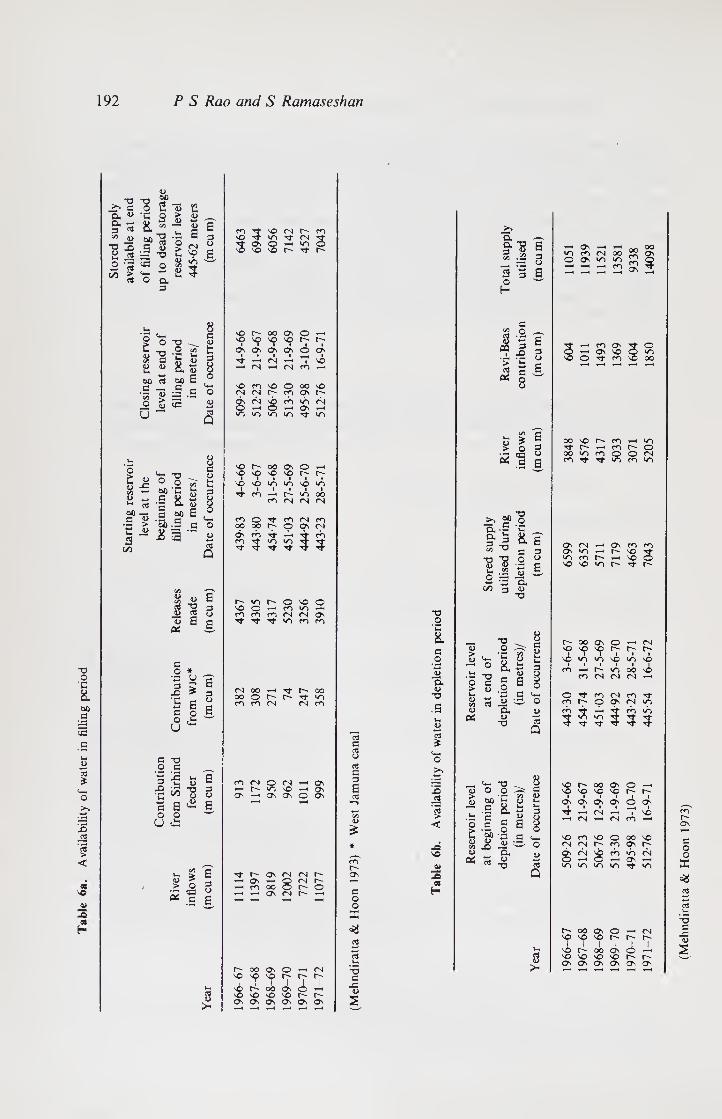
Tab
le
6a.
Av
ail
ab
ilit
y o
f w
ate
r in fil
ling perio
d
192 P S Rao and S Ramaseshan
u
•o TJ “ o 2 u >? c
a. u u. §■*8. „ - M 00 -S •§
o > •3 t>
■g 3 .s J > “ JS = 13 h
« o a 3
O *3 <C o 8 12 C/D > 4 A 4
O
I ■§
O -T3 O
'-D k-H 2 « 8.S oc (3 oti £ a _ e _
•3 S3's 5 5 *
U ~ 3
Q
« o "§
o
£ _ 85 oo 'c g S 3| s.|
.1 HI6 i-is
C/D
c o
aj
0
G O *
1 j8 X) > 3 ‘C c ° «-» C e G O «, O cH u
G -O
.2 .5 ^
| -5 « B
~ ^ "2 3
s e & e o o
U £
c/5 r* i- > G
£ ^ 0 .5 6
S >-
co Tf VO 4 ^ On VO VO
vo cm r- co *0 Nt n O —1 «o o vo i tj*
vo r- OO On O VO vo SO vo
On ON ON ON O
Tf 1 1
(N •
C9 (N m
vO m vO O 00 <N (N r- rp On
8 <N
s <0 *0
ON VO •0 •0
vo 00 ON O _
vO vO ^0 NO r-
SO VO VO vn vO •A
4 rA NO 00 f<N <N <N (N
m O m (N cn 00 op r- O On <N
ON fA tT «1h 4 <A m
5
VO v^N 1 5
C/5 V
1 -s E r- *0 r- O vO
2 2 s 3 VO 0 T—1 ro (l> <3 0 m rn m (N (X ON u £
36 £ Tf v/~i m
M OO H Tt h » oo o r- r- o n n n cm co
(N O (N -H ^ -H h 1^1 \0 ^ ^ On -h On On O On
tT h O' (N fN h ^ ON —' Q (N
co 00 o O —I —1 ON CM r-
OO On vO v^ -
v£ r- vo vo vo
t
CM O —I r- r-
I 1 I 00 On O ▼“ ' vo h
Ov On On O' O' On
d>
£
co r- ON
c o o
X
T3 G
-G
s
-o o c
8. G O
o
2. d>
"O
d>
c3 £
O
jS
rG c3 > <
-£ 2
QQ H
cx ,—„
§■■8 6 3 .2 g
2 3 6 O w H
G O ^ W G
3 5 ■ ± rz <j > h c 5 el 06 o
0
> C o > “ > O g ;■£ <c y
a g
o. -c
3 3 3 -o
T3 g <D *' lx O
J5
g> o
8. s'
8 G O
d>
a d>
■o
3 o
d>
_u W>
.1= '£ o c
£ '3j <D <U C/5 X> 1)
0^ cn
ctj <u >
1 Ov *“1 u-) m <n 00 O On ^ »0 S|
s ^
S^h m on t* o ^ On vo O *
vO O ^t
O' . _ VO
m vo 00
00 vo r- ro ___ VO r- m r- O
00 vo m O O <N >0 <0 VO
On (N <—H ON CO On vo r- vo «o CO r- 1-H 0 vO vO VO r-
“O 0 j3 00 ON O CM
<u >
JU O kn (75
(U 0> ix
VO 1
VO
sO 1
VO
VO 1
vo 0
r-
VO
r- ■
vO 0 !1 l—1
3 CO J. 1 r-
1 VO
1 OO VO
*0 >
■0 c 0
G .O
i 8 O
CO <N <N <N
t— "03 c <4H O CO (N CO 8 <u O CO r- O OS (N WO <u 2, <u CO 4 r—i CO VO
0 “O 03 5
*0 VO Tf 4 5 5
"O 0 vO r- OO ON 0 O G
<u NO VO vO vo r- r-
‘C
8.
d> Uh t
a
On 1
GTn 1
ON
CM
ON 1
O X
On
VO
G O B §
CM CM CO
G d-H VO CO VO O 00 VO o> O CM CM r- CO p r- u d)
d) 8
CM s
CO »o ON
CM X
"O c3 VO VO vo vo vo
00 ON 0 04 vO sO so r-
1 r-
vO 1
t" 00 1
0 ci 1
f1 ■< VO vO so vO r- r- ON ON ON ON ON ON
(Meh
nd
iratt
a &
Ho
on
1973
)
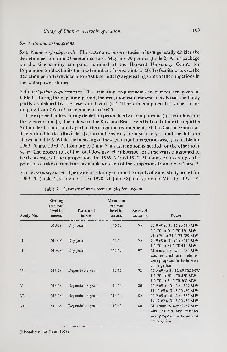
Study of Bhakra reservoir operation 193
5.4 Data and assumptions
5.4a Number of subperiods: The water and power studies of bmb generally divides the
depletion period from 23 September to 31 May into 29 periods (table 2). An lp package
on the time-sharing computer terminal at the Harvard University Centre for
Population Studies limits the total number of constraints to 50. To facilitate its use, the
depletion period is divided into 24 subperiods by aggregating some of the subperiods in
the waterpower studies.
5.4b Irrigation requirements: The irrigation requirements in cumecs are given in
table 1. During the depletion period, the irrigation requirements may be satisfied only
partly as defined by the reservoir factor (rf). They are computed for values of rf
ranging from 0-6 to 1 at increments of 0 05.
The expected inflow during depletion period has two components: (i) the inflow into
the reservoir and (ii) the inflows of the Ravi and Beas rivers that contribute through the
Sirhind feeder and supply part of the irrigation requirements of the Bhakra command.
The Sirhind feeder (Ravi-Beas) contributions vary from year to year and the data are
shown in table 6. While the break-up of these contributions period-wise is available for
1969-70 and 1970-71 from tables 2 and 3, an assumption is needed for the other four
years. The proportion of the total flow in each subperiod for these years is assumed to
be the average of such proportions for 1969-70 and 1970-71. Gains or losses upto the
point of offtake of canals are available for each of the subperiods from tables 2 and 3.
5.4c Firm power level: Tfie bmb chose for operation the results of water study no. VI for
1969-70 (table 7), study no. 1 for 1970-71 (table 8) and study no. VIII for 1971-72
Table 7. Summary of water power studies for 1969-70
Study No.
Starting reservoir level in meters
Pattern of inflow
Minimum reservoir level in meters
Reservoir factor % Power
I 513-28 Dry year 445-62 75 22-9-69 to 31-12-69 550 MW 1-1-70 to 20-5-70 450 MW 21-5-70 to 31-5-70 289 MW
II 513-28 Dry year 445-62 75 22-9-69 to 31-12-69 512 MW 1-1-70 to 31-5-70 441 MW
III 513-28 Dry year 445-62 97 Minimum power 282 MW was ensured and releases were proposed in the interest of irrigation
IV 513-28 Dependable year 445-62 78 22-9-69 to 31-12-69 500 MW 1-1-70 to 30-4-70 450 MW 1-5-70 to 31-5-70 500 MW
V 513-28 Dependable year 445-62 80 22-9-69 to 10-12-69 524 MW 11-12-69 to 31-5-70450 MW
VI 513-28 Dependable year 445-62 85 22-9-69 to 10-12-69 552 MW 11-12-69 to 31-5-70 438 MW
VII 513-28 Dependable year 445-62 100 Minimum power of 282 MW was ensured and releases were proposed in the interest of irrigation
(Mehndiratta & Hoon 1973)

194 P S Rao and S Ramaseshan
Table 8. Summary of water power studies for 1970-71
Study No.
Starting reservoir level in metres
Pattern of
inflows
Minimum reservoir level in metres
Reservoir factor % Power
I 494-76 on 1st October
Dependable year
445.62 75 Up to 10th Dec. 1970—400 MW 11th December 1970 to 31st May 1971 — 312 MW
II 494.76 on 31st October
Dry year 445-62 75 Up to 10th Dec. 1970—400 MW 11th December 1970 to 31st May 1971 300 MW
(Mehndiratta & Hoon 1973)
(table 9). The /?, values corresponding to the same were used in this study for the
respective years. The /?,• were found to be respectively 1-26 in 1969-70 and 1282 in
1970-71. For 1966 to 1969 for which no data are available, a distribution similar to
1969- 70 and 1970-71 with a value of 1-27 is used.
5.4d Power conversion factors: The power conversion factors K, for 1969-70 and 1970- 71 are deduced from the data in tables 2 and 3 respectively and the relationship
between Kt and reservoir elevation is derived. For the other four years, the
approximate reservoir elevations for each of the subperiods are estimated from the
anticipated and actual depletion curves in figures 3 (a to f) and the power conversion
factors corresponding to these elevations are used in this study. These depletion curves
generally correspond to rf values in the ranges of 075 to 0 85. For other rf values, the
depletion curves would be somewhat different and the reservoir elevations and hence
the power conversion factors would also be different. However, for simplicity, it is
assumed that the conversion factors are independent of the rf value and the same
conversion factors as in the water power studies of bmb are used in each of the
subperiods. From the solution thus obtained, it is possible to determine the reservoir
elevations implied and hence determine a new set of values of and repeat the
procedure till convergence is obtained. However, the irrigation requirement is
constraining generally only from 23 September to 10 December when the reservoir
elevation is very high and the depletion rate is low. Such refinement is not considered
here.
5.4e Sutlej river inflows'. This study assumes the dependable year inflows for
planning as in the case of water power studies of bmb. They are obtained from
Mehndiratta & Hoon (1973) and Lamba & Prem (1975) for all years except for 1971-72
for which there is a discrepancy between the two reported values. The dependable year
inflow for that year is corrected by interpolation. These are shown in table 10. For
actual operation, actual river inflows (table 6b) are used.

Study of Bhakra reservoir operation 195
Table 9. Summary of water power studies 1971-72
Study No.
Starting reservoir level in metres
Pattern of
inflows
Minimum reservoir level in metres
Reservoir factor up to
10th Dec. 71 Power
I 51206 Dependable year 445-92 85% 512 MW up to 10th December 1971 and 444 MW thereafter up to 31-5-72
II 51206 Dependable year 451-41 85% 512 MW up to 10-12- 71 and 430 MW from 11-12-71 to 31-5-72
III 51206 Dependable year 456-90 85% 512 MW up to 10-12- 71 and 414 MW from 11-12-71 to 31-5-72
IV 51206 Dry year 445-92 81% 484 MW up to 10-12- 71 and 432 MW from 11-12-71 to 31-5-72
V 51206 Dry year 451-41 81% 484 MW up to 10-12- 71 and 419 MW from 11-12-71 to 31-5-72
VI 51206 Dry year 457-20 81% 484 MW up to 10-12- 71 arid 402 MW from 11-12-71 to 31-5-72
VII 51205 Dependable year with month of May as per driest year
44623 75% 512 MW or more up to 10-12-71 and 425 MW from 11-12- 71 to 31-5-72
VIII 51206 Dependable year 452-32 85% 500 MW up to 31-12- 71 and 430 MW for 1/72, 3/72 and 5/72 and 420 MW for 2/72 and 4/72
IX 512-76 Dependable year 452-32 85% 500 MW upto 31-12- 71 and 430 MW for 1/72, 3/72 and 5/72 and 420 MW for 2/72 and 4/72.
X 512-76 -do- 445-62 85% -do- XI 512-76 Actual 445-62 85% -do-
Note: (1) Study Nos. I to VIII are bmb Water Power Studies for 1971-72 (Mehndiratta & Hoon 1973). (2) Study No. XI is one of actual operation.
5.4f Stored volume: For planning studies, live storage available above dead storage
level (dsl) is used in the different studies. In case carryover was planned for, carryover
storage was estimated from volume elevation curves and deducted from live storage
above dsl to give utilizable storage with carryover. It is presumed that the losses due to
evaporation and infiltration from the reservoir are considered by bmb in the
specification of demands or in specifying inflows. The total volume of water for

196 P S Rao and S Ramaseshan
utilization during the years is assumed to be the sum of dependable year inflows and the
utilizable storage from the reservoir as in the water power studies of bmb. For studies of
actual operation the volume of water actually utilized during the depletion period is
used. The details of the data are given in table 10.
c. 1968 -69 d. 1969-70
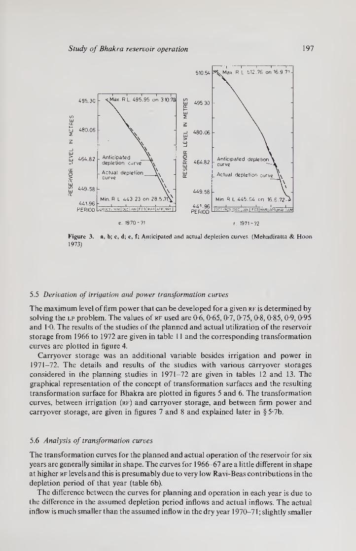
Study of Bhakra reservoir operation 197
Figure 3. a, b; c, d; e, f; Anticipated and actual depletion curves. (Mehndiratta & Hoon
1973)
5.5 Derivation of irrigation and power transformation curves
The maximum level of firm power that can be developed for a given rf is determined by
solving the lp problem. The values of rf used are 06, 065, 07, 075, 08, 085, 09, 095
and 10. The results of the studies of the planned and actual utilization of the reservoir
storage from 1966 to 1972 are given in table 11 and the corresponding transformation
curves are plotted in figure 4.
Carryover storage was an additional variable besides irrigation and power in
1971-72. The details and results of the studies with various carryover storages
considered in the planning studies in 1971-72 are given in tables 12 and 13. The
graphical representation of the concept of transformation surfaces and the resulting
transformation surface for Bhakra are plotted in figures 5 and 6. The transformation
curves, between irrigation (rf) and carryover storage, and between firm power and
carryover storage, are given in figures 7 and 8 and explained later in §5-7b.
5.6 Analysis of transformation curves
The transformation curves for the planned and actual operation of the reservoir for six
years are generally similar in shape. The curves for 1966-67 are a little different in shape
at higher rf levels and this is presumably due to very low Ravi-Beas contributions in the
depletion period of that year (table 6b).
The difference between the curves for planning and operation in each year is due to
the difference in the assumed depletion period inflows and actual inflows. The actual
inflow is much smaller than the assumed inflow in the dry year 1970-71; slightly smaller
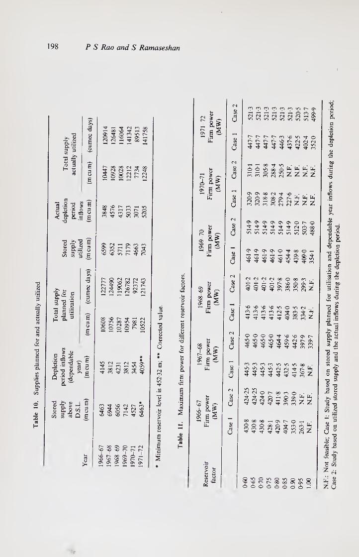
Tab
le
10
. S
uppli
es p
lan
ned for an
d actu
all
y uti
lized
198 P S Rao and S Ramaseshan
TJ
£ § a 32 a © 3 3 C/5
ert 33
o 3
03
>»
-3 8 e 3 o
3 U
t - 't rs n oo -H oo Ov ’’S © ro vo © v£ vO —< On —h (N M -< rt OO Tf
r- oo oo <n tj- oo 5 m (N -i ^ tJ ^ Os Q (N (N O © O C\J t"~ fN
c ,_, 0 -0
'©3 0 C/3
E 00 vo r- ro , , •O oj - — O 3 r- ro ©
8- a S3 O 00 »o ro © © <N G £
ro ■*fr »o ro »o T3
•o >>33 c fli —■ <i> c 2 B,.Jj 3 O O
m 2 3 E
T3 o
>> u- JJ a £ c E S .2 => 3 13 “ “ S S a c r=
O -2 3 H & 3
o
Q. T3 ■■ 0
& a
jd 3
CT3 .-s T3 C 03
a£ <u
T3
*D a g
w a _g
a 3 « o s
_, <D 1' a > H - ^ go
03 <D >
O <N -h On n n On >0 -h h- NO rt vo ro 1"^ ' \0 © vo so «o rt r-
© n n n n r- os vo 00 rt ^■^©r-mr^ MtJ-On^M-h (N n -h M o> fN
00 \C h Tt ’H M © vo 00 »o 00 <n VO h (N O' ON ^ © © © © ©
* V} M rH (N Tt On
-- m -h in in H 00 (N 00 t © rj- co co co Tt
't no m h m NO Tf ^ Tf M j Ov ~ - ■
vO 3
2 (N
r- r- r- 00 On ©
? 7 *T 00 os
VO NO VO NO . Ov On On On On On
<±
<D J3 ’cS >
TO <L>
o U
CM m <N VO rt
U r?*
O >* u <L> C/3 <D U>
G <u M
£ •6
£
a
<C
e 3
s * 03
2 98
H
D M *
a *1 ^ E ^ «-H _ 1—1
£
4> *
1 &|
2 E -
© r-
I Ov vO On
&g E d u.
£
(D S> *
2al
U
ai e e U
£
a> r- >
2 S a 2
.b o £ <L> 05 <L>
es:
cm
<u 00
(3
c3
CM
1) C/3
c3
3
3
s 6
CM
<U
<3
3
<N <D C/3
3
3
CM
0) C/3
3
3
rpcntpcnTpcpinr-ON t © cb OV
MMMM(NMM-Oi fi'/i'Aininininintt
7 00 tj* tm . ©OuSobo^H^^tin
On On OO <N rf VO OOoboodvr-^NLiCL, N(N«Oh(N77 7
OnOnOnOvOvOn©^©
^t^trfTf^tTf-rsirbob 'a-Hi—ta-HOOO vocncocncncncocoTt
On^nOn^nOtJ-000-h NONONOvoNOinmo^
(N M n fN 00
? ? §
©oom * r- VO 6 On 7 OVOOU-iOn^ w n m n ^
no vp vp vo in ©
n ri n rn n j
T rf nJ- Tf
•n N , • rb Tf ^ 00 m 7 n n ^
OOOO^vOvoovr^ ‘O'O'O'OtONfNhdN VO vo VO NO 3 vo Tj- rf rf rf Tt Tf 4 On ro
ro ro
rororprovoinvocxD vovovoiorNr-iTtr- TT^r'T^trj-rfTtro
vo vo <N (N © r- 00 fO © aaNroN.oa^l*'
^ Z Z (N fS M M 't Vf Tt Tj- Tt ro ro
00 00 00 ^HONr-©^H 0©<© 00 6 -rf o o ^onrioO^NO ^ t rf o (N
U,
Z
O *0 © 10 © 10 © «o vpvOhhOOOOONON 00©©©©©50
T3 O C
a a o
a o
T3
<D
00 _c C 3
T3
C/3
O S3 C
rt «5 >N
JJ
~6 ~o o c ‘C
a a ■s §
D. (U
T3
4>
00 c
'C 3
"O
-o ^ g o
§ .S 'a
>,1
3 D C/3 ^
"O I! <D T3 Jr C O 03
c *a o a
3 T3 c^
<D __ C/3 T3
g g X) ^3
</3 T3 3 TD w (U
N
c3
c o
T3 (D
.■s Jg cn cv3 >n
eg T3 5
o
z<^ ' '■ CJ
U_ cm
£ u

RE
SE
RV
OIR
FA
CT
OR
Study of Bhakra reservoir operation 199
0.5___i_i____j 200 30 0 400 500
FIRM POWER (MW)
Figure 4. Transformation curves for the Bhakra reservoir (1966-72)
IRRIGATION
Figure 5. Graphical representation of transformation surface.

200 P S Rao and S Ramaseshan
r-
r- On
T3 3
0> £ O a
$
o
-o 55
H
T3 3
<55
>» -o 3
SO <N t— SO * <N wo co wo
, , O 5 s o <N
X »/o
VO (N r- so <N •O co on
WO 5 s wo ©^
X
1 2 <55
vo r-
GO _c
'2 3
oo oo O O Tf WO <N <n —<" T-H Tf
o o
C'J co ^r
Tf co vo_ co"
©^
<N OO O wo ’-H Tf
t-T oo" —< CNl
co uo on on
co vo ob wo ON <N © vo Tt
O’ co" —* <N
VO (N OO CO CO O co VO ON ON rs r-j (N Os <N ro ON CO -r—< CO VO >o <N Tf o
"o S wo Tf Tfr CO •O 3 cr vo" cT
on ^ *—< ol
VO O <N OO fN O Ov CO o C*~l <N sb <N Os (N o
S o
co VO CO CN r- ■a h-h WO i—i O <N <N r- 3 £2 ■*—» vo" Tf" o’ oo"
CO »—C ’"H
VO Os (N Tf O •q- SO ON ON <N *—« ON _4 VO ON
CO rxj CO OO r}- ■o _ 3 JZJ
wo Tf »n
sO P, T^r
CO
o’ r4 CO
00 <N
VO (N O ON VO
CO J-l ON — CO r~~l
5 r- CO co r-
TD CO 00 On Tt 3 ^
■«—* vo" O" vo" <>n —< <N
GO C ■
GO -O V c
o 5 <u jz ^ jo ~ X) ~
3 "O
3 -© T3 £ 3 3 I E
21 g
E T3 w <D ___ N T3 33 O •©
'C 3
21 ><
c « Q ,_
•o o
"C
21
3
“O X> D ca N N
2 s
• 2 3
a> O
£ a <u <u ft *o
Tv T3 S' 22
2 <55
c W o o 5 g
’© 03 s© ^ *3 co
g- 5 *
T3
Q .2
3 3
a, g, a, a 3 3 CO CO
° 3 ~ g B E o —■
c- vo
3 21 - E r- 52 oo •—- 3 vo
<U <D C~ G0 GO O 3 3
o o co CO
Uh U, <D <U > > o o >* >>
o o H H c3
<u GO 3
T3 1) N
a a. 3
2 o H
£ o <33 C
"2 3
t> <

Study of Bhakra reservoir operation 201
Table 13. Maximum firm power for different reservoir factors and carryover storages (water power studies for 1971-72)
Reservoir factor
Firm power (MW)
Study 1 Study 2 Study 3 Study 8 Study 9 Study 10 Study 11*
060 465-1 4502 434-9 447-7 4550 472-4 521-3 065 465-1 4502 434-9 447-7 4550 472-4 521-3 070 465-1 4502 434-9 447-7 455-0 472-4 521-3 075 465-1 4502 434-6 447-7 455-0 472-4 521-3 080 464-7 449 1 431-9 446-3 454-2 472-3 521-3 085 461-3 441-2 419-3 437-6 447-9 469-8 521-3 090 448-2 426-3 403-2 422-5 433-5 458-6 5205 095 432-2 407-7 3692 402-4 416-4 443-2 513-7 100 400-9 359-0 314-1 352-0 372-5 420-5 5000
Carryover storage (m cum) 19 4 349-9 709-1 408-9 408-9 0 0
* Actual operation
in the below average years 1966-61 and 1968-69; slightly larger in the above average year
1967-68 and very much larger in the wet years 1969-70 and 1971-72. It shows that
using dependable year inflows for planning every year irrespective of how wet the year
has been and how high the reservoir has filled up led to very conservative planning in
wet years and the opposite of it in a dry year. It is not sound practice. It seems possible to
delineate an average year with a transformation curve between the above average and
RESERVOIR FACTOR
Figure 6. Transformation surface for the Bhakra reservoir.

202 P S Rao and S Ramaseshan
Figure 7. Transformation curve at constant firm power (1971-72).
Figure 8. Transformation curve at constant reservoir factor (1971-72).
below average years for which the assumption of dependable year inflows in depletion
period would be correct. Forecasting models for the stochastic inflows (Krishnasami
1976) are required to predict depletion period inflows for use in planning.
The points of operation D chosen in the planning studies in 1969-70 and 1971-72
(figure 4) lie inside the respective transformation curves indicating that the planned
operation is inferior and nonoptimal. The point D could be moved on to the curve at Dx or
D2 and the operation would be Pareto-superior to that at D. A higher firm power level
would be attained for the same rf of 0-85 at Dl while a higher rf would be obtained for
the same firm power level at D2. rf planned was never higher than 0-85 and so it seems
reasonable to suppose that the points Di would be the decision points of bmb for
operation in 1969-70 and 1971-72.
The rf planned for was 0 75 in the dry year 1970-71. The decision point chosen in
planning is not feasible with respect to the actual transformation curve. The firm power

Study of Bhakra reservoir operation 203
level planned for was stuck to and the adverse impact of the shortage must have been
borne by irrigation only. So the actual rf provided would have been lower than 0-75.
Irrigation supplies at rf of 1 were feasible in 3 out of 6 years and at rf of 0-9 to 0-95 in
2 out of 6 years. In the dry year an rf of only 0-8 was feasible.
Firm power levels planned for varied from 312 mw in a dry year to 438 mw in a wet
year. In actual operation it seemed that 510 to 520 mw of power was generated in the wet
years of 1969-70 and 1971-72 and 280 to 300 mw in the dry year of 1970-71. The high
order of fluctuations in firm power from year to year can be reduced by carryover
storage from wet to dry years. For example, a carryover of about 1500m cum storage
from 1969-70 to 1970-71 would have facilitated operation in both years around the
level of an average year (1968-69) with firm power of about 400 to 420 mw. The
recommendation of Minhas et al (1972) that a high dead storage level should be
maintained for high levels of firm power (which are possible in years of good inflows)
implies, in a way, the concept of carryover storage. Carryover storage was planned for
in 1971-72 possibly because of the experience of the previous two years, but in actual
operation this sound policy was not carried out.
Irrigation and power are almost wholly complementary up to an rf level of about 09
in years of good inflows but the complementarity could not be exploited because of the
uncertainty of depletion period inflows. This again points to using appropriate
streamflow forecasting models for planning reservoir operation.
5.7 “Top-down ’ and “bottom-up” planning
The transformation curves provide the frontier on which an optimal decision point for
operation should lie. If the social welfare function or the preference function of the
decision makers is available, the optimal point is obtained as the point of tangency
between the transformation curve and the welfare function or preference curve
respectively and the slope of the tangent gives the trade-off between the objectives. The
slope of the tangent to the transformation curve gives the marginal rate of technical
transformation between the objectives at that level of attainment of the objectives. The
slope of the tangent to the preference curve provides a measure of the relative marginal
economic worth of the two objectives (ratio of the shadow prices) at that level of
attainment of the objectives. At the decision point they are equal and the converse is
also true.
Well-defined preference functions do not exist. Shadow prices of the objectives vary
from time to time and depend on the levels of attainment of the objectives. They need to
be derived from an overall economic framework by a central planning organisation and
given to the project operators for use in decision-making. This is “top-down” planning.
If the ratio of shadow prices of the objectives are so defined exogenously (along the
transformation curve) the point on the transformation curve where the slope equals this
ratio defines the decision point. If it is not available from decision makers it is possible
to arrive at a decision point by interaction with the decision makers using techniques
like swt method or Paretian analysis. In the absence of these, a “bottom-up” planning
procedure seems possible.
5.7a Analysis and discussion of implied trade-offs: The results presented in § 5.4 are
analysed and discussed in the framework of “bottom-up” methodology to elicit the
trade-ofis implied in the choice of the decision points in the planned and actual
operation of the reservoir during six years.

204 P S Rao and S Ramaseshan
The trade-offs between irrigation and firm power in the planned and actual operation
for the six years are given in table 14. The trade-offs implied in planned operation vary
from 200 MW/rf in average years to 360 MW/rf in a dry year. Since the results
indicate a higher trade-off for irrigation in a dry year, the value system adopted in
planning is consistent.
In 1969-70 (figure 4), the trade-offs of 200 MW/rf at Dx and 500 MW/rf at D2
provide the bounds for the marginal rates of transformation implied in the choice of
decision point D for operation. The bmb has used a maximum rf of 0-85 for operation
(tables 7, 8 and 9). Assuming, therefore, an rf of 0-85 corresponding to Dx the trade-off
implied is 200 MW/rf. The trade-off on the transformation curve of actual operation
at the level of corresponding to rf of 0-85 is 0 0 MW/rf. This implies that, in actual
operation, there is complete complementarity between irrigation and firm power up to
rf of 0-85 and that the irrigation supply could have been increased upto rf levels of 0-9 or even upto 1 with a small loss of firm power. Even at an rf of 10,50 MW more of firm
power than that planned for would have been produced (table 11).
In the dry year 1970-71 (figure 4) the trade-off between irrigation and power implied
by the decision is 360 MW/rf. The planned operation at point D is not feasible for
actual inflows. If an rf level of 0-75 was maintained, a firm power level of 288-4 MW
would have been reached on the transformation curve for actual operation and it would
have meant a trade-off of 490 MW/rf at that point. This is larger than the trade-off in
an average year. During the early part of the depletion period from 3 October 1970 to
about 15 December 1970 the operation was as per the plan, i.e. at point D with rf of 0-75
and firm power level of400 MW (figure 3e). The adverse effect of the shortage seems to
have been borne by the latter part of the depletion period from 15 December 1970 to 31
May 1971. The average power generation for the year 1970-71 was 335 MW. It can be
deduced from these that the rf level achieved was certainly less than 0-75 and must have
been somewhere between 0-65 and 0-7 with a trade-off of 160 MW/rf or less. This, in
turn, implies a higher value for power than irrigation compared to an average year. This
indicates not only a contradiction between planning and operation but also an
inconsistency in economic evaluation. If, as pointed out earlier, the reservoir was not
depleted as it was in 1969-70 but some storage was carried over to 1970-71, it would
have greatly cushioned the adverse impact due to poor inflows in 1970-71 and enabled
the achievement of a higher rf for irrigation.
Table 14. Trade-off between firm power and irrigation
Year
Irrigation level (RF)
Trade-off (mw/rf)
Planned operation
Actual operation
1966-67* 0-85 450 600 1867- 68 0-85 260 210 1968-69 0-85 240 360 1969-70 0-85 200 0 1970-71 0-75 360 490 1971-72 0-85 230 0
Ravi-Beas contribution is low as compared to other years.

Study of Bhakra reservoir operation 205
5.7b Transformation surface for 1971-72: The concept of the transformation surface
among the three objectives has been illustrated in figure 5. ABC constitutes the surface
bounded by the three coordinate planes. D is the decision point for operation. If it is on
the surface, it is Pareto-optimal. Curves a2a3, b2b3 and c2c3 pass through the decision
point and lie respectively in planes axa2a3 parallel to the coordinate plane BOC, bxb2b3
parallel to OAC and cxc2c3 parallel to OAB. The trade-off implied by decision point D
between any two of the objectives can be derived as the negative of the slope of the curve
in the plane parallel to the coordinate plane defined by the same objectives.
For 1971-72, water power studies for planning the reservoir operation were
conducted by bmb assuming different levels of irrigation and firm power supplies and
different carryover storages. They are listed in table 9. Four of the studies, viz., I, II, III
and VIII assumed an irrigation level at rf 085 and dependable year inflows during
depletion period but they differ in that they assume different carryover storages. Details
of these studies are given in table 12.
The maximum firm power levels for different reservoir factors and carryover storages
are given in table 13. The transformation surface among the three objectives, irrigation,
firm power and carryover storage for the four planning studies is shown in figure 6. The
bmb decided to operate the reservoir according to study No. VIII with a carryover
storage of 408-93 mcum, a firm power level of 420 MW and rf of 0-85. A firm power
level of437-6 MW was possible for an rf of 0-85 and carryover storage of408-93 m cu m
(table 13, figure 4). Hence the decision point D (figure 4) is inside the transformation
curve and though feasible is not Pareto-optimal. For the same carryover storage, any
operation between Dx (rf of 0-85 and firm power of 437-6 MW) and D2 (rf of 0-905 and
firm power of 420 MW) will be better than the point D chosen and will be Pareto-
superior. The trade-offs implied by choice of Dx or D2 as decision points can be
obtained from the transformation curves in figures 4,7 and 8 and are respectively 230 to
350 MW/rf between irrigation and power, 4824 to 5976 m cu m/RF between carryover
storage and irrigation, and 60-6 to 67-6 MW/b cu m (billion cubic metres) between firm
power and carryover storage. As the rf level of 0-85 was always adhered to as an upper
limit, it appears that Dx would have been the choice. Hence the trade-offs implied by Dx
are relevant indicators of decision makers’ values.
The planning studies of bmb (table 9) assumed that the reservoir would reach an
elevation of 512 06 m on 16 September 1971. But the reservoir actually filled to an
elevation of 512-76m on that date with 171 mcum more storage than planned for in
these studies. Study Nos. IX and X (table 9) are revisions to account for this increase.
Study No. IX assumes carryover storage of 408-9 mcum as in study No. VI and
corresponds to planned operation. Study No. X assumes no carryover storage as in
Study No. XI and corresponds to actual operation. They are reported in tables 12 and
13. The transformation curve for actual operation (figure 4) indicates that irrigation
could have been supplied at an rf of 0-9 instead of 085 without any loss of firm power
and this too at a power level of 521-30 mw as against 420 mw planned for. An increase in
rf to 1 would have resulted in a loss of only about 20 mw.
If the reservoir was operated according to the decision on 16 September, 1971 the
carryover storage would have been much more than what was planned for because the
excess of actual inflows over the assumed dependable year inflows, would have been
stored, and carried over to the subsequent year. The reservoir elevation at the end of the
depletion period would have been about 8 m higher than the planned elevation of
452-32 m. In actual operation the reservoir was drawn down to about the dead storage
S 15
206 P S Rao and S Ramaseshan
elevation of 445-62m. Thus 1746mcum of water consisting of excess storage and
excess inflows was used over and above the planned volume of 10,522 m cu m and all the
excess was used in the interest of power alone and the trade-off implied is 0 0 mw/rf
which considered irrigation above rf of 0-85 to be completely worthless. Such a value
judgement needs justification. Thus, carryover storage, though planned for, was not
realized in practice. This was particularly striking after the dismal experience of the
previous year.
6. Summary of results
The analysis of the results of the study of the Bhakra reservoir operation from 1966 to
1972 indicates that (i) the depletion period inflows are correlated to the filling period
inflows and planning should be based on appropriate estimates of depletion period
inflows; (ii) an rf of085 or above can be attained in an average year and an rf of 1 can
be obtained at a loss of firm power of about 80 mw in an average year; (iii) planning and
operation should be based on consistent estimates of economic parameters; and (iv) carryover storage will serve to reduce year to year fluctuations in firm power and
irrigation levels.
References
Ansari N 1968 Economics of irrigation rates—a study in Punjab and Uttar Pradesh (Bombay: Asia Publishing
House)
Irrigation Commission, Reports of the Irrigation Commission 1972 Vols. I, II, III. Ministry of Irrigation and
Power, New Delhi
Krishnasami M 1976 Decoupled multivariate time series models for multisite streamflows Ph.D. thesis, IIT,
Kanpur
Lamba S S, Prem K S 1975 Integrated development of rivers Sutlej, Beas, and Ravi for optimum utility of
water in north-western areas of India, Presented at the IWRA Second World Congress on Water
Resources, New Delhi, Reprint Vol. 3, p. 79
Mehndiratta K R, Hoon R N 1973 J. Central Board of Irrigation and Power India 30: 349
Minhas B S, Parikh K S, Srinivasan T N 1972 Sankhya, Indian J. Stat. B34: 105
Raj K N 1960 Some economic aspects of the Bhakra Nangal Project-a preliminary analysis in terms of selected
investment criteria
Reidinger R B 1974 Econ. Dev. Cult. Change 23: 79
Singh H 1964 J. Central Board of Irrigation and Power, India 21: 471
Singh J 1965 in Proceedings of the sixth regional conference on water resources development in Asia and the far
East, Water Resources Series, United Nations, p. 281-295
Thomas H A Jr, Revelle R 1966 Manage. Sci. 12: 13-296
Integrated operation of the Beas-Sutlej system
P S RAO* and S RAMASESHANf
‘Indian Institute of Management, Bannerghatta Road, Bangalore 560076, India
tCivil Engineering Department, Indian Institute of Technology, Kanpur 208 016, India
Abstract. The study deals with the integrated operation of the Beas and Sutlej link, a complex system. It utilizes the methodology developed in an earlier paper for reservoir operation. The results show the definite advantages of conjunctive use and carry over storage. The results also show that it is advantageous to divert as much water from the Beas to the Sutlej as possible.
Keywords. Integrated reservoir operation; conjunctive use.
1. Introduction
To study the conventional operation of a reservoir system in a multiobjective
framework in order to evaluate the trade-offs between irrigation and power implied by
past decisions, a case study of the Bhakra reservoir was undertaken. This study
demonstrates the methodology and procedures of multi-objective analysis in an
integrated framework.
2. System description
2.1 The Beas-Sutlej system
The Beas river originates in the lower ranges of the Shiwaliks. The catchment area of the
river upstream of Pong, where a storage dam has just been completed is 12,561 km2.
The average rainfall in the catchment is 1,778 mm. For a mean year the discharge at the
Mandi plain varies from 152cumecs in the dry season to 1,830 cumecs during the
monsoon, with an annual average run-off of 16,763 mcu m. For a dependable year, the
run-off is 12,835 mcum. The Beas joins the Sutlej river at Harike.
The Beas project was undertaken to harness the water and power resources of the
Beas river by storage and diversion works. It consists of (i) the Beas-Sutlej link, which
comprises a diversion dam at Pandoh across the Beas in the Kulu Valley to transfer
4727 m cu m of water to the Bhakra reservoir through tunnels and open conduits
capable of passing a maximum discharge of 255 cumecs; and (ii) the Pong dam which
provides for a storage dam at Pong with a maximum height of 132-6 m, a gross storage
of 8141 m cu m. and a live storage capacity of 6,767 m cu m. The power plant will have 4
units with an installed capacity of 60 MW each with provision for two additional units
in the future. The water released from the Pong dam and utilized for generation of
power will be used for irrigation through the canal system from the Harike headworks.
Water from the Ravi is transferred by a diversion at the Madhopur headworks through
the Madhopur-Beas link (maximum capacity: 283 cumecs) to the Beas river. This can be
207

208 P S Rao and S Ramaseshan
diverted at Harike to irrigate the Beas command. The Bhakra component of this system
has been described in Rao & Ramaseshan (1985) and the interconnected system of the
Beas, the Sutlej and the Ravi is shown in figure 1 of that paper. The inflows of the three
rivers for a dependable year are summarized in table 1 and those for a mean year are
shown in figure 1.
2.2 Irrigation and power demands
A salient feature of the irrigation system is that the releases from the Bhakra reservoir
can supply the Sutlej and Beas canal command areas and the releases from the Pong
reservoir can be used only in the Beas canal command areas. Gross irrigation
requirements for the Sutlej and Beas canals adopted by the Beas Designs Organization
(bdo) are given in table 2. A comparison of the irrigation requirements of the Sutlej
canal command with those of table 1, Rao & Ramaseshan (1985) reveals that there has
been a slight upward revision of the requirements perhaps due to the increased crop
water requirements of the high-yielding varieties.
Constant firm power throughout the year for the Bhakra system was assumed by
Minhas et al (1972). Table 3 indicates that planned levels of power generation vary widely between 766 MW from December through April to 1,697 MW in September. It
seems that considerable secondary power is generated during the filling season when
irrigation requirements are met fully by surface water at a reservoir factor (rf) of 1.
From the available data, three types of firm power distribution over the years are
abstracted and used in this study. They are shown in figure 2. The firm power level from
December to April is denoted by P, and /I, is the ratio of the firm power level in any
Inflow U/S
Madhopur
RAVI
18598 I
BEAS
n
44
Kashmir Canal , pre partition J utilization G'
Al Lorji 17gQ8 |
395
Available for
transfer throughl 34 on I M B Link 'ii1
--—| -do-additional 1 utilization 1 U B D C pre par- I tition utilization , - do-additional J utilization
2195
2135
At U/Sf Pandohl
Dam
At D/S
Pandoh
Dam
8203
3487
OAi" 18560)
Actual transfer- [2710 able capacity ——— of M. B Link
[12047 |
318 1 Transit J losses
Net to Harike 2410 1 Pong Can) 1 1 3 29
At Harike
SUTLEJ
At Bhakra |l64 411
H 4716
From B S 4716 Link
I Diverted to I Bhakra Lake
123 Reservoir tosses
Bhakra Lake ai | 1
through B SL 8h0*k" li!°34|
(212 m3/sec)
Gain
718 Losses | 220 [—»
From WJ
Hi 1523
contribution
Required for irrigation
620 |—>
—->[1357 |
—>fl8985 |
—H1695
—>[19159
Releases for power Releases for
Rupar canals Releases for Harike
292
ITT
152
Required for
1 Punjab and I Haryana canals I Required for Delhi 1 water supply I Required for Rajasthan canal
[ Transit losses
Net to Harike 11543
4 15273
-*[45411
—*[ 10920|
Required for Punjab
Required for Rajasthan
Notei Figures are in m cu m
and are for a mean year
Figure 1. Surface water budget for Punjab water resources system (Lamba & Prem 1975)

Integrated operation of the Beas-Sutlej system 209
Table 1. Inflow of rivers Sutlej, Beas and Ravi in cumecs for a dependable year
River Sutlej
River Beas
at Mandi River Ravi Total
Month at Bhakra Plain at Madhopur inflow
June 11-20 707-5 360-5 312-3 1380-3
21-30 857-9 420-8 327-1 1605-8
July 1233-4 918-7 513-8 2665-9
August 1293-9 1464-6 530-6 3289-1
Sept 1-10 821-1 944-1 317-7 2082-9
11-20 582-2 649-9 221-0 1453-1
21-30 366-1 436-8 151-7 9546
October 233-8 256-4 95-7 585-9
November 153-8 148-5 62-9 365-2
December 122-9 130-5 53-0 306-4
January 109-4 125-7 55-6 290-7
February 108-7 131-2 76-8 316-7
March 124-2 157-6 128-4 410-2
April 162-6 193-6 195-2 551-4
May 314 3 249-9 257-4 821-6
June 1-10 524-3 272-5 295-1 1086-9
Total inflow in million hec-
tare metres 1-3723 1-2835 0-6713 3-3271
(Bhalla & Bansal 1975).
Table 2. Irrigation requirements for Sutlej and Beas canal systems in cumecs
Sutlej canal Beas canal Total of Sutlej
system at system at and Beas
Month Ropar Harike canal systems
1 2 3 4
April 388-3 262-5 650-8
May 760-9 406-1 1167-0
June 1-10 773-2 620-6 1393-8
11-30 773-2 628-3 1401-5
July 658-0 570-5 1228-5
August 658-0 570-5 1228-5
Sept. 1-10 770-8 623-2 1394-0
11-20 770-8 683-3 1454-1
21-30 770-8 803-5 1574-3
Oct. 1-15 776-7 713-6 1490-3
16-31 776-7 602-9 1379-6
November 703-6 492-2 1195-8
December 1-10 675-8 381-5 1057-3
11-31 392-3 328-6 715-9
Jan. 1-15 388-9 317-6 706-5
16-31 395-6 317-6 713-2
Feb. 1-10 409-8 338-6 748-4
11-28 582-8 374-8 957-6
March 5890 519-9 1108-9
(Bhalla & Bansal 1975)
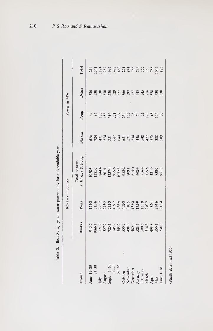
210 P S Rao and S Ramaseshan
<3 <u
X
-D G
& o T3
"O 3
* a
3 C/D
oj 0> CO
ro _a/ -o
H
15 Tf rf r- r- r- OO so SO SO X X fN 90 1-H fN «o Os fN SO *0 Tf SO SO so X X
S fN
o fN fO r-H fN SO Tf (N Os r- r- r^ t"" i-H H
Uh 3 o o o o o Os SO r- fN 90 X oo o o -C co CO co co co fN fN •O Os 90 o- O’ i-H r- CO CO
is
s 0
90 90 90 90 90 90 90 (N CO 90 90
c
M <D £
00 c
o A
3 r- co ro so H ro »o •^t CO CO X Tf X Mm Q oo fN 90 — 90 Os t"~ r^- r- fN 1-H Ol oo
Om co fN fN fN
3 X O Tf ,H ti- i-H r—
3 *-H — o oo r- fN OO OS
n fN r- r- »r> o- 90 r** m 90, O’ fN r- oo O X X r- tj- 90 oo so sO SO 90 90 90 •O co CO 90 co
00 3
C/5 o D C/5 Oh
oo p o- rj- sO OO fN o so O' 90 p r- CO <L> rtf © 1-1-,
3 X X «o fN fN 6s 90 fN sb 90 X o X
1— r- oo o co 90 co iO o i-H so i-H *o CO C^, 90 *3 X o fN oo oo fN Os O Os oo SO SO r- 90 oo Os
cd •—< 1“M *-H 1-H c^ O X O <D H CQ
£ IS 3 o c
C/5 <D C/5 cd <D 00 <N SO fN CN co r-" On O 90 O Os ON r- -H so
13 c 90 »o co cb fN 6s x fN o 90 90 90 o fN Tf fN o 90 r- r** o oo O i-H fO CO CO ’'t CO i-H
Oh CL, fN fN fN 90 ^t CO CN fN fN
<3 In so —H cn qs ON qs fN sO o r- 90 OO OO p X 03 90 sb X X 90 ST) 9/0 O OO O sb O tT 6s so OO
»—i X r- Cl CN o- lo Os c<j fN oo 1-H OS 90 CO
OQ Os o 90 90 r- 90 90 un 90 90 90 Tt 90 r-
o o o o © <N CO fN co V-c M o
1 1 1 1 1 a
U >1 ■»—< t-H X) >-» U 1 X
G o
OJ G
<N C/5 3 00 p a
fN 25 O o
E u > o
£ (U Q CD
u. 73 3 G
33 3 u. X
X o (h a M
D- cd <u G
s 3 3
< <u
C/5 o z Q <3
•“l <L>
U- < 3 (B
hal
la &
Ban
sal
1975
)

Integrated operation of the Beas-Sutlej system 211
f _I_
June 11 June 10
TYPE 1
1.23 P 1.23 P
i . i Nov. 30 Apr. 30 June 10
TYPE 2
i |
1 ^ 1.47 P 1.23 P p 1.36 P 1.47 P
1 L L June 11 Sept. 20 Nov. 30 Apr. 30 June 10
May 31
TYPE 3
Figure 2. Firm power distributions
month i to P. A uniform firm power level, i.e. /f, = 1 for all i, is assumed in type 1, while
in type 2, /?, — 1 from December to April and = 1.23 for other months. Similarly in
type 3, values of i vary in different months from 1 to 1-47.
2.3 Planned operating policies
The planned operation of the reservoirs of the interconnected Beas-Sutlej system is
described by Bhalla & Bansal (1975) and Lamba & Prem (1975). The operating policy
of the system of reservoirs is the same as that of the Bhakra reservoir (§2.4, Rao &
Ramaseshan 1985). In the original Beas project report, the Bhakra and Pong reservoirs
were assumed to be depleted almost simultaneously to their dead pond levels, the firm
power being 766 MW. Releases from the two reservoirs and power generation during different months of the year are given in tables 2 and 3. Bhalla & Bansal suggested
staggering the time of depletion of the Bhakra and Pong reservoirs to their respective
dead pond levels and thus increasing the firm power from 766 to 799 MW. Planning by bdo is confined to the management of the surface waters. Conjunctive utilization of
surface and ground waters has not been considered by them.
3. Conjunctive utilization
3.1 System model
Conjunctive utilization models are developed for integrated management of surface
and ground waters. They are necessarily simplified representations of a more complex
reality, as in the planning studies of bdo, and are limited to the use of published
information. The aim is essentially to focus on the methodology and demonstrate the
utility of model building and systems studies for improvement.

212 P S Rao and S Ramaseshan
The system is shown in figure 3. A linear programming model of the system is
developed and used in these studies. The model maximizes the level of firm power P.
Irrigation demands are to be satisfied in each of the subperiods. The power required to
lift groundwater is over and above the firm power that is to be supplied. The
mathematical formulation of the model is as follows:
Objective function: Maximize P (1)
3.2 Constraints
3.2a Power constraint: The power generated in the system in any period should be
equal to or greater than the firm power demand plus the power required to lift
groundwater in the Bhakra and Beas irrigation commands. The model assumes that
dump power has no value and is indifferent to whether this constraint is defined as an
equality or inequality. In this study, power constraints are equality constraints.
KUTU + K2iT2i + K3DIt - niptP -Pu- P2i > 0, (2)
with i = 1, 2,, 16.
where the first subscripts 1, 2 & 3 refer to the Bhakra, Pong and Dehar plants
respectively; the second subscript i indicates the variable in a subperiod i; coefficients
Ku, K2i and K3 are the power conversion factors (or energy rate functions) for power
plants and represent power generated by a unit volume of water in megawatts per
cumec and K3 is a constant for all the subperiods; Tu, T2i are the flows through the
turbines at the power plants; DI is the inflow diverted through the Beas-Sutlej link and
passing through the Dehar power plant in cumec days; nt is the number of days; and Pu
and P2i are power in megawatt days used for lifting groundwater in the Bhakra and
Beas command areas respectively.
Beas Sutlej Rivet River
Figure 3. The Beas-Sutlej system model
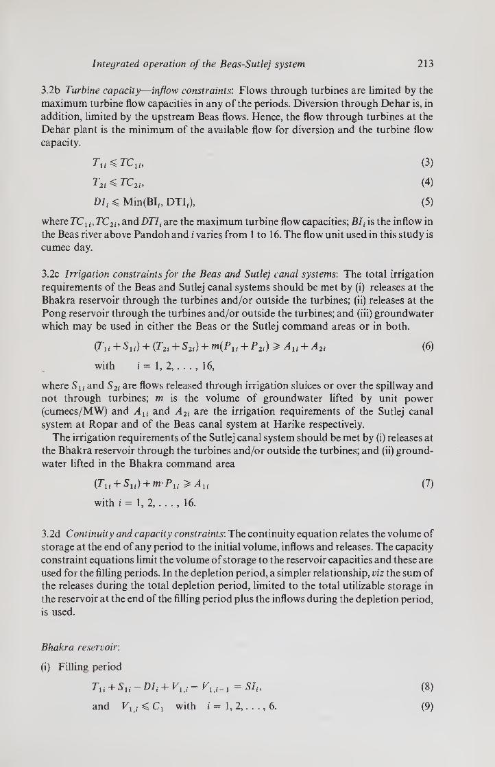
Integrated operation of the Beas-Sutlej system 213
3.2b Turbine capacity—inflow constraints: Flows through turbines are limited by the
maximum turbine flow capacities in any of the periods. Diversion through Dehar is, in
addition, limited by the upstream Beas flows. Hence, the flow through turbines at the
Dehar plant is the minimum of the available flow for diversion and the turbine flow
capacity.
(3)
(4)
(5)
Tu ^ TCU,
T2i ^ TC2i,
Df ^ Min(BI„ DTI,),
where TCu,TC2i, and DTf are the maximum turbine flow capacities; BIt is the inflow in
the Beas river above Pandoh and i varies from 1 to 16. The flow unit used in this study is
cumec day.
3.2c Irrigation constraints for the Beas and Sutlej canal systems: The total irrigation
requirements of the Beas and Sutlej canal systems should be met by (i) releases at the
Bhakra reservoir through the turbines and/or outside the turbines; (ii) releases at the
Pong reservoir through the turbines and/or outside the turbines; and (iii) groundwater
which may be used in either the Beas or the Sutlej command areas or in both.
(Tn + Su) + (T2i + S2i) + m(P 1( + P2,) ^ Au + A2i
with i = 1, 2, ... , 16,
(6)
where Su and S2i are flows released through irrigation sluices or over the spillway and not through turbines; m is the volume of groundwater lifted by unit power
(cumecs/MW) and Au and A2i are the irrigation requirements of the Sutlej canal
system at Ropar and of the Beas canal system at Harike respectively.
The irrigation requirements of the Sutlej canal system should be met by (i) releases at
the Bhakra reservoir through the turbines and/or outside the turbines; and (ii) ground-
water lifted in the Bhakra command area
(Tu + Su) + m-Pu > Au (7)
with i = 1, 2, ..., 16.
3.2d Continuity and capacity constraints: The continuity equation relates the volume of
storage at the end of any period to the initial volume, inflows and releases. The capacity
constraint equations limit the volume of storage to the reservoir capacities and these are
used for the filling periods. In the depletion period, a simpler relationship, viz the sum of the releases during the total depletion period, limited to the total utilizable storage in
the reservoir at the end of the filling period plus the inflows during the depletion period,
is used.
Bhakra reservoir:
(i) Filling period
(8)
(9)

214 P S Rao and S Ramaseshan
(ii) Depletion period
16 16
X (Tu+Su-DIi)-V1'6 + Vlt0= £ SI,. (10)
Pong reservoir:
(i) Filling period
(11)
(12)
(ii) Depletion period
16 16
(13) i=7 i= 7
where Vx, V2 are the volumes of storage; Ct and C2 are the reservoir capacities; and SI
and UI are the inflows in the Sutlej river and in the Uhl river which joins the Beas river
at Mandi; the unit is cumec day for all variables.
3.3 Data and assumptions
3.3a Number of subperiods: As in the bdo studies, the year is divided into sixteen
subperiods, six in the filling period and ten in the depletion period.
3.3b Power conversion factors: The power conversion factors (Ku, K2i, and K3) are
calculated for each reservoir for each subperiod from the bdo data in table 3 and are shown in table 4. As in the study on the Bhakra reservoir (Rao & Ramaseshan 1985)
their variation as a function of the actual reservoir level in each subperiod is ignored.
Dehar is a constant head power plant and the power conversion factor is computed as 2.616 MW/cumec from the total power generated and the total flow through the plant
in a year.
3.3c Irrigation requirements: The irrigation requirement of the Sutlej canal system to
be supplied from the Bhakra reservoir in any subperiod is taken as the minimum of the
Sutlej canal requirement (table 2) and the Bhakra reservoir release (table 3). The total
irrigation requirements for the system are available from the bdo study. Both are shown
in table 4. With contributions from other sources, namely, the Western Jamuna canal
and the Madhopur-Beas link, accounted for, they correspond to a filling period rf of
about 1 and a depletion period rf of about 0-85.
3.3d Turbine capacities: Assuming a standby unit of 120 MW and a maximum power
plant capacity of 930 MW at Bhakra, and a standby of 60 MW and a maximum power
plant capacity of 300 MW at Pong and using the power conversion factors, the
maximum turbine flow capacities are calculated (table 4). The Beas river flow available
for diversion at Pandoh is calculated from the Beas river flow at Mandi in proportion to
the ratio of the respective catchment areas.
3.3e Volume of storage in reservoirs: A summary of river inflows and reservoir releases
in the filling and depletion periods for a dependable year is shown in figure 4. The
storage capacities of Bhakra and Pong reservoirs are respectively 9,320 and
6,767 m cu m. The storage capacities in the bdo study in a dependable year are

Table
4.
Data f
or
Bea
s-S
utl
ej s
yst
em.
Integrated operation of the Beas-Sutlej system 215
G <D
s <D Uh „—s
'G c/5 p|, >*» ST 2 "O
<D
Z
O a
8 | ^ u O <D
g
cd 3 G O
3 H
1.) > G O o Uh CD £ O
CU
S'
6 OO O" Tf VO OO oo CO VO 04 O- 04 ro op <D o t—i r- CO r- VO 04 t-H O' vO Os 04 •o VO t-h
o- oo i-H OO co VO ro VO 04 O VO O" Os O- VO C/5 C/5 o 04 VO Tf 04 Os O Os Os o y—1 CO VO VO Os 3
£
C/5 04 04 0-1 04 04 04 04 04
G c a E O £
S % H-> C/5 G
GO
<D
o S a g
G Cl, O
Oh
CD £ o a
M <3 X CQ
00 O G >
n° « Oh c/5 <D
C/5 VO VO OO vO O O o VO O VO y—t OO y—{ O' VO Os P vo •O vO CO 04 VO oo vO ro y—i 04 o iO VO Os O rrt VO vO OS «0 Os OO oo co co Os VO vO O' o vo 3"
--2 t—i »—i 3- VO o- r- r- O' O’ VO O- O' 3- oo o o- cx *—1 t-< CO 04 04 04 04 04 04 <o 1 04
C O £
04 04 O' WO _H Os Os SO oo o 3^ oo Os Os Os os ro ro o vO VO VO •O VO vo oo vo oo iO 3- ro oo O' O' O' ro 04 3* 3- o OS oo T—H VO Os VO 04 ro O' O' O' VO O' vo VO o 3" 3" 04 "3- VO O' O'
ioiovosotj-o-ooO'CO o- co vo o vo os —c o* vr> fSTt^'OOOOOOON'-lhO r-r-ovOTfrtTf«o,s0'O
04 —< t-H t-H t-H
o o o- os as o- oi rf oo ro os tj- oo ro
'O ^ ^ h vr> oo co
3^ 04
•O ro
04 O 8 OO
vo vo 04 g 04
04 O'
vo »o
VO 3*
04 O'
o 3 oo
vo Os 3
■ ■ ■* O vo vo y—( t-H r-H OO VO vo # ro r-H OS VO o 3" 3" 3- vo vo VO VO »0 »0 VO VO vo VO 3 3 3 o o O O © © © © © O © <6 © O © ©
a3 Uh Q _ VO CO VO ro O' 04 o vo CO VO >0 ro O' OO
\/{ O' Os 3 O' CO VO OS CO vo 04 Tf CO Os O' oo Uh O' O' 04 00 O' oo O' OO O' T—H 04 O' os oo
-G CD vo vo OO o t-H T—1 1 T-H 1 ^-1 O os OO O' vo vo
PQ C/5 CD © o © T-H O O o O o
o O o o o 04
1 CO
| T-H 04 CO Uh
1 1 1 (D T-H u, X
y—* 04 <D X 6
(D G G
Ju
ly
Augu
Sept.
o
o
o
<D > o
Z
<D X
£ (D
3 G u.
X) (D
Uh
c a ^ < s

216 P S Rao and S Ramaseshan
Figure 4. Water balance of the Beas Sutlej system
respectively 5,112 and 3,477 mcum corresponding to final volumes of storage at the
end of the depletion period, 4,208 and 3,290 m cu m respectively. These are assumed to
be the levels of storage at the beginning of the filling period (case 1) and are referred to
as initial volumes in this study. In case 6 the initial volumes of storage are 2,426 m cu m
in Bhakra corresponding to a dead storage level of 445 62 m, and zero in Pong. Cases 2
to 5 correspond to intermediate values and details are given in table 5.
3.3f Power for groundwater: It is assumed that 1 MW of power can lift 2.832 cumecs of
groundwater. This corresponds to a lift of 25 m and for Punjab this is a conservative
assumption (Minhas et al 1972).
3.3g Dehar diversion flows: The system is studied with two different assumptions
regarding the Beas-Sutlej diversion flows.
Model 1: For comparability of results, Dehar inflows are calculated from the seasonal
distribution of power generation and total diversion as specified by the bdo study
(Mehndiratta & Hoon 1973; Bhalla & Bansal 1975). It is assumed in this model that
they are prespecified and are not subject to control. Model 1 has 109 variables and 106
constraints.
Model 2: It is assumed that the Beas-Sutlej diversions can be changed, if necessary,
subject to the availability of flows in the Beas above Pandoh for diversion and limited
by the turbine flow capacity at Dehar. Additional diversion of water through Dehar
generates power at Dehar and Bhakra at heads higher than at Pong and can also meet
irrigation demands in the Bhakra or Beas canal systems. This flexibility can and does
increase the firm power level. Model 2 has 125 variables and 122 constraints.
4. Discussion of results
The firm power level is maximized for each case defining initial reservoir volumes for
each type of firm power distribution and for specified (model 1) and variable (model 2)
Dehar diversions, mpsx (Mathematical Programming System Extended) available in
the Harvard-MiT Computer system was used and each solution required about 45 to 50
seconds for computation and execution. The maximum firm power levels for all the
cases are shown in table 5.

Tab
le
5.
Max
imu
m fi
rm p
ow
er
in B
eas-S
utl
ej
syste
m
Integrated operation of the Beas-Sutlej system 217
ed £ 03 OO <D s
<D £ o a
<D s 3 o >
o £ <D
rn
21 H
<N 21
H
21 H
oo c o
CLh
oj _G
CO
X) .2
03 X ’55
u V") o oo
<r> O
o-i O o S C
cd Q <D >
oo 00 ON ON On ON
T3 g « £ O CC Cd T2 .3 <—i C/5
S-l £ 00 -O
QJ C-
2S.2 .2 -g 2 Ui W D
* Q .> ^ -a
T3 g <U h o £ S ’53 a * s 21 Q > C/D T3
JU c
X> Wh cd
o <N NT) NO IA> <N
.2 X *C/5 NO ON <N NO OO ON <D ON ON O o o o
cd >
Q *3
-o c U >- o X cd .Th f C/5
a ;5 s a Q > 00 T3
3 E S' 3
E 3 o E
a “ E ^
3
E 3 u E
u 2 o U Z
On c<d m m ro f"~ oo oo oo oo oo
m o r- NO oo i—H ,,d- r** r- oo ON ON ON On On
tt n n -h m g <N oo O O O 00 OO 00 Os On Os
r~i m un r- oo no On <N *T5 oo © O oo os ON ON O O
r-» r- r- r- r- NO o Tf oo <N o rn r- o oo m oo m ON m m <N <N
O ON r- NO ON r- NO CT) <N oo rf O NO CO n (N <N —<
On on ON ON ON NO OO o <N 3: NO sO NO NO vn m © OO m oo m oo 00 ■*fr •*t m m <N <N
oo ON o T-i <N NO O NO m ON vn <N <N r< m OO 'Tf
m m <N cs <N
<N fO rf iT) NO

218 P S Rao and S Ramaseshan
For any level of initial storage, the firm power level for type 1 distribution is higher
than that for type 2, which in turn is higher than that for type 3. This implies that higher
values of variable /?* reduce the firm power level.
Even in case 1 with wasteful spillage of the order of 10% of total storage, the firm
power is 797,824 and 891 MW respectively for firm power distribution types 3,2 and 1.
With no spillage, the firm power increases respectively to 835,902 and 1008 MW. Thus
conjunctive utilization can increase firm power at least by 36 MW above that of
improved operation and 69 MW above the original planned operation of bdo. In case
firm power distribution can be represented by type 1 or type 2, the firm power levels
increase further by 173 MW and 67 MW aboye those of type 3. The small differences
between case 5 and case 6 seem to be due to numerical errors.
Since in this study the power conversion factors are considered to be independent of
the variations of the actual reservoir level in any period, the variation between case 1
and case 6 corresponds to various levels of spillages. Variable Dehar diversion
(model 2) increases firm power levels over specified Dehar diversion (model 1) by
54 MW to 86 MW or 7 to 8 %.
The details of power generation and of groundwater utilization are not reported in
the study but are summarised below:
(i) Generally, in June and July, the Pong reservoir is filling up and no releases are
made; and for a continuous period of two to three months between November and February also, no releases are made from Pong.
(ii) Whenever possible, water is diverted through Dehar as the power generation at
Dehar and Bhakra is much larger than that at Pong.
(iii) The current practice is to release surface water liberally in the filling period to meet
the irrigation demand and use groundwater essentially in the depletion period.
However, the results of this study are contrary to the current practice and they indicate
groundwater use generally between May and November and not from December to
April. Groundwater utilization peaks in September, is significant for parts of July,
August and October, and is somewhat smaller in May, June and November. The
quantities vary from solution to solution. For example, the groundwater used for case
1, type 1 of model 1 varies as follows: 36,298 and 438 cumecs in the three subperiods of
June: 236 cumecs in July; 226 cumecs in August; 500, 286 and 110 cumecs in the three
subperiods of September; and 193 cumecs in November. A maximum pumping
capacity of 500 cumecs is indicated and in case the pumps operate only for part of the
day and not fully, the installed capacity should be proportionately higher. By staggering
the cropping pattern, the peak groundwater use may be reduced resulting in a higher
utilization of the installed pumping capacity.
In the Kharif season, irrigation demands are high and constraining and a large
amount of secondary or dump power is currently generated. By lifting groundwater in
this period, it is possible to conserve surface water for future use and to eliminate any
secondary power generation except when unavoidable. The surface water so conserved
is generally adequate to meet the full irrigation demands in the Rabi season except
perhaps for very limited groundwater use in one or two periods. In addition to this, the
firm power level is also raised significantly i.e., part of the seasonal excess power of low
value is converted to firm power of high value. This is similar to the concept of using a
pumped storage scheme. But rather than looking for a smaller reservoir at a higher
elevation, the larger and lower ground-water reservoir is used advantageously. It may
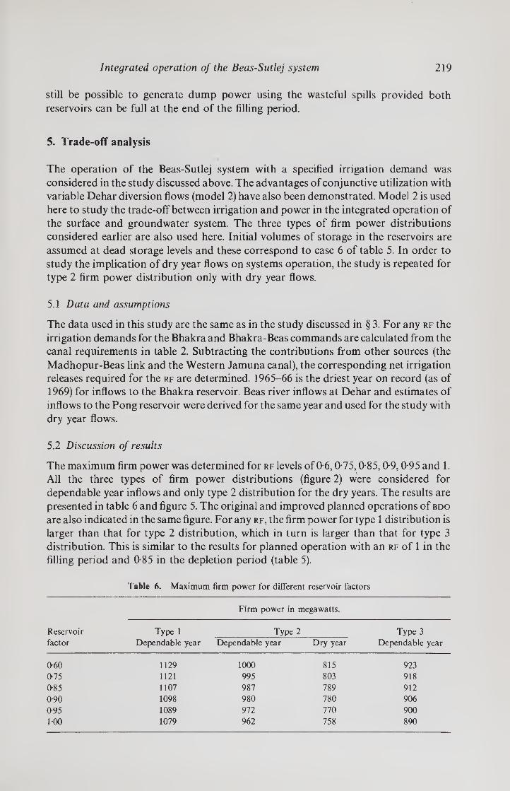
Integrated operation of the Beas-Sutlej system 219
still be possible to generate dump power using the wasteful spills provided both
reservoirs can be full at the end of the filling period.
5. Trade-off analysis
The operation of the Beas-Sutlej system with a specified irrigation demand was
considered in the study discussed above. The advantages of conjunctive utilization with
variable Dehar diversion flows (model 2) have also been demonstrated. Model 2 is used
here to study the trade-off between irrigation and power in the integrated operation of
the surface and groundwater system. The three types of firm power distributions
considered earlier are also used here. Initial volumes of storage in the reservoirs are
assumed at dead storage levels and these correspond to case 6 of table 5. In order to
study the implication of dry year flows on systems operation, the study is repeated for
type 2 firm power distribution only with dry year flows.
5.1 Data and assumptions
The data used in this study are the same as in the study discussed in § 3. For any rf the
irrigation demands for the Bhakra and Bhakra-Beas commands are calculated from the
canal requirements in table 2. Subtracting the contributions from other sources (the
Madhopur-Beas link and the Western Jamuna canal), the corresponding net irrigation releases required for the rf are determined. 1965-66 is the driest year on record (as of
1969) for inflows to the Bhakra reservoir. Beas river inflows at Dehar and estimates of
inflows to the Pong reservoir were derived for the same year and used for the study with
dry year flows.
5.2 Discussion of results
The maximum firm power was determined for rf levels of 0-6,0-75,0-85,0-9,0-95 and 1. All the three types of firm power distributions (figure 2) were considered for
dependable year inflows and only type 2 distribution for the dry years. The results are
presented in table 6 and figure 5. The original and improved planned operations of bdo
are also indicated in the same figure. For any rf, the firm power for type 1 distribution is
larger than that for type 2 distribution, which in turn is larger than that for type 3
distribution. This is similar to the results for planned operation with an rf of 1 in the
filling period and 0-85 in the depletion period (table 5).
Table 6. Maximum firm power for different reservoir factors
Reservoir
factor
Firm power in megawatts.
Type 1
Dependable year
Type 2
Dependable year Dry year
Type 3
Dependable year
060 1129 1000 815 923
075 1121 995 803 918
085 1107 987 789 912
0-90 1098 980 780 906
095 1089 972 770 900
100 1079 962 758 890
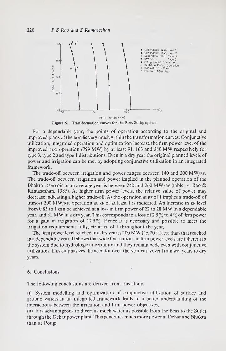
220 P S Rao and S Ramaseshan
Figure 5. Transformation curves for the Beas-Sutlej system
For a dependable year, the points of operation according to the original and
improved plans of the bdo lie very much within the transformation curves. Conjunctive
utilization, integrated operation and optimization increase the firm power level of the
improved bdo operation (799 MW) by at least 91, 163 and 280 MW respectively for
type 3, type 2 and type 1 distributions. Even in a dry year the original planned levels of
power and irrigation can be met by adopting conjunctive utilization in an integrated
framework.
The trade-off between irrigation and power ranges between 140 and 200 MW/rf.
The trade-off between irrigation and power implied in the planned operation of the
Bhakra reservoir in an average year is between 240 and 260 MW/rf (table 14, Rao & Ramaseshan, 1985). At higher firm power levels, the relative value of power may
decrease indicating a higher trade-off. As the operation at rf of 1 implies a trade-off of
utmost 200 MW/rf, operation at rf of at least 1 is indicated. An increase in rf level
from 0-85 to 1 can be achieved at a loss in firm power of 22 to 28 MW in a dependable
year, and 31 MW in a dry year. This corresponds to a loss of 2-5 % to 4 % of firm power
for a gain in irrigation of 17-5%. Flence it is necessary and possible to meet the
irrigation requirements fully, viz at rf of 1 throughout the year.
The firm power level reached in a dry year is 200 MW (i.e. 20 %) less than that reached
in a dependable year. It shows that wide fluctuations in firm power levels are inherent in
the system due to hydrologic uncertainty and they remain wide even with conjunctive
utilization. This emphasizes the need for over-the-year carryover from wet years to dry
years.
6. Conclusions
The following conclusions are derived from this study.
(i) System modelling and optimization of conjunctive utilization of surface and
ground waters in an integrated framework leads to a better understanding of the
interactions between the irrigation and firm power objectives;
(ii) It is advantageous to divert as much water as possible from the Beas to the Sutlej
through the Dehar power plant. This generates much more power at Dehar and Bhakra
than at Pong;

Integrated operation of the Beas-Sutlej system 221
(iii) Contrary to current practice groundwater should be used from May to November
and surface water conserved in reservoirs during the period. This raises the firm power
level significantly;
(iv) The levels of irrigation and power planned for a dependable year from the
reservoirs of the Beas-Sutlej system can be attained even in a dry year by conjunctive
utilization of surface and groundwaters;
(v) It is desirable and certainly possible to meet the full irrigation requirements of the
system throughout the year; and
(vi) Over-the-year carryover storage from wet years to dry years is essential to reduce
the wide fluctuations in the levels of objectives attained in different years.
References
Bhalla B S, Bansal R N 1975 J. Central Bd Irrigation Power 32: 15
Lamba S S, Prem K S 1975 Integrated development of rivers Sutlej, Beas and Ravi for optimum utility of
water in north-western area of India; Presented at the IWRA II World Congress on Water Resources,
New Delhi, Reprint, Vol. 3; p. 79
Mehndiratta K R, Hoon R N 1973 J. Central Bd Irrigation Power 30: 349
Minhas B S, Parikh K S, Srinivasan, T N 1972 Sankya, Indian J. Stat. B34: 105
Rao P S, Ramaseshan S 1985 Sadhana 8: 179-206
S— 1-6

.
-

Optimal irrigation planning in river basin development: The case of the Upper Cauvery river basin
S VEDULA
Ford India Project, Department of City and Regional Planning, Harvard University, Cambridge, Massachusetts, USA
Present address: Department of Civil Engineering, Indian Institute of Science, Bangalore 560012.
Abstract. The study deals with the irrigation planning of the Cauvery river basin in peninsular India which is extensively developed in the downstream reaches and has a high potential for development in the upper reaches. A four-reservoir system is modelled on a monthly basis by using a mathematical programming (LP) formulation to find optimum cropping patterns, subject to land, water and downstream release constraints, and applied to the Cauvery basin. Two objectives, maximizing net economic benefits and maximizing irrigated cropped area, considered in the model are analysed in the context of multiobjective planning and the trade¬ offs discussed.
Key words. Irrigation planning, multiobjective planning; Cauvery basin; four-reservoir system; Karnataka master plan.
1. Introduction
There is an increasing awareness in recent times of a need to evolve comprehensive
basin plans for river basin development to meet the national or regional objectives as
best as possible. Irrigation has been one of the most important aspects of this planning.
Development plans call for improved strategies to conserve water by adopting better
and more efficient water management techniques in existing areas and an optimum
irrigation planning in those areas proposed to be brought under new irrigation. Linear
programming models of various kinds have been used in the past as planning models in
river basin development.
The present study concerns the case of the interstate Cauvery river basin in South India. The lower reaches of the basin have excellent irrigation facilities and extensive
irrigation has been in practice in these areas since the beginning of the century.
Irrigation development in the upper reaches of the basin has been rather slow and
restricted by bilateral agreements between the basin states viz. Karnataka, Kerala and
Tamil Nadu.
Thus there is a need to extend irrigation facilities to the areas of the upper reaches of
the basin subject to providing adequate water supplies to all the areas presently under
irrigation in the basin. The present study is based on this hypothesis. An irrigation
planning model is formulated for the upper basin (basin above Mettur) to optimize
1. Parts of this paper have been reprinted with permission from the American Geophysical Union: Vedula S
and Rogers P P Water Resources Res. 17: 1304-1311, 1981 ©AGU.
2. A list of symbols is given at the end of the paper.
223

224 S Vedula
crop patterns in the proposed area of development, while meeting the irrigation
requirements of the lower basin according to the existing cropping pattern. A linear
programming technique was used to find solutions for different objectives. Keeping the
proposals made by the Karnataka Master Plan in view, a multi-objective analysis is also
made and the implicit trade-off relationships between the different objectives used in
planning are determined.
2. The Cauvery basin
2.1 Basin description
The Cauvery is one of the major interstate rivers of South India. The river rises in the
Coorg district of Karnataka, flows in a general south-east direction across the plateau
of Karnataka, and after traversing a distance of 400 km runs along the boundary
between Karnataka and Tamil Nadu for 60 km before entering Tamil Nadu upstream
of the Mettur Reservoir (built in 1934). The river then flows through Tamil Nadu for
230 km before reaching the Grand Anicut, the head of the Delta, and thereafter it
divides into a number of branches and finally joins the Bay of Bengal in Tamil Nadu.
The total length of the river from its origin to the sea is 800 km. Figure 1 gives a plan of
the basin.
The salient features of the basin are given in detail in the Karnataka State Master
Plan (1976). The Cauvery has 21 principal tributaries (drainage area of each of which is
greater than 250 km2). Of these, 9 are located wholly or largely in Karnataka and 12 in
Tamil Nadu. The basin has a total drainage area of 81,155 km2 of which 34,273 km2
KARNATAKA -Basin boundary
Figure 1. Cauvery basin plan (not to scale).

Optimal irrigation planning 225
(42.2 %) lies in Karnataka, 2866 km2 (3.5 %) in Kerala and 44,016 km2 (54.3 %) in Tamil
Nadu.
2.2 Rainfall
The basin is under the influence of both the south-west (June to September) the
north-east (October to December) monsoons. The annual rainfall in the basin varies
from less than 60 cm over the north-western part of the Amaravathi sub-basin to more
than 600 cm near the source of the Cauvery River in the extreme west of the basin. The
high rainfall however diminishes rapidly eastward. The basin in the east (Lower
Coleroon sub-basin and the Delta) has an average annual normal rainfall of about
120 cm. Elsewhere in the basin the annual rainfall is lower than 80-85 cm.
2.3 Surface water resources
There are 24 discharge sites on the Cauvery River and its tributaries, of which 8 are on
the main river. Fifteen discharge sites are in Karnataka, while 9 are in Tamil Nadu.
The mean annual flows in the Cauvery River at different locations along its course are
as follows, the flows indicated being exclusive of consumptive use by upstream
irrigation: at Chunchanakatte, 48 km upstream of the Krishnaraja Sagara (krs) dam,
2908mcum; at the krs dam, 5904mcum; at Dhanagere Ane, upstream of its
confluence with the Shimsha, 8874mcum; and at Mettur, 9628mcum.
The net gain (average annual gain) in the river flow in each of the three important
reaches is as follows: KRS-Mettur, 2973mcum; Mettur-Grand Anicut, 2690mcum;
and Grand Anicut-Lower Coleroon Anicut, 827mcum.
2.4 Groundwater resources
No estimates of groundwater potential are available for the Cauvery basin in
Karnataka. However, Karnataka estimated the quantum of deep percolation in its part
of the basin as 3936 m cu m (Master Plan, Part I, page 52) of which a substantial part is
supposed to be flowing down to the lower reaches of the basin (in Tamil Nadu). The
groundwater development to date has been estimated to be 538mcum only. The
reason for this low rate of groundwater development is that the area in Karnataka is
largely rocky comprising mainly of igneous and metamorphic rocks. However, the
geological settings are believed to be quite favourable for groundwater development in
the delta region with the thickness of sedimentary formations extending to great
depths. The total quantity of replenishable groundwater that can eventually be
extracted in the delta, according to undp investigations, amounts to about 3650 m cu m
per year (Master Plan, Part 1,1976). This is apparently unused at the present time. The
total recharge in the non deltaic area in Tamil Nadu is estimated to be 2718mcum,
whereas the groundwater utilization is to the extent of 1954mcum.
2.5 Development of irrigation
Irrigation has been practised in the Cauvery Basin from ancient times, by inundation
from delta channels and by tanks and river/anicut channels in the entire basin above the
delta.
At the beginning of the 20th century, the aggregate ayacut developed for irrigation
was about 700,000 ha out of which nearly 430,000 ha was in the delta. Two major

226 S Vedula
reservoirs were constructed in the early thirties on the main river: the krs reservoir in
Karnataka with a live storage of 1269mcum and the Mettur reservoir in Tamil Nadu
with a live storage of 2648 m cu m. The third major irrigation project on the river is the
delta canal irrigation, the canals taking off from the Grand Anicut in Tamil Nadu. Thus
by 1971 this aggregate ayacut progressively increased to 840,000 ha. The position in
1971 indicates that Karnataka had irrigation facilities available to 11 % of its culturable
area in the basin as against 30 % in Tamil Nadu (table 1). The irrigated cropped area in
the basin in 1971 was 1-57 million ha, of which 1 -26 million ha was in Tamil Nadu
(table 2). Thus irrigation facilities are not evenly distributed over the whole basin.
2.6 The problem
One fourth of the people of Karnataka, about 7T4 million, live in the Cauvery Basin,
the second largest river basin in the State, covering 18 % of its total area. Almost 2/3 of
the basin area in Karnataka State has been identified by the Irrigation Commission
(1972) as drought-affected. Thus large areas of the basin with scanty rainfall are starved
of irrigation waters in Karnataka, whereas lower downstream the methods of
irrigation are old, with the result that a large amount of water is being wasted by going
into the sea unutilized. An examination of the withdrawal rates of water for canal
irrigation indicates that the withdrawals are far greater than the irrigation requirements
Table 1. Area irrigated in Cauvery basin (ayacuts)
Karnataka Kerala Tamil Nadu
(in lakh hectares*)
Total
1. Culturable area in basin 24-8 1-5 28-9 55-2
Area developed as in 1971
2. Ayacut
(a) Under tanks or minor works 10 0-2 1-2 2-4
(b) Under river/anicut channels 0-8 0-9 1-7 (c) In delta, old 4-3 4-3 (d) Under major and medium 0-9 2-3** 3-2
schemes of twentieth century
(e) Total 2-7 0-2 8-7 116
3. Percentage of total ayacut to (11) (13) (30) (21)
culturable area
Developments as per Master plan
4. New ayacut
(a) Under minor schemes 0-5 01 01 0-7 (b) Under major and medium 5-6 0-7 IT*** 7-4
projects
(c) Total 61 0-8 1-2 81
5. Aggregate ayacut 2e + 4c 8-8 1-0 9-9 19-7
6. Percentage of aggregate ayacut (36) (67) (34) (36)
to culturable area
Source: Karnataka Master Plan (1976)
* except figures in brackets which are percentages, correct to the nearest whole number.
** including 43,700 ha outside the basin developed by Cauvery waters.
*** including 72,500 ha developed by waters imported from outside the basin.

Optimal irrigation planning 227
Table 2. Irrigated cropped areas in Cauvery basin
Karnataka Kerala Tamil Nadu
(in lakh hectares)
Total
1. Culturable area in basin 24-8 1-5 28-9 55-2
Developments as in 1971
2. Irrigated cropped area (ica)
(a) Under tanks or minor works 10 0-3 1-2 2-5
(100) (150) (100)
(b) Under river/anicut channels 0-8 1-5 2-3
(100) (167)
(c) In delta, old 71 7-1
(165)
(d) Under major and medium
schemes of twentieth century 10 2-8 3-8
(111) (122)
(e) Total 2-8 0-3 12 6 15-7
(104) (150) (145)
Developments as per Master plan (as in a dependable year)
3. Increased cropped area on
2(b), (c) and (d) above 2-8 14 6 17 4
(155) (195)
4. New cropped area
(a) Under minor schemes 0-5 01 01 0-7
(100) (150) (100)
(b) Under major and medium 7-9 1-4 1-4 10-7
projects (141) (200) (127)
5. Aggregate cropped area 12-2 1-8 17-3 31-3
(139) (180) (175)
(Figures in brackets represent intensity of irrigation over ayacut in per cent)
Source: Karnataka Master Plan (1976)
and that a substantial amount of water is just flowing into the sea. Severe waterlogging
and drainage problems have been reported in the downstream reaches and in the delta
(Master Plan, Part 1,1976). Development of irrigation in Karnataka had been severely
restricted after the construction of the krs and Mettur reservoirs by a 50 year bilateral
agreement between the states of Karnataka and Tamil Nadu, commonly known as the
1924 agreement (which expired in 1974). There has been considerable development in
the basin in recent times and consequently the upstream states are demanding a better
share of the river waters.
Karnataka took a critical view of the position as it existed in 1971 and proposed a
number of developments and new projects in the Master Pian (1976) and also
recommended cropping patterns in the whole basin, based on an analysis of rainfall
distribution. Tamil Nadu, on the other hand, essentially proposed a modernization of
the entire delta system. This is meant to put the waters presently available to more
efficient use, alleviate the drainage problems in the delta and bring about better
management of the irrigation system as a whole. Negotiations are presently underway
for an amicable solution regarding sharing of waters among basin states.
2.7 The Karnataka Master Plan
The Karnataka Master Plan divides the entire Cauvery Basin into 16 sub-basins for its

228 S Vedula
analysis. The improvement of irrigation envisaged in the plan is shown in tables 1 and 2.
The plan was developed on the premise that only one crop of paddy will be grown in the
entire basin (including those areas in Tamil Nadu where extensive double cropping of
paddy has been in vogue traditionally for many years). The Master Plan recommends
construction of three new reservoirs across the Cauvery river, two in Karnataka and
one in the river reach common to Karnataka and Tamil Nadu to gain better control of
the waters for irrigation development and to substantially increase the power
production. The plan suggests that the cost be shared by the two states appropriately.
The details of the plan are contained in the three part publication of the Master Plan
(1976).
2.8 Assumptions in the present study
There are already a few major storage structures under construction in the upper basin
and there is great need for planning the optimum use of the diversions from these
reservoirs. It may not be easy to radically change the cropping patterns in areas below
Mettur to a single paddy cropping as suggested in the Master Plan. Earlier experience
in the Lower Bhavani (Planning Commission 1965) clearly shows the difficulty of
adopting the planned cropping patterns in practice. Radical changes in existing
cropping patterns which have been in existence for a long time could be expected to be
even more difficult to accomplish. This forms one of the working assumptions for the
present study. Secondly, the present withdrawals into the canals and the diversions
seem to be far greater than the actual requirements in certain areas. Also there is great
potential for developing the groundwater resources available in the delta to augment
the surface supplies.
3. The Upper Cauvery Basin Study
3.1 Object of the study
This study aims at bringing out an optimum plan of cropping in the upper basin
ensuring adequate supplies for irrigation according to the existing cropping pattern in
the lower basin. For the present investigation, the reservoir site at Mettur forms the
boundary between the upper basin and the lower basin. This is considered appropriate
because (i) most of the proposed new irrigation developments are upstream of Mettur
and (ii) Mettur reservoir primarily regulates the flow for downstream irrigation needs
along the main river and in the delta.
All major irrigation projects in the upper basin are considered in the study. The
activity points for study in the upper basin are the diversions at the four reservoirs:
Hemavathy, krs, Kabini and Mettur (table 3). The water diversion requirements for
existing irrigation considered are for those areas presently being irrigated by diversions
from the main river. These areas comprise of (i) the delta including the ayacut of the
Grand Anicut canal and (ii) the non delta. The non delta area comprises the ayacuts
of the Mettur canal, Salem Trichy channels, Kattalai channels, New Kattalai high level
canal and Pullambadi canal. It is assumed that the requirements of the Lower Coleroon
sub-basin would be met by the river gains between the Grand Anicut-Lower Coleroon
Anicut reach and from the groundwater available in the sub-basin.
Optimal irrigation planning 229
Table 3. Reservoir capacities and areas planned for irrigation
Status Reservoir
Capacity
mcum
Land area proposed
for irrigation (ha)
Under construction Hemavathy 962-77 248,900
Existing KRS 1268-59 77,900*
Under construction Kabini 453-07 87,800
Existing Mettur 2647-60 —
* This is in addition to the existing irrigation at KRS reservoir.
3.2 Features of the study
Optimum crop patterns in the upper basin are arrived at by an optimization process
using a linear programming model for the upper basin. Two systems are formulated: a
four-reservoir system consisting of the Hemavathy, krs, Kabini and Mettur reservoirs
and a three-reservoir system consisting of the Hemavathy, krs and Kabini reservoirs. In
the three-reservoir system, the storage at Mettur is not considered and the release from
the three-reservoir system is controlled in such a way that the inflows at Mettur are
adequate to meet the requirements of the lower basin. For each of the two systems
studied, two cases are examined, with and without considering the ‘upstream
developments’. The ‘upstream developments’ considered provide for the water
requirements of all projects under construction and proposed (in the Master Plan)
upstream of krs reservoir. These include irrigation by storages at (i) Harangi (under
construction), and (ii) Votehole, Yagachi, Cauvery reservoir project, Chicklihole and
Lakshmanathirtha (proposed). For each of the cases considered above, three objectives
viz maximizing (i) the net benefit from agriculture, (ii) the total irrigated cropped area
and (iii) the total reservoir diversions are studied. The trade-off relationships between
the first two objectives are also discussed.
In all cases, it is ensured that the water available at Mettur is adequate to meet the
irrigation requirements of the lower basin as defined earlier on a monthly basis
according to the existing cropping pattern. Out of the four major reservoirs in the
upper basin, two exist and two are under construction. The Hemavathy and Kabini
reservoirs are presently under construction with ayacuts of 248,900 ha and 87,800 ha
respectively. The ayacut of the existing krs reservoir which is presently at 716,600 ha is
proposed to be extended by an additional 77,900 ha. The Mettur reservoir supplies water to the Mettur canal which has an ayacut of 18,200 ha.
3.3 The model
A twelve season (monthly) linear programming model is formulated for the reservoir
system in the upper basin. The input for the deterministic model consists of the mean
monthly inflows into the reservoirs, mean monthly evaporation and mean monthly
water diversion requirements at existing areas (if any) irrigated by reservoir diversions
(krs and Mettur reservoirs). Two models are formulated, one for the four-reservoir
system and another for the three-reservoir system. In the formulation of the model, the
reservoirs are represented as A, B, C, and D (explained in figure 2). The models have a
lot in common. Departures occur in the formulation of constraints which will be
mentioned where necessary. The objectives are common for both the models.
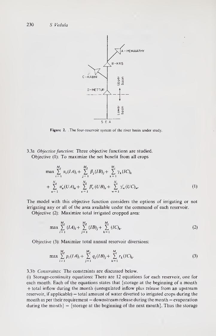
230 S Vedula
Figure 2. The four-reservoir system of the river basin under study.
3.3a Objective function: Three objective functions are studied.
Objective (1): To maximize the net benefit from all crops
Mb Mc max Z Z Pj(IB)j+ Z 7k(IC)k
i = 1 j = 1 k = 1 N N N + Z <(UA)U+ z P'V(UB)V+ z y'Aucx. (1)
U = 1 l?=l W=1
The model with this objective function considers the options of irrigating or not
irrigating any or all of the area available under the command of each reservoir.
Objective (2): Maximize total irrigated cropped area:
M„ Mc
max Z UA\+ Z Z (*C)t. (2) i=1 j=1 k=l
Objective (3): Maximize total annual reservoir diversions:
m„ mc
max Z Pt(IA)t+ Z <lj(IB)j+ Z rk(!Qk- (3) i=l j=1 k=1
3.3b Constraints: The constraints are discussed below.
(i) Storage-continuity equations: There are 12 equations for each reservoir, one for
each month. Each of the equations states that (storage at the beginning of a month
+ total inflow during the month (unregulated inflow plus release from an upstream
reservoir, if applicable) — total amount of water diverted to irrigated crops during the
month as per their requirement — downstream release during the month — evaporation
during the month} = (storage at the beginning of the next month}. Thus the storage

Optimal irrigation planning 231
continuity equations for the four reservoirs A, B, C and D for the month m read (after
rearrangement) as,
m„
(SA) m-(SA)m + l - X = (EA)m-(FA)m. (4) i = 1
(SB) m-(SB)m + 1 + (RA)m- £ qmj(IB)mj — {RB)m j= i
(5)
(SC) m - (SC)m + 1- I rm k (7C)m.* - (RC)m = (£C)m - (£C)m, (6) k = 1
(SD) m - (SD)m +, + (RB)m + (RC)m - (RD)m
= (ED)m - (FD)m + (WD)m, m= 1, 2,... 12. (7)
The three-reservoir system model will not involve (7) given above.
(ii) Land area constraints: The total cropped area (irrigated and unirrigated) in each
month is limited to the land that is in command of each of the reservoirs. There can be a
maximum of 12 such constraints for each reservoir. The actual number of constraints
depends on the cropping pattern. The constraint for reservoir A in a typical month m is
expressed in the form
M. X (lA)mJ+ X (UA)mtU < (LA), m = 1, 2,. . , 12. (8)
1=1 u = 1
Similarly, the constraints for month m in the case of reservoirs B and C are expressed as
A£ Nb
X X (^)m, ^ (LB), m = 1, 2,. . . . , 12, (9) j= i j=i
and
X (fC)m,k+ X (uc)m,k ^ (LC), m = 1, 2,. . . , 12, respectively. (10) k = 1 k = 1
In a month where one crop ends and another begins, the area of ending crop is not
included in the constraint to permit the possible use of the land for both the crops
during different times in that month. No such constraints are needed for reservoir D as
there is no new irrigation proposed. The requirements of existing irrigation are
accounted for in the storage continuity equations (7) and the only decision variable at
reservoir D is the downstream release.
(iii) Downstream release constraints: For a three-reservoir system, the sum of the
releases from the reservoirs B and C (krs and Kabini reservoirs respectively) in each
month should not be less than a specified value for that month, i.e.
(RB)m + (RC)m > (DM)m, w = 1, 2,.... 12. (11)
The values (DM)m for m = 1,2,. . . , 12 were computed such that if the river flows are
maintained at these values, they ensure adequate water supply for existing irrigation in
the delta and the non delta areas below Mettur as defined earlier.
232 S Vedula
For the four-reservoir system, the storage at reservoir D is also taken into account
and the downstream release, (DD)m in each month m, is specified as the minimum release
to ensure adequate water supply for existing irrigation in the delta and the non delta
areas below Mettur as defined. In this case however, the area irrigated by the Mettur
canals is not included in the ‘non delta’ area as their water requirements were accounted
for by the term (IFD)m in (7). Thus for reservoir D, the release constraints are
(RT)m>(DD)m, m= 1,2,..., 12. (12)
The values of (DM)m in (1 l)and (DD)m in (12) were computed from the data as described
later.
(iv) Storage capacity constraints: The storage in any month is limited to the capacity
(live storage capacity) of the reservoir. For a given month m {m = 1, 2, 3, ... 12),
(SA)m ^ (SA)max, (13)
(SB)m ^ (SB)max, (14)
(SC)m ^ (SC)max, (15)
(SD)m ^ (SZ))max, (16)
where (SA)max, (SB)max, (SC)max and (SD)max
reservoirs A, B, C. and D respectively.
represent the live storage capacities of
The decision variables in the model are the cropped areas (irrigated and unirrigated)
in the areas commanded by each of the reservoirs A, B and C, beginning-of-the month
storage and the monthly downstream releases at each of the reservoirs. As the reservoirs
are assumed to be operated for irrigation only, the fluctuations of the reservoir level are
not considered to pose any problems.
3.4 Data input to the model
Most of the data used in this study were either taken directly or computed from the
information provided in the Karnataka Master Plan (1976).
3.4a Inflow: The mean monthly unregulated inflows into the four reservoirs
(Hemavathy, krs, Kabini and Mettur) in the upper basin are given in table 4. These
inflows are exclusive of the existing consumptive use upstream of the reservoir sites. The
river gain in the KRS-Mettur reach is taken as the unregulated inflow into reservoir D
(for modelling) and is given in table 4. Table 5 gives the estimated mean monthly
evaporation at the four reservoirs. The monthly distribution of the total annual
evaporation at each reservoir is obtained by proportioning it according to the observed
monthly evaporation in the area (Master Plan, appendix V, p. 30, statement I).
3.4b Cropping and crop water requirements: There are 12 principal crops proposed (in
the Master Plan) to be grown in the areas commanded by reservoir A (Hemavathy
Reservoir), 10 crops by reservoir B (krs Reservoir extension) and 14 by reservoir C
(Kabini). The model exercises the option of irrigating or not irrigating any or all of these
crops depending on the objective used. Table 6 lists the crops considered for irrigation
from reservoir A, table 8 shows those from reservoir B and table 10 from reservoir C.
Tables 7,9 and 11 list the unirrigated crops considered for cropping by reservoirs A, B
and C respectively, with the growing months for each indicated by the symbol x . These
are the same crops as the irrigated crops listed earlier in tables 6, 8 and 10 where the

Optimal irrigation planning 233
Table 4. Mean monthly inflows (unregulated) into the
reservoirs (in mcum)
Month
m
(1)
A
(FA)m
(2)
Reservoir
B C
(FB)m (FC)m
(3) (4)
D
(FD)m
(5)
June 10913 254-49 256-2 -1-7
July 71610 1552-56 997-7 77-3
August 566-79 1121-51 714-0 360-3
September 238-41 407-29 303-0 495-2
October 255-85 325-31 257-1 884-6
November 98-81 101-13 131-6 471-9
December 44-18 53-81 64-6 282-6
January 25-61 3509 35-8 109-2
February 15-92 26-39 27-0 25-8
March 12-25 15-00 21-8 17 9
April 11-99 23-25 28-2 47-2
May 28-20 49-27 59-9 194-1
2124-23 3965 10 2896-9 2964-4
(2): Average of 38 years; (3): Average of 35 years at reservoir B — value at (2);
(4): Average of 38 years; (5): Net river gain above reservoir D and below
reservoirs B and C (Average of 38 years)
Table 5. Estimated monthly reservoir evaporation losses
(in mcum)
Reservoir
A B C D
m (EA)m (EB)m (EC)m (ED)m
June 8-2 12 9 80 15 4
July 7-0 111 6-9 13 9
August 69 10 8 6-6 13-3
September 6-2 9-7 60 13-7
October 6-6 10 3 6-4 113
November 6-2 9-7 60 9-1
December 7-2 114 7-0 90
January 8-5 13 4 8-3 10 7
February 9-6 15 1 9-3 11-9
March 12-6 19 6 12 2 14-7
April 113 17-8 110 13-2
May 8-8 139 8-6 13 8
99 1 155-7 96-3 150-0
monthly water diversion requirements for irrigation are given during the growing
months for each crop. Monthly crop water requirements were computed based on the guidelines given by
the Water Technology Division of the Indian Council of Agricultural Research (1971).
(Minor modifications were introduced to facilitate computations on a computer in

234 S Vedula
a. <U
~o C/5
o
a. o
"O
cd SC
C
E
3 a*
c o
<u
cd
£
sd
-c
H
<N cd
a, <
2 g
ON u, X)
ii
i!
> O
Z
is »/"> o
JS £ <U
Oh
3 rn 00 3 <
E 3
z
a. o
OO NO *—< m Q\
O © © © ©
oo m oo m no <N (■"- c<5 f" <N —i m O m <N
© © © © ©
O rs (N
©
rs ^ ■ r-' O * O ’—'GO m n n n H © © © © ©
^ X rn r- © r- © ^ <N O
© © © © ©
On On On OO OO Tt O O (N
© © ©
© o
s o
r- m o ©
r- r- o " ^ O © © ©
^ o o o o o m m
S 3 © o o
cn r- On On no no i— r^~ r— ro m *-h o o o o o © © © o © ©
8«ri in Tl in ini in
<N —' -H
© © © ©
o o
© © © ©
r4 2 o o o ©
—ir^f^^inNNOr^ooON fN
X cd
« C4) «'£ CO — os S
c cd
i5 O
C/5
Optimal irrigation planning 235
respect of averaging the water requirements during a month). Net irrigation
requirements of all crops proposed to be grown in all projects (under construction and
proposed) in the upper basin were computed taking into account the crop consumptive
use and the effective rainfall in the area. In the case of the krs reservoir, irrigation
requirements of existing and proposed (extension) ayacuts were computed as required
by the data input to the model, Farm losses are assumed to be 30% and a conveyance
efficiency of 70% is assumed. Thus the water diversion requirements (wdr) at the
reservoir is twice the net irrigation requirement (nir) at the farm. The actual crops and
the crop periods are chosen according to the proposals of the Karnataka Master Plan at
each of the ayacuts. The computed crop water diversion requirements at the
Hemavathy, krs and Kabini reservoirs are given in tables 6, 8 and 10 respectively. The
water diversion requirements for existing irrigation at the krs and Mettur reservoirs are
given in table 12.
3.4c Crop water requirements for areas below Mettur An estimate is made of the
monthly water diversion requirements for existing irrigated areas in the delta and the
non-delta areas downstream of Mettur. Only those areas that are irrigated by
diversions from the main river are considered. The non-delta areas comprise those
areas irrigated by (i) Salem-Trichy channels (ii) Kattalai channels (iii) New Kattalai
high level canal (iv) Pullambadi canal and (v) Mettur canal. The delta area is taken to
include the ayacut of the Grand Anicut canal.
The total annual water diversion requirements for existing irrigation in the Lower
Coleroon sub-basin were estimated at 483-6 mcum, whereas the average river gain in
the reach between the Grand Anicut and the Lower Coleroon Anicut is 827 m cu m. The
Master Plan (appendix V, p. 105) estimates that the groundwater potential in the sub¬
basin is 651 m cu m. For these reasons, it is assumed in the present study that the Lower
Coleroon sub-basin does not require any releases from the upstream areas other than
the unregulated river flow into the sub-basin.
The minimum downstream release requirements at Mettur reservoir for the four-
reservoir system were obtained by summing up the total water diversion requirements
for the lower basin (delta and non-delta excluding the Mettur canal area) and deducting
the river gain in the Mettur-Grand Anicut reach. The requirement is set at zero in those
months when the river gain is greater than the diversion requirement. The monthly
releases computed thus, (DD)m, are shown in table 13.
In the case of the three-reservoir system, the minimum sum of the releases from the
krs and Kabini reservoirs has to be specified for each month. To work it out, first the
water diversion requirements of the delta and non-delta areas are summed up. The river
gain between the Mettur-Grand Anicut reach is deducted from this, rounding off the
negative values to zeros. This then gives the inflow requirement at Mettur. The average
river gain between krs and Mettur is deducted from this next, again rounding the
negative values to zeros. The monthly releases computed thus, (DM)m, are also shown in
table 13.
3.4d Effect of‘upstream developments' on river inflows A modification of the inflows
given in table 4 is necessary when the proposed ‘upstream developments’ are taken into
account. The computations of water diversion requirements at the projects Yagachi,
Harangi, Votehole, Lakshmanathirtha, Chicklihole, and the Cauvery reservoir project,
revealed that the annual inflow into the krs reservoir and into the Hemavathy reservoir
would be reduced by 19-7 % and 5-7% respectively. The monthly inflows into the krs
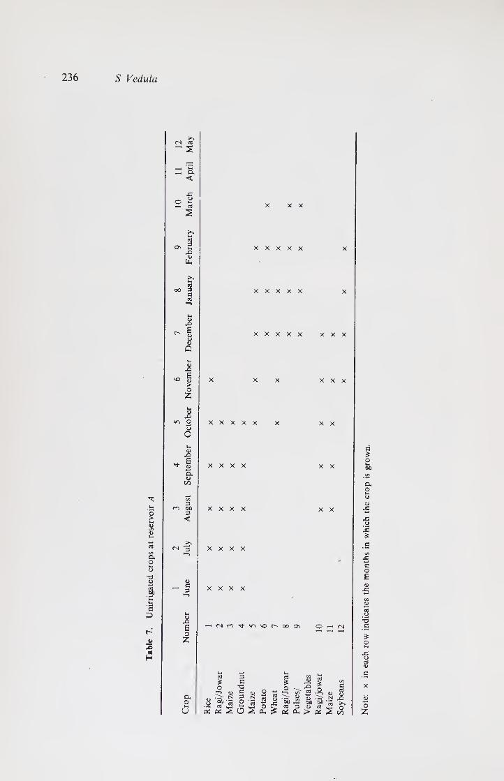
236 S Vedula
o >
a o
-a <D
a
c O
H
12
May
11
Apri
l
10
Mar
ch
X XX
U cd
On 2 X)
<D Uh
X X X X X X
8
Jan
uary
X X X X X X
7
Dec
emb
er
X X X X X XXX
6
No
vem
ber
1
X X X XXX
U>
£ *s~) O
a o
X X XXX X X X
u.
£ _ e ^ £
a <u
00
X X X X X X
3
Au
gu
st
X X X X X X
<N 3 X X X X
1
Num
ber
June
X X X X
-H CN n 'f ^ h oo a\ O ^ CN
Cro
p
Ric
e
Ragi/
Jow
ar
Mai
ze
Gro
undnut
Mai
ze
Po
tato
Whea
t
Ragi/
Jow
ar
Pu
lses
/
Veg
etab
les
Rag
i/jo
war
Mai
ze
So
yb
ean
s
.s
■o c £ o u.
<J cd <U
.S X
aj O z

Tab
le
8.
Wat
er d
iver
sion r
eq
uir
em
en
ts o
f ir
rigat
ed c
rops
at
rese
rvoir B
(as
dep
th i
n m
etre
s)
Optimal irrigation planning 211
<N 3
a <
2 §
Os Z, X> a> Uh
£ £
<D Q
£ £ <D > o Z
£ O
o
£ 6 o a a> c/3
3 3 <
3
C 3
JS E 3
z
8- V-H
o
o o
oo o
Os «/?> O ©
<N O <6
s
m rt OO — o o O ©
os on © © © o o
*—< Os o- no 0 — 0 © © ©
>n \0 O' go Tf <N —
© © ©
(N a M O © Tt — <N —
Tt »/■> o — — o © © o
— oi m
3
St
U~) i •o O'
T}- SO nO O-
io> O-
m on O on — o O © © © © ©
o- ro
SO o
3
on 3“
O ©
£ 3
2 u.
a 3
"O c 3 o u O
m ©
OQ ’fpH o
5b 3
"O 3 3 O u.
O
©
<N
m ro O CO fO on © © ©
on On (N ^ ^ <N <N —
© © o
o o © © o
<L> . JO
3
«u OD <u >
G 3 £ £ ° >N ?E O 3
C/3 CO
17
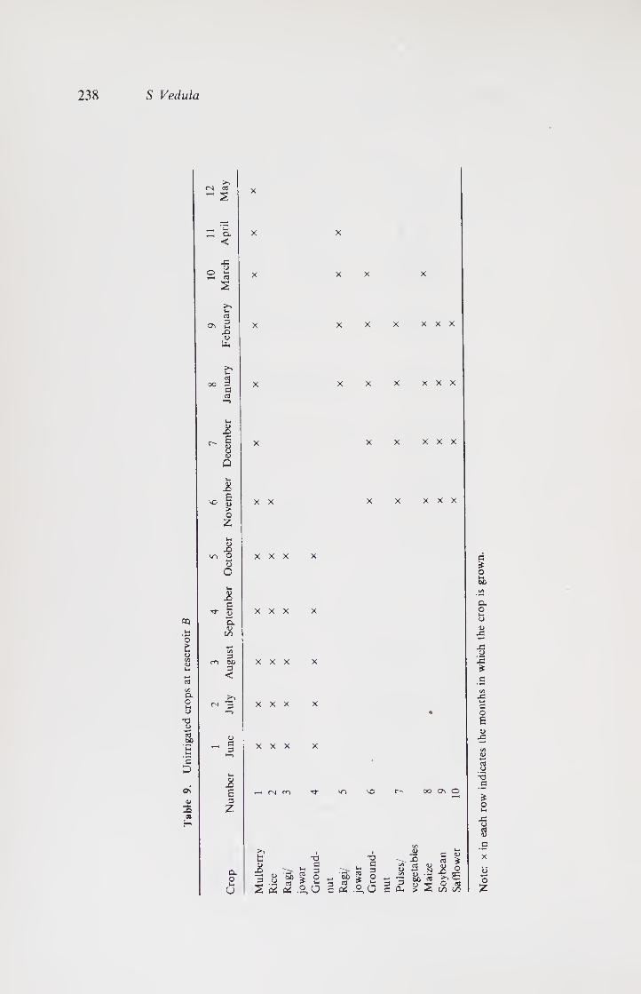
238 S Vedula
-a O GO
<N 03
a. <
2 £
aj ON 2
X> o U-
J5
£ « |
> o Z
v->
X m o
J
a cJ5
3 m oo 3
<
C^J 3
D- O v_
u
x x
X X
X X
X XXX
X XXX
XXX
XXX
XXX
XXX
XXX
XXX
c^) tJ- \Q r- oo On O
T3 - §
00 g o
-a C ■ago
3 fl J!
I 2 5 .lo IS .1,6 12 ?s<*3i I i
O \ 3 o Own
c/i iu 3 OD.t)
Ih
£ l >>e
a, o
o -C
.G CJ
2 * G
G O
<u -G
"O G
jC o3 o G X
ai O
row

Optimal irrigation planning 239
Cu <D TJ
Uh ’o
<u C/5 0)
a. o u- O
•o ID od
^5 <N 03
a <
-C o
X) D
Un
i5 E 8 D 0
»-<
£
> o Z
J5 >r~) o
o
ii E <U O-
=3 m cjo
3 <
£ E 3
z
a. o j—i
U
8 (N
©
oo o v-> X oo r- <N <N O rr
© © ©
m c*i m Q\ m 09 O rtxxoor^’-'^ C<ir](NTt'-lfflHfp
OOOOOOOO
i/~) ’—i-*——iOOn (NmroTfO—' Om
OOOOOOOO
-h r- r' ^ m ^ (N STtTtM«nO^- (N (N r j ^ -i -i O © © © © © ©
O O © ©
o o o
O X v*0 VO X sssss © © © © ©
t"~ ^ T-H T-H T-H OO 'O OO oo oo 00 © ^ p o o o © o o © © © ©
O —i ,—i ^ m ^ ^ ^ Tf ^
OOOOcOO
m on os os os r-
o © o © © ©
r-
© o o o o o ©
(N n Tf
cd £ o
oo cd
OC
3 G
X3 C 3 O
3 3
TP G 3 O ■jr . . u- (—> -G cd > o o d ^

240 S Vedula
Table 11 Unirrigated crops at reservoir C
1 2 3 4 5 6 7 8 9 10 1! 12
Num- June July Aug- Septem- Octo- Novem- Decern- Janu- Febru-March April May
Crop ber ust ber ber ber ber ary ary
Rice 1 X X X X X X
Ragi/ 2 X X X X X
jowar
Jowar 3 X X X X X
Maize 4 X X X X X
Ground- 5 X X X X X
nut
Potato 6 X X X X
Wheat 7 X X X X X
Maize 8 X X X X
Jowar 9 X X X X
Ground- 10 X X X X X
nut
Potato 11 X X X X
Soybeans 12 X X X X
Vegetables 13 X X X X
Ragi/ 14 X XXX
jowar
Note: x in each row indicates the months in which the crop is grown.
Table 12 Water diversion requirements at existing reservoirs in mcum.
Reservoir Reservoir Month B D* Month B D*
June 82-4 0 December 32-2 4-4 July 1490 31-2 January 50-2 0 August 134-6 50-0 February 58-8 0 September 95-6 56-0 March 59-2 0
October 52-8 30-4 April 18-2 0
November 24-2 26-0 May 5-2 0
* Mettur canal paddy sowing in mid-July
Table 13 Minimum monthly downstream releases (computed in mcum)
Four-reservoir Three-reservoir Four-reservoir Three-reservoir
Month system* system** Month system* system**
June 5700 610-47 December 0 0
July 1668-5 1719-22 January 329-2 220-04
August 1360-8 1061-47 February 569-5 543-73
September 775-9 308-30 March 708-6 690-73
October 0 0 April 140-0 64-95
November 0 0 May 0 0
* release from Mettur reservoir
** total release from the KRSand Kabini reservoirs, Mettur canal paddy sowing in mid-June

Optimal irrigation planning 241
and Hemavathy reservoirs given in table 4 were thus reduced by 19-7% and 5-7%
respectively and the modified inflows were then used as the input to the model in those
studies which included the effect of upstream development.
3.4e Net benefits from crops Estimates of net benefit per unit area of irrigated and
unirrigated crops are given in table 14. The gross income was computed at the
wholesale price of the crop produce and from representative values of crop yield per
hectare for the region under study. The only cost of inputs deducted to estimate net
benefits is of fertilizers. The dosage of fertilizers is assumed at the optimum value to give
maximum yield (Parikh & Srinivasan 1974). All other costs such as labour, pesticides,
insecticides and cost of water were not deducted. Thus net benefit, as used in this study,
is the gross income less the cost of fertilizer only.
3.5 Cases studied and their solutions
The computer solutions were obtained using a mpsx linear programming package on
the ibm 370/168 system at Harvard University, Cambridge, Massachusetts. In all runs,
the value of (IB)l, the irrigated area for crop 1 (mulberry) at the krs reservoir, was fixed
at 20,700 hectares as proposed in the Karnataka Master Plan. This was done because of
the growing demand for the mulberry leaves for sericulture in Karnataka which
produces 82% of the total mulberry silk in the country (Report of the National
Commission on Agriculture, 1976). The net benefits arrived at in all the solutions
exclude those associated with the fixed mulberry cropping.
The following are the various cases considered for detailed analysis, and the table
numbers are also given in brackets for reference to their detailed solution: 4YN (15); 4YI
(16); 4YD (17); 4NN (18); 4NI (19); 4ND (20); 3YN (21); 317 (22); 3YD (23); 3NN (24); 3NI
(25); 3ND (26); where 3 and 4 in the first place indicate a three-and a four-reservoir
system, respectively; Yand N in the second place indicate that “upstream developments”
were considered and not considered, respectively; N, I and D in the third place maximize
total net benefits, total irrigated cropped area and total reservoir diversions,
respectively.
4. Results and discussion
The results of all cases analysed in respect of the four-reservoir system are summarised
below.
Case
Net benefits
(106 Rs)
Irrigated cropped
area
(100 ha)
Total diversion
(m cu m)
4YN 2084.709 527,570 3463.88
4YI 1659.623 755,600 3540.15
4 YD 1738.194 666,061 3994.09
4 NN 2124.313 621,860 4365.90
4 NI 1809.500 756,680 4516.80
4 ND 2008.316 688,090 4767.30
It may be noted that the maximum net benefits for the four-reservoir system increase
by only 2 % when the upstream developments are not considered. This is because the
inflows into the krs reservoir are not affected significantly by considering upstream
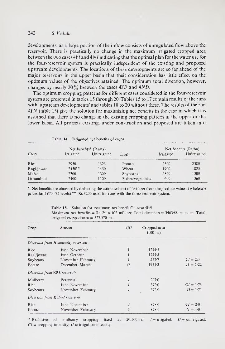
242 S Vedula
developments, as a large portion of the inflow consists of unregulated flow above the
reservoir. There is practically no change in the maximum irrigated cropped area
between the two cases 4YI and 4NI indicating that the optimal plan for the water use for
the four-reservoir system is practically independent of the existing and proposed
upstream developments. The locations of these developments are so far ahead of the
major reservoirs in the upper basin that their consideration has little effect on the
optimum values of the objectives attained. The optimum total diversion, however,
changes by nearly 20 % between the cases 4YD and AND. The optimum cropping patterns for different cases considered in the four-reservoir
system are presented in tables 15 through 20. Tables 15 to 17 contain results of the runs
with ‘upstream developments’ and tables 18 to 20 without these. The results of the run
4YN (table 15) give the solution for maximizing net benefits in the case in which it is
assumed that there is no change in the existing cropping pattern in the upper or the
lower basin. All projects existing, under construction and proposed are taken into
Table 14 Estimated net benefits of crops
Net benefits* (Rs/ha) Net benefits (Rs/ha)
Crop Irrigated Unirrigated Crop Irrigated Unirrigated
Rice 2950 1525 Potato 2500 2380
Ragi/jowar 2450** 1450 Wheat 1900 825
Maize 2300 1300 Soybeans 2800 1300
Groundnut 2400 1100 Pulses/vegetables 600 360
* Net benefits are obtained by deducting the estimated cost of fertilizer from the produce value at wholesale
prices (at 1970-72 levels) ** Rs 3200 used for runs with the three-reservoir system.
Table 15. Solution for maximum net benefits*—case 4YN
Maximum net benefits = Rs 21 x 103
irrigated cropped area = 527,570 ha.
million; Total diversion = 3463 88 m cu m; Total
Crop Season i/v Cropped area
(100 ha)
Diversion from Hemavalhy reservoir
Rice June-November I 1244-5
Ragi/jowar June October I 1244-5
Soybeans November-February I 557-7 Cl = 2.0
Potato December-March U 1931-3 II = 1-22
Diversion from KRS reservoir
Mulberry Perennial I 207-0
Rice June-November I 572-0 Cl = 1 -73
Soybeans November-February I 572-0 //= 1-73
Diversion from Kabini reservoir
Rice June-November I 8780 Cl = 2-0
Potato November-February u 878-0 II = 10
* Exclusive of mulberry cropping fixed at 20,700 ha; I = irrigated, U = unirrigated;
Cl = cropping intensity; II = irrigation intensity.

Optimal irrigation planning 243
Table 16. Solution for maximum irrigated cropped area—case 4YI
Maximum irrigated cropped area = 755,600 ha; Total diversion = 3540 151 mcu m; Total net
benefits (excluding mulberry) = Rs 1-7 x 10³ million.
Crop Season I/U
Cropped area
(100 ha)
Diversion from Hemavathy reservoir
Rice June-November I 264-5
Maize June-October I 492 1
Groundnut June-October I 1732-4
Wheat October February I 1960-0 Cl = 2-0
Potato December March u 529-0 11 = 1-79
Diversion from KRS reservoir
Mulberry Perennial I 207-0*
Groundnut June-October I 572-0
Pulses/Vegetables November-February I 108-7 Cl = 1-73
Soybeans November-February I 463-3 II = 1-73
Diversion from Kabini reservoir
Rice June-November I 260-6
Ragi/jowar June October I 617-4 Cl = 2-0 Vegetables and
minor crops November-March I 878-0 II = 2-0
/ = irrigated, U = unirrigated; Cl = cropping intensity; II = irrigation intensity; * fixed value
Table 17. Solution for maximum total diversion—case 4YD
Maximum reservoir diversion = 3994 092 m cu m; Total irrigated cropped area = 666,061 ha;
Total net benefits (excluding mulberry) = Rs T7 x 103 million
Crop Season I/U
Cropped area
(100 ha)
Diversion from Hemavathy reservoir
Maize June-October I 2489-0
Maize October-February I 297-5
Wheat October-February I 1554-7 Cl = 2-0
Potato December-March u 636-8 11 = 1-74
Diversion from KRS reservoir
Mulberry Perennial I 207-0*
Groundnut June-October I 214-8
Ragi/jowar January-April I 572-0 Cl = : 1-73
Rice June-November u 357-2 II = 1-28
Diversion from Kabini reservoir
Rice June-November I 878-0
Ragi/jowar January-April I 447-6 Cl = 2-0
Wheat November-March u 430-4 II = 151
/ = irrigated, U = unirrigated; Cl = cropping intensity; II = irrigation intensity; * Fixed value

244 S Vedula
Table 18. Solution for maximum net benefits*—case 4NN
Maximum net benefits = Rs 21 x 10J million; Total diversion = 4365 9 m cu m; Total
irrigated cropped area = 621, 860 ha.
Crop Season I/U
Cropped area
(100 ha)
Diversion from reservoir A
Rice June-November I 1244 5
Ragi/jowar June-October I 1244-5 Cl = 20
Soybeans November-February I 981 1 II = 1-39
Potato December- March u 1507-9
Diversion from reservoir B
Mulberry Perennial / 207-0
Rice June-November I 572-0 Cl = 1 73
Soybeans November-February I 572-0 II = 1-73
Diversion from reservoir C
Rice June-November I 878-0
Soybeans Decern be r M a rch I 519-5 Cl = 2-00
Potato November- February u 358-5 II = 1 59
* Exclusive of mulberry cropping fixed at 20,700 ha, / = irrigated, U = unirrigated; Cl = cropping
intensity; II = irrigation intensity.
Table 19. Solution for maximum irrigated cropped area—case 4NI
Maximum irrigated cropped area = 756,680 ha; Total diversions = 4,516.8 m cu m; Total net
benefits = Rs 18 x 103 million.
Cropped area
Crop Season I/U (100 ha)
Diversion from reservoir A
Rice June November I 259-1
Ragi/jowar June-October I 1478-6 C/= 20
Maize June-October I 751-3 II = 1 79
Wheat October- February I 1970-8
Potato December March u 518-2
Diversion from reservoir B
Mulberry Perennial I 207-0*
Rice June-November I 572-0 Cl = 1-73
Ragi/jowar January-April I 572-0 II = 1-73
Diversion from reservoir C
Rice June-November I 8780
Wheat November-March I 495-6 Cl = 20
Vegetables/pulses November-March I 300-1 II = 20
Ragi/jowar January-April I 82-3
/ = irrigated, U = unirrigated; Cl = cropping intensity, II = irrigation intensity; *Value fixed in model.

Optimal irrigation planning 245
Table 20. Solution for maximum total diversion—ease 4ND
Maximum reservoir diversions =
Total net benefits = Rs 2 0 x 103
4767-3 m cu m; Total irrigated cropped area
million.
= 688,900 ha;
Cropped area
Crop Season i/u (100 ha)
Diversion from reservoir A
Rice June November 1 811-7
Maize June October 1 1677-3
Maize October- F ebruary 1 608-7 Cl = 2-0
Wheat October-February I 256-9 II = 1 58
Soybeans November February I 573-9
Potato December March u 1049-5
Diversion from reservoir B
Mulberry Perennial I 207-0*
Rice June-November I 572-0 Cl = 1-73
Ragi/jowar January-April I 572-0 II = 1-73
Diversion from reservoir C
Rice June November I 878-0
Potato November -February I 376-4 Cl = 2-0
Ragi/jowar January-April I 346-9 II = 1 82
Potato November February u 154-7
I = irrigated, U = unirrigated; Cl = cropping intensity; II = irrigation intensity; ‘Value fixed in model.
Table 21. Solution for maximum net benefits*—case 3YN.
Maximum net benefits = Rs 12 x 103 million; Total irrigated cropped area
= 447,722 ha; Total diversion = 1826-5 mcum.
Crop Season I/U
Cropped area
(100 ha)
Diversion from reservoir A
Ragi/jowar June-October I 2489-0 Cl = 2-0
Potato December-May u 2489-0 II = 1-0
Diversion from reservoir B
Mulberry Perennial I 207-0
Ragi/jowar June-October I 572-0 Cl = 1-73
Ragi/jowar January April I 331-2 II = 1 43
Ragi/jowar January-April u 240-8
Diversion from reservoir C
Jowar June-October I 8780 Cl = 2-0
Potato November-F ebruary u 878-0 II = 1-0
* Exclusive of mulberry cropping fixed at 20,700 ha; / = irrigated. U = unirrigated;
Cl = cropping intensity; II = irrigation intensity.

246 S Vedula
Table 22. Solution for maximum irrigated cropped area—case 3YI.
Maximum irrigated cropped area = 578,910 ha; Total deversion
= 2136-5 mcum; Total net benefits = Rs 16 x 103 million
Crop Season I/U Cropped area
(100 ha)
Diversion from reservoir A
Maize June October I 24890
Pulses/vegetables August-December I 193-1 Cl = 20
Potato December-March u 2295-9 II = 1 08
Diversion from reservoir B
Mulberry Perennial I 207-0* Cl = 1-73
Ragi/jowar June October I 572-0 II = 1-73
Pulses/vegetables No vember-F ebraury I 572-0
Diversion from reservoir C
Potato June-September I 878-0 Cl = 20
Vegetables November-March I 878-0 II = 20
* Fixed, excluded in computing net benefits; I = irrigated, U — unirrigated; Cl = cropping intensity; II = irrigation intensity.
Table 23. Solution for maximum diversion—case 3YD.
Maximum diversion = 2277-1 mcum; Total irrigated cropped area
= 444,012 ha; Total net benefits = - Rs 1-8 x 10³ million.
Crop Season I/U Cropped area
(100 ha)
Diversion from reservoir A
Maize June October I 2489-0 Cl = 20
Potato December-March u 2489-0 II = 10
Diversion from reservoir B
Mulberry Perennial I 207-0* Cl = 1-73 Ragi/jowar January-April I 572-0 II = 1-00
Ragi/jowar June-October u 572-0
Diversion from reservoir C
Maize June October I 851-5 Cl = 20
Ragi/jowar June-October I 320-6 II = 1-33
Rice June- November u 26-5
Wheat November-March u 557-4
* Fixed, excluded in computing net benefits; / = irrigated. U = unirrigated; Cl = cropping intensity; II = irrigation intensity.
account above the krs reservoir including those on the tributaries. In other words, this
solution gives the optimum cropping patterns at each of the reservoirs A, B and C,
which maximizes the total net benefits. The maximum net benefit from table 15 is Rs 21
x 103 million and the corresponding irrigated cropped area is 527,570 ha, while the
maximum irrigated cropped area possible is 755,600 ha (table 16), which reduces the net
benefit to Rs 1-7 x 10³ million. Table 17 gives the results of the same case but for the

Optimal irrigation planning 247
Table 24. Solution for maximum net benefits—-case 3NN.
Maximum net benefits = Rs 2-3 x 10³ million; Total irrigated cropped area
= 537,896 ha; Total diversion = 2636-9 mcum.
Crop Season I/U Cropped area (100 ha)
Diversion from reservoir A
Ragi/jowar June-October I 2448-5 Cl = 20
Ragi/jowar August December I 40-5 II = 10
Potato December March u 2489-0
Diversion from reservoir B
Mulberry Perennial I 207-0* Cl = 1-73
Ragi/jowar June-October I 572-0 II = 1-73
Ragi/jowar January-April I 483-4
Soybeans November-February I 88-6
Diversion from reservoir C
Ragi/jowar June-October I 878-0 Cl = 2-0
Jowar November-February I 661-0 II = 1-75
Potato N o vember-F ebruary u 217-0
* Fixed, excluded in computing net benefits; 1 = irrigated, U = unirrigated;
Cl = cropping intensity; II = irrigation intensity.
Table 25. Solution for maximum irrigated cropped area—case 3NI.
Maximum irrigated cropped area = 647,795 ha; Total diversion
= 2557-2 mcum; Total net benefits = Rs 1-9 x 10³ million.
Crop Season I/U Cropped area (100 ha)
Diversion from reservoir A
Ragi/jowar June-October I 2376-9 CI = 1-65
Maize June-October i 1121 II = 1-65
Wheat October-February i 1607-0
Diversion from reservoir B
Mulberry Perennial I 207-0* CI = 1-73
Ragi/jowar June-October i 572-0 II = 1-73
Pulses/vegetables November-February I 572-0
Diversion from reservoir C
Ragi/jowar June-October i 878-0 CI = 2-0
Vegetables November-March i 878-0 II = 2-0
* Fixed, excluded in computing net benefits; / = irrigated, U = unirrigated;
Cl = cropping intensity; II = irrigation intensity.
of maximizing the total diversions. The maximum diversions are objective
3994-1 m cu m which yield net benefits of Rs 1-7 x 10³ million (all these benefits are at
1970-72 levels). As far as the net benefits are concerned, the results of the case 4YD are
somewhat midway between the cases 4YN and 4YI.
There is a definite trade-off between the objectives of maximizing net benefits and
maximizing the irrigated cropped area. The latter objective brings a larger number of

248 S Vedula
Table 26. Solution for maximum diversions—ease 3ND.
Maximum diversion = 3158 5 mcum; Total irrigated cropped area
= 537,561 ha; Total net benefits = Rs 19 x 103 million.
**•
Crop Season I/U Cropped area (100 ha)
Diversion from reservoir A
Rice June-November / 710
Maize June-October / 24180 Cl = 2-0
Maize Octo ber February / 281 1 //= Ml
Potato December March U 2207-9
Diversion from reservoir B
Mulberry Perennial I 207-0* Cl = 1 73
Rice June-November I 572-0 II = 1-73
Ragi/jo war January- April I 572-0
Diversion from reservoir C
Rice June-November I 8780 Cl = 20
Soybeans December-March I 376-5 II = 1 43
Wheat November-March u 501-5
* Fixed, excluded in computing net benefits; / = irrigated. U = unirrigated; Cl = cropping intensity; II = irrigation intensity.
less water intensive crops into the solution than the former. In this case, rice and
soybeans are reduced or replaced by crops requiring less water like ragi, jowar and
wheat, vegetables and pulses. The object of maximizing the irrigated cropped area, has
been cited (Report of the Irrigation Commission, 1972, Vol. I, p. 112) as one of the goals set by the Irrigation Commission in irrigation planning. This is meant to
primarily increase employment and improve the economic base of the areas proposed
for development. In this present case, the maximum irrigated cropped area is
755,600 ha, an increase of 43%, and the corresponding benefits are about Rs 1-7
x 103 million (1970-72 level), a reduction of 20%, compared to the results for the
objective of maximizing net benefits. The (total) cropping intensity however remains
the same. The net effect of increasing the irrigated cropped area by choosing low water
requiring crops on the diversions is that the diversions for maximizing the irrigated
cropped area are increased by 2.2 % compared with that for net benefits. The aim of
maximizing diversions is to some extent complementary to that of maximizing the
irrigated cropped area and the results for this are also presented for each case although
the objective by itself may not have any practical significance.
The three-reservoir system consisting of the Hemavathy, krs and Kabini reservoirs is
operated such that the releases from the system are adequate to meet the downstream
irrigation requirements. In this analysis, the storage at Mettur was not considered. This
gives a flexibility of using Mettur storages in lean years. The solutions for this case,
again with and without considering upstream developments are given in tables 21, 22,
23 and 24, 25, 26 respectively.
4.1 Trade-off analysis
As the sole purpose of diversions is assumed to be irrigation, the objectives of
maximizing diversions and irrigated cropped area complement each other. However,

Optimal irrigation planning 249
Figure 3. Transformation curves for the four-reservoir system.
the objective of maximizing net benefits is in conflict with either of the other two. Thus,
from the point of view of evaluating the trade-offs, it is useful to consider maximizing
net income and irrigated cropped area. This is best done by plotting the transformation
curve between the irrigated cropped area and the maximum net benefits as in figure 3.
Each of the points plotted in the figure is obtained by maximizing the net benefits for a
fixed value of the irrigated cropped area and for each of these points, there exists a
solution similar to the one given in table 15.
4.1a Reservoir system with ‘upstream developments'—Cases 4YN, 4YI and 4YD: These
cases of the four reservoir system take the upstream developments into account. The
solutions for these cases are given in tables 15,16 and 17. The irrigated cropped area is
varied between 527,570 ha and the maximum possible value of 755,600 ha to obtain the
corresponding net benefits. The values obtained are given below and their plot is shown
in figure 3(a)
Irrigated cropped area Maximum net benefits
fixed at (100 ha) (109 Rupees)
5276 2.08
5732 2.07
6188 2.05
6644 2.03
7100 1.97
7300 1.93
7556 (max) 1.87
Any point on the curve defined by these points is then Pareto admissible.

250 S Yedula
The total irrigated cropped area proposed by the Karnataka Master Plan at reservoirs A, B and C is 576,800 ha after considering the rainfall and local conditions.
The model shows that the irrigated cropped area can be increased to any value upto
755,600 ha. It should now be interesting to determine the implied trade-off in the
proposed value of 576,800 ha by finding the slope of the tangent to the curve plotted in
figure 3(a) at the point corresponding to the irrigated cropped area of 576,800 ha. This
was found to be Rs 360 of net benefits per hectare of irrigated cropped area.
4.1b Four-reservoir system without upstream developments—Cases 4NN, 4NI and
4ND\ These are the cases of the four-reservoir system without the upstream
developments, which aim at maximizing net benefits, irrigated cropped area and total
diversions, respectively. The solutions for these three cases are given in tables 18,19 and
20 respectively. The trade-off curve between the net income and the irrigated cropped
area is developed for the present case in the same way as in the case with upstream
developments. The resulting transformation curve is shown in figure 3(b).
4.2 Limitations of the study
The most obvious limitation of the study is that it does not consider the variability of
river flows. The model is deterministic with the input consisting of mean monthly
values of river flows and evaporation losses. It also does not consider overyear storage.
Estimation of crop water requirements is based on general guidelines and assumptions
but the actual requirements may vary significantly from place to place depending on the
local soil conditions and climatology. Similarly, the farm losses and the conveyance
losses to estimate the water diversion requirements from net irrigation requirements
may vary from place to place depending on local conditions. In addition, the study
carries with it all the limitations of the basic data itself used in various other
computations and estimates. Crop yields and net returns for the irrigated and
unirrigated crops were estimated based on the data for the whole state, wherever
available, and representative values used on consulting available sources of published
information (fao 1975; Government of India 1974). Another limitation may seem to stem from the argument that the optimum crop
patterns obtained from the model may not be acceptable to the farmers. It is
emphasized that the present model is a planning model which determines what the
optimum or the best cropping pattern should be depending on the objective. Once the
possibilities are tested to the limit to see the maximum possible output, the next course
of action could be to formulate an operational model to find out how much of this
optimum output can actually be realized and in what way.
5. Concluding remarks
The application of the techniques of operations research to the study of the upper
Cauvery river basin reveals the extent of irrigation potential at the major projects
(existing, under construction and proposed) of the basin. The study is based on mean
monthly flows and on a linear programming model. Of all the cases considered, the case
of the four-reservoir system comprising the Hemavathy, krs, Kabini and Mettur
reservoirs and which considers the proposed developments upstream of the krs
reservoir is the most interesting. The analysis for the trade-off between the objectives of

Optimal irrigation planning 251
maximizing net benefits and irrigated cropped area has been carried out, which reveals
the implicit trade-off relationships used in the proposals made by the Karnataka Master Plan.
References
Dorfman R 1972 in Models for managing regional water quality, (eds) R Dorfman, H D Jacoby, H A Thomas
Jr (Harvard: University Press)
FAO 1975 Production Yearbook
Government of India 1965 Evaluation of major irrigation projects - some case studies, Programme
Evaluation Organization
Haith D A, Loucks D P 1976 in Systems approach to water management, (ed.) A K Biswas (New York,
McGraw Hill)
Hall W A, Dracup J A 1970 Water resources systems engineering, (New York, McGraw Hill)
Irrigation Commission 1972 The Cauvery Basin, Vol. Ill, Pt. 2, Chap. X, Report, Ministry of Irrigation and
Power
Lakshminarayana V, Rajagopalan S P 1977 Irrigation and Drainage, ASCE, March
Master Plan 1976 Master plan for an equitable use of the waters of the Cauvery Basin in Karnataka-an
outline in three parts. Government of Karnataka, Water Resources Development Organization
Ministry of Agriculture 1971 A guide for estimating irrigation water requirements, Water Management
Division, Ministry of Agriculture, Government of India
Ministry of Agriculture 1974 Estimates of area and production of principal crops in India, 1972-73,
Directorate of Economics and Statistics, Ministry of Agriculture, Government of India
National Commission on Agriculture 1976 Report, Part VI Ministry of Agriculture and Irrigation,
Government of India
Parikh K J, Srinivasan T N 1974 Optimum requirement of fertilizers for the fifth plan period, Indian
Statistical Institute, Planning Unit, New Delhi
Rogers P, Rao P S, Ramaseshan S 1976 Multiobjective analysis for planning and operation of water resource
systems: some examples from India, Joint Automatic Control Conference, Purdue University, West
Lafayette, Indiana
Rogers P, Smith D 1970 Bulletin of ICID
Sampath R K, Anandalingam G 1976 An interregional programming approach to planning of agricultural
production in India, Center for Population Studies, Harvard University, Cambridge, Mass., August
Verma R D 1977 Technology transfer for irrigation planning of arid lands, Seminar paper. Center for
Population Studies, Harvard University, Cambridge, Mass.
List of symbols
(DD)m = minimum release requirement at reservoir D in month m
(EA)m, (EB)m, (EC)m, (ED)m, = evaporation in month m at reservoirs A, B, C and D
respectively.
(FA)m, (FB)m, (FC)m, (FD)m = mean inflows in month m to reservoirs A, B, C and D
respectively.
i,j, k = irrigated crop index at reservoir A, B and C respectively.
{lAf, (IB)j, (lC)k = irrigated cropped area under crop i at reservoir A, j at B, k at C
respectively.
(IA)m j — (IA)h the irrigated cropped area for the crop i during the growth month m at
reservoir A; (and similar notations for corresponding symbols in (5), (6), and (7), for
reservoirs B, C, and D, respectively) = 0, for all other (non-growing) months.

252 S Vedula
(LA), (LB), (LC) = total land available under the command of reservoirs A, B and C
respectively.
P.> Qp rk — total water diversion requirement of crop i at reservoir A,j at B and k at C
respectively.
Pm, . > <?m. j, rm, k = water diversion requirement for irrigating crop i at reservoir A,j at B,
and k' at C respectively, during the month m.
(RA)m, (RB)m, (RC)m, (RD)m = downstream releases from reservoirs A, B, C and D
respectively in the month m
(RT)m = downstream release from reservoir D in month m
(5/4)m, (SB)m, (SC)m, (SD)m — storage at the beginning of month m at reservoirs A, B, C
and D respectively.
u,v,w — unirrigated crop index at reservoirs A, B and C respectively
(UA)U, (UB)v, (UC)W — unirrigated cropped area under crop u at reservoir A, v at B and
w at C, respectively.
(U A)m u = (UA)m, the unirrigated cropped area under crop u during the growing month
m (similar notations for corresponding symbols in (9) and (10) for reservoirs Band C
respectively) which = 0, for all other (non-growing) months.
(kVB)m, (WD)m = water diversion requirements for existing irrigation at reservoirs B
and D respectively, during month m
ah ftp yk = net benefit per unit area of crops i, j and k respectively.
°C Pv> y'w — net benefit per unit area of crops u, v, and w respectively.

A case study of the Rajasthan canal
RAMESHWAR D VARMA
Department of Civil Engineering, MR. Engineering College, Jaipur 302017, India
Abstract. The study deals with the policy issues relevant to agriculture development in arid regions where water has a very high economic value. The experience gained in irrigation planning under such conditions in different parts of the world is described. The issues relevant for such a study are the level of technology, the cropping pattern, the area under cultivation and the size of the holdings. For the study of these issues a linear programming model maximizing returns, subject to land and water constraints, has been developed and is applied in the Rajasthan canal command area. The study concludes that agriculture and irrigation technology of a high level should be used to maximize benefits and production, which would also generate more employment.
Keywords. Irrigation planning; arid region; Linear programming model.
1. Introduction
About 36 % of the total land area of the world is arid, housing only about 13 % of the
world’s population. With the increasing population of the world the use of arid lands
for the settlement of people, food production and other economic activities will
increase. Although the experience of some arid lands (e.g., Arizona in the United States
and Negev in Israel) has established that economic growth in such areas is possible
through agriculture, it is generally believed that because of the acute shortage of water,
agriculture may not be a very desirable sector for the economic development of such
regions. Whether agriculture should be a primary activity or not, the extent of this
activity in desert areas should be determined by formulating a desert development plan
for the economic growth of the region, which should take into account the available
resources and the expectations of the people. While formulating the plan it should be
kept in mind that the delicate environmental balance of the area is easily disturbed and
that the unplanned depletion of the productive resources of the region could be
dangerous.
The issues involving agricultural development in an arid environment are quite
different from those in a humid environment. The important factors for this difference
are water shortage, low atmospheric humidity resulting in high rates of evaporation,
different soil characteristics, low population density, uneven topography and high cost
of regional infrastructure.
The most important input limiting agricultural development in arid lands is water.
Water for agriculture is available in the form of precipitation or groundwater or surface
water imported from other drainage basins. It can also be made available by treating
and purifying waste water or by desalinating seawater; however such waters are usually
too expensive to use for agriculture. Water in the form of precipitation is very meagre
for sustaining plant life and its availability in quantity as well as in time is highly
uncertain. It may become even more uncertain with the unpredictable changes that
253
254 Rameshwar D Varma
seem to be taking place in the world climates. Unless good water-harvesting techniques,
which are usually capital-intensive, are used rain-fed agriculture will be a risky
enterprise and the farmer will be tempted justifiably not to use the essential inputs
thereby limiting agricultural production to a very low level. The situation can be
improved by developing better predictive methods of rain-water availability and by
extending insurance policies to the farmers against crop failures. Policies relating to this
dry farming agricultural development involve decisions under risk and uncertainty and
have not been considered further in this discussion.
The groundwater resources in arid lands are usually not replenishable. Mining of
groundwater for a limited period for agricultural development has been used for some
desert areas. However unless definite plans for replenishing these resources are in
operation, mining the productive resources of an arid area usually leaves behind an
exploited and impoverished resources base. The various issues involved in mining
groundwater resources in an arid environment have been discussed by Domenico
(1968).
Agricultural development in arid areas is mostly achieved by importing water from
other areas. This water has a very high economic value and many policy issues such as
the level of technology to be used, cropping pattern, area to be committed for
agricult ure and size of holdings are involved in its use for the agricultural development
and the overall economic growth of the region. Some of these policy issues for the arid
lands in India with particular reference to the arid areas commanded by the Rajasthan
Canal Project in India are discussed in this paper.
2. Experiences of some other countries
2.1 USA (Arizona)
Most of Arizona state in the United States is arid. The average precipitation in most
parts of the state is less than 50 cm. But with proper planning and water resources
management the state has been able to achieve substantial economic growth. The water
scarcity was resolved by evolving a set of water-related institutions that would facilitate
change in water development and use so that each unit of scarce water used will make its
maximum contribution to economic well-being directly through its consumption and
indirectly through its use in production (Kelso et al 1973). A solution to the problem
was found not only in improving water supplies but, more important, in reducing water
demands by encouraging change in the structure of the state economy and pattern of
water uses.
2.2 Israel
Some of the policies followed by Israel in planning its irrigation system were included in
the following development criteria (Wiener 1964).
(i) Intensive conservation of available w'ater resources and design of projects to
minimize losses. (ii) A complex resources appraisal methodology.
(iii) Sophisticated management planning of uses of resources.
(iv) Selective use, where feasible, of substandard water for less sensitive uses.
(v) Minimizing (within economic reason) the quantity of water consumed per production unit. In agriculture this requires the proper choice of crops and the
A case study of the Rajasthan canal 255
regions where they are to be grown, increasing efficiency in irrigation, artificial
reduction of evaporation and evapotranspiration and seed selection.
Table 1 compares the yields at Arizona, Israel and Rajasthan, and also the average for
India. The figures indicate the positive effect of proper planning and water resources
management in agriculture in the arid regions of Arizona and Israel.
2.3 USSR
The New York Times (Anon 1977) reported that the largest canal of its kind in the
world, constructed by the Russians, has transformed the economic and social life in
Turkmenia, a Soviet Central Asian Republic lying just North of Iran and Afghanistan.
More than 80% of Turkmenia is desert. The canal which presently extends 912 km will
eventually be 1392 km long with the final section swinging southwest to Turkmenia’s
subtropical region while a smaller pipeline splits Northwest to carry water for drinking
and industrial use. It has been reported that the canal has already paid for itself;
Turkemenia’s cotton production increased nearly five-fold over the last three decades to 1 12 million tonnes last year with at least half of this growth attributed to the canal.
Increases in some other crops like fruit have been nearly as dramatic.
3. Rajasthan canal project
Conceived at the turn of the century to rejuvenate a part of the Indian desert, the
Rajasthan Canal Project was formally launched some six decades later in 1958. It
contemplates the conveyance of a portion of the Ravi-Beas run-off' in Punjab for
irrigating 1T5 million hectares of an assorted arid area of Rajasthan State in its districts of Ganganagar, Bikaner and Jaisalmer all bordering Pakistan. Under a treaty between
India and Pakistan in 1960, an annual supply of more than 18500 mcum has been
made available to India in which Rajasthan will be entitled to about 9866 m cu m. With
the construction of the Pong Dam, assured monthly flows for the year are now available for the Rajasthan canal project (Rao 1975). The Rajasthan canal with a full supply ca¬
pacity of about 530 cumecs (18700 cusecs) takes off from the Harike Barrage across the
Sutlej. The total length of the canal is about 680 km; the main canal and distributaries
are to be lined (Irrigation Commission 1972). The conveyance losses in the main canal
and distributaries are estimated to be 10 %. Water distribution losses in the field (on the
farm) are estimated to be 20 %. Efforts are being made to reduce these losses by levelling
the fields and lining the water courses. The irrigation intensity of the project is expected
to be 130 %. The project is divided into two stages, the first stage commands an area of
about 0 54 million hectares. The construction of the project is an engineering feat
achieved by Indian engineers under extremely difficult environmental conditions. A
map of Rajasthan showing its soils and the canal is given in figure 1.
Statistics of the arid land of Rajasthan, giving area, population and mean annual
rainfall, are given in table 2 districtwise. This shows that the population density in the
area commanded by the Rajasthan Canal is low and the project will induce migration of
agricultural workers to the area and will provide self employment to the people already
there. The existing cropping patterns in the various districts of the desert area of
Rajasthan along with the adopted cropping pattern of the project are given in table 3.
In this table the cropping pattern in the arid state of Arizona has also been given for

256 Rameshwar D Varma
G O
'5b
G
G z o feb C/5 o, o
3 O c oj >
%- o <u U.
S 8
-C
l-x
G O
G
*o
«S Cu
£ o U
2 «Q H
03 "O
VO
On
so VO Os
2 "C
£
a>
« ■£ -o
■g a 2 TO 00 "O w *0 O C
a d. 8 >.0 2
13 &
o £
5 a z S
a —. cs B. x: oc W 03 c/d u. 03 <U
•ZP >
c2 -
03 Oft -o 2 G ^ O! >
03
Oh O Wh u
o^sorsoooso^ 6 (N ri r-i n ^ rf oo
Oh £ ^ ‘G Oft ^
uj in
•o G
o3 o3
O <N ©
<N
S£ 3 .2 — w5 i2 T* '-m G 03 T-
<D hG
t§ 2
^2 in
o)oofs|pnoohooq\'0 obfn'tTf^vb'b^'bh —• Tf <N
w~> Os <N
•v^ so OO X Qs
vs ^ ^ ^ H fS ^ n
h- OO M rj rj- 0- o ro sO\UP
r^OOOOO>XooX
r^r-io^osoomw^ioort — 0000^-^000
a> G
8 G
£ 2 2 o
c« U
o3 V-H
’c? «
<u
13 T3 ^
C/5 C >■* tZ “ 3-0 « O T3 Ji
2 fi S E 3
C/5 o3 *> c/5
m o « C x r£ o SohOOh^SOOh
G o3 X c/5 o3
c? £*
r~~
r- Os
G <D
u Ih 3
*3 O C Oft
OO VI so r- Os Os OJ »—« H—• -C
fM Os <N Ci
O > M O o X
• 8.
f <£ c 3 X
> > S
G O
o 3
T3 O M
Oh
O
< Uh’
G O
o 3
*o o u. a, o
< u.
03
a:
6 G u <u > O
a
<D O G
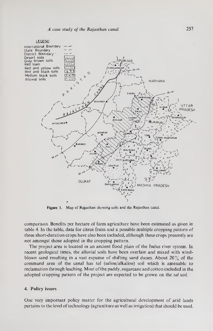
A case study of the Rajasthan canal 257
LEGEND
International Boundary State Boundary District Boundary Desert soils Grey brown soils Red loam Red and yellow soils Red and black soils Medium black soils Alluvial soils
PUNJAB
't W'' " /GANGANAGAR, ~
® JAIPUR :.
UTTAR J alwar / v.' ^
-j • ^‘' PRADESH
- f\ \ BHARA.TPIJR
y V TONK { *
• ySAWAI MAPHOPUR
_<u/ • ^BNNm J~
. .jt
s> . I
<*• 6H.LWARA / /BU.N0' _j
‘ V- e S’ ~/£* ■) 'n v
CHITTAURG^rr-_'
• } <
ir' • ■ r.
KOTA + ’
^ + l- 't T( • *
C: JHALAWAR 1
1 A
>.J oungarpur / MADHYA PRADESH
U -\$J BANSWARA
r
Figure 1. Map of Rajasthan showing soils and the Rajasthan canal.
comparison. Benefits per hectare of farm agriculture have been estimated as given in
table 4. In the table, data for citrus fruits and a possible multiple cropping pattern of
three short-duration crops have also been included, although these crops presently are
not amongst those adopted in the cropping pattern.
The project area is located in an ancient flood plain of the Indus river system. In
recent geological times, the alluvial soils have been overlain and mixed with wind¬
blown sand resulting in a vast expanse of shifting sand dunes. About 20% of the
command area of the canal has tal (saline/alkaline) soil which is amenable to
reclamation through leaching. Most of the paddy, sugarcane and cotton included in the
adopted cropping pattern of the project are expected to be grown on the tal soil.
4. Policy issues
One very important policy matter for the agricultural development of arid lands
pertains to the level of technology (agriculture as well as irrigation) that should be used.

258 Rameshwar D Varma
cd e?
oc
cd
•o
o XJ
2 0?
JlJ -o 98 H
cd 3 C S
S '* cd
S £ •o M C 'jJ o £
3 a o
On
? o© 04 ON rn 1 Jh ON 1 | rn r- NO | | NO | 04 04 ■’Vfr co Os|
c 4— r-
8 »—H »-H n o O' o- 04 'Vt O NO
ON »o co m r- o s
NO VO y—> »o Ui NO m —H o ON oo VO NO OO 00
D <N 04 04 04
"cd 4— 1-4 r~" 04 r- *—i rn Tt VO co »—■ VO
S »o
3 vo »—i ro ro 4—1 ro NO r- <N ro
oc
co Tf On ro O' C4 o VO oo 04 3 ON r- t- 04
3 NO O NO r- r- NO NO
o rp »o> oo On *—< NO 04 ON r- NO 04
H © © © © © o o o ON
G cd O r- ON 04 r- Tf O' VO oo NO o VO
to ro vn NO r- 04 On vo O VO ro m X) l_ oi oi 04 *—• O o O NO
p O © © © © © © (6 o o O
cd 3 NO NO o~ »o 04 ON <N ON OO VO
u, cO NO NO Tf 5
o NO ro 04 3 <—i m NO r- OO »—< »—< OO NO NO
c* © © © © © O o c±> O o~
ON On On 04 o oo r- O' "cd 04 co 04 04 m © NO — ON oc ^r
NO 04 oo ON r- oo ro *o O' CP
f__ o NO VO o> oc 04 CN OO o oo H CM 04 co 04 *—> 04 »—» o
04
vOTf-»00<—'©vOOcOTfr oor^o4ooNO*ovoTtc\co
— 04 co tT oj —<
O' 3
ON , , 00 oo ro ON oo VO TT O' VO o O' ON 04 CO o O OO NO o "Vt t m
s oo
o- 04
sO VO O' oo CO
04 04
O' 04 oo 04 3
04
& cd c cd ~ 00 c „ C 3 3
3 3 3
P ^ G 3
X!
0> u.
E g. cd x:
,52 "O cd O
3 cd taO ■ 6
3 v 3 3 3 11/5 *rd _r — fc* '
ON o ON
<L> Ot) cd
> <
u U
2* t> x:
cd G cd
CJ G cd x:
C/i cd cd'
C*
O 2
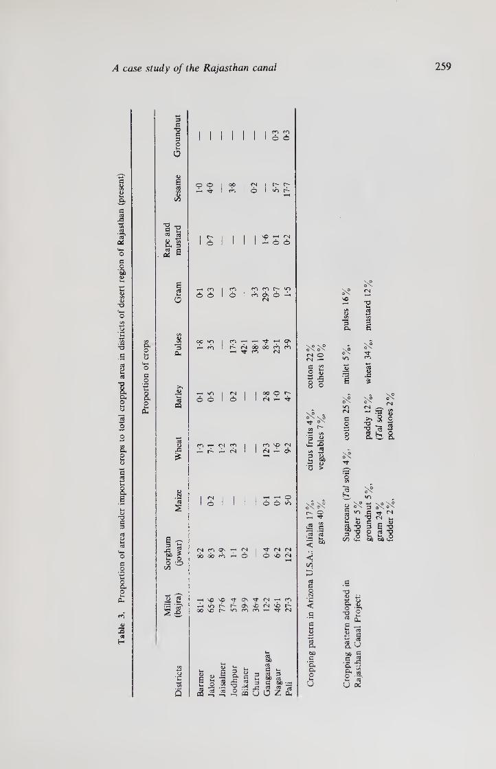
A case study of the Rajasthan canal 259
G
8
G
1
3 0* 4-4 O
S3 O
’5b
u -o
"O
S3
I a o
3 o
a o
g eg
8. s <D P G 3 3 <D
a o u
(X
jS * H
a o
a o x
3 G P G 3 O u.
o
E I $
G 3 S 8.1
a
3 (X
>» »-< 3
ffl
3 <D p
3
s
e ~ 3 Ul
5 5 co > u. O O O
CO
I .2 i I
p p P rt¬
f'- O
*—< m
© ©
OO Wp Xh rn
<N
©
m ro © <6
r- r-
»r> r-
ro
©
-H fN X O ©
rn cp r-
ro On ©
^ ^ ^ t T1 ^ ^ rs oo ob rh rn i—I Tt fO <N
© © r9
©
ro <N tH h H
<N
©
<N rp qs OO CO CO
CN
©
oo © r~~ (N rf
n \o n <N P Os
^ -H © © © W3
3- <N <N © <N
H'OvOtt'ON^^T'rn Xuor-r^ds'jbtN'sbr- oc o r-~ '.n r^i ro —< rj-
3 60 3 G Uh 3 3 60 3 G 60 : I 8 t o
« 3
e a 3 P
"O
<d
S u* 3 ’■r _) W-. uu '-I
■3 X -C .2 5 ^ 4 ■? s u o z fc
<N O <N —
1 8 S JS
8 o
p 3 ^
£ s c/3 w 3 <D u 60 P <L> 5 >
\o o\ o\
- § (3
3 G O N c <
G |H ID
I 60 G
'a o- o M u
o
3 o.
JD
p
E
<N
p u. 3 co 3
E
m ■*-*
s p £
NO NO ON o\
>* P P 3 Cu
G O
CXX •3*
t?
S °x° = S’Cl
<D G P 3
-J P O G r, •
OO P a:
60
P V
K, o p 3
S. 60 S .s i Cl a
2 « U Oti
3
gra
m 2
4 %
(Tal
soil
)
fodder
2%
, p
ota
toes
2%

Tab
le
4.
Benefit
s per h
ecta
re o
f farm
agriculture
260 Rameshwar D Varma
c
a I*
£ l
2 3 C (2
"O «-» "fl --.
5 g.1 5 i.s 8 2
^ c/5 O ' '
w
c <*- o O *J3 ^ O c« w 3 v
u o
"O l_ C/5
« 3 « ai hh l-U
Hi 5 a2
<a oo E
ui
.2 C/3 O
T3 C
51
a o
On rn o vi o O O r- r- m NO r^i On m t
8 NO oo <N
<N ro CT) NO <N
8 0^^0^00000 w'in^r^noo'-i'^r-v-i
h- OO Ti n
00 O O O Q Q OO oo *T) © © © © >o
fN »0 oo X (N rf rf r- M M M
8 S 8 8 § 8 — *-< a© c-J rt
<N *-« —<
m r? CO vp <N
O ro ^ m n >T) OO Tf
Q O 8 (2 On <3,
<N
O
a> G
S c S 2
3 O i\n U
C/3
3 C
Uh TD ^ M U C >»
3rii!
c$
■o u«
3
w C/J
3 a.
<D
6 E <3 ,—1 (N m ■'T vi ■o o c ft. ft. ft. a ft, ft.
U u u u U u u
8 8 NTt «A) v~» <N
§ r~~
8 <N NO
x 00
8.
o V-5 ON
<N rn
O
8 00
o NO
?« a
o < § 2
</5 •».
= 2 E u
Ol.
$
g* 2
H u 2
U U
^ 3 £3 o " a ~ c ^ « 3 3
-H <N
a, ft. U U S 2
3 o
Oh
m a, U
S
(O
cto
ber to D
ecem
ber)
A case study of the Rajasthan canal 261
As will be discussed later, there are divergent views on this issue in literature.
Another important policy question pertains to the use of water. Water in an arid land
can be used to meet the full irrigation requirements of the plants in a limited area thereby
obtaining maximum crop yield per unit land area (assuming adequate supplies of other
inputs) or the water could be used to meet only part of the irrigation requirements of the
plants in a greater cropped area. The basic difference on this question between an arid
and humid environment is that while in the case of the former, the plant will grow and
survive only because of the water supplied from the irrigation system, the soil moisture
in a humid environment may always remain above the permanent wilting point and
therefore the plant can grow even without the use of irrigation water.
A third policy question deals with the appropriate size of land holdings in areas to be
colonized. Should the holding size be large, small or some in-between size?
The fourth important policy area is that of the employment generated by the
developments. As will be seen later, these four policy questions cannot be considered as
separate issues. Choices in one area make large impacts in other areas.
S. Study model
The objective of this study is to evolve the effect of technology transfer on the total
benefits of the project and on the agricultural income of the farmers after full project
development has taken place and all the capital expenditure incurred initially has been
recovered. Two parameters of the technology transfer were considered. One parameter
was the level of technology used in improving the irrigation efficiency of the system. It
was assumed that with the furrow or the border strip irrigation system, an irrigation
efficiency of 70% could be achieved, while with the use of drip irrigation or sprinklers,
an irrigation efficiency of 90 or even 95 % may be quite valid. The other parameter
considered was biological, that is, the effect of short-duration high-yielding varieties of
seed (commonly used in multiple cropping) on the benefits of the project and on the
income of the farmer. In addition, the possibility of growing citrus fruits was also
considered.
A linear programming (lp) model to maximise the benefits from the cropping pattern
in the 12 months with only the available water (and in some cases also the land) as
constraints was used. Such models have often been used for determining optimum
cropping patterns by Heady & Nicol (1975) and others.
An lp model was used to maximize (i) benefits (ii) cropped area from a given fixed
quantity of water in each of the twelve months of the year in the Rajasthan canal. The
maximum benefits (or the maximum cropped area) and the optimum cropping patterns
in the twelve months were determined with available water in the canal as the only
constraints. Three levels of agricultural technology (giving high, medium, and low crop
yields) and two levels of irrigation technology (95 % irrigation efficiency with sprinklers
or drip irrigation and 70 % irrigation efficiency with furrow or border strip irrigation)
and with two strategies (maximize benefits or maximize cropped area) were used to
determine the benefits, cropped area and the cropping pattern with water supplied to
the plants equalling their consumptive requirements.
The objective function is
m
Maximize Z = ^ j= i
(1)

262 Rameshwar D Varma
subject to constraints of water and land, where y} = area of crops (j =1,2,... n) in
hectares and pj = coefficient of return from a unit of land for each crop.
(i) Water constraint
12
Z xtjyj < xh / = 1, 2, ... 12 (2) i = 1
where x,7 = quantity of water required by one hectare of crop j during month i and X(
= volume of water available for irrigation in month i.
(ii) Land constraints
iyj^ A (3) j= 1
where A is the total area of land available
yj ^ 0 for 7=1,2,... n.
The consumptive use water requirements for growing per unit crop area were determined by using climatic data and the monthly consumptive use coefficients of
various crops given by Christensen (1968), Hargreaves (1956), Ministry of Agriculture
(1970) and Ministry of Irrigation and Power (1971). The available water
for the consumptive use was determined by allowing 10 % loss in the main canal and its distributaries and 5 % loss in the field water courses. In addition, allowance was made for
the irrigation method assuming 95% irrigation efficiency for drip irrigation or
sprinklers and 70 % irrigation efficiency for furrow or border strip irrigation systems.
The model also explored the case when the water supplied to the plants was only 60 % of
their consumptive requirements for high agricultural technology and for both levels of
irrigation technology.
The benefits per unit crop area are given in table 4 and were obtained assuming crop
yield with adequate use of fertilizers and assured supply of water. The labour cost was
not considered as it was assumed that each unit of the farm can be managed by a farmer
and his family. The agricultural labour requirements for each of the above cases for the
full command area of the Rajasthan canal project as well as for farms of 4 and 6 ha area
were also determined using farm management practices in India.
6. Discussion of results
6.1 Agricultural technology
Three levels of agricultural technology viz high, medium and low are considered in the
study. High technology would involve assured supply of all inputs such as water,
fertilizers, pesticides and the use of high yielding varieties (labour has not been
considered at any level in this study as explained earlier in §5). This would also require
good agricultural management practices. The crop yield per unit area of land for high
technology will be high. Low agricultural technology implies inadequate and inefficient
use of essential inputs and use of poor agricultural practices. Medium technology
indicates a midway position between high and low technologies. The crop yields and net
benefits determined per hectare of agricultural land for various crops in the study
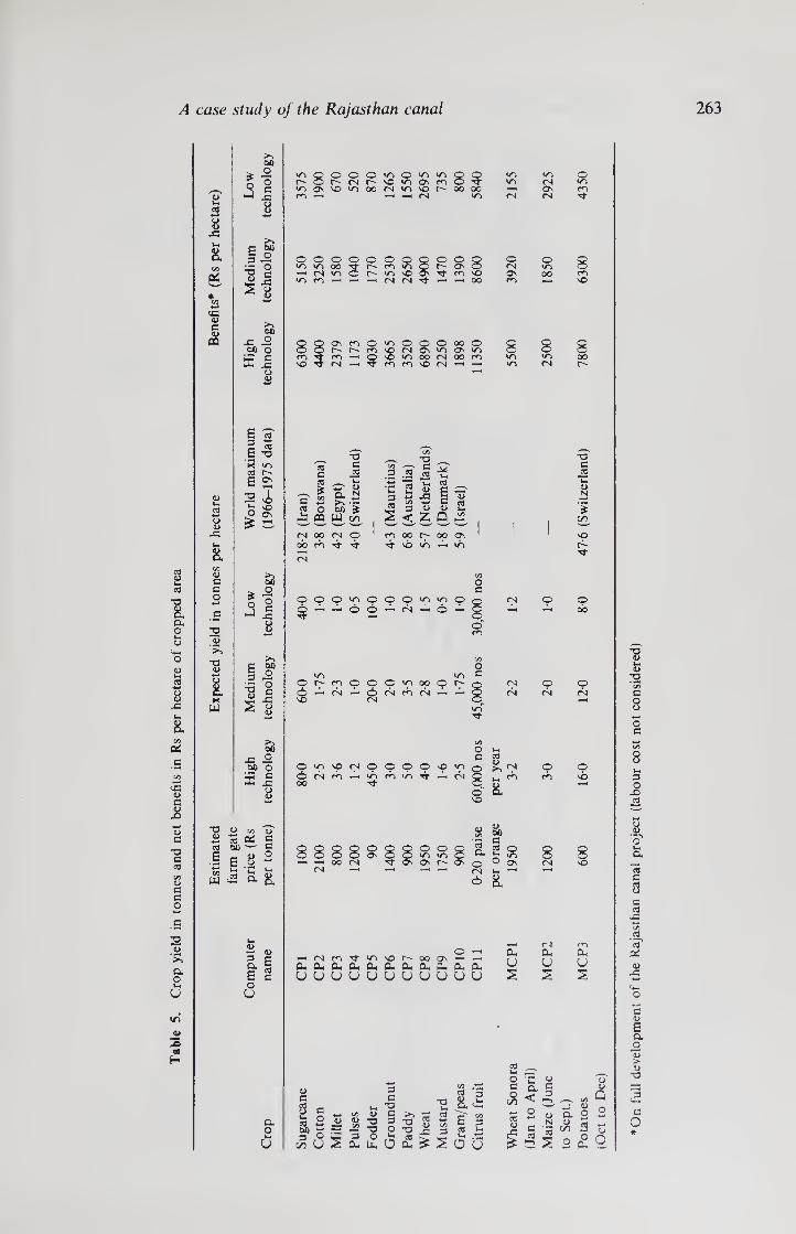
Table
5.
Cro
p y
ield i
n t
onnes
an
d n
et
benefi
ts i
n R
s p
er
hecta
re o
f cro
pped a
rea
A case study of the Rajasthan canal 263
3 2 j= w*
8. z
w
% *■> S3 1) C
<8
CD t-
-2 o <u
-C t-i
8. z o G G o
2 13
*o D
8 X
W
00
Jl S3
So §2 © o O © © © © © © © © ©
o sri oo ‘/i © t-~ Os © <N Ts G T—< <N u-i © r- to SO Os rr m sO Os i{ S3 lo rn i”H »—H <N <N Tf *—i OO m
oo S3 -2 00 o
'£ J
E a)
|3 X »/S cd r-
E 2
2 vi o £
00
?!
S 2
*5 o>
op o
£ M 8
"O 4> vi “ - c
B. 8.
<D ti ^ 8. | E c o U
a o
‘OQOOO^O'^^QQ ^ r-©r^<Nr^so‘/iosfc©’<t ^ •na'O^ooiNm'Ohoooo —< m ^ -H -H M l/"i CM
8 8 ro Tf SO TT
os m © t/o © 8
© OO © r- r- m so CN u~> OS m —i SO oo (N OO m <N c*-) m SO (N
cd G cd
_ * c 2 cd o £ OQ
— .2 •- J3 a n oo £
U3 on 3 cd
S3
cd
E "u g V <u
ZQ^
(N oo rs CO CO Tf
O Tf
p OO C- OO ON tj ic -h ici
OOO'OOOO^i^O §
00 o
o © SO r- © ©
G © rS, rs ^ © S3 SO <N
o W~i c*
o r- 0 <N CS
ppsocspppp Orsn^irifn'nTr OO rf
CN <N
O 8.
uuuuuuouuuu
(X u s
<N as <N
(N
O <N
<N a* U S
a a S G Cd 2 g>5
U
<D <D 0)
-o •—* < "O w tj #-« -3 co « P 3 O t Cd 5 ^ r<r .ti SdhU.Oq.#SOu
3 c
"O g ^ 2 T3 O -o
X (m
B z 3
C/5
is «z> 2
o G o
CO
cd <L>
S3
£
©
rc •*t
8 8 00 ^ —< so
OO
x G cd
* c/5
r-
o oo
o SO
8 90
00
8 © SC ©
*o Q S 3 © ST) 8 8 Cl Os Os r- Os o ° Os <N sO
a, U S
a <u Q
a <u C/5 o
a,
On f
ull d
evel
op
men
t o
f th
e R
ajas
than
canal
pro
ject
(labour
co
st n
ot
co
nsi
dere
d)

264 Rameshwar D Varma
00 o o c 43 8 G O
«—*
3) *c
■a G cd
3 cj ’& <
VO
-G OS H
x:
1 G O w O 3
■8
SI ■= « 3 > (J -^3 &cd
* 5 j>» GS XI cd cd 4>
00 G ^
lx: <2 a s b * * .2
s'"^ /—v 33 2 S3 <o o ' e ° v 3 u > 5 3 -a ■“On) >• -I £
T= -2 S3 Cd 4> -3
>H *
43 ■*->
O
% 8.
<u
£
S c 2
C
G o jrt a
Is ir ^ o cd
6 ^ • 3 a> X G
!■*
8
| X cd s
Is O cd u. o
41 .3 ^2 G
• 3 <L) x G
<5 J5
'3
5
a o
§G <u
X G
■3 £
B S 2 8 -a g u- a. g
s
3
S'
a> >
00 _o o G
J3
S H
a g o\ •2 -2 * * g 3) .sp g £ g •§
<u
^ »o ^ cs
81
?• 5
1-5
oo
11 i
vO
II » ^ ■ o o- 5 a, 2 „ ft. s .a-S
-o tb s s * ■§ !
ob -O -o C 3
^ -a -o cd cd ta 3 CO 3 3 3 u o U 0 u a u a
oo no
<N <N
u a
VO oo
r~ r-
vr> Ov
•a
© oo
p Tf
oo <N ©
3 Oh ^ II
| g ll 2
Bu O U
p r^
oo M“ oo “O
VO
G cd
VO
u o
fp _. rr CO II 3 II
.5 Oh OO
° T3 o co C >.
,3 3 H
BU O
•p-
v^> Ov C4
vn <N CN
O VO
<0 Ov 43 00
o r-
s 3
•5 <L>
vp ro
O
oo
CS|
vn vo
o VO
© r-
e 3
‘I
2
<u t-4 3
2 2 <D
2 13
2 3
3 >* >v '>* _o ob -a
JG oo 43
OO 43 oo
< X X X X
Cit
rus
= 0
-21
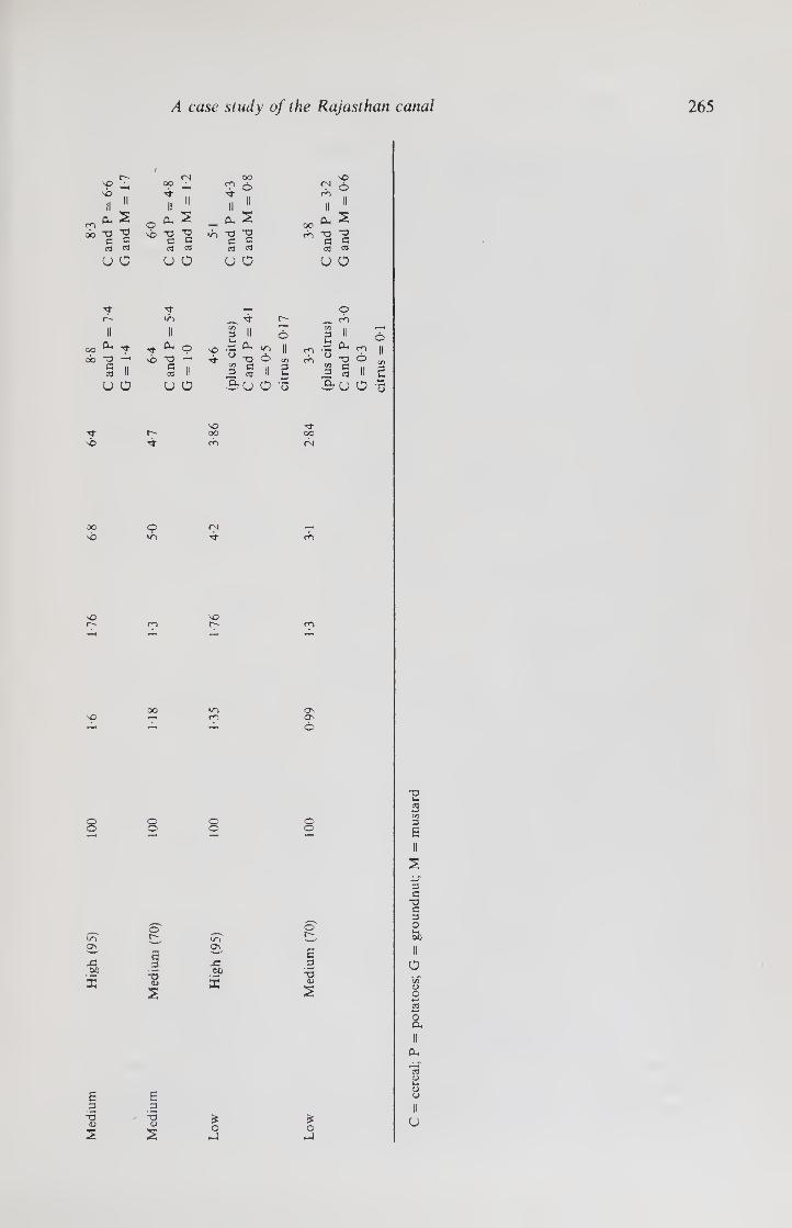
Med
ium
Hig
h (9
5)
100
1-6
1-76
A case study of the Rajasthan canal 265
vO rp
oo <N
•3
0-8
•2
0-6
vb
II II
3
II II
1 « 7 *
Cl, rp 5 o ^
_ ft, 5 ao**
oo 3 *3 vb *3 “O vb 3 3 T3 "2 g C c G G C C c cd cd cd cd cd & c« «1
u a u a U o u a
3 3 T-H O o- VO _ 3 O' ___ cb
II II 3 II © (/) 3 II
Cl oc ^ 3 T* ^ © b: cu
VO •- ^ vo, II
1-H
CO Oh ro
6c 3 6-4 vb 3 1 3 3 © </> cb ° 3 O G cd II § ii
3 G ,3 3 II 2
<z> 3 § ii
U o u a So O O D,
u o
vO 3-0-00
vb rr cb
3 oc 04
OC O fN vo vo 3
Ov O'. o
8 8 8
O o-
3
s
VO Ov
-C 60
O O'
g 2 •3 S
s 3
s
* o
2 o
3 u. cd
3 G
"3 G 3 O
O
o C
a
cd (D
u

266 Rameshwar D Varma
model, at the three levels of agricultural technology considered in the earlier studies,
(Verma 1977a, b) are given in table 5. The results given in tables 6 and 7 indicate that the benefits from the canal water will
be more than doubled if the agricultural technology level is changed from low to high,
while they will be more than one and a half times if the change is from low to medium
technology. The percentage increase in the total agricultural production is even more
than the percentage increase in benefits for a change from low to medium or low to high
technology. The strategy of maximizing benefits yields higher economic efficiency as
compared to the strategy of maximizing cropped area. The yearly farm income is
increased about three times (from Rs 8800 to Rs 22800 for a 4-ha farm and from
Rs 13200 to Rs 34200 for a 6-ha farm) if the agricultural technology is improved from
low to high and the strategy is changed from ‘maximizing cropped area’ to ‘maximizing
benefits’. The agricultural labour requirements remain the same for the three levels of
agricultural technology (for the same irrigation technology) if the strategy used is of
maximizing cropped area and if the water supplied to the plant equals its consumptive
requirements. With the strategy of maximizing benefits the agricultural labour
requirements increase with the improvement of the agricultural technology. If the total
labour requirements are compared for the two strategies viz ‘maximize benefits’ and
‘maximize cropped area’ it is found that the difference is insignificant (when water
supplied to the plant equals its consumptive requirement) for high and medium
agricultural technology; however the difference is about 30% for low agricultural
technology. For the price structure and the crop water requirements adopted in the
study, the choice of crops in the optimum cropping pattern remains almost the same for
the three technology levels.
Discussion of the policy issues of agricultural development in literature is dominated
by a polarization of opinion on whether the principal objective of policy should be
equity or efficiency. Hopper (1968) states the view that agricultural development
policies should be based on the single-minded pursuit of the goal of increased output.
He argues, particularly from the Indian context, that the production of food must be
accepted as the priority objective. Hopper emphasizes that the development program¬
mes should aim at the application of the latest in science and technology. On the other
hand, Maass (1966) stresses on equity for agricultural development policies in
developing countries. He suggests that government economic programmes intended to
attain multiple objectives should be designed to achieve the desired distribution of
income. Frankel (1969) and Ruttan & Hayami (1973) explain the problem of income
distribution with technology transfer in agricultural development; it has been pointed
out that the technological change is likely to contribute to the widening income
disparities among farmers. Johnston el at (1972) consider that the objectives
particularly relevant to the design of strategies for agricultural development should be
(i) contributing to the overall rate of economic growth and the process of structural
transformation, (ii) achieving a satisfactory rate of increase in farm output at minimum
cost, (iii) achieving a broad-based improvement in the welfare of the rural population
and (iv) facilitating the process of social modernization. In other words, Johnston et al
suggest that agricultural development policies should be directed at multiple objectives.
It seems that the main criticism against technology transfer for agricultural
development in developing countries is that this transfer may lead to inequality in the
income distribution of the farmers and thus may result in social and political problems.
The reason for this criticism appears to be that the technology change may necessitate
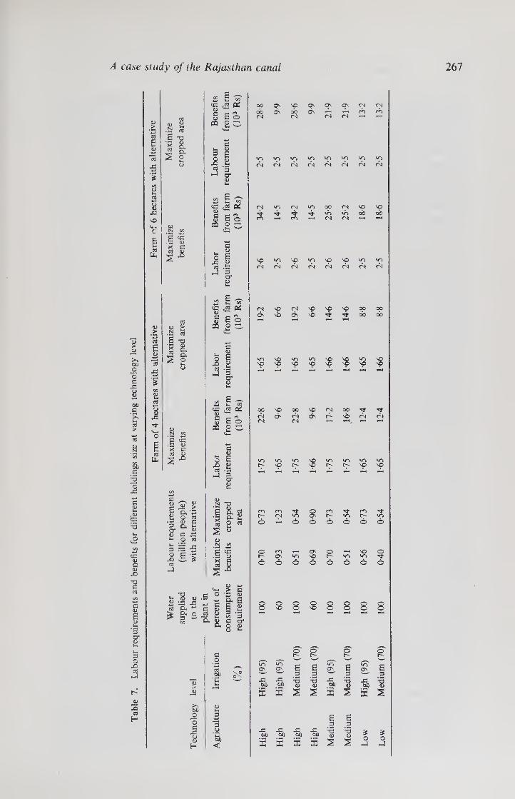
A case study of the Rajasthan canal
1 <0
b
3 8 b
no
c
cd b
K § .M cd £ "O | 8.
42 °- 5 o
S3
B * .G V * G
5 JS
<e £ a: a> ^ C o'** i; Eo «o r*,
G W< <L»
3 £ 8 s .3 1
£ § 'to <5 <2 * 5 E£>
aa o -
O B j5 o Jf
p
<u > w Cd C w
15
cd *— 8 je
• H cd
£ T3
■g 8. I &
g ^ -5 <d X G cd V
s ■*
£ C 9 b ci3 ctf § £ o
P3 P w
G <u £ 0)
*3 cr 0>
cG .03 <3 u- C e ^ S E o
ffl 2 w
£ Oi
'3 a* 4)
£ g a b o cd
8. e «u a b: O as 3 b
S/1
N "O 1 | 8 « 2 »< b o
b (D G
J5
■q c ° l-< G li -3 o •» J5 Sfc-Sg ^ §*2| K
3 8.
<u r* a>
bO
3 a G b o 0) H
G O cd bo
G O G OXJ
<
o-°
00 ON NO ON ON ON 04 04 oo On ob ON b b rb rb <N C4 04 04 t~i
NO <0 «0 NO NO «o ■O »o 04 04 04 04 04 04 04 04
04 *0 04 NO oo <N NO NO br br b b- NO NO oo ob CO co ’-H 04 04 *—•
NO «o NO NO NO NO NO NO 04 04 04 04 04 04 04 04
04 NO 04 NO NO NO Op op ON NO ON NO b b ob ob
»o NO NO NO NO NO NO NO NO NO NO NO NO NO NO NO b b b b1 b b b b
OC NO OO NO 04 oo ’*r ■'3' 04 ON 04 ON o- NO 04 04 04 04
NO NO NO NO NO NO NO NO o- NO O' NO O' O' Np Np b b b b b b b b
co co o CO ro rr O' 04 NO Os O' NO O' NO © b O O O o o o
o CO OS o y-4 NO o o- O'. NO NO o- NO NO) o o o o o o o o
8 o NO 8
o NO 8 8 8 8
o o O o O' O' O' r~
y—»s _ _'
NO O'.
NO Os £ E
•o ON £
NO Os E
3 3 '—' G 3 yC GO
yC bo ■§ %
b bo
-G bO
X X s 5 2 S X s
£ £ _G 3
-G bO
-C bO
J3 £>0
3 3 s »
2 2 X X s s O b
O J
267

268 Rameshwar D Varma
mechanization converting small holdings into bigger ones. However, mechanization is
not necessary for the transfer of agricultural technology. The use of high-yielding
varieties and good agricultural practices, choice of proper crops and adequate and
efficient use of inputs do not require large holdings and use of agricultural machinery.
Lau & Yotopoulos (1971) have found by using a profit function of the Cobb-
Douglas form and data derived from the farm management studies in India that the
relative economic efficiency of small farms is higher than for large farms and that small
farms attain higher levels of price efficiency and/or that they operate at higher levels of
technical efficiency. The problem of income distribution can have an easy solution in
the case of agricultural development of arid lands. Here the proper allocation of water
among the various farmers can help in manipulating equity. In many cases the arid land
may belong to the central or the state governments (as is the case for most of the
command area of the Rajasthan canal project). In such situations proper settlement and
water allocation policies will result in even distribution of income derived from
technology transfer. The results of the Rajasthan canal project study indicate that if the
size of holdings is changed from 6 to 4 ha for high agricultural technology the average
yearly income of a farmer is reduced from Rs 34,200 to Rs 22,800 (which is still about
double the income of a 6 ha farm with low technology) but the benefits of the
technology change are made available to many more people (from 0 25 million people
to 0-4 million people). Also agricultural tax reforms as suggested by Kaldor (1964)
should greatly help even distribution of income amongst farmers as a result of
technology transfer.
The results of the Rajasthan canal project presented in this paper clearly show that
the agricultural development policies of arid lands should be based on intensive
agriculture and on maximizing benefits with modern technology.
6.2 Irrigation technology
The results given in tables 6 and 7 consider two levels of irrigation technology (i) high,
with an irrigation efficiency of about 95 % using sprinklers or drip irrigation systems
and (ii) medium with irrigation efficiency of about 70% with furrow or border strip
irrigation systems. The results indicate that when the irrigation technology is improved from medium to high the total benefits at every level of agricultural technology also
increase by about 40 %. The total agricultural production also increases by almost the
same percentage. This increase in benefits and production is the result of more water
becoming available, making it possible to increase the irrigated crop area. In the case of
the Rajasthan canal project it was assumed that assured and known quantities of water
are available in the canal for each of the 12 months of the year. If this water is not
assured, as for example in the case of dry land farming or groundwater development,
the scope of improvement in irrigation technology would not be limited only by the additional quantity of water available at a certain location but also by its reliability in
time and space. In this context the point stressed by Levine (1970) regarding the
importance of better coordination between the operation of irrigation systems and the
farmer's use of the available water and the need for improving on-farm w'ater
management practices is very significant. A change from the furrow or border strip irrigation system to sprinklers or the drip
irrigation system would require additional capital. Most of the cases of improvement in
irrigation technology are capital-intensive. However, since water has a very high

A case study of the Rajasthan canal 269
economic value in arid lands the capital expenditure in improving irrigation technology
is usually paid off. The experiences of sprinklers or drip irrigation systems in parts of
Israel and Arizona indicate that the capital expenditure is recovered by the farmers in
about 5 to 10 years. The same seems to be applicable for the Rajasthan canal project.
The importance of improving irrigation technology in an arid land should not be
underestimated. This may bring even higher dividends as compared to the improve¬
ment in agricultural technology (e.g., the results indicate that the yearly benefits as well
as the agricultural employment from the Rajasthan canal project with medium
agriculture technology and high irrigation technology are greater than with high
agriculture technology and medium irrigation technology).
6.3 Water—use of less than full consumptive requirement
The fixed quantity of water available in the canal can be used to meet the full
consumptive water requirements of the plants in a limited area thereby getting
maximum crop yield per unit area or this could be utilized for a greater cropped area
with water use by the plants per unit area being less than their consumptive
requirements and thus, with crop yields less than the maximum. This policy question
was looked into by determining the benefits and agricultural employment opportuni¬
ties for the high agricultural technology (using both the strategies of maximizing
benefits and maximizing cropped area) for two cases (i) water supplied to the plants is
for 100 % of their consumptive requirements and (ii) water supplied to the plants is for
only 60 % of their consumptive requirements. The results indicate that when the water
supplied to the plants was for only 60 % of their consumptive requirements the total
benefits of the Rajasthan canal project were reduced to about 40 % while the cropped
area of the project increased by about 50%. If the additional cost required in developing on-farm works for the increased cropped area is taken into account, the
total benefits of the project with water use of 60% of the consumptive requirements
should be less than half of what these will be if full consumptive requirements of the
plants are satisfied from the canal water. The agricultural labour requirements increase
from about 30 to 70% (from 0-7 million to 0-9 million with the strategy ‘maximize
benefits’ and from 0-7 to 1-2 million with the strategy ‘maximize cropped area’) due to
the increased cropped area. However, by using less water per unit cropped area farm
benefits are reduced to about one-third from Rs 28,000 to Rs 9900 for a 6-ha farm and
from Rs 19,200 to Rs 6,600 for a 4-ha farm (the reduction will be even more significant
if the costs of farm-development works for increased cropped area are considered).
These results clearly indicate that in an arid land if the water is spread too thinly even
with the good intention of increasing cropped area thereby benefitting more people,
this will result in highly inefficient use of a very scarce resource. It will be like going from
a production level to a subsistence level for the farmers. On the other hand, Collinson
(1972) while analyzing the rural-based African economies found that improved
productivity requires the orientation of resources from subsistence to production for
the market. In developing countries where in addition to water, land may also be a
limiting factor the policy of increasing cropped area at the cost of getting significantly
lower benefits and lower agricultural production will be dangerous. Statistics of land
area and the gnp per capita of some countries are given in table 4. These data indicate
that India is not only very low in gnp but its available area per capita (0-59 ha) is one of
the lowest in the world. This suggests that on a long-term basis land will also become a
270 Rameshwar D Varma
limiting factor for the economic growth of the country and therefore the conclusions of
Hopper (1968) that “the poor countries can feed themselves if their agriculture is
modernized and their rural economies are restructured. That requires infusions of
technology and capital from rich nations” is very pertinent in formulating policies for
the agricultural development in India and particularly in the arid lands of India.
6.4 Employment potential and farm size
The agriculture labour requirements for various levels of agricultural and irrigation
technologies were also determined using data from farm management practices in
India. The results given in table 7 indicate that an additional 25 % labour requirement
(from 0-4 to 051 million people for 70% irrigation efficiency and from 0-56 to 0-70
million people for 95 % irrigation efficiency) is generated with a change in agriculture
technology from low to medium. The impact of changing irrigation technology from
medium to high on agricultural employment potential is even more significant as the results indicate an increase of about 40% (from 0-4 to 0-56 million people for low
agricultural technology and from 0-51 to 0-7 million people for medium and high
agricultural technologies). These results suggest that if increasing employment
potential is an important objective of agricultural development in an arid area then
irrigation facilities should be provided to more areas and atleast medium agricultural
technology should be used. In the absence of farm mechanization, as has been assumed in this study, the size of
holding for colonization will depend upon the technology level and upon the economic
expectations of the farmers. For example, if on full development of the project, it is
aimed that a farmer should have an annual income of atleast Rs 22,000/-, this can be achieved either with a 6 ha farm with medium agricultural technology or with a 4 ha
farm holding with high agricultural technology (refer table 7).
7. Conclusions
Agricultural development policies in arid lands should be based on the principle of
maximizing benefits and/or agricultural production. High agricultural and irrigation
technologies should be used to maximize benefits/production per unit of water and
land area. Proper settlement, water allocation and agricultural tax policies will help in
achieving equity amongst the farmers. Intensive agriculture at high technology levels
will result in higher economic efficiency as well as opportunities for higher agricultural
employment.
References
Anon 1977 The New York Times April 14, A5
Christiansen J E 1968 J. Irrigation and Drainage Division ASCE 94: 243-263
Collinson M P 1972 A handbook for rural development Planning in Africa (Preger Publishers) p. 15
Domenico P A, Anderson D V, Case C M 1968 Water Resources Res. 4: 247-255
Frankel F R 1969 J. Asian Studies 692
Hargreaves G H 1956 J. Irrigation and Drainage Division ASCE 1105
Heady E O, Nicol J K 1975 Water Resources Res. 11:
Hopper W D 1968 in Strategy for the conquest of hunger (New York: Rockefeller Foundation)
Johnston B F, Page Jr J M, Warr P 1972 Studies in agricultural economic trade and development 11: 28

A case study of the Rajasthan canal 271
Kaldor N 1964 Essays on economic policy (Gerald Duckworth) 1: 216
Kelso M M, Martin W E, Mack L E 1973 Water supplies and economic growth in an arid environment; An
Arizona case study (Tucson: The University of Arizona Press) p. 225
Lau L J, Yotopoulos PA 1971 Am. Eco. Rev. 61(1) 94-109
Levine G 1970 The water environment and crop production, Paper presented at the Cornell Workshop on
some emerging issues accompanying recent breakthrough in food production, Ithaca N.Y. 1970
Maass A 1966 Q. J. Econ. 214
Ministry of Agriculture, Water Management Division, New Delhi 1970 A guide for estimating irrigation
water requirements, Tech. Ser. No. 2, 8: 39
Ministry of Irrigation and Power 1971 Dynamics of shifting sand dunes in Western Rajasthan and its
stabilization, CWPC No. 262, Central Water and Power Commission, Government of India, New Delhi
Ministry of Irrigation and Power 1972 Report of the Irrigation Commission, New Delhi 2: 342
Rao K L 1975 India’s water wealth—its assessment, uses and projections (New Delhi: Orient Longman) p. 204
Ruttan V W, Hayami Y 1973 Technol. Cult. 14: 119
Verma R D 1977a Technology transfer for irrigation planning of arid lands, Paper presented at the Second
Int. Conf. transfer of water resources knowledge, Colorado State University, Colorado.
Verma R D 1977b Technology transfer for irrigation planning of arid lands (case study of Rajasthan Canal
Project), Research Report and Seminar Papers of the Centre for Population Studies, Harvard University,
Cambridge
Wiener A 1964 Development and management of water supplies under conditions of scarcity of resources,
three lectures P N 422

.
.
■

A study for optimum utilization of the Damodar water resources
BASAWAN SINHA* and P RAMAKR1SHNA RAOt
* Centra! Flood Forecasting, Central Water Commission, “Kamata Sadan”, 427/c, East Borning, Canal Road, Patna 800001, India
t Central Water Commission, Room 514, Sewa Bhavan, Ramakrishnapuram, New Delhi
110 066, India
Abstract. The study describes the existing and proposed water resources development in the Damodar river basin and the systems study carried out for estimating the consequences of implementing a proposed set of management and development measures. A simulation model was considered appropriate for the study and a computer program developed by the US Army Corps of Engineers was used The results of various simulation runs are discussed The analysis of results have indicated that an integrated operation of all reservoirs on the Damodar system, both existing and proposed, would help in maximization of utilisation and benefits. It is also concluded that a simulation model would help not only the long range planning but also the day-to-day operation.
Key Words. River basin development; integrated operation; simulation model.
1. Introduction
The wandering and capricious Damodar rises in the hills of Chhotanagpur at an
elevation of 2000 feet, and after flowing for 180 miles in Bihar, enters the deltaic plains
of West Bengal and ultimately joins the Hooghly. The total drainage area is
8500 miles2, of which 6960 miles2 are the catchment of the upper Damodar, just below
its confluence with the Barakar. Figure 1 shows the region through which the river flows.
The river used to cause serious floods in its lower reaches lying in West Bengal
Voorduin (1945) of the Tennessee Valley Authority (tva) prepared a preliminary
memorandum on the unified development of the Damodar river, and the Damodar
Valley Corporation (dvc) was set up in 1948 to implement schemes for integrated and
coordinated development of the Damodar Basin.
Voorduin’s plan of development of the water resources of the valley envisaged
construction of seven storage dams across the Damodar and its tributaries at Tilaiya,
Konar, Maithon, Panchet, Bokaro, Balpahari and Aiyar; a diversion dam at Bermo and
a barrage at Durgapur with a canal network system. This development was to be carried
out in two stages. The first stage was to cover the construction of four dams at Tilaiya,
Konar, Maithon and Panchet and the barrage with canal system at Durgapur (figure 2).
Construction of the remaining four dams was included in the second stage. The first
stage was completed in 1958, and the second stage has not yet been implemented.
Subsequently, a dam at Tenughat on the Damodar river has been constructed by the
Bihar Government. This envisaged utilization of 900cusecs all the year round for
Conversion table
1 inch = 2 54 cm; 1 foot = 0 3048 m; 1 mile = 1-609 km; 1 mile2 = 2 59 km2; 1 acre = 0 405 ha; 1 acre foot
= 0T234 ham; 1 cusec = 002832 cumec.
273

BIH
AR
BE
NG
AL
274 Basawan Sinha and P Ramakrishna Rao
Fig
ure
1. D
am
odar
river
: T
enta
tiv
e pla
n o
f dev
elopm
ent

Optimum utilization of the Damodar resources 275
Figure 2. Damodar valley reservoirs
irrigation and industrial water supply. Upstream of this dam, yet another small
dam to control about 100 miles2 was constructed by the Bihar State Electricity Board to
meet the requirements of Pathrathu Thermal Power Station. The Government of Bihar
has also prepared some major, medium and minor schemes for utilization of the
Damodar waters in the upper reaches for irrigation and industrial uses. This plan of
utilization by Bihar includes the use of waters from the existing Konar and Tilaiya dams
of dvc. Salient features of existing major projects in the Damodar Valley are given in
table 1.
Voorduin's original plan of development provided for a total storage of 4 68 million
acre feet (maf) in seven storage dams, of which 2 915 map was earmarked for
moderating floods. Against this, only four dams with a gross storage of 2-92 maf were
built in the first stage, out of which 1 52 maf is the flood storage; 0-97 maf is
conservation storage and 043 maf is the silt storage. But the whole flood storage of
1-52 maf is not available as yet due to non-acquisition of land in the Maithon and
Panchet reservoirs beyond rl (reduced level) 495 and rl 425 respectively. As a result,
the effective flood storage at present is only 068 maf.
2. Surface water resources in the basin
2.1 Water utilization
According to the regulations issued by the Central Water Commission (1969), the
principal requirements for stored waters are kharif irrigation, power generation and
flushing doses during the monsoon season (June to October), and rabi irrigation,
navigation, power generation and water supply for industrial and domestic uses during
the non-monsoon season (November to June).

276 Basawan Sinha and P Ramakrishna Rao
Table 1. Salient features of the Damodar valley
Name of dam and
river stream
Catchment Dead storage
area (miles2) (acre feet)
Conservation
storage
(acre feet)
Flood
storage
(acre feet)
Installed
capacity
of power
house (MW)
Tilaiya: Barakar 380 60,680 114,800 143,900 4
Maithon: Barakar 2430 168,090 495,540 446,370 3x20
Konar: Konar— 385 49,530 178,770 216,370* —
tributary 44,200
of Damodar
Panchet: Damodar 4234 148,060 184,930 881,000 1 x 40
277,000*
Total for 7430 426,400 974,000 1,515,500
DVC 681,470*
Tenughat: Damodar 1730 170,000 621,100 — —
* Flood storage available with land acquisition upto RL 495 and RL 425 in Maithon and Panchet reservoirs
respectively; rl—reduced level
The requirement of kharif irrigation has been worked out on the basis suggested by
the Water Management Division, Ministry of Food and Agriculture (table 2). The
overall requirement works out to 1-792 maf, which includes 0 579 maf during October.
According to the regulation schedule, the reservoirs have to be operated such that they
are full at the monsoon storage level after meeting all the requirements. The
conservation storage available in all the four dams of the dvc system is 0974 maf and it
Table 2. Monthly requirements of water for kharif irrigation (June to October).
Month
Irrigation
requirement
of the crops (in inches)
on the basis suggested
by Ministry of
Food & Agriculture
Irrigation
requirement
at canal head
inches feet
Total requirement
at canal head
103 acre ft.
June 0.2 0.286 0.024 24
July 40 5-714 0-476 467
August 1-3 2-2 3143 0-262 255
September 2-6 40 5-714 0-476 467
October 8-2 50 7-143 0-595 579
Total 121 15 4 22-000 1-833 1792
Notes:
1. Irrigated area during kharif season = 973 x 103 acres.
2. Canal and outlet efficiencies are assumed to be 82 % and 85 %, i.e. overall efficiency during kharif is 70 %.
3. Monthly water requirements suggested by Water Management Division (column 2) have been suitably
modified (see column 3) allowing for seed beds in June and accounting for uneven distribution of rainfall
during the monsoon.
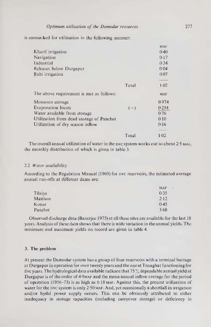
Optimum utilization of the Damodar resources 277
is earmarked for utilization in the following manner:
MAF
Kharif irrigation 0 40
Navigation 017
Industrial 0-34
Releases below Durgapur 0 04
Rabi irrigation 0 07
Total 102
The above requirement is met as follows: maf
Monsoon storage 0-974
Evaporation losses (—) 0-214
Water available from storage 0-76
Utilization from dead storage of Panchet 0 10
Utilization of dry season inflow 0T6
Total 102
The overall annual utilization of water in the dvc system works out to about 2-5 maf,
the monthly distribution of which is given in table 3.
2.2 Water availability
According to the Regulation Manual (1969) for dvc reservoirs, the estimated average
annual run-offs at different dams are:
maf
Tilaiya 0-35
Maithon 2-12
Konar 0-45
Panchet 3-68
Observed discharge data (Banerjee 1975) at all these sites are available for the last 18
years. Analysis of these data shows that there is wide variation in the annual yields. The
minimum and maximum yields on record are given in table 4.
3. The problem
At present the Damodar system has a group of four reservoirs with a terminal barrage
at Durgapur in operation for over twenty years and the one at Tenughat functioning for
five years. The hydrological data available indicate that 75 % dependable annual yield at
Durgapur is of the order of 4 9maf and the mean annual inflow average for the period
of operation (1956-73) is as high as 618maf. Against this, the present utilisation of
water for the dvc system is only 2-50 maf. And, yet occasionally a shortfall in irrigation
and/or hydel power supply occurs. This can be obviously attributed to either
inadequacy in storage capacities (including carryover storage) or deficiency in
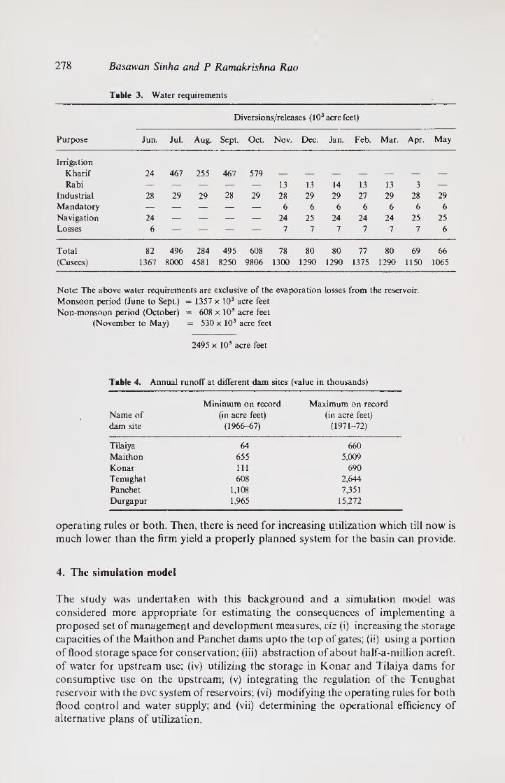
278 Basawan Sinha and P Ramakrishna Rao
Table 3. Water requirements
Diversions/releases (103 acre feet)
Purpose Jun. Jul. Aug. Sept. Oct. Nov. Dec. Jan. Feb. Mar. Apr. May
Irrigation
Kharif 24 467 255 467 579 — — — — — — —
Rabi — — — — — 13 13 14 13 13 3 —
Industrial 28 29 29 28 29 28 29 29 27 29 28 29
Mandatory — — — — — 6 6 6 6 6 6 6 Navigation 24 — — — — 24 25 24 24 24 25 25
Losses 6 — — — — 7 7 7 7 7 7 6
Total 82 496 284 495 608 78 80 80 77 80 69 66
(Cusecs) 1367 8000 4581 8250 9806 1300 1290 1290 1375 1290 1150 1065
Note: The above water requirements are exclusive of the evaporation losses from the reservoir.
Monsoon period (June to Sept.) = 1357 x 103 acre feet
Non-monsoon period (October) = 608 x 103 acre feet
(November to May) = 530 x 103 acre feet
2495 x 103 acre feet
Table 4. Annual runoff at different dam sites (value in thousands)
Name of
dam site
Minimum on record
(in acre feet)
(1966-67)
Maximum on record
(in acre feet)
(1971-72)
Tilaiya 64 660
Maithon 655 5,009
Konar 111 690
Tenughat 608 2,644
Panchet 1,108 7,351
Durgapur 1,965 15,272
operating rules or both. Then, there is need for increasing utilization which till now is
much lower than the firm yield a properly planned system for the basin can provide.
4. The simulation model
The study was undertaken with this background and a simulation model was
considered more appropriate for estimating the consequences of implementing a
proposed set of management and development measures, viz (i) increasing the storage
capacities of the Maithon and Panchet dams upto the top of gates; (ii) using a portion
of flood storage space for conservation; (iii) abstraction of about half-a-million acreft.
of water for upstream use; (iv) utilizing the storage in Konar and Tilaiya dams for
consumptive use on the upstream; (v) integrating the regulation of the Tenughat
reservoir with the dvc system of reservoirs; (vi) modifying the operating rules for both flood control and water supply; and (vii) determining the operational efficiency of
alternative plans of utilization.

Optimum utilization of the Damodar resources 279
For this purpose, a computer program (No. 723-x6-L 2030) developed at the
Hydrologic Engineering Centre, us Army Corps of Engineers (1976) seemed appropri¬
ate and hence, has been chosen for the simulation studies. This program performs a
multipurpose routing of flows in a reservoir system for upto twelve periods of uniform
or varying lengths per year based on varying flow requirements at reservoirs, diversions
and downstream control points. It can accommodate power peaking and energy
requirements at reservoirs and can assign economic values to all outputs and allocate
these in various ways. It can automatically iterate to optimize yield at a specified
location.
5. The system
5.1 System components
There are five basic system components which are generally used by the program to
model a reservoir system viz. the system hydrology, reservoirs, control points, power
plants and diversions.
5.1a Hydrologic characteristics: The system inflows which are the primary hydrologic components of the programs, are specified by identifying their location (i.e. the control
point where they occur), their magnitude and the period when they occur. Incremental
local flows are equal to the difference between inflows at adjacent control points.
Reservoir evaporation, an important part of the system’s water balance computation, is
input into the model by- specifying a net evaporation rate (difference between
evaporation and rainfall) for each reservoir.
5.1b Reservoir characteristics: Storage, surface area and outlet capacity are specified
on 10 reservoir elevations to describe adequately the physical features (area and
capacity curves given in the Regulation Manual) of each reservoir necessary to model
the storage and release features of the reservoir. To simulate the operation of a reservoir system the operating criteria are expressed in quantitative terms by dividing each
reservoir storage into six horizontal levels. The difference between the levels is taken as
the zone of potential storage volume. The lowest level corresponds to the bottom of the
conservation pool (top of the inactive pool), the second lowest level is the top of the
buffer zone, the highest level is the full pool level (top of the flood control), and the
second highest level is the top of conservation (bottom of flood control). Additional
levels to facilitate individual reservoir operating criteria are specified.
Each reservoir is operated to meet stream flow targets at specified locations in the
system. Priority of withdrawals from reservoirs serving the same location is established
by specifying additional levels. The highest storage zone is withdrawn first, then the
second highest and so on down to the lowest keeping all reservoirs in the system in
balance to the extent possible. Other operating criteria specified in the model are initial
reservoir storage and spillway surcharge.
5.1c Hydrologic balance: Computations in the model are based on the principle of
continuity equation.
5. Id Control point characteristics: Control points, which are not reservoirs, are used to
regulate system operation by establishing constraints and targets on streamflow. Both
reservoirs and selected locations along the stream network are assigned control point

280 Basawan Sinha and P Ramakrishna Rao
numbers. There are three types of controls specified for any stream control point:
maximum permissible flow, minimum desired flow and minimum required flow.
5.1e Power plant characteristics: Power plant characteristics which are used in the
model to simulate power operations include installed power plant nameplate capacity,
maximum plant factor for generation, power plant efficiency, tailwater elevation clus
hydraulic loss, overload ratio for the power installation and power load requirements
for each plant for each time period.
5.If Diversions: One diversion exists at each control point except at Maithon anG the
actual flow diverted is specified. Diversion shown at Panchet actually relates to
withdrawals above it and below Tenughat.
5.1 g Economic evaluation: An economic analysis of the system operation is available at
each control point by specifying a functional relationship between a hydroiogic
quantity such as streamflow, reservoir storage, power generation and the economic
value of meeting the hydrologic quantities during a given month. In the present study,
however, the economic parameters have not been assigned.
5.2 System operation
The simulation model operates by considering the water and power requirements at
each pertinent control point in the system in a sequential fashion, beginning at an
upstream point and moving in a downstream direction through each river basin The
release required to meet these requirements for all pertinent purposes is determined by
evaluating each operational requirement and all physical and operational constrai nts at
each site. Also, an index of the relative state of each reservoir (as a function of rese rvoir
storage) is determined according to the specified operation guides. After the require¬
ments have been met at all control points (or shortages declared if upstream water is not
available), “system requirements” are examined to determine whether additional water
releases for power generation will be needed to satisfy the system power demands If so, the additional needs are proportioned among the reservoirs that have been specified to
be available for meeting that system requirement in accordance with the relative state of
the reservoirs as evidenced by the indices previously computed. The additional releases
are added to the previously computed releases for meeting at-site requirements, and the
system and at-site requirements are thus met (or shortages are declared if water is not
available). This process is repeated for each period of the study, with the ending state of
the reservoirs in the system for the current period being the beginning state for the next
period.
Results from the successive applications of these calculations on a period-by-period
basis are recorded for all points in the system (including non-reservoirs) by an
accounting procedure which accounts for the movement of the water through the
system by using the specified relative location of the reservoirs and downstream control
points.
For the power plants included in the system, the requirements for the system as a
whole as well as the minimum requirements for each plant are specified. During the first
search of the system, the minimum power requirement at each plant will be established,
and the total generation during the period at each plant will be computed. This total can
exceed the minimum required generation if other services call for additional releases
from the particular reservoir.

Optimum utilization of the Damodar resources 281
At the end of the first search, a summary is made of the total power generated and
required and of the total power generated and used to satisfy system requirements. If
the system requirement has not been satisfied, water levels at those reservoirs where
additional generated power could be used for meeting system requirements would then
be drawn towards a common storage-balancing level such that the full system
requirement is generated. The allocated system requirements are then used in making a
second search of the entire system for all purposes.
Since satisfying these additional requirements will usually change releases at many
reservoirs, the average head during the second search will be different from the average
obtained from the first search and used in the second search. Accordingly, accurate
system power (and evaporation) computations require a third complete search of the
entire water resource system for each operation period.
6. Simulation model studies
There are at present six major reservoirs in operation in the Damodar Basin, four under
dvc, the fifth under the Bihar Government departmental control and the sixth under
the Bihar State Electricity Board. The three agencies operate the reservoirs, constructed
and maintained by them independently. Schemes for utilization of Tilaiya and Konar
reservoirs for irrigation in Bihar have been formulated. There is further demand for
atleast 05 maf of the Damodar waters in Bihar (upstream of Maithon and Panchet
dams), but the proposed schemes are not yei cleared for implementation due to the
apprehension that they may adversely affect the existing dvc system, which caters to the
needs of irrigation, hydel power, navigation, industrial and drinking water supply,
through Tilaiya and Maithon dams on Barakar, Konar and Panchet dams on the
Damodar, and Durgapur barrage on the Damodar below the confluence of the
Damodar and the Barakar. The present annual utilization of water for the dvc system is
only 2-5 maf (see the breakdown given in table 3) as against the assessed 75%
dependable yield of 4-9 maf and 50 % dependable yield of 6-8 maf at Durgapur. If the
inflows from catchments above Tilaiya, Konar and Tenughat are excluded, the
corresponding dependable yields at Durgapur would still be 3-4 and 4-8 maf and that at
Maithon-Panchet would be about 2-5 and 3-4 maf. Therefore, the first set of studies
using simulation models is aimed at investigating the effect of the proposed schemes of
upstream abstraction on the dvc system. For the sake of simplification, the entire yield
from above Tilaiya, Konar and Tenughat dams has been excluded from the total
catchment areas of Maithon and Panchet dams. This means that the effective
catchment areas at Maithon and Panchet would be reduced to 2010 and 2100 miles2
from 2390 and 4215 miles2. Monthly yield data as available since 1956 have been
utilized for the studies. In the first study, the reservoir capacity and the regulation
schedule as at present, have been maintained.
The second set of studies was carried out keeping in view the proposal for acquisition
of land up to the top of the gates in Panchet and Maithon dams to increase their
effective gross storage capacity from 0-980 to 1 11 maf in Maithon and from 0-61 to
1-21 maf in Panchet, i.e. a net increase of 0-73 maf. In these studies it was proposed that
a part of the additional storage likely to be available through further land acquisition,
should go for increasing the conservation storage and the rest to flood storage. Lesser
flood storage than originally envisaged at Panchet seems justified in view of the fact that
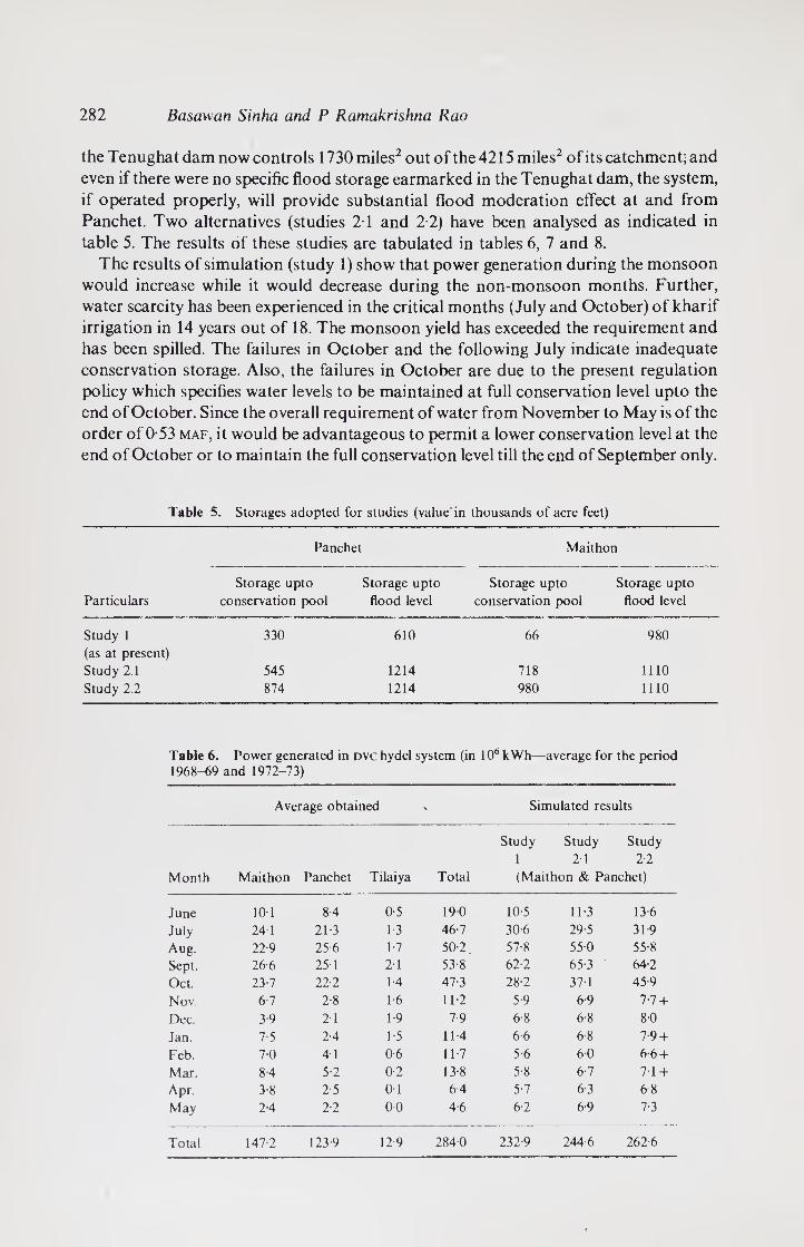
282 Basawan Sinha and P Ramakrishna Rao
the Tenughat dam now controls 1730 miles2 out of the 4215 miles2 of its catchment; and
even if there were no specific flood storage earmarked in the Tenughat dam, the system,
if operated properly, will provide substantial flood moderation effect at and from
Panchet. Two alternatives (studies 21 and 2-2) have been analysed as indicated in
table 5. The results of these studies are tabulated in tables 6, 7 and 8.
The results of simulation (study 1) show that power generation during the monsoon
would increase while it would decrease during the non-monsoon months. Further,
water scarcity has been experienced in the critical months (July and October) of kharif
irrigation in 14 years out of 18. The monsoon yield has exceeded the requirement and
has been spilled. The failures in October and the following July indicate inadequate
conservation storage. Also, the failures in October are due to the present regulation
policy which specifies water levels to be maintained at full conservation level upto the
end of October. Since the overall requirement of water from November to May is of the
order of 053 maf, it would be advantageous to permit a lower conservation level at the
end of October or to maintain the full conservation level till the end of September only.
Table 5. Storages adopted for studies (value in thousands of acre feet)
Panchet Maithon
Particulars
Storage upto
conservation pool
Storage upto
flood level
Storage upto
conservation pool
Storage upto
flood level
Study 1 330 610 66 980
(as at present)
Study 2.1 545 1214 718 1110
Study 2.2 874 1214 980 1110
Table 6. Power generated in Dvchydel system (in 106 kWh—; 1968-69 and 1972-73)
average for the period
Average obtained \ Simulated results
Study Study Study
1 2-1 2-2
Month Maithon Panchet Tilaiya Total (Maithon & Panchet)
June 10 1 8-4 0-5 190 10-5 11-3 13 6
July 24 1 213 1-3 46-7 30-6 29-5 319
Aug. 22-9 256 1-7 50-2 57-8 55-0 55-8
Sept. 26-6 25 1 2-1 53 8 62-2 65-3 64-2
Oct. 23-7 22-2 1-4 47-3 28-2 37-1 45-9
Nov. 6-7 2-8 1-6 11-2 5-9 6-9 7-7 +
Dec. 3-9 21 19 7-9 6-8 6-8 80
Jan. 7-5 2-4 1-5 114 6-6 6-8 7-9 +
Feb. 7-0 41 0-6 11-7 5-6 6-0 6-6 +
Mar. 8-4 5-2 0-2 13-8 5-8 6-7 71 +
Apr. 3-8 2-5 01 64 5-7 6-3 6-8
May 2-4 2-2 0-0 4-6 6-2 69 7-3
Total 147-2 123-9 12-9 2840 232-9 2446 262-6

Optimum utilization of the Damodar resources 283
-C
£ o © C
"S
V C u 00
<u * o Cl
s ■3
r-
01
H
04
04 •
NO OO OO CO tT p p o p M* NO o Tf Tf o CO 00 NO) NO) NO) NO) NO) NO) NO) CO
C/3 CO Tf
-—H ■<r NO NO NO Tf Tf p NO O NO Tf NO O'
co 04 no NO o ON o- NO) «iO NO) •O) NO) NO) NO) 1 r-
1 GO 04 CO
04 o- OS Op ”<* NO CO Tf p NO O p O o
i C/3 »o 'NI¬ NO OO
CO O' NO) NO) NO) NO) NO) NO) NO)
-
ON NO o O P p p P °P 04
< r-H ON NO © NO NO) Tf o co CO y—H -Is O 04 04
(N NO 04 CO O- p p °P OO p OO p o 04 NO o- -Is 6s 04 TT or rr rr tT tT OO
GO NO Tf 04
- o NO CO O- P p °p P OO NO O' 04 04 *o> NO -Is ON © 7t tT Tf tT NO) NO) O'
| GO NO 04
r- On NO T-H CO r— CO p Op p O NO) P O CO *—< i
GO rT -Is -Is 6s © Tf Tf NO) •O) NO) NO) NO) O'
NO 04
NO o 04 —S ON NO) p 04 04 p p NO 04 < © ON r- NO OO CO NO, OO ON NO) NO) 04 04
04 co CO CO 04 04
<N p NO NO O' OO p CO OO p OO p OO Os 04 •O «o NO 6s 6 Tf 6 Tf TT Tf CO
C/> Tf 04
p p NO o r- 04 p p OO P °p P °o NO 04 NO NO NO 6s O' Tf or rr tT tT rf tT 04
r-
d>
GO 04
t ON NO CO O' NO p °P OO P p Tf NO s-H
C/3 NO rr ON NO tT tT rr tT NO) NO) NO) 04
Tf 04
p NO NO co O p 04 04 p p o < rr OO TT 04 -1h NO) ON o —1 NO) CO
04 04
<N p NO CO p NO p cp cp p p p NO 04 NO NO —Is -1-1 Tf •6 tT ^r Tf NO) NO) NO)
GO NO TT
- p NO CO p p NO NO o NO p O CO o 04 «o NO -Is NO) NO) NO) NO) NO) NO) NO) Tf o-
1 On SO ON
GO NO CO
T-H p NO CO CO p p p O p P O 04
CO >o NO -1-1 o- Tf NO) NO) NO) NO) NO) NO NO)
NO CO
p P © ’Nt 04 O °p 04 NO O O' NO < NO -ls Tf NO 04 -Is -Is sb NO NO c6 o 04
04 04 04 04
p p CO co *0 OO p NO SO o p p p 04 CO -Is — -Is NO) NO) NO) NO) NO) NO) NO) O GO CO NO NO 04
-H NO CO co NO so P NO NO O p P NO OO
ON 04 CO -1< —S © CO NO) NO) NO) NO) NO) NO) NO) 00
T OO NO ON
CO 04 NO NO s—!
_s p CO co CO CO P NO NO O p P p NO *—'
CO -Is -Is — o CO NO) NO) NO) NO) NO) NO NO) OO 04 NO *o ,“l
ON 04 r- co co Os CO O NO P 04 P NO < o- NO On O- © -Is 04 rf NO)
n CO NT)
CO 04 04 04
-c
c o £ J
un
Jul
Aug
Sep
Oct
Nov
Dec
c a F
eb
Mar
Apr
May
Tota
3
C/3

284 Basfiwan Sinha and P Ramakrishna Rao
■8 2 e 1) 00
* £ E
-3
<u -C O c
Oh
00
.£} 08
H
rsj fN i
’T1 op OO CN cn cp
0-2
SO OO cn XT ri cn Tf fN r4 fN i—i o o r-
C/5 fN cn
O NO o tt fN so un CJ cn O oo un m fN fN cn C4 r- sb rb o O o O o O un r^
1 C/3 <N
fN r- OS _ OO sO up p rp fN sO r4 o oo Os *“*
C/3 O cn «--H r~ *-H O o O <6 6 o N" »—H
O cp sO Os Un fN cn o r- Tf p p OO < o Tf r-H r- ds fN O (N cn cn OS
fN fN
CN cn fN fN _ so rsj fN Os fN fN cn CN fN N- tJ- cn r- cn cn cn fN cn cn cn un C/3 cn cn m fN 1 -H oo fN CN fN fN fN cn tT OO
fN c4 fN tT tT cn cn cn cn cn cn r^ fN Tt r^
1 C/3 cn cn cn
r- Os -H fN fN p so —< CN un cn O Tf O cn 1—1
C/3 ch Ti¬ Tf cn ds cn cn Jh O o o o cn en m cn
so so so fN oo rp p- cn p qs r- o Os < r4 o ds OO sb »/S un r~~ ob Jh rsj o r-
fN cn fN fN fN T—'
CN cn cp SO un pj fN os fN fN cn fN Tf un cn cn cn cn cn fN cn cn cn Os C/3 cn fN
cp © rp ^H rp fN Os CN *—1 fN cn TT oo cn © cn cn cn fN cn cn cn OS r~ C/3 cn fN
r- Os cn hH H cn t-H (N fN Os so oo
C/3 CN TT ds cn cn
rb cn cn cn fN O O OO
oo OO p oo oo qs rp p up cn < fN r J r- ob r- Tf cn rf Tf un un tT
fN fN <N CN
CN fN Tf OO (N ^H fN fN Os Tj- cp qs cn fN sO fN sb tJ- cn cn cn fN fN fN ^H Os C/3 fN cn
fN (N Tf qs up un rr cn fN fN O Os
o fN sb Tf fN © r— o O O o o o OO r-*
1 On SO Os
C/3 cn cn
fN tt qs oo rr -H "cj- cn fN fN o o OS
C/3 fN SO b- r- un *L, o O O O d> o r- fN fN
O rp Os qs Os Tf oo r- un < SO oo r- yLi O yLf O fN rL, ^H o
H fN fN fN
csi CO Tf fN fN O cn Tf OO fN o fN un c4 fN fN ti- CO © fN fN ^Ih O o o O C/3 cn fN cn
-H cn cp fN p oo rp cn CN fN o fN 8 Os c4 <N un Ti¬ cn r- O O O o o
7 oo SO Os
C/3 en fN
CO rf fN p H r- cn CN fN o hH fN un 1
C/5 fN sb Tf Tf un o <±> P O o o oo fN cn
00 o qs Cp O so fN OO Os oo SO fN < O © OO r- o O fN (S| fN rn O
fN fN
.c G O
s Ju
n
3
Au
g
Sep
Oct
Nov
Dec
Jan
Feb
Mar
Apr
May
To
ta
5n T3 =3
</D
II 1/2
1 o cO II
<

Optimum utilization of the Damodar resources 285
It is seen from the results of the simulation study 2 that the average monthly
hydropower generation (based on actuals during the period 1968-73) will suffer in
January, February and March, though on an annual basis there is no substantial
decrease in hydel power generation. As the dvc hydel system places great emphasis on
peaking power to maintain the efficiency of the overall dvc power grid comprising
about 1000 MW of thermal power installation, further studies need to be carried out to
ensure that hydel power generation during non-monsoon months is not affected.
In order to examine the possibility of achieving this, a third set of studies was carried
out on the expanded system shown in figure 3. Table 10 summarises the various
stipulations made for the four case studies. It has been assumed in all the studies that
0-201 maf of the Tilaiya reservoir waters and 0-234 maf of the Konar reservoir waters
will be utilized for irrigation in Bihar as given in table 9. For industrial water supply,
600 cusecs throughout the year will be diverted; and for utilization above and through
the Panchet reservoir, 300 cusecs will be released from the Tenughat reservoir; and 10%
of the monsoon yield (July to September) from the catchments above Panchet and
Maithon reserved for utilization in Bihar. In other words, supplementing the Panchet
non-monsoon yield with the Tenughat reservoir releases was envisaged providing at the
same time for irrigation demands in Bihar.
The success of the scheme with respect to storage yield function is generally
determined by the following criteria: (a) there is no shortage in any period of the year in
75 % of the number of years for which the annual operation table is prepared or in 75 %
of the months for which the monthly operation table is prepared; (b) in any one
year/season the total irrigation shortage is not to exceed 50 % of the total annual output
for irrigation; and (c) in a 50-year period, the sum of all the shortages is not to exceed
150 % of the firm annual yield for irrigation. Analysing the results given in table 11, it
can be seen that judged from these criteria, the outcome of both the alternative plans,
that is, study 3-3 and study 3-4 is almost identical even though the plan in study 3-3 has
the annual inflow reduced by over half a million acre feet from that in study 3-4 (the
average river flow in study 3-3 is 6306 cusecs against 7097 cusecs in study 3-4). In study
3-3, there are failures in 14 months out of the 216 months for which the operation table
has been prepared. This decreases to 11 months in study 3-4. Both come well within
Figure 3. Schematic outline of the Damodar river basin system
^ 3
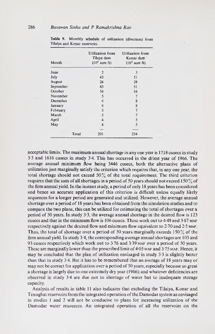
286 Basawan Sinha and P Ramakrishna Rao
Table 9. Monthly schedule of utilization (diversion) from
Tilaiya and Konar reservoirs
Month
Utilization from
Tilaya dam
(103 acre ft)
Utilization from
Konar dam
(103 acre ft)
June 2 3 July 43 51 August 24 28
September 43 51
October 54 54
November 5 7
December 6 8
January 6 8
February 5 7
March 5 7 April 4 5
May 4 5
Total 201 234
acceptable limits. The maximum annual shortage in any one year is 1718 cusecs in study
3-3 and 1616 cusecs in study 3-4. This has occurred in the driest year of 1966. The
average annual minimum flow being 3446 cusecs, both the alternative plans of
utilization just marginally satisfy the criterion which requires that, in any one year, the
total shortage should not exceed 50% of the total requirement. The third criterion
requires that the sum of all shortages in a period of 50 years should not exceed 150 % of
the firm annual yield. In the instant study, a period of only 18 years has been considered
and hence an accurate application of this criterion is difficult unless equally likely sequences for a longer period are generated and utilized. However, the average annual
shortage over a period of 18 years has been obtained from the simulation studies and to
compare the two plans, this can be utilized for estimating the total of shortages over a
period of 50 years. In study 3 3, the average annual shortage in the desired flow is 123
cusecs and that in the minimum flow is 106 cusecs. These work out to 4 49 and 3*87 maf
respectively against the desired flow and minimum flow equivalent to 2-70 and 2-5 maf.
Thus, the total of shortage over a period of 50 years marginally exceeds 150 % of the
firm annual yield. In study 3-4, the corresponding average annual shortages are 103 and 93 cusecs respectively which work out to 3 76 and 3 39 maf over a period of 50 years.
These are marginally lower than the prescribed limit of4 05 maf and 3-75 maf. Hence, it
may be concluded that the plan of utilization envisaged in study 3-3 is slightly better
than that in study 3 4. But it has to be remembered that an average of 18 years may or
may not be correct for application over a period of 50 years, especially because so great
a shortage is largely due to one extremely dry year (1966); and whatever deficiencies are
observed in study 3-4 are due not to shortage of water but to inadequate storage
capacity.
Analysis of results in table 11 also indicates that excluding the Tilaiya, Konar and
Tenughat reservoirs from the integrated operation of the Damodar system as envisaged
in studies 1 and 2 will not be conducive to plans for increasing utilization of the
Damodar water resources. An integrated operation of all the reservoirs on the

Tab
le
10
Det
ails o
f st
ud
ies
mad
e
Optimum utilization of the Damodar resources 287
_ — <N <N
m— as M £
cn CO CO CO co as 3 O
>> >» >> *5 05 t-i 3 3 3 3 3 o
Tf 3 3 3 3 3 • J? rn ■«-»
02 02 05 05 02 X ♦-/ as
o
£ as 05
>-» 3
G G .g .G G 3- *r>
X as
3
£
05 3
as
05 3
as 3
as i
as
05 3
as
uo Ov rf
G 3
Ox
as u-
as
£ E E £ E _G X as
3 1/5
3 C/5 1
o '-t
3
X as Ui
c 3
CL
as 05 3 as Wx
as 3
ro O
3 G 3 £J
as G X
o X
3 3
SO 3 3
>-> 3 3
<N O O'! VO
"O © 3 os as c
a, ss« * » 2
3 fi
o 3 cn O
G O
2 O
3 O O X
<U x
x 5 ^ > <N 1-
r. C/3 ^ 02 c >»
3 0-° 3 (J 3 C>0 ^ e O «
—* — —■ —1
co CO CO CO CO
>> >» So so 3 3 3 3 3 3 3 3 3 3 05 05 05 05 05
G C G G G
05 05 02 05 05 3 3 3 3 3
as as as as as
E E E E E 3 3 3 3 3
C/5 C/5 C/5 C/5 C/5
OS <N
g> r- 2 OS o co 05 O G ^
3 —« S O
G 3
CL-5 O o c -c " ca .t; U d «
£ C 2 o Z c
0— ' ~ C <u £ 3 i-" 73 3 OS
*0^0 G n 3 « O m
G
’« © GO ^
o x C 3"
^ O i/i
X
vO rt
w
3 as L~ o
3 u> O ^ 5 O O"
X 02 X
as x
3 oo as as as as as C5 02 Ov 3 05
3 3 G 05 G O 05
O E 5 as u, s
v< 3
Cl O U X
u> a
o cr <i= ^
as fl
Q G G
3 3
E c2
3 X
s G
C O
■*—<1 cd oo
SO -a 3
as E cd
C/5
cd X
£ c
c o
cd 00
>» 3 3
E cd
00
£ 6 a o o. >- 3 — C/5 t- OS OS on
3 3 as ^ <L>
u.
.5 OS u* X 02 3
*3 G
3 G 3
CL
X 00 3 o
3 G O
*3 *3 3
O Z
E x as
■3 <L> 00
s? ’> . G OS
G O
3 C o
■3 *3
N 3
£ o 3 Z
"3 3 OS rO 00 3 >» 02 73 > 3
s ^
X S 3 C?5
*3 3
3
as E $
>» *3 3
E <%
*3 as N ^ X ON
3 -S> X $
2 -S 02 3 U. OS as > 3 5b
u 3
o £ u x
V, a u ><
aj £ .«►> c
£ I
N ,_ X o
3 Ji
£ 1 o -2
as £ U- OS OS >
3 00
£ Ji£ ^ 3
o -g
£ a s ^
L- J=?
3 C 3
as > O X 3
c o
6 S 2 £ ^ qQ
as .£
£ u G 3 OS X
E S x G C 3 3 C o .2 £ 3
N
X o o O o
3 <D 00 3 05 U
.O -g; «u C
C/5 ^3 u Oil
a 1
2 £
3 3
^ W 3 05 U. P o
■° 3
J5 £ X <
02 u Q 0) ^
3 ^ S x 3 ^ as 3 i- ^ 3 O G X 3 X 3
O X U-
£ £
£ 13 O
G _
° s X o
X
c o o 05 .
£ 3 2 ^ E
e
2 o _ _
2 h c
§£ 3
3 X 00 3 C a> H
\ C >
° O x
<N 3
C o G fl> .S c X d u ^
w 3 qj V- Gh 1-h
O ° P c
N© > ■ —
o£ o ^ 3 X
3 as 00 3 05
> G
00 3
00
G
O _ c
o
3 0) 00 3 05
G as
3 G 3
C O
3 a- as 3
O
Z
— fN| cn u~>

288 Basawan Sinha and P Ramakrishna Rao
3 (3
3
<75
rv -—*• &o u,
^ O !L> Os <0 > t-H 01
c o c
3 o
r- NO
X) G 3
> ^ no
2 ^ £ 2 dj c 00 3 "O
t: p
5
3 X (D
00 — (3
3 O
<D X
* - «L> 4- 00 3 2 GO
3 2 < *5
- (U S £ 3 „
•—> r- no
G On
a> g 00 X eg ^
o no 2 p
i; E £ 00 o
■*3 U. G D. aj 00 G 2 3 cn c cj
o r- so m nO ON O O m O r- t—< oo r- m
m rn
>> -o 3
(75
G J3
U_ O G
G 00 53
3
Sr E
O On
>> 3
00 G C/5
3
u. 3-
2 r-" NO
1
O G C/5
O x: 2, .2
X) G
_C
3 3 s ° -P so
XJ ° c ^ * T3 ^ 3 a * < o c
o G § §
.3 <N g
d> G 00 "O S S O a> x x:
g
3*2
G c*_
O o
„ x
vO 3 O 3
? 1 n3 g
. X >s ■*--
-c 5 " 3 X d) ^ ^ X d) ^ r
„ G XT i"" 3 MD ON on g no —I c ON
a* «
3 — 00 3 3 G
< ‘oo
r- no no m O O <N no m r- —
r- no ro
<N
rS
>>
■o 3
<75
o G
G 00 3 u. . G X 05
d) • -C
3 d>
(N
G
O X
a g O X
3 d) >-,
O
£ * J35 “^2 c r- x
g oo 3
t_ O X
NO
no"
o l—I 3
'O s
K ^r 2 £
3
G & —
>> 3
3 00 3
<
O iv~i x >s ■’ 3
s
Cu
s < no o r- on NO G NO NO ON o O' O'
C/5
3 C/5
o >-> H 3
§ E 3
CO
_G
X 3 H
m*
■a 3
<75
G O
3 00
oo C/5 c
G
U. C3
G u,
00 G 3 ! ■ 3 oo
c/o" Q a
u. •3 G G G
o X
C/5
00 G
00 3
■4—» (-<
C/5 3 O
G X G
G C o Q G X 3 X •TN 00
E C/5
3
oo u. 3
G V-
G
G X X u.
O X
■ 6 On G ^
3
s x
3 O
O X
3 i—. G
'5b - U- NO 3 no
6 K u^l
G 2 O ^
>% 3
- G
O 3 U( C/5 3 X)
y 3 ^ oo
NO NO ON ON
05 -i O' cj | S' S3 ^ S S g" r- on G no NO 3 ON ON
3 O. 3 00 w 3
a O O' NO ON no no o m r<N —h r- —< co h- 3
3 x: G
1 ■o G
m r"
si NT) ON
G O
8. O
■a o c <L
ro no fN wo oo O vr> ro r- ’—• r- no m
G 00 3
> <
3 00 G t— C
D -
o 03
TD G
G (J 00 G 3 %
2 -3
5 Q
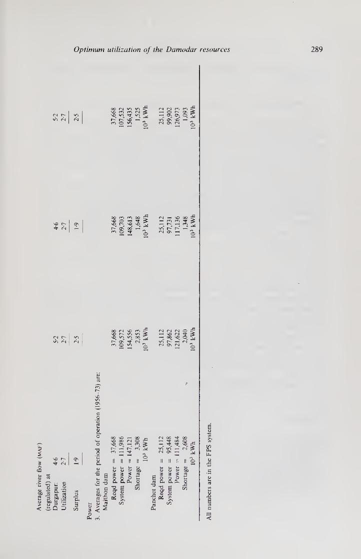
Aver
age
river
flo
w (
maf)
(reg
ula
ted
) at
Du
rgap
ur:
46
Uti
liza
tio
n
2-7
Optimum utilization of the Damodar resources 289
oo 04 «o »0 45 04 04 m m 45
sO m m 04 y—t O r- OS 04 r- so v© m m 4* Os ON o 4x! to 04 04 r-" C"" so" y—i
m O
*0 Os" so" m O
m o to 04 Os C4
SO r- Tf rs
3 a, Ur 3
C/5
x n m oo sO O so so r-" as oc mo rf
oo 5T
3*
^ O
3 ST) Os
G O
8. O
•u .2 8. <U 45
X 'O so oo 04 so Os —4 r-~-" »-h r«T m i rf
00 _e O 5 m ^4
II I! II ~
c2 -o G O
a> G £
I a
0) w
"O or o
C* u. <D ^
* < O
Pi cn
<u cd
> s
gt % aa E <L> CA
C/5
<u Oft 5 Ur o 45
C/5
—< sO OO m m tj-
’-h r-^ «o" r-" 04 os
oo 04 so CO 45 04 04 <N O
SO r- so SO y—> sO 04 04 r** *q so SO tq OO 00 sq © »0 04 04 0-" Os" 04 m
m
to" r~-" *—r <n" m o •O 04 Os 04
(N X t}- Tf OO
-X ^ so" <o" i-T 04 os ^
*-1 »— r- a> o) - * is * I a aa a -§. e “ U 2 | * £ § 1/5
Cu
00 Oft 3 Ur o
45 C/5
on Ok U- o> 3 C <D Ur <3 C/3 Ur
25 E G C

290 Basawan Sinha and P Ramakrishna Rao
Damodar system, both existing and proposed, will help in maximisation of utilization and benefits.
7. Conclusion
The following conclusions emerge from the simulation model studies discussed above:
(i) Hardly 50% of the available water resources of the Damodar are being utilized at present; and even after the proposed abstraction of about half a million acre feet materialises there will be surplus water to the extent of about 1-9 maf on an annual average. This includes the inflow contributed by the uncontrolled catchment between the Maithon and Panchet dams and the Durgapur barrage. (ii) Since over 80-85 % of the run-off occurs during the monsoon months and that too erratically, the scope of improvement in utilization is only through increased conservation storages. Thus, there is need to increase the conservation storage of the existing dams, as far as practicable, and for creating additional storage in the upper catchment. In the latter case, there should be ample provision for carry-over storage. (iii) The dams in the Damodar system should be operated as an integrated system under one unified control. (iv) There is need for review of the existing Regulation Manual, more so because hereafter there will be utilization on the upstream of the Maithon and Panchet dams through the Konar, Tilaiya and Tenughat reservoirs. The regulation of these reservoirs should be supported by inflow forecasting to improve their efficiency. (v) Additional dams to be constructed upstream for utilization of the Damodar waters should be planned so as to conserve the monsoon flows only. Status-quo in respect of dry-weather flows has to be maintained as the existing draws at Maithon and Panchet have limited conservation storage for meeting the demands of water supply and hydel power generation. (vi) There are various possibilities of meeting the committed requirements of water and of increasing utilization on the upstream in Bihar. This study had limitations, inter-alia, in respect of (a) length of period for which hydrologic data were available and (b) non¬ availability of particulars of works proposed to be implemented in the upper catchment. (vii) A simulation model for the Damodar system is needed not only for long-range planning of its water resources development but also for day-to-day operation.
References
Banerjee N K 1975 Optimal operation of reservoir using system analysis: Optimisation of hydropower output
from a 5-resetvoir system by incremental dynamic programming', M.E. dissertation, Roorkee University Central Water Commission 1969 Regulation manual for Damodar valley reservoirs. Central Water & Power
Commission, Government of India, New Delhi US Army Corps of Engineers 1976 HEC-3: Reservoir system analysis for conservation. Hydrologic
Engineering Centre Voorduin W L 1945 Preliminary memorandum on the unified development of the Damodar river

Planning for the Subernarekha river system in Eastern India
BASAWAN SINHA*, RAMESH BHATIA** and SUPRIYA LAHIRIt
‘Central Flood Forecasting, Central Water Commission, “Kamata Sadan”, 427/C, East Borning, Canal Road, Patna 800001, India
“Institute of Economic Growth, University of Delhi, Delhi 110007, India
tMIT Energy Laboratory, MIT, Cambridge, MA 02138, USA
Abstract. The study describes the systems studies carried out to plan a river basin in order to determine the nature and size of water storage facilities and releases for irrigation and industrial uses, and the associated cropping pattern. The model has been formulated in the framework of a linear programming model for a specific target year. This model is developed in the context of planning the Subernarekha river basin. The results are discussed and these provide information and insight suggesting the need for more disaggregated analysis of interaction between irrigation and related agroeconomic parameters.
Keywords. River basin planning; lp model; storages; Subernarekha river system; agroecon¬ omic parameters.
I. Introduction
The Subernarekha is an inter-state river flowing through Bihar, West Bengal and
Orissa. It rises in the Chhotanagpur plateau of Bihar and flows into the Bay of Bengal.
The upper part of the Subernarekha and its tributaries run through the fertile land of
Bihar, but the farming in this region is mainly dependent on the inadequate and
untimely rains, and the water resources of the Subernarekha river system remain largely
untapped. The upper basin, besides containing fertile land, also contains large reserves
of minerals. A number of important industries have therefore grown along the banks of
the river.
For integrated development of this basin the construction of dams, one on the
Subernarekha at Chandil and the other on its tributary Karkai and two barrages, one
on the Karkai at Bhua and the other on the Subernarekha at Galudih, is proposed. The
gross irrigated area envisaged under this programme is about 2,30,000 ha in Bihar.
This study aims at an economic appraisal of the scheme in a coordinated manner to
determine the nature and size of the water storage facilities and the releases for
irrigation and industrial uses as well as the associated cropping patterns such that the
water potential in this region is exploited optimally.
Detailed systems analysis studies are required for this purpose which incorporate the
interactions of hydrological, agronomic and economic considerations in an integrated
manner. Initially the model was formulated in the framework of a linear programming
(lp) model for a specific target year which would take into account some of the chief
interrelated factors affecting the optimum utilization of the water potential in this area.
Since the projects mainly benefit the agricultural sector, both the cropping pattern and
A list of symbols & indices is given at the end of the paper.
291
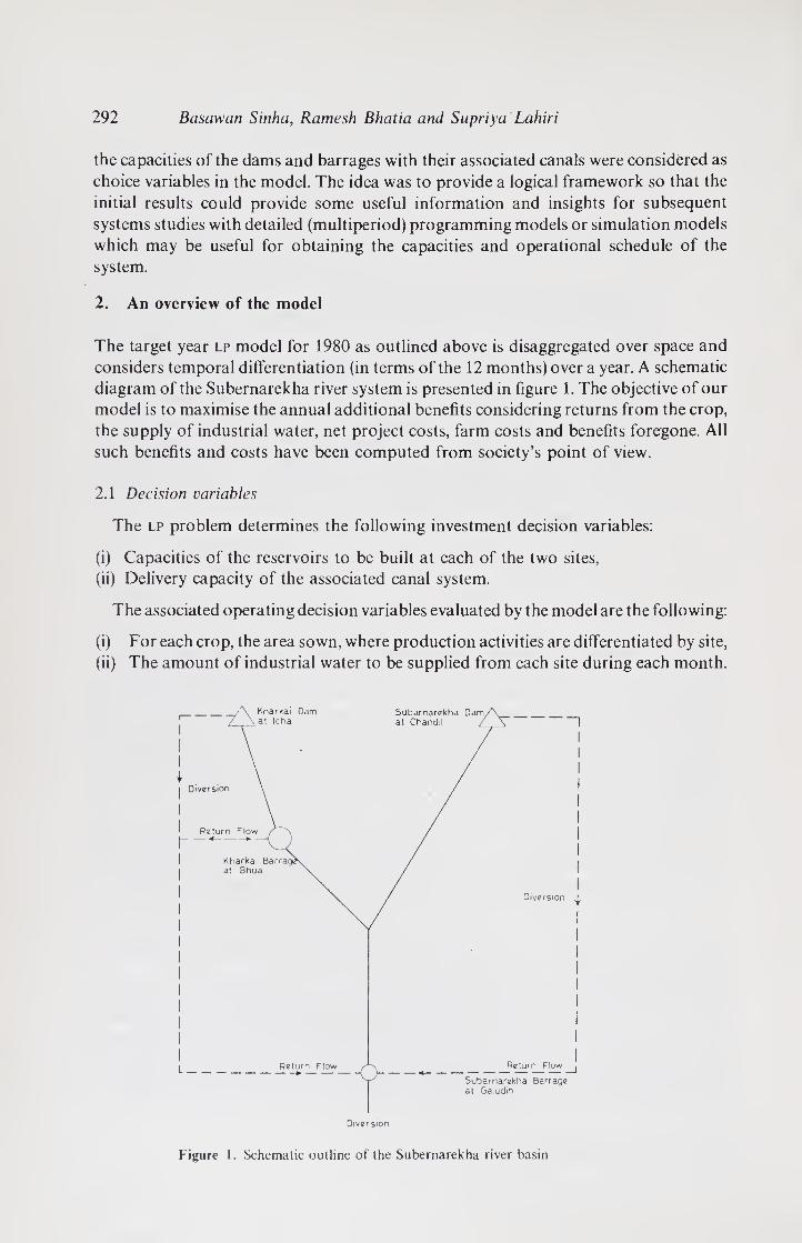
292 Basawan Sinha, Ramesh Bhatia and Supriya Lahiri
the capacities of the dams and barrages with their associated canals were considered as
choice variables in the model. The idea was to provide a logical framework so that the
initial results could provide some useful information and insights for subsequent
systems studies with detailed (multiperiod) programming models or simulation models
which may be useful for obtaining the capacities and operational schedule of the
system.
2. An overview of the model
The target year lp model for 1980 as outlined above is disaggregated over space and
considers temporal differentiation (in terms of the 12 months) over a year. A schematic
diagram of the Subernarekha river system is presented in figure 1. The objective of our
model is to maximise the annual additional benefits considering returns from the crop,
the supply of industrial water, net project costs, farm costs and benefits foregone. All
such benefits and costs have been computed from society’s point of view.
2.1 Decision variables
The lp problem determines the following investment decision variables:
(i) Capacities of the reservoirs to be built at each of the two sites,
(ii) Delivery capacity of the associated canal system.
The associated operating decision variables evaluated by the model are the following:
(i) For each crop, the area sown, where production activities are differentiated by site,
(ii) The amount of industrial water to be supplied from each site during each month.
Figure 1. Schematic outline of the Subernarekha river basin
Planning for the Subernarekha river system 293
(iii) The downstream flows from each of the dams and barrages during each month.
(iv) The diversion for irrigation purposes from each site in each month.
(v) Volume of water to be stored by the end of each month for the subsequent periods.
2.2 Constraints
The levels of both the investment decision variables and operating decision variables
are simultaneously determined in the model such that the total additional benefit to
society, less the project costs, is maximized subject to the following constraints of
continuity, capacity, agronomy and land area.
(i) The flow continuity constraint for the dams for each period states that the inflows
should equal the outflows plus the water that is stored for the next period. The water
that is stored for the next period should not go below a minimum level (i.e. the dead
storage level). Since there are no storage facilities in barrages, the flow continuity
constraints simply require that the inflows should equal the outflows from such modes.
(ii) The capacity constraints for dams require that the volume of water to be stored in
each decision period should not exceed the capacity of the dam to be built at that site.
Similarly, the amount of water for irrigation purposes in each period should not exceed
the delivery capacity of the canal.
(iii) The irrigation flow constraints state that the amount of water diverted for
irrigation purposes each month should be at least as large as the water requirements of
perennial and non-perennial crops.
(iv) The land area constraint requires that the total planting in each season should be
restricted to the culturable command area less the acreage required for fodder crops
and the area left fallow in a particular season.
(v) Certain limits have also been imposed on the production of certain crops (for
example, vegetables) as commodity demand functions have not been included in our
model. Certain constraints have also been introduced on the acreage under paddy to
reflect consumer preference for rice.
Detailed sensitivity analyses have also been carried out on different assumptions with
respect to the river flow data and detailed parametric programming has also been
performed on the coefficients of the objective functions (especially with respect to
changes in the relative price of wheat to that of other crops) for mapping out the
different patterns of irrigation development with respect to changes in the above
parameters.
3 The algebraic formulation of the model
The mathematical model is described by (A1)-(A14) (appendix A). There are four sites
considered in the model which are differentiated by the subscript i (see list of symbols &
indices).
Fourteen crops have been considered indexed by t. Irrigated crops with different
levels of irrigation have been designated as different crops. The figures in brackets
denote water supplied corresponding to which appropriate yields are adopted.
The activities or choice variables, of which the two land use activities are measured in
thousand hectares and all the remaining which are hydrologic activities, are measured in
million cubic metres.

294 Basawan Sinha, Ramesh Bhatia and Supriya Lahiri
4. Data base
The main data inputs for the model are: benefit and cost coefficients in the objective
function, water requirements of various crops for each month, hydrological inputs for
different months at various sites, downstream flow requirements at the Subernarekha
barrage for downstream use, coefficients of return flows from irrigation and industrial
water supplies and coefficients of reservoir losses in each month.
In the objective function, the coefficients required are: value of each crop net of
variable farm costs, fixed farm costs, unit revenue from the sale of industrial water, the
annualized investment costs of reservoirs and canals and annual maintenance costs of
reservoirs and canals. Gross value of each crop has been estimated as the sum of the
value of grain output and the value of fodder. The assumptions regarding yield rates,
prices and value of output have been given in table 1. The yield rates are based on the
data obtained from the Agriculture Department (Ministry of Agriculture 1971) and
from the Project Report (Ministry of Irrigation and Power 1972). The yield of paddy is assumed to decline by 10% when the total water requirements (at canal head) are
reduced from 75 to 67-5 cm. Similarly, the yield of wheat is assumed to be 10% lower
when the total water input is reduced from 70 to 57-5cm. The accounting (or
shadow) prices used to estimate benefits from major crops are expected to reflect the
social value of these agricultural commodities since these prices take into account
(i) economic cost of production of additional foodgrains in a surplus region of the
country plus (ii) the economic cost of transportation (including cost of distribution
and storage) of these commodities to the project region. We have used prices of
foodgrains fixed by the Agricultural Prices Commission in the nearest surplus region plus the average cost of transporting these commodities to the project region (Sinha &
Bhatia 1976). Valuation of agricultural output on this basis is expected to reflect the
need for increasing agricultural output in regions away from the granaries of the
country. The net value of each crop has been estimated by deducting the cost of seeds,
fertilizers and manures, pesticides and human labour. To reflect the relatively higher
levels of unemployment of unskilled agricultural labour in the region, we have used
shadow wage rates which are lower than the market wages. We have assumed the ratio
of shadow wages to market wages to be 0-25. The estimated values for various elements
of variable costs and net benefit for each crop are given in tables 2 and 3. The fixed farm
costs are assumed to include the following elements: (i) annualized costs of additional
bullocks and implements required in irrigated agriculture, (ii) annual costs of mainten¬
ance of bullocks, command area development costs such as those of land levelling and
shaping, field channels, field drains, improvement in facilities for storage, marketing,
transport and communication. These costs have been estimated to be Rs 136 per acre
and are relevant for the culturable command area at different sites (Sinha & Bhatia
1976).
The social cost of investment for the dams and canals has been calculated by giving
due consideration to the foreign exchange component, wage component due to
unskilled labour and the construction period of the project. The social investment cost
per unit has been calculated by applying the following formula.
/ = £ XP. MtMl+r)*-’ 1=1 i
(1)

Tab
le
1.
Yie
lds, p
rice
s an
d b
enef
its
for
dif
fere
nt
crops
(at
soci
al p
rice
s)
Planning for the Suhernarekha river system 295
o '— u. Q SO
g 8 u~> O O o o o © 00 O
D ■*-* o3 o r*"> 00 oo OS */“> OO m r-i 3 3 tj cc oo oo r- m so oo oo r~ <N OS SO Os cd o, 8
*“! r- <N <N cn cn oo Os rsj SO
z o
-o CO JC C/5
o »-< <U X-V V -a £ 3 *g * a cP >
-o O'
o,^ *
1) <r>
31 t2 a
° - 3 ~
•g S* «2 £ 60 o ~
a> 3
* o
"O o3 J= C/5
8 o; C VD cx pc:
<u h 2 2 jj 8 > =5.
a
D. O u,
u
OO O s© SO wp o so oo 6 rf ^ O rn ab oo oo fN M r- n ^
m r*->
m n n r) ^ n
■o r- rn rp r- <N <N a b rs n t fN b fN (N -H -H n (N
O O O rr o o r- «/"> m
(N
so OC O
r*“> u~) m <n m
r- o O rn ^ O O rT r^i
fNsoojC'jvnt^-CNioor-'QOCO -Hfnoooono-'00oo^Ol^fr’H oo»nr-r^mas^ooooor^oasvcos
♦rou-iOO^^OOOOrslu^oO 0'0s^0'fOronrOrf'-<'-'0'!>r<i
r- sor^oooor-r^rfo bvbdvp'^rsribr^’i-
fN
•o 0)
o "O <D
¥°|lg .— o t-c x) “ “ ^ g
& a« fc H O .t* u.
"8
SS.a .a S S S! £ <2 5 s =t £ <2
JJ JJ V) a •C -O — St 3S^H u <u 2 td 60 60 "O 60 u u cd 3 > > ft. 00
^ a § 'E (/i -r* <U C c/5 ^
3 w (X
il
O’
§
quin
tal
(100
kg)
; K =
kh
arif
; R
- ra
bi; S
= s
um
mer
(th
is i
s so
fo
r al
l th
e ta
ble
s)
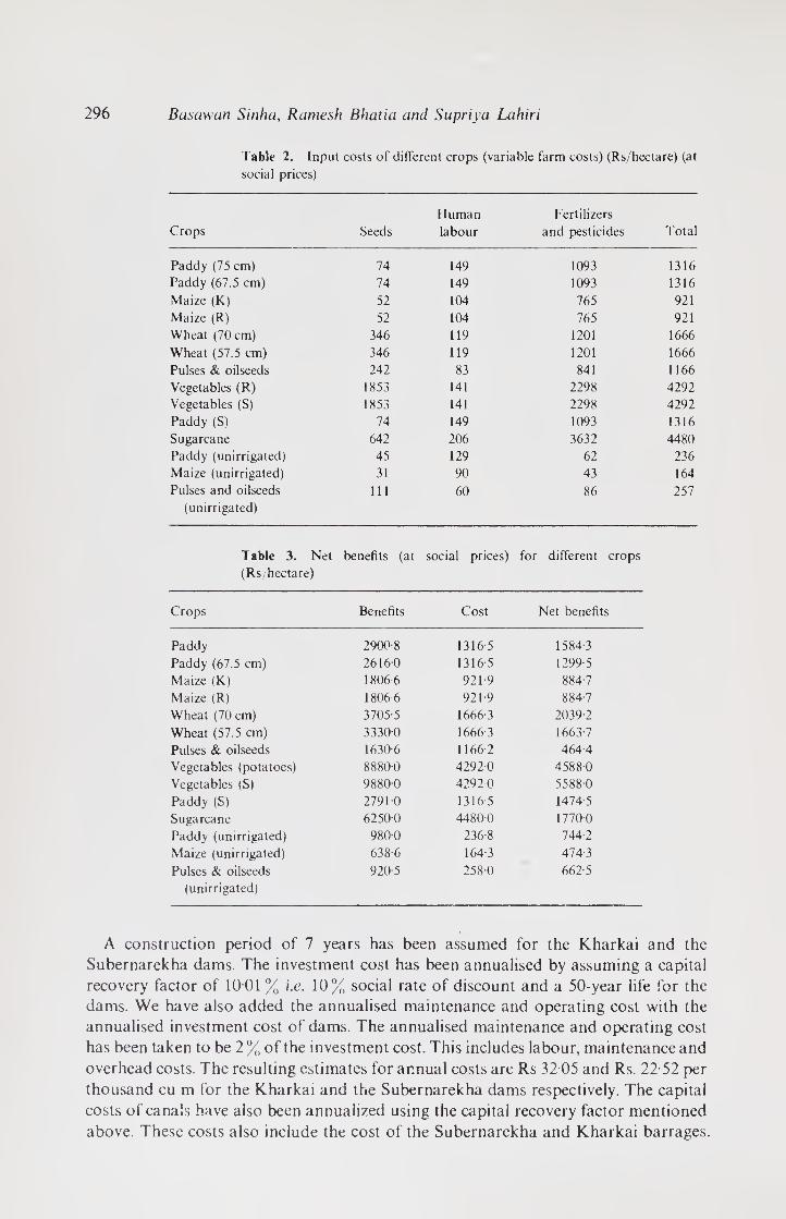
296 Basawan Sinha, Ramesh Bhatia and Supriya Lahiri
Table 2. Input costs of different crops (variable farm costs) (Rs/hectare) (at
social prices)
Crops Seeds
Human
labour
Fertilizers
and pesticides Total
Paddy (75 cm) 74 149 1093 1316
Paddy (67.5 cm) 74 149 1093 1316
Maize (K) 52 104 765 921
Maize (R) 52 104 765 921
Wheat (70 cm) 346 119 1201 1666
Wheat (57.5 cm) 346 119 1201 1666
Pulses & oilseeds 242 83 841 1166
Vegetables (R) 1853 141 2298 4292
Vegetables (S) 1853 141 2298 4292
Paddy (S) 74 149 1093 1316
Sugarcane 642 206 3632 4480
Paddy (unirrigated) 45 129 62 236
Maize (unirrigated) 31 90 43 164
Pulses and oilseeds
(unirrigated)
ill 60 86 257
Table 3. Net
(Rs/hectare)
benefits (at social prices) for different crops
Crops Benefits Cost Net benefits
Paddy 2900-8 1316-5 1584-3
Paddy (67.5 cm) 2616-0 1316-5 1299-5
Maize (K) 1806 6 921-9 884-7
Maize (R) 1806-6 921-9 884-7
Wheat (70 cm) 3705-5 16663 2039-2
Wheat (57.5 cm) 33300 1666-3 1663-7
Pulses & oilseeds 1630-6 1166-2 464-4
Vegetables (potatoes) 8880-0 4292-0 4588-0
Vegetables (S) 9880-0 42920 5588-0
Paddy (S) 2791-0 1316-5 1474-5
Sugarcane 6250-0 4480-0 1770-0
Paddy (unirrigated) 980-0 236-8 744-2
Maize (unirrigated) 638-6 1643 474-3
Pulses & oilseeds 920-5 258-0 662-5
(unirrigated)
A construction period of 7 years has been assumed for the Kharkai and the
Subernarekha dams. The investment cost has been annualised by assuming a capital
recovery factor of 10 01 % i.e. 10% social rate of discount and a 50-year life for the
dams. We have also added the annualised maintenance and operating cost with the
annualised investment cost of dams. The annualised maintenance and operating cost
has been taken to be 2 % of the investment cost. This includes labour, maintenance and
overhead costs. The resulting estimates for annual costs are Rs 32 05 and Rs. 22-52 per
thousand cu m for the Kharkai and the Subernarekha dams respectively. The capital
costs of canals have also been annualized using the capital recovery factor mentioned
above. These costs also include the cost of the Subernarekha and Kharkai barrages.
Planning for the Subernarekha river system 297
The revenue from the sale of industrial water has been taken to be Rs. 61-32 per
thousand cu m.
The yield series for water for the two dams and the two barrages have been developed
on the basis of rainfall series computed at each site separately. The rainfall runoff
correlations which have been used for computing the yield series have been developed
for Mango Weir (Jamshedpur site) at which runoff data were available for the period
June 1961 to October 1973, assuming that the same will hold good at these dam and
barrage sites. Since the Subernarekha waters have been allocated to the three cobasin
states on the basis of an estimated 75 % dependable annual water yield, the hydrological
input in this model for the year in which the annual yield corresponded to 75%
dependability is different for different control points. Therefore the adoption of
different years for different sites in a static linear programming model could neither be
considered appropriate nor consistent with the principle underlying the sharing of
waters among the States on the basis of water yield as estimated at Kokpara at 75 %
dependability. Accordingly, the year corresponding to 75% dependability at the
terminal structure, that is, the Subernarekha barrage site, was first found out in the 32-
year series and the computed month wise yield in this year separately at each site has
been utilized for this study. This procedure has also facilitated earmarking or reserving
water for utilization from above the control points by excluding catchment areas in
proportion to the 75 % dependable water yield.
In this study for 75% dependability, the monthly runoffs net of project/protected
utilization on the upstream of each site, corresponding to the year 1957-58 have been
considered. An alternative solution considers the yield series for 1946-47 which
corresponds to 50% dependability at the terminal structure i.e. at Subernarekha
barrage.
The economic and hydrologic data are given in tables 1 to 9.
5. Results
The results obtained from the model have been presented in the form of a Reference
Solution ( rs ) as well as in terms of sensitivity analysis. The rs is based on the following
assumptions: (i) 75 % dependability factor for water availability (ii) no bounds on area
under major irrigated crops such as paddy, wheat and maize, except for vegetables in
rabi and summer (5 % of culturable command area (cca) in each case); (iii) no upper
bounds on capacities of dams and canals; (iv) minimum flow required at Subernarekha
barrage for downstream use; (v) bounds have been imposed on industrial water supply
using exogeneously given estimates; (vi) upper bounds have been imposed on the
following unirrigated crops: paddy (25% of cca), maize (15% of cca) and pulses and
oilseeds (5 % of cca). The sensitivity analysis is presented mainly in terms of changes in
relative prices of crops and area under different crops.
The results of the rs have been analyzed with respect to the following: (i) optimum
cropping pattern suggesting area allocated to different crops in various seasons (i.e. in
kharif, rabi and summer): (ii) the optimum capacities of the two reservoirs and the
associated releases for irrigation, industrial water supply and downstream uses; and
(iii) the associated diversions from the two barrages for the above-mentioned uses.
Table 5 presents the optimum cropping pattern in the rs and tables 6-9 give the
corresponding water balances at each of the 4 sites. It may be seen that irrigation
intensity (gross area irrigated as a ratio of culturable command area) for the two dams
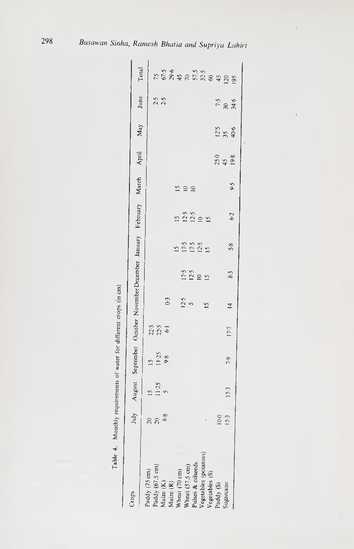
298 Basawan Sinha, Ramesh Bhatia and Supriya Lahiri
3 o H
c 3
03
wo ''P wo &\ wo N *0 (N ^
wo wo <N rN
wo wo © i"-’ <N . . O WO © ^ n \D ’t M O'
wo o
w~> vO rsj wo Q — cn rt
D. < WO wo On <N Tf
O u. <3 5
wo O © wo d\
cd 3 u»
X> <D
Un
WO wo
^ (N (N O ^ rs| vb
as 3 G 03
IT)
r' cn tn
E (J C
Cl O
£ E <L>
8 Q u.
J
> O £
wo wo t''- rN © wo
wo <N wo
£ O o o
<N <N vO <N <N
t*- r-
03 *
J5 E <D
O.
<N 0C
wo On
G
£
3 CT <U u,
2 c o S
jB «
H
3 GO 3
<
3
a o
wo cn wo X- 1/0
O O rN (N © ro © wo
V O
c/5 •*-*
“O ^
E c ¥ c »8.55 O wo O wo "G '—■ '—
>o K ^ o r»- O c/s vs
— — — — — '— X) JO <D '‘O '•O C/5 ^ C3 >-
S S^ss-os « « « « ^ - 5* 59 ^ «
ft. oo
on c 3
u I c2<2ss£££££
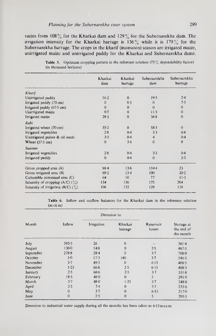
Planning for the Suhernarekha river system 299
varies from 108% for the Kharkai dam and 129% for the Suhernarekha dam. The
irrigation intensity for the Kharkai barrage is 136% while it is 179% for the
Suhernarekha barrage. The crops in the kharif (monsoon) season are irrigated maize,
unirrigated maize and unirrigated paddy for the Kharkai and Suhernarekha dams.
Table 5. Optimum cropping pattern in the reference solution (75% dependability factor)
(in thousand hectares)
Kharkai
dam
Kharkai
barrage
Suhernarekha
dam
Suhernarekha
barrage
Kharif
Unirrigated paddy 16 2 0 19 5 2-4
Irrigated paddy (75 cm) 0 8-5 0 7-3
Irrigated paddy (67-5 cm) 0 0 0 0
Unirrigated maize 97 0 11-3 0
Irrigated maize 28-3 0 34-8 0
Rabi
Irrigated wheat (70 cm) 35-2 0 58-3 0
Irrigated vegetables 2-8 0-4 3-3 0-4
Unirrigated pulses & oil seeds 3-3 04 4 0-4
Wheat (57-5 cm) 0 3-6 0 9
Summer
Irrigated vegetables 2-8 0-4 3-3 0-4
Irrigated paddy 0 0-4 0 3-3
Gross cropped area (A) 98-4 13-8 134-4 23
Gross irrigated area (B) 69-2 13-4 100 20-2
Culturable command area (C) 64 10 77 11-3
Intensity of cropping (A/C) (%) 154 136 175 204
Intensity of irrigation (B/C) (%) 108 132 129 179
Table 6. Inflow and outflow balances for the Kharkai dam in the
(m cu m)
reference solution
Month Inflow
Diversion to
Irrigation Kharkai
barrage
Reservoir
losses
Storage at
the end of
the month
July 393-5 26 0 _ 361-4
August 130-0 14-8 0 2-5 467-5
September 278-8 28-4 0 3-7 708-0 October 5-0 17-3 140 3-7 546-5
November 3-7 49-3 0 6 15 488-5 December 1-23 66-6 2-5 6-15 408-3 January 2-5 66-6 2-5 3-7 331-8 February 18-5 48-0 0 5 291-0 March 3-7 48-0 1-23 3-7 248-0
April 2-5 7-4 0 3-7 233 0
May 0 3-7 0 6 15 217-0
June 0 2-5 0 5 203-5
Diversion to industrial water supply during all the months has been taken as 615mcum.
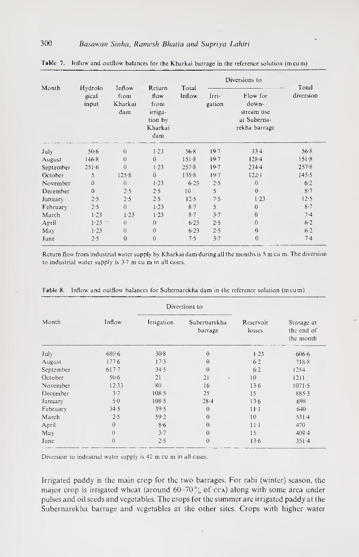
300 Basawan Sinha, Ramesh Bhatia and Supriya Lahiri
Table 7. Inflow and outflow balances for the Kharkai barrage in the reference solution (mcum)
Month Hydrolo Inflow Return Total
Diversions to
Total
gical from flow Inflow Irri- Flow for diversion
input Kharkai from gation down-
dam irriga- stream use
tion by at Suberna-
Kharkai rekha barrage
dam
July 50-6 0 1-23 56-8 19 7 33-4 56-8
August 146 8 0 0 151-8 19-7 128-4 151-8
September 251-6 0 1-23 257-8 19-7 234-4 257-8
October 5 125-8 0 135-8 19 7 122-1 145-5
November 0 0 1-23 6-23 2-5 0 6-2
December 0 2-5 2-5 10 5 0 8-7
January 2-5 2-5 2-5 12 5 7-5 1-23 12-5
February 2-5 0 1-23 8-7 5 0 8-7
March 1-23 1-23 1-23 8-7 3-7 0 7-4
April 1 23 0 0 6-23 2-5 0 6-2
May 1-23 0 0 6-23 2-5 0 62
June 2-5 0 0 7-5 3-7 0 7-4
Return flow from industrial water supply by Kharkai dam during all the months is 5 m cu m. The diversion
to industrial water supply is 3-7 m cu m in all cases.
Table 8. Inflow and outflow balances for Subernarekha dam in the reference solution (mcum)
Month Inflow
Diversions to
Irrigation Subernarekha
barrage
Reservoir
losses
Storage at
the end of
the month
July 680-6 30-8 0 1-23 6066
August 177-6 17-3 0 6-2 718-8
September 617-7 34-5 0 6-2 1254
October 50-6 21 21 10 1211
November 12-33 80 16 13 6 1071-5
December 3-7 108-5 25 15 885-3
January 5-0 108-5 28-4 13-6 698
February 34-5 39 5 0 11-1 640
March 2-5 59-2 0 10 531-4
April 0 8-6 0- 11-1 470
May 0 3-7 0 15 409-4
June 0 2-5 0 13-6 351-4
Diversion to industrial water supply is 42 m cu m in all cases.
Irrigated paddy is the main crop for the two barrages. For rabi (winter) season, the
major crop is irrigated wheat (around 60-70°G of cca) along with some area under
pulses and oil seeds and vegetables. The crops for the summer are irrigated paddy at the
Subernarekha barrage and vegetables at the other sites. Crops with higher water

Planning for the Suhernarekha river system 301
*
3 X M
o D <D OX) 53 Ui
3
■8 C U<
3 fcj
u. C/J (U
£ 3
3 X
i5 (X)
3
ooONmoommi/n^ m ^hh^oboboonOOOn NOOONOmmmC'X '
U-
Q s-? l/-:
<D OX) 03 V-. V-l 3
X)
3 X M D t>« 03 C u_ 0> x 3
on
a* o c
j3
X)
£ o
<c 3 o
*o c o3
£ o
53 C
On ju JB * H
c o
5 o> C o .£ o
H Q
6 2 o3 X £ W <0 C/D c =t m o i> 2
T3 u- . 3 3
s ^ «
C O
03 OX)
03
3 o o «c H .S
03 X
C O <D
- — l— 3 o3
ox) £ ’C <u 3 x» 3 a ^ £ 6
o
£ o
q3
<D C6
£ O
53 C
03 X
> _ <D Ǥ I i 1
3 on
■£ g> 5 X -
c o
s
3 a c
rf- m OO 'O On >n NO <N oo m m >n
rn h (N no O c© oo mi m
r- oo — 'O 3" no rt m
m rn >n rs <N <N m m m
no no m m c-x r-x m up up XO'-'^obobcbNOOr-r'-r-x
<NONOmmm<N’—< m m m —<
hhnri'OMr-hhr-i
Ooornu^OrNr^^oxoooooo hNOobrXht^O'cbin'nin
M h oo n io io rf m m m m m m u'N -—
m co m mm c-x <px <N up rp rp <N <N
«^<NmmX<X<ooo
O m
oo tp NO O g o o — rx —<
m <n o o o o o
wn <N OOOooi/^fNNoOOOOO
«-l r- rx (N
m u'-j cp r- »/*> up up fN
^moc^-mcxrxrx^ooo O r- m —> —■ m t—« m
&
a § OX) 3
< IX)
D. o
3 ^ 2 a 4> x
tx 2
•c & g a, J2 5 < S £
*o c 03
3 3
OX) o3 G G o3
X)
3 V-. o3 X
X)
a o
3 o a
NO ON <N 03 X
0) (-< <3 C V-
£ 3 on
0X) 3 H 1-4 3
X)
3 M
V-4 3 X
X
(X cx 3
3 £
3 "O C
a o <£ £ o
53 C G 3 ox (-4 <u X H b
y K
hark
ai
dam
3-7 m
cu
m

302 Basawan Sinha, Ramesh Bhatia and Supriya Lahiri
requirements had a substantially greater yield than crops with lower water requirement
although the fixed costs were the same. For this reason the former crops have been
preferred to the latter.
The solution suggests that the optimum economic use of water would be to use it
mainly on maize in the kharif season (around 45 % of cca) and wheat in the rabi season.
It is economic to add adequate storage capacities in the two reservoirs such that
available water yield in the monsoon period is carried over to the next season for use in
the rabi crops. This is because the net social value of wheat per hectare is Rs 2040
compared with Rs 1584.30 per hectare of paddy, although the total water requirement
for wheat (70 cm) is less than that for paddy (75 cm). Even within kharif crops, irrigated
maize is preferred over irrigated paddy on account of lower water requirements
although the yield (and the benefit) for maize is lower than that for paddy.
These results have to be analyzed further by changing the assumptions regarding
(i) net benefit from wheat to net benefit from other crops (ii) preference of
consumers for rice vis-a-vis wheat or maize. In table 10 we have presented the results of
changes in optimum cropping pattern when the net benefit from wheat is parametri¬
cally decreased up to 40 % of the estimated value in the rs. There is no significant change
in the cropping pattern until the net benefit from wheat is decreased to 60 % of its level
in the rs. When the wheat benefit is reduced by 40%, substantial area is allocated to
irrigated paddy in the kharif and irrigated maize in the rabi seasons. In the rabi season,
the entire area under wheat gets shifted to irrigated maize and in the kharif, area under
maize gets reallocated to paddy. The area under irrigated paddy during the kharif also
increases mainly on account of the total available area in the rabi season going to
irrigated maize. If additional crop area was available, the model may have preferred to
store more water in the kharif to be used later in the rabi season.
Table 11 shows the optimal cropping pattern when at least 65 % of the land is
assumed to be under paddy cultivation to reflect the consumer preference for rice.
When comparing this table with table 5 we see that: (i) the irrigated maize has been
almost totally replaced by irrigated paddy in both dams and (ii) the irrigated wheat
(70 cm) cultivated has been decreased by half in the Kharkai Dam and by about a third
in the Subernarekha dam, while the unirrigated crops have not been affected.
Although the benefit from irrigated maize is about two times that from unirrigated
maize, it is substantially lower than that of irrigated wheat. So the cropping pattern is in
favour of using the kharif land for unirrigated maize and saving the water for wheat in
the rabi season. Since the requirement of water for paddy .is about twice that for
irrigated maize, the increase in paddy cultivation increased the diversion of water from
the dams for irrigation. Thus the water yield in the kharif season carried over to the rabi
season is less than before. This in turn reduces the irrigated area under wheat as
reflected in the results.
The capacities of the two reservoirs do not change significantly until the net benefit
from wheat decreases by 35 to 40%. In the rs the optimum storage capacity of the
Kharkai dam is 707 8mcum (table 6). This is lower than the capacity planned at
present, which also takes into account the carryover storage from year to year besides
carryover from season to season. The optimum storage capacity for the Subernarekha
dam is 1254 m cu m (table 8). This is only marginally less than the 1470 m cu m planned.
The optimum capacities in the solution with lower net benefit (60 % of that in the rs) are
616 5mcum and 1233mcum (table 10).
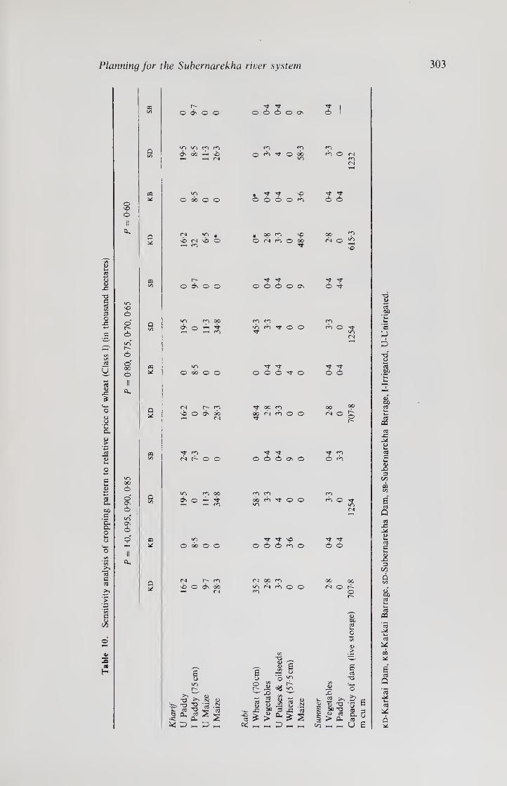
Table
10.
Sen
siti
vit
y a
nal
ysi
s of
cro
pp
ing p
att
ern
to r
elat
ive
pri
ce o
f w
hea
t (C
lass 1
) (i
n t
ho
usa
nd h
ecta
res)
Planning for the Subernarekha river system 303
O sO
CO
U
a u
SO ©
o'
i/~i r- ©
cT oo CO *
Q *
oo ©
o' Os
o^ o
co *
a u
o 6s o o
up O ob o o
CN| wp * SO <N v© o
O ds o O
wn <n oo Os © *-* Th
O oo O O
fNl C- cn sb O On CO ^ <N
Tf rn
n h O O
v> f*“i oo 60^6 — — <n
10 O 00 o o
<N r- rn sb o ds ob
6 o r-
•S' ^ N d> ^ ’O 2 ’cd o (X « 2 5
0- 2 ^ D D -
O © © O OS
# Tf Tj- Sp O © O O rb
O <N rn © OO Tf
’'t O O © O os
m rt O O 'rt
Tf rf O O © Tf o
t* 0© rn ob fN rb O ©
"<t rf O © © Os O
00 m Tt O O wn
TT Tf so O © O rb O
<N 0O rn ub cb rb O O
■S £ C< _
T3 _
I i o 'O
C/5 r~^
a> 2 n g> P X! rt
> ^ ^ S hDmh
Tf O
rn m rn rn rn
6s ob Oh sb O b O ob rb O <N y—i «-H rsj un m
<N
rt- rt o ©
op <N O ^
so
Tf Tf © rt
rn fb O t un
<N
rt rt o ©
00 cb 0 5
rt rn © rb
O rt >n <N
rt rt © ©
00 00 bob
o
<u 0L rt
V >
~o o >s
a> jc
£ u "O '3 E £ oo T3 3 3 s £ £ g- 3 3 ^ Oh rt ^ H H U G K
D-K
arkai D
am,
KB
-Kar
kai B
arra
ge, S
D-S
uber
nar
ekha
Dam
, S
B-S
ub
ern
arek
ha
Bar
rage,
I-I
rrig
ated
, U
-Unir
ngate
d.

304 Basawan Sinha, Ramesh Bhatia and Supriya Lahiri
Table 11. Optimum cropping pattern in Reference Solution with lower bounds on paddy
(in thousand hectares)
Kharkai
dam
Kharkai
barrage
Suberna
rekha
dam
Suberna
rekha
barrage
Kharif
Unirrigated paddy 16 2 0 195 2
Irrigated paddy (75 cm) 25-5 8-5 30-8 7-7
Irrigated paddy (67-5 cm) 0 0 0 0
Unirrigated maize 9-7 0 113 0
Irrigated maize 2-8 0 4 0
Rabi
Irrigated wheat (70 cm) 18 0 38 0
Irrigated wheat (57 5 cm) 0 3-3 0 8-9
Unirrigated pulses and oil seeds 3-3 0-4 4 0-4
Irrigated Vegetables 2-8 0-4 3-3 0-4
Summer
Irrigated vegetables 2-8 0-4 3-3 0-4
Irrigated paddy (75 cm) 0 0-4 0 3-7
Gross cropped area (A) 803 13 4 114 2 23-5
Gross irrigated area (B) 52-2 13 79-3 21
Culturable command area (C) 64 10 77 11-3
Intensity of cropping (A/C) (%) 127 132 148 207
Intensity of irrigation (B/C) (%) 82 128 103 186
To summarize, the tentative results do indicate the importance of analyzing the
possible choices available in utilization of water for different crops. It seems more
economical to increase the storage capacities mainly for use in the rabi season when
rainfall is relatively lower than in the kharif season. Since optimum cropping pattern
depends on many other agro-economic variables besides water supply, such as size and
ownership of land, availability of inputs, farmer’s attitude to risk, home-consumption
requirements and consumer’s preferences, there is need for more disaggregated analysis
of interaction between irrigation planning and related agroeconomic variables.

Planning for the Suhernarekha river system 305
(N <
m <
CO
o o
e
£
13 U
£
3-'
+
C/5
-o B 3 cx r cx O <D Vx D <D
15 5? > &
+-*
Z -c
T3 O
'C <u cx
o .i <D -*—»
' 00 JZ
rr
~ e : o - tfc!
<N t*-
05
I I
II 8 (73 <D
£ 13 Oi ix
8. -3
Ot) c
'E 3
T3 <D
4“"^
’ C/5
-C 4->
U(
£
3 O
’co t-. <U >
3-tJ
"H. _
§■£ ^ <D
is &jQ ^ c o
© -r-< -X rj b ^
1 -i &
a> "O ©
#x
-3 e v £X a.
><
-3
w-
-0“
W-
U
3“
W
c ■2 x> c
<3
XI N
■c a x> -S3 x X
'■S'S O 2
0 o 3
■a os (U o
3 c 03 O 3 \J3 3 3 s ,2P <. t
o o
T3 <U
_N
"c3 3 C 3 <
CO
e 3 -a
CO S
cx £ o ,3
o x>
o-S J‘5
173 ^
<D
CD o G CD
c/> to-* .C *5
© o
3 e
OD to-» ^ c
© © a
w VI c © © ©
£ ©
x~
I
i;£
+
a -3
'5 -x: x.
3 ~e
*
1-. -3 S .O ~ - C<
3 O c/5
+_> <d cd -G ■j-j XT to* . O o "O
*G <+■« O
S> « ■" X 3 u
<D >
C/5
fc-4
a I
— W) <D C
•t2 ‘5 “ 3 3
O „ * g>x: g
1 & -o _ "? 03 © « X O co
1- 3 3 O CX ^
:© -3 <_. <*h <U OXw fl O CX
+
<U -3 ■4—* -4—•
‘So . , <u
3
S 3
3
? 33-^5 O 3 O
id’ d-S-o a
£“ d
3 J3
2 a
~3
3 -C
XI X 3 C X 3
~C3 3
on
3
©
rn ‘C a> -a a G
cd -♦-* CN
a> II GJ • ■-* ■4—»
O
T> u. a O
" <D C4—<
■3 on < <
<to-< o
13 >
(U ^ .b: 2 § o t
<D C/5 CD
C/5 "O _
C3 CD <D o iQ 3 -S
3 ■3
3 k.
■w. CO C O 3
Cj 3 CX 3
V/ A\

Co
nti
nu
ity c
onst
rain
t fo
r K
hark
ai
barr
ag
e
306 Basawan Sinha, Ramesh Bhatia and Supriya Lahiri
, .£ 3
X) C &> ’ ” E 4—* 0 * E
0 ,U( 0 cc CD 4-* ■-, c oj •
^ 3 ri <U cd
-e- +
OeS
-a a <N
SI g o3 o
©»£ G d
+
1 .c 50 .1 £ E ^ o *S
<is c E
■2 ,2 2 u <U C/D
G X & 3
is <D - QS, g.
+ -o c <N G
-o o ‘C d Oh
n i!33
'O <
g o • ftH
C/3 li OJ >
tN-O
+
>> -Q
a o Oh l_ 3 D C/3 (X
p <3 "2 G £
o T3 ~ O
-a •G CU V3 cx "2 J=! eg
OJ
s o
S o ■-.<c
1 3 o
00 c
’C 3 T3
-3 it
+ i3 O
C "E
.2 a G _C 00 .3
03 O x. X o ~C3 o -c -S£ S- a c v
-o 3 03 V ,o
JS *—» It
>-< ft cu a •4-* 3 D
£ .g . C/D
? O x o5 * ^
£ 2 3 ?
“I"
V-. <D
O
'C
D.
D
CO •t 0
cSg
42 4-* G -Q
’d G ^ c ts ^
<N . CJ
3 C xj E +
c 2 •-1 cE c
o c3 x: > .ti
C/D ^
"O C/D O
is Tt
E E o o / *"• rU
CL) -C C/3 +-»
4-> ct3 G .2 u. CD .2 <D rO
>< a CD c3 ’£d
T3 .2
rf fO
Cl
G>0 <D u.
*c u.
■o v-
m
’C
a +
S E o o
cd *h .?8
CD
<D C/5 3 c o
— -o gl ^ o
-t “> -ft 73 ' G. +
-u t s « • h <N D,
6u. C CD -3
O > d ti: id
0) C/3 3
G O
C/3
a +
D G ■*-' D G Sb.SP E t d -S
E o 2 ‘S - a,
3 c- CD •£ 4—* G. — C X3 c2 •- ^ C/5 3 V. CL
g x: ■_ Q G -73 C/5 G h
• 2 a .2 G f/D O-i Uh
c 0 Sj i .s
00 _ 0 -£ 0 '~i
J= G -a ■—
^ G CN • G Q _4-J
3 ‘5b d 0 ,t;
"0 ^ l- t- .^X P 0*1 D 2 2 >>G X .G --' C/5 1! 0
O
r~ _
-< .2 W’S E rft
3 X) C i-i
£ G O
3 +
£ G D
D 4-> a £
Oh
C/3 G"
1? a
c •s w
■a’s
ii ”5 c5 it
G
t*3 +
o D ,-^CC c/3
^ 3
G 00
o «2 C4—1
C/D G _
.2 ■£ VD Tf
S g o
, U,
E
<2^
3 3 cl •ft
Tt G 00 m £ .£ -- c
rt a 'S 73
C/D T3* D +
-£}
it -H
c£
C" cy3 G O u
o
.00
<
w +
pG ’S G D i-> U Oh
G D
s ^ 2 G
*G cd 2. 0 cr u. cj cd u w) u, 3 <D Cd Oh O
V-. o
.2 ’5 c iD u a
1 ■ G O C
G D
3 CT D hH
L) 5 ^ ?g a
<0 > 2 W c. o A\
D ■4—»
*VD
-C 4—»
E o
G O G 00
-©- 0
i; m
ta a
V-H
u
+ is :-> O
T3 G cd
.2 4-4 cd
£ x
c -2
'X
•~P 53
? 3 iJ
(N .2° *c
kM
.2 u ^3 Q, V—1
.2 C/5 CD
M ^ 4G "C -e- 2 > 4-*
D a
1 5) + pp C/5 ri (D
in
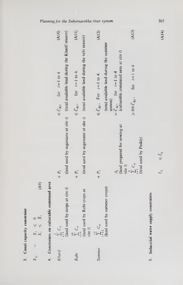
Canal
capacit
y c
onst
rain
t Planning for the Subernarekha river system 307
o
<
o
G O C/5
G © C/5
G O C/D
G © C/5
S G t-<
CD
-♦—»
U) _G 'C G
T3 T3 C
jg
ju 3
3 3 s* > 03 03
03 x U to X ■*-»
oo _g 'C 3
"O T3 a
_3
x 03
of o
03
<
Tt" o
o Pu,
*G cs G -
2 IU
O -4-*
5 IU
O £ IU
V/ V/ V/
to E E 3 C/3
to XI 4-*
00 c
'C 3
"O -o G
J2 <u X _3
>
”3 -4-*
o
(U 4—*
7r> -4-*
3 3 to u,
•3- 3
O T3 *■' G t-H 3
I O
u. u .O (U W—. '--
X 3 IH 3 C
O C/3 .—.
3 ^3 8lU 3
m
<
■^t o
IU x o A\
T—1
<
©
G
© G
3 Ih G &D G C/5
X) "O © C/5
G
"O G
G
© G
8 S-l
3 00 3 C/3
>> X
•o (U ft 3
33 G
3 00 G
'I O ft
~o to 1-4
3 a <D ltd a
"O ^ c
U
>-4 -o T3 3
(X So X
~o to
•a c
1-4“ V/
cC £ or s cC ■I? *-s* + + +
03 <
3 as I* 3
■c c 3
E E o to
to 4-*
' ft
4-4 3
ft o. o !— to
0 l><
V/ V/
U 3 -w
O
-D
"O © C/D G
C u" -O u= c
C/5 -w [^-3 n
G
-2 _ r ■, 0
- ^ 11
3 C/3 Cl. O £j
X 3
os So X
T3 to C/3 3
-a ^ 3 52
O
C/D
CL o
©
E E 3 ft So X
-a a> ft 3
, ! G
3
C • «■! 3
X s o U
3 -c
3^ £ X s
3 3 OS 00 1r>
Indust
rial
wate
r su
pp
ly c
onst
rain
ts

308 Basawan Sinha, Ramesh Bhatia and Supriya Lahiri
List of indices and symbols
Indices
i = 1 Kharkai reservoir at Icha
2 Kharkai barrage at Bhua
3 Subernarekha reservoir at Chandil
4 Subernarekha barrage at Galudih
t = 1 kharif unirrigated paddy.
2 kharif irrigated paddy (75 cm).
3 kharif irrigated paddy (67-5 cm). 4 kharif unirrigated maize.
5 kharif irrigated maize.
6 rabi irrigated wheat (70 cm)
7 rabi irrigated wheat (57-5 cm)
8 rabi irrigated pulses and oilseeds,
9 rabi unirrigated pulses and oilseeds,
10 rabi irrigated maize
11 rabi irrigated vegetables,
12 summer irrigated vegetables
13 summer irrigated paddy
14 perennial sugarcane
(The figures in brackets denote water supplied corresponding to which appropriate
yields are adopted)
Symbols
a, i
bt
Cti
<k
di
Ej
fj
h
lu
Ii(t)
K,
Pi
Qik.j
—net value of crop t at site i (Rs million per thousand hectares)
—annualised cost of reservoir i (Rs million per m cu m) for i = 1,3)
—land used by crop t (t = 1 to 10) at site i (i = 1 to 4)
—coefficient of fixed cost at site i
- annualised cost of canals, including cost of barrage at sites 2 and 4,
at site i (Rs million per m cu m)
flow for downstream use at Subernarekha Barrage during the jlh
period
unit value of industrial water supply at site i during the jih period
(Rs million per m cu m)
—investment per thousand cu m
Industrial water supply from site i during period j (j = 1 to 12)
—investment cost due to the iih element in the tth period
—capacity of the /'th reservoir
land used by the perennial crop (sugarcane) at site i (in (A1)-(A14); the
appropriate shadow price of the /th element in investment cost (in (1)).
— flow of water from site i to site k during the jth period

Planning for the Suhernarekha river system 309
r
Vii
Pu
lt,J
Pik.j
e
—the rate of interest
—the running time variable
—storage of water at site / at the end of the jth period
—capacity of irrigation canal at site /
flow of irrigation water from site i during period j
—reservoir losses at the ith site during the jth period
—efficiency coefficient for flow from site i to site k during the j th period
water required by crop / at site / during the y'th period (cm)
—coefficient of return flow from industrial water supply from the ith site
to the kth site/yth period
—water required by sugarcane during the yth period (cm)
—coefficient of return flow from the ith site to the A:th site during the /th
period
—the total number of years for the construction of the project
References
Ministry of Agriculture 1971 A guide for estimating irrigation water requirements, Tech. Ser. No. 2, Water
Management Division, New Delhi
Ministry of Irrigation and Power 1972 Report of the Irrigation Commission, Government of India, Delhi (3
volumes)
Sinha B. Bhatia R 1976 Economic appraisal of irrigation projects in India, Harvard University, Centre for
Population Studies

%
■
Study of a complex water resources system with screening and
simulation models
M C CHATURVEDI* and D K SRIVASTAVAf
* Applied Mechanics Department, Indian Institute of Technology, Hauzkhas, New Delhi 110016
t School of Hydrology, University of Roorkee, Roorkee 247 667, India
Abstract. The study describes a sequential iterative modelling process for a complex water resource system. Two types of analytical models are used to find a reasonably small set of possible systems optimal design alternatives for a complex river basin. These models are a linear programming deterministic continuous (lpdc) model and a linear programing deterministic discontirtous (lpdd) model. Linear programing has been used with linear approximation of the nonlinear functions. A simulation program has been developed which continues screening on the basis of the information obtained from the linear programing model. The models are developed in the context of analysis of the Narmada river, a large river
basin in India, for which in the first instance alternative combinations and capacities of six major dams have to be decided.
Keywords. River basin planning; lp models; simulation techniques.
1. Introduction
Although considerable interest has developed of late in systems planning of water
resources and it has been generally accepted that real-life applications are required to
validate the efficacy and worthwhileness of certain techniques, studies of real-life
complex systems are still relatively rare. For instance, it is well known that in view of the
non-linearities and discontinuities in the objective function, the final analysis of a
complex large real-life system could be best carried out by simulation. On the other hand,
simulation over even a promising feasible set would be computationally impossible.
Preliminary screening by a mathematical programming technique on the basis of which
simulation could be planned has often been recommended (Dorfman 1962;
Hufschmidt & Fiering 1966; Roefs 1968; Roefs & Bodin 1970; Loucks 3969). In this
context, it is profitable to investigate the value of mathematical programming in
preliminary screening and how it should be coupled with a simulation study. For
instance it may be instructive to ascertain how deterministic linear programming
models would help in identifying the optimal set in view of the stochastic inputs. An
attempt was therefore made to study a real-life large scale complex system, the
Narmada basin in India, by a combination of a mathematical programming screening
model and a simulation model.
1. This paper has been reprinted with permission from the American Geophysical Union: Chaturvedi M C
and Srivastava D K, Water Resources Res. 17: 783- 796 (1981) © AGU
2. A list of symbols and indices is given at the end of the paper
3. Conversion table
1 inch = 2-54 cm; 1 foot = 0-3048 m; 1 mile = 1 -609 km; 1 mile1 2 3 = 2-59 km2; 1 acre = 0-405 ha; 1 acre foot
= 0-1234 ham, 1 cusec = 0-02832 cumec.
311
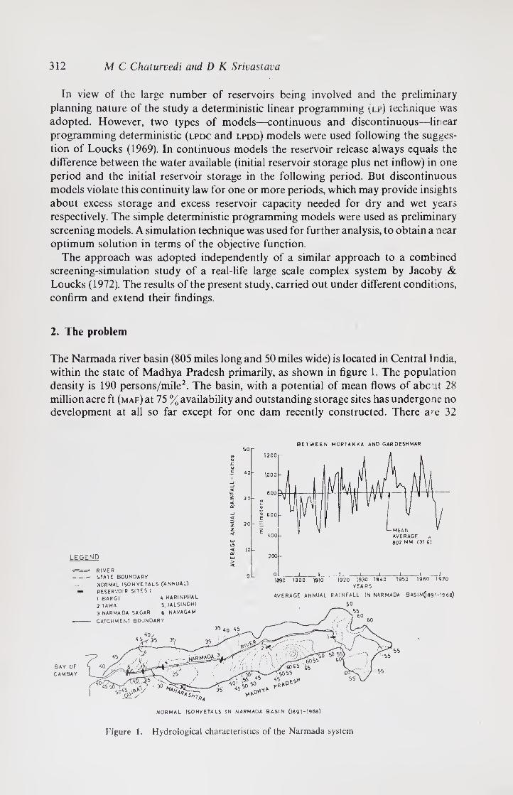
312 M C Chaturvedi and D K Srivasiava
In view of the large number of reservoirs being involved and the preliminary
planning nature of the study a deterministic linear programming ^lp) technique was
adopted. However, two types of models—continuous and discontinuous—linear
programming deterministic (lpdc and lpdd) models were used following the sugges¬
tion of Loucks (1969). In continuous models the reservoir release always equals the
difference between the water available (initial reservoir storage plus net inflow) in one
period and the initial reservoir storage in the following period. But discontinuous
models violate this continuity law for one or more periods, which may provide insights
about excess storage and excess reservoir capacity needed for dry and wet years
respectively. The simple deterministic programming models were used as preliminary
screening models. A simulation technique was used for further analysis, to obtain a near
optimum solution in terms of the objective function.
The approach was adopted independently of a similar approach to a combined
screening-simulation study of a real-life large scale complex system by Jacoby &
Loucks (1972). The results of the present study, carried out under different conditions,
confirm and extend their findings.
2. The problem
The Narmada river basin (805 miles long and 50 miles wide) is located in Central India,
within the state of Madhya Pradesh primarily, as shown in figure 1. The population
density is 190 persons/mile2. The basin, with a potential of mean flows of abc it 28
million acre ft (map) at 75 % availability and outstanding storage sites has undergone no development at all so far except for one dam recently constructed. There a*e 32
BETWEEN MORTAKKA AND GARDESHWAR 50
LEGEND 200 >
RIVER -- STATE BOUNDARY
1090 19 0 0 1910 19 2 0 193 0 1940 1950 1960 1970 YEARS
AVERAGE ANNUAL RAINFALL IN NARMADA BASIN^flgl-IS68)
50
NORMAL ISOHYETALS (ANNUAL)
RESERVOIR SITES :
1 BARG I 2TAWA
A. HARINPHAL
5. JALSINDHI
6 NAVAGAM
BAY OF
CAMBAY
NORMAL ISOHYETALS IN NARMADA BASIN (1091-1968)
Figure 1. Hydrological characteristics of the Narmada system

Water resources system with screening models 313
proposed reservoir sites, of which six are major ones. Thirty one lie in Madhya Pradesh
and the last one, Navagam lies on the border of Madhya Pradesh and the downstream
state of Gujarat. The sharing of waters between the two states and the proposed height
of this dam are controversial. The yearly rainfall, and typical yearly rainfall pattern are
shown in figure 1. The data have been collected from different reports (Master Plan
1972; Narmada Water Resources Development Committee 1965; and various Project
Reports). The observed river flow data are over a period of 16 years.
In the first instance, alternative combinations, capacities and operating policies of six
major dams—Bargi, Tawa, Narmadasagar, Harinphal, Jalsindhi and Navagam, as
shown in figure 2, are proposed to be investigated. There are three distinct alternatives
listed in table 1 for this set of dams as three possible values for the height of the last dam,
Navagam, have been chosen for analysis. In the first alternative shown in figure 2,
Navagam dam has the lowest height. In the second case, the height is raised till the first
upstream dam, Jalsindhi, is submerged. In the third case the height is further increased
till the next upstream dam, Harinphal, is also submerged. With increased water
requirements at Navagam in the latter two cases, irrigation diversions of the upper
dams would have to be modified. Two more alternatives, shown in table 1 are tried by
replacing the single-purpose irrigation projects to single-purpose hydropower projects
as suggested by some engineers. Multipurpose use has not been considered feasible for
the first two dams.
The capacity, cost and net benefits at the various sites vary considerably because of
hydrological and geological conditions. The average monthly flows based on a record
of 16 years at the dam sites are shown in figure 3. The reservoir capacity and capital
costs are shown in figure 4 for illustration. For each of the alternatives the maximum
permissible capacity is given from the physical configuration.
F6,t
A RESERVOIR
IRRIGATION AREA
Y‘A d6Jt ^ *
£h6
JE^>h
(C) ALTERNATIVE-3
£ POWER PLANT
RE SERVOIR SITES
1. BARGI 2.TAWA
3- NARMADA SAGAR A. HARINPHAL 5. JALSINDHI 6. NAVA GAM
Figure 2. Alternative configurations of the Narmada system

314 M C Chaturvedi and D K Srivastava
Table 1. Alternative configurations of the Narmada system
Alternative 1 Alternative 2 Alternative 3
Project name Purpose Project name Purpose Project name Purpose
1. Bargi I* 1. Bargi I 1. Bargi I
2. Tawa I 2. Tawa I 2. Tawa I
3. Narmadasagar I and E** 3. Narmadasagar I and E 3. Narmadasagar I and E
4. Harinphal E 4. Harinphal E 4. Navagam I and E
5. Jalsinghi E 5. Navagam I and E
6. Navagam I and E
Alternative 4 Alternative 5
Project name Purpose Project name Purpose
1. Bargi E 1. Bargi E
2. Tawa I 2. Tawa E
3. Narmadasagar I and E 3. Narmadasagar I and E
4. Harinphal E 4. Navagam 1 and E
5. Navagam I and E
* I = irrigation; ** E = energy production
o
zu. o<
NARMADA SAGAR-.
NOTE THE FLOWS AT A DAM SITE ARE THE CONTRIBUTIONS FROM ITS OWN CATCHMENT
CATCHMENT AREA CSQ
1. BARGI 5,6 20
2. TAWA 2,4 4 5
3 NARMAOA SAGAR 2 3,800
A harinphal 31,4 3 6
5. JALSINDHI 33,450
6 NAVAGAM 33,79 0
Figure 3. Average monthly flows at dam sites
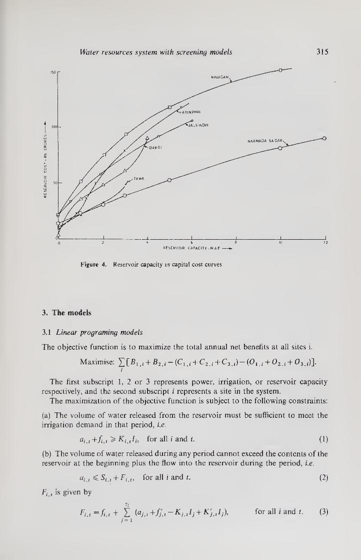
Water resources system with screening models 315
Figure 4. Reservoir capacity vs capital cost curves
3. The models
3.1 Linear programing models
The objective function is to maximize the total annual net benefits at all sites i.
Maximise: y^[BlJ + B2J-(Cij + C2ji + C3J)-{0ij + 02ii + 0iti)]. i
The first subscript 1, 2 or 3 represents power, irrigation, or reservoir capacity respectively, and the second subscript i represents a site in the system.
The maximization of the objective function is subject to the following constraints:
(a) The volume of water released from the reservoir must be sufficient to meet the irrigation demand in that period, i.e.
ai.t +f.t ^ KiitIh for all i and t. (1)
(b) The volume of water released during any period cannot exceed the contents of the reservoir at the beginning plus the flow into the reservoir during the period, i.e.
ait ^ Siit + Fi t, for all i and t.
Fi t is given by
(2)
Fift —f,t + X + j= i
for all i and t. (3)

316 M C Chaturvedi and D K Srivastava
(c) The continuity equation for each reservoir site is defined as
Si<t+1 = 5,+ t — ai t, for all i and t. (4)
In the continuous (lpdc) model the reservoir contents at the end of the year, Sj I+15are
assumed equal to the reservoir contents at the starting of the year S, t, for all reservoir
sites, but discontinuous (lpdd) models violated this continuity law for one or more
periods.
(d) The contents of the reservoir at any period cannot exceed the capacity of the
reservoir, or
Si, ^ Yt, for all i and t. (5)
(e) The flow through the turbines should meet energy generation demand. Variation of
generation efficiency at different sites is neglected at this stage
d,Ei — (l,025)(e)(HeM)(aM) ^ 0, for all i and t, (6)
where 1,025 converts million acre feet-feet to megawatt hours (MWh). At variable head
sites, He, , is not a known constant. Therefore, together with ai t it makes (6) a nonlinear
one. Appropriate He,.t was determined by trial and error as discussed later.
(f) Power production is also limited by the percent of time that the plant will produce
power specified by the load factor
ii tht(Hi) — 5,Ei ^ 0, for all i and t. (7)
3.2 Simulation model
A simulation program has been developed which continues the screening on the
basis of information obtained from the lp models given above. The rationale for
adopting a particular operating procedure, i.e. a set of rules for storing and releasing
water in reservoirs, is discussed later; it depends upon the alternative found most
suitable for simulation.
4. Computation
In the first instance and also because of limited hydrologic data, historic hydrologic
flows have been adopted for analysis. Hydrologic risk, evaporation losses, and flood
control benefits were not included in these models, while seasonal flows were used. The
lp model had 4 periods of equal length each year and the standard simplex program,
the mathematical programing system (mps) available with the ibm 360 Computer was
used for solving the lp problem. The simulation model considered 12-monthly periods
and the simulation program was developed on an International Computers Limited
(icl) 1909 computer.
The design values for cost and benefit were available for one capacity. These were
therefore estimated for different possible ranges for each of the six projects on the basis
of appropriate engineering approaches and suitable functions were developed
(Srivastava 1976). On the basis of the project design and with the help of project
authorities, sections for concrete dams (overflow and non-overflow section) and earth
dams were developed and quantities and costs were worked out. The cost of auxiliary
works was developed on a unit cost basis. The costs for the generating plant and

Water resources system with screening models 317
equipment and auxiliary works were developed on a unit cost basis. The cost of
irrigation and diversion works was also developed on a unit cost basis. Under these
three major heads both direct and indirect charges were estimated for 1973 prices.
Although they involved considerable work, it must be understood that the estimates are
for a methodological study rather than for detailed design. The reservoir functions are
given in figure 4. All capital costs were converted to annual costs for the linear
programs. A time horizon of 16 years was used in the analysis and annual costs were
calculated from the capital costs as the sum of the following items: (i) Interest on the
capital cost of irrigation and power projects at 7 % per annum; (2) depreciation on the
capital cost of irrigation projects at 1 %; (3) annual depreciation and replacement of the power plant at 2 % of the total cost of power plants; (4) maintenance cost of irrigation
at Rs 6 per acre for the area to be irrigated; (5) annual cost of operation and
maintenance for hydropower at Rs 10 per kW of installed capacity. In simulation the
present value of net benefits extending over the period of study for the system was
calculated.
4.1 lp computations
For both types of lp model, constraints were written only for one year. The decision
variables were namely aUt; Sit; Ij; H, and £;. lpdc models were the first type to be used
and mean monthly flows were used as the input, as shown in table 2. Values of K, , and
S, for each time period are given in table 3.
Table 2. Mean flows at dam sites (/)_,)
Time Mean flow* average taken for 16 years historic flow data (maf)
period Bargi Tawa Narmadasagar Harinphal Jalsindhi Navagam
t i = 1 i = 2 i = 3 i = 4 i = 5 i = 6
1 008101 0 04118 0-54620 0-01405 003768 0-00288 2 0 10043 0-04232 0-37251 007613 0-02936 0-00492 3 6-23475 2-78181 15-29213 0-86832 1-26628 0 12533 4 0-62159 0-29899 2-73611 0-19188 0-16823 002666
Total 7-03778 3 16430 18-94695 1-15038 1-50155 0 15979
* The flows at a dam site are the contribution from its own catchment and are the sum of average monthly flows.
Table 3. Values of Ki t and d,
Time Percentage of total annual irrigation requirement Ki t Total
period Bargi Tawa Narmadasagar Navagam requirement* (%)
t i = 1 i = 2 i = 3 i = 6 t
1 24-87 19-49 30-52 9 39 27 2 21-73 5-55 32-01 28-07 21 3 15-65 51-12 11-06 30-93 24 4 37-75 23-84 26 41 31-61 28
Total 100 00 1
100 00 100-00 100-00 100
At 60% load factor
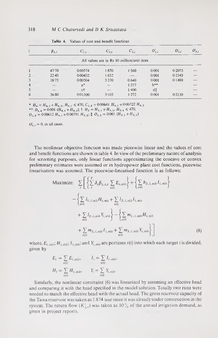
318 M C Chaturvedi and D K Srivastava
Table 4. Values of cost and benefit functions
i fii., C'u C'2,i C'3,i O’u 0'2.i 0'3,
All values are in Rs 10 million/unit item
i 47-70 0-00574 1-870 1-560 0 001 0-2075 — 2 22-45 000432 1-632 — 0 001 0-2345 —
3 18-75 000504 3-370 0-640 0-001 0-1488 —
4 — a* — 1-377 b** — —
5 — cf — 1-400 dt — — 6 36-80 0-01500 3105 1-272 0 001 0-2130 —
* H4 = W4t1 +H4,2, H41 <470, C,,4 = 0-00641 tf4>1 +000722 H4,2 ** D,.4 = 6-001 (H4>1+H4i2); t Hs = Hyi+Hy2, Hyl < 470, Oi 5 = 0-00612 HS1 +0-00791 H52; f 0,,5 = 0-001 (Hyi+Hy2)
0'3i = 0, in all cases.
The nonlinear objective function was made piecewise linear and the values of cost
and benefit functions are shown in table 4. In view of the preliminary nature of analysis
for screening purposes, only linear functions approximating the concave or convex
preliminary estimates were assumed or in hydropower plant cost functions, piecewise
linearisation was assumed. The piecewise-linearised function is as follows:
Maximize: I Y Y Ei,s(i) ( + ) Y ^2 ,i,s(i)Ii,s(i)
i L l t s(i) )
) Yd , >, s(i) Hi, sii) E Yd 12, i, s(i) Ls(i) s(i)
+ Y ^3, i,s(i) Yi s(i) J U(0
+ Ym2,i,s(i)i ri,S(i) + Zm3,i
,s(i)
,s(i) j
s(i) s(i) (8)
where, Ei s(i); Hl s(i); /, s(l); and Yi<s(i) are portions s(i) into which each target i is divided,
given by
Ei ~ Y Ei.sd)’ s(i)
Yd Hi'S(i)’ s(i)
li Yi s(i)
Yi = Y Yi.sii)- s(i)
Similarly, the nonlinear constraint (6) was linearized by assuming an effective head
and comparing it with the head specified in the model solution. Totally two runs were
needed to match the effective head with the actual head. The gross reservoir capacity of
the Tawa reservoir was taken as 1.874 maf since it was already under construction in the
system. The return flow (K'j t) was taken as 10% of the annual irrigation demand, as
given in project reports.

Water resources system with screening models 319
A few more constraints were added on the basis of some design criteria:
(i) In the Report of the Narmada Water Resources Development Committee (1965),
it was recommended that sharing of water for irrigation between Madhya Pradesh and
Gujarat should start when the total storage in all Madhya Pradesh reservoirs including
Navagam reservoir is less than 16 maf on 1 October. This fixes a lower limit of 16 as the
total storage in all reservoirs on 1 October, i.e.,
XX4^16. (9) i
(ii) It is also recommended that the total irrigation water used by Madhya Pradesh
should be at least 1-442 times that used by Gujarat in view of the greater area of the former, i.e.
£ /,$* 1-442J6. (10) i = 1
(iii) The maximum irrigation water used by Gujarat should not exceed 10-65 maf out
of consideration of respective irrigable areas, i.e.
/6< 10-65. (11)
(iv) The total energy constraint fixed by the project authorities from consideration of
hydropower component of total energy supply gave
££, ^ 5,214,000, for all i. (12) i
(v) The dead storage of a reservoir puts a lower limit on the reservoir storage in case of
its producing power.
S; ( ^ Dh for all i and t. (13)
The values used were = 0-6, D3 — 2, DA — 0-342, D5 — 0-15, and Db — 0-31 all in
maf, as determined from usual engineering practice in design reports.
The results of the lpdc model when applied to various alternatives of table 1 are
given in table 5. The computational time taken by the largest problem containing 142
rows and 211 variables inclusive of slack variables was approximately 2 minutes.
Results show that the maximum present value of net benefit of Rs 9,200 crores is
obtained for alternative 3. The difference in the first three alternatives is not appreciable
because the cost and contribution of the two replaced projects is comparatively small.
Similarly, in schemes 4 and 5 replacement of irrigation by energy in projects 1 and 2
respectively is not economical. It is significant to note that benefits of energy go to
project 1 at the cost of project 6 in scheme 4 while additional benefits accrue to project 3
in scheme 5. Their results could not be anticipated by judgement as costs and benefits
are not correlated in a simple transitive manner.
Alternative 3 identified as the optimal was chosen for analysis by the lpdd model.
Dry years were defined using 0-95 and 0-75 of the mean flow, whereas only one wet year
was considered using 1 -25 of the mean flow. The results obtained are shown in table 6 as
well as in figure 5 as percent of average flow figures for each item. Bounds were also
included for the reservoir contents St l to avoid unbounded solutions, such that
Si t ^ Yi, for all i and t. (14)
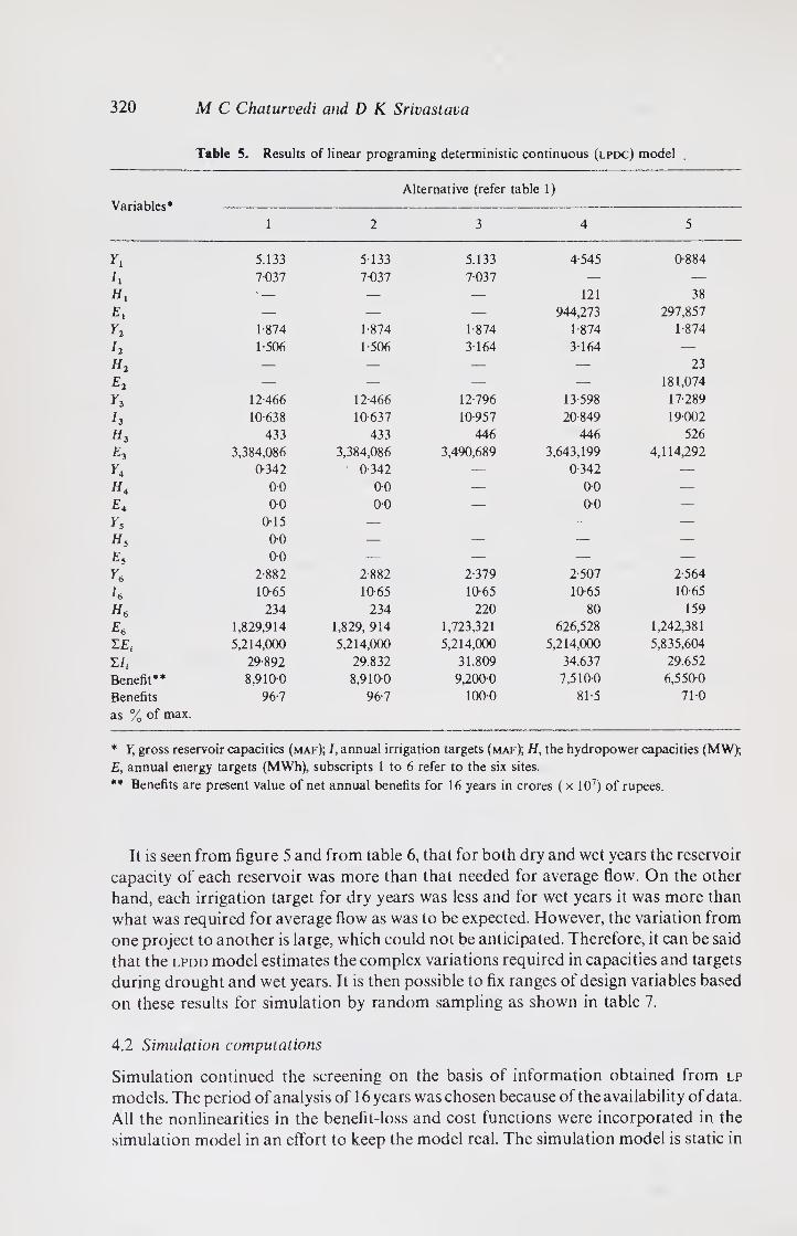
320 M C Chaturvedi and D K Srivastava
Table 5. Results of linear programing deterministic continuous (lpdc) model
Variables* Alternative (refer table 1)
1 2 3 4 5
Y, 5.133 5-133 5.133 4-545 0-884
h 7037 7-037 7-037 — —
Hi ' - — — 121 38 — — — 944,273 297,857
y2 1 874 1-874 1-874 1-874 1-874
h 1-506 1-506 3164 3164 — — — — — 23
e2 — — — — 181,074
y3 12-466 12-466 12-796 13-598 17-289
I3 10-638 10-637 10-957 20-849 19 002
tf3 433 433 446 446 526
E3 3,384,086 3,384,086 3,490,689 3,643.199 4,114,292
Y* 0-342 0-342 — 0-342 —
h4 00 0-0 — 0-0 —
e* 0-0 0-0 — 0-0 —
Ys 0-15 — — — —
h5 0-0 — — — —
e5 0-0 — — — —
y6 2-882 2-882 2-379 2-507 2-564
h 10-65 10-65 10-65 10-65 10-65
H6 234 234 220 80 159
e6 1,829,914 1,829, 914 1,723,321 626,528 1,242,381 I£, 5,214,000 5,214,000 5,214,000 5,214,000 5,835,604
Eh 29-892 29.832 31.809 34.637 29.652
Benefit** 8,9100 8,910-0 9,2000 7,510-0 6,5500
Benefits as % of max.
96-7 96-7 100-0 81-5 710
* Y, gross reservoir capacities (maf); /, annual irrigation targets (maf); H, the hydropower capacities (MW); E, annual energy targets (MWh), subscripts 1 to 6 refer to the six sites. ** Benefits are present value of net annual benefits for 16 years in crores ( x 107) of rupees.
It is seen from figure 5 and from table 6, that for both dry and wet years the reservoir
capacity of each reservoir was more than that needed for average flow. On the other
hand, each irrigation target for dry years was less and for wet years it was more than
what was required for average flow as was to be expected. However, the variation from
one project to another is large, which could not be anticipated. Therefore, it can be said
that the lpdd model estimates the complex variations required in capacities and targets
during drought and wet years. It is then possible to fix ranges of design variables based
on these results for simulation by random sampling as shown in table 7.
4.2 Simulation computations
Simulation continued the screening on the basis of information obtained from lp
models. The period of analysis of 16 years was chosen because of the availability of data.
All the nonlinearities in the benefit-loss and cost functions were incorporated in the
simulation model in an effort to keep the model real. The simulation model is static in
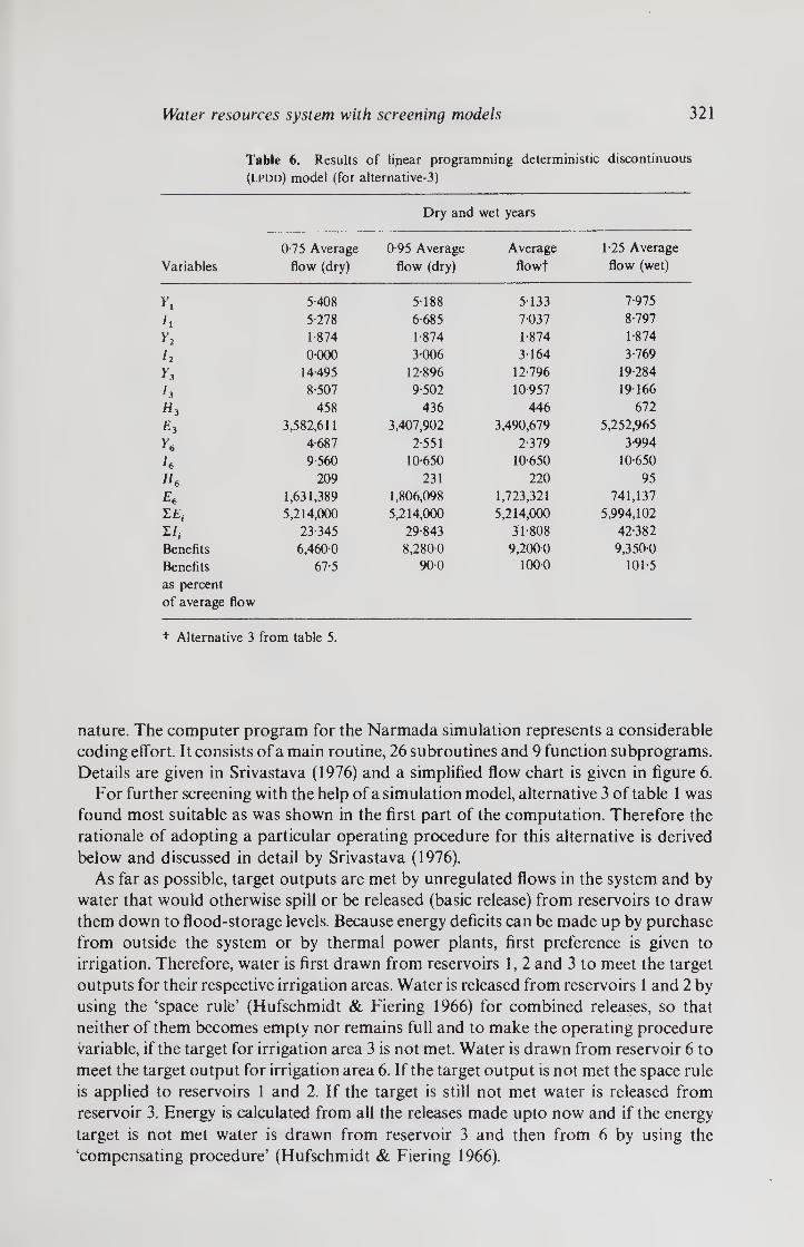
Water resources system with screening models 321
Table 6. Results of linear programming deterministic discontinuous
(LPDD) model (for alternative-3)
Variables
Dry and wet years
075 Average
flow (dry)
0-95 Average
flow (dry)
Average
flowt
1 -25 Average
flow (wet)
Yl 5-408 5188 5-133 7-975
h 5-278 6-685 7-037 8-797
y2 1-874 1-874 1-874 1-874
h 0-000 3-006 3-164 3-769
Y, 14-495 12-896 12-796 19-284
l3 8-507 9-502 10-957 19166
458 436 446 672
£3 3,582,611 3,407,902 3,490,679 5,252,965
4-687 2-551 2-379 3-994
h 9-560 10-650 10-650 10-650
209 231 220 95
E6 1,631,389 1,806,098 1,723,321 741,137
YEt 5,214,000 5,214,000 5,214,000 5,994,102
Eh 23-345 29-843 31-808 42-382
Benefits 6,460-0 8,280-0 9,200-0 9,350-0
Benefits 67 5 90-0 100-0 101-5
as percent
of average flow
t Alternative 3 from table 5.
nature. The computer program for the Narmada simulation represents a considerable
coding effort. It consists of a main routine, 26 subroutines and 9 function subprograms.
Details are given in Srivastava (1976) and a simplified flow chart is given in figure 6.
For further screening with the help of a simulation model, alternative 3 of table 1 was
found most suitable as was shown in the first part of the computation. Therefore the
rationale of adopting a particular operating procedure for this alternative is derived
below and discussed in detail by Srivastava (1976).
As far as possible, target outputs are met by unregulated flows in the system and by
water that would otherwise spill or be released (basic release) from reservoirs to draw
them down to flood-storage levels. Because energy deficits can be made up by purchase
from outside the system or by thermal power plants, first preference is given to
irrigation. Therefore, water is first drawn from reservoirs 1, 2 and 3 to meet the target
outputs for their respective irrigation areas. Water is released from reservoirs 1 and 2 by
using the ‘space rule’ (Hufschmidt & Fiering 1966) for combined releases, so that
neither of them becomes empty nor remains full and to make the operating procedure
variable, if the target for irrigation area 3 is not met. Water is drawn from reservoir 6 to
meet the target output for irrigation area 6. If the target output is not met the space rule
is applied to reservoirs 1 and 2. If the target is still not met water is released from
reservoir 3. Energy is calculated from all the releases made upto now and if the energy
target is not met water is drawn from reservoir 3 and then from 6 by using the
‘compensating procedure’ (Hufschmidt & Fiering 1966).

VA
LU
ES
OF
I A
ND
Y
AS
PE
RC
EN
TA
GE
OF
AV
ER
AG
E
FL
OW
S
322 M C Chaturvedi and D K Srivastava
Figure 5. Variation of / and Y values for dry and wet years as percentage of average flows

Water resources system with screening models 323
Figure 6. General flow chart of the Narmada simulation program
Table 7. Ranges and values of variables assigned for first random sample
Variables Ranges of variables
Values of variables assigned
for combination 42*
Yi 4-9 5-746
y2 1 874 1-874
y3 8-22 19063
d3 2-5 3-743
y6 2-6 4471
£>6 0-31-2-0 0-760
11 3-9 6-070
h 0-4 2-338
h 6-20 12-547
h 9-10-65 10-635
I£; 2,000,000-5,214,000 3,437,100
H 3 300-1,200 808
He 50-800 382
FSt t 0-2 0464
fs3 0-4 2-947
fs6 0-1-5 1-334
* This combination resulted in highest present value of net benefits of Rs 7,873 crores (i.e. x 107 among the combinations simulated,
t FSi is the flood storage capacity in maf for reservoir i.

324 M C Chaturvedi and D K Srivabtava
Table 8. Values of variables for combinations resulting in maximum
present value of net benefits (in Rs crores) for different samples
Variables
Types of samples
Second
random
sample
Third
random
sample
Fourth random
sample (from
lpdc model)
LPDC
model
solution
6-559 6-230 4-730 5-133
y2 1-874 1-874 1-874 1-874
y3 20-656 17-633 11-072 12-797
D3 3-401 2-163 2-082 2000
y6 5-150 3-186 1-624 2-380
d6 1-205 0-353 0-343 0-310
h 7-383 6-504 7-181 7-039
h 2-003 2-027 2-541 3164
h 13-279 12-105 8-647 10-957
h 9-836 10-616 10-605 10-650
I£, 2,383,961 1,999,670 1,999,670 5,214,000
W3 532 758 607 446
h6 164 266 214 220
fSjt 0-702 0-550 1-114 1000
FS3 2-445 2-200 1-920 2-000
fs6 0-766 0-700 0509 0-750
St 7,9980 7,914-0 7,468-0 7,8300
D = dead storage capacities
t FSj = flood storage capacity provided in maf in reservoir i.
Simulation was carried out with the help of random sampling. Computational time
for each simulation run was of the order of 40 seconds. In the first random sample
ranges were selected for each variable as shown in table 7, based on the results of the
lpdd model from table 6. Fifty one combinations of 16 system variables were sampled
at random. These were reservoir capacities, dead storage capacities, irrigation
requirements, energy requirements, hydropower plant capacities and flood
constraints. This was done by assigning values to the variables in combinations
through a computer program random, such that the allocations for flood and dead
storages were not more than the gross reservoir capacity at each site individually or
combined depending on the types of allocations to be made. The values of variables
assigned in a first random sample to combination 42 which resulted in the highest present
value of net benefits of Rs 7,873 crores are given in table 7. Three more random samples
were tried and their values of variables for combinations resulting in maximum present
value of net benefits are given in table 8. Their present values of net benefits were
Rs 7,998, Rs 7,914 and Rs 7,468 crores respectively. Similarly, the values of variables
obtained by the lpdc model solution were also simulated. The present value of net
benefits obtained was Rs 7,830 crores.
5. Analysis of results
An lp screening technique was developed to determine the optimal configuration,
capacities and multipurpose releases. It may, however, be noted that since linearization

Water resources system with screening models 325
of concave cost functions is involved, there is a possibility of being trapped into local
optimals. Looking at the results of the lpdc model in table 5, alternative 3 gave a
maximum net annual benefit of Rs 9,200 crores. Results for other alternatives show that
the capacities of reservoir Harinphal (no. 4) and Jalsindhi (no. 5) were restricted to their
dead storage values in all the alternatives. This necessarily follows from the formulation
adopted and to avoid this deficiency mixed integer programing would be required at
subsequent more detailed analysis. The same holds for the power plants at these
reservoirs. Hence, alternative 3 gives the probable optimal configuration of the physical
facilities as well as their probable near optimal values.
If the results obtained in table 5 for alternative 3 and their corresponding values from
the conventional design methods as shown in table 9 are compared the results from the
lpdc model are reasonable and distinctly improved. The conventional design method is
used here as the basis for comparison of the lpdc model results because it is the only one
available as the system as such does not exist. This shows that the lpdc model is useful
in choosing from the large number of alternative combinations of design, which would
result in maximum net benefits.
Table 8 shows that the maximum present value of net benefits obtained in
simulation for each case of random sampling and lpdc model simulation were nearly
equal. On the other hand all combinations were efficient due to no excess reservoir
capacity but inadmissible due to monthly irrigation and energy deficits (not shown in
table 8 but for this refer to Srivastava 1976). The number of monthly deficits for
irrigation in the lpdc: model simulation was more than that obtained in the random
sampling simulation, the reason being that the lpdc model specified higher annual output targets for irrigation. For energy the case was very much different: in most
combinations the total energy deficits were large. This is because the relationship
between the power plant capacity and the output is very complex and the lpdc model
Table 9. Comparison between lpdc and conventional design methods
Annual irrigation Reservoir capacity (maf) requirement (maf)
From report* From lpdc model**
Upto No.
Gross capa¬ city
Live capa¬ city
Gross capa¬ city
Live Capa¬
city From
reportf
From lpdc
model**
1. Bargi 5-548 5-548 5133 5-133 6-01 7-037 2. Tawa 1-874 1-874 1-874 1-874 3164 3. Narmada 12-689 10-023 12-796 10-796 14-97+ 10-957
sagar 4. Navagam 4-435 2-728 2-379 2-069 11-02 10-650
Total 24 546 20173 22-182 19-872 32-00 31-808
* Diagram 181, and Table 181, Vol. Ia (Master Plan for Development, 1972); ** Table 5 for Alternative 3; t Statement 18-1 Vol. II (Master Plan for Development of water resources of the Narmada in Madhya Pradesh, 1972); t Between Bargi and Narmadasagar.
326 M C Chaturvedi and D K Srivastava
specified very low power plant capacities. Hence the values between power plant
capacity specified by the lpdc model and that actually needed for simulation could vary.
Even with the deviation between these results, it is seen that the lpdc model provided
values of variables which were quite close to their corresponding values obtained by
simulation.
6. Conclusion
For the systems analysis of a large complex water resources system a screening-
simulation model was developed. The Narmada river basin was taken as the system.
Two types of lp screening models were used to find a reasonably small set of possible
optimal design alternatives. These were lpdc and lpdd models. Simulation was used for
further analysis to obtain the near optimum solution in terms of objective function.
The results showed firstly that the lpdc screening model gave realistic results as
compared with those determined by the conventional design methods of project-by-
project analysis. Second, the results of this model were helpful in simulation. Third, due
to the introduction of some design and practical aspects as constraints in the lp model,
the results obtained were more realistic and the solution was nearly optimal in terms of
objective function. Fourth, this model specified output targets and capacities so as to
better regulate mean monthly flows at all sites. Lastly, the lpdd model gave some idea of
the excess storage and the reservoir capacity needed for drought and wet years
respectively and helped in selecting the ranges of variables for simulation by random
sampling for the alternative selected by the lpdc model.
The results of the simulation run from the lpdc model showed good resemblance of
the design variables and results of simulation as did the results of simulation runs
obtained by random sampling also. Within the limitations of the models, it may be
concluded that the solution resulting from the lpdc model may be assumed to be near optimum in terms of objective function and can serve as an input or as an initial base for
further screening by simulation.
List of symbols
ai,t
t>2 ,i,s(i)
Cl.ii C2,h C3,i
Ci,„ C'2>1, C'3>i
Di
Ei
Ei'Sii)’ Hi,s(i)’
I Y ■ *i,s(i)> -*1,5(1)
e
E i,t
A.
water release from reservoir i in time t
gross annual hydropower benefits and irrigation respectively at site i
slope of linear segment s(i) of the benefit function /?2>l for irrigation i
annual capital cost of hydropower plant, irrigation and reservoir
capacity respectively at site i
capital cost function for hydropower plant capacity, irrigation work
and reservoir storage capacity respectively at site i
dead storage capacity of reservoir i
yearly firm power target at site 1
a linearised target portion of power, hydropower capacity, irrigation
and reservoir capacity respectively
turbine and generator efficiency
total inflow to the reservoir i in time t
natural flow at site i from its catchment area in time t
Water resources system with screening models 327
He,.,
h,
Hi
Ii
average storage head at site i for period t
number of hours in the particular period t
hydropower capacity at site i
yearly target amount of water to be provided for irrigation for the ith
irrigation area
i site, irrigation K, ( proportion of irrigation demand /, to be diverted for irrigation in time
^3, i.s(i)
ml. i,s(i)i ^2,i,s(i)>
m3. i,s(i)
Ox, it ^2,i> i
O'x, h 02,h
0'3, i su
s(i)
Yt
Zi
*i,t
Pl.i.t
02.1 <5,
t from site i proportion of irrigation demand /, as irrigation return flow from the
jth irrigation area in time t
slope of linear segment s(i) of the capital cost function for hydro-
power plant, irrigation work and reservoir storage capcity
respectively slope of linear segment of the omr cost function for hydropower
plant, irrigation work and reservoir storage capacity respectively
annual omr cost of hydropower plant, irrigation work and reservoir
capacity respectively, at site i
omr cost function at site i for hydropower plant, irrigation work and
reservoir storage capacity resepctively
content of the reservoir i at the beginning of period f
number of portions into which target i is divided for linearization of
benefit and cost functions
time capacity of the ith reservoir
set of reservoir sites upstream of site i from where water can reach the
site i (or the sites that contribute to the inflow at the site i) load factor at each hydropower site i and for each period t is an
indicator of the energy demand
benefit per unit of firm energy for site i in time t the long run benefit function for irrigation at site i
proportion of annual firm hydropower target £, for period t
References
Dorfman R 1962 Mathematical models: the multi-structure approach design of water resources systems
(Cambridge, Mass: Harvard University Press) p. 494 Hufschmidt M M, Fiering M B 1966 Simulation techniques for design of water resources systems (Cambridge,
Mass: Harvard University Press) Jacoby H D, Loucks D P 1972 Water Resources Res. 8. 1401
Loucks D P 1969 Stochastic methods for analysing river basin systems. Research Project Technical Completion Report, Department of Water Resources Engg. and the Water Resources and Marine Science Centre, Cornell Univ., Ithaca, New York
Master Plan for Development of Water Resources of the Narmada in Madhya Pradesh 1972, Government of Madhya Pradesh, Irrigation Department, Bhopal
Report of the Narmada Water Resources Development Committee 1965 Government of India, Ministry of Irrigation and Power, New Delhi
Roefs T G 1968 Reservoir management: the state-of-the-art. Report No. 320-350B, ibm, Washington Sci. Centre, Wheaton, Maryland, usa

328 M C Chaturvedi and D K Srivastava
Roefs T G, Bodin L D 1970 Water Resources Res. 6: 410 Srivastava D K 1976 Optimisation of complex water resources systems by screening-simulation model, Ph.D.
Thesis, Indian Institute of Technology, New Delhi Various project reports: Project Reports of Bargi 1968; Tawa 1972; Narmadasagar 1969; Harinphal 1970;
Jalsindhi 1970 and Navagam (Broach) 1956, available with Central Water and Power Commission, New Delhi

Overview and reflections
M C CHATURVEDI^ and PETER ROGERS*
Applied Mechanics Department, Indian Institute of Technology, Hauz Khas, New Delhi 110016 •Department of Environmental Engineering, Harvard University, Pierce Hall, 121, Cambridge Mass. 02138 USA
1. Introduction
Modern technology is becoming increasingly large scale and powerfully pervasive.
Although, in the last analysis, technology is mediated through specific projects, often
these projects are part of a large-scale complex system. For instance, a number of power
projects of varying types and capacities are interconnected through power grids to act
as one system. Several dams and barrages on a river are interconnected through
continuity of the hydrological flow. To give another example, the surface water
development is interlinked with groundwater development as both serve the purpose of
meeting the water demand and one has to think of conjunctive surface and ground water development. Further, since surface waters generate energy and provide
irrigation, while development of groundwater sources consumes energy, conjunctive
surface-groundwater-energy systems planning becomes attractive.
New technical advances are being introduced at an increasingly rapid rate leading to
what has been said to be a discontinuous world. In view of the scale, pervasiveness and
uncertainty of modern technology, it becomes increasingly important that its
development is undertaken creatively and in a scientific manner. Secondly, in view of
the relationship between technology in space and time it is necessary that a
comprehensive though dynamic view' of the technology be attempted. It is also equally
necessary that the impacts of technology are creatively assessed and the technological
choices are scientifically evaluated.
Of late, a new scientific discipline known as systems analysis has evolved through developments in the separate disciplines of engineering, economics and mathematics.
Rapid developments have taken place in this science and the availability of high-speed,
efficient and economical computers has contributed to its development. As the science
of systems analysis has advanced over the last two decades and as the scale of modern
water resources projects has grown, systems planning of water resources has been made
mandatory by law in many developed countries. International agencies also emphasize
systems planning. For instance, at the United Nations Water Conference held in
Argentina in 1977, the need for water resources planning was promulgated as follows
(un document E/Conf. 70/29, 1977).
“Systems analysis and modelling techniques should be applied to improve efficiency
and efficacy in storage operation and distribution systems. Studies should explore the
possibility of effecting interbasin transfer of water and special attention should be paid
to environmental impact studies . . . Water management plans may be prepared by
329

330 M C Chaturvedi and Peter Rogers
using systems analysis techniques and developed on the basis of already adopted
indicators and criteria taking into account the economic and social evolution of the
basin . . . Master plans should be formulated for countries and river basins to provide a
long term perspective for planning, using such techniques as systems analysis and
mathematical modelling as planning tools wherever appropriate . . .
Systems planning of water resources is particularly important in India for a number
of reasons. First the scale of development is monumental. According to the proposed
targets for the Sixth Five Year Plan, irrigation at the highest level in the world, and
almost five times the present level in USA, would be achieved. Second, the magnitude of
the contemplated work is also very great. For instance, development of the Ganga-
Yamuna basin envisages construction of five very high dams and 22 hydroelectric run-
of-river schemes which have to be planned integrally. As another example, under the
National Water Plan, interbasin interlinkage of several river basins is being planned.
Third, while the water resources development is extremely important and critical,
there are competing demands from other sectors. With water resources development
accounting for almost 20% of the National Plan allocations it is necessary that the
development is carried out in an efficient manner.
In contrast to the need for efficient development, the present achievements, as noted
in the Sixth Five Year Plan, are not efficient. We do not mean to negate the scale of
technological development or their rate of development. Irrigation works of India have
been, and continue to be, some of the wonders of the world, but their technological
functioning is not one of the best. If the present state continues there will be a serious
problem of resource depletion and environmental degradation, both in surface water
and groundwater (Chaturvedi 1976). It is, therefore, necessary that an appropriate
policy and systems plan be followed. This will require integrated planning from the
micro-level to the macro-national level.
Importance of systems planning has been recognized by decision makers in India.
One of the present authors (MCC) was invited for the systems planning of the Ganga
basin as far back as 1968 by the Indian government and a preliminary study was carried out. From the Fourth Plan onwards, the need for systems planning has been
emphasized in the National Plan. The author was also invited by the Planning
Commission to carry out the systems planning of Punjab. The Expert Committee of
the National Committee of the International Hydrological Programme on Research
and Education strongly recommended scientific development of water resources through systems analysis. But the development in real life continues to be fairly
ad hoc. The reasons for the present approach are understandable. Not many professionals
are yet aware of the potential and scope of these modern approaches. The institutional
constraints are such that specialisation in different activities of engineering viz research,
planning, design, construction and management, of course with due interlinkage, is not
developed. While in the last analysis institutional modernisation is the most important
requirement for modernization of water resources development, it is necessary to
develop widespread indigenous capability of systems planning amongst the pro¬
fessionals and academicians and demonstrate the applicability of systems analysis
techniques to Indian conditions. It was in this context that the present project
was undertaken and it is hoped that some contribution has been made to this
end.
Overview and reflections 331
2. Systems analysis
Systems analysis is often taken to mean mathematical modelling and it is necessary that
this misunderstanding is removed. Systems analysis is a body of concepts, approaches
and techniques. We shall try to give a brief introduction to systems analysis and for
details reference may be made to Klir (1969), Sage (1977), Hall & Dracup (1970), Meta Systems Inc. (1975), Biswas (1976) and Chaturvedi (1984).
Although technology has been practised since the early history of man, a new
understanding of technology is gradually developing. Technology is not merely a set of
constructed facilities, tools or processes, but it is a totality of activities transforming the
environment. This transformation involves resources, energy or/and information
according to certain technological laws. While technological activities in the context of
art and science of different disciplines have to be carried out, in the last analysis
technology basically results in a change of environmental state and processes. With this
change there is a concomittant change in the scope of life activities. Confining this to the
human system, our perceptions, values and opportunities may change. For instance,
with the availability of transportation and communication systems, the concept of
space and time changes. Similarly, with the availability of modern energy systems, the scope of human power and opportunities of action dramatically change. With the
availability of modern production capability a new world of action is unfolded.
Modern technology is interconnected. Various elements or projects operate in the
context of certain technological objectives. Even when they are differentiated in space
and time they are integrated in terms of these overall objectives. These systems are
organic-dynamic as they evolve over and decay with time.
Technology interacts with society in a circular manner. On the one hand technology
is brought about by the capabilities of society. Technology, by providing a new
environment, shapes the perceptions, opportunities and values of society. In the final
analysis, technology acts as an agent of social change. There is thus another
commonality of objectives, the socio-economic objectives interlinked with
technological-environmental objectives.
It becomes necessary that the development and evaluation of technology be
undertaken integrally as one set of activities. Technology has to be created through a
sensitive understanding of technological sciences and arts and evaluated critically so that hopefully we move into a better future. There is a paradox here. With the increasing
scale and the discontinuity in the development of technology, there is going to be an
increasing uncertainty about opportunities and impacts. It is thus all the more
necessary that we try to instill as much certainty as possible in the choice of technology
and its concomittant effects. This paradox is not a contradiction, but is a continuation
of the paradox of life.
The perceptions vary from individual to individual, from group to group, and
furthermore are not constant over time. It thus becomes necessary that technology is
evaluated through a participatory open mechanism. A new body of approaches and
techniques for evaluation has also developed as will be discussed later.
Technology involves development of hardware and software, but in addition it involves development of institutional systems and motivational mechanisms. It is this
set of three issues which defines the technological system and not mere hardware as was
often the view of the past.
To sum up, technological projects are part of an organic-dynamic system brought

332 M C Chaturvedi and Peter Rogers
into being for transforming environment in terms of certain techno-environmental and
socio-economic objectives. The system consists, besides the software and hardware, of
appropriate institutional and motivational mechanisms.
Systems analysis emphasises an approach so that technology is developed scientifi¬
cally and creatively. A five-step systems approach has been developed. First, we try to
identify the various issues. In that context we next try to be precise by specifying the
objective and developing a set of measures to evaluate the objectives. In the third step,
in the context of these objectives, various technological options are developed which in
the totality of a system define the technological system. The system consists of a
portfolio of projects which will have to be taken over time and space and the evolution
has to be not in terms of the project, but in the totality of the system. In the fourth step
we try to evaluate the various alternative technological options, and finally in the fifth
step we select one of the systems in terms of quantified and non-quantified objectives.
There is a morphology in systems planning. Starting with an idea one tends to
become more and more specific in a set of hierarchical evolutionary stages. In the first
instance, we have the feasibility study where the techno-economic feasibility is
identified so that a decision could be taken on the investment of further resources of
time and of man, if deemed appropriate. In the second phase we have detailed planning
leading to detailed design. These three stages of planning and design lead to the fourth
stage of construction following which, we have the management of the constructed
facilities. The environment in which the technological system functions, the functioning
of the technological system along with man who is involved in the physical system, and
the demands placed on the technological system are probabilistic or uncertain. Hence
the need for scientific management. Technological systems planning embraces all these
stages including the management.
The evaluation relates to several aspects of the impact of the technological system.
One is thus the issue of economic evaluation basically deciding the allocation of scarce
resources. Over a period of time attempts have been made to make the evaluation more
and more comprehensive leading to the social-benefit cost analysis (unido 1972,1978).
Attempts have been made to develop an evaluation approach from the point of view of
economic efficiency and equity. Attempts have also been made to take into account the
nonlinearities of demands and supply functions, the externalities, the multiple
objectives, the inter- and intra-temporal impacts, and the uncertainties.
Besides the socio-economic evaluation we have the environmental impact analysis
which tries essentially to take a long term view of the situation in the context of the
complex facets of environment and ecology. In view of the large scale and pervasiveness
of technology with possible significant changes in environment which may be
irreversible and the possibility of resource depletion, it becomes necessary to take this
comprehensive view. The third evaluation which has not yet been fully systematised is
that of trying to assess and visualise the social impact of technology in terms of values.
This is a difficult subject and is still in an initial stage of development.
The central point is that technology has to be developed creatively and scientifically,
accessing all technological possibilities and socio-economic-environmental impacts.
The development and evaluation are integral activities and have to follow systemati¬
cally so that, like science, they are reproducible activities.
In view of the complexity of developing technology, a large number of complex
alternatives have to be developed and evaluated. This is considerably facilitated by
computer-oriented mathematical models and simulation. The value of these models

Overview and reflections 333
and techniques lies in the following: (i) they allow, so to say, ‘thought experiments’ to
be effected with generation of alternatives and evaluation of their performance under
different configurations and policies; (ii) they allow decisions on the sensitivity to
varying input assumptions and system parameters; (iii) they provide a monitoring
device that helps to ensure internal consistency among projects and plans and (iv) they
depict qualitative relations among the various factors affecting the supply and demand.
It is important to caution that the models do not usually provide the qualitative
assessment, but illustrate them schematically (cones 1981).
The techniques have become possible only due to the availability of modern high¬
speed computers. Systems analysis does not by any chance negate modern engineering
analysis. In fact, these form the input to the systems studies which try to develop
alternative options or study the sensitivity.
There is always the danger in the use of models that the numerical results will be
taken literally. It must be emphasized that real life issues are extremely complex and not
always quantifiable and commensurate. Many simplifications and uncertain assump¬
tions must be made to construct models and a great deal must be simplified and left out
of consideration. Judgement alone decides whether some factors are important or
whether effects can be separately included, atleast in the first approximation. Models do
not negate judgement but complement creativity and judgement by enabling painting
over a wide canvas and carrying out the analysis over a wide range. Judgement is also a
pre-requisite for modelling, otherwise models can become caricatures of reality.
A variety of techniques are used for modelling such as linear programing, dynamic
programing, non-linear programing, queueing theory, graph-theoretic approach,
calculus of variations, etc. Each one may be suitable in certain situations. Much work
has gone into this area to apply these to different systems and the practitioner has to
learn through much detailed study in this area.
One of the reasons why the systems approach has not been adequately applied in real
life studies is that examples of applications are generally not available to administra¬
tion. In this context Rogers (1979) analysed some studies and 22 cases were
summarised. The list was not exhaustive and was only meant to provide examples of
work that has been used or is in the process of being used and is easily accessible in
literature. Some of the studies reported in the book have not been included in the above
cases. These cases, given in the appendix, have been summarized under ten separate
headings.
(i) Origin and purpose: This is to give some idea of the history of the problem and the purposes of the study.
(ii) Sponsors: Attempts to identify agencies which have sponsored the studies and who
may be contacted for further information by persons interested in a particular study.
(iii) Organization of study: How the study was organized. Who did what and where,
are important aspects of any systems study.
(iv) Technical team: The details of the technical manpower, leadership and the amount of time from each discipline are given wherever possible.
(v) Structure of analysis: How the original problem was rearranged and structured for analysis.
(vi) Mathematical models: Details of the mathematical models used are given where appropriate.
(vii) Boundaries of study: The real and conceptual scope of the study is given.

334 M C Chaturvedi and Peter Rogers
(viii) Evaluation and critique: An evaluation is attempted based on available documen¬
tation. Whether the application was used or not for an actual decision is emphasized.
(ix) Study results: Based upon the documentation itself, the pertinent results are outlined.
(x) Documentation: Only readily available documentation is listed.
In tables 1 and 2 all these cases have been summarised to show the issues they were
concerned with and the systems analysis techniques that were employed. In these tables
the studies are ordered by the date of major publication. The reader should be aware
that, based upon the reports alone, it is quite difficult to fill in these tables. A fair amount
of judgement has to be exercised. This tends to favour the studies that we are familiar with over those we only know from literature.
The most important observation about table 1 is that despite the fact that we have
carefully chosen from literature those studies purporting to be the actual case studies
performed in, or on, developing countries we feel confident in stating that only 7 out of
the 22 studies (or about 1 /3) have ever been used in making decisions on water planning
and management by the sponsoring agencies. Is this a poor batting average?
Table 2, which shows which of the cases use the major systems analysis techniques is, very instructive. Fifteen of the studies (about 2/3) used linear programing techniques,
none used queueing theory, inventory theory and statistical decision theory and only
one used any kind of stochastic model and one used the game theory. There must be
some implications here for how one would organize a training programme for
professionals interested in applying systems analysis to water planning and manage¬
ment in developing countries.
In concluding this section it should be re-emphasized that the listed case studies are
not the only applications made or known to the authors of this report. Numerous other
studies are known to have been completed but their documentation is either not
available or incomplete. We have chosen to present only those cases which have readily
available documentation.
3. Overview
An attempt has been made through the studies in this volume to illuminate the systems
approach of water resources development. First, the environment and resource
availability of water in India and the background of development in a historical context have been given (Chaturvedi 1985a). Formulation of issues for future development,
currently proposed policies, a scientific approach to development of the river basin at a
national level, and systems approaches for further policy studies have been tried.
Following these general formulations, an issue for a large river basin has been
identified and modelled. The particular river basin selected is the Ganga-Brahmaputra
basin which is one of the largest basins of the world in hydrological terms. To start with,
therefore, a general description of the system follows (Chaturvedi 1985b). Next the
approach to planning has been formulated and as a first step a coordinating-screening
model is developed to assist in identifying the possible developmental scenarios, taking
into account the hydrologic-environmental-economic-interlinkages (Chaturvedi et al 1985). The methodology for trade-offs amongst multi objectives is demonstrated by
considering trade offs between different seasons of irrigation and between irrigatton

Tab
le
i S
om
e ch
arac
teri
stic
s of
rep
ort
ed c
ase
studie
s
Overview and reflections 335
© JC
3 cud
|.£ E c c/5 3 g cd su
-o 3 w C/5
O 8J 8.
o
»-i c a o © E g 2.§
c£ S3
o a,
t-" c2 © • — 2 $
£*5 .2
3 3 O U
-C a. I o © O
3 O
‘5b ©
8 o
a*
cd 3 IN cj cd
.22 E "6 u ©
3
■v C © o u! 5 8j © r3 ^ 3
3 3 O U
X X
Panam
a
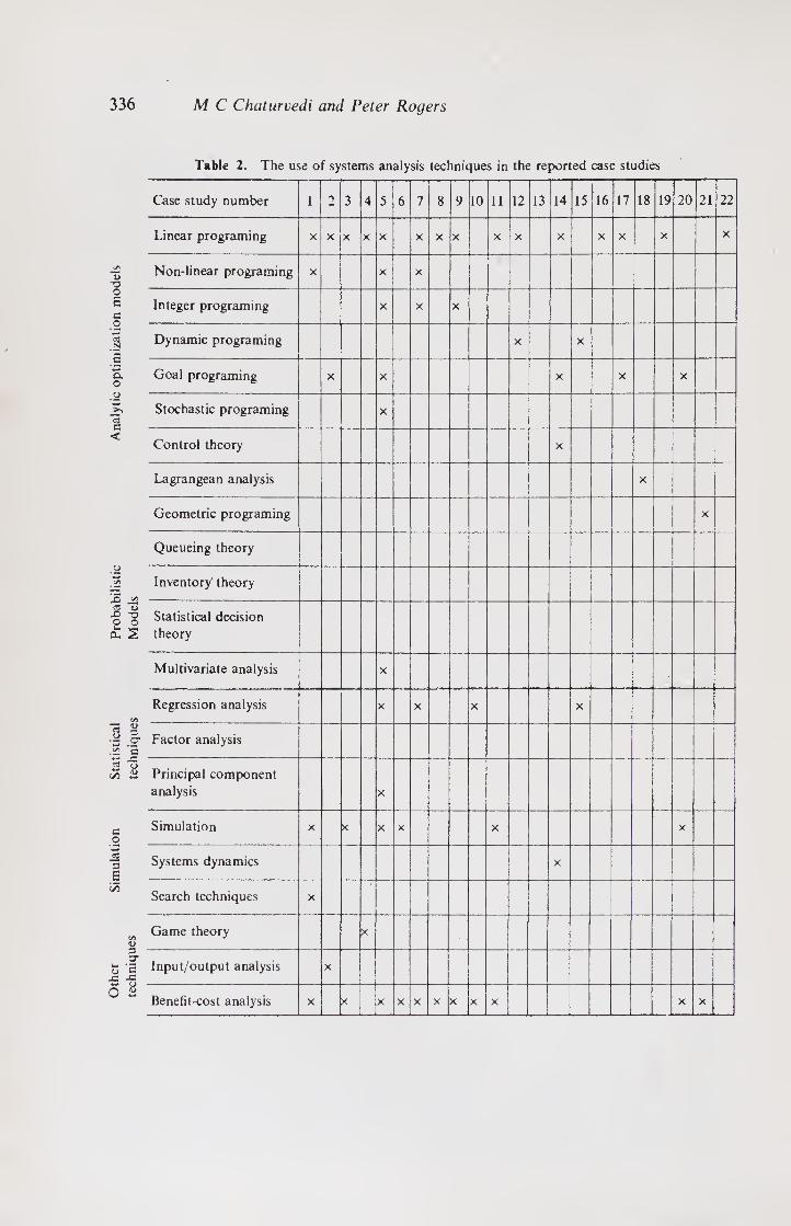
Oth
er
Sim
ula
tion
Sta
tist
ical
Pro
bab
ilis
tic
An
aly
tic
op
tim
izati
on m
od
els
tech
niq
ues
tech
niq
ues
Mo
del
s
336 M C Chaturvedi and Peter Rogers
Table 2. The use of systems analysis techniques in the reported case studies
Case study number 1 ■*) 3 4 5 6 7 8 9 10 11 12 13 14 15 16 17 18 19 20 21 22
Linear programing X X X X X X X X X X X X X X X
Non-linear programing X X X
Integer programing X X X
Dynamic programing X X
Goal programing X X X X X
Stochastic programing X
Control theory X
Lagrangean analysis X
Geometric programing X
Queueing theory
Inventory' theory
Statistical decision
theory
Multivariate analysis X
Regression analysis X X X X
Factor analysis
Principal component
analysis X
Simulation X X X X X X
Systems dynamics X
Search techniques X
Game theory X
Input/output analysis X
Benefit-cost analysis X X X X X X X X X X X

Overview and reflections 337
and power. This coordinating-screening model is extended to more detailed analysis by
dividing the system in terms of hydrological sub-basins (Rogers & Kung 1985) or
administrative-political units of development (Karady & Rogers 1985). A marginal
incremental model has accordingly been formulated. Thus these three studies
contribute to an approach for assisting in planning the development of large scale
complex river basins.
We have emphasized that the systems approach, first and foremost, is an aid to creative engineering in a scientific manner. In this context we have tried to emphasize the
importance of developing all possible technological options. An attempt has been made
to develop an unconventional technique of mitigating floods on the one hand and
enhancing the water resources on the other through induced groundwater recharge
(Revelle & Lakshminarayana 1985). It is shown that flood flows can be stored by heavy
pumping along the perennial rivers for irrigation during the prior low river flow season.
The concept proposed by Revelle was only one of the possible techniques. Other
technologies are also possible, such as pumping along non-perennial rivers, and kharif
irrigation. Furthermore, these technologies require regional groundwater-aquifer
interaction modelling and estimation of optimal groundwater pumping configuration.
Therefore, in the following study more refined analysis and in this context three
additional alternatives over the basic theme have been proposed and modelled for
analysis through a sophisticated regional groundwater simulation-optimization pro¬
graming model (Chaturvedi & Srivastava 1985b). This is an important component of
the possible technological options in the Ganga Basin. In terms of systems approach
principles it demonstrates the opportunity for creative engineering even in conven¬
tional areas.
In large scale systems, differences are always likely to arise amongst different uses and
users in different parts of the river basin. These could be at the national level or at the
international level and an approach to aid in the resolution of these differences through
scientific analysis designed to identify optimal systems development in the context of
identified mutual interests through bargaining processes has been developed through
Game theoretic analysis. This is the pioneering study in the Ganga Basin carried out
way back in 1967 by Rogers.
In the development of water resources, generally, emphasis is laid either on the
upland water resources for diverse demands or the water quality modelling at the
waters edge in terms of the estuary. The fact that a river represents the continuity of the
land-water system is very often neglected. For instance, as more and more upland
development takes place the flows available at the waters edge are likely to be modified
and it would be necessary to take an integrated picture of the upland and the deltaic
region estuarine development. In this context a study at the waters edge has been
carried out by Rogers. This issue is equally applicable to other river basins of the
country.
As we have tried to identify at the outset, systems planning studies require a
considerable set of integrated studies. For instance, a detailed analysis of the water
demand, particularly of the agricultural demand has to be carried out. While this has
not been done for the Ganga Basin, the studies have been carried out for a number of
other river basins of the country, such as, Rajasthan Canal (Verma 1985) and the
Rangola Irrigation Scheme (Basu et al unpublished). In estimating the water demand
and the application principal for irrigation, diverse factors such as economic efficiency,
economic equity and/or assurance o ' food requirement for nutritional considerations

338 M C Chaturvedi and Peter Rogers
in a dynamic context of developing agriculture technology are required. Some of these
issues have been analysed in the two studies mentioned above.
A variety of problems arise which have a lot of commonality as well as specificity The
commonality is in terms of the integrality of these large scale projects. The specificity
stems from the unique configuration of the systems and the specific supply and demand
specifications. To illuminate these points several river basins have been studied. These
include the two studies for the Indus basin as well as a large component of the Indus
basin and the Bhakra dam (Rao & Ramaseshan 1985a, b), studies of the Cauvery basin
(Vedula 1985), Damodar river basin (Sinha & Rao 1985) and Subernarekha river
system (Sinha et al 1985).
A variety of techniques can be used for systems modelling. In the last analysis
perhaps simulation will be most convincing and convenient, particularly the stochastic
aspects of the development; however, simulating the entire system in the diverse
conditions would be extremely time-consuming. A reasonable approach is that a
programing model may first be used to find out the range over which simulation
studies should be carried out particularly taking into account the stochastic nature of
inputs and outputs. This methodologic approach has been tried and applied
successfully to the Narmada system (Chaturvedi & Srivastava 1985a).
4. Reflections
Although the present studies do not represent a complete and detailed picture of one
particular river basin, the studies taken together, to a large extent cover the diverse
problems likely to be encountered in large scale systems planning and we consider that
the set of studies would contribute to the art and science of systems planning. We are
aware of the shortcomings of the studies reported, which are inherent in the manner in
which they were carried out with the essential purpose of developing appreciation and
capability in systems analysis amongst some scientists in this field. It is hoped that an
integrated study oi a real life situation will be carried out at the earliest to contribute to
the science and art oi the subject and for developing appropriately trained engineers for
planning. Water resources development in India is crucial to the development oi the
country, as emphasized in the 20-pomt programme of the late Prime Minister as well as in
the Planning Documents. A large number of persons are required to carry out thi^ task
as sensitive professionals and scientists trained in the best use of the tools of analysis, it
is hoped that the present study would contribute to the tremendous challenge posed to
the professionals in the country and abroad.
It is unfortunate that much time has been lost. A historic incident may be
nostalgically mentioned at the end. Following Rogers study entitled, “A game theory
approach to the international aspects of the Ganga Basin”, the Indian author was asked
by the government in 1968 to carry out the study independently as stated earlier.
Following this he was convinced that systems studies of the river basins were required
for their efficient development and it was decided that systems studies of the Ganga
basin be carried out by the Indian author. A three-month summer school, sponsored by
the Ministry of Irrigation was held at the Indian Institute of Technology, Delhi in 1972
to train about 30 officers also in this context. But the activities did not continue and
more than a decade has already been lost.
We believe that the development of trained manpower is the most important pre-

Overview and reflections 339
requisite for water resources development and the present volume is dedicated towards this end.
References
Biswas A K (ed.) Systems approach to water management (Kogakusha, Tokyo: McGraw Hill)
Chaturvedi M C 1976 Water—second India studies (New Delhi: Macmillan)
Chaturvedi M C 1984 Water resources systems engineering (New Delhi: Tata McGraw Hill) (in press)
Chaturvedi M C 1985a Sadhana 8: 13-38
Chaturvedi M C 1985b Sadhana 8: 73-92
Chaturvedi M C, Rogers P, Kung S L 1985 Sadhana 8: 93-121
Chaturvedi M C, Srivastava D K 1985a Sadhana 8: 311-328
Chaturvedi M C, Snvastava V K 1985b Sadhana 8: 159-177
(cones) Committee on Nuclear and Alternative Energy Systems 1979, National Acad. Sci., Washington DC
Hall W A, Dracup J A 1970 Water resources systems engineering (New York: McGraw Hill)
Karady G, Rogers P 1985 Sadhana 8: 135-145
Klir G J 1969 An approach to general systems theory (New York: Van Nostrand Reinhoid)
Meta Systems Inc. 1975 Systems analysis in water resources planning, Water Information Center, Inc.
Rao P S, Ramaseshan S 1985a Sadhana 8: 179-206
Rao P S, Ramaseshan S 1985b Sadhana 8: 207-221
Revelle R, Lakshminarayana V 1985 Sadhana 8: 147-157
Rogers P 1979 The role of systems analysis as a tool in water policy, planning and management, UN
Workshop, Water Resources Planning Experiences in a regional and national context, Rome
Rogers P, Kung S L 1985 Sadhana 8: 123-134
Sage A P 1977 Methodology for large-scale systems (New York: McGraw Hill)
Sinha B, Bhatia R, Lahiri S 1985 Sadhana 8: 291-309
Sinha B, Rao P R 1985 Sadhana 8: 273-290
(unido) United National Industrial Development Organisation 1972 Guidelines for project evaluation un
(unido) United Nations Industrial Development Organisation 1978 Guide to practical project appraisal,
United Nations, New York
un Document E/Conf. 70/29 1977 Report of the un Water Conference, Mar del Plata, New York, United
Nations
Vedula S 1985 Sadhana 8: 223-252
Verma R D 1985 Sadhana 8: 253-271
Appendix
Case 1 Waterlogging and salinity in the Indus Plain
Origin and purpose To suggest methods to solve waterlogging and salinity in the groundwater of
the Indus Plain in W'est Pakistan. Pakistan President requested help from
President Kennedy.
Sponsor White House and Government of Pakistan
Organization of Highlevel panel for one year period. Most of analysis performed at various
study locations in the us. Report written by Professor Revelle and Harvard University
group who performed the systems analysis.
Technical team Panel drawn from Government and universities consisting of scientists,
engineers, agronomists and economists.
Structure of analysis To make a detailed investigation of possible approaches to the waterlogging
and salinity problems. Problem broken down into several pieces, solution
undertaken by different groups and then integrated at the end by a core group
of the panel.

340 M C Chaturvedi and Peter Rogers
Mathematical Linear and quadratic programing, simulation models for groundwater move- models ment and mixing.
Boundaries of study The basin of the Indus river and its major tributaries in Pakistan (then West area Pakistan).
Study results Showed that the waterlogging and salinity could be most effectively controlled through vertical drainage using tubewells. In addition, it demonstrated how this drainage water could be used to further develop irrigation.
Evaluation and A benchmark study using systems analysis in water management. Many new critique models were developed. Even though some of the detailed findings and recom¬
mendations were later not upheld, the report has been the fundamental policy document of the development of irrigation in Pakistan.
Documentation White House—Department of Interior Panel on Waterlogging and Salinity in West Pakistan, Report on Land and Water Development in the Indus Plain, White House, Washington, D.C., Jan. 1964. Dorfman R, Revelle R, Thomas H A Jr 1965. Pakistan Dev. Rev., 5: 331-372 Fiering M B 1965 Water Resources Res. 1: 41-61.
Case 2 Use of Aswan High Dam in Egypt for hydropower and irrigation
Origin and purpose
Sponsor
Organization of study
Technical team
Structure of analysis
Mathematical models
Boundaries of study
Study results
Evaluation and critique
Documentation
Studies of operation of the new Aswan High dam. Particular emphasis on the resolution of conflicts between energy and irrigation uses.
Ministry of the Aswan High dam, Egypt and Ford Foundation, Cairo.
Performed by Center for Population Studies, Harvard University. Small team; most of work performed in the US. Period 1 year.
2 engineers, 1 economist, 1 regional planner and 1 population scientist on a part-time basis.
To establish the ultimate resource potential of the Nile in Egypt.
Goal programing (linear programing) use of I/O models
Nile river basin within Egypt
Established the degree of complementarity between conflicting uses for power and irrigation. Identified possible developments of downstream underground storage to achieve 100% complementarity of water use.
An early application of goal programing to w'ater management. Raised inter¬ esting research questions about alternative investments. Was not continued because of lack of follow up by the government departments.
Thomas H A Jr, Revelle R 1966 Manage. Sci. 12B: 296-311
Case 3 Water and power resources of West Pakistan
Origin and purpose
Sponsor
Organization of study
Technical team
Structure of analysis
Part of the Indus Water Treaty. A sector plan for water and power for Pakistan was needed to evaluate the further development of the system, par¬ ticularly, the decision to build Tarbela dam.
Government of Pakistan, World Bank.
Bank provided an interdisciplinary group to coordinate a series of specialist studies which were then integrated into a coherent study by the Bank.
Cordinating group mainly administrators, and development economists, con¬ sultants from many other disciplines.
A macroeconomic model was made to coordinate separate studies of the power
Overview and reflections 341
Mathematical
models
and agricultural sectors. Agricultural sector chooses water technology as well as
cropping pattern via a linear programing model. The power model simulates
the detailed functioning of the electrical energy system.
Linear programing models of the agricultural sector and simulation models
for the hydrology and the power sector.
Boundaries of study
Study results
Province of West Pakistan
Confirmed the strategy of groundwater exploitation and the timing of the con¬
struction of Tarbela dam
Evaluation and
critique A large and complex study. Extremely well carried out. This is probably the
landmark study of the 1960’s. In addition to the Bank and the consultants
work, the officials of the Government of Pakistan were deeply involved in the
interpretation of the results. The cost of the overall study which is not reported
in the literature must have been substantial (in millions of us dollars).
Documentation Lieftinck P R, Sadove A R, Creyke T C 1969 Water and power resources of
West Pakistan: A study in sector planning, 3 vols., (Baltimore: Johns Hopkins).
Case 4 Resource potential of the lower Ganga-Brahmaputra basin
Origin and purpose Study to find the resource development potential in the Lower Ganga-
Sponsors
Brahmaputra Basin and the costs and benefits of international cooperation
between the riparian states.
Ford Foundation and Harvard University with the collaboration of the
Governments of India and Pakistan.
Organization of
study
Technical team
Structure of analysis
Performed as a desk study by a small team at the Center for Population
Studies, Harvard University.
One engineer and one economist part time for one year.
To search for the ultimate development potential of the Lower Basin of the
Ganga-Brahmaputra rivers for irrigation, flood protection, hydropower, navig¬
ation and water supply. To examine the costs and benefits of international
cooperation on the ultimate development.
Mathematical
models
Game theory, Linear Programing (720 variables and 450 constraints)
Boundaries of study
area
Basins of the Ganga and Brahmaputra rivers including Bangladesh and Nepal
but not China or the Indian states further upstream than Bihar.
Study results The study showed that the problem was a classical “prisoners-dilemma” game
problem. The benefits for cooperation were large (about 25% of total) but not
overwhelming.
Evaluation and
critique
Innovative approach to this class of problem. The data used were, however,
very unreliable and the study was never acceptable to the Government of India
for further elaboration although the Government of Pakistan supported (with
UNDP support) elaboration of the East Bengal part of the study area.
Documentation Rogers P 1969 Water Resources Res. 5: 749-760.
Case 5 Land water and power studies for Bangladesh
Origin and purpose Part of a proposed larger study of the entire Ganga and Brahmaputra basins.
Sponsors
This study attempted to look at the integrated development of land, water and
power in East Bengal from 1969 to the year 2000.
Government of Pakistan (later Government of Bangladesh), UN Development
Program with the International Bank foi Reconstruction and Development as
their executing agents.
342 M C Chaturvedi and Peter Rogers
Organization of
study
Technical team
Model work was carried out at the Harvard University Center for Population
Studies. Extensive collection of secondary data in the field.
Small team of 2-3 engineers, 2 economists, 1 geographer and 1 population
scientist.
Structure of analysis The emphasis was on the human ecology of the region. The analysis started
with an elaborate population prediction model which responded to the rates of
economic development.
Mathematical
models
A variety of mathematical programing and simulation models were made.
The major model was a two level mixed integerquadratic programing model
of the entire agricultural sector. These models had 100 integer and 1300 con¬
tinuous variables and 1000 constraints.
Boundaries of study
Study results
Entire region of Bangladesh excluding the Chittagong hill tracts.
The studies indicated a water resources development strategy relying on small
pumps and tubewells in the next decade. While indicating self sufficiency in
food as a possibility for Bangladesh the models indicated severe
energy/fertilizer shortages in the near future.
Evaluation and
critique
An ambitious study integrating population, land, water and energy. There were
too many models made with consequent integration problems The hydrolo¬
gical constraints were explored in great detail. Due to the change of govern¬
ments the transfer of the model studies application by the various government
agencies in Bangladesh has not yet (1979) taken place 7 years after the study
was completed.
Documentation Rogers P et al 1972 Bangladesh land water and power studies Draft Report,
Harvard University Center for Population Studies; Rogers P, Smith D V 1970
Am. J. Agric. Econ. 52: 13-24; Rogers P 1974 ITCC Rev. 111: 110-119.
Case 6 Project selections and macroeconomic objectives: A methodology applied to Peruvian irrig¬
ation projects
Origin and purpose An attempt to bridge the gap between macroeconomic objectives and detailed
project investment criteria. The methodology was tested on 11 public irrigation
piojects in Peru.
Sponsors
Organization of
study
Technical teams
Not mentioned.
Details not given. Eleven projects were selected on the basis of completed feasi¬
bility reports, covering a range of project sizes, and geographical zones.
Details not given.
Structure of analysis Four classes of investment criteria were investigated in addition to a fifth
method putting together the income balance of payments, and the employment
objectives.
Mathematical
models
No formal models used. Simple national preference function was hypothesized
and the project selection rankings simulated under a variety of weights on the
objectives.
Boundaries of study
Study results
All irrigation projects within the national boundary.
The study showed that the ranking of the projects was very insensitive to quite
large variations in the weights on goals.
Evaluation and
critique
The study is a good example of the combined use of various economic and
social criteria for choosing irrigation projects. There were no constraints on re¬
source use nor were there any interactions either economic or hydrological al¬
lowed between the projects. Hence, a large part of the “systems approach”
could not be applied.
Documentation McGaughey E, Thorbeke E 1972 Am. J. Agric. Econ. 54: 32-40.

Overview and reflections 343
Case 7 Programing models of Mexican agriculture
Origin and purpose These studies were part of an integrated multi-level national planning model
Sponsors
for Mexico. The irrigation models were just one part of the overall study.
International Bank for Reconstruction and Development (IBRD) (Development
Research Center)
Organization of
study
Mainly carried out in Washington, DC by a group of agricultural and develop¬
ment economists with collaboration on data from various Mexican government
agencies.
Technical team Exact details not given, mainly economists.
Structure of analysis A very elaborate multi-level structure was given to the study Each of the sec¬
tors (agriculture and power) had to choose its best investment schedule subject
to resource availabilities predicted by a multi sector input/output model.
Mathematical model Variety of simulation, integer programing and linear and quadratic program¬
ing models. Main model was solved as a linear program (with 2,345 variables
and 1,500 constraints).
Boundaries of study
area
All the agricultural regions of Mexico.
Study results Elaborate projections detailing expected regional demand for water, crop pro¬
duction, and the market equilibrium prices for the products were made. These
were also shown to be consistent with expected macroeconomic growth in the
other major economic sectors.
Evaluation and
critique
The study received the Lanchester Prize of the Operations Research Society of
America for the best or publication of 1976. The study is very innovative in
the handling of some of the economic features such as endogenous prices and
in the models to check sectoral consistency. The multi-level models only
worked in an ad hoc way and the resource constraints particularly the water
constraints, are handled casually. The authors claim that the models are in use
by the Ministry of the Presidency in Mexico. There is, however, some dispute
whether the water agencies are indeed using the models to guide investments.
Documentation Goreux L, Manne A S 1973 Multi-level planning: Case studies in Mexico
(Amsterdam: North Holland); Bassaco L M, Norton R D, Silas J S 1974 Water
Resources Res. 10: 1071-1079.
Case 8 Cost-benefit analysis of irrigation projects in Northeastern Brazil
Origin and study The study examined irrigation projects in Northeastern Brazil which had been
Sponsor
Organization of
study
Technical team
Structure of analysis
found acceptable by the Ministry of Interior and re evaluated them using an
empirically estimated shadow price on labour.
Brazilian Planning Ministry.
Carried out by Cline as Visiting Professor in the Planning Ministry with the
help of Tahal for data and engineering advice.
Development economist aided by engineering consultant.
Reviewed 24 major projects out of a possible 56 available. Recomputed benefit
cost ratios with shadow prices on labour and optimal cropping patterns ob¬
tained from a linear programing model.
Mathematical
models
Linear programing (119 constraints, number of variables not given).
Boundaries of study
area
Northeast Brazil.

344 M C Chaturvedi and Peter Rogers
Study results
Evaluation and
critique
Documentation
Of the 24 projects studied only 14 had a benefit-cost ratio greater than unity
when the shadow prices and optimal cropping were applied. Only about 55 %
of the total predicted area could, therefore, be justified on the revised economic
basis.
A unique study. It clearly demonstrates an effective way to generate the shadow
prices to evaluate projects in the water sector.
Cline W R 1973 Am. J. Agric. Econ. 55: 622-627.
Case 9 Mu river valley multipurpose scheme, Burma
Origin and purpose
Sponsors
Organization of
study
Technical team
Structure of analysis
Mathematical model
Boundaries of study
Study results
Evaluation and
critique
Documentation
Irrigation feasibility study for the Mu river valley multipurpose scheme, also
considered hydro power production. Study area 1,000,000 acres* with 8 poss¬
ible dam/reservoir alternatives and pumped and gravity flow irrigation systems
considered.
Burmese Government and the United Nations.
Details not reported.
Booz, Allen, and Hamilton and Italconsult
Both conventional and systems analysis methods were used. Choose that
system of dams, reservoir, river diversion points and major irrigation canals
and determine which crops to grow, where, when and in what quantities in
order to maximize the internal rate of return of project over its first 50-year
period.
Mixed integer programing (750 continuous variables, 50 integer variables, and
250 constraints)
Basins of the Mu, Chindwin and Irrawaddy.
The systems analysis studies chose a smaller capital cost, $142 instead of $179
million with the same level of steady state net annual benefits but with an 11 %
internal rate of return rather than 9%. The developed area also declined from
5 lakh to 3 lakh acres. Acceptance of results by sponsors not reported.
Valuable exercise in comparing conventional methods with system analysis
methods. Some problems with completing the integer programing algorithm.
Rose C J 1973 Manage. Sci., 20: 423-438.
Case 10 Rural water supply program effectiveness in Thailand
Origin and purpose
Sponsor
Organization of
study
Technical team
Structure of analysis
Mathematical
models
To improve the methodology of impact evaluation of rural water supplies look¬
ing ex post at a variety of completed projects.
Ministry of Public Health, Thailand, usaid and the Asian Institute of
Technology.
79 rural water supply plants were evaluated in Northeast Thailand. 3 man-years
went into visiting each of the villages and rural areas where the plants were lo¬
cated. Six typical village plants were studied in detail.
Department of Environmental Engineering, Asian Institute of Technology ( ait),
Bangkok.
Systems analysis was used mainly to structure the problem being studied.
Only simple statistical models were utilized.
*1 acre = 0-405 ha

Overview and reflections 345
Boundaries of study
Study results
Evaluation and
critique
Documentation
Northeast region, Thailand.
Showed the need for broader impact analysis than those based entirely upon
conventional benefit/cost analysis.
This study is a “soft” use of systems analysis. The systems approach being used
to “structure the problem” to be analysed, the analysis itself being rather trivial
in nature.
Trankel R J 1974 Water Resources Res. 10: 163-169.
Case 11 Pricing irrigation water in Iran
Origin and purpose
Sponsor
Organization of
study
Technical team
In 1968 Iran nationalized water supplies. The study is part of a methodology
for the government to set water charges for irrigation.
Industrial Management Institute, Tehran, Iran
Joint study by groups at the Industrial Management Institute. Organizational
details not given.
Economists
Structure of analysis The study was based upon an exploration of classical economic theories of
public sector investments.
Mathematical A simulation model was derived to simulate alternative pricing rules,
models
Study results
Evaluation and
critique
Documentation
A framework for evaluating irrigation water pricing was derived based upon
ability to pay, costs of supplying water and covering reimbursable costs.
Reported work is based upon theoretical consideration only. No empirical tests
of the model are reported. The system appears to be reasonably easy to
implement.
Gardner B D, Madhi Y, Partovi S, Martega H, Mehdi S 1974 Water Resources Res.
10: 1080-1084.
Case 12 Groundwater management and salinity control: A case study
Origin and purpose
Sponsor
Organization of
study
Technical team
Structure of analysis
Mathematical
models
Boundaries of study
area
Study results
Evaluation and
critique
The primary policy issues in coastal groundwater development are the rate of
groundwater use, allocation between irrigation and leaching, and the selection
of crops.
Resources for the Future
Details of organization not reported.
1 resource economist
Study looked for the optimal rate of exploitation of the scarce groundwater
resource when consideration is given to future costs and benefits including the
impact of salt-water intrusion.
Dynamic programing and parametric linear programing
Sahvarsal irrigation district, Sonora, Mexico.
The groundwater stock should be mined at a rapid rate for the first decade.
The leaching rate should be between 33 % and 43 %. Soil salinity is maintained
below 6 mmho/cm over the entire decision horizon of 30 years. Substantial
changes in the current cropping patterns are recommended. Salt water intrusion
is increased by 8 km.
A clever combination of linear and dynamic programing. The author ex¬
pressed a major concern regarding the availability of sufficient data to use this

346 M C Chaturvedi and Peter Rogers
method. No indication if it has been used by the Mexican government to
evaluate its proposed major interbasin water transfer.
Documentation McFarland J W 1975 Am. J. Agric. Econ 57: 457-462.
Case 13 Long term policies for the recovery of the Sahel
Origin and purpose
Sponsor
Organization of
study
Technical team
Structure of analysis
Mathematical
models
Boundaries of study
area
Study results
Evaluation and
critique
Documentation
An attempt to study the 1969-72 drought in the Sahel of West Central Africa
and look to long term policies for recovery and restoration.
USAID
Professors and students at the MIT Center for Policy Alternatives organized
around the use of Forrester models. Details not reported.
Multi-disciplinary team, predominantly engineers.
To analyze the historical pattern of animal husbandry and use them to predict
future behaviour under a variety of management scenarios.
Systems dynamics simulation models used.
Pastoral zone of Niger north of Tahoua
Sudden collapse of the human and animal population were predicted if present
policies were pursued. The proposed solution was to concentrate on range con¬
servation with the cattle population being adjusted each year to the carrying
capacity of the range.
The approach is innovative but the models are highly aggregated. The “sudden
collapse” syndrome of thse types of models is suspicious. The study did not
address practical implementation problems.
Picardi A C, Seifert W W 1976 Technol. Rev. 78(6): 42-52.
Case 14 Joint operation of Bhakra reservoir for power and irrigation
Origin and
purpose
Sponsor
Organization
of study
Technical team
Structure of
analysis
Mathematical models
Boundaries of
study
Study results
An attempt to view the operations of the Bhakra Management Board from the
point of view of goal programing.
Indian Institute of Technology (iit), Kanpur.
This was a desk study carried out at iit Kanpur and Harvard University as a
PhD thesis.
1 civil engineer and his advisor (a hydrologist).
The studies focussed on the detailed operation of the system starting in
September until February. The models were arranged to compare actual oper¬
ations with hypothetical ones.
Goal programing model (200 variables and 150 constraints) and control
model.
Bhakra dam and reservoir.
Study showed that the current operations of the dam could be changed slightly
to increase both the amounts of energy produced and the irrigation water
available.
Evaluation and This is an extremely simple and elegant study. Since its completion the Bhakra
critique Management Board has been considering testing it out to modify their release
rules.

Overview and reflections 347
Documentation Rao P S 1977 Multiobjective analysis of Punjab water resources system, Ph.D.
Thesis, Indian Institute of Technology, Kanpur, India.
Rogers P, Rao P S, Ramaseshan S 1976 Multiobjective analysis for planning
and operations of water resource systems: Some examples from India,
Presented at the 1976 Joint Automatic Control Conference, Purdue University,
Lafayette, Indiana, mimeo.
Case 15 Irrigation system operating policies for mature tea in Malawi
Origin and
purpose
Sponsor
Organization
of study
Technical team
Structure of
analysis
Mathematical
models
Study results
Evaluation and
critique
Documentation
To appraise the economic return to investments in irrigation systems for
mature tea in Malawi. To test the hypothesis that distribution of soil moisture
within the root zone is an important determinant of the irrigation response of
tea.
Tea Research Foundation of Central Africa, Overseas Development
Administration (UK), and Tea Research Foundation.
Details not given.
1 agricultural economist.
The yield of tea as a function of soil moisture was established by conventional
agronomic methods. This was then used to evaluate the objective function of
the major optimizing model.
Regression models and Dynamic Programing.
Optimal irrigation policy does not attempt to refill the whole root zone to field
capacity.
Not many systems studies are available for non-cereal crops. This study is an
interesting combination of empirical data generation and theoretical modelling.
Palmer-Jones R W 1977 Water Resources Res. 13: 1-7.
Case 16 Optimal cropping pattern for a basin in India
Origin and
purpose
Sponsor
Organization of
study
Technical teams
Structure of
analysis
Mathematical
model
Boundaries of
study
Study results
Part of a larger study of the conjunctive use of ground and surface water in
the Punjab state of India.
Punjab Irrigation Department.
Joint study between Punjab Irrigation Department and iits Delhi and Kanpur.
Data provided by the Irrigation Department engineers to university teams.
Engineers.
A study of the optimal cropping pattern and water release from canals and tu-
bewells. The object is to determine the amount of seasonal water releases from
the two sources during a 1-year period of operation.
Linear programing (size not given).
Ravi Doab tract in Punjab
Canals are used to maximum capacity in all months. Tubewells are used to
maximum capacity only in October. Sensitivity analysis was carried out on tu-
bewell capacity, area available for irrigation, and the operation costs for canals
and tubewells.

348 M C Chaturvedi and Peter Rogers
Evaluation and
critique
Documentation
A empirical test of some models already in literature. There are some problems
with the crop responses as cotton does not enter the solution at all and an in¬
crease in available irrigable area reduces the area sown with rice. These may be
artifacts of the linear program.
Lakshminarayana V, Rajagopalan S P 1977 J. Irrig. Drainage Div. ASCE 103:
53-70.
Case 17 An application of interactive multiobjective water resource planning in Algeria
Origin and
purpose
Sponsor
Organization
of study
Technical team
Structure of
analysis
Mathematical
models
As part of the planning for large scale diversion of water for irrigation away
from the coastal plain in Algeria the need for appropriate planning objective
arose. This study, which is part of the larger study, specifically addresses the
setting of planning goals.
Ministry of Industry, Government of Algeria.
Designed as an interactive study in which goal programing produces sets of
solutions which government officials discuss and accept or reject. This is then
the basis for another iteration in which the objectives are slightly modified in
response to the governments initial reaction.
Details not given. Predominantly engineers.
The analysis was arranged specifically to allow for administrative interaction
throughout the study. Explicit use of political judgements were made use of
throughout the study.
Linear goal programing (the stem method).
Study results
Evaluation and
critique
Documentation
Details not given. During the iterative process new objectives and new con¬
straints were identified and the models modified. Trade-offs were made among
the targets for irrigation, the yield reliability, and the costs of the projects.
This case is unusual in that it reports the use of socio-political evaluation
during the study itself. Work on the engineering designs based upon this study
is now under way.
Loucks D P 1977 Interfaces 8: 70-75.
Case 18 Optimization method for estimating aquifer parameters
Origin and
purpose
Sponsor
Technical team
Structure of
analysis
Mathematical
models
Boundaries of
study area
Study results
Evaluation and
critique
Future development of aquifers requires reliable calibration of transmissivity
and storage coefficients. Several large groundwater basins in Argentina needed
quantitative evaluation. Scarcity of data required good calibration of the
groundwater models.
United Nations, Office of Technical Cooperation, Government of Argentina.
Groundwater hydrologists.
The appraoch taken was to assume a model and optimize the fit of this model
to the observed data. In doing so, the optitum estimates for the aquifer charac¬
teristics are generated.
Lagrangean analysis (unconstrained optimization)
Tulum Valley (80,000 ha), and Mendoza Valley (100,000 ha), Argentina.
Model calibrated extremely well within estimated field parameters.
First developing country application of these methods. The result shows the
power of those techniques to argument poor quality data bases.

Overview and reflections 349
Documentation Navarro A 1977 Water Resources Res. 13: 935-939.
Case 19 Water shortage in Israel
Origin and
purpose
Sponsors
Organization of
study
Technical team
Structure of
analysis
Mathematical
models
Boundaries of
study
Study results
Evaluation and
critique
Documentation
Israel faces limited water supply and increasing demands. Study analyses the
policy of reducing allocations of water to irrigation.
Ministry of Agriculture, Israel.
Details not given.
Agricultural economists.
In each of the regions the economic impact of reducing water quotas was de¬
rived using an optimizing model which was constrained by water constraints.
These constraints were then varied parametically.
Linear programing for each of 16 regions.
Israel.
Shows that response of income to water reduction is “inelastic", 10%, 20% or
30% reduction in water quotas to irrigation will result in 6%, 12% or 18% re¬
duction in farm income if no technological change is assumed. If technological
changes are assumed then reductions in agricultural income will be 1 %, 7 %
and 12%.
A very simple yet elegant approach to a very serious problem (agriculture uses
70% of total water supply). No indication that the policy assumptions will be
followed.
Gisser M, Pokaryles S 1977 Water Resources Res. 13: 865-872.
Case 20 The economic value of the Panama Canal
Origin and
purpose
Sponsor
Organization of
Study
Technical team
Structure of
analysis
Mathematical
models
Boundaries of
study
Study results
Evaluation and
critique
Documentation
An attempt to assess the worldwide economic consequences of the Panama
Canal becoming unavailable. This is part of the analysis of the costs of the new
Panama Canal treaty between the us and Panama.
Details not given.
Details not given.
Commodity Transportation and Development Laboratory, Massachusetts
Institute of Technology (MIT).
A variety of plausible alternative scenarios were assumed and the economic
consequences of them evaluated.
Simulation and multiobjective analysis.
World ocean trading system.
Shows the net present economic value to the world of US$6 billion and to the
US of $1.6 billion.
Despite some heroic assumptions in the analysis the results are probably suf¬
ficient to arrive at the nature of the trade-offs which could potentially face the
US.
Gibbs S R Water Resources Research 14: 185-189.

350 M C Chaturvedi and Peter Rogers
Case 21 Algerian agricultural water conveyance system
Origin and
purpose
Engineering feasibility for transporting water to the inland Setif region of
Algeria from several rivers flowing north into the Mediterranean. 50,000 hec¬
tares are expected to be brought under irrigation.
Sponsors Algerian Government.
Organization
of study
Details not reported.
Technical team Bechtel Inc., San Francisco, details not reported.
Structure of
analysis
To select the most efficient design parameters for a 30 km water transport
pipeline.
Mathematical
models
Geometric programing.
Boundaries of
study area
From coastal reservoir to inland irrigation system.
Study results Savings of over $1 million per year were predicted using the parameters selec¬
ted over the best “hand” designed system. Project results accepted by Algerian
Government and are now in detailed engineering design phase.
Evaluation and
critique
The system was narrowly defined and only the costs considered (cost miniz-
ation objective function), however, the predicted savings are substantial.
Documentation Wyman F P 1978 Interfaces 8: 1-6.
Case 22 Water utilization and reallocation in Chile
Origin and
purpose
Sponsor
Organization of
study
Technical team
Structure of
analysis
Mathematical
model
Boundaries of
study area
Study area
results
Evaluation and
critique
Documentation
1967 Water Code requires equalization of water rights per hectare in each ho¬
mogeneous farming area. This study was made to assess the income redistri¬
bution impacts that would result from such equalization.
Ford Foundation and National Institute of Agricultural Research of Chile.
Details not given.
2 agricultural economists.
118 farms of 5 hectares and larger were surveyed and broken down into 3 cate¬
gories. One typical farm from each category was modelled using a deterministic
linear programing model.
Linear programing at farm level (size not given).
Pirque Valley in Central Chile.
Equality pursued on a per hectare basis will result in economic inefficiency and
a worsened income distribution.
An elegant approach to the problem of equity in irrigation water allocation.
However, conclusions are based upon a relatively small sample of farms. No in¬
dication that the results have been utilized by the Government.
Parks L L, Hansen D E 1978 Am. J. Agric. Econ. 59: 207-213.

AUTHOR INDEX
A
Ackermann W C 5 Anandalingam G 251 Anderson D V
see Domenico P A 254 Anon 255 Ansari 183
B
Baneijee N K 276 Bansel R N 209-211, 216 Basrur V 106 Bassaco L M 343 Basu D N 9, 337 Bhalla B S 209-211, 216 Bhatia B M 41 Bhatia R 291, 295 Bhatia R
see Sinha B 9, 338 Birkoff G 163 Biswas A K 93, 331 Bodin L D 311 Bredehoeft J D 163 Briscoe J 98 Burden R P 169
C
Case C M see Domenico P A 254
Cautley P T 41, 90
Chaturvedi M C 1, 4, 7-10, 13-15, 18, 20-27, 32, 39, 45, 46, 51, 52, 54-56, 60, 67, 69, 73, 83, 86, 89-91, 93, 94, 123, 124, 126, 130, 131, 135, 159, 160, 311, 329-331, 334, 337, 338
Chi TV 102 Christiansen J E 118,262 Clarimonte F 41
Cline W R 344
Collinson M P 269
Cooper H H 153
Creyke T C 341
Creyke T see Lieftink P 41
D
de Mare L 40 Domenico P A 254
Dorfman R see Mass M M 2
Dorfman R 251, 311 Dracup J A 93, 251, 331 Duggal K N
F
69
Fair G M see Mass M M 2
Fiering M B 311, 320 Frankel F R 266
G
Gardener B D 345 Gibbs S R 349 Gisser M 349 Gopinath C Gopinath C
9
see Basu D N 337 Goreux L 343
H
Haimes Y Y 93 Haith D A 251 Hall W A 93,331 Hansen D E 350 Hantush M S 157 Hargreaves G H 262 Hayami Y 266 Heady E O 261 Herman T 51, 147, 149, 160, 165,
181, 183, 191-195, 197, 216 Hooper W D Hufschmidt A
266, 270
see Mass M M 2 Hufschmidt M M 311, 320
I
Ince S 1
J
Jacoby H D 312 Jacoby R D 93 Johnston B R 266
351

352 Author Index
K P
Kaldor N Karady G Kelso M M Klir G J Khepar S D Kornai J Krishnasami M Kung S L Kung S L
see Chaturvedi M C
L
268 8, 9, 124, 131, 135, 337
254
331 51, 54, 56
145 202
93, 123, 337
8, 123, 126, 130, 131, 135, 139, 143, 334
Page J M Jr see Johnston B F
Palmer Jones R W Parikh K S
see Minhas B S Parks L L Pathak B D Peaceman D W Picardi A C Pinder G. F Pokaryles S Prem K S Prickett T A
266 347
183, 187, 189, 203, 208 251 350 148 163 346 163 349
194, 208, 211 163
Lahiri A 45 Lahiri S 291 Lahiri S
see Sinha B 9, 338 Lakshminarayana V 8, 51, 147, 251, 337, 348 Lamba S S 194, 208, 211 Lansing J B 41 Lasdon L 93 Lau L J 268 Leeden F 39, 62, 84 Leeden S 40 Levine G 268 Lieftink P 41 Lieftinck P R 341 Lonnquist C G 163 Loucks D P 93, 251, 311, 312, 349
M
Maass A 266 Mack L E
see Kelso M M 254 Maddock T III 1, 163 Manne A S 343 Marglin S A
see Mass M M 2 Mass M M 2 Martin W E
see Kelso M M 254 McFarland J W 346 McGaughey E 342 Mehndiratta K R 181, 183, 191-195, 197, 216 Minhas B S 183, 187, 189, 203, 208 Murthy Y K 43
N
Nicol J K 261
R
Rachford H H Jr 163 Raj K N 183 Rajgopalan S P 251, 348 Rama 147, 160 Ramaseshan S 9, 179, 207, 208, 211,
214, 220, 251, 338, 347 Rao K L 13, 38, 43, 56, 58, 59, 84, 255 Rao P R 9, 273, 338 Rao P S 9, 179, 207, 208, 211,
214, 220, 251, 338, 347 Reidinger R B 191 Revelle R 8, 51, 147, 149, 160,
165, 187, 188, 191, 337, 340 Roefs T G 311 Rogers P
Rogers P
1, 54, 67, 73, 93, 94, 102, 334, 341, 342, 347
see Chaturvedi MC 8,123,124,126,130, 131, 135, 139, 143, 329, 333, 337
Rorabaugh M J 153 Rose C J 344 Rouse H 1 Ruben H 176 Ruttan V W
S
266
Sadove A R see Lieftink P 41
Sadove A R 341 Sage A P 331 Sampath R K 251 Saul'yev V K 175 Schwarz H E 10 Seifert W W 346 Singh 35 Singh H 183, 187, 189

Author Index 353
Singh R 61, 62, 69 Vedula S 9, 223, 338 Sinha B 9, 273, 291, 295, 338 Virga R S Smith D V 342 see Birkoff G 163 Sohoni V M Srinivasan T N
51
see Minhas B S Srivastava
183, 187, 189, 203, 208, 251
W see Chaturvedi M C 51
Srivastava D K 10, 93, 311, 315, 320, 324, 338 Wachspress E L 163 Srivastava V K 9, 51, 159, 160, 163, 165, 337 Warr P Swamy S 39 see Johnston B F 266
Wiener A 254 T Wyman F P 350
Thomas H A see Mass MM 2 Thomas H A Jr Thorbeke E Trankel R J Trescott P C
169, 187, 188, 191, 340 342 345
163, 176
Y
Yotopoulos P A 268
v Young D M Jr V
see Birkoff G 163 Varma R D 9, 251, 253, 266, 337 Young R A 163

■

SUBJECT INDEX
Agroeconomic parameters
Planning for the Subemarekha river system in
Eastern India 291
Arid region
A case study of the Rajasthan canal 253
Cauvery basin
Optimal irrigation planning in river basin de¬
velopment: The case of the Upper Cauvery river
basin 223
Conjunctive use
An unconventional approach to integrated
ground and surface water development 147
Integrated operation of the Beas-Sutlej system
207 Conjunctive use of water
Study of Bhakra reservoir operation 179
Consistency model
Decentralized planning for the Ganga basin:
Decomposition by river basins 123
Co-ordinating screening model
The coordinating model of the Ganga Basin 93
Decentralized planning
Decentralized planning for the
Decomposition by river basins
Decentralized planning for the
Decomposition by political units
Decomposition
Decentralized planning for the
Decomposition by river basins
Decentralized planning for the
Decomposition by political units
Developmental policy
Water in India’s development: Issues, develop¬
mental policy and programmes, and planning
approach 39
Flow quota scheme
Decentralized planning for the Ganga Basin:
Decomposition by political units 135
Four-reservoir system
Optimal irrigation planning in river basin de¬
velopment: The case of the Upper Cauvery river
basin 223
Ganga Basin:
The Ganga-Brahmaputra-Barak Basin 73
Groundwater
An unconventional approach to integrated
ground and surface water development 147
Groundwater simulation
Storage of surface flows through groundwater
recharge 159
Induced groundwater recharge
Storage of surface flows through groundwater
recharge 159
Integrated operation
A study for optimum utilisation of the Damodar
water resources 273
Integrated reservoir operation
Integrated operation of the Beas-Sutlej system
207
Irrigation planning
Optimal irrigation planning in river basin de¬
velopment: The case of the Upper Cauvery river
basin 223
A case study of the Rajasthan canal 253
Karnataka master plan
Optimal irrigation planning in river basin de¬
velopment: The case of the Upper Cauvery river
basin 223
Large scale systems
The coordinating model of the Ganga Basin 93
Decentralized planning for the Ganga basin:
Decomposition by river basins 123
Decentralized planning for the Ganga Basin.
Decomposition by political units 135
Linear programming model
The coordinating model of the Ganga Basin
93
A case study of the Rajasthan canal 253
LP model
Planning for the Subemarekha river system in
Eastern India 291
Study of a complex water resources system with
screening and simulation models 311
Master problem
Decentralized planning for the Ganga basin:
Decomposition by river basins 123
Multilevel hierarchical approach
The coordinating model of the Ganga Basin
93
Multiobjective analysis
Study of Bhakra reservoir operation 179
Multiobjective planning
Optimal irrigation planning in river basin de¬
velopment: The case of the Upper Cauvery river
basin 223
Reservoir operation
Study of Bhakra reservoir operation 179
Resource allocation scheme
Decentralized planning for the Ganga Basin.
Decomposition by political units 135
Ganga basin:
123
Ganga Basin:
135
Ganga basin:
123
Ganga Basin:
135
355
356 Subject Index
River basin development
A study for optimum utilisation of the Damodar
water resources 273
River basin planning
Planning for the Subemarekha river system in
Eastern India 291
Study of a complex water resources system with
screening and simulation models 311
Sensitivity analysis
Storage of surface flows through groundwater
recharge 159
Simulation model
A study for optimum utilisation of the Damodar
water resources 273
Simulation-optimization model
Storage of surface flows through groundwater
recharge 159
Simulation techniques
Study of a complex water resources system
with screening and simulation models 311
Storages
Planning for the Subemarekha river system in
Eastern India 291
Subemarekha river system
Planning for the Subemarekha river system
in Eastern India 291
Sub-problem model
Decentralized planning for the Ganga basin:
Decomposition by river basins 123
Surface flows
Storage of surface flows through groundwater
recharge 159
Surface water
An unconventional approach to integrated
ground and surface water development 147
Systems approach
The Ganga-Brahmaputra-Barak Basin 73
Technological planning
Water in India’s development: Issues, develop¬
mental policy and programmes, and planning
approach 39
Underground water storage
An unconventional approach to integrated
ground and surface water development 147
Water resources development
Water in India’s development: Issues, develop¬
mental policy and programmes, and planning
approach 39

ACADEMY PUBLICATIONS IN
ENGINEERING SCIENCES
General Editor: R. Narasimha
Volume 1. The Aryabhata Project
Edited by U.R. Rao, K. Kasturirangan
Volume 2. Computer Simulation
Edited by N. Seshagiri, R. Narasimha
Volume 3. Rural Technology
Edited by A.K.N. Reddy
Volume 4. Alloy Design
Edited by S. Ranganathan, V.S. Arunachalam, R.W. Cahn
Volume 5. Surveys in Fluid Mechanics
Edited by R. Narasimha, S.M. Deshpande
An informal and stimulating publication... (provides) a survey of many important topics in Fluid Mechanics... All the papers are of excellent technical content and most are very well written. Many include lengthy reference lists, which are as useful as the body of the paper... The publishing quality is very good...
(IEEE Journal of Ocean Engineering)
... The general level (of papers) is high ... Several are likely to have wide appeal... Judging by the invited lectures, the Asian Congresses of Fluid Mechanics are off to a good start.
(Journal of Fluid Mechanics)
Volume 6. Wood Heat for Cooking
Edited by K. Krishna Prasad, P. Verhaart
Volume 7. Remote Sensing
Edited by B.L. Deekshatulu, Y.S. Rajan
Volume 8. Water Resources Systems Planning
Edited by M.C. Chaturvedi, P. Rogers