Water quality monitoring protocols for streams and - PA DEP
568
-
Upload
khangminh22 -
Category
Documents
-
view
1 -
download
0
Transcript of Water quality monitoring protocols for streams and - PA DEP


THIS PAGE INTENTIONALLY LEFT BLANK

OFFICE OF WATER PROGRAMS
BUREAU OF CLEAN WATER
WATER QUALITY MONITORING PROTOCOLS FOR STREAMS AND RIVERS
2021

i
Prepared by: Dustin Shull and Josh Lookenbill PA Department of Environmental Protection Office of Water Programs Bureau of Clean Water 11th Floor: Rachel Carson State Office Building Harrisburg, PA 17105 2018
Edited by: Josh Lookenbill and Rebecca Whiteash PA Department of Environmental Protection Office of Water Programs Bureau of Clean Water 11th Floor: Rachel Carson State Office Building Harrisburg, PA 17105
Cover image created by:
Matthew Shank, PA Department of Environmental Protection
Cover photographs by:
Top, bottom center, and bottom right: Matthew Shank, PA Department of Environmental
Protection
Bottom left: Chris Custer, Pennsylvania State University
2021

ii
TABLE OF CONTENTS
Table of Contents ............................................................................................................ ii
Abbreviations .................................................................................................................. v
Introduction .................................................................................................. 1-1
Purpose..................................................................................................................... 1-2
Updates..................................................................................................................... 1-4
Collection Framework and Processes ....................................................................... 1-4
Sampling Design and Planning .................................................................... 2-1
Types of Sampling Design ........................................................................................ 2-3
Sampling Plans ......................................................................................................... 2-4
2.2 Cause and Effect Surveys .................................................................................. 2-7
2.3 Combined Sewer Overflow (CSO) Compliance Data Collection ...................... 2-15
Biological Data Collection Protocols ............................................................ 3-1
3.1 Wadeable Riffle-Run Stream Macroinvertebrate Data Collection Protocol ........ 3-2
3.2 Wadeable Limestone Stream Macroinvertebrate Data Collection Protocol ........ 3-9
3.3 Wadeable Multihabitat Stream Macroinvertebrate Data Collection Protocol .... 3-14
3.4 Semi-Wadeable Large River Macroinvertebrate Data Collection Protocol ....... 3-20
3.5 Qualitative Benthic Macroinvertebrate Data Collection Protocol ...................... 3-28
3.6 Macroinvertebrate Laboratory Subsampling and Identification Protocol .......... 3-33
3.7 Fish Data Collection Protocol ........................................................................... 3-44
3.8 Fish Tissue Data Collection Protocol ............................................................... 3-64
3.9 Mussel Data Collection Protocol ...................................................................... 3-74
3.10 Periphyton Data Collection Protocol .............................................................. 3-88
3.11 Bacteriological Data Collection Protocol ...................................................... 3-143
Chemical Data Collection Protocols ............................................................ 4-1
4.1 In-Situ Field Meter and Transect Data Collection Protocol ................................. 4-2
4.2 Discrete Water Chemistry Data Collection Protocol ........................................... 4-9
4.3 Continuous Physicochemical Data Collection Protocol .................................... 4-25
4.4 Sediment Chemistry Data Collection Protocol ................................................. 4-93
4.5 Passive Water Chemistry Data Collection Protocol ....................................... 4-111
4.6 Sample Information System (SIS) Data Entry Protocol .................................. 4-120

iii
Physical Data Collection Protocols .............................................................. 5-1
5.1 Stream Habitat Data Collection Protocol ............................................................ 5-2
5.2 Pebble Count Data Collection Protocol .............................................................. 5-8
5.3 Water Flow Data Collection Protocol ............................................................... 5-14
Appendix A: Biological Data Collection Information and Forms ................................... A-1
A.1 Macroinvertebrate Field Data Sheet .................................................................. A-2
A.2 Macroinvertebrate Enumeration Bench Sheet ................................................... A-5
A.3 Fish Field Data Collection Sheet ....................................................................... A-7
A.4 Fish Tissue Field Data Collection Sheet .......................................................... A-15
A.5 Mussel Field Data Collection Sheets ............................................................... A-18
A.6 QBE Periphyton Field Data Collection Sheet ................................................... A-21
A.7 QMH Periphyton Field Data Collection Sheet .................................................. A-24
A.8 Algae Identification and Enumeration Laboratory Submission Data Sheet ...... A-27
A.9 Microbiology Sample Submission Sheet for Acidified Chlorophyll-a,
Phycocyanin, and AFDM ........................................................................................ A-29
A.10 Bacteria Monitoring Field and Site Data Sheet .............................................. A-31
Appendix B: Chemical Data Collection Information and Forms .................................... B-1
B.1 Field Meter Calibration Form ............................................................................. B-2
B.2 Transect Data Collection Form .......................................................................... B-4
B.3 Sample Information System User’s Guide ......................................................... B-7
B.4 Sediment Field Data Collection Sheet ............................................................. B-43
B.5 CIM Deployment Form ..................................................................................... B-46
B.6 CIM Maintenance Visit Field Form ................................................................... B-49
B.7 Temperature Adjustments for pH Buffers ........................................................ B-54
B.8 DO 100% Saturation Chart for Fresh Water .................................................... B-57
Appendix C: Physical Data Collection Information and Forms .................................... C-1
C.1 Riffle/Run Prevalence Habitat Data Collection Form ........................................ C-2
C.2 Riffle/Run Prevalence Habitat Data Collection Abbreviated (One-Page)
Form ........................................................................................................................ C-5
C.3 Low Gradient Habitat Data Collection Form ..................................................... C-7
C.4 Pebble Count Data Collection Form ............................................................... C-10
C.5 Alternative Pebble Count Data Collection Form ............................................. C-12

iv
Appendix D: Pennsylvania’s Surface Water Qulaity Monitoring Network (WQN)
Manual ........................................................................................................................ D-1
D.1 Standard Analysis Codes (SAC) .................................................................... D-14
D.2 Active Water Chemistry Stations .................................................................... D-19
D.3 Active Benthic Macroinvertebrate Stations ..................................................... D-31
D.4 Discontinued Stations ..................................................................................... D-44
D.5 WQN Objectives ............................................................................................. D-58
D.6 Field Preparation and Fixative Chart .............................................................. D-64
D.7 Stream Flow Measurement Protocols ............................................................. D-67
Appendix E: Quality Assurance Project Plan (QAPP): Data Collection for the Purpose
of Existing Use Evluations, Protected Use Assessment, and Evaluations of Point and
Nonpoint Source Impacts to Surface Water ................................................................. E-1

v
ABBREVIATIONS
AFDM Ash Free Dry Mass
AIS Aquatic Invasive Species
AL Auditing Laboratory
ALU Aquatic Life Use
ANS Academy of Natural Sciences
AWS Wildlife Water Supply
BAH Best Available Habitat
BAT Best Available Technology
BCD Buoyancy Control Device
BOD Biological Oxygen Demand
BOL Bureau of Laboratories
CBOD Carbonaceous Biological Oxygen Demand
CIM Continuous Instream Monitoring
CPOM Coarse Particulate Organic Matter
CWF Cold Water Fishes
DELTP Deformities, Erosions, Lesions, Tumors and Parasites
DEP Pennsylvania Department of Environmental Protection
DCNR Pennsylvania Department of Conservation and Natural Resources
DES PFBC Division of Environmental Services
DO Dissolved Oxygen
DOH Pennsylvania Department of Health
DTH Depositional Targeted Habitat
DWM Diving Safety Manual
DWQ Division of Water Quality
EDC Endocrine Disrupting Compounds
EPT Ephemeroptera, Plecoptera, and Trichoptera
EST Environmental Sampling Technologies
EV Exceptional Value Waters
FNU Formazin Nephelometric Units
GPS Global Positioning System
GRTS Generalized Random Tessellation Stratified
HDPE High-Density Polyethylene
HQ High Quality Waters
HUC Hydrologic Unit Code
IBI Index of Biotic Integrity
ICE Instream Comprehensive Evaluation
IRS Irrigation Water Supply
IWS Industrial Water Supply
LDB Left Descending Bank
LIS Line-Intercept Sampling

vi
LWS Livestock Water Supply
MF Migratory Fishes
MMI Multi-Metric Index
MSDS Material Safety Data Sheets
NAWQA National Water-Quality Assessment
NELAP National Environmental Laboratory Accreditation Program
NOAA National Oceanic and Atmospheric Administration
NPDES National Pollutant Discharge Elimination System
NHD National Hydrologic Dataset
NTU Nephelometric Turbidity Units
PAH Polycyclic Aromatic Hydrocarbons
PCB Polychlorinated Biphenyls
PEP Pennsylvania Epilithic Periphyton Sampler
PFBC Pennsylvania Fish and Boat Commission
PFD Personal Floatation Device
PHY Phytoplankton
PL Participating Laboratory
POCIS Polar Organic Chemical Integrative Sampler
PPE Personal Protective Equipment
PRC Performance Reference Compounds
PWS Potable Water Supply
QA Quality Assurance
QBE Quantitative Benthic Epilithic
QC Quality Control
QMH Qualitative Multi-Habitat
qPCR Quantitative Polymerase Chain Reaction
RBP Rapid Bioassessment Protocol
RDB Right Descending Bank
RTH Richest Targeted Habitat
SAC Standard Analysis Code
SAV Submerged Aquatic Vegetation
SCP Scientific Collectors Permit
SIS Sample Information System
SOP Standard Operating Procedure
SPMD Semi-Permeable Membrane Device
SRBC Susquehanna River Basin Commission
TDS Total Dissolved Solids
TE Threatened and Endangered Species
TL Total Length
TMDL Total Maximum Daily Loads
TSF Trout Stocking
UDO Unit Diving Officer
USEPA United States Environmental Protection Agency

vii
USGS United States Geological Survey
VOA Volatile Organic Analysis
WQD Water Quality Division
WQN Water Quality Network
WQS Water Quality Standards
WWF Warm Water Fishes


1-2
Prepared by:
Josh Lookenbill and Dustin Shull
PA Department of Environmental Protection
Office of Water Programs
Bureau of Clean Water
11th Floor: Rachel Carson State Office Building
Harrisburg, PA 17105
2017
Edited by:
Josh Lookenbill
PA Department of Environmental Protection
Office of Water Programs
Bureau of Clean Water
11th Floor: Rachael Carson State Office Building
Harrisburg, PA 17105
2021
1-3
PURPOSE
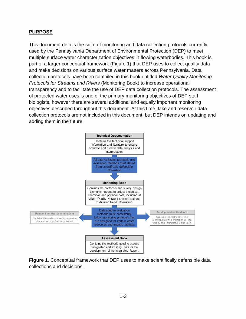
This document details the suite of monitoring and data collection protocols currently
used by the Pennsylvania Department of Environmental Protection (DEP) to meet
multiple surface water characterization objectives in flowing waterbodies. This book is
part of a larger conceptual framework (Figure 1) that DEP uses to collect quality data
and make decisions on various surface water matters across Pennsylvania. Data
collection protocols have been compiled in this book entitled Water Quality Monitoring
Protocols for Streams and Rivers (Monitoring Book) to increase operational
transparency and to facilitate the use of DEP data collection protocols. The assessment
of protected water uses is one of the primary monitoring objectives of DEP staff
biologists, however there are several additional and equally important monitoring
objectives described throughout this document. At this time, lake and reservoir data
collection protocols are not included in this document, but DEP intends on updating and
adding them in the future.
Figure 1. Conceptual framework that DEP uses to make scientifically defensible data
collections and decisions.

1-4
UPDATES
This is the first update to the Monitoring Book since the initial 2018 publication that
effectively consolidated DEP data collection protocols for flowing waterbodies. Data
collection protocols for lakes have not been consolidated into this document. This 2021
update includes the following updates that are worth noting:
• A new subchapter has been added to Chapter 2, Sampling Design and Planning
(Lookenbill 2020b), titled Combined Sewer Overflow (CSO) Compliance
Monitoring (Lookenbill 2020a). This new subchapter was developed in response
to requests by DEP permitting staff for guidance in reviewing post-construction
monitoring plans. The updates are primarily design and planning elements that
rely on existing data collection protocols.
• Updates to the Taxonomic Identification section of the Macroinvertebrate
Laboratory Subsampling and Identification Protocol (Brickner 2020) located in
Chapter 3, Biological Data Collection Protocols were made that more definitively
describe the appropriate levels of macroinvertebrate identification and the
process for addressing less than confident identifications.
• Updates to the Bacteriological Data Collection Protocol (Miller 2021) located in
Chapter 3 were made to account for the adoption of updated bacteriological
criteria in 25 Pa. § Code 93.7 during the swimming season (May 1 through
September 30).
• New sections were added to the In-Situ Field Meter and Transect Data Collection
Protocol (Hoger 2020) found in Chapter 4, titled Evaluation of Transect Data and
Display and Storage of Transect Data.
• Appendix D has been added to include the Water Quality Network (WQN). This
new appendix, Pennsylvania’s Surface Water Quality Network (WQN) Manual
(Pulket and Lookenbill 2020), was once a separate document and has now been
incorporated into this Monitoring Book to take advantage of existing resources
and consolidate this information.
• Appendix E has been added to include the latest EPA approved Quality
Assurance Protocol (QAPP).
COLLECTION FRAMEWORK AND PROCESSES
Collectors will need to adhere to an established framework and process. In doing so,
consistency will be maintained to produce quality data. All data collection should follow
the framework described here and throughout this book.
1-5
• IDENTIFY THE MONITORING OBJECTIVE – Why are data being collected?
The primary and any secondary objectives will need to be identified before any
data are collected. DEP staff will often identify the primary data collection
objective and consider other, secondary objectives which may require additional
data collections, which would simultaneously meet requirements of both the
primary and secondary objectives. Consequently, considering both objectives
would require less effort if pursued independently. As an example, DEP staff
biologists will identify the primary objective as the assessment of protected water
uses. Based on the information gathered during the reconnaissance process,
there may be indications that the target waterbody may have an existing use that
is different than the designated use. Employing additional requirements that
satisfy the stream redesignation evaluation objective requirements, like the
collection of reference stations and targeting additional analytical tests, could
provide the opportunity to meet this secondary objective. The following is a list of
monitoring objectives:
o Assessment of Protected Water Uses
o Stream Redesignation Evaluation
o Point of First Use
o Cause and Effect
o Water Quality Network Monitoring
o Protocol, Method and Water Quality Standards Development
• RECONNAISANCE AND DATA GATHERING – Reconnaissance includes the
delineation of the targeted waterbody or basin and the gathering of historical and
other information that will provide the best opportunity to meet data collection
objectives.
• SELECT A SAMPLING DESIGN – Select a sampling design that will meet the
monitoring objective(s).
o Probabilistic
o Targeted
• DEVELOP A SAMPLING PLAN – A sampling plan should be developed that
outlines objectives, protocols, methods, standards, and other important
information and resources that need to be referenced and followed.
• QUALITY ASSURANCE – Water quality data that will be used by DEP will need
to meet quality assurance (QA) criteria. A review of the QA criteria for specific

1-6
objectives will need to be performed before any collection occurs. Water quality
data that are used by DEP need to be collected by individuals trained and
subsequently audited by DEP staff. Documentation of trainings and audits will
need to be provided upon request. DEP maintains documentation of trainings
and audits as part of the QA requirements.
Monitoring for The Assessment of Protected Water Uses
DEP staff biologists are tasked with monitoring and assessing surface waters of
Pennsylvania for the protected water uses listed at 25 Pa. Code § 93.3. Monitoring to
assess protected water uses is one of the primary objectives of DEP staff biologists. To
successfully complete an assessment of protected water uses, requirements should be
met as described in the appropriate data collection protocols as wells as requirements
described in the appropriate assessment methods established in Assessment
Methodology for Streams and Rivers (Assessment Book, Shull and Whiteash 2021).
The protected water uses include Aquatic Life, Water Supply, Recreation and Fish
Consumption, and Special Protection.
Aquatic Life Use Monitoring
Aquatic Life Uses (ALU) include Cold Water Fishes (CWF), Warm Water Fishes (WWF),
Trout Stocking (TSF), and Migratory Fishes (MF). See 25 Pa. Code § 93.3 for
definitions and standards.
There are multiple approaches that can be considered in developing a sampling
collection plan with the objective of assessing an ALU. The first includes employing a
biological data collection protocol (Chapter 3) with a method in the Assessment Book
(Shull and Whiteash 2021). DEP currently has four benthic macroinvertebrate data
collection protocols with assessment methods. Each data collection protocol describes
criteria that will need to be evaluated to determine the appropriate protocol required for
a specific waterbody, waterbody reach, or sampling location. Each assessment method
establishes impairment thresholds and/or decision-making matrices to determine
impairment. Progressively, alternative approaches include employing a biological data
collection protocol or protocols with additional physical, chemical and/or other biological
data collections. These additional data collections, often determined during the
reconnaissance process, can be used to further assess a waterbody and used to
identify potential sources and causes of impairment.
Physical habitat data collection will be completed when employing all biological data
collection protocols. Physical habitat data can be used in conjunction with biological
assessment data or can be used independently to make ALU assessments. Guidance
on physical habitat data collection can be found in Chapter 5 of this book, or in the
1-7
specific biological data collection protocols in Chapter 3. Specific ALU physical
assessment methodology can be found in the Assessment Book, Chapter 4.1, Physical
Habitat Assessment Method (Walters 2017). Collectors should be familiar with physical
habitat assessments and should consult associated habitat data sheets during field
reconnaissance to aid in properly identifying and locating sampling locations.
Chemical data can also be collected to characterize water quality during biological data
collection or the field reconnaissance process. Chemical data collection protocols can
be found in Chapter 4 and are required for many of the data collection protocols found
in this book. In-situ field meter data, including cross-section surveys, are highly
recommended as a screening process to determine changing water quality that may
drive differences in aquatic life. For surface waters with perceived or documented water
quality complexities (incomplete mixing, dynamic seasonal/temporal changes, etc.), and
especially on larger waterbodies (> 1000 mi2), multiple field meter data collections,
cross-section surveys, and/or discrete water chemistry data collections may be
completed multiple times targeting changing conditions throughout a period leading up
to biological data collection. A “period” is delineated by seasonality or index periods
described in the biological collection protocols and assessment methods. For example,
instream macroinvertebrate communities significantly change throughout late-May and
into June and again typically in October, depending on climatic conditions.
Consequently, collectors will usually employ macroinvertebrate collection in November
or in April. If collection is scheduled for April, multiple chemical data collection efforts
that target changing conditions beginning November and continuing through April would
provide data as to the source and/or cause of differences in biological sample results.
This information could be collected after biological data collection and after realization of
aquatic life use impairment. However, subsequent data collections may not be directly
representative of water quality conditions that caused the impairment, especially with
highly variable surface waters.
DEP also employs fish data collection, mussel data collection and periphyton (algal)
data collection protocols that can be found in Chapter 3. The latest edition of the
Assessment Book (Shull and Whiteash 2021) does include the Stream Fish
Assemblage Assessment Method (Wertz 2021d), which is designed to make
assessment determinations across Pennsylvania’s lotic surface waters. While
assessment method development is actively being pursued for fish data collection in
lentic surface waters, mussel data collection and periphyton (algal) data collection,
currently there are no assessment methods for these biological data collection
protocols, however they are employed to assess the narrative criteria and measure
changes in water quality.

1-8
Water Supply Use Monitoring
Water Supply uses include Potable Water Supply (PWS), Industrial Water Supply
(IWS), Livestock Water Supply (LWS), Wildlife Water Supply (AWS), and Irrigation
(IRS). See 25 Pa. Code § 93.3 for definitions and standards.
Water supply use employs chemical data collection protocols including the In-Situ Field
Meter and Transect Data Collection Protocol (Hoger 2020) and the Discrete Water
Chemistry Data Collection Protocol (Shull 2017), found in Chapter 4. While 25 Pa. Code
§ 93.4 and § 96.3(c) identifies PWS as applying to all surfaces waters, § 96.3(d) states,
“(d) As an exception to subsection (c), the water quality criteria for total dissolved
solids, nitrite-nitrate nitrogen, phenolics, chloride, sulfate and fluoride established
for the protection of potable water supply [PWS] shall be met at least 99% of the
time at the point of all existing or planned surface potable water supply
withdrawals unless otherwise specified in this title”
Therefore, reconnaissance will need to identify surface potable water supply
withdrawals and sampling plans will need to target these locations, especially when
chemistry data collected involves the parameters listed in § 96.3(d).
Recreational Use and Fish Consumption Monitoring
Recreation and Fish Consumption uses include Boating (B), Fishing (F), Water Contact
(WC), and Esthetics (E). Primary objectives for recreational use and fish consumption
are Fishing (F) and Water Contact (WC). See 25 Pa. Code § 93.3 for definitions and
standards.
A sample collection plan with the objective of assessing the water contact (WC) Use will
employ Chapter 3.11, Bacteriological Data Collection Protocol (Miller 2021) and Chapter
2.5 of the Assessment Book (Shull and Whiteash 2021), Bacteriological Assessment
Method for Water Contact Sports (Miller and Whiteash 2021). Chemical data collection
protocols found in Chapter 4 of this book, including the In-situ Field Meter and Transect
Data Collection Protocol (Hoger 2020) and the Discrete Water Chemistry Data
Collection Protocol (Shull 2017), should also be considered as part of the field
reconnaissance effort.
Collecting fish consumption/fish tissue samples is typically accomplished by employing
the Fish Data Collection Protocol (Wertz 2021a) as well as the Fish Tissue Data
Collection Protocol (Wertz 2021c), Chapter 3, and samples are often collected as a
secondary objective during community surveys. Other acceptable collection procedures
include seine, gill net, rotenone, angling, etc. Refer to Chapter 2 of the Assessment
1-9
Book (Shull and Whiteash 2021), Fish Tissue Consumption Assessment Method (Wertz
2021b) for additional requirements that will need to be addressed in the sample
collection plan.
Special Protection Monitoring
Special Protection uses include High Quality Waters (HQ) and Exceptional Value
Waters (EV). See 25 Pa. Code § 93.3 for definitions and standards.
Developing a sample collection plan for special protection waters will include employing
a biological data collection protocol (Chapter 3) with an assessment method. Each data
collection protocol describes criteria that will need to be evaluated to determine the
appropriate protocol required for a specific waterbody, waterbody reach, or sampling
location. When appropriate, biological assessment methods will include, index periods
and impairment thresholds and decision matrices specific to special protection waters
that will need to be addressed in the sample collection plan. Otherwise, sample
collection plan development is consistent with aquatic life use monitoring.
Stream Redesignation Evaluation Monitoring
Stream redesignation evaluations are initiated to determine the existing and designated
uses of a given waterbody. The terms “existing use” and “designated use” are defined at
25 Pa. Code § 93.1. Evaluations can be initiated as part of a petition process, permitting
process, or due to the results of a use assessment reconnaissance or survey that
indicates an existing use may be different than the designated use. Redesignation
evaluations can lead to redesignation to a more restrictive use, a less restrictive use, no
change to the use, or a demonstration of “natural quality” as defined at 25 Pa. Code §
93.1.
A sample collection plan for redesignation evaluations will include and refer to
information at 25 Pa. Code § 93.4b, ‘Qualifying as High Quality or Exceptional Value
Waters’ and the DEP Water Quality Antidegradation Implementation Guidance (DEP
2003). This includes the application of biological and chemical data collection protocols.
Physical habitat assessments will also be completed when employing biological data
collection protocols. Thermal components of ALU (WWF, TSF, and CWF) are evaluated
using fish community data and will employ the Fish Data Collection Protocol (Wertz
2021c) found in Chapter 3.
Point of First Surface Water Use Monitoring
Point of first use surveys are completed as part of the evaluation and permitting of
wastewater discharges to intermittent and ephemeral streams, drainage channels and
swales, and storm sewer. The point of first surface water use establishes where

1-10
Chapter 93 Water Quality Standards (WQS) must be attained. Collectors will need to
become familiar with DEP technical guidance document 391-2000-014, Policy and
Procedures for Evaluating Wastewater Discharges to Intermittent and Ephemeral
Streams, Drainage Channels and Swales, and Storm Sewers (DEP 2000). Point of first
use surveys will employ biological data collection protocols found in Chapter 3.
Cause and Effect Monitoring
A cause and effect sampling design is employed to investigate possible relationships
between point or nonpoint sources of conventional pollutants and known or suspected
instream water quality problems through the collection and analysis of biological,
physical, and chemical data. These surveys are designed primarily to monitor the
effectiveness of permitted treatment facilities but are also used to investigate reported
or suspected water quality impacts for nonpoint source and other pollution sources.
Cause and Effect Surveys (Lookenbill and Wertz 2021) found in Chapter 2.1 includes
specific survey design requirements. Cause and effect monitoring will employ biological,
chemical, and physical data collection protocols found in this book.
Water Quality Network Monitoring
The Pennsylvania Water Quality Network (WQN) is a statewide, fixed station water
quality sampling system operated by DEP. It is designed to assess both the quality of
Pennsylvania’s surface waters and the effectiveness of the water quality management
program by accomplishing four basic objectives:
• Monitor temporal water quality trends in major surface streams throughout
Pennsylvania.
• Monitor temporal water quality trends in selected reference waters.
• Monitor the trends of nutrient and sediment loads in the major tributaries entering
the Chesapeake Bay.
• Monitor temporal water quality trends in selected Pennsylvania lakes.
Data collection is a collaborative effort between the US Geological Survey (USGS) PA
Water Science Center, Susquehanna River Basin Commission (SRBC), and DEP. WQN
monitoring employs routine biological data collection (primarily benthic
macroinvertebrate data collection, chemical/physical data collection, and stream
discharge data collection. Appendix D contains Pennsylvania’s Surface Water Quality
Monitoring Network (WQN) Manual (Pulket and Lookenbill 2020) which details the
network’s sampling design, station locations, and the water chemistry analytes
collected.

1-11
Protocol, Method, and Standards Development
The DEP Water Quality Division (WQD) is responsible for developing surface water
data collection protocols, water quality criteria and protected water uses, assessment
methods, Pennsylvania’s biannual integrated monitoring and assessment report, and
Total Maximum Daily Loads (TMDLs) that allow impaired waters to meet WQS. Data
collection to meet an objective of protocol, method or WQS development is unique from
other data collection objectives. The ultimate purpose is to implement The Pennsylvania
Clean Streams Law and the Federal Clean Water Act. To achieve this, at a statewide
level, WQS are developed to establish the criteria and protected uses that surface
waters must meet. Data collection protocols and assessment methods are developed,
at a statewide level, to collect consistent data that will be used to determine if surface
waters meet WQS. In addition, data collection protocols also need to be applicable to
other data collection objectives.
Sampling design for a development objective will pursue the range of possible water
quality conditions across the State. Reconnaissance will focus on a range of conditions
and attributes that describe this range and not necessarily the potential to delineate a
water quality condition or the source or cause on a waterbody. A range of conditions will
be qualified by identifying classification of waterbodies. Attributes that are selected to
describe a range of water quality conditions will rely on published literature.
Development objectives, particularly the development of standards, may also rely on
laboratory investigations.
LITERATURE CITED
Brickner, M. (editor). 2020. Macroinvertebrate laboratory subsampling and identification.
Chapter 3.6, pages 32–42 in M. J. Lookenbill and R. Whiteash (editors). Water
quality monitoring protocols for streams and rivers. Pennsylvania Department of
Environmental Protection, Harrisburg, Pennsylvania.
DEP. 2000. Policy and procedures for evaluating wastewater discharges to intermittent
and ephemeral streams, drainage channels and swales, and storm sewers.
Pennsylvania Department of Environmental Protection, Harrisburg, Pennsylvania
(Available from:
http://www.depgreenport.state.pa.us/elibrary/GetDocument?docId=7790&DocNa
me=391-2000-014.pdf)
DEP. 2003. Water quality antidegradation implementation guidance. Pennsylvania
Department of Environmental Protection, Harrisburg, Pennsylvania. (Available
from: http://www.depgreenport.state.pa.us/elibrary/GetFolder?FolderID=4664)
Hoger, M. 2020. In-situ field meter and transect data collection protocol. Chapter 4.1,
pages 2–8 in M. J. Lookenbill and R. Whiteash (editors). Water quality monitoring

1-12
protocols for streams and rivers. Pennsylvania Department of Environmental
Protection, Harrisburg, Pennsylvania.
Lookenbill, M. J. 2020a. Combined sewer overflow (CSO) compliance monitoring.
Chapter 2.1, pages 14–23 in M. J. Lookenbill and R. Whiteash (editors). Water
quality monitoring protocols for streams and rivers. Pennsylvania Department of
Environmental Protection, Harrisburg, Pennsylvania.
Lookenbill, M. J. 2020. Sampling design and planning. Chapter 2, pages 1–25 in M. J.
Lookenbill and R. Whiteash (editors). Water quality monitoring protocols for
streams and rivers. Pennsylvania Department of Environmental Protection,
Harrisburg, Pennsylvania.
Lookenbill, M. J. and Wertz, T. A. (editors). 2021. Cause and effect surveys. Chapter
2.1, pages 7–15 in M. J. Lookenbill and R. Whiteash (editors). Water quality
monitoring protocols for streams and rivers. Pennsylvania Department of
Environmental Protection, Harrisburg, Pennsylvania.
Miller, S. (editor). 2021. Bacteriological data collection protocol. Chapter 3.11, pages
142–158 in M. J. Lookenbill and R. Whiteash (editors). Water quality monitoring
protocols for streams and rivers. Pennsylvania Department of Environmental
Protection, Harrisburg, Pennsylvania.
Miller, S., and R. Whiteash. 2021 (editors). Bacteriological assessment method for
water contact sports. Chapter 2.5, pages 75–79 in D. R. Shull, and R. Whiteash
(editors). Assessment methodology for streams and rivers. Pennsylvania
Department of Environmental Protection, Harrisburg, Pennsylvania.
Pulket, M., and M. J. Lookenbill (editors). 2020. Pennsylvania’s surface water quality
monitoring network manual. Appendix D, pages 1–71 in M. J. Lookenbill, and R.
Whiteash (editors). Water quality monitoring protocols for streams and rivers.
Pennsylvania Department of Environmental Protection, Harrisburg,
Pennsylvania.
Shull, D. R. 2017. Discrete water chemistry data collection protocol. Chapter 4.2, pages
9–24 in M. J. Lookenbill, and R. Whiteash (editors). Water quality monitoring
protocols for streams and rivers. Pennsylvania Department of Environmental
Protection, Harrisburg, Pennsylvania.
Shull, D. R., and R. Whiteash (editors). 2021. Assessment methodology for streams and
rivers. Pennsylvania Department of Environmental Protection, Harrisburg,
Pennsylvania.
Wertz, T. A. (editor). 2021a. Fish data collection protocol. Chapter 3.7, pages 43–62 in
M. J. Lookenbill, and R. Whiteash (editors). Water quality monitoring protocols for
streams and rivers. Pennsylvania Department of Environmental Protection,
Harrisburg, Pennsylvania.
Wertz, T. A. (editor). 2021b. Fish tissue consumption assessment method. Chapter 2.6,
pages 80–87 in D. R. Shull, and R. Whiteash (editors). Assessment methodology

1-13
for streams and rivers. Pennsylvania Department of Environmental Protection,
Harrisburg, Pennsylvania.
Wertz, T. A. (editor). 2021c. Fish tissue data collection protocol. Chapter 3.8, pages 63–
73 in M. J. Lookenbill, and R. Whiteash (editors). Water quality monitoring
protocols for streams and rivers. Pennsylvania Department of Environmental
Protection, Harrisburg, Pennsylvania.
Wertz, T. A. 2021d. Stream fish assemblage assessment method. Chapter 2.7, pages
88–107 in D. R. Shull, and R. Whiteash (editors). Assessment methodology for
streams and rivers. Pennsylvania Department of Environmental Protection,
Harrisburg, Pennsylvania.
Walters, G. 2017. Physical habitat assessment method. Chapter 4.1, pages 2–6 in D. R.
Shull, and R. Whiteash (editors). Assessment methodology for streams and
rivers. Pennsylvania Department of Environmental Protection, Harrisburg,
Pennsylvania.


2-2
Prepared by:
Josh Lookenbill
PA Department of Environmental Protection
Office of Water Programs
Bureau of Clean Water
11th Floor: Rachel Carson State Office Building
Harrisburg, PA 17105
2018
Edited by:
Josh Lookenbill
PA Department of Environmental Protection
Office of Water Programs
Bureau of Clean Water
11th Floor: Rachel Carson State Office Building
Harrisburg, PA 17105
2020

2-3
TYPES OF SAMPLING DESIGN
A sampling design must be chosen in order to form a data set that is appropriate to
describe the desired objective. The two general sample design categories are
probabilistic (also called “statistical” or “random”) sampling designs and judgmental or
targeted sampling designs (USEPA 2002a).
Probabilistic Sampling
A probabilistic or probability-based sampling design utilizes randomization in the
selection of sample locations (USEPA 2002a). A probabilistic sampling design requires
accurate information about the population being sampled to ensure that a consistent
distribution of the population is sampled. The sampling location selection process must
consider population characteristics (Strahler stream order, landuse, number and
location of point source discharges, etc.) and must be weighted accordingly. There are
various ways that sites can be picked for a probabilistic monitoring study. One approach
is a Generalized Random Tessellation Stratified (GRTS) design procedure. This
procedure was employed for DEP’s recreational use monitoring and statewide statistical
survey requirements. GRTS provides a random sample that is balanced spatially. The
sites are chosen using an R-program package called ‘spsurvey’ (Kincaid and Olsen
2011). The package ‘spsurvey’ also helps analyze the results and can give estimations
of the proportion of samples in each category analyzed, along with standard error and
total estimates (Kincaid 2012a, Kincaid 2012b). Other procedures may be employed to
choose sites statistically; however, without a detailed characterization and classification,
a probabilistic sampling design does not necessarily provide for detailed assessment
delineations and is not the preferred sampling design.
Targeted Sampling
DEP’s primary monitoring objective is to collect data to assess protected water uses of
specific water segments or reaches, where most other states assess larger watershed
units. DEP believes the targeted “judgment-based” sampling design is the most suited
procedure to assess WQS including uses of specific water segments or reaches. A
targeted or judgmental sampling design provides for the selection of sample locations
based on professional judgment and does not utilize randomization. This approach
requires intense reconnaissance and information gathering but can result in an
accurately delineated assessment and is the preferred sampling approach for DEP
monitoring protocols and subsequent assessment methods.
Reconnaissance includes the delineation of the targeted waterbody or basin and the
gathering of historical and other information. A review of any gathered data or
information may influence the geographical extent of the survey. Aerial photography,

2-4
topographic maps, and/or geographical information system (GIS) information are used
to delineate the targeted waterbody, identify major tributaries, characterize land use and
any potential sources of nonpoint source impacts (agriculture, urban areas, etc.),
potential sources of point source impacts (industrial discharges, sewage treatment
discharges, combined sewer overflow (CSO discharges, etc.), geology, and soil
characteristics. Historical information includes past water quality data and associated
use assessments. Other information can include designated and existing water uses
and ongoing water quality monitoring like the DEP Water Quality Network (WQN) and
US Geological Survey (USGS) stream gaging network.
Sampling sites and locations are positioned to account for changes in water quality due
to influences such as major tributaries, point and nonpoint source impacts, land use
changes, soil characteristics, and geology. Additional samples are collected at the limits
of these changes to effectively “bracket” potential sources of water quality differences.
Initial sampling site placement should target 3rd order or higher waterbodies. Sampling
sites located on 1st and 2nd order waterbodies are chosen based on the variability of
potential changes to water quality, but not all 1st and 2nd order waterbodies will have
sampling sites located on them. It is important to identify 1st and 2nd order tributaries that
may be ephemeral or intermittent, as assessment methods are typically not developed
to account for this variable. Also, the minimum length of any use assessment unit is ½
mile. Any impact delineated in length that is less than ½ mile is considered a localized
impact, potentially a compliance issue, but not a non-attainment of use. Additional field
reconnaissance is highly recommended to verify potential sources of water quality
impacts. Field reconnaissance will include visual observations and physical habitat
evaluations (see Chapter 5) and can also include chemical data collection and/or field
meter and cross-section survey data collection (see Chapter 4). Cross-section surveys
performed using a clean and calibrated field meter that collects water temperature,
specific conductance, dissolved oxygen, pH, and – preferably – turbidity are required to
determine if major water quality influences exist at the sampling location.
SAMPLING PLANS
A sample collection plan is recommended before commencing a sampling project. This
should include the primary and any secondary objectives, subsequent monitoring
protocols and assessment methods that will be employed to meet objectives, tentative
sampling/site location(s), timing and frequency of samples, media of interest (water,
sediment, soil, macroinvertebrates, etc.), parameters to sample, QA and Quality Control
(QC) plans, sampling supplies and equipment, and any other notes or comments
pertaining to the project. More information on developing Project Plans can be found in

2-5
United States Environmental Protection Agency (USEPA) resources (USEPA 2002a,
USEPA 2002b, and USEPA 2006).
A sample collection plan should describe how the data will be used. Analyses and data
interpretation should be anticipated in advance. A collector should consider if an
objective is to defend an enforcement action or recommend regulatory changes. Also,
consider what criteria may be used during its interpretation. DEP has numeric and
narrative water quality criteria documented in 25 Pa. Code Chapter 93, Water Quality
Standards. Numeric criteria allow for screenings during sampling. In some cases, there
may be no numeric criteria for a substance or sampling matrix. For example, DEP has
no numeric sediment criteria at this time. However, in order to apply these or other
results that do not have numeric criteria, one can refer to the 25 Pa. Code § 93.6:
“(a) Water may not contain substances attributable to point or nonpoint source
discharges in concentration or amounts sufficient to be inimical or harmful to the
water uses to be protected or to human, animal, plant or aquatic life. and (b) In
addition to other substances listed within or addressed by this Chapter, specific
substances to be controlled include, but are not limited to, floating materials, oil,
grease, scum and substances that produce color, tastes, odors, turbidity or settle
to form deposits.”
The numeric criteria, narrative criteria, or biological standard to be measured should be
described prior to study commencement.
LITERATURE CITED
Kincaid, T. M., and A. R. Olsen. 2011. spsurvey: Spatial Survey Design and Analysis. R
package version 2.2.
Kincaid, T. M. 2012a. Analysis of a GRTS survey design for a linear resource. CRAN
– R project.
Kincaid, T. M. 2012b. GRTS survey designs for a linear resource. CRAN – R project.
USEPA. 2002a. Guidance on choosing a sampling design for environmental data
collection for use in developing a quality assurance project plan.
EPA/240/R02/005. EPA QA/G-5S. U.S. Environmental Protection Agency, Office
of Environmental Information, Washington, DC.
USEPA. 2002b. Guidance for quality assurance project plans. EPA/240/R-02/009. EPA
QA/G-5. U.S. Environmental Protection Agency, Office of Environmental
Information, Washington, DC.

2-6
USEPA. 2006. Guidance on systematic planning using the data quality objectives
process. EPA/240/B-06/001. EPA QA/G-4. U.S. Environmental Protection
Agency, Office of Environmental Information, Washington, DC.

2-7
2.1 CAUSE AND EFFECT SURVEYS

2-8
Prepared by:
Josh Lookenbill
PA Department of Environmental Protection
Office of Water Programs
Bureau of Clean Water
11th Floor: Rachel Carson State Office Building
Harrisburg, PA 17105
2018
Edited by:
Josh Lookenbill and Timothy Wertz
PA Department of Environmental Protection
Office of Water Programs
Bureau of Clean Water
11th Floor: Rachel Carson State Office Building
Harrisburg, PA 17105
2021

2-9
INTRODUCTION
Cause and effect surveys are designed to investigate possible relationships between
point or nonpoint sources of conventional pollutants and known or suspected instream
water quality problems through the collection and analysis of biological, physical, and
chemical data. This protocol was developed to establish and standardize cause and
effect survey procedures and provide guidance to DEP staff for conducting such
surveys. The protocol should be used in conjunction with other DEP data collection
protocols and assessment methods.
These surveys are performed primarily to monitor the effectiveness of permitted
treatment facilities but are also used to investigate reported or suspected water quality
impacts from nonpoint source and other pollution sources. Since such discharges exist
on a wide variety of stream and river habitats, the sampling design and type of sampling
gear used are dependent on stream-type, site-specific conditions, and the nature of the
discharge under investigation. DEP staff are responsible for sampling design and any
modifications to sampling design due to unforeseen site-specific conditions.
SAMPLING DESIGN
The sampling design for a cause and effect survey requires a minimum of two sampling
stations. One station is placed upstream from the subject discharge(s) or impact(s) to
serve as a control or reference condition and at least one station is placed in a
potentially impacted zone downstream. Additional sampling stations may be necessary,
either placed downstream to define zones of impact and recovery; upstream to bracket
multiple discharges; or across a stream transect in wider waterbodies. For point
sources, observations in the immediate vicinity of a discharge may also be useful.
Observations in the immediate vicinity of a discharge should include:
• Floating solids, scum, sheen, or substances that result in observed deposits in
the receiving water (a small amount of foam that rapidly dissipates is typical);
• Oil and grease in amounts that cause a film or sheen upon or discoloration of the
surface waters or adjoining shoreline, or that exceed 15 mg/l as a daily average
or 30 mg/l at any time (or lesser amounts if specified in the respective permit);
• Substances in concentration or amounts sufficient to be inimical or harmful to
the water uses to be protected or to human, animal, plant, or aquatic life;
2-10
• Foam or substances that produce an observed change in the color, taste, odor,
or turbidity of the receiving water, unless those conditions are otherwise
controlled through effluent limitations or other requirements in the respective
permit.
Any noted observations may or may not indicate non-attainment of WQS or a violation
of associated permit conditions. Regulatory requirements and permit conditions
(including 25 Pa. Code §§ 93.6, 92a.41(c), 95.2(2)(i)) should be consulted.
With the exception of observations previously described, stations sampled downstream
of the discharge(s) or nonpoint sources should not be placed in the immediate vicinity of
the discharge or nonpoint source, but instead should generally be located a distance
downstream in a potentially impacted zone. Selecting downstream station locations is
unrelated to “criteria compliance times” used to generate National Pollutant Discharge
Elimination System (NPDES) permit limits. Similarly, it is not necessary to restrict the
location of downstream stations to points at or downstream of the point of complete mix,
as defined as the point where water quality and/or other characteristics are
homogenous across a transect. If a tributary or other compromising influence is located
just downstream of the discharge or source of potential impact, which would not make
an upstream/downstream comparison directly applicable, DEP staff may need to modify
the sampling design to account for differences in water quality that are not necessarily
due to the discharge or source of potential impact.
Complete mix occurs rapidly in smaller streams at most flow conditions and it is typically
appropriate to locate downstream stations in smaller streams at a point of complete mix.
In larger streams or rivers, a plume of effluent could extend a significant distance
laterally and longitudinally. An indicator station may be located at or downstream of this
point recognizing that any chemical, physical, or biological sampling could be conducted
as a composite across the transect, but effects within the plume will also be assessed if
a significant portion of the receiving water is impacted. The number and placement of
any in-situ collections across a transect and subsequent compositing should be
completed according to Chapter 4.1, In-situ Field Meter and Transect Data Collection
Protocol (Hoger 2020), or equal-width-increment or equal-discharge-increment
procedures (USGS 2006). When collecting biological samples, the equal-width-
increment procedure can be considered (i.e., effort physically distributed equally across
the/a transect), but the sample should be collected in a manner such that the sample
represents the waterbody across the transect and targets best available habitat
according to the DEP protocols and methodologies.

2-11
If the downstream station is placed where homogenous conditions do not exist,
additional downstream cross-section surveys and sampling stations may be necessary
to characterize the effect. Any critical habitat of threatened or endangered species, as
defined by the United States Fish and Wildlife Service, or any rare or endemic
ecological community types, as defined by the Pennsylvania Natural Heritage Program,
or any migration impediments must be identified within the defined plume or within the
vicinity of the plume. The water quality and its effect on identified habitat or ecological
communities and/or WQS will be assessed specific to identified habitat or ecological
communities.
Control or reference sampling stations may be placed at any point upstream from the
discharge or source where there is no potential impact from the discharge at any river
flow condition. In a low-gradient situation such as a pool, it may be most appropriate to
locate the reference station far enough upstream from the discharge to preclude
possible effects from pooling effluent during low river flow conditions. If there is an
intake structure present, it may be most appropriate to locate the reference station
upstream from the intake structure to preclude possible effects from recirculating
effluent during low river flow conditions.
In some instances, if upstream conditions do not adequately represent control or
reference conditions, it may be necessary to sample a separate waterbody for reference
purposes. Ideally, this reference station would be selected within the same watershed or
if no available reference station is found, an appropriate station should be in an adjacent
watershed. Water quality impacts to impounded waters present at least the
compounding effect the impoundment itself has on water quality and water quality
indicators and may prevent traditional upstream/downstream sampling designs from
detecting changes in water quality due to impacts other than the impoundment. To
reduce or eliminate compounding sources of variability, physical habitat conditions
should be as similar as possible, for each segment or separate waterbody selected for
sampling. The following data will be collected at all sampling stations: benthic
macroinvertebrates, habitat assessment, field measurements or water chemistry,
channel cross-section and stream flow (as needed), cross-section surveys (as needed),
bacteria (as needed), and fish (as needed).
DATA COLLECTION
Benthic Macroinvertebrates (required)
For wadeable freestone streams, limestone-influenced streams, low gradient streams,
or large semi-wadable rivers, benthic macroinvertebrate samples are collected utilizing
protocols detailed in Chapter 3 of this book. Each benthic macroinvertebrate data

2-12
collection protocol describes what will need to be evaluated to determine which protocol
to use. Data collection protocols include semi-quantitative (population densities derived
by estimation), qualitative (population densities not calculated), and quantitative
(population densities derived by measurement) protocols. The survey data needs will
determine which protocol is most suitable. In most instances, semi-quantitative data
collection protocols are preferred and will meet most data requirements. Other optional
data collection protocols include qualitative and quantitative. Qualitative protocols
(Chapter 3) are appropriate Cause and Effect Survey protocols. Qualitative protocols
may be more appropriate than quantitative or semi-quantitative protocols, and may be
used in place of, or in conjunction with semi-quantitative data collection when the survey
requires a more immediate result or the targeted surface water is not characteristic of
surface waters used to develop a method or index. Qualitative surveys are also
appropriate as preliminary evaluations immediately following acute pollution events
where the impact to the biological community doesn’t occur for a period of one to three
weeks. Qualitative surveys could be used to determine the timing of subsequent
quantitative or semi-quantitative surveys.
Regardless of the data collection protocol used, sampling stations consist of a control or
background station placed upstream from the discharge(s) and at least one affected or
impacted station downstream from the discharge(s) in the best available riffle and run
habitat. When multiple discharges are present, sampling stations are placed between
discharges to characterize the effect of each input. Physical variables of all sample
stations should be matched as closely as possible between background and impacted
stations to minimize or eliminate the effects of compounding variables. Sample points
are placed to obtain a representative benthic sample and to avoid over sampling of
clustered populations.
DEP developed an index of biotic integrity (IBI) for benthic macroinvertebrate
communities collected via semi-quantitative protocols in Pennsylvania’s wadeable,
freestone, riffle-run streams. See Chapter 2 of the Assessment Book (Shull and
Whiteash 2021). Through direct quantification of biological attributes along a gradient of
ecosystem conditions, this IBI measures the extent to which anthropogenic activities
compromise a stream’s ability to support healthy aquatic communities (Davis and Simon
1995) and can be used to compare control or reference conditions versus impacted
conditions. DEP’s latest IBIs describe precision estimates for temporal variability
(...whether a site’s biological condition has improved or degraded over time) and
intersite variability (…whether a site’s biological condition is improved or degraded when
compared to a nearby site). Samples collected for cause and effect surveys should be
collected on the same day to eliminate the need to consider temporal variability.
Intrasite variability, as determined by the IBI for benthic macroinvertebrates applies to
2-13
samples collected from a single site/station (within 100 meters). Cause and effect
survey upstream and downstream stations are collected from separate sites and
therefore an intersite precision estimate was developed and should be applied to
compare upstream, downstream and recovery zone sites/stations. Cause and effect
upstream or control versus downstream or recovery stations collected using the latest
semi-quantitative protocols for wadeable, freestone, riffle-run streams with IBI scores
greater than the intersite precision estimate will be considered impacted. The
appropriate intersite precision estimate is determined by DEP Water Quality Division,
Assessment Section. Follow-up surveys may be conducted when small IBI score
differences are found between control and impact sites, to confirm, or re-evaluate initial
cause and effect survey results.
Fish (optional)
For most cause and effect surveys semi-quantitative fish sampling should be
considered. See Chapter 3.7, Fish Data Collection Protocol (Wertz 2021a). The
objective is to acquire a representative sample of the fish population by sampling all
physical stream habitats in relative proportion to their availability.
DEP developed Stream Fish Assemblage Assessment Method (Wertz 2021b) using a
Thermal Fish Index (TFI) for fish communities collected via semi-quantitative protocols
in Pennsylvania’s lotic streams and rivers. The assessment method provides additional
guidance for initiating and evaluating cause and effect surveys.
If fish kills are a component of a cause and effect survey investigation, quantitative
procedures would be required in cases where economic damages may need to be
calculated resulting from incidents causing fish kills. In these instances, to support
fish/aquatic life penalties, the required fish/aquatic life data should be collected in a
manner consistent with The American Fisheries Society (Southwick and Loftus 2017) or
Pennsylvania Fish and Boat Commission (PFBC) fish kill survey procedures. In many
cases, it may be more practical to coordinate field sampling activities with the regional
PFBC Fisheries Management staff.
Bacteria (optional)
Because of the survey and cost complexities imposed by bacterial sampling (sample
frequency and short holding times), bacteria sample collection is an optional
consideration limited to when sanitary impacts from discharges are suspected. Samples
for bacteriological analysis are collected to define the sanitary significance of point and
nonpoint sources and assess the use attainment status of stream segments for potable
water supply and recreational uses. The samples are collected using protocols outlined
in Chapter 3 of this book.

2-14
Habitat Evaluation (required)
A habitat evaluation is conducted on a measured 100-meter reach of stream at a
minimum for wadeable surface waters according to Chapter 5.1, Stream Habitat Data
Collection Protocol (Lookenbill 2017) in this Monitoring Book and Chapter 4.1, Physical
Habitat Assessment Method (Walters 2017) in the Assessment Book. The habitat
evaluation process involves rating twelve parameters for riffle/run prevalent waterbodies
or nine parameters for low gradient waterbodies as optimal, suboptimal, marginal, or
poor by using a numeric value (ranging from 20-0).
Field Measurements and Water Chemistry (required)
Detailed field observations on land use and potential sources of pollution are recorded
on field data collection forms or in field books. Dissolved oxygen, pH, specific
conductance, and temperature are measured in the field using hand-held meters
calibrated according to manufacturer specifications and the latest DEP protocols found
in Chapter 4 of this book.
One-time grab samples are collected, at a minimum, from a control or background
station upstream from the discharge, from the discharge, and from at least one
downstream affected or impacted station when evaluating point source discharges.
Point source discharges that do not continuously discharge or those that discharge
subsurface may prevent grab samples from being collected. In these situations,
Discharge Monitoring Reports (DMRs) that document the chemical violation of the
NPDES permit would suffice. For nonpoint discharges, grab samples are collected
upstream of the impacted segment and from within the impacted segment.
Discharge (optional)
Discharge data is collected as needed according to the latest version of USGS
Techniques and Methods book 3, chap. A8, Discharge Measurements at Gaging
Stations (Turnipseed and Sauer 2010).
LITERATURE CITED
Davis, W. S. and T. P. Simon. 1995. Introduction to biological assessment and criteria:
Tools for water resource planning and decision making. Pages 3–6 in W. S.
Davis, and T. P. Simon (editors). CRC Press, Boca Raton.
Hoger, M. 2020. In-situ field meter and transect data collection protocol. Chapter 4.1,
pages 2–8 in M. J. Lookenbill and R. Whiteash (editors). Water quality monitoring
protocols for streams and rivers. Pennsylvania Department of Environmental
Protection, Harrisburg, Pennsylvania.
2-15
Lookenbill, M. J. (editor). 2017. Stream habitat data collection protocol. Chapter 5.1,
pages 2–7 in M. J. Lookenbill and R. Whiteash (editors). Water quality monitoring
protocols for streams and rivers. Pennsylvania Department of Environmental
Protection, Harrisburg, Pennsylvania.
Shull, D. R., and R. Whiteash (editors). 2021. Assessment methodology for streams and
rivers. Pennsylvania Department of Environmental Protection, Harrisburg,
Pennsylvania.
Southwick, R. I., and A. J. Loftus. 2017. Investigations and monetary values of fish and
freshwater mussel kills. American Fisheries Society. ISBN 978-1-934874-47-9.
Turnipseed, D. P. and V. B. Sauer. 2010. Discharge measurements at gaging stations:
United States Geologic Survey. Book 3, chapter A8. in National field manual for
the collection of water quality data: Techniques and methods. U.S. Department of
the Interior, U.S. Geological Survey, Reston, VA. (Available online at:
https://pubs.usgs.gov/twri/twri3a8/.)
USGS. 2006. Collection of water samples. Book 9, chapter A4 (version 2.0). in National
field manual for the collection of water quality data: Techniques and methods.
U.S. Department of the Interior, U.S. Geological Survey, Reston, VA. (Available
online at: https://www.usgs.gov/mission-areas/water-resources/science/national-
field-manual-collection-water-quality-data-nfm?qt-science center objects=0#qt-
science center objects.)
Walters, G. 2017. Physical habitat assessment method. Chapter 4.1, pages 2–6 in D. R.
Shull, and R. Whiteash (editors). Assessment methodology for streams and
rivers. Pennsylvania Department of Environmental Protection, Harrisburg,
Pennsylvania.
Wertz, T. A. 2021a. Fish data collection protocol. Chapter 3.7, pages 43–62 in M. J.
Lookenbill, and R. Whiteash (editors). Water quality monitoring protocols for
streams and rivers. Pennsylvania Department of Environmental Protection,
Harrisburg, Pennsylvania.
Wertz, T. A. 2021b. Stream fish assemblage assessment method. Chapter 2.7, pages
88–107 in D. R. Shull, and R. Whiteash (editors). Assessment methodology for
streams and rivers. Pennsylvania Department of Environmental Protection,
Harrisburg, Pennsylvania.
2-16
2.2 COMBINED SEWER OVERFLOW (CSO) COMPLIANCE DATA COLLECTION

2-17
Prepared by:
Josh Lookenbill
PA Department of Environmental Protection
Office of Water Programs
Bureau of Clean Water
11th Floor: Rachel Carson State Office Building
Harrisburg, PA 17105
2020

2-18
INTRODUCTION
CSOs are unique in the way they are regulated and so require unique sampling plans to
meet the demands of compliance monitoring. The Federal Register details the
requirements of CSO policy and monitoring requirements. Specifically, 59 FR 18688
explains:
“The CSO policy represents a comprehensive national strategy to ensure
that municipalities, permitting authorities, water quality standards
authorities and the public engage in a comprehensive and coordinated
planning effort to achieve cost effective CSO controls that ultimately meet
appropriate health and environmental objectives. …State water quality
standards authorities will be involved in the long-term CSO control planning
effort as well. The water quality standards authorities will help ensure that
development of the CSO permittees’ long-term CSO control plans are
coordinated with the review and possible revision of water quality standards
on CSO-impacted waters.”
59 FR 18696, under section 2 explains:
“Once the permittee has completed development of the long-term CSO
control plan and the selection of the controls necessary to meet CWA
requirements has been coordinated with the permitting and WQS
authorities, the permitting authority should include, in an appropriate
enforceable mechanism, requirements for implementation of the long-term
CSO control plan as soon as practicable. Where the permittee has selected
controls based on the "presumption" approach described in Section II.C.4,
the permitting authority must have determined that the presumption that
such level of treatment will achieve water quality standards is reasonable in
light of the data and analysis conducted under this Policy.”
Additionally, the Phase II permit should contain:
“A requirement to implement, with an established schedule, the approved
post-construction water quality assessment program including
requirements to monitor and collect sufficient information to demonstrate
compliance with WQS and protection of designated uses as well as to
determine the effectiveness of CSO controls.”

2-19
USEPA’s draft CSO Post Construction Compliance Monitoring Guidance (USEPA 2011)
also recommends the information to be collected for monitoring CSO compliance,
consistent with the Federal Register. This guidance states that CSO Monitoring
programs should include both CSO effluent and ambient in-stream monitoring. USEPA’s
draft guidance also suggests, where appropriate, biological assessments, toxicity
testing, and sediment sampling are also implemented.
Based on the information found in the Federal Register and USEPA’s guidance (USEPA
2011), designing a sampling plan for CSO compliance monitoring involves answering
two important questions:
1. Does the receiving waterbody meet attainment thresholds?
2. Is the CSO causing or contributing to a WQS impairment?
These two questions are not the same, because the sampling plan will be different for
each question. To answer the first question, sampling must be designed in accordance
with making protected use assessment determinations, which are determinations on the
entire waterbody, or on defined zones as discussed in the Assessment Book (Shull and
Whiteash 2021). The assessment determination process inherently avoids collecting
data at or very near single discharge points, because of the possibility of using results
from one discharge to make an assessment determination on the entire waterbody.
Conversely, the second question requires that the sampling plan incorporates sampling
at or very near single points of discharge to determine contribution to a potential WQS
impairment. It is important to note that sampling must be conducted to answer both
questions regardless of an assessment determination that shows attainment of WQS
upstream and downstream of the CSO.
SAMPLING DESIGN
Sampling design for CSO compliance requires a combination of use assessment and
cause and effect sampling design. Both sampling designs typically include biological,
physical, and chemical data collection. To evaluate any impacts from CSOs, biological
and chemical evaluations will be the primary targets. Biological data collection will
specifically require bacteriological monitoring. Chemical data collections will require at
least discrete water chemistry monitoring. In addition, performance monitoring of the
combined sewer system(s) (CSS) will also be conducted.
All monitoring plans will be submitted to DEP for approval prior to being implemented. A
final report will be submitted within 90 days following the collection of the last samples
for DEP review.

2-20
DATA COLLECTION
Does the receiving waterbody meet attainment thresholds?
Bacteria (required)
Bacteria data collection is conducted according to protocols outlined in Chapter 3 of this
book during the swimming season (May 1st through September 30th). Assessment
determinations will be conducted on upstream and downstream segments of the CSO
or multiple CSOs if there is not the opportunity to sample between according to methods
outlined in Chapter 2 of the Assessment Book (Shull and Whiteash 2021).
Field Measurements and Water Chemistry (required)
Data collection for other parameters identified in the CSO Control Policy are conducted
according to the latest DEP protocols found in Chapter 4 of this book. Assessment
determinations will be conducted on upstream and downstream segments of the CSO
or multiple CSOs if there is not the opportunity to sample between according to methods
outlined in Chapter 3 of the Assessment Book (Shull and Whiteash 2021).
Is the CSO causing or contributing to a WQS impairment?
Bacteria (required)
Bacteria data collection is conducted according to procedures outlined in Chapter 3 of
this book for at least 1 year (4 seasons) as follows:
• During each month of the recreational season (May 1st through September 30th),
samples are collected upstream and downstream of each outfall (or groups of
outfalls as appropriate).
o Samples must be analyzed for fecal coliform1 and E. coli.2
o 5 samples must be collected under “normal” recreating conditions.
o 5 samples must be collected under other, critical conditions to capture
high flows, storm events, etc. when CSOs are discharging.
o Corresponding qPCR samples should also be collected for each set of
samples. A minimum of 1 sample per monthly set is recommended, but
additional samples are encouraged as they will better characterize the
source(s) of bacteria to determine whether the CSO is contributing to the
bacterial load.
1, 2 At the time of publication, fecal coliform limitations are referenced at 25 Pa. Code § 92a.47 and E. coli
criteria are listed at § 93.7.

2-21
• During each month of the non-recreational season (October 1st through April
30th), samples are collected at the same upstream and downstream locations
established during the recreational season following the same protocol.
o Samples must be analyzed for fecal coliform1 and E. coli.2
o 5 samples must be collected in accordance with data collection protocols
during normal/low flow conditions.
o 5 samples must be collected under other, critical conditions to capture
high flows, storm events, etc.
o Corresponding qPCR samples should also be collected for each set of
samples. A minimum of 1 sample per monthly set is recommended, but
additional samples are encouraged as they will better characterize the
source(s) of bacteria to determine whether the CSO is contributing to a
use impairment or impact to the surface water.
1, 2 At the time of publication, fecal coliform limitations are referenced at 25 Pa. Code § 92a.47 and E. coli
criteria are listed at § 93.7.
Field Measurements and Water Chemistry (required)
Data collection for other parameters identified in the CSO Control Policy are conducted
according to the latest DEP protocols found in Chapter 4 of this book for at least 1 year
(4 seasons) as follows:
• At minimum, these parameters include BOD, TSS, ammonia-N, specific
conductance, pH, temperature and DO as well as any other parameters
reasonably expected to be in the discharge.
• A minimum of 1 sample should be collected during each CSO discharge event
throughout the 1-year sampling period unless dangerous conditions prohibit
sample collection.
CSS Performance Monitoring (required)
The purpose of performance monitoring is to document frequency and duration of CSO
activations. A specific CSO activation event definition should be defined for each CSS.
Performance monitoring includes the characterization of CSO activations and the
collection of discharge data at strategic locations throughout and rainfall data within the
CSS catchment area(s).

2-22
CASE STUDY
The following case study demonstrates the need to collect data using both sampling
designs. Briefly, this study demonstrates adequate sampling design to answer question
2 (Is the CSO contributing to a WQS impairment?), but there is insufficient information
to determine the answer to question 1 (Does the receiving waterbody meet attainment
thresholds?). Therefore, more data needs to be collected to make use assessment
determinations on stream segments upstream and downstream of the CSO.
A Post-Construction Monitoring Plan and subsequent results from 2014–
2017 were provided to a DEP regional office. The plan outlined routine
surface water monitoring that took place at 7 sites, upstream and
downstream of discharges. All samples were collected from the shoreline.
Sites were identified as Site 1 through Site 8, moving upstream to
downstream, respectively (Site 5 was discontinued). Site 1 was located
upstream of all urbanized area and all CSO outfalls. Sites 2 through 6
were located appropriately to measure the contribution of several CSO
outfalls and bracket one tributary influence. Site 7 was located
downstream of all CSO outfalls, an urban influenced tributary, and a
sanitary sewer outfall. Site 8 was located downstream of the entire
urbanized area.
Sampling frequency was five times per month during the swimming
season (May 1st – September 30th). The goal of this approach was to
capture both wet and dry weather events, if possible. Samples were
collected on the first four Tuesdays of each month during the swimming
season with a fifth “floating” sample taken each month. There was no data
collected during the non-swimming season, and no qPCR samples were
collected.
A review of the data revealed that 5-base flow (0 – 0.25” rain in the
previous 24-hours) samples were successfully collected within any rolling
30-day period 7 times in 2014, 4 times in 2015, 0 times in 2016, and 1
time in 2017. These periods were not well distributed throughout the
swimming season, which emphasizes the need to specifically target 5
base flow events for each 30-day period. An excursion of the 5-day
geometric mean criterion for fecal coliform of 200/100 ml occurred for the
periods of 8/19/2014 – 9/16/2014 and 8/26/2014 – 9/23/2014 at Site 6;
8/19/2014 – 9/16/2014, 8/26/2014 – 9/23/2014, and 5/26/2015 –
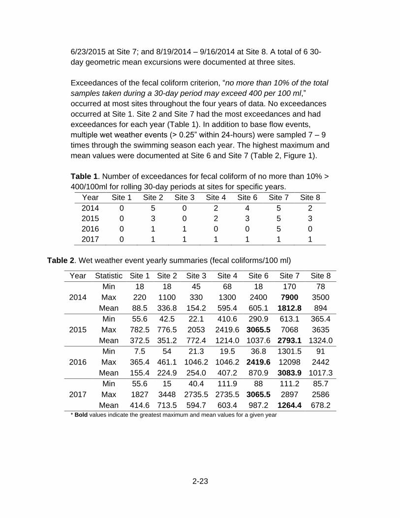
2-23
6/23/2015 at Site 7; and 8/19/2014 – 9/16/2014 at Site 8. A total of 6 30-
day geometric mean excursions were documented at three sites.
Exceedances of the fecal coliform criterion, “no more than 10% of the total
samples taken during a 30-day period may exceed 400 per 100 ml,”
occurred at most sites throughout the four years of data. No exceedances
occurred at Site 1. Site 2 and Site 7 had the most exceedances and had
exceedances for each year (Table 1). In addition to base flow events,
multiple wet weather events (> 0.25” within 24-hours) were sampled 7 – 9
times through the swimming season each year. The highest maximum and
mean values were documented at Site 6 and Site 7 (Table 2, Figure 1).
Table 1. Number of exceedances for fecal coliform of no more than 10% >
400/100ml for rolling 30-day periods at sites for specific years.
Year Site 1 Site 2 Site 3 Site 4 Site 6 Site 7 Site 8
2014 0 5 0 2 4 5 2
2015 0 3 0 2 3 5 3
2016 0 1 1 0 0 5 0
2017 0 1 1 1 1 1 1
Table 2. Wet weather event yearly summaries (fecal coliforms/100 ml)
Year Statistic Site 1 Site 2 Site 3 Site 4 Site 6 Site 7 Site 8
2014
Min 18 18 45 68 18 170 78
Max 220 1100 330 1300 2400 7900 3500
Mean 88.5 336.8 154.2 595.4 605.1 1812.8 894
2015
Min 55.6 42.5 22.1 410.6 290.9 613.1 365.4
Max 782.5 776.5 2053 2419.6 3065.5 7068 3635
Mean 372.5 351.2 772.4 1214.0 1037.6 2793.1 1324.0
2016
Min 7.5 54 21.3 19.5 36.8 1301.5 91
Max 365.4 461.1 1046.2 1046.2 2419.6 12098 2442
Mean 155.4 224.9 254.0 407.2 870.9 3083.9 1017.3
2017
Min 55.6 15 40.4 111.9 88 111.2 85.7
Max 1827 3448 2735.5 2735.5 3065.5 2897 2586
Mean 414.6 713.5 594.7 603.4 987.2 1264.4 678.2 * Bold values indicate the greatest maximum and mean values for a given year


2-25
USEPA. 2011. CSO post construction compliance monitoring guidance. EPA-833-K-11-
001. U.S. Environmental Protection Agency, Office of Wastewater Management,
Washington, DC.


3-2
3.1 WADEABLE RIFFLE-RUN STREAM MACROINVERTEBRATE DATA
COLLECTION PROTOCOL

3-3
Prepared by:
Brian Chalfant
PA Department of Environmental Protection
Office of Water Programs
Bureau of Clean Water
11th Floor: Rachel Carson State Office Building
Harrisburg, PA 17105
2013
Edited by:
Dustin Shull
PA Department of Environmental Protection
Office of Water Programs
Bureau of Clean Water
11th Floor: Rachel Carson State Office Building
Harrisburg, PA 17105
2017

3-4
INTRODUCTION
USEPA’s Rapid Bioassessment Protocols for Use in Streams and Wadeable Rivers
(Barbour et al.1999) describes two general approaches to collecting stream
macroinvertebrate communities for water quality assessment purposes. These
approaches are the “single, most productive habitat” approach, described here, and
the “multihabitat” approach, later described in Chapter 3.3, Wadeable Multihabitat
Stream Macroinvertebrate Collection Protocol (Pulket 2017). The single, most
productive habitat approach is typically used to assess streams where cobble
substrate and riffle/run habitat is predominant (generally referred to as high gradient
freestone streams). This protocol identifies appropriate field collection procedures
needed to evaluate macroinvertebrate communities in wadeable freestone streams
where riffle-run habitat is sufficiently abundant and is a modification of the USEPA
Rapid Bioassessment Protocols (Barbour et al. 1999). Samples can be collected year-
round; however, certain periods of the year are required depending on the purpose of
the study. Refer to Chapter 2.1, Wadeable Freestone Riffle-Run Stream
Macroinvertebrate Assessment Method (Shull 2017b) of the Assessment Book for
more information on collection results and season.
MACROINVERTEBRATE FIELD COLLECTION
A benthic macroinvertebrate sample collection begins with delineating a 100-meter
reach along the stream where the best available representation of riffle-run habitat
exists for the stream segment of interest. Within the reach, six one-minute (each kick
must be at least 45 to 60 seconds in duration) kicks are conducted immediately
upstream of a non-truncated D-framed net with 500 µm mesh (Figure 1). Truncated nets
are shorter with less meshed surface area and are not recommended for this collection
protocol.
Each kick should disturb approximately 1 m2 immediately upstream of the net to an
approximate depth of 10 cm, as substrate allows. During each kick, the net should be
held stationary. Kicks are completed in a downstream-to-upstream direction to avoid
disturbing the upstream portions of the targeted reach. Collectors must ensure kicks are
distributed throughout the 100-meter reach and are representative of the variety of riffle-
run habitats present (e.g., slow-flowing, shallow riffles and fast-flowing, deeper riffles). It
is important to note that riffle-run habitat differences will be respective of the stream
segment being sampled. For example, a slow-flowing deep riffle will be different in a
small stream than in a larger stream. Kicks must also be conducted throughout the
width of the stream to include the left-descending, middle, and right-descending areas.
The only exception to this is if a specific area of the stream is being targeted for a

3-5
reason. If that is the case, then the collector must clearly document that the sample is
not a complete composite and state the purpose for collection on the sample form.
Figure 1. A non-truncated D-framed net with 500 µm mesh.
When collecting same day replicate samples within the same reach, it is important not
to disturb the same areas of the stream with both sets of kicks. It is also important to be
cognizant of macroinvertebrate drift after kicking the first sample. For example, a kick
during the replicate collection may be very close and immediately downstream of an
original sample kick without being in the same location. Disturbance from the original
kick just upstream of a replicate kick may have disturbed macroinvertebrates and skew
the replicate sample. An example of good kick selection and incorrect kick selection is
illustrated in Figure 2. It is recommended that a replicate sample be collected after
every 10 regular samples for QA/QC purposes.

3-6
Figure 2. Blue rectangles illustrate a 100-meter reach within a stream, dark blue
ellipses show the initial set of kicks during sample collection, and yellow ellipses show
the replicate set of kicks during sample collection. (A) Correct sample collection with
replicate collection; all kicks are collected within 100 meters and across the entire width
of the stream, replicate kicks are not collected in the same location, and replicate kicks
are not placed in close proximity, directly downstream of any other kicks. (B) Incorrect
sample collection (with replicate); not all kicks are collected within 100 meters and
across the width of the stream, replicate kicks are collected in the same location, and in
close proximity, directly downstream of other kicks.
Once collected from the stream, each of the six kicks are composited into one sample
jar (or as few samples jars as possible). Each jar is labeled with the date, time, collector,
collectively referred to as a station ID (yyyymmdd-HHMM-Collector) and location. If
more than one jar is needed then each jar will also be labeled with a number (e.g., 1 of
2, 2 of 2). It is recommended that paper tags labeled using indelible ink or pencil be
placed inside the sample jar(s) as well. Care must be taken to minimize damage to the
collected organisms when compositing the materials. For this reason, only larger rocks,
3-7
detritus, and other debris are rinsed and removed before the sample is preserved.
Buckets and 500 µm mesh sieves are permitted when compositing kicks; however,
swirling the composited material in a bucket filled with water to reduce the amount of
debris (elutriation) is not recommended as this action can unnecessarily damage fragile
organisms, or allow for heavier organisms to be discarded unintentionally. Composited
samples are preserved with at least 70% ethanol (95% ethanol is preferred) in the field.
Collectors must ensure that the percentage of ethanol is high enough to properly
preserve the sample and that there is ample space left in the sample jar to properly
preserve organisms. Composited samples are then transported back to the laboratory
for processing and all field information is recorded on a macroinvertebrate field data
sheet (Appendix A.1) or mobile data collection application.
ADDITIONAL DATA
During a DEP riffle-run macroinvertebrate survey, field meter (temperature, specific
conductance, pH, dissolved oxygen, and turbidity if available), water chemistry, and
habitat assessment data should also be collected. Recommended Standard Analysis
Codes (SAC) for riffle-run macroinvertebrate collections are SAC 612 or SAC 18 (for
special protection). For more information on water chemistry collection and SACs, refer
to Chapter 4.2, Discrete Water Chemistry Data Collection Protocol (Shull 2017a).
Because riffle-run surveys are designed for high gradient streams, the high gradient
habitat assessment form should be used. The DEP riffle/run prevalent habitat form can
be found in Appendices C.1 and C.2.
LITERATURE CITED
Barbour, M.T., J. Gerritsen, B. D. Snyder, and J. B. Stribling. 1999. Rapid
bioassessment protocols for use in streams and wadeable rivers: Periphyton,
benthic macroinvertebrates and fish. 2nd edition. EPA 841-B-99-002. U.S.
Environmental Protection Agency, Office of Water, Washington, D.C.
Pulket, M. (editor). 2017. Wadeable multihabitat stream macroinvertebrate data
collection protocol. Chapter 3.3, pages 14–19 in M. J. Lookenbill, and R.
Whiteash (editors). Water quality monitoring protocols for streams and rivers.
Pennsylvania Department of Environmental Protection, Harrisburg,
Pennsylvania.
Shull, D. R. 2017a. Discrete water chemistry data collection protocol. Chapter 4.2,
pages 9–24 in M. J. Lookenbill, and R. Whiteash (editors). Water quality
monitoring protocols for streams and rivers. Pennsylvania Department of
Environmental Protection, Harrisburg, Pennsylvania.

3-8
Shull, D. R. (editor). 2017b. Wadeable freestone riffle-run stream macroinvertebrate
assessment method. Chapter 2.1, pages 2–24 in D. R. Shull, and R. Whiteash
(editors). Assessment methodology for streams and rivers. Pennsylvania
Department of Environmental Protection, Harrisburg, Pennsylvania.

3-9
3.2 WADEABLE LIMESTONE STREAM MACROINVERTEBRATE DATA
COLLECTION PROTOCOL

3-10
Prepared by:
William Botts
PA Department of Environmental Protection
Office of Water Programs
Bureau of Clean Water
11th Floor: Rachel Carson State Office Building
Harrisburg, PA 17105
2009
Edited by:
Amy Williams
PA Department of Environmental Protection
Office of Water Programs
Bureau of Clean Water
11th Floor: Rachel Carson State Office Building
Harrisburg, PA 17105
2017

3-11
INTRODUCTION
Limestone streams are unique aquatic systems that are typically very popular for
recreational fishing. To properly protect the ecological integrity of limestone streams,
they must be assessed correctly. This data collection protocol is intended to aid in
assessing the aquatic life uses of Pennsylvania’s wadable limestone streams. In the
case of these limestone stream assessments, the following field procedures will apply.
A stream must meet certain criteria for this protocol to be applicable for assessments
(Table 1). Limestone streams will often display low-gradient flow conditions and are
almost completely void of clearly defined freestone habitat beds.
Table 1. Limestone streams definition criteria
Parameter Criterion Explanation
Alkalinity Minimum 140 mg/l Stream must maintain high
alkalinity throughout the year
Temperature 40 to 65°F 4 to 18°C
Constant temperatures are very
important. Check to see if stream
is ice-free in the winter.
Known Influences
Stream originates from
limestone springs or very
strongly influenced by
limestone springs.
N/A
Drainage Area Maximum 20 sq. miles
There may be exception to this
parameter if all other criteria are
met.
Water Use Definition of Cold Water
Fishes (CWF)
Meets the definition of a CWF
stream in Chapter 93.
FIELD SAMPLING CONSIDERATIONS
Net Mesh & Sieve
Many state water quality programs, federal agencies (e.g., USEPA, USGS), and other
water quality monitoring organizations use net sampling devices with 500μm mesh nets.
Due to the natural conditions of limestone streams, 500μm mesh size quickly clogs,
preventing macroinvertebrates and vegetation from entering the net resulting in a poor
sample. To ensure an accurate assessment, 800 - 900μm net mesh must be used to
collect samples. A standard 500μm mesh sieve should be used to process samples.

3-12
Semi-Quantitative Procedure
The DEP Rapid Bioassessment Protocol (RBP) is a modification of the USEPA RBP III
(Plafkin et al. 1989). Modifications include: 1) the use of a D-frame net for the collection
of the riffle-run samples, 2) different laboratory sorting procedures, 3) elimination of the
CPOM (coarse particulate organic matter) sampling, and 4) metrics substitutions. Unlike
USEPA’s RBP III methodology, no field sorting is done. Only larger rocks, detritus, and
other debris are rinsed and removed while in the field before the sample is preserved.
While USEPA’s RBP III method was designed to compare impacted waters to reference
conditions (cause and effect approach), the DEP-RBP modifications were designed for
unimpacted waters, as well as impacted waters.
FIELD PROCEDURES
Benthic Macroinvertebrate Sampling
The handheld D-frame sampler consists of a bag net attached to a half-circle (“D”
shaped) frame that is 1 ft. wide. The net is employed by one person facing downstream
and holding the net firmly on the stream bottom. One “D-frame effort” is defined as:
vigorous kicks in an approximate area of 1m2 (1 x 1 m) immediately upstream of the net
to a depth of 10cm (approximately 4 inches, as the substrate allows) for approximately
one minute. All benthic dislodgement and substrate scrubbing should be done by kicks
only. Substrate handling should be limited to the removal of large rocks or debris (as
needed) with no hand washing. Since the width of the kick area is wider than the net
opening, net placement is critical to assure all kicked material flows toward the net.
Avoiding areas with crosscurrents, the substrate material from within the 1 m2 area
should be kicked toward the center of the square meter area.
The purpose of the standardized DEP-RBP sampling procedure is to obtain
representative macroinvertebrate fauna from comparable stations. The DEP-RBP
assumes the riffle/run to be the most productive habitat. Riffle/run habitats are sampled
using the D-frame net procedure described above. For limestone stream surveys, two
D-frame efforts (kicks) are collected - one from an area of fast velocity and one from an
area of slower velocity within the same riffle. Limestone streams have low gradient often
making it difficult to locate well developed riffles. If there are no riffles in the sample
area, a run, or the best rock substrate available is sampled. The two kicks are then
composited into one sample jar (or more as necessary). Each jar is labeled with the
date, time, collector, collectively referred to as a station ID (yyyymmdd-HHMM-
Collector) and location. If more than one jar is needed then each jar will also be labeled
with a number (e.g., 1 of 2, 2 of 2). It is recommended that paper tags labeled using
indelible ink or pencil be placed inside the sample jar(s) as well. Care must be taken to
minimize damage to the collected organisms when compositing the materials. It is

3-13
recommended that the benthic material be placed in a bucket filled with water to
facilitate gentle stirring and mixing as not to damage fragile organisms. Because
limestone samples are very abundant in organic material, the sample is preserved with
at least 70% ethanol (95% ethanol is preferred). Composited samples are then
transported back to the laboratory for processing and all field information is recorded on
a macroinvertebrate field data sheet (Appendix A.1) or mobile data collection
application.
Sample Collection Period
Samples must be collected from January through May. Limestone streams have a low
number of sensitive taxa and only a few of these taxa are generally found in large
numbers. One very important sensitive taxon is Ephemerella. A good population of
Ephemerella generally indicates better water quality. The three species of Ephemerella:
invaria (rotunda) and dorothea found in Pennsylvania limestone streams emerge in May
and June and are normally difficult or impossible to collect after emergence and until
nymphs mature. Collecting samples from January through May ensures these very
important ecological indicator taxa will not be missed.
ADDITIONAL DATA
During a DEP limestone macroinvertebrate survey, field meter (temperature, specific
conductance, pH, dissolved oxygen, and turbidity if available), water chemistry, and
habitat assessment data should also be collected. Recommended Standard Analysis
Codes (SAC) for limestone macroinvertebrate collections are SAC 612 or SAC 18 (for
special protection). For more information on water chemistry collection and SACs, refer
to Chapter 4.2, Discrete Water Chemistry Data Collection Protocol (Shull 2017). The
Riffle/Run Prevalence Habitat assessment form should be used for limestone
macroinvertebrate collections. This form can be found in Appendices C.1 and C.2.
LITERATURE CITED
Plafkin, J. L, M. T. Barbour, K. D. Porter, S. K. Gross, and R. M. Hughes. 1989. Rapid
bioassessment protocols for use in rivers and streams: Benthic
macroinvertebrates and fish. EPA/440/4-89-001. U.S. Environmental Protection
Agency, Office of Water, Washington, D.C.
Shull, D. R. 2017. Discrete water chemistry data collection protocol. Chapter 4.2, pages
9–24 in M. J. Lookenbill, and R. Whiteash (editors). Water quality monitoring
protocols for streams and rivers. Pennsylvania Department of Environmental
Protection, Harrisburg, Pennsylvania.
3-14
3.3 WADEABLE MULTIHABITAT STREAM MACROINVERTEBRATE DATA
COLLECTION PROTOCOL

3-15
Prepared by:
Charles McGarrell and Molly Pulket
PA Department of Environmental Protection
Office of Water Programs
Bureau of Clean Water
11th Floor: Rachel Carson State Office Building
Harrisburg, PA 17105
2007
Edited by:
Molly Pulket
PA Department of Environmental Protection
Office of Water Programs
Bureau of Clean Water
11th Floor: Rachel Carson State Office Building
Harrisburg, PA 17105
2017

3-16
INTRODUCTION
USEPA’s Rapid Bioassessment Protocols for Use in Streams and Wadeable Rivers
(Barbour et al.1999) describes two general approaches to assessing stream
macroinvertebrate communities. These approaches are the “single, most productive
habitat” approach, previously described in Chapter 3.1, Wadeable Riffle-Run Stream
Macroinvertebrate Data Collection Protocol (Shull 2017b), and the “multihabitat”
approach, described here. The multihabitat approach involves sampling a variety of
habitat types instead of sampling a single habitat, such as cobble substrate in riffles
and/or runs. This data collection protocol identifies appropriate field collection
procedures needed to evaluate macroinvertebrate communities in wadeable low-
gradient Pennsylvania streams.
A low-gradient waterway in Pennsylvania is defined as having pool/glide channel
morphology and naturally lacking riffles. There should be no riffles within 300
consecutive meters of the sampling reach. Cobble outcrops extending less than 1/8 of
the stream width are not considered riffles. In addition, small areas with slightly
increased velocities and gravel substrates are not considered riffles. Besides lack of
riffle/run sequences, low-gradient streams are characterized by a gradient less than
0.5%, substrates of fine sediment or infrequent aggregations of coarse sediments, and
an aggregate of the five habitat types as described in Table 1. Moderate or high
gradient stream segments that have been influenced by impoundments or beaver
dams are not appropriate sites for the multihabitat field sampling protocol.
MACROINVERTEBRATE FIELD COLLECTION
Aquatic macroinvertebrate samples are collected using a multihabitat sample collection
procedure modified from that described in Barbour et al. (1999). Sampling should occur
during the months of November through May. A 100-meter length of stream is
determined and set as the sample reach. The investigator then identifies which low-
gradient habitat types are present within the sample reach. Table 1 describes the five
habitat types and explains the different sampling techniques for each habitat. Sampling
consists of 10 D-frame net jabs, 2 in each of the five habitat types or distributed
proportionally in the available habitats. A minimum surface area of approximately 0.46
m2 is required for a given habitat type to be sampled. If the total number of jabs (10) is
not evenly divisible by the number of habitat types present, the remaining jab(s) are
distributed among the most abundant habitat type(s) in the reach. Each jab consists of a
30-inch-long sweep of a 0.3-meter wide area, using a 500-micron mesh D-frame dip
net. The jabs are composited while the investigator works progressively upstream from
the first collection site. After the 10 jabs are completed, all jabs are combined into

3-17
sampling jars and preserved with at least 70% ethanol (95% ethanol is preferred) in the
field. Each jar is labeled with the date, time, collector (collectively referred to as a station
ID (yyyymmdd-HHMM-Collector)), and location. If more than one jar is needed, then
each jar will also be labeled with a number (e.g., 1 of 2, 2 of 2). Jars should only be
filled 2/3 full of debris to allow for adequate sample preservation (ethanol should fill jar
completely). If a lot of debris or large pieces were collected, the debris can be carefully
rinsed in buckets, inspected for organisms, and then discarded. The rinse water is
poured through a 500 µm mesh sieve to retain the macroinvertebrates before being
discarded. The net, sieve, and bucket should be thoroughly inspected for
macroinvertebrates. Composited samples are then transported back to the laboratory
for processing and all field information is recorded on the macroinvertebrate field data
sheet (Appendix A.1) or mobile data collection application.

3-18
Table 1. Stream Habitat Types and Field Sampling Techniques
Habitat Type Description Sample Technique
Cobble/ Gravel Substrate
Stream bottom areas consisting of mixed gravel and larger substrate particles; Cobble/gravel substrates are typically
located in relatively fast-flowing, “erosional” areas of the stream channel
Macroinvertebrates are collected by placing the net on the substrate near the downstream end of an area of gravel or larger substrate particles and simultaneously pushing down on the net while pulling it in an upstream direction with adequate force to dislodge substrate materials and
the aquatic macroinvertebrate fauna associated with these materials; Large stones and organic matter
contained in the net are discarded after they are carefully inspected for the presence of attached organisms which
are removed and retained with the remainder of the sample; One jab consists of passing the net over
approximately 30 inches of substrate.
Snag
Snag habitat consists of submerged sticks, branches, and other woody debris that appears to have been submerged long enough to be adequately colonized by
aquatic macroinvertebrates; Preferred snags for sampling include small to medium-sized sticks and branches (preferably < ~4 inches
in diameter) that have accumulated a substantial amount of organic matter (twigs, leaves, uprooted aquatic macrophytes, etc.)
that is colonized by aquatic macroinvertebrates.
When possible, the net is to be placed immediately downstream of the snag, in either the water column or on
the stream bottom, in an area where water is flowing through the snag at a moderate velocity; The snag is then kicked in a manner such that aquatic macroinvertebrates
and organic matter are dislodged from the snag and carried by the current into the net; If the snag cannot be
kicked, than it is sampled by jabbing the net into a downstream area of the snag and moving it in an
upstream direction with enough force to dislodge and capture aquatic macroinvertebrates that have colonized
the snag; One jab equals disturbing and capturing organisms from an area of ~0.23 m2 (12” x 30”)
Coarse Particulate
Organic Matter (CPOM)
Coarse particulate organic matter (CPOM) consists of a mix of plant parts (leaves, bark, twigs, seeds, etc.) that have accumulated on the stream bottom in “depositional” areas of
the stream channel; In situations where there is substantial variability in the
composition of CPOM deposits within a given sample reach (e.g., deposits
consisting primarily of white pine needles and other deposits consisting primarily of hardwood tree leaves), a variety of CPOM deposits are sampled; However, leaf packs in higher-velocity (“erosional”) areas of the channel are not included in CPOM samples
CPOM deposits are sampled by lightly passing the net along a 30-inch long path through the accumulated
organic material to collect the material and its associated aquatic macroinvertebrate fauna; When CPOM deposits are extensive, only the upper portion of the accumulated organic matter is collected to ensure that the collected
material is from the aerobic zone
Submerged Aquatic
Vegetation (SAV)
Submerged aquatic vegetation (SAV) habitat consists of rooted aquatic macrophytes
SAV is sampled by drawing the net in an upstream direction along a 30-inch long path through the
vegetation; Efforts should be made to avoid collecting stream bottom sediments and organisms when sampling
SAV areas.
Sand/Fine Sediment
Sand/fine sediment habitat includes stream bottom areas that are composed primarily of
sand, silt, and/or clay.
Sand/fine sediment areas are sampled by bumping or tapping the net along the surface of the substrate while slowly drawing the net in an upstream direction along a 30-inch long path of stream bottom; Efforts should be
made to minimize the amount of debris collected in the net by penetrating only the upper-most layer of sand/silt
deposits; Excess sand and silt are removed from the sample by repeatedly dipping the net into the water column and lifting it out of the stream to remove fine
sediment from the sample

3-19
ADDITIONAL DATA
During a DEP multihabitat macroinvertebrate survey, field meter (temperature, specific
conductance, pH, dissolved oxygen, and turbidity if available), water chemistry, and
habitat assessment data should also be collected. Recommended SAC for multihabitat
collections are SAC 612, SAC 87, and SAC 18 (for special protection). For more
information on water chemistry collection and SACs, refer to Chapter 4.2, Discrete
Water Chemistry Data Collection Protocol (Shull 2017a). Because multihabitat surveys
are designed for low gradient streams, the low gradient habitat assessment form should
be used. The DEP low gradient habitat form can be found in Appendix C.3.
LITERATURE CITED
Barbour, M. T., J. Gerritsen, B. D. Snyder, and J. B. Stribling. 1999. Rapid
bioassessment protocols for use in streams and wadeable rivers: Periphyton,
benthic macroinvertebrates and fish. 2nd edition. EPA 841-B-99-002. U.S.
Environmental Protection Agency, Office of Water, Washington, D.C.
Shull, D. R. 2017a. Discrete water chemistry data collection protocol. Chapter 4.2,
pages 9–24 in M. J. Lookenbill, and R. Whiteash (editors). Water quality
monitoring protocols for streams and rivers. Pennsylvania Department of
Environmental Protection, Harrisburg, Pennsylvania.
Shull, D. R. (editor). 2017. Wadeable riffle-run stream macroinvertebrate data collection
protocol. Chapter 3.1, pages 2–8 in M. J. Lookenbill, and R. Whiteash (editors).
Water quality monitoring protocols for streams and rivers. Pennsylvania
Department of Environmental Protection, Harrisburg, Pennsylvania.
3-20
3.4 SEMI-WADEABLE LARGE RIVER MACROINVERTEBRATE DATA
COLLECTION PROTOCOL

3-21
Prepared by:
Dustin Shull
PA Department of Environmental Protection
Office of Water Programs
Bureau of Clean Water
11th Floor: Rachel Carson State Office Building
Harrisburg, PA 17105
2017

3-22
INTRODUCTION
Collection of macroinvertebrate data in large semi-wadeable rivers can be a daunting
and complex process. To appropriately collect biological community data in large rivers
and to increase efficiency, DEP separates large rivers into two categories, semi-
wadeable and non-wadeable. Semi-wadeable rivers are defined as predominantly free-
flowing systems with drainage areas > 1,000 mi2 and have physical characteristics that
allow for riffle and run sections to occur with relative frequency. These river systems
tend to lack a well-defined and navigable U-shaped channel for any significant distance
and frequently present difficulties for both wadeable and non-wadeable
macroinvertebrate data collection protocols. In addition, large semi-wadeable rivers
potentially have differences in water quality across their width. Well over half of the
large rivers within Pennsylvania are considered semi-wadeable (Figure 1). Therefore, it
is important that a standardized protocol be established for the collection of physical,
chemical, biological data in these river systems.
Figure 1. Semi-wadeable and non-wadeable rivers throughout Pennsylvania.
The goal of this document is to lay the framework for how DEP intends on collecting
macroinvertebrate and supplementary data for making Aquatic Life Use (ALU)
determinations in large semi-wadeable rivers within the boundaries of Pennsylvania.

3-23
Working on, in, and around large semi-wadeable rivers can be challenging and
dangerous. This discussion seeks to provide guidance on when and how to collect
these data, as well as important safety considerations that must be considered. Making
accurate and defensible assessment decisions requires both enough data types (e.g.,
physical, chemical, and biological) and a specificity of those data within a water
influence (zone) and season.
SAFETY PROCEDURES
Appropriate ALU assessment begins with data collection that follows proper guidelines
and safety procedures. Safety is of utmost concern when working in and on large semi-
wadeable rivers. Individuals that lack experience and education related to navigating
these waterbodies put themselves and others at risk of injury or loss of life. In most, if
not all cases, some form of watercraft is required for this sampling protocol. Whether a
kayak, canoe, or powered boat is used, DEP recommends – and in most cases PFBC
requires by law – that individuals using watercrafts take boating courses and obtain a
boating safety certificate. However, whether laws apply to certain individuals or
watercraft or not, DEP strongly recommends that all individuals regardless of age,
experience, or navigation procedure obtain and keep a boating safety certification on
them during semi-wadeable surveys. More information on boating courses and safety
certifications are available here:
http://www.fishandboat.com/Boat/BoatingCourses/Pages/default.aspx
Large semi-wadeable rivers present difficulties for both wadeable and non-wadeable
water navigation. Certain locations on rivers such as the Susquehanna River around
Harrisburg, PA may be fully or partially wadeable during certain times of year, but there
are also highly variable currents and drop-offs that are dangerous to wading collectors.
Therefore, personal floatation devices (PFD) should always be worn. However, PFDs
should not be used to facilitate wading or navigating the waterbody. Navigation using a
watercraft can be equally if not more challenging than wading. Many boats that frequent
the large semi-wadeable rivers such as the Susquehanna River are outfitted with
modified jet propulsion to reduce the risk of serious damage associated with impacting
the streambed with the lower unit. Therefore, consideration for modified equipment may
be needed to conduct this protocol. In addition, riffles and bedrock substrate often
dominate these rivers regardless of size. Consequently, DEP recommends that at least
two individuals work together during these surveys. This is critical for many safety
reasons, particularly important when a powered watercraft is underway. While in motion,
DEP recommends that the individual not operating the powered watercraft is actively
looking for obstacles on and just under the surface. This individual should be actively
and clearly communicating obstacles to the operator. This is best done with the use of

3-24
hand signals that are agreed upon between collectors prior to navigating the water. All
of this is not to say that macroinvertebrate sampling in large semi-wadeable rivers is
overly risky. In fact, with the proper training and experience this sampling protocol can
be conducted efficiently and safely using limited resources, and without restrictions
based on the collector’s physical stature.
Inherent in these recommendations is the understanding that collectors must be well
informed of the unique characteristics of each river they intend to sample and be aware
of current flow and weather conditions. Equipment considerations may be different
between similar sized large semi-wadeable rivers, and certainly different when visiting
multiple semi-wadeable rivers of different sizes. For instance, boat selection and safety
equipment lists would be different depending on whether the collector is visiting a 1,000
mi2 river or 10,000 mi2 river. These differing characteristics require thorough planning
before going into the field, so resources are not wasted due to a lack of preparation. It is
also imperative that collectors have access to and continually check river flow
conditions. There will be situations when weather in one part of Pennsylvania may be
optimal for sampling a site, but weather in another part of Pennsylvania – two or three
days before the sampling period – created conditions that reduces the ability to collect.
Analysis of flow conditions at all available points upstream of the intended sampling
locations are highly recommended. Commonly used discharge data are available here:
https://waterdata.usgs.gov/pa/nwis/current.
WATER QUALITY DATA COLLECTION
Cross-section surveys and water chemistry samples must be collected before
macroinvertebrate sampling. This is needed to determine where the macroinvertebrate
sample(s) are collected. All cross-section surveys are conducted using a clean and
calibrated field meter that collects water temperature, specific conductance, dissolved
oxygen, pH, and – preferably – turbidity (see Chapter 4). Transects (discrete points
within the cross-section survey) are taken at regular intervals (each point representing
approximately 5-10% of the total wetted width) across the width of the river. This is the
least amount of information required to determine if major water quality influences exist
at the sampling location. A major water quality influence that shows a 10% difference or
greater in any field meter parameter necessitates a unique water chemistry and
macroinvertebrate sample be collected. It is often helpful to create a drawing or map of
the site with transect points depicted to help delimit the locations of water influence
transitions across the width of the river (Figure 2). When new major water influences are
identified, additional transects and water chemistry samples will be collected on
upstream reaches to identify and characterize the source of variable water quality
across the width of the targeted reach of river. Cross-section surveys and water

3-25
chemistries will also be collected downstream, if possible, to determine the extent that
the water influences do not mix. Multiple water chemistry samples over a period are
recommended to provide additional information for assessments. Cross-section surveys
and water chemistry data collected through the season prior to macroinvertebrate
collection provides the most utility for complete and accurate assessments, but routine
year-round data collection has also proven useful for ALU assessments and method
development efforts. Cross-section surveys and water chemistry data collection prior to
macroinvertebrate collections also provides opportunities to complete a thorough
reconnaissance of the targeted semi-wadable river.
Figure 2. Example of cross-section data collection where data are collected at
established transect points over time. In this example, the cross-section survey data
identify three unique major water influences that create the three zones where
macroinvertebrate, chemical, and physical data should be collected.
There are three water chemistry collection protocols that are acceptable when collecting
chemical data on semi-wadeable rivers: fixed-width sampling, isokinetic sampling
(USGS 2006), and discrete mid-channel/mid-depth sampling (see Chapter 4.2, Discrete
Water Chemistry Data Collection Protocol (Shull 2017a)). Fixed width and isokinetic
3-26
sampling is useful for characterizing water chemistry for the entire width of the surface
water, while discrete samples are useful for characterizing unique water quality
influences. Water chemistry characterization is also driven by the need to identify
sources and causes of impairment. Water chemistries should include a comprehensive
list of constituents including total and dissolved nitrogen and phosphorus species, total
metals, and ions. For water chemistry collection, DEP routinely uses SAC 612 for semi-
wadeable rivers. In addition, constituents such as dissolved metals, pesticides,
hormones, wastewater compounds, and pharmaceuticals are added if necessary. For
more information on water chemistry collection and SACs, refer to Chapter 4.2, Discrete
Water Chemistry Data Collection Protocol (Shull 2017a).
MACROINVERTEBRATE COLLECTION
Semi-wadeable large river macroinvertebrate samples are collected using 6D-200 field
collection described in the Wadeable Riffle-Run Stream Macroinvertebrate Data
Collection Protocol (Shull 2017b). Briefly, this consists of 6 one-minute kicks evenly
distributed across the entire width of the waterbody using a 500 µm mesh D-frame net.
With the transect procedure modification, additional 6D-200 samples are collected in
accordance with the number of major water quality influences discovered during water
quality transect data collection. For instance, if three distinctly different water influences
were discovered, then three 6D-200 samples are collected, with each sample
composited across the entire width of the respective water influence. Jars are labeled
with the date, time, collector, collectively referred to as a station ID (yyyymmdd-HHMM-
Collector), and location description. If more than one jar is needed then each jar will
also be labeled with a number (e.g., 1 of 2, 2 of 2). Samples are preserved with at least
70% ethanol (95% ethanol is preferred). Once field collections are complete, samples
are taken to the laboratory for analysis. Macroinvertebrate processing and identification
is conducted using standard DEP protocols, which are also described in detail in
Chapter 3.6, Macroinvertebrate Laboratory Subsampling and Identification Protocol
(Brickner 2020).
Macroinvertebrate samples collected at or above median flow conditions can cause a
lower confidence in the results. Therefore, if collectors are not confident that the
sampling was representative of the zone (e.g., collector could not collect the 6 kicks
relatively evenly across the entire width of the influence) or they have collected in an
appropriate habitat type, then samples should not be used for assessments. The
responsibility for this is decision is left to the most experienced individual in the field
during the sampling event. Individuals that are experienced with working in large rivers
quickly realize when an inappropriate sample has been collected and will either discard

3-27
the sample or annotate their concerns in the comments section of the macroinvertebrate
data collection field form (Appendix A.1) or mobile data entry application.
ADDITIONAL DATA
Additional field meter (temperature, specific conductance, pH, dissolved oxygen, and
turbidity if available) and water chemistry data does not need to be collected if the
cross-sectional surveys and chemistry collection were completed as described above. A
habitat assessment should also be collected for every macroinvertebrate collection.
Because semi-wadeable large river surveys target riffle-run habitat, the DEP Riffle-Run
Prevalence Habitat Form should be used. This form is found in Appendix C.1 and C.2.
LITERATURE CITED
Brickner, M. (editor). 2020. Macroinvertebrate laboratory subsampling and identification
protocol. Chapter 3.6, pages 32–42 in M. J. Lookenbill and R. Whiteash (editors).
Water quality monitoring protocols for streams and rivers. Pennsylvania
Department of Environmental Protection, Harrisburg, Pennsylvania.
Shull, D. R. 2017a. Discrete water chemistry data collection protocol. Chapter 4.2,
pages 9–24 in M. J. Lookenbill, and R. Whiteash (editors). Water quality
monitoring protocols for streams and rivers. Pennsylvania Department of
Environmental Protection, Harrisburg, Pennsylvania.
Shull, D. R. (editor). 2017b. Wadeable riffle-run stream macroinvertebrate data
collection protocol. Chapter 3.1, pages 2–8 in M. J. Lookenbill, and R. Whiteash
(editors). Water quality monitoring protocols for streams and rivers. Pennsylvania
Department of Environmental Protection, Harrisburg, Pennsylvania.
USGS. 2006. National field manual for the collection of water quality data. Chapter 4.1
in Surface water sampling: Collection methods at flowing-water and still-water
sites. U.S. Geological Survey, Water Resources Office of Water Quality, Reston,
VA. (Available online at:
https://water.usgs.gov/owq/FieldManual/Chapter4/pdf/Chap4 v2.pdf.)

3-28
3.5 QUALITATIVE BENTHIC MACROINVERTEBRATE DATA COLLECTION
PROTOCOL

3-29
Prepared by:
Tony Shaw
PA Department of Environmental Protection
Office of Water Programs
Bureau of Clean Water
11th Floor: Rachel Carson State Office Building
Harrisburg, PA 17105
2006
Edited by:
Josh Lookenbill
PA Department of Environmental Protection
Office of Water Programs
Bureau of Clean Water
11th Floor: Rachel Carson State Office Building
Harrisburg, PA 17105
2017

3-30
INTRODUCTION
While DEP primarily relies on semi-quantitative benthic macroinvertebrate data
collection protocols described previously in this chapter, qualitative data collection
protocols could also be considered. Qualitative macroinvertebrate data collection
protocols may be appropriate for cause and effect surveys and point of first use
surveys; however, this collection protocol is no longer used for ALU determinations.
The type of sampling gear used is dependent on waterbody type, available habitat, and
other site-specific conditions. The recommended gear for sampling wadeable streams is
a 1m2, flexible kick-screen, or a non-truncated D-framed net. The type of gear,
dimensions, and mesh size must be reported for all data collections. When more than
one gear type is used, the results must be recorded separately. Physical stream
variables should be matched as closely as possible when comparing reference stations
to candidate/impacted stations during location placement. Gear-type should also match
between stations within the same survey. Matching these variables helps minimize or
eliminate the effects of compounding variability.
KICK-SCREEN
A common qualitative sampling protocol uses a simple hand-held kick-screen. This
device is designed to be used by two persons. However, with experience, it may be
used by one person. The kick-screen is constructed with a 1x1meter piece of net
material fastened to two dowel handles.
Facing up stream, one person places the net in the stream with the bottom edge of the
net held firmly against the streambed. An assistant then vigorously kicks the substrate
within a 1x1m area immediately upstream of the net to a depth of 7-10cm, as substrate
allows. The functional depth sampled may vary due to ease of disturbance as
influenced by substrate embeddedness. The amount of effort expended in collecting
each sample should be approximately equivalent to make valid comparisons.
As many as four screens are collected at each site or until no new taxa are collected.
Initial sampling should target riffle/run habitat. Collection in additional habitats to
generate a more complete taxa list can be conducted at the discretion of the
investigator.
Station data will be recorded on the macroinvertebrate data collection forms
(Appendices A.1 and A.2) and habitat data will be recorded on the appropriate habitat
data collection forms (Appendices C.1, C.2, or C.3) in this book.
3-31
D-FRAMED NET
DEP has standardized a non-truncated D-framed net with 500µm mesh for all semi-
quantitative benthic macroinvertebrate data collections in freestone streams and rivers,
however it may also be appropriate to use this gear for qualitative collections.
Qualitative D-framed data collection could be employed where the width of the targeted
waterbody is less than 1 meter, or the targeted reach is small with very little available
habitat.
In wadable, flowing waters with available riffle/run habitat, a D-framed net can be
employed using a “single, most productive habitat” approach, previously described in
this chapter. Facing upstream, each one-minute (each kick must be at least 45 to 60
seconds in duration) kick is conducted immediately upstream of a non-truncated D-
framed net. Each kick should disturb approximately 1m2 immediately upstream of the
net to an approximate depth of 10 cm, as substrate allows. During each kick, the net
should be held stationary. With semi-quantitative protocols a prescribed, a standardized
effort (number of kicks) is required. Qualitatively this gear should be used until no new
taxa are collected. Kicks are completed in a downstream-to-upstream direction to avoid
disturbing the other targeted portions of reach before kicks are conducted in that area.
Collectors must ensure kicks are representative of the variety of riffle-run habitats
present (e.g., slow-flowing, shallow riffles and fast-flowing, deeper riffles). It is important
to note that riffle-run habitat differences will be respective of the stream segment being
sampled. For example, a slow-flowing deep riffle will be different in a small stream than
in a larger stream. Kicks must also be conducted throughout the width of the stream to
include the left-descending, middle, and right-descending areas. The only exception to
this is if a specific area of the stream is being targeted for a reason. If that is the case,
then the collector must clearly document that the sample is not a complete composite
and state the purpose for collection on the sample form.
In wadable, low-gradient waters without riffle/run habitat the “multihabitat” approach
may be appropriate. The multihabitat approach involves sampling a variety of habitat
types instead of sampling a single habitat, such as cobble substrate in riffles and/or
runs. The investigator first identifies which low-gradient habitat types are present within
the sample reach. The five habitat types and the different sampling techniques are
described in Chapter 3.3, Wadeable Multihabitat Stream Macroinvertebrate Data
Collection Protocol (Pulket 2017). Qualitatively this gear should be used until no new
taxa are collected. Sampling consists of D-frame net jabs, in each of the available
habitat types. A minimum surface area of approximately 0.46 m2 is required for a given
habitat type to be sampled. Each jab consists of a 30-inch-long sweep of a 0.3-meter

3-32
wide area, using a 500-micron mesh D-frame dip net. Jabs are completed in a
downstream-to-upstream direction to avoid disturbing the other targeted portions of
reach before jabs are conducted in that area.
ADDITIONAL DATA
Field meter (temperature, specific conductance, pH, dissolved oxygen, and turbidity if
available), water chemistry, and habitat assessment data should also be collected.
Station data will be recorded on the macroinvertebrate data collection forms
(Appendices A.1 and A.2) and habitat data will be recorded on the appropriate habitat
data collection forms (Appendices C.1, C.2, or C.3) in this book.
LITERATURE CITED
Pulket, M. (editor). 2017. Wadeable multihabitat stream macroinvertebrate data
collection protocol. Chapter 3.3, pages 14–19 in M. J. Lookenbill, and R.
Whiteash (editors). Water quality monitoring protocols for streams and rivers.
Pennsylvania Department of Environmental Protection, Harrisburg,
Pennsylvania.

3-33
3.6 MACROINVERTEBRATE LABORATORY SUBSAMPLING AND
IDENTIFICATION PROTOCOL

3-34
Prepared by:
Dustin Shull
PA Department of Environmental Protection
Office of Water Programs
Bureau of Clean Water
11th Floor: Rachel Carson State Office Building
Harrisburg, PA 17105
2017
R script provided by:
Zachary Smith
Interstate Commission on the Potomac River Basin
30 West Gude Drive Suite 450
Rockville, Maryland 20850 USA
Edited by:
Mark Brickner
PA Department of Environmental Protection
Office of Water Programs
Bureau of Clean Water
11th Floor: Rachel Carson State Office Building
Harrisburg, PA 17105
2020

3-35
INTRODUCTION
This laboratory subsampling and identification protocol applies to the freestone riffle-
run, limestone (with exception of subsample target), multihabitat, and semi-wadeable
macroinvertebrate collection protocols. The limestone collection protocol is currently the
only macroinvertebrate collection protocol with a subsample target of 300 ± 30
organisms. All other macroinvertebrate collection protocols described above have a
subsample target of 200 ± 20 organisms.
SUBSAMPLING PROCEDURES
Laboratory Subsampling
Subsampling procedures are adapted from Barbour et al. (1999). Subsampling should
take place in a controlled environment with good lighting, access to water, and plenty of
workspace. Equipment and supplies needed for the benthic sample processing are:
• At least 2 large laboratory pans gridded into 28 squares. The specific size of a
pan is not critical, but the number of grids (28) must be maintained if any basic
density comparisons wish to be made between samples. DEP Central Office staff
use Rubbermaid 2 Gallon White Durex® Container 18" x 12" x 3 1/2", because
the bottom of the pan is 14" x 8", which allows for 28, 4in2 grid cutters to be used
• A standard USGS No. 35 sieve (or 500 µm mesh sieve bucket) to remove fine
materials and residual preservative prior to sub-sampling
• A random number generator or uniform objects (numbered from 1 to 28) for
drawing random numbers
• Forceps (or any tools that can be used to pick organisms and debris)
• Grid cutters that approximate 1/28th of pan surface area.
• A lighted magnifier (10x magnification maximum) may also be used during the
sorting process but is not required. This equipment can make seeing organisms
among debris easier and is good for training, but it does not make
microorganisms (not visible with the naked eye) visible.
• Handheld counter
• Dissecting microscope (primarily used for identifications, but also used to confirm
if organisms are identifiable).
• Storage vials for subsampled organisms
• 70-90% ethanol
• Petri dishes
To begin subsampling, the composited sample is removed from the collection container
and placed in the first gridded pan (pan 1). It is recommended to remove fine materials

3-36
and residual preservative prior to subsampling by rinsing the sample through a sieve (or
sieve bucket) that matches the mesh size (or smaller) of the net gear used to collect the
sample. The sample is then gently distributed evenly throughout pan 1. Water may be
added to the pan before distributing to reduce damage to the organisms.
At this point, there are several ways to achieve the targeted subsample of 200 ± 20 (300
± 30 for limestone stream samples) organisms. It is important to note that this protocol
is a 200 or 300 organism target; thus, collectors should avoid consistently biasing
toward the lower limits of 180 organisms (270 for limestone stream samples) or upper
limits of 220 (330 for limestone stream samples) organisms in the final identifiable
count. Depending on the nature of the sample and the abundance of organisms, one
subsampling procedure may be more efficient than another. The subsampling
procedure is acceptable if it remains random/unbiased and the number of grids in pan 1
and pan 2 can be recorded. Only identifiable organisms (to the taxonomic level
recommended in the identification section below) are counted during subsampling.
Organisms that are not considered identifiable include pupae, larval bodies missing too
many critical structures to render confident identifications, extremely small instars,
empty shells or cases, and terrestrial organisms. If an organism is lying between two
grids it is considered in the grid that contains the head. If the head is not easily seen,
then the organism is considered in the grid containing most of the body. If a large
volume sample necessitates the use of two first pans, material and organisms are
removed from the same grid of both pans. For example, a large amount of debris is
distributed evenly into two first pans. Then, if grid 17 is randomly selected, grid 17 must
be pulled from both pans and sorted. These two grids are then counted as 1 grid from
the first pan.
The following describes two potential ways of conducting randomized subsamples:
Option 1: (good for suspected high abundance samples)
The following option requires three pans (2 gridded pans and 1 viewing pan).
Randomly select 1 grid from the first gridded pan (pan 1) and remove all material and
organisms. Place material and organisms in a viewing pan (pan should be as large as
gridded pans to facilitate quick identification of organisms from debris). If the number of
organisms (through a cursory count) appears to be much greater than 50 (e.g., 75
organisms), then move the material and organisms into the second gridded pan (pan 2).
Randomly select 3 more grids from pan 1 and place all material and organisms evenly
throughout pan 2. This process quickly confirms a high likelihood that there will be more
than 220 (330 for limestone stream samples) organisms in the first 4 grids of pan 1 and

3-37
a second gridded pan will be needed. This process also significantly reduces the
amount of debris a collector must sort through before determining a second pan is
needed. Once material and organisms are evenly distributed throughout pan 2, grids
are randomly picked until the target number of organisms is reached. The total number
of grids for each pan is recorded on the laboratory bench sheet (Appendix A-2) or
annotated in the appropriate section of a mobile data entry application.
Option 2: (good for suspected low abundance samples)
The following only requires 2 pans (1 gridded pan and 1 viewing pan) if the sample has,
in fact, a low abundance of organisms.
Randomly pick 1 grid at a time from the first gridded pan (pan 1) and place all material
and organisms in a viewing pan to be sorted. Once all organisms are removed, the
debris can be discarded. This allows for the viewing pan to be clear of debris for the
next randomly selected grid from pan 1. Continue subsampling 1 grid at a time until the
target number of organisms is reached. With low abundance samples, more than 4
grids from pan 1 will be selected, so there will be no need to use a second gridded pan.
The total number of grids for each pan is recorded on the laboratory bench sheet
(Appendix A-2) or annotated in the appropriate section of a mobile data entry
application.
Once subsampling is completed, all organisms are placed in a clean vial with fresh
70%-80% ethanol. The vial is labeled using indelible ink with date, time, collector,
collectively referred to as a station ID (yyyymmdd-HHMM-Collector), and location and
then stored for later identification. If more than one vial is needed then each vial will also
be labeled with a number (e.g., 1 of 2, 2 of 2). In addition, if identification occurred
immediately after subsampling, then organisms can be placed into a petri dish instead
of a labeled vial.
There will be rare occasions when subsampling results in more than 220 organisms (or
330 organisms for limestone samples) at the end of the subsampling process. If this
occurs, pour the organisms out of the vial and into a clean gridded pan. Evenly
distribute the organisms with fresh ethanol and then randomly select grids to remove
organisms until the target number is achieved. This can be done in a backwards fashion
to save time. For instance, a collector followed the procedures above, but got 244
organisms in 4 grids total. The collector then poured and evenly distributed organisms
into a clean gridded pan. After removing organisms out of 4 randomly selected grids,
the collector had 208 organisms in the gridded pan and 36 organisms set aside. At this
point the collector simply needed to place the organisms in the gridded pan back into

3-38
the vial. The 36 organisms left over were placed back into the original sample jar.
Because the collector subsampled in a backwards fashion, the count of grids in pan 1
remains “4”, but the 4 grids removed during this additional process are subtracted from
28 in a “pan 2” to get 24 grids.
Digital Subsampling (Rarefaction)
Rarefaction Process
Digital subsampling or “rarefaction” is used to reduce sample size of a previously
collected and processed sample. Rarefaction should not be considered a substitute for
the subsampling procedures described above, but this process is acceptable when the
physical sample is unavailable, or an immediate answer is needed. The concept of
rarefaction was developed by Howard Sanders (Sanders 1968), modified by a number
of other scientists (i.e., Hurlbert 1971, Heck et al. 1975, Simberloff 1978). Rarefaction
has since been incorporated into several computer programs. Normally, rarefaction
programs use the original sample numbers and, using a specified subsample amount,
produce the expected number of species and a variance of this expected number of
species. Depending on the program, confidence limits and plots/curves may be
produced. Two important aspects of any rarefaction program are that, 1) the program
can randomly reduce the number of individuals in each taxon, and 2) the program can
randomly reduce sample richness. This ensures that the program functionally replicates
the physical subsampling process.
For conducting rarefaction using spread sheets or designing a rarefaction program, the
following steps should be followed:
1) Calculate how many macroinvertebrates would be in each grid of a 28-grid pan,
assuming they are spread evenly across the pan.
2) Calculate the number of macroinvertebrates to remove based on the desired
subsample (e.g., target for freestone IBI = 200 ± 20 individuals).
3) Divide the number of macroinvertebrates to remove by the number of
macroinvertebrates found per grid.
4) Round this result to the nearest whole number grid.
5) Multiply the number of macroinvertebrates per grid by the number of grids to
subsample.
6) Round this result to the nearest whole number (because entire organisms are
removed, not partial). This is the number of macroinvertebrates that will be
removed from the sample to reach a correct subsample. The remaining
macroinvertebrates will be the correct subsample.
7) Number each individual macroinvertebrate from one to the total number of
individuals in the sample on a spreadsheet.


3-42
made to have other taxonomists assist with a positive identification. Otherwise, the taxa
should be included on the enumeration sheet, separate and distinct from other
identifications within the same taxonomic group. Other orders may be identified to the
lowest level attainable if they are immature and do not exhibit the characteristics
necessary for confident genus level identifications; however, this should be rare if the
proper subsampling process is followed. Identifications with a mixture of higher and
lower taxonomic levels within the same taxonomic group will skew sample scoring and
may result in the sample not meeting quality assurance standards. If identifications with
a mixture of higher and lower taxonomic levels within the same taxonomic group cannot
be avoided, higher level identifications will not be used to calculate metrics. Eliminating
these individuals from the sample avoids artificially inflating richness metrics. In
addition, the sample and the identifications must be forwarded to a certified taxonomist
for further evaluation, and the identified organisms should be preserved and maintained
indefinitely.
Table 3. The taxonomic groups that are identified to a higher taxonomic level than
genus.
Group Identification Level
Midges Family
Snails Family
Clams Family
Mussels Family
Flatworms Phylum (Turbellaria)
Aquatic Earthworms & Tubificid Worms Class (Oligochaeta)
Leeches Class (Hirudinea)
Proboscis worms Phylum (Nemertea)
Roundworms Phylum (Nematoda)
Moss Animalcules Phylum (Bryozoa)
Water mites Subclass (Acari)
All organisms are identified and enumerated on a bench sheet (Appendix A.2) or data
entry application. Organisms are then returned to the labeled vial and stored in a safe
location.
Quality Assurance
At least 10% of all samples identified by a biologist are quality assured by a certified
taxonomist. The most common type of certification is the genus level EPT certification
provided by the Society of Freshwater Science. Identification results between the
biologist and certified taxonomist must be 90% or greater. DEP may request sample
vials for any results entered into internal databases for quality assurance purposes.
3-43
LITERATURE CITED
Barbour, M. T., J. Gerritsen, B. D. Snyder, and J. B. Stribling. 1999. Rapid
bioassessment protocols for use in streams and wadeable rivers: Periphyton,
benthic macroinvertebrates and fish. 2nd edition. EPA 841-B-99-002. U.S.
Environmental Protection Agency, Office of Water, Washington, D.C.
Heck, K. L., G. Belle, and D. Simberloff. 1975. Explicit calculation of the rarefaction
diversity measurement and the determination of sufficient sample size. Ecology
56:1459–1461.
Hurlbert, S. H. 1971. The nonconcept of species diversity: A critique and alternative
parameters. Ecology 52:577–586.
Sanders, H. L. 1968. Marine benthic diversity: A comparative study. The American
Naturalist 102:243–282.
Simberloff, D. 1978. Use of rarefaction and related methods in ecology. ASTM STP 652
in K. L. Dickson, J. Cairns, and R. J. Livingston (editors). Biological data in water
pollution assessment: Quantitative and statistical analyses. American Society for
Testing and Materials.

3-44
3.7 FISH DATA COLLECTION PROTOCOL

3-45
Prepared by:
Timothy Wertz
PA Department of Environmental Protection
Office of Water Programs
Bureau of Clean Water
11th Floor: Rachel Carson State Office Building
Harrisburg, PA 17105
2017
Edited by:
Timothy Wertz
PA Department of Environmental Protection
Office of Water Programs
Bureau of Clean Water
11th Floor: Rachel Carson State Office Building
Harrisburg, PA 17105
2021

3-46
INTRODUCTION
Fish community assessments are important as they represent a biological community
that are captive to water resources during all life stages, have longer life spans, and
have a greater socioeconomic status than macroinvertebrate communities alone.
Standardized semi-quantitative sampling protocols can be applied to all wadeable and
non-wadeable streams. The data generated from standardized protocols are vital for
making ALU assessments and evaluations, developing indices and other assessment
methods, promoting spatial and temporal trend analyses, and providing the foundation
for a robust fish bioassessment program. The Assessment Book (Shull and Whiteash
2021), Chapter 2, includes the Stream Fish Assemblage Assessment Method (Wertz
2021) which requires strict adherence to the following standardized collection protocol.
Other collection protocols may be considered for various assessment purposes only
after rigorous analysis for similarity.
BASIC REQUIREMENTS
Field sampling procedures, species identification and enumeration, and other site tasks
must be applied consistently with the same level of rigor at each sample site. To
maintain consistency, a field crew is directed on site by a crew leader who maintains a
valid scientific collector permit (SCP) as required by PFBC and has met the quality
control requirements of DEP (described below). Accurate species level identification of
each fish collected is essential, as it provides the foundation for subsequent
assessment. A minimum of one crew member must be proficient in the accurate
identification of Pennsylvania fishes and should also be versed in fishes of the
surrounding areas and potential exotics. Electrofishing techniques are the primary
procedures adopted by DEP. Other fish collection procedures are not discussed here.
Electrofishing crews will have a crew leader trained and experienced in the proper
operation of electrofishing gear and appropriate electrofishing safety and strategy
(described below).
REPRESENTATIVE SAMPLING
The objective of this semi-quantitative fish data collection protocol is to acquire a
representative sample of the overall fish community, here referred to as the fish
assemblage. Fish assemblage data is considered representative when it is collected
with a standardized collection protocol that is robust enough to produce repeatable
biological response(s) to environmental and/or anthropogenic conditions. The collection
protocols may or may not provide a complete inventory of all species present at a site

3-47
but should be able to consistently characterize most species present and their relative
abundance.
Sampling Considerations
Sampling effort is measured by both distance and time and accurate measures of both
are considered essential. Accumulated electrofishing time can legitimately vary over the
same distance as dictated by cover, stream conditions, and the number of fish
encountered. While it is understood that some individual fish will not be captured, a
concerted effort by the crew members should be made to capture every fish sighted as
this is fundamental to relative abundance measures. Dipnet design and mesh size will
largely dictate the size range of fishes captured; frame diameter, net depth and handle
length should be of sufficient size to capture all anticipated fishes and size ranges. Net
mesh should be approximately 6mm (1/4in). Since the ability of the netters to see
stunned and immobilized fish is partly dependent on water clarity, sampling is to be
conducted only during periods of “normal” water clarity and flows (e.g., baseflow
conditions). Sites that are turbid should not be sampled if water clarity is under one
meter unless this clarity is considered normal. The sampling period for all semi-
quantitative fish collection protocols is from June 1st through September 30th and this
period may provide a wide variety of stream flow conditions. Periods of high turbidity
and high flows should be avoided due to their negative influence on sampling efficiency.
If high flow conditions occur, sampling must be delayed until flows and water clarity
return to seasonal norms. The crew leader will decide if conditions are acceptable and
direct their crews accordingly. A representative fish assemblage is not only based on
conditions but also on sample reach and habitat selection. A sample reach at a site is
considered most representative when it;
• Contains all the best available habitat (BAH) types (geomorphic units, flow
regimes, fish cover, and substrate material) within a contiguous reach.
• Is similar to that of the local area (i.e., unique habitats should be avoided).
SITE SELECTION
Two semi-quantitative sampling procedures, wadeable and non-wadeable, are
described below. Strict a priori designations of wadeable or non-wadeable have been
avoided due to complex limitations, but see Flotemersch et al. (2006) for a detailed
description of these designations used elsewhere. A stream reach at a site is
considered wadeable or non-wadeable not by size, but in its ability to be efficiently
surveyed during the June 1st -September 30th sampling season utilizing the following
collection protocols (a stream reach may be considered for both protocols throughout
the same period if both protocols can efficiently be implemented). Sites that can have

3-48
both protocols efficiently implemented are referred to as “transitional zones” and are
typically large wadeable sites and small non-wadeable sites (Flotemersch et al. 2006). If
a site is considered within a transitional zone both protocols should be applied within a
short timeframe (days-week), as feasible, to facilitate direct comparisons between
collection protocols. Sites that are too large for efficient coverage using wadeable
techniques (large rivers) are not considered transitional and should only be sampled
using non-wadeable techniques. Duplicates (a second sample reach at a site
comparable to the first, sampled the same day) and replicates (repeating the same site
within the same sampling season) should be performed as often as feasible (preferably
1 out of every 10 sites) for both collection protocols to maintain a calibration dataset for
future assessments.
Final Site Determination
Specific site locations will first be determined by the type of study and its design (e.g.,
cause and effect, protected use assessment) secondly by access feasibility (e.g., public
access, private landowner permission, distance to stream etc.) and lastly by
representative habitat. Desktop reconnaissance as well as a field reconnaissance
should be implemented prior to sampling to determine the appropriate gear and
manpower needed to achieve a representative sample. Further consideration should be
applied to the site selection process to ensure a representative sample of the conditions
that are being measured. Sites located near the mouth, near an instream dam or
impoundment, or near the mouth of a feeding tributary should be avoided unless these
influences are inherent in the study design. General guidance for distances represents
modifications from literature and preliminary data exploration (Gorman 1986, Schaefer
and Kerfoot 2004, Hitt and Angermeier 2008, DEP unpublished data) and are provided
in Table 1. In any case, potentially influencing factors should be noted on the field forms
to facilitate data management and analysis. Applying a detailed reconnaissance to the
site selection process will greatly reduce down-time the day of the sampling event,
ensure repeatability and provide high-quality data.

3-49
Table 1. General guidelines for site selection based on distance from potential
influencing factors.
Influence Category
Distance
(km) Description
In-stream dam and
its impoundment Minor 0.5
- Defined by dam NOT restricting fish
passage under normal to high flow
conditions.
In-stream dam and
its impoundment Major 1.5
-Defined by dam restricting fish passage
under all flow conditions.
Proximity to mouth Minor 0.5 - Defined as target stream within one
stream order of receiving stream.
Proximity to mouth Major 1.5 - Defined as target stream being at least
two stream orders smaller than
receiving stream.
Proximity to tributary Minor 0.5 - Defined as tributaries within three
stream orders of receiving stream.
Proximity to tributary Major 1.5 - Defined as tributaries three stream
orders smaller (adventitious). Should be
avoided within the reach, when feasible.
WADEABLE PROTOCOL
For semi-quantitative fish sampling in wadeable streams, sample reach lengths will be
determined by the width of the stream. The average wetted width is multiplied by 10,
with a minimum reach length of 100 meters and a maximum of 400 meters (Table 2).
Sample reach width is determined by measuring five wetted channel widths spaced
twenty meters apart within the first 100 meters of the proposed sample reach, and
averaged. Once the wetted width has been calculated, it is best to establish the
stopping point before establishing the starting point. Due to the nature of this protocol,
fishes will naturally be “pushed” upstream to avoid the electrical field. The stopping point
should subsequently be a section that provides a natural barrier to escape (e.g., shallow
riffle or cascade) and should be established first. Sample reach length can then be
measured in a downstream direction to determine the starting point. For consistency,
the reach should adhere to the minimum reach lengths but can be lengthened if
necessary, to include additional habitat types. The use of downstream blocknets should
be avoided based on the size range of wadeable streams in Pennsylvania and by the
bias that may be inherent in blocknetting small streams but not large.

3-50
Table 2. Sample reach lengths based on stream width.
Average Stream Width Minimum Reach Length
<10m 100m
10 to 40m 10 X average stream width
>40m Maximum of 400m
Before sampling, the crew leader will brief the electrofishing crew on safety and strategy
(discussed below) and will adjust the electrofishing equipment to the desired settings
(Appendix A.3). When the crew is ready to begin, the crew leader will take note of the
GPS location, will start the clock, and electrofishing will commence in an upstream
direction. The electrofishing crew will be positioned along a transect, adequately
covering the width of the stream, and should maintain this position while proceeding
upstream to avoid gaps in the electrical field which may decrease coverage. The crew
leader must be cognizant of this coverage throughout the survey and adjust as needed.
For best coverage and standardization of effort the rule-of-thumb for determining the
amount of gear needed at a reach is one probe for every five meters of stream width
(Figure 1). For the large wadeable streams this will inherently require a great deal of
planning to ensure the best coverage is achieved (e.g., equipment and manpower). If
gaps are still present along the stream width, the crew can adapt by doing small zigzags
as they proceed upstream for adequate coverage. Similar collection protocols that may
employ transect zigzags across the width of the stream (see, Lazorchak 1998), multiple
pass (see, Pusey et al. 1998, Meador 2003, Shank et al. 2016), or other variant, will not
be considered comparable until a detailed analysis can be performed. If a stream width
is too large for best coverage, nonwadeable techniques should be pursued. Each crew
member with an anode probe should continuously sweep the probe side to side for best
coverage. The number of nets to anode probes must be a minimum of one to one,
additional netters may be used as needed. When the crew reaches the predetermined
stopping point, the crew leader will instruct the crew to stop and take note of the
stoppage time and GPS location. Fish processing will then commence and is described
in detail below.


3-52
extra reach for every 30K sq/km of drainage area over 30K sq/km. For example, if a site
is less than 30K sq/km, RDB and LDB would be sampled, if a site is 30-60K sq/km a
middle reach would be included. Strict definitions are avoided to provide the crew leader
with discretion for best coverage.
Sample reaches are surveyed using one-pass, daytime electrofishing. Reaches are
surveyed in a downstream direction for a longitudinal distance of 500 meters for a
minimum of 30 minutes. Specific sample reaches should be established by desktop and
field reconnaissance prior to sampling. Measures of stream width may be problematic
on large rivers based on rangefinder capabilities and may have to be performed digitally
during the desktop reconnaissance. To maintain strict adherence to the reach length
requirements, starting and stopping locations should be adequately marked with
flagging tape or other distinguishable features in the field prior to sampling. Before
sampling, the crew leader will brief the electrofishing crew on safety and strategy
(discussed below) and will adjust the electrofishing equipment to the desired settings
(Appendix A.3). When the crew is ready to begin, the crew leader will take note of the
GPS location, will start the clock, and electrofishing will commence. A single boat-
mounted electrofishing unit is maneuvered in a zigzag fashion from littoral shoreline
areas toward the thalweg for a distance of 30 meters from the shoreline or to where
stream depth reaches six meters, whichever comes first. If a mid-channel reach of the
river is to be sampled, island habitat must be targeted to satisfy the littoral shoreline
requirement. For non-wadeable sampling, BAH is both representative of the local
conditions, and within a contiguous 500-meter reach. The habitat should be uniformly
navigated and electrofished based on the proportional abundance of the habitat within
the reach. Prolonged electrofishing within a single habitat type is not recommended. If a
small section of the reach cannot be adequately surveyed due to navigational obstacles
or flow restrictions, the area can be avoided and the same distance added to the end of
the reach (electrofishing time must be adjusted accordingly). Best effort should be made
to net all fishes observed and in proportion to their abundance. The strict targeting of
the largest fishes must be avoided.
Each boat crew will have one navigator (usually the crew leader), and a minimum of one
netter for each anode “dropper”. Additional crew members may be utilized to aid in
netting large fishes and monitoring fish stress levels. When the crew reaches the
predetermined stopping point, the crew leader will instruct the crew to stop and take
note of the stoppage time and GPS location. Fish processing will then commence and is
described in detail below.

3-53
FISH HANDLING AND PROCESSING
General Considerations
Since semi-quantitative fish surveys depend on the collection of fish for species
identification, temporary retention of a significant number of fish is required. To minimize
stress and lethality to the greatest extent possible, the following field procedures should
be followed:
• Remove stunned fish from the electrical field as soon as possible.
• Netted fish should be transferred to containment devices as soon as possible.
Containment devices vary depending on the type of survey and situations but
may be a combination of:
o Large buckets or tubs
o Live-wells constructed of framed netting that form a cage that is
submerged in the stream
• Water is replaced regularly in warm weather to maintain adequate dissolved
oxygen levels in the water, reduce waste by-products, and minimize mortality.
• Aeration should be provided to further minimize stress and mortality if necessary.
• Field identifications and releases should commence immediately after collection
• Every feasible effort will be made to minimize holding and handling times.
Special handling procedures may be necessary for species of special concern as
outlined by the SCP requirements. Fish that are not retained for vouchers or other
purposes are released back into the water after they are identified to species and
enumerated. Invasive species will be kept and appropriately disposed of out of the
water, if requested by SCP requirements. Each sample crew must have at least one
person qualified as a taxonomic specialist in field fish identification and must also be
trained in the identification of gross anomalies inherent to the fish health assessment.
FISH HEALTH ASSESSMENT
Incidence and prevalence of gross anomalies are important measures of fish health that
have been used as an indicator of anthropogenic stress (Bauman et al. 2000) and allow
for both spatial and temporal comparison. The measures of deformities, erosions,
lesions, tumors and parasites (DELTP) are completed immediately after sampling. The
intent of the fish health assessment is to record the species, length, and various
anomalies that may be present on each individual fish. This data can then be used to
elucidate any potential issues that may be inherent to a specific species or length-class.
The health assessment is not intended to be diagnostic but should be able to
consistently classify specific gross anomalies by general DELTP type. Because small-
3-54
bodied fishes generally have a shorter life span (or shorter exposure time) the health
assessment is generally intended for fishes >100mm. It is recommended that all fish
>100mm in length be assessed, however, it is understood that large surveys may have
an inordinate amount of fish and may need to be subsampled. Subsampling should be
random (i.e., fish with anomalies should not be targeted), should represent all species
available, and should be of significant sample size relative to their abundance in the
sample. The goal during this process is to record as much information about the fishes
without inflicting undue stress. It is best when fishes that are to be processed for health
are held in live-wells. If the fish appear to be stressed, even after all attempts have been
made to reduce stress, the priority is to release and not collect health assessment data.
When fish are released without health data, only species identification and enumeration
are needed.
To conduct the health assessment the crew leader will assign the following three duties
to the crew: inspector, handler, and recorder. The inspector (generally the crew leader)
should be familiar with common fish diseases, experienced in the identification of fish
and gross anomalies, and have participated in numerous fish health assessments as
either handler or recorder. It is the inspector’s duty to give a species identification,
measure the total length (TL) of the fish (to the nearest 5mm increment), and inspect
the fish for anomalies. TL is measured from the tip of the snout to the end of the slightly
compressed caudal fin. The fish will be inspected along the right and left sides of the
body, head, fins, and gills. Specific anomalies found during this inspection will be voiced
to the recorder. Once the data has been collected, the inspector can release the fish.
The crew leader (or inspector) should determine where fish should be released; fish
should not be released near anticipated sample reaches to avoid immigration and bias
in the next sample. The handler is responsible for monitoring and reducing the stress
level of the fish while in retention and subsampling the fish that are then given to the
inspector. The recorder observes the inspection and records the data voiced by the
inspector. The recorder sets the pace of the health assessment and the inspector
should adjust accordingly. The recorder should be able to anticipate the amount of
space needed to record the data based on the number of fish that are in the sample, as
well as write neatly to avoid error in data management. A quick reference field guide for
anomalies is imbedded in the field data collection form in Appendix A.3.
FISH PRESERVATION
Most captured fish are identified to species in the field and released; however, any
uncertainty about the field identification of individual fish requires their preservation for
future laboratory identification (except for large specimens or species of special concern
which may need to be photographed). Only the fish necessary for vouchering and
3-55
laboratory confirmation will be retained. Fish are fixed for future identification in buffered
10% formalin. The container is labeled, at minimum, with date, time, waterbody, site
location, and geographic coordinates. Species level identification is required and may
be necessary to the subspecies level in certain instances. If a species level identification
is not possible in the field, voucher(s) specimens should be retained, or properly
photographed, for later laboratory analysis. Proper photographs should include a picture
of the left side of the fish body in the anatomical position, a label with site information
and individual identification number, and taxonomically important characters needed for
species level identification. In any case, strict adherence to SCP requirements and
subsequent annual updates must be considered.
The PFBC’s Division of Environmental Services (DES) maintains the general SCP
requirements as well as Qualified Threatened and Endangered Species (TE) Surveyor
requirements. More information on SCP and TE survey requirements can be found at
http://www.fishandboat.com/Resource/EnvironmentalServices/Pages/default.aspx
DES also has guidance for vouchering, and specific species that may be important to
voucher if encountered.
SITE DATA
Prior to leaving the site, the field collection sheet in Appendix A.3 must be completed,
ensuring that all field-based data is recorded. Location information is critical to ensuring
repeatability of a collection, and detailed descriptions are encouraged. Descriptions of
location should include relative position to a stable landmark. For example,
“downstream of bridge” is ambiguous, whereas “250 meters below SR144 bridge
upstream of Crossfork, PA” ensures repeatability. Water quality measures must follow
guidelines as described in Chapter 4.1, In-Situ Field Meter and Transect Data Collection
Protocol (Hoger 2020). Gear and effort descriptions should be as specific as the
equipment allows and are considered essential to normalizing data for effort. Qualitative
habitat measures (Mesohabitat, Velocity/Depth Regimes, Habitat, and Substrate) are
recorded as a percent-occurrence within the sampled reach and should not be applied
to a larger scale. Habitat measures are considered typical except for Percent of Fish in
Habitat. Here, the percent of fish (the number of individuals regardless of species) that
were netted out of each habitat type within the reach is recorded. This measure is
atypical but provides insight into habitat utilization. This measure is not always required
as it can be influenced by reduced visibility or when fish are “pushed” into another
habitat by the electrical field.

3-56
LABORATORY PROCEDURES
Important Note- All chemicals that are integral to the preservation and long-term
storage of fish vouchers should be treated as hazardous. Chemical specific Material
Safety Data Sheets (MSDS) forms should be referenced and be readily accessible at
the laboratory. Containers should be labeled appropriately, and nitrile gloves worn at all
times. General considerations for vouchering specimens come from Walsh and Meador
(1998) and can be referenced for a more detailed analysis.
Sample Preparation
Before fishes can be safely handled in the lab, they must first be transferred from 10%
formalin fixative and washed. Washing includes soaking fish in fresh (tap) water for a
24-hour period per wash, for a minimum of three washes (three days). Larger samples,
with more biomass, may need additional washes. After the last washing period, the
sample can be gradually (over a period of days) introduced to sequential levels of ethyl
alcohol washes from 35% to 50% to 70%. The ideal concentration for long term storage
is a 70% ethyl solution and should be confirmed with a hydrometer after immersion for
24 hours. Once the sample has been properly washed and preserved, laboratory
identifications can be completed.
Identification and Enumeration
Taxonomic identification and enumeration are the two most important factors for quality
lab data. The first step is to obtain the taxonomic identification. Fishes are identified and
segregated into species groups, or taxonomic units. The second step is to lay each
species out and enumerate them, this provides for a second-chance opportunity to spot
any taxonomic errors. It is best to lay species out for enumeration in smaller groups, by
fives or tens, to facilitate a recount. If a second taxonomic expert is available, it is best
to have them confirm the identification and enumeration, which provides a third and final
opportunity to catch any mistakes. Laboratory taxonomic identifications and
enumerations are then added to the original field data sheet to obtain the final taxa list
and enumerations. Nomenclature should follow the most recent update provided by the
American Fisheries Society (Page et al. 2013). Regional taxonomic keys should be
used for identification and range distribution comparisons. Notable identifications of
species outside of their known range should be documented and verified before data
are considered final. Fishes should be identified to the lowest taxonomic level possible,
to include species, subspecies, and hybrids (with comments on parental genus or
species). If identification to this level is not possible (due to size, condition, or other
variable) the use of genus or possibly family level identification may be considered. To
maintain data consistency, fishes <25mm (TL) should not be included in the final
identification and enumeration, but can be included as separate “comments”. For
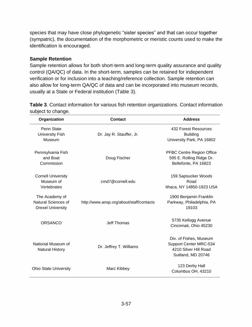
3-57
species that may have close phylogenetic “sister species” and that can occur together
(sympatric), the documentation of the morphometric or meristic counts used to make the
identification is encouraged.
Sample Retention
Sample retention allows for both short-term and long-term quality assurance and quality
control (QA/QC) of data. In the short-term, samples can be retained for independent
verification or for inclusion into a teaching/reference collection. Sample retention can
also allow for long-term QA/QC of data and can be incorporated into museum records,
usually at a State or Federal institution (Table 3).
Table 3. Contact information for various fish retention organizations. Contact information
subject to change.
Organization Contact Address
Penn State
University Fish
Museum
Dr. Jay R. Stauffer, Jr.
432 Forest Resources
Building
University Park, PA 16802
Pennsylvania Fish
and Boat
Commission
Doug Fischer
PFBC Centre Region Office
595 E. Rolling Ridge Dr.
Bellefonte, PA 16823
Cornell University
Museum of
Vertebrates
159 Sapsucker Woods
Road
Ithaca, NY 14850-1923 USA
The Academy of
Natural Sciences of
Drexel University
http://www.ansp.org/about/staff/contacts
1900 Benjamin Franklin
Parkway, Philadelphia, PA
19103
ORSANCO Jeff Thomas 5735 Kellogg Avenue
Cincinnati, Ohio 45230
National Museum of
Natural History Dr. Jeffrey T. Williams
Div. of Fishes, Museum
Support Center MRC-534
4210 Silver Hill Road
Suitland, MD 20746
Ohio State University Marc Kibbey 123 Derby Hall
Columbus OH, 43210

3-58
To fulfil the requirements of this protocol, a minimum of one “Site Composite Voucher”
is needed for every site, and a second “Audit Voucher” may also be needed as
described below.
• Site Composite Vouchers- A site voucher is for verifying species
spatiotemporal occurrence at a known site. A site voucher is comprised of a
minimum of one individual representing each of the lowest taxonomic units
identified in the sample. At sites with multiple reaches (e.g., nonwadeable) only
one site voucher is needed, but should represent the lowest taxonomic units
combined across all reaches. Not all species will necessarily need to be
vouchered. Larger-bodied fishes, gamefish, or generally common species may
be excluded if desired. These vouchers are labeled using waterproof, chemical-
resistant paper (placed inside the jar) with a minimum of:
o Site- Waterbody and location
o Date- Either Date/Time or a DEP GIS key in the form of
YYYYMMDD-TIME-NAME (Name = Initial of first name and full last
name “JSmith”)
o GPS Location- Latitude, Longitude
o Type- “Site Composite”
o Taxa list- The taxa list should mirror the completed field and lab
compilation and should include the number of specimens
vouchered out of the total number identified (e.g., Moxostoma sp.-
5 of 5, Percina maculata- 1 of 11, Micropterus dolomieu- 0 of 25).
• Audit Vouchers- An audit voucher is for QA/QC of the taxonomic identification
and enumeration. An audit voucher is comprised of all individuals identified and
enumerated at the lab. All fishes identified in the lab are segregated into distinct
containers (or separated within a few containers by a permeable membrane) by
their respective lowest taxonomic unit and are shared with the DEP auditor.
These vouchers are labeled using waterproof, chemical-resistant paper (placed
inside the jar) with a minimum of:
o Site- Waterbody and location
o Date- Either Date/Time or a DEP GIS key in the form of
YYYYMMDD-TIME-NAME (Name = Initial of first name and full last
name “JSmith”)
o GPS Location- Latitude, Longitude
o Type- “Audit Sample”
o Container #- “__ of __”
o Species- Lowest taxonomic unit(s) contained in the jar
(enumeration is not needed for each species, and is described in
detail below).

3-59
QUALITY CONTROL
The QA/QC of data collection is needed to maintain consistent application of these
protocols. This will enhance the precision and accuracy of assessments. The project
coordinator (DEP Quality Assurance Officer), will perform audits on both the field and
laboratory data collection before these data are entered in the DEP database. For field
data collection, a minimum of one audit for each protocol (e.g., wadeable and non-
wadeable) will be conducted for each crew leader. For laboratory data collection, a
minimum of one (but possibly as high as 10% of samples per year) “Audit Sample” will
be required for each taxonomic expert.
Important Note- It is understood that there may be some inherent subjectivity in
defining the “lowest taxonomic unit”, as this is likely to vary between taxonomic experts.
The goal of the laboratory audit is to make these data as consistent as possible, across
the range of expertise. To this end, the project coordinator may require multiple audit
samples before this consistency can be achieved. The auditor may have additional
taxonomic experts perform the laboratory audit to increase consistency. Final
determinations of similarity and consistency within the laboratory audits will be made by
DEP.
Original, signed audit forms will be retained by the auditor and copies will be sent to the
auditee for record. Audit forms for field and laboratory data collection are available upon
request.
ELECTROFISHING SAFETY
DEP recognizes that electrofishing is an inherently hazardous activity for which safety is
a primary concern. The environmental conditions under which these operations are
conducted further increase the risks. Due to these important concerns for electrofishing
safety, all field team members should be familiar with electrofishing techniques, safety
precautions, and equipment manufacturer’s operating procedures. It is the responsibility
of the project coordinator (or crew leader) to verify that crewmembers have a basic
understanding of these principles prior to sampling. The safety of all personnel and the
quality of the data are assured through the adequate education, training, and
experience of all members of the fish collection crew. To this end, the crew leader must
have completed electrofishing training and safety courses, be certified in CPR, and
should have a minimum of five years of electrofishing experience. The US Fish and
Wildlife Service offers educational guidance and certification in electrofishing principles
and safety and is considered the standard training source for electrofishing. Currently,
3-60
US Fish and Wildlife Service offers two courses that are available online. The
Electrofishing Principles and Techniques course is required for crew leaders and the
Electrofishing Safety course should be completed by every crewmember prior to
sampling.
• Principles and Techniques of Electrofishing (Online) - CSP2C01
o https://nctc.fws.gov/courses/CSP/CSP2C01/resources/
• Electrofishing Safety (Online) - CSP2202
o https://training.fws.gov/courses/csp/csp2202/resources/index.html
Electrofishing protocols rely on one of three main types of gear platforms: backpacks
and towboats with hand-held probes for wadeable streams and standard boats with
fixed-boom probes for non-wadeable streams and rivers. Collection gear consists of a
wide variety of net sizes, shapes, and configurations. Each team member must be
insulated from the water and the electrodes; therefore, non-breathable waders are
necessary as they are considered personal protective equipment (PPE), and rubber
(linesman) gloves are recommended. Nonbreathable waders or rubber boots are also
considered PPE and may be worn during boat electrofishing at the discretion of the
crew leader. All waders should have non-slip, rubber soles (no felt soles). Electrode and
dip net handles must be constructed of non-conductive materials (fiberglass or wood).
Additional equipment used during the survey should also be constructed of non-
conductive materials to reduce inadvertent shock potential (e.g., buckets, live-well
frames). Electrofishing units must be equipped with functional safety switches and
represent best available technology (BAT). Field crew members must remain cognizant
of their surroundings and not reach into the water unless the electrodes have been
removed from the water or the electrofishing unit has been disengaged. A good
anacronym to remember for safety is S-H-O-C-K-E-D.
Safety Brief- Crew leaders brief the crew on safety and strategy prior to each collection.
Handle- Be aware of what is touched, stepped on, or ducked under.
Operate- Be aware of probes and the electrical field at all times.
Communicate- Let others know of any potential hazards that may become apparent.
Key Personnel- Know which crew members are trained in case of emergency.
Equipment- Inspect equipment for damage before and after each sampling event.
Debrief- Discuss and critique the survey for improvement.
Each crewmember should also wear polarized glasses to reduce surface glare which
enhances their ability to safely negotiate the stream bottom and to see and net fish.
Important Note- All chemicals that are integral to the preservation and long-term
storage of fish vouchers should be treated as hazardous. Combustible materials used

3-61
for equipment (e.g., gasoline) should also be considered hazardous. Chemical specific
MSDS forms should be referenced and be readily accessible while conducting fish
surveys.
ELECTROFISHING STRATEGY
The efficiency of electrofishing is largely determined by the user’s knowledge of the
equipment. Due to the vast amount of gear types and manufacturers available, it is
imperative that the user is familiar with the gear and the manufacturers
recommendations specific to each unit. Here, only general guidelines are outlined to
standardize capture efficiency. The nature of this protocol inherently targets fishes of all
shapes, sizes, and body forms from the smallest of minnows to the largest catfishes. As
body size and shape varies, so does the transfer of electricity. As size increases
susceptibility to the electrical field also increases. Adjustments of waveform (AC, DC,
pulsed DC), frequency (pulses per second or hertz, Hz) and duty cycle (percent “on” for
a pulsed current) can all have profound effects on the electrofishing efficiency. For
optimal efficiency and consistency waveform, frequency, and duty cycle must be
standardized (Table 4). Environmental conditions, most notably specific conductance,
may require a deviation from the standard waveform from PDC to AC. Using AC is only
advised when specific conductance is very low, and PDC is not able to produce the
desired response.
Table 4. Standardized electrofishing settings
Setting Category Required Setting
Waveform Pulsed Direct Current (PDC)
Frequency 60 Hz
Duty Cycle 25%
The desired response from fish to the electrical field is immobilization with minimal
injury. By standardizing waveform, frequency and duty cycle, the output wattage (amps
x volts) is the remaining adjustment needed to achieve the desired response. Adjusting
the wattage is typically done by adjusting voltage (refer to the manufacturers
specifications for wattage adjustments, as many of these adjustments vary across
units). Testing for the desired response should be done prior to beginning the survey,
outside of the survey area. To this end, output wattage is set to minimum and gradually
increased until the desired response from fish is observed. It is best to use small-bodied
fish for the observed response, as they are generally less susceptible to the electrical
field. A quick reference guide to electrofishing adjustment is in Appendix A-3.

3-62
BIOSECURITY – AQUATIC INVASIVE SPECIES
The spread of aquatic invasive species (AIS) is always a potential concern when
conducting stream surveys. Biosecurity measures should be considered and
implemented for all fish collections. AIS covers a wide range of taxa that include but are
not limited to fish, reptiles, mussels, invertebrates, aquatic plants, algae, pathogens,
and parasites. While many of the streams within Pennsylvania have, or have had
documentation of AIS, it is best to consider all streams as potential candidates for AIS
transfer. To this end, sampling design should be adjusted accordingly. Whenever
possible, site selection priority should be placed on sites within the same watershed and
ordered upstream to downstream. All gear that may come in contact with the water
should be decontaminated prior to leaving the site if they are to be used at another site
within the same day, this includes but is not limited to boats, trailers, live-wells, buckets,
nets, and waders. Various decontamination products are commercially available and
include but are not limited to chlorine solutions or peroxygen solutions. Whenever gear
must be used in multiple watersheds adequate time must be allotted for additional
decontamination practices that include but are not limited to high-temperature pressure
washing, freezing, or drying. Additional information regarding AIS can be found in the
PFBC’s Biosecurity Protocol (available upon request).
LITERATURE CITED
Baumann, P., V. Cairns, B. Kurey, L. Lambert, I. Smith, and R. Thoma. 2000. Lake Erie
lakewide management plan (LaMP). Technical Report Series. LaMP.
Flotemersch, J. E., J. B. Stribling, and M. J. Paul. 2006. Concepts and approaches for
the bioassessment of non-wadeable streams and rivers. U.S. Environmental
Protection Agency, Office of Research and Development, Washington, DC.
Gorman, O. T. 1986. Assemblage organization of stream fishes: The effect of rivers on
adventitious streams. The American Naturalist 128(4):611–616.
Hoger, M. S. 2020. In-situ field meter and transect data collection protocol. Chapter 4.1,
pages 2–8 in M. J. Lookenbill, and R. Whiteash (editors). Water quality
monitoring protocols for streams and rivers. Pennsylvania Department of
Environmental Protection, Harrisburg, Pennsylvania.
Hitt, N. P., and P. L. Angermeier. 2008. Evidence for fish dispersal from spatial analysis
of stream network topology. Journal of the North American Benthological Society
27(2):304–320.
Lazorchak, J. M., D. J. Klemm, and D. V. Peck (editors). 1998. Environmental
monitoring and assessment program surface waters: Field operations and
methods for measuring the ecological condition of wadeable streams.

3-63
EPA/620/R-94/004F. U.S. Environmental Protection Agency, Office of Research
and Development, Research Triangle Park, North Carolina.
Meador, M.R., McIntyre, J.P. and Pollock, K.H., 2003. Assessing the efficacy of single-
pass backpack electrofishing to characterize fish community structure.
Transactions of the American Fisheries Society 132(1):39-46.
Page, L. M., H. Espinosa-Pérez, L. T. Findley, C. R. Gilbert, R. N. Lea, N. E. Mandrak,
R. L. Mayden, and J. S. Nelson. 2013. Common and scientific names of fishes
from the United States, Canada, and Mexico. Page 243. American Fisheries
Society, Bethesda, Maryland.
Pusey, B. J., M. J. Kennard, J. M. Arthur, and A. H. Arthington. 1998. Quantitative
sampling of stream fish assemblages: Single‐vs multiple‐pass electrofishing.
Australian Journal of Ecology 23(4):365–374.
Schaefer, J. F., and J. R. Kerfoot. 2004. Fish assemblage dynamics in an adventitious
stream: A landscape perspective. The American Midland Naturalist 151(1):134–
145.
Shank, M. K., A. M. Henning, and A. S. Leakey. 2016. Examination of a single-unit,
multiple-pass electrofishing protocol to reliably estimate fish assemblage
composition in wadeable streams of the Mid-Atlantic region of the USA. North
American Journal of Fisheries Management 36(3):497–505.
Walsh, S. J., and M. R. Meador. 1998. Guidelines for quality assurance and quality
control of fish taxonomic data collected as part of the National Water-Quality
Assessment Program. US Department of the Interior, US Geological Survey.

3-64
3.8 FISH TISSUE DATA COLLECTION PROTOCOL

3-65
Prepared by:
Timothy Wertz and Josh Lookenbill
PA Department of Environmental Protection
Office of Water Programs
Bureau of Clean Water
11th Floor: Rachel Carson State Office Building
Harrisburg, PA 17105
2017
Edited by:
Timothy Wertz
PA Department of Environmental Protection
Office of Water Programs
Bureau of Clean Water
11th Floor: Rachel Carson State Office Building
Harrisburg, PA 17105
2021

3-66
INTRODUCTION
Routine monitoring for contaminants in fish tissue was initiated in 1979 as part of a
nationwide network of stations encouraged by USEPA. In 1983, Pennsylvania decided
the fish tissue sampling program should be designed to support public health protection.
The USEPA outline for the nationwide program included a list of parameters for analysis
in fish, including PCBs, pesticides and selected heavy metals. This parameter list is
used in Pennsylvania’s fish tissue sampling program. The importance of the fish tissue
sampling and advisory issuance program was fully recognized in May 1986 with the
signing of an interagency agreement between the Department of Environmental
Resources (now DEP), the Pennsylvania Department of Health (DOH), and the PFBC.
This agreement was developed because the agencies desired to pursue a systematic
approach for the detection and evaluation of fish tissue contamination and to develop
procedures for informing the public that may consume such fish of possible adverse
health impacts. The agreement listed the responsibilities of each agency and provided
for the “timely joint issuance of a health advisory” when fish tissue contamination
constituted a health risk. The first joint advisory was issued in June 1986 and included
several waters throughout Pennsylvania. Fish tissue monitoring continues to this day for
303(d) impairment listings and the protection of human health through tiered meal
advisories.
SITE SELECTION
It is important to understand fish tissue evaluations when making site selection as this is
an important component of fish tissue monitoring. To facilitate this understanding, the
term site is a monitoring term for a general area at a local scale and delineation is the
area within the site that’s being evaluated. Herein, a sample is collected at a site that
will be within a previously assessed delineation, unless of course, it is the first sample.
This relationship is important to understand because site selection is largely based on
knowledge of previous assessments and their delineations as established in the
Assessment Book (Shull and Whiteash 2021), Chapter 2, Biological Assessment
Methods. The priority list for determining fish tissue sampling sites is provided in Table
1.

3-67
Table 1. Site selection priority descriptions.
PRIORITY DESCRIPTION
1
Previously unassessed waterbody, specifically those with questionable water
quality and/or elevated angling pressure
2
Previously assessed delineation, needs a verification (resample) to change a
current advisory
3 Rotations, WQN stations = 5YR, Large River Stations = 2YR
4 Follow-ups, existing advisories based on historic data collections
Once a site has been prioritized, a sampling location must be identified. Sampling
locations should be determined by access feasibility and must also be representative of
the site. For example, if a tributary that flows into a large river has been prioritized as a
site, and the current assessment delineation is the entire sub-basin the sample should
not be collected at the mouth where riverine fish may frequently reside. In this case,
samples should be collected from angler-use areas further upstream that are more
representative of the site.
SAMPLE COLLECTION
Once the site and representative sample location are determined, the next step is to
determine what gear is needed survey the area. The most common protocol is by
electrofishing. Electrofishing gear should be suited to the size of the waterbody at the
site and should be capable of efficient capture. While electrofishing remains the most
common, seines, gill nets, trotlines, and angling may be more suitable in certain
situations. Gear and nets should be kept clean and in good working condition to avoid
dirt, oil, and grease from contaminating the sample.
Species are targeted by their recreational and/or consumptive importance. Generally,
the most common game fishes, that are of legal harvest size, are targeted as they are
the most likely to be consumed. In trout streams, samples should be wild fish or hold-
overs greater than, or equal to, seven inches. The targeted size of the fish within a
sample is an important component to the assessment of the data. Fish tend to
bioaccumulate contaminants so older, large-bodied fish will typically have the highest
contamination level. With only a few exceptions, a sample is a composite of fillets from
three to five individual fish representing the same species, that are similar in size. The
75% rule is described on the back of the fish tissue field data sheet (Appendix A.4), and
states that the smallest fish within a sample should be 75% the length of the largest fish
within the sample. Once enough fish are collected at a site to satisfy the targeted
priorities, sample preparation can begin.

3-68
FIELD SAMPLE PREPARATION
Individual fish within a sample are measured for length to the nearest tenth of an inch
and weighed to the nearest ounce. A health inspection is visually conducted for
DELTP’s using the anomaly reference guide located on the back of the field data sheet.
If multiple samples are collected at the same site, the samples should be processed
separately and on clean restaurant-grade aluminum foil (dull side always contacting the
sample). Latex or nitrile gloves are recommended during sample preparation and
should be changed between samples. Before filet preparation, the filet knife is washed
and rinsed with purified hexane labeled as suitable for pesticide residue analysis. Filet
preparation will vary slightly depending on the species, to mimic the most common
preparation techniques for consumption by anglers. For American Eels, five one-inch
cross sections are removed from a skinned and eviscerated individual. For catfishes,
skinless filets are removed from each individual. For typical scaled fishes, the scales are
removed and the skin remains on the filet. Two filets are usually taken from all species;
however, for eels, the sample then contains six to ten filets. If the sample is comprised
of large-bodied fishes (>12in), only one filet from each fish should be included. Once a
sample is filleted it is wrapped in aluminum foil and taped. To avoid processing errors,
the sample needs to be labeled with a minimum of Station Name, Waterbody, Location,
Date and Time, Species, Collector Number and Sequence Number information. The
wrapped and labeled sample can then be placed in a Ziploc® bag and kept on ice in a
cooler until they can be transported to a deep freezer. It is helpful to double check field
sheets for completeness and consistency with the labeled sample before leaving the
sampling site.
DATA MANAGEMENT
Field data should be entered into the SIS database as soon as possible after the
sample has been collected. General SIS data entry procedures are described in
Chapter 4.6, Sample Information System (SIS) Data Entry Protocol (Shull 2017). Fish
tissue data entry is similar to most SIS data entry, with only a few unique differences
described in Figures 1-3.

3-69
Figure 1. Important SIS data entry blocks for Project/Facility data.
Figure 2. Important SIS data entry blocks and fish tissue button (red arrow), for
Sampling Conditions data.

3-70
Figure 3. Important SIS data entry blocks for Fish Tissue data.
All fish tissue data are tied to the project FISH in SIS to maintain a segregated dataset
for monitoring and assessment purposes. The sampling locations under the project
FISH are either WQN stations or WQF stations. If a new location has been sampled, the
DEP fish tissue coordinator should be advised and can add the new location
information.
SHIPPING SAMPLES
Before samples can be delivered to the BOL for analysis, a laboratory sample
submission sheet (Submission Sheet) must be completed for each sample with the
collection information and SAC needed. Make a note that samples are “Fish Tissue
Samples” in the additional information section of the laboratory sample submission
sheet. A list of common fish tissue SACs are listed in Tables 2-4. SACs should be
chosen based on previous results from the same species (of the same length group if
there is a size range description) from a delineated assessment. If the sample is the first
sample at a location, or if there is reason to believe the fish are subject to
contamination, all reasonable SACs should be requested.
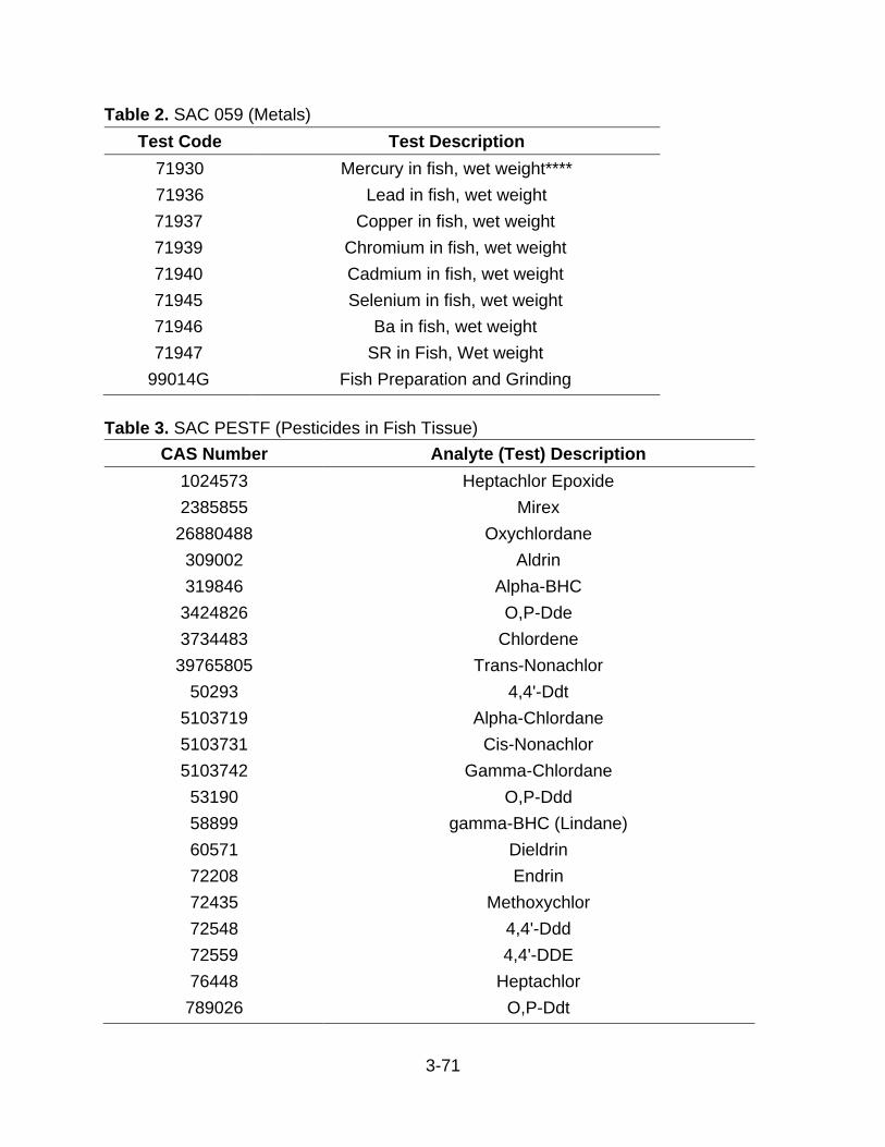
3-71
Table 2. SAC 059 (Metals)
Test Code Test Description
71930 Mercury in fish, wet weight****
71936 Lead in fish, wet weight
71937 Copper in fish, wet weight
71939 Chromium in fish, wet weight
71940 Cadmium in fish, wet weight
71945 Selenium in fish, wet weight
71946 Ba in fish, wet weight
71947 SR in Fish, Wet weight
99014G Fish Preparation and Grinding
Table 3. SAC PESTF (Pesticides in Fish Tissue)
CAS Number Analyte (Test) Description
1024573 Heptachlor Epoxide
2385855 Mirex
26880488 Oxychlordane
309002 Aldrin
319846 Alpha-BHC
3424826 O,P-Dde
3734483 Chlordene
39765805 Trans-Nonachlor
50293 4,4'-Ddt
5103719 Alpha-Chlordane
5103731 Cis-Nonachlor
5103742 Gamma-Chlordane
53190 O,P-Ddd
58899 gamma-BHC (Lindane)
60571 Dieldrin
72208 Endrin
72435 Methoxychlor
72548 4,4'-Ddd
72559 4,4'-DDE
76448 Heptachlor
789026 O,P-Ddt

3-72
Table 4. SAC PCBF (PCBs in Fish Tissue)
CAS Number Analyte (Test) Description
Lipids
EXTRACTED DATE
11096825 Arochlor 1260
11097691 Arochlor 1254
11104282 Arochlor 1221
11141165 Arochlor 1232
12672296 Arochlor 1248
53469219 Arochlor 1242
Before shipping the sample to the lab for analysis, the lab sample submission sheet as
well as the field data sheets should be scanned and forwarded to the DEP fish tissue
data coordinator and the BOL fish tissue data representative. The estimated
shipment/receipt date should be described to ensure lab representatives will be
available to receive the frozen samples upon arrival. Once a shipment/receipt date has
been confirmed the samples are ready to send. Completely frozen samples that are of
considerable mass can be placed in a cooler without additional ice and couriered to the
BOL. Small and medium samples should always be shipped on dry ice. The completed
sample submission sheet should be placed in a separate Ziploc® bag and placed inside
the cooler with the sample. To ensure adequate time for lab preparation, analysis and
quality control of the samples, all samples should be shipped to the lab by November 1st
of the collection-year.
LAB SAMPLE PREPARATION
Once the sample has been received and inventoried at the BOL, the samples will need
to be prepared for analysis. The processing equipment is washed and then rinsed with
purified hexane labeled as suitable for pesticide residue analysis. Clean, restaurant-
grade aluminum foil (dull side contacting the sample) should be placed on all surfaces
the sample contacts. Each sample is ground in a meat grinder until all fillets are
considered homogenous (large samples may need to be ground multiple times). The
sample is then subsampled into four 30-gram aliquots that will be used for the analysis
of each SAC, with a backup for reanalysis or archival as desired. The aliquots are
wrapped in foil, pressed to form a patty, labeled with sample number, and refrozen for
analysis. Equipment cleaning, hexane rinses, and foil changes must be completed
before the next sample can be processed. All samples should be processed for lab
analysis by December 31st of the collection-year.

3-73
LITERATURE CITED
Shull, D. R. 2017. Sample information system (SIS) data entry protocol. Chapter 4.6,
pages 120–122 in M. J. Lookenbill, and R. Whiteash (editors). Water quality
monitoring protocols for streams and rivers. Pennsylvania Department of
Environmental Protection, Harrisburg, Pennsylvania.
Shull, D. R., and R. Whiteash (editors). 2021. Assessment methodology for streams and
rivers. Pennsylvania Department of Environmental Protection, Harrisburg,
Pennsylvania.

3-74
3.9 MUSSEL DATA COLLECTION PROTOCOL

3-75
Prepared by:
Richard Spear, Daniel Counahan, and Dustin Shull
PA Department of Environmental Protection
Southwest Regional Office
Office of Water Programs
Clean Water Program
400 Waterfront Street
Pittsburgh, PA 15222
2017
3-76
INTRODUCTION
Larger rivers and streams are highly complex ecosystems with a great deal of
interdependence between biological communities. As a result, biological components of
this assessment must include a diversity of sampling including, but not limited to fish,
benthic macroinvertebrates, and mollusk sampling. Current mussel data collection
protocols are not suited for a rapid and cost-effective means of assessing a
representative portion of the mussel community. Therefore, DEP developed a mussel
sampling protocol that incorporates random sampling to allow for a semi-quantitative
assessment of mussel communities. The DEP freshwater mussel data collection
protocol enables sampling in reaches where fishes and benthic macroinvertebrates
were sampled to provide comprehensive sampling of aquatic biological communities.
This protocol can also be described as a cursory evaluation of the mussel community so
that future/more intensive surveys can be conducted.
The DEP freshwater mussel data collection protocol is designed to enumerate several
aspects of a mussel community. All live mussels are identified to species and
individuals are counted to obtain a representative description of the community in terms
of relative abundance and species richness. Size measurements such as length, width
and depth can be used to approximate age classes of each species. Additionally, this
survey can be used as a rapid and cost-effective way of searching for rare, threatened,
endangered, and invasive mussels. Protocols such as the ones described by Smith
(2006) and Clayton et al. (2013) are also recommended for this purpose.
This protocol is composed of 12 five-minute dives along linear transects that are
randomly spaced from both the downstream sampling point and the shoreline. The
objective of this survey protocol is to build Pennsylvania’s capacity to assess conditions
of large rivers by providing a foundation for the development of large river assessment
protocols for non-wadeable streams. These large river protocols will provide the
capability to conduct bioassessments and monitor environmental conditions with a
scientifically defensible protocol applicable to Pennsylvania’s rivers and streams.
SAFETY PROCEDURES
DEP recognizes the need to structure and oversee this activity due to the inherent
hazards involved in underwater diving. Due to these important concerns for diving
safety, all dive team members must be trained in mussel sampling techniques, safety
precautions, and equipment manufacturers’ operating procedures. In addition, all
scientific divers must have completed, at minimum, an approved SCUBA Certification
Course, and have adequate training to conduct mussel surveys. It is the responsibility of

3-77
the Unit Diving Officer (UDO) to verify that the team members have the appropriate
training. Specific team member duties should be reviewed during each sampling event.
The safety of all personnel and the quality of the data are assured through the adequate
education, training, and experience of all members of the scientific diving team. At least
one UDO must be involved in each sampling event.
The safety standards which will apply and will be followed for all DEP operations are
derived from USEPA's Diving Safety Manual Revision 1.2, (DSM, USEPA 2010b).
Safety Plan
This safety plan establishes general guidelines and procedures for safe and efficient
scientific diving. The intent is to provide written guidance for quick reference in the field
by the Unit Dive Officer (UDO) and scientific divers and is based on the DEP’s Policy for
Scientific Diving Personnel and Diving Operations (DEP 2012). This plan is comparable
to and was derived from USEPA's DSM, and specifically, Appendix A of the DSM,
USEPA Diving Safety Rules (USEPA 2010a). A copy of this safety plan is required to be
available in the field for all diving operations.
Dive Operations and Rules
1. A Dive Plan for each proposed diving operation will be approved by the UDO.
2. Diving with air will be conducted in accordance with the U.S. Navy No-
Decompression Limits and Repetitive Group Designation Table for No-
Decompression Air Dives, located in Appendix H-10 of the DSM (USEPA 2010b).
Diving with Nitrox will be conducted in accordance with the National Oceanic
and Atmospheric Administration (NOAA) Nitrox Tables for No-Decompression
Limits and Repetitive Group Designation Table for No-Decompression Dives
(NOAA 2016).
3. During "live-boat" diving, the tender or UDO will maintain continuous visual
contact with the divers, or their bubbles after they descend, and keep the boat
operator informed of their position. The boat should always be positioned to
render immediate assistance to the divers.
4. The dive plan should require that the deepest dive be scheduled first and be
followed by shallower dives. If this is not possible, the divers must comply with
rule Nos. 5 and 6, below.
5. Generally, all dives should be terminated 5 minutes before the no-decompression
limit.
6. During repetitive diving at water depths greater than 50 feet, on ascent the diver
should stop at approximately 20 feet for 2 minutes for a safety decompression

3-78
stop on the second and succeeding dives. If a safety decompression stop is
taken, the time spent at the stop must be added to the bottom time for that dive.
7. While diving, divers will remain in contact (visual, auditory, tactile, or through
communications from the tender) with at least one other diver. All divers must
surface if contact or communication is lost. No one may dive unattended.
8. A diver should start their ascent from the bottom when their tank pressure
decreases to 500 psi. A diver must begin an ascent with at least 500 psi in
his/her cylinder if they must make a safety stop at 20 feet or if required by
environmental conditions.
9. When diving in extremely limited visibility and overhead environments such as
piers or other situations presenting entrapment or entanglement hazards, the rule
of thirds should be followed: one third of the tank pressure may be used to get to
the dive objective, the second third may be used to complete the work
assignment and return to the surface, and the final third of the tank pressure is
for a safety reserve. This rule does not supersede the 500-psi rule (Rule No. 8).
10. When diving in areas with possibilities of entrapment or entanglement such as
described above in Rule No. 9, an extra open-circuit SCUBA regulator will be at
the dive site and attached to a standby full SCUBA cylinder complete with
backpack.
11. During dives always ascend at a rate of 30 fpm (minor variations in ascent rate
between 20 and 40 fpm are acceptable).
12. No dive will go beyond 130 feet of depth.
13. Diving operations must be conducted in accordance with all appropriate DEP
policies and standards (e.g., for Nitrox diving or flying after diving).
14. In an emergency, the UDO in charge of the diving operation may have to make
field decisions that deviate from the requirements of this safety plan to prevent or
minimize a situation which will likely cause death or serious physical harm.
15. Oxygen will be provided on-scene and on boats participating in dive operation.
Responsibilities of Dive Personnel
UDO:
1. Preparing for the diving operation including checking equipment such as the
pressure in the O2 cylinders.
2. Ensuring that all divers are physically fit to dive.
3. Assisting the Tender and is completely in-charge of the diving operation.
4. Ensuring that all diving operations are conducted safely in accordance with
USEPA's DSM and standards (USEPA 2010b).
5. Promptly prepares a Dive Report upon completion of the diving activities.
6. Giving the pre-dive Briefing which will include:
a. Designating dive buddy pairs including the alternate UDO.

3-79
b. Providing a brief description of the dive site.
c. Discussing the objectives of the diving operation.
d. Reviewing the operation of equipment to be used.
e. Identifying any potential pollution sources.
f. Discussing environmental and any hazardous conditions.
g. Monitoring divers for signs/symptoms of "bubble trouble."
h. Reviewing emergency and evacuation procedures.
7. For the emergency and evacuation procedures, the following will be identified and
discussed in as much detail as is appropriate for conditions at the dive site:
a. Establish evacuation routes and means of transportation.
b. Review methods of communication.
c. Review CPR and the use of medical O2, if necessary.
8. In the Event of a Diving Accident the following will be conducted:
a. Maintain heart and breathing functions.
b. Do NOT remove O2 from patient unless necessary.
c. Reconstruct dive profiles while in route to the chamber.
d. Ensure dive partner accompanies victim or goes to chamber ASAP.
e. Retain all dive gear for examination.
Scientific Divers:
1. Dive only if they are physically and mentally fit and properly trained for the task to
be performed.
2. Keep their diving equipment in safe operating condition.
3. Wear a compass and depth and tank pressure gauges and, when necessary, a
dive watch or bottom timing device.
4. Refuse to dive if diving conditions are unsafe or unfavorable, or if the diving
operation breaches the dictates of USEPA's safety policies or standards (USEPA
2010a, USEPA 2010b).
Standby Divers:
1. Be fully equipped and ready to give immediate assistance at the dive site.
2. Receive the same briefing and instructions as the working divers.
3. Monitor the progress of the diving operations.
Tenders:
1. Assist divers and track their location in the water.
2. Record each diver's bottom time, tank pressures, and maximum depth.
3. Alert the divers, when necessary, on the status of their bottom time via the Diver
Recall Unit.

3-80
4. Advise other vessels of diving operations and warn off boat traffic which may
pose a hazard to the divers.
5. Perform no other concurrent function which interferes with these duties.
Number of Personnel Per Dive Team
Except under emergency conditions, the minimum number of personnel required per
dive team will be as follows (Table 1).
Table 1. Dive team members required.
Water Depth/Situation
Number
of
Divers
Number of
Standby Divers
Number of
Tenders
Total
Individuals
Under 15ft/diver visible at
all times 1 11/ 1 3
Between 15 and
60ft/without unusual
conditions3/
2 - 12/ 3
Between 15 and 60ft/with
unusual conditions 2 11/ 1 4
Between 60 and 130ft/all
conditions 2 11/ 1 4
1/ The Standby Diver will be the UDO or Alternate UDO, if the UDO is diving. 2/ The Tender will also be the UDO or Alternate UDO, if the UDO is diving. 3/ Unusual conditions as determined by the UDO considering weather, water
currents, visibility in the water, potential entanglements, or any other factor that may
compromise the safety of the diving operations.
Decompression Diving
No decompression diving will be conducted
Dive Buddy
No one may dive unattended. Divers must have visible, auditory, or tactile,
communication with at least one dive buddy or a tender at all times.
Dive Computers
As specified in the Dive Plan, determined by the UDO, and in accordance with the DSM,
dive computers may be used to control the dive profile.
Dive Equipment
All dive equipment will conform to USEPA regulations.
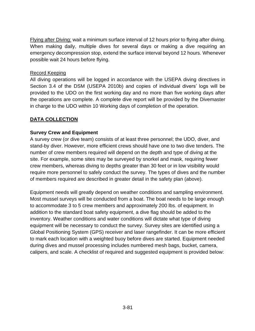
3-81
Flying after Diving: wait a minimum surface interval of 12 hours prior to flying after diving.
When making daily, multiple dives for several days or making a dive requiring an
emergency decompression stop, extend the surface interval beyond 12 hours. Whenever
possible wait 24 hours before flying.
Record Keeping
All diving operations will be logged in accordance with the USEPA diving directives in
Section 3.4 of the DSM (USEPA 2010b) and copies of individual divers’ logs will be
provided to the UDO on the first working day and no more than five working days after
the operations are complete. A complete dive report will be provided by the Divemaster
in charge to the UDO within 10 Working days of completion of the operation.
DATA COLLECTION
Survey Crew and Equipment
A survey crew (or dive team) consists of at least three personnel; the UDO, diver, and
stand-by diver. However, more efficient crews should have one to two dive tenders. The
number of crew members required will depend on the depth and type of diving at the
site. For example, some sites may be surveyed by snorkel and mask, requiring fewer
crew members, whereas diving to depths greater than 30 feet or in low visibility would
require more personnel to safely conduct the survey. The types of dives and the number
of members required are described in greater detail in the safety plan (above).
Equipment needs will greatly depend on weather conditions and sampling environment.
Most mussel surveys will be conducted from a boat. The boat needs to be large enough
to accommodate 3 to 5 crew members and approximately 200 lbs. of equipment. In
addition to the standard boat safety equipment, a dive flag should be added to the
inventory. Weather conditions and water conditions will dictate what type of diving
equipment will be necessary to conduct the survey. Survey sites are identified using a
Global Positioning System (GPS) receiver and laser rangefinder. It can be more efficient
to mark each location with a weighted buoy before dives are started. Equipment needed
during dives and mussel processing includes numbered mesh bags, bucket, camera,
calipers, and scale. A checklist of required and suggested equipment is provided below:

3-82
Dive Equipment
Masks
Snorkels
Wetsuits
Gloves
Boots
Hoods (If Applicable)
Fins (If Applicable)
Buoyance Control Devices (BCDs)
Regulators, Octos And Hoses
Air Tanks
Dive Weights
Communication Gear
Dive Flags
Dive Knives
Dive Lights
First Aid Kit
Emergency Oxygen Kit
Other: __________
Field Meters & Related Supplies
Dissolved Oxygen Meter
Replacement Membrane Kits
Do Probe Solution
Zero % Calibrating Solution (If
Applicable)
Ph Meter
Buffers (Ph 4, 7, 10)
KCl Probe Solution
Conductivity Meter
Calibrating Solution (If
Applicable)
Thermometer
Meter Field Manuals (If Applicable)
Secchi Disk
Other: __________________
Mussel Sampling Equipment
GPS
Laser Rangefinder
Numbered Mesh Bags
Bucket
Calipers (Mm)
Scale (Grams)
Camera
Other: __________________
Forms
Field Survey Sheets
Mussel Data Sheets
Other: __________________
Misc.
Maps
Markers, Pens, & Pencils
Calculator
Insect Repellent
Sunscreen
Screwdriver/Tools
Batteries (D-Cell, Other: ________)
Other: _______________

3-83
Survey Location and Site Selection
Survey locations are typically situated at or near large river fish and macroinvertebrate
sample sites and are along the left bank, right bank, or island shore. At each survey
location, dives are conducted at 12 randomly selected sites in a 500m by 50m reach
(Figure 1). The 12 sites will be selected to proportionally reflect shallow and deep-water
habitats. This is supported by previous work by DEP showing distinct shallow or deep
mussel communities. A minimum of 4 shallow water sites will be selected at each
sample site to ensure adequate coverage of this habitat type. For some survey
locations, mid-channel sites may be limited by commercial or recreational traffic that
could pose unsafe diving conditions. Any intake structures or other potential hazards will
be avoided by an approximate 50m buffer. No transects will be performed between any
lock chamber mooring points and the lock and dam structure. If a survey is located near
a US Army Corp of Engineer lock and dam, then the US Army Corp of Engineer must
be notified prior to the survey date. When on site, the lockmaster must be notified via
marine radio that the dive team is ready to commence operations.
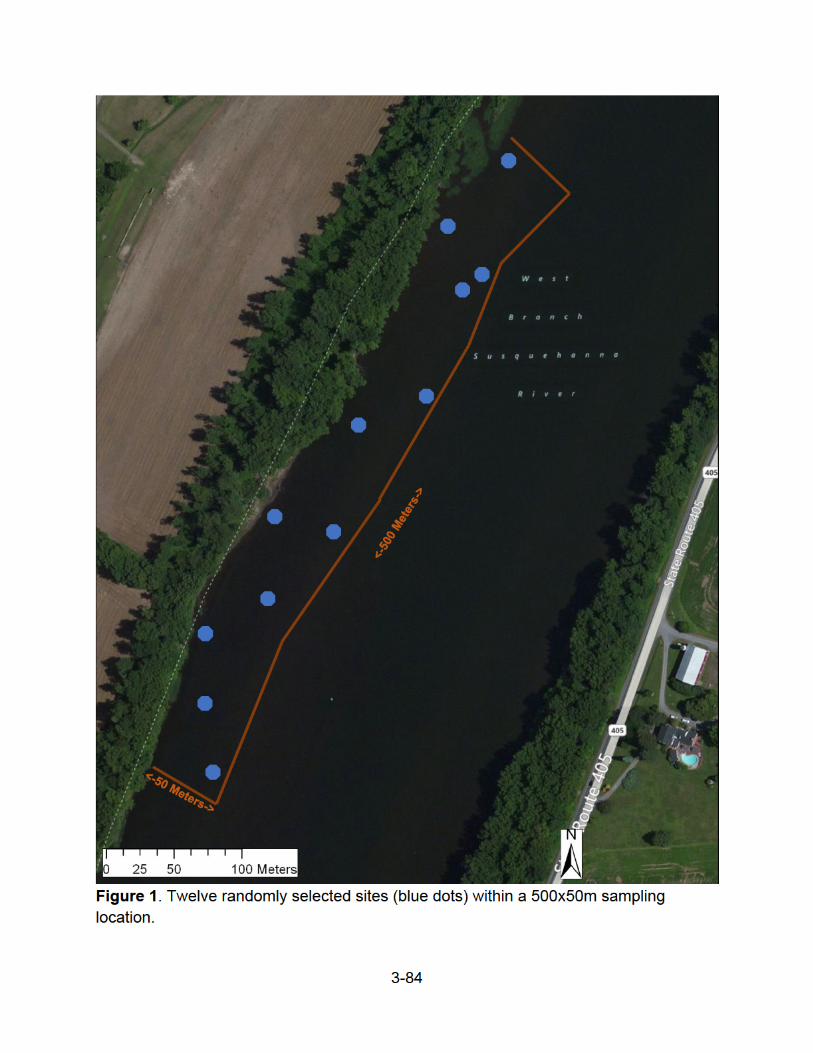

3-85
Mussel Data Collection Procedure
A crew member will use a GPS to identify the downstream point of the survey location.
This site is the “X” site in the field survey sheet (Appendix A.5). A range finder will be
used to determine the location of each of the 12 sample locations by measuring the
distance from the shore and the distance from the “X” site. Once at a site, a Latitude
and Longitude is taken using a GPS, and the stand-by diver will deploy the anchor.
In deeper diving conditions or in low visibility, the diver and stand-by diver will dive
together and at least one of those individuals will have communications with the surface.
In shallow diving conditions or if the diver is visible from the surface the stand-by diver
may stay on the surface, but will maintain auditory or tactile contact with the diver. In both
shallow and deeper dives, the diver will record an upstream compass heading while
onboard for underwater orientation. The diver will also be equipped with a 250-foot dive
reel that is marked in 1-meter increments. The UDO will perform a safety check using
communication gear. The diver will descend along the anchor line to the bottom of the
river with the stand-by diver and clip the dive reel to the anchor.
At the beginning of the survey the diver may collect a bucket excavation sample to check
for the presence of mussels in deeper sediment. The diver will communicate to the stand-
by diver that the time interval should begin. The stand-by diver will keep time. For five
minutes, the diver will travel upstream searching (visual and tactile) a one-meter wide
area and collect live mussels and dead mussel shells in the search area. The diver will
search under any large rocks that can easily be turned. The diver will also sweep across
the top of the fine substrate to feel for mussels which may be partially buried. The
sampling protocol recommends a surface search only; subsurface searching will not be
conducted. At the end of five minutes, the stand-by diver will call to the diver via
communication equipment or other diver recall system to conclude the search. All shell
material, live or dead, will be placed in a numbered bag. On a wrist dive slate or verbally,
the diver will record or communicate the substrate composition percentages for fines,
sand, gravel, cobble, boulder, and bedrock. Invasive mollusks (Zebra mussels and
Corbicula) will be scored: 0 = no invasive mollusks; 1 = 1 individual; 2 = multiple
individuals; 3 = small clumps of individuals; 4 = greater than 50% coverage; 5 = complete
coverage of available substrate. The average depth of the searched area will be recorded.
While returning to the boat, the diver will record or communicate the total distance traveled
in meters by counting the number of marked increments on the dive reel. Distance/area
searched will vary based on visibility, mussel density and habitat.
A crew member will use a cleaned and calibrated water quality field meter to record
temperature, pH, dissolved oxygen, percent dissolved oxygen, turbidity, and specific
conductivity according to Chapter 4.1, In-Situ Field Meter and Transect Data Collection
Protocol (Hoger 2020). A Secchi disk is used to measure the depth of the photic zone.

3-86
Water chemistry measurements will be recorded at one of the 12 sites. All live mussels
are identified to species level on-site. However, some representatives may be taken back
to the laboratory for verification if a photograph is insufficient (State and/or Federal
permits required). Live mussels are then weighed (in grams), measured (length, width,
and depth in millimeters), photographed and returned to the river. Measurements of
length, width and depth are described in Figure 2. When returning live mussels, care
should be taken to orient the mussel posterior side up. All mussel data are recorded on
mussel data sheets provided in Appendix A.5. Mussel shells will be identified if both
valves are present and noted as “dead” on the data sheet. Mussels and shells found near
the sampling sites can be identified, measured if live, and recorded on mussel data
sheets, noted as “incidental.”
A. B.
C.
Figure 2. A. Measurement of length is the maximum distanced between the anterior
and posterior margins. B. Measurement of width is the maximum distance between

3-87
dorsal and ventral margins. C. Measurement of depth is the maximum distance between
left and right valves (shell halves).
LITERATURE CITED
Clayton, J., B. Douglas, P. Morrison, and R. F. Villella. 2013. West Virginia mussel
survey protocols. US Fish and Wildlife Service, US Department of the Interior,
Washington, DC.
DEP. 2012. Policy for Scientific Diving Personnel and Diving Operations. Pennsylvania
Department of Environmental Protection, Harrisburg, Pennsylvania.
Hoger, M. S. 2020. In-situ field meter and transect data collection protocol. Chapter 4.1,
pages 2–8 in M. J. Lookenbill, and R. Whiteash (editors). Water quality
monitoring protocols for streams and rivers. Pennsylvania Department of
Environmental Protection, Harrisburg, Pennsylvania.
NOAA. 2016. NOAA No-decompression tables for Nitrox Dives. NDP 07 -2015. U.S.
Department of Commerce, National Oceanic and Atmospheric Administration,
Office of Marine and Aviation Operations, Silver Spring, MD.
Smith, D. R. 2006. Survey design for detecting rare freshwater mussels. Journal of the
North American Benthological Society 25(3):701–711.
USEPA. 2010a. Appendix A EPA diving safety rules. Diving safety manual (Revision
1.2). U.S. Environmental Protection Agency, Office of Administration and
Resources Management, Safety, Health and Environmental Management
Division, Washington, DC.
USEPA. 2010b. Diving safety manual (Revision 1.2). U.S. Environmental Protection
Agency, Office of Administration and Resources Management, Safety, Health
and Environmental Management Division, Washington, DC.

3-88
3.10 PERIPHYTON DATA COLLECTION PROTOCOL
3-89
Prepared by:
Jeffery Butt
PA Department of Environmental Protection
Office of Water Programs
Bureau of Clean Water
11th Floor: Rachel Carson State Office Building
Harrisburg, PA 17105
2017
Disclaimer:
The mention of specific trade names or commercial products does not constitute
endorsement or recommendation for use.

3-90
PURPOSE
The purpose of this document is to provide a standard protocol for DEP’s collection of
periphyton in lotic systems of Pennsylvania. The following sample and subsampling
types and protocols, laboratory procedures, as well as quality issues, will be discussed:
• Collection of Qualitative Multi-Habitat Periphyton samples
• Collection of Quantitative Benthic Epilithic Periphyton samples
• Subsample for Identification and Enumeration of Algal Taxa
• Subsample for the quantitative determination of Chlorophyll-a and Phycocyanin
Photopigments
• Subsample for the quantitative determination of Ash Free Dry Mass (AFDM)
• Subsample for the characterization of Cyanotoxins as part of qualitative multi-
habitat periphyton and benthic epilithic periphyton quantitative samples
• General laboratory considerations and procedures required to process the above
sample types
• Quality and harmonization issues concerning the identification and counting of
algae taxa.
INTRODUCTION
Characterizing lotic benthic algae communities is an important tool used by DEP in
determining the quality of its natural flowing waters. This is because, as is pointed out
by authors R. Jan Stevenson and Loren L Bahls,
“Benthic algae (periphyton or phytobenthos) are primary producers and an
important foundation of many stream food webs. These organisms also stabilize
substrata and serve as habitat for many other organisms. Because benthic algal
assemblages are attached to substrate, their characteristics are affected by
physical, chemical, and biological disturbances that occur in the stream reach
during the time which the assemblage developed (Barbour et al. 1999).”
In short, benthic algae and its analysis provides important information concerning the
condition of streams and rivers.
Algae, in this document, is a term used to describe a group of aquatic organisms that do
not represent a single formal taxonomic group. Rather, algae are defined as, in the
words of authors John D. Wehr and Robert G. Sheath, “… a loose group of organisms
that… [are] aquatic, photosynthetic, [and with] simple vegetative structures without a
vascular system…” (Wehr and Sheath 2003). Lotic periphyton includes several major

3-91
taxonomic groups which, in Pennsylvania, are dominated by cyanobacteria, diatoms,
and green algae.
Benthic algae, in lotic systems, is collected by DEP as part of its on-going monitoring
responsibilities needed evaluate protection of surface water quality. Certain benthic
algae organisms, such as diatoms, are very useful because they have a very strong
relationship with nutrient concentrations and have been used as trophic indicators
(Potapova and Charles 2007, Porter et al. 2008, Hausmann et al. 2016).
Consequentially, collecting algae samples provides DEP with a tool that facilitates the
determination of trophic status and evaluate protection of surface water quality of rivers
and streams.
DEP biologists currently use two data collection procedures to collect periphyton from
lotic systems. These procedures are:
• Qualitative Multi-Habitat (QMH) Periphyton Data Collection Procedures
• Quantitative Benthic Epilithic (QBE) Periphyton Data Collection Procedures
The field procedures employed to collect both the QMH Periphyton and the QBE
Periphyton samples are appreciably derived from those described in the USGS
document Revised Protocols for Sampling Algal, Invertebrate, and Fish Communities as
Part of the National Water-Quality Assessment Program (USGS OFR 02-150, Moulton
et al. 2002). Many of the terms used in this DEP protocol are also found in this USGS
protocol and it is there that the reader may refer for definitions of these terms.
This document will also stipulate procedures and requirements that participating
laboratories must follow to consistently process and report results for the various
subsample types. Quality control practices needed to validate the identification and
enumeration of algal, cyanobacteria, and diatom taxa will also be discussed.
DEP biologists also collect water chemistry samples and discrete water parameters with
a properly calibrated field meter during algae sampling. Although a variety of chemical
analytes are often collected, which frequently depend upon the monitoring needs to
serve other objectives, the water chemistry that must be collected to support a
comprehensive analysis of the algae community should include Total Nitrate & Nitrite
Nitrogen, Total Nitrogen as N, Total Organic Carbon, Total Ortho Phosphorus as P,
Total Phosphorus as P, Dissolved Nitrate & Nitrite Nitrogen, Dissolved Ortho
Phosphorus, and Dissolved Phosphorus as P. Discrete water parameters collected with
a field meter should include Temperature, Specific Conductivity, pH, and Dissolved
Oxygen (both mg/l and % saturation).

3-92
This document doesn’t address the data protocols for the collection and processing of
water chemistry samples or those for the collection of discrete water chemistry
parameters with a field meter. For these protocols, the reader is referred to Chapter 4 of
the Monitoring Book (Lookenbill and Whiteash 2021)
HISTORY OF LOTIC PERIPHYTON SAMPLING BY DEP
DEP began actively collecting lotic periphyton samples in 2005 at locations associated
with its Water Quality Network (WQN) sites. In 2012, biologists began collecting
samples for use in the development of a nutrient trophic index and concluded this
sampling in 2014. The samples collected for the nutrient trophic index have also been
applied to the development of an algae based Multi-Metric Index (MMI) for assessing
wadable and semi-wadeable Pennsylvania rivers and streams. DEP periphyton
sampling continues to this day for the purposes of developing this MMI as well as for
routine monitoring to document existing or changing biological conditions in rivers and
streams.
SAMPLING CONSIDERATIONS
Many different aquatic algae sampling options are available for the biologist to consider.
For example, the USGS OFR 02-150 lists four separate data collection protocols. These
include three quantitative protocols and one qualitative protocol, each of which are
designed to target different aquatic algae habitats. These USGS data collection
protocols include:
• Richest Targeted Habitat (RTH) – quantitative, represents a riffle or hard
substrate “… where the taxonomically richest algal or invertebrate community is
theoretically located.”
• Depositional Targeted Habitat (DTH) – quantitative, represents a depositional
habitat where fine sediments such as silt and sand accumulate.
• Phytoplankton (PHY) – quantitative, represents the water column habitat.
• Qualitative Multi-Habitat (QMH) – qualitative, whereas each of the three
quantitative sampling protocols defined above, in general, targets a single habitat
type, this sampling protocol is intended to represent the several different habitats
that may be present in a reach.
Currently DEP collects algae samples from lotic waters by using two different algae.
These two procedures include:
• QMH Periphyton Sampling Procedure (Similar to the USGS QMH procedure)
• QBE Periphyton Sampling Procedure (Similar to the USGS RTH procedure).

3-93
The timing of algae sample collection is another important consideration for the
biologist. Algae growing in streams and rivers are readily influenced by high flow events,
temperature, and sunlight. Consequentially, the question of how long the biologist
should wait before sampling a stream or river after a high flow event must be
considered. Various researchers have studied the recovery of benthic algae
communities following a scouring flow and have made suggestions. For example,
Peterson and Stevenson (1990) suggested a three-week postponement in sampling
after a scour event to allow for recolonization (Peterson and Stevenson 1990, Barbour
1999). DEP biologists have considered the three-week “wait” period and, based on the
experience gained from observing the recovery of many streams in Pennsylvania, as
well as considering other logistical issues, have decided to use, in general, a two-week
“wait” period to resume sampling after a scour event. However, each stream or river
possesses its own scour response to flow which is based upon its own geomorphic
characteristic. The biologist must use knowledge of the watershed and best professional
judgement, as well as stream gauge data available on the USGS website (available at
https://waterwatch.usgs.gov/new/index.php?r=pa&id=ww current) to make decisions
regarding sampling delay after a scour event.
Temperature and sunlight availability also play a major role in the growth of algae in
rivers and streams. Typically, DEP biologists will begin sampling benthic algae in the
early spring in those streams that will later be shaded by the surrounding forest when
leaf-out occurs. Obviously, stream water temperatures are relatively cool in this early
spring-time period and will influence the composition of the algae community. Later,
biologists may return to the same stream to sample the algae community in mid-
summer and/or early fall when the stream is fully shaded and water temperatures are
more elevated so that they may characterize an algae community that may differ
appreciably from that observed in the spring. Sampling these streams across seasons
allows the biologist to better understand the transition in algae community composition
that occur with temperature and shading changes.
QMH PERIPHYTON SAMPLING PROCEDURE
The biologist may need to collect a QMH Periphyton Sample of microalgae and/or
macroalgae so that they may better understand the algal community present in any of
the multiple habitats available within a stream reach or area but not require area-based
(for area-based sampling, refer to the QBE Procedure discussed below) community
data, photopigment, or AFDM measures. This type of sampling aligns, in part, with the
USGS OFR 02-150 QMH sampling procedure. Because this procedure may sample
many types of algae habitats, there may be a cross over into the sampling situations

3-94
referred to as DTH (Depositional Targeted Habitats) and RTH (Richest Targeted
Habitats) in the USGS OFR 02-150.
This sampling procedure provides DEP biologists with a tool to investigate special
monitoring questions. Such questions, for example, may address monitoring concerns
related to the habitat of early life phases of fish species or perhaps the algae community
composition that may lead to the production of cyanotoxin in non-thalweg stream
environments. In these examples, the sample location might be better described as a
specific habitat or area, such as a smallmouth bass young-of-the-year nursery habitat or
that of a small area where cyanobacteria are observed to be growing. Deciding to
delineate a sample reach versus a sample area is in part dictated by the question or
concern that the DEP biologist is attempting to address. Ultimately, the biologist must
characterize the habitat they sample and does so as described below in the data
collection section of this protocol.
With this protocol, the biologist should submit a subsample to a laboratory for algae
identification and enumeration. Also, the biologist should submit another subsample to a
laboratory to test for the presence of, cyanotoxins.
This protocol is intended for use in Pennsylvania wadeable riffle-run streams and semi-
wadeable large rivers. Refer also to Chapter 3.1, Wadeable Riffle-Run Stream
Macroinvertebrate Data Collection Protocol (Shull 2017b) and Chapter 3.4, Semi-
Wadeable Large River Macroinvertebrate Data Collection Protocol (Shull 2017a) for
terms and definitions that also apply to this section, as well as provide important safety
information for field staff to consider.
Field Data Sheet
The biologist will also complete the DEP QMH Periphyton Field Data Sheet (Appendix
A.7) at each monitoring site. To complete this field data sheet, the biologist must
provide information pertaining to the following (refer to the QMH Periphyton Field Data
Sheet in Appendix A.7 for more specific requirements for each data record):
• Site/sample information including water chemistry collection information and
personnel involved
• Latitude and longitude of the site
• Watershed Area – determined prior to making the field visit
• Field Meter Discrete Values – refer to Chapter 4.1, In-Situ Field Meter and
Transect Data Collection Protocol (Hoger 2020) for field meter use and
calibration requirements
• Total algae slurry volume (ml, minimum volume rules apply – refer to Table 1 in
the Subsampling Procedure section)

3-95
• Densiometer and Compass Readings (refer to the Densiometer and Compass
Data Collection section – located near the end of the periphyton protocol - for
instructions in using these devices)
• Percent relative qualification of the periphyton habitat
• Notes pertaining to the three Algae ID Bottles collected
• Other notes (including any pertaining to cyanotoxin testing, if collected).
Habitat Types
To collect a QMH periphyton sample the biologist will need to employ several
approaches to sample across multiple habitats. The multiple habitats that may be
sampled will include any one or more of the following:
• Epilithic (Rock)
• Epiphytic (Plant)
• Epipelic (Silt)
• Epidendritic (Wood)
• Episammic (Sand)
• Gravel (subset of Epilithic material but listed independently here due to difference
in sampling protocol).
Data Collection
When sampling across multiple habitats, the biologist should proportionally represent
each habitat type in the targeted reach or area when making a composite sample. For
example, if after inspecting the targeted stream area, the biologist observes that the
multiple habitats present include about 45% Epiphytic, 10% Epipelic, 30% Epidendritic,
and 15% Episammic and no rock cobble or gravel (these percentages are recorded on
the field data sheet in the Periphyton Habitats section), then the final composited algae
slurry should be accumulated from a quantity of materials proportionally collected to
represent this habitat observation as best as possible. Because this protocol is
qualitative in nature the biologist must select sample material in a fashion that, in their
professional opinion, best reflects this observed habitat characterization. In other words,
based upon the above habitat characterization, the biologist would attempt to sample
material surfaces that roughly represents 45% Epiphytic, 10% Epipelic, 30%
Epidendritic, and 15% Episammic.
The multiple habitat sampling procedures, by type, will be performed as follows:
• For each sampling procedure described below, use de-ionized water to rinse the
scrubbed material into the algae slurry pan. The collector must remain aware of
the total amount of rinsate generated for the complete composited sample. In
short, the final accumulated algal slurry should be kept to a minimum by
conserving rinse water so that the total algae slurry (from all substrate) isn’t
3-96
greater than that needed for lab analysis by a factor of two or three. This is
intended to maintain total slurry concentrations that better enable algae
identification and enumeration and cyanotoxin tests as well as facilitating
handling during sub-sampling homogenization.
• Epilithic (Rock) sampling performed by DEP is restricted to rock that is in the size
range of cobble (generally 2.5 to 10 inches) and is thus more easily moved by
the biologist. Boulders or bedrock are not readily transportable and are not
considered here. Gravel, which is a subset of epilithic, is treated separately in
this protocol because it is sampled differently. Cobble sampling is best
accomplished by removing cobble substrate from the benthos and transporting it
to the bank where the sampled surfaces may be scrubbed by a plastic or steel
brush while collecting the rinsate into the algae slurry pan. The sampled surface
should include scrubbing all that surface which is exposed to the aquatic
environment above the benthos.
• Epiphytic (Plant) sampling is best accomplished by clipping the aquatic plant,
using pruning shears or scissors, just above the sediment level (allowing roots to
remain in the sediment) and at the water line (retaining only the submerged
portion) and transporting the material to the bank where the total plant surface
may be scrubbed by a plastic brush. Collect the rinsate from this scrubbing into
the algae slurry pan. When scrubbing the plant surface, care should be taken so
that plant material is not inadvertently pulled off the plant and collected in the
pan. For plants that are less physically robust, such as grasses, the plants may
be placed in a capped plastic container, along with some de-ionized water, and
agitated vigorously. After agitating, the de-ionized water may be poured into the
collection pan and the plant material discarded. On the field data sheet, record
notes regarding the plant taxa from which samples were collected.
• Epipelic (Silt) sampling may be accomplished by using a silt/sand/gravel PVC
sampler and a kitchen spatula (see Figure 1). The silt/sand/gravel PVC sampler
may be constructed from a short section (about 3 or 4-inch length) of PVC pipe
(4 or 5-inch diameter) and capped at one end. After placing this PVC sampler in
the water, rotate it up-side-down to remove air. Once the air is removed, push the
open end of the PVC sampler a few millimeters into the silt. Without moving the
PVC sampler, slide the plastic kitchen spatula underneath the PVC sampler to
secure the upper layer of silt inside the PVC sampler. Carefully extract the PVC
sampler and spatula from the stream without spilling the contents. Pour the
contents of the PVC sampler into the collection pan. As with all collecting
strategies used for this QMH procedure, the final accumulated algal slurry should
be kept to a minimum so that the total algae slurry (from all substrate) isn’t
greater than that needed for lab analysis by a factor of two or three. Quantities of

3-97
homogenized algal slurry needed to perform each laboratory test are indicated in
Table 1.
Figure 1. Silt/sand/gravel PVC and spatula sampling apparatus. This apparatus
may consist of a section of capped 4 or 5-inch diameter PVC pipe and a kitchen
spatula. The spatula must be large enough so that when it is slid under the PVC
pipe it will prevent the loss of silt, sand, or gravel from the sample as it is pulled
from the benthos.
• Epidendritic (Wood) sampling may be best accomplished by collecting
submerged wood and transporting it to the bank where the surfaces may be
scrubbed with a plastic or metal brush while collecting the rinsate into the algae
slurry pan. Use de-ionized water to wash the scrubbed material into the algae
slurry pan. When scrubbing the wood surface, care should be taken so that wood
material is not inadvertently pulled off and collected in the pan. The biologist may
find it useful to use a small saw to cut portions of larger submerged branches for
removal to the scrubbing area. As with all collecting strategies used for this QMH
procedure, the final accumulated algal slurry should be kept to a minimum by
conserving rinse water so that the total algae slurry (from all substrate) isn’t
greater than that needed for lab analysis by a factor of two or three. Quantities of
homogenized algal slurry needed to perform each laboratory test are indicated in
Table 1.
• Episammic (Sand) sampling is accomplished in much the same way as that
described for Epipelic (Silt) by using a silt/sand/gravel PVC sampler and a plastic
kitchen spatula (see Figure 1). The silt/sand/gravel PVC sampler may be
constructed from a short section (about 3 or 4-inch length) of PVC pipe (4 or 5-
inch diameter) and capped at one end. After placing this PVC sampler in the
water, rotate it up-side-down to remove air. Once the air is removed push the
open end of the PVC sampler a few millimeters into the sand. Without moving the
PVC sampler, slide the plastic kitchen spatula underneath the PVC sampler to
secure the upper layer of sand inside the PVC sampler. Carefully extract the

3-98
PVC sampler and spatula from the stream without spilling the contents. Pour the
contents of the PVC sampler into a capped plastic bottle and agitate vigorously.
After allowing the sand to settle to the bottom of the container pour the agitate
(with algae entrained) into the collection pan. As with all collecting strategies
used for this QMH procedure, the final accumulated algal slurry should be kept to
a minimum so that the total algae slurry (from all substrate) isn’t greater than that
needed for lab analysis by a factor of two or three. Quantities of homogenized
algal slurry needed to perform each laboratory test are indicated in Table 1.
• Gravel sampling is accomplished in the same way as that described for
Episammic (Sand). Refer to the Episammic (Sand) sampling procedure provided
above.
Subsampling Procedure
QMH Periphyton samples must always be subsampled for algae identification and
enumeration and sometimes, depending on the requirements of the project, cyanotoxin
analysis. Subsampling may be performed in the field if electric is available to operate a
blender and a magnetic stirrer. If subsampling can’t be performed in the field the sample
may be temporarily stored in labeled 500ml bottles that are capped and stored in a wet
ice cooler to await later treatment.
Note: This is an important step needed to prevent cross-contamination between
samples. Prior to performing any subsampling procedures on a site sample, thoroughly
clean all equipment that may come in contact with the algae slurry sample and, at the
conclusion of this cleaning, rinse with de-ionized water. Because site samples are often
accumulated through the field day and subsampled at the conclusion of that day’s work,
all equipment must be appropriated cleaned between samples.

3-99
Table 1. QMH Periphyton Subsample Tests: Homogenized Volume (ml), Bottleware,
Preservation, Transportation, and Storage
Subsample Test Homogenized
Volume (ml) Bottleware Preservation Transportation Storage
Algae ID Bottle #1 100 120ml
Plastic
7ml
Formaldehyde Cool, dry, dark
Cool, dry,
dark
Algae ID Bottle #2 100 120ml
Plastic
7ml
Formaldehyde Cool, dry, dark
Cool, dry,
dark
Algae ID Bottle #3 100 120ml
Plastic
7ml
Formaldehyde Cool, dry, dark
Cool, dry,
dark
Minimum Algae Slurry Volume
(plus excess) without
Cyanotoxin Test
400
Cyanotoxin Test 250 Whirl-Pak® None Dry-ice -80°C
Minimum Algae Slurry Volume
(plus excess) with Cyanotoxin
Test
700
Subsampling consists of the following steps:
Slurry Preparation
Once all algae slurry is collected, pour the contents of the collection pan into a large
plastic beaker (beaker should be large enough to contain at least 2000 ml of algae
slurry). Dilute the algae slurry with de-ionized water to provide enough material for all
subsample tests (refer to Table 1 for minimum quantities required). Since this procedure
is intended to be qualitative in nature, sample surface area is not determined and the
ID/enumeration laboratory will not report results in the same units as that provided for
quantitative samples (see below). Consequentially, the quantity of surface area sampled
or quantity of algae slurry collected is not reported to the laboratory.
Further, the identification/enumeration QA process requires the submission of blind
duplicates to laboratories. Typically, identification/enumeration blind duplicates are
submitted at a quantity approximately equal to 10% of the total quantity of samples
submitted to the laboratory. Consequentially, multiple ID/Enumeration bottles are
collected from each sample.
Subsampling for Algae Identification/Enumeration and Cyanotoxin
Once the dilution process (if required to achieve minimum quantities stipulated in Table
1) is complete and the final algae slurry sample volume is recorded, the sample must be
homogenized. Often a handheld low-speed blender is applied to the contents of the
beaker to break apart the larger pieces of algae. This blending also helps to better
homogenize the algae slurry. A high-speed blender shouldn’t be used at this point

3-100
because at high speeds the blender may lyse the algae cells, making the identifications
more difficult.
Once blended, the algae slurry beaker may then be placed on a magnetic stirrer to be
maintained in a homogenized state as subsamples are extracted (see Figure 4). Pour
100ml of well homogenized algae slurry into a graduated cylinder to ensure accuracy of
volume measurement – then pour this volume into a labeled 120ml algae
ID/enumeration sample bottle being careful to leave no algae residue in the graduated
cylinder. Return the slurry beaker to the magnetic stirrer to resume homogenization
prior to pouring the second and third 100ml algae ID/enumeration subsamples.
Preserve each identification and enumerations subsample with 7ml of formaldehyde
(volume of formaldehyde preservative must be reported to the ID/enumeration
laboratory). Refer also to Table 1 for subsample and preservative volumes as well as for
transportation and storage requirements.
To subsample for Cyanotoxin return the algae slurry beaker to the magnetic stirrer to re-
homogenize. Pour 250ml of homogenized sample into a Whirl-Pak® bag and seal. Then
transport and store as prescribed in Table 1.
Labels and Submission
Algae Identification and Enumeration bottles will be labeled with a GIS Key (e.g.,
20170516-1115-jbutt, indicating the date, time, and collector name), DEP Algae
Sampling Site ID Number, Stream/River Name, and Location Description.
An example of an Algae Identification and Enumeration Laboratory Submission Data
sheet can be found in Appendix A.8. This data sheet provides essential information
required by the laboratory performing identifications and is used to determine final
reporting values to DEP. Also, location information is provided on this submission sheet.
This location information may assist the laboratory performing identifications in
providing more accurate algae taxa identifications, especially as they may pertain to
species or variation level identifications of diatoms.
QBE PERIPHYTON SAMPLING PROCEDURE
Benthic epilithic periphyton is the preferred sampling substrate targeted by DEP to
collect data pertaining to lotic algal communities for use in its monitoring program. One
reason for this preference is that many streams and rivers in Pennsylvania are relatively
fast-flowing and have a geomorphology that creates riffles where cobble substrate is
plentiful. These cobbled riffles present the DEP biologist with a consistent substrate
from which to extract samples across many streams in Pennsylvania. Consistency in

3-101
sample substrate is needed to support the diatom MMI development and
implementation. As noted by Barbour et al., “For comparability of results, the same
substrate/habitat combination should be sampled in all reference and test streams”
(Barbour et al. 1999). Also, as described by Kelly et al., “Under many circumstances
(particularly at fast-flowing sites), the epilithon is the most abundant substratum,
sampling procedures are relatively straight-forward and ecological preferences of most
common species are well understood” (Kelly et al. 1998). Kelly et al. also points out
that, regarding the epilithon, “The performance of major diatom-based indices on this
substratum is well understood” (Kelly et al. 1998).
In 2005, Marina Potapova and Donald Charles analyzed the large algae data set
created by the USGS National Water-Quality Assessment Program (USGS NAWQA,
Potapova and Charles 2005) and demonstrated several important findings regarding the
type of substrate sampled. The USGS NAWQA program collected as many as four
different sample types and compared results from paired samples from hard and soft
substrates. From this analysis, those findings that support the use of the benthic epilithic
periphyton, given the typically good availability of cobble substrate in many
Pennsylvania streams, are:
• “Ordinations of assemblages from hard and soft substrates were highly
concordant and provided similar information on environmental gradients
underlying species patterns.”
• “…only one sample has to be collected at each site for water quality assessment
surveys, and that sample can come from whatever substrate is available.”
Consequentially, based upon the recommendations from the scientific literature, the
nature of the monitoring activity pursued by DEP, and the characteristic of the streams
and rivers typically being sampled in Pennsylvania, DEP chose and continues to use a
benthic epilithic periphyton sampling protocol. This protocol is intended for use in
Pennsylvania wadeable riffle-run streams and semi-wadeable large rivers.
Site Selection
Within the area where the stream is to be sampled, select a reach in which a riffle is
located and which is, in general, representative of the stream in that locale.
Representative feature considerations should include wetted width, substrate type and
size, shading, and standing periphyton crop.
Transects and Rock Selection
Rocks must be extracted randomly from the stream or river along three transects at
each sampling site. The term transects, as it is used here, should not be confused with
the same term as it is used in Chapter 4.1, In-Situ Field Meter and Transect Data
3-102
Collection Protocol (Hoger 2020). Regarding periphyton sample collection, these
transects are only used to facilitate the random selection of rocks as demonstrated in
Figure 3 and to measure wetted width of the stream for data recording on the field data
sheet.
Rocks (sometimes referred to as cobble) to be extracted for sampling must be of the
size and shape to facilitate the rock scrub. A suitable sample rock is one that allows the
foam ring on the PEP Sampler to seal properly (refer to the section “Collecting the
Periphyton Slurry – The Rock Scrub,” located below, for a description of the PEP
Sampler and refer to Figure 4). For the foam ring to seal properly, the sample rock must
be small enough to fit in the PEP Sampler but be larger than the approximately 3-inch
diameter foam gasket. Also, the rock must be relatively smooth (flat) so that ridges or
other irregularities in the scrub surface area do not interfere with the foam gasket seal
and allow the use of the scrubbing and slurry collection tools. If the first rock picked at
each location will likely not facilitate the scrub process, choose the next suitable rock
located immediately upstream at that same transect location. As with all other aspects
of this protocol, experience will be the best guide for the biologist in making appropriate
choices in selecting appropriate sample rocks.
The quantity of rocks that must be sampled at each site varies based upon the size of
the watershed located upstream of the site location. Watersheds with areas equal to or
greater than 1,000 square miles (2,590 square kilometers) are to be considered as a
semi-wadeable large river and will require a 27-rock QBE periphyton sample to properly
represent the habitat and species variability in that sample reach. Watersheds smaller
than 1,000 square miles in area should be considered as a wadeable riffle-run stream
that will require a 9-rock sample. Watershed area is an attribute that must be
determined through a GIS based inquiry which must be performed prior to sampling in
the field. For example, Pine Creek in Lycoming County, immediately upstream of the
confluence with Ramsey Run at N41.283650 W77.320917, has an upstream watershed
area of 940 square miles and is classified as a wadeable riffle-run stream thus requiring
a 9-rock sample. Whereas, the West Branch Susquehanna River at Lewisburg,
downstream of the Route 45 bridge at N40.9653 W76.8782, has an upstream
watershed area of 6,820 square miles and is considered a semi-wadeable large river
requiring a 27-rock sample. Refer to Chapter 3.1, Wadeable Riffle-Run Stream
Macroinvertebrate Data Collection Protocol (Shull 2017b) and Chapter 3.4, Semi-
Wadeable Large River Macroinvertebrate Data Collection Protocol (Shull 2017a) for a
more complete definition of these types of surface water characterizations as well as
important safety procedures that must be considered by field staff before working in
these waterbodies.

3-103
Setting up Transects and Making the Sample Rock Selections in Wadeable Riffle-Run
Streams
To facilitate the random rock selection in wadeable riffle-run streams, the biologist must
choose a sample reach that longitudinally (parallel to the stream thalweg) measures no
more than about 100 meters in length and in which is located enough riffle to deploy the
three sample transects – each transect must be deployed over a riffle. An example of
such a sample reach is shown in Figure 2.
Figure 2. An example of a periphyton sample reach in a wadeable riffle-run stream.
Three transect measuring tapes are pulled across the riffle section of the stream to
facilitate random rock selections.
The step-by-step process for setting the three transect lines, computing the random
rock sample pick locations, and collecting the rocks is as follows:
1. Three measuring tapes must be pulled across the stream to create three
transects. Each tape is pulled across the stream so that it is oriented
perpendicular to the direction of flow in the stream in a manner like that shown in
Figure 2.
2. The biologist must exercise care when pulling the transect tapes across the
stream so that they do not step on, or interfere with, the substrate that will be
targeted for sampling. In general, the collector should remain within a few feet of
the tape on the downstream side, thereby leaving substrate on the upstream side
of the tape undisturbed and available for sampling. Also, to lessen the chance of
disturbing the substrate along any transect, the biologist should not closely
situate any of the transect tapes to one-another. Widely spacing the transect

3-104
tapes over the sample reach helps to prevent biologists from disturbing substrate
in adjacent transects and additionally helps the biologist to better represent the
potential habitat variation in that stream.
3. Transect tapes should be pulled beyond the wetted margins of the stream so that
wetted width may be accurately measured. The wetted stream width parameter is
used to calculate random rock selection locations.
4. Record the wetted margin tape measurements for each transect at the RDB
(Right Descending Bank) and the LDB (Left Descending Bank) locations on the
QBE Periphyton Field Data Sheet. In streams to wide for pulling a tape, the
biologist should use a laser range finder. An example of this record, along with a
transect random rock pick calculation, is provided in Figure 3. This figure is an
excerpt from the DEP QBE Periphyton Field Data Sheet (Appendix A.6).
5. Determine the wetted width for each transect and record this width in the QBE
Periphyton Field Data Sheet.
6. Divide the wetted width for each transect by 3. The result of this mathematical
operation is referred to as the 1/3rd transect distance. Record this 1/3rd distance
for each transect on the data sheet. Essentially, each transect is divided into
equal thirds and, for a 9-rock sample (wadeable riffle-run stream), a single rock is
extracted from a randomly determined location in each of the 1/3rd transect
sections. In a 27-rock semi-wadeable sample, three rocks will be extracted from
randomly determined locations in each of the 1/3rd transect sections.
7. Random percentage numbers are used to compute sample locations along the
tape in each of the 1/3rd transect sections. Random percentage numbers may be
taken from a random number table or from the roll of a 10-sided die (the first die
roll represents the tens place of a percentage use in the location calculation – for
example, a roll of 1 represents 10. The second die roll represents the units place
– for example, a roll of 5, when combined with the previous die roll, will be
recorded as the random percentage of 15%). Record three random percentages
– which may range from 0% to 99% - for each 1/3rd transect section in the
designated spaces of the field data sheet.
8. Compute the tape locations on each transect to determine where random picks
are to occur. For example, as shown in Figure 3 below, the rock pick location on
Transect 1 in the first 1/3rd location would be computed as: (15% x 16.3ft) + 3.8 =
6.2ft on the tape measure. In this example, 16.3ft is the 1/3rd distance on transect
1 tape and 3.8ft is the RDB location. The second rock pick location on Transect
1, located in the second 1/3rd section would be computed as: (78% x 16.3ft) +
16.3ft (first 1/3rd section) + 3.8ft (the RDB) = 32.8ft on the tape measure. The
remaining rock pick locations for this 9-rock sample are similarly computed.
Locations for a 27-rock semi-wadable sample are computed in a similar fashion
3-105
except each 1/3rd transect section will use three random percentage numbers
instead of one random percentage number.
9. Once the random sample locations along each transect are computed, the
biologist must collect suitable sample rocks from each location. Rock samples
must be collected from upstream of the transect tape and the biologist should
collect the first suitable sample rock encountered when moving upstream from
the transect tape location. As previously discussed, a suitable sample rock is one
with the characteristics that allows the foam ring on the PEP Sampler to seal
properly. Refer to the section “Collecting the Periphyton Slurry – The Rock
Scrub,” located below, for a description of the PEP Sampler and refer to Figure 4.
If the first rock picked at each location will likely not facilitate the scrub process,
choose the next suitable rock located immediately upstream at that same
transect location.
10. When collecting the sample rocks, the biologist should prevent any contact with
the surface of the rock exposed to the stream water – in other words, lift the rock
by touching it only from the embedded surface (bottom) side. Collect the sample
rocks into a plastic bin, being careful to avoid any contact of the upper surface of
the rock with the container or other rocks. This care is needed because even the
slightest disturbance to the sample area on the rock will skew the results
generated during the laboratory subsample analyses. (refer to the section
“Collecting the Periphyton Slurry” for a description of that sample area)
11. Transport the sample rocks to the field sample processing station and prepare for
the collection of the Periphyton Slurry. Collection of the Periphyton Slurry is
described below. The field sample processing station, as shown in Figure 4,
should be setup in a fashion that allows for the positioning of all field sampling
hardware on a horizontal surface, such as on a table or the foredeck of a boat,
and located where biologists may process the sample in a manner that minimizes
the likelihood of fouling or loss of sample material due to environmental elements
such as rain or wind, for example.

3-106
Figure 3. Excerpt from the DEP QBE Periphyton Datasheet demonstrating the random
rock pick calculation made for a hypothetical small stream (wadeable riffle-run) that
requires a 9-rock sample.
Setting up Transects and Making the Sample Rock Selections in Semi-Wadeable Large
Rivers
To facilitate the random rock selection in semi-wadeable large rivers, the biologist must
choose a sample reach that longitudinally (parallel to the river thalweg) measures no
more than about 100 meters in length and in which is located enough riffle to deploy the
three sample transects – each transect must be deployed over a riffle.
Sampling in semi-wadable large rivers often differs from that of sampling in wadeable
riffle-run streams in four important ways. One difference may be the wetted width of the
river – it may be too wide for the positioning of a measuring tape. In these wide wetted-
width locations a laser range finder should be used instead of a tape measure. A
second important difference relates to depth – in such rivers, the biologist may
encounter sections of the transect that are too deep to sample. A section of river is too
deep to sample if the biologist is unable to safely grab substrate from the benthos while
wearing waders. If an area of the transect is too deep for sampling, the biologist must
bypass that area and collect additional sample rocks from those sections of the transect
that may be safely sampled and note this adjustment on the QBE Periphyton Field Data
Sheet. A third difference is that the biologist should expect to facilitate the sampling by
using a power boat, canoe, or kayak. The last difference relates to the possibility of
multiple sampling zones, as defined by water influence transitions, occurring at a river
site. Situations involving multiple sampling zones, and how to handle them, are
discussed in the next paragraph.
Multiple sampling zones may need to be created to properly sample periphyton in semi-
wadeable large rivers. This occurs when field meter transect data indicates a relative
lack of homogeneity in parameters such as temperature, pH, specific conductivity,
Transect 1
RDB LDB W / 1/3
3.8 ft 52.7 ft 48.9 / 16.3
Transect 2
RDB LDB W / 1/3
7.8 ft 49.6 ft 41.8 / 13.9
Transect 3
RDB LDB W / 1/3
14.2 ft 63.1 ft 48.9 / 16.3
Random #'s: 89 Random #'s: 72
Transect Random Rock Pick Calculation
(Upstream) Random #'s: 15 Random #'s: 78 Random #'s: 25
6.2 ft 32.8 ft 40.5 ft
(Middle) Random #'s: 33 Random #'s: 42 Random #'s: 11
15.0 ft 45.0 ft 58.5 ft
12.4 ft 27.5 ft 37.1 ft
(Downstream) Random #'s: 5

3-107
dissolved oxygen, or turbidity when measured along a river transect and is
characteristic of water influences originating from un-mixed tributary influences. When
such water quality heterogeneity is observed, a semi-wadeable river will need to be
subdivided into separate sampling zones and a 27-rock periphyton sample be
independently collected from each zone of influence. For example, the Susquehanna
River near Harrisburg, based on transect data, shows three distinct zones of water
influence, these being the “East” zone, the “Middle” zone, and the “West” zone. When a
river must be subdivided into multiple zones, transect sets in each zone must be
restricted to the width of river section that defines that zone.
Once these differences are accounted for, the step-by-step process for setting the three
transect lines, computing the random rock pick locations, and collecting the rocks is
identical to that defined above for a 9-rock wadeable riffle-run stream except that a 27-
rock sample is used.
Regarding the use of a boats, the biologist should familiarize themselves with the
targeted site prior to going to the field to sample. The target sample locations may be
located some distance from points of access and will thus require the use of a power
boat to facilitate the field work. In some instances, all that is needed is a canoe or a
kayak. The biologist is reminded that all Pennsylvania Fish and Boat Commission
boating laws and safe boater guidance must be observed if sampling with a boat.
Collecting the Periphyton Slurry – The Rock Scrub
After the rocks are transported to the field sample processing station location, the
biologist will scrub the rocks to collect the periphyton slurry. This slurry collection is
made using a Pennsylvania Epilithic Periphyton (PEP) Sampler, de-ionized water, scrub
brushes, pipets, squirt bottles, and collection containers (500ml plastic bottles, refer to
Figure 4). The PEP Sampler is a clamping device that secures a rock sample and
provides a fixed circular sample area (equal to 20.6cm2) and a foam gasket seal (toilet
seal) that is clamped to rock (cobble) substrates using partially flexible clamping boards
that can be tightened with quick release clamps. The following procedure steps will be
used to conduct the rock scrubs:
1. After clamping the rock in the PEP Sampler, with the top face of the rock facing
up, verify that the foam ring seal is secure by squirting an adequate amount of
de-ionized water into the scrub chamber and observing that no water leaks out. If
no leaks are observed, continue to step 2, otherwise re-clamp the rock in the
PEP Sampler and re-verify that the seal does not leak. As previously discussed,
for the foam ring to seal properly the rock must be small enough to fit in the PEP
Sampler but be larger than the approximately 3-inch diameter foam gasket. Also,
the rock must be relatively smooth (flat) so that ridges or other irregularities in the
3-108
scrub surface area do not interfere with the foam gasket seal and allow the use
of the scrubbing and slurry collection tools.
2. Using the scrub brushes and a small amount of de-ionized water, scrub the rock
area within the PEP sampler. After a liberal amount of scrubbing, pipet the algae
slurry out of the PEP sampler and into the 500ml sample collection bottle(s).
Repeat this process until the rock surface area within the PEP sampler is clean –
the rock surface is clean when the de-ionized water is relatively clear after
scrubbing. Determining when this process is complete and the scrub water is
clear, is a matter of professional judgement and experience because, depending
on the composition of the rock, continued scrubbing may displace mineral
rendering the scrub water unclear. When scrubbing is complete, unclamp the
rock and dispose of the rock. However, if stream site is to be repeatedly sampled
and cobble is scarce, the biologist may choose to return the cobble to the riffle so
that sampleable substrate is not depleted.
At this point, it is important to note that because the periphyton community is a
three-dimensional arrangement of often microscopic organisms, sometimes
stratified into layers, all of which contribute to the base of the food web within the
stream and may strongly influence the cascade of energy and nutrients through
all trophic levels in the stream, it is important for the biologist to accurately
represent that community through the diligent collection of algae material.
3. Repeat steps 1 and 2 until all rocks have been scrubbed and all algae slurry is
collected into the 500ml collection bottles. Sometimes multiple 500ml collection
bottles will need to be utilized for a single sample. All 500ml bottles used to
collect the algae slurry at a site should be labeled and the quantity of bottles
noted in a comments field for the QBE Periphyton Field Data Sheet – this is to
ensure that the biologist, when processing subsamples at the end of the
sampling day, doesn’t forget to include all sample bottles when compositing the
algae slurry.
4. Cap the 500ml collection bottles, being careful not to spill any of the slurry. Label
the bottles with the date and site information and place in a dark cooler with wet
ice to await the subsampling procedure – do not freeze.
5. Clean all equipment including the PEP sampler, brushes, etc. First scrub all
equipment in the stream water followed by a rinse with de-ionized water. Through
cleaning is required to prevent the contamination of samples with residue from
other sites.
6. Organize and stow all gear for safe transport to the next work site.
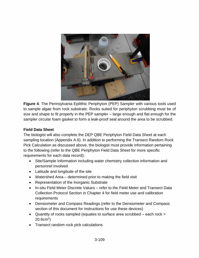
3-109
Figure 4. The Pennsylvania Epilithic Periphyton (PEP) Sampler with various tools used
to sample algae from rock substrate. Rocks suited for periphyton scrubbing must be of
size and shape to fit properly in the PEP sampler – large enough and flat enough for the
sampler circular foam gasket to form a leak-proof seal around the area to be scrubbed.
Field Data Sheet
The biologist will also complete the DEP QBE Periphyton Field Data Sheet at each
sampling location (Appendix A.6). In addition to performing the Transect Random Rock
Pick Calculation as discussed above, the biologist must provide information pertaining
to the following (refer to the QBE Periphyton Field Data Sheet for more specific
requirements for each data record):
• Site/Sample Information including water chemistry collection information and
personnel involved
• Latitude and longitude of the site
• Watershed Area – determined prior to making the field visit
• Representation of the Inorganic Substrate
• In-situ Field Meter Discrete Values – refer to the Field Meter and Transect Data
Collection Protocol Section in Chapter 4 for field meter use and calibration
requirements
• Densiometer and Compass Readings (refer to the Densiometer and Compass
section of this document for instructions for use these devices)
• Quantity of rocks sampled (equates to surface area scrubbed – each rock =
20.6cm2)
• Transect random rock pick calculations

3-110
• Total algae slurry volume (ml, minimum volume rules apply – refer to
Subsampling Procedure section)
• Notes pertaining to the Algae ID Bottles collected
• Notes, including collector and sequence numbers, pertaining to the Phycocyanin
sample bottle
• Notes, including collector and sequence numbers, pertaining to the Acidified
Chlorophyll-a filters
• Notes, including collector and sequence numbers, pertaining to the AFDM filters
• Other notes (including any pertaining to cyanotoxin testing, if collected).
Subsampling Procedure
The QBE Periphyton Sampling procedure requires subsampling for the identification
and enumeration of algal taxa, the quantitative determination of chlorophyll-a and
phycocyanin photopigments, the quantitative determination of AFDM, and in some
cases for the characterization of cyanotoxins. This subsampling may be performed in
the field at the sample site (if electricity is available for operating a blender and a
magnetic stirrer) or the sample may be temporarily stored in labeled 500ml bottles that
are capped and stored in a wet ice cooler to await later (same day) subsampling
treatment. Table 2 provides information regarding test volumes, bottle or filter
requirements, preservation procedure, as well as transportation and storage needs for
the QBE subsamples.
Note: This is an important step needed to prevent cross-contamination between
samples. Prior to performing any subsampling procedures on a site sample, thoroughly
clean all equipment that may come in contact with the algae slurry sample and, at the
conclusion of this cleaning, rinse with de-ionized water. Because site samples are often
accumulated through the field day and subsampled at the conclusion of that day’s work,
all equipment must be appropriated cleaned between samples.
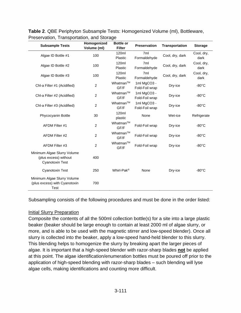
3-111
Table 2. QBE Periphyton Subsample Tests: Homogenized Volume (ml), Bottleware,
Preservation, Transportation, and Storage
Subsample Tests Homogenized
Volume (ml)
Bottle or
Filter Preservation Transportation Storage
Algae ID Bottle #1 100 120ml
Plastic
7ml
Formaldehyde Cool, dry, dark
Cool, dry,
dark
Algae ID Bottle #2 100 120ml
Plastic
7ml
Formaldehyde Cool, dry, dark
Cool, dry,
dark
Algae ID Bottle #3 100 120ml
Plastic
7ml
Formaldehyde Cool, dry, dark
Cool, dry,
dark
Chl-a Filter #1 (Acidified) 2 WhatmanTM
GF/F
1ml MgCO3 -
Fold-Foil wrap Dry-ice -80°C
Chl-a Filter #2 (Acidified) 2 WhatmanTM
GF/F
1ml MgCO3 -
Fold-Foil wrap Dry-ice -80°C
Chl-a Filter #3 (Acidified) 2 WhatmanTM
GF/F
1ml MgCO3 -
Fold-Foil wrap Dry-ice -80°C
Phycocyanin Bottle 30 120ml
plastic None Wet-ice Refrigerate
AFDM Filter #1 2 WhatmanTM
GF/F Fold-Foil wrap Dry-ice -80°C
AFDM Filter #2 2 WhatmanTM
GF/F Fold-Foil wrap Dry-ice -80°C
AFDM Filter #3 2 WhatmanTM
GF/F Fold-Foil wrap Dry-ice -80°C
Minimum Algae Slurry Volume
(plus excess) without
Cyanotoxin Test
400
Cyanotoxin Test 250 Whirl-Pak® None Dry-ice -80°C
Minimum Algae Slurry Volume
(plus excess) with Cyanotoxin
Test
700
Subsampling consists of the following procedures and must be done in the order listed:
Initial Slurry Preparation
Composite the contents of all the 500ml collection bottle(s) for a site into a large plastic
beaker (beaker should be large enough to contain at least 2000 ml of algae slurry, or
more, and is able to be used with the magnetic stirrer and low-speed blender). Once all
slurry is collected into the beaker, apply a low-speed hand-held blender to this slurry.
This blending helps to homogenize the slurry by breaking apart the larger pieces of
algae. It is important that a high-speed blender with razor-sharp blades not be applied
at this point. The algae identification/enumeration bottles must be poured off prior to the
application of high-speed blending with razor-sharp blades – such blending will lyse
algae cells, making identifications and counting more difficult.

3-112
Once this initial blending is complete in the 2000ml beaker, pour the complete algae
sample into multiple 1000ml graduated cylinders – as many as is required to contain the
entire sample. Next, dilute the algae slurry with de-ionized water to provide enough
material for all subsample tests (refer to Table 2 for minimum quantities required). For
example, if the biologist is electing not to subsample for the cyanotoxin test, but is
intending to subsample for ID/Enumeration, Chlorophyll-a, Phycocyanin, and AFDM
only, then the minimum quantity of algae slurry needed is 400ml. However, if the
biologist is electing to subsample for cyanotoxin, in addition to all the other subsamples,
then the minimum quantity of algae slurry needed is 700ml. These minimum quantities
will insure that enough algae slurry is available for all subsamples plus a little extra (in
case of small spills and enough material being available for the magnetic stirrer to work
and the Hensen-Stemple extractions to be made). The biologist should not over dilute
the algae slurry – the laboratory tests are best facilitated by providing as concentrated a
subsample as possible. If after compositing all the 500ml collection bottles for a site, the
total algae slurry is greater than the minimum quantity required, do not further dilute
beyond that needed to move the volume to the next highest 100ml increment level – for
example, if after compositing all bottles, the total volume is found to be about 1,244ml,
then dilute to 1,300ml. Doing this helps to insure accuracy of volume measurement in a
1000ml graduated cylinder which are often incremented in units of 100ml.
The total algae slurry volume must be recorded on the field data sheet and, eventually,
reported to the laboratory performing the identifications/enumerations. Since the
ID/enumeration laboratory must provide results to DEP that enable the biologist to
convert results to cells/cm2 and report biovolume (unit of µm3/cm2) estimates, accurate
reporting of algae slurry volume and surface area scrubbed is essential. Also note that
the identification/enumeration QA process requires the submission of blind duplicates to
laboratories. Typically, identification/enumeration blind duplicates are submitted at a
quantity approximately equal to 10% of the total quantity of samples submitted to the
laboratory. This is why multiple ID/Enumeration bottles are collected from each sample.
This QA process is discussed in detail later in this protocol.
Subsampling for Algae Identification/Enumeration
Once the Initial Slurry Preparation process is complete, the first subsampling that must
be completed is that needed for the Algae Identification and Enumeration.
Pour all graduated cylinders from the Initial Slurry Preparation Process back into the
2000ml beaker. This total sample is then homogenized on a magnetic stirrer (see Figure
5). Once the sample is well homogenized (this may take approximately 30 seconds on
the magnetic stirrer and is evident when a good vortex is observed to be established in
the beaker), pour 100ml of the homogenized algae slurry into a 100ml graduated

3-113
cylinder to insure accuracy of volume measurement. Thereafter, pour this volume into a
labeled 120ml algae ID/enumeration sample bottle while being careful to leave no algae
residue in the graduated cylinder. Do not use de-ionized water to rinse this residue into
the ID/enumeration bottles – adding de-ionized water at this point will further dilute the
sample and introduce volume related discrepancies into the final results reporting. A
swirling motion on the 100ml graduated cylinder followed by a quick pour into the
sample bottle will usually prevent sample material from being retained in the graduated
cylinder and will insure that all material is transferred. Sometimes a small quantity of
sample material must be returned to the graduated cylinder from the sample bottle and
a re-pour used to transfer all algae material. After collecting an ID/enumeration bottle,
return the slurry beaker to the magnetic stirrer to re-establish homogenization prior to
pouring the second 100ml algae ID/enumeration sample and later, the third 100ml algae
ID/enumeration subsample.
Preserve each 100ml ID/enumeration subsample with 7ml of formaldehyde (volume of
formaldehyde preservative must also be reported to the ID/enumeration laboratory).
Refer also to Table 2 for preservative volumes as well as for transportation and storage
requirements.
Algae Identification and Enumeration bottles will be labeled with a GIS Key (e.g.,
20170516-1115-jbutt, indicating the date, time, and collector name), Stream/River
Name, and Location Description.
Prior to submitting the algae ID samples to a laboratory, an Algae Identification and
Enumeration Laboratory Submission Data sheet must be made and submitted to the
laboratory along with the samples. An example of such a submission sheet can be
found in Appendix A.8. This data sheet provides essential information required by the
laboratory performing identifications and is used to determine final reporting values to
DEP. Also, sample site location information is provided on this submission sheet. This
location information may assist the laboratory performing identifications in providing
more accurate algae taxa identifications, especially as they may pertain to species or
variation level identifications of diatoms.
Note that algae ID sample bottles, once preserved, may be stored in a cool, dry, and
dark location (refer to Table 2), for upwards of several months prior to sending to an
identification lab. Often, DEP will retain these samples until the end of a collection
season prior to shipping all samples together to the identification/enumeration
laboratory.
3-114
When ID/Enumeration subsampling is complete, the biologist may then proceed to
subsampling for Phycocyanin, Acidified Chlorophyll-a, AFDM, and Cyanotoxins.
Subsampling for Phycocyanin, Acidified Chlorophyll-a, and AFDM
After the Algae Identification/Enumeration subsampling has been completed, the slurry
may be further blended in a highspeed blender. Highspeed blending in a food-grade
processing type of blender (those with stainless steel “razor sharp” blender blades) is
needed to properly prepare the algae for phycocyanin, acidified chlorophyll-a, and
AFDM subsampling in samples with robust filamentous or other forms of algae that
resisted the low-speed blending. When highspeed blending is complete, return the
sample to the 2000ml beaker and magnetic stirrer to provide continuous
homogenization.
Hereafter, the order of subsampling will first be phycocyanin, followed by AFDM, then
acidified chlorophyll-a, and lastly, if needed, cyanotoxin.
At present, all phycocyanin, acidified chlorophyll-a and AFDM subsamples are delivered
to DEP Bureau of Laboratories (BOL) for further processing. These samples may either
be hand delivered to BOL or may be shipped to BOL by courier. Refer to Table 2 for
methods of transportation and storage. All necessary laboratory submission sheets
must be completed and delivered to BOL along with the sample delivery. Phycocyanin
has a very short holding time for pre-processing at BOL and should either be hand-
delivered to BOL at the end of the field day or delivered overnight by courier.
Replicate samples for Phycocyanin, Acidified Chlorophyll-a, and AFDM
Although appreciable effort is made by DEP biologists to thoroughly homogenize the
algae slurry, variation in duplicate subsample results have been noted in nearly all
reported lab results. This variation is, in part, due to robust forms of filamentous algae
that resist complete homogenization, even after the use of a highspeed food-grade
blender. The best way to deal with this unavoidable variation in photopigment and
AFDM results is to run replicate subsamples. What has proven to be effective is
collecting three replicate subsamples each for phycocyanin, acidified chlorophyll-a, and
AFDM tests. The biologist may then utilize the average, median, minimum, and
maximum values generated by the three replicate subsamples to better estimate the
true values of each parameter.
Phycocyanin and acidified chlorophyll-a photopigments and AFDM are used by DEP to
estimate the algae biomass in a stream. This algae biomass, in turn, may be used to
infer characteristics regarding the nutrient status of a stream and also provide
information used to judge the biological condition status of that stream. Phycocyanin is

3-115
a photopigment that, in Pennsylvania, is nearly exclusively descriptive of cyanobacteria.
Chlorophyll-a is a photopigment that is present in all major algal groups.
Subsampling for Phycocyanin
Phycocyanin is subsampled by measuring 30ml of homogenized algae slurry in a 100ml
graduated cylinder then transferring that quantity to a 120ml plastic sample bottle. Swirl
the sample in the 100ml graduated cylinder then pour rapidly into the sample bottle to
help prevent residue from sticking to the graduated cylinder. As with the algae
identification/enumeration subsampling procedure, don’t use de-ionized water to rinse
the graduated cylinder as doing that would introduce error into the final results. A
swirling motion on the 100ml graduated cylinder followed by a quick pour into the
sample bottle will usually prevent sample material from being retained in the graduated
cylinder and will insure that all material is transferred. Sometimes a small quantity of
sample material must be returned to the graduated cylinder from the sample bottle and
a re-pour used to transfer all algae material.
As indicated in Table 2, phycocyanin subsamples require no preservation additives but
does require appropriate low temperature transportation and storage.
The phycocyanin bottle should be labeled with the same GIS Key as was used for the
Algae ID/Enumeration sample, the word “Phycocyanin,” the stream name, and the three
collector-sequence numbers assigned to the subsamples.
Since periphyton algae slurry solution is usually quite concentrated, with regard to
phycocyanin photopigments, BOL will be able to extract three separate phycocyanin
samples from this single 30ml submission – BOL typically does this by re-homogenizing
the 30ml sample and then extracting three ~5ml subsamples. Thus, the three-
subsample replicate requirement is achieved through this single 30ml submission to
BOL.
On the field data sheet, record the three collector-sequence numbers that are to be
used for phycocyanin submissions to BOL. Transfer these collector-sequence numbers,
along with an accurate date and time, the GIS Key, and stream name to the BOL
Microbiology Sample Submission Sheet. Indicate the BOL SAC Code of B031 for the
phycocyanin test on the Sample Submission Sheet. Also, indicate on the BOL
submission sheet that 30ml of sample is supplied and that three 5ml subsamples are
drawn from this single submission (Refer to Appendix A.9 for BOL Microbiology Sample
Submission Sheet).
After subsampling for phycocyanin, place the algae slurry beaker back on the magnetic
stirrer to re-homogenize the sample prior to proceeding to the AFDM subsampling.

3-116
Prepare the bottled phycocyanin sample for transportation as defined in Table 2. If the
biologist hand delivers this sample to BOL, it must be placed into the appropriate
refrigerator in the in the Bacteriological Services Section (consult with lab staff to
confirm the location of this refrigerator). In this case, sample submission sheets should
be hand-delivered to a member of the Bacteriological Services Section so that they are
made aware that a phycocyanin sample has been dropped off – phycocyanin samples
have a short pre-processing holding time (~24 hours, which requires the BOL
microbiologists to preform preliminary processing procedures to stabilize the sample
and protect against degradation of the phycocyanin photopigment. When phycocyanin
samples are delivered by overnight courier, the Bacteriological Services section is made
aware of the arrival of the sample as part of BOL’s normal morning sample check-in
process. Due to the short holding times for pre-processing at BOL, phycocyanin
subsamples should either be hand-delivered at the end of each field day or transported
to BOL by overnight courier at the end of each field day. In either case, phycocyanin
samples should be transported on wet-ice.
Subsampling for AFDM
AFDM is subsampled in a manner very much like that used for acidified chlorophyll-a
(see below). However, preservation procedures differ between the AFDM and acidified
chlorophyll-a subsampling procedures (see Table 2).
AFDM is subsampled by extracting three 2ml replicates of homogenized algae slurry.
This is performed using a 2ml spring loaded Hensen-Stemple Pipette (Wilco part
number 1806-D52) that extracts a subsample from the algae slurry beaker while the
slurry remains on the magnetic stirrer and is continuously homogenized during
subsample extraction.
The contents of the 2ml Hensen-Stemple Pipette is then deposited on a WhatmanTM
GF/F type filter. This is facilitated by a vacuum-draw filtering device (see Figure 5)
which includes a cup-like design that holds the GF/F filter and into which the 2ml
Hensen-Stemple Pipette algae slurry subsample is deposited. While maintaining the
Hensen-Stemple Pipette in an open position, and inside the vacuum-draw filtering
device, rinse the sampler with de-ionized water, also depositing this onto the GF/F
Filter, to be sure that all algae slurry material from the sampler has been deposited on
the filter. After depositing the algae slurry into the filtering device, draw a vacuum on the
filtering device that isn’t greater than 3psi (higher pressure may damage the GF/F filter,
resulting in the loss of periphyton slurry material).
With the vacuum still applied, rinse the side walls of the filter apparatus cup with
deionized water to make sure that all algae material is deposited on the GF/F filter.
3-117
Allow this rinse water to thoroughly drain prior to releasing the vacuum on the filter
apparatus.
Remove the WhatmanTM GF/F filter from the filter apparatus with forceps in a manner
that doesn’t touch or disturb the algae material deposited on the filter. Using two
forceps, one in each hand, carefully fold the round GF/F filter in half so that the algae
material is “sandwiched” inside this now folded half-circle. Continuing to use forceps,
perform one more fold, creating a quartered circle (see Figure 6). Place this folded filter
on a small piece of aluminum foil. Fold the aluminum foil over the filter to contain the
filter entirely within the foil while allowing ample overlap of the foil. Fold the foil edges
over several times to create a sealed envelope around the filter. Each filter replicate is
to be folded into its own foil envelope. Place this foil envelop into a small plastic Ziploc®
bag. Each AFDM filter is to be placed into its own small plastic Ziploc® bag. Place the
three plastic bags into a small paper envelop and seal this paper envelope. This paper
envelope should be labeled with the same GIS Key as was used for the Algae
ID/Enumeration sample, the word “AFDM,” the stream name, and the three collector-
sequence numbers assigned to the subsamples. This envelope is then sealed inside a
Ziploc® plastic bag - multiple paper envelopes may be sealed into a single Ziploc® plastic
bag. Record the three collector-sequence numbers for this sub on the field data sheet.
Transfer the three collector-sequence numbers, along with date and time, the GIS Key,
and stream name to the BOL Microbiology Sample Submission Sheet (Appendix A.9).
The BOL SAC Code for AFDM-a is B027.
Prepare the AFDM sample for transportation as defined in Table 3. When delivering this
sample to BOL, it must be placed into the appropriate -80°C freezer in the
Bacteriological Services Section (consult with lab staff to understand the location of this
freezer). Sample submission sheets should be hand-delivered to a member of the
Bacteriological Services Section so that they are made aware that AFDM samples have
been delivered. AFDM samples may also be delivered to BOL via courier on dry-ice.
However, because of relatively long holding times, AFDM samples may be held for a
few days on dry-ice in coolers and delivered to BOL at the end of the field week.
Quality control measures for AFDM include a laboratory duplicate, a field duplicate, and
a field blank, each done at a rate of once per basin. Field blanks will utilize “ultra-pure
water” instead of the periphyton slurry and will use the same AFDM subsampling
procedures as those described above. Because the term “basin” could cover a broad
geographic area and thus include much of the sampling that occurs in Pennsylvania, for
example the Susquehanna River basin, it will be left to the field biologist to decide the
extent that the term “once per basin” will imply – DEP recommends a conservative

3-118
approach, preferring to submit QA samples regularly (once per week per designated
basin, for example).
Figure 5. Vacuum-draw filtering devices on left and algal slurry beaker on a magnetic
stirrer on the right.
Figure 6. The proper procedure for folding the chlorophyll-a and AFDM filters.
Subsampling for Acidified Chlorophyll-a
Prior to proceeding with the acidified chlorophyll-a subsampling, thoroughly clean the
vacuum-draw filtering cups then rinse with de-ionized water. Acidified Chlorophyll-a is
subsampled in a manner very much like that used for AFDM (see above). However,
preservation procedures differ between the AFDM and acidified chlorophyll-a
subsampling procedures (see Table 2).
Chlorophyll-a is subsampled by extracting three 2ml replicates of homogenized algae
slurry. This is performed using a 2ml spring loaded Hensen-Stemple Pipette (Wildco®
part number 1806-D52) that extracts a subsample from the algae slurry beaker while
the slurry remains on the magnetic stirrer and is continuously homogenized during
subsample extraction.
3-119
The contents of the 2ml Hensen-Stemple Pipette is then deposited on a WhatmanTM
GF/F type filter. This is facilitated by a vacuum-draw filtering device (see Figure 5)
which includes a cup-like design that holds the GF/F filter and into which the 2ml
Hensen-Stemple Pipette algae slurry subsample is deposited. While maintaining the
Hensen-Stemple Pipette in an open position, and inside the vacuum-draw filtering
device, rinse the sampler with de-ionized water, also depositing this onto the GF/F
Filter, to be sure that all algae slurry material from the sampler has been deposited on
the filter. After depositing the algae slurry into the filtering device, draw a vacuum on the
filtering device that isn’t greater than 3psi or persists for longer than 10 minutes, as
greater pressure and/or duration may damage cells resulting the loss of photopigments
(Arar and Collins 1997).
With the vacuum still applied, rinse the side walls of the filter apparatus cup with
deionized water to make sure that all algae material is deposited on the GF/F filter.
Allow this rinse water to thoroughly drain prior to releasing the vacuum on the filter
apparatus.
After the algae slurry water is drawn through the filter, and the algae is deposited on the
GF/F filter, release the vacuum on the filtering device. Fill the filter cup with a small
quantity of de-ionized water so that a few milliliters of water pools on top of the filter.
Into this maintained pool of water, add drop-wise 1ml of saturated MgCO3 solution
preservative. This 1ml of MgCO3 should be uniformly distributed around the pool of de-
ionized water so that it distributes evenly across the entire filter surface. Then re-draw
the vacuum on the filtering device (again, no greater than 3psi) and allow the water and
MgCO3 to drain. New saturated MgCO3 preservative may be obtained from BOL
Microbiological Services at the beginning of the sampling season. This saturated
MgCO3 has a long shelf-life and will remain viable through the entire sampling season
but should be stored in a cool and dry place in the sampling kit.
With the vacuum still applied, rinse the side walls of the filter apparatus cup with enough
de-ionized water to make sure that all MgCO3 is deposited on the GF/F filter. Allow this
rinse water to thoroughly drain prior to releasing the vacuum on the filter apparatus.
Remove the WhatmanTM GF/F filter from the filter apparatus with forceps in a manner
that doesn’t touch or disturb the algae material deposited on the filter. Using two
forceps, one in each hand, carefully fold the circular GF/F filter in half so that the algae
material is “sandwiched” inside the now folded half-circle. Continuing to use forceps,
perform one more fold, creating a quartered circle (see Figure 6). Place this folded filter
on a small piece of aluminum foil. Fold the aluminum foil over the filter to contain the
filter entirely within the foil while allowing ample foil to overlap the filter. Fold the foil
3-120
edges over several times to create a sealed envelope around the filter. Each filter
replicate is to be folded into its own foil envelope. Each acidified chlorophyll-a filter is to
be placed into its own small plastic Ziploc® bag. Place these plastic bags into a single
small paper envelop and seal this paper envelope. This paper envelope should be
labeled with the same GIS Key as was used for the Algae ID/Enumeration sample, the
words “Chl-a Acidified,” the stream name, and the three assigned collector-sequence
numbers. This paper envelope is then sealed inside a Ziploc® plastic bag – multiple
paper envelopes may be sealed into a single Ziploc® plastic bag. Record the three
collector-sequence numbers for this subsample on the field data sheet.
Transfer the three collector-sequence numbers, along with an accurate date and time,
the GIS Key, and stream name to the BOL Microbiology Sample Submission Sheet. The
BOL SAC Code for Chlorophyll-a is B019 – additionally state on the Sample Submission
Sheet that the test is for “Acidified Chlorophyll-a with Pheophytin.” SAC code B019 is
also used for Non-acidified Chlorophyll-a, so care must be taken to clearly communicate
the need for the acidified chlorophyll-a with pheophytin test.
Prepare the acidified chlorophyll-a samples for transportation as defined in Table 3.
When hand-delivering this sample to BOL, it must be placed into the appropriate -80°C
freezer in the Bacteriological Services Section (consult with lab staff to understand the
location of this freezer). Sample submission sheets should be hand-delivered to a
member of the Bacteriological Services Section so that they are made aware that
chlorophyll-a samples have been delivered. Acidified chlorophyll-a samples may be
delivered to BOL via courier on dry-ice. However, because of the holding times involved
(30 days), acidified chlorophyll-a samples may be held for a few days on dry-ice and
delivered to BOL at the end of the field week.
USEPA recommends that quality control measures for chlorophyll-a include a laboratory
duplicate, a field duplicate, and a field blank, each done at a rate of once per basin
(USEPA 2013). Field blanks will utilize “ultra-pure water” instead of the periphyton slurry
and will use the same acidified chlorophyll-a subsampling procedures as those
described above. Because the term “basin” could include a broad geographic area and
thus include much of the sampling that occurs in Pennsylvania, for example the
Susquehanna River basin, it will be left to the field biologist to decide the extent that the
term “once per basin” will imply – DEP recommends a conservative approach,
preferring to submit QA samples regularly (once per week per designated basin, for
example). USEPA suggests an acceptance criteria of 25% relative percent difference
for the laboratory and field duplicates, and 0.00µg/L ±0.11µg/L for the field blank
(USEPA 2013).
3-121
Subsampling for Cyanotoxins
After the acidified chlorophyll-a subsamples are collected, continue homogenizing the
algae slurry on the magnetic stirrer. Pour 250ml of this homogenized slurry into a 500ml
graduated cylinder. Swirl this slurry around the graduated cylinder and quickly pour it
into a Whirl-Pak® bag to prevent algae material from adhering to the sides of the
graduated cylinder. Again, don’t rinse down with additional de-ionized water as that
would dilute the sample and introduce error into the final results. Seal the Whirl-Pak®
bag then transport and store as prescribed in Table 2.
DENSIOMETER AND COMPASS DATA COLLECTION
In smaller streams, the riparian vegetative cover may intercept much of the incident
solar radiation that may otherwise be available for supporting primary production in the
lotic habitat. Trees situated along the riparian corridor are very effective at appreciably
reducing the quantity of light reaching the stream (Hill and Roberts 2009). There is great
potential for a combination of both light and nutrients to colimit algal growth (Hill 1996).
Additionally, the East/West or North/South orientation of the stream reach being
sampled will also seasonally contribute to the quantity of incident sunlight on the stream
reach. Consequentially, a measurement of canopy closure (thus inferring intercepted
solar radiation) over the stream reach, and stream orientation, should be made by the
biologist and considered, in conjunction with water chemistry measures, when analyzing
the results of algae sampling.
Stream orientation is measured with a compass. Facing downstream at the
Densiometer “1/2 Downstream” location (refer to either the QBE or QMH Field Data
Sheets in Appendices A.6 and A.7), site the compass along the thalweg in the
downstream direction and orient the compass with magnetic north. Record this sighted
azimuth direction clockwise from magnetic north (in degrees) on the data sheet.
Stream canopy closure is measured with a Concave Spherical Densiometer (for
example, part number 43888 available from Forestry Suppliers, Inc at www.forestry-
suppliers.com). Procedures for estimating canopy closure follow Platts et al. (1987).
Measuring canopy closure is suggested over measurement of canopy density since
canopy closure measures are less affected by seasonality (Fitzpatrick et al. 1998).
Vegetative canopy closure is the area of the sky bracketed by vegetation. The
densiometer's concave mirror surface has 37 grid intersections forming 24 squares. To
eliminate bias from overlap, only 17 of the 37 grid intersections are used as recording
points. The 17 grid intersections to be used are delimited by taping a right angle on the
densiometer (see Figure 6).

3-122
For streams measuring less than 25 meters across (82 feet), densiometer readings are
recorded at four locations along the mid-reach transect – these being, facing the right-
descending bank, facing mid-channel downstream, facing mid-channel upstream, and
facing left-descending bank. This is accomplished, for example at the right-descending
bank, by facing the right wetted edge of the stream and holding the densiometer about 1
foot from the shoreline and about 1 foot above the water surface (see Figure 7). With
the leveled (bubble level) densiometer now pointed toward the bank (taped right-angle
points toward the recorder) and with the observer’s head reflection near the top grid line
(see Figure 6) then determining canopy closure at that location. Thereafter, canopy
closure is counted at each of the remaining mid-reach transect locations in a similar
fashion. Canopy closure count is equal to the number of densiometer line intersections
(maximum of 17) that are surrounded by vegetation (representing canopy closure) or
intercepted. Finally, the count for each location is then summed together and divided by
68 (4 x 17) to calculate a percent closure. For example, if the canopy closure count at
the right-descending bank is 15, the count at mid-channel facing upstream is 3, the
count at mid-channel facing downstream is 5, and the left-descending bank count is 16,
then the canopy closure value for the site is determined by the following: [(15 + 3 + 5 +
16)/68] x 100 = 57% (round to nearest whole percent).
For streams larger than 25 meters across the same procedure is used except eight
recordings are made. In addition to right bank, left bank, and mid channel (upstream
and downstream) locations, mid-reach upstream and downstream densiometer
measurements are additionally made at the ¼ and ¾ intervals on the mid-reach
transect. Canopy closure or density scores are summed and divided by 136 (8 x 17) to
calculate a percent closure.
Figure 6. Concave spherical densiometer with placement of head reflection, and 17
observation points. From Platts et al. (1987).

3-123
Figure 7. Proper use of the densitometer at the right descending bank location.
LABORATORY PROCEDURES
Although strict adherence to the field data collection procedures is necessary to achieve
comparability between samples, field data collection represents only a portion of that
which is needed to insure robust periphyton data results. Laboratory procedures are
also extremely important and must also be defined and strictly adhered to if sample
comparability is to be achieved. The purpose of this section is to define those laboratory
procedures needed to process periphyton related samples. These laboratory
procedures include those applied by BOL as well as those that must be applied by
contracted labs. These protocols are as follows:
• Phycocyanin by Fluorometry
• Acidified Chlorophyll-a by Fluorometry with Pheophytin
• Ash-Free Dry Mass by SM10200-I
• Algae Identification and Enumeration
• Quality Assurance (QA) Audit of Algae Identification and Enumeration.
At present, DEP’s Algae Monitoring Program processes Phycocyanin, Acidified
Chlorophyll-a (which includes Pheophytin reporting), and Ash-Free Dry Mass samples
at its BOL facility. The laboratory procedures used to process these samples are
extensively defined in BOL documentation and may be obtained from that DEP bureau.
BOL methods currently used include:
• Phycocyanin by Fluorometry Rev 001, effective November 2017
• [Acidified] Chlorophyll-a in NPW by SM10200H 1 & 3 (Fluorometric Method Rev
002, effective 3/27/2017

3-124
• Ash-Free Dry Mass by SM10200-I Rev 001, effective 2/26/2016
• Plankton Identification and Enumeration Rev 002, effective 5/7/2015.
Algae Identification and Enumeration samples collected by DEP are processed through
private companies, academic institutions, as well as through DEP BOL. Because these
identification samples are processed through several different facilities the reader is
directed to both the BOL Plankton Identification and Enumeration document as well as
to the Algae identification and Enumeration Protocol description provided below.
Further, the use of multiple identification and enumeration processing facilities obligates
DEP to employ a rigorous QA Audit process designed to insure consistency, and thus
comparability, between the results produced by the various labs. This QA Audit process
is also discussed below.
General Description of Algae Identification and Enumeration Procedure
The identification and enumeration of periphyton samples collected by either the QMH
or the QBE periphyton field procedures requires that two separate procedures be
performed to completely characterize the sample. These include a Palmer-Maloney
Chamber procedure as well as a Diatom Slide procedure.
The Palmer-Maloney Chamber procedure, sometimes referred to by lab technicians as
the “wet count,” or “soft algae count,” identifies and counts all algae taxa to the genera
level, at a minimum, at moderate magnification (e.g., 100x or 400x). However, if certain
morphological structures are observable during this procedure, identifications may be
made to the species, or sometimes variety, taxonomic level. It is important to recognize
that during the Palmer-Maloney procedure, diatom counts are also made. Diatoms,
however, are only characterized as living or as dead and are not taxonomically
identified in this procedure. Palmer-Maloney Chambers used in this process must be
calibrated.
As previously mentioned, the Palmer-Maloney procedure is sometimes referred to as
the “wet count” or the “soft algae count” as a way of distinguishing it from the Diatom
Slide count. The “wet count” name originates from the fact that the submitted
identification subsample is further subsampled by placing a small homogenized quantity
of liquid (hence the term “wet”) into a Palmer-Maloney chamber for microscopic
inspection. The term soft algae is also often applied to this procedure because the algae
taxa identified and counted in this procedure frequently contain those possessing only
soft cell tissues that would otherwise be destroyed as part of the nitric acid digestion
used to create slides for the diatom slide procedure. Examples of such “soft algae”
commonly identified in samples collected from Pennsylvania streams and rivers include
cyanobacteria or green algae taxa. However, Palmer-Maloney results do sometimes

3-125
include other “soft algae” taxa, which are less commonly found in Pennsylvanian
freshwater periphyton samples.
In contrast to the Palmer-Maloney procedure, diatoms are identified to the species, and
often to variety, taxonomic level in the Diatom Slide procedure. In this procedure, liquid
from the subsample is processed with nitric acid to dissolve away all soft tissues in the
sample thereby exposing the glass frustules of the diatoms. A detailed microscopic
analysis of the diatom glass frustule morphology is then performed to make the species
or variety identification at high magnification (1000x oil immersion). The identifications
and counts obtained during this procedure produce what is often referred to as the
“permanent slide” result. Permanent slides are a product of the procedure referred to as
the Preparation of Diatom Slides Using NaphraxTM Mounting Medium, as listed below.
DEP requires the identification laboratory to produce three permanent slides per
submitted algae identification subsample. These three permanent slides are maintained
by DEP as voucher specimens and are also used in the QA audit.
As a separate option, the BOL Algae Identification and Enumeration procedure may be
used to produce genera level taxonomic identifications and enumerations. Also, the
BOL procedure only provides results corresponding to the Palmer-Maloney procedure
described above. These results, though less informative than those produced by the
complete procedure, which combines results from both the Palmer-Maloney and Diatom
Slide procedures, are used when an algae community result is needed from a
laboratory in a very short period of time (historically, DEP has experienced that
complete sample results from laboratories are often obtained only after many months of
processing time at those facilities). If this BOL option is to be used, modifications to the
standard BOL Algae Identification and Enumeration procedure are needed. These
modifications include counts of living and dead diatoms during the Palmer-Maloney
count phase and the fact that the BOL method specifies “phytoplankton… samples”
whereas a periphyton sample is submitted. [Note: living diatoms are those that are
observed to contain soft tissue within the frustule during the Palmer-Maloney procedure
whereas those that contain no such soft tissue are considered to be dead at the time of
sampling. Also, the QA procedures expected of Participating Labs (see below) must be
required of samples processed by DEP BOL.]
Algae Identifications that use both the Palmer-Maloney soft algae analysis as well as
the diatom slide analysis will rely, in general, upon the Protocols for the Analysis of
Algal Samples Collected as Part of the U.S. Geological Survey National Water-Quality
Assessment Program, Report No. 02-06 by Charles et al. 2002 (available at
https://water.usgs.gov/nawqa/protocols/algprotocol/algprotocol.pdf). The protocols from
Report No 02-06 that are routinely applied, in part or in whole, by DEP include:

3-126
• P-13-58: Tracking of Algae Sample Analysis – Figure 1 (Sample process and
analytical flow)
• P-13-48: Subsampling Procedures for USGS NAWQA Program Periphyton
Samples
• P-13-42: Diatom Cleaning by Nitric Acid Digestion with Microwave Apparatus
• P-13-49: Preparation of Diatom Slides Using NaphraxTM Mounting Medium
• P-13-50: Preparation of Algal Samples for Analysis Using Palmer-Maloney Cells
• P-13-39: Analysis of Diatoms on Microscope Slides Prepared from USGS
NAWQA Program Algae Samples
• P-13-63: Analysis of Soft Algae and Enumeration of Total Number of Diatoms in
USGS NAWQA Program Quantitative Targeted-Habitat (RTH and DTH)
Samples.
The rationale for performing the QBE and QMH Periphyton Sampling Procedures as
well as the Algae Identification and Enumeration Procedures, as based upon the USGS
NAWQA protocols, is to produce results of the quality needed for the development of a
trophic index, that needed for a diatom based Multi-Metric Index (MMI), as well as that
needed to provide information that contributes to aquatic life use considerations. These
procedures provide community-level data as well as the identification of pollution
sensitive or insensitive diatoms. To achieve segregation between potential levels of
pollution tolerance within the diatom group, identification to the species or variety
taxonomic level is required in the Diatom Slide Procedure. In short, diatoms, when
identified to species or a variety of taxonomic levels, provide information concerning the
nutrient and organic enrichment condition of natural waters (Porter et al. 2008) and will
also serve as indicators for determining biological condition gradients and developing
nutrient criteria (Hausmann et al. 2016).
Detailed Description of Analytic Services for Algae Identification and
Enumeration
DEP requires that algae identification and enumeration of benthic algae samples be
done in a way that produces results “comparable” to those provided by The Academy of
Natural Sciences (ANS). ANS produces results as described by the previously
mentioned protocols for the analysis of algal samples collected as part of the U.S.
Geological Survey National Water-Quality Assessment Program (NAWQA Protocol,
Charles et al. 2002).
The word “comparable,” in the above paragraph, is emphasized because DEP is
primarily interested that the results produced by the identification and enumeration
process completely harmonize with those produced by the ANS. Consequentially, there
may be a limited opportunity for flexibility regarding the exact procedures by which the

3-127
identification and enumeration laboratory results are produced. This creates the
possibility for the processing laboratory to slightly modify the procedures of performing
identification and enumeration as detailed by the NAWQA Protocol so long as that
laboratory does so in close consultation with, and approval by, DEP.
Algae identification and enumeration results will be achieved by performing the following
process steps. It is important to note that this process requires a close collaboration
between DEP and the Participating Laboratory (PL). To facilitate this collaboration, the
areas of responsibility are indicated in each step. Also, the applicable NAWQA protocol
is also indicated, where appropriate. The process steps will include:
1. Collection of periphyton sample and division into 100ml subsample bottles
preserved with 5% to 10% formaldehyde. Service provided by DEP as
described above.
2. Preparation of permanent diatom microscope slides via acid digestion to
produce “clean” identification and enumeration slides as well as three
permanent archive (voucher) slides for each sample – refer to NAWQA
Protocols P-13-58 Figure 1, P-13-48, P-13-42, and P-13-49. In general, a
permanent slide diatom specimen density should be constructed so that
between 5 and 10 diatom specimens are observable in a single microscope
field at 1000x magnification (recommendation by Charles et al. 2002).
3. 300 Natural Unit ID/Count Analysis of soft algae and diatoms in a calibrated
Palmer-Maloney chamber for each sample – refer to NAWQA Protocol P-13-
58 Figure 1, P-13-48, P-13-50 and P-13-63. Identification of soft algae to
lowest possible taxonomic level (at discretion of analyst but minimum of at
least general level expected). Differentiate diatoms into living (containing
cytoplasm) and dead (containing no cytoplasm). Identifications and counts
must be harmonized. Identifications and counts provided by the PL.
Harmonization coordinated between DEP and PL as defined in the
harmonization section below.
4. 600 Valve ID/Count Analysis of diatom microscope slides for each sample –
refer to NAWQA Protocol P-13-39. Identification to species or variety
taxonomic level. Identifications and names must be harmonized.
Identifications and counts provided by the PL. Details on coordinating
harmonization between DEP and PL is defined in the harmonization section
below.
5. Blind Duplicate and QA Audit. DEP will provide blind duplicates samples to
the PL. The QA Audit process for these blind duplicates is defined below.
Also included in this QA process is the collecting of taxa specific
photomicrographs by the PL, as defined in the QA Audit Process below. The
PL will also complete its own internal QA Audit process to help insure its own
3-128
method quality, particularly as it relates to the processing of the Palmer-
Maloney slides and the diatom slides. The PL will design and implement its
internal QA Audit process in consultation with DEP. The PL will share the
results of their internal QA Audit process with DEP.
6. Reporting Identification and Enumeration Results to DEP. The PL will make a
final identification and enumeration results report (preliminary reports are
made prior to the completion of the QA Audit process) to DEP in the format
discussed below. The final results report will include all necessary changes to
preliminary results reports provided by the PL as required by the outcome of
the Blind Duplicate and QA Audit processes. This is a collaborative process
between the PL and DEP.
Blind Duplicates and Other QA Audit Process:
Blind Duplicate QA Audit processing success will be determined with reference to
published and peer reviewed scientific literature. The scientific literature referenced and
currently consulted by DEP for this QA Audit process is included in the Literature Cited
section of this document and is summarized below. However, the rapid pace at which
the algae science is progressing will require DEP and the PL to frequently review and
discuss the current body of applicable scientific literature and accepted procedures.
Both the PL and DEP will be expected to make on-going adjustments to incorporate the
recent changes and advances in the applicable scientific literature. Scientific literature
for performing the QA Audit process includes:
• Barbour et al. 1999
• Kahlert et al. 2009
• Kelly 2001
• Whittaker and Fairbanks 1958
• Wolda 1981
• PCER 1998
The body of scientific literature consulted suggested that the appropriate procedure for
determining the quality of reported diatom identifications and enumerations is to use
indices of similarity to compare the results of a sample with those from a corresponding
blind duplicate sample, also processed by the PL, as well as a comparison with results
independently produced by an auditor. Whereas the blind duplicate is intended to
demonstrate the ability of the PL to replicate their own results, the comparison to the
auditor is intended to confirm the accuracy of identification and enumerations. Deciding
who in DEP or what outside laboratory will serve as the auditor will be decided by DEP
at the beginning of each project. DEP typically submits blind duplicates at a rate of 10%
of the regular sample load. If blind duplicate or auditor similarity comparisons fail to

3-129
pass (see below for pass scores), DEP must consult with the PL to resolve this quality
issue before incorporating data into the DEP Algae Database.
The QA process will also require the PL to provide photomicrographs (in a digital format
agreed upon by both the PL and DEP) to DEP at the time of data submission. These
photomicrographs will include an image example of each taxa type identified in the DEP
sample set and must be photographed from the DEP sample set. Diatom identification
images must be photographed at 1000x and must clearly show all structures needed to
confirm the identification to the appropriate species or taxonomic level. Images collected
during the Palmer-Maloney 300 Natural Unit process must be photographed at the
appropriate magnification needed to make the identification and must also clearly show
all structures needed to confirm the identification. Photomicrographs must include a
calibrated scale bar. Photomicrograph files must be entitled to include the taxon name,
magnification, date of photograph, and DEP sample from which it was obtained. Again,
the PL is required to provide only one type image for each taxon identified in the entirety
of the DEP sample set (per contract or Purchase Order), regardless of how many times
the taxa is re-identified throughout the sample set.
The indices of similarity that DEP uses in the QA Audit process will include the
following:
• Percent Community Similarity of Diatoms (PS) – this is also referred to as the
Whittaker and Fairbanks (1958) similarity and is recommended by USEPA
RBP. The USEPA RBP suggests a percent similarity score of > 75% to pass.
This index is based upon relative abundance and places more emphasis
upon the more abundant taxa while de-emphasizing the rare taxa. Computed
as:
PS = 100 – ( 0.5Σ│ai – bi │ )
where:
ai = percent abundance of species i in sample A
bi = percent abundance of species i in sample B.
• Bray-Curtis Similarity Index (D) – This index is also based upon relative
abundance. Note that Whitaker-Fairbanks Percent Community Similarity and
the Bray-Curtis Similarity Index are numerically equivalent. The scientific
literature (Kelly 2001) suggests that a Bray-Curtis score of > 60% is generally
considered to be a good agreement between the taxonomist and the auditor,
especially when taxa diversity is relatively high. However, this pass score
should be increased to 70% when taxa diversity is relatively low. Computed
as:

3-130
D = Σ min ( ai , bi )
where:
ai = percent abundance of species i in sample A
bi = percent abundance of species i in sample B.
Harmonization:
The harmonization of algae sample identification and enumeration procedures between
DEP and the PL, and between processing laboratories, is essential to the success of
DEP’s algae monitoring and method development effort. DEP has experienced
inconsistencies between laboratories regarding their reported identifications and counts.
Such inconsistencies were also noted by USEPA during the analysis of their 2008/2009
National Rivers and Streams Assessment (NRSA) diatom data (Lee et al. 2017). There
are several possible reasons for these inconsistencies, many of which are described by
Kahlert et al. (2009). Kahlert et al. (2009) suggests that harmonization is likely
imperative to achieve consistency between laboratories and taxonomists. Kahlert et al.
(2016) suggests methods by which this is may be achieved. Currently, DEP recognizes
that to achieve proper harmonization, the following operational considerations and
activities must be continuously reviewed and coordinated between both DEP and the
PL:
• The body of current taxonomic references and literature to which the
taxonomist refers to properly identify algae taxa
• Defining appropriate species complexes into which are grouped problematic
identification OTU’s (Operational Taxonomic Units) (Refer to Lee et al. 2017)
as well as summarizing taxa that may easily be misidentified (Refer to Kahlert
et al 2016).
• All laboratory procedures involved with the processes of subsampling, and
identifying/enumerating algae samples
• Possible use of taxonomic intercalibration exercises and other harmonization
procedures (Kahlert et al. 2009, Kahlert et al. 2016).
Because of the importance of diatom related data to DEP, the proper harmonization of
diatom taxa is especially emphasized. In demonstration of the importance of
harmonization, refer to Kahlert et al 2009 in which the authors suggest that proper
diatom taxa harmonization, rather than long experience with diatoms, is more important
for achieving similarity between samples (and between taxonomist and auditor).
Initial steps for achieving harmonization between DEP and the PL will involve the
following at the beginning of the project:

3-131
• DEP will provide to the PL the currently acceptable taxa list. This taxa list will
include reference codes for each taxa along with authorship information.
• DEP and the PL will review the PL’s identification and enumeration procedures.
Notes regarding taxa lists, DEP naming conventions, and identifications:
• The taxa list to which DEP refers, in general, is typically that offered by The
Academy of Natural Sciences in their current list of Diatom and Non-Diatom (soft
algae) This current downloadable Academy taxa list is available at
http://diatom.ansp.org/Taxa.aspx. DEP also frequently refers to Diatoms of the
United States (DOTUS) for taxa nomenclatural details (available at
https://westerndiatoms.colorado.edu/). The Academy list is preferred because it
is downloadable and is easily incorporated into a database.
• By DEP naming conventions, taxa names must include the source of authorship
as part of the name. For example, Achnanthidium minutissimum (Kützing)
Czarnecki, Achnanthidium minutissimum var. gracillima (Meister) Bukhtiyarova,
or Phormidium autumnale (Agardh) Trevisan ex Gomont. This convention is used
by The Academy and must be rigidly adhered to by the PL, thus facilitating
compatibility with the DEP database.
• For identifications, DEP also consults DOTUS (available at
https://westerndiatoms.colorado.edu/), AlgaeBase (available at
http://www.algaebase.org/), the Diatom New Taxon File maintained by The
Academy of Natural Sciences (available at http://dh.ansp.org/dntf), the Catalogue
of Diatom Names maintained by the California Academy of Sciences (available at
http://researcharchive.calacademy.org/research/diatoms/names/index.asp ). And
USGS Biodata (available at https://aquatic.biodata.usgs.gov).
• The above notes, and institutional references, are not exhaustive and may
include others when deemed appropriate.
The above represents initial harmonization steps that must be performed at the
beginning of each project. Bear in mind that changes in algae taxonomy occur
frequently and issues with problematic identifications will always exist. Consequentially,
DEP and the PL will continuously confer so that they together may contend with
taxonomy changes and problematic identifications as frequently as is deemed
necessary by either of the two parties.
DEP will appoint an Auditing Laboratory at the beginning of each project. DEP will
advise the PL as to the identity of the Auditing Laboratory at the beginning of the
project.

3-132
Algae Identification and Enumeration Results Reporting, Data Formatting, and PL
Internal Diatom and Palmer-Maloney Slide Processing QA Audit Report
Requirements:
DEP will require that certain types of data be generated by the PL when processing
Algae ID and enumeration samples. Data transfer between DEP and the PL must follow
a specific format, as demonstrated by the tables presented in this section. This specific
table format is necessary to efficiently support data transfer into DEP’s Microsoft®
Access based Algae Database. Three data table transfers are needed to properly
exchange data between DEP and the PL. These tables include:
• Algae Identification and Enumeration Laboratory Submission Data Sheet,
provided by DEP to the PL upon submission of samples
• Palmer-Maloney and Diatom Slide Applied Factors Table, provided by the PL to
DEP
• Identification/Enumeration Results Table, provided by the PL to DEP.
Results will not be fully incorporated into the DEP Algae Database until all PL
processing quality issues (as per blind duplicate results and auditor comparison results)
are resolved and corrected data is received from the PL.
Each of the Results Reporting Tables will be defined and formatted as follows:
1. Algae Identification and Enumeration Laboratory Submission Data Table. DEP
will transfer samples and the Algae Identification and Enumeration Laboratory
Submission Data Table to the PL at the beginning of the laboratory processing
phase of the project. This data table will exist in the form of a Microsoft® Access
data table (or Excel data table if necessary). Refer to Appendix A-8 for the format
of this table. The following fields are required in this table to fully describe each
sample to the PL (origin of information from the DEP Algae Database are
included in parenthesis):
• DEP Algae Sample GIS Key ID. Access Foreign Key that references the
corresponding Primary Access Key in the DEP Algae Database Samples
Table. Configuration of this GIS KEY ID is YYYYMMDD-HHMM-Collector.
For example, Algae Sample GIS Key ID’s have, in the past, included
20140813-0800-jbutt, and 20140821-0800-ggocek.
• Date sample was collected. (Duplication from the DEP Algae Database
Samples Table).
• Sample Type. QMH (Qualitative Multi-Habitat) or QBE (Quantitative
Benthic Epilithic) periphyton sample.
• DEP Algae Sampling Site ID number. Access Foreign Key that references
the corresponding Primary Access Key in the DEP Algae Database Sites
Table

3-133
• Stream Name. (Duplication from the DEP Algae Database Sites table)
• Location Description. (Duplication from the DEP Algae Database Sites
Table).
• County. (Duplication from the DEP Algae Database Sites Table)
• Latitude and Longitude. (Duplication from the DEP Algae Database Sites
Table).
• Benthic Surface Area (cm2). Applies only to QBE Periphyton samples
(Duplication from the DEP Algae Database Samples Table).
• Algae Slurry Total Sample Volume (ml). Applies only to QBE Periphyton
samples (Duplication from the DEP Algae Database Samples Table).
• ID Bottle SubSample Volume (ml). (Duplication from the DEP Algae
Database Samples Table). Typically 100ml.
• Formaldehyde Added to ID SubSample Bottle (ml). (Duplication from the
DEP Algae Database Samples Table).
• Note: Transfer of all this data to the PL is necessary. Location of sample
may help the algae taxonomist in deciding species or variety level taxa ID
due to possible geographic floristic variations. Surface areas and volumes
are required by the PL to perform sample specific calculations that effect
values of the Palmer-Maloney Correction Factors and the Diatom Slide
Applied Factors.
2. Palmer-Maloney and Diatom Slide Applied Factors Table. The PL will transfer to
DEP sample specific values as determined during the analysis of the Palmer-
Maloney slide and reported in the Palmer-Maloney and Diatom Slide Applied
Factors Table (as a reminder, any Palmer-Maloney Chambers used to produce
for DEP must be calibrated). To facilitate this data transfer process, DEP will
provide a Microsoft® Access data table (or Excel data table if necessary)
template to the PL at the beginning of the identification/enumeration project,
which the PL will then populate and return to DEP. An abbreviated example of
this table is provided in Table 3 and demonstrates real data provided by The
Academy of Natural Sciences for samples collected in 2013.. This table will
include the following fields to fully characterize each sample to DEP:
• DEP Algae Sample GIS Key ID. Access Foreign Key that references
corresponding Primary Access Key in the DEP Algae Database Samples
Table. Obtained by PL from the Algae Identification and Enumeration
Laboratory Submission Data Table
• Field Dilution Correction Factor (FDCF). DEP submits to the PL a 100ml
algae ID/enumeration subsample bottle to which is added a formaldehyde
preservative. This correction factor is determined by the PL from values
provided on the Algae Identification and Enumeration Laboratory

3-134
Submission Data Table and is computed as: (Volume of ID/enumeration
subsample (ml) + Volume of Formaldehyde added (ml)) / Volume of
ID/enumeration subsample (ml). For example, if volume of ID/enumeration
subsample = 100ml and the amount of formaldehyde added to that
subsample is 5 ml, then this correction factor = (100ml + 5ml)/100ml =
1.05.
• Subsample Dilution Correction Factor (SDCF). If the PL needs to make a
dilution to the submitted ID/enumeration subsample bottle the SDCF is
recorded in this field by the PL. SDCF is computed as: (Volume of original
subsample ID/enumeration bottle (ml) + Volume of distilled water added
(ml)) / Volume of original subsample ID/enumeration bottle(ml)).
• Palmer-Maloney Dilution Correction Factor (PMDCF). If the PL needs to
make a dilution during the Palmer-Maloney analysis, the PMDCF will be
recorded in this field by the PL. Computation is similar to those field
dilution correction factors demonstrated above.
• Palmer-Maloney Microscope Field of View Volume, and Palmer-Maloney
Number of Fields Observed. Each field of view in the microscope will
contain a certain volume, and is dependent upon the Palmer-Maloney
chamber depth and the diameter of the field of view of the microscope. For
example, from DEP sample 20130424-0800-jbutt, the PL microscope’s
field of view volume in the Palmer-Maloney was 0.000048497ml/field of
view. The number of fields of view is a record of the number of fields of
view that must be completely counted to reach, or slightly surpassed, the
300-natural units threshold required by the Palmer-Maloney analysis.
• Palmer-Maloney Total Volume of all Fields Observed. This value is
calculated by the PL by multiplying the field of view volume by the quantity
of fields observed. For example, from the DEP sample 20130424-0800-
jbutt, this value was (0.000048497ml/field of view) x (10 fields of view) =
0.0004897ml.
• Algal Slurry Total Sample Volume (ml). Duplicated from the Algae
Identification and Enumeration Laboratory Submission Data Sheet.
• Benthic Surface Area of sample (cm2). Applies only to QBE Periphyton
samples Duplicated from the Algae Identification and Enumeration
Laboratory Submission Data Sheet.
• Cell Density Factor (CDF). This factor is computed by CDF = (FDCF *
SDCF * PMDCF * Algae Slurry Total Sample Volume) / (Total Volume of
all Fields observed in the Palmer-Maloney * Benthic Area Sampled).

3-135
Table 3. Example of the Palmer-Maloney and Diatom Slide Applied Factors Table for
2013 DEP algae Samples processed by The Academy of Natural Sciences.
3. Identification/Enumeration Results Table. The PL will transfer to DEP, taxa
specific values for each sample as determined during the analysis of the Palmer-
Maloney chamber and diatom slides and reported in the
Identification/Enumeration Results Table. To facilitate this data transfer process,
DEP will provide a Microsoft® Access data table (or Excel data table if
necessary) template to the PL at the beginning of the identification/enumeration
project, which the PL will then populate and return to DEP. An abbreviated
example (shows only the results from a single sample and not those generated
from all samples) of this table is provided in Table 4. This table will include the
following fields to fully characterize each sample to DEP:
• DEP Algae Sample GIS Key ID. Access Foreign Key that references
corresponding Primary Access Key in the DEP Algae Database Samples
Table.
• Taxonomic NADED ID Number. Access Foreign Key that references
corresponding Primary Key in the DEP Algae Database Taxa List Table.
North American Diatom Ecological Database (NADED) ID numbers,
unique for each taxa name-taxa author, are available from The Academy
of Natural Science current taxa list at http://diatom.ansp.org/Taxa.aspx
and are also found in the Diatoms of the United States website available
at https://westerndiatoms.colorado.edu/ . For example, Achnanthidium
minutissimum (Kützing) Czarnecki is listed as NADED 1010,
Achnanthidium minutissimum var. gracillima (Meister) Bukhtiyarova as
NADED 1063, and Phormidium autumnale (Agardh) Trevisan ex Gomont
as NADED 890028 in the Academy current taxa list.
• Algae Taxon Name with Author Reference. Refer to the Harmonization
section, above, for requirements.
• Natural Units Counted in Palmer-Maloney. Natural Units are counted for
each sample during the soft algae analysis in a Palmer-Maloney counting
20130424-1100-jbutt 700 185.4 1.05 1 00 2.00 0 000048497 10 0.00048497 16349.1
20130424-1400-jbutt 700 185.4 1.05 1 00 2.00 0 000048497 13 0.00063046 12576 2
20130424-0800-jbutt 700 185.4 1.05 1 00 1.00 0 000048497 10 0.00048497 8174 5
20130916-0800-jbutt 1784 556.2 1.05 1 00 2.00 0 000048497 43 0.00208537 3230 0
20130916-1400-jbutt 1099 556.2 1.05 1 00 1.00 0 000048497 47 0.00227936 910.2
20130916-1100-jbutt 1109 556.2 1.05 1 00 1.00 0 000048497 66 0.00320080 654.1
20130917-1100-jbutt 1214 556.2 1.05 1 00 1.00 0 000048497 47 0.00227936 1005 5
20130917-1400-jbutt 1834 556.2 1.05 1 00 4.00 0 000048497 37 0.00179439 7717 9
20130917-0800-jbutt 1014 556.2 1.05 1 00 2.00 0 000048497 39 0.00189138 2024 2
PADEP Algae Sample
GIS Key ID (PADEP)
FDCF -
Field
Dilution
Correction
Factor
SDCF -
SubSample
Dillution
Correction
Factor
Algae Slurrry
Total Sample
Volume (ml)
Benthic
Area
Sampled
(cm2)
CDF - Cell
Density
Factor in
Palmer-
Maloney
PMDCF -
Palmer-
Maloney
Dilution
Correction
Factor
Microscope
Field of View
Volume in
Palmer-
Maloney (ml)
Number of
Fields
Observed
in Palmer-
Maloney
Total Volume
of all Fields
Observed in
Palmer-
Maloney

3-136
chamber. Natural Units are natural groupings of algae such as an
individual filament, colony, or isolated cell and represent the usual
grouping of cells that occur in a natural setting. Each such natural
grouping is counted as one natural unit. For example, a colony of
microcystis, which may contain dozens or perhaps hundreds of cells, is
counted in a soft algae sample as one natural unit. This counting
procedure is used for all non-diatom taxa. Living and dead diatoms,
regardless of their colonial grouping, are counted so that each cell is a
natural unit, even when they are observed in colony form. Living diatoms
must be distinguished from dead diatoms. This unit exists to prevent
colonies or filaments from dominating the result of the 300 Natural Unit
ID/count, thereby enabling a good representation of the taxa diversity in
the soft algae sample.
• Number of Cells Counted in Palmer-Maloney. The number of cells are
counted during the soft algae analysis in a Palmer-Maloney counting
chamber. In soft algae samples, an attempt to count (or estimate, if a
count of a colony is impractical) the number of cells will be performed.
Each diatom frustule or valve is counted as a cell in a soft algae sample.
Care needs to be exercised in producing this result, especially when
colony estimation is performed since the cell count is used to derive cell
abundance and biovolume in the permanent slide results.
• Number of Valves Counted in Diatom Slide for each Taxa. These are the
number of diatom valves counted for each taxa in the microscope fields of
view during the analysis of the diatom slide. Diatoms contained on these
slides have been treated to remove soft tissues from the sample, thereby
rendering the silicate structure of the diatom frustules highly visible in a
microscopic study.
• Total Number Valves Counted on Diatom Slide. Equal to the sum of all
valves for each taxa counted in the microscope fields of view during the
analysis of the diatom slide. Microscope fields of view on the diatom slide
are completely counted until a threshold quantity of 600 total valves is
reached or slightly surpassed.
• Diatom Valve Relative Abundance. This computed value is equal to the
number of diatom valves counted in each taxa on the diatom slide divided
by total number of valves counted on the diatom slide.
• Number of Living Diatoms Counted in Palmer-Maloney Analysis. This is
the quantity of living diatom cells counted as part of the Palmer-Maloney
identification and Enumeration Process. This value is derived for the entire
sample and consequentially is the same for each taxa in the sample. [Special Note: At this point it is necessary to describe, in detail, the difference between
living and dead diatoms. By definition, Undifferentiated Diatoms - Living (NADED

3-137
249999) are the number of diatoms containing cytoplasm counted during the Palmer-
Maloney analysis. Because of the presence of cytoplasm, these diatoms are to be
considered as having been alive at the time the sample was collected in the field. Note
that the cytoplasm in a living cell, along with all the cell’s organelles, may be reduced into
a small packet, of sorts, due to the formaldehyde preservation and/or the storage time.
Whereas, by definition, Undifferentiated Diatoms – Dead (NADED 249998) are the
number of diatoms or diatom valves counted during the Palmer-Maloney analysis that
don’t contain any evidence of cytoplasm. Because these diatoms or valves do not contain
cytoplasm these diatoms are to be considered as having been dead at the time the
sample was collected.] Living and dead diatoms are identified and counted as
taxa types in the Palmer-Maloney Identification and Enumeration process.
Because living and dead diatoms contribute to the Natural Unit count, this
distinction must be made to correct the diatom slide count to eliminate that
proportion of diatoms presumed to have been dead at the time the sample
was collected in the field (in other words, the diatom slide result must be
adjusted to estimate only the quantity of diatoms that were alive at the
time of sampling). This data field is needed because the nitric acid
treatment used to prepare the diatom slide dissolves all soft tissues
making it impossible to distinguish between diatoms that were living
versus those that were dead at the time the sample was collected.
Consequentially, the taxonomist must ID and count all observed diatoms
then make the correction discussed in the Proportioned Diatoms field.
• Proportioned Living Diatom Valves. This computed value is equal to
Diatom Valve Relative Abundance value multiplied by the number of
Undifferentiated Diatoms – Living (NADED 249999). This value is the
number of diatoms valves of each taxa estimated to have originated from
living diatoms in the sample.
• Cell Density Factor. This is a duplication of the CDF from the Palmer-
Maloney and Diatom Slide Applied Factors Table – see above. This value
is derived for the sample as a whole and consequentially is the same for
each taxa in the sample.
• Benthic Cell Density. This computed value reflects the quantity of cells for
each taxa estimated to occur per cm2 of benthic surface. For each taxa
identified from the diatom slide, the Benthic Cell Density is equal to that
taxa’s Proportioned Living Diatom Valves multiplied by the sample CDF.
Whereas, for each taxa identified in the Palmer-Maloney slide, the Benthic
Cell Density is equal to Number of cells counted in the Palmer-Maloney
slide multiplied by the sample CDF.
• Biovolume per Cell – Applied Constants. This value will be incorporated by
DEP as part of its data upload into the DEP Algae Database. Estimated
biovolumes per cell for each taxa type may be determined by two
procedures. One procedure is to make measurements on each algae cell
3-138
observed in the diatom slide or in the Palmer-Maloney chamber and
compute an average biovolume per cell for each taxa. The procedure for
calculation may follow that offered by the Academy of Natural Sciences,
which is available at http://diatom.ansp.org/nawqa/Biovol2001.aspx. The
benefit of this procedure is that the biovolumes used are more reflective of
the sample. However, the difficulty with the process of making
measurements of every cell observed, or even a subsampling of those
observed, is that a large amount of time may be expended to obtain such
measurements. A less time consumptive procedure is to use archived
taxa-level biovolume data from the Academy of Natural Sciences. This
archived data is available from
https://diatom.ansp.org/autecology/download.asp?file id=4 and provides
various biovolume statistics for each taxon. These biovolume statistics are
compiled from the data the Academy has accumulated over many years of
research and would provide a reliable representation of the sampled taxa
population. When relying upon this later procedure, DEP would typically
use the average biovolume data statistic for each taxon, although other
values such as minimum, and maximum biovolumes are also available.
The problems with this alternative procedure are that it is not sample
specific and the data offered on the Academy website was last updated in
2001. This Academy provided biovolume data is further complicated by
the fact that many taxa names have changed since 2001 and many new
taxa may have since be added to this now dated list. Because of possible
taxa name changes, synonyms may have to be researched to determine
the biovolume of a taxon from this dated Academy list. However, these
problems could be partially solved by simply referring to that biovolume
data already existing as part of DEP Algae Database from samples
collected and processed by The Academy in 2013, 2014, 2015, and 2016.
At the beginning of each project, DEP will stipulate to the PL which of
these two procedures are to be used. [Note: connections to both of the
mentioned web sources may also be found at The Academy Autecology
site found at https://diatom.ansp.org/autecology/#browse.]
• Benthic Cell Biovolume. This historically PL reported value is presently not
included in this table exchanged between DEP and the PL. This value will
be incorporated by DEP as part of its data upload into the DEP Algae
Database. This computed value is equal to the Benthic Cell Density
multiplied by Biovolume per Cell-Applied Constant.
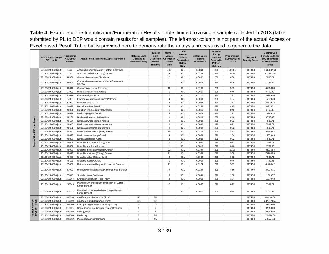
3-139
Table 4. Example of the Identification/Enumeration Results Table, limited to a single sample collected in 2013 (table
submitted by PL to DEP would contain results for all samples). The left-most column is not part of the actual Access or
Excel based Result Table but is provided here to demonstrate the analysis process used to generate the data.
PADEP Algae Sample
GIS Key ID
Taxonomic
NADED ID
Number
Algae Taxon Name with Author Reference
Natuaral Units
Counted in
Palmer-Maloney
Number
Cells
Counted in
Palmer-
Maloney
Number
Valves
Counted in
Diatom
Slide
Total
Number
Valves
Counted on
Datom
Slide
Diatom Valve
Relative
Abundance
Number
Living
Diatoms
Counted in
Palmer-
Maloney
Proportioned
Living Diatom
Valves
CDF - Cell
Density Factor
Benthic Cell
Density (cells per
cm2 of sampled
benthic surface
area)
20130424-0800-jbutt 1023 Achnanthidium pyrenaicum (Hustedt) Kobayashi 435 631 0.6894 291 200.61 8174.50 1639887.61
20130424-0800-jbutt 7043 Amphora pediculus (Kützing) Grunow 46 631 0.0729 291 21.21 8174.50 173413.40
20130424-0800-jbutt 16004 Cocconeis placentula Ehrenberg 2 631 0.0032 291 0.92 8174.50 7539.71
20130424-0800-jbutt 16005Cocconeis placentula var. euglypta (Ehrenberg)
Grunow1 631 0.0016 291 0.46 8174.50 3769.86
20130424-0800-jbutt 16011 Cocconeis pediculus Ehrenberg 12 631 0.0190 291 5.53 8174.50 45238.28
20130424-0800-jbutt 27008 Diatoma moniliformis Kützing 1 631 0.0016 291 0.46 8174.50 3769.86
20130424-0800-jbutt 27013 Diatoma vulgaris Bory 7 631 0.0111 291 3.23 8174.50 26389.00
20130424-0800-jbutt 34030 Fragilaria vaucheriae (Kützing) Petersen 4 631 0.0063 291 1.84 8174.50 15079.43
20130424-0800-jbutt 37990 Gomphonema sp. 1 ? 6 631 0.0095 291 2.77 8174.50 22619.14
20130424-0800-jbutt 44073 Melosira varians Agardh 9 631 0.0143 291 4.15 8174.50 33928.71
20130424-0800-jbutt 45001 Meridion circulare (Greville) Agardh 1 631 0.0016 291 0.46 8174.50 3769.86
20130424-0800-jbutt 46023 Navicula gregaria Donkin 5 631 0.0079 291 2.31 8174.50 18849.28
20130424-0800-jbutt 46104 Navicula tripunctata (Müller) Bory 1 631 0.0016 291 0.46 8174.50 3769.86
20130424-0800-jbutt 46154 Navicula rhynchocephala Kützing 2 631 0.0032 291 0.92 8174.50 7539.71
20130424-0800-jbutt 46646 Navicula caterva Hohn et Hellerman 2 631 0.0032 291 0.92 8174.50 7539.71
20130424-0800-jbutt 46661 Navicula capitatoradiata Germain 2 631 0.0032 291 0.92 8174.50 7539.71
20130424-0800-jbutt 46859 Navicula lanceolata (Agardh) Kützing 10 631 0.0158 291 4.61 8174.50 37698.57
20130424-0800-jbutt 46893 Navicula antonii Lange-Bertalot 4 631 0.0063 291 1.84 8174.50 15079.43
20130424-0800-jbutt 46896 Navicula rostellata Kützing 2 631 0.0032 291 0.92 8174.50 7539.71
20130424-0800-jbutt 48002 Nitzschia acicularis (Kützing) Smith 2 631 0.0032 291 0.92 8174.50 7539.71
20130424-0800-jbutt 48004 Nitzschia amphibia Grunow 1 631 0.0016 291 0.46 8174.50 3769.86
20130424-0800-jbutt 48008 Nitzschia dissipata (Kützing) Grunow 22 631 0.0349 291 10.15 8174.50 82936.84
20130424-0800-jbutt 48013 Nitzschia frustulum (Kützing) Grunow 21 631 0.0333 291 9.68 8174.50 79166.99
20130424-0800-jbutt 48025 Nitzschia palea (Kützing) Smith 2 631 0.0032 291 0.92 8174.50 7539.71
20130424-0800-jbutt 48123 Nitzschia pusilla Grunow 1 631 0.0016 291 0.46 8174.50 3769.86
20130424-0800-jbutt 55002 Reimeria sinuata (Gregory) Kociolek et Stoermer 11 631 0.0174 291 5.07 8174.50 41468.42
20130424-0800-jbutt 57002 Rhoicosphenia abbreviata (Agardh) Lange-Bertalot 9 631 0.0143 291 4.15 8174.50 33928.71
20130424-0800-jbutt 65048 Surirella minuta Brébisson 3 631 0.0048 291 1.38 8174.50 11309.57
20130424-0800-jbutt 110004 Encyonema minutum (Hilse) Mann 4 631 0.0063 291 1.84 8174.50 15079.43
20130424-0800-jbutt 155003Planothidium lanceolatum (Brébisson ex Kützing)
Lange-Bertalot2 631 0.0032 291 0.92 8174.50 7539.71
20130424-0800-jbutt 155017Planothidium frequentissimum (Lange-Bertalot)
Lange-Bertalot1 631 0.0016 291 0.46 8174.50 3769.86
20130424-0800-jbutt 249998 (undifferentiated) diatoms> (dead) 53 53 8174.50 433248.50
20130424-0800-jbutt 249999 (undifferentiated) (diatoms)>(living) 291 291 8174.50 2378779.50
20130424-0800-jbutt 309000 Cladophora glomerata (Linnaeus) Kützing 3 11 8174.50 89919.50
20130424-0800-jbutt 510001 Scenedesmus quadricauda (Turpin) Brébisson 1 4 8174.50 32698.00
20130424-0800-jbutt 533000 Spirogyra sp. 1 4 8174.50 32698.00
20130424-0800-jbutt 569000 Ulothrix sp. 5 52 8174.50 425074.00
20130424-0800-jbutt 893002 Pleurocapsa minor Hansgirg 5 95 8174.50 776577.50
Pa
lme
r-M
alo
ne
y
ID/C
ou
nt
Re
su
ltD
iato
m S
lid
e ID
/Co
un
t R
es
ult

3-140
LITERATURE CITED
Arar, E. J., G. B. Collins. 1997. Method 445.0: In vitro determination of chlorophyll a and
pheophytin a in marine and freshwater algae by fluorescence. EPA method
445.0. Available from:
https://cfpub.epa.gov/si/si public record report.cfm?dirEntryId=309417).
Barbour, M. T., J. Gerritsen, B. D. Snyder, and J. B. Stribling. 1999. Rapid
bioassessment protocols for use in streams and wadeable rivers: Periphyton,
benthic macroinvertebrates and fish. 2nd edition. EPA 841-B-99-002. (Available
from: https://www3.epa.gov/region1/npdes/merrimackstation/pdfs/ar/AR-
1164.pdf).
Charles, D. F., C. Knowles, and R. S. Davis. 2002. Protocols for the analysis of algal
samples collected as part of the U.S. Geological Survey National Water-Quality
Assessment Program, Report No. 02–06. The Academy of Natural Sciences,
Patrick Center for Environmental Research–Phycology Section, Philadelphia, PA
(Available from:
https://water.usgs.gov/nawqa/protocols/algprotocol/algprotocol.pdf).
Fitzpatrick, F. A., I. R. Waite, P. J. D’Arconte, M. R. Meador, M. A. Maupin, and M. E.
Gurtz. 1998. Revised methods for characterizing stream habitat in the National
Water-Quality Assessment Program. Water-Resources Investigations Report 98–
4052. U.S. Geological Survey, Raleigh, North Carolina. (Available online at:
https://pubs.er.usgs.gov/publication/wri984052.)
Hausmann, S., D. F. Charles, J. Gerritsen, and T. J. Belton. 2016. A diatom-based
biological condition gradient (BCG) approach for assessing impairment and
developing nutrient criteria for streams. Science of the Total Environment
562:914–927.
Hill, W. R. 1996. Effects of light. Chapter 5, pages 121–144 in P. J. Stevenson, M. L.
Bothwell, and R. L. Lowe (editors). Algal Ecology. Freshwater benthic
ecosystems. Academic Press, San Diego.
Hill, W. R., and B. J. Roberts. 2009. Quantifying phosphorus and light effects in stream
algae. Limnology and Oceanography 54(1):368–380.
Hoger, M. S. 2020. In-situ field meter and transect data collection protocol. Chapter 4.1,
pages 2–8 in M. J. Lookenbill, and R. Whiteash (editors). Water quality
monitoring protocols for streams and rivers. Pennsylvania Department of
Environmental Protection, Harrisburg, Pennsylvania.
Kahlert, M., R. L. Albert, E. L. Anttila, R. Bengtsson, C. Bigler, T. Eskola, V. Gӓlman, S.
Gottschalk, E. Herlitz, A. Jarlman, J. Kasperoviciene, M. Kokociński, H. Luup, J.
Miettinen, I. Paunksnyte, K. Piirsoo, I. Quintana, J. Raunio, B. Sandell, H.
Simola, I. Sundberg, S. Vilbaste, and J. Weckström. 2009. Harmonization is
more important than experience – Results of the first Nordic-Baltic diatom

3-141
intercalibration exercise, 2007 (stream monitoring). Journal of Applied Phycology
21:471–482.
Kahlert, M., É. Ács, A. S. F. Almeida, S. Blanco, M. Dreβler, L. Ector, S. M. Karjalainen,
A. Liess, A. Mertens, J. van der Wall, and S. Vilbaste.. 2016. Quality assurance
of diatom counts in Europe: Towards harmonized datasets. Hydrobiologia
772(1):1–14.
Kelly, M. G, A. Cazaubon, E. Coring, A. Dell’Uomo, L. Ector, B. Goldsmith, H. Guasch,
J. Hürlimann, A. Jarlman, B. Kawecka, J. Kwandrans, R. Laugaste, E. A.
Lindstrøm, M. Leitao, P. Marvan, J. Padisák, E. Pipp, J. Prygiel, E. Rott, S.
Sabater, H. van Dam, and J. Vizinet. 1998. Recommendations for the routine
sampling of diatoms for water quality assessments in Europe. Journal of Applied
Phycology 10:215–224.
Kelly, M. G. 2001. Use of similarity measures for quality control of benthic diatom
samples. Water Research 35(11):2784–2788.
Lee, S., I. Bishop, and S. Spaulding. 2017. Improving diatom taxonomic consistency
and reference site detection in NRSA. U.S. Environmental Protection Ag Webinar
PowerPoint presentation.
Lookenbill, M. J. and R. Whiteash (editors). 2021. Water quality monitoring protocols for
streams and rivers. Pennsylvania Department of Environmental Protection,
Harrisburg, Pennsylvania.
Moulton II, S. R., J. G. Kennen, R. M. Goldstein, and J. A. Hambrook. 2002. Revised
protocols for sampling algal, invertebrate, and fish communities as part of the
National Water-Quality Assessment Program. USGS Open file Report 02–150.
(Available from: https://pubs.usgs.gov/of/2002/ofr-02-150/pdf/ofr02-150.pdf).
Peterson, C. G., and R. J. Stevenson. 1990. Post-spate development of epilithic
communities in different current environments. Canadian Journal of Botany
68:2092–2102.
Platts, W. S., E. Armour, G. D. Booth, M. Bryant, J. L. Bufford, P. Cuplin, S. Jensen, G.
W. Lienkaemper, G. W. Minshall, S. B. Monsen, R. L. Nelson, J. R. Sedell, and J.
S. Tuhy. 1987. Methods for evaluating riparian habitats with applications to
management. General Technical Report INT-GRT-221. US Department of
Agriculture, Forest Service, Intermountain Research Station.
Porter, S. D., D. K. Mueller, N. E. Spahr, M. D. Munn, and N. M. Dubrovsky. 2008.
Efficacy of algal metrics for assessing nutrient and organic enrichment in flowing
waters. Freshwater Biology 53:1036–1054.
Potapova, M., and D. F. Charles. 2005. Choice of substrate in algae-based water-
quality assessment. Journal of the North American Benthological Society
24(2):415–427.
Potapova, M., and D. F. Charles. 2008. Diatom metrics for monitoring eutrophication in
rivers of the United States. Ecological Indicators 7:48–70.

3-142
PCER. 1998. Diatom and Non-Diatom Taxa lists. The Academy of Natural Sciences of
Drexel University, Philadelphia, PA (Available from:
https://diatom.ansp.org/Taxa.aspx).
Shull, D. R. 2017a. Semi-wadeable large river macroinvertebrate data collection
protocol. Chapter 3.4, pages 20–27 in M. J. Lookenbill, and R. Whiteash
(editors). Water quality monitoring protocols for streams and rivers. Pennsylvania
Department of Environmental Protection, Harrisburg, Pennsylvania.
Shull, D. R. (editor). 2017b. Wadeable riffle-run stream macroinvertebrate data
collection protocol. Chapter 3.1, pages 2–8 in M. J. Lookenbill, and R. Whiteash
(editors). Water quality monitoring protocols for streams and rivers. Pennsylvania
Department of Environmental Protection, Harrisburg, Pennsylvania.
USEPA. 2013. Standard operating procedure for In vitro determination of chlorophyll a
in freshwater phytoplankton by fluorescence. (Available from
https://www.epa.gov/sites/production/files/2017-01/documents/sop-for-in-vitro-
determination-of-chlorophyll-a-in-freshwater-201303-11pp.pdf).
Wehr, J. D., and R. G. Sheath. 2003. Introduction to freshwater algae. Pages 1–5 in
Freshwater Algae of North America: Ecology and Classification. Academic Press,
New York, NY.
Whittaker, R. H., and C. W. Fairbanks. 1958. A study of plankton copepod communities
in the Columbia basin, southeastern Washington. Ecology 39(1):46–65.
Wolda, H. 1981. Similarity indices, sample size and diversity. Oecologia 50:296–302.

3-143
3.11 BACTERIOLOGICAL DATA COLLECTION PROTOCOL

3-144
Prepared by:
Megan Bradburn and Shawn Miller
PA Department of Environmental Protection
Office of Water Programs
Bureau of Clean Water
11th Floor: Rachel Carson State Office Building
Harrisburg, PA 17105
2015
Edited by:
Josh Lookenbill
PA Department of Environmental Protection
Office of Water Programs
Bureau of Clean Water
11th Floor: Rachel Carson State Office Building
Harrisburg, PA 17105
2017
Edited by:
Shawn Miller
PA Department of Environmental Protection
Office of Water Programs
Bureau of Clean Water
11th Floor: Rachel Carson State Office Building
Harrisburg, PA 17105
2021

3-145
INTRODUCTION
All waters of Pennsylvania are evaluated for Water Contact Sports (WC) recreational
use (RU) attainment according to the criterion for bacteria in §93.7 of 25 Pa. Code
Chapter 93. This protocol identifies appropriate sample collection procedures needed to
assess for WC RU for applicable waters.
SAMPLING DESIGN CONSIDERATIONS SPECIFIC TO BACTERIA MONITORING
Probability-based or targeted (judgmental) sampling designs can both be used for
bacteria monitoring; however, DEP prefers a targeted sampling design. Both sampling
design procedures are described in more detail in Chapter 2, Sampling Design and
Planning (Lookenbill 2020). Watersheds that have not been assessed and waters that
are heavily used for recreational activities by the public or those that support public
beaches are prioritized and specifically targeted for recreational use monitoring.
Additional sampling locations are chosen throughout a watershed based on changes in
landuse, location of major tributaries, and potential sources of impairment. Impairment
sources can include municipal point sources, combined sewer overflows (CSOs), and
agricultural sources relating to manure application, livestock grazing, and animal
feeding. In most cases multiple sampling locations will be needed to bracket potential
sources of impairment. Smaller headwater streams (Strahler 2nd order or smaller),
especially those with no potential sources of impairment are not prioritized. For larger
rivers, streams, or lakes multiple sampling locations across a transect and along the
shore (cross-section surveys) are recommended to accurately delineate an
assessment. Cross-section surveys and multiple sampling locations across a transect
are highly recommended to be established on rivers and streams greater than 1000 mi2.
Cross-section surveys performed using a clean and calibrated field meter that collects
water temperature, specific conductance, dissolved oxygen, pH, and – preferably –
turbidity are required to determine if major water quality influences exist at the sampling
location according to Chapter 4.1, In-Situ Field Meter and Transect Data Collection
Protocol (Hoger 2020). The number and distribution of docks, boating areas,
residences, cabins, and access areas should be considered in locating sample sites.
Lakes and reservoirs with beaches or swimming areas must include sampling locations
from the left perimeter, center, and right perimeter of the swimming area, unless the
swimming area is less than 100 feet. If less than 100 feet, sampling locations from the
left perimeter and right perimeter are sufficient.
During the swimming season, the DOH and DCNR collect weekly samples for
Escherichia coli (E. coli) at public beaches for monitoring purposes. See 28 Pa. Code
§18.30. When exceedances of criteria occur at public beaches, closure notices are

3-146
issued by DOH. In cooperation with DEP, DOH, and DCNR compiles a list of closures
that DEP will utilize to identify possible recreational use impairment and focus future
bacteriological data collection and WC RU assessment efforts.
SAFETY PROCEDURES
Appropriate WC RU assessment begins with data collection that follows proper
guidelines and safety procedures. Safety is of utmost concern when working in and on
any waterbody. Individuals that lack experience and education related to navigating
these waterbodies put themselves and others at risk of injury or loss of life. On large
waterbodies some form of watercraft can be required for this data collection protocol.
Whether a kayak, canoe, or powered boat is used, DEP recommends – and in most
cases PFBC requires by law – that individuals using watercrafts take boating courses
and obtain a boating safety certificate. However, whether laws apply to certain
individuals or watercraft or not, DEP strongly recommends that all individuals regardless
of age, experience, or navigation procedure obtain and keep a boating safety
certification on them during surveys that require watercraft. More information on boating
courses and safety certifications are available here:
http://www.fishandboat.com/Boat/BoatingCourses/Pages/default.aspx
Surface waters present difficulties for both wadeable and non-wadeable water
navigation. Certain locations, especially on large rivers, may be fully or partially
wadeable during certain times of the targeted recreation season, but there are also
highly variable currents and drop-offs that are dangerous to wading collectors.
Inherent in these recommendations is the understanding that collectors must be well
informed of the unique characteristics of each surface water they intend to sample and
be aware of current flow and weather conditions. Equipment considerations may be
different between similar sized surface waters, and certainly different when visiting
multiple surface waters of different size and type. For instance, boat selection and
safety equipment lists would be different depending on whether the collector is visiting a
small 3rd order stream or a large 7th order river. These differing characteristics require
thorough planning before going into the field so resources are not wasted due to a lack
of preparation. It is also imperative that collectors have access to and continually check
surface water flow conditions. There will be situations when weather in one part of
Pennsylvania may be optimal for sampling a site, but weather in another part of
Pennsylvania – two or three days before the sampling period – created conditions that
reduces the ability to collect. Analysis of flow conditions at all available points upstream
of the intended sampling locations are highly recommended. Commonly used discharge
data are available here: https://waterdata.usgs.gov/pa/nwis/current/?type=flow

3-147
DATA COLLECTION
Bacteriological sampling for determining WC RU attainment is conducted during the
swimming season (May 1st through September 30th). This is the timeframe the public is
likely to be engaging in primary WC activities. WC recreational activities are defined
activities where immersion and ingestion are likely and there is a high degree of bodily
contact with the water, such as swimming, bathing, surfing, water skiing, tubing, skin
diving, snorkeling, water play by children, or similar water-contact activities (USEPA
2012). As a general rule, bacteriological sampling should not take place during those
times when physical conditions, such as stream discharge, render primary contact
recreation hazardous to the public. Samples collected for assessment purposes should
provide the ability to identify an impaired RU due to chronic long-term impacts and not
acute or transitory situations. In the past, there was guidance that sampling should not
take place immediately following 0.25 inch of rain or more to avoid collecting samples
during elevated discharge when bacteria levels are elevated, but not necessarily
characteristic of a chronic condition. This guidance is usually applicable to smaller
waterbodies where discharge responds quickly to precipitation events but becomes
more difficult to apply to larger waterbodies and to some lakes where increased
discharge and water quality changes can occur days following 0.25 inch of rain.
The WC RU bacteria criterion at 25 Pa. Code §93.7:
“(Escherichia coli colony forming unit per 100 milliliters (CFU per 100 ml)) During
the swimming season (May 1 through September 30), the maximum E. coli level
shall be a geometric mean of 126 CFU per 100 ml. The geometric mean for the
samples collected in the waterbody should not be greater than 126 CFU per 100
ml in any 30-day interval. There should not be greater than a 10% excursion
frequency of 410 CFU per 100 ml for the samples collected in the same 30-day
duration interval. (Fecal coliforms/100 ml) For the remainder of the year, the
maximum fecal coliform level shall be a geometric mean of 2,000 CFU per 100
ml based on a minimum of five consecutive samples collected on different days
during a 30-day period.”
The criterion specifically defines sample duration during the bathing season and
magnitude, frequency, and duration during the non-bathing season for determining
impairment for WC RU. The DEP Bacteriological Assessment Method for Water Contact
Sports, defines magnitude, frequency, and duration during the bathing season and
remainder of the year as at least 5 samples, each separated by at least 24 hours,
spanning a maximum of 30 days and a minimum of 14 days (Miller and Whiteash 2021).
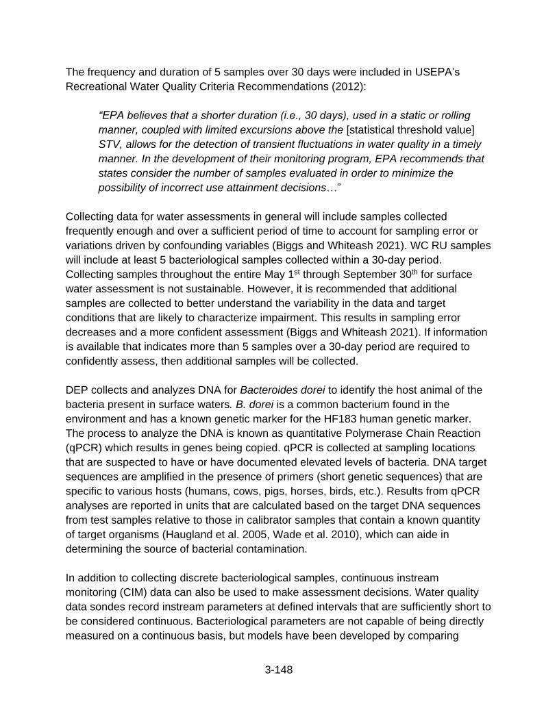
3-148
The frequency and duration of 5 samples over 30 days were included in USEPA’s
Recreational Water Quality Criteria Recommendations (2012):
“EPA believes that a shorter duration (i.e., 30 days), used in a static or rolling
manner, coupled with limited excursions above the [statistical threshold value]
STV, allows for the detection of transient fluctuations in water quality in a timely
manner. In the development of their monitoring program, EPA recommends that
states consider the number of samples evaluated in order to minimize the
possibility of incorrect use attainment decisions…”
Collecting data for water assessments in general will include samples collected
frequently enough and over a sufficient period of time to account for sampling error or
variations driven by confounding variables (Biggs and Whiteash 2021). WC RU samples
will include at least 5 bacteriological samples collected within a 30-day period.
Collecting samples throughout the entire May 1st through September 30th for surface
water assessment is not sustainable. However, it is recommended that additional
samples are collected to better understand the variability in the data and target
conditions that are likely to characterize impairment. This results in sampling error
decreases and a more confident assessment (Biggs and Whiteash 2021). If information
is available that indicates more than 5 samples over a 30-day period are required to
confidently assess, then additional samples will be collected.
DEP collects and analyzes DNA for Bacteroides dorei to identify the host animal of the
bacteria present in surface waters. B. dorei is a common bacterium found in the
environment and has a known genetic marker for the HF183 human genetic marker.
The process to analyze the DNA is known as quantitative Polymerase Chain Reaction
(qPCR) which results in genes being copied. qPCR is collected at sampling locations
that are suspected to have or have documented elevated levels of bacteria. DNA target
sequences are amplified in the presence of primers (short genetic sequences) that are
specific to various hosts (humans, cows, pigs, horses, birds, etc.). Results from qPCR
analyses are reported in units that are calculated based on the target DNA sequences
from test samples relative to those in calibrator samples that contain a known quantity
of target organisms (Haugland et al. 2005, Wade et al. 2010), which can aide in
determining the source of bacterial contamination.
In addition to collecting discrete bacteriological samples, continuous instream
monitoring (CIM) data can also be used to make assessment decisions. Water quality
data sondes record instream parameters at defined intervals that are sufficiently short to
be considered continuous. Bacteriological parameters are not capable of being directly
measured on a continuous basis, but models have been developed by comparing

3-149
discrete bacteriological samples to recorded CIM data (Hoger 2018, Rasmussen et al.
2008, Stone and Graham 2014). Models may be used to collect water contact
recreational use data for assessment purposes, provide that CIM data collection
protocols are followed (Hoger et al. 2017).
COLLECTION REQUIREMENTS
Collector Identification Number
Collectors must have an assigned four-digit collector identification number (e.g., 0925).
This number along with a sequential three-digit sample number (e.g., 0925-001), and
date/time of sample are used to identify individual samples. Supervisory staff can
request collector identification numbers for their field staff with the “Collector ID Request
Form” found at the eLibrary website (ID Request Form).
DEP Laboratory Submission Sheet
Collectors must submit samples to the DEP Bureau of Labs (BOL) using the “Sample
Submission Sheet” (Submission Sheet). Field staff are required to document collector
identification number, reason code, cost center, program code, sequence number, date
collected, time collected (in military time format), fixative(s), Standard Analysis Code
(SAC), legal seal numbers for each sample collected (if required), the number of bottles
submitted per test suite, collector name, date, phone number, and any additional
comments that lab analysts will use to properly handle samples.
As described previously, collector identification numbers are unique to each field staff
collecting samples. Reason codes, cost centers, and program codes are program
specific and should be obtained from the program responsible for coordinating sampling
efforts. Sample sequence numbers are three-digit sequential numbers (001-999) unique
to a sample collected on a given day generated by field staff collecting samples. Date
and time collected should be accurately documented, especially if field parameters with
specific diurnal fluctuations (temperature, dissolved oxygen) will accompany analytical
results. To avoid complications with daylight savings time, collection time should be
recorded using eastern standard time or UTC-5 throughout the year.
A SAC is a unique code that details analytical tests to be applied to a specific sample.
Each DEP program uses specific SACs for specific projects or purposes. For example,
SAC B021 is used by “Water Management” when submitting bacteriological samples for
bot Fecal and E.coli with a 24-hour hold time. Unique SACs are created for specific
purposes. Table 1 lists other bacteriological test descriptions and SACs.
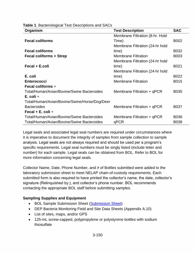
3-150
Table 1. Bacteriological Test Descriptions and SACs
Organism Test Description SAC
Fecal coliforms
Membrane Filtration (8-hr. Hold
Time) B002
Fecal coliforms
Membrane Filtration (24-hr hold
time) B032
Fecal coliforms + Strep Membrane Filtration B003
Fecal + E.coli
Membrane Filtration (24-hr hold
time) B021
E. coli
Membrane Filtration (24-hr hold
time) B022
Enterococci Membrane Filtration B015
Fecal coliforms +
Total/Human/Avian/Bovine/Swine Bacteroides Membrane Filtration + qPCR B035
E. coli +
Total/Human/Avian/Bovine/Swine/Horse/Dog/Deer
Bacteroides Membrane Filtration + qPCR B037
Fecal + E. coli +
Total/Human/Avian/Bovine/Swine Bacteroides Membrane Filtration + qPCR B036
Total/Human/Avian/Bovine/Swine Bacteroides qPCR B038
Legal seals and associated legal seal numbers are required under circumstances where
it is imperative to document the integrity of samples from sample collection to sample
analysis. Legal seals are not always required and should be used per a program’s
specific requirements. Legal seal numbers must be singly listed (include letter and
number) for each sample. Legal seals can be obtained from BOL. Refer to BOL for
more information concerning legal seals.
Collector Name, Date, Phone Number, and # of Bottles submitted were added to the
laboratory submission sheet to meet NELAP chain-of-custody requirements. Each
submitted form is also required to have printed the collector’s name, the date, collector’s
signature (Relinquished by:), and collector’s phone number. BOL recommends
contacting the appropriate BOL staff before submitting samples.
Sampling Supplies and Equipment
• BOL Sample Submission Sheet (Submission Sheet)
• DEP Bacteria Monitoring Field and Site Data Sheets (Appendix A.10)
• List of sites, maps, and/or GPS
• 125-mL screw-capped, polypropylene or polystyrene bottles with sodium
thiosulfate

3-151
• 1-L screw-capped, polypropylene bottles with sodium thiosulfate (qPCR)
• Sample blanks containing sterile (autoclaved) water obtained from BOL
• Disposable, powderless gloves (such as nitrile)
• Coolers and ice
• Courier shipping labels
• Van Dorn or Kemmerer (Lakes)
• Field meter (required for rivers and streams greater than 1000 mi2)
• Sampling pole and zip-ties (optional)
• Boots and waders (optional)
COLLECTION PROCEDURES
Collectors must ensure that the samples collected will be representative of the aquatic
system of interest. Interference of the sampling process must be minimized; collectors
must be alert to conditions that could compromise the integrity of a water sample. The
most common causes of sample interference during collection include poor sample-
handling and preservation techniques, input from atmospheric sources, and
contaminated equipment or reagents. Each sampling location needs to be selected and
sampled in a manner that minimizes bias caused by the collection process and that best
represents the intended environmental conditions at the time of sampling.
Before handling sample bottles, the collector should ensure his or her hands are clean
and not contaminated from sources such as food, coins, fuels, mud, insect repellent,
sunscreen, sweat, nicotine, etc. Alternatively, collectors should wear disposable,
powderless gloves (such as nitrile).
Labeling Bottles
While the minimum required information for samples submitted to BOL is the collector
number and sequential sample number, collectors may add additional information such
as date and time collected, general test(s) description. This will help prevent confusing
what bottles are for which tests and to ensure the sample is properly preserved.
Labeling should be done so that at least 1” of space is left at the top of the bottle to
allow BOL to apply lab labels.
Permanent marker will rub off bottles during collection and transport. So, clear packing
tape is wrapped around the bottle to protect the hand-written labels. Using ball-point
and other non-permanent ink pens must be avoided. BOL discourages the use of
masking tape. Collectors must complete the field and site data sheets (Appendix A.10)
for samples collected and sites visited.

3-152
Flowing Waterbodies
For flowing waterbodies, bacteriological samples will be collected by direct surface
water sampling. Avoid sampling in eddies, pools, side-channels, or in tributary mixing
zones unless necessary due to site-specific or other environmental considerations. The
collector should face upstream, taking care to not alter flow patterns or disturb substrate
sediments upstream of where they will collect the sample. Collection bottles should be
inserted into the water column vertically, facing down to avoid inadvertently collecting
surface debris/films. For slow moving streams with easily disturbed sediment, the
collector should sample from the stream bank, boat, or bridge using a sampling
extension pole. If sampling from a boat, the collector should sample near the bow as the
boat moves upstream or faces upwind. In smaller waterbodies that do not require
multiple locations across a transect, samples are collected at mid-depth in the
approximate thalweg (the line defining the points along the length of a stream bed with
the greatest depth). The collector should remove the stopper/lid from the sampling
container just before sampling, taking care not to contaminate the cap, neck, or the
inside of the bottle with his or her fingers, wind-blown particles, precipitation, clothes,
body, or overhanging structures. DEP uses 125-mL or 1-L (qPCR) screw-capped bottles
with sodium thiosulfate added to neutralize the effects of residual chlorine. DO NOT
RINSE THE BOTTLE BEFORE SAMPLING. Fill the bottle to the shoulder leaving
headspace. Once the sample is collected and capped, the collector should rinse any
large amount of dirt or debris from the outside of the container.
Lakes and Reservoirs
Bacteriological samples will be collected using disposable, powderless gloves (such as
nitrile (elbow length preferred) from lakes. Samples are collected at a depth of one
meter when possible and at least a 0.3-meter depth at a minimum. Samples collected at
a depth of one meter can be collected using a sampling pole or dispensed from depth
specific water sampling equipment (e.g., Van Dorn, Kemmerer). Samples from a boat
are collected with motor off. The collector should remove the stopper/lid from the
sampling container just before sampling, taking care not to contaminate the cap, neck,
or the inside of the bottle with his or her fingers, wind-blown particles, precipitation,
clothes, body, or overhanging structures. DEP uses 125-mL or 1-L (qPCR) screw-
capped bottles with sodium thiosulfate added to neutralize the effects of residual
chlorine. DO NOT RINSE THE BOTTLE BEFORE SAMPLING. Fill the bottle to the
shoulder leaving headspace. Once the sample is collected and capped, the collector
should rinse any large amount of dirt or debris from the outside of the container.
Preservation
The collector should vertically insert bottles into a cooler, right-side up. The samples
should be cooled with cubed or crushed ice. A sufficient amount of ice should be added
3-153
to the cooler to ensure samples remain at ≤6°C during overnight shipping. BOL
personnel will note whether samples were shipped properly. Improperly shipped
samples may be subject to a data release request. The “Sample Submission Sheet”
(Submission Sheet) should be filled out, inserted into a Ziploc® bag, and attached to the
inside of the cooler lid. Courier shipping labels should be printed out during ordering so
they can be attached to the top of the cooler lid during sample drop-off. Shipping labels
are secured to the cooler lip with two pieces of packing tape on the left and right side;
taping all sides of the label makes removal difficult for lab technicians.
Quality Assurance
For quality assurance purposes, sample blanks containing sterile (autoclaved) water
obtained from BOL or the laboratory analyzing samples should be submitted for every
20 samples for each sampling trip/day to determine whether contamination is occurring
in any part of the sample collection, handling, or preservation process. Sample blanks
are “collected” by transferring sterile water from container received from BOL to a
labeled 125-mL. A duplicate grab sample should also be collected every 20 samples or
for each sampling trip/day to gauge testing variability and potential sources of
contamination due to collection procedures. Duplicate samples are collected
simultaneously with the associated environmental sample, using identical sampling and
preservation procedures. Both sample blanks and sample duplicates are assigned
unique, sequential sample numbers. Label duplicate and blank samples in the same
manner as environmental samples. DO NOT IDENTIFY DUPLICATE OR BLANK ON
THE SAMPLE BOTTLE. Duplicates and blanks must be documented appropriately in
SIS under the ‘Comments/Quality Assurance’ tab and linked to a monitoring point.
Field Meters
Field meters provide the ability to collect in-situ data that is not available through grab
samples submitted to BOL. Standard field parameters include dissolved oxygen,
temperature, specific conductance, pH, and turbidity. Collection of field meter data is
recommended for bacteriological sampling and required for rivers and streams greater
than 1000 mi2. See Chapter 4.1, In-Situ Field Meter and Transect Data Collection
Protocol (Hoger 2020) for more information on the use and proper calibration of field
meters.
Sample Holding Times
Water samples need to be shipped or delivered to BOL as soon as possible. The
collector should understand that certain laboratory analyses have “holding times” during
which tests must be conducted for result validity. Bacteria samples collected and
submitted for compliance purposes have a hold time of 8 hours. A hold time of 24 hours
may be applied to samples collected and submitted for WC RU assessment purposes.

3-154
Shipping Samples
All DEP district and regional offices are designated pick-up locations for water samples;
the samples must be dropped off for pick up by 1600 hours. Other locations exist, such
as at some Pennsylvania Department of Transportation facilities and some private
businesses, but these drop-off locations may require call-ahead notice to the current
courier, as they may not be visited daily. Further, the drop-off locations may require a
drop-off specific key to open the drop-off entrance lock. Drop-off locations are available
on the BOL website.
SAMPLE INFORMATION SYSTEM DOCUMENTATION
General guidelines for data entry are provided in Chapter 4.6, Sample Information
System (SIS) Data Entry Protocol (Shull 2017). Step-by-step processes of SIS data
entry are also provided in Appendix B.3. However, the following includes
recommendations specific to managing projects, monitoring points, and samples using
bacteriological data.
Projects
Create a project specific to each recreational use monitoring and assessment effort.
This will include delineation of subbasin targeted for a specific project. ‘Project ID’
should be formatted to include the letters ‘BAC’, four alpha characters, followed by two-
digit year. ‘Description’ should include four-digit year, “Bacteria Monitoring Project”,
followed by the targeted subbasin or watershed. Include in the ‘Comments’ a general
description of the purpose and scope of the project along with any pertinent specific
information (Figure 1)

3-155
Figure 1. SIS Project entry and edit screen with template information.
Monitoring Points
Create a monitoring point for each sampling location. The ‘Name’ of each monitoring
point will begin with the same four alpha characters followed by sequential numbers.
Within the location tab populate ‘State’, ‘County’, ‘Latitude’, ‘Longitude’, ‘Datum’
(NAD83), and ‘Location’. Include a general location description in ‘Location’ (Figure 2).
Within the Function/Administration tab ‘Medium Type’ should be “Water” and for surface
water samples ‘Sample Medium’ will be “Surface Water” (Figure 3). Within the Aliases
tab ‘Alias ID’ will begin with the same four alpha characters followed by sequential
numbers as ‘Name’. Description will include the watershed, year, and targeted site
number (Figure 4). Within the NHD tab click ‘Launch NHD Locator, snap the monitoring
point to a NHD reach, and ‘Get NHD. Lastly, link the Monitoring Point to the Project by
clicking ‘Projects’, populating the ‘Project ID’, ‘Alias ID’, and ‘Effective Date’ (Figure 5).
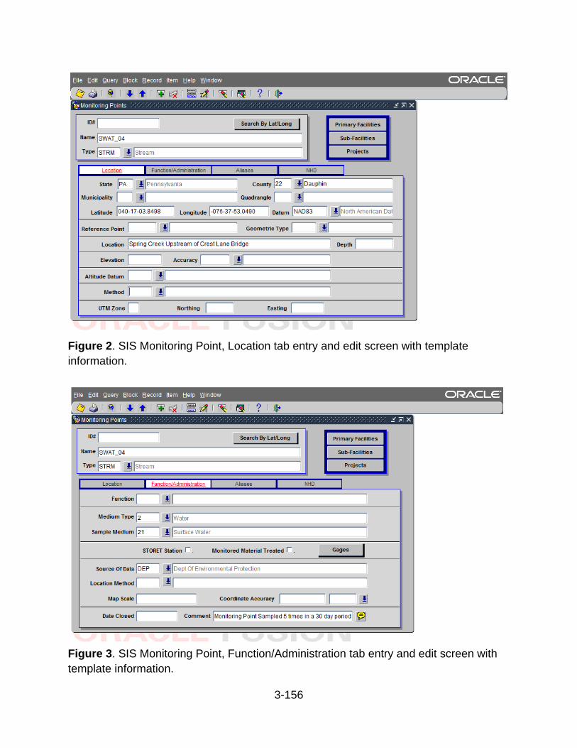
3-156
Figure 2. SIS Monitoring Point, Location tab entry and edit screen with template
information.
Figure 3. SIS Monitoring Point, Function/Administration tab entry and edit screen with
template information.

3-157
Figure 4. SIS Monitoring Point, Aliases tab entry and edit screen with template
information.
Figure 5. SIS Monitoring Point, Project link and edit screen with template information.

3-158
LITERATURE CITED
Biggs, H., and R. Whiteash. 2021 (editors). Discrete physicochemical assessment
method. Chapter 3.1, pages 2–13 in D. R. Shull, and R. Whiteash (editors).
Assessment methodology for streams and rivers. Pennsylvania Department of
Environmental Protection, Harrisburg, Pennsylvania.
Miller, S., and R. Whiteash. 2021 (editors). Bacteriological assessment method for
water contact sports. Chapter 2.5, pages 75–79 in D. R. Shull, and R. Whiteash
(editors). Assessment methodology for streams and rivers. Pennsylvania
Department of Environmental Protection, Harrisburg, Pennsylvania.
Haugland, R. A., S. C. Siefring, L. J. Wymer, K. P. Brenner, and A. Durfour. 2005.
Comparison of Enterococcus measurements in fresh water at two recreational
beaches by quantitative polymerase chain reaction and membrane filter culture
analysis. Water Research 39:559–568.
Hoger, M. S. 2020. In-situ field meter and transect data collection protocol. Chapter 4.1,
pages 2–8 in M. J. Lookenbill, and R. Whiteash (editors). Water quality
monitoring protocols for streams and rivers. Pennsylvania Department of
Environmental Protection, Harrisburg, Pennsylvania.
Hoger, M. S., D. R. Shull, and M. J. Lookenbill. 2017. Continuous physicochemical data
collection protocol. Chapter 4.3, pages 25–92 in M. J. Lookenbill, and R.
Whiteash (editors). Water quality monitoring protocols for streams and rivers.
Pennsylvania Department of Environmental Protection, Harrisburg,
Pennsylvania.
Hoger, M. S. 2018. Continuous physiochemical assessment method. Chapter 3.2,
pages 14–34 in D. R. Shull, and R. Whiteash (editors). Assessment methodology
for streams and rivers. Pennsylvania Department of Environmental Protection,
Harrisburg, Pennsylvania.
Lookenbill, M. J. 2020. Sampling design and planning. Chapter 2, pages 1–25 in M. J.
Lookenbill and R. Whiteash (editors). Water quality monitoring protocols for
streams and rivers. Pennsylvania Department of Environmental Protection,
Harrisburg, Pennsylvania.
Rasmussen, T. J., Lee, C. J., and Ziegler, A. C. 2008. Estimation of constituent
concentrations, loads, and yields in streams of Johnson County, northeast
Kansas, using continuous water-quality monitoring and regression models,
October 2002 through December 2006: U.S. Geological Survey Scientific
Investigations Report 2008–5014. U.S. Geological Survey, Kansas Water
Science Center, Lawrence, Kansas. (Available online at:
https://pubs.er.usgs.gov/publication/sir20085014.)

3-159
Shull, D. R. 2017. Sample information system (SIS) data entry protocol. Chapter 4.6,
pages 120–122 in M. J. Lookenbill, and R. Whiteash (editors). Water quality
monitoring protocols for streams and rivers. Pennsylvania Department of
Environmental Protection, Harrisburg, Pennsylvania.
Stone, M. L., and J. L. Graham. 2014. Model documentation for relations between
continuous real-time and discrete water-quality constituents in Indian Creek,
Johnson County, Kansas, June 2004 through May 2013: U.S. Geological Survey
Open-File Report 2014–1170. U.S. Geological Survey, Reston, VA. (Available
online at: https://pubs.usgs.gov/of/2013/1014/of13-1014.pdf.)
USEPA. 2012. Recreational water quality criteria. EPA 820-F12-058. Environmental
Protection Agency, Office of Environmental Information, Washington, DC.
Wade, T. J., E. Sams, K. P. Brenner, R. Haugland, E. Chern, M. Beach, L. Wymer, C.
C. Rankin, D. Love, Q. Li, R. Noble, and A. P. Dufour. 2010. Rapidly measured
indicators of recreational water quality and swimming-associated illness at
marine beaches: A prospective cohort study. Environmental Health 9:66.


4-2
4.1 IN-SITU FIELD METER AND TRANSECT DATA COLLECTION PROTOCOL

4-3
Prepared by:
Mark Hoger
PA Department of Environmental Protection
Office of Water Programs
Bureau of Clean Water
11th Floor: Rachel Carson State Office Building
Harrisburg, PA 17105
2017
Edited by:
Mark Hoger
PA Department of Environmental Protection
Office of Water Programs
Bureau of Clean Water
11th Floor: Rachel Carson State Office Building
Harrisburg, PA 17105
2020

4-4
INTRODUCTION
Water quality instruments provide the opportunity to quickly gather current water quality
data but proper care and calibration of the equipment, and QA/QC documentation are
required for these data to be accurate and defensible. Many water quality meters have
interchangeable probes to record a wide variety of parameters. The most common
parameters are temperature, conductivity, pH, dissolved oxygen, turbidity, and depth. A
full discussion of probe technology and considerations for their selection and use is
provided in Chapter 4.3, Continuous Physiochemical Data Collection Protocol (Hoger et
al. 2017).
CALIBRATION
Proper calibration should follow manufacturers’ guidelines. In addition, DEP strongly
recommends several procedures to further insure reliability and defensibility of data. At
a minimum, meters should have calibration checked before each day of use. In most
circumstances, it is recommended that the sensors are calibrated at this time. All
calibration activity, including checks, need to be logged and records maintained for
quality assurance. A calibration form is provided in Appendix B.1.
Calibration for all parameters should bracket any expected values. A summary of
calibration recommendations is provided in Table 1. Before calibration, the sensors
should be rinsed three times with the calibration solution. While other parameters can
be calibrated before going out into the field, dissolved oxygen (DO) sensors should be
calibrated onsite to avoid any influence of changes in barometric pressure from changes
in altitude, weather, or pressurization in buildings. It is also recommended that DO
calibration be checked periodically throughout the day. Accurate turbidity calibration can
be more challenging than other parameters as the sensors are very sensitive to
standard contamination and light infiltration. Clean, dedicated sensor guards and
calibration cups should be used. In addition, when calibrating in zero standard, or any
other very low standard, it can be necessary to have the guard in place and use an
opaque container to submerge the sensor in the standard. This procedure more closely
replicates the deployed environment than calibrating in just the calibration cup, and
therefore, can provide more consistent and accurate calibration.
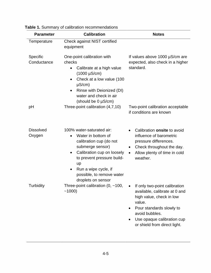
4-5
Table 1. Summary of calibration recommendations
Parameter Calibration Notes
Temperature Check against NIST certified
equipment
Specific
Conductance
One-point calibration with
checks
• Calibrate at a high value
(1000 µS/cm)
• Check at a low value (100
µS/cm)
• Rinse with Deionized (DI)
water and check in air
(should be 0 µS/cm)
If values above 1000 µS/cm are
expected, also check in a higher
standard.
pH Three-point calibration (4,7,10) Two-point calibration acceptable
if conditions are known
Dissolved
Oxygen
100% water-saturated air:
• Water in bottom of
calibration cup (do not
submerge sensor)
• Calibration cup on loosely
to prevent pressure build-
up
• Run a wipe cycle, if
possible, to remove water
droplets on sensor
• Calibration onsite to avoid
influence of barometric
pressure differences.
• Check throughout the day.
• Allow plenty of time in cold
weather.
Turbidity Three-point calibration (0, ~100,
~1000)
• If only two-point calibration
available, calibrate at 0 and
high value, check in low
value.
• Pour standards slowly to
avoid bubbles.
• Use opaque calibration cup
or shield from direct light.

4-6
CLEANING AND MAINTENANCE
Water quality instruments dedicated to periodic field meter use generally do not require
an intensive cleaning regiment. Sensors should be visually inspected during calibration
and any deposits or biological growth removed following manufacturers’
recommendations. An occasional cleaning with mild soap and water is recommended.
With proper maintenance and care, many sensors have a life-span of several years.
One exception is pH probes that have a limited supply of reference solution. Some
manufacturers provide a refillable reservoir of reference solution to prolong the life of
their pH probes. Those that do not have a refillable reservoir often need to be replaced
yearly. The pH millivolt readings should be recorded during calibration to track the life of
the probe. Additional information on cleaning and maintenance is provided by Hoger et
al. (2017) and the equipment’s manufacturer.
STORAGE
Most probes require being stored in a moist environment. A small amount of fluid in the
bottom of the calibration cup is sufficient. Submerging pH probes or other sensors with
a reference solution will deplete that solution and reduce the life of the sensor.
RECORDING
Care should be taken to allow meters to stabilize before any readings are recorded.
Temperature and conductivity should often stabilize within seconds. Depending on the
environment and life of the probe, other sensors like pH or DO may take a couple
minutes to fully stabilize. If necessary, leave the meter in situ while other tasks are
completed, so all parameters have plenty of time to stabilize.
Division of Water Quality stores field meter readings in the DEP’s Samples Information
System (SIS). Discrete readings at continuous instream monitoring (CIM) stations are
additionally stored with the CIM data as field visits in Aquarius.
CROSS-SECTION SURVEYS
Waterbodies are dynamic systems changing throughout time and space. Regular cross-
section surveys help determine how homogenous a system is, allow for better
understanding of the system as a whole, and lead to better study design and
management decisions. The confluence of a tributary, groundwater infiltration, point-
source discharges, and differences in flow, depth, and growth of photosynthetic
organisms can all result in inconsistent water quality. In general, wide, flat, slow-moving

4-7
streams are more heterogeneous. As stream channels narrow and slope increases,
better mixing often occurs. DEP frequently utilizes cross-section surveys to determine
proper deployment of continuous monitoring equipment and direct the collection of
biological and chemical samples.
As with any water quality meter work, DEP requires daily calibration (or calibration
checks) of the meter before performing cross-section surveys. In addition, post-survey
calibration checks are completed to confirm that any variation in the survey was not due
to calibration drift of the instrument.
Cross-section surveys should be conducted multiple times to document differences (or
similarities) over time. DEP refers to these repeated survey points as a water quality
transect. Established transects are often repeated monthly, but more importantly should
target various flow levels and other events that may lead to variation in the survey.
The number of measurement points in a transect is influenced by the stream size and
heterogeneity. In the smallest streams (width < 15m), surveys usually consist of three
points: left-descending bank (LDB), mid-channel, and right-descending bank (RDB).
Streams 15m to 50m wide often have five points: LDB, ¼ across, mid-channel, ¾
across, and RDB. As streams become wider than 50m, surveys are established at 10-
20m intervals. However, in Pennsylvania’s largest rivers, widths can reach over one
mile across; and in these cases, intervals may be in excess of 100m. These large-river
transects frequently use bridge piers or other reference points to facilitate consistency of
subsequent surveys. In the absence of stable reference points, a range finder is used to
measure distance to the bank.
Evaluation of Transect Data
When evaluating water quality transect data, compare each point to a reference point in
the transect. The reference point can be a point of interest in the transect (e.g., CIM
location, grab sample location) or just a point from the transect that is likely to be well
representative of the waterbody (e.g., mid-point). The difference between each point
and the reference point is then evaluated for significance. For temperature and pH, the
difference in readings between the reference point and a transect point is considered
significant if the difference is greater than 0.5 units. For specific conductance, DO, and
turbidity, the difference is considered significant if it is greater than 10% of the reference
point reading. If transects are conducted when turbidity is low (less than 10 FNU), a
difference of one FNU is equivalent to a 10% difference.
It is important to evaluate transects over a range of conditions to best understand shifts
in mixing patterns under various conditions. Most streams will show significant
4-8
differences in water quality in at least small sections of a transect for short periods of
time (e.g., along the bank, during a rain event). Transect evaluations should
characterize the extent of these spatial and temporal fluctuations.
Display and Storage of Transect Data
Properly collected transects, under a variety of water quality conditions, are likely to
encompass a wide range of values. Because of this, charting the raw values together
often leads to difficulty in discerning meaningful differences. For example, it would be
difficult to see a 0.5°C difference in temperature when charting together a summer
transect with water temperatures around 30°C and a winter transect with water
temperatures around 3°C. Therefore, transect data are best displayed by charting the
comparisons of transect points and the reference point. The thresholds of significance
should be included in the chart to facilitate a quick evaluation of the data.
All transect survey data are recorded and archived along with meter calibration
documentation. A sample transect form is provided in Appendix B.2. Measurement data
from established water quality transects are entered and stored in the SIS database.
More information on SIS is found in Chapter 4.6, Sample Information System (SIS) Data
Entry Protocol (Shull 2017).
LITERATURE CITED
Hoger, M. S., D. R. Shull, and M. J. Lookenbill. 2017. Continuous physicochemical data
collection protocol. Chapter 4.3, pages 25–92 in M. J. Lookenbill, and R.
Whiteash (editors). Water quality monitoring protocols for streams and rivers.
Pennsylvania Department of Environmental Protection, Harrisburg,
Pennsylvania.
Shull, D. R. 2017. Sample information system (SIS) data entry protocol. Chapter 4.6,
pages 120–122 in M. J. Lookenbill, and R. Whiteash (editors). Water quality
monitoring protocols for streams and rivers. Pennsylvania Department of
Environmental Protection, Harrisburg, Pennsylvania.
4-9
4.2 DISCRETE WATER CHEMISTRY DATA COLLECTION PROTOCOL
4-10
Prepared by:
Dustin Shull
PA Department of Environmental Protection
Office of Water Programs
Bureau of Clean Water
11th Floor: Rachel Carson State Office Building
Harrisburg, PA 17105
2013
Edited by:
Dustin Shull
PA Department of Environmental Protection
Office of Water Programs
Bureau of Clean Water
11th Floor: Rachel Carson State Office Building
Harrisburg, PA 17105
2017
Disclaimer:
The mention of specific trade names or commercial products does not constitute
endorsement or recommendation for use.

4-11
INTRODUCTION
As part of its water quality monitoring programs, DEP collects water chemistry data to
assess the quality of Pennsylvania’s surface water resources. This information is used
to detect or confirm pollution sources and causes, for routine water quality monitoring,
and to establish abiotic-biotic relationships. This document provides guidelines for
standardized water chemistry collection from surface waters. The procedures described
here are adapted from scientific, peer-reviewed procedures, and were developed by
technical experts. This protocol does not attempt to describe the entire spectrum of
water quality data-collection techniques (such as continuous instream monitors), but
does describe the surface water sampling procedures appropriate for typical DEP
investigations and may require modification as situations dictate.
Variations to this protocol will be dependent upon site conditions, equipment limitations,
or limitations imposed by the procedure. Investigators should document modifications
and report the final procedures employed. Investigators should be aware of, and work to
mitigate, the potential for sample contamination at all phases of the sample collection
process by observing proper sample collection, handling, and preservation procedures
described here. The most common sources of error (also known as “interference”) are
cross-contamination, poor sampling locations, and incorrect preservation.
COLLECTION REQUIREMENTS
Collector Identification Number
Field staff required to collect surface water samples must have an assigned four-digit
collector identification number (e.g., 0925). This number along with a sequential three-
digit sample number (e.g., 0925-001), and date/time of sample are used to identify
individual samples. Supervisory staff will request collector identification numbers for
their field staff with the “Collector ID Request Form” found at the eLibrary website (ID
Request Form).
DEP Laboratory Submission Sheet
Field staff will need to have at least Querying and Sample Entry security roles for the
program or business unit that they are collecting samples for. The program or business
unit will be consistent with the Program Code entered on the “DEP Laboratory
Submission Sheet” (Submission Sheet). Collectors must submit samples to the DEP
Bureau of Labs (BOL) using the laboratory submission sheet”. Field staff are required to
document collector identification number, reason code, cost center, program code,
sequence number, date collected, time collected (in military time format), fixative(s),
Standard Analysis Code (SAC), legal seal numbers for each sample collected (if

4-12
required), the number of bottles submitted per test suite, collector name, date, phone
number, and any additional comments that lab analysts will use to properly handle
samples.
As described previously, collector identification numbers are unique to each field staff
collecting samples. Reason codes, cost centers, and program codes are program
specific and should be obtained from the program responsible for coordinating sampling
efforts. Sample sequence numbers are three-digit sequential numbers (001-999) unique
to a sample collected on a given day generated by field staff collecting samples. Date
and time collected should be accurately documented, especially if field parameters with
specific diurnal fluctuations (temperature, dissolved oxygen) will accompany analytical
results. To avoid complications with daylight savings time, collection time should be
recorded using eastern standard or UTC-5 time throughout the year. However, sample
holding times will need to be considered when there are time differentials.
A SAC is a unique code that details analytical tests to be applied to a specific sample.
Each DEP program uses specific SACs for specific projects or purposes. For example,
SAC 018 is used by collectors when submitting water chemistry samples for Special
Protection Surveys. The analytes/tests listed under SAC 018 are those specifically
identified by regulations that surface water must meet and therefore be assessed for, if
a special protection determination is warranted. Other programs have developed unique
SACs for their specific purposes, and the DEP BOL encourages programs to create
SACs tailored to a program’s specific needs. New SACs can be requested by filling out
the Request Form for Standard Analysis Code. An example of a commonly used SAC is
provided below (Table 1).

4-13
Table 1. Chemical parameters collected per SAC 612 during routine semi-wadeable
river surveys.
Test
Code Test Description
Reporting
Limit Units Reference
00095 Specific Conductance
at 25C 1 UMH/CM SM 2510B
00403 pH 0 pH UNITS SM 4500H-B
00410 Alkalinity, pH 4.5 0 MG/L SM 2320B
00530 Total Suspended
Solids 2 MG/L USGS-I-3765
00600A Total Nitrogen 0.064 MG/L SM 4500N-ORG
00602A Dissolved Nitrogen 0.064 MG/L SM 4500N-ORG
00608A Dissolved Ammonia 0.02 MG/L EPA 350.1
00610A Total Ammonia 0.02 MG/L EPA 350.1
00630A Total Nitrite and
Nitrate 0.04 MG/L EPA 353.2
00631A Dissolved Nitrite and
Nitrate 0.04 MG/L EPA 353.2
00665A Total Phosphorous 0.01 MG/L EPA 365.1
00666A Dissolved
Phosphorous 0.01 MG/L EPA 365.1
00671A Dissolved
Orthophosphate 0.01 MG/L EPA 365.1
00680 Total Organic Carbon 0.5 MG/L SM 5310C
00900 Total Hardness 0.11 MG/L SM 2340A+B and EPA 200.7
revision 4.4
00916A Total Calcium 30 UG/L EPA 200.7 Revision 4.4
00927A Total Magnesium 10 UG/L EPA 200.7 Revision 4.4
00929A Total Sodium 200 UG/L EPA 200.7 Revision 4.4
00937A Total Potassium 1 MG/L EPA 200.7 Revision 4.4
00940 Total Chloride 0.5 MG/L EPA 300.0
00945 Total Sulfate 1 MG/L EPA 300.0
01007A Total Barium 10 UG/L EPA 200.7 Revision 4.4
01022K Total Boron 200 UG/L EPA 200.7 Revision 4.4
01042H Total Copper 4 UG/L EPA 200.8 Revision 5.4
01045A Total Iron 20 UG/L EPA 200.7 Revision 4.4
01051H Total Lead 1 UG/L EPA 200.8 Revision 5.4
01055A Total Manganese 10 UG/L EPA 200.7 Revision 4.4
01067H Total Nickle 4 UG/L EPA 200.8 Revision 5.4
01082A Total Strontium 10 UG/L EPA 200.7 Revision 4.4
01092A Total Zinc 10 UG/L EPA 200.7 Revision 4.4
01105A Total Aluminum 200 UG/L EPA 200.7 Revision 4.4
01132A Total Lithium 25 UG/L EPA 200.7 Revision 4.4
01147H Total Selenium 7 UG/L EPA 200.8 Revision 5.4
70300 Total Dissolved Solids 2 MG/L USGS-I-1750
70507A Total Orthophosphate 0.01 MG/L EPA 365.1
82550 Osmotic Pressure 1 MOSM/KG DEP BOL
99020 Total Bromide 50 UG/L EPA 300.1

4-14
Legal seals and associated legal seal numbers are required under circumstances where
it is imperative to document the integrity of samples from sample collection to sample
analysis. Legal seals are not always required, and should be used per a program’s
specific requirements. Legal seal numbers must be singly listed (include letter and
number) for each sample. Legal seals can be obtained from BOL. Refer to BOL for
more information concerning legal seals.
Collector Name, Date, Phone Number, and # of Bottles submitted were added to the
laboratory submission sheet to meet NELAP chain-of-custody requirements. Using the
area at the bottom of the form, each bottle submitted for the samples identified must be
accounted for by enumerating the number of bottles per category listed for inorganic
and organic analyses/tests. Each submitted form is also required to have printed the
collector’s name, the date, collector’s signature (Relinquished by:), and collector’s
phone number. There are also spaces to document a facility name, facility identification
number, and an alternate contact. These three pieces of information are not required.
The last piece of information to be documented is additional comments that lab analysts
will use to properly handle samples. This information is documented in the ‘Comment’
field at the bottom of the form. The most common use of this field is to add or delete
tests to or from a specified SAC. For example, SAC 018 does not include a test for
turbidity; however, a sample collector may want BOL to document turbidity for a sample
so they would indicate in the ‘Comment’ field to add the turbidity test to the sample. If
many samples will be submitted with consistent modifications of a SAC, the BOL prefers
a new SAC be created for those samples. Other important comments to consider
include identifying potentially toxic or otherwise dangerous samples, samples submitted
for individual tests, and other important information that lab analysts will need to know to
handle the samples correctly. The BOL recommends contacting the appropriate BOL
staff before submitting samples requesting organic tests, potentially dangerous
samples, or samples that need to be handled differently.
Sampling Supplies and Equipment
DEP programs can and do employ a multitude of program specific surface water
sampling techniques that will require standard supplies (e.g., sampling bottles,
preservatives, etc.), and specialized supplies (e.g., 0.10µm filters) or equipment (e.g.,
Van Dorn sampler). This section describes the equipment and supplies required to
collect the most commonly used surface water sampling techniques that may be
employed. Additional techniques are added as they become applicable and as standard
procedures are formalized.

4-15
Typically, a 500ml HDPE bottle is used for storing an unfiltered, non-chemically
preserved sample for inorganic constituent analyses and 125ml High-Density
Polyethylene (HDPE) bottles are used for storing filtered or unfiltered samples such as
metals and nutrients. Water samples collected for total or dissolved organic carbon or
volatile organic compound analyses are stored in two 40ml Volatile Organic Analysis
(VOA) amber glass vials. Additional analyses may require other specialized containers,
so it is important to check the BOL site when working with new analyses. A suggested
check list of recommended supplies and equipment is provided below:

4-16
SAMPLE CONTAINERS
500 ml sample bottles - inorganic, total metals, cyanides, phenolics, other
125 ml sample bottles - dissolved metals 1000 ml amber glass bottles - organics:
semi- volatiles, pesticides, PCBs 40 ml glass vials - organics: VOAs 125 ml bac-t’ bottles - bacteriological
analysis (fecal coliform & E.coli) other:
_______________________________ FIXATIVES
HNO3 H2SO4
pH test strips other: NaOH, HCl
FIELD METERS & RELATED SUPPLIES
dissolved oxygen meter DO probe solution zero % calibrating solution (if applicable)
pH meter buffers (pH 4, 7, 10) KCl probe storage solution
conductivity meter calibrating solution (if applicable)
thermometer meter field manuals (if applicable)
OTHER
0.45µm groundwater filters or appropriate filtration apparatus with filters
Alkalinity test kit Blank water (lab tested) Extra bottles for duplicates pipetter & pipettes buckets & rope (applicable length for
bridge sampling) rinse squirt bottle eyewash bottle
FLOW
flow meter rods (for anchoring tape bank-to-bank) tape measure wading rod
FORMS
laboratory water chem. sheets bac-t’ forms physical data field forms flow field form habitat assessment forms chlorine demand forms other:__________________
SHIPPING
courier shipping forms tape & dispenser shipping coolers ice
MISC.
maps GPS waders gloves markers, pens, & pencils calculator insect repellent screwdriver/tools batteries (D-cell, other:________) other:
_______________________________

4-17
COLLECTION PROCEDURES
Many surface water samples are manually collected instantaneous “grab” samples.
Water samples should be collected before conducting other types of in-stream field
work in the study reach, such as discharge measurements or benthic macroinvertebrate
collection to avoid disturbing the water column. Water samples are normally collected in
HDPE, VOA vials or amber glass bottles (for organic compound analysis). Samples
should be preserved immediately upon collection, if necessary, with the proper type and
amount of chemical fixative (usually an acid to an amount where the matrix pH is less
than 2.0 pH units). All sample bottles should be cooled and held at ≤6°C until receipt by
the laboratory. The sample bottles should be labeled in accordance with the procedure
described later in this document. The bottles used for a sample are determined by the
analyses required for that sample and the different types of preservation required for the
analyses of interest.
Some chemical analyses require laboratory technicians to calibrate specialized
laboratory equipment, prepare specialized reagents, or otherwise perform pre-analytical
preparation before samples can be analyzed. If a collector is going to submit several
samples involving specialized preparation (such as for bacteriological analyses, which
involve agar plating), they should contact the appropriate technician at the laboratory to
ensure enough time is allocated for the pre-test procedures. If the laboratory is not
notified to expect a large volume of these samples, holding times may be surpassed
and the sample may be voided.
Field personnel must ensure that the samples collected will be representative of the
aquatic system of interest. A grab sample temporally and spatially represents the part of
the surface water system being investigated. The data collection protocol and
constituents chosen for analysis is critically dependent on the purpose and scope of the
survey being conducted. Obtaining representative samples is of primary importance for
a relevant description of the aquatic environment. Interference of the sampling process
must be minimized; collectors must be alert to conditions that could compromise the
integrity of a water sample. The most common causes of sample interference during
collection include poor sample-handling and preservation techniques, input from
atmospheric sources, and contaminated equipment or reagents. Each sampling site
needs to be selected and sampled in a manner that minimizes bias caused by the
collection process and that best represents the intended environmental conditions at the
time of sampling.
Before handling sample bottles, the collector should ensure his or her hands are clean
and not contaminated from sources such as food, coins, fuels, mud, insect repellent,

4-18
sunscreen, sweat, nicotine, etc. Alternatively, collectors should wear disposable,
powderless gloves (such as nitrile).
Labeling Bottles
While the minimum required information is the collector number and sequential sample
number, collectors may add additional information such as date and time collected,
general test(s) description (total metals, TOC, etc.), “filtered”, and preservation type.
This will help prevent confusing what bottles are for which tests and to ensure the
sample is properly preserved. Labeling should be done so that at least 1” of space is left
at the top of the bottle to allow BOL to apply lab labels.
Permanent marker will rub off HDPE bottles during collection and transport. So, clear
packing tape is wrapped around the bottle to protect the hand-written labels. Using ball-
point and other non-permanent ink pens must be avoided. BOL discourages the use of
masking tape. Collectors should keep a log book of all samples they collect for later
reference. The sample log entry should annotate the unique collector identification and
sequence number, date and time, the waterbody name, sample location, SAC code,
and any additional analytical tests performed or excluded. Additional information on
labeling samples can be found on the BOL website.
Direct Surface Water Sampling of Wadeable, Flowing Waterbodies
The most common type of water sampling is conducted in wadeable, flowing
waterbodies, where water is collected directly into the sample bottle. This procedure is
not generally used in situations where contact with contaminants is a concern.
The collector should face upstream, taking care to not alter flow patterns or disturb
substrate sediments upstream of where they will collect the sample. Collection bottles
should be inserted into the water column vertically, facing down to avoid inadvertently
collecting surface debris/films. In most situations, samples are collected at mid-depth in
the approximate thalweg (the line defining the points along the length of a stream bed
with the greatest depth). The collector should remove the stopper/lid from the sampling
container just before sampling, taking care not to contaminate the cap, neck, or the
inside of the bottle with his or her fingers, wind-blown particles, precipitation, clothes,
body, or overhanging structures. All bottles are rinsed three times instream before filling
the bottle. Once the sample is collected and capped, the collector should rinse any dirt
or debris from the outside of the container.
Field Meters
Field meters provide the ability to collect in-situ data that is not available through grab
samples submitted to BOL. Standard field parameters include dissolved oxygen (DO),
temperature, specific conductance, pH, and turbidity. While BOL does report pH, it is

4-19
understood that the laboratory reported pH of a grab sample can and will migrate.
Therefore, the lab result may not reflect the actual instream pH. Collection of field meter
data is highly recommended and required depending on the specific field survey
protocol being used. Field meter data will be collected per Chapter 4.1, In-Situ Field
Meter and Transect Data Collection Protocol (Hoger 2020)
Collecting Unfiltered Samples
For unfiltered samples, the collection bottle is rinsed at least three times with the water
to be sampled. The collector removes the lid from the bottle and partially fills the bottle
under water. The bottle is then removed from the water, capped, shaken vigorously,
uncapped, and inverted. Rinsing waste is discarded downstream of the collector to
ensure no contamination reenters the sample bottle. Unfiltered, inorganic samples will
be filled to the neck of the bottle, allowing for “head space” as requested by the BOL.
Specialized bottles, such as VOAs and 1L amber glass jars, are not rinsed. VOAs used
to collect volatile samples, however, are filled to the top and capped so that no air
remains in the bottle. 1L Amber glass jars are submerged and filled only to the neck. 4L
cube containers (Cubitainers) are rinsed three times and filled. Regardless the bottle
type, it is imperative that the bottle is filled with water the same way every time to
maintain consistency. The proper amount of chemical preservative is then added (Table
2); the bottle is recapped and then inverted several times to mix the reagent with the
sample.
Collecting Dissolved (Filtered) Samples
Dissolved samples must be filtered and fixed immediately after sample collection using
a 0.45µm disposable (single-use, metals free) filter (e.g., AquaPrep 600 Groundwater
Filters, VWR: #28145-142 or equivalent). Filters should be rinsed with trace-metal free
deionized (“ultrapure”) water before sample collection begins. Rinsing removes trace
contaminants (if any) from the manufacturing process.
A 1000ml squeeze-type bottle or churn is typically used to collect the raw water to be
filtered. This container is rinsed three times in the same manner as for an unfiltered
sample. The filtering device (e.g., syringe) is also rinsed three times using the raw water
in the container before filtration begins. Raw water is then aliquoted from the container
into the filtering device and rinsed through the filter. Once all equipment is rinsed, raw
water may pass through the filter into the sample bottle. Again, the sample bottle must
be rinsed three times with filtered water before filling the sample bottle. As with the
unfiltered 125ml sample, water is filled to the neck of the bottle. It is imperative that the
collector accurately fills water to this line to ensure consistent dilution of the fixative
between samples. If the collector is not consistent in performing this quality assurance
step, his or her dissolved constituent concentrations may be greater than the equivalent

4-20
total constituent concentration in the unfiltered sample. The reagent preservative is then
added and mixed.
Preservation
Without preservation, water sample constituents will continue chemical interactions or
undergo other physical processes, such as metals precipitation. Moreover, laboratory
pH measurements are usually higher than field measurements because of carbon
dioxide degassing from the matrix. Keeping the water samples ≤6°C minimizes these
processes. Most chemical preservatives function by decreasing the matrix’s pH below
2.0 (or above pH 12 for cyanide - fixed with NaOH), which limits constituent reaction.
For example, 125ml bottles require 2 ml of preservative to achieve a pH threshold <2.0
(Table 2). Most water samples measuring metals concentrations use 1:1 HNO3;
however, it is important to note that ferrous iron is preserved with 1:1 HCl, not HNO3.
The 10% H2SO4 solution is used for storing water samples measuring phosphorus and
nitrogen species such as ammonia. However, for VOA samples such as TOC, the 10%
H2SO4 solution should be obtained from the organics laboratory, because it is not the
same as standard 10% H2SO4 solution. If the recommended amount of preservative is
added then pH does not need to be checked after preservation. If a pH check is still
desired, then the testing device (pH test strip) is held below the sample bottle and a
small amount of the sample is poured on the device. The testing device should not
contact with the sample bottle.
Table 2. Recommended chemical preservative amount for commonly used sample
bottle sizes.
Bottle Size Preservative Amount
40ml VOA ≈ 1.0 ml
125ml HDPE 2.0 ml
500ml HDPE 8.0 ml
Reusing graduated pipettes to dispense preservatives is permitted, but the collector
should understand that doing so introduces potential for contamination at several points
in the preservation process. The pipette must be carefully guarded against contacting
any surface and should be replaced often. Additionally, the preservative contained in
the bulk storage container can become contaminated from constant opening and
insertion of the pipette. Therefore, it is recommended that preservatives and bulk
containers are refreshed regularly. Most preservatives are highly reactive acids that can
cause chemical burns to skin, reactive equipment, and clothing, so collectors should
exercise caution when handling, transporting and storing these chemicals. Refer to
material safety data sheets (MSDS) for proper safety precautionary procedures.

4-21
Sample location considerations
In general, collectors should avoid sampling in eddies, pools, side-channels, or in
tributary mixing zones unless necessary due to site-specific or other environmental
considerations. Collectors must also be aware of potential point-source and non-point
sources of water quality influence.
For slow moving streams with easily disturbed sediment, the collector should sample
from the stream bank, boat, or bridge using a sampling extension pole. If sampling from
a boat, the collector should sample near the bow as the boat moves upstream or faces
upwind.
For point source surveys and characterizing other influences, representative water
samples are collected from the discharge pipe/influence, from upstream (control), and
downstream locations at a minimum. Sampling stations located upstream of the
discharge pipe should be in a non-impacted zone to serve as a control. If there are
multiple discharges, then sample stations should be placed to bracket individual
discharges to better characterize each source. When sampling downstream of the
discharge pipe, the investigator should avoid the immediate vicinity of the
discharge/influence point and select a sample point far enough downstream to allow for
mixing between the discharge and stream flow.
To decide where an acceptable downstream sampling point should be located, consider
the following. For pollutants controlled by acute concerns, enforcement of numeric
criteria is at the point of complete mix, or after 15 minutes of travel time, whichever
occurs first. For pollutants controlled by chronic concerns, enforcement of numeric
criteria is at the point of complete mix, or after 12 hours of travel time, whichever occurs
first. These are all projections at design conditions (Q7-10 or harmonic mean flow). The
actual point of complete-mix depends on the stream size, its width and depth, its flow on
that day, the velocity of the plume, the angle at which it enters the stream, and the
roughness of the stream bed.
Field specific conductance measurements may help determine the point of complete
mix. If the point of complete mix is unclear or too far downstream for representative
sampling, then multiple samples should be collected across the width of the waterbody.
For very large rivers it may be necessary to composite water samples collected along a
cross channel transect to accurately characterize water quality of the sampled stream
segment.
Before collecting data to assess the Potable Water Supply (PWS) use, collectors should
consider that while 25 Pa. Code § 93.4 and § 96.3(c) identify PWS as applying to all
surfaces waters, § 96.3(d) states,
4-22
“(d) As an exception to subsection (c), the water quality criteria for total dissolved
solids, nitrite-nitrate nitrogen, phenolics, chloride, sulfate and fluoride established
for the protection of potable water supply [PWS] shall be met at least 99% of the
time at the point of all existing or planned surface potable water supply
withdrawals unless otherwise specified in this title”
For these parameters, the PWS use can be evaluated by collecting samples upstream
of the surface water withdrawal at a minimum of one location or from the facilities raw
water faucet that they use for their testing. However, multiple locations may be
necessary to identify potential sources of pollution. Analyses are performed for total
nitrites, total and dissolved metals, chloride, fluoride, sulfate, color, and dissolved solids
using SAC 166. Additional microbiological parameters can be added on a site-specific
basis.
Quality Assurance
For quality assurance purposes, sample blanks containing ultrapure water obtained
from BOL should be submitted for every 20 samples for each sampling trip/day to
determine whether contamination is occurring in any part of the sample collection,
handling, or preservation process. A duplicate grab sample should also be collected
every 20 samples or for each sampling trip/day to gauge testing variability and potential
sources of contamination due to collection procedures. Duplicate samples are collected
simultaneously with the associated environmental sample, using identical sampling and
preservation procedures. Both sample blanks and sample duplicates are assigned
unique, sequential sample numbers. The collector needs to carefully annotate which
sample is a duplicate or blank. Duplicates and blanks must be documented
appropriately in SIS under the ‘Comments/Quality Assurance’ tab.
Sample Holding Times
Water samples need to be shipped or delivered to BOL as soon as possible. The
collector should understand that certain laboratory analyses have “holding times” during
which tests must be conducted for result validity. Nitrate concentrations, for example,
must be measured within 48 hours of sample collection. If a sample surpasses holding
time requirements, the results will not be reported unless a “Request to Analyze
Voidable Samples” form (see the BOL website) is submitted to the BOL. It is not
advisable to collect and ship samples on Fridays, as the laboratory does not operate on
weekends; samples shipped on Friday will not be received and logged until Monday
morning. Doing so will guarantee that holding times of 48 hours or less will not be met.
Collectors essentially need to plan their water sampling from Monday through Thursday,
dropping off samples collected those days by 1600 hours, and verify shipped samples

4-23
will reach DEP BOL by early Friday morning at the latest. Samples collected for
Carbonaceous Biological Oxygen Demand (CBOD) and Biological Oxygen Demand
(BOD) analyses have a 48-hour holding time. Holding time begins at the time of
sample(s) collection. Initial DO is not performed on CBOD/BOD samples until
Wednesday due to the five-day incubation period; consequently, if samples must be
collected on Mondays, collect only after 1300 hours to ensure the test is within holding
time.
Shipping Samples
All DEP district and regional offices are designated pick-up locations for water samples;
the samples must be dropped off for pick up by 1600 hours. Other locations exist, such
as at some Pennsylvania Department of Transportation facilities and some private
businesses, but these drop-off locations may require call-ahead notice to the current
courier, as they may not be visited daily. Furthermore, some drop-off locations may
require a drop-off specific key to open the drop-off entrance lock, and access should be
arranged with the point of contact prior to sampling. Drop-off locations are available on
the BOL website.
The collector should vertically insert bottles into a cooler, right-side up. The samples
should be cooled with cubed or crushed ice. A sufficient amount of ice should be added
to the cooler to ensure samples remain at ≤6°C during overnight shipping. Laboratory
personnel will note whether samples were shipped properly. Improperly shipped
samples may be subject to a data release request. Dry ice will freeze water samples
and should never be used for storage or shipping of water chemistry samples. The
“Sample Submission Sheet” should be filled out, inserted into a Ziploc® bag, and
attached to the inside of the cooler lid. Courier shipping labels should be printed out
during ordering so they can be attached to the top of the cooler lid during sample drop-
off. Shipping labels are secured to the cooler lip with two pieces of packing tape on the
left and right side; taping all sides of the label makes removal difficult for lab
technicians.
Other Sampling Considerations
For storm water surveys, a minimum of one sample is collected during low or dry
weather flow to determine background conditions and from 3 to 5 high flow (storm)
events in conjunction with stream flow measurements to characterize pollutant loadings.
For storm events, it is important to make collections during the first flush and/or while
the hydrograph is rising. Analyses should be performed for metals (Fe, Al, Cu, Pb, Zn,
Cd, Cr, Hg), oils and grease, pathogens, and for total and dissolved nutrients. Analysis
is not limited to the above, and parameters of special concern (e.g., fertilizers,
pesticides and other organic chemicals) may be added as necessary.

4-24
If deemed necessary by the investigator, nutrient sampling will occur during the growing
season at least once a month from May through October. Sampling should occur during
both dry and wet weather to adequately characterize loadings. Wet weather samples
should be collected during the rising hydrograph. In addition, stream discharge will be
measured at least once. Water quality analyses should be conducted for total and
dissolved nutrients using SAC 047.
For abandoned mine discharges or acid mine discharges, samples should be collected
from the point(s) of discharge, if possible. In addition, flow from the discharge(s) should
be measured to determine loading rates for Total Maximum Daily Load (TMDL)
development. Flow and channel cross section are measured in the field per standard
USGS stream gauging techniques (USGS 2006). Analyses are performed for metals,
alkalinity, and acidity using SAC 909.
Atmospheric deposition sampling should occur in late winter/early spring during heavy
snowmelt and/or storm events to capture episodic acidification. Sampling should occur
during base flow and peak flow to characterize worst-case and document the difference
between base flow and worst-case conditions. This protocol includes a filtering
procedure for dissolved monomeric aluminum that differs from that prescribed for other
dissolved metals. Water for the dissolved aluminum analysis is filtered through a 0.1µm
filter rather than through the standard 0.45µm filter. A pump is recommended to aid this
filtration process. The result from this alternate dissolved aluminum analysis correlates
well with the occurrence of inorganic monomeric aluminum species, which causes lethal
responses in fish. Analyses are performed for metals, alkalinity and acidity using SAC
122, or as otherwise described in the corresponding assessment method (Shank 2021).
LITERATURE CITED
Hoger, M. S. 2020. In-situ field meter and transect data collection protocol. Chapter 4.1,
pages 2–8 in M. J. Lookenbill, and R. Whiteash (editors). Water quality
monitoring protocols for streams and rivers. Pennsylvania Department of
Environmental Protection, Harrisburg, Pennsylvania.
Shank, M. K. (editor). 2021. Atmospheric deposition source and cause determination
method. Chapter 6.2, pages 6–12 in D. R. Shull, and R. Whiteash (editors).
Assessment methodology for streams and rivers. Pennsylvania Department of
Environmental Protection, Harrisburg, Pennsylvania.
USGS. 2006. Collection methods at flowing-water and still-water sites. Book 9, chapter
A4, section 4.1.3 in National field manual for the collection of water quality data.
U.S. Geological Survey, Office of Water Quality, Reston, VA. (Available online at:
https://pubs.usgs.gov/twri/twri9a4/twri9a4 Chap4 v2.pdf.)

4-25
4.3 CONTINUOUS PHYSICOCHEMICAL DATA COLLECTION PROTOCOL

4-26
Prepared by:
Mark Hoger, Dustin Shull, and Josh Lookenbill
PA Department of Environmental Protection
Office of Water Programs
Bureau of Clean Water
11th Floor: Rachel Carson State Office Building
Harrisburg, PA 17105
2017

4-27
INTRODUCTION
DEP uses continuous instream monitors to assess the quality of Pennsylvania’s
streams. Data collected using continuous instream monitoring will be used in
conjunction with other data for evaluation of use attainment. Most instream monitoring
configurations include at least four parameters: water temperature, specific
conductance, pH, and dissolved oxygen. Monitors can also be configured to measure
additional properties, such as turbidity, water stage, and fluorescence. Sensor data are
valuable for a variety of purposes including but not limited to, characterizing baseline
physicochemical stream conditions, describing seasonal and diel fluctuations, and
documenting potential exceedances of water quality criteria. These data are also used
in conjunction with flow measurements and chemical analyses of grab samples to
estimate chemical loads. Sensors that are used to measure water quality field
parameters require careful field observation, cleaning, and calibration procedures. The
resulting data requires systematic actions for the computation and publication of final
records.
This protocol provides guidelines for site and monitor selection, sensor inspection and
calibration procedures, field maintenance, data evaluation and correction, and reporting
procedures. Many of these criteria and procedures were developed from and mirror the
USGS Guidelines and Standard Procedures for Continuous Water Quality Monitors:
Station Operation, Record Computation, and Data Reporting (Wagner et al. 2006).
Water quality parameters are dynamic, necessitating frequent and repeated
measurements to adequately characterize variations in quality. When the time interval
between repeated measurements is adequately small, the resulting water quality record
can be considered continuous. A device that measures water quality in this way is
called a continuous water quality monitor. These monitors have sensors and recording
systems to measure physicochemical water quality field parameters at discrete time
intervals and at discrete locations. Operation of a water quality monitor provides a
record of water quality that can be processed and reported. The water quality data
provides a record of changes in water quality that also serve as the basis for
computation of constituent loads at a given site. Data from the sensors are also used to
estimate other constituents if a significant correlation (typically through regression
analyses) can be established.
Water temperature, conductivity, dissolved oxygen (DO), pH, and turbidity are
commonly recorded using continuous monitors. Water temperature and conductivity are
true physical properties of waterbodies, whereas DO and pH are measured
concentrations. Turbidity is an expression of the optical properties of water. Additional
4-28
sensors are available to measure other field parameters, such as oxidation-reduction
potential, water stage, ammonia, nitrate, chloride, and fluorescence. Some monitors
also include algorithms to report calculated parameters, such as specific conductance,
total dissolved solids, and percentage of DO saturation. Calculated parameters can be
useful; however, consideration for the potential error in the algorithms should be taken
into account. Sensor technology broadens the variety of measurable chemical
constituents and reduces the limits of detection. As a result, continual progress is being
made to improve applications and refine quality-control procedures.
The vast majority of continuous monitoring of water quality field parameters takes place
in Pennsylvania’s lotic surface waters which may vary significantly in size, clarity,
chemical composition, and biological production. Procedures for continuous monitoring
in pristine, headwater streams differ from those in large, impacted rivers. Continuous
monitoring in impacted environments can be challenging because of rapid biofouling
from microscopic and macroscopic organisms, corrosion of electronic components from
salts, and wide ranges in values of field parameters associated with changing weather.
This protocol provides basic guidelines and procedures for use by DEP personnel in
site/monitor selection, field maintenance and calibration of continuous water quality
monitors, record computation, review, and data reporting. This protocol details the
primary technique used by DEP for deploying and servicing continuous instream
monitors. This protocol highlights basic guidelines that may need to be modified to meet
local environmental conditions. Data management procedures provided in this protocol
are designed to offer basic guidelines and may need to be manipulated to suit other
purposes and different software. In-depth knowledge of equipment operation and
familiarity with the watershed are imperative in the data evaluation process. Examples
of the application of scientific judgment in the evaluation of data records are discussed
and are, by necessity, site specific.
MONITOR DEPLOYMENT
Major considerations in the design of a continuous instream monitoring station include
site selection, monitor selection, monitor configuration, and sensor selection. Sensor
and site selection are guided by the purpose of monitoring and the data objectives. The
main objective in the placement of the sensors is the selection of a stable, secure
location that is representative of the aquatic environment.

4-29
Site Selection
The main factors to consider in selecting a water quality monitoring site are the purpose
of monitoring and the data quality objectives. All other factors used in the site selection
process must be balanced against these two key factors. Defining the purpose of
monitoring includes making decisions about the field parameters to be measured, the
period and duration of monitoring, and the frequency of data collection. More site-
specific considerations in monitor placement include site-design requirements, monitor-
installation type, physical constraints of the site, and servicing requirements.
Once the purposes of monitoring and data-quality objectives are defined, balancing the
numerous considerations for placement of a continuous water quality monitoring system
still can be difficult. Obtaining measurements representative of the waterbody usually is
an important data quality objective. The optimum site consideration for achieving this
objective is placing the sonde in a location that best represents the waterbody being
measured. Thus, an optimal site is one that permits sensors to be located at a point that
best represents the section of interest for the aquatic environment being monitored.
Cross-section variability and upstream influences are major factors for site selection.
Cross-section surveys of field parameters must be made to determine the most
representative location for monitor placement. A site must not be selected without first
determining that the data-quality objective for cross-section variability will be met.
Sufficient measurements must be made at the cross-section to determine the degree of
mixing at the prospective site under different flow conditions and to verify that cross-
section variability at the site is not greater than conditions necessary to meet data-
quality objectives. Cross-section measurements must continue to be made after
equipment installation to ensure that the measurements are representative of the
stream during all seasons and hydrographic flow conditions (Wagner et al. 2006).
Additional information on cross-section surveys can be found in Chapter 4.1, In-Situ
Field Meter and Transect Data Collection Protocol (Hoger 2020).
Some aquatic environments may present unique challenges for optimal site location.
Lateral mixing in large rivers often is not complete for tens of miles downstream from a
tributary or outfall. Therefore, a location near the streambank may be more
representative of local runoff or affected by point-source discharges upstream, whereas
a location in the channel center may be more representative of areas farther upstream
in the drainage basin. Turbulent streamflow may aid in mixing, but turbulence can
create problems in monitoring field parameters, such as DO or turbidity. The ideal
location for a CIM site is often one that is best for measuring surface-water discharge.
Both purposes require a representative site that approaches uniform conditions across
the entire width of the stream.
4-30
Instream Site Selection
The measurement point in the vertical dimension also needs to be appropriate for the
primary purpose of the monitoring installation. Flow condition should be considered
during this evaluation. For a medium to small stream with alternating pools and riffles,
the best flow and mixing occurs in the riffle portion of the stream; however, if flooding
changes the locations of shoals upstream of the monitoring site, the measurement point
may no longer represent the overall water quality characteristics of the waterbody.
Streams subject to substantial bed movement can result in the sensors being lost or
located out of water following a major streamflow event, or at a point no longer
representative of the flow. A site may be ideal for monitoring high flow but not
satisfactory during low flows.
Assessment of a site also is dependent on fouling potential, ease of access, and
susceptibility to vandalism. The configuration and placement of water quality monitoring
sensors in cold regions require additional considerations in order to obtain data during
periods of ice formation. Overall, a monitoring site should be safe and accessible, meet
minimum depth requirements of the equipment, avoid vandalism, and be characteristic
of the system. It may be necessary to reconnoiter the site under several flow conditions
before a determination is made. The site should continue to be evaluated throughout
the deployment, and if necessary, the monitor moved to a more appropriate location.
Monitor Selection
According to Wagner et al. (2006) the selection of a water quality monitor involves four
major interrelated elements: (1) the purpose of the data collection, (2) the type of
installation, (3) the type of sensor deployed at the installation, and (4) the specific
sensors needed to satisfy the accuracy and precision requirements of the data-quality
objectives. The DEP Water Quality Division uses a wide variety of instream monitors;
however, these monitors are all designed to work with DEP’s preferred monitor
configuration which eliminates the need to consider the type of installation (element
number 2 above).
Sensors are available as individual instruments or as a single combined instrument that
has several different sensors in various combinations. For clarity, in this protocol, a
sensor is the fixed or detachable part of the instrument that measures a particular field
parameter. A group of sensors configured together commonly is referred to as a sonde.
A sonde typically has a single recording unit or electronic data logger to record the
output of multiple sensors. The term monitor refers to the combination of sensor(s) and
the recording unit or data logger (Wagner et al. 2006). The most widely used water

4-31
quality sensors in monitoring installations are water temperature, conductivity, DO, pH,
turbidity, and water stage. These sensors are the focus of this protocol.
Monitor Configuration
The monitor configuration preferred by DEP is an internal-logging, multi-parameter,
recording monitor that is entirely immersed and requires no external power. Power is
supplied by conventional batteries located internally, and sensor data are stored within
the sonde on nonvolatile recording devices. DEP uses monitors from multiple
companies but prefers models that can provide live readings to facilitate fouling and
calibration checks outlined below, and that allow calibration of the sensors to minimize
corrections of recorded data. Models that do not have these features can be used but
performing the necessary checks will be more challenging.
The standard deployment procedure consists of the monitor placed inside a well vented
schedule 80 Poly Vinyl Chloride (PVC) shroud attached to two form stakes with
carabiners and a steel cable (Figure 1). The form stakes are driven into the sediment
paralleled to stream flow. In this configuration, the stakes act as a primary and
secondary anchor for the monitor. Smaller monitors are also configured in this style,
however shrouds are smaller and may only have one form stake anchor based on
stream flow characteristics (Figure 2). In both small and large monitor configurations,
equipment is covered by large rocks for protection and concealment. Figure 3 illustrates
the standard instream configuration for DEP.
The primary advantages of the internal-logging configuration are that AC power or large
batteries and shelters are not needed. As a result, the upfront cost associated with
emplacement is greatly reduced and mobility of the monitors is increased. Additionally,
mid-channel deployment is much easier. Some disadvantages to this configuration
include the lack of telemetry and solar panels which increases the need for regular
maintenance and data retrieval visits. Additional monitor configurations are discussed in
Wagner et al. (2006).


4-33
Figure 3. The standard instream configuration for monitors operated by DEP. Large, but
manageable, rocks (not shown in figure) are placed around the monitor for stability,
concealment, and protection.
Adjusting for Sediment Fouling
In streams characterized by high sediment deposition, monitors can quickly become
buried if deployed on the stream bottom. Even when monitors are equipped with wipers,
sediment accumulation can quickly lead to erratic readings that usually render data
unusable. In these environments, DEP suggests trying the following adjustments to the
standard deployment:
• Prop the monitor up slightly off the bottom with a small rock. With mild
deposition, this procedure is often sufficient.
• Angle the monitoring into the flow of the stream. Support this angle with the rocks
covering the sonde. This angle can increase flow across the probes and help
flush sediment.
• Shorten the PVC shroud. When the sonde guard and probes protrude from the
PVC, sediment accumulation is often reduced. Employing this strategy does
leave the probes less protected.
When severe sediment fouling conditions are present, it is necessary to deploy the
sonde in a way that keeps it off the stream bottom. One effective strategy is to anchor a
section of PVC to rocks or trees on the bank and slide the sonde down the PVC into the
water (Figure 4). A long bolt through the PVC is used to create a stop for the sonde at
the correct height, suspending it in the water column. Cross-section surveys are crucial
when employing this strategy to ensure that the water quality near the bank is
representative of the stream. Another option to keep the sonde off the bottom of the
stream is to suspend the sonde using a bridge or bridge pier (Figure 5). With either
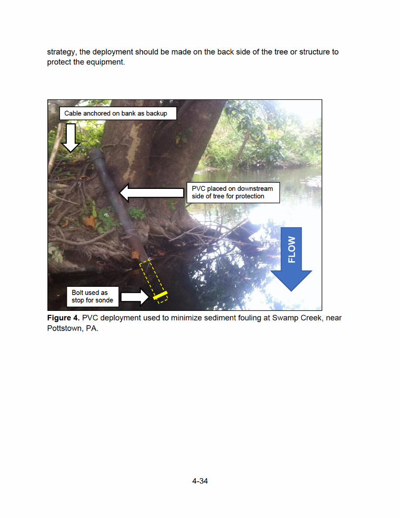


4-37
work is the Celsius scale. Modern thermistors can measure temperature to ± 0.1°C, but
accuracy should be verified with the manufacturer (Wilde 2006).
Specific Conductance
Electrical conductivity is a measure of the capacity of water to conduct an electrical
current and is a function of the types and quantities of dissolved substances in water.
As concentrations of dissolved ions increase, conductivity also increases. Specific
conductance is the temperature specific calculation of conductivity expressed in units of
microsiemens per centimeter (Radtke et al. 2005). DEP’s Water Quality Division
measures and reports specific conductance in microsiemens per centimeter (μS/cm) at
25 °C. Specific conductance measurements can be a good surrogate for total dissolved
solids and total ion concentrations, but there is no universal linear relation between total
dissolved solids (TDS) and specific conductance. A relation between specific conduc-
tance and constituent concentration must be determined for each site (Radtke et al.
2005). In many circumstances, the amplitude and variability of specific conductance is
not sufficient to predict other constituent concentrations (such as TDS) within the
stream. Therefore, it is important to note that TDS measurements from monitors are
calculated from conductivity and are not always accurate or reliable without further
evaluation of the ion constituents.
Monitoring systems used by DEP usually contain automatic temperature compensation
circuits to compensate specific conductance to 25 °C. This can be verified by checking
the manufacturer’s instruction manual. Most modern sensors are designed to measure
specific conductance in the range of 0–2,000 μS/cm or higher. Specific conductance
sensors are reliable, accurate, and durable but are susceptible to fouling from aquatic
organisms and sediment. Typical accuracy of specific conductance probes in freshwater
is ± 1 μS/cm or 0.5% of reading, whichever is greater.
pH
The pH of a solution is a measure of the effective hydrogen-ion concentration. Solutions
having a pH below 7 are described as acidic, and solutions with a pH greater than 7 are
described as basic or alkaline. Dissolved gases, such as carbon dioxide, hydrogen
sulfide, and ammonia, affect pH. Degasification (for example, loss of carbon dioxide) or
precipitation of a solid phase (for example, calcium carbonate) and other chemical,
physical, and biological reactions may cause the pH of a water sample to change
appreciably soon after sample collection (Ritz and Collins 2008).
The electrometric pH-measurement procedure, using a hydrogen-ion electrode,
commonly is used in continuous water quality pH sensors. A correctly calibrated pH
sensor can accurately measure pH to ± 0.2 pH units; however, the sensor can be

4-38
scratched, broken, or fouled easily. If flow rates are high, the accuracy of the pH
measurement can be affected by streaming-potential effects (Ritz and Collins 2008).
These types of probes typically have a life-span of 1-2 years as the reference solution is
depleted (some manufacturers offer refillable reference solution receptacles to extend
the life of the probe). This life-span is affected by the ionic concentration of the solution
and water in which a probe is stored and deployed. Lower ionic concentrations more
quickly deplete the reference solution. The pH mV readings provide insight to the
current condition of the probe. DEP’s Water Quality Division recommends recording
these values at each calibration. The pH mV values should be within the following
criteria:
• Buffer 7: readings should be -50 to 50 mV, 0 mV is ideal
• Buffer 4: readings should be +165 to +180 mV from the buffer 7 reading
• Buffer 10: readings should be -165 to -180 mV from the buffer 7 reading.
As pH probes age and reach the thresholds listed above, they can become slower to
respond and the data becomes increasingly erratic (Figure 7).
Dissolved Oxygen
Dissolved oxygen of streams is produced by diffusion from atmospheric oxygen and
photosynthetic productivity, and drives chemical reactions within and above the
substrate and is critical for the survival of aquatic organisms. Expected DO
concentrations vary based on temperature and other factors but are generally from 6 to
14 milligrams per liter (mg/L). Dissolved oxygen is also reported as percent saturation,
which will decrease with increasing water temperature, and increase with increasing
atmospheric pressure. Another impact to DO solubility is salinity. Dissolved oxygen
measurements in waters that have specific conductance values >2,000 μS/cm should
be corrected for salinity. Most modern sensors automatically compensate for the effects
of salinity or have manual compensation techniques, but this should be verified by
checking the manufacturer’s instruction manual (Rounds et al. 2013).


4-40
or reducing chemical agent, such as a chemical spill, by metal-rich drainage water, or
by organic-rich waters. Typical accuracy of a membrane-type DO sensor is ± 0.2 mg/L
or 2% of the reading, whichever is greater (within the range 0-20 mg/L).
Turbidity
Turbidity is defined as an expression of the optical properties of a sample that cause
light to be scattered and absorbed rather than transmitted through a sample. Most
turbidity sensors emit light from an LED into the water and measure the light that
scatters or is absorbed by the suspended particles in the water. The sensor response is
related to the wavelength of the incident light and the size, shape, and composition of
the particulate matter in the water. The effect of temperature on turbidity sensors is
minimal, and the software for modern sensors provides temperature compensation.
Sensors that are regularly maintained and calibrated are somewhat error free. Turbidity
sensors should be calibrated directly rather than by comparison with another meter
(Anderson 2005). Turbidity can be reported in several different units depending on what
type of sensor is being used. One common unit of measure is nephelometric turbidity
units (NTU); however, DEP uses sensors that report data in formazin nephelometric
units (FNU), because these sensors use near infra-red light (780-900nm) with a
detection angle of 90°. For the purposes of measuring a calibration solution, turbidity
units are equivalent; however, instruments may not produce equivalent results for
environmental samples, which is why different turbidity units are required. Turbidity
sensors typically have a range of 0–1,000 FNU and an accuracy of ± 0.3 FNU or 2%,
whichever is greater. Some sensors can report values reliably up to about 4,000 FNU.
Water Stage
Most stream monitors employ pressure transducers to measure water stage. The
physical force measured is made up of various factors such as atmospheric pressure,
temperature fluctuations, and water pressure. Pressure transducers convert physical
force into an electronic signal to be calculated into water stage. Most modern stage
sensors will automatically compensate for fluctuations in temperature.
Water stage sensors come in two common forms, non-vented and vented. Non-vented
(absolute) sensors measure both atmospheric pressure and water stage
simultaneously. Resulting data from non-vented sensors require corrections provided by
either a separate barometric pressure monitor or by using barometric data from a near-
by airport/weather station. Vented (gage) sensors employ a vent tube that is open to the
air. As a result, these sensors will automatically compensate for the changes in
atmospheric pressure as long as the vent tube remains unobstructed and dry.
Due to the monitor deployment procedure, DEP generally uses non-vented pressure
sensors to record water stage. A nearby barometric pressure monitor is typically used to

4-41
correct for atmospheric pressure changes. If separate barometric monitors are used,
they should be set to the same sampling interval as the stream monitor to facilitate the
data management process. Both stream monitor and barometric monitor must be
calibrated at the respective monitoring site before logging begins.
When considering the use of a non-vented water stage sensor and a separate
barometric monitor it is important to account for distance (between stream and
barometric monitor) and elevation. DEP’s Water Quality Division generally recommends
that the distance between stream monitor and barometric monitor is not greater than 30
miles. This reduces the potential for barometric correction errors due to localized
weather patterns. As a general rule for Pennsylvania, barometric pressure changes with
elevation at a rate of 1 in-Hg for every 1000 ft. If the elevation difference from stream
monitor to barometric monitor is minimal, then no elevation compensation is needed.
Correcting for barometric pressure using another instrument adds to the total potential
error within the data set. Unless the accuracy of each instrument can be documented,
and verified depth measurements are taken at each maintenance visit, the data must be
dealt with in a qualitative manner.
USE OF FIELD METERS
The three major uses for a field meter during servicing of a continuous water quality
monitor are (1) as a general check of reasonableness of monitor readings, (2) as an
independent check of environmental changes during the service interval, and (3) to
make cross-section surveys or vertical profiles in order to verify the representativeness
of the location of the sonde in the aquatic environment. Data collected by the field meter
should not be used to calibrate the instream monitor. However, some instream monitors
cannot be calibrated, in which case the calibrated field meter must be used in the
calibration correction of monitor records. In addition, DEP may use a calibrated field
meter measurement for undocumented data error corrections (a potential result from the
DEP deployment procedure, discussed in detail later). Independent field measurements
must be made before, during, and after servicing the monitor in order to document
environmental changes during the service. Side-by-side measurements between the
field meter and the monitor are made by placing the calibrated field meter as close to
the monitor sensors as possible. The field meter should refresh data on the display at
10 second intervals, or more frequently, to ensure the most accurate data are recorded
during measurements.
Before site visits, all field meters should be checked for operation and accuracy.
Minimum calibration frequency should be once per day in the field. Recalibration will be
necessary when a sensor is replaced, and during dramatic changes in elevation or

4-42
barometric pressure. Calibrations must be recorded in instrument log sheets. The Field
Meter Calibration Form is provided in Appendix B.1. DEP recommends that all sensors
are calibrated in accordance with manufacturer’s specifications. Additional tips and
guidance on field meter use are provided in Hoger (2020).
MONITOR OPERATION AND MAINTENANCE
The objective during continuous instream monitoring is to obtain the most accurate and
complete record possible. The common operational categories include maintenance
frequency, field visits, troubleshooting, and comprehensive record keeping.
This instream monitoring protocol details one operating procedure designed for well-
mixed, stable, and relativity slow changing systems. Slowly changing is defined as
changes in field measurements during maintenance that are less than the calibration
criteria (see Sensor Field Calibration). The wadeable streams of Pennsylvania generally
fall into this category.
Field Notes and Instrument Logs
Logs and field notes are essential for accurate and efficient record processing.
Operation and maintenance records are maintained in an electronic spreadsheet similar
to the USGS standard field form for water quality monitors in Wagner et al. (2006). A
copy of the spreadsheet is available upon request. The deployment and maintenance
visit field forms from the spreadsheet are provided in Appendices B.5 and B.6,
respectively. Field-note requirements for instream monitors include:
1. Station name
2. Date and time of measurements
3. Name(s) of data collector(s)
4. Serial number of field meters and monitor
5. Lot numbers and expiration of dates of standard solutions
6. Location description and picture of monitor in the stream
7. Name of file downloaded from the monitor
8. Monitor values, field meter values, and corresponding time for cleaning checks
(for fouling), calibration checks, calibrations/recalibrations, and final readings
9. Battery voltage of monitor at departure and if the batteries were replaced, name
of new file, and start time of logging
10. Notes on sensor/monitor changes or replacements, and other comments that
facilitate processing of the record
11. Cross-section survey data (locations of points, measured values, and corresponding times), and monitor values before and after the cross-section survey (Hoger 2020)
4-43
12. Measured flow or gage-height data.
Logging Interval and Settings
Most monitors can be set for a wide range of recording intervals. The interval used
should account for the expected rate of change in the water quality parameters being
measured. In most streams in Pennsylvania, a 30-minute interval adequately captures
changes and therefore is the most common interval used by DEP. “Flashy” streams,
that are high gradient or have a significant amount of impervious cover in the
watershed, change more rapidly and may necessitate a 15-minute interval. When
recording turbidity, many prefer to have the additional data points of a 15-minute interval
so that the curves of storm events are better represented. A five-minute interval has
even been used for a deployment directly downstream of a point-source discharge to
capture its short, concentrated discharges. When deploying the monitor independently,
however, battery life can be an important consideration and may necessitate a longer
interval or a unit with greater battery capacity.
To avoid confusion when comparing continuous data and discrete samples, DEP does
not recognize daylight saving time when working with its continuous data. All sondes
are set to record in EST (UTC-05:00) and all associated measurements, such as
discretes, should be recorded in the same manner to avoid confusion.
Setting the monitor to log is different with each unit, so follow the manufacturer’s
instructions. When setting the monitor to log, make note of the interval, name of the file,
battery life, and start time. If possible, DEP recommends delaying the start time by at
least one hour to allow the monitor plenty of time to stabilize. It is also recommended
that the battery voltage parameter is set to record throughout the deployment to aid in
determination of battery life. Finally, employing a consistent naming convention (e.g.,
Newport_1, Newport_2, etc.) can aid in the organization and uploading of files later.
Maintenance Frequency
DEP Water Quality Division monitors are typically placed at a station for approximately
one year and revisited 10-12 times during the deployment. However, maintenance
frequency will generally depend on fouling rate of the sensors, which varies by sensor
type, environmental conditions, and season. The performance of water temperature,
specific conductance, and water stage sensors tends to be less affected by fouling than
DO, pH, and turbidity sensors. Wiper mechanisms on turbidity and optical DO sensors
can substantially decrease fouling in certain aquatic environments. Monitoring sites with
nutrient-enriched waters and moderate to high temperatures may require more frequent
maintenance. In cases of severe environmental fouling or in remote locations, the use of
an observer (e.g., landowner, volunteer, or local watershed group) to provide more

4-44
frequent maintenance to the water quality monitor should be considered. Monitoring
disruptions as a result of equipment malfunction, sedimentation, electrical disruption,
debris, ice, or vandalism also may require additional site visits.
Field Visits
Field visits are undoubtedly the most important step in certifying that quality data are
being recorded. The purpose of field visits is to verify that a sensor is working
accurately, upload recorded data, confirm calibrations, and provide a reference point for
subsequent data management. Quality assurance is accomplished by recording field
fouling observations before and after cleaning sensor readings in the environment,
calibration checks, and final readings. It is important to conduct field checks at, or close
to, the monitor’s deployment location to record checks that best represent stream
conditions recorded by the monitor. To prevent complications from freezing, caution
should be exercised when performing maintenance at temperatures below 0˚C, and
maintenance should be avoided at temperatures below -7°C or 20˚F.
The standard protocol for servicing instream monitors is described below:
1. Obtain a discrete measurement from a clean, calibrated field meter at the sonde
location
2. Remove sonde from the monitoring location being careful to minimize
disturbance
3. Connect monitor to field instrument (i.e., computer or handheld device)
a. If monitor is to be submerged during read-out, ensure the cable is
designed to operate under water
b. Stop unattened monitoring
c. Upload data
d. Do a quick review of data to detect any data abnormalities or defects in probes
e. Record any significant fouling observed during monitor removal
4. Conduct before-cleaning, initial monitor inspection
a. Record time, readings, and monitor conditions
b. With an independent field meter, record instream readings and time near
the monitor
5. Clean sensors (see Sensor Field Cleaning)
6. Return sonde to the stream and conduct after-cleaning monitor inspection
a. Record monitor readings and time
b. Using an independent field meter, record instream readings near the
monitor
7. Remove sonde, and check calibration (see Sensor Field Calibration)
a. Record calibration-check values
4-45
b. Recalibrate if necessary
8. Conduct final readings
a. Record monitor readings and time
b. Using an independent field meter, observe and record readings near the
monitor
9. Restart unattended sampling with appropriate logging interval, start time, and file
name
a. DEP recommends a delay start time of 1-2 hours to allow equipment to
acclimate following disturbance of the site
b. Check monitor’s battery levels, change if necessary
10. Return sonde to monitoring location and inspect anchoring equipment and
shroud for deterioration and damage.
The initial monitor readings during a field visit may not accurately represent the
recording conditions because of disturbance while retrieving and connecting the
monitor. Care should be taken to minimize disturbance and placement of the monitor
during retrieval, and the field meter should be upstream of any disturbed area. If
observed, significant fouling should be noted in the field sheet. Monitors and field
meters should be given ample time to stabilize before readings are recorded. During
extreme conditions (extreme cold/heat, early morning, etc.) monitors and field meters
may require more time to stabilize.
Comparison of the initial monitor and field meter readings provides a sense of the
reasonableness of the recorded data and an indication of any potential errors. The
disturbance of a stand-alone monitor during retrieval can prevent the capture of a true
fouling error, so care should be taken to minimize this disturbance as much as possible.
The difference between the last recorded value on the deployed monitor and the initial
reading after retrieval helps establish any effects of disturbance during the monitor
retrieval, and can be used to calculate what is then referred to as undocumented fouling
(described in further detail in Data Correction). A monitor that is connected to an
external recording device can typically be accessed for initial side-by-side readings
without disturbance—eliminating the potential for undocumented fouling error.
After initial sensor readings, the monitor’s sensors are inspected for signs of fouling.
These observations are recorded in the field notes before cleaning, and then individual
sensors are cleaned according to the manufacturer’s specifications. The monitor is then
returned to the water. Cleaned sensor readings, field meter readings, and times are
recorded in the field notes. If the conditions are steady state, the field meter readings
should not change substantially during the time that the monitoring sensors are cleaned.
The observed difference between the initial sensor reading and the cleaned-sensor
4-46
reading is a result of fouling (chemical precipitates, stains, siltation, or biological
growths).
After cleaned-sensor readings are recorded, the monitor is removed from the water,
calibration is checked in calibration standard solutions, and the readings are recorded.
Differences between the cleaned-sensor readings in calibration standard solutions and
the expected reading in these solutions are the result of calibration error (drift). The
sonde is recalibrated if necessary, and replaced in the aquatic environment for a final
reading.
The set of final readings may not necessarily accurately represent the start of the new
record period due to site disturbance. Care should be taken to minimize disturbance
and placement of the monitor and field meters should be upstream of any disturbed
area. Monitors and field meters should be given ample time to stabilize before readings
are recorded. Final sensor readings should be used in conjunction with the first data
record recorded to determine any affect disturbance may have had on final sensor
readings, field meter readings, and data collected as part of the new record period.
Sensor Field Cleaning
During the cleaning process, care should be taken to ensure that the electrical
connections are kept clean and dry. Water on the connector pins can cause erratic
readings. For this reason, a container of compressed air is useful. Procedures for
cleaning specific sensors, as described below, are general guidelines and should not
replace manufacturer’s instructions. Most commercial thermistors can be cleaned with a
soft-bristle brush and rinsed with deionized water (Wilde 2004).
Rinse specific conductance sensors thoroughly with de-ionized water before and after
making a measurement. Oily residue or other chemical residues (salts) can be removed
by using a detergent solution. Specific conductance sensors can soak in detergent
solution for many hours without damage. Carbon and stainless-steel sensors can be
cleaned with a soft brush, but platinum-coated sensors should never be cleaned with a
brush (Radtke et al. 2005). Platinum-coated sensors may be cleaned with a cotton
swab.
The pH electrode must be kept clean in order to produce accurate pH values. The body
of the electrode should be thoroughly rinsed with de-ionized water before and after use.
In general, this is the only routine cleaning needed for pH electrodes; however, in cases
of extreme fouling or contamination, the manufacturer’s cleaning instructions must be
followed (Ritz and Collins 2008).
4-47
Optical DO sensors are cleaned with a soft bristle brush and rinsed with deionized
water. If the optical DO sensor is equipped with a wiper, ensure the motor is operating
properly and parking in the correct position. Also, ensure that the wiping mechanism
(pad or brush) is in good condition and clean. The black membrane is sometimes
scratched off by coarse debris caught in the wiper. The membrane should be replaced if
over half of the surface has been worn off.
Routine cleaning of polarographic DO sensors involves using a soft-bristle brush to
remove silt from the outside of the sensor, wiping the membrane with a damp, lint-free
cotton swab (available at local electronics stores), and rinsing with de-ionized water.
The sensor usually is covered with a permeable membrane and filled with a potassium
chloride solution. The membrane is fouled easily and typically will need to be replaced
every 2 to 4 weeks. When the membrane is replaced, the potassium chloride solution
must be rinsed out of the sensor with de-ionized water followed by several rinses with
potassium chloride solution before the sensor is refilled. The membrane must be
replaced with care so that the surface of the membrane is not damaged or
contaminated with grease, and no bubbles are trapped beneath the membrane. The
surface of the membrane should be smooth, and the membrane should be secured
tightly with the retaining ring. The sensor must be stored in water for a minimum of 2 to
4 hours, preferably longer, to relax the membrane before installation and calibration.
Because of the time required to relax the membrane, replacement of a membrane
during a field visit would require having a pre-relaxed membrane on hand to allow for
immediate calibration, otherwise it would be necessary to revisit the site after replacing
the membrane waiting the required amount of time before calibration. The retaining ring
must be replaced annually or more frequently to prevent loss of electrolytes. Replacing
the retaining ring when membranes are changed ensures a tight seal.
The gold cathode of the DO sensor also can be fouled with silver over an extended
period of time, and a special abrasive tool usually is required to recondition the sensor.
A fouled anode, usually indicated by the white silver electrode turning gray or black, can
prevent successful calibration. As with the cathode, the sensor anode usually can be
reconditioned following the manufacturer’s instructions. Following reconditioning, the
sensor cup must be rinsed, refilled with fresh potassium chloride solution, and a new
membrane installed (Rounds et al. 2013).
Turbidity sensors are extremely susceptible to fouling; thus, frequent maintenance trips
may be necessary to prevent fouling of the turbidity sensor in a benthic environment
high in fine sediment, algae accumulation, or other biological or chemical debris. In
environments that cause severe algal fouling, however, algae can accumulate on the
wiper pad preventing complete removal of debris from the optical lens, resulting in

4-48
erratic turbidity data. If the turbidity sensor is not equipped with a mechanical cleaning
device that removes solids accumulation or a shutter that prevents accumulation on the
lens before readings are recorded, reliable data collection is very difficult. Sensors first
should be inspected for damage, ensuring that the optical surfaces of the probe are in
good condition. The wiper pad or other cleaning device should be inspected for wear
and cleaned or replaced if necessary. Before placing the turbidity sensor in standards,
the optic lens should be carefully cleaned with alcohol by using a soft cloth to prevent
scratching (or as recommended by the manufacturer), rinsed three times with turbidity-
free water, and carefully dried. If the readings are unusually high or erratic during the
sensor inspection, entrained air bubbles may be present on the optic lens and must be
removed (Anderson 2005).
Sensor Field Calibration
Calibration should only be performed with standards of known quality. All calibrations
and calibration checks should be completed with at least two standard solutions. At a
minimum, these standard solutions should bracket the entire range of recorded values.
An additional standard may be necessary that is proximate to expected environmental
conditions to insure linearity of sensor response. Frequently used standards are
described for each parameter below.
Field calibration is performed if the cleaned-sensor readings obtained during the
calibration check differ by more than the calibration criteria (Table 1). Spare monitoring
sondes or sensors are used to replace water quality monitors that fail calibration after
troubleshooting steps have been applied (see Troubleshooting Procedures). All
calibration equipment and supplies must be kept clean, stored in protective cases
during transportation, and protected from extreme temperatures.
The following example is helpful for understanding the calibration criteria given in Table
1. The calibration criterion for specific conductance is 5 µS/cm or 3%, whichever is
greater. Therefore, if a sonde is in 1000 µS/cm standard and reported a reading of 1025
µS/cm the reading would still be within the calibration criteria because 3% of 1000
µS/cm (30 µS/cm) is greater than 5 µS/cm. For a calibration check in 100 µS/cm
standard the criteria would be 5 µS/cm, because 5 µS/cm is greater than 3% of 100
µS/cm. Sensors with readings outside of criteria will be recalibrated during the field
visits. Best professional judgment should be used with values that read close to
calibration criteria. Data management is often facilitated by eliminating unnecessary
calibration events.
4-49
Table 1. Calibration criteria for measured parameters.
Field Parameter Calibration Criteria
Temperature ± 0.2°C
Specific Conductance ± 5 µS/cm or 3%, whichever is greater
pH ± 0.2 units
Dissolved Oxygen ± 0.3 mg/L
Turbidity ± 0.5 FNU or ± 5%, whichever is greater
Using Standard Solutions
Expiration dates and lot numbers for the standard solutions must be recorded and
sufficient time provided for the sensor to stabilize in the solution. After the readings in
the calibration standard solutions are checked and recorded (without making any
adjustments), the monitor is recalibrated, if necessary, using the appropriate calibration
standard solutions and following the manufacturer’s calibration procedures. When using
standard solutions, the process for both field checks and calibration are the same. The
sensor, thermistor, and measuring container must be rinsed three times with a standard
solution. Gentle tapping will ensure that no air bubbles are trapped in or on the sensor.
After the series of rinses, fresh standard solution is poured into the calibration cup
ensuring both the thermistor and the sensor are submerged; the sensor values,
calibration standard values, and temperature are recorded in the field log sheet. A
temperature correction may be necessary if the monitor does not have automatic
temperature correction. Standard solution that has been used is discarded. If an error
arises during calibration, see manufacturer’s guidelines or reference Troubleshooting
Procedures below. If these steps fail, the sonde or monitoring sensor must be replaced
and the backup instrument calibrated.
Water Temperature Sensors
Manufacturers generally make no provisions for field calibration of water temperature
sensors, but sensors can be periodically NIST certified to ensure accuracy. The water
temperature sensor and the calibrated field thermistor are placed adjacent to each
other, preferably in flowing water. Sufficient time for temperature equilibration must
elapse before a reading is made. The two water temperature sensors must be read and
recorded simultaneously. If the monitoring water temperature sensor fails to agree
within ± 0.2 °C, troubleshooting steps must be taken; if troubleshooting fails, the sensor
must be replaced, as calibration is not possible.
Specific Conductance Sensors
Specific conductance sensors should be checked with at least two calibration standard
solutions of known quality before any adjustments are made. Most frequently, the two

4-50
checks are 100 µS/cm and 1000 µS/cm, however, if stream conditions are likely to be
greater than 1000 µS/cm, a 5000 µS/cm standard is also used to ensure the measured
values are within the limits of the standards used. In addition, the zero response of the
dry sensor in air should be checked and recorded to ensure linearity of sensor response
at low values. If the sensor-cleaning process fails to bring a specific conductance
sensor within the calibration criteria (Table 1), the sensor must be recalibrated.
Calibration of a specific conductance sensor is a single point calibration. The high
standard should be used for the calibration (often 1000 µS/cm but 5000 µS/cm could be
necessary in some streams) and a lower standard, nearer the ambient conditions (often
100 µS/cm), is used as an intermediate check of linearity after calibration.
pH Sensors
DEP’s Water Quality Division uses three buffers (4, 7, 10) to first check and then, if
necessary, recalibrate pH sensors; this ensures all likely field conditions are bracketed.
It is also necessary during checks and calibration to account for deviations from the
listed pH value of the buffers at different temperatures. The listed value of the buffer is
the pH at a specific temperature (typically 25 C). The manufacturer of the buffer
solution should offer a table of expected values at other temperatures. While these
tables are very similar across major manufacturers, it is important that tables specific to
the manufacturer are used to account for any differences. The tables are often provided
at five-degree increments; however, particularly with the 10 buffer, the five-degree
interval results in significant jumps in the adjusted pH values. To fill these gaps,
regression lines can be fitted to the provided data points. An example table of
temperature adjusted pH values and the steps to create the more specific table values
are provided in Appendix B.7.
Expiration dates of the buffer solutions are checked and recorded. The pH mV readings
in each buffer should also be recorded to track the performance of the sensor (see
Sensor Selection for more information). Spare pH sensors or entire backup monitors are
carried in case replacement of the sensor is required.
Dissolved Oxygen Sensors
Dissolved oxygen in water is related to water temperature, atmospheric pressure, and
salinity. Calibration of optical DO sensors should be checked at 100% saturation and
with a fresh zero-DO solution before any adjustments are made. The manufacturer’s
calibration procedures must be followed closely to achieve a calibrated accuracy of ±
0.1 mg/L concentration of DO (Rounds et al. 2013). Theoretical charts based on water
temperature and barometric pressure should be used to confirm calibration of monitors.
A general 100% saturation chart for fresh water is provided in Appendix B.8.
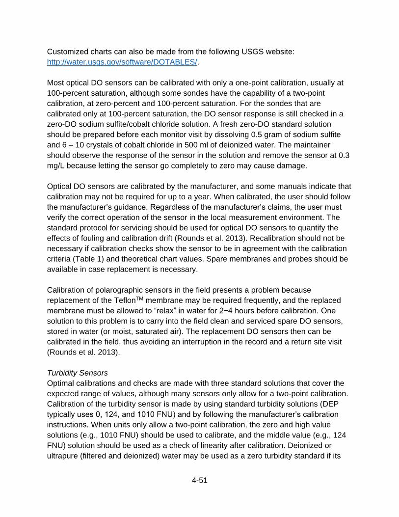
4-51
Customized charts can also be made from the following USGS website:
http://water.usgs.gov/software/DOTABLES/.
Most optical DO sensors can be calibrated with only a one-point calibration, usually at
100-percent saturation, although some sondes have the capability of a two-point
calibration, at zero-percent and 100-percent saturation. For the sondes that are
calibrated only at 100-percent saturation, the DO sensor response is still checked in a
zero-DO sodium sulfite/cobalt chloride solution. A fresh zero-DO standard solution
should be prepared before each monitor visit by dissolving 0.5 gram of sodium sulfite
and 6 – 10 crystals of cobalt chloride in 500 ml of deionized water. The maintainer
should observe the response of the sensor in the solution and remove the sensor at 0.3
mg/L because letting the sensor go completely to zero may cause damage.
Optical DO sensors are calibrated by the manufacturer, and some manuals indicate that
calibration may not be required for up to a year. When calibrated, the user should follow
the manufacturer’s guidance. Regardless of the manufacturer’s claims, the user must
verify the correct operation of the sensor in the local measurement environment. The
standard protocol for servicing should be used for optical DO sensors to quantify the
effects of fouling and calibration drift (Rounds et al. 2013). Recalibration should not be
necessary if calibration checks show the sensor to be in agreement with the calibration
criteria (Table 1) and theoretical chart values. Spare membranes and probes should be
available in case replacement is necessary.
Calibration of polarographic sensors in the field presents a problem because
replacement of the TeflonTM membrane may be required frequently, and the replaced
membrane must be allowed to “relax” in water for 2−4 hours before calibration. One
solution to this problem is to carry into the field clean and serviced spare DO sensors,
stored in water (or moist, saturated air). The replacement DO sensors then can be
calibrated in the field, thus avoiding an interruption in the record and a return site visit
(Rounds et al. 2013).
Turbidity Sensors
Optimal calibrations and checks are made with three standard solutions that cover the
expected range of values, although many sensors only allow for a two-point calibration.
Calibration of the turbidity sensor is made by using standard turbidity solutions (DEP
typically uses 0, 124, and 1010 FNU) and by following the manufacturer’s calibration
instructions. When units only allow a two-point calibration, the zero and high value
solutions (e.g., 1010 FNU) should be used to calibrate, and the middle value (e.g., 124
FNU) solution should be used as a check of linearity after calibration. Deionized or
ultrapure (filtered and deionized) water may be used as a zero turbidity standard if its

4-52
turbidity is measured by a laboratory. Laboratory measurements are necessary because
deionized or ultrapure turbidity can measure as high as 1.0 FNU. The measured
turbidity from the laboratory can be set as an offset calibration in the monitor, or the
data can be offset corrected later in data management. Checking or calibrating the
turbidity sensor should occur in a stable environment with minimal movement, wind, or
exposure to sunlight. Sufficient space between the sensor and the bottom of the
calibration cup is also critical during checks and calibration. Calibration in zero standard
is best performed with the sensor guard in place to simulate conditions when deployed.
Bubbles in the solution can interfere with readings so care should be taken to minimize
bubbles when pouring. Running the wiper before each reading or calibration in each
solution will help remove any remaining bubbles.
When using polymer-based turbidity standards, it is important to understand that
different sensors often read the solution differently. Even different model sensors from
the same manufacturer will likely not read a given turbidity standard the same.
Therefore, only polymer-based solutions with documentation for the specific sensor
should be used. In most cases this means that genuine manufacturer solution is
necessary, as standards from other manufacturers lack the necessary documentation –
making proper calibration impossible. Currently, the only alternative is Formazin
turbidity standard. Formazin turbidity standard has the benefit of being read the same
by all sensors, but it is considered moderately toxic, contains a known carcinogen, and
is more difficult to work. Therefore, DEP recommends using polymer-based turbidity
standard—with the proper, sensor-specific documentation—whenever possible.
Water Stage Sensors
Water stage calibration procedures vary slightly with manufacturer, so DEP
recommends following manufacture’s recommendations. When calibrating water stage
for deployment, it is important to calibrate at the monitoring location. Most non-vented
sensors will calibrate to a depth of zero in the air. This accounts for the elevation and
atmospheric pressure at the monitoring site. Since there is no change in elevation
during deployment and most pressure transducers automatically compensate for water
temperature, the only corrections needed are changes in barometric pressure (see
Calculated Derived Series).
In locations where an immobile reference cannot be found, a staff plate or form/rebar
stake may be employed (Figure 8). A staff plate or stake that is driven into the stream
bed provides a point of reference for consistent manual stage measurements which can
be compared to monitor recordings at the time of a field visit. Staff plate or stake
measurements may serve as verified discrete data for subsequent data management
purposes.
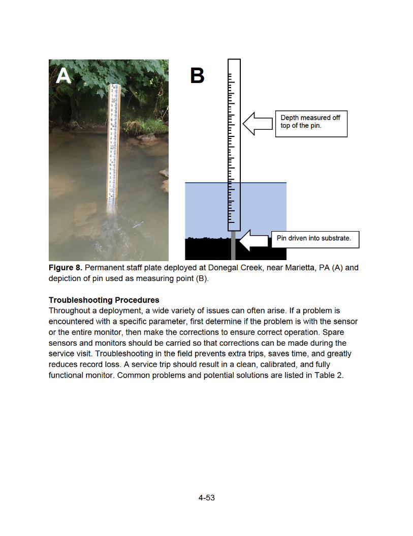

4-54
Table 2. Troubleshooting procedures for common issues encountered in the field.
Symptom Possible Issue Likely Solution
Water Temperature
Thermistor is not reading
accurately
Dirty sensor Clean sensor
Erratic readings Poor or wet connection Dry and tighten connection
Slow to stabilize Dirty sensor Clean sensor
Reading off scale Failure in electronics Replace sensor or monitor
Specific Conductance
Will not calibrate Standard solution old or
contaminated
Use fresh standard solution
Electrodes dirty Clean with brush
Air trapped around sensor Tap gently to expel air
Weak batteries Replace batteries
Erratic readings Poor or wet connection Dry and tighten connection
Requires frequent
calibration
Broken cables Replace cables
Replace monitor
pH
Will not calibrate Standard solution old or
contaminated
Use fresh standard solution
Faulty Sensor Replace sensor
Erratic readings Poor or wet connection Dry and tighten connection
Defective sensor Replace sensor
Slow response time Dirty sensor bulb Clean sensor
Water is cold or of low ionic strength Be patient
Dissolved Oxygen
Will not calibrate Membrane damaged Replace membrane
Electrolyte diluted Replace membrane and electrolyte
Erratic readings Poor or wet connection Dry and tighten connection
Fouled sensor Check for obstructions or replace
Slow to stabilize Gold cathode tarnished Buff with eraser or recondition sensor
Fouled membrane Replace membrane and recondition
Silver anode corroded Replace sensor and soak fouled
sensor in 3% ammonia for 24 hours
Will not zero Zero DO solution contains oxygen Add additional sodium
Zero DO solution is old Mix fresh solution
Turbidity
Unusually high or erratic
readings
Entrained air bubbles on the sensor Gently tap or run wipe cycle
Damaged Sensor Replace sensor
Dirty sensor Clean, using soft brush
Poor or wet connection Dry and tighten connection

4-55
DATA MANAGEMENT
The data management process verifies data, corrects for errors, and sets a grade based
on overall quality of the record. Accurate and concise field notes and logs are
indispensable in processing collected data. The steps in processing data records are:
initial data evaluation, data import, data corrections, grading, and final approval. Data
Management should begin when the record is uploaded in the field to ensure the
equipment is operating properly. Data management is not complete until the monitor is
pulled from the stream, data is graded and approved, and a final Continuous Instream
Monitoring Report (CIMR) is written, reviewed, and approved by DEP staff. DEP uses
Aquarius software (current version: 3.10) from Aquatic Informatics for all data
management. This protocol will cover basic operation of the Aquarius software for data
management purposes. Two interfaces in Aquarius software aid in data management,
Whiteboard and Springboard. This protocol focuses on data management within the
Aquarius Springboard application, a more user-friendly environment than Aquarius
Whiteboard. Additional training and support can be found at:
http://www.aquaticinformatics.com/support.
Initial Data Evaluation
The initial data evaluation is conducted both in the field and back in the office to verify
the accuracy of data transfer to the database, to identify erroneous data, and to confirm
the monitor is operating as expected. Once data are uploaded from the monitor, they
should be quickly reviewed to identify any inconsistencies. Ideally the manufacturer’s
software will allow the data to be displayed visually. This will allow for a quick
determination of the reasonableness of the data including expected range, identification
of erratic readings, and/or presence of expected behavior like diel swings or response to
changes in flow. Various formats are available to store raw field data. Data formatting
will typically depend on the make of the monitor used.
Data Import
Creating New Stations
Data are organized in a cascading folder structure. Stations are organized by internal
(to DEP) or external data, basin, HUC, stream name, and finally a specific location.
Stations are considered unique if they could represent different water quality conditions.
The two main considerations are cross-sectional variability and distance upstream or
downstream. If cross-sectional surveys demonstrate variations in water quality, DEP
may deploy monitors in multiple locations horizontally across the stream; In Aquarius,
each are considered unique stations. Deployments >100 m apart upstream or
downstream are considered unique stations, however, deployments separated by
shorter distances may be considered unique if conditions warrant. Most deployments by

4-56
DEP are in relatively shallow, lotic systems; therefore, vertical variations within the
water column are often not an issue. If introduced, this variable should also be
considered in creating a new station.
Before data can be uploaded to the database server, a station with the appropriate time
series needs to be created. To create a new station first navigate to the correct stream
in the folder structure. If the stream or HUC folders are missing, they first need to be
created. To create the location either right-click on the stream folder and select “New
Location” or highlight the stream folder and click the Location Manager button on the
toolbar. Under the General tab, the following fields need to be populated:
o Identifier: This is a unique number consisting of the ComID from the
NHDFlowline the station is on, followed by a unique identifier. If the ComID of the
NHDFlowline was 57465467 the Identifier of the first site on that segment would
be 57465467-001. If another station is located on that segment at the same time
or in the future, its Identifier would be 57465467-002, etc.
o Name: The name should include both the stream name and a short description
of the location such as a road crossing (e.g., Little Beaver Creek at Little Beaver
Rd). Including the stream name allows for better search results when using
Aquarius. The short location description should be descriptive enough that
anyone can understand its general location.
o Type: Water Quality Site
o Description: Additional information can be added here such as a more thorough
description of the location, whether the location is part of a specific study, etc.
o Latitude: Decimal degree format
o Longitude: Decimal degree format
o Elevation: Required in Aquarius when using latitude/longitude
o Time Zone: DEP does not recognize daylight saving time when working with its
continuous data; therefore, this should be set to EST (UTC-05:00) for all internal
data.
Under the Data Sets tab, create a “Time Series – Basic” for each continuous parameter
to be stored in the database. Field Visit (discrete) Time Series do not need to be
created in advance; they will be auto-generated when data are input. For each basic
time series created, the following fields need to be populated (description and comment
fields are optional):
• Identifier: This field is auto-populated using the location identifier created in the
general tab, the label name created next, and the parameter selected.

4-57
• Label: Short description of the site (often just the stream name or the stream
name and crossing or nearby town). No spaces, capitalize first letter of each
word.
• Parameter: Use the “…” button to search for a parameter if not in the recently
used parameters in the drop-down box. For temperature, use “Water
Temperature” not “Temperature”. There are many options for turbidity, “Water
Turbidity” is the standard parameter used by DEP. Depth should be entered
under “Stage”.
• Units: Select the appropriate units.
• Time Zone: EST (UTC-05:00).
• Gap Tolerance: If time between readings is greater than the value set in this
box, Aquarius implies a gap and the points are not connected. Set this value to
one minute greater than the recording interval (e.g., if interval is 30 minutes Gap
Tolerance should be 31).
Uploading Data
Data can be brought into Aquarius from multiple formats. The most common file type is
a delimited text file such as “.csv”; however, Aquarius will recognize some
manufacturer-specific files (e.g., YSI’s “.dat” file). To upload data, navigate to the site
location in Springboard and then select the “Append to Logger” icon . This tool allows
for the manual uploading of data and the setup of hot folders, an automated upload
process. In the Append to Logger toolbox, first select the file for upload. The second
step is to tell Aquarius how to interpret the file. If a configuration file has already been
created, select it and click the “Load File” button. (Note that configuration files can be
used for different sites as long as the formatting of the files is identical [i.e., headers,
parameters, parameter order, etc.]) If a configuration file has not been created, it will be
necessary to use the configuration toolbox by clicking “Config Settings…”.
Config File Setup
1. Select file type: will most likely be “Text File (CSV, etc)”. Click Next.
2. Make sure the proper delimiter is selected and establish the row to start import
and number of headers. The number of headers used is not important but it is
helpful to include enough to see what the parameter is for the next step. If done
correctly, data will be broken into appropriate columns, header rows will be gray,
and data rows will be white (Figure 9). Click Next.
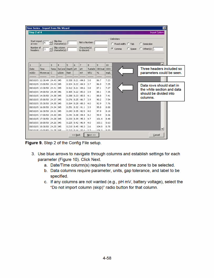


4-62
To add additional file type parsers within the hot folder, go through the same process in
the Append toolbox as above. Once the parameter has been designated for a specific
parameter, an Add to Hot Folder button will appear. This process will be identical to the
first time around, just specify a description and a filename filter. To change any of these
specifications later, go through the same process in the Append toolbox and select the
Manage Hot Folder button that will appear.
Important Notes Regarding Hot Folders
• Consistency of the naming of files and the layout of the content within the files
themselves is imperative; therefore:
o Give files a consistent name for each site (e.g., Newport1, Newport2, etc.)
o Do not edit the content of files before uploading. While technically this is
not an issue, the edited files are more likely to be inconsistent than the
original, equipment-generated file. Therefore, do not edit or clean up
headers, move columns, etc.
o Do not edit the parameters during deployment. This means do not add or
delete parameters or in the case of Eureka sondes, do not change the
order of display. This would in turn change the layout of the data file, so
the Config File will need updated.
o If the recording sonde is changed, it may be necessary to update the
Config File unless the data files are formatted in the same way.
• The Config File that is associated with the hot folder is copied and stored
elsewhere once the association is made. This means that after making any edits
to a Config File in the Append window, the file must be reassociated to the hot
folder.
Entering Discrete Data
Discrete data are stored as Field Visits in Aquarius. With the site selected, click the
Field Visit icon . Select New from the toolbar, and choose Field Visit. Enter the date
and time of the discrete reading. Make sure the new Field Visit is highlighted in the left
column, select New from the toolbar again, and choose Measurement Activity. Click the
green circle with a white plus sign to add a parameter. In the Parameter column, select
a recent parameter from the drop-down menu by clicking the magnifying glass to find a
parameter. Make sure to choose the exact parameter as established for the continuous
data sets. Enter the reading in the Value column and confirm the units in the next
column are correct. Continue adding parameters until all discrete data are entered
(Figure 13). After entering the last value, be sure to click outside the box before clicking
Save.


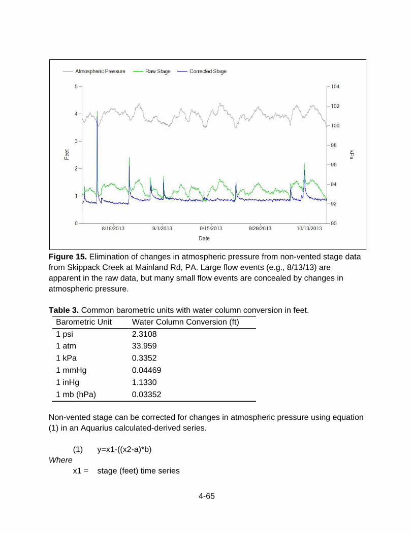
4-65
Figure 15. Elimination of changes in atmospheric pressure from non-vented stage data
from Skippack Creek at Mainland Rd, PA. Large flow events (e.g., 8/13/13) are
apparent in the raw data, but many small flow events are concealed by changes in
atmospheric pressure.
Table 3. Common barometric units with water column conversion in feet.
Barometric Unit Water Column Conversion (ft)
1 psi 2.3108
1 atm 33.959
1 kPa 0.3352
1 mmHg 0.04469
1 inHg 1.1330
1 mb (hPa) 0.03352
Non-vented stage can be corrected for changes in atmospheric pressure using equation
(1) in an Aquarius calculated-derived series.
(1) y=x1-((x2-a)*b)
Where
x1 = stage (feet) time series

4-66
x2 = atmospheric pressure time series
a = first reading from the atmospheric pressure data file (only subtract the
changes in atmospheric pressure)
b = conversion factor from Table 3 for atmospheric pressure series x2
Other DEP applications of the calculated-derived series have included conversion of
conductivity data to specific conductance and the generation of continuous ammonia
criteria using the acute and chronic formulas from Chapter 93 water quality criteria.
Conductivity can be converted to specific conductance at 25C using equation (2),
assuming a temperature coefficient of 0.0191. This is the standard coefficient used by
YSI water quality instruments.
(2) y=x1/(1+(0.0191*(x2-25)))
Where
x1 = conductivity time series
x2 = temperature time series (C)
Formulas for ammonia criteria from PA §93.7(a), Table 3 have been converted into
equations for acute (3) and chronic (4) criteria time series. These time series are
generated to establish continuous ammonia criteria thresholds and identify critical time
periods. This analysis saves time and money by focusing collection of ammonia grab
samples during these critical periods.
(3) if (x2<10) {
y=0.12*(((1+pow(10,(9.73-x1)))/(1+pow(10,((0.09+(2730/(x2+
273.2)))-x1))))/(1+pow(10,(1.03*(7.32-x1)))))*((pow(10,((0.09+
(2730/(x2+273.2)))-x1)))+1);
}
else {
y=0.12*(1/(1+pow(10,(1.03*(7.32-x1)))))*((pow(10,((0.09+(2730/
(x2+273.2)))-x1)))+1);
}
(4) if (x2<10) {
if (x1<7.7) {y=0.025*(((1+pow(10,(9.73-x1)))/(1+pow(10,((0.09+
(2730/(x2+273.2)))-x1))))/(pow(10,(0.74*(7.7-x1)))))*((pow(10,
((0.09+(2730/(x2+273.2)))-x1)))+1);
}
else {
y=0.025*(((1+pow(10,(9.73-x1)))/(1+pow(10,((0.09+(2730/(x2+

4-67
273.2)))-x1))))/1)*((pow(10,((0.09+(2730/(x2+273.2)))-x1)))+1);
}
}
else {
if (x1<7.7) {
y=0.025*(1/(pow(10,(0.74*(7.7-x1)))))*((pow(10,((0.09+(2730/(x2+
273.2)))-x1)))+1);
}
else {
y=0.025*((pow(10,((0.09+(2730/(x2+273.2)))-x1)))+1);
}
}
Where
x1 = pH time series
x2 = temperature time series (C)
DATA EVALUATION
Systematic adoption of a standardized data-evaluation process, including rating criteria
and maximum allowable limits are vital in finalizing instream monitoring records.
Corrections are completed and then data are graded by the individual responsible for
the data. If the measured error deviates by more than the maximum allowable limits, the
data are deleted and not included in reports or analyses. Final approval of the data is
completed by a separate individual before it can be finalized in a report.
Data Correction
During the deployment period, the sensors can experience calibration drift or be
influenced by various types of fouling (biological growth, accumulation of sediment or
other debris, etc). The checks performed during the field visits allow these influences on
the data to be corrected in post-processing. These checks, however, should not be
blindly applied as corrections without review. If for instance, a correction would move
the continuous data away from both a discrete field measurement and the subsequent
continuous data set, the field check directing that correction is likely erroneous and the
correction should not be applied. Final correction of data is determined by best
professional judgment, guided by the field checks.
Typically, a data correction period begins and ends on servicing dates. If fouling,
calibration, or undocumented errors are small (within the data correction criteria, Table
4), corrections are not necessary. If an error is larger than the criterion, a correction

4-68
should be applied. The decision to apply data corrections when total errors are smaller
than the correction criterion or to correct for other factors is left to best professional
judgment. Corrections to be applied are calculated using the DEP digital CIM Field
Form spreadsheet. The spreadsheet contains correction worksheets for each field
parameter. These worksheets use the field checks performed at the various site visits to
calculate the corrections and errors for each period. These calculations are then used in
Aquarius to apply corrections. If access to the digital field form is not available, manual
error calculations are provided below.
Table 4. Correction criteria for measured field parameters.
Field Parameter Data Correction Criteria
Temperature ± 0.2°C
Specific Conductance ± 5 µS/cm or 3%, whichever is greater
pH ± 0.2 units
Dissolved Oxygen ± 0.3 mg/L
Turbidity ± 0.5 FNU or ± 5%, whichever is greater
Manual Error Calculations
Quantifying error is performed in accordance with Wagner et al. (2006). Numerically,
total error (Et), as defined by USGS, is equal to the sum of the absolute values of fouling
error (Ef) and calibration drift error (Ec):
(5) Et = |Ef| + |Ec|
When highly reliable discrete data is available, it may be used to bracket the time series
of data for which error is being determined, thereby allowing the computation of an
undocumented error and/or discrete error. This error is equal to the difference between
data corrected for fouling and calibration drift and the discrete data. If discrete data is in
line with the subsequent data set, an undocumented drift correction may be warranted
and the error is referred to as an undocumented error (Eu). If an undocumented drift
correction is not warranted, the difference between the corrected data and the discrete
data is referred to as a discrete error (Ed). If present, these errors should be included in
the total error calculation, modifying equation (5) to:
(6) Et = |Ef| + |Ec| + |Eu| + |Ed|
Total error, as shown in equation (6) may then be applied in data grading.
One important distinction when calculating errors is the difference between a percent
correction and percent error. A percent correction is the calculated percentage that is

4-69
used to correct the continuous data. Percent error is the percentage difference that the
raw continuous data is from the correct value. The difference in the calculations is the
denominator. Correction calculations are made in relation to the original, raw data and
therefore the raw value is used in the denominator. Error calculations are made in
relation to the “true” value and therefore the denominator is the “true” value (e.g.,
reading in standard or buffer, reading after cleaning, etc.). Percent correction should
only be used for correcting data and should not be used as a measure of error. Percent
error should be used to quantify error but should not be used to correct data. When the
unit error is small, the difference between these two percentages will be minimal;
however, as the error increases, the difference between these calculations will quickly
become significant.
Fouling error (Ef), percent fouling correction (%Cf), and percent fouling error (%Ef) may
be determined using equations (7), (8), and (9), as shown below.
(7) Ef = (Sondeac – Sondebc) – (FMac – FMbc)
(8) %Cf = 100 * (Ef / Sondebc)
(9) %Ef = 100 * (Ef / Sondeac)
Where
Sondeac = sonde measurement after cleaning
Sondebc = sonde measurement before cleaning
FMac = field meter measurement after cleaning
FMbc = field meter measurement before cleaning
Calibration drift error (Ec), percent calibration drift correction (%Cc), and percent
calibration drift error (%Ec) may be determined using equations (10), (11) and (12), as
shown below.
(10) Ec = Vstd – Vsonde
(11) %Cc = 100 * [(Vstd – Vsonde) / Vsonde]
(12) %Ec = 100 * [(Vstd – Vsonde) / Vstd]
Where
Vstd = value of the standard or buffer
Vsonde = value measured by the sonde

4-70
Types of Data Corrections
The parameter type and the data obtained during the checks determine the type of
correction applied. Multipoint corrections that bracket the range of recorded values are
the most accurate corrections and should be used whenever possible. Fouling checks
only have a single point of reference (the stream conditions at the time) and therefore,
multipoint corrections cannot be used. Calibration checks for specific conductance, pH,
and turbidity should all consist of multiple standards that bracket the range of values so
those checks should be used to apply a multipoint correction. If a multipoint correction is
not possible, a drift (unit based) or percent correction should be applied. Guidelines for
which correction to use are summarized in Table 5.
In general, percent corrections are preferred over drift corrections because they adjust
to the scale of the measurements like the sensors (a 10 µS/cm difference in specific
conductance at 1000 µS/cm is not equivalent to a 10 µS/cm difference at 100 µS/cm).
Drift corrections are appropriate for temperature because the range is typically small. If
the range is large or is close to zero, a percent correction may be more appropriate.
Drift corrections are also used for pH because it is a log-based scale.
Because of the potential for a very large range of values, turbidity can present some
difficulty in selecting between drift and percent corrections. Because turbidity is often
low during base flow in Pennsylvania streams, a drift correction is usually most
appropriate. Small errors can represent large percent differences when values are low.
Using a percent correction in these circumstances could lead to a dramatic,
inappropriate adjustment to peaks during the period. Likewise, if a maintenance visit
occurred during one of these peak events, a drift correction could lead to large,
inappropriate shifts in the baseline values. Best professional judgment will need to be
used in these circumstances.

4-71
Table 5. Types of corrections to use based on parameter and type of error being
corrected. Undocumented errors should use the same correction type as the fouling
correction listed.
Parameter Correction Type
Fouling Calibration
Temperature Drift* N/A
Specific Conductance Percent Multi-point
pH Drift Multi-point
Dissolved Oxygen Percent Percent
Turbidity Drift** Multi-point
*Percent correction may be appropriate if range is large or values near zero
**Percent correction may be appropriate if range is low
All of the above correction types apply the correction in an incremental, linear fashion
where no correction is applied at the beginning of the period and the correction
increases evenly to the end of the period where the full correction is applied. A less
frequently used correction is an offset correction, which applies the same correction to
all points in the period. One common use for an offset correction is for stage. When a
sonde is returned to the stream, the depth is not always exactly the same as the
previous deployment. This change in stage is consistent for the duration of the
deployment so an offset correction is used to adjust the data to the previous
deployment.
Applying Corrections in Aquarius
Corrections can be applied using alternative procedures; however, using software like
Aquarius has multiple advantages. First, is the tracking of all changes to data. All events
(corrections, deletions, approvals, etc.) are time stamped and logged with the user ID
who made the change. This provides transparency and the ability to implement quality
assurance checks. The second benefit is that all changes are input as layers over the
raw data. These layers provide great flexibility as they can be turned on/off or adjusted
at a later time. It also maintains both raw and corrected datasets without requiring a
complete second set of data to be stored. A third benefit is the easy application of
complex corrections like multipoint corrections. Multipoint corrections apply the
correction not only incrementally and linearly over the period but with respect to the raw
value’s position relative to the multiple checks entered in the system.
To apply corrections in Aquarius, select a parameter and click Data Correction .
Multiple parameters can be selected by holding Ctrl. Select the parameter to edit first;
all other parameters will be considered surrogates and will appear as reference(s) only.


4-75
corrections can be entered in the same correction. Figure 19 shows an example of a 0.2
unit drift correction for pH fouling drift.
Figure 19. Continuous pH data from the Susquehanna River at Rockville, PA with a drift
correction of 0.2 units applied.
Percent Corrections
Percent corrections function similarly to drift corrections but, instead of a unit-based
correction, the correction is a percentage of the raw value. This has most importance
when the range of values is high. Figure 20 shows specific conductance from Goose
Creek at Mosteller Park, PA. This watershed has high impervious cover and the stream
is very “flashy”. Baseline specific conductance is over 800 µS/cm but during rain events
the specific conductance drops dramatically. If a drift correction was applied, corrections
during periods following rain events would be almost four times greater relative to their
raw value; therefore, a percent correction should be used instead.
One difference in the application of the correction in Aquarius is that there is not an
option to enter fouling and calibration corrections in separate boxes for the same
correction. The corrections must be done separately or their sum can be entered and
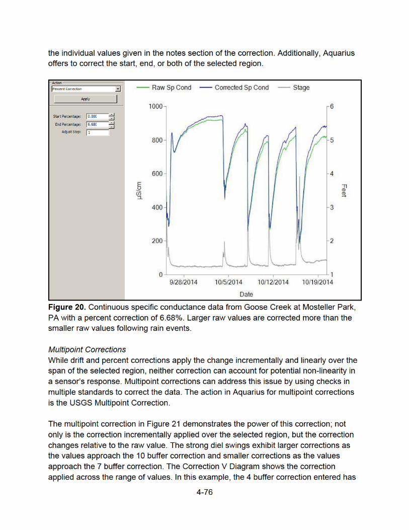

4-77
no influence on the data because all values are between 7 and 10 pH. The correction is
still entered, however, in order to catalog a record of corrections in Aquarius.
Additionally, if a subsequent correction were to move any data below 7 pH, the 4 buffer
correction would become applicable. Like the percent correction, both the start and end
of the period can be adjusted.
Figure 21. Continuous pH data from the Susquehanna River at Rockville, PA with a
USGS multipoint correction applied. Buffers 4, 7, and 10 were used to check pH
calibration. Values in buffer are entered under Input (3.90, 6.95, 10.20, respectively).
The second column is the correction necessary (0.10, 0.05, -0.20, respectively).
Offset Corrections
Offset corrections are a unit-based correction; however, unlike drift corrections, the
value of adjustment is applied equally to the marked region. Offset corrections can be
used on data that has not been calibrated or was incorrectly calibrated; however,
percent or multipoint corrections can also be used in these circumstances, and often are
the more appropriate procedure. A common use of an offset correction is to correct
stage data when the equipment was returned to the stream at a different depth. This
change in depth is constant for the duration of the next period and is best corrected by
an offset correction (Figure 22).


4-79
to be closely reviewed—and perhaps deleted—if temperature data are found to contain
significant error. Wagner et al. (2006) states that for each 1 C change in temperature,
specific conductance and DO concentrations vary 3 percent. For Yellow Spring
Instrument (YSI) equipment, a 1 C change in temperature affects conductivity, pH, and
DO by 4.0%, 0.5%, and 2.0%, respectively, while a 5 C change in temperature results
in changes of 22.0%, 2.0%, and 9.0%, respectively (YSI Tech Support, personal
communication, January 18, 2017). The equations establishing these relationships are
often proprietary and therefore the exact influence of errors in temperature data cannot
be derived. In addition, without these equations, specific conductance, pH, and DO
cannot be corrected for errors in temperature data.
Undocumented corrections are corrections that move the continuous data based on a
verified discrete sample and/or an adjoining dataset (Figure 23). The type of correction
used depends on the parameter, and should be the same as that used for fouling
corrections. For example, if based on the parameter type the type of fouling correction is
a percent correction, an undocumented correction would also be applied as a percent
correction. It’s important to note that undocumented corrections should be made with
care; the reviewer should ensure that the discrete datum agrees with the continuous
data after redeployment before continuous data are corrected to the discrete.
Grading
Grades are determined based on total error (Et) as defined in equation (2), and are
applied using the Data Correction window in Aquarius. Division of Water Quality
uses a standardized procedure of grading to remain consistent throughout the data
evaluation process (Figure 24). Data are generally classified as either usable or
unusable. Data that fall outside the maximum allowable limits (Table 6) are graded
Unusable and deleted in Aquarius. The maximum allowable limits are established at
approximately 6–10 times the calibration criteria for all standard continuous-monitoring
data-collection activities. These limits and rating criteria are taken from the USGS and
will be considered minimum standards for DEP. The criteria in Table 7 are used to
establish ratings for each period of usable data. The Field Form spreadsheet will help
determine cutoff points between ratings. This process is described in the Correction and
Grading Example.

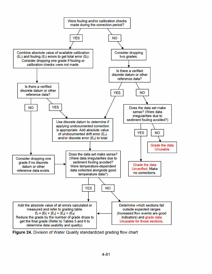
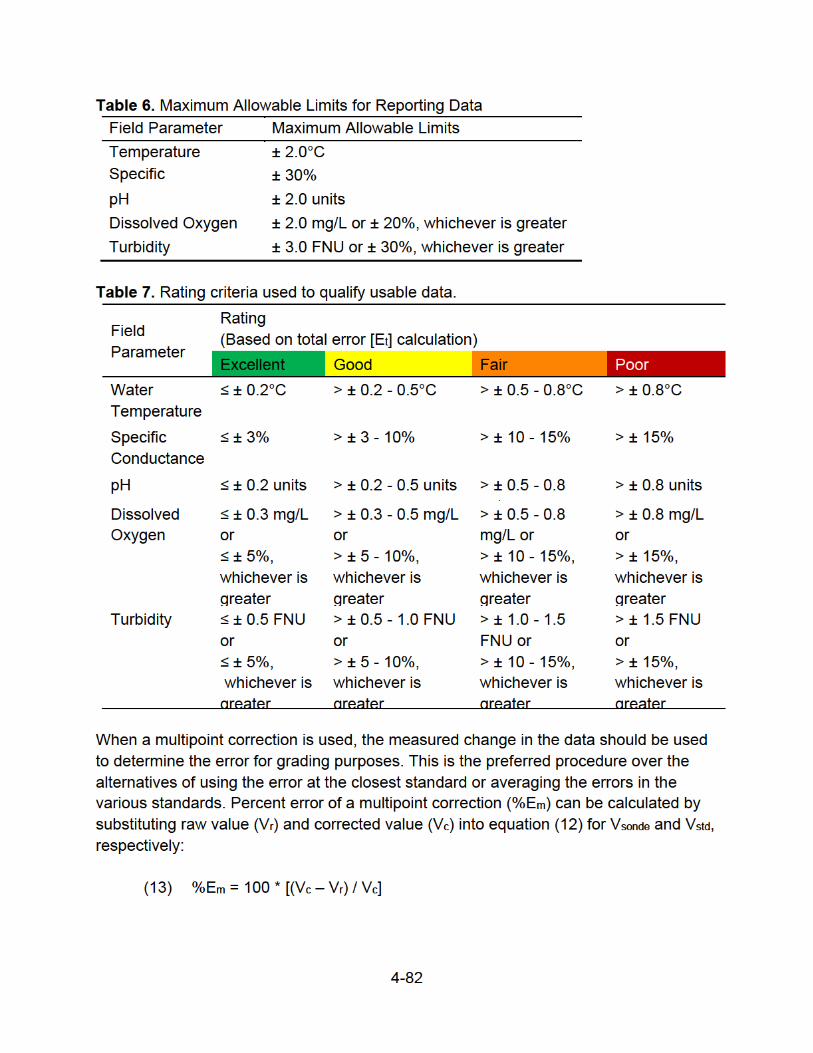

4-83
Using the last data point in the period usually provides the maximum error applied,
however, if there is a significant change in the data near the end of the period the
maximum error may be at the preceding peak or valley in the data.
When both percent and unit-based thresholds are present in Table 7 (i.e., DO and
turbidity), the procedure to be used is determined in the same way as the calibration
criteria described earlier—whichever procedure would result in a better grade is the
procedure used. This is because when values are low, even small changes can result in
very high percentage differences that would lead to unusable data. Similarly, when
values are high, small percent differences represent large unit differences that would
lead to unusable data.
Selecting whether to use percent or unit-based rating criteria can be problematic with
turbidity data when multiple discretes were taken at drastically different values. Unit-
based ratings are usually used for turbidity data from Pennsylvania streams because
turbidity at base flow is typically low. Discrete readings, however, are often targeted
during peak flow events to facilitate the building of rating curves. These turbidity
discretes at peak flow may have low percent error but high unit-based error. Using
exclusively percent or unit-based rating criteria in this situation will often result in data
being rated as unusable. In order to properly rate the data under these circumstances, it
is necessary to convert the percent error for the discretes taken at peak flows to a unit-
based error that can be summed with the rest of the equation. The turbidity rating scale
has a 1:10 ratio of FNU to percent units and therefore the conversion can be made by
dividing the percent error by 10 to get the unit-based rating equivalent. Alternatively, a
unit-based error can be multiplied by 10 to get a percent rating equivalent.
After the rating is determined based on Et, the grader must determine if any “grade
drops” are warranted. A grade is decreased if there is added uncertainty to the data.
The most common reason for decreasing a grade is a missing verification (fouling
check, calibration check, or discrete measurement during the period). Because the
verification is missing, the grade is dropped by one rating. If two verifications are
missing, the grade should be dropped by two ratings. If all verifications are missing, the
data should be graded unverified. Grade drop determinations are outlined in Figure 24.
To aid the approval process, the person applying the grade should include a short note
in the comment section in Aquarius. The comment section is provided after clicking
Apply. The note, at a minimum, should include the errors calculated and note the
reason for any grade drops.
4-84
Correction and Grading Example
An example of the entire correction and grading process is outlined in Figures 25 and
26 for specific conductance data from the Susquehanna River at Rockville for the period
from 6/9/15 to 7/9/15. The basis for these corrections is taken from the Specific
Conductance tab of the DEP Field Form. These parameter-specific tabs calculate the
errors and anticipated corrections to be applied using the data entered during the
maintenance visit. The section of the Specific Conductance tab related to the period
being corrected is displayed in the upper portion of Figure 25. Many of the cells in this
spreadsheet are populated straight from the individual field visit tabs. The cells
highlighted in purple are the cells to be used to enter corrections in Aquarius or used in
the grading process. Only the cells highlighted in yellow should be edited.
The period was first reviewed visually for outliers or abnormalities such as sections of
erratic readings that needed to be deleted. While these data were slightly more erratic
point-to-point than average, no points needed to be deleted. The erratic behavior of the
sensor was likely due to fouling as the subsequent dataset, after cleaning the sensor,
looked much smoother.
Next, the information from the calibration checks was used to apply a USGS Multi-point
Correction. Because the meter was not calibrated during the maintenance visit on
6/9/15, the correction included adjustments to both the beginning and end of the period.
Under Start Point, the inputs were 0, 103, and 1019 with corrections of 0, -3, and -19,
respectively. End Point inputs were 0, 103, and 1020 with corrections of 0, -3, and -20,
respectively. The Start Point inputs and corrections are the End Point inputs and
corrections from the previous section of the spreadsheet (not depicted in Figure 25).
Once the correction is applied (Figure 26), the error can be calculated. The raw value
was 234.0 µS/cm and the corrected value was 228.6 µS/cm; therefore, using equation
(13) the calibration error for the period is -2.36%:
%Em = 100 * [(228.6 – 234.0) / 228.6] = -2.36%.
It is recommended that calibration corrections are applied first for parameters that
require multi-point corrections. This isolates the multi-point correction, allowing the
above calculation to be made. If the multi-point correction is made after other
corrections, those other corrections will need to be temporarily turned off in Aquarius in
order to make the calibration error calculation.
A Percent Correction was then applied to the period to correct for fouling drift. The Start
Percentage was 0% because the sonde was cleaned at the 6/9/15 maintenance visit,

4-85
and therefore it is assumed that no fouling is present. The End Percentage was -0.88%
which was taken from the Fouling Correction box in the spreadsheet (Figure 25).
If the either correction did not make sense (i.e., data were moved away from the
discrete and/or adjoining datasets), the beginning, end, or both parts of the correction(s)
could have been removed. In this case, the calibration and fouling corrections made
sense because both moved the data closer to the discrete and adjoining datasets;
therefore, both corrections remained applied.
After applying calibration and fouling corrections, the discrete was still 2.0% different
than the corrected data (Figure 26). Because the discrete lined up with the subsequent
dataset, an undocumented correction was deemed appropriate. A Percent Correction
with a Start Percentage of 0.0% and an End Percentage of 2.0% was applied to offset
the undocumented error. It is important to note that this determination was made after
applying the calibration correction to the next period. Because the sensor was calibrated
during the 7/9/15 visit, the beginning of the next period also needed to be corrected.
After all corrections were applied, total error (Et) was calculated using equation (6):
Et = |Ef| + |Ec| + |Eu| + |Ed| = |-0.88%| + |-2.36%| + |-2.0%| + |0.0%| = 5.24%
Fouling error (Ef) was taken from the Fouling Error box of the spreadsheet. This number
happened to be the same as the fouling correction applied because the error was small
in this case. If the error was larger, these numbers would have been different from each
other; therefore, care should be taken to use the correct value. Calibration error (Ec)
was %Em, from the calculation above. Undocumented drift error (Eu) was from the final
correction applied. Because there was only one discrete and an undocumented drift
correction was applied to meet the discrete, discrete error (Ed) was zero for the period.
The grade is “Good” for specific conductance, when Et = 5.24% (Table 7). Additionally,
Et can be entered into the spreadsheet (“Total Error (%)” box, Figure 25) to generate a
schedule of prorated grades for the period. For simplicity, these prorated grades are
typically not applied. Instead, the lowest grade is applied for the entire period. One
exception is when Et results in unusable data. In this circumstance, the division between
poor and unusable is used to isolate only the data that are unusable.


4-88
Final Approval
Final approval is the last step in the data management process that confirms the data
by validating the corrections, grading, and decision making processes of the individual
originally responsible for the data. Final approval is typically conducted by individuals
with the most experience with continuous instream monitoring. In Aquarius, approvals
are applied using the Set Approval action in the data corrections tool box. Division of
Water Quality uses two types of approvals, “Approved” and “In Review”. If a reviewer
disagrees with, or has a question about a correction or grade, the section is marked “In
Review” and the section is discussed with a third party. The third party helps come to a
conclusion on the data management, at which time the data are then approved. Once
data are approved (Figure 27), it may be placed into the report and used in analyses.
Figure 27. Specific conductance data at Aughwick Creek from 2014 displaying the
grades and approval status within the Aquarius data correction tool box. The upper and
lower rows of colored bars at the bottom represent grades and approvals, respectively.
Because the last period was graded unusable (purple), the data were deleted. All
sections were approved (green) except the last section. Since the final reviewer did not
agree with the correction and/or grade, that period of data was marked “In Review”
(yellow) until the discrepancy was resolved with a third party.

4-89
REPORTING
DEP’s Water Quality Division compiles, interprets, and reports instream monitor data in
Continuous Instream Monitoring Reports (CIMR). Continuous instream monitors
produce large amounts of data that, without the proper software, can be difficult to
manage, interpret, and report. Division of Water Quality staff uses both numeric and
visual procedures to report on time series data. Reporting conventions for time series
data often include the maximum, minimum, and median or mean for a measured value
as well as graphical representation of the entire dataset. Data are made available to the
public online after final review and approval are complete. Standard reporting units and
resolutions are detailed in Table 8.
Table 8. Field parameter reporting conventions.
Field Parameter Reporting Units Reporting Resolution
Temperature °C 0.01 °C
Specific Conductance µS/cm 0.1 µS/cm
pH Standard pH units 0.01 standard pH unit
Dissolved Oxygen Concentration mg/L 0.01 mg/L
Dissolved Oxygen Saturation % 0.1 %
Turbidity FNU 0.1 FNU
Aquarius software is used for graphical representation of time series data. When
possible, these graphs will incorporate at least one measured parameter with either a
measured depth or a calculated discharge (Figure 28). Depth or discharge will often
contextualize events of interest (i.e., sudden changes) within the dataset.
A great deal of significance is placed on the relationship of the five water quality
properties and discharge variations, but other event-related changes are equally vital
and can be factored into the relation only through historical measurements, field
experience, and on-site observation. Some examples include but are not limited to
changes in ambient temperature, periods of sustained cloud cover, chemical spills,
increased photosynthetic production, increased wind conditions, sewage overflows,
road construction, and ice formation. Understanding these relations is an essential
element of accurate instream record management (Wagner 2006).
A CIMR not only includes time series data, it also contains any other associated data
collected during the survey period. These data include, but are not limited to, chemical
grab samples, macroinvertebrates, fish, and habitat assessments. When combined,

4-90
these data provide a powerful assessment tool and excellent information on the aquatic
environment.
Figure 28. Depth and pH data for the East Branch Clarion River near the mouth of Gum
Boot Run from September, 2010 to February, 2011. A critical depression in pH can be
seen around the beginning of December, 2010. The depth time series helps identify and
explain that the problem is most likely due to atmospheric deposition through
precipitation.
ARCHIVING RECORDS
Once a report is written and reviewed it will be archived into digital stream files within
DEP and made public online. Monitoring Section personnel within DEP are responsible
for the collection, analysis, manipulation, and storage of instream monitoring data, and
must ensure that the specified requirements of archiving electronic data are fulfilled.
In addition to electronic data, original water-quality monitoring data on paper may
include field notes, field measurements, calibration notes, and service requests. Field
notes and measurements should be included in the appropriate electronic Field Form
for the site that is then archived in the network CIM folder (field measurements are also
stored in Aquarius). Physical calibration logs are scanned and archived in the CIM
folder and all documentation of equipment servicing is logged in the sonde management

4-91
database. It is the responsibility of Monitoring Section to ensure that project files are
organized, complete, and entered into the instream monitor archive. The archive should
be well documented and maintained by appointed personnel in the Monitoring Section
of DEP.
SUMMARY
This protocol offers guidelines for DEP personnel and others in site and monitor
selection considerations, field inspection and calibration procedures, data evaluation
and correction, and data reporting processes. Evolving sensor technology increases the
variety of measurable chemical constituents, allows lower detection limits, and provides
improved stability and accuracy. Protocol guidelines and quality assurance procedures
will continue to be refined as equipment and software progress.
LITERATURE CITED
Anderson, C. W. 2005. Turbidity. Book 9, chapter A6, section 6.7 (version 2.1). in
National field manual for the collection of water quality data: Techniques and
methods. U.S. Department of the Interior, U.S. Geological Survey, Reston, VA.
(Available online at: https://www.usgs.gov/mission-areas/water-
resources/science/national-field-manual-collection-water-quality-data-nfm?qt-
science center objects=0#qt-science center objects.)
Hoger, M. S. 2020. In-situ field meter and transect data collection protocol. Chapter 4.1,
pages 2–8 in M. J. Lookenbill, and R. Whiteash (editors). Water quality
monitoring protocols for streams and rivers. Pennsylvania Department of
Environmental Protection, Harrisburg, Pennsylvania.
Radtke, D. B., J. V. Davis, and F. D. Wilde. 2005. Specific conductance. Book 9,
chapter A6.3 (version 1.2). in National field manual for the collection of water
quality data: Techniques and methods. U.S. Department of the Interior, U.S.
Geological Survey, Reston, VA. (Available online at:
https://pubs.er.usgs.gov/publication/tm9A6.3.)
Ritz, G. F., and J. A. Collins. 2008. Measurement of pH. Book 9, chapter A6.4 (version
2.0). in National field manual for the collection of water quality data: Techniques
and methods. U.S. Department of the Interior, U.S. Geological Survey, Reston,
VA. (Available online at: https://pubs.er.usgs.gov/publication/tm9A6.3.)
Rounds, S. A., F. D. Wilde, and G. F. Ritz. 2013. Dissolved oxygen. Book 9, chapter
A6.2 (version 3.0). in National field manual for the collection of water quality data:
Techniques and methods. U.S. Department of the Interior, U.S. Geological
Survey, Reston, VA. (Available online at:
https://pubs.er.usgs.gov/publication/tm9A6.3.)

4-92
Wagner, R. J., R. W. Boulger, C. J. Oblinger, and B. A. Smith. 2006. Guidelines and
standard procedures for continuous water-quality monitors: Station operation,
record computation, and data reporting. in U.S. Geological Survey Techniques
and Methods. (Available online at: https://pubs.er.usgs.gov/publication/tm1D3.)
Wilde, F. D. (editor). 2004. Processing of water samples. Book 9, chapter A5 (version
2.2). in National field manual for the collection of water quality data: Techniques
and methods. U.S. Department of the Interior, U.S. Geological Survey. (Available
online at: https://www.usgs.gov/mission-areas/water-resources/science/national-
field-manual-collection-water-quality-data-nfm?qt-science center objects=0#qt-
science center objects.)

4-93
4.4 SEDIMENT CHEMISTRY DATA COLLECTION PROTOCOL

4-94
Prepared by:
Amy Williams
PA Department of Environmental Protection
Office of Water Programs
Bureau of Clean Water
11th Floor: Rachel Carson State Office Building
Harrisburg, PA 17105
2015
Edited by:
Amy Williams
PA Department of Environmental Protection
Office of Water Programs
Bureau of Clean Water
11th Floor: Rachel Carson State Office Building
Harrisburg, PA 17105
2017
4-95
INTRODUCTION
DEP strives to better understand environmental issues and systems through various
forms of data collection. Water, macroinvertebrates, and fish are routinely collected to
help determine a waterbody’s health and analyze pollution sources and causes.
Streambed sediment is another parameter that can explain a lot about a system.
Bed sediments can accumulate substances that may not be detectable in a single
discrete water sample. They have the potential for accumulating a variety of trace
elements and toxins. Additionally, they could re-enter the water column as suspended
sediment, introducing those substances into the system and causing further problems
downstream. It has been shown that bed and suspended sediments accumulate more
trace metals than are normally present in the water column (Horowitz 1985).
Monitoring streambed sediment parameters can assist in point and non-point source
investigations, spill and complaint issues, and routine monitoring. Testing sediment
could show if contaminants are present, such as high levels of metals, radionuclides, or
organic compounds, and assist in making assessment decisions on impairment or
attainment of flowing waterbodies.
This document provides guidelines for the standardized collection of streambed
sediment samples from flowing waterbody systems. The procedures described here are
adapted from scientific, peer-reviewed procedures, and were developed, field tested,
and implemented by DEP’s technical experts. This protocol does not attempt to
describe the entire spectrum of sediment sample collection techniques, and review of
other documentation is encouraged depending on the specific sampling situation.
Because sampling situations vary largely, no single sediment sampling procedure can
be universally recommended. This document describes sediment sampling procedures
appropriate for typical DEP investigations and may require modification as situations
dictate. Variations to this protocol will be dependent upon site conditions, equipment
limitations, or limitations imposed by the procedure. Investigators should document
modifications and report the final procedures and equipment employed.
Investigators should be aware of, and work to prevent, the potential for sample
contamination at all phases of the sample collection process by observing proper
sample collection, handling, and preservation procedures described here. The most
common sources of error (also known as “interference”) are cross-contamination and
improper sample collection and preservation.
4-96
COLLECTION REQUIREMENTS
Collector Identification Number
Field staff required to collect surface water samples must have an assigned four-digit
collector identification number (e.g., 0925). This number along with a sequential three-
digit sample number (e.g., 0925-001), and date/time of sample are used to identify
individual samples. Supervisory staff can request collector identification numbers for
their field staff with the “Collector ID Request Form” found at the eLibrary website (ID
Request Form).
DEP Laboratory Sample Submission Sheet
Field staff will need to have at least Querying and Sample Entry security roles for the
program or business unit that they are collecting samples for. The program or business
unit will be consistent with the Program Code entered on the “DEP Laboratory
Submission Sheet” (Submission Sheet). Collectors must submit samples to the DEP
Bureau of Laboratories (BOL) using a “Sample Submission Sheet”. Field staff are
required to document collector identification number; reason code; cost center; program
code; sequence number; date collected; time collected (military time); fixative(s) used;
standard analysis code (SAC); under certain circumstances, legal seal numbers for
each sample collected; the number of bottles submitted per test suite; collector name;
current date; phone number; and any additional comments that lab analysts will use to
properly handle samples.
As described previously, collector identification numbers are unique to each field staff
member collecting samples. Reason codes, cost centers, and program codes are
program-specific and should be obtained from the program responsible for coordinating
sampling efforts. Sample sequence numbers are three-digit sequential numbers (001-
999) unique to a sample collected on a given day. Date and time collected should be
accurately documented. If a sample is “fixed” or preserved with acid this must be
documented in the appropriate space.
A standard analysis code or SAC is a unique code that details analytical tests to be
applied to a specific sample. Suite codes are also available, and are often used for
radionuclide and organic samples. Each DEP program uses different SACs or suites for
specific projects or purposes. For example, SAC 018 is used by “Water Supply
Management” when submitting water chemistry samples for Special Protection Surveys.
The analytes/tests listed under SAC 018 are those specifically identified by regulation
that surface water must meet and therefore be assessed for if a special protection
determination is warranted. Other programs have developed SACs for their unique

4-97
purposes, and the DEP BOL encourages programs to create SACs tailored to a
program’s specific needs.
Legal seals and associated legal seal numbers are required under circumstances where
it is imperative to document the integrity of samples from sample collection to sample
analysis. Legal seals are not always needed, and should be used according to a
program’s specific requirements. Legal seal numbers must be singly listed (include
letter and number) for each sample. Legal seals can be obtained from BOL. Refer to
BOL for more information concerning legal seals for the particular needs.
Collector name, current date, phone number, and number of bottles submitted per test
suite were added to the DEP laboratory “Sample Submission Sheet” to meet National
Environmental Laboratory Accreditation Program (NELAP) chain-of-custody
requirements. Using the area at the bottom of the form, each bottle submitted for the
samples identified must be accounted for by enumerating the number of bottles per
category listed for inorganic and organic analyses/tests. Each submitted form is also
required to have printed the collector’s name, current date, collector’s signature
(Relinquished by:), and collector’s phone number. There are also spaces to document a
facility name, facility identification number, and an alternate contact. These three pieces
of information are not required.
The last pieces of information to be documented are any additional comments that lab
analysts need to properly handle samples. This information is documented in the
‘Comment’ field at the bottom of the form. The most common use of this field is to add
or delete tests to or from a specified SAC. For example, SAC 018 does not include a
test for turbidity; however, a sample collector may need to document turbidity for a
particular sample. The sample collector would identify SAC 018 in the appropriate field
and indicate in the ‘Comment’ field to add the turbidity test to the particular sample. If a
large number of samples will be submitted with consistent modifications of a particular
SAC, the BOL prefers a new SAC be created specifically for those samples. Other
important comments to consider include odor, sheen, color, viscosity, foaming, field
meter readings, historical knowledge about the site, and any other information that lab
analysts may need to safely and correctly handle the samples. The BOL requests
collectors contact the appropriate BOL staff before submitting samples requesting
organic tests, potentially dangerous samples, or samples that need to be handled
differently.
Sampling Supplies and Equipment
DEP programs can and do employ a variety of program-specific sediment sampling
techniques that require a multitude of supplies (sampling bottles, bags, etc.), and can

4-98
include specialized equipment (En Core™ soil corer, Ponar dredge, etc.). This section
describes equipment and supplies required to employ the most commonly used
sampling techniques and does not include all streambed sediment sampling techniques
that could be employed. Additional techniques may be added as they become
applicable and as standard procedures are solidified. Much of the equipment used to
sample soils can be used to sample sediments as long as sediment is not lost in the
water column on the way to the surface; sampling equipment will be determined by
water depth, velocity, and other physical parameters.
Parameter-specific equipment requirements, sample collection, labeling, and storage
will be covered in subsequent sections below. Recommended sampling equipment and
other gear are listed in the below check list:
SEDIMENT SAMPLING
Equipment:
spatulas/trowels/scoops (plastic = metals collecting; stainless steel = organics
collecting)
dredges (e.g., Eckman, Ponar)
corers with vials (e.g., En Core™)
Sample containers:
500 ml plastic sample bottles – trace elements
500 ml amber glass sample bottles – organics
40 ml amber glass vials – organics moisture
determination
plastic bags, 4 Mil thickness - radiological samples
Sample processing:
compositing bowl(s) (plastic = metals collecting; stainless steel = organics collecting)
sieve(s) - < 63 micron
cloth mesh (disposable sieve)
Other
brushes
Munsell color chart
Equipment cleaning:
wash bottle/deionized water
detergent (0.2% phosphate-free)
methanol (to rinse organics equipment)
hexane (to rinse organics equipment)
5% HCl (to rinse trace elements equipment)

4-99
FORMS
sediment field forms
laboratory sediment chem. sheets
SHIPPING
courier shipping forms
tape & dispenser
ice
coolers
Misc.
hip boots
waders
nitrile gloves
markers (black Sharpies), pens, & pencils
GPS/maps
Ziploc® bags (for bottles and/or sample submission sheets)
field meter (e.g., YSI), calibration solutions, spare batteries
calculator
insect repellent
screwdriver/tools
batteries (D-cell, other:________________)
other: _______________________________
The numbers and types of sample bottles field staff need for one sediment sample
depend on the specific SAC or suite. Sample bottle and preservative requirements can
be obtained by contacting DEP’s BOL directly.
The choice to use scoops/spatulas, corers, or dredges depends heavily on-site
conditions and the specific project requirements. Hand-held scoops and spatulas are
convenient for shallow, slow-moving, wadeable streams. They are easy to use and
clean. Unfortunately, with this procedure, it can be easy to lose fine sediment, which is
desirable for most tests. Additionally, it can be more difficult to gather in deeper water,
and if contamination is a concern, it increases the likelihood of skin contact with
material. Deeper and faster-moving water may require the use of a hand-held or
mechanical dredge, such as an Eckman or Ponar. The use of a boat may be required
or, alternatively, dredges can often be lowered from bridges. However, the project aim
should be considered in choosing where to lower a dredge from; runoff from the bridge
may or may not be desired. These are convenient ways to gather bed sediment when
the bottom cannot be manually reached, but a downside is that it is easy to gather too
much deeper sediment, and there is far less control over where and what is actually
collected. If historical sediment information is desired, corers are an option. These

4-100
range from large, cumbersome varieties to small, handheld corers, such as those used
for volatile organic compounds (e.g., En Core™). In all cases, excessive ornamentation
or wooden parts are discouraged to permit easy and thorough decontamination (USEPA
2012). Collectors are encouraged to seek guidance on the variety of dredges and corers
available from the literature at the end of this document.
Some chemical analyses require laboratory technicians to calibrate specialized
laboratory equipment, prepare specialized reagents, or otherwise perform pre-analytical
preparation before samples can be analyzed. If a collector is going to submit several
samples involving specialized preparation, such as allowing radionuclide samples to
ingrow, he or she should contact the appropriate technician at the laboratory to ensure
enough time is allocated for the pre-test procedures. Additionally, large quantities of
samples should always be pre-authorized with the laboratory to avoid surpassing
holding times.
SAMPLING DESIGN CONSIDERATIONS SPECIFIC TO SEDIMENT
Determining sample design is one of the most important parts of a field collection plan.
It is necessary to determine whether a statistical or judgment-based approach is
desired. This depends substantially on the project questions – for example, whether or
not background samples are being collected, or a spill or discharge effect is being
investigated. See Chapter 2, Sampling Design and Planning (Lookenbill 2020) for
suggested sampling plans.
During or after completing a sample collection plan, the collector should perform field
reconnaissance of the site(s). Ease of site access, stream flow, and sediment
deposition locations should be reviewed. One should ideally avoid sampling sediment
immediately after a significant precipitation event where runoff from the surrounding
land could occur (Shelton and Capel 1994). Manmade structures, such as bridges,
should be noted and sampling immediately downstream of them should be avoided.
Runoff from structures can easily impact surrounding sediment downstream. Point and
non-point sources of pollution should be noted. Field reconnaissance is also an
opportunity to determine necessary equipment for sediment collection, such as dredges
versus scoops. Additionally, it can assist in determining locations where it is most likely
for sediment to deposit and where concentrations of contaminants could be highest.
Locations where sediment can accumulate, and therefore accumulate contaminants,
include areas with aquatic vegetation, where velocity decreases, and inside bends in
the stream (Oak Ridge Associated Universities (ORAU) Training 2012). Sediment can
also accumulate near man-made structures, but again, care must be taken to ensure

4-101
sediment in those locations is of interest to the project and not a result of surrounding
land runoff, if that is not the target.
COLLECTION PROCEDURES
General Considerations
Collectors need to first ensure they have formed an adequate sampling plan that will be
representative of the system under investigation. Care must be utilized during collection
to reduce contamination from outside sources and maximize the integrity of the sample.
The most common causes of sample interference during collection include poor sample-
handling and preservation techniques, input from atmospheric sources, and
contaminated equipment or reagents. Each sampling site needs to be selected and
sampled in a manner that minimizes bias caused by the collection process and that best
represents the intended environmental conditions at the time of sampling.
As stated above, the lab should be contacted prior to large or unique sampling events.
Previous weather conditions and discharge may be analyzed to ensure samples are
being collected with the stream characteristics required to answer the problem in
question. Large precipitation events resulting in high discharge and runoff are not the
best time to sample to judge maximum sediment contamination from a point source
discharge. In addition, rapid water velocities and increased turbidity make sediment
collection with traditional trowels difficult. Discharge data for continuous monitors
throughout the state can be found on the United States Geological Survey website.
Equipment should be gathered and a checklist made prior to departure. Once at the
site, before handling sample containers, the collector should ensure his or her hands
are clean and not contaminated from sources such as food, coins, fuels, mud, insect
repellent, sunscreen, sweat, or nicotine. Gloves should be worn for all sediment
sampling due to the high possibility of sample contamination. Unlike water samples,
sediment samples are handled quite a bit more and there are many more opportunities
to introduce contaminants.
For most sediment sampling, the surficial 1 to 6 cm of sediment with grain sizes < 0.06
mm (silts and clays) are desired. It is best to avoid sands (0.06 – 2 mm) and larger grain
sizes. Fine grained particles tend to accumulate more trace elements than coarser
particles. This is due to a number of factors, including higher available surface area on
finer particles (Horowitz 1985). For some organics analyses, grain size < 2.0 mm (sand,
silt, clay) is acceptable (Shelton and Capel 1994). In general, the way to distinguish
between sand, silt, and clay is displayed in Table 1.

4-102
Table 1. Sediment grain sizes. Adapted from: Ohio EPA. 2001. Sediment sampling
guide and methodologies. 2nd edition.
Soil Type Grain Size Description
Sand 0.06 – 2.0 mm gritty, non-plastic, loose particulates
Silt
0.004 – 0.06
mm
smooth, talc-like, non-plastic, loose
particulates
Clay < 0.004 mm dense, moldable like putty, cohesive
In the event that a site contains large amounts of sandy material, sieving may be
necessary if the aim is to determine the highest concentrations present. In general, it is
a good idea to make sure the sample contains > 30% fine material, i.e., silts and clays
(Ohio Environmental Protection Agency 2001).
All equipment is cleaned prior to being used. It is advisable to wash and soak it for 30
minutes in a 0.2% phosphate-free detergent (Shelton and Capel 1994). After soaking,
rinse the equipment thoroughly in deionized water, air dry (if possible), and store in
individual, sealable containers or bags. If sampling for organic contaminants, clean the
stainless steel or TeflonTM equipment with soap and tap water, rinse with deionized
water, dry, rinse with acetone, and, lastly, rinse with hexane (as recommended by DEP
BOL staff). Wrap organics equipment in aluminum foil. It is highly advised to have
several sets of equipment, particularly if planning to sample reference (background) and
impacted sites in one trip. It is difficult to fully clean equipment in the field. If doing so,
save the rinsate and dispose of it properly. It is also advisable to occasionally collect a
rinsate blank.
First, calibrate any field sampling equipment, such as field meters according to Chapter
4.1, In-Situ Field Meter and Transect Data Collection Protocol (Hoger 2020). If dealing
with a possibly impacted site and reference location(s) have been chosen, sample
reference locations first if combining impacted and reference sites into one trip. This will
help lessen the possibility of contamination between sites. It is important to note that
safety is always first – avoid wading into high flow areas or locations where slippage
could occur, wear appropriate wading gear, and have the proper length and type of
gloves on if dealing with impacted sites or chemicals.
If sampling is taking place due to a point-source pollution incident, it is advised to
sample downstream of the discharge, at the discharge, and upstream of the discharge,
at minimum. In order to collect a sample representative of a particular location, plan to
collect at between 5 to 10 depositional zones within a study site and composite those

4-103
into one sample (Shelton and Capel 1994). For example, if collecting at a point of acid
mine discharge (AMD), composite sediment at between 5 to 10 depositional zones
downstream of the discharge, composite sediment at between 5 to 10 depositional
zones at the discharge, and composite sediment at between 5 to 10 depositional zones
upstream of the discharge. Compositing several “zones” of sediment will allow for a
more representative description of the sample area and will not target one spot.
Additionally, due to lack of sediment buildup at some locations, compositing several
spots of sediment buildup facilitates obtaining only the first 1 to 6 cm of sediment. Of
course, specific project needs may deviate from this, so plan and document the study
accordingly. Additionally, composite sampling is not appropriate for the collection of
volatile organics samples because compounds could be lost.
Sampling stations located upstream of the discharge pipe should be in non-impacted
areas to serve as controls. If there are multiple discharges, then sample stations should
be placed to bracket individual discharges in order to better characterize each source.
For sampling downstream of the discharge pipe, if the investigator is interested in
determining the downstream point where the discharge ceases to be an effect in the
sediment, the investigator should avoid the immediate vicinity of the discharge/influence
point and select a sample point far enough downstream to allow for mixing between the
discharge and stream flow. Sampling can occur at any noted deposition points between
in order to characterize effects of the discharge. Depending on stream size, flow,
velocity of the plume, and angle at which it enters the stream, solids may deposit at a
variety of locations.
As a summary, composite-sampling 5 to 10 depositional zones in a single location
(upstream of a discharge, for example) is recommended in most cases. In addition, the
sampling reach is discretionary and based upon site-specific characteristics and
questions being answered. Regardless of the technique implemented, similar sampling
procedures should be used if sampling several locations in one single study, to allow for
comparability of data.
At each site, always collect water samples first to avoid stirring up sediment that could
contaminate the water sample. Take any water field measurements before sediment
sampling. Additionally, always work in a downstream to upstream fashion at a site.
Lastly, always document the appearance, odor, sheen, and feel of the sediment on the
‘Sediment Field Data Collection Sheet’ (see Appendix B.4).
Wadeable Samples
Gather the equipment (scoop, appropriate sampling container [see parameter-specific
instructions, below], gloves) and enter stream at the most downstream of the sampling
4-104
locations. If interested in surficial, recent deposition, sample only the top 1 – 6 cm of
sediment; if interested in historical sediment accumulation, sample > 6 cm. Facing
upstream, rinse the sampling container several times with native water, emptying it
behind you (downstream) to avoid stirring up any additional sediment. In addition, rinse
all sampling equipment in native water as well, including scoops, sieves, and bowls.
Enter water column at the first sediment depositional area, using care to gather
upstream of the current standing position and not stepping where collection will occur,
and gather a scoopful of sediment. Slowly raise the scoop out of the water to avoid
losing fine material and place sediment into sampling container. Move to the next
depositional zone and repeat, working from downstream to upstream. If too much water
is collected, carefully decant as it is collected, trying to allow it to settle first as much as
possible to avoid loss of fine materials. Additionally, avoid collecting vegetation or other
debris. The lab needs to pulverize samples before analysis, so the finer sediment and
the less debris collected, the better.
Once enough sediment is collected, exit the stream and empty the sample into an
appropriate compositing container. Remove any large pebbles, sticks, vegetation, or
other debris. Allow the sediment to settle and carefully decant the water off, or,
alternatively, sieve the sample to ensure only fine grained materials are collected.
Generally, if one sample is sieved in a project, all samples in that project should be
sieved for consistency. In any case, fully note on the field sheet the texture, color, and
odor of the sediment. Homogenize the sample using a spatula or trowel. One
recommendation to fully homogenize is to “quarter” the sample into four parts, mix those
parts, and then mix the entire sample together (USEPA 2012). Place sample back into
the sampling container and record all details about the site and collection procedures on
the field sheet. Add fixative to the sample, if required. If refrigeration is necessary, place
the sample in a cooler with ice in order to cool the sample to 4°C. Do not use dry ice
because the sample may freeze. Record GPS coordinates of the location and take
photographs, if necessary.
Corers may be necessary if the interest is in collecting historical sediment or volatile
organic compounds that cannot be exposed to air. Coring allows stratification of the
sediment and the possibility of testing individual layers. A corer is pushed into the
sediment and the core is captured in the sample tube (ORAU Training 2012). They can
be particularly useful in fast-moving streams where grab samplers would be difficult to
use. They come in a variety of shapes and sizes for different needs. Many include a
valve or catcher that will prevent loss of the core as it is being brought to the surface.
The DEP BOL requires the use of an En Core™ corer (or similar) or a corer using pre-
preserved (methanol) vials for volatile organic compound soil and sediment samples. If
it is not possible to use these types of corers, a note must be made on the “Sample
4-105
Submission Sheet” or a data release form will be sent. USEPA has a detailed
description on how to collect volatile organic compounds in USEPA Test Method 5035A
(2002) - Appendix A. Refer to the DEP BOL for more information regarding volatile
organic compound collecting.
To collect sediment with a corer, either push or hammer it into the sediment (ORAU
Training 2012). Be sure to push it straight down and pull it straight up without turning it,
and do not fill the tube completely. Keep the sampler vertical when pulled out of the
sediment to avoid mixing. Cap the bottom of the sample tube as soon as possible, then
the top. If there is some water left in the tube, carefully decant it off and stuff a cloth into
the end – this reduces mixing. Augers, often used for soil, can be used for collecting
sediment and are turned and pushed into sediment; however, sample loss could be an
issue. Refer to the references in the “Literature Cited” section of this document for
further information on using a variety of corers, augers, and dredges to collect
streambed sediment.
Nonwadeable Samples
If the water flow is too deep and/or fast moving to manually collect sediment, consider
using a dredge. These can either be lowered from a boat or a structure such as a
bridge. Depending on size, they can be manually lowered or lowered using a winch. If
boating, turn off the engine before using the dredge to eliminate impact on the sample.
If an anchor is used, make sure dredging is not collecting the sediment that the anchor
disturbed.
Once at the desired location, set the dredge according to user instructions and carefully
lower it to the stream bottom. Trip the dredge, and slowly bring it to the surface. Avoid
lowering and raising it too fast, which risks disturbing the sediment before it reaches the
bottom or losing sediment on the way up. Once at the surface, examine the sample and
determine if the dredge was properly tripped; if it was not, discard the sediment and re-
sample. Dispense the sample in an appropriate compositing container, collect the rest
of the depositional zones, and follow the instructions above for decanting/sieving and
compositing the sample. See the references in the “Literature Cited” section of this
document for further information on using a variety of dredges to collect streambed
sediment.
Parameter-Specific Considerations: Radionuclides
Stainless steel, high-density polypropylene (HDPP), or polyethylene (HDPE) sampling
equipment is recommended for sampling for radionuclides (USEPA 2012). Sampling
containers should also be made of the same plastics and have a polytetrafluoroethylene
(PTFE) or TeflonTM lined lid (USEPA 2012). Verify that the lid will not absorb any water.

4-106
Stainless steel or plastic compositing containers are recommended. If testing for
gamma-emitting radioisotopes, bags are recommended due to large sample volume.
DEP BOL recommends collecting one (1) kg of wet sediment in order to verify having
enough sample to analyze ½ kg of dry sediment in the lab. Two 500-mL bottles are also
a sufficient amount of sample for analysis. Double or triple-bagging samples is highly
recommended. Properly close the bags and use a non-absorbing tape to seal. Gamma-
emitting radioisotope sediment samples do not require refrigeration or preservatives.
The sample holding time is 72 hours if iodine analysis is needed, otherwise it is 6
months. For other tests and details, contact the DEP BOL.
Parameter-Specific Considerations: Metals
High-density polypropylene (HDPP) or polyethylene (HDPE) sampling equipment is
recommended; avoid metal sampling equipment whenever possible. There is always
the chance of metals in the equipment influencing sample results. Plastic compositing
containers are recommended. Most standard plastic water-sampling bottles can be
used to store sediment for metals testing. A typical sediment metals sample at DEP
BOL requires a 500-mL plastic or glass container. No preservatives are required and
refrigeration to 4°C is necessary. Holding time is 6 months. Contact the DEP BOL for
specific parameter details.
Parameter-Specific Considerations: Volatile & Semi-Volatile Organic Compounds
As stated above, DEP BOL requires samples for volatile organics to be collected with
corers. There are two coring procedures available: The first is the En Core™ - for each
analysis, 2 x 5g En Core™ vials are needed, plus one (1) 40mL amber glass vial, to be
used for moisture determination. There is also a 25g size available, but this is not
recommended and will also require a data release form. A second procedure uses a
small, disposable corer that contains pre-preserved (5mL of methanol), pre-weighed
vials. Weight is recorded on the outside of the vial. The core is collected, the sample is
ejected into the vial, and the vial is quickly capped. The vial is not to be packed full and
care should be used to avoid losing methanol. The threads of the vial should be cleaned
before capping so methanol does not leak out. Do not attach additional labels to the vial
since this will change the weight of the vial. Two pre-preserved vials and one (1) 40mL
amber glass vial are required for analysis. Only “high concentration” vials are required.
If unable to use these types of samplers, specifically state the reasons why on the
“Sample Submission Sheet” or a “Client Request for Data Release” form will be sent. In
the instance of not using a core sampler, volatile organics samples need to be packed
tightly in 2 x 40mL amber bottles (unpreserved). A recommended procedure to avoid air
contact is to take a scoop of sediment, remove the top layer in the scoop, and
immediately fill the vial with sediment from the scoop. Samples have a holding time of
4-107
48 hours using the En Core™, and must be received by the lab within 24 hours after
collection. Samples collected and preserved with methanol have a holding time of 14
days. See USEPA Test Method 5035A (2002) - Appendix A for more details.
If testing for semi-volatile organic compounds, fill a 500mL amber glass sampling jar.
Volatile and semi-volatile organics sediment samples need to be refrigerated to 4°C and
do not require field preservation, unless collecting volatile organics in the pre-preserved
vials. When possible, always schedule with the lab before collecting samples for organic
analyses.
Labeling
While the minimum requirement is the collector number and sequential sample number,
collectors are encouraged to add date and time collected, general test(s) description
(total metals, etc.), and preservation indication. This will help prevent confusing what
bottles are from which tests and to help ensure the sample is properly preserved and
stored. Labeling should be done so that at least 1” of space is left at the top of the bottle
to allow BOL to apply lab labels.
Permanent marker will rub off HDPE bottles during collection and transport. Therefore,
clear packing tape should be wrapped around the bottle to protect hand-written labels.
BOL discourages the use of masking tape. Collectors should keep a log book of all
samples they take, and should not re-use sequential numbers in order to avoid
confusion. The sample log should annotate the unique collector identification and
sample number, date and time, the waterbody name, sample location, SAC code, and
any additional analytical tests performed or excluded.
Quality Assurance
A duplicate grab sample should be collected every 20 samples or for each sampling
trip/day to gauge testing variability and potential sources of contamination due to
collection procedures. Duplicate samples are collected simultaneously or sequentially
with the associated environmental sample, using identical sampling and preservation
procedures. Sequentially collected duplicates may measure inhomogeneities present in
the sediment. Duplicates are assigned unique sequential sample numbers. The
collector needs to carefully annotate which sample is a duplicate in their field book.
Duplicates must be documented appropriately in SIS under the ‘Comments/Quality
Assurance’ tab.
“Split samples” are collected as one sample and then divided in two for separate
analysis (Radtke 2005). These can be sent to different labs for analysis or be tested at
the same lab, and can help determine lab analysis variability.

4-108
“Rinsate blanks” may be necessary at times if a highly-impacted site was sampled. After
cleaning equipment, a sample of the cleaning rinsate water is saved and analyzed for
parameters of concern (USEPA 2012). This verifies whether or not the equipment was
properly cleaned.
DEP BOL does not require sediment or soil blanks, although they can be submitted.
Normally these are purified sand or water.
Post-Sampling Decontamination
If sampling multiple locations in one trip, try to have multiple sets of equipment, since
decontamination in the field can be difficult. If only one set of equipment is available and
multiple locations must be sampled, decontamination must occur in the field. Whether
completed in the field or back at the office, wash all used equipment first in phosphate-
free detergent. Brushes are helpful for removing caked-on soil. Rinse thoroughly. Then,
rinse all non-plastic equipment with methanol. Rinse non-metallic equipment, such as
those used to sample metals, with a dilute acid, such as 5% HCl (Radtke 2005, Shelton
and Capel 1994). It may be necessary to rinse equipment used to sample for
radioisotopes with a radioactive decontaminant, such as NoCount®. Afterwards, rinse
all equipment thoroughly with deionized water and allow to air dry (if possible).
Equipment that is used to sample for organic contaminants should be rinsed with
acetone and then hexane, rather than methanol or acid, after the soap and water wash.
Discard disposable equipment rather than clean it. Always be sure to store
contaminated/dirty equipment separately from unused/clean equipment. Store
equipment in individual, sealable containers or plastic bags. Store equipment used to
sample organics in aluminum foil.
Sample Holding Times
Samples need to be shipped or delivered to the lab as soon as possible. The collector
should understand that certain laboratory analyses have “holding times” during which
tests must be conducted for result validity. Volatile organics, for example, must be
received by the laboratory within 24 hours after collection. If a sample surpasses
holding time requirements the results will not be reported unless a “Client Request for
Data Release” form (see the BOL website) is submitted to the Bureau of Laboratories. It
is not advisable to collect and ship samples on Fridays, as the laboratory does not
operate on weekends; samples shipped on Friday will not be received and logged until
Monday morning. Collectors essentially need to plan their sampling from Monday
through Thursday and verify the samples will reach DEP BOL by early Friday morning
at the latest. The days before holidays will also need to be considered.

4-109
Shipping
All DEP district and regional offices are designated pick-up locations for water and
sediment samples. In most cases, samples must be dropped off for pick up by 1600
hours. Other locations exist, such as at some Pennsylvania Department of
Transportation facilities and private businesses, but these drop-off locations may require
call-ahead notice to the current courier, as they may not be visited daily. Further, the
drop-off locations may require a drop-off specific key to open the drop-off entrance lock.
Collectors need to coordinate with the current courier for specific drop-off and pick-up
requirements.
The collector should vertically insert bottles into a cooler, right-side up. The samples
should be cooled with cubed or crushed ice. A sufficient amount of ice should be added
to the cooler to ensure samples remain at 4°C during overnight shipping. Laboratory
personnel will note whether samples were shipped properly. Improperly shipped
samples may be subject to a data release request. Dry ice will freeze samples and
should never be used for storage or shipping. The “Sample Submission Sheet” should
be filled out, inserted into a Ziploc® bag, and attached to the inside of the cooler lid.
Courier shipping labels should be printed out during ordering so they can be attached to
the top of the cooler lid during sample drop-off. Shipping labels are secured to the
cooler lip with two pieces of packing tape on the left and right side; taping all sides of
the label makes removal difficult for lab technicians. Be sure that any required legal
seals are in place.
LITERATURE CITED
Hoger, M. S. 2020. In-situ field meter and transect data collection protocol. Chapter 4.1,
pages 2–8 in M. J. Lookenbill, and R. Whiteash (editors). Water quality
monitoring protocols for streams and rivers. Pennsylvania Department of
Environmental Protection, Harrisburg, Pennsylvania.
Horowitz, A. J. 1985. A primer on trace metal-sediment chemistry. Water-Supply Paper
2277. U.S. Geological Survey, Alexandria, Virginia.
Lookenbill, M. J. 2020. Sampling design and planning. Chapter 2, pages 1–25 in M. J.
Lookenbill and R. Whiteash (editors). Water quality monitoring protocols for
streams and rivers. Pennsylvania Department of Environmental Protection,
Harrisburg, Pennsylvania.
Oak Ridge Associated Universities (ORAU) Training. 2012. Environmental Monitoring
for Radiation. Oak Ridge, Tennessee.
Ohio Environmental Protection Agency. 2001. Sediment sampling guide and
methodologies. 2nd edition. Division of Surface Water, Columbus, Ohio (Available
from: http://www.epa.ohio.gov/portals/35/guidance/sedman2001.pdf).

4-110
Radtke, D.B. 2005. National field manual for the collection of water-quality data,
Chapter A8: Bottom-material samples. Techniques of Water-Resources
Investigations. Book 9: Handbooks for Water-Resources Investigations. U.S.
Geological Survey, Reston, Virginia.
Shelton, L.R. & P.D. Capel. 1994. Guidelines for collecting and processing samples of
stream bed sediment for analysis of trace elements and organic contaminants for
the national water-quality assessment program. Open-File Report 94–458. U.S.
Geological Survey, Sacramento, California.
USEPA. 2002. Method 5035A – Closed-System-Purge-and-Trap and Extraction for
Volatile Organics in Soil and Waste Samples. Appendix A: The collection and
preservation of aqueous and solid samples for volatile organic compound (VOC)
analysis.
USEPA. 2012. Sample collection procedures for radiochemical analytes in
environmental matrices. U.S. Environmental Protection Agency, Office of
Research and Development, National Homeland Security Research Center,
Cincinnati, Ohio.

4-111
4.5 PASSIVE WATER CHEMISTRY DATA COLLECTION PROTOCOL

4-112
Prepared by:
Amy Williams
PA Department of Environmental Protection
Office of Water Programs
Bureau of Clean Water
11th Floor: Rachel Carson State Office Building
Harrisburg, PA 17105
2013
Edited by:
Amy Williams
PA Department of Environmental Protection
Office of Water Programs
Bureau of Clean Water
11th Floor: Rachel Carson State Office Building
Harrisburg, PA 17105
2017
Disclaimer:
Mention of trade names or commercial products does not constitute endorsement or
recommendation for use.

4-113
INTRODUCTION
The Pennsylvania Department of Environmental Protection (DEP) often utilizes unique
and innovative techniques to explore environmental issues and determine if
environmental problems exist. One technique that has been employed in recent years is
the use of passive sampling devices to collect water quality samples of low-level
environmental contaminants.
Some contaminants, such as hormones and other endocrine-disrupting compounds
(EDCs), can have detrimental effects on aquatic life at extremely low levels (in the ng/L
range). In addition, it is very easy to miss a time period where a low-level compound
may be detected, which a passive sampler would capture. Therefore, using a sampling
device to collect compounds in a large volume of water over a period of time (days) is a
great way to collect low-level or sporadically-present compounds.
Although this document refers to the use of passive samplers in surface water, they are
also used to sample groundwater and air. There are many types of passive water
samplers available today. The samplers employed by the Water Quality Division have
been the Semi-Permeable Membrane Device (SPMD) and the Polar Organic Chemical
Integrative Sampler (POCIS). SPMDs are used for sampling neutral organic compounds
that have a log octanol-water partition coefficient (Kow) that is greater than 3 (Alvarez
2010). Examples of compounds that can be sampled with SPMDs are organochlorine
pesticides, polychlorinated biphenyls (PCBs), polybrominated diphenyl ethers (PBDEs),
and polycyclic aromatic hydrocarbons (PAHs). A POCIS is used to sample water
soluble organic compounds with a log Kow less than 3. Examples of compounds that can
be sampled with POCIS are various wastewater indicators, many currently-used
pesticides, pharmaceuticals, and hormones.
This document provides guidelines for the standardized collection of passive water
samples from flowing waterbody systems. The procedures described here are adapted
from scientific, peer-reviewed procedures, and were developed, field tested, and
implemented by DEP’s technical experts. This protocol does not attempt to describe the
entire spectrum of passive sample collection techniques, and review of other
documentation is encouraged depending upon the specific sampling situation.
Because sampling situations vary largely, no single passive sampling procedure can be
universally recommended. This document describes passive sampling procedures
appropriate for typical DEP investigations and may require modifications as situations
dictate. Variations to this protocol will be dependent upon site conditions, equipment

4-114
limitations, or limitations imposed by the procedure. Investigators should document
modifications and report the final procedures and equipment employed.
Investigators should be aware of, and work to prevent, the potential for sample
contamination at all phases of the sample collection process by observing proper
sample collection, handling, and preservation procedures described here. The most
common sources of error (also known as “interference”) are cross-contamination and
improper sample collection and preservation.
COLLECTION REQUIREMENTS
Sampling Supplies
This section describes equipment and supplies required to employ POCIS and SPMD
sampling techniques and does not include all passive water sampling techniques that
could be employed. Additional techniques and equipment may be added as they
become applicable and as standard procedures are solidified or altered. Very little
equipment is needed to deploy a passive sampler; the sampler, a canister or holder for
it, gloves, and a securing pin are all that is necessary. The following supplies are
recommended:
• Passive sampler(s), already assembled and in a tin until deployment in the field
• Canister or other holder for passive sampler(s)
• Nitrile Gloves (material cannot be composed of any compounds to be tested)
• Stake/pin for securing in streambed
• Carabineers and eye bolts for securing passive sampler holder to stake/pin
• Sledge hammer
Samplers should be pre-assembled and stored in a tin or other container in a
refrigerator (POCIS) or freezer (SPMD or POCIS). New paint can tins are perfect
containers because they seal tightly; no air should be allowed to escape or get in.
Sampler contamination pre-deployment could be an issue; therefore, assemblage in a
sterile environment is necessary.
Factors such as temperature and biofilm buildup can affect the samplers’ ability to
collect chemicals. Performance reference compounds (PRCs) can help alleviate this
problem (Alvarez 2010). These are compounds added to the samplers pre-deployment,
and are measured after deployment to see how much chemical is lost. Adjustments can
then be made to targeted chemical measurements based on the amount of loss
measured in the PRCs. Photo-sensitive PRCs can also be used if the compounds of

4-115
interest are prone to photo-degradation and the samplers will be exposed to direct
sunlight.
Field blanks are also required. Blanks are just regular samplers that will be exposed to
air in the field while the passive samplers are being deployed and retrieved from the
water. Any air contamination will be picked up and measured by these blanks. Air
contamination is common, particularly with SPMDs, depending on the compounds
measured. Industrial areas and cities may produce airborne contaminants that are
easily picked up by SPMDs. The number of blanks implemented is up to the collector’s
discretion – DEP normally uses one blank per three sites/deployments, but more blanks
are always optimal. The only issue with this procedure is that any contamination that
results will be unable to be pinpointed to any one site or sampler.
Analysis Lab(s)
Since many of the compounds that may be analyzed by passive water samplers are
emerging contaminants, there are a limited number of labs that may be able to analyze
extracts. DEP BOL may be able to perform some analyses. Past analyses that have
been performed by BOL on passive sampler extracts include PAHs, pesticides, and
PCBs. DEP will also use USGS and private laboratories to analyze additional
parameters.
SITE SELECTION AND SAMPLING DESIGN
A sample collection plan is recommended before commencing a sampling project. This
should include the location(s) to be sampled, reasons for sampling, number of samples,
media of interest (water, sediment, soil, macroinvertebrates, etc.), parameters to
sample, QA/QC plans, equipment, preservatives, sample container types, estimated
costs, maps, and any other notes or comments pertaining to the project. More
information on developing Project Plans can be found in USEPA 2002a, USEPA 2002b,
and USEPA 2006. It can be very helpful and more descriptive of a site to take grab
water samples, at a minimum, in conjunction with sediment sampling. Macroinvertebrate
and fish samples can also help describe overall impacts to a system regardless of the
chemicals of interest or the problem being investigated.
Prior to sampling, any historical information, aerial photography, and/or topographic
maps of the locations should be gathered and analyzed. Geomorphology and
underlying geology around the waterbody may be helpful in determining parameters of
interest. Point and non-point source pollution possibilities should be documented. Past
water quality and/or biological monitoring results should be gathered. Additionally, it
should be noted whether sampling locations are in close proximity to gaging stations or

4-116
other continuous monitoring stations – this data could prove useful during final data
analysis.
Determining sample design is one of the most important parts of a field collection plan.
It is necessary to determine whether a statistical or judgment-based approach is
desired. This depends substantially on the project questions – for example, whether or
not background samples are being collected, or a spill or discharge effect is being
investigated. Many sampling design options exist, with many options being statistical in
nature. These include systemic sampling, where the distance between sampling
locations is kept consistent (Horowitz 1985). This is not appropriate if a known
contaminant is present in an area of sediment. Another statistical approach is random
sampling, where sample locations are arbitrarily selected so that one area is not more
likely to be chosen over another. If the area is homogenous, this is recommended
(Horowitz 1985). Stratified random sampling is another option. This involves dividing a
target area that may have a contaminant or area of interest into several areas that are
homogenous. Random sample sites are then chosen within those areas. This helps
remove heterogeneity at a site (Horowitz 1985). A non-statistical design approach is
judgmental or targeted sampling – sampling sites are chosen based on professional
judgment, not scientific theory. This is a good approach to use for sites where a known
contaminant is present (i.e., discharge pipe) and can be extremely resource-efficient if
there is a lack of funds or equipment.
It can be helpful to anticipate how the data will be used. Consider if it will impact legal or
regulatory actions, and how the data will be analyzed and presented. Also consider
what criteria may be used during its interpretation. DEP does not have narrative or
numeric passive sampler criteria at this time, but does have numeric water quality
criteria for many chemicals that may be sampled. One can refer to 25 Pa. Code Chapter
93 for details. One thing to keep in mind is that these chemicals are being sampled over
a long period of time, normally at least a month, so the criteria should not be applied as
written since they are normally based on grab samples.
Some SACs/suites are available for passive sampler extract analysis from DEP BOL.
Contact DEP BOL organic section for more details and to set up a sample submission
schedule.
During or after completing a sample collection plan, the collector should perform field
reconnaissance of the site(s). It’s a good idea to view the site or deploy at a lower flow,
particularly if rain or increased flow is expected in the weeks after deployment. If
samplers are deployed at high flow, low flow levels should be approximately known.
4-117
Samplers cannot be exposed to the air during low flow conditions or sample results will
be compromised.
COLLECTION PROCEDURES
General Considerations
Collectors need to first ensure they have formed an adequate sampling plan that will be
representative of the system under investigation. Care must be utilized during collection
to reduce contamination from outside sources and maximize the integrity of the sample.
The most common causes of sample interference during passive sampler collection
include input from atmospheric sources and contaminated equipment. Each sampling
site needs to be selected and sampled in a manner that minimizes bias caused by the
collection process and that best represents the intended environmental conditions at the
time of sampling.
Samplers should be stored in their containers under refrigerated or frozen conditions
until deployment. SPMDs must be kept frozen (to -20°C, or the temperature that the
laboratory requires) until deployment. POCIS can be stored at ambient temperature for
up to two weeks until deployment; any longer than that and they should be frozen (to -
20°C, or the temperature that the laboratory requires). Once in the field, nitrile gloves
should be put on before sample containers are opened. Blank samplers should be
opened and exposed to air. Samplers should be placed in canisters/holders in a timely
fashion and moved to the water where stakes have been pre-set. Samplers should be
fastened to stakes using carabineers, with careful attention paid to how noticeable the
canisters are. Canisters can be supported with rocks but care should be used to avoid
covering them entirely so that water flow is still possible. Samplers should not be placed
directly in areas of large sediment deposits, if possible, or sediment will clog the
filters/membranes. If the samplers are too visible from shore or from bridges, tampering
of the equipment could occur. Samplers also cannot be exposed to air during periods of
low flow – lowest possible flow during the time period of deployment should be
anticipated. Stakes should be very securely hammered into sediment, or high flows
could loosen samplers. Blanks should be tightly closed after deployment and stored
frozen until sampler retrieval. They should be labeled appropriately so they are used at
the same site(s) during retrieval.
The number of passive samplers needed for any one sample will depend on the
analyses desired (Alvarez 2010). Discuss this with the analysis lab(s) and equipment
lab(s).

4-118
Date and time of deployment, as well as location site conditions (such as pH,
temperature, conductivity, and flow) should be noted. Passive samplers are designed to
be deployed for days to months, although 30 days is the average time (Alvarez 2010).
Short deployments reduce the advantages of using passive samplers; too long of a
deployment could compromise the data. DEP normally deploys passive samplers for
around 30 days, or one month. At the time of retrieval, date, time, and field conditions
should be noted again. The same blanks used during deployment should be air-
exposed and samplers should be removed from the water with the same caution as
deployment. If available, new blanks could be used. The passive samplers should be
placed immediately into containers that remained sealed during deployment (to avoid
contamination). Samplers should then be frozen until received by the lab. Samplers
should be extracted as soon as possible or mailed overnight on ice (packs, not loose
ice, to avoid water contamination as the ice melts) to a lab for extraction. Analysis
should occur in the specified timeframe of holding times of the compounds of interest.
Labeling
Container labeling is not necessary until samplers are retrieved. Be sure to put POCIS
in POCIS tins and SPMDs in SPMD tins since solvents may remain in the tins. Once
they are retrieved, label the containers with sampling locations, dates, and times. Label
blanks accordingly.
Quality Assurance
Because of the expense of deploying passive samplers, DEP does not often do
duplicates as it would other samples; however, at least one duplicate per set of around
10 is recommended. Blanks are described above.
Post-Sampling Decontamination of Equipment
After deployment, passive sampler canisters/holders need to be decontaminated. They
should be scrubbed with non-ionized soap and water to remove sediments and organic
contaminants. If organic compounds were sampled, containers should be rinsed with
acetone to remove any water and then rinsed with hexane (Environmental Sampling
Technologies SOP E-13). Soaking canisters briefly in a solution of hydrochloric acid (2-
4N) with hot water will remove rust and calcium.
Sample Holding Times
Holding times depend on the compounds analyzed. Discuss with the analysis lab(s)
regarding holding times.

4-119
Shipping
Samplers need to be processed as soon as possible after retrieval or shipped as soon
as possible to the lab performing the processing. Samplers will need to be shipped
priority overnight in coolers with ice packs. No loose ice should be used, as it may melt
and get inside the containers, compromising the samples. Processed extracts should be
mailed immediately to the labs performing the analyses.
LITERATURE CITED
Alvarez, D. A. 2010. Guidelines for the use of the semipermeable membrane device
(SPMD) & the polar organic chemical integrative sampler (POCIS) in
environmental monitoring studies. Techniques and Methods 1–D4. U.S. Geologic
Survey, Reston, Virginia.
Environmental Sampling Technologies. SOP E–13, Cleaning of SPMD/POCIS
Deployment Devices. Environmental Sampling Technologies, St. Joseph, MO.
Horowitz, A. J. 1985. A primer on trace metal-sediment chemistry. Water-Supply Paper
2277. U.S. Geological Survey, Alexandria, Virginia.
USEPA. 2002a. Guidance on Choosing a Sampling Design for Environmental Data
Collection for Use in Developing a Quality Assurance Project Plan. EPA QA/G-
5S. U.S. Environmental Protection Agency, Office of Environmental Information,
Washington, DC.
USEPA. 2002b. Guidance for quality assurance project plans. EPA QA/G-5. U.S.
Environmental Protection Agency, Office of Environmental Information,
Washington, DC.
USEPA. 2006. Guidance on systematic planning using the data quality objectives
process. EPA QA/G-4. U.S. Environmental Protection Agency, Office of
Environmental Information, Washington, DC.
4-120
4.6 SAMPLE INFORMATION SYSTEM (SIS) DATA ENTRY PROTOCOL

4-121
Prepared by:
Dustin Shull
PA Department of Environmental Protection
Office of Water Programs
Bureau of Clean Water
11th Floor: Rachel Carson State Office Building
Harrisburg, PA 17105
2017

4-122
INTRODUCTION
SIS is an Oracle® application that DEP collectors use to store, manage, and retrieve
chemical sample data, except for continuous physicochemical data. Continuous
physicochemical data is stored and managed using a separate system due to the
structure of the data, which is not handled by SIS. This protocol outlines the data
requirements and documentation procedures for handling chemical data after it has
been collected in the field.
SIS REQUIREMENTS
Sample collectors, at the very least, must have security roles for their program to
perform Sample Entry and Querying. Collectors must obtain a SIS login name and
password to enter/edit sample information. Collectors will also need to contact a system
coordinator or eFACTS coordinator to obtain the correct SIS securities (see SIS
Security Request Form, doc # 1300-FM-IT1016 SIS), which will allow them to manage
sample information in SIS. SIS securities are broken down into roles. Roles include (1)
Querying, (2) Project Entry, (3) Monitoring Point Entry, and (4) Sample Entry. Each role
is then applied to one of 52 specific programs or business units such as (1) Watershed
Conservation, (2) Water Supply Management, (3) Land Recycling and Waste
Management. Program or business unit names periodically change, pending
reorganizations and other circumstances.
Samples submitted to the BOL will have the following information populated in SIS:
collector identification number, sample sequence number, sample time and date, and
sample results. It is the responsibility of the collector to populate, at the minimum,
sample medium, sample collection location, field parameters, quality control
identification, and general comment information.
SIS can be accessed through the DEP Intradep website by selecting ‘Oracle
Applications’. DEP maintains several Oracle applications, so users must select ‘SIS -
Samples Information System’. Users will be prompted to enter a unique Commonwealth
of Pennsylvania (CWOPA) username and password, in addition to a database identifier.
The database identifier is ‘prod’. Samples can be entered into SIS by the sample
collector before or after BOL populates sample results. It is important to enter the
collector identification number, sample sequence number, and date and time collected
correctly. If samples are entered into SIS before BOL populates sample results these
attributes will be used to associate sample results. If samples are entered after BOL
populates results, the sample collector will need to query to find the sample and
populate attributes. Additional information and step-by-step instructions are available
through the Sample Information Users Guide (Appendix B.3).


5-2
5.1 STREAM HABITAT DATA COLLECTION PROTOCOL

5-3
Prepared by:
Tony Shaw
PA Department of Environmental Protection
Office of Water Programs
Bureau of Clean Water
11th Floor: Rachel Carson State Office Building
Harrisburg, PA 17105
2002
Edited by:
Josh Lookenbill
PA Department of Environmental Protection
Office of Water Programs
Bureau of Clean Water
11th Floor: Rachel Carson State Office Building
Harrisburg, PA 17105
2017

5-4
INTRODUCTION
DEP has adopted a modification of the habitat evaluation procedures outlined in
USEPA’s Rapid Bioassessment Protocols (Barbour et al. 1999). DEP riffle/run stream
habitat is evaluated based on 12 parameters rather than the 10 parameters of Barbour
et al. (1999) and multihabitat stream habitat is evaluated on nine of the 10 parameters,
dropping channel sinuosity of Barbour et al. (1999). The matrix used to assess habitat
quality is based on key physical characteristics of the waterbody and surrounding lands.
All parameters evaluated represent potential limitations to the quality and quantity of
instream habitat available to aquatic biota. These, in turn, affect community structure
and composition. The main purpose of the habitat assessment is to account for the
limitations that are due to existing stream conditions. This is particularly important in
cause/effect and cumulative impact studies where the benthic community at any given
station may already be self-limited by background watershed and habitat conditions or
impacts from current landuses. In order to minimize the effects of habitat variability,
every effort is made to sample similar habitats at all stations. The habitat assessment
process involves rating twelve parameters for riffle/run prevalence waterbodies or nine
for low gradient waterbodies as excellent, good, fair, or poor, by assigning a numeric
value (ranging from 20 - 0), based on the criteria included on the Habitat Assessment
Field Data Sheets (Appendix C) and the information provided below.
The habitat assessment parameters used in the evaluations for riffle/run prevalent
waterbodies as well as for low gradient waterbodies are identified and discussed below.
The first six parameters evaluate stream conditions in the immediate vicinity of the
benthic macroinvertebrate sampling reach.
• Instream Fish Cover (riffle/run & low gradient)
Evaluates the percent makeup of the substrate (boulders, cobble, other rock
material) and submerged objects (logs, undercut banks) that provide refuge for a
variety of fish including both large bodied pelagic species as well as smaller
benthic specialists.
• Epifaunal Substrate
(riffle/run) – Evaluates riffle quality, i.e., areal extent relative to stream width and
dominant substrate materials (cobble, boulders, gravel) that are present.
(low gradient) – Evaluates the relative quantity and variety of natural structures in
the stream, such as large rocks, fallen trees, logs and branches, and undercut
banks.
• Embeddedness (riffle/run)
Evaluates the extent to which rocks (gravel, cobble, and boulders) and snags are
covered or sunken into the silt, sand, or mud of the stream bottom. The rating of

5-5
this parameter may be variable depending on where the observations are taken.
To avoid confusion with sediment deposition (another habitat parameter),
observations of embeddedness should be taken in the upstream and central
portions of riffles and cobble substrate areas.
• Pool Substrate Characterization (low gradient)
Evaluates the type and condition of bottom substrates found in pools. Firmer
sediment types (e.g., gravel, sand) and rooted aquatic plants support a wider
variety of organisms and are scored higher than a pool substrate dominated by
mud or bedrock and no plants.
• Velocity/Depth Regime (riffle/run)
Evaluates the presence/absence of four velocity/depth regimes (fast-deep, fast-
shallow, slow-deep, and slow-shallow). Generally, shallow is < 0.5m and slow is
< 0.3m/sec.
• Pool Variability (low gradient)
Evaluates the overall mixture of pool types found in streams, according to size
and depth (large-shallow, large-deep, small-shallow, and small-deep).
The next four parameters evaluate a larger area surrounding the sampled reach. This
expanded area is the stream length defined by at least how far upstream the
investigator can see from the downstream point of the sample reach, but at least 100
meters upstream of the sampled reach.
• Channel Alteration (riffle/run & low gradient)
Evaluates the extent of channelization or dredging, but can include any other
large-scale changes in the shape of the stream channel that would be
detrimental to the habitat. Channel alteration is present when artificial
embankments, riprap, and other forms of artificial bank stabilization or structures
are present; when the stream is very straight for significant distances; when
dams and bridges are present; and when other such changes have occurred.
• Sediment Deposition (riffle/run & low gradient)
Estimates the extent of sediment effects in the formation of islands, point bars,
and pool deposition. Deposition is typically evident in areas that are obstructed
by natural or manmade debris and areas where the stream flow decreases, such
as bends.
• Riffle Frequency (riffle/run)
Estimates the frequency of riffle occurrence based on stream width and thus the
heterogeneity occurring in a stream. For riffle/run prevalent streams where
distinct riffles are uncommon, a run/bend ratio is used as a measure of
meandering or sinuosity.
• Channel Flow Status (riffle/run & low gradient)

5-6
Estimates the areal extent of exposed substrates due to water level or flow
conditions. The flow status will change as the channel enlarges (e.g., aggrading
stream beds with actively widening channels) or as flow decreases as a result of
dams and other obstructions, diversions for irrigation, or drought. In riffle/run
prevalent streams, riffles and cobble substrate are exposed; in low gradient
streams, the decrease in water level exposes logs and snags, thereby reducing
the areas of good habitat.
The last four parameters apply to riffle/run prevalent as well as low gradient streams,
and evaluate an even greater area. This area is usually defined as the length of stream
that was electrofished (or an approximate 100-meter stream reach when no fish were
sampled). It can also take into consideration upstream land-use activities in the
watershed.
• Condition of Banks (riffle/run & low gradient)
Evaluates the extent of bank failure, signs of erosion, or the potential for erosion.
The stream bank is defined as the area from the water’s surface to the bankfull
delineation. Steep banks are more likely to collapse and suffer from erosion than
are gently sloping banks, and are therefore considered to be unstable. Signs of
erosion include crumbling, unvegetated banks, exposed tree roots, and exposed
soil.
• Bank Vegetative Protection (riffle/run & low gradient)
Estimates the extent of stream bank that is covered by plant growth providing
stability through well-developed root systems. The stream bank is defined as the
area from the water’s surface to the bankfull delineation. This parameter supplies
information on the ability of the bank to resist erosion as well as some additional
information on the uptake of nutrients by the plants, the control of instream
scouring, and stream shading. This parameter is made more effective by defining
the native vegetation for the region and stream type (i.e., shrubs, trees, etc.). In
some regions, the introduction of exotics has virtually replaced all native
vegetation. The value of exotic vegetation to the quality of the habitat structure
and contribution to the stream ecosystem must be considered in this parameter.
In areas of high grazing pressure from livestock or where residential and urban
development activities disrupt the riparian zone, the growth of a natural plant
community is impeded and can extend to the bank vegetative protection zone.
• Grazing or Other Disruptive Pressures (riffle/run & low gradient)
Evaluates disruptions to surrounding land vegetation due to common human
activities, such as crop harvesting, lawn care, excavations, fill, construction
projects, and other intrusive activities.
• Riparian Vegetative Zone Width (riffle/run & low gradient)

5-7
Estimates the width of natural vegetation from the edge of the stream bank out
through the riparian zone. Narrow riparian zones occur when roads, parking lots,
fields, lawns, bare soil, rocks, or buildings are near the stream bank. Residential
developments, urban centers, golf courses, and rangeland are the common
causes of anthropogenic degradation of the riparian zone. Conversely, the
presence of "old field" (i.e., a previously developed field not currently in use),
paths, and walkways in an otherwise undisturbed riparian zone may be judged to
be inconsequential to altering the riparian zone and may be given relatively high
scores.
After all parameters in the matrix are evaluated, the scores are summed to derive a total
habitat score for that station. Please refer to the Assessment Book, Chapter 4.1,
Physical Habitat Assessment Method (Walters 2017) for accompanying assessment
method.
LITERATURE CITED
Barbour, M. T., J. Gerritsen, B.D. Snyder, and J. B. Stribling. 1999. Rapid
bioassessment protocols for use in streams and wadeable rivers: periphyton,
benthic macroinvertebrates and fish, second edition. EPA 841-B-99-002. U.S.
Environmental Protection Agency, Office of Water, Washington, D.C.
Walters, G. 2017. Physical habitat assessment method. Chapter 4.1, pages 2–6 in D. R.
Shull, and R. Whiteash (editors). Assessment methodology for streams and
rivers. Pennsylvania Department of Environmental Protection, Harrisburg,
Pennsylvania.

5-8
5.2 PEBBLE COUNT DATA COLLECTION PROTOCOL

5-9
Prepared by:
Gary Walters
PA Department of Environmental Protection
Office of Water Programs
Bureau of Clean Water
11th Floor: Rachel Carson State Office Building
Harrisburg, PA 17105
2009
Edited by:
Gary Walters
PA Department of Environmental Protection
Office of Water Programs
Bureau of Clean Water
11th Floor: Rachel Carson State Office Building
Harrisburg, PA 17105
2017

5-10
INTRODUCTION
This survey protocol is to be applied to riffle/run dominated, gravel or cobble bed stream
segments to determine substrate stability. Flow regime alteration (change in volume
and/or timing of discharge) is a major cause of stream instability and habitat alteration.
One aspect of concern is the delivery of fine sediments to streams and their effects on
aquatic habitat. One approach to monitoring these sediment effects is “A Pebble Count
Procedure for Assessing Watershed Cumulative Effects” by Bevenger and King (1995).
This procedure utilizes a reference stream approach in evaluating the stability of study
or candidate streams. The procedure characterizes particle size distributions of
reference and study streams, where reference streams are defined as “natural” or “least
disturbed” and study streams as “disturbed” or “impacted”. These particle size
distributions can be used for comparative purposes to determine, with statistical
reliability, if there has been a shift toward finer size materials in the study stream. This
protocol employs a modification of the Wolman (1954) pebble count procedure to a
zigzag pattern through a continuum along a longitudinal reach of the stream. This allows
for numerous meander bends and associated habitat features to be sampled as an
integrated unit.
COLLECTION PROCEDURES
Wadeable reference and study streams should be selected from the same ecoregion,
and the streams should be classified according to the Rosgen stream classification
system (Rosgen 1994, 1996) prior to conducting the field collection. Streams
classification can be accomplished in the office using topographic quadrangles and
aerial photographs, and the classification should be confirmed when the sample site is
visited. This protocol should only be applied to those streams that are classified as
B and C types with cobble (B3 or C3) or gravel beds (B4 or C4). If the classification
results in stream types G, F, or D, then data collection may not be necessary since, in
most cases, these stream types are the result of channel instability. If the instability
were a result of natural conditions the stream would not be classified as impaired. Also,
if the classification results in stream types A and E, which are ordinarily stable, then
data collection is not necessary. In addition, this procedure should not be conducted on
“natural” sand or silt/clay bottom streams, as fine particles will be the predominate
substrate type, thus resulting in potentially misleading indications of instability.
PARTICLE COUNT PROCEDURE
Once reference and study streams have been identified, the sample stream reach should
include at least two riffle and two pool habitat units if present, or a minimum of 200 meters.
5-11
The chosen sample reach habitat units should be representative of the streams. Study
and reference streams must have a minimum mean width of 3 meters. If mean stream
width is greater than 20 meters, then sample reach should be extended 100 meters for
each 10-meter increment increase in width. Sampling of reference streams should occur
within a few days of the sampling of study streams when possible and should always
occur within the same year and season. In order to confirm stream classification, at least
two stream cross-sections (one riffle and one pool) should be measured from bankfull
elevation to bankfull elevation within the study reach, prior to conducting the pebble count.
Pebble counts are conducted on the selected reach beginning at the head of a riffle and
continuing through 4 habitat units (2 riffle, 2 pools if present), or for a minimum of
200 meters. At least 200 particles are to be sampled from the stream reach. Pebble
counts are conducted along a zigzag transect from bank toe to bank toe in the active
channel (Figure 1). The angle of the transect from the bank should be maintained as
best as possible and can be aided by identifying a location to walk to on the opposite
bank. Particles are selected beginning at the start point by placing a finger at the toe of
one boot, and without looking, sliding a finger down to the stream bottom until making
contact with a particle (Figure 1). Each particle selected is measured along the
intermediate axis (Figure 1) and the measurement is recorded on the Pebble Count
Data Collection Form (Appendix C.4). Alternatively, each particle measurement may be
tallied according to Wentworth size classes (<2 mm, 2-4 mm, >4-8 mm, >8-16 mm, etc.)
on the Alternative Pebble Count Field Data Collection Form (Appendix C.5). The
investigator then paces off a chosen distance to the next point and samples another
particle in the same manner as the first. The distance to the next sample point should
be no less than 2.1 meters to avoid correlation between particles sampled.
Data analysis is conducted as described in the Assessment Book, Chapter 4.1, Physical
Habitat Assessment Method (Walters 2017) for habitat assessment method.
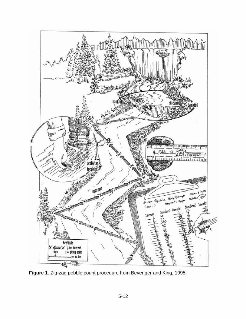
5-12
Figure 1. Zig-zag pebble count procedure from Bevenger and King, 1995.
5-13
LITERATURE CITED
Bevenger, G. S., and R. M. King. 1995. A pebble count procedure for assessing
watershed cumulative effects. U.S. Department of Agriculture, Fort Collins
Colorado.
Rosgen, David L. 1994. A stream classification system. Catena. Elsevier Science,
Amsterdam 22: 169–199.
Rosgen, David L. 1996. Applied river morphology. Wildlands Hydrology Books, Pagosa
Springs, Colorado.
Walters, G. 2017. Physical habitat assessment method. Chapter 4.1, pages 2–6 in D. R.
Shull, and R. Whiteash (editors). Assessment methodology for streams and
rivers. Pennsylvania Department of Environmental Protection, Harrisburg,
Pennsylvania.
Wolman, M. G. 1954. A method of sampling coarse river-bed material. Transactions
American Geophysical Union 35(6):951–956.

5-14
5.3 WATER FLOW DATA COLLECTION PROTOCOL

5-15
Prepared by:
Josh Lookenbill
PA Department of Environmental Protection
Office of Water Programs
Bureau of Clean Water
11th Floor: Rachel Carson State Office Building
Harrisburg, PA 17105
2009
Edited by:
Josh Lookenbill
PA Department of Environmental Protection
Office of Water Programs
Bureau of Clean Water
11th Floor: Rachel Carson State Office Building
Harrisburg, PA 17105
2017

5-16
INTRODUCTION
Water flow (hereto referred to as discharge) is the volume of water that passes through
a conduit over a period of time. For the purposes of this document, the conduit is
typically an open stream channel, but it could also include storm drain infrastructure and
other water conveyances. Discharge data is collected along with other water quality
data in order to characterize yields or quantities of pollutants that are transported by
waterbodies. Chemical data is collected and reported as concentrations. Discharge data
allows those concentrations to be further characterized as standardized quantities or
yields. This is required in characterizing the amount of a pollutant transported by a
waterbody that may be affecting water quality.
Historically, DEP has collected discharge data by implementing cross-section
measurements using the “Mid-Section” approach described by Buchanan and Somers
(1969); where depth and velocity is measured at subdivisions across a transect,
discharge is calculated at each subdivision, and the discharge at each of the
subdivisions is summed to calculate total discharge. This approach has been utilized in
small to medium wadable waterbodies and continues to be a valid discharge data
collection protocol.
Over time the utility and consequently the number and frequency of discharge
measurements has dramatically increased. Routine discharge is required to regulate
water allocation, pollution control programs, generate flood prediction forecasts, and
support other important socioeconomic functions. The USGS originally set the standard
for collecting discharge data with USGS Techniques of Water Resources Investigations
book 3, chapter A8 (TWRI 3–A8), “Discharge Measurements at Gaging Stations” by
Buchanan and Somers (1969). Since then technology and data collection protocols
have evolved, and USGS has continued to set the standard for collecting discharge
data. Additional USGS publications include “Measurement and Computation of
Streamflow, volumes 1 and 2,” by Rantz et al. (1982); “Discharge measurements using
a broad-band acoustic Doppler current profiler,” by Simpson (2002); “Quality-assurance
plan for discharge measurements using acoustic Doppler current profiler,” by Oberg et
al. (2005); and “Measuring discharge with acoustic Doppler current profilers from a
moving boat,” by Mueller and Wagner (2009).
DEP no longer maintains a detailed discharge data collection protocol, but references
and implements the latest USGS techniques and standards for collecting discharge
data. USGS Techniques and Methods book 3, chap. A8, “Discharge Measurements at
Gaging Stations” (Turnipseed and Sauer 2010) is the latest techniques and standards
that supersedes or supplements previous USGS publications.
5-17
LITERATURE CITED
Buchanan, T. J., and W. P. Somers. 1969. Discharge measurements at gaging stations.
Book 3, chapter A8, page 65. in National field manual for the collection of water
quality data: Techniques and methods. U.S. Department of the Interior, U.S.
Geological Survey, Reston, VA. (Available online at:
https://pubs.er.usgs.gov/publication/tm3A8.)
Mueller, D. S. and C. R. Wagner. 2009. Measuring discharge with acoustic Doppler
current profilers from a moving boat. Book 3, section A, chapter 22. in National
field manual for the collection of water quality data: Techniques and methods.
U.S. Department of the Interior, U.S. Geological Survey, Reston, VA. (Available
online at: https://pubs.usgs.gov/tm/3a22/.)
Oberg, K. A., S. E. Morlock, and W. S. Caldwell. 2005. Quality assurance plan for
discharge measurements using acoustic Doppler current profilers: United States
Geological Survey Scientific Investigations report 2005–5183. U.S. Department
of the Interior, U.S. Geological Survey, Reston, VA. (Available online at:
https://pubs.usgs.gov/sir/2005/5183/SIR 2005-5183.pdf.)
Rantz, S. E. 1982. Measurement and computation of streamflow: Water supply paper
2175. U.S. Department of the Interior, U.S. Geological Survey, Reston, VA.
(Available online at: https://pubs.er.usgs.gov/publication/wsp2175.)
Simpson, M. R. 2002. Discharge measurements using a Broad-Band Acoustic Doppler
Current Profiler: United States Geological Survey Open-File Report 01–01. U.S.
Department of the Interior, U.S. Geological Survey, Sacramento, CA. (Available
online at: https://pubs.usgs.gov/of/2001/ofr0101/.)
Turnipseed, D. P. and V. B. Sauer. 2010. Discharge measurements at gaging stations:
United States Geologic Survey. Book 3, chapter A8. in National field manual for
the collection of water quality data: Techniques and methods. U.S. Department of
the Interior, U.S. Geological Survey, Reston, VA. (Available online at:
https://pubs.usgs.gov/twri/twri3a8/.)

A-1
APPENDIX A: BIOLOGICAL DATA COLLECTION INFORMATION AND FORMS

A-2
A.1 MACROINVERTEBRATE FIELD DATA SHEET
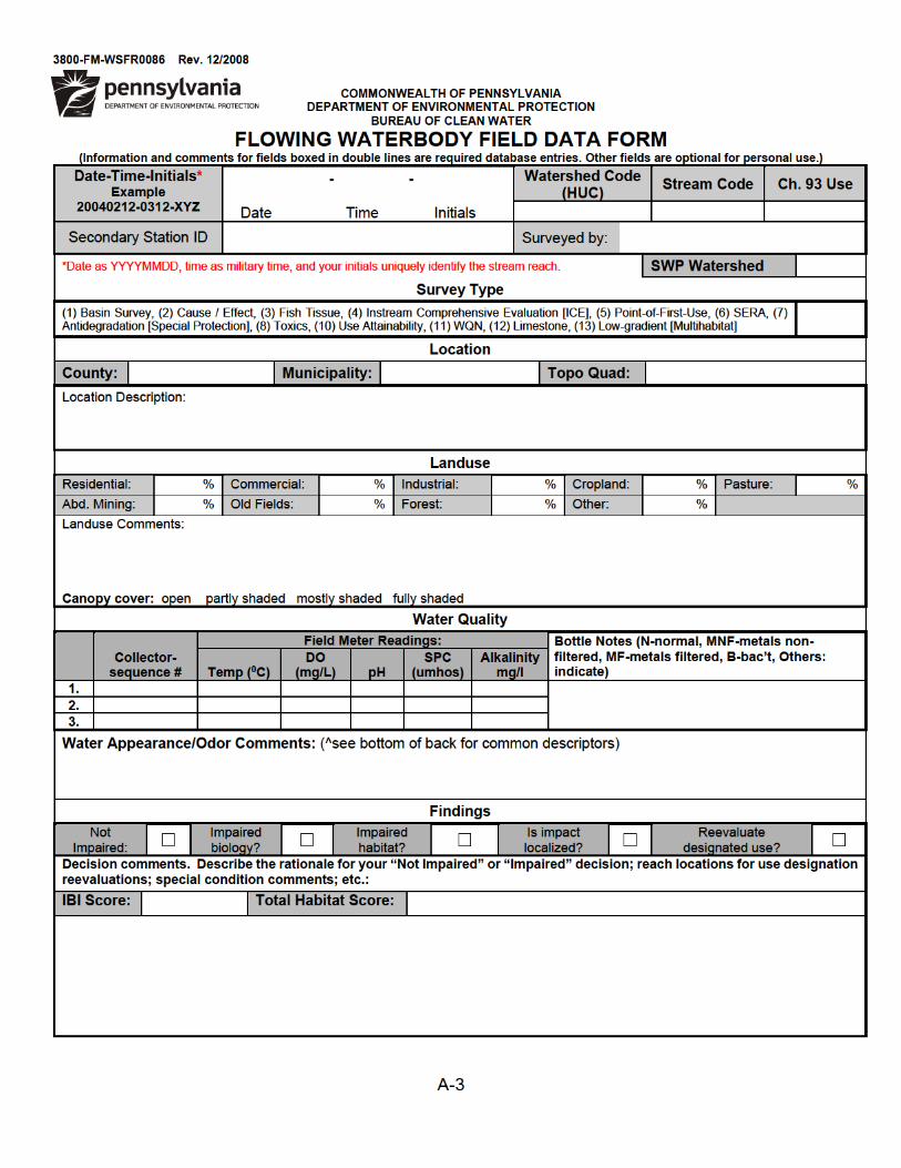
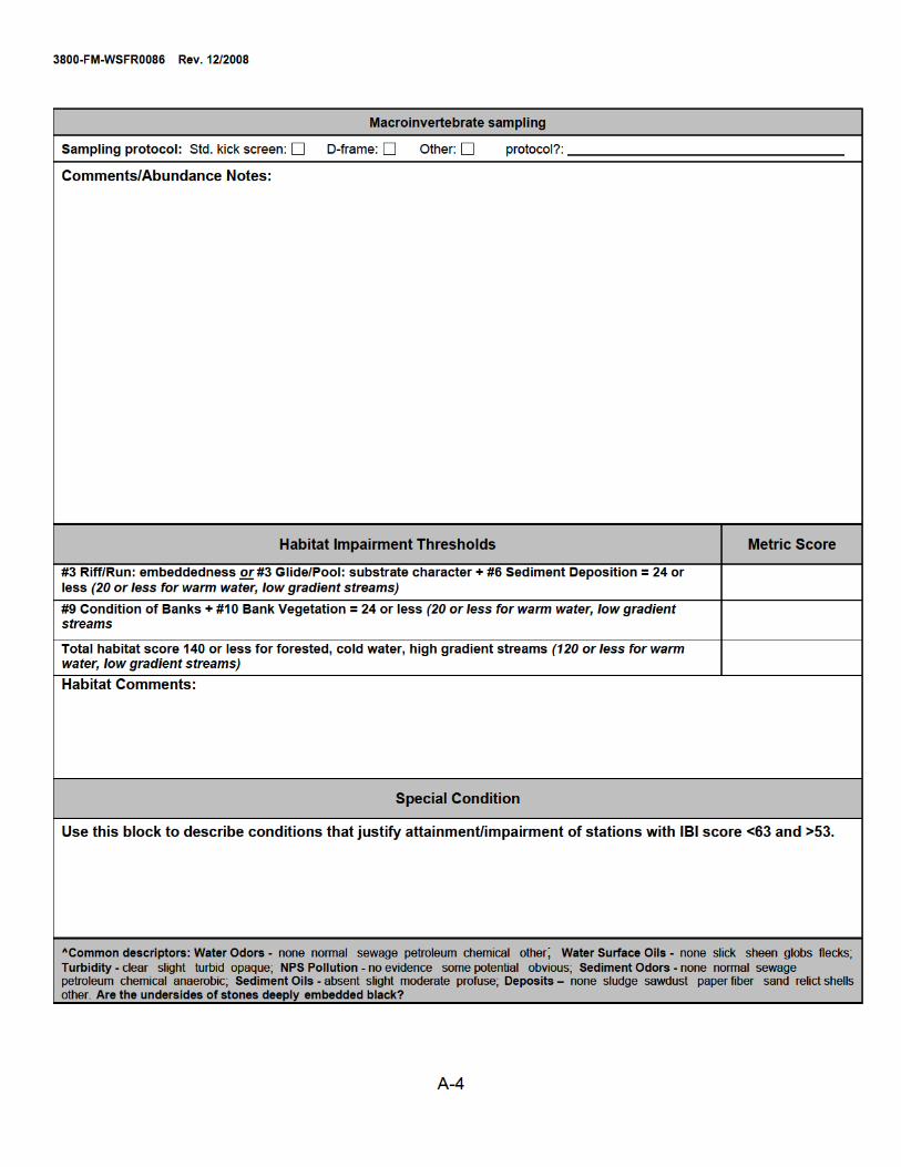

A-5
A.2 MACROINVERTEBRATE ENUMERATION BENCH SHEET
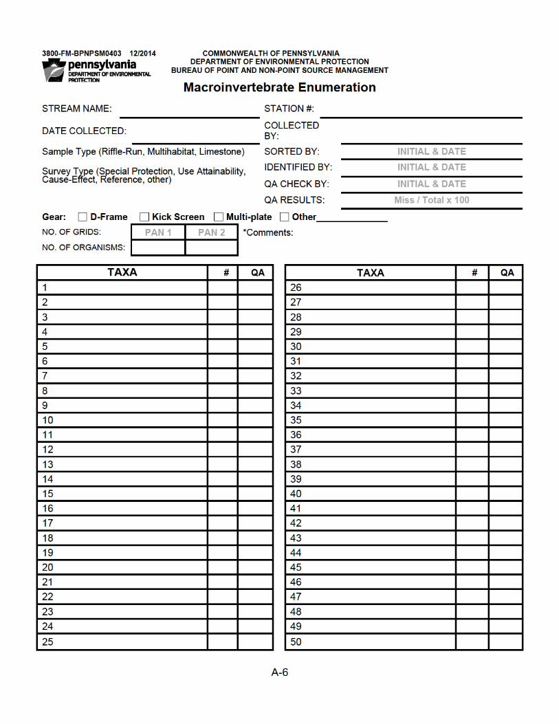

A-7
A.3 FISH FIELD DATA COLLECTION SHEET

B-8
FIELD DATA SHEET SEMI QUANTITATIVE FISH SURVEY SAMPLING
Site ID: Stream Name: Date:
Crew/Agency:
Location:
Reach Desc:
County: Municipality:
Start-End Time (Military): -
Mean Site Width (M): Site Length (M):
Latitude (dec. deg.): Longitude (dec. deg.):
Temperature (°C):
Sp. Conductance (µs/cmc):
pH (SU):
DO (MG/L):
Alkalinity (MG/L):
Habitat Score:
Water Clarity: Turbidity (NTU): Secchi Depth: Meters
Or if you forgot your Secchi Disk or Turbidity Meter circle one: 1 2 3 4 5 6 7 8 9 10
(Turbid ≤ 1 m) (Discolored 1-2 m) (Clear > 2 m)
Gear(s):
Backpack AC Volts: Button time seconds: # passes:
Towboat DC Watts: Pulse rate (Hz): # netters:
Boat P-DC Amps: Pulse Width (ms): # probes:
Make/Model:
Comments:
% Mesohabitat:
Riffle % Run % Pool %
% Velocity/Depth Regimes
Slow-Deep % Slow-Shallow % Fast-Deep % Fast-Shallow %
% Habitat: (% fish in habitat (# individuals) / % habitat within reach)
Root Wads / % Mud Bank __/__% Macrophyte / % Artificial (Docks, Piers, etc.) / %
Boulder / % Cobble / % Gravel / % Sand / % Silt / %
Large Woody Debris / % Small Wood Debris / %
Comments:
% Substrate:
Boulder % Cobble % Gravel % Sand % Silt %
Detritus % Bedrock % Artificial or Channelized %
Comments:


A-11
FIELD DATA SHEET SEMI-QUANTITATIVE FISH SURVEY SAMPLING (continued)
Site ID:
Stream Name: Date:
Abv. Common
Name DELTP* Description BODY
Bg Black grub (Black spot) P Small black cyst approximately one millimeter in diameter, caused by a larval trematode.
Pe External parasite P Ectoparasite attached to body, fins or gills (Leech, Fish louse, Anchor parasite etc.) De Deformities D Body structure is abnormal, ex. curvature of the spine Fi Fungal infection L Fungal infections may include a fuzzy (cotton) appearance w/ discolored areas or
lesions. Ma Melanistic area L Darkly pigmented spot(s), not raised from the skin. Os Open sore L Lesions, (Note any mucus or necrotic tissue that may be in or around the sore) Rr Raised red sore L A bulging or bubbled red sore Sh Scales hemorrhagic L Evidence of bleeding or hemorrhaging at base of scales Tu Tumor T Unusual mass or fatty growth Cw White cysts P Usually a small crème-colored wart or bubble appearance Cc Caudal cysts P Small cysts specifically found on caudal peduncle, or at the base of anal/dorsal
fins Em Emaciated D Body thin and lacks normal robustness, "starved"
EYES Ec Eye cloudy L Eye cloudy or opaque Ee Eye exophthalmic L Eye bulging out of socket Eh Eye hemorrhagic L Eye bleeding or has evidence of burst blood vessels Ed Eye deteriorated L Eye deteriorated, obviously blind, eye missing completely
FINS Fe Fins eroded E Erosion of the fin (make note of spawning, as some species will erode fins during
this active time) Fh Fins hemorrhagic E Evidence of bleeding or hemorrhaging of fins Ff Fins frayed E Fins appear worn out and stressed (make note of spawning)
GILLS Ge Gills eroded E Necrotic tissue or eroded to the point that sections of the gill filaments are
missing Gf Gills frayed E Gill lamellae appear worn out and stressed Gs Gill spots P Small white spots throughout the lamellae Gc Gill cysts P Cyst attached to gills, usually a small crème-colored wart or bubble appearance
OTHER G Gravid
Female fish full of eggs, releases upon handling
P Post spawn
Egg sack has already released, abdominal wall stretched but empty, (Only if OBVIOUS)
M Milting
Male fish releases milt upon handling
Record as- Species- Length(to nearest 5 mm) Anomaly
Example- Smallmouth bass- 310WcEc, 470, 225Ge *DELTP- Deformities, Eroded fins/gills, Lesions, Tumors, Parasites

A-12
FIELD DATA SHEET SEMI-QUANTITATIVE FISH SURVEY SAMPLING (continued)
Site ID: Stream Name: Date:
SPECIES (length > 25mm) #
Photo(s) Field Count
Lab Count Total Count
1.
2.
3.
4.
5.
6.
7.
8.
9.
10.
11.
12.
13.
14.
15.
16.
17.
18.
19.
20.
21.
22.
23.
24.
25.
26.
27.
28.
29.
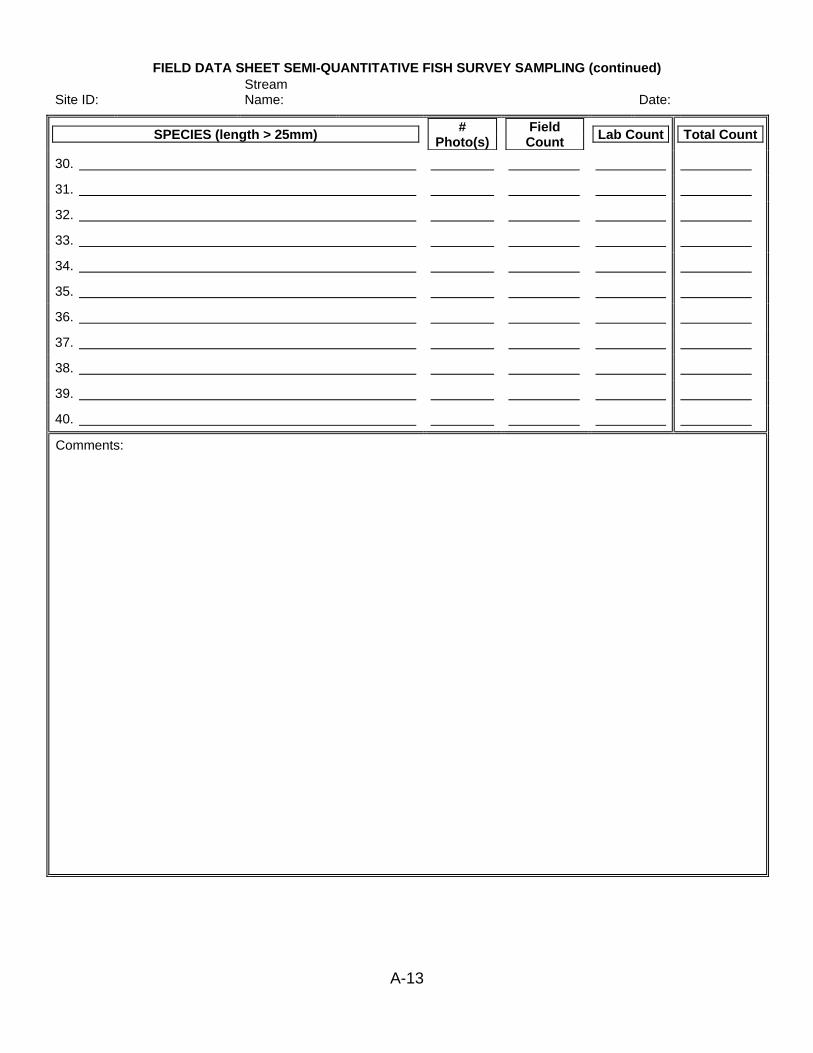
A-13
FIELD DATA SHEET SEMI-QUANTITATIVE FISH SURVEY SAMPLING (continued)
Site ID: Stream Name: Date:
SPECIES (length > 25mm) #
Photo(s) Field Count
Lab Count Total Count
30.
31.
32.
33.
34.
35.
36.
37.
38.
39.
40.
Comments:

A-14
GENERAL INSTRUCTIONS FOR FIELD DATA SHEET SEMI-QUANTITATIVE FISH SURVEY SAMPLING
Station ID: YEARMMDD-TIME-AGENCY, example: (20080601-1200-DEP). TIME = START TIME
Crew/Agency: List each crew member and agency or affiliation.
Location: General description, example: Transect is located 500 meters north of Pine Run and 1000 meters south of Rt. 441 bridge.
Start-End Time: Enter military time, start of shocking to end of shocking.
Mean Site Width: In the first 100 meters, 5 wetted channel widths are measured using a graduated measuring tape or range finder (every 20 meters from the starting point) and averaged.
Site Length: Wadeable = Minimum site length of 100 meters should be surveyed. Increased site length can be used as necessary to cover all habitats (pools, riffles, runs, and cascades).
Average Stream Width (m) Minimum Site Length
<10m 100m
10 to 40m 10 times the average stream width
>40m Maximum of 400m
Nonwadeable = Minimum site length of 500 meters should be surveyed. Increased site length can be used as necessary to cover all habitats (pools, riffles, runs, and cascades).
Latitude/Longitude: Decimal Degrees.
Current: Check one.
Species: List species and count all individuals > 25mm.
Column – Photo #: Number fish photographed.
Column – Field Count: The number of the fish identified in the field.
Column – Lab Count: The number of the fish identified in the laboratory.
Comments: Water/weather conditions, problems, etc.

A-15
A.4 FISH TISSUE FIELD DATA COLLECTION SHEET

A-16
COMMONWEALTH OF PENNSYLVANIA
DEPARTMENT OF ENVIRONMENTAL PROTECTION
BUREAU OF WATER STANDARDS AND FACILITY REGULATION
GENERAL INSTRUCTIONS FOR
FIELD DATA SHEET TISSUE SAMPLING
STATION Enter WQN Station Number, WQF Station Number or Survey Station Number as
NUMBER: appropriate. Leave blank if none of these apply.
NOTE: If WQN Number is entered, then Waterbody Name, Location, County and Municipality can
be left blank.
DATE, COLLECTOR, AGENCY and COLLECTOR NUMBER: Must be completed.
PROJECT ID: FISH
NEW STATIONS: If a WQF station number has not previously been assigned, Quad. Name, Quad. Number, either
Lat/Long or inches-N/inches-W and RMI (to nearest 0.1 mile) must be entered (for STORET input).
TISSUE TYPE: Standard samples are:
1. Skin-on, scaled fillets for gamefish, panfish and rough fish.
2. Skinless fillets for catfishes.
3. Skinless one-inch cross-sections for American Eel
SAMPLE: A normal sample is a composite of 10 fillets from 5 fish. For large fish, 5 fillets can be used.
75 PERCENT RULE: The individual fish in each composite should be as close to the same size as possible. A general
guideline is that the length of the smallest individual in the composite should be no less than 75
percent of the length of the largest individual.
Black grub (Black spot) Bg Tumor Tu Fins eroded Fe
External parasite Pe White cysts Cw Fins hemorrhagic Fh
Deformities De Caudal cysts Cc Fins frayed Ff
Fungal infection Fi Emaciated Em Gills eroded Ge
Melanistic area Ma Eye cloudy Ec Gills frayed Gf
Open sore Os Eye exophthalmic Ee Gill spots Gs
Raised red sore Rr Eye hemorrhagic Eh Gill cysts Gc
Scales hemorrhagic Sh Eye deteriorated Ed
Gravid G Post spawn Ps Milting male M
Fish Health:
Life History:
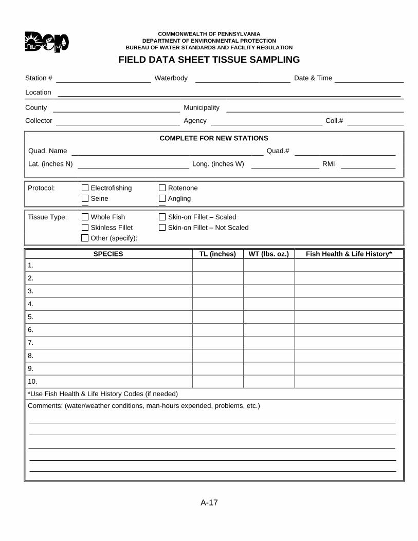
A-17
COMMONWEALTH OF PENNSYLVANIA
DEPARTMENT OF ENVIRONMENTAL PROTECTION
BUREAU OF WATER STANDARDS AND FACILITY REGULATION
FIELD DATA SHEET TISSUE SAMPLING
Station # Waterbody Date & Time
Location
County Municipality
Collector Agency Coll.#
COMPLETE FOR NEW STATIONS
Quad. Name Quad.#
Lat. (inches N) Long. (inches W) RMI
Protocol: Electrofishing
Seine
Rotenone
Angling
Tissue Type: Whole Fish
Skinless Fillet
Skin-on Fillet – Scaled
Skin-on Fillet – Not Scaled
Other (specify):
SPECIES TL (inches) WT (lbs. oz.) Fish Health & Life History*
1.
2.
3.
4.
5.
6.
7.
8.
9.
10.
*Use Fish Health & Life History Codes (if needed)
Comments: (water/weather conditions, man-hours expended, problems, etc.)
A-18
A.5 MUSSEL FIELD DATA COLLECTION SHEETS

A-19
Date: Site#: Location:
Water Temperature: Air Temperature: page of
Dive #
Distance
from X site
Distance
from Shore Latitude Longitude Diver
Backup
Diver Air In Air Out Time In
Time
Out
Invasive
Mussel Score
and Species
Max
Depth
Comments: Bucket Dive
% Boulder: % Boulder:
% Cobble: % Cobble:
%Gravel: %Gravel:
%Sand: %Sand:
%Silt: %Silt:
Dive #
Distance
from X site
Distance
from Shore Latitude Longitude Diver
Backup
Diver Air In Air Out Time In
Time
Out
Invasive
Mussel Score
and Species
Max
Depth
Comments: Bucket Dive
% Boulder: % Boulder:
% Cobble: % Cobble:
%Gravel: %Gravel:
%Sand: %Sand:
%Silt: %Silt:
Dive #
Distance
from X site
Distance
from Shore Latitude Longitude Diver
Backup
Diver Air In Air Out Time In
Time
Out
Invasive
Mussel Score
and Species
Max
Depth
Comments: Bucket Dive
% Boulder: % Boulder:
% Cobble: % Cobble:
%Gravel: %Gravel:
%Sand: %Sand:
%Silt: %Silt:
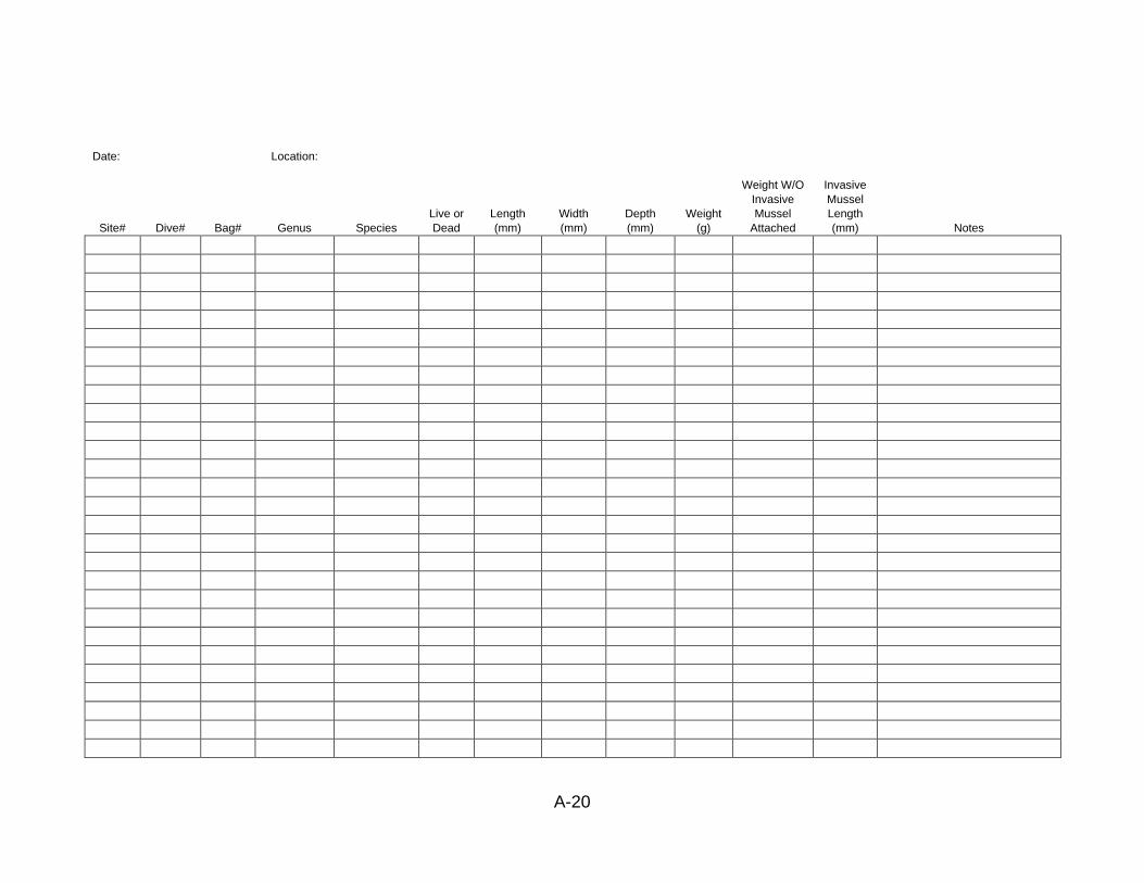
A-20
Date: Location:
Site# Dive# Bag# Genus Species
Live or
Dead
Length
(mm)
Width
(mm)
Depth
(mm)
Weight
(g)
Weight W/O
Invasive
Mussel
Attached
Invasive
Mussel
Length
(mm) Notes

A-21
A.6 QBE PERIPHYTON FIELD DATA COLLECTION SHEET
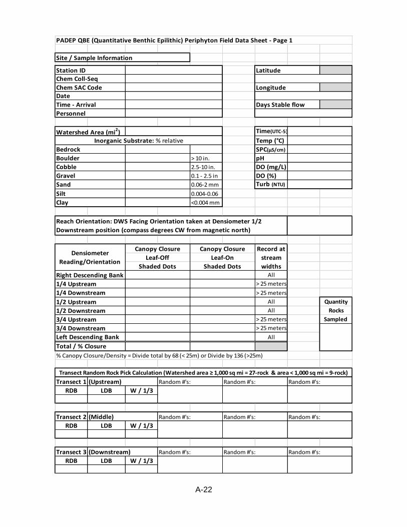
A-22
Time(UTC-5)
Temp (°C)
SPC(µS/cm)
> 10 in. pH
2.5-10 in. DO (mg/L)
0.1 - 2.5 in DO (%)
0.06-2 mm Turb (NTU)
0.004-0.06
<0.004 mm
All
> 25 meters
> 25 meters
All Quantity
All Rocks
> 25 meters Sampled
> 25 meters
All
Transect 1
RDB LDB W / 1/3
Transect 2
RDB LDB W / 1/3
Transect 3
RDB LDB W / 1/3
Transect Random Rock Pick Calculation (Watershed area ≥ 1,000 sq mi = 27-rock & area < 1,000 sq mi = 9-rock)
Random #'s: Random #'s: Random #'s:
Random #'s: Random #'s: Random #'s:
3/4 Downstream
Left Descending Bank
Reach Orientation: DWS Facing Orientation taken at Densiometer 1/2
Downstream position (compass degrees CW from magnetic north)
Shaded Dots
Densiometer
Reading/Orientation
Right Descending Bank
1/4 Upstream
Canopy Closure Canopy Closure
Leaf-Off Leaf-On
(Middle)
(Downstream) Random #'s: Random #'s: Random #'s:
Sand
PADEP QBE (Quantitative Benthic Epilithic) Periphyton Field Data Sheet - Page 1
Record at
stream
widths
% Canopy Closure/Density = Divide total by 68 (< 25m) or Divide by 136 (>25m)
(Upstream)
Total / % Closure
1/2 Upstream
1/2 Downstream
3/4 Upstream
Shaded Dots
Inorganic Substrate: % relative
Station ID
Chem Coll-Seq
Date
Time - Arrival
Personnel
1/4 Downstream
Silt
Clay
Bedrock
Boulder
Cobble
Gravel
Latitude
Longitude
Days Stable flow
Site / Sample Information
Watershed Area (mi2)
Chem SAC Code

A-23
Collector # Sequence #
Collector # Sequence #
Collector # Sequence #
PADEP QBE - 2 (Quantitative Benthic Epilithic) Periphyton Field Data Sheet - Page 2
Sub-Sample Processing Information:
AFDM Filter & Notes - 2ml on GFF filter - foil wrapped. (Collect 3 replicate filters).
Store/transport on dry ice then store at -80°C in BOL Bacti freezer.
Phycocyanin Bottle & Notes - 30ml in 120ml white plastic sample bottle.
Store/transport on wet ice. Upon arrival at BOL deliver to BOL Bacti refrigerator. BOL
will pull 3 sub-samples from this single bottle.
Algal ID Bottles & Notes - 100ml well homoginized slurry in 120ml white plastic sample
bottle + 7ml formaldehyde preservative (Collelct min three 100ml replicate bottles).
Total Diluted Algae Slurry Volume (ml): Dilute as needed to achieve
min required: 700ml with cyanotoxin test, 400ml without cyanotoxin
If col lecting for cyanotoxin testing: 250ml in whirl -pak bag then place whirl -pak in ziplock bag. Store/transport
on dry ice then s tore at -80°C in Monitoring Section freezer.
Chlorophyll-a Filter & Notes - 2ml on GFF filter with 1ml MgCO3 fixative - foil wrapped.
(Collect 3 replicate filters). Store/transport on dry ice then store at -80 °C in BOL Bacti
freezer. Indicate if submitting for acidified or non-acidified processing.
Other Notes
A-24
A.7 QMH PERIPHYTON FIELD DATA COLLECTION SHEET
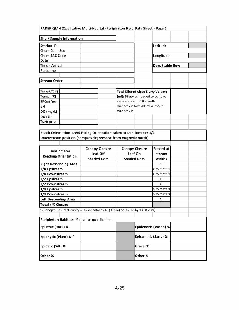
A-25
Time(UTC-5)
Temp (°C)
SPC(µS/cm)
pH
DO (mg/L)
DO (%)Turb (NTU)
All
> 25 meters
> 25 meters
All
All
> 25 meters
> 25 meters
All
1/2 Upstream
Right Descending Area
1/4 Upstream
1/4 Downstream
Stream Order
Total Diluted Algae Slurry Volume
(ml): Dilute as needed to achieve
min required: 700ml with
cyanotoxin test, 400ml without
cyanotoxin
Personnel
PADEP QMH (Qualitative Multi-Habitat) Periphyton Field Data Sheet - Page 1
Station ID Latitude
Site / Sample Information
Date
Time - Arrival Days Stable flow
Chem Coll - Seq
Chem SAC Code Longitude
Other % Other %
Periphyton Habitats: % relative qualification
Epidendric (Wood) %
Epiphytic (Plant) % a
Epilithic (Rock) %
Episammic (Sand) %
Epipelic (Silt) % Gravel %
Reach Orientation: DWS Facing Orientation taken at Densiometer 1/2
Downstream position (compass degrees CW from magnetic north)
Densiometer
Reading/Orientation
Canopy Closure Canopy Closure Record at
stream
widths
Leaf-Off Leaf-On
Shaded Dots Shaded Dots
1/2 Downstream
3/4 Upstream
Total / % Closure
% Canopy Closure/Density = Divide total by 68 (< 25m) or Divide by 136 (>25m)
3/4 Downstream
Left Descending Area
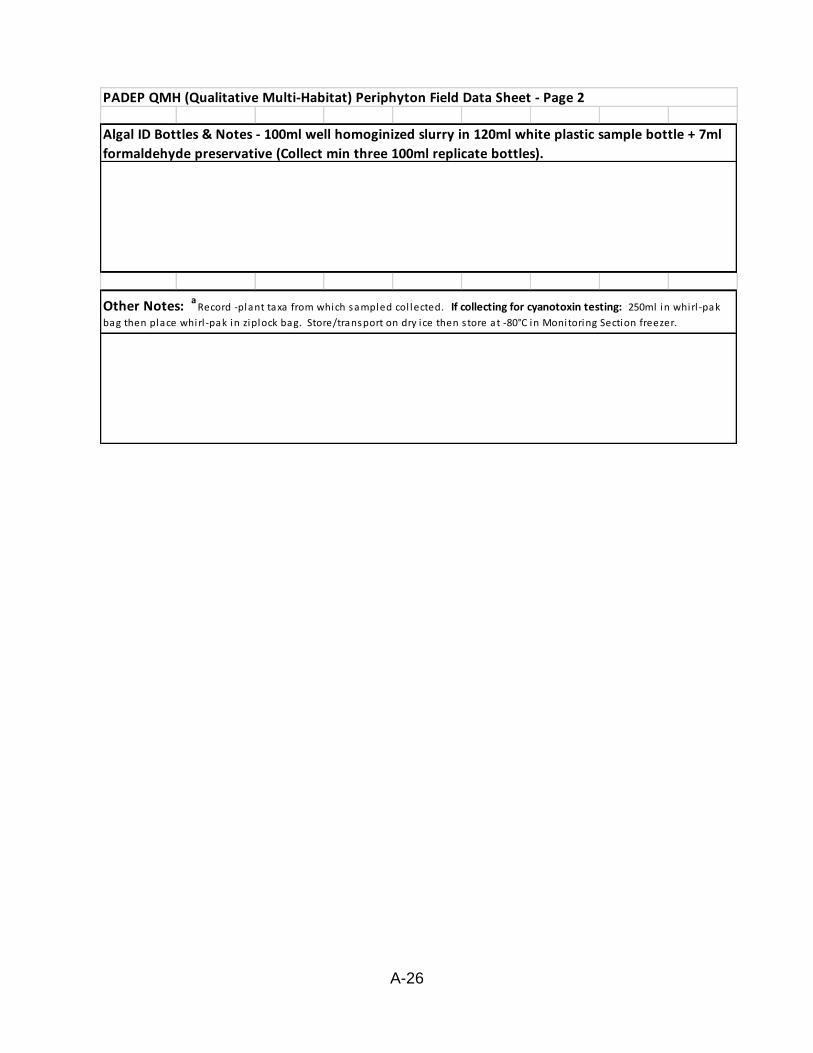
A-26
Other Notes: a Record -plant taxa from which sampled col lected. If collecting for cyanotoxin testing: 250ml in whirl -pak
bag then place whirl -pak in ziplock bag. Store/transport on dry ice then s tore at -80°C in Monitoring Section freezer.
Algal ID Bottles & Notes - 100ml well homoginized slurry in 120ml white plastic sample bottle + 7ml
formaldehyde preservative (Collect min three 100ml replicate bottles).
PADEP QMH (Qualitative Multi-Habitat) Periphyton Field Data Sheet - Page 2

A-27
A.8 ALGAE IDENTIFICATION AND ENUMERATION LABORATORY SUBMISSION DATA
SHEET

A-28
PA DEP GIS Key
IDDate
Sample Type
(QMH = Quitative
Multi-Habitat, QBE
= Quantitative
Benthic Epilithic)
Stream Name Location Description County Latitude Longitude
Surface
Area
(cm^2)
Initial Sample
Volume (ml)
ID Bottle
Sub-
Sample
Volume
(ml)
Formaldehyde
Added (ml)
Algae Identification and Enumeration Laboratory Submission Data Sheet

A-29
A.9 MICROBIOLOGY SAMPLE SUBMISSION SHEET FOR ACIDIFIED CHLOROPHYLL-A,
PHYCOCYANIN, AND AFDM

A-30

A-31
A.10 BACTERIA MONITORING FIELD AND SITE DATA SHEET

A-32

33

A-34

A-35

B-1
APPENDIX B: CHEMICAL DATA COLLECTION INFORMATION AND FORMS

B-2
B.1 FIELD METER CALIBRATION FORM


B-4
B.2 TRANSECT DATA COLLECTION FORM


B-7
B.3 SAMPLE INFORMATION SYSTEM USER’S GUIDE


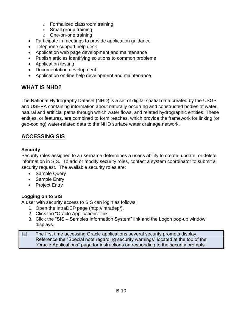
B-10
o Formalized classroom training o Small group training o One-on-one training
• Participate in meetings to provide application guidance
• Telephone support help desk
• Application web page development and maintenance
• Publish articles identifying solutions to common problems
• Application testing
• Documentation development
• Application on-line help development and maintenance
WHAT IS NHD?
The National Hydrography Dataset (NHD) is a set of digital spatial data created by the USGS
and USEPA containing information about naturally occurring and constructed bodies of water,
natural and artificial paths through which water flows, and related hydrographic entities. These
entities, or features, are combined to form reaches, which provide the framework for linking (or
geo-coding) water-related data to the NHD surface water drainage network.
ACCESSING SIS
Security
Security roles assigned to a username determines a user’s ability to create, update, or delete
information in SIS. To add or modify security roles, contact a system coordinator to submit a
security request. The available security roles are:
• Sample Query
• Sample Entry
• Project Entry
Logging on to SIS
A user with security access to SIS can login as follows:
1. Open the IntraDEP page (http://intradep/). 2. Click the “Oracle Applications” link. 3. Click the “SIS – Samples Information System” link and the Logon pop-up window
displays.
The first time accessing Oracle applications several security prompts display. Reference the “Special note regarding security warnings” located at the top of the “Oracle Applications” page for instructions on responding to the security prompts.

B-11
Figure 1: The Logon pop-up window.
4. Click in the Username field and enter a user name. 5. Click in the Password field and enter the password. 6. Click in the Database field and enter “PROD”. 7. Click the CONNECT button to log on to SIS.
Changing an Oracle Password
Each user has a single password for all Oracle applications. Changing the password used to
access SIS also changes the password for eFACTS, CTS, etc.
Change an Oracle password as follows:
1. Open the IntraDEP page (http://intradep/). 2. Click the “Oracle Applications” link. 3. Click the CHANGE PASSWORD button and the Logon pop-up window displays. 4. Click in the Username field and enter a user name. 5. Click in the Password field and enter the current password. 6. Click in the Database field and enter PROD. 7. Click the CONNECT button and the “Change Oracle Password” pop-up window
displays.
Figure 2: The “Change Oracle Password” pop-up window.
8. Click in the Old Password field and enter the current password. 9. Click in the New Password field and enter a new password. 10. Click in the Confirm Password field and enter the new password a second time. 11. Click the OK button. 12. A message in the hint line at the bottom of the screen will indicate if the password was
successfully changed.
SIS OVERVIEW
This section provides an overview of the screen layout, common structure, fields, and buttons
within SIS.
Title Bar
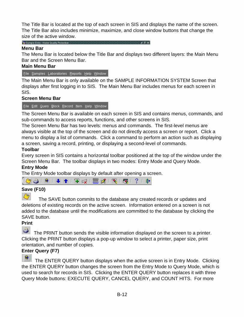
B-12
The Title Bar is located at the top of each screen in SIS and displays the name of the screen.
The Title Bar also includes minimize, maximize, and close window buttons that change the
size of the active window.
Menu Bar
The Menu Bar is located below the Title Bar and displays two different layers: the Main Menu
Bar and the Screen Menu Bar.
Main Menu Bar
The Main Menu Bar is only available on the SAMPLE INFORMATION SYSTEM Screen that
displays after first logging in to SIS. The Main Menu Bar includes menus for each screen in
SIS.
Screen Menu Bar
The Screen Menu Bar is available on each screen in SIS and contains menus, commands, and
sub-commands to access reports, functions, and other screens in SIS.
The Screen Menu Bar has two levels: menus and commands. The first-level menus are
always visible at the top of the screen and do not directly access a screen or report. Click a
menu to display a list of commands. Click a command to perform an action such as displaying
a screen, saving a record, printing, or displaying a second-level of commands.
Toolbar
Every screen in SIS contains a horizontal toolbar positioned at the top of the window under the
Screen Menu Bar. The toolbar displays in two modes: Entry Mode and Query Mode.
Entry Mode
The Entry Mode toolbar displays by default after opening a screen.
Save (F10)
The SAVE button commits to the database any created records or updates and
deletions of existing records on the active screen. Information entered on a screen is not
added to the database until the modifications are committed to the database by clicking the
SAVE button.
The PRINT button sends the visible information displayed on the screen to a printer.
Clicking the PRINT button displays a pop-up window to select a printer, paper size, print
orientation, and number of copies.
Enter Query (F7)
The ENTER QUERY button displays when the active screen is in Entry Mode. Clicking
the ENTER QUERY button changes the screen from the Entry Mode to Query Mode, which is
used to search for records in SIS. Clicking the ENTER QUERY button replaces it with three
Query Mode buttons: EXECUTE QUERY, CANCEL QUERY, and COUNT HITS. For more

B-13
information on the three Query Mode buttons, reference the QUERY MODE section of the user
guide.
Next Record ( )
The NEXT RECORD button displays, or navigates to, the next record of the current
block. Use this button to view additional records when a query is executed and retrieves more
than one record.
Previous Record ( )
The PREVIOUS RECORD button displays, or navigates to, the previous record of the
current block.
Create Record (F6)
The CREATE RECORD button clears the current record from the screen and creates a
new, blank record.
Delete Record (Shift + F6)
The DELETE RECORD button deletes the current record. Clicking the DELETE
RECORD button will delete the current record on which the cursor is residing. The record is
not permanently deleted until the SAVE button is clicked.
Duplicate Record
The DUPLICATE RECORD button duplicates the previously displayed record into the
current, empty record. Update any fields on the duplicated record and then save the changes.
Use this button to enter multiple similar records.
Edit Item (Ctrl + E)
The EDIT ITEM button displays the Editor pop-up window with the contents of the
currently selected field. The Editor pop-up window provides the user with a larger space to
view or update the contents of a field.
Clear Record (Shift + F4)
The CLEAR RECORD button clears the current record from the screen without deleting
it. This button removes the currently displayed record from the buffer of queried records and
displays the next record in the queried buffer.
Clear Form
The CLEAR FORM button clears the current screen of all records without updating the
records. Clicking the CLEAR FORM button places the screen in a similar state to when it is
first opened.
Help
The HELP button provides the technical properties of the field in which the cursor
resides.
Exit (CTRL + Q)
The EXIT button closes the current screen.
QUERY MODE

B-14
Use Query Mode to display records that match user-specified criteria. Screens open in Entry
Mode with the ENTER QUERY button visible. Click the ENTER QUERY button to place the
screen into Query Mode, which hides the ENTER QUERY button and displays the EXECUTE
QUERY, COUNT HITS and CANCEL QUERY buttons.
Execute Query (F8)
The EXECUTE QUERY button retrieves all records that match the user-defined query
criteria.
Caution: If no criteria are specified, a “blind query” is executed which retrieves all records.
Running blind queries is not recommended.
Count Hits (Shift + F2)
The COUNT HITS button displays a number in the hint line indicating how many records
match the query criteria. Click this button prior to executing a query to see the number of
results and determine whether to specify additional criteria to limit the results.
Cancel Query (Ctrl + Q)
The CANCEL QUERY button exits QUERY MODE and places the screen into the Entry
Mode. The CANCEL QUERY button does not stop an executed query that is currently
running.
SCREEN STRUCTURE
The screens in SIS use a standard layout with common elements described in this section.
Header and Detail Block
A header block identifies a specific sample displayed on the screen.
A detail block displays information related to the sample identified in the header block.
Figure 3: The SAMPLE ENTRY Screen with the header and detail blocks identified.

B-15
Tabs
Detail blocks are separated into tabs that display additional information related to the record in
the header block. Click on a tab name to activate it and display the related details. The
header block continues to display the current sample record and the activated tab displays the
related detail record. The label of the currently displayed tab displays underlined and in red
font.
List of Values (F9)
A list of values (LOV) button, typically located to the right of a field, displays a list of codes
or a calendar for the related field.
Figure 4: A list of values with the first value selected.
Using the list of values button:
1. Click the list of values button to the right of the field and a list of values pop-up window displays.
2. Click on an entry in the list to select it.
The list may contain numerous values. Filter the list by clicking in the Find field, entering a wildcard (%) followed by part of a code or description, and then clicking the FIND button. The list displays only values containing the text entered in the Find field.
Click the OK button to select the highlighted entry or click the CANCEL button to return to the
screen without retrieving a value.
Pop-Up Messages
Pop-up messages alert or warn the user about certain actions, information, or functionality
throughout the system. Users should read the pop-up message for directions to follow or to
confirm an action.
Figure 5: A pop-up message confirming an action.

B-16
Hint Line
Every window in SIS, except the SAMPLE INFORMATION SYSTEM Screen, contains a
horizontal bar at the bottom of the screen called the hint line. The hint line displays information
about the screen, an operation in progress, the result of an operation, or a description of the
currently selected field.
Figure 6: The hint line displaying a description for the Collector ID field.
QUERYING FOR SAMPLES
The following sections provide information on how to query an existing sample and the
associated details using the SAMPLES Screen. Access the SAMPLES Screen by clicking the
Samples Menu and then clicking the Query samples command.

B-17
Figure 7: The samples screen.
Querying Using the Collector and Date Collected
This section provides steps for querying an existing sample using the collector, date collector,
and/or sequence number.
1. Access the SAMPLES Screen and then click the ENTER QUERY button on the toolbar or press the [F7] key.
2. Enter the four-digit collector ID assigned to the employee or monitoring point that collected the sample or select it by clicking the list of values button to the right of the Collector ID field. Press the [TAB] key.
3. If known, enter the date that the sample was collected. Press the [TAB] key. 4. If known, enter the time that the sample was collected. Press the [TAB] key. 5. If known, enter the sequence number assigned to the sample. 6. Click the EXECUTE QUERY button on the toolbar or press the [F8] key. 7. If more than one sample is retrieved, use the NEXT RECORD button on the toolbar or
press the [ ] key to locate the correct record.
If more than one record was retrieved, “Record: 1/?” displays below the hint line.
Querying using the Query Options Button
The Query Options button allows querying using a range of dates, sequence numbers, and
test results.
1. To use the QUERY OPTIONS button, access the SAMPLES Screen and then click the ENTER QUERY button on the toolbar or press the [F7] key.
2. Click the QUERY OPTIONS button and the “Query Options” pop-up window displays.

B-18
Figure 8: The “Query Options” pop-up window.
3. Enter query criteria in any of the fields on the screen. 4. Click the COUNT HITS button on the toolbar to determine how many records will be
retrieved. 5. If the query count is extensive, further qualify the query before executing. 6. Click the EXECUTE QUERY button on the toolbar or press the [F8] key. 7. If more than one sample is retrieved, use the NEXT RECORD button on the toolbar or
press the [ ] key to locate the correct record.
If more than one record was retrieved, “Record: 1/?” displays below the hint line.
8. To view the results and details of the sample, reference the VIEWING SAMPLE DETAILS section of the user guide.
Querying using Multiple Criteria
This section provides steps for querying a sample using the fields in the header block and the
fields under the detail tabs on the SAMPLES Screen.
If the complete query value for a field is not known, use the wildcard (%) at the beginning and/or end of one or two key characters. For example, to match both Lower Paxton and Paxtang municipalities enter: %PAXT%
1. Access the SAMPLES Screen and then click the ENTER QUERY button on the toolbar or press the [F7] key.
2. Click on a tab that contains a desired field for entering query criteria.
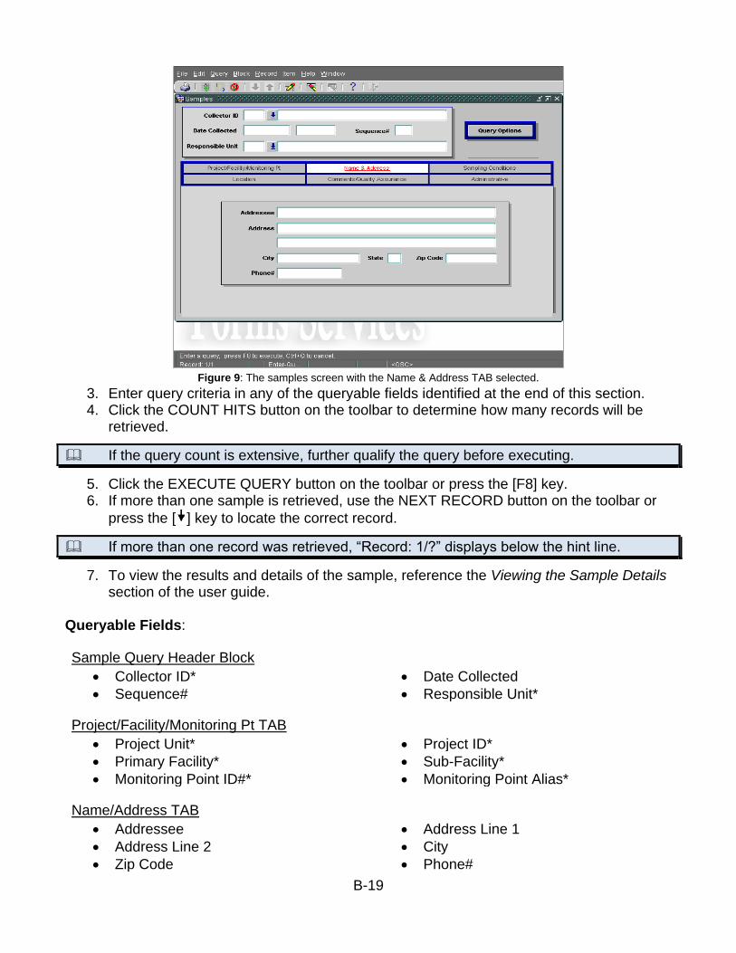
B-19
Figure 9: The samples screen with the Name & Address TAB selected.
3. Enter query criteria in any of the queryable fields identified at the end of this section. 4. Click the COUNT HITS button on the toolbar to determine how many records will be
retrieved.
If the query count is extensive, further qualify the query before executing.
5. Click the EXECUTE QUERY button on the toolbar or press the [F8] key. 6. If more than one sample is retrieved, use the NEXT RECORD button on the toolbar or
press the [ ] key to locate the correct record.
If more than one record was retrieved, “Record: 1/?” displays below the hint line.
7. To view the results and details of the sample, reference the Viewing the Sample Details section of the user guide.
Queryable Fields:
Sample Query Header Block
• Collector ID* • Date Collected
• Sequence# • Responsible Unit*
Project/Facility/Monitoring Pt TAB
• Project Unit* • Project ID*
• Primary Facility* • Sub-Facility*
• Monitoring Point ID#* • Monitoring Point Alias*
Name/Address TAB
• Addressee • Address Line 1
• Address Line 2 • City
• Zip Code • Phone#

B-20
Sampling Conditions TAB
• Sampling Reason* • Sampling Protocol*
• Medium Type* • Medium*
• Stream Condition* • Initial Flow
• Final Flow • Units*
• Determination* • Depth To Water
• Units* • Determination*
Location TAB
• State* • County
• Municipality • Latitude
• Longitude • Datum
• Reference Point* • Geometric Type*
• Location Procedure* • Location
• Elevation • Accuracy
• Altitude Datum* • Method *
Comments/Quality Assurance TAB
• Appearance • Duplicate of Sample
• Quality Assurance Type* • Voided/Dry Sample
• Confidentiality Reason*
Administrative TAB
• Cost Center* • Entry Complete
• Date Created • Created By
• Date Last Modified • Last Modified By
*A list of values is available.
VIEWING SAMPLE DETAILS
This section provides steps for how to view the details associated with a sample.
1. Access the SAMPLES Screen and query a sample record. 2. Click the SHOW RESULTS button to display the SAMPLE ANALYSES/RESULTS
Screen, which includes the lab results of sample testing.
Figure 10: The SAMPLE ANALYSES/RESULTS Screen.

B-21
3. The SAMPLE ANALYSES/RESULTS Screen displays the laboratory that tested the sample and a list of test codes with results. If there are multiple laboratory sample analyses, then click the NEXT RECORD or PREVIOUS RECORD buttons view a different analysis.
4. To view details about the laboratory identifiers for the sample, click the DETAILS button on the right-hand side of the screen. The “Lab Sample” pop-up window displays.
Figure 11: The “Lab Sample” pop-up window.
5. If available, click the LEGAL SEALS or COMMENTS button to view additional details. 6. Click the to exit the pop-up window and return to the SAMPLE
ANALYSES/RESULTS Screen. 7. To view the complete details of a specific test, click on a test code in the
Analyses/Results section of the screen to select it and then click the DETAILS button located at the bottom of the screen. The “Analysis/Result Details” pop-up window displays.
Figure 12: The “Analysis/Result Details” pop-up window.
8. If available, click the COMMENTS button to view additional comments. 9. Click the to exit the pop-up window and return to the SAMPLE
ANALYSES/RESULTS Screen. 10. Click the again to return to the SAMPLES Screen. 11. Six tabs containing information about the collection of the sample display in the detail
block of the screen.

B-22
Figure 13: The six detail tabs on the samples screen.
12. Click on a tab to display the details:
• Project/Facility/Monitoring Pt TAB This tab identifies the specific project for which a sample was taken; the regulated entities (primary and sub-facilities) that may impact the soil, water, or air sample; and/or the monitoring point established for sample collection.
• Name & Address TAB This tab displays the name and address at which the sample was collected.
• Sampling Conditions TAB This tab displays the conditions under which the sample was collected including the sampling reason, method, medium, and stream condition.
• Location TAB This tab displays the location at which the sample was collected including county, municipality, latitude/longitude, and locational metadata.
• Comments/Quality Assurance TAB This tab displays comments and quality assurance indicators about the sample.
• Administrative TAB This tab displays cost center associated with the sample, who created and last updated the sample, and when the sample was created and last updated.
13. To generate a printed a report displaying the laboratory that tested the sample, a summary of the analysis methods, and results of the tests, click the PRINT REPORT button on the SAMPLE QUERY Screen.
EXPORTING A SAMPLE
The EXPORT button located on the SAMPLES Screen generates a customizable report using
the queried samples. The report is saved as file on the local computer. Contact the
Applications Helpdesk to request the “Sample Export” security role required to use this
function.
1. Access the SAMPLES Screen and query sample records to export. 2. Click the EXPORT button and the “Export Samples” pop-up window displays.
Figure 14: The “Export Samples” pop-up window.
3. Select which samples to include in the report and then click the CONTINUE button. The EXPORT SAMPLES Screen displays.
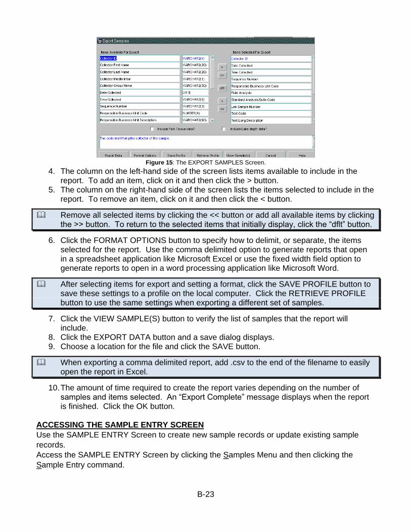
B-23
Figure 15: The EXPORT SAMPLES Screen.
4. The column on the left-hand side of the screen lists items available to include in the report. To add an item, click on it and then click the > button.
5. The column on the right-hand side of the screen lists the items selected to include in the report. To remove an item, click on it and then click the < button.
Remove all selected items by clicking the << button or add all available items by clicking the >> button. To return to the selected items that initially display, click the “dflt” button.
6. Click the FORMAT OPTIONS button to specify how to delimit, or separate, the items selected for the report. Use the comma delimited option to generate reports that open in a spreadsheet application like Microsoft Excel or use the fixed width field option to generate reports to open in a word processing application like Microsoft Word.
After selecting items for export and setting a format, click the SAVE PROFILE button to save these settings to a profile on the local computer. Click the RETRIEVE PROFILE button to use the same settings when exporting a different set of samples.
7. Click the VIEW SAMPLE(S) button to verify the list of samples that the report will include.
8. Click the EXPORT DATA button and a save dialog displays. 9. Choose a location for the file and click the SAVE button.
When exporting a comma delimited report, add .csv to the end of the filename to easily open the report in Excel.
10. The amount of time required to create the report varies depending on the number of samples and items selected. An “Export Complete” message displays when the report is finished. Click the OK button.
ACCESSING THE SAMPLE ENTRY SCREEN
Use the SAMPLE ENTRY Screen to create new sample records or update existing sample
records.
Access the SAMPLE ENTRY Screen by clicking the Samples Menu and then clicking the
Sample Entry command.

B-24
Figure 16: The SAMPLE ENTRY Screen.
The “Business Unit List of Values” pop-up window displays for users authorized for more than one business unit. Select the relevant Business Unit to enter samples for and then click the OK button.
CREATING SAMPLE RECORDS
This section provides steps for creating sample records in SIS using the SAMPLE ENTRY
Screen. The Sample Header and Sampling Conditions TAB contain the only required fields.
The rest of the fields are optional and should be entered when applicable.
Sample Header
The sample header is required. It identifies the general sample information including collector,
date and time collected, sequence number, and sampling reason.
Figure 17: A sample header.
1. Access the SAMPLE ENTRY Screen. 2. Enter the four-digit collector number assigned to the employee, group, or monitoring
device that collected the sample in the Collector ID field. Press the [TAB] key. 3. Enter the date the sample was collected in the first Date Collected field (format
MM/DD/YYYY). Press the [TAB] key. 4. Optionally, enter the time the sample was collected in military time (i.e., enter 1:00 pm
as 1300, enter 9:00 am as 0900) in the second Date Collected field. Press the [TAB] key.

B-25
5. Enter the sequence number for the sample in the Sequence# field. Press the [TAB] key.
6. Click the list of values button next to the Reason field to select a reason for sampling. The field defaults to “Routine Sampling.”
Project/Facility/Monitoring Point TAB
This section is used to indicate if the collected sample is related to a project, eFACTS facility,
or a monitoring point.
1. Click the Project/Facility/Monitoring Pt TAB.
Figure 18: The Project/Facility/Monitoring Pt TAB.
2. If the sample was collected for an existing project, complete the following steps: a. Enter the code identifying the project’s business unit or select using the list of
values button to the right of the Project Unit field. Press the [TAB] key. b. Enter the identification number assigned to the project or select using the list of
values button to the right of the Project ID field. 3. If the sample was collected to monitor an existing primary facility and/or sub facility,
complete the following steps: a. Enter the program-specific identification number in the Primary Facility field or
select a primary facility from the list of values by entering a facility name or program. Press the [TAB] key.
b. Optionally, select a sub-facility by clicking the list of values button to the right of the Sub-Facility field.
4. If the sample was collected at a particular monitoring point, identify the monitoring point using one of the following methods:
a. Enter the Monitoring Point ID assigned to the monitoring point and press the [TAB] key.
b. Enter the Monitoring Point Alias and press the [TAB] key. c. Click the list of values button to the right of either Monitoring Point field, enter a
latitude and longitude, and click the ACCEPT button to display a list of monitoring points to select from.
Coordinates are entered in the format DD-MM-SS.SSSS (e.g., 41-29-46.3034 or -79-38-09.6071)
5. If a monitoring point was entered, click the SAVE button on the toolbar or press the [F10] key. If necessary, proceed to the next tab.

B-26
6. If a monitoring point was not entered, proceed to the Sampling Conditions TAB.
Sampling Conditions TAB
This section is used to enter the conditions under which the sample was collected. The
Medium Type and Medium fields are required. If the sample is linked to a monitoring point on
the Project/Facility/Monitoring Pt TAB, the Medium Type and Medium fields are populated
using information from the monitoring point.
1. Click the Sampling Conditions TAB.
Figure 19: The Sampling Conditions TAB.
2. The Medium Type field is required. Enter the code that identifies the type (category) of sample medium (soil, water, air, plants, etc.) or select by using the list of values button to the right of the Medium Type field. Press the [TAB] key.
3. The Medium field is required. Enter the code that identifies the sample medium or select by using the list of values button to the right of the Medium field. Press the [TAB] key.
4. The fields that display vary based on the Business Area selected when first accessing the SAMPLE ENTRY Screen. Enter data in the optional fields as necessary.
5. Click the SAVE button on the toolbar or press the [F10] key. 6. If necessary, proceed to the next TAB.
Location TAB
This section is used to identify the location at which a sample was collected.
The latitude, longitude and datum are required in order to link an NHD record to a sample.
If a sample is linked to a monitoring point on the Project/Facility/Monitoring Pt TAB, the
Locational TAB automatically displays the locational information from the monitoring point.

B-27
Figure 20: The Location TAB.
1. Click the Location TAB. 2. Click the AUTO-FILL button (The county and municipality displays based on the linked
primary facility, sub facility, or monitoring point). If the county and municipality does not display, complete Steps c through e; otherwise, proceed to Step f.
3. The state defaults to “PA”. Update if necessary. Press the [TAB] key. 4. Select the county by using the list of values button. 5. Select the municipality by using list of values button. 6. Select the quadrangle by using the list of values button. 7. (Required to insert NHD) Enter the latitude where the sample was taken in the Latitude
field. Press the [TAB] key. 8. (Required to insert NHD) Enter the longitude where the sample was taken in the
Longitude field. Press the [TAB] key.
Coordinates are entered in the format DD-MM-SS.SSSS (e.g., 41-29-46.3034 or -79-38-09.6071)
9. Enter the UTM Zone where the sample was taken in the UTM field. Press the [TAB] key.
10. Enter the northing where the sample was taken in the Northing field. Press the [TAB] key.
11. Enter the easting where the sample was taken in the Easting field. Press the [TAB] key. 12. (Required to insert NHD) Enter the horizontal reference datum used to calculate the
point at which the sample was collected or select by using the list of values button to the right of the Datum field. Press the [TAB] key.
13. Enter the method used to identify the point at which the sample was collected or select by using the list of values button to the right of the Location Method field. Press the [TAB] key.
14. Enter a description of the location at which the sample was collected in the Location field.
15. Click the SAVE button on the toolbar or press the [F10] key. 16. Proceed with linking the sample to an NHD record or to the next tab.
Linking the Sample to a NHD Record
This section identifies the steps for linking a sample to a NHD record. Complete the step for
entering details on the Location TAB before linking the sample to a NHD record.

B-28
If the sample is associated with a monitoring point, the NHD record for the monitoring point will “automatically” display for the sample and cannot be updated. Therefore, this procedure cannot be completed.
1. Click the Location TAB. 2. Verify that the latitude, longitude, and datum exist for the sample. If not, insert the
latitude, longitude, and datum.
To insert an NHD record for a sample, the latitude, longitude and datum must be entered on the Location TAB.
3. Click the GET/VIEW NHD DATA button at the bottom of the Location TAB. The NHD pop-up window displays.
Figure 21: The NHD pop-up window.
4. Click the LAUNCH NHD LOCATOR button at the bottom of the screen.
Figure 22: The NHD locator.
5. Use the NHD Locator Tool to either accept the default snapped point or create a user-defined, new snapped point to accept. Reference the NHD Locator Tool User Guide for the steps.

B-29
6. Click the ACCEPT SNAPPED POINT(S) button and then click the OK button to exit the NHD Locator Tool and return to the SAMPLE ENTRY Screen.
7. Click the GET NHD DATA button to add the NHD record created via the NHD Locator Tool to the sample.
8. Click the CLOSE button to return to the Location TAB.
Name and Address TAB
This section is used to enter a name and address associated with the collection location of the
sample.
1. Click the Name & Address TAB.
Figure 23: The Name & Address TAB.
2. Enter the name of the location where the sample was collected in the Addressee field. Press the [TAB] key.
3. Enter the first line of the address where the sample was collected on the first line in the Address field. Press the [TAB] key.
4. If necessary, enter the second line of the address where the sample was collected in the Address field. Press the [TAB] key.
5. Enter the city where the sample was collected in the City field. Press the [TAB] key. The state defaults to “PA”.
6. Enter the zip code where the sample was collected in the Zip Code field. Press the [TAB] key.
7. Enter the phone number where the sample was collected in the Phone# field. 8. Click the SAVE button on the toolbar or press the [F10] key. 9. If necessary, proceed to the next tab.
Comment/Quality Assurance TAB
This section is used to enter the comments and quality assurance details regarding the
sample.
1. Click the Comments/Quality Assurance TAB.
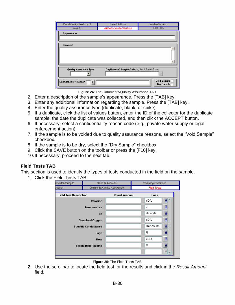
B-30
Figure 24: The Comments/Quality Assurance TAB.
2. Enter a description of the sample’s appearance. Press the [TAB] key. 3. Enter any additional information regarding the sample. Press the [TAB] key. 4. Enter the quality assurance type (duplicate, blank, or spike). 5. If a duplicate, click the list of values button, enter the ID of the collector for the duplicate
sample, the date the duplicate was collected, and then click the ACCEPT button. 6. If necessary, select a confidentiality reason code (e.g., private water supply or legal
enforcement action). 7. If the sample is to be voided due to quality assurance reasons, select the “Void Sample”
checkbox. 8. If the sample is to be dry, select the “Dry Sample” checkbox. 9. Click the SAVE button on the toolbar or press the [F10] key. 10. If necessary, proceed to the next tab.
Field Tests TAB
This section is used to identify the types of tests conducted in the field on the sample.
1. Click the Field Tests TAB.
Figure 25: The Field Tests TAB.
2. Use the scrollbar to locate the field test for the results and click in the Result Amount field.

B-31
The list of field tests varies based on the Business Unit.
3. Enter the amount for the test. Press the [TAB] key. 4. Update the unit of measurement if necessary. 5. Repeat the previous steps all applicable field tests are entered. 6. Click the SAVE button on the toolbar or press the [F10] key.
Inserting Additional Samples for the Same Location
This section identifies how to enter an additional sample at the same location as the previously
entered sample.
1. While the previous sample is displayed on the screen, click the SAME LOCATION button. A new record matching the header, project, facility, monitoring point, and location details of the previous sample is created.
2. Update the sequence number. 3. Update the sample detail tabs as described in the CREATING SAMPLE RECORDS
section of the user guide.
Inserting Additional Samples at a New Location
To enter an additional sample at a new location:
1. While the previous sample is displayed on the screen, click the NEW LOCATION button. A new record with header details matching the previous sample will be created.
2. Update the sequence number and reason. 3. Update the sample detail tabs as described in the CREATING SAMPLE RECORDS
section of the user guide.
Voiding a Sample
1. Access the SAMPLES Screen by clicking the Samples Menu and then clicking the Query sample command.
2. Query the sample to be voided. 3. Click the Comments/Quality Assurance TAB.
Figure 26: The Comments/Quality Assurance TAB.
4. If applicable, select a quality assurance type to identify a reason for voiding the sample. Press the [TAB] key.
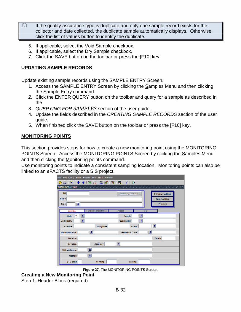
B-32
If the quality assurance type is duplicate and only one sample record exists for the collector and date collected, the duplicate sample automatically displays. Otherwise, click the list of values button to identify the duplicate.
5. If applicable, select the Void Sample checkbox. 6. If applicable, select the Dry Sample checkbox. 7. Click the SAVE button on the toolbar or press the [F10] key.
UPDATING SAMPLE RECORDS
Update existing sample records using the SAMPLE ENTRY Screen.
1. Access the SAMPLE ENTRY Screen by clicking the Samples Menu and then clicking the Sample Entry command.
2. Click the ENTER QUERY button on the toolbar and query for a sample as described in the
3. QUERYING FOR SAMPLES section of the user guide.
4. Update the fields described in the CREATING SAMPLE RECORDS section of the user guide.
5. When finished click the SAVE button on the toolbar or press the [F10] key.
MONITORING POINTS
This section provides steps for how to create a new monitoring point using the MONITORING
POINTS Screen. Access the MONITORING POINTS Screen by clicking the Samples Menu
and then clicking the Monitoring points command.
Use monitoring points to indicate a consistent sampling location. Monitoring points can also be
linked to an eFACTS facility or a SIS project.
Figure 27: The MONITORING POINTS Screen.
Creating a New Monitoring Point
Step 1: Header Block (required)

B-33
Use the header block to identify the monitoring point name and type.
Figure 28: The monitoring point header block.
1. Click the CREATE RECORD button on the toolbar or press the [F6] key. 2. Enter the name of the monitoring point and press the [TAB] key. 3. Enter the code that identifies the type of monitoring point or select one using the list
of values button. Step 2: Location TAB (required)
Use the Location TAB to identify the location of the monitoring point from a general location
description to specific coordinates. The following fields are required:
• State
• County
• Latitude
• Longitude
The Datum field is required if linking an NHD record to the monitoring point.
1. Click the Location TAB.
Figure 29: The Location TAB.
2. The state defaults to “PA”. Update if necessary. 3. Select a code identifying the county in which the sample was collected using the list
of values button. 4. Optionally, select the code identifying the municipality in which the sample was
collected by using the list of values button. 5. Enter the latitude where the sample was taken in Degrees-Minutes-Seconds (e.g.,
40-15-42.8394). 6. Enter the longitude where the sample was taken in Degrees-Minutes-Seconds (e.g.,
-76-52-46.9194). 7. Optionally, enter the horizontal reference datum used to calculate the point at which
the sample was collected or select by using the list of values button. 8. Complete any of the optional fields with available information:
• Municipality

B-34
• Quadrangle
• Datum
• Reference Point
• Geometric Type
• Location
• Depth
• Elevation
• Accuracy
• Altitude Datum
• UTM Zone
• Northing
• Easting
Click in a field to display a description in the hint line.
Step 3: Function/Administration TAB (required)
Use the Function/Administration TAB to identify the function, medium type, and sample
medium for a monitoring point as well as administrative details such as the closed date for a
monitoring point. The Medium Type and Sample Medium fields are required.
1. Click the Function/Administration TAB.
Figure 30: The Function/Administration TAB.
2. Optionally, enter a code identifying the function of the monitoring point or select by using the list of values button.
3. Enter the code identifying the sample medium type monitored by the monitoring point or select by using the list of values button.
4. Enter the code identifying the sample medium monitored by the monitoring point or select by using the list of values button.
5. If the monitoring point is a STORET station, select the STORET Station checkbox. 6. If the monitored material is treated, select the Monitored Material Treated checkbox. 7. If monitoring gages are associated with the monitoring point, complete the following
steps: a. Click the GAGES button and the “Monitoring Gages” pop-up window
displays.
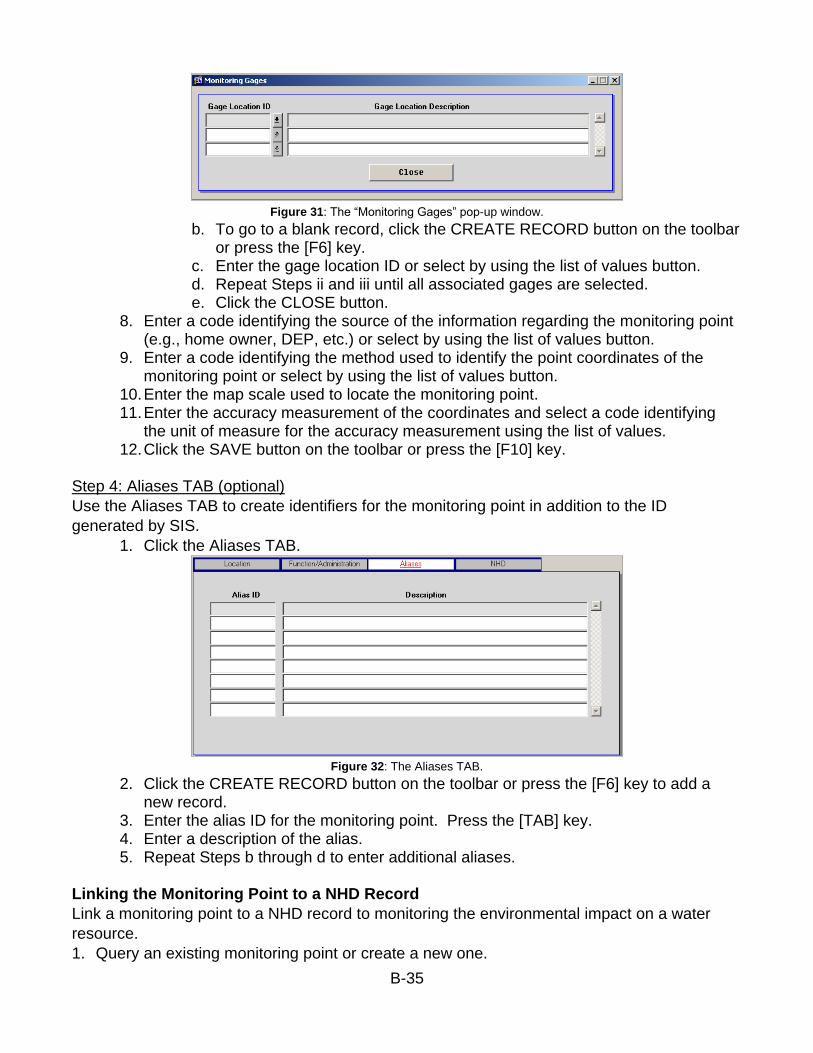
B-35
Figure 31: The “Monitoring Gages” pop-up window.
b. To go to a blank record, click the CREATE RECORD button on the toolbar or press the [F6] key.
c. Enter the gage location ID or select by using the list of values button. d. Repeat Steps ii and iii until all associated gages are selected. e. Click the CLOSE button.
8. Enter a code identifying the source of the information regarding the monitoring point (e.g., home owner, DEP, etc.) or select by using the list of values button.
9. Enter a code identifying the method used to identify the point coordinates of the monitoring point or select by using the list of values button.
10. Enter the map scale used to locate the monitoring point. 11. Enter the accuracy measurement of the coordinates and select a code identifying
the unit of measure for the accuracy measurement using the list of values. 12. Click the SAVE button on the toolbar or press the [F10] key.
Step 4: Aliases TAB (optional)
Use the Aliases TAB to create identifiers for the monitoring point in addition to the ID
generated by SIS.
1. Click the Aliases TAB.
Figure 32: The Aliases TAB.
2. Click the CREATE RECORD button on the toolbar or press the [F6] key to add a new record.
3. Enter the alias ID for the monitoring point. Press the [TAB] key. 4. Enter a description of the alias. 5. Repeat Steps b through d to enter additional aliases.
Linking the Monitoring Point to a NHD Record
Link a monitoring point to a NHD record to monitoring the environmental impact on a water
resource.
1. Query an existing monitoring point or create a new one.

B-36
2. Click the Location TAB. 3. Verify that the latitude, longitude, and datum are entered. 4. Click the NHD TAB.
Figure 33: The NHD TAB.
5. Click the LAUNCH NHD LOCATOR button at the bottom of the screen and the NHD Locator Screen displays.
Figure 34: The NHD locator.
6. Use the NHD Locator Tool to either accept the default snapped point or create a user-defined, new snapped point to accept.
7. Click the ACCEPT SNAPPED POINT(S) button and then click the OK button to exit the NHD Locator Tool and return to the SAMPLE ENTRY Screen.
8. Click the GET NHD DATA button to add the NHD record created via the NHD Locator Tool to the sample.
9. Click the SAVE button on the toolbar or press the [F10] key.

B-37
Linking Primary Facilities to a Monitoring Point
Link a monitoring point to an eFACTS primary facility to monitor its environmental impact on
the soil, water, or air.
Caution: Do NOT link the monitoring point to a primary facility if intending to link to specific
sub-facilities of that primary facility. Instead proceed to the section on linking sub-facilities.
1. Query an existing monitoring point or create a new one. 2. Click the PRIMARY FACILITIES button and the “Monitoring Point/Primary Facilities” pop-up
window displays. 3. Click the CREATE RECORD button on the toolbar or press the [F6] key.
Figure 35: The “Monitoring Point/Primary Facilities” pop-up window.
4. Select a primary facility by entering the “Other ID” from eFACTS (i.e., permit, registration, or license number) or search for a primary facility by name. To search for a primary facility by name:
a. Click the list of values button to display the “List Reduction Criteria” pop-up window.
b. Enter the name of the facility (use the wildcard symbol if necessary) c. Optionally, select a program to limit the list of matching primary facilities. d. Click the ACCEPT button and the “FIX Primary Facilities” pop-up window
displays. e. Select the correct facility from the list and click the OK button.
5. Optionally, select an Alias ID to associate this primary facility with one of the aliases created for the monitoring point
6. Update the effective date if necessary. 7. Click the SAVE button on the toolbar or press the [F10] key. 8. Click the CLOSE button.
Linking Sub-facilities to a Monitoring Point
Link a monitoring point to an eFACTS sub-facility to monitor its environmental impact on the
soil, water, or air.
1. Query an existing monitoring point or create a new one. 2. Click the SUB-FACILITIES button and the “Monitoring Points/Sub-Facilities” pop-up window
displays. 3. Click the CREATE RECORD button on the toolbar or press the [F6] key.

B-38
Figure 36: The “Monitoring Point/Sub-Facilities” pop-up window.
4. Select a primary facility by entering the “Other ID” from eFACTS (e.g., permit, registration, license) or search for a primary facility by name.
To search for a primary facility by name:
a. Click the list of values button to display the “List Reduction Criteria” pop-up window. b. Enter the name of the facility (use the wildcard symbol if necessary) c. Optionally, select a program to limit the list of matching primary facilities. d. Click the ACCEPT button and the “FIX Primary Facilities” pop-up window displays. e. Select the correct facility from the list and click the OK button.
5. Optionally, select an Alias ID to associate this primary facility with one of the aliases created for the monitoring point
6. Select a sub-facility using the list of values button. 7. Update the effective date if necessary. 8. Click the SAVE button on the toolbar or press the [F10] key. 9. Click the CLOSE button.
Linking Projects to a Monitoring Point
Link a monitoring point to a project to monitor its environmental impact on the soil, water, or
air.
1. Query an existing monitoring point or create a new one. 2. Click the PROJECTS button and the “Monitoring Point/Projects” pop-up window displays.
Figure 37: The “Monitoring Point/Projects” pop-up window.
3. Click the CREATE RECORD button on the toolbar or press the [F6] key. 4. Optionally, enter a business unit code in the Project Unit field or select one using the list of
values. 5. Enter a Project ID or select one using the list of values. 6. Optionally, select an Alias ID to associate this project with one of the aliases created for the
monitoring point 7. Update the effective date if necessary. 8. Click the SAVE button on the toolbar or press the [F10] key.
Closing a Monitoring Point
Closing monitoring point disallows linking samples to it.
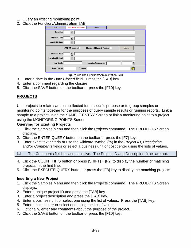
B-39
1. Query an existing monitoring point. 2. Click the Function/Administration TAB.
Figure 38: The Function/Administration TAB.
3. Enter a date in the Date Closed field. Press the [TAB] key. 4. Enter a comment regarding the closure. 5. Click the SAVE button on the toolbar or press the [F10] key.
PROJECTS
Use projects to relate samples collected for a specific purpose or to group samples or
monitoring points together for the purposes of query sample results or running reports. Link a
sample to a project using the SAMPLE ENTRY Screen or link a monitoring point to a project
using the MONITORING POINTS Screen.
Querying for Existing Projects
1. Click the Samples Menu and then click the Projects command. The PROJECTS Screen displays.
2. Click the ENTER QUERY button on the toolbar or press the [F7] key. 3. Enter exact text criteria or use the wildcard symbol (%) in the Project ID, Description,
and/or Comments fields or select a business unit or cost center using the lists of values.
The Comments field is case-sensitive. The Project ID and Description fields are not.
4. Click the COUNT HITS button or press [SHIFT] + [F2] to display the number of matching projects in the hint line.
5. Click the EXECUTE QUERY button or press the [F8] key to display the matching projects.
Inserting a New Project
1. Click the Samples Menu and then click the Projects command. The PROJECTS Screen displays.
2. Enter a unique project ID and press the [TAB] key. 3. Enter a project description and press the [TAB] key. 4. Enter a business unit or select one using the list of values. Press the [TAB] key. 5. Enter a cost center or select one using the list of values. 6. Optionally, enter any comments about the purpose of the project. 7. Click the SAVE button on the toolbar or press the [F10] key.
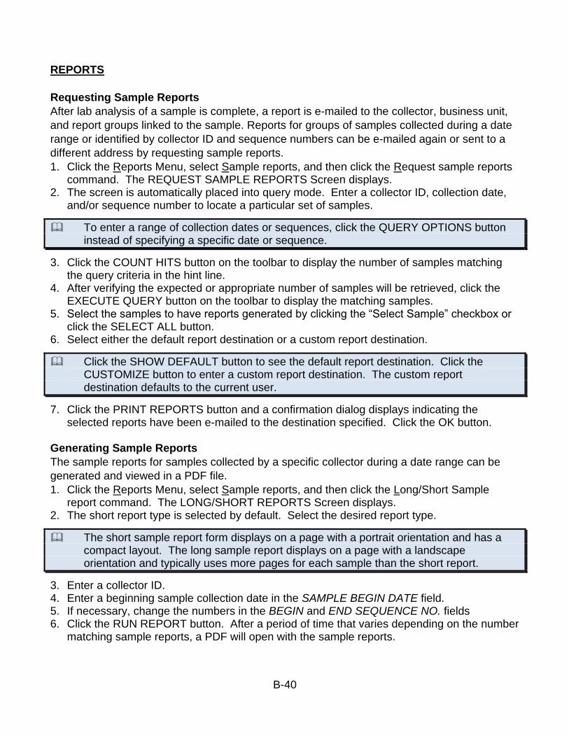
B-40
REPORTS
Requesting Sample Reports
After lab analysis of a sample is complete, a report is e-mailed to the collector, business unit,
and report groups linked to the sample. Reports for groups of samples collected during a date
range or identified by collector ID and sequence numbers can be e-mailed again or sent to a
different address by requesting sample reports.
1. Click the Reports Menu, select Sample reports, and then click the Request sample reports command. The REQUEST SAMPLE REPORTS Screen displays.
2. The screen is automatically placed into query mode. Enter a collector ID, collection date, and/or sequence number to locate a particular set of samples.
To enter a range of collection dates or sequences, click the QUERY OPTIONS button instead of specifying a specific date or sequence.
3. Click the COUNT HITS button on the toolbar to display the number of samples matching the query criteria in the hint line.
4. After verifying the expected or appropriate number of samples will be retrieved, click the EXECUTE QUERY button on the toolbar to display the matching samples.
5. Select the samples to have reports generated by clicking the “Select Sample” checkbox or click the SELECT ALL button.
6. Select either the default report destination or a custom report destination.
Click the SHOW DEFAULT button to see the default report destination. Click the CUSTOMIZE button to enter a custom report destination. The custom report destination defaults to the current user.
7. Click the PRINT REPORTS button and a confirmation dialog displays indicating the selected reports have been e-mailed to the destination specified. Click the OK button.
Generating Sample Reports
The sample reports for samples collected by a specific collector during a date range can be
generated and viewed in a PDF file.
1. Click the Reports Menu, select Sample reports, and then click the Long/Short Sample report command. The LONG/SHORT REPORTS Screen displays.
2. The short report type is selected by default. Select the desired report type.
The short sample report form displays on a page with a portrait orientation and has a compact layout. The long sample report displays on a page with a landscape orientation and typically uses more pages for each sample than the short report.
3. Enter a collector ID. 4. Enter a beginning sample collection date in the SAMPLE BEGIN DATE field. 5. If necessary, change the numbers in the BEGIN and END SEQUENCE NO. fields 6. Click the RUN REPORT button. After a period of time that varies depending on the number
matching sample reports, a PDF will open with the sample reports.

B-41
Missing Sample Header/Results Report
Use the Missing Sample Header/Results report to view a list of sample records entered into
SIS that do not have a lab results or to view a list of lab results available in SIS that have not
had a sample record entered.
1. Click the Reports Menu and then click the Missing sample header/results command. The MISSING HEADER/RESULTS REPORTS Screen displays.
2. Select the Missing Header report to generate a list of sample reports awaiting entry of the sample in SIS or select the Missing Result report to generate a list of samples in SIS awaiting sample reports.
3. Select a Collector Group, Business Unit, or Collector to run the report for from the lists of values.
4. Enter a collection date range for either the Missing Header or Missing Results report. 5. Click the RUN REPORT(S) button.
Monitoring Points Report
The Monitoring Points report lists all of the monitoring points linked to a specified project,
primary facility, or sub-facility including the location of the monitoring point, whether it is active,
and the date last sampled.
1. Click the Reports Menu and then click the mOnitoring points command. The MONITORING POINT REPORTS Screen displays.
2. Select either a PDF or Excel file for the report destination. 3. Select report type to indicate whether the monitoring points will be identified by project,
primary facility, or sub-facility. If running a report by project:
a. Optionally, identify a project unit to narrow down the list of projects. b. Select a project ID. c. Click the RUN REPORT button.
If running a report by primary facility:
a. Enter the eFACTS “Other ID” for a primary facility. The “Other ID” is typically a permit or registration number assigned by the related program.
b. Alternatively, use the list of values to select a facility by either facility name or associated program.
c. Click the RUN REPORT button. If running a report by sub-facility:
a. First, enter the eFACTS “Other ID” for a primary facility. The “Other ID” is typically a permit or registration number assigned by the related program.
b. Alternatively, use the list of values to select a primary facility by either facility name or associated program.
c. Select the sub-facility using the list of values. d. Click the RUN REPORT button.
4. Optionally, select the checkbox to include the date each monitoring point was last sampled.
Including the date last sampled for each monitoring point lists the most recent sample regardless of which business unit collected the sample. Use the list of values to restrict it to a specific business unit.
Module 8.1A Report

B-42
SIS can generate Module 8.1A reports for a specific monitoring point related to a project or
eFACTS primary facility or for all monitoring points between a pair of latitudes and longitudes.
To run the report for an individual monitoring point related to a project or eFACTS primary
facility:
1. Click the Reports Menu and then click the module 8.1A command. The MODULE 8.1A REPORTS Screen displays.
2. Select either a PDF or Excel file for the report destination. 3. Select a report type to indicate whether the monitoring points will be identified by project or
primary facility. If running a report by project:
a. Optionally, identify a project unit to narrow down the list of projects. b. Select a project ID. c. Select a monitoring point alias from the MP Alias list of values.
If running a report by primary facility:
a. Enter the eFACTS “Other ID” for a primary facility. The “Other ID” is typically a permit or registration number assigned by the related program.
b. Alternatively, use the list of values to select a facility by either facility name or associated program.
c. Select a monitoring point alias from the MP Alias list of values. 4. Enter a beginning and ending sample collection date range. 5. Optionally, identify to include only samples collected by a specific business unit. 6. Click the RUN REPORT button.
To run the report for all monitoring points between a pair of latitudes and a pair of longitudes:
1. Click the Reports Menu and then click the module 8.1A command. The MODULE 8.1A REPORTS Screen displays.
2. Select either a PDF or Excel file for the report destination. 3. Select the By Latitude/Longitude report type. 4. Enter the latitude values in the low and high fields. 5. Enter the longitude values in the low and high fields.
Coordinates are entered in the format DD-MM-SS.SSSS (e.g., 41-29-46.3034 or -79-38-09.6071)
6. Enter a beginning and ending sample collection date range. 7. Optionally, identify to include only samples collected by a specific business unit. 8. Click the RUN REPORT button.

B-43
B.4 SEDIMENT FIELD DATA COLLECTION SHEET


B-46
B.5 CIM DEPLOYMENT FORM


B-49
B.6 CIM MAINTENANCE VISIT FIELD FORM

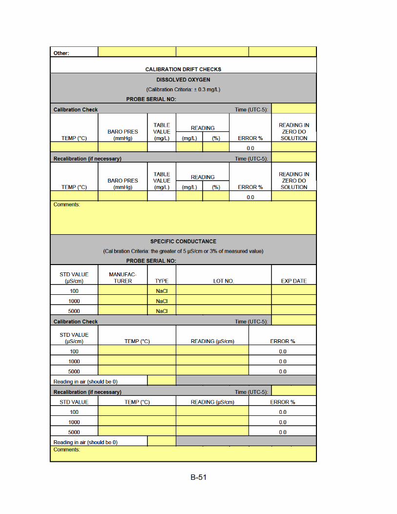


B-54
B.7 TEMPERATURE ADJUSTMENTS FOR PH BUFFERS

B-55
Table 1. Temperature adjusted pH buffer values from British Drug House (BDH;
“Temperature Dependence of pH,” n.d.)
TEMP (C) 0 5 10 15 20 25 30 35 40 45 50
BDH5022 4.00 4.00 4.00 4.00 4.00 4.00 4.01 4.02 4.03 4.04 4.06
BDH5050 7.12 7.09 7.06 7.04 7.02 7.00 6.99 6.98 6.98 6.97 6.97
BDH5076 10.31 10.23 10.17 10.11 10.05 10.00 9.95 9.91 9.87 9.81
4 Buffer y = 0.0000357143x2 - 0.0003928571x + 3.9885714286
7 Buffer y = 0.0000680653x2 - 0.0063487179x + 7.1191608392
10 Buffer y = 0.0000954898x2 - 0.0147159972x + 10.3068957012
Figure 1. Second-order polynomial regression lines fitted to temperature-corrected pH
values for BDH buffers.
3.96
4.00
4.04
4.08
0 10 20 30 40 50 60
pH
Va
lue
Temperature (C)
6.95
7.00
7.05
7.10
7.15
0 10 20 30 40 50 60
pH
Va
lue
Temperature (C)
9.60
9.80
10.00
10.20
10.40
0 10 20 30 40 50 60
pH
Va
lue
Temperature (C)
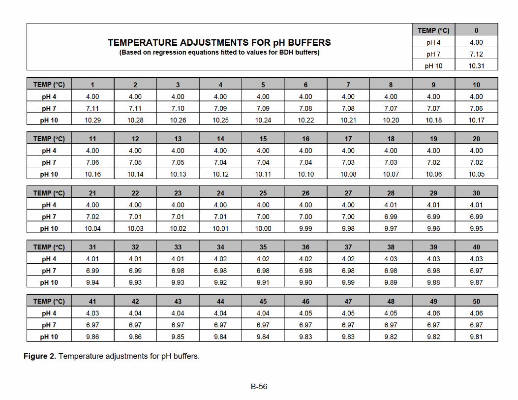
B-57
B.8 DO 100% SATURATION CHART FOR FRESH WATER


C-1
APPENDIX C: PHYSICAL DATA COLLECTION INFORMATION AND FORMS

C-2
C.1 RIFFLE/RUN PREVALENCE HABITAT DATA COLLECTION FORM
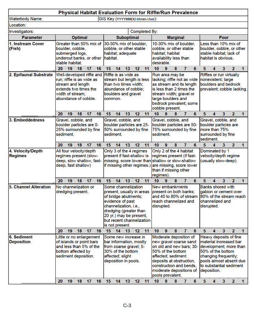
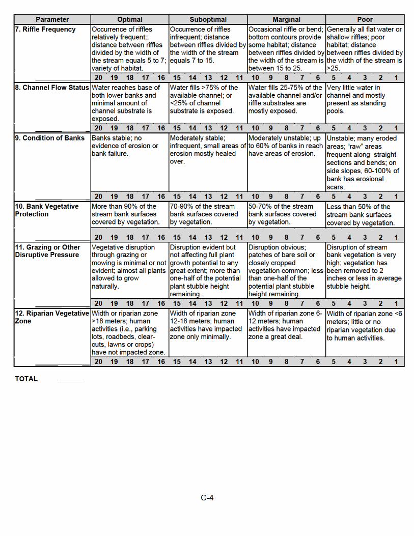

C-5
C.2 RIFFLE/RUN PREVALENCE HABITAT DATA COLLECTION ABBREVIATED (ONE-PAGE)
FORM
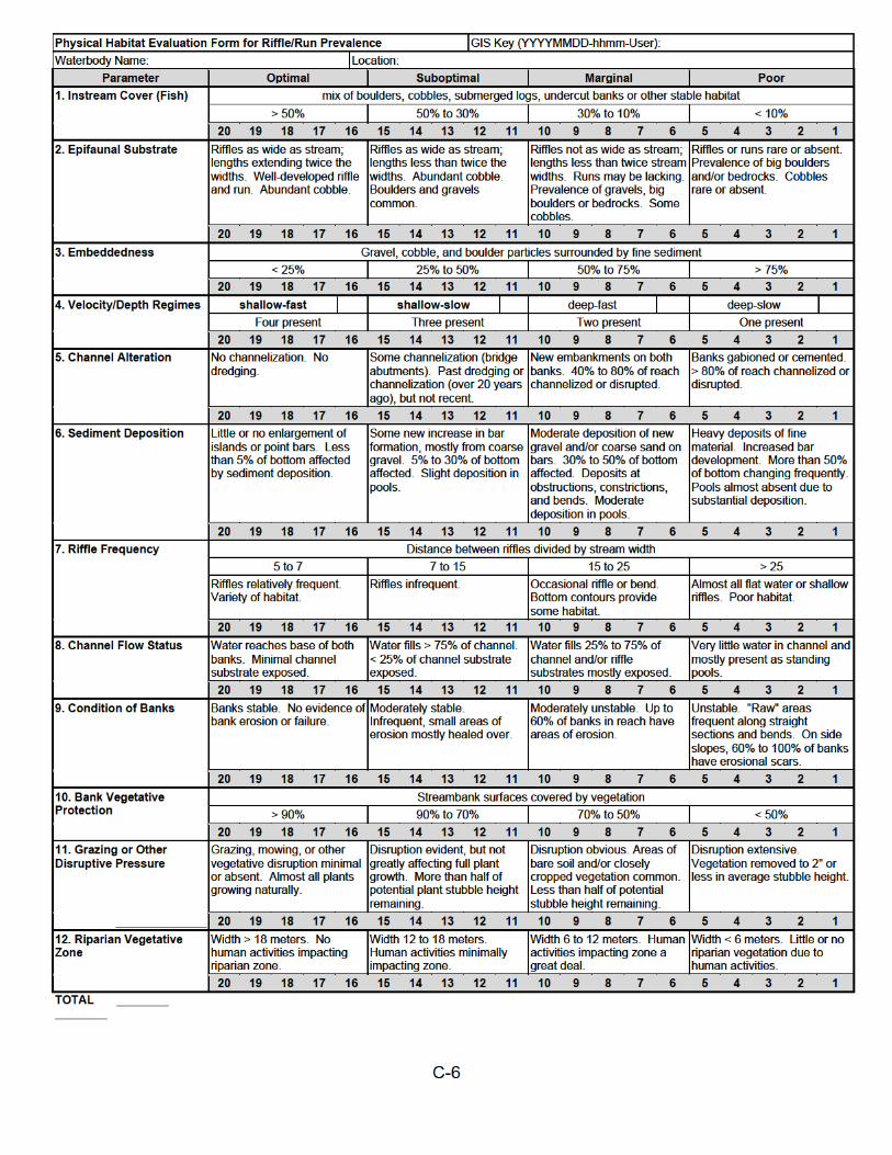

C-7
C.3 LOW GRADIENT HABITAT DATA COLLECTION FORM


C-10
C.4 PEBBLE COUNT DATA COLLECTION FORM

C-11
PEBBLE COUNT FORM GIS Key:
Survey Crew:
Stream:
County:
SWP:
Mean Width:
Sample Interval:
Reach Length:
Station Description:
1 35 69 102 135 168
2 36 70 103 136 169
3 37 71 104 137 170
4 38 72 105 138 171
5 39 73 106 139 172
6 40 74 107 140 173
7 41 75 108 141 174
8 42 76 109 142 175
9 43 77 110 143 176
10 44 78 111 144 177
11 45 79 112 145 178
12 46 80 113 146 179
13 47 81 114 147 180
14 48 82 115 148 181
15 49 83 116 149 182
16 50 84 117 150 183
17 51 85 118 151 184
18 52 86 119 152 185
19 53 87 120 153 186
20 54 88 121 154 187
21 55 89 122 155 188
22 56 90 123 156 189
23 57 91 124 157 190
24 58 92 125 158 191
25 59 93 126 159 192
26 60 94 127 160 193
27 61 95 128 161 194
28 62 96 129 162 195
29 63 97 130 163 196
30 64 98 131 164 197
31 65 99 132 165 198
32 66 100 133 166 199
33 67 101 134 167 200
34 68
Comments:

C-12
C.5 ALTERNATIVE PEBBLE COUNT DATA COLLECTION FORM


D-1
APPENDIX D: PENNSYLVANIA’S SURFACE WATER QULAITY MONITORING NETWORK
(WQN) MANUAL


D-3
[This page intentionally left blank]

D-4
OFFICE OF WATER PROGRAMS
BUREAU OF CLEAN WATER
PENNSYLVANIA ’S SURFACE WATER QUALITY MONITORING NETWORK (WQN) MANUAL
2020
D-5
Originally prepared: 1972
Update prepared by:
Molly Pulket
PA Department of Environmental Protection
Office of Water Programs
Bureau of Clean Water
11th Floor: Rachel Carson State Office Building
Harrisburg, PA 17105
Edited by:
Molly Pulket and Josh Lookenbill
Office of Water Programs
PA Department of Environmental Protection
Bureau of Clean Water
11th Floor: Rachel Carson State Office Building
Harrisburg, PA 17105
2019
Molly Pulket and Josh Lookenbill
Office of Water Programs
PA Department of Environmental Protection
Bureau of Clean Water
11th Floor: Rachel Carson State Office Building
Harrisburg, PA 17105
2020

D-6
INTRODUCTION
The Pennsylvania Water Quality Network (WQN) is a statewide, fixed-station water quality sampling
system operated by the Pennsylvania Department of Environmental Protection’s (DEP) Bureau of
Clean Water (BCW). It is designed to track both the quality of Pennsylvania’s surface waters and the
effectiveness of the water quality management program by accomplishing four basic objectives:
• Monitor temporal water quality trends in major surface streams throughout Pennsylvania.
• Monitor temporal water quality trends in selected reference waters.
• Monitor the trends of nutrient and sediment loads in the major tributaries entering the
Chesapeake Bay.
• Monitor temporal water quality trends in selected Pennsylvania lakes.
“Major” streams, for the purposes of this document, are interstate and intrastate waters with drainage
areas of roughly 200 square miles or greater. These waters receive both point and non-point source
pollutants and are sampled at or near their mouths to measure overall quality before flows enter the
next higher order stream or before exiting the state. In this way, trends can be established, and the
effectiveness of water quality management programs can be assessed by watershed. For more
detailed information on the objectives of the WQN, see Subappendix D.5.
The monitoring of the WQN is conducted collaboratively between DEP, USGS Pennsylvania Water
Science Centers, and Susquehanna River Basin Commission (SRBC).
WQN resources can be found on DEP’s WQN webpage: www.dep.pa.gov, keywords: Water Quality
Network.
STATION TYPES
The WQN consists of 177 active stations grouped into three primary station types: standard,
Chesapeake Bay nutrient loading, and reference.
The 116 standard stations are generally sampled every other month for stream discharge
measurements and chemical analysis, and every other year for a biological and physical evaluation. Of
these, 28 are sampled monthly for chemical analysis and 17 are considered low alkalinity stations
which are analyzed for a few additional parameters. See Subappendix D.1 for the list of parameters
collected at low alkalinity stations.
The 36 Chesapeake Bay Nutrient Loading (Chesapeake Bay) stations are sampled monthly for stream
discharge measurements and chemical analysis, and once a year for biological and physical
evaluation. These stations are also part of the Chesapeake Bay Program nontidal monitoring network
(CBP NTN) which requires eight additional water chemistry samples to be collected annually during

D-7
storm events. More information on the CBP NTN can be found at:
CBP nontidal water quality monitoring.
The 23 reference stations are sampled monthly for stream discharge measurements and chemical
analysis and typically once a year (spring or fall) for biological and physical evaluation. For method
development purposes, some reference stations are sampled twice a year, once in the spring and once
in the fall. Reference stations are selected to represent minimally disturbed waters within
Pennsylvania’s various bioregions. Bioregions are areas with similar water quality characteristics
because of like features such as topography, land use, soils, and potential natural vegetation. Although
it may be argued that Pennsylvania has no unaffected waters (by atmospheric deposition), reference
stations reasonably describe water quality that could be achieved in the absence of point source
discharges and in the presence of minimal or typical non-point source impacts. Thus, these stations
can provide, in the absence of site-specific data, a benchmark for use in the water quality management
permitting program as well as a measure of changing water quality in areas of the state not directly
impacted by development. Of the 23 reference stations, 16 are monitored for atmospheric deposition
and therefore, are analyzed for a few additional parameters (Subappendix D.1).
WQN lake stations (excludes Lake Erie and Presque Isle Bay which are standard WQN stations) are
selected after consideration of size, public access, intensity of use, and availability of existing data.
Large lakes with heavy public use and/or historical data are favored for inclusion in this program
because changing trends in the water quality of these resources have the potential for serious impacts
on water uses. Approximately 90 lakes are included in this network, however, sampling occurs in
groups of 15-20 lakes on a rotation. These lake groups are sampled once a year for five consecutive
years before initiating a new group. The five-year data sets are then used to assess lake water quality
trends. Monitoring at the current group of 15 lakes started in 2016 and will continue through 2020.
Station specific details are included in the Active, Macroinvertebrate, and Discontinued Stations tables
found in Subappendices D.2-D.4. A web mapping application is also available to view each station at
WQN web application.
UPDATES TO THE WQN
This revision of the WQN manual covers changes that occurred from October 2018 through September
2020. All information in this edition is reflective of the WQN’s status as of October 1st, 2020.
Dissolved arsenic, nitrate, and nitrite were removed from Standard Analysis Code (SAC) 015. While six
new parameters were added to SAC 015: Ammonia D, NO2 + NO3 T, NO2 + NO3 D, Phosphorus D,
Ortho Phos D, and DOC. All SAC 013 stations will use the new, modified SAC 015 to simplify data
collection. A new SAC 122 was created to provide additional information associated with atmospheric
deposition effects at 16 of the reference stations. All lake stations that used SAC 017 will now use SAC
083. All SACs used for the WQN and the parameters they contain are listed in Subappendix D.1. The
SACs assigned to each WQN station can be found in Subappendices D.2 and D.4 (Active and
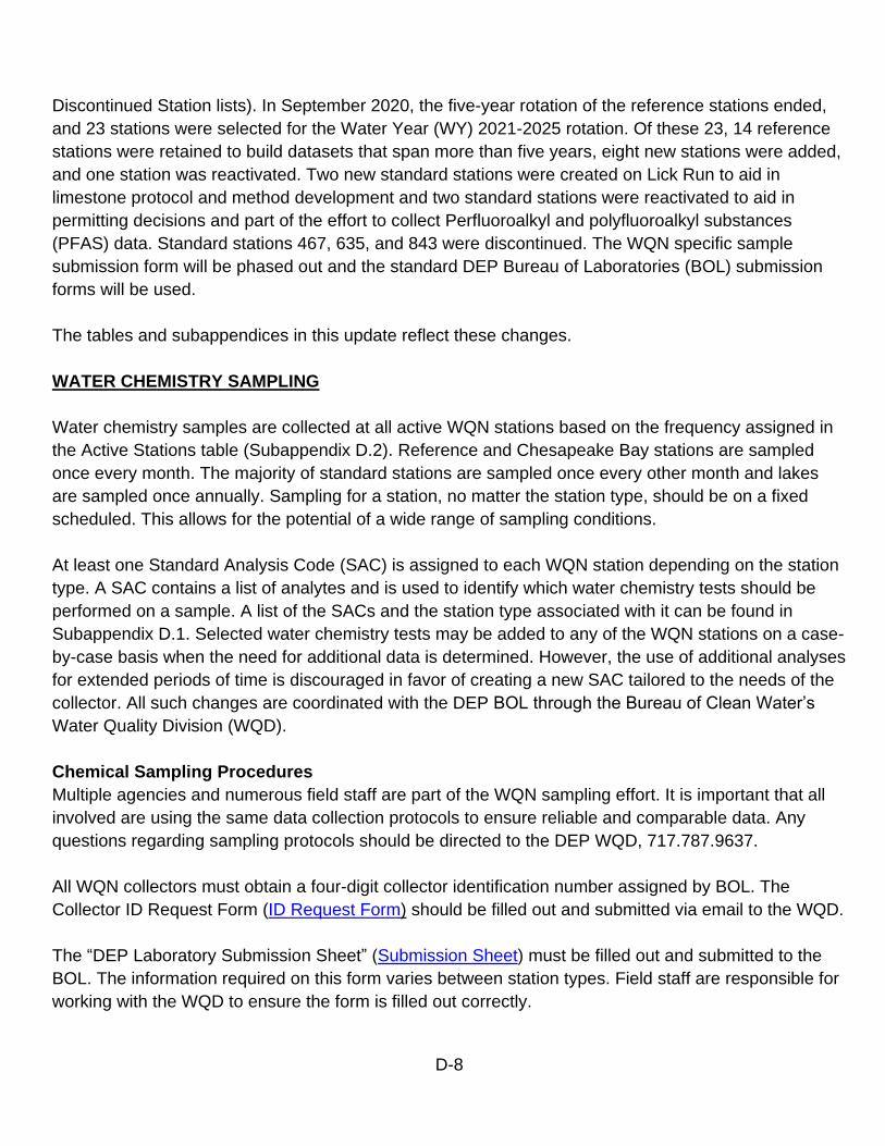
D-8
Discontinued Station lists). In September 2020, the five-year rotation of the reference stations ended,
and 23 stations were selected for the Water Year (WY) 2021-2025 rotation. Of these 23, 14 reference
stations were retained to build datasets that span more than five years, eight new stations were added,
and one station was reactivated. Two new standard stations were created on Lick Run to aid in
limestone protocol and method development and two standard stations were reactivated to aid in
permitting decisions and part of the effort to collect Perfluoroalkyl and polyfluoroalkyl substances
(PFAS) data. Standard stations 467, 635, and 843 were discontinued. The WQN specific sample
submission form will be phased out and the standard DEP Bureau of Laboratories (BOL) submission
forms will be used.
The tables and subappendices in this update reflect these changes.
WATER CHEMISTRY SAMPLING
Water chemistry samples are collected at all active WQN stations based on the frequency assigned in
the Active Stations table (Subappendix D.2). Reference and Chesapeake Bay stations are sampled
once every month. The majority of standard stations are sampled once every other month and lakes
are sampled once annually. Sampling for a station, no matter the station type, should be on a fixed
scheduled. This allows for the potential of a wide range of sampling conditions.
At least one Standard Analysis Code (SAC) is assigned to each WQN station depending on the station
type. A SAC contains a list of analytes and is used to identify which water chemistry tests should be
performed on a sample. A list of the SACs and the station type associated with it can be found in
Subappendix D.1. Selected water chemistry tests may be added to any of the WQN stations on a case-
by-case basis when the need for additional data is determined. However, the use of additional analyses
for extended periods of time is discouraged in favor of creating a new SAC tailored to the needs of the
collector. All such changes are coordinated with the DEP BOL through the Bureau of Clean Water’s
Water Quality Division (WQD).
Chemical Sampling Procedures
Multiple agencies and numerous field staff are part of the WQN sampling effort. It is important that all
involved are using the same data collection protocols to ensure reliable and comparable data. Any
questions regarding sampling protocols should be directed to the DEP WQD, 717.787.9637.
All WQN collectors must obtain a four-digit collector identification number assigned by BOL. The
Collector ID Request Form (ID Request Form) should be filled out and submitted via email to the WQD.
The “DEP Laboratory Submission Sheet” (Submission Sheet) must be filled out and submitted to the
BOL. The information required on this form varies between station types. Field staff are responsible for
working with the WQD to ensure the form is filled out correctly.

D-9
Surface water samples are collected as isokinetic, depth integrated, single mid-channel or equal-width
samples. Samples are normally collected in High-Density Polyethylene (HDPE) or amber glass (for
organic compound analysis) sample bottles. A sample volume and field preservation chart are available
for reference in Subappendix D.6. Bottles must be labeled with the WQN number, collector ID number,
sequence number, date, and time. If space allows, adding the SAC, general test descriptions (total
metals, TOC, etc.), filtered, and preservation type can help minimize any questions concerning the
sample analyses. Depending on the station, samples may be collected from a bridge, boat, or by
wading.
Detailed descriptions on how to collect surface water samples can be found in Chapter 4 of DEP’s
Water Quality Monitoring Protocols for Streams and Rivers (the Monitoring Book, Shull and Lookenbill
2021) and in Chapters 4 and 5 of the USGS’s National Field Manual for the Collection of Water Quality
Data (USGS 2006, Wilde 2004).
Standard Stations
A standard station is typically assigned SAC 010 or 610 and can be located anywhere in Pennsylvania.
SACs 016 and 616 are used if the watershed experiences low alkalinity. The 610 and 616 SACs are
used for stations in geographic areas that could be underlain by Marcellus shale; these SACs contain a
few additional analytes typically associated with Marcellus formation water. Reason Code 01 should be
used on the Sample Submission Sheet for all standard stations.
Reference Stations
These stations are assigned either SAC 015 or the Atmospheric Deposition SAC 122, depending on
drainage area and location. Both SACs contain the analyte dissolved organic carbon (DOC). The
analytical method for DOC requires that a blank sample is associated with every DOC sample. To
satisfy this requirement, a blank DOC sample is collected with the first SAC 015 or 122 sample in a
sampling group. A sampling group can contain the samples collected in the same day, week, project,
etc. but should not be more than 20 samples. The collector ID and sequence number for that blank
should be recorded on all the Sample Submission forms for that sampling group and specify that it is
the blank to be associated with these DOC samples. A new blank DOC sample should be collected
with each sampling group. Reference stations are additionally sampled for fecal coliforms and E. coli; a
sterilized 125 ml bacteriological bottle pretreated with sodium thiosulfate (neutralizes the effects of
residual chlorine) is used. A separate Sample Submission Sheet should be filled out for this analysis
and SAC B021 is used. Reason Code 02 should be used on all reference station Sample Submission
Sheets.
Chesapeake Bay Nutrient Loading Stations
This station type is assigned either SAC 012 or 612 and all sites are within the Chesapeake Bay
watershed. SAC 612 stations are in geographic areas that could be underlain by Marcellus shale; this
SAC contains a few additional analytes typically associated with Marcellus formation water. Reason
Code 01 is used on the Sample Submission Sheet for the monthly, routine sample collected at these
Chesapeake Bay stations.

D-10
Storm Sampling: Since these stations are also part of the CBP NTN, in addition to the monthly routine
sample, eight additional storm samples are collected throughout the sampling year. A storm event is
characterized with a rising discharge (cfs) of at least twice that of the pre-storm average daily
discharge. The assigned SAC, field parameters, and a suspended sediment sample is collected. These
samples are identified with Reason Code 014 on the datasheet. Ideally, one suspended sediment
concentration (SSC) and one SSC with sand and fine particle analyses should be collected per quarter.
If a storm event occurs on the scheduled routine sampling day, the sample is identified as “routine,
storm-impacted” and should be assigned Reason Code 015 on the datasheet. If feasible, an SSC
sample should be collected also. These “routine, storm-impacted” samples are identified as the routine
monthly sample and not as one of the eight storm samples. All suspended sediment samples are
shipped to the USGS Ohio-Kentucky-Indiana Water Science Center Sediment Laboratory in Louisville,
KY.
Storm sampling for Chesapeake Bay Nutrient Loading stations is the only targeted sampling in the
WQN. More detailed information on the sampling requirements for storm samples can be found in the
CBP’s Non-Tidal Water Quality Monitoring document (CBP 2008).
Lake Stations
Lake stations are assigned SAC 083. Lakes are additionally sampled for chlorophyll-a and pheophytin
under SAC B059. Lake Erie and Presque Isle Bay bimonthly samples are collected at mid-depth. For
all other lakes, two samples are collected from one site during mid-summer stratification conditions.
These sites correspond to the deepest point in each lake with one sample collected a meter below the
surface (top sample) and the second sample from one meter from the bottom (bottom sample). A water
quality profile, to include temperature, dissolved oxygen, pH, and specific conductance, is recorded at
this site through the vertical water column and an aliquot from the top sample is filtered for chlorophyll-
a analysis. Chlorophyll-a sampling is conducted according to Chlorophyll A Sampling Method in Lakes,
Ponds and Reservoirs (Lathrop 2017). Lake sampling protocols can be found in Evaluations of
Phosphorus Discharges to Lakes, Ponds, and Impoundments (DEP 2013). It is recommended that at
least one other site should be collected near the lake inlet. This site will follow the same procedures as
the deepest point site.
Pesticide Sampling
Due to the sampling design of the Water Quality Network, WQN stations are often utilized to gather
data for specific projects. Pesticide grab samples are collected between March 1st and September 30th
at eleven stations. Three of these are sampled monthly with two additional samples collected during
storm events. The remaining stations are sampled once during the March 1st through September 30th
sampling window. All samples are sent to the USGS National Water Quality Laboratory (NWQL) for
analysis. Samples will be delivered to the USGS for shipment within one day of sampling or will be
shipped directly to the NWQL within one day of sampling.

D-11
POCIS Sampling
The WQN is also being utilized to monitor hormones and other endocrine-disrupting compounds
(EDCs). Polar Organic Chemical Integrative Samplers (POCIS) are a type of passive sampling device
being deployed at 21 WQN stations to collect water quality samples of low-level environmental
contaminants. POCIS sampling will follow the procedures outlined in the Passive Water Chemistry
Data Collection Protocol in Chapter 4 for the Monitoring Book (Shull and Lookenbill 2021). Analysis of
the wastewater indicators will be performed at the USGS National Water Quality Laboratory (NWQL) in
Denver, CO and the estrogenicity samples at the USGS Leetown Science Center in Kearneyville, WV.
BIOLOGICAL SAMPLING
All biological sampling is conducted using the protocols outlined in Chapter 3 of the Monitoring Book
(Shull and Lookenbill 2021). At a minimum, benthic macroinvertebrate data are collected at standard
stations every other year between August 1st and September 30th. Standard stations that are wadeable
in the non-summer months will be sampled between November 1st and April 30th. Macroinvertebrates
are collected annually at Chesapeake Bay stations between November 1st and April 30th. Reference
stations either rotate annually between a spring (March 1st to April 30th) and fall (Nov. 1st to Dec. 31st)
collection or are sampled twice per year (once in spring and once in fall).
Data collection per the wadeable riffle-run protocol is appropriate at most stations, however, WQN
stations can be sampled using any of the protocols outlined in Chapter 3 of the Monitoring Book (Shull
and Lookenbill 2021) if appropriate. The appropriate data collection protocols for each WQN is listed in
Subappendix D.3.
A physical habitat evaluation is conducted with every macroinvertebrate data collection effort. The
procedures in the Stream Habitat Data Collection Protocol within Chapter 5 of the Monitoring Book
(Shull and Lookenbill 2021) should be used. The majority of WQN stations will use the riffle/run habitat
parameters, however, a few stations will use the multihabitat parameters if they are determined to be
low gradient. Please contact the WQD if clarification is needed. Habitat field data sheets are available
in Appendix C in the Monitoring Book (Shull and Lookenbill 2021).
Qualitative plankton samples are collected annually at Lake Erie stations. Quantitative invertebrate or
plankton sampling and quantitative or qualitative fish sampling is optional at any station and may be
conducted at the discretion of the collector. Plankton data collection protocols are detailed in
Quantitative Plankton Sampling Method for Lakes (DEP 2015) and fish sampling protocols are in
Chapter 3 of the Monitoring Book (Shull and Lookenbill 2021).
Fish tissue is sampled periodically at the rate of approximately 100 stations per year following the
protocols outlined in Chapter 3 of the Monitoring Book (Shull and Lookenbill 2021). Tissue sampling
locations are determined annually during the first quarter of the calendar year preceding sample
analysis and rotated throughout the WQN to provide periodic but statewide coverage and to maintain
surveillance on problem waters. Fish tissue (fillets) is analyzed for appropriate priority pollutants to

D-12
assess its suitability for human consumption.
FLOW MEASUREMENT
Stream discharge (flow volume) is measured or calculated each time a water chemistry sample is
collected. USGS stream gaging facilities and/or extrapolation equations are utilized whenever possible.
Where no USGS facilities/equations exist, stream discharge is measured using U.S. Army Corps of
Engineers and private gaging facilities or calculated according to procedures outlined by USGS
(Turnipseed and Sauer 2010). Lake levels for Lake Erie and Presque Isle Bay stations are measured at
the U.S. Coast Guard station at the entrance to Erie Harbor.
Flow Measurement Procedures
The Pennsylvania WQN utilizes several types of stage gages to provide stream discharge. The two
dominant types are the Wire-Weight (WW) gage and the Electric Tape (ET) gage. Both are non-
recording gages that yield readings indirectly via measurement from a fixed point to the water surface.
Other gages that may be used include a Staff gage, Analog-to-Digital Recorder (ADR) dial, Strip Chart,
Hand Tape, Crest Stage Gage, Lock Chamber or Telemark (TMK). Descriptions on the various flow
measurement procedures are in Subappendix D.7.
The Water Resources Division of the USGS recommends that an outside gage such as a Staff gage or
a WW gage be used by DEP personnel. If no outside gage is present or it is unreadable, USGS prefers
a reading from the ADR dial or the ET gage, in that order. The base gages for the network stations are
primarily ET gages or WW gages. If neither of these types are present, a Staff gage may function as
the base gage for that site.
DATA AVAILABITY AND MANAGEMENT
All chemical data analyzed by DEP BOL are entered by BOL staff into DEP’s internal Oracle database.
The collector or DEP WQD staff are responsible for entering the field chemistry, station information,
comments, and USGS OH-KY-IN Sediment Lab results into the Oracle database. The data are
uploaded quarterly by DEP via the Water Quality Exchange (WQX) to the United States Environmental
Protection Agency’s (EPA) database. This data is made available to the public on the Water Quality
Portal (https://www.waterqualitydata.us). Macroinvertebrate samples are processed, and the taxa
identified and enumerated by a contractor or by WQD staff. The macroinvertebrate data are entered
into the WQD’s internal Streams and Lakes Integrated Management System (SLIMS) database.
Analyses of trends at selected WQN stations are published in DEP's Biennial Integrated Water Quality
Monitoring and Assessment Report.
QUALITY ASSURANCE
A quality assurance project plan has been developed to describe the procedures used to implement the
WQN in both the field and laboratory. Copies of this plan can be obtained from the Bureau of Clean

D-13
Water’s WQD or EPA Region III. One sample "blank" is submitted bimonthly by each field office
involved in sample collection and duplicate or "split samples" are collected at the rate of one in every
20 routine WQN samples. Qualified WQD staff routinely audit WQN field staff to ensure sampling
consistency between staff and to evaluate the utility of each station. Additional quality assurance for
specific data collection protocols can be found throughout the Monitoring Book (Shull and Lookenbill
2021).
LITERATURE CITED
Barbour, M. T., J. Gerritsen, B. D. Snyder, and J. B. Stribling. 1999. Rapid bioassessment protocols for
use in streams and wadeable rivers: Periphyton, benthic macroinvertebrates and fish. 2nd
edition. EPA 841-B-99-002. U.S. Environmental Protection Agency, Office of Water,
Washington, D.C.
Buchanan, T. J., and W. P. Somers. 1969. Discharge measurements at gaging stations. Book 3,
chapter A8, page 65. in National field manual for the collection of water quality data: Techniques
and methods. U.S. Department of the Interior, U.S. Geological Survey, Reston, VA. (Available
online at: https://pubs.er.usgs.gov/publication/tm3A8.)
CPB. 2008. Non-tidal water quality monitoring. Chapter V in Non-Tidal Water Quality Field Procedures.
Chesapeake Bay Program, Annapolis, MD.
DEP. 2013. Evaluations of phosphorus discharges to lakes, ponds, and impoundments. Pennsylvania
Department of Environmental Protection, Harrisburg, PA.
DEP. 2015. Quantitative plankton sampling method for lakes (modified standard Method 1002a).
Pennsylvania Department of Environmental Protection, Harrisburg, PA.
Lathrop, B. F. 2017. Chlorophyll a sampling method in lakes, ponds and reservoirs. Pennsylvania
Department of Environmental Protection, Harrisburg, PA.
Lookenbill, M. J., and R. Whiteash (editors). 2021. Water quality monitoring protocols for streams and
rivers. PA Department of Environmental Protection, Harrisburg, PA.
Turnipseed, D. P. and V. B. Sauer. 2010. Discharge measurements at gaging stations: United States
Geologic Survey. Book 3, chapter A8. in National field manual for the collection of water quality
data: Techniques and methods. U.S. Department of the Interior, U.S. Geological Survey,
Reston, VA. (Available online at: https://pubs.usgs.gov/twri/twri3a8/.)
Wilde, F. D. (editor). 2004. Processing of water samples. Book 9, chapter A5 (version 2.2). in National
field manual for the collection of water quality data: Techniques and methods. U.S. Department
of the Interior, U.S. Geological Survey, Reston, VA. (Available online at:
https://www.usgs.gov/mission-areas/water-resources/science/national-field-manual-collection-
water-quality-data-nfm?qt-science center objects=0#qt-science center objects.)
USGS. 2006. Collection of water samples. Book 9, chapter A4 (version 2.0). in National field manual for
the collection of water quality data: Techniques and methods. U.S. Department of the Interior,
U.S. Geological Survey, Reston, VA. Available online at:
https://pubs.er.usgs.gov/publication/twri09A4.

D-14
D.1 STANDARD ANALYSIS CODES (SAC)

D-15
WQN PARAMETER LISTS
1. ALL STATIONS (standard field analyses) pH Temperature Dissolved Oxygen Specific Conductance
** % Dissolved Oxygen and Turbidity should also be reported, if collected, using data collection protocols in Lookenbill and
Whiteash (2021).
2. STANDARD STATIONS (SAC 010)
Test Code Test Description Test Code Test Description 00410 Alkalinity (Alk) 01105H Aluminum, Total (Al)
00610A Ammonia Nitrogen (NH3 N) 99020 Bromide (Br)
00916A Calcium, Total (Ca) 00940 Chloride (Cl)
01042H Copper, Total (Cu) 00900 Hardness, Total (Hard)
01045A Iron, Total (Fe) 01051H Lead, Total (Pb)
00927A Magnesium, Total (Mg) 01055A Manganese, Total (Mn)
01067A Nickel, Total (Ni) 00620 Nitrate Nitrogen (NO3 N)
00615 Nitrite Nitrogen (NO2 N) 00600A Nitrogen, Total (N)
00403 pH, Lab (PH) 00665A Phosphorus, Total (P)
70507A Phosphorus Orthophosphate, Total P(O) 00937A Potassium, Total (K)
00929A Sodium, Total (Na) 00095 Specific Conductivity (SPC)
00945 Sulfate, Total (SO4) 70300U Total Dissolved Solids @ 180C (TDS)
00530 Total Suspended Solids (TSS) 01092A Zinc, Total (Zn)
3. CHESAPEAKE BAY NUTRIENT LOADING STATIONS (SAC 012)
Test Code Test Description Test Code Test Description
00410 Alkalinity (Alk) 01105A Aluminum, Total (Al)
00608A Ammonia Nitrogen, Dissolved (NH3 N) 00610A Ammonia Nitrogen, Total (NH3 N)
99020 Bromide (Br) 00916A Calcium, Total (Ca)
00940 Chloride (Cl) 01042H Copper, Total (Cu)
00900 Hardness, Total (Hard) 01045A Iron, Total (Fe)
01051H Lead, Total (Pb) 00927A Magnesium, Total (Mg)
01055A Manganese, Total (Mn) 01067A Nickel, Total (Ni)
00631A Nitrate & Nitrite, Dissolved (NO3 + NO2) 00630A Nitrate & Nitrite, Total (NO3 + NO2)
00602A Nitrogen, Dissolved (N) 00600A Nitrogen, Total (N)
00680 Organic Carbon, Total 00403 pH, Lab (PH)
00671A Phosphorus Orthophosphate, Dissolved P(O) 70507A Phosphorus Orthophosphate, Total P(O)
00666A Phosphorus, Dissolved (P) 00665A Phosphorus, Total (P)
00937A Potassium, Total (K) 00929A Sodium, Total (Na)
00095 Specific Conductivity (SPC) 00945 Sulfate, Total (SO4)
70300U Total Dissolved Solids @ 180C (TDS) 00530 Total Suspended Solids (TSS)
01092A Zinc, Total (Zn)

D-16
4. REFERENCE STATIONS (SAC 015 & B021*)
Test Code Test Description Test Code Test Description 70508
01106H
Acidity, Total
Aluminum, Dissolved (Al) 00410
01105H
Alkalinity (Alk)
Aluminum, Total (Al)
00608A Ammonia Nitrogen, Dissolved (NH3 N) 00610A Ammonia Nitrogen, Total (NH3 N)
01007H Barium, Total (Ba) 00314 Biochemical Oxygen Demand (CBOD)
01022K Boron, Total (B) 99020 Bromide (Br)
01025H Cadmium, Dissolved (Cd) 00915A Calcium, Dissolved (Ca)
00916A Calcium, Total (Ca) 00940 Chloride (Cl)
01040H Copper, Dissolved (Cu) 01042H Copper, Total (Cu)
MMTECMF E. coli* 31616 Fecal Coliform* (FC)
00900 Hardness, Total (Hard) 01046A Iron, Dissolved (Fe)
01045A Iron, Total (Fe) 01130A Lithium, Dissolved (Li)
01132A Lithium, Total (Li) 01049H Lead, Dissolved (Pb)
01051H Lead, Total (Pb) 00925A Magnesium, Dissolved (Mg)
00927A Magnesium, Total (Mg) 01056H Manganese, Dissolved (Mn)
01055H Manganese, Total (Mn) 01065H Nickel, Dissolved (Ni)
01067H Nickel, Total (Ni) 00631A Nitrate + Nitrite N, Dissolved
00630A Nitrate + Nitrite N, Total 00600A Nitrogen, Total (N)
00681 Organic Carbon, Dissolved 00680 Organic Carbon, Total
82550 Osmotic Pressure (OP) 00403 pH, Lab (PH)
00666A Phosphorus, Dissolved (P) 00665A Phosphorus, Total (P)
00671A
00937A
Phosphorus Orthophosphate, Dissolved P
Potassium, Total (K) 70507A
01147H
Phosphorus Orthophosphate, Total P
Selenium, Total (Se)
00929A Sodium, Total (Na 00095 Specific Conductivity (SPC)
01082A Strontium, Total (Sr) 00945 Sulfate, Total (SO4)
70300U Total Dissolved Solids @ 180C (TDS) 00530 Total Suspended Solids (TSS)
01090H Zinc, Dissolved (Zn) 01092A Zinc, Total (Zn)
5. LOW ALKALINITY STATIONS (SAC 016)
Test Code Test Description Test Code Test Description
70508 Acidity, Total 00410 Alkalinity (Alk)
01106H Aluminum, Dissolved (Al) 01105H Aluminum, Total (Al)
00610A Ammonia Nitrogen, Total (NH3 N) 00314 Biochemical Oxygen Demand (CBOD)
99020 Bromide (Br) 00915A Calcium, Dissolved (Ca)
00916A Calcium, Total (Ca) 00940 Chloride (Cl)
01040H Copper, Dissolved (Cu) 01042H Copper, Total (Cu)
00900 Hardness, Total (Hard) 01046A Iron, Dissolved (Fe)
01045A Iron, Total (Fe) 01130A Lithium, Dissolved (Li)
01132A Lithium, Total (Li) 01049H Lead, Dissolved (Pb)
01051H Lead, Total (Pb) 00925A Magnesium, Dissolved (Mg)
00927A Magnesium, Total (Mg) 01056H Manganese, Dissolved (Mn)
01055H Manganese, Total (Mn) 01065H Nickel, Dissolved (Ni)
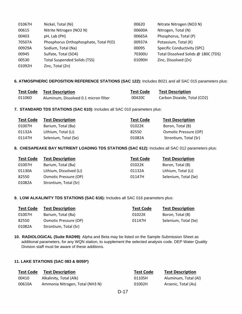
D-17
01067H Nickel, Total (Ni) 00620 Nitrate Nitrogen (NO3 N)
00615 Nitrite Nitrogen (NO2 N) 00600A Nitrogen, Total (N)
00403 pH, Lab (PH) 00665A Phosphorus, Total (P)
70507A Phosphorus Orthophosphate, Total P(O) 00937A Potassium, Total (K)
00929A Sodium, Total (Na) 00095 Specific Conductivity (SPC)
00945 Sulfate, Total (SO4) 70300U Total Dissolved Solids @ 180C (TDS)
00530 Total Suspended Solids (TSS) 01090H Zinc, Dissolved (Zn)
01092H Zinc, Total (Zn)
6. ATMOSPHERIC DEPOSITION REFERENCE STATIONS (SAC 122): Includes B021 and all SAC 015 parameters plus:
Test Code 01106D
Test Description Aluminum, Dissolved 0.1 micron filter
Test Code 00420C
Test Description Carbon Dioxide, Total (CO2)
7. STANDARD TDS STATIONS (SAC 610): Includes all SAC 010 parameters plus:
Test Code Test Description Test Code Test Description
01007H Barium, Total (Ba) 01022K Boron, Total (B)
01132A Lithium, Total (Li) 82550 Osmotic Pressure (OP)
01147H Selenium, Total (Se) 01082A Strontium, Total (Sr)
8. CHESAPEAKE BAY NUTRIENT LOADING TDS STATIONS (SAC 612): Includes all SAC 012 parameters plus:
Test Code Test Description Test Code Test Description
01007H Barium, Total (Ba) 01022K Boron, Total (B)
01130A Lithium, Dissolved (Li) 01132A Lithium, Total (Li)
82550 Osmotic Pressure (OP) 01147H Selenium, Total (Se)
01082A Strontium, Total (Sr)
9. LOW ALKALINITY TDS STATIONS (SAC 616): Includes all SAC 016 parameters plus:
Test Code Test Description Test Code Test Description
01007H Barium, Total (Ba) 01022K Boron, Total (B)
82550 Osmotic Pressure (OP) 01147H Selenium, Total (Se)
01082A Strontium, Total (Sr)
10. RADIOLOGICAL (Suite RAD99): Alpha and Beta may be listed on the Sample Submission Sheet as
additional parameters, for any WQN station, to supplement the selected analysis code. DEP Water Quality
Division staff must be aware of these additions.
11. LAKE STATIONS (SAC 083 & B059*)
Test Code Test Description Test Code Test Description
00410 Alkalinity, Total (Alk) 01105H Aluminum, Total (Al)
00610A Ammonia Nitrogen, Total (NH3 N) 01002H Arsenic, Total (As)

D-18
01007A
71870
Barium, Total (Ba)
Bromide (Br)
01022K
00916A
Boron, Total (B)
Calcium, Total (Ca) 00940
01042H
Chloride (Cl)
Copper, Total (Cu)
962*
00900
Chlorophyll a (fluorometric)
Hardness, Total (Hard)
01045A Iron, Total (Fe) 01051H Lead, Total (Pb)
00927A Magnesium, Total (Mg) 01055H Manganese, Total (Mn)
71900I
00600A
PHEOPHY*
01147H
Mercury, Total
Nitrogen, Total (N)
Pheophytin
Selenium, Total (Se)
00620A
00403
00665A
00929A
Nitrate Nitrogen (NO3 N)
pH, Lab (PH)
Phosphorus, Total (P)
Sodium, Total (Na)
00095 Specific Conductivity (SPC) 01082A Strontium, Total (Sr)
00945
00530
01092H
Sulfate, Total (SO4)
Total Suspended Solids (TSS)
Zinc, Total (Zn)
70300U
82079
Total Dissolved Solids @ 180C
Turbidity, Nephelmetric
12. FISH TISSUE STATIONS
a. SAC 059
Test Code Test Description Test Code Test Description
71946 Barium, Total (Ba) 71940 Cadmium, Total (Cd)
71939 Chromium, Total (Cr) 71937 Copper, Total (Cu)
71936 Lead, Total (Pb) 71930 Mercury, Total (Hg)
71945 Selenium, Total (Se) 71947 Strontium, Total (Sr)
b. PCBs (SAC PCBF)
CAS # Test Description CAS # Test Description
11104282 Arochlor 1221 11141165 Arochlor 1232
53469219 Arochlor 1242 12672296 Arochlor 1248
11097697 Arochlor 1254 11096825 Arochlor 1260
c. PESTICIDES (SAC PESTF)
CAS # Test Description CAS # Test Description
72548 4,4-DDD 72559 4,4-DDE
50293 4,4-DDT 309002 Aldrin
319846 Alpha-BHC 5103719 Alpha-Chlordane
3734483 Chlordene 5103731 Cis-Nonachlor
60571 Dieldrin 72208 Endrin
5103742 Gamma-Chlordane 58899 Gamma-BHC (Lindane)
76448 Heptachlor 1024573 Heptachlor Epoxide
72435 Methoxychlor 2385855 Mirex
53190 O,P-DDD 3424826 O,P-DDE
789026 O,P-DDT 26880488 Oxychlordane
39765805 Trans-Nonachlor

D-19
D.2 ACTIVE WATER CHEMISTRY STATIONS

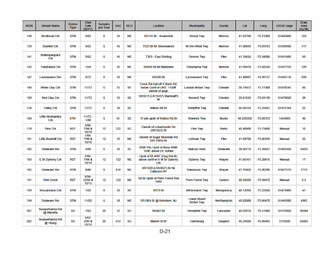


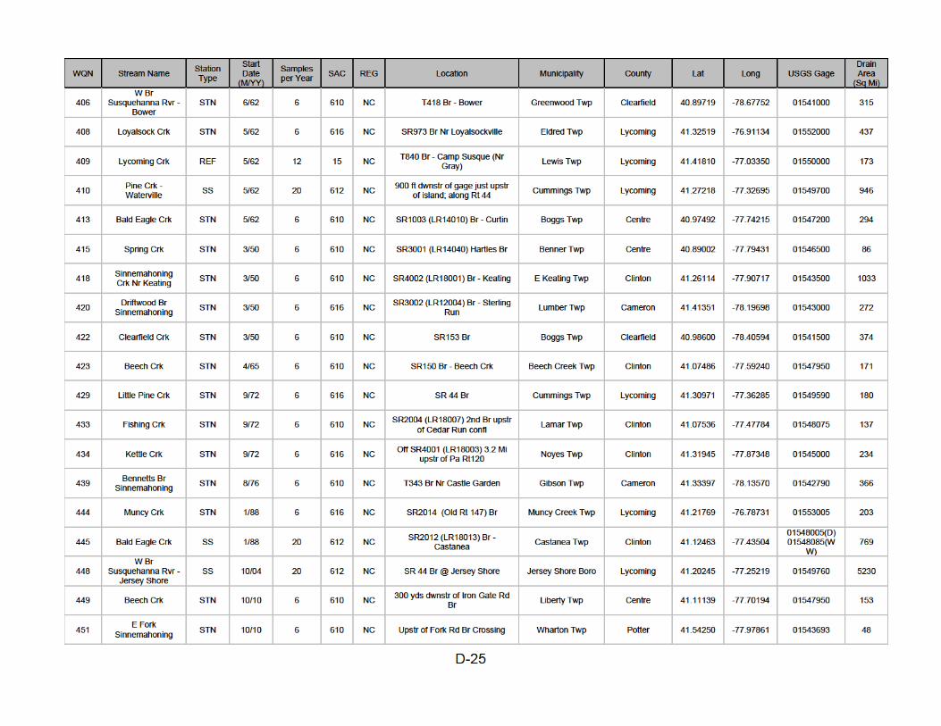
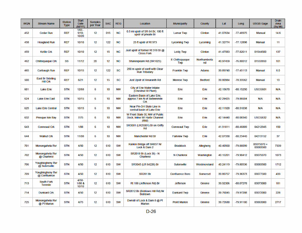

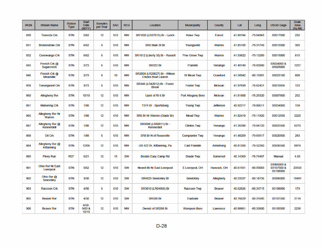

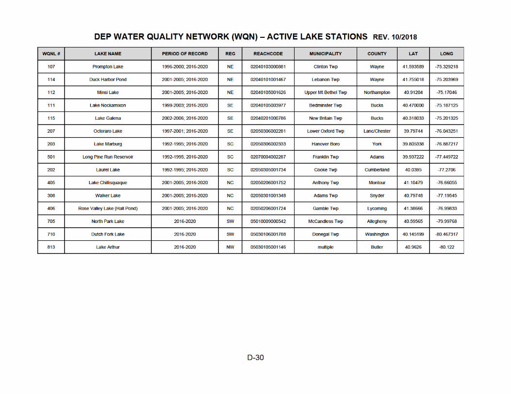

D-31
D.3 ACTIVE BENTHIC MACROINVERTEBRATE STATIONS


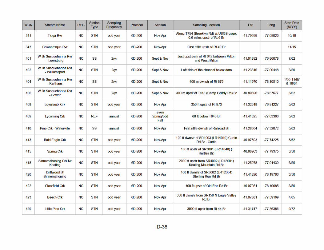
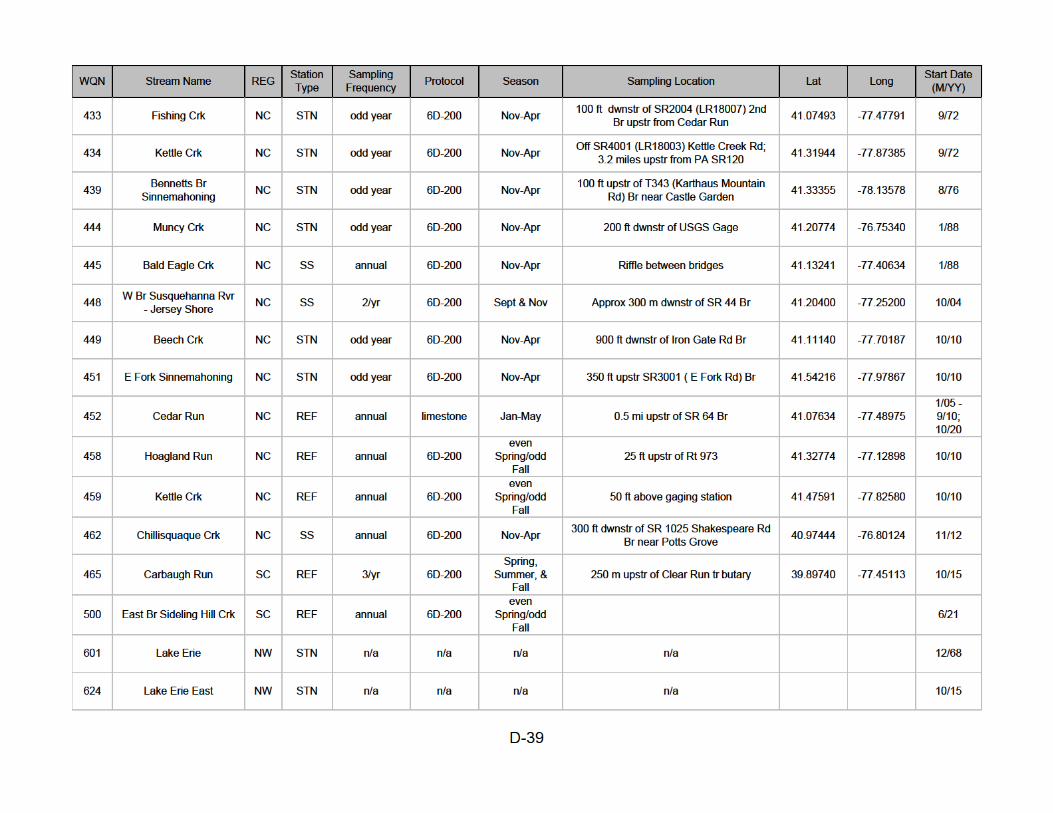
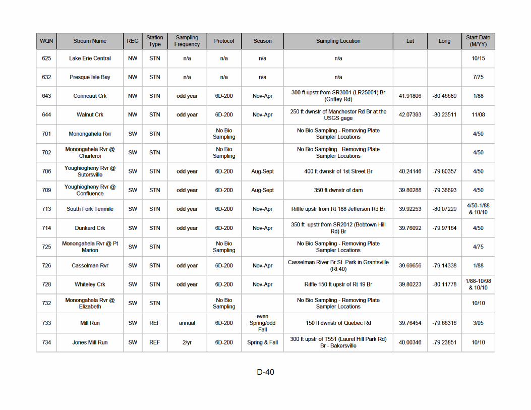
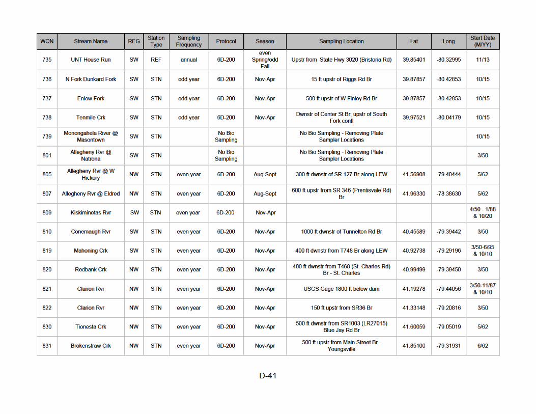


D-44
D.4 DISCONTINUED STATIONS


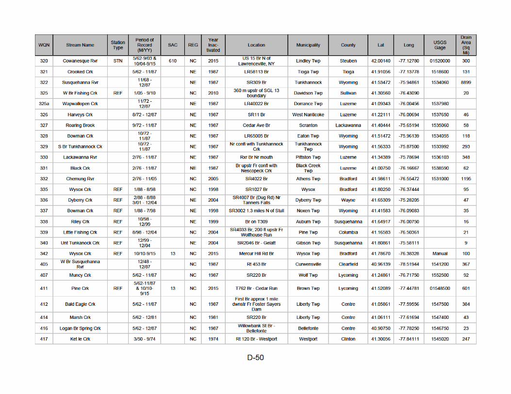

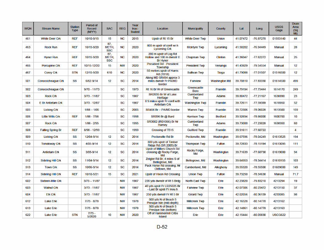
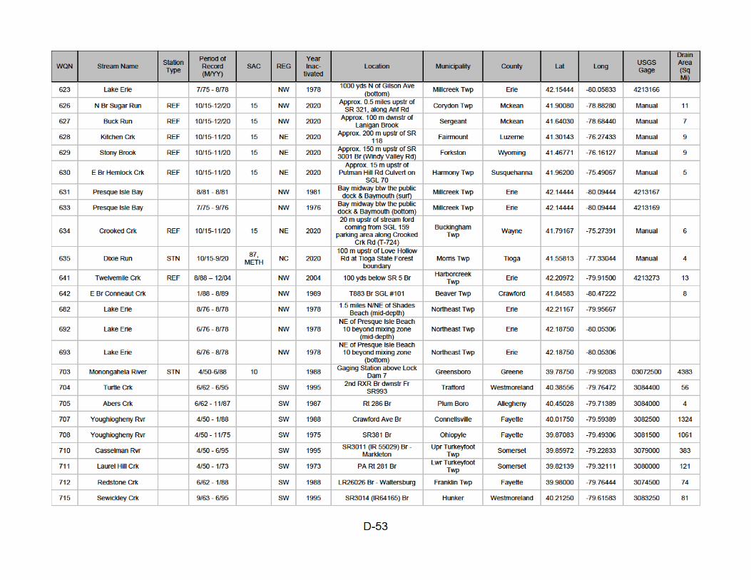


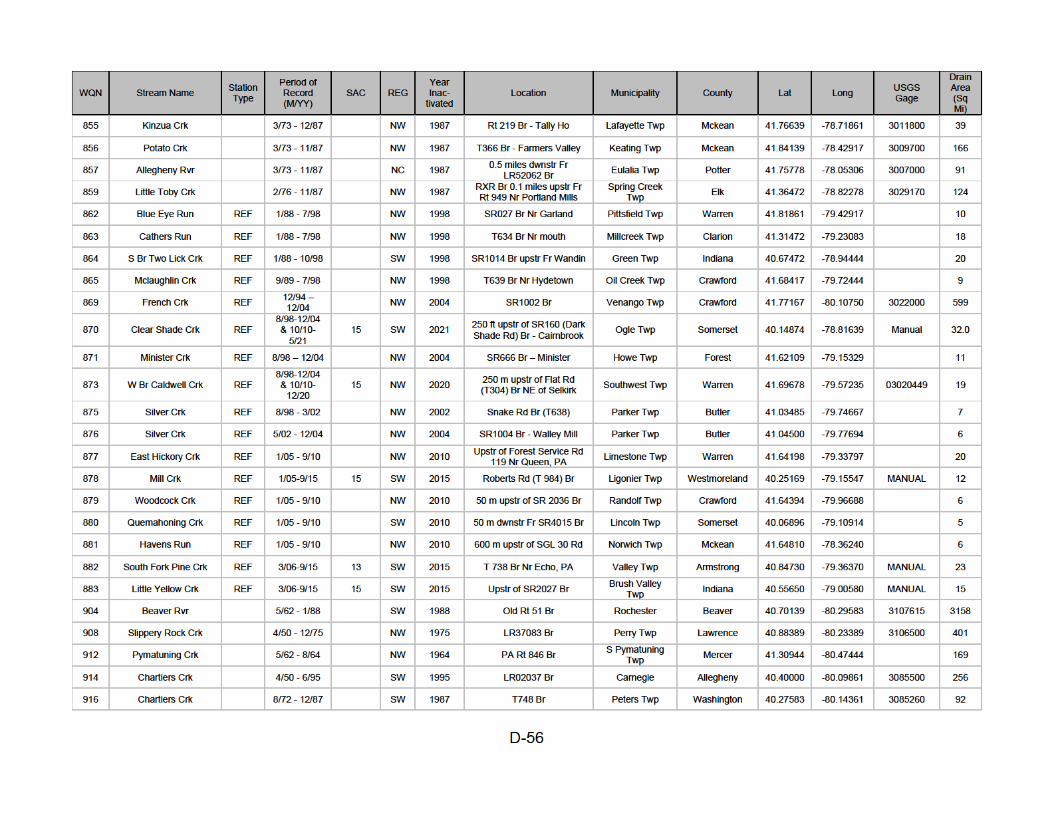


D-58
D.5 WQN OBJECTIVES

D-59
OFFICE OF WATER PROGRAMS
BUREAU OF CLEAN WATER
WATER QUALITY NETWORK OBJECTIVES
2020

D-60
Prepared by:
Molly Pulket and Heidi Biggs
Pennsylvania Department of Environmental Protection
Office of Water Programs
Bureau of Clean Water
11th Floor: Rachel Carson State Office Building
Harrisburg, PA 17105
2019
Edited by:
Molly Pulket
Office of Water Programs
PA Department of Environmental Protection
Bureau of Clean Water
11th Floor: Rachel Carson State Office Building
Harrisburg, PA 17105
2020

D-61
OBJECTIVES OF THE WATER QUALITY NETWORK
The Pennsylvania Water Quality Network (WQN) is a statewide, fixed-station sampling network that
has been gathering important surface water quality data across the Commonwealth for decades. The
design of the network, the design of sampling plans in the network, and the decades of data available
at some stations have allowed WQN data to be used for many purposes by the Pennsylvania
Department of Environmental Protection (DEP), other state and federal agencies, and other interested
parties. This document describes the key uses of WQN water chemistry and macroinvertebrate data.
For more information on this sampling network, please visit the WQN webpage at DEP Water Quality
Network.
Trend Analysis
Trend analysis is one of the core functions of the WQN. The WQN’s fixed-station monitoring strategy is
uniquely suited for measuring changes in water quality through time. Trend data collected in the WQN
is used to monitor incremental progress in water quality, to calibrate Total Maximum Daily Load (TMDL)
models, and to track sources and timing of potential impacts to water quality. Analyses of trend data
are also one of the most efficient and accessible ways to communicate vast amounts of water quality
data to a variety of stakeholders, including the public, which promotes transparency.
Example
As part of a joint effort, DEP partners with the Susquehanna River Basin Commission (SRBC), the
United States Geological Survey (USGS), and the Chesapeake Bay Program (CBP) in a rigorous
sampling program to measure nutrient and sediment concentrations at strategic locations within the
Susquehanna River basin to better understand nutrient and sediment inputs to the Chesapeake Bay.
This monitoring network is incorporated into the WQN and consists of six mainstem river stations and
thirty tributary stations. From this extended WQN program, SRBC reports on trends in nutrient and
suspended sediment concentrations, loads, and yields in the Susquehanna River basin. Information
from these reports helps managers from multiple agencies create and adapt appropriate action plans.
Permitting
Data from the WQN informs the evaluation and development of water quality-based effluent limitations
(WQBEL) in National Pollutant Discharge Elimination System (NPDES) permits which control the
discharge of pollutants from point sources into surface waters. WQBELs, as defined in 25 Pa. Code
section 96.1, are effluent limitations based on the need to maintain or attain the water quality criteria
and to assure protection of existing and designated uses. DEP often uses WQN data as background
data for naturally occurring pollutants when determining whether a stream has assimilative capacity to
accept a pollutant limit and in developing WQBELs where there is reasonable potential to exceed water
quality criteria.
WQN data also provide important background data when permitting discharges in High Quality Waters
(HQ) and Exceptional Value Waters (EV) where existing water quality is protected and maintained. In
permitting discharges to these special protection waters, data from a WQN station near the proposed

D-62
or existing discharge site, or from a WQN station that is representative of the proposed or existing
discharge site, can be used to develop non-degrading effluent limitations.
Additionally, since the toxicity of several pollutants vary with hardness (e.g., copper, lead, nickel, silver,
and other metals) or pH (e.g., ammonia), many Chapter 93 water quality criteria require background
hardness or pH to use in calculating criteria values. In these situations, WQN data can be used to
eliminate the use of default hardness or pH values, or the need for additional data collection to
calculate appropriate water quality criteria values.
Example
DEP permit writers can use WQN data to develop non-degrading effluent permit limits for discharges to
HQ and EV streams. A DEP permit writer used water chemistry data collected at WQN station 195 on
Rock Run to calculate the non-degrading effluent limitations for an Exceptional Value tributary to
French Creek in Chester County. The WQN station allowed the permit writer to use data that is
representative of the watershed containing the permitted discharge, instead of default data values or
requiring the need to collect additional data.
Water Quality Assessments for Federal Clean Water Act Sections 303(d) and 305(b)
The WQN is crucial for Pennsylvania to meet federal mandates to monitor water quality and to assess
monitored water quality against water quality standards. Depending on the type of WQN station, certain
chemical parameters are collected frequently enough to determine if water quality criteria are being
met. This information is one part of the overall surface water monitoring program that helps build the
Pennsylvania Integrated Water Quality Monitoring and Assessment Report, which is required by the
federal Clean Water Act on a biennial basis. In addition, biological assessment determinations can also
be made at WQN stations where biological data is collected using current assessment methodologies.
Example
Historical and current data for nitrates collected at the WQN station on Connoquenessing Creek
located downstream of an industrial discharge in Butler County was instrumental in documenting the
impairment and subsequent restoration of the creek’s Potable Water Supply (PWS) use. The PWS use
of Connoquenessing Creek downstream of the discharge was listed as impaired on the 303(d) list for
exceeding the nitrite plus nitrate PWS criterion in 25 Pa. Code § 93.7 as documented in historical WQN
data. After the industrial discharger discontinued nitric acid pickling, WQN data documented water
quality in Connoquenessing Creek downstream of the discharge as no longer exceeding the nitrite plus
nitrate PWS criterion. In this instance, WQN data was central to both the listing and subsequent
delisting of Connoquenessing Creek.
Data to Inform Permits
The WQN is specifically designed to evaluate both the quality of Pennsylvania's surface waters and the
effectiveness of DEP’s water quality management program. Identifying changes in water quality at
certain locations over time helps ensure permits are written accurately and are protective of water
quality standards. Additionally, the WQN serves not only to help inform permitting, but also help
operators describe in permit applications how they are able to comply with water quality standards.

D-63
Example
The WQN data was essential in helping show compliance with water quality standards as discussed in
the industrial discharge example above. Although the WQN data initially documented the impairment,
WQN data also helped the operator demonstrate compliance with water quality standards after the
process change at the plant.
Threatened and Endangered Species Protection
Threatened and endangered species are an ongoing concern related to NPDES discharges. The
United States Fish and Wildlife Service has recommended stringent criteria for multiple pollutants
including ammonia-nitrogen, chloride, TDS, and nickel to protect threatened and endangered mussel
species. As noted in the permitting discussion above, WQN data is essential in accurately evaluating
appropriate criteria for some of these pollutants since the availability of background data can have a
significant impact on these evaluations. Not only is it critical to have accurate background data of the
pollutants of concern but it is also critical to have accurate hardness and pH background data to
calculate appropriate pollutant criteria and associated potential impact areas.
Example
Endangered mussels are of special concern in the Allegheny River, French Creek, Shenango River,
and many tributaries to these surface waters. Segments of all three main streams have been
designated as “critical habitat” for the rabbitsfoot mussel, and many other threatened and endangered
mussel species. Numerous NPDES permits in this region of Pennsylvania have been issued with
concurrence by US Fish and Wildlife Service as protective of endangered species, using a permitting
strategy that includes a robust evaluation of WQN data.
Emerging Science
Due to the years- to decades-long historical records of physical, chemical, and biological data collected
at many stations, WQN sites often serve as prime locations to collect new data (e.g., contaminants of
emerging concern) and to develop new collection protocols (e.g., periphyton monitoring protocols).
The ability to contextualize new kinds of data in robust historical records characterizing particular sites
across a range of parameters and assemblages can greatly reduce the cost and time needed to
expand monitoring approaches when novel environmental concerns arise.
Example
During an intensive study of the Susquehanna River, WQN stations were almost exclusively used when
selecting locations to place passive chemical samplers designed to detect hundreds of contaminants of
emerging concern. The combination of this new data and the existing WQN data substantially reduced
the overall cost of the project, compared with project costs if the passive samplers were deployed in
locations without robust water quality network data.
D-64
D.6 FIELD PREPARATION AND FIXATIVE CHART

D-65
Standard Analysis Code
(SAC) Parameters Bottle Ware Field Prep/Fixative
010
general chemistry 1 - 500 ml HDPE plastic bottle iced to 4°C
N/P 1 - 500 ml HDPE plastic bottle 10% H2SO4 to pH <2; iced to 4°C
metals, total 1 - 125 ml HDPE plastic bottle 1:1 HNO3 to pH <2; iced to 4°C
012
general chemistry 2 - 500 ml HDPE plastic bottle iced to 4°C
general chemistry, dissolved 1 - 125 ml HDPE plastic bottle field filtered; iced to 4°C
N/P 1 - 500 ml HDPE plastic bottle 10% H2SO4 to pH <2; iced to 4°C
N/P, dissolved 1 - 125 ml HDPE plastic bottle field filtered; 10% H2SO4 to pH <2; iced to 4°C
metals, total 1 - 125 ml HDPE plastic bottle 1:1 HNO3 to pH <2; iced to 4°C
TOC 2 - 40 ml amber VOA vials 10% H2SO4 to pH <2; iced to 4°C
015
general chemistry plus CBOD 3 - 500 ml HDPE plastic bottle iced to 4°C
general chemistry, dissolved 1 - 125 ml HDPE plastic bottle field filtered; iced to 4°C
N/P 1 - 125 ml HDPE plastic bottle 10% H2SO4 to pH <2; iced to 4°C
N/P, dissolved 1 - 125 ml HDPE plastic bottle field filtered; 10% H2SO4 to pH <2; iced to 4°C
metals, total 1 - 125 ml HDPE plastic bottle 1:1 HNO3 to pH <2; iced to 4°C
metals, dissolved 1 - 125 ml HDPE plastic bottle field filtered; 1:1 HNO3 to pH <2; iced to 4°C
Organic Carbon, Total 2 - 40 ml amber VOA vials 10% H2SO4 to pH <2; iced to 4°C
Organic Carbon, Dissolved 2 - 40 ml amber VOA vials field filtered: 10% H2SO4 to pH <2; iced to 4°C
016
general chemistry plus CBOD 2 - 500 ml HDPE plastic bottle iced to 4°C
N/P 1 - 500 ml HDPE plastic bottle 10% H2SO4 to pH <2; iced to 4°C
metals, total 1 - 125 ml HDPE plastic bottle 1:1 HNO3 to pH <2; iced to 4°C
metals, dissolved 1 - 125 ml HDPE plastic bottle field filtered; 1:1 HNO3 to pH <2; iced to 4°C
083
general chemistry 2 - 500 ml HDPE plastic bottle iced to 4°C
N/P 1 - 125 ml HDPE plastic bottle 10% H2SO4 to pH <2; iced to 4°C
metals, total 1 - 125 ml HDPE plastic bottle 1:1 HNO3 to pH <2; iced to 4°C
122
general chemistry plus CBOD 3 - 500 ml HDPE plastic bottle iced to 4°C
general chemistry, dissolved 1 - 125 ml HDPE plastic bottle field filtered; iced to 4°C
N/P 1 - 125 ml HDPE plastic bottle 10% H2SO4 to pH <2; iced to 4°C
N/P, dissolved 1 - 125 ml HDPE plastic bottle field filtered; 10% H2SO4 to pH <2; iced to 4°C
metals, total 1 - 125 ml HDPE plastic bottle 1:1 HNO3 to pH <2; iced to 4°C

D-66
metals, dissolved 1 - 125 ml HDPE plastic bottle field filtered; 1:1 HNO3 to pH <2; iced to 4°C
Organic Carbon, Total 2 - 40 ml amber VOA vials 10% H2SO4 to pH <2; iced to 4°C
Organic Carbon, Dissolved 2 - 40 ml amber VOA vials field filtered: 10% H2SO4 to pH <2; iced to 4°C
aluminum, monomeric (R01106D) 1 - 125 ml HDPE plastic bottle field filtered (0.1 um); 1:1 HNO3 to pH <2; iced to 4°C
610 *all SAC010 bottles plus
general chemistry 1 - 500 ml HDPE plastic bottle iced to 4°C
612 *all SAC012 bottles plus
general chemistry 1 - 500 ml HDPE plastic bottle iced to 4°C
616 *all SAC016 bottles plus
general chemistry 1 - 500 ml HDPE plastic bottle iced to 4°C
B021 fecal coliform, E.coli 1 - 125 ml plastic bottle sterilized & pretreated with sodium thiosulfate
iced to ≤ 6°C
RAD99 gross alpha, gross beta 2 - 500 ml glass bottle iced to 4°C
B029 chlorophyll a 1 - 47 mm glass fiber filter in
petri dish wrap in aluminum foil and place on dry ice or ice to 4°C &
freeze within 24 hrs
-- suspended sediment 1 - 500 ml plastic bottle store in cool dark place
All WQN stations require the following STANDARD FIELD ANALYSES: Temp (°C), pH, Dissolved Oxygen, and Specific Conductance. These results should be recorded on the Sample Submission Sheet.
* Must be shipped to USGS lab in Louisville, KY.
D-67
D.7 STREAM FLOW MEASUREMENT PROTOCOLS

D-68
Wire-Weight Gages
A wire-weight (WW) gage consists of a drum wound with a single layer of cable, a bronze weight
attached to the end of the cable, a graduated disc and counter, and a check bar of known elevation.
The gage is housed within a small cast aluminum lockable box and generally mounted to a rigid
structure (i.e., bridge or trestle) directly above the water surface. The graduated disc is permanently
connected to the counter and to the shaft of the drum. The drum reel is equipped with pawl and ratchet
for holding the suspended weight at any desired elevation.
The check-bar for the WW gage is set by levels as a reference elevation to gate datum. The gage is set
so that when the bottom of the suspended weight is at the water surface, the gage height is indicated
by the combined readings of the counter and the graduated disc.
Reading Instructions
• Unlock the case and gently open the cover. If the cover jams and will not open freely, do not
force it open. The cover has probably become jammed against the crank handle. Try to move
the handle into a position that will allow the cover to open. At this point, make sure the pawl is
engaged or that you can hold onto the handle to prevent the weight falling to the stream bed
and unspooling the cable.
• Inspect the cable. It should be tightly wound with windings that touch each other, with no
overlaps. If cable is not properly wound, check-bar and water-surface readings will be
incorrect. If necessary, unwind the cable and utilizing the level-wind pulley and gloves, rewind
the cable onto the reel. (This should only be necessary in extreme situations.)
• The check-bar is found directly under the weight as it hangs in the box and has two positions,
the forward position (away from you) which prevents the weight from falling to the bottom of
the box while locked (and into the stream when opened), and a rear position (toward you)
which allows the weight to be lowered to the stream. You should find the check-bar in the
forward position. Elevations are run to the check-bar in the forward position and the gage is set
to read this elevation when the weight just makes contact with the check-bar.
• In order to determine the check-bar reading,
o Make sure the check-bar is in the forward position.
o Lower the weight until the weight just lightly touches the check-bar.
o Record this reading to three decimal places. This will involve estimating the last digit.
• Raise the weight and slide the check-bar to the rear position. Lower the weight until it just
lightly touches the surface of the water and record your reading to two decimal places.
Average the peaks and troughs of elevation if the water surface is surging. You should repeat
this process at least once. If the air temperature is below freezing, the first time the weight
touches the water, a layer of ice will form on the bottom of the weight causing it to become
slightly longer. Repeated contacts with the water surface continues to add layers of ice to the
bottom of the weight. For this reason, water surface elevations should be made as accurately
as possible on the first or second try.
• Engage the pawl (this will prevent the weight from falling and unspooling the cable should the
crank slip from your hand while rewinding) and crank the weight to its original position. Slide
D-69
the check-bar to its forward notch. The crank handle should be located in the rear position,
allowing the cover to close without touching the crank handle.
• Close the cover and lock the case.
Electric Tape Gages
The electric tape (ET) gage consists of a steel tape graduated in feet and hundredths, to which is
fastened a cylindrical weight (usually brass), a reel in a frame for the tape, a 4½-volt battery and a
voltmeter. One terminal of the battery is attached to a ground connection and the other to one terminal
of the voltmeter. The other terminal of the voltmeter is connected through the frame, reel and tape, to
the weight. The weight is lowered until it contacts the water surface. This contact completes the electric
circuit and produces a signal on the voltmeter. With the weight held in the position of first contact, the
water surface elevation reading is observed at the tape index (a black line indented just below the
voltmeter and usually immediately above the shelf) provided on the reel mounting. ET gages are
installed in a manner that will produce a dependable circuit, yielding a strong signal when the weight
touches the water surface.
Reading Instructions
The dog on the left side of the reel is disengaged by lifting the rear portion in an upward direction while
holding onto the handle on the right side. This allows the weight and tape to be lowered until it contacts
the water surface. This contact completes the electric circuit and produces a fluctuation on the
voltmeter on the front of the tape reel frame. Once a contact with the water surface has been made, the
weight is raised slightly until contact is broken, and then lowered very slowly until the water surface is
again contacted. This procedure is repeated until a consistent reading at the index line is produced.
This reading may be confirmed visually by shining a flashlight into the well at the spot where the weight
will make contact with the surface of the water and lowering the weight very slowly until contact with the
surface is visually confirmed (the voltmeter needle should also deflect at this time if working correctly).
The reading of the water surface elevation is then taken by observing the reading of the steel tape at
the index line on the gage. NOTE: HAZARD!! In order to make a visual observation of the weight
touching the water surface in the well, it is often necessary to raise the door (located on the floor) to the
well. Once the door is opened, extreme care should be exercised to ensure that nothing is dropped into
the well. This type of reading is best left to experienced personnel.
Possible Interferences
• If the weight touches any grounded item (steel piping or the steel side of an oil tube or a steel
pipe well) the circuit will be completed, and the voltmeter will deflect as if the water surface
has been contacted.
Solution: Physically move the tape past any items in the well that will produce a false reading.
Keep in mind that the tape should be kept as vertical as possible for accurate readings.
• If any oil has seeped into the well onto the water surface from the oil tube, the needle will not
deflect upon hitting the oil, but will deflect when weight is lowered through the oil and contacts
the water surface (this will not be an accurate water elevation).
Solution:

D-70
o Visually determine elevation of the top of the oil surface using the procedure described
above for visual readings and record this number.
o From the top of the oil very slowly lower the weight until a deflection of the voltmeter
occurs. This is the top of the water surface.
o Subtract this reading from the one made in step 1. and multiply the answer by 0.2.
o Subtract this value from the top of oil reading determined in step 1. This is the actual
surface elevation.
Example: 5.28 surface of oil
5.23 surface of water
0.05 difference
X.20 = .0100
5.28-.01 = 5.27 (actual water surface elevation)
• If the bottom of the weight is corroded, even slightly, the meter will not deflect until the water
in the well encounters a portion of the weight free of corrosion, completing the circuit. This
produces an erroneous reading as the circuit is not completed at the bottom of the weight, but
at some point along the side.
Solution: Using a piece of emery paper rub lightly over the bottom of the weight to remove
corrosion. It is also acceptable to lightly scrape the edge of a knife across the bottom of the
weight. Care must be taken to avoid removing any brass from the bottom of the weight as
repeated cleanings over years may change the weight length.
• The cleaning of the weight is a delicate procedure as the weight must first be lowered a few
feet, so it may be grasped through the shelf door or opening. Very often the tape may be very
rusted at the point the tape enters the weight or just below that point. "Any twisting or bending
will break the tape off the weight." Should this happen, lay the weight on the shelf and
contact the USGS as soon as possible.
• Ice in the well.
Solution: Ice must be broken loose and, in some cases, removed. This is a solution that is
best left to experienced USGS technicians, and in no instance should DEP personnel enter
the well.
Staff Gages
Staff gages are simply rods or boards that are securely attached to a backing or permanent foundation.
These non-recording gages are graduated, and stage can be directly read. Vertical staff gages are

D-71
used as reference gages within stilling wells, and both vertical and inclined staff gages may be used as
outside reference gages. Lake height measurements for the WQN are obtained from staff gages.
Digital Recorders
Digital recorders are slow speed, battery operated instruments which record information in the binary
decimal code form by use of a paper-tape punch mechanism. Sixteen channel paper-tape is punched
with a four-digit number at preselected time intervals of 5, 15, 30 or 60 minutes. Stage heights of zero
to 99.99 feet can be recorded in increments of hundredths of a foot. A battery powers the sequencing
camshaft and electro-mechanical timing devices. Pins on the punch block are forced against the paper-
tape and code discs by spring action thereby recording the position of the discs at that moment. After
the paper-tape is punched, it is advanced, and the punch spring is compressed for the next readout
cycle. The tape can be either manually read to determine stage, or electronic translators can then
convert the punch-tape records to a magnetic tape form that is utilized to compute daily mean gage
height and daily stream discharge via digital computers.
Manual Measurement
A full stream width transect is required to manually measure stream flows. Total stream flow must be
calculated across this transect using the procedure of Buchanan and Somers (1969) described briefly
below. Record the depths and velocities for each of a minimum of 20 equally spaced points along the
transect, thereby constructing a stream channel profile and accompanying current velocity
measurements. Sum the products of each cell area calculation multiplied by velocity to determine total
flow (cfs) across the transect.
Telemark
Some gages are equipped with telecommunication capabilities that provide for their remote reading via
the internet.

E-1
APPENDIX E: QUALITY ASSURANCE PROJECT PLAN (QAPP): DATA COLLECTION FOR
THE PURPOSE OF EXISTING USE EVLUATIONS, PROTECTED USE ASSESSMENT, AND
EVALUATIONS OF POINT AND NONPOINT SOURCE IMPACTS TO SURFACE WATER

E-2
Prepared by:
Josh Lookenbill and Mark Hoger
PA Department of Environmental Protection
Office of Water Programs
Bureau of Clean Water
11th Floor: Rachel Carson State Office Building
Harrisburg, PA 17105
2021
Disclaimer:
Appendix E is a copy of a QAPP approved by EPA in July 2021. An official, signed copy of the QAPP is
available upon request.

Project 2021: Document QA # 210096.2 Revision 02 July 2021
E-3
PENNSYLVANIA DEPARTMENT OF ENVIRONMENTAL PROTECTION
Bureau of Clean Water (BCW)
Water Quality Division (WQD)
SECTION A: PROJECT MANAGEMENT
A1. Title Page and Approval Sheet
TITLE: Quality Assurance Project Plan (QAPP): Data collection for
the purpose of existing use evaluations, protected use
assessments, and evaluations of point and nonpoint source
impacts to surface waters
EFFECTIVE DATE: August 1, 2021
AUTHORITY: Pennsylvania Clean Streams Law, 35 P.S. §§ 691.1 et. seq.,
the Federal Clean Water Act, 33 U.S.C.A §§ 1251 et. seq.,
25 Pa. Code Chapters 93 and 96.
POLICY: This guidance provides the established QAPP for water
quality data collection in surface waters of Pennsylvania
PURPOSE: The guidance was developed to establish and standardize
the Department of Environmental Protection’s (DEP) QAPP
procedures for data collection for existing use evaluations,
protected use assessments, and evaluations of point and
nonpoint source impacts to surface waters.
DISCLAIMER: The policies and procedures outlined in this guidance
document are intended to supplement existing requirements.
Nothing in the policies or procedures shall affect regulatory
requirements.
The policies and procedures herein are not an adjudication
or a regulation. There is no intent on the part of DEP to give
these rules that weight or deference. This document
establishes the framework within which DEP will exercise its
administrative discretion in the future. DEP reserves the

Project 2021: Document QA # 210096.2 Revision 02 July 2021
E-4
discretion to deviate from this policy statement if
circumstances warrant.
PAGE LENGTH: 37 Pages
DEP Project Manager’s Signature:
DEP Project Manager: Michael (Josh) Lookenbill
DEP Project Quality Assurance Manager’s Signature:
DEP Project Quality Assurance Manager: Mark Hoger
EPA Project Manager’s Signature: Note: This approval action represents EPA’s determination that the document(s) under review comply with
applicable requirements of the EPA Region 3 Quality Management Plan
[https://www.epa.gov/sites/production/files/2020-06/documents/r3qmp-final-r3-signatures-
2020.pdf] and other applicable requirements in EPA quality regulations and policies
[https://www.epa.gov/quality]. This approval action does not represent EPA’s verification of
the accuracy or completeness of document(s) under review, and is not intended to constitute
EPA direction of work by contractors, grantees or subgrantees, or other non-EPA parties.
EPA Project Manager: Steve Hohman
EPA Project Quality Assurance Manager’s Signature: Note: This approval action represents EPA’s determination that the document(s) under review comply with
applicable requirements of the EPA Region 3 Quality Management Plan
[https://www.epa.gov/sites/production/files/2020-06/documents/r3qmp-final-r3-signatures-
2020.pdf] and other applicable requirements in EPA quality regulations and policies
[https://www.epa.gov/quality]. This approval action does not represent EPA’s verification of
the accuracy or completeness of document(s) under review, and is not intended to constitute
EPA direction of work by contractors, grantees or subgrantees, or other non-EPA parties.
EPA Project Quality Assurance Officer: Elizabeth Gaige
Last Revised July 2021
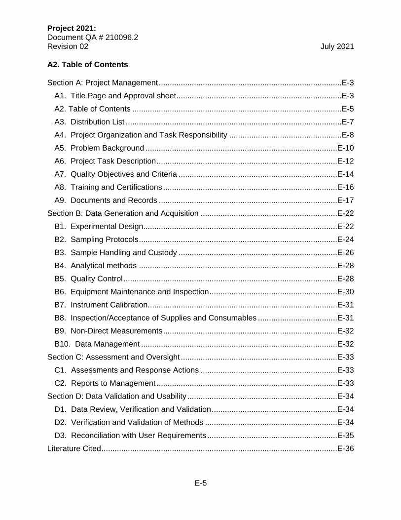
Project 2021: Document QA # 210096.2 Revision 02 July 2021
E-5
A2. Table of Contents
Section A: Project Management ................................................................................... E-3
A1. Title Page and Approval sheet ........................................................................... E-3
A2. Table of Contents ............................................................................................... E-5
A3. Distribution List .................................................................................................. E-7
A4. Project Organization and Task Responsibility ................................................... E-8
A5. Problem Background ....................................................................................... E-10
A6. Project Task Description .................................................................................. E-12
A7. Quality Objectives and Criteria ........................................................................ E-14
A8. Training and Certifications ............................................................................... E-16
A9. Documents and Records ................................................................................. E-17
Section B: Data Generation and Acquisition .............................................................. E-22
B1. Experimental Design ........................................................................................ E-22
B2. Sampling Protocols .......................................................................................... E-24
B3. Sample Handling and Custody ........................................................................ E-26
B4. Analytical methods .......................................................................................... E-28
B5. Quality Control ................................................................................................. E-28
B6. Equipment Maintenance and Inspection .......................................................... E-30
B7. Instrument Calibration ...................................................................................... E-31
B8. Inspection/Acceptance of Supplies and Consumables .................................... E-31
B9. Non-Direct Measurements ............................................................................... E-32
B10. Data Management ......................................................................................... E-32
Section C: Assessment and Oversight ....................................................................... E-33
C1. Assessments and Response Actions .............................................................. E-33
C2. Reports to Management .................................................................................. E-33
Section D: Data Validation and Usability .................................................................... E-34
D1. Data Review, Verification and Validation ......................................................... E-34
D2. Verification and Validation of Methods ............................................................ E-34
D3. Reconciliation with User Requirements ........................................................... E-35
Literature Cited ........................................................................................................... E-36

Project 2021: Document QA # 210096.2 Revision 02 July 2021
E-6
E.1: Benthic Macroinvertebrate Subsampling and Taxonomic Identification Quality
Control ........................................................................................................................ E-39
Introduction ............................................................................................................. E-40
QC – Benthic Macroinvertebrate Subsampling ....................................................... E-40
QC – Benthic Macroinvertebrate Identification ........................................................ E-42
QC – Fish Identification ........................................................................................... E-43
Literature Cited ....................................................................................................... E-44
Project 2021: Document QA # 210096.2 Revision 02 July 2021
E-7
A3. Distribution List
This QAPP will be appended to the latest edition of the DEP Water Quality Monitoring
Protocols for Stream and Rivers (Lookenbill and Whiteash 2021), which is available on
the DEP Water Quality Division website at:
https://www.dep.pa.gov/Business/Water/CleanWater/WaterQuality/Pages/Data-
Collection-Protocols.aspx.
It will also be placed electronically in in-house records at the DEP. It can be made
available upon request. QAPP revisions will also be re-appended to DEP monitoring
protocols. In addition, this QAPP will be distributed to each of the DEP Regions and
cooperating programs who are involved with surface water and data collection. This will
ensure data will be collected according to the quality addressed in this QAPP. Any
revisions to this document will also be sent to those on the distribution list. The following
is the distribution list of current staff that oversees coordination in each region and each
respective agency:
• DEP Northwest Region – Joseph Brancato, Aquatic Biologist Supervisor
• DEP Southwest Region – Richard Spear, Aquatic Biologist Supervisor
• DEP Northcentral Region – Anne Hughes, Environmental Group Manager
• DEP Southcentral Region – Kristen Bardell, Aquatic Biologist Supervisor
• DEP Northeast Region – Walter Holtsmaster, Aquatic Biologist Supervisor
• DEP Southeast Region – Steven Unger, Aquatic Biologist Supervisor
• DEP Central Office – Josh Lookenbill, Monitoring Section Chief
• Department of Natural Resources and Conservation (DCNR) – Nick Decker,
Resource Manager
• Bureau of Laboratories (BOL) – Pamela Higgins, Special Assistant to Laboratory
Operations

Project 2021: Document QA # 210096.2 Revision 02 July 2021
E-8
A4. Project Organization and Task Responsibility
The following is a list of key project personnel and their corresponding responsibilities.
Due to staff turnover, the list provided gives a general description of those involved. See
Figure 1 – Organizational Chart to better define their relationships.
• Sampling Operations – WQD Central Office Biologists, DEP Regional Biologists
• Sampling Quality Control (QC) – DEP Project Manager
• Laboratory Analysis – DEP Bureau of Laboratories (BOL), Outside laboratories
as needed
o Inorganic Division – Trace Metals & Sample Receiving Section and
Automated Analysis & Biochemistry Analytical Section
o Organic Division – Organic Chemistry Section
o Biological Services Division – Microbiology Lab, Giardia Lab and Microbial
Source Tracking Lab
• Laboratory Quality Control – BOL Quality Assurance and Safety Section
• Data and QC Processing – DEP Project Manager, WQD Central Office
Biologists, DEP Regional Biologists
• Data Review and Review QC – Falls to staff responsible for survey, could include
WQD Central Office Biologist or DEP Regional Biologist
• Performance and Systems Auditing – WQD, Monitoring Section and Assessment
Section
• Overall Project Coordination and QA – WQD, Monitoring Section
• Maintenance and Distribution of Official Approved QAPP – DEP Project Quality
Assurance Manager

Project 2021: Document QA # 210096.2 Revision 02 July 2021
E-9
Figure 1. Organizational Chart

Project 2021: Document QA # 210096.2 Revision 02 July 2021
E-10
A5. Problem Background
The primary purpose for monitoring surface waters is to assess and evaluate protected
uses and to broadly evaluate point and nonpoint sources and associated impacts on
surface waters in accordance with 25 Pa. Code §§ 93 and 96 of DEP’s regulations.
Monitoring is driven by the following primary objectives:
Assessment of Protected Water Uses
To investigate and determine attainment of water quality standards (WQS) and possible
sources and causes of impairment from point or non-point sources of conventional
pollutants and known or suspected water quality problems in streams, rivers and lakes.
These surveys are performed to reevaluate existing assessments and identify additional
sources and causes of water quality impairments identified by previous assessment
efforts. Chemical and bacteriological data is typically compared to water quality criteria
while considering frequency and duration with which a given criterion was developed
according to supporting technical documentation and assessment methods.
• Pennsylvania surface water quality criteria can be found in 25 Pa. Code § 93
(https://www.pacodeandbulletin.gov/Display/pacode?file=/secure/pacode/data/02
5/chapter93/chap93toc.html)
• Technical documentation
(https://www.dep.pa.gov/Business/Water/CleanWater/WaterQuality/Pages/Macro
invertebrates.aspx)
• Assessment methods
(https://www.dep.pa.gov/Business/Water/CleanWater/WaterQuality/Pages/Asses
sment-Methodology.aspx)
Biological data (macroinvertebrates and fish) is used to calculate indices that are
compared to attainment thresholds described in the assessment methods (Lookenbill
and Whiteash 2021) and accompanying technical documentation.
Data Usage
Data are used for generating the integrated report, listing impaired waterbodies as
required by Section 303(d), and to support the compliance and permitting programs by
defining the impact of specific discharges or land-based activities on receiving waters.
Physical, chemical and/or biological data collected during surveys are generally
evaluated using non-parametric, classification type analyses designed to display
differences or similarities between sampling stations and metric thresholds.

Project 2021: Document QA # 210096.2 Revision 02 July 2021
E-11
Stream Redesignation and Existing Use Evaluations
To review and revise, if necessary, WQS to ensure that protected uses are accurate.
Data Usage
Data will be used to evaluate the need for antidegradation protection in selected
Pennsylvania waters. The evaluation will consider biotic and abiotic components of the
watershed ecosystem. Features such as water quality sensitivity, land use activities,
and the environmental and ecological significance of the watershed are evaluated in an
effort to determine the correct protected use per the requirements in 25 Pa. Code §
93.4b.
Maintenance of fixed station Water Quality Network (WQN)
To establish and maintain a database to assist in a) describing water quality conditions
across Pennsylvania streams, rivers and lakes; b) identifying long-term trends of
improvement or degradation in major waterbodies; c) determining the suitability of
waterbodies for water supply, recreation, fish, aquatic life, and other uses; d) providing a
limited measure of “background” water quality throughout Pennsylvania’s Ecoregions;
and e) providing a basis for evaluating success of the water quality management
program.
Data Usage
WQN data will be used to generate basic statistics to generally characterize water
quality by station; these values can then be compared to established standards and
criteria to determine the effectiveness of water quality management programs.
Furthermore, seasonally adjusted Kendall tests are applied to historic WQN data to
assess long-term trends in water quality using a Weighted Regressions on Time,
Discharge, and Season (WRTDS) model (Hirsch et al. 2010). Additionally, collection of
data at “ambient” stations provides a measure of background conditions at unaffected or
minimally affected sampling locations. These data provide both a measure of long-term
water quality trends resulting from airborne contaminants and background water quality
as identified by ecoregion. This information can then be used to develop permits by the
permitting programs or to determine the potential use attainment of nearby streams
degraded by anthropogenic inputs.
Other Objectives
To include cause and effect monitoring, point of first use determinations and protocol,
method and standards development.
Date Usage
Cause and effect monitoring data will be employed to investigate possible relationships

Project 2021: Document QA # 210096.2 Revision 02 July 2021
E-12
between point or nonpoint sources of conventional pollutants and known or suspected
water quality problems through the collection and analysis of biological, physical, and
chemical data. These surveys are designed primarily to monitor the effectiveness of
permitted treatment facilities but are also used to investigate reported or suspected
water quality impacts for nonpoint source and other pollution sources.
Point of first use surveys are completed as part of the evaluation and permitting of
wastewater discharges to intermittent and ephemeral streams, drainage channels and
swales, and storm sewer. The point of first surface water use establishes where
Chapter 93 WQS must be attained.
Protocol, method and standard development data collections will be used to implement
the Pennsylvania Clean Streams Law and the Federal Clean Water Act. To achieve
this, at a statewide level, WQS are developed to establish the protected uses, criteria,
and antidegradation requirements that surface waters must meet.
A6. Project Task Description
Routine surface water data collections for the purpose of evaluating protected uses
(existing and designated), assessing protected uses, and investigating point and
nonpoint source impacts will be conducted. Products include existing use evaluations,
redesignation recommendations, protected use assessments, and evaluations of point
and nonpoint source discharges or impacts. DEP implements a hybrid approach with
respect to selecting monitoring locations. One component includes a fixed station,
Pennsylvania Water Quality Network (WQN) where stations are established indefinitely
for the purpose of developing long-term datasets that allow for the development of water
quality trends, the ability to measure the effectiveness of water management programs,
the ability to develop water quality assessment methods and standards, and to provide
data that will inform permitted activities. The WQN also includes locations where data is
collected at fixed intervals of five years. Every five years data is evaluated to determine
if the data is serving the previously identified objectives. After each five-year cycle new
stations may be added, stations may be discontinued, and some stations may be
modified.
In addition to the WQN, fixed station approach, more intense short-term locations are
established to evaluate protected uses, assess protected uses and to evaluate point
and nonpoint source impacts. Short-term stations are chosen to ensure that data
representative of conditions in a given stream reach will be obtained. Factors
considered in locating these stations include watershed land uses, volume and chemical
characteristics of known point source wastewater discharges, physiographic and
demographic conditions that contribute to non-point source problems, and stream

Project 2021: Document QA # 210096.2 Revision 02 July 2021
E-13
hydrology. Every effort is made to sample representative, homogeneous, low-flow water
columns at comparable locations. However, because weather, stream flow conditions,
and accessibility vary, observations of instream and riparian physical characteristics are
recorded for reference in estimating water quality under various conditions. Data
collection includes biological, chemical and physical data.
Frequency of sampling varies depending on sampling objectives and are described in
Pennsylvania’s Surface Water Quality Monitoring Network Manual (Pulket and
Lookenbill 2020). At WQN stations, waters samples are collected bimonthly (water
samples at ambient and bay loading stations are collected monthly) as discrete samples
at mid-channel, mid-depth on small streams and laterally composited, depth integrated
samples on larger streams or rivers. Semi-quantitative benthic macroinvertebrate
samples are collected annually according to DEP data collection protocols. At WQN
lake stations, an annual qualitative plankton tow is substituted for semi-quantitative
macroinvertebrate sampling. Lake water samples (except Lake Erie) are collected once
a year during summer stratification and consist of a sample collected one meter below
the surface and a sample collected one meter off the bottom at the deepest part of the
lake. Sampling schedules for short-term stations are either limited to one-time
collections and/or governed by protocol and the water quality criteria evaluation needs.
Since data collection is ongoing, only a general timeline is provided below (Table 1).
Sample collection and reporting requirements are further described in Section B of this
QAPP. WQN stations and sampling objectives can be found appended to DEP’s
Monitoring Book as the WQN Manual (Pulket and Lookenbill 2020).
Table 1. General timeline schedule
Month
(represents monthly sequence from project start and not calendar months)
Activity 1 2 3 4 5 6 7 8 9 10 11 12
File Search
Field Recon.
Field Survey
Laboratory Work-up
Report Writing
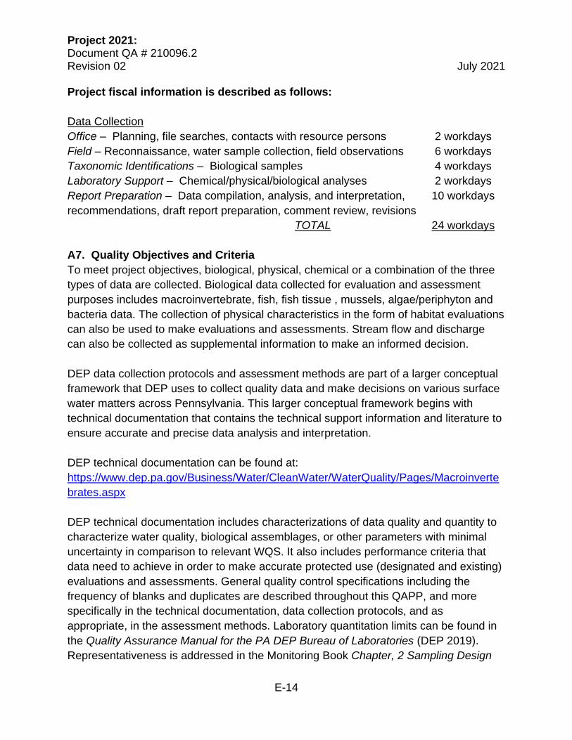
Project 2021: Document QA # 210096.2 Revision 02 July 2021
E-14
Project fiscal information is described as follows:
Data Collection
Office – Planning, file searches, contacts with resource persons
2 workdays
Field – Reconnaissance, water sample collection, field observations 6 workdays
Taxonomic Identifications – Biological samples 4 workdays
Laboratory Support – Chemical/physical/biological analyses 2 workdays
Report Preparation – Data compilation, analysis, and interpretation,
recommendations, draft report preparation, comment review, revisions
10 workdays
TOTAL 24 workdays
A7. Quality Objectives and Criteria
To meet project objectives, biological, physical, chemical or a combination of the three
types of data are collected. Biological data collected for evaluation and assessment
purposes includes macroinvertebrate, fish, fish tissue , mussels, algae/periphyton and
bacteria data. The collection of physical characteristics in the form of habitat evaluations
can also be used to make evaluations and assessments. Stream flow and discharge
can also be collected as supplemental information to make an informed decision.
DEP data collection protocols and assessment methods are part of a larger conceptual
framework that DEP uses to collect quality data and make decisions on various surface
water matters across Pennsylvania. This larger conceptual framework begins with
technical documentation that contains the technical support information and literature to
ensure accurate and precise data analysis and interpretation.
DEP technical documentation can be found at:
https://www.dep.pa.gov/Business/Water/CleanWater/WaterQuality/Pages/Macroinverte
brates.aspx
DEP technical documentation includes characterizations of data quality and quantity to
characterize water quality, biological assemblages, or other parameters with minimal
uncertainty in comparison to relevant WQS. It also includes performance criteria that
data need to achieve in order to make accurate protected use (designated and existing)
evaluations and assessments. General quality control specifications including the
frequency of blanks and duplicates are described throughout this QAPP, and more
specifically in the technical documentation, data collection protocols, and as
appropriate, in the assessment methods. Laboratory quantitation limits can be found in
the Quality Assurance Manual for the PA DEP Bureau of Laboratories (DEP 2019).
Representativeness is addressed in the Monitoring Book Chapter, 2 Sampling Design

Project 2021: Document QA # 210096.2 Revision 02 July 2021
E-15
and Planning (Lookenbill 2020) and more specifically, within the appropriate data
collection protocols. Precision estimates for biological methods are described in detail in
respective technical documentation as is detailed development efforts that resulted in
these precision statistics.
Use (designated and existing) evaluations and use assessments based on
physicochemical data can be collected via discrete chemistry data collection or
continuous instream monitoring (CIM). Sediment samples, passive samplers and in-situ
discrete field observations may also be collected to provide additional insight into water
quality conditions. To ensure discrete chemistry samples are collected with the analytes
of interest, the DEP provides specific Standard Analysis Codes (SAC) which collectors
are required to use for chemical and biological samples submitted to DEP Bureau of
Labs. Any deviation from the SACs provided should be approved by the DEP Project
Manager. In addition, at the discretion of WQD, analytes can be added or removed at
any time. Addition of analytes may be warranted if limiting conditions are met and an
analysis to include a more robust suite is needed (e.g. the addition of dissolved
constituents, the addition of phaeophytin, etc.).
All data collection will be conducted according to DEP reviewed and approved
monitoring protocols. Protocols specific to these projects are found in Water Quality
Monitoring Protocols for Streams and Rivers (Monitoring Book, Lookenbill and Whiteash
2021), DEP’s Lake Assessment Protocol (Lathrop 2015), DEP’s Chlorophyl-a Sampling
Method in Lakes, Ponds, and Reservoirs (Lathrop 2017) and DEP’s Evaluations of
Phosphorus Discharges to Lakes, Ponds, and Impoundments (DEP 2013a).
Quality control efforts specific to these projects will be further described in Section B of
this QAPP and are briefly described herein. All biological and chemical samples shall
undergo the collection of replicates every 20 samples or once per project. Chemical
samples shall also undergo collection of blanks every 20 samples or once per project. If
sampling equipment is noted as malfunctioning at time of collection, it should be noted
in a field notebook or on a field data sheet and the DEP project manager should be
informed. If corrective action can be made in the field, the collector should take the
necessary actions to problem-solve. If a solution cannot be determined in the field, field
work should cease and be rescheduled until the problem is solved. For instance, if the
chemistry filtering equipment breaks or malfunctions, no samples should be taken and
sampling should be rescheduled; or for instance, if a field meter probe gives erroneous
readings the collector should determine if calibration drifted, requiring equipment
recalibration. Further information regarding probe accuracies warranting recalibration
are outlined in Hoger et al. 2017; criteria are summarized in Table 2. Additionally,

Project 2021: Document QA # 210096.2 Revision 02 July 2021
E-16
assurance of sample integrity is required of any collector. Steps should be taken to
avoid contamination of the sample by an outside source; if at any point during sample
processing contamination is observed, the sample must be properly disposed of and
recollected.
Table 2. Calibration criteria for field measured parameters
Field Parameter Calibration Criteria Warranting Equipment Recalibration
Temperature ± 0.2°C
Specific Conductance ± 5 μS/cm or 3%, whichever is
greater
pH ± 0.2 units
Dissolved Oxygen ± 0.3 mg/L
Turbidity ± 0.5 FNU or ± 5%, whichever is
greater
Furthermore, chemical samples go through an accuracy check by requiring spikes,
duplicate and blank analyses. Accuracy is determined by routine laboratory protocol
described in the Quality Assurance Manual for the PA Department of Environmental
Protection Bureau of Laboratories (DEP 2019) and in test specific Standard Operating
Procedures (SOP). The BOL Quality Assurance Manual is provided in Supplemental
Document # 1 and SOPs can be made available upon request.
Sensors used for field chemistry measures, whether discrete readings or continuous
deployments, are selected that have a range that will cover expected environmental
conditions for the project, with sufficient precision and accuracy. For all continuous
deployments and preferably for all discrete readings as well, optical DO sensors will be
used as they have higher degrees of accuracy and hold calibration much better. Further
details on sensor selection can be found in the Sensor Selection section of Hoger et al.
(2017).
A8. Training and Certifications
All data collectors need to be properly trained prior to involvement in data collections
and data management. Ensuring data collectors are properly trained is the responsibility
of the quality assurance manager and/or project manager. Training involves reading
DEP’s protocols and training by DEP senior staff or program specialists. New collectors
will go through a training period at the discretion of the supervising biologist or water
program specialist. DEP staff who perform macroinvertebrate identification are required
to maintain Society for Freshwater Science Ephemeroptera Plecoptera Trichoptera
(EPT) East Genus-Level Certification. Any new biologist will endure quality assurance

Project 2021: Document QA # 210096.2 Revision 02 July 2021
E-17
audits to ensure adherence to protocols. In addition, an auditor shall accompany an
individual collector on at least one survey at a minimum of every five years. The auditor
shall also randomly select any documentation to verify that data is accurate and
complete, and that appropriate analytical techniques are used. The auditor will maintain
records for each individual to include: (1) the date of the audit; (2) a list of protocols for
which the individual was evaluated; (3) any deficiencies noted; and
(4) recommendations offered and corrective actions taken. Training and quality
assurance records will be maintained in DEP electronic training record files.
All taxonomy should be completed by specialized and/or certified taxonomists.
Taxonomists may be in-house DEP biologist or be contracted out to recognized
laboratories. Taxonomists should use the most updated resources to aid in taxonomic
identifications. Furthermore, taxonomists should undergo QA/QC checks on 10% of
samples identified by a certified taxonomist.
The laboratories used for sample analyses must be accredited. The DEP Bureau of
Laboratories (BOL) will primarily be used for laboratory analyses. BOL is accredited by
the National Environmental Laboratory Accreditation Program (NELAP) through the
New Jersey and Pennsylvania Department of Environmental Protection (DEP)
accreditation bodies. If at any time during the project a new laboratory needs selected to
process samples, the laboratory needs to be a DEP contracted lab and accredited by
bodies within the NELAP.
A9. Documents and Records
Historic and current QAPP documents are housed in WQD’s shared electronic files that
are backed up according to DEP’s information technology security protocols.
Documents are to be maintained and retained permanently. This QAPP will be internally
reviewed annually and will be submitted to EPA for reapproval if material changes are
made. Any amendments or updates to the document should be labeled as such. Every
5 years and as needed, this QAPP should be updated, revised and approved as a new
document that designates signatures and the date of final approval. This will aid in
keeping track of 5-year QAPP resubmission as required by the EPA. Updated versions
will be shared with those on the distribution list given above. Table 3 characterizes
changes to this controlled, QAPP over time. The most recent version is presented in the
top row of the table. Quality assurance data can be obtained through a request to the
DEP Quality Assurance Officer.
Table 3. QAPP document control
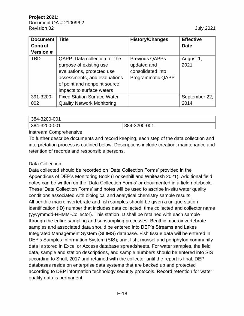
Project 2021: Document QA # 210096.2 Revision 02 July 2021
E-18
Document
Control
Version #
Title History/Changes Effective
Date
TBD QAPP: Data collection for the
purpose of existing use
evaluations, protected use
assessments, and evaluations
of point and nonpoint source
impacts to surface waters
Previous QAPPs
updated and
consolidated into
Programmatic QAPP
August 1,
2021
391-3200-
002
Fixed Station Surface Water
Quality Network Monitoring
September 22,
2014
384-3200-001
384-3200-001 384-3200-001
Instream Comprehensive
To further describe documents and record keeping, each step of the data collection and
interpretation process is outlined below. Descriptions include creation, maintenance and
retention of records and responsible persons.
Data Collection
Data collected should be recorded on ‘Data Collection Forms’ provided in the
Appendices of DEP’s Monitoring Book (Lookenbill and Whiteash 2021). Additional field
notes can be written on the ‘Data Collection Forms’ or documented in a field notebook.
These ‘Data Collection Forms’ and notes will be used to ascribe in-situ water quality
conditions associated with biological and analytical chemistry sample results.
All benthic macroinvertebrate and fish samples should be given a unique station
identification (ID) number that includes data collected, time collected and collector name
(yyyymmdd-HHMM-Collector). This station ID shall be retained with each sample
through the entire sampling and subsampling processes. Benthic macroinvertebrate
samples and associated data should be entered into DEP’s Streams and Lakes
Integrated Management System (SLIMS) database. Fish tissue data will be entered in
DEP’s Samples Information System (SIS); and, fish, mussel and periphyton community
data is stored in Excel or Access database spreadsheets. For water samples, the field
data, sample and station descriptions, and sample numbers should be entered into SIS
according to Shull, 2017 and retained with the collector until the report is final. DEP
databases reside on enterprise data systems that are backed up and protected
according to DEP information technology security protocols. Record retention for water
quality data is permanent.

Project 2021: Document QA # 210096.2 Revision 02 July 2021
E-19
At the end of each sampling season, all ‘Data Collection Forms’ should be filed and
retained for future reference. A filing system will be maintained by each collector. It is
recommended that the collector keep hard copies of completed ‘Data Collection Forms’
as well as maintain specific folders on their computer as an electronic backup labeled
for each data type as a repository for all ‘Data Collection Forms’ (i.e. Macroinvertebrate
Data, Fish Data, CIM Data, WQN Data, etc.). It is further recommended to help facilitate
order that all ‘Data Collection Forms’ be arranged by date and scanned by year to be
placed in a folder that is labeled as ‘YYYY Fish – ‘Field Data Sheets.’ Paper copies can
be archived at the discretion of the field collector and field notebooks should be retained
by the collector.
Calibration logs and calibration equipment checks should be maintained similar to ‘Data
Collection Forms’. It is recommended that calibration logs be kept with each unique
piece of equipment. At the end of the sampling season, the calibration logs shall be
scanned into an electronic file and paper copies archived. Archives are stored in DEP
electronic files that are backed up and protected according to DEP information
technology security protocols. Paper copies can be archived at the discretion of the
equipment manager.
Data Processing
Biological samples that have been processed and identified will be enumerated on
bench sheets found in Appendices of DEP’s Monitoring Book (Lookenbill and Whiteash
2021) Benthic macroinvertebrate taxonomic data will be entered into DEP’s SLIMS
database. Fish, mussel and periphyton community data will be entered into Excel and
Access databases.
All chemical and physicochemical data with the exception of continuous instream
monitoring data are entered into DEP’s SIS database (Shull 2017b). Date, time, location
and the unique sample identifier will be stored in the SIS database. This database will
be used by the BOL to import their analytical results to match field information; BOL will
do this according to the directive found in BOL’s Quality Assurance Manual (DEP 2019).
Each collecting biologist is responsible for following-up on the status of samples
submitted. This includes ensuring samples are analyzed, cross checking samples with
replicate and blank samples and exporting the data from SIS for interpretation.
Continuous instream monitoring data will be housed in a database capable of handling
large continuous files. DEP uses AQUARIUS database and software to store, manage,
and visualize continuous water quality data. AQUARIUS allows for documenting and

Project 2021: Document QA # 210096.2 Revision 02 July 2021
E-20
performing corrections of the data according to Continuous Physicochemical Data
Collection Protocol (Hoger et al. 2017).
In preparation for data interpretation and report writing, formatted templates containing
formulas and report requirements are provided to collectors. These templates or
another suitable data organization matrix may be used. If the latter option is used by the
biologist, they must ensure all calculations and visual displays maintain integrity. This
option requires additional quality assurance by a second (or third party if needed) and
the Project Manager before contents can be used to generate reports.
Reports
Data will be reported in the form of tables, figures, maps and/or charts. If warranted, a
full report will be written. Scenarios in which a full report is needed include but is not
limited to redesignation recommendations, integrated report delistings and phosphorus
control recommendations. Redesignation report guidance can be found in DEP’s Water
Quality Antidegradation Implementation Guidance, Document Number 391-0300-002
(DEP 2003). Delisting requirements can be found in DEP’s Assessment Determination
and Delisting Methods (Pulket and Shull 2021). Phosphorus control reports will follow a
general format as described in DEP’s Evaluations of Phosphorus Discharges to Lakes,
Ponds, and Impoundments (DEP 2013a). Continuous instream monitoring reports are
posted on the DEP website at:
https://www.dep.pa.gov/Business/Water/CleanWater/WaterQuality/Pages/CIMReports.a
spx.
Reports are not limited to those items described in the guidance and methods
documents, some projects provide for special cases that require additional analyses
and discussions; these additions can be included at the discretion of the reporting
biologist.
Reports should go through a review process by a second party to address any grammar
or reporting errors/discrepancies. Corrective action should be taken by the report writer
and reviewer; if no agreement can be made, the reviewing party should reach out to the
DEP Project Manager for an additional review. Once finalized, a copy should be dated
and filed appropriately. For final filing the document should be converted from a .docx
file to a .pdf file.
Final Filing
Reports which have been reviewed and finalized should be saved in DEP’s electronic
stream files. Stream files are organized by a unique 5-digit code, which is associated

Project 2021: Document QA # 210096.2 Revision 02 July 2021
E-21
with DEP’s historic stream codes associated with the NHD Flowline flowing through the
waterbody, and the stream, river or lake name. Reports shall remain in the stream files
permanently.
Management of QA Record
QA records including training records, quality assurance audits and corrective actions
will be maintained in DEP electronic training record files permanently.

Project 2021: Document QA # 210096.2 Revision 02 July 2021
E-22
SECTION B: DATA GENERATION AND ACQUISITION
B1. Experimental Design
Project design will be applied to surface waters statewide. The type of experimental
project design used is based off data of interest. Collectors should use DEP’s
Monitoring Book (Lookenbill and Whiteash 2021) to develop a sampling plan conducive
to each project’s objective. The sampling plan will be objective specific but typically
include a combination of:
• Chemical Data Collection
o In-Situ Field Meter and Transect Data Collection
o Discrete Water Chemistry
o Continuous Water Chemistry
• Physical Data Collection
o Habitat Evaluation
o Water Flow Data Collection
• Biological Data Collection
o Benthic Macroinvertebrates
o Fish
o Bacteria
Site location selection is fluid from year to year based on regional and state priorities. In
addition, environmental factors play a role in selecting sites year to year. For this
reason, site specific maps are not provided in this QAPP. Site locations are documented
as locational attributes in the SLIMS and SIS applications.
Biological samples are collected across a transect or throughout a large portion of the
waterbody to ensure inclusion of all available habitat. In flowing waterbodies water
samples are collected at mid-channel, mid-depth unless stream width, hydrology,
discharge locations or volumes, or observed biological conditions indicate stratification
of flow than integrated type sampling is used. Lake water samples are collected with the
use of a Van Dorn or Kemmerer sampler at a depth of one meter below the surface and
one meter above the lake’s bottom. Parameters frequently analyzed are listed in
Table 3. All water chemistry samples are cooled to less than or equal to 6ºC without
freezing and shipped to the laboratory. Additional parameters may be required based on
the specific nature of the waterbody survey; details regarding field collection
requirements and laboratory test methods can be obtained upon request.

Project 2021: Document QA # 210096.2 Revision 02 July 2021
E-23
Table 4. Analyte Tests (commonly used Standard Analysis Code 087)
Test Codes Test Description Test Method
410 ALKALINITY AS CaCO3 @ pH 4.5 SM 2320B 01106H ALUMINUM, DISSOLVED (WATER & WASTE) BY ICPMS EPA 200.8 01105H ALUMINUM, TOTAL (WATER & WASTE) ICPMS EPA 200.8 00608A AMMONIA DISSOLVED AS NITROGEN EPA 350.1 00610A AMMONIA TOTAL AS NITROGEN EPA 350.1 01007A BARIUM, TOTAL (WATER & WASTE) BY ICP EPA 200.7 01022K BORON, TOTAL (WATER & WASTE) BY ICP EPA 200.7 01025H CADMIUM, DISSOLVED (WATER & WASTE) BY ICPMS EPA 200.8 00916A CALCIUM, TOTAL (WATER & WASTE) BY ICP EPA 200.7 01040H COPPER, DISSOLVED (WATER & WASTE) BY ICPMS EPA 200.8 01042H COPPER, TOTAL (WATER & WASTE) BY ICPMS EPA 200.8 00631A DISSOLVE NITRATE & NITRITE NITROGEN EPA 353.2 00671A DISSOLVE ORTHO PHOSPHORUS EPA 365.1 00602A DISSOLVED NITROGEN AS N SM 4500-NC 00666A DISSOLVED PHOSPHORUS AS P EPA 365.1
900 HARDNESS, TOTAL (CALCULATED) SM 2340 B 01046A IRON, DISSOLVED (WATER & WASTE) BY ICP EPA 200.7 01045A IRON, TOTAL (WATER & WASTE) BY ICP EPA 200.7 01049H LEAD, DISSOLVED (WATER & WASTE) BY ICPMS EPA 200.8 01051H LEAD, TOTAL (WATER & WASTE) BY ICPMS EPA 200.8 01130A LITHIUM, DISSOLVED (WATER &WASTE) BY ICP EPA 200.7 01132A LITHIUM, TOTAL (WATER & WASTE) BY ICP EPA 200.7 99020 LOW BROMIDE BY IC EPA 300.1 B
00927A MAGNESIUM, TOTAL (WATER & WASTE) BY ICP EPA 200.7 01056A MANGANESE, DISSOLVED (WATER & WASTE) BY ICP EPA 200.7 01055A MANGANESE, TOTAL (WATER & WASTE) BY ICP EPA 200.7 01065A NICKEL, DISSOLVED (WATER & WASTE) BY ICP EPA 200.7 01067A NICKEL, TOTAL (WATER & WASTE) BY ICP EPA 200.7 82550 OSMOTIC PRESSURE, MOS/KG BOL 3003 403 pH, LAB (ELECTROMETRIC) SM 4500-H+ B
00937A POTASSIUM, TOTAL (WATER & WASTE) BY ICP EPA 200.7 01147H SELENIUM, TOTAL (WATER & WASTE) BY ICPMS EPA 200.8 00929A SODIUM, TOTAL (WATER & WASTE) BY ICP EPA 200.7
95 SPECIFIC CONDUCTIVITY @ 25.0 C SM 2510B 01082A STRONTIUM, TOTAL (WATER & WASTE) BY ICP EPA 200.7 00403T TEMPERATURE AT WHICH PH IS MEASURED SM 4500-H+ B
940 TOTAL CHLORIDE-ION CHROMATOGRAPH EPA 300.0 70300U TOTAL DISSOLVED SOLIDS @ 180C BY USGS-I-1750 USGS I-1750 00630A TOTAL NITRATE & NITRITE NITROGEN EPA 353.2 00600A TOTAL NITROGEN AS N SM 4500-NC
680 TOTAL ORGANIC CARBON SM 5310 C 70507A TOTAL ORTHO PHOSPHORUS AS P EPA 365.1 00665A TOTAL PHOSPHORUS AS P EPA 365.1
945 TOTAL SULFATE-ION CHROMATOGRAPH EPA 300.0 530 TOTAL SUSPENDED SOLIDS USGS I-3765
01090A ZINC, DISSOLVED (WATER & WASTE) BY ICP EPA 200.7 01092A ZINC, TOTAL (WATER & WASTE) BY ICP EPA 200.7
Project 2021: Document QA # 210096.2 Revision 02 July 2021
E-24
B2. Sampling Protocols
Biological data collection will be conducted according to protocols described in Chapter
3 of DEP’s Monitoring Book (Lookenbill and Whiteash 2021). Depending on waterbody
classification, benthic macroinvertebrate data collection shall follow one of the four
stream macroinvertebrate data collection protocols (riffle-run, limestone, multihabitat or
semi-wadeable large river streams). Regardless of macroinvertebrate protocols used,
all samples will be processed according to Macroinvertebrate Laboratory Subsampling
and Identification Protocol (Brickner 2020). Fish tissue will be collected according to
DEP’s Fish Tissue Data Collection Protocol (Wertz 2021). Bacteriological data will be
collected according to DEP’s Bacteriological Data Collection Protocol (Miller 2021).
These three types of biological data will be used for the purpose of conducting use
evaluations and use assessments.
Other biological data that may be collected for purposes of describing water quality
conditions and supporting evaluation and assessment decisions are briefly described
herein. Fish community data will be collected according to DEP’s Fish Data Collection
Protocol (Wertz 2021) and mussel community data will be collected according to DEP’s
Mussel Data Collection Protocol (Spear et al. 2017). Periphyton and chlorophyll-a
samples from streams and rivers will be collected according to DEP’s Periphyton Data
Collection Protocol (Butt 2017). Plankton, macrophyte and chlorophyll-a samples from
lakes will be collected according to DEP’s Quantitative Plankton Sampling Method for
Lakes (DEP 2015b), Aquatic Macrophyte Coverage Procedures for Lake Assessments
(DEP 2015a), and Chlorophyll-a Sampling Method for Lakes, Ponds and Reservoirs
(Lathrop 2017) respectively.
Physical data collection in streams and rivers can include stream habitat assessments
and water flow data collection. Descriptions of protocols to collect physical data are
found in Chapter 5 of DEP’s Monitoring Book (Lookenbill and Whiteash 2021). Physical
habitat assessment data collection will be completed when employing all biological data
collection protocols.
Water samples will be collected according to Shull, 2017; modifications may be made
depending on waterbody type and size. All sampling equipment should be rinsed with
surface water three times prior to collection and/or transfer. Most water samples are
collected into HDPE plastic bottles with the exception of organic chemistry samples
which are to be collected in amber glass bottleware. Water samples containing water for
metal analyses should be fixed with HNO3 to a pH of <2. Water samples containing
water for ammonia, phosphorus and organic carbon analyses should be fixed with
H2SO4 to a pH of <2. Samples are immediately placed on ice until submission to BOL.
Project 2021: Document QA # 210096.2 Revision 02 July 2021
E-25
Samples should be submitted the day of sampling or the morning after the sampling
event to ensure 48-hour holding times are not exceeded. Analytes with 48-hour holding
times are nitrate, phosphorus and turbidity. Alkalinity has a holding time of 14 days,
specific conductivity, bromide, sulfate and total nitrogen have 28-day holding times; all
other parameters have a holding time of six months or longer. After each use, water
sampling equipment should be thoroughly rinsed with deionized water and cleaned
according to protocols in DEP’s Monitoring Book (Lookenbill and Whiteash 2021). All
other chemistry collections, such as sediment sampling and passive sampler analysis
should follow methodologies found in Chapter 4 of DEP’s Monitoring Book (Lookenbill
and Whiteash 2021).
With any data collection protocol used during a sampling project, it is recommended that
in-situ field meter water quality readings be taken. Measurements could be a single
discrete reading to describe current water quality conditions, transect readings across
the width of the stream or river to verify homogeneity of the water system, or profile
depth reading to determine stratification of larger bodies of water such as
impoundments and lakes. To collect in-situ readings, a calibrated field meter is used. At
a minimum, temperature, pH, dissolved oxygen (DO) and specific conductance
measurements are recorded; other parameters are optional. The field meter should be
calibrated according to procedures outlined in Hoger, 2020 and guidelines referenced
from the equipment’s operation manual. A summary of calibration recommendations is
provided in Table 5. DEP does not use any one specific field meter, to that end specific
guidance on calibration operating procedures cannot be made. At the end of the field
day, calibration checks are recommended as a check against standards to ensure
readings are within the criteria found in Table 2. The collector should also perform
calibration checks anytime field parameters do not make sense for expected conditions.
At the end of the day, the collector should ensure the field meter is free from debris prior
to storage. To clean the field meter equipment, run clean tap water over the probes to
rinse large particles; if a more thorough cleaning is required use a small amount of soap
and a soft bristled brush on the probes. For storage, a small amount of tap water or pH
4 standard should be placed in the storage cup; probes should not be submerged for
overnight or long-term storage.
In addition to discrete physicochemical data, monitoring objectives may require the
collection of continuous physicochemical data according to Hoger et al., 2017. Discrete
physicochemical data typically includes at least four parameters: water temperature,
specific conductance, pH and dissolved oxygen. Continuous water quality monitors
should be calibrated according to procedures outlined in Hoger, 2020 and guidelines
referenced from the equipment’s operation manual. A summary of calibration

Project 2021: Document QA # 210096.2 Revision 02 July 2021
E-26
recommendations is provided in Table 5. Calibration follows guidelines referenced from
the equipment’s operation manual. DEP does not use any one specific continuous water
quality monitor, to that end specific guidance on calibration operating procedures cannot
be made. Field meters are used during servicing of a continuous water quality monitor
(1) as a general check of reasonableness of monitor readings, (2) as an independent
check of environmental changes during the service interval, and (3) to make cross-
section surveys or vertical profiles in order to verify the representativeness of the
location of the sonde in the aquatic environment. Data collected by the field meter
should not be used to calibrate the instream monitor. However, some instream monitors
cannot be calibrated, in which case the calibrated field meter must be used in the
calibration correction of monitor records. In addition, DEP may use a calibrated field
meter measurement for undocumented data error corrections (a potential result from the
DEP deployment method, discussed in detail Hoger et al. 2017). Independent field
measurements must be made before, during, and after servicing the monitor in order to
document environmental changes during the service. Side-by-side measurements
between the field meter and the monitor are made by placing the calibrated field meter
as close to the monitor sensors as possible. The field meter should refresh data on the
display at 10 second intervals, or more frequently, to ensure the most accurate data are
recorded during measurements.
B3. Sample Handling and Custody
For biological samples, macroinvertebrates and fishes, samples can be processed for
enumeration by the collector or by other designated staff. Sample containers are
labeled with date, time and user (yyyymm-hhmm-user); stream name; location and
number of containers per sample. A database and archive system shall be maintained
for all samples in which identifications have been completed. Each Regional Office shall
maintain their own archiving system; Central Office will maintain their own archiving
system which can be used by Regional Offices if requested.
Sample handling and chain of custody for chemistry samples should be followed
according to the description provided in Shull 2017a. Steps are summarized herein. The
field collector will use a unique identifier, a seven-digit number that contains a four-digit
collector number and a three-digit sample number. The collector is responsible for
recording locational information and the date and time of the sample. The above
information should be recorded on a sample submission form which is submitted to BOL
at time of relinquishment. Samples can be submitted one of two ways. The collector can
hand deliver samples to BOL’s sample receiving. Under this option, the collector
unloads cooler contents and places samples in designated refrigerators and/or freezers;
the sample submission form remains with the samples. The collector also has the option

Project 2021: Document QA # 210096.2 Revision 02 July 2021
E-27
of using a courier service contracted by the DEP. Under this option the collector will
drop coolers at a designated location, located throughout the state, for courier pick-up
and delivery to BOL. The collector should insert their sample submission form into a
plastic sealable bag or whirl-pack (preferably double bagged) and tape it to the inside lid
of the cooler. It is recommended that collectors either scan or take a picture of sample
submission forms for their records. Upon receipt by BOL staff, the temperature of each
sample bottle is measured using a calibrated infrared thermometer to ensure proper
shipping, handling and holding requirements. If samples are found to be above 6°C,
BOL will flag the sample and contact the collector. The flag will remain with the sample
and the reporting biologist shall qualify the data.
Continuous physicochemical data, including operational and maintenance records, are
recorded on portable electronic devices and transferred to AQUARIUS.
Table 5. Summary of Calibration Recommendations
Parameter Calibration Notes
Temperature Check against NIST certified equipment
pH Three-point calibration (4,7,10) Two-point calibration acceptable if conditions are known
Dissolved Oxygen (DO)
100% water-saturated air: • Water in bottom of calibration cup (do not submerge sensor) • Calibration cup on loosely to prevent pressure buildup • Run a wipe cycle, if possible, to remove water droplets on sensor
• Calibration onsite to avoid influence of barometric pressure differences. • Check throughout the day. • Allow plenty of time in cold weather.
Specific Conductance
One-point calibration with checks • Calibrate at a high value (1000 μS/cm) • Check at a low value (100 μS/cm) • Rinse with Deionized (DI) water and check in air (should be 0 μS/cm)
If values above 1000 μS/cm are expected, also check in a higher standard.
Project 2021: Document QA # 210096.2 Revision 02 July 2021
E-28
B4. Analytical Methods
Table 3 above references analytical methods used in analyses of discrete chemistry
samples. The BOL is responsible for setting SOPs for analytical analyses. BOL SOPs
are currently not housed with the WQD but can be obtained upon request. If at any time
during lab analyses sample integrity is compromised, the chemist is responsible for
documenting the flag in the final BOL results report. Occasionally, holding times are
exceeded or samples are incorrectly preserved; if so, BOL notifies the collector
immediately. The collector must then respond to BOL within 10 days to request or
decline results. The collector’s supervisor and any other interested parties must be
copied on their response. If analytes used to make assessment decisions are impacted
by either lab equipment failure or collection error, the sample should be recollected.
While not ideal, the collector may accept the data for the analytes; though, results
should not be used to make assessment determinations.
Other data including biological, physical, field meter and continuous water quality that is
not submitted to BOL are analyzed according to specific data collection protocols and
assessment methods.
B5. Quality Control
Data Collection Audits
All data collected in the field need to be recorded for verification purposes in the
appropriate field data sheets or field notebooks. Field meters used for in-situ water
quality readings should be calibrated according to manufacturer’s instructions at the
start of each field outing. A calibration log should be kept with the field meter and
archived in-house for reference at the end of each sampling year. Calibration checks
should be performed throughout the day if multiple samples will be collected. Results of
calibration and preventive maintenance recommended by the manufacturer must be
recorded in an equipment logbook maintained for each piece of equipment. Dates of
equipment use, calibration results and operator maintenance activities are recorded.
Duplicates for water samples for chemical analysis are collected at least once on each
survey or once every 20 samples. These samples ensure data completeness and
quality assurance of lab analysis techniques. The field investigator will review sample
results and note if target parameters are detected in the blank and flag samples
accordingly.
Duplicate benthic macroinvertebrate samples should be collected within the same reach
as the initial sampling. Habitat, which was sampled previously should not be resampled,
but rather other similar and suitable habitat should be sampled. For semi-wadable

Project 2021: Document QA # 210096.2 Revision 02 July 2021
E-29
benthic macroinvertebrate collections of duplicates should be collected as a site
duplicate; this means if it was determined that there were three water quality zones and
three samples across the width of the river need be collected, the replicate should also
contain three samples each in the same reach as the respective water quality zones. In
addition, it is recommended to collect intra-site and inter-site replicates to discriminate
against variation within and between sites in the same stream reach. Fish, mussel, and
plankton samples should undergo, a similar replicate collection schedule of benthic
macroinvertebrate samples. Periphyton sampling QC is detailed more extensively in
Periphyton Data Collection Protocol (Butt 2017).
Quality control of CIM data incorporates multiple field visits throughout the sampling
period. It is recommended that data be downloaded, equipment be cleaned and
checked against calibration standards to describe the accuracy of the continuous
measurements every three to six weeks. QC documentation collected during field visits
will be used to aid in data management prior to making data final. Methods to perform
field visits and correct data are further detailed in DEP’s Continuous Physicochemical
Data Collection Protocol (Hoger et al. 2017).
Results QC
The protocol for validation of chemical data is found in the Quality Assurance Manual for
the PA Department of Environmental Protection Bureau of Laboratories (DEP 2019).
Each collector is also responsible for checking duplicates and field blanks against
samples used for final reporting and calculations. If values are erroneously off from
duplicate and field blanks, those data must by flagged and further investigated. If a
sample is suspected those data should be removed from the final reporting data set.
The field investigator will review sample results to determine if the original sample and
replicate(s) are less than 10% comparatively. For blanks the collector should note if
target parameters are detected in any blank samples. If discrepancies exist, the
collector should flag samples accordingly and leave out of any data interpretation
analyses.
Continuous data that do not meet the thresholds given in the table Maximum Allowable
Limits for Reporting Data (Hoger et al. 2017) are removed from the dataset and will not
be used for assessment or other regulatory decisions. Continuous data that are graded
“Unverified” due to a lack of quality control checks, will be reported but not used for
assessments or regulatory decisions.
Project 2021: Document QA # 210096.2 Revision 02 July 2021
E-30
Protocols for biological data validation are found in DEP’s Monitoring Book, Chapter 3
(Lookenbill and Whiteash 2021). Biologist should submit 10% of each type of biological
sample to the Project Manager for taxonomic verification and QA. To accomplish the
10% quality assurance of all samples identified, taxonomists should submit 10% of the
samples they have identified in a calendar year. Documentation of taxonomic QC
results will be stored in WQD, Central Office and samples which were quality assured
will be indicated as so in the SLIMS database. Similarly, fish identifications will be
documented in the associated Excel and Access databases. Furthermore, all data
entries should undergo verification by checking one’s work. During results retrieval and
data interpretation of results, biological data should again be verified against
enumeration forms and database entries.
Subsampling procedures for benthic macroinvertebrate samples and the sequential
identifications will undergo QA/QC. Biologists who are involved with macroinvertebrate
subsampling will need to be properly trained with documentation that tracks sorting error
as is described in the QAPP, Appendix A. Macroinvertebrate identifications will undergo
QC for each biologist involved in taxonomy. The macroinvertebrate identification QC will
be documented according to details provided in Appendix A. Fish identification QC is
also detailed in Appendix A.
The protocol for validation of chemical data is found in the Quality Assurance Manual for
the PA Department of Environmental Protection Bureau of Laboratories (DEP 2019).
Each collector is also responsible for checking duplicates and field blanks against
samples used for final reporting and calculations. If values are erroneously off from
duplicate and field blanks, those data must by flagged and further investigated. If a
sample is suspected those data should be removed from the final reporting data set.
B6. Equipment Maintenance and Inspection
Collectors are expected to care for their own equipment. Equipment should be
inspected prior to each scheduled field outing. If the equipment malfunctions the
collector should trouble shoot or seek assistance from the program specialist. Parts
should be replaced, or back-up equipment should be used.
Field meters, continuous water quality monitoring and flow meters should be inspected
for malfunctions during each use and/or during routine maintenance visits. Probes
should be inspected for damage such as cracks and scrapes. Calibration logs aid in
tracking a probe’s life. Temperature probes are checked against another piece of
equipment. This should be done periodically to ensure proper readings. DO probe
toppers should be replaced every few years as general maintenance; in addition, zero-

Project 2021: Document QA # 210096.2 Revision 02 July 2021
E-31
DO checks should be done periodically to determine how well the probe responds to
changing conditions. To make a zero-DO solution dissolve 0.5g of sodium sulfite and 6-
10 crystals of cobalt chloride in 500mL of water, place the probe in solution and
document response time for DO to reach 0.3mg/L. If the response is slow and readings
do not stabilize within 2-3 minutes the probe may need to be replaced. Probes that
measure pH have a short life span and should be replaced at least every year or sooner
if warranted. DEP records pH millivolts in calibration logs to determine the response life
of the pH probe. If pH millivolts drift outside the ranges indicated below, the probe
should be replaced. All other parameters follow specifications found in the equipment’s
operational manual.
• Buffer 7: readings should be -50 to 50 mV, 0 mV is ideal
• Buffer 4: readings should be +165 to +180 mV from the buffer 7 reading
• Buffer 10: readings should be -165 to -180 mV from the buffer 7 reading.
B7. Instrument Calibration
Field meters used to collect in-situ discrete readings, transects and vertical profiles
need calibrated at the start of each sampling day. Continuous water quality monitors are
calibrated and maintained prior to deployment and during routine maintenance visits.
Flow meters are calibrated by the manufacturer every three years. Calibration logs are
kept separate with each unique piece of equipment. See Table 5 for calibration
recommendations. Calibration logs should contain ‘Before’ calibration and ‘After’
calibration readings. Collectors can find calibration log forms in Appendix B of DEP’s
Monitoring Book (Lookenbill and Whiteash). It is recommended that collectors perform
calibration checks on field meters at the end of day that included collecting transect
and/or vertical profile data. Performing end of day checks aid in verifying data are
accurate according to criteria. These checks can be logged in the same logbook using
the same form as the calibration log, where ‘After’ calibration readings are rendered ‘Not
Applicable (NA).’ More detail on field meter use and maintenance can be found in The
Monitoring Book Chapter 4.1, In-Situ Field Meter and Transect Data Collection Protocol,
(Hoger 2020).
B8. Inspection/Acceptance of Supplies and Consumables
All supplies used in data collection should be inspected by the collecting biologist prior
to initial use. Equipment should be checked over at the time of purchase and/or
receiving. Equipment should be returned to the manufacturer if defects are found. In
addition, equipment quality should be inspected prior to and during each use.
Standards used for calibration and sample preservation should be used within
expiration dates and a log of standards used should be maintained. Expired solutions
should be disposed of or recycled properly.

Project 2021: Document QA # 210096.2 Revision 02 July 2021
E-32
B9. Non-Direct Measurements
Non-direct measurements associated with projects are tools to help define watershed
and land use characteristics. These characteristics are provided in the final report. To
obtain land use descriptions, DEP often uses USGS Streamstats or ArcGIS software.
These are tools commonly used in the field of hydrology and are acceptable tools to
obtain watershed and land characteristics.
B10. Data Management
Data management should generally follow that which is described herein and DEP data
collection protocols and assessment methods. Data management starts in the field
through the use of field forms and field notebooks. Data contained in field
documentation are entered or transferred into DEP’s SIS, SLIMS, AQUARIUS, Excel or
Access databases as soon as possible. The SIS database is used to store in-situ
discrete field readings and laboratory results. This database organizes, stores and geo-
references data for multiple end uses within DEP. SIS will generate reports which are
emailed to the collector once all chemistry results have been completed by BOL. The
collector is responsible for tracking and filing these BOL auto-generated reports at their
discretion. The final BOL report is used as documentation that samples have been
marked complete by BOL. SIS will also be used by the reporting biologist to obtain
results for organization and interpretation in a final report. The SLIMS database will
generate IBI metric reports for benthic macroinvertebrate samples. In addition, SLIMS
will assist in documenting use assessment determinations for stream segments and
waterbodies.
Data should further be organized into templated spreadsheets for calculations of
indices, models and Chapter 93 WQS criteria violations. These spreadsheets should be
maintained by the biologist responsible for the data. It is recommended that each lake,
stream, river, or basin have its own working folder on the responsible biologist’s
computer, which is separate from the final “Stream File,” where spreadsheets, tables,
charts and draft reports are created. The information in these files should be organized
into a final report, which is placed in the final “Stream File” folder which was mentioned
in the Final Filling Section of A9 of this QAPP.

Project 2021: Document QA # 210096.2 Revision 02 July 2021
E-33
SECTION C: ASSESSMENT AND OVERSIGHT
C1. Assessments and Response Actions
Assessments to be made include progress reports which will be provided to EPA mid-
cycle and annually as is required. Additionally, performance assessments will be
provided to collectors and report writers at the time of auditing; and project assessments
will be made on an as needed basis.
On-going QC by all participating parties should have a line of communication open
between the field biologist, the data assessor and the DEP Project Manager. If at any
point during data collection, processing, interpreting and reporting an issue arises, the
responsible party should reach out to resources by providing a summary of the issue to
include the problem description and the corrective action needed. The responsible party
needs to document steps taken until the issue has been resolved; documentation can
include retaining email chains or creating a timeline spreadsheet.
C2. Reports to Management
Reports regarding ongoing performance and system audits, data quality evaluations
and significant quality assurance problems will be included in the mid-cycle and annual
grant status report to EPA and will be provided to the DEP’s Quality Systems Program
Manager and the WQD, Monitoring Section.
Based on priorities, the field biologist should complete a final report to the DEP Project
Manager in a timely fashion. It is understood that project priorities may change within
the DEP due to time sensitive deadlines; if an extension or assistance in data
management is needed, biologists can request assistance from WQD, Central Office
staff.

Project 2021: Document QA # 210096.2 Revision 02 July 2021
E-34
SECTION D: DATA VALIDATION AND USABILITY
D1. Data Review, Verification and Validation
The protocol for validation of biological data is found in DEP’s Monitoring Book, Chapter
3 (Lookenbill and Whiteash). The protocol for validation of chemical data is found in the
Bureau of Laboratories, Quality Assurance Manual for the PA Department of
Environmental Protection Bureau of Laboratories (DEP 2019) and BOL’s SOPs. The
protocol for validation of physicochemical data is found in DEP’s Continuous
Physicochemical Data Collection Protocol (Hoger et al. 2017).
A log is maintained of field instrumentation calibrations, performance, and repairs.
Additionally, the biologist responsible for interpreting data will provide a review of results
to include duplicate and blank comparison and best professional judgement
determinations based on knowledge of the site and equipment used. If detected,
erroneous data will be flagged, described and ultimately removed from the final dataset.
Calculations using indices, models and Chapter 93 WQS criteria are checked during
internal review. All continuous data undergoes final review approval according to DEP
data collection protocols.
D2. Verification and Validation of Protocols
Errors are detected through verification of data by the biologist in charge of the survey,
in-house review of reports, and supporting calculations and field audits. When
problems are noted, the responsible individual is notified, provided with the appropriate
protocol and training, and reevaluated before performing the task again. The auditor
shall maintain the records of any corrective actions on additional auditing forms.
With any data management, integrity is of upmost importance to provide quality results
and analyses of the data. It is necessary that collectors cross-validate all field notes with
data entries into DEP’s data management databases. DEP currently maintains a
biological (SLIMS), discrete physicochemical (SIS) and continuous physicochemical
(AQUARIUS) databases. The collector should quality assure their data at the end of the
sampling event and again prior to the development of any reports. In addition, all reports
will need to be reviewed internally and by the DEP Project Manager prior to submittal to
EPA and prior to distribution to the public to ensure accuracy of the reporting. In
addition, all calculations used to generate index scores, models, and water quality
criteria exceedances will be reviewed for integrity prior to distributing for use by
biologists responsible for interpreting the data. If any problems arise with calculations,
formulas, spreadsheets, databases, etc., which are provided to facilitate data
interpretation, the user should note issues and inform the DEP Project Manager of

Project 2021: Document QA # 210096.2 Revision 02 July 2021
E-35
discrepancies and problems, at which time the appropriate corrective action will be
determined, and updated materials will be distributed.
D3. Reconciliation with User Requirements
The data generated from the surveys and reports will be analyzed and reconciled by
cross referencing DEP assessment methods (Shull and Whiteash 2021); assessments
are made in accordance with Section 96.3 and 96.5(b) of DEP’s regulations. The end
product should reconcile with requirements documented in DEP’s Monitoring Book
(Lookenbill and Whiteash 2021), DEP’s Assessment methodology for Streams and
Rivers (Shull and Whiteash 2021), DEP’s Water Quality Antidegradation Implementation
Guidance (DEP 2013b) and DEP’s lake assessment methods which are listed on DEP’s
website
https://www.dep.pa.gov/Business/Water/CleanWater/WaterQuality/Pages/Assessment-
Methodology.aspx.

E-36
LITERATURE CITED
Brickner, M. (editor) 2020. Macroinvertebrate laboratory subsampling and identification
protocol. Chapter 3.6, pages 33–43 in M. J. Lookenbill, and R. Whiteash
(editors). Water quality monitoring protocols for streams and rivers. Pennsylvania
Department of Environmental Protection, Harrisburg, Pennsylvania.
Butt, J. S. 2017. Periphyton data collection protocol. Chapter 3.10, pages 88–142 in M.
J. Lookenbill, and R. Whiteash (editors). Water quality monitoring protocols for
streams and rivers. Pennsylvania Department of Environmental Protection,
Harrisburg, Pennsylvania.
DEP. 2019. Quality assurance manual for the Pennsylvania Department of
Environmental Protection Bureau of Laboratories. Supporting Document #1.
DEP. 2015a. Aquatic macrophyte coverage procedures for lake assessments.
Pennsylvania Department of Environmental Protection, Harrisburg,
Pennsylvania.
DEP. 2015b. Quantitative plankton sampling method for lakes (Modified Standard
Method 1002A). Pennsylvania Department of Environmental Protection,
Harrisburg, Pennsylvania.
DEP. 2013a. Evaluations of phosphorus discharges to lakes, ponds, and
impoundments. Pennsylvania Department of Environmental Protection,
Harrisburg, Pennsylvania.
DEP. 2013b. Water quality antidegradation implementation guidance, Document
Number 391-0300-002. Pennsylvania Department of Environmental Protection,
Harrisburg, Pennsylvania.
Hirsch, R. M., D. L. Moyer, and S. A. Archfield. 2010. Weighted regressions on time,
discharge, and season (WRTDS), with an application to Chesapeake Bay river
inputs. JAWRA 46(5):857–880.
Hoger, M. S. 2020. In-situ field meter and transect data collection protocol. Chapter 4.1,
pages 2–8 in M. J. Lookenbill, and R. Whiteash (editors). Water quality
monitoring protocols for streams and rivers. Pennsylvania Department of
Environmental Protection, Harrisburg, Pennsylvania.
Hoger, M. S., D. R. Shull, and M. J. Lookenbill. 2017. Continuous physicochemical data
collection protocol. Chapter 4.3, pages 25–92 in M. J. Lookenbill, and R.
Whiteash (editors). Water quality monitoring protocols for streams and rivers.
Pennsylvania Department of Environmental Protection, Harrisburg,
Pennsylvania.
Lathrop, B. F. 2017. Chlorophyl a sampling method in lakes, ponds, and reservoirs.
Pennsylvania Department of Environmental Protection, Harrisburg,
Pennsylvania. (Available online at:
E-37
https://www.dep.pa.gov/Business/Water/CleanWater/WaterQuality/Pages/Assess
ment-Methodology.aspx.)
Lathrop, B. F. 2015. Lake assessment protocol. Pennsylvania Department of
Environmental Protection, Harrisburg, Pennsylvania. (Available online at:
https://www.dep.pa.gov/Business/Water/CleanWater/WaterQuality/Pages/Assess
ment-Methodology.aspx.)
Lookenbill, M. J. and R. Whiteash (editors). 2021. Water quality monitoring protocols for
streams and rivers. Pennsylvania Department of Environmental Protection,
Harrisburg, Pennsylvania.
Miller, S. (editor). 2021. Bacteriological data collection protocol. Chapter 3.11, pages
143–159 in M. J. Lookenbill, and R. Whiteash (editors). Water quality monitoring
protocols for streams and rivers. Pennsylvania Department of Environmental
Protection, Harrisburg, Pennsylvania.
Pulket, M., and M. J. Lookenbill. Pennsylvania’s surface water quality monitoring
network manual. Appendix D pages 1–71 in M. J. Lookenbill, and R. Whiteash
(editors). Water quality monitoring protocols for streams and rivers. Pennsylvania
Department of Environmental Protection, Harrisburg, Pennsylvania.
Spear, R., D. Counahan and Shull, D. R. 2017. Mussel data collection protocol. Chapter
3.9, pages 74–87 in M. J. Lookenbill, and R. Whiteash (editors). Water quality
monitoring protocols for streams and rivers. Pennsylvania Department of
Environmental Protection, Harrisburg, Pennsylvania.
Shull, D. R. 2017a. Discrete water chemistry data collection protocol. Chapter 4.2,
pages 9–24 in M. J. Lookenbill, and R. Whiteash (editors). Water quality
monitoring protocols for streams and rivers. Pennsylvania Department of
Environmental Protection, Harrisburg, Pennsylvania.
Shull, D. R. 2017b. Sample information system (SIS) data entry protocol. Chapter 4.6,
pages 120–122 in M. J. Lookenbill, and R. Whiteash (editors). Water quality
monitoring protocols for streams and rivers. Pennsylvania Department of
Environmental Protection, Harrisburg, Pennsylvania.
Shull, D. R., and R. Whiteash (editors). 2021. Assessment methodology for streams
and rivers. Pennsylvania Department of Environmental Protection, Harrisburg,
Pennsylvania.
Shull, D. R., and M. Pulket. 2021. Assessment determination and delisting methods.
Chapter 5, pages 1–15 In Shull, D. R. and, R. Whiteash (editors). Assessment
methodology for streams and rivers. Pennsylvania Department of Environmental
Protection, Harrisburg, Pennsylvania.
Wertz, T. A. 2021. Fish data collection protocol. Chapter 3.7, pages 44–63 in M. J.
Lookenbill, and R. Whiteash (editors). Water quality monitoring protocols for
streams and rivers. Pennsylvania Department of Environmental Protection,
Harrisburg, Pennsylvania.

E-38
Wertz, T. A. (editor). 2021. Fish tissue data collection protocol. Chapter 3.8, pages 64–
73 in M. J. Lookenbill, and R. Whiteash (editors). Water quality monitoring
protocols for streams and rivers. Pennsylvania Department of Environmental
Protection, Harrisburg, Pennsylvania.

E-39
E.1 BENTHIC MACROINVERTEBRATE SUBSAMPLING AND TAXONOMIC IDENTIFICATION QUALITY CONTROL

E-40
INTRODUCTION
The Department of Environmental Protection, Bureau of Clean Water, Water Quality
Division (WQD) maintains that all biologist involved in the processing and identification
of macroinvertebrate samples be properly trained and audited by WQD staff according
to protocols found in Chapter 3 of DEP’s Water Quality Monitoring Protocols for
Streams and Rivers (Lookenbill and Whiteash 2021).
Steps to ensure the proper identification of benthic macroinvertebrate and fish
taxonomy are summarized as follows:
1) At least 10% of all samples identified by a biologist are to be quality assured by a
certified taxonomist. Identification results between the biologist and certified
taxonomist must be 90% or greater.
2) DEP, at its discretion, may request sample vials for any results entered into
internal databases for QA purposes.
As part of the taxonomic quality control (QC), documentation of quality assurance of
subsampling and identification procedures shall follow that described below.
QC – BENTHIC MACROINVERTEBRATE SUBSAMPLING
Subsampling macroinvertebrates in the laboratory should follow a training, audit and QA
schedule, as described herein. Each new sorter will go through a period of training. This
training requires samples be sorted and checked by supervising staff. A sample here is
defined as being a sample that has been picked to completeness, following the
procedures outlined in the Macroinvertebrate Laboratory Subsampling and Identification
Protocol (Brickner 2020). The individual must follow protocol sorting grid by grid by
taking contents out of the randomly selected grid and placing the contents into a viewing
pan. The sorter will then pick out all organisms one by one and place them in a petri
dish. After each grid is sorted and no remaining organisms can be found, the viewing
pan should be checked by supervising staff. In addition, the supervising staff should
check the petri dish for any specimens that do not belong; specimens that do not belong
include pupae, half body specimens, adult specimens (except aquatic adult
Coleopterans), exoskeletons (exuviae) and specimens degraded beyond identification.
The supervising staff and sorter will track the number of misses per viewing pan and
number of specimens that do not belong after each petri dish check. If the supervising
staff finds the sorter missing more than 10 specimens on their first scan check, the
sorter will be given a second opportunity to re-look with instruction given to pay better

E-41
attention to commonly missed specimens. A re-look does not count against the sorter
and their training; however, the supervising staff should document a re-look was
required and should document the instruction given. During the initial training, if grid
error (Equation 1) calculated across all grids sorted during the full sample sort is greater
than 10% the individual fails their training and will need to go through a subsequent
training period until the individual passes; it is recommended that a minimum of three
full samples be checked prior to completing an audit for sign-off of independent sorting,
but this is left up to the discretion of supervising staff.
Once training is passed the individual will complete one more ‘full’ sample sort for the
final audit. If the four or more grids sorted out of Pan 1 results in a GE of greater than
5%, the audit fails, otherwise the sorter passes and can be cleared to pick without any
oversite. At the discretion of supervising staff, seasonal staff will be audited as needed;
and, agency wide, permeant staff will be audited every three years. An audit will consist
of one sample that is picked to completeness and checked by supervising staff. To pass
the audit, the one sample QA check should yield no greater than 5% grid error
(Equation 1). If the audit fails, the individual will need monitored until a passing grade is
achieved. With two subsequent fails the individual will have to be re-trained. If the audit
passes the individual may continue to sort independently, until the next auditing event.
Equation 1: Grid Error (GE), expressed as a percentage
Described as the mean weighted grid error for the full sample sort. Calculated according
to percent error documented in each pan and weighted by the ratio of organisms per
viewing pan divided by the total number of organisms sorted.
GE = (∑ 𝑠𝑜𝑟𝑡𝐸 ∗ 𝑊𝑖 )/P
Where: sortE = sorting error calculated by number of misses divided by the total number
of
organisms sorted out of the viewing pan; W = weight given to each viewing pan based
on the total population of the full sample sort; P= number of pans sorted
Example:
Pan 1: Number sorted 33, misses 5, petri remove 0, total 38
Pan 2: Number sorted 41, misses 5, petri remove 1, total 45
Pan 3: Number sorted 79, misses 11, petri remove 0, total 90
Pan 4: Number sorted 62, misses 5, petri remove 0, total 67
Total number after four girds 240
Sorting error calculation (sortE):
E-42
Pan 1 = (1-(33/38))*100 = 13.16%
Pan 2 = (1-(41/45))*100 = 8.88%
Pan 3 = (1-(79/90))*100 = 12.22%
Pan 4 = (1-(62/67))*100 = 7.46%
Weight calculation (W):
Pan 1 = 38/240 = 0.158
Pan 2 = 45/240 = 0.188
Pan 3 = 90/240 = 0.375
Pan 4 = 67/240 = 0.279
GE = ((13.16*0.158)+(8.88*0.188)+(12.22*0.375)+(7.46+0.279))/4 = 2.6%
QC – BENTHIC MACROINVERTEBRATE IDENTIFICATION
As described above, biologists are to uphold standards of identifying organisms to
specific taxonomic levels. Ephemeroptera, Plecoptera, and Trichoptera (EPT) taxa are
to be identified to Genus; midges, snails, clams and mussels are to be identified to
Family level; flatworms, proboscis worms, roundworms and moss animalcules are to be
identified to Phylum level; aquatic earthworms and tubificid worms are to be identified to
Class; and water mites are to be identified to Subclass. If for any reason the highest
taxonomic identification requirements cannot be made, the Monitoring Book states that
“…the biologist must forward identifications to a certified taxonomist for further
evaluation…(Lookenbill and Whiteash 2021).” It was noted that 10% of all samples
identified by a biologist are to be QAed by a certified taxonomist. To accomplish the
10% quality assurance of all samples identified, taxonomists should submit 10% of the
samples they have identified for a calendar year. The easiest way to accomplish this is
to flag every tenth sample identified to be submitted for QA. This subset should
represent an even distribution of all samples collected and/or identified for a calendar
year. Samples should be delivered to the DEP staff responsible for sample QA
beginning January first of the succeeding year and no later than February first. DEP
staff, Regional and Central Office, have the option to request the QA of samples that
were not collected or identified by them if they have a specific interest in it (i.e.
permitting).
Samples submitted for taxonomic verification will undergo calculations to determine
percent disagreements in taxonomy, enumeration and Index of Biotic Integrity (IBI)
metrics between the biologist and quality assurer results. Errors documented by the
taxonomic verification QA procedure were developed similarly to that described in
Stribling et al. 2008. Of interest is Percent Taxonomic Disagreement (PTD), Percent

E-43
Enumeration Disagreement (PED), Percent IBI Disagreement (PID). Percent taxonomic
disagreement takes into account differences in specimen identifications between the
biologist and the quality assurer. Individual taxon agreements are determined by
comparing lists, and a percent difference is calculated according to Equation 2;
calculated PTD error should be no greater than 10%. Percent enumeration
disagreement is a calculation that determines the counting error. PED is calculated
according to Equation 3 and should be no greater than 5%. Percent IBI disagreement
considers differences in the IBI scores generated by the two taxa lists (Equation 4);
calculated PID error should be no greater than 10%. If any calculated error, (PTD, PED
or PID) is greater than the 10% or 5% criteria, corrective action be taken. Corrective
action could include an opportunity for the biologist to re-look at the samples, a
conversation between the biologist and quality assurer or the recommendation to seek
further training in the identification of problem taxa.
Equation 2 – Percent Taxonomic Disagreement (PTD), expressed as a percentage
PTD = (1 − [a
Nmax] ) x 100
Where: a = total number of agreements (summed across all individuals and taxa); Nmax
= total number of individuals identified (the greater of the two totals)
Equation 3 – Percent Enumeration Disagreement (PED), expressed as a
percentage
PED = ([(ni−nq)
(ni+nq)]) x 100
Where: ni = number of individuals counted by the biologist; nq = number of individuals
counted by the quality assurer
Equation 4 – Percent IBI Disagreement (PID), expressed as a percentage
PID = ([(Si−Sq)
Sq]) x 100
Where: Si = the IBI score generated by the taxa list provided by the biologist; Sq = the
IBI score generated by the taxa list provided by the quality assurer
QC – FISH IDENTIFICATION
Fish samples identified by DEP biologists should undergo QA/QC similarly to benthic
macroinvertebrate samples. 10% of all samples identified by a biologist are to be QAed
by a certified taxonomist. To accomplish the 10% quality assurance of all samples
identified, taxonomists should submit 10% of the samples they have identified for a

E-44
calendar year. The easiest way to accomplish this is to flag every tenth sample
identified to be submitted for QA. This subset should represent an even distribution of
all samples collected and/or identified for a calendar year. Samples should be delivered
to the DEP staff responsible for sample QA beginning January first of the succeeding
year and no later than February first. DEP staff, regional and central office, have the
option to request the QA of samples that were not collected or identified by them if they
have a specific interest in it (i.e. permitting).
Samples submitted for taxonomic verification will undergo calculations to determine
percent disagreements in taxonomy and enumeration between the biologist and quality
assurer results. Errors documented by the taxonomic verification QA procedure were
developed similarly to that described in Stribling et al. 2008. Of interest is Percent
Taxonomic Disagreement (PTD) and Percent Enumeration Disagreement (PED).
Percent taxonomic disagreement takes into account differences in specimen
identifications between the biologist and the quality assurer. Individual taxon
agreements are determined by comparing lists, and a percent difference is calculated
according to Equation 2; calculated PTD error should be no greater than 10%. Percent
enumeration disagreement is a calculation that determines the counting error. PED is
calculated according to Equation 3 and should be no greater than 5%. If any calculated
error, (PTD or PED) is greater than the 10% or 5% criteria, corrective action be taken.
Corrective action could include an opportunity for the biologist to re-look at the samples,
a conversation between the biologist and quality assurer or the recommendation to seek
further training in the identification of problem taxa.
LITERATURE CITED
Lookenbill, M. J. and R. Whiteash (editors). 2021. Water quality monitoring protocols for
streams and rivers. Pennsylvania Department of Environmental Protection,
Harrisburg, Pennsylvania.
Shull, D. R., and R. Whiteash (editors). 2021. Assessment methodology for streams and
rivers. Pennsylvania Department of Environmental Protection, Harrisburg,
Pennsylvania.
Stribling J. B., K. L. Pavlik, S. M. Holdsworth, and E. W. Leppo. 2008. Data quality,
performance, and uncertainty in taxonomic identification for biological
assessments. Journal of North American Benthological Society 27(4):906–919.