International Review of Economics and Finance 45 (2016) 470–484

Contents lists available at ScienceDirect

International Review of Economics and Finance

j ourna l homepage: www.e lsev ie r .com/ locate / i re f

Does inflation cause growth in the reform-era China? Theoryand evidence

Qichun He a,⁎, Heng-fu Zou a,b

a Central University of Finance and Economics, No. 39 South College Road, Haidian District, Beijing 100081, Chinab World Bank, Washington, D.C., USA

a r t i c l e i n f o

⁎ Corresponding author at: CEMA, Central UniversityE-mail addresses: qichunhe@gmail.com, heqichun@c

http://dx.doi.org/10.1016/j.iref.2016.07.0121059-0560/© 2016 Elsevier Inc. All rights reserved.

a b s t r a c t

Article history:Received 25 March 2016Received in revised form 20 July 2016Accepted 20 July 2016Available online 22 July 2016

The government reaps seigniorage revenue from higher rates of money growth, hiring awaymore workers from entrepreneurs (the government crowding-out effect). There is also a positiveseigniorage effect when part of the revenue goes to entrepreneurs, acting as a subsidy to R&D.When the government retains a larger share of the revenue, the government crowding-out effectdominates, and inflation retards growth. When entrepreneurs get the larger share, the seignior-age effect dominates, and inflation increases growth. Both OLS (ordinary least squares) and IV(instrumental variable) regressions using time-series data during 1979–2014 in China showthat differenced inflation (to ensure stationarity) has a significantly positive effect on growth.When we use the level of inflation, we find that a 1 percentage point increase in annual infla-tion would bring a 0.53 percentage point increase in annual growth of per worker real GDP.The robust, causal effect of inflation on growth in China provides support for our theory.

© 2016 Elsevier Inc. All rights reserved.

Keywords:Seigniorage revenueR&DAugmented Solow modelInstrumental variables estimation

1. Introduction

There exists a theoretical debate on how inflation affects economic growth — one fundamental issue in monetary economics(see, e.g., Tobin, 1965; Sidrauski, 1967; Stockman, 1981; Gomme, 1993; Jones & Manuelli, 1995; Marquis & Reffett, 1994; Funk &Kromen, 2010; Chu & Ji, 2012; Chu & Lai, 2013; Wang & Xie, 2013; Chu & Cozzi, 2014). In our paper, we revisit this issue by ex-amining whether inflation may foster economic growth if the monetary authority does not rebate the seigniorage revenue as alump-sum transfer to households, but rather use it to subsidize the entrepreneurs instead. The seigniorage channel – the amountof resources allocated to entrepreneurs' R&D affected by seigniorage – is an overlooked, yet important mechanism for inflation topositively affect economic growth.

The traditional approach in monetary economics concerning the seigniorage revenue from steady inflation is to rebate it as alump-sum transfer to households (see Wang & Yip, 1992, and references therein). Recent monetary new growth models (NGMs)a la Romer (1990) or Aghion and Howitt (1992) maintain this traditional assumption (e.g., Chu and Cozzi (2014), and referencestherein). By contrast, our study builds on monetary NGMs, but we depart from the prototypical setup. If one were to follow thetraditional approach in NGMs, growth would inevitably be decreasing in inflation (welfare may not be so). That is why most mon-etary NGMs still predict a negative effect of inflation on growth. By contrast, according to our assumption, when government re-bates part of the seigniorage revenue to entrepreneurs, it would act as a subsidy to entrepreneurs. Therefore, more innovationswould be forthcoming and would yield a positive effect of inflation on growth.

of Finance and Economics, No. 39 South College Road, Haidian District, Beijing 100081, China.ufe.edu.cn (Q. He), hzoucema@gmail.com (H. Zou).

471Q. He, H. Zou / International Review of Economics and Finance 45 (2016) 470–484

Our approach is motivated by how the government spends the seigniorage revenue.1 In real world situations, it is unclear howthe government spends seigniorage revenue, but the importance of the money injection rules has been noticed by authors such asLucas (1972), as discussed in Wang and Xie (2013). Seigniorage revenue is argued to be used by the government to finance itsspending in developing countries (see De Haan & Zelhorst, 1990). This is possible given the fact that the central bank generallycomes under direct control of the minister of finance in developing countries. China is a perfect example of a country withoutcentral bank independence. In China, the autocratic government is able to direct funds both to itself and to other specific sectorsof the economy. It is more likely that the Chinese government either uses the seigniorage revenue to finance its own expendituresor to subsidize entrepreneurs because they have never rebated the seigniorage revenue in a lump-sum transfer to the households.

The theme of our paper is general because many developing countries share similar institutional features with China. More-over, seigniorage is also important in developed countries. Obstfeld and Rogoff (1996, p.527) illustrate the importance of seignior-age revenues for a select group of industrialized countries between 1990 and 94. In Sweden, seigniorage revenue amounted to1.52% of GDP and N3% of total government spending. For both the United States and Germany, seigniorage revenues amountedto N2% of total government spending. Obstfeld and Rogoff further state that seigniorage revenues can be much higher for devel-oping countries. For instance, the average annual growth of M2 was 18.3% during the period 2003–2011 in China, and therefore,seigniorage revenue in China amounted to 17% of total GDP annually.2 Although our calculation may over-estimate the impor-tance of seigniorage revenue in China, the autocratic government of China can reap much larger seigniorage revenues than dem-ocratic countries with central bank independence.

Given the institutional setup concerning the distribution of seigniorage revenue in China and the large magnitude of seignior-age revenue, the Chinese experience constitutes a suitable case for an empirical test of our model. Using the Chinese data between1979 and 2014, we find that differenced inflation (to ensure stationarity) has a significantly positive effect on growth in OLS (or-dinary least squares) estimation. The result holds up in the IV (instrumental variable) estimation that employs the M2 growth inthe US and Japan's inflation rates as instruments for China's inflation. The robust, causal effect of inflation on growth in China pro-vides strong support for our theory.

Our approach also provides a plausible explanation for the empirical findings of a positive effect of inflation on growth. Em-pirical studies also debate on the effect of inflation on growth (Kormendi & Meguire, 1985; Barro, 1995; Bullard & Keating,1995; Bruno & Easterly, 1996; Fischer, 1993; Ahmed & Rogers, 2000; Chu, Furukawa, & Ji, 2014; Chu, Kan, Lai, & Liao, 2014).3 Au-thors such as Bullard and Keating (1995) and Ahmed and Rogers (2000) have found zero or a positive correlation between infla-tion and growth in industrialized economies with low inflation. There are also studies that could predict a positive effect ofinflation on growth (e.g., Jones & Manuelli, 1995; Chu & Lai, 2013; Wang & Xie, 2013). For instance, Chu and Lai (2013) also the-oretically show that if the elasticity of substitution between consumption and the real money balance is less (greater) than unity,then R&D and output growth would decrease (increase) in inflation. Wang and Xie (2013) incorporate labor market friction incapital accumulation models to allow inflation to positively impact real activities. By contrast, we focus on the seigniorage channelin monetary NGMs.

As discussed, our study related to the traditional approach in monetary economics that rebates the seigniorage revenue fromsteady inflation as a lump-sum transfer to households. Authors follow this approach in capital accumulation models(e.g., Sidrauski, 1967; Wang & Yip, 1992), and in endogenous growth frameworks such as Gomme (1993) and Jones andManuelli (1995). In these models, where the source of long-run growth is not from entrepreneur's R&D as in NGMs, relaxingthis traditional assumption is trivial. The distribution of the seigniorage revenue would not change money superneutrality in cap-ital accumulation models, and it would not change the main predictions in endogenous growth frameworks, either. Jones andManuelli, for instance, focus on the labor-leisure trade-off for inflation to affect growth. In their model the source of growth isnonconvex technology that combines hours and human capital to produce effective labor. The steady state number of hours sup-plied to the market is determined by the relative prices of consumption and leisure, which is affected by inflation. The distributionof the seigniorage revenue is irrelevant in their model because it would not distort the relative prices of consumption and leisure.

Specifically, in order to illustrate our mechanism, we incorporate money demand via a cash-in-advance (CIA) constraint onconsumption into a Schumpeterian quality-ladder model following Chu and Cozzi (2014). Our results are robust when we usea monetary expanding variety model (available upon request). To avoid confusion, we focus on the Chinese case where the gov-ernment controls the banking system, there is no central bank independence, and the central bank has to work under the com-mand of the government (denoted government-bank). The government-bank (the monetary authority) controls the moneysupply. Employment in the government-bank sector represents the total employment in both the government sector and thebanking sector. Labor is mobile across sectors.

1 The same approach is used in He (2016a) to study how central bank independence affects the marginal effect of inflation on growth, and He (2016b) on the opti-mality of Friedman Rule (Friedman, 1969).

2 According to the data provided by the China Statistical Yearbook (2012), the average annual inflation rate was 5.8% during the period 2003–2011, and the averageannual growth ofM2was 18.3% during 2003–2011 in China.We can rewrite the seigniorage revenueMt−Mt−1

PtasMt−Mt−1

Mt−1

Pt−1Pt

Mt−1Pt−1

. Using the data, we find that seignioragerevenue in China during 2003–2011 amounted to 17% (≈ 18:3%

1þ5:8%) of total GDP annually. Our simple calculation may over-estimate China's seigniorage revenue. Zhangand Zhang (2009) focus on calculating China's seigniorage revenue. According to Zhang and Zhang, the China'smonetary seigniorage revenue is as low as 0.92% of GDPin 2000 and as high as 5.03% of GDP in 1993

3 Althoughmany empirical studies since the 1980sfind a negative effect of inflation on growth (e.g., Kormendi &Meguire, 1985; Chu, Furukawa, & Ji, 2014; Chu, Kan,Lai, & Liao, 2014), there are critics of the findings. For instance, Khan and Senhadji (2001) have identified a threshold effect in the inflation-growth nexus. Barro (1995)finds that there is no relationship between pooled decade averages of growth and inflation in economies with annual inflation below 15%. Bruno and Easterly (1996)find that the results are sensitive and depend on outliers with episodes of high inflation.

472 Q. He, H. Zou / International Review of Economics and Finance 45 (2016) 470–484

The government reaps revenue from a higher rate of monetary growth (i.e., the seigniorage revenue). When part of the rev-enue is allocated to entrepreneurs, more resources will be attracted into R&D, which promotes growth. We refer to this positiveeffect of inflation on growth as the seigniorage effect for easier reference. The remaining seigniorage revenue to the governmenthires away more workers, who could otherwise be employed for production/R&D. This effect decreases the profit of entrepreneursand thereby growth. We denote this negative effect the government crowding-out effect. When the government retains a largershare of the revenue, the government crowding-out effect dominates and inflation retards growth. When entrepreneurs get thelarger share of the revenue, the seigniorage effect dominates and inflation increases growth.

As discussed, the Chinese experience constitutes a suitable case for an empirical test of our model. Using time-series data inChina during 1979–2014, we find that annual growth rate is integrated of order zero, I(0), while the explanatory variable, the in-flation rate, is integrated of order one, I(1). To avoid spurious correlations, we use the first difference of the inflation rate as theexplanatory variable, which is found to be stationary. We find that differenced inflation has a positive, significant effect on thegrowth rate of per worker real GDP, after controlling for conditional convergence, physical and human capital investment rates,and labor force growth. The result holds up in the IV estimation that uses the M2 growth in the US and Japan's inflation ratesas instruments.

Some readers may not think we should be differencing inflation in the specification. This makes the results somewhat hard tointerpret, and tests of the null of a unit root have simply low power. It is hard to imagine inflation truly has a unit root. Therefore,we checked the robustness of our results with the level of inflation and its coefficient remained positive and significant in bothOLS and IV estimations. We find that a 1 percentage point increase in annual inflation would bring a 0.53 percentage point in-crease in annual growth of per worker real GDP. Given the average annual inflation rate of 4.9% in our data sample, inflation ex-plains 2.6% annual growth in real GDP per worker (which is around 32% of the average 8.0% annual growth rate in real GDP perworker during 1979–2014). Therefore, the magnitude of the estimated effect of inflation on growth is large in China during thepast three and a half decades after its market-oriented reform initiated in 1978.

The paper proceeds as follows. Section 2 presents the monetary quality-ladder model. Section 3 provides the empirical evi-dence. Section 4 concludes.

2. A monetary Schumpeterian model

As discussed, in order to illustrate our mechanism, we incorporate money demand via a CIA constraint on consumption into aSchumpeterian quality-ladder model following Chu and Cozzi (2014).4 Our results are robust when we use the expanding-varietymodel (available upon request), because the two channels through which inflation affects growth – the seigniorage effect and thegovernment crowding-out effect – always coexist.

2.1. The households

At time t, the population size of each household is fixed at L. There is a unit continuum of identical households, which have alifetime utility function

4 Seeinto a R

U ¼ ∫∞0 e−ρt ln ctð Þdt; ð1Þ

where ct is per capita real consumption at time t, and ρ N 0 is the rate of time preference. Although considering an elastic laborsupply would enrich our analysis, the mechanism that we are emphasizing in this paper does not depend on it. Therefore, for sim-plicity, we focus on fixed labor supply. Each individual is endowed with one unit of labor. Therefore, L is also equal to the aggre-gate labor supply.

Each household maximizes its lifetime utility given in Eq. (1) subject to the asset-accumulation equation given by

_at þ _mt ¼ rtat þwt−ct−πtmt; ð2Þ

where at is the real value of equity shares in monopolistic intermediate-goods firms owned by each member of households; rt andwt are the rate of real interest and the wage, respectively; mt is the real money balance held by each person; and πt is the cost ofholding money.

The CIA constraint is given by ct≤mt. Our results hold up when the CIA constraint applies to both consumption and R&D in-vestment. Nevertheless, it is worth discussing the following point. If we had a CIA constraint for R&D investment, an increase inthe nominal interest rate would have an additional negative effect on R&D. Therefore, with an R&D CIA constraint, the conditionshould be different and the positive seigniorage effect would be less likely to dominate. Nevertheless, because our mechanism doesnot crucially hinge on the form of the CIA constraint, we choose the simplest case to illustrate our mechanism.

Eq. (2) is where our model differs from the previous literature on inflation versus growth. In that literature, researchers as-sume that the monetary authority rebates the seigniorage revenue as a lump-sum transfer to the households. In contrast, inour model the seigniorage revenue is not rebated to the households.

Laincz and Peretto (2006) for a discussion of scale effects in R&D-based growth models. Peretto and Valente (2015) incorporate resource scarcity and fertility&D-based growth model.

473Q. He, H. Zou / International Review of Economics and Finance 45 (2016) 470–484

The no-arbitrage condition is it=πt+rt, where it is also the nominal interest rate. Using Hamiltonian, the optimality conditionfor consumption is

5 ForChu, Ka

6 In twould n

1ct

¼ μ t 1þ itð Þ; ð3Þ

where μt the Hamiltonian co-state variable on (2).The Euler equation is− _μ t

μ t¼ rt−ρ. (4)

2.2. The final-goods sector

The final-goods sector is competitive. The production function of the final-goods firms is

yt ¼ expZ 1

0lnxt jð Þdj

� �; ð5Þ

where xt(j) denotes intermediate goods j∈[0,1]. The final goods firms maximize their profit, taking the price of each intermediategood j, denoted pt(j), as given. The demand function for xt(j) is

xt jð Þ ¼ yt=pt jð Þ ð6Þ

2.3. The intermediate-goods sector

There is a unit continuum of industries producing differentiated intermediate goods. Each industry is temporarily dominatedby an industry leader until the arrival of the next innovation, and the owner of the new innovation becomes the next industryleader. The leader in industry j has the following production function:

xt jð Þ ¼ γqt jð ÞLx;t jð Þ: ð7Þ

The parameter γ N 1 is the step size of a productivity improvement, and qt(j) is the number of productivity improvements thathave occurred in industry j by time t. Lx,t(j) is the production-labor in industry j. (7) adopts a cost-reducing view of vertical in-novation. Given γqt(j), the marginal cost of production for the industry leader in industry j is mct(j)=wt/γqt(j). Standard Bertrandprice competition leads to a profit-maximizing price pt(j) determined by a markup γ over the marginal cost.5 The amount of mo-nopolistic profit is

Πt jð Þ ¼ γ−1γ

� �pt jð Þxt jð Þ ¼ γ−1

γ

� �yt: ð8Þ

The labor income from production is

wtLx;t jð Þ ¼ 1γ

� �pt jð Þxt jð Þ ¼ 1

γ

� �yt: ð9Þ

2.4. The labor market

The fixed stock of aggregate labor supply L has three uses. First, some labor is used in producing intermediate goods. Second,some labor is used as research input. Third, some labor is used as the only input for the government (for simplicity and real worldrelevance, we assume there is no labor input in the central bank6). The first two uses are the same as in Aghion and Howitt(1998), ch. 2) and Chu and Cozzi (2014). The third use is new, and it drives the negative effect of inflation on R&D and therebygrowth.

The labor market clearing condition is

Lx;t þ Lr;t þ Lg;t ¼ L; ð10Þ

the literature on the effects of patents and intellectual property rights on innovation and growth, see, e.g., Cozzi and Galli (2014); Chu, Furukawa, and Ji (2014);n, Lai, and Liao (2014); Pan (2011), and Chu, Pan, and Sun (2012).he real world, the employment in the government sector would be much larger than that in the central bank. Considering the employment in the central bankot fundamentally change our results.

474 Q. He, H. Zou / International Review of Economics and Finance 45 (2016) 470–484

where Lx,t, Lr,t and Lg,t are the total employment in manufacturing, R&D and government, respectively.

2.5. The government-banking sector

2.5.1. The seigniorage revenue from inflationThe government-bank controls the nominal money supply, denoted Mt. Given an exogenously chosen monetary growth rate

_Mt=Mt (as discussed in Chu and Cozzi, it is equivalent to the case in which the nominal interest rate is chosen as the policy in-strument because it ¼ _Mt

Mtþ ρ. Given a chosen monetary growth rate _Mt=Mt, the inflation rate is endogenously determined by πt ¼

_MtMt

− _mtmt

¼ _MtMt

−gt, where the last equality uses the fact that on the balanced growth path, m grows at rate gt (the growth rate). Theseigniorage revenue is

_MtPt

¼ ð _MtMtÞmtL. Therefore, if the growth rate of the money supply is above zero (i.e., _Mt=MtN0, which is equiv-

alent to gt+πtN0, there will be positive seigniorage revenue.We denote the total seigniorage revenue by Rt. We refer to the price of final goods as Pt. The seigniorage revenue Rt is

Rt ¼_Mt

Pt

!¼ _mt þ πtmtð ÞL ¼ _mt

mtþ πt

� �mtLyt

yt ¼ gt þ πtð Þ∅tyt; ð11Þ

where we use the fact that on the balanced growth path mt, ct, and yt all grow at the same rate; we define ∅t as the money-output ratio mtL

yt, and ∅t will be pinned down later.

As stated, we assume that the government-bank shares the seigniorage revenue with entrepreneurs. The cases in which thegovernment does not share seigniorage revenue with entrepreneurs are easy to study and we leave them to readers. We assumethat the government-bank sector and entrepreneurs get (1-β) and β share of the seigniorage revenue, respectively, where β isexogenously given. The exogeneity of β can be rationalized as follows.

First, considering all the institutional constraints, we deem the exogenous β as the ability of the government to use seignioragerevenue to subsidize entrepreneurs. Second, the value of β also depends on whether the government is self-interested or benev-olent. Therefore, an exogenous β captures the weight that the government attaches to social welfare when compared to its ownspending. A higher value of β means the government attaches a lower weight to social welfare. Third, as discussed, the impor-tance of the money injection rules has been noted by authors such as Lucas (1972), as discussed in Wang and Xie (2013) whohave checked the validity of their results to different money injection rules such as proportional injection. The money injectionrule adopted by the government would also determine the share of seigniorage revenue allocated to the entrepreneurs (i.e., β).

Zhang and Zhang (2009) focus on measuring the size of China's seigniorage revenue during 1986–2008. They also discuss howthe seigniorage revenue gets spent in China. They show that the PBC (People's Bank of China, i.e., the central bank of China) usedpart of the base money to buy government bond. In many cases, the government did not pay any interest to the PBC, whichmeans part of the seigniorage revenue went to financing the fiscal expenditures of the government. They also show that thePBC used part of the base money to buy the equities and bonds of the state-owned banks to finance their lending. Similarly,often the state-owned banks failed to pay back, which was because the borrowing state-owned firms cannot pay back thestate-owned banks or the state-owned firms paid below-market interest rates to the state-owned banks. Using the firm-leveldata on Chinese enterprises during 2001–2007, Chen, Li, and Zhang (2016) find that the bank-centered financial system inChina has assisted in the development of state-owned enterprises, while the development of private enterprises has been imped-ed by Chinese banks. These institutional features of China indicate that part of the seigniorage revenue went to the state-ownedfirms.

Capturing the institutional features, we assume that the government can only keep part of the seigniorage revenue for con-sumption, while the rest of the seigniorage revenue has to be channeled to subsidize innovations. In summary, β would reflectall the underlying institutional factors. Moreover, β would be fixed over time as long as there are no major institutional changes,the government is still in power and they do not change their preference.

We denote the amount of seigniorage revenue to the government and that to entrepreneurs Dt, and Et, respectively. Wehave

Dt ¼ 1−βð ÞRt; ð12Þ

Et ¼ βRt ð13Þ

where the total seigniorage revenue Rt is given in (11).

2.5.2. Employment in the government-bank sectorThe seigniorage revenue retained by the government-bank will hire away more labor. This assumption can be rationalized as

follows. The government uses the seigniorage revenue that it keeps for government expenditures. Unlike the usual assumption oftreating government expenditures as government consumption of final goods, we assume that government expenditures requirethe use of labor for the production of nonproductive and nonutility-enhancing government goods and services.

475Q. He, H. Zou / International Review of Economics and Finance 45 (2016) 470–484

In the study on the causal effect of corruption on growth in China, He (2016c) states: “Since 1978, economic decision-makingin China has been devolved to local officials. Autocratic provincial officials can get things done quickly, as reflected by the 9% an-nual rate of growth during 1978–2015, but in an authoritarian political regime with no checks and balances, it is also hard to pre-vent them from becoming corrupt. As a consequence, bureaucratic corruption has become widespread in reform-era China.”Therefore, the reason why we assume that the government wastes scarce resource is as follows: In an authoritarian political re-gime with no checks and balances, the widespread bureaucratic corruption would waste the scare resource. Moreover, we needthe government crowding-out effect to generate the usual negative effect of inflation on growth. However, this assumption is notnecessary. In our model, if we assume the government rebates its share of seigniorage revenue to households as in the traditionalliterature, then all labor would be employed in manufacturing and R&D. Because entrepreneurs are still subsidized, higher infla-tion would shift labor from manufacturing to R&D. As a result, growth would still be increasing in inflation.

Labor mobility means people can choose to work in the government sector, in manufacturing or in R&D. The seigniorage rev-enue retained by the government will hire away more labor. Using (11) to substitute out Rt in Eq. (12), we have

Dt ¼ 1−βð Þ gt þ πtð Þ∅tyt; ð14Þ

The entry of workers into the government sector will stop when the wage of all sectors equalizes, which pins down the em-

ployment, Lg,t, in the government sector:

wtLg;t ¼ Dt ¼ 1−βð Þ gt þ πtð Þ∅tyt: ð15Þ

According to (15), all else equal, a higher rate of inflation would yield a larger seigniorage revenue. For a given β, the seignior-age revenue kept by the government increases, ending up increasing the employment in the government sector. All else equal, alarger value of (1-β) increases the amount of seigniorage revenue kept by the government, ending up increasing the employmentin the government sector (the aforementioned negative government crowding-out effect).

2.6. Research arbitrage

In this section we illustrate that the entrepreneurs would use their share of seigniorage revenue to conduct more R&D. Becauseentrepreneurs get β share of the seigniorage revenue, their profit will be the usual monopolistic profit from innovations (the Πt inEq. (8)) plus the extra seigniorage revenue (the Et given in Eq. (13).

Similarly, using the Eq. (11), the profit of entrepreneurship, Πt, becomes

Πt� ¼ Πt jð Þ þ βRt ¼

γ−1γ

� �yt þ β gt þ πtð Þ∅tyt: ð16Þ

As in Chu and Cozzi, we denote by vt(j) the value of the monopolistic firm in industry j. In a symmetric equilibrium, vt(j)=vt.The no-arbitrage condition for vt is

rtvt ¼ Πt� þ _vt−λtvt: ð17Þ

Eq. (17) says that the return of holding an innovation, rtvt, equals the sum of the flow profit of innovation, Πt�

, and potentialcapital gain ( _vt), less the expected capital loss, λtvt, where λt is the arrival rate of the next innovation.

The zero-expected-profit condition of R&D firm kϵ[0,1] in each industry is

λt kð Þvt ¼ wtLr;t kð Þ; ð18Þ

where Lr,t(k) is the amount of labor hired by R&D firm k, and λt(k) (the firm-level innovation rate per unit time) is λtðkÞ ¼ φL Lr;t

ðkÞ. This assumption follows Chu and Cozzi to eliminate the scale effects in NGMs. The aggregate arrival rate of innovationis

λt ¼Z 1

0λt kð Þdk ¼ φ

LLr;t ¼ φlr;t; ð19Þ

where lr,t is the share of population employed in the R&D sector. Similarly, the shares of population in the government sec-tor and in production are lg,t=Lg,t/L and lx,t=Lx,t/L, respectively.

2.7. 2.7. The general equilibrium

The general equilibrium is a time path of prices {pt(j), rt, wt, it, vt and allocations {ct, mt, yt, xt(j), Lx,t(j), Lr,t(k), Lg,t, which sat-isfy the following conditions at each instant of time:

• households maximize utility taking prices {rt, wt, it} as given;• competitive final-goods firms maximize profit taking{pt(j)} as given;

476 Q. He, H. Zou / International Review of Economics and Finance 45 (2016) 470–484

• monopolistic intermediate-goods firms choose {Lx,t(j), pt(j)} to maximize profit taking {wt} as given;• R&D firms choose {Lr,t(k)} to maximize expected profit taking {wt, it, vt} as given;• the labor market clears (that is, Lx,t+Lr,t+Lg,t=L);• the final goods market clears (that is, yt=ctL);• the value of monopolistic firms adds up to the value of households' assets (i.e., vt=atL).

In this paper we focus on the balanced growth path. On the balanced growth path, the growth rate of aggregate technol-ogy (and thus the growth rate of such allocation variables as ct, mt and yt,) is gt=(φlnγ)lr , t. The balanced growth rate islinear in the share of labor employed by R&D firms, as in standard quality-ladder models (see e.g., Aghion & Howitt,1998, ch. 2).

2.8. The steady-state growth rate and inflation

Because the balanced growth rate is uniquely pinned down by the share of labor employed by R&D firms, we solve for theequilibrium labor allocation. The equilibrium labor allocation is stationary on a balanced growth path. Using the conditions _vt

vt¼

g, λΠt� ¼ ðρþ λÞwtLr;ttð jÞ, (9), (16), and (19), we end up with

γ−1ð Þ þ γβ πþ gð Þ∅½ �lx ¼ lr þ ρ=φð Þ: ð20Þ

The labor market clearing condition is

lx;t þ lr;t þ lg;t ¼ 1; ð21Þ

where the share of labor employed in the government sector, using Eqs. (15) and (9), is determined by

lg ¼ 1−βð Þ πþ gð Þ∅γlx: ð22Þ

Using the goods market clearing condition and the binding CIA constraint, we have cL=mL=y. Therefore, ∅=1 in this case.Using g+π=i−ρ, solving (20)–(22) yields the equilibrium labor allocation as:

lr ¼γ−1ð Þ þ γβ i−ρð Þ½ �

γþ γ i−ρð Þ 1þ ρφ

� �−

ρφ; ð23Þ

lx ¼ 1γþ γ i−ρð Þ 1þ ρ

φ

� �ð24Þ

lg ¼ 1−βð Þ i−ρð Þγγþ γ i−ρð Þ 1þ ρ

φ

� �; ð25Þ

Proposition 1. When the nominal interest rate is the exogenous policy instrument, growth is an increasing function of the nominal in-terest rate if βϵ(1 – 1/γ,1]; growth is a decreasing function of the nominal interest rate if βϵ[0,1 – 1/γ). Moreover, there is a positivecorrelation between the nominal interest rate and the inflation rate. Therefore, growth is positively related to the inflation rate ifβϵ(1–1/γ,1]; growth is negatively related to the inflation rate if βϵ(1 – 1/γ,1].

Proof: Using (23), differentiating lr with respect to i yields

sign∂lr∂i

� �¼ sign γ 1−γþ γβð Þ½ �: ð26Þ

The cutoff value βd (where d stands for decentralized economy) that makes signð∂lr∂i Þ ¼ 0 is given by βd ¼ ð1− 1γÞ∈ð0;1Þ (be-

cause the step size of innovation γN1). Therefore, we have

sign∂lr∂i

� �N0; if βN 1−

1γ

� �; ð27Þ

sign∂lr∂i

� �b0; if βb 1−

1γ

� �: ð28Þ

477Q. He, H. Zou / International Review of Economics and Finance 45 (2016) 470–484

The steady-state growth rate is g=(φlnγ)lr, which is linear in the steady-state share of labor employed in R&D, lr. Therefore,growth is an increasing function of the nominal interest rate if βϵ(1–1/γ,1]; growth is a decreasing function of the nominal inter-est rate if βϵ[0,1–1/γ).

Moreover, we have πt=it−g(i)−ρ. We can show that with ordinary parameter values, g ′(i)b1. Therefore, there is always apositive correlation between the nominal interest rate it and the inflation rate πt. Taken together, an increase in the nominal in-terest rate causes an increase in π and a decrease in lr and g if β b 1 – (1/γ); an increase in the nominal interest rate causes anincrease in π, lr and g if β N 1 – (1/γ). In the former case, growth is a decreasing function of inflation; in the latter case, an in-creasing function of inflation. Q.E.D.

Proposition 1 is intuitive. Inflation will tax away some real resources from the economy. When they are used in governmentconsumption that competes for labor services with the entrepreneurs, growth will be retarded. When they are used in R&D, moreinnovations will be forthcoming, which yield higher steady-state growth. The mechanism can be seen from Eqs. (16) and (15) aselaborated below.

An increase in the rate of inflation yields larger seigniorage revenue. This will have two opposing effects on the steady-stategrowth. On the one hand, the share β of the seigniorage revenue goes to the entrepreneurs, which increases the return to entre-preneurship and attracts more resources into R&D. This is captured by the last term in (16). This effect (the seigniorage effect)tends to increase the steady state amount of research. On the other hand, the share 1-β of the seigniorage revenue goes to thegovernment, which would absorb more labor to produce government consumption. This is given in (15). Therefore, fewerworkers will be employed in the manufacturing sector, which yields a lower monopolistic profit from innovations to entrepre-neurs. This can be seen from the first term in (16), in which the monopolistic profit of entrepreneur increases with the amountof labor used in manufacturing. This negative effect of inflation on growth is the government crowding-out effect.

When β is high, the seigniorage effect dominates because the majority of seigniorage revenue goes to entrepreneurs. As a re-sult, the steady state growth rate will increase as inflation goes up. In contrast, when β is low, the government crowding-out effectdominates because seigniorage revenue mainly goes to the government, and growth will be decreasing as the rate of inflationgoes up.

3. Empirical evidence from China

The Chinese experience provides an appealing case for us to test our theory. First, the Chinese government reaps large sei-gniorage revenues (see Section 3.2.1). As discussed, the autocratic Chinese government is able to direct funds both to itself andto other specific sectors of the economy. Second, previous empirical studies on the inflation-growth nexus mainly used cross-country data (see the studies cited above and the references therein). However, countries differ a lot in terms of institutions,legal systems, culture and language. Therefore, cross-country regressions suffer from the bias of omitting important cross-country characteristics that cannot be fully dealt with by country fixed effects. The differences in institutions, culture and languageare much smaller across provinces within China. Third, to test our theory, we need the share of seigniorage revenue kept by thegovernment to be fixed. The effect of inflation on growth differs when the government share differs. The variation in the govern-ment share within a country would be much smaller comparing to that across countries. Fourth, the association between inflationand growth cannot be taken as causal. The fixed exchange rate regime of China allows us to use the monetary factors in the USand Japan to deal with the potential endogeneity of China's inflation, establishing a causal effect of inflation on growth.

3.1. Empirical specification

Following the seminal study of Mankiw, Romer, and Weil (1992), we use the following modified conditional convergenceequation (i.e., the augmented Solow model) in our empirical regressions:

growtht ¼ β0 þ β₁πCPIt þ β₂ ln

GDPL

� �t−1

þ β₃ lnI

GDP

� �tþ β₄ ln Schoolð Þt þ β5 ln nð Þt þ εt; ð29Þ

where growtht is the annual growth of real GDP per worker for China at year t; πtCPI is the rate of inflation; lnðGDPL Þt−1 is the real

GDP per worker at the beginning of period t to control for conditional convergence. The variables ð IGDPÞ and School are physical-

capital investment rate and human-capital investment rate, respectively. The variable n measures labor force growth, as elaborat-ed in Section 3.2.2.

We will first estimate the effect of inflation on growth using OLS estimation in Section 3.3. We are aware that inflation may beendogenous to the growth process. Therefore, we will also use IV estimation to deal with the endogeneity of inflation (seeSection 3.4).

3.1.1. The data sample and the data sourceAs it has already been established, the Chinese economy experienced a structural break in 1978. Before 1978, China was under

the central-planning regime. In 1978, China initiated the market-oriented reform. Therefore, to avoid the bias from underlying in-stitutional changes, we only cover the reform period 1979–2014 (the latest CSY available on the web of the China Statistical Bu-reau is 2015), which produces time-series data with 36 observations.

478 Q. He, H. Zou / International Review of Economics and Finance 45 (2016) 470–484

We rely on the CSYs (annual) for our data source. The CSYs are the most authoritative in providing macro-data on China. Al-though there are critics on the Chinese data (Young, 2003), some researchers (e.g., Chow, 1993; Holz, 2003) argue that Chinesedata is intrinsically consistent.

3.2. Constructing the variables

3.2.1. Measuring the inflation rateThe CSYs provide annual data on consumer price index (CPI) for our data sample. Based on the CPI data, we calculate the an-

nual inflation rate, denoted πtCPI. According to the data, the average annual inflation rate is 4.9% during the period 1979–2014.

The seigniorage revenue is large in China. For instance, the average annual growth of M2 was 18.3% during 2003–2011 inChina. We can rewrite the seigniorage revenue revenue Mt−Mt−1

Ptas Mt−Mt−1

Mt−1

Pt−1Pt

Mt−1Pt−1

. We find that seigniorage revenue in China dur-ing 2003–2011 amounted to 17% of total GDP annually. As discussed, although our calculation may over-estimate the importanceof seigniorage revenue in China, the autocratic government of China can reap much larger seigniorage revenues than democraticcountries with central bank independence.

3.2.2. Constructing the other variablesThe CSY only provides nominal GDP and GDP indexes for each year. With 1978 as our base year, the real GDP can be calcu-

lated as follows. We multiply the nominal GDP in 1978 by the GDP index in that year then divide the result by 100. To calculateour dependent variable, the annual growth of real GDP per worker in China, we need data on the labor force. The CSYs providethe annual data on total employment, which we use as the measurement on labor force. With the labor force data and the realGDP data, we can calculate three needed variables. First, we calculate the growth rate of real GDP per worker (our dependent var-iable growth). Second, we get the initial real GDP per worker, lnðGDPL Þt−1. Third, we can calculate the variable n (the labor forcegrowth rate). The labor force data is also used to measure the human-capital investment rate, as elaborated below.

Based on the augmented Solow model, the human-capital investment rate is an important determinant of growth. Mankiwet al. (1992) use the secondary school enrollment rate – the ratio of the secondary school enrollment to the working age popu-lation – to measure the human-capital investment rate. We calculate School as the ratio of secondary school enrollment to laborforce. We use the total secondary school enrollment, which is the sum of ordinary secondary school enrollment (grades 7 to 12),specialized secondary school enrollment and vocational secondary school enrollment.

China's physical-capital investment generates the largest controversy in previous literature (see Chow, 1993; Young,Section VI). According to Young, the deflator of physical-capital investment (the gross capital formation in CSY) has been down-wardly reported in China. We use the nominal investment rate, which is the ratio of nominal physical capital investment to thenominal GDP to avoid the deflators' problem.

We find that year 1989 is an outlier. The growth rate of real GDP per worker in 1989 is only 2.19%, which is far below the 8.1%in 1988 and the average annual growth of 8% during our sample period 1979–2014. Given the fact that 1989 was the year inwhich the Tiananmen Square political turmoil happened, we exclude 1989 from our sample. We end up with 35 observations.

Table 1 lists the summary statistics of our data. Appendix A presents the final data.

3.2.3. Unit-root testsBecause we are using time-series data, we need to make sure that our results are not driven by spurious correlations. We use

augmented Dickey-Fuller unit-root tests to check whether our dependent variable (the annual growth rate) and the inflation rateare stationary. The results presented in Table 2 illustrate that our dependent variable (the annual growth rate) is integrated oforder zero, I(0), while the explanatory variable, the inflation rate, is integrated of order one, I(1). Therefore, the results ofregressing the growth rate on the inflation rate would be driven by spurious correlations. To deal with this, we use the first dif-ference of the inflation rate as the explanatory variable. According to Table 2, the difference of the inflation rate is stationary.

Table 1Descriptive statistics.

Mean Standard deviation Minimum Maximum

Growth (annual, %) 7.99 4.19 −11.19 13.67πCPI (annual, %) 4.94 5.79 −1.41 24.10ln(GDP/L)t-1 8.01 0.82 6.81 9.43ln(School) 2.40 0.18 2.06 2.69ln(I/GDP) 3.66 0.11 3.47 3.85ln(n) 0.11 0.94 −1.13 2.83M2usGrowth (annual, %) 6.24 2.50 1.01 12.22ljpinflation (annual, %) 1.19 1.95 −1.34 7.81

Observations: 35 (China's time-series data during 1979–2014, excluding 1989). Growth is the annual growth of real GDP per worker, andπCPI is the annual rate ofCPI inflation. GDP/L is the lagged value of real GDP per worker. School is the percentage of labor force in secondary school. n is labor force growth. I/GDP is invest-ment as a percentage of GDP.M2usGrowth is the annual growth rate of M2 Stock in the US.ljpinflation is the lagged value of Japan's CPI inflation.Except for growth, πCPI, and ln(GDP/L)t-1, M2usGrowth, ljpinflation, all other variables are multiplied by 100 and then taken logarithms.

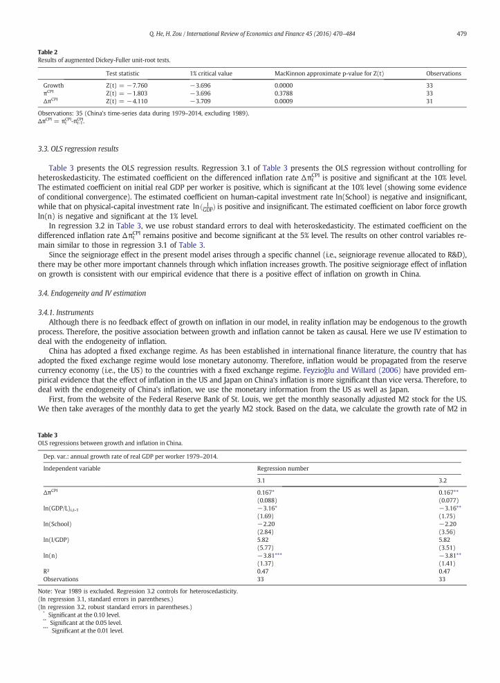
Table 2Results of augmented Dickey-Fuller unit-root tests.

Test statistic 1% critical value MacKinnon approximate p-value for Z(t) Observations

Growth Z(t) = −7.760 −3.696 0.0000 33πCPI Z(t) = −1.803 −3.696 0.3788 33ΔπCPI Z(t) = −4.110 −3.709 0.0009 31

Observations: 35 (China's time-series data during 1979–2014, excluding 1989).ΔπCPI = πt

CPI-πt-1CPI.

479Q. He, H. Zou / International Review of Economics and Finance 45 (2016) 470–484

3.3. OLS regression results

Table 3 presents the OLS regression results. Regression 3.1 of Table 3 presents the OLS regression without controlling forheteroskedasticity. The estimated coefficient on the differenced inflation rate Δπt

CPI is positive and significant at the 10% level.The estimated coefficient on initial real GDP per worker is positive, which is significant at the 10% level (showing some evidenceof conditional convergence). The estimated coefficient on human-capital investment rate ln(School) is negative and insignificant,while that on physical-capital investment rate lnð I

GDPÞ is positive and insignificant. The estimated coefficient on labor force growthln(n) is negative and significant at the 1% level.

In regression 3.2 in Table 3, we use robust standard errors to deal with heteroskedasticity. The estimated coefficient on thedifferenced inflation rate Δπt

CPI remains positive and become significant at the 5% level. The results on other control variables re-main similar to those in regression 3.1 of Table 3.

Since the seigniorage effect in the present model arises through a specific channel (i.e., seigniorage revenue allocated to R&D),there may be other more important channels through which inflation increases growth. The positive seigniorage effect of inflationon growth is consistent with our empirical evidence that there is a positive effect of inflation on growth in China.

3.4. Endogeneity and IV estimation

3.4.1. InstrumentsAlthough there is no feedback effect of growth on inflation in our model, in reality inflation may be endogenous to the growth

process. Therefore, the positive association between growth and inflation cannot be taken as causal. Here we use IV estimation todeal with the endogeneity of inflation.

China has adopted a fixed exchange regime. As has been established in international finance literature, the country that hasadopted the fixed exchange regime would lose monetary autonomy. Therefore, inflation would be propagated from the reservecurrency economy (i.e., the US) to the countries with a fixed exchange regime. Feyzioğlu and Willard (2006) have provided em-pirical evidence that the effect of inflation in the US and Japan on China's inflation is more significant than vice versa. Therefore, todeal with the endogeneity of China's inflation, we use the monetary information from the US as well as Japan.

First, from the website of the Federal Reserve Bank of St. Louis, we get the monthly seasonally adjusted M2 stock for the US.We then take averages of the monthly data to get the yearly M2 stock. Based on the data, we calculate the growth rate of M2 in

Table 3OLS regressions between growth and inflation in China.

Dep. var.: annual growth rate of real GDP per worker 1979–2014.

Independent variable Regression number

3.1 3.2

ΔπCPI 0.167*(0.088)

0.167**(0.077)

ln(GDP/L)i,t-1 −3.16*(1.69)

−3.16**(1.75)

ln(School) −2.20(2.84)

−2.20(3.56)

ln(I/GDP) 5.82(5.77)

5.82(3.51)

ln(n) −3.81***(1.37)

−3.81**(1.41)

R² 0.47 0.47Observations 33 33

Note: Year 1989 is excluded. Regression 3.2 controls for heteroscedasticity.(In regression 3.1, standard errors in parentheses.)(In regression 3.2, robust standard errors in parentheses.)

* Significant at the 0.10 level.** Significant at the 0.05 level.*** Significant at the 0.01 level.

480 Q. He, H. Zou / International Review of Economics and Finance 45 (2016) 470–484

the US, denoted M2usGrowth, as our first instrumental variable for China's inflation. Second, we accessed www.inflation.eu to ac-quire the yearly CPI inflation for Japan. To alleviate the potential endogeneity problem, we use the lagged value of Japan's CPI in-flation, denoted ljpinflation, as our second instrument. With more instruments than endogenous variables, we will use over-identification tests to check the validity of the instruments.

3.4.2. Results from IV estimationWith the constructed instruments, we now estimate the effect of inflation on growth using the 2SLS (Two-stage least squares)

estimation. We present the regression results in Table 4.Regression 4.1 of Table 4 presents the first-stage results of the 2SLS estimation. According to the first-stage results, the estimat-

ed coefficient on the growth rate of M2 in the US (i.e., M2usGrowth) is negative and insignificant at the 10% level, while that onthe lagged value of Japan's CPI inflation (i.e., ljpinflation) is negative and significant at the 10% level. The F-test on the joint sig-nificance of the two instruments (the growth rate of M2 in the US and the lagged value of Japan's CPI inflation) yields a p-valueabove 10%. Therefore, the two instruments (the growth rate of M2 in the US and the lagged value of Japan's CPI inflation) jointlyhave insignificant effects on China's inflation (the instruments become strong when we use the level of inflation, as elaborated onin Section 3.5).

Regression 4.2 of Table 4 reports the second-stage results of the 2SLS estimation. The over-identification test yields a p-valuemuch larger than 10%, meaning we accept the null that the instruments are valid. The over-identification test is known to beweak, and the inflation of Japan could also be influenced by the monetary policies in the US. However, the monetary policiesof Japan and those in the US cannot be totally grounded on the same rationale. Therefore, passing the over-identification test sig-nificantly enhances the validity of the instruments.

According to the second-stage results in regression 4.2 of Table 4, the estimated coefficient on the differenced inflation rateΔπt

CPI remains positive and significant at the 10% level, with an estimated magnitude more than three times as large as that ofthe OLS regressions in Table 3.

Andrews and Stock (2005) state that now the common approach is to use 2SLS if instruments are strong and to adopt a robuststrategy if instruments are weak. In the presence of many weak instruments, Stock and Yogo (2002) show that LIML (Limited-in-formation maximum likelihood) estimation is far superior to 2SLS, therefore, we check the robustness of our results with the LIMLestimation. The second-stage results of the LIML estimation are presented in regression 4.3 of Table 4, which indicate that the es-timated coefficient on the differenced inflation rate Δπt

CPI remains positive and significant at the 10% level.

Table 4IV regressions between growth and inflation in China.

Indep. variable Regression number

4.1 4.2 4.3 4.4 4.5

First-stage results Second-stage results of

2SLS LIML 2SLS LIML

Dependent variable as

ΔπCPI Annual growth of real GDPper worker: 1979–2014

ΔπCPI 0.90*(0.47)

0.92*(0.50)

0.84**(0.42)

0.87*(0.45)

ln(GDP/L)i,t-1 −6.16*(3.21)

0.39(4.12)

0.51(4.28)

−0.35(3.72)

−0.23(3.88)

ln(School) 6.33(4.44)

−5.15(6.33)

−5.24(6.51)

−6.38(6.31)

−6.49(6.53)

ln(I/GDP) 28.18**(11.66)

−15.95***(17.02)

−16.67(17.90)

−16.06(16.01)

−16.85(16.93)

ln(n) 0.003(3.67)

−3.64(2.52)

−3.64(2.58)

−4.40*(2.46)

−4.40*(2.53)

M2usGrowth −0.22(3.00)

ljpinflation −0.79*(0.43)

F-test on instruments(p-value)

F(2,26) = 1.68(0.2065)

OverID test p-value 0.57 0.58 0.53 0.54R² (uncentered) 0.30 0.85 0.86Observations 33 33 33 32 32

Note: Year 1989 is excluded for regressions 4.1 to 4.3. Years 1989 and 1990 are excluded for regressions 4.4 and 4.5. All regressions controls for heteroscedasticity.(Robust standard errors in parentheses.)

* Significant at the 0.10 level.** Significant at the 0.05 level.*** Significant at the 0.01 level.

481Q. He, H. Zou / International Review of Economics and Finance 45 (2016) 470–484

It is worth noting that, there is a large statistical adjustment in 1990 on labor force in China. This has been analyzed in Young(1233–1234). As a result, China's labor force jumps from 553 million in 1989 to 647 million in 1990 (an annual growth of 17%comparing to around 2–3% during 1978–89, see the data in Appendix A), and the annual growth of real GDP per worker in1990 becomes −11% (see the data in Appendix A), which is solely due to the statistical adjustment on labor force. We excludeyear 1990 from the regressions to avoid “spurious labor force growth” (Young, p. 1234). The second-stage results of the 2SLS es-timation presented in regression 4.4 of Table 4 indicate that the estimated coefficient on the differenced inflation rate Δπt

CPI re-mains positive and become significant at the 5% level. The over-identification test yields a p-value much larger than 10%,meaning we accept the null that the instruments are valid. The second-stage results of the LIML estimation presented in regres-sion 4.5 of Table 4 indicate that our results remain robust when we use the LIML estimation to deal with weak instruments.

Overall, we find that differenced inflation rate ΔπtCPI has a positive, significant effect on growth in both OLS and 2SLS estima-

tions. Therefore, the positive, significant effect of inflation on growth in China is robust and causal. Using regression 4.2, we findthat a one-percentage-point increase in differenced annual inflation rate Δπt

CPI would bring a 0.90-percentage-point increase inannual growth of per worker real GDP. Therefore, the magnitude of the estimated effect of inflation on growth was large inChina during the past three and a half decades after its market-oriented reform was initiated in 1978.

3.5. Regressions with the level of inflation

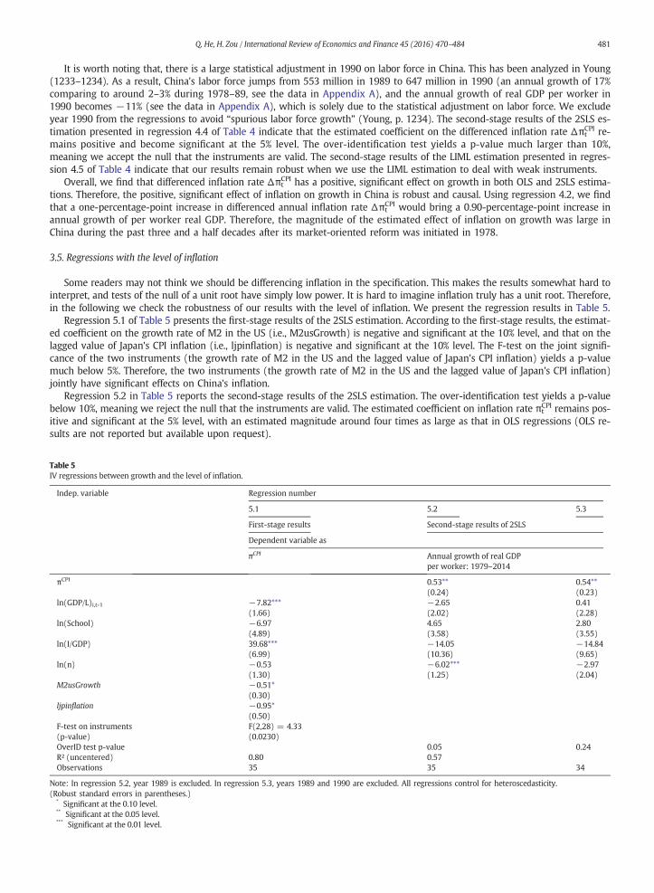
Some readers may not think we should be differencing inflation in the specification. This makes the results somewhat hard tointerpret, and tests of the null of a unit root have simply low power. It is hard to imagine inflation truly has a unit root. Therefore,in the following we check the robustness of our results with the level of inflation. We present the regression results in Table 5.

Regression 5.1 of Table 5 presents the first-stage results of the 2SLS estimation. According to the first-stage results, the estimat-ed coefficient on the growth rate of M2 in the US (i.e., M2usGrowth) is negative and significant at the 10% level, and that on thelagged value of Japan's CPI inflation (i.e., ljpinflation) is negative and significant at the 10% level. The F-test on the joint signifi-cance of the two instruments (the growth rate of M2 in the US and the lagged value of Japan's CPI inflation) yields a p-valuemuch below 5%. Therefore, the two instruments (the growth rate of M2 in the US and the lagged value of Japan's CPI inflation)jointly have significant effects on China's inflation.

Regression 5.2 in Table 5 reports the second-stage results of the 2SLS estimation. The over-identification test yields a p-valuebelow 10%, meaning we reject the null that the instruments are valid. The estimated coefficient on inflation rate πt

CPI remains pos-itive and significant at the 5% level, with an estimated magnitude around four times as large as that in OLS regressions (OLS re-sults are not reported but available upon request).

Table 5IV regressions between growth and the level of inflation.

Indep. variable Regression number

5.1 5.2 5.3

First-stage results Second-stage results of 2SLS

Dependent variable as

πCPI Annual growth of real GDPper worker: 1979–2014

πCPI 0.53**(0.24)

0.54**(0.23)

ln(GDP/L)i,t-1 −7.82***(1.66)

−2.65(2.02)

0.41(2.28)

ln(School) −6.97(4.89)

4.65(3.58)

2.80(3.55)

ln(I/GDP) 39.68***(6.99)

−14.05(10.36)

−14.84(9.65)

ln(n) −0.53(1.30)

−6.02***(1.25)

−2.97(2.04)

M2usGrowth −0.51*(0.30)

ljpinflation −0.95*(0.50)

F-test on instruments(p-value)

F(2,28) = 4.33(0.0230)

OverID test p-value 0.05 0.24R² (uncentered) 0.80 0.57Observations 35 35 34

Note: In regression 5.2, year 1989 is excluded. In regression 5.3, years 1989 and 1990 are excluded. All regressions control for heteroscedasticity.(Robust standard errors in parentheses.)

* Significant at the 0.10 level.** Significant at the 0.05 level.*** Significant at the 0.01 level.

482 Q. He, H. Zou / International Review of Economics and Finance 45 (2016) 470–484

As discussed, there is a large statistical adjustment in 1990 on labor force in China. Therefore, it is meaningful for us to checkthe robustness of our results by excluding year 1990 from the regressions. Regression 5.3 in Table 5 reports the second-stage re-sults of the 2SLS estimation. The over-identification test yields a p-value above 10%, meaning we accept the null that the instru-ments are valid. The over-identification test is known to be weak, and the inflation of Japan could also be influenced by themonetary policies in the US. However, the monetary policies of Japan and those in the US cannot be totally grounded on thesame rationale. Therefore, passing the over-identification test significantly enhances the validity of the instruments. The estimatedcoefficient on inflation rate πt

CPI remains positive and significant at the 5% level, with an estimated magnitude similar to that inregression 5.2.

Therefore, the positive, significant effect of inflation on growth in China is robust and causal. Using regression 5.2, we find thata 1 percentage point increase in annual inflation would bring a 0.53 percentage point increase in annual growth of per workerreal GDP. Given the average annual inflation rate of 4.9% in our data sample, inflation explains 2.6% annual growth in real GDPper worker (which is around 32% of the average 8.0% annual growth rate in real GDP per worker during 1979–2014). Therefore,the magnitude of the estimated effect of inflation on growth is large in China during the past three and a half decades after itsmarket-oriented reform initiated in 1978.

4. Conclusions

In this paper we argue that inflation affects growth and welfare through an overlooked, but important mechanism. The gov-ernment reaps seigniorage revenue from higher rates of money growth, attracting more labor into the government and bankingsectors and thereby decreasing the profit of entrepreneurs (the government crowding-out effect). When part of the revenue goes toentrepreneurs, more resources would be attracted into R&D (the seigniorage effect). When the government retains a larger shareof the revenue, the government crowding-out effect dominates and inflation retards growth. When entrepreneurs get the largershare, the seigniorage effect dominates and inflation increases growth.

Regressions using time-series data in China during 1979–2014 show that differenced inflation (to ensure stationarity) has apositive and significant effect on growth. The result holds up in the IV estimation that uses the M2 growth in the US andJapan's inflation rates as instruments for China's inflation. When we use the level of inflation, we find that a 1 percentagepoint increase in annual inflation would bring a 0.53 percentage point increase in annual growth of per worker real GDP.Given the average annual inflation rate of 5.1% in our data sample, inflation explains 2.6% annual growth in real GDP per worker(which is around 32% of the average 8.0% annual growth rate in real GDP per worker during 1979–2014). Therefore, the magni-tude of the estimated effect of inflation on growth is large in China during the past three and a half decades after its market-oriented reform initiated in 1978. The robust, causal effect of inflation on growth in China provides support for our theory. There-fore, the government may reconsider how to use the seigniorage revenue, which has important consequences for growth andwelfare.

Some readers may find our use of the term “government-bank” misleading. The government-bank in our model is analogousto a central bank. That is, it is possible to interpret the government-bank in our model as a central bank that issues outsidemoney, but which now rebates part of the seigniorage revenue to the entrepreneurs. The rest of the seigniorage revenuewould be retained by the government to finance its spending. The implication of the model is not any different. We use theterm “government-bank” for China that does not have central bank independence (see Bade & Parkin, 1988, for an early studyon central bank independence).

Our model may have more resemblance to China's monetary system without central bank independence. Because manydeveloping countries share similar institutional features with China, our theory, and particularly the positive, significanteffect of inflation on growth in China, could provide lessons for developing countries. As discussed, the theme of ourpaper is general because seigniorage is also important in developed countries as illustrated in Obstfeld and Rogoff(1996, p. 527).

As a side note, as we have highlighted in the introduction, China has an autocratic political regime. Without checks and bal-ances, the Chinese government can reap much larger seigniorage revenues than democratic countries with central bank indepen-dence and also is able to direct funds both to itself and to other specific sectors of the economy (e.g., the state-owned industries).As a result, it is possible that some of the seigniorage revenue may be used to subsidize the firms, which helps to increase growth.However, faster growth does not necessarily mean higher welfare. Therefore, although the Chinese success therefore offers someeconomic and philosophical wisdom, increased democracy and separation of powers may be necessary to monitor and disciplinethe government (see e.g., Friedman, 2002; Rousseau, 1762; Montesquieu, 1748; Schumpeter, 1942; Hayek, 1944) to protect thewelfare of the people.

Acknowledgements

We are grateful to two anonymous referees for comments that substantially improved the paper. We are also grateful to AngusChu for comments that substantially improved the paper. We also thank Paul Beaudry, Patrick Francois, Nobuhiro Kiyotaki, andseminar participants at Renmin University of China, Beijing Normal University, and Central University of Finance and Economicsfor helpful comments on the earlier version of this paper.

483Q. He, H. Zou / International Review of Economics and Finance 45 (2016) 470–484

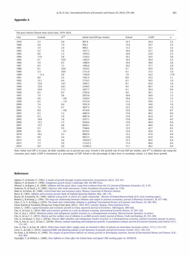
Appendix A

The post-reform Chinese time-series data: 1979–2014

Year Growth πCPI Initial real GDP per worker School I/GDP n

1979 5.3 2.0 907.9 14.7 36.4 2.21980 4.4 7.4 956.1 13.4 34.7 3.31981 1.9 2.4 998.3 11.5 33.1 3.21982 5.2 1.9 1017.1 10.4 32.1 3.61983 8.0 1.5 1070.3 10.0 32.0 2.51984 11.0 2.8 1156.3 10.1 34.5 3.81985 9.7 10.0 1283.5 10.2 39.4 3.51986 5.9 6.5 1408.4 10.4 38.0 2.81987 8.5 7.3 1492.0 10.2 37.7 2.91988 8.1 18.8 1619.5 9.7 39.5 2.91989 2.3 18.0 1751.0 9.1 37.5 1.81990 −11.2 3.0 1792.0 7.9 34.3 17.01991 8.0 3.5 1591.5 8.0 35.5 1.11992 13.1 6.4 1719.3 8.1 39.5 1.01993 12.8 14.7 1945.1 8.1 43.9 1.01994 12.0 24.1 2194.5 8.5 40.7 1.01995 10.0 17.1 2457.7 9.1 39.4 0.91996 8.5 8.3 2703.4 9.6 38.1 1.31997 7.9 2.8 2933.6 10.0 36.0 1.31998 6.6 −0.8 3164.4 10.4 35.4 1.21999 6.5 −1.4 3373.4 11.2 34.6 1.12000 7.4 0.4 3591.9 11.8 34.0 1.02001 7.2 0.7 3857.3 12.2 36.0 1.02002 8.4 −0.8 4136.6 12.6 36.6 0.72003 9.3 1.2 4482.9 13.0 40.2 0.62004 9.3 3.9 4901.6 13.8 42.4 0.72005 10.8 1.8 5357.1 13.8 40.9 0.52006 12.2 1.5 5934.6 13.8 40.4 0.42007 13.7 4.8 6658.1 13.7 40.9 0.52008 9.3 5.9 7568.6 13.5 42.7 0.32009 8.9 −0.7 8270.2 13.4 45.8 0.32010 10.2 3.3 9002.4 13.2 47.0 0.42011 9.0 5.4 9923.3 12.8 47.0 0.42012 7.4 2.6 10,819.7 12.3 46.5 0.42013 7.3 2.6 11,615.1 11.4 46.6 0.42014 6.9 2.0 12,463.2 11.1 46.2 0.4

Note: Initial real GDP is in yuan; all other variables are in percent per year. Growth is the growth rate of real GDP per worker, and πCPI is inflation rate using theconsumer price index. I/GDP is investment as a percentage of GDP. School is the percentage of labor force in secondary school. n is labor force growth.

References

Aghion, P., & Howitt, P. (1992). A model of growth through creative destruction. Econometrica, 60(2), 323–351.Aghion, P., & Howitt, P. (1998). Endogenous growth theory. Cambridge, MA: the MIT Press.Ahmed, S., & Rogers, J. H. (2000). Inflation and the great ratios: Long term evidence from the U.S. Journal of Monetary Economics, 45, 3–35.Andrews, D., & Stock, J. H. (2005). Inference with weak instruments. Cowles Foundation discussion paper no. 1530.Bade, R., & Parkin, M. (1988). Central bank laws and monetary policy. Mimeo, University of Western Ontario.Barro, R. (1995). Inflation and economic growth. Bank of England Quarterly Bulletin, May, 166–176.Bruno, M., & Easterly, W. (1996). Inflation and growth: In search of a stable relationship. (Review of Federal Reserve Bank of St. Louis working paper).Bullard, J., & Keating, J. (1995). The long-run relationship between inflation and output in postwar economies. Journal of Monetary Economics, 36, 477–496.Chen, Z., Li, Y., & Zhang, J. (2016). The bank–firm relationship: Helping or grabbing? International Review of Economics and Finance, 42, 385–403.China Statistical Yearbook [Zhong Guo Tong Ji Nian Jian] (2012). 1983–2015 (annual). Beijing: China Statistical Press.Chow, G. (1993). Capital formation and economic growth in China. Quarterly Journal of Economics, 108(August), 809–842.Chu, A., & Cozzi, G. (2014). R&D and economic growth in a cash-in-advance economy. International Economic Review, 55, 507–524.Chu, A., & Ji, L. (2012). Monetary policy and endogenous market structure in a Schumpeterian economy. Macroeconomic Dynamics (in press).Chu, A., & Lai, C. C. (2013). Money and the welfare cost of inflation in an R&D growth model. Journal of Money, Credit and Banking, 45, 233–249.Chu, A., Furukawa, Y., & Ji, L. (2014a). Patents, R&D subsidies and endogenous market structure in a Schumpeterian economy. Southern Economic Journal (in press).Chu, A., Kan, K., Lai, C., & Liao, C. (2014b). Money, randommatching and endogenous growth: A quantitative analysis. Journal of Economic Dynamics and Control, 41(C),

173–187.Chu, A., Pan, S., & Sun, M. (2012). When does elastic labor supply cause an inverted-U effect of patents on innovation. Economics Letters, 117(1), 211–213.Cozzi, G., & Galli, S. (2014). Sequential R&D and blocking patents in the dynamics of growth. Journal of Economic Growth, 19(2), 183–219.De Haan, J., & Zelhorst, D. (1990). The impact of government deficits on money growth in developing countries. Journal of International Money and Finance, 9(4),

455–469.Feyzioğlu, T., & Willard, L. (2006). Does inflation in China affect the United States and Japan? IMF working paper no. WP/06/36.

484 Q. He, H. Zou / International Review of Economics and Finance 45 (2016) 470–484

Fischer, S. (1993). The role of macroeconomic factors in growth. Journal of Monetary Economics(Dec.), 485–512.Friedman, M. (1969). The optimum quantity of money. Macmillan.Friedman, M. (2002). Capitalism and freedom. The University of Chicago Press.Funk, P., & Kromen, B. (2010). Inflation and innovation-driven growth. B.E. Journal of Macroeconomics, 10(1), 1–52.Gomme, P. (1993). Money and growth: Revisited. Journal of Monetary Economics, 32, 51–77.Hayek, F. A. (1944). The road to serfdom. The University of Chicago Press, 2007.He, Q. (2016a). Inflation and growth: The role of central bank independence. Working paper. Beijing, China: China Economics andManagement Academy, Central Univer-

sity of Finance and Economics.He, Q. (2016b). Friedman rule in an innovation-led growthmodel with monetized government spending.Working paper. Beijing, China: China Economics andManagement

Academy, Central University of Finance and Economics.He, Q. (2016c). Corruption and growth in China: Causality and mechanism by an instrumental variables approach. Working paper. Beijing, China: China Economics and

Management Academy, Central University of Finance and Economics.Holz, C. A. (2003). ‘Fast, clear and accurate’: How reliable are Chinese output and economic growth statistics? The China Quarterly, 173, 122–163.Jones, L., & Manuelli, R. (1995). Growth and the effects of inflation. Journal of Economic Dynamics and Control, 19, 1405–1428.Khan, M., & Senhadji, A. (2001). Threshold effects in the relationship between inflation and growth. IMF Staff Papers, 48(1).Kormendi, R., & Meguire, P. (1985). Macroeconomic determinants of growth: Cross-country evidence. Journal of Monetary Economics, 16, 141–163.Laincz, C., & Peretto, P. (2006). Scale effects in endogenous growth theory: An error of aggregation not specification. Journal of Economic Growth, 11(3), 263–288.Lucas, R. E., Jr. (1972). Expectations and the neutrality of money. Journal of Economic Theory, 4, 103–124.Mankiw, G., Romer, D., & Weil, D. (1992). A contribution to the empirics of economic growth. Quarterly Journal of Economics, 107, 407–437.Marquis, M., & Reffett, K. (1994). New technology spillovers into the payment system. The Economic Journal, 104, 1123–1138.Montesquieu, C. (1748). The spirit of the laws.Obstfeld, M., & Rogoff, K. (1996). Foundations of international macroeconomics. Cambridge, MA: the MIT Press.Pan, S. (2011). Competition among the elites, property rights protection and economic performance. Journal of Economics, 104(2), 139–158.Peretto, P. F., & Valente, S. (2015). Growth on a finite planet: Resources, technology and population in the long run. Journal of Economic Growth, 20(3), 305–331.Romer, P. M. (1990). Endogenous technological change. Journal of Political Economy, 98(October), S71–102.Rousseau, J. J. (1762). English edition: ‘The social contract’ and other later political writings, trans. Victor Gourevitch. Cambridge: Cambridge University Press. 1997.Schumpeter, J. E. (1942). Capitalism, socialism, and democracy. Harper Perennial Modern Thought Edition, 2008.Sidrauski, M. (1967). Inflation and economic growth. Journal of Political Economy, 75, 796–810.Stock, J. H., & Yogo, M. (2002). Testing for weak instruments in linear IV regression. NBER technical working paper no. 284.Stockman, A. (1981). Anticipated inflation and the capital stock in a cash-in-advance economy. Journal of Monetary Economics, 8, 387–393.Tobin, J. (1965). Money and economic growth. Econometrica, 33, 671–684.Wang, P., & Xie, D. (2013). Real effect of money growth and optimal rate of inflation in a cash-in-advance economywith labor-market frictions. Journal of Money, Credit

and Banking, 45(8), 1517–1546.Wang, P., & Yip, C. (1992). Alternative approaches to money and growth. Journal of Money, Credit and Banking, 24, 553–562.Young, A. (2003). Gold into base metals: Productivity growth in the People's Republic of China during the reform period. Journal of Political Economy, 111(December),

1220–1261.Zhang, J., & Zhang, H. (2009). The measure and use of seigniorage of PBC (1986–2008). Jingji Yanjiu [Economic Research Journal], 7, 79–90 (in Chinese).