VYSOKÉ UČENÍ TECHNICKÉ V BRNĚ BRNO UNIVERSITY OF TECHNOLOGY

FAKULTA STROJNÍHO INŽENÝRSTVÍ ÚSTAV PROCESNÍHO A EKOLOGICKÉHO INŽENÝRSTVÍ FACULTY OF MECHANICAL ENGINEERING

INSTITUTE OF PROCESS AND ENVIRONMENTAL ENGINEERING

COMPUTATIONS OF FLUID FLOW AND HEAT TRANSFER FOR DESIGN OPTIMIZATION OF TUMBLE CLOTHES DRYER

VÝPOČTY PROUDĚNÍ A PŘENOSU TEPLA PRO OPTIMALIZACI KONSTRUKCE BUBNOVÉ SUŠICKY PRÁDLA

DIPLOMOVÁ PRÁCE MASTER´S THESIS

AUTOR PRÁCE Bc. MARTIN ČERMÁK AUTHOR

VEDOUCÍ PRÁCE doc. Ing. JIŘÍ HÁJEK, Ph.D. SUPERVISOR

BRNO 2013

This page has been intentionally left blank

This page has been intentionally left blank

4

Anotace V rámci této práce byla provedena komplexní analýza elektricky vyhřívané bubnové sušičky prádla s cílem identifikovat možnosti optimalizace její konstrukce vedoucí ke zlepšení přestupu tepla. Pro řešení byl zvolen postup využívající výpočtovou dynamiku tekutin (CFD). K dosažení dostatečně detailního popisu zadaného problému byl využit komerční software Fluent společně se speciálně vyvinutým modelem přenosu tepla.

Annotation Within this thesis a complex analysis of an

electrically heated tumble clothes dryer was

performed in order to identify design

optimization possibilities leading to an

improvement of a heat transfer. A

computational fluid dynamics (CFD) approach

involving an employment of the commercial

software Fluent and development of a custom

heat transfer model was selected to resolve the

problem in a required level of detail.

Klíčová slova Bubnová sušička prádla, elektrické vytápění, spirálové topné těleso, CFD, model přenosu tepla, optimalizace

Keywords Tumble clothes dryer, resistance heating,

helically coiled heating wire, CFD, heat transfer

model, optimization

5

Bibliografická citace této práce

dle ČSN ISO 690

ČERMÁK, M. Výpočty proudění a přenosu tepla pro optimalizaci konstrukce bubnové sušičky prádla.

Brno: Vysoké učení technické v Brně, Fakulta strojního inženýrství, 2013. 69 s. Vedoucí diplomové

práce doc. Ing. Jiří Hájek, Ph.D..

6

Prohlášení o původnosti práce

Prohlašuji, že jsem tuto práci vypracoval samostatně s využitím uvedených zdrojů, na základě konzultací a pod vedením vedoucího diplomové práce.

V Brně dne 23. května 2013 …………………………………………………..

Martin Čermák

7

Table of contents

1 List of symbols ...................................................................................................................... 9

2 Introduction........................................................................................................................ 12

3 Tumble dryer description .................................................................................................... 13

3.1 Air flow characteristics .......................................................................................................... 13

3.2 Electric heating ...................................................................................................................... 15

3.3 Drivetrain and regulation ...................................................................................................... 17

4 Solution method overview .................................................................................................. 18

4.1 Heat transfer model .............................................................................................................. 18

4.2 Fluid-wire interaction ............................................................................................................ 19

5 Heat transfer model ............................................................................................................ 20

5.1 Development of elemental relationships .............................................................................. 20

5.1.1 Heat generation rate ..................................................................................................... 20

5.1.2 Heating wire energy equation ....................................................................................... 21

5.1.3 Discretization of the heating wire energy equation ...................................................... 23

5.1.4 Convection heat transfer coefficient ............................................................................. 25

5.1.5 Three phase circuit solution .......................................................................................... 26

5.2 Model description ................................................................................................................. 28

5.3 Model abilities and limitations .............................................................................................. 30

5.4 Implementation ..................................................................................................................... 31

5.4.1 Flow field data export .................................................................................................... 32

5.4.2 Calculation of the volumetric heat source terms .......................................................... 33

5.4.3 Linear systems definition............................................................................................... 38

6 Present Case CFD Analysis ................................................................................................... 41

6.1 Computational Domain and Boundary Conditions ............................................................... 41

6.2 Computational grid ................................................................................................................ 44

6.3 Solver ..................................................................................................................................... 47

6.4 Solution process .................................................................................................................... 48

7 Results interpretation ......................................................................................................... 52

7.1 Flow field ............................................................................................................................... 52

7.1.1 Heating blocks ............................................................................................................... 52

7.1.2 Outlet ............................................................................................................................. 53

7.2 Heating unit ........................................................................................................................... 54

8 Optimization ....................................................................................................................... 57

8.1 Targeting ................................................................................................................................ 57

8.1.1 Overheating ................................................................................................................... 57

8

8.1.2 Flow uniformity ............................................................................................................. 61

8.1.3 Heating channel velocity ............................................................................................... 63

8.1.4 Heating coil geometry ................................................................................................... 66

8.2 Evaluation of optimization possibilities................................................................................. 67

9 Conclusion .......................................................................................................................... 68

10 References .......................................................................................................................... 69

Appendix A – Fluent UDF source code

Appendix B – Heat transfer model Matlab code

Appendix C – CFD results visualizations

Appendix D – Attached DVD content

9

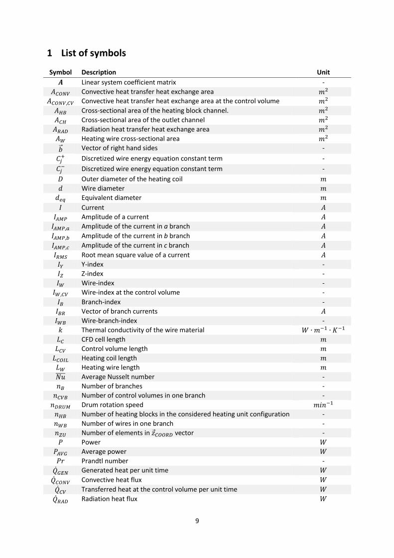
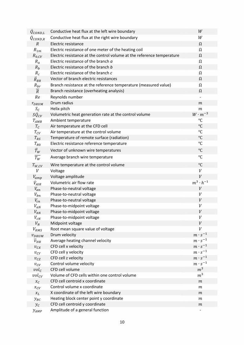
1 List of symbols

Symbol Description Unit

Linear system coefficient matrix -

Convective heat transfer heat exchange area Convective heat transfer heat exchange area at the control volume

Cross-sectional area of the heating block channel.

Cross-sectional area of the outlet channel

Radiation heat transfer heat exchange area

Heating wire cross-sectional area

Vector of right hand sides -

Discretized wire energy equation constant term -

Discretized wire energy equation constant term -

Outer diameter of the heating coil

Wire diameter

Equivalent diameter

Current

Amplitude of a current

Amplitude of the current in a branch

Amplitude of the current in b branch

Amplitude of the current in c branch

Root mean square value of a current

Y-index -

Z-index -

Wire-index -

Wire-index at the control volume -

Branch-index -

Vector of branch currents

Wire-branch-index -

Thermal conductivity of the wire material

CFD cell length

Control volume length

Heating coil length

Heating wire length

Average Nusselt number -

Number of branches -

Number of control volumes in one branch -

Drum rotation speed

Number of heating blocks in the considered heating unit configuration -

Number of wires in one branch -

Number of elements in vector -

Power

Average power

Prandtl number -

Generated heat per unit time

Convective heat flux

Transferred heat at the control volume per unit time

Radiation heat flux

10

Conductive heat flux at the left wire boundary

Conductive heat flux at the right wire boundary

Electric resistance

Electric resistance of one meter of the heating coil

Electric resistance at the control volume at the reference temperature

Electric resistance of the branch a

Electric resistance of the branch b

Electric resistance of the branch c

Vector of branch electric resistances

Branch resistance at the reference temperature (measured value)

Branch resistance (overheating analysis)

Reynolds number -

Drum radius

Helix pitch

Volumetric heat generation rate at the control volume

Ambient temperature

Air temperature at the CFD cell

Air temperature at the control volume

Temperature of remote surface (radiation)

Electric resistance reference temperature

Vector of unknown wire temperatures

Average branch wire temperature

Wire temperature at the control volume

Voltage

Voltage amplitude

Volumetric air flow rate

Phase-to-neutral voltage

Phase-to-neutral voltage

Phase-to-neutral voltage

Phase-to-midpoint voltage

Phase-to-midpoint voltage

Phase-to-midpoint voltage

Midpoint voltage

Root mean square value of voltage

Drum velocity Average heating channel velocity

CFD cell x velocity

CFD cell y velocity

CFD cell z velocity Control volume velocity

CFD cell volume Volume of CFD cells within one control volume

CFD cell centroid x coordinate

Control volume x coordinate

X coordinate of the left wire boundary

Heating block center point y coordinate

CFD cell centroid y coordinate

Amplitude of a general function -

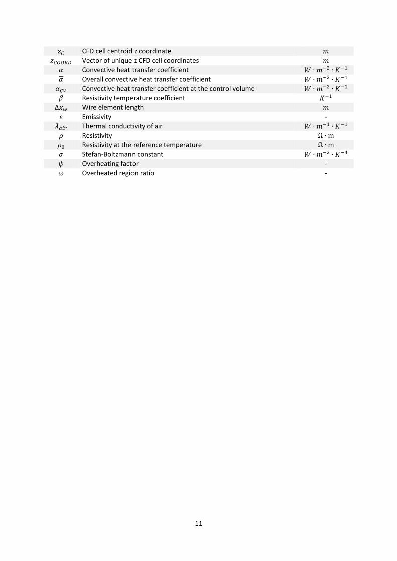
11

CFD cell centroid z coordinate

Vector of unique z CFD cell coordinates

Convective heat transfer coefficient

Overall convective heat transfer coefficient Convective heat transfer coefficient at the control volume

Resistivity temperature coefficient Wire element length

Emissivity -

Thermal conductivity of air

Resistivity

Resistivity at the reference temperature

Stefan-Boltzmann constant Overheating factor -

Overheated region ratio -

12

2 Introduction

The topic of this thesis arose from the collaboration between the laundry equipment manufacturer

Primus CE and NETME Centre – a research and development center attached to the Faculty of

Mechanical Engineering at Brno University of Technology. During the initial talks aimed at the details

of the collaboration, the need to address an optimization of electrically heated tumble clothes dryers

was expressed by the Primus company representatives. As a result the task of this thesis was

formulated.

To ensure an appropriate selection of a solution method, a further discussion revealing the details of

the task was necessary. Since the dryer geometry was designed in the time when tools such as

computational fluid dynamics (CFD) were not available, the main concern of the manufacturer was

the influence of the geometry on the heat transfer. A special emphasis was placed on an

investigation of overheating and its connection with the dryer design.

The view of the problem from a broader perspective perfectly represents the changes in engineering

in the current era. Great improvements in computer power and software development allow the

manufacturers of standard domestic appliances to utilize tools such as the abovementioned CFD to

improve a design and therefore to support a competitiveness of the company. Even though in many

cases it is still unsuitable to employ purely computational methods and an experimental work

together with experienced personnel able to predict the relevant dependencies prevails, a number of

industrial applications of numerical problem solutions has been increasing significantly in the last few

years. In this context it is essential to mention the frequent misuse of commercial CFD or FEM

packages leading to completely incorrect results. These situations underline a great value of

know-how required to achieve relevant results in simulations of a fluid flow or in other applications

of FEM/FVM methods.

The structure of the thesis can be split into two main logical parts. In the first part all the steps

necessary to obtain data crucial for a description of the present case are presented. The second part

investigates improvement possibilities in both qualitative and quantitative ways.

13

3 Tumble dryer description

A tumble clothes dryer is a standard domestic appliance that uses hot air to remove moisture from

wet laundry. Depending on a target customer, there are several conventional energy sources used

for air heating. While small domestic tumble dryers use electric energy, larger industrial dryers can

be equipped with steam or gas burner heating. This thesis is concerned with the electrically heated

variants.

Fig. 1 - Layout of Primus T24/T35 tumble clothes dryer [5]

Fig. 1a shows a layout of the high capacity tumble clothes dryer produced by the Primus company. In

the highest capacity series there are currently two models available – T24 and T35. The main

difference between the two models lies in the volume of the drum and heating unit power. Because

the drum diameter is identical for the both models, the larger volume of T35 is achieved by

increasing the drum length and therefore the depth dimension of the whole device, as can be seen in

fig. 1b.

3.1 Air flow characteristics

The flow through the dryer described above can be characterized as a suction based fan driven flow

with significant heat and mass transfer. Drying air enters the device through the set of perforations

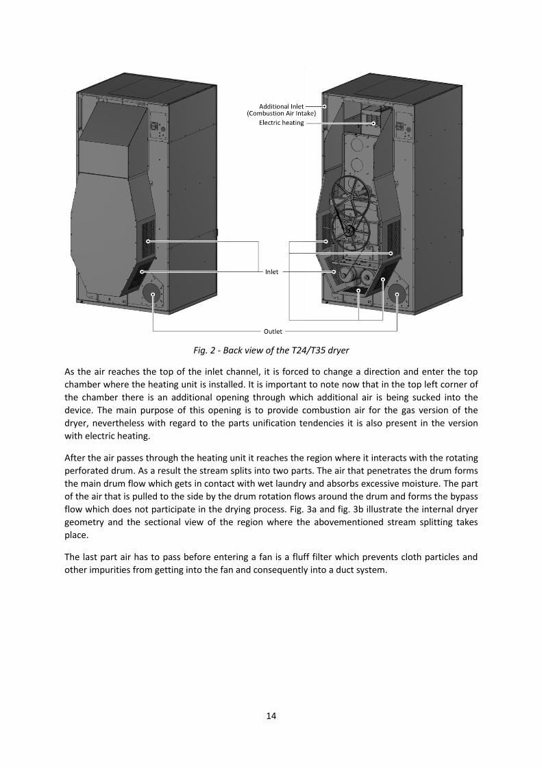
located at the back side of the dryer and continues upwards through the inlet channel. Fig. 2 shows

the visualization of the dryer with and without the back cover. It can be seen that inlet channel is

partly blocked by the drivetrain which influences the flow immediately after the entry.

14

Fig. 2 - Back view of the T24/T35 dryer

As the air reaches the top of the inlet channel, it is forced to change a direction and enter the top

chamber where the heating unit is installed. It is important to note now that in the top left corner of

the chamber there is an additional opening through which additional air is being sucked into the

device. The main purpose of this opening is to provide combustion air for the gas version of the

dryer, nevertheless with regard to the parts unification tendencies it is also present in the version

with electric heating.

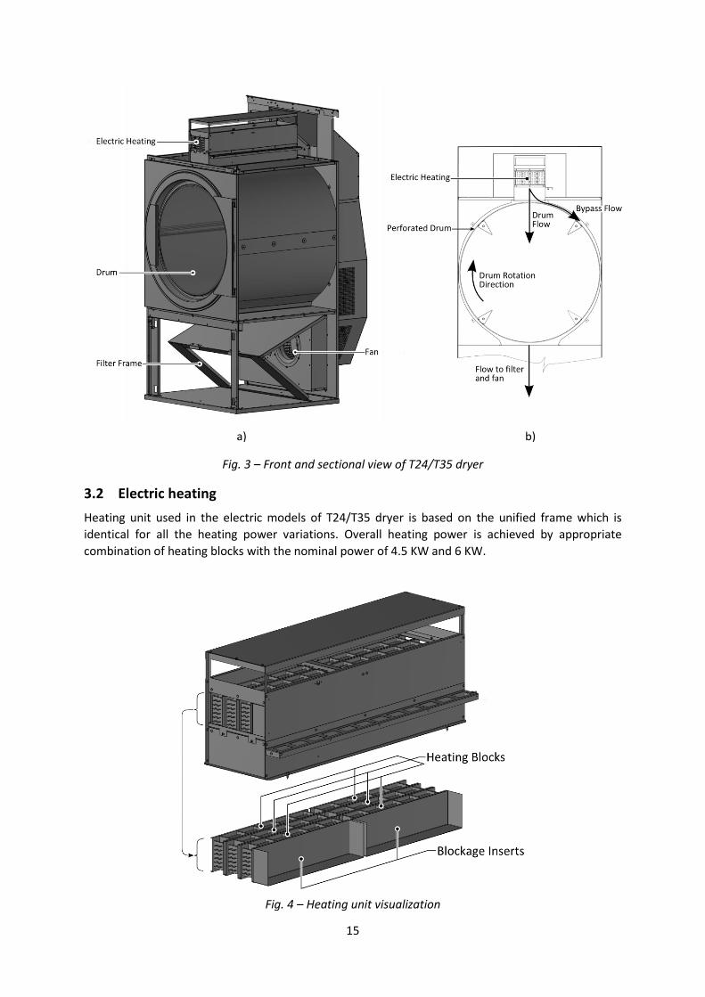
After the air passes through the heating unit it reaches the region where it interacts with the rotating

perforated drum. As a result the stream splits into two parts. The air that penetrates the drum forms

the main drum flow which gets in contact with wet laundry and absorbs excessive moisture. The part

of the air that is pulled to the side by the drum rotation flows around the drum and forms the bypass

flow which does not participate in the drying process. Fig. 3a and fig. 3b illustrate the internal dryer

geometry and the sectional view of the region where the abovementioned stream splitting takes

place.

The last part air has to pass before entering a fan is a fluff filter which prevents cloth particles and

other impurities from getting into the fan and consequently into a duct system.

15

Fig. 3 – Front and sectional view of T24/T35 dryer

3.2 Electric heating

Heating unit used in the electric models of T24/T35 dryer is based on the unified frame which is

identical for all the heating power variations. Overall heating power is achieved by appropriate

combination of heating blocks with the nominal power of 4.5 KW and 6 KW.

Fig. 4 – Heating unit visualization

16

From fig. 4 it is clear that when less than eight blocks is used, blockage inserts are placed into all

empty slots in order to prevent the air from bypassing the heating channel. The distributions of

heating blocks and blockage inserts in 30, 36 and 48KW variants are shown in fig. 5a, fig. 5b, and fig.

5c respectively. Within the scope of this thesis the 36KW variant was further examined. However an

emphasis was placed on a simple applicability of developed solution methods to all the heating unit

configurations.

Fig. 5 – Distribution of heating blocks in a) 36KW b) 48KW c) 30KW heating unit

The heating block, depicted in fig. 6a, is a simple device consisting of three basic parts – heating wires

formed into helical coils, wire supports and a terminal board. As can be seen from fig. 6b, a set of

twelve wires is divided into three branches. One branch is formed by four wires connected in series.

The terminal board contacts allow the heating block to be connected in a variety of ways. In the

considered case a three phase wye connection with absent neutral line has been used. The electric

circuit diagram of the connection is shown in fig. 6c.

Fig. 6 – Heating block description

17

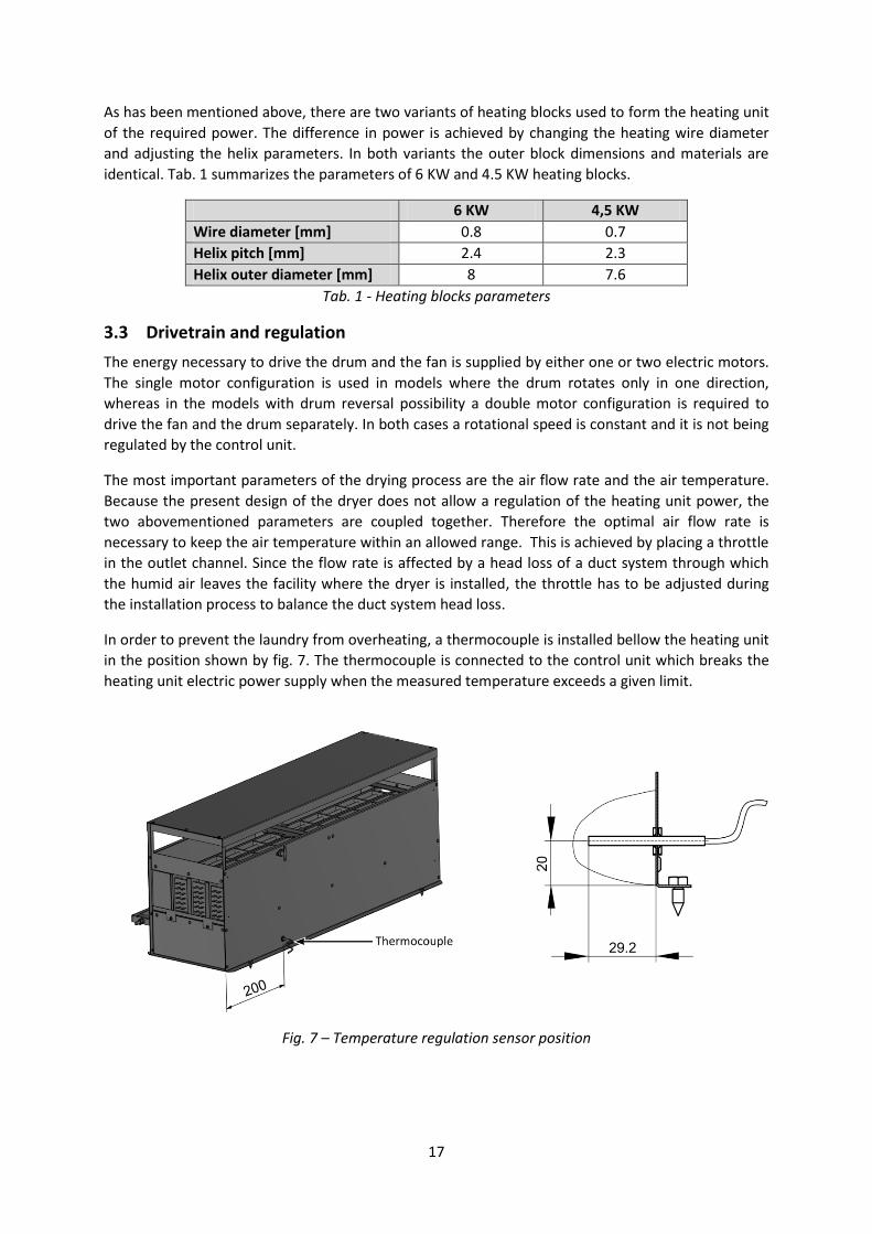
As has been mentioned above, there are two variants of heating blocks used to form the heating unit

of the required power. The difference in power is achieved by changing the heating wire diameter

and adjusting the helix parameters. In both variants the outer block dimensions and materials are

identical. Tab. 1 summarizes the parameters of 6 KW and 4.5 KW heating blocks.

6 KW 4,5 KW

Wire diameter [mm] 0.8 0.7

Helix pitch [mm] 2.4 2.3

Helix outer diameter [mm] 8 7.6

Tab. 1 - Heating blocks parameters

3.3 Drivetrain and regulation

The energy necessary to drive the drum and the fan is supplied by either one or two electric motors.

The single motor configuration is used in models where the drum rotates only in one direction,

whereas in the models with drum reversal possibility a double motor configuration is required to

drive the fan and the drum separately. In both cases a rotational speed is constant and it is not being

regulated by the control unit.

The most important parameters of the drying process are the air flow rate and the air temperature.

Because the present design of the dryer does not allow a regulation of the heating unit power, the

two abovementioned parameters are coupled together. Therefore the optimal air flow rate is

necessary to keep the air temperature within an allowed range. This is achieved by placing a throttle

in the outlet channel. Since the flow rate is affected by a head loss of a duct system through which

the humid air leaves the facility where the dryer is installed, the throttle has to be adjusted during

the installation process to balance the duct system head loss.

In order to prevent the laundry from overheating, a thermocouple is installed bellow the heating unit

in the position shown by fig. 7. The thermocouple is connected to the control unit which breaks the

heating unit electric power supply when the measured temperature exceeds a given limit.

Fig. 7 – Temperature regulation sensor position

18

4 Solution method overview

In order to allow a reader to be aware of all the logical connections, this chapter aims to give the

basic solution procedure overview and to discuss the elemental features and simplifications. The

details of individual steps can be found in the subsequent chapters.

With regard to the optimization nature of the task, a solution method capable of resolving the flow

field details is needed in order to identify the improvement possibilities. This need is fully met by

computational fluid dynamics (CFD) approach which has therefore been selected as the main

solution method. While leaving the CFD details to be sought in one of the many literature sources,

brief description can be formulated as following. The fluid flow governing equations describing the

elemental fluid flow laws are applied to the discretized flow domain which results in a system of

equations. The converged numerical solution of the system reveals the values of all the flow variables

at each cell of the discretized domain.

The assessment of the flow domain discretization possibilities has identified the need to further

analyze the discretization method of the helically coiled heating wires region. Because a full

discretization of the region adjacent to the heating wires requires a high number of cells resulting in

high computing power requirements, a simplified approach was sought. From a general engineering

point of view, it is common to employ a modeling approach. When applied to the considered case,

the modeling approach avoids the detailed resolution of the heating wire region and introduces a

computational relationship which is able to describe the heat transfer and fluid-wire interaction

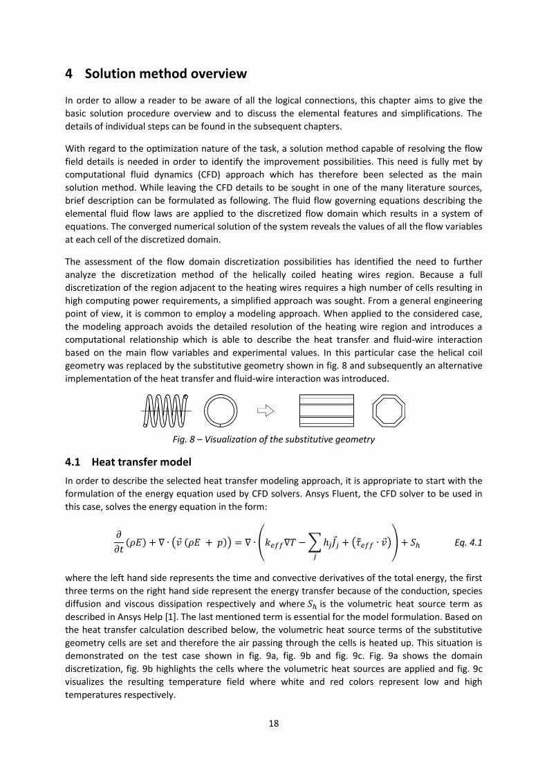
based on the main flow variables and experimental values. In this particular case the helical coil

geometry was replaced by the substitutive geometry shown in fig. 8 and subsequently an alternative

implementation of the heat transfer and fluid-wire interaction was introduced.

Fig. 8 – Visualization of the substitutive geometry

4.1 Heat transfer model

In order to describe the selected heat transfer modeling approach, it is appropriate to start with the

formulation of the energy equation used by CFD solvers. Ansys Fluent, the CFD solver to be used in

this case, solves the energy equation in the form:

( ) ( ( )) ( ∑ ( )

) Eq. 4.1

where the left hand side represents the time and convective derivatives of the total energy, the first

three terms on the right hand side represent the energy transfer because of the conduction, species

diffusion and viscous dissipation respectively and where is the volumetric heat source term as

described in Ansys Help [1]. The last mentioned term is essential for the model formulation. Based on

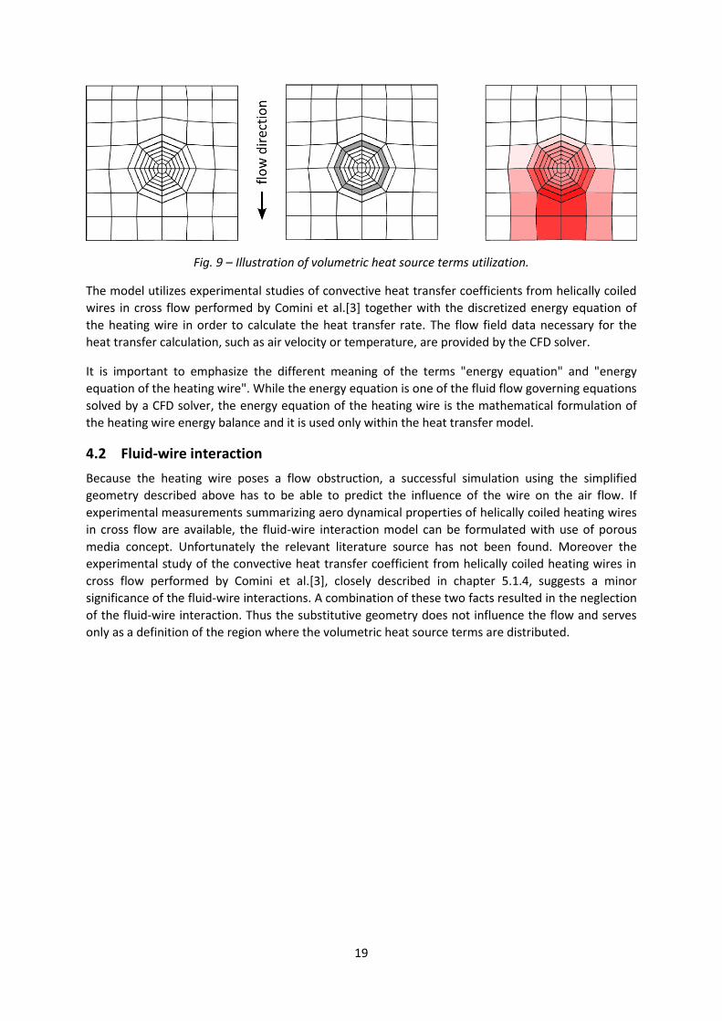
the heat transfer calculation described below, the volumetric heat source terms of the substitutive

geometry cells are set and therefore the air passing through the cells is heated up. This situation is

demonstrated on the test case shown in fig. 9a, fig. 9b and fig. 9c. Fig. 9a shows the domain

discretization, fig. 9b highlights the cells where the volumetric heat sources are applied and fig. 9c

visualizes the resulting temperature field where white and red colors represent low and high

temperatures respectively.

19

Fig. 9 – Illustration of volumetric heat source terms utilization.

The model utilizes experimental studies of convective heat transfer coefficients from helically coiled

wires in cross flow performed by Comini et al.[3] together with the discretized energy equation of

the heating wire in order to calculate the heat transfer rate. The flow field data necessary for the

heat transfer calculation, such as air velocity or temperature, are provided by the CFD solver.

It is important to emphasize the different meaning of the terms "energy equation" and "energy

equation of the heating wire". While the energy equation is one of the fluid flow governing equations

solved by a CFD solver, the energy equation of the heating wire is the mathematical formulation of

the heating wire energy balance and it is used only within the heat transfer model.

4.2 Fluid-wire interaction

Because the heating wire poses a flow obstruction, a successful simulation using the simplified

geometry described above has to be able to predict the influence of the wire on the air flow. If

experimental measurements summarizing aero dynamical properties of helically coiled heating wires

in cross flow are available, the fluid-wire interaction model can be formulated with use of porous

media concept. Unfortunately the relevant literature source has not been found. Moreover the

experimental study of the convective heat transfer coefficient from helically coiled heating wires in

cross flow performed by Comini et al.[3], closely described in chapter 5.1.4, suggests a minor

significance of the fluid-wire interactions. A combination of these two facts resulted in the neglection

of the fluid-wire interaction. Thus the substitutive geometry does not influence the flow and serves

only as a definition of the region where the volumetric heat source terms are distributed.

20

5 Heat transfer model

The crucial part of the solution method was the formulation and implementation of the heat transfer

model. As outlined in the previous chapter, the goal of the model is to predict the heat transfer from

the complicated heating coil geometry.

5.1 Development of elemental relationships

A successful model of an engineering problem should be based on a solid knowledge of elemental

principles present in the considered case. The following part of the thesis gathers all the necessary

theoretical background and develops relationships to be used in the formulation of the model.

5.1.1 Heat generation rate

Resistance heating, also known as Joule heating, resistive heating or ohmic heating, is a process

where electric energy is transformed into heat energy. When electric current passes through a

conductor, energy dissipation takes place as a result of collisions of charge carriers and elemental

particles of the conductor. From a macroscopic point of view, the increase in the kinetic energy of

the elemental particles of the conductor is observed as an increase of the conductor temperature.

The quantitative description of the heat generation rate is based on the basic direct current power

formula:

Eq. 5.1

where is the power, is the current and is the voltage drop. Because the current is the amount

of the charge transported per time unit and the voltage is the amount of energy necessary to move a

particle of unit charge across the potential difference , it is clear that the product of the two is the

amount of energy per time unit necessary to maintain the charge flow across the potential

difference . In the simple circuit consisting of a voltage source and a resistor, the power calculated

by eq. 5.1 represents the amount of energy per time unit which the voltage source has to exert in

order to keep the voltage drop between its plus and minus contacts equal to . Because the only way

how the energy flow rate supplied by the voltage source can be used is heat dissipation at the

resistor, the energy conservation principle requires those energy flow rates to be equal in magnitude.

Therefore the power calculated by the formula eq. 5.1 is equal to the heat generation rate of the

resistor in a direct current circuit.

The considered heating unit described in chapter 3.2 utilizes the standard electric grid as an energy

source. Therefore it is necessary to modify eq. 5.1 to the form suitable for alternating current

calculations. It is possible to formulate the instantaneous power given by:

( ) ( ) ( ) Eq. 5.2

where ( ) , ( ) and ( ) are instantaneous power, current and voltage drop respectively.

Nevertheless instead of instantaneous quantities it is appropriate to use time averaged quantities,

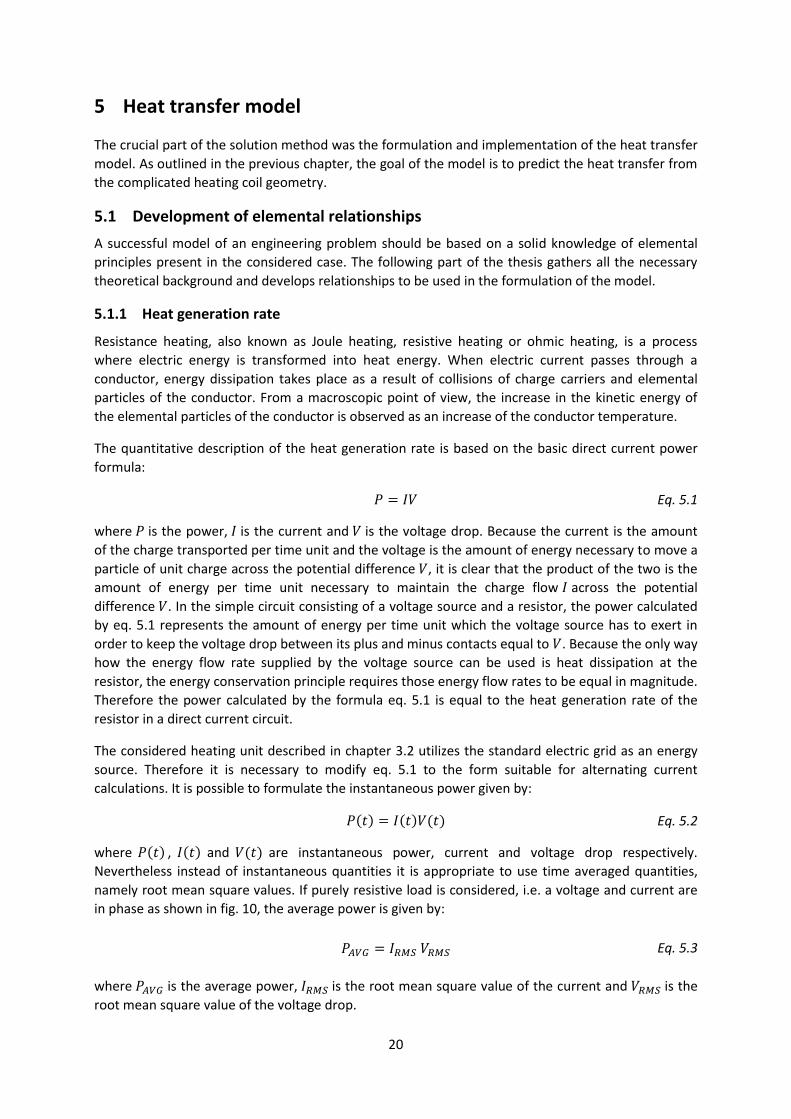
namely root mean square values. If purely resistive load is considered, i.e. a voltage and current are

in phase as shown in fig. 10, the average power is given by:

Eq. 5.3

where is the average power, is the root mean square value of the current and is the

root mean square value of the voltage drop.

21

Fig. 10 – Purely resistive load – the current and voltage in phase

It can be proven that the root mean square value of a sine function is:

( )

√ Eq. 5.4

where is the amplitude of the sine function. With use of eq. 5.4 and Ohm’s law, eq. 5.3

becomes:

Eq. 5.5

where is the current amplitude and R is the resistance of a resistor.

5.1.2 Heating wire energy equation

When an electric current starts to flow through a heating wire, a transient process involving heat

transfer and an increase in the wire temperature begins. The wire temperature grows until an

equilibrium state is reached. During the equilibrium state all the heat generated by the electric

current is transferred and no heat is accumulated in the wire. A stability of the equilibrium state is

enhanced by the usage of materials that show an increase of resistivity with temperature. This can be

proven by applying Ohm’s law on eq. 5.4 which gains:

Eq. 5.6

An increase in temperature causes an increase of a wire resistance, which results in a decrease of a

heat generation rate. This self-regulation property helps to prevent the wire from overheating.

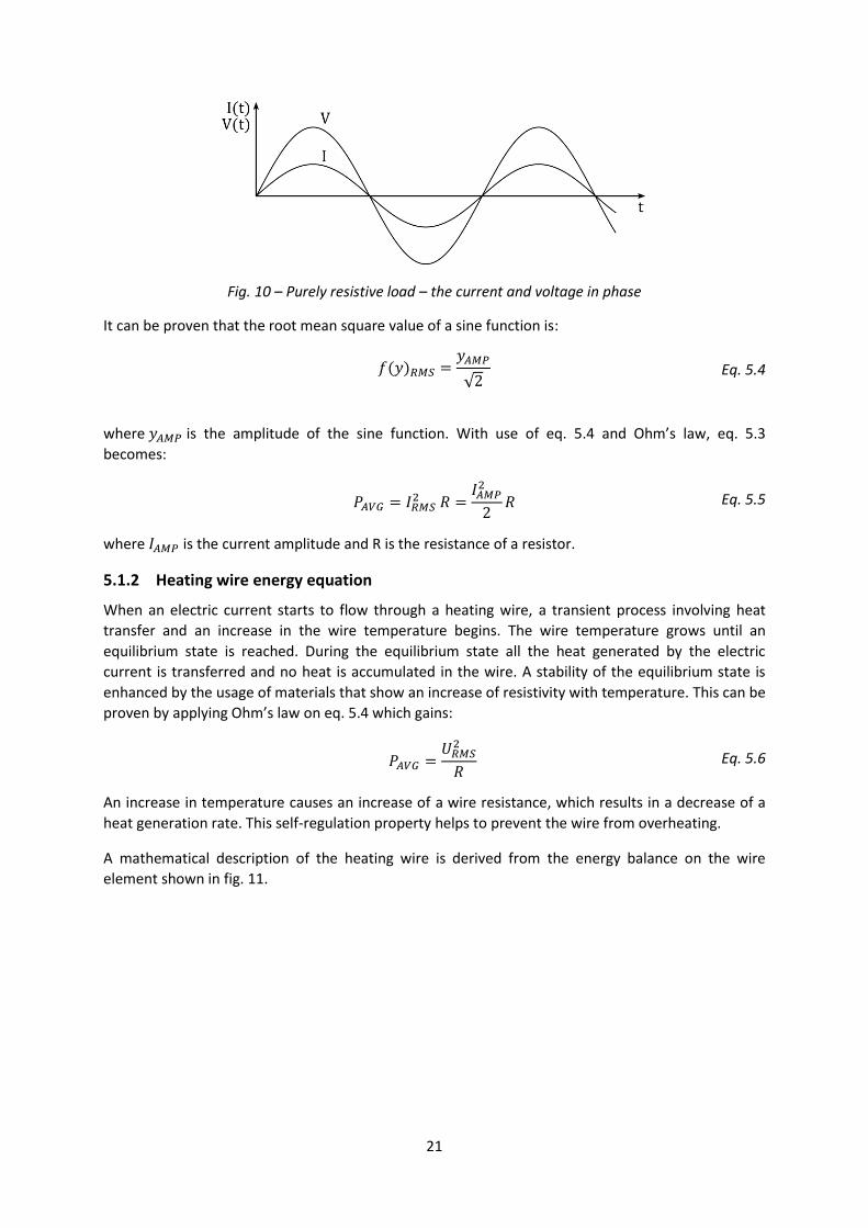
A mathematical description of the heating wire is derived from the energy balance on the wire

element shown in fig. 11.

22

Fig. 11 – Heating wire element with visualization of heat flow rates

Since a steady state formulation is needed, a basic relationship that fulfills the energy conservation

principle reads:

Eq. 5.7

where is the heat generation rate, is the convection heat transfer rate, is the

radiation heat transfer rate, is the conduction heat transfer rate at the left boundary and

is the conduction heat transfer rate at the right boundary. The four heat transfer rate terms

can be further expressed as

( ) ( ) Eq. 5.8

(

) Eq. 5.9

|

|

Eq. 5.10

|

|

Eq. 5.11

where is the convective heat transfer coefficient, is the wire temperature, is the ambient

air temperature, is the convection heat transfer area, is the wire diameter, is the wire

element length, is the emissivity, is the Stefan-Boltzmann constant, is the remote surface

temperature, is the wire material thermal conductivity, is the radiation heat transfer area,

|

is the temperature gradient at the left boundary and

|

is the temperature

gradient at the right boundary.

Since the resistivity temperature dependence of materials used for heating wires shows a linear

character, its mathematical formulation reads:

( ) ( ) Eq. 5.12

where ( ) is the resistivity at the temperature , is the resistivity temperature coefficient,

is the reference resistivity and is the temperature at which the reference resistivity is given. With

use of the basic equation relating resistivity and resistance

Eq. 5.13

23

where is the wire resistance, is the wire cross sectional area and is the wire length, eq. 5.12

can be written as:

( ) ( ) ( ) Eq. 5.14

where ( ) is the resistance at the temperature and is the reference resistance given at

temperature .

Substituting eq. 5.5, eq. 5.8, eq. 5.10, eq. 5.11 and eq. 5.14 into eq. 5.7 and neglecting the radiation

heat transfer term yields:

( ) ( )

|

|

Eq. 5.15

which is the final form of the heating wire energy equation.

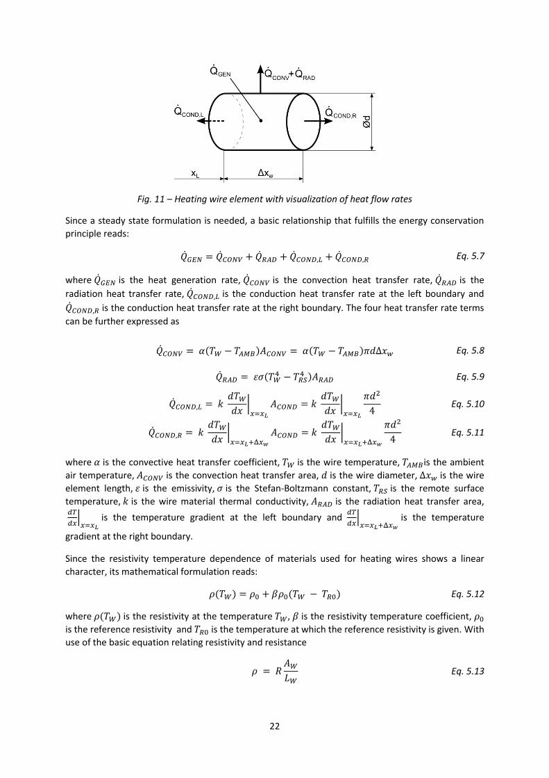
5.1.3 Discretization of the heating wire energy equation

A discrete nature of the CFD approach, together with complicated analytical solution of the

differential form of the heating wire energy equation, demands a discrete solution to be used. Eq.

5.15 implies the need to approximate only the temperature gradients at the left and right boundaries

provided that a constant thermal conductivity is assumed. Fig. 12 illustrates the discretization

problem.

Fig. 12 – Illustration of the heating wire equation discretization

The purely diffusive nature of the conduction terms in eq. 5.15 suggests the first order central

differencing approach to be used to approximate the heat conduction fluxes. In other words this

means a linear interpolation of the cell temperatures marked in fig. 12. The temperature

gradients can therefore be expressed as:

|

Eq. 5.16

24

|

Eq. 5.17

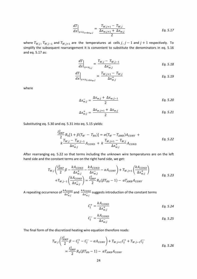
where , and are the temperatures at cells , and respectively. To

simplify the subsequent rearrangement it is convenient to substitute the denominators in eq. 5.16

and eq. 5.17 as:

|

Eq. 5.18

|

Eq. 5.19

where

Eq. 5.20

Eq. 5.21

Substituting eq. 5.30 and eq. 5.31 into eq. 5.15 yields:

( ) ( )

Eq. 5.22

After rearranging eq. 5.22 so that terms including the unknown wire temperatures are on the left

hand side and the constant terms are on the right hand side, we get:

(

) (

)

(

)

( )

Eq. 5.23

A repeating occurrence of

and

suggests introduction of the constant terms

Eq. 5.24

Eq. 5.25

The final form of the discretized heating wire equation therefore reads:

(

)

( )

Eq. 5.26

25

An application of eq. 5.26 on a heating wire discretized by cells results in a system of linear

equations which can be written in a matrix form as

Eq. 5.27

where is the coefficient matrix, is the vector of the unknown wire temperature and is the

vector of the right hand sides. With regard to the form of eq. 5.26, is a tridiagonal matrix

while and are column vectors containing elements.

5.1.4 Convection heat transfer coefficient

The model based approach discussed in chapter 4 requires a heat transfer coefficient from helically

coiled heating wires in cross flow to be determined. Comini et al.[3] have concluded the

experimental study of the method for calculating the required convective heat transfer coefficient,

which serves as the basis for the model development in this thesis.

As stated in Comini et al.[3], “despite the widespread use of open-coil air heaters, forced convection

heat transfer from helical coiled resistance wires in cross flow has not been considered in the

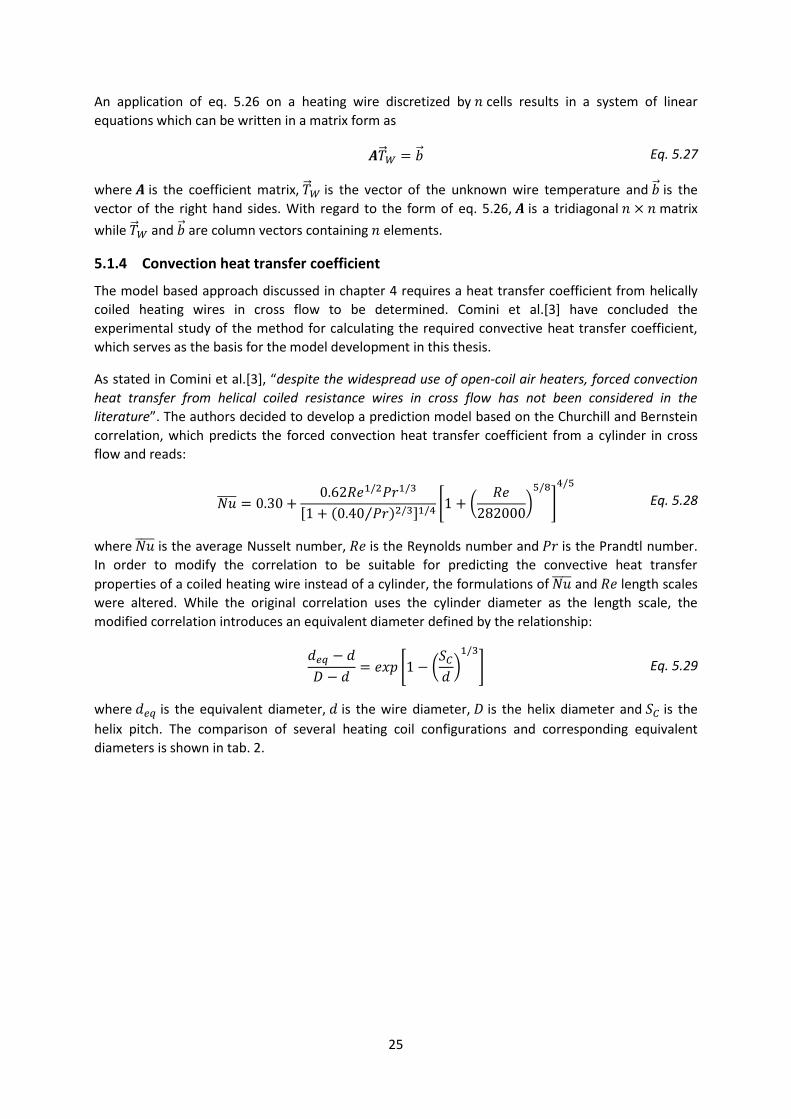
literature”. The authors decided to develop a prediction model based on the Churchill and Bernstein

correlation, which predicts the forced convection heat transfer coefficient from a cylinder in cross

flow and reads:

( ⁄ ) [ (

)

]

Eq. 5.28

where is the average Nusselt number, is the Reynolds number and is the Prandtl number.

In order to modify the correlation to be suitable for predicting the convective heat transfer

properties of a coiled heating wire instead of a cylinder, the formulations of and length scales

were altered. While the original correlation uses the cylinder diameter as the length scale, the

modified correlation introduces an equivalent diameter defined by the relationship:

[ (

)

] Eq. 5.29

where is the equivalent diameter, is the wire diameter, is the helix diameter and is the

helix pitch. The comparison of several heating coil configurations and corresponding equivalent

diameters is shown in tab. 2.

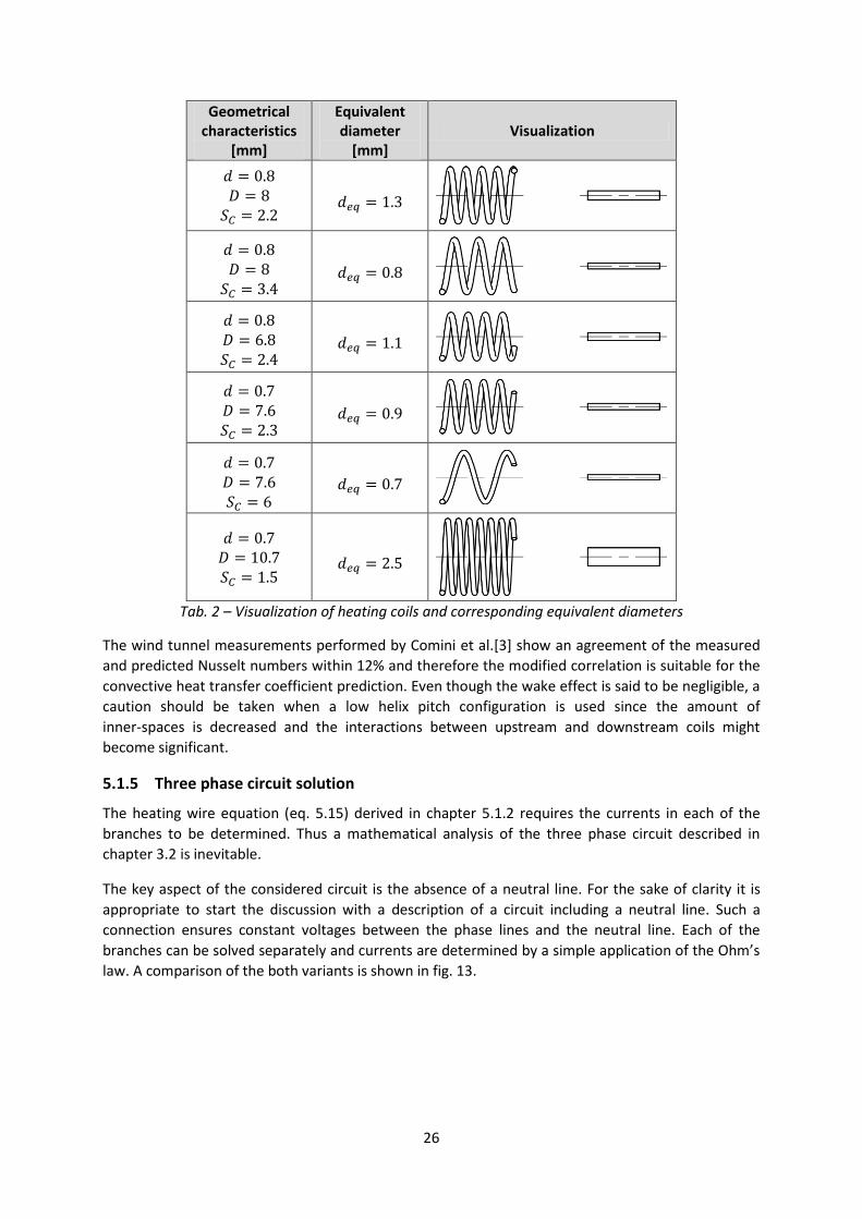
26

Geometrical characteristics

[mm]

Equivalent diameter

[mm] Visualization

Tab. 2 – Visualization of heating coils and corresponding equivalent diameters

The wind tunnel measurements performed by Comini et al.[3] show an agreement of the measured

and predicted Nusselt numbers within 12% and therefore the modified correlation is suitable for the

convective heat transfer coefficient prediction. Even though the wake effect is said to be negligible, a

caution should be taken when a low helix pitch configuration is used since the amount of

inner-spaces is decreased and the interactions between upstream and downstream coils might

become significant.

5.1.5 Three phase circuit solution

The heating wire equation (eq. 5.15) derived in chapter 5.1.2 requires the currents in each of the

branches to be determined. Thus a mathematical analysis of the three phase circuit described in

chapter 3.2 is inevitable.

The key aspect of the considered circuit is the absence of a neutral line. For the sake of clarity it is

appropriate to start the discussion with a description of a circuit including a neutral line. Such a

connection ensures constant voltages between the phase lines and the neutral line. Each of the

branches can be solved separately and currents are determined by a simple application of the Ohm’s

law. A comparison of the both variants is shown in fig. 13.

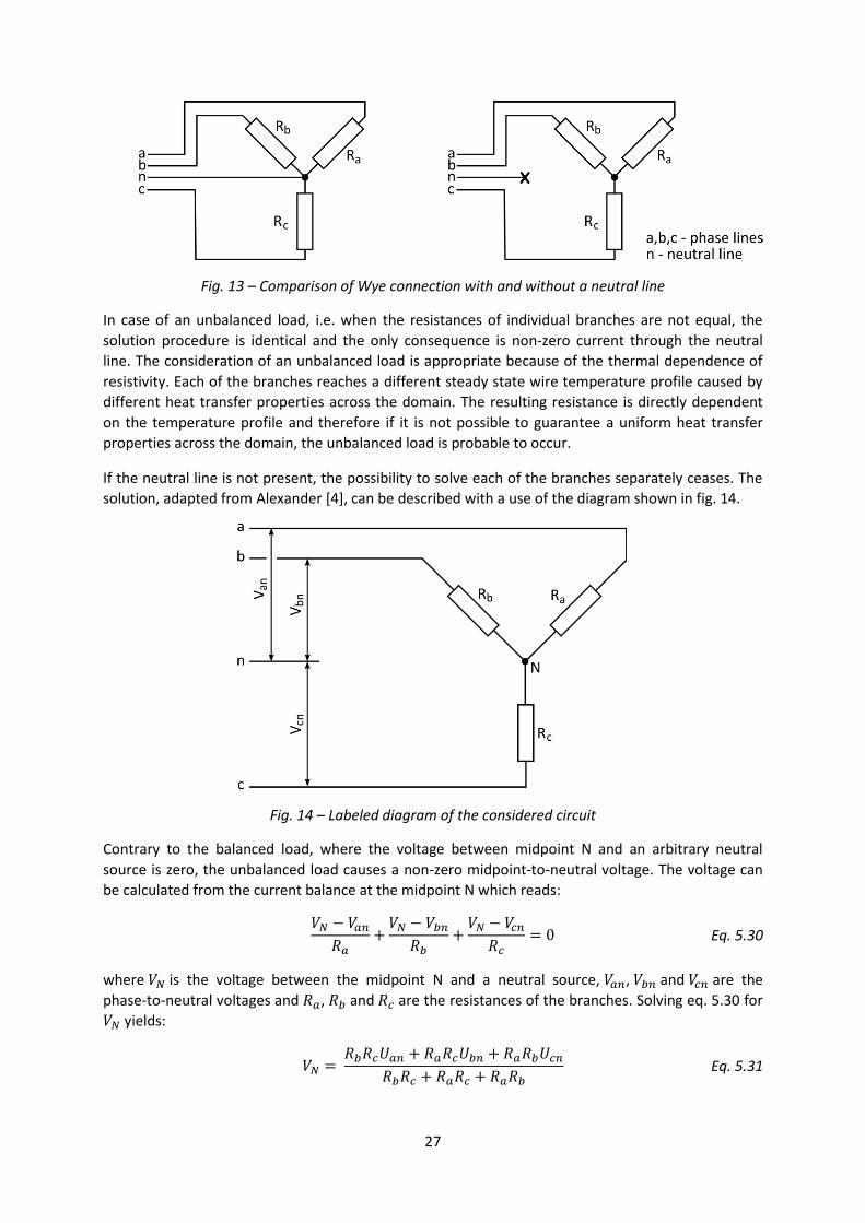
27

Fig. 13 – Comparison of Wye connection with and without a neutral line

In case of an unbalanced load, i.e. when the resistances of individual branches are not equal, the

solution procedure is identical and the only consequence is non-zero current through the neutral

line. The consideration of an unbalanced load is appropriate because of the thermal dependence of

resistivity. Each of the branches reaches a different steady state wire temperature profile caused by

different heat transfer properties across the domain. The resulting resistance is directly dependent

on the temperature profile and therefore if it is not possible to guarantee a uniform heat transfer

properties across the domain, the unbalanced load is probable to occur.

If the neutral line is not present, the possibility to solve each of the branches separately ceases. The

solution, adapted from Alexander [4], can be described with a use of the diagram shown in fig. 14.

Fig. 14 – Labeled diagram of the considered circuit

Contrary to the balanced load, where the voltage between midpoint N and an arbitrary neutral

source is zero, the unbalanced load causes a non-zero midpoint-to-neutral voltage. The voltage can

be calculated from the current balance at the midpoint N which reads:

Eq. 5.30

where is the voltage between the midpoint N and a neutral source, , and are the

phase-to-neutral voltages and , and are the resistances of the branches. Solving eq. 5.30 for

yields:

Eq. 5.31

28

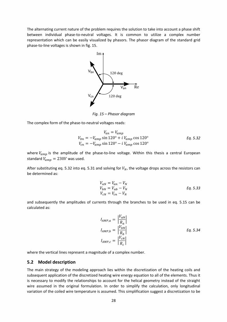
The alternating current nature of the problem requires the solution to take into account a phase shift

between individual phase-to-neutral voltages. It is common to utilize a complex number

representation which can be easily visualized by phasors. The phasor diagram of the standard grid

phase-to-line voltages is shown in fig. 15.

Fig. 15 – Phasor diagram

The complex form of the phase-to-neutral voltages reads:

Eq. 5.32

where is the amplitude of the phase-to-line voltage. Within this thesis a central European

standard was used.

After substituting eq. 5.32 into eq. 5.31 and solving for , the voltage drops across the resistors can

be determined as:

Eq. 5.33

and subsequently the amplitudes of currents through the branches to be used in eq. 5.15 can be

calculated as:

|

|

|

|

|

|

Eq. 5.34

where the vertical lines represent a magnitude of a complex number.

5.2 Model description

The main strategy of the modeling approach lies within the discretization of the heating coils and

subsequent application of the discretized heating wire energy equation to all of the elements. Thus it

is necessary to modify the relationships to account for the helical geometry instead of the straight

wire assumed in the original formulation. In order to simplify the calculation, only longitudinal

variation of the coiled wire temperature is assumed. This simplification suggest a discretization to be

29

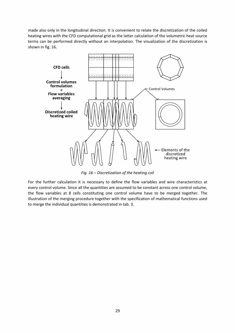
made also only in the longitudinal direction. It is convenient to relate the discretization of the coiled

heating wires with the CFD computational grid as the latter calculation of the volumetric heat source

terms can be performed directly without an interpolation. The visualization of the discretization is

shown in fig. 16.

Fig. 16 – Discretization of the heating coil

For the further calculation it is necessary to define the flow variables and wire characteristics at

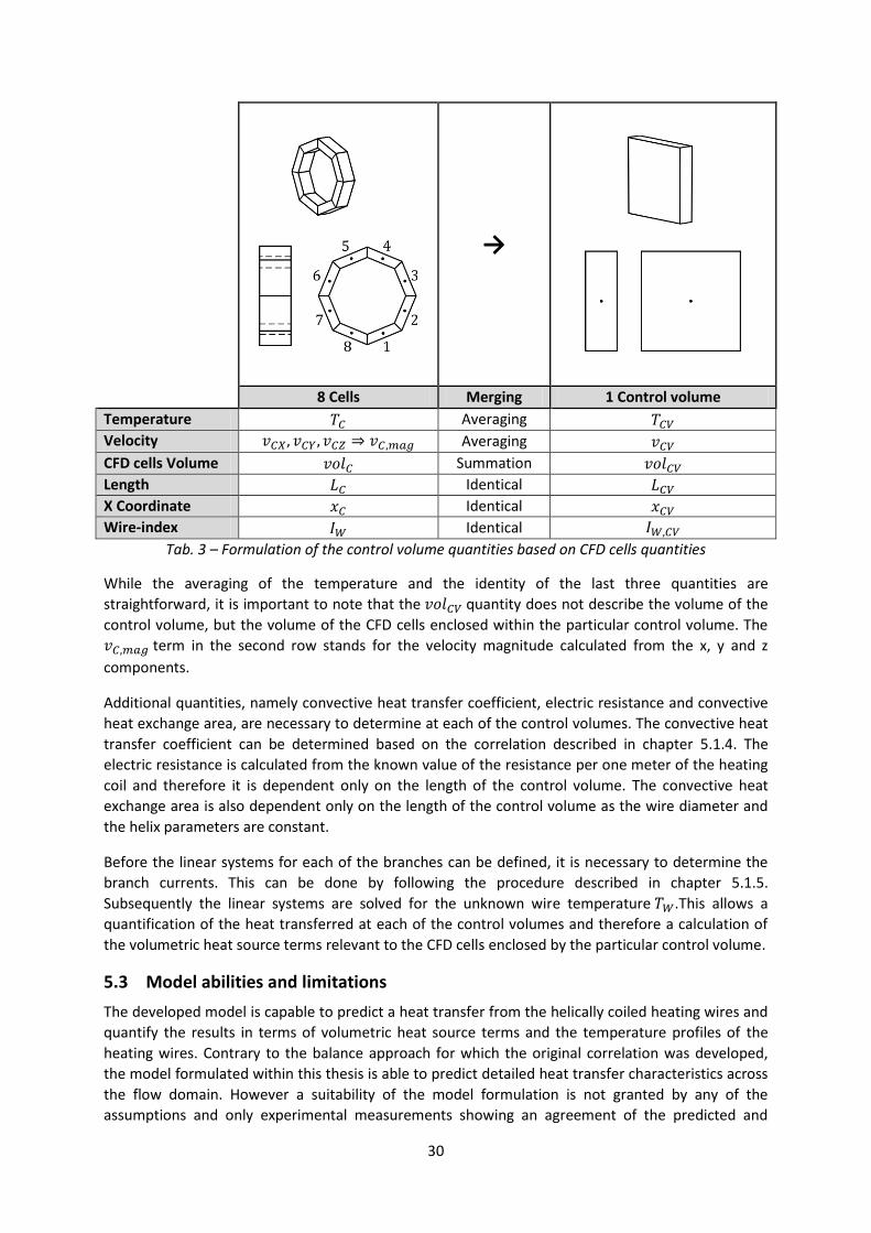
every control volume. Since all the quantities are assumed to be constant across one control volume,

the flow variables at 8 cells constituting one control volume have to be merged together. The

illustration of the merging procedure together with the specification of mathematical functions used

to merge the individual quantities is demonstrated in tab. 3.

30

→

8 Cells Merging 1 Control volume

Temperature Averaging

Velocity Averaging

CFD cells Volume Summation

Length Identical

X Coordinate Identical

Wire-index Identical

Tab. 3 – Formulation of the control volume quantities based on CFD cells quantities

While the averaging of the temperature and the identity of the last three quantities are

straightforward, it is important to note that the quantity does not describe the volume of the

control volume, but the volume of the CFD cells enclosed within the particular control volume. The

term in the second row stands for the velocity magnitude calculated from the x, y and z

components.

Additional quantities, namely convective heat transfer coefficient, electric resistance and convective

heat exchange area, are necessary to determine at each of the control volumes. The convective heat

transfer coefficient can be determined based on the correlation described in chapter 5.1.4. The

electric resistance is calculated from the known value of the resistance per one meter of the heating

coil and therefore it is dependent only on the length of the control volume. The convective heat

exchange area is also dependent only on the length of the control volume as the wire diameter and

the helix parameters are constant.

Before the linear systems for each of the branches can be defined, it is necessary to determine the

branch currents. This can be done by following the procedure described in chapter 5.1.5.

Subsequently the linear systems are solved for the unknown wire temperature .This allows a

quantification of the heat transferred at each of the control volumes and therefore a calculation of

the volumetric heat source terms relevant to the CFD cells enclosed by the particular control volume.

5.3 Model abilities and limitations

The developed model is capable to predict a heat transfer from the helically coiled heating wires and

quantify the results in terms of volumetric heat source terms and the temperature profiles of the

heating wires. Contrary to the balance approach for which the original correlation was developed,

the model formulated within this thesis is able to predict detailed heat transfer characteristics across

the flow domain. However a suitability of the model formulation is not granted by any of the

assumptions and only experimental measurements showing an agreement of the predicted and

31

measured values can support the validity of this approach. Since the cross flow condition, assumed in

the experimental study of the convective heat transfer coefficient, is violated in the wire supports

region, the transferred heat and wire temperatures in this region are expected to be over or

under-predicted.

Because of the complicated geometry a radiation heat transfer was neglected. As air in the

atmospheric composition and temperatures reached in the dryer does not significantly participate in

the radiation heat transfer, the main expected source of error caused by the neglection of the

radiation heat transfer lies in the increase in the surface temperature of the metal parts that

surround the heating coils and subsequent convective heat transfer from the parts to the air.

Since the experimental data used to formulate the model does not include the influence of the free

stream turbulence levels, also the model is unable to predict the relationship between the

turbulence properties and the heat transfer.

5.4 Implementation

The need to employ a custom code demanded a programming platform to be chosen. Ansys Fluent

offers a possibility to implement custom code calculations as user defined functions (UDF). By using a

C programming language and predefined macros, one can easily access the flow variables, perform

additional calculations and integrate the calculation results into the solution process. Even though

the Fluent's UDF interface offers all the necessary tools, it has been decided to use it only for data

export/import and to perform the main body of the model related calculations in Matlab. The reason

for this is the user friendly environment allowing an effective debugging together with a great

number of predefined functions allowing a fast solution of elementary vector and matrix operations.

A negative consequence of the Matlab approach is an increase in the computational time caused by

the need to export the data from Fluent, process it and import it back. However, during a

development stage, this approach appears to be perfectly suitable. The final deployment of the

model should nevertheless utilize some of the lower level programming languages to guarantee a

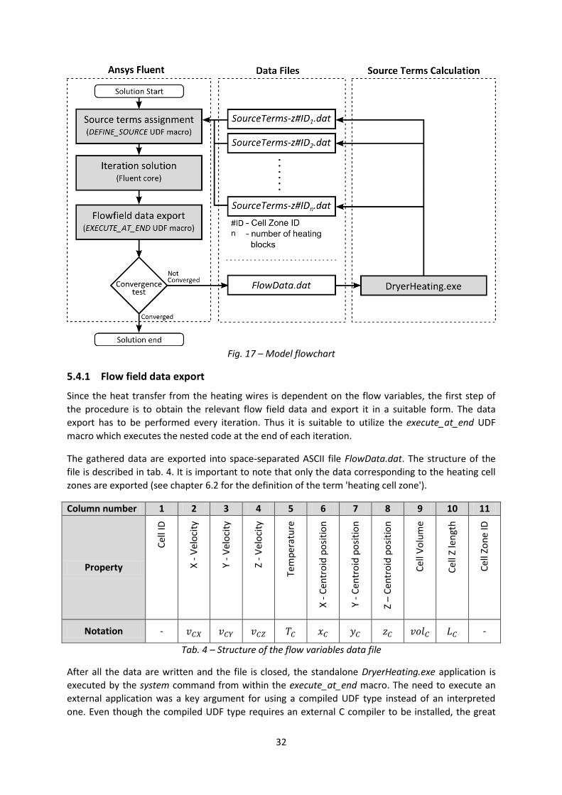
maximum computational efficiency. A flowchart of the model implementation is shown in fig. 17. The

following chapters discuss the individual steps in detail.

32

Fig. 17 – Model flowchart

5.4.1 Flow field data export

Since the heat transfer from the heating wires is dependent on the flow variables, the first step of

the procedure is to obtain the relevant flow field data and export it in a suitable form. The data

export has to be performed every iteration. Thus it is suitable to utilize the execute_at_end UDF

macro which executes the nested code at the end of each iteration.

The gathered data are exported into space-separated ASCII file FlowData.dat. The structure of the

file is described in tab. 4. It is important to note that only the data corresponding to the heating cell

zones are exported (see chapter 6.2 for the definition of the term 'heating cell zone').

Column number 1 2 3 4 5 6 7 8 9 10 11

Property

Cel

l ID

X -

Vel

oci

ty

Y -

Vel

oci

ty

Z -

Vel

oci

ty

Tem

per

atu

re

X -

Cen

tro

id p

osi

tio

n

Y -

Cen

tro

id p

osi

tio

n

Z –

Cen

tro

id p

osi

tio

n

Cel

l Vo

lum

e

Cel

l Z le

ngt

h

Cel

l Zo

ne

ID

Notation - -

Tab. 4 – Structure of the flow variables data file

After all the data are written and the file is closed, the standalone DryerHeating.exe application is

executed by the system command from within the execute_at_end macro. The need to execute an

external application was a key argument for using a compiled UDF type instead of an interpreted

one. Even though the compiled UDF type requires an external C compiler to be installed, the great

33

benefit, besides being faster, is the possibility to include standard C libraries and consequently use

functions such as system. The source code of the UDF is attached as appendix A.

5.4.2 Calculation of the volumetric heat source terms

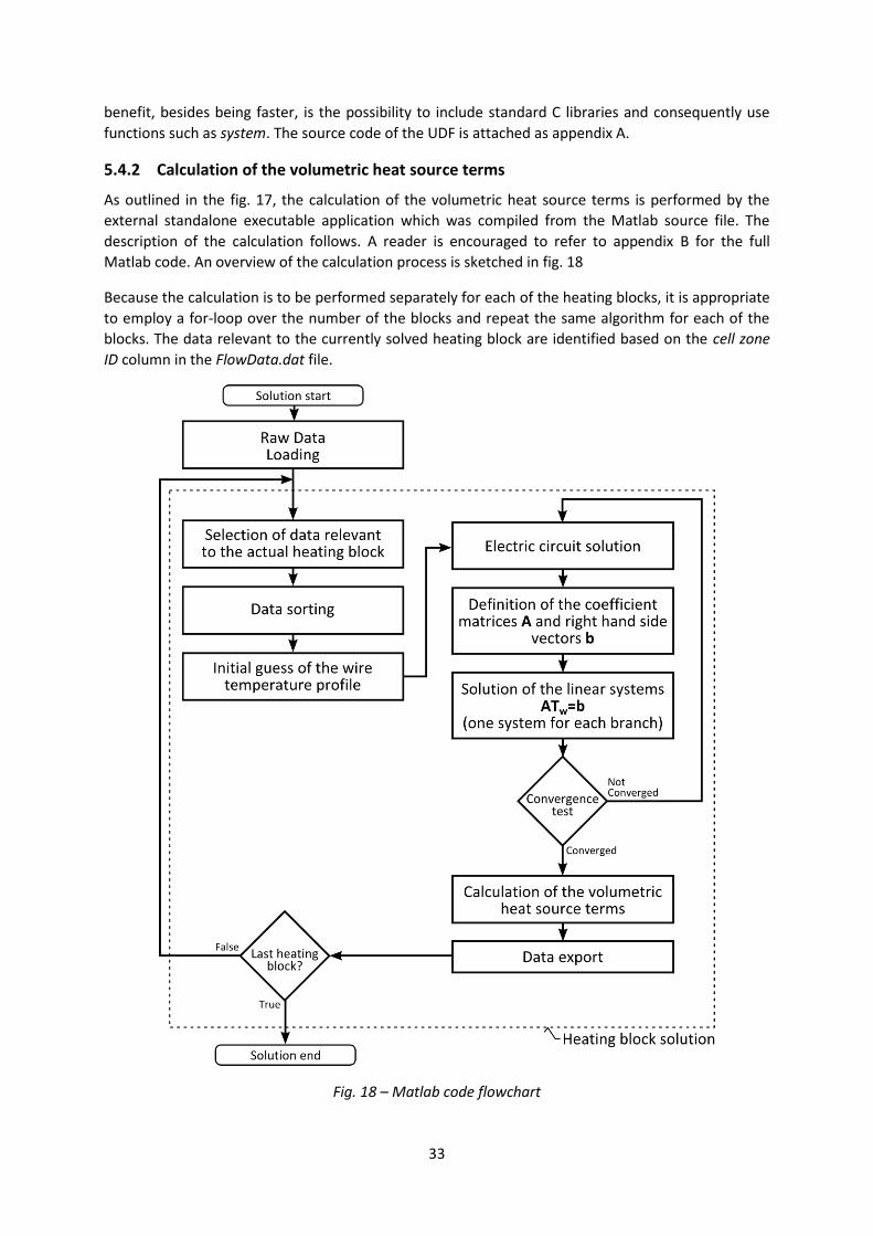
As outlined in the fig. 17, the calculation of the volumetric heat source terms is performed by the

external standalone executable application which was compiled from the Matlab source file. The

description of the calculation follows. A reader is encouraged to refer to appendix B for the full

Matlab code. An overview of the calculation process is sketched in fig. 18

Because the calculation is to be performed separately for each of the heating blocks, it is appropriate

to employ a for-loop over the number of the blocks and repeat the same algorithm for each of the

blocks. The data relevant to the currently solved heating block are identified based on the cell zone

ID column in the FlowData.dat file.

Fig. 18 – Matlab code flowchart

34

In the next step an extensive data manipulation is inevitable in order to process the data into a form

suitable for a solution of the linear systems resulting from the application of the discretized heat wire

equation to each of the branches. The linear systems cannot be explicitly solved for because the

current term which is present on both the left and the right hand side of eq. 5.26. The

magnitude of is dependent on the resistances of each of the branches within the block and

since these resistances are functions of , a necessity to utilize an iterative approach arises.

To start the iterative solution, the wire temperature profiles have to be guessed. Subsequently the

resistances can be calculated and used to determine the currents through the individual branches. At

this stage, the coefficient matrices and the vectors of the right hand sides can be defined, allowing a

solution of the linear systems. At each iteration the currents are adjusted with regard to the actual

wire temperatures. After the solution has converged, the volumetric heat source terms can be

determined and exported.

It can be noted here that the Matlab code was formulated in a way that allows a future usage of the

model to take into account a variable heating coil geometry in each of the heating blocks. This aspect

is necessary when the heating unit configuration including both the 4.5KW and 6KW heating blocks is

considered. The variable heating geometry implementation is based on the fact that the coil and wire

parameters are stored as vectors. The code utilizes a dist.dat data file to specify the vector index to

be used for the particular heating block represented by the heating cell zone ID.

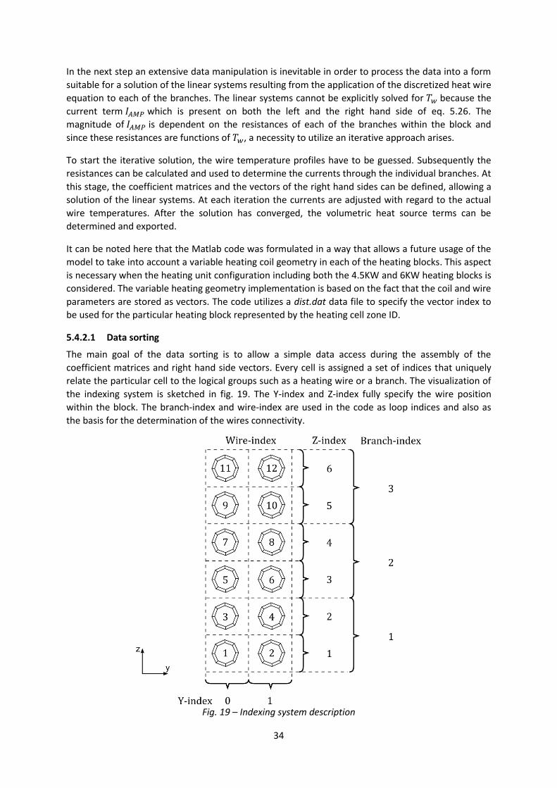
5.4.2.1 Data sorting

The main goal of the data sorting is to allow a simple data access during the assembly of the

coefficient matrices and right hand side vectors. Every cell is assigned a set of indices that uniquely

relate the particular cell to the logical groups such as a heating wire or a branch. The visualization of

the indexing system is sketched in fig. 19. The Y-index and Z-index fully specify the wire position

within the block. The branch-index and wire-index are used in the code as loop indices and also as

the basis for the determination of the wires connectivity.

Fig. 19 – Indexing system description

35

The Y-index can be defined as:

{

Eq. 5.35

where is the Y-index, is the y coordinate of the cell centroid and is the y coordinate of the

heating block center point, defined as:

( ) ( )

Eq. 5.36

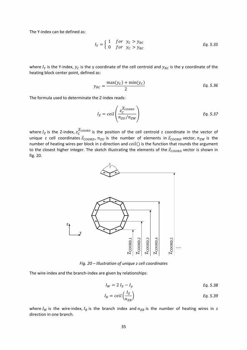
The formula used to determinate the Z-index reads:

(

⁄) Eq. 5.37

where is the Z-index, is the position of the cell centroid z coordinate in the vector of

unique z cell coordinates , is the number of elements in vector, is the

number of heating wires per block in z-direction and () is the function that rounds the argument

to the closest higher integer. The sketch illustrating the elements of the vector is shown in

fig. 20.

Fig. 20 – Illustration of unique z cell coordinates

The wire-index and the branch-index are given by relationships:

Eq. 5.38

(

) Eq. 5.39

where is the wire-index, is the branch index and is the number of heating wires in z

direction in one branch.

36

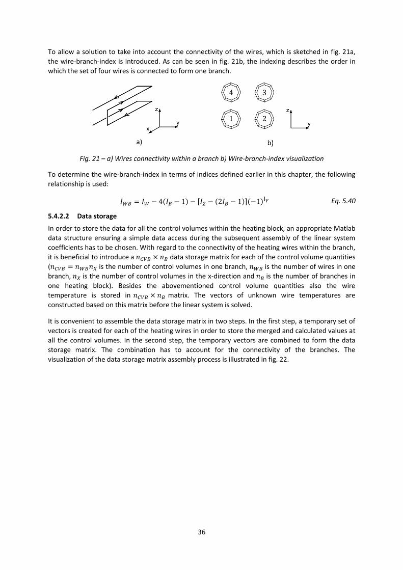
To allow a solution to take into account the connectivity of the wires, which is sketched in fig. 21a,

the wire-branch-index is introduced. As can be seen in fig. 21b, the indexing describes the order in

which the set of four wires is connected to form one branch.

Fig. 21 – a) Wires connectivity within a branch b) Wire-branch-index visualization

To determine the wire-branch-index in terms of indices defined earlier in this chapter, the following

relationship is used:

( ) ( ) ( ) Eq. 5.40

5.4.2.2 Data storage

In order to store the data for all the control volumes within the heating block, an appropriate Matlab

data structure ensuring a simple data access during the subsequent assembly of the linear system

coefficients has to be chosen. With regard to the connectivity of the heating wires within the branch,

it is beneficial to introduce a data storage matrix for each of the control volume quantities

( is the number of control volumes in one branch, is the number of wires in one

branch, is the number of control volumes in the x-direction and is the number of branches in

one heating block). Besides the abovementioned control volume quantities also the wire

temperature is stored in matrix. The vectors of unknown wire temperatures are

constructed based on this matrix before the linear system is solved.

It is convenient to assemble the data storage matrix in two steps. In the first step, a temporary set of

vectors is created for each of the heating wires in order to store the merged and calculated values at

all the control volumes. In the second step, the temporary vectors are combined to form the data

storage matrix. The combination has to account for the connectivity of the branches. The

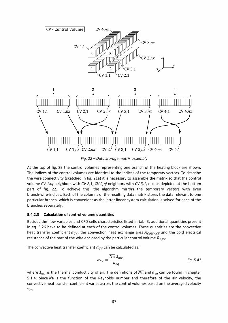
visualization of the data storage matrix assembly process is illustrated in fig. 22.

37

Fig. 22 – Data storage matrix assembly

At the top of fig. 22 the control volumes representing one branch of the heating block are shown.

The indices of the control volumes are identical to the indices of the temporary vectors. To describe

the wire connectivity (sketched in fig. 21a) it is necessary to assemble the matrix so that the control

volume CV 1,nj neighbors with CV 2,1, CV 2,nj neighbors with CV 3,1, etc. as depicted at the bottom

part of fig. 22. To achieve this, the algorithm mirrors the temporary vectors with even

branch-wire-indices. Each of the columns of the resulting data matrix stores the data relevant to one

particular branch, which is convenient as the latter linear system calculation is solved for each of the

branches separately.

5.4.2.3 Calculation of control volume quantities

Besides the flow variables and CFD cells characteristics listed in tab. 3, additional quantities present

in eq. 5.26 have to be defined at each of the control volumes. These quantities are the convective

heat transfer coefficient , the convection heat exchange area and the cold electrical

resistance of the part of the wire enclosed by the particular control volume .

The convective heat transfer coefficient can be calculated as:

Eq. 5.41

where is the thermal conductivity of air. The definitions of and can be found in chapter

5.1.4. Since is the function of the Reynolds number and therefore of the air velocity, the

convective heat transfer coefficient varies across the control volumes based on the averaged velocity

.

38

The relationship used to determine the convection heat transfer area reads:

( )( )

Eq. 5.42

The control volume resistance is given as:

Eq. 5.43

Where is the resistance of one meter of the heating coil, which was calculated from the

experimentally measured cold branch resistance as:

Eq. 5.44

where is the length of the heating coil. It is important not to confuse the term 'length of the

heating coil' with the length of the wire used as a semi-product to form the coiled wire geometry.

5.4.3 Linear systems definition

With all the necessary data sorted and the coiled wire geometry discretized, it is possible to apply the

discretized heating wire energy equation to the coiled heating wire, which for the jth control volume

in the kth branch reads:

(

)

( )

Eq. 5.45

where is the matrix of the unknown wire temperature, and are the

matrices of the constant terms and is the vector of the currents through the branches.

In order to determine the wire temperature at all the control volumes, one linear system for each of

the branches has to be solved. The matrix notation of the linear systems can be written as:

Eq. 5.46

where is the coefficient matrix of the kth branch, is the vector of the unknown wire

temperature for the kth branch and is the right hand sides vector for the kth branch. The

coefficient matrix can be defined as:

( )

{

Eq. 5.47

which results in a tridiagonal matrix. The vector of the unknown wire temperature

can be extracted from the matrix as:

( ) ( )

Eq. 5.48

39

The right hand side vector is given by

( )

( )

Eq. 5.49

Because both the coefficient matrix and the right hand side vector contain the vector which is

dependent on the wire temperature, the solution of the wire temperature field cannot be calculated

explicitly. An iteration approach is therefore utilized and described below.

5.4.3.1 Iterative solution of the wire temperature field

The first inevitable step for an arbitrary iteration process is the initial guess. In the present case the

temperature field has to be guessed in order to allow the branch resistances and subsequently the

branch currents to be determined. A constant temperature guess of 250°C is used in the Matlab

code.

In the beginning of every iteration, the branch resistances are determined as:

( ) ∑ ( )

Eq. 5.50

where ( ) is the kth element of the vector of branch resistances . With known branch

resistances the currents can be determined based on the three phase circuit solution procedure

described in chapter 5.1.5.

Now the coefficient matrix and the right hand side vector can be assembled. The assumption of

adiabatic boundary conditions implies:

Eq. 5.51

The complete linear systems were solved by linsolve matlab function. However if the model is to be

implemented in some of the lower level programming languages, the solution can be obtained by an

implementation of numerical algorithms such as LU decomposition, Gauss-Seidel method, etc.

At the end of every iteration the two norm value of the

matrix is calculated and used

as the convergence criterion (the superscript stands for the current iteration and stands for

the previous iteration). The iteration procedure is repeated until the convergence criterion value is

larger than the required accuracy . For the calculations performed within this thesis, the value

was used.

5.4.3.2 Calculation and export of the volumetric heat source terms

With known values of the wire temperature at each of the control volumes, the calculation of the

volumetric heat source terms is straightforward. The amount of transferred heat at each of the

control volumes is given by:

( )

( ) Eq. 5.52

where is the matrix of the transferred heat. To obtain the value of the volumetric heat source,

the transferred heat has to be divided by the reference volume, which for this case is the volume of

40

the eight CFD cells enclosed by each of the control volumes (stored in the matrix). Therefore

the volumetric heat source is given by:

( )

( )

( ) Eq. 5.53

where is the matrix of the volumetric heat sources.

As the last step, the data has to be exported in a format suitable for the subsequent use in fluent. It is

necessary to specify the volumetric heat source value at each of the CFD cells represented by the cell

ID, which requires an identification of cell ID values related to each of the control volumes. The

related cell ID values can be identified in the raw data matrix based on the x-position value and

the wire-index . The obtained Cell ID values are linked together with the corresponding

volumetric heat source values and wire temperatures and exported into data files. A separate data

file with structure given by tab. 5 is used for each of the heating blocks as indicated in the flowchart

in fig. 17.

Column 1 2 3

Property Cell ID Volumetric Heat Source Term value Wire temperature

Tab. 5 – Data structure of the volumetric heat source terms data file

41

6 Present Case CFD Analysis

Within this chapter all the steps and considerations performed in order to obtain the flow field

solution are discussed. The simplifications and relationships introduced in chapters 4 and 5 are

utilized and applied to the CFD solver environment. To realize the CFD simulation, a software

combination of Gambit 2.4.6, Ansys Fluent 14.0 and Matlab R2010b has been used.

6.1 Computational Domain and Boundary Conditions

The first step of a general CFD problem is the formulation of a computational domain with regard to

the goals of a simulation. The confined flow nature of the considered case implies the dryer walls to

form the domain boundaries. In order to fully define the domain, upstream and downstream

boundaries have to be specified. This selection is usually a trade-off between accuracy and

computing power requirements, because a larger domain, ensuring a higher accuracy, obviously

demands a higher number of discretization cells and therefore higher computing power

requirements.

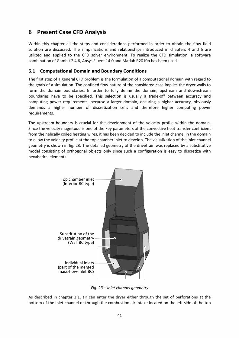
The upstream boundary is crucial for the development of the velocity profile within the domain.

Since the velocity magnitude is one of the key parameters of the convective heat transfer coefficient

from the helically coiled heating wires, it has been decided to include the inlet channel in the domain

to allow the velocity profile at the top chamber inlet to develop. The visualization of the inlet channel

geometry is shown in fig. 23. The detailed geometry of the drivetrain was replaced by a substitutive

model consisting of orthogonal objects only since such a configuration is easy to discretize with

hexahedral elements.

Fig. 23 – Inlet channel geometry

As described in chapter 3.1, air can enter the dryer either through the set of perforations at the

bottom of the inlet channel or through the combustion air intake located on the left side of the top

42

chamber. Since the only known value is the total air flow rate measured at the outlet, an accurate

solution of this multiple inlet configuration demands a computational domain enclosing all the inlets.

Such a domain configuration ensures a flow field solution allowing for a non-uniform distribution of

the mass flow across the individual inlet parts. The assessment of the inlet uniformity significance

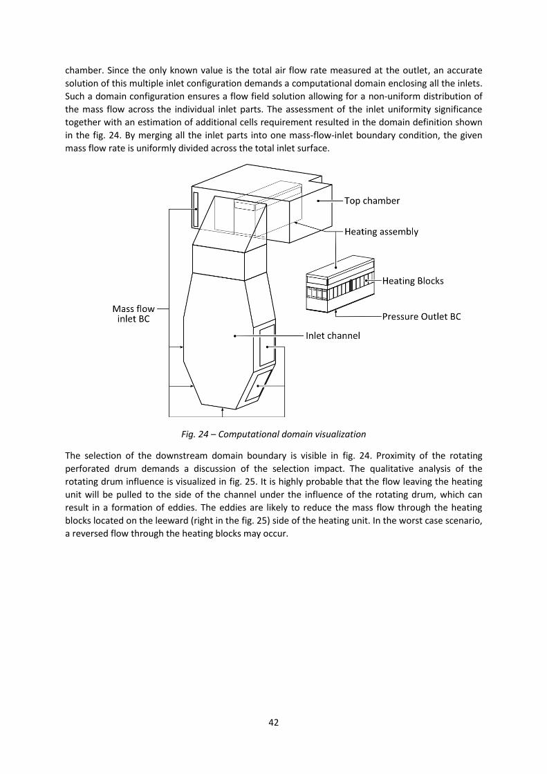
together with an estimation of additional cells requirement resulted in the domain definition shown

in the fig. 24. By merging all the inlet parts into one mass-flow-inlet boundary condition, the given

mass flow rate is uniformly divided across the total inlet surface.

Fig. 24 – Computational domain visualization

The selection of the downstream domain boundary is visible in fig. 24. Proximity of the rotating

perforated drum demands a discussion of the selection impact. The qualitative analysis of the

rotating drum influence is visualized in fig. 25. It is highly probable that the flow leaving the heating

unit will be pulled to the side of the channel under the influence of the rotating drum, which can

result in a formation of eddies. The eddies are likely to reduce the mass flow through the heating

blocks located on the leeward (right in the fig. 25) side of the heating unit. In the worst case scenario,

a reversed flow through the heating blocks may occur.

43

Fig. 25 – The influence of the rotating drum on the heating channel flow

A basic quantitative analysis of the rotating drum influence can be based on the comparison of the

drum and air velocities. The drum velocity can be calculated as:

where is the drum velocity, is the rotational speed of the drum in rpm and is

the radius of the drum. The velocity of the air at the heating unit outlet is given by

where is the air velocity, is the air volumetric flow rate and is the cross-sectional area

of the channel. The comparison of the calculated velocities reveals a slight dominance of the drum

velocity. Thus the pulling effect described above cannot be neglected. However a simple solution

taking into account the pulling effect while keeping the original domain boundary has not been

found. Therefore the only possible solution is to move the outlet boundary further downstream and

to include the drum geometry in the computational domain. If no simplifications are introduced, a

number of additional cells can be estimated as

Where is the number of cells required for the discretization of the drum region, is the

number of perforations, is the number of cells required to discretize one perforation, is

the number of cells required to discretize the internal region of the drum and is number of cells

required to discretize the outer drum region. Using estimated values (shorter drum

version used in T24 model), , the number of required

cells is

44

which is unacceptable due to immense computing power requirements. Moreover a brief literature

research has not discovered any source applicable to the drum geometry in order to formulate a

simplified model of the drum flow. As a result, it is inevitable to use the original definition of the

computational domain and do not include the drum in the simulation.

The downstream boundary type was selected to be a pressure outlet. The value of the gauge

pressure was set to zero. Since the main pressure drop is expected to take a place in the drum

region, this assumption is considered to be valid within the required accuracy.

6.2 Computational grid

A grid generation procedure has to take into account several requirements. Beside a choice of

discretization elements type, a grid size has to be appropriate to the required accuracy, available

computing power and physical processes to be resolved. Too coarse grid can degrade the solution

accuracy while too fine grid can exceed the computing hardware limits.

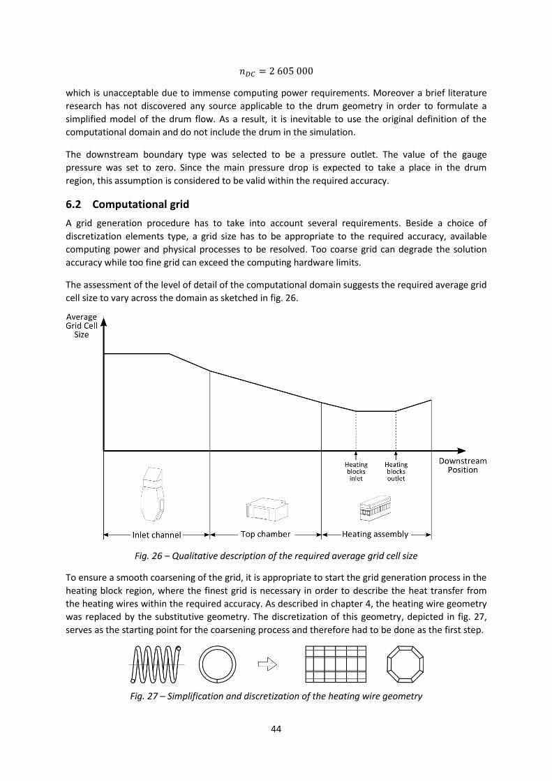
The assessment of the level of detail of the computational domain suggests the required average grid

cell size to vary across the domain as sketched in fig. 26.

Fig. 26 – Qualitative description of the required average grid cell size

To ensure a smooth coarsening of the grid, it is appropriate to start the grid generation process in the

heating block region, where the finest grid is necessary in order to describe the heat transfer from

the heating wires within the required accuracy. As described in chapter 4, the heating wire geometry

was replaced by the substitutive geometry. The discretization of this geometry, depicted in fig. 27,

serves as the starting point for the coarsening process and therefore had to be done as the first step.

Fig. 27 – Simplification and discretization of the heating wire geometry

45

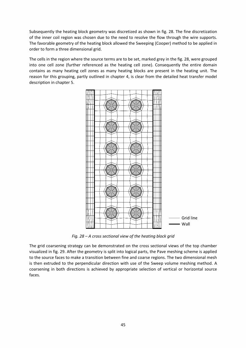
Subsequently the heating block geometry was discretized as shown in fig. 28. The fine discretization

of the inner coil region was chosen due to the need to resolve the flow through the wire supports.

The favorable geometry of the heating block allowed the Sweeping (Cooper) method to be applied in

order to form a three dimensional grid.

The cells in the region where the source terms are to be set, marked grey in the fig. 28, were grouped

into one cell zone (further referenced as the heating cell zone). Consequently the entire domain

contains as many heating cell zones as many heating blocks are present in the heating unit. The

reason for this grouping, partly outlined in chapter 4, is clear from the detailed heat transfer model

description in chapter 5.

Fig. 28 – A cross sectional view of the heating block grid

The grid coarsening strategy can be demonstrated on the cross sectional views of the top chamber

visualized in fig. 29. After the geometry is split into logical parts, the Pave meshing scheme is applied

to the source faces to make a transition between fine and coarse regions. The two dimensional mesh

is then extruded to the perpendicular direction with use of the Sweep volume meshing method. A

coarsening in both directions is achieved by appropriate selection of vertical or horizontal source

faces.

46

Fig. 29 – Top chamber grid visualization

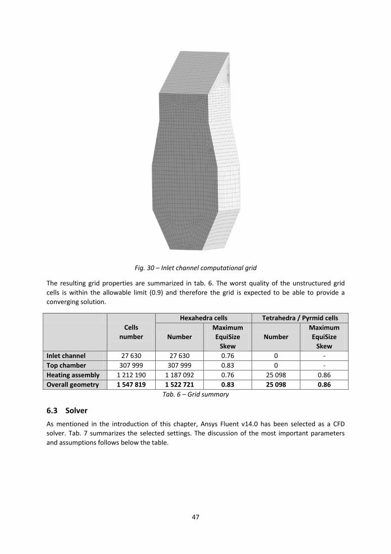
The abovementioned method of bidirectional pave-sweep coarsening was used also in the top region

of the inlet channel as shown in fig. 30.

47

Fig. 30 – Inlet channel computational grid

The resulting grid properties are summarized in tab. 6. The worst quality of the unstructured grid

cells is within the allowable limit (0.9) and therefore the grid is expected to be able to provide a

converging solution.

Cells

number

Hexahedra cells Tetrahedra / Pyrmid cells

Number

Maximum

EquiSize

Skew

Number

Maximum

EquiSize

Skew

Inlet channel 27 630 27 630 0.76 0 -

Top chamber 307 999 307 999 0.83 0 -

Heating assembly 1 212 190 1 187 092 0.76 25 098 0.86

Overall geometry 1 547 819 1 522 721 0.83 25 098 0.86

Tab. 6 – Grid summary

6.3 Solver

As mentioned in the introduction of this chapter, Ansys Fluent v14.0 has been selected as a CFD

solver. Tab. 7 summarizes the selected settings. The discussion of the most important parameters

and assumptions follows below the table.

48

Logical Section Property Setting

Solver

Dimension 3D

Double precision yes

Type Pressure-based

Time Steady state

Energy equation On

Turbulence model Realizable k-ε

Standard wall function

Gravity On

Material

Properties

Density Incompressible ideal gas

Heat capacity Piecewise polynomial interpolation

Viscosity Constant - 1.7894e-05 [kg∙m-1∙s-1]

Thermal conductivity Constant - 0.0242 [W∙m-1∙K-1]

Molecular weight Constant - 28.966 [kg∙kmol-1]

Inlet

Boundary

Boundary condition type Mass-flow-inlet

Mass flow rate 0.3167 [kg∙s-1]

Turbulence specification method Intensity and hydraulic diameter

Turbulence intensity 10%

Hydraulic diameter 0.25

Temperature 20°C

Outlet

Boundary

Boundary condition type Pressure outlet

Gauge pressure 0 [Pa]

Tab. 7 – Solver settings

The low speed nature of the considered flow problem allows the flow to be considered

incompressible, which implies the density not to be related to the pressure. The temperature

variations of the density are possible to resolve using the ‘Incompressible ideal gas’ approach which

uses an equation of state together with the reference pressure level to determine the density value.

Since the flow is expected to be turbulent, it is crucial to utilize an appropriate turbulence model. In

last several years, the two equations turbulence models such as - have become dominant in

industrial CFD applications because of the favorable accuracy-to-costs ratio. Despite the fact that the

- model is known to fail when the isotropic turbulence assumption is violated and also to under-

predict separated flows, it has been selected as the turbulence model in the current case due to high

computing power requirements of more accurate models such as Reynolds stress model or LES.

The qualitative reasoning of the selection of the boundary conditions was discussed in chapter 6.1.

While the values of the temperature and inlet turbulence characteristics are straightforward, it is

appropriate to note that the value of the inlet mass flow rate was determined based on the

measured values provided by the manufacturer.

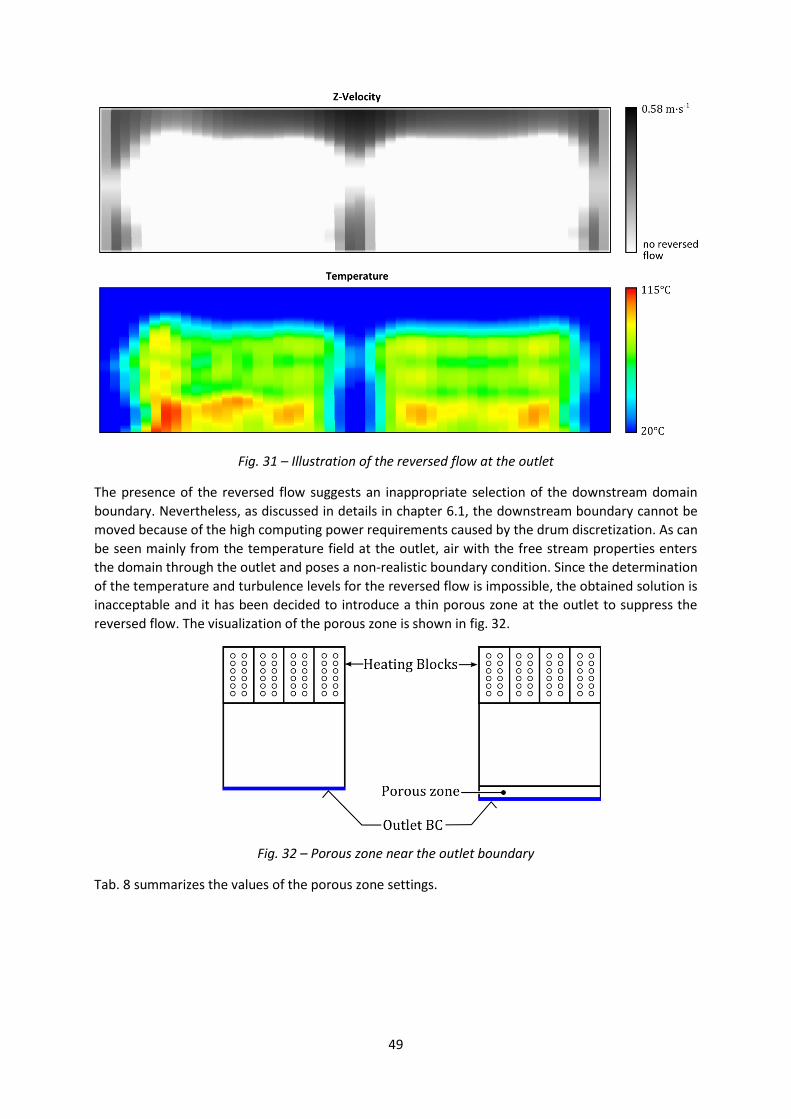
6.4 Solution process

The Fluent iteration process with the computational grid and solver settings described in chapters 6.2

and 6.3 resulted in a converging solution. However, the solution included a reversed flow in 1579

faces of the outlet, which is illustrated in the fig. 31.

49

Fig. 31 – Illustration of the reversed flow at the outlet

The presence of the reversed flow suggests an inappropriate selection of the downstream domain

boundary. Nevertheless, as discussed in details in chapter 6.1, the downstream boundary cannot be

moved because of the high computing power requirements caused by the drum discretization. As can

be seen mainly from the temperature field at the outlet, air with the free stream properties enters

the domain through the outlet and poses a non-realistic boundary condition. Since the determination

of the temperature and turbulence levels for the reversed flow is impossible, the obtained solution is

inacceptable and it has been decided to introduce a thin porous zone at the outlet to suppress the

reversed flow. The visualization of the porous zone is shown in fig. 32.

Fig. 32 – Porous zone near the outlet boundary

Tab. 8 summarizes the values of the porous zone settings.

50

Property Value

Direction-1 Vector (1,0,0)

Direction-2 Vector (0,1,0)

Relative Velocity Resistance Formulation On

Viscous resistance

Direction-1 0

Direction-2 0

Direction-3 1e+08

Fluid porosity 1

Tab. 8 – Porous zone settings

With the modified geometry including the porous zone, the second iteration process was performed.

The formation of reversed flow was successfully suppressed. To allow the continuity equation

residue to drop below the stochastic Fluent convergence criterion 1e-3 it was necessary to calculate

1078 iterations. The development of the residues together with other quantities monitored in order

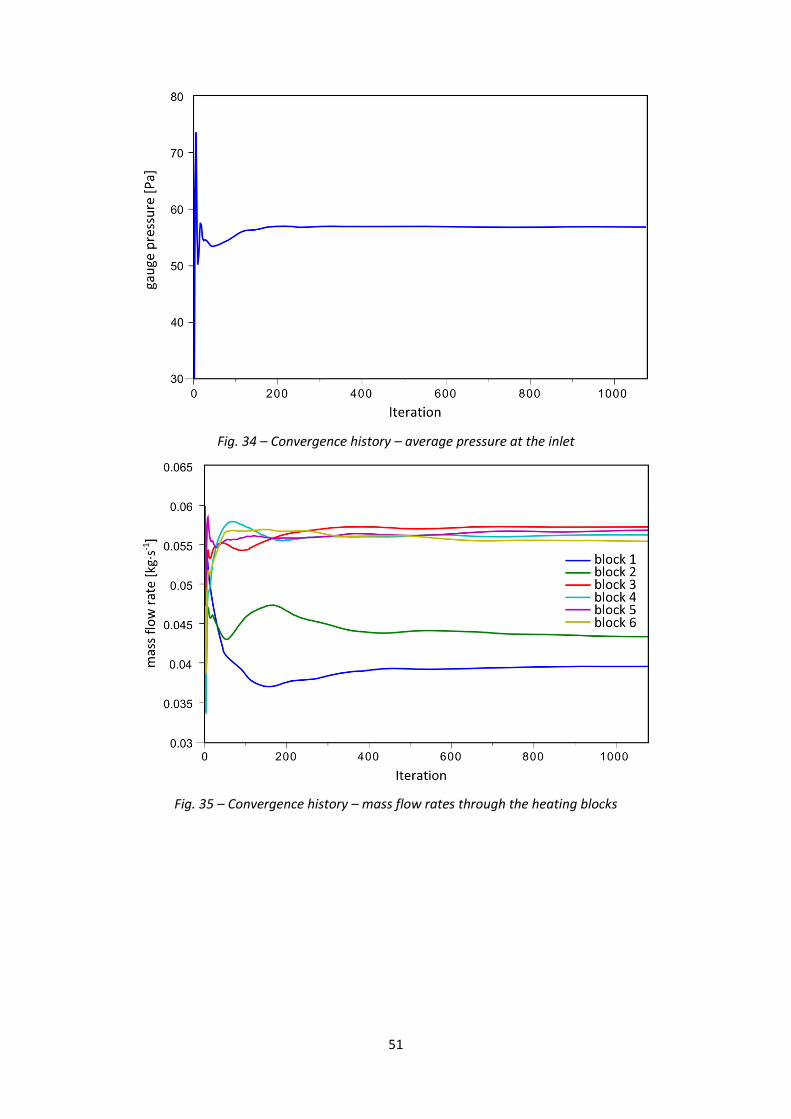
to verify the convergence is shown in fig. 33, fig. 34 and fig. 35.

Fig. 33 – Convergence history - residues

51

Fig. 34 – Convergence history – average pressure at the inlet

Fig. 35 – Convergence history – mass flow rates through the heating blocks

52

7 Results interpretation

In this chapter the data obtained by the CFD simulation are analyzed in detail. The correct

interpretation of the data is essential to the identification of the weak spots and therefore to the

subsequent optimization targeting.

7.1 Flow field

The following text presents the crucial aspects of the resulting flow field. Only a limited number of

flow visualizations directly relevant to the text is included and a reader is encouraged to find the

complete set of flow field data in appendix C.

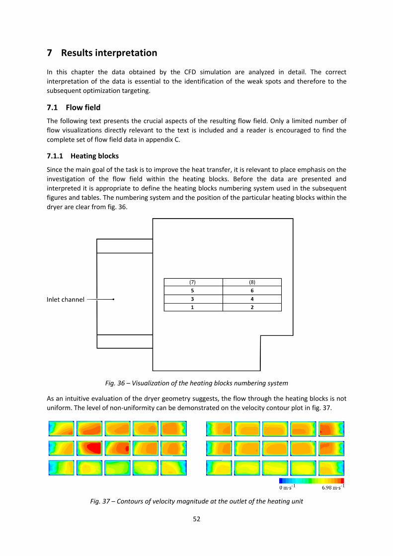
7.1.1 Heating blocks

Since the main goal of the task is to improve the heat transfer, it is relevant to place emphasis on the

investigation of the flow field within the heating blocks. Before the data are presented and

interpreted it is appropriate to define the heating blocks numbering system used in the subsequent

figures and tables. The numbering system and the position of the particular heating blocks within the

dryer are clear from fig. 36.

Fig. 36 – Visualization of the heating blocks numbering system

As an intuitive evaluation of the dryer geometry suggests, the flow through the heating blocks is not

uniform. The level of non-uniformity can be demonstrated on the velocity contour plot in fig. 37.

Fig. 37 – Contours of velocity magnitude at the outlet of the heating unit

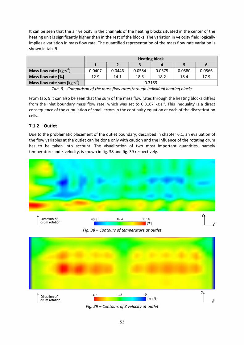
53

It can be seen that the air velocity in the channels of the heating blocks situated in the center of the

heating unit is significantly higher than in the rest of the blocks. The variation in velocity field logically

implies a variation in mass flow rate. The quantified representation of the mass flow rate variation is

shown in tab. 9.

Heating block

1 2 3 4 5 6

Mass flow rate [kg∙s-1] 0.0407 0.0446 0.0584 0.0575 0.0580 0.0566

Mass flow rate [%] 12.9 14.1 18.5 18.2 18.4 17.9

Mass flow rate sum [kg∙s-1] 0.3159

Tab. 9 – Comparison of the mass flow rates through individual heating blocks

From tab. 9 it can also be seen that the sum of the mass flow rates through the heating blocks differs

from the inlet boundary mass flow rate, which was set to 0.3167 kg∙s-1. This inequality is a direct

consequence of the cumulation of small errors in the continuity equation at each of the discretization

cells.

7.1.2 Outlet

Due to the problematic placement of the outlet boundary, described in chapter 6.1, an evaluation of

the flow variables at the outlet can be done only with caution and the influence of the rotating drum

has to be taken into account. The visualization of two most important quantities, namely

temperature and z-velocity, is shown in fig. 38 and fig. 39 respectively.

Fig. 38 – Contours of temperature at outlet

Fig. 39 – Contours of Z velocity at outlet

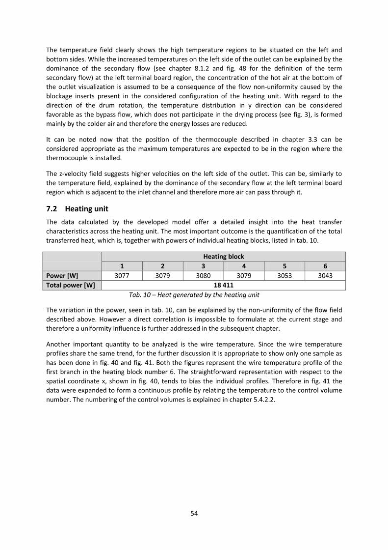
54

The temperature field clearly shows the high temperature regions to be situated on the left and

bottom sides. While the increased temperatures on the left side of the outlet can be explained by the

dominance of the secondary flow (see chapter 8.1.2 and fig. 48 for the definition of the term

secondary flow) at the left terminal board region, the concentration of the hot air at the bottom of

the outlet visualization is assumed to be a consequence of the flow non-uniformity caused by the

blockage inserts present in the considered configuration of the heating unit. With regard to the

direction of the drum rotation, the temperature distribution in y direction can be considered

favorable as the bypass flow, which does not participate in the drying process (see fig. 3), is formed

mainly by the colder air and therefore the energy losses are reduced.

It can be noted now that the position of the thermocouple described in chapter 3.3 can be

considered appropriate as the maximum temperatures are expected to be in the region where the

thermocouple is installed.

The z-velocity field suggests higher velocities on the left side of the outlet. This can be, similarly to

the temperature field, explained by the dominance of the secondary flow at the left terminal board

region which is adjacent to the inlet channel and therefore more air can pass through it.

7.2 Heating unit

The data calculated by the developed model offer a detailed insight into the heat transfer

characteristics across the heating unit. The most important outcome is the quantification of the total

transferred heat, which is, together with powers of individual heating blocks, listed in tab. 10.

Heating block

1 2 3 4 5 6

Power [W] 3077 3079 3080 3079 3053 3043

Total power [W] 18 411

Tab. 10 – Heat generated by the heating unit

The variation in the power, seen in tab. 10, can be explained by the non-uniformity of the flow field

described above. However a direct correlation is impossible to formulate at the current stage and

therefore a uniformity influence is further addressed in the subsequent chapter.

Another important quantity to be analyzed is the wire temperature. Since the wire temperature

profiles share the same trend, for the further discussion it is appropriate to show only one sample as

has been done in fig. 40 and fig. 41. Both the figures represent the wire temperature profile of the

first branch in the heating block number 6. The straightforward representation with respect to the

spatial coordinate x, shown in fig. 40, tends to bias the individual profiles. Therefore in fig. 41 the

data were expanded to form a continuous profile by relating the temperature to the control volume

number. The numbering of the control volumes is explained in chapter 5.4.2.2.

55

Fig. 40 – Heating wire temperature profile

Fig. 41 – Heating wire temperature profile (expanded data relevant to one branch)

It can be seen that the overheating is localized at the regions where the wires are enclosed by the

wire supports. The peak temperatures reach significant values and therefore a detailed analysis of

the influence of the overheating on the heating unit power is necessary.

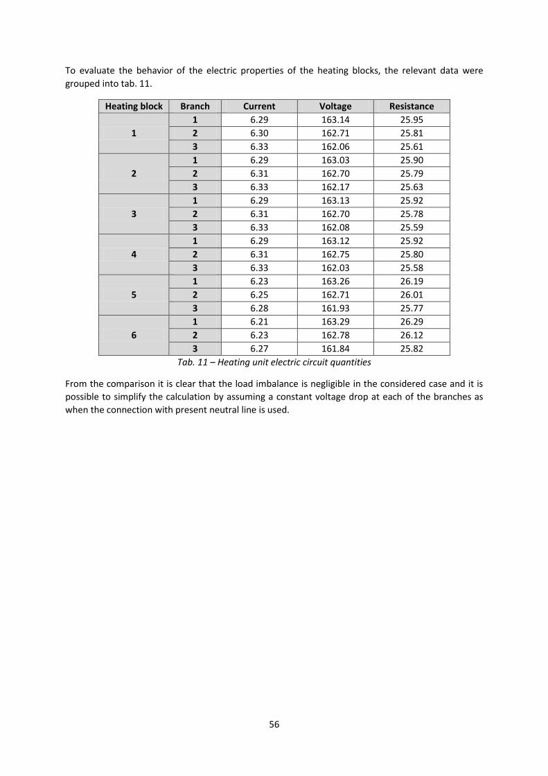
56

To evaluate the behavior of the electric properties of the heating blocks, the relevant data were

grouped into tab. 11.

Heating block Branch Current Voltage Resistance

1

1 6.29 163.14 25.95

2 6.30 162.71 25.81

3 6.33 162.06 25.61

2

1 6.29 163.03 25.90

2 6.31 162.70 25.79

3 6.33 162.17 25.63

3

1 6.29 163.13 25.92

2 6.31 162.70 25.78

3 6.33 162.08 25.59

4

1 6.29 163.12 25.92

2 6.31 162.75 25.80

3 6.33 162.03 25.58

5

1 6.23 163.26 26.19

2 6.25 162.71 26.01

3 6.28 161.93 25.77

6

1 6.21 163.29 26.29

2 6.23 162.78 26.12

3 6.27 161.84 25.82

Tab. 11 – Heating unit electric circuit quantities

From the comparison it is clear that the load imbalance is negligible in the considered case and it is

possible to simplify the calculation by assuming a constant voltage drop at each of the branches as

when the connection with present neutral line is used.

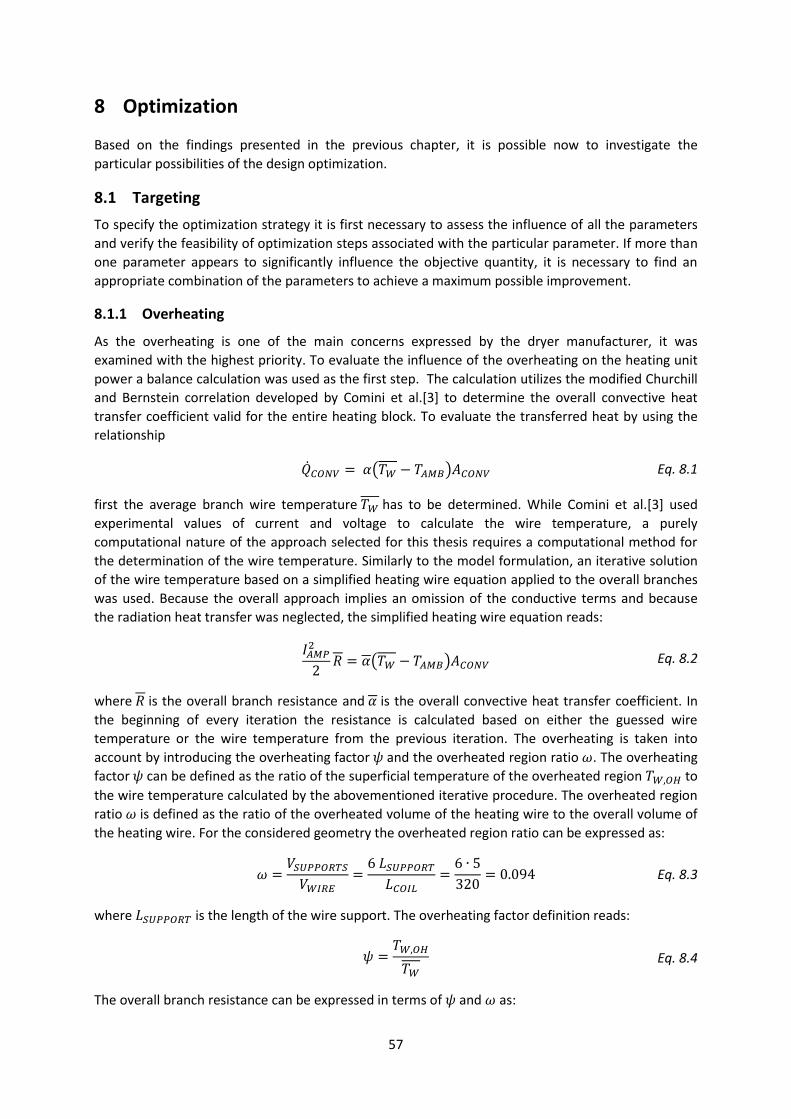
57

8 Optimization

Based on the findings presented in the previous chapter, it is possible now to investigate the

particular possibilities of the design optimization.

8.1 Targeting

To specify the optimization strategy it is first necessary to assess the influence of all the parameters

and verify the feasibility of optimization steps associated with the particular parameter. If more than

one parameter appears to significantly influence the objective quantity, it is necessary to find an

appropriate combination of the parameters to achieve a maximum possible improvement.

8.1.1 Overheating

As the overheating is one of the main concerns expressed by the dryer manufacturer, it was

examined with the highest priority. To evaluate the influence of the overheating on the heating unit

power a balance calculation was used as the first step. The calculation utilizes the modified Churchill

and Bernstein correlation developed by Comini et al.[3] to determine the overall convective heat

transfer coefficient valid for the entire heating block. To evaluate the transferred heat by using the

relationship

( ) Eq. 8.1

first the average branch wire temperature has to be determined. While Comini et al.[3] used

experimental values of current and voltage to calculate the wire temperature, a purely

computational nature of the approach selected for this thesis requires a computational method for

the determination of the wire temperature. Similarly to the model formulation, an iterative solution

of the wire temperature based on a simplified heating wire equation applied to the overall branches

was used. Because the overall approach implies an omission of the conductive terms and because

the radiation heat transfer was neglected, the simplified heating wire equation reads:

( ) Eq. 8.2

where is the overall branch resistance and is the overall convective heat transfer coefficient. In

the beginning of every iteration the resistance is calculated based on either the guessed wire

temperature or the wire temperature from the previous iteration. The overheating is taken into

account by introducing the overheating factor and the overheated region ratio . The overheating

factor can be defined as the ratio of the superficial temperature of the overheated region to

the wire temperature calculated by the abovementioned iterative procedure. The overheated region

ratio is defined as the ratio of the overheated volume of the heating wire to the overall volume of

the heating wire. For the considered geometry the overheated region ratio can be expressed as:

Eq. 8.3

where is the length of the wire support. The overheating factor definition reads:

Eq. 8.4

The overall branch resistance can be expressed in terms of and as:

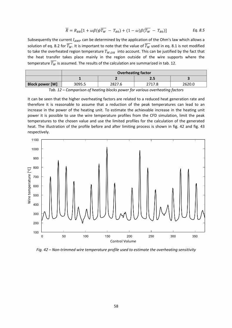
58

( ) ( ) ( ) Eq. 8.5

Subsequently the current can be determined by the application of the Ohm's law which allows a

solution of eq. 8.2 for . It is important to note that the value of used in eq. 8.1 is not modified

to take the overheated region temperature into account. This can be justified by the fact that

the heat transfer takes place mainly in the region outside of the wire supports where the

temperature is assumed. The results of the calculation are summarized in tab. 12.

Overheating factor

1 2 2.5 3

Block power [W] 3095.5 2827.6 2717.8 2620.0

Tab. 12 – Comparison of heating blocks power for various overheating factors

It can be seen that the higher overheating factors are related to a reduced heat generation rate and

therefore it is reasonable to assume that a reduction of the peak temperatures can lead to an

increase in the power of the heating unit. To estimate the achievable increase in the heating unit

power it is possible to use the wire temperature profiles from the CFD simulation, limit the peak

temperatures to the chosen value and use the limited profiles for the calculation of the generated

heat. The illustration of the profile before and after limiting process is shown in fig. 42 and fig. 43

respectively.

Fig. 42 – Non-trimmed wire temperature profile used to estimate the overheating sensitivity

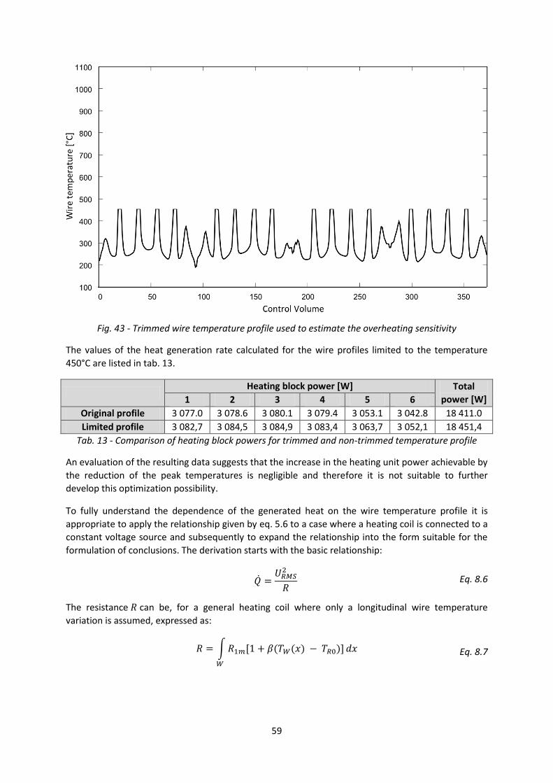
59

Fig. 43 - Trimmed wire temperature profile used to estimate the overheating sensitivity

The values of the heat generation rate calculated for the wire profiles limited to the temperature

450°C are listed in tab. 13.

Heating block power [W] Total

power [W] 1 2 3 4 5 6

Original profile 3 077.0 3 078.6 3 080.1 3 079.4 3 053.1 3 042.8 18 411.0

Limited profile 3 082,7 3 084,5 3 084,9 3 083,4 3 063,7 3 052,1 18 451,4

Tab. 13 - Comparison of heating block powers for trimmed and non-trimmed temperature profile

An evaluation of the resulting data suggests that the increase in the heating unit power achievable by

the reduction of the peak temperatures is negligible and therefore it is not suitable to further

develop this optimization possibility.

To fully understand the dependence of the generated heat on the wire temperature profile it is

appropriate to apply the relationship given by eq. 5.6 to a case where a heating coil is connected to a

constant voltage source and subsequently to expand the relationship into the form suitable for the

formulation of conclusions. The derivation starts with the basic relationship:

Eq. 8.6

The resistance can be, for a general heating coil where only a longitudinal wire temperature

variation is assumed, expressed as:

∫ ( ( ) )

Eq. 8.7

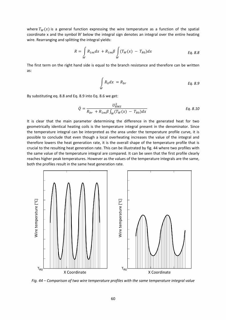
60

where ( ) is a general function expressing the wire temperature as a function of the spatial

coordinate x and the symbol below the integral sign denotes an integral over the entire heating

wire. Rearranging and splitting the integral yields:

∫

∫( ( ) )

Eq. 8.8

The first term on the right hand side is equal to the branch resistance and therefore can be written

as:

∫

Eq. 8.9

By substituting eq. 8.8 and Eq. 8.9 into Eq. 8.6 we get:

∫ ( ( ) )

Eq. 8.10

It is clear that the main parameter determining the difference in the generated heat for two

geometrically identical heating coils is the temperature integral present in the denominator. Since

the temperature integral can be interpreted as the area under the temperature profile curve, it is

possible to conclude that even though a local overheating increases the value of the integral and

therefore lowers the heat generation rate, it is the overall shape of the temperature profile that is

crucial to the resulting heat generation rate. This can be illustrated by fig. 44 where two profiles with

the same value of the temperature integral are compared. It can be seen that the first profile clearly

reaches higher peak temperatures. However as the values of the temperature integrals are the same,

both the profiles result in the same heat generation rate.

Fig. 44 – Comparison of two wire temperature profiles with the same temperature integral value

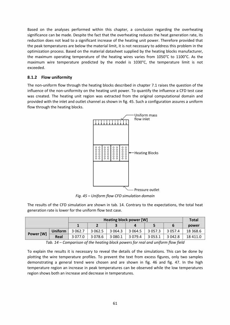
61

Based on the analyses performed within this chapter, a conclusion regarding the overheating

significance can be made. Despite the fact that the overheating reduces the heat generation rate, its

reduction does not lead to a significant increase of the heating unit power. Therefore provided that

the peak temperatures are below the material limit, it is not necessary to address this problem in the

optimization process. Based on the material datasheet supplied by the heating blocks manufacturer,

the maximum operating temperature of the heating wires varies from 1050°C to 1100°C. As the

maximum wire temperature predicted by the model is 1030°C, the temperature limit is not

exceeded.

8.1.2 Flow uniformity

The non-uniform flow through the heating blocks described in chapter 7.1 raises the question of the

influence of the non-uniformity on the heating unit power. To quantify the influence a CFD test case

was created. The heating unit region was extracted from the original computational domain and

provided with the inlet and outlet channel as shown in fig. 45. Such a configuration assures a uniform

flow through the heating blocks.

Fig. 45 – Uniform flow CFD simulation domain

The results of the CFD simulation are shown in tab. 14. Contrary to the expectations, the total heat

generation rate is lower for the uniform flow test case.

Heating block power [W] Total

power 1 2 3 4 5 6

Power [W] Uniform 3 062.7 3 062.5 3 064.3 3 064.5 3 057.3 3 057.4 18 368.6

Real 3 077.0 3 078.6 3 080.1 3 079.4 3 053.1 3 042.8 18 411.0

Tab. 14 – Comparison of the heating block powers for real and uniform flow field

To explain the results it is necessary to reveal the details of the simulations. This can be done by

plotting the wire temperature profiles. To prevent the text from excess figures, only two samples

demonstrating a general trend were chosen and are shown in fig. 46 and fig. 47. In the high

temperature region an increase in peak temperatures can be observed while the low temperatures

region shows both an increase and decrease in temperatures.

62

Fig. 46 – Wire temperature profiles for the heating block 1 and branch 1

Fig. 47 - Wire temperature profiles for the heating block 6 and branch 1

The results of the uniform flow CFD simulation can be explained by a qualitative examination of the

flow pattern within the heating blocks. As visualized in the fig. 48 it is possible to identify two main

streams of incoming air, namely the primary and secondary flow.

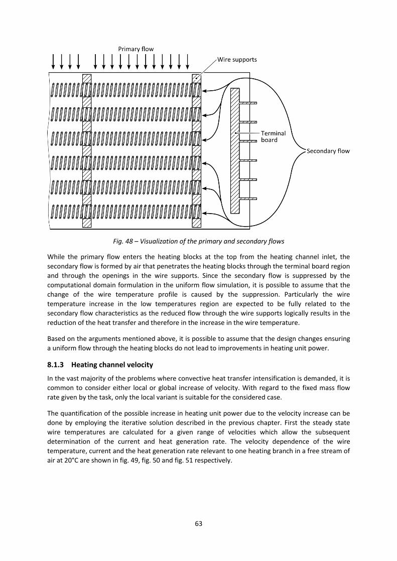
63

Fig. 48 – Visualization of the primary and secondary flows

While the primary flow enters the heating blocks at the top from the heating channel inlet, the

secondary flow is formed by air that penetrates the heating blocks through the terminal board region

and through the openings in the wire supports. Since the secondary flow is suppressed by the

computational domain formulation in the uniform flow simulation, it is possible to assume that the

change of the wire temperature profile is caused by the suppression. Particularly the wire

temperature increase in the low temperatures region are expected to be fully related to the

secondary flow characteristics as the reduced flow through the wire supports logically results in the

reduction of the heat transfer and therefore in the increase in the wire temperature.

Based on the arguments mentioned above, it is possible to assume that the design changes ensuring

a uniform flow through the heating blocks do not lead to improvements in heating unit power.

8.1.3 Heating channel velocity

In the vast majority of the problems where convective heat transfer intensification is demanded, it is

common to consider either local or global increase of velocity. With regard to the fixed mass flow

rate given by the task, only the local variant is suitable for the considered case.

The quantification of the possible increase in heating unit power due to the velocity increase can be

done by employing the iterative solution described in the previous chapter. First the steady state

wire temperatures are calculated for a given range of velocities which allow the subsequent

determination of the current and heat generation rate. The velocity dependence of the wire

temperature, current and the heat generation rate relevant to one heating branch in a free stream of

air at 20°C are shown in fig. 49, fig. 50 and fig. 51 respectively.

64

Fig. 49 – Graphical representation of the wire temperature as a function of the air velocity

Fig. 50 - Graphical representation of the branch current as a function of the air velocity

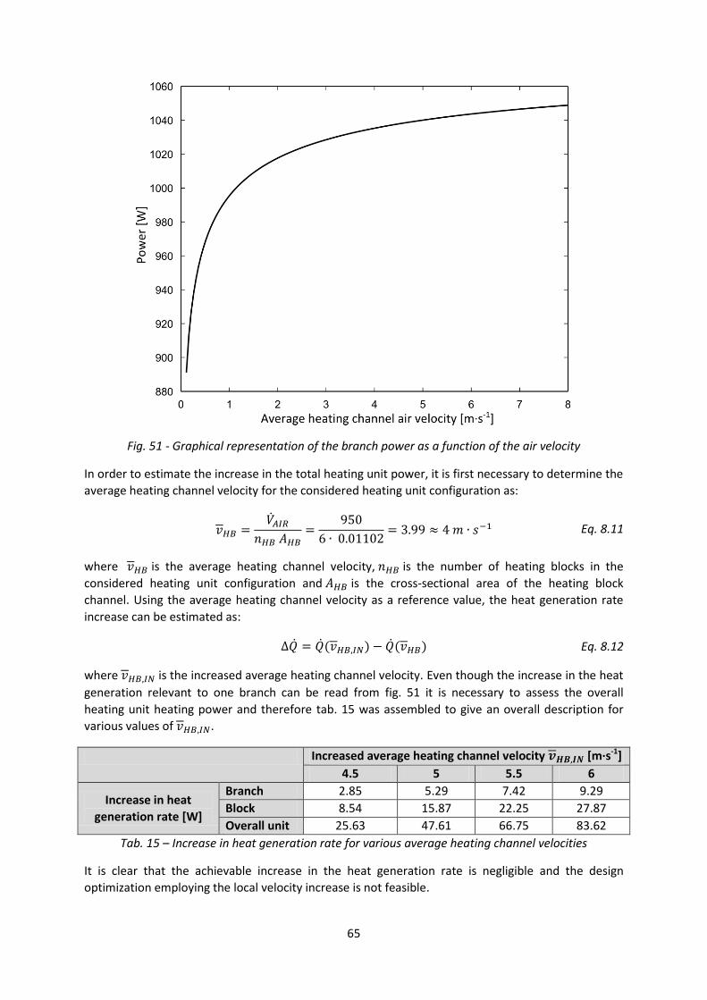
65

Fig. 51 - Graphical representation of the branch power as a function of the air velocity

In order to estimate the increase in the total heating unit power, it is first necessary to determine the

average heating channel velocity for the considered heating unit configuration as:

Eq. 8.11

where is the average heating channel velocity, is the number of heating blocks in the

considered heating unit configuration and is the cross-sectional area of the heating block

channel. Using the average heating channel velocity as a reference value, the heat generation rate

increase can be estimated as:

( ) ( ) Eq. 8.12

where is the increased average heating channel velocity. Even though the increase in the heat

generation relevant to one branch can be read from fig. 51 it is necessary to assess the overall

heating unit heating power and therefore tab. 15 was assembled to give an overall description for

various values of .

Increased average heating channel velocity [m∙s-1]

4.5 5 5.5 6

Increase in heat

generation rate [W]

Branch 2.85 5.29 7.42 9.29

Block 8.54 15.87 22.25 27.87

Overall unit 25.63 47.61 66.75 83.62

Tab. 15 – Increase in heat generation rate for various average heating channel velocities

It is clear that the achievable increase in the heat generation rate is negligible and the design

optimization employing the local velocity increase is not feasible.

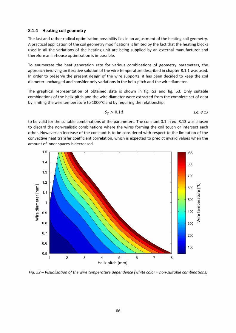
66

8.1.4 Heating coil geometry

The last and rather radical optimization possibility lies in an adjustment of the heating coil geometry.

A practical application of the coil geometry modifications is limited by the fact that the heating blocks

used in all the variations of the heating unit are being supplied by an external manufacturer and

therefore an in-house optimization is impossible.

To enumerate the heat generation rate for various combinations of geometry parameters, the

approach involving an iterative solution of the wire temperature described in chapter 8.1.1 was used.

In order to preserve the present design of the wire supports, it has been decided to keep the coil

diameter unchanged and consider only variations in the helix pitch and the wire diameter.

The graphical representation of obtained data is shown in fig. 52 and fig. 53. Only suitable

combinations of the helix pitch and the wire diameter were extracted from the complete set of data

by limiting the wire temperature to 1000°C and by requiring the relationship:

Eq. 8.13

to be valid for the suitable combinations of the parameters. The constant 0.1 in eq. 8.13 was chosen

to discard the non-realistic combinations where the wires forming the coil touch or intersect each

other. However an increase of the constant is to be considered with respect to the limitation of the

convective heat transfer coefficient correlation, which is expected to predict invalid values when the

amount of inner spaces is decreased.

Fig. 52 – Visualization of the wire temperature dependence (white color = non-suitable combinations)

67

Fig. 53 - Visualization of the branch power dependence (white color = non-suitable combinations)

From the trends of the contour plots it is clear that a significant increase in the heating branch power

is achievable. It is important to note that an increase in the power is always connected with an

increase in the wire temperature. This poses a substantial complication as an increase in the wire

temperature causes an increase in the peak wire temperatures due to the overheating in the wire

supports region. Since the values of the overheated regions in the present design case are at the top

of the allowable limit, any changes of the coil parameters can be introduced only if the overheating

effect is reduced.

To select an appropriate combination of the coil parameters, many factors such as standard wire

diameters and other production related characteristics have to be considered and therefore an

explicit specification of the optimal parameter values is omitted.

8.2 Evaluation of optimization possibilities

The targeting procedure described in the previous chapter revealed a narrow space for the

optimization of the heat transfer within the considered tumble clothes dryer. Except for the heating

coil geometry modifications, none of the considered optimization techniques shows a significant

improvement potential.

68

9 Conclusion

Within a scope of this thesis a complex optimization analysis of an electrically heated tumble clothes

dryer was performed. The present case of the dryer was evaluated by the CFD simulation. Due to the

geometrical simplifications necessary to reduce computing power requirements it was inevitable to

introduce a model describing the heat transfer from the helically coiled heating wires in cross flow.

The concept of the model was based on the experimental study of heating wires in cross flow

performed by Comini et al.[3]. The overall balance approach was modified in order to resolve the

details of the heat transfer. While conductive and convective heat transfer mechanisms were taken

into account, radiation was neglected. The main source of error is expected to be located in the wire

supports region where the cross flow condition is locally violated.

Since the pulling effect of the rotating drum in the region adjacent to the outlet was, after extensive

considerations, neglected, the results of the present case CFD analysis are expected to be distorted in

the vicinity of the outlet boundary. To ensure a correct solution it is necessary to include a rotating

drum in the simulation, which was unacceptable due to the available computing power. With respect

to the long term research plan of NETME Centre, the question of the drum flow will be addressed in a

close future as drying processes optimization is one of the key features of the collaboration with

laundry equipment manufacturers. Thus the current work can be expanded and made more accurate

by introducing a suitable method for the description of the drum flow.

The assessment of the improvement possibilities revealed a very narrow space for the heat transfer

optimization. Neither of the factors emphasized in the task, namely the local wire overheating and

the non-uniform flow through the heating blocks, does not significantly influence the resulting power

of the heating unit. The only suitable improvement possibility including modifications of the heating

coil geometry is limited by a combination of two negative factors. The first one, being purely of a

manufacturing nature, lies in the fact that the heating blocks are supplied by an external company

and the process involving the modifications of the heating coils geometry is therefore complicated.

The second factor is related to the overheating located in the wire supports region. The present case

analysis revealed the maximum temperature of the heating wire to be only approximately 50°C lower

than the maximum allowed operating temperature. Since all the improvements based on the

modifications of the heating coil geometry are connected with an increase in the wire temperature, it

is possible to employ such a modification only if the overheating effect is reduced in the problematic

region.

From a wider perspective, a resistive heating can be, after neglecting the heat losses in wiring,

considered as 100% effective. Therefore the only optimization possibility employing the present

heating coil geometry lies in the temperature dependence of the heating wire resistance. A reduced

wire temperature causes a lower resistance which results in a higher heat generation rate. Since the

change in resistance of the considered heating wire material is approximately 3% per 100°C it is clear

that the heat generation rate cannot be increased significantly by lowering the wire temperature.

The presented thesis delivers a comprehensive answer to a practical problem given by a leading

manufacturer of laundry equipment. Even though the demanded enhancement was proven to be

unachievable for the considered conditions, it is necessary to highlight the fact that the detailed

insight in the device characteristics together with the found physical limitations can serve as a basis

for future design improvements. Moreover the heat transfer model developed within the thesis can

be utilized in CFD simulations of devices including helically coiled heating wires.

69

10 References

[1] ANSYS INC., Ansys 14.0 Help: Fluent, c 2011

[2] MEIER, ALEXANDRA VON. Electric power systems: a conceptual introduction, New Jersey, A

Wiley-Interscience publication, c 2006, xv, 309 p., ISBN-13: 978-0-471-17859-0

[3] G. COMINI, et al., Forced convection heat transfer from banks of helical coiled resistance wires,

International Journal of Thermal Sciences, Volume 47, Issue 4, April 2008, Pages 442-449, ISSN

1290-0729, 10.1016/j.ijthermalsci.2007.03.009.

[4] ALEXANDER, C.K., SADIKU, M.N.O., Fundamentals of Electric Circuits, McGraw-Hill Higher

Education, 2005

[5] PRIMUS CE, Technical specifications: Industrial tumble dryers, Product brochure, 2012

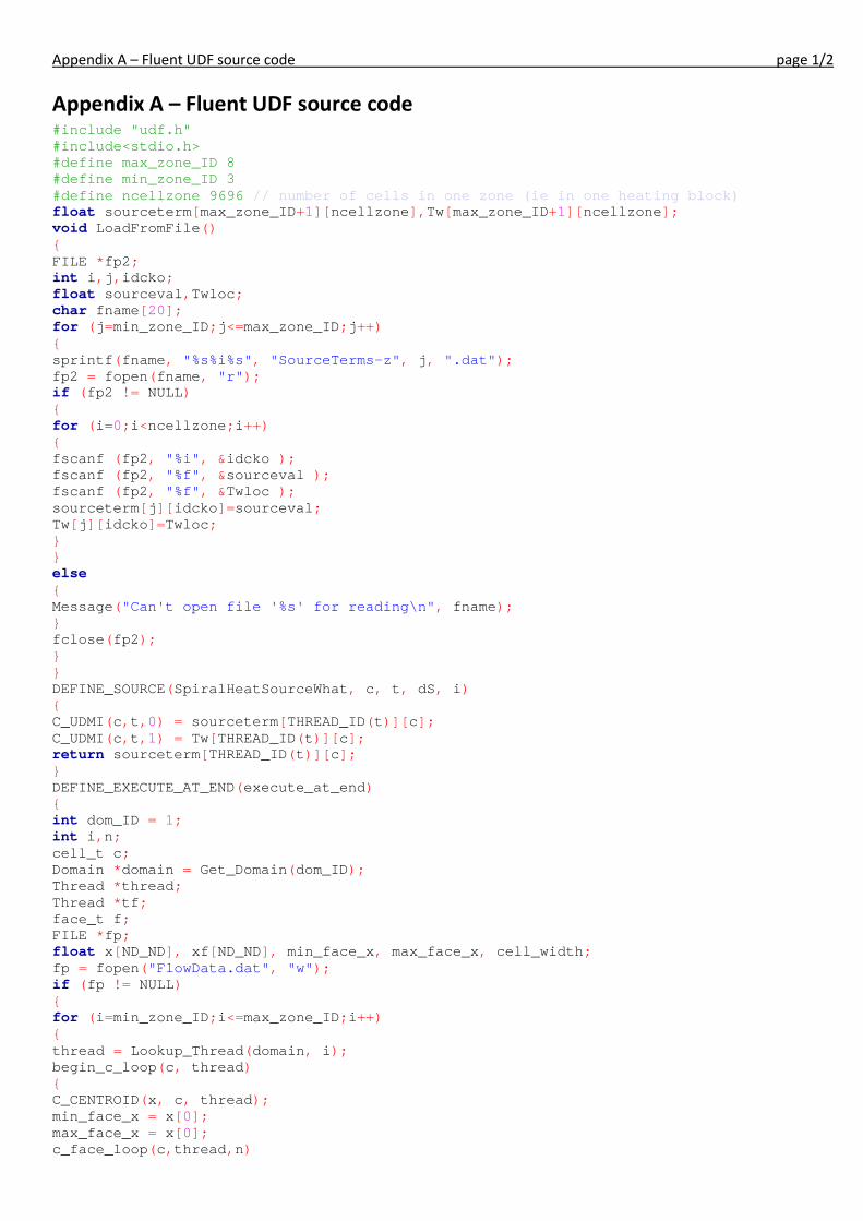
Appendix A – Fluent UDF source code page 1/2

Appendix A – Fluent UDF source code #include "udf.h" #include<stdio.h> #define max_zone_ID 8 #define min_zone_ID 3 #define ncellzone 9696 // number of cells in one zone (ie in one heating block) float sourceterm[max_zone_ID+1][ncellzone],Tw[max_zone_ID+1][ncellzone]; void LoadFromFile() { FILE *fp2; int i,j,idcko; float sourceval,Twloc; char fname[20]; for (j=min_zone_ID;j<=max_zone_ID;j++) { sprintf(fname, "%s%i%s", "SourceTerms-z", j, ".dat"); fp2 = fopen(fname, "r"); if (fp2 != NULL) { for (i=0;i<ncellzone;i++) { fscanf (fp2, "%i", &idcko ); fscanf (fp2, "%f", &sourceval ); fscanf (fp2, "%f", &Twloc ); sourceterm[j][idcko]=sourceval; Tw[j][idcko]=Twloc; } } else { Message("Can't open file '%s' for reading\n", fname); } fclose(fp2); } } DEFINE_SOURCE(SpiralHeatSourceWhat, c, t, dS, i) { C_UDMI(c,t,0) = sourceterm[THREAD_ID(t)][c]; C_UDMI(c,t,1) = Tw[THREAD_ID(t)][c]; return sourceterm[THREAD_ID(t)][c]; } DEFINE_EXECUTE_AT_END(execute_at_end) { int dom_ID = 1; int i,n; cell_t c; Domain *domain = Get_Domain(dom_ID); Thread *thread; Thread *tf; face_t f; FILE *fp; float x[ND_ND], xf[ND_ND], min_face_x, max_face_x, cell_width; fp = fopen("FlowData.dat", "w"); if (fp != NULL) { for (i=min_zone_ID;i<=max_zone_ID;i++) { thread = Lookup_Thread(domain, i); begin_c_loop(c, thread) { C_CENTROID(x, c, thread); min_face_x = x[0]; max_face_x = x[0]; c_face_loop(c,thread,n)

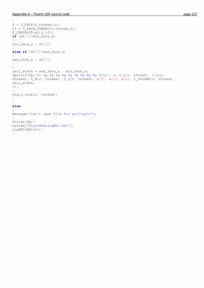
Appendix A – Fluent UDF source code page 2/2

{ f = C_FACE(c,thread,n); tf = C_FACE_THREAD(c,thread,n); F_CENTROID(xf,f,tf); if (xf[0]<min_face_x) { min_face_x = xf[0]; } else if (xf[0]>max_face_x) { max_face_x = xf[0]; } } cell_width = max_face_x - min_face_x; fprintf(fp,"%i %g %g %g %g %g %g %g %g %g %i\n", c, C_U(c, thread), C_V(c, thread), C_W(c, thread), C_T(c, thread), x[0], x[1], x[2], C_VOLUME(c, thread), cell_width, i); } end_c_loop(c, thread); } } else { Message("Can't open file for writing\n"); } fclose(fp); system("DryerHeatingMin.bat"); LoadFromFile(); }

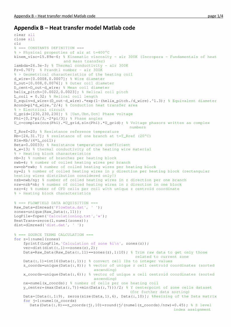
Appendix B – Heat transfer model Matlab code page 1/4

Appendix B – Heat transfer model Matlab code clear all close all clc % === CONSTANTS DEFINITION === % > Physical properties of air at t=400°C kinem_visc=15.89e-6; % Kinematic viscosity - air 300K (Incropera - Fundamentals of heat

and mass transfer) lambda=26.3e-3; % Thermal conductivity - air 300K Pr=0.707; % Prandtl number - air 300K % > Geometrical characteristics of the heating coil d_wire=[0.0008,0.0007]; % Wire diameter D_out=[0.008,0.0076]; % Outer coil diameter D_cent=D_out-d_wire; % Mean coil diameter helix_pitch=[0.0022,0.0023]; % Helical coil pitch L_coil = 0.32; % Helical coil length D_equiv=d_wire+(D_out-d_wire).*exp(1-(helix_pitch./d_wire).^1.3); % Equivalent diameter Acond=pi*d_wire.^2/4; % Conduction heat transfer area % > Electrical circuit U_grid=[230,230,230]; % [Uan,Ubn,Ucn] Phase voltage Phi=[0,2*pi/3,-2*pi/3]; % Phase angles U_c=complex(cos(Phi).*U_grid,sin(Phi).*U_grid); % Voltage phasors written as complex

numbers T_Rref=20; % Resistance reference temperature Rb=[24,31.7]; % resistance of one branch at t=T_Rref (20°C) R1m=Rb/(4*L_coil); Beta=0.00033; % Resistance temperature coefficient k_w=13; % thermal conductivity of the heating wire material % > Heating block characteristics nb=3; % number of branches per heating block nwb=4; % number of coiled heating wires per branch nw=nb*nwb; % number of coiled heating wires per heating block ny=2; % number of coiled heating wires in y direction per heating block (rectangular heating wires distribution considered only!) nzb=nwb/ny; % number of coiled heating wires in z direction per one branch nzw=nzb*nb; % number of coiled heating wires in z direction in one block nzc=4; % number of CFD cells per coil with unique z centroid coordinate % > Heating block characteristics % === FLOWFIELD DATA ACQUISITION === Raw_Data=dlmread('FlowData.dat', ' '); zones=unique(Raw_Data(:,11)); LogFile=fopen('CalculationLog.txt','w'); HeatTrans=zeros(1,numel(zones)); dist=dlmread('dist.dat', ' '); % === SOURCE TERMS CALCULATION === for z=1:numel(zones) fprintf(LogFile,'Calculation of zone %i\n', zones(z)); ver=dist(dist(:,1)==zones(z),2); Data=Raw_Data(Raw_Data(:,11)==zones(z),1:10); % Trim raw data to get only those

related to current zone Data(:,1)=int16(Data(:,1)); % convert cell IDs to integer values z_coords=unique(Data(:,8)); % vector of unique z cell centroid coordinates (sorted

ascending) x_coords=unique(Data(:,6)); % vector of unique x cell centroid coordinates (sorted

ascending) nx=numel(x_coords); % number of cells per one heating coil y_center=(max(Data(:,7))+min(Data(:,7)))/2; % Y centerpoint of zone cells dataset

(for further data sorting) Data=[Data(:,1:9), zeros(size(Data,1),6), Data(:,10)]; %Resizing of the Data matrix for j=1:numel(z_coords)

Data(Data(:,8)==z_coords(j),10)=round(j/(numel(z_coords)/nzw)+0.45); % Z level index assignment

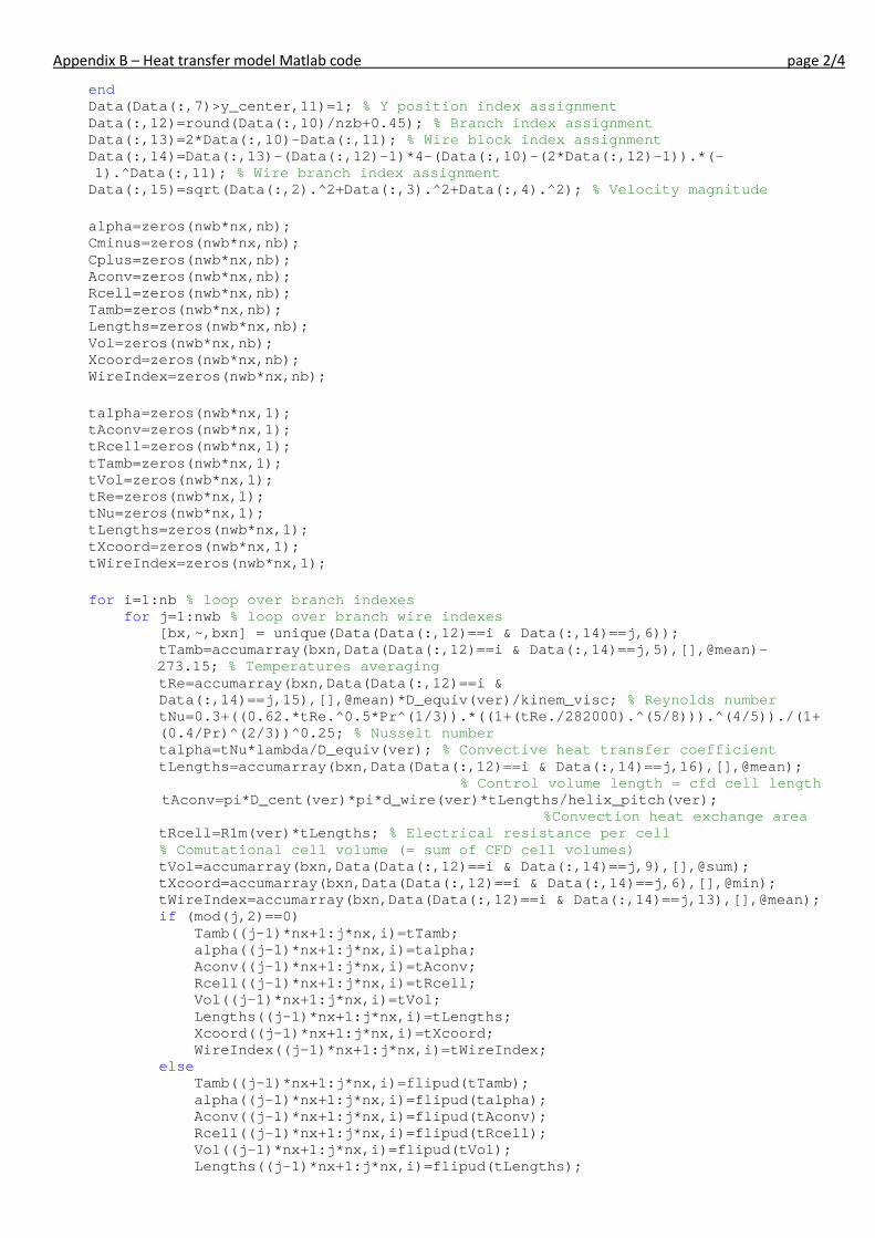
Appendix B – Heat transfer model Matlab code page 2/4

end Data(Data(:,7)>y_center,11)=1; % Y position index assignment Data(:,12)=round(Data(:,10)/nzb+0.45); % Branch index assignment Data(:,13)=2*Data(:,10)-Data(:,11); % Wire block index assignment Data(:,14)=Data(:,13)-(Data(:,12)-1)*4-(Data(:,10)-(2*Data(:,12)-1)).*(-

1).^Data(:,11); % Wire branch index assignment Data(:,15)=sqrt(Data(:,2).^2+Data(:,3).^2+Data(:,4).^2); % Velocity magnitude alpha=zeros(nwb*nx,nb); Cminus=zeros(nwb*nx,nb); Cplus=zeros(nwb*nx,nb); Aconv=zeros(nwb*nx,nb); Rcell=zeros(nwb*nx,nb); Tamb=zeros(nwb*nx,nb); Lengths=zeros(nwb*nx,nb); Vol=zeros(nwb*nx,nb); Xcoord=zeros(nwb*nx,nb); WireIndex=zeros(nwb*nx,nb); talpha=zeros(nwb*nx,1); tAconv=zeros(nwb*nx,1); tRcell=zeros(nwb*nx,1); tTamb=zeros(nwb*nx,1); tVol=zeros(nwb*nx,1); tRe=zeros(nwb*nx,1); tNu=zeros(nwb*nx,1); tLengths=zeros(nwb*nx,1); tXcoord=zeros(nwb*nx,1); tWireIndex=zeros(nwb*nx,1); for i=1:nb % loop over branch indexes for j=1:nwb % loop over branch wire indexes [bx,~,bxn] = unique(Data(Data(:,12)==i & Data(:,14)==j,6)); tTamb=accumarray(bxn,Data(Data(:,12)==i & Data(:,14)==j,5),[],@mean)-

273.15; % Temperatures averaging tRe=accumarray(bxn,Data(Data(:,12)==i & Data(:,14)==j,15),[],@mean)*D_equiv(ver)/kinem_visc; % Reynolds number tNu=0.3+((0.62.*tRe.^0.5*Pr^(1/3)).*((1+(tRe./282000).^(5/8))).^(4/5))./(1+(0.4/Pr)^(2/3))^0.25; % Nusselt number

talpha=tNu*lambda/D_equiv(ver); % Convective heat transfer coefficient tLengths=accumarray(bxn,Data(Data(:,12)==i & Data(:,14)==j,16),[],@mean);

% Control volume length = cfd cell length tAconv=pi*D_cent(ver)*pi*d_wire(ver)*tLengths/helix_pitch(ver);

%Convection heat exchange area tRcell=R1m(ver)*tLengths; % Electrical resistance per cell

% Comutational cell volume (= sum of CFD cell volumes) tVol=accumarray(bxn,Data(Data(:,12)==i & Data(:,14)==j,9),[],@sum); tXcoord=accumarray(bxn,Data(Data(:,12)==i & Data(:,14)==j,6),[],@min); tWireIndex=accumarray(bxn,Data(Data(:,12)==i & Data(:,14)==j,13),[],@mean); if (mod(j,2)==0) Tamb((j-1)*nx+1:j*nx,i)=tTamb; alpha((j-1)*nx+1:j*nx,i)=talpha; Aconv((j-1)*nx+1:j*nx,i)=tAconv; Rcell((j-1)*nx+1:j*nx,i)=tRcell; Vol((j-1)*nx+1:j*nx,i)=tVol; Lengths((j-1)*nx+1:j*nx,i)=tLengths; Xcoord((j-1)*nx+1:j*nx,i)=tXcoord; WireIndex((j-1)*nx+1:j*nx,i)=tWireIndex; else Tamb((j-1)*nx+1:j*nx,i)=flipud(tTamb); alpha((j-1)*nx+1:j*nx,i)=flipud(talpha); Aconv((j-1)*nx+1:j*nx,i)=flipud(tAconv); Rcell((j-1)*nx+1:j*nx,i)=flipud(tRcell); Vol((j-1)*nx+1:j*nx,i)=flipud(tVol); Lengths((j-1)*nx+1:j*nx,i)=flipud(tLengths);

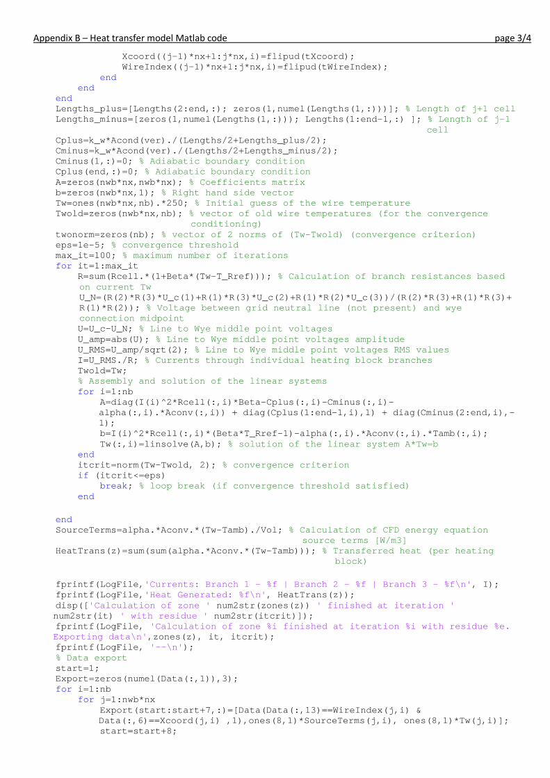
Appendix B – Heat transfer model Matlab code page 3/4

Xcoord((j-1)*nx+1:j*nx,i)=flipud(tXcoord); WireIndex((j-1)*nx+1:j*nx,i)=flipud(tWireIndex); end end end Lengths_plus=[Lengths(2:end,:); zeros(1,numel(Lengths(1,:)))]; % Length of j+1 cell Lengths_minus=[zeros(1,numel(Lengths(1,:))); Lengths(1:end-1,:) ]; % Length of j-1

cell Cplus=k_w*Acond(ver)./(Lengths/2+Lengths_plus/2); Cminus=k_w*Acond(ver)./(Lengths/2+Lengths_minus/2); Cminus(1,:)=0; % Adiabatic boundary condition Cplus(end,:)=0; % Adiabatic boundary condition A=zeros(nwb*nx,nwb*nx); % Coefficients matrix b=zeros(nwb*nx,1); % Right hand side vector Tw=ones(nwb*nx,nb).*250; % Initial guess of the wire temperature Twold=zeros(nwb*nx,nb); % vector of old wire temperatures (for the convergence

conditioning) twonorm=zeros(nb); % vector of 2 norms of (Tw-Twold) (convergence criterion) eps=1e-5; % convergence threshold max_it=100; % maximum number of iterations for it=1:max_it R=sum(Rcell.*(1+Beta*(Tw-T_Rref))); % Calculation of branch resistances based

on current Tw U_N=(R(2)*R(3)*U_c(1)+R(1)*R(3)*U_c(2)+R(1)*R(2)*U_c(3))/(R(2)*R(3)+R(1)*R(3)+R(1)*R(2)); % Voltage between grid neutral line (not present) and wye connection midpoint

U=U_c-U_N; % Line to Wye middle point voltages U_amp=abs(U); % Line to Wye middle point voltages amplitude U_RMS=U_amp/sqrt(2); % Line to Wye middle point voltages RMS values I=U_RMS./R; % Currents through individual heating block branches Twold=Tw; % Assembly and solution of the linear systems for i=1:nb A=diag(I(i)^2*Rcell(:,i)*Beta-Cplus(:,i)-Cminus(:,i)-

alpha(:,i).*Aconv(:,i)) + diag(Cplus(1:end-1,i),1) + diag(Cminus(2:end,i),-1);

b=I(i)^2*Rcell(:,i)*(Beta*T_Rref-1)-alpha(:,i).*Aconv(:,i).*Tamb(:,i); Tw(:,i)=linsolve(A,b); % solution of the linear system A*Tw=b end itcrit=norm(Tw-Twold, 2); % convergence criterion if (itcrit<=eps) break; % loop break (if convergence threshold satisfied) end end SourceTerms=alpha.*Aconv.*(Tw-Tamb)./Vol; % Calculation of CFD energy equation

source terms [W/m3] HeatTrans(z)=sum(sum(alpha.*Aconv.*(Tw-Tamb))); % Transferred heat (per heating

block) fprintf(LogFile,'Currents: Branch 1 - %f | Branch 2 - %f | Branch 3 - %f\n', I); fprintf(LogFile,'Heat Generated: %f\n', HeatTrans(z)); disp(['Calculation of zone ' num2str(zones(z)) ' finished at iteration '

num2str(it) ' with residue ' num2str(itcrit)]); fprintf(LogFile, 'Calculation of zone %i finished at iteration %i with residue %e.

Exporting data\n',zones(z), it, itcrit); fprintf(LogFile, '--\n'); % Data export start=1; Export=zeros(numel(Data(:,1)),3); for i=1:nb for j=1:nwb*nx Export(start:start+7,:)=[Data(Data(:,13)==WireIndex(j,i) &

Data(:,6)==Xcoord(j,i) ,1),ones(8,1)*SourceTerms(j,i), ones(8,1)*Tw(j,i)]; start=start+8;

Appendix B – Heat transfer model Matlab code page 4/4

end end exp_fname = strcat('SourceTerms-z',num2str(zones(z)),'.dat'); dlmwrite(exp_fname, Export, ' '); end HeatTransTot=sum(HeatTrans); % Total transferred heat fprintf(LogFile, 'Total heat transfered: %f\n', HeatTransTot); fclose(LogFile);

Appendix C – Visualization of the CFD results page 1/16

Appendix C – Visualization of the CFD results

Appendix content

Velocity vectors at plane Y1

Velocity vectors at plane X2

Velocity vectors at plane Y5

Contours of velocity magnitudes at plane Y1

Contours of velocity magnitudes at plane Y2

Contours of velocity magnitudes at plane Y3

Contours of velocity magnitudes at plane Y4

Contours of velocity magnitudes at plane Y5

Contours of velocity magnitudes at plane Y6

Contours of velocity magnitude at plane Z1

Contours of velocity magnitude at plane Z2

Contours of velocity magnitude at plane Z3

Contours of velocity magnitude at plane Z4

Contours of temperature at plane Y1

Contours of temperature at plane Y3

Contours of temperature at plane Y6

Contours of temperature at plane X1

Contours of temperature at plane X2

Contours of temperature at plane X3

Contours of temperature at plane X4

Contours of temperature at plane X5

Contours of temperature at plane X6

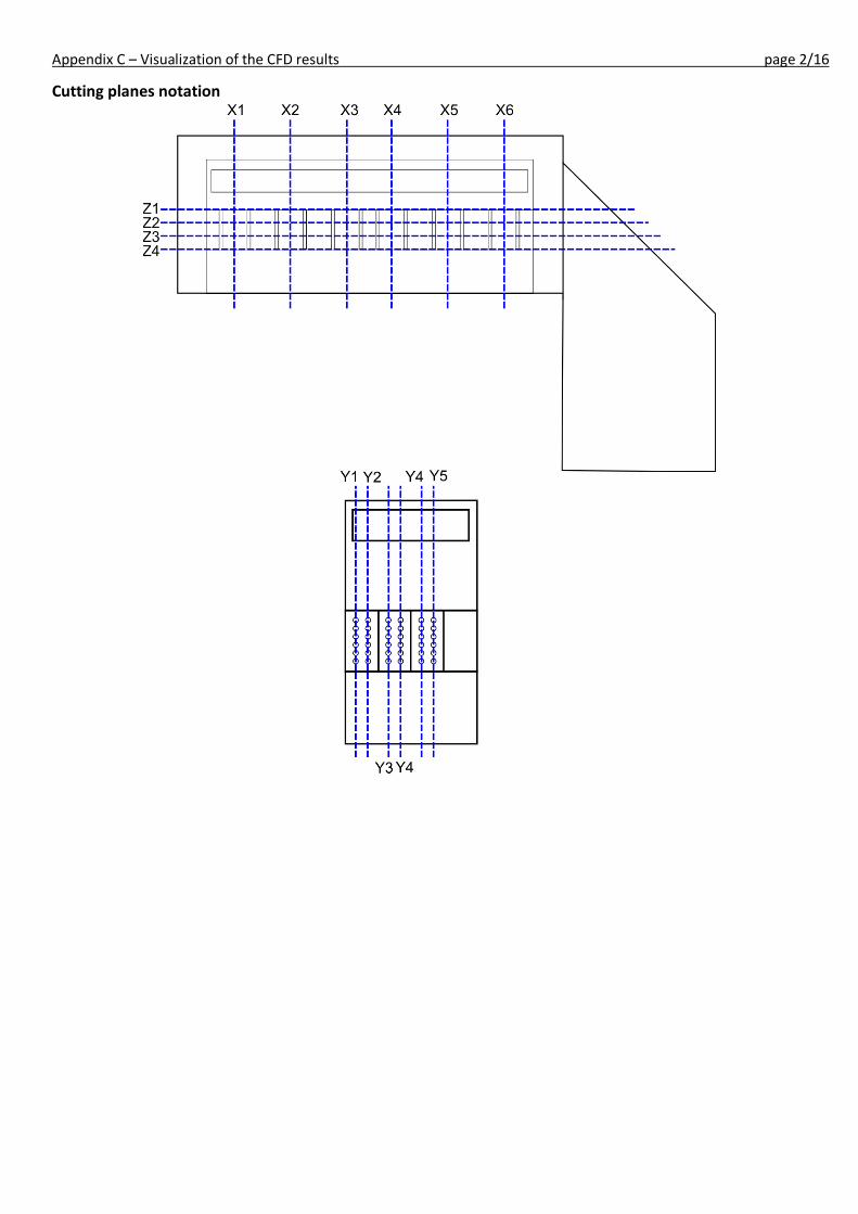
Appendix C – Visualization of the CFD results page 2/16

Cutting planes notation

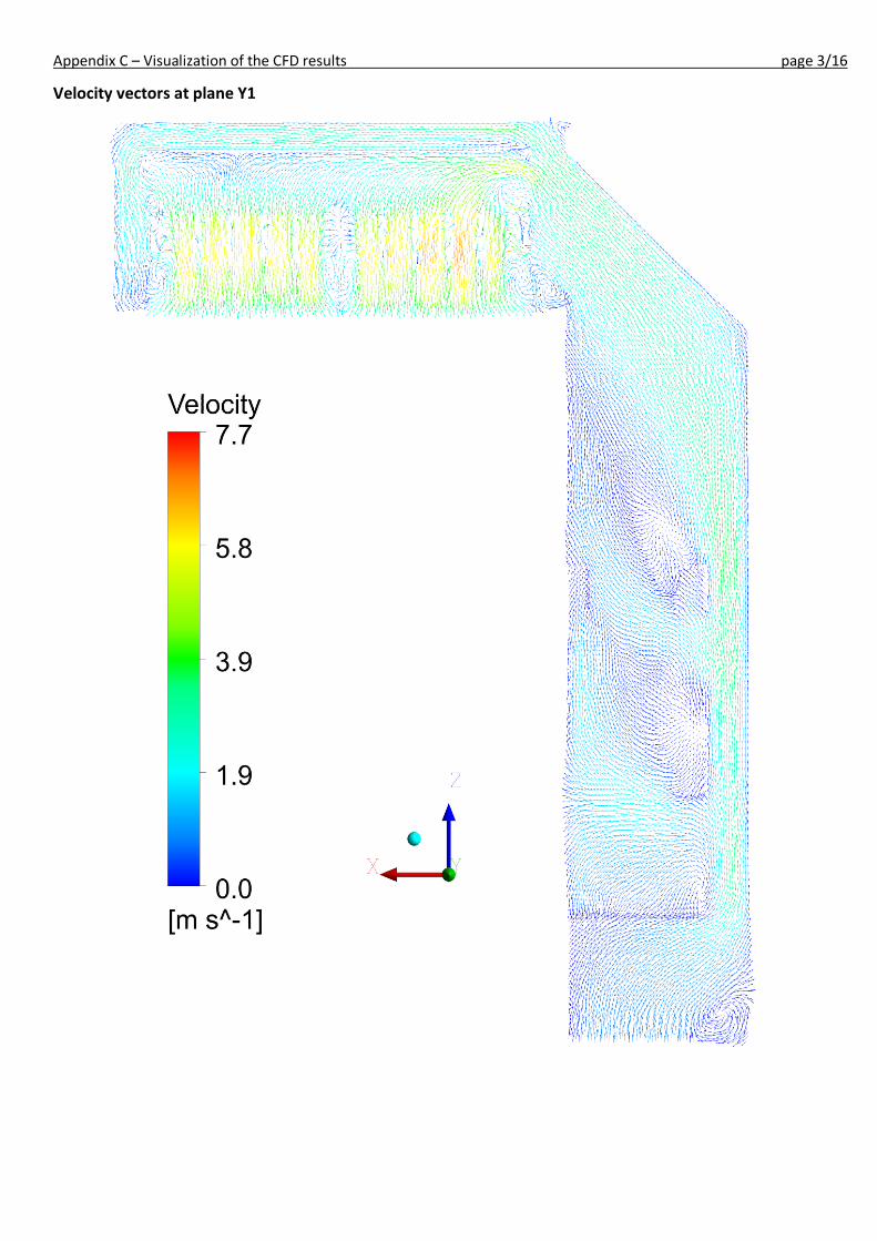
Appendix C – Visualization of the CFD results page 3/16

Velocity vectors at plane Y1

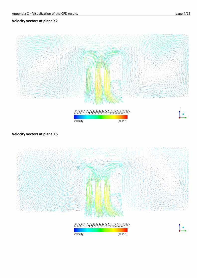
Appendix C – Visualization of the CFD results page 4/16

Velocity vectors at plane X2

Velocity vectors at plane X5

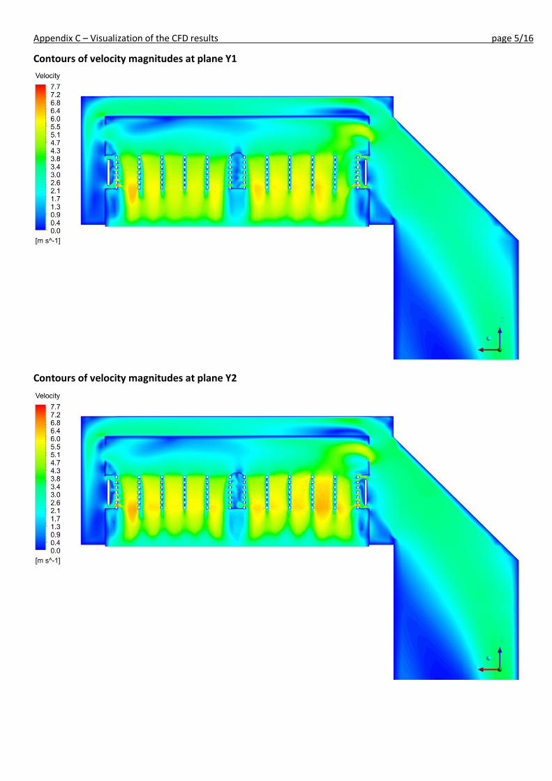
Appendix C – Visualization of the CFD results page 5/16

Contours of velocity magnitudes at plane Y1

Contours of velocity magnitudes at plane Y2

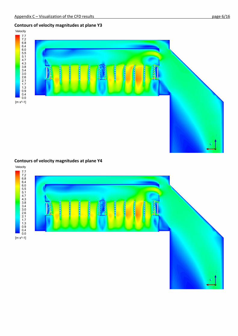
Appendix C – Visualization of the CFD results page 6/16

Contours of velocity magnitudes at plane Y3

Contours of velocity magnitudes at plane Y4

Appendix C – Visualization of the CFD results page 7/16

Contours of velocity magnitudes at plane Y5

Contours of velocity magnitudes at plane Y6

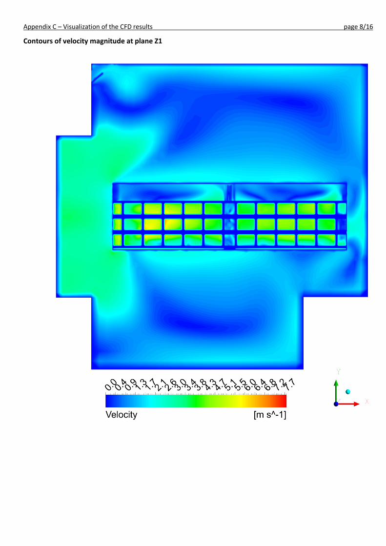
Appendix C – Visualization of the CFD results page 8/16

Contours of velocity magnitude at plane Z1

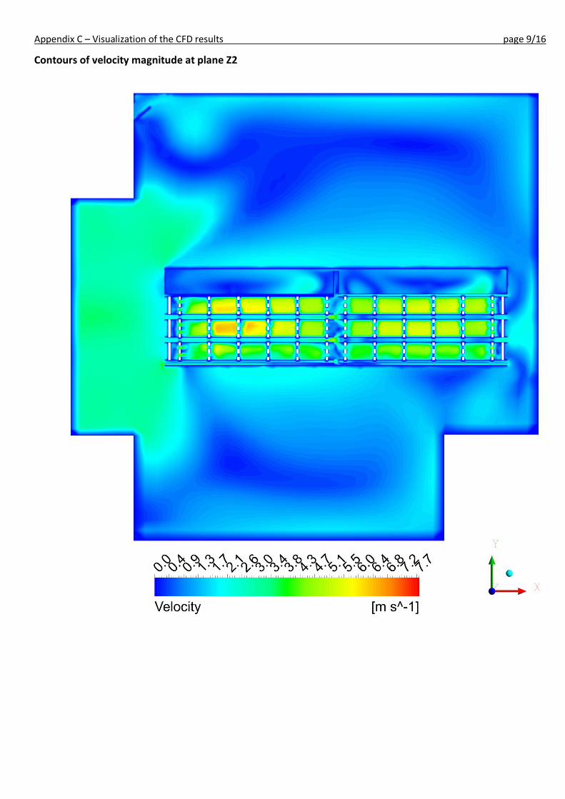
Appendix C – Visualization of the CFD results page 9/16

Contours of velocity magnitude at plane Z2

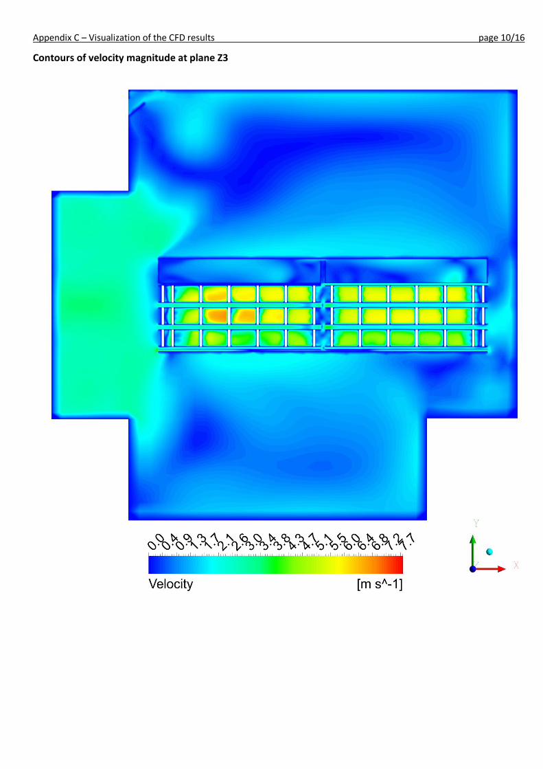
Appendix C – Visualization of the CFD results page 10/16

Contours of velocity magnitude at plane Z3

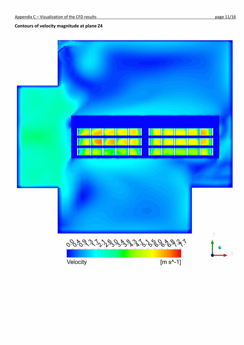
Appendix C – Visualization of the CFD results page 11/16

Contours of velocity magnitude at plane Z4

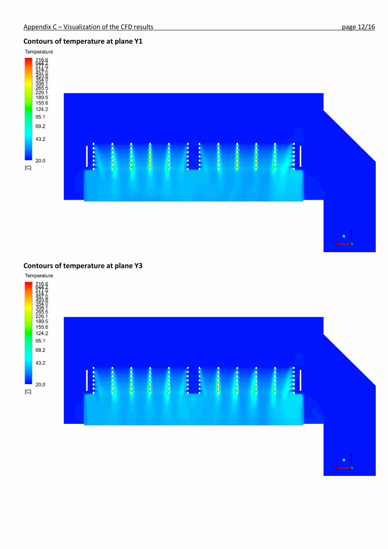
Appendix C – Visualization of the CFD results page 12/16

Contours of temperature at plane Y1

Contours of temperature at plane Y3

Appendix C – Visualization of the CFD results page 13/16

Contours of temperature at plane Y6

Contours of temperature at plane X1

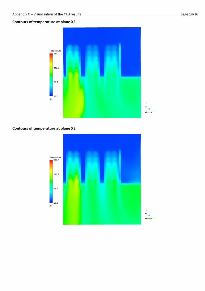
Appendix C – Visualization of the CFD results page 14/16

Contours of temperature at plane X2

Contours of temperature at plane X3

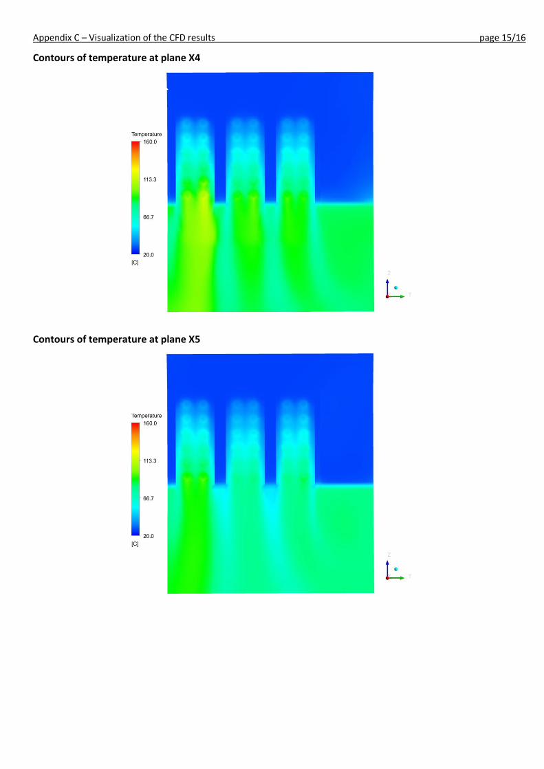
Appendix C – Visualization of the CFD results page 15/16

Contours of temperature at plane X4

Contours of temperature at plane X5

Appendix C – Visualization of the CFD results page 16/16

Contours of temperature at plane X6

Appendix D – Attached DVD content page 1/1

Appendix D – Attached DVD content • /HeatingUDF/ - Compiled version of the Fluent UDF • /Cermak-Martin_MastersThesis_2013.pdf - PDF version of the thesis • /DryerHeating.exe - Compiled version of the heat transfer model • /DryerFluent.cas - Fluent case file • /DryerFluent.dat - Fluent data file • /DryerMesh.msh - Mesh file in msh format • /DryerMesh_Gambit.dbs - Gambit geometry and mesh file • /dist.dat - Heating unit configuration data file • /FlowData.dat - Flow field data file (necessary to run the Matlab script) • /HeatingUDF.c - Fluent UDF source code • /HeatTransferModel.m - Heat transfer model Matlab code