Volume, Order Flow and the FX market:Does it matter who you are?∗

Geir H. Bjønnes† Dagfinn Rime‡

Haakon O.Aa. Solheim§

February 2002Comments welcome

Preliminary and incomplete. Do not quote

Abstract

We study the impact of order flow and volume using an uniquedata set of daily trading in the Swedish krona (SEK) market. Thedata set covers 95 per cent of worldwide SEK-trading, and is disag-gregated on 13 reporting banks’ buying and selling with seven differentcounterparties in five different instruments. The preliminary samplecovers the first six months of 1998, while the whole data set, whichwe will receive during the spring 2002, begins in 1993.

A unique feature in our data is the ability to differentiate betweencounterparties. We focus on three relationships: Between (i) volumeand volatility, (ii) order flow and exchange rate changes and (iii)the dynamics of liquidity to the market. We find that while we canrestate previously reported findings from the literature, the findingsdepend on the identity of the counterparty. We find that the volumeof the presumably least informed counterpart contributes positivelyto volatility, indicating a noise-trader role for this group. Further-more, customers’ order flow contribute significantly to exchange ratechanges, supporting the importance of these flows previously stated in

∗We thank Antti Koivisto for helpful discussions and assistance with collecting the dataset.

†Stockholm Institute for Financial Research, email: geir.bjonnes@sifr.org.‡Norges Bank (Central Bank of Norway) and Stockholm Institute for Financial Re-

search. email: dagfinn.rime@norges-bank.no.§Corresponding author. Norwegian School of Management (BI). email:

haakon.o.solheim@bi.no.

1

the literature. Finally, we find that customer order flow is a functionof past returns in the equity markets, changes in the interest rate dif-ferential and exchange rate movements. Again this process will differbetween different groups of counterparties, indicating the importanceof heterogeneity.Keywords: Order flow analysis, volume volatility relation, microstruc-ture, exchange ratesJEL Classification: F31

1 Introduction

This paper revisits three previously studied topics in the financial literature;the relationship between volume and volatility, between order flow and ex-change rate changes and the topic of liquidity provision. In the FX-marketsuch research has until recently been difficult due to the lack of good tradingdata. In this paper we use a unique data set provided by Sveriges Riksbank(the Swedish central bank). The data is based on daily reporting from 13primary dealers. Each primary dealer reports total purchases and sales withsix categories of counterparties: (1) Swedish primary dealer, (2) foreign pri-mary dealer, (3) Swedish bank, (4) foreign bank, (5) Swedish customer, and(6) foreign customer. For each counterparty-category total purchases andsales are split into different instruments, (i) spot, (ii) outright forwards, (iii)short swaps (tomorrow-next), (iv) FX swaps, and (v) options.1 The datacovers as much as 95 per cent of all currency trading in Swedish kroner.

This paper makes several contributions. First, we use transaction volumedata which covers almost the entire market for Swedish kroner to examinethe relationship between volatility and transaction volume. This is an im-portant contribution considering the lack of transaction volume data fromother currency markets. As in many other studies from different market set-tings (see Karpoff, 1987), we find a positive relationship between volatilityand volume. The results are also consistent with Galati (2000) who findsa positive relationship between volatility and volume for five of the sevencurrencies measured against dollar. Compared with the currency marketsstudied by Galati (2000), the Swedish currency market is larger.

Second, with our detailed data we can for the first time study the under-lying source of the relationship between volume and volatility in the foreignexchange market. In particular, we examine the importance of heterogene-ity in explaining volatility. This is possible since total transaction volumecan be split into different categories of counterparties. Studies from other

1A short swap is a contract to be delivered within two days, e.g. before a spot contract.

2

market settings suggest that heterogeneity among the market players maybe important in understanding volatility (see e.g. Grinblatt and Keloharju,2001). In asymmetric information models (e.g. Kyle, 1985; Admati and Pflei-derer, 1988) more trade from informed investors increase volatility becauseof the generation of private information. On the other hand, Shalen (1993)argue that uninformed traders increase volatility because they cannot differ-entiate liquidity demand from fundamental value change. Daigler and Wiley(1999), studying futures markets, find that trade of presumable less informedinvestors tend to be more correlated with volatility than trade of more in-formed investors. Our results point in the same direction, as we we find apositive correlation between volume from customers and volatility.

Third, we use our data to explain movements in foreign exchange rates.In particular, we study the effects of customer trades. Recent literature byEvans and Lyons (2002) and Fan and Lyons (2000) suggest that orders fromcustomers are important in explaining movements in foreign exchange ratesbecause customer orders are the ultimate driver of all interdealer trading. Weare able to test for the relationship between order flow and the exchange ratedifferentiating between customer order flow, interbank flows and central bankinterventions. We find that customer order flow2 is much more importantthan interbank flows for the determination of exchange rates.

Fourth, we test for exogeneity between order flow and the exchange rate.Killeen, Lyons and Moore (2001) argue that order flow shall be both weaklyand strongly exogenous with regard to a flexible exchange rate. They findthat order flow is strongly exogenous before the EMS exchange rates werefixed, and endogenous after the rates were fixed. However, we do not findthat order flow is strongly exogenous with regard to the exchange rate in oursample. Rather the exchange rate seems to Granger cause changes in orderflow.

Last, we will look at the dynamics of liquidity provisions. Chordia, Sarkarand Subrahmanyam (2001) investigate the determinants of bond and stockmarket liquidity. They find that volume changes in bond and stock mar-kets “are predictable to a considerable degree using lagged market returns,lagged spreads, and lagged volume.”(Chordia et al., 2001). However, littletheoretical work has been done on movements in liquidity.

We identify determinants of order flow. We find that customer order flowdoes depend on returns in the exchange market, as well as past returns inthe Swedish equity markets and changes in interest differentials. However,the determinants of order flows differ between groups. This confirms our

2Notice that our definition of customer order flow contain trades made by customersas well as by non-reporting banks with reporting banks.

3

Figure 1: Swedish and German Interest rates and the SEK/EUR exchangerate

0.6

0.7

0.8

0.9

1.0

1.1

1.2

1.3

3.2

3.6

4.0

4.4

4.8

5.2

1/01 1/29 2/26 3/26 4/23 5/21 6/18

Interest rate diff (left axis)Swedish 3 monthGerman 3 month

8.4

8.5

8.6

8.7

8.8

8.9

1/01 1/29 2/26 3/26 4/23 5/21 6/18

SEK/EUR exchange rate

indication that foreigners and locals, customers and interbank markets aredifferent.

The paper is organized as follows. Section 2 gives a detailed presentationof our data. In Section 3 we derive testable hypothesis and present theresults. Section 4 concludes.

2 Data

The sample used is daily observations for the first six months of 1998, makinga total of 129 observations.3 According to the market survey conducted byBIS in 1998 this period was calm. Our dependent variable is the SEK/DEMexchange rate.4 In the order flow regressions we use return (∆ log SEK/DEM),while in the volatility regressions we use the absolute value of return. Wefocus on SEK/DEM since this covers close to 100 of all interbank tradingand 80–90% of customer trading. We use the 3 month money market inter-est rate from Sweden and Germany. These series, together with the interestrate differential, is showed in figure 1.

The figure confirms that this was a calm period. Interest rates are verystable throughout (the exception being a reduction of the Swedish repo rateby 25 points June 10), with a mean interest rate differential around 100

3The whole data set on transaction flow starts in 1993 and run up to present. We willreceive all the data during the spring.

4Note however, that as the standard is changing to EUR, the exchange rate is indexedto the EUR equivalent terms (SEK/DEM*1.95583).

4

points and a standard deviation of 14 point. The exchange rate is similarlystable, with only 4.6% between top and bottom. Mean return is 0.004% with0.3 standard deviation and maximum return being ca. 1%. Although thefall of 1998 was very turbulent in financial markets we are apparently notpicking up anything from that period in this sample. This is assuring as wedo not want to pick extreme events in the current analysis.

The remainder here will be devoted to the description of the transactionflows since they represent the most novel part of this paper. The data set isprovided to us from the Sveriges Riksbank (Central Bank of Sweden), andwill eventually contain daily observations starting in 1993 until today.

The data set is extremely detailed. The Riksbank receives daily reportsfrom 13 Swedish and foreign banks on their buying and selling of five differentinstruments against seven different counterparts. The reported series is anaggregate of Swedish krona trading against all other currencies, measured inkrona, and covers 90–95 of all worldwide trading in SEK exchange rates. Asmentioned above, the vast majority of the flows is SEK/DEM transactions.

The 13 reporting banks are anonymized. We know however that there arefive Swedish banks, five foreign banks, and three branches of foreign bankslocated in Sweden. The reporters are the main liquidity providers in theSEK-market. The five instruments are spot, forward, options, short swaps(tomorrow/next) and long swaps. In this paper we focus on the spot andforward flows.

Particularly important is the counterparty information. The seven coun-terparties are Swedish and foreign customers, reporting banks, and otherbanks, and in addition the Riksbank. This enables us to distinguish cus-tomer order flow from interbank trading between the liquidity providers andinterbank trading with more speculative banks. This is to the best of ourknowledge an unique feature of the present data set.

Figure 2 shows the net selling of foreign currency to different counterpartsby the reporting banks in the spot market. A positive number indicates thatthe counterpart group has accumulated currency from the reporters. Weimmediately see that Swedish customers and other banks are accumulatingcurrency in the spot market (right panel). This is in line with the current ac-count surplus of Sweden. Figure 3 shows the net purchase of foreign currencyspot and forward.

These data are unique in several aspects. (i) The series are longer and/orof higher frequency than in many previously available data sets.5 Evans andLyons (2002) have daily observations from the interbank market but only for

5The whole data set is long (nine years). The present sample however is of similarlength as Evans and Lyons (2002).

5

Figure 2: Net spot position of foreign and Swedish Customers+Other banks

-40000

-30000

-20000

-10000

0

10000

1/01 1/29 2/26 3/26 4/23 5/21 6/18

Net SEK-sale (FG-group)

-5000

0

5000

10000

15000

20000

25000

30000

1/01 1/29 2/26 3/26 4/23 5/21 6/18

Net SEK-sale (SG group)

[FG-group: foreign customers and other banks, SG-group: Swedish customersand other banks.]

Figure 3: Net spot+forward position of foreign and Swedish Cus-tomers+Other banks

-40000

-30000

-20000

-10000

0

10000

1/01 29/01 26/02 26/03 23/04 21/05 18/06

Net spot+forward (FG-group)

-10000

-5000

0

5000

10000

15000

1/01 29/01 26/02 26/03 23/04 21/05 18/06

Net spot+forward (SG-group)

[FG-group: foreign customers and other banks, SG-group: Swedish customersand other banks.]

6

79 days. Wei and Kim (1997), Cai, Cheung, Lee and Melvin (2001) and Rime(2001) have long series, but only at weekly frequency. Fan and Lyons (seeLyons, 2001) also have long series, but only for the monthly frequency. (ii)We have the complete trading of several banks. The weekly series mentionedabove aggregate over the banks. (iii) Detailed counterparty information.The data in Evans and Lyons (2002) is only interbank flow, but do notdifferentiate between groups of banks, while the data in Wei and Kim (1997),Cai et al. (2001) lump all flows, customers and interbank, together. The datain Rime (2001) differentiate between local customers and foreigners whichprimarily are banks. Information on customer flow is important becausethis is the basic source of demand. Fan and Lyons can distinguish betweenfinancial and non-financial customers, but have only series for one bank. Onthe other hand, Evans and Lyons and Cai et al. have observations on themain exchange rates.

3 Results

In this section we present some results. One should have in mind that theseestimations are only conducted on a set covering 129 trading days of data. Alonger set is necessary to confirm the trends reported below. However, thisis a problem experienced in much of the microstructure literature.

The large number of variables that can be extracted from our set dohowever make for a rather complex system of variable names. To assure thatall tables can be understood properly table 1 provides variable names andexplanations.

In the first section we discuss the relationship between volume and volatil-ity. In the second section we discuss contemporaneous correlation betweenorder flow and returns. In the last section we look at the dynamics of orderflow and test for Granger causality between order flow and exchange rates.Notice that all estimations are done using daily observations.

3.1 Volume versus volatility

How to measure volatility is not given. As mentioned above, volatility is lowin the period under investigation. We find no evidence of an ARCH processin in the exchange rate over this sample period.

The optimal way to measure volatility in a sample of this kind wouldprobably be to take the difference between highest and lowest observed valueintra day. However, for some reason such series do not seem to be available

7

Tab

le1:

Var

iable

expla

nat

ions

Var

iable

Exp

lanat

ion

lSEK

The

log

ofth

epri

ceof

EC

Uden

omin

ated

inSE

Kre

turn

sd(l

SE

K)

absr

etu

rns

absd

(lSE

K)

rdif3

Sw

edis

h3

mon

thin

terb

ank

rate

-G

erm

an3

mon

thin

terb

ank

rdif10

Sw

edis

h10

year

gov.bon

ds

-G

erm

an10

year

sgo

v.bon

ds

lOM

XLog

ofth

eO

MX

equity

index

(Sto

ckhol

mex

chan

ge)

OFLG

GL

Agg

rega

teor

der

flow

allcu

stom

ers

and

non

-rep

orti

ng

ban

ks,

spot

and

forw

ard

OFSG

GL

Agg

.or

der

flow

from

Sw

edis

hcu

stom

ers

and

non

-rep

orting

ban

ks

inth

esp

otan

dfo

rwar

dm

arke

tO

FFG

GL

Agg

.or

der

flow

from

fore

ign

cust

omer

san

dnon

-rep

orting

ban

ks

inth

esp

otan

dfo

rwar

dm

arke

tO

FLR

GL

Agg

rega

teor

der

flow

inth

ein

terb

ank

mar

ket,

spot

and

forw

ard

OFSSG

LA

ggre

gate

order

flow

,Sve

rige

sR

iksb

ank

d()

Fir

stdiff

eren

tial

LLSLL

Tot

alvo

lum

etr

ansa

cted

inth

esp

otm

arke

tLLSLLU

Unex

pec

ted

volu

me

LLSLLE

Expec

ted

volu

me

SG

SLLU

Tot

alunex

p.vo

lum

efr

omSw

edis

hcu

stom

ers

and

other

ban

ks

inth

esp

otm

arke

tFG

SLLU

Tot

alunex

p.vo

lum

efr

omfo

reig

ncu

stom

ers

and

other

ban

ks

inth

esp

otm

arke

tLR

SLLU

Tot

alunex

p.vo

lum

e,in

terb

ank,sp

otm

arke

tSSSLLU

Tot

alunep

x.vo

lum

e,R

iksb

anke

n,sp

otm

arke

tD

1,D

2,D

3,D

4D

um

mie

sfo

rM

onday

,Tues

day

,W

ednes

day

and

Thurs

day

resp

ecti

vely

8

in the SEK/DEM currency cross, only in SEK/USD. We choose to measurevolatility as the absolute value of return from close to close.6

Table 2 report the first four estimations on volatility. In estimation (1) weexplain volatility using a number of “fundamental variables”—e.g. absolutechange in the stock market index and short term interest rates, and withdaily dummies. As can be seen, the explanatory power is weak.

In estimation (2) we add the change in total volume in the spot market,d(LLSLL). In line with a number of previous papers we find a significantrelationship between volume and volatility.

Hartmann (1999) report that “unexpected” flows increase spreads in theexchange rate market, while expected flows reduce spreads. We differentiatebetween expected and unexpected flows by using an AR(5) model. We esti-mate an AR(5) for each variable, and use the fitted values as expected flows,and the residuals as the unexpected flows. As can be seen from estimation(3) unexpected flows seems to drive the volume-volatility relationship. Ex-pected flows have no significant relationship with volatility. Estimation (4)is conducted using only unexpected flows.

As pointed out, an interesting part of our data is the ability to differentiatebetween counterparties. Daigler and Wiley (1999) are able to distinguishbetween counterparties on the basis of their proximity to the market. Theyfind that the volume from customers far from the market seems to increasevolatility more than volume from presumably more informed traders. In oursample we can distinguish between the Riksbank, reporting currency banks,other banks and customers. We choose to pool customers and other banksin two distinct groups: Swedish and foreign. We pool all inter-reporter tradein one group.

“Reporters” comprise the main large banks trading in SEK. One shouldtherefore expect reporters to be well informed about the SEK-market. Like-wise, the Riksbank should be expected to have superior knowledge of thismarket. The least informed counterparties are expected to be customers andother banks.

In table 3 we report a number of estimation where we differentiate be-tween counterparties. In estimation (5) we include all the four groups. Weonly include unexpected flows, as expected flows have little or no power. Wefind that only the volume of foreign customers seem to have significant re-lationship with volatility. One should however remark that our results arenot clear cut. The sign for both reporters and the Riksbank is also posi-tive, indicating a positive relationship between volume and volatility. Only

6The results for high-low in SEK/USD do not differ significantly from those reportedbelow. However, R2 is somewhat lower.

9

Tab

le2:

Est

imat

ing|r

eturn

s|(a

)—01

.01.

1998

to06

.30.

1998

|ret

urn

s|(1

)t-st

at(2

)t-st

at(3

)t-st

at(4

)t-st

atC

onst

ant

0.00

214.

83**

0.00

040.

760.

0020

1.49

0.00

2414

.82

**M

arke

tsp

otvo

lum

e,D

(LL

SL

L)

0.00

003.

89**

Unex

pec

ted

volu

me,

D(L

LSL

LU

)7.

69E

-08

4.34

**7.

30E

-08

4.35

**E

xpec

ted

volu

me,

D(L

LSL

LE

)4.

88E

-09

0.10

Mon

day

dum

my,

D1

-0.0

001

-0.1

70.

0004

0.82

0.00

030.

60Tues

day

dum

my,

D2

0.00

000.

050.

0001

0.18

-0.0

001

-0.2

0W

ednes

day

dum

my,

D3

-0.0

002

-0.3

20.

0000

-0.0

2-0

.000

1-0

.22

Thurs

day

dum

my,

D4

0.00

010.

140.

0001

0.16

0.00

000.

03A

bs.

stock

index

retu

rn,|d

(lO

MX

C)|

0.04

321.

960.

0263

1.24

0.03

481.

54A

bs.

inte

rest

diff

eren

tial

,|d

(rdif

)|-0

.002

8-0

.30

-0.0

064

-0.7

2-0

.005

3-0

.57

Adj

ust

edR

2-0

.02

0.09

0.11

0.13

DW

2.03

2.11

2.10

2.00

S.E

.ofre

gres

sion

0.00

190.

0018

0.00

180.

0018

Note

1:

Est

imate

dw

ith

OLS

Note

2:

*-5

per

cent,

**

-1

per

cent

Not

e3:

Coeffi

cien

tsi

zes:

All

retu

rns

are

mea

sure

dsu

chth

ata

retu

rnof

1per

cent

is0.

01.

Vol

um

eis

mea

sure

din

million

SE

K.

10

the sign for Swedish customers and other banks is negative. We probablyneed a longer data set to be able to confirm whether information (or lack ofinformation) is really the driving force in the volume-volatility relationship.

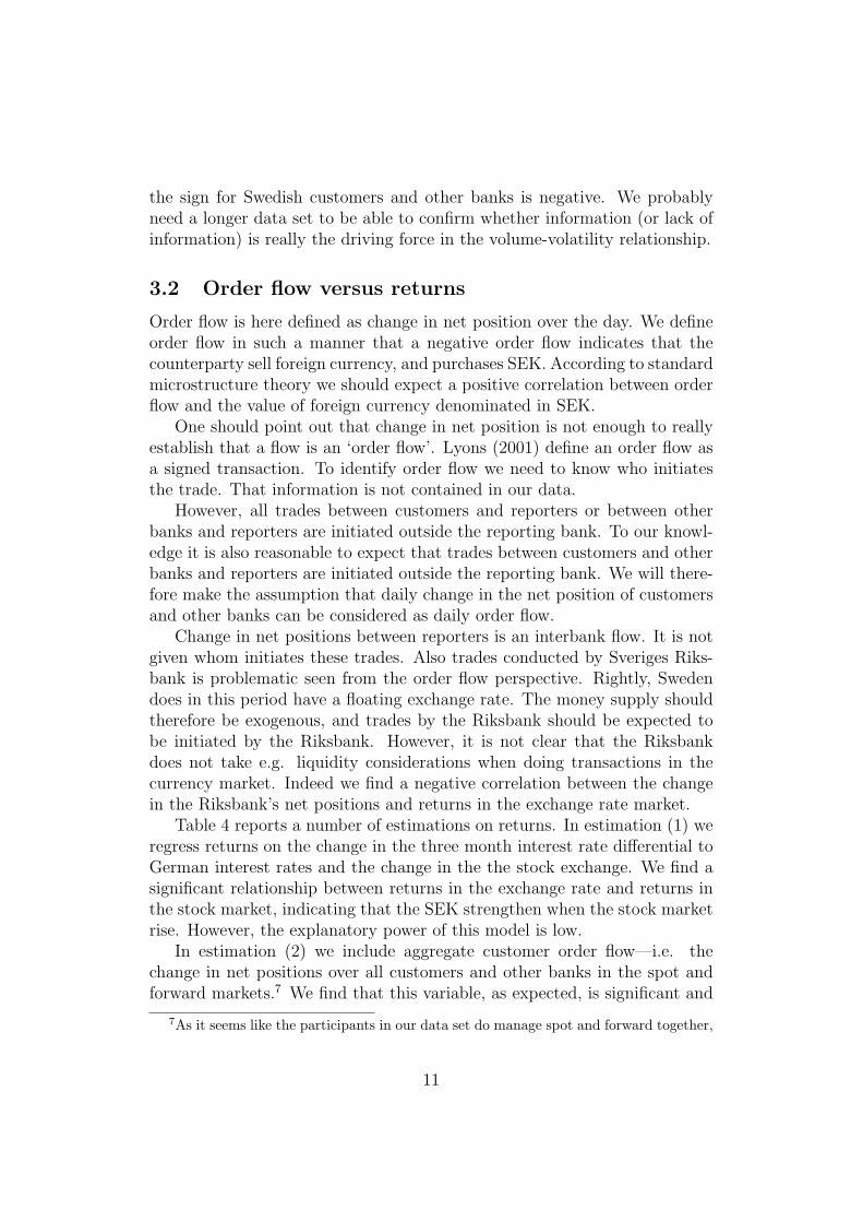
3.2 Order flow versus returns

Order flow is here defined as change in net position over the day. We defineorder flow in such a manner that a negative order flow indicates that thecounterparty sell foreign currency, and purchases SEK. According to standardmicrostructure theory we should expect a positive correlation between orderflow and the value of foreign currency denominated in SEK.

One should point out that change in net position is not enough to reallyestablish that a flow is an ‘order flow’. Lyons (2001) define an order flow asa signed transaction. To identify order flow we need to know who initiatesthe trade. That information is not contained in our data.

However, all trades between customers and reporters or between otherbanks and reporters are initiated outside the reporting bank. To our knowl-edge it is also reasonable to expect that trades between customers and otherbanks and reporters are initiated outside the reporting bank. We will there-fore make the assumption that daily change in the net position of customersand other banks can be considered as daily order flow.

Change in net positions between reporters is an interbank flow. It is notgiven whom initiates these trades. Also trades conducted by Sveriges Riks-bank is problematic seen from the order flow perspective. Rightly, Swedendoes in this period have a floating exchange rate. The money supply shouldtherefore be exogenous, and trades by the Riksbank should be expected tobe initiated by the Riksbank. However, it is not clear that the Riksbankdoes not take e.g. liquidity considerations when doing transactions in thecurrency market. Indeed we find a negative correlation between the changein the Riksbank’s net positions and returns in the exchange rate market.

Table 4 reports a number of estimations on returns. In estimation (1) weregress returns on the change in the three month interest rate differential toGerman interest rates and the change in the the stock exchange. We find asignificant relationship between returns in the exchange rate and returns inthe stock market, indicating that the SEK strengthen when the stock marketrise. However, the explanatory power of this model is low.

In estimation (2) we include aggregate customer order flow—i.e. thechange in net positions over all customers and other banks in the spot andforward markets.7 We find that this variable, as expected, is significant and

7As it seems like the participants in our data set do manage spot and forward together,

11

Tab

le3:

Est

imat

ing|r

eturn

s|(b

)—01

.01.

1998

to06

.30.

1998

|ret

urn

s|(1

)t-st

at(5

)t-st

at(6

)t-st

at(7

)t-st

atC

onst

ant

0.00

24.

825

**0.

002

4.97

7**

0.00

215

.209

**0.

002

15.2

08**

Unex

p.,

spot

,SG

p,D

(SG

SL

LU

)-1

.42E

-08

-0.2

41-7

.97E

-09

-0.1

42U

nex

p.,

spot

,FG

,D

(FG

SL

LU

)1.

39E

-07

3.94

6**

1.31

E-0

73.

803

**1.

52E

-07

5.13

4**

Unex

p.,

spot

,re

p.,

D(L

RSL

LU

)8.

23E

-08

1.11

47.

58E

-08

1.04

0U

nex

p.,

spot

,R

iksb

.,D

(SSSL

LU

)1.

02E

-06

1.17

61.

01E

-06

1.17

5M

onday

dum

my,

D1

0.00

0-0

.167

0.00

00.

860

Tues

day

dum

my,

D2

0.00

00.

050

0.00

00.

124

Wed

nes

day

dum

my,

D3

0.00

0-0

.318

0.00

00.

098

Thurs

day

dum

my,

D4

0.00

00.

137

0.00

00.

003

Abs.

stock

index

ret.,|d

(lO

MX

C)|

0.04

31.

963

0.03

51.

675

Abs.

inte

rest

dif.,

|d(r

dif

)|-0

.003

-0.2

99-0

.005

-0.5

84Adj

ust

edR

2-0

.02

0.17

0.17

0.17

DW

2.03

2.01

1.92

1.89

S.E

.ofre

gres

sion

0.00

20.

002

0.00

20.

002

Note

1:

Est

imate

dw

ith

OLS

Note

2:

*-5

per

cent,

**

-1

per

cent

12

positive. The size of the parameter might be difficult to interpret. However,notice that returns is measured in change in logarithms of the exchange rate.Flows are measured in millions of SEK. Evans and Lyons (2002) report anorder flow effect of 0.5 per cent in the DEM/USD market for a trade of 1billion USD. A trade of 1 billion USD would equal approximately a trade of8000 million SEK. That would give an effect of 0.006 on the exchange rate,or in other terms, an effect of 0.6 per cent. This is close to the findings ofEvans and Lyons.

In estimation (3) we differentiate between counterparties. Interestingly,we find that Swedish and foreign customers and other banks behave as ex-pected: the parameter is significant and the sign is positive.8 Inter-reporterflows are not significant. Order flow from the Riksbank is significant, butwith a negative sign. This might indicate that we do not interpret the or-der flow definition properly with regard to the central bank. The lack ofeffect from interbank trade may also be due to noise introduced through ourdefinition of order flow.

A potential problem in estimations (1-3) is the question whether or notorder flows ar endogenous with regard to the exchange rate. The microstruc-ture theory clearly predicts that order flow should be exogenous. However,as the results in the next section will show, this is not clear in our data. Onepossibility is that order flow is partly a function of feedback trading. Thiscould affect our results significantly.

To control for feedback trading we include 5 lags of the return in theexchange rate in estimation (4). Only one of the five lags is significant—lag4. However, as can be seen when comparing estimation (3) and (4), althoughR2 rises considerably, the results for the order flow variables does not changenoticeably.

3.3 The dynamics of order flow

On volume vs. volatility there is a vaste theoretical literature. On order flowvs. returns there is a growing literature. On the dynamics of order flow littlehas been done in the theoretical area.

Some hypotheses have been put forward. Killeen et al. (2001) argue thatunder a flexible exchange rate one should expect order flow and exchangerates to be (i) cointegrated, (ii) the order flow should be weakly exogenouswith regard to the exchange rate, and (iii) the order flow should be strongly

we find it reasonable to include both spot and forward positions when calculating orderflow.

8Notice that the size of the order flow parameter for these two groups is no in factexactly 0.5 per cent per 1 billion USD equivalent.

13

Tab

le4:

Est

imat

ing

retu

rns—

01.0

1.19

98to

06.3

0.19

98re

turn

s(1

)t-st

at(2

)t-st

at(3

)t-st

at(4

)t-st

atC

onst

ant

0.00

00.

576

0.00

00.

984

0.00

12.

776

**0.

001

2.79

8**

Tot

.cu

stom

erO

F,D

(OF

LG

GL

)7.

72E

-07

3.98

7**

Sw

e.cu

stom

erO

F,D

(OF

SG

GL

)6.

61E

-07

2.97

9**

6.24

E-0

72.

880

**For

.cu

stom

erO

F,D

(OF

FG

GL

)6.

11E

-07

2.95

1**

7.06

E-0

73.

442

**R

epor

ter

OF,D

(OF

LR

GL

)-1

.94E

-07

-0.6

37-1

.76E

-07

-0.5

94R

eser

ves,

D(O

FSSG

L)

-3.6

3E-0

6-3

.026

**-3

.78E

-06

-3.1

94**

Inte

rest

dif.,

d(r

dif

)0.

002

0.17

3-0

.002

-0.1

51-0

.006

-0.5

070.

000

-0.0

35Sto

ckin

dex

retu

rn,d(l

OM

XC

)-0

.054

-2.4

72*

-0.0

51-2

.437

*-0

.055

-2.6

95**

-0.0

53-2

.689

**Lag

ged

retu

rn(4

)0.

195

2.44

5*

Adj

ust

edR

20.

030.

140.

180.

30D

W2.

092.

022.

052.

15S.E

.ofre

gres

sion

0.00

30.

003

0.00

30.

001

Note

1:

Est

imate

dw

ith

OLS

Note

2:

*-5

per

cent,

**

-1

per

cent

:W

ein

clude

5la

gged

valu

esof

retu

rnin

this

regr

essi

on.

Only

the

fourt

hla

gis

sign

ifica

nt.

14

Table 5: Estimating Granger causality—01.01.1998 to 06.30.1998d(OFSGGL) does not Granger cause d(lSEK) F-stat 0.70 0.62d(OFFGGL) does not Granger cause d(lSEK) F-stat 1.00 0.42d(OFLRGGL) does not Granger cause d(lSEK) F-stat 1.20 0.32d(lSEK) does not Granger cause d(OFSGGL) F-stat 2.56 0.03 *d(lSEK) does not Granger cause d(OFFGGL) F-stat 3.91 0.00 **d(lSEK) does not Granger cause d(OFLRGGL) F-stat 1.55 0.18

Note1: Estimated with bivariate VAR, 5 lags. Probability levels in the right-most column.Note2: * - 5 per cent, ** - 1 per cent

exogenous with regard to the exchange rate. Strong exogeneity is defined byKilleen et al. (2001) as the observation that order flow should Granger causethe exchange rate.

The sample is to short to conduct satisfactory cointegration analysis.9

However, we believe that we can with some degree of reason do a Grangercausality test. The results are reported in table 5. Evidence seems to bethat one can not reject that there is no relationship from order flows to theexchange rate. This is the case for order flows from Swedish customers andother banks, for foreign customers and other banks, and for changes in netpositions of reporters. However, one can reject a hypothesis of no relationshipfrom the exchange rate to order flow for Swedish and foreign customers andother banks. This indicates that order flow in this sample seems to react topast returns, not the other way around.

The Granger causality tests indicate that past returns in the currencymarket might be one explanatory variable for order flow. Chordia et al.(2001) find a relationship between the volume and past returns in the stockand bond markets. To investigate this issue closer we conduct a process ofeconometric modelling. 10 We use the general to specific modelling approach,and begin with a model containing the same period and five lags of returns in(i) the exchange rate and (ii) the Swedish stock index (OMX), (iii) the changein the three month and (iv) 10 year interest differential to Germany (the lastindicating uncertainty about future inflation differentials), and order flowsfor the the four groups (v) Swedish customers and other banks, (vi) foreigncustomers and other banks, (vii) net changes in positions between reportersand (viii) net changes in reserves (measured as net changes in the positionsof the Riksbank). We also include dummies for different week-days. We theneliminate variables have no explanatory power, and test modelling progress

9Some preliminary results do indicate the presence of a stable cointegration vector.However, it seems like the exchange rate is weakly exogenous, not the order flow.

10Since there is little theory in this area, we feel that this approach is justified.

15

using F-tests. We report only final modelling results.The results for order flow from Swedish customers and other banks is

reported in table 6. We see that our model has reasonable explanatorypower—the R2 is above 0.5. Order flow from Swedish customers and otherbanks seems to depend on simultaneous and past flows, as could be expected.However, order flow also seems to depend on past returns in the exchangerate, past returns in the OMX and past interest rate changes. To summariseour findings:

• As expected, a same day depreciation leads to flow out of SEK. Howevera depreciation leads to purchases of SEK two days hence. Assumingthat this group contains a number of importers and exporters, this seemreasonable.

• A change in the short term interest rate on the same day the previousweek tends to affect flows.

• Past returns on the Stockholm stock exchange is positively correlatedwith the purchase of SEK (remember that a purchase of SEK is anegative number).

• An increase in the 10 year interest differential to Germany seems tomake Swedish customers and other banks depart from SEK. This mightindicate that an increase in the long term spread indicates increaseduncertainty about conditions in Sweden.

The results for the order flow of Swedish customers and other banksbecome even more interesting when compared with similar results for foreigncustomers and other banks, as reported in table 7. As can be seen, neithershort-term interest rates nor the stock market index is contained in thisregression. In fact the only lagged macro variable included is the long-terminterest rate differential. On the other hand, daily dummies are importanthere. It seems like foreign flows depend on an other set of variables thanlocal flows.

With regard to inter-reporter flows, these do not depend on macro vari-ables at all. However, one should notice that our ability to explain theseflows are much less than our ability to explain customer flows. It is a wellknown from the banking literature that the amount of interbank flows arevery difficult to justify in standard models. We must conclude that it is sat-isfying to find that macro variables do not explain changes in net positionsbetween reporting banks. However, our findings in this area provides evenmore indications of the need for a good general equilibrium model of theinterbank market.

16

Table 6: Estimating d(OFSGGL)—01.01.1998 to 06.30.1998t-stat

Constant 270.43 1.85d(OFSGGL)3 0.13 2.01 *d(OFFGGL) -0.63 -10.82 **d(OFFGGL)4 -0.11 -1.88d(OFLRGL) -0.35 -3.05 **d(OFLRGL)1 0.23 1.95d(OFSSGL)5 -1.11 -2.44 *d(lSEK) 1023.20 3.27 **d(lSEK)2 -907.48 -2.85 **d(rdif3)5 -126.03 -2.75 **d(lOMX)2 -206.16 -2.37 *d(lOMX)3 -223.92 -2.55 *d(lOMX)5 -153.50 -1.92d(rdif10) 9739.16 2.78 **d(rdif10)1 4957.39 1.49d(rdif10)3 -7323.82 -2.29 *D2 -268.04 -1.10Adjusted R2 0.61AR 1-4 test 0.367 (0.83)ARCH 1-4 test 0.370 (0.83)

Note1: Estimated with OLSNote2: * - 5 per cent, ** - 1 per cent

Table 7: Estimating d(OFFGGL)—01.01.1998 to 06.30.1998t-stat

Constant 372.1383 2.229 *d(OFSGGL) -0.72631 -10.615 **d(lSEK) 1236.07 3.575 **d(rdif10)1 8208.599 2.364 *d(rdif10)4 -7736.53 -2.309 *D2 -884.934 -3.063 **D3 -842.137 -2.837 **D4 -839.289 -2.873 **Adjusted R2 0.55AR 1-4 test 0.973 (0.43)ARCH 1-4 test 0.588 (0.67)

Note1: Estimated with OLSNote2: * - 5 per cent, ** - 1 per cent

17

Table 8: Estimating d(OFLRGL)—01.01.1998 to 06.30.1998t-stat

d(OFSGGL) -0.16 -3.41 **d(OFLRGL)1 0.31 3.58 **Adjusted R2 0.15AR 1-4 test 1.100 (0.36)ARCH 1-4 test 0.918 (0.46)

Note1: Estimated with OLSNote2: * - 5 per cent, ** - 1 per cent

4 Conclusions

Our starting point was: does it matter for the FX markets who you are? Theanswer is that different counterparties clearly seems to affect the marketsdifferently. This opens a wide field of possible research questions.

We have used this paper to investigate a number of different questionsrelated to microstructure theory. As pointed out on several occasions above,our results should at this point be interpreted with care. However, we believeour results illustrate the potential in this kind of data. Such data can bothbe used to test the number of existing (and in part competing) theoriesthat exists in the microstructure literature. It can also be used to point outinteresting avenues for new theoretical research.

References

Admati, A. R. and P. Pfleiderer (1988). “A theory of intraday patterns:Volume and price variability.” Review of Financial Studies, 1(1), 3–40.

Cai, J., Y.-L. Cheung, R. S. K. Lee and M. Melvin (2001). “‘once-in-a-generation’ yen volatility in 1998: Fundamentals, intervention, and orderflow.” Journal of International Money and Finance, 20(3), 327–47.

Chordia, T., A. Sarkar and A. Subrahmanyam (2001). “Common determi-nants of bond and stock market liquidity: The impact of financial crises,monetary policy and mutual funds.” Tech. Rep. 140, Federal Reserve Bankof New York.

Clark, P. K. (1973). “A subordinated stochastic process model with finitevariance for speculative prices.” Econometrica, 41, 135–55.

Copeland, T. E. (1976). “A model of asset trading under the assumption ofsequential information arrival.” Journal of Finance, 31, 1149–68.

18

Copeland, T. E. (1977). “A probability model of asset trading.” Journal ofFinancial and Quantitative Analysis, 12, 563–78.

Daigler, R. T. and M. K. Wiley (1999). “The impact of trader type on thefutures volatility-volume relation.” Journal of Finance, 54(6), 2297–2316.

Evans, M. D. and R. K. Lyons (2002). “Order flow and exchange rate dy-namics.” Journal of Political Economy, 110, 170–180.

Fan, M. and R. K. Lyons (2000). “Customer-dealer trading in the foreignexchange market.” typescript.

Galati, G. (2000). “Trading volumes, volatility and spreads in foreign ex-change markets: Evidence from emerging market countries.” Workingpaper 93, Bank for International Settlements.

Grinblatt, M. and M. Keloharju (2001). “How distance, language, and cultureinfluence stockholdings and trades.” Journal of Finance, 56(3), 1053–73.

Harris, M. A. and A. Raviv (1993). “Differences of opinion make a horserace.” Review of Financial Studies, 6(3), 473–506.

Hartmann, P. (1999). “Trading volumes and transaction costs in the foreignexchange market. evidence from daily dollar–yen spot data.” Journal ofBanking and Finance, 23, 801–24.

Isard, P. (1995). Exchange Rate Economics. Cambridge University Press.

Jorion, P. (1996). Risk and Turnover in the Foreign Exchange Market, pp.19–37. ucp, Chicago.

Karpoff, J. M. (1987). “The relation between price changes and tradingvolume: A survey.” Journal of Financial and Quantitative Analysis, 22(1),109–26.

Killeen, W. P., R. K. Lyons and M. J. Moore (2001). “Fixed versus flexible:Lessons from EMS order flow.” Tech. Rep. 8491, NBER.

Kyle, A. S. (1985). “Continuous auctions and insider trading.” Econometrica,53(6), 1315–35.

Lyons, R. K. (2001). The Microstructure Approach to Exchange Rates. MITPress, Cambridge, Mass.

Melvin, M. and X. Yin (2000). “Public information arrival, exchange ratevolatility, and quote frequency.” Economic Journal, 110(465), 644–61.

19

Rime, D. (2001). “Private or public information in foreign exchange markets?An empirical analysis.” University of Oslo.

Shalen, C. T. (1993). “Volume, volatility, and the dispersion of beliefs.”Review of Financial Studies, 6(2), 405–34.

Wei, S.-J. and J. Kim (1997). “The big players in the foreign exchangemarket: Do they trade on information or noise.” Working Paper 6256,NBER.

20