Volume 1, Issue 2, December 2010 - Index of
162
Volume 1, Issue 2, December 2010 E-ISSN: 2045-5364
-
Upload
khangminh22 -
Category
Documents
-
view
0 -
download
0
Transcript of Volume 1, Issue 2, December 2010 - Index of

Volume 1, Issue 2, December 2010
E-ISSN: 2045-5364

International Journal of Latest Trends in Computing (E-ISSN: 2045-5364) Volume 1, Issue 2, December 2010
i
IJLTC Board Members
Editor In Chief
I .Khan United Kingdom
Advisory Editor
N .Aslam United Kingdom
Editorial Board
A.Srinivasan India
Oleksandr Dorokhov Ukraine
Yau Jim Yip United Kingdom
Azween Bin Abdullah Malaysia
Bilal ALATAS Turkey
Khosrow Kaikhah USA
Ion Mierlus Mazilu Romania
Jaime Lloret Mauri Spain
Padmaraj Nair USA
Diego Reforgiato Recupero USA
Chiranjeev Kumar India
Saurabh Mukherjee India
Changhua Wu USA
Chandrashekar D.V India
Constantin Volosencu Romania
Acu Ana Maria Romania
Nitin Paharia India
Bhaskar N. Patel India
Arun Sharma India

International Journal of Latest Trends in Computing (E-ISSN: 2045-5364) Volume 1, Issue 2, December 2010
ii
TABLE OF CONTENTS
1. Paper 01: De-Cliticizing Context Dependent Clitics in Pashto Text (pp-1:7)
o Aziz-Ud-Din, Mohammad Abid Khan
University of Peshawar, Pakistan
2. Paper 02: Factors of the Project Failure (pp-8:11)
o Muhammad Salim Javed, Ahmed Kamil Bin Mahmood, Suziah B. Sulaiman
Universiti Teknologi PETRONAS
3. Paper 03: WiMAX Standars and Implementation Challenges (pp-12:17)
o Charanjit Singh Punjabi University
o Dr Manjeet Singh Punjabi University
o Dr Sanjay Sharma Thapar University

International Journal of Latest Trends in Computing (E-ISSN: 2045-5364) Volume 1, Issue 2, December 2010
iii
TABLE OF CONTENTS
1. A FAULT DETECTION AND RECOVERY ALGORITHM IN WIRELESS SENSOR
NETWORKS ............................................................................................................................................... 1
Abolfazl Akbari, Neda Beikmahdavi
2. BACTERIAL FORAGING OPTIMIZATION BASED LOAD FREQUENCY CONTROL OF
INTERCONNECTED POWER SYSTEMS WITH STATIC SYNCHRONOUS SERIES
COMPENSATOR ....................................................................................................................................... 7
B.Paramasivam, Dr. I.A. Chidambaram
3. MOTION HEURISTICS APPROACH OF SEARCH AN OPTIMAL PATH FROM SOURCE
TO DESTINATION IN ROBOTS .........................................................................................................14
Dr. T.C. Manjunath
4. ANALYSIS OF SOFTWARE QUALITY MODELS FOR ORGANIZATIONS.............................19
Dr. Deepshikha Jamwal
5. MINIMIZATION OF NUMBER OF HANDOFF USING GENETIC ALGORITHM IN
HETROGENEOUS WIRELESS NETWORKS ..................................................................................24
Mrs.Chandralekha, Dr. Praffula Kumar Behera
6. ENHANCED DEVELOPMENTS IN WIRELESS MOBILE NETWORKS (4G
TECHNOLOGIES) ...................................................................................................................................29
Dr. G.Srinivasa Rao, Dr.G.Appa Rao, S.Venkata Lakshmi, D.Veerabadhra Rao, D.Rajani
7. PARAMETER OPTIMIZATION OF QUANTUM WELL NANOSTRUCTURE: A PSO AND
GA BASED COMPARATIVE STUDY .................................................................................................35
Sanjoy Deba, C. J. Clement Singha, N Basanta Singhb, A. K Dec and S K Sarkara
8. EXPERIMENTAL PROTOCOL DEVELOPMENT FOR A PASSIVE THERMAL
MANAGEMENT SYSTEM ....................................................................................................................41
Emily D. Pertl, Daniel K. Carder and James E. Smith
9. HARDWARE PLATFORM FOR MULTI-AGENT SYSTEM DEVELOPMENT .......................47
Michael J. Spencer, Ali Feliachi, Franz A. Pertl, Emily D. Pertl and James E. Smith

International Journal of Latest Trends in Computing (E-ISSN: 2045-5364) Volume 1, Issue 2, December 2010
iv
10. DOCUMENT CLASSIFICATION USING NOVEL SELF ORGANIZING TEXT CLASSIFIER
......................................................................................................................................................................53
Seyyed Mohammad Reza Farshchi, Taghi Karimi
11. SEPARATION OF TABLA FROM SINGING VOICE USING PERCUSSIVE FEATURE
DETECTION IN A POLYPHONIC CHANNEL ...............................................................................63
Neeraj Dubey , Parveen Lehana, and Maitreyee Dutta
12. AN ALTERNATIVE METHOD OF FINDING THE MEMBERSHIP OF A FUZZY NUMBER
......................................................................................................................................................................69
Rituparna Chutia, Supahi Mahanta, Hemanta K. Baruah
13. FUZZY ARITHMETIC WITHOUT USING THE METHOD OF α - CUTS ................................73
Supahi Mahanta, Rituparna Chutia, Hemanta K Baruah
14. NHPP AND S-SHAPED MODELS FOR TESTING THE SOFTWARE FAILURE PROCESS
......................................................................................................................................................................81
Dr. Kirti Arekar
15. A COMPARATIVE STUDY OF IMPROVED REGION SELECTION PROCESS IN IMAGE
COMPRESSION USING SPIHT AND WDR ....................................................................................86
T.Ramaprabha, Dr M.Mohamed Sathik
16. NOVEL INTELLIGENT LOW COST CHILD DISEASE DIAGNOSTIC SYSTEM ....................91
A.M. Agarkar, Dr. A.A. Ghatol
17. TOOLS AND TECHNIQUES FOR EVALUATING WEB INFORMATION RETRIEVAL
USING CLICK-THROUGH DATA ......................................................................................................97
Amarjeet Singh, Dr. Mohd. Husain, Rakesh Ranjan, Manoj Kumar
18. IMPROVE THE CLASSIFICATION AND PREDICTION PERFORMANCE FOR THE IP
MANAGEMENT SYSTEM IN A SUPER-CAPACITOR PILOT PLANT ................................ 102
Zhi Yuan Chen, Dino Isa, Peter Blanchfield and Roselina Arelhi

International Journal of Latest Trends in Computing (E-ISSN: 2045-5364) Volume 1, Issue 2, December 2010
v
19. WATERMARKING OF H.264 CODED VIDEO BASED ON THE SHIFTED-HISTOGRAM
TECHNIQUE ........................................................................................................................................ 109
S. Bouchama, L. Hamami, M.T. Qadri and M. Ghanbari
20. SUPPRESSION OF RANDOM VALUED IMPULSIVE NOISE USING ADAPTIVE
THRESHOLD ....................................................................................................................................... 116
Gunamani Jena and R Baliarsingh
21. PAPER CURRENCY RECOGNITION SYSTEM USING CHARACTERISTICS EXTRACTION
AND NEGATIVELY CORRELATED NN ENSEMBLE ............................................................... 121
A. Ms. Trupti Pathrabe and B. Dr. N. G. Bawane
22. AN EFFICIENT DICTIONARY BASED COMPRESSION AND DECOMPRESSION
TECHNIQUE FOR FAST AND SECURE DATA TRANSMISSION .......................................... 125
Prof. Leena K. Gautam, Prof V.S. Gulhane
23. EFFECTIVE COMPRESSION TECHNIQUE BY USING ADAPTIVE HUFFMAN CODING
ALGORITHM FOR XML DATABASE ............................................................................................. 129
Ms. Rashmi N. Gadbail, Prof.V.S.Gulhane
24. CONGESTION CONTROL AND BUFFERING TECHNIQUE FOR VIDEO STREAMING
OVER IP .................................................................................................................................................. 133
Md .Taslim Arefin, Md. Ruhul Amin
25. THE EMPIRICAL STUDY ON THE FACTORS AFFECTING DATA WAREHOUSING
SUCCESS ............................................................................................................................................... 138
Md. Ruhul Amin, Md .Taslim Arefin
26. SHOULD YOU STAY SAFE WITH BI TOOLS AND ONLY SELECT THOSE THAT ARE
HIGHEST RATED BY GARTNER ................................................................................................... 143
Md. Ruhul Amin, Md .Taslim Arefin
27. MEDICAL VIDEO COMPRESSION BY ADAPTIVE PARTICLE COMPRESSION ............. 152
A.K. Deshmane and S.N. Talbar

International Journal of Latest Trends in Computing (E-ISSN: 2045-5364) 1 Volume 1, Issue 2, December 2010
A Fault Detection and Recovery Algorithm in Wireless
Sensor Networks
Abolfazl Akbari
Department of computer Engineering
Islamic Azad University Science and Research Branch
Tehran, Iran
Neda Beikmahdavi Department of computer Engineering
Islamic Azad University Ayatollah Amoli Branch
Amol, Iran
Abstract—in the past few years wireless sensor networks have received
a greater interest in application such as disaster management, border
protection, combat field reconnaissance and security surveillance.
Sensor nodes are expected to operate autonomously in unattended
environments and potentially in large numbers. Failures are inevitable
in wireless sensor networks due to inhospitable environment and
unattended deployment. The data communication and various network
operations cause energy depletion in sensor nodes and therefore, it is
common for sensor nodes to exhaust its energy completely and stop
operating. This may cause connectivity and data loss. Therefore, it is
necessary that network failures are detected in advance and
appropriate measures are taken to sustain network operation. In this
paper we proposed a new mechanism to sustain network operation in
the event of failure cause of energy-drained nodes. The proposed
technique relies on the cluster members to recover the connectivity. The
proposed recovery algorithm has been compared with some existing
related work and proven to be more energy efficient [20].
Key words: Sensor Networks, clustering, fault detection, fault
recovery.
1. Introduction
Recent advances in MEMS (Micro-electro-mechanical systems)
and wireless network technology have made the development of
small, inexpensive, low power distributed devices, which are
capable of local processing and wireless communication, a
reality. Such devices are called sensor nodes. Sensors provide an
easy solution to those applications that are based in the
inhospitable and low maintenance areas where conventional
approaches prove to be impossible and very costly. Sensors are
generally equipped with limited data processing and
communication capabilities and are usually deployed in an ad-
hoc manner to in an area of interest to monitor events and gather
data about the environment. Examples include environmental
monitoring- which involves monitoring air soil and water,
condition based maintenance, habitat monitoring, seismic
detection, military surveillance, inventory tracking, smart spaces
etc. Sensor nodes are typically disposable and expected to last
until their energy drains. Therefore, it is vital to manage energy
wisely in order to extend the life of the sensors for the duration
of a particular task. [1-6]. Failures in sensor networks due to
energy depletion are continuous and may increase. This often
results in scenarios where a certain part of the network become
energy constrained and stop operating after sometime. Sensor
nodes failure may cause connectivity loss and in some cases
network partitioning. In clustered networks, it creates holes in
the network topology and disconnects the clusters, thereby
causing data loss and connectivity loss [10]. Good numbers of
fault tolerance solutions are available but they are limited at
different levels. Existing approaches are based on hardware
faults and consider hardware components malfunctioning only.
Some assume that system software's are already fault tolerant as
in [7, 8]. Some are solely focused on fault detection and do not
provide any recovery mechanism [9]. Sensor network faults
cannot be approached similarly as in traditional wired or
wireless networks due to the following reasons [11]:
1. Traditional wired network protocol are not
concerned with the energy consumptions as they are constantly
powered and wireless ad hoc network are also rechargeable
regularly.
2. Traditional network protocols aim to achieve point to point
reliability, where as wireless sensor networks are more
concerned with reliable event detection.
3. Faults occur more frequently in wireless sensor networks than
traditional networks, where client machine, servers and routers
are assumed to operate normally.
Therefore, it is important to identify failed nodes to guarantee
network connectivity and avoid network partitioning. The New
Algorithm recovery scheme is compared to Venkataraman
algorithm proposed in [10]. The Venkataraman algorithm is the
latest approach towards fault detection and recovery in wireless
sensor networks and proven to be more efficient than some
existing related work. It solely focused on nodes notifying its
neighboring nodes to initiate the recovery mechanism. It can be
observed from the simulation results that failure detection and
recovery in our proposed algorithm is more energy efficient and
quicker than that of Venkataraman algorithm. In [10], it has
been found that Venkataraman algorithm is more energy
efficient in comparison with Gupta and Younis [15].

International Journal of Latest Trends in Computing (E-ISSN: 2045-5364) 2 Volume 1, Issue 2, December 2010
Therefore, we conclude that our proposed algorithm is also more
efficient than Gupta and Crash fault detection algorithm in term
of fault detection and recovery.
This paper is organized as follows: Section 2 provides a brief
review of related work in the literature. . In section 3, we
provided a detail description of our clustering algorithm.
In section 4, we provided a detail description of our proposed
solution. The performance evaluation of our proposed algorithm
can be found in Section 5, Finally, section 6 concludes the
paper.
2. Related Work
In this section we will give an overview about existing fault
detection and recovery approaches in wireless sensor networks.
A survey on fault tolerance in wireless sensor networks can be
found in [12]. A detailed description on fault detection and
recovery is available at [11]. WinMS [13] provides a centralized
fault management approach. It uses the central manager with
global view of the network to continually analyses network
states and executes corrective and preventive management
actions according to management policies predefined by human
managers. The central manager detects and localized fault by
analyzing anomalies in sensor network models. The central
manager analyses the collected topology map and the energy
map information to detect faults and link qualities. WinMS is a
centralized approach and approach is suitable for certain
application. However, it is composed of various limitations. It is
not scalable and cannot be used for large networks. Also, due to
centralize mechanism all the traffic is directed to and from the
central point. This creates communication overhead and quick
energy depletions. Neighboring co-ordination is another
approach to detect faulty nodes. . For Example, the algorithm
proposed for faulty sensor identification in [16] is based on
neighboring co-ordination. In this scheme, the reading of a
sensor is compared with its neighboring‟ median reading, if the
resulting difference is large or large but negative then the sensor
is very likely to be faulty. Chihfan et. al [17] developed a Self
monitoring fault detection model on the bases of accuracy. This
scheme does not support network dynamics and required to be
pre configured. In [14], fault tolerance management architecture
has been proposed called MANNA (Management architecture
for wireless sensor networks). This approach is used for fault
diagnosis using management architecture, termed as MANNA.
This scheme creates a manager located externally to the wireless
sensor network and has a global vision of the network and can
perform complex operations that would not be possible inside
the network. However, this scheme performs centralized
diagnosis and requires an external manager. Also, the
communication between nodes and the manager is too expensive
for WSNs. In Crash fault detection scheme [18], an initiator
starts fault detection mechanism by gathering information of its
neighbors to access the neighborhood and this process continue
until all the faulty nodes are identified. Gathering neighboring
nodes information consumes significant energy and time
consuming. It does not perform recovery in terms of failure.
Gupta algorithm [15] proposed a method to recover from a
gateway fault. It incorporates two types of nodes: gateway nodes
which are less energy constrained nodes (cluster headers) and
sensor nodes which are energy constrained. The less energy
constrained gateway nodes maintain the state of sensors as well
as multi-hop route for collecting sensors. The disadvantage is
that since the gateway nodes are less energy constraint and static
than the rest of the network nodes and they are also fixed for the
life of the network. Therefore sensor nodes close to the gateway
node die quickly while creating holes near gateway nodes and
decrease network connectivity.
Also, when a gateway node die, the cluster is dissolved and all
its nodes are reallocated to other healthy gateways. This
consume more time as all the cluster members are involved in
the recovery process. Venkataraman algorithm [10], proposed a
failure detection and recovery mechanism due to energy
exhaustion. It focused on node notifying its neighboring nodes
before it completely shut down due to energy exhaustion. They
proposed four types of failure mechanism depending on the type
of node in the cluster. The nodes in the cluster are classified into
four types, boundary node, pre-boundary node, internal node and
the cluster head. Boundary nodes do not require any recovery
but pre-boundary node, internal node and the cluster head have
to take appropriate actions to connect the cluster. Usually, if
node energy becomes below a threshold value, it will send a
fail_report_msg to its parent and children. This will initiate the
failure recovery procedure so that failing node parent and
children remain connected to the cluster.
3. Cluster formation
The sensor nodes are dispersed over a terrain and are assumed to
be active nodes during clustering.
Problem Definition
The clustering strategy limits the admissible degree, D and the
number of nodes in each cluster, S. The clustering aims to
associate every node with one cluster. Every node does not
violate the admissible degree constraint, D and every cluster
does not violate the size constraint, S while forming the cluster.
The number of clusters(C) in the network is restricted to a
minimum of N/S, N > C > N/S, where N is the number of nodes
in the terrain.
Sensor Network model
A set of sensors are deployed in a square terrain. The nodes
possesses the following properties
i. The sensor nodes are stationary.

International Journal of Latest Trends in Computing (E-ISSN: 2045-5364) 3 Volume 1, Issue 2, December 2010
ii. The sensor nodes have a sensing range and a transmission
range. The sensing range can be related to the transmission
range, Rt> 2rs.
iii. Two nodes communicate with each other directly if they are
within the transmission range
iv. The sensor nodes are assumed to be homogeneous i.e. they
have the same processing power and initial energy.
v. The sensor nodes are assumed to use different power levels to
communicate within and across clusters.
vi. The sensor nodes are assumed to know their location and the
limits S and D.
Description of the Clustering Algorithm
Initially a set of sensor nodes are dispersed in the terrain. We
assume that sensor nodes know their location and the limits S
and D. Algorithms for estimating geographic or logical
coordinates have been explored at length in the sensor network
research [21, 22].
In our algorithm, the first step is to calculate Eth and Eic for
every node i, N >I > 1. Eth is the energy spent to communicate
with the farthest next hop neighbor. Eic is the total energy spent
on each link of its next hop neighbors. Every node i has an
initial energy, Einit. A flag bit called “covered flag” is used to
denote whether the node is a member of any cluster or not. It is
set to 0 for each node initially.
Calculation of Eth and Eic
i. Nodes send a message hello_msg along with their coordinates
which are received by nodes within the transmission range. For
example in figure (1) nodes a,b,c,d,w,x,y are within transmission
range of v.
ii. After receiving the hello_msg, the node v calculates the
distance between itself and nodes a,b,c,d,w,x,y using the
coordinates from hello_msg. It stores the distance di and the
locations in the dist_table.
iii. Nodes within the sensing range are the neighbours of a node.
In figure (1) nodes w,x,y,b are neighbours of v.
iv. Among the nodes within the sensing range, it chooses the
first D closest neighbours as its potential candidates for next
hop. Assuming D=3, in figure (1), the closest neighbours of v
are w,x,y. v. Among the potential candidates, the farthest node‟s
distance, dmax is taken for the calculation of E th .
Figure 1. Topology
vi. Suppose a node needs power E to transmit a message to
another node who is at a distance „d‟ away, we use the formula
E = E=kd c
[7,8], where k and c are constants for a specific
wireless system. Usually 2<c<4. In our algorithm we assume
k=1, c=2. For a node v, d *1*d2max = E thv, since there are D
members to which a node sends message.
vii. Eic is the total energy spent on each of link of the Dclosest
neighbours. For a node v,
where k= 1. div is the distance between node i and node v. After
the calculation of threshold energy Eth, nodes become eligible
for cluster head position based on their energies. A node v
becomes eligible for the cluster head position if its Einit> Ethv.
and. node with the second Einit> Ethv becomes secondary Cluster
heed. . When no nodes satisfy this condition or when there is
insufficient number of cluster heads, the admissible degree D is
reduced by one and then Eth is recalculated. The lowest value
that D can reach is one. In a case where the condition Einit> Ethv
is never satisfied at all, clustering is not possible because no
node can support nodes other than itself. There may also be
situations where all the nodes or more number of nodes are
eligible for being cluster heads. A method has been devised by
which the excess cluster heads are made to relinquish their
position.
Relinquishing of the cluster head position
i. Every cluster head sends a message cluster_head_status msg
and Eic to its neighbours (within sensing range).
ii. Every cluster head keeps a list of its neighbor cluster heads
along with its Eic
iii. The nodes which receive Eic lesser than itself relinquishes
its position as a cluster head.

International Journal of Latest Trends in Computing (E-ISSN: 2045-5364) 4 Volume 1, Issue 2, December 2010
iv. The cluster heads which are active send their messages to the
cluster_head_manager outside the network.
Thecluster_head_manager has the information of the desired
cluster head count.
v. If the number of cluster heads are still much more than
expected, then another round of cluster head relinquishing starts.
This time the area covered would be greater than sensing range.
vi. The area covered for cluster head relinquishing keeps
increasing till the desired count is reached.
Choosing cluster members
i. The cluster head select the closest D neighbours as next hop
and sends them the message cluster_join_msg. The
cluster_join_msg consists of cluster ID, Sa, D, S, covered flag. Sa
is (S-1)/number of next hop members
ii. Energy is expended when messages are sent. This energy, Eic
is calculated and reduced from the cluster head‟s energy.
iii. The cluster head‟s residual energy Er = Einit – Eic. Einit is the
initial energy when the cluster is formed by the cluster head.
iv. After receiving the cluster_join_msg, the nodes send a
message, cluster_join_confirm_msg to the cluster head if they
are uncovered, else they send a message,
cluster_join_reject_msg.
v. After a cluster_join_confirm_msg, they set their covered_flag
to 1.
vi. The next hop nodes now select D-1 members as their next
hop members. D-1 members are selected because they are
already associated with the node which selected them. For
example, in figure (1) where D =3, a node v selects node w, node
x and node y. In the next stage, node y selects
only node a and node b because it is already connected to node v
making the D = 3.
vii. After selecting the next hop members, the residual energy is
calculated , Er ( new) = Er ( old) - Eic
viii. This proceeds until S is reached or until all nodes have their
covered_flag set to 1.
Tracking of the size
The size S of the cluster is tracked by each and every node. The
cluster head accounts for itself and equally distributes S-1
among its next hop neighbors by sending a message to each one
of them. The neighbours that receive the message account for
themselves and distribute the remaining among all their
neighbours except the parent. The messages propagate until they
reach a stage where the size is exhausted. If the size is not
satisfied, then the algorithms terminates if all the nodes have
been covered. After the cluster formation, the cluster is ready for
operation. The nodes communicate with each other for the
period of network operation time.
4. Cluster Heed Failure recovery Algorithm
We employ a backup secondary cluster heed which will replace
the cluster heed in case of failure, no further messages are
required to send to other cluster members to inform them about
the new cluster heed. Cluster heed and secondary cluster heed
are known to their cluster members. If cluster heed energy drops
below the threshold value, it then sends a message to its cluster
member including secondary cluster heed. Which is an
indication for secondary cluster heed to standup as a new cluster
heed and the existing cell manager becomes common node and
goes to a low computational mode. Common nodes will
automatically start treating the secondary cluster heed as their
new cluster heed and the new cluster heed upon receiving
updates from its cluster members; choose a new secondary
cluster heed. Recovery from cluster heeds failure involved in
invoking a backup node to standup as a new cluster heed.
5. Performance Evaluation
The energy model used is a simple model shown in [19] for the
radio hardware energy dissipation where the transmitter
dissipates energy to run the radio electronics and the power
amplifier, and the receiver dissipates energy to run the radio
electronics. In the simple radio model [19], the radio dissipates
Eelec = 50 nJ/bit to run the transmitter or receiver circuitry and
Eamp = 100 (pJ/bit)/m2 for the transmit amplifier to achieve an
acceptable signal-to-noise ratio. We use MATLAB Software as
the simulation platform, a high performance discrete-event Java-
based simulation engine that runs over a standard Java virtual
machine.
The simulation parameters are explained in Table 1.
We compared our work with that of Venkataraman algorithm
[10], which is based on recovery due to energy exhaustion.
Table 1.Simulation parameters
In Venkataraman algorithm, nodes in the cluster are classified into
four types: boundary node, pre-boundary node, internal node and
the cluster head. Boundary nodes does not require any recovery but

International Journal of Latest Trends in Computing (E-ISSN: 2045-5364) 5 Volume 1, Issue 2, December 2010
pre-boundary node, internal node and the cluster head have to take
appropriate actions to connect the cluster. Usually, if node energy
becomes below a threshold value, it will send a fail_report_msg to
its parent and children. This will initiate the failure recovery
procedure so that failing node parent and children remain connected
to the cluster. A join_request_mesg is sent by the healthy child of
the failing node to its neighbors. All the neighbors with in the transmission range respond with a join_reply_mesg/join_reject_mesg messages. The healthy child of
the failing node then selects a suitable parent by checking whether
the neighbor is not one among the children of the failing node and
whether the neighbor is also not a failing node. In our proposed
mechanism, common nodes does not require any recovery but goes
to low computational mode after informing their cell managers. In
Venkataraman algorithm, cluster head failure cause its children to
exchange energy messages. The children who are failing are not
considered for the new cluster-head election. The healthy child with
the maximum residual energy is selected as the new cluster head
and sends a final_CH_mesg to its members. After the new cluster
head is selected, the other children of the failing cluster head are
attached to the new cluster head and the new cluster head becomes
the parent for these children. This cluster head failure recovery
procedure consumes more energy as it exchange energy messages
to select the new cluster head. Also, if the child of the failing cluster
head node is failing as well, then it also require appropriate steps to
get connected to the cluster. This can abrupt network operation and
is time consuming.
In our proposed algorithm, we employ a back up secondary cluster
heed which will replace the cluster heed in case of failure.
Fig. 2. Average time for cluster head recovery
no further messages are required to send to other cluster members to
inform them about the new cluster heed Figs. 2 and 3 compare the
average energy loss for the failure recovery of the three
algorithms. It can be observed from Fig. 2 that when the
transmission range increases, the greedy algorithm expends the
maximum energy when compared with the Gupta algorithm and
the proposed algorithm. However, in Fig. 3, it can be observed
that the Gupta algorithm spends the maximum energy among the
other algorithms when the number of nodes in the terrain
increases.
Fig. 3. Average time for cluster head recovery
6. Conclusion
In this paper, we have proposed a cluster-based recovery
algorithm, which is energy-efficient and responsive to network
topology changes due to sensor node failures. The proposed
cluster-head failure-recovery mechanism recovers the
connectivity of the cluster in almost less than of the time taken
by the fault-tolerant clustering proposed by Venkataraman. The
Venkataraman algorithm is the latest approach towards fault
detection and recovery in wireless sensor networks and proven to be
more efficient than some existing related work. Venkataraman
algorithm is more energy efficient in comparison with Gupta and
Algorithm Greedy Therefore, we conclude that our proposed
algorithm is also more efficient than Gupta and Greedy[20]
algorithm in term of fault recovery.
The faster response time of our algorithm ensures uninterrupted
operation of the sensor networks and the energy efficiency
contributes to a healthy lifetime for the prolonged operation of
the sensor network.
References
[1] A. Bharathidasas, and V. Anand, “Sensor networks: An
overview”, Technical report, Dept. of Computer Science,
University of California at Davis, 2002
[2] D. Estrin, R. Govindan, J. Heidemann, and S. Kumar, "Next
century challenges: Scalable coordination in sensor networks",
in Proceedings of ACM Mobicom, Seattle, Washington, USA,
August 1999, pp. 263-- 270, ACM.
[3] I.F. Akyildiz, W. Su, Y. Sankarasubramaniam and E.
Cayirci, "A Survey on Sensor Networks", IEEE
Communications Magazine, pp. 102--114, August 2002.
[4] D. Estrin, L. Girod, G. Pottie, M. Srivastava, “Instrumenting
the world with wireless sensor networks”, In Proceedings of the
International Conference on Acoustics, Speech and Signal
Processing (ICASSP 2001.
[5] E. S. Biagioni and G. Sasaki, “Wireless sensor placement
for reliable and efficient data collection”, in the 36th

International Journal of Latest Trends in Computing (E-ISSN: 2045-5364) 6 Volume 1, Issue 2, December 2010
International Conference on Systems Sciences, Hawaii, January
2003.
[6] G. Gupta and M. Younis, “Load-Balanced Clustering in
Wireless Sensor Networks”, in the Proceedings of International
Conference on Communication (ICC 2003), Anchorage, AK,
May 2003.
[7] J. Chen, S. Kher and A. Somani, “Distributed Fault
Detection of Wireless Sensor Networks”, in DIWANS'06. 2006.
Los Angeles, USA: ACM Pres.
[8] F. Koushanfar, M. Potkonjak, A. Sangiovanni- Vincentelli,
“Fault Tolerance in Wireless Ad-hoc Sensor Networks”,
Proceedings of IEEE Sensors 2002, June, 2002.
[9] W. L. Lee, A. Datta, and R. Cardell-Oliver, “Network
Management in Wireless Sensor Networks”, to appear in
Handbook on Mobile Ad Hoc and Pervasive Communications,
edited by M. K. Denko and L. T. Yang, American Scientific
Publishers.
[10] G. Venkataraman, S. Emmanuel and S.Thambipillai,
“Energy-efficient cluster-based scheme for failure management
in sensor networks” IET Commun, Volume 2, Issue 4, April
2008 Page(s):528 – 537
[11] L. Paradis and Q. Han, “A Survey of Fault Management in
Wireless Sensor Networks”, Journal of Network and Systems
Management, vol. 15, no. 2, pp. 171-190, 2007.
[12] L. M. S. D. Souza, H. Vogt and M. Beigl, “A survey on
fault tolerance in wireless sensor networks”, 2007.
[13] W. L Lee, A.D., R. Cordell-Oliver, WinMS: Wireless
Sensor Network-Management System, An Adaptive Policy-
Based Management for Wireless Sensor Networks. 2006.
[14] L. B. Ruiz, I. G.Siqueira, L. B. Oliveira, H. C. Wong, J.M.
S. Nigeria, and A. A. F. Loureiro. “Fault management in event-
driven wireless sensor networks”, MSWiM‟04, October 4-6,
2004, Venezia, Italy
[15] G. Gupta and M. Younis; Fault tolerant clustering of
wireless sensor networks; WCNC‟03, pp. 1579.1584.
[16] M. Ding, D. Chen, K. Xing, and X. Cheng, “Localized
fault-tolerant event boundary detection in sensor networks”, in
Proceedings of the 24th Annual Joint Conference of the IEEE
Computer and Communications Societies (INFOCOM '05), vol.
2, pp. 902–913, Miami, Fla, USA, March 2005
[17] C. Hsin and M.Liu, “Self-monitoring of Wireless Sensor
Networks”, Computer Communications, 2005. 29: p. 462-478
[18] S. Chessa and P. Santi, “Crash faults identification in
wireless sensor networks”, Comput. Commun., 2002, 25, (14),
pp. 1273-1282.
[19] W. R. Heinzelman, A. Chandrakasan, and H. Balakrishnan,
"Energy-Efficient Communication Protocol for Wireless
Microsensor Networks," Proc. Hawaii Int'l Conf. System
Sciences 2000.
[20] GUPTA G., YOUNIS M.: „Fault-tolerant clustering of wireless
sensor networks‟. Proc. IEEE WCNC, New Orleans,
USA,March 2003, vol. 3, p. 1579 – 1584
[21] N. Bulusu, J. Heidemann and D. Estrin, ”GPS-less Low
Cost Outdoor Localization For Very Small Devices”, IEEE
Personal Communications, Special Issue on "Smart Spaces and
Environments", Vol. 7, No. 5, pp. 28-34, October 2000.
[22] Radhika Nagpal, ”Organizing a Global Coordinate System
from Local Information on an Amorphous Computer”, MIT AI
Memo 1666, August 1999

International Journal of Latest Trends in Computing (E-ISSN: 2045-5364) 7 Volume 1, Issue 2, December 2010
Bacterial Foraging Optimization Based Load
Frequency Control of Interconnected Power
Systems with Static Synchronous
Series Compensator
B.Paramasivam1 and
Dr. I.A.Chidambaram
2
1Assistant Professor, 2Professor
1,2Department of Electrical Engineering, Annamalai University,
Annamalainagar – 608002, Tamilnadu, India [email protected] ,2 [email protected]
Abstract: This paper proposes a design of Bacterial Foraging
Optimization (BFO) based optimal integral controller for the load-
frequency control of two-area interconnected thermal reheat power
systems without and with Static Synchronous Series Compensator
(SSSC) in the Tie-line. The BFO Technique is used to optimize the
optimal integral gain setting by minimizing quadratic performance
index. The main application of SSSC is to stabilize the frequency
oscillations of the inter area mode in the interconnected power
system by the dynamic control of tie-line power flow. Simulation
studies reveal that with SSSC units, the deviations in area
frequencies and inter area tie-line power are considerably improved
in terms of peak deviations and setting time as compared to the
output responses of the system obtained without SSSC units.
Keywords: Bacterial Foraging Optimization, Integral Controller,
Integral Square Error Criterion, Static Synchronous
Series Compensator, Load-Frequency Control.
1. Introduction
Power systems, with the increase in size and complexity,
require interconnection between the systems to ensure more
reliable power supply even under emergencies by sharing the
spinning reserve capacities. In this aspect, the Load-
Frequency Control (LFC) and inter- area tie-line power flow
control, a decentralized control scheme is essential. The
paper proposes a control scheme that ensures reliability and
quality of power supply, with minimum transient deviations
and ensures zero steady state error. The importance of
decentralized controllers for multi area load-frequency
control system, where in, each area controller uses only the
local states for feedback, is well known. The stabilization of
frequency oscillations in an interconnected power system
becomes challenging when implemented in the future
competitive environment. So advanced economic, high
efficiency and improved control schemes [1]-[6] are required
to ensure the power system reliability. The conventional
load-frequency controller may no longer be able to attenuate
the large frequency oscillation due to the slow response of
the governor [7]. The recent advances in power electronics
have led to the development of the Flexible Alternating
Current Transmission Systems (FACTS). These FACTS
devices are capable of controlling the network condition in a
very fast manner [6] and because of this reason the usage of
FACTS devices are more apt to improve the stability of
power system. SSSC can be installed in series with tie line
between any interconnected areas, can be applied to stabilize
the area frequency oscillations by high speed control of
tie-line power through the interconnections. In addition it can
also be expected that the high speed control of SSSC can be
coordinated with slow speed control of governor system for
enhancing stabilization of area frequency oscillations
effectively [7]. A conventional lead/lag structure is preferred
by the power system utilities because of the
ease often on-line tuning and also lack of assurance of the
stability by few adaptive or variable structure techniques.
Nowadays power system complex are being solved with the
use of Evolutionary Computation (EC) such as Differential
Evolution (DE) [9], Genetic Algorithms [GAs],
Practical Swarm Optimizations [PSO][10] Ant Colony
Optimization[ACO][11], which are some of the heuristic
techniques having immense capability of determining global
optimum. Classical approach based optimization for controller
gains is a trial and error method and extremely time
consuming when several parameters have to be optimized
simultaneously and provides suboptimal result. Some authors
have applied genetic algorithm (GA) to optimize controller
gains more effectively and efficiently than the classical
approach. Recent research has brought out some
deficiencies in GA performance [13], [14]. The
premature convergence of GA degrades its search capability.
The Bacterial Foraging Optimization [BFO] mimics how
bacteria forage over a landscape of nutrients to perform
parallel non gradient optimization [15]. The BFO algorithm
is a computational intelligence based technique that is not
large affected by the size and non-linearity of the problem
and can be convergence to the optimal solution in many
problems where most analytical methods faith convergence.
A more recent and powerful evolutionary computational
technique “Bacterial Foraging” (BF) [16] is found to be user
friendly and is adopted for simultaneous optimization of
several parameters for both primary and secondary control
loops of the governor.
The simulation results show that the dynamic
performance of the system is improved by using the proposed
controller. The organizations of this paper are as follows. In
section 2 problem formulation is described. In section 3
focuses on the design and implementation of SSSC unit. The
output response of the system is investigated with the
application of SSSC unit in section 4. Overview of BFO is

International Journal of Latest Trends in Computing (E-ISSN: 2045-5364) 8 Volume 1, Issue 2, December 2010
described in section 5.Section 6 presents the simulations and
its results; finally a conclusion is discussed in section 7.
2. Problem Formulation
The state variable equation of the minimum realization model
of „ N ‟ area interconnected power system may be expressed
as [5]
du
xx (1)
Cx y
where TTN1)-e(N
T1)-(Nei
T1 ]...xp,...xp,[xx ,
n - state vector
n
N
i
i Nn
1
)1(
NPPuuu TCNC
TN ,]...[],...[ 11 -Control input vector
NPPddd TDND
TN ,]...[],...[ 11 - Disturbance input
vector
,]...[y 1T
Nyy N2 - Measurable output vector
where A is system matrix, B is the input distribution
matrix, is the disturbance distribution matrix, C is the
control output distribution matrix, x is the state vector, u is
the control vector and d is the disturbance vector consisting
of load changes.
3. Application of SSSC for the Proposed Work
Figure 1. An SSSC in a two area interconnected power
system
Figure.1 shows the two-area interconnected power system
with a configuration of SSSC used for the proposed control
design. It is assumed that a large load with rapid step load
change has been experienced by area1.This load change
causes serious frequency oscillations in the system. Under
this situation, the governors in an area 1 cannot sufficiently
provide adequate frequency control. On the other hand, the
area 2 has large control capability enough to spare for other
area. Therefore, an area 2 offers a service of frequency
stabilization to area 1 using the SSSC. Since SSSC is a series
connected device, the power flow control effect is
independent of an installed location. In the proposed design
method, the SSSC controller uses the frequency deviation of
area 1 a local signal input. Therefore the SSSC is placed at
the point near area1. Moreover the SSSC is utilized as the
energy transfer device from area 2 to area1. As the frequency
fluctuation in area 1 occurs, the SSSC will provide the
dynamic control of the tie-line power by exploiting the
system interconnections as the control channels and the
frequency oscillation can be stabilized
3.1 Mathematical Model of the SSSC
In this study, the mathematical model of the SSSC for
stabilization of frequency oscillations is derived from the
characteristics of power flow control by SSSC [8]. By
adjusting the output voltage of SSSC (V SSSC), the tie-line
power flow (P12+jQ12), can be directly controlled as shown in
fig1. Since the SSSC fundamentally controls only the
reactive power, then the phasor SSSCV is perpendicular to
the phasor of line current I , which can be expressed as
IIjVV SSSCSSSC / (2)
Where SSSCV and I are magnitudes of SSSCV and I
respectively. Note That
Where II / is a unit vector of line current. Therefore, the
current I in fig 1, can be expressed as
lsssc jXIIjVVVI /)/( 21 (3)
Where Xl is the reactance of the tie line, 1V and 2V are the
bus voltages at bus 1 & 2 respectively. The active power and
reactive power flow through bus 1 are *
11212 IVjQP (4)
Where *
I is conjugate of I . Substituting I from (3) in (4),
)cos()sin( 21
212
1
*
1
2121
1212 lll
ssscl X
VV
X
Vj
IX
IVV
X
VVjQP
(5)
Where 111
jeVV and 2
22j
eVV .
From eqn (5) and (4), gives
ssscll
VIX
P
X
VVP 12
2121
12 )sin( (6)
The second term of right hand side of eqn(6) is the active
power controlled by SSSC. Here, it is assumed that V1 and V2
are constant, and the initial value of VSSSC is zero. i.e.,
VSSSC=0. By linearzing (5) about an initial operating point
ssscoll
VIX
P
X
VVP
120
21201021
12 )()cos(
(7)
where subscript “0” denotes the value at the initial operating
point by varying the SSSC output voltage ∆VSSSC ,the power
output of SSSC can be controlled as
sssclsssc VIXPP )/( 0120 . In equation (7) implies that the
SSSC is capable of controlling the active power
independently. In this study, the SSSC is represented by the
power flow controller where the control effect of active
power by SSSC is expressed by ∆PSSSC instead
of ssscl VIXP )/( 0120 . Eqn (7) can also be expressed as
ssscT PPP 1212 (7a)
Where )()cos(
21201021
12
l
TX
VVP
= )( 2112 T (8)
Where T12 is the synchronizing power co-efficient
3.2 Structure of SSSC used as Damping Controller
The active power controller of SSSC has a structure of the
Lead/Lag compensator with output signal ∆Pref. In this study
the dynamic characteristics of SSSC is modeled as the first
order controller with time constant TSSSC. It is to be noted
that the injected power deviations of SSSC, ∆PSSSC, acting
positively on the area1 reacts negatively on the area2.

International Journal of Latest Trends in Computing (E-ISSN: 2045-5364) 9 Volume 1, Issue 2, December 2010
Therefore ∆PSSSC flow into both area with different signs
(+,-) simultaneously.
The commonly used Lead-Lag structure is chosen in this
study as SSSC based supplementary damping controller as
shown in Fig2. The structure consists of a gain block. A
signal washout block and Two-stage phase compensation
block. The phase compensation block provides the
appropriate phase-lead characteristics to compensate for the
phase lag between input and output signals. The signals
associated with oscillations in input signal to pass unchanged
without it steady changes in input would modify the output
the input signal of the proposed SSSC-based controller is
frequency deviation ∆f and the output is the change in control
vector ∆PSSSC . From the view point of the washout
function the value of washout time constant is not critical in
Lead-Lag structured controllers and may be in the range 1 to
20seconds. From the view point of the washout function the
value of washout time constant is not critical in Lead-Lag
structured controllers and may be in the range 1 to
20seconds. In the present study, a washout time constant of
Tw=10s is used. The controller gain K; and the time constant
T1, T2, T3 and T4 are searched on the objective function
using BFO Technique are determined
Figure 2. Structure of SSSC-based damping controller
4. System Investigated
Since the system under consideration is exposed to a small
change in load during its normal operation, a linearized
model is taken for the study.
Figure:3 Transfer function model of tow area interconnected
thermal re-heat power systems with SSSC unit
Investigations have been carried out in the two equal area
interconnected thermal power system and each area consists
of two reheat units as shown in Figure 3. The nominal
parameters are given in Appendix. apf11 and apf12 are the
ACE participation factors in area 1 and apf21 and apf22 are
the ACE participation factor in area2. Note that apf11+apf12
= 1.0 and apf21+apf22 = 1.0. In this study the active power
model of SSSC is fitted in the tie-line near area1 to examine
its effect on the power system performance. The following
objective function (9) is used to find the optimum gain of
Integral controller using BFO technique for the two-area two
unit reheat power system without and with SSSC unit.
MATLAB version 7.01 has been used to obtain the dynamic
responses for a step load perturbation of 1% in area1.
)()()( 212
222
211
0tie
T
PffJ (9)
5. Bacterial Foraging Optimization
Technique
BFO method was invented by Kevin M. Possino [16]
motivated by the natural selection which tends to eliminates
the animals with poor foraging strategies and favor those
having successful foraging strategies. The foraging strategy is
governed by four processes namely chemotaxis, swarming,
reproduction and elimination and dispersal
(1) Chemotaxis:
Chemotaxis process is the characteristics of movement of
bacteria in search of food and consists of two processes
namely swimming and tumbling .A bacterium is said to be
swimming if it moves in a predefined direction, and tumbling
if it starts moving in an altogether different direction. Let, j
be the index of chemotactic step, k be reproduction step and
l‟ be the elimination dispersal event. lkji ,, is the
position of ith
bacteria at jth
chemo tactic step kth
reproduction
step and lth
elimination
ii
iiClkjlkj
T
ii
,,,,1 (10)
Where iC denotes step size
i Random vector
iT Transpose of vector i
If the health of the bacteria improves after the tumble, the
bacteria will continue to swim to the same direction for
specified steps (or) until the health degrades
(2) Swarming :
Bacteria exhibits swarm behavior ie. Healthy bacteria try to
attract other bacterium so that together they reach the desired
location (solution point) more rapidly .The effect of
swarming is to make the bacteria congregate into groups and
moves as concentric patterns with high bacterial density
Mathematically swarming behavior can be model .
S
i
iCCi
CC lkjJlkjpJ
1
,,,,,,
S
i
p
m
im
mrepelentrepelent
S
i
p
m
im
mattractattract hd
1 1
2
1 1
2expexp
(11)
Where
CCJ - Relative distance of each bacterium from the fittest
bacterium
S - Number of bacteria
p - Number of parameters to be optimized
m - Position of the fittest bacteria
attractd , attract , repelenth , repelent - parameters

International Journal of Latest Trends in Computing (E-ISSN: 2045-5364) 10 Volume 1, Issue 2, December 2010
(3) Reproduction:
In this step, population members who have had sufficient
nutrients will reproduce and the least healthy bacteria will
die. The healthier population replaces unhealthy bacteria
which gets eliminated wing to their poorer foraging abilities.
This makes the population of bacteria constant in the
evolution process.
(4) Elimination and dispersal:
In the evolution process a sudden unforeseen event may
drastically alter the evolution and may cause the elimination
and or dispersion to a new environment .Elimination and
dispersal helps in reducing the behavior of stagnation i.e,
being trapped in a premature solution point or local optima.
5.1 Bacterial Foraging Algorithm
In case of BFO technique each bacterium is assigned with a
set of variable to be optimized and are assigned with random
values [ ] within the universe of discourse defined through
upper and lower limit between which the optimum value is
likely to fall. In the proposed method integral gain KIi(i=1,2)
scheduling, each bacterium is allowed to take all possible
values within the range and the cost objective function [J]
which is represented by eqn (9) is minimized . In this study,
the BFO algorithm reported in [16] is found to have better
convergence characteristics and is implemented as follows.
Step 1- Initialization
a. Number of parameter ( p ) to be optimized. In this study
KI1 and KI2
b. Number of bacterial ( S ) to be used for searching the total
region.
c. Swimming length (Ns), after which tumbling of bacteria
will be undertaken in a chemotcatic loop
d. NC, the number of iteration to be undertaken in a
chemotactic loop (NC>NS)
e. Nre ,the maximum number of reproduction to be
undertaken.
f. Ned ,the maximum number of elimination and dispersal
events to be imposed over bacteria.
g. ped ,the probability with which the elimination and
dispersal will continue.
h. The location of each bacterium P(1-p,1-s,1) which is
specified by random numbers within [-1,1].
i. The value of C (i), which is assumed to be constant in our
case for all bacteria to simplify the design strategy.
j. The value of d attract ,W attract ,h repelent and W repelent .it is to be
noted here that the value of dattract and h repelent must be same
so that the penalty imposed on the cost function through
“JCC‟‟ of (11) well be “0‟‟ when all the bacteria will have
same value , i.e. ,they have converged.
After initialization of all the above variables, keeping one
variable changing and others fixed the value of “J‟‟ proposed.
Using eqn(9) the optimum cost function values are obtained
by simulating the two-area interconnected power system
without and with SSSC in the tie-line. Corresponding to the
minimum cost, the magnitude of the changing variables is
selected.
Table 1. BFO parameters
Step - 2 Iterative algorithms for optimization:
This section models the bacterial population chemotaxis is
Swarming, reproduction, elimination, and dispersal (initially,
j=k=l=0).for the algorithm updating i automatically results
in updating of `P‟.
(1) Elimination –dispersal loop: 1 ll
(2) Reproduction loop: 1 kk
(3) Chemotaxis loop: 1 jj
(a) For i=1,2,…..S, calculate cost for each bacterium i
as follows.
Compute value of cost ),,,( jkjiJ , Let
)),,(),,,((),,,(),,,( lkjPlkjJlkjiJlkjiJ iccsw
[ie, add on the cell to cell attractant effect obtain
through (12) for swarming behavior to the cost
value obtained through(9) ].
Let ),,,( lkjiJJ swlast to save this value since
we may find a better cost via a run
End of For loop.
(b) for i=1,2….S take the tumbling / swimming
decision
Tumble: generate a random vector pi )( with each element
pmim ,.......2,1)( , a random number
on [-1,1].
Move let
ii
iiClkjlkj
T
ii
,,,,1
(12)
Fixed step size in the direction of tumble
for bacterium `i‟ is considered
Compute ),,1,( lkjiJ and then let
)),,1(),,,1((),,1,(),,1,( lkjPlkjJlkjiJlkjiJ i
ccsw
(13)
Swim:
(i) Let m=0 ;(counter for swim length)
(ii) While m<Ns (have not climbed
down too long)
Sl.No Parameters Value
1 Number of Bacterium (s) 6
2 Swimming length (Ns) 3
3 Number of iteration in a
Chemotactic loop (Nc)
10
4 Number of reproduction (Nre) 15
5 Number of elimination and
dispersal event (Ned)
2
6 Probability with which the
elimination and dispersal(Ped)
0.25
7 Number of Parameters(P) 2
8 Wattract 0.04
9 d attract 0.01
10 h repellent 0.01
11 Wrepelent 10

International Journal of Latest Trends in Computing (E-ISSN: 2045-5364) 11 Volume 1, Issue 2, December 2010
Let m=m+1
If lastsw JlkjiJ ),,1,( (if doing
better), let
l)k,1,j(i,J sw lastJ and in eqn(12)
And use this ),,1( lkji to compute the
new ),,1,( lkjiJ .
Else let m=Ns. This the end of while statement
c) Next bacterium (i+1) is selected if i ≠S (ie go to b) to
process the next bacterium
4) If j< Nc, go to step 3 .In this case, chemotaxis is continued
since the life of the bacteria in not over
5) Reproduction.
a) for the given k and l for each i=1,2………S let
),,,(min ...1 lkjiJJ swNcjhealthi
be the health of the
bacterium i (a measure of how many nutrients it )got over
its life time and how successful if was at avoiding noxious
substance).Sort bacteria in order of ascending cost Jhealth
(higher cost means lower health ).
b) the Sr =S/2 bacteria with highest Jhealth valves die
and other Sr bacteria with the best value split [and the copies
that are placed at the same location as their parent
6) it k<Nre, go to 2; in this case ,as the number of specified
reproduction steps have not been reached ,so we start the
next generation in the chemotactic loop is to be started
7) Elimination –dispersal: for i = 1,2… S with probability
Ped, eliminates and disperses each bacterium [this keeps
the number of bacteria in the population constant] to a
random location on the optimization domain
Figure 4. Flow Chart for bacterial foraging algorithm
5. Simulation Results and Observations The optimal gain of Integral controllers (KI1, KI2), SSSC
based damping controller gain (K) and time constants
(T1,T2.T3,T4) of SSSC unit are determined on the basis of
BFO technique. These controllers are implemented in a
interconnected two-area power system without and with
SSSC units for 1 % step load disturbance in area 1. The
integral gain values, cost function values, settling time and
peak over/under shoot for the frequency deviations in each
area and tie-line power deviation for interconnected two-area
power system without and with SSSC units are tabulated in
table2. The optimal gain and time constant of SSSC based
damping controller are found as K = 0.1; T1 = 0.2651;
T2 = 0.2011; T3 = 0.6851; T4 = 0.2258; The output responses
of the two-area interconnected system have been shown in fig
5-7. From fig 5-6, it is evident that the dynamic responses
have Improved significantly with the use of SSSC units. Fig7
shows the generation responses considering apf11=apf12=0.5
and apf21= apf22 = 0.5with out and with SSSC units having
∆f1 as the control logic signals
From the tabulation, it can be found that the controller
designed for two area thermal reheat power system with
SSSC have not only reduces the cost function but also ensure
better stability, moreover possesses less over/ under shoot
and faster settling time when compared with the controller
designed for the two area-two unit thermal reheat power
system without SSSC. As the SSSC units, suppresses the
peak frequency deviations of both areas, governor system
continue to eliminate the steady state error of frequency
deviations as expected.
Figure 5. Dynamic responses of the frequency deviations
and tie line power deviation considering a step load
disturbance of 0.01p.u in area1.

International Journal of Latest Trends in Computing (E-ISSN: 2045-5364) 12 Volume 1, Issue 2, December 2010
Figure 6. Dynamic responses of the Control input deviations
considering a step load disturbance of 0.01p.u in
area1.
Figure 7. Dynamic responses of the required additional
mechanical power generation for step load disturbance of
0.01p.u in area1
Table 2: Comparison of the system performance for the two
case studies
Two area two
unit
interconnecte
d thermal
reheat power
system under
0.01 p.u.MW
step load
disturbance
in area 1
Feedbac
k
gain(Ki)
Cost
function
value
[J]
Setting time ( s ) in
seconds
Peak over / under shoot
F1 F2 Ptie F1 in
Hz
F2 in
Hz
Ptie
p.u. MW
Case:1
without SSSC
unit
1.0848
0.5879
16.37
15.19
16.48
0.02157
0.01662
0.00578
Case:2
with SSSC unit
1.1656
0.3790
9.643
9.541
12.96
0.01488
0.01454
0.004943
Conclusion
In this paper, the responses of a two area interconnected,
thermal reheat power system without and with SSSC units
have been studied. Integral gain setting have been optimized
by bacterial forging optimization technique. Small rating
SSSC units are connected is series with tie-line of the two
area interconnected power system and responses shows that
they are capable of consuming the oscillations in area
frequency deviations and tie-line power deviations of the
power system. Further SSSC units reduce the over/under
shoot and settling time of the output responses. Hence, it
may be concluded that SSSC units are efficient and effective
for improving the dynamic performance of load frequency
control of inter connected power system than that of the
system without SSSC unit.
Acknowledgment
The authors wish to thank the authorities of Annamalai
University, Annamalainagar, Tamilnadu, India for the
facilities provided to prepare this paper.
Nomenclature
f Area frequency in Hz
iJ Cost function of area i
rk Reheat coefficient of the steam turbine
Ik
Optimum Integral feedback gain
N Number of interconnected areas
eiP The total power exchange of area i in p.u.MW / Hz
DiP Area real power load in p.u.MW
GP Mechanical (turbine) power output in p.u.MW
R Steady state regulation of the governor in Hz /
p.u.MW
s Laplace frequency variable
pT Area time constant in seconds
gT Time constant of the governing mechanism in
seconds
rT Reheat time constant of the steam turbine in seconds
tT Time constant of the steam turbine in seconds
EX Governor valve position in p.u.MW
iB Frequency bias constant in p.u.MW / Hz

International Journal of Latest Trends in Computing (E-ISSN: 2045-5364) 13 Volume 1, Issue 2, December 2010
Incremental change of a variable
Tsssc Time constant of SSSC in seconds Superscript T
Transpose of a matrix
Subscripts ji, Area indices Nji ,...2,1,
References
[1] Shayeghi.H, Shayanfar.H.A, Jalili.A, “Load frequency
Control Strategies: A state-of-the-art survey for the
researcher”, Energy Conservation and Management,
Vol 50(2), pp.344-353, 2009
[2] Ibraheem I, Kumar P and Kothari DP, “Recent
philosophies of automatic generation control strategies
in power systems” IEEE Transactions on power system,
Vol 20(1), pp. 346-357, 2005
[3] Malik OP, Ashok Kumar, Hope GS, “A load-frequency
control algorithm based on a generalized approach”
IEEE Transactions on Power Systems, Vol3(2), pp.
375-382, 1988
[4] Hiyama T., “Design of decentralized load frequency
regulators for interconnected power system”, IEE
Proceedings, Vol1, pp.17-23, 1982
[5] Chidambaram IA, Velusami S, “Design of decentralized
biased controllers for load-frequency control of
interconnected power systems”, International Journal of
Electric Power Components and Systems, Vol 33(12),
pp.1313-1331, 2005
[6] Gyugyi L, Schauder C, Sen K, “Static synchronous
series compensator: a solid –state approach to the series
compensation of transmission lines”, IEEE Transaction
on Power Delivery, Vol 12(1), pp. 406-417, 1997
[7] Issarachai Ngamroo, “A Stabilization of Frequency
Oscillations in an interconnected Power System Using
Static Synchronous Series Compensator” Thammasat
Int J.Sc.Tech, Vol 6, No.1, pp.52-60, 2001
[8] Ngamroo. I, Kongprawechnon. W, “A robust controller
design of SSSC for stabilization of frequency
oscillations in inter connected power system”,
International Journal of Electric Power System
Research,, Vol 67, pp.161-176, 2003
[9] Liang CH, Chung C.Y, Wong K.P, Duan X.Z,. Tse C.T,
”Study of Differential Evolution for Optimal Reactive
Power Dispatch”, IET, Generation Transmission and
Distribution,Vol1, pp.253-260, 2007
[10] Shi Y and Eberhart R.C, “Parameter Selection in PSO”,
Proceedings of 7th
Annual Conference on Evolutionary
Computation, pp.591-601. 1998
[11] Dorigo M and Birattari M and Stutzle T, “Ant Colony
optimization: artificial ants as a computational
intelligence technique”, IEEE Computational
Intelligence Magazine, pp.28-39, 2007
[12] Djukanovic.m, Novicevic.M, Sobajic.D.J., Pao.Y.P.,
“Conceptual development of optimal load frequency
control using artificial neural networks and fuzzy set
theory”, International Journal of Engineering Intelligent
System in Electronic Engineering Communication,
Vol.3,No.2, pp.95-108, 1995
[13] Ghoshal, “Application of GA/GA-SA based fuzzy
automatic control of multi-area thermal generating
system”, Electric Power System Research, Vol.70,
pp.115-127, 2004
[14] Abido.M.A., “Optimal design of power system
stabilizers using particle swarm optimization”, IEEE
Transaction Energy conversion, Vol.17, No.3,
pp.406-413, 2002
[15] Janardan Nanda, Mishra.S., Lalit Chandra Saikia
“Maiden Application of Bacterial Foraging-Based
optimization technique in multi-area Automatic
Generation Control”, IEEE Transaction .Power
Systems, Vol.24, No.2, 2009
[16] Passino.K.M, “Biomimicry of bacterial foraging for
distributed optimization and control”, IEEE Control
System Magazine, Vol.22, No.3, pp.52-67, 2002
[17] Mishra.S and Bhende.C.N, “Bacterial foraging
technique-based optimized active power filter for Load
Compensation”, IEEE Transactions on Power Delivery,
Vol.22, No.1, pp.457-465, 2007
[18] Elgerd.O.I., Electric Energy Systems Theory and
Introduction, 2nd
edition, New Delhi, India; Tata MC
Graw-Hill, 1983
Biographies
B.Paramasivam (1976) received Bachelor of Engineering
in Electrical and Electronics Engineering (2002), Master
of Engineering in Power System Engineering (2006) and
he is working as Assistant Professor in the Department of
Electrical Engineering, Annamalai University He is
currently pursuing Ph.D degree in Electrical Engineering at Annamalai
University, Annamalainagar. His research interests are in Power System,
Control Systems, Electrical Measurements. (Electrical Measurements
Laboratory, Department of Electrical Engineering, Annamalai University,
Annamalainagar-608002, Tamilnadu, India, [email protected]
I.A.Chidambaram (1966) received Bachelor of
Engineering in Electrical and Electronics Engineering
(1987), Master of Engineering in Power System
Engineering (1992) and Ph.D in Electrical Engineering
(2007) from Annamalai University, Annamalainagar.
During 1988 - 1993 he was working as Lecturer in the
Department of Electrical Engineering, Annamalai
University and from 2007 he is working as Professor in the Department of
Electrical Engineering, Annamalai University, Annamalainagar. He is a
member of ISTE and ISCA. His research interests are in Power Systems,
Electrical Measurements and Controls. (Electrical Measurements
Laboratory, Department of Electrical Engineering, Annamalai University,
Annamalainagar – 608002, Tamilnadu, India, Tel: - 91-04144-238501, Fax:
-91-04144-238275) [email protected]
Appendix System Data [5, 7]
Rating of each area = 2000 MW, Base power = 2000 MVA,
fo = 60 Hz,R1 = R2 = R3 = R4 = 2.4 Hz / p.u.MW, Tg1 = Tg2 =
Tg3 = Tg4 = 0.08 sec, Tr1 = Tr2 = Tr1 = Tr2 = 10 sec, Tt1 = Tt2
= Tt3 = Tt4 = 0.3 sec, Kp1 = Kp2 = 120Hz/p.u.MW, Tp1 = Tp2 =
20 sec, 1 = 2 = 0.425 p.u.MW / Hz, Kr1 = Kr2 = Kr3 = Kr4 =
0.5, 122 T = 0.545 p.u.MW / Hz, a12 = -1, PD1 = 0.01
p.u.MW, TSSSC = 0.03sec

International Journal of Latest Trends in Computing (E-ISSN: 2045-5364) 14 Volume 1, Issue 2, December 2010
Motion Heuristics Approach of Search an Optimal
Path from Source to Destination in Robots
Dr. T.C. MANJUNATH, Ph.D., IIT Bombay, Member-IEEE, Fellow-IETE
PRINCIPAL, Atria Institute of Technology, Bangalore, Karnataka, India
Email : [email protected], [email protected]
Abstract—One of the most important problem in robotics is
the task planning problem. A task is a job or an application
or an operation that has to be done by the robot, whether it is
a stationary robot or a mobile robot. The word planning
means deciding on a course of action before acting. Before a
robot does a particular task, how the task has to be done or
performed in its workspace has to be planned. This is what is
called as Robot Task Planning. A plan is a representation of a
course of action for achieving the goal. How the problem has
to be solved has to be planned properly. Robot task planning
is also called as problem solving techniques and is one of the
important topics of Artificial Intelligence. For example, when a
problem is given to a human being to be solved ; first, he or
she thinks about how to solve the problem, then devises a
strategy or a plan how to tackle the problem. Then only he or
she starts solving the problem. Hence, robot task planning is
also called as robot problem solving techniques. Many of the
items in the task planning are currently under active research in
the fields of Artificial Intelligence, Image Processing and
Robotics. Lot of research is going on in the robot problem
solving techniques. In this paper, a optimal path planning algorithm
using motion heuristics search problem is designed for a robot in a
workspace full of obstacles which are polyhedral and consisting of
only triangular objects.
Keywords — Robot, Uncertainty, Optical distortion, Precision,
Workspace fixture, Camera.
I. INTRODUCTION
typical robot problem solving consists of doing a
household work ; say, opening a door and passing
through various doors to a room to get a object. Here, it
should take into consideration, the various types of
obstacles that come in its way, also the front image of
the scene has to be considered the most. Hence, robot
vision plays a important role. In a typical formulation of
a robot problem, we have a robot that is equipped with
an array of various types of sensors and a set of
primitive actions that it can perform in some easy way to
understand the world [37]. Robot actions change one state
or configuration of one world into another. For example,
there are several labeled blocks lying on a table and are
scattered [40]. A robot arm along with a camera system
is also there [38]. The task is to pick up these blocks
and place them in order [39]. In a majority of the other
problems, a mobile robot with a vision system can be
used to perform various tasks in a robot environment
containing other objects such as to move objects from
one place to another ; i.e., doing assembly operations
avoiding all the collisions with the obstacles [1].
The paper is organized as follows. A brief introduction
about the work was presented in the previous paragraphs.
Section 2 gives the interpretation of the design of the obstacle
collision free path. The mathematical interpretation is
developed in the section 3 with its graphical design. Motion
heuristics is dealt with in section 4. The section 5 shows the
simulation results. The conclusions are presented in section 6
followed by the references.
II. INRERPRETATION OF THE DESIGN OF THE
OBSTACLE COLLISION FREE PATH
One of the most important method of solving the gross
motion planning problem is to go on searching all the
available free paths in the work space of the robot [35].
The space in between the obstacles is referred to as the
freeways along which the robot or the object can move.
Translations are performed along the freeways and
rotations are performed at the intersection / junctions of
freeways [36]. This is an efficient method of obtaining an
obstacle collision free path in the work space of the
robot from source to the goal and is defined as the
locus of all the points which are equidistant from two or
more than two obstacle boundaries as shown in the Fig. 1
[37]. Once, the obstacle collision free paths are obtained from
then source to the goal, then, the shortest path is found
using graph theory techniques, search techniques and the
motion heuristics [2].
There are certain advantages / disadvantages of this
method of gross motion planning. They are
It generates paths for the mobile part that stays well
away from the obstacles ; since, the path is equidistant
or midway between the obstacles and avoids collision
with the obstacles [3].
A

International Journal of Latest Trends in Computing (E-ISSN: 2045-5364) 15 Volume 1, Issue 2, December 2010
This method of planning the path using gross motion
technique is, it is quite effective especially when the
workspace of the robot is sparsely populated with
obstacles [34].
The path obtained is the shortest path [33].
The path is a obstacle collision free path [31].
The path is equidistant from the obstacles and there
is no chance of collisions [30].
The method also works successfully when the
workspace is cluttered with closely spaced obstacles, as a
result of which the designed graph becomes more
complex [4].
Ob
sta
cle
1 O
bsta
cle
2
G V D p a th
O b je c t
Fig. 1: Obstacle collision free path
III. MATHEMATICAL DEVELOPMENT & GRAPHICAL
DESIGN OF THE PATH
P1
P4
P2
P3
O2
O1
Fig. 2 : Interaction b/w a pair of edges of 2 obstacles O1 and
O2
Here, in this section, we develop the mathematical
interpretation of the obstacle collision free path. The robot
work space consists of a number of obstacles. The
parameters of any obstacles are the edges and the
vertices [29]. So, while constructing the obstacle collision
free path from the S to the G, many types of interactions
occur [28]. Because, when we move from the source to
the goal, we come across edges and vertices of many
obstacles [5]. Here, we have considered only the interaction
between a pair of edges of two obstacles as shown in the Fig. 2
[27], [1].
In this type of interaction between a pair of edges
(interaction between an edge of one obstacle with an
edge of another obstacle) as shown in the Fig. 2 [26]. How
to construct the obstacle collision free path from S to the
G when the obstacles are like this ? Consider two edges
P1P2 and P3P4 of two obstacles O1 and O2 as shown in
the Fig. 2. Here, P3P4 is an edge interacting with P1P2 at
the point P3 [6], [25].
P1P
2 ; P
3P
4 - Two edges of obstacles O1 and O2
meeting at the point P3 [1]
R - Radius of the GVD cone.
- Be the distance parameter measured along the
edge P1P2 measured from P1.
l0 - Distance from P1 to P3 along P1P2.
l1 - Distance from P1 to P5 along P1P2.
l2 - Length of P3P4.
d - Perpendicular distance from P4 to P1P2.
The radius of the obstacle collision free path along P1P2
can be expressed by a piece-wise linear function of
and is given by Eq. (1), where sgn denotes the signum
function or the sign of the particular parameter l2 and d, l0
, l1 and l2 are as shown in the Fig. 3 [7], [24], [1].
R() =d
1)1(λ11)1(λ 20100 sgn. (1)
From this equation (1), we can come to a conclusion that [8]
If ( l0 ) > 0 ; i.e., the point P is lying to the right of
P3 ; then, l2 is positive , sgn ( ) is +.
If ( l0 ) < 0 ; i.e., the point P is lying to the left of P3
; then, l2 is negative , sgn ( ) is –
Fig. 3 Interaction between a pair of edges

International Journal of Latest Trends in Computing (E-ISSN: 2045-5364) 16 Volume 1, Issue 2, December 2010
First Method of Obtaining the obstacle collision free
path :
Consider a point P any where on the line P1
P2 and
which is at a radial distance of from P1. Draw a r
line (dotted) from P [9]. Find the length of this line r
line (dotted) by using the Eq. (1) and mark the length
(PO), where PO is the radius of the obstacle collision free
path circle with O as the center. With O as center, draw
a circle to pass through the points Q, P. Like this, go on
taking different points (P’s) on the line P1
P2 and which is
at a radial distance of different ’s from P1. Go on
drawing r lines from P. Go on finding the length of
these r lines (radii) using the formula, with their centers,
go on drawing circles to touch the two edges. Go on
joining all the centers of the obstacle collision free path
circles. Thus, we get the obstacle collision free path from
the source to the goal when the obstacles edges are straight
lines [1].
Second Method of Obtaining the obstacle collision free
path :
Bisect the angles P4
P3
P2 and P
4 P
3 P
1 to get different
point (O’s). With these points as centers, draw the circles
with the radii as the perpendicular distances [11]. Join the
centers of all the circles, we get the obstacle collision free
path, which is nothing but the angle bisector P3 T [12].
Similarly, we get another angle bisector P3 M along which
the robot or the object would move, the path being
perpendicular to the previous path [10], [1].
L1
l1
l2
d2d1
F1
P1
P3P4
F2
P2
GVD pathlinear
L0
Fig. 4 : When the two edges P1
P2 and P
3 P
4 are parallel
Special Case of Interaction Between Two Edges :
When two edges P1
P2 and P
3 P
4 are parallel as shown
in the Fig. 4, the obstacle collision free path is the mid-way
path between the two edges of the obstacles [24]. Hence,
to conclude, the interaction between a pair of edges is
linear or a straight line [13]. If the robot or the object
held by the tool / gripper moves along the obstacle
collision free path, then definitely, there would be no
collision of the object or the robot itself with the obstacles
[14], [1].
IV. MOTION HEURISTICS
Motion heuristics is the method of searching an
obstacle collision free path in the free work space of the
robot from the source to the destination by making use
of search techniques such as the graph theory (AND / OR
graphs), chain coding techniques and the state space
search techniques (best first search, breadth first search)
used in Artificial Intelligence [23]. The search techniques
used in AI to find the path from the source S to the
goal G are called as motion heuristics or the robot
problem solving techniques [15]. The word ‘heuristic’
means to search , what to search ? an obstacle collision
free path to search [16].
V. PROBLEM SIMULATION & SIMULATION RESULTS
We consider a workspace cluttered with obstacles,
especially triangular obstacles. These triangular obstacles are
placed either on the table or on the floor, which is simulated
on the computer as a 2D rectangular workspace [22]. Using
the mouse or using a rectangular coordinates, we specify the
source coordinates ( x1 , y1 ) [17]. Similarly, using the mouse
or using rectangular coordinates, we specify the destination
coordinates ( x2 , y2 ) [18]. A computer algorithm is written
using the user-friendly language C++ to find the shortest path
using the formula given in Eq. (1). The results of the
simulation are shown in the Figs. 5 and 6 respectively [19].
The motion heuristics used in Artificial Intelligence is used to
find the shortest path from the source to the goal [21]. Using
this motion heuristics, a number of paths are available from the
source to the goal, but it selects a shortest path which is the
path shown in yellow color in the Fig. 6 [20], [1].
Fig. 5 : Instruction for entering the rectangular coordinates

International Journal of Latest Trends in Computing (E-ISSN: 2045-5364) 17 Volume 1, Issue 2, December 2010
Fig. 6 : Graph showing all the available free paths from S to G
VI. CONCLUSION
A new method of finding an obstacle collision free path
from the source to the goal when the workspace is
cluttered with obstacles is developed using motion
heuristics using an user friendly GUI developed in C++.
This method is similar to the method of finding /
searching a path by the humans. The method was also
implemented on a real time system, say a robot and was
successful. Thus, the Artificial Intelligence which uses
motion heuristics (search methods) is used to find the
obstacle collision free path.
REFERENCES
[1]. Robert, J.S., Fundamentals of Robotics : Analysis and
Control, PHI, New Delhi., 1992.
[2]. Klafter, Thomas and Negin, Robotic Engineering, PHI, New
Delhi, 1990.
[3]. Fu, Gonzalez and Lee, Robotics : Control, Sensing, Vision
and Intelligence, McGraw Hill, Singapore, 1995.
[4]. Ranky, P. G., C. Y. Ho, Robot Modeling, Control &
Applications, IFS Publishers, Springer, UK., 1998.
[5]. T.C.Manjunath, Fundamentals of Robotics, Nandu
Publishers, 5th Revised Edition, Mumbai., 2005.
[6]. T.C.Manjunath, Fast Track To Robotics, Nandu Publishers,
3nd Edition, Mumbai, 2005.
[7]. Ranky, P. G., C. Y. Ho, Robot Modeling, Control &
Applications, IFS Publishers, Springer, UK, 2005.
[8]. Groover, Weiss, Nagel and Odrey, Industrial Robotics,
McGraw Hill, Singapore, 2000.
[9]. William Burns and Janet Evans, Practical Robotics - Systems,
Interfacing, Applications, Reston Publishing Co., 2000.
[10]. Phillip Coiffette, Robotics Series, Volume I to VIII, Kogan
Page, London, UK, 1995.
[11]. Luh, C.S.G., M.W. Walker, and R.P.C. Paul, On-line
computational scheme for mechanical manipulators, Journal
of Dynamic Systems, Measurement & Control, Vol. 102, pp.
69-76, 1998.
[12]. Mohsen Shahinpoor, A Robotic Engineering Text Book,
Harper and Row Publishers, UK.
[13]. Janakiraman, Robotics and Image Processing, Tata
McGraw Hill.
[14]. Richard A Paul, Robotic Manipulators, MIT press,
Cambridge.
[15]. Fairhunt, Computer Vision for Robotic Systems, New
Delhi.
[16]. Yoram Koren, Robotics for Engineers, McGraw Hill.
[17]. Bernard Hodges, Industrial Robotics, Jaico Publishing
House, Mumbai, India.
[18]. Tsuneo Yoshikawa, Foundations of Robotics : Analysis
and Control, PHI.
[19]. Dr. Jain and Dr. Aggarwal, Robotics : Principles &
Practice, Khanna Publishers, Delhi.
[20]. Lorenzo and Siciliano, Modeling and Control of Robotic
Manipulators, McGraw Hill.
[21]. Dr. Amitabha Bhattacharya, Mechanotronics of Robotics
Systems, Calcutta, 1975.
[22]. S.R. Deb, Industrial Robotics, Tata McGraw Hill, New
Delhi, India.
[23]. Edward Kafrissen and Mark Stephans, Industrial Robots and
Robotics, Prentice Hall Inc., Virginia.
[24]. Rex Miller, Fundamentals of Industrial Robots and
Robotics, PWS Kent Pub Co., Boston.
[25]. Doughlas R Malcom Jr., Robotics … An introduction,
Breton Publishing Co., Boston.
[26]. Wesseley E Synder, Industrial Robots : Computer
Interfacing and Control, Prentice Hall.
[27]. Carl D Crane and Joseph Duffy, Kinematic Analysis of Robot
Manipulators, Cambridge Press, UK.
[28]. C Y Ho and Jen Sriwattamathamma, Robotic Kinematics …
Symbolic Automatic and Numeric Synthesis, Alex
Publishing Corp, New Jersey.
[29]. Francis N Nagy, Engineering Foundations of Robotics,
Andreas Siegler, Prentice Hall.
[30]. William Burns and Janet Evans, Practical Robotics -
Systems, Interfacing, Applications, Reston Publishing Co.
[31]. Robert H Hoekstra, Robotics and Automated Systems.
[32]. Lee C S G, Robotics , Kinematics and Dynamics.
[33]. Gonzalez and Woods, Digital Image Processing, Addison
Wesseley.
[34]. Anil K Jain, Digital Image Processing, PHI.
[35]. Joseph Engelberger, Robotics for Practice and for
Engineers, PHI, USA.
[36]. Yoshikawa T., Analysis and Control of Robot
Manipulators with Redundancy, Proc. First Int. Symp. on
Robotics Research, Cambridge, MIT Press (1984), pp. 735-
748.
[37]. Whitney DE., The Mathematics of Coordinated Control of
Prosthetic Arms and Manipulators, Trans. ASM J.
Dynamic Systems, Measurements and Control, Vol. 122
(1972), pp. 303-309.

International Journal of Latest Trends in Computing (E-ISSN: 2045-5364) 18 Volume 1, Issue 2, December 2010
[38]. Whitney DE., Resolved Motion Rate Control of
Manipulators and Human Prostheses, IEEE Trans. Syst.
Man, Cybernetics, Vol. MMS-10, No. 2 (1969), pp. 47-53.
[39]. Lovass Nagy V, R.J. Schilling, Control of Kinematically
Redundant Robots Using 1-inverses, IEEE Trans. Syst.
Man, Cybernetics, Vol. SMC-17, No. 4 (1987), pp. 644-649.
[40]. Lovass Nagy V., R J Miller and D L Powers, An Introduction
to the Application of the Simplest Matrix-Generalized
Inverse in Systems Science, IEEE Trans. Circuits and
Systems, Vol. CAS-25, No. 9 (1978), pp. 776.

International Journal of Latest Trends in Computing (E-ISSN: 2045-5364) 19 Volume 1, Issue 2, December 2010
Analysis of Software Quality Models for Organizations
Dr. Deepshikha Jamwal University of Jammu
Department Of Computer Science & IT
Abstract Software Quality model is a vital to obtained data so that
actions can be taken to improve the performance. Such
improvement can be measured quality, increased customer
satisfaction and decreased cost of quality. Software metrics
and quality models play a pivotal role in measurement of
software quality. A number of well known qualities models
are used to build quality software. Different researchers
have proposed different software quality models to help
measure the quality of software products. In our research,
we are discussing the different software quality models and
compare the software quality models with each other. Also
a framework containing steps is proposed by authors. Some
recommendations are also framed hereby in the following
research paper.
Keywords Software Quality Models, McCall model, Dromey‟s model,
FURPS model, ISO 9126 model.
Objectives To begin with there are some common objectives:-
To analysis various software quality models
w.r.t various attributes.
The presence, or absence, of these attributes
can be measured objectively.
The degree to which each of these attributes
is present reflects the overall quality of the
software product.
These attributes facilitate continuous
improvement, allowing cause and effect
analysis which maps to these attributes, or
measure of the attribute.
1. INTRODUCTION “Quality comprises all characteristics and significant
features of a product or an activity which relate to the
satisfying of given requirements”. Software is critical
in providing a competitive edge to many
organizations, and is progressively becoming a key
component of business systems, products and
services. The quality of software products is now
considered to be an essential element in business
success. Furthermore, the quality of software product
is very important and essential since for example in
some sensitive systems – such as, real-time systems,
control systems, etc. – the poor quality may lead to
financial loss, mission failure, permanent injury or
even loss of human life. There are several definitions
for “software Quality” term, for examples, it is
defined by the IEEE [1990] as the degree to which a
system, component or process meets specified
requirements and customer (user) needs
(expectations). Pressman [2004] defines it as
“conformance to explicitly stated functional and
performance requirements, explicitly documented
development standards, and implicit characteristics
that are expected of all professionally developed
software.” The ISO, by contrast, defines “quality” in
ISO 14598-1 [ISO, 1999] as “the totality of
characteristics of an entity that bear on its ability to
satisfy stated and implied needs,” and Petrasch
[1999] defines it as “the existence of characteristics
of a product which can be assigned to requirements.”
There are a number of quality models in software
engineering literature, each one of these quality
models consists of a number of quality characteristics
(or factors, as called in some models). These quality
characteristics could be used to reflect the quality of
the software product from the view of that
characteristic. Selecting which one of the quality
models to use is a real challenge. In this paper, we
will discuss the contents of the following quality
models:
1. McCall’s Quality Model.
2. Boehm’s Quality Model.
3. Dromey's Quality Model.
4. FURPS Quality Model.
5. ISO 9126 Quality Model.
In addition, we will focus on a comparison between
these quality models, and find the key differences
between them.
1.1 McCall software Quality Model
One of the more renown predecessors of today‟s
quality models is the quality model presented by Jim
McCall (also known as the General Electrics Model
of 1977).McCall‟s quality model defines and
identifies the quality of a software product through
addressing three perspectives: (i) Product operation
is the product‟s ability to be quickly understood,
operated and capable of providing the results required

International Journal of Latest Trends in Computing (E-ISSN: 2045-5364) 20 Volume 1, Issue 2, December 2010
by the user. It covers correctness, reliability,
efficiency, integrity and usability criteria. (ii)
Product revision is the ability to undergo changes,
including error correction and system adaptation. It
covers maintainability, flexibility and testability
criteria. (iii)Product transition is the adaptability to
new environments, distributed processing together
with rapidly changing hardware.
It covers portability, reusability and interoperability
criteria. Not all the software evolvability sub
characteristics are explicitly addressed in this model.
Analyzability is not explicitly included as one of the
perceived aspects of quality. However, as the model
is further detailed into a hierarchy of factors, criteria
and metrics, some of the measurable properties and
metrics are related to the achievement of
analyzability, e.g. simplicity and modularity.
Architectural integrity is not covered in the model.
Moreover, none of the factors or quality criteria in
the model is related to architectural integrity with
respect to the understanding and coherence to the
architectural decisions. This model is proposed for
general application systems, and thus the domain-
specific attributes are not explicitly addressed in the
scope of the model.
1.2 ISO 9126 Software Quality Model
ISO 9126 is an international standard for the
evolution of software. The standard is divided into
four parts which address respectively the following
subjects: Quality model, External metrics, internal
metrics and quality in use metrics. ISO 9126 Part-1 is
an extension of previous work done by McCall
(1977), Boehm (1978), FURPS etc. ISO 9126
specifies and evaluates the quality of a software
product in terms of internal and external software
qualities and their connection to attributes. The
model follows the factor-criteria-metric model and
categorizes software quality attributes into six
independent high-level quality characteristics:
functionality, reliability, usability, efficiency,
maintainability and portability. Each of these is
broken down into secondary quality attributes, e.g.
maintainability is refined into analyzability,
changeability, stability, testability and compliance to
standards, conventions or regulations. One may also
argue if the enhancement-with-new features type of
change is embedded within the types of modifications
defined in the quality model, i.e. corrections,
improvements or adaptations of the software to
changes in environment, requirements and functional
specifications.
1.3 Boehm’s Software Quality Model
Boehm [1976, 1978] introduced his quality model to
automatically and quantitatively evaluate the quality
of software. This model attempts to qualitatively
define the quality of software by a predefined set of
attributes and metrics. Boehm‟s quality model
represents a hierarchical structure of characteristics,
each of which contributes to the total quality. The
model begins with the software‟s general utility, i.e.
the high level characteristics that represent basic
high-level requirements of actual use. The general
utility is refined into a set of factors and each factor is
composed of several criteria which contribute to it in
a structured manner. The factors include: (i)
portability; (ii) utility which is further refined into
reliability, efficiency and human engineering; and
(iii) maintainability which is further refined into
testability, understandability and modifiability.
Neither in the Boehm quality model is all the
software evolvability sub characteristics explicitly
addressed. Analyzability is partially addressed
through the characteristic understandability, which
describes that the purpose of the code is clear to the
inspector. However, none of the factors or
measurable properties describes the capability to
analyze the impact at the software architecture level
due to a change stimulus. Architectural integrity is
not covered in the model.
1.4 Dromey’s Software Quality Model
Dromey‟s proposes a working framework for
evaluating Requirement determination, design and
implementation phases. The framework consists of
three models, i.e. Requirement quality model, Design
quality model and Implementation quality model. The
high-level product properties for the implementation
quality model include: (i) Correctness evaluates if
some basic principles are violated, with functionality
and reliability as software quality attributes; (ii)
Internal measures how well a component has been
deployed according to its intended use, with
maintainability, efficiency and reliability as software
quality attributes; (iii) Contextual deals with the
external influences on the use of a component, with
software quality attributes in maintainability,
reusability, portability and reliability; (iv) Descriptive
measures the descriptiveness of a component, with
software quality attributes in maintainability,
reusability, portability and usability. In this model,
characteristics with regard to process maturity and
reusability are more explicit in comparison with the
other quality models. However, not all the
evolvability sub characteristics are explicitly
addressed in this model. Analyzability is only
partially covered within the contextual and
descriptive product properties at individual

International Journal of Latest Trends in Computing (E-ISSN: 2045-5364) 21 Volume 1, Issue 2, December 2010
component level, though none of these product
properties describes the capability to analyze the
impact at the software architecture level due to a
change stimulus. Architectural integrity is not fully
addressed despite the design quality model takes into
account explicitly the early stages (analysis and
design) of the development process. The focus of the
design quality model is that a design must accurately
satisfy the requirements, and be understandable,
adaptable in terms of supporting changes and
developed using a mature process. However, it is not
sufficient for capturing architectural design decisions.
Extensibility is not addressed as an explicit
characteristic to represent future growths. Testability
is implicitly embedded in the internal product
property. Domain-specific attributes are not
addressed. Moreover, one disadvantage of the
Dromey model is associated with reliability and
maintainability, as it is not feasible to judge them
before the software system is actually operational in
the production area.
1.5 FURPS Software Quality Model
The characteristics that are taken into consideration
in FURPS model [9] are:
(i) Functionality includes feature sets, capabilities
and security;
(ii) Usability includes human factors, consistency in
the user interface, online and context-sensitive help,
wizards, user documentation, and training materials;
(iii) Reliability includes frequency and severity of
failure, recoverability, predictability, accuracy, and
mean time between failure (MTBF);
(iv) Performance prescribes conditions on functional
requirements such as speed, efficiency, availability,
accuracy, throughput, response time, recovery time,
and resource usage;
(v)Supportability includes testability, extensibility,
adaptability, maintainability, compatibility,
Configurability, serviceability, installability, and
localizability / internationalization. Architectural
integrity is not covered in the model. None of the
characteristics or sub characteristics in the model is
related to architectural integrity with respect to the
understanding and coherence to the architectural
decisions. Moreover, one disadvantage of this model
is that it fails to take account of the software
portability. Domain-specific attributes are not
addressed either in the model.
2. METHODOLOGY
This section discusses the chosen research
methodology. A discussion of alternative research
methods is included in Appendix at the last of
conclusion.
I. The First method selected will use questionnaires
to measures the impact of lifecycles on the factors
that influence the outcomes of software project. The
resultant data will be used to drive a model selection
framework. Which will suggest how suggest how
suitable a lifecycle model is for a given project. The
framework recommendations will be examined and
discussed using a set of case studies.
2 Questionnaires provide „a structured approach to
gathering date‟ and that „closed questions, providing
a limited list of responses, ensures easy transcription
for processing‟. This makes closed questions suitable
for gathering lifecycle impact data, while open
questions can be used to solicit and would typically
be gathered from free-text entry boxes.
3. In my experience, project lifecycle model choice is
often made automatically and without consciously
considering alternative models. This suggests
volunteers may need time to gather their thoughts
before answering model selection questions.
Questionnaires are ideal in this situation, since there
is no (realistic) set time limit for completing them.
3. ANALYSIS/COMPARISON
In this research paper, we have studied different types
of software quality models like McCall, ISO 9126,
Dromey‟s etc. From the 17 characteristics, only one
characteristic is common to all quality models, that
is, the „reliability‟. Also, there are only three
characteristics (i.e. „efficiency‟, „usability‟ and
„portability‟) which are belonging to four quality
models. Two characteristic is common only to three
quality models, that is, the „functionality‟ and
„maintainability‟ characteristics. Two characteristic
belong to two quality models, that is, the „testability‟
and „reusability‟ characteristics. And, nine
characteristics (i.e. „flexibility‟, „correctness‟,
„integrity‟ and „interoperability‟ in McCall‟s quality
model; „human engineering‟, „understandability‟ and
„modifiability‟ in Boehm‟s quality model;
„performance‟ and „supportability‟ in FURPS quality
model) are defined in only one quality model.
Furthermore, it can be noted that the „testability‟,
„interoperability‟ and „understandability‟ are used as
factors/attributes/characteristics in some quality
models. However, in ISO 9126-1, these
factors/attributes/characteristics are defined as sub

International Journal of Latest Trends in Computing (E-ISSN: 2045-5364) 22 Volume 1, Issue 2, December 2010
characteristics. More specifically, the „testability‟ is
belonging to the „maintainability‟ characteristic, the
„understandability‟ is belonging to the „usability‟
characteristic, and the „interoperability‟ is belonging
to the „functionality‟ characteristic. From our point of
view, the ISO 9126-1 quality model is the most
useful one since it has been built based on an
international consensus and agreement from all the
country members of the ISO organization.
1. There are some criteria‟s/ goals that support
McCall model are: Correctness, Maintainability,
Testability, Flexibility, Reliability, Usability,
Interoperability
Reusability, Integrity, Efficiency, and Portability.
2. There are some criteria‟s/goals that support Boehm
model are: Testability, Understandability, Efficiency
Modifiability, Reliability, Portability, and Human
Engineering.
3. There are some criteria‟s/goals that support ISO
9126 model are: Reliability, Maintainability,
Portability, Usability, Functionality, and Efficiency.
4. There are some characteristics/attributes/goals that
support FURPS model is: Reliability, Usability,
Functionality Performance, and Supportability.
5. There are some characteristics/attributes/goals that
support Dromey‟s model are: Maintainability,
Reliability, Efficiency, Usability, Portability,
Reusability, Functionality.
4. PROPOSAL
1. Define your organization‟s need and goals for
software quality. If you don‟t know what your
organizations need in terms of quality, you should
not waste time on a software quality model.
Answer the following questions:
What are your customer quality priorities?
Do you have processes in place to monitor
customer preferences?
How do your customers feel about your products
and services versus those of yours competitors?
Do you have special needs such as regulations or
safety concerns?
Do you have special needs such as regulations or
safety concerns?
Do you have contractual or legal requirements to
use a particular model?
2. Identify which quality elements are most
important to your business goals.
3. Choose a model. Based on elements you
selected in step 2.
4. Develop details and examples to explain the
software quality factors which are most
important to your organization. These will
help communicate priorities to your teams.
5. Build the quality factors and the quality
model into your development and test
methodologies.
6. If you have accomplished the steps above,
you have organized a software development,
test and quality process which
systematically addresses the software quality
elements which match your organization‟s
strategic goals. But things change, so
periodically recalibrate with your staff and
customers to ensure agreement on goals and
priorities.
4.1 Recommendations
Step1. Identify a small set of agreed-upon, high-
level quality attributes, and then, in a top-down
fashion decompose each attribute into a set of
subordinate attributes.
Step2. Distinguish between internal and external
metrics.
Step3. Identify type of users for each high-level
quality attributes.
Step4. Put the pieces together; constructing the
new models that implement ideas from
international standards: ISO-9126, Drome,
ISO.IEC TR 15504-2, and accordingly recognize
appropriate Stakeholders for each set of attributes.
5. CONCLUSION
We have studied different types of software quality
models in software engineering each of these quality
models consists of number of characteristics.
Selecting which one of the quality models to use is a
real challenge. In this paper, we have discussed and
compared the following quality models:
1. McCall‟s Quality Mode.
2. Boehm‟s Quality Model.
3. Dromey's Quality Model.
4. FURPS Quality Model.
5. ISO 9126 Quality Model
Based on the discussion of the five quality models
and on the comparison between them, the following
comments could be written:

International Journal of Latest Trends in Computing (E-ISSN: 2045-5364) 23 Volume 1, Issue 2, December 2010
1. In McCall‟s quality model, the quality is
subjectively measured based on the judgment on the
person(s) answering the questions („yes‟ or „no‟
questions).
2. Three of the characteristics are used in the ISO
9126-1 quality model as sub-characteristics from
other characteristics.
3. The FURPS quality model is built and extended to
be used in the IBM Rational Software Company.
Therefore, it is a special-purpose quality model, that
is, for the benefits of that company.
The ISO 9126-1 quality model is the most useful one
since it has been build based on an international
consensus and agreement from all the country
members of the ISO organization.
6. Future Work
After studied of all these models we can build a new
software quality model. During creating a new model
the analysis step assisted us to benefit from existing
general quality models and simultaneously avoiding
repetition of such limitations.
7. ACKNOWLEDGMENTS
This work is partially been supported by University
of Jammu & Lovely Professional University. The
authors would like to various Software companies
and professionals for providing data, with which the
paper get framed.
REFERENCES [1] Hoyer, R. W. and Hoyer, B. B. Y., "What is quality?”
Quality Progress, no. 7, pp. 52-62, 2001.
[2]. Humphrey, Watts, “The Software Quality Profile”,
Software Engineering Institute. Carnegi-Mellon University.
Nov. 2001.
http://www.sei.cmu.edu/publications;/articles/qualtiy-
profile/index.html
[3] Geoff, D., “A model for Software Product Quality”,
IEEE Transactions on Software Engineering, 21(2nd): 146-
162.1995.
[4] B. W., Brown,et.al, “Characteristics of Software
Quality. North Holland Publishing, Amsterdam, The
Netherlands, 1978.
[5] M. Broy, F. Deissenboeck, and M. Pizka. Demystifying
maintainability. In Proc. 4th Workshop on Software
Quality (4-WoSQ), pages 21–26. ACM Press, 2006.
[6] R. G. Dromey, “A model for software product quality”,
IEEE Transactions on Software Engineering, 21(2):146–
162, 1995.
[7] Breivold, H.P. et.al, „Using Software Evolvability
Model for Evolvability Analysis‟, Mälardalen University,
2008.
[8] Forrest Shull, et.al, “Contributions to Software
Quality", IEEE Software, vol. 23, no. 1, pp. 16-18, Jan/Feb,
2006.
[9] R. G. Dromey, “A model for software product quality”.
IEEE Transactions on Software Engineering, 21(2):146–
162, 1995.
AUTHORS
Dr. Deepshikha Jamwal, (Diploma In Electronics
engineering, Bsc. BCA, MCA, M.Phil, Ph.d), currently
working as Asst. Prof. in Department of Computer Science
& IT, University of Jammu, having teaching experience
around four years. Numbers of publications are around
seventy-five in various Journals, International conferences
& National Conferences.

International Journal of Latest Trends in Computing (E-ISSN: 2045-5364) 24 Volume 1, Issue 2, December 2010
Minimization of Number of Handoff Using Genetic
Algorithm in Heterogeneous Wireless Networks
Mrs.Chandralekha 1, Dr.Praffula Kumar Behera
2
1Orissa Computer Academy, Krupajal Group of Institutions,
2School of Mathematics and statistics, Utkal University,
Bhubaneswar, Orissa, India
[email protected], [email protected]
Abstract: A new vertical handoff decision algorithm is proposed
to minimize the number of handoff in heterogeneous wireless
networks, which comprise a number of wireless networks. In this
paper we have proposed a multi criteria vertical handoff decision
algorithm which will select the best available network with
optimized parameter values (such as cost of network should be
minimum) in the heterogeneous wireless network. The decision
problem is formulated as multiple objective optimization problems
and simulated using genetic algorithm. The simulation result shows
that the number of handoff can be minimized if we take optimized
network parameter values.
Keywords: vertical handoff, genetic algorithm, no of handoff,
heterogeneous network, neural network, parameter optimization
1. Introduction
The emergence and development of mobile devices continues
to expand and reshape our living standards. In the recent
years, advances in miniaturization, low-power circuit design,
and development in radio access technologies and increase in
user demand for high speed internet access are the main
aspects leading to the deployment of a wide array of wireless
and mobile networks. The varying wireless technologies are
driving today’s wireless networks to become heterogeneous
and provide a variety of new applications (such as
multimedia) that eases and smoothes the transition across
multiple wireless network interfaces. Fourth generation
wireless communication system is the promising solution for
heterogeneous wireless networks. A heterogeneous (or
hybrid) network can be defined as a network which
comprises of two or more different access network
technologies (VANET, WLAN, UMTS, CDMA, MANET)
to provide ubiquitous coverage. The 4G wireless system has
the potential to provide high data transfer rates, effective user
control, seamless mobility.
Many internetworking mechanisms have been proposed
[1]-[4] to combine different wireless technologies. Two main
architectures (a) Tightly coupled (b) Loosely-coupled have
been proposed for describing internetworking of
heterogeneous networks. However, roaming across the
heterogeneous networks creates many challenges such as
mobility management and vertical handoff, resource
management, location management, providing QoS , security
and pricing etc. In this kind of environment, mobility
management is the essential issue that supports the roaming
of users from one network to another. One of the mobility
management component called as handoff management,
controls the change of the mobile terminal’s point of
attachment during active communication [5].
Handoffs are extremely important in heterogeneous
network because of the cellular architecture employed to
maximize spectrum utilization. Handoff is the process of
changing the channel (frequency, time slot, spreading code
etc.) associated with the current connection while a call is in
progress. Handoff management issues [6] include mobility
scenarios, decision parameters, decision strategies and
procedures. Mobility scenarios can be classified into
horizontal (between different cells of the same networks) and
vertical (between different types of network) .In
homogeneous networks, horizontal handoffs are typically
required when the serving access router becomes unavailable
due to mobile terminal’s movement. In heterogeneous
networks, the need for vertical handoff s can be initiated for
convenience rather than connectivity reasons. The decision
may depend on various groups of parameters such as
network-related, terminal related, user-related and service
related. The network-related parameters are mainly defined
as bandwidth, latency, RSS, SIR (Signal to inference ratio),
cost, security etc. The terminal related parameters are
velocity, battery power, location information etc. User related
deals with user profile and preferences, service capacities,
QoS etc. A number of vertical handoff decision strategies
[4]such as (1)traditional(2) function-based (3)user-
centric(4)Multiple attribute decision (5)Fuzzy logic-based(6)
neural networks-based and context-aware have been
proposed in the literature .The handover procedures can be
characterized as hard or soft handoff .The handoff can be
hard when the mobile terminal is connected to only one point
of attachment at a time whereas the handoff can be soft when
the mobile terminal is connected to two point of attachment.
The process of vertical handoff can be divided into
three steps, namely system discovery, handoff decision and
handoff execution. During the system discovery, mobile
terminal equipped with multiple interfaces have to determine
which networks can be used and what services are available
in each network. During the handoff decision phase, the
mobile device determines which network it should connect
to. During the handoff execution phase, connections are
needed to be re-routed from the existing network to the new
network in a seamless manner .This requirement refers to the
Always Best connected (ABC) concept, which includes the
authentication ,authorization , as well as the transfer of user’s
context information.

International Journal of Latest Trends in Computing (E-ISSN: 2045-5364) 25 Volume 1, Issue 2, December 2010
This paper presents the vertical handoff
management and focuses mainly on the handoff decision
problem. It is necessary to keep the decision phase in the
global phase and to prove its contributions in the
optimization of vertical handoff performance. For instance,
the first choice can minimize the handoff latency, operation
cost and avoid unnecessary handoffs. The second choice can
satisfy network requirement such as maximizing network
utilization. The third choice can satisfy user requirement such
as providing active application with required degree of QoS.
This process needs decision factors: decision criteria,
policies, algorithms, control schemes. The decision criteria
mentioned previously have to be evaluated and compared to
detect and to trigger a vertical handoff. To handle [4] this
problem many methodologies such as policy-enabled
scheme, fuzzy logic and neural network concepts, advanced
algorithms such as multiple attribute decision making,
context-aware concept etc. have been explored.
The rest of the paper is organized as follows. We
first describe the related works that has been done till date
which helped us to propose the new approach. The next
section describes the details of vertical handoff process and
the heterogeneous wireless networking system model. At last
the simulation results have been defined for the proposed
approach, followed by the conclusion and future work.
1.1 Related work
The vertical handoff decision algorithms that are proposed in
the current research literature can be divided into different
categories. The first category is based on the traditional
strategy of using the received signal strength (RSS) combined
with other parameters. In [8], Ylianttila et al. show that the
optimal value for the dwelling timer is dependent on the
difference between the available data rates in both networks.
Another category uses a cost function as a measurement of
the benefit obtained by handing off to a particular access
network. In [9], the authors propose a policy-enabled handoff
across a heterogeneous network environment using a cost
function defined by different parameters such as available
bandwidth, power consumption, and service cost. The cost
function is estimated for the available access networks and
then used in the handoff decision of the mobile terminal
(MT). Using a similar approach as in [8], a cost function –
based vertical handoff decision algorithm for multi-services
handoff was presented in [10]. The available network with
the lowest cost function value becomes the handoff target.
However, only the available bandwidth and the RSS of the
available networks were considered in the handoff decision
performance comparisons. The third category of handoff
decision algorithm uses multiple criteria (attributes and/or
objectives) for handover decision. An integrated network
selection algorithm using two multiple attribute decision
making (MADM) methods, analytical hierarchy
process(AHP) and Grey relational analysis (GRA), is
presented in [11] with a number of parameters.
Multiplicative Exponent Weighting (MEW), Simple Additive
Weighting (SAW), and Technique for Order Preference by
Similarity to Ideal Solution (TOPOSIS) [12] algorithm allow
a variety of attributes to be included for vertical handoff
decision. Simulation results show that MEW, SAW and
TOPSIS provide similar performance to all four traffic
classes (conversational, streaming, interactive and
background). GRA provides a slightly higher bandwidth and
lower delay for interactive and background traffic classes. In
[13], Nasser et al. propose a vertical handoff decision
function that provides handoff decision when roaming across
heterogeneous wireless networks.
The fourth category of vertical handoff decision algorithm
uses computational intelligence techniques. In [14], an
Artificial Neural Network (ANN) is used to control and
manage handoffs across heterogeneous wireless networks.
The proposed method is capable of distinguishing the best
existing wireless network that matches predefined user
preferences set on a mobile device when performing a
vertical handoff. A fuzzy logic inference system has been
proposed [15] to process a multi-criteria vertical handoff
decision metrics for integration and interoperation of
heterogeneous networks. In [16], two vertical handoff (VHO)
decision making schemes has been proposed based on fuzzy
logic and neural networks. In [17], a mobility management
was proposed in a packet-oriented multi-segment using
Mobile IP and fuzzy logic concepts. Fuzzy logic systems and
neural network classifiers are good candidates for pattern
classifiers due to their non-linearity and generalization
capabilities. The fifth category is based on the knowledge of
the context information of the mobile terminal and the
networks in order to take intelligent and better decisions [18].
In [19], the authors present a framework with an analytical
context categorization and a detailed handover decision
algorithm.
2. Vertical handover decision system
configuration
The aim of our approach is to design an intelligent system
that has the ability to select the best available wireless
network by considering user preferences, device capabilities
and wireless features for handling vertical handoff in
heterogeneous wireless environment. Here, we consider that
the mobile node is moving in an overlapping area covered by
a group of wireless networks providing small and large
coverage area and managed by different service providers.
The mobile node may run a VOIP application and video
conference that requires an appropriate QoS level. Networks
are divided into three categories: Home Network (HN),
which is the network in which the mobile node has initiates
its connection, the target networks (TNs) which are the
networks to which mobile nodes intend to roam into, and the
selected network (SN), which is the best network chosen by
the mobile node using the intelligent scheme described in this
paper.
A mobile node can be existing at a given time in the
coverage area of an UMTS alone. But due to mobility ,it can
move into the regions covered by more than one access
networks, i.e. simultaneously within the coverage areas of ,
say , an UMTS BS and an 802.11 AP. Multiple 802.11
WLAN coverage areas are usually contained within an
UMTS coverage area. So, at any given time , the choice of
an appropriate attachment point(BS or AP) for each MN

International Journal of Latest Trends in Computing (E-ISSN: 2045-5364) 26 Volume 1, Issue 2, December 2010
needs to be made , and with vertical handoff capability the
service continuity and QoS experience of the MN can be
significantly enhanced.
Generally, the performance parameters of vertical handoff
algorithms are (a) handover delay (b) number of handovers
(c) handover failure probability (d) throughput. In our model,
we have taken into consideration the following network
parameters for vertical handoff decision function
(i)bandwidth(B) (ii)latency(L) (iii)signal-to-noise ratio(SNR)
(iv)throughput(TH) (v)cost(C) (vi)power consumption(P)
and the network with minimum latency, cost, SNR and power
consumption and maximum throughput will be selected, so
that an appropriate QoS level can be maintained and the
number of handoff can be minimized for all the networks.
This proposed technique consists of two parts. The first part
defines a neural network approach to select a suitable access
network once the handoff initiation algorithm indicates the
need to handoff from the home network to a target network.
The network selection decision process is formulated as a
Multiple Attribute Decision Making (MADM) problem that
deals with the evaluation of a set of alternative access
networks using a multiple attribute access network selection
(MANSF) defined on a set of attributes (parameters). The
MANSF is an objective function that measures the efficiency
in utilizing radio resources by handing off to a particular
network. The MANSF is triggered when any of the following
events occur: (a) a new service request is made(b) a user
changes his/her preferences (c) the MN detects the
availability of a new network (d) there is severe signal
degradation or complete signal loss of the current radio link.
The network quality Qi, which provides a measure of the
appropriateness of certain network i is measured via the
function:
Q i = f Bi, 1/Li, 1/SNRi, THi, 1/Ci, 1/Pi (1)
In order to allow for different circumstances, it is necessary
to weigh each factor relative to the magnitude it endows upon
for vertical handoff decision. Therefore, a different weight is
introduced as follows:
Q i = f wb *Bi, wl*1/Li, wsn*1/SNi, wth*THi, wc*1/Ci,
wp* 1/Pi (2)
Where wb, wl, wsn wth, wc,wp are the weights for each
network and device parameters respectively. The values of
these weights are fractions between 0 and 1. The sum of all
these weights are equal to 1.Each weight is proportional to
the significance of a parameter to the vertical handoff
decision. The larger the weight of a specific factor, the more
important that factor is to the user and vice versa. The
optimum wireless access network must satisfy:
Maximize Qi (p),
Where Qi(p) is MANSF calculated for each network i, and
p is the input vector parameters. Due to the fact that each of
the preferences chosen by the user has an associated unit that
is different from the other (cost is measured in Rs, power
consumption is measured in watt etc.), it is necessary to find
a way for equation (2) to generate an optimized output using
associated weights. The network selection algorithm has been
implemented using Linear Vector Quantization (Mat lab 6
help) neural network model. The performance of the
algorithm has been measured by using the number of handoff
parameter for all networks. This approach can be considered
as the non-optimized technique for vertical handoff decision.
The second part defines an approach to minimize the total
number handoffs in the complete heterogeneous wireless
network environment. The selection algorithm select that
network for the handoff where the bandwidth, power
consumption, signal-to noise ratio, handoff latency, operation
cost is minimum and throughput is maximum. Basically the
problem has been considered as an optimization problem
that can be represented as
Minimize ∑ Xi,
Where Xi, is the number of handoff evaluated for the
network i. This problem has been implemented using genetic
algorithm and simulated using genetic algorithm pattern
search tool box (Mat lab 6).
3. Simulation
In this section, we provide the evaluation parameters used to
analyze the performance of the proposed schemes. In our
work we consider that mobile nodes are moving uniformly in
an area covered by a set of networks managed by six
network service providers ( NSPi, i=1..6). The simulation
scenario consists of the following access networks GSM,
CDMA, WiMax, for macro cell, WiFi for micro cell,
Bluetooth and LAN for pico cell. A mobile device is busy in
downloading some audio and video files from the internet
while moving in the environment. Then, the first proposed
algorithm will select a target network from the list of
available networks by taking the non-optimized parameter
values of all the networks in the integrated heterogeneous
environment. As defined previously, the scheme is simulated
using a neural network approach.
Data used in this paper was customized in a way to suit the
purpose of this method. Bandwidth values are taken in the
ranges[14…10000]k bits/s, latency values are provided by
the networks is in the range of[.3..600]ms, cost values are in
the range of [227..2700]Rs, SN ratio values are in the range-
12.5 100],power consumption values are in the
range[2..340]db and throughput values are in the
range[22..144000] kbps .We assume that the user is running
a VoIP application ,which needs a stable amount of latency
and consumption of power. There were 120 samples each
containing six feature of the wireless networks and a seventh
feature representing the type of network. The simulation has
been carried out using about 120 samples. The simulation
result that the total number of handoff is 88 independent of
percentage of training data and testing data without
optimizing the network parameters.

International Journal of Latest Trends in Computing (E-ISSN: 2045-5364) 27 Volume 1, Issue 2, December 2010
0 100 200 300 4000.7412
0.7412
0.7412
0.7412
Iteration
Function v
alu
e
Best Function Value: 0.74116
0 100 200 300 4000
5
10
15x 10
8
Iteration
Mesh s
ize
Current Mesh Size: 1.9073e-006
0 100 200 300 4000
5
10
15
20
Iteration
Function e
valu
ations p
er
inte
rval
Total Function Evaluations: 1507
1 2 3 4 5 6-2
-1
0
1
2Current Best Point
Number of variables (6)
Curr
ent
best
poin
t
Figure 1
In the second scheme we have taken the optimized value of
different parameters so as to minimize the total number of
handoff for all the networks .As described previously ,we
have simulated the scheme using genetic algorithm
(psearchtool of Matlab 6).The simulation result shows that
the number of handoff is less if all the parameters are
optimized. The problem is represented as a minimization
problem with the constraints such as that network will be
selected where the bandwidth requirement ,power
consumption ,handoff latency, signal to noise ratio and cost is
minimum and the throughput is maximum. The figure
1(current best point graph) shows the total number of
handoff is less (about 50) in comparison to non-optimized
parameter values. The positive values shows the number of
good handoff and the negative values shows the number of
bad handoff. The best-function value and the mesh size graph
shows that the function value is decreasing means the number
of handoff is decreasing if the optimize parameter values are
taken during handoff decision.
4. Conclusion and future work
4G in its evolutionary and revolutionary context does not
allow an exact vision of the future. However, if past
evolutionary developments are an indication of the future,
there is a need to promote technological adaptability and
interoperability for the next generation of wireless
communications. This paper presents the design and
performance issues for achieving an adaptable vertical
handoff in heterogeneous 4G environment. Traditional
handoff protocols are not sufficient to deal with the goal of
seamless mobility with context-aware services. In this paper
we have presented a context-aware vertical handoff scheme
for 4G heterogeneous wireless communication environment.
It uses a wide range of context information about networks,
users, user devices and user applications and provides
adaptations to a variety of context changes which are
applicable to static and mobile users. The proposed handoff
approach can meet the following requirements of handoff in
heterogeneous wireless network(a)handoff is done fast and its
delay is as less as possible (b)Number of handoff is
minimized, which avoids degradation in signal quality and
additional loads of the network(c)Handoff procedure is
reliable and successful (d)Handoff algorithm is simple and
has less computational complexity etc. This handoff scheme
can be extended further to optimize the QoS for different
types of multimedia applications in heterogeneous wireless
environment.
References
1. 3GPP TR 23.234 v7.1.0, “3GPP System to WLAN
Internetworking;System Description (Release 7),”March
2006, http://www.3gpp.org/specs/specs.html
2. A.K. Salkintzis,”Internetworking Techniques and
Architectures for WLAN/3G Integration Toward 4G Mobile
Data Networks,” IEEE Wireless Communications
Magazine,vol.11,no. 3,pp.50-61,June 2004
3. M. Buddhikot,G. Chandramenon, S. Han, Y. W. Lee, S.
Miller, and L. Salgarellim , “Integration of 802.11 and Third
–Generation Wireless Data Networks,”IEEE Infocom ’03,
vol. 1,pp. 503-512, San Francisco, USA, March 2003.
4. V. Verma, S. Ramesh, K. Wong, and J. Friedhoffer,”
Mobility Management in Integrated UMTS/WLAN
Networks”, IEEE ICC’03, vol. 2 pp. 1048-1053, Ottawa,
Cannada, May 2003.
5. I. Akyildiz , J. Xie, S. Mohanty, A survey of Mobility
Management in Next-Generation all-IP-based Wireless
Systems, IEEE Wireless Communication 11(4) (2004) 16-
28.
6. M. Kassar, Brigitte Kervella, Guy Pujolle,” An Overview
of Vertical Handover Decision Strategies in Heterogeneous
Wireless network,” ScienceDirect, Elsevier, Jan 2008.
7. “IEEE 802.21 Standard and Metropolitan area Networks:
Media Independent Handover Services,” Draft
P802.21/D00.05,January 2006.
8. M. Ylianttila et al., “Optimization scheme for mobile
Users Performing Vertical Handoffs between IEEE 802.11
and GPRS/EDGE Networks”, Proc. Of IEEE
GLOBECOMM’01, San Antinio, Texas, USA , Nov 2001.
9. H. Wang et al., “Policy –enabled Handoffs across
Heterogeneous Wireless Networks”, Proc. Of Mobile Comp.
Sys. and Apps., New Orleans, LA , Feb 1999
10. F. Zhu and J. McNair, “Vertical handoffs in fourth –
Generation Multinetwork Environments”, IEEE Wireless
Communications,June 2004.
11. Q. Song and A. Jamalipur ,” Network Selection in an
integrated Wireless LAN and UMTS Environment using
Mathematical Modeling and Computing Techniques “, IEEE
Wireless Communications, June 2005.
12. M.Stoyanova & P.Mahonen, ’Algorithmic approaches
for vertical handoff in Heterogeneous wireless environment’,
IEEE WCNC 2007.
13. N. Nasser , A. Hasswa, and H. Hassanein ,” handoffs in
Fourth Generation Heterogeneous networks”, IEEE
Communications Magazine , October 2006
14. N. Nasser ,Bader Al.Manturi & H. Hassanein, ’A
performance comparison of cross-based scheduling
algorithms in future UMTS access’, Proc. of the IEEE
IPCCC, Phoenix, Afizona, April 2005.
15. F. Zhu and J. McNair, ’Optimizations for vertical
handoff decision algorithms’, IEEE WCNC, March2005.

International Journal of Latest Trends in Computing (E-ISSN: 2045-5364) 28 Volume 1, Issue 2, December 2010
16. M.Ylianttila,J.Makela & P.Mohenen, ’Optimization
scheme for mobile users performing vertical handoffs
between IEEE 802.11 and GPRS/EDGE network’, IEEE
PIMRC, vol1, sept. 2002.
17. P.M.L. Chan et al., “Mobility Management Incorporating
Fuzzy Logic for a Heterogeneous IP Environment “, IEEE
Communications Magazine, December 2001.
18. Q. Wei., K. Farkas, C. Prehofer, P. Mendes, B. Plattner,
Context-aware Handover Using Active Network
Technology, Computer Network 50 (15) 2006 2855-2872.
19. S. Balsubramaniam, J. Indulska, Vertical handover
Supporting Pervasive Computing in future Wireless
Networks, Computer Communications 27 (8) (2004) 708-
719.
20. B.Kaur, urvashi Mittal,”Optimization of TCP using
Genetic Algorithm,”Advances in Comutational Sciences and
Technology,ISSN 0973-6107, Vol. 3 ,No. 2,(2010) pp119-
125.
21. QiangMeng, Genetic Algorithm:Basics
22. HartMut Pohleim, “Genetic and Evolutionary
Algorithms: Principles, Methods and Algorithms”
http://www.geatbx.comldocu/algindex.html”.
Author Biographies
Mrs. Chadralekha received her MCA
degree in Computer Science from Utkal
University, Orisa, India in 2000. Currently
she is working as an assistant professor in
MCA department at Krupajal Group of
Institution in Orissa, India. Her current
research interests include mobility
management in wireless mobile and ad
hoc network.
Dr. Praffulla Kumar Behera received his
MCA degree in Computer Science from
Andhra University Engineering College in
1991. He has received his Doctoral degree
in Computer science in 2007. Currently he
is working as an associate professor in
Utkal University in Orissa, India. His
current research interests include routing
and mobility managementrin mobile ad hoc network .

International Journal of Latest Trends in Computing (E-ISSN: 2045-5364) 29 Volume 1, Issue 2, December 2010
Enhanced Developments in Wireless Mobile
Networks (4G Technologies) 1*.Dr. G.Srinivasa Rao,
2*.Dr.G.Appa Rao,
3*. S.Venkata Lakshmi,
4*.D.Veerabadhra Rao 5**D.Rajani
[email protected], 2 [email protected] , 3 [email protected], 4 [email protected]
*GITAM University ** Govt.Polytechnic for womens ,Bheemili.
Abstract - The latest mobile technology must have new
features. With the advent of the Internet, the most-wanted
feature is better, faster access to information. Cellular
subscribers pay extra on top of their basic bills for such
features as instant messaging, stock quotes, and even
Internet access right on their phones. To support such a
powerful system, we need pervasive, high-speed wireless
connectivity. A number of technologies currently exist to
provide users with high-speed digital wireless connectivity;
Bluetooth and 802.11 are examples. The introduction of 4G
has widened the scope of mobile communication. Now
mobile is not only a device used for talking but it’s more or
less a portable computer that can serve different purposes.
4G offers higher data rates with seamless roaming. The
mobile user can communicate without any disturbance
while switching his coverage network. 4G is still passing
through research and therefore there are some problems
that need to be fixed in order to benefit the users from it
fully. In this report we discuss various challenges 4G is
facing and solutions to those problems are discussed. We
propose our own way of improving QoS in 4G by using
combination of mobility protocol SMIP and SIP. We
propose that by using such scheme we can achieve better
QoS during the process of handover.
Key Words
4G resp 3G: 4th (resp. 3rd) Generation
CDMA: Code Division Multiple Access
TDMA: Time Division Multiple Access
MIMO: Multiple Input Multiple Output
QoS: Quality of Service
OFDMA Orthogonal Frequency Division
Multiple Access.
WiBro: Wireless Broadband
MANET: Mobile Ad-Hoc Network
1. Introduction
Mobile communication means communicating while
on move. Mobile communication itself has seen
various developmental stages such as first generation
(1G), second generation (2G), third generation (3G)
and fourth generation (4G). The Brief description of
the generations of mobile communication is given in
the bellow.
1G First generation of network came into use for the
first time in July 1978 in USA.1G consisted of
distributed transceivers that helped in communicating
with mobile phone. The structure of the mobile phone
was analogue and it could only be used for voice
traffic. For the transmission of signals frequency
modulation was in use. There was one 25MHZ
frequency band allocation from cell base station to
the mobile phone and another 25MHZ frequency
band allocation for the signal from phone to the base
station. In order to accommodate more users to the
network each channel was separated from the other
by a spacing of 30KHZ, but it was not effective
enough in terms of the available spectrum.
2G The first 2G system was introduced in Finland in
1991, by Radiolinja (now part of Elisa Oyj). In 2G
the shift was made to fully digital encrypted
communication rather than analogue in 1G. 2G
solved the problem of higher number of active
customers in the network. Now more users could use
the service simultaneously. 2G also introduced the
additional data transfer through mobile rather than
only voice data as in 1G. For example SMS text
messages. As an example of successful 2G system
we can study GSM, it was developed in 1980s and is
currently under control of ETSI.
3G
Figure 1 3G applications
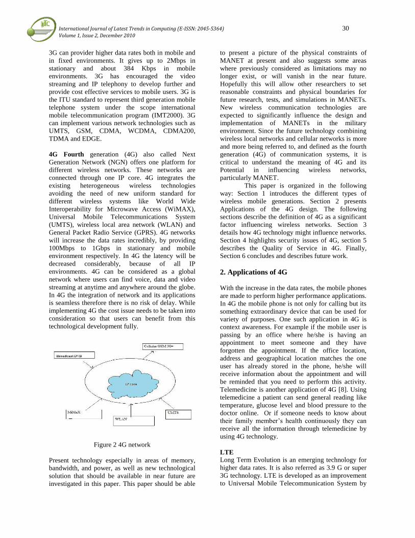
International Journal of Latest Trends in Computing (E-ISSN: 2045-5364) 30 Volume 1, Issue 2, December 2010
3G can provider higher data rates both in mobile and
in fixed environments. It gives up to 2Mbps in
stationary and about 384 Kbps in mobile
environments. 3G has encouraged the video
streaming and IP telephony to develop further and
provide cost effective services to mobile users. 3G is
the ITU standard to represent third generation mobile
telephone system under the scope international
mobile telecommunication program (IMT2000). 3G
can implement various network technologies such as
UMTS, GSM, CDMA, WCDMA, CDMA200,
TDMA and EDGE.
4G Fourth generation (4G) also called Next
Generation Network (NGN) offers one platform for
different wireless networks. These networks are
connected through one IP core. 4G integrates the
existing heterogeneous wireless technologies
avoiding the need of new uniform standard for
different wireless systems like World Wide
Interoperability for Microwave Access (WiMAX),
Universal Mobile Telecommunications System
(UMTS), wireless local area network (WLAN) and
General Packet Radio Service (GPRS). 4G networks
will increase the data rates incredibly, by providing
100Mbps to 1Gbps in stationary and mobile
environment respectively. In 4G the latency will be
decreased considerably, because of all IP
environments. 4G can be considered as a global
network where users can find voice, data and video
streaming at anytime and anywhere around the globe.
In 4G the integration of network and its applications
is seamless therefore there is no risk of delay. While
implementing 4G the cost issue needs to be taken into
consideration so that users can benefit from this
technological development fully.
Figure 2 4G network
Present technology especially in areas of memory,
bandwidth, and power, as well as new technological
solution that should be available in near future are
investigated in this paper. This paper should be able
to present a picture of the physical constraints of
MANET at present and also suggests some areas
where previously considered as limitations may no
longer exist, or will vanish in the near future.
Hopefully this will allow other researchers to set
reasonable constraints and physical boundaries for
future research, tests, and simulations in MANETs.
New wireless communication technologies are
expected to significantly influence the design and
implementation of MANETs in the military
environment. Since the future technology combining
wireless local networks and cellular networks is more
and more being referred to, and defined as the fourth
generation (4G) of communication systems, it is
critical to understand the meaning of 4G and its
Potential in influencing wireless networks,
particularly MANET.
This paper is organized in the following
way: Section 1 introduces the different types of
wireless mobile generations. Section 2 presents
Applications of the 4G design. The following
sections describe the definition of 4G as a significant
factor influencing wireless networks. Section 3
details how 4G technology might influence networks.
Section 4 highlights security issues of 4G, section 5
describes the Quality of Service in 4G. Finally,
Section 6 concludes and describes future work.
2. Applications of 4G
With the increase in the data rates, the mobile phones
are made to perform higher performance applications.
In 4G the mobile phone is not only for calling but its
something extraordinary device that can be used for
variety of purposes. One such application in 4G is
context awareness. For example if the mobile user is
passing by an office where he/she is having an
appointment to meet someone and they have
forgotten the appointment. If the office location,
address and geographical location matches the one
user has already stored in the phone, he/she will
receive information about the appointment and will
be reminded that you need to perform this activity.
Telemedicine is another application of 4G [8]. Using
telemedicine a patient can send general reading like
temperature, glucose level and blood pressure to the
doctor online. Or if someone needs to know about
their family member’s health continuously they can
receive all the information through telemedicine by
using 4G technology.
LTE
Long Term Evolution is an emerging technology for
higher data rates. It is also referred as 3.9 G or super
3G technology. LTE is developed as an improvement
to Universal Mobile Telecommunication System by

International Journal of Latest Trends in Computing (E-ISSN: 2045-5364) 31 Volume 1, Issue 2, December 2010
3G Generation Partnership Project (3GPP). LTE uses
Orthogonal Frequency Division Multiple Access
(OFDMA). The download rate in LTE is 150 Mbps
and it utilizes the available spectrum in a very
sophisticated way. In LTE the IP packet delay is less
than 5 mille seconds which provides the experience
of wired broadband internet access in wireless
environment. The mobile TV broadcast is facilitated
by LTE over LTE network.
3. Networks of 4G
Although there are different ideas leading towards
4G, some concept and network components
frequently come up as a supporting and significant
solutions that help achieve progress towards 4G. In
this section we are going to investigate and explain
technological innovations such as MIMO (Multiple-
Input Multiple-Output), OFDMA (Orthogonal
Frequency Division Multiple Access)
That could significantly increase security, mobility
and throughput of 4G.
3.1 MIMO
Figure 3 MIMO works
Imagine that you can hear better what you want to
listen, and don’t hear what bothers you, just by
pointing out where message and noises are coming
from. Beam forming that is the significant concept of
MIMO (Multiple-Input Multiple-Output) allows you
do just that using smart antennas system. But that’s
not all what MIMO has to offer. Spatial multiplexing,
achieved by independent simultaneously working
antennas, increases bandwidth Capacity by
modulating and transmitting signal through many
paths. Using space-time coding, reliability is
improved. MIMO achieves great success thanks to
multiple antennas that allows simultaneous
directional transmission of two or more unique data
streams sharing the same channel. Increasing speed
and range, MIMO is already accepted by researchers
as one of the main components of projects such as
WiBro, WiMAX, WLAN, 802.11n, UMTS R8 LTE,
and UMB.
3.2 OFDMA Evolution
Data comm. Research Company proposed the
simplest way to implement MIMO is by sharing
frequency using OFDM, that together significantly
can increase performance by extending range,
boosting speed and Improving reliability. Together
with MIMO, OFDMA is another component of 4G
that as the alternative to CDMA, promises high data
capacity and spectral efficiency. OFDM (Orthogonal
Frequency-Division Multiplexing) is the modulation
scheme which divides allocated frequency channel
into many narrow bands guaranteeing mutual
independency between subcarriers such that there is
no interference between them; signals are orthogonal.
Figure 4 FDMA
Before OFDM become popular, three other solutions
were presented to share radio spectrum between
multiple users. Used by 1G, FDMA (Frequency
Division Multiple Access,
Fig. 4) partitioned channel between users. To
increase channel capacity, TDMA (Time Division
Multiple Access, Fig. 5) was proposed that allocate
each user access to the whole bandwidth for short
period of time.
Figure 5 TDMA
Because TDMA in 2G caused interference problem,
CDMA (Code Division Multiple Access) was

International Journal of Latest Trends in Computing (E-ISSN: 2045-5364) 32 Volume 1, Issue 2, December 2010
proposed as a new form of multiplexing where each
user was allowed to use the whole channel capacity
all the time. Different messages were transmitted
with associated special code which was later used to
distinguish between them.
Figure 6 CDMA
The better data throughput become possible, when
using orthogonal frequency division multiplexing, the
radio bandwidth could be subdivided into narrow
bands.
Figure 7Sharing frequency in FDMA, TDMA, and
CDMA
4. Security
Security in digital world means to protect the digital
systems from criminal and unauthorized usage. In
terms of computers and mobile communications the
need for security has increased overwhelmingly with
the improvement in technology. Some decades ago
when first generation of mobile networks were in use
the concept of security was not so much in practice or
we can say that awareness was not that much
highlighted. But as technology kept on improving
and new advents were introduced the need of security
kept on creeping. These days no one likes to be
insecure digitally. Because of the heavy dependence
on digital media for the use of private, sensitive,
financial and important communication. There can be
many attacks on digital data some of them are
eavesdropping, man in the middle attack, denial of
service (DOS) attack, spoofing and lot more.
Figure 8 Eavesdropping
Figure 9 Denial of Service
Traditionally network security is considered to secure
network edges from external attacks. Unfortunately
this is not sufficient as attackers look for breaches in
network protocols, traditionally network security is
considered to secure network edges from external
attacks. Unfortunately this is not sufficient as
attackers look for breaches in network protocols,
operating systems and applications. Therefore we
need a comprehensive security mechanism that can
protect the whole network. We can design security
architecture on the basis of following objectives:
Availability: keeping the network and its
components secure from malicious attacks so that
there is no break during service flow.
Interoperability: using security solutions that are
applicable to most of the 4G applications. They
should avoid interoperability issues.
Usability: end user shall use the security mechanism
easily.
QoS: security solutions should follow QoS metrics.
Cryptographic algorithms used for voice and
multimedia shall meet QoS constraints.
Cost effectiveness: security mechanism should cost
as less as possible.
Third generation of networks provide voice
and paging service to facilitate interactive
multimedia. The applications include
teleconferencing, internet access, video streaming,
multimedia messaging and so many others. In fact 3G
provide a launching pad for applications such as
wireless web, email (SMS, MMS), multimedia
services like video streaming etc. Fourth generation
is to address the future uses of the customers in terms
of higher data rates and increased bandwidth
utilization. 4G is built on the concept of IP core

International Journal of Latest Trends in Computing (E-ISSN: 2045-5364) 33 Volume 1, Issue 2, December 2010
accommodating various heterogeneous networks. In
fact 4G acts as a platform for heterogeneous
networks. A service subscriber uses one of the access
networks providing service from one platform. This
openness and flexibility increase the probability of
security breach in one of the main components of the
system. Therefore the need for security has become
more dominant because of the nature of the
participating networks.
5. Quality of Service in 4G
In telecommunication the term QoS (Quality of
Service) stands for the resource reservation control
mechanism, instead of the translation of term as
achieved service quality. Communication occurs
when the data flows from source to destination and
QoS guarantees a specified level of bit rate, jitter, and
delay and packet drop probability to the flow. QoS
assurance is important for real time traffics like
Voice over IP (VoIP), online gaming, IP TV and
video streaming etc. QoS enables network
administrators to avoid network congestion and
manage the network resources efficiently.
The goal of the 4G is to provide the users
the facility of Always Best Connected (ABC
concept). Fourth generation of networks is a
combination of different networks. It gives a platform
for various technologies to be accessed. To provide
QoS in 4G is not simple and easy job as one has to
deal with different parameters in different
technologies. Like if a user is moving and changing
his coverage network, so to provide service under
QoS framework is challenging. While a mobile user
is moving from one network to another network his
communication session needs to be maintained
seamlessly irrelevant of the coverage network.
Similar is the case with video conferencing and video
streaming, the users like to receive the services
seamlessly.
There are some protocols designed to maintain the
seamless communication of the users while moving
or in other words to minimize the latency and packet
loss of the ongoing communication session. The
mobility protocols are Mobile IPv6, Hierarchical
MIPv6, Fast MIPv6 and some more (details of all
these protocols are given in chapter Handovers).
These protocols can help in improving the mobility
management of mobile users. In order to provide QoS
to the mobile users we propose a combination of
mobility protocol Seamless Mobile IPv6 (SMIPv6)
and Session Imitation Protocol (SIP). There are two
types of losses when a mobile user switches network,
one is called segment packet loss and the other is
called edge packet loss. Segment packet loss is
because of the undeterministic nature of the handoff
.While the edge packet loss is between the Mobility
Anchor Point (MAP) and the MN. To minimize these
losses different approaches are used, to minimize
edge packet loss the MN is moved as close to the
MAP as possible, while for the segmented packet loss
two approaches are used one is synchronized packet
simulcast (SPS) and hybrid simulcast mechanism are
used. In SPS the packets are sent to both the current
network as well the potential network the MN is
approaching [14]. While hybrid simulcast mean that
the mobile node informs the network about the
handoff to be taken into effect but it is decided by the
network to which AR the MN shall attach. This way
the packet loss is minimized (the detailed mechanism
is given in chapter of handover). Session Initiation
Protocol (SIP) is used to manage mobility of different
entities such as session, terminal, service and
personal mobility. It facilitates mobility and
maintains the real time multimedia sessions. SIP is an
application layer protocol therefore it can work both
in IPv4 and IPv6. SIP work along with other
protocols Such as Real Time Transport Protocol
(RTP).
6. Conclusion
In this paper we are describing about the various
wireless mobile technologies, and various
applications of 4G mobile communication as well as
the LTE (Long Term Evolution). And also we
describe about various networks we are used in 4G,
such as MIMO and OFDMA Evolution, in that we
discus about FDMA, CDMA, as well as TDMA. And
also describes the Security, Quality of Service in 4G.
We present the challenges that 4G faces and their up-
to-date solutions. To improve the QoS in 4G we
propose our own scheme of combining mobility
protocol SMIP and application layer protocol SIP.
With this scheme the QoS level in 4G can be
improved because both the protocols provide support
in handovers. Together they can decrease the packet
loss and can improve security during the handover
process. We can make sure the resource allocation
during the handover process by combining the two
protocols and mobility management can be
optimized.
Future work
In future work we suggest that SIP could be
combined with other mobility protocols to facilitate
the mobility management and improve QoS in 4G
networks.

International Journal of Latest Trends in Computing (E-ISSN: 2045-5364) 34 Volume 1, Issue 2, December 2010
References
1. http://www.mobile-phone- directory.org.
Visited 09, February 2010.
2. http://en.wikipedia.org/wiki/2.5G. Visited 10
February 2010.
3.http://www.mobileinfo.com/3G/3G_Wireless.htm.
Visited10, February 2010.
4Http://en.wikipedia.org/wiki/ 3G. Visited11
February 2010.
5.http://techcrunchies.com/3g-subscription-
penetration-worldwide/. Visited 11, February 2010.
6. 4G wireless technology: when will it happen?
What will it offer? Krenik, B.; Solid-State Circuits
Conference, 2008. A-SSCC '08. IEEE Asian Digital
Object Identifier:10.1109/ ASSCC.2008.4708715
Publication Year: 2008 , Page(s): 141 – 144
7. Research on coexistence of WiMAX and
WCDMA systems, Zheng Ruiming; Zhang
Xin; Li Xi; Pan Qun; Fang Yinglong; Yang Dacheng;
Vehicular TechnologyConference Fall (VTC 2009-
Fall), 2009 IEEE 70th Digital Object
Identifier:10.1109/VETECF. 2009. 5378806
Publication Year: 2009
8.http://www.ericsson.com/thecompany/press
/releases/2010/01/1372929 visited 25, February 2010.
9. A Survey of Security Threats on 4G Networks,
Yongsuk Park; Taejoon Park; Globecom Workshops,
2007 IEEE Digital Object
identifier:10.1109/GLOCOMW. 2007.4437813
Publication Year: 2007 , Page(s): 1 - 6
10. Integrating fast mobile IPv6 and SIP in 4G
network for real-time mobility, Nursimloo, D.S.;
Chan, H.A.; Networks, 2005. Jointly held with the
2005 IEEE 7th Malaysia International Conference on
Communication. 2005 13th IEEE International
Conference on Volume: 2 Digital Object Identifier:
10.1109/ICON.2005.1635641 Publication Year: 2005
11. “Ericsson Demos Live LTE at 144Mbps”, ABI
Research Wireless Daily Newsletter, February 09,
2007
Dr. G.Srinivasa Rao,
M.Tech,Ph.D, Sr.Asst.Professor.
Four years industrial experience
and over 10 Years of teaching
experience with GITAM
University, handled courses for
B.Tech, M.Tech. Research areas
include Computer Networks and
Data Communications. Published 6 papers in
various National and International Conferences
and Journals.
Dr. G.Appa Rao., M.Tech.,
M.B.A.,Ph.D., in computer science
and Engineering form Andhra
Universiy. Over 12 Years of
teaching experience with GITAM
University, handled courses for
B.Tech, M.Tech. Research areas
include Data Mining and AI. Published 8 papers in
various National and International Conferences and
Journals.
Mr. D. Veerabhadra Rao.,
M.Tech., in Information
Technology. Over 7 Years of
teaching experience with GITAM
University, handled courses for
B.Tech and M.Tech .One research
paper was published in
international journal and one conference.
Mrs. S. Venkata Lakshmi M.Tech in Information
Technology from Andhra
University. Asst.Prof in GITAM
University. Over 2 years of
teaching experience with GITAM
University and Andhra
University. Handled courses for B.Tech, and M.C.A.
and 2 years of industry experience as a software
engineer. published 3 papers in various National and
International conferences and Journals.
Mrs. D. Rajani., M.Tech in Artificial intelligence
and Robotics(AI&R) from Andhra University. She is
working as Sr.Lecturer in Govt.polytechnic for
womens ,Bheemunipatnam. Over 10 years of
teaching experience. Published 2 papers in various
National and International conferences and journals.

International Journal of Latest Trends in Computing (E-ISSN: 2045-5364) 35 Volume 1, Issue 2, December 2010
Parameter Optimization of Quantum Well
Nanostructure: A PSO and GA Based Comparative
Study Sanjoy Deb
a, C. J. Clement Singh
a, N Basanta Singh
b, A. K De
c and S K Sarkar
a
aDepartment of Electronics & Telecommunication Engineering, Jadavpur University, Kolkata-700032, India
bDepartment of Electronics & Communication Engineering, Manipur Institute of Technology, Imphal –795004,India cDepartment of Electronics & Communication Engineering, National Institute of Technology, Durgapur -713201, India
[email protected], [email protected],[email protected], [email protected] and [email protected]
Abstract: Carrier transport properties of nanodevices are
controlled by biasing field, frequency of the applied field and
system parameters like lattice temperature, quantum well width,
spacer width and carrier concentration. All these parameters are
related in such a way that it is very difficult to predict optimized
system parameters for desired electrical characteristics using the
traditional mathematical optimization techniques. Evolutionary
algorithms are stochastic methods that mimic the natural biological
evolution or the social behaviour of species. Such algorithms have
been used for large-scale optimization problems in many
applications. In this work, two evolutionary algorithms, Genetic
Algorithm (GA) and Particle Swarm Optimization (PSO), are
applied to get optimized system parameters for AlxGa1-xAs/GaAs
quantum well nanostructure, which may be utilized during
fabrication for better nanodevices. The results obtained are
compared in terms of convergence speed, processing time and
quality of results. The PSO based algorithm is found to
convergence faster than GA for almost same quality of results. And
also the processing time is faster in case of PSO based algorithm for
the present application of parameter optimization for nanodevice
modeling.
Keywords: Optimization, GA, PSO, quantum well, scattering
mechanism, mobility, frequency response.
1. Introduction
Recent advances in crystal growth techniques like fine line
lithography, metal organic chemical vapour deposition
(MOCVD) and molecular beam epitaxy (MBE) have made
possible the fabrication of low dimensional semiconductor
structures such as quantum well, quantum wires and quantum
dots [1-5]. A quantum well (QW) is formed when a thin layer
of lower bandgap semiconductor is sandwiched between two
layers of higher band-gap semiconductor [6-7]. In the
quantum well structure, electrical and optical properties of
the semiconductor are totally different from those in the bulk
material due to quantum effect [8-9]. Due to modulation
doping in QW structures, carriers are separated from ionized
impurity thereby increasing the mobility of carrier due to
reduced ionized impurity scattering. The carrier
concentration in QW is high and the coulomb scattering is
also reduced with sufficient thickness of spacer layer [10].
Theoretical studies of the electrical characteristics are clearly
vital to understand the physics of these devices.
Electrical characteristics of the carrier in a QW are controlled
by the system parameters like lattice temperature, well width,
spacer width, carrier concentration, external dc biasing field
and the frequency of applied ac field. All these parameters
are related in such a way that it is very difficult to predict
optimized values of parameter for desired electrical
characteristics [11-12] using the traditional mathematical
optimization techniques. Evolutionary algorithms that mimic
the natural biological evolution or the social behaviour of
species have been developed for fast and robust solution to
complex optimization problems. Genetic algorithm (GA) is a
computationally simple but powerful algorithm developed
based on the principle of the „survival of the fittest‟ and the
natural process of evolution through reproduction [13].
Theoretically and empirically it is proven that GA provides
robust search in complex spaces. As a result, GA is now
finding more widespread applications in sociological,
scientific and technological circles [14]. Despite its
simplicity, GA may require long processing time to get a
near-optimum solution.
PSO is an evolutionary computational intelligence-based
technique, which was inspired by the social behaviour of bird
flocking and fish schooling [15]. PSO algorithm shares many
common points with GA. Both the algorithms start with a
group of a randomly generated population, have fitness
values to evaluate the population, searches for optima by
updating generations and none of them guarantee success
[15]. Each solution in PSO is a „bird‟ and is referred as a
„particle‟, which is analogous to a chromosome in GA. As
opposed to GAs, PSO does not create new birds from
parents. PSO utilizes a population of particles that fly
through the problem hyperspace with given velocities. The
velocities of the individual particles are stochastically
adjusted according to the historical best position for the
particle itself and the neighbourhood best position at each
iteration. Both the particle best and the neighbourhood best
are derived according to a user defined fitness function. The
movement of each particle naturally evolves to an optimal or
near-optimal solution. The performance of PSO is not largely
affected by the size and nonlinearity of the problem, and can
converge to the optimal solution in many problems where
most analytical methods fail to converge. It can, therefore, be
effectively applied to different optimization problems.
Moreover, PSO has some advantages over other similar
optimization techniques such as GA, namely the following
[16].

International Journal of Latest Trends in Computing (E-ISSN: 2045-5364) 36 Volume 1, Issue 2, December 2010
1) PSO is easier to implement and there are fewer
parameters to adjust.
2) In PSO, every particle remembers its own previous
best value as well as the neighbourhood best;
therefore, it has a more effective memory capability
than the GA.
3) PSO is more efficient in maintaining the diversity of
the swarm [17], since all the particles use the
information related to the most successful particle in
order to improve themselves, whereas in GA, the
worse solutions are discarded and only the good
ones are saved; therefore, in GA the population
evolves around a subset of the best individuals.
In the present work, both PSO and GA based optimization
techniques are employed to determine the optimized system
parameters for AlxGa1-xAs/GaAs quantum well nanostructure
for nanodevice applications. The parameters to be optimized
include lattice temperature, channel length, carrier
concentration and spacer width to get the maximized values
of mobility and cut-off frequency. Performance comparison
of the two algorithms is then presented in terms of
convergence speed, processing time and quality of results.
2. Analytical Model of Fitness Function
A square QW of AlxGa1-xAs/GaAs of infinite barrier height is
considered. Reduced ionized impurity scattering and
improved carrier concentration in the QW establish a strong
electron-electron interaction which favors a heated drifted
Fermi-Dirac distribution function for the carriers
characterized by an electron temperature Te, and a drifted
crystal momentum pd. In the presence of an electric field F
applied parallel to the heterojunction interface, the carrier
distribution function )(Kf can be expressed as;
cos|||| 0
*0
E
f
m
kpEfkf d
(1)
where, )(0 Ef is the Fermi-Dirac distribution function for
the carriers, ħ is Planck's constant divided by 2п, k is the
two-dimensional wave vector of the carriers with energy E,
m* is the electronic effective mass and γ is the angle between
the applied electric field F and the two dimensional wave
vector k .
An ac electric field of magnitude F1 with the angular
frequency ω superimposed on a moderate dc bias field F0 is
assumed to act parallel to the heterojunction interface and
thus the overall field is given by;
tFFF o sin1 (2)
As the electron temperature and the drift momentum depend
on the field and the scattering processes, they will also have
similar alternating components, generally differing in phase.
tTtTTT iroe cossin 11 (3)
tptppp irod cossin 11 (4)
Where, T0 and p0 are the steady state parts, T1r and p1r are
real and T1i and p1i are imaginary parts of Te, and pd
respectively. The energy and momentum balance equations
obeyed by the carrier can be given as;
Edt
d
dt
dE
m
Fep
scat
d *
(5)
and
dt
dp
dt
dpeF d
scat
(6)
Where dtdp / and dtdE / , represents, respectively,
the average momentum and energy loss due to scatterings
and E depicts the average energy of a carrier with charge
e. In the present model the effects of delta doping is included
in the energy and momentum loss calculations to give more
accurate results. We insert (3) and (4) in (5) and (6), retain
terms up to the linear in alternating components and equate
the steady parts and the coefficients of sinωt and cosωt on
the two sides of the resulting equations following the
procedure adopted in reference 6. For a given electric field
Fo, we solve for po and To. The dc mobility μdc and ac
mobility μac are then expressed as:
o
o
dcFm
p*
(7)
1
*
2
1
2
1
Fm
pp ir
ac
(8)
The phase lag , the resulting alternating current lags behind
the applied field is expressed as;
r
i
p
p
1
11tan (9)
Equations 7, 8 and 9 are used as the fitness functions of ac
mobility, dc mobility and phase angle, respectively. Detailed
derivations of the fitness functions are available in the Ref. 7
and not deliberately included in the present analysis for
brevity of this paper.
3. GA Based Optimization
In GA, a solution to a given optimization problem is
represented in the form of a string, called „chromosome‟,
consisting of a set of elements, called „genes‟, that hold a set
of values for the optimization variables [18]. For appropriate
binary representation four parameters (carrier concentration
(N2D), quatum well width (LZ),lattice temperature (TL) and
spacer width (LS) ) are coded into a single finite length string
of twenty three bits as shown in Fig 1.
Figure 1. A chromosome with 23 bits.
To start with, a random population of chromosomes is
generated. The fitness of each chromosome is determined by
evaluating it against a fitness function and an average is
computed which is considered as the starting average fitness
value. Strings/chromosomes are then selected from the
generation according to their fitness value. Strings, whose
fitness value is less then the average fitness value, are
rejected and will not pass to the next generation. Subsequent
generations are developed by selecting pairs of parent strings
from present genetic pool to produce offspring strings in the

International Journal of Latest Trends in Computing (E-ISSN: 2045-5364) 37 Volume 1, Issue 2, December 2010
next generation, which is called "crossover" operation. For
crossover operation an integer position (t) along the string is
selected randomly between 1 and the P-1, where P is the
maximum string length. Two new strings are created by
swapping all binary bits between positions (t + 1) and P
inclusively. As an example, two consecutive strings Sk and
Sk+1 are shown in Fig. 2. A random number is chosen
between 1 and 22 (23 - 1), as P = 23 here. Then the result of
cross over which produces two new strings S‟k and S‟k+1 are
indicated in Fig. 2.
Figure 2. Cross over operation between two consecutive
strings.
Gradually, generation-by-generation the algorithm will
progress towards the optimum solution. When the
improvement in the average fitness value falls in the range of
0.00 - 0.05% for at least ten consecutive generations,
program will be terminated. The mutation operator plays a
secondary role in the simple GA and mutation rates are
simply small in natural population. It is also a rare process
that resembles a sudden change to an offspring. This can be
done by randomly selecting one chromosome from the
population and then arbitrarily changing some of its
information. The benefit of mutation is that it randomly
introduces new genetic material to the evolutionary process
thereby avoiding stagnation around local minima [19]. The
four parameters that affect the performance of GA are
population size, number of generations, crossover rate, and
mutation rate. Larger population size and large number of
generations increase the likelihood of obtaining a global
optimum solution, but substantially increase processing time.
4. PSO Based Optimization
The PSO algorithm begins by initializing a group of random
particles (solutions) and then searches for optima by updating
generations. The fitness values of all the particles are
evaluated by the fitness function to be optimized. An iterative
process to improve these candidate solutions is set in motion.
With the progress of „iteration‟, which is synonymous to
generation in case of GA, every particle updates its position,
velocity and moves through the problem or solution space. In
iteration, position of each particle is updated by following
two "best" values. The first one is the best solution or fitness
value that the particular particle has achieved so far and is
called “pbest” and the second one is the best solution obtained
by any particle in the entire population and is known as the
global best or “gbest”[20]. After finding pbest and gbest the
particle updates its velocity and positions using the following
two equations:
))1((()
))1((())1()(
2
1
txgrandc
txprandctvwtv
ibest
ibestii
(10)
)()1()( tvtxtx iii
(11)
Where )(tvi
is the particle velocity, )(txi
is the current
position of the particle, w is called the inertia factor, rand ()
is a random number between (0,1), c1 and c2 are learning
factors.
The following procedure can be used for implementing the
PSO algorithm [21].
1) Initialize the swarm by assigning a random position
in the problem hyperspace to each particle.
2) Evaluate the fitness function for each particle.
3) For each individual particle, compare the particle‟s
fitness value with its pbest. If the current value is
better than the pbest value, then set this value as the
pbest and the current particle‟s position, xi, as pi.
4) Identify the particle that has the best fitness value.
The value of its fitness function is identified as gbest
and its position as pg.
5) Update the velocities and positions of all the
particles using equations (10) and (11).
6) Repeat steps 2–5 until a stopping criterion is met
(e.g., maximum number of iterations or a
sufficiently good fitness value).
5. Results and Disquisitions
The GA and PSO algorithms have been coded using
MATLAB7.5 and all experiments were conducted on a
2.20GHz AMD ATHLON Processor with 2GB RAM
Desktop PC. The parameters used for the algorithms are
given in Table 1 and they are taken based on the
consideration presented in Refs. 18 and 20.
Parameters GA PSO
Population Size 100 100
Max Generation/ Iteration Varies Varies
Selection Type Random NA
Crossover Rate 80% NA
Mutation Rate 9% NA
wman ,wmin NA 0.9,0.1
c1,c2 NA 1.49
Table 1. Parameters used for GA and PSO algorithm.
The material parameters for the Al0.3Ga0.7As/GaAs QW are
taken from Ref. 7. The range of QW parameters taken for
optimization are based on theoretical assumptions and
physical phenomenon and are as follows:
1. 2-D carrier concentration (N2D) is 61015
/m2 to
101015
/m2
2. Quantum well width (LZ) is 8nm to 12nm.
3. Spacer width (LS) is 10nm to 50nm.
4. Lattice temperature (TL) is 77 K to 300K.

International Journal of Latest Trends in Computing (E-ISSN: 2045-5364) 38 Volume 1, Issue 2, December 2010
Since the parameter optimization is to be carried out during
fabrication of nanodevices (i.e real time application), an
algorithm with high average performance is the best option
[22]. Therefore, GA and PSO algorithms are compared based
on the Mean Best Fitness measure (MBF)/average fitness
value obtained over 300 runs for ac mobility and 400 runs for
dc mobility and cut-off frequency.
Figure 3. Plot of average dc mobility with iterations (PSO)
/generations(GA).
Figure 4. Plot of ac mobility with iterations (PSO)
/generations(GA).
Using Eqs. 7 and 8 as the fitness functions, the GA and PSO
algorithms are applied to get the optimized values of dc and
ac mobility. The simulation of the search space is depicted in
Figs. 3 and 4. It is found that the PSO based algorithm
converges faster than GA based algorithm. For dc mobility
optimization, PSO took 230 iterations and 81.23 seconds to
converge whereas GA took 350 generations and 124.41
seconds. For ac mobility optimization, it was found that 165
iterations and 62.03 seconds were required by PSO and
whereas it was 292 generations and 98.11 seconds for GA.
GA and PSO algorithms are applied using equation 9 as the
fitness function to get the optimized value of cut-off
frequency. The simulation of the search space is depicted in
Fig. 5.
Figure 5. Plot of cut-off frequency with iterations (PSO)
/generations(GA).
As in the case of mobility mobilization, it is found that the
PSO based algorithm converges faster than GA based
algorithm. The results obtained from using GA and PSO are
summarized in Table 2.
Table 2. Performance comparison of GA and PSO.

International Journal of Latest Trends in Computing (E-ISSN: 2045-5364) 39 Volume 1, Issue 2, December 2010
Sch
eme
Co
nv
erg
ence
Tim
e
Pro
cess
ing
Tim
e
Par
amet
er v
alu
e MBF N2D Lz LS TL
dc mobility optimization
GA
350
Genera-
tions
124.4 1.821 10 12 34 80
PSO 230
Iterati-
ons
81.23 1.818 9.8 11.8 35.6 78.8
ac mobility optimization
GA
292
Genera-
tions
98.11 0.818 10 11 31 279.5
PSO 165
Iterat-
ions
62.03 0.820 9.9 10.9 31 278
Cut-off frequency optimization
GA
305
Genera-
tions
103.1 353 6 8 23 296
PSO 262
Iterat-
ions
93.03 350 6.3 8.5 21 293.8
AMPT: Processing time for a single run of analytical model
with given parameters.
The performance of the algorithms was compared using three
criteria: (1) convergence speed; (2) processing time to reach
the optimum value and (3) the quality of results. The
processing time, and not the number of iteration/generation
cycles, was used to measure the speed of each algorithm,
because the number of generations is different from one
algorithm to another. To make processing time comparison
more relevant and processing system independent, processing
time of two proposed schemes are compared in terms of
analytical model processing time (AMPT).
Both the algorithms perform well at finding optimal
solution. Therefore, in terms of quality of solution there
seems to be no difference to distinguish GA and PSO.
However, when the number of generations or iterations is
taken into account, there are differences in the number taken
to obtain the optimal solution. The PSO based algorithm is
shown to convergence faster than the GA based algorithm.
And also the processing time is less in case of PSO based
algorithm for the present application of parameter
optimization for nanodevice modeling.
5. Conclusion
Application of soft-computing tool, especially PSO, for
parameter optimization in quantum well structure is new and
quite useful to understand optimum combinations of
parameters to get better quantum well nanostructure. Under
similar software and hardware environment, PSO and GA is
applied for parameter optimization of AlxGa1-xAs/GaAs QW
nanostructure and performance of the two schemes are
compared in terms of convergence speed, processing time
and quality of results. The particle swarm optimization based
algorithm is found to convergence faster than GA for almost
same quality of results. Another reason why PSO based
algorithm is attractive is that there are few parameters to
adjust making it much simpler to implement. Through this
computational study, mobility (ac and dc) and cut-off
frequency values are optimized with respect to parameters of
quantum well nanostructure, which will provide valuable
information for the technologists involved in the fabrication
of QW nanodevices. Successful implementation of such types
of soft computing tools for parameter optimization of QW
revels that those schemes can be successfully implemented
for parameter optimization of other nanostructures.
References
[1] S. K. Sarkar, D. Chattopadhyay, One dimensional
warm electron transport in GaN quantum well
wires at low temperature, Phys. Rev., 6 (2000)
264-268.
[2] R. Akimoto, B.S. Li, K. Akita, T. Hasama, Sub-
picosecond saturation of intersubband absorption
in (CdS/ZnSe)/BeTe quantum-well waveguides at
telecommunication wavelength, Appl. Phys. Lett.,
87 (2005) 181104.
[3] C. Fujihashi, T. Yukiya, A. Asenov, Electron and
Hole Current Characteristics of n-i-p-Type
Semiconductor Quantum Dot Transistor, IEEE
Transactions on Nanotechnology, 6(2007)320 –
327.
[4] G. Dewey, M. K. Hudait, K. Lee, R. Pillarisetty,
W. Rachmady, M. Radosavljevic, T. Rakshit, R.
Chau, Carrier Transport in High-Mobility III–V
Quantum-Well Transistors and Performance
Impact for High-Speed Low-Power Logic
Applications, IEEE Electron Device Letters, 29
(2008) 1094.
[5] C. Weisbuch, B. Vinter, Quantum Semiconductor
Structures: Fundamentals and applications,
Academic Press, New York, 1991.
[6] D. Chattopadhyay, Two-dimensional electronic
transport in In0.53Ga0.47As quantum Wells, Appl.
Phys. A, 53 (1991) 35.
[7] S. K. Sarkar, P. K. Ghosh, D. Chattopadhyay,
Calculation of high frequency response of two
dimensional hot electron in GaAs quantum well,
J. Appl.Phys. 78 (1995) 283-287.
[8] A. Gold, Mobility of thin AlAs quantum wells:
Theory compared to experiment, Appl. Phys.
Lett., 92 (2008) 082111.
[9] Kevin F. Brennan and April S. Brown, Theory of
Modern Electronic Semiconductor Devices, John
Wiley & Sons, 2002.
[10] L.D. Nguyen, Ultra-High-Speed Modulation-
Doped Field-Effect Transistors: A Tutorial
Review, Proceedings of the IEEE, 80 (1992) 494-
518.

International Journal of Latest Trends in Computing (E-ISSN: 2045-5364) 40 Volume 1, Issue 2, December 2010
[11] Y.F. Yang, C.C. Hsu, E.S. Yang, Integeration of
GaInP/GaAs heterojunction bipolar transistor and
high electron mobility, IEEE Electron Device
Letters,17 (1996) 363–365.
[12] C . Weisbuch and B. Vinter, Quantum
Semiconductor Structures: Fundamentals and
applications, Academic Press, New York, 1991.
[13] Holland J., Adaptation in natural and artificial
systems. Ann Arbor, MI: University of Michigan
Press, 1975.
[14] R. S. Zebulum, M. S. Vellasco, M. A. Pacheco,
Variable Length Representation in Evolutionary
Electronics Evolutionary Computation, MIT
Press, 8(2000) 93 -120.
[15] J. Kennedy, R. Eberhart, Swarm intelligence,
Morgan Kaufmann Publishers, San Francisco, CA,
2001.
[16] Y. D. Valle, G. K. Venayagamoorthy, S.
Mohagheghi, J. C. Hernandez, R. G. Harley,
Particle swarm optimization: Basic concepts,
variants and applications in power system, IEEE
Trans. on Evolutionary Computation, Vol. 2 (2)
(2008) 171-195
[17] A. P. Engelbrecht, Particle swarm optimization:
Where does it belong ?, in Proc. IEEE Swarm
Intell. Symp., (2006) 48–54
[18] Goldberg DE., Genetic algorithms in search,
optimization and machine learning. Reading, MA:
Addison-Wesley Publishing Co, 1989
[19] Subir Kumar Sarkar , Multiple lavel optimization
of high frequency ac mobility in GaAs quantum
wells under hot electron condition, Elsevier, 29
(2004) 243-249.
[20] Nadia Nedjah, Luiza de Macedo Mourelle, Swarm
Intelligent Systems, Springer-Verlag Berlin
Heidelberg 2006
[21] Y. Shi, Feature article on particle swarm
optimization, IEEE NeuralNetwork Society,
Feature Article, (2004) 8–13.
[22] A.E. Eiben, M. Jelasity, A critical note on
experimental research methodology in EC, WCCI,
vol. 1 pp. 582-587, Computational Intelligence,
WCCI, Proc. of the 2002 Congress on
Evolutionary Computing (CEC‟2002)
Author Biographies
Sanjoy Deb was born in Kolkata, India. He received the
M.Sc degrees in Electronics from G.G.D.U, Madhyay
Pradesh, India in 2005 and M-Tech degree in
Nanoscience and Technology from Jadavpur University
in 2008. He is currently working as a U.G.C research
scholar in the department of Electronics and
Telecommunication Engineering, Jadavpu University.
His current research interests include analytical modeling of nano-devices
and application of soft computing tools for parameter optimization of
nanodevices.
N. Basanta Singh was born in Imphal, Manipur, India.
He received the B-Tech degree in Electronics and
Communication Engineering from Kerala University,
Kerala, India in 1992 and the M.E degree in Electronics
and Communication Engineering from Thapar Institute
of Engineering and Technology, Patiala, India in 2000.
He is currently an Assistant Professor with the
Department of Electronics and Communication
Engineering, MIT, Manipur University, Manipur, India. His current
research interests include carrier transport in low-dimensional structures,
design and modeling of single electron devices. He is a life member of
Institution of Electronics and Telecommunication Engineers.
Subir Kumar Sarkar received the B. Tech and M.
Tech. Degree from the Institute of Radio Physics
and Electronics, University of Calcutta in 1981 and
1983, respectively and PhD (Tech) degree in
Microelectronics from University of Calcutta.
He served Oil and Natural Gas Commission
(ONGC) as an Executive Engineer for about 10 years (1982 to 1992) before
coming to teaching profession. He joined as a faculty member in the Dept.
of Electronics and Telecommunication Engineering, Bengal Engineering
and Science University, Shibpur in April 1992 (from 1992 to 1999). In
1999 he joined in Jadavpur University in the same dept. where he is
presently a Professor. He has developed several short courses for the needs
of the Engineers. He has published three Engineering text books and more
than 260 technical research papers in archival journals and peer – reviewed
conferences. Thirteen students have been awarded PhD (Engg) degree
under his guidance and eight more are presently perusing PhD under his
guidance. He is on the TCP of several major international/ national
conferences/ symposiums and was the organizing Secretary of International
conferences on communications, devices and intelligent systems
(CODIS2004). As Principal Investigator he has successfully completed four
R&D projects and two more are running. He has visited several countries
like France, UK, Switzerland and Japan for Technical reasons like training,
presenting papers or visiting sophisticated laboratories. He was invited as a
post doctoral Research scholar in the Dept. of Electrical and Computer
Engineering, Virginia Commonwealth University to work on quantum
computing, spintronics, quantum dot memory and electronic transport in
Nanostructures. His most recent research focus is in the areas of simulations
of nanodevice models, transport phenomenon, single electron & spintronics
devices and their applications in VLSI circuits, low power VLSI design, ad
hoc wireless networks, wireless mobile communication and watermarking.
He is a life Fellow of the Institution of Engineers and Institution of
Electronics and Telecommunication Engineers, life member of Indian
Association for the cultivation of Science.
C. J. Clement Singh received the B.E. and M.E. in
Electronics and Telecomm. Engineering from Madurai
Kamaraj University, Tamil Nadu, India and Jadavpur
University, Kolkata, India respectively. He is currently
working towards the Ph.D. degree at Jadavpur University.
His research interest include physics of nano-devices and
their applications.

International Journal of Latest Trends in Computing (E-ISSN: 2045-5364) 41
Volume 1, Issue 2, December 2010
Experimental Protocol Development for a Passive
Thermal Management System
Emily D. Pertl, Daniel K. Carder and James E. Smith
Mechanical and Aerospace Engineering Department
Center for Industrial Research Applications
West Virginia University
Morgantown, WV 26506, USA
[email protected], [email protected], [email protected]
Abstract: Techniques to reduce the increasing energy costs have
become a necessity for homeowners. For a typical residence,
heating and cooling are two of the major energy consuming sources.
A new technology was designed and developed in the Center for
Industrial Research Applications at West Virginia University which
utilizes passive convective cooling to help reduce this energy usage.
The experimental testing protocol was developed for this novel
passive thermal management system based upon typical materials
and techniques used in the construction of residential homes. The
base construction for the two units was identical. Each unit was
equipped with 13 temperature sensors in identical positions on the
shingled roof and inside the attic space. Each sensor was connected
to a data logger installed in each unit. Baseline data was established
in both controlled and environmentally exposed environments. The
testing protocol and baseline data for both units are presented in this
paper.
Keywords: Convective Cooling, Energy Conservation, Buoyancy
1 Introduction
The impact of rising energy prices on household budgets and
the overall economy has increasingly become a focal point of
public concern. A significant portion of the total energy costs
can be attributed to heating and cooling. In 2005,
approximately 111 million homes contained at least one
heating unit with 65% of them for a single family detached
dwelling [1]. For this type of home, the major heating
sources are electricity and natural gas.
A typical residence has numerous energy consuming
appliances and devices. Major contributors include air
conditioning, refrigeration, and heating. Approximately 85%
of the homes in the United States have cooling equipment,
76% of which use central air, while the remaining 24% have
at least a window/wall unit [1].
With both heating and cooling being the major
contributors to energy expenditures in most building
structures, energy savings on these sources was the focus of
this research. Currently, energy savings in a home can be
accomplished in a variety of ways. One way is to replace
normal window glass throughout the home with low
emissivity (low-e) glass. Low-E glass has a special thin
coating that will let visible light in, but helps to reduce the
heat transfer between surfaces. Another alternative would
include the planting of trees and/or shrubs to shade a
building structure in summer and to provide a wind break in
winter. The R-value of the insulation can be increased and it
is also recommended that thermostats be adjusted to decrease
energy usage. In addition, shading room air conditioners
from direct sun will reduce their workload. Such energy
savings measures will translate into reduced heating and
cooling costs. [2]
The natural ventilation method that occurs in most
structures takes advantage of two principles. First, as air is
heated it becomes less dense and rises. Second, wind
movement over and around a home creates areas of high and
low pressure. If a space has high air outlets in conjunction
with low inlets, ventilation occurs as the air within the space
is heated, rises and escapes though the high outlets to be
replaced by cooler air entering at the lower inlets. The
greater the temperature differences between the outlet and
inlet, the greater the ventilation rate. This is a natural result
of buoyancy effects. Additionally, the structure serves as a
differential pressure mechanism driven by creating a slightly
higher pressure around the windward side of the structure.
As the air passes over the ridge or top of the structure it
creates a slightly lower than ambient pressure, the Bernoulli
effect, and thus encouraging mass flow through the structure
[3] - [5].
Enhancing and exploiting this buoyancy effect and taking
advantage of the wind/structure interaction for convective
ventilation is the goal of the current research. Traditional
natural ventilation occurs in the interior of the attic. On the
other hand, this research aims to enhance natural buoyancy
driven convection in an exterior space immediately along the
top most surface of a building to reduce attic temperatures.
This could be accomplished with a variety of structures and
control schemes retrofitted on top of an existing roof, or the
design of a new roof structure with an air gap between the
additional structure and the existing roof.
2 Experimental Setup
Two units were constructed for experimental verification
testing, one for the control and the other as the experimental.
Each unit was equipped with sensors to monitor the thermal
attributes inside and outside of each unit, as well as the air
velocity inside the stack vent. The base construction of each
unit was identical with the only difference being that the
second unit has the add-on roof feature. The construction of
each building, as well as the experimental testing setup, is
described next.
The attic test module is a gabled attic built with roof pitch
of 45 degrees. The frame of the unit was constructed out of
two-by-six pieces of lumber, placed 16 inches on center, and
covered on the outside with plywood sheets for rigidity and
strength. Tar paper was placed directly over the plywood

International Journal of Latest Trends in Computing (E-ISSN: 2045-5364) 42
Volume 1, Issue 2, December 2010
sheets and 1/8 inch thick asphalt shingles were layered on
both sides of the roof.
Figure 1 Experimental Test Units during Construction
The exterior of the building has standard tan vinyl siding,
thin (~2 mm thick), installed over the house wrap which was
attached directly against the plywood. Typical R-13
fiberglass home insulation was installed in between each of
the two-by-four studs with drywall installed in the interior of
the unit. A layer of thin plastic was placed over the insulation
to create a vapor barrier. The interior ceiling consisted of R-
30 insulation between the two-by-six ceiling joists and
drywall. Both the ceiling and each wall was painted white to
help to seal and maintain a steady temperature inside of each
building. The interior floor was constructed in a similar
fashion as the exterior walls without vinyl siding on the
exterior.
In addition, the roof has an overhang located on both sides
to create a 12 inch soffit vent and a gable on the front side of
each building. The soffit vent was constructed of one porous
vent located in the middle with a solid piece on either side
with the same pattern to the ends of the overhang. A 7 ft steel
exterior door was installed on the front side of each building
to mimic the effect of typical building openings. In addition,
a hexagon-shaped gable was installed directly over the
exterior door to allow access to the attic area, as shown in
Figure 2. During testing, the exterior door was closed and the
gable was sealed shut. In order to analyze the impact of the
convective heat roof and to keep the influence of the roof
between experimental and control the same, the ridge vent
was excluded for this phase of this research.
Environmental monitoring was used to determine which
method provided the best protection against temperature
elevation caused by exposure to solar radiation. This was
accomplished by using two data loggers, 44 resistance
temperature detectors, and downloading the weather for the
test site.
Test data collection was performed using two data loggers
setup to monitor 15 and 29 temperature sensors for the 500
and 800 data units, respectively. Temperature sensors were
placed in identical positions on each test unit to minimize the
effects that varying the probe position could have on the test
data. The test points for each unit are located twelve inches
from the ridge (top), twelve inches from the attic floor
(bottom), and in the middle of the top and bottom sensors
(~30 inches from ridge) on both the exterior and interior of
each roof surface. Each sensor was encased with a flame
retardant, thermal urethane, as depicted in Figure 3 and
Figure 4. Every exposed lead was also covered with this
thermal urethane to negate radiation effects.
Figure 2 Exterior of the Test Units
Figure 3 Resistance Temperature Detector Secured with
Thermal Urethane on the Roof
Figure 4 Resistance Temperature Detector Secured with
Thermal Urethane in the Attic

International Journal of Latest Trends in Computing (E-ISSN: 2045-5364) 43
Volume 1, Issue 2, December 2010
The temperature sensors were monitored using two data
loggers. The dataTaker® DT505 and DT800 were installed
in the control and experimental units, as shown in Figure 5
and Figure 6, respectively. The 6-outlet power supply is on
the far left with the data logger located in the middle. The
dataTaker® DT505 setup also included an Omega®
iServer™ Microserver to convert the serial DB-9 to an
Ethernet RJ45 connection. The heat load from each
datalogger setup was relatively small (5 W) and hence
considered negligible for this research.
Figure 5 Data Logger Installed Inside of Experimental
(800 Unit)
Figure 6 Data Logger Installed Inside of Control (500
Unit)
A 3-wire RTD configuration was used in the DT800 with
six sensors sharing a common return to increase the amount
of sensors to be measured. One lead resistance sensing loop
was used for each set of six sensors necessitating each wire
in the set to be the same length.
On the other hand, the dataTaker® DT505 was setup with
a 4-wire configuration which used two wires to supply a
constant current to the sensor while the other two wires
carried no current and therefore could sense the exact voltage
across the resistor without any voltage drop in the wire.
The dataTaker® software was utilized to configure, set
schedules and download data from each data logger unit. The
configuration included channel selection, sensor type, data
logger, and label for each sensor. The labels started with the
number one and were preceded with a letter for the type of
location (e.g. A1 indicated attic sensor in position location
one). In addition, each data logger was programmed to have
Schedule A take data once a minute for each sensor. The data
from each unit was downloaded at least twice per week in a
comma separated values (.csv) file format over the internet
or Ethernet configurations.
3 Results
Two sets of baseline data were collected for the control and
experimental test units. The first set of tests was performed
in a controlled environment. The units were exposed to
environmental conditions for the second set of tests.
3.1 Controlled Baseline
After each unit was fully constructed, each unit remained
inside of a large hangar bay, for a period of 2 months to
establish baseline data in a controlled environment. During
this time period, the gable was open and hence natural
convective air currents would flow in through the soffit and
exit through the gable. A representative set of data for the
attic temperatures is shown in Figure 7 and Figure 8 for the
500 (control) and 800 (experimental) units, respectively. In
addition, the same time period is shown as a representative
set of data for the roof temperatures shown in Figure 9 and
Figure 10 for the 500 and 800 units, respectively.
Figure 7 Controlled Baseline Attic Temperatures (500
Unit)
Figure 8 Controlled Baseline Attic Temperatures (800
Unit)
01/05 01/07 01/10 01/12 01/14 01/16 01/19 01/21-5
0
5
10
15
20
25
30
Date [mm/dd]
Tem
pera
ture
[deg C
]
Attic Temperatures (500 unit)
A1
A2
A3
A4
A5
A6
01/05 01/07 01/10 01/12 01/14 01/16 01/19 01/21-5
0
5
10
15
20
25
30
Date [mm/dd]
Tem
pera
ture
[deg C
]
Attic Temperatures (800 unit)
A1
A2
A3
A4
A5
A6
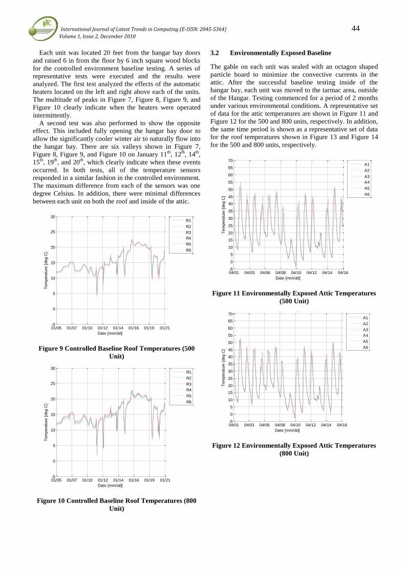
International Journal of Latest Trends in Computing (E-ISSN: 2045-5364) 44
Volume 1, Issue 2, December 2010
Each unit was located 20 feet from the hangar bay doors
and raised 6 in from the floor by 6 inch square wood blocks
for the controlled environment baseline testing. A series of
representative tests were executed and the results were
analyzed. The first test analyzed the effects of the automatic
heaters located on the left and right above each of the units.
The multitude of peaks in Figure 7, Figure 8, Figure 9, and
Figure 10 clearly indicate when the heaters were operated
intermittently.
A second test was also performed to show the opposite
effect. This included fully opening the hangar bay door to
allow the significantly cooler winter air to naturally flow into
the hangar bay. There are six valleys shown in Figure 7,
Figure 8, Figure 9, and Figure 10 on January 11th
, 12th
, 14th,
15th
, 19th
, and 20th
, which clearly indicate when these events
occurred. In both tests, all of the temperature sensors
responded in a similar fashion in the controlled environment.
The maximum difference from each of the sensors was one
degree Celsius. In addition, there were minimal differences
between each unit on both the roof and inside of the attic.
Figure 9 Controlled Baseline Roof Temperatures (500
Unit)
Figure 10 Controlled Baseline Roof Temperatures (800
Unit)
3.2 Environmentally Exposed Baseline
The gable on each unit was sealed with an octagon shaped
particle board to minimize the convective currents in the
attic. After the successful baseline testing inside of the
hangar bay, each unit was moved to the tarmac area, outside
of the Hangar. Testing commenced for a period of 2 months
under various environmental conditions. A representative set
of data for the attic temperatures are shown in Figure 11 and
Figure 12 for the 500 and 800 units, respectively. In addition,
the same time period is shown as a representative set of data
for the roof temperatures shown in Figure 13 and Figure 14
for the 500 and 800 units, respectively.
Figure 11 Environmentally Exposed Attic Temperatures
(500 Unit)
Figure 12 Environmentally Exposed Attic Temperatures
(800 Unit)
01/05 01/07 01/10 01/12 01/14 01/16 01/19 01/21-5
0
5
10
15
20
25
30
Date [mm/dd]
Tem
pera
ture
[deg C
]
Roof Temperatures (500 unit)
R1
R2
R3
R4
R5
R6
01/05 01/07 01/10 01/12 01/14 01/16 01/19 01/21-5
0
5
10
15
20
25
30
Date [mm/dd]
Tem
pera
ture
[deg C
]
Roof Temperatures (800 unit)
R1
R2
R3
R4
R5
R6
04/01 04/03 04/06 04/08 04/10 04/12 04/14 04/16-5
0
5
10
15
20
25
30
35
40
45
50
55
60
65
70
Date [mm/dd]
Tem
pera
ture
[deg C
]
Attic Temperatures (500 unit)
A1
A2
A3
A4
A5
A6
04/01 04/03 04/06 04/08 04/10 04/12 04/14 04/16-5
0
5
10
15
20
25
30
35
40
45
50
55
60
65
70
Date [mm/dd]
Tem
pera
ture
[deg C
]
Attic Temperatures (800 unit)
A1
A2
A3
A4
A5
A6

International Journal of Latest Trends in Computing (E-ISSN: 2045-5364) 45
Volume 1, Issue 2, December 2010
Figure 13 Environmentally Exposed Attic Temperatures
(500 Unit)
Figure 14 Environmentally Exposed Attic Temperatures
(800 Unit)
Each unit was located 150 feet from the front of the hangar
and placed such that they were not in the shadows of any
structure for the environmentally exposed testing. The
temperatures on the left hand side (LHS) and right hand side
(RHS) of the roof and attic were within one degree Celsius,
so an average of each side was calculated and shown in
Figure 15 and Figure 16 for the 500 and 800 units,
respectively. In addition, the ambient temperature for that
time period is shown in each figure [6].
As expected, both sides of each unit increased as the
ambient temperature increased. The LHS reached its peak
temperature first, after which the RHS followed, but did not
reach the same peak temperature. In this data set, there were
two days (April 9th
and 13th
) in which the ambient
temperature was significantly lower where most of the day
was cloudy and hence the peak for both the RHS and LHS
were similar and lower than the other testing days. In
addition, the data for the LHS and RHS both follow the
ambient temperature trend. For example, when there were
noticeable ambient temperature fluctuations, the LHS and
RHS exhibited the same pattern, as shown in Figure 17 and
Figure 18, for the time period of April 13th
through the April
15th
when both cloudy and sunny days were observed.
Figure 15 Baseline Average Data (500 Unit)
Figure 16 Baseline Average Data (800 Unit)
Figure 17 Environmentally Exposed Baseline
Temperatures (500 Unit)
04/01 04/03 04/06 04/08 04/10 04/12 04/14 04/16-5
0
5
10
15
20
25
30
35
40
45
50
55
60
65
70
Date [mm/dd]
Tem
pera
ture
[deg C
]Roof Temperatures (500 unit)
R1
R2
R3
R4
R5
R6
04/01 04/03 04/06 04/08 04/10 04/12 04/14 04/16-5
0
5
10
15
20
25
30
35
40
45
50
55
60
65
70
Date [mm/dd]
Tem
pera
ture
[deg C
]
Roof Temperatures (800 unit)
R1
R2
R3
R4
R5
R6
04/01 04/03 04/06 04/08 04/10 04/12 04/14 04/16-5
0
5
10
15
20
25
30
35
40
45
50
55
60
65
70
Date [mm/dd]
Tem
pera
ture
[deg C
]
Average Temperatures (500 unit)
Attic LHS
Attic RHS
Roof LHS
Roof RHS
Tamb
04/01 04/03 04/06 04/08 04/10 04/12 04/14 04/16-5
0
5
10
15
20
25
30
35
40
45
50
55
60
65
70
Date [mm/dd]
Tem
pera
ture
[deg C
]
Average Temperatures (800 unit)
Attic LHS
Attic RHS
Roof LHS
Roof RHS
Tamb
04/14
-5
0
5
10
15
20
25
30
35
40
45
50
55
60
65
Date [mm/dd]
Tem
pera
ture
[deg C
]
Average Temperatures (500 unit)
Attic LHS
Attic RHS
Roof LHS
Roof RHS
Tamb

International Journal of Latest Trends in Computing (E-ISSN: 2045-5364) 46
Volume 1, Issue 2, December 2010
Figure 18 Environmentally Exposed Baseline
Temperatures (800 Unit)
4 Conclusions
An experimental testing protocol was designed and
developed for a novel thermal management system utilizing
passive convective cooling. Baseline data was established in
both controlled and environmentally exposed environments
which confirmed each unit was built identically and can be
used for further experimental testing.
References
[1] Energy Efficiency and Renewable Energy. [Online].
www1.eere.energy.gov/consumer/tips/insulation.html
[2] (2000, January) Kansas State University. [Online].
http://www.oznet.ksu.edu/
[3] Frank M. White, Heat and Mass Transfer. Reading,
Massachusetts, 1988.
[4] Yunus A. Çengel and Robert H. Turner, Fundamentals of
Thermal-Fluid Sciences, 2nd ed. New York, New York:
McGraw-Hill, 2005.
[5] Adrian Bejan, Convection Heat Transfer, 3rd ed.
Hoboken, New Jersey: John Wiley & Sons, Inc. , 2004.
[6] (2010) Weather. [Online].
http://www.wunderground.com
Author Biographies
Emily D. Pertl received her B.S., M.S. and Ph.D. degrees in Mechanical
Engineering from West Virginia University (WVU), Morgantown, WV,
USA, in 1999, 2001, and 2010, respectively. She is currently a Program Coordinator in the Center for Industrial Research Applications (CIRA) at
West Virginia University (WVU) before which she was a Mechanical
Engineer at Aquatech International Corporation. She has been the co-principal investigator for several projects funded by several agencies and has
published 15 conference papers and journal articles. Dr. Pertl is a member of
SAE, ASME, ASHRAE, and an Engineering Intern.
Daniel K. Carder received his B.S. in mechanical engineering from West
Virginia University, Morgantown, WV and his M.S. in mechanical engineering from West Virginia University. He currently holds a program
coordinator position with the mechanical and aerospace engineering
department at West Virginia University and works as a Research Engineer for the Center for Alternate Fuels, Engines and Emissions (CAFEE). He has
published numerous conference papers and journal articles and has been
principal or co-principal investigator on several research projects.
James E. Smith received the B.S. and M.S. degrees in Aerospace
Engineering and the Ph.D. degree in Mechanical Engineering from West Virginia University (WVU), Morgantown, WV, in 1972, 1974, and 1984,
respectively. He is currently the Director of the Center for Industrial
Research Applications at West Virginia University, where he is also a Professor in the Mechanical and Aerospace Engineering (MAE)
Department. He has taught at the University since 1976, before which he
was a Research Engineer for the Department of Energy (DOE). During his 30-plus-year scientific career, he has been the principal and/or co-principal
investigator for various projects funded by federal agencies (TACOM,
DOD, HEW, DOT, U.S. Navy, DARPA, and DOE), international corporations, and numerous U.S. corporations. The work in these projects
has resulted in the publication of 164 conference papers and 50 journal or
bound transaction papers. This work has resulted in the granting of 30 U.S. patents and numerous foreign patents on mechanical and energy-related
devices. Dr. Smith is a member of AIAA, SAE, ASME, ISCA, ASEE, and
SPIE.
04/14
0
5
10
15
20
25
30
35
40
45
50
55
60
65
Date [mm/dd]
Tem
pera
ture
[deg C
]Average Temperatures (800 unit)
Attic LHS
Attic RHS
Roof LHS
Roof RHS
Tamb

International Journal of Latest Trends in Computing (E-ISSN: 2045-5364) 47
Volume 1, Issue 2, December 2010
Hardware Platform for Multi-Agent System
Development
Michael J. Spencer, Ali Feliachi, Franz A. Pertl, Emily D. Pertl and James E. Smith
College of Engineering and Mineral Resources
Advanced Power & Electricity Research Center, Center for Industrial Research Applications
West Virginia University
Morgantown, WV 26506, USA
[email protected], [email protected], [email protected], [email protected], [email protected]
Abstract: This paper describes the conversion of WVU's analog
power simulator into a micro-grid of the future test bed by installing
digital relays and intelligent electronic switches. The simulator is a
hardware representation of the grid which contains traditional
hardware, both digital and analog, as well as the recent addition of
highly connected, via Ethernet and potentially wireless
communication, smart switching and monitoring devices. These new
devices were chosen specifically for their cyber security capability to
explore that facet of smart grid development. It is important to note
that this simulator is a hardware implementation, and as such is
capable of testing smart grid ideas in the most realistic setting
available without affecting real customers. This simulator also has
the potential to have renewable resources, like wind and solar as well
as fuel cell and battery storage distributed resources tied in to test
smart grid adaptability for these next generation ideas. New digital
relays were installed. Microcontroller units and energy meter
integrated circuits were investigated based on the desire to provide
many modes of communication and as much processing power as
was available in a small package. Solid state switches were designed
and implemented for speed, compactness and reduced power
consumption. The final configuration of this system is presented in
this paper.
Keywords: Smart Grid, Power System, Hardware Prototype, Real-
Time Control, Reconfigurable Power System, Multi-Agent System
1. Introduction
The United States government has recently decided to invest
billions of dollars into the existing, and maybe antiquated,
power grid in an effort to make it more efficient and reliable.
The name given to the new power grid is the Smart Grid, the
main idea being that through more intelligent devices and
communication systems, both on the consumer and utilities
side the grid can be made more reliable with autonomous
reconfiguration and disaster mediation and more efficient
with potential consumer interaction on a real time basis. This
paper proposes to deliver a platform where ideas on
automated reconfiguration and control via multi-agent
systems (MAS's) or other control algorithms can be tested.
This will be accomplished by converting a small scale analog
distribution simulator using 1970's technology into a micro-
grid of the future by the addition of modern digital relay
equipment and micro-controlled switches.
The Lane Department of Computer Science and Electrical
Engineering at West Virginia University maintains an analog
power simulator that was donated to the University and
installed in the 1970s. The simulator, as shown in Figure 1,
the WVU power simulator in its original configuration, is a
low power hardware replica of a distribution system that
contains commercial, industrial and residential loads. It
measures 22 feet long by 8 feet high and is 5 feet in depth.
Power can be supplied to the loads from different internal and
external circuits and generators and routed in a variety of
ways. The simulator is, at this time, being retrofitted to
represent a micro-grid of the future by installing digital relays,
intelligent electronic devices, distributed energy resources
(generation and storage), and potentially a FACTS device.
The new digital hardware will be integrated with the older
electromechanical hardware, as is found in real world power
systems. This will allow the system to be used for research
into autonomous reconfiguration schemes.
Figure 1: WVU power simulator in original configuration
1.1 Addition of Digital Relays
The first step in the upgrade was to install new digital
relays donated by, Schweitzer Engineering Laboratories,
(SEL) Inc. These are listed in table 1. The relays have been
installed next to their electromechanical counter-parts and
will be wired in parallel with them. This will allow either, or
both, to be used if required. Figure 2 shows these new relays
mounted in the simulator. Three of the relays will not be
installed, the 300G generator relay and two of the 751 feeder
protection relays. These will be reserved for use with the
distributed generation equipment to be acquired later.
Table 1: List of equipment donated by SEL
Qty. Relay Type
4 SEL 751A Feeder Protection Relays
1 SEL 387A Current Differential Relay
1 SEL 300G Generator Relay
4 SEL 351 Over-Current Protection Relays
1 SEL 351S Protection Relay
1 SEL 734 Revenue Metering System
1 SEL 3351 System Computing Platform with Subnet
Software

International Journal of Latest Trends in Computing (E-ISSN: 2045-5364) 48
Volume 1, Issue 2, December 2010
Figure 2: Power simulator with added digital relays
1.2 Addition of Intelligent Electronic Switches
The simulator has approximately 100 manually operated
switches that allow power to be routed over different paths
between the generators and loads. The majority of those
switches will be redundant with microcontroller switched
optically isolated triacs. Each microcontroller will also be
paired with an ADE 7758 three-phase energy metering chip to
monitor current and voltage at that node and to allow the
microcontroller units (MCU’s) to focus on communications
and higher level intelligence functions. All of the ADE7758
metering chips will be fed the same 10 MHz clock signal
making it possible to synchronize waveform sampling across
all nodes. When they are not needed the MCU controlled
switches can be turned off and the simulator used in its
original configuration.
2. Research and Development Potential
The system, with its new functionality will provide the
capability to test and refine future grid handling problems and
still remain familiar to the operators and designers likely to
use it. The authors and their colleagues have been doing
research on using distributed intelligent agents with
communication capability for several years as a solution to
the communications bottleneck and information overload that
are fundamental problems of the present day grid. This multi-
agent system (MAS) approach has been simulated in software
but real world hardware with its associated timing and
throughput issues is needed to really explore the concept; the
upgrade to the simulator was designed with this specifically in
mind. The communication requirements and processing
capabilities needed for studies on MAS were at the forefront
of the hardware selection process. A side benefit is that the
hardware is then also applicable to other ideas using immune
system based algorithms for example as intelligence models
for adaptive control of the grid.
One of the first problems to be addressed by the upgraded
simulator was the reconfiguration of the system in response to
an outage. With the intelligent connectivity available in the
upgrade there will be ways to route power around faults and
restore power to much of the system. MAS algorithms [1]
would have direct applicability here as would the immune
based approach [2]. Once this problem has been explored and
the lessons learned, it can be applied to more subtle and
complicated predictive control scenarios.
With the ability to monitor load flow at virtually every
node comes the ability to determine optimum power flow
through the system as well as to automatically prioritize and
shed load when needed or bring on distributed generation to
abate a critical condition all using the distributed intelligence
built into the system. These are all ideas that could be
explored with the simulator that could have a tremendous
impact on the grid of the future.
Communications is a critical component of any distributed
intelligent system and models have shown that a multilayered
communication scheme can offer a dramatic improvement in
communication integrity and throughput. The MCU's chosen
to act as the distributed intelligence were picked in large part
for their ability to communicate via many distinct ports.
Ethernet, Can bus, and RS-232 that could be used as wireless
ports are all available to the algorithm explorer.
Recently Moheuddin et al. [3], published a paper on the
optimization of the number and placement of distributed
agents in a system that is scalable, meaning the algorithm
employed to pick the placement and number was unaffected
by the size of the system. Their work could be implemented
and verified on the new system and could also have great
impact on the evolving smart grid.
Cyber security is a very large concern in the new grid and
the upgraded simulator has been designed with this in mind.
A very attractive feature of these particular MCU’s is that
they handle cryptographic processing not with the main
processor but with a dedicated cryptographic co-processor.
The MCU's were designed specifically to be used in a secure
mode and there is no processing capability lost by
implementing state of the art security measures.
3. Intelligent Electronic Switch Hardware
Selection
The digital relays bring the micro grid up to a current state of
the art level, but to allow for advanced reconfiguration
algorithm testing, automation of the manual switches on the
simulator is desired. It would be possible to use commercial
relays for this function except the size and cost of the system
would be prohibitive. The solution was to design a compact
solid state switch that could be controlled by a
microcontroller that would also sample current and voltage at
that node.
A search was made to find a compact microcontroller that
gave as much processing and communication capability as
currently available to provide the algorithm developers as
large a canvas to try their ideas on as possible. A demo board
from Freescale, the M52259DEMOKIT was chosen. It has a
32 bit 80MHZ processor with 512 Kbytes of flash memory,
64 Kbytes SRAM, and a cryptographic accelerator unit to
allow for secure communications without taxing the main
processor. It comes with two USB ports, one 10/100 Ethernet
port, an RS-232 port and a high speed CAN bus port all in a 3
in x 3.5 in two board package. Figure 3 shows the demo board
with its communication ports.
From the beginning of this project it was determined that
communication was a high priority. This came directly from
the desire to test MAS ideas and from the desire to have
multiple communication paths to insure data integrity. The
single biggest reason this particular demo board was selected
was the multiple communication ports available. Both CAN
bus and Ethernet can be used for a multiple wired
communications scheme and the RS-232 port can then be
dedicated to a wireless module. This still leaves the on board
diagnostics USB port available for programming and the
QSPI for interface with the ADE7758 meter chip. It is
believed that the remaining USB port could be used for a
memory device and that still leaves an I2C interface available
for future use.

International Journal of Latest Trends in Computing (E-ISSN: 2045-5364) 49
Volume 1, Issue 2, December 2010
Figure 3: Freescale M52259DEMOKIT
In addition to communications it was also apparent early on
that security will be a very big issue. To address this issue the
processor comes with a dedicated cryptographic co processor
specifically to handle secure communication.
The power simulator can have voltages as high as 750 VAC
and currents in the 5 ampere range. The triacs selected are of
the snubberless type and rated for 8 amps at 1000 VAC in
order to give a comfortable safety margin. The triacs are
driven by opto-isolators specifically designed to work with
triacs. Non-zero crossing devices were chosen. Since all three
phases will be switched at the same time it seemed that zero
crossing switching might pose a problem during powering up.
Initially the idea was to use the A/D capability of the MCU
to sample current and voltage at the node. While searching for
triacs and opto-isolators a multifunction energy meter IC was
discovered that would perform those functions and many
more leaving the MCU with more processing and
communications capabilities. The specific one chosen, the
Analog Devices ADE7758, is a three phase high accuracy
energy measurement IC. It has a SPI interface and a wide
variety of relay type features making it an ideal if not
serendipitous find. All of these parts fit together in a
straightforward module as shown in the block diagram of
Figure 4.
Figure 4: Block diagram of intelligent electronic switch
4. Circuit Design and Board Fabrication
The ADE7758 is only available in a surface mount package.
This necessitates fabrication of a printed circuit board and
surface mount soldering techniques. A design was drawn up
and sent out for fabrication and a surface mount soldering
station assembled and tested.
The ADE7758 Poly Phase Multifunction Energy Metering
IC has built in analog to digital converters for sampling all
three phases in both voltage and current. The input of the
A/D’s is -0.5 V to +0.5 V so the line voltages must be scaled
down to that range with voltage dividers.
Traditionally, current is sensed with a current shunt of
some sort often with an isolation transformer to step down the
current. Effectively what this does is convert the current to a
proportional voltage where that voltage is sampled and the
corresponding current derived from the amplitude of the
voltage. Alternatively a Hall Effect sensor could be used but
they are too large for this project. The ADE7758 can be used
in the normal current shunt mode but the engineers at Analog
Devices have also come up with a unique alternative solution.
The voltage induced in the secondary of a transformer is
proportional to dI/dT of the primary. The constant of
proportionality is the mutual inductance between the primary
and the secondary. Since this circuit is really only set up for
signals with no DC component, the engineers decided that the
secondary voltage could be sampled and then mathematically
integrated to determine the current though the primary. An
advantage of this is that there is almost no power that has to
be dissipated in the secondary circuit.
As is common when using analog to digital conversion,
anti-aliasing filters need to be used. The circuit recommended
by Analog Devices was used and a copy taken directly from
the data sheet as shown in Figure 5 [4].
Figure 5: Circuit recommended by Analog Devices [4]
The output circuits at pins 1 and 17 were not installed nor
were the capacitors for the clock circuit but the rest of the
circuit was used as shown. The 5 VDC required by the IC
comes directly from a regulator on the printed circuit board.
This ensures that the IC receives a stable voltage. Since the
M52259DEMOKIT also takes 5 VDC, they can both be
supplied by the same source set so the voltage at the boards is
above the 5.5V needed for ample headroom at the regulator.

International Journal of Latest Trends in Computing (E-ISSN: 2045-5364) 50
Volume 1, Issue 2, December 2010
The regulator chosen only supplies 50 mA but the ADE7758
only draws 21 mA maximum.
The M52259 microprocessor runs on 3.3 VDC,
unfortunately the ADE7758 runs on 5 VDC causing a
problem when the two are setup to talk to each other. The
specifications for the input to the ADE7758 are within the
output range of the M52259, so no level shifting is needed.
The input to the M52259 is not specified to handle the logic
levels supplied by the 5 volt ADE7758, so a level shifter
74LVC08AD was used between the two.
Only three of the four gates are needed for level shifting
leaving a spare gate which can be used as a buffer between
the MCU and the opto-isolators (see Figure 6). The output of
the level shifter is 50 mA per gate. The opto-isolators are
wired in parallel to stay under the 3 VDC supplied by the
M52259DEMOKIT and draws 10 to 20 mA each. The
operating load was chosen to be 20 mA so the combined draw
is about 60 mA and beyond the range of the level shifter. A
simple transistor circuit composed of a 2N2222 NPN small
signal transistor running in saturation when on and a couple of
10 ohm current limiting resistors R1 and R2 were used as a
current amplifier to ensure all parts were within their design
limitations.
The triacs need a minimum gate current to turn on and that
is determined by gate resistors R3 for phase A, R4 for phase
B and R5 for phase C. In order to get the largest voltage range
for the triac, a gate resistor was chosen that would give a bit
less than the recommended maximum gate current of about
100 mA for the maximum voltage on the line. The maximum
selected was 750 VAC and 75 mA as the largest RMS current
desired. A 10K ohm resistor in the gate circuit then limits the
gate current to about 75 mA. This should allow the triacs to
work down to about 180 VAC based on the typical values for
gate trigger current, but their value may have to be adjusted if
the operating voltage is used in that range, because the triacs
are specified to work at a 50 mA max gate trigger current
which corresponds to 500 VAC.
The circuit boards were drawn up using Sunstone Circuit’s
PCB123® CAD software and the boards were then fabricated
(see Figure 7). This was effectively a prototype so the board
was designed with the ability to change the layout to
accommodate minor changes. There are places in the triac
section where snubber circuits can be added if they are found
to be needed later. The level shifter is left disconnected with
solder pads so that it can be reconfigured. Parts of the meter
chip like the clock and SPI interface are left open with solder
pads. With this setup, the clock signal can be supplied by an
external clock or an individually dedicated one may be used.
Figure 6: Triac triggering circuit
Figure 7: Sense and control PCB layout
Figure 8: Current sensors being bench tested with the
ADE7758 evaluation board
In an effort to minimize cost and size, the current sensors
were hand wound on salvaged toroid cores for initial testing.
The integration method of current measurement was chosen to
keep part count down and power dissipation at a minimum
since that power would have to be dissipated in the electronic
switch. The sensors are simple transformers wound on the
toroidial core with about 85 turns of 30 AWG as the
secondary which gets attached to the ADE7758 A/D and
about 3 turns of the 14 AWG that connects to the triac. This
arrangement makes a very compact transformer that fits easily
in the switch box and is very tolerant to noise pickup because
of the toroidial configuration. The current sensors being tested
are shown in Figure 8.
5. Hardware Test and Results
Since the A/D’s have very high input impedance, simple
voltage dividers are used for voltage sensing. The current
sensor configuration chosen was novel so a bit of
experimentation was required in their design. An evaluation
board for the ADE7758 was purchased from Analog Devices.
The board comes with LabVIEW based software with a GUI
that makes it very easy to access all of the chip’s capabilities.
The only downside to the evaluation board is that it requires a
parallel printer port for an interface to the board which is
rather rare anymore. It is hoped that the source code can be
modified to use an Ethernet port instead in which case the
ADE7758’s could be accessed though the MCU’s in the
intelligent switches.
To test the triacs a sample code that turns an LED on for
one second then off for the next was used to do the same with
Triac switches on with 2.0VDC at pins 9 and 10,
off at 0.8 VDC

International Journal of Latest Trends in Computing (E-ISSN: 2045-5364) 51
Volume 1, Issue 2, December 2010
the triacs on the simulator. The entire load that was available
on the simulator was switched-in gradually and the triacs
performed as expected. The circuit was modified for 120
VAC by changing the gate resistors to 1.8K ohm instead of
the 10K ohm that were in place for the 750 VAC of the
simulator. The setup was then moved to one of the test
benches where three-phase at 120 VAC was switched in the
same way and the turn-on and turn-off of current and voltage
waveforms were captured with a Yokogawa PZ4000 power
analyzer.
The turn-on waveforms were just as expected with the
addition of some noise that was not considered but can be
easily explained see Figure 9. The turn-on is immediate as
expected but the crossovers and distortion in the other phases
at the same time are not as expected from a normal three
phase power sinusoid waveform at first glance. The delay in
turn-on after each cycle goes through zero is due to the finite
current required through the gate to trigger the triac. Until the
voltage has reached a point where that current is attained there
is no conduction. The reason that the other phases are
distorted during that time is that this is a three phase delta
wired circuit so the sum of the currents and voltage must be
zero at all times. If there is no current flow in one phase,
effectively an open, the other phases will have to sum to zero
regardless.
The turn-off wave forms although also not exactly what
was expected makes sense in light of the previous argument,
see Figure 10. The triacs lose their trigger at the mid way
point of the plot and the first triac turns off, channels 5 and 6
as expected.
The turn-off with an inductive load is widely described in
the literature, see Figure 11. In this case the trigger happens at
the first division, or 10%. The current in each phase shuts off
as expected, but the voltage in each phase tapers off very
slowly. This is due to the voltage induced across the inductor
and resistor in parallel as the magnetic field collapses in the
inductor.
Figure 9: Three phase triac turn-on waveforms with
resistive load
Figure 10: Three phase triac turn-off waveforms with
resistive load
Figure 11: Three phase triac turn-off with inductive load
6. Conclusions
The sense and control boards have been designed and
fabricated. A procedure is now in place for the assembly of
the boards. All testing done on them has been successful. The
open issues are the SPI interface and the verification of the
sensor filter circuits which require some sort of
communication with the ADE7758 on the board so may be
best left until that issue is resolved. The 50 boards that are in
house are all suitable for use. If a next version of the board is
made and incorporates the new layout of the level shifter and
transistor buffer it would probably save some time and make
for a neater package.
The current sensors seem to work just fine, they give a
voltage that’s in a good range for the ADE7758 A/D’s and
have been shown to be acceptably linear over the range of
currents expected. There may be room here for improvement
with more attention paid to core selection and size. More
experience with the present devices may indicate that more or
less coupling would be advantageous on the power simulator.
It may also be found that more than one type would give the
greatest benefit. The evaluation board will be a great tool for
exploring this topic in more detail
The triacs performed very well and despite the added noise
induced at crossover they look to be a very satisfactory

International Journal of Latest Trends in Computing (E-ISSN: 2045-5364) 52
Volume 1, Issue 2, December 2010
solution as AC switches on the simulator. There is also room
for experimentation and possible improvement through the
design and testing of snubbers for switching more inductive
loads if needed in the future, and the impact of zero crossing
opto-isolators would also be an interesting topic to explore
further.
References
[1] Koushaly Nareshkumar, Application of multi-agents to
power distribution systems. Morgantown, WV: West
Virginia University Libraries, 2008.
[2] Ali Feliachi Rabie Belkacemi, "Multi-Agent Design for
Power Distribution System Reconfiguration Based on the
Artificial Immune System Algorithm," in ISCAS 2010,
2010, May 30-June 2.
[3] Afzel Noore, and Muhammad Choudhry Summiya
Moheuddin, "A Reconfigurable Distributed Multiagent
System Optimized for Scalability," International Journal
of Computational Intelligence, vol. 5, no. 1, pp. 60-71,
2009.
[4] Analog Devices, "ADE7758 Poly Phase Multifunction
Energy Metering IC Data Sheet," 2008.
Author Biographies
Michael J. Spencer received his B.S. in electrical engineering from the
University of Hawaii, Manoa in 1993, and his M.S. in electrical engineering from West Virginia University in 2010. He is currently pursuing a Ph.D in
mechanical engineering with the mechanical and aerospace engineering
department at West Virginia University and works as a graduate research assistant for the Center of Industrial Research Applications (CIRA). Prior to
returning to graduate school he worked as a millimeter wave antenna and
passive microwave component engineer for TRW and with the IR Lab in UCLA's Department of Physics and Astronomy as electronics lead
developing cryogenic electronics systems for astronomical infrared imagers
for the Keck telescopes in Hawaii, NASA’s Stratospheric Observatory for Infrared Astronomy (SOFIA) and Lick Observatory.
Ali Feliachi received the Diplôme d’Ingéenieur en Electrotechnique from the Ecole Nationale Polytechnique of Algiers, Algeria, in 1976, and the MS and
Ph.D. degrees in Electrical Engineering from the Georgia Institute of
Technology (Ga Tech) in 1979 and 1983 respectively. He joined the Lane Department of Computer Science and Electrical Engineering at West Virginia
University in 1984 where he is currently a Full Professor, the holder of the Electric Power Systems Endowed Chair Position, and the Director of the
Advanced Power & Electricity Research Center (APERC). His research
interests are modeling, control and simulation of electric power systems.
Franz A. Pertl received his B.S. in electrical and computer engineering from
West Virginia University, Morgantown, WV, in 1994, and his M.S. in electrical engineering from West Virginia University in 1996 and his Ph.D. in
Mechanical Engineering from West Virginia University in 2008. He currently
holds a program coordinator position with the mechanical and aerospace engineering department at West Virginia University and works as a Research
Engineer for the Center of Industrial Research Applications (CIRA). He has
also worked for the Engine and Emissions Research Center at West Virginia University and taught summer courses at the University. His areas of
expertise include software design, data acquisition, microprocessor
applications, color machine vision, controls, wind turbines and other areas of electrical engineering. He has published 26 conference papers, 8 journal
papers and has been awarded 5 US patents to date and has been principal or
co-principal investigator on several research projects. His current interests include electromagnetic and microwave plasma ignition. Dr. Pertl is a
member of Sigma Xi Scientific Research Society and the Society of
Automotive Engineers.
Emily D. Pertl received her B.S., M.S. and Ph.D. degrees in Mechanical
Engineering from West Virginia University (WVU), Morgantown, WV, USA, in 1999, 2001, and 2010, respectively. She is currently a Program
Coordinator in the Center for Industrial Research Applications (CIRA) at
West Virginia University (WVU) before which she was a Mechanical
Engineer at Aquatech International Corporation. She has been the co-
principal investigator for several projects funded by several agencies and has
published 15 conference papers and journal articles. Dr. Pertl is a member of SAE, ASME, ASHRAE, and an Engineering Intern.
James E. Smith received the B.S. and M.S. degrees in Aerospace Engineering and the Ph.D. degree in Mechanical Engineering from West
Virginia University (WVU), Morgantown, WV, in 1972, 1974, and 1984,
respectively. He is currently the Director of the Center for Industrial Research Applications at West Virginia University, where he is also a Professor in the
Mechanical and Aerospace Engineering (MAE) Department. He has taught
at the University since 1976, before which he was a Research Engineer for the Department of Energy (DOE). During his 30-plus-year scientific career,
he has been the principal and/or co-principal investigator for various projects
funded by federal agencies (TACOM, DOD, HEW, DOT, U.S. Navy, DARPA, and DOE), international corporations, and numerous U.S.
corporations. The work in these projects has resulted in the publication of 164
conference papers and 50 journal or bound transaction papers. This work has resulted in the granting of 30 U.S. patents and numerous foreign patents on
mechanical and energy-related devices. Dr. Smith is a member of AIAA,
SAE, ASME, ISCA, ASEE, and SPIE.
International Journal of Latest Trends in Computing (E-ISSN: 2045-5364) 53 Volume 1, Issue 2, December 2010
Document Classification using Novel Self
Organizing Text Classifier
Seyyed Mohammad Reza Farshchi1, Taghi Karimi
2
1Islamic Azad University, Mashhad Branch, Dep. of Artificial Intelligence,
2Dep. of Mathematics, Payam Noor University, Fariman Branch,
Iran, Mashhad.
Abstract: Text categorization is one of the well studied problems
in data mining and information retrieval. Given a large quantity of
documents in a data set where each document is associated with its
corresponding category. This research proposes a novel approach
for documents classification with using novel method that
combined competitive self organizing neural text categorizer with
new vectors that we called, string vectors. Even if the research on
document categorization has been progressed very much,
documents should be still encoded into numerical vectors. Such
encoding so causes the two main problems: huge dimensionality
and sparse distribution. Although many various feature selection
methods are developed to address the first problem, but the reduced
dimension remains still large. If the dimension is reduced
excessively by a feature selection method, robustness of document
categorization is degraded. The idea of this research as the solution
to the problems is to encode the documents into string vectors and
apply it to the novel competitive self organizing neural text
categorizer as a string vector. The quantitative and qualitative
experiment results demonstrate that this method can significantly
improve the performance of documents classification.
Keywords: Text Classification (TC), Documents Classification,
Information Management, Data Mining.
1. Introduction
As the volume of information continues to increase, there is
growing interest in helping people better find, filter, and
manage these resources. Text categorization (TC a.k.a. Text
classification, or topic spotting) - the assignment of natural
language documents to one or more predefined categories
based on their semantic content - is an important component
in many information organization and management tasks [1].
Automatic text categorization task can play an important role
in a wide variety of more flexible, dynamic and personalized
tasks as well: real-time sorting of email or files, document
management systems, search engines, digital libraries.
In the last 10 years content-based document management
tasks (collectively known as information retrieval—IR) have
gained a prominent status in the information systems field,
due to the increased availability of documents in digital form
and the ensuing need to access them in flexible ways [2].
TC the activity of labeling natural language texts with
thematic categories from a predefined set, is one such task.
TC dates back to the early 60's, but only in the early 90's did
it become a major sub field of the information systems
discipline, thanks to increased applicative interest and to the
availability of more powerful hardware. TC is now being
applied in many contexts, ranging from document indexing
based on a controlled vocabulary [3], to document filtering,
automated meta data generation, word sense disambiguation,
population of hierarchical catalogues of Web resources, and
in general any application requiring document organization
or selective and adaptive document dispatching.
In many contexts trained professionals are employed to
categorize new items. This process is very time-consuming
and costly, thus limiting its applicability. Consequently there
is an increasing interest in developing technologies for
automatic text categorization [4].
A number of statistical classification and machine learning
techniques has been applied to text categorization, including
regression models, nearest neighbor classifiers, decision
trees, Bayesian classifiers, Support Vector Machines (SVM),
rule learning algorithms, relevance feedback, voted
classification, and neural networks.
The research on text categorization has been made very much
progress in context of machine learning and data mining. It
requires encoding documents into numerical vectors for using
one of traditional algorithms for text categorization [5].
A corpus which is a collection of documents is mapped into a
list of words as the feature candidates. Among the candidates,
only some are selected as the features. For each document, a
numerical value is assigned to each of the selected features,
depending on the importance and presence of each feature.
However, encoding documents so causes the two main
problems: huge dimensionality and sparse distribution [6].
In order to solve the two main problems, this research uses
the novel method that documents should be encoded into
string vectors. A string vector refers to a finite set of strings
which are words in context of a natural language. In
numerical vectors representing documents, words are given
as features, while in string vectors, words are given as feature
values. Features of string vectors are defined very variously
as properties of words with respect to their posting, lexical
category, and statistical properties, but in this research, the
highest frequent word, the second highest frequent one, and
so on are defined as features of string vectors for easy
implementation.
By encoding documents into string vectors, we can avoid
completely the two main problems: huge dimensionality and
sparse distribution.
We proposed the competitive neural text categorizer, as the
approach to text categorization and proposed the application
of it to documents categorization. Before creating the
International Journal of Latest Trends in Computing (E-ISSN: 2045-5364) 54 Volume 1, Issue 2, December 2010
proposed neural network, traditional neural networks, such as
MLP (Multi Layers Perceptron) with BP (Back Propagation)
receives numerical vectors as its input data. Differently from
the traditional neural networks, the proposed neural network
receives string vectors. It has the two layers as its
architecture: the input layer and the competitive layer. It is
expected for the proposed model to improve the performance
of text categorization by solving the two main problems.
The rest of this paper is organized as follows. The principle
of TC and previous works is given in next sections. Strategies
of encoding documents were given in sections 2. Section 3
describes the novel competitive self organizing neural text
categorizer model. In section 4 we will mention the
simulation result and significance of this research.
Conclusions are presented in Section 5.
2. Related Work
This section is concerned with previous works relevant to this
research and we will survey previous relevant works, and
point out their limitations. There exist other kinds of
approaches to text categorization than machine learning
based ones: heuristic and rule based approaches. Heuristic
approaches were already applied to early commercial text
categorization systems [7]. However, we count out the kind
of approaches in our exploration, since they are rule of
thumbs. Since rule based approaches have poor recall and
require a time consuming job of building rules manually as
mentioned in the previous section, they are not covered in
this article, either. Therefore, this article counts only machine
learning based approaches to text categorization considered
as state of the art ones. Even if many machine learning
approaches to text categorization already proposed, we will
mention the four representative and popular approaches:
KNN (K Nearest Neighbor), NB (Naive Bayes), SVM, and
BP Neural Networks (NNBP or briefly BP) [8].
It requires encoding documents into numerical vectors for
using one of them for text categorization; the two main
problems are caused. String kernel was proposed in using the
SVM for text categorization as the solution to the two main
problems, but it failed to improve the performance [9]. In this
section, we will explore the previous works on traditional
approaches to text categorization and previous solution to the
two main problems.
The KNN may be considered as a typical and popular
approach to text categorization [10]. The KNN was initially
created by Cover and Hart in 1967 as a genetic classification
algorithm [11]. It was initially applied to text categorization
by Massand et al at 1993 in [12]. The KNN algorithm is
quite simple: given a test documents, and uses the categories
of the K neighbors to weight the category candidates. The
similarity score of each neighbor documents to test
documents is used as the weight of the K nearest neighbor
documents. If several of nearest neighbor share a category,
then the per-neighbor weights of that category are added
together, and the resulting weighted sum is used as the like
hood score of that category with respect to the test document.
By scoring the scores of candidate categories, a ranked list is
obtained for the rest document. KNN was recommended by
Yang at 1999 in [13] and by Sebastiani at 2002 in [14] as a
practical approach to text categorization. Therefore, the KNN
has been aimed as the base approach in other literature as the
base approach. The Naive Bayes may be considered as
another approach to text categorization. It was initially
created by Kononenko in 1989, based on Bayes Rule [15]. Its
application to text categorization was mentioned in the
textbook by Mitchell in [16]. Assuming that the Naive Bayes
is the popular approach, in 1999, Mladenic and Grobelink
proposed and evaluated feature selection methods [17]. The
Naive Bayes has been compared with other subsequent
approaches in text categorization at [18].
Recently, the SVM was recommended as the practical
approach to text categorization [19]. It was initially
introduced in Hearst magazine in [20]. In the same year, it
was applied to text categorization by Joachims [21]. Its idea
is derived from a linear classifier perceptron, which is an
early neural network. Since the neural network classifies
objects by defining a hyper-plane as a boundary of classes, it
is applicable to only linearly separable distribution of
training examples. The main idea of SVM is that if a
distribution of training examples is not linearly separable,
these examples are mapped into another space where their
distribution is linearly separable, as illustrated in the left side
of figure 1. SVM optimizes the weights of the inner products
of training examples and its input vector, called Lagrange
multipliers [22], instead of those of its input vector, itself, as
its learning process. In fact, the method is defined over a
vector space where the problem is to find a decision surface
that "best" separate the data points in two classes. In order to
define the "best" separation, we need to introduce the
"margin" between two classes. Figure 2 and 3 illustrate the
idea. For simplicity, we only show a case in a two
dimensional space with linearity separable data points. It was
adopted as the approach to spam mail filtering as a practical
instance of text categorization by Druker et al in [23].
Furthermore, the SVM is popularly used not only for text
categorization tasks but also for any other pattern
classification tasks [24].
In 1995, BP was initially applied to text categorization by
Wiener in his master thesis [25]. He used Reuter 21578 [26]
as the test bed for evaluating the approach to text
categorization and shown that back propagation is better than
KNN in the context of classification performance. In 2002,
Gabriel applied continually BP to text categorization [27].
They used a hierarchical combination of BPs, called HME
(Hierarchical Mixture of Experts), to text categorization,
instead of a single BP. They compared HME of BPs with a
flat combination of BPs, and observed that HME is the better
combination of BPs. Since BP learns training examples very
slowly, it is not practical, in spite of its broad applicability
and high accuracy, for implementing a text categorization
system where training time is critical.
Research on machine learning based approaches to text
categorization has been progressed very much, and they have
been surveyed and evaluated systematically. In 1999, neural
networks may be considered as an approach to text
categorization, and among them, the MLP with BP is the
most popular model [28].
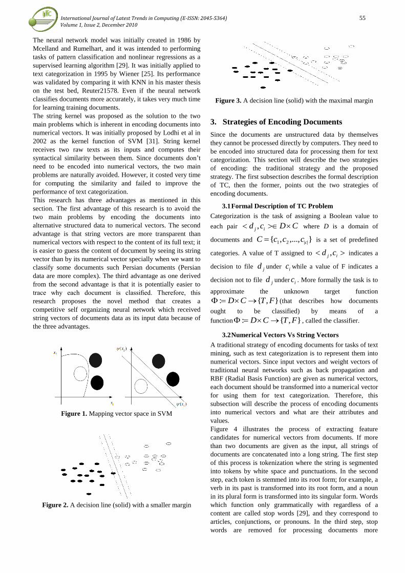
International Journal of Latest Trends in Computing (E-ISSN: 2045-5364) 55 Volume 1, Issue 2, December 2010
The neural network model was initially created in 1986 by
Mcelland and Rumelhart, and it was intended to performing
tasks of pattern classification and nonlinear regressions as a
supervised learning algorithm [29]. It was initially applied to
text categorization in 1995 by Wiener [25]. Its performance
was validated by comparing it with KNN in his master thesis
on the test bed, Reuter21578. Even if the neural network
classifies documents more accurately, it takes very much time
for learning training documents.
The string kernel was proposed as the solution to the two
main problems which is inherent in encoding documents into
numerical vectors. It was initially proposed by Lodhi et al in
2002 as the kernel function of SVM [31]. String kernel
receives two raw texts as its inputs and computes their
syntactical similarity between them. Since documents don’t
need to be encoded into numerical vectors, the two main
problems are naturally avoided. However, it costed very time
for computing the similarity and failed to improve the
performance of text categorization.
This research has three advantages as mentioned in this
section. The first advantage of this research is to avoid the
two main problems by encoding the documents into
alternative structured data to numerical vectors. The second
advantage is that string vectors are more transparent than
numerical vectors with respect to the content of its full text; it
is easier to guess the content of document by seeing its string
vector than by its numerical vector specially when we want to
classify some documents such Persian documents (Persian
data are more complex). The third advantage as one derived
from the second advantage is that it is potentially easier to
trace why each document is classified. Therefore, this
research proposes the novel method that creates a
competitive self organizing neural network which received
string vectors of documents data as its input data because of
the three advantages.
Figure 1. Mapping vector space in SVM
Figure 2. A decision line (solid) with a smaller margin
Figure 3. A decision line (solid) with the maximal margin
3. Strategies of Encoding Documents
Since the documents are unstructured data by themselves
they cannot be processed directly by computers. They need to
be encoded into structured data for processing them for text
categorization. This section will describe the two strategies
of encoding: the traditional strategy and the proposed
strategy. The first subsection describes the formal description
of TC, then the former, points out the two strategies of
encoding documents.
3.1 Formal Description of TC Problem
Categorization is the task of assigning a Boolean value to
each pair CDcd ij , where D is a domain of
documents and ,...,, ||21 ccccC is a set of predefined
categories. A value of T assigned to ij cd , indicates a
decision to file jd under ic while a value of F indicates a
decision not to file jd under ic . More formally the task is to
approximate the unknown target function
,: FTCD (that describes how documents
ought to be classified) by means of a
function ,: FTCD , called the classifier.
3.2 Numerical Vectors Vs String Vectors
A traditional strategy of encoding documents for tasks of text
mining, such as text categorization is to represent them into
numerical vectors. Since input vectors and weight vectors of
traditional neural networks such as back propagation and
RBF (Radial Basis Function) are given as numerical vectors,
each document should be transformed into a numerical vector
for using them for text categorization. Therefore, this
subsection will describe the process of encoding documents
into numerical vectors and what are their attributes and
values.
Figure 4 illustrates the process of extracting feature
candidates for numerical vectors from documents. If more
than two documents are given as the input, all strings of
documents are concatenated into a long string. The first step
of this process is tokenization where the string is segmented
into tokens by white space and punctuations. In the second
step, each token is stemmed into its root form; for example, a
verb in its past is transformed into its root form, and a noun
in its plural form is transformed into its singular form. Words
which function only grammatically with regardless of a
content are called stop words [29], and they correspond to
articles, conjunctions, or pronouns. In the third step, stop
words are removed for processing documents more

International Journal of Latest Trends in Computing (E-ISSN: 2045-5364) 56 Volume 1, Issue 2, December 2010
efficiently and reliably for text categorization.
An alternative strategy of encoding documents for text
categorization is to represent them into string vectors. In this
part, we describe this strategy and its advantage in detail.
However, this strategy is applicable to only proposed
competitive self organizing neural network, while the
previous one is applicable to any traditional machine learning
algorithm.
A string vector is defined as a finite ordered set of words. In
other words, a string vector is a vector whose elements are
words, instead of numerical values. Note that a string vector
is different from a bag of words, although both of them are
similar as each other in their appearance. A bag of words is
an infinite unordered set of words; the number of words is
variable and they are independent of their positions. In string
vectors, words are dependent on their positions as elements,
since words correspond to their features.
Features of string vectors are defined as properties of words
to the given document. The features are classified into the
three types: linguistic features, statistical features, and
positional features. Linguistic features are features defined
based on linguistic knowledge about words in the given
document: the first or last noun, verb, and adjective, in a
paragraph, title, or full text. Statistical features are features
defined based statistical properties of words in the given
documents; the highest frequent word and the highest
weighted word using following equation.
)1)()(log()( 22 kik wdfLogDwktfwweight (1)
Where )(wktf i is the frequency of words, kw , D is the total
number of document categories in corpus.
Positional features are features defined based on positions of
words in a paragraph or the full text: a random word in the
first or last sentence or paragraph, or the full text.
We can define features of string vectors by combining some
of the three types, such as the first noun in the first sentence,
the highest frequent noun in the first paragraph, and so on. A
formal description of string vector is defined as a set of
words which is ordered and has its fixed size. It is denoted
by ],...,,[ 21 dsss where is denotes a string, and there are d
elements. When representing documents into string vectors,
their sizes are fixed with d, and it is called the dimension of
string vectors. Since the elements are ordered in each string
vector, two string vectors with their identical elements but
different orders are treated as different ones. The reason is
that each position of an element has its own different feature.
Table 1 illustrate differences between string vectors and
numerical vectors. The first difference is that numerical
values are given as elements in numerical vectors, while
strings are given as elements in string vectors. The second
difference is that the similarity measure between two
numerical vectors is the cosine similarity or the Euclidean
distance, while that between two string vectors is the
semantic average similarity. The third difference between the
two types of structured data is that features for encoding
documents into numerical vectors are words, while those for
encoding them into string vectors are statistical linguistic and
posting properties of words. Therefore, a string vector is the
vector where numerical values are replaced by strings in a
numerical vector.
The differences between string vectors and bags of words are
illustrated in table 2. Both types of structured data have
strings as their elements.
Figure 4. Flowchart of feature extraction of documents
As the similarity measure, cardinality of intersection of two
bags of words is used while the average semantic similarity is
used in string vectors. A bag of words is defined as an
unordered infinite set of words, while a string vector is
defined as an ordered finite set of words. Although a bag of
words and a string vector look similar as each other, they
should be distinguished from each other, based on table 2.
Table 1. The comparison of numerical and string vectors
Numerical Vector String Vector
Element Numerical value String
Similarity
Measure
Inner products, Euclidean
distance Semantics similarity
Attributes Words Property of words
There are three advantages in representing documents into
string vectors. The first advantage is to avoid completely the
two main problems: the huge dimensionality and the sparse
distribution. The second advantage is that the string vectors
are characterized as more transparent representations of
documents than numerical vectors; it is easier to guess the
content of documents only from their representations. The
third advantage is that there is the potential possibility of
tracing more easily why each documents are classified so.
Figure 5 illustrates the process of encoding a document into
its string vector with the simple definition of features. In the
first step of figure 5, a document is indexed into a list of
words and their frequencies. Its detail process of the first step
is illustrated in figure 4. If the dimension of string vectors is
set to d, d highest frequent words are selected from the list, in
the second step. In the third step, the selected words are
sorted in the descending order of their frequencies. This
ordered list of words becomes a string vector representing the
document given as the input.
This section describes the proposed competitive self
organizing neural network, in detail, with respect to its
architecture, training, classification, and properties.

International Journal of Latest Trends in Computing (E-ISSN: 2045-5364) 57 Volume 1, Issue 2, December 2010
Competitive self organizing neural networks belong to a class
of recurrent networks, and-they are based on algorithms of
unsupervised learning, such as the competitive algorithm
explained in this section.
Table 2. The comparison of bag of words and string vectors
Numerical Vector String Vector
Element String
Similarity
measure Number of shared words Semantics similarity
Set Unordered infinite set Ordered finite set
In competitive learning, the output neurons of a neural
network compete among themselves to become active (to be
"fired"). Whereas in MLP several output neurons may be
active simultaneously, in competitive learning only a single
output neuron is active at any time.
Figure 5. The process of mapping documents into a string
vector
In other words, competitive learning is a learning procedure
that divides a set of input patterns in clusters that are inherent
to the input data. A competitive learning network is provided
only with input vectors x and thus implements an
unsupervised learning procedure.
A simple competitive learning network was depicted in
Figure 6. A basic competitive network has an input layer and
a competitive layer. The nodes in the competitive layer
“compete” with each other, and the node that has the largest
output becomes the “winning” neuron. The winning neuron is
set to 1 and all other neurons are set to 0.
The training of the basic competitive network uses the
Kohonen learning rule. For each input pattern, the weight
vector of the winning node is moved closer to the input
vector using the following formula:
))1()(()1()( qwqpqwqw iii (2)
Where iw is the weight of the winning neuron, p is the
corresponding input vector (string value) and D is the
Kohonen learning rate. However, a problem of this model is
that if the initial weight of a neuron is far from any vector, it
will never be trained, so a bias vector is added to the result of
the competition. The winning node would cause the bias
vector to decrease. Under this mechanism, it is more difficult
for a neuron to continue to win. The degree of bias is
represented by a factor called conscience rate. As we show in
figure 6 each of the four outputs O is connected to all inputs i
with weight 0iw . When an input string vector x is presented
only a single output unit of the network (the winner) will be
activated. In a correctly trained network, all x in one cluster
will have the same winner. For the determination of the
winner and the corresponding learning rule, two methods
exist: dot products and Euclidean distance. For simplicity of
calculation we used the Euclidean distance in proposed
network.
Figure 6. A simple competitive learning network
The proposed neural network follows self organizing map
(SOM) in that synaptic weights are connected directly
between the input layer and the competitive layer, and the
weights are updated only when each training example is
misclassified.
However, note that the proposed neural network is different
from SOM in context of its detail process of learning and
classification, since it uses string vectors as its input vectors,
instead of numerical vectors. The competitive layer given as
an additional layer to the input layer is different from the
hidden layer of back propagation with respect to its role. The
learning layer determines synaptic weights between the input
and the competitive layer by referring to the tables owned by
learning nodes. The learning of proposed neural network
refers to the process of competition between weights stored
in the tables.
Each training example is classified by summing the initial
weights and selecting the category corresponding to the
maximal sum. If the training example is classified correctly,
the weights are not updated. Otherwise, the weights are
incremented toward the target category and those are
decremented toward the classified category. The winner
weights (target category) are generated as the output of this
process.
In the competitive neural network, each example is classified
by summing the winner optimized weights, whether it is a
training or unseen example. In addition weights connected to
itself from the input nodes as its categorical score. The
weights are decided by referring the table which is owned by
its corresponding learning node. The category corresponding
to the output node which generate its maximum categorical
score (winner category) is decided as the category of the
given example. Therefore, the output of this process is one of
the predefined categories, assuming that the competitive
neural network is applied to text categorization without the

International Journal of Latest Trends in Computing (E-ISSN: 2045-5364) 58 Volume 1, Issue 2, December 2010
decomposition. Figure 7 shows the diagram of proposed
neural network. Complete algorithm of competitive neural
text classifier and competitive learning algorithm was
mentioned in classifier training algorithm and learning
algorithm, respectively.
Figure 7. Proposed self organizing neural text classifier
Algorithm 1: Classifier Training
Input: A Series of Documents, Number of Categories
Output: The Winner Categories
1: Encode these sample documents into string vectors
2: Design the architecture of competitive text categorizer
3: Initialize weights in each learning node in competitive
layer with its document
4: Repeat step 1-3 with the number of given documents
5: For each encoded sample document
6: Compute the values of winner nodes of the encoded
6-1: Classify each training vector into the corresponding
category
6-2: Output: winner node in each learning node
6-2-1: If the winner node classify the documents correctly go
to step 7
6-2-2: Update table weights
7: Output calculated weights
8: End
Algorithm 2: Winner Selection
Input: The Architecture of competitive self organizing
neural text categorizer
Output: Selected Winner
1: Given one of string vector that in previous stage was
created.
2: Compute the output value of nodes in the encoded
document using the equation (2).
3: Classify the unseen string vector into the category
corresponding to the output node (winner node)
4: End
4. Experimental Consideration
This section is concerned with the empirical validation of the
performance of proposed method in several experiments.
An important issue of text categorization is how to measure
the performance of the classifiers. Many measures have been
used, each of which has been designed to evaluate some
aspect of the categorization performance of a system [28]. In
this section we discuss and analysis the important measures
that have been reported in the literature.
We use the collection of Persian news categories, called
irna.ir. In addition, For evaluating our method on English
documents the standard test bed, Reuter 21578, was used.
The Reuter 21578 is popularly used as the standard test bed
for evaluating approaches to text categorization.
This set of experiments involves the five approaches: KNN,
NB, SVM, NNBP, and our proposed method. In experiment
result, the test bed and configurations of the approaches
involved in the set of experiments are described, and the
results of the set of experiments are presented and discussed.
The partition of the test bed, Reuter 21578 and irna.ir into the
training and test set is illustrated in table 3 and 4,
respectively. The test bed contains the most frequent
categories of different type of news for entering the first
evaluation, and its source is the web site, www.irna.ir. The
collection was built by copying and pasting the news
documents individually as the plain text files. In the test bed,
the five categories and the 5,436 Persian and English news
documents are available. The collection of news articles is
partitioned into the training and test set by the ratio 7:3, as
shown in table 3 and 4.
Table 3. Collection of different news articles on Reuter
21578
Category Name Training Set Test Set Total
Trade 869 380 575
Earn 500 214 515
Grain 220 94 245
Wheat 430 185 615
Ship 250 110 360
Corn 280 120 400
Total 1890 820 2710
The configurations of the involved approaches are illustrated
in table 5. The parameters of the SVM and the KNN, the
capacity and the number of nearest neighbors, are set as five
and six, respectively, but the NB has no parameter. The
parameters of the NNBP such as the number of hidden nodes
And the learning rate are arbitrary set as shown in table 5.
Persian news documents are encoded into 420 dimensional
numerical vectors and 123 dimensional string vectors.
English documents are encoded into 398 numerical vectors
and 116 dimensional string vectors. We compared
performance of the proposed method with four traditional
approaches in following experiments.
4.1 Micro and Macro Averaging
For evaluating performance average across categories, there
are two conventional methods, namely macro-averaging and
micro-averaging. Macro-averaged performance scores are
determined by first computing the performance measures per
category and then averaging these to compute the global
means. Micro-average performance scores are determined by
first computing the totals of a, b, c, and d for all categories

International Journal of Latest Trends in Computing (E-ISSN: 2045-5364) 59 Volume 1, Issue 2, December 2010
and then use these totals to compute the performance
measures. There is an important distinction between the two
types of averaging. Micro-averaging gives equal weight to
every document, while macro-averaging gives equal weight
to each category. For evaluating the performance of the
classifiers, we define four parameters:
• a - The number of documents correctly assigned to this
category.
• b -The number of documents incorrectly assigned to this
category.
• c - The number of documents incorrectly rejected from this
category.
• d - The number of documents correctly rejected from this
category.
The results of this experiment on Reuter 21578 test bed are
presented in figure 8. Among the five methods, the left
picture indicates the micro-averaged measure of each
method. The right picture indicates the macro-averaged
measure of each method, respectively. Our proposed
approach shows its best performance to the NNBP, but the
performance of our proposed approach is comparable to that
of NNBP.
Table 4. Collection of different news articles on irna.ir
Category Name Training Set Test Set Total
Politics 350 175 525
Law 360 145 505
Computer 150 75 225
Education 110 47 157
Economics 472 203 675
Sports 466 200 666
Total 1908 845 2753
Let’s discuss the results from the set of experiments which
were illustrated in figure 8. Even if the macro-averaged
proposed neural network is not better than NNBP in the task,
both are comparable to each other with respect to the
performance of text categorization. Note that it requires very
much time for training NNBP as the payment for the best
performance. In addition, the NNBP is not practical in
dynamic environments where NNBP must be trained again,
very frequently. Hence, the proposed method is more
recommendable than NNBP with respect to both the learning
time and the performance.
4.2 F-Measure
Another evaluation criterion that combines recall and
precision is the F-measure. In fact, the F1 measure is used for
evaluating the performance of TC. The F1measure can be
calculated as following equation:
),(),(Re
),(),(Re)1()(
kiprecisionkicall
kiprecisionkicallPE
(3)
Precision and recall are widely used for evaluation measures
in TC. For calculating the F1 measure, in each category and
each documents we should determines whether the document
belongs to the category or not. So we need to define the
recall and precision rate with the parameters that defined in
previous section as:
ba
aprecision
ca
arecall
(4)
Table 5. Parameter settings of algorithms
Algorithms Parameter Settings
SVM Capacity = 5.0
KNN # Nearest Value= 6
Naïve Bayes N/A
NN With Back Propagation (BP)
# Hidden Layer=15
Learning Rate=0.2
#Training Epoch=500
Proposed Method Learning Rate=0.2
#Training Epoch=150
Figure 8. The left side of figure indicates the micro-averaged
measure and the right one shows the macro-averaged for (left
to right): proposed method, NNBP, SVM, NB, KNN
Figure 9 shows the result of evaluating the F1 measure for
five approaches on the irna.ir test bed. Science each category
contain identical number of test documents, micro-averaged
and macro-averaged F1 are same as each other. Therefore,
their performances are presented in an integrated group,
instead of two separated groups, in figure 9. This result
shows that back propagation is the best approach in
comparison to another three traditional algorithms, while NB
is the worst approach with the decomposition of the task on
this test bed. Unlike the previous experiment set, NTC is
comparable and competitive with back propagation. So we
discuss this analysis in next subsections with combined to
another experiments
4.3 Accuracy
Figure 10 show the accuracy of all methods on Reuter 21578
news document test bed. This picture show that the proposed
neural network has more reliable than other traditional
method.

International Journal of Latest Trends in Computing (E-ISSN: 2045-5364) 60 Volume 1, Issue 2, December 2010
The accuracy rate of the proposed neural network on test bed
is more than 86% but the best traditional approach have 80%
accuracy rate.
Figure 9. The F1 measure evaluation for (left to right):
proposed method, KNN, NB, SVM, NNBP
4.4 Recall and Precision Rate
We also tried another performance measure for our proposed
method to show the quality of document classification. We
validate the performance of novel approach by comparing it
with other machine learning algorithms on the irna.ir test bed
in this experiment. Table 7 shows these rate for best
traditional method and novel method.
Figure 10. Accuracy rate of news classifier on Reuter 21578
From the above result (and section 4.2) we can see that the
documents classifier based on competitive self organizing
neural network with string vector can classify document of
different categories correctly, represented by a high accuracy
rate. If we use the positive and negative accuracy rate for
evaluating the performance of proposed text classifier we
have:
Table 6. Positive and negative accuracy for news text
classifier
Positive Accuracy Negative Accuracy Average Accuracy
0.4894 0.9368 0.7131
Where a low positive accuracy rate shows that many
documents from different categories are not clustered
together. This is partly because it is difficult to have
information about the correct category in unsupervised
learning. In addition this result shows that the classifiers
based on BP network (NNBP) couldn't classify documents
(in most categories) correctly.
Table 7. Precision and Recall rate of best traditional and
novel text classifier
Precision Recall
SVM 0.6398 0.4
NNBP 0.4367 0.4
KNN 0.5612 0.8
NB 0.7866 0.65
Our Method 0.9107 0.9
In SVM experiment, precision and recall are low in some
categories. The novel method takes less than one-tenth of the
time BP takes when training. At the same time, it performs
well in the categories in which the results are satisfactory. In
the different news category, it even outperforms the NB
method. Figure 11 shows the complete recall and precision
rate on some category on irna.ir test bed. This picture shows
the robustness and quality of text categorization by the
competitive self organizing neural text categorizer. The novel
method can over perform the traditional method with classify
precision rate of 0.8.
Figure 11. Precision and Recall rate between best traditional
and novel algorithm on each categories
5. Conclusion
This research proposes a novel method that used competitive
self organizing neural network with string vector for text
categorization which uses alternative representations of
documents to numerical vectors. In this method we used a
full inverted index as the basis for the operation on string
vectors, instead of a restricted sized similarity matrix. It was
cheaper to build an inverted index from a corpus than a
similarity matrix, as mentioned in section 2. In the previous
attempt, a restricted sized similarity matrix was used as the
basis for the operation on string vectors. Therefore,
information loss from the similarity matrix degraded the
performance of the modified version. This research addresses
the information loss by using a full inverted index, instead of
a restricted sized similarity matrix.
The four contributions are considered as the significance of
this research. For first, this research proposes the practical
approach for documents categorization, according to the
results of the set of experiments. For second, it solved the
two main problems, the huge dimensionality and the sparse

International Journal of Latest Trends in Computing (E-ISSN: 2045-5364) 61 Volume 1, Issue 2, December 2010
distribution which are inherent in encoding documents into
numerical vectors. For third, it created a new neural network,
called competitive self organizing neural text categorizer,
which receives string vectors differently from the previous
neural networks. For last, it provides the potential easiness
for tracing why each news document is classified so. Other
machine learning algorithms such as Naïve Bayes and back
propagation are considered to be modified into their
adaptable versions to string vectors. The operation may be
insufficient for modifying other machine learning algorithms.
For example, it requires the definition of a string vector
which is representative of string vectors corresponding to a
mean vector in numerical vectors for modifying k-means
algorithm into the adaptable version. Various operations on
string vectors should be defined in a future research for
modifying other machine learning algorithms.
Let’s consider another remaining task as the further research.
The first task is to apply the proposed competitive self
organizing neural network to categorization of documents
within a specific domain such as medicine, law, and
engineering. The second task is to modify it into the static
version.
References
[1] K. Androutsopoulos, K. V. Koutsias, Chandrinos, C. D.
Spyropoulos, “An Experimental Comparison of Naïve Bayes
and Keyword-based Anti-spam Filtering with Personal Email
Message”, Proceedings of 23rd
ACM SIGIR, pp.160-167,
2000.
[2] N. Cristianini, J. Shawe-Taylor, “Support Vector
Machines and Other Kernel-based Learning Methods”,
Cambridge University Press, 2000.
[3] N.L. Bhamidipati, S.K. Pal, “Stemming via Distribution-
Based Word Segregation for Classification and Retrieval”,
IEEE Transactions on Systems Man. and Cybernetics,
Vol.37, No.2, pp.350-360, 2007.
[4] R.O. Duda, P.E. Hart, D.G. Stork, “Pattern
Classification”, John Wiley & Sons, Inc, 2001.
[5] V.I. Frants, J. Shapiro, V.G. Voiskunskii, “Automated
Information Retrieval: Theory and Methods”, Academic
Press, 1997.
[6] M.T. Hagan, H.B. Demuth, M. Beale, “Neural Network
Design”, PWS Publishing Company, 1995.
[7] S. Haykin, “Neural Networks: Comprehensive
Foundation”, Macmillan College Publishing Company, 1994.
[8] A. Frolov, D. Husek, “Recurrent Neural Network based
Boolean Factor Analysis and Its Application to Word
Clustering”, IEEE Transactions on Neural Networks, Vol.20,
No.7, pp.1073-1086, 2009.
[9] P. Jackson, I. Mouliner, “Natural Language Processing
for Online Applications: Text Retrieval, Extraction and
Categorization”, John Benjamins Publishing Company, 2002.
[10] T. Martin, H.B. Hagan, H. Demuth, M. Beale, “Neural
Network Design”, PWS Publishing Company, 1995.
[11] L. Man, S. Jian, “Empirical Investigations into Full-Text
Protein Interaction Article Categorization Task (ACT) in the
Procreative II Challenge”, IEEE/ACM Transactions on
Computational Biology and Bioinformatics, Vol.7, No.3,
pp.421-427, 2010.
[12] B. Massand, G. Linoff, D. Waltz, “Classifying News
Stories using Memory based Reasoning”, Proceedings of
15th ACM International Conference on Research and
Development in Information Retrieval, pp.59-65, 1992.
[13] Y. Yang, “An evaluation of statistical approaches to text
categorization”, Information Retrieval, Vol.1, No.1-2, pp.67-
88, 1999.
[14] F. Sebastiani, “Machine Learning in Automated Text
Categorization”, ACM Computing Survey, Vol.34, No.1,
pp.1-47, 2002.
[15] J. Rennie, “Improving Multi-class Text Classification
with Support Vector Machine”, Master's thesis,
Massachusetts Institute of Technology, 2001.
[16] T. M. Mitchell, “Machine Learning”, McGrawHill,
1997.
[17] D. Mladenic, M. Grobelink, “Feature Selection for
Unbalanced Class Distribution and Naïve Bayes”,
Proceedings of International Conference on Machine
Learning, pp.256-267, 1999.
[18] M.E. Ruiz, P. Srinivasan, “Hierarchical Text
Categorization Using Neural Networks”, Information
Retrieval, Vol.5, No.1, pp.87-118, 2002.
[19] J.C. Platt, “Sequential Minimal Optimization: A Fast
Algorithm for Training Support Vector Machines”, Technical
Report MSR-TR-98-14, 1998.
[20] M. Hearst, “Support Vector Machines”, IEEE Intelligent
Systems, Vol.13, No.4, pp.18-28, 1998.
[21] T. Joachims, “Text Categorization with Support Vector
Machines: Learning with many Relevant Features”, The
Proceedings of 10th European Conference on Machine
Learning, pp.143-151, 1998.
[22] D.A. Bell, J.W. Guan, “On Combining Classifier Mass
Functions for Text Categorization”, IEEE Transactions on
Knowledge and Data Engineering, Vol.17, No.10, pp.1307-
1319, 2005.
[23] H. Drucker, D. Wu, V.N. Vapnik, “Support Vector
Machines for Spam Categorization”, IEEE Transaction on
Neural Networks, Vol.10, No.5, pp.1048-1054, 1999.
[24] P.G Espejo, S. Ventura, “A Survey on the Application of
Genetic Programming to Classification”, Systems, IEEE
Transactions on Man. and Cybernetics, Vol.40, No.2,
pp.121-144, 2010.

International Journal of Latest Trends in Computing (E-ISSN: 2045-5364) 62 Volume 1, Issue 2, December 2010
[25] E.D. Wiener, “A Neural Network Approach to Topic
Spotting in Text”, The Thesis of Master of University of
Colorado, 1995.
[26] http://www.research.att.com/~lewis/reuters21578.html.
[27] F. Gabriel Pui Cheong, J. Yu, “Text Classification
without Negative Examples Revisit”, IEEE Transactions on
Knowledge and Data Engineering, Vol.18, No.1, pp.6-20,
2006.
[28] D. Isa, L. Lee, “Text Document Preprocessing with the
Bayes Formula for Classification Using the Support Vector
Machine”, IEEE Transactions on Knowledge and Data
Engineering, Vol.20, No.9 pp.1264-1272, 2008.
[29] V. Lertnattee, T. Theeramunkong, “Multidimensional
Text Classification for Drug Information”, IEEE
Transactions on Information Technology in Bio medicine,
Vol.8, No.3, pp.306-312, 2008.
[30] L. Man, Chew, T. Lim, “Supervised and Traditional
Term Weighting Methods for Automatic Text
Categorization”, IEEE Transactions on Pattern Analysis and
Machine Intelligence, Vol.31, No.4, pp.721-735, 2009.
[31] H. Lodhi, C. Saunders, J. Shawe-Taylor, N. Cristianini,
C. Watkins, “Text Classification with String Kernels”,
Journal of Machine Learning Research, Vol.2, No.2, pp.419-
444, 2002.
S.M.R Farshchi was born in Mashhad, Iran, 1988.
He received the Ms degree in Artificial Intelligence
from the Islamic Azad University, Mashhad Branch,
Iran, 2010. He was a Research Scientist with the
Institute of Iran Cognitive Science Laboratory from
2006 to 2010 and with the National Institute of
Advanced Industrial Science and Technology,
Mashhad, from 2006 to 2010. From 2008 to 2010, he
was a Visiting Scientist with the Machine Learning in
the Institute of Sadjad University . In Oct. 2009, he
became a Faculty Member with the Imaging Science and Engineering
Laboratory, Sadjad Institute of Technology, Mashhad, Iran.
Taghi Karimi Was born in Iran. He received the B.S. and the M S.
Degrees in mathematics from Ferdowsi University, Mashhad, Iran, and the
Ph.D. Degree in Computer Science at 2008 from Payam Noor University,
Mashhad Branch. He was doing postdoctoral research at Payam Noor
University. He is currently a Professor at Sadjad University. He was a
Research Associate at the Sadjad University of Technology From 2005 to
now. He has published over 50 academic journal and conference papers.
Currently, his main research interests include machine learning, neural
networks, nonlinear dynamical systems, bifurcation and chaos,
synchronization and control of chaos, and signal processing.

International Journal of Latest Trends in Computing (E-ISSN: 2045-5364) 63 Volume 1, Issue 2, December 2010
Separation of Tabla from Singing Voice using
Percussive Feature Detection in a Polyphonic
Channel
Neeraj Dubey *, Parveen Lehana
**, and Maitreyee Dutta
**
*Dept of CSE,GCET, Jammu
**Dept of Physics and Electronics, University of Jammu **Dept of CSE, NITTTR, Chandigarh
Abstract - In many signal processing applications, different
sources of sound are to be separated for further
modifications. Here, a method for the separation of tabla
sound from a mixer of vocal and tabla is presented. For this,
the short-time Fourier transform (STFT) of the mixed signal
is taken. The log difference of each frequency component
between consecutive frames in the magnitude spectra is
obtained. If the log difference of the magnitude of frequency
components exceeds a user specified threshold value (Th) the
bin corresponding to that position is incremented by ‘1’. If the
threshold condition is met, it is deemed to belong to a
percussive onset. The final value of this counter, once each
frequency bin has been analyzed, is then taken to be a
measure of percussivity of the current frame. Once all frames
have been processed, we have a temporal profile which
describes the percussion characteristics of the signal. This
profile is then used to modulate the spectrogram before
resynthesis. The magnitude of all the frequency components in
the consecutive frames for which the log difference exceeds
threshold value is then added with the original phase. The
inverse FFT is then computed of the resultant signal to
generate a signal which is none other than separated tabla
signal. In addition to producing high quality separation
results, the method we describe is also a useful pre-process
for tabla transcription in the mixer of tabla and vocal.
Although the separated tabla sound does not contain any
residual of vocal sound, the quality of the sound needs to be
further enhanced. The quality of the o/p signal is further
smoothening by using a straight method which is a very
popular technique for signal analysis and synthesis.
1. Introduction
Only a few systems directly address the
separation of music instrument from singing voice. A
system proposed by meron and hirose [1] aims to
separate piano accompaniment from singing voice In
recent years, some focus has shifted from pitched
instrument transcription to drum transcription [2]; and
likewise in the field of sound source separation, some
particular attention has been given to drum separation
in the presence of pitched instruments [3]. Algorithms
such as ADRess [4] and those described in [5] are
capable of drum separation in stereo signals if certain
constraints are met. Other algorithms such as [6] [7]
have attempted drum separation from single polyphonic
mixture signals with varying results. In this paper we
present a fast and efficient way to decompose a
spectrogram using a simple technique which involves
percussive feature detection which results in the
extraction of the tabla parts from a polyphonic mixture

International Journal of Latest Trends in Computing (E-ISSN: 2045-5364) 64 Volume 1, Issue 2, December 2010
of singing voice. The quality of the o/p signal is further
smoothened by using a straight method which is a very
popular technique for signal analysis and synthesis. The
algorithm is applicable for the separation of almost any
audio features which exhibit rapid broadband
fluctuations such as tabla in music or plosives,
fricatives and transients in speech. Automatic tabla
separation and transcription is in itself can be a useful
tool in applications such as processing of old song
records. In the present work we investigate audio
features suitable for use in a threshold based detector to
detect tabla segments from a mixture of tabla and
singing voice.
2. Method Overview
Tabla used in popular music can be
characterized by a rapid broadband rise in energy
followed by a fast decay. The tabla consists of a pair of
drums, one large base drum, the bayan, and a smaller
treble drum, the dayan. Tabla percussion consists of a
variety of strokes, often played in rapid succession,
each labeled with a mnemonic. Two broad classes of
strokes, in terms of acoustic characteristics, are: 1. tonal
strokes that decay slowly and have a near-harmonic
spectral structure and 2. impulsive strokes that decay
rapidly and have a noisy spectral structure. The pitch
percept by tonal tabla strokes falls within the pitch
range of the human singing voice. It was found that
while all the impulsive strokes had similar acoustic
characteristics, there was a large variability in those of
the different tonal strokes. On the other hand the pitch
dynamics (the evolution of pitch in time) of singing
voice tends to be piece-wise constant with abrupt pitch
changes in between. A percussive temporal profile is
derived by computing STFT of the signal per frame and
assigning a percussive measure to it. The frame is then
scaled according to this measure. It should be seen that
regions of the spectrogram with low percussive
measures will be scaled down significantly. Upon
resynthesis, only the percussive regions remain.
STFT
Log Difference
Percussive Feature Detector
Temporal Envelope Estimation
ISTFT
X(k,m) Magnitude
i/p signal
User
i/p
Φ Phase
Tabla Separated
Figure 1. System Overview
The above Figure1, demonstrates the general
operation of the algorithm. The magnitude STFT of the
mixture (Tabla+Vocal) is taken, while the phase (Φ) is
retained for resynthesis purposes at the later stage. The
log difference of each frequency component between
consecutive frames in the magnitude spectra is
obtained. This measure effectively tells us how rapidly
the spectrogram is fluctuating. If the log difference of

International Journal of Latest Trends in Computing (E-ISSN: 2045-5364) 65 Volume 1, Issue 2, December 2010
the magnitude of frequency components exceeds a user
specified threshold value (Th) the bin corresponding to
that position is incremented by „1‟. If the threshold
condition is met, it is deemed to belong to a percussive
onset and a counter is incremented. The final value of
this counter, once each frequency bin has been
analyzed, is then taken to be a measure of percussivity
of the current frame. Once all frames have been
processed, we have a temporal profile which describes
the percussion characteristics of the signal. This profile
is then used to modulate the spectrogram before
resynthesis. The magnitude of all the frequency
components in the consecutive frames for which the log
difference exceeds threshold value is then added with
the original phase. The inverse FFT is then computed of
the resultant signal to generate a signal which is none
other than separated tabla signal. It is found that
separated o/p contains little bit of noise which is further
smoothened by using Straight Algorithm method for
signal analysis and synthesis.
3. System Implementation
The given i/p signal comprises of a mixture
of vocal & tabla signal. The short-time Fourier
transform (STFT) of the mixed signal is taken. The
magnitude X(k,m) STFT (Short Time Fourier
Transform) of the given input signal is taken and the
phase(Φ) is retained for resynthesis purposes later on.
12 /
0
( , ) ( ). ( ).N
j nk N
n
X k m abs w n x n mH e
- - 1
where X(k,m) is the absolute value of the complex
STFT given in equation 1 and where m is the time
frame index, k is the frequency bin index, H is the hop
size between frames and N is the FFT window size and
where w(n) is a suitable window of length N also.
The log difference of each frequency component
between consecutive frames in the magnitude spectra is
obtained.
10
( , 1)( , ) 20log
( , )
X k mX k m
X k m
---2
For all m and 1 k K
Where ( , )X k m
is the log difference of the
spectrogram w. r. t. time.
If the log difference of the magnitude of frequency
components exceeds a user specified threshold value
(Th) the bin corresponding to that position is
incremented by „1‟. If the threshold condition is met, it
is deemed to belong to a percussive onset and a counter
is incremented.
( , ) 1 ( , )
( , ) 0
1
( )K
P k m if X k m T
P k m otherwise
k
Pe m
-- 3
Where Pe(m) is the percussive measure and T is
the threshold value. The Final value of this counter
once each frequency bin has been analyzed is then
taken to be a measure of percussivity of the current
frame. Once all frames have been processed, we have a
temporal profile which describes the percussion
characteristics of the signal. This profile is then used to
modulate the spectrogram before resynthesis.
( , ) ( ) ( , )Y k m Pe m X k m -- 4
For all m and 1 k K

International Journal of Latest Trends in Computing (E-ISSN: 2045-5364) 66 Volume 1, Issue 2, December 2010
The magnitude of all the frequency
components in the consecutive frames for which the log
difference exceeds threshold value is then added with
the original phase (Φ).
( , ) ( ) . ( , ). ( , )Y k m Pe m X k m P k m -- 5
The inverse FFT is then computed of the resultant
signal to generate a signal which is none other than
separated Tabla signal.
( , )
1
1( ) ( ) ( , ).
normK
j x k m
k
Y n mH w n Y k m eK
-- 6
4. Results
The investigations were carried out using
different proportions of tabla and vocal sounds. It has
been observed from the various experiments that by
keeping the proportion of tabla fixed and by varying the
proportion of vocal in a given mixture; we can achieve
the separation of tabla from the given mixture. But, it
has also been observed that when the vocal is at very
less proportion in a given mixture, we get a very pure
tabla signal in the o/p signal. As we go on increasing
the proportion of vocal in a given mixture, the quality
of separated tabla signal is degraded. It has been seen
that when the vocal proportion is 50% of tabla in a
given mixture, we get a distorted tabla signal in the o/p.
when we kept the threshold value (Th) at –ve level; we
get a mixed (Tabla + Vocal) signal in the o/p. The
desired o/p results are obtained by keeping the value of
threshold parameter at fixed level and by varying the
value of chip (Ψ- power). Therefore, we can say that if
the proportion of vocal is very less, i.e. 0.01 of tabla in
a given mixture, the value of chip (Ψ- power) will keep
at high value, on the other hand, if the proportion of
vocal is 0.5 of tabla in a given mixture, the value of
chip (Ψ- power) needs to be kept at low.
The analysis of the results is carried out using
time domain waveforms & spectrograms. The
smoothness of the time domain waveforms indicates the
good quality of the separated out tabla sound. The
spectrograms represent the frequency contents of the
signal with respect to time. Smooth transition of the
spectrogram segments represent good quality of the
separated out tabla sound.
I n p u t W a v e f o r m
Figure 2. Original waveform & spectrogram of mixed
Tabla + Vocal01.
O u t p u t W a v e f o r m s
Figure 3. Original waveform & spectrogram of mixed
Tabla + Vocal01_pm using Percussive method.
Figure 4. Original waveform & spectrogram of mixed
Tabla + Vocal01_pm_st using Straight method.

International Journal of Latest Trends in Computing (E-ISSN: 2045-5364) 67 Volume 1, Issue 2, December 2010
5. Conclusions
In this thesis investigation were carried out to
evaluate the quality of the separated out tabla sound
from the mixture of different proportion of tabla and
vocal sounds. Two techniques were used for separating
out the tabla sound. In the first technique, the
percussiveness of the tabla was exploited to separate the
tabla sound. In the 2nd
technique, the separate out tabla
sounds from technique first was further smoothened by
using the straight technique for improving the quality of
the output. In addition to producing high quality
separation results, the method we describe is also a
useful pre-process for tabla transcription in the mixer of
tabla and vocal. Although the separated tabla sound
does not contain any residual of vocal sound, the
quality of the sound needs to be further enhanced. It
was also observed that there is a limit of the proportion
of vocal sound for obtaining satisfactory quality of the
tabla sound from the mixture. It means that if we
increase the proportion of the vocal sound above this
limit, the quality of the separated out tabla sound is
deteriorated. If we go on raising the limit of vocal in the
given mixture, the tabla sounds in the output gets
distorted.
References
[1] Y Meron and K. Hirose, “Separation of singing
and piano sounds,” in Proceedings of the 5th
International Conference on Spoken Language
Processing, 1998.
[2] D. FitzGerald, E. Coyle, and B. Lawlor, “Sub-
band independent subspace analysis for drum
transcription,” in Proceedings of the Digital
Audio Effects Conference, Hamburg, pp. 65-69,
2002.
[3] D. FitzGerald, E.Coyle, and B. Lawlor, “Drum
transcription in the presence of pitched
instruments using prior subspace analysis,” in
Proceedings of the Irish Signals and Systems
Conference 2003, Limerick. July 1-2 2003.
[4] D. Barry, R. Lawlor, and E. Coyle, “Real-time
sound source separation using azimuth
discrimination and resynthesis,” in Proceedings
of the Audio Engineering Society Convention,
October 28-31, San Francisco, CA, USA, 2004.
[5] C. Avendano, “Frequency domain source
identification and manipulation in stereo mixes
for enhancement, suppression and re-panning
applications,” in Proceedings of the IEEE
Input Waveform
Figure 5. Original waveform & spectrogram of mixed Tabla
+ Vocal02.
Output Waveforms
Figure 6. Original waveform & spectrogram of mixed Tabla
+ Vocal02_pm using Percussive method.
Figure 7. Original waveform & spectrogram of mixed Tabla
+ Vocal02_pm_st using Straight method.

International Journal of Latest Trends in Computing (E-ISSN: 2045-5364) 68 Volume 1, Issue 2, December 2010
Workshop on Applications of Signal Processing
to Audio and Acoustics, pp. 55-58 New Paltz,
NY, October 19-22, 2003.
[6] A. Zils, F. Pachet, O. Delerue, and F. Gouyon,
“Automatic extraction of drum tracks from
polyphonic music signals,” in Proceedings. of
the 2nd
International Conference on Web
Delivering of Music, Darmstadt, Germany, Dec.
9-11, 2002.
[7] C. Uhle, C. Dittmar, and T. Sporer, “Extraction
of drum tracks from polyphonic music using
independent subspace analysis,” in Proceedings
of 4th International Symposium on Independent
Component Analysis and Blind Signal
Separation, April 2003, Nara, Japan.
[8] D. Barry, R. Lawlor, and E. Coyle,
“Comparison of signal reconstruction methods
for the azimuth discrimination and resynthesis
algorithm,” in Proceedings of the 118th Audio
Engineering Society Convention, May 28-31,
Barcelona, Spain, 2005.
[9] D. Barry, R. Lawlor, and E. Coyle, “Drum
Source Separation using Percussive Feature
Detection and Spectral Modulation,” in ISSC
2005,Dublin, September 1-2 2005.
[10] V. Rao and P. Rao, “ Vocal melody detection in
the presence of pitched accompaniment using
harmonic matching methods”, in Proceedings
of the 11th
International Conference on Digital
Audio Effects (DAFx-08), Espoo, Finland, 2008.
[11] H. Kawahara, I. Masuda-Katsuse and A. de
Cheveigne, “Restructuring speech
representations using a pitch-adaptive time
frequency smoothing and an instantaneous-
frequency based F0 extraction”, Speech
Communication, vol. 27, pp. 187–207, 1999.
[12] A. Bapat, V. Rao, and P. Rao, “Melodic contour
extraction of Indian classical vocal music”, in
Proceedings of International Workshop on
Artificial Intelligence and Music (Music-AI „07),
Hyderabad, Jan. 2007.

International Journal of Latest Trends in Computing (E-ISSN: 2045-5364) 69 Volume 1, Issue 2, December 2010
An Alternative Method of Finding the
Membership of a Fuzzy Number
Rituparna Chutia1, Supahi Mahanta
2, Hemanta K. Baruah
3
1(Corresponding author) Research Scholar, Department of Mathematics, Gauhati University, E-mail:
[email protected] 2Research Scholar, Department of Statistics, Gauhati University, E-mail: [email protected]
3Professor of Statistics, Gauhati University, Guwahati, E-mail: [email protected], [email protected]
Abstract: In this article, it has been shown that the Dubois-Prade
left and right reference functions of a fuzzy number viewing as a
distribution function and a complementary distribution function
respectively, leads to a very simple alternative method of finding
the membership of any function of a fuzzy number. This alternative
method has been demonstrated with the help of different examples.
Key words and phases: Fuzzy membership function, Dubois-Prade
reference function, Distribution function, Superimposition.
1. Introduction
Finding the fuzzy membership function (fmf) using
the standard method of α-cuts is sometime impossible. For
example, the method of α-cuts fails to find the fmf of even
the simple function when is fuzzy. Indeed, for in
particular, Chou (2009) has actually forwarded a method of
finding the fmf for triangular fuzzy number (tfn) . We shall
in this article, put forward an alternative method of finding
the membership of functions of fuzzy numbers.
Dubois and Prade (Kaufmann and Gupta (1984))
have defined a fuzzy number with
membership function
(1.1)
being a continuous non-decreasing function in the
interval [a, b], and being a continuous non-increasing
function in the interval [b, c], with and
. Dubois and Prade named as left
reference function and as right reference function of
the concerned fuzzy number. A continuous non-decreasing
function of this type is also called a distribution function
with reference to a Lebesgue-Stieltjes measure (de Barra,
pp-156).
In this article, we are going to show how easy the
whole process of finding an fmf can be if start from the
simple assumption that the Dubois-Prade left reference
function is a distribution function in the measure theoretic
sense, and similarly the Dubois-Prade right reference
function is complementary distribution function.
Accordingly, the functions and would have
to be associated with densities and
in [a, b] and [b, c] respectively (Baruah (2010 a, b)).
2. Superimposition of Sets
The superimposition of sets defined by Baruah
(1999) is defined as such that if the set A is superimposed
over the set B, we get
A(S) B= (A-B) ∪ (A ∩ B) (2) ∪ (B-A) (2.1)
where S represents the operation of superimposition, and (A
∩ B) (2)
represents the elements of (A ∩ B) occurring twice.
It can be seen that for two intervals [a1, b1] and [a2, b2]
superimposed gives
[a1, b1] (S) [a2, b2]
= [a (1), a (2)] ∪ [a (2), b (1)] (2)∪ [b (1), b (2)]
where a (1) = min (a1, a2), a (2) = max (a1, a2), b (1) = min (b1,
b2), and b (2) = max (b1, b2).
Indeed, in the same way if [a1, b1] (1/2)
and [a2, b2]
(1/2) represent two uniformly fuzzy intervals both with
membership value equal to half everywhere,
superimposition of [a1, b1] (1/2)
and [a2, b2] (1/2)
would give
rise to
[a1, b1](1/2)
(S) [a2, b2] (1/2)
= [a (1), a (2)] (1/2)∪ [a (2), b (1)]
(1)∪ [b (1), b (2)] (1/2)
.
(2.2)

International Journal of Latest Trends in Computing (E-ISSN: 2045-5364) 70 Volume 1, Issue 2, December 2010
So for n fuzzy intervals [a1, b1] (1/n)
, [a2, b2] (1/n)
,…, [an, bn]
(1/n) all with membership value equal to1/n everywhere, [a1,
b1] (1/n)
(S) [a2, b2] (1/n)
(S) ……… (S) [an, bn] (1/n)
= [a (1), a (2)] (1/n)∪ [a (2), a (3)]
(2/n)∪………∪ [a (n-1), a
(n)] ((n-1) /n)∪ [a (n), b (1)]
(1) ∪ [b (1), b (2)] ((n-1) /n)∪ ………∪ [b (n-
2), b (n-1)] (2/n)∪ [b (n-1), b (n)]
(1/n),
(2.3)
where, for example, [b (1), b (2)]((n-1) /n)
represents the
uniformly fuzzy interval [b (1), b (2)] with membership ((n-1)
/n) in the entire interval, a (1), a (2),…, a (n) being values of a1,
a2, …, an arranged in increasing order of magnitude, and b
(1), b (2),…, b (n) being values of b1, b2, …, bn arranged in
increasing order of magnitude.
We now define a random vector X = (X1, X2,…, Xn)
as a family of Xk, k = 1, 2,…, n, with every Xk inducing a
sub-σ field so that X is measurable. Let (x1, x2… xn) be a
particular realization of X, and let X(k) realize the value x(k)
where x (1), x (2), ……, x (n) are ordered values of x1, x2,
……, xn in increasing order of magnitude. Further let the
sub-σ fields induced by Xk be independent and identical.
Define now
Фn(x) = 0, if x < x (1),
= (r-1)/n, if x (r-1)≤ x ≤ x (r), r= 2, 3,…, n,
=1, ifx≥x(n); (2.4)
Фn(x) here is an empirical distribution function of a
theoretical distribution function Ф(x).
As there is a one to one correspondence between a
Lebesgue-Stieltjes measure and the distribution function, we
would have
Π (a, b) = Ф (b) –Ф (a) (2.5)
where Π is a measure in (Ω, A, Π), A being the σ- field
common to every xk.
Now the Glivenko-Cantelli theorem (see e.g. Loeve
(1977), pp-20) states that Фn(x) converges to Ф(x) uniformly
in x. This means,
supФn(x)-Ф(x) →0. (2.6)
Observe that (r-1)/n in (2.4), for x (r-1)≤ x ≤ x (r), are
membership values of [a (r -1), a (r)] ((r -1) /n)
and [b (n – r + 1), b (n -
r)] ((r -1) /n)
in (2.3), for r = 2, 3,…, n. Indeed this fact found
from superimposition of uniformly fuzzy sets has led us to
look into the possibility that there could possibly be a link
between distribution functions and fuzzy membership.
3. The fmf of for a tfn
Consider a tfn , with
fmf
(3.1)
where is the left reference function and is the
right reference function. is a distribution function and
is a complementary distribution function. Accordingly,
the density functions for the distribution functions
and be and . Then,
and .
Let so that .
The distribution function for, would now be given by
,
and the complementary distribution for is
.
Indeed this distribution function and the
complementary distribution function constitute the fmf
of as,
It can be seen that this tallies with the findings of
Chou (2009). We could thus establish this result without
actually using any mathematical rigour; we now proceed to
generalize our idea in the next section.
4. The fmf of Functions of Fuzzy Numbers
Let , be a fuzzy
number. Let , be the fuzzy
number of any function . Suppose the fmf of with
membership as in (3.1). The left reference function and
the right reference function are distribution function
and a complementary distribution function respectively

International Journal of Latest Trends in Computing (E-ISSN: 2045-5364) 71 Volume 1, Issue 2, December 2010
(Baruah (2010b)). If the density functions of and
are and respectively, i.e.
and .
Let or,
or, , say. Replacing by in
and , we obtain
and , say. Then the
membership function of would be given by
We now proceed to demonstrate this result with a few
examples.
Example 1.
Let be a tfn. Suppose
the fmf of X with membership as in (3.1).
Let nnnn cbaX ,, be the fuzzy nth root of the
tfn . Let so that , which
implies . Then the density functions
and would be
and . Then the
fmf of would be given by
Example 2.
Let us consider a fuzzy
number , with fmf
Clearly, here is not a tfn. Suppose, we are to find the fmf
of this . Let so that which
implies . The density functions would
now be given by
and .
Then the fmf of would be given by
Indeed, this is nothing but fmf of , when is fuzzy.
Example 3.
Let be a tfn. Suppose
the fmf of X with membership as in (3.1). Let
exp(X)=[exp(a), exp(b), exp(c)] be the fuzzy nth root of the
tfn X. Let xy exp so that xx ln , which
implies y
ym1
. Then the density functions f(x) and g(x)
would be yab
xf 1
1
and
ybc
xg 2
1
. Then the fmf of exp(X) would be
given by

International Journal of Latest Trends in Computing (E-ISSN: 2045-5364) 72 Volume 1, Issue 2, December 2010
Example 4.
Let be a tfn.
Let, be the fuzzy inverse of the tfn .
Then the fmf of would similarly be found as,
5. Conclusion
The standard method of α-cuts to the membership
of a fuzzy number does not always yield result. We have
demonstrated that an assumption that the Dubois-Prade left
reference function is a distribution function and that the right
reference function is a complementary distribution function
leads to the finding membership in a very simpler way.
6. Acknowledgement
This work was funded by a BRNS Research Project,
Department of Atomic Energy. Government of India.
References
[1]. Baruah, Hemanta K.; (1999), Set Superimposition and
Its Applications to the Theory of Fuzzy Sets, Journal of the
Assam Science Society, Vol. 40, Nos. 1 & 2, 25-31.
[2]. Baruah Hemanta K.; (2010a); Construction of The
Membership Function of a Fuzzy Number, ICIC Express
Letters (Accepted for Publication: to appear in February
2011).
[3] Baruah Hemanta K.; (2010b); The Mathematics of
Fuzziness: Myths and Realities, Lambert Academic
Publishing, Saarbruken, Germeny.
[4]. Chou, Chien-Chang; (2009), The Square Roots of
Triangular Fuzzy Number, ICIC Express Letters. Vol. 3,
Nos. 2, pp. 207-212.
[5]. de Barra, G.; (1987), Measure Theory and Integration,
Wiley Eastern Limited, New Delhi.
[6]. Kaufmann A., and M. M. Gupta; (1984), Introduction to
Fuzzy Arithmetic, Theory and Applications, Van Nostrand
Reinhold Co. Inc., Wokingham, Berkshire.
[7]. Loeve M., (1977), Probability Theory, Vol.I, Springer
Verlag, New York.

International Journal of Latest Trends in Computing (E-ISSN: 2045-5364) 73 Volume 1, Issue 2, December 2010
FUZZY ARITHMETIC WITHOUT USING THE
METHOD OF - CUTS
Supahi Mahanta1, Rituparna Chutia
2, Hemanta K Baruah
3
1(Corresponding author) Research Scholar, Department of Statistics, Gauhati University, E-mail: [email protected]
2Research Scholar, Department of Mathematics, Gauhati University, E-mail: [email protected] 3Professor of Statistics, Gauhati University, Guwahati, E-mail: [email protected], [email protected]
Abstract: In this article, an alternative method to
evaluate the arithmetic operations on fuzzy number has
been developed, on the assumption that the Dubois-
Prade left and right reference functions of a fuzzy
number are distribution function and complementary
distribution function respectively. Using the method, the
arithmetic operations of fuzzy numbers can be done in a
very simple way. This alternative method has been
demonstrated with the help of numerical examples.
Key words and phrases: Fuzzy membership function,
Dubois-Prade reference function, distribution function,
Set superimposition, Glivenko-Cantelli theorem.
1. INTRODUCTION
The standard method of -cuts to the
membership of fuzzy number does not always yield
results. For example, the method of -cuts fails to find
the fuzzy membership function (fmf) of even the simple
function X when X is fuzzy. Indeed, for X in
particular, Chou (2009) has forwarded a method of
finding the fmf for a triangular fuzzy number X . We
shall in this article, put forward an alternative method
for dealing with the arithmetic of fuzzy numbers which
are not necessarily triangular.
Dubois and Prade (see e.g. Kaufmann and
Gupta (1984)) have defined a fuzzy number
cbaX ,, with membership function
otherwise
cxbxR
bxaxL
xX
,0
,
,
(1.1)
xL being continuous non-decreasing function in the
interval [a, b], and xR being a continuous non-
increasing function in the interval [b, c], with
0 cRaL and 1 bRbL . Dubois and
Prade named xL as left reference function and xR
as right reference function of the concerned fuzzy
number. A continuous non-decreasing function of this
type is also called a distribution function with reference
to a Lebesgue-Stieltjes measure (de Barra (1987). pp-
156).
In this article, we are going to demonstrate the
easiness of applying our method in evaluating the
arithmetic of fuzzy numbers if start from the simple
assumption that the Dubois-Prade left reference function
is a distribution function, and similarly the Dubois-
Prade right reference function is a complementary
distribution function. Accordingly, the functions xL
and xR1 would have to be associated with
densities xLdx
d and xR
dx
d1 in [a,b] and
[b,c] respectively (Baruah (2010 a, b)).
2. SUPERIMPOSITION OF SETS

International Journal of Latest Trends in Computing (E-ISSN: 2045-5364) 74 Volume 1, Issue 2, December 2010
The superimposition of sets defined by Baruah
(1999), and later used successfully in recognizing
periodic patterns (Mahanta et al. (2008)), the operation
of set superimposition is defined as follows: if the set A
is superimposed over the set B, we get
A(S) B= (A-B) ∪ (A ∩ B) (2) ∪ (B-A) (2.1)
where S represents the operation of superimposition,
and (A ∩ B) (2)
represents the elements of (A ∩ B)
occurring twice. It can be seen that for two intervals [a1,
b1] and [a2, b2] superimposed gives
[a1, b1] (S) [a2, b2]
= [a (1), a (2)] ∪ [a (2), b (1)] (2)∪ [b (1), b (2)]
where a (1) = min (a1, a2), a (2) = max (a1, a2), b (1) = min
(b1, b2), and b (2) = max (b1, b2).
Indeed, in the same way if [a1, b1] (1/2)
and [a2,
b2] (1/2)
represent two uniformly fuzzy intervals both
with membership value equal to half everywhere,
superimposition of [a1, b1] (1/2)
and [a2, b2] (1/2)
would
give rise to
[a1, b1](1/2)
(S) [a2, b2] (1/2)
= [a (1), a (2)] (1/2)∪ [a (2), b (1)]
(1)∪ [b (1), b (2)] (1/2)
. (2.2)
So for n fuzzy intervals [a1, b1] (1/n)
, [a2, b2]
(1/n)… [an, bn]
(1/n) all with membership value equal to 1/n
everywhere,
[a1, b1] (1/n)
(S) [a2, b2] (1/n)
(S) ……… (S) [an, bn] (1/n)
= [a (1), a (2)] (1/n)∪ [a (2), a (3)]
(2/n)∪………∪ [a (n-1), a (n)]
((n-1) /n)∪ [a (n), b (1)] (1) ∪ [b (1), b (2)]
((n-1) /n)∪ ………∪ [b (n-
2), b (n-1)] (2/n)∪ [b (n-1), b (n)]
(1/n), (2.3)
where, for example, [b (1), b (2)]((n-1) /n)
represents the
uniformly fuzzy interval [b (1), b (2)] with membership
((n-1) /n) in the entire interval, a (1), a (2),………, a (n)
being values of a1, a2, ………, an arranged in increasing
order of magnitude, and b (1), b (2),………, b (n) being
values of b1, b2, ………, bn arranged in increasing order
of magnitude.
We now define a random vector X = (X1, X2,
……,Xn) as a family of Xk, k = 1, 2,……, n, with every
Xkinducing a sub-σ field so that X is measurable. Let
(x1, x2… xn) be a particular realization of X, and let X(k)
realize the value x(k) where x (1), x (2), …, x(n) are
ordered values of x1, x2, ……, xnin increasing order of
magnitude. Further let the sub-σ fields induced by Xkbe
independent and identical. Define now
Фn(x) = 0, if x < x (1),
= (r-1)/n, if x (r-1)≤ x ≤ x (r), r= 2, 3, …, n,
= 1, if x ≥ x (n) ; (2.4)
Фn(x) here is an empirical distribution function of a
theoretical distribution function Ф(x).
As there is a one to one correspondence
between a Lebesgue-Stieltjes measure and the
distribution function, we would have
Π (a, b) = Ф (b) – Ф (a) (2.5)
whereΠ is a measure in (Ω, A, Π), A being the σ- field
common to every xk.
Now the Glivenko-Cantelli theorem (see e.g.
Loeve (1977), pp-20) states that
Фn(x) converges to Ф(x) uniformly in x. This means,
sup Фn(x) - Ф(x) → 0 (2.6)

International Journal of Latest Trends in Computing (E-ISSN: 2045-5364) 75 Volume 1, Issue 2, December 2010
Observe that (r-1)/n in (2.4), for x (r-1)≤ x ≤ x
(r), are membership values of [a (r -1), a (r)] ((r -1) /n)
and
[b (n – r + 1), b (n - r)] ((r -1) /n)
in (2.3), for r = 2, 3, …, n.
Indeed this fact found from superimposition of
uniformly fuzzy sets has led us to look into the
possibility that there could possibly be a link between
distribution functions and fuzzy membership.
In the sections 3, 4, 5 and 6 we are going to
discuss the arithmetic of fuzzy numbers.
3. ADDITION OF FUZZY NUMBERS
Consider cbaX ,, and rqpY ,, be
two triangular fuzzy numbers.
Suppose YXZ rcqbpa ,, be the
fuzzy number of YX . Let the fmf of X and Y be
xX and yY as mentioned below
otherwise
cxbxR
bxaxL
xX
,0
,
,
(3.1)
and
otherwise
cybyR
byayL
yY
,0
,
,
(3.2)
where xL and yL are the left reference functions
and xR and yR are the right reference functions
respectively. We assume that xL and yL are
distribution function and xR and yR are
complementary distribution function. Accordingly, there
would exist some density functions for the distribution
functions xL and xR1 . Say,
bxaxLdx
dxf ,
and cxbxRdx
dxg ,1
We start with equating xL with yL , and
xR with yR . And so, we obtain xy 1 and
xy 2 respectively. Let yxz , so we have
xxz 1 and xxz 2 , so that zx 1
and zx 2 , say. Replacing x by z1 in xf ,
and by z2 in xg , we obtain zxf 1 and
zxg 2 say.
Now let, 1 1
dx dz m z
dz dz
and 2 2
dx dz m z
dz dz
The distribution function for YX , would now be given
by
1 1 ,
x
a p
z m z dz a p x b q
and the complementary distribution function would be
given by
2 21 ,
x
b q
z m z dz b q x c r
We claim that this distribution function and the
complementary distribution function constitute the fuzzy
membership function of YX as,
1 1
2 2
,
1 ,
0 ,
x
a p
x
X Y
b q
z m z dz a p x b q
x z m z dz b q x c r
otherwise
4. SUBTRACTION OF FUZZY NUMBERS

International Journal of Latest Trends in Computing (E-ISSN: 2045-5364) 76 Volume 1, Issue 2, December 2010
Let cbaX ,, and rqpY ,, be two
fuzzy numbers with fuzzy membership function as in
(3.1) and (3.2). Suppose YXZ . Then the fuzzy
membership function of YXZ would be given
by YXZ .
Suppose pqrY ,, be the fuzzy
number of Y . We assume that the Dubois-Prade
reference functions yL and yR as distribution and
complementary distribution function respectively.
Accordingly, there would exist some density functions
for the distribution functions yL and yR1 .
Say,
qypyLdy
dyf ,
and ryqyRdy
dyg ,1
Let yt so that tmdt
dy 1 , say. Replacing
ty in yf and yg , we obtain
tyf 1 and tyg 2 , say. Then the fmf of
Y would be given by
otherwise
pyqdttmt
qyrdttmt
y
y
q
y
r
Y
,0
,1
,
1
2
Then we can easily find the fmf of YX by addition
of fuzzy numbers X and Y as described in the
earlier section.
5. MULTIPLICATION OF FUZZY
NUMBERS
Let cbaX ,, , 0,, cba
and rqpY ,, , 0,, rqp be two triangular
fuzzy numbers with fuzzy membership function as in
(3.1) and (3.2). Suppose rcqbpaYXZ .,.,.. be
the fuzzy number of YX . . xL and yL are the left
reference functions and xR and yR are the right
reference functions respectively. We assume that xL
and yL are distribution function and xR and yR
are complementary distribution function. Accordingly,
there would exist some density functions for the
distribution functions xL and xR1 . Say,
bxaxLdx
dxf ,
and cxbxRdx
dxg ,1
We again start with equating xL with yL ,
and xR with yR . And so, we obtain xy 1
and xy 2 respectively. Let yxz . , so we have
xxz 1. and xxz 2. , so that zx 1
and zx 2 , say. Replacing x by z1 in xf ,
and by z2 in xg , we obtain zxf 1 and
zxg 2 say.
Now let, 1 1
dx dz m z
dz dz
and 2 2
dx dz m z
dz dz
The distribution function for YX . , would now be given
by

International Journal of Latest Trends in Computing (E-ISSN: 2045-5364) 77 Volume 1, Issue 2, December 2010
x
ap
bqxapdzzmz ,11
and the complementary distribution function would be
given by
x
bq
crxbqdzzmz ,1 22
We are claiming that this distribution function
and the complementary distribution function constitute the
fuzzy membership function of YX . as,
otherwise
crxbqdzzmz
bqxapdzzmz
x
x
bq
x
ap
XY
,0
,1
,
22
11
6. DIVISION OF FUZZY NUMBERS
Let cbaX ,, , 0,, cba
and rqpY ,, , 0,, rqp be two triangular
fuzzy numbers with fuzzy membership function as in
(3.1) and (3.2). SupposeY
XZ . Then the fuzzy
membership function of Y
XZ would be given
by1. YXZ .
At first, we have to find the fmf of1Y .
Suppose 1111 ,, pqrY be the fuzzy number
of1Y . We assume that the Dubois-Prade reference
functions yL and yR as distribution and
complementary distribution function respectively.
Accordingly, there would exist some density functions
for the distribution functions yL and yR1 .Say,
qypyLdy
dyf ,
and ryqyRdy
dyg ,1
Let 1 yt so that tm
tdt
dy
2
1, say.
Replacing 1 ty in yf and yg , we obtain
tyf 1 and tyg 2 , say. Then the fmf of
1Y would be given by
otherwise
pyqdttmt
qyrdttmt
y
y
q
y
r
Y
,0
,1
,
1
1
1
11
1
11
2
Next, we can easily find the fmf of Y
X
by
multiplication of fuzzy numbers X and1Y as
described in the earlier section.
In the next section we are going to cite some
numerical examples for the above discussed methods.
7. NUMERICAL EXAMPLES
Example 1:
Let 4,2,1X and 6,5,3Y be two
triangular fuzzy numbers with fmf
otherwise
xx
xx
xX
,0
42,2
4
21,1
(7.1)

International Journal of Latest Trends in Computing (E-ISSN: 2045-5364) 78 Volume 1, Issue 2, December 2010
And
otherwise
yy
yy
yY
,0
65,6
53,2
3
(7.2)
Here 10,7,4YX . Equating the
distribution function and complementary distribution
function, we obtain 121 xxy
and 2
82
xxy . Let yxz , so we shall
have
131 xxxz and 2
832
xxxz ,
so that 3
11
zzx and
3
822
zzx ,
respectively. Replacing x by z1 and z2 in the
density functions xf and xg respectively, we
have zxf 11 and zxg 22
1 .
Now 3
111 z
dz
dzm
and
3
222 z
dz
dzm .
Then the fmf of YX would be given by,
otherwise
xx
xx
xYX
,0
107,3
10
74,3
4
Example 2:
Let 4,2,1X and 6,5,3Y be two
triangular fuzzy numbers with membership functions as
in (7.1) and (7.2). Suppose,
YXZ or )( YXZ .
Now, 3,5,6 Y be the fuzzy number
of )( Y . Let yt so that ty , which
implies 1tm . Then the density function
yf and yg would be, say,
53,2
1
2
31
yt
y
dy
dyf and
65,161 2 ytydy
dyg .
Then the fmf of Y would be given by
otherwise
yy
yy
yY
,0
35,53
3
56,56
6
Then by addition of fuzzy numbers 4,2,1X and
3,5,6 Y the fmf of YX is given by,
otherwise
xx
xx
xYX
,0
13,4
1
35,2
5
Example 3:
Let 4,2,1X and 6,5,3Y be two
triangular fuzzy numbers with membership functions as
in (7.1) and (7.2). Suppose, 24,10,3. YX be the
fuzzy number of YX . . Equating the distribution
function and complementary distribution function, we
obtain 121 xxy and 2
82
xxy .

International Journal of Latest Trends in Computing (E-ISSN: 2045-5364) 79 Volume 1, Issue 2, December 2010
Let yxz . , so we shall have
xxxxz 2
1 2. and
2
8.
2
2
xxxxz
, so that
4
8111
zzx
and zzx 21642 . Replacing x by
z1 and z2 in the density functions xf and
xg respectively, we have zxf 11
and zxg 22
1 .
Now zdz
dzm 11 and z
dz
dzm 22 .
Then the fmf of YX . would be given by
otherwise
xx
xx
xYX
,0
2410,2
2168
103,4
581
.
Example 4:
Let 4,2,1X and 6,5,3Y be two
triangular fuzzy numbers with membership functions as
in (7.1) and (7.2). Suppose, Y
XZ or
1. YXZ .
Then the fmf of 1111 3,5,6 Y is given as
otherwise
yy
yy
yY
,0
3
1
5
1,
35
31
5
1
6
1,
56
16
1
Then by multiplication of fuzzy numbers 4,2,1X
and 1111 3,5,6 Y the fuzzy membership
function of Y
Xwould be given by,
otherwise
xx
x
xx
x
xY
X
,0
3
4
5
2,
12
34
5
2
6
1,
1
16
Example 5:
Let 5,4,2X be a triangular fuzzy number
and 25,16,4Y which is a non-triangular fuzzy
number with membership functions respectively as,
otherwise
xx
xx
xX
,0
54,5
42,2
2
and
otherwise
yy
yy
yY
,0
2516,5
164,2
2
We can find the fmf of YX which is given by,

International Journal of Latest Trends in Computing (E-ISSN: 2045-5364) 80 Volume 1, Issue 2, December 2010
otherwise
xx
xx
xYX
,0
3020,2
4111
206,4
241
All four demonstrations above can be verified to be true,
using the method of -cuts.
9. CONCLUSION
The standard method of -cuts to the
membership of a fuzzy number does not always yield
results. We have demonstrated that an assumption that
the Dubois-Prade left reference function is a distribution
function and that the right reference function is a
complementary distribution function leads to a very
simple way of dealing with fuzzy arithmetic. Further,
this alternative method can be utilized in the cases
where the method of -cuts fails, e.g. in finding the
fmf of X .
10. ACKNOWLEDGEMENT
This work was funded by a BRNS Research
Project, Department of Atomic Energy,
Government of India.
REFERENCES
[1]. Baruah, Hemanta K.; (1999), “Set Superimposition
and Its Applications to the Theory of Fuzzy Sets”,
Journal of the Assam Science Society, Vol. 40, Nos. 1
& 2, 25-31.
[2]. Baruah, Hemanta K.; (2010 a), “Construction of
The Membership Function of a Fuzzy Number”, ICIC
Express Letters (Accepted for Publication: to appear in
February, 2011).
[3]. Baruah, Hemanta K.; (2010 b), “The Mathematics
of Fuzziness: Myths and Realities”, Lambert Academic
Publishing, Saarbrucken, Germany.
[4]. Chou, Chien-Chang; (2009), “The Square Roots of
Triangular Fuzzy Number”, ICIC Express Letters. Vol.
3, Nos. 2, pp. 207-212.
[5]. de Barra, G.; (1987), “Measure Theory and
Integration”, Wiley Eastern Limited, New Delhi.
[6]. Kaufmann A., and M. M. Gupta; (1984),
“Introduction to Fuzzy Arithmetic, Theory and
Applications”, Van Nostrand Reinhold Co. Inc.,
Wokingham, Berkshire.
[7]. Loeve M., (1977), “Probability Theory”, Vol.I,
Springer Verlag, New York.
[8]. Mahanta, Anjana K., Fokrul A. Mazarbhuiya and
Hemanta K. Baruah; (2008), “Finding Calendar Based
Periodic Patterns”, Pattern Recognition Letters, 29 (9),
1274-1284.

International Journal of Latest Trends in Computing (E-ISSN: 2045-5364) 81 Volume 1, Issue 2, December 2010
NHPP and S-Shaped Models for Testing the
Software Failure Process
Dr. Kirti Arekar
Assistant Professor
K.J. Somaiya Institute of Management Studies & Research
Vidya Nagar; Vidya Vihar; Mumbai. India.
[email protected]/[email protected]
Abstract: Non-homogeneous Poisson process plays an important
role in software and hardware reliability engineering. In many
realistic situations there are two or more change points in NHPP
models. In the software reliability, the nature of the failure data is
affected by many factors, such as testing environment, testing
strategy, and resource allocation. These factors are stable through
the entire process of reliability analysis. In this paper, we test the
different change points according to their existence by using some
test statistics.
Keywords: Change points, reliability and S -Shaped Model.
1. Introduction
NHPP models play an important role in software and
hardware reliability. Musa et.al (1987), Xie (1991),
Pham (1999) and Singpurwalla and Wilson (1999)
among others developed the different software
reliability models. The first NHPP software reliability
model is proposed by Goel and Okumoto (1979), they
assumed that the software failure intensity is
proportional to the expected number of undetected
failures. Musa anf Okumoto (1984) give the log-
arithmetic Poisson execution time model.
Zhao1993), first considered the change-point
problem in software reliability. He modified the
Jelinski-Moranda model (1972) to estimate the
location of change point. Chang (2001) and Zou(2003)
uses some useful NHPP software reliability models
with change point. Shyur(2003) incorporated both
imperfect debugging and change-point problem into
NHPP model. In the NHPP model, there is only one
change-point and the unknown change point can be
estimated by the maximum likelihood method or the
LS method. However, in many realistic situations, the
change-point is unknown. Chang (2001) shows that the
two change-points oppose each other. Chen and
Gupta (2001) considered a problem of multiple change
points. In the present paper, we considered change-
point detections. At first, we give the NHPP models
with multiple change points and maximum likelihood
method is used to estimate the change points and other
parameters of model. To test the existence of change-
point(s) the test statistics is proposed.
2. NHPP Models with Change Points
Many NHPP models are very useful to describe the
software failure process. In the present paper the
delayed S – Shaped model with one change point is
considered, and after that delayed S-Shaped model
with multiple change points are considered.
2.1 S-Shaped Model
Software failure processes are called as fault
counting process. Let 0;)( ttN is considered as
the cumulative number of software failure time by t.
The N (t) is called as NHPP with mean value function
m (t) and failure intensity )(t . Geol and Okumoto
(1979) assume that the software failure intensity
)(0 t is proportional to the expected number of
undetected failure i.e.,
)()(
)( 00
0 tmabdt
tmdt … (1)
Where, a is initial number of faults contained in the
software and b is called as the fault detection rate, the
mean value function and intensity function are,
bteatm 1)(0 … (2)
And
Rteabt t ;0;)( 20 … (3)
Suppose that n software failures are obtained and
software process lasted at time T. Let
Tttt n ..........0 21 in which failures are

International Journal of Latest Trends in Computing (E-ISSN: 2045-5364) 82 Volume 1, Issue 2, December 2010
observed. The log-likelihood functions of the observed
data are,
bTe1abTT2logblogan
n
1i
(T)0
mibt
ei
t2
ab
n
1i
(T)0
m)i
(t0λlogb)(a,
0Llog
The maximum likelihood estimator of parameters a, b
are obtained by solving the following two equations,
bTe1a
n … (4)
0e1
nTtT
b
2n
1ibTi
… (5)
3. S- Shaped Model with Change-Points
Whenever the software testing process is going on, the
nature of the failure data can be affected many factors
such as testing environment, testing strategy, resources
allocation and so on. In this case, it is good to use a
change-point method in reliability analysis.
The fault detection rate b is not a constant; it is
assumed to have a change-point. Therefore, the fault
detection rate at testing time t can be defined as,
t;b
t0;b)t(b
2
1 … (6)
The is the change points 1b and 2b are the fault
detection rates before and after the change points. If
21 bb the change point model is equivalent to delayed
S-Shaped model. Under the assumption,
)t(ma)t(bdt
)t(dm)t( 1
11
The mean value function and intensity function can be
expressed as,
t;e1a
t0;e1a)t(m
)t(2b1b
bt
1
… (7)
And
t;etba
t0;etab)t(
)t(2b1b22
t1b21
1
… (8)
The log-likelihood function is,
)(
11
)21
log(
)(21log)
2,
1,,(
1log
N
ii
tbi
tab
tbbaeabbaL
n
Ni
ii tbbtab
1)(
2122 )()log(
By Ngugen et.al (1984), assumes the log-likelihood
function tends to infinity as the change point tends to
failure time nt from below. Hence, the estimate value of
cannot be obtained by maximizing the log-likelihood
function over T,0 . Wang and Wang (2005) restrict the
change point in the interval 1n2 t,t . Here, we
considered the change point lying in the
interval 1n2 t,t . Therefore the estimates value of the
parameters 21 b,b,a, are,
211
2b,1b,a,1nt.......,3t,1nt........,2t
211
2b,1b,a,nt,2t
211
b,b,a,Llog
b,b,a,Llog)b,b,a,ˆ(Llog
maxmax
maxmax
If 1nm2,tm , then the estimates of parameter
of 21 b,b,a are obtained by following equations,
(1) For parameter a,
)mtT(2bmt1b
e1a
n … (9)
(2) For parameter 1b ,
0e1
nttt
b
m2)mtT(2bmt1b
mm
1i
im1
… (10)
(3) For parameter 2b ,
0e1
tTntttTm2
b
mn2)mtT(2bmt1b
mm
1i
imm2
…. (11)
Similarly, optimal solution of m2m1,m b,b,a are obtained as,

International Journal of Latest Trends in Computing (E-ISSN: 2045-5364) 83 Volume 1, Issue 2, December 2010
(1) For parameter ma ,
)mtT(2bmt1b
m
e1a
n … (12)
(2) For parameter m1b ,
0e1
nttt
b
m2)mtT(m2bmtm1b
mm
1i
imm1
… (13)
(3) For parameter m2b
0
e1
tTntttTm2
b
mn2)mtT(m2bmtm1b
mm
1i
immm2
… (14)
In addition, if 1nm3;tm , the estimate of
21 bandb,a can be obtained accordingly,
)mtT(2bmt1be1
a
n … (15)
0e1
nttt
b
1m2)mtT(m2bmtm1b
mm
1i
im1
… (16)
0e1
tTntttTm2
b
1mn2)mtT(m2bmtm1b
mm
1i
imm2
… (17)
The optimal solution is denoted by
m2m1m b,b,a respectively. Then the estimates 21 b,b,a,
can be obtained by comparing the values of
1n,.....,2m;b,b,a,tLlog m2m1,mm1
and 1,.....,3;,,,log 21,1 nmbbatL mmmm .
Here, we present S-Shaped model with k change point, fault
detection rate is given by,
kk ttbbbtb ;;.......0;,......,,)( 1121
Where, k21 ,.....,, is change point and
1k21 b,.....,b,b are fault detection rates. The mean value
function and intensity function are as follows:
k)kt(1kb)......12(2b11b
21)1t(2b11b
1t1b
k
t;e1a
t;e1a
t0;e1a
)t(m
The log-likelihood function is.
n
)1k(Ni
k1k122112
1k
)1(N
1i
i121
kt(1kb)...12(2b11b1k21k1k
)t(b).....(bb)........tlog()ablog(
.....................................tb)tlog()ablog(
aealog)b,....,b,b,a,,.....,(Llog
The change points are restricted in the interval
n1 t,t , the log-likelihood function is bounded and
estimates of 1k21,k21 b,...,b,bˆ,.....,ˆ,ˆ can be maximum
log likelihood function is expressed as,
1k2111k
1kb,...,1b,a),nt,2t(k,..,11k21k21k
b,....,b,b,a,.....,,Llog
maxmaxb,...,b,b,ˆ.,,.........ˆ,ˆLlog
The estimates 1k21,k21 b,...,b,bˆ,.....,ˆ,ˆ can be obtained
similarly.
4. Test Statistics of Single Change Point
Suppose the failure times n21 t,...,t,t are
distributed as the order statistics in a independent and
identical random sample of size n from the density,
tt;0
Tt;)e1(
teb
t0;)e1(
teb
Tt0I)t(m
)t(,b,b;tf
)T(2b1b
t2b22
)T(2b1b
t1b21
1
121
Where T
0(.)Ianddt)t()T(m are the indication
functions?
So we construct the likelihood ratio test statistics:

International Journal of Latest Trends in Computing (E-ISSN: 2045-5364) 84 Volume 1, Issue 2, December 2010
)b~
,a~(Llogˆ,b,b,aLlog2
)b,a(Lmax
)b,b,a,(Lmaxmaxlog2
,b;b;tfmax
,b;b;tfmax
log2S
0211
0b,a
2112b,1b,a1nt,2t
n
1i
21i1nt,2t,2b1b
n
1i
21i1nt,2t,2b,1b
n
… (18)
5. Steps for Testing Procedure
STEP: 1- For the S-Shaped delayed model the estimates
of b~
,a~ are obtained by solving equation 4 and 5.
Step: 2- For the S-Shaped delayed model with change-
point, the estimates 21 b,b,a, can be obtained by
comparing the values of
)b,b,a,t(LLogand,1n,....,2m);b,b,a,t(Llog m2m1mm1m2m11m1
as discussed earlier.
Step: 3- Calculate nS by equation (18).
Step: 4- The test at -level is to reject 0H if
)(21 nS ,
Where )(21 is the upper point of the 2 -distribution
with one degree of freedom. Otherwise we accept the
hypothesis.
5.1 An Example
The data set shown in table 1. Are collected from the
system T1 and Musa (1979). This data set includes 136
faults in the testing phase. Here we use the method
proposed earlier to test the existence of change-points.
The S-Shaped Delayed model fit of this data with one
change-point resulted in parameter estimates of
3.140a0 and 50 1075.3b .
The S-Shaped Delayed model with one change-point
resulted in parameter estimates
of5
124
111 1012.3ˆ;1076.1ˆ;4.146ˆ bba, and
1058ˆ (i.e., m = 16). Our estimation of change-point
agrees with that of Wang and Wang (2005) and Zou
(2003).
Although it is clear that the estimates 11band 12b
are
significantly different. If the difference between the
estimates 11band 12b
is larger than the threshold value,
then there is a change-point. Here we can use out test
statistics to test if = 1056 is a change-point. The value
of the test statistics is nS= 18.20 >
21 (0.05) = 3.84, and
we reject the null hypothesis i.e. there is a change-point
in the testing process.
Table 1. Software failure times data: system T1
Software Failure times (CPUs)
3 1846 5324 1025 1580 2677 4229 5648
33 1872 5389 1049 1618 2775 4229 5656
146 1986 5565 1062 1622 2846 4540 5702
227 2311 5623 1098 1635 2849 4665 6255
342 2366 6080 1111 1716 2936 4759 6265
351 2608 6380 1141 1745 3008 4829 6266
353 2676 6477 1144 1775 3240 4917 6373
444 3098 6740 1181 1828 3533 4941 6410
556 3278 7192 1255 1856 3679 5014 6489
571 3288 7447 1255 1872 3764 5204 7104
709 4434 7644 1279 1955 3765 5248 7436
759 5034 7837 1312 2056 3791 5287 7540
836 5049 7843 1348 2101 3971 5332 7605
860 5085 7922 1470 2130 4058 5344 8154
968 5089 8738 1525 2306 4201 5443 8270
105 5089 1008 1526 2412 4204 5538 8456
172 5097 1023 1527 2591 4218 5646 8868
6. Conclusion
In software reliability the problem of change-point
is considered and some NHPP software reliability model
with change-point has been proposed. Practically, the
change-point is unknown, and it is possible that there is
more than one change-point. In this article, we construct
test statistics to test the existence of change-point by
using S-Shaped Model. In the testing process we find that
there is existence of change-points.
In the software testing phase, sometimes the failure
cannot be observed exactly and only the number of
failures up to a given time is known. The data use of this
testing is a grouped data. But, the limitation of my study

International Journal of Latest Trends in Computing (E-ISSN: 2045-5364) 85 Volume 1, Issue 2, December 2010
that my test statistics is not used for the grouped data.
Chang (2001) suggested the testing for grouped type of
data.
References
(1) Chang, Y.P. (2001) : Estimation of parameters for
non-homogeneous Poisson process: software
reliability with change point model,
Communication in Statistics: Simulation and
Computation; 30; 623-635.
(2) Chen, J., Gupta, A. K. (2001): On change-point
detection and estimation; Communication in
Statistics: Simulation and Computation; 30; 665-
697.
(3) Goel, A. L., Okumoto, K. (1979) : Time dependent
error detection rate model for software reliability
and other performance measures, IEEE
Transaction on Reliability;28;206-211.
(4) Jeliski, Z., Moranda, P.B. (1972) : Software
reliability research, In : Freiberger, W., ed.
Statistics computer Performance Evaluation. New
York: Academic Press, pp. 465-497.
(5) Nguyen, H. T., Rogers, G.S., Walker, E. A.
(1984): Estimation in change-point hazard rate
models; Biometrika; 71;299-304.
(6) Zhao. (1993): Change-point problem in software
and hardware reliability, Communication in
Statistics: Theory and Methods; 22; 757-768.
(7) Zou, F. Z. (2003) : change-point perspective on
the software failure process; Software Testing
Verification and Reliability;13;85-93.

International Journal of Latest Trends in Computing (E-ISSN: 2045-5364) 86 Volume 1, Issue 2, December 2010
A Comparative Study of
Improved Region Selection Process in Image
Compression
using SPIHT and WDR
T.Ramaprabha M Sc M Phil #1
Dr M.Mohamed Sathik#2
1Sarah Tucker College(Autonomous),
2 Sadakkathulla Appa College(Autonomous)
1Tirunelveli- 627 011 ,
2Tirunelveli– 627 007. Tamil Nadu ,South India.
Abstract: The SPIHT algorithm was powerful, efficient and
simple image compression algorithm. By using this algorithm,
the highest PSNR values for given compression ratios for a
variety of images can be obtained. SPIHT stands for Set
Partitioning in Hierarchical Trees. SPIHT was designed for
optimal progressive transmission, as well as for compression.
The important SPIHT feature is its use of embedded coding.
The pixels of the original image can be transformed to wavelet
coefficients by using wavelet filters. The problem in SPIHT is
that it only implicitly locates the position of significant
coefficients. This makes it difficult to perform operations, such
as region selection on compressed data. By region selection,
selecting a portion of a compressed image which requires
increased resolution. Compressed data operations are possible
with the Wavelet Difference Reduction (WDR) algorithm. The
term difference reduction refers to the way in which WDR
encodes the locations of significant wavelet transform values, in
this paper I describe about SPIHT and WDR both are
compressed algorithm with embedded coding. By experimental
approach, I find that WDR is better than SPIHT for high
resolution images.
Keywords: image compression, Set Partitioning in Hierarchical
Trees, significant and insignificant pixels, Wavelet Difference
Reduction, bit plane encoding.
1. Compression using SPIHT
One of the defects of SPIHT[1] is that it only implicitly
locates the position of significant coefficients. This makes
it difficult to perform operations, such as region selection
on compressed data, which depend on the exact position of
significant transform values. By region selection, also
known as region of interest (ROI), we mean selecting a
portion of a compressed image which requires increased
resolution. The term difference reduction refers to the way
in which WDR encodes the locations of significant
wavelet transform values. WDR[4] can produce
perceptually superior images, especially at high
compression ratios.
In a progressive transmission method, the decoder starts
by setting the reconstruction image to zero. It then inputs
(encoded) transform coefficients, decodes them, and uses
them to generate an improved reconstruction image. The
main aim in progressive transmission is to transmit the
most important image information first. This is the
information that results in the largest reduction of the
distortion. SPIHT uses the mean squared error (MSE)
distortion measure.
22ˆ| | 1
ˆ ˆ( ) ( )IJ IJ
I J
P Pmse P P P P
N ND
… (1)
Where N is the total number of pixels. So the largest
coefficients contain the information that reduces the MSE
distortion.
1.1 SPIHT Process
SPIHT sorts the coefficients and transmits their most
significant bits first. A wavelet transform has already been
applied to the image and that the transformed coefficients
are sorted.
The next step of the encoder is the refinement pass. The
encoder performs a sorting step and a refinement step in
each iteration. SPIHT uses the fact that sorting is done by
comparing two elements at a time, and each comparison
results in a simple yes/no result. The encoder and decoder
use the same sorting algorithm, the encoder can simply
send the decoder the sequence of yes/no results, and the
decoder can use those to duplicate the operations of the
encoder. The main task of the sorting pass in each iteration
is to select those coefficients that satisfy 2n<=|ci,j |<2n+1.
This task is divided into two parts. For a given value of n,
if a coefficient ci,j satisfies |ci,j|>=2n, then that it is said as
significant; otherwise, it is called insignificant. The
encoder partitions all the coefficients into a number of sets
Tk and performs the significance test.

International Journal of Latest Trends in Computing (E-ISSN: 2045-5364) 87 Volume 1, Issue 2, December 2010
( , ) , |1,max | | 2
0, .( )N
i j T I JC
n OtherwiseS T
… (1.2)
On each set Tk. The result may be either “no” This
result is transmitted to the decoder. If the result is “yes,”
then Tk is partitioned by both encoder and decoder, using
the same rule, into subsets and the same significance test is
performed on all the subsets. This partitioning is repeated
until all the significant sets are reduced to size 1. The
result, Sn(T), is a single bit that is transmitted to the
decoder.
The sets Tk are created and partitioned using a spatial
orientation tree. This set partitioning sorting algorithm
uses the following four sets of coordinates:
1. The set contain the coordinates of the four offspring of
node is Off [i,j]. If node is a leaf of a spatial orientation
tree, then Off [i, j] is empty.
2. The set contain the set of coordinates of the descendants
of node is called Des[i,j].
3. The set contain the set of coordinates of the roots of all
the spatial orientation trees called R.
4. Next the set is a difference set Des[i,j]- Off[i,j]. This set
contains all the descendants of tree node except its four
offspring as Diff [i,j].
The spatial orientation trees are used to create and
partition the sets Tk. The partitioning rules are given
below:
1. Each spatial orientation tree need initial set.
2. If set Des[i, j] is significant, then it is partitioned
into Diff[i, j] plus the four single element sets with
the four offspring of the node.
3. If Diff[i, j] is significant, then it is partitioned into
the four sets Des[k, l], where k=1..4 of node .The
Fig. 3.1 shows the Spatial Orientation Trees in
SPIHT.
Figure 3.1: Spatial Orientation Trees in SPIHT
1.2 SPIHT Algorithm
It is important to have the encoder and decoder test sets
for significance .So the coding algorithm uses three lists
called SP for list of significant pixels , initialized as empty,
IP is list of insignificant pixels for the coordinates of all
the root node belongs to root set R, and IS is list of
insignificant sets to the coordinates of all the root node in
R that have descendants and treated as special type entries.
Procedure:
Step 1: Initialization: Set n to target bit rate.
for each node in IP do:
if Sn [ i, j] = 1,(according to eq 1.2)
move pixel coordinates to the SP and
keep the sign of ci,j ;
X: for each entry in the IS do the following steps:
if the entry is root node with descendants
if Sn(Des[i, j]) = 1, then
for each offspring (k, i ) in Off[i, j] do:
if ( Sn(k, i) = 1) then
add to the SP,
output the sign of ck,l;
else
attach (k, l) to the IP;
if (Diff[i, j] <> 0)
move (i, j) to the end of the IS,
go to X;
else
remove entry from the IS;
If the entry is root node without descendants then
output Sn(Diff[i, j]);
if Sn(Diff[i, j]) = 1, then
append each (k, l) in Off(i, j) to the IS as a special
entry and remove node from the IS:
Step 3: Refinement pass: for each entry in the SP, except
those included in the last process for sorting , output the nth
most significant bit of |i,j|;
Step 4: Loop: reduced n by 1 and go to X if needed.
2. Compression using WDR
Although WDR can produce perceptually superior
images, especially at high compression ratios. The WDR
compression and decompression systems are shown in Fig.
2.1 and Fig. 2..2.
Figure 2.1: WDR Compression Steps
Figure 2.2:WDR Decompression Steps
Compressed
bit stream
Wdr
encoding
Inverse
transform
Reconstructed
image
IMAGE Wavelet
transform
WDR
encoding
Compressed
Bit stream

International Journal of Latest Trends in Computing (E-ISSN: 2045-5364) 88 Volume 1, Issue 2, December 2010
The only difference between WDR and the Bit-plane
encoding is in the significance pass. In WDR, the output
from the significance pass consists of the signs of
significant values along with sequences of bits which
concisely describe the precise locations of significant
values.
2.1 WDR Algorithm
The WDR algorithm is a very simple procedure. A
wavelet transform is first applied to the image, and then
the bit-plane based WDR encoding algorithm for the
wavelet coefficients is carried out. WDR mainly consists
of five steps as follows:
Step 1: Initialization: During this step an assignment of
a scan order should first be made. For an image with P
pixels, a scan order is a one-to-one and onto mapping
= Xk , for k =1,2,..., P between the wavelet
coefficient ( ) and a linear ordering (Xk). The scan
order is a zigzag through sub bands from higher to lower
levels. For coefficients in sub bands, row-based scanning
is used in the horizontal sub bands, column based scanning
is used in the vertical sub bands, and zigzag scanning is
used for the diagonal and low-pass sub bands. As the
scanning order is made, an initial threshold T0 is chosen
so that all the transform values satisfy |Xm|< T0 and at
least one transform value satisfies |Xm|>= T0 / 2.
Step 2: Update threshold: Let Tk=Tk-1 / 2.
Step 3: Significance pass: In this part, transform values
are significant if they are greater than or equal to the
threshold value. The difference reduction method consists
of a binary encoding of the number of steps to go from the
index of the last significant value to the index of the
current significant value. The output from the significance
pass is the signs of significant values along with sequences
of bits, generated by difference reduction, which describes
the precise locations of significant values.
Step 4: Refinement pass: The refinement pass is to
generate the refined bits via the standard bit-plane
quantization procedure like the refinement process in
SPHIT method. Each refined value is a better
approximation of an exact transform value.
Step 5: Repeat steps (2) through (4) until the bit budget
is reached.
3. Experiment with SPIHT
3.1 Experimental Images
The images Lena, Cameraman and Boat are used
for the experiments. The original images are shown in Fig.
3.1(a), Fig. 3.2(a), and Fig. 3.3(a), The results of
experiments are used to find the PSNR (Peak Signal to
Noise Ratio) values using the formulae
22551010 og dB
msePSNR l
Where P is source imagep
is image reconstructed by
compression, N total no of pixels is range of pixel values.
PSNR is the ratio between the maximum possible power of
a signal and power of corrupting noise that affect the
fidelity of its representation. It expressed by logarithmic
decibel scale. It is used to measure the quality of
reconstruction of compression codec’s. If PSNR is high ,
then reconstruction of image quality is high. The formulae
for finding MSE (Mean Square Error) values for the
reconstructed image are given. here P and P are noisy
approximation of one another. When two images are
identical MSE value is zero.
2ˆ[ ]IJ IJP PMSE
N
In SPIHT, a wavelet transform is applied to the input
image and the wavelet coefficients are got. Then the
wavelet coefficients are sorted. Then in each iteration a
sorting step and a refinement step can be performed.
Embedded coding method is used to encode the
coefficients. Then the decoder starts by setting the
reconstruction image to zero. It then gets the transform
coefficients, decodes them, and generates an improved
reconstruction image. The results that got by using SPIHT
technique are shown in the Fig. 3.1(b), Fig. 3.2(b), Fig.
3.3(b). Some of the best results highest PSNR values for
given compression ratios for the sample images have
obtained with SPIHT.

International Journal of Latest Trends in Computing (E-ISSN: 2045-5364) 89 Volume 1, Issue 2, December 2010
Figure 3.1: (a) 3.1(b)
Lena Original Image Compressed by SPIHT
Figure 3.2: (a) 3.2 (b)
Original Image After Compression using SPIHT
Figure 3..3: (a) 3.3(b)
Original Image After Compression using SPIHT
4. Experiment with WDR
4.1 Experimental Images
The images Lena, Cameraman, and Boat are used
for the experiments. The original images are shown in Fig.
4.1(a), Fig. 4.2(a) and Fig. 4.3(a), The results of
experiments are used to find the PSNR (Peak Signal to
Noise Ratio) values and MSE (Mean Square Error) values
for the reconstructed images. WDR employs similar
encoding stages to SPIHT.
It also conducts a sorting pass and a refinement pass for
each bit plane. As the counterparts of the three lists in
SPIHT, three sets are defined in WDR, i.e. the set of
insignificant coefficients (ICS), the set of significant
coefficients (SCS), and the temporary set of significant
coefficients (TPS). Since WDR does not utilize the zero
tree data structure, it does not have a list of insignificant
sets as in SPIHT. Instead of directly concatenating the
significant coefficients found in a given bit plane to the
SCS, like SPIHT adding such coefficients to the LSP,
WDR adds newly identified significant coefficients to the
TPS. The TPS is later concatenated to the end of the SCS
after the refinement pass. The only difference in bit plane
encoding between WDR and SPIHT is in the sorting pass.
Instead of using zero trees to represent insignificant
coefficients, WDR defines a scan order of wavelet
coefficients, which traverses all sub bands in a wavelet
pyramid from coarse resolutions to fine resolutions. The
results that got by using WDR technique are shown in the
Fig. 4.1(b), Fig. 4.2(b) and Fig. 4.3(b). Some of the best
results highest PSNR values for given compression ratios
for the sample images have obtained with WDR.
Figure 4.1: (a) 4.1 (b)
Original Image Compressed by WDR Compression
Figure 4.2: (a) 4.2(b)
Original Image Compressed by WDR
Figure 4.3: (a) 4.3(b)
Original Image Compressed by WDR
5. Performance Analysis
The PSNR values for the images compressed by
SPIHT and WDR are tabulated in Table 4.1. The MSE
values for the images compressed by SPIHT and WDR are
tabulated in Table 4.2. The graphical representation of
PSNR and MSE values are expressed as a bar graph are
shown in Fig. 4.3 and Fig. 4.4.
TABLE 4.1
PSNR VALUES FOR SPIHT Vs WDR COMPRESSION
Image SPIHT WDR
Lena 39.85 32.34
Cameraman 35.56 26.07
Boat 37.59 28.85
TABLE 4.2
MSE VALUES FOR SPIHT Vs WDR
COMPRESSION

International Journal of Latest Trends in Computing (E-ISSN: 2045-5364) 90 Volume 1, Issue 2, December 2010
Image SPIHT WDR
Lena 6.7242 6.1524
Cameraman 18.0679 12.6651
Boat 11.32 9.20
GRAPH 4.3
MSE values for SPIHT and WDR Compression
SPIHT Verses WDR
0
10
2030
40
50
1 2 3
IMAGE
Peak S
ign
al
No
ise
Rati
o SPIHT
WDR
The SPIHT method provides highest image
quality, progressive image transmission, fully embedded
coded file, Simple quantization algorithm, fast
coding/decoding, completely adaptive, lossless
compression, exact bit rate coding and Error protection.
GRAPH 4.4
MSE for SPIHT Vs WDR
0
5
10
15
20
Lena Cameraman Boat
IMAGE
MS
E V
AL
UE
S
SPIHT
WDR
6. Conclusion
Furthermore, its embedded coding process
proved to be effective in a broad range of reconstruction
qualities. From the experiment and performance analysis it
was observed that the reconstructed images are having
high PSNR values and low MSE values.
It is not hard to see that WDR is of no greater
computational complexity than SPIHT. For one thing,
WDR does not need to search through quad trees as
SPIHT does. The calculations of the reduced binary
expansions add some complexity to WDR, but they can be
done rapidly with bit-shift operations. WDR provides such
good results when compare to SPIHT. From the
experiment and performance analysis, it was observed that
the PSNR and MSE values are good on the images.
Reference
[1] A. Said, W.A. Pearlman. “A new, fast, and efficient
image codec based on set partitioning in hierarchical trees”.
IEEE Trans. on Circuits and Systems for Video Technology,
Vol. 6, No. 3, pp. 243-250, 1996.
[2] Shapiro J.M. “Embedded image coding using zero trees
of wavelet coefficients”. IEEE Trans. Signal Proc., Vol. 41,
No. 12, pp. 34453462, 1993.
[3] J. Tian, R.O. Wells. “A lossy image codec based in index
coding”, IEEE Data Compression Conference, DCC’96,
1996, pp.456.
[4] J. Tian, R.O. Wells, Jr. “Image data processing in the
compressed wavelet domain”. 3rd International Conference
on Signal Processing Proc., B. Yuan and X. Tang, Eds., pp.
978981, Beijing, China, 1996.
[5] Y. Yuan, M. K. Mandal. “Novel embedded image coding
algorithms based on wavelet difference reduction”, in:
Proceedings of IEEE International Conference on Vision,
Image and Signal Processing, vol.152, 2005, pp. 9-19.
[6] Ahmed, N., Natarajan, T., and Rao, K. R. “Discrete
Cosine Transform”, IEEE Trans. Computers, vol. C-23, Jan.
1974, pp. 90-93.
[7] M. Antonini, M. Bar laud, P. Mathieu, I. Daubechies.
“Image coding using wavelet transform”. IEEE Trans. Image
Proc., Vol. 5, No. 1, pp. 205-220, 1992.
[8] Anil K. Jain, Fundamentals of Digital Image Processing,
Englewood Cliff, NJ: Prentice Hall, 1989.
[8] G.M. Davis, A. Nosratinia. “Wavelet-based Image
Coding: An Overview. Applied and Computational Control”,
Signals and Circuits, Vol. 1, No. 1, 1998.

International Journal of Latest Trends in Computing (E-ISSN: 2045-5364) 91 Volume 1, Issue 2, December 2010
Abstract: In India, 30% to 40 % babies are low birth weight
babies (LBW) as opposed to about 5% to 7% of newborn in the
west. In India, 7 to 10 million LBW infants are born annually.
About 10 % to 12% of Indian babies are born preterm (less than 37
completed weeks) as compared with 5% to 7% incidence in the
west. These infants are physically immature and therefore their
neonatal mortality is high. It is possible to increase the survival of
the infants and quality of human life through prompt and adequate
disease management of the newborn.
The proposed novel model of intelligent low cost child disease
diagnostic system based on Artificial Intelligence Algorithm is
helpful for diagnostic- cum- preventive approach to reduce the
immaturity, fragility, vulnerability and dependence of the neonates
in the developing countries like India especially in the state of M.P.
, Bihar, U.P. and eastern states to reduce neonatal and child
mortality. Secondly, a significant proportion of the pediatricians’
time, especially in major hospitals, large cities and overpopulated
areas is spent on examination and evaluation of apparently healthy
babies and detection of minor developmental defects.
In addition to these facts, India and other third world countries
face the major problem of child health diagnosis and malnutrition
mostly in rural and remote part of it. Medical facilities and expertise
is either absent or out of reach of these tribal and poor communities,
many public health centers (PHCs) lack in advice by experts on
immediate basis in case of emergencies. Major hurdles include the
lack of medical experts and trained manpower, scarcity of funds and
improper budgetary allocation for rural health at state and central
government level.
Keywords—Artificial Neural Network, Infant Disease
Management, Malaria, Typhoid, FFANN.
1. Introduction
Conventional medical diagnosis in clinical examinations
relies highly upon the physicians’ experience. Physicians
intuitively exercise knowledge obtained from previous
patients’ symptoms. In everyday practice, the amount of
medical knowledge grows steadily, such that it may become
difficult for physicians to keep up with all the essential
information gained. To quickly and accurately diagnose a
patient, there is a critical need in employing computerized
technologies to assist in medical diagnosis and access the
related information. Computer-assisted technology is
certainly helpful for inexperienced physicians in making
medical diagnosis as well as for experienced physicians in
supporting complex decisions.
Computer-assisted technology has become an attractive
tool to help physicians in retrieving the medical information
as well as in making decisions in face of today’s medical
complications. Machine learning techniques with computer-
aided medical diagnosis should have good
comprehensibility, i.e., the transparency of diagnostic
knowledge and the explanation ability. Nowadays, as the
computational power increases, the role of automatic visual
inspection becomes more important. Image processing and
artificial intelligence techniques are introduced that may
provide a valuable tool. Currently in Malaysia the traditional
method for the identification of Malaria parasites requires a
trained technologist to manually examine and detect the
number of the parasites subsequently by reading the slides.
This is a very time consuming process, causes operator
fatigue and is prone to human errors and inconsistency. An
automated system is therefore needed to complete as much
work as possible for the identification of Malaria parasites.
The integrated system including soft computing tools has
been successfully designed with the capability to improve the
quality of the image, analyze and classify the image as well
as calculating the number of Malaria parasites [1]. The cost
of such system is high enough and hence not recommended
for third world countries, especially India which has a dense
rural population living below poverty line. Such systems do
not consider multiple diseases at the same time for diagnosis.
Medical expert systems in various areas are certain to
grow because huge medical data are provided according to
increment of performance of medical systems/scanners. In
them, the most
famous medical expert system would be MYCIN [2].
MYCIN did not use fuzzy logic directly; one of primary
components was the use of certainty factors. The medical
expert systems using fuzzy logic directly are in References
[3], [4] and [5]. In them, fuzzy degree of uncertainty or
possibility degree of certain diagnosis is employed.
Artificial Intelligence (AI) is the study of mental
facilities through the use of computational models. It has
produced a number of tools. These tools are of great practical
significance in engineering to solve various complex
problems normally requiring human intelligence. In general,
an artificial neural network is built in two steps, that is,
generating component artificial neural networks and then
combining their predictions. The powerful tools among these
are expert system (knowledge-based system), ANN, Genetic
Algorithm based ANN, Neural-Fuzzy, and Support Vector
Machines (SVM).
1.1 Expert System:
The expert system (ES), also known as knowledge-based
systems (KBS), is basically computer programs embodying
knowledge about a narrow domain for the solution of
problems related to that domain. An ES mainly consists of a
knowledge base and an inference mechanism. The
knowledge base contains domain knowledge, which may be
expressed as any combinations of ‘IF-THEN' rules, factual
statements, frames, objects, procedures and cases. The
inference mechanism manipulates the stored knowledge to
Novel Intelligent Low Cost Child Disease
Diagnostic System
1A.M.Agarkar
2Dr. A.A.Ghatol
1Department of Electronics and Telecom. Engineering, S.S.G.M. College of Engineering Shegaon. 444203,India,
(1corresponding author phone: +91-7265-252478 Ext.473; fax: +91-7265-254699; e-mail: [email protected]). 2 Ex-Vice Chancellor, Dr. BATU, Lonere, Ex-Director, PIET, Pune, Technical Advisor,Dr. DYPU, Pune, India

International Journal of Latest Trends in Computing (E-ISSN: 2045-5364) 92 Volume 1, Issue 2, December 2010
produce solutions. The general structure of a knowledge
based system is given in the Fig.1.
Fig. 1 General Structure of a Knowledge Based System
1.2 Fuzzy Logic System:
A demerit of an ordinary rule-based ES is that they cannot
handle new situations not covered explicitly in their
knowledge bases. Hence, ESs cannot give any conclusions in
these situations. The fuzzy logic systems (FLSs) are based on
a set of rules. These rules allow the input to be fuzzy, i.e.
more like the natural way that human express knowledge
[XS]. The use of fuzzy logic can enable ESs to be more
practical. The knowledge in an ES employing fuzzy logic
can be expressed as fuzzy rules (or qualitative statements). A
reasoning procedure, the compositional rule of inference and
conclusions are to be drawn by extrapolation or interpolation
from the qualitative information stored in the knowledge
base. The Overall decision support system is shown in Fig. 2.
Fig.2 Decision-support System
1.3 Artificial Neural Network:
Artificial neural network (ANN) can capture domain
knowledge from examples they can readily handle both
continuous and discrete data and have good generalization
capability as with fuzzy expert systems. An ANN is a
computational model of the human brain. ANNs assume that
computation is distributed over several simple units called
neurons, which are interconnected and operate in parallel
thus known as parallel distributed processing systems or
connectionist systems. Implicit knowledge is built into a
neural network by training it. Some ANNs can be trained by
typical input patterns and the corresponding expected output
patterns. The error between the actual and expected outputs
is used to strengthen the weights of the connections between
the neurons. This type of training is known as supervised
training. Some of the ANNs are trained in an unsupervised
mode, where only the input patterns are provided during
training and the network learns automatically to cluster them
in groups with similar features.
1.4 Genetic Algorithm:
Genetic algorithm (GA) is a stochastic optimization
procedure inspired by natural evolution. It can yield the
global optimum solution in a complex multi-model search
space without requiring specific knowledge about the
problem to be solved. A genetic or evolutionary algorithm
operates on a group or population of chromosomes at a time,
iteratively applying genetically based operators such as
crossover and mutation to produce fitter populations
containing better solution chromosomes.
1.5 Support Vector Machine:
Support Vector Machines (SVMs) are the methods for
creating functions from a set of labeled training data. The
function can be a classification function or the function can
be a general regression function. For classification, SVMs
operate by finding a hyper surface in the space of possible
inputs, which will attempt to split the positive examples from
the negative examples.
In this paper a novel intelligent very low cost child disease
diagnostic system using ANN is proposed which helps in
diagnostic-cum-preventive approach to reduce the
immaturity, fragility, vulnerability and dependence of the
neonates.
There are a number of different answers possible to the
question of how to define neural networks. At one extreme,
the answer could be that neural networks are simply a class
of mathematical algorithms, since a network can be regarded
essentially as a graphic notation for a large, class of
algorithms. Such algorithms produce solutions to a number
of specific problems. At the other end the reply may be that
these are synthetic networks that emulate the biological
neural networks found in living organism. In light of today's
limited knowledge of biological neural networks and
organisms, the more plausible answer seems to be closer to
the algorithmic one.
There has been a long history of interest in the biological
sciences on the part of engineers, mathematicians, and
physicists endeavoring to gain new ideas, inspirations, and
designs. Artificial neural networks have undoubtedly been

International Journal of Latest Trends in Computing (E-ISSN: 2045-5364) 93 Volume 1, Issue 2, December 2010
biologically inspired, but the close correspondence between
them and real neural systems is still rather weak. Vast
discrepancies exist between both the architectures and
capabilities of artificial and natural neural networks.
Knowledge about actual brain functions is so limited,
however, that there is little to guide those who try to emulate
it.
Despite of loose analogy between artificial and natural
neural system, we will briefly review the biological neuron
model.
2. Biological Neuron
The elementary nerve cell, called a neuron, is the
fundamental building block of the biological neural network.
Its schematic diagram is shown in fig. A typical cell has
three major regions: the cell body, which is also called the
soma, the axon, and the dendrites. Dendrites form the
dendritic tree, which is a very fine bush of thin fibers around
the neuron’s body. Dendrites receive information from
neurons through axons-long fibers that serve as transmission
lines. An axon is a long cylindrical connection that carries
impulses fron the neuron. The end part of an axon splits into
a fine arborization. Each branch of it terminates in a small
endbulb almost touching the dendrites of neighboring
neuron. The axon-dendrite contact organ is called a synapse.
The synapse is where the neuron introduces its signal to the
neighboring neuron. The signals reaching a synapse and
received by dendrites are electrical impulse. The
inteneuronal transmission is sometimes electrical but is
usually effected by the release of chemical transmitters at the
synapse.
The neuron is able to respond to the total of its inputs
aggregated within a short time interval called the period of
latent summation. The neuron’s response is generated if the
total potential of its membrane reaches a certain level. Let us
consider the conditions necessary for the firing of a neuron.
Incoming impulses can be excitatory if they cause the firing,
or inhibitory if they hinder the firing of the response. A more
precise condition for firing is that the excitation should
exceed the inhibition by the amount called the threshold of
the neuron. Since a synaptic connection causes the excitatory
or inhibitory reactions of the receiving neuron, it is practical
to assign positive and negative unity weight values,
respectively, to such connections. This allows us to
reformulate the neuron's firing condition. The neuron fires
when the total of the weights to receive impulses exceeds the
threshold valve during the latent summation period.
3.Details of the artificial intelligent method
employed
ANNs are highly interconnected processing units inspired in
the human brain and its actual learning process.
Interconnections between units have weights that multiply
the values which go through them. Also, units normally have
a fixed input called bias. Each of these units forms a
weighted sum of its inputs, to which the bias is added. This
sum is then passed through a transfer function.
Prediction with ANNs involves two steps, one is training
and the other is learning. Training of Feed forward artificial
neural networks (FFANNs) is normally performed in a
supervised manner. The success of training is greatly
affected by proper selection of inputs. In the learning
process, a neural network constructs an input-output
mapping, adjusting the weights and biases at each iteration
based on the minimization or optimization of some error
measured between the output produced and the desired
output. This process is repeated until an acceptable criterion
for convergence is reached. The most common learning
algorithm is the back propagation (BP) algorithm, in which
the input is passed layer through layer until the final output is
calculated, and it is compared to the real output to find the
error. The error is then propagated back to the input
adjusting the weights and biases in each layer. The standard
BP learning algorithm is a steepest descent algorithm that
minimizes the sum of square errors. In order to accelerate the
learning process, two parameters of the BP algorithm are
adjusted: the learning rate and the momentum. The learning
rate is the proportion of error gradient by which the weights
are to be adjusted. Larger values give a faster convergence to
the minimum. The momentum determines the proportion of
the change of past weights that are used in the calculation of
the new weights.
In this paper, the fully-connected feed forward multilayer
perceptron network is used and trained. The network consists
of an input layer representing the input data to the network,
hidden layers and an output layer representing the response
of the network. Each layer consists of a certain number of
neurons; each neuron is connected to other neurons of the
previous layer through adaptable synaptic weights w and
biases b.
If the inputs of neuron j are the variables x1, x2, .. xi, .., xN,
the output uj of neuron j is obtained as ,
)( bxwu ji
N
1iijj
.
where, wij is the weight of the connection between neuron j
and i-th input; bj is the bias of neuron j and is the transfer
(activation) function of neuron j.
An ANN of three layers (one hidden layer) is considered
with N, M and Q neurons for the input, hidden and output
layers, respectively. The input patterns of the ANN
represented by a vector of variables x = (x1, x2, …, xi, …, xN)
submitted to the NN by the input layer are transferred to the
hidden layer. Using the weight of the connection between the
input and the hidden layer and the bias of the hidden layer,
the output vector u = (u1, u2, . . . ,uj , . .. ,uM) of the hidden
layer is determined.
The output uj of neuron j is obtained as,
)(1
bxwuhid
ji
N
ij
hidij
hid
where, whidij is the weight of connection between neuron j in
the hidden layer and the i-th neuron of the input layer,
bhid
jrepresents the bias of neuron j and hid is the
activation function of the hidden layer.
The values of the vector u of the hidden layer are
transferred to the output layer. Using the weight of the
connection between the hidden and output layers and the bias
of the output layer, the output vector y = (y1, y2, …. yk , … ,
yQ) of the output layer is determined.

International Journal of Latest Trends in Computing (E-ISSN: 2045-5364) 94 Volume 1, Issue 2, December 2010
The output yk of neuron k (of the output layer) is obtained
as,
)(1
buwyout
kj
M
jk
outjk
out
where, woutjk
is the weight of the connection between neuron
k in the output layer and the j-th neuron of the hidden layer,
boutk
is the bias of neuron k and out is the activation
function of the output layer.
The output yk is compared with the desired output (target
value) ydk . The error E in the output layer between yk and
ydk ( y
dk − yk ) is minimized using the mean square error at
the output layer (which is composed of Q output neurons),
defined by,
Q
kk
d
kyyE
1
2
)(2
1
Training is the process of adjusting connection weights w
and biases b. In the first step, the network outputs and the
difference between the actual (obtained) output and the
desired (target) output (i.e., the error) is calculated for the
initialized weights and biases (arbitrary values). In the
second stage, the initialized weights in all links and biases in
all neurons are adjusted to minimize the error by propagating
the error backwards (the BP algorithm). The network outputs
and the error are calculated again with the adapted weights
and biases, and this training process is repeated at each
epoch until a satisfied output yk is obtained corresponding
with minimum error. This is done by adjusting the weights
and biases of the BP algorithm to minimize the total mean
square error and is computed as,
w
E
wold
wnew
w
(1a)
b
E
bold
bnew
b
(1b)
where, is the learning rate. Equations (1a) and (1b) show
the generic rule used by the BP algorithm. Equations (2a)
and (2b) illustrate this generic rule of adjusting the weights
and biases. For the output layer, we have,
ykkwold
jkwnew
jk (2a)
kbold
kbnew
k (2b)
where, is the momentum factor (a constant between 0 and
1) and ykyd
kk
For the hidden layer, we get,
y jjwold
ijwnew
ij (3a)
jb
old
jbnew
j (3b)
where,
Qk w jkδkδ j
and ykyd
kk
The general structure of a Supervised Learning Data-Based
System is shown in Fig.3.
Fig. 3. General structure of Supervised Learning
Data-Based System
4. Symptomatic studies of some diseases
4.1 Typhoid:
Typhoid is also known as enteric fever or salmonellosis. It is
an infectious disease and is a very common cause of
persistent high grade fever. Typhoid is a bacterial disease
caused by Salmonella typhi. A related bacterium called
Salmonella paratyphi causes paratyphoid fever. The disease
is transmitted by contaminated food or water. These bacteria
live within the gall bladders of some human beings without
causing disease for years. These carriers pass these bacteria
in their stools and if the carrier is a food handler, the disease
spreads to a large number of people. The illness is also
spread by a contaminated water supply. Since the bacteria
are passed in the stools of the carriers as well as patients
afflicted with acute illness, any contamination of the water
supply with sewage spreads the disease in epidemic
proportions [6].
4.2 The symptoms of the Typhoid:
Fever is the main symptom that gradually increases over four
to five days. The fever is high grade (up to 40.5ºC or 105ºF)
and almost continuous unless some fever-relieving drugs
(antipyretics) are taken. The appetite is poor and the patient
feels weak. The liver and spleen become enlarged. In serious
conditions, perforation of the intestines may occur in a few
cases[6].

International Journal of Latest Trends in Computing (E-ISSN: 2045-5364) 95 Volume 1, Issue 2, December 2010
4.3 Malaria:
Malaria is a parasitic disease characterized by high fever,
chills and rigors. Falciparum malaria, one of four different
types, affects a greater proportion of the red blood cells than
the other types and is more serious. The disease is a major
health problem in India as in most of the tropics and
subtropics. Malaria is caused by a parasite (Plasmodium) that
is transmitted from one human to another by the bite of
infected anopheles mosquitoes. The symptoms occur in
cycles of 48 to 72 hours. This is the time taken by the
parasites to multiply inside the red blood cells, which then
rupture, and the parasites infect more red blood cells.
Malaria can also be transmitted congenitally (from a mother
to her unborn baby) and, rarely, by blood transfusions [6].
4.4 Symptoms of Malaria:
There are sequential chills, fever, and sweating accompanied
by headache, nausea and vomiting, muscle pain and anemia.
In severe cases, there may also be jaundice, convulsions or
coma [6].
Table 1 shows the sample data collection and weight
assignment for malaria and typhoid. Data for normal patient
with normal range is also given in the fourth column for
immediate comparison.
Table 1:
Constraints Malaria Thyphoid
Normal
Onset
Sudden
fever
0.6 to1.0
Slow rising
fever
.0.1 to 0.4
No
fever/Small
fever
0.1 to0.3
Kind of
fever
Periodic
1
Continuous
throughout
day
-1
Any type
possible
1 or –1
Rose spots
on body Absent
Present
0.5 to 1
Absent
0.1 to 0.2
Heart beat
relative to
temperature
Increases
with
temperature
0.5 to 1
Decreases
with
temperature
-0.5 to –1
Normal.
No change
with
temperature
0.2 to –0.2
Leukopenia Absent
0 to 0.2
Present
0.6 to 1
Absent
0 to 0.2
RBC Ring
formation
Present
0.8 to 1
Absent
0 to 0.1
Absent
0 to 0.1
Tongue Normal
0 to 0.1
Thickly
coated V-
Shaped
0.6 to 1
Normal
0 to 0.1
Spleen
enlargement
No
0 to 0.2
Yes
0.5 to 0.8
No
0 to 0.2
Plasmodium
test
Positive
1
Negative
0
Negative
0
Widal test Negative
0
Positive
1
Negative
0
5. Results and Discussion
The FFANN is a widely accepted classifier. However, the
success of FFANN to distinguish between Malaria and
Thyphoid is strongly related to the success in the pre-
processing of its input data. The inputs should contain lot of
information in order for the network to properly classify the
events. In this paper, three-layer FFANN is used and trained
with a supervised learning algorithm called back propagation
(BP). The FFANN consists of one input layer, one hidden
layer and one output layer. The input layer consists of
neurons: the inputs to these neurons are various symptoms
for Malaria and Thyphoid like temperature, abdominal pain,
pulse, vomiting, rashes, joint pain etc. The output layer
consists of two neurons representing the Malaria and
Thyphoid. With respect to the hidden layer, it is customary
that the number of neurons in the hidden layer is done by
trial and error. The same approach is used in the proposed
algorithm. Symptoms of two diseases were used as an input
to the network. For generalization, the randomized data is
fed to the network and is trained for different hidden layers.
Various training methods of Conjugate Gradient (CG) BP
and Levenberg– Marquardt BP are used for training the
network and average minimum MSE on training and testing
data is obtained. For all training methods, it is assumed that
learning rate LR = 0.8, momentum MM = 0.7, data used for
training purpose TR = 10%, for cross validation CV = 20%
and for testing purpose TS = 70%. With these assumptions,
the variation of average MSE and percent accuracy of
classification for both Malaria and Thyphoid with respect to
the number of processing elements in the hidden layer is
obtained.
Fig. 4 shows variation of percent of classification accuracy
with respect to the number processing elements in the hidden
layer. It is found that in Levenberg–Marquardt BP (‘trainlm’)
method for four processing elements in the hidden layer the
minimum MSE (0.00012) is obtained, which the lowest
value is obtained by any method and 100% classification
between Malaria and Thyphoid, which means there is a clear
discrimination between Malaria and Thyphoid with this
method. Hence, this network of Levenberg–Marquardt BP
‘trainlm’ for learning rate LR = 0.8, momentum MM = 0.7,
training data TR = 10%, cross validation CV = 20% and
testing data TS = 70% with 04 number of processing
elements in the hidden layer is the best-suited network.

International Journal of Latest Trends in Computing (E-ISSN: 2045-5364) 96 Volume 1, Issue 2, December 2010
Fig.4 Variation of percentage accuracy with number of
processing elements in hidden layer
6. Conclusion
The artificial neural network for the diagnosis provides an
efficient way to assist doctor in the diagnosis of the Malaria
and Typhoid. The feedback error propagation learning allows
the programmer to use doctor’s experience in training the
network. The assistant of doctors can feed symptoms and
the diagnosis given is similar to that of given by doctor itself.
Also it is a monotony free and presumption free diagnostic
system. It also provides a better alternative to process
abstract medical data over the conventional programming
method.
References:
[1] S.F. Tohal and U.K. Ngah, “Computer Aided Medical
Diagnosis for the Identification of Malaria Parasites”,
IEEE - ICSCN 2007, MIT Campus, Anna University,
Chennai, India. Feb. 22-24, 2007. pp.521-522.
[2] E. H. Shordiffe: Computer-Based Medical Consultation,
MYCIN., Elsevier /North Holland, New York ,1976.
[3] K. P. Adlassnig, A survey on medical diagnosis and
fuzzy subsets in M.M. Gupta and E. Sanchez (Eds):
Approximate Reasoning in Decision Analysis, North-
Holland, pp.203-217, 1982.
[4] A.O. Esogbue, "Measurement and valuation of a fuzzy
mathematical model for medical diagnosis" Fuzzy sets
and Systems, 10, pp.223-242,1983.
[5] D. L. Hudson and M. E. Cohen, "Fuzzy Logic in
Medical Expert System", IEEE Eng. Med. and Bio., pp.
693-698, 1994.
[6] Suraj Gupte, “The Short Textbook of Pediatrics”, 11th
Edition, Jaypee Pub. New Delhi, 2009.
Author Information
A.M. Agarkar, born in India on 24th Sept. 1969, obtained B.E.degree in Electronics Engg. (1989)
with first class first from Amravati University,
Amravati (India) and M.S. degree in Electronics and Control with First class from B.I.T.S. Pilani
(India) in 1993.He has obtained DBME from
EDI, Ahmedabad (India) in 2003. He is pursuing Ph.D. in the faculty of Electronics Engg. from
Amravati University, Amravati (India). He worked as Assistant Professor in Electronics and
Telecommunication Department, Member of Research Promotion
Committee of SGIARC and Chief Coordinator of PG-PhD Sponsorship Cell of S.S.G.M.C.E.Shegaon. He has also worked as Professor, Head (EXTC,
BME) and Dean (Admin and HR) at BN College of Engineering and
Technology, Yavatmal (India) . Currently, he is working as a Researcher and Coordinator Embedded Systems Division at Shri Sant Gajanan
Invention and Research Centre, S.S.G.M.C.E.Shegaon. He has more than 20
years of vast experience of teaching more than 24 subjects to B.E. (Electronics), B.E. (Industrial Electronics), B.E. (Electronics and
Telecommunication) B.E (Computer Science), B.E. (Information
Technology) and B.E. (Electrical Power System). He has guided more than 45 UG projects and 09 PG projects and has to his credit 30 publications
including research and review papers, in national and international
conferences and journals and also a few monographs. He is engaged in teaching Advanced Computer Architecture and Parallel Computing to M.E.
Digital Electronics since 2001. He has filed one patent in VLSI applications
in Consumer / Industrial Electronics in 2007. His research areas include Parallel Computing, Embedded Systems, Optical Fiber Communication and
Artificial Neural Network.
Dr. A.A. Ghatol born in India on 29th August,
1948, holds a B.E. (Electrical), Nagpur
University (India), M.Tech. (Electrical) and Ph.D
Electrical from IIT, Mumbai (India) in the field of
High Power Semiconductor Devices. He is
presently working as Technical Advisor, Dr. D.Y.Patil Group of Institutions, Dr.DYPU, Pune
(India) after working as a Vice-Chancellor of Dr.
Babasaheb Ambedkar Technological University, Lonere-Raigad (India). Before joining as Vice-
Chancellor, he was Principal/Director at College of Engineering, Pune
(India) during 2001-2005 and Principal at Government College of Engineering, Amaravati (India)during 1994-2001. He has widely traveled
within and outside India. He has lectured extensively in various National
and International Conferences and has earned Unique honour and distinctions. He has to his credit 12 Ph.D. Students, 3 books and number of
research scholars working under him for Ph.D. degree in the area including
DSP, ANN and Digitlal Communication

International Journal of Latest Trends in Computing (E-ISSN: 2045-5364) 97 Volume 1, Issue 2, December 2010
Tools and Techniques for Evaluating Web Information
Retrieval Using Click-through Data
Amarjeet Singh1, Dr. Mohd. Husain
2, Rakesh Ranjan
3, Manoj Kumar
4
1Institute of Environment and Management, Lucknow, 2Azad Institute of Engineering and Technology, Lucknow
3Institute of Environment and Management, Lucknow, 4International Institute of Special Education, Lucknow
[email protected], [email protected], [email protected], [email protected]
Abstract. Search has arguably become the dominant paradigm for
finding information on the World Wide Web. In order to build a
successful search engine, there are a number of challenges that arise
where techniques from artificial intelligence can be used to have a
significant impact. In this paper, we explore a number of problems
related to finding information on the web and discuss approaches that
have been employed in various research programs, including some of
those at Google. Specifically, we examine issues of such as web graph
analysis, statistical methods for inferring meaning in text, and the
retrieval and analysis of newsgroup postings, images, and sounds. We
show that leveraging the vast amounts of data on web, it is possible to
successfully address problems in innovative ways that vastly improve
on standard, but often data impoverished, methods. We also present a
number of open research problems to help spur further research in these
areas.
Keywords: Information Retrieval, pageRank, Query, Search Engine
1. Introduction Search engines are critically important to help users find
relevant information on the World Wide Web. In order to best
serve the needs of users, a search engine must find and filter the
most relevant information matching a user’s query, and then
present that information in a manner that makes the information
most readily palatable to the user. Moreover, the task of
information retrieval and presentation must be done in a scalable
fashion to serve the hundreds of millions of user queries that are
issued every day to a popular web search engines such as
Google. In addressing the problem of information retrieval on
the web, there are a number of challenges in which Artificial
Intelligence (AI) techniques can be successfully brought to bear.
We outline some of these challenges in this paper and identify
additional problems that may motivate future work in the AI
research community.
We also describe some work in these areas that has been
conducted at Google. We begin by briefly outlining some of the
issues that arise in web information retrieval that showcase its
differences with research traditionally done in Information
Retrieval (IR), and then focus on more specific problems.
Section 2 describes the unique properties of information
retrieval on the web. Section 3 presents a statistical method for
determining similarity in text motivated by both AI and IR
methodologies. Section 4 deals with the retrieval of UseNet
(newsgroups) postings, while Section 5 addresses the retrieval
of non-textual objects such as images and sounds. Section 6
gives a brief overview of innovative applications that harness
the vast amount of text available on the Web. Finally, Section 7
provides some concluding thoughts.
2. Information Retrieval on the Web A critical goal of successful information retrieval on the web is
to identify which pages are of high quality and relevance to a
user’s query. There are many aspects of web IR that differentiate
it and make it somewhat more challenging than traditional
problems exemplified by the TREC competition. Foremost,
pages on the web contain links to other pages and by analyzing
this web graph structure it is possible to determine a more global
notion of page quality. Notable early successes in this area
include the PageRank algorithm, which globally analyzes the
entire web graph and provided the original basis for ranking in
the Google search engine, and Kleinberg’s HITS algorithm,
which analyzes a local neighborhood of the web graph
containing an initial set of web pages matching the user’s query.
Since that time, several other linked-based methods for ranking
web pages have been proposed including variants of both
PageRank and HITS, and this remains an active research area in
which there is still much fertile research ground to be explored.
Besides just looking at the link structure in web pages, it is also
possible to exploit the anchor text contained in links as an
indication of the content of the web page being pointed to.
Especially since anchor text tends to be short, it often gives a
concise human generated description of the content of a web
page. By harnessing anchor text, it is possible to have index
terms for a web page even if the page contains only images.
Determining which terms from anchors and surrounding text
should be used in indexing a page presents other interesting
research venues.
2.1 Adversarial Classification: Dealing with Spam on the
Web
One particularly intriguing problem in web IR arises from the
attempt by some commercial interests to unduly heighten the
ranking of their web pages by engaging in various forms of
spamming. One common method of spamming involves placing
additional keywords in invisible text on a web page so that the
page potentially matches many more user queries, even if the
page is really irrelevant to these queries. Such methods can be
effective against traditional IR ranking schemes that do not
make use of link structure, but have more limited utility in the
context of global link analysis. Realizing this, spammers now

International Journal of Latest Trends in Computing (E-ISSN: 2045-5364) 98 Volume 1, Issue 2, December 2010
also utilize link spam where they will create large numbers of
web pages that contain links to other pages whose rankings they
wish to raise. Identifying such spam in both text-based and
linked-based analyses of the web are open problems where AI
techniques such as Natural Language Processing (NLP) and
Machine Learning (ML) can have a direct impact. For example,
statistical NLP methods can be used to determine the likelihood
that text on a web page represents ―natural‖ writing. Similarly,
classification methods can be applied to the problem of
identifying ―spam‖ versus ―non-spam‖ pages, where both
textual and non-textual information can be used by the classifier.
Especially interesting is that such classification schemes must
work in an adversarial context as spammers will continually
seek ways of thwarting automatic filters. Adversarial
classification is an area in which precious little work has been
done, but effective methods can provide large gains both for
web search as well as other adversarial text classification tasks
such as spam filtering in email.
2.2 Evaluating Search Results
Even when advances are made in the ranking of search results,
proper evaluation of these improvements is a non-trivial task. In
contrast to traditional IR evaluation methods using manually
classified corpora such as the TREC collections, evaluating the
efficacy of web search engines remains an open problem and
has been the subject of various workshops. Recent efforts in this
area have examined interleaving the results of two different
ranking schemes and using statistical tests based on the results
users clicked on to determine which ranking scheme is ―better‖.
There has also been work along the lines of using decision
theoretic analysis as a means for determining the ―goodness‖ of
a ranking scheme. Commercial search engines often make use of
various manual and statistical evaluation criteria in evaluating
their ranking functions. Still, principled automated means for
large-scale evaluation of ranking results are wanting, and their
development would help improve commercial search engines
and create better methodologies to evaluate IR research in
broader contexts.
3. Using the Web to Create “Kernels” of Meaning Another challenge in web search is determining the relatedness
of fragments of text, even when the fragments may contain few
or no terms in common. In our experience, English web queries
are on average two to three terms long. Thus, a simple measure
of similarity, such as computing the cosine of the terms in both
queries, is very coarse and likely to lead to many zero values.
For example, consider the fragments ―Captain Kirk‖ and ―Star
Trek‖. Clearly, these two fragments are more semantically
similar than ―Captain Kirk‖ and ―Fried Chicken‖, but a simple
term-based cosine score would give the same (zero) value in
both cases. Generalizing this problem, we can define a real-
valued kernel function K(x, y), where x and y are arbitrary text
fragments. Importantly, we note that K can utilize external
resources, such as a search engine in order, to determine a
similarity score1.
To this end, we can perform query expansion on both x and y
using the results of a search engine and then compute the cosine
between these expanded queries. More formally, let QE(t)
denote the query expansion of text t, where (for example) we
could define QE(t) as the centroid of the TFIDF vector
representations of the top 30 documents returned by a search
engine in response to query t. We can now define K(x, y) as the
cosine between QE(x) and QE(y). Illustratively, we obtain the
following results with such a kernel function, anecdotally
showing its efficacy:
K(―Captain Kirk‖, ―Mister Spock‖) = 0.49
K(―Captain Kirk‖, ―Star Trek‖) = 0.38
K(―Captain Kirk‖, ―Fried Chicken‖) = 0.02
While such a web contextual kernel function has obvious utility
in determining the semantic relatedness of two text fragments by
harnessing the vast quantities of text on the web, open research
issues remain. For example, future research could help identify
more effective text expansion algorithms that are particularly
well suited to certain tasks. Also, various methods such as
statistical dispersion measures or clustering could be used to
identify poor expansions and cases where a text fragment may
have an expansion that encompasses multiple meanings.
4. Retrieval of UseNet Articles One of the less visible document collections in the context of
general purpose search engines is the UseNet archive, which is
conservatively estimated to be at least 800 million documents.
The UseNet archive, mostly ignored in traditional academic IR
work—with the one exception of the 20 newsgroups data set
used in text classification tasks—is extremely interesting.
UseNet started as a loosely structured collection of groups that
people could post to. Over the years, it evolved into a large
hierarchy of over 50,000 groups with topics ranging from sex to
theological musings. IR in the context of UseNet articles raises
some very interesting issues. As in the case of the Web, spam is
a constant problem. However, unlike the web, there is no clear
concept of a home page in UseNet. For example, what should
the canonical page for queries such as ―IBM‖ or ―Digital
Cameras‖ be? One previously explored possibility is to address
retrieval in UseNet as a two stage IR problem:
(1) find the most relevant newsgroup, and
(2) find the most relevant document within that newsgroup.
While this may appear to be a simple scheme, consider the fact
that there are at least 20 newsgroups that contain the token
―IBM‖. This leads us to the problem of determining whether the
canonical newsgroup should be based on having ―IBM‖ at the
highest level the group with the most subgroups underneath it,
or simply the most trafficked group. Still, other questions arise,
such as whether moderated newsgroups should give more
weight that un moderated newsgroups or if the Big-8 portion of
the UseNet hierarchy should be considered more credible than
other portions. At the article or posting level, one can similarly
rank not just by content relevance, but also take into account
aspects of articles that not normally associated with web pages,
such as temporal information, thread information, the author of
the article, whether the article quotes another post, whether the
proportion of quoted content is much more than the proportion
of original content, etc. Moreover, recognizing that certain
postings may be FAQs or ―flames‖ would also aid in
determining the appropriate ranking for an article. Along these
lines, previous research has examined building models of
newsgroups, communication patterns within message threads,

International Journal of Latest Trends in Computing (E-ISSN: 2045-5364) 99 Volume 1, Issue 2, December 2010
and language models that are indicative of content. Still,
questions remain of how to go about using such factors to build
an effective ranking function and how to display these results
effectively to users.
Furthermore, one can also attempt to compute the inherent
quality or credibility level of an author independent of the query,
much as PageRank does for the Web. Such a computation would
operate on a graph of relatively modest size since, for example,
if we were to filter authors to only those that had posted at least
twice in a year to the same newsgroup, we would be left with
only on the order of 100,000 authors. This is a much more
manageable size than the web graph which has several billion
nodes. Computing community structures—rather than pure
linear structures as in posting threads—can also generate
interesting insights as to how various authors and groups
participate in and influence discussions. One of the most
comprehensive studies on bulletin board postings is the Netscan
project. This work examined characteristics of authors and
posting patterns, such as identifying characteristics of people
who start discussions, people who ―flame‖, people who cross-
post to multiple newsgroups, people who spam, people who
seem to terminate threads, etc. More recently, work on filtering
technologies in the context of information retrieval has also
focused attention on building better models of the likely content
in messages and routing them to appropriate people, bringing
together work on user modeling, IR, and text analysis. An
advantage of working with the UseNet archive is the fact that it
alleviates many of the infrastructural problems that might
otherwise slow research in the web domain, such as building
HTML parsers, properly handling different languages and
character sets, and managing the exceptional volume of
available data. Contrastingly, much of the older UseNet posting
archive was previously available on a few CD-ROMs, making
the archive relatively easy to store, index and process on a single
machine. More recently, researchers have started looking at an
even smaller scale problem: culling information from bulletin
board postings and trying to ascribe a quality level to the
information contained therein. For example, Arnt and
Zilberstein analyzed postings on the Slashdot bulletin board,
attempting to learn the moderation system used. Slashdot
moderators assign both a genre label— such as ―informative‖,
―funny‖, etc.—and a score between -1 and +5 indicating their
view on how relevant a posting is. Given these score and label
pairs, it is a challenging task to use the rich structure of the
domain to predict both the label and score for new postings.
More generally, improving ranking methods for UseNet or
bulletin board postings is an open area of research with many
interesting similarities to the web, but also with very many
significant differences that make it a fascinating subject of
further study.
Results obtained by Searching Google image for “Cars”
5. Retrieval of Images and Sounds With the proliferation of digital still and video cameras, camera
phones, audio recording devices, and mp3 music, there is a
rapidly increasing number of non-textual ―documents‖ available
to users. One of the challenges faced in the quest to organize and
make useful all of the world’s information, is the process by
which the contents of these non-textual objects should indexed.
An equally important line of study (although not a focus of this
paper) is how to present the user with intuitive methods by
which to query and access this information. The difficulties in
addressing the problem of non-textual object retrieval are best
illustrated through an example. Figure 1 shows 12 results
obtained by searching Google’s image repository for ―cars‖.
Note the diverse set of content related to cars that is present. In
the first 12 results, we see everything from different car poses,
pictures of cars on billboards, cars barely visible through the
snow, cars for parades, and even hand drawn illustrations. In
addressing this sort of diversity, we presently give three basic
approaches to the task of retrieving images and music.
1. Content Detection: For images, this method means that the
individual objects in the image are detected, possibly
segmented, and recognized. The image is then labeled with
detected objects. For music, this method may include
recognizing the instruments that are played as well as the words
that are even determining the artists. Of the three approaches,
this is the one that is the furthest from being adequately realized,
and involves the most signal processing.
2. Content Similarity Assessment: In this approach, we do not
attempt to recognize the content of the images. Instead, we
attempt to find images that are similar to the query items. For
example, the user may provide an image of what the types of
results that they are interested in finding, and based on low-level
similarity measures, such as color histograms, audio frequency
histograms, etc, similar objects are returned. Systems such as
these have often been used to find images of sunsets, blue skies,
etc. and have also been applied to the task of finding similar
music genres.
3. Using Surrounding Textual Information: A common
method of assigning labels to non-textual objects is to use

International Journal of Latest Trends in Computing (E-ISSN: 2045-5364) 100 Volume 1, Issue 2, December 2010
information that surrounds these objects in the documents that
they are found. For example, when images are found in web
documents, there is a wealth of information that can be used as
evidence of the image contents. For example, the site on which
the image appears, how the image is referred to, the image’s
filename, and even the surrounding text all provide potentially
relevant information about the image.
All of these approaches can, of course, be used in conjunction
with each other, and each provides a fairly diverse set of
benefits and drawbacks. For example, surrounding textual
information is the easiest method to use; however it is the most
susceptible to misclassification of the image content, due to both
errors and malicious web site designers. Content Similarity
Assessment can provide some indication of the image content,
but is rarely able in practice to find particular objects or
particular people. Content Detection is the only method that
attempts to recognize the objects in the scene; however, building
detectors for arbitrary objects is a time consuming task that
usually involves quite a bit of custom research for each object.
For example, the most studied object detection domain to date is
finding faces in images, and work has continued on improving
the quality for almost a decade. Work in using these systems to
detect people and cars are progressing; extending to arbitrary
objects is also the focus of a significant amount of research.
Finally, looking into the future, how many of these ideas can be
extended to video retrieval? Combining the audio track from
videos with the images that are being displayed may not only
provide additional sources of information on how to index the
video, but also provide a tremendous amount of (noisy) training
data for training object recognition algorithms en masse.
6. Harnessing Vast Quantities of Data Even with the variety of research topics discussed previously,
we are only still scratching the surface of the myriad of issues
that AI technologies can address with respect to web search.
One of the most interesting aspects of working with web data is
the insight and appreciation that one can get for large data sets.
This has been exemplified by Banko and Brill in the case of
word sense disambiguation, but as a practical example, we also
briefly discuss our own experiences in two different contexts at
Google: Spelling Correction and Query Classification.
Spelling Correction. In contrast to traditional approaches which
solely make use of standard term lexicons to make spelling
corrections, the Google spelling corrector takes a Machine
Learning approach that leverages an enormous volume of text to
build a very fine grained probabilistic context sensitive model
for spelling correction. This allows the system to recognize far
more terms than a standard spelling correction system,
especially proper names which commonly appear in web queries
but not in standard lexicons. For example, many standard
spelling systems would suggest the text ―Mehran Sahami‖ be
corrected to ―Tehran Salami‖, being completely ignorant of the
proper name and simply suggesting common terms with small
edit distance to the original text. Contrastingly, the Google
spelling corrector does not attempt to correct the text ―Mehran
Sahami‖ since this term combination is recognized by its highly
granular model. More interesting, however, is the fact that by
employing a context sensitive model, the system will correct the
text ―Mehran Salhami‖ to ―Mehran Sahami‖ even though
―Salami‖ is a common English word and is the same edit
distance from ―Salhami‖ as ―Sahami.‖ Such fine grained context
sensitivity can only be achieved through analyzing very large
quantities of text.
Query Classification into the Open Directory Project. The
Open Directory Project (ODP) is a large open source topic
hierarchy into which web pages have been manually classified.
The hierarchy contains roughly 500,000 classes/topics. Since
this is a useful source of hand-classified information, we sought
to build a query classifier that would identify and suggest
categories in the ODP that would be relevant to a user query. At
first blush, this would appear to be a standard text classification
task. It becomes more challenging when we consider that the
―documents‖ to be classified are user queries, which have an
average length of just over two words. Moreover, the set of
classes from the ODP is much larger than any previously studied
classification task, and the classes are non-mutually exclusive
which can create additional confusion between topics. Despite
these challenges, we have available roughly four million pre-
classified documents, giving us quite a substantial training set.
We tried a variety of different approaches that explored many
different aspects of the classifier model space: independence
assumptions between words, modeling word order and
dependencies for two and three word queries, generative and
discriminative models, boosting, and others. The complete list
of methods compared is not included since some portions of the
study were conducted in an iterative piecemeal fashion, so a
direct comparison of all methods applied to all the data is not
possible to provide. Nevertheless, we found that the various
algorithms performed as expected relative to previously
published results in text classification when training data set
sizes were small. Interestingly, as we steadily grew the amount
of data available for training, however, we reached a critical
point at which most of the algorithms were generally
indistinguishable in performance. Furthermore, most probability
smoothing techniques, which generally seem to help in limited
data situations, either showed no appreciably improvements or
actually decreased performance in the data rich case for Naïve
Bayes. While the set of alternative algorithms used was by no
means exhaustive, and the results here are still somewhat
anecdotal, we hypothesize that, as in the case of the Banko and
Brill study, an abundance of data often can, and usually does,
make up for weaker modeling techniques. This perspective can
be unusually liberating—it implies that given enough training
data, the simpler, more obvious solutions can work, perhaps
even better than more complex models that attempt to
compensate for lack of sufficient data points.
7. Conclusions Web information retrieval presents a wonderfully rich and
varied set of problems where AI techniques can make critical
advances. In this paper, we have presented a number of
challenges, giving an overview of some approaches taken
toward these problems and outlining many directions for future
work. As a result, we hope to stimulate still more research in
this area that will make use of the vast amount of information on
the web in order to better achieve the goal of organizing the
world’s information and making it universally accessible and
useful.

International Journal of Latest Trends in Computing (E-ISSN: 2045-5364) 101 Volume 1, Issue 2, December 2010
References:
[1] Wu, J., Rehg, J.M., Mullin, M.D.: Learning a Rare Event
Detection Cascade by Direct Feature Selection. In: Advances in
Neural Information Processing Systems 16, 2004
[2] Berenzweig, A., Logan, B., Ellis, D., Whitman, B.: A Large-
Scale Evaluation of Acoustic and Subjective Music Similarity
Measures. In: Proc. of the 4th International Symposium on
Music Information Retrieval, 2003
[3] Dumais, S., Bharat, K., Joachims, T., Weigend, A. (eds.):
Workshop on Implicit Measures of User Interests and
Preferences at SIGIR, 2003
[4] Arnt, A., and Zilberstein, S.: Learning to Perform
Moderation in Online Forums. In: Proc. of the IEEE/WIC
International Conference onWeb Intelligence, 2003
[5] Viola, P., Jones, M., Snow, D.: Detecting Pedestrians Using
Patterns of Motion and Appearance. Mitsubishi Electric
Research Lab Technical Report. TR-2003-90, 2003
[6] Tomlin, J.A.: A New Paradigm for Ranking Pages on the
World Wide Web. In: Proc. of the 12th International World
Wide Web Conference, 350-355, 2003
[7] Zhang, Y., Callan, J., Minka, T.P.: Novelty and Redundancy
Detection in Adaptive Filtering. In: Proc. of the 25th
International ACM-SIGIR Conference on Research and
Development in Information Retrieval, 2002
[8] Fiore, A., Tiernan, S.L., Smith, M.: Observed Behaviour and
Perceived Value of Authors in Usenet Newsgroups: Bridging
the Gap, In: Proc. of the ACM SIGCHI Conference on Human
Factors in Computing Systems, 323-330, 2002
[9 Agosti, M., and Melucci, M. (eds.): Workshop on Evaluation
of Web Document Retrieval at SIGIR, 1999
Author Biographies
1. Assistant Professor,
Place – Lucknow, Date of Birth - 09-06-1977,
Qualification - Pursuing Ph.D in Computer Science from
UPRTOU, Allahabad, INDIA.
Major Field - Computer Science
2. Director,
Place – Lucknow
Qualification – Completed Ph.D in Computer Science
from Integral University, Lucknow, INDIA.
Major Field – Computer Science and IT
3. Assistant Professor,
Place – Lucknow, Date of Birth - 07-04-1976,
Qualification – M.Tech form Karnataka State Open
University, INDIA.
Major Field – Information Technology
4. Assistant Professor,
Place – Lucknow,
Qualification - Pursuing Ph.D in Computer Science from
UPRTOU, Allahabad, INDIA.
Major Field - Computer Science and IT
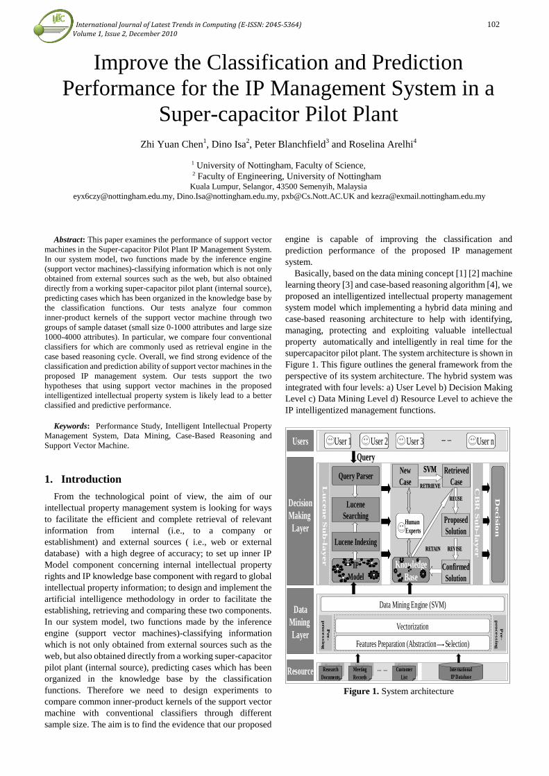
International Journal of Latest Trends in Computing (E-ISSN: 2045-5364) 102 Volume 1, Issue 2, December 2010
Improve the Classification and Prediction
Performance for the IP Management System in a
Super-capacitor Pilot Plant
Zhi Yuan Chen1, Dino Isa
2, Peter Blanchfield
3 and Roselina Arelhi
4
1 University of Nottingham, Faculty of Science, 2 Faculty of Engineering, University of Nottingham
Kuala Lumpur, Selangor, 43500 Semenyih, Malaysia
[email protected], [email protected], [email protected] and [email protected]
Abstract: This paper examines the performance of support vector
machines in the Super-capacitor Pilot Plant IP Management System.
In our system model, two functions made by the inference engine
(support vector machines)-classifying information which is not only
obtained from external sources such as the web, but also obtained
directly from a working super-capacitor pilot plant (internal source),
predicting cases which has been organized in the knowledge base by
the classification functions. Our tests analyze four common
inner-product kernels of the support vector machine through two
groups of sample dataset (small size 0-1000 attributes and large size
1000-4000 attributes). In particular, we compare four conventional
classifiers for which are commonly used as retrieval engine in the
case based reasoning cycle. Overall, we find strong evidence of the
classification and prediction ability of support vector machines in the
proposed IP management system. Our tests support the two
hypotheses that using support vector machines in the proposed
intelligentized intellectual property system is likely lead to a better
classified and predictive performance.
Keywords: Performance Study, Intelligent Intellectual Property
Management System, Data Mining, Case-Based Reasoning and
Support Vector Machine.
1. Introduction
From the technological point of view, the aim of our
intellectual property management system is looking for ways
to facilitate the efficient and complete retrieval of relevant
information from internal (i.e., to a company or
establishment) and external sources ( i.e., web or external
database) with a high degree of accuracy; to set up inner IP
Model component concerning internal intellectual property
rights and IP knowledge base component with regard to global
intellectual property information; to design and implement the
artificial intelligence methodology in order to facilitate the
establishing, retrieving and comparing these two components.
In our system model, two functions made by the inference
engine (support vector machines)-classifying information
which is not only obtained from external sources such as the
web, but also obtained directly from a working super-capacitor
pilot plant (internal source), predicting cases which has been
organized in the knowledge base by the classification
functions. Therefore we need to design experiments to
compare common inner-product kernels of the support vector
machine with conventional classifiers through different
sample size. The aim is to find the evidence that our proposed
engine is capable of improving the classification and
prediction performance of the proposed IP management
system.
Basically, based on the data mining concept [1] [2] machine
learning theory [3] and case-based reasoning algorithm [4], we
proposed an intelligentized intellectual property management
system model which implementing a hybrid data mining and
case-based reasoning architecture to help with identifying,
managing, protecting and exploiting valuable intellectual
property automatically and intelligently in real time for the
supercapacitor pilot plant. The system architecture is shown in
Figure 1. This figure outlines the general framework from the
perspective of its system architecture. The hybrid system was
integrated with four levels: a) User Level b) Decision Making
Level c) Data Mining Level d) Resource Level to achieve the
IP intelligentized management functions.
Decision
Making
Layer
Users
Data
Mining
Layer
Resource
Query
International
IP Database
Research
DocumentsResearch
Documents
… …Meeting
RecordsMeeting
Records
Customer
ListCustomer
List
User 1 User n User 2 … …User 3
Decisio
n
New
Case
Human
Experts
Retrieved
Case
Confirmed
Solution
Proposed
Solution
SVM
RETRIEVE
RETAIN
Knowledge
Base
IP
Model
Lucene Indexing
Lucene
Searching
Query Parser
Lu
cen
e S
ub
-la
yer
CB
R S
ub
-la
yerREVISE
REUSE
Vectorization
Data Mining Engine (SVM)
Features Preparation (Abstraction Selection)
Pre
-
pro
cessin
g
Pre
-
pro
cessin
g
Decision
Making
Layer
Users
Data
Mining
Layer
Resource
Query
International
IP Database
Research
DocumentsResearch
Documents
… …Meeting
RecordsMeeting
Records
Customer
ListCustomer
List
User 1 User n User 2 … …User 3User 1 User n User 2User 2 … …User 3User 3
Decisio
n
New
Case
Human
Experts
Retrieved
Case
Confirmed
Solution
Proposed
Solution
SVM
RETRIEVE
RETAIN
Knowledge
Base
IP
Model
Lucene Indexing
Lucene
Searching
Query Parser
Lu
cen
e S
ub
-la
yer
CB
R S
ub
-la
yerREVISE
REUSE Decisio
n
New
Case
Human
Experts
Retrieved
Case
Confirmed
Solution
Proposed
Solution
SVM
RETRIEVE
RETAIN
Knowledge
Base
Knowledge
Base
IP
Model
Lucene Indexing
Lucene
Searching
Query Parser
IP
Model
IP
Model
Lucene Indexing
Lucene
Searching
Query Parser
Lu
cen
e S
ub
-la
yer
CB
R S
ub
-la
yer
CB
R S
ub
-la
yerREVISE
REUSE
Vectorization
Data Mining Engine (SVM)
Features Preparation (Abstraction Selection)
Pre
-
pro
cessin
g
Pre
-
pro
cessin
g
Figure 1. System architecture

International Journal of Latest Trends in Computing (E-ISSN: 2045-5364) 103 Volume 1, Issue 2, December 2010
2. Theoretical Framework and Hypothesis
2.1 Data Mining Layer
In 1989 G. P. Shapiro [1] defined the standard knowledge
discovery in database (KDD) process to prove data mining
was central to successfully extract knowledge in data. Building
on this, we hypothesized that data mining process will ensure
the establishment of inner IP model and IP knowledge base for
our system.
The original KDD process was modified to fit our
supercapacitor pilot plant by:
Replacing target data preprocessed data and transformed
data with feature and vector, because they are more
accurate and suitable for the data mining engine;
Adding support vector machine to serve as data mining
engine.
The high-level goals of data mining layer tend to be
descriptive, predictive, or a combination of predictive and
descriptive [5]. In our hybrid system, this layer is to achieve
the descriptive goal, focuses on understanding the underlying
data; while the case-based reasoning sub-layer is for the
predictive goal focuses on testing the accuracy in the
descriptive ability which is going to be introduced in the next
section.
2.2 Case-Based Reasoning Sub-layer
The basic premise of machine learning is that data preserving
previous decision experience exist [3]. These
experience-based patterns are called cases which have been
prepared by the data mining layer. Case-based reasoning uses
these patterns to support similar decision. The foundation of
this algorithm is the knowledge base containing a number of
pervious cases for decision-making. Researches [6] have now
proved case-based reasoning approach is extremely effective
for problems in which the rules are inadequate same as our
pilot plant.
The original case-based reasoning cycle has been modified
by:
Loading the retrieve reuse revise retain functions into the
task pool;
Adding method library;
Using SVM to serve as retrieval engine;
Treating user’s query as a new case, computing similarities
between query and cases.
A retrieval engine [7] should retrieve the most similar cases
to the current query (new case) which relies on directly
searching the knowledge base to get the potentially useful
cases. Only when retrieval engine is efficient at handling
thousands of cases the Case-based reasoning will be
applicable for large scale problems. Comparing with the
database searching that specific value in a record, retrieval of
cases from the case-base must be equipped with heuristics that
perform partial matches, because in general there is no existing
case that exactly matches the new case [7].
Well known methods for case retrieval in the case-based
reasoning cycle are [8, 9] from artificial intelligence (AI),
information retrieval (IR), database (DB), and statistics
(STAT). These typical classifiers include the K-Nearest
Neighbors (K-NN), the Naïve Bayes (NB), the Random
Decision Tree (RDT) and the One Rule-based reasoning
(ORBR) [10].
In our method, support vector machines (SVMs) [11] are
implemented here again to serve as retrieval engine in this
sub-layer; theoretically, the training session of SVMs
corresponds to the data mining process which is used for
creating IP models and knowledge base, while the retrieval
function of the case-based reasoning can be looked as the
testing session of SVMs which is used for testing of the
usability of IP models and knowledge base.
2.3 Support Vector Machines
The Support Vector Machine is a universal feed-forward
network, pioneered by Vapnik [11]. The promising
application for this technique is data classification and
retrieval.
From the learning theory perspective, the support vector
machine has the inherent ability to solve the pattern
classification problem in a manner close to the optimum for
the problem of interest [11]. Moreover, it is able to achieve a
remarkable performance with no problem domain knowledge
built into the design of the machine which is more applicable
for the intellectual property management problem in our
supercapacitor pilot plant case.
The support vector machine is built as follows:
In accordance with Cover’s theorem [12] which is a
complex pattern classification problem cast in a high
dimensional space nonlinearly is more likely to be linearly
separable than in a low dimensional space;
Nonlinear mapping of an input vector into a high
dimensional attributes space that is hidden from both the
input and output.
Following the structural risk minimization principle [12],
that is the error rate of a learning machine on test data is
bounded by the sum of the training-error rate and VC
dimension [12];
Construction of an optimal maximum margin hyper plane
for separating attributes discovered in step1 as the decision
surface, producing a value of zero for the first term and
minimizing the second term.
Accordingly, the VC dimension is minimized and good
generalization performance on data classification problems
which arose in the establishment process for the IP model and
global IP knowledge base is achieved. In term of learning
process, this is the training session, during which the support
vector machine is repeatedly presented a set of input vector
along with the category to which each particular pattern
belongs.
Therefore, we expected that,
Hypothesis 1 Using support vector machine to serve as data
mining engine in the proposed intelligentized intellectual
property management system is likely lead to a better
classified performance.
On the other hand, in the case-based reasoning cycle, a new
case is presented to the support vector machine that has not
seen before, but which might belong to the same population of
patterns used to train the support vector machine. The support
vector machine is able to identify the class of that new case
because of the information it has extracted from the training

International Journal of Latest Trends in Computing (E-ISSN: 2045-5364) 104 Volume 1, Issue 2, December 2010
session.
Therefore, we expected that,
Hypothesis 2 Using support vector machine to serve as
case-based reasoning retrieval engine in the proposed
intelligentized intellectual property management system is
likely lead to a better predictive performance.
3. Method
3.1 Experiment Design
Since we have hypothesized the support vector machine which
served as data mining engine and case-based reasoning
retrieval engine will likely get the better performance, to test it
two different series of experiments are considered:
Do the weighting of four common inner-product kernels of
the support vector machine [11]: Poly Kernel, Normalized
Poly Kernel, Puk and Radial Basis Function (RBF) Kernel;
each with two groups of sample dataset, small size sample
and large size sample.
Do the weighting of four conventional classifiers [13] the
K-Nearest Neighbors (K-NN), the Naïve Bayes (NB), the
Decision Tree (DT) and the Rule based reasoning function,
each with the same two groups of sample dataset, small
size sample and large size sample.
The tool used in these experiments is Weka [14], which is a
machine learning algorithms workbench. The overall
performance measures [15] [16] used in our study are: root
means, squared error, root relative squared error, mean
absolute error, relative absolute error, and kappa statistic.
Detailed performance measure: the true positives (TP), the
false positive (FP), precision, recall, F-measure and receiver
operating characteristic (ROC) are choose to test the specified
class (C1).
According to the Sample Size Determination Table in [17],
two groups of sample have been selected in our experiments,
small size sample have attached attribute ranging from 0001 to
1000, and we choose a random start data point at 200 attribute,
and then pick every 200th attribute, thereafter give us our
sample 400 attribute, 600 attribute, 800 attribute; large size
sample have attached attribute ranging from 1000 to 4000, and
we chose a random start data point at 1000 attribute and then
pick every 1000th attribute, thereafter took 2000 attribute,
3000 attribute, 4000 attribute.
Table 1. Experiment results with 200 attribute
Classifiers
200 Attribute
Poly NPoly Puk RBF KNN NB RDT ORBR
Correctly
Classified 0.9565 0.9275 0.7246 0.6572 0.8116 0.5652 0.5072 0.2464
Seconds to build
Model 3.3300 3.4100 6.4200 3.3000 0.0500 0.000 0.1700 0.0500
Root Mean
Squared Error 0.3012 0.3027 0.3239 0.3250 0.3491 0.3525 0.3752 0.4640
Root Relative
Squared Error 0.8606 0.8649 0.9254 0.9287 0.9325 1.0072 1.0720 1.3259
Mean Absolute
Error 0.2047 0.2051 0.2183 0.2208 0.0729 0.1246 0.1408 0.2153
Relative
Absolute Error 0.8357 0.8374 0.8913 0.9018 0.2976 0.5086 0.5749 0.8792
Kappa
Statistic 0.9493 0.9154 0.6780 0.5934 0.7800 0.4924 0.4250 0.1186
Class C3
TP 0.9000 0.9000 0.7000 0.5000 0.8000 0.6000 0.5000 0.4000
FP 0.0170 0.0340 0.0170 0.0000 0.0340 0.1020 0.1020 0.3220
Precision 0.9000 0.8180 0.8750 1.000 0.8000 0.5000 0.4550 0.1740
Recall 0.9000 0.9000 0.7000 0.5000 0.8000 0.6000 0.5000 0.4000
F-measure 0.9000 0.8570 0.7780 0.6670 0.8000 0.5450 0.4760 0.2420
Roc Area 0.9900 0.9780 0.9790 0.9350 0.8980 0.8100 0.6990 0.5390
3.2 ExperimentⅠ
In this series of experiments, we compared the following four
kernel types [11] of the support vector machine:
Poly Kernel
Normalized Poly Kernel
Puk
Radial Basis Function (RBF) Kernel

International Journal of Latest Trends in Computing (E-ISSN: 2045-5364) 105 Volume 1, Issue 2, December 2010
For each of these kernels we implemented the learning
process. Table 1 presents the experiment result for small size
sample at the random start data point (200 attribute), two
groups of measure were applied, one was the overall
performance measurement of the support vector machine and
another was the detailed accuracy performance measurement
by a specified class (i.e., C3). The experiment results for large
size sample at the random start data point (1000 attribute) with
the same measurements in Table 1 was shown in Table 2. As
for other data point 400 attribute 600 attribute 800 attribute
2000 attribute 3000 attribute 4000 attribute, the accuracy
experiment result can be found in Figure 2.
WEKA provides several options for testing the results of the
IP model and knowledge base. In our study we tested them on
the training data by using cross-validation [18] method and
indicated folds to 10, which means the IP model will be tested
ten times by:
Holding out 1/10 of the training data set
Developing a model for the remaining 9/10 of the training
data set
Testing the resulting IP model on the 1/10 withheld.
The data withheld is selected at random from the data not
yet tested, at the conclusion all data will have been used as test
data, so that the testing accuracy in the experiment have been
assured.
As far as other parameters, all followed the
recommendation from the Weka too. For all these kernels the
cache size was set to 250007, the number of kernel evaluations
was 210, support vectors was 20. The parameter of the
support vector machine was set to 1.0. In table 2, the exponent
was denoted to 2.0 for the Normalized Poly Kernel, and it was
1.0 for the Poly kernel. In the Puk kernel and was set to 1.0.
In the Radial Basis Function (RBF) Kernel, was set to 0.01.
This study attempts to understand the competence of
different kernel function within the support vector machine in
determining the performance of classification and prediction.
Table 2. Experiment Results with 1000 attribute
Classifiers
1000 Attribute
Poly NPoly Puk RBF KNN NB RDT ORBR
Correctly
Classified 0.8406 0.6812 0.6232 0.5942 0.4783 0.3623 0.2899 0.2464
Seconds to build
Model 3.4200 2.8800 1.7700 1.7800 0.0000 0.2000 0.7700 0.3000
Root Mean
Squared Error 0.3065 0.3169 0.3317 0.3262 0.3677 0.4268 0.4504 0.4640
Root Relative
Squared Error 0.8758 0.9056 0.9477 0.9322 1.0508 1.2197 1.2871 1.3259
Mean Absolute
Error 0.2074 0.2139 0.2236 0.2212 0.1588 0.1822 0.2029 0.2153
Relative
Absolute Error 0.8470 0.8376 0.9130 0.9034 0.6484 0.7440 0.8285 0.8792
Kappa
statistic 0.8140 0.6276 0.5594 0.5255 0.3907 0.2557 0.1707 0.1186
Class C3
TP 0.7000 0.6000 0.4000 0.6000 0.6000 0.7000 0.6000 0.5000
FP 0.0340 0.0170 0.0170 0.0170 0.0170 0.1860 0.0850 0.4580
Precision 0.7780 0.8570 0.8000 0.8570 0.8570 0.3890 0.5450 0.1560
Recall 0.7000 0.6000 0.4000 0.6000 0.6000 0.7000 0.6000 0.5000
F-measure 0.7370 0.7060 0.5330 0.7060 0.7060 0.5000 0.5710 0.2380
Roc Area 0.9780 0.8720 0.7800 0.8810 0.7590 0.7320 0.7580 0.5210
3.3 ExperimentⅡ
In this series of experiments, Conventional classification
methods [13] in the case-based reasoning cycle tested in our
research included:
K-Nearest Neighbors (K-NN)
Naïve Bayes (NB)
Random Decision Tree (RDT)
One Rule Base Reasoning (ORBR)
We evaluated the different methods on the experimental
dataset which was same in Experiment I. Table 1 and 2 showed
the evaluation experiment result concerning the overall
performance of the four conventional classifiers and also the

International Journal of Latest Trends in Computing (E-ISSN: 2045-5364) 106 Volume 1, Issue 2, December 2010
detailed predictive accuracy performance by a specified class
(i.e., C3) according to the random start data point in different
size of sample.
During the test process, cross-validation method was used
and folds were indicated to 10 same as it was in experimentⅠ
. Other parameters all followed the basic setting provided by
the Weka.
For the K-Nearest Neighbors, the number of neighbors to
use was set to 1. In the Random Decision Tree, the number of
randomly chosen attribute (KValue) was denoted to 1; the
maximum depth of the tree was unlimited; the minimum total
weight of the samples in a leaf was set to 1.0; the random
number seed used for selecting attribute was denoted to 1. As
for the One Rule Based Reasoning method, the minimum
bucket size for discretizing the attribute was chosen to 6.
This study attempts to understand the ability of the typically
used retrieval engine within the case-based reasoning cycle for
determining the performance of classification and prediction.
4. Results and Conclusions
In Figure 2, we showed the overall performance, as measured
by classified-accuracy, of all methods at 8 data point in two
groups of different attribute sample size. We tuned each
method (support vector machines with four different kernels
and convention classifier) to the basic set recommended by the
Weka.
The averaged experiments results over all 200 and 1000
attributes in Table 1 and 2 and Figure 2 show two major
findings:
(1) In the whole class classification task, Poly kernel is the
best learning function for both small and large size sample
classification task. Support vector machines with all kernels
almost outperform all conventional classifiers, except
K-Nearest Neighbors in 200 attribute data point which is
better than Puk and RBF kernels but worse than Poly and
NPoly kernels.
(2) In the specified class (C3) prediction task, RBF kernel
is the best learning function for both small and large attribute
sample size. Although K-Nearest Neighbors also provide best
result for the same task in the large size sample, considering
other measurements (Kappa Statistic and Roc Area), support
vector machines with all kernels outperform conventional
classifiers
These empirical results provided evidence for two
Hypotheses. First, let us consider the overall performance. In
Figure 2, we grouped all these methods by accuracy in order to
find out whether there was difference in performance between
the support vector machine with different kernels and
conventional classifiers. A good classification and prediction
method, we would expect, has about equal better performance
for different attribute sample size by either side. Comparing
accuracy performance for all these methods in our
experiments, shown in Fig. 7, we found that only the support
vector machine with different kernels satisfied this
requirement. Poly kernel achieved the best performance with
95.65% accuracy at 200 attributes data point and 56.52% at
4000 attribute data point; followed by NPoly kernel, with
92.75% at 200 attributes data point and 53.62% at 4000
attributes data point, even the RBF kernel which got the worst
performance in the kernels group reached 43.48% at 4000
attribute data point. While for the best conventional classifiers
K-Nearest Neighbors, although obtained 81.16% accuracy at
200 attribute data point, when the attribute sample size
increased to 4000, its performance accuracy dropped
dramatically to 30.43%
In conclusion, support vector machines with all kernels
outperform the best conventional classifiers K-Nearest
Neighbors (1 time better in total 32 times comparison) by up to
96.88%. In Table 4 and 5, focusing on the root mean squared
error and root relative squared error, the Poly kernel was also
the best function which had lowest value of these two error rate
measure, that is 0.3012 and 0.8606 at 200 attributes data point;
0.3065 and 0.8758 at 1000. While the value of the best
conventional classifiers K-Nearest Neighbors was 0.3491 and
0.9325 at 200; and 0.3677 and 1.0508 at 1000. Since error rate
measurement is negatively-oriented scores: Lower values are
better, Poly kernel was the best function whether in support
vector machines group or in conventional classifiers group. As
for mean absolute error and relative absolute error, things were
slightly different, in experiment Ⅰ indicated that the
differences among all the four kernels were statistically
significant. For the results with Poly kernel, lowest for both of
these two measurements whether at 200 attributes data point or
1000 attributes data point. And in experimentⅡ, for these two
measures the K-Nearest Neighbor got the lowest value and the
differences among all the conventional classifiers were
statically significant too. One question is that these two error
rate measurements in the group of support vector machines
with different kernels were much higher than most of the
conventional classifiers, such as K-Nearest Neighbor, the
Naive Bayes and the Random Decision Tree, which is not
consistent with two Hypotheses. Actually, these two
differences are not statistically significant when comparing
between machine learning methods and traditional
classification methods. The observed experiments results of
correctly classified measurement in Table 4 and 5 provided the
evidence that such two kinds of measurement are not ideal for
our task.

International Journal of Latest Trends in Computing (E-ISSN: 2045-5364) 107 Volume 1, Issue 2, December 2010
0
10
20
30
40
50
60
70
80
90
100
200 400 600 800 1000 2000 3000 4000
Poly
NPoly
Puk
RBF
KNN
NB
RDT
ORBR
Figure 2. Accuracy comparison result
Secondly, in order to see if the accuracy of different
methods for a selected class (C3) is still reliable, detailed
accuracy experiments were performed. Using TP FP Precision
and Recall to calculate F-measure and Roc Area, as expected,
support vector machines with different kernels was observed a
superior accuracy performance whether at 200 or 1000
attribute data point. Experiments result in Table 4 and 5;
showed for a specified class prediction task, support vector
machines with all kernels outperformed the best conventional
classifiers K-Nearest Neighbors (1 time better in total 8 times
comparison) by up to 75 %. The interesting phenomenon was
the RBF kernel, the worst overall kernel performance in the
support vector machine group, had the greatest precision for
predicting the given class C3 for both attribute sample size. In
particular at 200 attributes data point it reached 100%
precision. This saturation was interpreted as additional
evidence for the Hypothesis II. Furthermore, as expected, Poly
kernel achieved the best F-measure and Roc Area that was
0.9000 and 0.9900 at 200 attributes data point; 0.7370 and
0.9780 at 1000 attribute data point. For the K-Nearest
Neighbors, got 0.8000 and 0.8980 at 200 attribute data point,
but after the attribute increased to 1000, we saw a drop to
0.706 and 0.7590. From all these results, it appeared clearly
that nearly all of these kernel approaches achieved the larger
F-measure and Roc Area. More surprisingly was the absolute
superiority in the Roc Area of all kernels at both attribute
sample size. Roughly speaking, the larger the ROC area is, the
better the classified performance. Additionally, Kappa
Statistic, which is a statistical measure of overall inter-class
items, suggests kernel functions are more reliable than
conventional classifiers. Poly kernel got the Kappa Statistic
value of 0.9493 at 200 attribute data point and 0.8140 at 1000
attribute data point; the best conventional classifiers
K-Nearest Neighbors got 0.7800 at 200 attribute data, but
when the attribute sample size reached 1000, the value fell
dramatically to 0.3907.
Overall, the experiment results were encouraging in that
supporting the two hypotheses. The support vector machine
was found to assist in data mining layer and case-based
reasoning sub-layer effectively and reliantly which was
capable of classifying and predicting relevant case for new
input IP case.
5. Acknowledgments
This work was supported by the Ministry of Science,
Technology & Innovation, Malaysia.
[TF0908D098 & TF0106D212].
This work was cooperated with Sahz Holdings Sdn BhD.
References
[1] U. M. Fayyad, G. Piatetsky-Shapiro and P. Smyth, “From
data mining to knowledge discovery: an overview.
Advances in knowledge discovery and data mining”,
American Association for Artificial Intelligence, Menlo
Park, CA, 1996.
[2] J. Han, M. Kamber, “Data Mining: Concepts and
Techniques”, Morgan Kaufmann, academic press, 2001.
[3] T. Mitchell, “Machine Learning”, McGraw-Hill, Boston,
MA, 1997.
[4] A. Aamodt, E. Plaza, “Case-based reasoning:
foundational issues, Methodological variations, and
system approaches”, AI communications, 7(1), pp. 39-59,
1994.
[5] U.Fayyad, G. Piatetsky-Shapiro and P. Smyth, “The KDD
process for extracting useful knowledge from volumes of
data”, Communications of the ACM, Vol. 39(11),
pp.27-34, Nov. 1996.
[6] J. Zeleznikow, “Book review: CASE-BASED
REASONING by Janet Kolodner (Morgan Kaufmann
Publishers, 1993)”, ACM SIGART Bulletin, Vol. 7(3),
pp. 20 - 22, 1996.
[7] I. Watson, F. Marir, “Case-Based Reasoning: A Review.
The Knowledge Engineering Review”, Vol. 9(4), 1994.
[8] H. Li, “Case-based reasoning for intelligent support of
construction negotiation”, Information & Management,
Vol.30, pp. 231-238, 1996.
[9] L. A. Breslow, D. W. Aha, “Simplifying decision trees: A
survey”, The Knowledge Engineering Review, Vol.12
Cambridge University Press, 1997.

International Journal of Latest Trends in Computing (E-ISSN: 2045-5364) 108 Volume 1, Issue 2, December 2010
[10] R.C. Holte, “Very simple classification rules perform well
on most commonly used datasets”, Machine Learning,
Vol.11, pp. 63-91, 1993.
[11] C. Cortes, V. Vapnik. “Support-vector network”,
Machine Learning, pp.273-297, 1995.
[12] C. M. Bishop, “Neural Networks for Pattern
Recognition”, Oxford University Press, Inc., New York,
NY, 1995.
[13] A. Singhal, “Modern Information Retrieval: A Brief
Overview”, Bulletin of the IEEE Computer Society
Technical Committee on Data Engineering, Vol. 24 (4),
pp.35–43, 2004.
[14] I. H. Witten, E. Frank, “Data Mining: Practical machine
learning tools and techniques”, 2nd Edition, Kaufmann,
Morgan, San Francisco, 2005.
[15] E. R. House, “Assumptions underlying evaluation
models”, Assessment & Evaluation in Higher Education,
1469-297X, Vol. 21(4), pp. 347-356, 1996.
[16] M. Y. Kiang, “A comparative assessment of classification
methods”, Decision Support Systems, Vol. 35(4), pp.
441 – 454, 2003.
[17] J. E. Bartlett, J. W. Kotrlik and C. Higgins,
“Organizational research: Determining appropriate
sample size for survey research. Information
Technology”, Learning, and Performance Journal, Vol.
19(1), pp. 43-50, 2001.
[18] B. Efron, R. Tibshirani, “Improvements on
cross-validation: The .632 + Bootstrap Method”, Journal
of the American Statistical Association, 92 (438), pp.
548-560, 1997.
Author Biographies
Chen ZhiYuan HeiLongJiang China, 21-10-1977.
PhD in Computer Science, University of Nottingham
Dino Isa Kuala Lumpur Malaysia. He is a Professor in the Department of
Electrical and Electronics Engineering, University of Nottingham. He
obtained a BSEE (Hons) from the University of Tennessee, USA in 1986 and
a PhD from the University of Nottingham, University Park, Nottingham, UK
in 1991.
Peter Blanchfield Nottingham UK. He is Associate Professor in School of
Computer Science, University of Nottingham. Up to July 2009 he was
Director of the IT Institute in the School, before that he was the Director of
Computer Science and IT Division at the Malaysia Campus of the University
of Nottingham.
Roselina Arelhi Kuala Lumpur Malaysia. She is an Assistant Professor in
School of Electrical and Electronic Engineering, Faculty of Engineering,
University of Nottingham. PhD in Control Engineering, University of
Strathclyde, UK.

International Journal of Latest Trends in Computing (E-ISSN: 2045-5364) 109 Volume 1, Issue 2, December 2010
Watermarking of h.264 Coded Video
Based on the Shifted-Histogram Technique
S. Bouchama1, L.Hamami
2 , M.T.Qadri
3 and M. Ghanbari
3
1Research Center on Scientific and Technical Information of Algiers,
2National Polytechnic School of Algiers, 3School of Computer Science and Electronic Engineering, University of Essex,
[email protected], [email protected]
mtqadr,[email protected]
Abstract: Reversible video watermarking through shifted
histogram of the quantized coefficients of the H.264/AVC coded
video is introduced. In CIF sequences, the embedded data of a
capacity of more than 2500 bits in I frame is possible and can
exceed 7000 bits if we also exploit about 10 P frames in the GOP
for the embedding. While the degradation introduced by the
watermarked can achieve around 13 dB, the subjective impacts are
almost negligible. This data hiding is reversible and it increases the
encoded bits by less than 1 % and less than the embedding capacity
offering the opportunity to carry information at a lower bitrate
rather than a second channel..
Keywords: H264/AVC standard; shifted- histogram technique;
video quality assessment; video watermarking.
1. Introduction
The video is often being manipulated in a compressed format
for storage and transmission. For various applications that
require watermarking techniques such as copyright protection
or authentication control, researchers are nowadays moving
to the video compressed field and especially towards the
latest video codec H264/AVC.
The H264/AVC is today widely adopted and related
products and implementations are increasingly appearing. It
has demonstrated a high coding efficiency comparing to the
previous standards and it becomes then essential to consider
the security aspects of this codec. An overview of this
standard can be found in reference [1].
Several watermarking techniques were proposed for the
H264/AVC video standard, where the embedding is usually
performed in I frames, since P and B are highly compressed,
and the quantized DCT coefficients are chosen for the
insertion because the quantization is a lossy operation, and
the signature could be lost if embedded before this step.
Though, in most of the proposed methods, even if the video
quality and the bitrate are maintained, the embedding
capacity is often limited and this can be a real obstacle for
some applications.
Indeed, in embedding watermark into a compressed video
various watermark requirements such as the embedding
capacity and the video quality should be taken into
consideration, and for this video standard, increasing the
embedding capacity constitute a real challenge rarely
addressed in literature. To reach the compromise between
video quality and data embedding capacity, the reversible
video watermarking schemes seem to be a logical solution for
a higher capacity embedding and for recovering the encoded
video at the detection step. In this paper we apply a
reversible watermarking method based on the shifted-
histogram technique to the luma quantized DCT coefficients
of the H264/AVC video standard. We evaluate the
embedding capacity and the increase in bitrate. The video
quality is also assessed before applying any video restoration.
Results show that despite heavy degradation on objective
video quality of watermarked images, the subjective quality
is almost not disturbed by this method.
This paper is organized as follows: in section 2 a
presentation of the related work is exposed, in section 3 we
describe the application of the shifted histogram technique to
the H264/AVC codec and we explain the video quality
assessment that has been performed. Results and analysis are
exposed in section 4. Three points are essentially discussed:
The embedding capacity, the video quality and the increase
in bitrate. Finally, we draw conclusions in section 5.
2. Related work
The use of DCT coefficient for embedding the watermark is
very common in both compressed image (such as JPEG) and
video, this is because compression does not leave much
choice as a watermark location. For the H264/AVC video
codec, the quantization DCT coefficients and the motion
vectors are the most used to insert the signature. Coefficients
of low, middle or high frequencies may be selected to embed
the watermark and respond to the needs of the application in
terms of robustness or fragility. For the embedding process,
the choice of the DCT blocks and the DCT coefficients
usually relies on the human visual properties to mask the
degradation introduced by the watermark. Among these
methods, Chen et al. [2] present a video watermarking
method based on blocks energy. Two algorithms were
proposed for low and high energy blocks of Intra frame, the
objective is to consider the high frequency noise attack and
the low-pass filter attack. The security of the watermark is
ensured by an encryption using a Torus Automorphisms
algorithm and the Secret Image Sharing technology to
increase robustness. In another example, Noorkami et al. [3]
proposed a low comlplexity watermarking method where the
watermark is embedded in the AC coefficients of I frames. In
order to preserve the video quality, only one coefficient per
macroblock is selected to embed the watermark. The
security of the algorithm is based on the randomness of the
watermark location which is determined by a public key
extracted from the feature of the macroblock such as the DC
coefficient. A general scheme of the watermarking process
based on DCT coefficients is represented in figure 1.

International Journal of Latest Trends in Computing (E-ISSN: 2045-5364) 110 Volume 1, Issue 2, December 2010
Our method is based on the shifted histogram data hiding
technique applied to the quantized DCT coefficients. It was
initially proposed by Ni et al. [4] for still images and
improved later by other authors [5]. The method consists of
selecting the peak/ zero pairs from the image histogram and
apply a shift between pixels’ levels (p,z) of the maximum and
the minimum frequencies, so that a gap is created in p. The
aim is to maximize the embedding capacity by inserting the
watermark in the largest frequency.
The image is scanned after applying the shift, and the
watermark bits are hidden as follows:
For L as the pixel level and w as a watermark bit,
1st case: p > z and L=(p-1)
If (w= 1) then L=L+1=p, otherwise,
L= (p-1) (not modified)
2nd
case: p < z and L =(p+1)
If (w= 1) then L=L - 1=p, otherwise,
L=(p+1)(not modified)
The data hiding is reversible and detection is done by
rescanning the image. If the value of L is equal to p the
watermark bit is “1”, and if L is equal to p-1 (for the first
case) or p+1 (for the second case) the watermark bit is “0”.
Several ranges of pairs of peak/zero values could be
chosen from the histogram in order to increase the
embedding capacity. The values (p,z) need to be identified
as side information for a reversible data hiding and need to
be transmitted to the receiving side. If the minimum
frequency is not equal to zero, the related pixel positions
need also to be transmitted as side information [5].
3. Description of the method
3.1 Watermark Insertion/extraction
We have applied the shifted histogram technique to the
quantized luma DCT coefficients of I and P frames of the
H264 /AVC video sequences. The histogram of the
significant DCT coefficients shows almost symmetric
positive and negative sides. The following steps describe
how to apply the method to the positive side of the
histogram:
Find a pair of maxima and minima (p,z) in the
positive significant levels and shift the values within
the range [p, z-1] to the right (toward the minimum
frequency) by incrementing the values by 1.
If the Watermark bit is equal to “1”, reduce (p+1) by
1 otherwise the coefficient is not modified.
To apply the method in both positive and negative sides,
the previous steps are repeated in the negative side of the
histogram by shifting the levels within the range [z’+1, p’] to
the left. (p’,z’) is the pair of maxima and minima values in
the negative side of the histogram. In our case we have
applied the embedding to both sides in order to maximize the
embedding capacity.
The watermark detection step is done during the video
decoding, after the entropy decoding stage. If the value of the
level is equal to p or p’, it means that the watermark bit is
“1”, and if the value of the level is (p-1) or (p’+1), the
watermark is equal to “0” as mentioned previously.
3.2 Video quality assessment
In order to assess the video quality after embedding the
watermark, the objective quality is measured by the PSNR of
the sequences. For subjective assessment, we have used a
quality meter based on blockiness and blurriness
detectors [6]. In this meter, FFT within a window of 32×32
pixels of the gradients of reference and processed images are
taken. The added energy to the phase of the harmonics over
the reference image is an indication of blockiness and the
loss of energy in the amplitude of the harmonics would be
that of blurriness [7]. Therefore by measuring the picture
blockiness and blurriness one can gauge the video quality.
Measurement results are normalized in the range 0 to 100 %.
Scores higher than 60 % would be interpreted as a Good
subjective quality in terms of blockiness or blurriness effects.
4. Results and analysis
In our experiments, the first 50 frames of the four CIF video
clips: Walk, Coast Guard, Silent and Foreman (with Siemens
logo) were coded at the quantizer parameter (Qp=28), at a
frame rate of 30 pictures/s generating almost between 253 to
1139 kbits/ second. With the base-line profile, only the first
frame was intra coded and the remaining frames were coded
as P.
We suppose that the watermark was previously encrypted
to ensure its security. For tests we used a pseudo random
binary sequence which was inserted first in the I-frame then
in the first 10 P frames and finally the embedding is applied
in both I and P frames. The objective is to estimate the
embedding capacity for CIF sequences and to evaluate the
Bitstream
Input
signal (Macroblock)
Prediction
(Intra/inter)
Transf.
(Integer DCT)
and Quant.
Watermark
pre-
processing
(encryption,
etc…)
Watermark
The 4x4
Quantized
DCT coefficients
Entropy
coding
Figure 1. General scheme of watermarking of H264/AVC based
on DCT coefficients

International Journal of Latest Trends in Computing (E-ISSN: 2045-5364) 111 Volume 1, Issue 2, December 2010
impact of the watermark insertion on the video quality and
the increase of the bitrate.
In a first step of our work, the embedding was done in
coefficients +1 and – 1 because they offer the maximum
embedding capacity as shown in the histogram of the
quantized DCT coefficients of Walk sequence represented on
figure 2. However, that introduces visible artifacts and a
relatively high increase in bitrate. This is due to the fact that,
in H.264 Levels ±1 play a crucial role in the encoding chain.
Coefficients 2 have instead been chosen to embed the
signature because they seem to offer the best compromise
between the embedding capacity, the increase in bitrate and
the video quality.
The embedding was performed using both of the modes
intra 16x16 and intra 4x4. Though, to improve the video
quality for the sequences Silent and Foreman, tests have been
redone, after experiments, by discarding the Intra 16x16
mode because of the distortion it may cause. Indeed, the
number of the watermarked coefficients of a block depends
on the picture content ; in some blocks many coefficients
might be affected. Thus there is more chance that the
distortion appears in intra 16x16 mode which is applied for
homogeneous areas.
In the following points we will present results obtained for
the embedding capacity, video quality and increase in bitrate.
We will discuss the impact of the embedded signature on
these two last parameters for the three following cases:
Embedding the watermark in I frames, in P frames and in
both of them.
4.1 Embedding capacity and Video quality
The embedding capacity depends on the picture content. In I
frame, it varies between 1123 and 2925 bits corresponding to
the CIF size sequences of Foreman and Coast Guard
respectively.
Figures 3, 4 and 5 show the four unwatermarked I frames
and the correspondent watermarked frames. An example of
frame restoration is given in figure 3 (c) and an example of
watermarked P frame is given in figure 5 (c).
For the case of embedding the signature in I frame, the
objective video quality, for all pictures, the inserted frame
and the remaining ones, drops by almost between 12 to
13.5 dB (figure 6). These values along with the data hiding
capacity and the increase in bitrate are tabulated in Tables 1,
2, 3 and 4.
Figure 2. Histogram of the significant quantized DCT
coefficients of I frame of Walk sequence.
Figure 3 : (a) I frame of the unwatermarked Coast Guard
sequence, (b) is the corresponding watermarked frame, (c)
is the restored frame .
(a) (b)
(c)

International Journal of Latest Trends in Computing (E-ISSN: 2045-5364) 112 Volume 1, Issue 2, December 2010
Tables 1, 2, 3, and 4 also show the impact of the
watermark on the subjective quality of the video, at various
frames, (frame 1, F1 to frame 30, F30). The watermark is
being embedded in the first frame, we are looking at the
quality of I frame, the first P frame and three other P frames.
Although the objective quality is deteriorated but subjective
quality is maintained. The highest degradation is measured
for Coast guard sequence which presents a blockiness of 72
% due to the high embedding capacity it offers (higher than
the embedding capacity of Foreman I frame more than 2.5
times) but still visually may be acceptable as shown in
figure 3 (b). The impact of this I watermark embedding on
the rest of the frames is negligible in terms of blockiness or
blurriness.
This can be explained by the fact that in shifted histogram
technique the shift is generally applied to a relatively high
number of coefficients. The effect of this shift is transmitted
with the Inter prediction to P frames which reduces the PSNR
for the whole sequence even if the watermark has not been
embedded. Subjectively we can notice slight changes in the
brightness of the frames (figure 4), but any possible
degradation caused by the watermark embedding remains
masked in the image texture.
For the case of embedding the watermark in P frames, instead
of embedding the signature in one frame, it is spread over
several frames since the embedding capacity in each P frame
is very low comparing to I frame. Tables 1,2, 3 and 4 show
that the embedding capacity for the four sequences varies
between 168 and 5403 bits/10 P frames. The highest
measured of this rate is observed for Walk and Coast Guard
sequences which also present the highest encoding rates
(1111.15 and 1139 kbits/ second respectively). The reduction
in PSNR is relatively low, it varies - in accordance with the
embedding capacity- between 0.02 and 1.28 dB
corresponding to the sequences Silent and Walk respectively.
Regarding the subjective quality, it is perfectly preserved, the
highest degradation is shown for Walk sequence which
presents a negligible blockiness of 95%, if we don’t consider
the blockiness effect already existing in the unwatermarked
sequences. In addition to that, in our test the watermark
embedding was done only in 10 P frames, the rest of the P
frames of the GOP can also be exploited to hide more
information without disturbing the video quality.

International Journal of Latest Trends in Computing (E-ISSN: 2045-5364) 113 Volume 1, Issue 2, December 2010
Table 1. The embedding capacity, the increase in bitrate
and the video quality of Walk sequence
Video seq. Embed.
capacity (bits / fra.)
Incre.
bitrate (%)
Red.
PSNR
(dB)
Blockiness % Blurriness %
F1 F2 F10 F20 F30 F1 F2 F10 F20 F30
Unwatermarked
Walk seq. - - - 92 100 100 100 100 100 100 98 100 99
Walk seq.
Watermark in I 1975 0.17 12.47 85 95 100 100 100 100 100 98 97 96
Walk seq.
Watermark in 10
P
5403 0.42 1.28 92 95 98 99 100 100 100 100 100 100
Walk seq.
Watermark in I
& 10 P
7378 0.59 12.38 85 93 99 100 100 100 100 100 100 99
Video seq. Embed.
capacity (bits / fra.)
Incre.
bitrate
(%)
Red.
PSNR
(dB)
Blockiness % Blurriness %
F1 F2 F10 F20 F30 F1 F2 F10 F20 F30
Unwatermarked
Coast Guard
seq.
- - - 100 100 100 100 98 96 98 99 95 98
CG seq.
Watermark in I 2925 0.19 12.04 72 78 86 90 88 100 100 100 100 100
CG seq.
Watermark in 10
P
4327 0.21 0.81 100 100 100 100 98 98 100 100 98 99
CG seq.
Watermark in I
& 10 P
7252 0.41 12 72 85 83 87 86 100 100 100 100 100
Table 2. The embedding capacity, the increase in bitrate
and the video quality of Coast Guard sequence
Video seq. Embed.
capacity (bits / fra.)
Incre.
bitrate
(%)
Red.
PSNR
(dB)
Blockiness % Blurriness %
F1 F2 F10 F20 F30 F1 F2 F10 F20 F30
Unwatermarked
Silent seq. - - - 96 95 100 96 100 99 100 99 98 98
Silent seq.
Watermark in I 1791 0.56 13.5 89 90 93 91 94 100 100 98 97 97
Silent seq.
Watermark in 10
P
168 0.04 0.02 96 95 99 96 100 99 100 99 98 98
Silent seq.
Watermark in I
& 10 P
1959 0.60 13.5 89 90 92 93 97 99 100 98 97 96
Table 3. The embedding capacity, the increase in bitrate
and the video quality of Silent sequence
Video seq. Embed.
capacity (bits / fra.)
Incre.
bitrate
(%)
Red.
PSNR
(dB)
Blockiness % Blurriness %
F1 F2 F10 F20 F30 F1 F2 F10 F20 F30
Unwatermarked
Foreman seq. - - - 89 92 100 100 100 100 100 100 100 99
Foreman seq.
Watermark in I 1123 0.23 12.3 91 95 100 100 100 97 97 97 97 95
Foreman seq.
Watermark in 10
P
839 0.19 0.41 89 92 100 100 100 100 100 100 100 99
Foreman seq.
Watermark in I
& 10 P
1962 0.43 12.25 91 95 100 100 100 97 97 97 97 95
Table 4. The embedding capacity, the increase in bitrate
and the video quality Foreman sequence

International Journal of Latest Trends in Computing (E-ISSN: 2045-5364) 114 Volume 1, Issue 2, December 2010
Concerning the embedding performed in I and P frames, in
terms of video quality results are close to those obtained for I
frame embedding. Moreover, we can notice that, picture
blurriness is preserved or even improved for Walk and Coast
guard sequences. This is expected as the inserted data may
act as dither in the image, creating artificial details to reduce
picture blurriness for especially almost regular areas, which
explain the fact that this is not observed when the signature is
only embedded using the Inta 4x4 mode as presented in
Table 3 and 4.
The embedding Capacity is obviously much more
interesting since it is the addition of the two previous cases.
4.2 Increase in bitrate
Tables 1, 2,3 and 4 show that , the lowest and highest rates of
the increase in bitrate are observed for Silent sequence.
0.04 % is the lowest rate corresponding to embedding the
signature in P frames, and 0.6 % is the highest rate
corresponding to embedding the signature in both I and P
frames. However, to have a better idea on what represents
that increase comparing to the embedding capacity, we
calculated the rate between the embedding capacity and the
increase in bitrate and we have noticed that for all the cases
the embedding capacity is higher than the increase in bitrate
introduced by the watermark insertion, the worse case in
observed when the watermark is embedded in I for Walk
sequence for which the bitrate increases by 1904.64 bits
/second for an embedding capacity of 1975 bits and the best
case when the watermark is embedded in P frames for Coast
Guard sequent for which the bitrate increases by 2990.08
bits /second for an embedding capacity of 4327 bits. This is
interesting insofar that rather than a second channel, data can
be embedded and sent at lower bitrate.
Finally, the choice of I frame, P frames or both of them for
the signature embedding depends on the application needs.
Of course in case of the brightness modification introduced
by the watermarking process is localized in only some areas
of the watermarked frame, that may be noticeable as
presented in figure 5 (b), it is thus preferable to choose only
P frames to embed the signature and preserve the same video
quality (figure 5 (c)). Though, in general, according to the
tolerated increase in the bitrate and to the amount of
information we need to carry in the video it is possible to
choose between P frames that preserve the best the video
quality, or in I frame because of its importance in the
encoded sequence or in both of them so that the embedding
capacity is maximized.
5. Conclusion
The shifted-histogram based method can be applied to the
H264/AVC video standard. Indeed, despite the large
differences between the objective quality (PSNR) of the
watermarked and non-watermarked video sequences, their
subjective quality differences are almost negligible.
For the four test video sequences, we noticed that the
increase in bitrate varied according to the embedding frames
type and number, but it didn’t exceed the embedding
capacity. This represents an advantage to carry information
in the video sequence instead of a second channel.
Finally, According to the pictures content, the embedding
capacity can reach interesting rates in I and P frames which
can used separately or together according to the application
demands in terms of embedding capacity, video quality and
increase in bitrate.
References
[1] T.Weigand , G.Sullivan, G.Bjontegaard and A.Luthra,
“Overview of the H.264/AVC video coding standard, ”
IEEE Trans. on Circuits and System for Video
Technology, Vol.13, No.7, pp. 560-576, 2003.
[2] W-M. Chen, C-J. Lai and C-C. Chang, “H.264 Video
Watermarking With Secret Image Sharing, ” IEEE
International Symposium on Broadband Multimedia
Systems and Broadcasting (BMSB '09), Bilbao, Spain,
2009.
[3] M. Noorkami and R.M.Mersereau, “Compressed
domain video watermarking for H264,” IEEE Int. Conf.
Image Processing, Genoa, Italy, 2005.
[4] Z. Ni, Y.Q. Shi, N. Ansari, and W. Su, “Reversible data
hiding, ” IEEE Transactions on Circuits and Systems for
Video Technology, Vol.16, No.3 , pp.354-362, 2006.
[5] M.Fallahpour, D.Megias, M. Ghanbari, “High
capacity, reversible data hiding in medical images,”
IEEE Int. Conf. on Image Processing (ICIP 2009),
Cairo, Nov. 2009 (to be published in IET Image
Processing, 2010).
[6] K.T.Tan, and M.Ghanbari, “Blockiness detection for
MPEG2-coded video,” IEEE Signal Processing Letters,
Vol.7, No.8, pp. 213-215, 2000.
[7] I.P.Gunawan, and M.Ghanbari, “Reduced-reference
video quality assessment using discriminative local
harmonic strength with motion,” IEEE Trans. on Circuits
and Systems for Video Technology, IEEE-CSVT,
Vol.18, No.1, pp. 71-73, 2008.
Author Biographies
Samira Bouchama has received the Electrical engineering degree from the
National Polytechnic School (ENP) of Algiers (Algeria). She achieved the
Master’s degree from the same school (Signal and Communications
Laboratory) in 2007. She is now working at the Research Center on
Scientific and Technical Information (CERIST) of Algiers and pursuing as a
doctoral student at ENP in the field of image and video watermarking.
Latifa Hamami is a Professor in the Electronic Department, in the National
Polytechnic School of Algiers (ENP) and head of Laboratory “Signal and
Communications”. She is the author of more than 100 publications in the
domain of image processing and particularly in medical imaging field. She
has been involved in the organization of several Conferences and
participated as a session chairperson. She is reviewer in national and
international Conferences and Journals.
Mohammed Tahir QADRI received the B.S. degree in Electronic
Engineering from Sir Syed University of Engineering and Technology,
Karachi, Pakistan in 2003, and MSc. degree in Advance Photonics and
Communication from University of Warwick, UK , in 2007. He is currently
doing PhD. from University of Essex, UK in Video Quality Measurement.
He is also teaching as Assistant Professor in Sir Syed University, Karachi
and currenlty on study leave in UK for his PhD. He has written a book on
Digital Signal Processing for engineering students and the book is being
used as reference book in Sir Syed University, Karachi. He has published 11
research papers in the field of image processing, telecommunication and

International Journal of Latest Trends in Computing (E-ISSN: 2045-5364) 115 Volume 1, Issue 2, December 2010
digital control systems. He is also registered as Professional Engineer from
Pakistan Engineering Council.
Mohammed Ghanbari is a Professor of video Networking in the
department of Computing and Electronic Systems, University of Essex,
United Kigdom. He is best known for the pioneering work on two layer
video coding of ATM networks, now is known as SNR scalability in the
standard video codecs, which earned him the Fellowship of IEEE in 2001.
He has registred for eleven international patents and published more than
400 technical papers on various aspects of video networking. He was the
corecipient of A.H. Reeves prize for the best paper published in the 1995
proceeding of IEE in the theme of digital coding. He was also a
coinvestigator of the European MOSAIC project studying the subjective
assessment of picture quality, which resulted to ITU-R
recommendation 500.
He is the co-author of Principles of Performance Engineering, book
published by IEE press in 1997, and the author of video coding: an
Introduction of standard codecs, book also published by IEE press in 1999,
which received the Rayleigh prize as the best book of year 2000 by IEE. His
latest book Standard Codecs: image compression to advanced video coding,
was published by IEE 2003. He has been an organizing member of several
international conferences and workshops. He was the general chair of 1997
international workshop on Packet Video and Guest Editor to 1997 IEEE
transactions on circuits and systems for video Technology, Special issue on
Multimedia technology and applications. He has served as Associate Editor
to IEEE transactions on Multimedia and represented University of Essex as
one of the six UK academic partners in the Virtual Centre of Excellence in
Digital Broadcasting and Multimedia. He is a Fellow of IEEE, Fellow of
IET and Charted Engineer (CEng).

International Journal of Latest Trends in Computing (E-ISSN: 2045-5364) 116 Volume 1, Issue 2, December 2010
Suppression of Random Valued Impulsive Noise
using Adaptive Threshold Gunamani Jena
1 and R Baliarsingh
2
1Professor and Head CSE Department 1BVC Engineering College, JNTUK,AP, INDIA
2National Institute of Technology, Rourkela, Orissa, India,
[email protected], [email protected]
Abstract: In the proposed schemes adaptive threshold selection
is emphasized for RVIN model. Incorporation of adaptive threshold
into the noise detection process led to more reliable and more
efficient detection of noise. Based on the noisy image
characteristics and their statistics, threshold values are selected.
Extensive simulations and comparisons are done with competent
schemes. It is observed that the proposed scheme is better in
suppressing impulsive noise at different noise ratios than their
counterparts
Keywords: RVIN: Random Valued Impulse Noise, SPN: Salt
and Pepper Noise, PSNR: Peak Signal to Noise Ratio, PSP:
Percentage of Spoiled Pixels.
1. Introduction
Noise Suppression from images is one of the most
important concerns in digital image processing. Impulsive
noise is one such noise, which may corrupt images during
their acquisition, transmission and storage etc. A variety of
techniques are reported to remove this type of noise. It is
observed that techniques which follow the two stage process
of detection of noise and filtering of noisy pixels achieve
better performance than others. In this paper such schemes of
impulsive noise detection and filtering thereof are proposed.
The models of impulsive noise considered in this paper are:
The first one is Salt & Pepper Noise (SPN) model, where
the noise value may be either the minimum or maximum of
the dynamic gray scale range of the image.
The second one is Random Valued Impulsive Noise (RVIN)
model, where the noise pixel value is bounded by the range
of the dynamic gray scale of the image.
The schemes used are:
The first scheme is based on second order difference of
pixels in order to identify noisy pixels. The second scheme
for SPN model uses fuzzy technique to locate contaminated
pixels. The contaminated pixels are then subjected to median filtering. This detection–filtration is done recursively so that
filtered pixels take part in the detection of noise in the next
pixel.
Fig1. Noise Removal Process
1.1 Filtering Techniques
Adaptive filtering has taken advantage of nonlinear
filtering techniques. Non-adaptive nonlinear filters are
usually optimized for a specific type of noise and signal.
Adaptive filters become the natural choice and their
performance depends on the accuracy of estimation of certain
signal and noise statistics
1.1.1 Filtering without Detection
In this type of filtering a window mask is moved across the
observed image. The mask is usually of size (2N+1)2, where
N is a positive integer. Generally the center element is the
pixel of interest. When the mask is moved starting from the
left-top corner of the image to the right-bottom corner, it
performs some arithmetical operations without discriminating
any pixel.
1.1.2 Detection followed by Filtering
This type of filtering involves two steps. In first step it
identifies noisy pixels and in second step it filters those
pixels. Here also a mask is moved across the image and some
arithmetical operations is carried out to detect the noisy
pixels. Then filtering operation is performed only on those
pixels which are found to be noisy in the previous step,
keeping the non-noisy intact.
1.1.3 Hybrid Filtering
In such filtering schemes, two or more filters are suggested
to filter a corrupted location. The decision to apply a
particular filter is based on the noise level at the test pixel
location or performance of the filter on a filtering mask.
1.2 Impulsive Noise
Different types of noise frequently contaminate images.
Impulsive noise is one such noise, which may affect images
at the time of acquisition due to noisy sensors or at the time
of transmission due to channel errors or in storage media due
to faulty hardware. Two types of impulsive noise models are
described below. Let Yi,j be the gray level of an original
image Y at pixel location (i, j) and [nmin, nmax] be the dynamic
range of Y. Let Xi,j be the gray level of the noisy image X at
pixel (i, j) location. Impulsive Noise may then be defined as:
(1)

International Journal of Latest Trends in Computing (E-ISSN: 2045-5364) 117 Volume 1, Issue 2, December 2010
where, Ri,j is the substitute for the original gray scale value
at the pixel location (i, j). When Ri,j ∈ [nmin, nmax], the image
is said to be corrupted with Random Valued Impulsive Noise
(RVIN) and when Ri,j ∈ nmin, nmax, it known as Fixed
Valued Impulsive Noise or Salt & Pepper Noise (SPN).
Pixels replaced with RVIN and their surroundings exhibit
very similar behavior. These pixels differ less in intensity,
making identification of noise in RVIN case far more
difficult than in SPN. The difference between SPN and RVIN
may be best described by Figure 2.
Fig.2. Representation of (a) Salt & Pepper Noise with Ri,j
∈nmin, nmax,
(b) Random Valued Impulsive Noise with Ri,j ∈ [nmin, nmax]
In the case of SPN the pixel substitute in the form of noise
may be either nmin(0) or nmax(255). Where as in RVIN
situation it may range from nmin to nmax.
The metrics used for performance comparison of different
filters (exists and proposed) are defined below.
a. Peak Signal to Noise Ratio (PSNR)
PSNR analysis uses a standard mathematical model to
measure an objective difference between two images. It
estimates the quality of a reconstructed image with respect to
an original image. The basic idea is to compute a single
number that reflects the quality of the reconstructed image.
Reconstructed images with higher PSNR are judged better.
Given an original image Y of size (M×N) pixels and a
reconstructed image ˆ Y , the PSNR(dB) is defined as:
(2)
b. Percentage of Spoiled Pixels (PSP)
PSP is a measure of percentage of non-noisy pixels changes
their gray scale values in the reconstructed image. In other
words it measures the efficiency of noise detectors. Hence,
lower the PSP value better is the detection, in turn better is
the filter performance
(3)
2. EFFICIENT IMPULSIVE NOISE REMOVAL SCHEMES
2.1 Decision Directed Median Filter (DDMF)
Usually the pixels located in the neighborhood of a test
pixel are correlated to each other and they possess almost
similar characteristics. Most of the reported impulse
detection schemes exploit this feature of pixels. The scheme
proposed here is one such novel technique of impulsive noise
detection-suppression strategy from corrupted images. This
scheme is simple but efficient and works alternatively in two
phases: detection of noisy pixels followed by median filtering
[2].
2.1.1 Methodology
In a practical situation, since the probability p (1.5) is less
than 1, all the pixels of a digital image are not corrupted with
the impulsive noise. In addition, when the probability of
corruption is not cent percent, it is expected that the noisy
pixel be surrounded by at least some healthy pixels.
However, this assumption is not true as the noise density
becomes very high. In any case, the total number of
corrupted pixels is less than the total number of pixels in the
image. Hence, it is not required to perform filtering operation
on every pixel for eliminating the impulsive noise. Rather, it
is computationally economical to filter only the corrupted
pixels leaving the healthy pixels unchanged. This approach
reduces the blurring effect in the restored image, as the
magnitude of healthy pixels is not affected by filtering.
Basically, the noise removal method proposed in this paper
constitutes two tasks: identification of corrupted pixels and
filtering operation on those corrupted pixels. Thus the
effectiveness of this scheme lies on the accuracy and
robustness of detection of noisy pixels and efficiency of the
filtering methodology employed. Many researchers have
suggested [5][6][7] various methods for locating the distorted
pixels as well as filtering techniques. Each of these methods
has different shortcomings and hence fails to reproduce
images very close to original ones. These are over-filtering
distortion, blurring effect or high computational involvement.
In addition, as the density of the impulsive noise is gradually
increased, the quality of the image recovered by the existing
methods correspondingly degrades. The scheme proposed
here, is an improved impulsive noise detection scheme
followed by recursive median filtering to overcome many of
the shortcomings observed in the existing methods. To
achieve this objective, it is necessary to devise an effective
impulse detection scheme prior to filtering operation. The
proposed scheme employs a second order difference based
impulse detection mechanism at the location of a test pixel.
The mathematical formulation of the proposed method is
presented in (2).
(4)
where, di,j is the decision index that controls the filtering
operation and estimates the filtered output ˆ Yi,j from the
observed image Xi,j and filtered pixel value Zi,j. If the
impulse detector determines that the center pixel of test
window is noisy, then di,j = 0, otherwise di,j = 1. When di,j =
0, the corrupted pixel undergoes median filtering. On the
other hand di,j = 1, the window is skipped and the process is
repeated. Unlike in conventional methods, the filtering
operation is performed selectively based on the decision of
the impulse detector. Hence the proposed method is named
as Decision Directed Median Filter (DDMF). The schematic
diagram of the proposed filtering scheme is shown in Fig.3.

International Journal of Latest Trends in Computing (E-ISSN: 2045-5364) 118 Volume 1, Issue 2, December 2010
Figure 3: Schematic Diagram of the Decision Directed Median Filter
2.2 Recursive Median Filtering Algorithm
Based on the algorithm corrupted pixels are identified
across the image. Then the filtering operation is carried out
only on those distorted pixels. The recursive filtering
operation computes the median value of a 3×3 window X(w)
surrounding the corrupted center pixel and substitutes this
value at the location of the faulty pixel unlike the
conventional median filter. In the next adjacent window, the
healthiness of its center pixel is tested considering the gray
level of the already filtered pixel rather than that of the
original one. Mathematically,
(5)
3. Fuzzy Impulsive Noise Detection
In this section, a fuzzy based filtering scheme namely
Fuzzy Impulsive Noise Detection (FIND) is proposed. It
employs a fuzzy detection scheme to identify pixels
corrupted with impulsive noise and subsequently filter the
noisy pixels using recursive median filter. The detector is
responsible for ascertaining the healthiness of a pixel in a test
window by utilizing the gray level information in its
neighborhood. The median filtering is applied to corrupted
locations only leaving the non-corrupted ones intact. Such
selective filtering operation prevents from edge jittering and
blurring of images
3.1 Methodology
The proposed filtering scheme is a selective one and
consists of two stages: decision making regarding the
presence of impulsive noise (salt & pepper) at a test pixel
location and median filtering only of corrupted pixels. Hence,
detection operation is carried out at all locations but filtering
is performed only at selected locations. From the corrupted
image a 3 × 3 window is selected and a fuzzy detection is
employed to derive a decision regarding the presence of
impulse at the center pixel. Accordingly, the center pixel is
replaced with the median value of the pixels in its
neighborhood prior to the selection of the next window. The
overall block diagram of the combined filter structure is
depicted in Figure 4.
3.2 The FIND Algorithm
The impulse detection for the proposed filter is based on
the fuzzy inference logic. In any fuzzy application, the
challenge lies in Fuzzification and defuzzification process
[11]. In our case, we use a triangular fuzzy membership
function that utilizes only two linguistic variables. In the
following, the proposed FIND algorithm is outlined stepwise.
i. Select the first test window of size 3 × 3 from the
corrupted image X
ii. Convolve Xw with the two kernels to obtained ∆1 and
∆2
iii. Apply Mamdani fuzzy model for two-input one-output
iv. Compute the strength of each linguistic variable using
triangular fuzzy membership functions
v. Evaluate the fuzzy rules using Zadeh logic for AND
implication.
vi. Construct the consequent membership function as
shown in Figure 2.5 from nine active rules for a
system with two inputs and one output.
vii. Obtain a crisp value (M) from the fuzzy set
(Defuzzification) by using center of-gravity method
and apply to a decision process
viii. Invoke the median filtering on Xi,j using Xw,if di,j = 0
else go to step (viii).
ix. Shift the test window column wise and then row wise to
cover the entire image pixels.
x. Repeat steps (ii) through (ix) for all windows.

International Journal of Latest Trends in Computing (E-ISSN: 2045-5364) 119 Volume 1, Issue 2, December 2010
Figure 4: Block Diagram of the Proposed Filter
Table1.
4. Simulations and Results The proposed schemes in this paper are simulated
and their performance is compared with some of the recently
reported schemes. Median (MED(3×3)) and (MED(5×5))
[2], Switching-Median (SM(5×5)) [3], Weighted Median
(WM(k =1)) and (WM(k = 2)) [8], Peak and Valley (P n V)
[9], TMED and ATMED [4] [10] are the compared schemes.
Lena image is corrupted with Salt & Pepper Noise with
density ranging from 1% to 30%. These images are then
subjected to filtering by the proposed schemes along with the
above listed schemes. The PSNR (dB) and PSP thus obtained
are plotted in Figures 5 and 6.
Figure 5 The PSNR (dB)
Figure 6 The PSP
Figure 7(a) is the true image of Lena and Figure 7(b) is the
noisy version (20% SPN)
. Figures 7(c) to 7(l) shows the restored images
Impulsive Noise filtering of Lena image corrupted with 20%
of SPN by different filters
.
Leena Girl Clown Gatlin
SM5X5 28.66 28.43 24.78 30.70
MED3X3 34.19 30.63 22.75 31.19
MED5X5 27.71 27.41 21.75 28.45
PnV 28.97 29.47 21.79 28.32
WMedk=1 29.87 28.63 23.47 28.43
WMedk=2 22.85 21.76 20.70 21.84
TMED 28.26 27.29 20.45 29.84
ATMED 28.03 27.05 20.13 29.75
DDMF 40.70 38.00 34.00 42.40
FIND 30.25 32.46 25.85 35.05

International Journal of Latest Trends in Computing (E-ISSN: 2045-5364) 120 Volume 1, Issue 2, December 2010
5. Conclusion:
Two different noise suppression approaches are proposed in
this chapter. Based on the second order difference the first
scheme uses a threshold to determine impulses. In the fuzzy
approach, two parameters are generated from the image.
These parameters are then subjected to different stages of
fuzzy techniques to identify the noise location. As can be
seen from the plots both the proposed schemes out performs
the existing schemes. One of limitations of these two
techniques is that it use fixed value of threshold
References:
1. T. Chen and H. R. Wu. Adaptive Impulse Detection Using
Center-Weighted Median Filters. IEEE Signal Processing
Letters, 8(1):1 – 3, January 2001.
2. E. Abreu, M. Lightstone, S. K. Mitra, and K Arakawa. A
New Efficient Approach for the Removal of Impulse Noise
from Highly Corrupted Images. IEEE Transactions on Image
Processing, 5(6):1012 – 1025, June 1996.
3. Z. Wang and D. Zhang. Progressive Switching Median
Filter for the Removal of Impulse Noise from Highly
Corrupted Images. IEEE Transactions on Circuits and
Systems–II: Analog and Digital Signal Processing, 46(1):78
– 80, January 1999.
4. X. Xu and E. L. Miller. Adaptive Two-Pass Median Filter
to Remove Impulsive Noise. In Proceedings of International
Conference on Image Processing 2002, pages I–808 – I–811,
September 2002.
5. K. Kondo, M. Haseyama, and H. Kitajima. An Accurate
Noise Detector for Image Restoration. In Proceedings of
International Conference on Image Processing 2002, volume
1, pages I–321 – I–324, September 2002.
6. C. Butakoff and I. Aizenberg. Effective Impulse Detector
Based on Rank-Order Criteria. IEEE Signal Processing
Letters, 11(3):363 – 366, March 2004.
7. R. Garnett, T. Huegerich, C. Chui, and W. He. A
Universal Noise Removal Algorithm With an Impulse
Detector. IEEE Transactions on Image
Processing,14(11):1747 – 1754, November 2005.
[8] S. J. Ko and Y. H. Lee. Center Weighted Median Filters
and Their Applications to Image Enhancement. IEEE
Transactions on Circuits and Systems, 38(9):984 – 993,
September 1991.
[9]P. S. Windyga. Fast Impulsive Noise Removal. IEEE
Transactions on Image Processing, 10(1):173 – 179, January
2001.
[10] H. K. Kwan and Y. Cai. Fuzzy Filter for Image
Filtering. In Proceedings of Circuits and Systems, MWSCAS-
2002, The 2002 45th Midwest Symposium, volume 3, pages
III–672 – III–675, August 2002.
[11] J. S. R. Jang, C. T. Sun, and E. Mizutani. Neuro-Fuzzy
and Soft Computing. Prentice Hall International, USA, 1997.
Author Biographies
First Author
Second Author
Dr. Gunamani Jena born in January 1962 in India.
After completing his M. E in Computer Science and
Engineering from Regional Engineering College,
Rourkela , Orissa ,joined as Assistant Professor in
CSE department of VITAM Engineering college. In
2002 he joined as Associate Professor in CSE/IT
department of SISTAM Engineering college,
Srikakulam. From 2006 onwards he has been
working as Professor and Head of CSE department
of B V C Engineering College, Amlapuram affiliated
to JNTU, Kakinada. His area of research is
Signal/Image Processing using Wavelet Transform, S
Transform and Neural Techniques. He completed his
Ph. D. from F. M. University, Balasore, Orissa.
Dr. Rameswar Baliarsingh working as Professor in
Computer Science Engineering Department of
National Institute of Technology, Rourkela. He has
more than twenty-one years of teaching experience
in NIT, Rourkela and has published more than
twenty papers in various International Journals,
Conferences. His area of research is Signal
Processing and Image Processing using advanced
Transformations and Neural Network. He is
presently guiding a number of Ph. D. candidates in
the same area.

International Journal of Latest Trends in Computing (E-ISSN: 2045-5364) 121 Volume 1, Issue 2, December 2010
Paper Currency Recognition System using Characteristics
Extraction and Negatively Correlated NN Ensemble
A. Ms. Trupti Pathrabe and B. Dr. N. G. Bawane
Department of Computer Science and Engineering
G. H. Raisoni College of Engineering,
Nagpur, India
Abstract: - An efficient currency recognition system is vital
for the automation in many sectors such as vending machine,
rail way ticket counter, banking system, shopping mall,
currency exchange service etc. The paper currency
recognition is significant for a number of reasons. a) They
become old early than coins; b) The possibility of joining
broken currency is greater than that of coin currency; c) Coin
currency is restricted to smaller range. This paper discusses a
technique for paper currency recognition. Three
characteristics of paper currencies are considered here
including size, color and texture. By using image histogram,
plenitude of different colors in a paper currency is calculated
and compared with the one in the reference paper currency.
The Markov chain concept has been considered to model
texture of the paper currencies as a random process. The
method discussed in this paper can be used for recognizing
paper currencies from different countries. This paper also
represents a currency recognition system using ensemble
neural network (ENN). The individual neural networks in an
ENN are skilled via negative correlation learning. The
purpose of using negative correlation learning is to skill the
individuals in an ensemble on different parts or portion of
input patterns. The obtainable currencies in the market
consist of new, old and noisy ones. It is sometime difficult
for a system to identify these currencies; therefore a system
that uses ENN to identify them is discussed. Ensemble
network is much helpful for the categorization of different
types of currency. It minimizes the chances of
misclassification than a single network and ensemble network
with independent training.
I. INTRODUCTION
By expansion of modern banking services, automatic
schemes for paper currency recognition are significant in
many applications. The requirements for an automatic
banknote recognition system offered many researchers to
build up a robust and dependable technique [1], [2], [3].
Speed and precision of processing are two vital factors in
such systems. Of course, the precision may be much
significant than the speed. Paper currency recognition
systems should be clever to recognize banknotes from each
side and each direction. Since banknotes may be faulty
during circulation, the designed system should have an
important precision in detecting torn or worn banknotes.
Artificial neural networks (ANN) have been applied in
various application domains for solving real world problems
such as, feature extraction from complex data sets, direct and
parallel implementation of matching and search algorithm,
forecasting and prediction in a rapidly changing environment,
recognition and image processing applications etc. The
currency recognition is one of the significant application
domains of artificial neural networks. This paper discusses
the ENN for currency recognition. NCL was used for the
training of the network [7]. The use of NCL is to produce the
diversity among the individual networks in ensemble. The
final decision of the network is taken from voting among the
individual NN. In voting each network gives a vote for a
certain class and it is done by the winning neuron of that
network.
II. LITERATURE REVIEW
Presently, there are a number of methods for paper
currency recognition [1][2][3]. Using symmetrical masks has
been used in [2] for recognizing paper currency in any
direction. In this technique, the summation of non-masked
pixel values in each banknote is evaluated and fed to a neural
network for recognizing paper currency. In this technique,
two sensors are used for recognition of the front and back of
the paper currency, but the image of the front is the only
criterion for decision. In another study for paper currency
recognition [1], initially the edges of patterns on a paper
currency are spotted. In the next step, paper currency is
divided into N equal parts along vertical vector. Then, for
each edge in these parts the number of pixels is added and
fed to a three-layer, back propagation neural network. In this
process, to conquer the problem of recognizing dirty worn
banknotes, the following linear function is used as a pre-
processor:
f(x) = Fax + Fb (1)
where x is the given (input) image in gray scale, f(x) is the
resultant image; and Fa, Fb and N are selected 3, -128 and 50
respectively [1]. In this technique, the algorithm depends to
the number of paper currency denominations. Here,
complexity of the system increases by increasing the number
of classes. Therefore, this technique can be used only for
recognition of a small number of banknote denominations.
The technique discussed in this paper is not dependent to the
number of paper currency classes. The features presented in
this paper are independent to the way that a paper currency is
placed in front of the sensor. It needs to be known that the
discussed technique may not be able to differentiate genuine
notes from counterfeits. Indeed, methods such as [8] which
use infrared or ultraviolet spectra may be used for
discriminating between genuine and counterfeits notes.

International Journal of Latest Trends in Computing (E-ISSN: 2045-5364) 122 Volume 1, Issue 2, December 2010
Most of paper currency recognition techniques use a
single multilayer feed-forward NN for the recognition [9]-
[13]. The features are first extracted from the image then it
applied to network for training. These uses edge detection
technique for feature extraction [9] and it reduces the
network size. For new notes feature extraction from edge
detection is simple. But for the noisy notes it is very difficult.
Furthermore the currency recognition system should be
highly consistent. If a network takes a false classification it
will be not practical. So a single network is not reliable
enough. Therefore ENN [14] is presented in this paper to
solve this problem. The negative correlation learning was to
generate different individual NN in the ensemble, so that
entire ensemble learns the input pattern completely.
III. CHARACTERISTICS EXTRACTION
In the discussed method characteristics of paper
currencies are employed that are used by people for
differentiating different banknote denominations. Basically,
at first instance, people may not pay attention to the details
and exact characteristics of banknotes for their recognition,
rather they consider the common characteristics of banknotes
such as the size, the background color (the basic color), and
texture present on the banknotes. In this method, these
characteristics are used in a decision tree to differentiate
between different banknote denominations [4].
A. Size
The first phase of recognition in the algorithm considers size
of the banknote. The significant issue in considering this
characteristic is that the edges of banknotes are generally
worn and torn due to circulations. Hence, its size is reduced,
or even is increased slightly in rejoining the torn banknotes.
Hence, the size condition in the decision tree is presented as:
| x – x0 |< dx & | y – y0 |< dy (2)
Where x0 and y0 are size of the testing paper currency, and x
and y are size of the reference paper currency. In eq (2) dx
and dy represent alteration in the vertical and horizontal
directions.
B. Color
Although a variety of colors are used in each paper currency,
people normally use one or more dominant color for
distinguishing between different paper currencies. In this
paper, image of the banknote is transformed to an image in
gray scale [5]. Then the gray scale level is reduced to have a
significant judgment about the background color. In this
paper the banknote images are quantized to 52 levels in gray
scale. Then histogram of the image is calculated to find the
plentitude of different color in the banknote.
C. Texture
In most of the countries, the size and color spectrum of some
banknotes are very similar to each other. Hence, these
characteristics of banknotes from different countries may be
too close to each other. So, these characteristics may not be
adequate to easily differentiate between different banknotes.
Consequently, template of the banknotes is considered in
addition to the forgoing characteristics. For recognizing the
template, Markov chain [6] concept is used in representing
random phenomenon.
A random process xk, k = 0, 1, 2,... is called a Markov
chain if the possibility value in state xn+1 depends on just the
possible value in state xn , that is:
P(xn+1 = | xn = , xn-1 = n-1 ,……..,x0 = 0 ) = P(xn+1
= |xn = ) (3)
This possibility can be shown by Pij. The state space of a
Markov chain can be shown in a matrix that is:
(4)
where n is the number of states in the chain.
IV. STEPS FOR PAPER CURRENCY
RECOGNITION
The algorithm for the discussed paper currency
recognition system is presented as follows:
i) Banknote Size (number of pixels on horizontal and vertical
axes) is calculated. If its size satisfies equation (2), it is
considered as a possible true banknote.
ii) The banknote image histogram is calculated using the bin
number set as 52.
iii) The transition matrices (Nx and Ny) are calculated for the
banknote, then, the main diagonal elements of the matrices
(namely Dx and Dy) are taken out as a feature for
distinguishing between different denominations.
iv) The paper currency under observation is assigned to a
denomination class if the Euclidean distances between the
main diagonal elements of its transition matrices (Dx and Dy)
and the main diagonal elements of the corresponding
matrices of the reference banknote (DRx and DRy ) are smaller
than a predefined value.
v) At the end, the computed histogram in stage ii is compared
with the histogram of the winner class in stage iv. If the
Euclidian distance between the two histograms is larger than
the predefined value, the banknote is assigned to an unknown
class.
V. AN APPROACH USING NEGATIVE
CORRELATION LEARNING
After discussing three characteristics of paper currencies
(including size, color and texture) for the paper currency
recognition, paper also focuses on ENN [14] for the same
purpose. ENN [14] is a learning paradigm where a set of
finite number of neural networks is trained for the similar
task. The resultant vectors are applied simultaneously in all
the ensembles. The negative correlation learning is to
generate the diversity among the individual networks using a
penalty term. NCL is used for the training of the network
[15]. The use of NCL is to produce the diversity among the
individual networks in ensemble. The final decision of the
network is taken from voting among the individual NN. In
voting each network gives a vote for a certain class and it is
done by the winning neuron of that network. The NCL can be
found elsewhere [15] and in brief, can be described below.

International Journal of Latest Trends in Computing (E-ISSN: 2045-5364) 123 Volume 1, Issue 2, December 2010
Assume a training set S of size N.
S = (x (l), d(l), x(2), d(2)),……..(x(N), d(N))
Where x is the input vector and d is the desired result.
Consider approximating d by forming an ensemble whose
result F(n) is the average in the component NN result Fi(n)
(5)
Where M and n refer to the number of NN in ensemble and
training pattern, respectively. The error function Ei of the
network i in NCL is given by the following eq (6).
(6)
+ (7)
Where Ei(n) is the value of the error function of the network i
for the nth
training pattern. The first term of (7) is the
empirical risk function of the network i. In the second term,
Pi is a correlation penalty function is given by eq (8).
(8)
The partial derivative of Ei(n) with respective to the output
network i on the nth
training pattern is
=(1- (9)
The NCL is a simple extension to the standard Back-
propagation algorithm [8]. In fact, the only alteration that is
needed is to compute an extra term of the form
for the ith
network. During the training
process, the entire ensemble interacts with each other through
their penalty terms in the error functions. Each network i
minimizes not only the difference between Fi(n) and d(n) ,
but also the difference between F(n) & d(n). That is, negative
correlation learning considers errors what all other networks
have learned while training a network.
VI. IMAGE PREPROCESSING
To give an image to the network an image needs to be
preprocessed. In the discussed system, the gray scale image is
used. The RGB image is converted into gray scale (Black-
White) image by scanner. To reduce the network size the
gray scale image is compressed. Each pixel of the
compressed image is applied as an input to the network. The
pixel values are kept in the range of 0-1.
VII. CONCLUSIONS
This paper discussed a technique for recognizing paper
currencies of different countries. The technique uses three
characteristics of paper currencies including size, color, and
template. In this method the system can be trained for a new
denomination banknote by just introducing one intact
example of the banknote to it. In addition the system may
recognize the banknote on each side or any direction.
Paper also focuses recognition system using negatively
correlated ensemble neural network. The Ensemble network
has better performance for recognition than single network.
For training the negative correlation learning is used. In
negative correlation the entire networks are negatively
correlated through the strength of penalty term. The entire
ensembles interact with each other and each network has
specialized for a particular portion of input vector. So when a
noisy pattern is applied the network will be able to recognize
as a whole.
REFERENCES
[1] E. H. Zhang, B. Jiang, J. H. Duan, Z. Z. Bian, “Research
on Paper Currency Reconition by Neural Networks”,
Proceedings of the 2nd Int. Conference on Machine Learning
and Cybernetics, 2003.
[2] F. Takeda and T. Nishikage, “Multiple Kinds of Paper
Currency Recognition using Neural Network and application
for Euro Currency”, IEEE Int. Joint Conf. on Neural
Networks, pp: 143-147, 2000.
[3] F. Takeda, T. Nishikage and Y. Vatsuwato,
“Characteristics Extraction of Paper Currency using
Symmetrical Masks Optimized by GA and Neurorecognition
of Multi-national paper currency”, World congress on
computational Intelligence, vol. 1, pp: 634-639, 1998.
[4] Rafael C. Gonzalez, Richard E. Woods, Steven L. Eddins
"Digital image processing using Matlab" .Printed in 2008.
[5] C. H. Gladwin, Ethnographic Decision Tree Modeling,
Sage Publications,1989.
[6] M. Iosifescu, Finite Markov Processes and Their
Applications, Wiley, New York, NY, 1980.
[7] M. Kim, D. Kim and S. Lee, “Face recognition using the
embedded HMM with second-order blockspecific
observations” Pattern Recognition, vol. 36,no. 11, pp. 2723-
273, 2003.
[8] A. Vila a, N. Ferrer b, J. Mantec´on c, D. Bret´on c, J.F.
Garc´ıa “Development of a fast and nondestructive procedure
for characterizing and distinguishing original and fake euro
notes”, Analytica Chimica Act,. no. 559, pp. 257–263, 2006.
[9] D. A. K. S. Gunaratna, N. D. Kodikara and H. L.
Premaratne, "ANN Based Currency Recognition System
using Compressed Gray Scale and Application for Sri
Lankan Currency Notes", Proceedings of world academy of

International Journal of Latest Trends in Computing (E-ISSN: 2045-5364) 124 Volume 1, Issue 2, December 2010
science,engineering and technology, vol. 35, Nov. 2008,
ISSN 2070-3740, pp.235-240.
[10] E. Zhang, B. Jiang, J. Duan and Z. Bian, "Research on
paper currency recognition by neural networks" in Proc. 2nd
International Conf. Machine Learning and Cybernetics,
Xi'an, 2003, pp2193-2196.
[11] S. Omatu, T. Fujinaka, T. Kosaka, H. Yanagimoto, and
M. Yoshioka. "Italian lira classification by lvq". In Proc.
International Joint Conference on Neural Networks, IJCNN,
pp 2947-2951, 2001,
[12] F. Takeda and T. Nishikage, "Multiple kinds of paper
currency recognition using neural Network and application
for euro currency". In Proc. IEEE International Joint
Conference on Neural Networks, 2000, pp 143-147.
[13] M. Gori, A. Frosini and P. Priami. "A neural network-
based model for paper currency
recognition and verification", IEEE Trans. Neural Networks,
Nov.1996, ppI482-1490.
[14] L.K Hansel and P. Salamon, "Neural networks
ensemble", IEEE Trans. Pattern Anal. Mach.
Intell., vol.12, no.l0, 1990, pp.993-1001.
[15] Yong Liu and Xin Yao "Ensemble Learning via
Negative Correlation" Neural Networks Vol. 12, pp 1399-
1404, 1999.

International Journal of Latest Trends in Computing (E-ISSN: 2045-5364) 125
Volume 1, Issue 2, December 2010
An Efficient Dictionary Based Compression and
Decompression Technique for Fast and Secure Data
Transmission.
Prof. Leena.K.Gautam1Prof.V.S.GulhaneAuthor
2
Sipna’s college of Engg. And Technology ,Amravati.
Corresponding Adresses
[email protected], [email protected]
Abstract: Compression algorithms reduce the redundancy in data
representation to decrease the storage required for that data. Data
compression offers an attractive approach to reducing
communication costs by using available bandwidth effectively.
Dictionary-based code compression techniques are popular as they
offer both good compression ratio and fast decompression scheme.
State of the art lossless data compressors are very efficient. While it
is not possible to prove that they always achieve their theoretical
limit (i.e. the source entropy), their effective performances for
specific data types are often very close to this limit. Lossless
compression researchers have developed highly sophisticated
approaches, such as Huffman encoding, arithmetic encoding, the
Lempel-Ziv family, Dynamic Markov Compression (DMC),
Prediction by Partial Matching (PPM), and Burrows-Wheeler
Transform (BWT) based algorithms. However, none of these
methods has been able to reach the theoretical best-case
compression ratio consistently, which suggests that better improved
method is needed. The Burrows-Wheeler Transform, or BWT,
transforms a block of data into a format that is extremely well
suited for compression. The block sorting algorithm they developed
works by applying a reversible transformation to a block of input
text. The transformation does not itself compress the data, but
reorders it to make it easy to compress with simple algorithms such
as move to front encoding[1]. The basic strategy adopted in this
paper is to preprocess the text and transform it into some
intermediate form which can be compressed with better efficiency
and which exploits the natural redundancy of the language in
making the transformation. A technique called efficient Dictionary
Based encoding is used to achieve this. It preprocesses the
standards text db prior to conventional compression to improve the
compression efficiency much better and provides security.
Keywords: Compression, decompression,star encoding, Efficient
dictionary based compression and decompression,BWT
1. Introduction
1.1 Compression
Data compression, in context is the science(the art) to
represent information in a compact form. It is the process of
converting an input data stream (the source stream or the
original raw data) into another data stream (the output, or the
compressed, stream) that has a smaller size[2]. A stream is
either a file or a buffer in memory. Data compression is
popular for two reasons: (1) People like to accumulate data
and hate to throw anything away. No matter how big a
storage device one has, sooner or later it is going to
overflow. Data compression seems useful because it delays
this inevitability. (2) People hate to wait a long time for data
transfers. When sitting at the computer, waiting for a Web
page to come in or for a file to download, we naturally feel
that anything longer than a few seconds is a long time to
wait[8]. There are two major families of compression
techniques when considering the possibility of reconstructing
exactly the original source. They are called lossless and lossy
compression. Certain compression methods are lossy. They
achieve better compression by losing some information.
When the compressed stream is decompressed, the result is
not identical to the original data stream. Such a method
makes sense especially in compressing images, movies, or
sounds. If the loss of data is small, we may not be able to tell
the difference. In contrast, text files, especially files
containing computer programs, may become worthless if
even one bit gets modified. Such files should be compressed
only by a lossless compression method. There are many
known methods for data compression. They are based on
different ideas, are suitable for different types of data, and
produce different results, but they are all based on the same
principle, namely they compress data by removing
redundancy from the original data in the source file. Data
compression also offers an attractive approach to reduce the
communication cost by effectively utilizing the available
bandwidth in the data links[8]. Use of compression for
storing text files has become inherent part of personal as well
as commercial computing. The various compression
applications available perform two functions, compression
and decompression. The text document is first compressed
and then the entire document is decompressed when
required.
1.2 Decompression
Any compression algorithm will not work unless a means of
decompression is also provided due to the nature of data
compression. When compression techniques are discussed in
general, the word compression alone actually implies the
context of both compression and decompression. In many
practical cases, the efficiency of the decompression
algorithm is of more concern than that of the compression
algorithm. For example, movies, photos, and audio data are
often compressed once by the artist and then the same
version of the compressed files is decompressed many times
by millions of viewers or listeners [2].
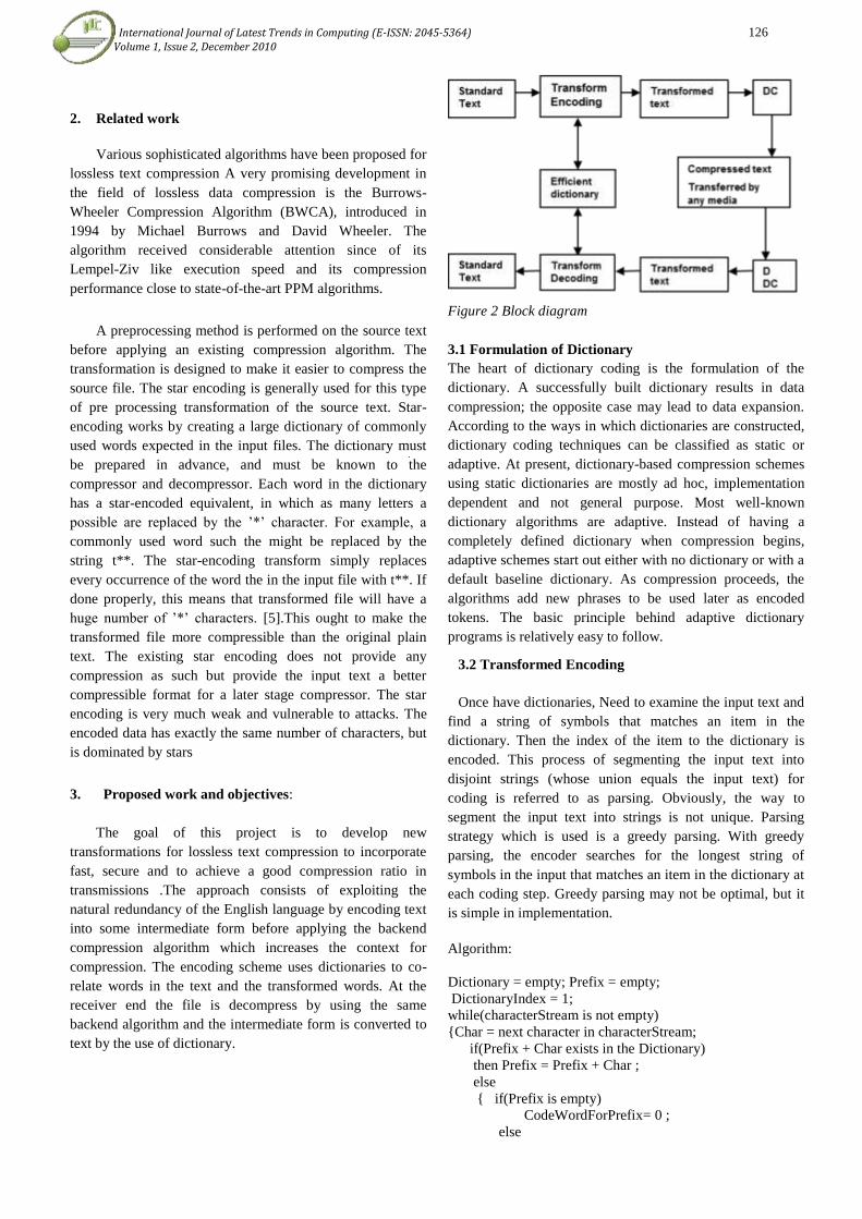
International Journal of Latest Trends in Computing (E-ISSN: 2045-5364) 126 Volume 1, Issue 2, December 2010
2. Related work
Various sophisticated algorithms have been proposed for
lossless text compression A very promising development in
the field of lossless data compression is the Burrows-
Wheeler Compression Algorithm (BWCA), introduced in
1994 by Michael Burrows and David Wheeler. The
algorithm received considerable attention since of its
Lempel-Ziv like execution speed and its compression
performance close to state-of-the-art PPM algorithms.
A preprocessing method is performed on the source text
before applying an existing compression algorithm. The
transformation is designed to make it easier to compress the
source file. The star encoding is generally used for this type
of pre processing transformation of the source text. Star-
encoding works by creating a large dictionary of commonly
used words expected in the input files. The dictionary must
be prepared in advance, and must be known to the
compressor and decompressor. Each word in the dictionary
has a star-encoded equivalent, in which as many letters a
possible are replaced by the ’*’ character. For example, a
commonly used word such the might be replaced by the
string t**. The star-encoding transform simply replaces
every occurrence of the word the in the input file with t**. If
done properly, this means that transformed file will have a
huge number of ’*’ characters. [5].This ought to make the
transformed file more compressible than the original plain
text. The existing star encoding does not provide any
compression as such but provide the input text a better
compressible format for a later stage compressor. The star
encoding is very much weak and vulnerable to attacks. The
encoded data has exactly the same number of characters, but
is dominated by stars
3. Proposed work and objectives:
The goal of this project is to develop new
transformations for lossless text compression to incorporate
fast, secure and to achieve a good compression ratio in
transmissions .The approach consists of exploiting the
natural redundancy of the English language by encoding text
into some intermediate form before applying the backend
compression algorithm which increases the context for
compression. The encoding scheme uses dictionaries to co-
relate words in the text and the transformed words. At the
receiver end the file is decompress by using the same
backend algorithm and the intermediate form is converted to
text by the use of dictionary.
Figure 2 Block diagram
3.1 Formulation of Dictionary
The heart of dictionary coding is the formulation of the
dictionary. A successfully built dictionary results in data
compression; the opposite case may lead to data expansion.
According to the ways in which dictionaries are constructed,
dictionary coding techniques can be classified as static or
adaptive. At present, dictionary-based compression schemes
using static dictionaries are mostly ad hoc, implementation
dependent and not general purpose. Most well-known
dictionary algorithms are adaptive. Instead of having a
completely defined dictionary when compression begins,
adaptive schemes start out either with no dictionary or with a
default baseline dictionary. As compression proceeds, the
algorithms add new phrases to be used later as encoded
tokens. The basic principle behind adaptive dictionary
programs is relatively easy to follow.
3.2 Transformed Encoding
Once have dictionaries, Need to examine the input text and
find a string of symbols that matches an item in the
dictionary. Then the index of the item to the dictionary is
encoded. This process of segmenting the input text into
disjoint strings (whose union equals the input text) for
coding is referred to as parsing. Obviously, the way to
segment the input text into strings is not unique. Parsing
strategy which is used is a greedy parsing. With greedy
parsing, the encoder searches for the longest string of
symbols in the input that matches an item in the dictionary at
each coding step. Greedy parsing may not be optimal, but it
is simple in implementation.
Algorithm:
Dictionary = empty; Prefix = empty;
DictionaryIndex = 1;
while(characterStream is not empty)
Char = next character in characterStream;
if(Prefix + Char exists in the Dictionary)
then Prefix = Prefix + Char ;
else
if(Prefix is empty)
CodeWordForPrefix= 0 ;
else

International Journal of Latest Trends in Computing (E-ISSN: 2045-5364) 127 Volume 1, Issue 2, December 2010
CodeWordForPrefix = DictionaryIndex for
Prefix ;
Output: (CodeWordForPrefix, Char) ;
insertInDictionary( ( DictionaryIndex , Prefix +
Char) );
DictionaryIndex++ ;
Prefix= empty ;
if(Prefix is not empty)
CodeWordForPrefix = DictionaryIndex for Prefix;
Output: (CodeWordForPrefix, ) ;
Example: Suppose the codeword are indexed starting from
1:Inputed string ABBCBCABABCAABCAAB
Compressed string (code words):
(0, A) (0, B) (2, C) (3, A) (2, A) (4, A) (6, B)
1 2 3 4 5 6 7 Index
Each code word consists of an integer and a character where
character is represented by 8 bits. The number of bits n
required to represent the integer part of the codeword with
index i is given by:
Number of Bits required is (1 + 8) + (1 + 8) + (2 + 8) + (2 +
8) + (3 + 8) + (3 + 8) + (3 + 8) = 71 bits
3.3 Compression and decompression using Backend
algorithm.
Any efficient backend algo(PPM/BWT) can be used to
compress as well as decompress the data.The lossless
Burrows-Wheeler compression algorithm has received
considerable attention over recent years for both its
simplicity and effectiveness. It is based on a permutation of
the input Sequence the Burrows-Wheeler transformation
which groups symbols with a similar context close together.
The BWT is performed on an entire block of data at once.
Most of today’s familiar lossless compression algorithms
operate in streaming mode, reading a single byte or a few
bytes at a time. But with this new transform, we want to
operate on the largest chunks of data possible. Since the
BWT operates on data in memory, you may encounter files
too big to process in one fell swoop. In these cases, the file
must be split up and processed a block at a time. A typical
scheme of the Burrows-Wheeler Compression Algorithm
(BWCA) is presented and consists of four stages.
I/p->BWTMTF->RLE->Huffman->O/p
Decompression
o/p<-BWT<-MTF<-RLE<-Huffman<-I/p
Each stage is a block transformation of the input buffer data
and forwards the output buffer data to the next stage. The
stages are processed sequentially from left to right for
compression; for decompression they are processed from
right to left with the respective backward transformations.
For compression, the first stage is the BWT. As the first
stage of the compression algorithm.The purpose of this stage
is the reordering of the input data depending on its context.
The reordering produces many runs of equal symbols inside
the output data of the BWT stage. In order to move the
reordered symbols back into their original positions, a
backward transformation exists, which reproduces exactly
the input sequence. [1]
3.4. Decoding
Decoding (decompressor) in dictionary method is very
simple. It will not parse the given input string. It will use the
same dictionary and will decode the sequence.
4. Performance Analysis:
The performance issues such as Bits Per Character
(BPC) and conversion time are compared for the three cases
i.e., simple BWT, BWT with Star encoding and BWT with
our proposed Efficient Dictionary method The results are
shown graphically which proves that the proposed method
has a good compression as well as reconstruction
(Decompression) time.
0
1
2
3
4
5
6
bib book1 book2 geo news
BWT
star
method
Eff.dict.
Figure 3: Encoding
0
1
2
3
4
5
6
bib book1 book2 geo news
BWT
star
method
Eff.dict.
Figure 4: Decoding
5. Conclusion
An efficient Dictionary-based compression techniques
use no statistical models. They focus on the memory on the
strings already seen. The compression algorithm and the
decompression algorithm build an identical dictionary
independently. The advantage of this is that the compression
algorithm does not have to pass the dictionary to the

International Journal of Latest Trends in Computing (E-ISSN: 2045-5364) 128 Volume 1, Issue 2, December 2010
decompressor.An efficient scheme is an excellent
improvement in text data compression and added levels of
security over the existing methods. This method will
maintain the compression ratio with a good reconstruction at
the receiver’s end.
6. References
[1] Burrows, M, Wheeler, D. A Block-Sorting Lossless Data
Compression Algorithm. Technical report, Digital
Equipment Corporation, Palo Alto, California, 1994, URL
(March 2006):
http://citeseer.ist.psu.edu/76182.html..
[2] E-book on Fundamentals of data compression by ida
mengui pu.
[3] Isal, R, Moffat, A, Ngai, A. Enhanced Word-Based
Block-Sorting Text Compression.In Proceedings of the
twenty-fifth Australasian conference on Computer science,
Volume 4,Janua
[4] [KrMu96] H. Kruse and A. Mukherjee. .Data
Compression Using Text Encryption. Proc.
Data Compression Conference, 1997, IEEE Computer
Society Press,1997.
[5] [KrMu97] H. Kruse and A. Mukherjee. .Preprocessing
Text to Improve Compression, IEEE
Computer Society Press,1997, p. 556.
[6] [Welc84] T. Welch, .A Technique for High-Performance
Data Compression.,IEEE Computer, Vol. 17, No. 6, 1984.
[7] [ZiLe77] J. Ziv and A. Lempel. .A Universal Algorithm
for Sequential Data Compression., IEEE Trans. Information
Theory, IT-23, pp.237-243.
[8] E-Book A complete Reference on data Compression by
David Solomon.
Author Biographies
First Author :Prof.L.K.Gautam received her Bachelor of computer technology in 2001 from RCERT chandrapur (MS),Currently pursuing her
M.E in Computer science and working as a lecturer in Sipna’s
C.O.E.T,Amravati.
Second Author: Prof.V.S.Gulhane received his Bachelor of Computer
Science in 1994 from Pusad Engg College (MS), Masters degree in computer science from RMIT Badnera ,Amravati in 2005 ,Currently
working as a Asst.Prof in sipna’s COET Amravati.
International Journal of Latest Trends in Computing (E-ISSN: 2045-5364) 129 Volume 1, Issue 2, December 2010
Effective Compression Technique by Using
Adaptive Huffman Coding Algorithm for Xml
Database Ms. Rashmi N. Gadbail
1,Prof.V.S.Gulhane
2
Sipna’s college of Engg. And Technology ,Amravati.
Corresponding Adresses
[email protected], [email protected]
Abstract: The Extensible Markup Language (XML) is one of the
most important formats for data interchange on the Internet. XML
documents are used for data exchange and to store large amount of
data over the web. These documents are extremely verbose and
require specific compression for efficient transformation. In this
proposed work we are enhancing the existing compressors which
uses Adaptive Huffman coding. It is based on the principle of
extracting data from the document, and grouping it based on
semantics. The document is encoded as a sequence of integers,
while the data grouping is based on XML tags/attributes/comments.
The main disadvantage of using XML documents is their large sizes
caused by highly repetitive (sub) structures of those documents and
often long tag and attribute names. Therefore, a need to compress
XML, both efficiently and conveniently to use. The re-organized
data is now compressed by adaptive Huffman coding. The special
feature of adaptive Huffman coding algorithm is that, it has
extremely accurate compression as well as it eliminates the
repetition of dictionary based words in xml database. Using
Adaptive Huffman algorithm, we derived probabilities which
dynamically changed with the incoming data, through Binary tree
construction.
Keywords: Compression, decompression, , Efficient XML
compression and decompression,Adaptive Huffman coding.
1. Introduction
The Extensible Markup Language (XML) is one of the
most important formats for data interchange on the Internet.
XML documents are used for data exchange and to store
large amount of data over the web. These documents are
extremely verbose and require specific compression for
efficient transformation. In this proposed work we are
enhancing the existing compressors which uses Adaptive
Huffman coding. It is based on the principle of extracting
data from the document, and grouping it based on
semantics[1].The document is encoded as a sequence of
integers, while the data grouping is based on XML
tags/attributes/comments. The main disadvantage of using
XML documents is their large sizes caused by highly
repetitive (sub) structures of those documents and often long
tag and attribute names. Therefore, a need to compress XML,
both efficiently and conveniently to use. The design goal of
Effective compression of XML database by using Adaptive
Huffman coding is to provide extremely efficient and
highly accurate compression of XML documents while
supporting "online" usage. In this context, "online" usage
means: (a) only one pass through the document is required to
compress it, (b) compressed data is sent to the output stream
incrementally as the document is read, and (c)
decompression can begin as soon as compressed data is
available to the decompressor. Thus transmission of a
document over a heterogeneous systems can begin as soon
as the compressor produces its first output, and,
consequently, the decompress or can start decompression
shortly thereafter, resulting in a compression scheme that is
well suited for transmission of XML documents over a wide-
area network.
2. Related work
Various sophisticated algorithms have been proposed for
lossless text compression. A very promising development in
the field of lossless data compression is the Burrows-
Wheeler Compression Algorithm (BWCA), introduced in
1994 by Michael Burrows and David Wheeler. The
algorithm received considerable attention since of its
Lempel-Ziv like execution speed and its compression
performance close to state-of-the-art PPM algorithms. A
preprocessing method is performed on the source text before
applying an existing compression algorithm. The
transformation is designed to make it easier to compress the
source file. The star encoding is generally used for this type
of preprocessing transformation of the source text. Star-
encoding works by creating a large dictionary of commonly
used words expected in the input files. The dictionary must
be prepared in advance, and must be known to the
compressor and decompressor.
Several proposals and references there in make use of
the observation that the pioneering work in this domain was
XGRind which was based on static Huffman coding.
XGRIND was the first XML-conscious compression scheme
to support querying without full decompression.[7] Element
and attribute names are encoded using a byte-based scheme,
and character data is compressed using static Huffman
coding. Use of the latter technique significantly slows down
the compression process, since two passes over the original
document are required (first to gather probability data for the

International Journal of Latest Trends in Computing (E-ISSN: 2045-5364) 130 Volume 1, Issue 2, December 2010
compression model, and a second time to perform the
encoding according to the generated model). XPRESS also
supports querying of compressed data and claims to achieve
better compression than XGRIND. [8] However, it uses a
semi-adaptive form of arithmetic coding which also
necessitates two passes Over the original XML document.
3. Proposed work and objectives:
3.1 Compression Techniques for XML Database
Lossless Compression
Lossless compression techniques provide exact
recovery of the original data from their compressed
version. Any information contained in an original cannot
be lost during compression and reconstruction. These
techniques are used widely in applications to save
storage space and network bandwidth. Since an XML
compressor needs to preserve all data content, only
lossless compression techniques can be used.
3.1.1Huffman coding
In computer science and information theory,
Huffman coding is an entropy encoding algorithm used
for lossless data compression. The term refers to the use
of a variable-length code table for encoding a source
symbol (such as a character in a file) where the variable-
length code table has been derived in a particular way
based on the estimated probability of occurrence for
each possible value of the source symbol. It was
developed by David A. Huffman "A Method for the
Construction of Minimum-Redundancy Codes.Huffman
coding uses a specific method for choosing the
representation for each symbol, resulting in a prefix
code (sometimes called "prefix-free codes", that is, the
bit string representing some particular symbol is never a
prefix of the bit string representing any other symbol)
that expresses the most common source symbols using
shorter strings of bits than are used for less common
source symbols.
In this proposed work we are enhancing the existing
compressors which uses Adaptive Huffman coding
Adaptive Huffman coding for xml database compression
XML simplifies data exchange among heterogeneous
computers, but it is notoriously verbose and has
spawned the development of many XML-specific
compressors and binary formats"[10]. We can present an
XML test and a combined efficiency metric integrating
compression ratio and execution speed. With the help of
adaptive Huffman compression technique. The Adaptive
Huffman compression is more efficient than static
Huffman compression it is an important dimension for
lossless data compression. In computer science and
information theory Huffman coding is an entropy
encoding algorithm used for lossless data compression.
Basically, the Adaptive algorithm states that a received
symbol’s node (current node) must be promoted (via the
Update method) as the highest numbered node among
nodes that are of equal weight. Simply swap the two
nodes (i.e., the highest numbered node and the current
node which must now become the new highest
numbered node) and the tree maintains the Sibling
property, as well as ensuring a correct tree. The parent of
the current node then becomes the new current node, and
the process continues until the root of the tree is reached
3.1.2Adaptive Huffman Compression Technique
The proposal here is that to design an efficient way
of compressing XML documents by using adaptive Huffman
coding. High compression ratio and speed is equally
important. We also require the transformation of xml
database to be fully reversible and decompress able so that
the decompressed document is a mirror image of the original.
Huffman coding requires prior knowledge of the
probabilities of the source sequence. If this knowledge is not
available, Huffman coding becomes a two pass procedure:
the statistics are collected in the first pass and the source is
Encoded in the second pass. In the Adaptive Huffman coding
procedure, neither transmitter nor receiver knows anything
about the statistics of the source sequence at the start of
transmission. Using Adaptive Huffman algorithm, we
derived probabilities which dynamically changed with the
incoming data, through Binary tree construction. Thus the
Adaptive Huffman algorithm provides effective compression
by just transmitting the node position in the tree without
transmitting the entire code. Unlike static Huffman algorithm
the statistics of the sensor data need not be known for
encoding the data.Thats why adaptive Huffman is extremely
accurate with respect to the compression.

International Journal of Latest Trends in Computing (E-ISSN: 2045-5364) 131 Volume 1, Issue 2, December 2010
The design goal of Effective compression of XML database
by using Adaptive Huffman coding is to provide extremely
efficient and highly accurate compression of XML
documents while supporting "online" usage. In this context,
"online" usage means: (a) only one pass through the
document is required to compress it, (b) compressed data is
sent to the output stream incrementally as the document is
read, and (c) decompression can begin as soon as
compressed data is available to the decompressor. Thus
transmission of a document over a heterogeneous systems
can begin as soon as the compressor produces its first output,
and, consequently, the decompress or can start
decompression shortly there after, resulting in a compression
scheme that is well suited for transmission of XML
documents over a wide-area network. Compression
Performance ,Compression Time (CT) and decompression
time. The
Objectives of proposed work are:
To provide an Effective compression technique by using
Adaptive Huffman coding algorithm
Adaptive Huffman coding for xml database
compression
XML simplifies data exchange among
heterogeneous computers, but it is notoriously verbose and
has spawned the development of many XML-specific
compressors and binary formats. We can present an XML
test and a combined efficiency metric integrating
compression ratio and execution speed. With the help of
adaptive Huffman compression technique. The Adaptive
Huffman compression is more efficient than static Huffman
compression it is an important dimension for lossless data
compression. In computer science and information theory
Huffman coding is an entropy encoding algorithm used for
lossless data compression.
The Sibling Property of Adaptive Huffman
Algorithm
In dynamic coding, it is not enough to just have a symbol
tree: the tree must be a “correct” Huffman tree. Thus, the tree
is recomputed or updated to ensure a correct tree. Re
computation of the tree is done dynamically, and the decoder
also maintains the same tree that the encoder creates.
Adaptive Huffman Algorithm maintains a property to create
a compact tree as much as possible. This is called the Sibling
Property. Accordingly, the Sibling property ensures a
Huffman tree in the fastest manner as possible; re
computation of the tree always maintains the Sibling
property.
The Sibling Property defines a binary tree to be a Huffman
tree if and only if:
all leaf nodes have non-negative weights (i.e., a leaf
node can have a 0 weight), all internal nodes have
exactly two children, and the weight of each parent
node is the sum of its children’s weights; and
the nodes are numbered in increasing order by non-
decreasing weight so that siblings are assigned
consecutive numbers or rank, and most importantly,
their parent node must be higher in the numbering
[Vitter 1987].
With the Sibling property, nodes are promoted up the tree
when necessary to assign them a minimal number of bits;
that is, if they are gaining weight, they are assigned shorter
bit codes. Some nodes may go down according to the
statistics of the source; if one node goes up, there is certainly
one node which goes down because the two nodes are simply
swapped in the tree positions. Node promotion involves
constant swapping of nodes.
Basically, the Adaptive algorithm states that a received
symbol’s node (current node) must be promoted (via the
Update method) as the highest numbered node among nodes
that are of equal weight. Simply swap the two nodes (i.e.,
the highest numbered node and the current node which must
now become the new highest numbered node) and the tree
maintains the Sibling property, as well as ensuring a correct
tree. The parent of the current node then becomes the new
current node, and the process continues until the root of the
tree is reached.
Why Compress XML
o XML is verbose
o XML documents has repetitive structures of data
o Each non-empty element tag must end with a
matching closing tag -- <tag>data</tag>
o Ordering of tags is often repeated in a document
(e.g. multiple records)
o Tag names are often long
4. Conclusion
Adaptive Huffman coding encodes an alphabet with
¯fixed codes. That allows us to directly search keywords in
the compressed data[6]. Since the data volumes reduced,
such compressing of xml data may be even faster than the
original data. The resulting output of proposed work will be
that xml document compresses with the help of adaptive
Huffman algorithm and that compressed data will be
decompressed as well and provide original xml document
over a heterogeneous systems.

International Journal of Latest Trends in Computing (E-ISSN: 2045-5364) 132 Volume 1, Issue 2, December 2010
References
[1] Bray, et al. “Extensible Markup Language
(XML) 1.0”, October 2000,
http://www.w3.org/TR/REC-xml.
[2]G. Girardot and N. Sundaresam,:an encoding
format for efficient representation
and exchange of XML over the
Web”,http://www9.org/w9cdrom/154/154.html
[3]D. Huffman, “A Method for Construction
ofMinimum-Redundancy Codes”, Proc. of IRE,
September 1952.
[4] H. Liefke and D. Suciu. XMill: An Efficient
Compressor for XML Data. In Proceedings of the
2000 ACM SIGMOD International Conference on
Management of Data, pages 153–164, May 2000.
[5] P. G. Howard and J. S. Vitter. Analysis of
Arithmetic Coding for Data Compression. In
Proceedings of the IEEE Data Compression
Conference, pages 3–12,April 1991.
[6] Tolani P.M. and Haritsa J.R., “XGRIND: a
query-friendly XML compressor,” in Proc. 2002
Int’l Conf. on DatabaseEng., pp. 225-34
[7] World Wide Web Consortium. Document
Object Model (DOM) Level 1
Speci_cation Version 1.0, W3C Recommendation 1
October, 1998 edition.
Author Biographies
First Author :Ms.Rashmi N. Gadbail received her Bachelor of
computer technology in 2009 from Sipna’s COET
Amravati.(MS),Currently pursuing her M.E in Information
Technology and working as a lecturer in IBSS C.O.E.T
Ghatkhed,Amravati.
Second Author: Prof.V.S.Gulhane received his Bachelor of
Computer Science in 1994 from Pusad Engg College (MS),
Masters degree in computer science from RMIT Badnera ,Amravati
in 2005 ,Currently working as a Asst.Prof in sipna’s COET
Amravati.

International Journal of Latest Trends in Computing (E-ISSN: 2045-5364) 133 Volume 1, Issue 2, December 2010
Congestion Control and Buffering Technique for
Video Streaming over IP
1Md .Taslim Arefin,
2Md. Ruhul Amin
1Dept. of Electronics & Telecommunication Engineering
Daffodil International University
Dhaka, Bangladesh
2 BRAC Bank Ltd.
Dept of Technology operations
Dhaka, Bangladesh
Email: [email protected]
Abstract: - Due to the fiery growth of the demand for
transmission of real-time video, streaming video over the
Internet has received marvelous concentration. An efficient
Quality of Service of video streaming depends on bandwidth,
delay, and loss requirements due to its real-time nature.
However, the current Internet system is not offering any
quality of service (QoS) guarantees to streaming video over
the Internet. Also it is difficult to support multicast video
efficiently while providing service suppleness to meet a wide
range of QoS requirements from the users. Thus, designing
mechanisms and protocols for Internet streaming video poses
many challenges. To converse to these challenges, extensive
researches has been conducted and has found six key areas of
streaming video for maintaining an acceptable QoS. We have
introduced an improved application layer QoS control to avoid
congestion and maximize video quality by reducing packet
loss and delay. For this, we address the packet loss issue and
review major approaches and mechanisms. On our approaches
for application layer QoS improves the video streaming
quality significantly. We also discuss the tradeoffs of the
approaches and point out future research directions.
Key words:- Application Layer Congestion Control, Video
Streaming, Receiver based Buffering technique, Video
Compression, Streaming Server, Media Synchronization.
I. INTRODUCTION
The demand for multimedia information on the web is
increasing day by day due to various multimedia applications
such as distance learning, digital libraries, home shopping, and
video-on-demand. Recent advances in computing technology,
compression technology, high-bandwidth storage devices, and
high-speed networks have made it feasible to provide real-time
multimedia services over the Internet. Real-time multimedia
[1] as the name implies, has timing constraints. For example,
audio and video data must be played out continuously. If the
data does not arrive on time, the play out process will pause,
which is irritating to human hearing and visuals. So this real-
time transport of live video or stored video is the predominant
part of real-time multimedia.
In this research paper, we are fretful with the video streaming,
which refers to real-time transmission of stored video.
Streaming video is a sequence of "moving image" that are sent
in compressed form over the Internet and displayed by the
viewer as they arrive. For the transmission of stored video
over the Internet there are two modes such as the download
mode and the streaming mode (i.e., video streaming). In the
download mode [2] a user downloads the entire video file and
then plays back the video file. However, full file transfer in the
download mode usually suffers long and perhaps unacceptable
transfer time. In compare [2] in the streaming mode, the video
content does not need be downloaded in full size, but is being
played out while parts of the content are being received and
decoded. Due to its real-time nature, video streaming typically
has bandwidth, delay and loss requirements. However, as we
know the current traditional Best effort Internet service does
not offer any quality of service (QoS) which guarantees to
streaming video over the Internet. In adding up, it is difficult
to support multicast video efficiently while providing service
flexibility to meet a wide range of QoS requirements from the
users. Thus, designing mechanisms and protocols for Internet
streaming video poses many challenges.
To address these challenges, extensive researches has been
conducted and have introduced six key areas of streaming
video, such as: (i) video compression, (ii) application-layer
QoS control, (iii) continuous media distribution services, (iv )
streaming servers, (v) media synchronization mechanisms, and
(vi) protocols for streaming media. Every one of these six
areas is a basic structure slab, with which architecture for
streaming video can be built. Figure 1 shows architecture for a
video streaming.
A. Video compression Firstly any raw video and audio data are pre-compressed by
video compression and audio compression algorithms and then
it is saved in the storage devices.
B. Application-layer QoS control
To cope with varying network conditions [3] and different
presentation quality requested by the users, various
application-layer QoS control techniques have been proposed.
The application-layer techniques include congestion control
and error control. Their respective functions are as follows.
Congestion control is employed to prevent packet loss and
reduce delay. Error control, on the other hand, is to improve

International Journal of Latest Trends in Computing (E-ISSN: 2045-5364) 134 Volume 1, Issue 2, December 2010
video presentation quality in the presence of packet loss. Error
control mechanisms include forward error correction (FEC),
retransmission, error-resilient encoding, and error
concealment. Any streaming server [3] first retrieves the
compressed video or audio data from the storage devices and
then the application layer QoS control module adapts the
video/audio bit-streams according to the network status and
QoS necessities. After the adaptation, the compressed bit-
streams are being packetize by the the transport protocols and
then send the video/audio packets to the Internet. Packets may
be dropped or may experience too much delay inside the
Internet due to congestion.
Figure 1: Architecture for video streaming.
C. Continuous media distribution services
In order to provide quality multimedia presentations, adequate
network support is crucial. [4] This is because network support
can reduce transport delay and packet loss ratio. Built on top
of the Internet (IP protocol), continuous media distribution
services are able to achieve QoS and efficiency for streaming
video/audio over the best-effort Internet. Continuous media
distribution services include network filtering, application-
level multicast, and content replication.
D. Streaming servers
Streaming servers play an important role in providing
streaming services. To offer quality streaming services,
streaming servers need to process multimedia data under
timing constraints and support interactive control operations
such as pause/resume, fast forward, and fast backward.
Furthermore, streaming servers need to retrieve media
components in a synchronous fashion. A streaming server
typically consists of three subsystems, namely, a
communicator (e.g., transport protocols), an operating system,
and a storage system.
E. Media synchronization mechanisms Media synchronization is a major feature that distinguishes
multimedia applications from other traditional data
applications. With media synchronization mechanisms, the
application at the receiver side can present various media
streams in the same way as they were originally captured. An
example of media synchronization is that the movements of a
speaker’s lips match the played-out audio.
F. Protocols for streaming media Protocols are designed and standardized for communication
between clients and streaming servers. Protocols for streaming
media provide such services as network addressing, transport,
and session control.
In the following Sections, we have discussed different types of
congestion control mechanism which are based on the
Application-layer QoS control in video streaming architecture
and have tried to propose an efficient way to reduce packet
loss and delay in video streaming.
II. APPLICATION-LAYER QOS - CONGESTION
CONTROL
Quality of Service is a major challenge in video streaming.
Packet loss and delay of arrival of video packet are the two
key threats [4] for any kind of Efficient QoS in video
streaming. Burst loss and excessive delay have a devastating
effect on video presentation quality, and they are usually
caused by network congestion. Thus, congestion-control
mechanisms at end systems are necessary to help reducing
packet loss and delay.
We have found that Application-layer QoS control deals with
the packet loss and delay of video packet. The objective of
application-layer QoS control is to avoid congestion and
maximize the video quality by reducing packet loss and delay.
The application-layer QoS control techniques include
congestion control and error control. These techniques are
employed by the end systems and do not require any QoS
support from the network.
We have surveyed on various approaches for congestion
control and propose a mechanism for packet loss and delay
reduction.
A. Congestion Control Congestion control depends on efficient rate control and rate
shaping. Rate shaping is required for Source-Based Rate
Control. Typically, for streaming video, congestion control
takes the form of rate control. Rate control attempts to
minimize the possibility of network congestion by matching
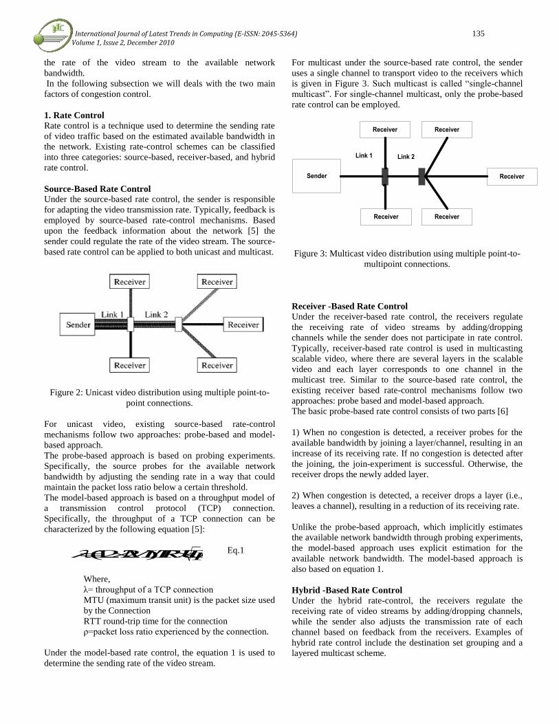
International Journal of Latest Trends in Computing (E-ISSN: 2045-5364) 135 Volume 1, Issue 2, December 2010
the rate of the video stream to the available network
bandwidth.
In the following subsection we will deals with the two main
factors of congestion control.
1. Rate Control Rate control is a technique used to determine the sending rate
of video traffic based on the estimated available bandwidth in
the network. Existing rate-control schemes can be classified
into three categories: source-based, receiver-based, and hybrid
rate control.
Source-Based Rate Control Under the source-based rate control, the sender is responsible
for adapting the video transmission rate. Typically, feedback is
employed by source-based rate-control mechanisms. Based
upon the feedback information about the network [5] the
sender could regulate the rate of the video stream. The source-
based rate control can be applied to both unicast and multicast.
Figure 2: Unicast video distribution using multiple point-to-
point connections.
For unicast video, existing source-based rate-control
mechanisms follow two approaches: probe-based and model-
based approach.
The probe-based approach is based on probing experiments.
Specifically, the source probes for the available network
bandwidth by adjusting the sending rate in a way that could
maintain the packet loss ratio below a certain threshold.
The model-based approach is based on a throughput model of
a transmission control protocol (TCP) connection.
Specifically, the throughput of a TCP connection can be
characterized by the following equation [5]:
pRTTMTU /)22.1( Eq.1
Where,
λ= throughput of a TCP connection
MTU (maximum transit unit) is the packet size used
by the Connection
RTT round-trip time for the connection
ρ=packet loss ratio experienced by the connection.
Under the model-based rate control, the equation 1 is used to
determine the sending rate of the video stream.
For multicast under the source-based rate control, the sender
uses a single channel to transport video to the receivers which
is given in Figure 3. Such multicast is called “single-channel
multicast”. For single-channel multicast, only the probe-based
rate control can be employed.
Sender Receiver
ReceiverReceiver
ReceiverReceiver
Link
1
Link 1 Link 2
Figure 3: Multicast video distribution using multiple point-to-
multipoint connections.
Receiver -Based Rate Control Under the receiver-based rate control, the receivers regulate
the receiving rate of video streams by adding/dropping
channels while the sender does not participate in rate control.
Typically, receiver-based rate control is used in multicasting
scalable video, where there are several layers in the scalable
video and each layer corresponds to one channel in the
multicast tree. Similar to the source-based rate control, the
existing receiver based rate-control mechanisms follow two
approaches: probe based and model-based approach.
The basic probe-based rate control consists of two parts [6]
1) When no congestion is detected, a receiver probes for the
available bandwidth by joining a layer/channel, resulting in an
increase of its receiving rate. If no congestion is detected after
the joining, the join-experiment is successful. Otherwise, the
receiver drops the newly added layer.
2) When congestion is detected, a receiver drops a layer (i.e.,
leaves a channel), resulting in a reduction of its receiving rate.
Unlike the probe-based approach, which implicitly estimates
the available network bandwidth through probing experiments,
the model-based approach uses explicit estimation for the
available network bandwidth. The model-based approach is
also based on equation 1.
Hybrid -Based Rate Control Under the hybrid rate-control, the receivers regulate the
receiving rate of video streams by adding/dropping channels,
while the sender also adjusts the transmission rate of each
channel based on feedback from the receivers. Examples of
hybrid rate control include the destination set grouping and a
layered multicast scheme.

International Journal of Latest Trends in Computing (E-ISSN: 2045-5364) 136 Volume 1, Issue 2, December 2010
2. Rate Shaping
The objective of rate shaping is to match the rate of a pre-
compressed video bit stream to the target rate constraint. A
rate shaper (or filter), which performs rate shaping, is required
for the source-based rate control which is given in Figure 4.
Internet
Transport
Protocols
Rate Sahper
Compressed
Video
Sourse
Based Rate
Control
Storage Device
Figure 4: Architecture for source-based rate control
This is because the stored video may be pre-compressed at a
certain rate, which may not match the available bandwidth in
the network.
III. EFFICIENT CONGESTION CONTROL AND
BUFFERING TECHNIQUE FOR REDUCING PACKET
LOSS AND DELAY IN VIDEO STREAMING OVER
THE INTERNET PROTOCOL
Efficient Congestion Control and Buffering technique for
reducing packet loss and delay in Video Streaming over the
Internet Protocol.
A. Efficient Congestion Control Congestion control technique may vary due to the type of
receiver. Single-channel multicast is efficient since all the
receivers share one channel. However, single-channel
multicast is unable to provide flexible services to meet the
different demands from receivers with various access link
bandwidths. In contrast, if multicast video were to be delivered
through individual unicast streams, the bandwidth efficiency is
low, but the services could be differentiated since each
receiver can negotiate the parameters of the services with the
source. Unicast and single-channel multicast are two extreme
cases shown in Figure 5.
Bandwidth
Efficiency
Service Flexibility
Low High
HighLow
UnicastSingle Channel Multicast
Receiver based/Hybrid based Control
Figure 5: Tradeoff between efficiency and flexibility.
To achieve good tradeoff between bandwidth efficiency and
service flexibility for multicast video, receiver-based and
hybrid rate-control are proposed. One the other hand for
efficiency in unicast video, source-based control gives good
performance.
B. Buffering video stream before playing to receiver In video streaming, [7] the video packet is sent in a continuous
stream and is played as it arrives. We have found that delay is
common problem for the video streaming. Sometimes it is
found that ith packet may reach at the receiver after i+1th
packet. As in real time transmission, the packet plays as soon
as it reaches so here ith packet plays after i+1th packet. So it
breaks the continuity of video streaming and degrades the
quality of video.
So we have proposed a buffering concept for storing video
packets at the receiver before playing the video. We have
proposed to store last three packets in the buffer before playing
these. According to our proposal the packet is not played as
soon as it reached at the receiver end. At the receiver end the
packet is stored in the buffer and the buffer can store three
packets. When the buffer is full then the packets will be
played.
We have found that this concept of using buffer at the receiver
end before playing will reduce the probably of playing i+1th
packet before ith packet. We have found that the buffering
system improves the continuity of the video streaming which
provides efficient quality of service.
IV. RESULT AND DISCUSSION
We have got the result of using Congestion Control technique
and buffering for storing video stream. We have got the result
from subjective test which is known as Mean Opinion Score.
A. Subjective Benchmark MOS (mean Opinion Score) Figure 6 shows a common subjective benchmark MOS (Mean
Opinion Score) obtained from a group of receiver for finding
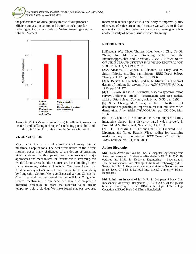
International Journal of Latest Trends in Computing (E-ISSN: 2045-5364) 137 Volume 1, Issue 2, December 2010
the performance of video quality in case of our proposed
efficient congestion control and buffering technique for
reducing packet loss and delay in Video Streaming over the
Internet Protocol.
Figure 6: MOS (Mean Opinion Score) for efficient congestion
control and buffering technique for reducing packet loss and
delay in Video Streaming over the Internet Protocol.
VI. CONCLUSION
Video streaming is a vital constituent of many Internet
multimedia applications. The best-effort nature of the current
Internet poses many challenges to the design of streaming
video systems. In this paper, we have surveyed major
approaches and mechanisms for Internet video streaming. We
would like to stress that the six areas are basic building blocks
for a streaming video architecture. We have found that
Application-layer QoS control deals the packet loss and delay
by Congestion Control. We have discussed various Congestion
Control procedures and found out an efficient Congestion
Control mechanism. In our paper we have also proposed a
buffering procedure to store the received voice stream
temporary before playing. We have found that our proposed
mechanism reduced packet loss and delay to improve quality
of service of voice streaming. In future we will try to find an
efficient error control technique for voice streaming which is
another quality of service issue in voice streaming.
REFERENCES
[1]Dapeng Wu, Yiwei Thomas Hou, Wenwu Zhu, Ya-Qin
Zhang, Jon M. Peha :Streaming Video over the
Internet:Approaches and Directions. IEEE TRANSACTIONS
ON CIRCUITS AND SYSTEMS FOR VIDEO TECHNOLOGY,
VOL. 11, NO. 3, MARCH 2001
[2]A. Albanese, J. Blömer, J. Edmonds, M. Luby, and M.
Sudan :Priority encoding transmission. IEEE Trans. Inform.
Theory, vol. 42, pp. 1737–1744, Nov. 1996.
[3] S. Berson, L. Golubchik, and R. R. Muntz :Fault tolerant
design of multimedia servers. Proc. ACM SIGMOD’95, May
1995, pp. 364–375.
[4] G. Blakowski and R. Steinmetz: A media synchronization
survey: Reference model, specification, and case studies.
IEEE J. Select. Areas Commun, vol. 14, pp. 5–35, Jan. 1996.
[5] S. Y. Cheung, M. Ammar, and X. Li :On the use of
destination set grouping to improve fairness in multicast video
distribution. Proc. IEEE INFOCOM’96, pp. 553–560, Mar.
1996.
[6] M. Chen, D. D. Kandlur, and P. S. Yu :Support for fully
interactive playout in a disk-array-based video server”, in
Proc. ACM Multimedia, 4, New York, Oct. 1994.
[7] G. J. Conklin, G. S. Greenbaum, K. O. Lillevold, A. F.
Lippman, and Y. A. Reznik :Video coding for streaming
media delivery on the Internet. IEEE Trans. Circuits Syst.
Video Technol., vol. 11, Mar. 2001.
Author Biography
Md. Taslim Arefin received his B.Sc. in Computer Engineering from
American International University –Bangladesh (AIUB) in 2005. He
obtained his M.Sc. in Electrical Engineering – Specialization
Telecommunications from Blekinge Institute of Technology (BTH),
Sweden in 2008. At the present time he is working as Senior Lecturer
in the Dept. of ETE at Daffodil International University, Dhaka,
Bangladesh.
Md. Ruhul Amin received his M.Sc. in Computer Science from
Independent University, Bangladesh (IUB) in 2007. At the present
time he is working as Senior DBA in the Dept. of Technology
Operation at BRAC Bank Ltd, Dhaka, Bangladesh.

International Journal of Latest Trends in Computing (E-ISSN: 2045-5364) 138 Volume 1, Issue 2, December 2010
The Empirical Study on the Factors Affecting Data
Warehousing Success
Md. Ruhul Amin1, Md. Taslim Arefin
2
1 BRAC Bank Ltd.
Dept of Technology operations,
Database Administrator(DBA) Team
Dhaka, Bangladesh
Email: [email protected]
2 Daffodil International University
Dept of Electronics & Telecommunication Engineering
Faculty of Science & Information Technology
Dhaka, Bangladesh
Email: [email protected]
Abstract: - Data Warehouse is the centralized store of detailed data
from all relevant source systems, allowing for ad hoc discovery and
drill-down analysis by multiple user groups. Various implementation
factors play critical role to successful data warehouse (DW) project
implementation. DW has unique characteristics that need to consider
during implementation. There is little empirical research about
implementation of DW to get success. Determining factors affecting
DW success are important in the deployment of this DSS technology
by organizations.
Keywords: - Data Warehouse, Business intelligence, Decision support
system
1. Introduction Data Warehouse is a technique for properly storing and
managing data from different data sources for the purpose of
business performance analysis.
Decision support system (DSS) is an area of the information
systems (IS) discipline that focuses on supporting and
improving managerial decision making [1]. In terms of
contemporary professional practice, DSS includes personal
decision support systems (PDSS), group support systems
(GSS), executive information systems (EIS), online analytical
processing systems (OLAP), data warehousing (DW), and
business intelligence (BI). Over the three decades of its history,
DSS has moved from a radical movement that has changed the
way IS were perceived in business, to a mainstream
commercial IT movement, in which all organizations engage
[1].
Successfully supporting managerial decision making has
become critically dependent upon the availability of integrated
and high quality information organized and presented to
managers in a timely and easily understood manner. DWs have
emerged to meet this need. Surrounded by analytical tools and
models, DWs have the potential to transform operational data
into BI by effectively identifying problems and opportunities.
Metadata
Repository
Data
Source
ETL -Tools
Data
Source
Data
Source
AnalyticBI
Data
MartOLAP
BI
Data
Warehouse
Figure1: A typical data warehousing system architecture
2. Aims of this Research Large organizations have different data source to manage
operation, so faced significant problem to build single view of
their business from different data sources. During the mid-to-
late 1990s, “DW became one of the most important
developments in the information systems field” [1]. It is
estimated that 95 percent of the Fortune 1000 companies either
have a DW in place or are planning to develop one [2].” In
2002, the Palo Alto Management Group predicted that the DW
market would grow to a $113.5 billion market, including the
sales of systems, software, services, and in-house
expenditures” [2].
About 3,000 data warehousing projects are undertaken each
year and if the lowest perceived data warehouse failure rate
(70%) is accurate, then each year there are 2,100 failures [3].
DW project is an expensive and risky undertaking [4]. The
typical project costs over $1 million in the first year alone and
it is estimated that one-half to two-thirds of all initial DW
efforts fail [5]. There is a common perception that the failure
rate of data warehousing projects is 70 to 80 percent (Inmon

International Journal of Latest Trends in Computing (E-ISSN: 2045-5364) 139 Volume 1, Issue 2, December 2010
2001) and one study reported a 90 percent failure rate
(Conning 2000) [3]. “According to a 2003 Gartner report, more
than 50 percent of data warehouse projects failed, in a 2007
study, Gartner predicted once more that 50 percent of data
warehouse projects would have limited acceptance or be
outright failures as a result of lack of attention to data quality
issues” [6].
According to [7], the average time for the construction of a
data warehouse is 12 to 36 months and the average cost for its
implementation is between $1 million to $1.5 million.
This study was undertaken to perform a detailed analysis of
these cases to determine whether the presence (or absence) of
any specific factors or combination of factors might be
correlated with instances of failures.
3. Factors affect DW success A very good discussion on the problems of data warehousing
projects is found in [7]. The paper mentions the logical fact
that nobody really speaks about data warehousing failures and
goes on to group the reasons for the failure of a data
warehousing project into four categories, namely design,
technical, procedural and socio-technical factors.
Serial #
---------
Factors affect the DW success
----------------------------------------
01 IT initiate DW project
02 Poor Data Quality
03 Metadata Management
04 Less important pay on business value
05 Database Schema flaws
06 Quality of feeder system
07 POC on vendor talk about their product
08 Project Is Over Budget
09 Slipped Schedule
10 Functions and capabilities not implemented
11 Incomplete user’s requirement
12 Unacceptable Performance
13 Poor Availability
14 Inability to expand
15 Poor Quality Reports
16 Tools is not user friendly
17 Project Not Cost Justified
18 Management does not recognize the benefits
19 Inadequate or no user involvement
20 Gap between researchers and practitioners
3.1 IT initiate DW project
In some organization IT used to provide different report to
business to understand the business performance. Due to some
reason (data volume increase, improper SQL write, Improper
Application design, System over utilized, etc) business
sometimes does not received the report right time. After that IT
started talked about DW to give report to business on right
time without proper analysis. Business agreed because they
need report on time to analysis. The DW project is very costly
and business talked about because of these report delay this
type of costly project they will not finance. IT says to business
you can do business analysis if we have DW, but business says
we want report as business people no aware about business
analysis with DW.
The IT Initiated DW/BI project may pay more attention on
technology rather than business. If get sucked into the
technology, then missing the whole point. Developed
technically great DW/BI system but less importance on
business, this DW project will be treating as fail. Need to start
with business value.
3.2 Data Quality issue
Quality of data produces quality of information. Poor quality of
data badly affects all company to run smoothly. Often the
cause of business problem such as faulty analysis, operational
inefficiency and dissatisfied customer are because of
inaccurate, inconsistent, incomplete data. The operation cost
increase due to poor quality data. The poor quality of data
creates the problem data integration.
“Many enterprises fail to recognize that they have an issue with
data quality. They focus only on identifying, extracting and
loading data to the data warehouse, but do not take the time to
assess quality, said Ted Friedman, principal analyst at Gartner”
[6]. “Consistency and accuracy of data is critical to success
with BI, and data quality must be viewed as a business issue
and responsibility, not just an IT problem.”[6]. “New federal
regulations and corporate governance requirements have
greatly increased the pressure for improved data quality.
Enterprises must eliminate multiple data silos, assign
stewardship to critical data, and implement a process for
continuous monitoring and measurement of data quality.”[6].
According to Gartner Inc ,through 2007 more than 50 percent
DW project will be outright failed because lack of attention to
data quality issue[6].
3.3 Metadata Management
The term Metadata is defined as “data about data"[8]. Metadata
help a person to locate and understand data. Metadata is often
generally described as “information about data.” More
precisely, metadata is the description of the data itself, its
purpose, how it is used, and the systems used to manage it.
Metadata play important role in DW development. Not only
does it shape the data integration process but it also enables the
business users to locate, understand and use the data once it is
loaded into the data warehouse. Metadata is very valuable to
the business because it facilitates the understanding of data.
Without this understanding the data would be useless.
Metadata need to integrate from different source and developed
metadata repository. “At the conceptual level the structure of
the repository is described by a metamodel or informational
model. To develop metamodel at least 4 modeling level are
required. To start with level, on the lowest level, level 0 there
are actual data item (e,g, the customer data). The level above
contains the metadata information: level 1 contains metadata
(e.g. database schema), level 2 specifies the schema used to
store the metadata (the so called metamodel, information
model or metadata schema).”[11]

International Journal of Latest Trends in Computing (E-ISSN: 2045-5364) 140 Volume 1, Issue 2, December 2010
3.4 Less important pay on business value
DW developed for analysis the business performance. So need
to pay significant attention on business requirement and
developed DW. Get the requirement from the business people
some time it is difficult task, because the entire business person
on the project may not from MBA background. Without work
closely with business people can’t deliver business. DW teams
need to pay more important on business value. Keep in mind,
Technology is important; business value is mandatory.
3.5 Database Schema flaws
The data stored in database and application access data. The
schema holds the data, business rules inside the database. In
one database may be more than one Schema. “The database
schema should be flawless in terms of consistency, integrity
and compliance to the rules of the relational technology before
a data warehouse project is initiated.”[11]
Schema
DSS user 1
Data
Warehouse
SchemaSchema
DSS user 2
Figure 2: Database quality information
”The quality of the information depends on 3 things: (1) the
quality of the data itself, (2) the quality of the application
programs and (3) the quality of the database schema.”[11]
3.6 Quality of feeder system
Data warehouse is depending on feeder system. If the feeder
system has flaws then information provided by the DW will be
flaws. All the feeder system integrated and stored required data
in DW. During running ETL process the feeder system should
capable enough to handle the process, in terms of performance
and availability. Another point is quality of data of feeder
system. If the quality of data is poor, need to clean before load
in DW.
3.7 POC (proofs of concept) on vendor talk about their
product
The proof of concept will help us to ensure vendor claim is true
or not. The popularity of DW grew exponential during last year
[10]. So there is huge number of product is now in market on
DW. Vendor say about a lot about their product they offered.
Organization need to carefully consider the vendors marketing
claim regarding the product feature. Vendor can provide the
customer reference of the product. Carefully need to choose the
product otherwise during implementation project will be
treated as fail. It is better to test the vendor claim on
organization before chose the product to build DW.
3.8 Project is over budget
Every company used to declare annual budget, if the project
required more budget, the project may be treated a failure.
“The DW is costly project so the inadequate budget might be
the result of not wanting to tell management the bitter truth
about the costs of a data warehouse and expensive consulting
help may have been needed. Performance or capacity
problems, more users, more queries or more complex queries
may have required more hardware to resolve the problems.
The scope of project may require updating on the middle of the
project running or other factors may have resulted in additional
expenses.”[12]
3.9 Slipped Schedule
“Most of the factors listed in the other section could also have
contributed to the schedule not being met, but the major reason
for a slipped schedule is the inexperience or optimism of those
creating the project plan. In many cases management wanting
to “put a stake in the ground” were the ones who set the
schedule by choosing an arbitrary date for delivery in the hope
of giving project managers something to shoot for. The
schedule becomes a deadline without any real reason for a
fixed delivery date. In those cases the schedule is usually
established without input from those who know how long it
takes to actually perform the data warehouse tasks. The
deadline is usually set without the benefit of a project plan.
Without a project plan that details the tasks, dependencies and
resources, it is impossible to develop a realistic date by which
the project should be completed.”[12]
3.10 Defined functions and capabilities not implemented
Before project implementation, the scope of project or
capabilities and functionalities of project need to well defined.
This scope is defined from the input given from business and
technical concern person. In this scope are specified certain
functionality and capabilities. If important function and
capabilities are not considered or postponed to some other
implementation phase, this can be indication of project failure.
3.11 Incomplete user’s requirement
Before project start DW user compile the requirement. User
expect that they will get their requirement fulfill. If the users
not get their requirement form get unhappy and due to this the
project should be considered a failure. Sometimes users expect
more than they got. “Users may be unhappy about the
cleanliness of their data, response time, availability, usability

International Journal of Latest Trends in Computing (E-ISSN: 2045-5364) 141 Volume 1, Issue 2, December 2010
of the system, anticipated function and capability, or the
quality and availability of support and training.”[12]
3.12 Unacceptable Performance
“Unacceptable performance has often been the reason that data
warehouse projects are cancelled. Data warehouse performance
should be explored for both the query response time and the
extract/transform/load time. Query response time is take couple
of minutes is acceptable, because some time millions of rows
need to calculate. We have seen queries where response time is
measured in days. Except for a few exceptions, this is clearly
unacceptable. This will impact the availability of the data
warehouse to the users. Not only user response but also
minimize the execution time of ETL process. “[12]
3.13 Poor Availability
“Availability is both scheduled availability (the days per week
and the number of hours per day) as well as the percentage of
time the system is accessible during scheduled hours.
Availability failure is usually the result of the data warehouse
being treated as a second-class system. Operational systems
usually demand availability service level agreements. The
performance evaluations and bonus plans of those IT members
who work in operations and in systems often depends on
reaching high availability percentages. If the same standards
are not applied to the data warehouse, problems will go
unnoticed and response to problems will be casual, untimely
and ineffective.”[12]
3.14 Inability to Expand
“If a robust architecture and design is not part of the data
warehouse implementation, any significant increase in the
number of users or increase in the number of queries or
complexity of queries may exceed the capabilities of the
system. If the data warehouse is successful, there will also be a
demand for more data, for more detailed data and, perhaps, a
demand for more historical data to perform extended trend
analysis, e.g. five years of monthly data.”[12]
3.15 Poor Quality Reports
“If the data is not clean and accurate, the queries and reports
will be wrong, In which case users will either make the wrong
decisions or, if they recognize that the data is wrong, will
mistrust the reports and not act on them. Users may spend
significant time validating the report figures, which in turn will
impact their productivity. This impact on productivity puts the
value of the data warehouse in question.”[12]
3.16 Tools is not user friendly
Should not expect that all the user who will use BI tools for
business analyses are IT expert. Some of the user may heard
about the BI tools is first time. If the tools is not user friendly
people will not used much and start blame on this tools even
though form technical and business point of view tools is great.
User may start asking ask IT to download the report and
provide them. The DW is not only some sort of report, it is
more that that where user will build up their own query and
design report to analysis the business performance. In this
scenario the project will be treating as failed, because the
purpose of DW is deviated.
3.17 Project Not Cost Justified
“Every organization should justify cost their data warehouse
projects. Justification includes an evaluation of both the costs
and the benefits. When the benefits were actually measured
after implementation, they may have turned out to be much
lower than expected, or the benefits came much later than
anticipated. The actual costs may have been much higher than
the estimated costs. In fact, the costs may have exceeded both
the tangible and intangible benefits.”[12]
3.18 Management does not recognize the benefits
Management should properly inform time to time about the
benefit getting from DW. “The project managers may believe
that everyone in the organization will automatically know how
wonderfully IT performed, and that everyone will recognize
the data warehouse for the success that it is. They are wrong. In
most cases, if management is not properly briefed on the data
warehouse, they will not recognize its benefits and will be
reluctant to continue funding something they do not
appreciate.”[12]
3.19 Inadequate or no user involvement
“It is hard to believe that IT organizations still build data
warehouses with little or no business involvement, said Frank
Buytendijk, research vice president at Gartner” [8]. “But some
IT experts still believe it is important to 'anticipate the needs of
the users.' They also suffer from the 'Atlas Syndrome' - trying
to carry the weight of the world on its shoulders- solving
problems the users 'do not understand.' As valid as this may
seem, it results in a negative outcome.”[8]
3.20 Gap between researchers and practitioners
“The gap between researchers and practitioners is widely
discussed in the IT community” [9]. The situation regarding
data warehousing seems to follow the general pattern where
practitioners complain that their practical problems are
overlooked by research and researchers are general unsatisfied
by the acceptance of their ideas in industry. Pvassil [9] show
possible new areas of research, based on practical problems
and at the same time to give an idea of how practice could
benefit from research results which seem to be rather ignored.
4. Conclusions There are many ways for a data warehouse project to fail. We
have research and found some factor, theses are discussed
above. Before start the DW project, we propose to organization
to understand the factor those affect the DW project success.
The working with DW project is different than other IT
projects, this also discussed. By knowing the factor of failures,
organization can try to avoid those factors and DW project will
be successes

International Journal of Latest Trends in Computing (E-ISSN: 2045-5364) 142 Volume 1, Issue 2, December 2010
References
[1] Arnott, D. and Pervan, G. (2005). A Critical Analysis of
Decision Support Systems Research. Journal of
Information Technology, 20(2), pp. 67 – 85.
[2] Eckerson, W.W. (2003). Evolution of Data
Warehousing: The Trend toward Analytical
Applications. Journal of Data Warehousing, 25(1), pp.
1-8
[3] Keith Lindsey, Mark N. Frolick. CURRENT ISSUES
IN DATA WAREHOUSING. 2002 ,Eighth Americas
Conference on Information Systems.
http://aisel.aisnet.org/amcis2002/7
[4] Grim, R., and Thorton, P. (2001). P. A Customer for
Life: The warehouse Approach. Journal of Data
Warehousing, 2(1), pp. 73-79.
[5] Watson, H. J., and Haley, B. J. (2004). Data
Warehousing: A Framework and Survey of Current
Practices, Journal of Data Warehousing,2(1), pp. 10 –
17.
[6] Analysts to Show How To Implement a Successful
Business Intelligence Program During the Gartner
Business Intelligence Summit, March 7-9 in Chicago,
IL
http://www.gartner.com/press_releases/asset_121817_1
1.html [5/28/2010 12:28:20 AM]
[7] M. Demarest. The politics of data warehousing.
http://www.noumenal.com/marc/dwpoly.html[9/23/201
0 5:49:34 PM]
[8] http://www.mpcer.nau.edu/metadata/index_md1.htm[9/
21/2010 5:44:34 PM]
[9] Panos Vassiliadis. Gulliver in the land of data
warehousing: practical experiences and observations of
a researcher. DMDW'2000. Stockholm, Sweden, June
5-6, 2000
[10] W.H. Inmon. Building the data Warehouse. John Wiley
& Sons, 1996
[11] Why Data Warehouse Projects Fail.
http://etnaweb04.embarcadero.com/resources/technical_
papers/Why-Data-Warehouse-Projects-Fail.pdf
[9/22/2010 5:44:34 PM]
[12] Sid Adelman, Larissa Moss. Data Warehouse Failures.
http://www.tdan.com/view-articles/4876[5/13/2010
2:46:53 PM]
Author Biographies
First Author Md. Ruhul Amin received his M.Sc. in Computer Science from
Independent University, Bangladesh (IUB) in 2007. At the present time he is
working as Senior DBA in the Dept. of Technology Operation at BRAC Bank Ltd, Dhaka, Bangladesh.
Second Author Md. Taslim Arefin received his B.Sc. in Computer Engineering from American International University –Bangladesh (AIUB) in
2005. He obtained his M.Sc. in Electrical Engineering – Specialization in
Telecommunications from Blekinge Institute of Technology (BTH), Sweden in 2008. At the present time he is working as Senior Lecturer in the Dept. of ETE
at Daffodil International University, Dhaka, Bangladesh.

International Journal of Latest Trends in Computing (E-ISSN: 2045-5364) 143 Volume 1, Issue 2, December 2010
Should you stay safe with BI tools and only select
those that are highest rated by Gartner
Md. Ruhul Amin1, Md. Taslim Arefin
2
1 BRAC Bank Ltd.
Dept of Technology operations
Dhaka, Bangladesh
Email: [email protected]
2 Daffodil International University
Dept of Electronics & Telecommunication Engineering
Faculty of Science & Information Technology
Dhaka, Bangladesh
Email: [email protected]
Abstract: - Assessing a market and its participants is a daunting
task. Vendor differentiation caused by differing sizes, levels of
complexity and strategies can inhibit comparisons of vendor
offerings, and the market's overall direction is often murky.
Markets vary in many ways, but all follow a predictable life
cycle with these phases: embryonic, emerging, high growth,
consolidating, maturity and declining [1]. Information exists
through the organization. So some solutions need to maximize
the value of that information and provide some benefit to
organization. Due to demand from enterprises which want to
invest in Business Intelligence (BI) solutions, vendors invest to
developed the Business Intelligence solution. Select the right
BI tools from vast range of product, is not so easy. To select
the right product from the market sometimes user want some
want some reports explores the competitive dynamics within
the BI market and helps businesses select a vendor based on its
technology strength, reputation among customers, and impact
in the market. Gartner provides a complete view of vendor
capabilities and advises on those you should explore, consider
and, most importantly, shortlist.
Keywords: - Data Warehouse, Business intelligence, Gartner
1. Introduction
In fact, according to a recent survey by Gartner, The business
priority "improving business processes" has been the No. 1
business expectation of IT since its introduction to the CIO
Agenda survey in 2005. In 2009, more than 57 percent of CIOs
reported this as one of their top five business expectations [2].
That worldwide survey of more than 1,500 CIOs by Gartner
Executive Programmes (EXP) identifies business intelligence
applications as the number one technology priority [2].
Software vendor develop the BI solution and each claim to
offer best solution. So there is huge number of product is now
in market on BI solution. Vendor say about a lot about their
product they offered. Organization need to carefully consider
the vendors marketing claim regarding the product feature.
Carefully need to choose the product. Magic Quadrants offer
visual snapshots of a market's direction, maturity and
participants, Understanding Gartner’s research methodology
will help organizations use these models effectively when
choosing a product or service, or managing a vendor
relationship[1].
2. Aims of this Research ―According to Datamonitor’s Global IT Applications Model
(IMTC0105), between 2007 and 2012 the BI market is set to
expand by a compound average growth rate (CAGR) of 12% to
13%. This is significantly higher than the growth rate in most
of the other enterprise application markets over the same
period.‖[3]. Chose wrong product is also one important factor
to fail the project. There are some companies given some
indicator to choose right BI product. To read these documents
and do analysis to find the best product is not so easy from BI
market. There are some companies doing analysis to find the
best product from BI market. Among them Gartner is one of
them. Gartner have defined criteria to find the best product
from the vast BI market. Our main objectives of this research is
to find the answer of ―Should you stay safe with BI tools and
only select those that are highest rated by Gartner‖
3. BI
Organization measures business performance on own
mechanism. To run the business smooth every organization
need to do some business performance analysis. Every IT
enabled company used business intelligence (BI) software in
some capacity and BI able to deliver high return on investment.
Data store in different database or flat file across the
organization. BI unlocks the valuable information assets from
these sources of data. It incorporates performance
management measures for tracking and acting on key
performance indicators. BI also provides more financial
transparency. "We'll have a complete picture of our finances,
where donations are coming in and where money is going out,"
says Mike Sabot, business analyst at Habitat [4].

International Journal of Latest Trends in Computing (E-ISSN: 2045-5364) 144 Volume 1, Issue 2, December 2010
Metadata
Repository
Data
Source
ETL -Tools
Data
Source
Data
Source
AnalyticBI
Data
MartOLAP
BI
Data
Warehouse
Figure1: A typical data warehouse and BI system architecture
4. Organizations: Without BI tools
Business intelligence tool provide technical feature that include
query reporting, online analytic processing (OLAP), data
miming and data visualization. To analysis the business
performance executives need data. The vast majority of
businesses have information scattered throughout the enterprise
on paper, in siloed databases and in email [5]. Data cannot be
easily extracted and mostly is unusable format. Most
companies have four or five different intelligence products to
meet their needs [5]. Companies have tended to buy BI
products individually to solve a perceived pain point [y].
Many organization used excel or other spreadsheet to analysis
the data. In a November 2003 survey, Softrax found 87% of
Global 1000 corporate financial executives use Excel or other
spreadsheets to track and monitor compliance and processes
not covered in their financial and accounting packages [5].
With over 150 million users, Excel is so pervasive Gartner
calls it the ―ubiquitous business process application in the
enterprise.‖[5]. Spreadsheets are highly inefficient and prone to
error. Moreover it is required huge amount of time compiling
and processing information.
5. Organizations: Too Many BI Tools:
―More companies are signing deals to implement business
intelligence software companywide, vendors claim. But only
33% of those queried in the InformationWeek survey have
standardized on one or a few BI tools deployed throughout
their companies, compared with 32% in last year's survey.‖[4]
Most companies still have a variety of business intelligence
tools from various vendors being used throughout departments,
operations, and locations, or being deployed on a project-by-
project basis.
6. Gartner ―Gartner, Inc. (NYSE: IT) is the world’s leading information
technology research and advisory company. Gartner deliver the
technology-related insight necessary for our clients to make the
right decisions, every day. No other research or consulting
firm can offer insight that is as accurate, impartial, objective
and consistent. Gartner does not sell technology, nor do
implement technology. Independence is the key to Gartner’s
objectivity. From CIOs and senior IT leaders in corporations
and government agencies, to business leaders in high-tech and
telecom enterprises and professional services firms, to
technology investors, Gartner’s are the valuable partner to
60,000 clients in 10,800 distinct organizations. Through the
resources of Gartner Research, Gartner Executive Programs,
Gartner Consulting and Gartner Events, we work with every
client to research, analyze and interpret the business of IT
within the context of their individual role. Founded in 1979,
Gartner is headquartered in Stamford, Connecticut, U.S.A., and
has 4,300 associates, including 1,200 research analysts and
consultants, and clients in 80 countries.‖[5]
7. Magic Quadrants
Magic Quadrants depict markets in the middle phases of their
life cycle by using a two dimensional matrix that evaluates
vendors based on their completeness of vision and ability to
execute. The Magic Quadrant has 15 weighted criteria that plot
vendors based on their relative strengths in the market. This
model is well suited for high-growth and consolidating markets
where market and vendor differentiations are distinct. Magic
Quadrants and MarketScopes are updated at least annually and
may be updated sooner to respond to market changes. Vendors
positioned in the four quadrants — Leaders, Challengers,
Visionaries and Niche Players — share certain characteristics.
Leaders
―Leaders provide mature offerings that meet market demand as
well as demonstrate the vision necessary to sustain their market
position as requirements evolve. The hallmark of leaders is that
they focus and invest in their offerings to the point that they
lead the market and can affect its overall direction. As a result,
leaders can become the vendors to watch as you try to
understand how new offerings might evolve.
Leaders typically possess a large, satisfied customer base
(relative to the size of the market) and enjoy high visibility
within the market. Their size and financial strength enable
them to remain viable in a challenging economy.
Leaders typically respond to a wide market audience by
supporting broad market requirements. However, they may fail
to meet the specific needs of vertical markets or other more-
specialized segments. ―[1]

International Journal of Latest Trends in Computing (E-ISSN: 2045-5364) 145 Volume 1, Issue 2, December 2010
Figure 1. The Magic Quadrant
Challengers
―Challengers have a strong ability to execute but may not have
a plan that will maintain a strong value proposition for new
customers. Larger vendors in mature markets may often be
positioned as challengers because they choose to minimize risk
or avoid disrupting their customers or their own activities.
Although challengers typically have significant size and
financial resources, they may lack a strong vision, innovation
or overall understanding of market needs. In some cases,
challengers may offer products nearing the end of their life that
dominate a large but shrinking segment.
Challengers can become leaders if their vision develops. Large
companies may fluctuate between the Challengers and Leaders
quadrants as their product cycles and market needs shift.‖[1]
Visionaries
―Visionaries align with Gartner's view of how a market will
evolve, but they have less-proven capabilities to deliver against
that vision. In early markets, this status is normal. In more-
mature markets, it may reflect a competitive strategy for a
smaller vendor — such as selling an innovation ahead of
mainstream demand — or a larger vendor trying to break out
of a rut or differentiate.
For vendors and customers, visionaries fall in the higher-
risk/higher-reward category. They often introduce new
technology, services or business models, and they may need to
build financial strength, service and support, and sales and
distribution channels. Whether visionaries become challengers
or leaders may depend on if companies accept the new
technology or if the vendors can develop partnerships that
complement their strengths. Visionaries sometimes are
attractive acquisition targets for leaders or challengers.‖[1]
Niche Players
―Niche players do well in a segment of a market, or they have
limited ability to innovate or outperform other vendors. This
may be because they focus on a functionality or geographic
region, or they are new entrants to the market. Alternatively,
they may be struggling to remain relevant in a market that is
moving away from them. Niche players may have reasonably
broad functionality but with limited implementation and
support capabilities, and relatively limited customer bases.
They have not yet established a strong vision for their
offerings.
Assessing niche players is more challenging than assessing
vendors in other quadrants because some niche players could
make progress, while others do not execute well and may not
have the vision to keep pace with broader market demands.
A niche player may be a perfect fit for your requirements.
However, if it goes against the direction of the market — even
if you like what it offers — it may be a risky choice because its
long-term viability will be threatened.[1]
8. Gartner’s Vendor section and market analysis
strategy
―MQ is cover vendor in a market based on the defined criteria.
A Magic Quadrant is not intended to be an exhaustive analysis
of every vendor in a market, but rather a focused analysis.
Inclusion criteria consist of market share, revenue, number of
clients, types of products or services, target market, or other
defining characteristics that help narrow the scope of the
research to those vendors that Gartner’s consider to be the most
important or best suited to Gartner clients' needs.
Research activities include but are not limited to:
1. Vendor briefings
2. Surveys
3. Vendor-provided references
4. Industry contacts
5. Client interviews
6. Public sources, such as U.S. Securities and Exchange
Commission filings, articles, speeches and published
papers
7. Input from Gartner analysts
Teams of analysts collaborate to evaluate and score each
vendor using the weighted criteria. The resulting scores are
used to generate a Magic Quadrant.
The Magic Quadrant or MarketScope is published as a research
document that explains the vendor positions and ratings, as
well as new developments in the market, and thus provides a

International Journal of Latest Trends in Computing (E-ISSN: 2045-5364) 146 Volume 1, Issue 2, December 2010
context in which to use the models. During this step, the
research undergoes rigorous internal peer review and
validation, followed by a factual review by the vendors
included on the Magic Quadrant or MarketScope.‖[1]
9. Define the Rating Criteria
Magic Quadrants use standard criteria in two categories:
completeness of vision and ability to execute. We then adapt
the inclusion criteria to a market by prioritizing and weighting
them based on a high, low or standard scale of importance. In
some cases, a criterion may have a "no rating" weight because
it has low relevance for the market.
9.1 Completeness of Vision
Summarizes factors such as the vendor's financial viability,
market responsiveness, product development, sales channels
and customer base.
Evaluation Criteria Weighting
Market Understanding High
Marketing Strategy High
Sales Strategy: Standard
Offering (Product) Strategy High
Business Model: No Rating
Vertical/Industry Strategy: Standard
Innovation High
Geographic Strategy Standard
Table 1. Completeness of Vision Evaluation Criteria
Market Understanding
―The ability of a vendor to understand buyers' needs and
translate these needs into products and services. A vendor that
shows the highest degree of vision listens and understands
buyers' wants and needs, which it can shape or enhance with its
vision.‖[1]
Marketing Strategy
―A clear, differentiated set of messages consistently
communicated throughout the organization and publicized
through the Web site, advertising, customer programs and
positioning statements. ―[1]
Sales Strategy
―A strategy for selling products that uses the appropriate
network of direct and indirect sales, marketing, service, and
communication affiliates to extend the scope and depth of a
vendor's market reach, skills, expertise, technologies, services
and customer base.‖[1]
Offering (Product) Strategy
"A vendor's approach to product development and delivery that
emphasizes differentiation, functions, methodology and feature
set in relation to current and future requirements. ―[1]
Business Mode
―The validity and logic of a vendor's underlying business
proposition. Not that this criterion has been given no rating
because all vendors in the market have a viable business
model. ―[1]
Vertical/Industry Strategy
―A vendor's strategy to direct resources, skills and offerings to
meet the needs of market segments, including vertical
industries. ―[1]
Innovation
Marshaling of resources, expertise or capital for competitive
advantage, investment, consolidation or defense against
acquisition. ―[1]
Geographic Strategy
―A vendor's strategy to direct resources, skills and offerings to
meet the needs of regions outside of the vendor's "home" or
native area, directly or through partners, channels and
subsidiaries, as appropriate for that region and market. ―[1]
9.2 Ability to Execute
―Summarizes factors such as the vendor's financial viability,
market responsiveness, product development, sales channels
and customer base. ―[1]
Evaluation Criteria Weighting
Product/Service High
Overall Viability High
Sales
Execution/Pricing: High
Market
Responsiveness and
Track Record Standard
Marketing Execution Standard
Customer Experience High
Operations Low
Table 2. Ability to Execute Evaluation Criteria
Product/Service ―Core goods and services offered by the vendor that compete
in and serve the market. This category includes product and
service capabilities, quality, feature sets and skills, offered
natively or through original equipment manufacturers as
defined in the market definition and detailed in sub criteria.
―[1]

International Journal of Latest Trends in Computing (E-ISSN: 2045-5364) 147 Volume 1, Issue 2, December 2010
Overall Viability
―Includes an assessment of the vendor's overall financial
health, the financial and practical success of the relevant
business unit, and the likelihood of that business unit to
continue to invest in and offer the product within the vendor's
portfolio of products. ―[1]
Sales Execution/Pricing
―The vendor's capabilities in pre-sales activities and the
structure that supports them. This criterion includes deal
management, pricing and negotiation, pre-sales support, and
the overall effectiveness of the sales channel. ―[1]
Market Responsiveness and Track Record
―Ability to respond, change direction, be flexible and achieve
competitive success as opportunities develop, competitors act,
customer needs evolve and market dynamics change. This
criterion also considers the vendor's history of responsiveness.
―[1]
Marketing Execution
―The clarity, quality, creativity and efficacy of programs
designed to deliver the vendor's message to influence the
market, promote its brand and business, increase awareness of
its products, and establish a positive identification with the
product, brand or vendor with buyers. This "mind share" can
be driven by a combination of publicity, promotions, thought
leadership, word of mouth and sales activities. ―[1]
Customer Experience
―Relationships, products, and services and programs that
enable clients to succeed with the products evaluated. This
criterion includes the ways customers receive technical support
or account support. It can also include ancillary tools, customer
support programs (and their quality), availability of user
groups and service-level agreements. ―[1]
Operations
―The vendor's ability to meet its goals and commitments.
Factors include the quality of the organizational structure, such
as skills, experiences, programs, systems and other vehicles
that enable the vendor to operate effectively and efficiently.
―[1]
10. Inclusion and Exclusion Criteria
―Vendors were included in the Magic Quadrant if they met the
following requirements:
Generate $20 million (Year2007-2009), $15(year
2010) or more total software revenue* from BI
platform software sales annually or, in the case of
open-source BI platform software, generate $20
million total company revenue annually.
Have customers that have deployed the vendor's BI
platform as their enterprise BI solution and, in the
case of vendors that also supply transactional
applications, the BI platform is routinely used by
organizations that do not use its transactional
applications.
Deliver at least eight out of 12 capabilities was year
2009 to 2007, on 2010 Deliver at least Nine out of 13
capabilities in the BI platform market definition.‖[1]
12. BI capabilities Define by Gartner
BI platforms are used to build applications that help
organizations learn and understand their business. Gartner
defines a BI platform as a software platform that delivers the
some capabilities. The number of capabilities is changed over
time. On 2010 report there are 13, 2009 to 2007[7-11] report,
there were 12 and on 2006 report mentioned 20 capabilities.
These capabilities are organized into three categories of
functionality: integration, information delivery and analysis
[7].
Categories
of
functionality Capabilities(2010
Capabilities(2009,
2008,2007)
Integration
BI infrastructure BI infrastructure
Metadata
management
Metadata
management
Development Development
Workflow and
collaboration
Workflow and
collaboration
Information
Delivery
Reporting Reporting
Dashboards Dashboards
Ad hoc query Ad hoc query
Microsoft Office
integration
Microsoft Office
integration
Search Based BI
Analysis
OLAP OLAP
Advanced
visualization
Advanced
visualization
Predictive
modeling and data
mining
Predictive
modeling and data
mining
Scorecards Scorecards
Table 3. BI capabilities defied by Gartner

International Journal of Latest Trends in Computing (E-ISSN: 2045-5364) 148 Volume 1, Issue 2, December 2010
BI infrastructure
―All tools in the platform should use the same security,
metadata, administration, portal integration, object model and
query engine, and should share the same look and feel.‖[7]
Metadata management
―This is arguably the most important of the 12 capabilities. Not
only should all tools leverage the same metadata, but the
offering should provide a robust way to search, capture, store,
and reuse and publish metadata objects such as dimensions,
hierarchies, measures, performance metrics and report layout
objects.‖[7]
Development
―The BI platform should provide a set of programmatic
development tools —coupled with a software developer's kit
for creating BI applications — that can be integrated into a
business process, and/or embedded in another application. The
BI platform should also enable developers to build BI
applications without coding by using wizard-like components
for a graphical assembly process. The development
environment should also support Web services in performing
common tasks such as scheduling, delivering, administering
and managing.‖[7]
Workflow and collaboration
―This capability enables BI users to share and discuss
information via public folders and discussion threads. In
addition, the BI application can assign and track events or tasks
allotted to specific users, based on predefined business rules.
Often, this capability is delivered by integrating with a separate
portal or workflow tool.‖[7]
Reporting
―Reporting provides the ability to create formatted and
interactive reports with highly scalable distribution and
scheduling capabilities. In addition, BI platform vendors
should handle a wide array of reporting styles (for example,
financial, operational and performance dashboards).‖[7]
Dashboards
―This subset of reporting includes the ability to publish
graphically intuitive displays of information, including dials,
gauges and traffic lights. These displays indicate the state of
the performance metric, compared with a goal or target value.
Increasingly, dashboards are used to disseminate real-time data
from operational applications.‖[7]
Ad hoc query
―This capability, also known as self-service reporting, enables
users to ask their own questions of the data, without relying on
IT to create a report. In particular, the tools must have a robust
semantic layer to allow users to navigate available data
sources. In addition, these tools should offer query governance
and auditing capabilities to ensure that queries perform
well.‖[7]
Microsoft Office integration
―In some cases, BI platforms are used as a middle tier to
manage, secure and execute BI tasks, but Microsoft Office
(particularly Excel) acts as the BI client. In these cases, it is
vital that the BI vendor provides integration with Microsoft
Office, including support for document formats, formulas, data
"refresh" and pivot tables. Advanced integration includes cell
locking and write-back.‖[7]
Search-Based BI
―Applies a search index to both structured and unstructured
data sources and maps them into a classification structure of
dimensions and measures( often leveraging the BI semantic
layer) that users can easily navigate and explore using a search
(Google- like) interface‖[7]
OLAP
―This enables end users to analyze data with extremely fast
query and calculation performance, enabling a style of analysis
known as "slicing and dicing." This capability could span a
variety of storage architectures such as relational,
multidimensional and in-memory.‖[7]
Advanced visualization
―This provides the ability to display numerous aspects of the
data more efficiently by using interactive pictures and charts,
instead of rows and columns. Over time, advanced
visualization will go beyond just slicing and dicing data to
include more process-driven BI projects, allowing all
stakeholders to better understand the workflow through a
visual representation.‖[7]
Predictive modeling and data mining
―This capability enables organizations to classify categorical
variables and estimate continuous variables using advanced
mathematical techniques.‖[7]
Scorecards
―These take the metrics displayed in a dashboard a step further
by applying them to a strategy map that aligns key
performance indicators to a strategic objective. Scorecard
metrics should be linked to related reports and information in
order to do further analysis. A scorecard implies the use of a
performance management methodology such as Six Sigma or a
balanced scorecard framework.‖[7]

International Journal of Latest Trends in Computing (E-ISSN: 2045-5364) 149 Volume 1, Issue 2, December 2010
13. Analysis on Gartner selection
Leader’s quadrant is the best product, criteria defined by
Gartner. The product exist on leader quadrant may not exit on
next year. I have done analysis Gartner report ―Gartner-Magic-
Quadrant-for-Business-Intelligence-platforms‖ published from
2006 to 2010. Here I have seen some of the product exist
continue on leader quadrant among the years but some are not.
Only three products (Cognos, Information Builder, SAS) are
continue on the leader quadrant.
However, looking for tools just as good that could end up
being in the upper leader quadrant according to garner reports
analysis [1]. From the analysis not a single product continue
on end up being in the upper quadrant according to garner
reports ―Gartner-Magic-Quadrant-for-Business-Intelligence-
platforms‖ published from 2006 to 2010[7-11].
Another point is BI product acquisition. Acquisition happened
on leader quadrant’s BI product from 2006 to 2010 three times.
Acquire product
name
Gartner
reported on
year
Acquired by
Hyperion 2008 Oracle
Cognos 2009 IBM
Business Object 2009 SAP
Table 4. Acquire product
Business Objects was acquired by SAP, and its BI platform
products are now sold alongside those developed by SAP itself
[7]. Hyperion was acquired by Oracle [8]. IBM acquired
Cognos[9]. Sometimes product is dropped after acquired by
other company.
Now he/she chose the product this year from leader quadrant or
end up being in the upper leader quadrant, may be during
implementation phase of BI he/she see that product is not
leader quadrant or not end up being in the upper leader
quadrant or it is dropped by accrued vendor.
Also, it is interesting to see how Gartner arrive at the ratings.
A major part of their ranking process relies on feedback from
the existing customers. They ask the product vendors to
nominate the customers from whom they seek the feedback.
Don't think for a minute that Gartner is not biased[12-16]].ZL
claims that Gartner’s use of their proprietary ―Magic
Quadrant‖ is misleading and favors large vendors with large
sales and marketing budgets over smaller innovators such as
ZL that have developed higher performing products[16].
Before use MQ, need to consider the comment: ―Your needs
and circumstances should determine how you use the Magic
Quadrant, not the other way around. To evaluate vendors in the
Leaders quadrant only and ignore those in other quadrants is
risky and thus discouraged. For example, a vendor in the Niche
Players quadrant could offer functions that are ideally suited to
your needs. Similarly, a leader may not offer functions that
meet your requirements — for example, its offerings may cost
more than competitors', or it may not support your region or
industry‖[1]. This comment is just confusing. Leader quadrant
product is best suit, criteria defined by Gartner. A lower
Gartner rating does not mean inferior product.
12. Conclusion:
The magic quadrant is not very useful. Gartner's ratings are
majorly based on customers' feedback on the products. Gartner
reaches out to the list of customers supplied by product
vendors (needless to say whom the vendors will chose) to carry
out the survey. Naturally, there is an element of 'bias' that is
introduced in the process. Microsoft jumped to a dramatic
leader position in the last survey. All the product vendors
naturally try to use this as a good marketing vehicle. In all,
independent ratings like Gartner are still important and
necessary to provide a "third party" view. I strongly suggest
instead of looking at Gartner Quadrant for product ratings, one
should look at the detailed analysis that Gartner provides for
each of the vendors in the detailed report. There is wealth of
information which will help you decide the right product for
your organization. Gartner should be used only as guideline to
select the product
References
[1] Magic Quadrants and MarketScopes: How Gartner
Evaluates Vendors Within a Market.
http://www.gartner.com/DisplayDocument?doc_cd=131166
[2] ―Meeting the Challenge: The 2009 CIO Agenda,‖ Gartner
Executive Programmes (EXP), January 2006.
http://www.gartner.com/it/page.jsp?id=855612[10/22/2010
9:42:45 PM]
[3] Decision Matrix: Selecting a Business Intelligence Vendor.
http://www.sas.com/news/analysts/datamonitor_bi_0407.pdf
[4] BI Spending To Increase. InformationWeek.
http://www.informationweek.com/news/global-
cio/showArticle.jhtml?articleID=181500685[10/22/2010
9:56:15 PM]

International Journal of Latest Trends in Computing (E-ISSN: 2045-5364) 150 Volume 1, Issue 2, December 2010
[5] HOW TO SELECT BUSINESS INTELLIGENCE QUERY
TOOLS. www.databi.com/downloads/bitools.pdf [10/18/2010
9:45:31 PM]
[6] About Gartner. http://www.gartner.com [10/22/2010
9:45:31 PM]
[7] Magic Quadrant for Business Intelligence Platforms, 2010
[8] Magic Quadrant for Business Intelligence Platforms, 2009
[9] Magic Quadrant for Business Intelligence Platforms, 2008
[10] Magic Quadrant for Business Intelligence Platforms,
1Q06
[11] Magic Quadrant for Business Intelligence Platforms,
1Q07
[12] http://marklogic.blogspot.com/2009/10/gartner-sued-over-
magic-quadrant-for.html[10/31/2010 10:07:25 AM]
[13] http://www.thebiggertruth.com/2009/12/zl-vs-gartner-
interesting-at-a-many-levels/[10/16/2010 11:46:25 AM]
[14] http://sagecircle.wordpress.com/2009/10/21/this-not-the-
first-time-that-gartner-has-been-sued/[10/16/2010 9:39:17 PM]
[15] http://www.scribd.com/doc/21362628/ZL-Opposition-to-
Gartner-Motion-to-Dismiss[10/16/2010 9:39:17 PM]
[16] http://www.scribd.com/doc/23841976/ZLFirst-Amended-
Complaint
Author Biographies
First Author Md. Ruhul Amin received his M.Sc. in Computer Science from
Independent University, Bangladesh (IUB) in 2007. At the present time he is
working as Senior DBA in the Dept. of Technology Operation at BRAC Bank Ltd, Dhaka, Bangladesh.
Second Author Md. Taslim Arefin received his B.Sc. in Computer
Engineering from American International University –Bangladesh (AIUB) in
2005. He obtained his M.Sc. in Electrical Engineering – Specialization in Telecommunications from Blekinge Institute of Technology (BTH), Sweden in
2008. At the present time he is working as Senior Lecturer in the Dept. of ETE
at Daffodil International University, Dhaka, Bangladesh.

International Journal of Latest Trends in Computing (E-ISSN: 2045-5364) 152 Volume 1, Issue 2, December 2010
Medical Video Compression by Adaptive Particle
Compression
A.K.Deshmane1 and S.N.Talbar
2
1Assistant Professor, ECE Dept, College of Engineering Osmanabad, India
2Professor, ECE Dept, S.G.G.S. College of Engineering and Technology, Nanded, India
Corresponding Adresses
[email protected], [email protected]
Abstract: This paper proposes Adaptive Particle Swarm
Optimization (APSO) for medical video compression. The proposed
technique is used to enhance quality of medical video with less
computational complexity during compression. In APSO, the
velocity and position equations of PSO are modified to achieve
adaptive step size for getting true motion vector during video
compression The new position of swarm depends on previous
motion vector, time varying nonlinear inertia weight and time
varying nonlinear acceleration coefficient which are also expressed
in terms of motion vectors. Zero motion prejudgment is used that
leads to faster convergence. The APSO is tested with three medical
videos and results are compared with other algorithms. The
proposed technique enhances quality of medical videos up to 1 db
in terms of peak signal to noise ratio by saving computational time
up to 85 % when compared with other published methods.
Keywords: Adaptive Particle Swarm Optimization (APSO). Video
Compression, Peak Signal to Noise Ratio (PSNR), CT
(Computerized Tomography), Computational Time, Medical Video
1. Introduction
Representing video material in a digital form requires a large
number of bits. The volume of data generated by digitizing a
video signal is too large for most storage and transmission
systems. This means that compression is essential for most
digital video applications. Statistical analysis of video signals
indicates that there is a strong correlation both between
successive picture frames and within the picture elements
themselves. However, better compression performance may
be achieved by exploiting the temporal redundancy in a video
sequence or the similarities between successive video frames.
This may be achieved by introducing two functions: 1.
Prediction: create a prediction of the current frame based on
one or more previously transmitted frames. 2. Compensation:
subtract the prediction from the current frame to produce a
residual frame. Then the residual frame is compressed by an
image CODEC. In order to decode the frame the technology,
decoder adds the prediction to the decoded residual frame.
This is described as inter-frame coding for frames are coded
based on some relationship with other video frames.
Video compression is necessary in a wide range of
applications to reduce the total data required for the
transmission or storage of video data. Video compression
algorithm aims at exploiting the temporal and spatial
redundancies by using some form of motion compensation
followed by transform coding. The key step in removing
temporal redundancy is the motion estimation where a
motion vector is predicted between the current frame and a
reference frame. Following the motion estimation, a motion
compensation stage is used to obtain the original frame with
the help of reference frame and motion vector [1]. Two major
approaches are used for video sequence coding: block-based
and object-based coding.
Several block-matching algorithms have been
proposed. The exhaustive search (ES) or full search
algorithm gives the highest peak signal to noise ratio amongst
any block-matching algorithm but requires more
computational time [1]. Over the past decade, many fast and
efficient block-matching algorithms (BMA) have been
proposed in order to achieve the accuracy and speed. Some
of the well-known algorithms are Simple and Efficient
Search (SES)[1], Three Step Search (TSS)[2], New Three
Step Search (NTSS)[2], Four Step Search (4SS)[3], Diamond
Search (DS)[4] and Adaptive Road Pattern Search
(ARPS)[5]. These algorithms are widely accepted by the
video compression community and have been used in
implementing various standards, ranging from MPEG
1/H.261 to MPEG 4/H.263.
In 1994, Tsai et al. [6] developed a compression
scheme for angiogram video sequence based on a full frame
discrete wavelet transform. Gibson et al. [7] proposed a lossy
wavelet-based approach for the compression of digital
angiogram videos. In [8], a hybrid model has been discussed
for the compression of CT sequences.
Real videos contain mixture of motions with slow
and fast contents. Larger motions require a larger search
parameter but it makes the process of motion estimation more
computationally expensive. Massive computation is required
for the implementation of ES. Many fast algorithms have
been developed like the TSS, NTSS, 4SS, DS, etc. to reduce
computational complexity. These algorithms are faster
because only selected possible displaced blocks are matched
within the search area in the reference frame, in order to find
the block with minimum distortion. It is well known that in
terms of computation these algorithms are better but the
PSNR of these algorithms are low as compared to ES and are
also motion dependent. The fixed step size algorithms are
suitable for small or large motion depending upon the step
size. Similarly, the prediction of true motion vector depends
upon the step size. Therefore, in a video compression
technique, step size plays vital role for getting true motion
vectors without loosing the quality of video. Compared with
fixed step-size motion estimation, the adaptive step algorithm
improves video compression efficiency and hence overall
video encoding speed.
Therefore, this paper presents the adaptive PSO
(APSO) for medical video compression. The novelty of the
proposed algorithm lies in adaptive step which dynamically

International Journal of Latest Trends in Computing (E-ISSN: 2045-5364) 153 Volume 1, Issue 2, December 2010
changes for small and large motion to locate the true motion
vector and to reduce computational complexity without
compromising the quality of video in terms of PSNR.
Section 2 reviews the basic PSO technique. The proposed
technique is discussed in section 3. In section 4, the APSO
used for motion estimation is presented. Section 5 provides
experimental results comparing APSO with other methods
for video compression. Finally, conclusion is presented in
section 6.
2. Particle Swarm Optimization
The Particle Swarm Optimizer (PSO) is a population-based
optimization method [9-11] developed by Eberhart and
Kennedy in 1995. PSO is inspired by social behavior of bird
flocking or fish schooling, can handle efficiently arbitrary
optimization problems. In Particle Swam Optimization, a
particle is defined as a moving point in hyperspace. It
follows the optimization process by means of local best
(Lbest), global best (Gbest), particle displacement or position
and particle velocity. In a PSO, particle changes their
positions by flying around in a multi-dimensional search
space until computational limitations are exceeded. The two
updating fundamental equations in a PSO are velocity and
position equations [9-11]. The particle velocity is expressed
as Eq (1).
)()(* 22111
i
k
i
k
i
k
i
K SGbestrCSLbestrCVWV (1)
and the particle position is expressed as Eq. (2)
i
k
i
k
i
k VSS 11 (2)
Where, V= Particle velocity
S= Particle Position
Lbest = Local best
Gbest = Global best
W = Inertia weight
C1 and C2 are acceleration constant
r1 and r2 are random values [0 1]
k = Current iteration
i = Particle number
In first parts, W plays the role of balancing the global
search and local search. Second and third parts contribute to
the change of the velocity. The second part of Eq. (1) is the
“cognition” part, which represents the personal thinking of
the particle itself. The third part of Eq (1) is “social part”,
which represents the collaboration among the particles [9-
11]. Without the first part of Eq (1), all the particles will tend
to move toward the same position. By adding the first part,
the particle has a tendency to expand the search space, that is,
they have ability to explore new area. Therefore, they acquire
a global search capability by adding the first parts.
3. Adaptive Particle Swarm Optimization
APSO technique makes use of the fact that the general
motion in a frame is usually coherent, i.e. if the macro block
around the current macro block is moved in a particular
direction then there is a high probability that the current
macro block will also have a similar motion vector. This
algorithm uses the motion vector of the macro block to its
immediate left to predict its own motion vector.
Instead of constant step size, the authors have
modified velocity and position equations of PSO to achieve
adaptive step size for video compression, which are used to
predict best matching macro block in the reference frame
with respect to macro block in the current frame for which
motion vector is found.
To get the adaptive step size, the velocity and
position equations of PPSO are modified as given below.
Instead of constant value of W and C as in PSO, the time
varying nonlinear inertia weight (W) and time varying
nonlinear acceleration coefficient(C) expressed in terms
motion vectors are used for getting the true motion vector
dynamically. The W and C are presented by Eq. (3) and Eq.
(4)
],[* YXMaxrW (3)
],[* YXMinrC (4)
X and Y is the x and y coordinates of the predicted motion
vector. r is the random number between 0 to 1.
In APSO, velocity equation is expressed as Eq. (5). The
parameters used in Eq. (5) are changed dynamically with
each generation.
rCWV i
K *1 (5)
The velocity term in Eq (5) is added with previous motion
vector to predict the next best matching block as given in Eq
(6)
XYXVS i
k
i
k /)(11 (6)
4. Adaptive Particle Swarm Optimization for
Video Compression
In APSO, for video compression for each block in
the frame, a search is made in an earlier frame of the
sequence over a random area of the frame. The search is for
the best matching block viz. the position that minimizes a
distortion measured between the two sets of pixels
comprising the blocks. The relative displacement between the
two blocks is taken to be the motion vector. Usually the
macro block is taken as a square of side consists of 16 pixels.
The compression ration is 128:1 or 256:2. The each block
size of 16 x 16 is compressed into two pixels which are
nothing but motion vectors.
In the APSO, small population i.e. five swarms are
used to find best matching block. The initial position of block
to be searched in reference frame is the predicted motion
vector as expressed in Eq. (6). In APSO, the number of
generations is taken as 2. In first step, the pbest is updated
among five swarms and gbest is nothing but pbest. Again in
second step, new pbest is found. The pbest and gbest are
compared and gbest is updated. The best matching block in
search space is the gbest. The cost required for finding best
matching block or gbest in the reference frame is ten blocks,
which is less than existing methods.
The mean absolute difference (MAD) is taken as
objective function or cost function in APSO and is expressed
as in Eq. (7).
]),(Re),([1
11
N
Q
M
P
QPckferenceBloQPckCurrentBloMN
MAD (7)

International Journal of Latest Trends in Computing (E-ISSN: 2045-5364) 154 Volume 1, Issue 2, December 2010
Where, M = Number of rows in the frame and N = Number
of columns in the frame. The objective quality obtained by
APSO has been measured by the peak signal-to-noise ratio
(PSNR), which is commonly used in the objective quality
comparison. The performance of the proposed method is
evaluated by following Eq (8)
.
(8)
A further small improvement in the APSO is to
check for zero motion prejudgment. If current macroblock
matches with macroblock in the reference frame i.e. cost is
zero then motion vector are directly stored as zero motion
vector instead of gaining the motion vector through APSO.
The zero motion prejudgment saves considerable amount of
computational time.
5. Results and Discussions
The presented method APSO has been tested for three
medical videos as shown in Figure 1 to 3. The performance
of the proposed method is measured in terms of the average
peak signal to noise ratio (PSNR) and percentage of saving in
the motion estimation time. To test the efficiency of the
proposed algorithm with existing methods, the algorithms are
executed in single machine i.e. PIV, 3 MHz CPU, 2GB RAM
and MATLAB 7.0. Video sequence with distance of two
frames between current frame and reference frame are used
to generate frame-by-frame results of the proposed algorithm.
The performance of APSO is compared with other existing
methods such as ES, DS, ARPS and the results are presented
in Table 1 and Table 2. Figure 4 to Figure 6 shows the
comparison of PSNR with other existing methods for three
medical video sequences respectively. The speed of APSO is
found to be faster than that of already published methods and
PSNR is close to published methods as shown in Table 3.
The APSO saves computational time up to 93.70% to
83.57% with PSNR degradation of -0.45 to -0.422 as
compared to ES. Similarly, APSO saves computational time
up to 48.78% to 28.42% with PSNR gain of +0.9152 to
+0.6859-0.422 as compared to DS and ARPS.
Figure 1 Original Frame of medical video CT1
Figure 2 Original Frame of medical video CT2
Figure 3 Original Frame of medical video CT3
Table 1: Comparison of average PSNR of APSO and
existing methods
Sr.
no
Type of
video
Sequenc
e
No. of
Frames Average PSNR in db
ES DS ARPS APSO
1 CT1 25 27.82 26.47 26.44 27.38
2 CT2 30 28.84 27.74 27.70 28.39
3 CT3 24 28.77 27.63 27.58 28.35
Table 2: Comparison of computational time of APSO and
existing methods
Sr.
no
Type of
video
Sequence
No. of
Frames Average PSNR in db
ES DS ARPS APSO
1 CT1 25
4.24
1.23
1.05
0.63
2 CT2 30
5.28
1.67
1.34
0.84
3 CT3 24
4.14
1.17
0.95
0.68
Table 3: Computational time saving and PSNR gain by
APSO over existing methods
2
10, 2
, 1
25510log
1( ( , ) ( , ))
M N
P Q
PSNR
OrigionalFrame P Q CompensatedFrame P QMN

International Journal of Latest Trends in Computing (E-ISSN: 2045-5364) 155 Volume 1, Issue 2, December 2010
Sr. no Type of
video
Sequence
No. of
Frames Existing methods
ES DS ARPS
1
CT1 25
85.14
48.78
40
CT2 30
84.091
49.70
37.31
CT3 24
83.57
41.88
28.42
2 CT1 25
-0.432
+0.9152
+0.9472
CT2 30
-0.45
+0.6434
+0.6859
CT3 24
-0.422
+0.7191
+0.7628
5 10 15 20 2525.5
26
26.5
27
27.5
28
28.5
29
Frame Number
PS
NR
in
db
Frame Number Vs PSNR
ES
DS
ARPS
APSO
Figure 4 Comparison of PSNR for medical video CT1
5 10 15 20 25 3027
27.5
28
28.5
29
29.5
30
Frame Number
PS
NR
in
db
Frame Number Vs PSNR
ES
DS
ARPS
APSO
Figure 5 Comparison of PSNR for medical video CT2
5 10 15 2027
27.5
28
28.5
29
29.5
30
Frame Number
PS
NR
in
db
Frame Number Vs PSNR
ES
DS
ARPS
APSO
Figure 6 Comparison of PSNR for medical video CT3
6. Conclusion
The paper presents APSO for medical video compression.
The velocity and position equations of PSO are modified to
achieve adaptive step size for video compression, which are
used to predict best matching macro block. The initial search
in APSO start in an area where there exists high probability
of finding a good matching block due to modified step
equation of PSO. The results show promising improvement
in terms of accuracy (PSNR), while drastically reducing the
computational time. More than 90% of computational time
saving in the video compression is achieved as compared to
ES algorithm. This saving comes with only -0.45 to -0.422
db degradation in the PSNR. APSO saves computational time
up to 48.78% to 28.42% with PSNR gain of +0.9152 to
+0.6859 as compared to DS and ARPS. In proposed
technique, zero motion is stored directly. The APSO
outperforms well than conventional fast block matching
methods in terms of both peak signal to noise ratio (PSNR)
and computational complexity.
References
[1] Jianhua Lu and Ming L. Liou, “A Simple and Efficient
Search Algorithm for Block Matching Motion
Estimation,” IEEE Trans. Circuits and Systems for
Video Technology, vol. 7, no.2, pp. 429-433, 1997.
[2] Renxiang Li, Bing Zeng and Ming L. Liou, “A New
Three- Step Search Algorithm for Block Motion
Estimation,” IEEE Trans. Circuits and Systems for
Video Technology, vol. 4, no. 4, pp. 438-442, 1994.
[3] Lai-Man Po and Wing –Chung Ma, “A Novel Four- Step
Search Algorithm for Fast Block Motion Estimation,”
IEEE Trans. Circuits and Systems for Video Technology,
vol. 6, no.3, pp. 313-317, 1996.
[4] Shan Zhu and Kai-Khuang Ma, “A New Diamond
Search Algorithm for Fast Matching Motion
Estimation,” IEEE Trans. Image Processing, vol. 9,
no.2, pp. 287-290, 2000.
[5] Yao Nie and Kai-Khuang Ma, “Adaptive Rood Pattern
Search for Fast Block-Matching Motion Estimation,”

International Journal of Latest Trends in Computing (E-ISSN: 2045-5364) 156 Volume 1, Issue 2, December 2010
IEEE Trans. Image Processing, vol.11, no.12, pp. 1442-
1448, 2002.
[6] M. J. Tsai, J. D. Villasenor, and B. K. T. Ho, “Coronary
angiogram video compression,” in Proceedings of 1994
IEEE Nuclear ScienceSymp. Medical Imaging Conf.,
Norfolk, VA, Oct. 1994, paper no. 8M65.
[7] D. Gibson, G. Tsibidis, M. Spann, and S. Woolley,
“Angiogram video compression using awavelet-based
texture modeling approach,” in Proc. 2001 British Conf.
Medical Image Understanding and Analysis,
Birmingham, U.K., Jul. 2001.
[8] S. B. Gokturk, C. Tomasi, B. Girod, and C. Beaulieu,
“Medical image compression based on region of interest,
with application to colon CT images,” in Proc. 23rd
Annual Int. Conf. IEEE Engineering in Medicine and
Biology Society, Istanbul, Turkey, Oct. 2001.
[9] R. C. Eberhart and Y. Shi, “Comparison between genetic
algorithm and particle swarm optimization,” IEEE Int.
Conf. Computt. Anchorage, AK, pp. 611-616, May
1998,
[10] R. Eberhart and Y. Shi, “Special issue on particle swarm
optimization,” IEEE Trans. Evol. Comput. vol. 8, no.3,
pp. 201–228, 2004.
[11] M. Senthil Arumugam, M. V. C. Rao and Alan W.C.
Tan, “A new novel and effective particle swarm
optimization like algorithm with extrapolation
technique,” International Journal of Applied Soft
Computing, Elsevier, vol. 9 , pp. 308-320, 2009.

www.sprinterglobal.org/ijltc
© Sprinter Global Publication, 2010
Irfan
Text Box
www.ijltc.excelingtech.co.uk