
VOL. 43 (3) AUG. 2020 - Pertanika
218
Journal of Tropical Agricultural Science Journal of Tropical Agricultural Science Journal of Tropical Agricultural Science VOL. 43 (3) AUG. 2020
-
Upload
khangminh22 -
Category
Documents
-
view
3 -
download
0
Transcript of VOL. 43 (3) AUG. 2020 - Pertanika

Journal of Tropical A
gricultural Science
Journal of T
ropical Agricultural S
cience Journal of T
ropical Agricultural S
cience
Vol. 43 (3) Aug. 2020
VOL. 43 (3) AUG. 2020
Pertanika JTAS
Pertanika Journal of Tropical Agricultural Science Vol. 43 (3) Aug. 2020
Contents
Pertanika Editorial Office, Journal DivisionPutra Science Park1st Floor, IDEA Tower IIUPM-MTDC Technology CentreUniversiti Putra Malaysia43400 UPM SerdangSelangor Darul EhsanMalaysiahttp://pertanika.upm.edu.myE-mail: [email protected] : +603 9769 1622
http://penerbit.upm.edu.myE-mail: [email protected] : +603 9769 8855 / 8854
ForewordAbu Bakar Salleh
i

Jour
nal o
f Tro
pica
l Agr
icul
tura
l Sci
ence
Jour
nal o
f Tro
pica
l Agr
icul
tura
l Sci
ence
Jo
urna
l of T
ropi
cal A
gric
ultu
ral S
cien
ce
JOURNAL OF TROPICAL AGRICULTURAL SCIENCEAbout the JournalOverview
Pertanika Journal of Tropical Agricultural Science is the official journal of Universiti Putra Malaysia. It is an open-access online scientific journal. It publishes the scientific outputs. It neither accepts nor commissions third party content.
Recognised internationally as the leading peer-reviewed interdisciplinary journal devoted to the publication of original papers, it serves as a forum for practical approaches to improving quality in issues pertaining to tropical agriculture and its related fields.
Pertanika Journal of Tropical Agricultural Science is a quarterly (February, May, August, and November) periodical that considers for publication original articles as per its scope. The journal publishes in English and it is open for submission by authors from all over the world.
The journal is available world-wide.
Aims and Scope
Pertanika Journal of Tropical Agricultural Science aims to provide a forum for high quality research related to tropical agricultural research. Areas relevant to the scope of the journal include agricultural biotechnology, biochemistry, biology, ecology, fisheries, forestry, food sciences, genetics, microbiology, pathology and management, physiology, plant and animal sciences, production of plants and animals of economic importance, and veterinary medicine.
History
Pertanika was founded in 1978. A decision was made in 1992 to streamline Pertanika into 3 journals as Pertanika Journal of Tropical Agricultural Science, Pertanika Journal of Science & Technology, and Pertanika Journal of Social Sciences & Humanities to meet the need for specialised journals in areas of study aligned with the interdisciplinary strengths of the university.
Currently, as an interdisciplinary journal of agriculture, the revamped journal, a leading agricultural journal in Malaysia now focuses on tropical agricultural research and its related fields.
Vision
To publish journals of international repute.
Mission
Our goal is to bring the highest quality research to the widest possible audience.
Quality
We aim for excellence, sustained by a responsible and professional approach to journal publishing. Submissions are guaranteed to receive a decision within 90 days. The elapsed time from submission to publication for the articles averages 180 days. We are working towards decreasing the processing time with the help of our editors and the reviewers.
Abstracting and Indexing of Pertanika
Pertanika is over 42 years old; this accumulated knowledge has resulted in Pertanika Journal of Tropical Agricultural Science being abstracted and indexed in SCOPUS (Elsevier), Clarivate Web of Science [ESCI], EBSCO, DOAJ, Agricola, ASEAN CITATION INDEX, ISC, Microsoft Academic, Google Scholar, National Agricultural Science (NAL), and MyCite.

Journal of Tropical A
gricultural Science
Journal of T
ropical Agricultural S
cience Journal of T
ropical Agricultural S
cience
Citing Journal Articles
The abbreviation for Pertanika Journal of Tropical Agricultural Science is Pertanika J. Trop. Agric. Sci.
Publication Policy
Pertanika policy prohibits an author from submitting the same manuscript for concurrent consideration by two or more publications. It prohibits as well publication of any manuscript that has already been published either in whole or substantial part elsewhere. It also does not permit publication of manuscript that has been published in full in proceedings.
Code of Ethics
The Pertanika journals and Universiti Putra Malaysia takes seriously the responsibility of all its journal publications to reflect the highest publication ethics. Thus, all journals and journal editors are expected to abide by the journal’s codes of ethics. Refer to Pertanika’s Code of Ethics for full details, or visit the journal’s web link at http://www.pertanika.upm.edu.my/code_of_ethics.php
Originality
The author must ensure that when a manuscript is submitted to Pertanika, the manuscript must be an original work. The author should check the manuscript for any possible plagiarism using any program such as Turn-It-In or any other software before submitting the manuscripts to the Pertanika Editorial Office, Journal Division.
All submitted manuscripts must be in the journal’s acceptable similarity index range: ≤ 20% – PASS; > 20% – REJECT.
International Standard Serial Number (ISSN)
An ISSN is an 8-digit code used to identify periodicals such as journals of all kinds and on all media–print and electronic. All Pertanika journals have an e-ISSN.
Pertanika Journal of Tropical Agricultural Science: e-ISSN 2231-8542 (Online).
Lag Time
A decision on acceptance or rejection of a manuscript is reached in 90 days (average). The elapsed time from submission to publication for the articles averages 180 days.
Authorship
Authors are not permitted to add or remove any names from the authorship provided at the time of initial submission without the consent of the journal’s Chief Executive Editor.
Manuscript Preparation
Most scientific papers are prepared according to a format called IMRAD. The term represents the first letters of the words Introduction, Materials and Methods, Results, And Discussion. IMRAD is simply a more ‘defined’ version of the “IBC” [Introduction, Body, Conclusion] format used for all academic writing. IMRAD indicates a pattern or format rather than a complete list of headings or components of research papers; the missing parts of a paper are: Title, Authors, Keywords, Abstract, Conclusions, References, and Acknowledgement. Additionally, some papers include Appendices.
The Introduction explains the scope and objective of the study in the light of current knowledge on the subject; the Materials and Methods describes how the study was conducted; the Results section reports what was found in the study; and the Discussion section explains meaning and significance of the results

Jour
nal o
f Tro
pica
l Agr
icul
tura
l Sci
ence
Jour
nal o
f Tro
pica
l Agr
icul
tura
l Sci
ence
Jo
urna
l of T
ropi
cal A
gric
ultu
ral S
cien
ce
and provides suggestions for future directions of research. The manuscript must be prepared according to the journal’s Instruction to Authors (http://www.pertanika.upm.edu.my/Resources/regular_issues/Regular_Issues_Instructions_to_Authors.pdf).
Editorial Process
Authors who complete any submission are notified with an acknowledgement containing a manuscript ID on receipt of a manuscript, and upon the editorial decision regarding publication.
Pertanika follows a double-blind peer review process. Manuscripts deemed suitable for publication are sent to reviewers. Authors are encouraged to suggest names of at least 3 potential reviewers at the time of submission of their manuscripts to Pertanika, but the editors will make the final choice. The editors are not, however, bound by these suggestions.
Notification of the editorial decision is usually provided within 90 days from the receipt of manuscript. Publication of solicited manuscripts is not guaranteed. In most cases, manuscripts are accepted conditionally, pending an author’s revision of the material.
As articles are double-blind reviewed, material that may identify authorship of the paper should be placed only on page 2 as described in the first-4-page format in Pertanika’s Instruction to Authors (http://www.pertanika.upm.edu.my/Resources/regular_issues/Regular_Issues_Instructions_to_Authors.pdf).
The Journal’s Peer Review
In the peer review process, 2 or 3 referees independently evaluate the scientific quality of the submitted manuscripts. At least 2 referee reports are required to help make a decision.
Peer reviewers are experts chosen by journal editors to provide written assessment of the strengths and weaknesses of written research, with the aim of improving the reporting of research and identifying the most appropriate and highest quality material for the journal.
Operating and Review Process
What happens to a manuscript once it is submitted to Pertanika? Typically, there are 7 steps to the editorial review process:
1. The journal’s Chief Executive Editor and the Editor-in-Chief examine the paper to determine whether it is relevance to journal needs in terms of novelty, impact, design, procedure, language as well as presentation and allow it to proceed to the reviewing process. If not appropriate, the manuscript is rejected outright and the author is informed.
2. The Chief Executive Editor sends the article-identifying information having been removed, to 2 or 3 reviewers. They are specialists in the subject matter of the article. The Chief Executive Editor requests that they complete the review within 3 weeks.
Comments to authors are about the appropriateness and adequacy of the theoretical or conceptual framework, literature review, method, results and discussion, and conclusions. Reviewers often include suggestions for strengthening of the manuscript. Comments to the editor are in the nature of the significance of the work and its potential contribution to the research field.
3. The Editor-in-Chief examines the review reports and decides whether to accept or reject the manuscript, invite the authors to revise and resubmit the manuscript, or seek additional review reports. In rare instances, the manuscript is accepted with almost no revision. Almost without exception, reviewers’ comments (to the authors) are forwarded to the authors. If a revision is indicated, the editor provides guidelines to the authors for attending to the reviewers’ suggestions and perhaps additional advice about revising the manuscript.

Journal of Tropical A
gricultural Science
Journal of T
ropical Agricultural S
cience Journal of T
ropical Agricultural S
cience
4. The authors decide whether and how to address the reviewers’ comments and criticisms and the editor’s concerns. The authors return a revised version of the paper to the Chief Executive Editor along with specific information describing how they have answered’ the concerns of the reviewers and the editor, usually in a tabular form. The authors may also submit a rebuttal if there is a need especially when the authors disagree with certain comments provided by reviewers.
5. The Chief Executive Editor sends the revised manuscript out for re-review. Typically, at least 1 of the original reviewers will be asked to examine the article.
6. When the reviewers have completed their work, the Editor-in-Chief examines their comments and decides whether the manuscript is ready to be published, needs another round of revisions, or should be rejected. If the decision is to accept, the Chief Executive Editor is notified.
7. The Chief Executive Editor reserves the final right to accept or reject any material for publication, if the processing of a particular manuscript is deemed not to be in compliance with the S.O.P. of Pertanika. An acceptance notification is sent to all the authors.
The editorial office ensures that the manuscript adheres to the correct style (in-text citations, the reference list, and tables are typical areas of concern, clarity, and grammar). The authors are asked to respond to any minor queries by the editorial office. Following these corrections, page proofs are mailed to the corresponding authors for their final approval. At this point, only essential changes are accepted. Finally, the manuscript appears in the pages of the journal and is posted on-line.


Vol. 43 (3) Aug. 2020
A scientific journal published by Universiti Putra Malaysia Press
TROPICAL AGRICULTURAL SCIENCE
P e r t a n i k a J o u r n a l o f


JTASJournal of Tropical Agricultural Science
AN INTERNATIONAL PEER-REVIEWED JOURNAL
EDITOR-IN-CHIEFMohd. Zamri-Saad, MalaysiaVeterinary Pathology
CHIEF EXECUTIVE EDITORAbu Bakar Salleh Biotechnology and Biomolecular Science
CHAIRMAN
UNIVERSITY PUBLICATIONS COMMITTEEZulkifli Idrus
EDITORIAL STAFFJournal Officers:Kanagamalar Silvarajoo, ScholarOne Siti Zuhaila Abd Wahid, ScholarOne
Tee Syin Ying, ScholarOne
Ummi Fairuz Hanapi, ScholarOne
Editorial Assistants:Ku Ida Mastura Ku BaharonSiti Juridah Mat Arip Zulinaardawati Kamarudin
PRODUCTION STAFFPre-press Officers:Nur Farrah Dila Ismail Wong Lih Jiun
WEBMASTERTo be appointed
EDITORIAL OFFICEJOURNAL DIVISION Putra Science Park1st Floor, IDEA Tower IIUPM-MTDC Technology CentreUniversiti Putra Malaysia43400 Serdang, Selangor Malaysia.Gen Enq.: +603 9769 1622 E-mail: [email protected]: www.journals-jd.upm.edu.my
PUBLISHERUPM PRESSUniversiti Putra Malaysia 43400 UPM, Serdang, Selangor, Malaysia.Tel: +603 9769 8855, 9769 8854 Fax: +603 9769 6172E-mail: [email protected] URL: http://penerbit.upm.edu.my
EDITORIAL BOARD2018-2020
Baharuddin SallehPlant Pathologist / Mycologist, Universiti Sains Malaysia, Malaysia.
David Edward Bignell Soil Biology and Termite Biology, University of London, UK.
Eric Standbridge Microbiology, Molecular Genetics, Universiti of California, USA.
Ghizan Saleh Plant Breeding and Genetics, Universiti Putra Malaysia, Malaysia.
Idris Abd. Ghani Entomology Insect Taxonomy and Biodiversity, Integrated Pest Management, Biological Control, Biopesticides, Universiti Kebangsaan Malaysia, Malaysia.
Jamilah BakarFood Science and Technology, Food Quality / Processing and Preservation, Universiti Putra Malaysia, Malaysia.
Alexander SalenikovichForestry, Wood and Forest Sciences, Université Laval, Canada.
Banpot NapompethEntomology, Kasetsart University, Thailand.
Denis J. WrightPest Management, Imperial College London, UK.
Graham MatthewsPest Management, Imperial College London, UK.
Kadambot H.M. Siddique, FTSECrop and Environment Physiology, Germplasm Enhancement, The University of Western Australia, Australia.
Leng-Guan Saw Botany and Conservation, Plant Ecology, Forest Research Institute Malaysia (FRIM), Kepong, Malaysia.
Mohd. Azmi Ambak Fisheries, Universiti Malaysia Terengganu, Malaysia.
Nor Aini Ab-Shukor Tree Improvement, Forestry Genetics & Biotechnology, Universiti Putra Malaysia, Malaysia.
Richard T. Corlett Biological Sciences, Terrestrial Ecology, Climate Change, Conservation Biology, Biogeography, National University of Singapore, Singapore.
Shamshuddin Jusop Soil Science, Soil Mineralogy, Universiti Putra Malaysia, Malaysia.
Son RaduFood Safety, Risk Assessment, Molecular Biology, Universiti Putra Malaysia, Malaysia.
Srini KaveriVeterinary, Immunology, INSERM, Centre de Recherche Cordeliers, Paris, France.
Suman Kapur Biological Sciences, Agricultural and Animal Biotechnology, Birla Institute of Technology and Science BITS-Pilani, Hyderabad, India.
Wen-Siang Tan Molecular Biology, Virology, Protein Chemistry, Universiti Putra Malaysia, Malaysia.
Zora Singh Horticulture, Production Technology and Post-handling of Fruit Crops, Curtin University, Australia.
INTERNATIONAL ADVISORY BOARD2018-2021
Jane M. Hughes Genetics, Griffith University, Australia.
Malcolm Walkinshaw Biochemistry, University of Edinburgh, Scotland.
Manjit S. Kang Plant Breeding and Genetics, Louisiana State University Agric. Center, Baton Rouge, USA.
Peter B. Mather Ecology and Genetics, Queensland University of Technology, Australia.
Syed M. Ilyas Project Director, National Institute of Rural Development, Post Harvest Engineering and Technology, Indian Council of Agricultural Research, Hyderabad, India.
Tanveer N. Khan Plant Breeding and Genetics, The UWA Institute of Agriculture, The University of Western Australia, Australia.
ABSTRACTING AND INDEXING OF PERTANIKA JOURNALSPertanika is over 40 years old; Pertanika has reached 40 years old; this accumulated knowledge has resulted in the journals being abstracted and indexed in SCOPUS (Elsevier), Clarivate-Emerging Sources Citation Index [ESCI (Web of Science)], BIOSIS, National Agricultural Science (NAL), Google Scholar, MyCite and ISC.
The publisher of Pertanika will not be responsible for the statements made by the authors in any articles published in the journal. Under no circumstances will the publisher of this publication be liable for any loss or damage caused by your reliance on the advice, opinion or information obtained either explicitly or implied through the contents of this publication.All rights of reproduction are reserved in respect of all papers, articles, illustrations, etc., published in Pertanika. Pertanika provides free access to the full text of research articles for anyone, web-wide. It does not charge either its authors or author-institution for refereeing/publishing outgoing articles or user-institution for accessing incoming articles.No material published in Pertanika may be reproduced or stored on microfilm or in electronic, optical or magnetic form without the written authorization of the Publisher.
Copyright © 2018 Universiti Putra Malaysia Press. All Rights Reserved.


Pertanika Journal of Tropical Agricultural Science Vol. 43 (3) Aug. 2020
ContentsForeword
Abu Bakar Sallehi
Crop and Pasture ProductionStudies on Genotype by Environment Interaction (GEI) and Stability Performances of 43 Accessions of Tropical Soybean (Glycine max (L.) Merrill)
Ibidunni Sakirat Adetiloye and Omolayo Johnson Ariyo
239
Analysis of Qualitative and Quantitative Trait Variability among Black Pepper (Piper nigrum L.) Cultivars in Malaysia
Yi Shang Chen and Cheksum Supiah Tawan
257
Chitosan as a Biopesticide against Rice (Oryza sativa) Fungal Pathogens, Pyricularia oryzae and Rhizoctonia solani
Mui-Yun Wong, Arthy Surendran, Nur Madhihah Saad and Farhana Burhanudin
275
BiotechnologyScreening and Evaluation of Biopesticide Compounds from Mirabilis jalapa L. (Caryophyllales: Nyctaginaceae) and Its Combination with Bacillus thuringiensis against Spodoptera litura F. (Lepidoptera: Noctudiae)
Dina Maulina, Mohamad Amin, Sutiman Bambang Sumitro, Sri Rahayu Lestari and Tri Suwandi
289
Bioactivity Evaluation of Melaleuca cajuputi (Myrtales: Myrtaceae) Crude Extracts against Aedes Mosquito
Azlinda Abu Bakar
303
Forestry SciencesTree Community Structure and Diversity of Shorea lumutensis (Balau Putih) Dominated Forest at Segari Melintang Forest Reserve, Perak
Nurul Hidayah Che Mat, Abdul Latiff, Ahmad Fitri Zohari, Nizam Mohd Said and Nur ’Aqilah Mustafa Bakray
315
Associations of Growth and Phenology Cycle with Environmental Variables on the Population Dynamics of Non-climbing Rattan Calamus castaneus Griff.
Nur Diana Mohd Rusdi, Asyraf Mansor, Shahrul Anuar Mohd Sah, Rahmad Zakaria, Nik Fadzly Nik Rosely and Wan Ruslan Ismail
327

Animal ProductionEffects of Age at Slaughter and Sex on Carcass Characteristics and Meat Quality of Betong Chicken
Piyanan Nualhnuplong and Chaiyawan Wattanachant
343
Food and Nutrition DevelopmentPhysicochemical Properties of Sodium Alginate Edible Film Incorporated with Mulberry (Morus australis) Leaf Extract
Yan Ling Kuan, S. Navin Sivanasvaran, Liew Phing Pui, Yus Aniza Yusof and Theeraphol Senphan
359
HorticultureScanning Electron Microscopy Analysis of Early Floral Development in Renanthera bella J. J. Wood, an Endemic Orchid from Sabah
Nurul Najwa Mohamad and Nor Azizun Rusdi
377
Plant PhysiologyPreliminary Study on the Effect of Nitrogen and Potassium Fertilization, and Evapotranspiration Replacement Interaction on Primary and Secondary Metabolites of Gynura procumbens Leaves
Mohamad Fhaizal Mohamad Bukhori, Muhd Kamal Izzat, Mohd Zuwairi Saiman, Nazia Abdul Majid, Hawa ZE Jaafar, Ali Ghasemzadeh and Uma Rani Sinniah
391
Soil and Water SciencesRelationship between Groundwater Level and Water Content in Oil Palm Plantation on Drained Peatland in Siak, Riau Province, Indonesia
Yudha Asmara Adhi1, Syaiful Anwar, Suria Darma Tarigan and Bandung Sahari
415

Foreword
Welcome to the Third Issue of 2020 for the Journal of Tropical Agricultural Science (JTAS)!
JTAS is an open-access journal for studies in Tropical Agricultural Science published by Universiti Putra Malaysia Press. It is independently owned and managed by the university for the benefit of the world-wide science community.
This issue contains 12 articles; all are regular articles. Articles submitted in this issue cover the scope of animal production; biotechnology; crop and pasture production; food and nutrition development; forestry sciences; horticulture; plant physiology; and soil and water sciences. The authors of these articles come from different countries namely Indonesia, Malaysia, Nigeria and Thailand.
A regular article entitled “Bioactivity Evaluation of Melaleuca cajuputi (Myrtales: Myrtaceae) Crude Extracts against Aedes Mosquito” discussed on the insecticidal properties of Melaleuca cajuputi crude extracts, which were in four different solvents viz dichloromethane, ethyl acetate, hexane, and methanol, against Aedes aegypti and Aedes albopictus mosquito. It concluded that the extract of M. cajuputi could potentially be the plant-based product in controlling dengue Aedes vectors, particularly in the adult mosquito. The detailed information of this article is presented on page 303.
Piyanan Nualhnuplong and Chaiyawan Wattanachant from Prince of Songkla University investigated on the effects of age at slaughter and sex on carcass characteristics and meat quality of Betong chickens. In order to control the quality of the meat, they found out that the males should be slaughtered at 20 weeks, while the females should be slaughtered when they reach the age of 24 weeks. Details of this study is available on page 343.
Nurul Najwa Mohamad and Nor Azizun Rusdi from Universiti Malaysia Sabah observed the morphological changes of flower initiation and early development by apical dissection and scanning electron microscopy (SEM). This study demonstrated ten stages of the early flower development pattern of Renanthera bella. The identification of the essential genes that may be involved and significant for the floral development process is needed. The further details of the study are found on page 377.
i

We anticipate that you will find the evidence presented in this issue to be intriguing, thought-provoking and useful in reaching new milestones in your own research. Please recommend the journal to your colleagues and students to make this endeavour meaningful.
All the papers published in this edition underwent Pertanika’s stringent peer-review process involving a minimum of two reviewers comprising internal as well as external referees. This was to ensure that the quality of the papers justified the high ranking of the journal, which is renowned as a heavily-cited journal not only by authors and researchers in Malaysia but by those in other countries around the world as well.
We would also like to express our gratitude to all the contributors, namely the authors, reviewers, Editor-in-Chief and Editorial Board Members of JTAS, who have made this issue possible.
JTAS is currently accepting manuscripts for upcoming issues based on original qualitative or quantitative research that opens new areas of inquiry and investigation.
Chief Executive EditorProf. Dato’ Dr. Abu Bakar [email protected]
ii

Pertanika J. Trop. Agric. Sci. 43 (3): 239 - 255 (2020)
© Universiti Putra Malaysia Press
TROPICAL AGRICULTURAL SCIENCEJournal homepage: http://www.pertanika.upm.edu.my/
Article history:Received: 12 November 2019Accepted: 5 March 2020Published: 28 August 2020
ARTICLE INFO
E-mail addresses:[email protected] (Ibidunni Sakirat Adetiloye)[email protected] (Omolayo Johnson Ariyo)* Corresponding author
ISSN: 1511-3701e-ISSN 2231-8542
Studies on Genotype by Environment Interaction (GEI) and Stability Performances of 43 Accessions of Tropical Soybean (Glycine max (L.) Merrill)
Ibidunni Sakirat Adetiloye1* and Omolayo Johnson Ariyo2
1National Centre for Genetic Resources and Biotechnology (NACGRAB), P.M.B. 5382,Moor Plantation, Ibadan, Nigeria2Department of Plant Breeding and Seed Technology, Federal University of Agriculture (FUNAAB),P.M.B. 2240, Alabata road, Abeokuta, Nigeria
ABSTRACT
Soybean is the one most important oil-producing crop in Nigeria and the world. Genotype by environment interaction has been a major hindrance to effective selection and production. This study was conducted to determine the response of 43 soybean accessions to three environments to identify accessions that are adapted to the specific location and those that have wide adaptation. The 43 accessions were collected from the International Institute for Tropical Agriculture (IITA), Ibadan, Nigeria, and tested during the growing seasons of the years 2013, 2014, and 2015 in Ibadan. The data were analyzed using the additive main effects and multiplicative interaction (AMMI) and genotype main effect plus genotype-by-environment interaction (GGE) biplot methods. The AMMI analysis showed significant G x E interaction and identified accessions TGm-107, TGm-1200, and TGm-802 as the most desirable genotypes, whereas, TGm-868 and TGm-1209 were the least stable. The first two PC of the GGE analysis were able to capture 88.8% of the total variability due to G x E interaction. Accessions TGm-107, TGm-1200, and TGm-802 were the best performing and stable accessions due to their shortest projections in GGE biplot.
Keywords: Adaptation, AMMI, environments, GGE
biplot, soybean, stability
INTRODUCTION
Soybean is one of the leading oil crops in the world, which produces significantly higher protein per hectare when compared to many other crops. Nigeria ranks second among

Ibidunni Sakirat Adetiloye and Omolayo Johnson Ariyo
240 Pertanika J. Trop. Agric. Sci. 43 (3): 239 - 255 (2020)
soybean-producing countries in sub-Saharan Africa. In 2014, Nigeria recorded production of 679,000 metric tons (Food and Agriculture Organization [FAO], 2016). It is cultivated by small- and large-scale farmers majorly for human consumption and livestock feed in various agro-ecological zones in Nigeria. Changes in climate can have a strong impact on agriculture, i.e. climatic conditions determine not only crop growth but also yield, so even little change of climatic conditions required for production can seriously reduce yield (Kang et al., 2009). Therefore, it is important to understand the effect of environmental factors on crop growth and development. This knowledge would reduce the G × E interactions and improve the selection of genotypes for specific and wide adaptations in the target environments. The genotypic performance of soybean germplasm in many environments and seasons can assess the stability and adaptations of genotypes (Gedif et al., 2014). Interaction between genotype and environment interaction (GEI) complicates evaluations/trials, selection, and release and recommendation decisions of superior and improved genotypes, and consequently, reduces genetic progress from the selection because breeders need to identify different genotypes from the evaluation (Rincent et al., 2017; Tariku, 2017). As a result, GEI alters the genotype rankings from one environment to the other, and genotypes selected from one environment may not do well in another environment. Hence, there is a need to conduct trials over a wide range of environments to ascertain the
selection of superior and stable genotypes. To this end, breeders usually conduct multi-environmental trials (MET) to identify high yielding and stable genotypes.
Many statistical models have been employed to detect and quantify the GEI. Currently, additive main effects and multiplicative interaction (AMMI) analysis models developed by Gauch (1992) and Zobel et al. (1988); and genotype main effect plus genotype-by-environment interaction (GGE) biplot developed by Yan and Kang (2003) and Yan and Rajcan (2002) are the most frequently used statistical models. However, before the advent of the two models mentioned above, breeders also used principal component analysis (PCA) developed by Hill and Godchild (1981), joint regression analysis developed by Eberhart and Russel (1966) as well as Finlay and Wilkinson (1963), and ANOVA developed by Snedecor and Cochran (1980).
Several studies reported on stability studies that focused on soybean. Cucolotto et al. (2007) found four cultivars out of thirty that combined good adaptation and stability, while Gurmu et al. (2009) reported that high yielding cultivars were more likely to have lower stability and vice versa. Jandong et al. (2011) examined seven genotypes grown in six different soil pH regimes for adaptability and stability and observed specific adaptation, implying that each genotype had specific soil requirements. Therefore, the main objective of the study was to evaluate Genotype × Environment Interaction (GEI) and the level of yield stability of the 43 accessions of soybean.

Studies on GEI and Stability Performances of Soybean
241Pertanika J. Trop. Agric. Sci. 43 (3): 239 - 255 (2020)
MATERIALS AND METHODS
Forty-three (43) soybean accessions collected from the Genetic Resources Center, International Institute for Tropical Agriculture (IITA) (Table 1), Nigeria were evaluated during the three years of 2013, 2014, and 2015. The trials were laid out in the research farms of the Department of Seed GenBank Unit, National Center for Genetic Resources and Biotechnology (NACGRAB), Ibadan (7.23 ′47″N 3.55 ′0″ E) in 2013 and 2014; and International Institute of Agriculture (IIA) (8.0’N 4.0’E), Ibadan, Nigeria in 2015, respectively. NACGRAB is situated at moor plantation, Apata along Abeokuta Ogun State, Nigeria while IITA is situated at Moniya along Oyo town in Oyo State, Nigeria. The meteorological data of the three years are shown as appendix I, II, and III. The 43 accessions were planted in single-row plots with 60 cm between-row and 5 cm within-row spacing, with three replications using a 1-m alley between blocks in a randomized complete block design. Data were collected on five yield characters: number of days to 50% flowering, number of days to maturity, number of pods per plant, 100 seed weight (gm), and seed yield per plant (g). They were analyzed using AMMI analysis, MATMODEL version 2.0 (Gauch & Zobel, 1996). In this analysis, each planting season was considered an environment. Thus, there were three environments in this study. The analysis was done to estimate the magnitude of the GE interaction.
The AMMI statistical model equation used was:
Yger = μ + αg + βe + Σλn ygn δen + Pge + Єger
AMMI’s Stability Value (ASV) was also estimated by using the formula of Purchase (1997):
ASV = AMMI’s stability value, SS = sum of squares, IPCA = interaction principal component axis.
Likewise, Yield Stability index (YSi) was also calculated by adding up the ranks obtained from ASV and mean yield according to Farshadfar et al. (2011):
YSi = RASVi + RGYi
where; RASVi = rank of AMMI stability value of the ith genotype and RYGi = rank of the mean of seed yield of the ith genotype. The collected data also underwent a GGE biplot analysis to view the GEI. This analysis was carried out according to Mandel’s site regression model (SREGm+1 biplot) for MET data (Yan et al., 2001). In this biplot, the genotype main effect is the primary effect. The secondary effect comes from the first principal component (PC1) that comes from applying singular value decomposition (SVD) of the environment-centered data to the residual (Mandel, 1961).
According to Mandel (1961), the following model was used for the analysis:
Yij – βj = bjαi + λ1ηj1 + Σij
GGE biplots were used to compare and

Ibidunni Sakirat Adetiloye and Omolayo Johnson Ariyo
242 Pertanika J. Trop. Agric. Sci. 43 (3): 239 - 255 (2020)
contrast among the performances of different genotypes in an environment as well as a genotype in different environments. It
identifies the highest yielding genotypes at the different mega-environments and identifies ideal genotypes and test locations.
S/N Accession Origin
1 TGm-107 Nigeria
2 TGm-109 Nigeria
3 TGm-1106 Taiwan
4 TGm-1200 Burkina Faso
5 TGm-1209 Burkina Faso
6 TGm-1215 Nigeria
7 TGm-136 Nigeria
8 TGm-138 Uganda
9 TGm-14 Nigeria
10 TGm-142 Uganda
11 TGm-150 Uganda
12 TGm-27 Nigeria
13 TGm-553 Nigeria
14 TGm-569 Nigeria
15 TGm-570 Nigeria
16 TGm-574 Nigeria
17 TGm-577 Nigeria
18 TGm-579 Nigeria
19 TGm-584 Taiwan
20 TGm-658 Indonesia
21 TGm-669 Indonesia
22 TGm-682 Indonesia
23 TGm-686 Indonesia
24 TGm-802 Burkina Faso
25 TGm-861 Taiwan
26 TGm-863 Taiwan
27 TGm-864 Taiwan
28 TGm-865 Taiwan
29 TGm-866 Taiwan
30 TGm-867 Taiwan
31 TGm-868 Taiwan
Table 1The accession names and origin of 43 genotypes of soybean
S/N Accession Origin32 TGm-869 Taiwan33 TGm-93 Nigeria34 TGm-94 Nigeria35 TGm-947 Nigeria36 TGm-948 Nigeria37 TGm-95 Nigeria38 TGm-96 Nigeria39 TGm-961 Nigeria40 TGm-97 Nigeria41 TGm-98 Nigeria42 TGm-99 Nigeria43 TGm-946 Nigeria
RESULTS AND DISCUSSION
The AMMI analysis results are presented in Table 2. The treatments (accessions + environments + interactions) accounted for 81.23% of the total sums of squares using approximately 33.16% of the total degrees of freedom. The accessions captured 38.39% of the total sums of squares explained and 47.26% of the total sum of treatment explained, while the environments explained 8.1% of the total sums of squares and 10.0% of the treatment sums of squares. The interactions explained 34.73% of the total sums of squares and 42.75% of the sums of squares for treatment (Table 2). Therefore, the accessions accounted for more variation, followed by the interactions

Studies on GEI and Stability Performances of Soybean
243Pertanika J. Trop. Agric. Sci. 43 (3): 239 - 255 (2020)
and the environment captured the least variation. These results suggest that the 43 accessions and the three environments used were significantly different from each other. The significant differences showed for genotype by environment interaction indicated that the 43 accessions responded to the 3 environments differently. Furthermore, the results revealed that the accession component had more influence on the performance of soybean accessions, indicating less environmental influence for the test years and also showed that the largest source of variation observed was mainly due to genetic component probably because the genotypes are evaluated in the same geographical locations through different years.
The seed yield, environment, year, and first IPCA scores are shown in Table
3. The range of genotype mean yields was between 12.32 g in TGm-14 and 39.15 g in TGm-868. The environment means ranged from 21.62 g in environment 1 to 27.67 g in environment 3. Genotype TGm-868 recorded the largest IPCA score of 3.01 while genotype TGm-107 recorded the lowest IPCA1 score of ‒0.05. However, the largest environmental IPCA1 score was observed in environment 3 (6.07), while the lowest was recorded for environment 2 (‒2.09). Accessions with IPCA1 scores close to zero had less interaction across the environments. It follows that out of the 43 accessions considered, TGm-1200 = G4 (0.10), TGm-570 = G15 (‒0.07), TGm-579 = G18 (0.31), TGm-686 = G23 (0.16), TGm-802 = G24 (‒0.06), TGm-865 = G28 (0.42) and TGm-869 = G32 (0.40) had negligible interaction with the test environments. All
Table 2Analysis of Variance for AMMI model
Source df SS MS% interaction explained
F% total SS explained
% total treatment explained
Treatments 128 30034 234.6 9.29** 81.23Accessions 42 14193 337.9 13.38** 38.39 47.26Environments 2 3000 1499.8 15.61** 8.1 10Block 6 576 96.1 3.80**Interactions 84 12841 152.9 6.05** 34.73 42.75IPCA 43 9792 227.7 76.26 9.02**IPCA 41 3049 74.4 23.74 2.95**Residuals 0 0Error 252 6363 25.3Total 386 36973 95.8
Note. *, ** significant at 5% and 1% levels, respectively.
df = degrees of freedom; SS = sum of squares; MS = mean squares

Ibidunni Sakirat Adetiloye and Omolayo Johnson Ariyo
244 Pertanika J. Trop. Agric. Sci. 43 (3): 239 - 255 (2020)
the remaining 36 accessions had high IPCA1 scores and were highly interactive with the environments.
The AMMI biplot for the 43 accessions of soybean is presented in Figure 1. In AMMI analysis, the IPCA scores of a genotype either positive or negative suggest its stability. The higher the IPCA score, the more adapted The IPCA scores of genotypes in the AMMI analysis indicate the stability of a genotype over environments. The greater the IPCA score of a genotype, either positive or negative, the more specifically adapted that genotype is to a specific environment. Also, the closer an IPCA score is to zero, the more stable the genotype is over all environments (Gauch & Zobel, 1996). Figure 1 indicates that G31 (TGm-868) gave the highest yield followed by
G26 (TGm-863) and G1 (TGm-107). The lowest yielding among the 43 accessions was G9 (TGm-14) due to its placement on the top left corner in the biplot. Accessions G1 (TGm-107), G4 (TGm-1200), and G24 (TGm-802) were most stable and high yielding considering their IPCA score being the closest to zero and can be considered adaptable to all the environments.
On the other hand, G31 (TGm-868) was the least stable as it was the farthest from the IPCA1 score of zero, however, due to its high mean seed yield, it can be considered a responsive accession for a specific environment. The most undesirable accession was G9 (TGm-14) as it combined low yield with instability. Accession G1 (TGm-107) was considered the most desirable.
Table 3Seed yield of forty-three (43) soybean accessions grown in three environments, mean values and the first PCA scores
Genotype code E1 E2 E3 GM (g) IPCA 1TGm-107 G1 34.51 35.44 40.30 36.75 –0.05TGm-109 G2 14.83 17.33 34.40 22.19 1.36TGm-1106 G3 25.14 19.00 36.13 26.76 0.76TGm-1200 G4 21.13 32.67 31.97 28.59 0.10TGm-1209 G5 29.59 18.67 6.90 18.39 –2.64TGm-1215 G6 16.21 20.67 16.37 17.75 –0.78TGm-136 G7 27.28 26.00 14.47 22.58 –1.95TGm-138 G8 19.55 30.67 32.40 27.54 0.33TGm-14 G9 17.17 14.63 5.17 12.32 –1.82TGm-142 G10 18.37 24.33 21.57 21.42 –0.51TGm-150 G11 24.14 16.00 6.50 15.55 –2.21TGm-27 G12 22.48 20.92 29.67 24.36 0.19TGm-553 G13 20.61 35.67 36.57 30.95 0.51

Studies on GEI and Stability Performances of Soybean
245Pertanika J. Trop. Agric. Sci. 43 (3): 239 - 255 (2020)
Table 3 (Continued)
Genotype code E1 E2 E3 GM (g) IPCA 1TGm-569 G14 21.75 14.60 11.10 15.82 –1.50TGm-570 G15 15.63 13.14 20.07 16.28 –0.07TGm-574 G16 24.43 22.36 32.20 26.33 0.27TGm-577 G17 38.09 27.67 23.37 29.71 -1.82TGm-579 G18 16.07 27.00 28.73 23.94 0.31TGm-584 G19 20.76 18.97 37.47 25.73 1.21TGm-658 G20 18.75 20.67 29.83 23.08 0.48TGm-669 G21 17.78 24.07 31.30 24.38 0.57TGm-682 G22 17.79 19.67 34.67 24.04 1.10TGm-686 G23 23.73 21.38 30.40 25.17 0.16TGm-802 G24 35.48 17.00 34.47 28.98 –0.06TGm-861 G25 23.67 17.67 24.00 21.78 –0.38TGm-863 G26 35.69 31.00 46.83 37.84 0.72TGm-864 G27 15.99 15.67 31.13 20.93 0.99TGm-865 G28 12.02 16.00 23.27 17.10 0.42TGm-866 G29 22.83 14.33 31.00 22.72 0.55TGm-867 G30 18.88 16.15 15.00 16.68 –0.94TGm-868 G31 22.09 34.67 60.70 39.15 3.01TGm-869 G32 20.24 15.67 28.37 21.42 0.40TGm-93 G33 16.46 17.67 31.97 22.03 0.97TGm-94 G34 15.48 24.00 41.33 26.94 1.80TGm-946 G35 22.11 22.97 22.13 22.40 –0.66TGm-947 G36 10.79 15.87 11.83 12.83 –0.71TGm-948 G37 23.48 14.97 31.40 23.28 0.52TGm-95 G38 18.25 21.33 30.27 23.28 0.53TGm-96 G39 27.73 24.67 38.33 30.24 0.61TGm-961 G40 25.48 34.67 15.30 25.15 –2.05TGm-97 G41 13.27 22.97 10.53 15.59 –1.28TGm-98 G42 16.14 18.01 32.33 22.16 1.02TGm-99MeanPCA 1 score
G43 27.7021.62–3.98
25.7821.92–2.09
38.0327.676.07
30.51 0.54
Note. E 1(NACGRAB) = 2013; E 2 (NACGRAB) = 2014; E 3 (IITA) = 2015; GM = grand mean;IPCA = interaction principal component axis

Ibidunni Sakirat Adetiloye and Omolayo Johnson Ariyo
246 Pertanika J. Trop. Agric. Sci. 43 (3): 239 - 255 (2020)
Therefore, AMMI revealed that TGm-107 (G1), TGm-1200 (G4), TGm-802 (G24), TGm-138 (G8), TGm-686 (G23), TGm-553 (G13), TGm-869 (G32), and TGm-574 (G16) were the most desirable as they combine stability with high yield. This made them the most suitable variety for cultivation across seasons. However, accessions TGm-868 (G31), TGm-1209 (G5), and TGm-150 (G11) had high IPCA values indicating that they were responsive to changes in environments, a sign of high interaction with environments. The accessions that had more interaction with environments were found to be unpredictable in performance (unstable) and hence could be recommended for specific adaptation. Mohammadi et al.
(2009) described a genotype exhibiting dynamic stability as one that responded to improved conditions and management practices with increased yield. Therefore, it would not be logical to recommend it for growing across environments. However, it would be better to recommend it for production in optimum growing conditions or environments. The differences among the test environments could be explained by climatic conditions, season length, and seasonal effects. Environment 1 (2013) was the least in terms of yield while environment 2 was the best in terms of stability in this study and therefore had little interaction effect with the 43 accessions studied. These results were consistent with
Figure 1. AMMI biplot of yield for 43 soybean accessions in three environments

Studies on GEI and Stability Performances of Soybean
247Pertanika J. Trop. Agric. Sci. 43 (3): 239 - 255 (2020)
numerous studies (Gurmu et al., 2009; Rao et al., 2002; Yothasiri & Somwang, 2000). Accession TGm-868 (G31) was identified to be the highest yielding and most unstable accession and therefore not reliable while TGm-107 (G1) was the best candidate in terms of stability and yield. These results were in agreement with the reports of Mut et al. (2009). Studies have shown that seed yield is heritable and conditioned by additive gene action (Spehar, 1999). Thus, simple selection methods could be applied to advance yield stability and plasticity for cultivation over a wide range of environments. These results suggested that seed yield could be maximized through selecting accessions showing consistently high yield performance across heterogeneous growing environments.
The AMMI stability value (ASV) and yield stability index (YSi) are presented in Table 4. The genotypes with a larger ASV
score, either positive or negative will be better adapted to a specific environment while those with a smaller ASV score indicate a more stable genotype across environments. Accordingly, TGm-107 with the lowest ASV (0.020 followed by TGm-570 (0.08) and TGm-686 (0.20) were the most stable accessions, whereas, TGm-868 (47.10) followed by TGm-1209 (36.27) and TGm-150 (25.35) were identified as more adapted and sensitive to environmental changes. Yield stability Index (YSi) (Farshadfar et al, 2011) measures stability and can be calculated by summing of genotype rank of mean seed yield across environments and rank of AMMI stability value of genotypes. The genotypes with the lowest value are desirable genotypes with high mean grain yield and stability. Hence, YSi identified TGm 107 and TGm 1200 as the most desirable accessions among all the 43 accessions of soybean.
Accession Code MY RANK ASV RANK YSiTGm-107 G1 36.75 3 0.02 1 4TGm-109 G2 22.19 27 9.54 33 60TGm-1107 G3 26.76 12 3.48 26 38TGm-1200 G4 28.59 9 1.05 8 17TGm-1209 G5 18.39 35 36.27 42 77TGm-1215 G6 17.75 34 3.40 25 59TGm-136 G7 22.58 25 19.66 39 64TGm-138 G8 27.54 10 1.41 12 22TGm-14 G9 12.32 43 17.09 37 80TGm-142 G10 21.42 32 1.69 15 47TGm-150 G11 15.55 41 25.35 41 82
Table 4
Ranking of 43 accessions of soya bean by AMMI stability value (ASV) and yield stability index (YSi)

Ibidunni Sakirat Adetiloye and Omolayo Johnson Ariyo
248 Pertanika J. Trop. Agric. Sci. 43 (3): 239 - 255 (2020)
Note. ASV = AMMI stability value; YSi = yield stability index; MY = mean yield
Table 4 (Continued)
Accession Code MY RANK ASV RANK YSiTGm-27 G12 24.36 18 0.23 4 22TGm-553 G13 30.95 4 2.87 22 26TGm-569 G14 15.82 39 11.78 35 74TGm-570 G15 16.28 38 0.08 2 40TGm-574 G16 26.33 13 0.44 5 18TGm-577 G17 29.71 7 17.52 38 45TGm-579 G18 23.94 20 1.32 11 31TGm-584 G19 25.73 14 7.71 32 46TGm-658 G20 23.08 23 1.19 10 33TGm-669 G21 24.38 17 1.87 16 33TGm-682 G22 24.04 19 6.32 31 50TGm-686 G23 25.17 15 0.20 3 18TGm-802 G24 28.98 8 2.83 21 29TGm-861 G25 21.78 30 1.00 7 37TGm-863 G26 37.84 2 3.00 24 26TGm-864 G27 20.93 33 5.11 29 62TGm-865 G28 17.10 36 0.98 6 42TGm-866 G29 22.72 24 2.34 20 44TGm-867 G30 16.68 37 4.57 27 64TGm-868 G31 39.15 1 47.10 43 44TGm-869 G32 21.42 31 1.08 9 40TGm-93 G33 22.03 29 4.86 28 57TGm-94 G34 26.94 11 16.90 36 47TGm-946 G35 22.40 26 2.27 19 45TGm-947 G36 12.83 42 2.90 23 65TGm-948 G37 23.28 21 2.18 18 39TGm-95 G38 23.28 22 1.48 13 35TGm-96 G39 30.24 6 2.08 17 23TGm-961 G40 25.15 16 22.99 40 56

Studies on GEI and Stability Performances of Soybean
249Pertanika J. Trop. Agric. Sci. 43 (3): 239 - 255 (2020)
The GGE biplot was also constructed for the 43 accessions. One of the important characteristics of a GGE biplot is its ability to reveal top-performing genotypes in a specific environment and it can also display low yielding genotypes across environments. Figure 2 illustrates the association of the 43 accessions of soybean within the three test environments. Five sectors were displayed in the biplot, which were generated by the perpendicular line that originated from the center of the biplot and runs perpendicular to the side of the polygon. Among the five sectors displayed, two had environments included within them. Accession(s) that fall in sectors where the environment(s) are included indicate the
association of the accession(s) with that specific environment(s). The accession at the various vertices of the polygon is expected to be responding well as they are the furthest from the origin. However, the responsive vertex accession is the best performing accession at the specific environments where it is found (Rakshit et al., 2012; Yan & Rajcan, 2002). Accession G17 (TGm-577) was the most suitable accession at E1 (2013) whereas accessions G26 (TGm-863), G1 (TGm-107), G31 (TGm-868), and G34 (TGm-94) were found to perform well in E2 (2014) and E3 (2015). However, G31 was the best performer and most suitable in E2 and E3.
Figure 2. Which-won-where polygon view of the GGE biplot analysis
Ibidunni Sakirat Adetiloye and Omolayo Johnson Ariyo
250 Pertanika J. Trop. Agric. Sci. 43 (3): 239 - 255 (2020)
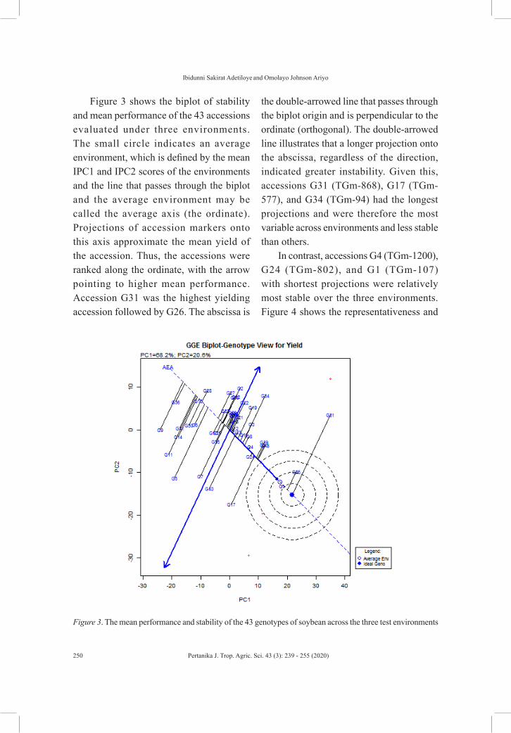
Figure 3 shows the biplot of stability and mean performance of the 43 accessions evaluated under three environments. The small circle indicates an average environment, which is defined by the mean IPC1 and IPC2 scores of the environments and the line that passes through the biplot and the average environment may be called the average axis (the ordinate). Projections of accession markers onto this axis approximate the mean yield of the accession. Thus, the accessions were ranked along the ordinate, with the arrow pointing to higher mean performance. Accession G31 was the highest yielding accession followed by G26. The abscissa is
the double-arrowed line that passes through the biplot origin and is perpendicular to the ordinate (orthogonal). The double-arrowed line illustrates that a longer projection onto the abscissa, regardless of the direction, indicated greater instability. Given this, accessions G31 (TGm-868), G17 (TGm-577), and G34 (TGm-94) had the longest projections and were therefore the most variable across environments and less stable than others.
In contrast, accessions G4 (TGm-1200), G24 (TGm-802), and G1 (TGm-107) with shortest projections were relatively most stable over the three environments. Figure 4 shows the representativeness and
Figure 3. The mean performance and stability of the 43 genotypes of soybean across the three test environments

Studies on GEI and Stability Performances of Soybean
251Pertanika J. Trop. Agric. Sci. 43 (3): 239 - 255 (2020)
discriminating ability of the environments. The biplot explains 88.80% of the total variation. In a biplot analysis the vector length of an environment indicates its discriminating power; the longer the vector from the plot origin, the more discriminatory the environment. The longer the projection, the less representative the environment. Thus, E3 (2015) was the most discriminating environment due to its longest distance from the origin of the biplot while E2 (2014) was the least discriminating. Environments with small vector angles tend to have closer similarity and those with wide vector angles show a minimum association. Environments E1 and E2 were displayed close to each other as the association between them was small. However, the wider angle between E3 and E2; as well as E3 and E1 environments
indicated the absence of association among them.
Similarly, accessions projected further from the ATC y-axis are considered less stable. The center of the concentric circle in a biplot is where an ideal accession should be. An ideal accession is considered as one with the highest yield and stable performance across test environments. Hence, the shorter the distance of accession to the ideal/virtual accession, the more suitable the accession (Yan & Kang, 2003). GGE also picked G31 (TGm-868) as the highest yielding in the E1 and E2 environments. The accessions that combined high yield with stability included G1 (TGm-107), G4 (TGm-1200), and G24 (TGm-802) because of their short projection on the genotype marker lines.
Figure 4. Discriminating ability versus representativeness of the test environmentsE = Environment, G = Genotype

Ibidunni Sakirat Adetiloye and Omolayo Johnson Ariyo
252 Pertanika J. Trop. Agric. Sci. 43 (3): 239 - 255 (2020)
CONCLUSION
AMMI and GGE biplot revealed that accessions G1 (TGm-107), G4 (TGm-1200), and G24 (TGm-802) were the best and stable accessions across environments. This made them the most suitable variety for cultivation across the years. Among the environments, E3 (2015) was found to be the most discriminating, and E2 (2014) was found to be the most representative environment. Both AMMI and GGE agreed on the grouping of environment and the ideal test environment, as well on winner genotypes in this study, although, GGE biplot is believed to be superior to AMMI because it eliminates the environmental components in the analysis.
ACKNOWLEDGMENTS
The authors are grateful to the Genetic Resources Center, International Institute of Tropical Agriculture, Ibadan for providing germplasm for the study.
REFERENCESCucolotto, M., Pipolo, V. C., Garbuglio, D. D., Junior,
N. S. F., Destro, D., & Kamikoga, M. K. (2007). Genotype x environment interaction in soybean: Evaluation through three methodologies. Crop Breeding and Applied Biotechnology, 7, 270-277.
Eberhart, S. A., & Russell, W. A. (1966). Stability parameters for comparing varieties. Crop Science, 6(1), 36-40.
Farshadfar, E., Mahmodi, N., & Yaghotipoor, A. (2011). AMMI stability value and simultaneous estimation of yield and yield stability in bread wheat (Triticum aestivum L.). Australian Journal of Crop Science, 5(13), 1837-1844.
Finlay, K. W., & Wilkinson, G. N. (1963). The analysis of adaptation in a plant-breeding programme. Australian Journal of Biological Science, 14(6), 742-754.
Food and Agriculture Organization. (2016). Country statistics, food and agriculture data network – Nigeria country data. Retrieved 25 September 2019, from www.fao.org
Gauch Jr, H. G. (1992). Statistical analysis of regional yield trials: AMMI analysis of factorial designs. Amsterdam, The Netherlands: Elsevier Science.
Gauch Jr., H. G., & Zobel, R. W. (1996). AMMI analysis of yield trials. In M. S. Kang & H. G. Gauch Jr. (Eds.), Genotype by environment interaction (pp. 85-122). Boca Raton, USA: CRC Press.
Gedif, M., Yigzaw D., & Tsige G. (2014). Genotype-environment interaction and correlation of some stability parameters of total starch yield in potato in Amhara region, Ethiopia. Journal of Plant Breeding and Crop Science, 6(3), 31-40.
Gurmu, F., Mohammed, H., & Alemaw, G. (2009). Genotype x environment interactions and stability of soya bean for grain yield and nutritional quality. African Crop Science Journal, 17(2), 87-99.
Hill, J., & Godchild, N. A. (1981). Analysing environments for plant breeding purposes as exemplified by multivariate analysis of long term wheat yields. Theoretical and Applied Genetics, 59(5), 317-325. doi: 10.1201/9781420049374.ch4
Jandong, E. A., Uguru, M. I., & Oyiga, B. C. (2011). Determination of yield stability of seven soya bean (Glycine max) genotypes across diverse soil pH levels using GGE biplot analysis. Journal of Applied Biosciences, 43, 2924-2941.

Studies on GEI and Stability Performances of Soybean
253Pertanika J. Trop. Agric. Sci. 43 (3): 239 - 255 (2020)
Kang, Y., Khan, S., & Ma, X. (2009). Climate change impacts on crop yield, crop water productivity and food security – A review. Progress in Natural Science, 19(12), 1665-1674.
Mandel, J. (1961). Non-additivity in two-way analysis of variance. Journal American Statistical Association, 65(296), 878-888.
Mohammadi, R., Aghaee, M., Haghparast, R., Pourdad, S. S., Rostaii, M., Ansari, Y., … Amari, A. (2009). Association among non-parametric measures of phenotypic stability in four annual crops. Middle Eastern and Russian Journal of Plant Science and Biotechnology, 3(Special Issue 1), 20-24.
Mut, Z., Aydin, N., Bayramoglu, H. O., & Ozcan, H. (2009). Interpreting genotype x environment interaction in bread wheat (Triticum aestivum L.) genotypes using non-parametric measures. Turkish Journal of Agriculture and Forestry, 33(2), 127-137. doi:10.3906/tar-0803-28
Purchase, J. L. (1997). Parametric analysis to describe genotype x environment interaction and yield stability in winter wheat (Doctoral thesis), University of Free State, Africa.
Rakshit, S., Ganapathy, K. N., Gomashe, S. S., Rathore, A., Ghorade, R. B., Kumar, M. V. N., … Patil, J. V. (2012). GGE biplot analysis to evaluate genotype, environment, and their interaction in sorghum multi-location data. Euphytica, 185(3), 465-479.
Rao, M. S. S., Mullix, B. G., Rangappa, M., Cebertd, V., Bhagsaria, A. S., Saprad, V. T., … Dadsone, R. B. (2002). Genotype × environment interactions and yield stability of food-grade soya bean genotypes. Agronomy Journal, 94(1), 72-80. doi: 10.2134/agronj2002.0072
Rincent, R., Kuhn, E., Monod, H., Oury, F. X., Rousset, M., Allard, V., & le Gouis, J. (2017). Optimization of multi-environment trials for genomic selection based on crop models.
Theoretical and Applied Genetics, 130(8), 1735-1752.
Snedecor, G. W., & Cochran, W. G. (1980). Statistical methods (7th ed.). Iowa City, USA: University of Iowa Press.
Spehar, C. R. (1999). Diallel analysis for grain yield and mineral absorption rate of soybeans grown in acid Brazilian savannah soil. Pesquisa Agropecuária Brasileira, 34(6), 1002-1009.
Tariku, S. (2017). Evaluation of upland rice genotypes and mega environment investigation based on GGE-biplot analysis. Retrieved 24 September, 2019, from https://www.omicsonline.org/open-access/evaluation-of-upland-rice-genotypes-and-mega-environment-investigationbased-on-ggebiplot-analysis-2375-4338-1000183.pdf
Yan, W., & Kang, M. S. (2003). GGE biplot analysis: A graphical tool for breeders, geneticists and agronomists. Boca Raton, USA: CRC Press.
Yan, W., & Rajcan, I. (2002). Biplot analysis of test sites and trait relations of soya bean in Ontario. Crop Science, 42(1), 11-20.
Yan, W., Cornelius, P. L., Crossa, J., & Hunt, L. A. (2001). Two types of GGE biplots for analyzing multi-environment trial data. Crop Science, 41(3), 656-663. doi:10.2135/cropsci2001.413656x
Yothasiri, A., & Somwang, T. (2000). Stability of soybean genotypes in central plain Thailand. National Science, 34(3), 315-322.
Zobel, R. W., Wright, M. J., & Gauch Jr., G. H. (1988). Statistical analysis of a yield trial. Agronomy Journal, 80(3), 388-393. doi:10.2134/agronj1988.0002196008000030002x

Ibidunni Sakirat Adetiloye and Omolayo Johnson Ariyo
254 Pertanika J. Trop. Agric. Sci. 43 (3): 239 - 255 (2020)
APPENDIXAppendix IMonthly meteorological data for the year 2013 at NACGRAB, Ibadan
Month Rainfall (mm) No. of rain day Temperature (oC) Humidity (%)January 0.0 NIL 27 70Febuary 2.1 1 29 66March 14.2 3 29 71April 120.1 5 29 78May 183.4 10 25.6 78June 223.1 10 25.0 78July 161.7 11 24.0 87August 151.5 9 26 87September 232.8 12 25 81October 248.5 16 26.0 87November 11.9 3 27.5 85December 0.0 NIL 26.0 78
Appendix IIMonthly meteorological data for the year 2014 at NACGRAB, Ibadan
Month Rainfall (mm) No. of rain day Temperature (oC) Humidity (%)January 15.3 2 28.0 60Febuary 0.0 Nil 25.0 79March 127.3 7 28.5 78April 261.1 6 24.9 85May 121.1 9 23.8 86June 185.6 13 26.2 88July 243 14 23.5 88August 101 10 24.2 84September 206.4 13 24.7 88October 211.6 14 25.9 87November 22.0 3 27.5 87December 3.0 2 26.8 80

Studies on GEI and Stability Performances of Soybean
255Pertanika J. Trop. Agric. Sci. 43 (3): 239 - 255 (2020)
Appendix IIIMonthly meteorological data for the year 2015 at IITA, Moniya
Month Rainfall (mm) No. of rain day Temperature (oC) Humidity (%)January 12.9 2 30 85Febuary 23.2 3 27.5 83March 90.3 6 27.4 83April 115.6 7 28.1 83May 117 10 26 84June 85.3 7 25.2 85July 462 19 26.6 86August 154.8 5 24.6 87September 345.9 18 24.3 88October 324.1 18 25.8 87November 43.4 3 27.4 82December 0.0 NIL 26.1 83

Pertanika J. Trop. Agric. Sci. 43 (3): 257 - 274 (2020)
© Universiti Putra Malaysia Press
TROPICAL AGRICULTURAL SCIENCEJournal homepage: http://www.pertanika.upm.edu.my/
Article history:Received: 8 January 2020Accepted: 27 April 2020Published: 28 August 2020
ARTICLE INFO
E-mail addresses:[email protected] (Yi Shang Chen)[email protected] (Cheksum Supiah Tawan)* Corresponding author
ISSN: 1511-3701e-ISSN 2231-8542
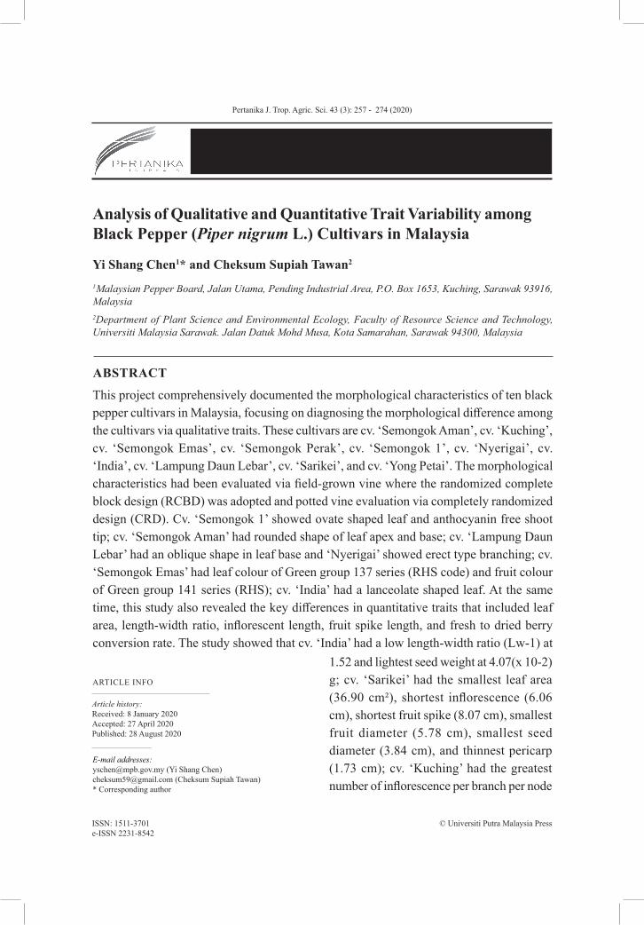
Analysis of Qualitative and Quantitative Trait Variability among Black Pepper (Piper nigrum L.) Cultivars in Malaysia
Yi Shang Chen1* and Cheksum Supiah Tawan2
1Malaysian Pepper Board, Jalan Utama, Pending Industrial Area, P.O. Box 1653, Kuching, Sarawak 93916, Malaysia 2Department of Plant Science and Environmental Ecology, Faculty of Resource Science and Technology, Universiti Malaysia Sarawak. Jalan Datuk Mohd Musa, Kota Samarahan, Sarawak 94300, Malaysia
ABSTRACT
This project comprehensively documented the morphological characteristics of ten black pepper cultivars in Malaysia, focusing on diagnosing the morphological difference among the cultivars via qualitative traits. These cultivars are cv. ‘Semongok Aman’, cv. ‘Kuching’, cv. ‘Semongok Emas’, cv. ‘Semongok Perak’, cv. ‘Semongok 1’, cv. ‘Nyerigai’, cv. ‘India’, cv. ‘Lampung Daun Lebar’, cv. ‘Sarikei’, and cv. ‘Yong Petai’. The morphological characteristics had been evaluated via field-grown vine where the randomized complete block design (RCBD) was adopted and potted vine evaluation via completely randomized design (CRD). Cv. ‘Semongok 1’ showed ovate shaped leaf and anthocyanin free shoot tip; cv. ‘Semongok Aman’ had rounded shape of leaf apex and base; cv. ‘Lampung Daun Lebar’ had an oblique shape in leaf base and ‘Nyerigai’ showed erect type branching; cv. ‘Semongok Emas’ had leaf colour of Green group 137 series (RHS code) and fruit colour of Green group 141 series (RHS); cv. ‘India’ had a lanceolate shaped leaf. At the same time, this study also revealed the key differences in quantitative traits that included leaf area, length-width ratio, inflorescent length, fruit spike length, and fresh to dried berry conversion rate. The study showed that cv. ‘India’ had a low length-width ratio (Lw-1) at
1.52 and lightest seed weight at 4.07(x 10-2)g; cv. ‘Sarikei’ had the smallest leaf area (36.90 cm²), shortest inflorescence (6.06 cm), shortest fruit spike (8.07 cm), smallest fruit diameter (5.78 cm), smallest seed diameter (3.84 cm), and thinnest pericarp (1.73 cm); cv. ‘Kuching’ had the greatest number of inflorescence per branch per node

Yi Shang Chen and Cheksum Supiah Tawan
258 Pertanika J. Trop. Agric. Sci. 43 (3): 257 - 274 (2020)
(ca.58.67) and the greatest number of node/feet of the stem (ca.4.73); cv. ‘Yong Petai’ had the longest inflorescence (12.75 cm), longest fruit spike (17.07 cm), but thinnest fruit spike (2.90 mm); and, lastly, cv. ‘Semongok Perak’ had the conversion rate (from fresh to dried black) (36.12 %) and conversion rate (from fresh to dried white) (24.21 %). The comprehensive evaluation of both qualitative and quantitative traits of all the black pepper cultivars has ensured the efficiency of cultivar identification.
Keywords: Black pepper cultivar, qualitative and
quantitative traits
INTRODUCTION
Black pepper, scientifically called Piper nigrum L., is known as the ‘King of Spice’ and is the most commonly used spice in the world. The plant is woody perennial climber required support, living or non-living to promote normal growth; leaves alternate and petiolate type, with shape commonly elliptical, lanceolate or ovate; inflorescence of catkin types and the flower is minute, bracteates, bisexual or unisexual and protogynous; the fruit of drupe type with thin pericarp and seed spherical shaped with diameter 3-5 mm; nodal stem with internode ranged from 8-13 cm when mature; shoot tip purplish-green or whitish green (Chen, 2011; Ravindran et al., 2000). In India, the morphological analyses of black pepper cultivars were comprehensively studied by Ravindran et al. (1997) through morphometric
analysis. Whilst in Malaysia, Chen et al. (2018) had comprehensive analysis on the morphology of ten important cultivars while Noorasmah et al. (2018) had also recorded the inflorescence characteristics of some important pepper variety.
The plant was introduced to Malaysia as early as 1856 (Dalton, 1912), with cultivation focus in the state of Sarawak. However, the diversity of the black pepper cultivar in Malaysia is unidentified because varietal control is not practised. The most common black pepper cultivars are cv. ‘Kuching’ and cv. ‘Sarikei’, both widely planted throughout Sarawak (Sim, 1993), while Paulus (2007) reported three important cultivars in his publication, i.e. cv. ‘Semongok Perak’, cv. ‘Semongok Aman’, and cv. ‘Kuching’. Through the International Pepper Community (IPC) exchange program, cv. ‘Lampung Daun Lebar’ and cv. ‘Lampung Daun Kecil’ was introduced to Malaysian farmers (Sim, 1993). A manual entitled ‘Pepper production technology in Malaysia’ was recently released by the Malaysian Pepper Board, mentioning the existence of seven cultivated varieties as common cultivars in Malaysia, including cv. ‘Semongok Aman’, cv. ‘Semongok Emas’, cv. ‘Kuching’, cv. ‘Semongok Perak’, cv. ‘Uthirancotta’, cv. ‘Nyerigai’, and cv. ‘PN129’ (Paulus, 2011). A total of 47 accessions of black pepper varieties and 46 accessions of wild Piper were reported, conserved in form of a living plant in the Agricultural Research Centre (ARC) in Sarawak, Malaysia, from 1957 until 1992 (Sim, 1993).

Morphological Analysis of Black Pepper Cultivars
259Pertanika J. Trop. Agric. Sci. 43 (3): 257 - 274 (2020)
Black Pepper Test Guideline for Plant Variety Protection Act implementation has been established by the Department of Agriculture Malaysia (2009). This guideline listed the entire important characteristic for the diagnosis of black pepper variety. However, the existing documentation on cultivated black pepper in Malaysia is less comprehensive, and none of the cultivars is registered under the National Crop List of Malaysia. The importance of this study is to comprehensively document the morphological characteristics of all the important black pepper cultivars in Malaysia, focusing on the diagnosis of the distinctness among the cultivars. The Malaysian government strategized a new policy to ensure the sustainability of the industry by strengthening the quality of peppercorn. A mono-varietal farm concept is believed able to strengthen the quality of peppercorn. This can be achieved through varietal control, and a pre-requisite to this policy is comprehensive documentation on all important cultivars in the country.
MATERIALS AND METHODS
Extensive fieldwork has been undertaken by the first author since January 2014, to cover all the possible black pepper cultivation areas throughout Malaysia, to verify the diversity of black pepper cultivars. The black pepper farm distribution info was sourced from the Department of Crop, Extension, and Farmer’s Development, from the Malaysian Pepper Board. Photography data particularly on the leaf, inflorescence, fruit spike, and shoot tip were comprehensively generated
for the preliminary cultivar’s diagnosis. The preliminary diagnosis must show at least one distinct character to be eligible for further cultivars verification study. The pepper germplasm centre situated at Agricultural Research Centre Semongok (ARC) Sarawak, Malaysia was referred for verification on the cultivar designation.
To develop a comprehensive guide for cultivar identification, a thorough assessment of morphological characteristics (qualitative or quantitative traits) had been conducted. Both potted peppers and field-grown vines were assessed in this study. Vine growing morphology or vigour was assessed on field-grown mature vines at the three field experimental plots while leaf, inflorescence, fruit, and seed morphology studies were based on samples collected from potted mature vines grown under a controlled environment. Data collection was carried out from January 2016 to December 2017. Microscopy assessment and data analysis were performed at the Malaysian Pepper Board, Kuching.
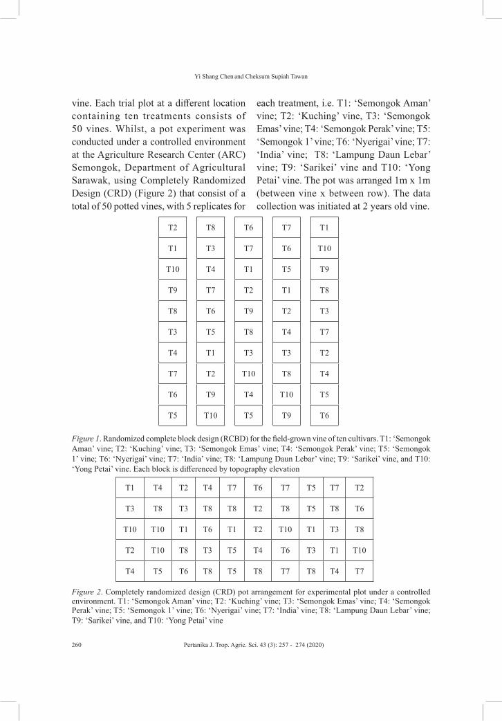
The field experiments were conducted at three locations, namely Kampung Jagoi, Serikin; Kampung Karu, Padawan and Kampung Belawan, Sri Aman. The plots were laid out in a Randomized Complete Block Design (RCBD) (Figure 1) having ten treatment with 5 replications, which are T1: ‘Semongok Aman’ vine; T2: ‘Kuching’ vine, T3: ‘Semongok Emas’ vine; T4: ‘Semongok Perak’ vine; T5: ‘Semongok 1’ vine; T6: ‘Nyerigai’ vine; T7: ‘India’ vine; T8: ‘Lampung Daun Lebar’ vine; T9: ‘Sarikei’ vine and T10: ‘Yong Petai’
Yi Shang Chen and Cheksum Supiah Tawan
260 Pertanika J. Trop. Agric. Sci. 43 (3): 257 - 274 (2020)
vine. Each trial plot at a different location containing ten treatments consists of 50 vines. Whilst, a pot experiment was conducted under a controlled environment at the Agriculture Research Center (ARC) Semongok, Department of Agricultural Sarawak, using Completely Randomized Design (CRD) (Figure 2) that consist of a total of 50 potted vines, with 5 replicates for
each treatment, i.e. T1: ‘Semongok Aman’ vine; T2: ‘Kuching’ vine, T3: ‘Semongok Emas’ vine; T4: ‘Semongok Perak’ vine; T5: ‘Semongok 1’ vine; T6: ‘Nyerigai’ vine; T7: ‘India’ vine; T8: ‘Lampung Daun Lebar’ vine; T9: ‘Sarikei’ vine and T10: ‘Yong Petai’ vine. The pot was arranged 1m x 1m (between vine x between row). The data collection was initiated at 2 years old vine.
T2 T8 T6 T7 T1
T1 T3 T7 T6 T10
T10 T4 T1 T5 T9
T9 T7 T2 T1 T8
T8 T6 T9 T2 T3
T3 T5 T8 T4 T7
T4 T1 T3 T3 T2
T7 T2 T10 T8 T4
T6 T9 T4 T10 T5
T5 T10 T5 T9 T6
Figure 1. Randomized complete block design (RCBD) for the field-grown vine of ten cultivars. T1: ‘Semongok Aman’ vine; T2: ‘Kuching’ vine; T3: ‘Semongok Emas’ vine; T4: ‘Semongok Perak’ vine; T5: ‘Semongok 1’ vine; T6: ‘Nyerigai’ vine; T7: ‘India’ vine; T8: ‘Lampung Daun Lebar’ vine; T9: ‘Sarikei’ vine, and T10: ‘Yong Petai’ vine. Each block is differenced by topography elevation
T1 T4 T2 T4 T7 T6 T7 T5 T7 T2
T3 T8 T3 T8 T8 T2 T8 T5 T8 T6
T10 T10 T1 T6 T1 T2 T10 T1 T3 T8
T2 T10 T8 T3 T5 T4 T6 T3 T1 T10
T4 T5 T6 T8 T5 T8 T7 T8 T4 T7
Figure 2. Completely randomized design (CRD) pot arrangement for experimental plot under a controlled environment. T1: ‘Semongok Aman’ vine; T2: ‘Kuching’ vine; T3: ‘Semongok Emas’ vine; T4: ‘Semongok Perak’ vine; T5: ‘Semongok 1’ vine; T6: ‘Nyerigai’ vine; T7: ‘India’ vine; T8: ‘Lampung Daun Lebar’ vine; T9: ‘Sarikei’ vine, and T10: ‘Yong Petai’ vine

Morphological Analysis of Black Pepper Cultivars
261Pertanika J. Trop. Agric. Sci. 43 (3): 257 - 274 (2020)
A total of 26 morphology characteristics, consisting of both qualitative and quantitative traits, had been assessed in this study, as
listed in Table 1. A dichotomous key for diagnosing the cultivars was constructed as the outcome for this study.
Morphological character Measurement methods
1.
Leaf characters Leaf shape; leaf apex and leaf base Leaf area (cm²); blade width (w) mm; blade length (L) mm and blade length-width ratio (Lw-1) Leaf colour (fully expanded leaf)
Description based on UPOV standardMeasured by WinFOLIA image analysis system
RHS colour codes used 2.
Inflorescence charactersInflorescence length at stigma withering stage (cm) and Inflorescence thickness at stigma withering stage (mm)* Inflorescence colour Number of flowers per inflorescence Number of inflorescence (spike) per branch per node
Measured by Vernier calliper
RHS colour codes usedCounted via stereomicroscope Counted manually
3.
Fruit charactersFruit spike length (cm) and fruit size in diameter (mm) Fruit weight (single fresh berry) (g) Fruit colour (hard dough stage) Per cent fruit set (%)
Conversion rate % (fresh to black pepper)
Conversion rate % (fresh to white pepper)
Pericarp thickness (mm)
Measured by Vernier calliper
Measured by analytical balanceRHS colour codes usedCounted manually. Percent = (Number of developed fruit)/ (Number of developed fruit + number of underdeveloped fruit) x 100%.Measured by analytical balance(Drying specification: Oven dry at 40°C; moisture content ≤12%)Measured by analytical balance(Drying specification: Oven dry at 40°C; moisture content ≤12%)Measured by Vernier calliper (Horizontal diameter of fresh berry - Horizontal diameter of seed)
4.
Seed charactersSeed diameter (mm)
Seed weight (g)
Measured by Vernier calliper (Horizontal diameter of seed)Measured by analytical balance
Table 1Morphological characteristic used for diagnosis of cultivar distinctness

Yi Shang Chen and Cheksum Supiah Tawan
262 Pertanika J. Trop. Agric. Sci. 43 (3): 257 - 274 (2020)
Table 1 (Continued)
Morphological character Measurement methods
5.
Vigour Branch column Internode length (cm) Number of node /1feet stem
By observation Measurement by a ruler (Node to node distance) Counted manually
6.
Shoot tips Anthocyanin: Absent or present By observation on shoot tip colouration
Greenish colour = Absent of anthocyanin; Purplish colour = Present of anthocyanin
RESULTS AND DISCUSSIONS
In this study, a total of ten black pepper cultivars have been assessed, including cul t ivars ‘Semongok Aman’ (SA), ‘Kuching’ (KCH), ‘Semongok Emas’ (SE), ‘Semongok Perak’ (SP), ‘Semongok 1’ (S1), ‘Nyerigai’ (NYE), ‘India’ (IND), ‘Lampung
Daun Lebar’ (LDL), ‘Sarikei’ (SAR), and ‘Yong Petai’ (YP). Comprehensive assessment consisting of both qualitative and quantitative traits had been carried out to reveal key diagnostic morphology for each of the cultivars. The results of the assessment are shown in Table 2.
Note. UPOV- International Union for the Protection of New Varieties of Plants; RHS - Royal Horticultural
Society
Table 2 Qualitative and quantitative traits used to diagnose the differences among black pepper cultivars
No. Morphological characteristic
CultivarsSA KCH SE SP S1
1.2.3.4.5.6.7.
8.
Leaf (Refer to Figure 3)Leaf shape Leaf apex Leaf base Leaf area (cm²)Blade width (w) (cm)Blade length (L) (cm) Blade length-width ratio (Lw-1) Leaf colour (fully expanded leaf)
Elliptical MucronateAcute45.40abc
6.36b
10.70a
1.70b
Green group 139 series
OvateAcute Rounded37.70ab
5.37a
10.83a
2.02d
Green group 139 series
Elliptical Acute Acute46.60bc
5.67a
13.31c
2.35ef
Green group 137 series
Elliptical Acute Oblique62.80d
7.47c
13.20c
1.77bc
Green group NN137
Cordate Acute Cordate132.60f
11.87e
16.67e
1.41a
Green group 139 series

Morphological Analysis of Black Pepper Cultivars
263Pertanika J. Trop. Agric. Sci. 43 (3): 257 - 274 (2020)
No. Morphological characteristic
CultivarsNYE IND LDL SAR YP
1.2.3.4.5.6.7.
8.
Leaf (Refer to Figure 3)Leaf shape Leaf apex Leaf base Leaf area (cm²)Blade width (w) (cm)Blade length (L) (cm) Blade length-width ratio (Lw-1) Leaf colour (fully expanded leaf)
EllipticalAcute Oblique53.60c
6.49b
12.07b
1.86c
Green group 139 series
LanceolateAcuminate Rounded 50.90c
5.75a
13.63c
2.39f
Green group 139 series
OvateAcuteOblique81.40e
8.85d
13.50c
1.52a
Green group NN137
Elliptical AcuteAcute36.90a
5.26a
10.93a
2.10d
Green group 139 series
EllipticalAcuteAcute66.50d
6.62b
14.75d
2.24e
Green group 139 series
Table 2 (Continued)
No. Morphological characteristic
CultivarsSA KCH SE SP S1
9.
10.
11.
12.
13.
Inflorescence (Refer to Figure 4)Inflorescence length (cm) Inflorescence thickness (mm) Inflorescence colour
Number of flowers per inflorescence (average) Number of inflorescence (spike) per branch per node (average)
7.84d
3.50d
Green group 144 series88.30de
12.47a
7.03bc
3.56d
Green group N14467.57ab
58.67f
7.95d
3.47d
Green group N14486.33de
19.57abc
6.93b
3.73e
Green group 145 series72.70abc 22.20bc
12.40e
3.85f
Green group N144127.90g
17.60ab
Yi Shang Chen and Cheksum Supiah Tawan
264 Pertanika J. Trop. Agric. Sci. 43 (3): 257 - 274 (2020)
No. Morphological characteristic
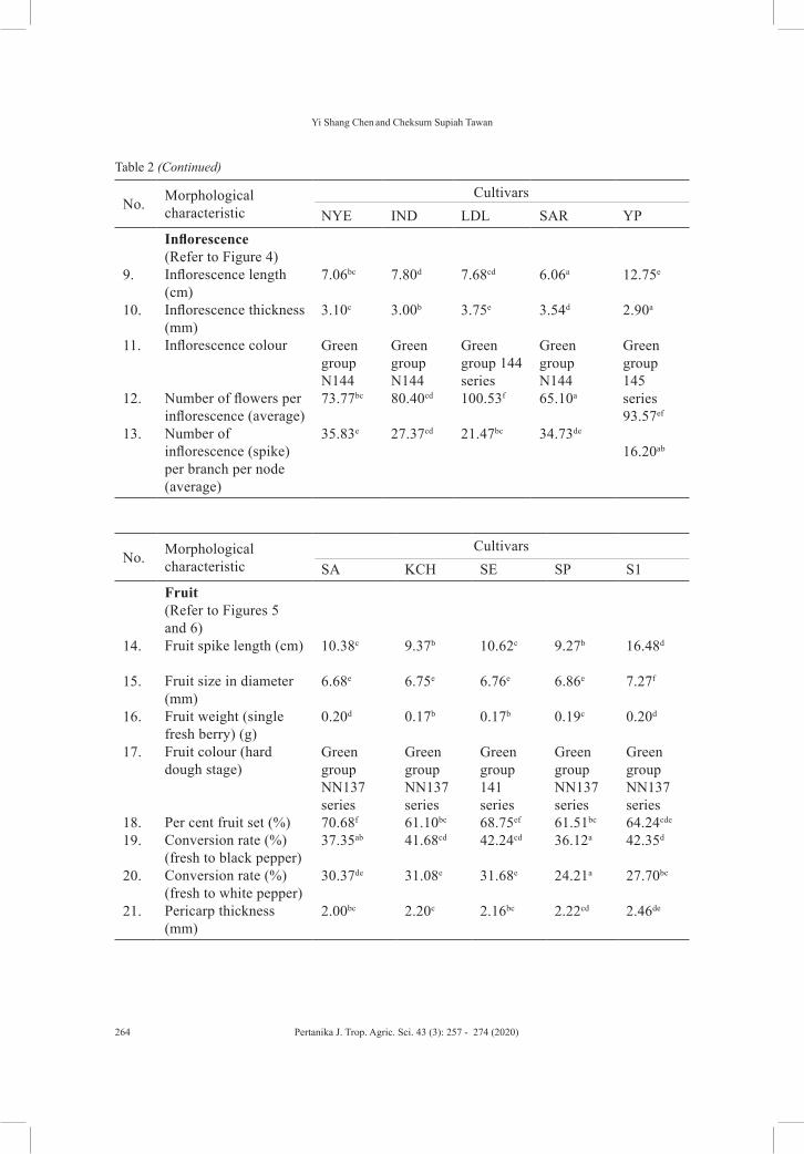
CultivarsNYE IND LDL SAR YP
9.
10.
11.
12.
13.
Inflorescence (Refer to Figure 4)Inflorescence length (cm) Inflorescence thickness (mm) Inflorescence colour
Number of flowers per inflorescence (average) Number of inflorescence (spike) per branch per node (average)
7.06bc
3.10c
Green group N14473.77bc
35.83e
7.80d
3.00b
Green group N14480.40cd
27.37cd
7.68cd
3.75e
Green group 144 series100.53f
21.47bc
6.06a
3.54d
Green group N14465.10a
34.73de
12.75e
2.90a
Green group 145 series 93.57ef
16.20ab
Table 2 (Continued)
No. Morphological characteristic
CultivarsSA KCH SE SP S1
14.
15.
16.
17.
18.19.
20.
21.
Fruit (Refer to Figures 5 and 6)Fruit spike length (cm)
Fruit size in diameter (mm) Fruit weight (single fresh berry) (g) Fruit colour (hard dough stage)
Per cent fruit set (%) Conversion rate (%) (fresh to black pepper) Conversion rate (%) (fresh to white pepper) Pericarp thickness (mm)
10.38c
6.68e
0.20d
Green group NN137 series70.68f
37.35ab
30.37de
2.00bc
9.37b
6.75e
0.17b
Green group NN137 series61.10bc
41.68cd
31.08e
2.20c
10.62c
6.76e
0.17b
Green group 141 series68.75ef
42.24cd
31.68e
2.16bc
9.27b
6.86e
0.19c
Green group NN137 series61.51bc
36.12a
24.21a
2.22cd
16.48d
7.27f
0.20d
Green group NN137 series64.24cde
42.35d
27.70bc
2.46de

Morphological Analysis of Black Pepper Cultivars
265Pertanika J. Trop. Agric. Sci. 43 (3): 257 - 274 (2020)
No. Morphological characteristic
CultivarsNYE IND LDL SAR YP
14.15.
16.
17.
18.19.
20.
21.
Fruit (Refer to Figures 5 and 6)Fruit spike length (cm) Fruit size in diameter (mm) Fruit weight (single fresh berry) (g) Fruit colour (hard dough stage)
Per cent fruit set (%) Conversion rate (%) (fresh to black pepper) Conversion rate (%) (fresh to white pepper) Pericarp thickness (mm)
9.39b
6.48d
0.14a
Green group NN137 series66.93def
41.06bcd
31.89e
2.25cd
10.38c
6.02b
0.14a
Green group NN137 series65.76cdef
40.51bcd
28.16cd
1.94ab
10.22c
6.30c
0.15a
Green group 139
55.10a
38.31abc
29.62cde
2.06bc
8.07a
5.78a
0.17b
Green group NN137 series64.28cde
39.55abcd
29.69cde
1.73a
17.07d
7.27f
0.19cd
Green group NN137 series56.26ab
36.25a
25.70ab
2.69e
Table 2 (Continued)
No. Morphological characteristic
CultivarsSA KCH SE SP S1
22.23.
Seed (Refer to Figure 6)Seed diameter (mm) Seed weight (g) (x 10-2)
4.80e
6.11g4.44c
5.13e4.60d
5.40f4.60d
4.85d4.82e
5.46f
No. Morphological characteristic
CultivarsNYE IND LDL SAR YP
22.23.
Seed (Refer to Figure 6)Seed diameter (mm) Seed weight (g) (x 10-2)
4.44c
4.91d3.90a
4.07a4.32b
4.30b3.84a
4.56c4.45c
4.98de

Yi Shang Chen and Cheksum Supiah Tawan
266 Pertanika J. Trop. Agric. Sci. 43 (3): 257 - 274 (2020)
No. Morphological characteristic
CultivarsSA KCH SE SP S1
24.25.26.
Vigour Branch column types Internode length (cm) Number of node /feet of stem (average)
Horizontal11.42e
3.67ab
Horizontal8.33a
4.73f
Drooping 11.40e
3.33a
Horizontal10.10cd
4.13cdf
Horizontal8.73ab
4.17cdf
No. Morphological characteristic
CultivarsNYE IND LDL SAR YP
24.25.26.
Vigour Branch column types Internode length (cm) Number of node /feet of stem (average)
Erect9.77bc
3.83bc
Horizontal9.57bc
4.30de
Drooping 11.23de
4.43ef
Horizontal9.83bc
3.97bcd
Horizontal12.7f
3.33a
Table 2 (Continued)
No. Morphological characteristic
Cultivars
SA KCH SE SP S1
27.
Shoot tips (Refer to Figure 7)Anthocyanin: Absent or present
Present Present Present Present Absent
No. Morphological characteristic
CultivarsNYE IND LDL SAR YP
27.
Shoot tips (Refer to Figure 7)Anthocyanin: Absent or present
Present Present Present Present Present
Note. SA - ‘Semongok Aman’; KCH - ‘Kuching’; SE - ‘Semongok Emas’; SP - ‘Semongok Perak’; S1 - ‘Semongok 1’; NYE - ‘Nyerigai’; IND - ‘India’; LDL - ‘Lampung Daun Lebar’; SAR - ‘Sarikei’, and YP - ‘Yong Petai’. Means followed by the different superscript letter within the same row are significantly different at P≤0.05

Morphological Analysis of Black Pepper Cultivars
267Pertanika J. Trop. Agric. Sci. 43 (3): 257 - 274 (2020)
The dichotomous key for cultivar diagnosis was constructed by considering both the qualitative and quantitative traits of the ten black peppers.
Identification key to black pepper cultivars in Malaysia:
1a Leaf area <80 cm² (fully developed leaf from matured and vigorous vine); Number of flowers per inflorescence less than 90
2
1b Leaf area >80 cm² (fully developed leaf from matured and vigorous vine); Number of flowers per inflorescence more than 90
8
2a Blade length less than 11 cm long; Blade width-length ratio (Lw-1) ranged from 2.0 to 2.3
3
2b Blade length more than 12 cm long; Blade width-length ratio (Lw-1) ranged from 1.7 to 2.0 or >2.3
4
3a Pericarp thickness 2.0-2.2 mm thick; Seed weight 5.0-5.2 (x 10-2) g
‘Kuching’
3b Pericarp thickness 1.6-1.8 mm thick; Seed weight <4.8 (x 10-2) g
‘Sarikei’
4a Leaf base acute; Percent fruit set >70%
‘Semongok Aman’
4b Leaf base rounded; Percent fruit set 60-70%
5
5a Inflorescence thickness 2.8-3.2 mm thick; Internode 9-10 cm long
6
5b Inflorescence thickness 3.2-4.0 mm thick; Internode 10-11 cm long
7
6a Leaf shape lanceolate; Leaf apex acuminate; Plagiotropic branching horizontal type
‘India’
6b Leaf shape elliptical; Leaf apex acute; Plagiotropic branching erect type
‘Nyerigai’
7a Mature leaf, blueish-green colour (RHS colour code: Green group137 series); Mature unripe fruit, pale green (RHS colour code: Green group 141 series)
‘Semongok Emas’
7b Mature leaf, greyish green colour (RHS colour code: Green group NN137); Mature unripe fruit, dark green (RHS colour code: Green group NN137 series)
‘Semongok Perak’
8a Anthocyanin absent in shoot tip (green whitish colour); Seed weight, >5.4(x 10-2) g; internode length, 8-9 cm
‘Semongok 1’

Yi Shang Chen and Cheksum Supiah Tawan
268 Pertanika J. Trop. Agric. Sci. 43 (3): 257 - 274 (2020)
8b Anthocyanin present in shoot tip (Purplish green colour); Seed weight, <4.8(x 10-2) g or 4.8-5.0(x 10-2) g; internode length, >11 cm
9
9a Fruit spike length, 7-9 cm; Fruit size in diameter, 6-7 mm
‘Lampung Daun Lebar’
9b Fruit spike length, >11 cm; Fruit size in diameter, >7 mm
‘Yong Petai’
Figure 3. Cultivar designation and leaf shape. A. cv. ‘Semongok Aman’- Elliptical; B. cv. ‘Kuching’- Ovate; C. cv. ‘Semongok Emas’- Elliptical; D. cv. ‘Semongok Perak’- Elliptical; E. cv. ‘Semongok 1’- Cordate; F. cv. ‘Nyerigai’- Elliptical; G. cv. ‘India’- Lanceolate; H. cv. ‘Lampung Daun Lebar’- Ovate; I. cv. ‘Sarikei’- Elliptical; J. cv. ‘Yong Petai’- Elliptical. Scale bar: 1cm

Morphological Analysis of Black Pepper Cultivars
269Pertanika J. Trop. Agric. Sci. 43 (3): 257 - 274 (2020)
Figure 4. Inflorescence. SA - ‘Semongok Aman’; SE - ‘Semongok Emas’; KCH - ‘Kuching’; SP - ‘Semongok Perak’; NYE - ‘Nyerigai’; SAR - ‘Sarikei’; IND - ‘India’; S1 - ‘Semongok 1’; YP - ‘Yong Petai’, and LDL - ‘Lampung Daun Lebar’. Scale bar: 2cm
Figure 5. Fruit spike. SA - ‘Semongok Aman’; KCH - ‘Kuching’; SE - ‘Semongok Emas’; SP - ‘Semongok Perak’; S1 - ‘Semongok 1’; NYE - ‘Nyerigai; IND - ‘India’; LDL - ‘Lampung Daun Lebar’; SAR - ‘Sarikei’, and YP - ‘Yong Petai’. Scale bar: 2cm

Yi Shang Chen and Cheksum Supiah Tawan
270 Pertanika J. Trop. Agric. Sci. 43 (3): 257 - 274 (2020)
Figure 6. Cross section of ripe and mature fruit. A. ‘Semongok Aman’; B. ‘Kuching’; C. ‘Semongok Emas’; D. ‘Semongok Perak’; E. ‘Semongok 1’; F. ‘Nyerigai; G. ‘Lampung Daun Lebar’; H. ‘Sarikei’, and I. ‘Yong Petai’. Scale bar: 2mm
Figure 7. Shoot tips. SA - ‘Semongok Aman’; KCH - ‘Kuching’; SE - ‘Semongok Emas’; SP - ‘Semongok Perak’; S1 - ‘Semongok 1’; NYE - ‘Nyerigai; IND - ‘India’; LDL - ‘Lampung Daun Lebar’; SAR - ‘Sarikei’, and YP - ‘Yong Petai’. Scale bar: 1cm

Morphological Analysis of Black Pepper Cultivars
271Pertanika J. Trop. Agric. Sci. 43 (3): 257 - 274 (2020)
Qualitative trait analysis showed leaf shape, leaf apex, leaf base, branch column types (branching behaviour), and anthocyanin colouration at shoot tip were crucial for diagnosing morphological differences among cultivars. Most of the cultivars exhibited elliptical shaped leaf; however, cultivar ‘India’ had a lanceolate shaped leaf and the cultivar ‘Semongok 1’ exhibited cordate-shaped leaf. Thus, leaf shape distinctness is an important key diagnosis for the two cultivars. Leaf apex observation showed cultivar ‘Semongok Aman’ was substantially distinct, with a mucronate-shaped leaf apex; thus, the cultivar could be identified through this trait easily. The only cultivar ‘Lampung Daun Lebar’ showed ovate leaf shape and oblique leaf base at the same time, another important key diagnosis. In branch column analysis, most cultivars showed a horizontal type of branching, but the cultivar ‘Nyerigai’ exhibited an erect type of branching, while both cultivar ‘Semongok Emas’ and cultivar ‘Lampung Daun Lebar’ exhibited a drooping type. Another important key diagnosis is to shoot tip colouration analysis, where the arrival of anthocyanin at the shoot tip will lead to an exhibition of a purplish colour. Among the ten cultivars, the only cultivar ‘Semongok 1’ was anthocyanin-free at the shoot tip, thus exhibiting a whitish-green shoot tip. However, qualitative traits, like leaf colour and inflorescence colour, were less substantial for the diagnosis, because the colour intensity is influenced greatly by biotic and abiotic factors (Anita & Anna, 2012; Szakiel et al., 2011). Analyses in this
study showed qualitative traits are more influential compared to quantitative traits. This is supported by Khan et al. (2015), Olakojo and Adetula (2014), and Stephan et al. (2016). However, qualitative traits alone with limited variability are insufficient for the diagnosis of certain black pepper cultivars. In this study, the ANOVA test proved the variability for quantitative traits was more substantial compare to qualitative traits. The analysis showed seed weight is among the most important quantitative trait, exhibiting seven significantly different groups among the ten cultivars. Next are traits like blade length-width ratio, fruit size in diameter, conversion rate (%) (fresh to black pepper), inflorescence thickness, number of inflorescence per branch per node, number of flower per inflorescence, per cent fruit set (%), number of node/feet of the stem, and internode length that exhibited six significant groups in the ANOVA test, respectively. The quantitative traits of blade width, blade length, pericarp thickness, seed diameter, and conversion rate (fresh to white pepper) showed five significant different groups, also an important diagnosis key for the ten black pepper cultivars. Thus, the quantitative plays a pivotal role as an additional indicator when the qualitative traits are unable to assist the identification.
The phenetic analysis was done by Chen et al. (2018) revealing that cultivars ‘Semongok Aman’ and ‘Semongok 1’ had high distinctive values for identification, thus varietal diagnostic could be very easy. Cultivars ‘Nyerigai’, ‘India’, ‘Semongok Perak’, and ‘Semongok Emas’ were grouped
Yi Shang Chen and Cheksum Supiah Tawan
272 Pertanika J. Trop. Agric. Sci. 43 (3): 257 - 274 (2020)
in the most diverse cluster among all clusters. The four cultivars had a similarity index as high as 92%; however, investigation on leaf width, leaf width-length ratio, seed weight, and conversion rate (fresh to black pepper) could determine the characteristic differences. Cultivar ‘Lampung Daun Lebar’ and the cultivar ‘Yong Petai’ had a similarity of 96%; however, the two showed distinctive differences on leaf width, leaf length-width ratio, spike thickness, and spike length characteristics. The study also reported cultivars ‘Kuching’ and ‘Sarikei’ showed the highest similarity index, thus were among the most difficult cultivars to diagnose morphological differences. This finding proved the importance of both qualitative analysis and quantitative analysis in varietal identification of black pepper cultivars.
CONCLUSIONS
Qualitative trait analysis has assisted the diagnosis of ten important cultivars of black pepper in Malaysia as mentioned above while the quantitative traits are crucial as an additional indicator for the diagnosis beside played the role as an indicator of the potential agronomic performance of the cultivar. This study showed cv. ‘Semongok 1’ exhibited two distinct qualitative traits, a cordate shaped leaf and anthocyanin free shoot tip, and was among the easiest cultivar to identify. Another cultivar with two distinct qualitative traits is cv. ‘Semongok Aman’, with mucronate shaped leaf apex. The identification for this cultivar can be further verified by quantitative traits, counting the
per cent of fruit set. This cultivar exhibited per cent fruit set as high as 76%, averagely. Qualitative trait analysis also discovered the morphological distinctness of cultivar ‘Lampung Daun Lebar’. This cultivar showed ovate leaf shape and oblique leaf base at the same time, unique among all the cultivars. The identification for this cultivar was further supported by the quantitative trait of blade length-width ratio (Lw-1), where the cultivar showed the lowest ratio among all cultivars. Cultivar ‘Nyerigai’ exhibited a unique branching behaviour (branch column type) of an erect type, while others exhibited horizontal or drooping behaviour. The only cultivar that showed a distinctness in leaf and fruit colouration was cv. ‘Semongok Emas’, with the leaf colour of green group 137 series (RHS code) and fruit colour of green group 141 series (RHS). Cultivar ‘India’ exhibited a lanceolate shaped leaf, an important diagnosis key for this cultivar. Quantitative trait uniqueness for this cultivar was seed weight; it was the lightest seed among all. Cv. ‘Kuching’, cv. ‘Sarikei’, cv. ‘Semongok Perak’, and cv. ‘Yong Petai’ did not show qualitative trait distinctness; however, quantitative trait analysis had assisted the diagnosis. Cv. ‘Sarikei’ had a great distinctness in quantitative traits, including the smallest leaf area, shortest inflorescence and fruit spike, smallest fruit and seed size, and thinnest pericarp. Cv. ‘Kuching’ showed the highest number of inflorescence (spike) per branch per node and the greatest number of node/feet of the stem, while cv. ‘Yong Petai’ had the longest inflorescence and

Morphological Analysis of Black Pepper Cultivars
273Pertanika J. Trop. Agric. Sci. 43 (3): 257 - 274 (2020)
fruit spike, but the thinnest fruit spike. Cv. ‘Semongok Perak’ only showed significant variability in the conversion rate (from fresh to dried berry), with the lowest rate in both conversions to black (pericarp remained) and white (pericarp removed) peppercorns. The findings of this study enable efficient identification of black pepper cultivar in Malaysia. This is prerequisite toward implementation of the varietal regulation act in the country, at the same time serve as conservation information for the crop.
ACKNOWLEDGMENTS
The authors would like to thank Mr. Kevin Muyang Anak Tawie for assistance in morphological assessment via WinFOLIA image analysis system. Appreciation also goes to Mr. Wan Ambi and Mr. Juvian Jacob, research assistants of the Malaysian Pepper Board, for their excellent technical assistance in the field. This project is fully funded by the Malaysian Pepper Board, sourced from the Economic Planning Unit (EPU) of Malaysia.
REFERENCES
Anita, B., & Anna, T. (2012). Biotic and abiotic factors affecting the content of the chosen antioxidant compounds in vegetables. Vegetable Crops Research Bulletin, 76(1), 55-78.
Chen, Y. S. (2011). A study on interspecific hybridization between Piper nigrum and Piper colubrinum (Unpublished Master thesis), Universiti Malaysia Sarawak, Malaysia.
Chen, Y. S., Dayod, M., & Tawan, C. S. (2018). Phenetic analysis of cultivated black pepper (Piper nigrum L.) in Malaysia. Retrieved
November 25, 2019, from https://www.hindawi.com/journals/ija/2018/3894924/
Dalton, G. (1912). Pepper growing in upper Sarawak. Sarawak Museum Journal, 1(2), 55.
Department of Agriculture Malaysia. (2009). Plant variety protection: Guidelines for the conduct of tests for distinctness, uniformity and stability on black pepper (Piper nigrum L.). Putrajaya, Malaysia: DOA.
Khan, S. A., Shah, A., Abbasi, F., Javed, A., Rahman, I. U., & Ahmad, H. (2015). Quantitative and qualitative traits analyses in the advance breeding lines of rice. International Journal of Biosciences, 6(8), 50-61.
Noorasmah, S., Nurul A’in, J., & Shiamala, D. R. (2019). Flower composition of black pepper (Piper nigrum L.) varieties in Bintulu, Sarawak. In 28th Malaysian Society of Plant Physiology Conference: Challenges and strategies for plant productivity and resilience, Kelantan, Malaysia, 28-30 August 2018 (pp. 33-38). Serdang, Malaysia: Malaysian Society of Plant Physiology (MSPP).
Olakojo, S. A., & Adetula, O. A. (2014). Comparison of qualitative and quantitative traits of some advanced breeding lines of tomato (Lycopersicon esculentum L.). African Journal of Plant Science, 8(10), 457-461.
Paulus, A. D. (2007). Development of superior genotypes and cultural practices for improving productivity of pepper in Sarawak, Malaysia: Progress, achievements and research needs. In Proceeding of the 2007 Conference on Plantation Commodities (pp. 149-155). Kuala Lumpur, Malaysia: Malaysian Cocoa Board.
Paulus, A. D. (2011). Pepper cultivar. In A. D. Paulus, S. L. Sim, L. Eng, G. Megir, & J. Rosmah (Eds.), Pepper production technology in Malaysia (pp. 60-65). Kuching, Malaysia: Malaysian Pepper Board.

Yi Shang Chen and Cheksum Supiah Tawan
274 Pertanika J. Trop. Agric. Sci. 43 (3): 257 - 274 (2020)
Ravindran, P. N., Balakrishnan, R., & Nirmal Babu, K. (1997). Morphometrical studies on black pepper (P. nigrum L.). I. cluster analysis of black pepper cultivars. Journal of Spices and Aromatic Crops, 6(1), 9-20.
Ravindran, P. N., Nirmal Baru, K., Sasikumar, B., & Krishnamurthy, K. S. (2000). Centres of pepper cultivation. In P. N. Ravindran (Ed.), Black pepper (Piper nigrum): Introduction (pp. 9-14). Amsterdam, Netherlands: Harwood Academy Publishers.
Sim, S. L. (1993). Clonal selection and hybridization in pepper. In M. Y. Ibrahim, C. J. Bong, & I. B. Ipor (Eds.), The pepper industry: Problems and prospects (pp. 48-57). Bintulu, Malaysia: Universiti Pertanian Bintulu Campus.
Stephan, N., Hussein, S., Julia, S., & Kiddo, M. (2016). Screening of Tanzanian sweet potato germplasm for yield and related traits and resistance to sweet potato virus disease. Acta Agriculturae Scandinavica, 66(1), 52-66.
Szakiel, A., Pączkowski, C., & Henry, M. (2011). Influence of environmental biotic factors on the content of saponins in plants. Phytochemistry Reviews, 10(4), 471-491.
Pertanika J. Trop. Agric. Sci. 43 (3): 275 - 287 (2020)
© Universiti Putra Malaysia Press
TROPICAL AGRICULTURAL SCIENCEJournal homepage: http://www.pertanika.upm.edu.my/
Article history:Received: 14 November 2019Accepted: 14 July 2020Published: 28 August 2020
ARTICLE INFO
E-mail addresses:[email protected] (Mui-Yun Wong) [email protected] (Arthy Surendran) [email protected] (Nur Madhihah Saad)[email protected] (Farhana Burhanudin)* Corresponding author
ISSN: 1511-3701e-ISSN: 2231-8542
Chitosan as a Biopesticide against Rice (Oryza sativa) Fungal Pathogens, Pyricularia oryzae and Rhizoctonia solani
Mui-Yun Wong1,2*, Arthy Surendran3, Nur Madhihah Saad1 and Farhana Burhanudin1
1Department of Plant Protection, Faculty of Agriculture, Universiti Putra Malaysia, Serdang, Selangor, Malaysia 2Institute of Plantation Studies, Universiti Putra Malaysia, Serdang, Selangor, Malaysia3School of Biological Sciences, Universiti Sains Malaysia, 11800 Minden, Penang, Malaysia
ABSTRACT
The antifungal potential of chitosan obtained from shellfish was studied in both in vitro and in vivo conditions against Pyricularia oryzae and Rhizoctonia solani, causal agents of the blast and sheath blight diseases in rice, respectively. A total of 100% inhibition of mycelial growth was observed on both P. oryzae and R. solani when a 4% concentration of chitosan was used in this study. A significant reduction in both disease incidence and disease severity was observed between the treated and untreated rice plants. The disease controlling efficacy of chitosan was concentration-dependent with a negative correlation. The disease reduction (DR) capacity of chitosan in this study ranged between 47-95%. Chitosan was able to reduce disease severity (DS) of blast by 85% and sheath blight by 95% while disease incidence (DI) of blast by 77% and sheath blight by 89%. The results demonstrated that chitosan extracted from shellfish has the potential to be developed as a biopesticide for sustainable control of both blast and sheath blight diseases in rice and has broad-spectrum capacity in controlling both diseases. Keywords: Biopesticide, chitosan, rice blast, sheath blight
INTRODUCTION
Rice is the world’s most important food crop and serves as the main source of carbohydrate for many people around the world (Dorairaj et al., 2017). Food security is jeopardized by the increasing world population. Global rice production was estimated to increase by 30% to meet the global food demand in 2030 (Wang

Mui-Yun Wong, Arthy Surendran, Nur Madhihah Saad and Farhana Burhanudin
276 Pertanika J. Trop. Agric. Sci. 43 (3): 275 - 287 (2020)
et al., 2009). However, rice production is threatened by diseases caused by various pathogens. Two (2) most economically important fungal diseases of rice are blast and sheath blight (Yin et al., 2010).
Both blast and sheath blight diseases are caused by fungal pathogens, Pyricularia oryzae and Rhizoctonia solani, respectively. Depending on the environmental factors, both diseases can cause yield loss of up to 85% (Singh et al., 2015). Several fungicides have been successfully employed to control these diseases. However, the emergence of resistant fungal populations, the increasing public awareness on the negative effects caused by excessive application of fungicides and their residues on human health, and the rising demands for chemical-free food have led to a search for safer and more sustainable disease management strategies (Zahid et al., 2014). Apart from chemical control (propiconazole), several cultural practices, namely, field sanitation, crop rotation, and maintaining low seeding rate can control these diseases to a certain extent but their efficacy is inconsistent (Bag, 2009). Hence, there is a need to explore new and ecological-friendly approaches to minimize the application of chemical fungicides such as the use of chitosan as an alternative.
C h i t o s a n [ p o l y - ( 1 - 4 ) - β - D -glucosamine], also known as deacetylated chitin is a marine-based (shellfish) biopolymer comprise of high molecular weight cationic polysaccharide (Yin et al., 2010). Chitosan is found to be one of the few cationic polymers found in nature. This
polycationic nature and the length of the polymer play a key role in the fungicidal property of chitosan. Chitosan which is positively charged by the protonated NH3+ groups interacts with the negatively charged microbial cells creating electrostatic forces that inhibit the growth of fungi (Lawrie et al., 2007) by developing internal osmotic imbalance and hydrolyzing the peptidoglycans in the cell membrane leading to the leakage of internal electrolytes such as potassium ions and low molecular weight proteinaceous constituents such as protein, nucleic acid, and glucose (Bautista-Baños et al., 2006).
Chitosan is known to induce various defense responses including the production of pathogenesis-related proteins as well as phytoalexin (Hassan & Chang, 2017). Chitosan was demonstrated as non-toxic, biodegradable, biocompatible, and possessed antimicrobial properties as well as used to produce an edible coating on fruits to increasing its shelf-life (Zahid et al., 2014). The edible nature of chitosan presents the most desirable aspect to be utilized for disease management in rice. Apart from these, nano/micro-sized chitosan has been used to protect various plants from pathogen infection such as dragon fruit, maize, bell pepper, and cucumber (Elsoud & El Kady, 2019). Liu et al. (2012) had also conducted studies to evaluate the effect of various chitosan to control sheath blight disease. In this study, we have assessed the efficacy of chitosan against both blast and sheath blight diseases in rice (Oryza sativa).

Biopesticide for Fungal Diseases of Rice
277Pertanika J. Trop. Agric. Sci. 43 (3): 275 - 287 (2020)
MATERIALS AND METHODS
Fungal Strains, Culture Conditions, and Plant Materials
Stock cultures of P. oryzae and R. solani were obtained from the Culture Collection Unit, Department of Plant Protection, Faculty of Agriculture, Universiti Putra Malaysia. P. oryzae and R. solani were sub-cultured and maintained on Potato Dextrose Agar (PDA) with a pH of 6, at 27±1°C, and alternating light and dark cycle.
Rice seeds of MR219 variety were obtained from the Department of Plant Protection, Faculty of Agriculture, Universiti Putra Malaysia. The experiment was conducted in the Laboratory of Mycology, Department of Plant Protection and greenhouse, Faculty of Agriculture, Universiti Putra Malaysia.
Preparation of Chitosan Solution
Chitosan powder from shellfish obtained from Pro Advance Technologies Sdn. Bhd. was used as a stock solution by mixing thoroughly 5 g of chitosan powder into 95 g acetic acid. The chitosan powder was made from shellfish. Chitosan solutions with concentrations of 1, 2, and 4% were prepared by diluting the stock solution with sterile distilled water.
In vitro Screening of Chitosan against Pyricularia oryzae and Rhizoctonia solani
Using Poison Agar Assay as described by Bautista-Baños et al. (2004), the preliminary screening was tested using three different chitosan concentrations and control with six
replications for each treatment. PDA was poured into 90 mm diameter Petri plates. Then, 200 µL of each concentration: 1% (T1), 2% (T2), and 4% (T3) was spread over the PDA medium with a sterilized L-shaped glass rod. Control plates contained PDA added with 200 µL of acetic acid (5 mL water mixed with 95 mL acetic acid). A fungal plug of 7 mm diameter from a pure culture of 10 days old P. oryzae and R. solani were inoculated on the center of the plates, respectively. Petri plates were incubated at 28±2°C for 5 days (Bautista Baños et al., 2004).
Percent inhibition of radial growth (PIRG) was ca l cu l a t ed according to Hayman et al. (2017):
PIRG % = [(C− T ) C⁄ ] × 100
where C - mycelium average growth on the control plate (cm); T - mycelium average growth on the treated plate (cm).
In vivo Screening of Chitosan against Pyricularia oryzae and Rhizoctonia solani
Seed Preparation. Rice seeds were surface sterilized with benomyl fungicide for 18 h to prevent any microbial infection. The seeds were soaked in distilled water and dried for 24 h. Germinated seeds were selected and sowed on trays until they produced true leaves (on the 14th day). On Day 15, the plants were transplanted into pots containing 5 kg soil (3: 2: 1 - topsoil: sand: compost). The water level was maintained at 1–2 cm above the soil surface during the early growth stage and was further raised to 5–7

Mui-Yun Wong, Arthy Surendran, Nur Madhihah Saad and Farhana Burhanudin
278 Pertanika J. Trop. Agric. Sci. 43 (3): 275 - 287 (2020)
cm at the later growth stage (Hashim et al., 2015). Each treatment was replicated five times and each replication consisted of four plants in a pot.
Chitosan Application on Rice Plants. Only the best two concentrations tested in vitro were selected for the greenhouse study. Leaves sprayed with 2% (T1) and 4% (T2) chitosan until run-off was performed as described by Liu et al. (2012) at 20 days after transplant with the aid of a hand-held sprayer. Control plants were sprayed with distilled water until run-off (T3).
Inoculum Preparation. Pyricularia oryzae inoculum was prepared as described by Tuhina-Khatun et al. (2015). P. oryzae was maintained on PDA and incubated in the growth chamber at 28±2°C. Conidia spores were harvested at 21 days. Spore density was adjusted to 2 × 10⁵ spores/mL using haemacytometer and 0.05% Tween 20 was added to the spore suspension as an adjuvant before inoculation.
Rhizoctonia solani was maintained on PDA and incubated in the growth chamber at 28±2°C for five days. The mycelium was cut into plugs of 5 mm diameter using sterilized cork borer and used as inoculum (Tuhina-Khatun et al., 2015).
Inoculat ion of MR219 Rice with Pyricularia oryzae and Rhizoctonia solani. Both P. oryzae and R. solani were inoculated on the 21st day after planting. P. oryzae was inoculated by spraying 25 mL spore suspension of 2 × 10⁵ spores/mL onto the whole plant. In the case of R. solani, mycelial plugs were placed on the stems at one cm below the axial o f fully mature leaf and wrapped with parafilm (Khaing et al., 2015; Park et al., 2008). After pathogen inoculation, the plants were covered with plastic bags for 12 h to stimulate infection.
Experimental Design. A completely randomized design (CRD) was implemented in a pot experiment with five replications for each treatment. The same experimental design was used for both the fungi. Three (3) treatments were conducted: T1 (2% chitosan + pathogens), T2 (4% chitosan + pathogens), and T3 (0% chitosan + pathogens) as control.
Disease Assessment. Each disease was assessed on the seventh day after inoculation using a disease rating scale as shown in Table 1 (Khaing et al., 2015).
Disease incidence (DI) was calculated based on the following equation (1) (Maclean et al., 2002) as follows:
Disease incidence (%) = Total number of infected tillersTotal number of tillers per hill
× 100% (1)
Disease severity (DS) was calculated based on the following equation (2) (Lim & Heong, 1984):
Disease Severity % =∑N umber of seedlings in the rating X rating number
Total number of seedling assessed X highest rating × 100 (2)

Biopesticide for Fungal Diseases of Rice
279Pertanika J. Trop. Agric. Sci. 43 (3): 275 - 287 (2020)
Disease reduction (DR) was calculated based on the following equation (3):
Disease Reduction % =DSc −DSt
DSc × 100 (3)
where DSc - disease severity of control plants; DSt – disease severity of treated plants.
Table 1Blast and sheath blight disease rating scale used in this study
Points DescriptionaBlast disease bSheath blight disease
0 No symptoms 1 Small brown specks of pinpoint size Restricted dark brown oval lesions at waterline or
infection points2 Small roundish to slightly elongated,
necrotic grey spots, about 1-2 mm in diameter, with a distinct brown margin. Lesions are mostly found on the lower leaves
Few oval or coalesced lesions with broad borders on lower sheaths or at infection points, 5% or less of tissue affected
3 Lesion type same as in 2, but a significant number of lesions on the upper leaves
Lesions on lower leaf sheaths or at infection points, lesions coalescing, less than 10% of tissues affected.
4 Typical susceptible blast lesions, 3 mm or longer infecting less than 4% of leaf area
Lesions mainly restricted to sheaths on the lower third of plant, lowest leaves, or other infection points, lesions discrete or coalescing with narrow red-brown border, 10 to 15% of leaf and sheath tissues affected
5 Typical susceptible blast lesions of 3 mm or longer infecting 4-10% of the leaf area
Lesions coalescing with large necrotic centers and narrow red-brown borders, 15 to 25% of tissues affected
6 Typical susceptible blast lesions of 3 mm or longer infecting 11-25% of the leaf area
Lesions extending to blades of lower leaves or lower leaves killed by injury to the sheath, 25 to 40% of tissues affected
7 Typical susceptible blast lesions of 3 mm or longer infecting 26-50% of the leaf area
Lesions extending to leaf blades of lower two-thirds of plant, 40 to 60% of tissues affected
8 Typical susceptible blast lesions of 3 mm or longer infecting 51-75% of the leaf area many leaves are dead
Lower and middle leaves dead or dying, 60 to 80% of tissues affected
9 Typical susceptible blast lesions of 3 mm or longer infecting more than 75% leaf area affected
Lesions reaching to flag leaf, lower leaves mostly dead, sheath dried, culms brown, collapsing, most tillers lodged, over 80% of tissues affected
Note. a Disease assessment score for blast disease (Lim & Heong, 1984); bDisease assessment score for Sheath blight disease (Khaing et al., 2015)
Statistical Analyses
All data were subjected to analysis of variance (ANOVA) (SAS, Cary, USA)
according to the experimental design used in this study and t h e least significant difference (LSD) was utilized to compare

Mui-Yun Wong, Arthy Surendran, Nur Madhihah Saad and Farhana Burhanudin
280 Pertanika J. Trop. Agric. Sci. 43 (3): 275 - 287 (2020)
the different means of treatment. The correlation analysis was performed using Microsoft Excel 2010.
RESULTS
In vitro Screening of Chitosan against Pyricularia oryzae and Rhizoctonia solani
Mycelial growth of P. oryzae and R. solani was inhibited by chitosan of different concentrations (Figure 1) and the e ff icacy of chitosan to inhibit the fungal growth was concentration-dependent. For P. oryzae, no significant mycelial inhibition was observed in T1 (1% chitosan) with only 0.4% of PIRG. As the concentration of chitosan was increased to 2% (T2), the PIRG value increased to 26.5%. An absolute inhibition of P. oryzae mycelial growth was observed on plates with 4% chitosan (T3).
A similar trend was observed in the inhibition of R. solani. Chitosan of 1% (T1) inhibited slightly the mycelial growth
of R. solani with PIRG 3.5% while chitosan of 2% (T2) was able to increase PIRG up to 30% and chitosan of 4% (T3) had achieved total inhibition of mycelial growth with PIRG 100%.
In vivo Screening of Chitosan against Pyricularia oryzae and Rhizoctonia solani
Disease Incidence and Disease Severity. Disease incidence (DI) and disease severity (DS) of rice plants infected with P. oryzae and R. solani in separate trials were tabulated in Table 2. Disease development in rice plants occurred between 7 to 12 days after the inoculation of both fungi separately. For P. oryzae, a pinpoint-sized brown color speck appeared on the seventh day and developed into diamond-shaped lesions with brown borders (Figure 2a) in five plants infected with P. oryzae in the control treatment (T3, 0% chitosan). There was a significant (p≤0.005) difference in both DI and DS between the treated (T1-2% chitosan, T2-
0
20
40
60
80
100
120
1 2 4
PIR
G (
%)
Concentration of chitosan (%)
Pyricularia oryzae
Rhizoctonia solani
a a
b b
c c
Figure 1. Percent inhibition of radial growth (PIRG) of Pyricularia oryzae and Rhizoctonia solani at 5 days after plating using poison agar assay with different concentrations of chitosan on PDA medium. Vertical bars indicate standard error of six replicates. Bars with the same alphabets are not significantly different. The standard error for concentration 4% was zero
Pyricularia oryzae
Rhizoctonia solani

Biopesticide for Fungal Diseases of Rice
281Pertanika J. Trop. Agric. Sci. 43 (3): 275 - 287 (2020)
Table 2Disease incidence and disease severity for blast and sheath blight diseases on rice plants with or without treatment of chitosan at 7 days after pathogen inoculation
Blast disease Sheath blight diseaseTreatment T1 T2 T3 T1 T2 T3Disease Incidence (%) 44.7±1.6b 19.4±1.5c 84.1±5.3a 28.8±5.5b 6.1±5.6c 56.4±7.1a
Disease Severity (%) 22.8±1.6b 10.9±0.6c 71.1±5.8a 7.8±1.7b 1.0±0.8b 22.9±9.9a
Note. T1 = 2% chitosan; T2 = 4% chitosan; T3 = 0% chitosan. Values are mean of five replications. Values with the same alphabets in the same row for a respective disease are not significantly different
4% chitosan) and the control (T3) plants. The control plants (T3) exhibited two folds higher DI (84.1%) and DS (71.1%) compared to the 2% chitosan treated (T1) plants (44.7% and 22.8%, respectively). The lowest DI (19.4%) and DS (10.9%) were observed in plants treated with 4% chitosan (T2).
A similar trend was observed for sheath blight disease. However, the intensity of sheath blight disease was slightly lower than the blast disease. The appearance of a very small dark brown lesion that was oval-shaped was observed in the control (T3, 0% chitosan) plants on the seventh day and developed into irregular lesions with white-gray centers and brown margins (Figure 2b). The result also revealed a significant difference in the values of DI
(a) (b)
Figure 2. Symptoms of rice blast (a) and sheath blight (b) diseases at 12 days after inoculation
and DS between the treated (T1, T2) and control (T3) plants. Rice plants treated with 4% chitosan (T2) were shown to be effective in controlling sheath blight disease with the minimum DI (7.8%) and DS (1.0%). However, no significant difference was observed in DI and DS between plants treated with 2% (T1) and 4% (T2) chitosan.
Disease Reduction (DR). Chitosan was shown to be effective in controlling both blast and sheath blight diseases in MR219 plants. For disease incidence (DI), there was no significant difference in DR of plants treated with 2% chitosan between blast and sheath blight diseases (46.8 and 48.9%, respectively) (Figure 3). The highest DR was observed in plants pre-treated with 4% chitosan and challenged with R. solani (89.1%) followed by those challenged with P. oryzae (76.9%) and there was also no significant difference in DR between the two diseases. However, there was a significant difference in DR between the concentrations used (2% vs 4%) for both blast and sheath blight diseases. Chitosan at 4% demonstrated significantly higher DR for DI compared to chitosan at 2% in both diseases.

Mui-Yun Wong, Arthy Surendran, Nur Madhihah Saad and Farhana Burhanudin
282 Pertanika J. Trop. Agric. Sci. 43 (3): 275 - 287 (2020)
A similar trend was observed for disease severity (DS) (Figure 4). At 2%, there was no significant difference in DR between plants challenged with P. oryzae (67%) and R. solani (61%), a n d at 4%, plants challenged with P. oryzae (84.5%) and R. solani (95.0%). However, for both diseases, there was a significant difference in DR between the concentrations used
(2% vs 4%). Chitosan at 4% demonstrated significantly higher DR for DS compared to chitosan at 2% in both diseases.
Correlation AnalysisTable 3 shows the correlation analysis (r values). For blast disease, the r-value (-0.6) between the treatment and DI was weak and negatively correlated but the r-value (-0.9)
Figure 3. Disease reduction (DR) in disease incidence (DI) of the blast and sheath blight diseases in greenhouse condition with two different concentrations of chitosan as treatments on rice plants. Vertical bars indicate standard error of five replicates. Bars with the same alphabets are not significantly different
0102030405060708090
100
2 4
Red
ucti
on o
f Dis
ease
Sev
erit
y (%
)
Concentration of Chitosan (%)
Blast diseaseSheath blight disease
aa
bb
0102030405060708090
100
2 4
Red
ucti
on o
f Dis
ease
Inci
denc
e (%
)
Concentration of Chitosan (%)
Blast diseaseSheath blight disease
b
aa
b
Figure 4. Disease reduction (DR) in disease severity (DS) of the blast and sheath blight diseases in greenhouse condition with two different concentrations of chitosan as treatments on rice plants. Vertical bars indicate standard error of five replicates. Bars with the same alphabets are not significantly different

Biopesticide for Fungal Diseases of Rice
283Pertanika J. Trop. Agric. Sci. 43 (3): 275 - 287 (2020)
between the treatment and DS was strong and negatively correlated. The negative r value indicates that the higher chitosan concentration used a higher reduction in DI and DS values in rice plants. This indicates that chitosan demonstrated a stronger effect in the reduction of DS than DI. In the case of sheath blight disease, the interaction between treatment, DI and DS was strong and negatively correlated (r = -0.9). In conclusion, chitosan has the potential to control blast and sheath blight diseases in the field.
DISCUSSION
The positive effects of chitosan have been documented in various pathosystems involved in a wide range of plants including both monocotyledon (rice) and dicotyledon (bell pepper, cucumber, dragon fruit), and a diverse range of pathogens including fungi, bacteria, and viruses (Zahid et al., 2014). In this study, we studied the effects of chitosan on rice against the infection of two important fungal pathogens, namely P. oryzae and R. solani.
In this study, the in vitro antifungal test revealed that chitosan was effective against both P. oryzae and R. solani, which inhibited the mycelial growth of both fungi at the highest concentration used (4%). The rate of inhibition of radial growth by chitosan was concentration-dependent similar to the biostimulants (Surendran et al., 2017). Other studies reported a similar effect when chitosan was used against various plant pathogenic fungi in vitro. When the concentration of chitosan was increased from 0.75 to 6.0 mg mL-1 in the PDA medium, decrement in the radial growth of Alternaria alternata, Botrytis cinerea, Rhizopus stolonifer, and Colletrotichum gloeosporioides was observed (El Ghaouth et al., 1992). A similar effect was also reported in Sclerotinia sclerotiorum when chitosan concentration was increased from 1 to 4% (W/V) (Junior et al., 2016). Complete inhibition of the fungi R. stolonifer, Fusarium oxysporum, Penicillium digitatum, and C. gloeosporioides was obtained at a concentration of 3% (w/v) (Bautista-Baños et al., 2003, 2004).
Table 3Correlation analysis between the treatment, disease incidence and disease severity in rice plants
Blast disease Treatments Disease Incidence Disease severity
Treatments 1Disease incidence -0.60 1Disease severity -0.94 0.83 1Sheath blight disease Treatments 1Disease incidence -0.99 1Disease severity -0.98 0.99 1

Mui-Yun Wong, Arthy Surendran, Nur Madhihah Saad and Farhana Burhanudin
284 Pertanika J. Trop. Agric. Sci. 43 (3): 275 - 287 (2020)
Similarly, in this study, the in vivo trial results demonstrated that chitosan at 4% concentration was effective to control both blast and sheath blight diseases with more than 80% disease reduction. Chitosan was used to control various Fusarium spp. in various economically important hosts including Fusarium oxysporum, Fusarium graminearum, and Fusarium solani in tomato, wheat, and peas, respectively by reducing DI more than 50% (Al‐Hetar et al., 2011; Prapagdee et al., 2007; Sharp, 2013). It was also found that chitosan (0.2 mg/mL) had induced a delayed disease appearance in rice plants (three weeks old) and thus, reduced the disease symptoms in plants (Liu et al., 2012). Boonreung and Boonlertnirun (2013) reported that chitosan sprayed at a concentration of 40 mg/L for four times throughout the crop season before the inoculation of Helminthosporium oryzae, Curvularia lunata, and Fusarium moniliformae reduced 12% of dirty panicle diseases in rice. However, in this study, 4% chitosan spray once throughout the crop season before inoculation of P. oryzae and R. solani was able to reduce disease severity by 85 and 95%, respectively.
Apart from disturbing the cell wall of the pathogens, chitosan by itself can be a physical barrier to pathogen attack by creating a barrier film or chelating the minerals and make them inaccessible to the pathogens. Chitosan is capable of eliminating the necrotrophic pathogens by neutralizing the mycotoxin produced by these pathogens (Sudarshan et al., 1992). Hence, we speculate that the inhibitory
effect of chitosan against P. oryzae (a hemibiotroph) in this study was by creating a barrier film or chelating minerals and against R. solani (a necrotroph) by neutralizing the mycotoxins produced. These phenomena indicate that chitosan may use a double mechanism of actions to control both types of pathogens.
The nano-sized chitosan was able to control blast disease caused by Pyricularia grisea with 100% disease reduction by inducing systemic acquired resistance (SAR) in rice (Xing et al., 2015). Most of the chitosan used in the above-mentioned studies were modified into different forms including nano-sized chitosan because some evidence stated that the negative effect of chitosan on plant growth, shoot length when used in higher concentration in the natural form has been reported (Sandford, 2003). However, the natural chitosan obtained from shellfish used in our study at 4% had revealed a superior disease reduction capacity of 95.0% against sheath blight and 84.5% against blast disease. Chitosan has been produced from various sources ranging from fungi to plants. However, chitosan extracted from shellfish will incur lower costs because it is produced from waste products of the seafood industry (Peniche et al., 2008).
Chitosan and its derivatives have emerged as the best eco-friendly bio-pesticides in the last few decades (Peniche et al., 2008). Other than controlling various plant diseases, chitosan also increases the population of nitrogen-fixing bacteria and vesicular-arbuscular mycorrhizal fungi

Biopesticide for Fungal Diseases of Rice
285Pertanika J. Trop. Agric. Sci. 43 (3): 275 - 287 (2020)
(VAM) (Bautista-Baños et al., 2006). US Environmental Protection Agency in 2015 has concluded that chitosan produces no negative impact on the environment (Hassan & Chang, 2017). Due to its eco-friendly and low production cost, chitosan has a huge potential to be used as a biocontrol strategy for sustainable disease management, not only in rice but in other crops as well.
CONCLUSION
To the best knowledge of the authors, this is the first report on the high efficacy and broad-spectrum capacity of chitosan at low concentrations for the control of both blast and sheath blight diseases of rice. Chitosan at 4% concentration had shown a disease severity reduction capacity of 85 and 95% in blast and sheath blight diseases, respectively. To validate this result, field study is required to test the consistency of chitosan in controlling these two fungal diseases in rice. Due to the high demand of rice around the world, these findings could potentially bridge the yield gap in the near future as well as contribute to a sustainable crop production system.
ACKNOWLEDGMENT
The authors thank Pro Advance Technologies Sdn. Bhd. for providing chitosan and Department of Plant Protection, Faculty of Agriculture, Universiti Putra Malaysia for providing research materials used in this study.
REFERENCES Al-Hetar, M. Y., Zainal Abidin, M. A., Sariah, M.,
& Wong, M. Y. (2011). Antifungal activity of chitosan against Fusarium oxysporum f. sp. cubense. Journal of Applied Polymer Science, 120(4), 2434-2439.
Bag, M. K. (2009). Efficacy of a new fungicide ‘Trifloxystrobin 25%+ Tebuconazole 50%’75WG against sheath blight (Rhizoctonia solani Kühn) of rice. Journal of Crop and Weed, 5(1), 224-226.
Bautista-Baños, S., Hernández-López, M., Bosquez-Molina, E., & Wilson, C. L. (2003). Effects of chitosan and plant extracts on growth of Colletotrichum gloeosporioides, anthracnose levels and quality of papaya fruit. Crop Protection, 22(9), 1087-1092.
Bautista-Baños, S., Hernandez-Lauzardo, A. N., Velazquez-Del Valle, M. G., Hernández-López, M., Barka, E. A., Bosquez-Molina, E., & Wilson, C. (2006). Chitosan as a potential natural compound to control pre and postharvest diseases of horticultural commodities. Crop Protection, 25(2), 108-118.
Bautista-Baños, S., Hernández-López, M., & Bosquez-Molina, E. (2004). Growth inhibition of selected fungi by chitosan and plant extracts. Mexican Journal of Phytopathology, 22, 178–186.
Boonreung, C., & Boonlertnirun, S. (2013). Efficiency of chitosan for controlling dirty panicle disease in rice plants. Journal of Agricultural and Biological Science, 8(5), 380-384.
Dorairaj, D., & Ismail, M. R. (2017). Distribution of silicified microstructures, regulation of cinnamyl alcohol dehydrogenase and lodging resistance in silicon and paclobutrazol mediated Oryza sativa. Frontiers in Physiology, 8, 491.
El Ghaouth, A., Arul, J., Grenier, J., & Asselin, A. (1992). Antifungal activity of chitosan on two postharvest pathogens of strawberry fruits. Phytopathology, 82(4), 398-402.
Mui-Yun Wong, Arthy Surendran, Nur Madhihah Saad and Farhana Burhanudin
286 Pertanika J. Trop. Agric. Sci. 43 (3): 275 - 287 (2020)
Elsoud, M. M. A., & El Kady, E. M. (2019). Current trends in fungal biosynthesis of chitin and chitosan. Bulletin of the National Research Centre, 43(1), 1-12.
Hashim, M. M. A., Yusop, M. K., Othman, R., & Wahid, S. A. (2015). Characterization of nitrogen uptake pattern in Malaysian rice MR219 at different growth stages using 15N isotope. Rice Science, 22(5), 250-254.
Hassan, O., & Chang, T. (2017). Chitosan for eco-friendly control of plant disease. Asian Journal of Plant Pathology, 11(2), 53-70.
Hayman, K. A, Tavga, S. R., Sathyapriya, H., & Mui-Yun, W. (2017). Plant growth-promoting abilities and biocontrol efficacy of Streptomyces sp. UPMRS4 against Pyricularia oryzae. Biological Control, 112, 55-63.
Junior, E. N. D. O. (2016). Fungal growth control by chitosan and derivatives. Retrieved October 27, 2019, from https://cdn.intechopen.com/pdfs/50273.pdf
Khaing, E. E., Ahmad, Z. A. M., Mui-Yun, W., & Ismail, M. R. (2015). Effect of silicon and spacing on rice sheath blight disease severity and yield. International Journal of Enhanced Research in Science Technology and Engineering, 4, 7-11.
Lawrie, G., Keen, I., Drew, B., Chandler-Temple, A., Rintoul, L., Fredericks, P., & Grøndahl, L. (2007). Interactions between alginate and chitosan biopolymers characterized using FTIR and XPS. Biomacromolecules, 8(8), 2533-2541.
Lim, G., & Heong, K. (1984). The role of insecticides in rice integrated pest management. In FAO/IRRI Workshop on Judicious and Efficient Use of Insectcides on Rice (pp. 19-39). Los Baños, Philippines: International Rice Research Institute.
Liu, H., Tian, W., Li, B., Wu, G., Ibrahim, M., Tao, Z., ... Sun, G. (2012). Antifungal effect and mechanism of chitosan against the rice
sheath blight pathogen, Rhizoctonia solani. Biotechnology Letters, 34(12), 2291-2298.
Maclean, J. L., Dawe, D. C., Hardy, B., & Hettel, G. P. (Eds.). (2002). Rice almanac: Source book for the most important economic activity on earth (3rd ed.). Wallingford, United Kingdom: CABI Publishing.
Park, S. J., Kim, S. L., Lee, S., Je, B. I., Piao, H. L., Park, S. H., . . . Xuan, Y. H. (2008). Rice Indeterminate 1 (OsId1) is necessary for the expression of Ehd1 (Early heading date 1) regardless of photoperiod. The Plant Journal, 56(6), 1018-1029.
Prapagdee, B., Kotchadat, K., Kumsopa, A., & Visarathanonth, N. (2007). The role of chitosan in protection of soybean from sudden death syndrome caused by Fusarium solani f. sp. glycines. Bioresource Technology, 98(7), 1353-1358.
Peniche, C., Argüelles-Monal, W., & Goycoolea, F. M. (2008). Chitin and chitosan: Major sources, properties and applications. In M. N. Belgacem & A. Gandini (Eds.), Monomers, polymers and composites from renewable resources (pp. 517-542). Oxford, United Kingdom: Elsevier.
Sandford, P. (2003). Commercial sources of chitin and chitosan and their utilization. Advances in Chitin Science, 6, 35-42.
Sharp, R. G. (2013). A review of the applications of chitin and its derivatives in agriculture to modify plant-microbial interactions and improve crop yields. Agronomy, 3(4), 757-793.
Singh, M., & Upadhyaya, H. D. (Eds.). (2015). Genetic and genomic resources for grain cereals improvement. London, United Kingdom: Academic Press.
Sudarshan, N., Hoover, D., & Knorr, D. (1992). Antibacterial action of chitosan. Food Biotechnology, 6(3), 257-272.

Biopesticide for Fungal Diseases of Rice
287Pertanika J. Trop. Agric. Sci. 43 (3): 275 - 287 (2020)
Surendran, A., Siddiqui, Y., Saud, H. M., & Manickam, N. (2017). The antagonistic effect of phenolic compounds on ligninolytic and cellulolytic enzymes of Ganoderma boninense, causing basal stem rot in Oil Palm. International Journal of Agriculture and Biology., 19, 1437-1446.
Tuhina-Khatun, M., Hanafi, M., Wong, M., & Rafii, M. (2015). Reactions and diversity analysis of upland rice genotypes against blast disease of rice (Oryza sativa L.). Australasian Plant Pathology, 44(4), 405-412.
Wang, G.-L.., & Valent, B. (Eds.). (2009). Advances in genetics, genomics and control of rice blast disease. Berlin, Germany: Springer Science and Business Media.
Xing, K., Zhu, X., Peng, X., & Qin, S. (2015). Chitosan antimicrobial and eliciting properties for pest control in agriculture: A review. Agronomy for Sustainable Development, 35(2), 569-588.
Yin, H., Zhao, X., & Du, Y. (2010). Oligochitosan: A plant diseases vaccine - A review. Carbohydrate Polymers, 82(1), 1-8.
Zahid, N., Ali, A., Manickam, S., Siddiqui, Y., Alderson, P. G., & Maqbool, M. (2014). Efficacy of curative applications of submicron chitosan dispersions on anthracnose intensity and vegetative growth of dragon fruit plants. Crop Protection, 62, 129-134.


Pertanika J. Trop. Agric. Sci. 43 (3): 289 - 302 (2020)
© Universiti Putra Malaysia Press
TROPICAL AGRICULTURAL SCIENCEJournal homepage: http://www.pertanika.upm.edu.my/
Article history:Received: 19 February 2020Accepted: 08 July 2020Published: 28 August 2020
ARTICLE INFO
E-mail addresses:[email protected] (Dina Maulina)[email protected] (Mohamad Amin)[email protected] (Sutiman Bambang Sumitro)[email protected] (Sri Rahayu Lestari)[email protected] (Tri Suwandi)* Corresponding author
ISSN: 1511-3701e-ISSN: 2231-8542
Screening and Evaluation of Biopesticide Compounds from Mirabilis jalapa L. (Caryophyllales: Nyctaginaceae) and Its Combination with Bacillus thuringiensis against Spodoptera litura F. (Lepidoptera: Noctudiae)
Dina Maulina1*, Mohamad Amin2, Sutiman Bambang Sumitro3, Sri Rahayu Lestari4 and Tri Suwandi5
1Biology Education, Faculty of Teacher Training and Education, Universitas Lampung, Prof. Dr. Soemantri Brojonegoro St. No.1 Bandar Lampung, Lampung 35145, Indonesia2Biology Education, Faculty of Mathematics and Sciences, Universitas Negeri Malang, Semarang St. No. 5 Malang, East Java 65145, Indonesia3Biology Departement, Faculty of Mathematics and Sciences, Universitas Brawijaya, Veteran St. No. 1 Malang, East Java 65145, Indonesia 4Biology Education, Faculty of Mathematics and Sciences, Universitas Negeri Malang, Semarang St. No. 5 Malang, East Java 65145, Indonesia 5Biology Education Department, Universitas Pendidikan Indonesia, Dr. Setiabudhi St. No. 229 Bandung, West Java 40154, Indonesia
ABSTRACT
Spodoptera litura is classified as a plant-disturbing organism. Efforts to control S. litura by using chemical insecticides have a detrimental impact on the environment and the potential to harm non-target organisms. Bioinsecticides provide a safe alternative for reducing the agricultural pest problem. The purpose of this study was to investigate the specific amino acid from Mirabilis jalapa extract using high performance-liquid chromatography (HP-LC) analysis and to identify their potency as a biopesticide. Mirabilis jalapa extract in combination with Bacillus thuringiensis influences the weakening of the S. litura immune system to explain the cause of S. litura death. The results showed that the M. jalapa
extract had seven sequences of the highest amino acid compounds from M. jalapa, namely: Glu, Asp, Lys, Val, Leu, Arg, and Ala. Alanine compound has the potential as a biopesticide that breaks down the muscle and nervous system and blocks its receptors. The combination of B. thuringiensis in LC50 concentration also caused the death of S. litura. Finally, the combination of

Dina Maulina, Mohamad Amin, Sutiman Bambang Sumitro, Sri Rahayu Lestari and Tri Suwandi
290 Pertanika J. Trop. Agric. Sci. 43 (3): 289 - 302 (2020)
0.2% concentration of M. jalapa and B. thuringiensis at a sublethal concentration (1.07%) applied in 12-hour intervals within 24 hours showed the optimum mortality of S. litura (p<0.05): the death of larvae was characterized by damage to the midgut organs in the digestive tract observed by the histological microanatomy.
Keywords: Bacillus thuringiensis, biopesticides, Mirabilis jalapa, mortality, Spodoptera litura
INTRODUCTION
The ever-increasing human demand for agricultural produce has an impact on the polluted environment. One of the causes of environmental damage is the use of chemical insecticides in agriculture. Agricultural pests are an obstacle to food production worldwide, and they have become increasingly resistant to a variety of insecticides. Insecticide synthesis has been widely used to kill various insect pests in agriculture farming, plantation, and even in residential areas because the pest is harmful and even acts as a vector in the spread of diseases (Isman, 2006). The accumulative impact of excessive use of insecticides has given rise to the resistance of insect pests. Insects’ resistance as a result of the increasing use of insecticidal doses has caused an urgent problem. Pest control becomes the world’s attention to obtain agricultural produce in good quantity and quality. Because of this problem, it is considered necessary to find solutions for the problem of pest resistance and the use of synthetic insecticide (Romeis et al.,
2008). Integrated pest management (IPM) offers a solution in controlling insect pests using physical, biological, and chemical combination techniques (Metcalf, 1989; Pedigo, 1999). The success of the IPM program is indispensable to the reduction of the insecticides’ purchasing funds and the protection of the environment from further pollution. Additionally, the sustainable nature-based IPM principles support the continuity of the food network that results in a lasting balance because no species are dominant in numbers. In other words, IPM is a program that increases agricultural production and environmentally friendly plantation (Yusof & Kueh, 2013).
The use of botanical insecticides is an offer as well as an effort to control pests (Kumar & Singh, 2015). Botanical insecticides are bioinsecticides made from plants that are known to be environmentally friendly to control insects (Gokce et al., 2010; Kumar et al., 2010). Mirabilis jalapa extract is one of the bioinsecticides that can be used to kill pests (Maulina et al., 2018b). The previous studies indicated that Mirabilis jalapa L. (Caryophyllales: Nyctaginaceae) as a botanical insecticide inflicted physiological damage on the insects by reducing the number of first and second offspring and refusing to lay eggs on plants that were being banned by botanical insecticides. Mirabilis jalapa can produce secondary metabolites in the form of specific compounds indicated as a biopesticide and antifeedant for Spodoptera litura F. (Lepidoptera: Noctuidae) (Maulina et al., 2018a, 2018c). Mirabilis jalapa

Screening and Evaluation of Biopesticide Compounds from Mirabilis
291Pertanika J. Trop. Agric. Sci. 43 (3): 289 - 302 (2020)
extracts do not kill the insect directly but can influence its physiology. Spodoptera litura is the most dangerous pest in crops. Spodoptera litura is a polyphagous insect pest that can defoliate up to 80% of the crops’ leaves. The resistance of S. litura to various chemical compounds needs to be the concern for controlling. Their distribution is very wide across Asia and the South Pacific (Schreiner, 2000; Sparks & Nauen, 2015). Therefore, there is an urgent reason for controlling Spodoptera pests with alternative efforts using biopesticides (Kandagal & Khetagoudar, 2013).
The previous study referring to the resistance cases reveals that the molecular mechanisms and physiology are important in preventing the occurrence of resistance in the use of bioinsecticides (Zhu et al., 2016). The mechanism of immune weakening as a physiologic response can be determined by testing the target pest precisely. Immune response indicators are seen in humoral and cellular activity. The use of sublethal biopesticide M. jalapa extract causes a low impact on the mortality of S. litura (Maulina & Anggraeni, 2014; Suryani & Anggraeni, 2014). Therefore, to improve the work of biopesticides in pest control it is necessary to combine the two types of biological agents in low dosage. Biopesticide M. jalapa extracts are applied in combination with the Bacillus thuringiensis as an entomopathogenic microbe. Bacillus thuringiensis is a bacterium producing delta-endotoxin compounds that damage the digestive system of the pests. The endotoxin crystalline proteins produced
by B. thuringiensis will work on specific target pests without affecting mortality on non-target organisms. Delta-endotoxins in B. thuringiensis are easily biodegradable resulting in no build-up of toxins that pollute the environment (Hansberger, 2000). The preventive response to the occurrence of resistance to larvae of S. litura larvae is by applying the combination of the sub-lethal concentration of M. jalapa extract with LC50 of B. thuringiensis.
Sub-lethal concentrations of M. jalapa and B. thuringiensis were selected as the best optimum concentration to be applied as an appropriate form of pest control. This information is the basis for the development of environmentally friendly IPM that involves a combination of physical, biological, and chemical controls that have never been done before. Thus, pest control that is carried out by measuring the mortality rate of S. litura pests is safe for the environment. The purpose of this study was to obtain an optimal formulation in attenuating the immune system of S. litura pest after exposure to the combination of insecticides from M. jalapa extract with sublethal concentration (0.1%, 0.2%, 0.4%, 0.8% (w/v) and B. thuringiensis.
MATERIALS AND METHODS
Insect Larvae Culture
Sample of Spodoptera litura larvae was obtained from the Indonesia Sweetener and Fiber Crop Research Institute (ISFCRI/BALITTAS), Malang, East Java, Indonesia. The fourth instar larvae of S. litura were used as a sample in this study. Spodoptera

Dina Maulina, Mohamad Amin, Sutiman Bambang Sumitro, Sri Rahayu Lestari and Tri Suwandi
292 Pertanika J. Trop. Agric. Sci. 43 (3): 289 - 302 (2020)
litura larvae were reared at 23°C in the rearing jars, with each jar containing 50 S. litura larvae. During the rearing process, the larvae were given a feed of green mustard leave.
Extract of Mirabilis jalapa
Mirabilis jalapa leaves were obtained from the field in the Lampung Province. M. jalapa leaves were dried (without being exposed to light) and dampened using 96% ethanol. The maceration process was carried out for three days until a crude extract was obtained from the whole M. jalapa leaf. The extract was concentrated using an evaporation process to obtain a paste (assumed to have 100% concentration).
The acquired sub-lethal concentration was obtained through multilevel dilution. The used of sub-lethal concentrations were 0.1%, 0.2%, 0.4%, 0.8% (w/v), and the control. In this study, % (w/v) is defined as the percent of the weight of M. jalapa extract (in gram) in the total volume of solution (100 ml ethanol). Mirabilis jalapa extract having a certain concentration was sprayed throughout the surface of the green mustard feed.
Analysis of Leaf Extract using High Performance-Liquid Chromatography (HP-LC)
The sample in the HP-LC analysis was M. jalapa leaf extract. The analysis has obtained a sequence of specific amino acid compounds from M. jalapa. This process was performed with test equipment with reverse-phase liquid chromatography (LC)
system, with a motion phase of trisodium citrate pH 3.25. The technique of splitting the LC pump gradient system (LC-20 AT) and vacuum pump flow rate was 1 ml/min. The detector was a RF 20-A Fluorescence detector, λ 450, OPA, and with wavelength detector at 450 nm. The LC was equipped with ASVP CTO 10 column volume of Shimadzu shim-pack VP ODS 5µm in column dimensions: 150 mm × 4.6 mm with column temperature 40°C. The injection volume was 100 μl of test material using a nitrogen generator at a gas temperature of 250°C. Mass spectrometry detector (SCL -10 AVP) with a positive ionization electro-spray ionization (ESI) technique with a period of 30 minutes. HP-LC analysis was conducted at the Natural Chemistry Laboratory, University of Muhammadiyah Malang.
Dose-response Bioassay of Bacillus thuringiensis
Bioinsecticide used in this study was delta-endotoxin of B. thuringiensis var. Aizawai strain GC-91: 3.8%. Endospores of Bacillus thuringiensis were diluted using distilled water. The fourth instar of S. litura larvae was used in these bioassays. The concentration of 0.2% was used as the highest concentration of 100% mortality (sense). Testing to find sublethal dose was conducted using 5 different concentrations; 0.2%, 0.15%, 0.1%, 0.05%, and 0% (w/v). The acquired sub-lethal concentration was obtained through multilevel dilution. Mortality was observed every 24 hours.

Screening and Evaluation of Biopesticide Compounds from Mirabilis
293Pertanika J. Trop. Agric. Sci. 43 (3): 289 - 302 (2020)
Treatments
This study employed a complete randomized design with five concentrations of M. jalapa extract: 0.2%, 0.15%, 0.1%, 0.05%, and 0% (w/v). The S. litura fourth instar larvas were placed in a petri dish, each containing five larvae. A test plot consisted of five Petri dishes. Every concentration condition hereinafter referred to as the test plot, consists of five plots. The experiments (exposure and measurement) were replicated on five different larvae for each plot condition. The treatment was implemented individually on each larva and was replicated on five different larvae for each condition.
The Combinations of the Two Biological Control Agents Analysis
Spodoptera litura fourth instar larvae were exposed to Mirabilis jalapa with different concentrations, and then after 3 and 12 hours (according to the plot experiment), the larvae food was replaced with food containing B. thuringiensis. After 24 hours, the number of larval mortalities was recorded. In this assay, bioinsecticides concentrations used were LC50 0.107%.
The combinations of the two biological control agent’s data analyses were performed with analysis of variance (ANOVA). Arcsine transformation was used to normalize the cumulative mortality percentage and subjected it to ANOVA using SPSS 17.0 software. Means were separated using the Tukey-Duncan significant difference test at p<0.05.
Histological Preparations of Digestive Spodoptera litura
Histological preparations were made with the paraffin method. This method began with the process of fixing the S. litura sample which had been given combination treatment of M. jalapa and B. thuringiensis with a different time interval. The sample was immersed in Bouin’s solution for 24-hour, then washed twice with 50% alcohol, and 70% ethanol soaked for two days. The next step processing was made with 85%, 95% absolute, and xylene glow alcohols each for two hours. The sample went into the clearing process using xylene absolute then xylene saturated with paraffin cuts by heating at a temperature of 60oC.
The samples were immersed in paraffin-xylene and replaced with pure paraffin. The embedding process used liquid paraffin and cooled to solidify. The trimming stage was done by putting the sample into a paraffin mold, then the sample was sliced using a microtome into an incision band. The result of the incision tape was glued on the glass of the object, to be further dyed using 0.5% eosin dye in 95% alcohol.
RESULTS
The results of HP-LC analysis of M. jalapa extract showed that there were 20 types of amino acid content shown in Figure 1. There were seven highest compounds of M. jalapa, namely: Glu, Asp, Lys, Val, Leu, Arg, and Ala. The representation of the content of amino acid compounds is shown in Table 1. Based on the magnitude of the content

Dina Maulina, Mohamad Amin, Sutiman Bambang Sumitro, Sri Rahayu Lestari and Tri Suwandi
294 Pertanika J. Trop. Agric. Sci. 43 (3): 289 - 302 (2020)
Figure 1. Chromatogram of amino acid compounds from Mirabilis jalapa extract
Table 1Amino acid compounds of Mirabilis jalapa extract
Curve peak number Real-time (min) Area curve Result (mg/g) Result of compound analysis1 1.33 6.90 0.38 Asn2 2.10 20.36 1.99 Thr3 7.10 18.73 1.80 Ser4 8.35 53.75 6.00 Glu5 9.27 17.32 1.59 Pro6 10.45 20.46 1.99 Gly7 11.98 23.62 2.37 Ala8 12.48 40.29 4.27 Val9 13.21 15.07 1.34 Met10 14.20 23.18 2.28 Ile11 15.55 32.48 3.31 Leu12 17.19 22.82 2.24 Tyr13 18.75 16.76 1.52 Phe14 19.94 30.62 3.15 His15 21.15 41.72 4.47 Lys16 22.61 29.31 2.98 Arg17 23.58 8.92 0.63 Trp18 25.38 46.59 4.89 Asp19 26.30 6.26 0.31 Gln20 28.12 6.8 0.40 Cys
Note. The grey columns show alanine compounds that identified as biopesticides
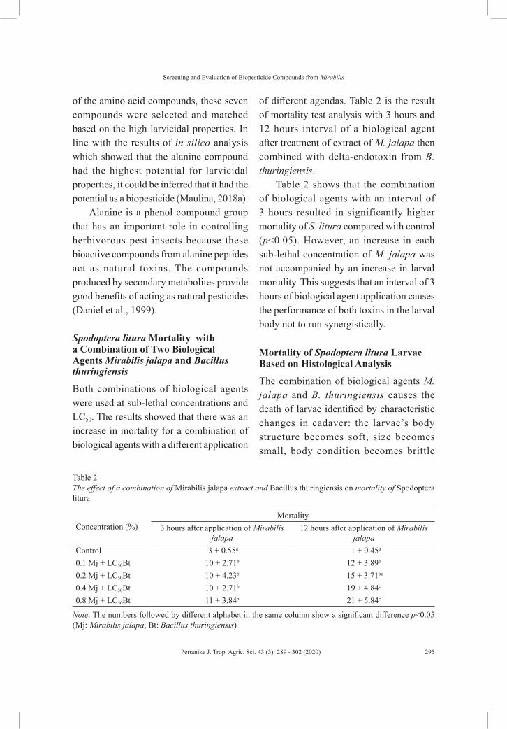
Screening and Evaluation of Biopesticide Compounds from Mirabilis
295Pertanika J. Trop. Agric. Sci. 43 (3): 289 - 302 (2020)
of the amino acid compounds, these seven compounds were selected and matched based on the high larvicidal properties. In line with the results of in silico analysis which showed that the alanine compound had the highest potential for larvicidal properties, it could be inferred that it had the potential as a biopesticide (Maulina, 2018a).
Alanine is a phenol compound group that has an important role in controlling herbivorous pest insects because these bioactive compounds from alanine peptides act as natural toxins. The compounds produced by secondary metabolites provide good benefits of acting as natural pesticides (Daniel et al., 1999).
Spodoptera litura Mortality with a Combination of Two Biological Agents Mirabilis jalapa and Bacillus thuringiensis
Both combinations of biological agents were used at sub-lethal concentrations and LC50. The results showed that there was an increase in mortality for a combination of biological agents with a different application
of different agendas. Table 2 is the result of mortality test analysis with 3 hours and 12 hours interval of a biological agent after treatment of extract of M. jalapa then combined with delta-endotoxin from B. thuringiensis.
Table 2 shows that the combination of biological agents with an interval of 3 hours resulted in significantly higher mortality of S. litura compared with control (p<0.05). However, an increase in each sub-lethal concentration of M. jalapa was not accompanied by an increase in larval mortality. This suggests that an interval of 3 hours of biological agent application causes the performance of both toxins in the larval body not to run synergistically.
Mortality of Spodoptera litura Larvae Based on Histological Analysis
The combination of biological agents M. jalapa and B. thuringiensis causes the death of larvae identified by characteristic changes in cadaver: the larvae’s body structure becomes soft, size becomes small, body condition becomes brittle
Table 2The effect of a combination of Mirabilis jalapa extract and Bacillus thuringiensis on mortality of Spodoptera litura
Concentration (%)Mortality
3 hours after application of Mirabilis jalapa
12 hours after application of Mirabilis jalapa
Control 3 + 0.55a 1 + 0.45a
0.1 Mj + LC50Bt 10 + 2.71b 12 + 3.89b
0.2 Mj + LC50Bt 10 + 4.23b 15 + 3.71bc
0.4 Mj + LC50Bt 10 + 2.71b 19 + 4.84c
0.8 Mj + LC50Bt 11 + 3.84b 21 + 5.84c
Note. The numbers followed by different alphabet in the same column show a significant difference p<0.05 (Mj: Mirabilis jalapa; Bt: Bacillus thuringiensis)

Dina Maulina, Mohamad Amin, Sutiman Bambang Sumitro, Sri Rahayu Lestari and Tri Suwandi
296 Pertanika J. Trop. Agric. Sci. 43 (3): 289 - 302 (2020)
accompanied by changes in body color that turns blackish and smelly. The results showed that the cross-sections of the midgut S. litura were composed of a composite columnar epithelial layer. Hemocoel was the cavity of a midgut pad where the food circulation was coated by the peritrophic membrane. Bacillus thuringiensis plays a role in destroying the epithelial midgut of S. litura epithelium. Delta-endotoxins can perforate the epithelial cell membrane of the midgut epithelial cells resulting in lysis due to osmotic events (Figure 2). The results showed that there was a difference in midgut S. litura treated with a combination of M. jalapa with B. thuringiensis at a 3-hour interval after being infected with M. jalapa (Figure 2). The concentration of 0.1% has been able to damage epithelial plot to
make a hole in the midgut of S. litura. The application of 0.2% concentration of M. jalapa extract causes epithelial cells in the midgut lysis and detaches from the basement membrane. Midgut damage is getting worse, this condition leads to the death of the organism. Concentrations of 0.4% and 0.8% result in acute tissue damage. Midgut organs become destroyed and organs functionally cannot work anymore.
DISCUSSIONS
The application of M. jalapa biopesticide did not not kill S. litura directly. However, it was able to induce an immune system reaction by decreasing physiological function. Sub-lethal concentration was aimed at preventing ongoing resistance to target pests (Leng et al., 2011). Resistance prevention
C P1 P2
P3 P4
Figure 2. The microanatomy of Spodoptera litura midgut treated by the combination of Mirabilis jalapa with Bacillus thuringiensis at 12 hours interval time Note. Each microanatomy image has a same size with DL0; L = 0.48mm and DL0; L = 0.26mmC : Control; P1: 0.1% concentration of M. jalapa and B. thuringiensis; P2: 0.2% concentration of M. jalapa and B. thuringiensis; P3: 0.4% concentration of M. jalapa and B. thuringiensis; P4: 0.8% concentration of M. jalapa and B. thuringiensis

Screening and Evaluation of Biopesticide Compounds from Mirabilis
297Pertanika J. Trop. Agric. Sci. 43 (3): 289 - 302 (2020)
is necessary for easy control of these pests through the application of botanical insecticides (Zibaee, 2011). In the event of resistance, a resurgence is confirmed by the multiplication of insecticidal dosage (Dutcher, 2007; Sparks & Nauen, 2015). Therefore, the use of biopesticide M. jalapa prevents these two things from happening following the principle of integrated pest management (IPM).
Alanine compound was detected in M. jalapa extract as a biopesticide that could act as an inhibitor of glutamate in the insect’s body by changing the conformation of the structure of glutamate in the neurotransmitter signaling (Maulina, 2018a). Glutamate blocking on the original receptors in the insect’s body results in a disturbance in response to the stimulating pathways of muscles and smell in insects (Kolodziejczyk et al., 2008; Missbach et al., 2014). Disruption of signaling from the pathway mechanism in neuromuscular has resulted in disruption of the mechanism of muscle movement throughout the insect’s body. It does not make body movements dysfunctional but there is a disruption in the muscle mechanism in the respiratory, digestive, and circulatory systems. Coordination of nerves and muscle disruption results in a decrease in motion activity that leads to insect paralysis.
The antenna is an important organ for insects. It is the center of the olfactory. The olfactory nerve cell disruption disrupts the recognition response to the environment. Besides, it fails potential membrane transduction which results in failed action potentials (Stengl et al., 1999). The effect
of this series is the failure to receive and continue stimuli originating in the olfactory regulation center, which leads to metabolic disorders.
The M. jalapa extract causes disorders of the olfactory and muscle nerve response (neuromuscular). The weakening of various responses to the entry of foreign substances is an indication of the weakening of the insect defense system. The biopesticide toxin of M. jalapa causes the defense mechanism in the insect body to become weak. Exposure of M. jalapa to S. litura causes an increasingly weakened state of immunity. The application of natural compounds from M. jalapa as biopesticide compounds to control the amount of S. litura could be used safely in nature. Efforts to control S. litura pests by measuring mortality rates were performed by combining M. jalapa extract and B. thuringiensis endotoxin. The two types of biological agents were combined to enhance the action of natural compounds from M. jalapa since the subaudible concentrations of M. jalapa and B. thuringiensis are used to prevent the possibility of resistance to the larvae. The results showed that there was an increase in mortality for the combination of biological agents with a different application of different agendas. Table 2 is the result of mortality analysis with 3 hours and 12 hours’ time interval of a biological agent after treatment of extract of M. jalapa then combined with delta-endotoxin from B. thuringiensis.
The combination of biological agents with an interval of 3 hours resulted in significantly increased mortality of S. litura compared with control (p<0.05). However,

Dina Maulina, Mohamad Amin, Sutiman Bambang Sumitro, Sri Rahayu Lestari and Tri Suwandi
298 Pertanika J. Trop. Agric. Sci. 43 (3): 289 - 302 (2020)
an increase in each sub-lethal concentration of M. jalapa was not accompanied by an increase in larval mortality. This suggests that an interval of 3 hours of biological agent application causes the performance of both toxins in the larval body not to run synergistically. Hillyer stated that the response of Aedes aegypti phagocytosis ran 5 minutes after being induced by bacteria (Hillyer et al., 2003). This suggests that an interval of 3 hours of biological agent application causes the performance of both toxins in the larval body not to run synergistically. When the larvae are re-infected with B. thuringiensis the larvae can eliminate the endotoxin that enters the body so that the mortality of the larvae becomes low. The average mortality at the time of application of larvae test of S. litura with a combination of the concentration of M. jalapa equal to 0.8% and delta-endotoxin with an application of time interval of 3 hours was increased by 20%.
The data showed that there was a difference when giving a combination of biological agents with an interval of 12 hours. It is shown in Table 2 that the mortality of S. litura differed significantly from controls in the exposure of the four sub-lethal concentrations of M. jalapa (p<0.05). The highest mortality occurred in the combination of 0.8% concentration of M. jalapa extract with B. thuringiensis sub-lethal concentration. The 12-hour physiological impairment performed by toxic compounds in M. jalapa can significantly weaken the S. litura larvae and the ability of the immune system decreases
significantly. The additional combination with delta-endotoxin B. thuringiensis results in S. litura larvae being unable to activate the immune defense mechanism and death. The M. jalapa extract infections given to S. litura larvae will affect the immunity characterized by enzyme PO and decrease in average. Giving a concentration of sub-lethal infections of M. jalapa is not lethal to S. litura pests. It only effectively weakens the larvae’s physiology. Therefore, to improve its pest control efficiency biological agents M. jalapa and B. thuringiensis need to be used (Maulina et al., 2018b).
A toxic substance produced by M. Jalapa weakens the insect immunity, while delta-endotoxins from B. thuringiensis invades S. litura by damaging intestinal epithelial cells along the gastrointestinal tract. When the insect’s body’s defenses weaken due to M. jalapa, the combination of delta-endotoxin B. thuringiensis entering the midgut will easily damage the entire tissue and organs. In an unstable condition due to M. jalapa’s invasion into the body, the insects will become very weak to repair their damaged ones. Damage to S. litura bodies occurs very easily when the immune defenses of S. litura larvae have been weakened, tissue and organ damage will occur thoroughly in insect bodies resulting in insect mortality.
The provision of toxins with a 12-hour time interval in the application of M. jalapa exposure with a concentration of 0.8% has an impact on increasing the mortality of S. litura. Bacillus thuringiensis application within 12 hours resulted in a 42% increase in

Screening and Evaluation of Biopesticide Compounds from Mirabilis
299Pertanika J. Trop. Agric. Sci. 43 (3): 289 - 302 (2020)
total mortality compared to controls. Thus, the time interval of combined exposure of biological agents in pest control applications such as combining the exposure of toxic substances greatly affects the increase in total lactational mortality of S. litura.
Bacillus thuringiensis has become a biocontrol of insects in many agricultural countries (Weinzierl et al., 1997). The results of the study using the combination of M. jalapa and B. thuringiensis were focused on the mortality of S. litura. The cause of death was found to be the damage to the gastrointestinal tract. Therefore, the results of this study in histopathology form in the damage of the tissue are caused by a combination of biological insecticides used. The combination was performed with a time interval, i.e. 24 hours given M. jalapa afterward 3 hours and 6 hours given B. thuringiensis. Both biological insecticides are administered simultaneously with oral feed with a synergistic mechanism of action (Agrebi et al., 2010).
The digestive tract of S. litura consists of foregut, midgut, and hindgut. Midgut plays a role in the process of food absorption which is a major part of the digestive tract and is an important organ for an insect. The midgut is a hemocoel consisting of a layer of epithelium. Functionally this section holds control of the nutrient traffic (Chapman, 2009). This organ plays an important role in other physiological regulations such as metabolism, immune response, electrolyte homeostasis, osmotic pressure, circulation, and more. Therefore, impaired function and tissue damage in midgut can result in the mortality of insects.
The results showed that the cross-section of the midgut S. litura was composed of a compact columnar epithelial layer (Figure 2). This research proved that M. jalapa played a role in weakening the immune system and B. thuringiensis played a role in damaging the digestive tissue in the body of S. litura (Castro et al., 2019). The level of tissue damage that occurred in the midgut depended on the level of concentration of M. jalapa and B. thuringiensis extracts. The higher treatment concentration of M. jalapa and B. thuringiensis caused the worse and more acute the tissue damage in the midgut of S. litura is. Hemocoel is the cavity of a midgut pad where food is circulated by the peritrophic membrane (Pigott et al., 2007). Bacillus thuringiensis plays a role in destroying the epithelial midgut of S. litura epithelium. Delta endotoxin can perforate the epithelial membrane of the midgut epithelium that causes the cell to become less because of the osmosis event (Pandey et al., 2009). The concentration of 0.1% had been able to damage epithelial plot to make a hole in the midgut of S. litura. The application of 0.2% concentration of M. jalapa extract caused epithelial cells to lyse and became detached from one another. Midgut damage got worse, this condition leading to death of the organism. Concentrations of 0.4% and 0.8% resulted in acute tissue damage. The midgut organs become destroyed and organs can not functionally work anymore. The midgut of S. litura treated with a combination of M. jalapa and B. thuringiensis at 6-hour time combination interval suffered severe organ

Dina Maulina, Mohamad Amin, Sutiman Bambang Sumitro, Sri Rahayu Lestari and Tri Suwandi
300 Pertanika J. Trop. Agric. Sci. 43 (3): 289 - 302 (2020)
damage. Each concentration resulted in severe tissue damage. The damage occurred throughout the midgut to the epithelial tissue and even the midgut organs were destroyed.
In the early stages of bacterial infection, insects exhibit a decrease in feeding activity and tend to seek shelter in a hidden place (under the leaves). Furthermore, the larvae experience diarrhea, secrete a fluid from their mouth, paralyzed on the food channel; resulting in decreased movement activity, and ending with death. Bacteria infect through the mouth and gastrointestinal tract, very little through eggs, integuments, and trachea. Bacteria enter as parasitoids and predators. By infecting through the gastrointestinal tract, the bacteria will produce enzymes (lecithinase, proteinase, and chitinase) that will attack the intestines before entering the hemocoel. The toxins will then damage the walls of the intestinal tract. When the intestinal tissue is damaged, the bacteria enter the insect hemocoel (Vega & Kaya, 2012). Here the poison of the bacteria will decompose (hydrolysis). These toxic substances will be released from their endotoxins, which will poison the epithelial cells of the food duct until they are destroyed.
CONCLUSION
Mirabilis jalapa extract had seven sequences of the highest amino acid compounds from M. jalapa namely: Glu, Asp, Lys, Val, Leu, Arg, and Ala. Alanine compound has the highest potential for larvicidal properties that have the potential as a biopesticide. The combination of 0.2% concentration of
M. jalapa and Bacillus thuringiensis at the sublethal concentration in 12-hour intervals within 24 hours showed the optimum mortality of Spodoptera litura as much as 15 +3.7bc (p<0.05). The death of larvae cadaver was characterized by damage to the midgut organs in the digestive tract observed by the histological microanatomy. Therefore, the combination of M. jalapa and B.thuringiensis with low concentrations could be considered as integrated pest management.
ACKNOWLEDGMENTS
We would like to thank Doctoral Dissertation Research Grant, Directorate of Research and Community Service, Directorate General of Research and Development Strengthening of Research Ministry, Technology and Higher Education of Indonesia No.062/SP2H/LT/DRPM/2018, which had provided funding for this research.
REFERENCESAgrebi, R., Hmidet, N., Hajji, M., Ktari, N., Haddar,
A., Fakhfakh-Zouari, N., & Nasri, M. (2010). Fibrinolytic serine protease isolation from Bacillus amyloliquefaciens An6 grown on Mirabilis jalapa tuber powders. Applied Biochemistry and Biotechnology, 162(1), 75-88. doi:10.1007/s12010-009-8800-z
Castro, B. M. C., Martinez, L. C., Barbosa, S. G., Serrão, J. E., Wilcken, C. F., Soares, M. A., … Zanucio, J. C. (2019). Toxicity and cytopathology mediated by Bacillus thuringiensis in the midgut of Anticarsia gemmatalis (Lepidoptera: Noctuidae). Retrieved January 03, 2020, from https://www.nature.com/articles/s41598-019-43074-0

Screening and Evaluation of Biopesticide Compounds from Mirabilis
301Pertanika J. Trop. Agric. Sci. 43 (3): 289 - 302 (2020)
Chapman, R. F. (2009). The insect structure and function (5th ed.). London, United Kingdom: Cambridge University Press.
Daniel , O. , Meier, M. S. , Schlat ter, J . , & Frischknecht, P. (1999). Selected phenolic compounds in cultivated plants: Ecologic functions, health implications, and modulation by pes t i c ides . Environmenta l Hea l th Perspectives, 107(suppl 1), 109-114.
Dutcher, J. D. (2007). A review of resurgence and replacement causing pest outbreaks in IPM. In A. Ciancio & K. G. Mukerji (Eds.), General concepts in integrated pest and disease management: Integrated management of plants pests and diseases (pp. 27-43). Dordrecht, Netherlands: Springer Publishing.
Gokce, A., Stelinski, L. L., Whalon, M. E., & Gut, L. J. (2010). Toxicity and antifeedant activity of selected plant extracts against larval oblique banded leafroller, Choristoneura rosaceana (Harris). The Open Entomology Journal, 4(1), 18-24. doi:10.2174/1874407901004010018
Hansberger, A. (2000). Bt (Bacillus thuringiensis): A microbial insecticide. Retrieved December 3, 2019, from https://www.doyourownpestcontrol.com/SPEC/LABELS/bt.pdf.
Hillyer, J. F., Schmidt, S. L., & Christensen, B. M. (2003). Rapid phagocytosis and melanization of bacteria and Plasmodium sporozoites by hemocytes of the mosquito Aedes aegypti. Journal of Parasitology, 89(1), 62-69.
Isman, M. B. (2006). Botanical insecticides, deterrents, and repellents in modern agriculture and an increasingly regulated world. Annual Review of Entomology, 51, 45-66. doi:10.1146/annurev.ento.51.110104.151146
Kandagal, A. S., & Khetagoudar, M. C. (2013). Study on larvicidal activity of weed extracts against Spodoptera litura. Journal of Environmental Biology, 34, 253-257. doi:10.1007/s00436-008-1142-x
Kolodziejczyk, A., Sun, X., Meinertzhagen, I. A., & Nässel, D. R. (2008). Glutamate, GABA and acetylcholine signaling components in the lamina of the Drosophila visual system. PLOS One, 3(5), 2110. doi:10.1371/journal.pone.0002110
Kumar, S., & Singh, A. (2015). Biopesticides: Present status and the future prospects. Journal of Fertilizer and Pesticide, 6(2), 100-129. doi:10.4172/jbfbp.1000e129
Kumar, V. K., Sankar, N. R., Ramya, S., Sahaja, R. V., Saritha, K., Reddy, K. G., & Naidu, N. V. (2010). Phytochemical screening and antimicrobial activity of the leaf extract of Mirabilis jalapa against pathogenic microorganisms. International Journal of Phytomedicine, 2(4), 402-407.
Leng, P. , Zhang, Z. , Pan, G., & Zhao, M. (2011). Applicat ions and development trends in biopesticides. African Journal of Bio technology , 10 (86) , 19864-19873. doi:10.5897/AJBX11.009
Maulina, D., & Anggraeni, T. (2014). The effect of the combination of two biological control agents , Mirabi l i s ja lapa and Baci l lus thuringiensis, to Spodoptera litura’s immune response and their mortality. Retrieved January 03, 2020, from https://aip.scitation.org/doi/abs/10.1063/1.4868809
Maulina, D., Amin, M., Lestari, S. R., & Aziz, M. (2018a). Alanine as natural biopesticide from Mirabilis jalapa and its interaction with glutamate as an inhibitor in insect’s immune system. Journal of Biological Researches, 23(2), 77–83. doi:10.23869/bphjbr.23.2.20185
Maulina, D., Sumitro, S. B., Amin, M., & Lestari, S. R. (2018b). Identification of bioactive compounds from Mirabilis jalapa L. (Caryophyllales: Nyctaginaceae) extract as biopesticides and their activity against the immune response of Spodoptera l i tura F. (Lepidoptera: Noctudiae). Journal of Biopesticides, 11(2), 89-97.

Dina Maulina, Mohamad Amin, Sutiman Bambang Sumitro, Sri Rahayu Lestari and Tri Suwandi
302 Pertanika J. Trop. Agric. Sci. 43 (3): 289 - 302 (2020)
Maulina, D., Sumitro, S. B., Amin, M., & Lestari, S. R. (2018c). Identification of peptides compounds from Mirabilis jalapa L. (Caryophyllales: Nyctaginaceae) potentially as a b iopes t ic ide . Re t r ieved January 03, 2020, from https://iopscience.iop.org/article/10.1088/1742-6596/1093/1/012009/pdf
Metcalf, R. L. (1989). Insect resistance to insecticides. Pesticide Science, 26(4), 333-358. doi:10.1002/ps.2780260403
Missbach, C., Dweck, H. K., Vogel, H., Vilcinskas, A., Stensmyr, M. C., Hansson, B. S., & Grosse-Wilde, E. (2014). Evolution of insect olfactory receptors. eLife, 3, e02115. doi:10.755/eLife.02115
Pandey, S., Joshi, B. D., & Tiwari, L. D. (2009). Histopathological changes in the midgut of Spodoptera litura larvae on ingestion of Bacillus thuringiensis delta endotoxin. Archives of Phytophatology and Plant Protection, 42(4), 376-383. doi: 10.1080/03235400601121497
Pedigo, L. P. (1999). Entomology and pest management (3rd ed.). Upper Saddle River, USA: Prentice Hall.
Pigott, C. R., & Ellar, D. J. (2007). Role of receptors in Bacillus thuringiensis crystal toxin activity. Microbiology and Molecular Biology Review, 71(2), 255–281. doi: 10.1128/MMBR.00034-06
Romeis, J., Bartsch, D., Bigler, F., Candolfi, M. P., Gielkens, M. M., Hartley, S. E., & Quemada, H. (2008). Assessment of risk of insect-resistant transgenic crops to nontarget arthropods. Nature Biotechnology, 26(2), 203-208. doi:10.1038/nbt1381
Schreiner, I. (2000). Cluster caterpillar (Spodoptera litura [Fabricius]). Retrieved January 04, 2020, from https://scholarspace.manoa.hawaii.edu/bitstream/10125/33420/1/2007-banana.pdf
Sparks, T. C., & Nauen, R. (2015). IRAC: Mode of action classification and insecticide resistance
management. Pesticide Biochemistry and Physiology, 121, 122-128. doi:10.1016/j.pestbl.2014.11.014
Stengl, M., Ziegelberger, G., Boekhoff, I., & Krieger, J. (1999). Perireceptor events and transduction mechanisms in insect olfaction. In B. S. Hansson (Ed.), Insect olfaction (pp. 49-66). Heidelberg, Germany: Springer Publishing.
Suryani, A. I., & Anggraeni, T. (2014). The effect of leaf biopesticide Mirabilis jalapa and fungi Metarhizium anisopliae to immune response and mortality of Spodoptera exigua instar IV. Retrieved January 04, 2020, from https://aip.scitation.org/doi/10.1063/1.4868808
Vega, F. E., & Kaya, H. K. (Eds.). (2012). Insect pathology (2nd ed.). London, United Kingdom: Academic Press Elsevier.
Weinzierl, R., Henn, T., & Koehler, P. G. (1997). Bt (Bacillus thuringiensis), a microbial insecticide. Retrieved January 04, 2020, from https://www.doyourownpestcontrol.com/SPEC/LABELS/bt.pdf
Yusof, I., & Kueh, T. F. (2013). Biological performance of Menochilus sexmaculatus Fabricius (Coleoptera Coccinellidae) upon exposure to sublethal concentration of imidacloprid. Pertanika Journal of Tropical Agricultural Science, 36(1), 51-60.
Zhu, F., Lavine, L., O’Neal, S., Lavine, M., Foss, C., & Walsh, D. (2016). Insecticide resistance and management strategies in urban ecosystems. Insects, 7(1), 2. doi:10.3390/insects7010002
Zibaee, A. (2011). Botanical insecticides and their effects on insect biochemistry and immunity. In S. Margarita (Ed.), Pesticides in the modern world-pests control and pesticides exposure and toxicity assessment (pp. 55-68). Shanghai, China: InTech China.

Pertanika J. Trop. Agric. Sci. 43 (3): 303 - 313 (2020)
© Universiti Putra Malaysia Press
TROPICAL AGRICULTURAL SCIENCEJournal homepage: http://www.pertanika.upm.edu.my/
Article history:Received: 4 February 2020Accepted: 27 April 2020Published: 28 August 2020
ARTICLE INFO
E-mail address:[email protected]
ISSN: 1511-3701e-ISSN 2231-8542
Bioactivity Evaluation of Melaleuca cajuputi (Myrtales: Myrtaceae) Crude Extracts against Aedes MosquitoAzlinda Abu Bakar1,2
1Department of Medical Microbiology & Parasitology, School of Medical Sciences, Universiti Sains Malaysia, 16150 Kubang Kerian, Kelantan2Department of Diagnostic and Applied Health Sciences, Faculty of Health Sciences, Universiti Kebangsaan Malaysia, Jalan Raja Muda Abdul Aziz, 50300 Kuala Lumpur
ABSTRACT
Melaleuca cajuputi crude extract in four different solvents viz dichloromethane, ethyl acetate, hexane, and methanol were evaluated for their insecticidal properties against Aedes aegypti and Aedes albopictus mosquito. Bioassay against larva and adult mosquito was done following World Health Organization’s guidelines. Late 3rd and/or early 4th instar of Aedes larvae were assayed for different concentrations ranging from 10 to 120 mg/L of M. cajuputi crude extract. Larvicidal effects were observed in dichloromethane, hexane, and methanol. Dichloromethane gave the highest of mean mortality, against Ae. aegypti (12.6 ± 0.98) and Ae. albopictus (10.2 ± 0.37) with LC50 of 104.8 mg/L and 106 mg/L, respectively. The adulticidal bioassay was tested against 3 - 5 days old of female mosquitoes with the range concentrations from 0.04 to 6.21 mg/cm2. Amongst solvents used, extracts of dichloromethane and hexane showed effects against the adult mosquito. Extract in hexane gave 100% mortality against both Aedes with LC50 of 0.015 mg/cm2 (Ae. aegypti) and 0.022 mg/cm2 (Ae. albopictus). In conclusion, the extract of M. cajuputi
Current affiliation
School of Biological Sciences, Universiti Sains Malaysia, 11800 Gelugor, Pulau Pinang
could be exploited in the development of potential plant-based products in controlling dengue Aedes vectors, particularly in the adult mosquito.
Keywords: Aedes sp., bioactivity, crude extracts,
Melaleuca cajuputi, solvents polarity

Azlinda Abu Bakar
304 Pertanika J. Trop. Agric. Sci. 43 (3): 303 - 313 (2020)
INTRODUCTION
In Asia, the mosquito Aedes aegypti is a primary vector for dengue and chikungunya (Sam & Abu Bakar, 2006). Meanwhile, its related taxon Aedes albopictus has been recognized as a secondary vector for dengue and serves as a vector competence in the maintenance of dengue, and chikungunya virus in areas where Ae. aegypti is less abundant or absent (Effler et al., 2005; Grard et al., 2014; Li et al., 2012; Wong et al., 2013). The global widespread of vector mosquitoes such as Aedes in certain tropical and sub-tropical areas causes a major outbreak of dengue and other mosquito-borne disease-related illness (Rezza, 2014). Utilization of insecticides in the strategy for disease outbreak control is undeniably effective, due to cost-effective, immediate action, and high efficiency against a broad range of vectors. Unfortunately, the effectiveness is threatened by negative and harmful side effects on human, non-target animals, and the environment have become apparent. Nevertheless, the development of resistance among vector populations (Hamid et al., 2018) is the biggest threat to the program’s efficacy. Thus, the urge and interest in searching less hazardous alternatives of vector/pest control from plant resources are therefore being renewed and continues today.
To date, many potential plant species with known insecticidal properties and phytochemicals which are rich with biodegradable active compounds are being screened and evaluated (Sharma et al., 2006). For instance, a study on the bioactivity
screening of various plant extracts in Malaysia, had shown that Melaleuca was the most effective when tested against Aedes spp. larva in the laboratory (Bakar et al., 2018). Nevertheless, evaluation of the essential oils of the same plant had also shown its potential insecticidal effects as well (Abu Bakar et al., 2012; Bakar et al., 2019). According to Lowe’s report (as cited in De Monte et al., 2014, p. 63), there are many different extractive techniques and approaches working together with various methodologies and solvents to improve the recovery and, the pharmacological profile of their extract products. However, as a result of the differences among the extractive processes and methods, there is a discrepancy in the qualitative and quantitative composition of the extracts obtained from the same plant.
It is known that various solvents of different polarities would extract different phenolic compounds from plants with a high degree of accuracy (Wong & Kitts, 2006). Furthermore, previous studies have shown that solvents with a high polarity such as methanol displayed high effectiveness as antioxidants (Altemimi et al., 2017). The objective of this present study was to evaluate the in vitro bioactivity of Melaleuca cajuputi plant extracts derived from four different solvents polarity viz. hexane (non-polar), dichloromethane (moderately polar), ethyl acetate (polar), and methanol (polar) against larvae and adult of dengue vector mosquitoes, Ae. aegypti and Ae. albopictus.

The Effect of M. cajuputi Extracts against Aedes
305Pertanika J. Trop. Agric. Sci. 43 (3): 303 - 313 (2020)
MATERIALS AND METHODS
Collection of Plant Specimens
The leaves of M. cajuputi were collected from Port Dickson, Negeri Sembilan area, 2° 31′ 21.1440″ N, 101° 47′ 46.6620″ E in Malaysia. Port Dickson is located 120 km towards the south from Kuala Lumpur 3° 8’ 27.0708’’ N and 101° 41’ 35.5452’’ E. The voucher specimen was sent to Forest Research Institute of Malaysia (FRIM) in Kepong, Selangor for species confirmation and specimen deposited at the herbarium.
Preparation of Mosquito
Laboratory strain mosquito was obtained from Vector Control Research Unit, School of Biological Sciences, Universiti Sains Malaysia, Pulau Pinang in the form of eggs. The mosquito colony was cultured and reared in the laboratory under the optimized condition: relative humidity (RH) 80% ± 5% and room temperature 28.5 °C ± 2 °C. During the maintenance period, mosquitoes’ larvae were provided with prepared powdered food which contains cat’s biscuit, powder milk, grounded (dried) cow liver, yeast, and vitamin B complex. The mosquito colony was continuously maintained throughout the study period.
Preparation of the Crude Extracts
The freshly collected leaves of M. cajuputi were dried at room temperature (29 - 31°C) for 5 - 7 days. The dried leaves were grounded mechanically using a household blender. The grounded leaves were extracted with solvents viz: hexane, ethyl acetate,
dichloromethane, and methanol with the ratio of 1g sample to 10 mL solvent in a 10L plastic container. The samples were shaken and mixed vigorously and left to sit for 72 hrs. The extracts were filtered through glass funnel with filter paper Whatman No.1. The extract was concentrated using rotary evaporator type EYELA (N-1001S-WD, Japan) at 45°C for eight hrs. The residue obtained was kept in an amber glass vial to be used for subsequent bioassay testing.
Larval Bioassay
The larval bioassay was following the standard guidel ines (World Health Organization [WHO], 2005). Five (5) different concentrations of extracts were prepared at 10, 50, 80, 100, and 120 mg/L. A 10 mL stock solution was prepared at a concentration of 100,000 mg/L (100,000 ppm) and kept in a refrigerator at 4 - 5 °C. Five replicates of 20 late third instar larvae were used in each bioassay. The numbers of dead larvae were counted after 24 hrs. of exposure. Positive and negative control solutions were prepared by mixing 1mL solvent in 199mL of distilled water and 2 mL of acetone in 198 mL of distilled water respectively. During the observation, food was not supplied to the larvae. The lethal concentrations (LC50 and LC90) were calculated by probit analysis (Finney, 1971).
Adulticidal Bioassay
Bioassay of adulticide was performed as described in the WHO (2016) guideline. Five (5) different concentrations of 2.0 mL plant extracts of 0.04, 0.08, 0.12, 2.48, and

Azlinda Abu Bakar
306 Pertanika J. Trop. Agric. Sci. 43 (3): 303 - 313 (2020)
6.21 mg/cm2 were applied homogeneously at the filter papers Whatman No 1 (12 x 15 cm). The control paper was treated with 2.0 mL acetone. The impregnated papers were dried at room temperature for 24 hrs and kept (4 - 5°C) in an aluminum foil. Four replicates of twenty-five female (3 - 5 days old, blood starved) mosquitoes were aspirated from the mosquito cage into a plastic holding tube. The mosquitoes were allowed to acclimatize in the tube for 1 hr. and later were exposed to the treated impregnated filter paper for 1 hr. At the end of the 1 hr. exposure period, the mosquitoes were transferred back to the holding tube and kept for mortality observation for 24 hrs. A pad of cotton wool soaked in 10% sugar water was placed on the mesh-screen. The number of moribund and dead mosquitoes was recorded at intervals of 1, 5, 10, 15, 20, 25, 30, 45-, and 60-minutes post-exposure. Any knocked down mosquitoes, were considered moribund and counted as dead. A mosquito was classified as dead or knocked down if it is immobile or unable to stand or take off.
Statistical Analysis
Percentage mortality that lies between 5% to 20% will be corrected using Abbott’s formula (Abbot, 1925). Larvicidal and adulticidal effects were reported in median lethal concentration (LC50) with a 95% confidence interval subjected to a log probit analysis test. The comparative effectiveness of crude extracts among different types of solvents and Aedes mean mortality were analyzed using paired t-test and one-way
ANOVA. Results with the value of p ≤ 0.05 were reported to be statistically significant. All data were analyzed and calculated using SPSS statistics software.
RESULTS
The insecticidal bioefficacy of the M. cajuputi crude extracts of dichloromethane, ethyl acetate, hexane, and methanol were tested at 10 mg/L, 50 mg/L, 80 mg/L, 100 mg/L, and 120 mg/L against dengue vectors, Ae. aegypti and Ae. albopictus. Table 1 summarizes the bioactivity against larvae and adults’ stage of Aedes vectors. From the results obtained, dichloromethane, hexane, and methanol showed some larvicidal effects when tested against Aedes larvae. Meanwhile, adulticidal effects were only observed in dichloromethane and methanol. The bioassay test against larvae and adults Aedes mosquito showed a significant increase in the mortality percentage (%) with the increase of concentration.
In Table 2, the paired t-test and the one-way analysis of variance (ANOVA) were analyzed in mean mortality of Aedes sp. larvae, and solvents used. Statistical analysis of one-way ANOVA revealed no significant difference between and within groups among solvents and Aedes sp. Meanwhile paired t-test between solvents and Aedes sp. showed a significant difference (p ≤ 0.05) in hexane (p = 0.04) and methanol (p=0.003) solvent respectively. The highest larvicidal activity was observed in dichloromethane against Aedes sp. with the LC50 values of 104.8 mg/L and 106.0 mg/L for Ae. aegypti and Ae. albopictus at 24 hrs. respectively

The Effect of M. cajuputi Extracts against Aedes
307Pertanika J. Trop. Agric. Sci. 43 (3): 303 - 313 (2020)
(Table 3). Figures 1 and 2 show the highest percentage mortality values of 63% in Ae. aegypti and 51% in Ae. albopictus at 120 mg/L of dichloromethane extract in M. cajuputi.
The results of the adulticidal activity of hexane and dichloromethane extracts of M. cajuputi against Ae. aegypti and Ae.
albopictus are presented in Table 4. There was a significant difference between hexane and dichloromethane in mean mortality of Aedes spp. with the p-values of 0.007 for Ae. aegypti and 0.003 for Ae. albopictus. However, no significant difference was observed in mean mortality between Aedes spp. in each solvent used, hexane and
Solvents Larvicidal AdulticidalDichloromethane √ √Ethyl acetate - -Hexane √ √Methanol √ -
Table 1
Bioactivity of Melaleuca cajuputi crude extracts against Ae. aegypti and Ae. albopictus
Note. √ toxic effects
Table 2 Mean mortality (± SE) of M. cajuputi crude extracts against larvae of Ae. aegypti and Ae. albopictus
Aedes sp. Dose *Mean mortality ± SE(mg/L) Dichloromethane1 Hexane2 Methanol3
aAe. aegypti 10 1.20 ± 0.20 0 1.40 ± 0.2550 3.40 ± 0.25 1.20 ± 0.20 1.60 ± 0.2580 6.80 ± 0.37 4.20 ± 0.37 2.40 ± 0.40100 9.80 ± 0.66 5.40 ± 0.51 2.80 ± 0.20120 12.6 ± 0.98 6.60 ± 0.51 3.00 ± 0.32Control** 0 0 0
bAe. albopictus 10 0 0 050 0 0 080 7.40 ± 0.25 0.60 ± 0.25 0100 10.0 ± 0.32 1.00 ± 0.32 1.60 ± 0.25120 10.2 ± 0.37 2.00 ± 0.32 2.00 ± 0.00Control** 0 0 0
Note. *Mean value of five replicates Control** = acetone 0.1%1, a,b No significant difference 1, 2, 3, a No significant difference2, a, b Significant difference p < 0.05(p = 0.04)
1, 2, 3, b No significant difference

Azlinda Abu Bakar
308 Pertanika J. Trop. Agric. Sci. 43 (3): 303 - 313 (2020)
Table 3 LC values of M. cajuputi crude extracts against Aedes sp. larvae
Ae. aegypti Ae. albopictus
Solvents LC50
(mg/L)95%
C o n f i d e n c e Limit
df χ2 LC50
(mg/L)95%
C o n f i d e n c e Limit
df χ2
LCL UCL LCL UCL
Dichloromethane 104.8 94.9 117.8 2 0.43 106.0 N/A N/A 2 15.9
Hexane 164.4 132.1 260.3 2 0.71 429.0 N/A N/A 2 1.60
Methanol 349.5 N/A N/A 2 0.19 N/A N/A N/A N/A N/A
Note. LCL = lower confidence limit; UCL = upper confidence limit; df = degree of freedom
06
21 2733
6
17
34
50
63
7 812 14 15
-20
-10
0
10
20
30
40
50
60
70
80
10 50 80 100 120
Mor
talit
y (%
)
Dose Concentration (mg/L)HexaneDichloromethaneMethanol
Figure 1. Percentage mortality of M. cajuputi crude extracts against Ae. aegypti larvae
0 0 3 510
0 0
37
50 51
0 0 08 10
-20
-10
0
10
20
30
40
50
60
70
0 50 80 100 120
Mor
talit
y (%
)
Dose Concentration (mg/L)HexaneDichloromethaneMethanol
Figure 2. Percentage mortality of M. cajuputi crude extracts against Ae. albopictus larvae

The Effect of M. cajuputi Extracts against Aedes
309Pertanika J. Trop. Agric. Sci. 43 (3): 303 - 313 (2020)
dichloromethane. The probit analysis of 95% confidence limits LC50 (UCL-LCL) was also calculated and presented in Table 5. The chi-square values were not significantly different at p ≤ 0.05. Among the solvents used, hexane gives lower LC50 of 0.015 mg/cm2 (0.005-0.025) and 0.022 mg/cm2 (0.009-0.003) in Ae. aegypti and Ae. albopictus, respectively.
In this study, the results showed that bioactivity of M. cajuputi crude extracts against Aedes spp. was varied according to the species, stage of life, and solvents used (Tables 1, 2, and 4). The extract of M. cajuputi in dichloromethane possessed moderate effects against Ae. aegypti larvae. On the other hand, the sensitivity of dichloromethane, hexane, and methanol
extract against Ae. albopictus showed minimal larvicidal effects after 24 hr. of exposure at various concentrations. Meanwhile, observation in adulticidal assays using dichloromethane, ethyl acetate, hexane, and methanol showed nonconformity with the results of the larvicidal assays. Of these, dichloromethane and hexane extracts of M. cajuputi showed adulticidal effects against Ae. aegypti and Ae. albopictus. However, hexane extract was the most effective against Ae. aegypti and Ae. albopictus adult’s mosquito. From Table 4, more than 50% mortality was observed in Ae. aegypti (74%) and Ae. albopictus (69%) at lowest concentration of 0.04 mg/cm2 and 100% mortality when exposed at higher concentrations of 2.48 and 6.21 mg/cm2.
Table 4
Adulticidal effects of M. cajuputi crude extracts against Aedes aegypti and Aedes albopictus Solvents Used
Dose(mg/cm2)
1 Ae. aegypti 2Ae. albopictus
Mortality(%)
*Mean mortality ± SD
Mortality (%)
*Mean mortality ± SD
aHexane 0.04 74 18.50 ± 1.29 69 17.25 ± 1.26
N=100 0.08 77 19.25 ± 0.96 71 17.75 ± 1.89
0.12 79 19.75 ± 0.96 89 22.25 ± 3.30
2.48 100 25.00 ± 0.00 100 25.00 ± 0.00
6.21 100 25.00 ± 0.00 100 25.00 ± 0.00
**Control 0 0 0 0bDichloromethane 0.04 31 7.75 ± 1.15 54 13.50 ± 3.00
N=100 0.08 50 12.50 ± 3.00 56 14.00 ± 2.16
0.12 55 13.75 ± 0.96 57 16.75 ± 2.50
2.48 80 20.00 ± 1.83 80 20.00 ± 0.00
6.21 87 19.25 ± 6.29 81 20.20 ± 0.5
**Control 0 0 0 0
Note. *Mean value of four replicates **Control=acetone 0.1%1, 2, a No significant difference p > 0.05 1, a, b Significant difference p ≤ 0.05 (p = 0.007)1, 2, b No significant difference p > 0.05 2, a, b Significant difference p ≤ 0.05 (p = 0.003)

Azlinda Abu Bakar
310 Pertanika J. Trop. Agric. Sci. 43 (3): 303 - 313 (2020)
DISCUSSION
Many researchers have reported the potential of plant extracts for controlling mosquito-borne diseases (Ghosh et al., 2012; Kamaraj et al., 2010; Rehimi et al., 2011). Up to date, there are now more than 2,000 potential plant species that have been evaluated for their insecticidal properties worldwide (Maiza et al., 2013; Roark, 1947; Shaalan et al., 2005; Sukumar et al., 1991). In some developing countries, pesticidal plants offer unique and challenging opportunities for the exploration and development of their botanical sources. Furthermore, one of the most important factors affecting the benefits and efficiency of bioactivity from plant materials and their consequent health is the extraction solvents used (Ngo et al., 2017). Thus, the selection of solvents used depends on the purpose either as of choice for yielding high content or for specific extraction of phytochemical compounds that would be useful for its medicinal and/or insecticidal properties.
The polarity effect depends on the reactivity and selectivity of radical chemistry that has been identified over 50
years ago (Walling, 1957). Most chemical reactions that are carried out in laboratories or the industry are in the form of solutions. Hence the proper and appropriate solvent selection as one of the reaction parameters is important for a good and successful reaction (Reichardt, 2005). According to Rawani et al. (2010), phytochemicals found in plants may play an important role (bioactivities) in vector control if applied appropriately. The phytochemicals in plants can be obtained from the whole plant or specific parts of the plant with different solvents such as petroleum ether, benzene, chlorophyll, methanol, and acetone.
Ghosh et al. (2012) showed that the extraction of active biochemical from plants depended upon the polarity of the solvents. Polar solvents will extract polar molecules and non-polar solvents extract non-polar molecules. In this study, hexane (polarity index of 0.1), dichloromethane (polarity index of 3.1), ethyl acetate (polarity index of 4.4), and methanol (polarity index of 5.1) (Corradini et al., 1998; Harris, 2015) had been used to investigate the insecticidal properties of M. cajuputi extract
Table 5 LC values of M. cajuputi crude extracts against Aedes sp. adults
Ae. aegypti Ae. albopictus
Solvents LC50
(mg/L)95%
C o n f i d e n c e Limit
df χ2 LC50
(mg/L)95%
C o n f i d e n c e Limit
df χ2
LCL UCL LCL UCL
Dichloromethane 0.116 0.071 0.176 3 3.73 0.030 0.007 0.069 3 0.83
Hexane 0.015 0.005 0.025 3 4.57 0.022 0.009 0.033 3 5.86
Note. LCL = lower confidence limit; UCL = upper confidence limit; df = degree of freedom
The Effect of M. cajuputi Extracts against Aedes
311Pertanika J. Trop. Agric. Sci. 43 (3): 303 - 313 (2020)
against Ae. aegypti and Ae. albopictus. From the results obtained, hexane and dichloromethane solvents that had lower to moderate polarity index were observed to give moderate effects against Aedes mosquito. These findings agree with the previous study by Ghosh et al. (2012), which described the efficacy of solvents polarity in the bioassays. Biochemical extracted using moderate polarity index solvents showed good results in a few bioassays. This study revealed the bioactivity variance of M. cajuputi crude extracts when tested against larvae and adults of Aedes sp. Even though larvicidal effects were observed in dichloromethane, hexane, and methanol extracts of M. cajuputi, the effectiveness was slightly weak. However, the adulticidal activity showed good effects against Ae. aegypti and Ae. albopictus.
CONCLUSION
The bioactivity of crude plant extracts is characterized by a mixture of complex active compounds. Thus, plants containing beneficial phytochemicals may supplement and would be useful plant-based insecticides for future development. Variations of an insecticidal potential of M. cajuputi crude extract varied with the different solvents used in the extraction process. Due to the variation’s efficacy in the larvicidal and adulticidal effects against Ae. aegypti and Ae. albopictus mosquitoes. More work is still needed to confirm its effectiveness, especially in the field. A study on the phytochemicals of an active compound of the M. cajuputi crude extract
in different solvents used can be carried out to characterize the insecticidal properties in different research settings. It can be used as a solution of variants efficacy in a situation of chemical instability of whole or unprocessed plant products.
ACKNOWLEDGEMENTS
The author is thankful to the Universiti Sains Malaysia and Ministry of Higher Education for the scholarship program. The gratitude is also extended to Dr. Sallehudin Sulaiman and Dr. Rasadah Mat Ali for their guidance and advice during the research, and for providing the laboratory facility at the Forest Research Institute Malaysia. This research did not receive any specific grant fromfunding agencies in the public, commercial, or not-for-profit sectors.
REFERENCESAbbott, W. S. (1925). A method of computing the
effectiveness of an insecticide. Journal of Economic Entomology, 18(2), 265-266.
Abu Bakar, A., Sulaiman, S., Omar, B., & Mat Ali, R. (2012). Evaluation of Melaleuca cajuputi (Family: Myrtaceae) essential oil in aerosol spray cans against dengue vectors in low cost housing flats. Journal of Arthropod Borne Diseases, 5(2), 28-35.
Altemimi, A., Lakhssassi, N., Baharlouei, A., Watson, D. G., & Lightfoot, D. A. (2017). Phytochemicals: Extraction, isolation, and identification of bioactive compounds from plant extracts. Plants, 6(4), 42. doi: 10.3390/plants6040042
Bakar, A. A., Sulaiman, S., Omar, B., & Ali, R. M. (2018). Screening of five plant extracts for larvicidal efficacy against larvae of Aedes aegypti

Azlinda Abu Bakar
312 Pertanika J. Trop. Agric. Sci. 43 (3): 303 - 313 (2020)
(L.) and Aedes albopictus (Skuse). ASM Science Journal, 11(2), 103-116.
Bakar, A. A., Sulaiman, S., Omar, B., & Ali, R. M. (2019). Evaluation of in vitro bioactivity of Melaleuca cajuputi powell essential oil against Aedes aegypti (L.) and Aedes albopictus (Skuse). Sains Malaysiana, 48(9), 1919-1926. doi: 10.17576/jsm-2019-4809-13
Corradini, D., Katz, E., Eksteen, R., Schoenmakers, P., & Miller, N. (1998). Handbook of HPLC. New York, NY: Marcel Dekker.
De Monte, C., Carradori, S., Granese, A., Di Pierro, G. B., Leonardo, C., & De Nunzio, C. (2014). Modern extraction techniques and their impact on the pharmacological profile of Serenoa repens extracts for the treatment of lower urinary tract symptoms. BMC Urology, 14(1), 63. doi: 10.1186/1471-2490-14-63
Effler, P. V., Pang, L., Kitsutani, P., Vorndam, V., Nakata, M., Ayers, T., … Hawaii dengue outbreak investigation team. (2005). Dengue fever, Hawaii, 2001-2002. Emerging Infectious Disease , 11(5), 742-749. doi: 10.3201/eid1105.041063
Finney, D. J. (1971). Probit analysis (3rd ed.). New York, NY: Cambridge University Press.
Ghosh, A., Chowdhury, N., & Chandra, G. (2012). Plant extracts as potential mosquito larvicides. Indian Journal of Medical Research, 135(5), 581-598.
Grard, G., Caron, M., Mombo, I. M., Nkoghe, D., Mboui Ondo, S., Jiolle, D., … Leroy, E. M. (2014). Zika virus in Gabon (Central Africa)—2007: A new threat from Aedes albopictus? PLOS Neglected Tropical Diseases, 8(2), e2681. doi: 10.1371/journal.pntd.0002681
Hamid, P. H., Ninditya, V. I., Prastowo, J., Haryanto, A., Taubert, A., & Hermosilla, C. (2018).
Current status of Aedes aegypti insecticide resistance development from Banjarmasin, Kalimantan, Indonesia. Retrieved January 08, 2020, from https://www.hindawi.com/journals/bmri/2018/1735358/
Harris, D. C. (2015). Quantitative chemical analysis (9th ed.). New York, NY: W. H. Freeman and Company.
Kamaraj, C., Rahuman, A. A., Mahapatra, A., Bagavan, A., & Elango, G. (2010). Insecticidal and larvicidal activities of medicinal plant extracts against mosquitoes. Parasitology Research, 107(6), 1337-1349. doi: 10.1007/s00436-010-2006-8
Li, M. I., Wong, P. S., Ng, L. C., & Tan, C. H. (2012). Oral susceptibility of Singapore Aedes (Stegomyia) aegypti (Linnaeus) to Zika virus. PLOS Neglected Tropical Diseases, 6(8), e1792. doi: 10.1371/journal.pntd.0001792
Maiza, A., Aribi, N., Smagghe, G., Kilani-Morakchi, S., Bendjedid, M., & Soltani, N. (2013). Sublethal effects on reproduction and biomarkers by spinosad and indoxacarb in cockroaches Blattella germanica. Bulletin of Insectology, 66(1), 11-20.
Ngo, T. V., Scarlett, C. J., Bowyer, M. C., Ngo, P. D., & Vuong, Q. V. (2017). Impact of different extraction solvents on bioactive compounds and antioxidant capacity from the root of Salacia chinensis L. Retrieved January 08, 2020, from https://www.hindawi.com/journals/jfq/2017/9305047/
Rawani, A., Ghosh, A., & Chandra, G. (2010). Mosquito larvicidal activities of Solanum nigrum L. leaf extract against Culex quinquefasciatus Say. Parasitology Research, 107(5), 1235-1240. doi: 10.1007/s00436-010-1993-9
Rehimi, N., Alouani, A., & Soltani, N. (2011). Efficacy of Azadirachtin against mosquito larvae Culex
The Effect of M. cajuputi Extracts against Aedes
313Pertanika J. Trop. Agric. Sci. 43 (3): 303 - 313 (2020)
pipiens (Diptera: Culicidae) under laboratory conditions. European Journal of Scientific Research, 57(2), 223-229.
Reichardt, C. (2005). Polarity of ionic liquids de te rmined empi r i ca l ly by means o f solvatochromic pyridinium N-phenolate betaine dyes. Green Chemistry, 7(5), 339–351.
Rezza, G. (2014). Dengue and chikungunya: Long-distance spread and outbreaks in naïve areas. Pathogens and Global Health, 108(8), 349–355. doi: 10.1179/2047773214Y.0000000163
Roark, R. C. (1947). Some promising insecticidal plants. Economic Botany, 1(4), 437–445. doi: 10.1007/BF02858908
Sam, I. C., & Abu Bakar, S. (2006). Chikungunya virus infection. Medical Journal of Malaysia, 61(2), 264-269.
Shaalan, E. A. S., Canyonb, D., Younesc, M. W. F., Abdel-Wahaba, H., & Mansoura, A. H. (2005). A review of botanical phytochemicals with mosquitocidal potential. Environment International, 31(8), 1149–1166. doi: 10.1016/j.envint.2005.03.003
Sharma, P., Mohan, L., & Srivastava, C. N. (2006). Phytoextract-induced developmental deformities in malaria vector. Bioresource Technology, 97(14), 1599–1604. doi: 10.1016/j.biortech.2005.07.024
Sukumar, K., Perich, M. J., & Boobar, L. R. (1991). Botanical derivatives in mosquito control: A review. Journal of American Mosquito Control Association, 7(2), 210–237.
Walling, C. (1957). Free radicals in solution. New York, NY: John Wiley and Sons.
Wong, P. Y. Y., & Kitts, D. D. (2006). Studies on the dual antioxidant and antibacterial properties of parsley (Petroselinum crispum) and cilantro (Coriandrum sativum) extracts. Food Chemistry, 97(3), 505–515. doi: 10.1016/j.foodchem.2005.05.031
Wong, P. S., Li, M. Z., Chong, C. S., Ng, L. C., & Tan, C. H. (2013). Aedes (Stegomyia) albopictus (Skuse): A potential vector of Zika virus in Singapore. PLOS Neglected Tropical Diseases, 7(8), e2348. doi: 10.1371/journal.pntd.0002348
World Health Organization. (2005). Guidelines for laboratory and field testing of mosquito larvicides. Retrieved November 21, 2019, from https://apps.who.int/iris/handle/10665/69101
World Health Organization. (2016). Test procedures for insecticide resistance monitoring in malaria vector mosquitoes. Retrieved November 21, 2019, from https:// https://apps.who.int/iris/bitstream/handle/10665/250677/9789241511575-eng.pdf


Pertanika J. Trop. Agric. Sci. 43 (3): 315 - 326 (2020)
© Universiti Putra Malaysia Press
TROPICAL AGRICULTURAL SCIENCEJournal homepage: http://www.pertanika.upm.edu.my/
Article history:Received: 12 March 2020Accepted: 13 July 2020Published: 28 August 2020
ARTICLE INFO
E-mail addresses:[email protected] (Nurul Hidayah Che Mat)[email protected] (Abdul Latiff Mohamad)[email protected] (Ahmad Fitri Zohari)[email protected] (Mohd Nizam Mohd Said)[email protected] (Nur Aqilah Mustafa Bakray)* Corresponding author
ISSN: 1511-3701e-ISSN: 2231-8542
Tree Community Structure and Diversity of Shorea lumutensis (Balau Putih) Dominated Forest at Segari Melintang Forest Reserve, Perak
Nurul Hidayah Che Mat, Abdul Latiff, Ahmad Fitri Zohari, Nizam Mohd Said and Nur ’Aqilah Mustafa Bakray*Department of Biological Sciences and Biotechnology, Faculty of Science and Technology, Universiti Kebangsaan Malaysia, 43600 Bangi, Selangor Darul Ehsan, Malaysia
ABSTRACT
Monodominant forests are often dominated by a single tree species at the canopy layer of the forest. At Segari Melintang Forest Reserve, Perak, where Shorea lumutensis dominates the forest, a study was conducted to understand the floristic composition and the soil properties that drove the abundance of S. lumutensis in the study area. To achieve the objectives, all trees with a diameter at breast height (DBH) of 5 cm and above and soil samples were collected within eight random subplots of 25 m × 50 m each. A total of 1,207 trees were enumerated, which comprised 117 species, 70 genera, and 35 families. The most speciose family and family with the highest density were Euphorbiaceae (12 species) and Dipterocarpaceae (201 individuals/ha), respectively. The total basal area for all trees in the study plots was 32.63 m2/ha, with Dipterocarpaceae and S. lumutensis showing the highest basal area of 10.64 and 2.9 m2/ha, respectively. For the diversity indices, the Shannon diversity index showed a value of 3.92, whilst the Shannon evenness index was 0.82. The redundancy analysis (RDA) ordination diagram showed that S. lumutensis is associated with magnesium (Mg) and calcium (Ca). The distribution pattern of tree communities is associated with the soil characteristics of the study site.
Keywords: Forest dynamic, Shorea lumutensis, tree association
INTRODUCTION
Shorea lumutensis is one of the hyper-endemic species from 160 species of the Dipterocarpaceae family found in Peninsular Malaysia. This species is known by the local community in Malaysia as

Nurul Hidayah Che Mat, Abdul Latiff, Ahmad Fitri Zohari, Nizam Mohd Said and Nur ’Aqilah Mustafa Bakray
316 Pertanika J. Trop. Agric. Sci. 43 (3): 315 - 326 (2020)
Balau Putih, Balau Bukit, and Damar Laut, and is easy to be identified based on the white color present underneath its leaves (Ashton, 1982; Smith & Kochummen, 1979; Symington, 1974; Turner, 1995). This species has a limited distribution (Lee et al., 2006) and only grows at altitudes of 300 to 500 m above sea level (a. s. l.) (Evans, 1995) with specific soil conditions and topography (Ashton, 1976, 1982; Plotkin et al., 2000; Rivers & Barstow, 2019; Whitmore, 1973).
Recently, S. lumutensis has been classified as one of the critically endangered species (Chua et al., 2010; International Union for Conservation of Nature [IUCN], 2012; Rivers & Barstow, 2019). Because of having recalcitrant seeds (Boshier, 2011; Dudash & Carr, 1998; Keller & Waller, 2002; Lee et al., 2006; Symington, 1974; Tompsett, 1992) and demanding conditions for growth. Ghollasimood et al. (2011) demonstrated that S. lumutensis was closely associated with two species of palms, Eugeissona tristis and Calamus castaneus. Abiotic and biotic factors are crucial in facilitating the distribution of tree species (Nik Norafida et al., 2018; Nizam et al., 2009); thus, an intensive study was conducted to assess the soil properties associated with S. lumutensis.
This study aimed to identify the ecological features of the forest dominated by S. lumutensis and the association of the tree community with soil factors. To achieve the main objectives, the ecological parameters, namely forest structure, species diversity, tree biomass, and soil characteristics, and their relationships between tree distribution
and soil component at Segari Melintang Forest Reserve, Perak were determined. The Segari Melintang Forest Reserve has an area of approximately 4,566 ha and is classified as a coastal lowland dipterocarp forest. It is a unique forest because it is a combination of forests, beaches, and sea, and has been designated as a high conservation value forest (HCVF) by the Perak State Forestry Department. The effort to conserve this species should be followed by a broad understanding of the biodiversity around it (Mohd. Zaki et al., 2013).
MATERIALS AND METHODS
Study Site
Eight subplots of 50 × 25 m each were established at random in compartments 40 and 42 at Segari Melintang Forest Reserve, Perak located between altitude 100°33ʹ30ʺT to 100°38ʹ00ʺT and longitude 04°17ʹ30ʺU to 04°26ʹ00ʺU.
Experimental Design and Sampling
All trees with a diameter at breast height (DBH) of 5 cm and above were marked, measured, and identified based on the taxonomic textbook (Ashton, 1982; Corner, 1978; Ng, 1978, 1989; Symington, 1943; Whitmore, 1972, 1973). Three (3) soil cores at depths 0–20 cm were taken from each subplot, air-dried, and pooled before analysis. The soil’s physical characteristics were determined accordingly, such as moisture content, organic matter (Avery & Bascomb, 1982), and particle size distribution (Abdulla, 1966). The soil’s

Tree Community Structure of Balau Putih Dominated Forest
317Pertanika J. Trop. Agric. Sci. 43 (3): 315 - 326 (2020)
chemical characteristics such as pH (Avery & Bascomb, 1982; Metson, 1957), available macronutrient (phosphorus [P], potassium [K], and magnesium [Mg]) (Murphy & Riley, 1962), cation exchange capabilities [CEC] (McLean, 1965), and inorganic nitrogen (ammonium–N [NH4–N] and nitrate–N [NO3–N]) were determined using a spectrophotometer based on calorimetry principles.
Data Analysis
The basic community structure in the study plot was further explained by floristic composition, dominance, and abundance parameters calculated based on Brower et al. (1997). The total biomass estimation comprised aboveground (Kato et al., 1978) and belowground (Niiyama et al., 2010) biomass estimations. Species diversity and richness were determined by using the Shannon diversity index (Spellerberg & Fedor, 2003) and Margalef index (Rʹ) (Brower et al., 1997), respectively. The relationships between tree communities and soil properties were analyzed using CANOCO program version 4.5 (Lepš & Šmilauer, 2003; ter Braak & Šmilauer, 1998) and the diagram was generated using CANODRAW 4.12. Before analysis, tree species in the data matrix having frequencies of one and two were omitted to improve the accuracy of the analysis, and soil data were log10 transformed. The significance of the degree of the relationship was assessed through the Monte Carlo permutation test based on 499 randomized tests at a significance of 0.05 (ter Braak, 1990).
RESULTS AND DISCUSSION
Floristic Composition and Species Diversity
In this study, 1,207 individuals were identified, which belong to 35 families of 70 genera and 117 species. The largest family and genus, represented by the greatest number of species, were the Euphorbiaceae (12 species) and Syzygium (10 species), respectively (Table 1). Table 2 shows Gluta elegans, Canarium littorale, Dacryodes costata, Santiria rubiginosa, Shorea multiflora, Vatica maingayi, and Palaquium herveyi were the species with the highest frequency at 100% and present in all eight subplots. Shorea lumutensis was only present in seven of the eight subplots. To determine the dominance of a family or species, the importance index (IVi) was calculated and the finding shows Gluta elegans (Anacardiaceae) (5.05%), Drypetes kikir (Euphorbiaceae) (4.24%), and Shorea lumutensis (Dipterocarpaceae) (4.04%) as the most dominant species in the study area. The total basal area of the 1,207 individuals was 32.63 m2/ha with S. lumutensis (Dipterocarpaceae) as the largest-basal species of 2.9 m2/ha. Two (2) individuals of S. lumutensis in the plots recorded the highest diameter of 90.1 cm and 80.2 cm, which contradicts Symington’s (1943) finding where the diameter of this species rarely exceeds 50 cm. A similar finding was also reported in Sungai Pinang Forest Reserve and Lumut Forest Reserve, where the tree diameter recorded was over 100 cm (Lee et al., 2006). Shannon diversity index (Hʹ) revealed a value of 3.92 and the

Nurul Hidayah Che Mat, Abdul Latiff, Ahmad Fitri Zohari, Nizam Mohd Said and Nur ’Aqilah Mustafa Bakray
318 Pertanika J. Trop. Agric. Sci. 43 (3): 315 - 326 (2020)
maximum value of the Shannon index, Hʹmax, was 4.76. This indicates that the forest is highly diverse as the index value exceeds 3.5. Such a finding is commonly reported in tropical rainforests (Magurran, 1988). The well-known high species richness of the tropical rainforest is displayed in a rather small study area at the study site (Phillips et al., 1994). The Margalef richness index (Rʹ) is used to assess species richness in a given area and, in this study, the Rʹ was 37.64. From biomass estimation, we can predict the productivity of the
vegetation. In this study, the total biomass was 462.41 tonnes/ha, contributed by the aboveground biomass (AGB) of 397.36 tonnes/ha and belowground biomass (BGB) of 62.18 tonnes/ha. Dipterocarpaceae was the largest family, contributing 169.68 tonnes/ha (37.08%), followed by Sapotaceae and Anacardiaceae with 63.89 tonnes/ha (13.96%) and 41.07 tonnes/ha (8.88%), respectively. At the species level, S. lumutensis (Dipterocarpaceae) was the species with the highest biomass value of 51.99 tonnes/ha, followed by Payena
Table 1Five leading families and genera based on the number of species in the Segari Melintang Forest Reserve, Perak
Family No. Species Genus No. SpeciesEuphorbiaceae 12 Syzygium 10Dipterocarpaceae 11 Shorea 5Myrtaceae 11 Diospyros 5Anacardiaceae 9 Santiria 4Sapotaceae 8 Gluta 3
Table 2Summary of abundance parameters of the five leading species in all subplot at Segari Melintang Forest Reserve, Perak
Species No. Individual BA (m2/ha) Frequency (%) IVi (%)Gluta elegans 93 1.69 100 5.05Drypetes kikir 94 0.96 88 4.24Shorea lumutensis 15 2.90 88 4.04Shorea multiflora 54 1.68 100 3.96Canarium littorale 67 1.19 100 3.82
Table 3Five leading families and genera based on the number of species in the Segari Melintang Forest Reserve, Perak
Family Total Biomass (tonnes/ha) Species Total Biomass (tonnes/ha)Dipterocarpaceae 169.68 Shorea lumutensis 51.99Sapotaceae 63.89 Payena lucida 29.04Anacardiaceae 41.07 Shorea laevis 24.30Euphorbiaceae 31.43 Shorea multiflora 24.09Burseraceae 28.11 Shorea curtisii 20.11

Tree Community Structure of Balau Putih Dominated Forest
319Pertanika J. Trop. Agric. Sci. 43 (3): 315 - 326 (2020)
lucida (Sapotaceae) at 29.04 tonnes/ha and Shorea laevis (Dipterocarpaceae) at 24.30 tonnes/ha (Table 3). According to Zani et al. (2018), the estimation of biomass within three different forests, which are lowland dipterocarp forest, riparian forest, and hill dipterocarp forest, does not greatly differ with mean total tree biomass values of 415.11, 323.33, and 579.05 tonnes/ha, respectively.
Soil Properties
The soil texture at the study site was dominated by a sandy clay texture with high sand content, as summarized in Table 4. The soil was acidic with an average pH of 4.39 and low in organic matter content (1.03 ± 0.09%). This is a common feature of tropical soil, which is acidic due to a high amount of organic matter and cationic substances, which consist of H+ and Al3+ (Neina, 2019; Othman & Shamshuddin, 1982). According to Longman and Jenik (1987) and Othman and Shamsuddin (1982), tropical soil has low organic matter because the rate of
decomposition, temperature, and moisture is high in the tropics (Longman & Jenik, 1987; Othman & Shamsuddin, 1982). The mean values of available macronutrients such as phosphorus (P), magnesium (Mg), and potassium (K) were 2.92 ± 0.19, 7.60 ± 0.64, and 75.99 ± 7.93 µg/g, respectively. The contributors to these three macronutrients are from the decomposition of leaves, bark, and seedlings; animal bones and feces; and weathering process (Parzych & Trojanowski, 2006; Samuel & Werner, 1975). Available phosphorus (P) in the soil was the least as it easily dissolves and the bond with organic matter is weak (Khan et al., 2009). The P concentration is also closely related to pH, which decreases as the soil acidity increases (Barrow & Debnath, 2014; Penn & Camberto, 2019). The available K is categorized as high as it exceeded 10.63 µg/g (Landon, 1991). The available Mg content is also categorized as low and its content is inversely correlated with soil pH and organic matter, where low soil pH and organic matter decrease its content in the soil (Choudhury & Khanif,
Table 4Summary of soil parameters in all subplots at Segari Melintang Forest Reserve, Perak
Soil parameter Mean ± Standard error (s.e.)pH 4.39 ± 0.04Organic matter content (OM) (%) 1.03 ± 0.09Available magnesium (Mg) (µg/g) 7.60 ± 0.64Available phosphorus (P) (µg/g) 2.92 ± 0.19Available potassium (K) (µg/g) 75.99 ± 7.93Nitrate–N (NO3–N) (µg/g) 2.91 ± 0.36Ammonium–N (NH4–N) (µg/g) 5.61 ± 0.15Silt (%) 11.54 ± 1.75Clay (%) 35.93 ± 1.77Sand (%) 52.52 ± 2.16

Nurul Hidayah Che Mat, Abdul Latiff, Ahmad Fitri Zohari, Nizam Mohd Said and Nur ’Aqilah Mustafa Bakray
320 Pertanika J. Trop. Agric. Sci. 43 (3): 315 - 326 (2020)
2003; Nizam et al., 2006). Furthermore, the contents of ammonia–nitrogen (NH4–N) and nitrate-nitrogen (NO3–N) at the study site were 5.61 ± 0.15 and 2.91 ± 0.36 µg/g, respectively. This inorganic nitrogen was crucial for the production of chlorophyll and plant growth.
Relationship between Tree Communities and Soil Properties
Before analysis, the tree community data were tested using detrended correspondence analysis (DCA) to confirm that the data were unimodal and constrained linear ordination, with the length of the gradient of 1.696, which was greater than 4.0 SD (standard deviation). Hence, the use of Redundancy detrended analysis (RDA) is appropriate (ter Braak & Prentice, 1988; ter Braak & Šmilauer, 2002; Svenning et al., 2004). Based on the RDA, the correlation of species-environment is low at 1.000 with the first and second axis eigenvalues of 0.360 and 0.193 (Table 5). The results of the Monte Carlo permutation test also show no significant difference between the eigenvalues for the three ordinal axes
(p = 1.000). This p-value explains that the distribution of tree species is independent and does not depend on soil characteristics.
T h e R D A d i a g r a m s h o w s t h e relationship between the tree species and the soil properties, indicated by the direction and magnitude of the arrow that exits the center of the ordering (Figure 1) in which each number in the figure represents a different species as listed in Table 6. This analysis shows that although the study was only conducted in a single hectare area, a variation of soil conditions might have influenced the distribution and abundance of species between subplots. Species Payena lucida (63), Gluta curtisii (1), Vatica cuspidata (21), and Stemonurus malaccensis (44) show a close association with phosphorus (P) factor, while Ixonanthes reticulata (45) and Botryophora geniculata (30) with nitrate–N (NO3–N) factor.
The species of interest, S. lumutensis, shows a close association with Ca2+ and Mg. Kapur trees (Dryobalanops aromatica) are highly associated with Mg and this is also supported by experiments in the glasshouse (Nik Norafida, 2018). The
Table 5Summary of redundancy detrended analysis (RDA) on the vegetation and soil data in all subplots at Segari Melintang Forest Reserve, Perak
Axes 1 2 3 4 Total inertiaEigenvalues 0.360 0.193 0.130 0.106 1.000Species–environment correlations 1.000 1.000 1.000 1.000Cumulative percentage variance 36.0 55.3 68.3 78.9of species data Cumulative percentage variance of species-environment relation 36.0 55.3 68.3 78.9
Sum of all eigenvalues 1.000Sum of all canonical eigenvalues 1.000

Tree Community Structure of Balau Putih Dominated Forest
321Pertanika J. Trop. Agric. Sci. 43 (3): 315 - 326 (2020)
Figure 1. Redundancy detrended analysis (RDA) biplot of species and soil variables showing the species occurrence in relation to edaphic variables. The lengths and directions of vectors indicate the strengths and directions of gradients. Note. pH = soil pH; moist = soil moisture; Mg = available magnesium; P = available phosphorus; OM = organic matter content; CEC = total cation exchange capacity; K = available potassium; NH4–N = ammonia–nitrogen; NO3–N = nitrate–nitrogen. List of species as in Table 6.
species has also been found to be closely related to its distribution with Drypetes kikir (32), Calophyllum canum (38), Canarium littorale (9), and Shorea laevis (18). Most other species of Dipterocarpaceae such as Dipterocarpus kerrii (15), Vatica cuspidata (21), and Dipterocarpus costatus (14) show a close association with P. According to Sukri et al. (2012) stated that dipterocarp species in Borneo forests are closely associated with particular nutrients such as exchangeable
and total calcium (Ca), magnesium (Mg) and potassium (K), total carbon (C), total nitrogen (N), total phosphorus (P). Overall, the distribution patterns of tree species in relation to the soil factors in this study illustrate that habitat variations influence the distribution of tree species communities in the study area. This statement is also supported by other studies conducted in various ecosystems (Nizam et al., 2012; Walthert & Meier, 2017).

Nurul Hidayah Che Mat, Abdul Latiff, Ahmad Fitri Zohari, Nizam Mohd Said and Nur ’Aqilah Mustafa Bakray
322 Pertanika J. Trop. Agric. Sci. 43 (3): 315 - 326 (2020)
Table 6List of species number in ordination diagram of Figure 1
No. Species No. Species1 Gluta curtisii 35 Mallotus lackeyi2 Gluta elegans 36 Castanopsis sp3 Gluta wallichii 37 Lithocarpus elegans 4 Mangifera quadrifida 38 Calophyllum canum5 Melanochyla angustifolia 39 Calophyllum sp.16 Parishia insignis 40 Garcinia parvifolia 7 Swintonia floribunda 41 Garcinia urophylla 8 Mezzettia parviflora 42 Mesua kunstleri 9 Canarium littorale 43 Mesua racemosa 10 Dacryodes costata 44 Stemonurus malaccensis 11 Santiria apiculata 45 Ixonanthes reticulata 12 Santiria rubiginosa 46 Cinnamomum sintoc 13 Crypteronia griffithii 47 Barringtonia macrostachya 14 Dipterocarpus costatus 48 Lijndenia laurina 15 Dipterocarpus kerrii 49 Memecylon campanulatum 16 Shorea balanocarpoides 50 Artocarpus lanceifolius 17 Shorea curtisii 51 Horsfieldia brachiata 18 Shorea laevis 52 Knema communis 19 Shorea lumutensis 53 Syzygium sp.120 Shorea multiflora 54 Brackenridgea hookeri 21 Vatica cuspidata 55 Xanthophyllum monticolum 22 Vatica maingayi 56 Diplospora malaccensis 23 Diospyros buxifolia 57 Porterandia anisophyllea 24 Diospyros maingayi 58 Xerospermum laevigatum 25 Elaeocarpus floribundus 59 Madhuca laurifolia 26 Elaeocarpus pedunculatus 60 Madhuca sp.127 Agrostistachys gaudichaudii 61 Madhuca sp.228 Baccaurea maingayi 62 Palaquium herveyi 29 Baccaurea minor 63 Payena lucida30 Botryophora geniculata 64 Payena sp.131 Cleistanthus lanuginosus 65 Eurycoma longifolia 32 Drypetes kikir 66 Gordonia multinervis 33 Drypetes pendula 67 Pentace curtisii 34 Endospermum diadenum 68 Gironniera parvifolia
CONCLUSION
The flora composition and soil nutrient data obtained can serve as supporting evidence for conservation purposes, specifically for S.
lumutensis and its habitat in general. Further study in greenhouses should be conducted to increase the information accuracy relating to plant-soil relationships.

Tree Community Structure of Balau Putih Dominated Forest
323Pertanika J. Trop. Agric. Sci. 43 (3): 315 - 326 (2020)
ACKNOWLEDGMENT
This study was supported by the UKM Research Grant [GIP2018006].
REFERENCESAbdulla, H. H. (1966). A study of the development
of podzol profiles in Dovey forest (Unpublished Doctoral thesis), University of Wales, United Kingdom.
Ashton, P. S. (1976). Mixed dipterocarp forest and its variation with habitat in the Malayan lowlands: A re-evaluation at Pasoh. Malayan Forester, 39, 56-72.
Ashton, P. S. (1982). Dipterocarpaceae. In C. G. G. J. van Steenis (Ed.), Flora Malesiana I (Vol. 9, No. 2, pp. 237-552). Leiden, Netherlands: Martinus Nijhoff Publishers.
Avery B. W., & Bascomb C. L. (1982). Soil survey laboratory methods: Technical monograph No. 6. Harpenden, United Kingdom: Soil Survey of Great Britain.
Barrow, N. J., & Debnath, A. (2014). Effect of phosphate status on the sorption and desorption properties of some soils of northern India. Plant and Soil, 378(1-2), 383–395.
Boshier, D. (2011). Shorea lumutensis: Genetic variation and conservation. Retrieved January 22, 2020, from http://forest-genetic-resources-training-guide.bioversityinternational.org/module-1-species-conservation-strategies/case-study-13-shorea-lumutensis/
Brower, J. E., Zar, J. H., & von Ende, C. N. (1997). Field and laboratory methods for general ecology (4th ed.). Boston, USA: McGraw-Hill.
Choudhury, A. T. M. A., & Khanif, Y. M. (2003). Magnesium adsorption behavior of three Malaysian rice soils. Pakistan Journal of Biological Sciences, 6(15), 1376-1379.
Chua, L. S. L., Suhaida, M., Hamidah, M., & Saw, L. G. (2010). Malaysia plant red list: Peninsular Malaysian Dipterocarpaceae. Kepong, Malaysia: Forest Research Institute Malaysia.
Corner, E. J. H. (1978). The freshwater swamp: Forest of south Johore and Singapore. Singapore: Botanic Gardens Parks and Recreation Department.
Dudash, M. R., & Carr, D. E. (1998). Genetics underlying inbreeding depression in Mimulus with contrasting mating systems. Nature, 393(6686), 682-684.
Evans, J. (1995). Hutan perladangan di kawasan tropika [Plantation forests in the tropics]. Kuala Lumpur, Malaysia: Dewan Bahasa dan Pustaka.
Ghollasimood, S., Hanum, I. F., Nazre, M., Kamziah, A. K., & Awang Noor, A. G. (2011). Vascular plant composition and diversity of a coastal hill forest in Perak, Malaysia. Pertanika Journal of Agricultural Science, 3(3), 111-126.
International Union for Conservation of Nature. (2012). IUCN red list of threatened species. Retrieved July 22, 2012, from http://www.redlist.org
Kato, R., Tadaki, Y., & Ogawa, H. (1978). Plant biomass and growth increment studies in Pasoh forest. Malayan Nature Journal, 30, 211-224.
Keller, L. F., & Waller, D. M. (2002). Inbreeding effects in wild populations. Trends in Ecology and Evolution, 17(5), 230-241.
Khan, A. A., Jilani, G., Akhtar, M. S., Naqvi, S. M. S., & Rasheed, M. (2009). Phosphorus solubilising bacteria: Occurrence, mechanism and their role in crop production. Journal of Agricultural Biological Science, 1(1), 48-58.
Landon, J. R. (1991). Booker tropical soil manual: A handbook for soil survey and agricultural land evaluation in the tropics and subtropics. Harlow, England: Longman Scientific and Technical.

Nurul Hidayah Che Mat, Abdul Latiff, Ahmad Fitri Zohari, Nizam Mohd Said and Nur ’Aqilah Mustafa Bakray
324 Pertanika J. Trop. Agric. Sci. 43 (3): 315 - 326 (2020)
Lee, S. L., Ng, K. K., Saw, L. G., Lee, C. T., Norwati, M., Tani, N., … Koskela, J. (2006). Linking the gaps between conservation research and conservation management of rare dipterocarps: A case study on Shorea lumutensis. Biological Conservation, 131(1), 72-92.
Lepš, J., & Šmilauer, P. (2003). Multivariate analysis of ecological data using CANOCO. Cambridge, United Kingdom: Cambridge University Press.
Longman, K. A., & Jenik, J. (1987). Tropical forest and its environment (2nd ed.). Harlow, England: Longman Scientific Technical.
Magurran, A. E. (1988). Ecology diversity and its measurement. London, United Kingdom: Chapman and Hall.
McLean, E. O. (1965). Aluminium. In C. A. Black (Ed.), Methods of soil analysis: Part 2 (pp. 978-998). Madison, USA: American Society of Agronomy.
Metson, A. J. (1957). Methods of chemical analysis for soil survey samples. Soil Science, 83(3), 245.
Mohd. Zaki, H., Nazre, M., Ismail Adnan, A. M., Mohamad Azani, A., Latifah, Z. A., Siti Eryani, S., & Priyono, S. (2013). Species diversity, dominance and management of Shorea lumutensis - Stand at Pangkor Island, Perak, Malaysia. Pertanika Journal of Tropical Agricultural Science, 36(S), 19-30.
Murphy, J., & Riley, J. P. (1962). A modified single solution method for the determination of phosphate in natural waters. Analytica Chemica Acta, 27, 31-36.
Neina, D. (2019). The role of soil pH in plant nutrition and soil remediation. Retrieved January 22, 2020, from http://ugspace.ug.edu.gh/bitstream/handle/123456789/34201/5794869.pdf?sequence=1&isAllowed=y
Ng, F. S. P. (1978). Tree flora of Malaya (Vol. 3). Kuala Lumpur, Malaysia: Longman.
Ng, F. S. P. (1989). Tree flora of Malaya (Vol. 4). Kuala Lumpur, Malaysia: Longman.
Niiyama, K., Kajimoto, T., Matsuura, Y., Yamashita, T., Matsuo, N., Yashiro, Y., … Noor, N. S. (2010). Estimation of root biomass based on excavation of individual root systems in a primary dipterocarp forest in Pasoh Forest Reserve, Peninsular Malaysia. Journal of Tropical Ecology, 26(3), 271-284.
Nik Norafida, N. A. (2018). Ecological characteristics of tree communities and its relationships with soil factors in kapur dominated forests of Peninsular Malaysia (Unpublished Doctoral thesis), Universiti Kebangsaan Malaysia, Malaysia.
Nik Norafida, N. A., Nizam, M. S., Wan Juliana, W. A., & Faezah, P. (2018). Edaphic relationships among tree species in the kapur (Dryobalanops aromatica Gaertn. f.) forests of Peninsular Malaysia. Advances in Environmental Biology, 12(2), 11-16.
Nizam, M. S., Norziana, J., Sahibin, A. R., & Latiff, A. (2006). Edaphic relationship among tree species in the National Park at Merapoh, Pahang, Malaysia. Jurnal Biosains, 17(2), 37-53.
Nizam, M. S., Rohani, S., & Wan Juliana, W. A. (2012). Floristic variation of tree communities in two distinct habitats within a forest park in Pahang, Peninsular Malaysia. Sains Malaysiana, 41(1), 1-10.
Nizam, M. S., Ismail, P., Latiff, A., Shamsudin, I., & Faridah-Hanum, I. (2009). Diversity of tree communities and its relationships with soil properties in a peat swamp forest in Pahang, Peninsular Malaysia. Ecology Environment and Conservation, 15(2), 3017-318.
Othman, Y., & Shamshuddin, J. (1982). Sains tanih [Soil science]. Kuala Lumpur, Malaysia: Dewan Bahasa dan Pustaka.

Tree Community Structure of Balau Putih Dominated Forest
325Pertanika J. Trop. Agric. Sci. 43 (3): 315 - 326 (2020)
Parzych, A., & Trojanowski, J. (2006). Precipitation and duff fall as natural sources of nitrogen and phosphorus for forest soils in the Slowiński National Park. Retrieved January 22, 2020, f rom ht tps: / /pdfs .semanticscholar.org/a0da/16ebf71cdd4c75f84c4a5f35da47508f7457.pdf
Penn, C. J., & Camberto, J. J. (2019). A critical review on soil chemical processes that control how soil pH affects phosphorus availability to plants. Agriculture, 9(6), 120–138.
Phillips, O. L., Hall, P., Gentry, A. H., Sawyer, S. A., & Vasquez, R. (1994). Dynamics and species richness of tropical rainforests. Proceedings of the National Academy of Sciences of the USA, 91(7), 2805-2809.
Plotkin, J. B., Potts, M., Leslie, N., Manokaran, N., LaFrankie, J., & Ashton, P. S. (2000). Species-area curves, spatial aggregation, and habitat specialization in tropical forests. Journal of Theoretical Biology, 207(1), 81-99.
Rivers, M. C., & Barstow, M. (2019). The IUCN red list of threatened species 2019: Shorea lumutensis. Retrieved January 22, 2020, from https://www.iucnredlist.org/search?query=Shorea%20lumutensis&searchType=species
Samuel, L. T., & Werner, L. N. (1975). Soil fertility and fertilizers. New York, NY: Macmillan Publishing Co. Inc.
Smith, J. W., & Kochummen, K. M. (1979). Pocket check list of timber trees. (3rd ed., No. 17). Kepong, Malaysia: Forest Research Institute.
Spellerberg, I. F., & Fedor, P. J. (2003). A tribute to Claude Shannon (1916–2001) and a plea for more rigorous use of species richness, species diversity and the ‘Shannon–Wiener’ Index. Global Ecology and Biogeography, 12(3), 177-179.
Sukri, R. S., Wahab, R., Salim, K. A., & Burslem, D. F. R. P. (2012). Habitat associations and community structure of dipterocarps in response
to environment and soil conditions in Brunei Darussalam, Northwest Borneo. Biotropica, 44(5), 595-605.
Svenning, J. C., Kinner, D. A., Stallard, R. F., Engelbrecht, B. M. J. & Wright, S. J. (2004). Ecological determinism in plant community structure across a tropical forest landscape. Ecology, 85(9), 2526–2538.
Symington, C. F. (1943). Malayan forest records No. 16: Forester’s manual of dipterocarps. Kepong, Malaysia: Forest Research Institute.
Symington, C. F. (1974). Malayan forest records No. 16: Forester’s manual of dipterocarps (2nd ed.). Kuala Lumpur, Malaysia: Penerbit Universiti Malaya.
ter Braak, C. J. F. (1990). Update notes: CANOCO reference manual and user ’s guide to Canoco for Window: Software for canonical community ordination (version 4). Ithaca, USA: Microcomputer Power.
ter Braak, C. J. F., & Prentice, I. C. (1988). A theory of gradient analysis. In Advances in ecological research (Vol. 18, pp. 271-317). Cambridge, USA: Academic Press.
ter Braak, C. J. F., & Šmilauer, P. (1998). CANOCO reference manual and user ’s guide to Canoco for Windows: Software for canonical community ordination (version 4). Ithaca, USA: Microcomputer Power.
ter Braak, C. J. F., & Šmilauer, P. (2002). CANOCO reference manual and CanoDraw for Windows user’s guide: Software for canonical community ordination (version 4.5). I thaca, USA: Microcomputer Power.
Tompsett, P. B. (1992). A review of the literature on storage of dipterocarp seeds. Seed Science and Technology, 20(2), 251-267.
Turner, I. M. (1995). A catalogue of the vascular plants of Malaya (Vol. 1). Singapore: National Parks Board.

Nurul Hidayah Che Mat, Abdul Latiff, Ahmad Fitri Zohari, Nizam Mohd Said and Nur ’Aqilah Mustafa Bakray
326 Pertanika J. Trop. Agric. Sci. 43 (3): 315 - 326 (2020)
Walthert, L., & Meier, E. S. (2017). Tree species distribution in temperate forests is more influenced by soil than by climate. Ecology and Evolution, 7(22), 9473-9484.
Whitmore, T. C. (1972). Tree flora of Malaya: A manual for foresters (Vol. 1). Kuala Lumpur, Malaysia: Longman.
Whitmore, T. C. (1973). Frequency and habitat of tree species in the rain forest of Ulu Kelantan. Gardens Bulletin of Singapore, 26(2), 195-210.
Zani, N. F., Suratman, M. N., Yaacob, A., & Asari, N. (2018). Biomass and carbon stocks estimation of lowland dipterocarp, riparian and hill dipterocarp forests in Pahang National Park. Malaysia. In M. N. Suratman (Ed.). National Parks: Management and conservation [Adobe Digital Editions version]. doi: 10.5772/intechopen.69940

Pertanika J. Trop. Agric. Sci. 43 (3): 327 - 342 (2020)
© Universiti Putra Malaysia Press
TROPICAL AGRICULTURAL SCIENCEJournal homepage: http://www.pertanika.upm.edu.my/
Article history:Received: 28 February 2020Accepted: 16 June 2020Published: 28 August 2020
ARTICLE INFO
E-mail addresses:[email protected] (Nur Diana Mohd Rusdi)[email protected] (Asyraf Mansor)[email protected] (Shahrul Anuar Mohd Sah)[email protected] (Rahmad Zakaria)[email protected] (Nik Fadzly Nik Rosely)[email protected] (Wan Ruslan Ismail)* Corresponding author
ISSN: 1511-3701e-ISSN: 2231-8542
Associations of Growth and Phenology Cycles with Environmental Variables on the Population Dynamics of Non-climbing Rattan Calamus castaneus Griff.
Nur Diana Mohd Rusdi1, Asyraf Mansor1,2*, Shahrul Anuar Mohd Sah1,2, Rahmad Zakaria1, Nik Fadzly Nik Rosely1 and Wan Ruslan Ismail3
1School of Biological Sciences, Universiti Sains Malaysia, 11800, Pulau Pinang, Malaysia2Centre for Marine and Coastal Studies (CEMACS), Universiti Sains Malaysia, 11800, Pulau Pinang, Malaysia3School of Humanities, Section of Geography, Universiti Sains Malaysia, 11800, Pulau Pinang, Malaysia
ABSTRACT
In Malaysian forests, the population dynamics of rattan has not been fully documented. Hence, this study was aimed to investigate the population dynamics pattern of the Calamus castaneus, a non-climbing rattan. The association of growth and phenology cycle to environmental variables on the population dynamics were studied for one year. Three forest reserves were selected as the study sites: Segari Melintang Forest Reserve (SMFR) in Perak, Teluk Bahang Forest Reserve (TBFR), and Bukit Mertajam Forest Eco-Park (BMFEP) in Penang. The fieldwork was conducted from March 2017 until March 2018. With the plot size of 10 m × 10 m (100 m²), five plots were established in each study site. All the C. castaneus individuals inside the plots were marked with numbered plastic tags. A total of 180 individuals were evaluated: TBFR (52 individuals), SMFR (86 individuals), and BMFEP (42 individuals). The findings have revealed that the C. castaneus abundancy is comparatively similar in all sites, as shown by the Kruskal-Wallis test with no significant difference (p > 0.05) between all life stages. The canonical correspondence
analysis (CCA) for all sites has displayed that the rattan growth parameters are closely associated with the microclimate parameters and soil properties. Overall, SMFR showed the fastest growth increment and the largest population size of C. castaneus among all three sites.
Keywords: Arecaceae, Calamus castaneus, non-climbing rattan, palm, population dynamics

Nur Diana Mohd Rusdi, Asyraf Mansor, Shahrul Anuar Mohd Sah, Rahmad Zakaria, Nik Fadzly Nik Rosely and Wan Ruslan Ismail
328 Pertanika J. Trop. Agric. Sci. 43 (3): 327 - 342 (2020)
INTRODUCTION
Rattan (derived from the Malay word “rotan”) is a type of a spiny climbing palm from the Arecaceae family under the subfamily of Calamoideae (Dransfield, 2001). Rattan is mostly used to make furniture (Sastry, 2001). Thirty (30) out of 106 species from 8 genera of rattan found in Peninsular Malaysia are harvested and utilized by the country’s rattan industry. Rattan from the genus Calamus mostly has high economic value with international rattan trade over USD 6.5 billion per year (Ali & Barizan, 2001; Dransfield, 1979; Wan Ariffin et al., 2018). However, in this study, the species monitored is the non-climbing rattan, Calamus castaneus (Figure 1). This species has no flagellum or cirrus which usually are the climbing parts of rattan. The C. castaneus is easily recognized by its striking scaly chestnut-colored fruits and dull dirty grey indumentose under the
leaflet. Primates such as macaques devour the sweet yet acidic taste of C. castaneus (Dransfield, 1979; Ruppert et al., 2016). This species prefers a watercourse area with a shady canopy to grow (Dransfield, 1979). Aside from roofing material, this species also possesses medicinal value. The fruit is utilized by the aboriginal people to treat cough (Dransfield, 1979; Sunderland & Dransfield, 2002).
Calamus castaneus is selected as the model rattan species to be studied is due to the availability of this species. It is a very familiar rattan in Peninsular Malaysia and this species can be easily found. According to Ruppert et al. (2012), this rattan species possesses broad lush green leaves which creates shade for growth of plants with low light tolerant. Dransfield (1979) stated that this genus was also known for its symbiosis with the ants. The leaves act as litter-collector which provide building materials
Figure 1. Calamus castaneus with yellowish-based spines
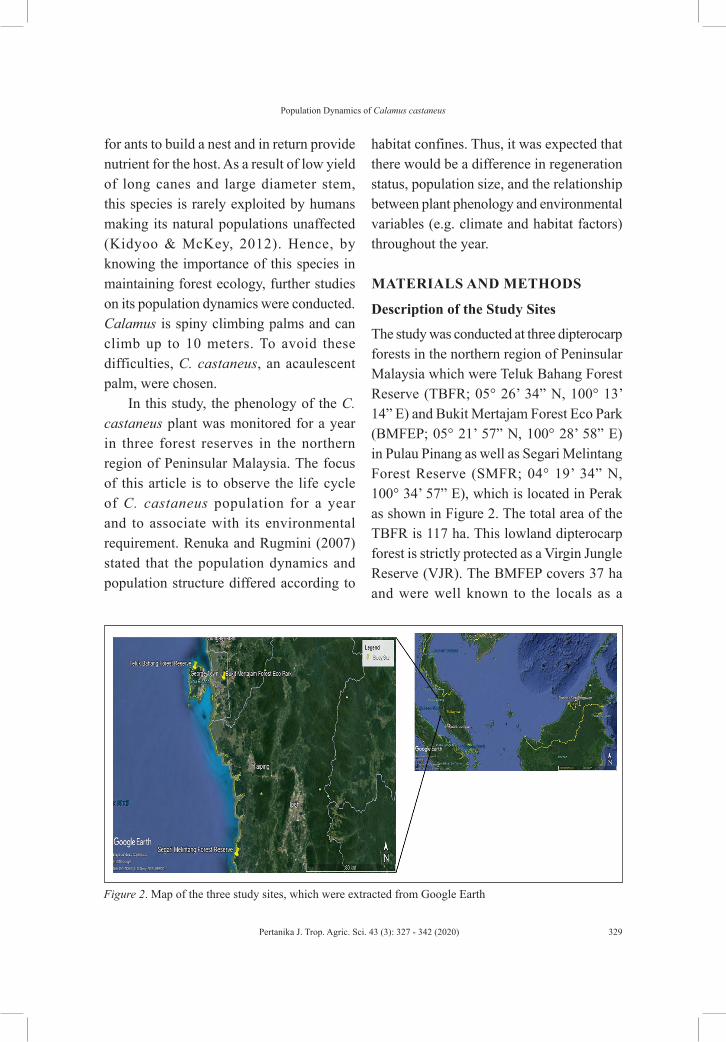
Population Dynamics of Calamus castaneus
329Pertanika J. Trop. Agric. Sci. 43 (3): 327 - 342 (2020)
for ants to build a nest and in return provide nutrient for the host. As a result of low yield of long canes and large diameter stem, this species is rarely exploited by humans making its natural populations unaffected (Kidyoo & McKey, 2012). Hence, by knowing the importance of this species in maintaining forest ecology, further studies on its population dynamics were conducted. Calamus is spiny climbing palms and can climb up to 10 meters. To avoid these difficulties, C. castaneus, an acaulescent palm, were chosen.
In this study, the phenology of the C. castaneus plant was monitored for a year in three forest reserves in the northern region of Peninsular Malaysia. The focus of this article is to observe the life cycle of C. castaneus population for a year and to associate with its environmental requirement. Renuka and Rugmini (2007) stated that the population dynamics and population structure differed according to
habitat confines. Thus, it was expected that there would be a difference in regeneration status, population size, and the relationship between plant phenology and environmental variables (e.g. climate and habitat factors) throughout the year.
MATERIALS AND METHODS
Description of the Study Sites
The study was conducted at three dipterocarp forests in the northern region of Peninsular Malaysia which were Teluk Bahang Forest Reserve (TBFR; 05° 26’ 34” N, 100° 13’ 14” E) and Bukit Mertajam Forest Eco Park (BMFEP; 05° 21’ 57” N, 100° 28’ 58” E) in Pulau Pinang as well as Segari Melintang Forest Reserve (SMFR; 04° 19’ 34” N, 100° 34’ 57” E), which is located in Perak as shown in Figure 2. The total area of the TBFR is 117 ha. This lowland dipterocarp forest is strictly protected as a Virgin Jungle Reserve (VJR). The BMFEP covers 37 ha and were well known to the locals as a
Figure 2. Map of the three study sites, which were extracted from Google Earth

Nur Diana Mohd Rusdi, Asyraf Mansor, Shahrul Anuar Mohd Sah, Rahmad Zakaria, Nik Fadzly Nik Rosely and Wan Ruslan Ismail
330 Pertanika J. Trop. Agric. Sci. 43 (3): 327 - 342 (2020)
famous hiking spot as it comprises of a hilly area. Both sites act as the water catchment area of which Teluk Bahang Dam is located near TBFR while Mengkuang Dam is close to BMFEP. The SMFR is located along the coastal area of the Manjung district and is mainly composed of primary coastal forest and alluvial freshwater swamp vegetation (Rusdi, 2019). There is a watercourse area inside the plot on this study site. Only 408 ha from 2741 ha of the SMFR is protected as a VJR while the rest was logged before and regenerated as Permanent Forest Reserve (PFR). This study was conducted for a year, between March 2017 to March 2018.
Plots Preparation and Rattan Assessment
Using the square plot design, five plots of 10 m × 10 m (100 m²) were established within each of the study sites. Forest trail was used as the main reference line where plots were established 500 m from the trail entrance. The cluster of rattan within the sampling plots was randomly distributed. To facilitate the monitoring of the whole population in a day, the distance between plots was fixed at 50 meters. In these plots, all individuals of the C. castaneus were identified and marked with numbered plastic tags (Bøgh, 1996). The identification of the specimens was based on the keys in “A Manual of the Rattans of the Malay Peninsula” (Dransfield, 1979). A complete sample of the C. castaneus stem with fresh sheath, inflorescences, and/or infructescences was collected from the field and deposited at the USM Herbarium. To analyze the influence
of climate on the recurrence of such annual phenomena of C. castaneus, parameters such as plant sexes, life stages, leaf sheath number, presence of flower, fruit, and length of petiole and rachis were recorded monthly for 12 months. Only one leaf with complete petiole and rachis were tagged and recorded throughout the studies. However, three readings were taken each time to get the average length. The life stages of the studied rattan species such as its seedling, young, or adult were noted. Life stages were classified according to height since this species in an acaulescent rattan: 1) seedling - ≤ 1 meter, 2) young plant - ≥ 1 meter but without signs of flowering and fruiting, and 3) adult - ≥ a 1-meter plant that bears flower or fruit. The sexes of each plant were identified by observing the flowers or fruits from the previous seasons (Kidyoo & McKey, 2012). Meanwhile, the length of petiole and rachis were measured using a measuring tape.
Microclimate Sampling and Soil Analysis
Microclimate readings (i.e. relative humidity, air temperature, soil temperature, light intensity, percentage of gap opening, and level of disturbance) were taken in situ every month between 10 a.m. until 12 p.m. time range (Hardwick et al., 2015). A portable thermo-hygrometer (Hanna Instrument model HI 9564) was used to measure the air temperature and relative humidity while a portable luxmeter (Hanna Instrument model HI 97500) was used in measuring light intensity. The readings were taken 1.5 meters from the ground near the cluster of
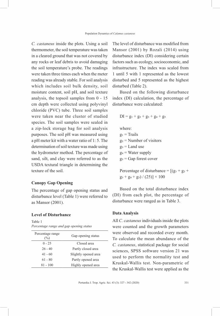
Population Dynamics of Calamus castaneus
331Pertanika J. Trop. Agric. Sci. 43 (3): 327 - 342 (2020)
C. castaneus inside the plots. Using a soil thermometer, the soil temperature was taken in a cleared ground that was not covered by any rocks or leaf debris to avoid damaging the soil temperature’s probe. The readings were taken three times each when the meter reading was already stable. For soil analysis which includes soil bulk density, soil moisture content, soil pH, and soil texture analysis, the topsoil samples from 0 - 15 cm depth were collected using polyvinyl chloride (PVC) tube. Three soil samples were taken near the cluster of studied species. The soil samples were sealed in a zip-lock storage bag for soil analysis purposes. The soil pH was measured using a pH meter kit with a water ratio of 1: 5. The determination of soil texture was made using the hydrometer method. The percentage of sand, silt, and clay were referred to as the USDA textural triangle in determining the texture of the soil.
Canopy Gap Opening
The percentage of gap opening status and disturbance level (Table 1) were referred to as Mansor (2001).
Level of DisturbanceTable 1Percentage range and gap opening status
Percentage range (%) Gap opening status
0 - 25 Closed area26 - 40 Partly closed area41 - 60 Slightly opened area61 - 80 Partly opened area81 - 100 Highly opened area
The level of disturbance was modified from Mansor (2001) by Rozali (2014) using disturbance index (DI) considering certain factors such as ecology, socioeconomic, and infrastructure. The index was scaled from 1 until 5 with 1 represented as the lowest disturbed and 5 represented as the highest disturbed (Table 2).
Based on the following disturbance index (DI) calculation, the percentage of disturbance were calculated:
DI = g₁ + g₂ + g₃ + g₄ + g₅
where:g₁ = Trailsg₂ = Number of visitorsg₃ = Land useg₄ = Water supplyg₅ = Gap forest cover Percentage of disturbance = [(g₁ + g₂ + g₃ + g₄ + g₅) / (25)] × 100
Based on the total disturbance index (DI) from each plot, the percentage of disturbance were ranged as in Table 3.
Data Analysis
All C. castaneus individuals inside the plots were counted and the growth parameters were observed and recorded every month. To calculate the mean abundance of the C. castaneus, statistical package for social sciences, SPSS software version 21 was used to perform the normality test and Kruskal-Wallis test. Non-parametric of the Kruskal-Wallis test were applied as the

Nur Diana Mohd Rusdi, Asyraf Mansor, Shahrul Anuar Mohd Sah, Rahmad Zakaria, Nik Fadzly Nik Rosely and Wan Ruslan Ismail
332 Pertanika J. Trop. Agric. Sci. 43 (3): 327 - 342 (2020)
Table 2Characterization for disturbance criteria
Feature Disturbance scaleTrails (g1)
Infrastructure:Unexplored forest overgrown by big trees 1Unexplored forest and filled with bushes 2Explored forest with small trails < 50 cm width (rarely used by visitors)
3
Explored forest with bigger trails > 50 cm width (always used by visitors)
4
Paved roads 5Visitors per day (g2)
Socioeconomics:1 - 15 visitors 116 - 25 visitors 226 - 35 visitors 336 - 45 visitors 4> 45 visitors 5
Land use (g3)Ecology:Virgin forest 1Secondary forest 2Reserve forest 3Agriculture 4Clearings forest 5
Water resource (g4)Big streams or waterfalls 1Watercourse 2Recreational ponds 3Damp 4Dried area, no watercourse in the forest 5
Canopy opening (g5)0 - 25 % 126 - 40 % 241 - 60 % 361 - 80 % 481 - 100 % 5
Table 3Percentage range and disturbance status
Percentage range (%) Disturbance status
0 - 25 Low disturbed area
25 - 50 The moderately low disturbed area
50 - 75 The moderately high disturbed area
75 - 100 Highly disturbed area
The association between the environmental parameter on the population dynamics of the C. castaneus were analyzed using the canonical correspondence analysis (CCA) and was performed with the CANOCO version 4.5. CCA was used as it performs quite well with highly intercorrelated environmental variables and with a situation where not all the factors determining species composition are known (Palmer, 1993).
RESULTS
Life Stages and Population Size
A total of 180 C. castaneus individuals were observed during the one-year sampling period. From Table 4, Segari Melintang Forest Reserve (SMFR) displayed the most abundant of seedling (40 individuals), adult plant (41 individuals), and the fewest amount of young plant (5 individuals) compared to the other two sites. This site also showed the highest abundance (86 individuals) of C. castaneus followed by Teluk Bahang Forest Reserve (TBFR) (52 individuals) and lastly Bukit Mertajam Forest Eco-Park (BMFEP) (42 individuals). TBFR displayed the smallest number of seedlings individual (10 individuals), adult plant (6 individuals) but with the highest
data for this analysis violates the parametric assumptions. Microclimate data were analyzed using the parametric test: one-way ANOVA with post-hoc Tukey test.
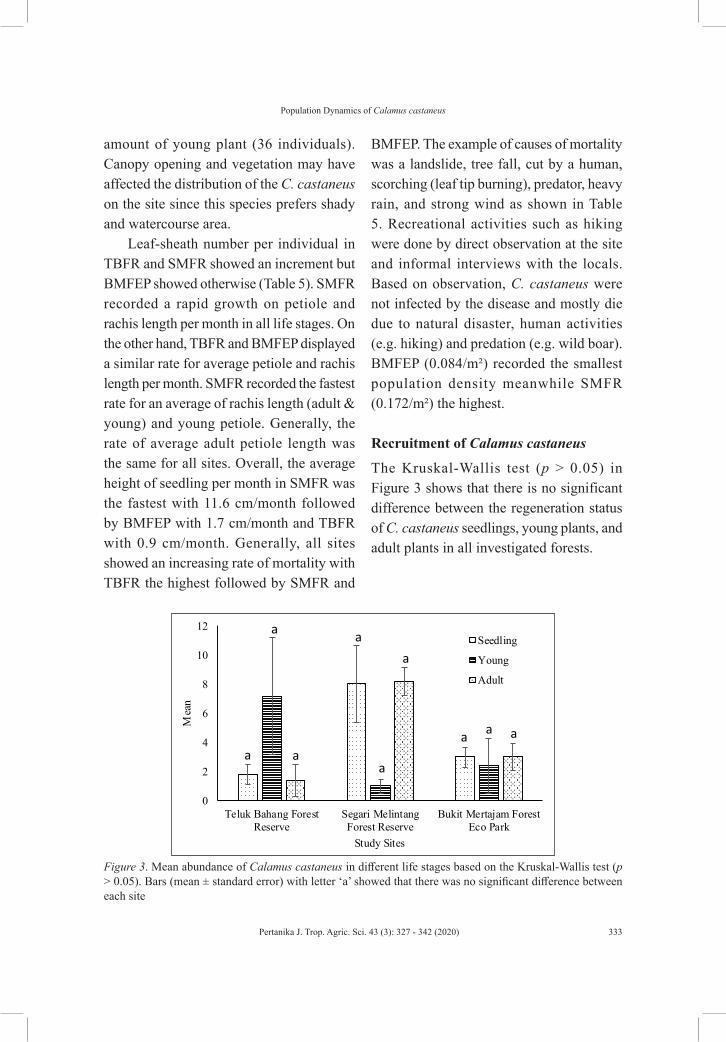
Population Dynamics of Calamus castaneus
333Pertanika J. Trop. Agric. Sci. 43 (3): 327 - 342 (2020)
amount of young plant (36 individuals). Canopy opening and vegetation may have affected the distribution of the C. castaneus on the site since this species prefers shady and watercourse area.
Leaf-sheath number per individual in TBFR and SMFR showed an increment but BMFEP showed otherwise (Table 5). SMFR recorded a rapid growth on petiole and rachis length per month in all life stages. On the other hand, TBFR and BMFEP displayed a similar rate for average petiole and rachis length per month. SMFR recorded the fastest rate for an average of rachis length (adult & young) and young petiole. Generally, the rate of average adult petiole length was the same for all sites. Overall, the average height of seedling per month in SMFR was the fastest with 11.6 cm/month followed by BMFEP with 1.7 cm/month and TBFR with 0.9 cm/month. Generally, all sites showed an increasing rate of mortality with TBFR the highest followed by SMFR and
BMFEP. The example of causes of mortality was a landslide, tree fall, cut by a human, scorching (leaf tip burning), predator, heavy rain, and strong wind as shown in Table 5. Recreational activities such as hiking were done by direct observation at the site and informal interviews with the locals. Based on observation, C. castaneus were not infected by the disease and mostly die due to natural disaster, human activities (e.g. hiking) and predation (e.g. wild boar). BMFEP (0.084/m²) recorded the smallest population density meanwhile SMFR (0.172/m²) the highest.
Recruitment of Calamus castaneus
The Kruskal-Wallis test (p > 0.05) in Figure 3 shows that there is no significant difference between the regeneration status of C. castaneus seedlings, young plants, and adult plants in all investigated forests.
Figure 3. Mean abundance of Calamus castaneus in different life stages based on the Kruskal-Wallis test (p > 0.05). Bars (mean ± standard error) with letter ‘a’ showed that there was no significant difference between each site
0
2
4
6
8
10
12
Teluk Bahang ForestReserve
Segari MelintangForest Reserve
Bukit Mertajam ForestEco Park
Mea
n
Study Sites
Seedling
Young
Adult
a a
aa
a
a
aaa

Nur Diana Mohd Rusdi, Asyraf Mansor, Shahrul Anuar Mohd Sah, Rahmad Zakaria, Nik Fadzly Nik Rosely and Wan Ruslan Ismail
334 Pertanika J. Trop. Agric. Sci. 43 (3): 327 - 342 (2020)
Tabl
e 5
Rate
of o
bser
ved
ratta
n pa
ram
eter
s, m
orta
lity
and
popu
latio
n de
nsity
of C
alam
us c
asta
neus
indi
vidu
als f
or a
yea
r
Site
Life
stag
esN
umbe
r of l
eaf
shea
th/ i
ndiv
idua
l
Aver
age
petio
le
leng
th (c
m)/
mon
th
Aver
age
rach
is
leng
th (c
m)/
mon
th
The
aver
age
heig
ht o
f se
edlin
g (c
m/m
onth
)
Mor
talit
y of
in
divi
dual
sC
ause
s of m
orta
lity
Popu
latio
n de
nsity
(p
er m
²)
t₀t₁
t₀t₁
TB
FRA
dult
1213
0.5
± 0.
1a0.
6 ±
0.1a
-6
2La
ndsl
ide,
tree
fall,
cut
by
hum
an, h
eavy
rain
an
d st
rong
win
dyo
ung
89
0.5
± 0.
0a0.
6 ±
0.0a
-36
160.
104
se
edlin
g
-
--
-0.
910
4
SMFR
Adu
lt12
139.
3 ±
2.7a
15.6
± 4
.0b
-41
32Tr
ee fa
ll, sc
orch
ing,
pr
edat
or, h
eavy
rain
and
st
rong
win
dyo
ung
812
4.2
± 3.
1b4.
2 ±
3.1b
-5
20.
172
se
edlin
g
-
--
-11
.640
35
BM
FEP
Adu
lt11
100.
6 ±
0.0a
0.6
± 0.
0a-
1514
Land
slid
e, tr
ee fa
ll, c
ut
by h
uman
, hea
vy ra
in
and
stro
ng w
ind
youn
g8
60.
6 ±
0.0a
0.6
± 0.
0a-
1212
0.08
4
seed
ling
--
--
1.7
1510
Not
e. t₀
: ini
tial r
eadi
ng (t
aken
in M
arch
201
7); t
₁: fin
al re
adin
g (ta
ken
in M
arch
201
8). S
uper
scrip
ts a
and
b in
dica
ted
the
sign
ifica
nt d
iffer
ence
s at
p <
0.0
5 by
po
st-h
oc T
ukey
test
in e
ach
para
met
er b
etw
een
site
s
Tabl
e 4
Num
ber o
f Cal
amus
cas
tane
us in
divi
dual
s acc
ordi
ng to
diff
eren
t life
stag
es in
all
stud
y si
tes
Life
stag
esTe
luk
Bah
ang
Fore
st
Res
erve
Sega
ri M
elin
tang
For
est
Res
erve
Buk
it M
erta
jam
For
est
Eco
Park
Seed
ling
1040
15Yo
ung
365
12A
dult
641
15To
tal
5286
42

Population Dynamics of Calamus castaneus
335Pertanika J. Trop. Agric. Sci. 43 (3): 327 - 342 (2020)
Relationship of Environmental Variables with the Calamus castaneus Phenology
Table 6 shows the mean environmental variables parameter that was recorded from March 2017 until March 2018. The data was collected twice each month. One-way ANOVA was used to analyze the significant difference between each site since microclimate is a parametric data. The significant difference between sites was denoted as in Table 6. From ten variables listed, only four which were air temperature,
light intensity, canopy gap opening, and soil bulk density displayed the same on each site.
The CCA of growth and environmental data which are summarized in Tables 7, 8, and 9 indicate that the species-environment correlations were low of which eigenvalues (the score of the maximized dispersion of the species on the ordination axis and the strength of an axis) were less than 0.5 (values over 0.5 often express a good division of the species along the axis). The cumulative variance explained by the first three axes of the species-environment
Table 6Environmental variables parameter (Mean ± SE) measured from March 2017 until March 2018
Parameter TBFR SMFR BMFEPRelative humidity (%) 83.70 ± 1.34b 71.59 ± 2.21a 81.14 ± 2.18b
Air temperature (°C) 25.0 ± 2.14a 28.50 ± 1.01a 25.35 ± 0.40a
Light intensity (kLux) 1.00 ± 0.18a 1.11 ± 0.18a 1.10 ± 0.18a
Soil temperature (°C) 26.15 ± 0.10b 26.81 ± 0.15c 24.28 ± 0.14a
Canopy gap opening (%) 25.5 ± 4.77a 46.7 ± 8.47a 36.4 ± 5.41a
Disturbance index (%) 37.6 ± 0.98b 30.8 ± 2.15a 60.8 ± 1.5c
Soil pH 5.74 ± 0.15b 6.09 ± 0.33b 4.82 ± 0.05a
Soil moisture content (%) 24.82 ± 0.65a 32.26 ± 3.30a 45.26 ± 3.70b
Soil bulk density (gcm-³) 0.97 ± 0.12a 0.91 ± 0.14a 0.76 ± 0.09a
Soil texture analysis Sand Sand Loamy sand
Note. Superscripts a, b and c indicated the significant differences at p < 0.05 by post-hoc Tukey test in each parameter between sites
Table 7Summary of the CCA of the Calamus castaneus plant growth and environmental data in Teluk Bahang Forest Reserve
Axes 1 2 3 4 Total inertia Eigenvalues 0.213 0.005 0.001 0 0.651 Species-environment correlations 0.744 0.159 0.147 0.226 Cumulative percentage variance
of species data 32.8 33.6 33.7 33.7 of species-environment relation 97.1 99.4 99.8 99.9
Sum of all eigenvalues 0.651 Sum of all canonical eigenvalues 0.22

Nur Diana Mohd Rusdi, Asyraf Mansor, Shahrul Anuar Mohd Sah, Rahmad Zakaria, Nik Fadzly Nik Rosely and Wan Ruslan Ismail
336 Pertanika J. Trop. Agric. Sci. 43 (3): 327 - 342 (2020)
Table 8Summary of the CCA of the Calamus castaneus plant growth and environmental data in Segari Melintang Forest Reserve
Axes 1 2 3 4 Total inertia Eigenvalues 0.119 0.017 0.002 0.001 0.738 Species-environment correlations 0.555 0.236 0.48 0.282 Cumulative percentage variance of species data 16.2 18.5 18.8 19 of species-environment relation 85.1 97.4 98.9 99.8 Sum of all eigenvalues 0.738 Sum of all canonical eigenvalues 0.14
Table 9Summary of the CCA of the Calamus castaneus plant growth and environmental data in Bukit Mertajam Forest Eco-Park
Axes 1 2 3 4 Total inertia Eigenvalues 0.193 0.008 0.002 0.001 0.699 Species-environment correlations 0.697 0.194 0.427 0.224 Cumulative percentage variance of species data 27.6 28.8 29 29.2 of species-environment relation 94.3 98.2 99.1 99.7 Sum of all eigenvalues 0.699 Sum of all canonical eigenvalues 0.205
relationship in the CCA in TBFR was 99.8% (Table 7), SMFR is 98.9 % (Table 8), and BMFEP with 99.1 % (Table 9). The CCA ordination plot is as displayed in Figures 4, 5, and 6. The direction and length of the arrows which spread out from the centre of the ordination diagram illustrate the strength and direction accordingly between plant growth and environmental variables.
Figure 4 displayed that three out of five plant growth parameters listed in a study such as a rachis length, petiole length and the number of leaf sheath were increased as the increasing value of soil bulk density, canopy gap opening, air temperature, disturbance index level, relative humidity,
soil temperature, soil pH, and percentage of soil moisture content. Light intensity gives no effect on the rattan parameter listed. The number of flowers has no relation to the environmental parameter listed.
From Figure 5, soil pH and soil bulk density give a negative influence on the number of leaf sheath produced, an average of petiole and rachis length. The higher the value of soil pH and soil bulk density will decrease the number of leaf sheath produced, an average of petiole and rachis length. Besides that, a high percentage of soil moisture content, disturbance index level, and canopy gap opening will also reduce the number of flowers produced throughout

Population Dynamics of Calamus castaneus
337Pertanika J. Trop. Agric. Sci. 43 (3): 327 - 342 (2020)
Figure 4. Ordination plot of canonical correspondence analysis (CCA) between environmental variables (arrows) and Calamus castaneus plant growth (triangles) in Teluk Bahang Forest Reserve. Note. SBD = soil bulk density; DI = disturbance index; RH = relative humidity; SOIL TEMP = soil temperature; AIR TEMP = air temperature; PH = soil pH; SMC = soil moisture content
Figure 5. Ordination plot of canonical correspondence analysis (CCA) between environmental variables (arrows) and Calamus castaneus plant growth (triangles) in Segari Melintang Forest Reserve. Note. SBD = soil bulk density; DI = disturbance index; PH = soil pH; SMC = soil moisture content
the year. Meanwhile, the production of C. castaneus fruits in SMFR will increase by lowering the percentage of soil moisture content, percentage of canopy gap opening, disturbance index, soil bulk density, and soil pH.
All nine environmental parameters that were tested in this study had a positive influence on the rattan parameter (Figure 6). In BMFEP site, as the increasing value of soil bulk density, light intensity, percentage of canopy gap opening, disturbance index

Nur Diana Mohd Rusdi, Asyraf Mansor, Shahrul Anuar Mohd Sah, Rahmad Zakaria, Nik Fadzly Nik Rosely and Wan Ruslan Ismail
338 Pertanika J. Trop. Agric. Sci. 43 (3): 327 - 342 (2020)
level, relative humidity, air temperature, soil temperature, soil pH, and soil moisture content would increase fruit and flower production, a number of leaf sheath produced, rachis length and also petiole length.
DISCUSSION
Recruitment, Mortality and Population Size
Segari Melintang Forest Reserve (SMFR) displayed a tremendous number of individuals followed by Bukit Mertajam Forest Eco-Park (BMFEP) and Teluk Bahang Forest Reserve (TBFR). From observation, TBFR, and BMFEP plots suffered from landslides, the tree falls from heavy rain and strong winds during monsoon season in November 2017 until January 2018. This had affected the population of C. castaneus in both sites. There was no
significant difference (p > 0.05) shown after performing the Kruskal-Wallis test in all life stages in all sites. This had proven that the abundance of C. castaneus is the same for all sites. According to Rozali (2014), the continuation of regeneration in a locality was dependent on the abundance of seedlings in that area. This is proven by looking at the small seedlings number in BMFEP which shows a lower level of a succession of this rattan growing into the adult plants compared to the other two sites.
Although SMFR displayed the greatest number of seedlings, only a few of them would make it to the young stage. The competitiveness between the young plant with the fully established mature plant was high, thus resulting in the lower population of the young C. castaneus plants in this site. Throughout this study, SMFR had suffered from large tree falls in July 2017 caused by
Figure 6. Ordination plot of canonical correspondence analysis (CCA) between environmental variables (arrows) and Calamus castaneus plant growth (triangles) in Bukit Mertajam Forest Eco-Park. Note. SBD = soil bulk density; DI = disturbance index; RH = relative humidity; SOIL TEMP = soil temperature; AIR TEMP = air temperature; PH = soil pH; SMC = soil moisture content; Light = light intensity

Population Dynamics of Calamus castaneus
339Pertanika J. Trop. Agric. Sci. 43 (3): 327 - 342 (2020)
strong coastal wind during heavy rain. This finding suggests that natural disasters such as tree falls had altered the regeneration of rattan and dispersion of seedlings in the site. The tree falls had generated gap opening that caused scorching during the seedling stage. Vongkaluang (1985) stated that the high opening of the canopy and direct penetration of light might be the major cause for the non-survival of seedlings in open areas. Strong wind and tree fall had also damaged the leaf sheath of C. castaneus. Based on Table 5, BMFEP displayed a decreased number of leaf sheath production throughout the year. It can be concluded that all three sites experienced high mortality due to tree falls. Another cause of mortality was predation. A predator such as wild boar had been noticed eating fallen fruit of C. castaneus and digging soil near the clump had crushed the new rattan seedlings which result in mortality.
Besides that, a high rate of recreational activities such as hiking in a site would reduce the rattan population and creating gap opening particularly in TBFR and BMFEP (personal observation). Hikers especially in the large group tend to cut off rattan or any disturbing plants that came across the trail. The low level of rattan formation in the sites are mostly due to these undesirable conditions. A large population size in SMFR might be due to its composition of background vegetation. C. castaneus prefers to grow on lower hillslopes and streamsides (Dransfield, 1979). Based on the observation in this study, this species fits more in a partially
cleared area with a shady canopy gap. The rattan habit of clumping makes this species to vegetate near one another, creating C. castaneus population. Human activities have put stress on rattan regeneration on the site. By avoiding these circumstances, the juveniles’ growth might raise (Renuka & Rugmini, 2007; Rusdi, 2019).
Overall, the SMFR displayed a speedy rate for young petiole length, rachis length, and a number of leaves produced per month compared to the other two sites (Table 5). On the other hand, TBFR and BMFEP show a similar rate for rachis and petiole length. A study on a threatened rattan species by Renuka and Rugmini (2007) found that the population structure and population dynamics would differ according to habitat confines. Hence, it is estimated that the SMFR provides the most favorable habitat and the requirement for the succession and growth of the C. castaneus, therefore increasing the population density of this species on the site.
In a natural population, the growth rate may vary among the rattan species as it relies upon environmental factors and genetic variations (Rusdi, 2019). In addition, it is common for the Arecaceae family to develop slower during the early stage (Bøgh, 1996; Dransfield & Manokaran, 1994). Moreover, rattan species that grow under larger trees in the forest also showed a slow growth rate (Table 5) (Dransfield, 1979). According to the percentage range and gap opening status by Mansor (2001), all three sites have partly closed and slightly opened areas within a range of 25% to 47%

Nur Diana Mohd Rusdi, Asyraf Mansor, Shahrul Anuar Mohd Sah, Rahmad Zakaria, Nik Fadzly Nik Rosely and Wan Ruslan Ismail
340 Pertanika J. Trop. Agric. Sci. 43 (3): 327 - 342 (2020)
canopy gap opening. Thus, this might be the reason for the slow growth in the height of the seedlings compared to other parts of the listed rattan growth (Table 5).
Association Between Microclimate Parameters and Soil Properties on Population Dynamics
Most of the environmental variables; relative humidity, air temperature, light intensity, soil temperature, percentage of canopy gap opening, disturbance index, soil pH, soil moisture content and soil bulk density have had a positive influence on the C. castaneus plant growth; a number of the leaf sheath, petiole length, rachis length, number of flowers and fruits produced in TBFR (Figure 4) and BMFEP (Figure 6). Soil temperature can influence the community structure of any plant species through the alteration of its anatomical and physiological processes (Rozali, 2014). Warmer soil temperature as in tropical regions probably relates to the high diversity and abundance of plants and rattan species. In addition, certain minerals are needed since growth in stem diameter is possible at a high acidity level. High soil bulk density would help in increasing the rate of nutrient absorbent from the soil (Rusdi, 2019). On the other hand, high relative humidity is caused by the small opening of the forest canopy. This situation is sufficient for the growth of these rattan species as it grows under the low light requirement of a well-aged forest with dense canopies (Powling, 2004). Some rattan species depend upon the soil with adequate moisture and high
light intensity to grow (Powling, 2004). Binh (2009) also stated that the increasing growth rate of rattan was dependent upon the amount of light exposure on its crown.
However, from the CCA ordination plot of the SMFR in Figure 4, it is shown that moisture content (32.26%), soil bulk density (0.91 gcm-³), percentage of gap opening (46.7%), soil pH (6.09), and disturbance index (30.8%) have had a negative influence on the C. castaneus. Highly acidic soil may affect rattan maturity and would cause retardation in plants (Lilly, 2010). Other than that, a high bulk density of soil restricts the growth of root, inhibits the gaseous exchange in the root zone, and might also decrease the penetration of water (Brady & Weil, 2013; Lilly, 2010). Based on one year of sampling, this species does have a specific environmental condition for its growth since it favored the watercourse and shady area (Dransfield, 1979).
CONCLUSION
The abundance of the C. castaneus is the same since there was no significant difference in each study site. Among the three sites, SMFR recorded the fastest increment of young petiole length and rachis length for adult and young plants. Meanwhile, the rate for rachis and petiole length for TBFR and BMFEP were similar. Causes of mortality such as tree fall, landslides, heavy rain, strong winds, scorching, and predation had damaged the leaf sheath and the plants itself hence resulting in death. SMFR showed the largest population size of C. castaneus with 0.172 individuals per m².

Population Dynamics of Calamus castaneus
341Pertanika J. Trop. Agric. Sci. 43 (3): 327 - 342 (2020)
Generally, the population size was strongly dependent on environmental factors. It can thus be concluded that almost all listed environmental parameters will give either a positive or negative influence on the phenology and mortality of the C. casteneus in all three sites.
ACKNOWLEDGEMENTS
The authors would like to show gratitude for the USM RU Research grant funding: 1001/PBIOLOGI/8011031 for financially supporting this research and the Peninsular Malaysia Forestry Department for issuing the respective permits.
REFERENCESAli, A. R. M., & Barizan, R. S. R. (2001). Important
rattan species of Malaysia. Retrieved July 1, 2018, from http://www.fao.org/3/x9923e07.htm#P0_0
Binh, B. M. (2009). Rattans of Vietnam: Ecology , demography and harvesting (Doctoral dissertation, Utrecht University, Netherlands). Retrieved March 21, 2019, from https://dspace.library.uu.nl/handle/1874/35946
Bøgh, A. (1996). Abundance and growth of rattans in Khao Chong National Park, Thailand. Forest Ecology and Management, 84(1-3), 71–80. doi:10.1016/0378-1127(96)03738-3
Brady, N. C., & Weil, R. R. (2013). The nature and properties of soils (14th ed.). London, United Kingdom: Pearson Education Limited.
Dransfield, J. (1979). A manual of the rattans of the Malay Peninsula. Kuala Lumpur, Malaysia: Ministry of Primary Industries Malaysia.
Dransfield, J. (2001). Taxonomy, biology and ecology of rattan. Retrieved July 1, 2018, from http://www.fao.org/3/x9923e06.htm#P0_0
Dransfield, J., & Manokaran, N. (Eds.) (1994). Plants resources of South-East Asia No. 6: Rattans. Bogor, Indonesia: Plant Resources of Southeast Asia (PROSEA).
Hardwick, R. S., Toumi, R., Pfeifer, M., Turner, E. C., Nilus, R., & Ewers, R. M. (2015). The relationship between leaf area index and microclimate in tropical forest and oil palm plantation: Forest disturbance drives changes in microclimate. Agricultural and Forest Meteorology, 201, 187-195. doi:10.1016/j.agrformet.2014.11.010
Lilly, S. (2010). Arborists’ certification study guide (3rd ed.). Atlanta, USA: International Society of Arboriculture.
Kidyoo, A. M., & McKey, D. (2012). Flowering phenology and mimicry of the rattan Calamus castaneus (Arecaceae) in southern Thailand. Botany, 90(9), 856-865. doi:10.1139/b2012-058
Mansor, A. (2001). Kajian kepelbagaian dan ekologi rumpai di kawasan hutan paya Semenanjung Malaysia [Study of weed diversity and ecology in the swamp forest areas of Peninsular Malaysia] (Unpublished Doctoral thesis), Universiti Sains Malaysia, Malaysia.
Palmer, M. W. (1993). Putting things in even better order: The advantages of canonical correspondence analysis. Ecology, 74(8), 2215-2230.
Powling, A. (2004). Rattans : Taxonomy and ecology ( LIPI report 2004). Retrieved March 27, 2019, from https://www.opwall.com/uploads/2017/11/Opwall-Indonesia-Buton-Rattan-Report-2004.pdf
Renuka, C., & Rugmini, P. (2007). Development of conservation strategies for selected, endangered rattan species of the Western Ghats. Retrieved March 25, 2019, from http://docs.kfri.res.in/KFRI-RR/KFRI-RR295.pdf
Rozali, W. N. F. Z. W. (2014). Composition of rattan communities (Arecaceae, Subfamily

Nur Diana Mohd Rusdi, Asyraf Mansor, Shahrul Anuar Mohd Sah, Rahmad Zakaria, Nik Fadzly Nik Rosely and Wan Ruslan Ismail
342 Pertanika J. Trop. Agric. Sci. 43 (3): 327 - 342 (2020)
Calamoideae) in forest reserves of Penang (Master’s thesis), Universiti Sains Malaysia, Malaysia.
Rusdi, N. D. M. (2019). Population dynamics of Calamus castaneus Griff. in selected forest reserve in northern region of Peninsular Malaysia (Master’s thesis), Universiti Sains Malaysia, Malaysia.
Ruppert, N., Mansor, A., & Anuar Mohd Sah, S. (2012). New shoot from inflorescences in Calamus castaneus in Peninsular Malaysia. Palms, 56(1), 36-40.
Ruppert, N., Mansor, A., & Anuar Mohd Sah, S. (2016). Rattan (Calamoideae) abundance and above-ground biomass at a primary rainforest of Peninsular Malaysia. Plant Ecology and Diversity, 9(1), 63–67. doi:10.1080/17550874.2015.1081650
Sastry, C. B. (2001). Rattan in the twenty-first century - An overview. Retrieved July 1, 2018, from http://www.fao.org/3/x9923e03.htm#P0_0
Sunderland, T. C. H., & Dransfield, J. (2002). Species profiles of rattan. In J. Dransfield, F. O. Tesoro, & N. Manokaran (Eds.), Rattan - Current research issues and prospects for conservation and development (pp. 9-22). Rome, Italy: FAO.
Vongkaluang, I. (1985). Preliminary study of the germination and some ecological aspects of Calamus peregrinus in Thailand. Retrieved April 4, 2019, from http://www.agris.upm.edu.my:8080/dspace/handle/0/12454
Wan Ariffin, W. T., Rene, K., Muralidharan, E. M., Sreekumar, V. B., Chowdhary, C., Sheng, L. R., … Hourt, H. E. (2018). Rattan terminologies. Retrieved April 4, 2019, from https://www.researchgate.net/publication/325487138_Rattan_Terminologies

Pertanika J. Trop. Agric. Sci. 43 (3): 343 - 357 (2020)
ISSN: 1511-3701e-ISSN 2231-8542
TROPICAL AGRICULTURAL SCIENCEJournal homepage: http://www.pertanika.upm.edu.my/
Article history:Received: 12 December 2019Accepted: 27 May 2020Published: 28 August 2020
ARTICLE INFO
E-mail addresses:[email protected] (Piyanan Nualhnuplong)[email protected] (Chaiyawan Wattanachant)* Corresponding author
© Universiti Putra Malaysia Press
Effects of Age at Slaughter and Sex on Carcass Characteristics and Meat Quality of Betong Chicken
Piyanan Nualhnuplong1 and Chaiyawan Wattanachant2*1Program in Tropical Agricultural Resource Management, Faculty of Natural Resources, Prince of Songkla University, Hat Yai, Songkhla 90112, Thailand 2Department of Animal Science, Faculty of Natural Resources, Prince of Songkla University, Hat Yai, Songkhla 90112, Thailand
ABSTRACT
The purpose of this study was to determine the effects of age at slaughter and sex on carcass characteristics and meat quality of Betong chickens that were raised under a semi-free-range system. A total of 360 chickens from Takbai, Narathiwat Province, Thailand were arranged into 3x2 factorial design with 3 levels of age at slaughter (16, 20, 24 weeks) and sex (male and female) in CRD. The experiment consisted of 6 treatments with 3 replications. Ten chickens of each replicate from each treatment group were randomly sampled for carcass yield and meat quality. Results showed that slaughter and carcass weights were significantly higher when the age at slaughter increased (P<0.01). Males had heavier slaughter and carcass weights (P<0.001) with lower breast percentage than the female chickens in each particular age. Higher yellowness value was significantly illustrated when the age of chickens increased. This color value was higher in both breast and thigh meat of the female chickens (P<0.05). Considering texture analysis, the males had significantly higher
shear force value than the females (P<0.05). This shear value tended to increase when the age of the chicken increased (P>0.05). There was no significant difference observed between age at slaughter on chemical composition (P>0.05). Nevertheless, the males had less fat content in breast meat and higher collagen content in thigh meat than the female Betong chickens (P<0.05). The results show that males should be slaughtered at 20 weeks, while the females

Piyanan Nualhnuplong and Chaiyawan Wattanachant
344 Pertanika J. Trop. Agric. Sci. 43(3): 343 - 357 (2020)
should be slaughtered when they reach the age of 24 weeks.
Keywords: Age at slaughter, Betong chicken, meat
quality, sex
INTRODUCTION
Betong chicken (Gallus domesticus) is a native Thai chicken predominantly found in the three provinces located in the Deep South of Thailand, especially in the Betong District, Yala Province, and in the northern part of Hulu Perak, Perak State, Malaysia. Farmers in the Deep South of Thailand commonly raise this chicken indoors until eight weeks into the growth period. Then they are raised under semi-free-range conditions until reaching the market weight of 1,500 to 2,000 g for females or 2,000 to 2,500 g for males (Chanjula et al., 2004; Chatreewong & Waree, 2006; Nualhnuplong et al., 2019b).
From a literature review, some research work on Betong chicken has been reported, for example, phenotypic characteristics and productive performance of this chicken (Chanjula et al., 2004); optimum age and weight of Betong chicken for the market (Chatreewong & Waree, 2006); dietary protein and energy level on growth performance and reproductive system development in the female during growth to pullet period (Buakeeree & Nualhnuplong, 2018); nitrogen-corrected true and apparent metabolizable energy (TMEn and AMEn) of crude glycerin (CG) for Betong chicken (Sopian et al., 2018); and effect of rearing system on meat quality (Nualhnuplong et
al., 2019a; Ritchoo et al., 2019). However, less information about the carcass yield and meat quality of Betong chicken has been reported. Thus, this study aimed to provide basic information about the effects of age at slaughter and sex on the carcass yield and meat quality in terms of physical characteristics and chemical composition. Results from this work will be used as reference information for managing Betong chicken production.
MATERIALS AND METHODS
Sample Preparation
A total of 360 male and female Betong chickens were randomly divided into 6 treatment groups. According to the treatment groups, The Betong chickens were arranged as 3 x 2 factorial in a completely randomized design with 3 levels of age at slaughter (16, 20, 24 weeks) and sex (male and female). Each treatment group consisted of 3 replicates (pens) of 20 Betong chickens. The chickens in each treatment were raised in a semi-free-range system. They were raised in the house (5 birds/m2) with access to grass paddock or backyard or garden (3 birds/m2). During week 1 to 3 chickens were kept in a house and fed commercial diet containing 21% of crude protein (CP), while they were allowed to walk outdoors and fed 19% CP from week 8 to 24. Nevertheless, cooked rice and corn were mixed with a commercial diet at a ratio of 0.5:0.5:1. Once they reached the target age, chickens were sampled from the flock and transferred to slaughter at a local abattoir. The slaughtering method used in this study
Age at Slaughter and Sex on Meat Quality of Betong Chicken
345Pertanika J. Trop. Agric. Sci. 43(3): 343 - 357 (2020)
had followed the regulations of the National Bureau of Agricultural Commodity and Food Standards (ACFS) (2007), Ministry of Agriculture and Cooperatives, Thailand. After slaughter, eviscerated carcasses were weighed and immediately stored at chill temperature for about 24 h for further determination.
Sample Collection and Analyses
After 24 h, the eviscerated carcasses were weighed and separated for retail parts, such as breasts, thighs, drumsticks, wings, feet, head, neck, and skeletal. The percentages of the chilled carcasses were expressed as a percentage of live weight, while the retail parts were determined based on chilled carcass weight. For meat quality determination, breast and thigh muscles were sampled for physical and chemical analysis. Ten (10) Betong chickens of each replicates from each treatment group were randomly sampled for the carcass yield and meat quality included physical characteristics and chemical composition of meat. The variables for analysis were the following:
Physical Properties Determination. The pH of breast and thigh muscles was measured by digital pH meter (Seven2Go, Mettler-Toledo, Switzerland) 45 min after slaughter for pH0 and 24 h after slaughter for pH24. Meat and skin color were measured on the raw muscle and skin with a Konica Minolta colorimeter (Konica Minolta, Japan) after 24 h chill at 4oC. The result was reported on the complete International
Commission on Illumination (CIE) system color profile of lightness (L*), redness (a*), and yellowness (b*). The meat samples for drip loss and cooking loss were trimmed to a dimension of 2.0 x 1.0 x 0.5 cm. Each piece was weighed (weight before storage = W1) and put into a sealed plastic bag, with drip loss stored at a chilled temperature (4oC) for 24 h. The sample was then removed from the sealed plastic bag, blotted, and weighed (W2 is the weight after storage); the cooking loss was measured by heating in a water bath at 80oC for 10 min. After cooking, the sample was cooled to room temperature and weighed (W2 is the weight after cooking). Drip loss and cooking loss were calculated as a percentage of weight loss: ((W1- W2)/ W1) x 100. Shear force was measured on cooked meat samples using a Texture Analyzer (TA-XT plus Stable Micro System Texture Analyzer, UK) with a 2 mm/s crosshead speed and a 50-load cell. The score obtained after a Warner-Bratzler blade cut the sample represented the shear force (Dawson et al., 1991).
Chemical Composition Determination. Moisture, crude protein, crude fat, and ash were analyzed according to the Association of Analytical Chemists (AOAC) (2006). Total collagen was determined after acid hydrolysis as described by Palka (1999). Hydroxyproline contents in the hydrolysate were determined by the procedure of Bergman and Loxley (1963) and converted to collagen contents using the factor 7.25, as described by Wattanachant et al. (2004).

Piyanan Nualhnuplong and Chaiyawan Wattanachant
346 Pertanika J. Trop. Agric. Sci. 43(3): 343 - 357 (2020)
Statistical Analysis. The data on carcass percentages and meat quality were analyzed by two-way Analysis of Variance (ANOVA) in a 3 x 2 factorial completely randomized design (3 age levels and 2 sex levels). The significance between means was analyzed using Duncan’s Multiple Range Test (DMRT) in the Statistical Analysis System (SAS) (1998).
RESULTS AND DISCUSSION
Effects of Age at Slaughter and Sex on Carcass Characteristics and Retail Cuts of Betong Chicken
The effects of age at slaughter and sex on carcass yield and retail part percentage of Betong chicken are shown in Tables 1 and 2, with a significant interaction effect between age at slaughter and sex on slaughter weight and breast percentage (P<0.05) (Figure 1). Figure 1 clearly shows that the slaughter weight of male Betong chickens tended to increase from the age of 16 weeks to
20 weeks and the weight was stable until reaching the age of 24 weeks, while the female chickens in the 16-20 weeks had no significant difference in weight. But slaughter weight tended to be higher when the chicken reached the age of 24 weeks old. Under this condition, both sexes had higher weight at slaughter at 24 weeks than the chicken aged 16 and 20 weeks. The range of slaughter weight obtained in this work was about 1,896-2,051 g in the male and 1,476-1,562 g in female.
When discussing the retail cuts, slaughter age did not show any significant effect on breast meat percentage of the male (P>0.05), but breast meat was significantly lower when the slaughter age increased (P<0.05). More breast muscle percentage in chicken aged 16 and 20 weeks old, after which it tended to decrease at the age of 24 weeks. Nevertheless, the male had a lower percent breast (18.39-19.10%) than the female (20.15-20.93%).
Items Slaughterweight
Warm carcass weight
Chill carcass weight
Carcass percentage
Age 16 1,689.17b 1,175.73b 1,158.82b 68.5020 1,770.17a 1,236.75a 1,217.30a 68.7324 1,787.60a 1,275.88a 1,238.98a 69.09
P-value 0.0005 <0.0001 0.0006 0.3746Sex Male 1,993.93a 1,401.79a 1,377.31a 69.24a
Female 1,505.23b 1,045.99b 1,025.51b 68.25b
P-value <0.0001 <0.0001 <0.0001 0.0040
Table 1Effects of age at slaughter and sex on carcass yield (g) and carcass percentage (%) of Betong chicken(mean ± SD)

Age at Slaughter and Sex on Meat Quality of Betong Chicken
347Pertanika J. Trop. Agric. Sci. 43(3): 343 - 357 (2020)
Table 1 (Continued)
Items Slaughterweight
Warm carcass weight
Chill carcass weight
Carcass percentage
Age 16 1,689.17b 1,175.73b 1,158.82b 68.5020 1,770.17a 1,236.75a 1,217.30a 68.7324 1,787.60a 1,275.88a 1,238.98a 69.09
P-value 0.0005 <0.0001 0.0006 0.3746Sex Male 1,993.93a 1,401.79a 1,377.31a 69.24a
Female 1,505.23b 1,045.99b 1,025.51b 68.25b
P-value <0.0001 <0.0001 <0.0001 0.0040Interaction between sex x ageMale 16 1,896.67±118.07b 1,326.87±94.95 1,308.83±86.20 69.02±1.92
20 2,045.16±154.10a 1,433.45±112.10 1,412.58±108.23 69.08±1.5724 2,051.74±170.58a 1,450.50±151.58 1,414.27±148.13 69.64±2.46
Female 16 1,481.67±122.93d 1,024.60±107.17 1,008.80±105.66 67.98±2.1220 1,476.21±158.96d 1,026.48±126.39 1,008.55±109.50 68.35±2.4924 1,562.59±118.08c 1,094.28±119.97 1,063.69±116.09 68.45±2.78
P-value 0.0020 0.1282 0.0603 0.9610SEM 27.136 22.566 21.423 0.408
Table 2Effects of age and sex on the retail cut (%) of Betong chicken (mean ± SD)
a,b Means within the column with different superscripts differ significantly (P<0.05)
Items Breast Thigh Drumstick Wing SkeletalAge 16 19.61 18.49 16.30 12.59a 30.25b
20 19.60 18.64 16.27 12.28b 32.38a
24 19.70 19.12 16.64 12.23b 31.64a
P-value 0.8949 0.0884 0.0921 0.0359 0.0004Sex Male 18.73b 19.37a 18.03a 12.64a 30.32b
Female 20.53a 18.13b 14.88b 12.09b 32.54a
P-value <0.0001 <0.0001 <0.0001 <0.0001 <0.0001Interaction between sex x ageMale 16 18.39±1.42c 18.95±1.49 17.97±0.92 12.75±0.81 29.42±3.12
20 19.10±1.05c 19.21±1.76 17.65±1.06 12.58±0.80 31.30±2.7924 18.75±1.15c 19.98±1.41 18.47±0.94 12.59±0.82 30.19±2.18
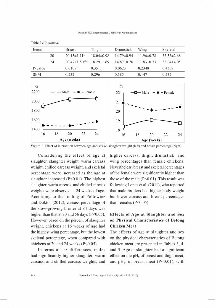
Piyanan Nualhnuplong and Chaiyawan Wattanachant
348 Pertanika J. Trop. Agric. Sci. 43(3): 343 - 357 (2020)
Considering the effect of age at slaughter, slaughter weight, warm carcass weight, chilled carcass weight, and skeletal percentage were increased as the age at slaughter increased (P<0.01). The highest slaughter, warm carcass, and chilled carcass weights were observed at 24 weeks of age. According to the finding of Poltowicz and Doktor (2012), carcass percentage of the slow-growing broiler at 84 days was higher than that at 70 and 56 days (P<0.05). However, based on the percent of slaughter weight, chickens at 16 weeks of age had the highest wing percentage, but the lowest skeletal percentage, when compared with chickens at 20 and 24 weeks (P<0.05).
In terms of sex differences, males had significantly higher slaughter, warm carcass, and chilled carcass weights, and
higher carcass, thigh, drumstick, and wing percentages than female chickens. Nevertheless, breast and skeletal percentages of the female were significantly higher than those of the male (P<0.01). This result was following Lopez et al. (2011), who reported that male broilers had higher body weight but lower carcass and breast percentages than females (P<0.05).
Effects of Age at Slaughter and Sex on Physical Characteristics of Betong Chicken MeatThe effects of age at slaughter and sex on the physical characteristics of Betong chicken meat are presented in Tables 3, 4, and 5. Age at slaughter had a significant effect on the pH0 of breast and thigh meat, and pH24 of breast meat (P<0.01), with
Table 2 (Continued)
Items Breast Thigh Drumstick Wing Skeletal20 20.15±1.11b 18.04±0.98 14.79±0.94 11.96±0.78 33.53±2.6824 20.47±1.50 ab 18.29±1.69 14.87±0.76 11.83±0.73 33.04±4.05
P-value 0.0108 0.3511 0.0623 0.2348 0.4369SEM 0.232 0.296 0.185 0.147 0.537
1400
1600
1800
2000
2200
16 18 20 22 24
G
Age (weeks)
Male Female
18
19
20
21
22
16 18 20 22 24
%
Age (weeks)
Male Female
Figure 1. Effect of interaction between age and sex on slaughter weight (left) and breast percentage (right)

Age at Slaughter and Sex on Meat Quality of Betong Chicken
349Pertanika J. Trop. Agric. Sci. 43(3): 343 - 357 (2020)
pH0 value tending to increase with age at slaughter. However, this work found that sex affected pH24 in both breast and thigh meat (P<0.01). The males had higher pH24 values in breast meat than the females. This was in concordance with the work of Poltowicz and Doktor (2012) who found a lower pH24 of broiler meat at 56 days than that of meat from broiler aged 70 and 84 days (P<0.05). Similar work was obtained by Atthaporn et al. (2009) who found that high pH24 value in Thai native chicken (Kai Nong Dang) when the age of chicken increased. The value of pH in meat was related to the amount of glycogen in the muscle and the stress condition of the animal (Warriss, 2000) which were resulting in the level of lactic acid in the meat. This result was closely associated with the color and water holding capacity of the meat (Warriss, 2000; Wattanachant, 2008).
From the results, significant interaction effects on the shear force value of breast meat, drip loss, and color (particularly lightness (L*) and redness (a*) of thigh meat) were noted among the age at slaughter and sex (P<0.05) (Figure 2).
Considering the effect of age at slaughter, this study indicated that the shear force value in male Betong chicken meat tended to be increased when the slaughter age increased. Although this value did not show any significant difference between the age of 16 and 20 weeks, it was significantly higher at the age of 24 weeks old. This work was similar to the work of Atthaporn et al. (2009) who found a higher shear force value of breast and thigh muscle when the
age of Thai native chicken increased. A similar result was reported by Poltowicz and Doktor (2012) on a slow-growing broiler. The increasing shear force value when the age of chicken increased is not only related to the increasing of muscle fiber diameter (Atthaporn et al., 2009; Dransfield & Sosnicki, 1999; Wattanachant, 2008) but also associated with a higher intermolecular cross-linking of connective tissue in meat (Castellini et al., 2002; Chen et al., 2013; Dawson et al., 1991; Husak et al., 2008). Sex had a significant effect on the shear force value of both breast and thigh meat (P<0.05), with males having higher values than females (P<0.05). This work was in agreement with Fanatico et al. (2005), and Chen et al. (2006). This was due to the larger diameter of muscle fiber and more thickness of perimysium (Wattanachant, 2008).
No interaction between age at slaughter and sex on drip and cooking losses of the breast meat (Table 3) was observed, but significantly interaction effect on drip loss of the thigh meat (Table 4). Both sexes had a lower drip loss percentage at the age of 16 weeks, but it significantly increased when the age at slaughter increased (P<0.01). This report was in agreement with the work of Li et al. (2020), although earlier researches found no significant differences between male and female chicken meat on water holding capacity (Chen et al., 2006; Fanatico et al., 2005; Kirmizibayrak et al., 2011; Lopez et al., 2011; Uhlirova et al., 2018).
In terms of the color of meat (Table 5), it was found that the female Betong chickens had higher L*, but lower a* than male

Piyanan Nualhnuplong and Chaiyawan Wattanachant
350 Pertanika J. Trop. Agric. Sci. 43(3): 343 - 357 (2020)
Table 3Effects of age at slaughter and sex on pH value, drip loss, cooking loss and shear force of breast meat Betong chicken (mean ± SD)
Items pH0 pH24Drip loss (%)
Cooking loss (%)
Shear force (kg/cm3)
Age 16 5.92b 5.77b 2.09 16.21b 3.0620 6.10a 5.80ab 2.09 18.64a 3.2224 6.10a 5.82a 1.85 17.47ab 3.67
P-value <0.0001 0.0032 0.3508 0.0010 0.0707Sex Male 6.04 5.82a 1.88 18.42a 3.61a
Female 6.04 5.77b 2.14 16.45b 3.12b
P-value 0.8877 0.0009 0.1000 0.0002 0.0273Interaction between sex x ageMale 16 5.94±0.19 5.79±0.06 2.09±0.78 17.61±2.93 2.83±1.13b
20 6.10±0.19 5.82±0.11 1.80±1.04 19.20±3.50 3.44±1.48ab
24 6.10±0.16 5.84±0.08 1.77±1.28 18.41±3.76 4.19±1.74a
Female 16 5.91±0.22 5.75±0.08 2.09±0.78 14.81±3.56 2.54±0.35b
20 6.11±0.25 5.77±0.09 2.42±0.58 18.04±3.32 2.99±1.27b
24 6.10±0.29 5.81±0.09 2.33±1.36 16.56±3.86 3.26±1.00b
P-value 0.8756 0.6225 0.2356 0.5263 0.0471SEM 0.040 0.016 0.190 0.639 0.244
a,b Means within the column with different superscripts differ significantly (P<0.05)
Table 4Effects of age at slaughter and sex on pH value, drip loss, cooking loss and shear force of thigh meat Betong chicken (mean ± SD)
Item pH0 pH24Drip loss (%)
Cooking loss (%)
Shear force (kg/cm3)
Age 16 6.26b 6.09 0.71b 21.05 3.7520 6.42a 6.07 1.11a 22.30 3.8124 6.44a 6.05 1.15a 20.94 4.18
P-value <0.0001 0.1184 <0.0001 0.3801 0.0715Sex Male 6.37 6.03b 0.89b 21.22 4.13a
Female 6.37 6.09a 1.08a 21.65 3.75b
P-value 0.8605 0.0066 0.0061 0.6269 0.0209Interaction between age x sexMale 16 6.28±0.24 6.04±0.12 0.77±0.33c 21.50±3.92 4.00±0.93
20 6.38±0.20 6.05±0.06 1.10±0.40b 21.60±6.50 3.91±0.94

Age at Slaughter and Sex on Meat Quality of Betong Chicken
351Pertanika J. Trop. Agric. Sci. 43(3): 343 - 357 (2020)
Table 4 (Continued)
Item pH0 pH24Drip loss (%)
Cooking loss (%)
Shear force (kg/cm3)
24 6.45±0.25 6.05±0.09 1.00±0.37bc 20.51±7.37 4.42±0.70Female 16 6.23±0.30 6.14±0.20 0.75±0.38c 20.59±5.80 3.42±1.35
20 6.47±0.17 6.09±0.06 1.11±0.40b 23.04±6.54 3.69±1.0424 6.43±0.19 6.05±0.07 1.40±0.70a 21.35±4.73 3.96±1.01
P-value 0.2785 0.0608 0.0083 0.5202 0.5479SEM 0.042 0.021 0.085 1.080 0.184
Table 5Effects of age at slaughter and sex on color meat of breast and thigh meat Betong chicken (mean ± SD)
a,b Means within the column with different superscripts differ significantly (P<0.05)
ItemsBreast meat Thigh meat
Lightness (L*)
Redness (a*)
Yellowness (b*) Lightness (L*) Redness (a*) Yellowness
(b*)
Age 16 48.52a 1.43 4.90b 49.86a 3.83b 4.82
20 48.51a 1.54 4.83b 51.30a 4.77b 5.07
24 45.90b 1.63 5.89a 45.92b 5.89a 5.34
P-value 0.0056 0.3173 0.0112 <0.0001 0.0002 0.7221
Sex Male 47.43 1.70a 4.51b 46.69b 6.70a 4.52b
Female 47.96 1.31b 5.87a 51.44a 2.65b 5.67a
P-value 0.4671 0.0005 <0.0001 <0.0001 <0.0001 0.0337
Interaction between age x sex
Male 16 48.09±4.14 1.53±0.76 4.03±1.59 48.86±6.50bc 5.57±2.91b 4.84±3.56
20 47.58±6.36 1.74±0.79 4.01±2.38 47.81±5.23c 7.50±3.18a 4.85±3.34
24 46.43±3.18 1.84±0.87 5.63±2.48 43.01±4.03d 8.02±2.51a 4.81±2.66
Female 16 48.95±4.00 1.33±0.26 5.78±1.71 50.87±4.45b 2.09±2.72d 4.80±1.86
20 49.43±5.40 1.30±0.26 5.72±2.33 55.03±5.02a 2.85±1.82d 5.28±3.92
24 45.47±4.32 1.29±0.95 6.12±1.93 48.55±3.45bc 4.01±1.90c 6.52±3.30
P-value 0.2689 0.6728 0.2833 0.0035 0.0235 0.0954
SEM 0.865 0.208 0.382 0.894 0.482 0.590
a,b Means within the column with different superscripts differ significantly (P<0.05)

Piyanan Nualhnuplong and Chaiyawan Wattanachant
352 Pertanika J. Trop. Agric. Sci. 43(3): 343 - 357 (2020)
chickens for 16-24 weeks. The L* of both males and females tended to decrease from the age of 16 weeks to the age of 24 weeks. Nevertheless, redness (a*) of both sexes tended to increase when the age of chicken increased. Although there was no significant effect on the lightness of breast meat of the male and female chickens (P>0.05), males showed higher reddish meat than the female Betong chickens. Likewise, we found that in chicken meat, higher b* was observed in the older Betong chickens. This value could result from xanthophyll in diet and natural carotenoids from plants’ free-range. The higher b* value was observed in the breast muscle (P<0.05), while the females had higher b* value than the male chickens.
The result of this present study was the following results from Kirmizibayrak et al. (2011) and Uhlirova et al. (2018), that male chicken’s meat had a higher a* value than the meat of females. Similar results were reported by Lopez et al. (2011) and Fanatico et al. (2005), who found higher b* values in female chicken meat than in male meat (P<0.05). Higher a* in the male than the female chicken was probably related to the higher activity of the male than the female. However, males had lower L*and b* values than female chickens. Besides, chicken meat color may depend on many factors such as genetic, raising system, type of feed, and age at slaughter (Wattanachant, 2008).
Figure 2. Effect of interaction between age and sex on the shear force of breast meat (kg/cm3) (a), lightness of thigh meat (b), redness of thigh meat (c), and a drip loss percentage of thigh meat (d)

Age at Slaughter and Sex on Meat Quality of Betong Chicken
353Pertanika J. Trop. Agric. Sci. 43(3): 343 - 357 (2020)
Tabl
e 6
Effec
ts o
f age
at s
laug
hter
and
sex
on c
hem
ical
mea
t qua
lity
of b
reas
t and
thig
h (m
ean
± SD
)
Item
sB
reas
t mea
tTh
igh
mea
tM
oist
ure
(%)
Prot
ein
(%)
Fat (
%)
Col
lage
n (%
)M
oist
ure
(%)
Prot
ein
(%)
Fat (
%)
Col
lage
n (m
g/10
0g)
Age
1674
.34
24.1
30.
405.
3475
.84
20.7
53.
129.
3920
74.5
224
.09
0.42
6.30
75.9
020
.70
3.23
10.1
824
74.7
324
.09
0.44
6.59
75.7
221
.09
3.30
12.3
0P-
valu
e0.
3235
0.98
790.
1376
0.25
730.
6786
0.45
640.
2523
0.13
95Se
xM
ale
74.9
6a23
.87b
0.34
b6.
8676
.16a
20.5
1b3.
1512
.75a
Fem
ale
74.1
2b24
.34a
0.50
a5.
5275
.41b
21.2
1a3.
329.
10b
P-va
lue
0.01
890.
0347
<0.0
001
0.26
97 <
0.00
010.
0159
0.2
126
0.01
17In
tera
ctio
n be
twee
n ag
e x
sex
Mal
e16
74.6
7±0.
6623
.82±
0.86
0.31
±0.0
36.
01±0
.37
76.3
3±0.
7020
.51±
0.91
3.06
±0.1
510
.57±
1.57
b
2074
.69±
1.02
23.8
4±0.
650.
35±0
.03
6.92
±0.8
076
.29±
0.46
20.3
6±1.
273.
13±0
.00
11.4
3±1.
55b
2474
.54±
0.73
23.9
3±0.
900.
36±0
.02
7.39
±1.0
875
.88±
0.64
20.6
6±0.
613.
25±0
.18
16.2
5±1.
70a
Fem
ale
1674
.03±
0.50
24.5
3±0.
920.
49±0
.00
4.90
±1.2
975
.15±
0.68
21.0
5±0.
463.
16±0
.03
8.22
±0.3
8 c
2074
.34±
1.38
24.3
2±0.
680.
50±0
.03
5.86
±1.6
375
.47±
0.61
21.0
3±1.
483.
32±0
.35
9.34
±1.1
0 b
2473
.73±
0.70
24.2
5±0.
510.
52±0
.04
5.79
±1.1
475
.55±
0.70
21.5
3±1.
203.
48±0
.37
9.67
±1.5
9 b
P-va
lue
1.00
000.
7400
00.
7051
1.00
000.
1635
0.94
550.
9124
0.05
00SE
M0.
167
0.13
90.
021
0.21
90.
117
0.19
60.
219
0.54
5a,
b M
eans
with
in th
e co
lum
n w
ith d
iffer
ent s
uper
scrip
ts d
iffer
sign
ifica
ntly
(P<0
.05)

Piyanan Nualhnuplong and Chaiyawan Wattanachant
354 Pertanika J. Trop. Agric. Sci. 43(3): 343 - 357 (2020)
Effects of Age at Slaughter and Sex on Chemical Composition of Betong Chicken MeatAs seen in Table 6, no significant interaction between age at slaughter and sex on the proximate composition of either breast or thigh meat (P>0.05). However, the highest collagen content was found in thigh meat from 24-week old male Betong chicken while the lowest collagen content was found in 16-week old females. Nevertheless, age at slaughter did not show any significant effect on any parameters (P>0.05), although the collagen content tended to increase as the age at slaughter increased. High collagen content when the age of chicken increased was following shear force value reported in Table 3. In this study, the result of proximate analysis contradicted that of Boni et al. (2010), who found a significantly higher fat content but lower levels of protein, moisture, and ash contents in older quail than in younger quail (P<0.05). However, in this study, the higher collagen content in meat from 24-week-old Betong chicken than in 16-and 20-week old was probably due to the type of collagen content and muscle fiber diameter as described by Wattanachant (2003). This was confirmed by Atthaporn et al. (2009), who found larger fiber diameter and perimysium thickness in Thai native chicken meat (Kai Nok Dang) as the age of the chicken increased. Fat contents tended to increase with age at slaughter in both breast and thigh meats (P>0.05). A high amount of fat deposition when the age of chicken increased was related to the reduction of energy for muscular growth, while high energy feed supplements could lead to more
body fat deposition. This was in agreement with the work of Atthaporn et al. (2009), Nikolova et al. (2007), and Zerhdaran et al. (2005).
In terms of sex, the breast and thigh meat of males had higher moisture content but lower protein content than that of females (P<0.05). In addition, the male Betong chickens had lower fat content in breast meat with higher collagen content in thigh meat than the females (P<0.05). This was similar to the work of Corzo et al. (2005) and Nikolova et al. (2007), who studied broilers, and Atthaporn et al. (2009), who studied in Thai native chicken (P<0.05).
CONCLUSIONBased on our findings, a distinctive feature of raising Betong chickens under a semi-free-range system was that the meat was low in fat content. (0.31 to 0.52% in breast and 3.06 to 3.48% in thigh meat). However, because the male Betong chicken grew much faster than the female, raising the male until 24 weeks old would increase the amount of collagen content that results in tougher meat than the female. Also, more reddish meat would be shown when the male was raised until 24 weeks of age. To control the quality of the meat, especially the redness, toughness, and amount of collagen, the male should be raised not more than 20 weeks while the female should be raised until the age of 24 weeks. However, it is recommended that the consumer’s preference for Betong chicken meat be explored in further studies.
Age at Slaughter and Sex on Meat Quality of Betong Chicken
355Pertanika J. Trop. Agric. Sci. 43(3): 343 - 357 (2020)
ACKNOWLEDGEMENTS
The authors would like to thank the Office of the Higher Education Commission (OHEC) and Graduate School, PSU, for financial support. We also would thank the Faculty of Natural Resources, PSU, for facilities support.
REFERENCESAgricultural Commodity and Food Standards. (2007).
Halal food (TAS 8400-2007): National Bureau of Agricultural Commodity and Food Standards, Ministry of Agriculture and Cooperatives. Bangkok, Thailand: Author.
Association of Analytical Chemists. (2006). Official methods of analysis (18th ed.). Gaithersburg, USA: AOAC International Press.
Atthaporn, S., Wattanachant, C., Wattanachant, S., & Wattanasit, S. (2009). Effect of rearing systems and age on carcass percentage, physical properties, microstructure and chemical composition of Kai Nok Dang (Thai native chicken) muscle. Journal of Science and Technology Mahasarakham University, 28(4), 412-423.
Bergman, I., & Loxley, R. (1963). Two improved and simplified methods for the spectrophotometric determination of hydroxyproline. Analytical Chemistry, 35(12), 1961-1965.
Boni, I., Nural, H., & Noryata, I. (2010). Comparison of meat quality characteristics between young and spent quails. International Food Research Journal, 17(3), 661-666.
Buakeeree, K., & Nualhnuplong, P. (2018). Effect of dietary protein and energy levels on growth performances and reproductive system development in female Betong chicken (Gallus domesticus) during growing-pullet period. Khon Kaen Agriculture Journal, 44(3), 469-478.
Castellini, C., Mugnai, C., & Dal Bosco, A. (2002). Effect of organic production system on broiler carcass and meat quality. Meat Science, 60(3), 219-225.
Chanjula, P., Wanichapichart, W., Thongchumroon, T., & Laochareonsuk, S. (2004). Village Betong chicken production in three Southernmost Thailand: A study of phenotypic characteristics, growth, carcass yield and egg performance of Betong chickens. Journal of Agriculture, 20(3), 278-288.
Chatreewong, D., & Waree, W. (2006). Optimum market age and weight of Betong chicken. Songklanakarin Journal of Science and Technology, 28(2), 311-319.
Chen, H. H., Cheng, J. H., Shuiep, E. S., Bao, W. B., & Musa, H. H. (2006). Breed and sex effect on meat quality of chicken. International Journal of Poultry Science, 5(6), 566-568.
Chen, X., Jiang, W., Tan, H. Z., Xu, G. F., Zhang, X. B., Wei, S., & Wang, X. G. (2013). Effect of outdoor access on growth performance, carcass composition, and meat characteristics of broiler chickens. Poultry Science, 92(2), 435-443.
Corzo, A., Kidd, M. T., Burnham, D. J., Miller, E. R., Branton, S. L., & Gonzalez Esquerra, R. (2005). Dietary amino acid density effects on growth and carcass of broilers differing in strain cross and sex. Journal of Applied Poultry Research, 14(1), 1-9.
Dawson, P. L., Sheldon, B., & Miles, J. J. (1991). Effect of aseptic processing on the texture of chicken meat. Poultry Science, 70(11), 2539-2367.
Dransfield, E., & Sosnicki, A. A. (1999). Relationship between muscle growth and poultry meat quality - A review. Poultry Science, 78(5), 743-746.
Fanatico, A. C., Cavitt, L. C., Pillai, P. B., Emmert, J. L., & Owens, C. M. (2005). Evaluation of slower-growing broiler genotypes grown with

Piyanan Nualhnuplong and Chaiyawan Wattanachant
356 Pertanika J. Trop. Agric. Sci. 43(3): 343 - 357 (2020)
and without outdoor access: Meat quality. Poultry Science, 84(11), 1785-1790.
Husak, R. L., Sebranek, J. G., & Bregendahl, K. (2008). A survey of commercially available broilers marketed as organic, free-range, and conventional broilers for cooked meat yields, meat composition, and relative value. Poultry Science. 87(11), 2367-2376.
Kirmizibayrak, T., Onk, K., Ekiz, B., Yalcintan, H., Yilmaz, A., Yazici, K., & Altinal, A. (2011). Effects of age and sex on meat quality of Turkish Native Geede raised under a free-range system. Kafkas Universitesi Veteriner Fakultesi Dregisi, 17(5), 817-823.
Li, J., Yang, C., Peng, H., Yin, H., Wang, Y., Hu, Y., … Liu, Y. (2020). Effect of slaughter age on muscle characteristics and meat quality traits of Da-Heng meat type birds. Animals, 10(1), 69.
Lopez, K. P., Schilling, M. W., & Corzo, A. (2011). Broiler genetic strain and sex effects on meat characteristics. Poultry Science, 90(5), 1105-1111.
Nikolova, N., Pavlovski, Z., Milosevic, N., & Peric, L. (2007). The quantity of abdominal fat in broiler chicken of different genotype from fifth to seventh week of age. Biotechnology in Animal Husbandry, 23(5-6-2), 331-338.
Nualhnuplong, P., Wattanachant, C., & Wattanasit, S. (2019a). Effect of rearing system on meat quality of Betong chickens. Khon Kaen Agriculture Journal, 47(2), 327-334.
Nualhnuplong, P., Wattanachant, C., Wattanasit, S., & Somboonsuke, B. (2019b). Commercial production system of Betong chicken in three Southern border provinces (Pattani, Yala and Narathiwat). Journal of Agricultural Research and Extension, 36(1), 11-21.
Palka, K. (1999). Changes in intramuscular connective tissue and collagen solubility of bovine M. semitendinosus during retorting. Meat Science, 53(3), 189-194.
Poltowicz, K., & Doktor, J. (2012). Effect of slaughter age on performance and meat quality of slow-growing broiler chickens. Annals of Animal Science, 12(4), 621-631.
Ritchoo, K., Wattanachant, C., & Wattanachant, S. (2019). The different of rearing systems on carcass characteristics and chemical composition of Betong chicken meat. Khon Kaen Agriculture Journal, 41(suppl.1), 411-416.
Sopian, Y., Wattanachant, C., & Wattanasit, S. (2018). True and apparent metabolizable energy of crude glycerin. Pertanika Journal of Tropical Agricultural Science, 41(4), 1905-1910.
Statistical Analysis System. (1998). SAS user’s guide. Version 6.12. Cary, USA: SAS Institute Incorporation.
Uhlirova, L., Tumova, E., Chodova, D., Vlckova, J., Ketta, M., Volek, Z., & Skrivanova, V. (2018). The effect of age, genotype and sex on carcass traits, meat quality and sensory attributes of geese. Asian-Australasian Journal of Animal Sciences, 31(3), 421-428.
Warriss, P. D. (2000). Meat science an introductory text. Wallingford, United Kingdom: Centre for Agriculture and Bioscience International.
Wattanachant, S. (2003). Chemical composition, properties and structure of muscle affecting textural characteristics of meat from Thai indigenous and broiler (Unpublished Doctoral thesis), Prince of Songkla University, Thailand.
Wattanachant, S. (2008). Factors affecting the quality characteristics of Thai indigenous chicken meat. Suranaree Journal of Science and Technology, 15(4), 317-332.

Age at Slaughter and Sex on Meat Quality of Betong Chicken
357Pertanika J. Trop. Agric. Sci. 43(3): 343 - 357 (2020)
Wattanachant, S., Benjakul, S., & Ledward, D. A. (2004). Composition, color, and texture of Thai indigenous and broiler chicken muscles. Poultry Science, 83(1), 123-128.
Zerhdaran, S., Vereijken, A. L. J., Arendonk, J. A. M., & Vander Waaij, E. H. (2005). Effect of age and housing system on genetic parameters for broiler carcass traits. Poultry Science, 84(6), 833-838.


Pertanika J. Trop. Agric. Sci. 43 (3): 359 - 376 (2020)
© Universiti Putra Malaysia Press
TROPICAL AGRICULTURAL SCIENCEJournal homepage: http://www.pertanika.upm.edu.my/
Article history:Received: 17 April 2020Accepted: 1 June 2020Published: 28 August 2020
ARTICLE INFO
E-mail addresses:[email protected] (Yan Ling Kuan)[email protected] (S. Navin Sivanasvaran)[email protected] (Liew Phing Pui)[email protected] (Yus Aniza Yusof)[email protected] (Theeraphol Senphan)* Corresponding author
ISSN: 1511-3701e-ISSN 2231-8542
Physicochemical Properties of Sodium Alginate Edible Film Incorporated with Mulberry (Morus australis) Leaf Extract
Yan Ling Kuan1, S. Navin Sivanasvaran1, Liew Phing Pui1*, Yus Aniza Yusof2,3
and Theeraphol Senphan4 1Department of Food Science with Nutrition, Faculty of Applied Sciences, UCSI University, No.1,Jalan Menara Gading, UCSI Heights, 56000 Cheras, Kuala Lumpur, Malaysia2Department of Process and Food Engineering, Faculty of Engineering, Universiti Putra Malaysia,43400 UPM Serdang, Selangor, Malaysia3Laboratory of Halal Services, Halal Products Research Institute, Universiti Putra Malaysia,43400 Selangor, Malaysia4Faculty of Engineering and Agro-Industry, Maejo University, Sansai, Chiangmai 50290, Thailand
ABSTRACT
In this study, sodium alginate film incorporated with mulberry leaf extract [0-4 % (v/v)] were evaluated in terms of its physicochemical properties. Results showed that with the increase of mulberry leaf extract concentration, the thickness of the film increased (from 0.07 mm to 0.11 mm), while the color of film produced increased in its green and yellow intensity. In terms of mechanical properties, with the increase of mulberry leaf extract concentration, a significant increase in the tensile strength but a significant decrease in the elongation at break of the film were observed, while no significant effect (p>0.05) on the puncture force was observed. Similarly, no significant effect (p>0.05) on moisture
content, water solubility, and water activity of sodium alginate films were found, with the increase of mulberry leaf extract. An increase in the total phenolic content from 8.92 mg GAE/100 g to 41.88 mg GAE/100 g was observed when 4 % (v/v) of mulberry leaf extract was added.
Keywords: Mulberry leaf extract, physicochemical
properties, sodium alginate, total phenolic content

Yan Ling Kuan, S. Navin Sivanasvaran, Liew Phing Pui, Yus Aniza Yusof and Theeraphol Senphan
360 Pertanika J. Trop. Agric. Sci. 43 (3): 359 - 376 (2020)
INTRODUCTION
The edible film can be defined as the coating of food material which can be consumed together with the food product itself (Pavlath & Orts, 2009). An increase in the demand from consumers towards natural and safe product leads to the work for the development of edible film, where it can serve as alternative coatings for plastic material coatings and packaging (Janjarasskul & Krochta, 2010; Shit & Shah, 2014).
Edible film base materials can be categorized into three groups, namely polysaccharide, protein, or lipid (Vieira et al., 2011). With the application of edible film, the shelf life of food can be extended by minimizing its contact with air, thus reducing prolong lipid oxidation (Cirillo & Spizzirri, 2015). In addition, the edible film can be incorporated with antimicrobial and antioxidant sources such as herbs and spices (Emiroğlu et al., 2010).
Among the different edible film base, alginate is one of the common polysaccharides used for the development of the edible film (Ferreira et al., 2016). It is extracted from seaweed and structured by 1-4b-D-mannuronic acid (M) and a-L-guluronic acid (G) (Kim, 2013). Its fibrous structure can form films, while its hydrophilic properties can reduce lipid oxidation when applied to foods (Pavlath & Orts, 2009; Varela & Fiszman, 2011).
For f i lm formation, glycerol is commonly used as a plasticizer to enhance flexibility, while calcium chloride forms
crosslinking between its calcium ions and sodium alginate, improving the film’s water resistance (Rhim, 2004; Vieira et al., 2011). In addition, herbs and spices that have an antimicrobial effect such as oregano, rosemary essential oil, thyme essential oil, Melastoma malabathricum extract, and ‘asam keping’ were also incorporated into film (Chan et al., in press; Choong et al., 2019; Jouki et al., 2014a, b; Seydim & Sarikus, 2006; Zaman et al., 2018).
Luís et al. (2019) incorporated licorice essential oil into carboxymethyl xylan film. They found that the film with the presence of licorice essential oil exhibited positive antimicrobial effect against Enterococcus faecalis and Listeria monocytogenes while Abdollahi et al. (2019) who added summer savory essential oil into carboxymethyl cellulose-agar biocomposite film reported on the high antimicrobial activity against Staphylococcus aureus, Bacillus cereus, and Listeria monocytogenes with essential oil at 1.5% (v/v). Also, rosemary and Aloe vera essential oil were added into cellulose acetate in which it had high antimicrobial activity against Escherichia coli and Bacillus subtilis in the study of El Fawal et al. (2019).
Mulberry leaf is a heart shape or mitten-shaped leaf belongs to Moraceae family (Rahman & Khanom, 2013; Srichaikul et al., 2011). It is used as silkworms’ foods, papermaking, Chinese medicine, diabetes, and blood pressure treatment (Chen et al., 2007; Vichasilp et al., 2012). Mulberry leaf was reported to have antimicrobial

Sodium Alginate Edible Film Incorporated with Mulberry Leaf Extract
361Pertanika J. Trop. Agric. Sci. 43 (3): 359 - 376 (2020)
and antioxidant properties, in which flavonoid such as quercetin-3-glucoside, kaempferol-3-glucoside, and quercetin-3-(6-malonylglucoside) was found (Islam et al., 2008). To the best of our knowledge, the information on mulberry leaf extract based edible film were scarce. Hence, this work aimed to study the effect of mulberry leaf extract on the physical, mechanical, chemical, antimicrobial, and antioxidant properties of alginate edible film.
MATERIALS AND METHODS
Preparation of Mulberry Leaf Extract
Mulberry leaf was obtained from roadside bushes near Puchong, Selangor, Malaysia. It was identified by the red and black mulberry fruit produced from the tree. It was cut and dried overnight at 40 °C and ground using a grinder (Sharp, EM-11, Malaysia).
The extraction process was performed according to Sarbadhikary et al. (2015) with slight modification. The mulberry powder (10 g) was added with ethanol (100 mL) and stirred for 24 hours in a rotary shaker (Infors AG, Switzerland) at 150 rpm before filtration with filter paper (Whatman No. 3, Filters Fiorini, Sweden) and centrifuged (Centrifuge 5810 R, Eppendorf, Germany) for 15 minutes at 9,860 x g. The extract was then subjected to the rotary evaporator (R-000, BÜCHI, Switzerland) under vacuum at 40 °C and the extract (50 mg/mL concentration of mulberry leaf extract, with 5 g extract dissolved 100mL solvent) was then kept at 4 °C for further analysis.
Analysis of Mulberry Leaf Extract
Antimicrobial Properties. The disc diffusion method was carried out with Staphylococcus aureus and Escherichia coli on Mueller-Hinton Agar (Sarbadhikary et al., 2015). Antibiotic chloramphenicol disc (Oxoid, UK, 30 μg) was used as positive control and a paper disc (6 mm diameter) infused with 50 µL of ethanol served as the negative control. The inhibition zone was measured with a micrometer.
Antioxidant Properties of Mulberry Leaf Extract. The antioxidant property of mulberry leaf extract was performed by utilizing DPPH (2,2-diphenyl-1-picrylhydrazyl) free radical scavenging assay (Wong et al., 2014). Mulberry leaf extract (0.1 mL) was added with 3.9 mL of 0.004% ethanolic DPPH solution into a test tube (wrapped with aluminum foil). The mixture was vortexed and left to stand in the dark for 30 minutes before measuring its absorbance value at 517 nm, using a UV-Vis Spectrophotometer (Uviline 9400, Secomam, France). Percentage of DPPH scavenging activity was calculated by using Equation 1:
(1) where Abs of DPPH is the absorbance value of 0.004% ethanolic DPPH solution and the Abs of sample is referring to the absorbance value of the extract at 517 nm.

Yan Ling Kuan, S. Navin Sivanasvaran, Liew Phing Pui, Yus Aniza Yusof and Theeraphol Senphan
362 Pertanika J. Trop. Agric. Sci. 43 (3): 359 - 376 (2020)
Total Phenolic Content of Mulberry Leaf Extract. Folin-Ciocalteu’s reagent (1.5 mL) was pre-diluted 10 times with distilled water and mixed with mulberry leaf extract (0.3 mL) and sodium carbonate (1.2 mL). The mixture was mixed and left for 30 minutes in dark, before measuring the absorbance at 765 nm with a UV-Vis spectrophotometer (Uviline 9400, Secomam, France). A standard curve was generated by using gallic acid solution (0- 0.1 mg/g), with regression equation of y = 0.0119x + 0.0124 and R² = 0.9991 (Wong et al., 2014).
Production of Edible Film Incorporated with Mulberry Leaf ExtractAbout 1.5% (w/v) of sodium alginate powder (Synertec, Malaysia) was added with 200 mL of distilled water and stirred for 30 minutes at 70 °C. Glycerol 0.75% (v/v) was added, followed by stirring for another 15 minutes. Mulberry leaf extract with concentration at 0, 1, 2, 3, and 4% (v/v) was added into film solution, respectively. A preliminary study shows with the addition of 5%, the film formed is sticky and not smooth.
The mixture (25 g) was poured on a petri dish (90 mm × 15 mm) and dried at 40 °C for 24 hours in an oven (Memmert, Germany) (Benavides et al., 2012). The sodium alginate film formed was dipped into the calcium chloride solution (45 mL) and dried again for 1 minute. The films formed peeled using forceps and kept in desiccators.
Analysis of Film
Thickness. Micrometer (JY, China) is used
to measure the thickness of the film, by placing it at 5 different locations of the film (Garsuch & Breitkreutz, 2009).
Moisture Content and Water Activity. The initial film weight was measured using an analytical balance (XT 220 A, Precisa, Switzerland). After measuring the initial weight, the film was dried in an oven (Memmert, Germany) at 90 °C for 24 hours, before measuring the dried film weight again (Choong et al., 2019). The moisture content was calculated according to Equation 2:
(2)
where M0 is defined as the initial mass of the film and Mi is defined as the final mass of the film.
On the other hand, the water activity of the film was determined using a water activity meter (AquaLab Pre, METER Group, USA).
Water Solubility. Determination of water solubility was carried out according to the work of Ma et al. (2016) with slight modifications. The film cut into 2 cm × 2 cm and dried in an oven (60 °C) for 24 hours, after which the weight for the dehydrated film (W1) was measured. The film was then immersed with distilled water (25 mL) for 2 hours at room temperature in a covered condition, after which the film was then dried again for 24 hours at 60 °C). The second weight measured was the final mass (W2). Water solubility was calculated according to Equation 3:

Sodium Alginate Edible Film Incorporated with Mulberry Leaf Extract
363Pertanika J. Trop. Agric. Sci. 43 (3): 359 - 376 (2020)
(3)
where W1 is interpreted as the initial mass of the film and W2 is interpreted as the final mass of the film.
Color Profile. The color of the film was determined using a colorimeter (ColorFlex Ez, Hunter lab, US) (Zaman et al., 2018). The colorimeter was a spectrophotometer with Pulsed Xenon Lamp as a light source, coupled with a 256-element diode array and a high- resolution concave holographic grating. The colorimeter was calibrated with white and black tile standards before the sample test. The films were then placed against the sample cup to measure the color.
The color was expressed as L* (lightness-darkness), a* (red-green) and b* (yellow-blue) values, while the total color differences (∆E) for the films was calculated according to the Equation 4:
(4)
where ∆L*, ∆a*, and ∆b* represent the difference of readings as the parameter values compared the sodium alginate with mulberry leaf extract film to the pure sodium alginate film.
Tensile Strength and Elongation at Break. The tensile analysis was performed using the tensile testing machine (TA-XT Plus, Surrey, UK) (Remya et al., 2015). Films strips (50 mm x 20 mm) were placed on the grip, with separation of the initial grip
fixed at 50 mm. The speed was set at 25 mm/min for the crosshead. Calculations for the tensile strength and elongation at break were proceeded by using Equations 5 and 6, respectively:
(5)
(6)
Puncture Force. Puncture force was determined using a texture analyzer, with the needle probe (2 mm diameter) moving at a constant rate of 1 mm/s (Muppalla et al., 2014). The puncture force was calculated using Eq. 7:
(7)
Fourier Transform Infrared Spectroscopy (FTIR). Fourier transform infrared spectroscopy (FTIR) spectrometer (Nicolet iS5, Thermo Fischer Scientific, USA) equipped with OMNIC Spectra Software in transmission mode was used to measure the spectra absorbance of the film (Pranoto et al., 2005). The resolution was set as 4 cm-1 with an average of 20 scans for wavenumbers in between the range of 500 cm-1 to 4000 cm-1 against a background spectrum from an empty cell.

Yan Ling Kuan, S. Navin Sivanasvaran, Liew Phing Pui, Yus Aniza Yusof and Theeraphol Senphan
364 Pertanika J. Trop. Agric. Sci. 43 (3): 359 - 376 (2020)
Antioxidant and Antimicrobial Properties of Film. The antioxidant properties (free scavenging activity and total phenolic content) were performed following the method of Wong et al. (2014), while antimicrobial properties were conducted according to Fernández-Pan et al. (2012).
Statistical Analysis
Data were represented as a mean value ± standard deviation and were analyzed using analysis of variance (one-way ANOVA) and Tukey’s post hoc test was used for analyzing the significant difference among the film properties (SPSS version 23). The p-value of ≤0.05 was defined as statically significant.
RESULTS AND DISCUSSION
Antimicrobial Properties of Mulberry Leaf Extract
Mulberry leaf extract (50 mg/mL) was found to have an antibacterial effect against E. coli with the minimal inhibition zone of 1.46 ± 0.34 mm while having no antimicrobial activity from the mulberry leaf extract against the S. aureus. This result is in agreement with the study done by Thabti et al. (2014), who showed that mulberry leaf extract exhibited antibacterial activity against E. coli. Besides that, the result of the antimicrobial activity against S. aureus is in agreement with the study done by Manjula and Shubha (2011), who reported that there was no antimicrobial activity against the S. aureus (concentration of mulberry leaf extract concentration at 25 µL/L).
Antioxidant Properties and Total Phenolic Content of Mulberry Leaf Extract
It was found that the mulberry leaf extract (50 mg/mL) had free radical scavenging activity of 49.88 ± 1.23%. On the other hand, the total phenolic content of mulberry leaf extract was found to be 553.93 mg GAE/100g. These findings are consistent with results shown by the study of Memon et al. (2010) who found similar free radical scavenging activity in mulberry leaf extract (48.13 ± 1.20%). The antioxidant activity and total phenolic content were contributed by flavonoid compounds such as quercetin and rutin (Katsube et al., 2009). According to Katsube et al. (2006), quercetin is the most abundant flavonoid compound present in mulberry leaf thus, contributing to the antioxidant activity of mulberry leaf.
Thickness
Figure 1 (a) shows the physical properties of sodium alginate incorporated with different concentrations of mulberry leaf extract. With the increase of the mulberry leaf extract, it was found that the thickness of the edible films increased after 3% (v/v) incorporation of mulberry leaf extract (from 0.07 mm to 0.10 mm). Further incorporation of the leaf extract (4% v/v) resulted in no significant difference (p>0.05) with those with 3% (v/v) leaf extract. The increase of thickness was also observed in the work of Benavides et al. (2012) in the film added with oregano essential oil, where the thickness increase was due to the increase of total solids in the film-forming solution. As reported by Utami

Sodium Alginate Edible Film Incorporated with Mulberry Leaf Extract
365Pertanika J. Trop. Agric. Sci. 43 (3): 359 - 376 (2020)
et al. (2019), the increase in cinnamon essential oil caused an increase in the total solids of the film-forming solution thus, increasing the film thickness.
Moisture Content and Water Activity
From Figure 1 (b) it was observed the moisture content was decreased with the addition of mulberry leaf extract concentration, with no significance between film added with different extract concentrations (p>0.05). This may be explained by the concentration of mulberry leaf extract at 1% (v/v) that had reached a sufficient level to occupy the microstructural network space of sodium alginate (DeMan et al., 2018). Adding on to that, the decrease in moisture content might be due to the decreased water affinity of films containing
more hydrophobic mulberry leaf extract (Han et al., 2018). This is in agreement with the result where an increase of mulberry leaf extract had no significant effect (p>0.05) on the water activity of film produced (Figure 1 c). Low water activity is favored for edible film because it inhibits the growth of organisms and extends shelf life (Ijabadeniyi & Pillay, 2017). Moisture content and water activity of the film influence its moisture absorption behavior, which in turn affects the water solubility (Gennadios & Weller, 1994).
Water Solubility
The result in Figure 1 (d) shows that the sodium alginate without mulberry leaf extract has 75.57% water solubility. Low
60
65
70
75
80
0% 1% 2% 3% 4%W
ater
solu
bilit
y (%
)
MLE concentration (v/v)
0
5
10
15
20
25
0% 1% 2% 3% 4%Moi
stur
e co
nten
t (%
)
MLE concentration (v/v)
0.000.020.040.060.080.100.12
0% 1% 2% 3% 4%
Thi
ckne
ss (m
m)
MLE concentration (% v/v)
0.0
0.2
0.4
0.6
0.8
1.0
0% 1% 2% 3% 4%
Wat
er a
ctiv
ity
MLE concentration (v/v)
(a)
(c)
(c)
(b)
(d)
Figure 1. Physical properties including (a) thickness, (b) moisture content, (c) water activity, and (d) water solubility of sodium alginate edible film incorporated with different concentration of mulberry leaf extract (MLE)

Yan Ling Kuan, S. Navin Sivanasvaran, Liew Phing Pui, Yus Aniza Yusof and Theeraphol Senphan
366 Pertanika J. Trop. Agric. Sci. 43 (3): 359 - 376 (2020)
Table 1 The color profile of sodium alginate edible films with mulberry leaf extract
The concentration of mulberry leaf extract incorporated (%)
Color
L* a* b* ∆E
0 25.32 ± 0.77c -0.26 ± 0.05b 0.27 ± 0.01a 0.00 ± 0.00a
1 21.43 ± 0.38b 0.11 ± 0.04c 2.58 ± 0.13b 4.54 ± 0.25a
2 20.86 ± 0.30b -0.32 ± 0.03b 4.08 ± 0.16c 5.87 ± 0.21a
3 19.28 ± 1.47a -0.49 ± 0.03a 4.91 ± 0.17d 7.62 ± 1.33b
4 18.55 ± 0.78a -0.52 ± 0.05a 5.31 ± 0.15e 8.44 ± 0.74c
Note. a-e Mean ± standard deviations followed by different superscript letters within the same column are significantly different at p≤0.05 according to Tukey’s test
water solubility is desirable for edible film, to avoid the complete dissolution of the film (Ozdemir & Floros, 2008). With the addition of mulberry leaf extract [1% - 4% (v/v)], the water solubility of the film was reported to be in the range of 78.35-79.74%. There was no significant difference (p>0.05) between the water solubility of the film when 1% to 4% (v/v) concentration of the mulberry leaf extract was added into the film.
The findings from this analysis are in agreement with the study done by Jutaporn et al. (2011), where the water solubility of the film increased when phayom wood extract was added. The increase in water solubility may be contributed by the decreased polymer network interaction density due to the presence of mulberry leaf
extract. Furthermore, alginate film is highly water-soluble, due to its hydrophilic nature (Shit & Shah, 2014).
Color Profile
The color of the film is important as it influences customer acceptance towards a product (Galus & Lenart, 2013). For the films, it is most favorable that the films are light in color or transparent so that it would not affect the food color (Acevedo-Fani et al., 2015). According to Table 1, with an increase in mulberry leaf extract, the sodium alginate film has a decrease in L* value, a* value, while an increase in its b* value and total color change (∆E). This indicates that the film is darker, greener, and yellower with an increase of extract due to the dark

Sodium Alginate Edible Film Incorporated with Mulberry Leaf Extract
367Pertanika J. Trop. Agric. Sci. 43 (3): 359 - 376 (2020)
color of mulberry leaf extract. The increase in yellowish and greenish color of the film was from the natural color of the mulberry leaf. Du et al. (2009) reported that the color of the films was influenced by essential oils added, which result in a decrease of L* and a* with the concentration cinnamon essential oil. The result is also in agreement with the study done by Mehdizadeh et al. (2012), who found that there was a decrease in L* and a* with increased Thymus kotschyanus essential oil.
Tensile Strength and Elongation at Break
Tensile strength is the maximum amount of stress that a sample can withstand during tensile testing (Benavides et al., 2012). According to Figure 2 (a), the tensile strength increases from 12.91 to 23.45 MPa when the concentration of mulberry leaf extract increased from 1% (v/v) to 3% (v/v). The decrease of tensile strength at high mulberry leaf extract concentrations may be attributed to the formation of
discontinuities creating stressed regions in the film matrix, leading to decreased tensile strength (Frank et al., 2018). The decrease of tensile strength at high concentration was also observed by Han et al. (2018) when sodium alginate/carboxymethyl cellulose films were incorporated with cinnamon essential oil.
In terms of elongation at break, the value decreases with the increase of mulberry leaf extract concentration from 0% (v/v) to 4% (v/v), which showed a reduction from 35.60% to 5.76% (Figure 2 b). This result correlates with the findings of Sánchez-González et al. (2010) who found that the addition of tea tree essential oil to chitosan films caused a decrease in elongation at break of the films. This may be due to the increase in compound concentration generating a cross-linking effect through the interaction between polymers with the compound, leading to the reduction of the flexibility for the molecular of the polymer (Ojagh et al., 2010).
0
5
10
15
20
25
0% 1% 2% 3% 4%
Tens
ile st
reng
th (M
Pa)
MLE concentration (v/v)
Figure 2. Mechanical properties: (a) tensile strength

Yan Ling Kuan, S. Navin Sivanasvaran, Liew Phing Pui, Yus Aniza Yusof and Theeraphol Senphan
368 Pertanika J. Trop. Agric. Sci. 43 (3): 359 - 376 (2020)
Puncture Force
From Figure 2 (c), it is observed that the puncture force of films ranges from 12.41-12.95 N, with no significant difference (p>0.05) among the films. This result is consistent with the study from Gómez-Estaca et al. (2009), with no significant difference (p>0.05) among the bovine-hide gelatin film incorporated with a low and high concentration of oregano extract. The puncture force did not decrease with an increase in the extract. This is favorable for film properties. Adding on, the same result was observed by Aguirre et al. (2013), who
found that there was no significant difference (p>0.05) on the puncture force of triticale protein films incorporated with different oregano essential oil concentrations.
Fourier Transform Infrared Spectroscopy (FTIR)
FTIR was conducted to identify and analyze the functional group of present and the FTIR spectra can be observed in Figure 3. The film samples had similar broadband around 3279 cm-1 to 3286 cm-1, where the absorbance peak was the intensity of O-H stretching (Ba et al., 2010). The appearance of an absorption band for O-H stretching was broad as it was
Figure 2 (Continued). Mechanical properties: (b) elongation at break, and (c) puncture force of sodium alginate edible films with mulberry leaf extract
0
10
20
30
40
0% 1% 2% 3% 4%
Elo
ngat
ion
of b
reak
(%
)
MLE concentration (v/v)
0
5
10
15
0% 1% 2% 3% 4%
Punc
ture
forc
e (N
)
MLE concentration (v/v)
(b)
(c)

Sodium Alginate Edible Film Incorporated with Mulberry Leaf Extract
369Pertanika J. Trop. Agric. Sci. 43 (3): 359 - 376 (2020)
influenced by the intermolecular hydrogen bonding between the O-H groups. A strong hydrogen bond causes a long O-H bond, and this allows the O-H bond to be stretched easily (Burrows et al., 2017). It can be observed that the amplitude of the band decreased when higher concentrations of mulberry leaf extract were added. This means that the interaction between the bonds was lower at high concentrations. This can explain the lower tensile strength observed when a higher concentration of mulberry leaf extract was added (Tongnuanchan et al., 2013).
The presence of the peak around at 1149 cm-1 on the film sample incorporated with 3% (v/v) and 4% (v/v) mulberry leaf
extract was associated with the epoxy C-O stretching vibration and glycosidic linkage C-O-C stretching (Čopíková et al., 2013; Hanifah et al., 2015).
The epoxy C-O and glycosidic linkage C-O-C stretching indicate the presence of polysaccharide compound from the mulberry leaf extract. There is also a peak around at 1600 cm-1 which indicate the presence of phenolic compound such as chlorogenic acid in the mulberry leaf extract (Liang et al., 2016). However, there is no peak observed around 1600 cm-1 for film added with 1% (v/v) and 2% (v/v) mulberry leaf extract, this may be due to the insufficient amount of the phenolic compound from the mulberry leaf extract.
Figure 3. Spectra of Fourier transform infrared spectroscopy (FTIR) of SA-MLE edible film (a) sodium alginate + 0% MLE, (b) sodium alginate + 1% MLE, (c) sodium alginate + 2% MLE, (d) sodium alginate + 3% MLE, and (e) sodium alginate + 4%

Yan Ling Kuan, S. Navin Sivanasvaran, Liew Phing Pui, Yus Aniza Yusof and Theeraphol Senphan
370 Pertanika J. Trop. Agric. Sci. 43 (3): 359 - 376 (2020)
Antioxidant Properties and Total Phenolic Content of Sodium Alginate Edible Films with Mulberry Leaf ExtractAccording to Figure 4 (a), sodium alginate film with no mulberry leaf extract have scavenging activity at 2.48% as the alginate polymer can provide scavenging activities (Ueno & Oda, 2014). With the addition of mulberry leaf extract (from 1%- 4% v/v), the scavenging activity in the film increased from 5.67% to 9.98%. Increasing scavenging activity was due to an increase of mulberry leaf extract concentration (Mehdizadeh et al., 2012).
Similarly, the total phenolic content of the film samples increased from 8.92 mg GAE/100g to 41.88 mg GAE/100g when the concentration of mulberry leaf extract range at 0% (v/v) to 4% (v/v) (Figure 4 b). This is to the addition of mulberry extract which has the total phenolic content (Jouki et al., 2014b). It was also found that there is much reduction of DPPH scavenging activity and total phenolic content, which has decreased 80% and 92%, respectively when the mulberry leave extract (100%) was added into the film in 4% (v/v) concentration.
0
4
8
12
0% 1% 2% 3% 4%
DPP
H sc
aven
ging
act
ivity
(%)
MLE concetration (v/v)
(a)
(b)
0
10
20
30
40
50
0% 1% 2% 3% 4%
Tot
al p
heno
lic c
onte
nt (m
g G
AE
/100
g)
MLE concentration (v/v)
Figure 4. (a) DPPH free radical scavenging activity and (b) total phenolic content of sodium alginate edible films with mulberry leaf extract

Sodium Alginate Edible Film Incorporated with Mulberry Leaf Extract
371Pertanika J. Trop. Agric. Sci. 43 (3): 359 - 376 (2020)
Antimicrobial Activity of Sodium Alginate Edible Films with Mulberry Leaf Extract
There was no antibacterial activity found for the sodium alginate edible films with mulberry leaf extract. However, antimicrobial activity was found in the mulberry leaf extract, this may be due to the lesser amount of mulberry leaf extract incorporated into the films as compared to the extract on its own (with 1.46 mm inhibition zone).
This was in agreement with the study of Benavides et al. (2012), where a low concentration of oregano essential oil incorporated into edible film showed no antimicrobial activity. In addition, Chan et al. (2020) also found no antimicrobial acidity in Melastoma malabathricum incorporated film, despite the inhibition zone found in the extract.
CONCLUSIONS
With a higher concentration of mulberry leaf extract incorporated, the sodium alginate film shows an increase in thickness which is important for the mechanical aspect of the film. Increased mulberry leaf extract concentration produces films that are darker, greenish, and yellowish. This may decrease consumer acceptance. Besides, the increase of mulberry leaf extract produced a film that is low in tensile strength, a decrease in elongation at the break while not affecting its puncture force. Mechanical properties of the film when added with extract is still weak, hence further study on improving mechanical strength is suggested, by optimizing the concentration of glycerol.
The films with mulberry leaf extract contain higher scavenging activity and total phenolic content compared with the film without extract. As the sodium alginate edible film with 3% (v/v) of mulberry leaf extract had higher tensile strength, it was considered as the best formulation among the 4 concentration, although overall the tensile strength is still quite low. The 3% mulberry leaf extract film can be further improved to be a potential film wrapping the foods for enhancing the antioxidant properties and total phenolic content.
ACKNOWLEDGEMENTS
The authors would like to acknowledge the support provided by the UCSI University for Pioneer Scientist Incentive Fund (PSIF), Project No. Proj-In-FAS-056.
REFERENCESAbdollahi, M., Damirchi, S., Shafafi, M., Rezaei,
M., & Ariaii, P. (2019). Carboxymethyl cellulose-agar biocomposite film activated with summer savory essential oil as an antimicrobial agent. International Journal of Biological Macromolecules, 126, 561-568. doi: 10.1016/j.ijbiomac.2018.12.115
Acevedo-Fani, A., Salvia-Trujillo, L., Rojas-Graü, M. A., & Martín-Belloso, O. (2015). Edible films from essential-oil-loaded nanoemulsions: Physicochemical character izat ion and antimicrobial properties. Food Hydrocolloids, 47, 168-177. doi: 10.1016/j.foodhyd.2015.01.032
Aguirre, A., Borneo, R., & León, A. E. (2013). Antimicrobial, mechanical and barrier properties of triticale protein films incorporated with oregano essential oil. Food Bioscience, 1, 2-9. doi: 10.1016/j.fbio.2012.12.001
Yan Ling Kuan, S. Navin Sivanasvaran, Liew Phing Pui, Yus Aniza Yusof and Theeraphol Senphan
372 Pertanika J. Trop. Agric. Sci. 43 (3): 359 - 376 (2020)
Ba, C., Ladner, D., & Economy, J. (2010). Using polyelectrolyte coatings to improve fouling resistance of a positively charged nanofiltration membrane. Journal of Membrane Science, 347(1-2), 250-259. doi: 10.1016/j.memsci.2009.10.031
Benavides , S. , Vi l la lobos-Carvajal , R. , & Reyes, J. (2012). Physical, mechanical and antibacterial properties of alginate film: Effect of the crosslinking degree and oregano essential oil concentration. Journal of Food Engineering, 110(2), 232-239. doi: 10.1016/j.jfoodeng.2011.05.023
Burrows, A., Holman, J., Parsons, A., Pilling, G., & Price, G. (2017). Chemistry: Introducing inorganic, organic and physical chemistry. Oxford, United Kingdom: Oxford University Press.
Chan, H. M., Nyam, K. L., Yusof, Y. A., & Pui, L. P. (2020). Investigation of properties of polysaccharide-based edible film incorporated with functional Melastoma malabathricum extract. Carpathian Journal of Food Science and Technology, 12(1), 120-133. doi: 10.34302/crpjfst/2020.12.1.12
Chen, H., Lin, Y., & Hsieh, C. (2007). Evaluation of antioxidant activity of aqueous extract of some selected nutraceutical herbs. Food Chemistry, 104(4), 1418-1424. doi: 10.1016/j.foodchem.2007.02.004
Choong, K. W., Tee, Y. B., Nyam, K. L., & Pui, L. P. (2019). Antibacterial properties of chitosan edible films incorporated with musk lime extracts for the preservation of squids. Malaysian Journal of Analytical Sciences, 23(6), 914-925.
Cirillo, G., & Spizzirri, U. (2015). Functional polymers in food science: From technology to biology. Beverly, USA: John Wiley and Sons.
Čopíková, J., Černá, M., Novotná, M., Kaasová, J., & Synytsya, A. (2013). Application of FT-IR spectroscopy in detection of food hydrocolloids in confectionery jellies and food supplements. Czech Journal of Food Sciences, 19(2), 51-56. doi: 10.17221/6575-cjfs
DeMan, J., Finley, J., Hurst, W., & Lee, C. (2018). Principles of food chemistry. New York, NY: Springer International Publishing.
Du, W. X., Olsen, C. W., Avena-Bustillos, R. J., McHugh, T. H., Levin, C. E., & Friedman, M. (2009). Effects of allspice, cinnamon, and clove bud essential oils in edible apple films on physical properties and antimicrobial activities. Journal of Food Science, 74(7), 372-378. doi: 10.1111/j.1750-3841.2009.01282.x
El Fawal, G. F., Omer, A. M., & Tamer, T. M. (2019). Evaluation of antimicrobial and antioxidant activities for cellulose acetate films incorporated with rosemary and aloe vera essential oils. Journal of Food Science and Technology, 56(3), 1510-1518. doi: 10.1007/s13197-019-03642-8
Emiroğlu, Z. K., Yemiş, G. P., Coşkun, B. K., & Candoğan, K. (2010). Antimicrobial activity of soy edible films incorporated with thyme and oregano essential oils on fresh ground beef patties. Meat Science, 86(2), 283-288. doi: 10.1016/j.meatsci.2010.04.016
Fernández-Pan, I., Royo, M., & Ignacio Maté, J. (2012). Antimicrobial activity of whey protein isolate edible films with essential oils against food spoilers and foodborne pathogens. Journal of Food Science, 77(7), M383-M390. doi: 10.1111/j.1750-3841.2012.02752.x
Ferreira, A. R. V., Alves, V. D., & Coelhoso, I. M. (2016). Polysaccharide-based membranes in

Sodium Alginate Edible Film Incorporated with Mulberry Leaf Extract
373Pertanika J. Trop. Agric. Sci. 43 (3): 359 - 376 (2020)
food packaging applications. Membranes, 6(2), 22. doi: 10.3390/membranes6020022
Frank, K., Garcia, C. V., Shin, G. H., & Kim, J. T. (2018). Alginate biocomposite films incorporated with cinnamon essential oil nanoemulsions: Physical, mechanical, and antibacterial properties. Retrieved February 04, 2020, from https://www.hindawi.com/journals/ijps/2018/1519407/
Galus, S., & Lenart, A. (2013). Development and characterization of composite edible films based on sodium alginate and pectin. Journal of Food Engineering, 115(4), 459-465. doi: 10.1016/j.jfoodeng.2012.03.006
Garsuch, V., & Breitkreutz, J. (2009). Novel analytical methods for the characterization of oral wafers. European Journal of Pharmaceutics and Biopharmaceutics, 73(1), 195-201. doi: 10.1016/j.ejpb.2009.05.010
Gennadios, A., & Weller, C. L. (1994). Moisture adsorption by grain protein films. Transactions of the ASAE, 37(2), 535-539.
Gómez-Estaca, J., Montero, P., Fernández-Martín, F., Alemán, A., & Gómez-Guillén, M. (2009). Physical and chemical properties of tuna-skin and bovine-hide gelatin films with added aqueous oregano and rosemary extracts. Food Hydrocolloids, 23(5), 1334-1341. doi: 10.1016/j.foodhyd.2008.09.013
Han, Y., Yu, M., & Wang, L. (2018). Physical and antimicrobial properties of sodium alginate/carboxymethyl cellulose films incorporated with cinnamon essential oil. Food Packaging and Shelf Life, 15, 35-42. doi: 10.1016/j.fpsl.2017.11.001
Hanifah, M. R. F., Jaafar, J., Aziz, M., Ismail, A. F., Rahman, M. A., & Othman, M. H. D. (2015). Synthesis of graphene oxide
nanosheets via modified hummers’ method and its physicochemical properties. Jurnal Teknologi, 74(1), 189-192. doi: 10.11113/jt.v74.3555
Ijabadeniyi, O. A., & Pillay, Y. (2017). Microbial safety of low water activity foods: Study of simulated and Durban household samples. Retrieved February 04, 2020, from https://www.hindawi.com/journals/jfq/2017/4931521/
Is lam, B. , Khan, S . N. , Haque, I . , Alam, M., Mushfiq, M., & Khan, A. U. (2008). Novel anti-adherence activity of mulberry leaves: Inhibition of Streptococcus mutans biofilm by 1-deoxynojirimycin isolated from Morus alba. Journal of Antimicrobial Chemotherapy, 62(4), 751-757. doi: 10.1093/jac/dkn253
Janjarasskul, T., & Krochta, J. M. (2010). Edible packaging materials. Annual Review of Food Science and Technology, 1(1), 415-448. doi: 10.1146/annurev.food.080708.100836
Jouki, M., Mortazavi, S. A., Yazdi, F. T., & Koocheki, A. (2014a). Characterization of antioxidant – Antibacterial quince seed mucilage films containing thyme essential oil. Carbohydrate Polymers , 99 , 537-546. doi: 10.1016/j.carbpol.2013.08.077
Jouki, M., Yazdi, F. T., Mortazavi, S., A. & Koocheki, A. (2014b). Quince seed mucilage films incorporated with oregano essential oil: Physical, thermal, barrier, antioxidant and antibacterial
properties. Food Hydrocolloids, 36, 9-19. doi:
10.1016/j.foodhyd.2013.08.030
Jutaporn, C. T., Suphitchaya, C., & Thawien, W.
(2011). Antimicrobial activity and characteristics
of edible films incorporated with Phayom wood
(Shorea tolura) extract. International Food
Research Journal, 18(1), 39-54.

Yan Ling Kuan, S. Navin Sivanasvaran, Liew Phing Pui, Yus Aniza Yusof and Theeraphol Senphan
374 Pertanika J. Trop. Agric. Sci. 43 (3): 359 - 376 (2020)
Katsube, T., Imawaka, N., Kawano, Y., Yamazaki, Y., Shiwaku, K., & Yamane, Y. (2006). Antioxidant flavonol glycosides in mulberry (Morus alba L.) leaves isolated based on LDL antioxidant activity. Food Chemistry, 97(1), 25-31. doi: 10.1016/j.foodchem.2005.03.019
Katsube, T., Tsurunaga, Y., Sugiyama, M., Furuno, T., & Yamasaki, Y. (2009). Effect of air-drying temperature on antioxidant capacity and stability of polyphenolic compounds in mulberry (Morus alba L.) leaves. Food Chemistry, 113(4), 964-969. doi: 10.1016/j.foodchem.2008.08.041
Kim, S. (2013). Marine nutraceuticals: Prospects and perspectives. Boca Raton, USA: CRC Press.
Liang, N., Lu, X., Hu, Y., & Kitts, D. D. (2016). Application of attenuated total reflectance–Fourier transformed infrared (ATR-FTIR) spectroscopy to determine the chlorogenic acid isomer profile and antioxidant capacity of coffee beans. Journal of Agricultural and Food Chemistry, 64(3), 681-689. doi: 10.1021/acs.jafc.5b05682
Luís, Â., Pereira, L., Domingues, F., & Ramos, A. (2019). Development of a carboxymethyl xylan film containing licorice essential oil with antioxidant properties to inhibit the growth of foodborne pathogens. LWT – Food Science and Technology, 111, 218-225. doi: 10.1016/j.lwt.2019.05.040
Ma, Q., Zhang, Y., & Zhong, Q. (2016). Physical and antimicrobial properties of chitosan films incorporated with lauric arginate, cinnamon oil, and ethylenediaminetetraacetate. LWT - Food Science and Technology, 65, 173-179. doi: 10.1016/j.lwt.2015.08.012
Manjula, A., & Shubha. (2011). Screening of antibacterial activity of total soluble protein
of mulberry varieties. International Journal of Current Pharmaceutical Research, 3(2), 60-61.
Mehdizadeh, T., Tajik, H., Rohani, S. M. R., & Oromiehie, A. R. (2012). Antibacterial, antioxidant and optical properties of edible starch-chitosan composite film containing Thymus kotschyanus essential oil. In Veterinary research forum (Vol. 3, No. 3, p. 167). Urmia, Iran: Urmia University.
Memon, A. A., Memon, N., Luthria, D. L., Bhanger, M. I., & Pitafi, A. A. (2010). Phenolic acids profiling and antioxidant potential of mulberry (Morus laevigata W., Morus nigra L., Morus alba L.) leaves and fruits grown in Pakistan. Polish Journal of Food and Nutrition Sciences, 60(1), 25-32.
Muppalla, S. R., Kanatt, S. R., Chawla, S. P., & Sharma, A. (2014). Carboxymethyl cellulose–polyvinyl alcohol films with clove oil for active packaging of ground chicken meat. Food Packaging and Shelf Life, 2(2), 51-58. doi: 10.1016/j.fpsl.2014.07.002
Ojagh, S. M., Rezaei, M., Razavi, S. H., & Hosseini, S. M. H. (2010). Development and evaluation of a novel biodegradable film made from chitosan and cinnamon essential oil with low affinity toward water. Food Chemistry, 122(1), 161-166. doi: 10.1016/j.foodchem.2010.02.033
Ozdemir, M., & Floros, J. D. (2008). Optimization of edible whey protein films containing preservatives for water vapor permeability, water solubility and sensory characteristics. Journal of Food Engineering, 86(2), 215-224. doi: 10.1016/j.jfoodeng.2007.09.028
Pavlath A.E., Orts W. (2009) Edible films and coatings: Why, What, and How?. In K. Huber & M. Embuscado (Eds.), Edible films and coatings

Sodium Alginate Edible Film Incorporated with Mulberry Leaf Extract
375Pertanika J. Trop. Agric. Sci. 43 (3): 359 - 376 (2020)
for food applications (pp. 1-23). New York, NY: Springer.
Pranoto, Y., Salokhe, V. M., & Rakshit, S. K. (2005). Physical and antibacterial properties of alginate-based edible film incorporated with garlic oil. Food Research International, 38(3), 267-272. doi: 10.1016/j.foodres.2004.04.009
Rahman, A., & Khanom, A. (2013). A taxonomic and ethno-medicinal study of species from Moraceae (Mulberry) family in Bangladesh flora. Research in Plant Sciences, 1(3), 53-57.
Remya, S., Mohan, C. O., Bindu, J., Sivaraman, G. K., Venkateshwarlu, G., & Ravishankar, C. N. (2015). Effect of chitosan based active packaging film on the keeping quality of chilled stored barracuda fish. Journal of Food Science and Technology, 53(1), 685-693. doi: 10.1007/s13197-015-2018-6
Rhim, J. W. (2004). Physical and mechanical properties of water resistant sodium alginate films. LWT - Food Science and Technology, 37(3), 323-330. doi: 10.1016/j.lwt.2003.09.008
Sánchez-González, L., González-Martínez, C., Chiralt, A., & Cháfer, M. (2010). Physical and antimicrobial properties of chitosan–tea tree essential oil composite films. Journal of Food Engineering, 98(4), 443-452. doi: 10.1016/j.jfoodeng.2010.01.026
Sarbadhikary, S. B., Bhowmik, S., Datta, B. K., Mandal, N.C., & Thakur, R. (2015). Antimicrobial and antioxidant activity of leaf extracts of two indigenous angiosperm species of Tripura. International Journal of Current Microbiology and Applied Science, 4(8), 643-665.
Seydim, A. C., & Sarikus, G. (2006). Antimicrobial activity of whey protein based edible films incorporated with oregano, rosemary and
ga r l i c e s sen t i a l o i l s . Food Research International, 39(5), 639-644. doi: 10.1016/j.foodres.2006.01.013
Shit, S. C., & Shah, P. M. (2014). Edible polymers: Challenges and opportunities. Retrieved February 04, 2020, from https://www.hindawi.com/journals/jpol/2014/427259/
Srichaikul, B., Bunsang, R., Samappito, S., Butkhup, L., & Bakker, G. (2011). Comparative study of chlorophyll content in leaves of Thai Morus alba Linn. species. Plant Sciences Research, 3(2), 17-20. doi: 10.3923/psres.2011.17.20
Thabti, I., Elfalleh, W., Tlili, N., Ziadi, M., Campos, M. G., & Ferchichi, A. (2014). Phenols, flavonoids, and antioxidant and antibacterial activity of leaves and stem bark of Morus species. International Journal of Food Properties, 17(4), 842-854. doi: 10.1080/10942912.2012.660722
Tongnuanchan, P., Benjakul, S., & Prodpran, T. (2013). Physico-chemical properties, morphology and antioxidant activity of film from fish skin gelatin incorporated with root essential oils. Journal of Food Engineering, 117(3), 350-360. doi: 10.1016/j.jfoodeng.2013.03.005
Ueno, M., & Oda, T. (2014). Biological activities of alginate. In Advances in food and nutrition research (Vol. 72, pp. 95-112). Cambridge, USA: Academic Press.
Utami, R., Khasanah, L. U., Manuhara, G. J., & Ayuningrum, Z. K. (2019). Effects of cinnamon bark essential oil (Cinnamomum burmannii) on characteristics of edible film and quality of fresh
beef. Pertanika Journal of Tropical Agricultural
Science, 42(4), 1173-1184. doi: 10.1088/1757-
899X/193/1/012057
Varela, P., & Fiszman, S. M. (2011). Hydrocolloids in
fried foods. A review. Food Hydrocolloids, 25(8),
1801-1812. doi: 10.1016/j.foodhyd.2011.01.016

Yan Ling Kuan, S. Navin Sivanasvaran, Liew Phing Pui, Yus Aniza Yusof and Theeraphol Senphan
376 Pertanika J. Trop. Agric. Sci. 43 (3): 359 - 376 (2020)
Vichasilp, C., Nakagawa, K., Sookwong, P., Higuchi,
O., Luemunkong, S., & Miyazawa, T. (2012).
Development of high 1-deoxynojirimycin (DNJ)
content mulberry tea and use of response surface
methodology to optimize tea-making conditions
for highest DNJ extraction. LWT - Food Science
and Technology, 45(2), 226-232. doi: 10.1016/j.
lwt.2011.09.008
Vieira, M. G. A., da Silva, M. M., dos Santos, L. O., &
Beppu, M. M. (2011). Natural-based plasticizers
and biopolymer films: A review. European
Polymer Journal, 47(3), 254-263. doi: 10.1016/j.
eurpolymj.2010.12.011
Wong, Y. H., Lau, H. W., Tan, C. P., Long, K., &
Nyam, K. L. (2014). Binary solvent extraction
system and extraction time effects on phenolic
antioxidants from kenaf seeds (Hibiscus
cannabinus L.) extracted by a pulsed ultrasonic-
assisted extraction. Retrieved February 04, 2020, from https://www.hindawi.com/journals/tswj/2014/789346/
Zaman, N. B. K., Lin, N. K., & Phing, P. L. (2018). Chitosan film incorporated with Garcinia atroviridis for the packaging of Indian mackerel (Rastrelliger kanagurta). Ciência e Agrotecnologia , 42(6), 666-675. doi: 10.1590/1413-705420

Pertanika J. Trop. Agric. Sci. 43 (3): 377 - 389 (2020)
© Universiti Putra Malaysia Press
TROPICAL AGRICULTURAL SCIENCEJournal homepage: http://www.pertanika.upm.edu.my/
Article history:Received: 18 March 2020Accepted: 17 June 2020Published: 28 August 2020
ARTICLE INFO
E-mail addresses:[email protected] (Nurul Najwa Mohamad)[email protected] (Nor Azizun Rusdi)* Corresponding author
ISSN: 1511-3701e-ISSN: 2231-8542
Scanning Electron Microscopy Analysis of Early Floral Development in Renanthera bella J. J. Wood, an Endemic Orchid from Sabah
Nurul Najwa Mohamad and Nor Azizun Rusdi*Unit for Orchid Studies, Institute for Tropical Biology and Conservation, Universiti Malaysia Sabah, Jalan UMS, 88400 Kota Kinabalu, Sabah, Malaysia
ABSTRACT
Renanthera bella J. J. Wood is an endemic orchid to Sabah with beautiful bright red petals. Most of the floral development of orchids is significantly affected by seasons and geographical factors. To date, the flower development stages of R. bella have never been studied. This study was conducted to observe the morphological changes of flower initiation and early development by apical dissection and scanning electron microscopy (SEM). The floral organs were dissected and fixed in 1.5% glutaraldehyde and dehydrated with alcohol. Characteristic stages of the initial flowering pattern were recorded until the flower was fully open and become senescent. Renanthera bella showed a typical acropetal pattern starting with early flowering from the base to the apex, forming a raceme-type inflorescence. Its flower development was divided into ten stages, which started with the flower bud appearance and the initiation of primordia. Next, the flower sepal started to develop within seven days of bud appearance. The final stage occurred after 25 days of observation when the bud opened, with an average bud length and diameter of 1.94 ± 0.56 cm and 0.50 ± 0.29 cm, respectively. The R. bella flower maturity stage was achieved between 38 to 40 days after anthesis, with the average length and diameter of petals and sepals increasing to 2.49 ± 0.23 cm and 0.38 ± 0.06 cm, respectively. A capsule successfully formed after one week of pollination. It reached the maturity stage at approximately 15 weeks after pollination. The orchid capsule started to break and expose the seeds inside
after 21 weeks. This analysis emphasized the early floral development pattern, which could help estimate the length of flower maturity and pollination.Keywords: Anther, flower development, pollen, Renanthera bella

Nurul Najwa Mohamad and Nor Azizun Rusdi
378 Pertanika J. Trop. Agric. Sci. 43 (3): 377 - 389 (2020)
INTRODUCTION
Renanthera bella J. J. Wood is an epiphytic orchid endemic to Sabah. This species is distributed from the Mount Kinabalu region to the Lahad Datu district (Chan et al., 1994). According to Pridgeon et al. (2014), R. bella can be found at an elevation between 400 to 1200 m and is confined to low-stature hill forests. Renanthera bella produces beautiful, attractive blotched-pink to crimson red flowers with a yellowish-cream to apricot yellow base. This species has been widely over-collected and is classified as endangered in Appendix I of the Convention on the International Trade of Endangered Species of Wild Flora and Fauna (Chan et al., 1994). Given the challenges it faces, no studies on the pattern of R. bella floral development have been conducted.
Most orchid species are at risk of habitat loss due to various human activities, such as natural habitat destruction and overcollection. Most attempts to culture endangered and rare orchid species in vitro have been supported by anatomical and morphological observations of flower development (Arditti & Pridgeon, 1997; Burgeff, 1932). Various reports on molecular genetic analysis of flower development of orchids have been made over the years, such as the floral organ-specific genes (Pan et al., 2014), the role of MADS-box genes in the flower development and evolution (Becker & Theissen, 2003; Tsai et al., 2004; Zahn et al., 2005), and the regulatory mechanisms
underlying orchid flower development (Xu et al., 2006). However, the morphological structure of buds and flowers in R. bella has not been well-identified.
Scanning electron microscopy (SEM) is used to increase the accuracy of plant and flower surface observations, as well as the development of floral organs. The images provide a more detailed view of the inner floral organs and the leaf surface features of the stomatal guard cells, epidermis, and hairs (if present). SEM was previously used to observe the stoma and micro-level character of the abaxial and adaxial surfaces of in vitro and in vivo Passiflora edulis leaves (Veeramohan et al., 2013).
Studies on the developmental stages of the inflorescence are essential as they relate to the control of plant reproduction, the pattern of plant growth, the timing of plant production, and how flowers interact with air movement for flowering (Friedman & Harder, 2005). An understanding of plant reproductive biology is essential in plant conservation efforts. In the present study, SEM was used to observe the morphological changes of flower initiation and early development until full bloom by apical dissection. During the observation, it was observed that different flower parts exhibit various patterns of development in their morphological characters. This study can provide basic background information that can be used to predict the maturity of the capsule that is important for seed germination.

Early Floral Development of Renanthera bella
379Pertanika J. Trop. Agric. Sci. 43 (3): 377 - 389 (2020)
MATERIALS AND METHODS
Plant Sources
Three-year-old R. bella plants were obtained from the greenhouse of the Institute for Tropical Biology and Conservation (ITBC), Universiti Malaysia Sabah (UMS). The plants were maintained in the greenhouse under natural light, 80% relative humidity, with a temperature of 28/24 ± 2°C day/night. The plants were grown in charcoal and coconut husk medium and fertilized using commercial fertilizer. Measurements for the R. bella flowers were recorded for length, diameter, and morphological changes. The R. bella flowers were hand-pollinated in September 2017 to form capsules. The plant species were identified by Mr. Johnny Gisil from ITBC and by a botanist from the Poring Orchid Conservation Centre (POCC; 0602ʹ 20.7ʺN, 116 06ʹ 38.2ʺE). This research was performed at the Tissue Culture Laboratory, ITBC, UMS (06003ʹ 33ʺ N, 116 012ʹ 29ʺE) under 24 ± 2°C temperature, 80% humidity, and 8/16 hours of light/dark condition.
Observation of Flower Bud Initiation and Development
The flower bud initiation and development of R. bella were recorded over two and a half months, starting with bud initiation, to the opening stages, and the formation of the full bloom or mature flower. The method of Smyth et al. (1990) was carried out with minor modifications. The samples were dried in the desiccator (for 1 h) instead of a critical point dryer. Additionally, the concentration of glutaraldehyde used was only 1.5% to prevent damage to the cells
and tissues of the flower, as well as the thin surface. Data on bud length, bud width, lip length, lip width, pollen and anther size, and mature petal and sepal length and diameter were recorded weekly. The experiment was conducted using three replicates of plants with a total of eight floral organs per plant. The data was determined by calculating their mean and standard deviation. In addition to these data, the changes in the development of the flowers were recorded from time to time.
Dissection of Floral Organs
The floral organs were dissected into different flower parts or tissue such as bud, anther, pollen, petal, sepal, lip, and column for further observation of their morphology and physiology under the SEM. Both immature and mature floral organs were dissected for the comparison of their development.
Scanning Electron Microscopy (SEM)
The inflorescence and the young buds of R. bella were harvested from the greenhouse and dissected immediately into various floral tissues such as bud, anther, pollen, petal, sepal, lip, and column. The bud was held tightly with a pair of forceps and dissected using a blade by cutting the base part of the petal and sepal vertically to reveal the inner tissue (lip, column, anther, and pollen) under the stereomicroscope. The tissues were then fixed in 1.5% glutaraldehyde and incubated at 4°C for 24 h. The samples were then rinsed three times in 0.1 M phosphate buffer with an interval of 10 min. Then, the tissue

Nurul Najwa Mohamad and Nor Azizun Rusdi
380 Pertanika J. Trop. Agric. Sci. 43 (3): 377 - 389 (2020)
materials were dehydrated in a series of ethanol (35%, 50%, 70%, 90%, and 100%) for 30 min at each ethanol concentration. The samples were desiccated for 1 h before mounted on a metal SEM stub and coated with gold in a sputter coater for further observation on the SEM (Zeiss, Germany), and the image was recorded (Smyth et al., 1990).
RESULTS AND DISCUSSIONS
The Morphology of Flower Initiation and Inflorescence Formation
The studies of morphological development of flower bud formation in R. bella were based on the methods of physical observation and measurement. To date, the studies and in-depth analysis of R. bella
flower development are scarce, making it difficult for comparison study.
Initially, the inflorescence started from the interstitial leaf (arrow; Figure 1A) and continue to develop and elongate rapidly after only five days (Figures 1B and 1C). It can grow to 30 cm and longer. Buds and flower organs arise at the peak of the inflorescence in the acropetal chain, where the flower buds begin to mature from the base to the top (Figure 1D). Usually, the inflorescence emerged from the fourth node below the apical leaf (Sakanishi et al., 1980). On the seventh day, cream and brown flower buds with a diameter of 0.02 cm appeared on the apical meristem and formed a raceme type of inflorescence (Figure 1E; stage 1). A raceme is an unbranched,
Figure 1. Inflorescence development of Renanthera bella. (A) Inflorescence started to arise from the interstitial leaf (arrow); (B) Inflorescence elongated and primordia bud started to appear (arrow); (C) Flower bud started to develop (arrow); (D) Renanthera bella flower development with acropetal growth pattern; (E) Formation of raceme inflorescence; (F) Lip started to arise and appear at the bottom of the bud (arrow); (G) Single dorsal sepal started to open (arrow)

Early Floral Development of Renanthera bella
381Pertanika J. Trop. Agric. Sci. 43 (3): 377 - 389 (2020)
elongated inflorescence with pedicellate flowers maturing from the bottom upwards (Harris & Harris, 2004). The lip starts to arise and appear at the bottom of the bud (Figure 1F), whereas the bud begins to open from its dorsal sepal (Figure 1F). There are approximately 7 to 15 flower buds in a single inflorescence. After 25 days, a single dorsal starts to open (Figure 1G).
The description of flower development has been reported in several studies. Previously, the flower development of Malus x domestica Borkh. (comprising 8 morphological stages) and Arabidopsis (comprising 12 stages) were recorded (Foster et al., 2003; Smyth et al., 1990). The overall results indicated that the early development of the inflorescence of R. bella followed a typical acropetal development pattern (Harris et al., 1991; Naghiloo & Claen-Bockhoff, 2017), whereby a
single dorsal started to open after 25 days (Figure 1G). Xu et al. (2006) reported that most of the angiosperm flowers had four whorls, namely sepals, petals, anthers, and pistils. Based on the observations and measurements from the inflorescences, the process development of R. bella flower from its initiation until the bud opening can be separated into ten stages, as shown in Table 1.
Bud Development
The studies of bud development in R. bella were based on the methods of physical measurement and SEM analysis, as described by Wang et al. (2014). Continuous observations of early primordial growth and flowering were carried out until the buds reached maturity (bud opening). The flower bud size increased weekly, and the buds started to open after 25 days of observation.
Table 1Morphological features in Renanthera bella flower development pattern
Stages Development eventFlower
development period (days)
Remarks
1 Flower bud started to appear and form a raceme type of inflorescence
7 The flower bud is creamy white, while the inflorescence stalk is light green
2 Flower bud primordia started to develop
7 The flower buds are creamy-white and brown
3 Sepals developed 12 The sepals are creamy red 4 Immature column developed 16 The column is red-brown 5 Lip developed and can be observed
between lateral bud sepals. 16 The lip is creamy
6 Stigma papillae appeared 16 -7 Pollen not fully developed 16 The pollen is light yellow and kidney-
shaped8 Anther cap enclosed the pollen 16 The anther cap is dark brown and has a
straight line with a deep curve 9 Sepal enclosed the flower bud 21 The adaxial sepal is pale red 10 Bud started to open 25 Bud is red maroon

Nurul Najwa Mohamad and Nor Azizun Rusdi
382 Pertanika J. Trop. Agric. Sci. 43 (3): 377 - 389 (2020)
Renanthera bella inflorescences will continue to develop under 27 ± 2°C, 10/14 h light/dark with 70% – 80% humidity. Overall measurement on the length and diameter of flower buds was recorded for 5, 12, 18, and 25 days of observation and summarized in Figure 2.
Figure 2A shows the early flower bud that is covered with leaf primordial (arrow). Within seven days of observation, the primordial leaf sheath elongated, and the bud size increased (Figure 2B). Then, the lower part of the lip (Figure 2C) and sepal line (Figure 2D) started to appear and emerged from the bottom of the flower bud
on the 16th day of observation. The flower bud developed and elongate then tapered at the apex (Figures 2E–2G). Some differences were noted on the surface character of the epidermal cell for abaxial and adaxial buds, where the abaxial immature bud character showed proximity to the epidermal cell and the presence of several stomata guard cells (Figure 2H), while the adaxial surface of the bud displayed a linear epidermal shape (Figure 2I). The flower induction process involved the triggering of the flowering bud by environmental factors, which result in the change of development patterns, leading to the formation of flowers.
Figure 2. Scanning electron microscope analysis of flower bud development of Renanthera bella. (A) Early-stage of epidermal shape; (B) Floral bud with enclosed by young leaf primordium (arrow); (C) Lip appears at the bottom of the bud (arrow); (D) Line of lateral sepal on the immature bud (arrow); (E) Front view of mature flower bud; (F) Lower bud with tapered apex showed the appearance of lip (lateral view) (arrow); (G) Bud reaches a diameter of 0.5 cm and starts to open; (H) Abaxial surface of immature bud showing the proximity of epidermal cell and stomata guard cell (arrow); (I) Adaxial surface of bud with epidermal cell in an irregular shape

Early Floral Development of Renanthera bella
383Pertanika J. Trop. Agric. Sci. 43 (3): 377 - 389 (2020)
The flower structure has been studied in various ways. Studies of natural history and evolutionary biology of flowers have emphasized understanding the ultimate (evolutionary) causes of a wide range of variants, such as color, symmetry, meristic arrangements (e.g., flower organ number), size, pollination syndrome and others (Alvarez-Buylla et al., 2010).
Lip and Column Development
The differences between the columns and the lip are shown in Figure 4A to Figure 4D through the front and lateral view. The column consists of the androecium, the male reproductive part, and the modified filaments and styles that fuse in orchid flowers. The immature column appears straight from the sides and has an average length of 0.50 mm (Figure 4A; stage 4), while the mature column reaches 3.5 mm in size and appears curved on the side (Figure 4B). The column contains anther, pollen, and stigmatic papillae that are part of the pollination process (stage 6). The stigmatic papillae have a rostellum character, and their
position is below the column (Figure 4C). At its mature level, the column changes to a curve formation (arrow) and has a smooth surface without hair (Figure 4E), while the immature column is straight and has a hairy surface (arrow; Figure 4F).
Lips appeared below the bud between the lateral sepals after 14 days (stage 5). The lip is a modified petal of the orchid flower. The immature R. bella lip has an average size of 0.09 mm and is tapered at the apex. The R. bella lip is broad and slightly spread at the base (Chan et al., 1994). Renanthera bella has gynandrous stamens that fuse with the pistil to form the reproductive part called the column.
Figures 4G–4H show the front and lateral view of the appearance of the mature lip as it tapered to the apex, while Figure 4I shows a vertical view of the lip that forms the hole inward. The nectary primordia initiate under the column and become mature and elongated at the base (Figure 4J). Moreover, the surface of the epidermal cells of the mature column is circular and thick, with wrinkles lining their cell walls (Figure
0
0.5
1
1.5
2
2.5
5 12 18 25
Mea
n le
ngth
and
dia
met
er o
f fl
ower
bud
(cm
)
Days of observation
length of bud diameter of bud
Figure 3. Length and diameter of the flower bud of Renanthera bella within 25 days of observation

Nurul Najwa Mohamad and Nor Azizun Rusdi
384 Pertanika J. Trop. Agric. Sci. 43 (3): 377 - 389 (2020)
4K). An epidermal cell in the middle of the column develops a thick, irregular circular shape that curves inward (Figure 4L). The cell surface of the lip tip has a hemispheric shape (Figure 4M).
Anther and Pollen Development
In stage 7, pollen is formed, while in stage 8, the anther cap develops and encloses the pollen for protection. R. bella has an anther cap structure that fuses in front of the column structure from the edge view, while the pollen is located inside the anther cap for protection before pollination at
maturity (Figure 5A). The immature anther cap is round and curved with a small circle that rises and forms a line pattern in the middle (Figure 5B). The whole structure of the anther cap has puberulent hair, while the mature anther cap is also hairy on its surface, with a faint line in the middle and a small circle arising in the middle that begins to disappear (Figures 5A–5B). Furthermore, R. bella mature pollen has a thick, wrinkled shape (Figure 5C). The anther sac is curved inward to protect the diploid pollen before pollination (Figure 5D), while the pollen stalk in the inner surface of the cell has hexagonal epidermal cells (Figure 5E).
Figure 4. Lip and column development of Renanthera bella. (A) Lateral view of immature column and lip; (B) Lateral view of matured column and lip; (C) Front view of immature column and lip; (D) Front view of matured column and lip; (E) Vertical view of mature column change to curve formation (arrow); (F) Vertical view of an immature column; (G) The matured lip is tapered to the apex (front view) (arrow); (H) Lateral view of matured lip (arrow); (I) Vertical view of the mature column forms the hole inward (arrow); (J) Nectary primordia under the column (arrow); (K) The surface of the mature column; (L) The surface of the immature column with thickening circle shape; (M) Epidermal cell from the adaxial surface of mature lip showing dams hemisphere shape (Note. Sepal and petal dissected away to reveal inner organ)

Early Floral Development of Renanthera bella
385Pertanika J. Trop. Agric. Sci. 43 (3): 377 - 389 (2020)
Renanthera bella pollen appears as two masses with kidney-like shapes (Figure 5F). Additionally, the stigma papillae have a sticky hole surface for pollination purposes (Figure 5G). Pollen begins to form together with column formation and develops along with the anther and cap. The pollen size in mature R. bella is approximately 0.05 mm. Mature anther of the epidermal cell surface of the epidermis shows a conical shape (Figure 5H).
Petal and Sepal Development
Data on the length and diameter of the outer flower organ (sepal and petal) is recorded in Table 2. The sepal line begins to appear, and curves inward to cover the apex (Figure 6A; stage 9). The primordial petals develop at the
same time as the sepals, and they proliferate to enclose the bud (Figure 6B). The sepals on the young flower buds overlap with each other and cover the flower’s internal organs (Figure 6C). The basal portion of the petal is broad and extends and tapers into the apex portion. The adaxial cell surface at the tip of the sepals begins to mature and forms a hexagonal cell when mature (Figure 6D). Stomata are observed on the adaxial surface of the sepals. The mature stomata are arranged far away from each other on the surface of the epidermal cell. Each stoma has two thickened guard cells (Figure 6D). Additionally, the mature septic surface of the sepals does not have a definite shape (Figure 6E). At maturity, the average length of the sepals was 0.38 ± 0.06 cm during
Figure 5. Anther and Pollen Development of Renanthera bella. (A) Vertical view of immature anther cap; (B) Matured sepal with pubescent hair; (C) The surface of mature pollen; (D) Vertical view of matured anther sac after pollen removed; (E) The surface of pollen stalk; (F) Mature pollen of R. bella; (G) Matured stigmatic papillae (arrow); (H) Vertical view of pollen surface (Note. Sepals and petals dissected away to reveal inner organ)

Nurul Najwa Mohamad and Nor Azizun Rusdi
386 Pertanika J. Trop. Agric. Sci. 43 (3): 377 - 389 (2020)
Table 2Length and diameter of outer flower organ on the primary inflorescence of Renanthera bella (n=3)
Days (Age) 27 30 33 35Length of lateral sepal 2.01 ± 0.16 cm 2.15 ± 0.14 cm 2.28 ± 0.10 cm 2.49 ± 0.23 cmDiameter of lateral sepal 0.31 ± 0.06 cm 0.34 ± 0.05 cm 0.38 ± 0.07 cm 0.38 ± 0.06 cmLength of petal 1.70 ± 0.05 cm 2.10 ± 0.08 cm 2.36 ± 0.14 cm 2.39 ± 0.14 cmLength of stalk 0.81 ± 0.50 cm 0.86 ± 0.49 cm 0.89 ± 0.54 cm 1.01 ± 0.55 cm
Figure 6. Petal and sepal development of Renanthera bella. (A) Sepal line begins to appear and curves inward to cover the apex; (B) Petals also develop an elongated first compare to sepals (arrow); (C) Line of immature sepal appears (arrow); (D) Enlarge the view of the adaxial surface of immature bud; (E) Enlarge the view of abaxial surface of immature bud; (F) Mature flower of R. bella (full bloom)
growth in this experiment. The epidermal surface of the abaxial and adaxial sections is similar to the sepals. The development of the petal just precedes the anthesis process, and the petals can reach a maximum average length of 2.39 ± 0.14 cm. Like most of the orchid species, R. bella flowers consist of four whorls, namely sepals, petals, anthers, and pistils, with a unique feature (Xu et al., 2006). The first whorl of orchid flowers is made up of one dorsal and two lateral petaloid sepals (Figure 6F). Stage 10 occurs when the sepals start to open and elongate rapidly to form the mature flower. The bud begins to open from its dorsal sepal.
Capsule Development in Renanthera bella
The formation of the R. bella capsule was investigated between September and October. Figure 7 shows the length and diameter of the R. bella capsule after 21 weeks of observation. The formation of the capsule was recorded in terms of length and diameter until it matured, starting from the day of hand pollination. Based on the observations, there was a drastic increase in the length of the capsule in the fifth week after pollination, with the diameter of the capsule increasing steadily. For the first six weeks, the diameter of the capsule increased

Early Floral Development of Renanthera bella
387Pertanika J. Trop. Agric. Sci. 43 (3): 377 - 389 (2020)
steadily. However, the rate of length of the capsule growth started to decrease after week 5, with only a total of 1 cm growth recorded.
After six weeks, the capsule reached a diameter of 0.6 cm and a length of 3.0 cm. However, the length and diameter of the capsule are not the primary factors in determining the maturity level of seed. According to Malarkodi and Srimathi (2007), the maturity level of a seed can be attributed to the physiological and functional changes that occur from the flower bud formation until full bloom event or the anthesis stage. From the observation, after week 21, the R. bella capsule started to break out, showing that it has overreached the mature phase (Figure 7E). The formation and development pattern of the capsules after pollination for week 1 until week 21 are shown in Figures 7A–7E.
CONCLUSIONS
In conclusion, the study demonstrated ten stages of the early flower development pattern of Renanthera bella. During the process, flower bud initiation, morphological characteristics of flower events, and capsule formation were revealed. The time required for R. bella to produce mature and full bloom flowers from bud inflorescence formation ranged from 7 to 25 days. In addition, approximately after weeks 21, R. bella seeds reached maturity. More studies of orchid flower organ identities are required to understand the evolution of the unique structures better. Further work is also needed to identify the essential genes that may be involved and significant for the floral development process.
ACKNOWLEDGMENTS
The research was supported by grant STD0002 and GUG0191 from Universiti
Figure 7. Formation of the Renanthera bella capsule after hand pollination. (A) Flower petal starts to shrink and the stalk starts to swollen; (B) Flower petal started to wilt, and the capsule formed; (C) Capsule increase in size; (D) Capsule change its color from green or brown to yellowish in a mature capsule; (E) Over matured capsule with an exposed seed (small figure)

Nurul Najwa Mohamad and Nor Azizun Rusdi
388 Pertanika J. Trop. Agric. Sci. 43 (3): 377 - 389 (2020)
Malaysia Sabah, Malaysia. We also thank Madam Malah Karim from the Center for Instrumentation and Science Services, University Malaysia Sabah for her advice and guidance on electron microscopy facility. Furthermore, the author would like to thank Mr. Ramlan Miadin from Poring Orchid Centre, Ranau, Sabah, and Mr. Johnny Gisil from Institute for Tropical Biology and Conservation, University Malaysia Sabah for the field assistance.
REFERENCESAlvarez-Buylla, E. R., Benítez, M., Corvera-Poiré, A.,
Cador, Á. C., de Folter, S., de Buen, A. G., ... & Piñeyro-Nelson, A. (2010). Flower development. Retrieved March 04, 2020, from https://www.ncbi.nlm.nih.gov/pmc/articles/PMC3244948/pdf/tab.0127.pd
Arditti, J., & Pridgeon, A. M. (1997). Orchid biology: Reviews and perspectives VII. Dordrecht, Netherland: Kluwer Academic Publishers.
Becker, A., & Theissen, G. (2003). The major clades of MADS-box genes and their role in the development and evolution of flowering plants. Molecular Phylogenetics and Evolution, 29(3), 464-489. doi: 10.1016/S1055-7903(03)00207-0
Burgeff, H. (1932). Saphrophitism and symbiosis studies on tropical orchids. Jena, Germany: Gustav Fischer Publishing.
Chan, C. L., Lamb, A., Shim, J. J., & Wood, J. J. (1994). Orchids of Borneo. Kota Kinabalu, Malaysia: The Sabah Society.
Foster, T., Johnston, R., & Seleznyova, A. (2003). A morphological and quantitative characterization of early floral development in apple (Malus x domestica Borkh.). Annals of Botany, 92(2), 199-206. doi: 10.1093/aob/mcg120
Friedman, J., & Harder, L. D. (2005). Functional associations of floret and inflorescence traits among grass species. American Journal of Botany, 92(11), 1862-1870. doi: 10.3732/ajb.92.11.1862
Harris, J. G., & Harris, M. W. (2004). Plant identification terminology (2nd ed.). Payson, USA: Spring Lake Publishing.
Harris, E. M., Tucker, S., & Urbatsch, L. (1991). Floral initiation and early development in Erigeron philadelphicus (Asteraceae). American Journal of Botany, 78(1), 108-121. doi: 10.2307/2445234
Malarkodi, K., & Srimathi, P. (2007). A review: Seed physiological maturity. International Journal of Plant Science, 2(1), 222-230.
Naghiloo, S., & Claßen-Bockhoff, R. (2017). Understanding the unique flowering sequence in Dipsacus fullonum: Evidence from geometrical changes during head development. PLOS One, 12(3), 1-11. doi: org/10.1371/journal.pone.0174091
Pan, Z. J., Chen, Y. Y., Du, J. S., Chen, Y. Y., Chung, M. C., Tsai, W. C., … Chen, H. H. (2014). Flower development of Phalaenopsis orchid involves functionally divergent SEPALLATA-like genes. New Phytologist, 202(3), 1024-1042. doi: 10.1111/nph.12723
Pridgeon, A. M., Cribb, P. J., Chase, M. W., & Rasmussen, F. N. (2014). Genera Orchidacearum, Volume 6: Epidendroideae. Oxford, United Kingdom: Oxford University Press.
Sakanishi, Y., Imanishi, H., & Ishida, G. (1980). Effect of temperature on growth and flowering of Phalaenopsis amabilis. Bulletin of the University of Osaka Prefecture B, 32, 1-9.
Smyth, D. R., Bowman, J. L., & Meyerowitz, E. M. (1990). Early flower development in Arabidopsis. The Plant Cells, 2(8), 755-767. doi: 10.1105/tpc.2.8.755
Early Floral Development of Renanthera bella
389Pertanika J. Trop. Agric. Sci. 43 (3): 377 - 389 (2020)
Tsai, W. C., Kuoh, C. S., Chuang, M. H., Chen, W. H., & Chen, H. H. (2004). Four DEF-like MADS box genes displayed distinct floral morphogenetic roles in Phalaenopsis orchid. Plant Cell Physiology, 45(7), 831-844. doi: 10.1093/pcp/pch095
Veeramohan, R., Normaa, W. H., & Rosnah, M. T. (2013). Scanning electron microscopy studies in vitro regeneration of Passiflora edulis Sims var. edulis for conservation. International Journal of Environmental Science and Development, 4(5), 586 – 590. doi: 10.7763/IJESD.2013.V4.418
Wang, X., Zhang, X., Zhao, L., & Guo, Z. (2014). Morphology and quantitative monitoring of gene expression patterns during floral induction and early flower development in Dendrocalamus
latiflorus. International Journal of Molecular Sciences, 15(7), 12074-12093. doi: org/10.3390/ijms150712074
Xu, Y., Teo, L. L., Zhou, J., Kumar, P. P., Yu, H., & Life, T. (2006). Floral organ identity genes in the orchid Dendrobium crumenatum. The Plant Journal, 46(1), 54-68. doi: org/10.1111/j.1365-313X.2006.02669.x
Zahn, L. M., Kong, H., Leebens-Mack, J. H., Kim, S., Soltis, P. S., Landherr, L. L., … Ma, H. (2005). The evolution of the SEPALLATA subfamily of MADS-box genes: A pre angiosperm origin with multiple duplications throughout angiosperm history. Genetics, 169(4), 2209-2223. doi: 10.1534/genetics.104.037770


Pertanika J. Trop. Agric. Sci. 43 (3): 391 - 413 (2020)
© Universiti Putra Malaysia Press
TROPICAL AGRICULTURAL SCIENCEJournal homepage: http://www.pertanika.upm.edu.my/
Article history:Received: 15 November 2019Accepted: 04 March 2020Published: 28 August 2020
ARTICLE INFO
E-mail addresses:[email protected] (Mohamad Fhaizal Mohamad Bukhori)[email protected] (Muhd Kamal Izzat) [email protected] (Mohd Zuwairi Saiman)[email protected] (Nazia Abdul Majid) [email protected] (Hawa Ze Jaafar) [email protected] (Ali Ghasemzadeh)[email protected] (Uma Rani Sinniah)* Corresponding author
ISSN: 1511-3701e-ISSN: 2231-8542
Preliminary Study on the Effect of Nitrogen and Potassium Fertilization, and Evapotranspiration Replacement Interaction on Primary and Secondary Metabolites of Gynura procumbens Leaves
Mohamad Fhaizal Mohamad Bukhori1,2*, Muhd Kamal Izzat3, Mohd Zuwairi Saiman3, Nazia Abdul Majid3, Hawa ZE Jaafar1, Ali Ghasemzadeh1
and Uma Rani Sinniah1
1Department of Crop Science, Faculty of Agriculture, Universiti Putra Malaysia, Serdang 43400, Selangor, Malaysia2Centre for Pre-University Studies, Universiti Malaysia Sarawak, 94300 Samarahan, Sarawak, Malaysia3Institute of Biological Sciences, Faculty of Science, Universiti Malaya, 50603 Kuala Lumpur, Malaysia
ABSTRACT
Despite progressive reports on pharmacological properties in Gynura procumbens, many are overlooking the importance of agronomic requirements for high yields and phytochemical content that vary due to environmental variations. The study was carried out to examine the effects of nitrogen (N), potassium (K), and evapotranspiration replacement (ER) on growth and phytochemical content. Treatments affected parameters significantly (p≤0.05) with a stronger effect on physiological and biochemical attributes (p≤0.0001). Highest and lowest yield of biomass and phytochemical content were observed under N0K30(70) and N90K0(25), respectively. Treatments interaction was highly significant (p≤0.0001) in Cond, TPrC, and TFC, (p≤0.05) in CF and PWP, and not significant (p>0.05) in Photo, TCC, and TPC. The 75% ER had significant (p≤0.05) output of biomass and phytochemical content. As ER decreased from 100 to 25%, the Photo and CF were reduced. Phytochemical content displayed a significant negative relationship with PWP. Caffeic acid, kaempferol,
and ferulic acid demonstrated as lead compounds. Following this, there were correlations between phenolic biosynthesis-regulated gene and gene expressions such as PAL, CHS, and F3H primers.
Keywords: Biosynthesis, flavanone3-hydroxylase, Gynura, metabolite, phenylalanine ammonia-lyase, phytochemical

Mohamad Fhaizal Mohamad Bukhori, Muhd Kamal Izzat, Mohd Zuwairi Saiman, Nazia Abdul Majid, Hawa ZE Jaafar, Ali Ghasemzadeh and Uma Rani Sinniah
392 Pertanika J. Trop. Agric. Sci. 43 (3): 391 - 413 (2020)
INTRODUCTION
Enzymes in photosynthesis and metabolite processes require nitrogen (N), potassium (K), and water as cofactors. Several studies have reported associations between single or interaction of N-, K-, and water-dependent enzymes such as pyruvate kinase, starch synthase, nitrate reductase, and Rubisco for specific metabolic regulation (Pant et al., 2015). Due to the increasing establishment of gene expression and protein modification role in metabolic regulation, studies of N, K, and water availability-dependent reactions have also come into the mechanisms. To understand how N, K, and water influence the metabolite, the studies must assess metabolic regulation at different biological levels including photosynthesis, phytochemical, and gene expression to identify target rates of N, K, and water. Concurrently, the functional genes are determined and their roles verified (Mongkhonsin et al., 2016).
Among the parameters, water content is most affecting metabolites composition because water is characterized as a source of energy to synthesize organic compounds in photosynthesis. Water supply has an important role in growth and essential to determine the yield and quality of plants. Deficit or surplus water content is an environmental stress and is a significant factor influencing growth and productivity (Selmar & Kleinwächter, 2013). Identifying growth stages and compounds profile will allow water supply regimes to optimize crop yield and efficiently use of water resources. Rates of water intervals affecting plant performance. Water treatment, water
use efficiency, and developmental stages have influenced overall plant performance including growth and metabolic activities. Generally, there are positive and negative effects exhibited by water treatment, depending on target treatment. There will be a target on growth and biomass, or biosynthesis of metabolites is a concern. The amount of water supply and selected rates of N and K will affect plant behavior regarding the biosynthesis of the metabolite (Kleinwächter & Selmar, 2014).
Besides, cellular and molecular regulation influences the biosynthesis and, therefore, affects the metabolites composition. Moreover, metabolites content and composition, and consistency in growth and development are especially susceptible to environmental factors such as water availability and fertilization due to plant heterogeneity. Therefore, it is significant to determine optimum evapotranspiration rate to optimize the productivity of the water unit, and at the same time to determine whether fertilizer supply may enhance or diminish the tolerance of plants to drought and possibly vice versa. Therefore, the general objective of the study was to examine the effects of different rates of N, K, and evapotranspiration replacement (ER) interaction on the growth and phytochemical content of Gynura procumbens (G. procumbens). And, specific objectives were to examine the correlation between total phenolic content biosynthesis and gene expressions such as phenylalanine ammonia-lyase and chalcone synthase to different rates effect of N, K and ER interaction,

Primary and Secondary Metabolites of Gynura procumbens Leaves
393Pertanika J. Trop. Agric. Sci. 43 (3): 391 - 413 (2020)
and to identify optimum harvesting time for biomass yield and total content of metabolite.
MATERIALS AND METHODS
TreatmentsThe study was a three-factorial experiment. The first factor was two selected rates of N and K, viz. 0 (0.00 g total per plant) and 90 (1.08 g) kg N/ha (N0 and N90), applied in the form of urea and 0 (0.00 g) and 30 (0.36 g) kg K/ha (K0 and K30) applied in the form of muriate of potash. The second factor was four rates of ER, viz. 100 (percent, % of water replacement of total water lost volume per plant) as a control, 75 (75%), 50 (50%), and 25 (25%) per plant (100% ER, 75% ER, 50% ER, and 25% ER), applied manually at alternate days of irrigation frequency. The N and K were split into three fertilization phases (three months), and each phase (each month) was about 33.3% of total N and K fertilizer applied in the first week of the month. Meanwhile, the third factor was three harvestings (H) times, viz. 4, 8, and 12 weeks after treatment (WAT). These gave combined treatments of 216. Each combined treatment gave 72 plants per block, giving a total of 216 plants.
Total Plant Dry WeightThree plants per treatment were harvested randomly and separately at 4, 8, and 12 WAT. The plants were separated into leaves, stems, and roots manually. Fresh plant materials were weighed and put in labeled paper bags. Then, dried at 40°C in a forced draft oven until constant weight attained
to obtain dry weight (TPDW) (Oyedeji et al., 2014). The biomass of fresh and dry weight was measured using an electronic weighing machine. The unit of weight used was g. Dried samples were ground to a fine powder (0.25 mm) using a grinder and kept until analysis.
Leaf Gas Exchange RateThe measurement was obtained from LI-COR® Environmental with a closed infrared gas analyzer. The measurements were carried out using fully expanded young leaves numbered three and four from plant apex to record photosynthetic carbon assimilation rate (Photo) and stomatal conductance to water (Cond). The unit of photosynthetic rate and stomatal conductance used was mol H2O m-2s-1 and µmol CO2 m-2s-1, respectively. The data were stored in the console and analyzed by the Photosyn Assistant software (Ibrahim et al., 2014).
Plant Water Potential Rate The measurement was obtained from the pressure chamber instrument. The measurements were carried out using fully expanded young leaves numbered three and four from plant apex to record water potential rate (PWP). The leaf was cut from the stem and placed in a chamber with the cut petiole surface (0.5 cm) protruding through the rubber chamber lid. The pressure was applied to the leaf in the chamber and reading was taken when the first water appeared at the cut surface of the petiole. The unit of water potential used was Mpa (Jamaludin et al., 2015).

Mohamad Fhaizal Mohamad Bukhori, Muhd Kamal Izzat, Mohd Zuwairi Saiman, Nazia Abdul Majid, Hawa ZE Jaafar, Ali Ghasemzadeh and Uma Rani Sinniah
394 Pertanika J. Trop. Agric. Sci. 43 (3): 391 - 413 (2020)
Chlorophyll Fluorescence Rate
The measurements were carried out using fully expanded young leaves numbered three and four from plant apex to record chlorophyll fluorescence rate (CF). Leaves were darkened for 15 min by attaching light-exclusion clips to the central region of the leaf surface. The rate was measured using a portable chlorophyll fluorescence meter. Measurements were recorded up for 5 s. The unit of quantum efficiency rate used was Fv/Fm (Ibrahim et al., 2017).
Total Chlorophyll Contents
Total chlorophyll content (TChlC) was measured spectrophotometrically using a fresh weight basis (Loh et al., 2002). Only fully expanded young leaves numbered three and four from plant apex were used in the analysis. Leaf disk of 3 mm in diameter was obtained using puncher to acquire 15 consistent sizes. The leaf disks were immersed and incubated in 20 mL of 80% acetone for homogenization in an aluminum foil-covered glass bottle for approximately 24 h at 5°C until all green color had bleached out. Finally, 15 μL solution was transferred into 96 well plates to determine the absorbance of chlorophyll a (Chl a), b (Chl b), and carotenoids (Car) using UV–Vis spectrophotometer at wavelengths of 645, 662, and 470 nm optical density (OD), respectively. The Chl a, Chl b, and Car content was calculated as μg g–1 fresh weight as per standard equations recommended:
Chl a = [(12.47 × OD at 662) - (3.62 × OD at 645) × 10] / (1000 × wt)
Chl b = [(25.06 × OD at 645) - (6.50 × OD at 662) × 10] / (1000 × wt)
Car = [(1000 × OD at 4700 – (1.29 × Chl a) – (53.78 × Chl b)] / 220
Total Carbohydrates Content
Total carbohydrates content (TCC) was measured spectrophotometrically using the Anthrone and Hofreiter method (Hansen & Moller, 1975). Samples (1g each) were weighed 1 g into a 50 mL conical tube. Then, hydrolyze by keeping it in a boiling water bath for three hours with 5 mL of 2.5 M hydrochloric acid and cool to room temperature. Next, neutralize with solid sodium carbonate until the effervescence ceases. Next, the volume was made up to 50 mL and centrifuged at 5,000 × g for 5 min. The supernatant separated and filtered with filter paper. The 1 mL aliquot was taken for analysis. Beforehand, the standards (liquid chromatography-grade glucose) were prepared by taking 0.0 (serves as blank), 0.2, 0.4, 0.6, 0.8, and 1 mL of the working standard. The volume was made up to 1 mL in all tubes including the sample tubes by adding distilled water. Cool the contents of all tubes on ice before adding ice-cold Anthrone reagent. Then, 4 mL of Anthrone reagent was added and heated for 8 min in a boiling water bath. The blanks used were absolute methanol. Finally, cool rapidly, then 15 μL solution was transferred into 96 well plates and read the sample absorbance at

Primary and Secondary Metabolites of Gynura procumbens Leaves
395Pertanika J. Trop. Agric. Sci. 43 (3): 391 - 413 (2020)
630 nm using a UV–Vis spectrophotometer. From the graph (concentration of standard stock solution versus sample absorbance readings), calculate the quantification of carbohydrate present according to the formulation. The concentration of TCC was calculated according to the equation obtained from the standard glucose graph:
y = 0.01x + 0.1813
R2 = 0.995
The TCC in the sample was expressed as mg glucose equivalent g−1 dry sample.
Total Protein Content
Total protein content (TPrC) was measured spectrophotometrically using the Lowry method (John, 1995). A 1g sample was weighed into 50 mL conical tube and extracted with 10 mL of 100% methanol (1:10 w/v) at room temperature for 24 h and centrifuged at 7,000 × g for 10 min. The supernatant separated and filtered with filter paper. Then, 0.2 mL of extract was pipette out and the volume was made up to 1 mL with distilled water. The 5 mL of alkaline copper reagent was added to all tubes and allowed it to stand for 10 min. Then, 0.5 mL of Folin’s Ciocalteau reagent was added and incubated in the dark for 30 min. The blanks used were absolute methanol. Finally, 15 μL solutions were transferred into 96 well plates to determine the absorbance. The intensity of color developed was read at 660 nm using UV–Vis spectrophotometer. Beforehand, the standards [liquid chromatography-grade bovine serum albumin (BSA)] were prepared
by dissolving 20 mg BSA in 10 mL of the same diluents for the samples. Then, dilute to 200, 400, 600, 800, 1,000, and 1,200 μg/mL. From the graph (actual protein content versus absorbance readings), calculate the quantification of protein present in the sample tube. The concentration of TPrC was calculated according to the equation obtained from the standard BSA graph:
y = 0.0621x + 0.1554
R2 = 0.9904
The TPrC in the sample was expressed as mg BSA equivalent g−1 dry sample.
Total Lipid Content
Total lipid content (TLiC) was measured using the Folch method (Shams et al., 2015). A 1g well-ground sample was weighed into 50 mL conical tube and extracted with chloroform and methanol (2:1, v/v) (20 mL) (1:20 w/v) for homogenization at room temperature for 24 h and centrifuged at 7,000 × g for 10 min. A lipid extract was purified to eliminate contaminants by pouring the extracts into a beaker through filter paper containing activated charcoal to remove coloring matters. A clear supernatant obtained was then further purified with 0.2 mL of aqueous 0.9% (w/v) sodium chloride. Purified lipids were transferred into evaporated and concentrated dryness at 40ºC, and the residue weighed. Quantification of crude lipids was performed based on dry weight determination. The weight of extract gives TLiC which was expressed as mg g−1 dry sample.

Mohamad Fhaizal Mohamad Bukhori, Muhd Kamal Izzat, Mohd Zuwairi Saiman, Nazia Abdul Majid, Hawa ZE Jaafar, Ali Ghasemzadeh and Uma Rani Sinniah
396 Pertanika J. Trop. Agric. Sci. 43 (3): 391 - 413 (2020)
Total Phenolic Content
Total phenolic content (TPC) was measured spectrophotometrically using the Folin-Ciocalteu colorimetric assay method. A 1g sample was weighed into 50 mL conical tube and extracted with 10 mL of 100% methanol (1:10 w/v) at room temperature for 24 h and centrifuged at 7,000 × g for 10 min. The supernatant separated and filtered with filter paper. Then, 1 mL of extract was pipetted out into 15 mL conical tube and 2 mL (10% v/v) of Folin-Ciocalteu reagent was added to the extracted sample and incubated for five min. Later, 1.6 mL (7.5%) of the sodium carbonate solution was added into the sample. The sample mixture was then vortexed and incubated in the dark for one hour at room temperature. The blanks used were absolute methanol. Finally, 15 μL solutions were transferred into 96 well plates to determine the absorbance. The absorbance of the samples was measured at 760 nm using UV–Vis spectrophotometer. Beforehand, a series of standard solutions (liquid chromatography-grade caffeic acid) (0.1 to 2 mg/mL) were prepared. From the graph (actual phenolic content versus absorbance readings), calculate the quantification of the phenolic present in the sample tube (Teoh et al., 2016). The concentration of phenolic compounds was calculated according to the equation obtained from the standard caffeic acid graph:
y = 0.0098x + 0.0427
R2 = 0.9942
The TPC in the sample was expressed as mg caffeic acid equivalents, CAE, in mg/g dry sample.
Total Flavonoid Content Total flavonoid content (TFC) was measured spectrophotometrically using aluminum chloride complex colorimetric assay method (Mongkhonsin et al., 2016). A 1g sample was weighed 1 g into 50 mL conical tube and extracted with 10 mL of 100% methanol (1:10 w/v) at room temperature for 24 h and centrifuged at 7,000 × g for 10 min. The supernatant separated and filtered with filter paper. Then, 1 mL of extract was pipetted out into a 15 mL conical tube, mixed with 5 mL of distilled water and 0.3 mL of 5% sodium nitrite solution. The mixture was mixed well and allowed to stand for 6 min. Then, 0.6 mL of 10% aluminum chloride solution was added. After 5 min, 2 mL of 1M sodium hydroxide was added to the mixture and made up to 10 mL with distilled water. The blanks used were absolute methanol. Finally, 15 μL solutions were transferred into 96 well plates to determine the absorbances. The absorbance of the samples was measured at 510 nm using UV–Vis spectrophotometer. Beforehand, a series of standard solutions (liquid chromatography-grade kaempferol) (0.04 to 1.80 mg/mL) were prepared. From the graph (actual flavonoid content versus absorbance readings), the quantification of flavonoid present in the sample tube was calculated. The concentration of flavonoid compounds was calculated according to the equation obtained from the standard kaempferol graph:

Primary and Secondary Metabolites of Gynura procumbens Leaves
397Pertanika J. Trop. Agric. Sci. 43 (3): 391 - 413 (2020)
y = 0.0108x + 0.0435
R2 = 0.9933
The TFC in the sample was expressed as mg kaempferol equivalents, KE, in mg/g dry sample.
Preparation of Plant ExtractA 1g well-ground sample was weighed into 50 mL conical tube and extracted with 10 mL of 100% methanol (1:10 w/v) at room temperature for 24 h, sonicated at normal mode for 5 min and centrifuged at 7,000 × g for 10 min. The supernatant separated and filtered with filter paper. The methanolic-extract was transferred into evaporated and concentrated dryness at 40 ºC using a rotary evaporator. It was weighed, re-dissolved in 1.5 mL liquid chromatography-grade methanol and filtered through a sterile membrane filter, 0.45 μm; 25 mm in 2 mL amber glass HPLC vials and ready for further chromatographic analysis (Li et al., 2016).
Thin Layer ChromatographyThe stationary phase used was 20 × 20 cm, 0.25 mm TLC plate pre-coated with silica gel 60 F254 on aluminum sheets and the mobile phase used was a mixture of toluene, ethyl acetate and formic acid (5:4:1). Marker or reference compounds used were caffeic acid, cinnamic acid, chlorogenic acid, gallic acid, ferulic acid, and vanillic acid for phenolic compounds. Meanwhile, kaempferol, quercetin, myricetin, and rutin for flavonoid compounds (Ismail et al., 2017). The 10 µL of each tested sample
and reference compound was applied as a 6 mm band, 2 mm apart, 10 mm from the lower, upper, left, and right edges of the plate using a microsyringe. In the glass tank, 50 mL developing solvent was poured and allowed to saturate for 5 to 10 min at room temperature. Migration (as in linear ascending development) distance of the developing solvent on the plate is 80 mm from the lower edge of the plate or equivalent to the time allowed for the development and maximal separation of the active compounds present in the samples was 15 to 25 min. The plates were then dried at 100ºC using a forced draft oven for 3 to 5 min. Dried plates were visualized under UV light at 254- and 366- nm. The color and distance of unknown spots were compared with the marker or reference compound. The Rf values were calculated using the formula of migration distance of the sport/migration distance of the solvent.
Total RNA Extraction
Samples were ground into fine powder in liquid nitrogen. About 100 mg of ground samples were transferred into 1.5 mL Eppendorf tube®. Total RNA was extracted from each sample using the Universal Plant Total RNA Extraction Kit (Spin-column) (BioTeke®, China) according to the manufacturer’s protocol. The 1 mL Lysis Buffer PL™ was added into the tube and incubated for 15 min at 65ºC. The mixture was centrifuged at 12,000 × g for 10 min at 4ºC and the supernatant was pipette into RNase-free Filtration Column. The column was centrifuged at 12,000 × g for 10 min

Mohamad Fhaizal Mohamad Bukhori, Muhd Kamal Izzat, Mohd Zuwairi Saiman, Nazia Abdul Majid, Hawa ZE Jaafar, Ali Ghasemzadeh and Uma Rani Sinniah
398 Pertanika J. Trop. Agric. Sci. 43 (3): 391 - 413 (2020)
and the flow-through was transferred into 1.5 mL Eppendorf tube®. One volume of 70 % ethanol was added, and mixtures were thoroughly mixed. Mixtures were then pipetted into Spin-column AC and centrifuged at 10,000 × g at 4ºC for 45 s. Flow-through was discarded and both Spin-column AC and collection tubes were reused. The 500 μL of Buffer RE was pipette to the center of Spin-column AC and the column was centrifuged at 10,000 × g for 45 s. Flow-through was discarded. Seven hundred (700) μL of Buffer RW was added and the column was centrifuged at 12,000 × g for 60 s followed by flow through the disposal. Five hundred (500) μL of Buffer RW was again added and the column was centrifuged at 12,000 × g for 60 s. Flow-through was discarded. Spin-column AC was replaced into the collection tube and spin for 2 min to remove excess ethanol. Spin-column AC was placed on 1.5 mL Eppendorf tube®. The 50 μL of pre-heated (at 75ºC) RNase-free water was applied into the center of Spin-column and left at room temperature for 2 min. The tube was centrifuged at 12,000 × g for 1 min. The RNA extracts were stored at -80ºC for further analysis.
RNA Quantification
The RNA extracts were quantif ied and characterized for puri ty using N a n o p h o t o m e t e r P e a r l U V- Vi s spectrophotometer (IMPLEN™, Germany).
Synthesis of Complementary DNA (cDNA)
Synthesis of cDNA was carried out using TransScript® II One-Step gDNA Removal and cDNA Synthesis SuperMix (TransGen Biotech™, China). The method was conducted according to the manufacturer protocol, consisting of 200 ng of each RNA samples, 1 μL anchored oligo (dT)20 primer (0.5 μg/μL), 10 μL 2X TS II reaction mix, 1 μL TransScript® II RT/RI enzyme mix, 1 μL gDNA remover, and nuclease-free water. The total volume of the reaction is 20 μL. The mixtures were incubated for 15 min at 50ºC and the reaction was terminated by heating the samples at 85 ºC for 5 s. The 5 μL of stock cDNA was aliquot into 45 μL of dH2O to be used for RT-PCR runs.
Real-time PCR Analysis
The analysis was carried out using the KAPA SYBR® FAST qPCR Master Mix (2X) Kit (Kapa Biosystems™, USA). The primers sequence of Gynura bicolor (Gb) phenylalanine ammonia-lyase (PAL) (GbPAL), chalcone synthase (CHS) (GbCHS), flavanone3-hydroxylase (F3H) (GbF3H) and one globular protein gene as a control gene (Tubulin) were used according to Fukuoka et al. (2014) (Table 1). The primer sequence was checked and verified using Primer3 software before synthesis. The qPCR samples were prepared to reach a final volume of 10 μL. None template control (NTC) was also prepared but without a cDNA template. The qPCR analysis was

Primary and Secondary Metabolites of Gynura procumbens Leaves
399Pertanika J. Trop. Agric. Sci. 43 (3): 391 - 413 (2020)
conducted using the QuantStudio 12K Flex Real-Time PCR System. The qPCR method was set up for 40 cycles.
Statistical Analysis
The collected data were subjected to analysis of variance (ANOVA) and correlation using SAS® 9.4 software. The analyses were done in triplicate and expressed as mean (n=3) ± standard error (SE) from the dependent treatments (Jaafar et al., 2012). All the variables from measurements were analyzed using the General Linear Model with N, K, and ER supply management. Any differences between treatment means were analyzed by two-way analysis and compared using Duncan’s multiple range test (DMRT) at p-value ≤0.05 levels. The regression model that best fitted the data, evaluated by an F-test, was chosen.
RESULTS
Total Plant Dry Weight, Leaf Gas Exchange Rate, Plant Water Potential Rate, Chlorophyll Fluorescence Rate, and Total Chlorophyll Contents
The effect of N, K, and ER rates as well as harvest time on TPDW, Photo, Cond, PWP,
and CF were recorded in Tables 2, 3, and 5. Meanwhile, the effect on TChlC was listed in Tables 2, 4, 5, and 6.
Total Carbohydrates Content
The TCC was statistically significant in all N and K interaction treatments, increasing with increasing harvesting time and significantly different with decreasing rate of ER including the control plants (p≤0.05). The content was highest at Week 12 compared to Week 4 (Figure 1, Tables 2 and 4). The TCC are significantly correlated with Photo, TPrC, TPC, and TFC at r=-0.360; p≤0.01, r=0.745; p≤0.0001, r=0.515; p≤0.0001 and r=0.262; p≤0.05, respectively. However, the TCC is not significantly correlated with TLiC at r=0.218; p>0.05 by a linear function (Tables 5 and 6). The contents of soluble sugar vary in plants and are subjected to different moisture conditions and nutritional status (Cheng et al., 2014). And, drought stress can also increase organic compounds required for cell osmotic adjustment, such as soluble sugars. The report is following the result when TCC was high at Week 12 compared to Week 4 with no significant difference (p>0.05) in decreasing the rate of
Table 1The primer used for qPCR
Gene Forward primer(5’ to 3’)
Reverse primer(5’ to 3’)
Size of product (bp)
PAL CTTACTTGACCGGCGAAAAGG TTTGCACATAGCCGTGAACAC 2181CHS CCTTGACACAAGCCTTTACTCCTT AGGGTGCGCGATCCAA 1197F3H ACCTTGTTGCTTCAGGACCAA ATCCAACTCTTGCCACCATCA 1068Tubulin TGGAGGAGACCTGGCTAAGGT CGGGAGAAGACTTCAGCAACA 275
Note. PAL = phenylalanine ammonia-lyase; CHS = chalcone synthase; F3H = flavanone-3-hydroxylase; Tubulin = globular protein; bp = base pair

Mohamad Fhaizal Mohamad Bukhori, Muhd Kamal Izzat, Mohd Zuwairi Saiman, Nazia Abdul Majid, Hawa ZE Jaafar, Ali Ghasemzadeh and Uma Rani Sinniah
400 Pertanika J. Trop. Agric. Sci. 43 (3): 391 - 413 (2020)
Table 2Probability of greater F (P>F) for the ANOVA on the effect of nitrogen, potassium and evapotranspiration rates, and harvest times on primary and secondary metabolite variables
Source NK ER H NK x ER NK x H ER x H NK x ER x H CoVdf 1 3 2 3 2 6 6TPDW ns ns **** * ns ns ns 28.399Photo ns ns **** * ** ns ns 41.464Cond ** **** **** *** **** **** **** 15.191PWP **** **** **** ns ns ns * 17.713CF **** **** *** ns ** ** * 8.765TChlC **** **** **** ns ** **** **** 2.737TCC * ** **** ns ns * ns 9.729TPrC **** **** **** **** **** **** **** 3.814TLiC ns ** * ** ns ns ns 48.295TPC ns ns **** * **** **** ns 14.454TFC *** **** **** **** **** **** **** 7.082
Note. All analyses are mean ± standard error of mean (SEM), N = 72 using DMRT. * significant at p≤0.05; ** significant at p≤0.01; *** significant at p≤0.001; **** significant at p≤0.0001; ns not significant at p>0.05; N = nitrogen rates; K = potassium rates; ER = evapotranspiration replacement rate; H = harvest time; CoV = coefficient of variation; df = degree of freedom; TPDW = total plant dry weight; Photo = photosynthetic rate; Cond = stomatal conductance rate; PWP = plant water potential rate; CF = chlorophyll fluorescence rate; TChlC = total chlorophyll content; TCC = total carbohydrate content; TPrC = total protein content; TLiC = total lipid content; TPC = total phenolic content; TFC = total flavonoid content
Table 3Effect of treatments and harvest times on growth and physiology variables
TPDW Photo Cond CF PWPNKN0K30 1.087a 3.131a 0.090a 0.525b 0.767b
N90K0 1.047a 3.627a 0.081b 0.599a 0.982a
ER100 1.004a 3.362a 0.088a 0.772a 0.725c
75 1.064a 3.342a 0.093a 0.660b 0.810bc
50 1.206a 3.144a 0.071b 0.506c 0.911b
25 0.992a 3.668a 0.088a 0.311d 1.053a
HWeek 4 0.517c 4.817a 0.049c 0.561b 0.890a
Week 8 0.748b 2.461b 0.057b 0.596a 0.760b
Week 12 1.935a 2.859b 0.149a 0.529c 0.975a
InteractionNK 0.578ns 0.140ns 0.005** <.0001**** <.0001****
ER 0.144ns 0.733ns <.0001**** <.0001**** <.0001****
H <.0001**** <.0001**** <.0001**** 0.0001*** <.0001****
NKxER 0.013* 0.043* 0.0003*** 0.167ns 0.336ns
NKxH 0.410ns 0.004** <.0001**** 0.009** 0.287ns
ERxH 0.289ns 0.845ns <.0001**** 0.005** 0.158ns
NKxERxH 0.072ns 0.666ns <.0001**** 0.013* 0.015*
Note. All analyses are mean ± SEM, N = 72 using DMRT. a,b,c,d Means with the same letter vertically within each factor are not significantly different (p>0.05)
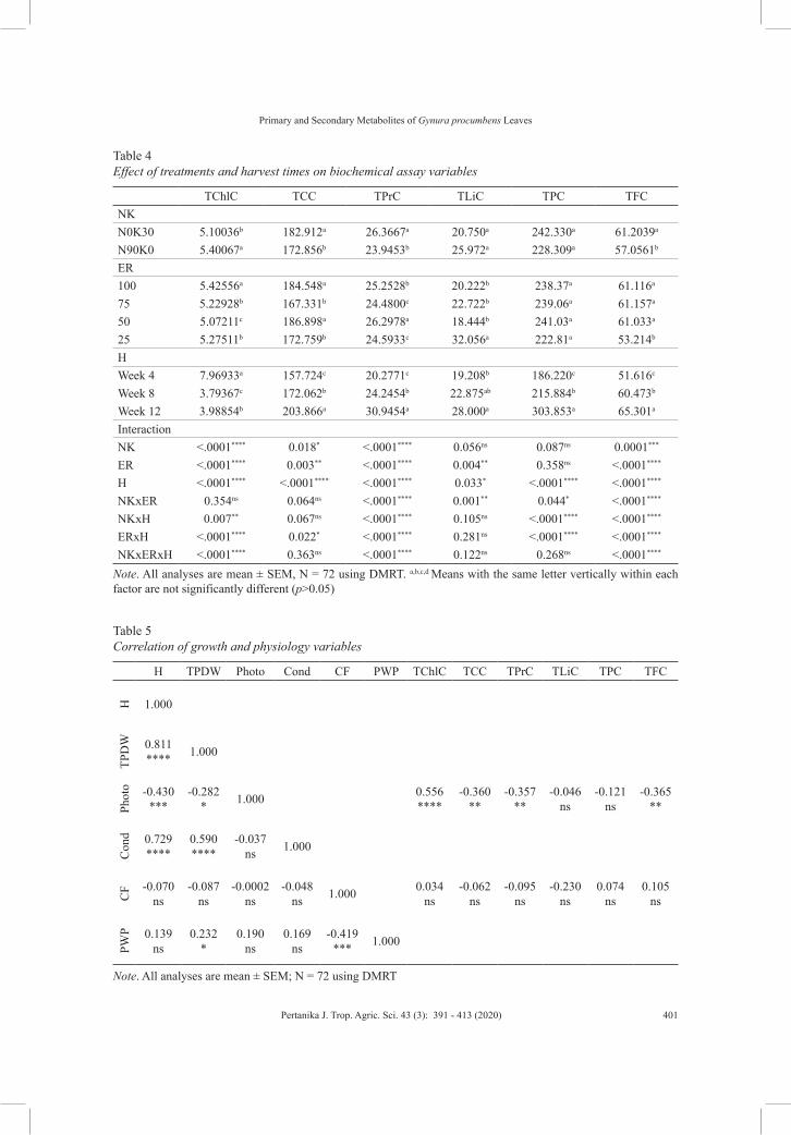
Primary and Secondary Metabolites of Gynura procumbens Leaves
401Pertanika J. Trop. Agric. Sci. 43 (3): 391 - 413 (2020)
Table 5Correlation of growth and physiology variables
H TPDW Photo Cond CF PWP TChlC TCC TPrC TLiC TPC TFC
H 1.000
TPD
W 0.811**** 1.000
Phot
o -0.430***
-0.282* 1.000 0.556
****-0.360
**-0.357
**-0.046
ns-0.121
ns-0.365
**
Con
d 0.729****
0.590****
-0.037ns 1.000
CF -0.070
ns-0.087
ns-0.0002
ns-0.048
ns 1.000 0.034ns
-0.062ns
-0.095ns
-0.230ns
0.074ns
0.105ns
PWP 0.139
ns0.232
*0.190
ns0.169
ns-0.419
*** 1.000
Note. All analyses are mean ± SEM; N = 72 using DMRT
Table 4Effect of treatments and harvest times on biochemical assay variables
TChlC TCC TPrC TLiC TPC TFCNKN0K30 5.10036b 182.912a 26.3667a 20.750a 242.330a 61.2039a
N90K0 5.40067a 172.856b 23.9453b 25.972a 228.309a 57.0561b
ER100 5.42556a 184.548a 25.2528b 20.222b 238.37a 61.116a
75 5.22928b 167.331b 24.4800c 22.722b 239.06a 61.157a
50 5.07211c 186.898a 26.2978a 18.444b 241.03a 61.033a
25 5.27511b 172.759b 24.5933c 32.056a 222.81a 53.214b
H Week 4 7.96933a 157.724c 20.2771c 19.208b 186.220c 51.616c
Week 8 3.79367c 172.062b 24.2454b 22.875ab 215.884b 60.473b
Week 12 3.98854b 203.866a 30.9454a 28.000a 303.853a 65.301a
InteractionNK <.0001**** 0.018* <.0001**** 0.056ns 0.087ns 0.0001***
ER <.0001**** 0.003** <.0001**** 0.004** 0.358ns <.0001****
H <.0001**** <.0001**** <.0001**** 0.033* <.0001**** <.0001****
NKxER 0.354ns 0.064ns <.0001**** 0.001** 0.044* <.0001****
NKxH 0.007** 0.067ns <.0001**** 0.105ns <.0001**** <.0001****
ERxH <.0001**** 0.022* <.0001**** 0.281ns <.0001**** <.0001****
NKxERxH <.0001**** 0.363ns <.0001**** 0.122ns 0.268ns <.0001****
Note. All analyses are mean ± SEM, N = 72 using DMRT. a,b,c,d Means with the same letter vertically within each factor are not significantly different (p>0.05)
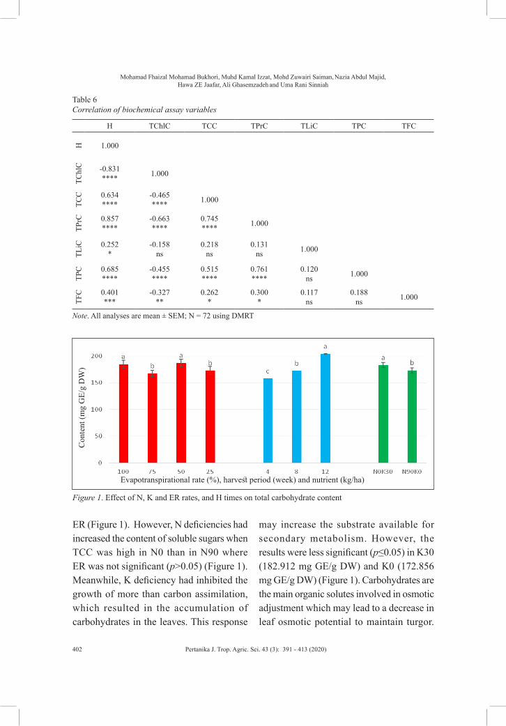
Mohamad Fhaizal Mohamad Bukhori, Muhd Kamal Izzat, Mohd Zuwairi Saiman, Nazia Abdul Majid, Hawa ZE Jaafar, Ali Ghasemzadeh and Uma Rani Sinniah
402 Pertanika J. Trop. Agric. Sci. 43 (3): 391 - 413 (2020)
ER (Figure 1). However, N deficiencies had increased the content of soluble sugars when TCC was high in N0 than in N90 where ER was not significant (p>0.05) (Figure 1). Meanwhile, K deficiency had inhibited the growth of more than carbon assimilation, which resulted in the accumulation of carbohydrates in the leaves. This response
may increase the substrate available for secondary metabolism. However, the results were less significant (p≤0.05) in K30 (182.912 mg GE/g DW) and K0 (172.856 mg GE/g DW) (Figure 1). Carbohydrates are the main organic solutes involved in osmotic adjustment which may lead to a decrease in leaf osmotic potential to maintain turgor.
Table 6Correlation of biochemical assay variables
H TChlC TCC TPrC TLiC TPC TFC
H 1.000
TChl
C -0.831**** 1.000
TCC 0.634
****-0.465**** 1.000
TPrC 0.857
****-0.663****
0.745**** 1.000
TLiC 0.252
*-0.158
ns0.218
ns0.131
ns 1.000
TPC 0.685
****-0.455****
0.515****
0.761****
0.120ns 1.000
TFC 0.401
***-0.327
**0.262
*0.300
*0.117
ns0.188
ns 1.000
Note. All analyses are mean ± SEM; N = 72 using DMRT
Figure 1. Effect of N, K and ER rates, and H times on total carbohydrate content
Evapotranspirational rate (%), harvest period (week) and nutrient (kg/ha)
Con
tent
(mg
GE/
g D
W)

Primary and Secondary Metabolites of Gynura procumbens Leaves
403Pertanika J. Trop. Agric. Sci. 43 (3): 391 - 413 (2020)
This is an important adaptive mechanism in plants subjected to deficit irrigation (Wang et al., 2015). The accumulation of soluble TCC is also due to a reduction in soluble sugar transportation under water stress, however, the result reported less significant (p≤0.05) to TCC and ER.
Total Protein Content
The TPrC was statistically significant in all treatments with increasing harvesting time (p≤0.0001) (Figure 2, Tables 2 and 4). The 50% ER in N0K30 treatment and 25% ER in N90K0 had shown the highest protein content, meanwhile, 25% ER in N0K30 and N90K0 have shown the lowest (Figure 2).
The content was highest under 50% ER in N0K30 at Week 12 compared to 25% ER in N90K0 at Week 4 (Figure 2 and Table 4). The TPrC was significantly correlated with Photo, TCC, TPC, and TFC at r=-0.357; p≤0.01, r=0.745; p≤0.0001, r=0.761; p≤0.0001 and r=0.300; p≤0.05, respectively. However, it was not significantly correlated with TLiC at r=0.131; p>0.05 by a linear function (Tables 5 and 6). The contents of proline (a proteinogenic amino acid in the biosynthesis of proteins) vary in plants and are subject to different moisture conditions and nutritional status (Mohd Zain & Ismail, 2016). And, drought stress can also increase organic compounds required for osmotic
Harvest
Harvest
Con
tent
(mg
BSA
E/g
DW
)C
onte
nt (m
g B
SAE/
g D
W)
Figure 2. Changes in total protein content as affected by the interactions between rates of N, K and ER, and H times

Mohamad Fhaizal Mohamad Bukhori, Muhd Kamal Izzat, Mohd Zuwairi Saiman, Nazia Abdul Majid, Hawa ZE Jaafar, Ali Ghasemzadeh and Uma Rani Sinniah
404 Pertanika J. Trop. Agric. Sci. 43 (3): 391 - 413 (2020)
adjustments, such as proline. The report is following the result when TPrC was high at Week 12 compared to Week 4, especially in N90K0 when 25% ER was reported high (Figure 2). Additionally, K is actively regulated in solute transport, protein synthesis, and enzyme activation point to a close relationship between K and metabolism (Armengaud et al., 2009). Potassium increases the plant’s drought resistance through its functions in protein synthesis when TPrC was generally high in N0K30 (17–34 mg BSAE/g DW) compared to N90K0 (16–32 mg BSAE/g DW) (Figure 2).
Total Lipid Content
The TLiC was statistically not significant in all N and K interaction treatments, increasing with increasing harvesting time and significant difference with decreasing rate of ER including the control plants (p≤0.05). Total lipid content was highest in 25% ER at Week 12 compared to the lowest in 50% ER at Week 4 (Figure 3, and Tables
2 and 4). The TLiC was not significantly correlated with Photo, TCC, TPrC, TPC, and TFC at r=-0.046; p>0.05, r=0.218; p>0.05, r=0.131; p>0.05, r=0.120; p>0.05 and r=0.117; p>0.05, respectively by a linear function (Tables 5 and 6). As water stress rates increased, the oxidative stress in cells and tissues was enhanced, thus implying the occurrence of lipid peroxidation under high water stress (Jaafar et al., 2012) in the respective treatments, 20.222 mg/g DW (100% ER), 22.722 mg/g DW (75% ER), 18.444 mg/g DW (50% ER), and 32.056 mg/g DW (25% ER) (Figure 3). The formation of Malondialdehyde (MDA) was considered as a measurement of lipid peroxidation induced by a high-water stress rate.
Total Phenolic Content
The TPC was statistically consistent in all N and K interaction treatments, increased with increasing harvesting time, and no significant difference with decreasing rate of ER including the control plants (p≤0.05).
Evapotranspirational rate (%), harvest period (week) and nutrient (kg/ha)
Con
tent
(mg/
g D
W)
Figure 3. Effect of N, K and ER rates, and H times on total lipid content

Primary and Secondary Metabolites of Gynura procumbens Leaves
405Pertanika J. Trop. Agric. Sci. 43 (3): 391 - 413 (2020)
Total phenolic content was highest at Week 12 compared to Week 4 (Figure 4, Tables 2 and 4). The TPC are significantly correlated with TCC and TPrC at r=0.515; p≤0.0001 and r=0.761; p≤0.0001, respectively. However, not significantly correlated with Photo, TLiC, and TFC at r=-0.121; p>0.05, r=0.120; p>0.05 and r=0.188; p>0.05, respectively by a linear function (Tables 5 and 6). There were studies which reported the effects of long-term and constant N limitation on carbon allocation for growth and synthesis of phenolics as well as N deficiency increases phenolic content in plants (Caretto et al., 2015). It was following the results when TPC was high in N0 at Week 12 compared to N90 when ER treatment was not significant (p≤0.05) (Figure 4). The increased content of phenolics in plant tissues was either as existing pools or by inducing their de novo synthesis (Romagni, 2009). Additionally, the accumulation of TCC had provided a signal of an increase in the production of secondary metabolites. However, less significant content of TCC in
this study was translated into non-significant production of TPC corresponded (Figures 1 and 4, Table 6).
Total Flavonoid Content
The TFC was statistically significant in all treatments with increasing harvesting time (p≤0.0001) (Figure 5, Tables 2 and 4). The 75% ER in N0K30 treatment and 50% ER in N90K0 had shown the highest flavonoid content, meanwhile, 25% ER in N0K30 and 75% ER in N90K0 have shown the lowest. The content was highest under 50% ER in N90K0 at Week 12 compared to 75% ER in N90K0 at Week 4 (Figure 5). The TFC was significantly correlated with Photo, TCC and TPrC at r=-0.365; p≤0.01, r=0.262; p≤0.05 and r=0.300; p≤0.05, respectively. However, not significantly correlated with TLiC and TPC at r=0.117; p>0.05 and r=0.188; p>0.05, respectively by a linear function (Tables 5 and 6). The event was probably because, in resource-limited environments, carbon partitioning to constitutive secondary metabolism often increases, which enhances
Evapotranspirational rate (%), harvest period (week) and nutrient (kg/ha)
Con
tent
(mg
CA
E/g
DW
)
Figure 4. Effect of N, K and ER rates, and H times on total phenolic content

Mohamad Fhaizal Mohamad Bukhori, Muhd Kamal Izzat, Mohd Zuwairi Saiman, Nazia Abdul Majid, Hawa ZE Jaafar, Ali Ghasemzadeh and Uma Rani Sinniah
406 Pertanika J. Trop. Agric. Sci. 43 (3): 391 - 413 (2020)
resistance to attack by pathogens and stress tolerance (Caretto et al., 2015). The results indicated the limitations in plant growth were generally accompanied by higher secondary metabolite content. And, N deficiency induces the synthesis of ascorbic acid, flavonoids, and flavonols. The result was following the report when TFC was generally high in N0 (40–80 mg KE/g DW) compared to N90 (20–80 mg KE/g DW). Coinciding with this prediction, the TFC increased with K starvation (N90K0), and an appropriate K rate (N0K30) (Figure 5) could maintain the concentration of flavonoids. In addition,
there was an increase in TFC (70 mg KE/g DW and 83 mg KE/g DW) under high water stress (50% ER and 25% ER) (Figure 5), respectively to an accumulation of soluble TCC in plants is also as a result of reduced transportation of soluble sugar under water limitation (Figure 1) (Kleczewski et al., 2010). Possibly, there was a reduction in maximum quantum yield (0.01–0.49 Fv/Fm) (Tables 2 and 3) with increasing content of secondary metabolites as water field capacity being reduced (25% and 50% ER) again demonstrated the possible production of secondary metabolites under increasing water stress (Figure 5).
Harvest
Harvest
Con
tent
(mg
KE/
g D
W)
Con
tent
(mg
KE/
g D
W)
Figure 5. Changes in total flavonoid content as affected by the interactions between rates of N, K and ER, and H time

Primary and Secondary Metabolites of Gynura procumbens Leaves
407Pertanika J. Trop. Agric. Sci. 43 (3): 391 - 413 (2020)
Thin Layer Chromatography
Qualitative analysis of the leaves methanol extract was performed using a mixture of toluene: ethyl acetate: formic acid (5:4:1 v/v) was used as the mobile phase
(Sasidharan et al., 2011) yielded a good resolution of caffeic acid and ferulic acid with bands at Rf=0.64 and 0.69, respectively (Figure 6) for phenolic content. Meanwhile, the analysis also yielded a good resolution
Figure 6. Thin-layer chromatography developed-profiles of caffeic and ferulic acid standard solution
Visible light before derivatization
254 nm before derivatization
366 nm before derivatization
Visible light before derivatization
254 nm before derivatization
366 nm before derivatization
Figure 7. Thin-layer chromatography developed-profiles of kaempferol standard solution
Mohamad Fhaizal Mohamad Bukhori, Muhd Kamal Izzat, Mohd Zuwairi Saiman, Nazia Abdul Majid, Hawa ZE Jaafar, Ali Ghasemzadeh and Uma Rani Sinniah
408 Pertanika J. Trop. Agric. Sci. 43 (3): 391 - 413 (2020)
of kaempferol with bands at Rf=0.70 (Figure 7) for flavonoid content. Caffeic acid, ferulic acid, and kaempferol were identified and quantified at visible light, 254 and 366 nm OD. The results revealed the methanol extract at 1 g/10 mL of 100% methanol contained caffeic acid and ferulic acid in accordance with TPC analysis, highest in N90K0(75) treatments at Week 12 compared to N90K0(75) at Week 8 (Figure 4). Meanwhile, kaempferol in accordance with TFC analysis, was highest in N90K0(75) at Week 12 compared to N90K0(75) at Week 8 (Figure 5). This TLC procedure can be used as a fast phytochemical markers screening method for G. procumbens leaf samples and herbal formulations.
Phenolic Gene Expression Profile
The analysis was to determine and identify G. procumbens phenolic gene expression and relation with selected phenolic biosynthetic genes. The analysis involved mother plant (control sample), and high and low phenolic content samples at Week 8 and 12 after treatment. The samples were selected based on the TPC analysis (Figure 4). The samples were subjected to real-time PCR analysis to substantiate the metabolites content is matched in quantification measurement with a spectrophotometer as well as to identify the responsible gene in modulating the metabolites synthesis. The control plants have shown the lowest content (Relative quantification, RQ 1) of phenolic content compared to other treatment samples. Phenolic content at Week 8 (RQ 1.482 and 0.974) were under the TPC analysis,
however, in Week 12 (RQ 3.926 and 8.37) had contradicted the TPC analysis, where low and high TPC had shown a reversal in phenolic content RQ (Figure 8).
The phenolic metabolism was assessed by monitoring the leaf phenolic content together with the expression of three phenolic biosynthetic genes regulation [phenylalanine ammonia-lyase (PAL), chalcone synthase (CHS), and flavanone3-hydroxylase (F3H)] and one globular protein gene as a control gene (Tubulin). The mechanisms underlying plant adaptation may involve several processes, such as accumulation of signaling proteins and transcription factors or epigenetic modification (de Rosas et al., 2017). Although the transcript levels of phenolic biosynthesis genes were repressed during fertilizer and water re-supply, the decrease in phenolic content in tissues was slower and appeared to be metabolite specific. From a mechanistic viewpoint, the response to fertilizer and water deficiency implies an early reprogramming of gene expression that starts within the first month of limitation, whereas the effects on growth and metabolic content have been proven to be significant between two and three months later.
The increase in the content of secondary metabolites in the present work could be related to an increase in PAL activities under low water field capacity replacement. Suggesting up-regulation of secondary metabolite production with increased PAL activity. This is basically due to PAL is an enzyme, which synthesizes a precursor for total phenolics and flavonoids

Primary and Secondary Metabolites of Gynura procumbens Leaves
409Pertanika J. Trop. Agric. Sci. 43 (3): 391 - 413 (2020)
biosynthesis (Koyama & Goto-Yamamoto, 2008). High water stress in the present study may have increased the availability of phenylalanine pool as less protein is used for plant maintenance under high water stress, hence, more phenylalanine is available to produce secondary metabolites. These results suggest the up-regulation of secondary metabolites production in G. procumbens under high water stress
may be due to an increase in PAL activity due in turn to the increased availability of phenylalanine under stress conditions. However, the synthesis of phenolics in plant tissues depends on genetics, the organ, and the developmental stage and is also greatly affected by environmental factors including N, K, and water availability (Turnbull et al., 2018).
Figure 8. RT-qPCR relative quantification of phenolic compounds gene expression on four samples (PH2 to PL3) and one control sample (C) extracted with the spot method. Serial dilutions of crude extraction were used to calculate the relative quantification using the relative standard curve method. Results from each sample were normalized to the highest value (from sample PL3) and expressed as relative quantification (RQ). Bars represent the standard error of differences between the means at p≤0.05. C = control plants (mother plants); PH2 = high phenolic (8 WAT); PH3 = high phenolic (12 WAT); PL2 = low phenolic (8 WAT), and PL3 = low phenolic (12 WAT)

Mohamad Fhaizal Mohamad Bukhori, Muhd Kamal Izzat, Mohd Zuwairi Saiman, Nazia Abdul Majid, Hawa ZE Jaafar, Ali Ghasemzadeh and Uma Rani Sinniah
410 Pertanika J. Trop. Agric. Sci. 43 (3): 391 - 413 (2020)
DISCUSSION
Water is crucial for productivity and quality. However, the requirements are differed according to plant types and growing media. Deficit or surplus water will induce water stress-related metabolic responses, and due to reduced Cond, the uptake of CO2 decreases significantly (Tables 2 and 3). Thus, the consumption of reduction equivalents (NADPH+H+) for CO2 fixation via the Calvin cycle declines, accordingly, generating large oxidative stress and over-supply of reduction equivalents. Consequently, metabolic processes shifted towards biosynthetic activities which consume reduction equivalents. Accordingly, the synthesis of reduced compounds, such as phenols, is enhanced (Figure 4 and Table 4). As stress-related metabolic changes affect all plant processes extensively, the synthesis of secondary metabolites also is affected (Ren et al., 2014). The present study has shown a discrete effect on growth, physiology, and metabolite content in the following manner, N0K30>N90K0 and ER 75>50>100>25%. The highest and lowest yield of biomass and metabolite content was recorded under N0K30(70) and N90K0(25), respectively. The results also showed the influence of treatments are highly significant (p≤0.0001) in Cond, TChlC, TPrC, and TFC, (p≤0.05) in CF and PWP, and not significance (p>0.05) in Photo, TCC, TLiC, and TPC (Tables 2, 3 and 4). Meanwhile, 75% of ER was significantly affected biomass, primary, and secondary metabolites content in all treatments (Tables 2, 3, and 4).
Total biomass and phenolic content negatively interacted with physiology, primary metabolic, and polyphenolic content (flavonoid) (Tables 5 and 6). The study has shown no-significant difference (p>0.05) in Photo has caused TPDW to be significantly affected (Tables 5). Meanwhile, maintaining the productivity of Cond, TChlC, and CF had affected the TCC, TPrC, TLiC, and TFC (Tables 5 and 6). The study suggesting the source (Photo) and sink (metabolites) invariably recorded during the plant growth and development was negatively interacted according to the GDB hypothesis in water stress and selected rates of N and K study (Le Bot et al., 2009). The justification proposes trade-off between primary (growth) and secondary (defense/stress tolerance) metabolism emerging from developmental constraints in growing cells, and in direct competition for resources between primary and secondary metabolism in mature cells. Therefore, when moderate resource limitation constrains relative growth rate to a greater degree than the net assimilation rate, photosynthate accumulates in tissues and becomes available to support secondary metabolic processes, resulting in higher levels of constitutive secondary metabolites in tissues (Shitan, 2016). These variations may be due to the inherent physiological abilities of the treated plants to absorb and utilize the given fertilizers and water rates with the requirements for growth and development.
In this study, Photo was decreased significantly (p≤0.05) under water deficit

Primary and Secondary Metabolites of Gynura procumbens Leaves
411Pertanika J. Trop. Agric. Sci. 43 (3): 391 - 413 (2020)
condition. The decrease is probably due to low CO2 availability as a result of reduced stomatal and mesophyll conductance. The limited CO2 assimilation of the leaf tissues may result in an increased allocation of photoassimilates to the secondary metabolites production (Ren et al., 2014). The increase in secondary metabolites production under low Photo was due to upregulated shikimic acid pathway activity under stressed conditions. Suggesting up-regulation of the shikimic acid pathway has involved in secondary metabolites production was under down-regulated Photo. Under high water stress, there is a limit on the translocation of carbon to sinks, with the remaining carbon accumulates as carbohydrates, leading to an increase in carbon pool allocated for secondary metabolism, with little or no competition with growth and development. However, in this study, the result has shown less significance of TCC with ER treatment and in harvest time (Tables 2 and 4). Therefore, the study relatively agrees that water stress usually enhances the production of secondary metabolites (Kleinwächter & Selmar, 2014). This is following plant resource allocation for growth influenced phenolic content in plant tissue, by affecting the plant CNB. When conditions are favorable, plants preferentially allocate carbon for growth. On the other hand, when water or fertilizers are low, carbon will often accumulate, and used for secondary metabolite synthesis (Soubeyrand et al., 2014).
CONCLUSION
The lowest rate of N, moderate of K and 75% ER had produced optimum biomass for required optimum primary and secondary metabolites content. Meanwhile, caffeic acid, kaempferol, and ferulic acid were demonstrated as lead compounds in this study. High phenolic content is probably due to the induction of phenolic-related biosynthesis genes regulation including PAL, CHS, and F3H, and attributed to defense response against ER rates. The N, K, and ER modulation are effective to promote phenolic content because the expressions of phenolic-related biosynthesis genes are high as a result of favorable abiotic influence.
ACKNOWLEDGEMENTS
The authors would like to thank the MoHE Malaysia, UNIMAS, PBRL UM, and UPM.
REFERENCESArmengaud, P., Sulpice, R., Miller, A. J., Stitt, M.,
Amtmann, A., & Gibon, Y. (2009). Multilevel analysis of primary metabolism provides new insights into the role of potassium nutrition for glycolysis and nitrogen assimilation in Arabidopsis roots. Plant Physiology, 150(2), 772–785.
Caretto, S., Linsalata, V., Colella, G., Mita, G., & Lattanzio, V. (2015). Carbon fluxes between primary metabolism and phenolic pathway in plant tissues under stress. International Journal of Molecular Sciences, 16(11), 26378–26394.
Cheng, X., Liu, J., Shu, J., & Yu, M. K. (2014). Effects of different light intensity on the growth and nutrients content of Gynura. Advanced Materials
Mohamad Fhaizal Mohamad Bukhori, Muhd Kamal Izzat, Mohd Zuwairi Saiman, Nazia Abdul Majid, Hawa ZE Jaafar, Ali Ghasemzadeh and Uma Rani Sinniah
412 Pertanika J. Trop. Agric. Sci. 43 (3): 391 - 413 (2020)
Research, 955–959, 3766–3769. doi: 10.4028/www.scientific.net/AMR.955-959.3766
de Rosas, I., Ponce, M. T., Malovini, E., Deis, L., Cavagnaro, B., & Cavagnaro, P. (2017). Loss of anthocyanins and modification of the anthocyanin profiles in grape berries of Malbec and Bonarda grown under high temperature conditions. Plant Science, 258, 137–145.
Fukuoka, N., Suzuki, T., Minamide, K., & Hamada, T. (2014). Effect of shading on anthocyanin and non-flavonoid polyphenol biosynthesis of Gynura bicolor leaves in midsummer. HortScience, 49(9), 1148-1153.
Hansen, J., & Moller, I. B. (1975). Analysis of starch and soluble sugars with Anthrone reagent. Analytical Biochemistry, 68, 87–94.
Ibrahim, M. H., Ismail, A., Omar, H., Mohd Nadzir, M. N. H., & Mohd Zain, N. A. (2017). Primary, secondary metabolites, biochemical and antioxidant activity of Orthosiphon staminues Benth. (Misai Kucing) under cadmium exposure. Annual Research and Review in Biology, 19(1), 1–14.
Ibrahim, M. H., Jaafar, H. Z. E., Karimi, E., & Ghasemzadeh, A. (2014). Allocation of secondary metabolites, photosynthetic capacity, and antioxidant activity of kacip fatimah (Labisia pumila Benth.) in response to CO2 and light intensity. Retrieved October 23, 2019, from https://www.hindawi.com/journals/tswj/2014/360290/
Ismail, N. Z., Arsad, H., Samian, M. R., & Hamdan, M. R. (2017). Determination of phenolic and flavonoid contents, antioxidant activities and GC-MS analysis of Clinacanthus nutans (Acanthaceae) in different locations. AGRIVITA Journal of Agricultural Science, 39(3), 335–344.
Jaafar, H. Z. E., Ibrahim, M. H., & Fakri, N. F. M. (2012). Impact of soil field water capacity on secondary metabolites, phenylalanine ammonia-lyase (PAL), maliondialdehyde (MDA) and
photosynthetic responses of Malaysian kacip fatimah (Labisia pumila Benth.). Molecules, 17(6), 7305–7322.
Jamaludin, D., Abd Aziz, S., Ahmad, D., & Jaafar, H. Z. E. (2015). Impedance analysis of Labisia pumila plant water status. Information Processing in Agriculture, 2(3-4), 161–168.
John, E. C. (1995). Current protocols in protein science. London, United Kingdom: John Wiley and Sons.
Kleczewski, N. M., Herms, D. A., & Bonello, P. (2010). Effects of soil type, fertilization and drought on carbon allocation to root growth and partitioning between secondary metabolism and ectomycorrhizae of Betula papyrifera. Tree Physiology, 30(7), 807–817.
Kleinwächter, M., & Selmar, D. (2014). New insights explain that drought stress enhances the quality of spice and medicinal plants: Potential applications. Agronomy for Sustainable Development, 35(1), 121–131.
Koyama, K., & Goto-Yamamoto, N. (2008). Bunch shading during different developmental stages affects the phenolic biosynthesis in berry skins of “Cabernet Sauvignon” grapes. Journal of the American Society for Horticultural Science, 133(6), 743–753.
Le Bot, J., Bénard, C., Robin, C., Bourgaud, F., & Adamowicz, S. (2009). The “trade-off” between synthesis of primary and secondary compounds in young tomato leaves is altered by nitrate nutrition: Experimental evidence and model consistency. Journal of Experimental Botany, 60(15), 4301–4314.
Li, F., Gao, J., Xue, F., Yu, X., & Shao, T. (2016). Extraction optimization, purification and physicochemical properties of polysaccharides from Gynura medica. Molecules, 21(4), 1–13.
Loh, F. C. W., Grabosky, J. C., & Bassuk, N. L. (2002). Using the SPAD 502 meter to assess chlorophyll and nitrogen content of benjamin

Primary and Secondary Metabolites of Gynura procumbens Leaves
413Pertanika J. Trop. Agric. Sci. 43 (3): 391 - 413 (2020)
fig and cottonwood leaves. HortTechnology, 12(4), 682-686.
Mohd Zain, N. A., & Ismail, M. R. (2016). Effects of potassium rates and types on growth, leaf gas exchange and biochemical changes in rice (Oryza sativa) planted under cyclic water stress. Agricultural Water Management, 164, 83–90.
Mongkhonsin, B., Nakbanpote, W., Hokura, A., Nuengchamnong, N., & Maneechai, S. (2016). Phenolic compounds responding to zinc and/or cadmium treatments in Gynura pseudochina (L.) DC. extracts and biomass. Plant Physiology and Biochemistry, 109, 549–560.
Oyedeji, S., Animasaun, D. A., Bello, A. A., & Agboola, O. O. (2014). Effect of NPK and poultry manure on growth, yield, and proximate composition of three Amaranths. Retrieved October 23, 2019, from https://www.hindawi.com/journals/jb/2014/828750/
Pant, B. D., Pant, P., Erban, A., Huhman, D., Kopka, J., & Scheible, W. R. (2015). Identification of primary and secondary metabolites with phosphorus status-dependent abundance in Arabidopsis, and of the transcription factor PHR1 as a major regulator of metabolic changes during phosphorus limitation. Plant, Cell and Environment, 38(1), 172–187.
Ren, J., Guo, S., Xu, C., Yang, C., Ai, W., Tang, Y., & Qin, L. (2014). Effects of different carbon dioxide and LED lighting levels on the anti-oxidative capabilities of Gynura bicolor DC. Advances in Space Research, 53(2), 353–361.
Romagni, J. G. (2009). Biosynthesis of chemical signals - De novo synthesis and secondary metabolites. In J. D. Hardege (Ed.), Chemical ecology (pp. 393 - 415). Oxford, United Kingdom: Encyclopedia of Life Support Systems (EOLSS) Publishers Co. Ltd.
Sasidharan, S., Chen, Y., Saravanan, D., Sundram, K. M., & Latha, L. Y. (2011). Extraction, isolation and characterization of bioactive
compounds from plants extracts. African Journal of Traditional Complementary and Alternative Medicine, 8(1), 1–10.
Selmar, D., & Kleinwächter, M. (2013). Stress enhances the synthesis of secondary plant products: The impact of stress-related over-reduction on the accumulation of natural products. Plant and Cell Physiology, 54(6), 817–826.
Shams, K. A., Abdel-Azim, N. S., Tawfik, W. A., Hassanein, H. D., Saleh, M. A., & Hammouda, F. M. (2015). Green extraction techniques: Effect of extraction method on lipid contents of three medicinal plants of Apiaceae. Journal of Chemical and Pharmaceutical Research, 7(4), 1080–1088.
Shitan, N. (2016). Secondary metabolites in plants: Transport and self-tolerance mechanisms. Bioscience, Biotechnology and Biochemistry, 80(7), 1283–1293.
Soubeyrand, E., Basteau, C., Hilbert, G., van Leeuwen, C., Delrot, S., & Gomès, E. (2014). Nitrogen supply affects anthocyanin biosynthetic and regulatory genes in grapevine cv. Cabernet-Sauvignon berries. Phytochemistry, 103, 38–49.
Teoh, W. Y., Wahab, N. A., Richardson, J. S., & Sim, K. S. (2016). Evaluation of antioxidant properties, cytotoxicity and acute oral toxicity of Gynura procumbens (Compositae). Sains Malaysiana, 45(2), 229–235.
Turnbull, J. M., Yang, L., Wen, K. S., Ruan, X., Zhao, Y. X., Wei, F., & Wang, Q. (2018). Response of plant secondary metabolites to environmental factors. Molecules, 23(4), 1–26.
Wang, M., Fu, Y., & Liu, H. (2015). Nutritional status and ion uptake response of Gynura bicolor DC. between Porous-tube and traditional hydroponic growth systems. Acta Astronautica, 113, 13–21.


Pertanika J. Trop. Agric. Sci. 43 (3): 415 - 427 (2020)
© Universiti Putra Malaysia Press
TROPICAL AGRICULTURAL SCIENCEJournal homepage: http://www.pertanika.upm.edu.my/
Article history:Received: 4 February 2020Accepted: 7 July 2020Published: 28 August 2020
ARTICLE INFO
E-mail addresses:[email protected] (Yudha Asmara Adhi)[email protected] (Syaiful Anwar)[email protected] (Suria Darma Tarigan)[email protected] (Bandung Sahari)* Corresponding author
ISSN: 1511-3701e-ISSN 2231-8542
Relationship between Groundwater Level and Water Content in Oil Palm Plantation on Drained Peatland in Siak, Riau Province, IndonesiaYudha Asmara Adhi1, Syaiful Anwar2*, Suria Darma Tarigan2 andBandung Sahari3
1Natural Resource and Environmental Management Study Program, IPB University, Bogor 16143, Indonesia 2Department of Soil Science and Land Resource, IPB University, Bogor 16680, Indonesia3Department of Sustainability, PT Astra Agro Lestari Tbk, Jakarta 13920, Indonesia
ABSTRACTThe decrease in groundwater level (GWL) on peatlands, especially in the dry season, can lead to extensive peat drying and making it more vulnerable to the occurrence of wildfire. This research aimed to study the relationship between GWL fluctuations and water content on the surface of peatlands. The study was carried out in a 14 to 17 years old palm oil plantation and a secondary forest located in Siak, Riau Province, Indonesia. Field observations were carried out by installing a water level data logger and soil moisture sensor at a depth of 10 cm and 30 cm from the peat surface, recorded at an hour interval for one year. The results showed that GWL fluctuation was highly correlated to the peat water content in the 10 cm layer both in oil palm plantation (R2 = 0.65) and secondary forest (R2 = 0.67). The peat water content in the 30 cm layer showed a low correlation with GWL fluctuation down to -90 cm in oil palm plantation (R2 = 0.01), however, it was strongly correlated in secondary forests (R2 = 0.89). Water capillarity in peat soils was able to increase to up to 10 – 30 cm layers from the surface, ranging from 284 to 476% w/w. The capillary water could rise to 68 to 76 cm. The result of the General Linear Model analysis
showed that there was a significant influence of land cover, GWL, and peat bulk density on soil water content. Oil palm cultivation activities on peatlands increase the peat bulk density, which in turn increases water capillarity and soil water content.
Keywords: Capillarity, peat bulk density, soil
moisture, tropical peatlands

Yudha Asmara Adhi, Syaiful Anwar, Suria Darma Tarigan and Bandung Sahari
416 Pertanika J. Trop. Agric. Sci. 43 (3): 415 - 427 (2020)
INTRODUCTION
The utilization of peatlands for agriculture in Indonesia, especially oil palm plantations, has reached a high number (i.e., 1.54 million ha from the total 13.4 million ha peatlands) in the past years (Ritung et al., 2019; Wahyunto & Dariah, 2013). Long-term use of peatlands and land drainage (Van Lanen et al., 2004) has resulted in a decrease in groundwater level, an increase in aeration, soil subsidence, and rapid compaction of peat (Rieley, 2007). In addition, peat excessive drainage may cause peat irreversible drying or hydrophobicity (Hooijer et al., 2010). This process may be accelerated if the peatlands’ groundwater level (GWL) is too deep, especially during the dry season, causing the water capillarity inhibition. The critical water content where the irreversible drying occurs is 184 – 213% w/w for peat with hemic maturity and 118 – 126% w/w for peat with sapric maturity (Winarna et al., 2016). Putra (2003) reported that when the peat water content was lesser than 117% w/w, the flammability increased, thus might trigger a large-scale fire. Rein et al. (2008) also added that the peat soil water levels below 125% w/w could start a spontaneous peat ignition.
Over the past decades, Indonesia has experienced a series of drought-related major forest and land fires, such as those that occurred in 1982/83, 1997/98, 2009, and the most recent 2015 fire. Nearly 70 million people have been exposed to unhealthy air during the 2015 fire (Crippa et al., 2016). The fire had caused enormous economic and social consequences, for instance, the
smoke/ haze pollution that caused billions of dollars economic loss (Varma, 2003; World Bank, 2016). When drought coincides with El Nino in the humid tropics area (e.g., Southeast Asia), the impact increases through forest fire which disrupts the global carbon cycle, including reduction of carbon stocks (Hooijer et al., 2010; Huijnen et al., 2016; Page et al., 2002; Page & Hooijer, 2016) and intensifies the danger of haze (Lee et al., 2016).
Peatlands can experience drought under an excessive drainage condition, thus increasing its susceptibility to fire (Szajdak & Szatylowicz, 2010). According to Wösten et al. (2008), peatlands’ fire vulnerability will increase when GWL falls below 40 cm from the surface of peatlands (i.e., -40 cm). Agreeing to this, the Indonesian government has declared through its regulation (PP No. 71/2014 juncto PP No. 57/2016) that the peat ecosystems are considered degraded if the GWL is lower than -40 cm and an urgent mitigation act should be focused in these areas. Indeed, the construction of a massive drainage system has a real impact on peatland hydrology, causing a major decrease in GWL (Ishii et al., 2016). In turn, the decrease in GWL affects the distribution of moisture throughout the peat soil profile. GWL acts as a water reservoir in peatlands and the dynamics of peat water content are related to the bulk density and the water capillarity capacity of the peat soil (McLay et al., 1992). Agricultural development on peatlands has impacted the physical characteristics of peat that are relevant to the influence of humidity,
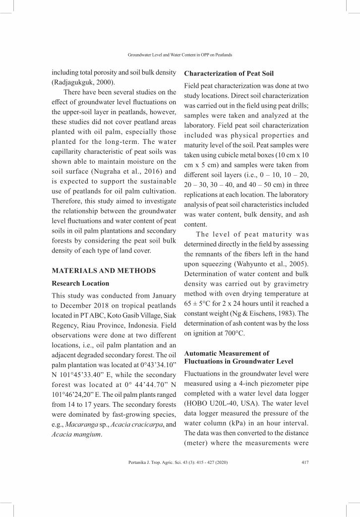
Groundwater Level and Water Content in OPP on Peatlands
417Pertanika J. Trop. Agric. Sci. 43 (3): 415 - 427 (2020)
including total porosity and soil bulk density (Radjagukguk, 2000).
There have been several studies on the effect of groundwater level fluctuations on the upper-soil layer in peatlands, however, these studies did not cover peatland areas planted with oil palm, especially those planted for the long-term. The water capillarity characteristic of peat soils was shown able to maintain moisture on the soil surface (Nugraha et al., 2016) and is expected to support the sustainable use of peatlands for oil palm cultivation. Therefore, this study aimed to investigate the relationship between the groundwater level fluctuations and water content of peat soils in oil palm plantations and secondary forests by considering the peat soil bulk density of each type of land cover.
MATERIALS AND METHODS
Research Location
This study was conducted from January to December 2018 on tropical peatlands located in PT ABC, Koto Gasib Village, Siak Regency, Riau Province, Indonesia. Field observations were done at two different locations, i.e., oil palm plantation and an adjacent degraded secondary forest. The oil palm plantation was located at 0°43’34.10” N 101°45’33.40” E, while the secondary forest was located at 0° 44’44.70” N 101°46’24,20” E. The oil palm plants ranged from 14 to 17 years. The secondary forests were dominated by fast-growing species, e.g., Macaranga sp., Acacia cracicarpa, and Acacia mangium.
Characterization of Peat Soil
Field peat characterization was done at two study locations. Direct soil characterization was carried out in the field using peat drills; samples were taken and analyzed at the laboratory. Field peat soil characterization included was physical properties and maturity level of the soil. Peat samples were taken using cubicle metal boxes (10 cm x 10 cm x 5 cm) and samples were taken from different soil layers (i.e., 0 – 10, 10 – 20, 20 – 30, 30 – 40, and 40 – 50 cm) in three replications at each location. The laboratory analysis of peat soil characteristics included was water content, bulk density, and ash content.
The level of peat maturi ty was determined directly in the field by assessing the remnants of the fibers left in the hand upon squeezing (Wahyunto et al., 2005). Determination of water content and bulk density was carried out by gravimetry method with oven drying temperature at 65 ± 5°C for 2 x 24 hours until it reached a constant weight (Ng & Eischens, 1983). The determination of ash content was by the loss on ignition at 700°C.
Automatic Measurement of Fluctuations in Groundwater Level
Fluctuations in the groundwater level were measured using a 4-inch piezometer pipe completed with a water level data logger (HOBO U20L-40, USA). The water level data logger measured the pressure of the water column (kPa) in an hour interval. The data was then converted to the distance (meter) where the measurements were

Yudha Asmara Adhi, Syaiful Anwar, Suria Darma Tarigan and Bandung Sahari
418 Pertanika J. Trop. Agric. Sci. 43 (3): 415 - 427 (2020)
conducted. Recorded data were downloaded using a USB Base Station. A unit of data logger was installed each in oil palm plantation and the secondary forest. The design of the water level measurement is presented in Figure 1. The water level height from the land surface was calculated using the following equation:
GWL = S – (H + X)where:GWL : Groundwater level (m)S : Length of the sling to the sensor
at the water level data logger (m)H : Height of piezometer head pipe
(m), which is the length of the piezometer body above ground
X : Height of the water column recorded by the sensor (m)
Automatic Measurement of Peat Water Content
The automatic measurement of peat water contents was done using a soil moisture sensor (Decagon EC5 S-SMC-M005, USA) that can measure soil moisture content from 0 to 0.550 (v/v). Soil moisture sensors were installed at a depth of 10 cm and 30 cm from the soil surface at each studied location. Each sensor retrieved data every one hour and automatically stored it into the micro station data logger (Hobo H21-USB Micro Station, USA). The soil moisture sensor was installed close to the water level data logger (Figure 1). The peat water content in volume (v/v) recorded by the sensor was converted to percent weight (% w/w) by dividing it with the related bulk density of the soil at each depth.
Figure 1. The design of groundwater level and peat water content measurement
Data Analysis
All col lected data were tes ted for homogeneity of variance using Levene’s test at p < 0.05 and the normality test using Kolmogorov-Smirnov at p < 0.05. The relationship between groundwater level and peat water content was analyzed using simple regression. General Linear Model analysis was used to study the effects of land cover, groundwater level, and peat bulk density on peat water content. Statistical analysis was conducted using SPSS version 16.0-2007 (SPSS Inc., USA). Groundwater level and soil moisture data processed using HOBOware Pro (Onset Computer Corp., Bourne, USA).
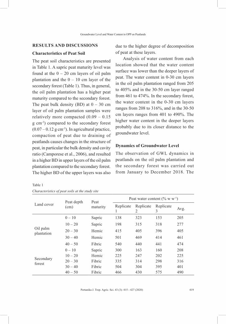
Groundwater Level and Water Content in OPP on Peatlands
419Pertanika J. Trop. Agric. Sci. 43 (3): 415 - 427 (2020)
RESULTS AND DISCUSSIONS
Characteristics of Peat Soil
The peat soil characteristics are presented in Table 1. A sapric peat maturity level was found at the 0 – 20 cm layers of oil palm plantation and the 0 – 10 cm layer of the secondary forest (Table 1). Thus, in general, the oil palm plantation has a higher peat maturity compared to the secondary forest. The peat bulk density (BD) at 0 – 30 cm layer of oil palm plantation samples were relatively more compacted (0.09 – 0.15 g cm-3) compared to the secondary forest (0.07 – 0.12 g cm-3). In agricultural practice, compaction of peat due to draining of peatlands causes changes in the structure of peat, in particular the bulk density and cavity ratio (Camporese et al., 2006), and resulted in a higher BD in upper layers of the oil palm plantation compared to the secondary forest. The higher BD of the upper layers was also
due to the higher degree of decomposition of peat at these layers.
Analysis of water content from each location showed that the water content surface was lower than the deeper layers of peat. The water content in 0-30 cm layers in the oil palm plantation ranged from 205 to 405% and in the 30-50 cm layer ranged from 461 to 474%. In the secondary forest, the water content in the 0-30 cm layers ranges from 208 to 316%, and in the 30-50 cm layers ranges from 401 to 490%. The higher water content in the deeper layers probably due to its closer distance to the groundwater level.
Dynamics of Groundwater Level
The observation of GWL dynamics in peatlands on the oil palm plantation and the secondary forest was carried out from January to December 2018. The
Table 1Characteristics of peat soils at the study site
Land cover Peat depth (cm)
Peat maturity
Peat water content (% w w-1)
Replicate 1
Replicate 2
Replicate 3 Avg.
Oil palm plantation
0 – 10 Sapric 138 323 153 20510 – 20 Sapric 198 315 318 27720 – 30 Hemic 415 405 396 40530 – 40 Hemic 501 469 414 46140 – 50 Fibric 540 440 441 474
Secondary forest
0 – 10 Sapric 300 163 160 20810 – 20 Hemic 225 247 202 22520 – 30 Fibric 335 314 298 31630 – 40 Fibric 504 304 395 40140 – 50 Fibric 466 430 575 490

Yudha Asmara Adhi, Syaiful Anwar, Suria Darma Tarigan and Bandung Sahari
420 Pertanika J. Trop. Agric. Sci. 43 (3): 415 - 427 (2020)
Table 1 (Continued)
Land cover Peat depth (cm)
Peat maturity
Bulk density (g cm-3)
Replicate 1
Replicate 2 Replicate 3 Avg.
Oil palm plantation
0 – 10 Sapric 0.18 0.11 0.16 0.15
10 – 20 Sapric 0.11 0.12 0.12 0.12
20 – 30 Hemic 0.10 0.09 0.08 0.09
30 – 40 Hemic 0.09 0.09 0.09 0.09
40 – 50 Fibric 0.09 0.08 0.08 0.08
Secondary forest
0 – 10 Sapric 0.09 0.13 0.14 0.12
10 – 20 Hemic 0.07 0.10 0.09 0.09
20 – 30 Fibric 0.07 0.07 0.08 0.07
30 – 40 Fibric 0.08 0.09 0.08 0.08
40 – 50 Fibric 0.08 0.07 0.06 0.07
Note. *WC = Water content (% w/w); BD = Bulk density (g cm-3)
Figure 2. Groundwater level fluctuations in oil palm plantation and secondary forest
results showed that the fluctuations in the groundwater level were strongly influenced by the rainfall conditions at the studied sites (Figure 2). A similar GWL dynamics pattern was observed at the two studied locations. The annual rainfall at the research location in 2018 reached a maximum of 2,169
mm, with 2 wet periods in April-June and October-December, also 2 dry periods in January-March and July-September.
The wet period in October-December with rainfall of 8.62 mm day-1 reached the highest GWL average in both sites (-0.47 m in the oil palm plantation, -0.33 in the

Groundwater Level and Water Content in OPP on Peatlands
421Pertanika J. Trop. Agric. Sci. 43 (3): 415 - 427 (2020)
secondary forest; see Table 2). On the contrary, the dry period in July-September with rainfall of 3.82 mm day-1 reached the lowest GWL average (-0.80 m in the oil palm plantation, -0.56 m in the secondary forest; see Table 2). In general, the GWL in the oil palm plantation is deeper compared to that in the secondary forest. A possible
explanation was due to the development of the canal system in the oil palm plantation to facilitate the rooting conditions of oil palm. The exploitation of forest resources on peat surfaces further reduces the ability of ecosystems to withstand rainfall, thus, water flows faster into rivers and the water level decreases in the dry season (Rieley, 2007).
Table 2Seasonal period and groundwater level (GWL) at the study site
Period (Month)
Rainfall (mm/day)
AverageGWL (m)
Land cover
Wet(April - June)
6.45 0.67 Oil palm plantation0.41 Secondary forest
Wet (October – December)
8.62 0.47 Oil palm plantation0.33 Secondary forest
Dry (January - March) 5.3 0.75 Oil palm plantation0.53 Secondary forest
Dry (July - September) 3.82 0.80 Oil palm plantation0.56 Secondary forest
Relationship between Water Level Fluctuation and Peat Water Content
The observation of peat water content at the oil palm plantation was successfully done in January to December 2018, while the observation in the secondary forest was only done from January until July 2018 due to the damage in the soil moisture sensor. The observation results of the peat water content and water level fluctuations are shown in Figure 3.
In both locations, the fluctuations of water contents to a certain extent
were affected by the fluctuations of the groundwater level. The effects of GWL were more pronounced in the surface up to the 10 cm depth in the secondary forest and up to 30 cm depth in the oil palm plantation. The decrease in the groundwater level decreases soil water content in the entire soil profile and resulting in the release of a number of groundwater volumes from the above layers (Kurnain et al., 2006). A high reduction of GWL in the oil palm plantation during the dry months (January-March and July-September) to around -0.90 m was related to

Yudha Asmara Adhi, Syaiful Anwar, Suria Darma Tarigan and Bandung Sahari
422 Pertanika J. Trop. Agric. Sci. 43 (3): 415 - 427 (2020)
the water content (10 cm layer: 244 - 267% in 10 cm layer 426 - 476% in 30 cm layer; see Figure 3a). During the dry months, GWL in the secondary forest only decreased to around -0.65 m and also related with its water content (284-312% in 10 cm layer and 389 – 415% in 30 cm layer; see Figure 3b). The observed water contents were much higher than the critical irreversible dry water content according to Winarna et al. (2016), which were 184-213% for hemic maturity and 118-126% for sapric maturity. The observed water contents were also much higher than the water content of a potentially burned peat material at 117% (Putra, 2003) or a peat material that can spontaneously ignite below 125% (Rein et al., 2008).
Fluctuations in peat water contents were strongly influenced by the groundwater
level dynamics (Figures 3 and 4). A strong correlation was found between GWL depth and water content in the 10 cm layer in both sites (plantation R2 = 0.65; p < 0.05 and secondary forest R2 = 0.67; p < 0.05; see Figure 4a). A very strong correlation (R2 = 0.89; p < 0.05) between GWL depth and water content in the 30 cm layer was found in the secondary forest (Figure 4b). Contrary to other results, there was only a very weak correlation (R2 = 0.01; p < 0.05) between the GWL and the water content in the 30 cm layer in the oil palm plantation (Figure 4b). As presented in Figure 3a, there were only low fluctuations in the water content of the 30 cm layer (435 to 510%) although there were high fluctuations in the related GWL (about -0.18 to -0.94 m). The relatively stable water content in this
Figure 3. Groundwater level and peat water content in (a) oil palm plantation and (b) secondary forest
(Note. GWL = groundwater level; PWC = peat water content]

Groundwater Level and Water Content in OPP on Peatlands
423Pertanika J. Trop. Agric. Sci. 43 (3): 415 - 427 (2020)
layer was probably due to the higher bulk density and maturity of peat in the profile of the oil palm plantation (Table 1), allowing a higher raise of water capillarity compared to that in the profile of the secondary forest. Capillary water can replace water lost by evapotranspiration in the upper layers (Chesworth, 2008; McCarter, 2012; Yazaki et al., 2006). The rise of capillary water in this study can be observed from the rainfall data, water content, and GWL during the dry period in the oil palm plantation. During the dry period of February 5-16 and June 28 to July 8 with daily rainfall of 0.5 mm, peat water contents in the 30 cm and the 10 cm layers were around 455-466% and 284-294%, respectively. These numbers were much higher than the hydrophobicity water content according to Masganti et al. (2002) and Winarna et al. (2016). The peat water contents were related to the GWL fluctuation (-78 to -86 cm) in the oil palm plantation. Considering the recorded
water content in the 10 cm layer, it can be suggested that the capillary water in the oil palm plantation could rise from about 68 to 76 cm. This result is higher compared to the laboratory study of Nugraha et al. (2016), where the water capillary increased for 50 cm.
Effects of Land Cover, Groundwater Level, and Bulk Density on Soil Water ContentThere were two General Linear Model (GLM) models developed in this study. The model I studied the effect of land cover (F1), depth of soil moisture sensor (F2), and groundwater level (X1) on peat water content (Y) (Table 3). The results of the GLM model I showed the significant influence of each of the factors and interactions between land cover factors (F1), depth of soil moisture sensor (F2) and groundwater level (X1) on peat water content (Y) with R2 = 0.960 at the significance level α < 5%. Model II studied
Figure 4. Correlation of groundwater level with peat water content in oil palm plantation and secondary forest on (a) 10 cm layer from the surface (a) and (b) 30 cm layer from the surface

Yudha Asmara Adhi, Syaiful Anwar, Suria Darma Tarigan and Bandung Sahari
424 Pertanika J. Trop. Agric. Sci. 43 (3): 415 - 427 (2020)
the effect of land cover (F1), depth of soil sample (F2), and bulk density (BD) on peat water content (Y) (Table 4). The results of the model II GLM analysis showed the significant effect of land cover factor (F1)
and interactions between land cover (F1) and bulk density (BD) on peat water content (Y) with R2 = 0.955 at the significant level α < 5%.
Table 3 Effect of land cover (F1), depth of soil moisture sensor (F2) and groundwater level (X1) on peat water content (Y)
a) R2 = 0.960 (Adjusted R2= 0.960); **) significant at α < 5%
Source Type III sum of squares df Mean square F Sig.
Corrected model 5561113.51a 7 794444.78 2713.20 .000**Intercept 11232491.28 1 11232491.28 38361.37 .000**F1 11838.62 1 11838.62 40.43 .000**F2 184386.09 1 184386.09 629.72 .000**X1 742117.84 1 742117.84 2534.49 .000**F1 * F2 63755.93 1 63755.93 217.74 .000**F1 * X1 103420.29 1 103420.29 353.20 .000**F2 * X1 2545.10 1 2545.10 8.69 .003**F1 * F2 * X1 151419.36 1 151419.36 517.13 .000**Error 231903.37 792 292.80Total 129349953.22 800Corrected total 5793016.89 799
Table 4 Effect of land cover (F1), depth of soil sample (F2) and bulk density (BD) on peat water content (Y)
Source Type III sum of squares df Mean square F Sig.
Corrected model 416251.46a 19 21907.97 11.17 .000**Intercept 22674.11 1 22674.11 11.56 .007**F1 9898.57 1 9898.57 5.05 .048**F2 16682.66 4 4170.66 2.13 .152BD 1532.91 1 1532.91 0.78 .397F1 * F2 16427.08 4 4106.77 2.09 .156F1 * BD 12264.76 1 12264.76 6.25 .031**F2 * BD 13895.27 4 3473.82 1.77 .211F1 * F2 * BD 17278.75 4 4319.69 2.20 .142
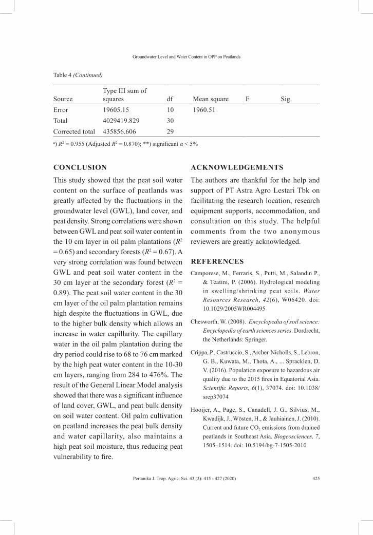
Groundwater Level and Water Content in OPP on Peatlands
425Pertanika J. Trop. Agric. Sci. 43 (3): 415 - 427 (2020)
CONCLUSION
This study showed that the peat soil water content on the surface of peatlands was greatly affected by the fluctuations in the groundwater level (GWL), land cover, and peat density. Strong correlations were shown between GWL and peat soil water content in the 10 cm layer in oil palm plantations (R2 = 0.65) and secondary forests (R2 = 0.67). A very strong correlation was found between GWL and peat soil water content in the 30 cm layer at the secondary forest (R2 = 0.89). The peat soil water content in the 30 cm layer of the oil palm plantation remains high despite the fluctuations in GWL, due to the higher bulk density which allows an increase in water capillarity. The capillary water in the oil palm plantation during the dry period could rise to 68 to 76 cm marked by the high peat water content in the 10-30 cm layers, ranging from 284 to 476%. The result of the General Linear Model analysis showed that there was a significant influence of land cover, GWL, and peat bulk density on soil water content. Oil palm cultivation on peatland increases the peat bulk density and water capillarity, also maintains a high peat soil moisture, thus reducing peat vulnerability to fire.
ACKNOWLEDGEMENTS
The authors are thankful for the help and support of PT Astra Agro Lestari Tbk on facilitating the research location, research equipment supports, accommodation, and consultation on this study. The helpful comments from the two anonymous reviewers are greatly acknowledged.
REFERENCESCamporese, M., Ferraris, S., Putti, M., Salandin P.,
& Teatini, P. (2006). Hydrological modeling in swelling/shrinking peat soils. Water Resources Research, 42(6), W06420. doi: 10.1029/2005WR004495
Chesworth, W. (2008). Encyclopedia of soil science: Encyclopedia of earth sciences series. Dordrecht, the Netherlands: Springer.
Crippa, P., Castruccio, S., Archer-Nicholls, S., Lebron, G. B., Kuwata, M., Thota, A., ... Spracklen, D. V. (2016). Population exposure to hazardous air quality due to the 2015 fires in Equatorial Asia. Scientific Reports, 6(1), 37074. doi: 10.1038/srep37074
Hooijer, A., Page, S., Canadell, J. G., Silvius, M., Kwadijk, J., Wösten, H., & Jauhiainen, J. (2010). Current and future CO2 emissions from drained peatlands in Southeast Asia. Biogeosciences, 7, 1505–1514. doi: 10.5194/bg-7-1505-2010
a) R2 = 0.955 (Adjusted R2 = 0.870); **) significant α < 5%
Table 4 (Continued)
SourceType III sum of squares df Mean square F Sig.
Error 19605.15 10 1960.51Total 4029419.829 30Corrected total 435856.606 29

Yudha Asmara Adhi, Syaiful Anwar, Suria Darma Tarigan and Bandung Sahari
426 Pertanika J. Trop. Agric. Sci. 43 (3): 415 - 427 (2020)
Huijnen, V., Wooster, M. J., Kaiser, J. W., Gaveau, D. L. A., Flemming, J., Parrington, M., ... van Weele, M. (2016). Fire carbon emissions over maritime Southeast Asia in 2015 largest since 1997. Scientific Reports, 6(1), 26886. doi: 10.1038/srep26886
Ishii, Y., Koizumi, K., Fukami, H., Yamamoto, K., Takahashi, H., Limin, S. H., … Susilo, G. E. (2016). Groundwater in peatland. In M. Osaki & N. Tsuji (Eds.), Tropical peatland ecosystems (pp. 265-279). Tokyo, Japan: Springer.
Kurnain, A., Notohadikusumo, T., & Radjagukguk, B. (2006). Impact of development and cultivation on hydro-physical properties of tropical peat soils. Tropics, 15(4), 383–389. doi: 10.3759/tropics.15.383
Lee, J. S. H., Jaafar, Z., Tan, A. K. J., Carrasco, L. R., Ewing, J. J., Bickford, D. P., ... Koh, L. P. (2016). Toward clearer skies: Challenges in regulating transboundary haze in Southeast Asia. Environmental Science and Policy, 55, 87–95. doi : 10.1016/j.envsci.2015.09.008
Masganti, Notohadikusumo, T., Maas, A., & Radjagukguk, B. (2002). Hydrophobicity and its impact on chemical properties of peat. In J. O. Rieley & S. E. Page (Eds.), Symposium Proceeding on Peatlands for People: Natural Resources Functions and Sustainable Management (pp. 109-113). Jakarta, Indonesia: Badan Pengkajian dan Penerapan Teknologi.
McCarter, C. (2012). The hydrology of the Bois-des-Bel bog peatland restoration a tale of two scales (Master’s thesis, University of Waterloo, Canada). Retrieved April 20, 2018, from https://ocul-wtl.primo.exlibrisgroup.com/discovery/ful ld isplay?vid=01OCUL_WTL:WTL_DEFAULT&search_scope=MyInst_and_CI&docid=alma9944404993505162&lang=en&context=L&adaptor=true
McLay, C. D. A., Allbrook, R. F., & Thompson, K. (1992). Effect of development and cultivation on
physical properties of peat soils in New Zealand. Geoderma, 54(1-4), 23–37. doi: 10.1016/0016-7061(92)90096-p
Ng, S. Y., & Eischens, G. R. (1983). Repeated short-term consolidation of peats. In P. M. Jarrett (Ed.), Testing of peats and organic soils (pp. 192-206). Philadelphia, USA: American Society for Testing and Materials.
Nugraha, M. I., Annisa, W., Syaufina, L., Anwar, S. (2016). Capillary water rice in peat soil as affected by various groundwater levels. Indonesian Journal of Agricultural Science, 17(2), 75-83. doi: 10.21082/ijas.v17n2.2016.p75-83
Page, S. E., & Hooijer, A. (2016). In the line of fire: The peatlands of Southeast Asia. Retrieved January 12, 2020, from https://royalsocietypublishing.org/doi/10.1098/rstb.2015.0176
Page, S. E., Siegert, F., Rieley, J. O., Boehm, H.-D. V., Jaya, A., & Limin, S. (2002). The amount of carbon released from peat and forest fires in Indonesia during 1997. Nature, 420(6911), 61–65. doi: 10.1038/nature01131
Putra, N. S. S. U. (2003). Hubungan kadar air dengan konsentrasi emisi gas rumah kaca pada kebakaran gambut [Relationship between water content and greenhouse gas emission concentration in peat fires] (Master’s thesis, Bogor Agricultural University, Indonesia). Retrieved Oktober 28, 2018, from http://repository.ipb.ac.id/handle/123456789/7546
Radjagukguk, B. (2000). Perubahan sifat-sifat fisik dan kimia tanah gambut akibat reklamasi lahan gambut untuk pertanian [Changes in the physical and chemical properties of peat due to reclamation of peatland for agriculture]. Jurnal Ilmu Tanah dan Lingkungan, 2(1), 1-15.
Rein, G., Cleaver, N., Ashton, C., Pironi, P., & Torero, J. L. (2008). The severity of smouldering peat fires and damage to the forest soil. Catena, 74(3), 304-309. doi: 10.1016/j.catena.2008.05.008

Groundwater Level and Water Content in OPP on Peatlands
427Pertanika J. Trop. Agric. Sci. 43 (3): 415 - 427 (2020)
Rieley, J. O. (2007). Tropical peatland – The amazing dual ecosystem: Co-existence and mutual benefit. Retrieved Oktober 28, 2019, from https://www.researchgate.net/publication/239924789
Ritung, S., Suryani, E., Yatno, E., Hikmatullah, Nugroho, K., Sukarman, ... Hartadi, A. (2019). Peta lahan gambut Indonesia skala 1: 50,000 [Map of Indonesian peatlands scale 1: 50,000]. Bogor, Indonesia: Balai Besar Penelitian dan Pengembangan Sumberdaya Lahan Pertanian.
Szajdak, L., & Szatylowicz, J. (2010). Impact of drainage on hydrophobicity of fen peat-moorsh soils. In M. Klavins (Ed.), Mires and peat (6th ed.) (pp. 158-174). Riga, Latvia: University of Latvia Press.
Van Lanen, H. A. J., Kašpárek, L., Novický, O., Querner, E. P., Fendeková, M., & Kupczyk, E. (2004). Human influences. In L. M. Tallaksen & H. A. J. Van Lanen (Eds.), Hydrological drought - Processes and estimation methods for streamflow and groundwater (pp. 347–410). Amsterdam, the Netherlands: Elsevier.
Varma, A. (2003). The economics of slash and burn: A case study of the 1997–1998 Indonesian forest fires. Ecological Economics, 46(1), 159–171. doi: 10.1016/S0921-8009(03)00139-3
Wahyunto, & Dariah, A. (2013). Pengelolaan lahan gambut tergedradasi dan terlantar untuk mendukung ketahanan pangan [Management of degraded and abandoned peatlands to support food security]. In H. Soeparno, E. Pasandaran, M. Syarwani, A. Dariah, S. M. Pasaribu, & N. S. Saad (Eds.), Politik pengembangan pertanian menghadapi perubahan iklim [Politics of agricultural development facing climate change] (pp. 329-347). Jakarta, Indonesia: Badan Penelitian dan Pengembangan Pertanian.
Wahyunto, Ritung, S., Suparto, & Subagjo, H. (2005). Sebaran gambut dan kandungan karbon di Sumatra dan Kalimantan [Distribution and carbon content of peat in Sumatra and Kalimantan]. Bogor, Indonesia: Wetlands International.
Winarna, Murtilaksono, K., Sabiham, S., Sutandi, A., & Sutarta, E. S. (2016). Hydrophobicity of tropical peat soil from an oil palm plantation in North Sumatra. Indonesian Journal of Agronomy, 15(3), 114-121. doi: 10.3923/ja.2016.114.121
World Bank. (2016). The cost of fire: An economic analysis of Indonesia’s 2015 fire crisis. Retrieved April 28, 2018, from http://documents.worldbank.org/curated/en/776101467990969768/The-cost-of-fire-an-economic-analysis-of-Indonesia-s-2015-fire-crisis
Wösten, J. H. M., Clymans, E., Page, S. E., Rieley, J. O., & Limin, S. H. (2008). Peat-water interrelationships in a tropical peatland ecosystem in Southeast Asia. Catena, 73(2), 212-224. doi: 10.1016/j.catena.2007.07.010
Yazaki, T., Urano, S., & Yabe, K. (2006). Water balance and water movement in unsaturated zones of Sphagnum hummocks in Fuhrengawa Mire, Hokkaido, Japan. Journal of Hydrology, 319(1-4), 312-327. doi: 10.1016/j.jhydrol.2005.06.037


REFEREES FOR THE PERTANIKA JOURNAL OF TROPICAL AGRICULTURAL SCIENCES
JTAS Vol. 43 (3) Aug. 2020
The Editorial Board of the Journal of Tropical Agricultural Sciences wishes to thank the following:
While every effort has been made to include a complete list of referees for the period stated above, however if any name(s) have been omitted unintentionally or spelt incorrectly, please notify the Chief Executive Editor, Pertanika Journals at [email protected]
Any inclusion or exclusion of name(s) on this page does not commit the Pertanika Editorial Office, nor the UPM Press or the University to provide any liability for whatsoever reason.
Abdul Hafiz Ab Majid (USM, Malaysia)
Abdul Salam Babji (UKM, Malaysia)
Amonrat Molee (SUT, Thailand)
Avtar Singh (PAU, India)
Banpot Napompeth (KU, Thailand)
Chuah Cheng Hock (UM, Malaysia)
Chuah Tse Seng (UMT, Malaysia)
Gan Chee Yuen (USM, Malaysia)
Hafizi Rosli (USM, Malaysia)
Ismail Jusoh (UNIMAS, Malaysia)
Izfa Riza Hazmi (UKM, Malaysia)
Jamilah Mohd Salim@Halim (UMT, Malaysia)
Janna Ong Abdullah(UPM, Malaysia)
Juju Nakasha Jaafar (UPM, Malaysia)
Kueh Roland Jui Heng (UPM, Malaysia)
Maqsood Khan (AUP, Pakistan)
Mohd Nazre Saleh (UPM, Malaysia)
Mohd Shukor Nordin (IIUM, Malaysia)
Nik Mohd Izham Mohamed Nor (USM, Malaysia)
Nor Hayati Ibrahim (UMT, Malaysia)
Norhafizah Md Zain (UMK, Malaysia)
Pakhriazad Hassan Zaki (UPM, Malaysia)
Phebe Ding (UPM, Malaysia)
Rosimah Nulit (UPM, Malaysia)
Rosma Ahmad (USM, Malaysia)
Sanimah Simoh (MARDI, Malaysia)
Shamshuddin Jusop (UPM, Malaysia)
Shanmugavelu Sithambaram(Malaysia)
Sunny Goh Eng Giap (UMT, Malaysia)
Tan Yee Shin (UM, Malaysia)
Tosiah Sadi (MARDI, Malaysia)
Uma Rani Sinniah (UPM, Malaysia)
Yusnita Hamzah (UMT, Malaysia)
AUP – University of Agriculture, PeshawarIIUM –InternationalIslamicUniversityMalaysiaKU – Kasetsart UniversityMARDI –MalaysianAgriculturalResearchandDevelopmentInstitutePAU – Punjab Agricultural UniversityPhilRice –PhilippineRiceResearchInstituteSUT – Suranaree University of TechnologyUKM –UniversitiKebangsaanMalaysia
UM –UniversitiMalayaUMK –UniversitiMalaysiaKelantanUMS –UniversitiMalaysiaSabahUMT –UniversitiMalaysiaTerengganuUNIMAS –UniversitiSarawakMalaysiaUPM –UniversitiPutraMalaysiaUSM –UniversitiSainsMalaysia

Pertanika Journals
Our goal is to bring high-quality research to the widest possible audience
INSTRUCTIONS TO AUTHORS
(REGULAR ISSUE) (Manuscript Preparation & Submission Guide)
Revised: July 2020
Please read the Pertanika guidelines and follow these instructions carefully. The Chief Executive Editor reserves the right to
return manuscripts that are not prepared in accordance with these guidelines.
MANUSCRIPT PREPARATION
Manuscript Types
Pertanika accepts submission of mainly 4 types of manuscripts - that have not been published elsewhere (including proceedings)
- that are not currently being submitted to other journals
1. Regular article
Regular article is a full-length original empirical investigation, consisting of introduction, methods, results, and
discussion. Original research work should present new and significant findings that contribute to the advancement
of the research area. Analysis and Discussion must be supported with relevant references.
Size: Generally, each manuscript is not to exceed 6000 words (excluding the abstract, references, tables, and/or figures), a maximum of 80 references, and an abstract of less than 250 words.
2. Review article
A review article reports a critical evaluation of materials about current research that has already been published by
organising, integrating, and evaluating previously published materials. It summarises the status of knowledge and
outlines future directions of research within the journal scope. A review article should aim to provide systemic
overviews, evaluations, and interpretations of research in a given field. Re-analyses as meta-analysis and systemic
reviews are encouraged.
Size: Generally, it is expected not to exceed 6000 words (excluding the abstract, references, tables, and/or figures), a maximum of 80 references, and an abstract of less than 250 words.
3. Short communications
Each article should be timely and brief. It is suitable for the publication of significant technical advances and maybe used to:
(a) reports new developments, significant advances and novel aspects of experimental and theoretical methods and
techniques which are relevant for scientific investigations within the journal scope;
(b) reports/discuss on significant matters of policy and perspective related to the science of the journal,
including ‘personal’ commentary;
(c) disseminates information and data on topical events of significant scientific and/or social interest within the
scope of the journal.
Size: It is limited to 3000 words and have a maximum of 3 figures and/or tables, from 8 to 20 references, and
an abstract length not exceeding 100 words. The information must be in short but complete form and it is not
intended to publish preliminary results or to be a reduced version of a regular paper.

4. Others
Brief reports, case studies, comments, concept papers, letters to the editor, and replies on previously published
articles may be considered.
Language Accuracy
Pertanika emphasises on the linguistic accuracy of every manuscript published. Articles must be in English and they
must be competently written and presented in clear and concise grammatical English. Contributors are strongly
advised to have the manuscript checked by a colleague with ample experience in writing English manuscripts or a
competent English language editor.
Author(s) may be required to provide a certificate confirming that their manuscripts have been adequately edited. All editing costs must be borne by the authors.
Linguistically hopeless manuscripts will be rejected straightaway (e.g., when the language is so poor that one cannot
be sure of what the authors are really trying to say). This process, taken by authors before submission, will greatly
facilitate reviewing, and thus, publication.
MANUSCRIPT FORMAT
The paper should be submitted in one-column format with 1.5 line spacing throughout. Authors are advised to use
Times New Roman 12-point font and MS Word format.
1. Manuscript Structure
The manuscripts, in general, should be organised in the following order:
• Page 1: Running title This page should only contain the running title of your paper. The running title is an abbreviated title used as the running head on every page of the manuscript. The running title should not exceed 60 characters, counting letters and spaces.
• Page 2: Author(s) and Corresponding author’s information
General information: This page should contain the full title of your paper not exceeding 25 words, with the
name of all the authors, institutions and corresponding author’s name, institution and full address (Street
address, telephone number (including extension), handphone number, and e-mail address) for editorial
correspondence. The corresponding author must be clearly indicated with a superscripted asterisk
symbol (*).
Authors’ name: The names of the authors should be named in full without academic titles. For Asian
(Chinese, Korean, Japanese, Vietnamese), please write first name and middle name before surname (family
name). The last name in the sequence is considered the surname.
Authors’ addresses: Multiple authors with different addresses must indicate their respective addresses separately by superscript numbers.
Tables/figures list: A list of the number of black and white/colour figures and tables should also be
indicated on this page. See “5. Figures & Photographs” for details.
Example (page 2):
In vivo Fecundity Evaluation of Phaleria macrocarpa Extract Supplementation in Male Adult Rats
Sui Sien Leong1* and Mohamad Aziz Dollah2
1Department of Animal Sciences and Fishery, Universiti Putra Malaysia, 97008 Bintulu, Sarawak, Malaysia 2Department of Biomedical Sciences, Universiti Putra Malaysia, 43400 Serdang, Malaysia
[email protected] (Sui Sien Leong), Contact number
[email protected] (Mohamad Aziz Dollah), Contact number *Corresponding author List of Table/Figure: Table 1. Figure 1.

• Page 3: Abstract
This page should repeat the full title of your paper with only the Abstract, usually in one paragraph and
Keywords.
Keywords: Not more than 8 keywords in alphabetical order must be provided to describe the content
of the manuscript.
• Page 4: Text
A regular paper should be prepared with the headings Introduction, Materials and Methods, Results and
Discussions, Conclusions, Acknowledgements, References, and Supplementary data (if any) in this order. The
literature review may be part of or separated from the Introduction.
2. Levels of Heading
Level of heading Format
1st LEFT, BOLD, UPPERCASE
2nd Flush left, Bold, Capitalise each word
3rd Bold, Capitalise each word, ending with .
4th Bold italic, Capitalise each word, ending with .
3. Equations and Formulae
These must be set up clearly and should be typed double-spaced. Numbers identifying equations should be in
square brackets and placed on the right margin of the text.
4. Tables
• All tables should be prepared in a form consistent with recent issues of Pertanika and should be numbered
consecutively with Roman numerals (Table 1, Table 2). • A brief title should be provided, which should be shown at the top of each table (APA format):
Example: Table 1
PVY infected Nicotiana tabacum plants optical density in ELISA
• Explanatory material should be given in the table legends and footnotes. • Each table should be prepared on a new page, embedded in the manuscript.
• Authors are advised to keep backup files of all tables.
** Please submit all tables in Microsoft word format only, because tables submitted as image data
cannot be edited for publication and are usually in low-resolution.
5. Figures & Photographs
• Submit an original figure or photograph. • Line drawings must be clear, with a high black and white contrast.

• Each figure or photograph should be prepared on a new page, embedded in the manuscript for
reviewing to keep the file of the manuscript under 5 MB. • These should be numbered consecutively with Roman numerals (Figure 1, Figure 2).
• Provide a brief title, which should be shown at the bottom of each table (APA format):
Example: Figure 1. PVY-infected in vitro callus of Nicotiana tabacum
• If a figure has been previously published, acknowledge the original source, and submit written permission
from the copyright holder to reproduce the material. • Authors are advised to keep backup files of all figures.
** Figures or photographs must also be submitted separately as TIFF or JPEG, because figures or
photographs submitted in low-resolution embedded in the manuscript cannot be accepted for
publication. For electronic figures, create your figures using applications that are capable of preparing
high-resolution TIFF files.
6. Acknowledgement
Any individuals and entities who have contributed to the research should be acknowledged appropriately.
7. References
References begin on their own page and are listed in alphabetical order by the first author’s last name. Only references cited within the text should be included. All references should be in 12-point font and double-spaced.
NOTE: When formatting your references, please follow the APA-reference style (6th edition) (refer to the examples). Ensure that the references are strictly in the journal’s prescribed style, failing which your article will not be accepted for peer-review. You may refer to the Publication Manual of the American Psychological Association (https://apastyle.apa.org/) for further details.
Examples of reference style are given below:
Books
Books Insertion in Text In Reference List
Book with 1-2
authors
Information prominent’ (the author’s
name is within parentheses):
… (Cochrane, 2007)
… Or
‘Author prominent’ (the author’s name
is outside the parentheses):
Cochrane (2007) …
Cochrane, A. (2007). Understanding urban policy: A
critical approach. Malden, United States: Blackwell
Publishing.
Book with 3 or
more authors
(Pertanika’s format)
For all in-text references, list only the first
author’s family name and followed by ‘et al.’
Information prominent’ (the author’s
name is within parentheses):
… (Seeley et al., 2011)
… Or
‘Author prominent’ (the author’s name is
outside the parentheses):
Seeley et al. (2011) …
Seeley, R., VanPutte, C., Regan, J., & Russo, A.
(2011). Seeley’s anatomy & physiology. New York,
United States: McGraw-Hill.

Books Insertion in Text In Reference List
Book with
6-7 authors
For all in-text references, list only the first
author’s family name and followed by ‘et al.’
Information prominent’ (the author ’s
name is within parentheses):
… (Bulliet et al., 2011) …
Or
‘Author prominent’ (the author’s name is
outside the parentheses):
Bulliet et al. (2011) …
Bulliet, R. W., Crossley, P. K., Headrick, D. R.,
Hirsch, S. W., Johnson, L. L., & Northrup, D. (2011).
The earth and its peoples: A global history (5th
ed.). Boston, United States: Wadsworth.
Book with
more than 8 authors
For all in-text references, list only the first
author’s family name and followed by ‘et al.’
A recent study (Edge et al., 2011)
concluded that…
Or
Edge et al. (2011) concluded that ….
For books with eight or more authors, please
follow the guidelines for journal articles with eight
or more authors.
Chapter in an
edited book
Information prominent’ (the author ’s
name is within parentheses):
… (Richards, 1997) …
Or
‘Author prominent’ (the author’s name
is outside the parentheses):
Richards (1997) …
Richards, K. C. (1997). Views on globalization. In
H. L. Vivaldi (Ed.), Australia in a global world (pp.
29-43). Sydney, Australia: Century.
e-book/online book Information prominent’ (the author’s
name is within parentheses):
… (Niemann et al., 2004) …
Or
‘Author prominent’ (the author’s name
is outside the parentheses):
Schiraldi (2001) …
Niemann, S., Greenstein, D., & David, D. (2004).
Helping children who are deaf : Family and
community support for children who do not hear well.
Retrieved June 1, 2019, from
http://www.hesperian.org/publications_download_
deaf.php
Schiraldi, G. R. (2001). The post-traumatic stress
disorder sourcebook: A guide to healing, recovery,
and growth [Adobe Digital Editions version].
doi:10.1036/0071393722
Editor Information prominent’ (the author’s
name is within parentheses):
… (Zairi, 1999) …
Or
‘Author prominent’ (the author’s name
is outside the parentheses):
Zairi (1999) …
Zairi, M. (Ed.). (1999). Best practice: Process
innovation management. Oxford, United Kingdom:
Butterworth-Heinemann.

Books Insertion in Text In Reference List
Several works by
the same author
in the same year
Information prominent’ (the author’s
name is within parentheses):
… (Fullan, 1996a, 1996b) …
Or
‘Author prominent’ (the author’s name
is outside the parentheses):
Fullan (1996a, 1996b) …
Fullan, M. (1996a). Leadership for change. In
International handbook for educational leadership
and administration. New York, United States: Kluwer
Academic.
Fullan, M. (1996b). The new meaning of
educational change. London, United Kingdom:
Casell.
Several authors,
different years
referred to
collectively in your
work
List sources alphabetically by the family
name in the in-text reference in the
order in which they appear in the
Reference List.
The cyclical process (Carr & Kemmis,
1986; Dick, 2000) suggests…
Carr, W., & Kemmis, S. (1986). Becoming critical:
Education knowledge and action research.
London, United Kingdom: Falmer Press.
Dick, B. (2000). A beginner ’s guide to action
research. Retrieved June 1, 2019, from http://www.
scu.edu.au/schools/gcm/ar/arp/guide.html
Journals
Journals Insertion in Text In Reference List
Journal article with
1-2 authors
Information prominent’ (the author’s
name is within parentheses):
… (Kramer & Bloggs, 2002) …
Or
‘Author prominent’ (the author’s name
is outside the parentheses):
Kramer and Bloggs (2002) …
Kramer, E., & Bloggs, T. (2002). On quality in art
and art therapy. American Journal of Art
Therapy, 40, 218-231.
Journal article with
3 or more
authors
(Pertanika’s
format)
For all in-text references, list only the first
author’s family name and followed by ‘et al.’
Information prominent’ (the author’s
name is within parentheses):
… (Erlo et al., 2008) …
Or
‘Author prominent’ (the author’s name is
outside the parentheses):
Erlo et al. (2008) …
Erlo, A., Ervasti, J., Kuosma, E., & Mattila, P.
(2008). Evaluation of an organizational stress
management program in a municipal public
works organization. Journal of Occupational
Health Psychology, 13(1), 10-23. doi:
10.1037/1076-8998.13.1.10

Journal article with
6-7 authors
For all in-text references, list only the first
author’s family name and followed by ‘et al.’
Information prominent’ (the author’s
name is within parentheses):
… (Restouin et al., 2009)
… Or
‘Author prominent’ (the author’s name is
outside the parentheses):
Restouin et al. (2009) …
Restouin, A., Aresta, S., Prébet, T., Borg, J.,
Badache, A., & Collette, Y. (2009). A simplified,
96- we l l -a da p t e d, AT P l um i ne sc e nc e -ba se
d motility assay. BioTechniques, 47, 871-875.
doi:10.2144/000113250
Journal article with
more than 8 or
more authors
Information prominent’ (the author’s
name is within parentheses):
… (Steel et al., 2010) …
Or
‘Author prominent’ (the author’s name
is outside the parentheses):
Steel et al. (2010) …
Steel, J., Youssef, M., Pfeifer, R., Ramirez, J.
M., Probst, C., Sellei, R., ... & Pape, H. C. (2010).
Health-related quality of life in patients with
multiple injuries and traumatic brain injury
10+ years postinjury. Journal of Trauma: Injury,
Infection, and Critical Care, 69(3), 523-531. doi:
10.1097/TA.0b013e3181e90c24
Journal article with
DOI
Information prominent’ (the author’s
name is within parentheses):
… (Shaw et al., 2005) …
Or
‘Author prominent’ (the author’s name
is outside the parentheses):
Shaw et al. (2005) …
Shaw, K., O’Rourke, P., Del Mar, C., & Kenardy, J.
(2005). Psychological interventions for overweight
or obesity. The Cochrane Database of
Systematic Reviews (2).
doi:10.1002/14651858.CD003818.pub2
Newspapers
Newspapers Insertion in Text In Reference List
Newspaper article –
with an author
… (Waterford, 2007) ... Waterford, J. (2007, May 30). Bill of rights gets it
wrong. The Canberra Times, p. 11.
Newspaper article –
without an author
… (“Internet pioneer”, 2007) … Internet pioneer to oversee network redesign.
(2007, May 28). The Canberra Times, p. 15.
Article in a
newsletter
... (“Australians and the Western Front”,
2009) ...
Austral ians and the Western Front . (2009,
November). Ozculture newsletter. Retrieved
June 1, 2019, from
http://www.cultureandrecreation.gov.au/
newsletter/
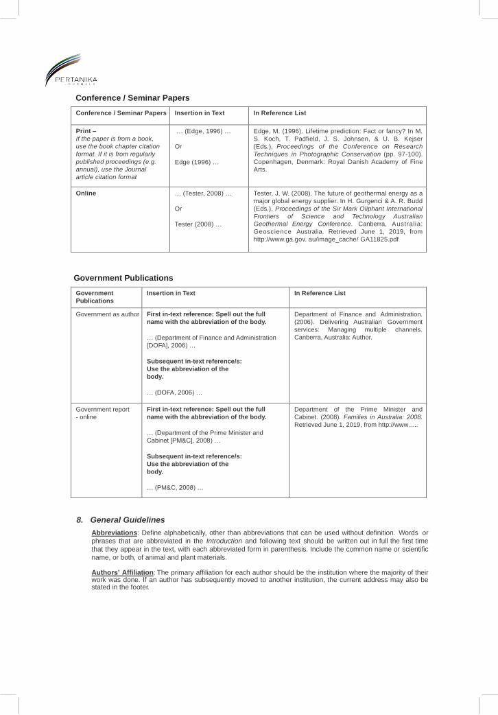
Conference / Seminar Papers
Conference / Seminar Papers Insertion in Text In Reference List
Print –
If the paper is from a book,
use the book chapter citation
format. If it is from regularly
published proceedings (e.g.
annual), use the Journal
article citation format
… (Edge, 1996) …
Or
Edge (1996) …
Edge, M. (1996). Lifetime prediction: Fact or fancy? In M.
S. Koch, T. Padfield, J. S. Johnsen, & U. B. Kejser
(Eds.), Proceedings of the Conference on Research
Techniques in Photographic Conservation (pp. 97-100).
Copenhagen, Denmark: Royal Danish Academy of Fine
Arts.
Online … (Tester, 2008) …
Or
Tester (2008) …
Tester, J. W. (2008). The future of geothermal energy as a
major global energy supplier. In H. Gurgenci & A. R. Budd
(Eds.), Proceedings of the Sir Mark Oliphant International
Frontiers of Science and Technology Australian
Geothermal Energy Conference. Canberra, Australia:
Geoscience Australia. Retrieved June 1, 2019, from
http://www.ga.gov. au/image_cache/ GA11825.pdf
Government Publications
Government
Publications
Insertion in Text In Reference List
Government as author First in-text reference: Spell out the full
name with the abbreviation of the body.
… (Department of Finance and Administration
[DOFA], 2006) …
Subsequent in-text reference/s:
Use the abbreviation of the
body.
… (DOFA, 2006) …
Department of Finance and Administration.
(2006). Delivering Australian Government
services: Managing multiple channels.
Canberra, Australia: Author.
Government report
- online
First in-text reference: Spell out the full
name with the abbreviation of the body.
… (Department of the Prime Minister and
Cabinet [PM&C], 2008) …
Subsequent in-text reference/s:
Use the abbreviation of the
body.
… (PM&C, 2008) …
Department of the Prime Minister and
Cabinet. (2008). Families in Australia: 2008.
Retrieved June 1, 2019, from http://www .....
8. General Guidelines
Abbreviations: Define alphabetically, other than abbreviations that can be used without definition. Words or
phrases that are abbreviated in the Introduction and following text should be written out in full the first time
that they appear in the text, with each abbreviated form in parenthesis. Include the common name or scientific
name, or both, of animal and plant materials.
Authors’ Affiliation: The primary affiliation for each author should be the institution where the majority of their work was done. If an author has subsequently moved to another institution, the current address may also be stated in the footer.

Co-Authors: The commonly accepted guideline for authorship is that one must have substantially contributed to
the development of the paper and share accountability for the results. Researchers should decide who will be
an author and what order they will be listed depending upon their order of importance to the study. Other
contributions should be cited in the manuscript’s Acknowledgements.
Similarity Index: All articles received must undergo the initial screening for originality before being sent for
peer review. Pertanika does not accept any article with a similarity index exceeding 20%.
Copyright Permissions: Authors should seek necessary permissions for quotations, artwork, boxes or tables taken from other publications or other freely available sources on the Internet before submission to Pertanika. The Acknowledgement must be given to the original source in the illustration legend, in a table footnote, or at the end of the quotation.
Footnotes: Current addresses of authors if different from heading may be inserted here.
Page Numbering: Every page of the manuscript, including the title page, references, and tables should be
numbered.
Spelling: The journal uses American or British spelling and authors may follow the latest edition of the Oxford
Advanced Learner’s Dictionary for British spellings. Each manuscript should follow one type of spelling only.
SUBMISSION OF MANUSCRIPTS
All submissions must be made electronically using the ScholarOne™ online submission system, a web-based
portal by Clarivate Analytics. For more information, go to our web page and click “Online Submission
(ScholarOneTM)”.
Submission Checklist
1. MANUSCRIPT:
Ensure your manuscript has followed the Pertanika style particularly the first-4-pages as explained earlier. The
article should be written in a good academic style and provide an accurate and succinct description of the
contents ensuring that grammar and spelling errors have been corrected before submission. It should also not
exceed the suggested length.
2. DECLARATION FORM:
• Author has to sign a declaration form. In signing the form, authors declare that the work submitted for publication
is original, previously unpublished, and not under consideration for any publication elsewhere.
• Author has to agree to pay the publishing fee once the paper is accepted for publication in Pertanika. 3. COVER LETTER:
In Step 6 of the ScholarOne system, author is asked to upload a cover letter in Pertanika format. Please ignore this instruction and replace the cover letter with the Declaration Form.
Note:
COPYRIGHT FORM: Author will be asked to sign a copyright form when the paper is accepted. In signing the form, it
is assumed that authors have obtained permission to use any copyrighted or previously published material. All
authors must read and agree to the conditions outlined in the form and must sign the form or agree that the
corresponding author can sign on their behalf. Articles cannot be published until a signed form (original pen-to-paper
signature) has been received.
Visit our Journal’s website for more details at http://www.pertanika.upm.edu.my/
ACCESS TO PUBLISHED MATERIALS
Under the journal’s open access initiative, authors can choose to download free material (via PDF link) from any of the
journal issues from Pertanika’s website. Under “Browse Journals” you will see a link, “Regular Issue”, “Special Issue”
or “Archives”. Here you will get access to all current and back-issues from 1978 onwards. No hard copy of journals or
offprints are printed.
Visit our Journal’s website at
http://www.pertanika.upm.edu.my/regular_issues.php for “Regular Issue”
http://www.pertanika.upm.edu.my/cspecial_issues.php for “Special Issue”
http://www.pertanika.upm.edu.my/journal_archives.php for “Archives”

PUBLICATION CHARGE
Upon acceptance of a manuscript, a processing fee of RM 750 / USD 250 will be imposed on authors; RM 750 for
any corresponding author affiliated to an institution in Malaysia; USD 250 for any corresponding author affiliated
to an institution outside Malaysia. Payment must be made online at https://paygate.upm.edu.my/action.do?do=
Any queries may be directed to the Chief Executive Editor’s office via email to [email protected]

Animal ProductionEffects of Age at Slaughter and Sex on Carcass Characteristics and Meat Quality of Betong Chicken
Piyanan Nualhnuplong and Chaiyawan Wattanachant
343
Food and Nutrition DevelopmentPhysicochemical Properties of Sodium Alginate Edible Film Incorporated with Mulberry (Morus australis) Leaf Extract
Yan Ling Kuan, S. Navin Sivanasvaran, Liew Phing Pui, Yus Aniza Yusof and Theeraphol Senphan
359
HorticultureScanning Electron Microscopy Analysis of Early Floral Development in Renanthera bella J. J. Wood, an Endemic Orchid from Sabah
Nurul Najwa Mohamad and Nor Azizun Rusdi
377
Plant PhysiologyPreliminary Study on the Effect of Nitrogen and Potassium Fertilization, and Evapotranspiration Replacement Interaction on Primary and Secondary Metabolites of Gynura procumbens Leaves
Mohamad Fhaizal Mohamad Bukhori, Muhd Kamal Izzat, Mohd Zuwairi Saiman, Nazia Abdul Majid, Hawa ZE Jaafar, Ali Ghasemzadeh and Uma Rani Sinniah
391
Soil and Water SciencesRelationship between Groundwater Level and Water Content in Oil Palm Plantation on Drained Peatland in Siak, Riau Province, Indonesia
Yudha Asmara Adhi1, Syaiful Anwar, Suria Darma Tarigan and Bandung Sahari
415

Vol. 43 (3) Aug. 2020
VOL. 43 (3) AUG. 2020
Pertanika JTAS
Pertanika Journal of Tropical Agricultural Science Vol. 43 (3) Aug. 2020
Contents
Pertanika Editorial Office, Journal DivisionPutra Science Park1st Floor, IDEA Tower IIUPM-MTDC Technology CentreUniversiti Putra Malaysia43400 UPM SerdangSelangor Darul EhsanMalaysiahttp://pertanika.upm.edu.myE-mail: [email protected] : +603 9769 1622
http://penerbit.upm.edu.myE-mail: [email protected] : +603 9769 8855 / 8854
ForewordAbu Bakar Salleh
i
Crop and Pasture ProductionStudies on Genotype by Environment Interaction (GEI) and Stability Performances of 43 Accessions of Tropical Soybean (Glycine max (L.) Merrill)
Ibidunni Sakirat Adetiloye and Omolayo Johnson Ariyo
239
Analysis of Qualitative and Quantitative Trait Variability among Black Pepper (Piper nigrum L.) Cultivars in Malaysia
Yi Shang Chen and Cheksum Supiah Tawan
257
Chitosan as a Biopesticide against Rice (Oryza sativa) Fungal Pathogens, Pyricularia oryzae and Rhizoctonia solani
Mui-Yun Wong, Arthy Surendran, Nur Madhihah Saad and Farhana Burhanudin
275
BiotechnologyScreening and Evaluation of Biopesticide Compounds from Mirabilis jalapa L. (Caryophyllales: Nyctaginaceae) and Its Combination with Bacillus thuringiensis against Spodoptera litura F. (Lepidoptera: Noctudiae)
Dina Maulina, Mohamad Amin, Sutiman Bambang Sumitro, Sri Rahayu Lestari and Tri Suwandi
289
Bioactivity Evaluation of Melaleuca cajuputi (Myrtales: Myrtaceae) Crude Extracts against Aedes Mosquito
Azlinda Abu Bakar
303
Forestry SciencesTree Community Structure and Diversity of Shorea lumutensis (Balau Putih) Dominated Forest at Segari Melintang Forest Reserve, Perak
Nurul Hidayah Che Mat, Abdul Latiff, Ahmad Fitri Zohari, Nizam Mohd Said and Nur ’Aqilah Mustafa Bakray
315
Associations of Growth and Phenology Cycle with Environmental Variables on the Population Dynamics of Non-climbing Rattan Calamus castaneus Griff.
Nur Diana Mohd Rusdi, Asyraf Mansor, Shahrul Anuar Mohd Sah, Rahmad Zakaria, Nik Fadzly Nik Rosely and Wan Ruslan Ismail
327


![arXiv:2008.07486v1 [stat.AP] 17 Aug 2020](https://static.fdokumen.com/doc/165x107/631ce10276d2a4450503bd91/arxiv200807486v1-statap-17-aug-2020.jpg)


![arXiv:1807.00938v2 [cs.CL] 7 Aug 2019](https://static.fdokumen.com/doc/165x107/63185f313394f2252e02ad29/arxiv180700938v2-cscl-7-aug-2019.jpg)


![arXiv:1808.03048v2 [math.DG] 14 Aug 2019](https://static.fdokumen.com/doc/165x107/631e372f25add517740af0db/arxiv180803048v2-mathdg-14-aug-2019.jpg)

