fh 2015 15 ir.pdf - Universiti Putra Malaysia Institutional ...
Upload
khangminh22Category
view
0download
0
VOL. 21 (2) JUL. 2013Pertanika JST
UPM
Press, Malaysia
Vol. 21 (2) Jul. 2013
Pertanika Journal of Science & TechnologyVol. 21 (2) Jul. 2013
Contents
Pertanika Editorial OceOce of the Deputy Vice Chancellor (R&I), 1st Floor, IDEA Tower II, UPM-MTDC Technology CentreUniversiti Putra Malaysia43400 UPM SerdangSelangor Darul EhsanMalaysia
http://www.pertanika.upm.edu.my/E-mail: [email protected]: +603 8947 1622/1620
Foreword
iNayan Deep S. Kanwal
Invited PaperSystems Informatics and Analysis of Biomass Feedstock Production 273
Shastri Y. N., Hansen A. C., Rodríguez L. F. and Ting K. C.
Review ArticlesA Review of Cosmetic and Personal Care Products: Halal Perspective and Detection of Ingredient
281
Hashim, P. and Mat Hashim, D.
A Review on the Effects of Probiotics and Antibiotics towards Infections
293
Hazirah, A., Loong, Y. Y., Rushdan, A. A., Rukman, A. H. and Yazid, M. M.
Methodologies for Measuring Sustainability of Product/Process: A Review 303Pezhman Ghadimi, Noordin Mohd Yusof, Muhamad Zameri Mat Saman and Mahmood Asadi
Regular ArticlesDetection of Ethanol Vapours Using Titanium Dioxide (TiO2) Catalytic Pellet by 327
Ang Gaik Tin, Mohamad Zailani Abu Bakar and Cheah Mooi Chen
Green Compression Strength of Tin Mine Tailing Sand for Green Sand Casting Mould
335
Azhar Abdullah, Shamsuddin Sulaiman, B. T. Hang Tuah Baharudin,
Web-Based Decision Support System for Paddy Planting Management 343C. Y. N. Norasma, A. R. M. Shariff, E. Jahanshiri, M. S. M. Amin, S. Khairunniza-Bejo and A. R. Mahmud
Development of an Automation and Control Design System for Lowland Tropical Greenhouses
365
W. I. Wan Ishak, R. M. Hudzari and M. Y. Tan
Recovery of Heavy Metals from Spent Etching Waste Solution of Printed Circuit Board (PCB) Manufacturing
375
A. H. M. Ali, S. Sobri, Salmiaton. A. and Faizah M. Y.

Journal of Sciences & Technology
About the JournalPertanika is an international peer-reviewed journal devoted to the publication of original papers, and it serves as a forum for practical approaches to improving quality in issues pertaining to tropical agriculture and its related fields. Pertanika began publication in 1978 as the Journal of Tropical Agricultural Science. In 1992, a decision was made to streamline Pertanika into three journals to meet the need for specialised journals in areas of study aligned with the interdisciplinary strengths of the university. The revamped Journal of Science & Technology (JST) aims to develop as a pioneer journal focusing on research in science and engineering, and its related fields. Other Pertanika series include Journal of Tropical Agricultural Science (JTAS); and Journal of Social Sciences and Humanities (JSSH).
JST is published in English and it is open to authors around the world regardless of the nationality. It is currently published two times a year, i.e. in January and July.
Goal of PertanikaOur goal is to bring the highest quality research to the widest possible audience.
Quality We aim for excellence, sustained by a responsible and professional approach to journal publishing. Submissions are guaranteed to receive a decision within 12 weeks. The elapsed time from submission to publication for the articles averages 5-6 months.
Indexing of PertanikaPertanika is now over 33 years old; this accumulated knowledge has resulted in Pertanika JST being indexed in SCOPUS (Elsevier), EBSCO, Thomson (ISI) Web of Knowledge [CAB Abstracts], DOAJ, Google Scholar, ERA, ISC, Citefactor, Rubriq and MyAIS.
Future visionWe are continuously improving access to our journal archives, content, and research services. We have the drive to realise exciting new horizons that will benefit not only the academic community, but society itself.
We also have views on the future of our journals. The emergence of the online medium as the predominant vehicle for the ‘consumption’ and distribution of much academic research will be the ultimate instrument in the dissemination of research news to our scientists and readers.
Aims and scopePertanika Journal of Science and Technology aims to provide a forum for high quality research related to science and engineering research. Areas relevant to the scope of the journal include: bioinformatics, bioscience, biotechnology and biomolecular sciences, chemistry, computer science, ecology, engineering, engineering design, environmental control and management, mathematics and statistics, medicine and health sciences, nanotechnology, physics, safety and emergency management, and related fields of study.
Editorial StatementPertanika is the official journal of Universiti Putra Malaysia. The abbreviation for Pertanika Journal of Science & Technology is Pertanika J. Sci. Technol.
Jour
nal o
f Sci
ence
& T
echn
olog
y
Jo
urna
l of S
cien
ce &
Tec
hnol
ogy
Jour
nal o
f Sci
ence
& T
echn
olog
y

Editorial Board2013-2015
Editor-in-ChiefMohd. Ali HASSAN, Malaysia
Bioprocess engineering, Environmental biotechnology
Chief Executive EditorNayan D.S. KANWAL, Malaysia
Environmental issues- landscape plant modelling applications
Editorial Board Members
Abdul Halim Shaari (Professor Dr), Superconductivity and Magnetism, Universiti Putra Malaysia, Malaysia.
Adem KILICMAN (Professor Dr), Mathematical Sciences, Universiti Putra Malaysia, Malaysia.
Ahmad Makmom Abdullah (Associate Professor Dr), Ecophysiology and Air Pollution Modelling, Universiti Putra Malaysia, Malaysia.
Ali A. MOOSAVI-MOVAHEDI (Professor Dr), Biophysical Chemistry, University of Tehran, Tehran, Iran.
Amu THERWATH (Professor Dr), Oncology, Molecular Biology, Université Paris, France.
Angelina CHIN (Professor Dr), Mathematics, Group Theory and Generalisations, Ring Theory, University of Malaya, Malaysia.
Bassim H. HAMEED (Professor Dr), Chemical Engineering: Reaction Engineering, Environmental Catalysis & Adsorption, Universiti Sains Malaysia, Malaysia.
Biswa Mohan BISWAL (Professor Dr), Medical, Clinical Oncology, Radiotherapy, Universiti Sains Malaysia, Malaysia.
Christopher G. JESUDASON (Professor Dr), Mathematical Chemistry, Molecular Dynamics Simulations, Thermodynamics and General Physical Theory, University of Malaya, Malaysia.
Ivan D. RUKHLENKO (Dr), Nonliner Optics, Silicon Photonics, Plasmonics and Nanotechnology, Monash University, Australia.
Kaniraj R. SHENBAGA (Professor Dr), Geotechnical Engineering, Universiti Malaysia Sarawak, Malaysia.
Kanury RAO (Professor Dr), Senior Scientist & Head, Immunology Group, International Center for Genetic Engineering and Biotechnology, Immunology, Infectious Disease Biology and Systems Biology, International Centre for Genetic Engineering & Biotechnology, New Delhi, India.
Karen Ann CROUSE (Professor Dr), Chemistry, Material Chemistry, Metal Complexes – Synthesis, Reactivity, Bioactivity, Universiti Putra Malaysia, Malaysia.
Ki-Hyung KIM (Professor Dr), Computer and Wireless Sensor Networks, AJOU University, Korea.
Kunnawee KANITPONG (Associate Professor Dr), Transportation Engineering- Road traffic safety, Highway Materials and Construction, Asian Institute of Technology, Thailand.
Megat Mohamad Hamdan MEGAT AHMAD (Professor Dr), Mechanical and Manufacturing Engineering, Universiti Pertahanan Nasional Malaysia, Malaysia.
Mirnalini KANDIAH (Professor Dr), Public Health Nutrition, Nutritional Epidemiology, Universiti Malaysia Perlis (UniMAP), Malaysia.
Mohamed Othman (Professor Dr), Communication Technology and Network, Scientific Computing, Universiti Putra Malaysia, Malaysia.
Mohd Adzir Mahdi (Professor Dr), Physics, Optical Communications, Universiti Putra Malaysia, Malaysia.
Mohd Sapuan Salit (Professor Dr), Concurrent Engineering and Composite Materials, Universiti Putra Malaysia, Malaysia.
Narongrit SOMBATSOMPOP (Professor Dr), Engineering and Technology: Materials and Polymer Research, King Mongkut’s University of Technology Thonburi (KMUTT), Thailand.
Prakash C. SINHA (Professor Dr), Physical Oceanography, Mathematical Modelling, Fluid Mechanics, Numerical Techniques, Universiti Malaysia Terengganu, Malaysia.
Rajinder SINGH (Dr), Biotechnology, Biomolecular Science, Molecular Markers/ Genetic Mapping, Malaysian Palm Oil Board, Kajang, Malaysia.
Renuganth VARATHARAJOO (Professor Dr-Ing Ir), Engineering, Space System, Universiti Putra Malaysia, Malaysia.
Riyanto T. BAMBANG (Professor Dr), Electrical Engineering, Control, Intelligent Systems & Robotics, Bandung Institute of Technology, Indonesia.
Sabira KHATUN (Professor Dr), Engineering, Computer Systems and Software Engineering, Applied Mathematics, Universiti Malaysia Pahang, Malaysia.
Shiv Dutt GUPTA (Dr), Director, IIHMR, Health Management, public health, Epidemiology, Chronic and Non-communicable Diseases, Indian Institute of Health Management Research, India.
Shoba RANGANATHAN (Professor Dr), UNESCO Chair of Biodiversity Informatics Bioinformatics and Computational Biology, Biodiversity Informatics, Protein Structure, DNA sequence, Macquarie University, Australia.
Suan-Choo CHEAH (Dr), Biotechnology, Plant Molecular Biology, Asiatic Centre for Genome Technology (ACGT), Kuala Lumpur, Malaysia.
Waqar ASRAR (Professor Dr), Engineering, Computational Fluid Dynamics, Experimental Aerodynamics, International Islamic University, Malaysia.
Wing-Keong NG (Professor Dr), Aquaculture, Aquatic Animal Nutrition, Aqua feed Technology, Universiti Sains Malaysia, Malaysia.
Yudi SAMYUDIA (Professor Dr Ir), Chemical Engineering, Advanced Process Engineering, Curtin University of Technology, Malaysia.

International Advisory Board
Adarsh SANDHU (Professor Dr), Editorial Consultant for Nature Nanotechnology and contributing writer for Nature Photonics, Physics, Magnetoresistive Semiconducting Magnetic Field Sensors, Nano-Bio-Magnetism, Magnetic Particle Colloids, Point of Care Diagnostics, Medical Physics, Scanning Hall Probe Microscopy, Synthesis and Application of Graphene, Electronics-Inspired Interdisciplinary Research Institute (EIIRIS), Toyohashi University of Technology, Japan.
Graham MEGSON (Professor Dr), Computer Science, The University of Westminster, U.K.
Kuan-Chong TING (Professor Dr), Agricultural and Biological Engineering, University of Illinois at Urbana-Champaign, USA.
Malin PREMARATNE (Professor Dr), Advanced Computing and Simulation, Monash University, Australia.
Mohammed Ismail ELNAGGAR (Professor Dr), Electrical Engineering, Ohio State University, USA.
Peter G. ALDERSON (Associate Professor Dr), Bioscience, The University of Nottingham, Malaysia Campus.
Peter J. HEGGS (Emeritus Professor Dr), Chemical Engineering, University of Leeds, U.K.
Ravi PRAKASH (Professor Dr), Vice Chancellor, JUIT, Mechanical Engineering, Machine Design, Biomedical and Materials Science, Jaypee University of Information Technology, India.
Said S.E.H. ELNASHAIE (Professor Dr), Environmental and Sustainable Engineering, Penn. State University at Harrisburg, USA.
Suhash Chandra DUTTA ROY (Emeritus Professor Dr), Electrical Engineering, Indian Institute of Technology (IIT) Delhi, India.
Vijay ARORA (Professor), Quantum and Nano-Engineering Processes, Wilkes University, USA.
Yi LI (Professor Dr), Chemistry, Photochemical Studies, Organic Compounds, Chemical Engineering, Chinese Academy of Sciences, Beijing, China.
Pertanika Editorial Office
Office of the Deputy Vice Chancellor (R&I), 1st Floor, IDEA Tower II, UPM-MTDC Technology CentreUniversiti Putra Malaysia, 43400 Serdang, Selangor, Malaysia
Tel: +603 8947 1622 | 8947 1619 | 8947 1616E-mail: [email protected]; [email protected]
URL: http://www.pertanika.upm.edu.my/editorial_board.htm
Publisher
The UPM Press Universiti Putra Malaysia
43400 UPM, Serdang, Selangor, Malaysia Tel: +603 8946 8855, 8946 8854 • Fax: +603 8941 6172
[email protected] URL: http://penerbit.upm.edu.my
The publisher of Pertanika will not be responsible for the statements made by the authors in any articles published in the journal. Under no circumstances will the publisher of this publication be liable for any loss or damage caused by your reliance on the advice, opinion or information obtained either explicitly or implied through the contents of this publication.
All rights of reproduction are reserved in respect of all papers, articles, illustrations, etc., published in Pertanika. Pertanika provides free access to the full text of research articles for anyone, web-wide. It does not charge either its authors or author-institution for refereeing/ publishing outgoing articles or user-institution for accessing incoming articles.
No material published in Pertanika may be reproduced or stored on microfilm or in electronic, optical or magnetic form without the written authorization of the Publisher.
Copyright © 2013 Universiti Putra Malaysia Press. All Rights Reserved.

Pertanika Journal of Science & Technology Vol. 21 (2) Jul. 2013
Contents
Foreword iNayan Deep S. Kanwal
Invited PaperSystems Informatics and Analysis of Biomass Feedstock Production 273
Shastri Y. N., Hansen A. C., Rodríguez L. F. and Ting K. C.
Review ArticlesA Review of Cosmetic and Personal Care Products: Halal Perspective and Detection of Ingredient
281
Hashim, P. and Mat Hashim, D.
A Review on the Effects of Probiotics and Antibiotics towards Clostridium difficile Infections
293
Hazirah, A., Loong, Y. Y., Rushdan, A. A., Rukman, A. H. and Yazid, M. M.
Methodologies for Measuring Sustainability of Product/Process: A Review 303Pezhman Ghadimi, Noordin Mohd Yusof, Muhamad Zameri Mat Saman and Mahmood Asadi
Regular ArticlesDetection of Ethanol Vapours Using Titanium Dioxide (TiO2) Catalytic Pellet by Conventional and Modified Sol Gel Dip-Coating Method
327
Ang Gaik Tin, Mohamad Zailani Abu Bakar and Cheah Mooi Chen
Green Compression Strength of Tin Mine Tailing Sand for Green Sand Casting Mould
335
Azhar Abdullah, Shamsuddin Sulaiman, B. T. Hang Tuah Baharudin, Mohd Khairol Anuar Mohd Ariffin and Thoguluva Raghvan Vijayaram
Web-Based Decision Support System for Paddy Planting Management 343C. Y. N. Norasma, A. R. M. Shariff, E. Jahanshiri, M. S. M. Amin, S. Khairunniza-Bejo and A. R. Mahmud
Development of an Automation and Control Design System for Lowland Tropical Greenhouses
365
W. I. Wan Ishak, R. M. Hudzari and M. Y. Tan
Recovery of Heavy Metals from Spent Etching Waste Solution of Printed Circuit Board (PCB) Manufacturing
375
A. H. M. Ali, S. Sobri, Salmiaton. A. and Faizah M. Y.
Production of Orthophoto and Volume Determination Using Low-Cost Digital Cameras
387
Khairul Nizam Tahar and Anuar Ahmad
Climate Change Resilience Assessment Using Livelihood Assets of Coastal Fishing Community in Nijhum Dwip, Bangladesh
397
Hossain, M. S., Rahman, M. F., Thompson, S., Nabi, M. R. and Kibria, M. M.
Goal Event Detection in Soccer Videos via Collaborative Multimodal Analysis 423Alfian Abdul Halin and Mandava Rajeswari
On the Diophantine Equation x2 + 4.7b = y2r 443Yow, K. S., Sapar, S. H. and Atan, K. A.
Electrical Conductivity of Anionic Surfactant-Doped Polypyrrole Nanoparticles Prepared via Emulsion Polymerization
459
Ghalib, H., Abdullah, I. and Daik, R.
Landslide Susceptibility Mapping Using Averaged Weightage Score and GIS: A Case Study at Kuala Lumpur
473
Mahmud, A. R., Awad, A. and Billa, R.
GIS Modeling for Selection of a Transfer Station Site for Residential Solid Waste Separation and Recycling
487
Billa, L. and Pradhan, B.
Comparative Study on the Effect of Density on Water Absorption of Particle Boards Produced from Nipa Palm Fibres with HDPE Wastes
499
Ekpunobi, U. E., Eboatu, A. N. and Okoye, P.-A.
Rootkit Guard (RG) - An Architecture for Rootkit Resistant File-System Implementation Based on TPM
507
Teh Jia Yew, Khairulmizam Samsudin, Nur Izura Udzir and Shaiful Jahari Hashim
Selected Articles from CUTSE International Conference 2011Guest Editor: Ashutosh Kumar SinghGuest Editorial Board: Sujan Debnath and Muhammad Ekhlasur Rahman
Theoretical Modeling of Pseudo Hydrostatic Force in Solid-Liquid Pipe Flow with Two Layers
521
Hussain H. Al-Kayiem and Iylia Elena Abdul Jamil
Improvement of Coke Strength by Phenolic Resin Coating: Experimental and Theoretical Studies of Strengthening Mechanism
533
Y. Asakuma, Y. Komatsu, S. Nishi, A. Kotani and M. Nishimura
Application of Markov Chain in the PageRank Algorithm 541Ravi Kumar, P., Alex Goh, K. L. and Ashutosh, K. S.
Harnessing Energy from Electromagnetic Field: Practical Implementation Integrating Coil Antenna and IC Load
555
Syahrizal Salleh and Zulkifli Abd Majid

Palm Oil Transesterification Processing to Biodiesel Using a Combine of Ultrasonic and Chemical Catalyst
567
Supranto, S.
Electricity Generation from Citronella Bagasse (CB) Using Dual Chamber Microbial Fuel Cell
581
Nik Azmi Nik Mahmood, Mohd Nazlee Faisal Md Ghazali, Kamarul’Asri Ibrahim and Nur Muhammad ElQarni Md Norodin
Experimental Design Analysis of Ultra Fine Fly Ash, Lime Water, and Basalt Fibre in Mix Proportion of High Volume Fly Ash Concrete
589
Mochamad Solikin, Sujeeva Setunge and Indubhushan Patnaikuni
Experimental Study on Shear Behaviour of High Strength Reinforced Recycled Concrete Beam
601
Oh Chai Lian, Lee Siong Wee, Mohd Asha’ari Masrom and Goh Ching Hua
Responsive Façades: Parametric Control of Moveable Tilings 611Sambit Datta and Michael Hobbs
A Numerical Study of Ground Improvement Technique Using Group of Soil-Column on Peat
625
Muntohar, A. S., Rahman, M. E., Hashim, R. and Islam, M. S.

Foreword
Welcome to the Second Issue 2013 of the Journal of Science and Technology (JST)!
JST is an open access journal for the science and technology published by Universiti Putra Malaysia Press. It is independently owned and managed by the university and run on a non-profit basis for the benefit of the world-wide science community.
In this issue, there are 27 articles published; out of which 3 articles are review articles, 14 articles are regular articles and 10 articles are from Curtin University Technology, Science and Engineering International Conference “Innovative Green Technology for Sustainable Development” (CUTSE 2011). The authors of these articles vary in country of origin (Malaysia, Bangladesh, Nigeria, Japan, Indonesia and Australia).
The review articles describe in details on halal perspective and detection of its ingredients in cosmetic and personal care products (Hashim, P. and Mat Hashim, D.), a review on the effects of probiotics and antibiotics towards Clostridium difficile Infections (Hazirah, A., Loong, Y. Y., Rushdan, A. A., Rukman, A. H. and Yazid, M. M.) and also a review on methodologies for measuring sustainability of product/process (Pezhman Ghadimi, Noordin Mohd Yusof, Muhamad Zameri Mat Saman and Mahmood Asadi).
The regular articles cover a wide range of study, from a detection of ethanol vapours using Titanium Dioxide (TiO2) catalytic pellet by conventional and modified sol gel dip-coating method (Ang Gaik Tin, Mohamad Zailani Abu Bakar and Cheah Mooi Chen), determination on green compression strength of tin mine tailing sand for green sand casting mould (Azhar Abdullah, Shamsuddin Sulaiman, B. T. Hang Tuah Baharudin, Mohd Khairol Anuar Mohd Ariffin and Thoguluva Raghvan Vijayaram), a web-based decision support system for paddy planting management (C. Y. N. Norasma, A. R. M. Shariff, E. Jahanshiri, M. S. M. Amin, S. Khairunniza-Bejo and A. R. Mahmud), a development of an automation and control design system for lowland tropical greenhouses (W. I. Wan Ishak, R. M. Hudzari and M. Y. Tan), a recovery of heavy metals from spent etching waste solution of printed circuit board (PCB) manufacturing (A. H. M. Ali, S. Sobri, Salmiaton. A. and Faizah M. Y.), a production of orthophoto and volume determination using low-cost digital cameras (Khairul Nizam Tahar and Anuar Ahmad), a climate change resilience assessment using livelihood assets of coastal fishing community in Nijhum Dwip, Bangladesh (Hossain, M. S., Rahman, M. F., Thompson, S., Nabi, M. R. and Kibria, M. M.), a goal event detection in soccer videos via collaborative multimodal analysis (Alfian Abdul Halin and Mandava Rajeswari), on the diophantine equation x2 + 4.7b = y2r (Yow, K. S., Sapar, S. H. and Atan, K. A.), an electrical conductivity of anionic surfactant-doped polypyrrole nanoparticles prepared via emulsion polymerization (Ghalib, H., Abdullah, I. and Daik, R.), a landslide susceptibility mapping using averaged weightage score and GIS: a case study at Kuala Lumpur (Mahmud, A. R., Awad, A. and Billa, R.), a GIS modeling for selection of a transfer

station site for residential solid waste separation and recycling (Billa, L. and Pradhan, B.), a comparative study on the effect of density on water absorption of particle boards produced from Nipa Palm fibres with HDPE wastes (Ekpunobi, U. E., Eboatu, A. N. and Okoye, P.-A.) and Rootkit Guard (RG) - an architecture for rootkit resistant file-system implementation based on TPM (Teh Jia Yew, Khairulmizam Samsudin, Nur Izura Udzir and Shaiful Jahari Hashim).
I conclude this issue with 10 articles arising from the CUTSE 2011 international conference; theoretical modeling of pseudo hydrostatic force in solid-liquid pipe flow with two layers (Hussain H. Al-Kayiem and Iylia Elena Abdul Jamil), improvement of coke strength by phenolic resin coating: experimental and theoretical studies of strengthening mechanism (Y. Asakuma, Y. Komatsu, S. Nishi, A. Kotani and M. Nishimura), application of markov chain in the PageRank algorithm (Ravi Kumar, P., Alex Goh, K. L. and Ashutosh, K. S.), harnessing energy from electromagnetic field: practical implementation integrating coil antenna and IC load (Syahrizal Salleh and Zulkifli Abd Majid), palm oil transesterification processing to biodiesel using a combine of ultrasonic and chemical catalyst (Supranto, S.), electricity generation from citronella bagasse (CB) using dual chamber microbial fuel cell (Nik Azmi Nik Mahmood, Mohd Nazlee Faisal Md Ghazali, Kamarul’Asri Ibrahim and Nur Muhammad ElQarni Md Norodin), experimental design analysis of ultra fine fly ash, lime water, and basalt fibre in mix proportion of high volume fly ash concrete (Mochamad Solikin, Sujeeva Setunge and Indubhushan Patnaikuni), experimental study on shear behaviour of high strength reinforced recycled concrete beam (Oh Chai Lian, Lee Siong Wee, Mohd Asha’ari Masrom and Goh Ching Hua), responsive façades: parametric control of moveable tilings (Sambit Datta and Michael Hobbs) and a numerical study of ground improvement technique using group of soil-column on peat (Muntohar, A. S., Rahman, M. E., Hashim, R. and Islam, M. S.).
I anticipate that you will find the evidence presented in this issue to be intriguing, thought provoking, and hopefully useful in setting up new milestones. Please recommend the journal to your colleagues and students to make this endeavour meaningful.
I would also like to express my gratitude to all the contributors; namely the authors, reviewers and editors for their professional contributions who have made this issue feasible. Last but not the least the editorial assistance of the journal division staff is fully appreciated.
JST is currently accepting manuscripts for upcoming issues based on original qualitative or quantitative research that opens new areas of inquiry and investigation.
Chief Executive EditorNayan Deep S. KANWAL, FRSA, ABIM, AMIS, Ph.D.

Pertanika J. Sci. & Technol. 21 (2): 273 - 280 (2013)
SCIENCE & TECHNOLOGYJournal homepage: http://www.pertanika.upm.edu.my/
ISSN: 0128-7680 © 2013 Universiti Putra Malaysia Press.
INTRODUCTION
Biomass based renewable energy will play a critical role in meeting the future global energy demands. A sustainable and competitive agricultural biomass feedstock production (BFP) system is critical for the success of a regional bioenergy system (Somerville et al.,
Invited Paper
Systems Informatics and Analysis of Biomass Feedstock Production
Shastri Y. N.1, Hansen A. C.2, Rodríguez L. F.2 and Ting K. C.2*1Energy Biosciences Institute, University of Illinois at Urbana-Champaign, USA2Department of Agricultural and Biological Engineering, University of Illinois at Urbana-Champaign, USA
ABSTRACT
Sustainable biomass feedstock production is critical for the success of a regional bioenergy system. Low energy and mass densities, seasonal availability, distributed supply, and lack of an established value chain for the feedstock create unique challenges that require an integrated systems approach. We have, therefore, developed a Concurrent Science, Engineering and Technology (ConSEnT) platform integrating informatics, modelling and analysis, as well as decision support for biomass feedstock production. An optimization model (BioFeed) and an agent-based model, which are supported by an informatics database and made accessible through a web-based decision support system, have been developed. This article summarizes the recent advances in this subject area by our research team.
Keywords: Biomass feedstock, bioenergy, systems analysis, modelling, informatics, decision support
Article history:Received: 16 February 2012Accepted: 7 May 2012
E-mail address: [email protected] (Ting K. C.)*Corresponding Author
2010). It provides the necessary material input for continuous operation of the processing facilities, and must do so by ensuring cost-efficiency, reliability and feedstock quality. Multiple tasks that comprise the BFP system include pre-harvest crop management, harvesting and handling, transport and pre-processing, and storage (Cushman et al., 2003). Our research programme at the Energy Biosciences Institute, titled ‘Engineering solutions for biomass feedstock production’, accordingly incorporates these four tasks, with the objective of developing new technological
Shastri Y. N., Hansen A. C., Rodríguez L. F. and Ting K. C.
274 Pertanika J. Sci. & Technol. 21 (2): 273 - 280 (2013)
solutions to perform these operations efficiently. However, these tasks are highly inter-dependent, and it must be ensured that they work together in an effective, seamless manner. Moreover, low energy and mass densities, seasonal availability, distributed supply, and lack of an established value chain for the feedstock create unique challenges that pervade all stages of feedstock production, and require a holistic approach (Ting, 2009).
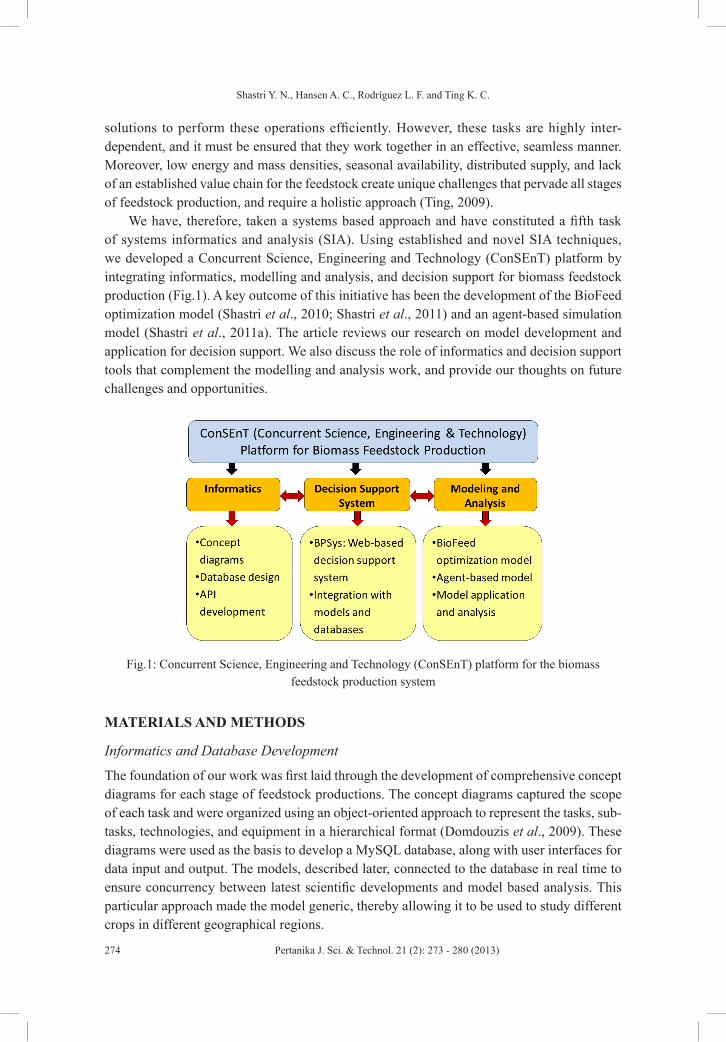
We have, therefore, taken a systems based approach and have constituted a fifth task of systems informatics and analysis (SIA). Using established and novel SIA techniques, we developed a Concurrent Science, Engineering and Technology (ConSEnT) platform by integrating informatics, modelling and analysis, and decision support for biomass feedstock production (Fig.1). A key outcome of this initiative has been the development of the BioFeed optimization model (Shastri et al., 2010; Shastri et al., 2011) and an agent-based simulation model (Shastri et al., 2011a). The article reviews our research on model development and application for decision support. We also discuss the role of informatics and decision support tools that complement the modelling and analysis work, and provide our thoughts on future challenges and opportunities.
Fig.1: Concurrent Science, Engineering and Technology (ConSEnT) platform for the biomass feedstock production system
MATERIALS AND METHODS
Informatics and Database Development
The foundation of our work was first laid through the development of comprehensive concept diagrams for each stage of feedstock productions. The concept diagrams captured the scope of each task and were organized using an object-oriented approach to represent the tasks, sub-tasks, technologies, and equipment in a hierarchical format (Domdouzis et al., 2009). These diagrams were used as the basis to develop a MySQL database, along with user interfaces for data input and output. The models, described later, connected to the database in real time to ensure concurrency between latest scientific developments and model based analysis. This particular approach made the model generic, thereby allowing it to be used to study different crops in different geographical regions.
Systems Informatics and Analysis of Biomass Feedstock Production
275Pertanika J. Sci. & Technol. 21 (2): 273 - 280 (2013)
BioFeed Optimization Model
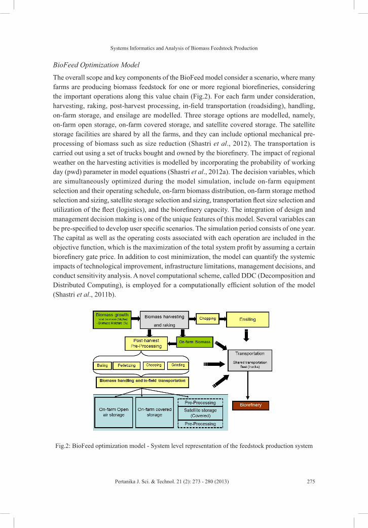
The overall scope and key components of the BioFeed model consider a scenario, where many farms are producing biomass feedstock for one or more regional biorefineries, considering the important operations along this value chain (Fig.2). For each farm under consideration, harvesting, raking, post-harvest processing, in-field transportation (roadsiding), handling, on-farm storage, and ensilage are modelled. Three storage options are modelled, namely, on-farm open storage, on-farm covered storage, and satellite covered storage. The satellite storage facilities are shared by all the farms, and they can include optional mechanical pre-processing of biomass such as size reduction (Shastri et al., 2012). The transportation is carried out using a set of trucks bought and owned by the biorefinery. The impact of regional weather on the harvesting activities is modelled by incorporating the probability of working day (pwd) parameter in model equations (Shastri et al., 2012a). The decision variables, which are simultaneously optimized during the model simulation, include on-farm equipment selection and their operating schedule, on-farm biomass distribution, on-farm storage method selection and sizing, satellite storage selection and sizing, transportation fleet size selection and utilization of the fleet (logistics), and the biorefinery capacity. The integration of design and management decision making is one of the unique features of this model. Several variables can be pre-specified to develop user specific scenarios. The simulation period consists of one year. The capital as well as the operating costs associated with each operation are included in the objective function, which is the maximization of the total system profit by assuming a certain biorefinery gate price. In addition to cost minimization, the model can quantify the systemic impacts of technological improvement, infrastructure limitations, management decisions, and conduct sensitivity analysis. A novel computational scheme, called DDC (Decomposition and Distributed Computing), is employed for a computationally efficient solution of the model (Shastri et al., 2011b).
Fig.2: BioFeed optimization model - System level representation of the feedstock production system

Shastri Y. N., Hansen A. C., Rodríguez L. F. and Ting K. C.
276 Pertanika J. Sci. & Technol. 21 (2): 273 - 280 (2013)
Agent-based Simulation Model
The success of the lignocellulosic feedstock based bioenergy sector will require transitioning to an agricultural system that co-produces food, feed, and fuel crops. In addition to scientific and technological development, this transition will be driven by the collective participation, behaviour and interaction of different stakeholders within the production system such as farmers, biorefinery, transportation and storage companies, custom harvesters, and farm consultants. Conventional engineering and macro-economic models cannot be used to study such complex systems. We have, therefore, developed an agent-based simulation model using the theory of complex adaptive systems (Shastri et al., 2011a). The first version of the model focuses primarily on the farmer and biorefinery agents. Each agent class is characterized by a set of attributes such as farm size and location for the farmer agent. These attributes take different values for different instantiations to capture variability. The decision making of each agent is modelled using rules that incorporate social, personal, and regulatory factors of an agent in addition to economic cost-benefit analysis. Attributes and rules are parameterized using data from literature. During simulation, long-term monthly delivery contracts, valid over multiple years, are competitively negotiated between the farmer and biorefinery agents. The agents modify selected attribute values based on profits or losses during the previous year to model learning and adaptation.
Web-based Decision Support System
The true value of systems analysis can only be realized if it can lead to better decisions. Unfortunately, this does not always happen because decision makers either lack access to the systems based tools or do not have the necessary expertise to develop and use them. We, therefore, developed a web-based decision support system named BPSys (Liao et al., 2011) that provides user-friendly access to the database and the BioFeed model. It is programmed in Java and enables users to build production scenario in BioFeed, select and modify data, as well as perform simulation and analysis, and visualize results.
RESULTS AND DISCUSSION
The BioFeed optimization model has been used extensively to study the production of switchgrass and Miscanthus, two perennial C4 grasses that have been proposed as candidate crops. A collection region of 17,400 km2 was considered. The collection region included 284 farms in 13 counties in southern Illinois. A biorefinery was assumed to be located at Nashville, IL. Crop harvestable yields and harvesting seasons were taken from the literature. The equipment performance data were adapted from previously published literature along with the ASABE machinery standards ASAE EP496.3 FEB2006 (R2011).
The optimal cost of switchgrass production was 45.1 $ Mg-1, which was almost evenly distributed among long distance transportation, harvesting, storage, and in-field transportation (Shastri et al., 2011). The on-farm baler selection varied based on farm size and storage requirements. It was found that 25% reduction in truck waiting time for loading/unloading, possibly through improved queue management, reduced the total cost by 22%.

Systems Informatics and Analysis of Biomass Feedstock Production
277Pertanika J. Sci. & Technol. 21 (2): 273 - 280 (2013)
The optimal production cost for Miscanthus was 44.7 $ Mg-1 (Shastri et al., 2010). The optimal pre-processing technology recommended for each farm was either baling or grinding (hammer mill or tub grinder). In contrast to switchgrass, pre-processing accounted for 37% of the total cost, reflecting the lack of efficient equipment. The production cost increased substantially for farms smaller than 100 ha. A supply chain configuration incorporating distributed storage and pre-processing at satellite storage was also studied for Miscanthus using three different pre-processing alternatives, namely, hammer milling, tub grinding, and pelletization (Shastri et al., 2012). Mandatory pre-processing at storage increased the total cost by 16-53% as compared to the base case, but reduced the farmers’ share of the total cost by 13-39%. The exact values depended on the pre-processing technology installed at the storage facility. The simulation results, therefore, recommended distributing the pre-processing operation between farms and storage facilities.
When the impact of weather in Illinois was quantified (Shastri et al., 2012a), the results showed that using a production system designed assuming 100% probability of working day (pwd) would incur an increase of actual production cost by 37% for Miscanthus and 12% for switchgrass. If the systems were instead optimized for typical pwd values for Illinois, the cost increase was less than 3.3%, but required higher investment in farm machinery by 34% for Miscanthus and 12% for switchgrass, respectively. Extending the Miscanthus harvesting season is, therefore, an option that must be rigorously evaluated.
The agent-based simulation model was used to study the establishment of Miscanthus production in Illinois by considering a set of 100 farmers currently growing corn and soybeans (Shastri et al., 2011a). The results showed that it took up to 15 years to reach stable regional production of Miscanthus, which was still only 60% of the maximum possible. Such a profile would have a significant impact on the capacity expansion, investment, and feedstock procurement decisions by the biorefinery. Meanwhile, a 25% reduction in the land opportunity cost led to a 63% increase in the stable production, suggesting that a region less attractive for conventional crops would be more suitable to establish Miscanthus.
CONCLUSION
In the study, the ConSEnT (Concurrent Science, Engineering and Technology) platform was developed by integrating informatics, modelling and analysis, and a decision support system for biomass feedstock production. The BioFeed optimization model and an agent-based simulation model constitute two key elements of this platform, and have provided valuable design and management recommendations for Miscanthus and switchgrass production. Such a decision-making platform would be extremely valuable in the future for large-scale deployment of the bioenergy sector. Various stakeholders that can benefit from this platform include biorefineries operators and investors, researchers, technology development engineers, regulators, and university teachers for educating the industry’s next generation of human capital. Incorporating uncertainty in decision making and studying the full life cycle impacts of decisions are key future modelling challenges. The ConSEnT platform must also be further enhanced to achieve true concurrency between research and application.

Shastri Y. N., Hansen A. C., Rodríguez L. F. and Ting K. C.
278 Pertanika J. Sci. & Technol. 21 (2): 273 - 280 (2013)
REFERENCESCushman, J. H., Easterly, J. L., Erbach, D. C., Foust, T. D., Hess, J. R., & Hettenhaus, J. R. (2003).
Roadmap for agriculture biomass feedstock supply in the United States, U.S. Department of Energy Office of Energy Efficiency and Renewable Energy Biomass Program, Washington DC.
Domdouzis, K., Rodriguez, L., Shastri, Y., Hu, M., Hansen, A., & Ting, K. (2009). Systems informatics for biomass feedstock production engineering, ASABE Annual Meeting 2009, Paper Number: 096702 Reno (NV), American Society of Agricultural and Biological Engineers, St. Joseph, MI.
Liao, Y., Rodriguez, L. F., Shastri, Y., Hansen, A. C., & Ting, K. C. (2011). Concurrent science, engineering and technology (ConSEnT) for biomass feedstock production decision support. ASABE Annual Meeting 2011, Paper Number: 1111666 Louisville (KY), American Society of Agricultural and Biological Engineers, St. Joseph, MI, August 2011.
Shastri, Y. N., Hansen, A. C., Rodríguez, L. F., & Ting, K. C. (2010). Optimization of Miscanthus harvesting and handling as an energy crop: BioFeed model application. Biological Engineering Transactions, 3(1), 37-69.
Shastri, Y. N., Hansen, A. C., Rodríguez, L. F., & Ting, K.C. (2011). Development and application of BioFeed model for optimization of herbaceous biomass feedstock production. Biomass and Bioenergy, 35(7), 2961-2974.
Shastri, Y. N., Rodriguez, L. F., Hansen, A. C., & Ting, K. C. (2011a). Agent-based analysis of biomass feedstock production system dynamics. BioEnergy Research, 4(4), 258-275.
Shastri, Y. N., Hansen, A. C., Rodríguez, L. F., & Ting, K. C. (2011b). A novel decomposition and distributed computing approach for the solution of large scale optimization models. Computers and Electronics in Agriculture, 76(1), 69-79.
Shastri, Y. N., Rodriguez, L. F., Hansen, A. C., & Ting, K. C. (2012). Impact of distributed storage and pre-processing on Miscanthus production and provision systems. Biofuels, Bioproducts and Biorefining, 6, 21-31.
Shastri, Y. N., Hansen, A. C., Rodriguez, L. F., & Ting, K. C. (2012b). Impact of probability of working day on planning and operation of biomass feedstock production systems. Biofuels, Bioproducts & Biorefining, DOI:10.1002/bbb.1329.
Somerville, C., Young, H., Taylor, C., Davis, S., & Long, S. (2010). Feedstocks for lignocellulosic biofuels. Science, 329, 790-792.
Ting, K. C. (2009). Engineering solutions for biomass feedstock production. Resource, April/May, 12-13.
Systems Informatics and Analysis of Biomass Feedstock Production
279Pertanika J. Sci. & Technol. 21 (2): 273 - 280 (2013)
Yogendra Shastri, PhD
AUTHOR’S BIOGRAPHY
Dr. Yogendra Shastri is an Assistant Professor in
the Department of Chemical Engineering, at the
Indian Institute of Technology, Bombay in India.
He has a B.Tech. in Chemical Engineering, M.Tech.
in Systems and Control Engineering, and Ph.D. in
Bioengineering. He conducts research in the area
of systems theory including optimization, optimal
control, and stochastic analysis, with applications in
the field of energy, sustainability, and process design.
He was a post-doctoral research associate and a
research assistant professor at the Energy Biosciences
Institute (EBI), University of Illinois at Urbana-Champaign, where he participated in the
research programme entitled, ‘Engineering solutions for biomass feedstock production’.
His research focused primarily on the development and application of model based tools
for decision making, including the BioFeed optimization model, which has been heavily
published and presented at various international meetings. In the past, Dr. Shastri also
worked on the topic of applying engineering methodologies for sustainable management
of complex systems, leading to several publications and citation by the Stanford Social
Innovation Review. He has also made methodological contributions through the
development of novel optimization algorithms.
Dr. Shastri has published 22 journal articles, 5 technical reports, and 3 book chapters.
He has also given several presentations at international meetings. He is also the lead
editor of a book on biomass feedstock production to be published soon by Springer. One
of his research papers was awarded the best graduate student paper award by the AIChE
(American Institute of Chemical Engineers) Environmental Division. He also received the
DAAD (German Academic Exchange Services) scholarship to conduct his M. Tech. thesis
research at the University of Stuttgart, Germany.

Pertanika J. Sci. & Technol. 21 (2): 281 - 292 (2013)
SCIENCE & TECHNOLOGYJournal homepage: http://www.pertanika.upm.edu.my/
ISSN: 0128-7680 © 2013 Universiti Putra Malaysia Press.
Review Article
A Review of Cosmetic and Personal Care Products: Halal Perspective and Detection of Ingredient
Hashim, P.* and Mat Hashim, D.Halal Products Research Institute, Universiti Putra Malaysia, Putra Infoport, 43400 Serdang, Selangor, Malaysia
ABSTRACT
The term halal refers to what ispermitted by Islamic law. It is a basic need for Muslims and encompasses all materials used in everyday life including cosmetics.Muslims want to be assured that the ingredients,handling, processing, distribution, transportation and types of cosmetic used are halal compliant. The halal aspects of cosmetic and personal care products cover ingredients, all the processes involved in production right up to delivery to consumers, safety and product efficacy evaluations. In order to verify halal compliance of cosmetic products, a method of detecting halal and non-halal ingredients is very important and critically needed. Halal cosmetic standards, halal certification and the halal logo can be used as benchmarks for halal compliance. In view of the importance of cosmetic and personal care products from the halal perspective, this review will cover the halal principles, halal cosmetic and personal care products, ingredients, standard and certification as well as safety. The development of the process of detecting non-halal ingredients and authenticating halal ingredients for potential cosmetic applications in recent years are included in this paper.
Keywords: Halal, cosmetic, personal care, detection, certification, safety
Article history:Received: 9 May 2011Accepted: 8 August 2012
E-mail addresses: [email protected] (Hashim, P.), [email protected] (Mat Hashim, D.), *Corresponding Author
INTRODUCTION
Cosmetics and personal care products have been around for a long time. These products are used daily by many people, and their consumption is on the rise every year. The use of these products isconsidered a necessity for personal hygiene,improved attractiveness, skin and hair protection from harmful ultraviolet light and pollutants and slowing
Hashim, P. and Mat Hashim, D.
282 Pertanika J. Sci. & Technol. 21 (2): 281 - 292 (2013)
down ofthe ageing process (Mitsui, 1996). Due to advancement in technology, the cosmetic industry is constantly looking for new and effective products that are readily available, cheap and safe.At the same time,information regarding the identity and the source of the ingredients used in cosmetics is not always readily available; therefore verification ofthe authenticity and acceptability of the ingredients may be needed (Lockley & Bardsley, 2000). In most countries, manufacturers choose to use lard as a substitute for oil because lard is cheaper and easily available. The use of pork and lard is aserious matterfrom the perspective of several religions,for instance, Islam and Judaism. Muslims require the products they use to be halal while the Jews require them to bekosher (Regenstein et al., 2003). The concern is the same: they are concerned that the products might contain ingredients that are questionable (Khattak, 2009). Halal refers to things or actions permitted by Islamic law for Muslim consumption (Al-Qardawi,1995; DSM, 2008), and its requirements extend to cosmetic and personal care products; naturally, then, Muslims would want to be certain that the cosmetic and personal care products they use are halal compliant. At the same time, Muslims and non-Muslims involved in the production and supply of these products need to understand the meaning of halal cosmetic and personal care products and the requirements of halal laws.
There are an estimated 2 billion Muslims in the world (MITI, 2006; HDC, 2009).In the Middle East, the growth of halal cosmetics has increased by 12% annually and the value of cosmetic product sales in the Middle Eastwas estimated at US$2.1 billion in 2007. Meanwhile, in Saudi Arabia, the total sales of cosmetic products reached USD 1.3 billion in 2006 (Kamaruzaman, 2008). Halal products including cosmetic products have the potential of being offerednot only to Muslims but to the world at large (Muhammad, 2007). Today there is increasing awareness concerning halal cosmetics; consumers buy halal cosmetics if the products are available (Kamaruzaman, 2008).
Detection of non-halal ingredients to determine the halal status of any cosmetic and personal care products is important to safeguard the integrity of the halal products and confidence of the consumers. In the last few years, detection methods for non-halal ingredients have been developed quite extensively to assist religious authoritiesin verifying halal compliance and to detect the presence of non-halal ingredients.Several detection techniques such as Fourier transform infrared (FTIR) spectroscopy, comprehensive two dimensional gas chromatography hyphenated with time-of-flight mass spectrometry (GCxGC-TOF-MS) and gas chromatography mass spectrometry (GCMS) have been developed to detect gelatin, alcohol, fats and oils in cosmetic products (Rohman et al., 2009; Norakasha et al., 2009; Hashim et al., 2009b). The methods developed could be extended to traditional cosmetic and personal care products that require halal certification. This review looks at both halal cosmetic and personal care products and the available scientific evidence on detecting non-halalingredients.
HALAL PRINCIPLES
According to Qur’an Surah 5 Al-Maaidah verses 87-88, halal is a Qur’anic term meaning ‘permitted, allowed or lawful’ (Din al-Hafiz, 2008). In the same verses, the term halal and thoyyib (‘good’) are also included. According to Al-Qardawi (1995), the term halal means ‘permissible for consumption and used by Muslims whereas haram is anything that is unlawful

A Review of Cosmetic and Personal Care Products: Halal Perspective and Detection of Ingredient
283Pertanika J. Sci. & Technol. 21 (2): 281 - 292 (2013)
or forbidden. Halal (lawful) and haram (unlawful) are clearly shown in Islam to be serious matters. The word thoyyib means the object it qualifies must meet the standards of quality, safety and wholesomeness (Che Man et al.,2009) as allowed in Islam.It does not only cover the requirements of religion but also sets a strict adherence to quality and hygiene compliance which is in line with good manufacturing practices (GMP) of the cosmetic industry (DSM, 2008; Amat, 2006). While the emphasis of GMP is on the standards of halal cosmetic and personal care products, it also extends to thoyyib, to produce clean and hygienic items (DSM,2008).Halal covers everything from raw material sourcing to distribution of products, right up to delivery to consumers (Che Man and Sazili, 2010). Halal is about trust, responsibility, respect and strict compliance (Che Man et al., 2007).
HALAL COSMETIC AND PERSONAL CARE PRODUCTS
In the past, many Muslims used cosmetic products without thinking of the need to meet the halal requirement. It seems that Muslims and non-Muslims do not fully understand the meaning and requirements of halal. They may think halal is only about the manner in which animals are slaughtered for consumption by Muslims (Muhammad, 2007). The halal-ness of these products is very important as it might affect the worship and prayers of Muslims.There are many interpretations of halal. Generally, halal from the perspective of the cosmetic industry means the product does not contain porcine by-products and derivatives and alcohol. However, halal as a term has a far wider meaning than that in scope and application. The manufacture and sale of cosmetic and personal care products are regulated in certain countries. The United States Food and Drug Administration (USFDA, 2004), the EU Cosmetic Directive (EU, 1976) and the ASEAN Cosmetic Directive (ASEAN, 2008) have laid down certain rulesfor the manufacture, labelling and sale of cosmetic products. The basic requirements of these regulations concern the safety of consumers who use cosmetic products. The requirement for safety also applies to halal cosmetics to ensure that the products are indeed not harmful to the user (DSM, 2008).
The Malaysian Standard MS 2200: Part 1: 2008 prescribes practical guidelines for halal cosmetics and the personal-care industry on the preparation and handling of halal cosmetic products (DSM, 2008). The standard definition for cosmetic and personal care products is given as “any products or preparation intended to be placed in contact with various external parts of the human body (epidermis, hair system, nails, lips and external genital organs) or with the oral cavity to clean, perfume, change their appearance and/or correct body odors and/or protect them or keep them in good condition” (DSM, 2008; NPCB, 2009a). The products are not for treating or preventing diseases in human beings. Cosmetic and personal care products are halal if they comply with Islamic law. Besides the products, accessories accompanying them such as brushes, bottles, containers, packaging, mirrors etc. must also comply with Islamic law. Islamic law states that these products must not contain human parts or ingredients derived from human parts or contain animal by-products that are forbidden to Muslim such as from pigs, dogs etc. Only by-products from animals permitted by and slaughtered according to Islamic requirementsare permissible in cosmetic products; examples of these animals are chickens, cows, buffaloes, turkeys, sheep and goats. Therefore, the source of the raw materials is very important in the formulation of halal cosmetic products. If genetically-modified organisms

Hashim, P. and Mat Hashim, D.
284 Pertanika J. Sci. & Technol. 21 (2): 281 - 292 (2013)
(GMO)are used in the products, the GMO must not contain components forbidden by Islam. The products must be prepared, processed, manufactured or stored and transported in a clean and hygienic condition. The product must not be contaminated with najs in any circumstances and condition. Najs is religiously-prohibited dirt (Che Man et al., 2007) or ritually unclean material. The product must be clean and not harmful to consumers.
Halal products must be recognised as symbols of cleanliness, safety and high quality (Rajikin et al., 1997), and this includes substantiation of its claim and performance. It should be recognised as a credible stamp of hygiene and standards (Amat, 2006). Therefore, the halal cosmetics can be used and accepted not only by Muslims but non-Muslims too. For non-Muslims, halal can become a mark of unquestioned conformance and quality in trade dealings with Muslims.
Halal cosmetic production activities cover all aspects of the process and production of cosmetic products. Production must be carried out under strict hygienic conditions in accordance with good manufacturing practices (GMP)(NPCB, 2009b) and public health legislations (NPCB, 2009a). If the cosmetic and personal care products are not prepared or processed according to halal requirements, they are forbidden from being used by Muslims.
All halal cosmetic production establishments are confined to halal processing only. They are required not to operate non-halal cosmetic processing to avoid mandatory ritual cleansing (DSM, 2008). Segregation at every stage is required for halal cosmetic products including storing, displaying and selling. All these activities must be labelled with a sign clearly carrying the word ‘halal’ to prevent them from being mixed with or contaminated by things deemed non-halal.
INGREDIENTS USED IN HALAL COSMETICS AND PERSONAL CARE PRODUCTS
Recently, halal aspects in the beauty industry have received great attention due to the revelation of the inclusion of halal and haram ingredients in cosmetic and personal care products. All ingredients, if they are used for halal cosmetics must be checked and must conform to halal requirements. This is to ascertain the purity, safety, quality and source of the ingredients. According to the standard (DSM, 2008), “the sources of ingredientsof halal cosmetic products can include halal animals (land and aquatic), plants, microorganism, alcohol, chemicals, soil, and water as long as they are not hazardous and najs.” The presence of alcohol, specifically ethanol, in cosmetics is of very great concern among Muslim consumers. According to Malaysian Standard (DSM, 2008), industrial alcohol is permitted. However, sources from alcoholic drinks are prohibited. All land animals are halal, except those that are clearly forbidden such as pigs and animals not slaughtered according to Islamic law. Thus, collagen and placenta from these animals are not permitted. Since anything from human origin is not allowed in halal practice, thus, human placenta and cysteine from human hair is not permitted in halal cosmetics. All aquatic animals are halal as long as they are not poisonous, intoxicating or hazardous to health. Aquatic animals are those that live in water such as fish but animals that live both on land and water such as crocodiles, turtles and frogs are forbidden in Islam. Ingredients and derivatives from plant origins can be used; this is not normally an issue. It
A Review of Cosmetic and Personal Care Products: Halal Perspective and Detection of Ingredient
285Pertanika J. Sci. & Technol. 21 (2): 281 - 292 (2013)
becomes an issue only if the plants are processed in an unhygienic manner or processed together with unlawful (haram) ingredients or if it contains najs (DSM, 2008). Therefore, the ingredients in cosmetic products must be stated on labels on the package for the information of consumers.
SAFETY ISSUES
Cosmetic and personal care products placed in the market must not cause any damage to human health when applied under normal or reasonably foreseeable conditions of use (EU, 1976; ASEAN, 2008; NPCB, 2009a). This is the standard of safety that cosmetic and personal hygiene products must fulfil. Safety of cosmetic and personal care products is regulated and required by law all over the world. The products are not allowed to be placed in the market unless their safety has been scientifically proven. Cosmetic products consist ofvarious chemical-based and natural-based ingredients. Many of these compounds are for general use and their properties, use and action are well documented. New ingredients must have proper documentation to prove their safety based on scientific evaluation of the ingredients (Wenninger, 1995). Safety is one of the requirements of halal products.The safety requirements also fulfil the halal and thoyyib requirement under Islamic law (Hashim et al., 2009a). A cosmetic product is halal if it is deemed safe (DSM, 2008). Hence, necessary safety assessmentsare required to ensure cosmetic products are safe for use by consumers and service providers such as hairdressers and beauticians. Care should be taken to avoid skin irritation and sensitisation. If the products are applied around the scalp, face and eyes, eye tolerance needs to be addressed as a major component of the safety assessment of cosmetic products. In ensuring the safety of the finished products, chemical, microbiological and toxicity tests are the basic requirements that need to be carried out. For most cosmetic products, a product deemed safe must have a pH value in the range of 5.0-6.5 (Hashim et al., 2009a). Skin and hair have a natural pH; therefore choosing products that are too high or too low in pH will affect the skin and hair by either nourishing or irritating it. Skin has an optimal pH of 5.5 which is mildly acidic in nature. Therefore, maintaining the pH of skin in this range is important because it wouldhelp skin stay healthy, fight blemishes, prevent infections andirritation as well as slow down skin ageing (Anonymous, 2012). Examples of skin care products in this pH range are cleansers, moisturisers and colour cosmetics. The pH range of hair is 4.5-5.5; therefore the healthy range of shampoos should be 6.5. Hair care products with a pH higher than 7.5 would cause the hair to be dry and brittle. Cosmetic products must also not cause any allergic reaction to the skin and eyes. The pH level of 5.5-6.5 is the safest level and will not cause skin and eye irritation. The pH levels below than 3.5 and higher than 9 would cause much irritation to the skin and eyes and should be avoided. As such, the in vitro skin and eye irritancy test conducted on these products should be non-irritant to mild-irritant (OECD, 2002; Hashim et al., 2009a). The tested results as mild irritant can be accepted as an indicator of a preliminary irritancy testing and used as a screening tool only. Further evaluation and reconfirmation need to be carried out on human subjects (in vivo). If the product tests as irritant, itis not released for sale as it is not safe for users (NPCB, 2009a). According to the Guidelines for Control of Cosmetic Products in Malaysia 2009, cosmetic products are safe if they comply with the toxic metals and total microbial allowable limits (NPCB, 2009a). Hence, the toxic metals in cosmetic products such as lead, arsenic and mercury shall be below 20,

Hashim, P. and Mat Hashim, D.
286 Pertanika J. Sci. & Technol. 21 (2): 281 - 292 (2013)
1 and 5 ppm respectively; and the total microbial count is less than 1000 cfu ml-1 or cfu g-1 (NPCB, 2009a). Careful selection of ingredients is important to make sure that the finished products are safe at a given concentration. Stability of the products might affect their safety; hence, shelf-life study and a challenge test for the preservative effectiveness must be tests that are frequently conducted.
HALAL COSMETICS STANDARDS, CERTIFICATION AND REGULATION
In Malaysia, cosmetic products have to comply with local regulations and meet local quality control requirements (NPCB, 2009a; Hashim et al., 2009b).To get halal certification from the Department of Islamic Development Malaysia (JAKIM), products must fulfil the requirements of Malaysian Standard MS 2200:2008 (DSM, 2008) and Halal Certification Procedure Manual which require strict factory inspection and audit (JAKIM, 1993). The certification ensures that halal cosmetics are of high-quality and are ethical products i.e. products that are compliant with Islamic law, keep within the parameters designed for health and safety and benefits of users regardless of age, faith or culture.Consumers should look for the halal logo/mark that certifies the product as halal compliant. The certification body responsible for granting the halallogo (Fig. 1) in Malaysia is JAKIM.The halallabel issued by JAKIM is a registered trademark under the Trade Mark Act 1975. Besides JAKIM, there are other certification bodies worldwide that certify and award the halal logo. However, these halal certification bodiesvary in their set-up inimplementing, inspecting, awarding and monitoring halal certification.
Fig.1: Malaysian halal logo
NON-HALAL INGREDIENT DETECTION
Detection of the ingredient authenticity in halal cosmetic products is important to determine that the products, especially the oils, fats, and proteins, are halal compliant. Muslim consumers are concerned about the mixing of animal fats, especially any form of lard in food, cosmetics and pharmaceutical products; indeed, this is a cause of great concern not only to Muslims but followers of several other religions, for instance, Judaism (Marikkar et al., 2002). Halal cosmetic products must not contain or be contaminated with porcine-derived products. Therefore, the detection of adulteration due to one or more of the ingredients is a very important criterion in halal verification.
A Review of Cosmetic and Personal Care Products: Halal Perspective and Detection of Ingredient
287Pertanika J. Sci. & Technol. 21 (2): 281 - 292 (2013)
Cosmetic products are complex and contain several components of highly processed products. These highly processed products are manufactured from ingredients of animal or plant origins, which undergo various and usually multiple treatments either chemical or physical, commercially processed, and used as ingredients in the cosmetic, food and other industries (CFIA, 2008). Examples of the products are amino acids, collagen, sorbitol, albumin, fatty acids and enzymes. As such, cosmetic analysis has become quite difficult due to the usually high complexity ofingredient usage.
Detection of halal/haram sources from raw materials and intermediate ingredients in these cosmetic products may be determined using several latest techniques of various state-of-the-art instruments. It is a critical aspect of ensuring ingredients as well as the final products are halal. Analysis of adulteration of oil and fats with cheaper oil-like animal fats has become attractive and common in recent years. Virgin coconut oil (VCO), for instance, is an excellent material to be used as a softener and skin moisturiser due to its effectiveness and safe mineral oil with no allergic reactions (Agero & Verallo-Rowell, 2004). If VCO has been adulterated with lard in cosmetic cream formulations, this adulteration can be detected using Fourier transform infrared (FTIR) spectroscopy in combination with attenuated total reflectance (ATR) (Rohman et al., 2009). The finger print region of 962 and 721 cm-1 was used asa marker to differentiate VCO from other components in the formulation. FTIR spectroscopy with ATR and partial least square (PLS) regression was able to detect the presence of lard in cocoa butter at the frequency region of 4000–650 cm-1 (Che Man et al., 2005b) and a similar FTIR method with ATR and discriminate analysis (DA) was able to classify cod-liver oil samples from common animal fats (beef, chicken, mutton, and lard) based on their infrared spectra at the selected fingerprint regions of 1,500-1,030 cm-1 (Rohman and Che Man, 2009). FTIR is able to differentiate lard in a mixture of animal fats (lamb, cow and chicken) at selected infrared fingerprint range of 1500-900 cm-1 (Rohman & Che Man, 2010) and differentiate mixtures of plant oils such as VCO, palm and olive oil in the frequency regions of 1,120-1,105 and 965-960 cm-1 (Rohman et al., 2010).
Since animals and vegetables are chemically different in their fatty acid composition, the use of fatty acid methyl esters (FAME) profiles could beused as a basis for discriminating lard from other animal fats in the halal detection process. Gas chromatography hyphenated with time-of-flight mass spectrometry (GC-TOF-MS) in combination with two different microbore columns (SLB-5ms and DB-wax) may also be used. This method was, in fact, able to detect the differences in animal-derived fats between lard, cattle, chicken and goat in a study by Indrasti et al. (2010). The detection allowed the differentiation of lard from other animal fats by three FAMEs constituents involving methyl trans-9,12,15-octadecatrienoate (C18:3 n3t), methyl 11,14,17-eicosatrienoate (C20:3 n3t) and methyl 11,14-eicosadienoate (C20:2 n6). These three FAMEs constituents are not present in other animal and plant fats.
Based on thermal profiles, differential scanning calorimetry (DSC) can be used to detect the presence of lard/chemically randomised lard (CRL) as adulterants in refined, bleached, deodorised (RBD) palm oil (Marikkar et al., 2001). The mixture of lard with other common animal fats such as mutton tallow, beef tallow and chicken fat from 0.2 to 20% showed that the lard adulteration peak could be distinctly identified at a detection limit of 1% lard/CRL.Both lard and CRL demonstrated two major exothermic peaks at 4.9 and -16.9ºC and 10.4 and
Hashim, P. and Mat Hashim, D.
288 Pertanika J. Sci. & Technol. 21 (2): 281 - 292 (2013)
-16.1ºC respectively. When the lard/CRL adulterated concentration in RBD increased from 1 to 20%, the shoulder peak at -43.9ºC was found to gradually increase in size and shift in peak position towards a higher temperature.
Lard adulterants in refined, bleached, deodorised (RBD) palm olein can be detected using the surface acoustic wave (SAW) sensing electronic nose (zNose) (Che Man et al., 2005a). The zNose produced a two-dimensional olfactory image called VaporPrintTM. This method was found to be reliable and could be used for rapid detection of 1% lard substances in sample admixtures. The VaporPrintTM demonstrated that the changes in the strength of the volatile compounds showed good correlation with the adulterants in RBD palm olein. The adulterated RBD palm olein with lard was found to produce distinct peaks in the range of 0.7-4.5 s.
Gelatin is common in food, cosmetic and pharmaceutical products as a thickening agent and casing for capsules. It has been used for many years in the cosmetic industry as ‘gelatin hydrolysate’ and is a source of collagenin topical creams, lipstick and hair care products (Schrieber & Gareis, 2007). Gelatin hydrolysates are important components of skin care products due to their ability to confer firmness, elasticity and moisture to skin, while in hair care products they improve hair gloss and facilitate combing. Gelatin from bovine and porcine by-products or derivatives that are used in food, cosmetic and pharmaceutical products can be detected using FTIR with ATR and discriminant analysis (Hashim et al., 2010). Using chemometric and principal component analysis (PCA) it was possible to yield spectra that were able to classify and characterise gelatin compounds using regions of FTIR spectra in the range of 3290–3280 cm-1 and 1660–1200 cm-1. The results of a PCA score plot showed that it is possible to distinguish gelatin sources (porcine and bovine) by utilising the main amino acids present in gelatin i.e.glycine, proline and hydroxyproline as potential markers (Norakasha et al., 2009). The amino acid composition of bovine skin gelatin (BSG) and porcine skin gelatin (PSG) can be differentiated by high performance liquid chromatography (HPLC). PSG contains high concentrationsof glycine (239), proline (151) andarginine (111) compared to BSG which has lower amounts of these substances i.e. its glycine (108), proline (63) and arginine (47) (Raja Mohd Hafidz et al., 2009). Based on detection and identification of marker peptides in digested gelatins, a new method for differentiation between bovine and porcine gelatin by high performance liquid chromatography/tandem mass spectrometry (HPLC-MS/MS) was developed (Zhang et al., 2009). The gelatins were digested by trypsin enzyme, and the peptides were analysed for sequence alignment. The bovine and porcine Type I collagen contained differential sequences. A key factor affecting the peptide identification was found to be proline hydroxylation. Digested bovine and porcine gelatin led to the detection of peptides such as GPPGSAGSPGK and GPPGSAGAPGK respectively.
A method for species identification from pork and lard samples using polymerase chain reaction (PCR) with restriction fragment length polymorphisms (RFLP) analysis of a conserved region in the mitochondrial (mt) cytochrome b (cyt b) gene has been developed for halal detection (Aida et al., 2005). In the study, the PCR products from pork and lard digested with restriction enzyme BsaJI were able to generate the expected fragments of 131 and 228 bp. Hence, the standard restriction pattern for pork can be generated by PCR-RFLP. This method is a potentially reliable technique for detection of pig meat and fats from other animals for halal
A Review of Cosmetic and Personal Care Products: Halal Perspective and Detection of Ingredient
289Pertanika J. Sci. & Technol. 21 (2): 281 - 292 (2013)
detection. In some countries, the manufacturers choose to use lard as a substitute ingredient for oil because it is cheaper and easily available.
Most Muslim consumers are very concerned about the presence of alcohol (ethanol) in their cosmetic products eventhough the ethanol used is industrial ethanol, which is permissible in Islamic law. Muslim consumers nevertheless still insist on alcohol-free products. In one instance as recorded by Hashim et al. (2009a), eleven cosmetic samples were tested including products that were attested to be alcohol-free such as attar perfume; the tests showed that the ethanol content of these products was below 0.06% (600 ppm). Attar perfume is the purest form of perfume oil that does not contain any alcoholic or chemical residues. However, with sensitive equipment, trace amounts of ethanol were detected in the attar perfume sample. The ethanol test was conducted by headspace-GC-MS equipped with DB-624 capillary column in the temperature programme from 50-200ºC with a holding time of 2 min for every 50ºC. The linear concentration range was 1-1000 ppm and the correlation coefficient was relatively good (R2=0.99270). The method was very sensitive as the limit of detection (LOD) was 7 ppb and limit of quantification (LOQ)was 34 ppb.
CONCLUSION
Halal products are a basic need for all Muslims. Halal cosmetic and personal care products cover all aspects of the production process beginning with the raw materials (ingredients) and on from there to encompass handling, processing, storage, distribution, transportation and delivery to the consumer. It also includes the safety of product and product efficacy. In order to verify the halal compliance of products, the development of a method of detecting and authenticating non-halal ingredients is very important and critically needed. The introduction of the new halal standard MS 2200:2008 for cosmetic and personal care products is an aspiration to set world standards to manufacture quality halal cosmetic products for consumers. Together with the halal certification and the halallogo/mark, halal standards can serve as a benchmark for halal compliance.
ACKNOWLEDGEMENTS
The author thanks Universiti Putra Malaysia (UPM) for its continuous support in completing this manuscript.
REFERENCESAgero, A. L., & Verallo-Rowell, V. M. (2004). A randomized double-blind controlled trial comparing
extra virgin coconut oil with mineral oil as a moisturizer for mild to moderate xerosis. Dermatitis, 15, 109-116.
Aida, A. A., Che Man, Y. B., Wong, C. M. V. L., Raha, A. R., & Son, R. (2005). Analysis of raw meats and fats of pigs using polymerase chain reaction for Halal authentication. Meat Science, 69, 47–52.
Al-Qardawi, Y.(1995). The lawful and the prohibited in Islam (p. 1-78). Islamic Book Trust, Kuala Lumpur.

Hashim, P. and Mat Hashim, D.
290 Pertanika J. Sci. & Technol. 21 (2): 281 - 292 (2013)
Amat, S. H. (2006). Halal – new market opportunities. Paper presented in the 9th Efficient Consumer Response (ECR) Conference, November 15, 2006, KLCC, Kuala Lumpur Malaysia. Retrieved on May, 2009 from http://www.islam.gov.my/portal/lihat.php?jakim=2140.
Anonymous. (2012). What you need to know about pH levels in your beauty products. Retrieved on July, 2012 from http://seecosmetics.com/beautyfashion/what-you-need-to-know-ph-levels-in-your-beauty-products.
ASEAN. (2008). ASEAN Cosmetic Directives (ACD). ASEAN Secretariats, Jakarta, Indonesia.
CFIA. (2008). Highly Processed Products. Canadian Food Inspection Agency. AHPD-IE-2001-8-3 (p. 1-10).
Che Man, Y. B., Bojei, J., Abdullah, A. N., & Latif, M. A. (2007). Halal Food. In Fatimah Arshad, Nik Mustafa Raja Abdullah, Kaur B., & Abdullah, A. M. (Eds.), 50 Years of Malaysian Agriculture: Transformational Issues Challenges & Direction (p. 195-266). Serdang, Malaysia: Penerbit Universiti Putra Malaysia.
Che Man, Y. B., Gan, H. L., NorAini, I., Nazimah, S. A. H., & Tan, C. P. (2005a).Detection of lard adulteration in RBD palm olein using an electronic nose. Food Chemistry, 90, 829–835.
Che Man, Y. B., & Sazili, A. Q. (2010). Food production from the halal perspective. In Guerrero-Legaretta I., & Hui Y. H.(Eds.), Handbook of poultry science and technology, Vol. 1: primary processing. New York, USA: John Wiley & Son, Inc.
Che Man, Y. B., Syahariza, Z. A., Mirghani, M. E. S., Jinap, S., & Bakar, J. (2005b). Analysis of potential lard adulteration in chocolate and chocolate products using Fourier transform infrared spectroscopy.Food Chemistry, 90, 815-819.
Din al-Hafiz, A. H. (2008). Surah Al-Maidah verse 87-88. In Al-Quran dan Terjemahanya (p. 122). Kuala Lumpur, Malaysia: Dar El-Fajr Publisher,
DSM. (2008). Malaysian Standard MS 2200: Part 1:2008 Islamic Consumer Goods – part 1: Cosmetic and personal Care - General Guidelines (p. 1-6). Shah Alam, Malaysia: Department of Standards Malaysia. Printing Department, SIRIM Berhad
EU. (1976). EU Cosmetic Directive 76/768/EEC. The European Union.
Hashim, D. M., Che Man, Y. B., Norakasha, R., Shuhaimi, M., Salmah, Y., & Syahariza, Z. A. (2010). Potential useof Fourier transform infrared spectroscopy for differentiation of bovine and porcine gelatins. Food Chemistry, 118, 856–860.
Hashim, P., Che Man, Y. B., & Kassim, N. (2009a). Analysis of alcohol in cosmetic products by headspace gas chromatography – mass spectrometry. In Puziah Hashim, Amin Ismail, Awis Q. Sazili, Nabiha N. Mohd Zaki, Syariena Arshad, & Nurfadhilah K. Mokhtar (Eds.),Proceeding of the 3rd IMT-GT International Symposium on Halal Science and Management 2009 (p. 110-114). Universiti Putra Malaysia, Malaysia.
Hashim, P., Shahab, N., Masilamani, T., Baharom, R., & Ibrahim, R. (2009b). A cosmetic analysis in compliance with the legislative requirements, halal and quality control. Malaysian Journal of Chemistry, 11, 1081-1087.
HDC. (2009). Halal and the current economic Malaise. Halal Industry Development Corporation.VIBE, April.

A Review of Cosmetic and Personal Care Products: Halal Perspective and Detection of Ingredient
291Pertanika J. Sci. & Technol. 21 (2): 281 - 292 (2013)
Indrasti, D., Che Man, Y. B., Mustafa, S., & Hashim, D. M.(2010). Lard detection based on fatty acids profile using comprehensive gaschromatographyhyphenated with time-of-flight mass spectrometry.Food Chemistry, 122,1273–1277.
JAKIM. (1993). Garis Panduan Makanan, Minuman dan Bahan Gunaan Orang Islam, Second Edition.Jabatan Kemajuan Islam Malaysia. Kuala Lumpur, Malaysia: Perniagaan Rita.
Kamaruzaman, K. A. (2008). Halal cosmetics between real concern and plain ignorance. The Halal Journal, 3-4, 26-28.
Khattak, H. (2009). Halal certified cosmetics and personal care products – where purity comes first. Halal Digest, 1, 1-3.Retrieved on February, 2011 from http://www.infanca.org/newsletter/2009.01.htm.
Lockley, A. K., & Bardsley, R. G. (2000). DNA-based methods for food authentication. Trends in Food Science and Technology, 11, 67–77.
Marikkar, J. M. N., Lai, O. M., Ghazali, H. M., & Che Man, Y. B. (2002). Compositional and thermal analysis of RBD palm oil adulterated with lipase-catalyzed interesterified lard. Food Chemistry,76, 249–258.
Marikkar, J. M. N., Lai,O. M.,Ghazali, H. M., & Che Man, Y. B. (2001).Detection of lard and randomized lard as adulterants in refined-bleached-deodorized palm oil by differential scanning calorimetry. Journal of American Oil Chemistry Society, 78, 1113-1119.
MITI. (2006). Development of the halal industry. IMP3 Third Industrial Master Plan 2006-2020 (p. 593-613). Ministry of International Trade and Industry, Kuala Lumpur, Malaysia.
Mitsui, T. (1996). New Cosmetic Science. Elsevier, Amsterdam – Lausanne – New York – Oxford – Shannon – Singapore – Tokyo.
Muhammad, R. (2007). Re-branding halal. The Halal Journal, 5-6.
Norakasha, R., Hashim, D. M., Che Man, Y. B., Shuhaimi, M., & Noorfaizan A (2009). Potential use of amino acids analysis for distinguishing bovine and porcine gelatins. In Puziah Hashim, Amin Ismail, Awis Q. Sazili, Nabiha N. Mohd Zaki, Syariena Arshad & Nurfadhilah K. Mokhtar (Eds.), Proceeding of the 3rd IMT-GT International Symposium on Halal Science and Management 2009 (p. 14-18). Universiti Putra Malaysia. Malaysia.
NPCB. (2009a). Guidelines for Control of Cosmetic Products in Malaysia (Revision 02).National Pharmaceutical Control Bureau, Ministry of Health, Malaysia.
NPCB. (2009b). Guidelines on Good Manufacturing Practice for Cosmetic, Annex 1, Part 9. Guidelines for Control of Cosmetic Products in Malaysia (Revision 02). National Pharmaceutical Control Bureau,Ministry of Health, Malaysia.
OECD. (2002). OECD Guidelines for Testing of Chemicals, No. 404 Acute Dermal Irritation, Corrosion Revised Test Guidelines (p. 1-13). Retrieved on July, 2012 from http://www.mattek.com/pages/pdf/OECD-404-Acute-Dermal-Irritation-Corrosion.pdf.htm.
Raja Mohd Hafidz, R. N., Che Man, Y. B., & Anuar, N. (2009). Comparison of bovine and porcine skin gelatin based on amino acid composition, polypeptide pattern and gel strength. In Puziah Hashim, Amin Ismail, Awis Q. Sazili, Nabiha N. Mohd Zaki, Syariena Arshad & Nurfadhilah K. Mokhtar (Eds.), Proceeding of the 3rd IMT-GT International Symposium on Halal Science and Management 2009 (p. 105-109). Universiti Putra Malaysia, Malaysia.

Hashim, P. and Mat Hashim, D.
292 Pertanika J. Sci. & Technol. 21 (2): 281 - 292 (2013)
Rajikin, M. H., Omar, B., & Sulaiman, S. (1997). Pemakanan dan Kesihatan. Kuala Lumpur, Malaysia: Dewan Bahasa dan Pustaka Publisher.
Regenstein, J. M., Chaudry, M. M., & Regenstein, C. E. (2003). The kosher and halal food laws. Comprehensive Reviews in Food Science and Food Safety, 2, 111-127.
Rohman, A., & Che Man, Y. B. (2010). FTIR spectroscopy combined with chemometrics for analysis of lard in the mixtures with body fats of lamb, cow, and chicken. International Food Research Journal, 17, 519-526.
Rohman, A., & Che Man, Y. B. (2009). Analysis of cod-liver oil adulteration using Fourier transform infrared (FTIR) spectroscopy. Journal of American Oil Chemistry Society, 86, 1149-1153.
Rohman, A., Che Man, Y. B., & Sismindari. (2009). Quantitative analysis of virgin coconut oil in cream cosmetics preparations using Fourier Transform Infrared (FTIR) spectroscopy. Pakistan Journal of Pharmaceutical Science, 22, 415-420.
Rohman, A., Che Man, Y. B., Ismail, A., & Hashim, P. (2010). Application of FTIR spectroscopy for the determination of virgin coconut oil in binary mixtures with olive oil and palm oil. Journal of American Oil Chemistry Society, 87, 601-606.
Schrieber, R., & Garies, H. (2007). Gelatine Handbook: Theory and Industrial Practice (p. 272-282). Weinheim, Germany: Wiley-VCH Verlag GmbH & Co.KgaA.
USFDA. (2004). Chapter VI: Cosmetics. In The Federal Food, Drug and Cosmetic Act (FD&C Act). U.S. Food and Drug Administration, USA.
Wenninger, J. A. (1995). International Cosmetic Ingredient Dictionary, 6th ed. Cosmetic, Toiletry and Fragrance Association.

Pertanika J. Sci. & Technol. 21 (2): 293 - 302 (2013)
SCIENCE & TECHNOLOGYJournal homepage: http://www.pertanika.upm.edu.my/
ISSN: 0128-7680 © 2013 Universiti Putra Malaysia Press.
INTRODUCTION
Clostridium difficile is one of the colonic microfloras which can be categorised as opportunistic pathogen, obligate anaerobe,
Review Article
A Review on the Effects of Probiotics and Antibiotics towards Clostridium difficile Infections
Hazirah, A.1, Loong, Y. Y.1*, Rushdan, A. A.1, Rukman, A. H.2 and Yazid, M. M.3
1Department of Medicine, Faculty of Medicine and Health Sciences, Universiti Putra Malaysia, 43400 Serdamg, Selangor, Malaysia2Department of Medical Microbiology and Parasitology, Faculty of Medicine and Health Sciences, Universiti Putra Malysia, 43400 Serdang, Selangor, Malaysia3Department of Food Technology, Faculty of Food Science and Technology, Universiti Putra Malaysia, 43400 Serdang, Selangor, Malaysia
ABSTRACT
Clostridium difficile can cause severe diseases with significant morbidity and mortality in infected patients. The rate of Clostridium difficile infection is high in North America and European countries. Metronidazole and vancomycin have been recommended as the treatments of choice since 1990s. Recurrent infection due to Clostridium difficile is common after several days of antibiotic administration. Probiotics have been used in these patients as an adjunct treatment with some successful findings. However, a detailed investigation on the use of probiotic for infected patients is still needed, particularly for its real efficacy.
Keywords: Clostridium difficile, Probiotic, Antibiotic
Article history:Received: 7 July 2011Accepted: 22 November 2011
E-mail addresses: [email protected] (Hazirah, A.), [email protected] (Loong, Y. Y.), [email protected] (Rushdan, A. A.), [email protected] (Rukman, A. H.), [email protected] (Yazid, M. M.)*Corresponding Author
Gram-positive and spore-forming bacterium (Bruno et al . , 2006; Pi tuch, 2009) . Approximately 3% of C. difficile tends to be found in intestines of healthy adults and 40% in neonates (Libby et al., 2009).
In 1978, C. difficile was identified as one of the opportunistic pathogens to have caused diarrhoea (Huang et al., 2009). It was reported that this bacterium responsible for 10-25% antibiotic-associated diarrhoea, 50-75% antibiotic-associated colitis and 90-100% cases of antibiotic-associated
Hazirah, A., Loong, Y. Y., Rushdan, A. A., Rukman, A. H. and Yazid, M. M.
294 Pertanika J. Sci. & Technol. 21 (2): 293 - 302 (2013)
pseudomembranous colitis, respectively (McMaster-Baxter et al., 2007).C. difficile produces two main toxins, namely, enterotoxin A (TcdA) and cytotoxin B
(TcdB) (Pituch, 2009). These toxins are among the virulent factors that are responsible for the pathogenesis of antibiotic-associated diarrhoea and pseudomembranous colitis (Pituch, 2009).
The bacteria can be further classified as non-toxigenic strains [A-B-] (not producing both toxins), toxigenic strains [A+B+] (i.e. producing both toxins), and [A-B+] strains (producing only toxin TcdB) (Rupnik et al., 2003). In addition, C. difficile also produces toxin called binary toxin CDT. This toxin is composed of two non-linked components: CDTa (enzymatic component) and CDTb (binding component) (Rupnik et al., 2003). However, the pathogenicity for this toxin is still unknown (Rupnik et al., 2003).
EPIDEMIOLOGY
Prior to 2001, epidemiological information was limited due to mild manifestation and inexpensive treatment of C. difficile infection [CDI] (Oughton et al., 2008). After 2001, however, the incidences of Clostridium difficile-associated diarrhoea [CDAD] had increased drastically to 26% in U.S. hospitals (Miller et al., 2006). A study by Walbrown et al. (2008) in North America showed more than 250,000 cases of CDAD in European countries, and the experience of CDI was almost similar in North America (Oughton et al., 2008; Denève et al., 2009). The information about C. difficile and CDAD was also limited in Asian countries (Oughton et al., 2008). For instance in Japan, the epidemiology of CDAD has not been well documented (Sawabe et al., 2007). In Malaysia, data on CDI is rather limited. The only documented data that could be traced was published by Parasakthi et al. (1988) who reported seven cases of CDAD.
CDAD does not only affect adults but it can also have few impacts on infants and neonates. It has been reported that 26.6 - 43.5% of neonates and infants in Europe and USA are carriers of C. difficile (Pituch, 2009). In Japan, the carrier rates for C. difficile were 84.4% and 30.3% in infants under 2 years old were 84.4% and 30.3% for children more than 2 year old (Pituch, 2009).
There are several C. difficile strains that can cause CDI. For instance, C. difficile strain 027 causes severe colitis, higher mortality and higher recurrent rates (CA Clements et al., 2010; Dawson et al., 2009). This strain can produce higher levels of TcdA and TcdB (Denève et al., 2009). In UK, strain 027 has increased from 25.9% to 41.3% and the increase pattern was similar to that in Canada where it reached 75.2% by the year 2003. In Japan, strain 027 infection was documented in a hospitalized patient in 2005 (Oughton et al., 2008). This strain was first detected in several cases reported from in Western Australia, South Korea, Hong Kong and Costa Rica were reported between 2008 and 2010 (Clements et al., 2010). Moreover in Japan, the most common strain that was responsible for causing outbreaks in several hospitals was PCR ribotype smz (Sawabe et al., 2007). This PCR ribotype smz has been identified from the analysis of 148 isolates in a Japanese teaching hospital (Oughton et al., 2008).

Effects of Probiotics and Antibiotics towards C. difficile Infections
295Pertanika J. Sci. & Technol. 21 (2): 293 - 302 (2013)
IMMUNE RESPONSE TO CDI
Patients with C. difficile diarrhoea have decreased amount of serum IgG antitoxin A (Wilcox, 2003). This antibody is important to reduce the severity of symptoms and reduce the rate of recurrent diarrhoea (McMaster-Baxter et al., 2007).
Several studies have examined the success developmental rate of immune response towards C. difficile toxins in recurrent CDAD (RCDAD) patients. Huebner et al. (2006) demonstrated that when intravenous immunoglobulin (IVIG) was given to five children who had RCDAD, their IgG antitoxin A levels were increased. Meanwhile, when IVIG was administered to five adult RCDAD patients, three of them had no further recurrence with one had a recurrence while one had died of uncontrolled CDAD (Huebner et al., 2006).
Orally administered antibodies have been used for humans but their effectiveness is still inconclusive. Whey protein concentrate from the milk of C. difficile-immunised cows contains high level of IgA antibodies. It is safe and is able to decrease the recurrence rates up to 50% (Bauer et al., 2009a). However in another study, nine out of 16 CDAD patients developed RCDAD when it was given to them (Huebner et al., 2006).
Immunoglobulins from the colostrums of cows immunised with C. difficle toxoids were used to neutralize the effects of toxins A and B in-vitro and had been shown to inhibit the enterotoxic effects in a hamster CDI model (Huebner et al., 2006; Bauer et al., 2009a). In addition, anti-toxin A antibodies and anti-toxin B antibodies were also found to inhibit the effects of CDAD although the mechanism of immune response to toxin B has not been well understood (Mylonakis et al., 2001).
Clostridium difficile ASSOCIATED DIARRHOEA (CDAD) AND PSEUDOMEMBRANOUS COLITIS
CDAD and pseudomembranous colitis are among the common diseases caused by CDI in hospitalized patients. The incidence and severity of CDAD have been shown to be increased in many studies. In the United States, for instance, this disease was identified as a major cause for hospital-acquired diarrhoea, especially among patients in long-term care facilities. The disease was also seen among patients aged 65 years and above (McCusker et al., 2003; Mylonakis et al., 2001; Pelleschi, 2008).
Usually, the colonic microflora of healthy adults is resistant to C. difficile colonization (Poutanen et al., 2004). However, the protection conferred by the colonic microflora will decrease when patients are treated with antibiotics. This causes an increase in the number of C. difficile in the colon, which may lead to severe diarrhoea or pseudomembranous colitis (McMaster-Baxter et al., 2007; Pelleschi, 2008).
The aetiology for CDAD is believed due to the release of to be toxins A and B (Pelleschi, 2008). When the spores enter the colon, C. difficile will proliferate and release toxins A and B (Miller et al., 2006). Once the toxins are secreted, toxin A will activate macrophages and mast cells and subsequently the inflammatory mediators will be released. Activation of these cells causes disruption of the cell wall junction, resulting in an increase in the permeability of the intestinal wall and subsequently diarrhoea. Meanwhile, toxin B degrades the epithelial cells in colon (Pelleschi, 2008). In addition, production of hydrolytic enzymes

Hazirah, A., Loong, Y. Y., Rushdan, A. A., Rukman, A. H. and Yazid, M. M.
296 Pertanika J. Sci. & Technol. 21 (2): 293 - 302 (2013)
leads to pseudomembranous colitis and watery bloody diarrhoea (Miller et al., 2006). Pseudomembranous colitis is a term used for severe CDI (Wilcox, 2003). Most patients will present with severe diarrhoea. It usually occurs within 1-2 weeks after the commencement of broad-spectrum antibiotics (Huebner et al., 2006).
SIGNS AND SYMPTOMS OF CDAD AND PSEUDOMEMBRANOUS COLITIS
The clinical manifestations of CDAD range from mild to severe symptoms which include malaise, lower abdominal cramps, nausea, vomiting, fever, loss of appetite and leukocytosis (Miller et al., 2006; Koo, 2008; Mylonakis et al., 2001). The symptoms of CDAD may appear on the first day or up to 6 weeks of the antibiotic therapy (Mylonakis et al., 2001). The stool can become watery, voluminous and non-bloody (McMaster-Baxter et al., 2007). As for pseudomembranous colitis, the common signs and symptoms are painful abdominal distension, watery diarrhoea, fever, and colonic bleeding (Tsourous et al., 2007; Mylonakis et al., 2001).
DIAGNOSIS
Currently, CDI can be diagnosed either by laboratory methods or endoscopy (Wilcox, 2003). In laboratory diagnosis, the bacterium is isolated and cultured but this method is very time consuming. However, epidemiology of C.difficile strains in a ward or hospital is determined by using this method.
The detection of the toxin B cytotoxicity can be performed by using tissue culture assay (Mylonakis et al., 2001). This test is the most sensitive (94%-100%) and specific (99%) for diagnosing CDI but it takes approximately 1 to 3 days (Mylonakis et al., 2001). The most frequently used method to detect the toxins of C. difficile is by ELISA test kit, which is easy to perform but it has low level of sensitivity (Wilcox, 2003; Mylonakis et al., 2001). Immunoassays are known to be the best method to perform cell cytotoxicity assay with sensitivity and specificity in the range of 85-95%. Toxins tcdA, tcdB, cdtA and cdtB can also be detected by using real-time polymerase chain reaction (RT-PCR) (Huang et al., 2009).
Diagnosis by sigmoidoscopy remains as the optimum way of distinguishing different pathological conditions in the large intestine. Common sigmoidoscopic findings are yellow adherent plaques measuring 2-10 mm in diameter, which are formed by pseudomembranes that are found scattered over the colonic mucosa and interspersed with hyperemic mucosa (Bonasera et al., 2004).
ANTIBIOTIC SUSCEPTIBILITY
Currently, antimicrobial therapy is the mainstay of treatment for CDI (Huang et al., 2009). Many studies have shown the use of metronidazole and vancomycin as the primary treatment for CDI as they are the most active agents in vitro, with narrow MIC50 and MIC90 ranges (Huang et al., 2008). Metronidazole commonly acts as the first line treatment, while vancomycin is normally used for the second line therapy (Johnson, 2009).
Fluoroquinolones and rifaximin have also been used in CDI treatment (Johnson et al., 2007; McCusker et al., 2003). Cases of fluoroquinolones-resistant C. difficile have been reported
Effects of Probiotics and Antibiotics towards C. difficile Infections
297Pertanika J. Sci. & Technol. 21 (2): 293 - 302 (2013)
in CDI (Huang et al., 2009). For example, 37.5%, 46.4%, 12% and 7% of C. difficile isolates have been reported to be resistant to moxifloxacin in European countries, Shanghai, Germany and France, respectively (Huang et al., 2009). Of interesting note, the use of fluoroquinolones has been documented as one of the main risk factors for CDAD (Miller et al., 2006; McCusker et al., 2003).
Rifaximin is commonly used for the treatment of patients with traveller’s diarrhea. However, this antibiotic can also be used to treat CDI as well. A study had reported that eight patients who had multiple RCDAD responded to rifaximin, except for one person who needed a second administration of rifaximin for complete resolution (Johnson, 2009).
Broad-spectrum antibiotics such as penicillins, cephalosporins and clindamycin can contribute to the changes of colonic microflora and cause the continuation of CDAD (Surawicz, 2003; Poutanen et al., 2004). In addition, the administration of meropenem and piperacillin or tazobactam may have an effect on other gut flora and probably increase the risk of CDI (Huang et al., 2008).
Giving antibiotics to all CDI patients is not a routine practice. This is because some patients will recover spontaneously from the disease but this happens mainly in mild cases of CDI. Thirty three percent of mild CDI patients had spontaneous recovery (Bauer et al., 2009b). Meanwhile, other studies showed that once the antibiotics were discontinued, 15-23% of CDAD patients had spontaneous recovery (McMaster-Baxter et al., 2007). However, there were possibilities that the recurrence would be increased if patients took another antibiotic for the second time after discontinuing the first antibiotic (Bauer et al., 2009b).
One of the problems of antibiotic usage is resistance. There were reports showing 7.7% and 6.3% cases of antibiotic resistance towards metronidazole in Spain in 1994 and 2002, respectively. There was a drastic increase from 20% to 47.2% in Canada, and this occurred after the patients had received metronidazole (Miller et al., 2006).
There was also resistance to vancomycin and this has been increased every year (Huang et al., 2009). For example in Scotland, it has been reported that the increase of vancomycin resistance was from 2.7% (1999-2000) to 21.6% (2005) (Huang et al., 2009). According to McMaster-Baxter et al. (2007), 3% of C. difficile isolates had intermediate level of resistance towards vancomycin; however the clinical implication of this finding was not studied.
RECURRENCES OF CDI AND PROBIOTIC
Recurrent CDI has seldom encountered in hospitalized patients. This usually occurs in 20-35% of the patients post 5-8 days of antibiotic therapy (Huebner et al., 2006). It had been stated that the recurrence could probably be due to the decrease in the colonisation resistance (Johnson, 2009). Apart from the use of antibiotics, other known risk factors for CDI recurrence are as follows: low level of immunization (anti-toxin IgM and IgG), older age, female sex and renal disease (Johnson, 2009; Huebner et al., 2006).
As an alternative, probiotics have been used as an adjunct treatment for CDI. Probiotics are living microorganisms which can provide benefits to the host (Miller, 2009). Commonly used probiotics are Lactobacillus species and Bifidobacteria species. They are available either in yogurt or food supplements. Probiotics are also found in the human colon. Approximately

Hazirah, A., Loong, Y. Y., Rushdan, A. A., Rukman, A. H. and Yazid, M. M.
298 Pertanika J. Sci. & Technol. 21 (2): 293 - 302 (2013)
102-106 of Lactobacillus species and 108-1012 of Bifidobacterium species form parts of the intestinal flora. However, the composition of the probiotics in the colon will decrease as the subjects get older (Salminen et al., 2004).
Probiotics should be taken after the administration of antibiotics. Usually, the effect of probiotics will be seen over certain time duration. According to several studies, probiotics recipients had a remarkable reduction in recurrences when these were administered to them for 21 to 38 days (Huebner et al., 2006).
Clinical evidence has supported the use of probiotics for the treatment of gastrointestinal infections, inflammatory bowel diseases and cancer (Saarela et al., 2000). Now, many scientists believe that the use of probiotic can prevent exacerbation of CDI. For instance, S. boulardii has successfully reduced CDI occurrence. On the other hand, L. rhamnosus GG has shown mixed results in CDAD prevention (Graul et al., 2009; Lawrence et al., 2005).
According to Gerding et al. (2008) and Miller (2009), the most effective way to prevent recurrences is by combining S. boulardii with a standard therapy (metronidazole or vancomycin). In their reports, 11 out of 13 patients with multiple recurrences of CDI had no further recurrences. Another study has shown that the rate of RCDAD in 60 patients decreased to 50% after combining S. boulardii with the standard therapy (Huebner et al., 2006). The high dose of vancomycin, with S. boulardii, had reduced the recurrence of CDI; however, this would not be effective if the low dose of standard therapy was prescribed with or without the combination with S. boulardii (Gerding et al., 2008).
The combination of Lactobacillus plantarum 299v with metronidazole had also been used in several studies. Unfortunately, this combination did not yield good results since recurrences occurred in four out of eleven patients, as compared to six out of nine patients who had received only metronidazole and placebo (Huebner et al., 2006).
Studies in Valley Lutheran Medical Centre and Mesa Lutheran Hospital have demonstrated the effectiveness of combining Lactobacillus species and Bifidobacterium species on CDAD. In particular, the results showed that CDAD in the year 1999, 2000 and 2001 had decreased to 66%. This finding indicates that the combination of probiotics with antibiotic therapy could be helpful in decreasing CDAD (Graul et al., 2009).
There are varying opinions against the use of probiotics as an adjunct therapy. It has been reported that probiotics are not effective in treating C. difficile and in fact may be harmful to human. Gerding et al. (2008) claimed that the current literature did not support the use of probiotics for CDI. It has been reported that Lactobacillus may cause bacteraemia whereas S. boulardii may cause fungemia in both immunocompetent and immunocompromised hosts (Gerding et al., 2008; Miller, 2009).
OTHER ALTERNATIVE TREATMENTS
Other novel alternative treatments for CDI have also been developed. A study on vaccine was conducted among healthy volunteers. The parenteral vaccine that inactivates toxins A and B demonstrated an increase in antibody levels. A combination of vaccine with vancomycin in three patients with multiple episodes of RCDAD showed no further recurrences (Huebner et al., 2006).

Effects of Probiotics and Antibiotics towards C. difficile Infections
299Pertanika J. Sci. & Technol. 21 (2): 293 - 302 (2013)
Faecal transplant is another innovative novel treatment. This approach has been used among patients who experienced CDI recurrence. A study was carried out among 18 patients who had suffered from recurrent C. difficile colitis. Their stools were treated with vancomycin hydrochloric tablet (250mg) and omeprazole capsules (20mg) for four days prior to the transplant procedure. Nasogastric tube was used to transfer the faeces obtained from healthy donors to these patients. As a result, 16 out of 18 did not experience any recurrence after the treatment (Aas et al., 2003).
A randomized trial using faecal transplant was done in the Netherland. In that study, vancomycin was given to patients with recurrent CDI. In order to reduce C. difficile load, gastrointestinal lavage was performed using Kleanprep [macrogol]. The donor faeces were then transferred to the patients through a nasoduodenal tube (Bauer et al., 2009a). Johnson (2009) showed that by using faecal transplant, 90% of 67 patients had reduced number of CDI recurrence.
Another alternative treatment that has been explored was tolevamer. Tolevamer is a polymer that has been tested in hamster CDI model and shown to be highly effective for C. difficle toxins. However, the use of this particular polymer in human needs further study (Bauer et al., 2009a).
CONCLUSION
C. difficle is a type of bacterium that causes a spectrum of diseases in human. The most challenging part in the CDI treatment is the recurrence cases of C. difficile and the high chances for patients to develop CDI recurrence. Metronidazole-resistant C. difficile is also need to be considered during the treatment. Thus, re-evaluating the use of metronidazole as the first-line treatment is needed in areas with high resistant rates. In addition, alternative ways should be explored to overcome this problem.
Probiotics have been shown to give some promising results in treating CDI patients. However, the use of probiotics as an adjunct treatment for CDI needs further investigations. In particular, the safety aspect and quality control of probiotics should be emphasized especially in immunocompromised patients. There is also a need for scientists to do more experiments and explore new types of probiotics. This will enable physicians to choose from a wider range of probiotics and develop a better combination to be used as adjunct treatments.
REFERENCESAas, J., Gessert, C. E, & Bakken, J. S. (2003). Recurrent Clostridium difficile colitis: Case Series
Involving 18 Patients Treated with Donor Stool Administered Via a Nasogastric Tube. Clinical Infectious Diseases, 36, 580-585.
Bauer, M. P., & van Dissel, J. T. (2009a). Alternative Strategies for Clostridium difficile Infection. International Journal of Antimicrobials Agents, 33, 51-56.
Bauer, M. P., Kuijper, E. J., & van Dissel, J. T. (2009b). European Society of Clinical Microbiology and Infectious Diseases (ESCMID): Treatment Guidance Document for Clostridium difficile Infection (CDI). Clinical Microbiology and Infection, 15, 1067-1079.
Bonasera, R. J., Kramer, J. K., & Ho, S. (2004). Relapsing Clostridium difficile Colitis. Practical Gastroenterology, 78-80.

Hazirah, A., Loong, Y. Y., Rushdan, A. A., Rukman, A. H. and Yazid, M. M.
300 Pertanika J. Sci. & Technol. 21 (2): 293 - 302 (2013)
Bruno, D., & Susana, M. (2006). Regulation of Toxin and Bacteriocin Synthesis in Clostridium species by A New Subgroup of RNA Polymerase σ-factors. Research in Microbiology, 157, 201-205.
CA Clement, A., Magalhães, R. J. S., Tatem, A. J., Paterson, D. L., & Riley, T. V. (2010). Clostridium difficile PCR ribotype 027: Assessing the Risks of Further Worldwide Spread. Lancet Infect, 10, 395-404.
Dawson, L. F., Valiente, E., & Wren, B. W. (2009). Clostridium difficile - A Continually Evolving and Problematic Pathogen. Infection, Genetics and Evolution, 9, 1410-1417.
Denève, C., Janoir, C., Poilane, I., Fantinato, C., & Collignon, A. (2009). New Trends in Clostridium difficile Virulence and Pathogenesis. International Journal of Antimicrobial Agents, 33, 24-28.
Gerding, D. N., Muto, C. A., & Owens, C. J. (2008). Treatment of Clostridium difficile Infection. Clinical Infectious Diseases, 46, 32-42.
Graul, T., Cain, A. M., & Karpa, K. D. (2009). Lactobacillus and bifidobacteria combinations: A strategy to reduce hospital-acquired Clostridium difficile diarrhea incidence and mortality. Medical Hypotheses, 73, 194-198.
Huang, H., Weintraub, A., Fang, H., & Nord, C. E. (2009). Antimicrobial Resistance in Clostridium difficile. International Journal of Antimicrobial Agents, 34, 516-522.
Huang, H., Wu, S., Wang, M., Zhang, Y., Fang, H., Palmgren, A., Weintraub, A., & Nord, C. E. (2008). Clostridium difficile Infections in a Shanghai Hospital: Antimicrobial Resistance, Toxin Profiles and Ribotypes. International Journal of Antimicrobial Agents, doi: 10.1016/j.ijantimicag.2008.09.022.
Huebner, E. S., & Surawicz, C. M. (2006). Treatment of recurrent Clostridium difficile Diarrhea. Gastroenterology & Hepatology, 2, 203-208.
Johnson, S. (2009). Recurrent Clostridium difficile Infection: Causality and Therapeutic Approaches. International Journal of Antimicrobial Agents, 33, 33-36.
Lawrence, S. J., Korzenik, J. R., & Mundy, L. M. (2005). Probiotics for recurrent Clostridium difficile disease. Journal of Medicine Microbiology, 54, 905-906.
Libby, D. B., & Bearman, G. (2009). Bacteremia due to Clostridium difficile- Review of The Literature. International Journal of Infectious Diseases, 13, 305-309.
McCusker, M. E., Harris, A. D., Perencevich, E., & Roghmann, M. (2003). Fluroquinolone Use and Clostrdium difficile-associated Diarrhea. Emerging Infectious Diseases, 9, 730-733.
Mcfarland, L. V. (2009). Evidence-based Review of Probiotics for Antibiotic-associated Diarrhea and Clostridium difficile Infections. Anaerobe, 15, 274-280.
McMaster-Baxter, N. L., & Musher, D. M. (2007). Clostridium difficile: Recent Epidemiologic Findings and Advances in Therapy. Pharmacotherapy, 27, 1029-1039.
Miller, A. D., Smith, K. M., Winstead, P .S., & Martin, C. A. (2006). Clostridium difficile- Associated Diarrhea: A Review and Update on Changes in Disease Virulence and Treatment Response. Pharmacy & Therapeutics, 31, 510-520.
Miller, M. (2009). The Fascination with Probiotics for Clostridium difficile Infection: Lack of Evidence for Prophylactic or Therapeutic Efficacy. Anaerobe, 15, 281-284.
Mutters, R., Nonnenmacher, C., Susin, C., Albrecht, U., Kropatsch, R., & Schumacher, S. (2009). Quantitative Detection of Clostridium difficile in Hospital Environmental Samples by Real-time

Effects of Probiotics and Antibiotics towards C. difficile Infections
301Pertanika J. Sci. & Technol. 21 (2): 293 - 302 (2013)
Polymerase Chain Reaction. Journal of Hospital Infection, 71, 43-48.
Mylonakis, E., Ryan, E. T., & Calderwood, S. B. (2001). Clostridium difficile-Associated Diarrhoea. Arch Intern Med., 161, 525-533.
Oughton, M. T., & Miller, M. A. (2008). Clinical and Epidemiological Aspects of Clostridium difficile. Clinical Microbiology Newsletter, 30, 87-95.
Parasakthi, N., Puthucheary, S. D., Goh, K. L., & Sivanesaratnam, V. (1988). Clostridium difficile Associated Diarrhoea: A Report of Seven Cases. Sing Med J, 29, 504-507.
Pelleschi, M. E. (2008). Clostridium difficile-Associated Disease: Diagnosis, Prevention, Treatment and Nursing Care. Crit Care Nurse, 28, 27-35.
Pituch, H., Obuch-Woszczatyński, P., Wultańska, D., Van Belkum, A., Meisel-Mikolajczyk, F., & Luczak, M. (2007). Laboratory Diagnosis of Antibiotic-associated Diarrhea: A Polish Pilot Study into the Clinical Relevance of Clostridium difficile and Clostridium perfringes Toxins. Diagnostic Microbiology and Infectious Disease, 58, 71-75.
Pituch, H. (2009). Clostridium difficile is no longer just a nosocomial infection or an infection of adults. International Journal of Antimicrobial Agents, 33, 42-45.
Poutanen, S. M., & Simor, A. E. (2004). Clostridium difficile-associated diarrhea in Adults. Canadian Medical Association Journal, 171, 51-58.
Rupnik, M., Kato, N., Grabnar, M., & Kato, H. (2003). New Types of Toxin A-Negative, Toxin B-Positive Strains among Clostridium difficile Isolates from Asia. Journal of Clinical Microbiology, 41, 1118-1125.
Saarela, M., Mogensen, G., Fondén, R., Mättö, J., & Mattila-Sandholm, T. (2000). Probiotic Bacteria: Safety, Functional and Technological Properties. Journal of Biotechnology, 84, 197-215.
Salminen, S., von Wright, A., & Ouwehand, A. (2004). Lactic Acid Bacteria: Microbiological and Functional Aspects: Third Edition, Revised and Expanded (p. 85). Marcel Dekker Inc.
Sawabe, E., Kato, H., Osawa, K., Chida, T., Tojo, N., Arakawa, Y., Okamura, N. (2007). Molecular analysis of Clostridium difficile at a university teaching hospital in Japan: a shift in the predominant type over a five-year period. Eur J Clin Microbial Infect Dis, 26, 695-703.
Tsourous, G. I., Raftopoulos, L. G., Kafe, E. E., Manoleris, E. K., Makaritsis, K. P., & Pinis, S. G. (2007). A Case of Pseudomembranous colitis Presenting with Massive Ascites. European Journal of Internal Medicine, 18, 328-330.
Walbrown, M. A., Aspinall, S. L., Baylliss, N. K., Stone, R. A., Squier, C. L., & Good, C. B. (2008). Evaluation of Clostridium difficile-Associated Diarrhea with a Drug Formulary Change in Preferred Fluoroquinolones. Journal of Managed Care Pharmacy, 14, 34-40.
Wilcox, M.H. (2003). Clostridium difficile infection and Pseudomembranous colitis. Best Practice and Research Clinical Gastroenterology, 17, 475-493.

Pertanika J. Sci. & Technol. 21 (2): 303 - 326 (2013)
SCIENCE & TECHNOLOGYJournal homepage: http://www.pertanika.upm.edu.my/
ISSN: 0128-7680 © 2013 Universiti Putra Malaysia Press.
Review Article
Methodologies for Measuring Sustainability of Product/Process: A Review
Pezhman Ghadimi, Noordin Mohd Yusof*, Muhamad Zameri Mat Saman and Mahmood AsadiDepartment of Manufacturing and Industrial Engineering, Faculty of Mechanical Engineering, Universiti Teknologi Malaysia, 81310 UTM Johor Bahru, Johor, Malaysia
ABSTRACT
Academic and corporate interest in sustainable product and process development has risen considerably in recent years. This can be seen by the number of papers published and in particular by special issued of journals. This paper reports the results of a review of published peer-reviewed literature from 1987 to 2012 to provide an up-to-date picture of sustainability and sustainable assessment. A structured methodology is followed to narrow down the search from around 3500 papers to 111. A variety of different sustainability assessment methodologies are reviewed in two classified research areas: product sustainability assessment and process sustainability assessment. In presenting a detailed taxonomy of product and process sustainability assessment methods, the paper also outlines the advantages and weaknesses of the sustainability assessment methods. The review sheds light on the weak points of current research in this area. The paper also highlights several key issues which have to be taken into account in attempting to develop a product or process sustainability assessment research paradigm for future applications in manufacturing systems.
Keywords: Sustainable product, sustainable manufacturing process,sustainability, sustainable development, measuring sustainability
Article history:Received: 8 September 2011Accepted: 28 November 2012
E-mail addresses: [email protected] (Pezhman Ghadimi), [email protected] (Noordin Mohd Yusof), [email protected] (Muhamad Zameri Mat Saman), [email protected] (Mahmood Asadi),*Corresponding Author
INTRODUCTION
Life in a fast changing world has led to an ever increasing uncertainty about what is in store in the future. Nowadays,dramatic changes in environment and economy may occur in just a few years and it is difficult for society to adjust themselves to these changes due to

Pezhman Ghadimi, Noordin Mohd Yusof, Muhamad Zameri Mat Saman and Mahmood Asadi
304 Pertanika J. Sci. & Technol. 21 (2): 303 - 326 (2013)
lack of time (Phillis et al., 2009). The human population is always growing but the earth will not be able to support the extraordinarily rapid growth of population due to limited capacity (Tsoulfasand Pappis, 2006). Therefore, a lower level of resource usage should be the order of the dayso that future generations will have an undiminished or even enhanced stock of natural resources and other assets (Munasinghe & Lutz, 1991).The Brundtland Commission in 1987 defined the concept of sustainability as development that meets the needs of the present without compromising the ability of future generations to meet their own needs. Sustainability is also defined or described by many researchers (Barbier, 1987; Common & Perrings, 1992; Dovers, 1990; Lele, 1991; Opschoor & Van der straaten, 1993; Pearce et al., 1989; Ravetz, 2000; Strange & Bayley, 2008).
Sustainability seems to be an attractive proposition because of its meeting points with environmental concerns, manufacturing and product design activities (Rusinko, 2007). As a matter of fact, reducing the total life-cycle cost of products andthe prevention of environmental problems can lead to improving sustainability (Kaebernick et al., 2002). Integrating and transforming environmental requirements into product design and development is becoming an outstanding issue (Brent & Labuschagne, 2004). Environmental requirements increase costs as it generates more design constraints. Consequently, Kaebernick et al. (2002) were concerned about current product designs which are focussing on reducing cost and increasing quality and profit. Addressing these concerns, Conteras et al. (2009) stated that by integrating all aspects of environmental requirements in every stage of product design and development can lead to possible solutions to these difficulties.
Interest from the manufacturers, decision makers, policy makers and also the public in the impact level of any manufactured product or manufacturing process on society has increased dramatically (van Weenen, 1995). However, to date only a few studies have been reported that concern sustainability assessment, which, in fact, are not focussed on process or product sustainability assessment. Diwekar et al. (2011) attempted to describe developments in process design for environmental considerations. Singh et al. (2012) provided an overview of various sustainability indices applied which are practically implemented to measure sustainable development. Mayyas et al. (2012) focused on current sustainability research within the automotive industry through a comprehensive review of the different studies on the life cycle of vehicles, disposal and end of life analyses and the different sustainability metrics and models used to quantify environmental impact. To our knowledge, there is no review paper addressed in the literature on compiling information specifically on sustainability assessment of a typical product or process. Consequently, it is high time to have an extensive review of the related literature. This paper provides a synthesis of the following issues: sustainability, sustainable development and sustainable product design with emphasis on existing tools and methodologies for measuring the sustainability level of any manufactured product and the manufacturing process. It aims to compare these methods with one another with a focus on their weaknesses and advantages. Finally, some topics for future research are presented.
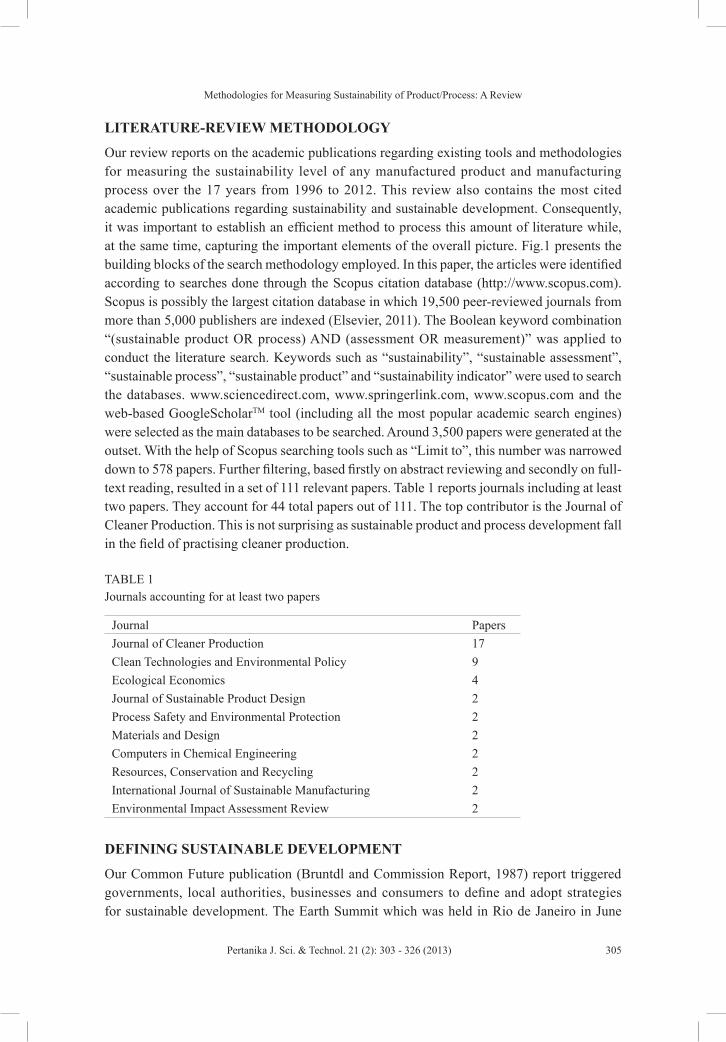
Methodologies for Measuring Sustainability of Product/Process: A Review
305Pertanika J. Sci. & Technol. 21 (2): 303 - 326 (2013)
LITERATURE-REVIEW METHODOLOGY
Our review reports on the academic publications regarding existing tools and methodologies for measuring the sustainability level of any manufactured product and manufacturing process over the 17 years from 1996 to 2012. This review also contains the most cited academic publications regarding sustainability and sustainable development. Consequently, it was important to establish an efficient method to process this amount of literature while, at the same time, capturing the important elements of the overall picture. Fig.1 presents the building blocks of the search methodology employed. In this paper, the articles were identified according to searches done through the Scopus citation database (http://www.scopus.com). Scopus is possibly the largest citation database in which 19,500 peer-reviewed journals from more than 5,000 publishers are indexed (Elsevier, 2011). The Boolean keyword combination “(sustainable product OR process) AND (assessment OR measurement)” was applied to conduct the literature search. Keywords such as “sustainability”, “sustainable assessment”, “sustainable process”, “sustainable product” and “sustainability indicator” were used to search the databases. www.sciencedirect.com, www.springerlink.com, www.scopus.com and the web-based GoogleScholarTM tool (including all the most popular academic search engines) were selected as the main databases to be searched. Around 3,500 papers were generated at the outset. With the help of Scopus searching tools such as “Limit to”, this number was narrowed down to 578 papers. Further filtering, based firstly on abstract reviewing and secondly on full-text reading, resulted in a set of 111 relevant papers. Table 1 reports journals including at least two papers. They account for 44 total papers out of 111. The top contributor is the Journal of Cleaner Production. This is not surprising as sustainable product and process development fall in the field of practising cleaner production.
TABLE 1 Journals accounting for at least two papers
Journal PapersJournal of Cleaner Production 17Clean Technologies and Environmental Policy 9Ecological Economics 4Journal of Sustainable Product Design 2Process Safety and Environmental Protection 2Materials and Design 2Computers in Chemical Engineering 2Resources, Conservation and Recycling 2International Journal of Sustainable Manufacturing 2Environmental Impact Assessment Review 2
DEFINING SUSTAINABLE DEVELOPMENT
Our Common Future publication (Bruntdl and Commission Report, 1987) report triggered governments, local authorities, businesses and consumers to define and adopt strategies for sustainable development. The Earth Summit which was held in Rio de Janeiro in June
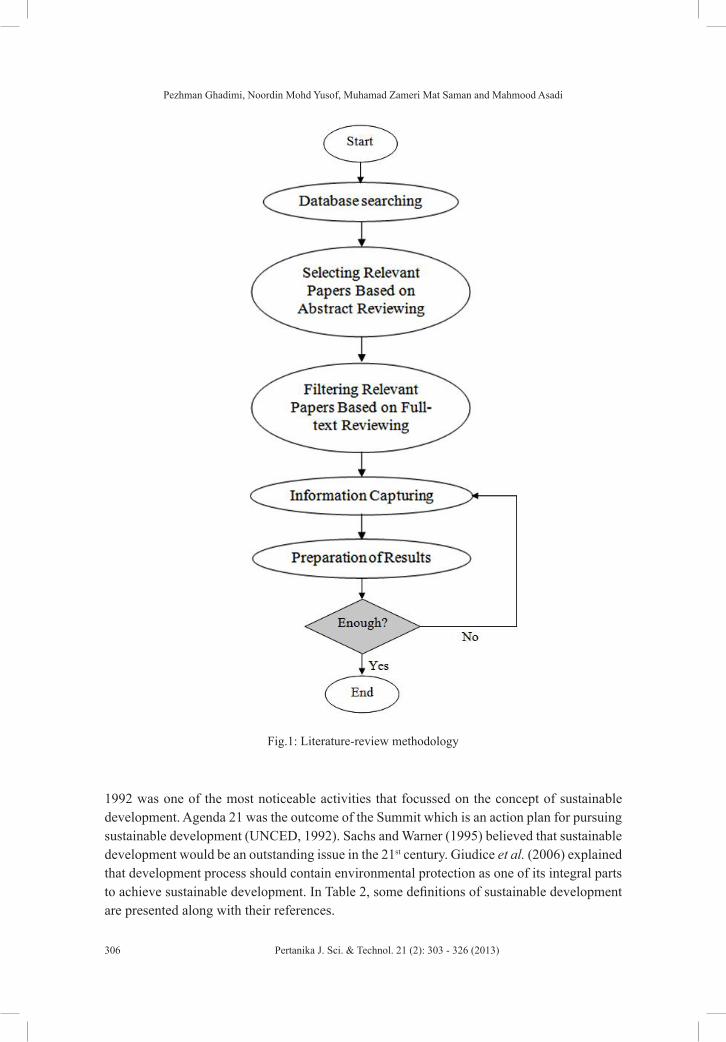
Pezhman Ghadimi, Noordin Mohd Yusof, Muhamad Zameri Mat Saman and Mahmood Asadi
306 Pertanika J. Sci. & Technol. 21 (2): 303 - 326 (2013)
Fig.1: Literature-review methodology
1992 was one of the most noticeable activities that focussed on the concept of sustainable development. Agenda 21 was the outcome of the Summit which is an action plan for pursuing sustainable development (UNCED, 1992). Sachs and Warner (1995) believed that sustainable development would be an outstanding issue in the 21st century. Giudice et al. (2006) explained that development process should contain environmental protection as one of its integral parts to achieve sustainable development. In Table 2, some definitions of sustainable development are presented along with their references.

Methodologies for Measuring Sustainability of Product/Process: A Review
307Pertanika J. Sci. & Technol. 21 (2): 303 - 326 (2013)
TABLE 2 Definitions of sustainable development
No. Definition
1
Sustainable development argues for: (1) development subject to a set of constraints which set resource harvest rates at levels not higher than managed natural regeneration rate, and (2) use of the environment as a “waste sink” on the basis that waste disposal rates should not exceed rates of managed or natural assimilative capacity of the ecosystem (Pearce, 1988).
2
Sustainable development means basing developmental and environmental policies on a comparison of costs and benefits and on careful economic analysis that will strengthen environmental protection and lead to rising and sustainable levels of welfare (World Bank, 1995).
3Sustainable development is about maintenance of essential ecological processes and life support systems, the preservation of genetic diversity, and the sustainable utilization of species and ecosystems (IUCN et al.,1991).
4
The term “sustainable development” suggests that the lessons of ecology can, and should be applied to economic processes. It encompasses the ideas in the World Conservation Strategy, providing an environmental rationale through which the claims of development to improve the quality of (all) life can be challenged and tested (Redclift, 1987).
5
Sustainable development involves a process of deep and profound change in the political, social, economic, institutional, and technological order, including redefinition of relations between developing and more developed countries (Strong, 1992).
6Sustainable development is a balancebetween the available technologies, strategies ofinnovation and the policies of governments (Vollenbroek, 2002).
7Development that improves the quality of human life while living within the carrying capacity of supporting ecosystems (IUCN, 1980).
ADVANTAGES OF SUSTAINABLE PRODUCTS
A product that has little possible impact on the environment can be classified as a sustainable product (Ljungberg, 2007; Maxwell et al., 2006; Maxwell & van der Vorst, 2003; Vinodh & Rathod, 2010; Huand & Bidanda, 2009; Kaebernick et al., 2003; Hanssen, 1999; Rydberg, 1995). However, the use phase of a product’s life cycle can have an outstanding impact on the environment (Jarvi & Paloviita,2007). As shown in Fig.2, Mcauley (2003) pointed out that the use phase of the motor vehicle has the highest percentage (almost 87%) of a vehicle’s life cycle energy consumption. Table 3 presents the variety of reasons indicating that sustainable products have the ability to boost both tangible and intangible corporate profits (USA Sustainable Products Corporation, 2002).
Satisfaction experienced by the end customer is an important feature of a good sustainable product. According to the estimations, 90% of all good products cannot find a way to stay in the market (Patrick, 1997). Risk of failure of a newly launched sustainable product in the market is high and, therefore, proper information for customers is needed to make them understand

Pezhman Ghadimi, Noordin Mohd Yusof, Muhamad Zameri Mat Saman and Mahmood Asadi
308 Pertanika J. Sci. & Technol. 21 (2): 303 - 326 (2013)
the basis on which the product can be considered as a sustainable one (Ljungberg, 2007).“Triple bottom line” balance focusses on achieving economic success, environment
cleanness and social responsibility all together and is considered as the central concept of sustainability, or sustainable development (Elkington, 1998; Hacking & Guthrie,2008; McDonough & Braungart, 2002; Fairley et al., 2011). Othman et al. (2010) stated that “Design for sustainability” is a concept and also a design philosophy. By this, a variety of design methodologies have been developed for improving process design, product design, material design etc. at different points and for different lengths of time .
Product designs that focus on eliminating waste and use of toxic materials and facilitating end-of-life activities will reduce costs and bring benefits to the manufacturer in the long run (Fiksel et al., 1998; Jaafar et al.,2007; Afrinaldi et al., 2009; Mat Saman et al., 2010; Zakuan et al., 2011). End-of-life activities should be handled at a dedicated treatment facility in which the consumer of the product will not incur any additional expenses. For instance, Fig.3 shows the recycling and recovery rate of End-of-Life of Vehicles (ELVs) at European Union in 2008.Dinh et al. (2009) stated that,“A sustainable product or process is one that constraints resource consumption and waste generation to an acceptable level, makes a positive contribution to the satisfaction of human needs and provides enduring economic value to the business enterprise.”
SUSTAINABILITY INDICATORS
Measuring environmental, social and economic impacts is important in assessing sustainability. When doing so, it is critical to select vital indicators. In general, sustainability assessment indicators can be divided into two groups, that is, hard and soft.
Quantitative evaluation of a process using formulas is the main feature of hard indicators. Some examples of indicators used by different researchers are net present value (NPV) and rate of return (ROR) (Ulrich, 1984; Baasel, 1990)ineconomic performance assessment; life cycle assessment (LCA) (Harding et al., 2007; Kasai, 1999; Guo et al., 2002; Klopffer & Rippen, 1992) and waste reduction (WAR) algorithm (Young & Cabezas, 1999; Heikkila,1999; Cabezas et al., 1999) in environmental performance assessment; and fault tree assessment (FTA) (Volkanovski et al., 2009) and chemical exposure index (AIChE, 1998) in safety-related
Fig.2: Energy consumption in auto life-cycle (Mcauley, 2003)
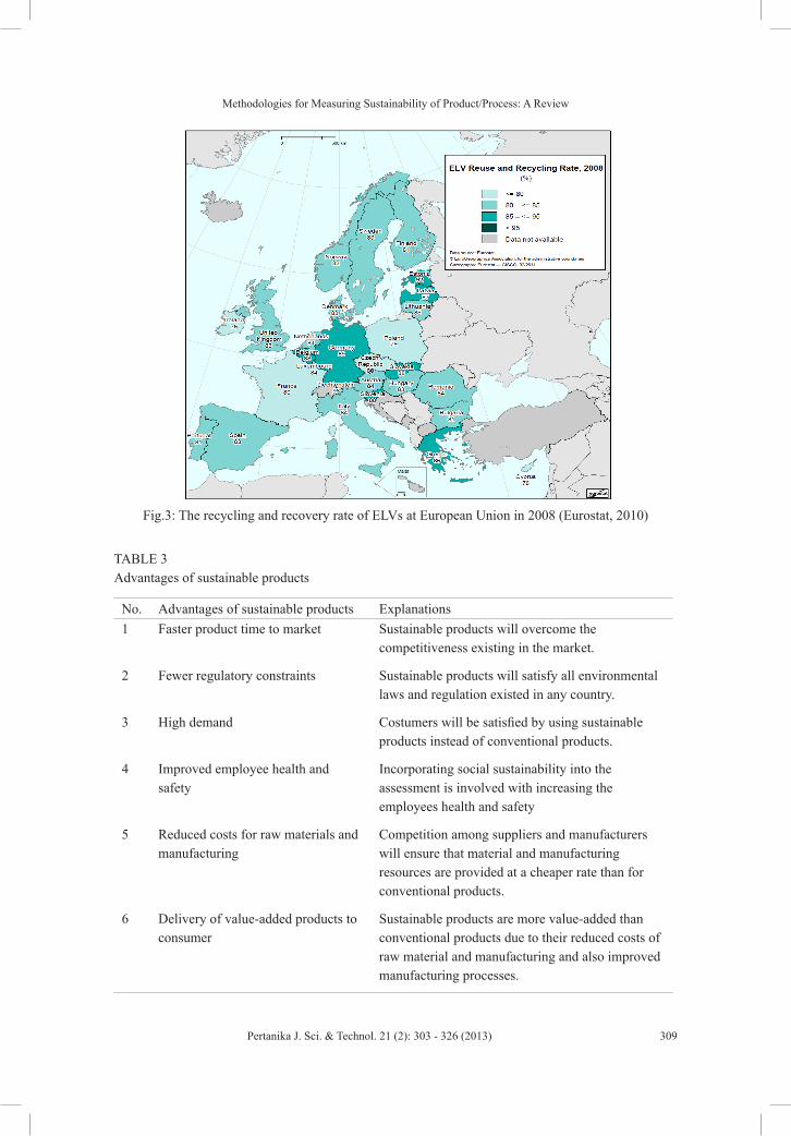
Methodologies for Measuring Sustainability of Product/Process: A Review
309Pertanika J. Sci. & Technol. 21 (2): 303 - 326 (2013)
Fig.3: The recycling and recovery rate of ELVs at European Union in 2008 (Eurostat, 2010)
TABLE 3 Advantages of sustainable products
No. Advantages of sustainable products Explanations1 Faster product time to market Sustainable products will overcome the
competitiveness existing in the market.
2 Fewer regulatory constraints Sustainable products will satisfy all environmental laws and regulation existed in any country.
3 High demand Costumers will be satisfied by using sustainable products instead of conventional products.
4 Improved employee health and safety
Incorporating social sustainability into the assessment is involved with increasing the employees health and safety
5 Reduced costs for raw materials and manufacturing
Competition among suppliers and manufacturers will ensure that material and manufacturing resources are provided at a cheaper rate than for conventional products.
6 Delivery of value-added products to consumer
Sustainable products are more value-added than conventional products due to their reduced costs of raw material and manufacturing and also improved manufacturing processes.

Pezhman Ghadimi, Noordin Mohd Yusof, Muhamad Zameri Mat Saman and Mahmood Asadi
310 Pertanika J. Sci. & Technol. 21 (2): 303 - 326 (2013)
social responsibility assessment.On the contrary, soft indicators depend solely on the designer and expert’s knowledge
and experiences. This would be categorised as qualitative evaluation due to different levels of understanding; these can be very subjective but at the same time are still very important. Soft indicators can be scaled numerically using proper ranking and scaling techniques (Othman et al., 2010). Several types of sustainability indicators have been used for different types of studies (Krajnc & Glavic, 2003; Azapagic & Perdan, 2000; Yan et al., 2009; Lems et al., 2003; Petrie et al., 2007; Pop-Jordanov, 2003; Tokos et al., 2011; Okkonen, 2008; Korhonen et al., 2004; Block et al., 2007; Jain, 2005). However, most product indicator frameworks focus exclusively on economic or environmental performance; very few address societal concerns (James, 1997).
EXISTING TOOLS AND METHODOLOGIES FOR MEASURING SUSTAINABILITY LEVELS
Several tools and methods can be applied in measuring the sustainability level of a product or process. Basically, each of these tools has some advantages and limitations. In this review, an attempt was made to list down all the published methodologies in the field of sustainable product and process assessment. The existing tools for measuring sustainability are described in the following sections. For the purpose of space limitations, main points of each methodology and their applications are described in each section. More detailed information is available in the related original articles.
Weighted fuzzy assessment method (WFAM)
WFAM is a product assessment methodology recently introduced by Ghadimi et al. (2012) which tries to incorporate expert knowledge in its assessment process. This effort was done with emphasis on weighing the assessment elements and sub-elements based on the expert opinions of any industry in whichthey are intended to be applied. This methodology was proposed for use as a road map for manufacturers to move towards manufacturing more sustainable products, and a the possibility of a simple improvement to product sustainability that could lead to sustainable manufacturing was illustrated. A case study of the automotive industry showed the efficiency of the proposed method. One of the challenging issues stemming from this method is dealing with the cradle-to-grave boundary that only covers the raw material extraction point and manufacturing stages of the lifecycle. The authors claimed that WFAM can be extended to embrace the whole lifecycle stages and be utilised as a fully functional assessment method, which can be considered as an advantage; this has not yet been done. Other than that, all three aspects of sustainability have been considered in this assessment methodology.
Sustainable process index (SPI)
The sustainable process index (SPI) was introduced by Krotscheck and Narodoslawsky (1996) for evaluating industrial process based on mass and energy balances and measures total environmental impact. The advantages of SPI are the use of natural concentrations of substances in the atmosphere, ground water and soil as a reference, which makes SPI independent of
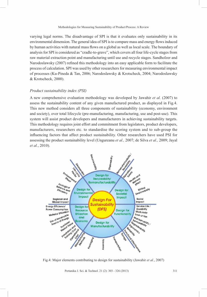
Methodologies for Measuring Sustainability of Product/Process: A Review
311Pertanika J. Sci. & Technol. 21 (2): 303 - 326 (2013)
varying legal norms. The disadvantage of SPI is that it evaluates only sustainability in its environmental dimension. The general idea of SPI is to compare mass and energy flows induced by human activities with natural mass flows on a global as well as local scale. The boundary of analysis for SPI is considered as “cradle-to-grave”, which covers all four life-cycle stages from raw material extraction point and manufacturing until use and recycle stages. Sandholzer and Narodoslawsky (2007) refined this methodology into an easy applicable form to facilitate the process of calculation. SPI was used by other researchers for measuring environmental impact of processes (Ku-Pineda & Tan, 2006; Narodoslawsky & Krotscheck, 2004; Narodoslawsky & Krotscheck, 2000).
Product sustainability index (PSI)
A new comprehensive evaluation methodology was developed by Jawahir et al. (2007) to assess the sustainability content of any given manufactured product, as displayed in Fig.4. This new method considers all three components of sustainability (economy, environment and society), over total lifecycle (pre-manufacturing, manufacturing, use and post-use). This system will assist product developers and manufacturers in achieving sustainability targets. This methodology requires joint effort and commitment from legislators, product developers, manufacturers, researchers etc. to standardise the scoring system and to sub-group the influencing factors that affect product sustainability. Other researchers have used PSI for assessing the product sustainability level (Ungureanu et al., 2007; de Silva et al., 2009; Jayal et al., 2010).
Fig.4: Major elements contributing to design for sustainability (Jawahir et al., 2007)
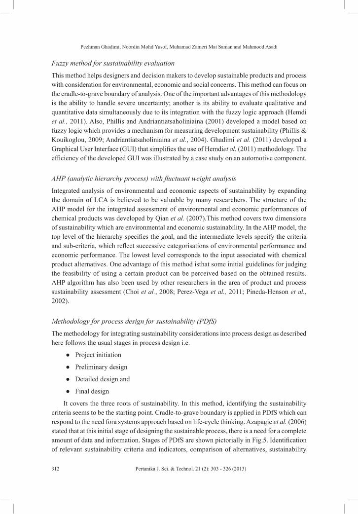
Pezhman Ghadimi, Noordin Mohd Yusof, Muhamad Zameri Mat Saman and Mahmood Asadi
312 Pertanika J. Sci. & Technol. 21 (2): 303 - 326 (2013)
Fuzzy method for sustainability evaluation
This method helps designers and decision makers to develop sustainable products and process with consideration for environmental, economic and social concerns. This method can focus on the cradle-to-grave boundary of analysis. One of the important advantages of this methodology is the ability to handle severe uncertainty; another is its ability to evaluate qualitative and quantitative data simultaneously due to its integration with the fuzzy logic approach (Hemdi et al., 2011). Also, Phillis and Andriantiatsaholiniaina (2001) developed a model based on fuzzy logic which provides a mechanism for measuring development sustainability (Phillis & Kouikoglou, 2009; Andriantiatsaholiniaina et al., 2004). Ghadimi et al. (2011) developed a Graphical User Interface (GUI) that simplifies the use of Hemdiet al. (2011) methodology. The efficiency of the developed GUI was illustrated by a case study on an automotive component.
AHP (analytic hierarchy process) with fluctuant weight analysis
Integrated analysis of environmental and economic aspects of sustainability by expanding the domain of LCA is believed to be valuable by many researchers. The structure of the AHP model for the integrated assessment of environmental and economic performances of chemical products was developed by Qian et al. (2007).This method covers two dimensions of sustainability which are environmental and economic sustainability. In the AHP model, the top level of the hierarchy specifies the goal, and the intermediate levels specify the criteria and sub-criteria, which reflect successive categorisations of environmental performance and economic performance. The lowest level corresponds to the input associated with chemical product alternatives. One advantage of this method isthat some initial guidelines for judging the feasibility of using a certain product can be perceived based on the obtained results. AHP algorithm has also been used by other researchers in the area of product and process sustainability assessment (Choi et al., 2008; Perez-Vega et al., 2011; Pineda-Henson et al., 2002).
Methodology for process design for sustainability (PDfS)
The methodology for integrating sustainability considerations into process design as described here follows the usual stages in process design i.e.
Project initiation
Preliminary design
Detailed design and
Final design
It covers the three roots of sustainability. In this method, identifying the sustainability criteria seems to be the starting point. Cradle-to-grave boundary is applied in PDfS which can respond to the need fora systems approach based on life-cycle thinking. Azapagic et al. (2006) stated that at this initial stage of designing the sustainable process, there is a need for a complete amount of data and information. Stages of PDfS are shown pictorially in Fig.5. Identification of relevant sustainability criteria and indicators, comparison of alternatives, sustainability
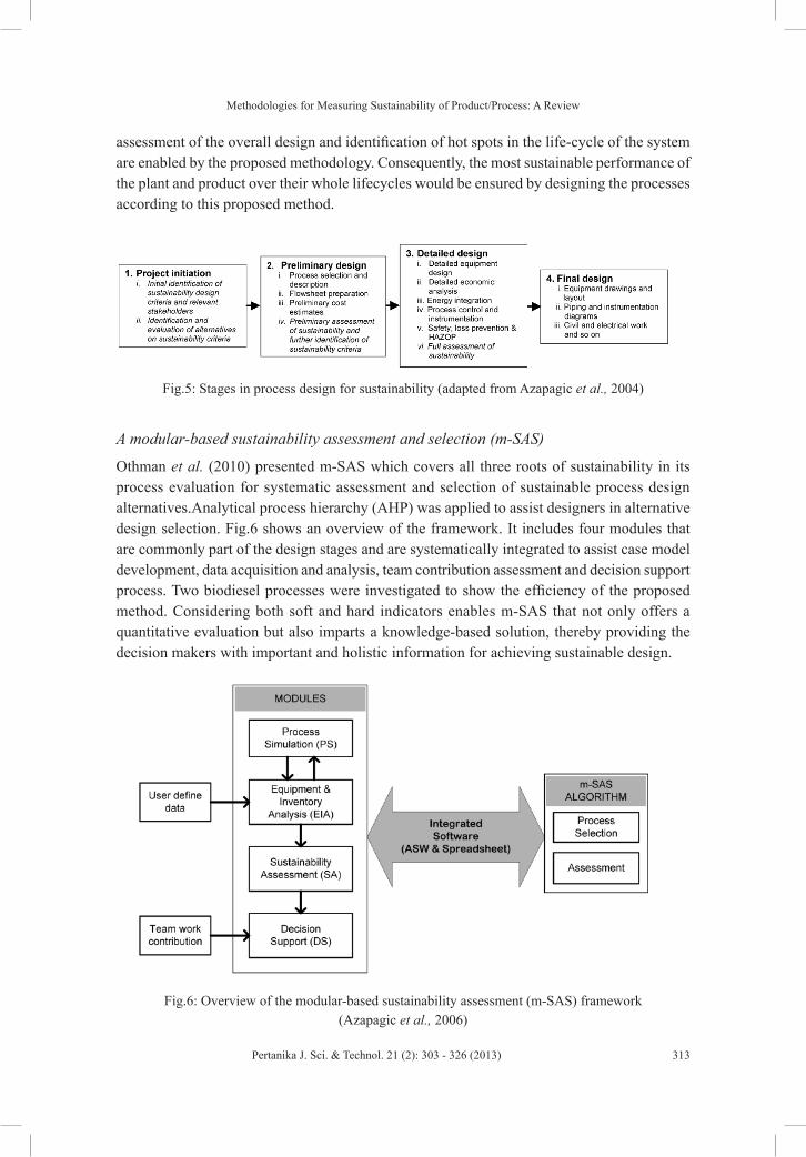
Methodologies for Measuring Sustainability of Product/Process: A Review
313Pertanika J. Sci. & Technol. 21 (2): 303 - 326 (2013)
assessment of the overall design and identification of hot spots in the life-cycle of the system are enabled by the proposed methodology. Consequently, the most sustainable performance of the plant and product over their whole lifecycles would be ensured by designing the processes according to this proposed method.
A modular-based sustainability assessment and selection (m-SAS)
Othman et al. (2010) presented m-SAS which covers all three roots of sustainability in its process evaluation for systematic assessment and selection of sustainable process design alternatives.Analytical process hierarchy (AHP) was applied to assist designers in alternative design selection. Fig.6 shows an overview of the framework. It includes four modules that are commonly part of the design stages and are systematically integrated to assist case model development, data acquisition and analysis, team contribution assessment and decision support process. Two biodiesel processes were investigated to show the efficiency of the proposed method. Considering both soft and hard indicators enables m-SAS that not only offers a quantitative evaluation but also imparts a knowledge-based solution, thereby providing the decision makers with important and holistic information for achieving sustainable design.
Fig.5: Stages in process design for sustainability (adapted from Azapagic et al., 2004)
Fig.6: Overview of the modular-based sustainability assessment (m-SAS) framework (Azapagic et al., 2006)
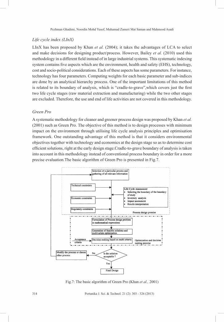
Pezhman Ghadimi, Noordin Mohd Yusof, Muhamad Zameri Mat Saman and Mahmood Asadi
314 Pertanika J. Sci. & Technol. 21 (2): 303 - 326 (2013)
Life cycle index (LInX)
LInX has been proposed by Khan et al. (2004); it takes the advantages of LCA to select and make decisions for designing product/process. However, Bailey et al. (2010) used this methodology in a different field instead of in large industrial systems. This systematic indexing system contains five aspects which are the environment, health and safety (EHS), technology, cost and socio-political considerations. Each of these aspects has some parameters. For instance, technology has four parameters. Computing weights for each basic parameter and sub-indices are done by an analytical hierarchy process. One of the important limitations of this method is related to its boundary of analysis, which is “cradle-to-grave”,which covers just the first two life cycle stages (raw material extraction and manufacturing) while the two other stages are excluded. Therefore, the use and end of life activities are not covered in this methodology.
Green Pro
A systematic methodology for cleaner and greener process design was proposed by Khan et al. (2001) such as Green Pro. The objective of this method is to design processes with minimum impact on the environment through utilising life cycle analysis principles and optimisation framework. One outstanding advantage of this method is that it considers environmental objectives together with technology and economics at the design stage so as to determine cost efficient solutions, right at the early design stage.Cradle-to-grave boundary of analysis is taken into account in this methodology instead of conventional process boundary in order for a more precise evaluation.The basic algorithm of Green Pro is presented in Fig.7.
Fig.7: The basic algorithm of Green Pro (Khan et al., 2001)
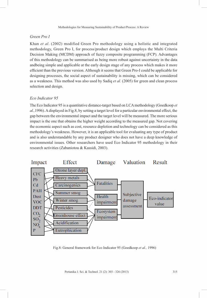
Methodologies for Measuring Sustainability of Product/Process: A Review
315Pertanika J. Sci. & Technol. 21 (2): 303 - 326 (2013)
Green Pro I
Khan et al. (2002) modified Green Pro methodology using a holistic and integrated methodology, Green Pro I, for process/product design which employs the Multi Criteria Decision Making (MCDM) approach of fuzzy composite programming (FCP). Advantages of this methodology can be summarised as being more robust against uncertainty in the data andbeing simple and applicable at the early design stage of any process which makes it more efficient than the previous version. Although it seems that Green Pro-I could be applicable for designing processes, the social aspect of sustainability is missing, which can be considered as a weakness. This method was also used by Sadiq et al. (2005) for green and clean process selection and design.
Eco Indicator 95
The Eco Indicator 95 is a quantitative distance-target based on LCA methodology (Goedkoop et al.,1996). A displayed in Fig.8, by setting a target level for a particular environmental effect, the gap between the environmental impact and the target level will be measured. The more serious impact is the one that obtains the higher weight according to the measured gap. Not covering the economic aspect such as cost, resource depletion and technology can be considered as this methodology’s weakness. However, it is an applicable tool for evaluating any type of product and is also understandable by any product designer who does not have a deep knowledge of environmental issues. Other researchers have used Eco Indicator 95 methodology in their research activities (Zabaniotou & Kassidi, 2003).
Fig.8: General framework for Eco Indicator 95 (Goedkoop et al., 1996)

Pezhman Ghadimi, Noordin Mohd Yusof, Muhamad Zameri Mat Saman and Mahmood Asadi
316 Pertanika J. Sci. & Technol. 21 (2): 303 - 326 (2013)
Eco Indicator 99
Goedkoop and Spriensma(2001) developed Eco indicator 99 based on the damage-oriented method for life-cycle assessment which is a modification of Eco Indicator 95. Human health, ecosystems and mineral resources are the main three damage categories. Eco Indicator 99 has the advantage of being a generalised tool to evaluate any product and is also well documented as an international standard (Li & Zhang, 2008). However, economic index of sustainability is not encompassed in this methodology. There are also several works in the literature related to assessing environmental sustainability using Eco Indicator as their assessment methodology (Dehghanian & Mansour, 2009; Bovea & Vidal,2004; Gernuks et al., 2007).
DISCUSSIONS AND KEY ISSUES
At the present time, developing sustainable products and designing sustainable processes are gaining attention due to the rising awareness of environmental changes, resource and energy prices. Both manufacturers and consumers look forward to manufacture and use more sustainable products. Lack of a broad literature review in the area of sustainability assessment methodologies seem to be missing in the existing literature. This paper tries to fill this gap in the literature. Table 4 presents a summary which covers all the 12 methods discussed in this paper together with their sustainable elements, boundary of analysis and method of analysis.
Based on the discussion ofthe 12 methodologies, it can be perceived that each of these methodologies has some advantages and weaknesses that can be considered for future work. There are some key issues that can be mentioned as follows:
Weaknesses:
1. Many of these methods are not able to assess the sustainability of products or processes regarding the three dimensions of sustainability. For instance, SPI mainly quantifies the environmental impact of the processes. This methodology, however, does not deal with other sustainability aspects such as social impact and economic impact.
2. Most of these methods are not able to analyse qualitative data, which can be considered as a great defect. It is the same for many of the discussed methods such as Eco Indicator 99, LiNX and PSI. This defect is due to the fact that large tracts of related data are expressed as opinions and ideas, which cannot be analysed using quantitative methods.
3. WFAM, m-SAS, Green Pro and Eco Indicator 95 are contained in a group of methodologies where the boundary of analysis is cradle-to-grave, which can only cover raw material extraction and manufacturing stages of process/product lifecycle. This review paper provides useful gathered information which can be applied in extending each of these methodologies with respect to their discussed weaknesses.
Advantages:
WFAM was noticed to be the only methodology that considered expert opinion in its assessment, which was undertaken by weighting their assessment elements and sub-elements. Using Multi Criteria Decision Making (MCDM), experts’ knowledge was incorporated into the assessment

Methodologies for Measuring Sustainability of Product/Process: A Review
317Pertanika J. Sci. & Technol. 21 (2): 303 - 326 (2013)
process. Fuzzy method for sustainability evaluation was used to assess both qualitative and quantitative data simultaneously. This ability was incorporated into this methodology by integrating fuzzy logic in its assessment procedure. Eco Indicator 99 and 95 proved to be promising tools in quantifying the environmental impact of each product. SPI provides reliable measures in evaluating industrial processes and can be applied to rate technologies from the viewpoint of sustainable development. LInX may be useful for government and researchers to be considered as sustainable tools in measuring smaller systems.
TABLE 4 Summary of existing sustainability assessment methodologies
Name of methodology Sustainable elements Boundary of analysis Method of analysisWeighted fuzzy assessment methodology (WFAM)
Environment, economic and social
Cradle to gate Quantitative and Qualitative
Sustainable process index (SPI)
Environment Cradle to grave Quantitative
Product Sustainability Index (PSI)
Environment, economic and social
Cradle to grave Quantitative
Fuzzy method for sustainability evaluation
Environment, economic and social
Cradle to grave andCradle to gate
Quantitative and Qualitative
AHP with fluctuant weight analysis
Environment and economic
Cradle to grave Quantitative
Process design for sustainability (PDfS)
Environment, economic and social
Cradle to grave Quantitative and Qualitative
Modular-based sustainability assessment and selection (m-SAS)
Environment, economic and social
Cradle to gate Quantitative and Qualitative
Life Cycle Index (LiNX) Environment, economic and social
Cradle to gate Quantitative
Green Pro Environment and economic
Cradle to gate Quantitative
Green Pro I Environment and economic
Cradle to gate Quantitative
Eco Indicator 95 Environment and social
Cradle to gate Quantitative
Eco Indicator 99 Environment and social
Cradle to grave Quantitative

Pezhman Ghadimi, Noordin Mohd Yusof, Muhamad Zameri Mat Saman and Mahmood Asadi
318 Pertanika J. Sci. & Technol. 21 (2): 303 - 326 (2013)
Unavailability of relevant data:
Besides the advantages of the introduced methodologies, one of the main concerns in this area could be addressed as unavailability of appropriate information. All of these methodologies are data driven methods, which means that they can be fully operative if all the needed data are provided. This prospective allows the assessment of products and processes to be limited to the available provided data. To solve this issue, full cooperation and coordination of all practitioners of sustainability assessment such as company managers, CEOs and government authorities would be most constructive.
Integrated assessment methodology:
From this review of 12 assessment methodologies it can be perceived that there is an absence of a hybrid methodology which can integrate the assessment procedure of both manufacturing process and its manufactured product simultaneouslywhile considering the manufacturing line’s entire supply chain and the optimisation of the manufacturing line in order to achieve continuous improvements.
CONCLUDING REMARKS
A broad literature review has been produced to give the reader a comprehensive discussion ofthe main topics related to different sustainability assessment methodologies in the field of manufacturing processes and manufactured products. A discussion of sustainable development was provided in this paper. Also, some challenges associated with advantages of sustainable products were highlighted such as end-of-life activities and use phase of product life-cycle. Moreover, various sustainability indicators have been presented with their application in different fields of research. The rest of the paper discussed the 12 existing methodologies developed for sustainability assessment of products and processes. In conclusion, it can be said that this review may be found to be useful by both practitioners in companies and academics as it outlines major lines of research in the field. Furthermore, it discusses specific features of sustainable products or process design assessment as well as the limitations of existing research; this should stimulate ideas for further research.
ACKNOWLEDGEMENTS
The authors gratefully acknowledge the support and constructive and kind comments of the reviewers of this paper which have helped to make this paper more informative and structured.
REFERENCESAfrinaldi, F., Mat Saman, M. Z., & Shaharoun A. M. (2009). A decision making software for End-of-Life
vehicle disassemblability and recyclability analysis. IEEE International Conference on Industrial Engineering and Engineering Management, IEEM. Hong Kong, 2261-2265.
American Institute of Chemical Engineers (AIChE) (1998). Dow’s Chemical Exposure Index Guide(1st
Ed.). New York: John Wiley & Sons.
Methodologies for Measuring Sustainability of Product/Process: A Review
319Pertanika J. Sci. & Technol. 21 (2): 303 - 326 (2013)
Andriantiatsaholiniaina, L. A., Kouikoglou, V. S., & Phillis, Y. A. (2004). Evaluating strategies for sustainable development: fuzzy logic reasoning and sensitivity analysis. Ecological Economics, 48, 149-172.
Azapagic, A., & Perdan, S. (2000). Indicators of sustainable development for industry: a general framework. Process Safety and Environmental Protection, 78(4), 243-261.
Azapagic, A., Millington, A. & Collett, A. (2004). Process design for sustainability: the case of vinyl chloride monomer. In Azapagic, A., Perdan, S., & Clift, R. (Eds.), Sustainable Development in Practice: Case Studies for Engineers and Scientists, p. 201-249. Chichester, UK John Wiley & Sons.
Azapagic, A., Millington, A., & Collett, A. (2006). A methodology for integrating sustainability considerations into process design. Chemical Engineering Research and Design, 84, 439-452.
Baasel, W. D. (1990).Preliminary Chemical Engineering Plant Design (2nd Ed.). New York: Van Nostrand.
Bailey, J. A., Amyotte, P., & Khan, F. I. (2010). Agricultural application of life cycle iNdeX (LInX) for effective decision making. Journal of Cleaner Production, 18, 1703-1713.
Barbier, E. B. (1987).The concept of sustainable economic development. Environmental Conservation, 14, 101-110.
Block, C., vanGerven, T., & vanDecasteele, C. (2007). Industry and energy sectors in Flanders: environmental performance and response indicators. Clean Technologies and Environmental Policy, 9, 43-51.
Bovea, M. D., & Vidal, R. (2004). Materials selection for sustainable product design: a case study of wood based furniture eco-design. Materials and Design, 25, 111-116.
Brent, A. C., & Labuschagne, C. (2004). Sustainable life cycle management: indicators to assess the sustainability of engineering projects and technologies. In the procedings of International Engineering Management Conference.
Bruntdland Commission Report. (1987). Our Common Future: From One Earth to One World p. 22-23. World Commission on Environment and Development, Oxford University Press.
Cabezas, H., Bare, C. J., & Mallick, S. K. (1999). Pollution prevention with chemical process simulators: the generalized waste (WAR) algorithm-full version. Computers in Chemical Engineering, 23, 623-634.
Choi, J. K., Niesb, L. F., & Ramani, K. (2008).A framework for the integration of environmental and business aspects toward sustainable product development. Journal of Engineering Design, 19(5), 431-446.
Common, M., & Perrings, C. (1992).Towards an ecological economics of sustainability. Ecological Economics, 6, 7-34.
Conteras, A. M., Rosa, E., Prez, M., Langenhove, H. V., & Dewulf, J.(2009). Comparative life cycle assessment of four alternatives for using by-products of cane sugar production. Journal of Cleaner Production, 17, 772-779.
Dehghanian, F., & Mansour, S. (2009).Designing sustainable recovery network of end-of-life products using genetic algorithm. Resources, Conservation and Recycling, 53, 559-570.

Pezhman Ghadimi, Noordin Mohd Yusof, Muhamad Zameri Mat Saman and Mahmood Asadi
320 Pertanika J. Sci. & Technol. 21 (2): 303 - 326 (2013)
de Silva, N., Jawahir, I. S., Dillon, O., & Russell, M. (2009). A New Comprehensive methodology for the evaluation of product sustainability at the design and development stage of consumer electronic products.International Journal of Sustainable Manufacturing, 1(3), 251-264.
Dinh, L. T. T., Guo, Y., & Mannan, M. S. (2009). Sustainability Evaluation of Biodiesel Production Using Multicriteria Decision-Making. Wiley InterScience.
Dovers, S. (1990). Sustainability in context: an Australian perspective. Environmental Management, 14, 297-305.
Elkington J. (1998). Cannibals with forks: the triple bottom line of 21st century business. London: New Society Publishers.
Elsevier B. V. (n.d.). Elsevier, Scopus in Detail: Facts and Figures. Retrieved on July 2, 2011 from http://www.info.sciverse.com/scopus/about
European Commission (n.d.). Eurostat 2010. Retrieved on February 3, 2012 from http://epp.eurostat.ec.europa.eu/portal/page/portal/waste/data/wastestreams/elvs.
Fairley, S., Tyler, B. D., Kellett, P., & D’Elia, K. (2011). The Formula One Australian Grand Prix: Exploring the triple bottom line. Sport Management Review, 14, 141-152.
Fiksel, J., Mcdaniel, J., & Spitzley, D. (1998). Measuring Product Sustainability. Journal of Sustainable Product Design, 6, 7-18.
Fink, A. (1998). Conducting research literature reviews: from paper to the internet. Thousand Oaks: Sage.
Gernuks, M., Buchgeister, J., & Schebek, L. (2007). Assessment of environmental aspects and determination of environmental targets within environmental management systems (EMS) -development of a procedure for Volkswagen. Journal of Cleaner Production, 15, 1063-1075.
Ghadimi, P., Noordin, M. Y., & Mat Saman, M. Z. (2011). A graphical user interface (GUI) for assessing the sustainability level of manufactured products: an automotive component case study. PERINTIS e-Journal, Special Issue on Science for Sustainability, 1, 13-19.
Ghadimi, P., Azadnia A. H., Noordin, M. Y., & Mat Saman, M. Z. (2012). A weighted fuzzy approach for product sustainability assessment: a case study in automotive industry. Journal of Cleaner Production, 33, 10-21.
Giudice, F., Rosa, G. L., & Risitano, A. (2006). Product Design for the Environment. USA: Taylor & Francis Group.
Goedkoop, M., & Spriensma, R. (2001). Eco indicator 99 A damage oriented method for life cycle impact assessment: Methodology report (3rd Ed.). Netherlands: Product Ecology Consultants (PRé).
Goedkoop, M., Demmers, M., & Collignon, M. (1996). Eco indicator 95: Manual for designer. Netherlands: Product Ecology Consultants (PRé).
Guo, X. Y., Xiao, S. W., Xiao, X., Li, Q. H., & Yamamoto, R., (2002). LCA case study for lead and zinc production by an imperial smelting process in China – A brief presentation. International Journal of Life Cycle Assessment, 7(5), 276-276.
Hacking, T., & Guthrie, P. (2008).A framework for clarifying the meaning of Triple Bottom-Line Integrated and Sustainability Assessment. Environmental Impact Assessment Review, 28(2-3), 73-89.
Hanssen, O. J. (1999). Sustainable product systems—experiences based on case projects in sustainable product development. Journal of Cleaner Production, 7, 27-41.

Methodologies for Measuring Sustainability of Product/Process: A Review
321Pertanika J. Sci. & Technol. 21 (2): 303 - 326 (2013)
Harding, K. G., Dennis, J. S., von Blottnitz, H., Harrison, S. T. L. (2007). Life-cycle comparison between inorganic and biological catalysis for the production of biodiesel.Journal of Cleaner Production, 16, 1368-1378.
Heikkila, A. -M.(1999). Inherent Safety in Process Plant Design - An Index-based Approach. (Ph.D-Thesis dissertation), p. 62-89.
Hemdi, A.R., Mat Saman, M. Z., & Sharif, S. (2011). Sustainability evaluation using fuzzy inference methods. International Journal of Sustainable Energy, iFirst, 1-17.
Hu, G. & Bidanda, B. (2009). Modeling sustainable product life cycle decision support systems.International Journal of Production Economics, 122, 366-375.
IUCN (1980).World conservation strategy: living resource conservation for sustainable development. By the International Union for Conservation of Nature and Natural Resources (IUCN).
IUCN (World Conservation Union), UNEP (United Nations Environment Programme) and WWF (World Wide Fund for Nature) (1991). Caring for the Earth: A Strategy for Sustainable Living, Switzerland: IUCN.
Jaafar, I. H., Venkatachalam, A., Joshi, K., Ungureanu, A. C., De Silva, N., Rouch, K. E., Dillon Jr., O. W., & Jawahir, I. S. (2007). Product design for sustainability: a new assessment methodology and case studies. In Kutz, M. (Ed.). Environmentally Conscious Mechanical Design. p. 24 -65. John Wiley & Sons, Inc.
Jain, R. (2005). Sustainability: metrics, specific indicators and preference index. Clean Technologies and Environmental Policy, 7, 71-72.
James, P. (1997). The Sustainability Cycle: A New Tool for Product Development and Design. Journal of Sustainable Product Design, 2.
Jarvi, P., & Paloviita, A. (2007). Product-related information for sustainable use of laundry detergents in Finnish households. Journal of Cleaner Production, 15, 681-689.
Jawahir, I. S., Rouch, K. E., Dillon, O. W., Holloway Jr., L., & Hall, A. (2007). Design for sustainability (DFS): new challenges in developing and implementing a curriculum for next generation design and manufacturing engineers. International Journal of Engineering Education, 23(6), 1053–1064.
Jayal, A. D., Badurdeen, F., Dillon Jr., O. W., & Jawahir, I. S. (2010). Sustainable manufacturing: Modeling and optimization challenges at the product, process and system levels. CIRP Journal of Manufacturing Science and Technology, 2, 144-152.
Kaebernick, H., Anityasari, M., & Kara, S.(2002). Technical and economic model for end-of-life (EOL) options of industrial products. International Journal on Environmental Sustainable Development, 1(2), 171-183.
Kaebernick, H., Kara, S., & Sun, M. (2003).Sustainable product development and manufacturing byconsidering environmental requirements. Robotics and Computer Integrated Manufacturing, 19, 461-468.
Kasai, J., (1999). Life Cycle Assessment, Evaluation Method for Sustainable Development. Japan Society of Automotive Engineers Review, 20(3), 387-394.
Khan, F. I, Sadiq, R., & Husain, T. (2002). GreenPro-I: A risk-based life cycle assessment and decision-making methodology for process plant design, EnvironmentalModelling & Software, 17, 669-692.

Pezhman Ghadimi, Noordin Mohd Yusof, Muhamad Zameri Mat Saman and Mahmood Asadi
322 Pertanika J. Sci. & Technol. 21 (2): 303 - 326 (2013)
Khan, F. I, Sadiq, R., & Veitch, B. (2004). Life cycle iNdeX (LInX): A new indexing procedure for process and product design and decision-making, Journal ofCleaner Production, 12, 59-76.
Khan, F. I., Natrajan, B. R., & Revathi, P. (2001).GreenPro: A new methodology for cleaner and greener process design, Journal of Loss Prevention in the ProcessIndustries, 14, 307-328.
Klopffer, W., & Rippen, G. (1992). Life Cycle Analysis and Ecological Balance: Methodical Approaches to Assessment of Environmental Aspects of Products. Environment International, 18(1), 55-61.
Korhonen, J., Okkonen, L., & Niutanen, V. (2004). Industrial ecosystem indicators—direct and indirect effects of integrated waste- and by-product management and energy production. Clean Technologies and Environmental Policy, 6, 162-173.
Krajnc, D., & Glavic, P. (2003). Indicators of sustainable production.Clean Technologies and Environmental Policy, 5, 279-288.
Krotscheck, C., & Narodoslawsky, M. (1996). The Sustainable Process Index: A new dimension in ecological evaluation. Ecological Engineering, 6, 241-258.
Ku-Pineda, V., & Tan, R. R. (2006). Environmental performance optimization using process water integration and Sustainable Process Index. Journal of Cleaner Production, 14, 1586-1592.
Li, J., Wu, Z., & Zhang, H. C. (2008). Application of neural network on environmental impact assessments tools. International Journal of Sustainable Manufacturing, 1(1/2), 100-121.
Lele, S. M. (1991). Sustainable development: a critical review. World Development, 19, 607-621.
Lems, S., van der Kooi, H. J., & de Swaan Arons, J. (2003). Quantifying technological aspects of process sustainability:a thermodynamic approach.Clean Technologies and Environmental Policy, 5, 248-253.
Ljungberg, L. Y. (2007). Materials selection and design for development of sustainable products. Materials and Design, 28,466-479.
Mat Saman, M. Z., Afrinaldi, F., Zakuan, N., Blount, G., Goodyer, J., Jones, R. & Jawaid, A. (2010).Strategic guidance model for product development in relation with recycling aspects for automotive products. Journal of Sustainable Development, 3(1), 142-158.
Mayyas, A., Qattawi, A., Omar, M., & Shan, D. (2012). Design for sustainability in automotive industry: A comprehensive review. Renewable and Sustainable Energy Reviews, 16, 1845-1862.
Maxwell, D., Sheate, W., & van der Vorst, R. (2006). Functional and systems aspects of the sustainable product and service development approach for industry. Journal of Cleaner Production, 14,1466-1479.
Maxwell, D., & van der Vorst, R. (2003).Developing sustainable products and services. Journal of Cleaner Production, 11, 883-895.
Mcauley , J. (2003). Global sustainability and key needs in future automotive design. Environmental Science & Technology, 37, 5414-5416.
McDonough, W., & Braungart, M. (2002). Design for the TripleTopLine: New Tools for Sustainable Commerce. Corporate Environmental Strategy, 9(3), 251-258.
Munasinghe, M., & Lutz, E. (1991). Environmental-Economic Evaluation of Projects and Policies for Sustain able Development. World Bank Environment Working Paper 42. Washington, D.C.: World Bank.

Methodologies for Measuring Sustainability of Product/Process: A Review
323Pertanika J. Sci. & Technol. 21 (2): 303 - 326 (2013)
Narodoslawsky, M., & Krotscheck, C. (2004). What can we learn from ecological valuation of processes with the sustainable process index (SPI) - the case study of energy production systems. Journal of Cleaner Production, 12, 111-115.
Narodoslawsky, M., & Krotscheck, C. (2000). Integrated ecological optimization of processes with the sustainable process index. Waste Management, 20, 599-603.
Okkonen, L. (2008). Applying industrial ecosystem indicators: case of Pielinen Karelia, Finland. Clean Technologies and Environmental Policy, 10, 327-339.
Opschoor, H., & Van der straaten, J. (1993). Sustainable development: an institutional approach. Ecological Economics, 7, 203-222.
Othman, M. R., Repke, J., Wozny, G., & Huang, Y. (2010). A Modular Approach to Sustainability Assessment and Decision Support in Chemical Process Design. Industrial & Engineering Chemistry Research, 49, 7870-7881.
Patrick, J. (1997). How to develop successful new products. Chicago: NTC Business Books.
Pearce, D. W., Markandya, A., & Barbier, E. B. (1989). Blueprint for a Green Economy. London: Earthscan.
Pearce, D. W. (1988). Optional Prices for Sustainable Development. In David Collard, David W. Pearce & David Ulph, (Eds.). Economics, Growth and Sustainable Environment. London: MacMillan Press.
Petrie, J., Cohen, B., & Stewart, M. (2007).Decision support frameworks and metrics for sustainabledevelopment of minerals and metals. Clean Technologies and Environmental Policy, 9, 133-145.
Phillis, Y. A., & Andriantiatsaholiniaina, L. A. (2001). Sustainability: an ill-defined concept and its assessment using fuzzy logic. Ecological Economics, 37, 435-456.
Phillis, Y. A., & Kouikoglou, V. S. (2009). Fuzzy measurement of sustainability. Nova science publishers, Inc.
Pineda-Henson, R., Culaba, A. B., & Mendoza, G. A. (2002).Evaluating Environmental Performance of Pulp and Paper Manufacturing Using the Analytic Hierarchy Process and Life-Cycle Assessment.Journal of Industrial Ecology, 6(1), 15-28.
Pop-Jordanov, J. (2003).Indicators for sustainable energy development from a negentropic perspective.Clean Technologies and Environmental Policy, 5, 273-278.
Perez-Vega, S., Peter, S., Salmeron-Ochoa, I., Nieva-de la Hidalga, A., & Sharratt, P. N. (2011). Analytical hierarchy processes (AHP) for the selection ofsolvents in early stages of pharmaceutical processdevelopment. Process Safety and Environmental Protection, 89, 261-267.
Prugh, T., Daly, H., & Costanza, R. (2000). The Local Politics of Global Sustainability. Washington, D.C: Island Press.
Qian, Y., Huang, Z., & Yan, Z. (2007). Integrated Assessment of Environmental and Economic Performance of Chemical Products Using Analytic Hierarchy Process Approach. Chinese Journal of Chemical Engineering, 15, 81-87.
Ravetz, J. (2000). Integrated assessment for sustainability appraisal in cities and regions. Environmental Impact Assessment Review, 20, 31-64.
Redclift, M. R. (1987). Sustainable Development: Exploring the Contradictions. London: Methuen.
Pezhman Ghadimi, Noordin Mohd Yusof, Muhamad Zameri Mat Saman and Mahmood Asadi
324 Pertanika J. Sci. & Technol. 21 (2): 303 - 326 (2013)
Rusinko, C. A. (2007). Green manufacturing: an evaluation of environmentally sustainable manufacturing practices and their impact on competitive outcomes. IEEE Transactions on Engineering Management, 54(3), 445-454.
Rydberg, T. (1995). Cleaner products in the Nordic countries based on the life cycle assessment approach. Journal of Cleaner Production, 3(1-2), 101-105.
Sachs, J., & Warner, A. (1995).Natural resource abundance and economic growth. Cambridge (MA): Harvard Institute for International Development.
Sadiq, R., Khan, F. I., & Veitch B. (2005). Evaluating offshore technologies for produced water management using GreenPro-I : a risk-based life cycle analysis for green and clean process selection and design. Computers and Chemical Engineering, 29, 1023-1039.
Sandholzer, D., & Narodoslawsky, M. (2007).SPIonExcel-Fast and easy calculation of the Sustainable Process Index via computer. Resources, Conservation and Recycling, 50, 130-142.
Singh, R. K., Murty, H. R., Gupta, S. K., & Dikshit, A. K.(2012).An overview of sustainability assessment methodologies.Ecological Indicators, 15, 281–299.
Strange, T., & Bayley, A. (2008). Sustainable Development: Linking economy, society, environment. Organization for economic co-operation and development (OECD) publications.
Strong, M. (1992). Required Global Changes: Close Linkages between Environment and Development. In Kirdar, U. (Ed.), Change: Threat or Opportunity. New York: United Nations.
Tokos, H., Pintaric, A. N., & Krajnc, D. (2011). An integrated sustainability performance assessment and benchmarking of breweries. Clean Technologies and Environmental Policy.
Tsoulfas, G. T., & Pappis, C. P. (2006). Environmental principles applicable to supply chains design and operation. Journal of Cleaner Production, 14, 1593-1602.
Ulrich, G. D. (1984). A Guide to Chemical Engineering Process Design and Economics. New York: John Wiley & Sons.
UNCED (1992). Agenda 21, United Nations Conference on Environment and Development, Rio de Janeiro.
Ungureanu, C. A., Das, S., & Jawahir, I. S. (2007). Development of a sustainability scoring method for manufactured automotive products: a case study of auto body panels. In the proceedings of ASME International Mechanical Engineering Congress and Exposition November 11-15, Seattle, Washington, USA.
USA Sustainable Products Corporation (2002). The Institute for Market Transformation to Sustainability (MTS). Retrieved on February 11, 2009, from http://MTS.sustainableproducts.com.
vanWeenen, J. C. (1995). Towards sustainable product development.Journal Cleaner Production,3(1-2), 95-100.
Vinodh, S., & Rathod, G. (2010). Integration of ECQFD and LCA for sustainable product design. Journal of Cleaner Production, 18, 833-842.
Volkanovski, A., Cepin, M., & Mavko, M. (2009). Application of the fault tree analysis for assessment of power system reliability. Reliability Engineering and System Safety, 94,1116-1127.
Vollenbroek, F. A. (2002).Sustainable development and the challenge of innovation. Journal of Cleaner Production, 10(3), 215-23.

Methodologies for Measuring Sustainability of Product/Process: A Review
325Pertanika J. Sci. & Technol. 21 (2): 303 - 326 (2013)
World Bank. (1995). Findings, Africa Region. Washington, D.C.: World Bank.
Yan, W., Chen, C-H., & Chang, W. (2009). An investigation into sustainable product conceptualization using a design knowledge hierarchy and Hopfield network. Computers & Industrial Engineering, 56, 1617-1626.
Young, D. M., & Cabezas, H. (1999).Designing Sustainable Processes with Simulation: The Waste Reduction (WAR) Algorithm. Computers in Chemical Engineering, 23, 1477-1491.
Zabaniotou, A., & Kassidi, E. (2003). Life cycle assessment applied to egg packaging made from polystyrene and recycled paper. Journal of Cleaner Production, 11, 549-559.
Zakuan, N., Mat Saman, M. Z., & Hemdi, A. R. (2011).Critical Success Factors of Green Design Implementation for Malaysia Automotive Industry. Advanced Materials Research, 383-390, 3395-3402.

Pertanika J. Sci. & Technol. 21 (2): 327 - 334 (2013)
SCIENCE & TECHNOLOGYJournal homepage: http://www.pertanika.upm.edu.my/
ISSN: 0128-7680 © 2013 Universiti Putra Malaysia Press.
Detection of Ethanol Vapours Using Titanium Dioxide (TiO2) Catalytic Pellet by Conventional and Modified Sol Gel Dip-Coating Method
Ang Gaik Tin, Mohamad Zailani Abu Bakar* and Cheah Mooi ChenSchool of Chemical Engineering, Engineering Campus, Universiti Sains Malaysia, 14300 Nibong Tebal, Pulau Pinang, Malaysia
ABSTRACT
The present investigation deals with the development of ethanol-vapour-sensing materials coated with the semiconducting oxide TiO2. Thick films of anatase TiO2 were deposited using the sol-gel dip-coating technique on alumina substrates by conventional alkoxide sol and modified sol added with Degussa P-25 as the sensing medium. It was shown that crystallised TiO2 anatase was obtained at the annealing temperature of 500oC. The fabricated TiO2 sensors exhibited highest sensitivity at the sensing temperature of 350 ºC. Sensitivity towards the ethanol vapour was further increased with UV light effect. The enhancement of the sensitivity of the modified catalytic pellet can be explained by the crystallite of anatase TiO2 and the effect of the photocatalytic of TiO2. The high sensitivity of the TiO2 film deposited with modified sol revealed that the modified sol could be a new alternative in the development of a TiO2 ethanol sensor.
Keywords: Dip coating, Sol gel, TiO2, VOCs sensor
Article history:Received: 29 January 2010Accepted: 13 December 2012
E-mail address: [email protected] (Mohamad Zailani Abu Bakar) *Corresponding Author
implementation and reliability (Ruiz et al., 2004). Among the metal oxides, TiO2 is one of the mostly investigated materials in a wide range of applications e.g. in the field of optics, electrical insulation, solar cells, antibacterial coatings and polluting gas sensing (in the anatase phase) (Taurino et al., 2004).
Homoudi et al. (2007) reported that the TiO2 semiconductor is markedly inert and has stable a crystalline structure. Anatase and rutile are different in the opacity and physical properties. Anatase phase is an n-type
INTRODUCTION
Metal-oxide semiconductor (MOS) gas sensors have been extensively studied to improve the sensing properties towards combustible and toxic gases. The advantages of the MOS are their low cost, easy
Ang Gaik Tin, Mohamad Zailani Abu Bakar and Cheah Mooi Chen
328 Pertanika J. Sci. & Technol. 21 (2): 327 - 334 (2013)
semiconductor and its resistance has been found to decrease on reduction with gases. On the other hand, rutile phase exhibits p-type conductivity. An anatase TiO2 thick film was developed for the alcohol sensor that operated at 400 and 500oC (Garzella et al., 2000). The improvement of the TiO2 as an effective ethanol sensor was carried out in this research.
TiO2 can be obtained by different deposition techniques such as chemical vapour deposition (CVD), sputtering and sol-gel (W. Chen et al., 2004; Garzella et al., 2000; Zhang, Zhou, & Lei, 2005). Sol-gel techniques were studied in this research due to the simple low-cost synthetic route, excellent compositional control and the feasibility of producing sensing film on the pellet shapes when dip coating is used (Mohammadi & Fray, 2007). In this research, the conventional sol and modified sol for the fabrication of a good ethanol sensor based on sensitivity was carried out. Other than that, the effect of UV light on the sensitivity of the sensors was studied to understand the photocatalytic properties of TiO2.
METHOD
In this work, the conventional TiO2 sol preparation is adapted from Takahashi et al. (Takahashi & Matsuoka, 1988). A 0.5 M solution of titanium isopropoxide (TTIP) in isopropanol was prepared and subsequently Diethanolamine (DEA) with molar ratio of DEA/TTIP = 4 was added to the solution. The solution was stirred at room temperature for 2 hours and subsequently water with molar ratio of H2O/TTIP = 2 was added drop by drop under vigorous stirring. A clear sol was obtained, sealed and left for ageing for at least one day. The modified TiO2 sol was adapted from Balasubramanian et al. (Balasubramanian et al., 2004). The modified sol-gel solution was prepared by addition of a calculated amount of TiO2 Degussa P-25 to the sol solution. The powder was added slowly with vigorous stirring to prevent the formation of agglomerates. A thick, white, viscous solution was obtained.
The substrate used is the alumina disk pellet with diameter 2cm and thickness 2mm. The alumina disk substrate was prepared by pressing 1.5g of advanced alumina powder (Sumitomo Chemical AA05) with a hydraulic press. The substrate was dried and sintered at 1200oC for 4 hours. The substrate was rinsed with DI water and dried in an oven at 100oC for 4 hours before it was deposited by TiO2. The sensing film was deposited on the substrate by dip coating in conventional and modified sol for 15 seconds. The coated pellet was dried for 10 minutes in ambient temperature. The completely dried pellet was then dipped in sol for 15 seconds again. The dip-coating procedure was repeated 5 times to obtain 5 layers of coating. The selection of 5 layers of TiO2 coating was based on the literature that 5 layers of TiO2 gave a better response in sensing hexanol (Katarzyna et al., 2005). The dried, coated pellet was then calcined at 400ºC, 450ºC and 500ºC respectively. The synthesised metal oxide gas sensor was characterised by Scanning Electron Microscope SEM (JSM-6460 LV) and X-ray Diffraction (Philips PW 1710).
The DC resistance of the pellet sensor was measured using the multimeter (Keithley 6517A) with an applied voltage range of 5V in a laboratory-fabricated experimental setup as shown in Fig.1. Mass flow controllers were used to control the flow rate of the purified air into the gas chamber and to evaporate the ethanol from the water bath. The ethanol vapour concentrations were determined using an offline gas chromatograph. An external heater was used to heat and control the working temperature of the sensors. The catalytic sensor was examined by measuring
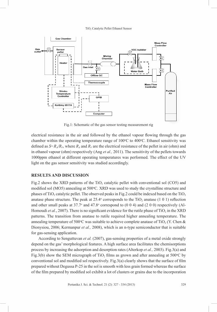
TiO2 Catalytic Pellet Ethanol Sensor
329Pertanika J. Sci. & Technol. 21 (2): 327 - 334 (2013)
electrical resistance in the air and followed by the ethanol vapour flowing through the gas chamber within the operating temperature range of 100oC to 400oC. Ethanol sensitivity was defined as S=RA/RV, where RA and RV are the electrical resistance of the pellet in air (ohm) and in ethanol vapour (ohm) respectively (Ang et al., 2011). The sensitivity of the pellets towards 1000ppm ethanol at different operating temperatures was performed. The effect of the UV light on the gas sensor sensitivity was studied accordingly.
RESULTS AND DISCUSSION
Fig.2 shows the XRD patterns of the TiO2 catalytic pellet with conventional sol (CO5) and modified sol (MO5) annealing at 500oC. XRD was used to study the crystalline structure and phases of TiO2 catalytic pellet. The observed peaks in Fig.2 could be indexed based on the TiO2 anatase phase structure. The peak at 25.4o corresponds to the TiO2 anatase (1 0 1) reflection and other small peaks at 37.7o and 47.8o correspond to (0 0 4) and (2 0 0) respectively (Al-Homoudi et al., 2007). There is no significant evidence for the rutile phase of TiO2 in the XRD patterns. The transition from anatase to rutile required higher annealing temperature. The annealing temperature of 500oC was suitable to achieve complete anatase of TiO2 (Y. Chen & Dionysiou, 2006; Kermanpur et al., 2008), which is an n-type semiconductor that is suitable for gas-sensing application.
According to Senguttuvan et al. (2007), gas-sensing properties of a metal oxide strongly depend on the gas’ morphological features. A high surface area facilitates the chemisorptions process by increasing the adsorption and desorption rates (Alterkop et al., 2003). Fig.3(a) and Fig.3(b) show the SEM micrograph of TiO2 films as grown and after annealing at 500oC by conventional sol and modified sol respectively. Fig.3(a) clearly shows that the surface of film prepared without Degussa P-25 in the sol is smooth with less grain formed whereas the surface of the film prepared by modified sol exhibit a lot of clusters or grains due to the incorporation
Fig.1: Schematic of the gas sensor testing measurement rig
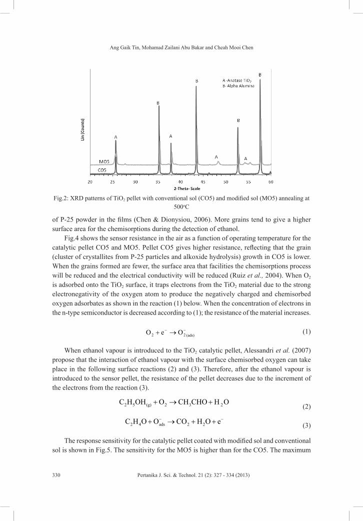
Ang Gaik Tin, Mohamad Zailani Abu Bakar and Cheah Mooi Chen
330 Pertanika J. Sci. & Technol. 21 (2): 327 - 334 (2013)
of P-25 powder in the films (Chen & Dionysiou, 2006). More grains tend to give a higher surface area for the chemisorptions during the detection of ethanol.
Fig.4 shows the sensor resistance in the air as a function of operating temperature for the catalytic pellet CO5 and MO5. Pellet CO5 gives higher resistance, reflecting that the grain (cluster of crystallites from P-25 particles and alkoxide hydrolysis) growth in CO5 is lower. When the grains formed are fewer, the surface area that facilities the chemisorptions process will be reduced and the electrical conductivity will be reduced (Ruiz et al., 2004). When O2 is adsorbed onto the TiO2 surface, it traps electrons from the TiO2 material due to the strong electronegativity of the oxygen atom to produce the negatively charged and chemisorbed oxygen adsorbates as shown in the reaction (1) below. When the concentration of electrons in the n-type semiconductor is decreased according to (1); the resistance of the material increases.
(ads)22 OeO −− →+ (1)
When ethanol vapour is introduced to the TiO2 catalytic pellet, Alessandri et al. (2007) propose that the interaction of ethanol vapour with the surface chemisorbed oxygen can take place in the following surface reactions (2) and (3). Therefore, after the ethanol vapour is introduced to the sensor pellet, the resistance of the pellet decreases due to the increment of the electrons from the reaction (3).
2 5 (g) 2 3 2C H OH O CH CHO H O+ → + (2)
2 4 ads 2 2C H O O CO H O e− −+ → + + (3)
The response sensitivity for the catalytic pellet coated with modified sol and conventional sol is shown in Fig.5. The sensitivity for the MO5 is higher than for the CO5. The maximum
Fig.2: XRD patterns of TiO2 pellet with conventional sol (CO5) and modified sol (MO5) annealing at 500oC
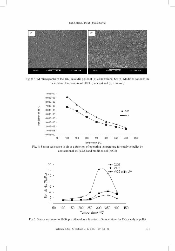
TiO2 Catalytic Pellet Ethanol Sensor
331Pertanika J. Sci. & Technol. 21 (2): 327 - 334 (2013)
(a) (b)
Fig.3: SEM micrographs of the TiO2 catalytic pellet of (a) Conventional Sol (b) Modified sol over the calcination temperature of 500oC (bars: (a) and (b) 1micron)
0,00E+00
1,00E+08
2,00E+08
3,00E+08
4,00E+08
5,00E+08
6,00E+08
7,00E+08
8,00E+08
9,00E+08
1,00E+09
50 100 150 200 250 300 350 400 450
Res
ista
nce
in a
ir R
a
Temperature (oC)
CO5
MO5
Fig. 4: Sensor resistance in air as a function of operating temperature for catalytic pellet by conventional sol (CO5) and modified sol (MO5)
Fig.5: Sensor response to 1000ppm ethanol as a function of temperature for TiO2 catalytic pellet
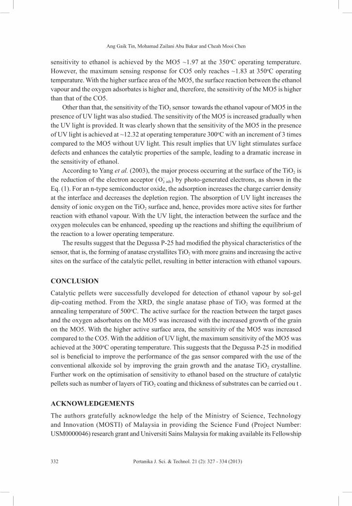
Ang Gaik Tin, Mohamad Zailani Abu Bakar and Cheah Mooi Chen
332 Pertanika J. Sci. & Technol. 21 (2): 327 - 334 (2013)
sensitivity to ethanol is achieved by the MO5 ~1.97 at the 350oC operating temperature. However, the maximum sensing response for CO5 only reaches ~1.83 at 350oC operating temperature. With the higher surface area of the MO5, the surface reaction between the ethanol vapour and the oxygen adsorbates is higher and, therefore, the sensitivity of the MO5 is higher than that of the CO5.
Other than that, the sensitivity of the TiO2 sensor towards the ethanol vapour of MO5 in the presence of UV light was also studied. The sensitivity of the MO5 is increased gradually when the UV light is provided. It was clearly shown that the sensitivity of the MO5 in the presence of UV light is achieved at ~12.32 at operating temperature 300oC with an increment of 3 times compared to the MO5 without UV light. This result implies that UV light stimulates surface defects and enhances the catalytic properties of the sample, leading to a dramatic increase in the sensitivity of ethanol.
According to Yang et al. (2003), the major process occurring at the surface of the TiO2 is the reduction of the electron acceptor ( 2O−
ads) by photo-generated electrons, as shown in the Eq. (1). For an n-type semiconductor oxide, the adsorption increases the charge carrier density at the interface and decreases the depletion region. The absorption of UV light increases the density of ionic oxygen on the TiO2 surface and, hence, provides more active sites for further reaction with ethanol vapour. With the UV light, the interaction between the surface and the oxygen molecules can be enhanced, speeding up the reactions and shifting the equilibrium of the reaction to a lower operating temperature.
The results suggest that the Degussa P-25 had modified the physical characteristics of the sensor, that is, the forming of anatase crystallites TiO2 with more grains and increasing the active sites on the surface of the catalytic pellet, resulting in better interaction with ethanol vapours.
CONCLUSION
Catalytic pellets were successfully developed for detection of ethanol vapour by sol-gel dip-coating method. From the XRD, the single anatase phase of TiO2 was formed at the annealing temperature of 500oC. The active surface for the reaction between the target gases and the oxygen adsorbates on the MO5 was increased with the increased growth of the grain on the MO5. With the higher active surface area, the sensitivity of the MO5 was increased compared to the CO5. With the addition of UV light, the maximum sensitivity of the MO5 was achieved at the 300oC operating temperature. This suggests that the Degussa P-25 in modified sol is beneficial to improve the performance of the gas sensor compared with the use of the conventional alkoxide sol by improving the grain growth and the anatase TiO2 crystalline. Further work on the optimisation of sensitivity to ethanol based on the structure of catalytic pellets such as number of layers of TiO2 coating and thickness of substrates can be carried ou t .
ACKNOWLEDGEMENTS
The authors gratefully acknowledge the help of the Ministry of Science, Technology and Innovation (MOSTI) of Malaysia in providing the Science Fund (Project Number: USM0000046) research grant and Universiti Sains Malaysia for making available its Fellowship

TiO2 Catalytic Pellet Ethanol Sensor
333Pertanika J. Sci. & Technol. 21 (2): 327 - 334 (2013)
scheme. The authors are also thankful to Inabata & Co. Ltd. for providing at no charge the Sumitomo Chemical alumina oxide powder AA05 that was used in this research.
REFERENCESAl-Homoudi, I. A., Thakur, J. S., Naik, R., Auner, G. W., & Newaz, G. (2007). Anatase TiO2 films
based CO gas sensor: Film thickness, substrate and temperature effects. Applied Surface Science, 253(21), 8607-8614.
Alessandri, I., Comini, E., Bontempi, E., Faglia, G., Depero, L. E., & Sberveglieri, G. (2007). Cr-inserted TiO2 thin films for chemical gas sensors. Sensors and Actuators B: Chemical, 128(1), 312-319.
Alterkop, B., Parkansky, A. N., Goldsmith, A. S., & Boxman, A. R. L. (2003). Effect of air annealing on opto-electrical properties of amorphous tin oxide films. Journal of Physics D: Applied Physics, 36, 552.
Ang, G. T., Toh, G. H., Bakar, M. Z. A., Abdullah, A. Z., & Othman, M. R. (2011). High sensitivity and fast response SnO2 and La-SnO2 catalytic pellet sensors in detecting volatile organic compounds. Process Safety and Environmental Protection, 89(3), 186-192.
Balasubramanian, G., Dionysiou, D. D., Suidan, M. T., Baudin, I., & Laine, J.-M. (2004). Evaluating the activities of immobilized TiO2 powder films for the photocatalytic degradation of organic contaminants in water. Applied Catalysis B: Environmental, 47(2), 73-84.
Chen, W., Zhang, J., Fang, Q., Li, S., Wu, J., Li, F., & Jiang, K. (2004). Sol-gel preparation of thick titania coatings aided by organic binder materials. Sensors and Actuators B: Chemical, 100(1-2), 195-199.
Chen, Y., & Dionysiou, D. D. (2006). TiO2 photocatalytic films on stainless steel: The role of Degussa P-25 in modified sol-gel methods. Applied Catalysis B: Environmental, 62(3-4), 255-264.
Garzella, C., Comini, E., Tempesti, E., Frigeri, C., & Sberveglieri, G. (2000). TiO2 thin films by a novel sol-gel processing for gas sensor applications. Sensors and Actuators B: Chemical, 68(1-3), 189-196.
Katarzyna Kozlowska, Anna Lukowiak, Andrzej Szczurek, Krzysztof Dudek, & Maruszewski, K. (2005). Sol-gel coatings for electrical gas sensors. Optica Applicata, 35(4), 783-790.
Kermanpur, A., Ghassemali, E., & Salemizadeh, S. (2008). Synthesis and characterisation of microporous titania membranes by dip-coating of anodised alumina substrates using sol-gel method. Journal of Alloys and Compounds, 461(1-2), 331-335.
Mohammadi, M. R., & Fray, D. J. (2007). Semiconductor TiO2-Ga2O3 thin film gas sensors derived from particulate sol-gel route. Acta Materialia, 55(13), 4455-4466.
Ruiz, A. M., Cornet, A., & Morante, J. R. (2004). Study of La and Cu influence on the growth inhibition and phase transformation of nano-TiO2 used for gas sensors. Sensors and Actuators B: Chemical, 100(1-2), 256-260.
Ruiz, A. M., Sakai, G., Cornet, A., Shimanoe, K., Morante, J. R., & Yamazoe, N. (2004). Microstructure control of thermally stable TiO2 obtained by hydrothermal process for gas sensors. Sensors and Actuators B: Chemical, 103(1-2), 312-317.
Senguttuvan, T. D., Rai, R., & Lakshmikumar, S. T. (2007). Gas sensing properties of lead doped tin oxide thick films. Materials Letters, 61(2), 582-584.
Takahashi, Y., & Matsuoka, Y. (1988). Dip-coating of TiO2 films using a sol derived from Ti(O-i-Pr)4-diethanolamine-H2O-i-PrOH system. Journal of Materials Science, 23(6), 2259-2266.

Ang Gaik Tin, Mohamad Zailani Abu Bakar and Cheah Mooi Chen
334 Pertanika J. Sci. & Technol. 21 (2): 327 - 334 (2013)
Taurino, A. M., Capone, S., Boschetti, A., Toccoli, T., Verucchi, R., Pallaoro, A., Iannotta, S. (2004). Titanium dioxide thin films prepared by seeded supersonic beams for gas sensing applications. Sensors and Actuators B: Chemical, 100(1-2), 177-184.
Yang, T., Lin, H., Wei, B., Wu, C., & Lin, C. (2003). UV enhancement of the gas sensing properties of nano-TiO2. Rev. Adv. Mater. Sci, 4, 48-54.
Zhang, X., Zhou, M., & Lei, L. (2005). Preparation of anatase TiO2 supported on alumina by different metal organic chemical vapor deposition methods. Applied Catalysis A: General, 282(1-2), 285-293.

Pertanika J. Sci. & Technol. 21 (2): 335 - 342 (2013)
SCIENCE & TECHNOLOGYJournal homepage: http://www.pertanika.upm.edu.my/
ISSN: 0128-7680 © 2013 Universiti Putra Malaysia Press.
Green Compression Strength of Tin Mine Tailing Sand for Green Sand Casting Mould
Azhar Abdullah1#*, Shamsuddin Sulaiman1, B. T. Hang Tuah Baharudin1, Mohd Khairol Anuar Mohd Ariffin1 and Thoguluva Raghvan Vijayaram2
1Department of Mechanical and Manufacturing Engineering, Faculty of Engineering, Universiti Putra Malaysia, 43400 Serdang, Selangor, Malaysia2Faculty of Engineering and Technology (FET), Multimedia University, Jalan Ayer Keroh Lama, Bukit Beruang, 75450, Melaka, Malaysia
ABSTRACT
Tailing sand is the residue mineral from tin extraction that contains between 94% and 99.5% silica, which can be used as moulding sand. It is found in abundance in the Kinta Valley in the state of Perak, Malaysia. Adequate water content and clay in moulding sand are important factors for better strength and casting quality of products made from tailing sand. Samples of tailing sand were investigated according to the American Foundrymen Society (AFS) standard. Cylindrical test pieces of Ø50 mm×50 mm in height from various sand-water ratios were compacted by applying three ramming blows of 6666g each using a Ridsdale-Dietert metric standard rammer. The specimens were tested for green compression strength using a Ridsdale-Dietert universal sand strength machine. Before the tests were conducted, moisture content of the tailing sand was measured using a moisture analyser. A mixture bonded with 8% clay possesses higher green compression strength compared to samples bonded with 4% clay. The results also show that in order to achieve maximum green compression strength, the optimum allowable moisture content for mixtures bonded with 8% clay is ranged between 3.75 and 6.5% and for mixtures bonded with 4% clay is 3-5.5%.
Keywords: Tailing sand, clay content, moisture content, green compression strength
Article history:Received: 19 October 2010Accepted: 3 June 2013
E-mail addresses: [email protected] (Azhar Abdullah), [email protected] (Shamsuddin Sulaiman), [email protected] (B. T. Hang Tuah Baharudin) [email protected] (Mohd Khairol Anuar Mohd Ariffin)*Corresponding Author#Author’s current affiliationDepartment of Mechanical Engineering, Politeknik Ungku Omar, 31400 Ipoh, Perak, Malaysia
INTRODUCTION
Tailing sand is the residue mineral from tin extraction, which contains between 94% and 99.5% silica and is found in abundance in the Kinta Valley in the state of Perak, Malaysia (Mackay, 2000). The objective of this study was to investigate the effects of moisture content on green compression strength of

Azhar Abdullah et al.
336 Pertanika J. Sci. & Technol. 21 (2): 335 - 342 (2013)
tailing sand from four identified tin-mining locations in Perak State for their potential for use in making green sand casting moulds. Samples were taken from Taiping (4.8648532N, 100.7061714E), Tronoh (4.4410824N, 101.0034513E), Batu Gajah (4.447543N, 101.061044E) and Tanjung Tualang (4.2995955N, 101.0588551E) (Google Earth, 2010).
The green compression strength of the tailing sand was studied to determine the maximum compressive stress that a mixture (tailing sand, clay and water) is capable of sustaining when prepared, rammed and tested according to standard procedure by the British Cast Iron Research Association (BCIRA). This is because sufficient strength of moulding sands is required during the withdrawal of the pattern from the mould and during pouring processes where the mould must retain shape independently without distortion or collapse. Usually, green compression strength for typical moulding sands run from about 30 to 150 kN/m2 (Loto, 1990). For instance, green sand properties for moulds prepared by jolt/squeeze machine are about 70-100 kN/m2 at 3-4% moisture and bonded with 5-5.5% clay (Heine et al., 1967).
Clay and water are the control additions in influencing the mechanical properties of moulding sand such as green compression strength. Incorrect amount of clay and water in the mould mixture can cause casting defects. When water is exposed to radiant heat from the metal, moisture is driven back from the mould surface, condensing in a wet, weak underlying layer that can easily fracture to produce expansion defects in castings such as scabs, rat-tails and buckles (Brown, 2000). Meanwhile, if clay content is higher in the mould mixture, the permeability and refractoriness of the moulding sand will decrease; thus, clay should be made in the order of 5-7% to produce moulds with better strength and higher permeability (Griffiths, 1990). Due to this fact, 4% and 8% clay was selected for this research.
Water present in the moulding sand to about 1.5% to 8%, activates the clay in the sand, causing the aggregate to develop plasticity and strength. Control of moisture in the moulding sand is necessary to develop the best properties (Heine et al., 1967). Suitable water content is the principal source of the strength and plasticity of moulding sand. Water in moulding sands is often referred to as tempering water. Too little water fails to develop adequate strength and plasticity. The clay adsorbs the water up to a limiting amount. Only the water rigidly held (adsorbed) by the clay appears to be effective in developing strength. This is due to increasing thickness of the water films, causing the clay to become less stiff and the sand grains to be held further apart (Webster et al., 1980). Additional water, however, can act as a lubricant, and makes the sand more plastic and more mouldable although strength may drop (Heine et al., 1967). Therefore, excess moisture must be avoided as it lowers permeability and increases the chance of a blown casting and may also lead to plasticity and deformation of the mould. Low permeability and green compression strength encourage entrapment of gas and the washing away of sand by molten metal (Griffiths, 1990).
Clay will act as a binder agent where it mixes with water to bind the sand particles and should be controlled due to the fineness of the particles. Clay can thus be made in the order of 5-7% to produce moulds with better strength. Increase in strength occurs because as the clay content of the moulding sand increases, its binding strength (properties) also increases which leads to increase in strength (Olasupo, 2009). The development of bond strength depends upon hydration of the clay; the green strength of a moulding mixture increases with water content

Green Compression Strength of Tin Mine Tailing Sand for Green Sand Casting Mould
337Pertanika J. Sci. & Technol. 21 (2): 335 - 342 (2013)
up to an optimum value determined by the proportion of clay. Beyond this value, additional free water causes the green strength to diminish (Beeley, 2001).
Fig.1 shows the relationship between clay content and addition of water on green compression strength for green sand casting moulds.
Fig.1: Relationship of clay content and percentage of tempering water on green compression strength from R. E. Grim and F. L. Cuthbert (Heine et al., 1967)
MATERIALS AND METHODS
A mixture was prepared by mixing 1000g of dry sand with 4% of bentonite clay by weight, and milled for 5 minutes. Then, water was added to the mixture starting with 20ml (approximately 2% moisture). The mixture was milled approximately for 3 minutes and then a sample was tested for moisture using a moisture analyser as shown in Fig.2.
The moulding sand mixture was tested for moisture using a moisture tester as shown in Fig.2. Approximately 10g of sand mixture was weighed out and put on the plate inside the tester. Then, the mixture was heated up and a reading was obtained within 3 minutes depending on moisture content of the mixtures.
A test piece of Ø50 mm×50 mm in height was prepared by weighing out specimens ranging from 138g to 150g depending on the sand/clay/water ratio. The mixture was then transferred to the Ridsdale-Dietert Metric Standard Rammer as shown in Fig.3 to form the test piece and was stripped using a strip block as shown in Fig.4. The test piece was then tested with a Ridsdale-Dietert universal sand strength machine as shown in Fig.5. After the readings were obtained, an addition of 20ml water was added until the moisture content reached approximately 9%, where the mixture became too wet and unmouldable. The procedure was repeated for a mixture bonded with 80g clay.

Azhar Abdullah et al.
338 Pertanika J. Sci. & Technol. 21 (2): 335 - 342 (2013)
Fig.2: Equipment for foundry sand testing. Moisture analyser(top left), Ridsdale-Dietert metric standard rammer (top right), strip block (bottom left) and Ridsdale-Dietert universal sand strength
(bottom right)
RESULTS AND DISCUSSION
The results of the tests on the green compression strength and moisture content of the tailing sand-clay mixture are presented in graphs in Fig.3 to Fig.6.
The results of the tests carried out showed that the green compression strength for all samples bonded with 4% and 8% bentonite clay increased incrementally with the increasing percentage of water added. The reason for this is that when the dried mixture (sand and clay) was mixed with water, the presence of water activated the clay, causing the aggregate to develop plasticity and strength. The strength had increased when the clay adsorbed the water up to its limiting amount. After reaching the maximum strength at 3.0-5.5% moisture for a mixture bonded with 4% clay and 3.75-6.5% moisture for a mixture bonded with 8% clay, the strength started to decrease. The was due to the additional water which acted as a lubricant and increased the thickness of the water films so that the clay became less stiff and was unable to hold the sand grains apart, thus making the mixture more plastic and causing the strength of the mixture to drop.
The results also show the comparison of green compression strength for mixture bonded with 4% clay and 8% clay. Mixture bonded with 8% clay had greater strength compared to mixture bonded with 4% clay. This can be observed from Fig.3 to Fig.6, where the strength curve for mixture bonded with 8% clay is higher than for 4% clay. This is because when the mixture contains more clay, more particle-bonding agent exists in the mixture, and this will increase the strength of the mixture when water is added.
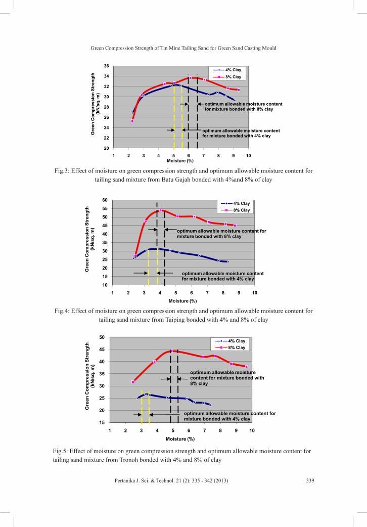
Green Compression Strength of Tin Mine Tailing Sand for Green Sand Casting Mould
339Pertanika J. Sci. & Technol. 21 (2): 335 - 342 (2013)
20
22
24
26
28
30
32
34
36
1 2 3 4 5 6 7 8 9 10
Gre
en C
ompr
essi
on S
tren
gth
(kN
/sq.
m)
Moisture (%)
4% Clay8% Clay
optimum allowable moisture content for mixture bonded with 8% clay
optimum allowable moisture content for mixture bonded with 4% clay
Fig.3: Effect of moisture on green compression strength and optimum allowable moisture content for tailing sand mixture from Batu Gajah bonded with 4%and 8% of clay
10
15
20
25
30
35
40
45
50
55
60
1 2 3 4 5 6 7 8 9 10
Gre
en C
ompr
essi
on S
tren
gth
(kN
/sq.
m)
Moisture (%)
4% Clay8% Clay
optimum allowable moisture content for mixture bonded with 8% clay
optimum allowable moisture content for mixture bonded with 4% clay
Fig.4: Effect of moisture on green compression strength and optimum allowable moisture content for tailing sand mixture from Taiping bonded with 4% and 8% of clay
15
20
25
30
35
40
45
50
1 2 3 4 5 6 7 8 9 10
Gre
en C
ompr
essi
on S
tren
gth
(kN
/sq.
m)
Moisture (%)
4% Clay8% Clay
optimum allowable moisture content for mixture bonded with 8% clay
optimum allowable moisture content for mixture bonded with 4% clay
Fig.5: Effect of moisture on green compression strength and optimum allowable moisture content for tailing sand mixture from Tronoh bonded with 4% and 8% of clay
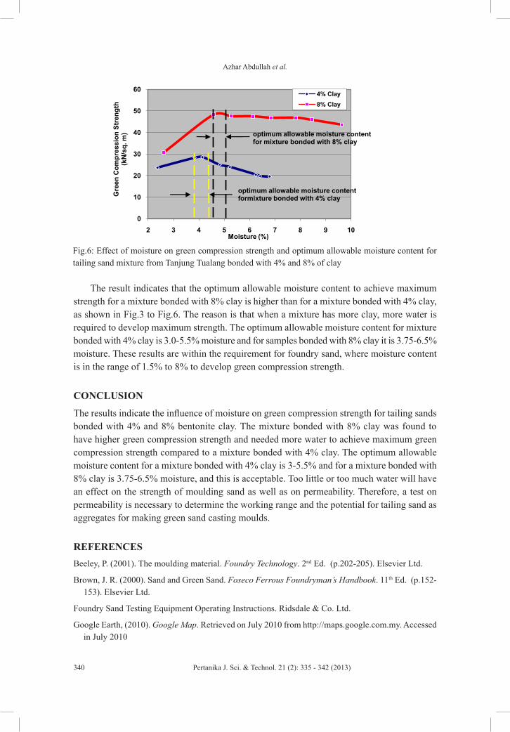
Azhar Abdullah et al.
340 Pertanika J. Sci. & Technol. 21 (2): 335 - 342 (2013)
The result indicates that the optimum allowable moisture content to achieve maximum strength for a mixture bonded with 8% clay is higher than for a mixture bonded with 4% clay, as shown in Fig.3 to Fig.6. The reason is that when a mixture has more clay, more water is required to develop maximum strength. The optimum allowable moisture content for mixture bonded with 4% clay is 3.0-5.5% moisture and for samples bonded with 8% clay it is 3.75-6.5% moisture. These results are within the requirement for foundry sand, where moisture content is in the range of 1.5% to 8% to develop green compression strength.
CONCLUSION
The results indicate the influence of moisture on green compression strength for tailing sands bonded with 4% and 8% bentonite clay. The mixture bonded with 8% clay was found to have higher green compression strength and needed more water to achieve maximum green compression strength compared to a mixture bonded with 4% clay. The optimum allowable moisture content for a mixture bonded with 4% clay is 3-5.5% and for a mixture bonded with 8% clay is 3.75-6.5% moisture, and this is acceptable. Too little or too much water will have an effect on the strength of moulding sand as well as on permeability. Therefore, a test on permeability is necessary to determine the working range and the potential for tailing sand as aggregates for making green sand casting moulds.
REFERENCESBeeley, P. (2001). The moulding material. Foundry Technology. 2nd Ed. (p.202-205). Elsevier Ltd.
Brown, J. R. (2000). Sand and Green Sand. Foseco Ferrous Foundryman’s Handbook. 11th Ed. (p.152-153). Elsevier Ltd.
Foundry Sand Testing Equipment Operating Instructions. Ridsdale & Co. Ltd.
Google Earth, (2010). Google Map. Retrieved on July 2010 from http://maps.google.com.my. Accessed in July 2010
0
10
20
30
40
50
60
2 3 4 5 6 7 8 9 10
Gre
en C
ompr
essi
on S
tren
gth
(kN
/sq.
m)
Moisture (%)
4% Clay8% Clay
optimum allowable moisture content for mixture bonded with 8% clay
optimum allowable moisture content formixture bonded with 4% clay
Fig.6: Effect of moisture on green compression strength and optimum allowable moisture content for tailing sand mixture from Tanjung Tualang bonded with 4% and 8% of clay

Green Compression Strength of Tin Mine Tailing Sand for Green Sand Casting Mould
341Pertanika J. Sci. & Technol. 21 (2): 335 - 342 (2013)
Griffiths, J. (1990). Minerals in Foundry Casting, Investment in The Future. Industrial Minerals (p. 39-51). London.
Heine, R. W., Loper, C. R. Jr., & Rosenthal, P. C. (1967). Moulding Sands. Principle of Metal Casting (p. 86-89). New York: McGraw-Hill Book Company.
Loto, C. A. (1990). Effect Of Cassava Flour And Coal Dust Additions On The Mechanical Properties Of Synthetic Moulding Sand. Journal of Applied Clay Science (p. 249-263). Elsevier Science Publisher B. V., Amsterdam.
Mackay, IMC., & Schnellmann. (2000). Final Report Of Mineral Processing Consultancy Silica Sand. (p. 6-12). International Mining Consultants Limited. Kuala Lumpur.
Olasupo O. A., Omotoyinbo, J. A. (2009). Moulding Properties of A Nigerian Silica–Clay Mixture for Foundry Use. Journal of Applied Clay Science (p. 244-247). Elsevier Science Publisher B.V., Amsterdam.
Webster, P. D. (1980). Sands and Binders. Fundamentals of Foundry Technology (p.116). Surrey: Portcullis Press.

Pertanika J. Sci. & Technol. 21 (2): 343 - 364 (2013)
SCIENCE & TECHNOLOGYJournal homepage: http://www.pertanika.upm.edu.my/
ISSN: 0128-7680 © 2013 Universiti Putra Malaysia Press.
Web-Based Decision Support System for Paddy Planting Management
C. Y. N. Norasma1,4, A. R. M. Shariff1,2*, E. Jahanshiri1, M. S. M. Amin2, S. Khairunniza-Bejo2 and A. R. Mahmud3
1Spatial and Numerical Modeling Laboratory, Institute of Advanced Technology (ITMA), Universiti Putra Malysia, 43400 Serdang, Selangor, Malaysia2Department of Biological and Agricultural Engineering, Faculty of Engineering, Universiti Putra Malaysia, 43400 Serdang, Selangor, Malaysia3Department of Civil Engineering, Faculty of Engineering, Universiti Putra Malaysia, 43400 Serdang, Selangor, Malaysia4Department of Agriculture Technology, Faculty of Agriculture, Universiti Putra Malaysia, 43400 Serdang, Selangor, Malaysia
ABSTRACT
Precision farming offers numerous benefits and advantages to the farming community for farm productivity improvement. Previous research has led to the development of the offline-based Precision Farmer©. Our current research extends further the previous work by developing a Web Paddy GIS©. The need for this arises due to limitations of Precision Farmer© such as portability, offline system accessibility and affordability by the end users, who include semi-literate farmers. This new system has been developed to function on Windows and Linux platforms. A user satisfaction assessment was conducted on website acceptability, and performance testing was made. This study demonstrates that Web Paddy GIS© can successfully run on both platforms. However, the Linux platform has proven to be superior to Windows, based on factors such as CPU usage, speed and user satisfaction. This paper presents a novel management tool of Web-based precision farming for the semi-literate paddy farming community of a developing country. The development of the Web Paddy GIS© is very useful for paddy farmers, farm managers, decision makers and researchers.
Keywords: Web GIS, precision farming, open source, Linux, Decision Support System
Article history:Received: 3 January 2011Accepted: 1 August 2012
E-mail addresses: [email protected] (C. Y. N. Norasma), [email protected] (A. R. M. Shariff), [email protected] (E. Jahanshiri), [email protected] (M. S. M. Amin), [email protected] (S. Khairunniza-Bejo), *Corresponding Author
INTRODUCTION
Background information
Site-specific crop management is a technique that is designed to utilise various technologies to provide spatially referenced information for

C. Y. N. Norasma, A. R. M. Shariff, E. Jahanshiri, M. S. M. Amin, S. Khairunniza-Bejo and A. R. Mahmud
344 Pertanika J. Sci. & Technol. 21 (2): 343 - 364 (2013)
better decision making. This management technique is also known as Precision Farming (PF) (Isgin et al., 2008; Auernhammer, 2001; Zhang et al., 2009; Camilli et al., 2007). Agricultural practices and profitability benefit through the utilisation of this technique. Many researchers have proven that it can assist to increase crop productivity. Population growth makes the highest demand on rice productivity and on the sustainability of global rice farming and supplies (Matsumura et al., 2009). Previously, Precision Farmer© was developed as a paddy Decision Support System (DSS) for managers and farmers (Azhan et al., 2008) to assist users in rice farming. DSS can help decision makers to aid their decision process (Antonopoulou et al., 2009). Precision Farmer© is very useful for users because it provides rich information on pests and diseases, scheduling of farming activities, farmer information and most importantly, contains a soil remedial fertiliser variability map function which provides a fertiliser application map. However, as the system is an offline system, it has major limitations as it requires installation of the software at the user’s local computer. Consequently, the motivation for the investigated solution in this paper is to have an online internet-based version of the previously developed Precision Farmer©.
Internet Geographic Information System (GIS) is a topic of growing interest and is highly beneficial for many applications such as forestry, aquaculture, road network and agriculture. In developing countries like Malaysia, the agricultural sector may greatly benefit from Information and Communication Technology (ICT). The opportunity for the use of ICT in precision farming is in addressing the problems of humankind (Schuler, 2007). In rural areas, agriculture productivity can be increased by using ICT (Thadaboina, 2009). Moreover, according to Simao et al. (2009), by using sophisticated ICT, we may not have to employ traditional computers. Web-based GIS provides farming information updates through online knowledge, consultation and spatial data (Jayasinghe & Machida, 2008; Kirilenko et al., 2007). Resource limitations such as time, data and communication can be resolved by using information technology and Spatial Decision Support System (SDSS) tools (Engel et al., 2003; Jarupathirun & Zahedi, 2007; Antonopoulou et al., 2009; Lemmens et al., 2007).
Open Source software development aimed at developing map-server applications using free software is now rooted in the GIS community (Steiniger and Hay, 2009). Web GIS technologies can provide data dissemination and have little or no online geoprocessing capabilities (Marcheggiani et al., 2009; Rao et al., 2007; Martino et al., 2007; Tsou, 2004). According to Flemons et al. (2007), the Web-based analysis in the raster data environment is slow and more complicated than a desktop upload. In this research we overcome this problem with the use of the Linux platform as it helps to analyse data faster. The development takes into account and fully utilises the open source and software. The merits of open source as we know are that it is free of charge, the coding can be shared with everyone in the world and it allows more support from others for any problem in the system.
Research on Web-based DSS
Antonopoulou et al. (2009) proposed a Web-based DSS capable of assisting farmers in the selection procedure of appropriate alternative crops. The crops involved were maize, soybean, sorghum, rapeseed and cardoon. They developed the DSS and offered its services via the
Web-Based Decision Support System for Paddy Planting Management
345Pertanika J. Sci. & Technol. 21 (2): 343 - 364 (2013)
internet. Zhang and Goddard (2007) presented an integrated method to help design and implement a Web-based DSS in a distributed environment. They focussed on the software’s architecture and framework. Zhang (2009) implemented a Web-based DSS as a component-based application that helps to transform a traditional DSS into a dynamic and evolvable distributed system. Martino et al. (2007) described a Web GIS application design approach that uses only basic functions like pan, zoom, data organisation and attribute table tool display.
Efficient management of paddy planting is hampered by lack of information. If the PF process is applied efficiently and effectively in the paddy field, it will be very beneficial in reducing cost, energy, time and environment. The Web Paddy GIS© is developed based on the PF principle and the database techniques accordingly so that users can easily access the information free of charge and apply the knowledge to their paddy field.
One of the major challenges in agriculture is to optimally plan cropping initiatives, fertiliser management, soil condition farming, and post harvesting. Analysis of spatial temporal variability in soil and yield data is generally performed with the help of relatively expensive commercial GIS software. Furthermore, it is costly to share the data and maintain the software. This research proposes a method to overcome this situation. Our approach allows centralised data management, data sharing between users and data evaluation using open source. Linux is one of the open source software. In this research we did for both platforms to make sure that by using open source, the performance of the system can be improved.
Web GIS DSS for paddy PF in Malaysia is a new field and no local references are available. Many researchers have developed web GIS but most of them do not use open source software; for example, Deepak et al. (2008) and Rowshan et al. (2008) used commercial software which is very costly and requires an annual license. Furthermore their work focussed on the irrigation aspects of paddy farming. Another is the Rice Irrigation Management Information System (RIMIS) developed by Rowshon et al. (2008). It was originally developed for allocation of irrigation water. It is an offline system that focusses only on irrigation and uses the commercial software, ArcMap. It is a very good system but it needs to be improved in terms of cost effectiveness because it uses commercial software. Another system for rice application is the Web-based Paddy Irrigation Productivity Assessment (WEB-PIPA) that was developed by Deepak et al. (2008). It focusses on a database for online irrigation. WEP PIPA involves spatial data but does not perform internet mapping. This is a system for database management of irrigation. The Web Paddy GIS© makes important improvements through the use of DSS, open source software and operating in the Linux environment.
Decision Support System for Precision Farming
DSS can perform analysis and provide a decision using computer-based tools (Matthews et al., 2008). There are many previously documented examples of DSS applied to crop production. Some of these are: Major Fields Crops (MAFIS-DSS) (Antonopoulou et al., 2009), a web-based decision support tool and zone mapping application for precision farming (ZoneMap) (Zhang et al., 2009), Worlds Inventory of Soil Emission Potentials (WISE) (Gijsman et al., 2007), Integrated Water Resource Management (IWRM) (Awad et al., 2009) and Web-based National Agricultural Decision Support System (NADSS) (Zhang & Goddard, 2007). These DSSs are
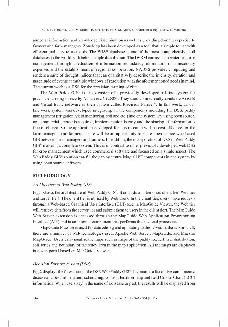
C. Y. N. Norasma, A. R. M. Shariff, E. Jahanshiri, M. S. M. Amin, S. Khairunniza-Bejo and A. R. Mahmud
346 Pertanika J. Sci. & Technol. 21 (2): 343 - 364 (2013)
aimed at information and knowledge dissemination as well as providing domain expertise to farmers and farm managers. ZoneMap has been developed as a tool that is simple to use with efficient and easy-to-use tools. The WISE database is one of the most comprehensive soil databases in the world with better sample distribution. The IWRM can assist in water resource management through a reduction of information redundancy, elimination of unnecessary expenses and the establishment of regional cooperation. NADSS provides computing and renders a suite of drought indices that can quantitatively describe the intensity, duration and magnitude of events at multiple windows of resolution with the aforementioned needs in mind. The current work is a DSS for the precision farming of rice.
The Web Paddy GIS© is an extension of a previously developed off-line system for precision farming of rice by Azhan et al. (2008). They used commercially available ArcGIS and Visual Basic software in their system called Precision Farmer©. In this work, an on-line work system was developed integrating all the components including PF, DSS, paddy management (irrigation, yield monitoring, soil and etc.) into one system. By using open source, no commercial license is required, implementation is easy and the sharing of information is free of charge. So the application developed for this research will be cost effective for the farm managers and farmers. There will be an opportunity to share open source web-based GIS between farm managers and farmers. In addition, the incorporation of DSS in Web Paddy GIS© makes it a complete system. This is in contrast to other previously developed web DSS for crop management which used commercial software and focussed on a single aspect. The Web Paddy GIS© solution can fill the gap by centralising all PF components in one system by using open source software.
METHODOLOGY
Architecture of Web Paddy GIS©
Fig.1 shows the architecture of Web Paddy GIS©. It consists of 3 tiers (i.e. client tier, Web tier and server tier). The client tier is utilised by Web users. In the client tier, users make requests through a Web-based Graphical User Interface (GUI) (e.g. in MapGuide Viewer, the Web tier will retrieve data from the server tier and submit them to users in the client tier). The MapGuide Web Server extension is accessed through the MapGuide Web Application Programming Interface (API) and is an internal component that performs the backend processes.
MapGuide Maestro is used for data editing and uploading to the server. In the server itself, there are a number of Web technologies used, Apache Web Server, MapGuide, and Maestro MapGuide. Users can visualise the maps such as maps of the paddy lot, fertiliser distribution, soil series and boundary of the study area in the map application. All the maps are displayed in a web portal based on MapGuide Viewer.
Decision Support System (DSS)
Fig.2 displays the flow chart of the DSS Web Paddy GIS©. It contains a list of five components: disease and pest information, scheduling, control, fertiliser map and Leaf Colour Chart (LCC) information. When users key in the name of a disease or pest, the results will be displayed from
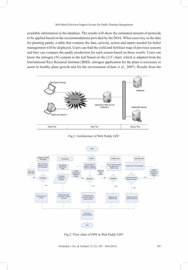
Web-Based Decision Support System for Paddy Planting Management
347Pertanika J. Sci. & Technol. 21 (2): 343 - 364 (2013)
available information in the database. The results will show the estimated amount of pesticide to be applied based on the recommendations provided by the DOA. When users key in the date for planting paddy, a table that contains the date, activity, action and inputs needed for better management will be displayed. Users can find the yield and fertiliser map of previous seasons and they can compare the paddy production for each season based on these results. Users can know the nitrogen (N) content in the leaf based on the LCC chart, which is adapted from the International Rice Research Institute (IRRI). nitrogen application for the plant is necessary to assist in healthy plant growth and for the environment (Islam et al., 2007). Results from the
Fig.1: Architecture of Web Paddy GIS©
Available?
key in the right name
Result table with date, action, activity
and input
Available?
Key in Name of disease, fungus or weed for controling
Contact developer to update the
system
Available?
Yield map and fertilizer map
key in the right
name
Does the leaf color match the chart?
Identify the chart and the value of N
Disease and Pest information Scheduling Control Fertilizer map Leaf color chart
Start
Key in name of disease or pest for information
Result table and picture
No
Action and recommendation
End
Key date for planting the
paddy
No
Result table with how, when where to
apply the input
No
Key in the plot number for yield map or
fertilizer map
Search for LCC information
Contact developer to update the
system
NoCalculate
the date for planting
Yes Yes YesYes
Fig.2: Flow chart of DSS in Web Paddy GIS©
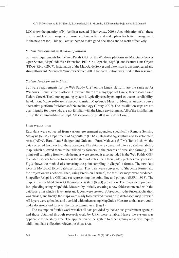
C. Y. N. Norasma, A. R. M. Shariff, E. Jahanshiri, M. S. M. Amin, S. Khairunniza-Bejo and A. R. Mahmud
348 Pertanika J. Sci. & Technol. 21 (2): 343 - 364 (2013)
LCC show the quantity of N- fertiliser needed (Islam et al., 2008). A combination of all these results enables the managers or farmers to take action and make plans for better management in the next season. This will assist them to make good decisions and to work effectively.
System development in Windows platform
Software requirements for the Web Paddy GIS© on the Windows platform are MapGuide Server Open Source, MapGuide Web Extension, PHP 5.2.1, Apache, MySQL and Feature Data Object (FDO) (Rbray, 2007). Installation of the MapGuide Server and Extension is uncomplicated and straightforward. Microsoft Windows Server 2003 Standard Edition was used in this research.
System development in Linux
Software requirements for the Web Paddy GIS© on the Linux platform are the same as for Windows. Linux is free platform. However, there are many types of Linux; this research used Fedora Core 6. The Linux operating system is typically used by enterprises due to its reliability. In addition, Mono software is needed to install MapGuide Maestro. Mono is an open source alternative platform for Microsoft.Net technology (Rbray, 2007). The installation steps are not user-friendly for those who are not familiar with the Linux environment. All of the installations utilise the command-line prompt. All software is installed in Fedora Core 6.
Data preparation
Raw data were collected from various government agencies, specifically Remote Sensing Malaysia (RSM), Department of Agriculture (DOA), Integrated Agriculture and Development Area (IADA), Barat Laut Selangor and Universiti Putra Malaysia (UPM). Table 1 shows the data collected from each of these agencies. The data were converted into a spatial variability map, which allowed them to be utilised by farmers in the process of precision farming. The point-soil sampling from which the maps were created is also included in the Web Paddy GIS© to enable users or farmers to access the status of nutrients in their paddy plots for every season. Fig.3 shows the method of converting the point sampling to Shapefile format. The raw data were in Microsoft Excel database format. This data were converted to Shapefile format and the projection was defined. Then, using Precision Farmer©, the fertiliser maps were produced. Shapefile (*.shp) is a GIS data set representing the point, line and polygon (ESRI, 1998). The map is in a Rectified Skew Orthomorphic system (RSO) projection. The maps were prepared for uploading using MapGuide Maestro by initially creating a new folder connected with the database, after which a layer, map and layout were created. Subsequently, the fusion application was chosen, and finally, the maps were ready to be viewed through the Web-based map browser. All layers were uploaded and overlaid with others using MapGuide Maestro so that users could make decisions and forecast the forthcoming yield (Fig.1).
The assumption for this work was that all data provided by the various government agencies and those obtained through research work by UPM were reliable. Hence the system was applicable to the study area. The application of the system to other granny areas will require additional data collection relevant to those area.

Web-Based Decision Support System for Paddy Planting Management
349Pertanika J. Sci. & Technol. 21 (2): 343 - 364 (2013)
TABLE 1 Sources for data acquisition
No Type of data Source of data1 Boundary Sawah Sempadan map MRSA, 20072 Block C map UPM, 20073 Paddy lot map UPM, 20074 ECa Zone map UPM, 20075 Soil Sampling map UPM, 20076 Fertiliser map UPM, 20087 Soil Series map DOA, 20078 Rice Check information IADA, 20079 Pest and Disease information DOA, 200710 Controlling pests and Diseases DOA, 200711 LCC information MRSA, 200712 Yield Value IADA, 200713 Farmers information IADA, 200714 Yield map UPM, 2007
MS EXCEL
ARCMAP
PRECISION FARMER©
MAPGUIDE MAESTRO
Fig.3: Data acquisition process
Performance evaluation on Linux and Windows
Although Linux is open source and free whereas Windows is a commercial product that is widely used, we wanted to test the implications of using Linux on the performance of the system. Testing was performed on the same machine and both operating systems were run in Virtual Machine Software (VMware) mode. The testing involved “zoom in”, “zoom out”, “zoom rectangle”, “pan”, “select” and “measure” functions. A good Web-based GIS application
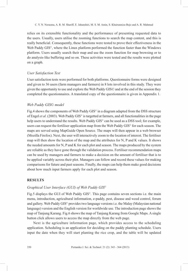
C. Y. N. Norasma, A. R. M. Shariff, E. Jahanshiri, M. S. M. Amin, S. Khairunniza-Bejo and A. R. Mahmud
350 Pertanika J. Sci. & Technol. 21 (2): 343 - 364 (2013)
relies on its extensible functionality and the performance of presenting requested data to the users. Usually, users utilise the zooming functions to search the map content, and this is really beneficial. Consequently, these functions were tested to prove their effectiveness in the Web Paddy GIS©, where the Linux platform performed the function faster than the Windows platform. Users usually search their map and use the zoom function for map browsing or to do analysis-like buffering and so on. These activities were tested and the results were plotted on a graph.
User Satisfaction Test
User satisfaction tests were performed for both platforms. Questionnaire forms were designed and given to 36 users (farm managers and farmers) in 8 lots involved in this study. They were given the opportunity to use and explore the Web Paddy GIS© and at the end of the session they completed the questionnaires. A translated copy of the questionnaire is given in Appendix 1.
Web Paddy GIS© model
Fig.4 shows the components of Web Paddy GIS© in a diagram adapted from the DSS structure of Engel et al. (2003). Web Paddy GIS© is targetted at farmers, and all functionalities in the page help users to understand the results. Web Paddy GIS© can be used as a DSS tool; for example, users can request the fertiliser application map from the Web Paddy GIS© for each season. The maps are served using MapGuide Open Source. The maps will then appear in a web browser (Mozilla Firefox). Next, the user will interactively zoom to the location of interest. The fertiliser map will then show the location of the map and the attributes for N, P and K values. It shows the needed amounts for N, P and K for each plot and season. The maps produced by the system are reliable as they have gone through the validation process. Fertiliser recommendation maps can be used by managers and farmers to make a decision on the amount of fertiliser that is to be applied variably across their plot. Managers can follow and record these values for making comparisons for future and past seasons. Finally, the maps can help them make good decisions about how much input farmers apply for each plot and season.
RESULTS
Graphical User Interface (GUI) of Web Paddy GIS©
Fig.5 displays the GUI of Web Paddy GIS©. This page contains seven sections i.e. the main menu, introduction, agricultural information, e-paddy, pest, disease and weed control, forum and gallery. Web Paddy GIS© provides two language versions i.e. the Malay (Malaysian national language) version and the English version for worldwide use. The introduction page shows the map of Tanjung Karang. Fig.6 shows the map of Tanjung Karang from Google Maps. A single button click allows users to access the map directly from the web page.
Next is the agriculture information page, which provides access to the scheduling application. Scheduling is an application for deciding on the paddy planting schedule. Users input the date when they will start planting the rice crop, and the table will be updated

Web-Based Decision Support System for Paddy Planting Management
351Pertanika J. Sci. & Technol. 21 (2): 343 - 364 (2013)
Fig.4: Description of Web Paddy GIS© as a DSS
Fig.5: The main menu for Web Paddy GIS© (English version)
Fig.6: Map of Tanjung Karang from Google Map
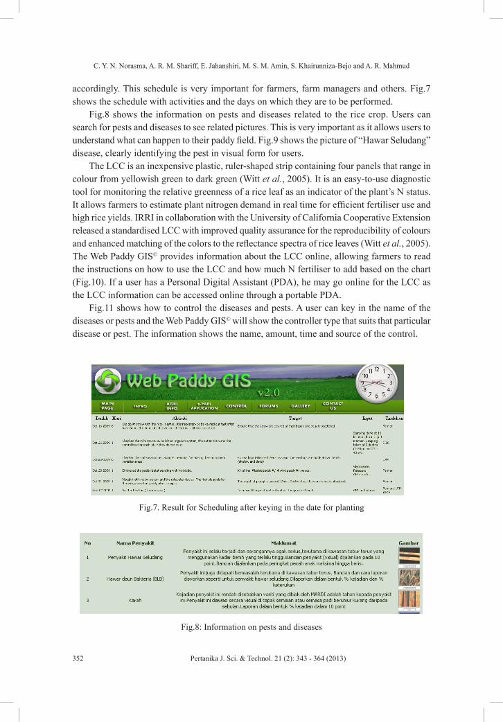
C. Y. N. Norasma, A. R. M. Shariff, E. Jahanshiri, M. S. M. Amin, S. Khairunniza-Bejo and A. R. Mahmud
352 Pertanika J. Sci. & Technol. 21 (2): 343 - 364 (2013)
accordingly. This schedule is very important for farmers, farm managers and others. Fig.7 shows the schedule with activities and the days on which they are to be performed.
Fig.8 shows the information on pests and diseases related to the rice crop. Users can search for pests and diseases to see related pictures. This is very important as it allows users to understand what can happen to their paddy field. Fig.9 shows the picture of “Hawar Seludang” disease, clearly identifying the pest in visual form for users.
The LCC is an inexpensive plastic, ruler-shaped strip containing four panels that range in colour from yellowish green to dark green (Witt et al., 2005). It is an easy-to-use diagnostic tool for monitoring the relative greenness of a rice leaf as an indicator of the plant’s N status. It allows farmers to estimate plant nitrogen demand in real time for efficient fertiliser use and high rice yields. IRRI in collaboration with the University of California Cooperative Extension released a standardised LCC with improved quality assurance for the reproducibility of colours and enhanced matching of the colors to the reflectance spectra of rice leaves (Witt et al., 2005). The Web Paddy GIS© provides information about the LCC online, allowing farmers to read the instructions on how to use the LCC and how much N fertiliser to add based on the chart (Fig.10). If a user has a Personal Digital Assistant (PDA), he may go online for the LCC as the LCC information can be accessed online through a portable PDA.
Fig.11 shows how to control the diseases and pests. A user can key in the name of the diseases or pests and the Web Paddy GIS© will show the controller type that suits that particular disease or pest. The information shows the name, amount, time and source of the control.
Fig.7. Result for Scheduling after keying in the date for planting
Fig.8: Information on pests and diseases

Web-Based Decision Support System for Paddy Planting Management
353Pertanika J. Sci. & Technol. 21 (2): 343 - 364 (2013)
Fig.9: Picture of pest and disease
Fig.10: Leaf Colour Chart as a guide for farmers to check nitrogen deficiency
Fig.11: Choosing the type of control for pest

C. Y. N. Norasma, A. R. M. Shariff, E. Jahanshiri, M. S. M. Amin, S. Khairunniza-Bejo and A. R. Mahmud
354 Pertanika J. Sci. & Technol. 21 (2): 343 - 364 (2013)
Table 2 shows the description of each section. Web Paddy GIS© has proven benefits for management and has the potential to assist farmers to increase production efficiency provided all steps are completed. The GIS Info module is an application map from soil sampling and season yield. Users can compare their yield from one season to another. Information also plays a central role in the DSS process (Simao et al., 2009).
Fig.12 also displays the map browser which allows users to browse (zoom in/out/pan) maps, change displayed layers and perform measurements and buffering. Users can view their map by clicking on the box of the menu layers. Users can also check the attributes by clicking on the right-hand side. This will show the attributes for each layer selected with the fertiliser map attributes so that users may see precisely how much fertiliser to apply and where to apply it. This will optimise their inputs, leading to efficient plot management.
One of the advantages of Web Paddy GIS© is the existence of a website forum. The forum provides an opportunity for users, especially farm managers and farmers, to share their experience and knowledge. These facilities also allow users to interact, communicate and network with others. Users are required to register in the forum, after which they may login using their username and password. They may create topics, promote their farms and upload photos in the forum. The topics are followed by experts who can provide guidance for farmers and managers.
TABLE 2 Description of each section
No Section Description1 Main menu Welcoming notes
Website links to other organisations like DOA, RSM and MARDI2 Introduction Concept of PF
Map of Tanjung Karang using Google Earth applicationAcknowledgments
3 Agricultural information
Crop scheduling for better managementPest and disease informationPest and disease pictures
4 E-paddy Map (Spatial data), fertiliser map, boundary map, soil series map, soil sampling mapYield information for each season, name, no of plot and personal detailsUser manual for paddy plantingSoil Sampling MapLCC information and how to use the LCCYield map for every season and for all criteria
5 Controlling pests and diseases
How to control fungus, weeds and pests
6 Gallery Photo gallery7 Forum Forum discussion for users to interact with each other. They can also
share their paddy planting experience and knowledge.
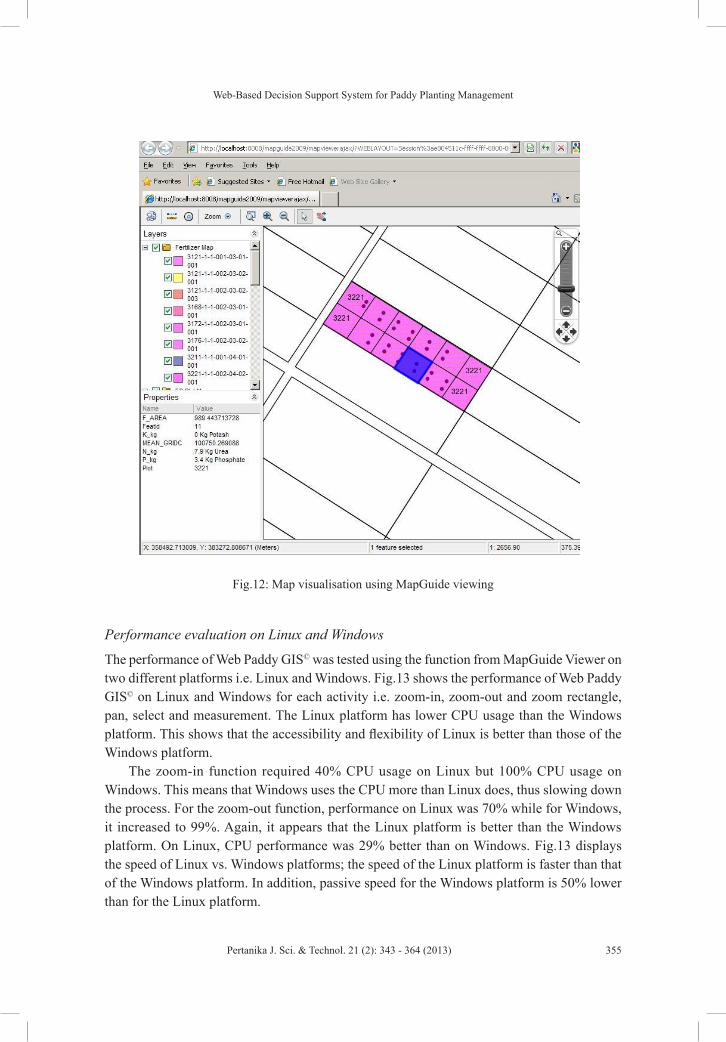
Web-Based Decision Support System for Paddy Planting Management
355Pertanika J. Sci. & Technol. 21 (2): 343 - 364 (2013)
Performance evaluation on Linux and Windows
The performance of Web Paddy GIS© was tested using the function from MapGuide Viewer on two different platforms i.e. Linux and Windows. Fig.13 shows the performance of Web Paddy GIS© on Linux and Windows for each activity i.e. zoom-in, zoom-out and zoom rectangle, pan, select and measurement. The Linux platform has lower CPU usage than the Windows platform. This shows that the accessibility and flexibility of Linux is better than those of the Windows platform.
The zoom-in function required 40% CPU usage on Linux but 100% CPU usage on Windows. This means that Windows uses the CPU more than Linux does, thus slowing down the process. For the zoom-out function, performance on Linux was 70% while for Windows, it increased to 99%. Again, it appears that the Linux platform is better than the Windows platform. On Linux, CPU performance was 29% better than on Windows. Fig.13 displays the speed of Linux vs. Windows platforms; the speed of the Linux platform is faster than that of the Windows platform. In addition, passive speed for the Windows platform is 50% lower than for the Linux platform.
Fig.12: Map visualisation using MapGuide viewing
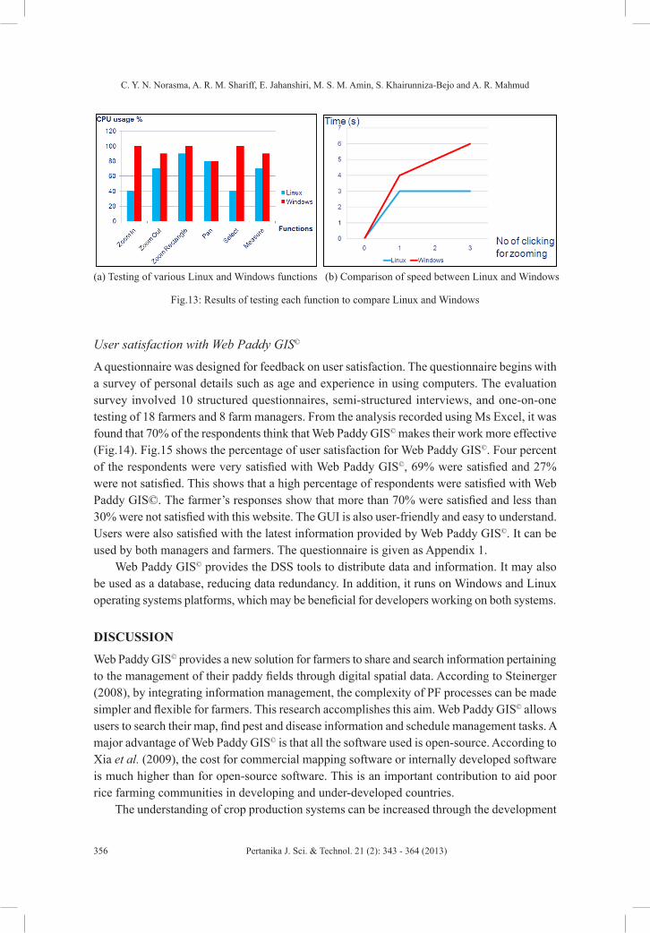
C. Y. N. Norasma, A. R. M. Shariff, E. Jahanshiri, M. S. M. Amin, S. Khairunniza-Bejo and A. R. Mahmud
356 Pertanika J. Sci. & Technol. 21 (2): 343 - 364 (2013)
User satisfaction with Web Paddy GIS©
A questionnaire was designed for feedback on user satisfaction. The questionnaire begins with a survey of personal details such as age and experience in using computers. The evaluation survey involved 10 structured questionnaires, semi-structured interviews, and one-on-one testing of 18 farmers and 8 farm managers. From the analysis recorded using Ms Excel, it was found that 70% of the respondents think that Web Paddy GIS© makes their work more effective (Fig.14). Fig.15 shows the percentage of user satisfaction for Web Paddy GIS©. Four percent of the respondents were very satisfied with Web Paddy GIS©, 69% were satisfied and 27% were not satisfied. This shows that a high percentage of respondents were satisfied with Web Paddy GIS©. The farmer’s responses show that more than 70% were satisfied and less than 30% were not satisfied with this website. The GUI is also user-friendly and easy to understand. Users were also satisfied with the latest information provided by Web Paddy GIS©. It can be used by both managers and farmers. The questionnaire is given as Appendix 1.
Web Paddy GIS© provides the DSS tools to distribute data and information. It may also be used as a database, reducing data redundancy. In addition, it runs on Windows and Linux operating systems platforms, which may be beneficial for developers working on both systems.
DISCUSSION
Web Paddy GIS© provides a new solution for farmers to share and search information pertaining to the management of their paddy fields through digital spatial data. According to Steinerger (2008), by integrating information management, the complexity of PF processes can be made simpler and flexible for farmers. This research accomplishes this aim. Web Paddy GIS© allows users to search their map, find pest and disease information and schedule management tasks. A major advantage of Web Paddy GIS© is that all the software used is open-source. According to Xia et al. (2009), the cost for commercial mapping software or internally developed software is much higher than for open-source software. This is an important contribution to aid poor rice farming communities in developing and under-developed countries.
The understanding of crop production systems can be increased through the development
(a) Testing of various Linux and Windows functions (b) Comparison of speed between Linux and Windows
Fig.13: Results of testing each function to compare Linux and Windows
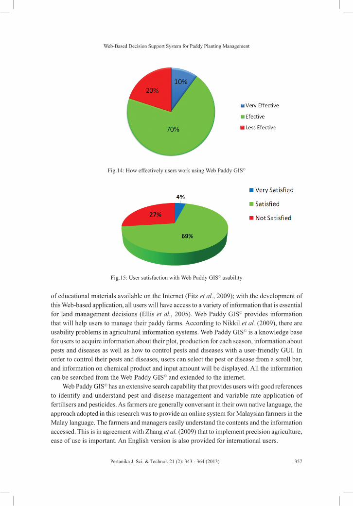
Web-Based Decision Support System for Paddy Planting Management
357Pertanika J. Sci. & Technol. 21 (2): 343 - 364 (2013)
of educational materials available on the Internet (Fitz et al., 2009); with the development of this Web-based application, all users will have access to a variety of information that is essential for land management decisions (Ellis et al., 2005). Web Paddy GIS© provides information that will help users to manage their paddy farms. According to Nikkil et al. (2009), there are usability problems in agricultural information systems. Web Paddy GIS© is a knowledge base for users to acquire information about their plot, production for each season, information about pests and diseases as well as how to control pests and diseases with a user-friendly GUI. In order to control their pests and diseases, users can select the pest or disease from a scroll bar, and information on chemical product and input amount will be displayed. All the information can be searched from the Web Paddy GIS© and extended to the internet.
Web Paddy GIS© has an extensive search capability that provides users with good references to identify and understand pest and disease management and variable rate application of fertilisers and pesticides. As farmers are generally conversant in their own native language, the approach adopted in this research was to provide an online system for Malaysian farmers in the Malay language. The farmers and managers easily understand the contents and the information accessed. This is in agreement with Zhang et al. (2009) that to implement precision agriculture, ease of use is important. An English version is also provided for international users.
Fig.14: How effectively users work using Web Paddy GIS©
Fig.15: User satisfaction with Web Paddy GIS© usability
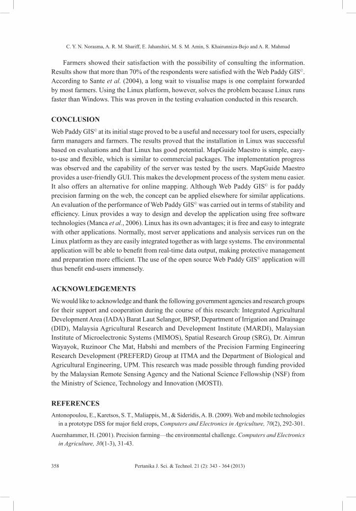
C. Y. N. Norasma, A. R. M. Shariff, E. Jahanshiri, M. S. M. Amin, S. Khairunniza-Bejo and A. R. Mahmud
358 Pertanika J. Sci. & Technol. 21 (2): 343 - 364 (2013)
Farmers showed their satisfaction with the possibility of consulting the information. Results show that more than 70% of the respondents were satisfied with the Web Paddy GIS©. According to Sante et al. (2004), a long wait to visualise maps is one complaint forwarded by most farmers. Using the Linux platform, however, solves the problem because Linux runs faster than Windows. This was proven in the testing evaluation conducted in this research.
CONCLUSION
Web Paddy GIS© at its initial stage proved to be a useful and necessary tool for users, especially farm managers and farmers. The results proved that the installation in Linux was successful based on evaluations and that Linux has good potential. MapGuide Maestro is simple, easy-to-use and flexible, which is similar to commercial packages. The implementation progress was observed and the capability of the server was tested by the users. MapGuide Maestro provides a user-friendly GUI. This makes the development process of the system menu easier. It also offers an alternative for online mapping. Although Web Paddy GIS© is for paddy precision farming on the web, the concept can be applied elsewhere for similar applications. An evaluation of the performance of Web Paddy GIS© was carried out in terms of stability and efficiency. Linux provides a way to design and develop the application using free software technologies (Manca et al., 2006). Linux has its own advantages; it is free and easy to integrate with other applications. Normally, most server applications and analysis services run on the Linux platform as they are easily integrated together as with large systems. The environmental application will be able to benefit from real-time data output, making protective management and preparation more efficient. The use of the open source Web Paddy GIS© application will thus benefit end-users immensely.
ACKNOWLEDGEMENTS
We would like to acknowledge and thank the following government agencies and research groups for their support and cooperation during the course of this research: Integrated Agricultural Development Area (IADA) Barat Laut Selangor, BPSP, Department of Irrigation and Drainage (DID), Malaysia Agricultural Research and Development Institute (MARDI), Malaysian Institute of Microelectronic Systems (MIMOS), Spatial Research Group (SRG), Dr. Aimrun Wayayok, Ruzinoor Che Mat, Habshi and members of the Precision Farming Engineering Research Development (PREFERD) Group at ITMA and the Department of Biological and Agricultural Engineering, UPM. This research was made possible through funding provided by the Malaysian Remote Sensing Agency and the National Science Fellowship (NSF) from the Ministry of Science, Technology and Innovation (MOSTI).
REFERENCESAntonopoulou, E., Karetsos, S. T., Maliappis, M., & Sideridis, A. B. (2009). Web and mobile technologies
in a prototype DSS for major field crops, Computers and Electronics in Agriculture, 70(2), 292-301.
Auernhammer, H. (2001). Precision farming—the environmental challenge. Computers and Electronics in Agriculture, 30(1-3), 31-43.

Web-Based Decision Support System for Paddy Planting Management
359Pertanika J. Sci. & Technol. 21 (2): 343 - 364 (2013)
Awad, M., Mohamad, K., & Talal, D. (2009). Web-Based Meta-database and its Role in improving Water Resources Management in the Mediterranean Basin. Water Resources Management Journal, 23(13), 2669-2680.
Azhan, Shariff, A. R. M., Amin, M. S. M., Rahim, A. A., Jahanshiri, E., & Norasma, C. Y. N. (2008). GIS based system for Paddy Precision Farmin. pp. 417-422. Paper presented in AFITA in World Conference on Agricultural Information and IT, Tokyo University of Agriculture, Atsugi, 2008, Japan.
Camilli, A., Cugnasca, C. E., Saraiva, A. M., Hirakawa, A. R., & Corrêa, P. L. P. (2007). From wireless sensors to field mapping: Anatomy of an application for precision agriculture. Computers and Electronics in Agriculture, 58(1), 25-36.
Deepak, T. J., Amin, M.S.M., Shariff, A. R. M., & Ramli, A. R. (2008). Web based paddy irrigation productivity assessment (WEB-PIPA). Paper presented at Consulting Workshop on Paddy Precision Farming, Malaysia Agro Exposition Park Serdang, Malaysia. August 2008.
Ellis, E. A., Nair, P. K. R., & Jeswani, S. D. (2005). Development of a Web-based application for agroforestry planning and tree selection. Computers and Electronics in Agriculture, 49(1), 129-141.
Engel, B. A., Choi, J.-Y., Harbor, J., & Pandey, S. (2003). Web-based DSS for hydrologic impact evaluation of small watershed land use changes. Computers and Electronics in Agriculture, 39(3), 241-249.
ESRI. (1998). ESRI Shapefile Technical Description. Retrieved on November 15, 2009 from http://www.esri.com/library/whitepapers/pdfs/shapefile.pdf
Fitz, E., Kubota, C., Giacomelli, G. A., Tignor, M. E., Wilson, S. B., & McMahon, M. (2009). Dynamic modeling and simulation of greenhouse environments under several scenarios: A Web-based application. Computers and Electronics in Agriculture, 70(1), 105-116.
Flemons, P., Guralnick, R., Krieger, J., Ranipeta, A., & Neufeld, D. (2007). A Web-based GIS tool for exploring the world’s biodiversity: The Global Biodiversity Information Facility Mapping and Analysis Portal Application (GBIF-MAPA). Ecological Informatics, 2(1), 49-60.
Gijsma, A. J., Philip, K. T., &Gerrit, H. (2007). Using the WISE database to parameterize soil inputs for crop simulation models. Computers and Electronics in Agriculture, 56(2), 85-100.
Isgin, T., Bilgic, A., Forster, D. L., & Batte, M. T. (2008). Using count data models to determine the factors affecting farmers’ quantity decisions of precision farming technology adoption. Computers and Electronics in Agriculture, 62(2), 231-242.
Islam, Z., Bagchi, B., & Hossain, M. (2007). Adoption of leaf color chart for nitrogen use efficiency in rice: Impact assessment of a farmer-participatory experiment in West Bengal, India. Field Crops Research, 103(1), 70-75.
Jarupathirun, S., & Zahedi, F. (2007). Exploring the influence of perceptual factors in the success of Web-based spatial DSS. Decision Support Systems, 43(3), 933-951.
Jayasinghe, P., & Machida, T. (2008). Web-Based GIS Online Consulting System with Crop-Land Suitability Identification. Agricultural Information Research, 17(1), 13-19.
Kirilenko, A., Chivoiu, B., Crick, J., Ross-Davis, A., Schaaf, K., Shao, G., et al., (2007). An Internet-based decision support tool for non-industrial private forest landowners, Environmental Modelling & Software Modelling, computer-assisted simulations, and mapping of dangerous phenomena for hazard assessment, 22(10), 1498-1508.

C. Y. N. Norasma, A. R. M. Shariff, E. Jahanshiri, M. S. M. Amin, S. Khairunniza-Bejo and A. R. Mahmud
360 Pertanika J. Sci. & Technol. 21 (2): 343 - 364 (2013)
Lemmens, R., By, R. d., Gould, M., Wytzisk, A., Granell, C., & Oosterom, P. v. (2007). Enhancing Geo-Service Chaining through Deep Service Descriptions. Transactions in GIS, 11(6), 849-871.
Manca, S., Cau, P., Bonomi, E., & Mazzella, A. (2006). The Datacrossing DSS: A Data-GRID Based Decision Support System for Groundwater Management. Paper presented at Second IEEE International Conference on e-Science and Grid Computing, 4-6 December, Amsterdam, Netherlands. Retrieved on February 20, 2009 from http://ieeexplore.ieee.org/stamp/stamp.jsp?tp=&arnumber=4031080
Marcheggiani, E., Nucci, M., & Galli, A. (2009). New Prospects in Territorial Resource Management: The Semantic Web GIS. In Gervasi et al., (Eds.). Lecture Notes in Computer Science, pp. 369-384. Springer-Verlag Berlin Heidelberg.
Martino, S. D., Ferrucci, F., Paolino, L., Sebillo, M., Vitiello, G., & Avagliano, G. (2007). A WebML-Based Approach for the Development of Web GIS Applications. Lecture notes in computer science, pp. 4831, 385.
Matsumura, K., Hijmans, R. J., Chemin, Y., Elvidge, C. D., Sugimoto, K., Wu, W., et al., (2009). Mapping the global supply and demand structure of rice, Sustainability Science, 4(2) 301-313.
Matthews, K. B., G. Schwarz, K. Buchan, M. Rivington, & D. Miller. (2008). Wither agriculture DSS?. Computers and Electronics in Agriculture, 61(2), 149-159.
Nikkil, R., Seilonen, I., & Koskinen, K. (2009). Software architecture for farm management information systems in precision agriculture. Computers and Electronics in Agriculture, 70(2), 328-336.
Panagos, P., Van Liedekerke, M., Montanarella, L., & Jones, R. (2008). Soil organic carbon content indicators and Web mapping applications. Environmental Modelling and Software, 23(9), 1207-1209.
Rao, M., Fan, G., Thomas, J., Cherian, G., Chudiwale, V., & Awawdeh, M. (2007). A Web-based GIS Decision Support System for managing and planning USDA’s Conservation Reserve Program (CRP). Environmental Modelling & Software, 22(9), 1270-1280.
Rbray, (2007). MapGuide Project Home. Retrievedn on November 12, 2008 from http://mapguide.osgeo.org/
Rowshan, M. K., Amin, M. S. M. (2008, August). Rice irrigation management information system (RIMIS). Paper presented at Consulting Workshop on Paddy Precision Farming, Malaysia Agro Exposition Park Serdang, Malaysia.
Sante, I., Crecente, R., Miranda, D., Tourio, J., Canzobre, F., |& Doallo, R. (2004). A GIS Web-based tool for the management of the PGI potato of Galicia. Computers and Electronics in Agriculture, 44(2), 161-171.
Schuler, D. (2007). Community networks and the evolution of civic intelligence. AI and Society Journal, in press.
Simao, A., Densham, P. J., & (Muki) Haklay, M. (2009). Web-based GIS for collaborative planning and public participation: An application to the strategic planning of wind farm sites, Journal of Environmental Management Collaborative GIS for spatial decision support and visualization, 90(6), 2027-2040.
Steiniger, S., & Hay, G. J. (2009). Free and open source geographic information tools for landscape ecology. Ecological Informatics, 4(4), 183-195.
Thadaboina, V. (2009). ICT and Rural Development: a Study of Warana Wired Village Project in India. Transition Studies Review, 16(2), 560-570.

Web-Based Decision Support System for Paddy Planting Management
361Pertanika J. Sci. & Technol. 21 (2): 343 - 364 (2013)
Tsou, M. H. (2004). Integrating Web-based GIS and image processing tools for environmental monitoring and natural resource management. Journal of Geographical Systems, 6(2), 155-174.
Witt, C., Pasuquin, J. M. C. A., Mutters, R., & Buresh R. J. (2005). New Leaf Color Chart for Effective Nitrogen Management in Rice. Better Crops, 89(1), 37-39.
Xia, Y., Guru, S., & VanKirk, J. (2009). pestMapper—An internet-based software tool for reporting and mapping biological invasions and other geographical and temporal events. Computers and Electronics in Agriculture, 69(2), 209-212.
Zhang, S., & Goddard, S. (2007). A software architecture and framework for Web-based distributed Decision Support Systems. Decision Support Systems, 43(4), 1133-1150.
Zhang, X., Shi, L., Jia, X., Seielstad, G., & Helgason, C. (2009). Zone mapping application for precision-farming: a decision support tool for variable rate application. Precision Agriculture, 11(2), 1-12

C. Y. N. Norasma, A. R. M. Shariff, E. Jahanshiri, M. S. M. Amin, S. Khairunniza-Bejo and A. R. Mahmud
362 Pertanika J. Sci. & Technol. 21 (2): 343 - 364 (2013)
APPENDIX 1
QUESTIONNAIRE (TRANSLATED FROM BAHASA MELAYU)
I am Nik Norasma Che’Ya (GS19340), a Master’s student in Universiti Putra Malaysia, and I am currently developing the Web Paddy GIS©. I hope you can complete this questionnaire so that improvements can be made. Thank you.
Personal information:
1. Are you a farmer or farm manager?
Farmer Farm manager
2. How old are you?___________________(years)
3. Have you ever used a computer?
Yes No
4. Have you ever used the Internet?
Yes No
Questions:
1. Is Web Paddy GIS© easy to use?
Very Easy Easy Difficult
2. Did you encounter any problems when using Web Paddy GIS©?
No problem Some problems A lot of problems
3. Is the information on rice cultivation that is provided easy to understand?
Very easy Easy Difficult
4. Was the information clear?
Very clear Clear Not clear
5. The information I want is easily found in this website:
Yes No
6. Web Paddy GIS© has all the functions to create a remedial action map:
Strongly agree Agree Disagree

Web-Based Decision Support System for Paddy Planting Management
363Pertanika J. Sci. & Technol. 21 (2): 343 - 364 (2013)
7. Web Paddy GIS© will help the performance of any daily tasks in rice cultivation to be more effective.
More effective Effective Not effective
8. The web interface is attractive:
Very attractive Attractive Not attractive
9. The colours, texts and photos on the webpage are clear and easy to read:
Very clear Clear Not clear
10. Overall, are you satisfied with the current developed system of Web Paddy GIS©? Very satisfied Satisfied Not satisfied
THANK YOU

Pertanika J. Sci. & Technol. 21 (2): 365 - 374 (2013)
SCIENCE & TECHNOLOGYJournal homepage: http://www.pertanika.upm.edu.my/
ISSN: 0128-7680 © 2013 Universiti Putra Malaysia Press.
INTRODUCTION
Agriculture is one of the most important industries all over the world. Even in the holy Quran, 83 verses were revealed concerning agriculture and this can be seen as a form of
Development of an Automation and Control Design System for Lowland Tropical Greenhouses
W. I. Wan Ishak*, R. M. Hudzari and M. Y. Tan1Department of Biological and Agriculture Engineering, Faculty of Engineering, Universiti Putra Malaysia, 43400 Serdang, Selangor, Malaysia
ABSTRACT
Vapour pressure deficit (VPD) analysis introduces an approach to develop a better basis for the control of the environment of lowland greenhouses in Malaysia. The study of vapour pressure deficit (VPD) is to show air moisture conditions for plant production while taking into account different temperature levels. The purpose of this project is to develop a real-time automatic temperature and relative humidity control system in the lowland tropical greenhouse using a PIC16f876A microcontroller. The controller will then be used to monitor the temperature, relative humidity and VPD in the planting of Chili Kulai (Titisan 15). The fertigation system was introduced to the greenhouse to fertilize and irrigate the plant as well as to provide moisture to the environment. A swamp cooler was used to bring down the temperature and increase moisture content in the greenhouse. Ventilators were installed to remove the heat in the greenhouse. The study was carried out in an experimental greenhouse located at the Institute of Advanced Technology, Universiti Putra Malaysia (UPM).
Keywords:Microcontroller, Gantry System, automation system, fertigation system, plant growth parameter
Article history:Received: 17 January 2011Accepted: 14 November 2011
E-mail addresses: [email protected] (W. I. Wan Ishak ), [email protected] (R. M. Hudzari) *Corresponding Author
worship to the creator Almighty, Allah. As reported in the writing of a famous Islamic scholar, Imam Nawawi in Kitab Sahih, the best work or effort for human beings is agriculture.
In Malaysia rapid population increase has led to a high demand for food in terms of quantity and quality, a trend that has attracted the government’s attention (Wan Ishak, 2007). In order to enhance crop production in the country, several enhancements and techniques have been conducted on the fabrication of
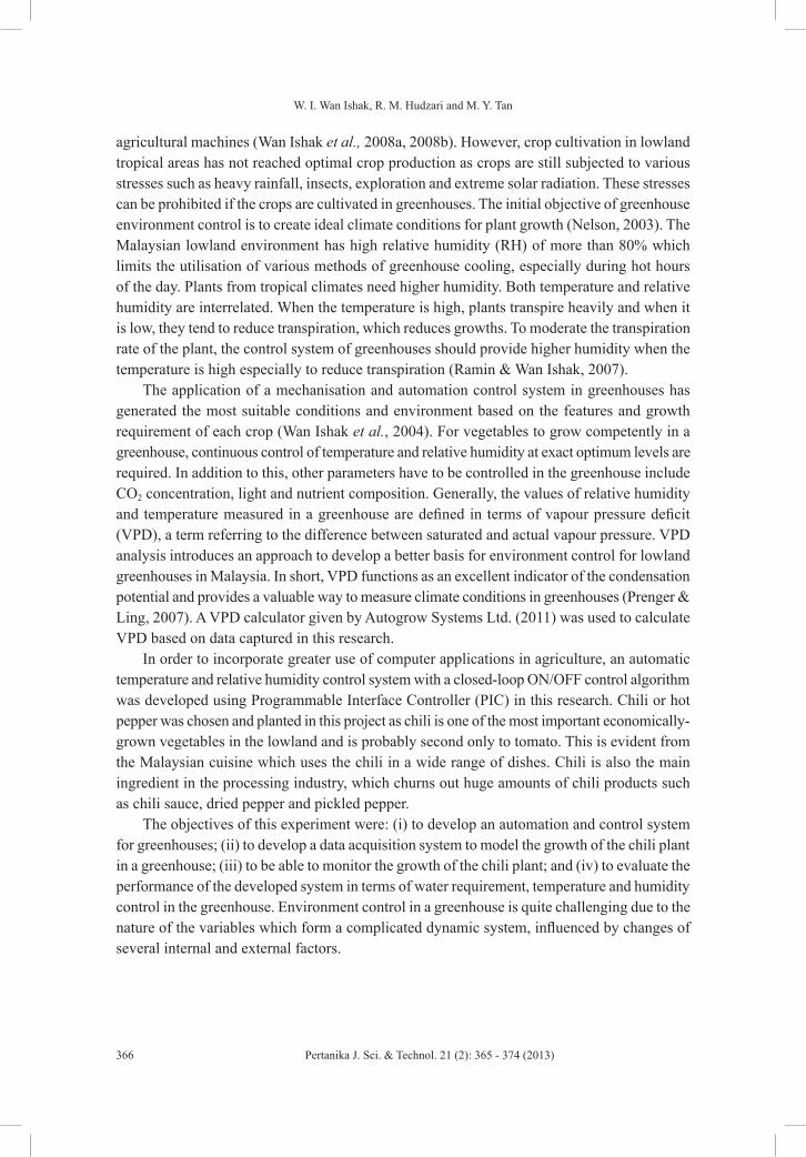
W. I. Wan Ishak, R. M. Hudzari and M. Y. Tan
366 Pertanika J. Sci. & Technol. 21 (2): 365 - 374 (2013)
agricultural machines (Wan Ishak et al., 2008a, 2008b). However, crop cultivation in lowland tropical areas has not reached optimal crop production as crops are still subjected to various stresses such as heavy rainfall, insects, exploration and extreme solar radiation. These stresses can be prohibited if the crops are cultivated in greenhouses. The initial objective of greenhouse environment control is to create ideal climate conditions for plant growth (Nelson, 2003). The Malaysian lowland environment has high relative humidity (RH) of more than 80% which limits the utilisation of various methods of greenhouse cooling, especially during hot hours of the day. Plants from tropical climates need higher humidity. Both temperature and relative humidity are interrelated. When the temperature is high, plants transpire heavily and when it is low, they tend to reduce transpiration, which reduces growths. To moderate the transpiration rate of the plant, the control system of greenhouses should provide higher humidity when the temperature is high especially to reduce transpiration (Ramin & Wan Ishak, 2007).
The application of a mechanisation and automation control system in greenhouses has generated the most suitable conditions and environment based on the features and growth requirement of each crop (Wan Ishak et al., 2004). For vegetables to grow competently in a greenhouse, continuous control of temperature and relative humidity at exact optimum levels are required. In addition to this, other parameters have to be controlled in the greenhouse include CO2 concentration, light and nutrient composition. Generally, the values of relative humidity and temperature measured in a greenhouse are defined in terms of vapour pressure deficit (VPD), a term referring to the difference between saturated and actual vapour pressure. VPD analysis introduces an approach to develop a better basis for environment control for lowland greenhouses in Malaysia. In short, VPD functions as an excellent indicator of the condensation potential and provides a valuable way to measure climate conditions in greenhouses (Prenger & Ling, 2007). A VPD calculator given by Autogrow Systems Ltd. (2011) was used to calculate VPD based on data captured in this research.
In order to incorporate greater use of computer applications in agriculture, an automatic temperature and relative humidity control system with a closed-loop ON/OFF control algorithm was developed using Programmable Interface Controller (PIC) in this research. Chili or hot pepper was chosen and planted in this project as chili is one of the most important economically-grown vegetables in the lowland and is probably second only to tomato. This is evident from the Malaysian cuisine which uses the chili in a wide range of dishes. Chili is also the main ingredient in the processing industry, which churns out huge amounts of chili products such as chili sauce, dried pepper and pickled pepper.
The objectives of this experiment were: (i) to develop an automation and control system for greenhouses; (ii) to develop a data acquisition system to model the growth of the chili plant in a greenhouse; (iii) to be able to monitor the growth of the chili plant; and (iv) to evaluate the performance of the developed system in terms of water requirement, temperature and humidity control in the greenhouse. Environment control in a greenhouse is quite challenging due to the nature of the variables which form a complicated dynamic system, influenced by changes of several internal and external factors.
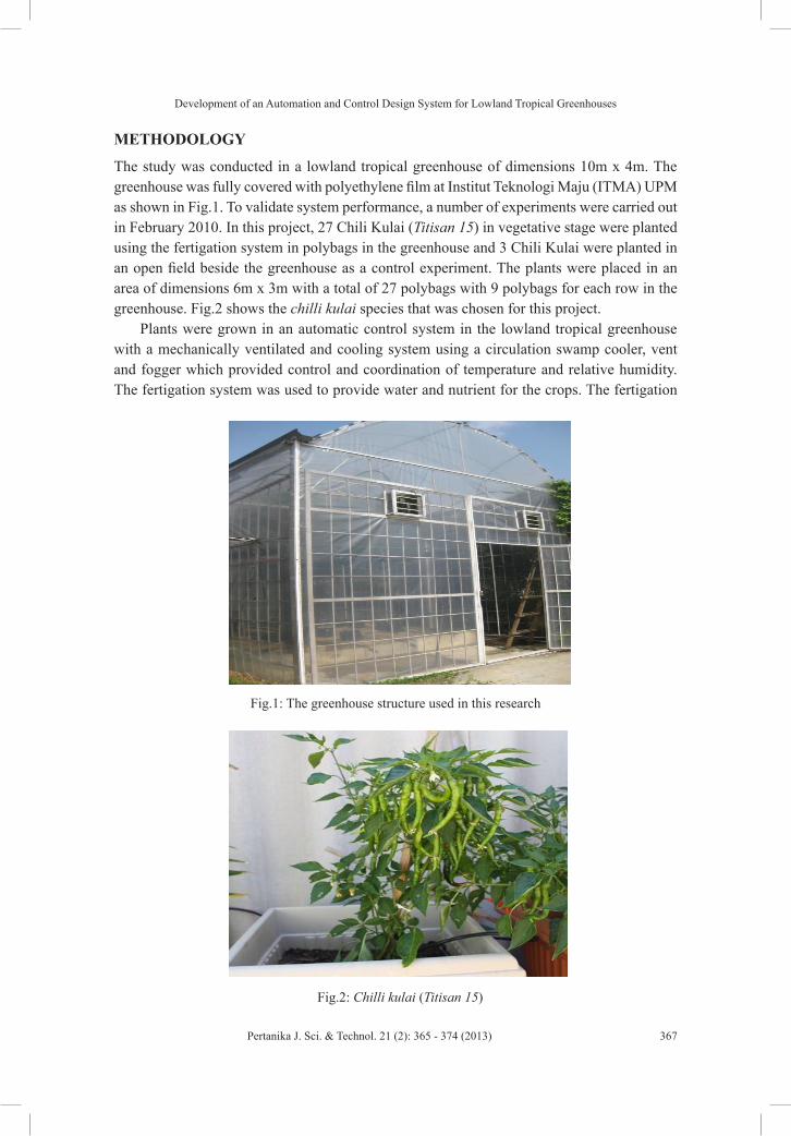
Development of an Automation and Control Design System for Lowland Tropical Greenhouses
367Pertanika J. Sci. & Technol. 21 (2): 365 - 374 (2013)
METHODOLOGY
The study was conducted in a lowland tropical greenhouse of dimensions 10m x 4m. The greenhouse was fully covered with polyethylene film at Institut Teknologi Maju (ITMA) UPM as shown in Fig.1. To validate system performance, a number of experiments were carried out in February 2010. In this project, 27 Chili Kulai (Titisan 15) in vegetative stage were planted using the fertigation system in polybags in the greenhouse and 3 Chili Kulai were planted in an open field beside the greenhouse as a control experiment. The plants were placed in an area of dimensions 6m x 3m with a total of 27 polybags with 9 polybags for each row in the greenhouse. Fig.2 shows the chilli kulai species that was chosen for this project.
Plants were grown in an automatic control system in the lowland tropical greenhouse with a mechanically ventilated and cooling system using a circulation swamp cooler, vent and fogger which provided control and coordination of temperature and relative humidity. The fertigation system was used to provide water and nutrient for the crops. The fertigation
Fig.1: The greenhouse structure used in this research
Fig.2: Chilli kulai (Titisan 15)
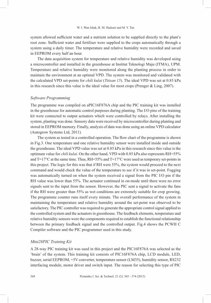
W. I. Wan Ishak, R. M. Hudzari and M. Y. Tan
368 Pertanika J. Sci. & Technol. 21 (2): 365 - 374 (2013)
system allowed sufficient water and a nutrient solution to be supplied directly to the plant’s root zone. Sufficient water and fertiliser were supplied to the crops automatically through a system using a daily timer. The temperature and relative humidity were recorded and saved in EEPROM every half an hour.
The data acquisition system for temperature and relative humidity was developed using a microcontroller and installed in the greenhouse at Institut Teknologi Maju (ITMA), UPM. Temperature and relative humidity were monitored along the planting process in order to maintain the environment at an optimal VPD. The system was monitored and validated with the calculated VPD set-points for chili kulai (Titisan 15). The ideal VPD was set at 0.85 kPa in this research since this value is the ideal value for most crops (Prenger & Ling, 2007).
Software Programming
The programme was compiled on aPIC16F876A chip and the PIC training kit was installed in the greenhouse for automatic control purposes during planting. The I/O pins of the training kit were connected to output actuators which were controlled by relays. After installing the system, planting was done. Sensory data were received by microcontroller during planting and stored in EEPROM memory. Finally, analysis of data was done using an online VPD calculator (Autogrow Systems Ltd, 2011).
The system as tested in a controlled operation. The flow chart of the programme is shown in Fig.3. One temperature and one relative humidity sensor were installed inside and outside the greenhouse. The ideal VPD value was set at 0.85 kPa in this research since this value is the optimum value for chili kulai. On the other hand, VPD with 0.85 kPa also represents RH=55% and T=17°C at the same time. Thus, RH=55% and T=17°C were used as temporary set-points in this project. The logic for this was that if RH were 55%, the system would proceed to the next command and would check the value of the temperature to see if it was in set-point. Fogging was automatically turned on when the system received a signal from the PIC I/O pin if the RH value was lower than 55%. The actuator continued in on-mode until there were no error signals sent to the input from the sensor. However, the PIC sent a signal to activate the fans if the RH were greater than 55% as wet conditions are extremely suitable for crop growing. The programme counter runs itself every minute. The overall performance of the system in maintaining the temperature and relative humidity around the set-point was observed to be satisfactory. The PIC controller was required to generate the appropriate control signal applied to the controlled system and the actuators in greenhouse. The feedback elements, temperature and relative humidity sensors were the components required to establish the functional relationship between the primary feedback signal and the controlled output. Fig.4 shows the PCWH C Compiler software and the PIC programmer used in this study.
Mini28PIC Training Kit
A 28-way PIC training kit was used in this project and the PIC16F876A was selected as the ‘brain’ of the system. This training kit consists of PIC16F876A chip, LCD module, LED, buzzer, serial EEPROM, +5V converter, temperature sensor (LM35), humidity sensor, RS232 interfacing module, motor driver and switch input. The reason for selecting this type of PIC
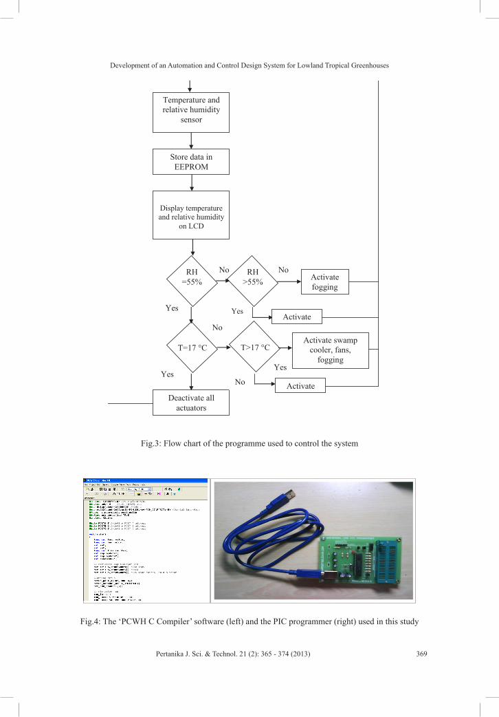
Development of an Automation and Control Design System for Lowland Tropical Greenhouses
369Pertanika J. Sci. & Technol. 21 (2): 365 - 374 (2013)
Yes
Display temperature and relative humidity
on LCD
Start
RH =55%
Activate swamp cooler, fans,
fogging
No
Yes
Temperature andrelative humidity
sensor
Store data in EEPROM
Deactivate all actuators
RH >55%
Activate fans
No
Yes
Yes
Activate fogging
No
No
Activate fan Fans
T>17 °C
T=17 °C
Fig.4: The ‘PCWH C Compiler’ software (left) and the PIC programmer (right) used in this study
Fig.3: Flow chart of the programme used to control the system

W. I. Wan Ishak, R. M. Hudzari and M. Y. Tan
370 Pertanika J. Sci. & Technol. 21 (2): 365 - 374 (2013)
as the microcontroller in this research was because it is an efficient tool that is very suitable to develop a simple and small project. It was used to collect the real-time data which can be shown in computer interfacing.
In this project, data from temperature and relative humidity were sent to the PIC via the I/O pins as input for the controller. Pins a0 and c0 were used as temperature and relative humidity input signals respectively while the pin of PORT B was used as the output for LCD display on the training kit. Pins a1, a2 and a3 of PORT C were used as the output to activate actuators in the greenhouse. Fig.5 shows the training kit and its components that were used in the research. The data from the temperature and humidity sensors were sent to PIC controller as the input signal and were converted to digital form through internal analog to the digital convertor (ADC) inside the controller. Output signals were sent to activate the actuators after running the programme.
Strip board
A strip board was developed and used to supply 5V to trigger relays in the controller box and regulate the DC adapter voltage from 12V to 5V. It consisted of an LM 7805, pin header, resistor and capacitor. LM35 is a simple but accurate 3-pin temperature sensor. It is included in the training kit to determine the temperature in the greenhouse at a certain time and period. Its temperature range is from 2°C to 100°C. This temperature range allows the sensor to detect the temperature value in the greenhouse where the temperature is different throughout the day. Fig.6 shows the circuit diagram of the strip board and the temperature sensor, LM35.
Graphical User Interface (GUI)
A Graphical User Interface (GUI) was developed by using Microsoft Visual Basic 2006 software. This GUI was developed to help the user to ensure that actuators are activated based on the temperature and relative humidity set-points.
8-LED
RS232 port
PIC16F876A
LCD module
EEPROM
7-segment 5V power supply Reset button
Fig.5: The PIC training kit and its components
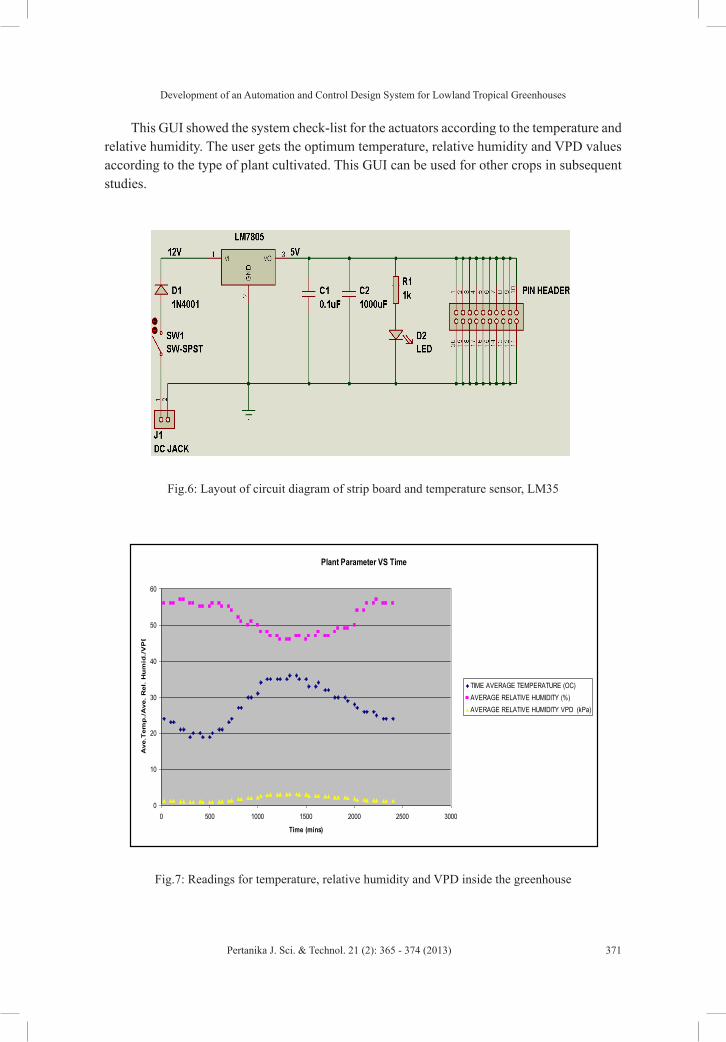
Development of an Automation and Control Design System for Lowland Tropical Greenhouses
371Pertanika J. Sci. & Technol. 21 (2): 365 - 374 (2013)
This GUI showed the system check-list for the actuators according to the temperature and relative humidity. The user gets the optimum temperature, relative humidity and VPD values according to the type of plant cultivated. This GUI can be used for other crops in subsequent studies.
Plant Parameter VS Time
0
10
20
30
40
50
60
0 500 1000 1500 2000 2500 3000
Time (mins)
Ave
.Tem
p./
Ave
. R
el.
Hu
mid
./V
PD
TIME AVERAGE TEMPERATURE (OC)AVERAGE RELATIVE HUMIDITY (%)AVERAGE RELATIVE HUMIDITY VPD (kPa)
Fig.6: Layout of circuit diagram of strip board and temperature sensor, LM35
Fig.7: Readings for temperature, relative humidity and VPD inside the greenhouse
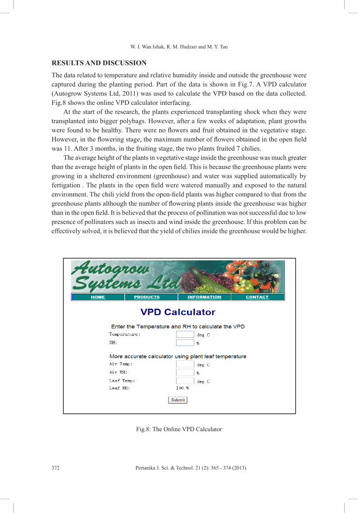
W. I. Wan Ishak, R. M. Hudzari and M. Y. Tan
372 Pertanika J. Sci. & Technol. 21 (2): 365 - 374 (2013)
RESULTS AND DISCUSSION
The data related to temperature and relative humidity inside and outside the greenhouse were captured during the planting period. Part of the data is shown in Fig.7. A VPD calculator (Autogrow Systems Ltd, 2011) was used to calculate the VPD based on the data collected. Fig.8 shows the online VPD calculator interfacing.
At the start of the research, the plants experienced transplanting shock when they were transplanted into bigger polybags. However, after a few weeks of adaptation, plant growths were found to be healthy. There were no flowers and fruit obtained in the vegetative stage. However, in the flowering stage, the maximum number of flowers obtained in the open field was 11. After 3 months, in the fruiting stage, the two plants fruited 7 chilies.
The average height of the plants in vegetative stage inside the greenhouse was much greater than the average height of plants in the open field. This is because the greenhouse plants were growing in a sheltered environment (greenhouse) and water was supplied automatically by fertigation . The plants in the open field were watered manually and exposed to the natural environment. The chili yield from the open-field plants was higher compared to that from the greenhouse plants although the number of flowering plants inside the greenhouse was higher than in the open field. It is believed that the process of pollination was not successful due to low presence of pollinators such as insects and wind inside the greenhouse. If this problem can be effectively solved, it is believed that the yield of chilies inside the greenhouse would be higher.
Fig.8: The Online VPD Calculator

Development of an Automation and Control Design System for Lowland Tropical Greenhouses
373Pertanika J. Sci. & Technol. 21 (2): 365 - 374 (2013)
The relative humidity (RH), temperature (T) and VPD for the chili plant are 55%, 17°C and 0.85 kPa respectively. GUI will run when it meets these conditions:
i. RH=55% and T=17°C
No actuator was keyed in in the GUI check-list box for conditions that reached RH = 55% T = 17°C . This was due to the fact that the temperature and RH had reached optimum conditions inside the greenhouse. This, therefore, illustrates that no actuator was activated by the control system.
ii. RH=45% and T=34°C
“Fogging” was activated as in the system check list when RH reached 45% and T reached 34 °C. Based on the scope of the programming that was written, the fogger was activated if the RH were less than the set-point, 55%. The fan and the swamp cooler would then be deactivated.
iii. RH=55% and T=20°C
When conditions inside the greenhouse reached RH=55% and T=20°C, all the actuators were activated via the GUI system check list. RH reached its set-point but T was higher than its set-point. Therefore, all actuators were activated to lower the temperature in the greenhouse until it reached the set-point, 17°C. This means that the user need not be present in or near the greenhouse to know which actuator is running as this can be monitored and adjusted by the GUI.
CONCLUSION
A data acquisition system to control the temperature and relative humidity of a greenhouse was successfully developed and used to record data every 30 minutes inside and outside the greenhouse. The data acquisition system was able to monitor the growth of the plants in the greenhouse via the control system. A PIC controller was successfully used and interfacing with a computer (read data) was achieved. The plant i.e. chili yield in the control sector i.e. an open field was observed to be higher compared to that of the greenhouse although the number of flowering plants inside the greenhouse was higher than in the open field. It is believed that the process of fertilisation was not successful due to low presence of pollinators such as insects or wind inside the greenhouse. If this problem can be successfully addressed, it is believed that the yield of chilies inside the greenhouse will be higher. Due to the fact that the greenhouse provides a shelter for plant cultivation under a roof system, the environment parameters can be controlled to suit the type of crop using computer applications and a sensory system.
ACKNOWLEDGEMENTS
The authors would like to thank the Ministry of Higher Education for the FRGS grant on ‘Development of Automation Control System for Lowland Greenhouse Crop Production’ to do this research work.

W. I. Wan Ishak, R. M. Hudzari and M. Y. Tan
374 Pertanika J. Sci. & Technol. 21 (2): 365 - 374 (2013)
REFERENCESAutogrow Systems Ltd. (2011) . VPD calculator. Retrieved from www.autogrow.com
Nelson, P. V. (2003). Greenhouse Operation and Management, pp. 692. Prentice Hall, New York.
Prenger, J. J., & Ling, P. P. (n.d.). Greenhouse Condensation Control: Understanding and Using Vapor Pressure Deficit (VPD). Retrieved on July 30, 2007 from http://ohioline.osu.edu/aex-fact/pdf/0804.pdf
Ramin Shamshiri, & W. I. Wan Ishak. (2007). Control System of Temperature and Relative Humidity for Tropical Lowland Greenhouse. Paper presented at the World Engineering Congress 2007 (WEC 07). 5-9 August 2007. Penang.
Wan Ishak, W. I., Mohd. Hudzari, R., W. Haffiz, & Ming, F. (2004). Development of Computer Integrated Agriculture for Gantry System. In the Proceedings of the 1st Asian Conference On Precision Agriculture (ACPA) 11-13 May 2004. Kuala Lumpur, Malaysia.
Wan Ishak, W. I. (2007). Development of Automation Technology For The Malaysian Agricultural Sector. March-May 2007. The Ingenieur. Board of Engineer Malaysia, 33(March-May 2007), 46-54.
Wan Ishak, W. I., Hazlina H., & Awal, M. A. (2008a). Development of Camera-Vision Guided Automatic Sprayer. Pertanika Journal of Science and Technology, 16(2), 97-105.
Wan Ishak, W. I., M. A. Awal, & R. Elango. (2008b). Development of an Automated Transplanter for the Gantry. Asian Journal of Scientific Research, 1(4), 451-457.
Pertanika J. Sci. & Technol. 21 (2): 375 - 386 (2013)
SCIENCE & TECHNOLOGYJournal homepage: http://www.pertanika.upm.edu.my/
ISSN: 0128-7680 © 2013 Universiti Putra Malaysia Press.
Recovery of Heavy Metals from Spent Etching Waste Solution of Printed Circuit Board (PCB) Manufacturing
A. H. M. Ali*, S. Sobri, Salmiaton. A. and Faizah M. Y.Department of Chemical and Environmental Engineering, Faculty of Engineering, Universiti Putra Malaysia, 43400 Serdang, Selangor, Malaysia
ABSTRACT
The process of etching is the most crucial part of the work of manufacturing printed circuit boards (PCB). In the etching process by nitric acid, a spent etching waste solution of composition 250 g/L HNO3, 30-40 g/L Cu, 30-40 g/L Sn, 30-40 g/L Pb and 20-25 g/L Fe is produced. High metal concentrations in the spent etching waste solution make it a viable candidate for the recovery of metals. Recovery of metals from spent etching waste solution is a significant concern as the recent growth in production of printed circuit boards has generated a drastic increase of spent etching waste solution each year. This study concerns itself with the recovery of metals from spent etching waste. In this study a dilution was made in order to increase the pH of the solution as spent etching waste solution has high acidity, and the electrowinning method was performed to recover metals from the spent etching waste solution. Glassy carbon and platinum were used as cathode and anode in order to investigate the electrodeposition of metals and cyclic voltammetry investigation suggests that the deposition of metals on glassy carbon electrodes occurs at four different overpotentials mainly at -0.15 V, -0.35 V, -0.45 V and -0.75 V. Microscopy observation demonstrates that there is a deposition of metals by applying the potentials in a set of current-time transient study for a duration of 60 seconds and the metals recovered formed as aggregates.
Keywords: PCB etching solution, electrowinning, linear sweep voltammetry, cyclic voltammetry
Article history:Received: 28 February 2011Accepted: 10 September 2012
E-mail addresses: [email protected] (A. H. M. Ali), [email protected] (S. Sobri), [email protected] (Salmiaton. A.), [email protected] (Faizah M. Y.)*Corresponding Author
INTRODUCTION
Etching waste solution produced in the process of printed circuit board manufacturing contains tin, copper, iron and lead as by-products. In the etching process by nitric acid, spent etching waste solution of composition 250 g/L HNO3, 30-40 g/L Cu, 30-40 g/L Sn, 30-40 g/L Pb and 20-25 g/L Fe is produced (Man-Seung et al., 2003). In recent years, it

A. H. M. Ali, S. Sobri, Salmiaton. A. and Faizah M. Y.
376 Pertanika J. Sci. & Technol. 21 (2): 375 - 386 (2013)
has been reported that the average rate of worldwide printed circuit board (PCBs) manufacturing increases by 8.7% with total value of 51.5 billion USD worldwide and this number is higher in Southeast Asia by 10.8% (Kui et al., 2009; WEEC, 2009). Technological innovation and intense marketing are factors accelerating the production rate of electric electronic equipment (EEE) and shortening the lifespan of EEE.[4] As the demand for production of EEE increases, the discharge of etching waste solution has become a major economic as well as environmental concern as it contains significant amounts of heavy metals and acid and has to be treated as hazardous waste.
Conventionally, etching waste solution resulting from the etching process is neutralised by adding sodium hydroxide, resulting in metal-bearing sludge. The neutralised sludge is incinerated and the residues dumped in special landfills (Man-Seung et al., 2003; Chang-Hoon et al., 2009). Due to the emission of nitrogen monoxide during the incineration and leaching of heavy metals from the dumped residues, the disposal of etching waste solution by neutralisation fails to solve the waste problem; in addition, the sludge contains a lot of valuable components that should be recovered economically (Man-Seung et al., 2003; Tiina et al., 2007).
At present, several methods exist for the treating and regenerating of etching waste such as solvent extraction (Man-Seung et al., 2003; Chang-Hoon et al., 2009), evaporation (Man-Seung et al., 2003), membrane technology and electrowinning (Tiina et al., 2007; Department of Environmental Protection, Florida, 2006). A comparison of the existing current treatments shows that electrowinning is the most well established technology for metal deposition from solution. Electrowinning can recover element metals directly from aqueous solutions in a single-stage process without the addition of reagents (Shafreeza, 2006; Walsh, 2001; Juttner et al., 2000). Electrowinning technologies are more efficient, green, compact and economical compared with existing technologies in terms of efficiency in metals recovery and clean technologies that help to prevent the production of unwanted by-products which in many cases have to be treated as waste.
In this study, we focus on recovery of heavy metals in etching waste solution produced in PCB manufacturing by electrowinning as an initial investigation for metal recovery from etching waste solution.
THEORY OF ELECTROWINNING
Electrowinning is a process where metals are deposited at the cathode from an electrolyte by the process of reduction. The term ‘electrowinning’ is often used in many technologies such as electroplating, electrodeposition and electrorefining. The process usually features as a process that is usually carried out in three electrode electrochemical cells that consist of a working electrode, a counter electrode and a reference electrode. Both working and counter electrodes are connected to a power supply.
The deposition of metals is achieved by applying a negative charge on the working electrode, and the metallic ions which carry a positive charge will be attracted to the cathode. When the positive charge of the metallic ions reaches the cathode, it receives an electron to reduce the positive-charged ions to their metallic form and causes them to be deposited on

Recovery of Heavy Metals from Spent Etching Waste Solution of Printed Circuit Board (PCB) Manufacturing
377Pertanika J. Sci. & Technol. 21 (2): 375 - 386 (2013)
the electrode surface as a thin layer. The electrodepositing mechanism for metal recovery on an electrode surface is very simple. It is basically a simple electron transfer and may be represented as:
Mn+ + nē → M
MATERIALS AND METHODS
Reagents
Experiments were conducted using a synthetic etching solution and prepared in the ratio shown in Table 1. A 3.5 M HNO3 solution was prepared by diluting 240.6 mL of 14.545 M HNO3 in distilled water and diluting it to 1000 mL. The final concentration of nitric acid in the synthetic etching solution was 250 g/L. 30 g/L Cu, 40 g/L Pb, 40 g/L Sn and 20 g/L Fe, dissolved in nitric acid (HNO3). The mixtures were stirred using a magnetic stirrer at 250 rpm for 30 minutes. The concentration of the synthetic spent nitric etching solution was analysed by inductively coupled plasma-atomic emission spectroscopy (ICP-AES) Optima 7300 from Perkin Elmer.
TABLE 1 Chemical composition of the synthetic spent nitric etching solution
ElementCopper (g/L)
Lead (g/L)
Tin (g/L)
Iron (g/L)
HNO3
NConcentration 30 40 40 20 3.5
Due to the high acidity of the etching waste solution, a dilution was made to increase the pH of the solution to pH > 2 in order to meet the requirements of the potentiometer to work at its optimum condition. The initial pH of the etching solution was -1.67 and a dilution of 100 times was made of the solution to increase the pH to 2.1.
Electrochemical experiments
Linear sweep voltammetry
Linear sweep voltammetry was performed to measure the current at the working electrode while the potential between the working electrode and a reference electrode was swept linearly in time. The linear sweep experiments were carried out at 0 to -1.0 V at scan rates ranging from 5-50 mVs-1. In linear sweep voltammetry experiment, reduction of species is registered as a peak in the current signal at the potential at which the species begins to reduce.
Cyclic Voltammetry
Cyclic voltammetry was performed to determine the potential for metal nucleation on glassy carbon electrodes. The voltammetry experiments were carried out from -1 to 1 V at scan rates ranging from 5-50 mVs-1. Surface area available for the deposition was 1.0 cm2.

A. H. M. Ali, S. Sobri, Salmiaton. A. and Faizah M. Y.
378 Pertanika J. Sci. & Technol. 21 (2): 375 - 386 (2013)
Current-time transient
Current-time transient for studying the deposition of metals in spent etching waste solution was accomplished by applying the potential voltage of each reduction peak gained in linear sweep voltammetry for 60 seconds. Metals deposited on the electrode were analysed by scanning electron microscopy (SEM) and energy-dispersive spectrometry (EDS).
Electrochemical system
Flat cell system
A Princeton Applied Research Model K0235 Flat Cell was used to study the electrochemical characteristic of the synthetic etching waste as well as the growth mechanism of the metals. K0235 Flat Cell is a cylindrical cell and consists of a glass cylinder clamped horizontally between two end plates. One end plate houses the working electrode and the other houses the counter electrode. The placement of the counter electrode is directly opposite to the working electrode. The reference electrode is housed in a luggin well, with a fixed Teflon luggin capillary protruding from the bottom of the well.
Electrochemical Instrumentation
All electrochemical experiments performed with flat cell, such as linear sweep, cyclic voltammetry and chronoamperometry were carried out using a potentiostat VersaSTAT 4 from Princeton Applied Research and operated by a PC using VersaStudio software. Two-electrode electrolytic cells were set up using a glassy carbon as cathode and platinum as anode. Experiments were conducted at room temperature. Current-potential data on the experiment were collected and interpreted using Microsoft Excel.
Microscopy imaging
Scanning Electron Microscopy (SEM) and Energy-Dispersive Spectrometry (EDS)
Microstructural properties of the deposited particles and the microscopy images of metal deposits were analysed using a S-3400N SEM model from Hitachi High-Technology Corporation and Thermo Scientific NORAN System Six (NSS) Energy Dispersive Spectrometry (EDS) system. SEM analysis for metals deposits were recorded at 3000 magnification and at an acceleration voltage of 15kV and the deposit characterisation was performed to investigate the influence of deposition overpotential over time and used to characterise elemental constituents of the metal deposited on the electrode.
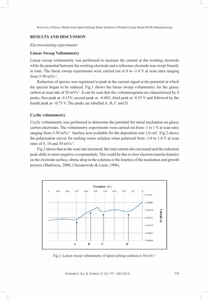
Recovery of Heavy Metals from Spent Etching Waste Solution of Printed Circuit Board (PCB) Manufacturing
379Pertanika J. Sci. & Technol. 21 (2): 375 - 386 (2013)
RESULTS AND DISCUSSION
Electrowinning experiments
Linear Sweep Voltammetry
Linear sweep voltammetry was performed to measure the current at the working electrode while the potential between the working electrode and a reference electrode was swept linearly in time. The linear sweep experiments were carried out at 0 to -1.0 V at scan rates ranging from 5-50 mVs-1.
Reduction of species was registered to peak in the current signal at the potential at which the species began to be reduced. Fig.1 shows the linear sweep voltammetry for the glassy carbon at scan rate of 50 mVs-1. It can be seen that the voltammograms are characterised by 4 peaks; first peak at -0.15V, second peak at –0.40V, third peak at -0.55 V and followed by the fourth peak at –0.75 V. The peaks are labelled A, B, C and D.
Cyclic voltammetry
Cyclic voltammetry was performed to determine the potential for metal nucleation on glassy carbon electrodes. The voltammetry experiments were carried out from -1 to 1 V at scan rates ranging from 5-50 mVs-1. Surface area available for the deposition was 1.0 cm2. Fig.2 shows the polarisation curves for etching waste solution when polarised from -1.0 to 1.0 V at scan rates of 5, 10 and 50 mVs-1.
Fig.2 shows that as the scan rate increased, the total current also increased and the reduction peak shifts to more negative overpotentials. This could be due to slow electron transfer kinetics on the electrode surface, ohmic drop in the solution or the kinetics of the nucleation and growth process (Shafreeza, 2006; Chrzanowski & Lasia, 1996).
A B C D
Fig.1: Linear sweep voltammetry of spent etching solution at 50 mVs-1
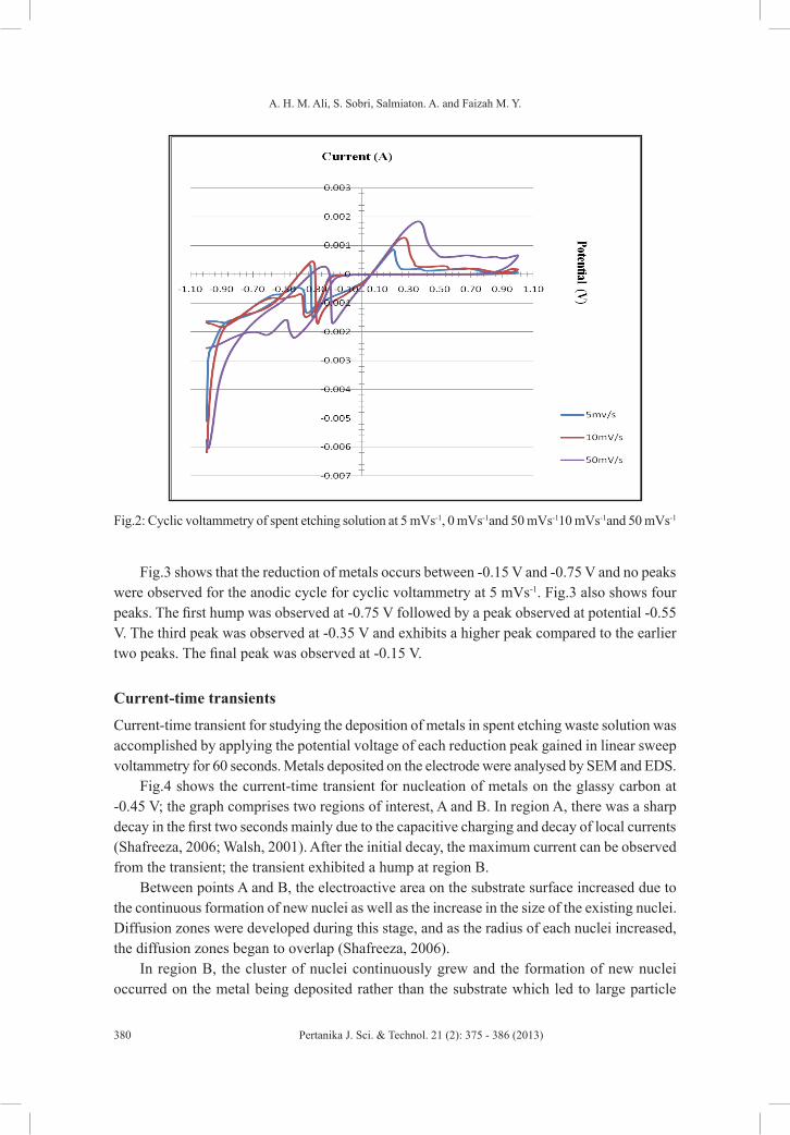
A. H. M. Ali, S. Sobri, Salmiaton. A. and Faizah M. Y.
380 Pertanika J. Sci. & Technol. 21 (2): 375 - 386 (2013)
Fig.3 shows that the reduction of metals occurs between -0.15 V and -0.75 V and no peaks were observed for the anodic cycle for cyclic voltammetry at 5 mVs-1. Fig.3 also shows four peaks. The first hump was observed at -0.75 V followed by a peak observed at potential -0.55 V. The third peak was observed at -0.35 V and exhibits a higher peak compared to the earlier two peaks. The final peak was observed at -0.15 V.
Current-time transients
Current-time transient for studying the deposition of metals in spent etching waste solution was accomplished by applying the potential voltage of each reduction peak gained in linear sweep voltammetry for 60 seconds. Metals deposited on the electrode were analysed by SEM and EDS.
Fig.4 shows the current-time transient for nucleation of metals on the glassy carbon at -0.45 V; the graph comprises two regions of interest, A and B. In region A, there was a sharp decay in the first two seconds mainly due to the capacitive charging and decay of local currents (Shafreeza, 2006; Walsh, 2001). After the initial decay, the maximum current can be observed from the transient; the transient exhibited a hump at region B.
Between points A and B, the electroactive area on the substrate surface increased due to the continuous formation of new nuclei as well as the increase in the size of the existing nuclei. Diffusion zones were developed during this stage, and as the radius of each nuclei increased, the diffusion zones began to overlap (Shafreeza, 2006).
In region B, the cluster of nuclei continuously grew and the formation of new nuclei occurred on the metal being deposited rather than the substrate which led to large particle
Fig.2: Cyclic voltammetry of spent etching solution at 5 mVs-1, 0 mVs-1and 50 mVs-110 mVs-1and 50 mVs-1

Recovery of Heavy Metals from Spent Etching Waste Solution of Printed Circuit Board (PCB) Manufacturing
381Pertanika J. Sci. & Technol. 21 (2): 375 - 386 (2013)
A
B
Fig.3: Cyclic voltammetry of spent etching solution at 5 mVs-1
Fig.4: Current-time transient for nucleation of metals on glassy carbon at -0.45 V

A. H. M. Ali, S. Sobri, Salmiaton. A. and Faizah M. Y.
382 Pertanika J. Sci. & Technol. 21 (2): 375 - 386 (2013)
aggregations. The decreasing of the current is mainly due to the combined effects of the depletion of the diffusion layer as well as the coagulation of nuclei.
The deposited metals on glassy carbon were analysed using SEM. As shown in Fig.5, deposition at -0.45 V formed in large aggregates and the distribution of the aggregates on the surface of the electrode was not even. Electrode surface was still visible as shown in Fig.5. X-ray diffraction patterns of metals deposited on the glassy carbon at -0.45 V were analysed using Energy Dispersive Spectrometry (EDS). Based on the weight percentage from EDS analysis, Pb dominated with 62.29% by weight while Sn with 3.61% and Fe with 2.40%. In order to determine the average particle size of metals nuclei, 6 areas were chosen at random from the micrographs of the substrate surface with each area being 100 µm2. Based on Fig.5, the average particle size of metals deposited on the glassy carbon at -0.45 V overpotentials was 20.6 x 10⁻¹² m2.
Fig.6 shows the current-time transient for nucleation of metals on glassy carbon at -0.75 V. A sharp decay was observed in the first three seconds as in region A. After the initial decay, the current transient exhibited a hump at region B.
Comparing Fig.4 and Fig.6, as the applied potential is lowered, the maximum current became more pronounced and its height and position increased as the applied potential
Fig.5: SEM images of metals on glassy carbon at -0.45 V deposition over potentials with 3K magnification
A B
Fig.6: Current-time transient for nucleation of metals on glassy carbon at -0.75 V

Recovery of Heavy Metals from Spent Etching Waste Solution of Printed Circuit Board (PCB) Manufacturing
383Pertanika J. Sci. & Technol. 21 (2): 375 - 386 (2013)
became more cathodic. The SEM image of metals deposited on the glassy carbon at -0.75 V overpotential is shown in Fig.7.
As shown in Fig.7, deposition at -0.75 V formed aggregates and the distribution of the aggregates on the surface of the electrode was even. The size of the aggregates deposited was smaller compared to the size of the aggregates deposited at -0.45 V. The average particle density of metals deposited on the glassy carbon at -0.75 V overpotentials was 18.1 x 10⁻¹² m2. Based on the EDS analysis, Cu deposited with 38.53% by weight, O with 51.87% and C with 2.76%.
Fig.8 contains representatives scanning electron micrographs of metals deposited on glassy carbon electrodes of each potential voltage. The figure shows the deposits after 60 seconds of each potential application. Based on Fig.8, as the applied potential is lowered, deposited metals started to form as aggregates and the deposition on the surface of the electrodes was even.
Fig.7: SEM images of metals on glassy carbon at -0.75V deposition overpotentials at 3K magnification
B
C D
A
Fig.8: SEM images of metals on glassy carbon at deposition overpotentials at 3K maginification : (A) -0.15 V (B) -0.45 V (C) -0.55 V (D) -0.75 V
A. H. M. Ali, S. Sobri, Salmiaton. A. and Faizah M. Y.
384 Pertanika J. Sci. & Technol. 21 (2): 375 - 386 (2013)
CONCLUSION
Spent etching waste solution contains a significant amount of heavy metals such as copper, iron, lead and tin. Since the discharge of etching waste is a major economic as well as environmental concern, this paper aimed to investigate if the heavy metals in spent etching waste solution can be recovered.
Due to the high acidity of the etching waste solution, a dilution was made to increase the pH to pH > 2. The initial pH of the etching solution was -1.67 and a dilution of 100 times was made to the solution to increase the pH to 2.1.
Glassy carbon and platinum were used as cathode and anode in order to investigate the electrodeposition of the metals. Cyclic voltammetry investigation suggests that the deposition of metals on the glassy carbon electrodes occurs at four different overpotentials mainly at -0.15 V, -0.35 V, -0.45 V and -0.75 V. Microscopy observation demonstrates that there is a deposition of metals by applying the potentials in a set of current-time transient studies for a duration of 60 seconds where the metals recovered formed as aggregates.
Based on this study, we can conclude that heavy metals in spent etching waste solution can be recovered by electrowinning methods. Unfortunately, selective recovery cannot be done as the metals recovered formed as aggregates and not as a single element. Due to the high acidity of etching waste solution, a future work with respect to eliminating acid in etching waste by solvent extraction can be done in order to increase the pH of the solution to replace the dilution method as acids and metals concentration in etching waste solution is relatively high and with effective recovery, acids and metals from the waste stream can be recycled to the main process and, thus, would greatly simplify any further treatment of the wastewater.
REFERENCESChang-Hoon, S., Ju-Yup, K., Jun-Young, K., Hyun-Sang, K., Hyang-Sook, L., Debasish, M., Jae-woo,
A., Jong-Gwan, A., & Wookeun, B. (2009). Recovery of nitric acid from waste etching solution using solvent extraction. Journal of Hazardous Materials, 163, 729-734
Chrzanowski, Y. G. W., & Lasia, A.(1996). Nucleation and crystal growth in gold electrodeposition from acid solution Part I: Soft gold. Journal of Applied Electrochemistry, 26, 843.
Department of Environmental Protection, Florida, USA. (2006). Recovery and Recycling of Bath Chemicals; Electroplatingy tip sheet, Pollution prevention program 2006. Department of Environmental Protection, Florida, USA.
Juttner, K., Galla, U., & Schmieder, H. (2000). Electrochemical approaches to environmental problems in the process industry. Electrochimica Acta, 45, 2575.
Kui, H., Jie, G., Zhenming, X. (2009). Recycling of waste printed circuit board: A review of current technologies and treatment status in China. Journal of Hazardous Materials, 164, 399-408.
Man-Seung, L., Jong-Gwan, A., & Jae-Woo, A. (2003). Recovery of copper, tin and lead from the spent nitric etching solution of printed circuit board and regeneration of the etching solution. Hydrometallurgy,70, 23-29.
Shafreeza, S. (2006). Electrocrystallisation and Recovery of Gold from Thiosulphate-sulphite Aged Electrolyte. (Unpublished doctoral dissertation). University of Newcastle Upon Tyne, UK.

Recovery of Heavy Metals from Spent Etching Waste Solution of Printed Circuit Board (PCB) Manufacturing
385Pertanika J. Sci. & Technol. 21 (2): 375 - 386 (2013)
Tiina, K., Juha, T., & Toivo, K. (2007). Analysis of key patents of the regeneration of acidic cupric chloride etchant waste and tin stripping waste. Resource, Conservation and Recycling, 49, 217-243.
Walsh, F. C. (2001). Electrochemical technology for environmental treatment and clean energy conversion. Pure and Applied Chemistry, 73, 1819
World Electronic Circuit Council. (2008, July). WECC Global PCB Production Report for 2008. (July 2009). World Electronic Circuit Council.
Young, J. P., & Derek, J. F.. (2009). Recovery of high purity precious metals from printed circuit boards. Journal of Hazardous Materials, 164, 1152-1158.

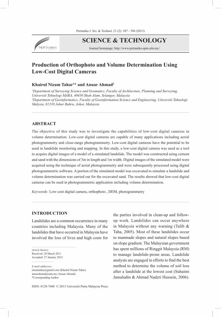
Pertanika J. Sci. & Technol. 21 (2): 387 - 396 (2013)
SCIENCE & TECHNOLOGYJournal homepage: http://www.pertanika.upm.edu.my/
ISSN: 0128-7680 © 2013 Universiti Putra Malaysia Press.
INTRODUCTION
Landslides are a common occurrence in many countries including Malaysia. Many of the landslides that have occurred in Malaysia have involved the loss of lives and high costs for
Production of Orthophoto and Volume Determination Using Low-Cost Digital Cameras
Khairul Nizam Tahar1* and Anuar Ahmad2
1Department of Surveying Science and Geomatics, Faculty of Architecture, Planning and Surveying, Universiti Teknologi MARA, 40450 Shah Alam, Selangor, Malaysia2Department of Geoinformatics, Faculty of Geoinformation Science and Engineering, Universiti Teknologi Malysia, 81310 Johor Bahru, Johor, Malaysia
ABSTRACT
The objective of this study was to investigate the capabilities of low-cost digital cameras in volume determination. Low-cost digital cameras are capable of many applications including aerial photogrammetry and close-range photogrammetry. Low-cost digital cameras have the potential to be used in landslide monitoring and mapping. In this study, a low-cost digital camera was used as a tool to acquire digital images of a model of a simulated landslide. The model was constructed using cement and sand with the dimensions of 3m in length and 1m width. Digital images of the simulated model were acquired using the technique of aerial photogrammetry and were subsequently processed using digital photogrammetric software. A portion of the simulated model was excavated to simulate a landslide and volume determination was carried out for the excavated sand. The results showed that low-cost digital cameras can be used in photogrammetric application including volume determination.
Keywords: Low-cost digital camera, orthophoto , DEM, photogrammetry
Article history:Received: 28 March 2011Accepted: 27 January 2012
E-mail addresses: [email protected] (Khairul Nizam Tahar), [email protected] (Anuar Ahmad)*Corresponding Author
the parties involved in clean-up and follow-up work. Landslides can occur anywhere in Malaysia without any warning (Talib & Taha, 2005). Most of these landslides occur to manmade slopes and natural slopes based on slope gradient. The Malaysian government has spent millions of Ringgit Malaysia (RM) to manage landslide-prone areas. Landslide analysts are engaged in efforts to find the best method to determine the volume of soil loss after a landslide at the lowest cost (Suhaimi Jamaludin & Ahmad Nadzri Hussein, 2006).

Khairul Nizam Tahar and Anuar Ahmad
388 Pertanika J. Sci. & Technol. 21 (2): 387 - 396 (2013)
The best method should be established by landslide analysts to estimate the clearance cost after a landslide. There are many methods of mapping landslides. Aerial photogrammetry, which utilises aerial photographs, is one of the methods that can be used for mapping a landslide area. The aerial photographs show images of the features on the ground, allowing for easy interpretation of the information on the ground. Aerial photographs are usually captured using a metric camera. A metric camera is very expensive and should be handled by skilful, professional personel (Wolf & Dewitt, 2004).
Today, there are many low-cost and high resolution digital cameras of different makes and models that are available in the market. The rapid development of digital technology has created oppurtunity for low-cost digital cameras to be used in acquiring digital images for photogrammetry. These images, which are good quality,can be used in many applications at certain degrees of accuracy. Low-cost digital cameras today provide different image resolutions from low to high. The term “low cost” refers to the low price of the digital camera i.e. less than RM1000 and “high resolution” refers to image resolution of more than 0.5 megapixel. The image resolution is defined by the sum of the number of horizontal pixels multiplied with the number of vertical pixels (Tahar & Ahmad, 2011). In this study, a Nikon Coolpix L4 digital camera which has an image resolution of about 4 megapixels (i.e 2272 pixels x 1704 pixels) was used (Fig.1).
Close-range photogrammetry is a technique in photogrammetry which can be used for obtaining object information from the object to a camera position of less than 100 metres (Atkinson, 1996). Images or photographs can be acquired from locations or positions in the air or on the ground. In this study, the close-range photogrammetry technique is used with a low-cost digital camera attached to a fixed platform. A fixed platform is a platform of fixed height; the low-cost digital camera is attached to a hole drilled on plane wood at a fixed height. In this study, the fixed platform was used to acquire digital aerial images of a simulated landslide model for volume computation.
In the photogrammetric method, a pair of aerial images or photographs with 60% overlap and 30% sidelap is commonly used; these images should comprise well distributed ground control points (GCPs) in the overlap area. The photogrammetric method allows a digital
Fig.1: Nikon Coolpix L4 used in the study
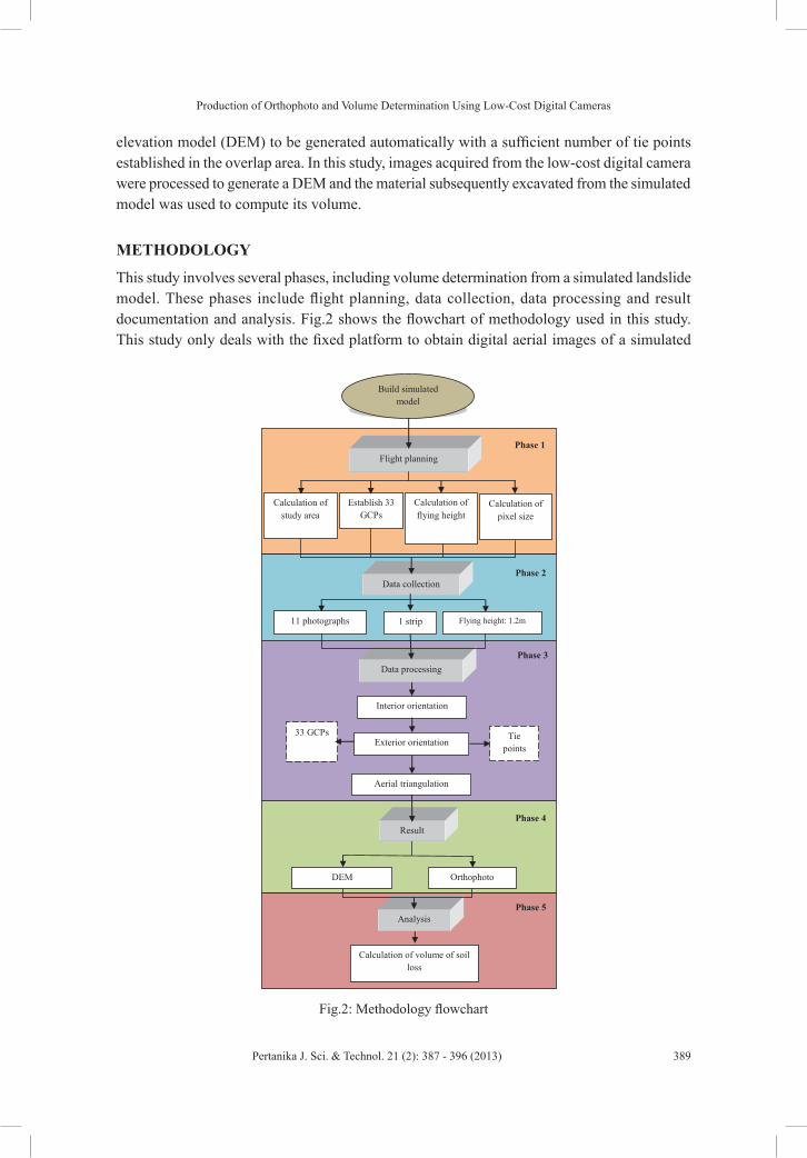
Production of Orthophoto and Volume Determination Using Low-Cost Digital Cameras
389Pertanika J. Sci. & Technol. 21 (2): 387 - 396 (2013)
elevation model (DEM) to be generated automatically with a sufficient number of tie points established in the overlap area. In this study, images acquired from the low-cost digital camera were processed to generate a DEM and the material subsequently excavated from the simulated model was used to compute its volume.
METHODOLOGY
This study involves several phases, including volume determination from a simulated landslide model. These phases include flight planning, data collection, data processing and result documentation and analysis. Fig.2 shows the flowchart of methodology used in this study. This study only deals with the fixed platform to obtain digital aerial images of a simulated
Fig.2: Methodology flowchart
Phase 1
Phase 2
Establish 33 GCPs
Data collection
11 photographs 1 strip Flying height: 1.2m
Build simulated model
Flight planning
Calculation of pixel size
Calculation of flying height
DEM Orthophoto
Phase 4
Phase 3
Interior orientation
Aerial triangulation
33 GCPs
Analysis
Calculation of volume of soil loss
Calculation of study area
Data processing
Exterior orientation Tie
points
Result
Phase 5
Khairul Nizam Tahar and Anuar Ahmad
390 Pertanika J. Sci. & Technol. 21 (2): 387 - 396 (2013)
landslide model. The simulated model was constructed using sand and cement with dimensions approximately 3m by 1m. Before photogrammetry work was carried out, all camera information was considered. In digital images, the main issue of importance is pixel size. Pixel size can be calculated using the following formula:
x fX H
= (1)
where x = number of pixel on the image of an objectX = length of the object f = focal lengthH = flying height
Pixel size is calculated based on the number of pixels of the object image, length of an object in real measurement, focal length of the camera and flying height during acquisition of the digital aerial image. After pixel size is calculated, the area of ground coverage can be determined. The area of ground coverage for an image is determined by multiplying the scale of the photography with its dimensions (i.e. length and width).
Flight planning
In this study, flight planning involved calculation of the study area, establishment of GCPs, calculation of flying height and calculation of pixel size. The area of the simulated model was calculated to ensure all segments were covered in the image acquisition stage. In photogrammetry, each pair of overlap photographs should be overlapped by 60% in order to get a 3D photogrammetric product of good quality.
The details of data acquisition are shown in the methodology flowchart where 11 photographs were captured to cover the whole simulated model in only one single strip with a flying height of 1.2m above ground. The flying height was determined based on pixel size and ground dimension. There were 33 GCPs well distributed along the entire simulated model and were established using a total station. GCPs were marked at random on the simulated model and were used in image processing. The coordinates of each GCP were determined using the intersection method for X and Y coordinates while the Z coordinate was determined using the tacheometry method where the Z coordinate is transferred from one point to another point utilising slope angle, horizontal distance and vertical distance.
Camera calibration
In this study, self calibration bundle adjustment was carried out for camera calibration. The low-cost digital camera was calibrated to obtain camera calibration parameters and the best results for image processing. All the camera calibration parameters were utilised in image processing for interior orientation using digital photogrammetric software. Fig.3 shows the position of the camera in camera calibration using the convergence method. The convergence
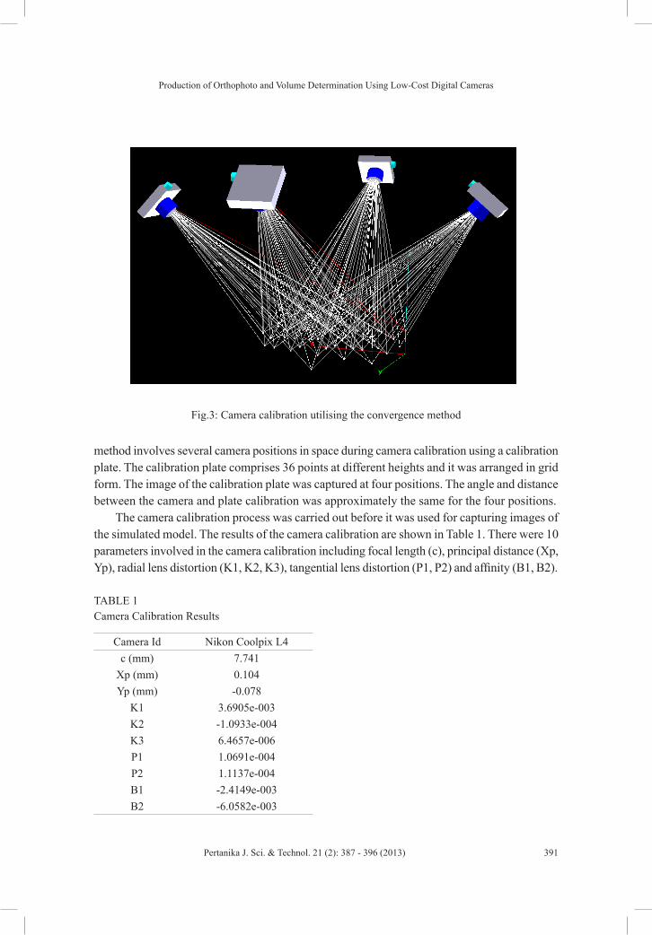
Production of Orthophoto and Volume Determination Using Low-Cost Digital Cameras
391Pertanika J. Sci. & Technol. 21 (2): 387 - 396 (2013)
method involves several camera positions in space during camera calibration using a calibration plate. The calibration plate comprises 36 points at different heights and it was arranged in grid form. The image of the calibration plate was captured at four positions. The angle and distance between the camera and plate calibration was approximately the same for the four positions.
The camera calibration process was carried out before it was used for capturing images of the simulated model. The results of the camera calibration are shown in Table 1. There were 10 parameters involved in the camera calibration including focal length (c), principal distance (Xp, Yp), radial lens distortion (K1, K2, K3), tangential lens distortion (P1, P2) and affinity (B1, B2).
TABLE 1 Camera Calibration Results
Camera Id Nikon Coolpix L4c (mm) 7.741
Xp (mm) 0.104Yp (mm) -0.078
K1 3.6905e-003K2 -1.0933e-004K3 6.4657e-006P1 1.0691e-004P2 1.1137e-004B1 -2.4149e-003B2 -6.0582e-003
Fig.3: Camera calibration utilising the convergence method

Khairul Nizam Tahar and Anuar Ahmad
392 Pertanika J. Sci. & Technol. 21 (2): 387 - 396 (2013)
DATA PROCESSING
Digital aerial images of the simulated model were acquired and then processed using photogrammetric software. In this study, ERDAS Imagine software was used for the production of photogrammetric products, such as DEM, contour lines and orthophoto. During the interior orientation, camera focal length and pixel size were obtained. GCPs were used for the exterior orientation process. This software needs at least four GCPs in each overlap photograph in order to perform aerial triangulation. The distribution of the GCPs and tie points for this study is shown in Fig.4. The figure shows the distribution of GCPs and tie points after performing aerial triangulation which involved interior and exterior orientations. Figure 4 also shows the footprint of a strip of digital images of the simulated model where the square represents the GCPs and the triangle represents tie points. There are 33 GCPs and 381 tie points used by 11 digital images. The tie points were selected automatically using the software based on image matching where the user could select any number of required tie points. It should be noted that if the surface is homogeneous, such as same tone, colour and texture then the software will fail to determine the tie points. Therefore, it is necessary that the material used, as was the case for the experiment, should be of different colours and textures i.e. not be homogeneous.
RESULTSTwo major results were obtained in this study i.e. digital orthophotos and DEM. The orthophoto for each overlapped pair is mosaiced in order to portray the whole simulated model. The DEM (Fig.5) and orthophotos (Fig.6) were generated after performing interior orientation, exterior orientation and digital mosaic operation. DEM is generated using a combination of GCPs and tie points after aerial triangulation, and the quality of the DEM and digital orthophoto depends on the accuracy of the GCPs. It should be noted that if the quality of the GCPs is poor then the results of the DEM and the digital orthophoto are less accurate.
The accuracy of the assessment of the DEM and the digital orthophoto was based on RMSE, mean and standard deviation of 30 sample dataset after image processing. The accuracy of the digital orthophoto and DEM are illustrated in Table 2.
TABLE 2 Accuracy of Digital Orthophoto and DEM
GCP RMSE(m) Mean(m) Std Dev.(m)X 0.002 0.001 0.001Y 0.001 0.001 0.001Z 0.214 0.147 0.163
ANALYSIS
The objective of this study was to investigate the capabilities of low-cost digital cameras in volume determination. In this study, some portion of the simulated model was excavated to simulate a landslide. DEMs were generated before and after the excavation. The DEMs before and after the landslide simulation were used as a primary data for volume calculation. Fig.7 shows the differences between the DEMs before and after the landslide simulation. It can be seen that the pixel value for
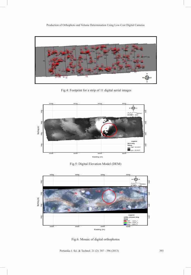
Production of Orthophoto and Volume Determination Using Low-Cost Digital Cameras
393Pertanika J. Sci. & Technol. 21 (2): 387 - 396 (2013)
Fig.4: Footprint for a strip of 11 digital aerial images
Fig.5: Digital Elevation Model (DEM)
Fig.6: Mosaic of digital orthophotos
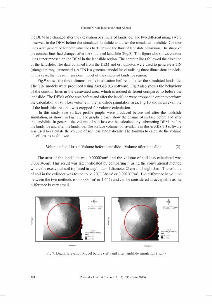
Khairul Nizam Tahar and Anuar Ahmad
394 Pertanika J. Sci. & Technol. 21 (2): 387 - 396 (2013)
the DEM had changed after the excavation or simulated landslide. The two different images were observed in the DEM before the simulated landslide and after the simulated landslide. Contour lines were generated for both situations to determine the flow of landslide behaviour. The shape of the contour lines had changed after the simulated landslide (Fig.8). This figure also shows contour lines superimposed on the DEM in the landslide region. The contour lines followed the direction of the landslide. The data obtained from the DEM and orthophotos were used to generate a TIN (triangular irregular network). A TIN is a generated model for visualising three-dimensional models, in this case, the three-dimensional model of the simulated landslide region.
Fig.9 shows the three-dimensional visualisation before and after the simulated landslide. The TIN models were produced using ArcGIS 9.3 software. Fig.9 also shows the behaviour of the contour lines in the excavated area, which is indeed different compared to before the landslide. The DEMs of the area before and after the landslide were cropped in order to perform the calculation of soil loss volume in the landslide simulation area. Fig.10 shows an example of the landslide area that was cropped for volume calculation.
In this study, two surface profile graphs were produced before and after the landslide simulation, as shown in Fig. 11. The graphs clearly show the change of surface before and after the landslide. In general, the volume of soil loss can be calculated by subtracting DEMs before the landslide and after the landslide. The surface volume tool available in the ArcGIS 9.3 software was used to calculate the volume of soil loss automatically. The formula to calculate the volume of soil loss is as follows:
Volume of soil loss = Volume before landslide - Volume after landslide (2)
The area of the landslide was 0.000026m² and the volume of soil loss calculated was 0.002043m³. This result was later validated by comparing it using the conventional method where the excavated soil is placed in a cylinder of diameter 23cm and height 5cm. The volume of soil in the cylinder was found to be 2077.38cm³ or 0.002077m³. The difference in volume between the two methods is 0.000034m³ or 1.64% and can be considered as acceptable as the difference is very small.
Fig.7: Digital Elevation Model before (left) and after landslide simulation (right)
(a) (b)
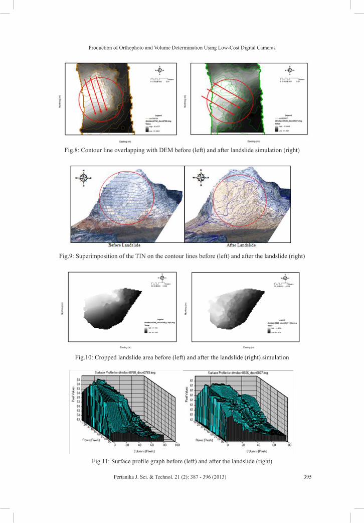
Production of Orthophoto and Volume Determination Using Low-Cost Digital Cameras
395Pertanika J. Sci. & Technol. 21 (2): 387 - 396 (2013)
Fig.8: Contour line overlapping with DEM before (left) and after landslide simulation (right)
Fig.9: Superimposition of the TIN on the contour lines before (left) and after the landslide (right)
Fig.10: Cropped landslide area before (left) and after the landslide (right) simulation
Fig.11: Surface profile graph before (left) and after the landslide (right)
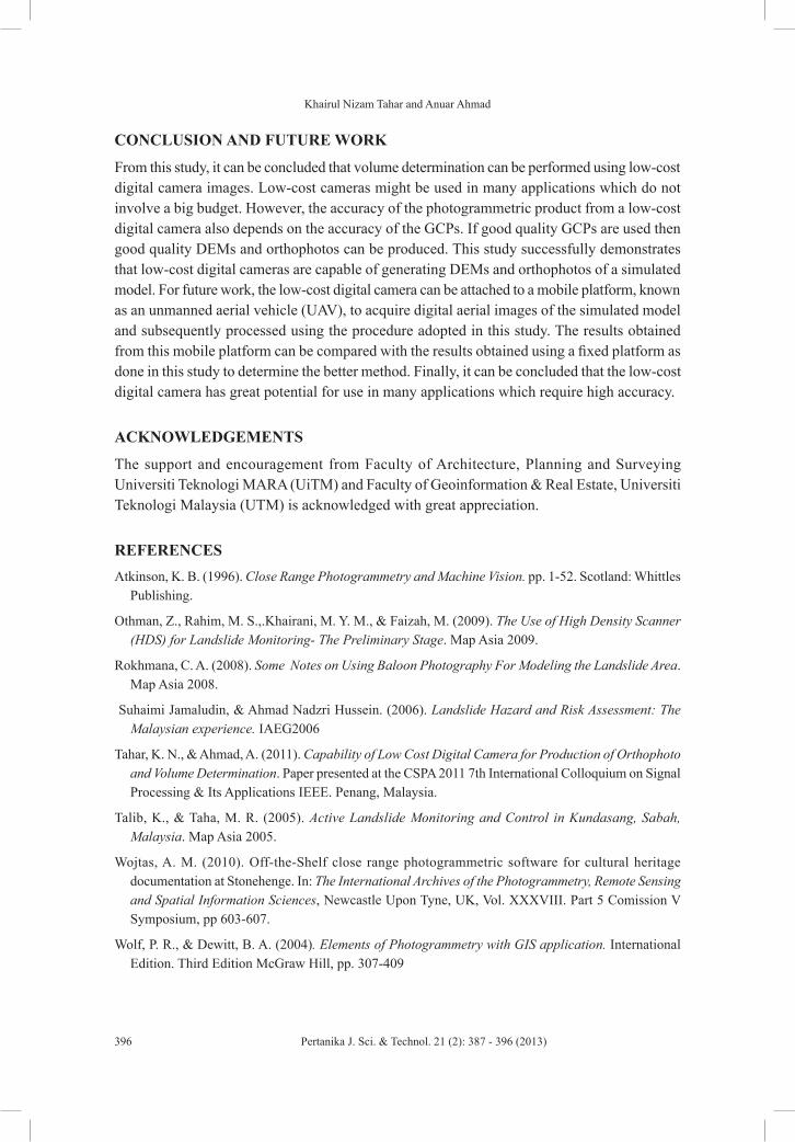
Khairul Nizam Tahar and Anuar Ahmad
396 Pertanika J. Sci. & Technol. 21 (2): 387 - 396 (2013)
CONCLUSION AND FUTURE WORK
From this study, it can be concluded that volume determination can be performed using low-cost digital camera images. Low-cost cameras might be used in many applications which do not involve a big budget. However, the accuracy of the photogrammetric product from a low-cost digital camera also depends on the accuracy of the GCPs. If good quality GCPs are used then good quality DEMs and orthophotos can be produced. This study successfully demonstrates that low-cost digital cameras are capable of generating DEMs and orthophotos of a simulated model. For future work, the low-cost digital camera can be attached to a mobile platform, known as an unmanned aerial vehicle (UAV), to acquire digital aerial images of the simulated model and subsequently processed using the procedure adopted in this study. The results obtained from this mobile platform can be compared with the results obtained using a fixed platform as done in this study to determine the better method. Finally, it can be concluded that the low-cost digital camera has great potential for use in many applications which require high accuracy.
ACKNOWLEDGEMENTS
The support and encouragement from Faculty of Architecture, Planning and Surveying Universiti Teknologi MARA (UiTM) and Faculty of Geoinformation & Real Estate, Universiti Teknologi Malaysia (UTM) is acknowledged with great appreciation.
REFERENCESAtkinson, K. B. (1996). Close Range Photogrammetry and Machine Vision. pp. 1-52. Scotland: Whittles
Publishing.
Othman, Z., Rahim, M. S.,.Khairani, M. Y. M., & Faizah, M. (2009). The Use of High Density Scanner (HDS) for Landslide Monitoring- The Preliminary Stage. Map Asia 2009.
Rokhmana, C. A. (2008). Some Notes on Using Baloon Photography For Modeling the Landslide Area. Map Asia 2008.
Suhaimi Jamaludin, & Ahmad Nadzri Hussein. (2006). Landslide Hazard and Risk Assessment: The Malaysian experience. IAEG2006
Tahar, K. N., & Ahmad, A. (2011). Capability of Low Cost Digital Camera for Production of Orthophoto and Volume Determination. Paper presented at the CSPA 2011 7th International Colloquium on Signal Processing & Its Applications IEEE. Penang, Malaysia.
Talib, K., & Taha, M. R. (2005). Active Landslide Monitoring and Control in Kundasang, Sabah, Malaysia. Map Asia 2005.
Wojtas, A. M. (2010). Off-the-Shelf close range photogrammetric software for cultural heritage documentation at Stonehenge. In: The International Archives of the Photogrammetry, Remote Sensing and Spatial Information Sciences, Newcastle Upon Tyne, UK, Vol. XXXVIII. Part 5 Comission V Symposium, pp 603-607.
Wolf, P. R., & Dewitt, B. A. (2004). Elements of Photogrammetry with GIS application. International Edition. Third Edition McGraw Hill, pp. 307-409
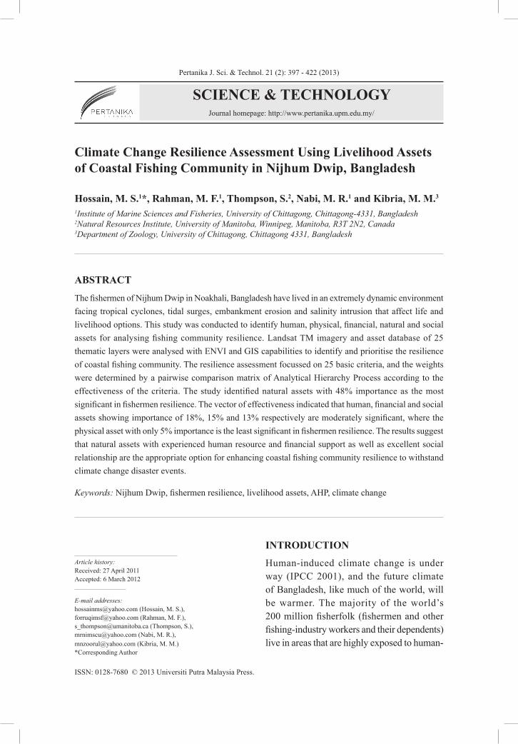
Pertanika J. Sci. & Technol. 21 (2): 397 - 422 (2013)
SCIENCE & TECHNOLOGYJournal homepage: http://www.pertanika.upm.edu.my/
ISSN: 0128-7680 © 2013 Universiti Putra Malaysia Press.
Climate Change Resilience Assessment Using Livelihood Assets of Coastal Fishing Community in Nijhum Dwip, Bangladesh
Hossain, M. S.1*, Rahman, M. F.1, Thompson, S.2, Nabi, M. R.1 and Kibria, M. M.3
1Institute of Marine Sciences and Fisheries, University of Chittagong, Chittagong-4331, Bangladesh2Natural Resources Institute, University of Manitoba, Winnipeg, Manitoba, R3T 2N2, Canada3Department of Zoology, University of Chittagong, Chittagong 4331, Bangladesh
ABSTRACT
The fishermen of Nijhum Dwip in Noakhali, Bangladesh have lived in an extremely dynamic environment facing tropical cyclones, tidal surges, embankment erosion and salinity intrusion that affect life and livelihood options. This study was conducted to identify human, physical, financial, natural and social assets for analysing fishing community resilience. Landsat TM imagery and asset database of 25 thematic layers were analysed with ENVI and GIS capabilities to identify and prioritise the resilience of coastal fishing community. The resilience assessment focussed on 25 basic criteria, and the weights were determined by a pairwise comparison matrix of Analytical Hierarchy Process according to the effectiveness of the criteria. The study identified natural assets with 48% importance as the most significant in fishermen resilience. The vector of effectiveness indicated that human, financial and social assets showing importance of 18%, 15% and 13% respectively are moderately significant, where the physical asset with only 5% importance is the least significant in fishermen resilience. The results suggest that natural assets with experienced human resource and financial support as well as excellent social relationship are the appropriate option for enhancing coastal fishing community resilience to withstand climate change disaster events.
Keywords: Nijhum Dwip, fishermen resilience, livelihood assets, AHP, climate change
Article history:Received: 27 April 2011Accepted: 6 March 2012
E-mail addresses: [email protected] (Hossain, M. S.), [email protected] (Rahman, M. F.), [email protected] (Thompson, S.), [email protected] (Nabi, M. R.), [email protected] (Kibria, M. M.)*Corresponding Author
INTRODUCTION
Human-induced climate change is under way (IPCC 2001), and the future climate of Bangladesh, like much of the world, will be warmer. The majority of the world’s 200 million fisherfolk (fishermen and other fishing-industry workers and their dependents) live in areas that are highly exposed to human-
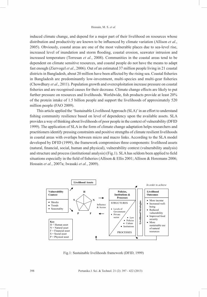
Hossain, M. S. et al.
398 Pertanika J. Sci. & Technol. 21 (2): 397 - 422 (2013)
induced climate change, and depend for a major part of their livelihood on resources whose distribution and productivity are known to be influenced by climate variation (Allison et al., 2005). Obviously, coastal areas are one of the most vulnerable places due to sea-level rise, increased level of inundation and storm flooding, coastal erosion, seawater intrusion and increased temperature (Torresan et al., 2008). Communities in the coastal areas tend to be dependent on climate sensitive resources, and coastal people do not have the means to adapt fast enough (Ziervogel et al., 2006). Out of an estimated 37 million people living in 21 coastal districts in Bangladesh, about 20 million have been affected by the rising sea. Coastal fisheries in Bangladesh are predominantly low-investment, multi-species and multi-gear fisheries (Chowdhury et al., 2011). Population growth and overexploitation increase pressure on coastal fisheries and are recognised causes for their decrease. Climate change effects are likely to put further pressure on resources and livelihoods. Worldwide, fish products provide at least 20% of the protein intake of 1.5 billion people and support the livelihoods of approximately 520 million people (FAO 2009).
This article applied the ‘Sustainable Livelihood Approach (SLA)’ in an effort to understand fishing community resilience based on level of dependency upon the available assets. SLA provides a way of thinking about livelihoods of poor people in the context of vulnerability (DFID 1999). The application of SLA in the form of climate change adaptation helps researchers and practitioners identify pressing constraints and positive strengths of climate resilient livelihoods in coastal areas with overlaps between micro and macro links. According to the SLA model developed by DFID (1999), the framework compromises three components: livelihood assets (natural, financial, social, human and physical), vulnerability context (vulnerability analysis) and structure and process (institutional analysis) (Fig.1). SLA has seldom been applied to field situations especially in the field of fisheries (Allison & Ellis 2001; Allison & Horemans 2006; Hossain et al., 2007a; Iwasaki et al., 2009).
H
S
P F
N
Vulnerability Context
Shocks Trends Seasonality
Livelihood Assets
Key H = Human asset N = Natural asset F = Financial asset S = Social asset P = Physical asset
Livelihood Outcomes
More income Increased well-
being Reduced
vulnerability Improved food
security More
sustainable use of natural resources
STRUCTURES Levels of
Government Private
sector Law Policies Culture
Institutions PROCESSES
Policies, Institutions &
Processes
Liv
elih
ood
Stra
tegi
es
Influence & Access
In order to achieve
Fig.1: Sustainable livelihoods framework (DFID, 1999)

Climate Change Resilience Assessment Using Livelihood Assets
399Pertanika J. Sci. & Technol. 21 (2): 397 - 422 (2013)
Resilience intuitively refers to the ability to bend without breaking and to regain the original “pre-bend” shape (Jacob & Showalter 2007). Resilience can be defined in various ways but it is essentially about how systems (bio-physical and socio-economic) are able to respond to change or shocks while maintaining their key characteristics or ‘identity’. Socio-economic resilience in terms of fishing communities refers to how they are able to maintain their livelihoods and desired ways of living, without outside assistance, following undesirable shocks. It would include, for instance, their flexibility to make substitutions that would yield more abundant fishery resources or lead to alternative economic activities to help offset declines in harvests from targetted fisheries. Resilience makes strong connections among management and human ecology because it is directed at evaluating responses to disturbances. Responses may include what is commonly referred to as indigenous knowledge, which is the cultural capital of a population in association with the environment. It may include, for example, knowledge of plant and animal, cultivation methods, local medicine and fishing craft and gear. There is a need to understand the resilience criteria and the level of importance of each criterion on coastal fishermen’s livelihood. The research used both qualitative and quantitative data including household-head interview, key-informants interviews, participatory field observation and satellite imagery (Hossain et al., 2007b). In addition, Venn diagrams, problem trees and seasonality maps were applied as the PRA exercises for identification of resources and analysing livelihood options. Likewise, semi-structured interviews with key informants (i.e. school teacher, government officer, village leader, NGO worker and mosque imam) were carried out to validate and complement the information. This article aims to identify the livelihood assets of fishermen in Nijhum Dwip and analyse the assets into bottom level criteria to measure the relative importance of each criterion in resilience assessment.
STUDY AREA
Profile of study site
Nijhum Dwip (literally “the island of silence”) is an accreted island in the central coastal zone of Bangladesh under Hatiya Upazila of Noakhali District, and is situated between latitude 22º1´ and 22º6´N and longitude 90º58´ and 91º3´E (Fig.2). Nijhum Dwip is separated from Hatiya by the Moktaria Channel, which is about 700-1200m wide: the island area is only 10 km2 in area (Fig.2). Fishermen of the nearby Hatiya Island started to use Nijhum Dwip during the 1940s as temporary homes during fishing season (personal communication with union parishad member). In the 1950s fishermen named it Ichamoti dwip (meaning mine of prawn; locals referred to island as icha mach, or prawn) due to a high abundance of prawn available in the waters surrounding the island (Amin, 2001). Temporary settlers later renamed it Baollar char (meaning accreted sand) , due to its high protuberance of sand. A land survey of Nijhum Dwip was conducted during 1959-1960, and after that, some of the fisherfolk came to live permanently on the island. However, Bangladesh’s most devastating cyclone of 12 November 1970, which killed about half a million coastal people in Bangladesh, killed all of the 300 households (1200 to 1500 people) settled on this exposed island. In an official visit to the island in 1973, government officials, politicians and social elites gave the island an official name in recognition of its natural beauty, Nijhum Dwip. In 2008, the government of Bangladesh

Hossain, M. S. et al.
400 Pertanika J. Sci. & Technol. 21 (2): 397 - 422 (2013)
declared Nijhum Dwip and the Char Bahauddin as a Union Parishad of Hatiya Upazila. The population has since increased to about 4500 households with an estimated 30,000 people living in different cluster villages. The literacy rate on the island is very low, at about 10%. Children below the age of 12 years account for 30% of the total population and married adults represent about 40%. The lack of sanitation facilities on the island causes severe problems because none of the households use sanitary latrines. Drinking water is available from shallow tube wells, which households share at a rate of one well per 50-75 households.
Biodiversity status
The environment surrounding the island is a unique assemblage of marine, brackish and fresh water ecosystem with estuarine characteristics. This combination has endowed Nijhum Dwip with a highly productive ecosystem for fisheries resources. Although limited quantitative data on marine biodiversity of Nijhum Dwip are available, the availability of fishes, shrimps, molluscs and crabs that is common to the rest of Bangladesh is believed to extend to these waters as well. Mangrove plantation started in 1973 with Sonneratia apetala (80%) and Avicennia officinalis (15%) that covered the northwest part of the island. The ecosystem is biologically diverse with 68 plant and 66 animal species (Rosario, 1997). The island is at the crossroads of two international flyways viz. the East-Asia Australasian flyways and Central Asian flyways and is the southern-most staging ground of around 60 species of migratory birds. The site supports critically endangered species from around the world such as the Indian Skimmer (Rynchops albicollis), Spoon-billed Sandpiper (Eurynorhynchus pygmeus), Nordmann’s Greenshank (Tringa guttifer) and Asian Dowitcher (Limnodromus semipalmatus) by providing them with their wintering ground (PDO-ICZMP 2004). To further enhance the
22° N
22° 30΄ N
91° E
91° 3
0΄ E
23° N
HATIYA
SANDWIP
BHOLA
NOAKHALI
M U K T E R I A CHANNEL
Fig.2: Geographical location of the Nijhum Dwip in the central coastal zone of Bangladesh, based on Landsat TM image of March 2007

Climate Change Resilience Assessment Using Livelihood Assets
401Pertanika J. Sci. & Technol. 21 (2): 397 - 422 (2013)
biodiversity of the island, three pairs of spotted deer (Axis axis) were released in the island in 1980 which increased to 14,400 (Iftekhar and Takama 2008). Subsequent introductions have included several pairs of monkeys (Macaca mulatta), snakes (Python molurus) and Leopard cat (Felis bengalensis). These vibrant biodiversity allowed Nijhum Dwip to be listed as a wetland of international importance under the Bangladesh Wildlife (Preservation) Order 1973, and it was made a National Park of Bangladesh in 2001. Insidious human activity such as hunting, killing or capturing wildlife and damaging or destroying plants or trees has been banned by the government (PDO-ICZMP 2004).
Temperature
Nijhum Dwip is typically tropical with average annual maximum and minimum temperatures of 30°C and 21.6°C respectively (BMD 2009). Changes in temperature, even small changes in water temperature, are expected to exert strong pressure upon fish ecology (WWF 2005). Temperature variations also affect human health, undermining their capacity for operating the fisheries. According to the statistical fixed-point observations in six meteorological stations i.e. Maijdee, Hatiya, Feni, Sandwip, Chittagong and Cox’s Bazaar , it seems that the apparent warming trend has not been seen in Nijhum Dwip (Fig.3), as opposed to the world’s expectation (IPCC 2007). However, it seems that there is a slight warming trend of mean maximum and minimum temperature especially in the hottest month. In a variation of 20 years (1988-2008), annual maximum temperature increased by 0.08oC, whereas annual minimum temperature decreased by 0.89oC and annual average temperature decreased by 0.32oC. The length of the winter season with a temperature less than 15oC has been recorded as 41 days and 55 days in 1988 and 2008 respectively, where the first day of winter shifted from 8 December to 18 November. Similarly, the length of the summer season with a temperature more than 35oC was recorded as 2 and 5 days in 1988 and 2008 respectively, where the first day of summer shifted from 14 February to 27 February (Table 1).
TABLE 1 Variation of climatic parameters in Hatiya Island of Noakhali District for a period of 20 years (1988-2008) (source: Bangladesh Meteorological Department, Dhaka)
Parameters 1988 2008 ChangeAnnual max temperature (°C) 29.91 29.99 0.08Annual min temperature (°C) 22.52 21.63 -0.89Annual average temperature (°C) 25.97 25.65 -0.32Length of winter (day <15 °C) 21 55 34First winter day (<18 °C) 8-Dec 18-Nov 10Length of summer (day >35 °C) 2 5 3First summer day (day >30 °C) 14-Feb 27-Feb 13Annual Rainfall (mm) 3561 3531 -30Length of rainy season (day >10 mm) 83 75 -8First rainy day (>10 mm) 13-May 18-May 5
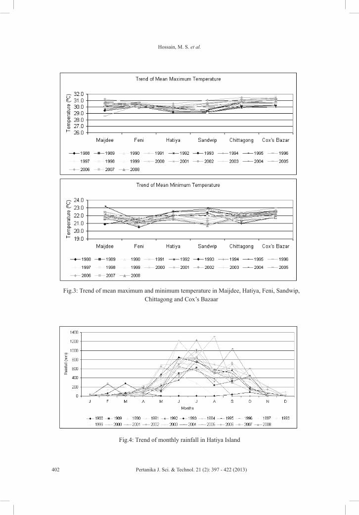
Hossain, M. S. et al.
402 Pertanika J. Sci. & Technol. 21 (2): 397 - 422 (2013)
Fig.3: Trend of mean maximum and minimum temperature in Maijdee, Hatiya, Feni, Sandwip, Chittagong and Cox’s Bazaar
Fig.4: Trend of monthly rainfall in Hatiya Island
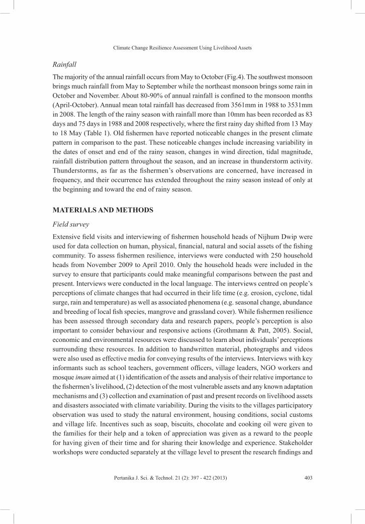
Climate Change Resilience Assessment Using Livelihood Assets
403Pertanika J. Sci. & Technol. 21 (2): 397 - 422 (2013)
Rainfall
The majority of the annual rainfall occurs from May to October (Fig.4). The southwest monsoon brings much rainfall from May to September while the northeast monsoon brings some rain in October and November. About 80-90% of annual rainfall is confined to the monsoon months (April-October). Annual mean total rainfall has decreased from 3561mm in 1988 to 3531mm in 2008. The length of the rainy season with rainfall more than 10mm has been recorded as 83 days and 75 days in 1988 and 2008 respectively, where the first rainy day shifted from 13 May to 18 May (Table 1). Old fishermen have reported noticeable changes in the present climate pattern in comparison to the past. These noticeable changes include increasing variability in the dates of onset and end of the rainy season, changes in wind direction, tidal magnitude, rainfall distribution pattern throughout the season, and an increase in thunderstorm activity. Thunderstorms, as far as the fishermen’s observations are concerned, have increased in frequency, and their occurrence has extended throughout the rainy season instead of only at the beginning and toward the end of rainy season.
MATERIALS AND METHODS
Field survey
Extensive field visits and interviewing of fishermen household heads of Nijhum Dwip were used for data collection on human, physical, financial, natural and social assets of the fishing community. To assess fishermen resilience, interviews were conducted with 250 household heads from November 2009 to April 2010. Only the household heads were included in the survey to ensure that participants could make meaningful comparisons between the past and present. Interviews were conducted in the local language. The interviews centred on people’s perceptions of climate changes that had occurred in their life time (e.g. erosion, cyclone, tidal surge, rain and temperature) as well as associated phenomena (e.g. seasonal change, abundance and breeding of local fish species, mangrove and grassland cover). While fishermen resilience has been assessed through secondary data and research papers, people’s perception is also important to consider behaviour and responsive actions (Grothmann & Patt, 2005). Social, economic and environmental resources were discussed to learn about individuals’ perceptions surrounding these resources. In addition to handwritten material, photographs and videos were also used as effective media for conveying results of the interviews. Interviews with key informants such as school teachers, government officers, village leaders, NGO workers and mosque imam aimed at (1) identification of the assets and analysis of their relative importance to the fishermen’s livelihood, (2) detection of the most vulnerable assets and any known adaptation mechanisms and (3) collection and examination of past and present records on livelihood assets and disasters associated with climate variability. During the visits to the villages participatory observation was used to study the natural environment, housing conditions, social customs and village life. Incentives such as soap, biscuits, chocolate and cooking oil were given to the families for their help and a token of appreciation was given as a reward to the people for having given of their time and for sharing their knowledge and experience. Stakeholder workshops were conducted separately at the village level to present the research findings and
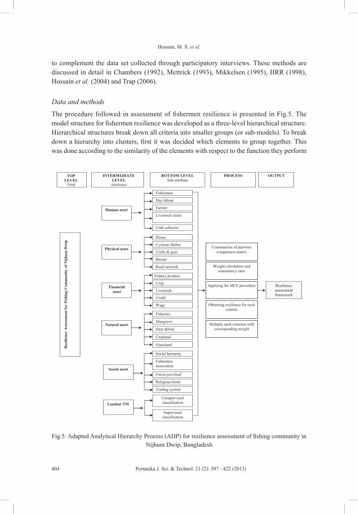
Hossain, M. S. et al.
404 Pertanika J. Sci. & Technol. 21 (2): 397 - 422 (2013)
to complement the data set collected through participatory interviews. These methods are discussed in detail in Chambers (1992), Mettrick (1993), Mikkelsen (1995), IIRR (1998), Hossain et al. (2004) and Trap (2006).
Data and methods
The procedure followed in assessment of fishermen resilience is presented in Fig.5. The model structure for fishermen resilience was developed as a three-level hierarchical structure. Hierarchical structures break down all criteria into smaller groups (or sub-models). To break down a hierarchy into clusters, first it was decided which elements to group together. This was done according to the similarity of the elements with respect to the function they perform
INTERMEDIATELEVEL
Attributes
BOTTOM LEVELSub-attribute
PROCESS OUTPUT
Res
ilien
ce A
sses
smen
t for
Fish
ing
Com
mun
ity o
f Nijh
um D
wip
Human asset
Physical asset
Financialasset
Natural asset
Social asset
Crab collector
Livestock raiser
Farmer
Day labour
Fishermen
Road network
Crafts & gear
Cyclone shelter
House
Bazaar
Wage
Livestock
Crop
Fishery product
Credit
Grassland
Deer &bird
Mangrove
Fisheries
Cropland
Trading system
Union parishad
Fishermen association
Religious bond
Social harmony
Resilience assessmentframework
Applying the MCE procedure
Construction of pairwise comparison matrix
Weight calculation and consistency ratio
Obtaining resilience for each criteria
Multiply each criterion with corresponding weight
Landsat TMUnsupervised classification
Supervised classification
TOPLEVELGoal
Fig.5: Adapted Analytical Hierarchy Process (AHP) for resilience assessment of fishing community in Nijhum Dwip, Bangladesh

Climate Change Resilience Assessment Using Livelihood Assets
405Pertanika J. Sci. & Technol. 21 (2): 397 - 422 (2013)
or properties they share (Saaty, 1988). The top or first level in the hierarchy represents the ultimate goal of the multi-criteria decision-making analysis process. The intermediate or second hierarchy level lists the relevant evaluation criteria that were compared pairwise to assess their relative weights. Each of these clusters was considered as a sub-model. The bottom level in the hierarchy contains the evaluation objects. All these criteria (sub-attributes) are identified to influence the goal of the study and may represent primary data or be the result of some secondary data.
The data sources were social survey, field measurement, administrative map, topographic maps of 1:10,000 scale and Landsat TM satellite image for land use pattern and spatial analysis of resources distribution. Land use patterns, road, embankment, cyclone shelter, market location and human settlement were taken from 1:10,000 scale topographic maps and 1:50,000 scale administrative maps, and then updated with Landsat TM satellite image, intensive field survey and participatory interviews. All this information was used to assess the resilience of the island fishing community. The GIS software used in this study was ArcGIS for windows (version 9.3) developed by Environmental Systems Research Institute Inc, USA. Remote-sensing image analysis was done using ENVI (version 4.3) developed by Research Systems Inc, USA. The selected and scored criteria were developed into a series of sub-models which logically grouped certain factors together within a general model. For example, respective sub-attributes were grouped to form sub-models (e.g. in human assets analysis; fishermen, day labour, farmer, livestock raiser and crab collector were grouped to form the sub-model, “human assets”), while other sub-attributes were grouped into sub-models to enable a better understanding (e.g. fisheries, mangrove, deer and bird, cropland and grassland were grouped to form the sub-model, “natural assets”).
Satellite image classification
Isodata unsupervised classification (use information from the image itself to identify spectral clusters, which are interpreted as classes,) was performed considering minimum and maximum classes of 5-10, 10-15 and 15-20, where the 5-10 classes turned out to be useful. Supervised classification was carried out on the basis of Region of Interest (ROIs), where the ground truth or so-called training areas (collected during field investigation) were regions of terrain with known properties or characteristics (Research Systems Inc., 2000; Hossain et al., 2009b; Hossain & Das, 2010a, 2010b). Maximum likelihood classification strategy was applied and found to be most useful for discriminating the category of interest. After image processing, reference points were chosen for ground verification. All the reference points were surveyed for the ground truthing of Nijhum Dwip and compared with the preliminary map to real position. ArcGIS (The Environmental systems Research Institute Inc., USA) and MS Excel (The Microsoft Corporation, USA) software were used to digitise and analyse all the classified and other necessary maps.

Hossain, M. S. et al.
406 Pertanika J. Sci. & Technol. 21 (2): 397 - 422 (2013)
Weight and score
The development of weights is based on pairwise comparison matrix. The comparisons are concerned with the relative importance of two criteria involved in determining resilience for the stated objective. In order to use this procedure, it is necessary for the weights to sum up to 1. Ratings are systematically scored on a 17-point continuous scale from 1/9 (least important) to 9/9 (most important) (Saaty, 1977) as in Table 2. In this research, scores were assigned in rank order according to the number of factors involved in the evaluation for resilience assessment without repetition. The pairwise comparison matrices developed are shown in Table 3. The consistency ratios (CR) of 0.0048 to 0.0139 for the table was well within the ratio of equal to or less than 0.10 recommended by Saaty (1977), signifying a small probability that the weights were developed by chance.
Although factor scores were objectively based upon real data, the assignment of weights during multi-criteria evaluation (MCE) was considered partly subjective because it was dependent upon decisions made by the authors. To help reduce some of this subjectivity, to verify the weights generated and to reach a consensus for weights, two analytical procedures were considered: a) use of questionnaires (Aguilar-Manjarrez, 1996) and b) group discussion for final weight consensus (Eastman et al., 1993; Kapetsky & Nath, 1997, Hossain & Das, 2010a). Because these procedures are complementary, this study combined the two in order to achieve increased objectivity. An important way of learning about local conditions and resources is to ask local communities what they know (Pelto & Pelto, 1978). Direct observation prevents rapid appraisal from being misled by myth and often provides more valid and less costly information than other research methods (Chambers, 1980; Hossain et al., 2007b).
The present study focussed on some basic criteria or sub-attributes. For instance, 25 base layers were developed to assess resilience of the fishing community i.e. human assets (fishermen, day labour, farmer, livestock raiser and crab collector), physical assets (house, cyclone shelter, craft and gear, bazaar and road network), financial assets (fishery yield, crop, livestock, credit and wage), natural assets (fisheries, mangrove, deer and bird, cropland and grassland) and social assets (social harmony, fishermen association, union parishad, religious bond and trading system). Weights were given according to the effectiveness of the criteria. The weight for each factor was determined by pairwise comparisons in the context of a decision-making process known as the analytical hierarchy process (Saaty, 1977, 1990), which was also recommended by Pereira and Duckstein (1993), Malczewski (1999), Kovacs et al., (2004), Hossain (2009b) and Hossain et al., (2009). The resilience rating for each level of a factor was determined from the survey results and professional judgment of the authors.
TABLE 2 The relative importance of two criteria (Saaty, 1977)
1/9 1/8 1/7 1/6 1/5 1/4 1/3 1/2 1 2 3 4 5 6 7 8 9Extremely Very
stronglyStrongly Moderately Equally Moderately Strongly Very
stronglyExtremely
LESS IMPORTANT MORE IMPORTANT
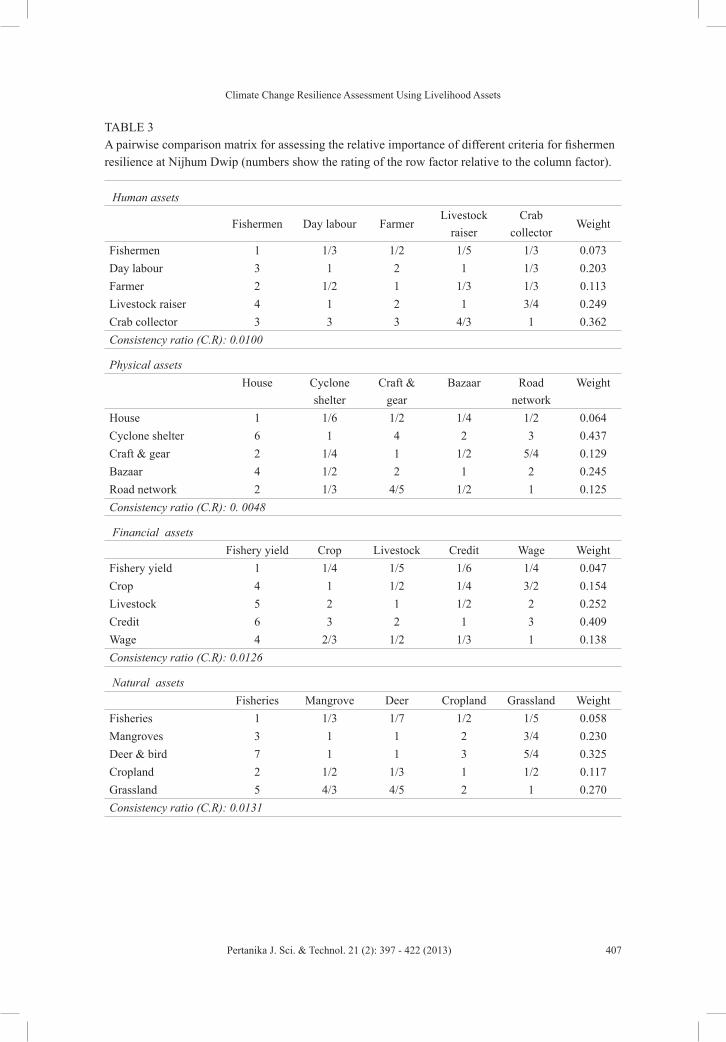
Climate Change Resilience Assessment Using Livelihood Assets
407Pertanika J. Sci. & Technol. 21 (2): 397 - 422 (2013)
TABLE 3 A pairwise comparison matrix for assessing the relative importance of different criteria for fishermen resilience at Nijhum Dwip (numbers show the rating of the row factor relative to the column factor).
Human assets
Fishermen Day labour FarmerLivestock
raiserCrab
collectorWeight
Fishermen 1 1/3 1/2 1/5 1/3 0.073Day labour 3 1 2 1 1/3 0.203Farmer 2 1/2 1 1/3 1/3 0.113Livestock raiser 4 1 2 1 3/4 0.249Crab collector 3 3 3 4/3 1 0.362Consistency ratio (C.R): 0.0100
Physical assetsHouse Cyclone
shelterCraft &
gearBazaar Road
networkWeight
House 1 1/6 1/2 1/4 1/2 0.064Cyclone shelter 6 1 4 2 3 0.437Craft & gear 2 1/4 1 1/2 5/4 0.129Bazaar 4 1/2 2 1 2 0.245Road network 2 1/3 4/5 1/2 1 0.125Consistency ratio (C.R): 0. 0048
Financial assetsFishery yield Crop Livestock Credit Wage Weight
Fishery yield 1 1/4 1/5 1/6 1/4 0.047Crop 4 1 1/2 1/4 3/2 0.154Livestock 5 2 1 1/2 2 0.252Credit 6 3 2 1 3 0.409Wage 4 2/3 1/2 1/3 1 0.138Consistency ratio (C.R): 0.0126
Natural assetsFisheries Mangrove Deer Cropland Grassland Weight
Fisheries 1 1/3 1/7 1/2 1/5 0.058Mangroves 3 1 1 2 3/4 0.230Deer & bird 7 1 1 3 5/4 0.325Cropland 2 1/2 1/3 1 1/2 0.117Grassland 5 4/3 4/5 2 1 0.270Consistency ratio (C.R): 0.0131
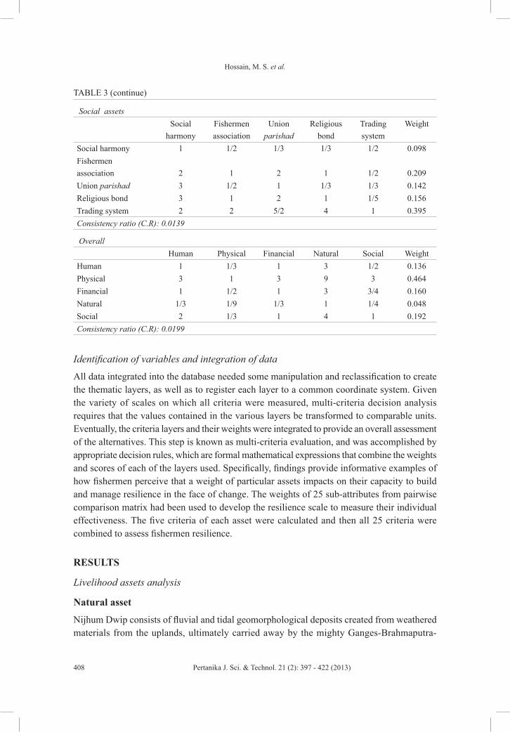
Hossain, M. S. et al.
408 Pertanika J. Sci. & Technol. 21 (2): 397 - 422 (2013)
Identification of variables and integration of data
All data integrated into the database needed some manipulation and reclassification to create the thematic layers, as well as to register each layer to a common coordinate system. Given the variety of scales on which all criteria were measured, multi-criteria decision analysis requires that the values contained in the various layers be transformed to comparable units. Eventually, the criteria layers and their weights were integrated to provide an overall assessment of the alternatives. This step is known as multi-criteria evaluation, and was accomplished by appropriate decision rules, which are formal mathematical expressions that combine the weights and scores of each of the layers used. Specifically, findings provide informative examples of how fishermen perceive that a weight of particular assets impacts on their capacity to build and manage resilience in the face of change. The weights of 25 sub-attributes from pairwise comparison matrix had been used to develop the resilience scale to measure their individual effectiveness. The five criteria of each asset were calculated and then all 25 criteria were combined to assess fishermen resilience.
RESULTS
Livelihood assets analysis
Natural asset
Nijhum Dwip consists of fluvial and tidal geomorphological deposits created from weathered materials from the uplands, ultimately carried away by the mighty Ganges-Brahmaputra-
Social assetsSocial
harmonyFishermen association
Union parishad
Religious bond
Trading system
Weight
Social harmony 1 1/2 1/3 1/3 1/2 0.098Fishermen association 2 1 2 1 1/2 0.209Union parishad 3 1/2 1 1/3 1/3 0.142Religious bond 3 1 2 1 1/5 0.156Trading system 2 2 5/2 4 1 0.395Consistency ratio (C.R): 0.0139
OverallHuman Physical Financial Natural Social Weight
Human 1 1/3 1 3 1/2 0.136Physical 3 1 3 9 3 0.464Financial 1 1/2 1 3 3/4 0.160Natural 1/3 1/9 1/3 1 1/4 0.048Social 2 1/3 1 4 1 0.192Consistency ratio (C.R): 0.0199
TABLE 3 (continue)

Climate Change Resilience Assessment Using Livelihood Assets
409Pertanika J. Sci. & Technol. 21 (2): 397 - 422 (2013)
Meghna River systems, and their numerous tributaries and deltaic channels, leading to the formation of a newly-accreted landscape. Analysing the Landsat TM image of January 1997 and March 2007 of the Nijhum Dwip revealed the increasing trend of the island from 4313ha in 1997 to 5231ha in 2007 (Fig.6). The accreted zone increased from 987ha to 1676ha in a duration of 10 years due to the heavy siltration of the Ganges-Brahmaputra-Meghna River systems. The plain land that increased by about 56% from 1078ha to 1686ha (Table 4) in 10 years has been used for ever increasing human settlement, agriculture, cyclone shelter, community market (locally called bazaar or hat) and road network. A road-cum-embankment has been constructed along the southeast side of the island, which is the zone exposed to the Bay of Bengal (Fig.7). Most of the human settlements are concentrated in the south and southeast of the island. The satellite-image analysis revealed that most of the tidal canals (locally called khal) and creeks are flowing in a southward direction through the mangrove forest and plain land of the island. These include the Char Kamlar Khal, Azam Khali Khal, Jarir Dona Khal and Chowdhury Khal. The mangrove forest decreased from 2248ha in 1997 to 1869ha in 2007 due to removal of forest produce for fuel wood, grazing pressure, agriculture and human settlement. Moreover, the islanders have become dependent on the mangrove forest for housing and boat-making materials. Mangrove plantation and a succession of natural grasses
Fig.6: Classified Landsat TM image of January 1997 and March 2007 revealed changing pattern of the Nijhum Dwip with pre-dominant land cover map
TABLE 4 Land use change of Nijhum Dwip over 20-year period (1997 to 2007)
Area in 1997 (ha) Area in 2007 (ha) Change (%)Mangrove forest 2248 1869 (-) 16.86 Plain land 1078 1686 56.40Accreted zone 987 1676 69.81Total 4313 5231 21.28
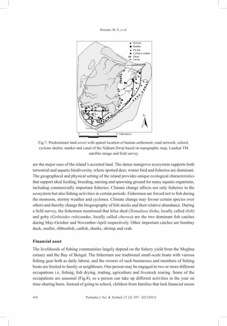
Hossain, M. S. et al.
410 Pertanika J. Sci. & Technol. 21 (2): 397 - 422 (2013)
are the major uses of the island’s accreted land. The dense mangrove ecosystem supports both terrestrial and aquatic biodiversity, where spotted deer, winter bird and fisheries are dominant. The geographical and physical setting of the island provides unique ecological characteristics that support ideal feeding, breeding, nursing and spawning ground for many aquatic organisms, including commercially important fisheries. Climate change affects not only fisheries in the ecosystem but also fishing activities in certain periods. Fishermen are forced not to fish during the monsoon, stormy weather and cyclones. Climate change may favour certain species over others and thereby change the biogeography of fish stocks and their relative abundance. During a field survey, the fishermen mentioned that hilsa shed (Tenualosa ilisha, locally called ilish) and goby (Gobioides rubicundus, locally called cheowa) are the two dominant fish catches during May-October and November-April respectively. Other important catches are bombay duck, mullet, ribbonfish, catfish, sharks, shrimp and crab.
Financial asset
The livelihoods of fishing communities largely depend on the fishery yield from the Meghna estuary and the Bay of Bengal. The fishermen use traditional small-scale boats with various fishing gear both as daily labour, and the owners of such businesses and members of fishing boats are limited to family or neighbours. One person may be engaged in two or more different occupations i.e. fishing, fish drying, trading, agriculture and livestock rearing. Some of the occupations are seasonal (Fig.8), so a person can take up different activities in the year on time-sharing basis. Instead of going to school, children from families that lack financial assets
Fig.7: Predominant land cover with spatial location of human settlement, road network, school, cyclone shelter, market and canal of the Nijhum Dwip based on topographic map, Landsat TM
satellite image and field survey
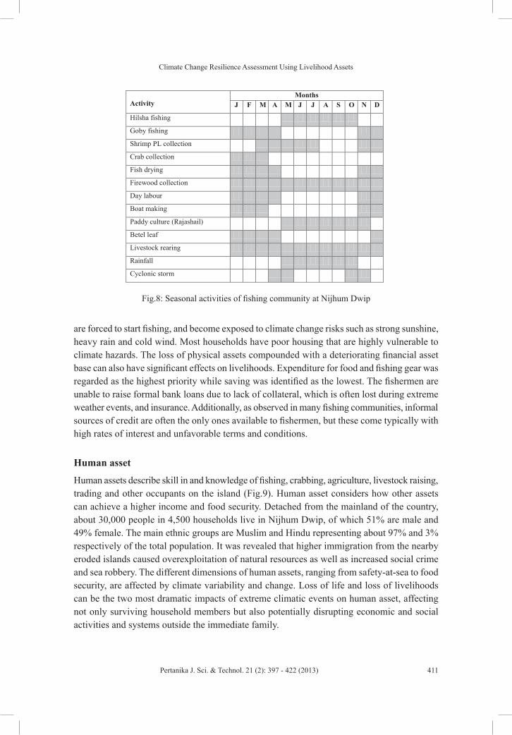
Climate Change Resilience Assessment Using Livelihood Assets
411Pertanika J. Sci. & Technol. 21 (2): 397 - 422 (2013)
are forced to start fishing, and become exposed to climate change risks such as strong sunshine, heavy rain and cold wind. Most households have poor housing that are highly vulnerable to climate hazards. The loss of physical assets compounded with a deteriorating financial asset base can also have significant effects on livelihoods. Expenditure for food and fishing gear was regarded as the highest priority while saving was identified as the lowest. The fishermen are unable to raise formal bank loans due to lack of collateral, which is often lost during extreme weather events, and insurance. Additionally, as observed in many fishing communities, informal sources of credit are often the only ones available to fishermen, but these come typically with high rates of interest and unfavorable terms and conditions.
Human asset
Human assets describe skill in and knowledge of fishing, crabbing, agriculture, livestock raising, trading and other occupants on the island (Fig.9). Human asset considers how other assets can achieve a higher income and food security. Detached from the mainland of the country, about 30,000 people in 4,500 households live in Nijhum Dwip, of which 51% are male and 49% female. The main ethnic groups are Muslim and Hindu representing about 97% and 3% respectively of the total population. It was revealed that higher immigration from the nearby eroded islands caused overexploitation of natural resources as well as increased social crime and sea robbery. The different dimensions of human assets, ranging from safety-at-sea to food security, are affected by climate variability and change. Loss of life and loss of livelihoods can be the two most dramatic impacts of extreme climatic events on human asset, affecting not only surviving household members but also potentially disrupting economic and social activities and systems outside the immediate family.
Activity
Months J F M A M J J A S O N D
Hilsha fishing
Goby fishing
Shrimp PL collection
Crab collection
Fish drying
Firewood collection
Day labour
Boat making
Paddy culture (Rajashail)
Betel leaf
Livestock rearing
Rainfall
Cyclonic storm
Fig.8: Seasonal activities of fishing community at Nijhum Dwip
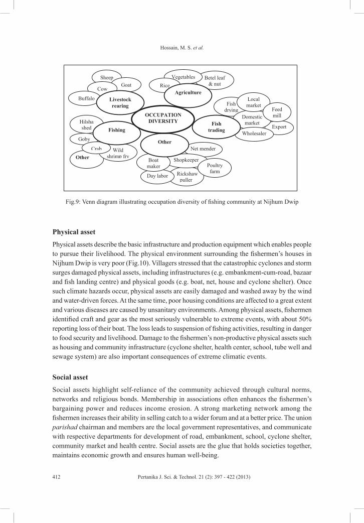
Hossain, M. S. et al.
412 Pertanika J. Sci. & Technol. 21 (2): 397 - 422 (2013)
Physical asset
Physical assets describe the basic infrastructure and production equipment which enables people to pursue their livelihood. The physical environment surrounding the fishermen’s houses in Nijhum Dwip is very poor (Fig.10). Villagers stressed that the catastrophic cyclones and storm surges damaged physical assets, including infrastructures (e.g. embankment-cum-road, bazaar and fish landing centre) and physical goods (e.g. boat, net, house and cyclone shelter). Once such climate hazards occur, physical assets are easily damaged and washed away by the wind and water-driven forces. At the same time, poor housing conditions are affected to a great extent and various diseases are caused by unsanitary environments. Among physical assets, fishermen identified craft and gear as the most seriously vulnerable to extreme events, with about 50% reporting loss of their boat. The loss leads to suspension of fishing activities, resulting in danger to food security and livelihood. Damage to the fishermen’s non-productive physical assets such as housing and community infrastructure (cyclone shelter, health center, school, tube well and sewage system) are also important consequences of extreme climatic events.
Social asset
Social assets highlight self-reliance of the community achieved through cultural norms, networks and religious bonds. Membership in associations often enhances the fishermen’s bargaining power and reduces income erosion. A strong marketing network among the fishermen increases their ability in selling catch to a wider forum and at a better price. The union parishad chairman and members are the local government representatives, and communicate with respective departments for development of road, embankment, school, cyclone shelter, community market and health centre. Social assets are the glue that holds societies together, maintains economic growth and ensures human well-being.
Sheep
Other
fish
Wild shrimp fry
Hilsha shed
Goby
Crab
Fishing
Net mender
Rickshaw puller
Shopkeeper
Day labor
Boat maker
Other
Betel leaf & nut
Vegetables
Fish drying
Export
Domestic market
Local market
Wholesaler
Poultry farm
Feed mill OCCUPATION
DIVERSITY
Rice Agriculture
Goat Cow
Buffalo Livestock rearing
Fish trading
Fig.9: Venn diagram illustrating occupation diversity of fishing community at Nijhum Dwip
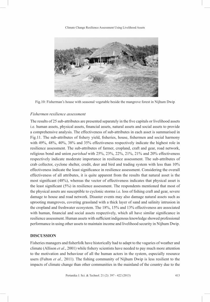
Climate Change Resilience Assessment Using Livelihood Assets
413Pertanika J. Sci. & Technol. 21 (2): 397 - 422 (2013)
Fishermen resilience assessment
The results of 25 sub-attributes are presented separately in the five capitals or livelihood assets i.e. human assets, physical assets, financial assets, natural assets and social assets to provide a comprehensive analysis. The effectiveness of sub-attributes in each asset is summarised in Fig.11. The sub-attributes of fishery yield, fisheries, house, fishermen and social harmony with 49%, 48%, 40%, 38% and 35% effectiveness respectively indicate the highest role in resilience assessment. The sub-attributes of farmer, cropland, craft and gear, road network, religious bond and union parishad with 25%, 23%, 22%, 21%, 21% and 20% effectiveness respectively indicate moderate importance in resilience assessment. The sub-attributes of crab collector, cyclone shelter, credit, deer and bird and trading system with less than 10% effectiveness indicate the least significance in resilience assessment. Considering the overall effectiveness of all attributes, it is quite apparent from the results that natural asset is the most significant (48%), whereas the vector of effectiveness indicates that physical asset is the least significant (5%) in resilience assessment. The respondents mentioned that most of the physical assets are susceptible to cyclonic storms i.e. loss of fishing craft and gear, severe damage to house and road network. Disaster events may also damage natural assets such as uprooting mangroves, covering grassland with a thick layer of sand and salinity intrusion in the cropland and freshwater ecosystem. The 18%, 15% and 13% effectiveness are associated with human, financial and social assets respectively, which all have similar significance in resilience assessment. Human assets with sufficient indigenous knowledge showed professional performance in using other assets to maintain income and livelihood security in Nijhum Dwip.
DISCUSSION
Fisheries managers and fisherfolk have historically had to adapt to the vagaries of weather and climate (Allison et al., 2001) while fishery scientists have needed to pay much more attention to the motivation and behaviour of all the human actors in the system, especially resource users (Fulton et al., 2011). The fishing community of Nijhum Dwip is less resilient to the impacts of climate change than other communities in the mainland of the country due to the
Fig.10: Fisherman’s house with seasonal vegetable beside the mangrove forest in Nijhum Dwip
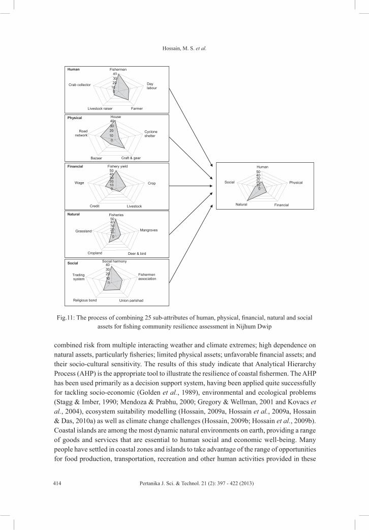
Hossain, M. S. et al.
414 Pertanika J. Sci. & Technol. 21 (2): 397 - 422 (2013)
0 10 20 30 40 50
Physical
Financial Natural
Social
Human
0 10 20 30 40 50
Crop
Livestock Credit
Wage
Fishery yield
Day labour
0 10 20 30 40
Fishermen
Farmer Livestock raiser
Crab collector
House
0 10 20 30 40
Cyclone shelter
Craft & gear Bazaar
Road network
0 10 20 30 40
Social harmony
Fishermen association
Union parishad Religious bond
Trading system
Human
0 10 20 30 40 50
Fisheries
Mangroves
Deer & bird Cropland
Grassland
Natural
Social
Financial
Physical
Fig.11: The process of combining 25 sub-attributes of human, physical, financial, natural and social assets for fishing community resilience assessment in Nijhum Dwip
combined risk from multiple interacting weather and climate extremes; high dependence on natural assets, particularly fisheries; limited physical assets; unfavorable financial assets; and their socio-cultural sensitivity. The results of this study indicate that Analytical Hierarchy Process (AHP) is the appropriate tool to illustrate the resilience of coastal fishermen. The AHP has been used primarily as a decision support system, having been applied quite successfully for tackling socio-economic (Golden et al., 1989), environmental and ecological problems (Stagg & Imber, 1990; Mendoza & Prabhu, 2000; Gregory & Wellman, 2001 and Kovacs et al., 2004), ecosystem suitability modelling (Hossain, 2009a, Hossain et al., 2009a, Hossain & Das, 2010a) as well as climate change challenges (Hossain, 2009b; Hossain et al., 2009b). Coastal islands are among the most dynamic natural environments on earth, providing a range of goods and services that are essential to human social and economic well-being. Many people have settled in coastal zones and islands to take advantage of the range of opportunities for food production, transportation, recreation and other human activities provided in these
Climate Change Resilience Assessment Using Livelihood Assets
415Pertanika J. Sci. & Technol. 21 (2): 397 - 422 (2013)
landscapes. This present investigation into the resilience of Nijhum Dwip’s fishing community used DFID’s sustainable livelihoods model (Iwasaki et al., 2009) that is based on five asset categories including natural, financial, human, social and physical. Five criteria for each asset allowed for resilience assessment. Subsequently, sub-attributes were sought with the perception of local people, which provided a complete picture of their resilience element. The total 25 resilience elements were arranged in ranking of dependency. A similar assessment was observed by Hossain (2009b) and Munny (2009) at Shyamnagar in the southwest coast and Meghna deltaic islands in the central coastal zone of Bangladesh.
The diversity of natural resources found in the Nijhum Dwip, and the open-access nature of many of them means that barriers to entry are low, attracting the poor to the island in search of livelihood opportunities. However, while the island presents many opportunities for the poor, it also exposes them to many forms of shocks that increase their vulnerability. Cyclone, tidal surge, embankment erosion and saline water intrusion are common in Nijhum Dwip, and the livelihoods of islanders have suffered from these. Most of the islanders are fishermen, and they have been specifically identified as one of the poorer groups in Bangladesh. Others are cattle raisers and farmers trying to make a living from soil which is often of poor quality or is degraded and over which they often have little formal control. Some people make a living from harvesting mangrove forests where access rights are often unclear, disputed or insecure. Multispecies fisheries can make the fishermen more resilient to environmental change and future uncertainty than highly specialised fisheries (Worm et al., 2006; Worldfish Centre, 2007; Chowdhury et al., 2008; Johnson & Welch, 2010). Start and Johnson (2004) stressed the importance of assets for coping, especially those that are easily convertible to cash to solve urgent needs. Moser (1998) recognised assets as the primary factor in determining vulnerability and resilience, but viewed assets in the broader perspective of the sustainable livelihoods framework, where assets can be physical, natural, financial, social, institutional or human resources. Moreover, day by day, increasing migration is a drawback to the islander’s stability. The islanders prefer more resilience locations for settlement based on their indigenous knowledge that justifies the well known expression “people are the real scientists”. The existing settlements can be developed by raising the level with homestead tree plantation for adaptation of climate change extreme events without temporary or permanent relocation -- either to other islands, or to the mainland. Relocation to other islands would not only encounter financial and land rights difficulties, but also significant cultural problems that agree with De Silva and Yamao (2007) and Mercer et al. (2010). Islanders do not want to move off their islands, and it is clear that the event of just one community moving would impact the region by affecting the cultural, social and economic resilience of other island communities (Alam & Collins, 2010). The problem tree analysis in Fig.12 revealed various causes why people migrated and effects on people i.e. the vulnerabilities to their life and livelihood in Nijhum Dwip.
Livelihood diversity receives considerable emphasis with regards to resilience and vulnerability (Ellis, 2000). The study specialises on the analysis of resilience, which has typically focussed on entire systems rather than their components or specific locations (Scheffer, 2009; Gibbs, 2009). This permits evaluation of the importance of community characteristics, such as geographic location, in the evaluation of resilience (Perz et al., 2011). Responses to climate change impacts will vary across scales (local, regional, national, global) by sector of
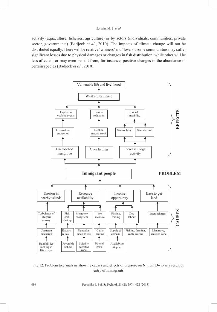
Hossain, M. S. et al.
416 Pertanika J. Sci. & Technol. 21 (2): 397 - 422 (2013)
Immigrant people E
FFE
CT
S C
AU
SES
PROBLEM
Erosion in nearby islands
Resource availability
Ease to get land
Income opportunity
Turbulence of Meghna estuary
Wet meadow
Cattle rearing
Fish, crab,
shrimp
Mangrove ecosystem
Upstream discharge
Estuary & sea
Favorable habitat
Plantation since 1960s
Natural grass
Fishing, trading
Day labour
Availability & price
Supply & demand
Fishing, farming, cattle rearing
Encroachment
Suitable accreted
zone
Encroached mangrove
Loss natural protection
Over fishing
Decline natural stock
Income reduction
Expose to cyclone events
Vulnerable life and livelihood
Weaken resilience
Increase illegal activity
Sea robbery Social crime
Social instability
Mangrove, accreted zone
Rainfall, ice melting in Himalayas
Fig.12: Problem tree analysis showing causes and effects of pressure on Nijhum Dwip as a result of entry of immigrants
activity (aquaculture, fisheries, agriculture) or by actors (individuals, communities, private sector, governments) (Badjeck et al., 2010). The impacts of climate change will not be distributed equally. There will be relative ‘winners’ and ‘losers’; some communities may suffer significant losses due to physical damages or changes in fish distribution, while other will be less affected, or may even benefit from, for instance, positive changes in the abundance of certain species (Badjeck et al., 2010).

Climate Change Resilience Assessment Using Livelihood Assets
417Pertanika J. Sci. & Technol. 21 (2): 397 - 422 (2013)
This resilience study revealed information regarding indigenous cyclone prediction or understanding of warnings that is significantly related to the age of the household head due to their level of experience: this agrees with Alam and Collins (2010) and Anderson-Berry (2003). On the other hand, owing to the erosion of physical capability, the elderly are less capable of storing up food and saving money, and as a consequence, meals for the day are reduced, family members must be engaged in income-earning activities, assets need to be disposed of and money must be borrowed to overcome the crisis; this agrees with Paul and Routray (2011) and Perry et al. (2010). This study also confirms the findings of Agarwal (1990), and Kesavan and Swaminathan (2007) that prevailing social and financial inequities greatly weaken the resilience level of the under-privileged sections of society.
CONCLUSION
This article applied the sustainable livelihood approach (SLA), which enables researchers and policy makers to identify a wide range of livelihood aspects that can provide clues to finding pressing constraints and positive strengths of fishermen resilience. This would further serve fishermen resilience by adding or removing sub-attributes in the long term due to climate change. Thus, practising community-based case studies can provide deep information on fishermen resilience especially through livelihood assets analysis. In this respect, SLA may play a leading role in analysing adaptive capacity to climate change through livelihood asset analysis at the community level. In this article, livelihood assets analysis related to fishermen resilience requires greater examination of the interaction among households on how to allocate their own resources and services to their family members. The consideration can develop a better understanding of climate change adaptation in fishing community context.
Emphasis must be given to conserve the existing mangrove ecosystem and undertake further plantation programs in newly accreted suitable zones to enhance natural barriers against extreme climate events as voiced out by the island dweller, local administrator, NGO worker, social elite as well as conservationist and researcher. Healthy mangroves ensure the fishing community receives diversified benefits in both tangible and non-tangible forms as well as in attracting mangrove-dependent species to boost biodiversity. A fishermen’s association and cooperative marketing activities may offer one way to improve their livelihoods and make sure that their children are able to go to school where they will be in a safe environment. In addition, village schools with sufficient facilities for the island’s growing population also need to be established. Therefore, the availability of a strategic financial loan scheme for fishing gear and education expense as well as for enhancing disaster awareness and the sense of unity among the islanders is of high importance in efforts to promote climate change adaptations.
ACKNOWLEDGEMENTS
The authors acknowledge the support of the Institute of Marine Sciences and Fisheries, University of Chittagong, Bangladesh.

Hossain, M. S. et al.
418 Pertanika J. Sci. & Technol. 21 (2): 397 - 422 (2013)
REFERENCES Agarwal, B. (1990). Social security and the family: coping with seasonality and calamity in rural India.
Journal of Peasant Study, 17(3), 341-412.
Aguilar-Manjarrez, J. (1996). Development and evaluation of GIS-based models for planning and management of coastal aquaculture: A case study in Sinaloa, México. (PhD Thesis dissertation). Institute of Aquaculture, University of Stirling, Scotland, UK, 375 pp.
Alam, E., & Collins, A. E. (2010). Cyclone disaster vulnerability and response experiences in coastal Bangladesh. Disasters, 34(4), 931-954.
Allison, H. E., & Ellis, F. (2001). The livelihoods approach and management of small-scale fisheries. Mar Policy, 25, 377-388.
Allison, H. E., & Horemans, B. (2006). Putting the principles of the sustainable livelihood approach into fisheries development policy and practice. Mar Policy, 30, 757-766.
Allison, E. H., Adger, W. N., Badjeck, M. C., Brown, K., Conway, D., & Dulvy, N. K. (2005). Effects of climate change on the sustainability of capture and enhancement fisheries important to the poor: analysis of the vulnerability and adaptability of fisherfolk living in poverty. Fisheries Management Science Programme project no. R4778J, MRAG, London.
Allison, E. H., Ellis, F., Mvula, P. M., & Mathieu, L. F. (2001). Fisheries management and uncertainty: the causes and consequences of variability in inland fisheries in Africa, with special reference to Malawi. In the Proceedings of the Lake Malawi Fisheries Management symposium, National resource management programme, Lilongwe, Malawi: Government of Malawi, 4-9 June 2001. Weyl, O.L.F. Weyl, M.V. (Eds), pp. 66-79.
Amin, M. (2001). Tilotoma Hatiya: History and Heritage (in Bangla). Hatiya Janakolyan Somiti, Dhaka, Bangladesh.
Anderson-Berry, L. J. (2003). Community vulnerability to tropical cyclones: cairns, 1996-2000. Natural Hazards 30(2), 209-232.
Badjeck, M. C., Allison, E. H., Halls, A. S., & Dulvy, N. K. (2010). Impacts of climate variability and change on fishery-based livelihoods. Marine Policy, 34, 375-383.
BMD. (Bangladesh Meteorological Department) (2009). Station-wise meteorological data. Meteorological Department, Ministry of Defense, Government of the People’s Republic of Bangladesh, Dhaka.
Chambers, R. (1992). Rapid and participatory rural appraisal. Africanus, 22(1&2), 6-15.
Chambers, R. (1980). Rapid rural appraisal: rationale and repertoire. Institute of Development Studies, Sussex, UK.
Chowdhury, M. S. N., Hossain, M. S., Barua, P. (2008). Artisanal Fisheries Status and Sustainable Management Options in Teknaf Coast, Bangladesh. Social Change, 1(1), 48-64.
De Silva, D. A. M., & Yamao, M. (2007) Effects of the tsunami on fisheries and coastal livelihood: a case study of tsunami-ravaged southern Sri Lanka. Disasters, 31(4), 386-404.
DFID. (1999). Sustainable livelihood guidance sheet. Department for International Development, UK.
Eastman, J. R., Kyem, P. A. K., Toledano, & J., Jin, W. (1993). GIS and decision making. United Nations Institute for training and research, explorations in geographic information systems technology. The Clarks Labs for Cartographic Technology and Geographic Analysis. Clark University, Worcester, MA, USA, 112 p.

Climate Change Resilience Assessment Using Livelihood Assets
419Pertanika J. Sci. & Technol. 21 (2): 397 - 422 (2013)
Ellis, F. (2000). Rural livelihoods and diversity in developing countries. Oxford: Oxford University Press.
FAO. (2009). The state of world fisheries and aquaculture: 2008. Rome: FAO Fisheries and Aquaculture Department, 176 pp.
Fulton, E. A. Smith, A. D. M., Smith, D. C., & van Putten, I. E. (2011). Human behaviour: the key source of uncertainty in fisheries management. Fish and Fisheries, 12, 2-17.
Gibbs, M. T. (2009). Resilience: What is it and what does it mean for marine policymakers? Marine Policy, 33, 322-331.
Golden, B. R., Wasil, E. A., & Harker, P. T. (1989). The Analytical Hierarchy Process-Applications and Studies. New York: Springer-Verlag.
Gregory, R., & Wellman, K. (2001) Bringing stakeholder values into environmental policy choices: a community based estuary case study. Ecological Economics, 39, 37-52.
Grothmann, T., & Patt, A. (2005). Adaptive capacity and human cognition: the process of individual adaptation to climate change. Global Environnent Change, 15, 199-213.
Hossain, M. S. (2009a). Floodplain Aquaculture in Begumgonj: New Horizon for Rural Livelihoods in Bangladesh. Aquaculture Asia, XIV(3), 7-10.
Hossain, M. S. (2009b). Coastal community resilience assessment: using Analytical Hierarchy Process. In Hossain, M. S. (Ed). Climate change resilience by mangrove ecosystem. PRDI, Dhaka, Bangladesg, pp 1-11.
Hossain, M. S., & Das, N. G. (2010a). GIS-based multi-criteria evaluation to land suitability modelling for giant prawn (Macrobrachium rosenbergii) farming in Companigonj Upazila of Noakhali, Bangladesh. Computers and Electronics in Agriculture, 70, 172-186.
Hossain, M .S., & Das, N. G. (2010b). Geospatial Modeling for Aquaculture Sustainability in Noakhali, Bangladesh. World Aquaculture, 41(4), 25-29.
Hossain, M. S., Wong, S., & Shamsuddoha, M. (2009a). Mangrove forest conservation for climate change risk reduction with emphasizing the socio-ecological resilience of coastal community in Bangladesh. Paper presented at the Third World Climate Conference (WCC-3) in Geneva, Switzerland from 30 August to 04 September.
Hossain, M. S., Chowdhury, S. R., Das, N. G., Sharifuzzaman, S. M., & Sultana, A. (2009b). Integration of GIS and multicriteria decision analysis for urban aquaculture development in Bangladesh. Landscape and Urban Planning, 90, 119-133.
Hossain, M. S., Das, N. G., Chowdhury, M. S. N. (2007a). Fisheries Management of the Naaf River. Coastal and Ocean Research Group of Bangladesh, 268 pp.
Hossain, M. S., Chowdhury, S. R., & Rashed-Un-Nabi, M. (2007b). Resource Mapping of Saint Martin’s Island using satellite image and ground observations. Journal of Forestry & Environment, 5, 23-36.
Hossain, M. S., Khan, Y. S. A., Chowdhury, S. R., Saifullah, S. M., Kashem, M. B., & Jabbar, S. M. A. (2004). Environment and Socio-Economic Aspects: A Community Based Approach from Chittagong Coast, Bangladesh. Jahangirnagar University Journal of Science, 27, 155-176.
Iftekhar, M. S., Takama, T. (2008). Perceptions of biodidersity, environmental services, and conservation of planted mangroves: a case study on Nijhum Dwip Island, Bangladesh. Wetlands Ecology Management, 16, 119-137.

Hossain, M. S. et al.
420 Pertanika J. Sci. & Technol. 21 (2): 397 - 422 (2013)
IlRR. (1998). Participatory methods in community-based Coastal Resources Management, vol. 3. International Institute of Rural Reconstruction, Silang, Cavite, Philipines.
IPCC. (2007). Climate change 2007: the physical science basis: summary for policymakers. Retrieved on December 21, 2008 from http://www.ipcc.ch.
IPCC. (2001). Climate change 2001: impacts, adaptation, and vulnerability. Contribution of Working Group II to the third assessment report of the Intergovernmental Panel on Climate Change. Cambridge University Press, New York, 1032 p.
Iwasaki, S., Razafindrabe, B. H. N., & Shaw, R. (2009). Fishery livelihoods and adaptation to climate change: a case study of Chilika lagoon, India. Mitigation and Adaptation Strategies for Global Change, 14(4), 339-55.
Johnson, J. E., & Welch, D. J. (2010). Marine fisheries management in a changing climate: a review of vulnerability and future options. Reviews in Fisheries Science, 18(1), 106-124.
Kapetsky, J. M., & Nath, S. S. (1997). A strategic assessment of the potential for freshwater fish farming in Latin America. COPESCAL Technical Paper No. 10, Rome, FAO, 128 p.
Kesavan, P. C., & Swaminathan, M. S. (2006). Managing extreme natural disasters in coastal areas. Philosophical Transactions A: Mathematical Physical and Engineering Sciences, 364(1845), 2191-16.
Kovacs, J. M., Malczewski, J., & Flores-Verdugo, F. (2004). Examining local ecological knowledge of hurricane impacts in a mangrove forest using an analytic hierarchy process (AHP) approach. Journal of coastal research, 20(3), 792-800.
Malczewski, J. (1999). GIS and multi-criteria decision analysis. New York, Wiley, 392 p.
Mendoza, G. A., Prabhu, R. (2000). Development of methodology for selecting criteria and indicators for sustainable forest management: A case study on participatory assessment. Environmental Management 26(6), 659-673.
Mercer, J., Kelman, I., Taranis, L., & Suchet-Pearson, S. (2010). Framework for integrating indigenous and scientific knowledge for disaster risk reduction. Disasters, 34(1), 214-239.
Mettrick, H. (1993). Development oriented research in agriculture: An ICRA textbook, pp. xii and 228. Wageningen, the Netherlands, International Centre for Development Oriented Research in Agriculture (ICRA).
Mikkelsen, B. (1995). Methods for development work and research: a guide for practitioners. Sage Publications, New Delhi.
Moser, C. (1998). The Asset Vulnerability Framework: Reassessing Urban Poverty Reduction Strategies. World Development, 26(1), 1-19.
Munny, F. I. (2009). Mangrove forest mapping in coastal islands of lower Meghna estuary and its role in climate change disaster mitigation. (MSc thesis dissertation). Institute of Marine Sciences and Fisheries, University of Chittagong, Bangladesh, 58 pp.
Paul, S. K., & Routray, J. K. (2011). Household response to cyclone and induced surge in coastal Bangladesh: coping strategies and explanatory variables. Natural Hazards, 57, 477-499.
PDO-ICZMP. (2004). Contribution of Integrated Coastal Zone Management Plan Project towards formulation of the PRSP for Bangladesh. Program Development Office for Integrated Coastal Zone Management Plan Project; Water Resources Planning Organization; Ministry of Water Resources, Bangladesh.

Climate Change Resilience Assessment Using Livelihood Assets
421Pertanika J. Sci. & Technol. 21 (2): 397 - 422 (2013)
Pelto, P., & Pelto, G. (1978). Anthropological Research: The Structure of Inquiry. Cambridge, Cambridge University Press.
Pereira, J. M. C., & Duckstein, L. (1993). A multiple criteria decision-making approach to GIS-based land suitability evaluation. International Journal of Geographical Information Systems, 7(5), 407-424.
Perry, R. I., Ommer, R. E., Barange, M., Jentoft, S., Neis, B., & Sumaila, U. R. (2010). Marine social-ecological responses to environmental change and the impacts of globalization. Fish and Fisheries, DOI: 10.1111/j.1467-2979.2010.00402.x.
Perz, S. G., Shenkin, A., Barnes, G., Cabrera, L., Carvalho, L. A., & Castillo, J. (2011). Connectivity and resilience: a multidimensional analysis of infrastructure impacts in the Southwestern Amazon. Soc Indic Res; DOI 10.1007/s11205-011-9802-0.
Research Systems Inc. (2000). Exploring ENVI, training course manual. Better Solutions Consulting Limited, Liability Company, USA.
Rosario, E. (1997). Conservation management plans for protected areas other than the Sundarbans Reserved Forests. Bangladesg Forest Department, Dhaka.
Saaty, T. L. (1977). A scaling method for priorities in hierarchical structures. Journal of Mathematics Physiology, 15, 234-281.
Saaty, T. L. (1988). The Analytic Hierarchy Process. Typesetters Ltd, Becceles, Suffolk.
Saaty, T. L. (1990). The analytic hierarchy process: planning, priority setting, resource allocation. RWS Publications, Pittsburgh, 287 p.
Scheffer, M. (2009). Critical transitions in nature and society. Princeton: Princeton University Press.
Stagg, C., & Imber, S. (1990). Application of the analytical hierarchy process to the development of a monitoring program for a recreational fishery. Operational Research and Management in Fishing, 14, 89-95.
Start, D., & Johnson, C. (2004). Livelihood Options? The Political Economy of Access, Opportunity and Diversification. Working Paper 233, Overseas Development Institute 111 Westminster Bridge Road, London, SE1 7JD, UK.
Torresan, S., Critto, A., Valle, D. M., Harvey, N., & Marcomini, A. (2008). Assessing coastal vulnerability to climate change: comparing segmentation at global and regional scales. Sustain Sci, 3, 45-65.
Trap, N. (2006). Vulnerability of fishing communities in Vietnam: an exploration of the scope to adapt to environmental change. Vrije Universiteit, Amsterdam, Netherlands, 45 p.
WWF. (2005). Are we putting our fish in hot water? Retrieved on December 21, 2008, from http://assets.panda.org/downloads/fisherie_web_final.pdf.
Worldfish Centre. (2007). The threat to fisheries and aquaculture from climate change. Policy Brief, Penang, Malaysia.
Worm, B., Barbier, E. B., & Beaumont, N. (2006). Impacts of biodiversity loss on ocean ecosystem services. Science, 314, 787-790.
Ziervogel, G., Bharwani, S., & Downing, E. T. (2006). Adapting to climate variability: pumpkins, people and policy. Nat Resour Forum, 30, 294-305.


Pertanika J. Sci. & Technol. 21 (2): 423 - 442 (2013)
SCIENCE & TECHNOLOGYJournal homepage: http://www.pertanika.upm.edu.my/
ISSN: 0128-7680 © 2013 Universiti Putra Malaysia Press.
Goal Event Detection in Soccer Videos via Collaborative Multimodal Analysis
Alfian Abdul Halin1* and Mandava Rajeswari2
1Faculty of Computer Science and Information Technology, Universiti Putra Malaysia, 43400 Serdang, Selangor, Malaysia2School of Computer Sciences, Universiti Sains Malaysia, 11800 Minden, Penang, Malaysia
ABSTRACT
Detecting semantic events in sports video is crucial for video indexing and retrieval. Most existing works have exclusively relied on video content features, namely, directly available and extractable data from the visual and/or aural channels. Sole reliance on such data however, can be problematic due to the high-level semantic nature of video and the difficulty to properly align detected events with their exact time of occurrences. This paper proposes a framework for soccer goal event detection through collaborative analysis of multimodal features. Unlike previous approaches, the visual and aural contents are not directly scrutinized. Instead, an external textual source (i.e., minute-by-minute reports from sports websites) is used to initially localize the event search space. This step is vital as the event search space can significantly be reduced. This also makes further visual and aural analysis more efficient since excessive and unnecessary non-eventful segments are discarded, culminating in the accurate identification of the actual goal event segment. Experiments conducted on thirteen soccer matches are very promising with high accuracy rates being reported.
Keywords: Soccer event detection, shot view classification, sports video summarization, semantic video indexing, webcasting-text
Article history:Received: 20 June 2011Accepted: 13 December 2011
E-mail addresses: [email protected] (Alfian Abdul Halin), [email protected] (Mandava Rajeswari)*Corresponding Author
2008). Effective consumption of such huge repositories has spurred interest in automatic indexing and retrieval techniques, especially those that cater for content-based semantics (Snoek, 2005). Semantic concepts strongly rely on specific domain context. Therefore, restricting the domain being addressed is to some extent, imperative in order to bridge the semantic gap between low-level features and the inherent semantics they represent. Sports,
INTRODUCTION
Technological advances have greatly enhanced broadcast, capture, transfer and storage of digital video (Tjondronegoro et al.,

Alfian Abdul Halin and Mandava Rajeswari
424 Pertanika J. Sci. & Technol. 21 (2): 423 - 442 (2013)
in particular, has attracted wide interest in the past decades. Domain knowledge of specific sports has been used to extract important semantic concepts such as tennis that serves and rallies (Huang et al., 2009), baseball pitch trajectories (Chen et al., 2008), as well as basketball dunks and layouts (Changsheng et al., 2008b).
Soccer is one particular domain that has also received great attention, where much work focuses on event detection. Since events are meaningful and easily recalled, they are highly suitable as semantic indices (Tjondronegoro, 2005). The identified events can in turn be used to facilitate production tasks including specialized programme production, automatic video summary generation, video abstracts creation, and archival tasks such as production and posterity logging (Assfalg et al., 2003). However, soccer event detection is very challenging due to the unscripted recordings and the loose dynamic structure of soccer broadcasts. Lengthy running time and sparseness of event occurrences further complicate matters, where traditional VHS “rewind and fast-forward” cannot cope for timely footage access. For this reason, content-based analysis assisted by domain knowledge is required to automate and facilitate event detection.
RELATED WORKS
A great body of literature has been dedicated to events or highlights detection in soccer, as well as other sports. Basically, audio and/or visual features are firstly extracted directly from the video contents, followed by a decision making algorithm to determine whether or not a video segment contains events. Sadlier and O’Connor (2005) analyzed soccer and Gaelic Football videos. A 5-dimensional feature vector containing visual concepts such as crowd presence and motion activity and aural speech band energy to train Support Vector Machines (SVM) and to classify whether shot are eventful or uneventful. Snoek and Worring (2003) fused camera views, object classes, aural energy and textual features into a Maximum Entropy interval based algorithm to detect soccer goals, yellow cards and substitutions. The work by Chung-Lin et al. (2006) detects penalties, cards, goals and corner kicks using colour, motion, texture, object and audio energy from each video frame. A Dynamic Bayesian Network architecture was constructed to calculate the probability of event occurrences in the video. In their work, Jinjun et al. (2004) applied a hierarchical architecture where audio and visual keywords are firstly inferred from low-level features using an SVM. Left-to-right four state Hidden Markov models were then trained to detect soccer goals, goal-kicks, corner kicks and shot on goals. Meanwhile, Leonardi et al. (2004) used Controlled Markov Chains to detect candidate soccer goal events based on camera motion features. Ranking of each candidate was then performed based on audio loudness, where the top results contained the goal events.
All the mentioned works share three common fundamental characteristics. Firstly, event detection solely relied on features directly extracted from the video. Secondly, the event search space spanned the whole duration of the video. Thirdly, the ultimate task of event detection is carried out using supervised learning algorithms, which discovers the audiovisual patterns of specific events based on a learned model using labelled training examples. Each of the characteristics above will be further elaborated and their underlying issues will also be stated.
It is important to note that sole reliance on the directly extracted audiovisual features can

Goal Event Detection in Soccer Videos
425Pertanika J. Sci. & Technol. 21 (2): 423 - 442 (2013)
lead to: (1) missed detections, and (2) confused detections. Missed detections occur when event patterns are not detected due to feature patterns being less prominent during event occurrences, such as the missed occurrences in Snoek and Worring (2003) and Jinjun et al. (2004) despite the use of sophisticated event models. Meanwhile, confused detections are events being misclassified as other events. For instance, Chung-Lin et al. (2006) reported off-sides being labelled as goals and long-passes as corner-kicks. These occurred due to the different events sharing somewhat similar audiovisual patterns. Furthermore, event boundaries are blurry and difficult to be effectively localized using audiovisual features alone.
A complete soccer game lasts for at least 90 minutes (~135,000-frames at 25-frames per second). Within this duration, the video signal is very asymmetric and noisy, where non-events1 outnumber interesting events by an enormous margin (Min et al., 2007). Hence, event detection algorithms face the challenge of recognizing event patterns from the majority of non-event patterns, which is not an easy task.
As for supervised learning algorithms, their robustness may be questionable since for some soccer events, the number of positive training examples is very limited. In the work of Ren (2008), it was asserted that even with 90-hour of footage and 190 instances of soccer goals, it was still insufficient to train a classifier for robust goal event detection. They further emphasized that the sample was too small to robustly estimate any form of sequential event pattern.
Due to these reasons, it is imperative that missed and confused detections be eliminated. Furthermore, event detection could benefit from a constrained or localized search space so that algorithms could work in a more symmetric and less noisy environment. Last but not least, due to the difficulty in obtaining sufficient positive training examples for some events, unsupervised approaches should be explored. Moreover, audiovisual information in a particular video should be fully utilized instead of relying on offline training from multiple sources.
CONTRIBUTIONS
In this paper, we proposed a soccer event detection framework that circumvents the issues mentioned in the previous section. Instead of solely relying on audiovisual features that are directly extracted from the video, an external textual resource was utilized to initiate event detection. Then, a rule-based approach was used to identify potential event candidates by firstly short-listing video segments exhibiting specific visual characteristics based on semantic shot view class transitions. Finally, event segments were determined from the shortlist by a ranking procedure based on the aural feature of mean pitch. Since the framework is unsupervised, all the audiovisual considerations and assumptions were based on prior knowledge by observing ~23-hours of soccer video from various broadcasters. Furthermore, the audiovisual considerations were solely made within each video itself, and without relying on any pre-trained model.
This work offers two insights. Firstly, the issues of missed and confused detections, as well as the issue of the huge and asymmetric search space, are solved by utilizing the minute-by-minute (MBM) reports from sports websites to initiate event detection. Since MBMs contain detailed and reliable annotations of a match’s progression, two crucial cues (namely, the
1 Uninteresting portions of the video such as throw-ins, normal passing of the ball, ball out of bounds, etc.

Alfian Abdul Halin and Mandava Rajeswari
426 Pertanika J. Sci. & Technol. 21 (2): 423 - 442 (2013)
event name and its corresponding minute time-stamp) were used. Here, missed and confused detections can be avoided since events are explicitly identified by the event name, and its time of occurrence is indicated by the time-stamp. This furthermore allows localization of the event occurrence to the one-minute video segment indicated by the time-stamp. Therefore, the event search space is significantly reduced to only the one-minute segment instead of the entire video duration. The use of MBMs is quite recent and has been shown to be effective in works such as by Changsheng et al. (2008a), and Changsheng et al. (2008b).
Secondly, since obtaining sufficient training examples for certain events is difficult (Ren, 2008), a rule-based method is proposed. It is crucial to highlight that the approach used in this study analyzed the visual and aural information only from the particular video under consideration. Therefore, no reliance is put on specific event models based on offline training. All the audiovisual considerations and assumptions are uncomplicated and therefore able to effectively identify goal event occurrences. More specifically, the authors relied on observed prior knowledge of the visual and/or aural characteristics during goal events. Initially, each shot was classified as belonging to either one of two labels, i.e., far or close-up view. These labels are consistent with camera views used during soccer broadcasts. Based on these labels, a shortlist of candidate segments exhibiting event-like characteristics is generated from within the localized one-minute video segment. Ultimately, one candidate is chosen as containing the actual goal event through a ranking procedure.
FRAMEWORK FOR GOAL EVENT DETECTION
The framework consists of four main components, which are: (1) video pre-processing, (2) textual cues utilization, (3) candidate shortlist generation, and (4) candidate ranking. An overview of the proposed framework is shown in Fig.1.
Video Pre-processing
For tractability, each video is firstly segmented into shots and assigned semantic labels. Both these steps are performed by the shot boundary detection and shot view classification steps, respectively.
Shot Boundary Detection
For videos to be processed and semantically analyzed, they firstly have to be segmented into tractable units. This process is commonly referred to as shot boundary detection (SBD), where video frame sequences taken by one continuous camera action are grouped together forming individual units called shots (Yuan et al., 2007). Since this work does not concern SBD, the existing algorithm by Abd-Almageed (2008) was used. This algorithm was chosen due to its robustness against variations to illumination and intensity. Basically, SBD partitions a video V into m-shots, represented as 1 , , i i mV S S S+= … .
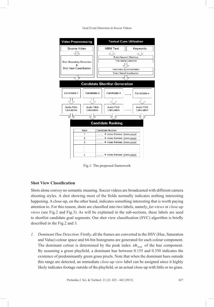
Goal Event Detection in Soccer Videos
427Pertanika J. Sci. & Technol. 21 (2): 423 - 442 (2013)
Shot View Classification
Shots alone convey no semantic meaning. Soccer videos are broadcasted with different camera shooting styles. A shot showing most of the fields normally indicates nothing interesting happening. A close-up, on the other hand, indicates something interesting that is worth paying attention to. For this reason, shots are classified into two labels, namely, far-views or close-up views (see Fig.2 and Fig.3). As will be explained in the sub-sections, these labels are used to shortlist candidate goal segments. Our shot view classification (SVC) algorithm is briefly described in the Fig.2 and 3.
1. Dominant Hue Detection: Firstly, all the frames are converted to the HSV (Hue, Saturation and Value) colour space and 64-bin histograms are generated for each colour component. The dominant colour is determined by the peak index peakidx of the hue component. By assuming a green playfield, a dominant hue between 0.155 and 0.350 indicates the existence of predominantly green grass pixels. Note that when the dominant hues outside this range are detected, an immediate close-up view label can be assigned since it highly likely indicates footage outside of the playfield, or an actual close-up with little or no grass.
Fig.1: The proposed framework

Alfian Abdul Halin and Mandava Rajeswari
428 Pertanika J. Sci. & Technol. 21 (2): 423 - 442 (2013)
2. Playfield Region Segmentation: A range is defined to determine other pixels perceived to be similar to the dominant hue. Empirically, the range [ , ]peak peakidx idx− α − α was determined with the optimal value for α being 0.1. All the pixels within this range are also resultantly classified as playfield pixels, if the saturation component is between 0.0 to 0.1, with the value component exceeding 0.13. For further refinement of the playfield region, morphological image processing and connected components analysis are applied (Halin et al., 2009).
3. Object-size Determination and Shot Classification: Large objects overlapping the playfield indicate close-up views, whereas smaller objects indicate far views. Some SVC techniques (e.g., Shu-Ching et al., 2004; Min et al., 2006; Xu et al., 2001) solely rely on the playfield ratio alone, which as suggested in Halin et al. (2009), can yield many incorrect labels. By calculating the largest object size, the accuracy of shot classification can improve by 8%-13% (Halin et al., 2009). From our experiments, a playfield with an overlapping object pixel count of more than 13,500 can be classified as a close-up view. A shot is then labelled as either a close-up or far view based on the majority voting of all the frame labels within the respective shot.
Textual Cues Utilization
The MBMs are obtained online from broadcasters such as ESPN (Espn, 2010) and BBC (Bbc, 2009), as well as sports information providers such as Sportinglife (2009) and UEFA (2010). An MBM of a match is annotated during a match’s progression by experts. It basically logs details of the match in the granularity of minutes. Two crucial cues are considered from this
Fig.2: Far-views
Fig.3: Close-up views

Goal Event Detection in Soccer Videos
429Pertanika J. Sci. & Technol. 21 (2): 423 - 442 (2013)
source, namely, the event name and its minute time-stamp. A screen capture of an MBM from ESPN is shown in Fig.4. These two cues from MBMs are invaluable since they eliminate guesswork in determining which event has occurred, as well as in allowing the event search to be localized to the approximate minute within the match video.
Goal Event Keyword Matching and Time Stamp Extraction
Fig.4 shows that the first column represents the minute time-stamps, whereas the match happenings are explained in the second column. Close inspection reveals that goals are annotated using dedicated keywords. After scrutinizing various sources of MBMs, a set of goal-related keywords was defined:
!, , , , , G goal goal by scored scores own goal convert= (1)
Given the task of detecting a goal event g, that has i-number of occurrences: If matching keywords are found within the MBM, the time-stamp of each of the i-th occurrences are noted. These can be written as a set g g
iT t= , where i > 0 if there is at least one goal event in the match. Then, for each i, the goal event search is initiated within the one-minute segment of each g
it .
Text-Video Synchronization and Event Search Localization
The time-stamp git indicates the minute within which the event has occurred. However, directly
mapping to the corresponding video frames can be erroneous due to the misalignment with the actual game time. Due to this, synchronization between the g
it and its corresponding video frame is necessary. A manual step is introduced here, where a reference frame is determined by matching a frame number to the actual elapsed game time of a match. This process is illustrated in Fig.5, where an elapsed game time of 0.25-minutes (15-seconds) corresponds with the 245-th frame of the match video. Each of these values is denoted as reft and
reff , respectively. Although the authors are aware that the process can be automated using the technique proposed by Chansheng (2008a), some matches fail to display superimposed game clocks, therefore this particular technique cannot be used. We argue that bit of automation needs to be sacrificed for the sake of reliability.
Fig.4: An expert of a minute-by-minute report from ESPN

Alfian Abdul Halin and Mandava Rajeswari
430 Pertanika J. Sci. & Technol. 21 (2): 423 - 442 (2013)
The values reft and reff can then be used to localize the event search to the one-minute eventful segment. With g
it being the minute time-stamp of the goal event, the beginning ( ,
gi beginf ) and ending ( ,
gi endf ) frames for the event minute can be determined via:
( )( )( ), 60 1g ref ref gi begin if f fr t t = − + −
(2)
, , 60g gi end i beginf f fr= + (3)
where fr is the video frame rate and ⋅ rounds-down the calculations to the nearest integer. Note that for ,
gi beginf , the time-stamp g
it (after being converted to seconds) is subtracted by 60-seconds since the actual event occurs between the minute range of 1,g g
i it t− . Note also that for ,
gi endf end, fr has been multiplied by 60 (seconds) in order to position the end boundary at
one-minute after ,g
i beginf . Consequently, the localized one-minute event search space is:
, ,,g g gi i begin i endf f ϒ = (3)
Candidate Shortlist Generation
Returning the whole one minute segment would be too coarse since a goal’s conception to finish is normally shown within a very short and condensed time period. Therefore, potential goal segments within g
iϒ need to be identified. During goal events, certain visual properties can be observed. By observing more than ~23-hours of soccer video footage from various
Fig.5: Manual determination of the reference frame and time

Goal Event Detection in Soccer Videos
431Pertanika J. Sci. & Technol. 21 (2): 423 - 442 (2013)
broadcasters (including the footage used in this paper), three generic visual-related properties were identified, and when present, they would highly likely indicate a potential goal event. These properties were exploited to decompose the one-minute segment into a shortlist of candidate segments, which could be explained as:
1. The camera transitions from a far-view to a close-up view. The former is meant to capture the build-up, whereas the latter focuses on player/crowd/coach reactions;
2. Close-up views during goals normally last at least 6-seconds;
3. It takes approximately 12-seconds to fully observe an event’s progression from conception to finish.
Note that these properties can be quite generic. In other words, they can also indicate other event occurrences such as yellow cards or red cards. However, since the search space has already been localized to the one-minute eventful segment, detecting other events is very unlikely. Moreover, it is already known from the MBM that this particular minute contains a goal event.
From these properties, the relevant 12-second segments are extracted as shortlisted candidates. Note that the transition point between the shot views serves as the mid-point, where preceding and superseding segments have equal lengths of 6-seconds. Consequently, the n-number of candidate segments is generated from g
iϒ :
1, ,g gi ikC c for k n= = … (4)
where g gi iC ⊂ ϒ is the set containing the shortlisted candidates, and g
ikc s the k-th 12-second candidate segment within g
iC . An illustration is shown in Fig.6, where two candidate segments have been shortlisted for a goal event.
Fig.6: Example of two shortlisted candidates

Alfian Abdul Halin and Mandava Rajeswari
432 Pertanika J. Sci. & Technol. 21 (2): 423 - 442 (2013)
Candidate Ranking
At this stage, we have obtained the candidate segments gikc , where one of them is the actual
goal event. Since the shot view transitions are similar across the candidates, another feature is needed from each g
ikc . It was observed that whenever a goal is scored, there would be an increase in the commentator’s excitement and intonation. Since the commentator can be considered a neutral party during any soccer match, his/her excited speech is less biased to any one team. The works by Tjondronegoro (2005), and Coldefy and Bouthemy (2004) demonstrated that pitch or the fundamental frequency of an audio signal 0f is reliable to detect excited human speech. Normally, as a direct result of speech excitement, 0f − measurements will increase. For the purpose of this work, the sub-harmonic to harmonic ratio analysis technique was chosen due to its insensitivity towards noise and prominent unvoiced segments. The algorithm used is called shrp.m, which is a MATLAB implementation of Xuejing (2002), and is available from Sun (2008).
For audio temporal segmentation, 20-milisecond (ms) frames and 500-ms clips were used. The value of 20-ms was chosen since audio signals could be assumed to be (pseudo) stationary within the 10 to 40-ms range (Yao, 2000), and that 20-ms seemed to be appropriate to capture a snapshot of the evolving audio signal for the data in this study. The clip size of 500-ms, on the other hand, was chosen as it managed to accurately capture the average measurement within a longer time window.
Basically, 0f is initially calculated at the frame level. The frame level results are then combined to obtain an averaged value at the clip level. Finally, all the clips’ average 0f values within the respective 12-second segments were averaged to obtain the mean pitch 0
g
ikffor each candidate.
The rule being applied here is that the candidate with the goal event will cause commentator speech to be very pronounced. This will result in high f0 values across audio frames, leading to high 0
g
ikf within the segment. It can then be argued that segment c*, with the maximum 0
g
ikf , contains the actual goal event.
EXPERIMENTAL RESULTS AND DISCUSSION
The experiments were conducted to evaluate the effectiveness of the SVC algorithm, shortlist generation and goal segment identification processes. A total of thirteen soccer matches, consisting of European Champions League, Barclay’s Premier League and Italian Serie-A matches, were used as test data. All the videos were in AVI format at 15-frames per second. The audio channel was MP3-mono, sampled at 22.5-KHz with a bit-rate of 32-kbps. Each of the match halves was recorded in a separate file, with non-game footage such as halftime commentaries, commercial breaks, match highlights, etc. excluded.
It is worth noting that, to the best of our knowledge, there is no publicly available dataset(s) for soccer video. Therefore, we have resorted to recorded matches from television broadcasters. Details for each of the recordings are available in Table 1. Note that some matches managed to be fully recorded (i.e. 90-minutes), whereas other were partially recorded (i.e. 45-minutes). The partial recordings were due to equipment setup failures during the recording process.

Goal Event Detection in Soccer Videos
433Pertanika J. Sci. & Technol. 21 (2): 423 - 442 (2013)
Note that for the following sub-sections of Shot View Classification and Candidate Shortlist Generation, the evaluation criteria used are precision and recall. Although sharing the same terminologies, the contexts within which both sections are evaluated are different. Sub-section Shot View Classification is basically a classification task, whereas Sub-section Candidate Shortlist Generation is a retrieval task. Therefore, two sets of formulas are presented to cater for each of these contexts, which will be further explained in detail within each of the respective sections.
Shot View Classification
In this work, SVC was tested on different subsets of our data, totalling 599-shots. Different subsets from different matches were used to demonstrate the robustness of the algorithm across different broadcasters. Precision and recall are calculated using Equations 5 and 6, respectively. SVC is treated as a two-class classification task. For clarity, true positives, false positives and false negatives are explained, supposing that the positive class being predicted is a far-view:
True positive: Assigning a shot as far-view, when the actual class is indeed a far-view;
False positive: Assigning a shot as far-view, when the actual class is a close-up view;
False negative: Assigning a shot as close-up view, when the actual class is a far-view.
The Table 2 shows the results obtained by the SVC algorithm.
## #
true positivesPrecision true positives false positives
=+ (5)
TABLE 1 Description of the dataset. ECL – European Champions League, BPL – Barclay’s Premiere League and ISA – Italian Serie – A
Match number Teams League Duration1 Chelsea vs. Man. United ECL 90-mins2 Man. United vs. Blackburn BPL 90-mins3 Man. United vs. Liverpool BPL 90-mins4 Newcastle vs. Fulham BPL 45-mins5 Stoke vs. Hull BPL 90-mins6 West Brom vs. Liverpool BPL 90-mins7 West Ham vs. Liverpool BPL 45-mins8 Barcelona vs. Man. United ECL 45-mins9 Arsenal vs. Celtic ECL 90-mins10 Arsenal vs. Portsmouth BPL 90-mins11 Inter Milan vs. Bari ISA 90-mins12 Bolton vs. Liverpool BPL 90-mins13 Everton vs. Wigan BPL 90-mins
TOTAL 1035-mins

Alfian Abdul Halin and Mandava Rajeswari
434 Pertanika J. Sci. & Technol. 21 (2): 423 - 442 (2013)
## #
true positivesRecall true positives false negatives
=+ (6)
The results are encouraging where very high recalls are reported. This is very important since further visual processing requires that each shot be properly labeled.
TABLE 2 Average Precision and Recall for Shot View Classification
Shot Type # of shots Data Precision Recall
Close-up view 415
Match-1 94.29% 98.51%Match-2 100.00% 100.00%Match-3 98.46% 98.46%Match-4 100.00% 92.00%Match-5 100.00% 93.24%Match-6 96.88% 95.38%Average 98.27% 96.27%
Far-view 184
Match-1 96.56% 87.50%Match-2 100.00% 100.00%Match-3 97.14% 97.14%Match-4 80.65% 100.00%Match-5 83.87% 100.00%Match-6 91.67% 94.29%Average 91.65% 96.49%
Candidate Shortlist Generation
The total number of goals from the thirteen matches was 36 altogether. In all, 84-candidates gikc
were generated for each time-stamp. Similar to the previous section, precision and recall are calculated. However, the calculations in this section are from the context of retrieval. Therefore, the formulas differ from that of the previous section, and are calculated using Equations 7 and 8, respectively. Relevant refers to the number of candidate segments generated that actually contain goal events. Retrieved refers to the total number of candidates generated based on the assumption of the changing camera views.
# ##
relevant retrievedPrecision
retrieved= ∩
(7)
# ##
relevant retrievedRecall
retr ed iev
= ∩ (8)
Table 3 shows the overall performance of the candidate segment generation process. It can be observed that the Average Number of Candidates per Shortlist is quite low (i.e. 2). This value indicates the average number of candidates being identified for each event occurrence.

Goal Event Detection in Soccer Videos
435Pertanika J. Sci. & Technol. 21 (2): 423 - 442 (2013)
Preferably, this value should be as low as possible so that in case ranking errors occur (i.e. Sub-section Candidate Ranking), the actual segment can still be retrieved without the need for extensive browsing.
Overall, the most important measurement is recall. It is crucial that this be 100% for all cases since it is mandatory that an actual goal event segment be present within each of the candidate segments for a particular minute. If for instance, a candidate set does not contain an actual goal event segment, the final step of candidate ranking (i.e. Sub-section Candidate Ranking) would be in vain as the top-ranked candidate would never be a goal event (and hence, be missed).
TABLE 3 Segment Generation Performance
Ground Truth 36Relevant 36Retrieved 84Missed 0Average Number of Candidates per Shortlist 2Precision 42.86%Recall 100.00%
Candidate Ranking
Table 4 shows the results of the candidate ranking process, where ideally, the candidate ranked top most will contain the actual goal event. The first column shows the respective matches whereas the second records the time-stamps of each goal event. The variable n represents the number of candidate segments g
ikc identified for each of the i-th goal instance. The mean pitch 0
g
ikf for each k-th. segment (for k = 1, ..., n) is recorded in the sub-columns of column 5, where the numeric boldface values indicate the maximum 0
g
ikf of that time-stamp, which is the top-ranked candidate within that particular shortlist. The final column (Decision) indicates whether the top-ranked candidate indeed contains the goal event. In all, 35 goal segments were ranked top most. This high percentage is very promising and shows that the modality collaboration technique is reliable at identifying goal events. The final row indicates one actual goal event segment being wrongly ranked second (i.e. Decision value X). Close observation showed that it was a goal resulting from a penalty kick. For this particular occurrence, the commentator’s reaction was louder during the foul that led to the penalty, than when the actual goal was scored.

Alfian Abdul Halin and Mandava Rajeswari
436 Pertanika J. Sci. & Technol. 21 (2): 423 - 442 (2013)
TABLE 4 Results of Candidate Ranking. The ‘Match number’ in column 1 corresponds to the same matches shown in TABLE 1
Match number
Num. of goals gT NMean pitch of candidate segments
( 0 ,... 0g g
ik inf f )Decision
1 31gt = 46 3 285.55 254.08 255.52 √
2gt = 56 2 246.87 290.08 √
3gt = 86 3 238.23 247.62 271.64 √
2 11gt = 90 2 301.55 273.28 √
3 5
1gt = 23 3 262.38 245.55 264.59 √
2gt = 28 1 275.99 √
3gt = 44 2 257.88 273.13 √
4gt = 77 3 239.41 245.73 267.05 √
5gt = 91 3 230.30 293.08 260.71 √
4 11gt = 41 2 305.79 285.74 √
5 2 1gt = 73 2 248.68 284.33 √
2gt = 95 3 234.65 250.76 281.00 √
6 2 1gt = 28 2 268.31 299.02 √
2gt = 63 2 276.63 277.35 √
7 2 1gt = 02 3 230.00 290.87 237.45 √
2gt = 38 2 251.61 286.89 √
8 11gt = 10 2 290.96 295.47 √
9 4
1gt = 28 3 279.46, 268.85 263.39 √
2gt = 53 1 283.63 √
3gt = 74 2 272.63 274.09 √
4gt = 92 2 248.21 278.12 √
10 5
1gt = 18 2 298.86 261.12 √
2gt = 21 2 228.40 301.02 √
3gt = 37 4 217.25 215.02 279.22 211.02 √
4gt = 51 2 224.77 300.38 √
5gt = 68 2 212.52 298.66 √
11 2 1gt = 56 3 280.48 281.59 279.54 √
2gt = 74 2 228.14 295.39 √

Goal Event Detection in Soccer Videos
437Pertanika J. Sci. & Technol. 21 (2): 423 - 442 (2013)
COMPARISON
The proposed framework was compared against three works to detect 12-goals from three randomly selected soccer matches taken from the same dataset. These works were selected due to their similarities in feature usage and event modelling (i.e., rule-based and/or unsupervised). Explanations regarding these works are as follows:
• Ekin et al. (2003) - (CT): Goals occur during game breaks lasting between 30 and 120 seconds. Throughout this duration, there must be at least one close-up and one replay shot, and the replay must directly follow the close-up shot;
• Eldib et al. (2009) - (CT2): Goals are detected based on a replay analysis. They further impose the rule that goals occur when replays last between 16 and 40-seconds;
• Yina et al. (2008) - (FCM-HR): Goals exhibit relatively lengthier close-up and replay durations. Data points representing the combination of the two durations are clustered using the fuzzy C-means (FCM) algorithm, where goals are expected to exhibit significant inter-cluster separability . The final goal event clusters are determined via specific conditions based on the known number of goals in a particular match.
Note that the approach proposed in this paper only considers two shot labels; the far and close-up views. The three other approaches, however, require the additional label of replay shots. Therefore, each shot corresponding to a replay had to be relabelled accordingly for the three matches, where the entire process was done manually.
From the results in Table 5, CT, CT2 and the proposed framework were able to obtain perfect recall scores, indicating that all actual goal segments were accounted for. FCM-HR, however, missed two goals for Match-2 (i.e. 60% recall), and this was due to the failure of the assumption that the goals and non-goals would exhibit clear inter-cluster separability. Precision-wise, the proposed work was able to achieve perfect scores for all the matches. As for the other works, precision was imperfect since certain segments sharing similar feature properties for goal events were also retained. This occurred mainly because the search space
12 5
1gt = 33 3 243.40 239.67 281.84 √
2gt = 41 3 264.61 272.70 265.61 √
3gt = 47 3 238.52 273.82 242.51 √
4gt = 56 3 284.34 306.16 √
5gt = 83 2 213.75 280.70 √
13 31gt = 57 3 252.49 300.00 √
2gt = 62 2 266.33 270.98 √
3gt = 93 2 286.75 293.71 X
TABLE 4 (continue)

Alfian Abdul Halin and Mandava Rajeswari
438 Pertanika J. Sci. & Technol. 21 (2): 423 - 442 (2013)
was unconstrained (i.e., the entire video duration), resulting in the detection of non-goal segments as well. As can be seen, this problem can be alleviated (and in this case, eliminated) by considering the time-stamp textual cue.
CT, CT2 and FCM-HR returned relevant frame ranges containing the goal events. However, event boundaries were not specified and this resulted in lengthy clip durations, including the replay segments. The proposed framework benefits from the specification of the 12-second time window, where although manually determined, is able to show relatively sufficient footage from the goal’s conception to finish. Eventful frame boundaries, however, are very subjective and depend on viewers’ preferences (Changsheng et al., 2008a). Therefore, although the proposed framework does return succinct event segments, further user study is still necessary to determine ideal frame boundaries.
TABLE 5 Comparisons of the goal event detection. The ‘match number’ in column 1 corresponds to the same matches shown in TABLE 1
Matchnumber
WorkGround Truth
Relevant Irrelevant Missed Precision Recall
5
CT
2
2 4 0 33.33% 100.00%CT2 2 3 0 40.00% 100.00%
FCM-HR 2 4 0 33.33% 100.00%Proposed
framework2 0 0 100.00% 100.00%
10
CT
5
5 2 0 71.43% 100.00%CT2 5 2 0 71.43% 100.00%
FCM-HR 3 7 2 30.00% 60.00%Proposed
framework5 0 0 100.00% 100.00%
12
CT
5
5 8 0 38.46% 100.00%CT2 5 3 0 62.50% 100.00%
FCM-HR 4 28 0 12.50% 100.00%Proposed
framework5 0 0 100.00% 100.00%
CONCLUSION
In this work, a multimodal collaborative framework was proposed for goal event detection. The framework uses event names and time-stamps extracted from minute-by-minute reports to distinctly identify event occurrences and to localize the video search space to only relevant and eventful portions, respectively. Shot labels analysis, which is used as the basis for candidate eventful segments shortlisting, was also carried out. A ranking step was finally performed based on the event-specific signatures, where the top-ranked candidate is most likely to contain the actual event occurrence. In all, the use of MBMs greatly facilitates event detection by decreasing the guesswork of locating specific events. Besides preventing misses and confusions,

Goal Event Detection in Soccer Videos
439Pertanika J. Sci. & Technol. 21 (2): 423 - 442 (2013)
it also enables processing of only relevant portions of the video. This further allows simple assumptions to be made about events’ visual and aural patterns, which could fit into an effective rule-based framework. Moreover, since all the relevant segments have been retained during shortlist generation, all the desired events were accounted for. Ultimately, although one ranking error has been reported, the framework ensures that eventful footage can still be accessed in a timely fashion since on average only 2 candidates are generated for each shortlist. In the future, this work will be improved by considering more robust techniques to extract textual resources from more than one provider. In addition, we would also like to detect other important events such as free-kicks on goal, shots on goal, saves, penalties and own-goals.
REFERENCESAbd-Almageed, W. (2008). Online, simultaneous shot boundary detection and key frame extraction for
sports videos using rank tracing. Paper presented at the 15th IEEE International Conference on Image Processing, pp. 3200-3203.
Assfalg, J., Bertini, M., Colombo, C., Del Bimbo, A., & Nunziati, W. (2003). Semantic annotation of soccer videos: automatic highlights identification. Computer Vision and Image Understanding, 92, 285-305.
BBC. (2009). Sport news images. BBC. Retrieved from http://newsimg.bbc.co.uk/sport1/hi/football/teams/a/arsenal/livedtext/default.stm?refresh.
Changsheng, X., Wang, J., Lu, L., & Zhang, Y. (2008a). A Novel Framework for Semantic Annotation and Personalized Retrieval of Sports Video. IEEE Transactions on Multimedia, 10, 421-436.
Changsheng, X., Yi-Fan, Z., Guangyu, Z., Yong, R., Hanqing, L., & Qingming, H. (2008b) Using webcast text for semantic event detection in broadcast sports video. IEEE Transactions on Multimedia, 10, 1342-1355.
Chen, H. T., Chen, H. S., Hsiao, M. H., Tsai, W. J., & Lee, S. Y. (2008). A trajectory-based ball tracking framework with visual enrichment for broadcast baseball videos. Journal of Information Science and Engineering, 24, 143-157.
Chung-Lin, H., Huang-Chia, S., & Chung-Yuan, C. (2006). Semantic analysis of soccer video using dynamic Bayesian network. IEEE Transactions on Multimedia, 8, 749-760.
Coldefy, F., & Bouthemy, P. (2004). Unsupervised soccer video abstraction based on pitch, dominant color and camera motion analysis. In the 12th Annual ACM International Conference on Multimedia, pp. 268-271.
Ekin, A., Tekalp, A. M., & Mehrotra, R. (2003). Automatic soccer video analysis and summarization. IEEE Transactions on Image Processing, 12, 796-807.
Eldib, M. Y., Zaid, B., Zawbaa, H. M., El-Zahar, M., & El-Saban, M. (2009). Soccer video summarization using enhanced logo detection. In the 16th IEEE International Conference on Image Processing, pp. 4345-4348.
ESPN Soccernet. (2010). Retrieved from http://soccernet.espn.go.com/commentary?id=244509\&cc= 4716\&league=eng.1.

Alfian Abdul Halin and Mandava Rajeswari
440 Pertanika J. Sci. & Technol. 21 (2): 423 - 442 (2013)
Halin, A. A., Rajeswari, M., & Ramachandram, D. (2009). Shot view classification for playfield-based sports video. In the IEEE International Conference on Signal and Image Processing Applications ICSIPA09, pp. 410-414.
Huang, Y.-P., Chiou, C.-L., & Sandnes, F. E. (2009). An intelligent strategy for the automatic detection of highlights in tennis video recordings. Expert Systems with Applications, 36, 9907-9918.
Jinjun, W., Changsheng, X., Engsiong, C., & Qi, T. (2004). Sports highlight detection from keyword sequences using HMM. Paper presented at the IEEE International Conference on Multimedia and Expo, pp. 599-602.
Leonardi, R., Migliorati, P., & Prandini, M. (2004). Semantic indexing of soccer audio-visual sequences: A multimodal approach based on controlled Markov chains. IEEE Transactions on Circuits and Systems for Video Technology, 14, 634-643.
Min, C., Shu-Ching, C., & Mei-Ling, S. (2007). Hierarchical temporal association mining for video event detection in video databases. Paper presented at the 23rd IEEE International Conference on Data Engineering Workshop, pp.137-145.
Min, C., Shu-Ching, C., Mei-Ling, S., & Wickramaratna, K. (2006). Semantic event detection via multimodal data mining. IEEE Signal Processing Magazine, 23, 38-46.
Ren, R. (2008). Audio-visual football video analysis, from structure detection to attention analysis. University of Glasgow.
Sadlier, D. A., & O’Connor, N. E. (2005). Event detection in field sports video using audio-visual features and a Support Vector Machine. IEEE Transactions on Circuits and Systems for Video Technology, 15, 1225-1233.
Shu-Ching, C., Mei-Ling, S., Min, C., & Chengcui, Z. (2004). A decision tree-based multimodal data mining framework for soccer goal detection. Paper presented at the IEEE International Conference on Multimedia and Expo, pp. 265-268.
Snoek, C. G. M. (2005). The authoring metaphor to machine understanding of multimedia. University of Amsterdam.
Snoek, C. G. M., & Worring, M. (2003). Time interval maximum entropy based event indexing in soccer video. Paper presented at the International Conference on Multimedia and Expo, pp.481-484.
Sportinglife. (2009). Live Match. Retrieved from ttp://www.sportinglife.com/football/live_match/200111.html.
Sun, X. (2008). Matlab central - file detail - pitch determination algorithm. Retrieved on 22 October 2010 from http://www.mathworks.com/matlabcentral/fileexchange/1230-pitch-determination-algorithm.
Tjondronegoro, D. W. (2005). Content-based video indexing for sports applications using multi-modal approach. Deakin University.
Tjondronegoro, D. W., Yi-Ping Phoebe, C., & Adrien, J. (2008). A scalable and extensible segment-event-object-based sports video retrieval system. ACM Transactions on Multimedia Computing, Communications, and Applications, 4, 1-40.
UEFA. (2010). Uefa champions League, Match Season 2011. Retrieved from http://www.uefa.com/uefachampionsleague/matchess/season=2011/live/index.html?matchday=3\&day=2\&match=2002855.

Goal Event Detection in Soccer Videos
441Pertanika J. Sci. & Technol. 21 (2): 423 - 442 (2013)
Xu, P., Lexing, X., Shih-Fu, C., Divakaran, A., Vetro, A., & Huifang, S. (2001). Algorithms and system for segmentation and structure analysis in soccer video. Paper presented at the IEEE International Conference on Multimedia and Expo, pp.721-724.
Xuejing, S. (2002). Pitch determination and voice quality analysis using subharmonic-to-harmonic ratio. Paper presented at the IEEE International Conference on Acoustics, Speech, and Signal Processing, pp.333-336.
Yao, W., Zhu, L., & Jin-Cheng, H. (2000). Multimedia content analysis-using both audio and visual clues. IEEE Signal Processing Magazine, IEEE, 17, 12-36.
Yina, H., Guizhong, L., & Chollet, G. (2008). Goal event detection in broadcast soccer videos by combining heuristic rules with unsupervised fuzzy c-means algorithm. Paper presented at the 10th International Conference on Control, Automation, Robotics and Vision, pp.888-891.
Yuan, J., Wang, H., Xiao, L., Zheng, W., Li, J., Lin, F., & Zhang, B. (2007) A formal study of shot boundary detection. IEEE Transactions on Circuits and Systems for Video Technology, 17, 168-186.


Pertanika J. Sci. & Technol. 21 (2): 443 - 458 (2013)
SCIENCE & TECHNOLOGYJournal homepage: http://www.pertanika.upm.edu.my/
ISSN: 0128-7680 © 2013 Universiti Putra Malaysia Press.
INTRODUCTION
Diophantine equation or indeterminate equation is an equation in which solutions for it are from some predetermined classes. It is one of the oldest branches of number theory, in fact, mathematics itself. It is usually difficult to tell whether a given diophantine equation is solvable. The fundamental problem when studying diophantine equation is whether a solution exists, and if it exists, how many solutions there are.
Over the years, different forms of diophantine equation have been considered
On the Diophantine Equation x2 + 4.7b = y2r
Yow, K. S.*, Sapar, S. H. and Atan, K. A.Institute for Mathematical Research, Universiti Putra Malaysia, 43400 Serdang, Selangor, Malaysia
ABSTRACT
This paper investigates and determines the solutions for the Diophantine equation x2 + 4.7b = y2r, where x, y, b are all positive intergers and r > 1. By substituting the values of r and b respectively, generators of x and yr can be determined and classified into different categories. Then, by using geometric progression method, a general formula for each category can be obtained. The necessary conditions to obtain the integral solutions of x and y are also investigated.
Keywords: Diophantine equation, generator, geometric progression
Article history:Received: 20 June 2011Accepted: 18 November 2011
E-mail addresses: [email protected] (Yow, K. S.), [email protected] (Sapar, S. H.), [email protected] (Atan, K. A.) *Corresponding Author
and the following equation, x2 + C =yn, x > 1, y > 1, n > 3, is among the most popular ones. When C = 1, the above equation has no solution, and Lebesgue (1850) was the first to obtain non-trivial solution from that case. The only solution of the above equation is x = 1 and y = 2 with C = –1, a result which has been sought for many years as a special case of the Catalan’s conjecture (Ko, 1965). Subsequently, Ljunggren (1943) studied the equation where C = 2 and showed that x = 5, y = 3 is the only solution. By setting C = 4, Nagell (1955) further explored the equation and discovered that (x,y) = (2,2), (11,5) are the only solutions to this equation. For C in the range of 1 ≤ C ≤ 100, Cohn developed a method by which he solved 77 values of parameter C for that equation (Cohn, 1993), followed by two additional values of C ≤ 100, namely, C = 74 and C = 86 (Mignotte &

Yow, K. S., Sapar, S. H. and Atan, K. A.
444 Pertanika J. Sci. & Technol. 21 (2): 443 - 458 (2013)
Weger, 1996). Nonetheless, equation x2 + 7 = yn is still unsolved.A different form of the above equation has been considered, i.e., the value of C is replaced
by a power of a fixed prime, let C = pk. Equation x2 + 2m = yn has been investigated (Le, 1997), while Arif and Muriefah (1998) solved for equation x2 + 3m = yn when m is odd. However, they also gave partial results in the case when m is even but that the general solution is even in the case m was found by Luca (2000). Subsequently, Luca completely solved the case, C = 2a .3b , where a and b denote non-negative integers (Luca, 2002). Eventually, all the integral solutions were found for constant C = 2a .5b (Luca & Togbe, 2008).
The above results prompted us to study on the diophantine equation with constant C = 2a .7b. Therefore, in this paper, we studied and investigated the integral solutions for the equation in which C = 4 .7b and n is an even integer. The approach is by looking at the possible combinations for the product C = 2a .7b and solving the equations simultaneously. From the results obtained, the value of a = 2 was substituted, followed by b to get integer the values of x and yr under each category. General formulae for the generators of solutions are then obtained.
AN INTEGRAL SOLUTION TO THE EQUATION
In this section, the formulae for finding the integral solutions (x,y) to the equation x2 = 2a .7b are determined, whereby a, b, and r are positive integers. For this purpose, a generator of solutions is defined for this equation, as follows:
Definition
Let r be a positive integer. The pair of integers (x0, y r0) is called a generator of solutions to the equation x2 + 2a .7b = y2r where a and b are positive integers, if x0
2 + 2a .7b =y2r0.
In Theorem 1.1, we give the generators of solutions to the equation x2 + 2a .7b =y2r where a = 2. First, we have the following assertion:
Lemma 1.1:
Let a, b and r be positive integers and, r >1. Then, the generators of solutions to the equation x2 + 2a .7b =y2r are given by:
x = 2a – p – 1.7q – 2p – 1.7b – q
yr = 2a – p – 1.7q + 2p – 1.7b – q
orx = 2a – p – 1.7b - q – 2p – 1.7q
yr = 2a – p – 1.7b - q + 2p – 1.7q
where 0 < p < a, 0 ≤ q ≤ b.
Proof:Rewriting the equation x2 + 2a .7b = y2r as y2r – x2 = 2a .7b = y2r , it follows that
(yr + x)(yr – x) = 2a .7b.

On the Diophantine Equation x2 + 4.7b = y2r
445Pertanika J. Sci. & Technol. 21 (2): 443 - 458 (2013)
Rewriting the constant on the right hand side of the equation as 2a – p.2p.7b – q.7q where 0 < p < a and 0 ≤ q ≤ b, the following is obtained:
(yr + x)(yr – x) = 2a – p.2p.7b – q.7q
Comparing the factors on the left and right sides of the expression, 8 pairs of possible expressions were successfully obtained for (yr + x) and (yr – x). Out of which, only 4 pairs of expressions will yield integral solutions and the results are as follows:
i. yr + x = 2a – p
yr – x = 2p.7b – q.7q
ii. yr+ x = 2p
yr– x = 2a – p.7b – q.7q
iii. yr+ x = 2a – p.7b – q
yr– x = 2p.7q
iv. yr+ x = 2a – p. 7q
yr– x = 2p. 7b – q
By solving the above equations simultaneously, the generators for the above equations are given by:
x = 2a – p – 1.7q - 2p – 1.7b - q
yr = 2a – p – 1.7q + 2p – 1.7b - q
orx = 2a – p – 1.7b - q - 2p – 1.7q
yr = 2a – p – 1.7q + 2p – 1.7q
where 0 < p < a and 0 ≤ q ≤ b. In particular, when q = 0, the generators of solution are obtained for equations (i) and (ii).
In Theorem 1.1, the generators of xb,i and y
rb,i are determined, where i is the ith set of non-
negative integral solutions associated with each b.
Theorem 1.1:Let b, r be positive integers, r > 1 and i denotes the ith set of non-negative integral solutions to the equation x2 + 4.7b = y2r associated with each b. Let (xb,i , y
rb,i) denote the generators of the ith
set of non-negative integral solutions to this equation. Then, (xb,i , y
rb,i) has the following form:
xb,i = 7i – 1(7b – 2i + 2 – 1)
y
rb,i = 7i – 1(7b – 2i + 2 + 1)
Proof:From the equation,x2 + 4.7b = y2r, it is observed that a = 2. As from Lemma 1.1, the generators for each i are given by xb,i = 22 – p – 1.7b – q – 2p - 1.7q and y
rb,i = 22 – p – 1.7b – q + 2p – 1.7q, where 0 <

Yow, K. S., Sapar, S. H. and Atan, K. A.
446 Pertanika J. Sci. & Technol. 21 (2): 443 - 458 (2013)
p < 2 and 0 ≤ q ≤ b. Clearly, p = 1. For each value of b, the results obtained are as follows:
When b = 1, 0 ≤ q ≤ 1. Hence q = 0 or q = 1.
When q = 0, the first (i = 1) set of solution is obtained, as follows:
x1,1 = 6
y r1,1 = 8
When q = 1, the second (i = 2) set of values is derived for x1,2 and y r1,2, as follows:
x1,2 = – 6
y r1,2 = 8
Nonetheless, these are ignored because x1,2 < 0.
Meanwhile, when b = 2, 0 ≤ q ≤ 2, and hence, q = 0, 1 or 2.
When q = 0, the first (i = 1) set of solution is obtained as follows:
x2,1 = 48 = 6(7) + 6
y r2,1 = 50 = 8(7) – 6
When q = 1, the second (i = 2) set of values is obtained for x2,2 and y r2,2 as follows:
x2,2 = 0
y r2,2 = 14
When q = 2, the third (i = 3) set of values is achieved for x2,3 and y r2,3 as follows:
x2,3 = – 48
y r2,3 = 50
These are also ignored because x2,3 < 0.
When b = 3, 0 ≤ q ≤ 3. Hence q = 0, 1, 2 or 3.
When q = 0, the first (i = 1) set of solution is retrieved, as follows:
x3,1 = 342 = 48(7) + 6 = [6(7) + 6] + 6 = 6(72) + 6(7) + 6
y r3,1 = 344 = 50(7) – 6 = [6(7) + 6] + 6 = 6(72) + 6(7) + 6
When q = 1, the second (i = 2) set of values is achieved for x3,2 and y r3,2, as follows:
x3,2 = 42 = 0(7) + 6(7)
y r3,2 = 56 = 14(7) – 6(7) = 8(7)
When q = 2, the third (i = 3) set of values is obtained for x3,3 and y r3,3, as follows:
x3,3 = – 42
y r3,3 = 56

On the Diophantine Equation x2 + 4.7b = y2r
447Pertanika J. Sci. & Technol. 21 (2): 443 - 458 (2013)
When q = 3, the fourth (i = 4) set of values is gained for x3,4 and y r3,4 as follows:
x3,4 = –342
y r3,4 = 344
Note that the third and fourth sets are also ignored because x3,3 and x3,4 are negative in values.
By using the same substitution method, other values of x and yr are obtained, as shown below:
When b = 4, 0 ≤ q ≤ 4.
When q = 0, x4,1 = 2400 = 6(73) + 6(72) + 6(7) + 6
y r4,1 = 2402 = 8(73) – 6(72) – 6(7) – 6
When q = 1, x4,2 = 336 = 6(72) + 6(7)
y r4,2 = 350 = 8(72) – 6(7)
When q = 2, x4,3 = 0
y r4,3 = 98 = 14(7)
When q = 3, x4,4 = –336
y r4,4 = 350
When q = 4, x4,5 = –2400
y r4,5 = 2402
Here, the fourth and fifth sets are neglected because x4,4 and x4,5 are negative in values.
When b = 5, 0 ≤ q ≤ 5.
When q = 0, x5,1 = 16806 = 6(74) + 6(73) + 6(72) + 6(7) + 6
y r5,1 = 16808 = 8(74) – 6(73) – 6(72) – 6(7) – 6
When q = 1, x5,2 = 2394 = 6(73) + 6(72) + 6(7) + 6
y r5,2 = 2408 = 8(73) – 6(72) – 6(7) – 6
When q = 2, x5,3 = 294 = 0(7) + 6(72)
y r5,3 = 392 = 8(72)
When q = 3, x5,4 = –294
y r5,4 = 392
When q = 4, x5,5 = –2394
y r5,5 = 2408
When q = 5, x5,6 = –16806
y r5,6 = 16808

Yow, K. S., Sapar, S. H. and Atan, K. A.
448 Pertanika J. Sci. & Technol. 21 (2): 443 - 458 (2013)
The fourth, fifth, and sixth sets are ignored because x5,4, x5,5 and x5,6 are negative in values.
When b = 6, 0 ≤ q ≤ 6.
When q = 0, x6,1 = 117648 = 6(75) + 6(74) + 6(73) + 6(72) + 6(7) + 6
y r6,1 = 117650 = 8(75) – 6(74) – 6(73) – 6(72) – 6(7) – 6
When q = 1, x6,2 = 11800 = 6(74) + 6(73) + 6(72) + 6(7)
y r6,2 = 16814 = 8(74) – 6(73) – 6(72) – 6(7)
When q = 2, x6,3 = 2352 = 6(73) + 6(72)
y r6,3 = 2450 = 8(73) – 6(72)
When q = 3, x6,4 = 0
y r6,4 = 686 = 14(72)
When q = 4, x6,5 = –2352
y r6,5 = 2450
When q = 5, x6,6 = –16800
y r6,6 = 16814
When q = 6, x6,7 = –117648
y r6,7 = 117650
Similarly, the fifth, sixth, and seventh sets are ignored because x6,5, x6,6 and x6,7 are negative in values.
When b = 7, 0 ≤ q ≤ 7.
When q = 0, x7,1 = 823542 = 6(76) + 6(75) + 6(74) + 6(73) + 6(72) + 6(7) + 6
y r7,1 = 823544 = 8(75) – 6(75) – 6(74) – 6(73) – 6(72) – 6(7) – 6
When q = 1, x7,2 = 117642 = 6(74) + 6(74) + 6(73) + 6(72) + 6(7)
y r7,2 = 117656 = 8(75) – 6(74) – 6(73) – 6(72) – 6(7)
When q = 2, x7,3 = 16758 = 6(74) + 6(73) + 6(72)
y r7,3 = 16856 = 8(74) – 6(72) – 6(72)
When q = 3, x7,4 = 2058 = 0(7) + 6(73)
y r7,4 = 2744 = 8(73)
When q = 4, x7,5 = –2058
y r7,5 = 2744

On the Diophantine Equation x2 + 4.7b = y2r
449Pertanika J. Sci. & Technol. 21 (2): 443 - 458 (2013)
When q = 5, x7,6 = –16758
y r7,6 = 16856
When q = 6, x7,7 = –117642
y r7,7 = 117656
When q = 6, x7,8 = –823542
y r7,8 = 823544
Here, the fifth, sixth, seventh and eighth sets are ignored because x7,5, x7,6, x7,7 and x7,8 are negative in values.
This sequence will continue with the value of b > 7 due to the infinite values of b and i. Meanwhile, collecting the generators xb,i and y
rb,i from the above for the different values of b
and i for each b, we obtained the following:
x1,1 = 6
x2,1 = 6(7) + 6
x3,1 = 6(72) + 6(7) + 6
x4,1 = 6(73) + 6(72) + 6(7) + 6
x5,1 = 6(74) + 6(73) + 6(72) + 6(7) + 6
y r1,1 = 8
y r2,1 = 8(7) – 6
y r3,1 = 8(72) – 6(7) – 6
y r4,1 = 8(73) – 6(72) – 6(7) – 6
y r5,1 = 8(74) – 6(73) – 6(72) – 6(7) – 6
The general form of xb,1 and y rb,1 , b = 1, 2, 3, … can be obtained by using the mathematical
induction method, as follows:
Let xb,1 = 6(7b – 1) + 6(7b – 2) + … + 6(7) + 6.
Clearly, the case is true when b = 1, since x1,1 = 6.
Based on the assumption that xk,1 = 6(7k – 1) + 6(7k – 2) + … 6(7) + 6, it can be seen that:
xk +1,1 = 6 (7k) + xk,1
= 6(7k) + 6(7k – 1) + 6(7k – 2) + … + 6(7) + 6
Hence, xb,1 = 6(7b – 1) + 6(7b – 2) + … + 6(7) + 6.

Yow, K. S., Sapar, S. H. and Atan, K. A.
450 Pertanika J. Sci. & Technol. 21 (2): 443 - 458 (2013)
Let y rb,1 = 8(7b – 1) – 6(7b – 2) – … – 6(7) – 6.
Through a similar induction process on b in y rb,1 it can be shown that y rb,1 = 8.
And, based on the assumption that y rk,1 = 8(7k – 1) – 6(7k – 2) – … – 6(7) – 6 is true,
y rk + 1,1 = 6(7k) + y rk,1
= 6(7k) + 8(7k – 1) – 6(7k – 2) – … – 6(7) – 6
= 6(7k) + 2(7k) – 2(7k) + 8(7k – 1) – 6(7k – 2) – … – 6(7) – 6
= 8(7k) – 14(7k – 1) + 8(7k – 1) – 6(7k – 2) – … – 6(7) – 6
= 8(7k) – 6(7k – 1) – 6(7k – 2) – … – 6(7) – 6
= 8(7(k + 1) – 1) – 6(7(k + 1) – 2) – 6(7(k + 1) – 3) – … – 6(7) – 6
Hence, y rb,1 = 8(7b – 1) – 6(7b – 2) – … – 6(7) – 6.
By applying the same mathematical induction on xb,i and y rb,i for the different values of b and i
= 2, 3, 4 as shown above, the general forms of xb,i and y rb,i are as follows:
When i = 2,
xb,2 = 6(7b – 2) + 6(7b – 3) + … + 6(7)
y rb,2 = 8(7b – 2) – 6(7b – 3) – … – 6(7)
When i = 3,
xb,3 = 6(7b – 3) + 6(7b – 4) + … + 6(72)
y rb,3 = 8(7b – 3) – 6(7b – 4) – … – 6(72)
When i = 4,
xb,4 = 6(7b – 4) + 6(7b – 5) + … + 6(73)
y rb,4 = 8(7b – 4) – 6(7b – 5) – … – 6(73)
The general form of generators xb,i and y rb,i are obtained by applying induction on i for each
b, as follows:
Let xb,i = 6(7b – i) + 6(7b – i – 1) + 6(7b – i – 2) + … + 6(7i) + 6(7i – 1).
Clearly, the case is true when i = 1, since
xb,1 = 6(7b – 1) + 6(7b – 2) + … + 6(72) + 6.
On the assumption that,
xb,k = 6(7b – k) + 6(7b – k – 1) + 6(7b – k – 2) + … + 6(7k) + 6(7k – 1).
It can be seen that,
xb,k + 1 = xb,k – 6(7b – k) – 6(7k – 1)
= 6(7b – k) + 6(7b – k –1) + 6(7b – k –2) + … + 6(7k) + 6(7k – 1) – 6(7b – k) – 6(7k – 1)
= 6(7b – k –1) + 6(7b – k –2) + … + 6(7k)
= 6(7b – (k + 1)) + 6(7b – (k + 1) – 1)) + … + 6(7(k + 1)) + 6(7(k + 1) – 1))

On the Diophantine Equation x2 + 4.7b = y2r
451Pertanika J. Sci. & Technol. 21 (2): 443 - 458 (2013)
Hence, xb,i = 6(7b – i) + 6(7b – i – 1) + 6(7b – i – 2) + … + 6(7i) + 6(7i – 1).
That is,
xb,i = 7 i – 1(7b – 2i +2 – 1) [1.1]
Let y rb,i = 8(7b – i) – 6(7b – i – 1) – 6(7b – i – 2) – … – 6(7i) – 6(7i – 1).
Through a similar induction process on i in y rb,i , it can be shown that,
y rb,i = 8(7b – i) – 6(7b – 2) – 6(7b – 3) – … – 6(7) – 6.
On the assumption that,
y rb,k = 8(7b – k) – 6(7b – k – 1) – 6(7b – k – 2) – … – 6(7k) – 6(7k – 1)
is true.
y rb,k + 1 = y
rb,k – 6(7b – k) + 6(7k – 1)
= 8(7b – k) – 6(7b – k – 1) – 6(7b – k – 2) – … – 6(7k) – 6(7k – 1) – 6(7b – 1) + 6(7k – 1)
= 2(7b – k) – 6(7b – k – 1) – 6(7b – k – 2) – … – 6(7k)
= 14(7b – k – 1) – 6(7b – k – 1) – 6(7b – k – 2) – … – 6(7k)
= 8(7b – k – 1) – 6(7b – k – 2) – … – 6(7k)
= 8(7b – (k + 1)) – 6(7b (k + 1) – 1) – 6(7b (k + 1) – 2) – … – 6(7b (k + 1) – 1)
Hence, y rb,i = 8(7b – 1) – 6(7b – i – 1) – 6(7b – i – 2) – … – 6(7i) – 6(7i – 1).
That is, y rb,i = 8(7b – 1) –
1 1 ( 2 1)
1
7 (1 7 )61 7
b b i− − − − +
−
− −
y rb,i = 8(7b – 1) –7b – i + 7i – 1
y rb,i = 7b – i + 1 + 7i – 1
y rb,i = 7i – 1(7b – 2i + 2 + 1) [1.2]
Remarks:It is clear that the i in the ith set of generators (xb,i, y
rb,i) corresponds to the ith pair of generators
for solution to the equation x2 + 4.7b =y2r.
Corollary 1.1:Let b be even and r is any positive integer. Suppose that i = 1
2 b + 1 is the number of generators of the non-negative integral solutions associated with each b in the equation x2 + 4
.7b =y2r, then xb,i = 0 and y rb,i = 2
.712 b are the generators of solutions to the equation.

Yow, K. S., Sapar, S. H. and Atan, K. A.
452 Pertanika J. Sci. & Technol. 21 (2): 443 - 458 (2013)
Proof:From [1.1] and [1.2] in Theorem 1.1, we obtain xb,i = 7(i – 1)(7b – 2i + 2 – 1)
xb,i = 7(i – 1)(7b – 2i + 2 + 1)
Since i = 12 b + 1 , we have
xb,i = 0
y rb,i = 2
.712 b.
Thus, xb,i = 0 and y rb,i = 2
.712 b are the solutions that satisfy the following equation,
x2 + 4 .7b =y2r for b even, r any positive integer and i = 1
2 b + 1 is the number of generators of non-negative integral solutions associated with each b.
Meanwhile, the following lemma will determine the range of i in xb,i and y rb,i for the different
values of b.
Lemma 1.2:Let b and r be positive integers. Then, the range of i, the number of generators of non-negative integral solutions associated with each b to the equation x2 + 4
.7b =y2r is given by:
0 < i ≤ 12 (b + 1), when b is odd
0 < i ≤ 12 b + 1, when b is even
Proof:From Theorem 1.1, we have,
xb,i = 7(i – 1)(7b – 2i + 2 – 1)
Since i denotes the number of generators of non-negative integral solutions associated with each b, we have xb,i ≥ 0, that is:
7b – 2i + 2 ≥ 1.
By simplifying the inequality, we obtained:
i ≤ 12 (b + 2).
Since i ≤ [ 12 (b + 2)] where [x] denotes the floor function of x, we obtain i ≤ 1
2 (b + 1) when b is odd and i ≤ 1
2 (b + 2) when b is even.
Therefore, i is given by:
0 < i ≤ 12 (b + 1), when b is odd
0 < i ≤ 12 b + 1, when b is even

On the Diophantine Equation x2 + 4.7b = y2r
453Pertanika J. Sci. & Technol. 21 (2): 443 - 458 (2013)
Theorems 1.2, 1.3 and 1.4 give the forms of integral solutions for xb,i and yb,i to the equation x2 + 4
.7b =y2r when r = 3, b =6t – 5 and i = 3t – 2. It is shown that there are no integral solutions when r ≠ 3.
Theorem 1.2:Let b, i and t be positive integers. Then, xb,i = 6
.73(t – 1) and yb,i = 2 .7t – 1 are the integral solutions
to the equation, x2 + 4 .7b = y6 if and only if b = 6t – 5 and i = 3t – 2.
Proof:
First, suppose that xb,i = 6 .73(t – 1) and yb,i = 2
.7t – 1 are the integral solutions to the equation x2 + 4
.7b = y6, we will have:
(6 .73(t – 1))2 + 4
.7b = (2 .7t – 1)6 [1.3]
By simplifying the equation [1.3], we obtained:
b = 6t – 5.
Since xb,i = 6 .73(t – 1), we have from Theorem 1.1with r = 3,
7(i – 1)(7b – 2i + 2 – 1) = 6 .73(t – 1).
Since b = 6t – 5,
76t – i – 4) – 7i – 1 = 6 .73(t – 1). [1.4]
Multiplying [1.4] by 7–i + 1, we obtained:
72(3t – i) – 3 – 1 = 6 .7(3t – 1) – 2. [1.5]
Now, let x = 73t – i ; rearranging [1.5], we will have:
7– 3. x2 – 7– 2.6x – 1 = 0
x2 – 42x – 343 = 0
That is,
(x + 7)(x – 49) = 0,
from which, we can see that;
x = 73t – i = –7
There is an inconsistency since 73t – i is always positive. Hence, this case need not be considered. Secondly, we have,
x = 73t – i = 49,
from which, we see that,
3t – i = 2
or
i = 3t – 2.

Yow, K. S., Sapar, S. H. and Atan, K. A.
454 Pertanika J. Sci. & Technol. 21 (2): 443 - 458 (2013)
Thus, b = 6t – 5 and i = 3t – 2 when xb,i = 6 .73(t – 1) and yb,i = 2
.7t – 1 are the integral solutions to the following equation, x2 + 4
.7b =y6.
Conversely, let b = 6t – 5 and i = 3t – 2. From Theorem 1.1, when a = 2 and r = 3, the generators of the solutions xb,i, y
3b,i to the equation x2 + 4
.7b =y6 are given by:
xb,i = 7i – 1(7b – 2i + 2 – 1)
y 3b,i = 7i – 1(7b – 2i + 2 + 1).
Hence, the integral solutions for xb,i and y 3b,i , in which b = 6t – 5 and i = 3t – 2, are:
x6t – 5,3t – 2 = 7(3t – 2) – 1(7(6t – 5) – 2 (3t – 2) + 2 – 1) [1.6]
y 36t – 5,3t – 2 = 7(3t – 2) – 1(7(6t – 5) – 2 (3t – 2) + 2 + 1). [1.7]
By simplifying [1.6] and [1.7], we have
xb,i = 6 .73(t – 1)
yb,i = 2 .7t – 1.
Clearly, xb,i and yb,i are integers for any positive number, t.
Thus, xb,i = 6 .73(t – 1) and yb,i = 2
.7t – 1 are the integral solutions to the equation x2 + 4 .7b =y6,
when b = 6t – 5 and i = 3t – 2.
Theorem 1.3:Let t be a positive integer, b = 6t – 5 and i = 3t – 2. Then, xb,i = 6
.73(t – 1) and yb,i = 2 .7t – 1 are
the integral solutions to the equation x2 + 4 .72r =y6 if and only if r = 3.
Proof:
Firstly, let xb,i = 6 .73(t – 1) and yb,i = 2
.7t – 1 be the integral solutions to the equation, x2 + 4
.7b =y2r. Then,
(6 .73(t – 1))2 + 4
.76t – 5 = (2 .7t – 1)2r [1.8]
By simplifying equation [1.8], we have:
(2 .7t – 1)6 = (2
.7t – 1)2r
Therefore,
2r = 6
Thus, r = 3 when xb,i = 6 .73(t – 1) and yb,i = 2
.7t – 1 are the integral solutions to the equation, x2 + 4
.7b =y2r, where b = 6t – 5 and i = 3t – 2, and t are positive integers.
Conversely, let suppose that r = 3. Then, the following equation x2 + 4 .7b =y6 is obtained.
Since b = 6t – 5, i = 3t – 2, and t are positive integers, we have from Theorem 1.2, xb,i = 6
.73(t – 1) and yb,i = 2 .7t – 1, which are the integral solutions to the equation, x2 + 4
.7b =y6.

On the Diophantine Equation x2 + 4.7b = y2r
455Pertanika J. Sci. & Technol. 21 (2): 443 - 458 (2013)
Thus, xb,i = 6 .73(t – 1) and yb,i = 2
.7t – 1 are the integral solutions to the equation x2 + 4 .7b =y2r
when r = 3, where b = 6t – 5, i = 3t – 2, and t are positive integers.
Theorem 1.4:
Let b = 6t – 5, i = 3t – 2, r > 1, and t be positive integers. If r ≠ 3, the equation x2 + 4
.7b =y2r has no integral solution.
Proof:
From Theorem 1.1, we obtained:
xb,i = 7i – 1(7b – 2i + 2 – 1)
y
rb,i = 7i – 1(7b – 2i + 2 + 1)
Since r > 1 and r ≠ 3, the possible values of r are as in the following table.
TABLE 1 The possible values of r to the equation x2 + 4
.7b =y2r
Cases Values of r Case 2.1.1 r ≡ 0 (mod 3), r = 3s , s > 1Case 2.1.2 r ≡ 1 (mod 3), r = 1 + 3s , s ≥ 1Case 2.1.3 r ≡ 1 (mod 3), r = 2 + 3s , s ≤ 1
By substituting the values of b and i into equation [1.2], we have
xb,i = 2 .(7(t – 1)) . [1.9]
By substituting the three different forms of r values into [1.9], we have from Table 1,
Case 1.1.1: when r = 3s.
yb,i = (2 .7(t – 1)) .
Since s > 1, 2 is an irrational number, there exists no integral values for yb,i. It follows that there is no integral solution to this equation when r = 3s.
Case 1.1.2: when r = 1 + 3s.
yb,i = (2 .7(t – 1))
31 + 3s .
Since s ≥ 1, 23
1 + 3s is an irrational number. It follows that there exists no integral solution for the equation when r = 1 + 3s.
Case 1.1.3: when r = 2 + 3s.
yb,i = (2 .7(t – 1))
32 + 3s.
3r
1s
1s

Yow, K. S., Sapar, S. H. and Atan, K. A.
456 Pertanika J. Sci. & Technol. 21 (2): 443 - 458 (2013)
Since s ≥ 0, 23
2 + 3s is an irrational number. Clearly, the integral values do not exist for yb,i. Consequently, there is no integral solution to the equation when r = 2 + 3s.
By combining all the three cases discussed above, we can therefore conclude that the following equation, x2 + 4
.7b =y2r, has no integral solution if r ≠ 3 when b = 6t – 5, i = 3t – 2, and t are positive integers.
CONCLUSIONS
From the results above, only a pair of generators for x and yr are obtained for the following equation, x2 + 4
.7b =y2r, that is:
xb,i = 7i – 1(7b – 2i + 2 – 1)
y rb,i = 7i – 1(7b – 2i + 2 + 1).
However, from Lemma 1.2, it can be noticed that the number of generator pairs increases in relation to the values of b, and it will continue to do so due to the infinite value of b. On the other hand, when r = 3, the equation x2 + 4
.7b =y6 is obtained. With values of b = 6t – 5 and i = 3t – 2 and t are positive integers as necessary conditions, the integral solutions to the equation for each value of t are xb,i = 6
.73(t – 1), yb,i = 2 .7t – 1. It can be obtained by finding the
r-th root of the generator yr. It has also been proven that there are no integral solutions if the above conditions are altered.
REFERENCESAbu Muriefah, F. S., & Arif, S. A. (1998). On a Diophantine equation. Bulletin of the Australian
Mathematical Society, 57, 189-198.
Arif, S. A., Abu Muriefah, F. S. (1998). On the Diophantine equation x2 + 3m = yn. International Journal of Mathematics and Mathematical Sciences, 21, 610-620.
Cohn, J. H. E. (1993). The Diophantine equation x2 + c = yn. Acta Arithmetica, 65, 367-381.
Ko, C. (1965). On the Diophantine equation x2 + yn + 1. Scientia Sinica, 14, 457-460.
Le, M. (1997). Diophantine equation x2 + 2m = yn. Chinese Science Bulletin, 42, 1515-1517.
Lebesgue, V. A. (1850). Sur l’impossibilité en nombres entiers de l’équation xm = y2 + 1. Nouvella Annals Des Mathemetics, 78, 26-35.
Ljunggren, W. (1943). Über einige Arcustangensgleichungen die auf interessante unbestimmte Gleichungen führen. Ark. Mat. Astr. Fys. 29A [13].
Luca, F. (2000). On a Diophantine equation. Bulletin of the Australian Mathematical Society, 61, 241-246.
Luca, F. (2002). On the equation x2 + 2a. 3b = yn International Journal of Mathematics and Mathematical Sciences, 29, 239-244.
Luca, F., & Togbe, A. (2008). On the Diophantine equation x2 + 2a. 5b = yn. International Journal of Number Theory, 4, 973-979.
Mignotte, M., & Weger, B. M. M. (1996). On the Diophantine equation x2 + 74 = y5 and x2 + 86 = y5. Glasgow Mathematical Journal, 38(1), 77-85.

On the Diophantine Equation x2 + 4.7b = y2r
457Pertanika J. Sci. & Technol. 21 (2): 443 - 458 (2013)
Nagell, T. (1955). Contributions to the theory of a category of Diophantine equations of the second degree with two unknowns (In Nova Acta Regiae Soc. Sci. Upsaliensis, ser 4, vol. 16, no.2). Almqvist & Wiksells boktr.

Pertanika J. Sci. & Technol. 21 (2): 459 - 472 (2013)
SCIENCE & TECHNOLOGYJournal homepage: http://www.pertanika.upm.edu.my/
ISSN: 0128-7680 © 2013 Universiti Putra Malaysia Press.
Electrical Conductivity of Anionic Surfactant-Doped Polypyrrole Nanoparticles Prepared via Emulsion Polymerization
Ghalib, H.1,2, Abdullah, I.1 and Daik, R.1,2*1School of Chemical Sciences and Food Technology, Faculty of Science and Technology, Universiti Kebangsaan Malaysia, 43600 Bangi, Selangor, Malaysia2Polymer Research Center (PORCE), Faculty of Science and Technology, Universiti Kebangsaan Malaysia, 43600 Bangi, Selangor, Malaysia
ABSTRACT
Conducting polypyrrole (PPy) nanoparticles were synthesized by chemical oxidative polymerization of pyrrole in aqueous solution containing ferric sulfate (Fe2(SO4)3), anionic surfactants (sodium dodecylbenzene-sulfonate (NaDBS) or sodium dodecyl sulfate (SDS)), 1-pentanol as the oxidant, dopant and co-emulsifier, respectively. The polymerization was carried out at 0 ºC and 25 ºC. Fourier transform infrared spectroscopy (FTIR) and elemental analysis indicated that anionic surfactants were successfully incorporated into the PPy backbone. Incorporation of anionic surfactants caused enhanced electrical conductivity, increased yield, decreased the size of particles as well as improved the thermal stability of the resultant PPy. The presence of anionic surfactant seems to inhibit undesirable side reactions so as to improve the regularity of the PPy backbone. Globular PPy particles were obtained with diameter ranged from 40 to 118 nm as revealed by field emission scanning electron microscopy (FE-SEM) and conductivity of 7.89×10⁻⁴ –2.35×10⁻² S cm-1, as measured using impedance analyzer. It was found that polymerization at low temperature (0 ºC) produced PPy particles with smaller size and higher conductivity. The sodium dodecyl sulfate-doped PPy (SDS-doped PPy) exhibited higher conductivity than that of the sodium dodecylbenzenesulfonate-doped PPy (NaDBS-doped PPy), due to the bulkiness of NaDBS as compared to SDS.
Keywords: Polymer nanoparticle, conducting polymer, conjugated polymer, emulsion polymerization
Article history:Received: 2 August 2011Accepted: 2 July 2012
E-mail addresses: [email protected] (Ghalib, H.), [email protected] (Abdullah, I.), [email protected] (Daik, R.)*Corresponding Author
INTRODUCTION
Over the last few decades, conducting polymers have attracted much attention because of their potential application in production of a variety of products such as electrodes for rechargeable batteries (Veeraraghavan et al., 2002), actuators (Pyo et
Ghalib, H., Abdullah, I. and Daik, R.
460 Pertanika J. Sci. & Technol. 21 (2): 459 - 472 (2013)
al., 2003), sensors (Ramanavicius et al., 2006), and solid electrolytes for capacitors (Yamamoto et al., 1999). Among these conducting polymers, polypyrole (PPy) attracted special attention because of their outstanding characteristics, for instance good electrical conductivity, ease of synthesis, environmental stability, and non-toxicity (Wang et al., 2001). PPy can be easily prepared by either electrochemical method to produce PPy films (Pringle et al., 2004) or chemical method to yield PPy powders (Abraham et al., 2001). The chemical method is suitable for commercial mass production and may produce processable PPy since this method allows a greater degree of control over the molecular weight and structural feature of the resulting polymer as compared to the electrochemical method (Lee et al., 1995; Lee et al., 1997).
Recently, the synthesis of nanostructured conducting materials has become an important branch of material research. These materials are expected to possess unique chemical and physical properties due to their finite small size and accordingly to offer a wide range of applications in a variety of fields including chemistry, physics, biomedical sciences, microelectronics and material science (Feng et al., 2000).
Emulsion polymerization allows the formation of polymer particles with diameter ranges from 10 nm to 100 nm. Usually, a number of emulsifiers, such as ionic surfactant (e.g., sodium dodecyl-benzene sulfonate (NaDBS)) together with short-chain alcohols are used in the reaction medium (Antony & Jayakannan 2009; Liu et al., 2006). It has been reported that PPy nanoparticles obtained from emulsion polymerization were in the range of about 50 to 100 nm and 100 to 200 nm with the change in the concentration of surfactant (dodecyltrimethyl ammonium bromide (DTAB)) from 0.8 to 0.44 M (Wang et al., 2005), respectively. Conducting PPy nanoparticles with diameter of 30–50 nm could also be prepared via emulsion polymerization with FeCl3 as the oxidant (Yan et al., 2000). It was found that, the emulsion polymerization produced higher yield of the resultant PPy as compared to the solution polymerization. PPy nanoparticles have been synthesized in the presence of different dopants including hydrochloric acid (HCl), p-toluene sulfonic acid (TSA), camphor sulfonic acid (CSA), and polystyrene sulfonic acid (PSSA). These doped PPy nanoparticles exhibited electrical conductivity in the range of 20×10-4 - 6×10⁻²
S cm-1 (Goel et al., 2010). Conductivity and environmental stability of doped PPy at room temperature were reported
by (Kudoh 1996). Omastova´ et al. (2003) reported the synthesis of PPy using Fe2(SO4)3 as the oxidant with different surfactants at 25 ºC. The effect of type of surfactant on stability, conductivity and morphology was studied. They suggested that the presence of anionic surfactant in polymerization mixture strongly influenced the morphology of chemically prepared PPy. However, to the best of our knowledge, the study on the synthesis of PPy nanoparticles with Fe2(SO4)3 and anionic surfactants (NaDBS, SDS) at 0 ºC and 25 ºC has seldom been reported.
Thus the purpose of this study is to examine the effect of polymerization temperature and type of doping agent (NaDBS and SDS) on the morphology, electrical conductivity and thermal stability of the PPy nanoparticles synthesized by chemical oxidation.

Polypyrrole Nanoparticle
461Pertanika J. Sci. & Technol. 21 (2): 459 - 472 (2013)
MATERIALS AND METHODS
Materials
Pyrrole of 97% purity (Aldrich) was purified by leaching through a column of activated basic alumina and then stored at 4 ºC prior to use. The oxidant, ferric sulfate (Fe2(SO4)3), was purchased from Riedel-De Haen Ag Seelze-Hannover. 1-Pentanol was obtained from BDH chemicals Ltd., Poole, England. Sodium dodecyl sulfate (SDS) and aluminum oxide were purchased from Merck while sodium dodecyl benzene sulphonate (NaDBS) was obtained from Aldrich. All chemicals were used as received. Deionized water was used in all experiments.
Preparation of PPy Nanoparticles
The typical experiment is described as follows. SDS (8.7 g) or NaDBS (10.5 g) was dissolved in deionized water (300 mL) and stirred vigorously at 0 ºC or 25 ºC. A mixture of pyrrole (2 mL) and 1-pentanol (4 mL) was added to this solution. After 1 h, a ferric sulfate aqueous solution (11.6 g of Fe2(SO4)3 in 50 mL of deionized water) was introduced dropwise over a period of 2 h to the above solution. The reaction was allowed to proceed for 3 h. An excessive amount of methanol was then added to the mixture. The resultant precipitate of the doped PPy nanoparticles was filtered and washed several times with deionized water, methanol and acetone, successively. Finally, the product was dried for 7 h under vacuum at 60–70 ºC. For comparison purposes, PPy (undoped PPy) was also synthesized under similar conditions, but without using surfactant.
Characterization
The FTIR spectra of PPy nanoparticles were obtained via KBr pellets on a Perkin Elmer FT-IR system Spectrum GX. The spectra were recorded over the wavenumber range of 600–4000 cm-1. The PPy contents were determined through elemental analysis using a CHNS Thermo Finnigan Eager 300 for EA 1112 elemental analyzer. The specimens used for conductivity measurement were in pellet form with diameter and thickness of 13 mm and 1.5 mm, respectively. The PPy samples were compressed using a load of 5 ton for 5 minutes. The obtained samples were analyzed by using a frequency response analyzer (Solatron Schlumberger 1260 HF). The impedance spectra were recorded over the frequency range of 1 Hz-10 MHz at room temperature.
Field emission scanning electron microscopy (FE-SEM) images were recorded with a SUPRA 55VP microscope (Zeiss, Germany). Thermal stability study was carried out using the thermogravimetry analyzer TGA/SDTA851.
RESULTS AND DISCUSSION
FTIR Spectroscopy
The FTIR spectra of various samples of PPy particles synthesized in this work are presented in Fig.1. The vibrational frequencies of the major infrared peaks and their assignment are summarized in Table 1. All the spectra displayed few strong bands in the 1600–600 cm-1 region
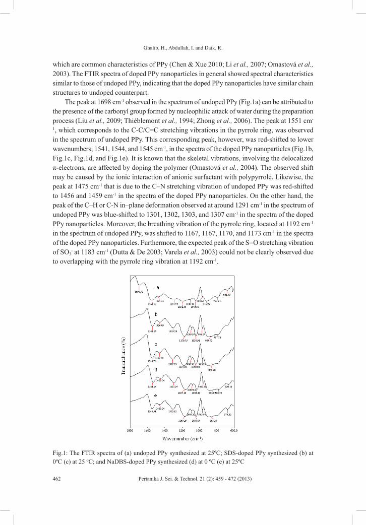
Ghalib, H., Abdullah, I. and Daik, R.
462 Pertanika J. Sci. & Technol. 21 (2): 459 - 472 (2013)
which are common characteristics of PPy (Chen & Xue 2010; Li et al., 2007; Omastová et al., 2003). The FTIR spectra of doped PPy nanoparticles in general showed spectral characteristics similar to those of undoped PPy, indicating that the doped PPy nanoparticles have similar chain structures to undoped counterpart.
The peak at 1698 cm-1 observed in the spectrum of undoped PPy (Fig.1a) can be attributed to the presence of the carbonyl group formed by nucleophilic attack of water during the preparation process (Liu et al., 2009; Thiéblemont et al., 1994; Zhong et al., 2006). The peak at 1551 cm-
1, which corresponds to the C-C/C=C stretching vibrations in the pyrrole ring, was observed in the spectrum of undoped PPy. This corresponding peak, however, was red-shifted to lower wavenumbers; 1541, 1544, and 1545 cm-1, in the spectra of the doped PPy nanoparticles (Fig.1b, Fig.1c, Fig.1d, and Fig.1e). It is known that the skeletal vibrations, involving the delocalized π-electrons, are affected by doping the polymer (Omastová et al., 2004). The observed shift may be caused by the ionic interaction of anionic surfactant with polypyrrole. Likewise, the peak at 1475 cm-1 that is due to the C–N stretching vibration of undoped PPy was red-shifted to 1456 and 1459 cm-1 in the spectra of the doped PPy nanoparticles. On the other hand, the peak of the C–H or C-N in–plane deformation observed at around 1291 cm-1 in the spectrum of undoped PPy was blue-shifted to 1301, 1302, 1303, and 1307 cm-1 in the spectra of the doped PPy nanoparticles. Moreover, the breathing vibration of the pyrrole ring, located at 1192 cm-1 in the spectrum of undoped PPy, was shifted to 1167, 1167, 1170, and 1173 cm-1 in the spectra of the doped PPy nanoparticles. Furthermore, the expected peak of the S=O stretching vibration of SO3
- at 1183 cm-1 (Dutta & De 2003; Varela et al., 2003) could not be clearly observed due to overlapping with the pyrrole ring vibration at 1192 cm-1.
Fig.1: The FTIR spectra of (a) undoped PPy synthesized at 25ºC; SDS-doped PPy synthesized (b) at 0ºC (c) at 25 ºC; and NaDBS-doped PPy synthesized (d) at 0 ºC (e) at 25ºC
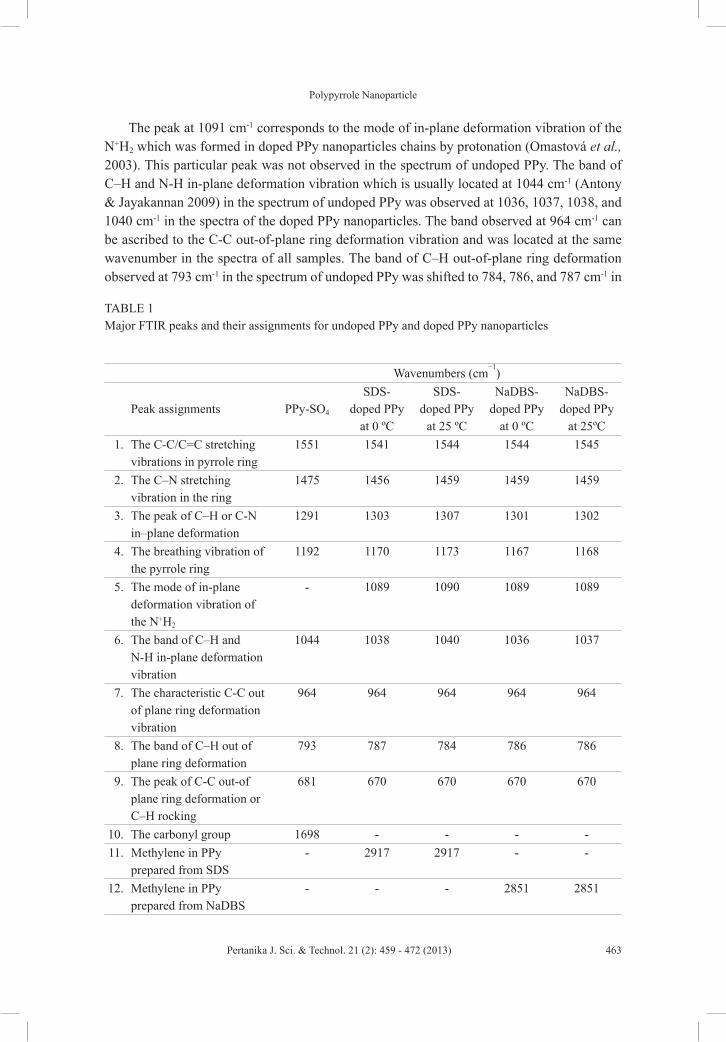
Polypyrrole Nanoparticle
463Pertanika J. Sci. & Technol. 21 (2): 459 - 472 (2013)
TABLE 1 Major FTIR peaks and their assignments for undoped PPy and doped PPy nanoparticles
Wavenumbers (cm−1)
Peak assignments PPy-SO4
SDS-doped PPy
at 0 ºC
SDS-doped PPy
at 25 ºC
NaDBS-doped PPy
at 0 ºC
NaDBS-doped PPy
at 25ºC1. The C-C/C=C stretching
vibrations in pyrrole ring 1551 1541 1544 1544 1545
2. The C–N stretching vibration in the ring
1475 1456 1459 1459 1459
3. The peak of C–H or C-N in–plane deformation
1291 1303 1307 1301 1302
4. The breathing vibration of the pyrrole ring
1192 1170 1173 1167 1168
5. The mode of in-plane deformation vibration of the N+H2
- 1089 1090 1089 1089
6. The band of C–H and N-H in-plane deformation vibration
1044 1038 1040 1036 1037
7. The characteristic C-C out of plane ring deformation vibration
964 964 964 964 964
8. The band of C–H out of plane ring deformation
793 787 784 786 786
9. The peak of C-C out-of plane ring deformation or C–H rocking
681 670 670 670 670
10. The carbonyl group 1698 - - - -11. Methylene in PPy
prepared from SDS- 2917 2917 - -
12. Methylene in PPy prepared from NaDBS
- - - 2851 2851
The peak at 1091 cm-1 corresponds to the mode of in-plane deformation vibration of the N+H2 which was formed in doped PPy nanoparticles chains by protonation (Omastová et al., 2003). This particular peak was not observed in the spectrum of undoped PPy. The band of C–H and N-H in-plane deformation vibration which is usually located at 1044 cm-1 (Antony & Jayakannan 2009) in the spectrum of undoped PPy was observed at 1036, 1037, 1038, and 1040 cm-1 in the spectra of the doped PPy nanoparticles. The band observed at 964 cm-1 can be ascribed to the C-C out-of-plane ring deformation vibration and was located at the same wavenumber in the spectra of all samples. The band of C–H out-of-plane ring deformation observed at 793 cm-1 in the spectrum of undoped PPy was shifted to 784, 786, and 787 cm-1 in
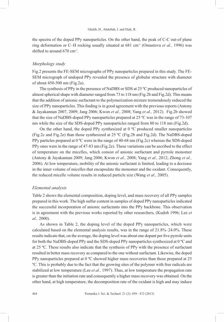
Ghalib, H., Abdullah, I. and Daik, R.
464 Pertanika J. Sci. & Technol. 21 (2): 459 - 472 (2013)
the spectra of the doped PPy nanoparticles. On the other hand, the peak of C-C out-of plane ring deformation or C–H rocking usually situated at 681 cm-1 (Omastova et al., 1996) was shifted to around 670 cm-1.
Morphology study
Fig.2 presents the FE-SEM micrographs of PPy nanoparticles prepared in this study. The FE-SEM micrograph of undoped PPy revealed the presence of globular structure with diameter of about 450-500 nm (Fig.2a).
The synthesis of PPy in the presence of NaDBS or SDS at 25 ºC produced nanoparticles of almost spherical shape with diameter ranged from 73 to 118 nm (Fig.2b and Fig.2d). This means that the addition of anionic surfactant to the polymerization mixture tremendously reduced the size of PPy nanoparticles. This finding is in good agreement with the previous reports (Antony & Jayakannan 2007, 2009; Jang 2006; Kwon et al., 2008; Yang et al., 2012). Fig.2b showed that the size of NaDBS-doped PPy nanoparticles prepared at 25 ºC was in the range of 73-107 nm while the size of the SDS-doped PPy nanoparticles ranged from 80 to 118 nm (Fig.2d).
On the other hand, the doped PPy synthesized at 0 ºC produced smaller nanoparticles (Fig.2c and Fig.2e) than those synthesized at 25 ºC (Fig.2b and Fig.2d). The NaDBS-doped PPy particles prepared at 0 ºC were in the range of 40-68 nm (Fig.2c) whereas the SDS-doped PPy ones were in the range of 47-83 nm (Fig.2e). These variations can be ascribed to the effect of temperature on the micelles, which consist of anionic surfactant and pyrrole monomer (Antony & Jayakannan 2009; Jang 2006; Kwon et al., 2008; Yang et al., 2012; Zhong et al., 2006). At low temperature, mobility of the anionic surfactant is limited, leading to a decrease in the inner volume of micelles that encapsulate the monomer and the oxidant. Consequently, the reduced micelle volume results in reduced particle size (Wang et al., 2005).
Elemental analysis
Table 2 shows the elemental composition, doping level, and mass recovery of all PPy samples prepared in this work. The high sulfur content in samples of doped PPy nanoparticles indicated the successful incorporation of anionic surfactants into the PPy backbone. This observation is in agreement with the previous works reported by other researchers, (Kudoh 1996; Lee et al., 2000).
As shown in Table 2, the doping level of the doped PPy nanoparticles, which were calculated based on the elemental analysis results, was in the range of 21.8%–24.0%. These results indicate that, on the average, the doping level was about one dopant per five pyrrole units for both the NaDBS-doped PPy and the SDS-doped PPy nanoparticles synthesized at 0 ºC and at 25 ºC. These results also indicate that the synthesis of PPy with the presence of surfactant resulted in better mass recovery as compared to the one without surfactant. Likewise, the doped PPy nanoparticles prepared at 0 ºC showed higher mass recoveries than those prepared at 25 ºC. This is probably due to the fact that the growing sites of the polymer with free radicals are stabilized at low temperature (Lee et al., 1997). Thus, at low temperature the propagation rate is greater than the initiation rate and consequently a higher mass recovery was obtained. On the other hand, at high temperature, the decomposition rate of the oxidant is high and may induce
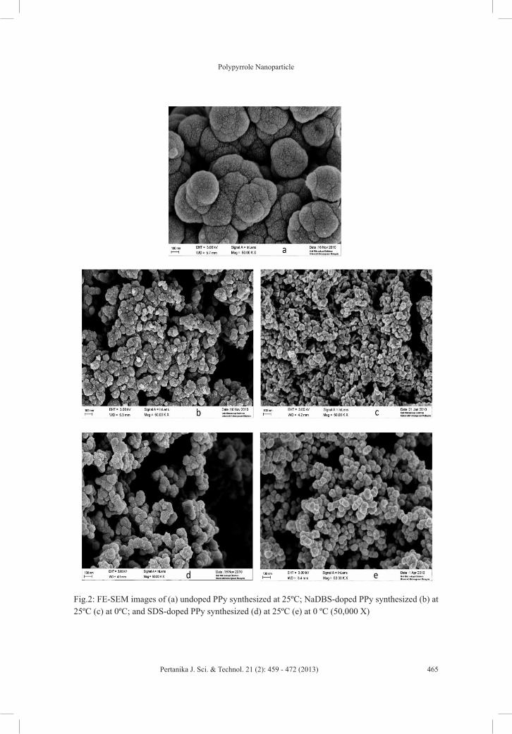
Polypyrrole Nanoparticle
465Pertanika J. Sci. & Technol. 21 (2): 459 - 472 (2013)
Fig.2: FE-SEM images of (a) undoped PPy synthesized at 25ºC; NaDBS-doped PPy synthesized (b) at 25ºC (c) at 0ºC; and SDS-doped PPy synthesized (d) at 25ºC (e) at 0 ºC (50,000 X)
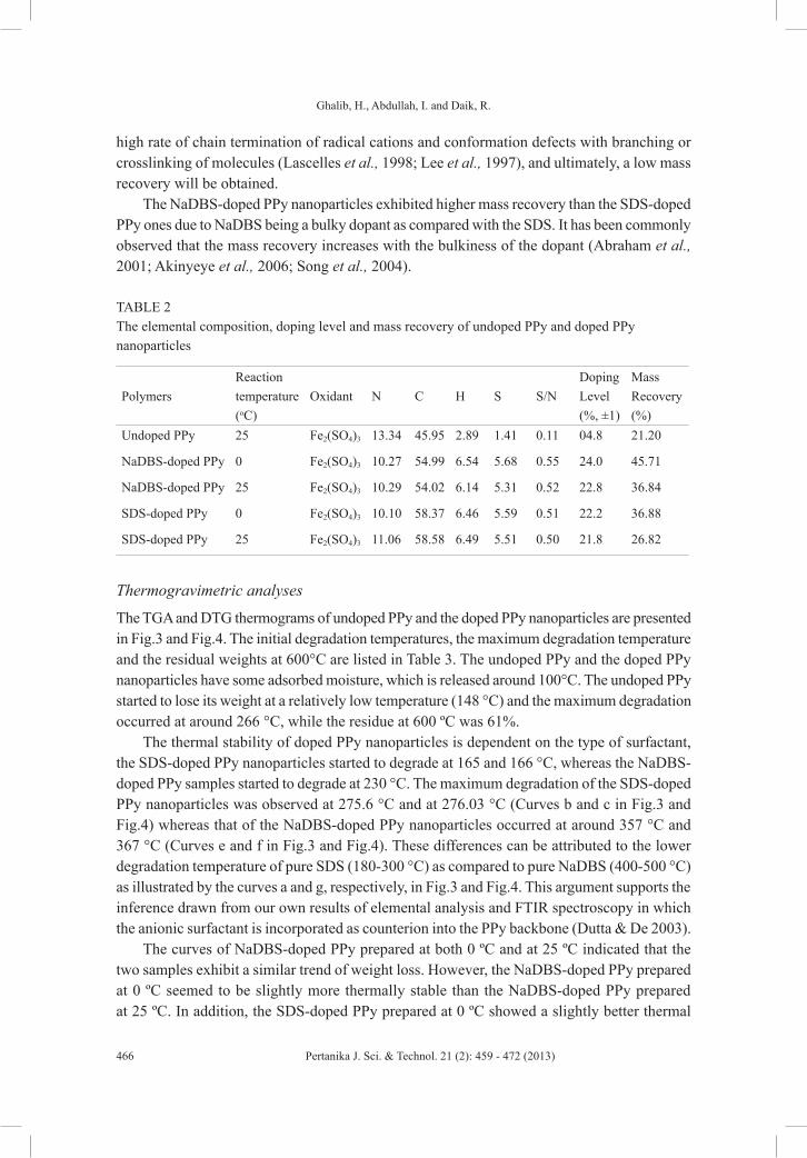
Ghalib, H., Abdullah, I. and Daik, R.
466 Pertanika J. Sci. & Technol. 21 (2): 459 - 472 (2013)
high rate of chain termination of radical cations and conformation defects with branching or crosslinking of molecules (Lascelles et al., 1998; Lee et al., 1997), and ultimately, a low mass recovery will be obtained.
The NaDBS-doped PPy nanoparticles exhibited higher mass recovery than the SDS-doped PPy ones due to NaDBS being a bulky dopant as compared with the SDS. It has been commonly observed that the mass recovery increases with the bulkiness of the dopant (Abraham et al., 2001; Akinyeye et al., 2006; Song et al., 2004).
TABLE 2 The elemental composition, doping level and mass recovery of undoped PPy and doped PPy nanoparticles
PolymersReaction temperature (οC)
Oxidant N C H S S/NDoping Level(%, ±1)
Mass Recovery (%)
Undoped PPy 25 Fe2(SO4)3 13.34 45.95 2.89 1.41 0.11 04.8 21.20
NaDBS-doped PPy 0 Fe2(SO4)3 10.27 54.99 6.54 5.68 0.55 24.0 45.71
NaDBS-doped PPy 25 Fe2(SO4)3 10.29 54.02 6.14 5.31 0.52 22.8 36.84
SDS-doped PPy 0 Fe2(SO4)3 10.10 58.37 6.46 5.59 0.51 22.2 36.88
SDS-doped PPy 25 Fe2(SO4)3 11.06 58.58 6.49 5.51 0.50 21.8 26.82
Thermogravimetric analyses
The TGA and DTG thermograms of undoped PPy and the doped PPy nanoparticles are presented in Fig.3 and Fig.4. The initial degradation temperatures, the maximum degradation temperature and the residual weights at 600°C are listed in Table 3. The undoped PPy and the doped PPy nanoparticles have some adsorbed moisture, which is released around 100°C. The undoped PPy started to lose its weight at a relatively low temperature (148 °C) and the maximum degradation occurred at around 266 °C, while the residue at 600 ºC was 61%.
The thermal stability of doped PPy nanoparticles is dependent on the type of surfactant, the SDS-doped PPy nanoparticles started to degrade at 165 and 166 °C, whereas the NaDBS-doped PPy samples started to degrade at 230 °C. The maximum degradation of the SDS-doped PPy nanoparticles was observed at 275.6 °C and at 276.03 °C (Curves b and c in Fig.3 and Fig.4) whereas that of the NaDBS-doped PPy nanoparticles occurred at around 357 °C and 367 °C (Curves e and f in Fig.3 and Fig.4). These differences can be attributed to the lower degradation temperature of pure SDS (180-300 °C) as compared to pure NaDBS (400-500 °C) as illustrated by the curves a and g, respectively, in Fig.3 and Fig.4. This argument supports the inference drawn from our own results of elemental analysis and FTIR spectroscopy in which the anionic surfactant is incorporated as counterion into the PPy backbone (Dutta & De 2003).
The curves of NaDBS-doped PPy prepared at both 0 ºC and at 25 ºC indicated that the two samples exhibit a similar trend of weight loss. However, the NaDBS-doped PPy prepared at 0 ºC seemed to be slightly more thermally stable than the NaDBS-doped PPy prepared at 25 ºC. In addition, the SDS-doped PPy prepared at 0 ºC showed a slightly better thermal
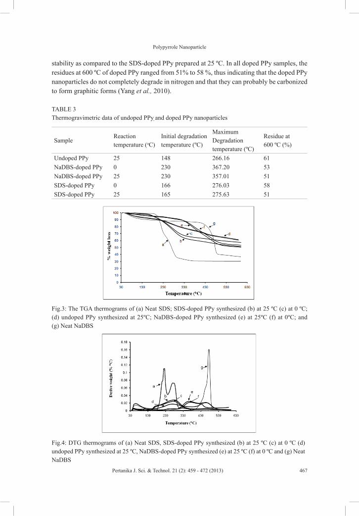
Polypyrrole Nanoparticle
467Pertanika J. Sci. & Technol. 21 (2): 459 - 472 (2013)
stability as compared to the SDS-doped PPy prepared at 25 ºC. In all doped PPy samples, the residues at 600 ºC of doped PPy ranged from 51% to 58 %, thus indicating that the doped PPy nanoparticles do not completely degrade in nitrogen and that they can probably be carbonized to form graphitic forms (Yang et al., 2010).
TABLE 3 Thermogravimetric data of undoped PPy, and doped PPy nanoparticles
SampleReaction temperature (oC)
Initial degradation temperature (ºC)
Maximum Degradation temperature (ºC)
Residue at600 ºC (%)
Undoped PPy 25 148 266.16 61NaDBS-doped PPy 0 230 367.20 53NaDBS-doped PPy 25 230 357.01 51SDS-doped PPy 0 166 276.03 58SDS-doped PPy 25 165 275.63 51
Fig.3: The TGA thermograms of (a) Neat SDS; SDS-doped PPy synthesized (b) at 25 ºC (c) at 0 ºC; (d) undoped PPy synthesized at 25ºC; NaDBS-doped PPy synthesized (e) at 25ºC (f) at 0ºC; and (g) Neat NaDBS
Fig.4: DTG thermograms of (a) Neat SDS, SDS-doped PPy synthesized (b) at 25 ºC (c) at 0 ºC (d) undoped PPy synthesized at 25 ºC, NaDBS-doped PPy synthesized (e) at 25 ºC (f) at 0 ºC and (g) Neat NaDBS
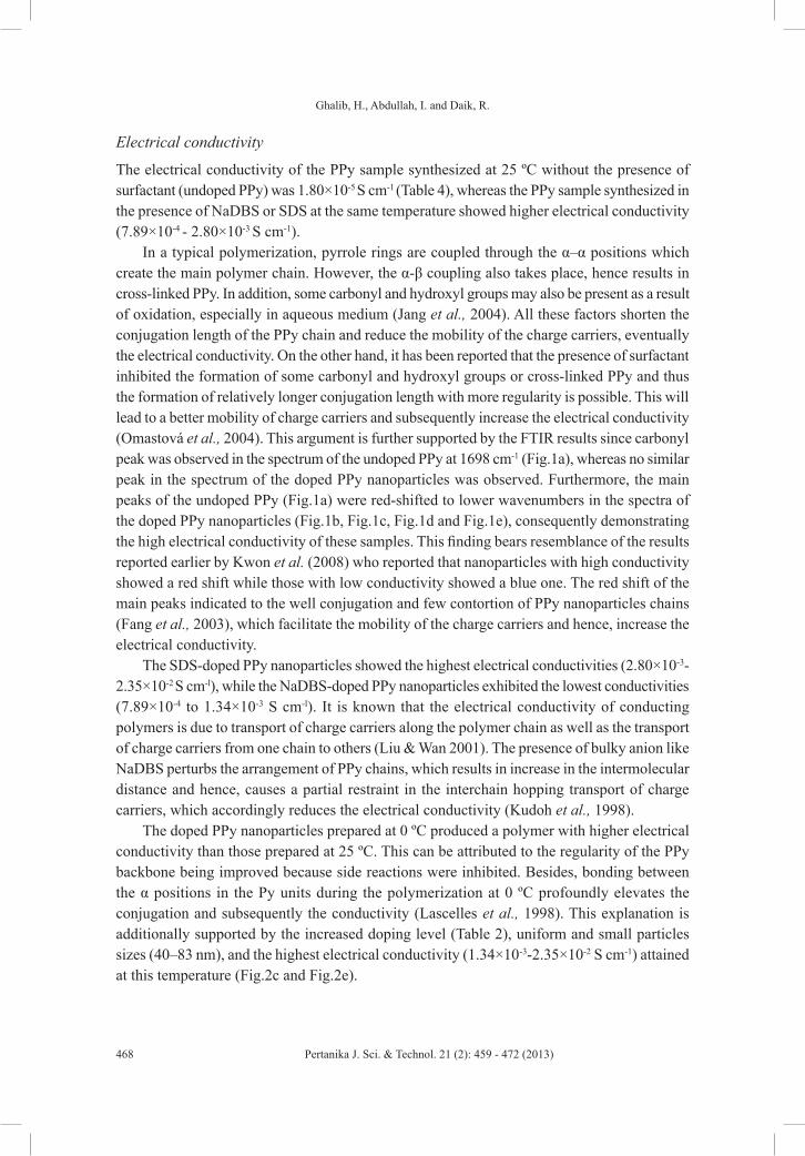
Ghalib, H., Abdullah, I. and Daik, R.
468 Pertanika J. Sci. & Technol. 21 (2): 459 - 472 (2013)
Electrical conductivity
The electrical conductivity of the PPy sample synthesized at 25 ºC without the presence of surfactant (undoped PPy) was 1.80×10⁻⁵ S cm-1 (Table 4), whereas the PPy sample synthesized in the presence of NaDBS or SDS at the same temperature showed higher electrical conductivity (7.89×10⁻⁴ - 2.80×10⁻³ S cm-1).
In a typical polymerization, pyrrole rings are coupled through the α–α positions which create the main polymer chain. However, the α-β coupling also takes place, hence results in cross-linked PPy. In addition, some carbonyl and hydroxyl groups may also be present as a result of oxidation, especially in aqueous medium (Jang et al., 2004). All these factors shorten the conjugation length of the PPy chain and reduce the mobility of the charge carriers, eventually the electrical conductivity. On the other hand, it has been reported that the presence of surfactant inhibited the formation of some carbonyl and hydroxyl groups or cross-linked PPy and thus the formation of relatively longer conjugation length with more regularity is possible. This will lead to a better mobility of charge carriers and subsequently increase the electrical conductivity (Omastová et al., 2004). This argument is further supported by the FTIR results since carbonyl peak was observed in the spectrum of the undoped PPy at 1698 cm-1 (Fig.1a), whereas no similar peak in the spectrum of the doped PPy nanoparticles was observed. Furthermore, the main peaks of the undoped PPy (Fig.1a) were red-shifted to lower wavenumbers in the spectra of the doped PPy nanoparticles (Fig.1b, Fig.1c, Fig.1d and Fig.1e), consequently demonstrating the high electrical conductivity of these samples. This finding bears resemblance of the results reported earlier by Kwon et al. (2008) who reported that nanoparticles with high conductivity showed a red shift while those with low conductivity showed a blue one. The red shift of the main peaks indicated to the well conjugation and few contortion of PPy nanoparticles chains (Fang et al., 2003), which facilitate the mobility of the charge carriers and hence, increase the electrical conductivity.
The SDS-doped PPy nanoparticles showed the highest electrical conductivities (2.80×10⁻³-2.35×10⁻² S cm-l), while the NaDBS-doped PPy nanoparticles exhibited the lowest conductivities (7.89×10⁻⁴ to 1.34×10⁻³ S cm-l). It is known that the electrical conductivity of conducting polymers is due to transport of charge carriers along the polymer chain as well as the transport of charge carriers from one chain to others (Liu & Wan 2001). The presence of bulky anion like NaDBS perturbs the arrangement of PPy chains, which results in increase in the intermolecular distance and hence, causes a partial restraint in the interchain hopping transport of charge carriers, which accordingly reduces the electrical conductivity (Kudoh et al., 1998).
The doped PPy nanoparticles prepared at 0 ºC produced a polymer with higher electrical conductivity than those prepared at 25 ºC. This can be attributed to the regularity of the PPy backbone being improved because side reactions were inhibited. Besides, bonding between the α positions in the Py units during the polymerization at 0 ºC profoundly elevates the conjugation and subsequently the conductivity (Lascelles et al., 1998). This explanation is additionally supported by the increased doping level (Table 2), uniform and small particles sizes (40–83 nm), and the highest electrical conductivity (1.34×10⁻³-2.35×10⁻² S cm-1) attained at this temperature (Fig.2c and Fig.2e).
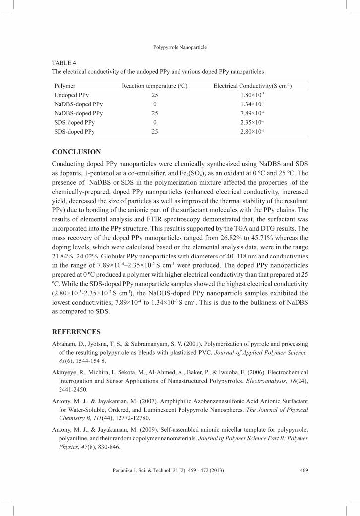
Polypyrrole Nanoparticle
469Pertanika J. Sci. & Technol. 21 (2): 459 - 472 (2013)
TABLE 4 The electrical conductivity of the undoped PPy and various doped PPy nanoparticles
Polymer Reaction temperature (oC) Electrical Conductivity(S cm-1)Undoped PPy 25 1.80×10⁻⁵
NaDBS-doped PPy 0 1.34×10⁻³
NaDBS-doped PPy 25 7.89×10⁻⁴
SDS-doped PPy 0 2.35×10⁻²
SDS-doped PPy 25 2.80×10⁻³
CONCLUSION
Conducting doped PPy nanoparticles were chemically synthesized using NaDBS and SDS as dopants, 1-pentanol as a co-emulsifier, and Fe2(SO4)3 as an oxidant at 0 ºC and 25 ºC. The presence of NaDBS or SDS in the polymerization mixture affected the properties of the chemically-prepared, doped PPy nanoparticles (enhanced electrical conductivity, increased yield, decreased the size of particles as well as improved the thermal stability of the resultant PPy) due to bonding of the anionic part of the surfactant molecules with the PPy chains. The results of elemental analysis and FTIR spectroscopy demonstrated that, the surfactant was incorporated into the PPy structure. This result is supported by the TGA and DTG results. The mass recovery of the doped PPy nanoparticles ranged from 26.82% to 45.71% whereas the doping levels, which were calculated based on the elemental analysis data, were in the range 21.84%–24.02%. Globular PPy nanoparticles with diameters of 40–118 nm and conductivities in the range of 7.89×10⁻⁴–2.35×10⁻² S cm-1 were produced. The doped PPy nanoparticles prepared at 0 ºC produced a polymer with higher electrical conductivity than that prepared at 25 ºC. While the SDS-doped PPy nanoparticle samples showed the highest electrical conductivity (2.80×10⁻³-2.35×10⁻² S cm-l), the NaDBS-doped PPy nanoparticle samples exhibited the lowest conductivities; 7.89×10⁻⁴ to 1.34×10⁻³ S cm-l. This is due to the bulkiness of NaDBS as compared to SDS.
REFERENCES Abraham, D., Jyotsna, T. S., & Subramanyam, S. V. (2001). Polymerization of pyrrole and processing
of the resulting polypyrrole as blends with plasticised PVC. Journal of Applied Polymer Science, 81(6), 1544-154 8.
Akinyeye, R., Michira, I., Sekota, M., Al-Ahmed, A., Baker, P., & Iwuoha, E. (2006). Electrochemical Interrogation and Sensor Applications of Nanostructured Polypyrroles. Electroanalysis, 18(24), 2441-2450.
Antony, M. J., & Jayakannan, M. (2007). Amphiphilic Azobenzenesulfonic Acid Anionic Surfactant for Water-Soluble, Ordered, and Luminescent Polypyrrole Nanospheres. The Journal of Physical Chemistry B, 111(44), 12772-12780.
Antony, M. J., & Jayakannan, M. (2009). Self-assembled anionic micellar template for polypyrrole, polyaniline, and their random copolymer nanomaterials. Journal of Polymer Science Part B: Polymer Physics, 47(8), 830-846.
Ghalib, H., Abdullah, I. and Daik, R.
470 Pertanika J. Sci. & Technol. 21 (2): 459 - 472 (2013)
Chen, W., & Xue, G. (2010). Formation of conducting polymer nanostructures with the help of surfactant crystallite templates. Frontiers of Materials Science in China, 4(2), 152-157.
Dutta, P. & De, S. K. (2003). Electrical properties of polypyrrole doped with [beta]-naphthalenesulfonicacid and polypyrrole-polymethyl methacrylate blends. Synthetic Metals, 139(2), 201-206.
Fang, Q., Xu, W., Lei, H., Xue, G., Chen, H., Xu, C., Jia, C., & Zhang, D. (2003). Synthesis, structure, and conductivity of molecular conductor (PyEt)[Ni(dmit)2]2. Science in China Series B: Chemistry, 46(6), 595-604.
Feng, Y., Gi, X., & Mingshi, Z. (2000). Preparation of electrically conducting polypyrrole in oil/water microemulsion. Journal of Applied Polymer Science, 77(1), 135-140.
Goel, S., Mazumdar, N. A., & Gupta, A. (2010). Synthesis and characterization of polypyrrole nanofibers with different dopants. Polymers for Advanced Technologies, 21(3), 205-210.
Jang, J. (2006). Conducting Polymer Nanomaterials and Their Applications. In (Eds.). Emissive Materials Nanomaterials. Berlin: Springer-Verlag Berlin.
Jang, J., Li, X. L., & Oh, J. H. (2004). Facile fabrication of polymer and carbon nanocapsules using polypyrrole core/shell nanomaterials. Chemical Communications, 7, 794-795.
Kudoh, Y. (1996). Properties of polypyrrole prepared by chemical polymerization using aqueous solution containing Fe2(SO4)3 and anionic surfactant. Synthetic Metals, 79(1), 17-22.
Kudoh, Y., Akami, K., & Matsuya, Y. (1998). Properties of chemically prepared polypyrrole with an aqueous solution containing Fe2(SO4)3, a sulfonic surfactant and a phenol derivative. Synthetic Metals, 95(3), 191-196.
Kwon, W. J., Suh, D. H., Chin, B. D., & Yu, J. W. (2008). Preparation of polypyrrole nanoparticles in mixed surfactants system. Journal of Applied Polymer Science, 110(3), 1324-1329.
Lascelles, S. F., McCarthy, G. P., Butterworth, M. D., & Armes, S. P. (1998). Effect of synthesis parameters on the particle size, composition and colloid stability of polypyrrole–silica nanocomposite particles. Colloid & Polymer Science, 276(10), 893-902.
Lee, J. Y., Kim, D. Y., & Kim, C. Y. (1995). Synthesis of soluble polypyrrole of the doped state in organic solvents. Synthetic Metals, 74(2), 103-106.
Lee, J. Y., Song, K. T., Kim, S. Y., Kim, Y. C., Kim, D. Y., & Kim, C. Y. (1997). Synthesis and Characterization of Soluble Polypyrrole. Synthetic Metals, 84(1-3), 137-140.
Lee, Y. H., Lee, J. Y., & Lee, D. S. (2000). A novel conducting soluble polypyrrole composite with a polymeric co-dopant. Synthetic Metals, 114(3), 347-353.
Li, X.-G., Wei, F., Huang, M.-R., & Xie, Y.-B. (2007). Facile Synthesis and Intrinsic Conductivity of Novel Pyrrole Copolymer Nanoparticles with Inherent Self-Stability. The Journal of Physical Chemistry B, 111(21), 5829-5836.
Liu, A. S., Bezerra, M. C., & Cho, L. Y. (2009). Electrodeposition of Polypyrrole Films on Aluminum Surfaces from a p-toluene Sulfonic Acid Medium. Materials Research, 12(4), 503-507.
Liu, J., & Wan, M. (2001). Synthesis, characterization and electrical properties of microtubules of polypyrrole synthesized by a template-free method. J. Mater. Chem., 11, 404-407.
Liu, Y., Chu, Y., & Yang, L. (2006). Adjusting the inner-structure of polypyrrole nanoparticles through microemulsion polymerization. Materials Chemistry and Physics, 98(2-3), 304-308.

Polypyrrole Nanoparticle
471Pertanika J. Sci. & Technol. 21 (2): 459 - 472 (2013)
Omastova, M., Kosina, S., Pionteck, J., Janke, A., & Pavlinec, J. (1996). Electrical properties and stability of polypyrrole containing conducting polymer composites. Synthetic MetaIs, 81, 49-57.
Omastová, M., Trchová, M., Kovárová, J., & Stejskal, J. (2003). Synthesis and structural study of polypyrroles prepared in the presence of surfactants. Synthetic Metals, 138(3), 447-455.
Omastová, M., Trchová, M., Pionteck, J., Prokes, J., & Stejskal, J. (2004). Effect of polymerization conditions on the properties of polypyrrole prepared in the presence of sodium bis(2-ethylhexyl) sulfosuccinate. Synthetic Metals, 143(2), 153-161.
Pringle, J. M., Efthimiadis, J., Howlett, P. C., Efthimiadis, J., MacFarlane, D. R., Chaplin, A. B., Hall, S. B., Officer, D. L., Wallace, G. G., & Forsyth, M. 2004. Electrochemical synthesis of polypyrrole in ionic liquids. Polymer, 45(5), 1447-1453.
Pyo, M., Bohn, C. C., Smela, E., Reynolds, J. R., & Brennan, A. B. (2003). Direct Strain Measurement of Polypyrrole Actuators Controlled by the Polymer/Gold Interface. Chemistry of Materials, 15(4), 916-922.
Ramanavicius, A., Ramanaviciene, A., & Malinauskas, A. (2006). Electrochemical sensors based on conducting polymer--polypyrrole. Electrochimica Acta, 51(27), 6025-6037.
Song, M.-K., Kim, Y.-T., Kim, B.-S., Kim, J., Char, K., & Rhee, H.-W. (2004). Synthesis and characterization of soluble polypyrrole doped with alkylbenzenesulfonic acids. Synthetic Metals 141(3), 315-319.
Thiéblemont, J. C., Gabelle, J. L., & Planche, M. F. (1994). Polypyrrole overoxidation during its chemical synthesis. Synthetic Metals, 66(3), 243-247.
Varela, H., Bruno, R. L., & Torresi, R. M. (2003). Ionic transport in conducting polymers/nickel tetrasulfonated phthalocyanine modified electrodes. Polymer, 44(18), 5369-5379.
Veeraraghavan, B., Paul, J., Haran, B., & Popov, B. (2002). Study of polypyrrole graphite composite as anode material for secondary lithium-ion batteries. Journal of Power Sources, 109(2), 377-387.
Wang, H., Lin, T., & Kaynak, A. (2005). Polypyrrole nanoparticles and dye absorption properties. Synthetic Metals, 151(2), 136-140.
Wang, L.-X., Li, X.-G., & Yang, Y.-L. (2001). Preparation, properties and applications of polypyrroles. Reactive and Functional Polymers, 47(2), 125-139.
Yamamoto, H., Oshima, M., Hosaka, T., & Isa, I. 1999. Solid electrolytic capacitors using an aluminum alloy electrode and conducting polymers. Synthetic Metals, 104(1), 33-38.
Yan, F., Xue, G., & Zhou, M. (2000). Preparation of electrically conducting polypyrrole in oil/water microemulsion. Journal of Applied Polymer Science, 77(1), 135-140.
Yang, C., Liu, P., Guo, J., & Wang, Y. (2010). Polypyrrole/vermiculite nanocomposites via self-assembling and in situ chemical oxidative polymerization. Synthetic Metals, 160(7-8), 592-598.
Yang, C., Wang, X., Wang, Y., & Liu, P. (2012). Polypyrrole nanoparticles with high dispersion stability via chemical oxidative polymerization in presence of an anionic–non-ionic bifunctional polymeric surfactant. Powder Technology, 217(0), 134-139.
Zhong, W., Liu, S., Chen, X., Wang, Y., & Yang, W. (2006). High-Yield Synthesis of Superhydrophilic Polypyrrole Nanowire Networks. Macromolecules, 39(9), 3224-3230.

Pertanika J. Sci. & Technol. 21 (2): 473 - 486 (2013)
SCIENCE & TECHNOLOGYJournal homepage: http://www.pertanika.upm.edu.my/
ISSN: 0128-7680 © 2013 Universiti Putra Malaysia Press.
Landslide Susceptibility Mapping Using Averaged Weightage Score and GIS: A Case Study at Kuala Lumpur
Mahmud, A. R.1, Awad, A.1 and Billa, R.2*1Spatial and Numerical Modelling Laboratory, Universiti Putra Malysia, 43400 Serdang, Selangor, Malaysia2School of Geography, University of Nottingham, Malaysia Campus, 43500 Semenyih, Selangor, Malaysia
ABSTRACT
Many residential areas of Kuala Lumpur are susceptible to landslides; this is seen in the frequency of landslide occurences in these areas. The objective of this study is to delineate landslide risk areas in support of development planning, monitoring and control of unstable areas. In this study, five landslide causative factors were extracted from satellite imagery and maps provided by the Geological Survey Department of Malaysia. Factors included in the study including land use, river density and lineament derived from Landsat ETM image, precipitation amount from rain gauge stations and lithology, were extracted from the geological map of the study area. Layers were analyzed and divided into subclasses. An average weightage score was applied to calculate the subclasses into percentage weights of influence on landslide. Overlay, geo-processing and geo-statistic techniques in GIS were used to discriminate these weighted subclasses into landslide susceptibility at low, medium and high levels of risk areas. Results showed very high susceptible areas covering 0.21% of Kuala Lumpur of which 5.02% were found in the highly urbanized areas. Meanwhile, a landslide susceptibility map was generated to show low, medium and high susceptible areas in Kuala Lumpur. Results were verified using recorded cases of landslides in Kuala Lumpur which showed a 77% agreement with the study.
Keywords: Landslide, weightage score, GIS, Landsat data, susceptibility mapping, Kuala Lumpur
Article history:Received: 8 September 2011Accepted: 10 November 2011
E-mail addresses: [email protected] (Mahmud, A. R.), [email protected] (Billa, L.)*Corresponding Author
INTRODUCTION
Landslides are one of the disasters that reshape the surface of the earth through natural processes and adversely impact on the economic lives of people. In recent years, there have been many occurrences of landslide in areas in Kuala Lumpur and in Malaysia in general. Most of these have occurred on cut slopes or on embankments alongside
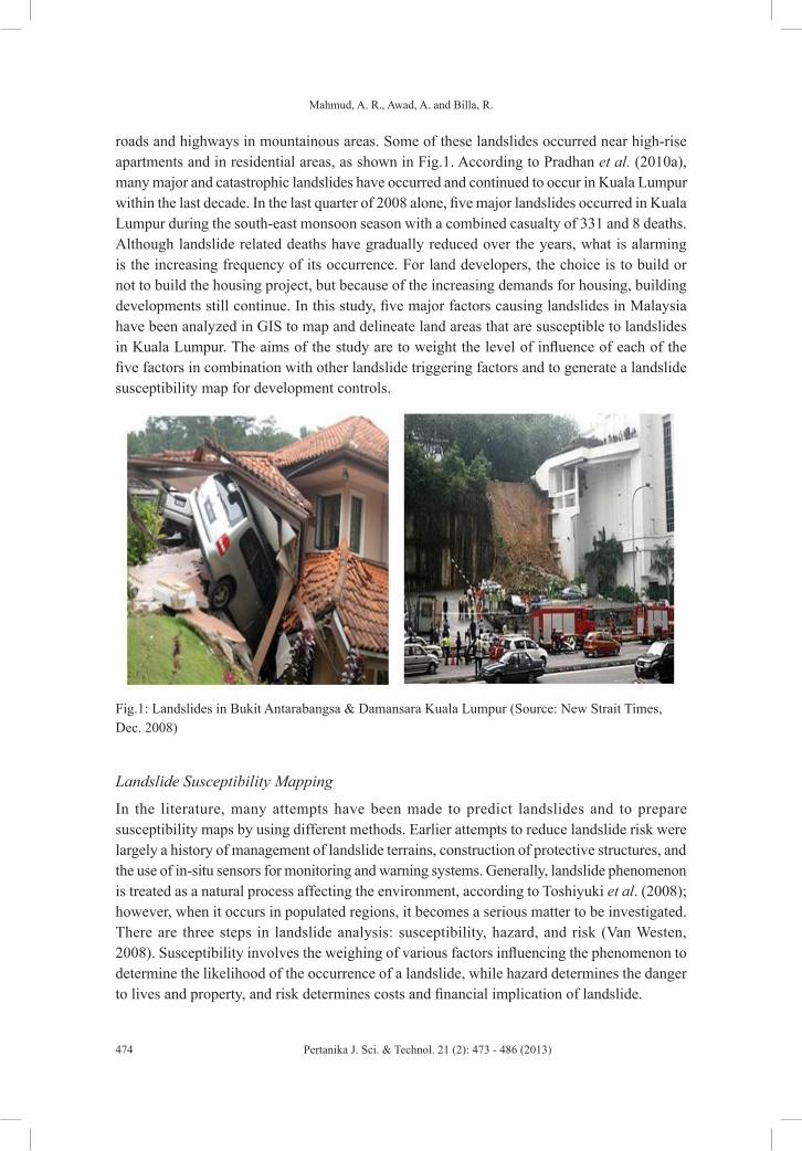
Mahmud, A. R., Awad, A. and Billa, R.
474 Pertanika J. Sci. & Technol. 21 (2): 473 - 486 (2013)
roads and highways in mountainous areas. Some of these landslides occurred near high-rise apartments and in residential areas, as shown in Fig.1. According to Pradhan et al. (2010a), many major and catastrophic landslides have occurred and continued to occur in Kuala Lumpur within the last decade. In the last quarter of 2008 alone, five major landslides occurred in Kuala Lumpur during the south-east monsoon season with a combined casualty of 331 and 8 deaths. Although landslide related deaths have gradually reduced over the years, what is alarming is the increasing frequency of its occurrence. For land developers, the choice is to build or not to build the housing project, but because of the increasing demands for housing, building developments still continue. In this study, five major factors causing landslides in Malaysia have been analyzed in GIS to map and delineate land areas that are susceptible to landslides in Kuala Lumpur. The aims of the study are to weight the level of influence of each of the five factors in combination with other landslide triggering factors and to generate a landslide susceptibility map for development controls.
Fig.1: Landslides in Bukit Antarabangsa & Damansara Kuala Lumpur (Source: New Strait Times, Dec. 2008)
Landslide Susceptibility Mapping
In the literature, many attempts have been made to predict landslides and to prepare susceptibility maps by using different methods. Earlier attempts to reduce landslide risk were largely a history of management of landslide terrains, construction of protective structures, and the use of in-situ sensors for monitoring and warning systems. Generally, landslide phenomenon is treated as a natural process affecting the environment, according to Toshiyuki et al. (2008); however, when it occurs in populated regions, it becomes a serious matter to be investigated. There are three steps in landslide analysis: susceptibility, hazard, and risk (Van Westen, 2008). Susceptibility involves the weighing of various factors influencing the phenomenon to determine the likelihood of the occurrence of a landslide, while hazard determines the danger to lives and property, and risk determines costs and financial implication of landslide.
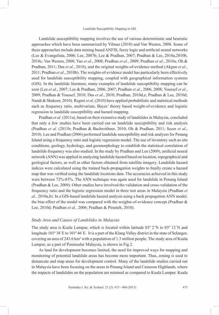
Landslide Susceptibility Mapping in GIS
475Pertanika J. Sci. & Technol. 21 (2): 473 - 486 (2013)
Landslide susceptibility mapping involves the use of various deterministic and heuristic approaches which have been summarized by Yilmaz (2010) and Van Westen, 2008. Some of these approaches include data mining based ANFIS, fuzzy logic and artificial neural networks (Lee & Evangelista, 2006; Lee, 2007b; Lee & Pradhan, 2007; Pradhan & Lee, 2010a,2010b, 2010c; Van Westen, 2008; Yao et al., 2008; Pradhan et al., 2009; Pradhan et al., 2010a; Oh & Pradhan, 2011; Das et al., 2010), and the original weights-of-evidence method (Akgun et al., 2011; Pradhan et al., 2010b). The weights-of-evidence model has particularly been effectively used for landslide susceptibility mapping, coupled with geographical information systems (GIS). In the landslide literature, many examples of landslide susceptibility mapping can be seen (Lee et al., 2007; Lee & Pradhan, 2006, 2007; Pradhan et al., 2006, 2008; Youssef et al., 2009; Pradhan & Youssef, 2010; Das et al., 2010; Pradhan, 2010d,e; Pradhan & Lee, 2010d; Nandi & Shakoor, 2010). Regmi et al. (2010) have applied probabilistic and statistical methods such as frequency ratio, multivariate, Bayes’ theory based weight-of-evidence and logistic regression to landslide susceptibility and hazard mapping.
Pradhan et al. (2011a), based on their extensive study of landslides in Malaysia, concluded that only a few studies have been carried out on landslide susceptibility and risk analysis (Pradhan et al. (2011b; Pradhan & Bachroithner, 2010; Oh & Pradhan, 2011; Sezer et al., 2010). Lee and Pradhan (2006) performed landslide susceptibility and risk analyses for Penang Island using a frequency ratio and logistic regression model. The use of inventory such as site conditions, geology, hydrology, and geomorphology to establish the statistical correlation of landslide frequency was also studied. In the study by Pradhan and Lee (2009), artificial neural network (ANN) was applied in analyzing landslide hazard based on location, topographical and geological factors, as well as other factors obtained from satellite imagery. Landslide hazard indices were calculated using the trained back-propagation weights to finally create a hazard map that was verified using the landslide locations data. The accuracies achieved in this study were between 72%-83%. The ANN technique was again used for landslide in Penang Island (Pradhan & Lee, 2009). Other studies have involved the validation and cross-validation of the frequency ratio and the logistic regression model in three test areas in Malaysia (Pradhan et al., 2010a,b). In a GIS-based landslide hazard analysis using a back propagation ANN model, the bias effect of the model was compared with the weights-of-evidence concept (Pradhan & Lee, 2010d; Pradhan et al., 2006; Pradhan & Pirasteh, 2010).
Study Area and Causes of Landslides in Malaysia
The study area is Kuala Lumpur, which is located within latitude 03º 2´N to 03º 12´N and longitude 101º 38´E to 101º 46´E. It is a part of the Klang Valley district in the state of Selangor, covering an area of 243.6 km2 with a population of 1.3 million people. The study area of Kuala Lumpur, as a part of Peninsular Malaysia, is shown in Fig.2.
As land for development becomes limited, the need for improved ways for mapping and monitoring of potential landslide areas has become more important. Thus, zoning is used to demarcate and map areas for development control. Many of the landslide studies carried out in Malaysia have been focusing on the areas in Penang Island and Cameron Highlands, where the impacts of landslides on the population are minimal as compared to Kuala Lumpur. Kuala
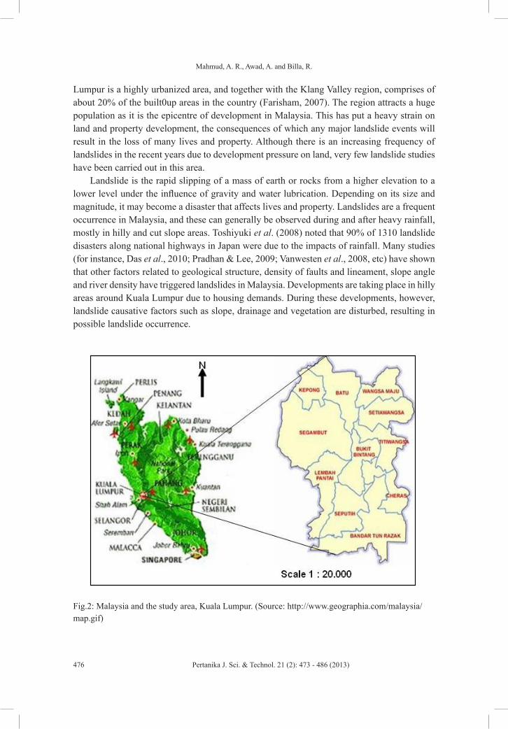
Mahmud, A. R., Awad, A. and Billa, R.
476 Pertanika J. Sci. & Technol. 21 (2): 473 - 486 (2013)
Lumpur is a highly urbanized area, and together with the Klang Valley region, comprises of about 20% of the built0up areas in the country (Farisham, 2007). The region attracts a huge population as it is the epicentre of development in Malaysia. This has put a heavy strain on land and property development, the consequences of which any major landslide events will result in the loss of many lives and property. Although there is an increasing frequency of landslides in the recent years due to development pressure on land, very few landslide studies have been carried out in this area.
Landslide is the rapid slipping of a mass of earth or rocks from a higher elevation to a lower level under the influence of gravity and water lubrication. Depending on its size and magnitude, it may become a disaster that affects lives and property. Landslides are a frequent occurrence in Malaysia, and these can generally be observed during and after heavy rainfall, mostly in hilly and cut slope areas. Toshiyuki et al. (2008) noted that 90% of 1310 landslide disasters along national highways in Japan were due to the impacts of rainfall. Many studies (for instance, Das et al., 2010; Pradhan & Lee, 2009; Vanwesten et al., 2008, etc) have shown that other factors related to geological structure, density of faults and lineament, slope angle and river density have triggered landslides in Malaysia. Developments are taking place in hilly areas around Kuala Lumpur due to housing demands. During these developments, however, landslide causative factors such as slope, drainage and vegetation are disturbed, resulting in possible landslide occurrence.
Fig.2: Malaysia and the study area, Kuala Lumpur. (Source: http://www.geographia.com/malaysia/map.gif)
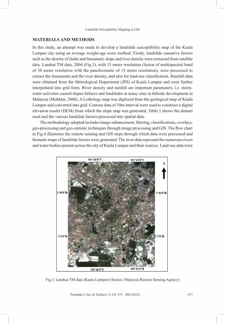
Landslide Susceptibility Mapping in GIS
477Pertanika J. Sci. & Technol. 21 (2): 473 - 486 (2013)
MATERIALS AND METHODS
In this study, an attempt was made to develop a landslide susceptibility map of the Kuala Lumpur city using an average weight-age score method. Firstly, landslide causative factors such as the density of faults and lineament, slope and river density were extracted from satellite data. Landsat TM data, 2004 (Fig.3), with 15 meter resolution (fusion of multispectral band of 30 meter resolution with the panchromatic of 15 meter resolution), were processed to extract the lineaments and the river density, and also for land-use classification. Rainfall data were obtained from the Metrological Department (JPS) of Kuala Lumpur and were further interpolated into grid form. River density and rainfall are important parameters, i.e. storm-water activities caused slopes failures and landslides at many sites in hillside development in Malaysia (Mokhtar, 2006). A Lothology map was digitized from the geological map of Kuala Lumpur and converted into grid. Contour data of 10m interval were used to construct a digital elevation model (DEM) from which the slope map was generated. Table 1 shows the dataset used and the various landslide factors processed into spatial data.
The methodology adopted includes image enhancement, filtering, classifications, overlays, geo-processing and geo-statistic techniques through image processing and GIS. The flow chart in Fig.4 illustrates the remote sensing and GIS steps through which data were processed and thematic maps of landslide factors were generated. The river data represent the numerous rivers and water bodies present across the city of Kuala Lumpur and their sources. Land-use data were
Fig.3: Landsat TM data (Kuala Lumpur) (Source: Malaysia Remote Sensing Agency)
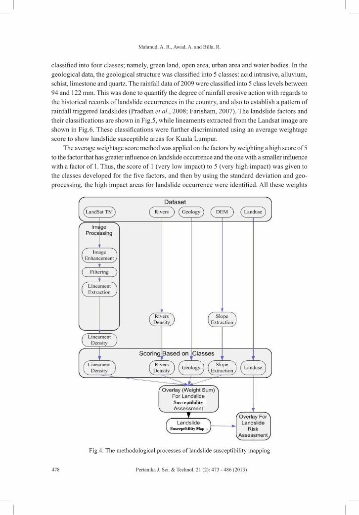
Mahmud, A. R., Awad, A. and Billa, R.
478 Pertanika J. Sci. & Technol. 21 (2): 473 - 486 (2013)
Fig.4: The methodological processes of landslide susceptibility mapping
classified into four classes; namely, green land, open area, urban area and water bodies. In the geological data, the geological structure was classified into 5 classes: acid intrusive, alluvium, schist, limestone and quartz. The rainfall data of 2009 were classified into 5 class levels between 94 and 122 mm. This was done to quantify the degree of rainfall erosive action with regards to the historical records of landslide occurrences in the country, and also to establish a pattern of rainfall triggered landslides (Pradhan et al., 2008; Farisham, 2007). The landslide factors and their classifications are shown in Fig.5, while lineaments extracted from the Landsat image are shown in Fig.6. These classifications were further discriminated using an average weightage score to show landslide susceptible areas for Kuala Lumpur.
The average weightage score method was applied on the factors by weighting a high score of 5 to the factor that has greater influence on landslide occurrence and the one with a smaller influence with a factor of 1. Thus, the score of 1 (very low impact) to 5 (very high impact) was given to the classes developed for the five factors, and then by using the standard deviation and geo-processing, the high impact areas for landslide occurrence were identified. All these weights
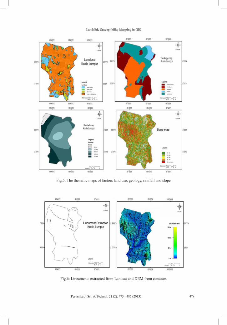
Landslide Susceptibility Mapping in GIS
479Pertanika J. Sci. & Technol. 21 (2): 473 - 486 (2013)
Fig.5: The thematic maps of factors land use, geology, rainfall and slope
Fig.6: Lineaments extracted from Landsat and DEM from contours

Mahmud, A. R., Awad, A. and Billa, R.
480 Pertanika J. Sci. & Technol. 21 (2): 473 - 486 (2013)
were assigned manually. High density of lineaments was found to be in the congested urban areas and places of human activities, especially in the north east of Kuala Lumpur, as shown in Fig.7. This complements the citations in most literature that areas with more fracturing and faulting are always prone to landslide occurrences.
The river density of a watershed is an important geomorphic parameter to understanding the extent of debris flow and seepage, possible consequences of landslide occurrence. River density (Fig.7) was classified into five levels of 0.2 km2 difference. Table 2 shows various factors, the classifications given, the score attributed to them, and the percentage area of coverage for each classification.
TABLE 1 Type of Data
Data type Format Scale / Resolution Rainfall Raster 50 x 50 meterLandSat TM Raster 15 x 15 meterRiver Vector 1: 100,000DEM/slope Grid 10 x 10 meterGeology Grid 1: 100,000Landuse Grid 1: 100,000
TABLE 2 Weightage score for the landslide factors
Factor Classes Score Pixels Count Percentage %Lineament Density
0.0 – 0.3 /km2
0.3 – 0.6 /km2
0.6 – 0.8 /km2
0.8 – 1.0 /km2
1.0 < /km2
12345
10240013569212662112866476486
17.9723.8122.2222.5813.42
Landuse Water BodiesGreen LandOpen AreaUrban or Built up Area
1225
299731371912355220678
10.834.994.4779.71
Rainfall 94mm 122 mm130 mm145 mm170 mm
13345
37151845738576333314884
3.7518.6538.9833.684.94
Geology Structure
Acid intrusiveGranite Vein QuartzSchistLimestone
12345
17810878221077833852199099
28.610.1233.855.4431.97
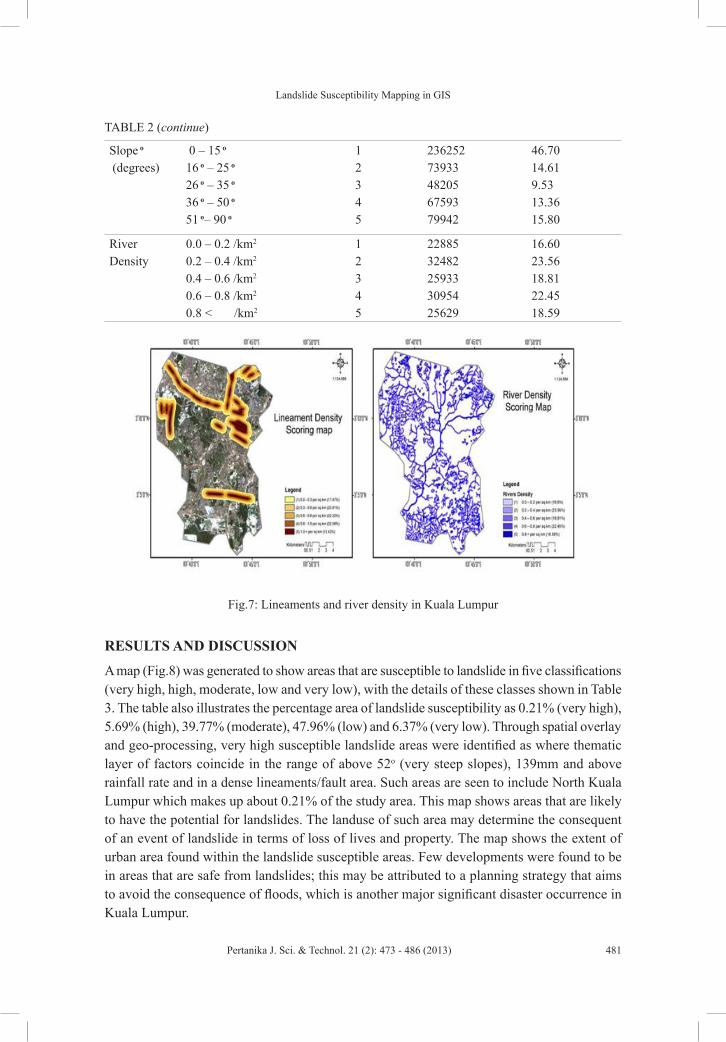
Landslide Susceptibility Mapping in GIS
481Pertanika J. Sci. & Technol. 21 (2): 473 - 486 (2013)
Slope o
(degrees) 0 – 15 o
16 o – 25 o
26 o – 35 o
36 o – 50 o
51 o– 90 o
12345
23625273933482056759379942
46.7014.619.5313.3615.80
River Density
0.0 – 0.2 /km2
0.2 – 0.4 /km2
0.4 – 0.6 /km2
0.6 – 0.8 /km2
0.8 < /km2
12345
2288532482259333095425629
16.6023.5618.8122.4518.59
Fig.7: Lineaments and river density in Kuala Lumpur
TABLE 2 (continue)
RESULTS AND DISCUSSION
A map (Fig.8) was generated to show areas that are susceptible to landslide in five classifications (very high, high, moderate, low and very low), with the details of these classes shown in Table 3. The table also illustrates the percentage area of landslide susceptibility as 0.21% (very high), 5.69% (high), 39.77% (moderate), 47.96% (low) and 6.37% (very low). Through spatial overlay and geo-processing, very high susceptible landslide areas were identified as where thematic layer of factors coincide in the range of above 52o (very steep slopes), 139mm and above rainfall rate and in a dense lineaments/fault area. Such areas are seen to include North Kuala Lumpur which makes up about 0.21% of the study area. This map shows areas that are likely to have the potential for landslides. The landuse of such area may determine the consequent of an event of landslide in terms of loss of lives and property. The map shows the extent of urban area found within the landslide susceptible areas. Few developments were found to be in areas that are safe from landslides; this may be attributed to a planning strategy that aims to avoid the consequence of floods, which is another major significant disaster occurrence in Kuala Lumpur.
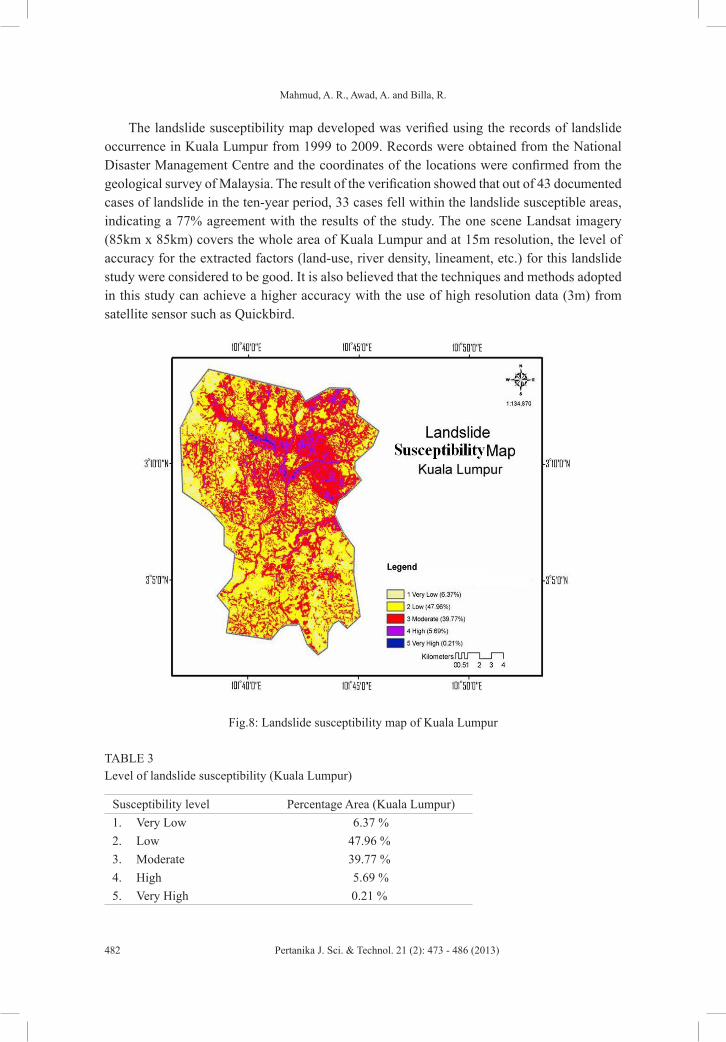
Mahmud, A. R., Awad, A. and Billa, R.
482 Pertanika J. Sci. & Technol. 21 (2): 473 - 486 (2013)
The landslide susceptibility map developed was verified using the records of landslide occurrence in Kuala Lumpur from 1999 to 2009. Records were obtained from the National Disaster Management Centre and the coordinates of the locations were confirmed from the geological survey of Malaysia. The result of the verification showed that out of 43 documented cases of landslide in the ten-year period, 33 cases fell within the landslide susceptible areas, indicating a 77% agreement with the results of the study. The one scene Landsat imagery (85km x 85km) covers the whole area of Kuala Lumpur and at 15m resolution, the level of accuracy for the extracted factors (land-use, river density, lineament, etc.) for this landslide study were considered to be good. It is also believed that the techniques and methods adopted in this study can achieve a higher accuracy with the use of high resolution data (3m) from satellite sensor such as Quickbird.
Fig.8: Landslide susceptibility map of Kuala Lumpur
TABLE 3 Level of landslide susceptibility (Kuala Lumpur)
Susceptibility level Percentage Area (Kuala Lumpur)1. Very Low 6.37 %2. Low 47.96 %3. Moderate 39.77 %4. High 5.69 %5. Very High 0.21 %
Landslide Susceptibility Mapping in GIS
483Pertanika J. Sci. & Technol. 21 (2): 473 - 486 (2013)
CONCLUSION
Factors causing landslides in Malaysia include geology, degree of slope, rainfall intensity, density of lineaments and faults and density of rivers. These factors were extracted from Landsat ETM imagery, while others obtained from the various government departments. The factors were processed using image processing, geo-processing and geo-statistic. Thematic layers were analyzed using average weightage score, overlay and geo-statistical processes to generate a landslide susceptibility map for Kuala Lumpur. The results showed that 0.21% of the areas in Kuala Lumpur have a very high susceptibility to landslides, and these cover about 5.02% of the urbanized area. A comparison of the recorded landslides in Kuala Lumpur showed 77% agreement with the study. The study has demonstrated that through streamlining of the main factors using remote sensing and GIS, landslide susceptibility maps can be developed for regular updates of development control maps. The susceptibility map clearly discriminates landslide prone areas by showing urban residential areas within the highly susceptible areas. The limitation of the study is that it uses only five major factors impacting on landslides in Malaysia and assumes these factors as having the same level of influence on landslide occurrence. Hence, the study is not applicable to other regions where the climatic and environmental conditions are different from those of Malaysia and areas where earthquakes and tremors are the major trigger of landslides.
ACKNOWLEDGEMENTS
The authors acknowledge the assistance and contributions of the Disaster Management Centre and the Geology Department of Malaysia for providing the records and data on landslide occurrences in Kuala Lumpur that were used to verify the susceptibility map. The authors are very thankful to the editors and anonymous reviewers whose critical comments and advice have helped to improve the manuscript and made it acceptable for publication.
REFERENCESAkgun, A., Sezer, E. A., Nefeslioglu, H. A., Gokceoglu, C., & Pradhan, B. (2011). An easy-to-use
MATLAB program (MamLand) for the assessment of landslide susceptibility using a Mamdani fuzzy algorithm. Computers & Geosciences (Article on-line first available), doi.10.1016/j.cageo. 2011.04.012.
Das, I., Sahoo, S., Van western, C., Stein, A., & Hack, R.. (2010). Landslide susceptibility assessment using logistic regression and its comparison with a rock mass classification system, along a road section in the northern Himalayas (India). Geomorphology, 114, 627–637.
Farisham, S. (2007). Landslide in hillside development in the Huluklang, Klang Valley. Post Graduate Seminar Semester 2 Session 2006/2007, 6 March 2007, Rumah Alumni, Universiti Teknologi Malaysia: 10 pp 148-162.
Lee, S. (2007a). Comparison of landslide susceptibility maps generated through multiple logistic regression for three test areas in Korea. Earth Surface Processes and Landforms, 32, 2133–2148.
Lee, S. (2007b). Application and verification of fuzzy algebraic operators to landslide susceptibility mapping. Environmental Geology, 52, 615–623.

Mahmud, A. R., Awad, A. and Billa, R.
484 Pertanika J. Sci. & Technol. 21 (2): 473 - 486 (2013)
Lee, S., & Evangelista, D. G. (2006). Earthquake induced landslide susceptibility mapping using an artificial neural network. Natural Hazard and Earth System Sciences, 6, 687–695.
Lee, S., & Pradhan, B. (2006). Probabilistic landslide risk mapping at Penang Island, Malaysia. Journal of Earth System Sciences, 115, 661–672.
Lee, S., & Pradhan, B. (2007). Landslide hazard mapping at Selangor, Malaysia using frequency ratio and logistic regression models. Landslides, 4, 33–41.
Lee, S., Ryu, J. H., & Kim, I. S. (2007). Landslide susceptibility analysis and its verification using likelihood ratio, logistic regression, and artificial neural network models: case study of Youngin, Korea. Landslides, 4, 327–338.
Mokhtar, W. (2006). Storm water management practices for hillside development in Malaysia. Paper presented at International Conference on Slopes, Malaysia, August 2006.
Nandi, A., & Shakoor, A. (2010). A GIS-based landslide susceptibility evaluation using bivariate and multivariate statistical analyses. Engineering Geology, 110, 11–20.
New Strait Times. (2008 ). Bukit Antarabangsa Landslide and Landslide disaster in Damansara Photo Gallery. Retrieved from http://savebukitgasing.wordpress.com/author /savegasinghil
Oh, H., & Pradhan, B. (2011). Application of a neuro-fuzzy model to landslide-susceptibility mapping for shallow landslides in a tropical hilly area. Computer and Geosciences, doi: 10.1016/j.cageo.2010.10.012.
Pradhan, B. (2010a). Remote sensing and GIS-based landslide hazard analysis and cross-validation using multivariate logistic regression model on three test areas in Malaysia. Advances in Space Research, 45(10), 1244–1256.
Pradhan, B. (2010b). Manifestation of an advanced fuzzy logic model coupled with geoinformation techniques for landslide susceptibility analysis. Environmental and Ecological Statistics, 18(3). doi:10.1007/s10651- 010-0147-7.
Pradhan, B. (2010c). Use of GIS-based fuzzy logic relations and its cross application to produce landslide susceptibility maps in three test areas in Malaysia. Environmental Earth Sciences, 63(2) 329-349. doi: 10.1007/s12665-010-0705-1.
Pradhan, B. (2010d). Application of an advanced fuzzy logic model for landslide susceptibility analysis. International Journal of Computational Intelligence Systems 3(3), 370–381.
Pradhan, B. (2010e). Landslide susceptibility mapping of a catchment area using frequency ratio, fuzzy logic and multivariate logistic regression approaches. Journal of the Indian Society of Remote Sensing, 38(2), 301-320. doi:10.1007/s12524-010-0020-z
Pradhan, B., & Buchroithner, M. F. (2010). Comparison and validation of landslide susceptibility maps using an artificial neural network model for three test areas in Malaysia. Environmental and Engineering Geoscience, 16(2), 107–126.
Pradhan, B., Chaudhari, A., Adinarayana, J., & Buchroithner M. F. (2011). Soil erosion assessment and its correlation with landslide events using remote sensing data and GIS: a case study at Penang Island, Malaysia. Environmental Monitoring & Assessment, (Article online first available). doi.10.1007/s10661-011-1996-8
Pradhan, B., & Lee, S. (2009).Landslide risk analysis using artificial neural network model focusing on different training sites. International Journal of Physical Sciences, 4(1), 1-15.

Landslide Susceptibility Mapping in GIS
485Pertanika J. Sci. & Technol. 21 (2): 473 - 486 (2013)
Pradhan, B., & Lee, S. (2010a). Delineation of land slide hazard area son Penang Island, Malaysia, by using frequency ratio, logistic regression, and artificial neural network models. Environmental Earth Sciences, 60(5), 1037–1054.
Pradhan, B., & Lee, S. (2010b). Landslide susceptibility assessment and factor effect analysis: back-propagation artificial neural networks and their comparison with frequency ratio and bivariate logistic regression modelling. Environmental Modelling & Software, 25(6), 747–759.
Pradhan, B., & Lee, S. (2010c). Regional landslide susceptibility analysis using back-propagation neural network model at Cameron Highland, Malaysia. Landslides, 7(1), 13–30.
Pradhan, B., & Lee, S. (2009d). Landslide risk analysis using artificial neural network model focusing on different training sites. International Journal of Physical Sciences, 3(11), 1–15.
Pradhan, B., Lee, S., & Buchroithner, M. F. (2009). Use of geospatial data for the development of fuzzy algebraic operators to landslide hazard mapping. Applied Geomatics, 1, 3–15.
Pradhan, B., Lee, S., & Buchroithner, M. F.(2010a). A GIS-based back-propagation neural network model and its cross application and validation for landslide susceptibility analyses. Computers Environment and Urban Systems, 34, 216–235.
Pradhan, B., Lee, S., & Buchroithner, M. F. (2010b). Remote sensing and GIS-based landslide susceptibility analysis and its cross-validation in three test areas using a frequency ratio model. Photogrammetrie, Fernerkundung, Geoinformation, 2010(1), 17–32. doi:10.1127/1432-8364/2010/0037.
Pradhan, B., Lee, S., Mansor, S., Buchroithner, M. F., Jallaluddin, N., & Khujaimah, Z. (2008). Utilization of optical remote sensing data and geographic information system tools for regional landslide hazard analysis by using binomial logistic regression model. Applied Remote Sensing, 2, 1–11.
Pradhan, B., & Pirasteh, S. (2010). Comparison between prediction capabilities of neural network and fuzzy logic techniques for landslide susceptibility mapping. Disaster Advances, 3(2), 26–34.
Pradhan, B., Mansor, S., Pirasteh, S., & Buchroithner, M. (2011b). Landslide hazard and risk analyses at a landslide prone catchment area using statistical based geospatial model. International Journal of Remote Sensing, 32(14), 4075–4087.
Pradhan, B. , Oh, H. J., & Buchroithner, M. F. (2010a). Weights-of-evidence model applied to landslide susceptibility mapping in a tropical hilly area. Geomatics, Natural Hazards and Risk, 1(3), 199- 223. doi: 10.1080/19475705.2010.498151.
Pradhan, B., Sezer, E.A., Gokceoglu, C., & Buchroithner, M. F. (2010b). Land- slide susceptibility mapping by neuro-fuzzy approach in a landslide prone area (Cameron Highland, Malaysia). IEEE Transactions on Geoscience and Remote Sensing, 48(12), 4164–4177. doi: 10.1109/TGRS. 2010. 2050328.
Pradhan, B., Singh, R. P., & Buchroithner, M. F. (2006). Estimation of stress and its use in evaluation of landslide prone regions using remote sensing data. Advances in Space Research, 37, 698–709.
Pradhan, B., & Youssef, A. M. (2010). Manifestation of remote sensing data and GIS on landslide hazard analysis using spatial-based statistical models. Arabian Journal of Geosciences, 3(3), 319–326.
Regmi, N. R., Giardino, J. R., & Vitek, J. D. (2010). Modeling susceptibility to landslides using the weight of evidence approach: western Colorado, USA. Geomorphology, 115, 172–187.

Mahmud, A. R., Awad, A. and Billa, R.
486 Pertanika J. Sci. & Technol. 21 (2): 473 - 486 (2013)
Sezer, E., Pradhan, B., & Gokceoglu, C. (2011) Manifestation of an adaptive neuro-fuzzy model on landslide susceptibility mapping: Klang valley, Malaysia. Expert Systems with Applications, 38(7), 8208-8219. doi.10.1016/j.eswa.2010.12.167
Toshiyuki K, Yoshinori Y., & Yasuhito, S. (2008). Landslide disasters and hazard maps along national highways in Japan. Paper presented at the East Asia Landslides Symposium, Seoul, Korea, May 22-23, 2008.
VanWesten, C. J.,Castellanos, E., & Kuriakose, S. L. (2008). Spatial data for landslide susceptibility, hazard, and vulnerability assessment: an overview. Engineering Geology, 102, 112–131.
Yao, X., Tham, L. G., & Dai, F. C. (2008). Landslide susceptibility mapping based on Support vector machine: a case study on natural slopes of Hong Kong, China. Geomorphology, 101, 572–582.
Yilmaz, I. (2010). Comparison of landslide susceptibility mapping methodologies for Koyulhisar, Turkey: conditional probability, logistic regression, artificial neural networks, and support vector machine. Environmental Earth Sciences, 61(4), 821–836.
Youssef, A. M., Pradhan, B., Gaber, A. F. D., & Buchroithner, M. F. (2009). Geomorphological hazard analysis along the Egyptian Red Sea Coast between Safaga and Quseir. Natural Hazards and Earth System Science, 9, 751–766.
Pertanika J. Sci. & Technol. 21 (2): 487 - 498 (2013)
SCIENCE & TECHNOLOGYJournal homepage: http://www.pertanika.upm.edu.my/
ISSN: 0128-7680 © 2013 Universiti Putra Malaysia Press.
GIS Modeling for Selection of a Transfer Station Site for Residential Solid Waste Separation and Recycling
Billa, L.1 and Pradhan, B.2,3*1School of Geography, University of Nottingham Malaysia Campus, 43500 Semenyih, Selangor, Malaysia2Geospatial Information Science Research Center (GIS RC), Faculty of Engineering, Universiti Putra Malysia, 43400 Serdang, Selangor, Malaysia3Department of Civil Engineering, Faculty of Engineering, Universiti Putra Malysia, 43400 Serdang, Selangor, Malaysia
ABSTRACT
In this study a GIS model was developed and spatial analytical techniques performed to identify and select a suitable location for a waste transfer station in the sprawling suburban town of Petaling Jaya. The lack of a transfer station in urban centres of Malaysia has caused many problems and affects the efficiency of waste collection and disposal. With diminishing space for landfills and the increasing cost of solid waste management, the need for urban solid-waste recycling has become very important. However, finding a place for waste to be efficiently sorted before unwanted waste can be carried to disposal landfills has social and physical constraints. This study applies GIS techniques and analysis for site selection and identifies an acceptable area. In the model, environmental, physical and social constraints were taken into account, resulting in the selection of a potential area that is acceptable to the residents of the area because it is out of range of causing public nuisance and within minimum travelling distance for collection vehicles. The results show that the potential location for the transfer station should be in proximity of the industrial area of Petaling Jaya, allowing for the possible sale of recyclable materials to local industries. The location is also sited near a major highway to allow quick transportation of the rest of the unwanted waste to the landfill.
Keywords: GIS, solid waste, recycling, transfer station, Petaling Jaya, Malaysia
Article history:Received: 22 November 2011Accepted: 20 March 2012
E-mail addresses: [email protected] (Billa, L.), [email protected] (Pradhan, B.)*Corresponding Author
INTRODUCTION
In recent years, municipal waste recycling has been encouraged as a sustainable method for waste management due to environmental concerns and diminishing land for landfills. Extensive studies of waste composition in Petaling Jaya and most urban centres of

Billa, L. and Pradhan, B.
488 Pertanika J. Sci. & Technol. 21 (2): 487 - 498 (2013)
Malaysia have shown that there is a high percentage of organic (71.2%) and of non-organic (28.8%) material in the waste produced (Meulen, 1996; UNCHS, 1994; Arshad, 1992). Waste composition in Malaysia shows that significant reduction of the amount disposed of at landfills can be achieved if an efficient system of waste separation is in place to separate waste for idea compost or recyclable materials (Triantafyllou & cherrett, 2009; Lopez et al., 2008). Attempts, however, to encourage people to separate their waste at home have not been successful. Suggestions have been made by different interest groups for the waste-management authorities and agencies to conduct waste separation by themselves. Till now, waste management companies have not been able to site and efficiently operate a transfer station in Malaysia due to social and operational constraints.
Geographic Information System (GIS) application and modelling in solid waste management
Geographical information systems have traditionally focussed on environmental mapping and monitoring of the changes within the local and regional environments. As computer technology improves more software is being developed to increase the range of research in the application of GIS in areas such as solid waste management (Ghose et al., 2008; Lopez et al., 2008; Goodchild, 2003; Li et al., 2001). Some of these GIS planning applications include the location and selection of sites, visualisation, interpretation and the forecasting and modelling of various spatial phenomena. They are best performed using a prescriptive model. A prescriptive model in its purest form is designed to impose a best solution for problems in which a description of existing conditions is insufficient as a decision aid (Chalkias & Lasaridi, 2010; Karadimas & Loumos, 2008; Tomlin 1991). According to DeMers (2002), the prescriptive model is more closely associated with answering the “what should be” type of question. GIS modelling scenarios may be applied to answer such questions as: What is the best location in which to site a factory?; and What is the most likely place to reintroduce falcons in the southwestern United States?
Geographic Information System (GIS) application in solid waste management
There is specific solid waste management software such as the Solid Waste Integrated Management Model (SWIM) (Wang et al., 1996). Although these packages have strong tools for waste statistical analysis, they lack the spatial analysis, modelling and visualisation tools that general GIS have. They are thus limited in spatial data processing that are sometimes required in site evaluation and the selection of suitable land for a transfer station or landfill. General GIS application in waste management involves the routing of waste collection and shortest path analysis. But perhaps the widest areas of GIS applications in waste management are in the selection, management and monitoring of waste disposal sites (Banerjee, et al., 2004). This involves the overlay factors that are processed into GIS thematic maps such as the slope of the land, the soil type, the depth of the bedrock, the depth of the ground water and the distances to historic sites, main roads and towns. Various spatial processing and geospatial analytical processes are performed to identify possible sites/locations best suited for the development of a waste disposal site (Oliveira & Borenstein, 2007; Wolfgang & Gang, 1997; Massie, 1997).

GIS Modeling for Site Selection
489Pertanika J. Sci. & Technol. 21 (2): 487 - 498 (2013)
Where the identification of a transfer station is a problem to be resolved, the factors that may be processed will include social-cultural considerations such as smell and proximity to residential areas (Chalkias and Lasaridi, 2010; Triantafyllou and Charrett, 2009; Vijay et al., 2008).
In a general GIS modelling, Gruenert et al. (2010) identified three stages i.e. data, process and parameter models to be executed in a hierarchical process. The first stage, “data model”, is concerned with the observational process which specifies the distribution of the data given the fundamental process of interest and parameters that describe the data model. The second stage then describes the process, conditional upon other process parameters. The last stage models the uncertainty in the parameters from both the data and process stages. This hierarchical process is not new in disciplines such as statistics; however, the basic formulation for modelling spatial and spatio-temporal processes in the environment is a new development (Longley et al., 2005). This method allows problems to be simplified by breaking them down into sub-problems.
MATERIALS AND METHODS
The study area is located in the fast growing urban municipality of Petaling Jaya in Malaysia (Fig.1). About 200tons of municipal waste is collected from the housing and residential areas of Petaling Jaya daily. This waste is disposed of at a sanitary landfill that is 26.6km away, a distance that has increased the cost of waste collection. The rising cost is a major concern for the local municipal council (MPPJ), and efforts are being made to minimise waste collected through waste recovery for reasons of environmental protection, cost of transportation and landfill and the diminishing space for landfill. There is a nationwide recycling programme, “Project Bumiku” the objectives of which are reflected in the waste recycling practices in
Fig.1: Study area (Petaling Jaya)

Billa, L. and Pradhan, B.
490 Pertanika J. Sci. & Technol. 21 (2): 487 - 498 (2013)
Petaling Jaya. The programme is ongoing, and aims to get citizen participation in community development, mobilise various interest groups, promote community development through a comprehensive community education programme and promote a clean and beautiful urban environment through a better community . According to Vijay et al. (2008), for recycling programmes to be successful especially in commercial and some housing areas, there is the need for transfer stations. At the transfer station waste can be effectively sorted out to remove recyclable items.
Waste collection for zone 8 and 9 study areas (MPPJ municipality)
Waste collection and the layout of the situation is better explained by the thematic map generated from GIS (Fig.2). The map displays the two zones considered in this study and the type and quantity of waste for each collection sector. This study revealed that the average population density in zone 9 is 93/ha and the average waste generation rate for the zone is calculated at 0.50kg/capita. The total daily waste production is 9,525.4kg and after effective recovery the expected waste for daily disposal in the zone is 4420.1kg. On average, waste collected from medium income households account for over 85% of the waste expected for collection. Details of the waste generation rate by sector in zone 9 are presented in Table 1.
Zone 8 collection sector has an average population density of 62/ha and the average waste generation rate is 0.55kg/cp/d. With the number of housing units at 3273, the population of the zone is calculated to be 16,365. The total waste generated is 8,875.2 kg/day. The low population
Fig.2: The type and quantity of waste for each sector
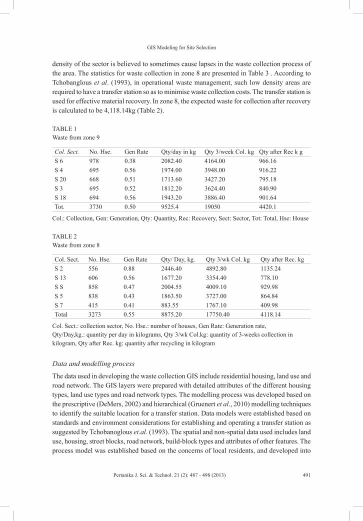
GIS Modeling for Site Selection
491Pertanika J. Sci. & Technol. 21 (2): 487 - 498 (2013)
density of the sector is believed to sometimes cause lapses in the waste collection process of the area. The statistics for waste collection in zone 8 are presented in Table 3 . According to Tchobanglous et al. (1993), in operational waste management, such low density areas are required to have a transfer station so as to minimise waste collection costs. The transfer station is used for effective material recovery. In zone 8, the expected waste for collection after recovery is calculated to be 4,118.14kg (Table 2).
TABLE 1 Waste from zone 9
Col. Sect. No. Hse. Gen Rate Qty/day in kg Qty 3/week Col. kg Qty after Rec k gS 6 978 0.38 2082.40 4164.00 966.16S 4 695 0.56 1974.00 3948.00 916.22S 20 668 0.51 1713.60 3427.20 795.18S 3 695 0.52 1812.20 3624.40 840.90S 18 694 0.56 1943.20 3886.40 901.64Tot. 3730 0.50 9525.4 19050 4420.1
Col.: Collection, Gen: Generation, Qty: Quantity, Rec: Recovery, Sect: Sector, Tot: Total, Hse: House
TABLE 2 Waste from zone 8
Col. Sect. No. Hse. Gen Rate Qty/ Day, kg. Qty 3/wk Col. kg Qty after Rec. kgS 2 556 0.88 2446.40 4892.80 1135.24S 13 606 0.56 1677.20 3354.40 778.10S S 858 0.47 2004.55 4009.10 929.98S 5 838 0.43 1863.50 3727.00 864.84S 7 415 0.41 883.55 1767.10 409.98Total 3273 0.55 8875.20 17750.40 4118.14
Col. Sect.: collection sector, No. Hse.: number of houses, Gen Rate: Generation rate, Qty/Day,kg.: quantity per day in kilograms, Qty 3/wk Col.kg: quantity of 3-weeks collection in kilogram, Qty after Rec. kg: quantity after recycling in kilogram
Data and modelling process
The data used in developing the waste collection GIS include residential housing, land use and road network. The GIS layers were prepared with detailed attributes of the different housing types, land use types and road network types. The modelling process was developed based on the prescriptive (DeMers, 2002) and hierarchical (Gruenert et al., 2010) modelling techniques to identify the suitable location for a transfer station. Data models were established based on standards and environment considerations for establishing and operating a transfer station as suggested by Tchobanoglous et.al. (1993). The spatial and non-spatial data used includes land use, housing, street blocks, road network, build-block types and attributes of other features. The process model was established based on the concerns of local residents, and developed into
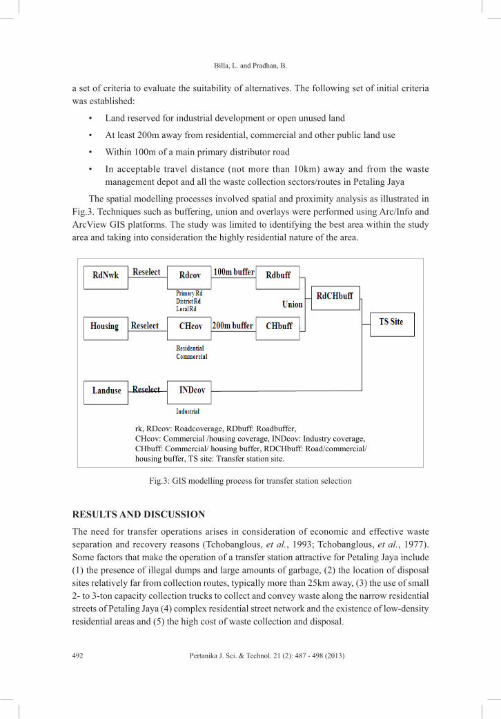
Billa, L. and Pradhan, B.
492 Pertanika J. Sci. & Technol. 21 (2): 487 - 498 (2013)
a set of criteria to evaluate the suitability of alternatives. The following set of initial criteria was established:
• Land reserved for industrial development or open unused land
• At least 200m away from residential, commercial and other public land use
• Within 100m of a main primary distributor road
• In acceptable travel distance (not more than 10km) away and from the waste management depot and all the waste collection sectors/routes in Petaling Jaya
The spatial modelling processes involved spatial and proximity analysis as illustrated in Fig.3. Techniques such as buffering, union and overlays were performed using Arc/Info and ArcView GIS platforms. The study was limited to identifying the best area within the study area and taking into consideration the highly residential nature of the area.
RdNwk: Roadnetwork, RDcov: Roadcoverage, RDbuff: Roadbuffer, CHcov: Commercial /housing coverage, INDcov: Industry coverage, CHbuff: Commercial/ housing buffer, RDCHbuff: Road/commercial/ housing buffer, TS site: Transfer station site.
Fig.3: GIS modelling process for transfer station selection
RESULTS AND DISCUSSION
The need for transfer operations arises in consideration of economic and effective waste separation and recovery reasons (Tchobanglous, et al., 1993; Tchobanglous, et al., 1977). Some factors that make the operation of a transfer station attractive for Petaling Jaya include (1) the presence of illegal dumps and large amounts of garbage, (2) the location of disposal sites relatively far from collection routes, typically more than 25km away, (3) the use of small 2- to 3-ton capacity collection trucks to collect and convey waste along the narrow residential streets of Petaling Jaya (4) complex residential street network and the existence of low-density residential areas and (5) the high cost of waste collection and disposal.
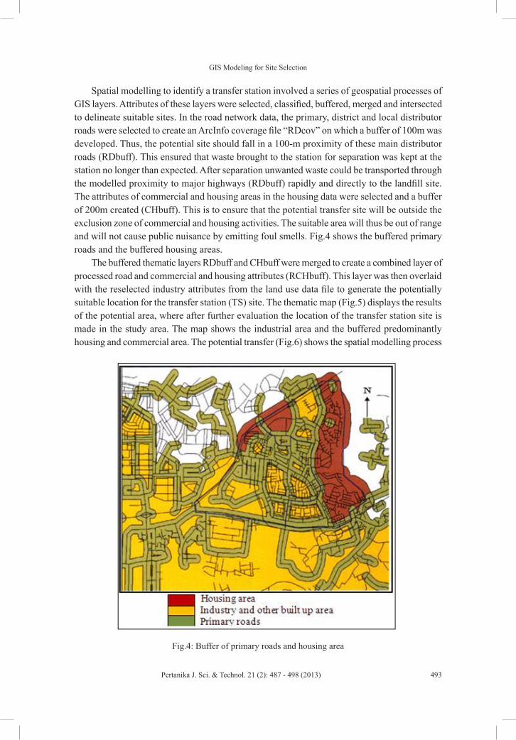
GIS Modeling for Site Selection
493Pertanika J. Sci. & Technol. 21 (2): 487 - 498 (2013)
Spatial modelling to identify a transfer station involved a series of geospatial processes of GIS layers. Attributes of these layers were selected, classified, buffered, merged and intersected to delineate suitable sites. In the road network data, the primary, district and local distributor roads were selected to create an ArcInfo coverage file “RDcov” on which a buffer of 100m was developed. Thus, the potential site should fall in a 100-m proximity of these main distributor roads (RDbuff). This ensured that waste brought to the station for separation was kept at the station no longer than expected. After separation unwanted waste could be transported through the modelled proximity to major highways (RDbuff) rapidly and directly to the landfill site. The attributes of commercial and housing areas in the housing data were selected and a buffer of 200m created (CHbuff). This is to ensure that the potential transfer site will be outside the exclusion zone of commercial and housing activities. The suitable area will thus be out of range and will not cause public nuisance by emitting foul smells. Fig.4 shows the buffered primary roads and the buffered housing areas.
The buffered thematic layers RDbuff and CHbuff were merged to create a combined layer of processed road and commercial and housing attributes (RCHbuff). This layer was then overlaid with the reselected industry attributes from the land use data file to generate the potentially suitable location for the transfer station (TS) site. The thematic map (Fig.5) displays the results of the potential area, where after further evaluation the location of the transfer station site is made in the study area. The map shows the industrial area and the buffered predominantly housing and commercial area. The potential transfer (Fig.6) shows the spatial modelling process
Fig.4: Buffer of primary roads and housing area

Billa, L. and Pradhan, B.
494 Pertanika J. Sci. & Technol. 21 (2): 487 - 498 (2013)
where factors under consideration were transformed into thematic layers. Using these thematic layers, the search for a potential location was narrowed to the area depicted in light colour covering about 76.3ha within the industrial zone. This site was further evaluated using on a ten-point weightage score based on (a) adjacent land uses, (b) off-site visibility, (c) closeness to collection areas, (d) closeness to a highway/primary road and (e) cost of land.
Fig.7 shows the area that has been identified for the development of the transfer station. All environment factors and the concerns of the residents were evaluated in the model. The site is located only 100m away from a major primary road; this was to allow quick and easy access for big waste collection trucks to move in and out of the area with undue obstruction. The immediate land use is a paint factory some distance away; moreover, being in an industrial zone also has it benefits as the sale of recycled materials such as paper, glass, metals etc. to other industries in the vicinity can be made. Residential houses were not located within the area and the transfer site was not visible from the housing area. People living nearby will thus not be able to see the activities at the transfer station.
Fig.5: Map of 100 m buffer of housing/commerce overlaid by industry
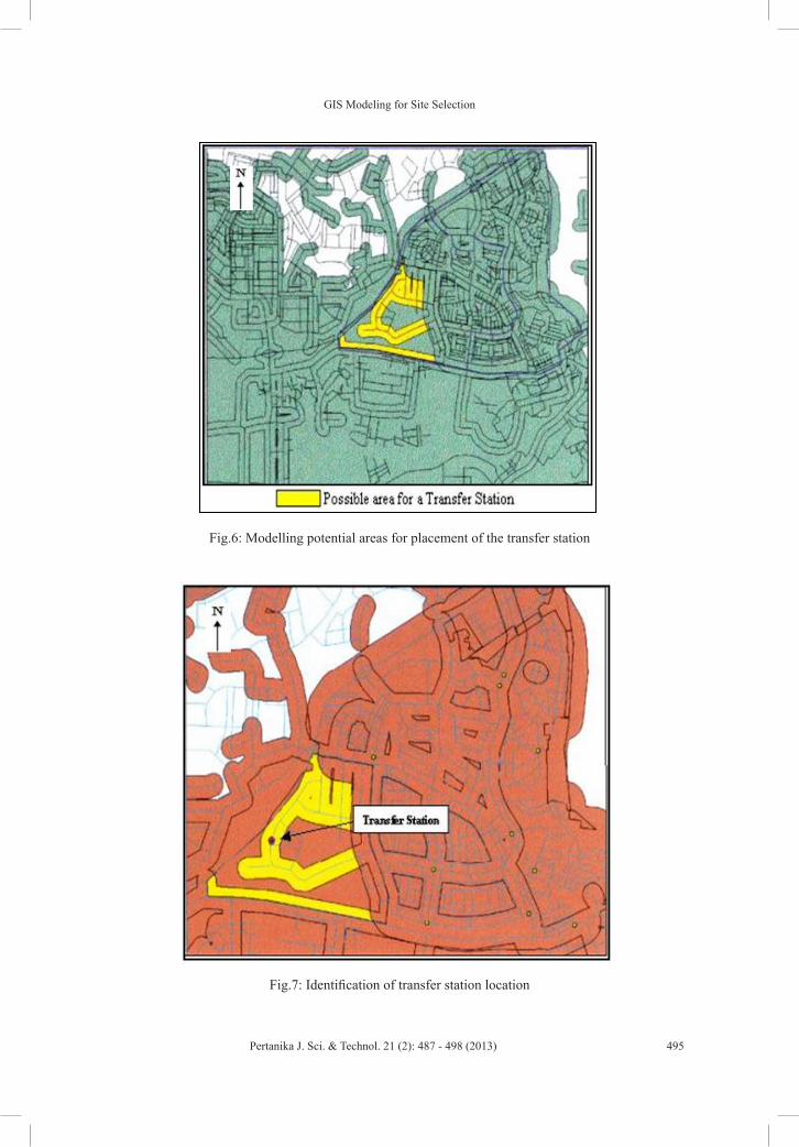
GIS Modeling for Site Selection
495Pertanika J. Sci. & Technol. 21 (2): 487 - 498 (2013)
Fig.6: Modelling potential areas for placement of the transfer station
Fig.7: Identification of transfer station location
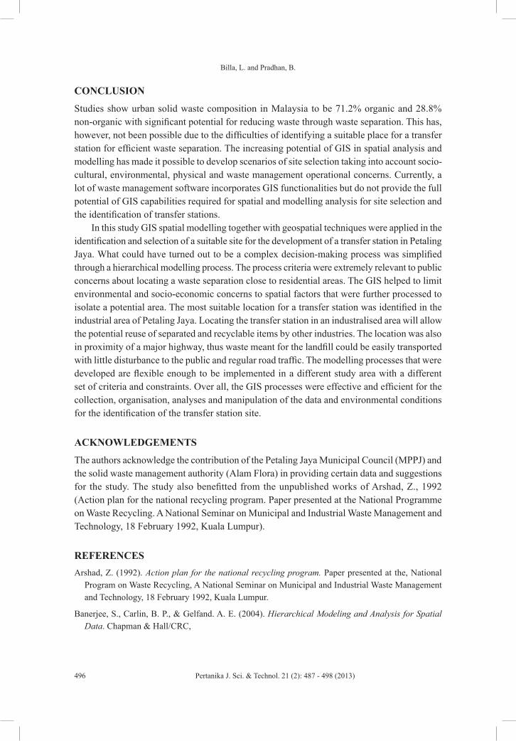
Billa, L. and Pradhan, B.
496 Pertanika J. Sci. & Technol. 21 (2): 487 - 498 (2013)
CONCLUSION
Studies show urban solid waste composition in Malaysia to be 71.2% organic and 28.8% non-organic with significant potential for reducing waste through waste separation. This has, however, not been possible due to the difficulties of identifying a suitable place for a transfer station for efficient waste separation. The increasing potential of GIS in spatial analysis and modelling has made it possible to develop scenarios of site selection taking into account socio-cultural, environmental, physical and waste management operational concerns. Currently, a lot of waste management software incorporates GIS functionalities but do not provide the full potential of GIS capabilities required for spatial and modelling analysis for site selection and the identification of transfer stations.
In this study GIS spatial modelling together with geospatial techniques were applied in the identification and selection of a suitable site for the development of a transfer station in Petaling Jaya. What could have turned out to be a complex decision-making process was simplified through a hierarchical modelling process. The process criteria were extremely relevant to public concerns about locating a waste separation close to residential areas. The GIS helped to limit environmental and socio-economic concerns to spatial factors that were further processed to isolate a potential area. The most suitable location for a transfer station was identified in the industrial area of Petaling Jaya. Locating the transfer station in an industralised area will allow the potential reuse of separated and recyclable items by other industries. The location was also in proximity of a major highway, thus waste meant for the landfill could be easily transported with little disturbance to the public and regular road traffic. The modelling processes that were developed are flexible enough to be implemented in a different study area with a different set of criteria and constraints. Over all, the GIS processes were effective and efficient for the collection, organisation, analyses and manipulation of the data and environmental conditions for the identification of the transfer station site.
ACKNOWLEDGEMENTS
The authors acknowledge the contribution of the Petaling Jaya Municipal Council (MPPJ) and the solid waste management authority (Alam Flora) in providing certain data and suggestions for the study. The study also benefitted from the unpublished works of Arshad, Z., 1992 (Action plan for the national recycling program. Paper presented at the National Programme on Waste Recycling. A National Seminar on Municipal and Industrial Waste Management and Technology, 18 February 1992, Kuala Lumpur).
REFERENCESArshad, Z. (1992). Action plan for the national recycling program. Paper presented at the, National
Program on Waste Recycling, A National Seminar on Municipal and Industrial Waste Management and Technology, 18 February 1992, Kuala Lumpur.
Banerjee, S., Carlin, B. P., & Gelfand. A. E. (2004). Hierarchical Modeling and Analysis for Spatial Data. Chapman & Hall/CRC,

GIS Modeling for Site Selection
497Pertanika J. Sci. & Technol. 21 (2): 487 - 498 (2013)
Chalkias, C., & Lasaridi, K. (2010).Benefits from GIS based modelling for municipal solid waste management. Integrated Waste Management, 1, 417-436
DeMers, M. N. (2002). GIS modeling in raster. John Wiley &Sons, Inc., 605 Third Avenue, New York, 113-120
Ghose, M. K., Dikshit, A. K., &Sharma, S. K. (2008). A GIS based transportation model for solid waste disposal – a case study of Asansol Municipality, Waste Management. 26,1287-93.
Goodchild, M. F. (2003). Geographic Information Science and Systems for Environmental Management. Annual Review of Environment and Resources, 28, 493-519.
Gruenert, G., Ibrahim, B., Lenser, T., Lohel, M, Hinze, T., & Dittrich, P. (2010). Rule-based spatial modeling with diffusing, geometrically constrained molecules, BMC Bioinformatics 2010, 11(307). doi:10.1186/1471-2105-11-307
Karadimas, N. V., & Loumos, V. G. (2008). GIS-based modelling for the estimation of municipal solid waste generation and collection .Journal of Waste Management and Research, 26.337-346. DOI: 10.1177/0734242X07081484.
Li, R. Liu, J. K., & Felus , Y. (2001). Spatial modeling and analysis for shoreline change detection and coastal erosion monitoring, marine geodesy.24: 1-12accessed 20/09/2010 at :http://shoreline.eng.ohio-state.edu/publications/mg_24_1.pdf
Longley P. A., Goodchild, M. F., Maguire, D. J., & Rhind. D. W. (2005). Geographic Information Systems and Science. Second Edition. John Wiley, Chichester, 2005.
Lopez, A. J. V., Aguilar, L. M., Fernandez-Carrion, Q. S., & Jimenez del Valle, A. (2008). Optimizing the collection of used paper from small businesses through GIS techniques: The Legane΄s case (Madrid, Spain). Waste Management, 28, 282–293
Massie, K. (1997). Solid waste planners at Portlands, Regional planning agency, Metro use GIS to evaluate their recycling Programs, GIS at work in the community Zeroing in, Andy Mitchell. ESRI, INC.
Meulen, G. (1996). Improved solid waste collection in Asian cities, Compuplan Foundation, Institute for Applied Spatial and Environmental Informatics. Mills & St. Hubert, The Netherlands.
MPPJ and AJC Planning Consultant and Associates. (1992). The Socio-Economic Study of Petaling Jaya, A survey report. MPPJ, Malaysia.
Nelly, A., & Yeow, Y. Y. (1992). Solid waste management master plan for a major metropolitan area in a developing country. Paper presented at the Solid waste Association of America a Annual Southwestern Symposium, Oklahoma, 1992. 12 pages
Oliveira, S. E., & Borenstein, D.A. (2007). Decision support system for the operational planning of solid waste collection. Waste Management, 27, 1286-1297.
Tchobanglous, G., Theisen, H., & Eliassen, R. (1977). Solid wastes: engineering principles and management issues. McGraw – Hill, Publishing Co. New York.
Tchobanglous, G., Theisen, H., & Vigil, S. (1993). Integrated Solid Waste Management, Engineering and Management Issues. McGraw – Hill, Inc New York. 7- 17.
Tomlin, C. D. (1991). Cartographic modeling. In Geographical information system: Principle and applications. In D. J. Maguire, M. F. Goodchild, & D. W. (Eds.). Rhind,: London Longman

Billa, L. and Pradhan, B.
498 Pertanika J. Sci. & Technol. 21 (2): 487 - 498 (2013)
Triantafyllou, M., & Cherrett, T. (2009). The logistics of managing hazardous waste-a case study analysis in the retail sector. Paper presented at the 14th Annual Logistics Research Network Conference, 9th – 11th September 2009, Cardiff 613
UNCHS. (1994). A reference hand book for training on the promotion of solid waste recycling and reuse in the developing countries of Asia. September 1994, Nairobi, Kenya.
Vijay, R., Goutam, A., Kalamdhad, A., Gupta, A., & Davotta, S. (2008). GIS-based locational analysis of collection bin in municipal waste management system. J Environ Eng Sci, 7, 38-43
Wang, F. S., Richardson, A. J., & Roddick, F. A. (1996). SWIM-A computer model for solid waste integrated management. Computer, Environment and Urban Systems, 20(4/5), 165 – 117
Wolfgang, T., & Gang, A. R.(1997). Management and monitoring of waste disposal sites with GIS. In the Proceedings of GIS AM/FM ASIA ‘97 & Geo-informatics ‘97 Mapping the Future of Asia Pacific, Taiwan. 2. 350–356.

Pertanika J. Sci. & Technol. 21 (2): 499 - 506 (2013)
SCIENCE & TECHNOLOGYJournal homepage: http://www.pertanika.upm.edu.my/
ISSN: 0128-7680 © 2013 Universiti Putra Malaysia Press.
INTRODUCTION
Fibre board is a type of engineered wood product that is made out of wood fibres (The American Heritage Dictionary of the English Language., 2004; Carll, 1986). Types of fibre board in order of increasing density include particle board, medium-density fibre board and hard board, also called high-density fibre board. Fibre board is sometimes used as a
Comparative Study on the Effect of Density on Water Absorption of Particle Boards Produced from Nipa Palm Fibres with HDPE Wastes
Ekpunobi, U. E.*, Eboatu, A. N. and Okoye, P.-A.Pure and Industrial Chemistry Department, Nnamdi Azikiwe University, P.M.B 5025, Awka. Nigeria
ABSTRACT
Nipa palm fibres were used in producing fibre boards with different mixtures of waste HDPE fibres. Density, swelling thickness and water absorption of the boards were determined and compared to know the combination that would yield the best quality. The relationship between the densities of boards produced and their ability to absorb water was also established. The significance of the results implies that the boards have special water resistant property, a feature that makes them suitable for use in areas of high humidity or occasional wetness. It is also noted that as more plastic waste is incorporated into Nipa fibres, the less density impacted on the particle boards and, hence, more water is absorbed.
Keywords: Nipa palm, fibre board, HDPE, density, production
Article history:Received: 20 February 2012Accepted: 23 April 2012
E-mail addresses: [email protected] (Ekpunobi, U. E.), [email protected] (Eboatu, A. N.), [email protected] (Okoye, P.-A.)*Corresponding Author
synonym for particle board, but particle board usually refers to low-density fibre board. Fibre board, particularly medium-density fibre board, is heavily used in the furniture industry. For pieces that will be visible, a veneer of wood is often glued onto fibre board to give it the appearance of conventional wood. Medium Density Fibreboard (MDF) was first developed in the United States during the 1960s, with production starting in Deposti, New York (Laurel, 1996). A similar product, hard board (compressed fibre board), was accidentally invented by William Mason in 1925, while he was trying to find a use for the huge quantities of wood chips that were being discarded by lumber mills (Laurel,
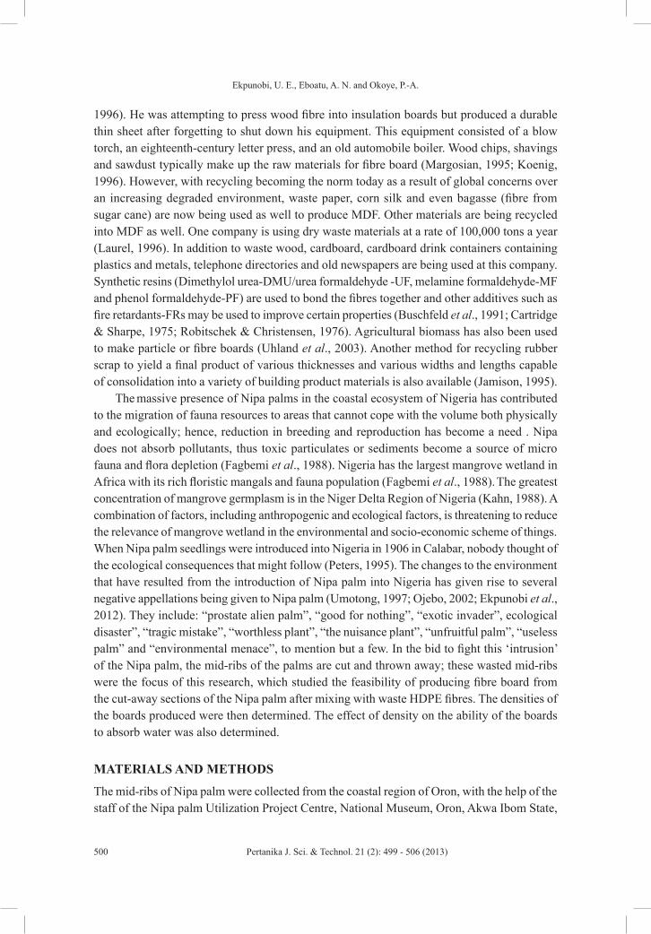
Ekpunobi, U. E., Eboatu, A. N. and Okoye, P.-A.
500 Pertanika J. Sci. & Technol. 21 (2): 499 - 506 (2013)
1996). He was attempting to press wood fibre into insulation boards but produced a durable thin sheet after forgetting to shut down his equipment. This equipment consisted of a blow torch, an eighteenth-century letter press, and an old automobile boiler. Wood chips, shavings and sawdust typically make up the raw materials for fibre board (Margosian, 1995; Koenig, 1996). However, with recycling becoming the norm today as a result of global concerns over an increasing degraded environment, waste paper, corn silk and even bagasse (fibre from sugar cane) are now being used as well to produce MDF. Other materials are being recycled into MDF as well. One company is using dry waste materials at a rate of 100,000 tons a year (Laurel, 1996). In addition to waste wood, cardboard, cardboard drink containers containing plastics and metals, telephone directories and old newspapers are being used at this company. Synthetic resins (Dimethylol urea-DMU/urea formaldehyde -UF, melamine formaldehyde-MF and phenol formaldehyde-PF) are used to bond the fibres together and other additives such as fire retardants-FRs may be used to improve certain properties (Buschfeld et al., 1991; Cartridge & Sharpe, 1975; Robitschek & Christensen, 1976). Agricultural biomass has also been used to make particle or fibre boards (Uhland et al., 2003). Another method for recycling rubber scrap to yield a final product of various thicknesses and various widths and lengths capable of consolidation into a variety of building product materials is also available (Jamison, 1995).
The massive presence of Nipa palms in the coastal ecosystem of Nigeria has contributed to the migration of fauna resources to areas that cannot cope with the volume both physically and ecologically; hence, reduction in breeding and reproduction has become a need . Nipa does not absorb pollutants, thus toxic particulates or sediments become a source of micro fauna and flora depletion (Fagbemi et al., 1988). Nigeria has the largest mangrove wetland in Africa with its rich floristic mangals and fauna population (Fagbemi et al., 1988). The greatest concentration of mangrove germplasm is in the Niger Delta Region of Nigeria (Kahn, 1988). A combination of factors, including anthropogenic and ecological factors, is threatening to reduce the relevance of mangrove wetland in the environmental and socio-economic scheme of things. When Nipa palm seedlings were introduced into Nigeria in 1906 in Calabar, nobody thought of the ecological consequences that might follow (Peters, 1995). The changes to the environment that have resulted from the introduction of Nipa palm into Nigeria has given rise to several negative appellations being given to Nipa palm (Umotong, 1997; Ojebo, 2002; Ekpunobi et al., 2012). They include: “prostate alien palm”, “good for nothing”, “exotic invader”, ecological disaster”, “tragic mistake”, “worthless plant”, “the nuisance plant”, “unfruitful palm”, “useless palm” and “environmental menace”, to mention but a few. In the bid to fight this ‘intrusion’ of the Nipa palm, the mid-ribs of the palms are cut and thrown away; these wasted mid-ribs were the focus of this research, which studied the feasibility of producing fibre board from the cut-away sections of the Nipa palm after mixing with waste HDPE fibres. The densities of the boards produced were then determined. The effect of density on the ability of the boards to absorb water was also determined.
MATERIALS AND METHODS
The mid-ribs of Nipa palm were collected from the coastal region of Oron, with the help of the staff of the Nipa palm Utilization Project Centre, National Museum, Oron, Akwa Ibom State,
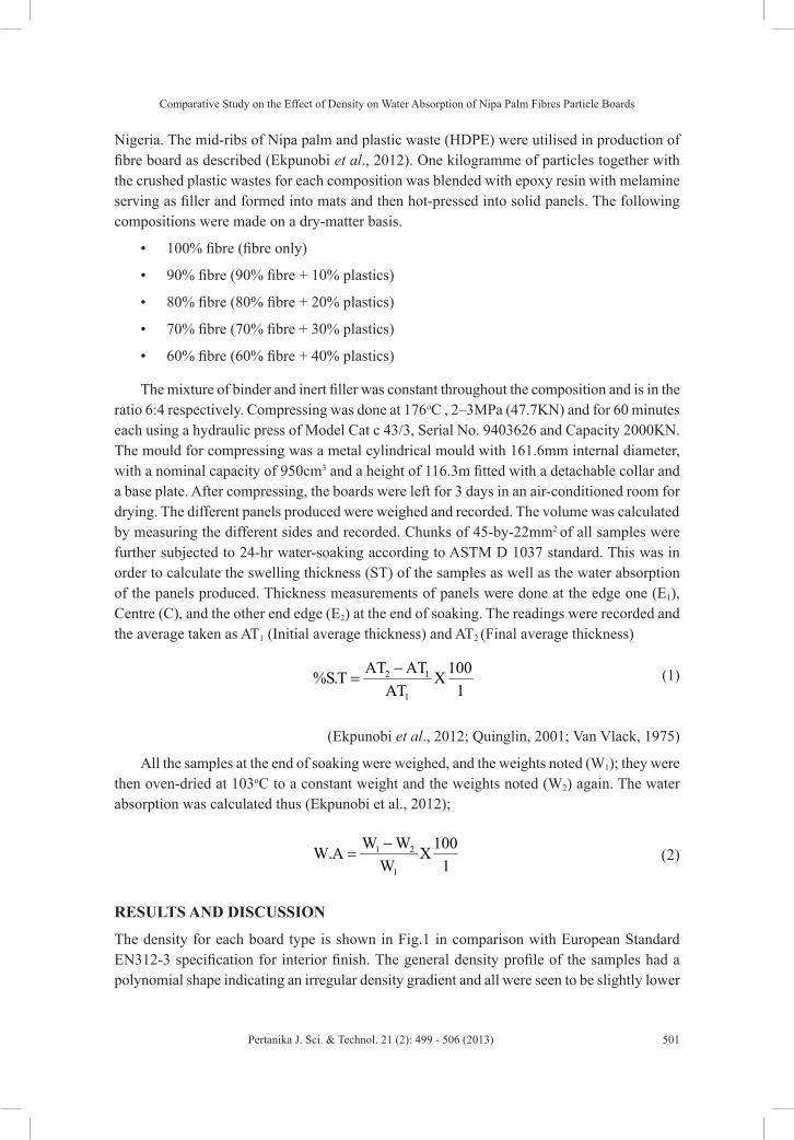
Comparative Study on the Effect of Density on Water Absorption of Nipa Palm Fibres Particle Boards
501Pertanika J. Sci. & Technol. 21 (2): 499 - 506 (2013)
Nigeria. The mid-ribs of Nipa palm and plastic waste (HDPE) were utilised in production of fibre board as described (Ekpunobi et al., 2012). One kilogramme of particles together with the crushed plastic wastes for each composition was blended with epoxy resin with melamine serving as filler and formed into mats and then hot-pressed into solid panels. The following compositions were made on a dry-matter basis.
• 100% fibre (fibre only)
• 90% fibre (90% fibre + 10% plastics)
• 80% fibre (80% fibre + 20% plastics)
• 70% fibre (70% fibre + 30% plastics)
• 60% fibre (60% fibre + 40% plastics)
The mixture of binder and inert filler was constant throughout the composition and is in the ratio 6:4 respectively. Compressing was done at 176oC , 2–3MPa (47.7KN) and for 60 minutes each using a hydraulic press of Model Cat c 43/3, Serial No. 9403626 and Capacity 2000KN. The mould for compressing was a metal cylindrical mould with 161.6mm internal diameter, with a nominal capacity of 950cm3 and a height of 116.3m fitted with a detachable collar and a base plate. After compressing, the boards were left for 3 days in an air-conditioned room for drying. The different panels produced were weighed and recorded. The volume was calculated by measuring the different sides and recorded. Chunks of 45-by-22mm2 of all samples were further subjected to 24-hr water-soaking according to ASTM D 1037 standard. This was in order to calculate the swelling thickness (ST) of the samples as well as the water absorption of the panels produced. Thickness measurements of panels were done at the edge one (E1), Centre (C), and the other end edge (E2) at the end of soaking. The readings were recorded and the average taken as AT1 (Initial average thickness) and AT2 (Final average thickness)
2 1
1
AT AT 100%S.T XAT 1
−= (1)
(Ekpunobi et al., 2012; Quinglin, 2001; Van Vlack, 1975)
All the samples at the end of soaking were weighed, and the weights noted (W1); they were then oven-dried at 103oC to a constant weight and the weights noted (W2) again. The water absorption was calculated thus (Ekpunobi et al., 2012);
1 2
1
W W 100W.A XW 1−
= (2)
RESULTS AND DISCUSSION
The density for each board type is shown in Fig.1 in comparison with European Standard EN312-3 specification for interior finish. The general density profile of the samples had a polynomial shape indicating an irregular density gradient and all were seen to be slightly lower

Ekpunobi, U. E., Eboatu, A. N. and Okoye, P.-A.
502 Pertanika J. Sci. & Technol. 21 (2): 499 - 506 (2013)
than the EN standard except for the 70% and 60% fibre which showed a great disparity. Density of the 100% fibre (fibre only) 648kg/dm3 was lower than that of 90% fibre (10% HDPE) 678kg/dm3 and 80% fibre ( 20% HDPE) 669kg/dm3 but higher than 70% fibre (30% HDPE) 601kg/dm3 and 60% fibre (40% HDPE) 536kg/dm3.
Swelling thickness as a function of % fibre is shown in Fig.2 after 24 hours of water soaking. A uniform swelling across the edges was obtained for all the samples except for 60% fibre, which gave a higher swelling at edge 2 followed by the centre and then edge 1 as shown in Table 1. A linear relationship was obtained. There was a gradual increase in the swelling thickness as % fibre decreases. 100% fibre has a swelling thickness value of 4.8, 90% fibre, 4.9, 80% fibre, 4.8, 70% fibre, 6.9 and 60% fibre, 8.0. In comparison with EN Standard, all but 60% fibre met the Standard value.
TABLE 1 Swelling across the edges % Fibre E1 (mm) C (mm) E2 (mm) Ave (mm) 100 1.20 1.20 1.20 1.20 90 1.25 1.25 1.25 1.25 80 1.25 1.25 1.25 1.25 70 1.70 1.70 1.70 1.70 60 1.90 1.95 2.00 1.95
Water absorption as a function of % fibre is shown in Fig.3. There was a slight decrease in water absorption from 90% fibre of value 10 to 80% fibre of value 9.7, after which the water absorption increased in linear fashion from 90% fibre to 50% fibre value 13. The increase was thought to have been due to low interaction of high dosage of HDPE waste with the binder as well as to the particle size distribution of the plastic waste. A predictive model equation was obtained by regression analysis as shown in equation (3). The equation gives an indication of what is expected from the water absorption capabilities of boards produced as the different % plastic wastes are incorporated into the Nipa palm fibres, invariably altering the density. The significance of this result implies that the boards have special water resistant property, a feature which makes them suitable for use in areas of high humidity or occasional wetness.
Predictive model equation :
Y= 0.0833x4- 1.0667x3+ 4.9667x2 - 8.9833x + 15 (3)
R2 = 1
Where Y = Dependent variable = Swelling thickness
X = Independent variable = % Fibre
R2 = Fitness coefficient
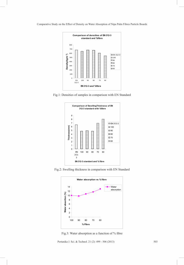
Comparative Study on the Effect of Density on Water Absorption of Nipa Palm Fibres Particle Boards
503Pertanika J. Sci. & Technol. 21 (2): 499 - 506 (2013)
Comparison of densities of EN 312-3 standard and %fibre
0
100
200
300
400
500
600
700
800
EN312-3
100 90 80 70 60
EN 312-3 and %fibre
Den
sity
(kg/
m3 ) EN 312-3
10090807060
Fig.1: Densities of samples in comparison with EN Standard
Comparison of SwellingThickness of EN 312-3 standard w ith %fibre
0
1
2
3
4
5
6
7
8
9
EN312-
3
100 90 80 70 60
EN 312-3 standard and % fibre
Thic
knes
s(m
m)
EN 312-3
100
90
80
70
60
Fig.2: Swelling thickness in comparison with EN Standard
Water absorption vs % fibre
0
2
4
6
8
10
12
14
100 90 80 70 60
% Fibre
Wat
er a
bsor
tion
(%)
Waterabsorption
Fig.3: Water absorption as a function of % fibre
Ekpunobi, U. E., Eboatu, A. N. and Okoye, P.-A.
504 Pertanika J. Sci. & Technol. 21 (2): 499 - 506 (2013)
On comparing the densities of the boards with the level of water absorption, it was observed, as given in Table 2, that as the density of the boards increased, the ability of the board to absorb water decreased and vice versa.
TABLE 2 Comparison of density and water absorption of boards Fibre % Density (kg/m3) % W.A 100 648 10.0 90 678 9.780 669 10.770 601 11.660 536 13.0 CONCLUSION
It is observed that the mid-ribs of the Nipa palm can be put to profitable use in particle-board production for targetted interior decoration application rather than simply throwing them away once they are cut. It is also observed that as more plastic wastes are incorporated into the Nipa fibres, the boards become less dense, and more water is absorbed. It is therefore possible to conclude that these Nipa-palm particle boards have a special water-resistant property, making them suitable for use in areas of high humidity or occasional wetness.
The impact of this finding on the future of Nigeria and other countries with a similar climate, for instance, Malaysia, is indeed significant. In the near future, an industry arising from uses of the Nipa palm may not only provide employment for ever increasing populations especially in the developing world; it can also yield an income for these countries that area able to nurture the Nipa palm.
REFERENCESAnswer Corposation. (n.d.). Particleboard. Retrieved on February 23, 2007 from http://www.answers.
com/topic/particleboard.
Buschfeld, A. F., Lattekamp, M., Ripkens, G., & Schitteck, H. (1991). Process for Producing Modified Phenolic Resin Boarding Agent and Use Thereof for Producing Particle Board. Retrieved on February 15, 2007 from http://www.freepatentsonline.com/5011886.html.
Carll, C. (1986). Wood particleboard and flakeboard: types, grades, and uses. Gen. Tech. Rep. FLP-GTR-53, Madison, XVI: US, 9.
Cartridge, D. M., & Sharpe, K. (1975). Method of Producing Fire-retardant Particleboard. Retrieved on Fenruary 15, 2007 from http://www.freepatentsonline.com/3873662.html.
Ekpunobi, U. E., Eboatu, A. N., Okoye, P. A. C., & Onuegbu, T. U. (2012). Mechanical Studies On The Particle Boards Produced From Nipa Palm Fibres And Mixtures of HDPE Wastes. Int. Jour. Chem., 22(2), 69-76. Available from http://www.intjourchem.co.in
Fagbemi, A. A., Udo, E. J., & Odu, C. T. (1988). Vegetation Change in an Oil Field in thr Niger Delta. Journal of Tropical Ecology, 4, 61–75.

Comparative Study on the Effect of Density on Water Absorption of Nipa Palm Fibres Particle Boards
505Pertanika J. Sci. & Technol. 21 (2): 499 - 506 (2013)
Jamison, D. G. (1995). Method for using scrap rubber, scrap synthetic & textile materials to create particleboard Product with Desirable Thermal and Acoustical Insulation Values. Retrived on February 15, 2007 from http://www.freepatentsonline.com/5439735.html.
Kahn, F. (1988). Ecology of Economically Important Palms in Peruvian Amazonia. Advances in Economic Botany, 6, 42 – 49.
Koenig, K. (1996). New MDF Plant in High Technology Quality. Wood and Wood Products, April, 68-74.
Laurel, M. S. (1996). Lasani wood - the ideal wood replacement. Economic Review, January, 48. Retrieved on Fenruary 23, 2007 from http://www.pbmdf.com.
Margosian, R. (1994). New standards for particle board and MDF. Wood and Wood Products, January, 90-92.
Ojebo, O. D. (2002). F. G Launches Delta State’s Nipa Palm Eradication Programme. Retrieved on April 21, 2006 from http://www.thisdayonline.com/archive/2002/07/09.
Peters, S. W. (1995). Environmental Problem and the Challenges of Environment Education in Nigeria. In the proceeding of 1st National Conference of Nigeria Conservation Foundation held at Oron, Akwa-Ibom State, pp.10–19.
Quinglin, Wu. (2001). Comparative Properties of Bagasse Particle Board. Forest Prod. J, 1-10.
Robitschek, P., & Christensen, R. L. (1976). Ligno-Cellulose Particleboard Cured with Alkali- and Acid- Catalyzed Phenol Aldehyde Thermosetting Resins. Retrieved on February 15, 2007.
The American Heritage Dictionary of the English Language. (2004). Houghton Mifflin Company, 4th Edition.
Uhland, J. R., Smith, D. C., & Farone, W. A. (2003). Production of Particle board from Agricultural Waste. Retrieved on February 15, 2007 from http://www.freepatentsonline.com/6596209.html.
Umotong, S. E. (1997). Negative Impacts of Nipa palm on the Environment of Akwa Ibom State. In the proceeding of the Conference of Nigeria Conservation Foundation (NCF) held at Oron, Akwa-Ibom State, pp.1–4.
Van Vlack, L. H. (1975). Elements of Materials Science and Engineering. Addison-Wesley Publishing Company Inc, USA, 3rd Edition, 7-12.

Pertanika J. Sci. & Technol. 21 (2): 507 - 520 (2013)
SCIENCE & TECHNOLOGYJournal homepage: http://www.pertanika.upm.edu.my/
ISSN: 0128-7680 © 2013 Universiti Putra Malaysia Press.
Rootkit Guard (RG) - An Architecture for Rootkit Resistant File-System Implementation Based on TPM
Teh Jia Yew1*, Khairulmizam Samsudin1, Nur Izura Udzir2 and Shaiful Jahari Hashim1
1Department of Computer Systems and Communications Engineering, Faculty of Engineering, Universiti Putra Malaysia, 43400 Serdang, Selangor, Malaysia2Department of Computer Science, Faculty of Computer Science and Information Technology, Universiti Putra Malysia, 43400 Serdang, Selangor, Malaysia
ABSTRACT
Recent rootkit-attack mitigation work neglected to address the integrity of the mitigation tool itself. Both detection and prevention arms of current rootkit-attack mitigation solutions can be given credit for the advancement of multiple methodologies for rootkit defense but if the defense system itself is compromised, how is the defense system to be trusted? Another deficiency not addressed is how platform integrity can be preserved without availability of current RIDS or RIPS solutions, which operate only upon the loading of the kernel i.e. without availability of a trusted boot environment. To address these deficiencies, we present our architecture for solving rootkit persistence – Rootkit Guard (RG). RG is a marriage between TrustedGRUB (providing trusted boot), IMA (Integrity Measurement Architecture) (serves as RIDS) and SELinux (serves as RIPS). TPM hardware is utilised to provide total integrity of our platform via storage of the aggregate of the clean snapshot of our platform OS kernel into TPM hardware registers (i.e. the PCR) – of which no software attacks have been demonstrated to date. RG solves rootkit persistence by leveraging on one vital but simple strategy: the mounting of rootkit defense via prevention of the execution of configuration binaries or build initialisation scripts. We adopted the technique of rootkit persistence prevention via thwarting the initialisation of a rootkit’s installation procedure; if the rootkit is successfully installed, proper deployment via thwarting of the rootkit’s configuration is prevented. We had subjected the RG to 8 real world Linux 2.6 rootkits and the RG was successful in solving rootkit persistence in all 8 evaluated rootkits. In terms of performance, the RG introduced a maximum of 11% overhead and an average of 4% overhead, hence permitting deployment in production environments. Article history:Received: 24 September 2012Accepted: 14 January 2013
E-mail addresses: [email protected] (Teh Jia Yew), [email protected] (Khairulmizam Samsudin), [email protected] (Nur Izura Udzir), [email protected] (Shaiful Jahari Hashim)*Corresponding Author
Keywords: Trusted Computing (TC), Trusted Platform Module (TPM), Malware and rootkits, SELinux, Linux Integr i ty Measurement Architecture (Linux-IMA), TrustedGRUB, rootkit detection and prevention
Teh Jia Yew, Khairulmizam Samsudin, Nur Izura Udzir and Shaiful Jahari Hashim
508 Pertanika J. Sci. & Technol. 21 (2): 507 - 520 (2013)
INTRODUCTION
Recent research into rootkit-attack mitigation focusses upon two major categories: detection and prevention. Recent works from the first category includes Nguyen et al. (2007), Doug et al. (2007) and Riley et al. (2007).
Two collective traits are identified within the RIDS works. The first is that the method employed rests on the fact that detection is based on kernel integrity. Violation of kernel integrity signifies rootkit compromise. The second is that there exists no mechanism for the guarantee of platform integrity from the moment the terminal is booted until the kernel loads. With the RIDS codes or tool deployed and functioning at the kernel level, we can assert that vulnerabilities exist even from the moment the BIOS boot block code loads until the OS kernel becomes available. Overcoming this vulnerability requires a trusted boot process, where integrity can be preserved from the moment the BIOS code loads until the kernel loads.
Realisation of the trusted boot is achievable via the availability of a boot-loader with Trusted Computing Group (TCG) support, which mandates the utilisation of hardware-based anchorage for a stage by stage integrity measurement, starting from the BIOS, boot-loader and finally the OS. In guaranteeing platform integrity, execution of the next stage is only permitted after the preceding stage has been guaranteed of its safety. Highly reliable integrity of RIDS solutions is attainable if existing RIDS solutions are complemented with TrustedGRUB (Ulrich Kühn, 2007).
In the detection category, we discovered that no mechanism is available to provide a truly reliable guard (the detection codes or tool) i.e. if the integrity of the guard is compromised, how do we trust the guard any further and who can we trust after a compromise occurs? Furthermore, how can we ensure that the guard can never lie about its current state, even in the compromised state?
The answer is of course to have a guard that can never be tampered with. We present the use of an IMA-based (Riener Sailer et al., 2004) RIDS (Integrity Measurement Architecture) with TPM hardware anchorage, which provides total reliability of the OS kernel via storage of digitally signed aggregate of the clean snapshot of the OS kernel into TPM hardware registers (i.e. PCRs), the theft of which is possible only with physical attacks mounted on the TPM chip. To date no theft or attacks have been found to be viable through software. The TPM PCR was able to anchor clean snapshots of the OS kernel, ensuring the availability of a truly reliable guard in the event of compromise.
Recent works in the second category include Secvisor by Arvind Seshadri et al. (2007), NICKLE by Riley et al. (2007), HookSafe by Zhi Wang et al. (2009) and IFEDAC by Ziqing Mao et al. (2011) . Secvisor employs enforcement of Write + Execute in memory pages of guest OS, barring non-authorized codes from being executed with kernel-level privileges. NICKLE employs memory shadowing technique utilising shadow physical memory in VMM (Virtual Machine Monitors) for performing authentication of kernel code in real-time execution, ensuring only trusted codes be permitted for execution , in turn ensuring freedom from rootkit codes. In Hooksafe, rootkit defense is mounted via protection of kernel hooks in guest OS of hypervisors from being hijacked via relocation of dedicated page-aligned memory, and hardware-based page-level protection is utilised for access regulation of kernel hooks. In

Rootkit Guard (RG) - An Architecture for Rootkit Resistant File-System Implementation Based on TPM
509Pertanika J. Sci. & Technol. 21 (2): 507 - 520 (2013)
IFEDAC, the marriage of DAC and MAC is utilised for achieving the best of both worlds for the aim of the development of a malware-resistant DAC-MAC system, which guarantees security via permitting user-defined objects (e.g. files) in the OS to be trusted, and employing MAC policies for ensuring malware such as Trojan Horses fails to remain persistent in the event the malware is successful in its deployment.
Although advanced techniques such as memory shadowing (as per NICKLE) and kernel-hook protection (as per HookSafe) were employed, the majority of rootkit-mitigation works neglected one simple but vital factor in rootkit defense i.e. rootkit defense can be mounted via prevention of the execution of configuration binaries or build initialisation scripts.
Taking this into consideration, we utilised SELinux (Richard Haines, 2010) MAC (Mandatory Access Control) mechanism where all files (objects) are assumed as a threat unless otherwise specified. The availability of the MAC configuration mechanism of SELinux, with its dynamic programming language like SELinux policies, enables the labelling of OS objects and files via file type enforcement labelling, which labels files into trusted and non-trusted objects, granting rwx (read, write and execute) permissions to objects deemed trustable by the OS administrator. In order to preserve normal OS operations, policies were written for the trusted and permitted execution of binaries only in the /bin and /sbin directories. Our experiment with 8 real-world Linux kernel 2.6 rootkits demonstrates that all these 8 rookits require some form of configuration prior to deployment and for proper operation and that SELinux is effective and successful in the prevention of the execution of configuration binaries and build initialisation scripts.
A collective trait of Secvisor, NICKLE and HookSafe, all rootkit defenses, was mounted in hypervisors (also known as Virtual Machine Monitors or VMM) using guest OS. We wish to point out that recent and the majority of rootkit prevention works are carried out in hypervised environments, hence, there is no benchmark to evaluate both the performance and effectiveness of the published rootkit-defense methodologies. IFEDAC, while deployed in real time, neglects to address the integrity of the guard itself, i.e. how does IFEDAC ensure that the DAC itself remains trustworthy in the event malware targets the DAC?
In an attempt to complement existing rootkit defenses, we present the RG (Rootkit Guard), an architecture of merged SELinux MAC (Mandatory Access Control), an IMA-based RIDS (Rootkit Intrusion Detection System), with TPM hardware-based anchorage and SELinux-based RIPS (Rootkit Intrusion Prevention System), deployed in real time. To ensure the integrity of our platform from boot-up until the kernel loads, whereupon SELinux would be available, we leverage such guarantee using TrustedGRUB. In short, RG possesses these features: ability to detect presence of rootkit, the ability to never lie about its compromised state and ability to prevent the manifestation of rootkits via the prevention of the execution of configuration binaries and build initialisation scripts. RG further provides an encrypted loopback partition for storage of vital data if a compromise is detected. The partition’s private key is stored in the TPM hardware register, hence, the impossibility of theft or software-mounted assaults.
Currently, to demonstrate the viability of the RG, we installed 8 real-world rootkits and attempted the prevention of the execution of both: i) the configuration binaries deemed essential for the proper deployment of the tested rootkits and ii) the build initialisations scripts (written in bash, perl). We demonstrated the successful thwarting of both via utilisation and enforcement
Teh Jia Yew, Khairulmizam Samsudin, Nur Izura Udzir and Shaiful Jahari Hashim
510 Pertanika J. Sci. & Technol. 21 (2): 507 - 520 (2013)
of SELinux MAC policies. In terms of performance, evaluation utilising the UnixBench 5.1.3 micro-benchmarking tool introduced only a maximum of 11.3 % of system overhead and an average of 3.78 % of system overhead. The reasonable overhead has minimal impact on a running OS and, hence, we believe, practical, real-world deployment is feasible.
As at the time of writing of this paper, RG has been implemented in virtualised environments using the VirtualBox VMM (Virtual Machine Monitor). We shall, at a later stage, port our RG implementation to real-time execution .Our work (conducted in real time) provides the actual scenario of rootkit prevention operating in real time. In terms of deployment in robustness, we dare assert that our work supplements the clearest and most accurate results for the consideration of the adoption of our RG in production environments or in environments where the use of virtualised guest OS is neither possible nor practical.
The rest of this paper is organised as follows: we present next the design of our RG, followed by details of implementation (under the section Materials and methods), proceeding to the evaluation of our RG in the section Results and discussion where we demonstrate the RG’s effectiveness in preventing rootkit configuration and performance benchmarking and, finally, end with the section Conclusion.
RG DESIGN GOALS AND ASSUMPTIONS
Design goals
The main design goal of RG was to merge TPM hardware-anchored RIDS i.e. IMA with the implementation of MAC-based Linux security i.e. SELinux for RIPS purposes with a trusted boot guaranteed by TrustedGRUB, the integrity of which is also guaranteed by the TPM hardware. We found that recent rootkit-defense work neglected to consider the importance of ensuring integrity from system boot until the deployment of rootkit defense mechanisms. The novelty of our work is that this is the first of its kind: we integrated TrustedGRUB, IMA and SELinux into a single entity, yielding a TPM hardware-anchored RIDS i.e. a RIPS rootkit defense mechanism with trusted boot feature. To summarise, we developed a rootkit-mitigation methodology or tool that can never lie about its state (feature provided by the TPM hardware), and for the effective implementation of rootkit-attack mitigation, permits only trusted objects to be granted security clearance (feature provided by SELinux).
As mentioned in the introduction, recent efforts in overcoming rootkit persistence have yielded numerous solutions to the variety of methods to overcome rootkit persistence. Our work discovered that rootkits would fail to be persistent if its installation is thwarted or if it failed to be properly configured prior to deployment. Hence, another goal of our RG was to attempt the prevention of rootkits before they can even begin installation procedure, and if the rootkit has been successfully installed, to prevent its deployment via thwarting its configuration.
Assumptions
Our RG design and operation are based on these assumptions:
i. Rootkits may infiltrate, but will fail to accomplish proper deployment if their binary fails to execute for initialising the rootkit or for configuration purposes.

Rootkit Guard (RG) - An Architecture for Rootkit Resistant File-System Implementation Based on TPM
511Pertanika J. Sci. & Technol. 21 (2): 507 - 520 (2013)
ii. A platform may be compromised but it will reveal that it is in compromised state i.e. the platform never lies on the integrity of its state.
iii. The RG’s RIDS, although employing a commonly deployed method of comparison of healthy with altered hash values in the IMA, operates without the availability of intelligent heuristics algorithms. Hence, the RG serves to alert the OS administrator of a possible compromise and the user can then decide if the alert is one of false positive or vice versa.
iv. Our incorporation of SELinux as rootkit prevention mechanism with MAC implementation operates based on the presumption that all files are treated as malicious unless otherwise specified in the SELinux policies. Hence, rwx file permission privileges are granted only to files permitted by deployed SELinux policy, configured by the OS administrator.
v. RG serves to complement the multiple, existing rootkit-defense methodologies available, especially Secvisor, NICKLE and Hooksfe. No one single tool can claim 100% effectiveness in rootkit-attack mitigation.
MATERIALS AND METHODS
We present the RG architecture (Fig.1) as the proposed solution to the malware threat as mentioned in the introduction. Our proposed solution is effective against solving binary rootkit persistence and any rootkit that operates via initialisation or configuration of a binary file, for example, to run the SuckIT rootkit, the rootkit will have to be configured and executed using ./sk c command on the victim’s machine (Phrack Magazine, 2012). Lrk5 i.e. (Linux Rootkit Documentation, Lrk5, 2012) and Adore-ng i.e. (Linux Rootkit Documentation, Adore , 2012) are other examples of rootkits with deployment methods similar to SuckIT.
Our RG comprises two major arms: Rootkit IDS (detection and alert) and Rootkit IPS (prevention). Effective implementation mandates our RG be compiled into the Linux kernel, hence, part of the Linux file-system. Availability of a TPM guarantees the integrity of a clean kernel state, as such state is utilised by RG IDS and serves as the essence of the RG’s reliability. The Rootkit IDS comprises:
i. IMA databases (clean and runtime) – protects kernel files and modules
ii. SELinux Policy database – protects user-defined critical files
iii. IMA database SHA1Comparison Engine
iv. IMA database Compromise Alert Mechanism
v. SELinux Security Policy Violation Alert Mechanism
while the Rootkit IPS encompasses the:
i. Encrypted Loopback Partition
ii. Deny File Access Features - to the infected file (via removal of rwx privileges)
SHA1 collision attacks occurring since 2004 (Bruce Schneier, 2005), Michael Szydlo, 2005), Xiaoyun Wang et al., 2005) can be employed for the aim of defeating the SHA1 digital finger-printing. In the event such attacks do occur, contamination only affects the
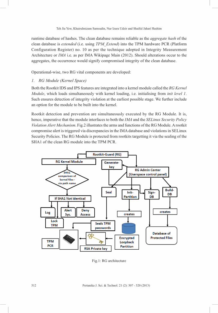
Teh Jia Yew, Khairulmizam Samsudin, Nur Izura Udzir and Shaiful Jahari Hashim
512 Pertanika J. Sci. & Technol. 21 (2): 507 - 520 (2013)
runtime database of hashes. The clean database remains reliable as the aggregate hash of the clean database is extended (i.e. using TPM_Extend) into the TPM hardware PCR (Platform Configuration Register) no. 10 as per the technique adopted in Integrity Measurement Architecture or IMA i.e. as per IMA Wikipage Main (2012). Should alterations occur to the aggregates, the occurrence would signify compromised integrity of the clean database.
Operational-wise, two RG vital components are developed:
1. RG Module (Kernel Space)
Both the Rootkit IDS and IPS features are integrated into a kernel module called the RG Kernel Module, which loads simultaneously with kernel loading, i.e. initialising from init level 1. Such ensures detection of integrity violation at the earliest possible stage. We further include an option for the module to be built into the kernel.
Rootkit detection and prevention are simultaneously executed by the RG Module. It is, hence, imperative that the module interfaces to both the IMA and the SELinux Security Policy Violation Alert Mechanism. Fig.2 illustrates the arms and functions of the RG Module. A rootkit compromise alert is triggered via discrepancies in the IMA database and violations in SELinux Security Policies. The RG Module is protected from rootkits targetting it via the sealing of the SHA1 of the clean RG module into the TPM PCR.
Fig.1: RG architecture

Rootkit Guard (RG) - An Architecture for Rootkit Resistant File-System Implementation Based on TPM
513Pertanika J. Sci. & Technol. 21 (2): 507 - 520 (2013)
Fig.2: RG Kernel module components
2. RG Admin Center(User Space)
The RG is equipped with a control panel i.e. the RG Admin Center, a user-space application permitting users to configure RG, at pre- and post-deployment stages; this is detailed in the next section. The list of RG Admin Center features is given here:
i. Creation of a database of kernel files and modules (Build -DB)
ii. Digitally signing the database in i) above using a private-key created by GPG (Sign-DB)
iii. Creation of an Encrypted Loopback Partition for storage of user-defined critical files (e.g. missile launch codes) (Init-Partition)
iv. Seal the key in ii) above to the TPM PCR (Seal)
TPM-protected Encrypted Loopback Partition
The RG incorporates an encrypted loopback partition (i.e. part of Rootkit IPS) for storage of user-defined critical files e.g. nuclear warhead launch codes. Protection of this partition is provided by 1024-bit RSA Encryption, whose private key is stored in the TPM; hence, the impossibility of theft.
IMPLEMENATION & TEST –BED
Implementation is conducted in two stages. See Fig.3:
a. Pre-Deployment Configurations: Essential set-ups and configurations necessary for the proper and effective operation of the RG
b. Actual, Real-Time Deployment of the RG: The RG in action, implemented in a production environment

Teh Jia Yew, Khairulmizam Samsudin, Nur Izura Udzir and Shaiful Jahari Hashim
514 Pertanika J. Sci. & Technol. 21 (2): 507 - 520 (2013)
Unlike most malware research work which performs implementation in VM environments and deployment in guest OSes (Ryan Riley et. al., 2008; Arvind Seshadri et. al. ,2007), our RG was deployed in an actual platform with no hypervisors utilised. RG deployment was ported and executed on a Dell Latitute E5400 laptop, with the following specifications: 3 GHz Core 2 Duo CPU, 4GB DDR-2 RAM, running Fedora Core Linux 16, with kernel 3.1.7. Currently, our implementation and test-bed is conducted on the same laptop as above, albeit in the VirtualBox Hypervisor (an open source hypervisor). We allocated 1.3 GB of RAM to the same Linux OS (installed as Guest OS in VirtualBox) running identical kernel. Each stage is detailed here:
a. Pre-Deployment Configurations
The pivotal part of the RG is the availability of a clean database of the IMA-measured SHA1 list of kernel files and modules from a freshly configured platform .We term this the Clean IMA Database. RG Admin’s Build-DB feature is utilised for this purpose. Upon deployment, the clean database is compared to a runtime database of similar SHA1 list for rootkit detection.
Next, SELinux is utilised to establish security context for user-defined critical files via the writing of a dynamic programming language like SELinux policies (SELinux rules) . A critical files and objects domain is created and these critical files are labelled by SELinux with file type enforcement: rg_secured_t. Only files and also objects labelled with rg_secured_t are granted execution privileges. A database of clean SELinux policies for the critical files-objects is established. TrustedGRUB is configured to preserve the integrity of boot essential files (esp. initrd and vmlinuz). Finally, the creation of an Encrypted Loopback Partition for storage of critical files accomplishes this stage.
b. Actual, Real Time Deployment of the RG
This section considers the rootkit infiltration events after a SuckIT-type rootkit was successfully planted on the victim’s machine (V). Configuration of the SuckIT binary is essential prior to the execution of a backdoor to permit access to V machine by a remote attacker (A) machine.
Upon rootkit binary execution (i.e. ./sk c), two mechanisms in the Rootkit IDS kick in to alert the user: the IMA database’s SHA1 Comparison Engine (see Fig.2) via SHA1 anomalies in the clean and runtime databases, and the SELinux Policy Violation Alert Mechanism issues an alert on the user’s Desktop due to policy violation for two possible actions: either i) the rootkit attempts to access files in the critical files domain with rg_secured_t file type enforcement or ii) files not labeled rg_secured_t file-type enforcement attempt execution.
The Rootkit IPS steps in and unmounts the Encrypted Loopback Partition, preventing possible data theft (e.g. missile launch codes) by the rootkit. Instinctively, the detected rootkit is denied rwx privileges by SELinux as a decontamination measure. Fig.3 details real-time deployment in a procedural illustrative view.

Rootkit Guard (RG) - An Architecture for Rootkit Resistant File-System Implementation Based on TPM
515Pertanika J. Sci. & Technol. 21 (2): 507 - 520 (2013)
Fig.3: Deployment of the RG – procedural flow illustration
RESULTS AND DISCUSSION
Effectiveness
We subjected our RG to 8 real-world Linux 2.6 rootkits to gauge its effectiveness and attempted the prevention of both the execution of the configuration binaries and build scripts, both actions deemed essential for the proper deployment and installation of the tested rootkits. We demonstrated the successful thwarting of a rootkit binaries configuration via utilisation and enforcement of SELinux MAC policies enforcing rg_secured_t file type enforcement in our platform. The results are summarised in Table 1. The prevention of the execution of the configuration binary of one of the rootkits experimented on i.e. SUCKIT is shown in Figure 4.
TABLE 1 RG Effectiveness in the Prevention of Real World Linux 2.6 Rootkits
Rootkit Pre-deployment means Prevention successful?Kbeast-v1
Installation via build script execution
Yes
Medusa– 0.7.1Sebek-3.2Lrk5Mood-ntSuckIT
Execution of configuration binarySuperkitAdore-ng

Teh Jia Yew, Khairulmizam Samsudin, Nur Izura Udzir and Shaiful Jahari Hashim
516 Pertanika J. Sci. & Technol. 21 (2): 507 - 520 (2013)
Performance
The Rootkit IDS: IMA integrity assessment via SHA1 Comparison Engine of all kernel files consumes 70s was measured using Bootchart (Bootchart, 2012). For the Rootkit IPS: we utilised UnixBench 5.1.3 for micro-benchmark evaluation of our RG. This tool is capable of providing a fine-grain performance impact of RG. The type and nature of tests performed are shown in Figure 5. Our results listed two highest overheads as the price of running our RG: 11% - from Filecopy 4KB (buffer size 8000 maxblocks) test and 9% from the Dhrystone test. The average overall performance overhead for our RG wass 3.78 %.
The performance penalty is due to the operation of the RG kernel module executing security checks on the kernel files in the Linux file-system. The SHA1 Comparison Engine executes via comparing hashes of runtime kernel files with hashes in the clean database. This requires the use of string handling and comparison functions (which explains the Dhrystone test overhead) and procurement of hashes of all kernel files (which explains the Filecopy test overhead). Near negligible overheads are possible due to the power of contemporary user-computing platform hardware i.e. 4GB RAM and 7,200 rpm HDD plus 3GHz Core 2 Duo CPU.
In terms of overhead, the performance of our RG was relatively on par with HookSafe, which reports a maximum overhead of 7% and an average overhead of 4%. Next, compared with another rootkit-attack mitigation model which is similar to our RG but without hardware-based anchorage for guaranteeing platform integrity i.e. the IFEDAC (Ziqing Mao et al., 2011), our RG showed better performance. The IFEDAC introduced an overhead of a maximum of 19% and an average of 5.4%. NICKLE rakes up a maximum of 13% of overhead and an average of 5.45%. All reported performance results were obtained using UnixBench.
CONCLUSION
This paper presents an architectural model i.e. Rootkit Guard (RG) for solving rootkit persistence. Our RG utilises the current trend in security solutions in the computing industry today, the TPM, in providing a complementing security solution with TPM-platform integrity guaranteed by the TPM hardware. RG incorporates Tripwire-like features and blends both IMA as the RIDS and SELinux security features as the RIPS in providing one weapon in the armory of tools/solutions against rootkit persistence. Our RG’s inclusion in the kernel ensures that RG is a limb of the platform; hence, RG is part of the platform’s ‘biological’ immune-defense system against rootkits. Evaluation of the RG, both in terms of effectiveness i.e. prevention of deployment of 8 real-world Linux 2.6 rootkits and performance i.e. with average overall performance overhead of only 3.78% underscores the fact that RG is viable for deployment in real-time due to its near-negligible consumption of system resources. The RG complements other existing rootkit-attack mitigation solutions in rootkit defense for OSs.

Rootkit Guard (RG) - An Architecture for Rootkit Resistant File-System Implementation Based on TPM
517Pertanika J. Sci. & Technol. 21 (2): 507 - 520 (2013)
Fig.4: Prevention of the SuckIT Configuration Binary, ./sk, from Execution
9,152
4,562
0,612
7,918
5,962
11,293
0,359 0,188 0,272 0,779 0,96
3,298
0
2
4
6
8
10
12
Performance Evaluation of RG
Overhead (in %)
Fig.5: Performance Evaluation Results of RG Using UnixBench 5.1.3

Teh Jia Yew, Khairulmizam Samsudin, Nur Izura Udzir and Shaiful Jahari Hashim
518 Pertanika J. Sci. & Technol. 21 (2): 507 - 520 (2013)
ACKNOWLEDGEMENT
We are indebted to the Research Management Centre (RMC), UPM, for the financial support on our work via Grant No. : UPM/700-2/1/RUGS/05-01-12-1638RU. The authors further wish to thank the Malaysian Ministry of Higher Education (MOHE) for the award of the myBrain – myPhD Scholarship to the corresponding author in support of this work.
REFERENCESArvind, S., Mark, L., Ning, Q., & Adrian, P. (2007). SecVisor: A Tiny Hypervisor to Provide Lifetime
Kernel Code Integrity for Commodity OSes, SOSP’07. October 14–17, Stevenson, Washington, USA. ACM.
Bickford, J., O’Hare, R., Baliga, A., Ganapathy, & V. Iftode, L. (2010). Rootkits on smartphones: attacks, implications and opportunities. In the Proceedings of the Eleventh Workshop on Mobile Computing Systems & Applications. ACM. New York. pp. 49–54.
Bootchart. (2012). Open Source Boot-time Measurement Tool. Retrieved on March 15, 2012 from http://www.bootchart.org.
Bruce, S., (2005). Schneier on Security- The blog covering security and security technology. Retrieved from http://www.schneier.com/blog/archives/2005/02/sha1_broken.html.
Doug, W., & James, H. G. (2007). A Normality Based Method for Detecting Kernel Rootkits. ACM.
IMA Wikipage Main. (2012). Integrity Measurement Architecture (IMA). Retrieved on March 15, 2012 from http://domino.research.ibm.com/comm/research_people.nsf/pages/sailer.index.html.
Jonathan, M., McCune, B., Parnoy, A., Perrigy, M., Reiteryz, K., & Hiroshi, I. (2008), Flicker: An Execution Infrastructure for TCB Minimization. EuroSys’08, April 1.4, 2008, ACM.
Kevin, R. B. B., Stephen, M., & Patrick, D. M. (2008). Rootkit-Resistant Disks. ACM CCS Journals - Conference on Computer and Communications Security in the Proceedings of the 15th ACM Conference on Computer and Communications Security, October 27–31.
Linux Rootkit Documentation, Lrk5 (2012). Linux Rootkit 5 Technical Documentation. Retrieved on March 22, 2012 from http://www.phrack.org/issues.html?issue=63&id=18.
Linux Rootkit Documentation, Adore (2012). Linux Rootkit Technical Documentation. Retrieved ofrom http://www.phrack.org/issues.html?issue=61&id=10.
McAfee Inc. (2006). Rootkits, part 1 of 3, The growing threat, White Paper. Retrieved on August 15, 2012 from http://download.nai.com/Products/mcafee-avert/whitepapers/akapoor_rootkits1.pdf.
Michael, S.(2005). SHA1 Collisions can be Found in 2^63 Operations, RSA Labs. Retrieved on December 15, 2012 from http://www.rsa.com/rsalabs/node.asp?id=2927.
Nguyen, A. Q., & Yoshiyasu, T. (2007). Towards a Tamper Resistant Kernel Rootkit Detector. ACM.
Phrack Magazine. (2012). SuckIT Rootkit Technical Documentation, Volume 0x0b. Issue 0x3a. Phile #0x07 of 0x0e. Linux on-the-fly kernel patching without LKM. Retrieved on March 11, 2012 from http://www.phrack.org/issues.html?id=7&issue=58.
Reiner, S., Zhang, X., Trent, J., & Leendert, v. D. (2004), Design and Implementation of a TCG based Integrity Measurement Architecture. In the Proceedings of the 13th USENIX symposium, CA , USA, USENIX Association.

Rootkit Guard (RG) - An Architecture for Rootkit Resistant File-System Implementation Based on TPM
519Pertanika J. Sci. & Technol. 21 (2): 507 - 520 (2013)
Riley, R., Jiang, X., & Xu, D. (2008). Guest-Transparent Prevention of Kernel Rootkits with VMM-Based Memory Shadowing. In Lippmann, R., Kirda, E., & Trachtenberg, A. (Eds.) RAID 2008. LNCS, vol. 5230, pp. 1–20. Springer, Heidelberg.
SANS Institute. (2012). Security Predict. Retrieved on March 15, 2012 from http://www.sans.edu/research/security-laboratory/article/security-predict2011.
Richard, H. (2010). The SELinux Notebook, Volume 1 – The Foundations. GNU Free Documentation, pp. 14 – 30.
Tripwire Homepage. (2010). Tripwire. Retrieved on April 5, 2010 from http://sourceforge.net/projects/tripwire/.
Ulrich, K., Marcel, S., & Christian, S. (2007). Realizing Property-Based Attestation and Sealing with Commonly Available Hard- and Software. STC’07, November 2, 2007, ACM, pp. 50 – 57.
Xiaoyun, W., Yiqun, Y., Hongbo, Y. (2005). Finding Collisions in the Full SHA-1. Advances in Cryptology-Crypto 05, LNCS Springer, 3621, pp. 17-36.
Zhi, W., XuXian, J., Weidong, C., Peng, N. (2009). Countering Kernel Rootkits with Lightweight Hook Protection, CCS’09, November 9–13, ACM.
Ziqing, M., NingHui, L., Hong, C., & XuXian, J. (2011). Combining Discretionary Policy with Mandatory Information Flow in Operating Systems. ACM Transactions on Information and System Security. Vol. 14. No. 3. Article 24.


Pertanika J. Sci. & Technol. 21 (2): 521 - 532 (2013)
SCIENCE & TECHNOLOGYJournal homepage: http://www.pertanika.upm.edu.my/
ISSN: 0128-7680 © 2013 Universiti Putra Malaysia Press.
Theoretical Modeling of Pseudo Hydrostatic Force in Solid-Liquid Pipe Flow with Two Layers
Hussain H. Al-Kayiem* and Iylia Elena Abdul JamilMechanical Engineering Department, Universiti Teknologi PETRONAS, Bandar Seri Iskandar, 31750 Tronoh, Perak, Malaysia.
ABSTRACT
In the moving layer of particles with variable concentration, the shear estimation is not directly predictable and there is no existing clear mathematical or empirical formula to achieve this objective. This paper presents a developed approach to estimate the shear forces in a flow having suspended and moving layers of solid particles in liquid flow. The two-layer approach was taken whereby the flow consisting of one upper suspended layer of particles in the liquid, and the bottom layer was the moving bed of particles. In the present work, the method of finding the force acting on the pipe wall by the particles in the layer, termed as the ‘dry force’, was presented using a “pseudo hydrostatic pressure” method. To attain the equation for the dry force, a mathematical approach is taken with the assumptions that the flow is horizontal, two-phase pipe flow (solid in Newtonian liquid), incompressible and it is at steady-state. The analysis was conducted considering various particles densities, various concentrations in the suspended layer and different thicknesses of the moving bed. Changing the concentration in the suspended layer from 0.00001 up to 0.001 didn’t showed significant changes in the dry force evaluation. The dry friction force is increasing with increasing moving bed thickness. The developed mathematical model can be applicable in solving for the shear force in horizontal solid liquid two-phase flows.
Keywords: Pseudo Hydrostatic, two phase flow, transport phenomena,
Article history:Received: 26 December 2011Accepted: 15 March 2012
E-mail addresses: [email protected] (Hussain H. Al-Kayiem), [email protected] (Iylia Elena Abdul Jamil)*Corresponding Author
on the pipe wall. In case of homogenous solid-in-liquid suspension flow, the properties can be treated as mixture properties with constant concentration profile across the flow area, which is not possible in the case of variable concentration profile, where two types of two-phase flow layers appear in the flow.
The solid-in-liquid flows are complex to be modeled, and due to this, the suspended layer is usually treated as a single-phase fluid
INTRODUCTION
In the study of solid-in-liquid two-phase flows, shear stress is an important parameter in determining the frictional forces that are acting
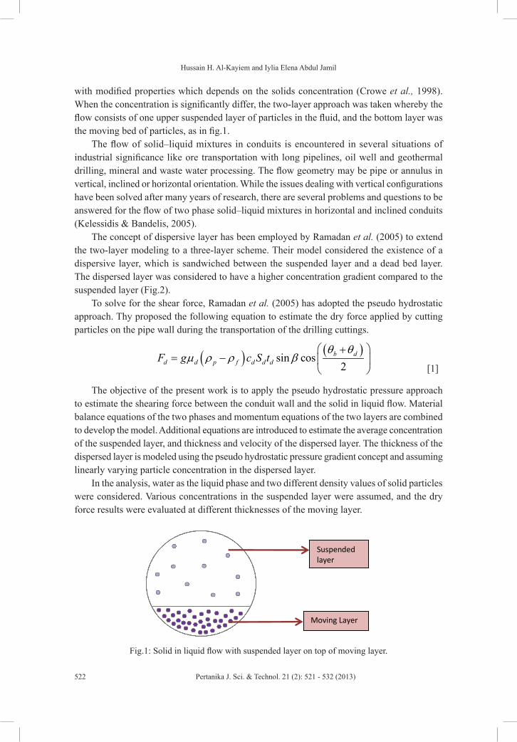
Hussain H. Al-Kayiem and Iylia Elena Abdul Jamil
522 Pertanika J. Sci. & Technol. 21 (2): 521 - 532 (2013)
with modified properties which depends on the solids concentration (Crowe et al., 1998). When the concentration is significantly differ, the two-layer approach was taken whereby the flow consists of one upper suspended layer of particles in the fluid, and the bottom layer was the moving bed of particles, as in fig.1.
The flow of solid–liquid mixtures in conduits is encountered in several situations of industrial significance like ore transportation with long pipelines, oil well and geothermal drilling, mineral and waste water processing. The flow geometry may be pipe or annulus in vertical, inclined or horizontal orientation. While the issues dealing with vertical configurations have been solved after many years of research, there are several problems and questions to be answered for the flow of two phase solid–liquid mixtures in horizontal and inclined conduits (Kelessidis & Bandelis, 2005).
The concept of dispersive layer has been employed by Ramadan et al. (2005) to extend the two-layer modeling to a three-layer scheme. Their model considered the existence of a dispersive layer, which is sandwiched between the suspended layer and a dead bed layer. The dispersed layer was considered to have a higher concentration gradient compared to the suspended layer (Fig.2).
To solve for the shear force, Ramadan et al. (2005) has adopted the pseudo hydrostatic approach. Thy proposed the following equation to estimate the dry force applied by cutting particles on the pipe wall during the transportation of the drilling cuttings.
( ) ( )sin cos2
b dd d p f d d dF g c S t
+= −
θ θµ ρ ρ β
[1]
The objective of the present work is to apply the pseudo hydrostatic pressure approach to estimate the shearing force between the conduit wall and the solid in liquid flow. Material balance equations of the two phases and momentum equations of the two layers are combined to develop the model. Additional equations are introduced to estimate the average concentration of the suspended layer, and thickness and velocity of the dispersed layer. The thickness of the dispersed layer is modeled using the pseudo hydrostatic pressure gradient concept and assuming linearly varying particle concentration in the dispersed layer.
In the analysis, water as the liquid phase and two different density values of solid particles were considered. Various concentrations in the suspended layer were assumed, and the dry force results were evaluated at different thicknesses of the moving layer.
Suspended layer
Moving Layer
Fig.1: Solid in liquid flow with suspended layer on top of moving layer.

Theoretical Modeling of Pseudo Hydrostatic Force in Solid-Liquid Pipe Flow with Two Layers
523Pertanika J. Sci. & Technol. 21 (2): 521 - 532 (2013)
PHYSICAL DESCRIPTION OF TWO LAYER SOLID-LIQUID FLOW
In the present work, the flow of solid-in-liquid in pipes was divided into two layers which are:
i. The upper layer: Homogeneous Suspended Layer.
ii. The lower layer: Moving Bed Layer.
In the top layer or the suspended layer, the concentration profile is considered as homogeneous, having a constant concentration profile. This is because; there is only a small variation in its concentration, (Fig.3b), which could be neglected and the profile of the suspended layer concentration, is constant
0sdCdy
= [2]
while the moving bed has a linearly increasing concentration profile.
y
Concentration
(a) (b) (c)
y
actual assumed
Fig.2: (a) Schematic representation of shear stresses acting in the three-layer mechanics model; and (b) assumed concentration profiles in three-layer modeling scheme (Ramadan et al., 2005)
Fig.3: (a) The two-layer approach with the suspended region and the moving bed, (b) the concentration profile for suspended layer shown in dashed line and (c) concentration profile of suspended layer assumed to be homogeneous while concentration profile of the moving bed is linear

Hussain H. Al-Kayiem and Iylia Elena Abdul Jamil
524 Pertanika J. Sci. & Technol. 21 (2): 521 - 532 (2013)
In a three-layer model, there is an additional layer at the bottom of the flow. This layer which is called dead bed or stationary bed has a maximum concentration. By both experimental and statistical methods, the bed concentration is found to have the range value (0.4805-0.52) (Cho, 2001). Therefore in this two-layer model, the maximum concentration of the moving bed is taken as 0.5, which is at the bottom of the pipe. The following have been assumed
• The flow is a two-phase pipe flow (solid-liquid)
• The flow is in horizontal pipe
• The fluid is taken as Newtonian fluid
• Two-layer approach is applied
· Upper layer is the homogeneous suspended layer
· Lower layer is the moving bed layer with linear concentration profile
• No-slip condition between the two layers which neglects the interstitial shear force between the two layers
• The flow is incompressible and at steady state
• Analysis is made per unit length basis (flow properties is constant in the horizontal direction)
DERIVATION OF THEORETICAL MODEL
The prediction of forces in two phase flow with multi layers requires prediction of the flow areas, the densities of the different layers, the concentration profiles in each layer, and the structure of forces created by each phase and how it applies on the conduits boundaries.
A. Forces
The total force, Fw acting on the pipe wall boundaries is the summation of the forces acting on the wall in contact with the upper suspended layer, Fsw and the wall of the lower moving bed, Fmw. It can be given by:
w sw mwF F F= + [3]
The average particle concentration in the suspended layer, cs is very small compared to the average concentration of the particles in the moving bed layer Cs << Cm (Newitt et al., 1955). Therefore, the force acting on the upper wall only comes from the shear between the homogeneous solid-liquid flow (of mixed density) and the pipe wall:
sw sw sF A=τ [4]
The moving bed layer has a higher concentration of particles which will exert additional force. This force is the dry friction force, Fd that is acted by the particles in the moving bed layer upon the bottom wall boundaries, Smw. The force between the moving bed and wall, Fmw becomes:

Theoretical Modeling of Pseudo Hydrostatic Force in Solid-Liquid Pipe Flow with Two Layers
525Pertanika J. Sci. & Technol. 21 (2): 521 - 532 (2013)
( ) mwmw m dF A F= +τ [5]
This frictional force between the moving bed layer and the wall will be determined using the pseudo hydrostatic pressure distribution on the wall and will be analysed per unit length basis.
B. Flow Area
By simplification of considering unit length basis, the area between each layer and the contact wall becomes the wetted perimeter between them:
1 unit lengths swA S x= [6] 1 unit lengthm swA S x= [7]
C. Density
According to the two phase flow assumption, the density of each of the two layers will be the mixed densities between the fluid and solids phases according to the solid concentrations in each layer. The density of the fluid phase ( ) 1s s p s fc c= + −ρ ρ ρ depends solely on the properties of fluid used. Meanwhile, the density of particles depends on both particle properties ( ) 1s s p s fc c= + −ρ ρ ρand particles volumetric concentration ci in the layer. This can be expressed by the following relation:
( ) 1s s p s fc c= + −ρ ρ ρ [8]
( ) 1m m p m fc c= + −ρ ρ ρ [9]
where, ( ) 1s s p s fc c= + −ρ ρ ρ and ( ) 1m m p m fc c= + −ρ ρ ρ are the densities of the mixture in the suspended layer and the mean density of the moving layer, respectively.
D. Dry Friction Force
Fig.4: Thickness and Perimeter of each layer in determining the pseudo hydrostatic pressure

Hussain H. Al-Kayiem and Iylia Elena Abdul Jamil
526 Pertanika J. Sci. & Technol. 21 (2): 521 - 532 (2013)
To get the dry friction force Fd on moving bed wall, the pseudo hydrostatic pressure approach shall be used. Following the simple definition of the pseudo hydrostatic pressure distribution on the moving bed boundary, the pressure can be estimated as total force acting on that boundary per the area of wall in contact with the moving bed region for one unit length:
/Pseudo wp F A= [10]
The dynamic friction coefficient between particles and channel wall is d d Pseudo mF P A= µ . Then the dry friction force will be written as:
d d Pseudo mF P A= µ [11]
Pseudo m mp p g= = ⋅ ⋅ρ [12]
E. The Pseudo Hydrostatic Pressure
Based on the pseudo hydrostatic pressure concept, the hydrostatic pressure distribution along the moving bed wall can be defined as:
( )
0
0 0
(1 )
1
m
m m
t
Pseudo p m f m
t t
Pseudo P m f m
p c c g t
p c g dt c g dt
= + −
= + −
∫
∫ ∫
ρ ρ
ρ ρ [13]
F. Concentration
The average particles volumetric concentration in the suspended layer is very small compared with the moving-bed layer. Thus we assume that the concentration profile is constant. Fredsoe and Deigaard (1992) suggested the assumption of linear variation for the dispersed layer. By adopting the pseudo hydrostatic gradient, the average concentration of the moving-bed layer can be approximated as follows:
( )o os
zc c c c= − − δδ [14]
In the equation, ( )o os
zc c c c= − − δδ is concentration at the top of the sheet layer and ( )o o
s
zc c c c= − − δδ is the maximum
concentration. In our case, ( )o os
zc c c c= − − δδ= ( ),max ,maxm m s
m
tc c c ct
= − − where at the interface of the suspended and moving layers, the concentration is equal. The maximum concentration is taken as the concentration at the bottom of the moving bed layer, therefore ( )o o
s
zc c c c= − − δδ = ( ),max ,maxm m s
m
tc c c ct
= − −. Hence, using the notations of fig.4, the following relation is obtained
( ),max ,maxm m sm
tc c c ct
= − − [15]

Theoretical Modeling of Pseudo Hydrostatic Force in Solid-Liquid Pipe Flow with Two Layers
527Pertanika J. Sci. & Technol. 21 (2): 521 - 532 (2013)
where, t is a height in the moving bed, and tm is the maximum height of the moving bed.
Substituting Equation [15] into Equation [13], and integrating to find Pm:
( ) ( )
( ) ( )
,max ,max ,max ,max0 0
2 2
,max ,max ,max ,max
1
0 02 2
m mt t
m p m m s f m m sm m
m mm p m m s f m m s
m m
t tp g c c c dt g c c c g dtt t
t tt tp g tc c c g t tc c ct t
= − − + − − −
= − − + − + −
∫ ∫ρ ρ
ρ ρ( ) ( )
( ) ( )
,max ,max ,max ,max0 0
2 2
,max ,max ,max ,max
1
0 02 2
m mt t
m p m m s f m m sm m
m mm p m m s f m m s
m m
t tp g c c c dt g c c c g dtt t
t tt tp g tc c c g t tc c ct t
= − − + − − −
= − − + − + −
∫ ∫ρ ρ
ρ ρ
Leading to:
( ) ( ), ,max12 2
m max s m sm p m f m
c c c cp gt gt
+ += + −
ρ ρ
[16]
Combining Equation [16] with equation [11], the moving layer dry friction force per unit length becomes:
( ) ( ),max ,max12 2
m s m sd d p f m mw
c c c cF gt S
+ + = + −
µ ρ ρ [17]
COMPUTATION PROCEDURE AND RESULTS
To test the validity of the developed model, a calculation program is created using Microsoft Excel, including all inputs and desired outputs to be calculated. The enveloped equation in this work, equation 14, to estimate the shear drag force is programmed. Also, equation 1 suggested by Ramadan et al. (2005) is programmed so that they are analysing input data simultaneously.
The selected materials for the present analysis are water and cutting particles from oil well drilling site. Same parameters used by Ramadan et al. (2005) were adopted here. The properties of the liquid phase are shown in table 1.
TABLE 1 Constant computational data of the liquid phase
Density of water 1000 kg/m3
Viscosity of water 0.001 Pa.sChannel diameter 70 mmDynamic friction factor 0.25
For the solid phase, the particles are selected with mean diameter of 3.8x10⁴ m. To standardize the calculations, initial concentration for suspended layer, cs is assumed to be
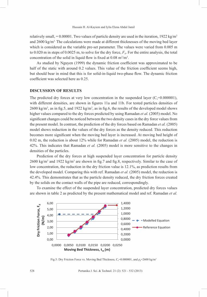
Hussain H. Al-Kayiem and Iylia Elena Abdul Jamil
528 Pertanika J. Sci. & Technol. 21 (2): 521 - 532 (2013)
relatively small, = 0.00001. Two values of particle density are used in the iteration, 1922 kg/m3
and 2600 kg/m3. The calculations were made at different thicknesses of the moving bed layer which is considered as the variable pre-set parameter. The values were varied from 0.005 m to 0.020 m in steps of 0.0025 m, to solve for the dry force, Fd. For the entire analysis, the total concentration of the solid in liquid flow is fixed at 0.08 m3/m3.
As studied by Nguyen (1999) the dynamic friction coefficient was approximated to be half of the static with around 0.2 values. This value of the friction coefficient seems high, but should bear in mind that this is for solid-in-liquid two-phase flow. The dynamic friction coefficient was selected here as 0.25.
DISCUSSION OF RESULTS
The predicted dry forces at very low concentration in the suspended layer (Cs=0.000001), with different densities, are shown in figures 11a and 11b. For tested particles densities of 2600 kg/m3, as in fig.5, and 1922 kg/m3, as in fig.6, the results of the developed model shows higher values compared to the dry forces predicted by using Ramadan et al. (2005) model. No significant changes could be noticed between the two density cases in the dry force values from the present model. In contrast, the prediction of the dry forces based on Ramadan et al. (2005) model shows reduction in the values of the dry forces as the density reduced. This reduction becomes more significant when the moving bed layer is increased. At moving bed height of 0.02 m, the reduction is about 12% while for Ramadan et al. (2005) model, the reduction is 42%. This indicates that Ramadan et al. (2005) model is more sensitive to the changes in densities of the particles.
Prediction of the dry forces at high suspended layer concentration for particle density 2600 kg/m3 and 1922 kg/m3 are shown in fig.7 and fig.8, respectively. Similar to the case of low concentration, the reduction in the dry friction value is 12.1%, as prediction results from the developed model. Comparing this with ref. Ramadan et al. (2005) model, the reduction is 42.4%. This demonstrates that as the particle density reduced, the dry friction forces created by the solids on the contact walls of the pipe are reduced, correspondingly.
To examine the effect of the suspended layer concentration, predicted dry forces values are shown in table 2 as predicted by the present mathematical model and ref. Ramadan et al.
0,0000
0,2000
0,4000
0,6000
0,8000
1,0000
1,2000
1,4000
0,00
1,00
2,00
3,00
4,00
5,00
6,00
0,0000 0,0050 0,0100 0,0150 0,0200 0,0250
Dry
Fri
ctio
n Fo
rce,
Fd
(N/m
)
Moving Bed Thickness, tm (m)
Modelled Equation
Reference Equation
Fig.5: Dry Friction Force vs. Moving Bed Thickness, Cs=0.000001, and ρp=2600 kg/m3
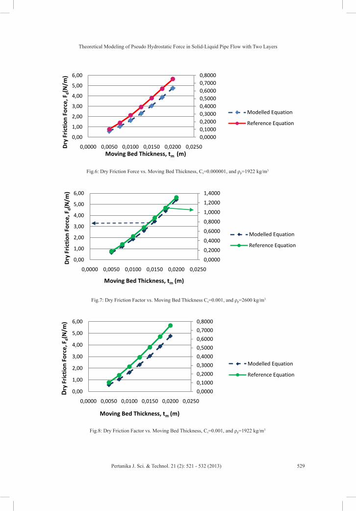
Theoretical Modeling of Pseudo Hydrostatic Force in Solid-Liquid Pipe Flow with Two Layers
529Pertanika J. Sci. & Technol. 21 (2): 521 - 532 (2013)
0,00000,10000,20000,30000,40000,50000,60000,70000,8000
0,00
1,00
2,00
3,00
4,00
5,00
6,00
0,0000 0,0050 0,0100 0,0150 0,0200 0,0250Dry
Fri
ctio
n Fo
rce,
Fd(
N/m
)
Moving Bed Thickness, tm (m)
Modelled Equation
Reference Equation
Fig.6: Dry Friction Force vs. Moving Bed Thickness, Cs=0.000001, and ρp=1922 kg/m3
0,0000
0,2000
0,4000
0,6000
0,8000
1,0000
1,2000
1,4000
0,00
1,00
2,00
3,00
4,00
5,00
6,00
0,0000 0,0050 0,0100 0,0150 0,0200 0,0250
Dry
Fri
ctio
n Fo
rce,
Fd(
N/m
)
Moving Bed Thickness, tm (m)
Modelled Equation
Reference Equation
Fig.7: Dry Friction Factor vs. Moving Bed Thickness Cs=0.001, and ρp=2600 kg/m3
0,0000
0,1000
0,2000
0,3000
0,4000
0,5000
0,6000
0,7000
0,8000
0,00
1,00
2,00
3,00
4,00
5,00
6,00
0,0000 0,0050 0,0100 0,0150 0,0200 0,0250
Dry
Fri
ctio
n Fo
rce,
Fd(
N/m
)
Moving Bed Thickness, tm (m)
Modelled Equation
Reference Equation
Fig.8: Dry Friction Factor vs. Moving Bed Thickness, Cs=0.001, and ρp=1922 kg/m3
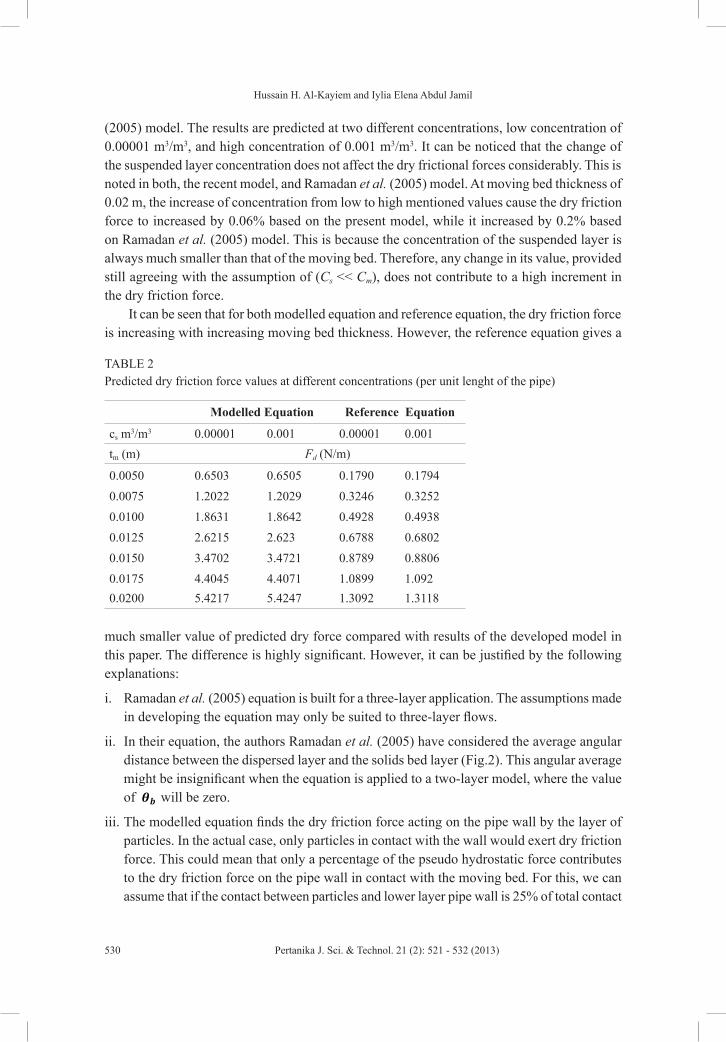
Hussain H. Al-Kayiem and Iylia Elena Abdul Jamil
530 Pertanika J. Sci. & Technol. 21 (2): 521 - 532 (2013)
(2005) model. The results are predicted at two different concentrations, low concentration of 0.00001 m3/m3, and high concentration of 0.001 m3/m3. It can be noticed that the change of the suspended layer concentration does not affect the dry frictional forces considerably. This is noted in both, the recent model, and Ramadan et al. (2005) model. At moving bed thickness of 0.02 m, the increase of concentration from low to high mentioned values cause the dry friction force to increased by 0.06% based on the present model, while it increased by 0.2% based on Ramadan et al. (2005) model. This is because the concentration of the suspended layer is always much smaller than that of the moving bed. Therefore, any change in its value, provided still agreeing with the assumption of (Cs << Cm), does not contribute to a high increment in the dry friction force.
It can be seen that for both modelled equation and reference equation, the dry friction force is increasing with increasing moving bed thickness. However, the reference equation gives a
TABLE 2 Predicted dry friction force values at different concentrations (per unit lenght of the pipe)
Modelled Equation Reference Equation
cs m3/m3 0.00001 0.001 0.00001 0.001tm (m) Fd (N/m)
0.0050 0.6503 0.6505 0.1790 0.17940.0075 1.2022 1.2029 0.3246 0.32520.0100 1.8631 1.8642 0.4928 0.49380.0125 2.6215 2.623 0.6788 0.68020.0150 3.4702 3.4721 0.8789 0.88060.0175 4.4045 4.4071 1.0899 1.0920.0200 5.4217 5.4247 1.3092 1.3118
much smaller value of predicted dry force compared with results of the developed model in this paper. The difference is highly significant. However, it can be justified by the following explanations:
i. Ramadan et al. (2005) equation is built for a three-layer application. The assumptions made in developing the equation may only be suited to three-layer flows.
ii. In their equation, the authors Ramadan et al. (2005) have considered the average angular distance between the dispersed layer and the solids bed layer (Fig.2). This angular average might be insignificant when the equation is applied to a two-layer model, where the value of will be zero.
iii. The modelled equation finds the dry friction force acting on the pipe wall by the layer of particles. In the actual case, only particles in contact with the wall would exert dry friction force. This could mean that only a percentage of the pseudo hydrostatic force contributes to the dry friction force on the pipe wall in contact with the moving bed. For this, we can assume that if the contact between particles and lower layer pipe wall is 25% of total contact

Theoretical Modeling of Pseudo Hydrostatic Force in Solid-Liquid Pipe Flow with Two Layers
531Pertanika J. Sci. & Technol. 21 (2): 521 - 532 (2013)
area between moving bed (fluid and particles) and pipe wall, the dry friction force could also be reduced to 25%, which could give an excellent agreement with the reference equation.
iv. The dry friction coefficient is selected as 0.25, while Ramadan et al. (2005) used value of 0.2.
CONCLUSION
A mathematical formula has been developed to estimate the dry friction force of a horizontal pipe solid-liquid flow using the two-layer approach. The model can be modified to match solid-liquid flow application to serve in solving the complexity of calculating the boundary-moving bed force in different types of two phase flow with multi layers of concentration. The model is useful in modelling and analysis of cutting particle transportation and sand-water sedimentation.
The basics of the calculation program have been made in Microsoft Excel. The developed mathematical model is tested against one available model that also applies the pseudo hydrostatic pressure method, using similar data (Ramadan et al., 2005). Based on the calculated results, there is lack of agreement between the modelled equation and the reference equation. This difference is justified by several factors which include assumptions made for mathematical modelling and dissimilar application for different flow models (two-phase or three-phase).
There are many improvements that can be made in order to achieve more reliable results wider applications of the approach:
i. The effect of particle size and channel diameter can be included in future investigations.
ii. An experiment could be conducted to compare the mathematical models with experimental results.
iii. The search can be extended to Non-Newtonian fluids.
iv. The application of the pseudo hydrostatic pressure can be considered in inclined channels.
ACKNOWLEDGEMENT
The authors would like to acknowledge Universiti Teknologi PETRONAS for the financial support to present the paper in CUTSE2011.
REFERENCESCrowe, C., Sommerfeld, M., & Tsuji, Y. (1998). Multiphase Flows with Droplets and Particles. CRC
Press. Florida: CRC Press LLC. 1998. pp. 3 – 9
Kelessidis, V. C., & Bandelis, G. E. (2005). Flow Pattern Transitions and Flow Pattern Detection of Dilute Solid-Liquid Mixtures in Horizontal Concentric and Eccentric Annulus. Paper presented at the 7th World Congress of Chemical Engineering. Glasgow, 2005.
Ramadan, A., Skalle, P., & Saasen, A. (2005). Application of a three-layer modelling approach for solids transport in horizontal and inclined channels. Chemical Engineering Science, 60, 2557 – 2570. DOI:10.1016/j.ces.2004.12.011
H. Cho. (2001). Development of a three-segment hydraulic model for cuttings transport in horizontal and deviated wells. pp. 259, 2001.

Hussain H. Al-Kayiem and Iylia Elena Abdul Jamil
532 Pertanika J. Sci. & Technol. 21 (2): 521 - 532 (2013)
Newitt, D. M., Richardson, J. F., Abbott, M., & Turtle, R. B. (1955). Hydraulic Conveying of Solids in Horizontal Pipes, Trans. Instn. Chem. Engrs., 33, 93-110.
Fredsoe, J., & Deigaard, R. (1992). Mechanics of Coastal Sediment Transport. World Scientific Publishing Company, ISBN: 9810208413.
Nguyen, D. (1999). Mathematical models of cuttings transport and drilling fluid displacement by cement slurry in horizontal wells. (Unpublished doctoral dissertation). University of New South Wales (Australia), Source DAI-B 59/08, p. 4436.
Pertanika J. Sci. & Technol. 21 (2): 533 - 540 (2013)
SCIENCE & TECHNOLOGYJournal homepage: http://www.pertanika.upm.edu.my/
ISSN: 0128-7680 © 2013 Universiti Putra Malaysia Press.
INTRODUCTION
Recently, the degradation of coke quality caused by long-term use of a coke oven has emerged as an important issue to be solved in iron making processes. Furthermore, vast quantities of natural resources are consumed in operating a blast furnace, and a high level
Improvement of Coke Strength by Phenolic Resin Coating: Experimental and Theoretical Studies of Strengthening Mechanism
Y. Asakuma1*, Y. Komatsu1, S. Nishi1, A. Kotani2 and M. Nishimura2
1Mechanical and System Engineering, University of Hyogo, 2167 Shosha, Himeji, Hyogo, Japan2Research and Development Center, Kansai Coke and Chemicals Co., Ltd., 1-1 Oh-hama-cho, Amagasaki, Hyogo, Japan
ABSTRACT
Coke strength is the most important characteristic for retaining permeability in the bed of a blast furnace. In the present study, coke was coated with phenolic resin in order to improve the coke strength, and a nanoindentation method was used to estimate the strength of the coated coke after reaction under CO2 atmosphere. The elastic modulus was measured for the microporous coke substrate,. The elastic modulus of coated coke before reaction was higher than that of uncoated coke. However, after reaction with CO2, the elastic modulus did not necessarily show an improvement in coke strength. The mechanism whereby the resin coating improved coke strength before and after the reaction was considered by a finite element analysis using a mesh superposition technique.
Keywords: Component, coke, phenolic resin, nanoindentation, elastic modulus, mesh superposition method, finite element method
Article history:Received: 26 December 2011Accepted: 15 March 2012
E-mail addresses: [email protected] (Y. Asakuma), [email protected] (A. Kotani)*Corresponding Author
of operational efficiency is required in order to reduce the emission of CO2. Accordingly, high-strength coke is needed for preventing poor permeability of the bed due to fracture and pulverization of coke at the bottom of a blast furnace. To improve coke strength, modification of the microstructure of coke has proved useful. Coke consists of inert and substrate containing various sizes of micropores, such that its material structure is heterogeneous and porous. In iron making processes, three mechanisms are thought to lead to the degradation of coke strength: fracture, that is, propagation of large cracks

Y. Asakuma, Y. Komatsu, S. Nishi, A. Kotani and M. Nishimura
534 Pertanika J. Sci. & Technol. 21 (2): 533 - 540 (2013)
in coke caused by loads in a blast furnace; pulverization, such as surface abrasion of coke in the raceway; and reaction with CO2 (Hayashizaki et al., 2009). These mechanisms are strongly linked to the heterogeneous and microporous structure of coke. Therefore, in this study, coke is dipped into an aqueous solution of phenol resin, and the resin seeps into the micropores to improve coke strength. Conventionally, the drum index and microstrength index are used to measure coke quality. Although these indices highlight macroscopic properties of coke, measurements are not always sufficient for evaluation of the heterogeneous microstructure. Consequently, a nanoindentation method has been introduced that can measure the elastic modulus and hardness of a microregion of coke (Mihashi et al., 2002). Improvement of coke strength by phenol resin is investigated through microhardness data obtained under various experimental conditions and through theoretical data from a finite element analysis of the nanoindentation method.
EXPERIMENTAL
Procedure
Coke was provided by Kansai Coke and Chemicals Co., Ltd., and all experimental samples used were fabricated under the same manufacturing conditions and were from the same section of a coke block (16 mm × 16 mm × 5 mm). First, coke is dipped into an aqueous solution of phenol resin (Oshika Co., Ltd; RS-05) at a concentration of 20, 30, or 40 wt % for 1 min. The specimen is then dried at room temperature for 24 h. Second, any moisture remaining in the phenol resin is removed by placing the sample in a drying oven for 3 h at 150 °C. Finally, the reaction between CO2 and the coated coke is run by using the experimental apparatus shown in Fig.1.
The experimental procedure is as follows:
1. Coke is positioned at the center of a quartz glass pipe (φ20 mm) and placed in the furnace.
2. Air in the pipe is replaced with N2 and the sample is heated to 950 °C.
3. For the reactions, N2 is replaced with CO2 (at 50 mL/s) at a given temperature.
4. Reaction with CO2 proceeds for 1 h, and the gas is replaced by N2 once more. Finally, the furnace is cooled.
5. Microhardness of coke after the reaction is measured as shown in next section.
Coke
N2 C
O2
Fig. 1: Apparatus for reaction experiments
Reactor
Fig. 2: Load–displacement curve for nanoindentation method
0
200
400
600
0 2 4 6 8Displacement [μm]
Load
[mN]
Hold
Hole
Unload
Load
Indenter Coke
Fig.1: Apparatus for reaction experiments
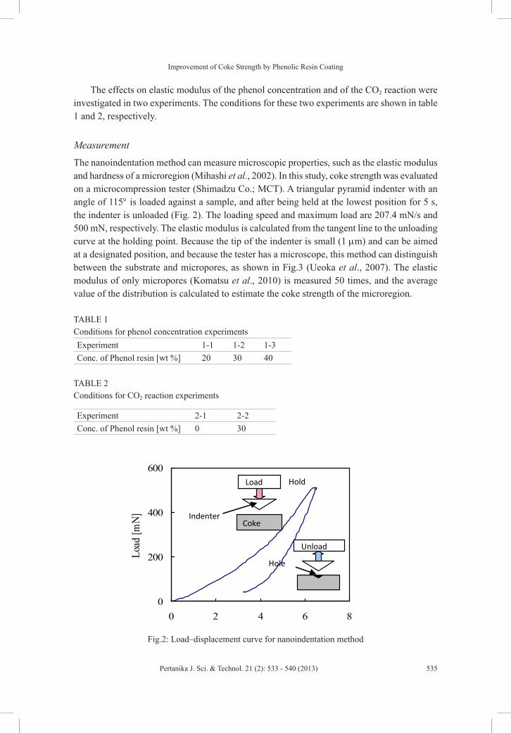
Improvement of Coke Strength by Phenolic Resin Coating
535Pertanika J. Sci. & Technol. 21 (2): 533 - 540 (2013)
The effects on elastic modulus of the phenol concentration and of the CO2 reaction were investigated in two experiments. The conditions for these two experiments are shown in table 1 and 2, respectively.
Measurement
The nanoindentation method can measure microscopic properties, such as the elastic modulus and hardness of a microregion (Mihashi et al., 2002). In this study, coke strength was evaluated on a microcompression tester (Shimadzu Co.; MCT). A triangular pyramid indenter with an angle of 115° is loaded against a sample, and after being held at the lowest position for 5 s, the indenter is unloaded (Fig. 2). The loading speed and maximum load are 207.4 mN/s and 500 mN, respectively. The elastic modulus is calculated from the tangent line to the unloading curve at the holding point. Because the tip of the indenter is small (1 µm) and can be aimed at a designated position, and because the tester has a microscope, this method can distinguish between the substrate and micropores, as shown in Fig.3 (Ueoka et al., 2007). The elastic modulus of only micropores (Komatsu et al., 2010) is measured 50 times, and the average value of the distribution is calculated to estimate the coke strength of the microregion.
TABLE 1 Conditions for phenol concentration experimentsExperiment 1-1 1-2 1-3Conc. of Phenol resin [wt %] 20 30 40
TABLE 2 Conditions for CO2 reaction experiments
Experiment 2-1 2-2Conc. of Phenol resin [wt %] 0 30
Coke
N2 C
O2
Fig. 1: Apparatus for reaction experiments
Reactor
Fig. 2: Load–displacement curve for nanoindentation method
0
200
400
600
0 2 4 6 8Displacement [μm]
Load
[mN]
Hold
Hole
Unload
Load
Indenter Coke
Fig.2: Load–displacement curve for nanoindentation method
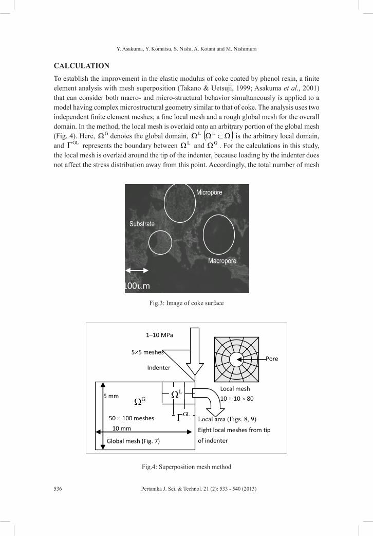
Y. Asakuma, Y. Komatsu, S. Nishi, A. Kotani and M. Nishimura
536 Pertanika J. Sci. & Technol. 21 (2): 533 - 540 (2013)
CALCULATION
To establish the improvement in the elastic modulus of coke coated by phenol resin, a finite element analysis with mesh superposition (Takano & Uetsuji, 1999; Asakuma et al., 2001) that can consider both macro- and micro-structural behavior simultaneously is applied to a model having complex microstructural geometry similar to that of coke. The analysis uses two independent finite element meshes; a fine local mesh and a rough global mesh for the overall domain. In the method, the local mesh is overlaid onto an arbitrary portion of the global mesh (Fig. 4). Here, GΩ denotes the global domain, LΩ ( )Ω⊂ΩL is the arbitrary local domain, and GLΓ represents the boundary between LΩ and GΩ . For the calculations in this study, the local mesh is overlaid around the tip of the indenter, because loading by the indenter does not affect the stress distribution away from this point. Accordingly, the total number of mesh
100 m
Fig.3: Image of coke surface
Substrate
Micropore
Macropore
10 mm
5 mm
1–10 MPa
50 100 meshes
5 5 meshes
Local area (Figs. 8, 9) Eight local meshes from tip
of indenter
Global mesh (Fig. 7)
Fig. 4: Superposition mesh method
Indenter Pore
Local mesh
10 10 80 L
G
GL
Fig.4: Superposition mesh method
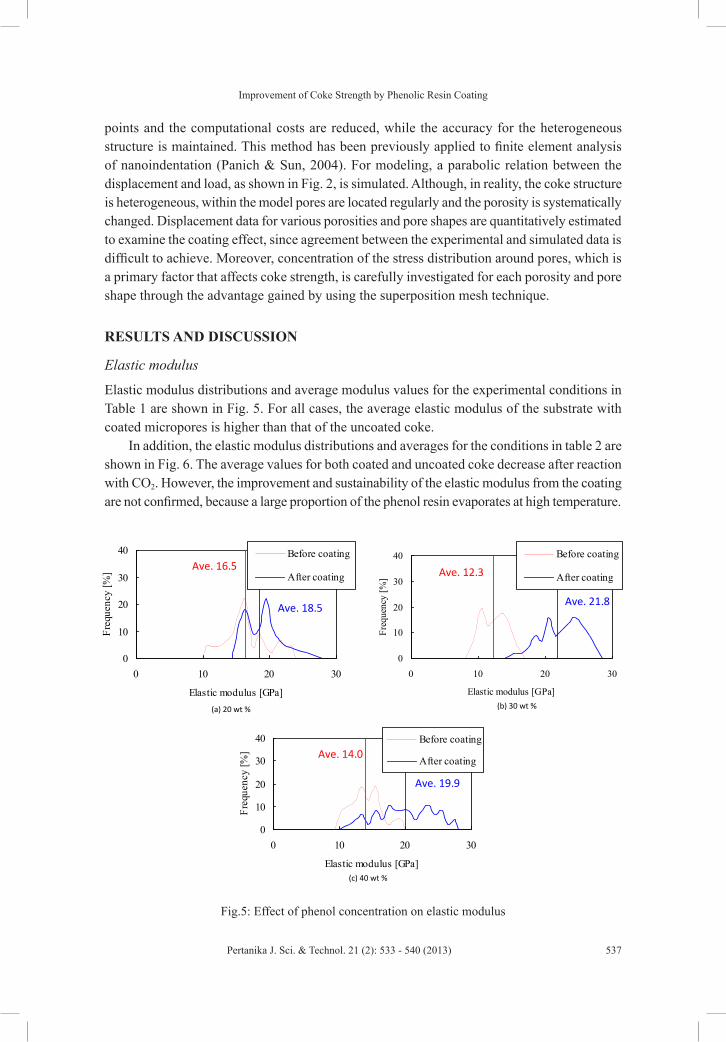
Improvement of Coke Strength by Phenolic Resin Coating
537Pertanika J. Sci. & Technol. 21 (2): 533 - 540 (2013)
points and the computational costs are reduced, while the accuracy for the heterogeneous structure is maintained. This method has been previously applied to finite element analysis of nanoindentation (Panich & Sun, 2004). For modeling, a parabolic relation between the displacement and load, as shown in Fig. 2, is simulated. Although, in reality, the coke structure is heterogeneous, within the model pores are located regularly and the porosity is systematically changed. Displacement data for various porosities and pore shapes are quantitatively estimated to examine the coating effect, since agreement between the experimental and simulated data is difficult to achieve. Moreover, concentration of the stress distribution around pores, which is a primary factor that affects coke strength, is carefully investigated for each porosity and pore shape through the advantage gained by using the superposition mesh technique.
RESULTS AND DISCUSSION
Elastic modulus
Elastic modulus distributions and average modulus values for the experimental conditions in Table 1 are shown in Fig. 5. For all cases, the average elastic modulus of the substrate with coated micropores is higher than that of the uncoated coke.
In addition, the elastic modulus distributions and averages for the conditions in table 2 are shown in Fig. 6. The average values for both coated and uncoated coke decrease after reaction with CO2. However, the improvement and sustainability of the elastic modulus from the coating are not confirmed, because a large proportion of the phenol resin evaporates at high temperature.
0
10
20
30
40
0 10 20 30
Elastic modulus [GPa]
Freq
uenc
y [%
]
Before coating
After coating
0
10
20
30
40
0 10 20 30
Elastic modulus [GPa]
Freq
uenc
y [%
]
Before coating
After coating
(b) 30 wt %
(c) 40 wt %
Fig. 5: Effect of phenol concentration on elastic modulus
0
10
20
30
40
0 10 20 30
Elastic modulus [GPa]
Freq
uenc
y [%
]
Before coating
After coating
Ave. 18.5
Ave. 16.5
Ave. 21.8
Ave. 12.3
Ave. 19.9
Ave. 14.0
(a) 20 wt %
0
10
20
30
40
0 10 20 30
Elastic modulus [GPa]
Freq
uenc
y [%
]
Before coating
After coating
0
10
20
30
40
0 10 20 30
Elastic modulus [GPa]
Freq
uenc
y [%
]
Before coating
After coating
(b) 30 wt %
(c) 40 wt %
Fig. 5: Effect of phenol concentration on elastic modulus
0
10
20
30
40
0 10 20 30
Elastic modulus [GPa]
Freq
uenc
y [%
]Before coating
After coating
Ave. 18.5
Ave. 16.5
Ave. 21.8
Ave. 12.3
Ave. 19.9
Ave. 14.0
(a) 20 wt %
0
10
20
30
40
0 10 20 30
Elastic modulus [GPa]
Freq
uenc
y [%
]
Before coating
After coating
0
10
20
30
40
0 10 20 30
Elastic modulus [GPa]
Freq
uenc
y [%
]
Before coating
After coating
(b) 30 wt %
(c) 40 wt %
Fig. 5: Effect of phenol concentration on elastic modulus
0
10
20
30
40
0 10 20 30
Elastic modulus [GPa]
Freq
uenc
y [%
]
Before coating
After coating
Ave. 18.5
Ave. 16.5
Ave. 21.8
Ave. 12.3
Ave. 19.9
Ave. 14.0
(a) 20 wt %
Fig.5: Effect of phenol concentration on elastic modulus
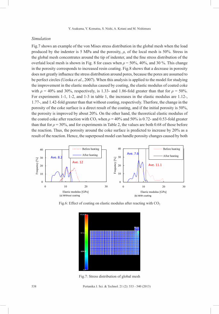
Y. Asakuma, Y. Komatsu, S. Nishi, A. Kotani and M. Nishimura
538 Pertanika J. Sci. & Technol. 21 (2): 533 - 540 (2013)
Fig. 6: Effect of coating on elastic modulus after reacting with CO2
0
10
20
30
40
0 10 20 30
Elastic modulus [GPa]
Freq
uenc
y [%
]
Before heating
After heating
0
10
20
30
40
0 10 20 30
Elastic modulus [GPa]
Freq
uenc
y [%
]
Before heating
After heating
Ave. 8.2 Ave. 12
Ave. 7.6
Ave. 11.1
(b) With coating
(a) Without coating
Fig.6: Effect of coating on elastic modulus after reacting with CO2
Simulation
Fig.7 shows an example of the von Mises stress distribution in the global mesh when the load produced by the indenter is 5 MPa and the porosity, ρ, of the local mesh is 50%. Stress in the global mesh concentrates around the tip of indenter, and the fine stress distribution of the overlaid local mesh is shown in Fig. 8 for cases when ρ = 50%, 40%, and 30 %. This change in the porosity corresponds to increased resin coating. Fig.8 shows that a decrease in porosity does not greatly influence the stress distribution around pores, because the pores are assumed to be perfect circles (Ueoka et al., 2007). When this analysis is applied to the model for studying the improvement in the elastic modulus caused by coating, the elastic modulus of coated coke with ρ = 40% and 30%, respectively, is 1.33- and 1.86-fold greater than that for ρ = 50%. For experiments 1-1, 1-2, and 1-3 in table 1, the increases in the elastic modulus are 1.12-, 1.77-, and 1.42-fold greater than that without coating, respectively. Therfore, the change in the porosity of the coke surface is a direct result of the coating, and if the initial porosity is 50%, the porosity is improved by about 20%. On the other hand, the theoretical elastic modulus of the coated coke after reaction with CO2 when ρ = 40% and 50% is 0.72- and 0.53-fold greater than that for ρ = 30%, and for experiments in Table 2, the values are both 0.68 of those before the reaction. Thus, the porosity around the coke surface is predicted to increase by 20% as a result of the reaction. Hence, the superposed model can handle porosity changes caused by both
Fig. 7: Stress distribution of global mesh
Fig. 9: Stress distributions for elliptical pores
(a) Vertical pores (b) Horizontal pores
Fig. 8: Stress distribution of local mesh for changing porosity
(b) 40%
(c) 30%
(a) 50%
Fig.7: Stress distribution of global mesh
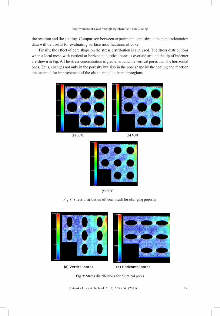
Improvement of Coke Strength by Phenolic Resin Coating
539Pertanika J. Sci. & Technol. 21 (2): 533 - 540 (2013)
the reaction and the coating. Comparison between experimental and simulated nanoindentation data will be useful for evaluating surface modifications of coke.
Finally, the effect of pore shape on the stress distribution is analyzed. The stress distributions when a local mesh with vertical or horizontal eliptical pores is overlaid around the tip of indenter are shown in Fig. 9. The stress concentration is greater around the vertical pores than the horizontal ones. Thus, changes not only in the porosity but also in the pore shape by the coating and reaction are essential for improvement of the elastic modulus in microregions.
Fig. 7: Stress distribution of global mesh
Fig. 9: Stress distributions for elliptical pores
(a) Vertical pores (b) Horizontal pores
Fig. 8: Stress distribution of local mesh for changing porosity
(b) 40%
(c) 30%
(a) 50%
Fig. 7: Stress distribution of global mesh
Fig. 9: Stress distributions for elliptical pores
(a) Vertical pores (b) Horizontal pores
Fig. 8: Stress distribution of local mesh for changing porosity
(b) 40%
(c) 30%
(a) 50%
Fig.8: Stress distribution of local mesh for changing porosity
Fig.9: Stress distributions for elliptical pores

Y. Asakuma, Y. Komatsu, S. Nishi, A. Kotani and M. Nishimura
540 Pertanika J. Sci. & Technol. 21 (2): 533 - 540 (2013)
CONCLUSION
Coke was coated with phenol resin in order to improve the mechanical strength of the coke. The elastic modulus of coke coated with various concentrations of phenol was measured in microregions by a nanoindentation method. Although the elastic modulus was increased by coating before reaction with CO2, the phenol resin coat was not effective in improving the coke strength observed after the reaction. The mesh superposition technique was useful for evaluating the heterogeneous microstructure of coke, such as the porosity and pore shapes, and proved to be an accurate tool for predicting changes in the elastic moduli of microregions.
REFERENCESAsakuma, Y. et al. (2001). Micro-structural analysis of coke using the overlaying mesh finite element
method. Paper presented at the 18th Annual international Pittsburgh Coal Conference, pp. 12-04, Newcastle, New South Wales, Australia, Dec., 4, 2001.
Hayashizaki, H., Ueoka, K., Ogata, T., Yamazaki, Y., Matsushita, Y., Aoki, H., Miura, T., Fukuda, K., & Matsudaira, K. (2009). Evaluation of mechanical properties in microscopic textures of coke before/after solution loss reaction, Tetsu-to-Hagane, 95, 460-466, 2009
Komatsu, Y. et al. (2010). Analysis of strength mechanism for coke impregnated by PVA aqueous solution. Paper presented at the 13th APCChE, Asian Pacific of Chemical Engineering (Taiwan, 2010)
Mihashi, M., Munetaka, S., Yuusuke, A., Tsuyoshi, Y., Hideyuki, A., Takatoshi, M., Kenji, K., & Shouzou, I. (2002). Evaluation of matrix of coke strength by nano-indentation method, Tetsu-to Hagane, 88, 188-194.
Panich, N., & Sun, Y. (2004). Effect of penetration depth on indentation response of soft coatings on hard substrates: a finite element analysis, Surface and Coatings Technology, 182, 342-350.
Sumi, H., Shimoyama, I., Anyashiki, T., Fukada, K., & Fujimoto, H. (2010). Effect of bubble growth on coarse defect generation behavior in coke, Tetsu-to-Hagane, 96, 258-264.
Takano, N., & Uetsuji, Y. (1999). Hierarchical modelling of textile composite materials and structures by the homogenization method, Modelling Simul. Mater. Sci. Eng., 7, 207-231.
Ueoka, K., Ogata, T., Matsushita, Y., Morozumi, Y., Aoki, H., Miura, T., Uebo, K., & Fukuda, K. (2007). Numerical investigation for the effect of shapes and arrangement of inerts on coke strength, ISIJ International, 47, 1723-1731.

Pertanika J. Sci. & Technol. 21 (2): 541 - 554 (2013)
SCIENCE & TECHNOLOGYJournal homepage: http://www.pertanika.upm.edu.my/
ISSN: 0128-7680 © 2013 Universiti Putra Malaysia Press.
INTRODUCTION
Ranking algorithms or link analysis algorithms determine the success of the Web search engines as they calculate the importance and relevance of individual page on the World Wide Web. Examples of link analysis algorithms are HITS (Hyperlink Induced Topic Search), PageRank
Application of Markov Chain in the PageRank Algorithm
Ravi Kumar, P.*, Alex Goh, K. L. and Ashutosh, K. S.Department of Electrical and Computer Engineering, Curtin University, Sarawak Campus, 98009 Miri, Sarawak, Malaysia
ABSTRACT
Link analysis algorithms for Web search engines determine the importance and relevance of Web pages. Among the link analysis algorithms, PageRank is the state of the art ranking mechanism that is used in Google search engine today. The PageRank algorithm is modeled as the behavior of a randomized Web surfer; this model can be seen as Markov chain to predict the behavior of a system that travels from one state to another state considering only the current condition. However, this model has the dangling node or hanging node problem because these nodes cannot be presented in a Markov chain model. This paper focuses on the application of Markov chain on PageRank algorithm and discussed a few methods to handle the dangling node problem. The Experiment is done running on WEBSPAM-UK2007 to show the rank results of the dangling nodes.
Keywords: Markov chain, web graph, information retrieval, PageRank, transition probability, dangling page.
Article history:Received: 26 December 2011Accepted: 15 March 2012
E-mail addresses: [email protected] (Ravi Kumar, P.), [email protected] (Alex Goh, K. L.), [email protected] (Ashutosh, K. S.)*Corresponding Author
and SALSA (Stochastic Approach for Link Structure Analysis). These algorithms rely on the link structure of the Web pages. HITS (Kleinberg, 1999) developed by Jon Kleinberg, is a query depend algorithm, which calculate the authorities and hubs value of a page while SALSA (Lempel & Moran, 1999) algorithm combines the random walk feature in PageRank and the hub authority idea from HITS algorithm.
This paper, we focus on PageRank algorithm. PageRank (Brin & Page, 1998) is a query and content independent algorithm (Borodin et al., 2005). Query independent means that the PageRank algorithm ranks all the pages offline after the crawler download

Ravi Kumar, P., Alex Goh, K. L. and Ashutosh, K. S.
542 Pertanika J. Sci. & Technol. 21 (2): 541 - 554 (2013)
and index the pages and the rank remains constant for all the pages. Content independent means the PageRank algorithm does not include the contents of a Web page for ranking rather it uses the link structure of the Web to calculate the rank. This PageRank algorithm is explained in section of Pagerank Algorithm. When a user types a query term on the search engine, the PageRank algorithm just finds the pages on the Web that matches the query term and presents those pages to the user in the order of their PageRank. It looks simple but the mathematical model behind is amazing. This paper explores the mathematical model behind the PageRank algorithm with experiments and results.
This paper is organized as follows. Next Section describes Markov chain and it’s Mathematics. Section of Pagerank Algorithm explains PageRank algorithm using a sample Web graph. Section of Use of Markov Chain in Pagerank Algorithm describes how Markov chain is applied in the PageRank algorithm. Experiments and results are shown in Section of Experimental Results and Section of Conclusion concludes this paper.
MARKOV CHAIN
Introduction
Markov chain (Norris, 1996; Gao et al., 2009) is invented by A. A. Markov; a Russian Mathematician in the early 1900’s to predict the behavior of a system that moves from one state to another state by considering only the current state. Markov chain uses only a matrix and a vector to model and predict it. Markov chains are used in places where there is a transition of states. It used in biology, economy, engineering, physics etc. But the recent application of Markov chain on the Google search engine is interesting and more challenging.
Markov Chain is a random process used by a system that at any given time t = 1, 2, 3 … n occupies one of a finite number of states (Gao et al., 2009). At each time t the system moves from state v to u with probability puv that does not depends on t. puv is called as transition probability which is an important feature of Markov chain and it decides the next state of the object by considering only the current state and not any previous states.
Transition Matrix
Transition Matrix T is an n x n matrix formed from the transition probability of the Markov process, where n represents the number of states. Each entry in the transition matrix tuv is equal to the probability of moving from state v to state u in one time slot. So, 0 ≤ tuv ≤ 1 must be true for all u,v = 1, 2, …, n. The following example shows a sample transition matrix of a 3 state Markov chain:
1/ 4 1/ 2 1/ 41/ 2 0 1/ 21/ 2 1/ 4 1/ 4
uvt =

Application of Markov Chain in the PageRank Algorithm
543Pertanika J. Sci. & Technol. 21 (2): 541 - 554 (2013)
The Transition matrix must have the following properties:
• The matrix must be square and nonnegative matrix i.e. the number of rows and columns must be equal and the entries must be non negative. Each row and column represents a state.
• All the entries in the matrix represent probabilities, so, each entry must be between 0 and 1 inclusive.
• The sum of the entries in a row is the sum of the transition probabilities from a state to another state. So, the sum of the entries in any row must equal to one. This is called as stochastic matrix.
In the above Transition matrix, tuv, we can easily see the probability of moving from one state to another state. For example t3,2 = ¼ i.e. the probability of moving from state 2 to state 3 is only 25%. This Markov chains are used to predict the probability of an event.
PAGERANK ALGORITHM
Web Graph
PageRank algorithm treats the Web as a directed labeled graph whose nodes are the pages and the edges are the hyperlinks between them (Broder et al., 2000). This directed graph structure in the Web is called as Web Graph. A graph G consists of two sets V and E. The set V is a finite, nonempty set of vertices. The set E is a set of pairs of vertices; these pairs are called edges. The notation V(G) and E(G) represent the sets of vertices and edges, respectively of graph G. It can also be expressed G = (V, E) to represent a graph. The graph in Fig.1 is a directed graph with 3 vertices and 3 edges.
The vertices V of G, V(G) = 1, 2, 3. The Edges E of G, E(G) = (1, 2), (2, 1), (2, 3), (1,3), (3,1). In a directed graph with n vertices, the maximum number of edges is n(n-1). With 3 vertices, the maximum number of edges can be 3(3-1) = 6.
1
2 3
Fig.1: A Directed Web Graph G

Ravi Kumar, P., Alex Goh, K. L. and Ashutosh, K. S.
544 Pertanika J. Sci. & Technol. 21 (2): 541 - 554 (2013)
There are a number of link based ranking algorithms (Brin & Page, 1998; Kleinberg, 1999; Lempel & Moran, 2000). Among them PageRank is the most popular link based ranking algorithm. PageRank algorithm and Google are developed by Brin and Page (1998) during their Ph D at Stanford University as a research project. The PageRank algorithm is the heart of the Google search engine. Google was introduced in the search engine business in 1998. Soon after its introduction, it became one of the most efficient search engine because it is a query independent and content independent search engine. It produces the results faster because it is query independent i.e. the Web pages are downloaded, indexed and ranked offline. When a user types a query on the search engine, the PageRank algorithm just finds the pages on the Web that matches the query term and presents those pages to the user in the order of their PageRank. PageRank algorithm uses only the link structure of the Web to determine the importance of a page rather than going into the contents of a page. PageRank provides a more efficient way to compute the importance of a Web page by counting the number of pages that are linking to it (in-coming links or backlinks). If an in-coming link comes from a reputed page, then that in-coming link is given a higher weighting than those in-coming links from a non-reputed pages. The PageRank PR of a page p can be computed by taking into account the set of pages pa(p) pointing to p as per the formula given by Page et al. (1999) is shown in equation [1] as follows:
( ) (1 )p
q
q q
PR p d dpa
PRO∈
= + −∑ [1]
Here, d is a damping factor such that 0 <d <1 and Oq is the number of out-going links of page q.
Let us take an example of a simple Web graph with 3 nodes 1, 2 and 3 as shown in Fig. 1. The PageRank for pages 1, 2 and 3 can be calculated by using equation [1]. To start with, we assume the initial PageRank as 1.0 and do the calculation. The damping factor d is set to 0.85. PageRank calculation of page 1 is shown in equation [2] and [3].
( )2 3
(2) (3)(1) 1 PR PRPR d dO O
= − + + [2]
1 1(1) 0.15 0.85 1.4252 1
PR = + + = [3]
( )1
(1)(2) 1 PRPR d dO
= − +
[4]
1.425(2) 0.15 0.85 0.7562
PR = + = [5]
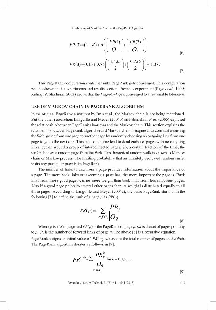
Application of Markov Chain in the PageRank Algorithm
545Pertanika J. Sci. & Technol. 21 (2): 541 - 554 (2013)
( )1 3
(1) (3)(3) 1 PR PRPR d dO O
= − + + [6]
1.425 0.756(3) 0.15 0.85 1.0772 2
PR = + + = [7]
This PageRank computation continues until PageRank gets converged. This computation will be shown in the experiments and results section. Previous experiment (Page et al., 1999; Ridings & Shishigin, 2002) shows that the PageRank gets converged to a reasonable tolerance.
USE OF MARKOV CHAIN IN PAGERANK ALGORITHM
In the original PageRank algorithm by Brin et al., the Markov chain is not being mentioned. But the other researchers Langville and Meyer (2004b) and Bianchini et al. (2005) explored the relationship between PageRank algorithm and the Markov chain. This section explains the relationship between PageRank algorithm and Markov chain. Imagine a random surfer surfing the Web, going from one page to another page by randomly choosing an outgoing link from one page to go to the next one. This can some time lead to dead ends i.e. pages with no outgoing links, cycles around a group of interconnected pages. So, a certain fraction of the time, the surfer chooses a random page from the Web. This theoretical random walk is known as Markov chain or Markov process. The limiting probability that an infinitely dedicated random surfer visits any particular page is its PageRank.
The number of links to and from a page provides information about the importance of a page. The more back links or in-coming a page has, the more important the page is. Back links from more good pages carries more weight than back links from less important pages. Also if a good page points to several other pages then its weight is distributed equally to all those pages. According to Langville and Meyer (2004a), the basic PageRank starts with the following [8] to define the rank of a page p as PR(p).
( )p
q
q
PR ppa q
PRO∈
= ∑ [8]
Where p is a Web page and PR(p) is the PageRank of page p. pa is the set of pages pointing to p. Oq is the number of forward links of page q. The above [8] is a recursive equation.PageRank assigns an initial value of (0) 1
p nPR = , where n is the total number of pages on the Web. The PageRank algorithm iterates as follows in [9].
( 1) for 0,1, 2,...,
p
kp
q
kq
kq
pa
PRPR
O+
∈
= =∑
[9]
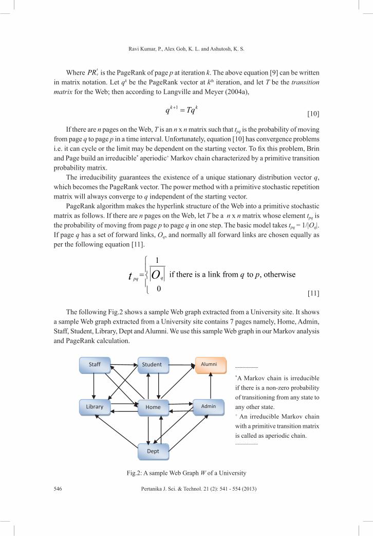
Ravi Kumar, P., Alex Goh, K. L. and Ashutosh, K. S.
546 Pertanika J. Sci. & Technol. 21 (2): 541 - 554 (2013)
Where kqPR is the PageRank of page p at iteration k. The above equation [9] can be written
in matrix notation. Let qk be the PageRank vector at kth iteration, and let T be the transition matrix for the Web; then according to Langville and Meyer (2004a),
1k kq Tq+ = [10]
If there are n pages on the Web, T is an n x n matrix such that tpq is the probability of moving from page q to page p in a time interval. Unfortunately, equation [10] has convergence problems i.e. it can cycle or the limit may be dependent on the starting vector. To fix this problem, Brin and Page build an irreducible* aperiodic+ Markov chain characterized by a primitive transition probability matrix.
The irreducibility guarantees the existence of a unique stationary distribution vector q, which becomes the PageRank vector. The power method with a primitive stochastic repetition matrix will always converge to q independent of the starting vector.
PageRank algorithm makes the hyperlink structure of the Web into a primitive stochastic matrix as follows. If there are n pages on the Web, let T be a n x n matrix whose element tpq is the probability of moving from page p to page q in one step. The basic model takes tpq = 1/|Oq|. If page q has a set of forward links, Oq, and normally all forward links are chosen equally as per the following equation [11].
1
if there is a link from to , otherwise
0qpq q pOt
= [11]
The following Fig.2 shows a sample Web graph extracted from a University site. It shows a sample Web graph extracted from a University site contains 7 pages namely, Home, Admin, Staff, Student, Library, Dept and Alumni. We use this sample Web graph in our Markov analysis and PageRank calculation.
Alumni
Library Home Admin
Dept
Staff Student
Fig.2: A sample Web Graph W of a University
------------------
*A Markov chain is irreducible if there is a non-zero probability of transitioning from any state to any other state. + An irreducible Markov chain with a primitive transition matrix is called as aperiodic chain. ------------------
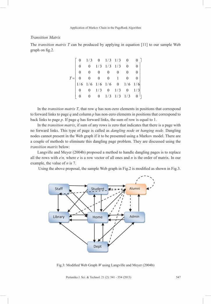
Application of Markov Chain in the PageRank Algorithm
547Pertanika J. Sci. & Technol. 21 (2): 541 - 554 (2013)
Transition Matrix
The transition matrix T can be produced by applying in equation [11] to our sample Web graph on fig.2.
0 1/ 3 0 1/ 3 1/ 3 0 00 0 1/ 3 1/ 3 1/ 3 0 00 0 0 0 0 0 00 0 0 0 1 0 0
1/ 6 1/ 6 1/ 6 1/ 6 0 1/ 6 1/ 60 0 1/ 3 0 1/ 3 0 1/ 30 0 0 1/ 3 1/ 3 1/ 3 0
T
=
In the transition matrix T, that row q has non-zero elements in positions that correspond to forward links to page q and column p has non-zero elements in positions that correspond to back links to page p. If page q has forward links, the sum of row is equal to 1.
In the transition matrix, if sum of any rows is zero that indicates that there is a page with no forward links. This type of page is called as dangling node or hanging node. Dangling nodes cannot present in the Web graph if it to be presented using a Markov model. There are a couple of methods to eliminate this dangling page problem. They are discussed using the transition matrix below:
Langville and Meyer (2004b) proposed a method to handle dangling pages is to replace all the rows with e/n, where e is a row vector of all ones and n is the order of matrix. In our example, the value of n is 7.
Using the above proposal, the sample Web graph in Fig.2 is modified as shown in Fig.3.
Alumni
Library Home Admin
Dept
Staff Student
Fig.3: Modified Web Graph W using Langville and Meyer (2004b)

Ravi Kumar, P., Alex Goh, K. L. and Ashutosh, K. S.
548 Pertanika J. Sci. & Technol. 21 (2): 541 - 554 (2013)
The new forward links from the Alumni page is shown using the dotted arrows. This makes the transition matrix T as stochastic as shown below:
0 1/ 3 0 1/ 3 1/ 3 0 00 0 1/ 3 1/ 3 1/ 3 0 0
1/ 7 1/ 7 1/ 7 1/ 7 1/ 7 1/ 7 1/ 70 0 0 0 1 0 0
1/ 6 1/ 6 1/ 6 1/ 6 0 1/ 6 1/ 60 0 1/ 3 0 1/ 3 0 1/ 30 0 0 1/ 3 1/ 3 1/ 3 0
T
=
The row 3 in the transition matrix T , (Alumni page) is connected to all the nodes and also connected back to it (shown in the dotted lines).
There is another proposal from Bianchini et al. (2005) and Singh et al. (2010) to connect a hypothetical node hi with self loop and connect all the dangling nodes to the hypothetical node as shown in Fig.4. This method also makes the transition matrix as stochastic matrix.
In Fig.4, hi is the hypothetical node with self loop (shown in blue dotted line) and the Alumni page is connected to it (shown in red dotted line) and the transition matrix for the modified graph is shown as follows:
0 1/ 3 0 1/ 3 1/ 3 0 0 00 0 1/ 3 1/ 3 1/ 3 0 0 00 0 0 0 0 0 0 10 0 0 0 1 0 0 0
1/ 6 1/ 6 1/ 6 1/ 6 0 1/ 6 1/ 6 00 0 1/ 3 0 1/ 3 0 1/ 3 00 0 0 1/ 3 1/ 3 1/ 3 0 00 0 0 0 0 0 0 1
T
=
The last row and last column in the above transition matrix T is the hypothetical node hi.
The transition probability for the Alumni page in the modified graph in Fig.4 is 1. Now the Alumni page is no more a dangling page. Similarly for the hypothetical node hi the transition probability is 1 because of the self loop. Now this Web graph on Fig.4 is also stochastic.
This stochastic property is not enough to guarantee that Markov model will converge and a steady state vector exists. There is another problem with is transition matrix T is that this matrix may not be regular. The general Web’s nature makes the transition matrix T is not regular. In the graph, every node needs to be connected to every other node (irreducible). But in the real Web, every page is not connected to every other page i.e. it is not strongly connected. Brin et al. [1] forced all the entries in the transition matrix to satisfy 0 < tpq < 1 to make it regular. This ensures convergence of qn to a unique, positive steady state vector.

Application of Markov Chain in the PageRank Algorithm
549Pertanika J. Sci. & Technol. 21 (2): 541 - 554 (2013)
Google Matrix
According to Langville and Meyer (2005), Brin and Page added a perturbation matrix E = eet/n to make this stochastic irreducible matrix as Google matrix as shown in equation [12].
(1 )T T Eα α= + − [12]
Where α is between 0 and 1. Google believed that this new matrix T tends to better model the real-life surfer. In the real-life a surfer has 1-α probability of jumping to a random page on the Web i.e. by typing a URL on the command line of a browser and an α probability of clicking on a forward link on a current page. Many researchers (Brin & Page, 1998; Langville & Meyer, 2004b; Bianchini et al., 2005) say the value of α used by the PageRank algorithm of Google is 0.85.
We calculate the Google Matrix in equation [12] using the sample Web graph W by having a value of 0.85 for α and shown in the matrix T .
This matrix computation can be normalized to a stationary vector by calculating the powers of the transition matrix. At one stage of the calculation, the values of the matrix get stationary.
Those values are the PageRank scores for the 7 pages from the sample Web graph W. Assume after the 30th iteration the following are the stationary vector for our sample 7 page Web graph.
[ ]0.043 0.334 0.047 0.341 0.441 0.041 0.041s =
Alumni
Library Home Admin
Dept
hi
Staff Student
Fig.4: Modified Web Graph W using Singh et at. (2010)

Ravi Kumar, P., Alex Goh, K. L. and Ashutosh, K. S.
550 Pertanika J. Sci. & Technol. 21 (2): 541 - 554 (2013)
0 1/ 3 0 1/ 3 1/ 3 0 0 1/ 7 1/ 7 1/ 7 1/ 7 1/ 7 1/ 7 1/ 70 0 1/ 3 1/ 3 1/ 3 0 0 1/ 7 1/ 7 1/ 7 1/ 7 1/ 7 1/ 7 1/ 7
1/ 7 1/ 7 1/ 7 1/ 7 1/ 7 1/ 7 1/ 7 1/ 7 1/ 7 1/ 7 1/ 7 1/ 7 1/ 7 1/ 70.85 0.150 0 0 0 1 0 0 1/ 7 1/
1/ 6 1/ 6 1/ 6 1/ 6 0 1/ 6 1/ 60 0 1/ 3 0 1/ 3 0 1/ 30 0 0 1/ 3 1/ 3 1/ 3 0
T
= +
7 1/ 7 1/ 7 1/ 7 1/ 7 1/ 71/ 7 1/ 7 1/ 7 1/ 7 1/ 7 1/ 7 1/ 71/ 7 1/ 7 1/ 7 1/ 7 1/ 7 1/ 7 1/ 71/ 7 1/ 7 1/ 7 1/ 7 1/ 7 1/ 7 1/ 7
0.021 0.304 0.021 0.304 0.304 0.021 0.0210.021 0.021 0.304 0.304 0.304 0.021 0.0210.142 0.142 0.142 0.142 0.142 0.142 0.1420.021 0.021 0.021 0.021 0.871 0.021 0.0210.163 0.163 0.163 0.163 0.021 0.163 0.1630.021 0.021 0.304 0.021 0.30
=
4 0.021 0.3040.021 0.021 0.021 0.304 0.304 0.304 0.021
PageRank Interpretation of Stationary Vector
PageRank interprets the stationary vector in the following way. For example, a user enters a query in the Google search window requesting for word 1 and word 2. Then the search engine looks for the inverted index database with the word 1 and word 2. This database contains the list of all the words or terms and the list of documents that contains the words or terms (Langville & Meyer, 2005).
Assume the following documents lists are stored in the inverted index database for word 1 and word 2 as shown in Table 1.
So, the relevancy set for the user’s query term word 1 and word 2 is 1, 2, 4, and 7. The PageRank of these 4 documents are compared to find out the order of importance. According to our sample 7 page Web, 1 is the Staff page, 2 is the Student page, 4 is the Library page and 7 is the Dept. page. The respective PageRank scores are s1 = 0.043, s2 = 0.334, s4 = 0.341 and s7 = 0.041. This PageRank algorithm treats that document 4 (Library) page is most relevant to the given query term, followed by document 2 (Student), document 1 (Staff) and document 7 (Dept). When a user types a new query term, the inverted index database is accessed again and a new relevancy set is created. This is how the PageRank algorithm works in the Google search engine.
TABLE 1 Inverted Index Document ListQuery Word/Term Document ListWord 1 Document 2, Document 4 & Document 7Word 2 Document 1 & Document 7

Application of Markov Chain in the PageRank Algorithm
551Pertanika J. Sci. & Technol. 21 (2): 541 - 554 (2013)
EXPERIMENTAL RESULTS
The dataset that is used in this experiment is WEBSPAM-UK2007, provided by Laboratory of Web Algorithmics, Università degli Studi di Milano with the support of the DELIS EU - FET research project (Yahoo! Research, n.d.). The collections contain 114549 hosts and among them, 49379 are dangling hosts. The distributions of hosts is as Fig.5.
The dataset is implemented with the algorithm in (Singh et al., 2010) and shows the results of the dangling hosts. We actually show the rank results of the first dangling host to the last one. The rank results of the dangling hosts is described as in Fig.6.
With the hypothetical node, now the Web graph is stochastic. Fig.6 shows the rank results of the dangling hosts in ascending order. The results are calculated with the damping factor α of 0.85 and 50 iterations.
Label No. of Hosts Dangling Hosts 49379 Non-dangling Hosts 65150 Total 114529
Fig.5: Distributions of Web Hosts
Fig.6: The rank results of the dangling hosts
Ravi Kumar, P., Alex Goh, K. L. and Ashutosh, K. S.
552 Pertanika J. Sci. & Technol. 21 (2): 541 - 554 (2013)
CONCLUSION
This paper starts with the introduction of Markov chain and PageRank algorithm. Then the mathematics behind the PageRank algorithm is explained theoretically. This paper also brings anonymity about how the PageRank algorithm uses the Markov chain and transition matrix to calculate the relevancy set. This paper highlights the different adjustments done to make the Web graph into a Markov model. In that, the dangling node problem and the methods to handle the dangling nodes were also discussed and the mathematical solutions are given. A Markov model is created for a sample Web graph and the PageRank calculation is shown for the Markov model. We implemented the PageRank algorithm just to support our mathematical model and shown the results.
REFERENCESBianchini, M., Gori, M., & Scarselli, F. (2005). Inside PageRank. ACM transactions on Internet
Technology, 2005.
Borodin, A., Roberts, G. O., Rosenthal, J. S., & TsaParas, P. (2005). Link Analysis Ranking: Algorithms, Theory and Experiments. In the Proceedings of the ACM Transactions on Internet Technology, Vol. 5, No 1, pp. 231-297.
Brin, S., & Page, L. (1998). The Anatomy of a Large Scale Hypertextual Web search engine. Computer Network and ISDN Systems, 30(1-7), 107-117.
Broder, A., Kumar, R., Maghoul, F., Raghavan, P., Rajagopalan, S., Stata, R., Tomkins, A., & Wiener, J. (2000). Graph Structure in the Web. Computer Networks : The International Journal of Computer and telecommunications Networking, 33(1-6), 309-320.
Gao, B., Liu, T. Y., Ma, Z., Wang, T., & Li, H. (2009). A General Markov Framework for Page Importance Computation. In the Proceeding of the 18th ACM conference on Information and knowledge management.
Kleinberg, J. (1999). Authoritative Sources in a Hyper-Linked Environment. Journal of the ACM, 46(5), 604-632.
Langville, A. N, & Meyer, C. D. (2004a). The Use of the Linear Algebra by Web Search Engines. Bulletin of the International Linear Algebra, 23, December 2004.
Langville, A. N. & Meyer, C. D. (2004b). Deeper Inside PageRank. Internet Mathematics, 1(3), 335-380.
Langville, A. N. & Meyer, C. D. (2005). A Survey of Eigenvector Methods of Web Information Retrieval. In the Proceedings of the SIAM, Vol. 47, No. 1, pp. 135—161, 2005.
Lempel, R., & Moran, S. (2000). The stochastic approach for link–structure analysis (SALSA) and the TKC effect. In Proceedings of the 9th World Wide Web Conference (WWW9). Elsevier Science. pp.387–401.
Norris, R. (1996). Markov Chains. Cambridge University Press. pp.1–4.
Page, L., Brin, S., Motwani, R., & Winograd, T. (1999). The Pagerank Citation Ranking: Bringing order to the Web. Technical Report, Stanford Digital Libraries SIDL-WP-1999-0120.
Ridings, C., & Shishigin, M. (2002). PageRank Uncovered. Technical Report, 2002.

Application of Markov Chain in the PageRank Algorithm
553Pertanika J. Sci. & Technol. 21 (2): 541 - 554 (2013)
Singh, A. K., Kumar, P. R., & Alex, G. K. L. (2010). Efficient Algorithm to handle Dangling Pages using Hypothetical node. In the Proceeding of 6th IDC2010, Seoul, Korea, 2010.
Yahoo! Research. (n.d.). Web Spam Collections. Retrieved on July 2011 from http://barcelona.research.yahoo.net/webspam/datasets/ Crawled by the laboratory of Web Algorithmics, University of Milan, http://law.dsi.unimi.it/.


Pertanika J. Sci. & Technol. 21 (2): 555 - 566 (2013)
SCIENCE & TECHNOLOGYJournal homepage: http://www.pertanika.upm.edu.my/
ISSN: 0128-7680 © 2013 Universiti Putra Malaysia Press.
INTRODUCTION
Wireless charging especially on mobile devices is a hot topic recently due to the convenience of replenishing battery power without lugging charger unit around. The wireless charging concept utilizing two coil antennas, one emanates electromagnetic field in area surrounding it while the other antenna
Harnessing Energy from Electromagnetic Field: Practical Implementation Integrating Coil Antenna and IC Load
Syahrizal Salleh1* and Zulkifli Abd Majid2
1Next Generation Access Network, TM Research and Development, Cyberjaya, Malaysia2Department of Electronics Engineering, University Teknologi MARA, 43450 Shah Alam, Malaysia
ABSTRACT
An AC to DC voltage rectifier and its respective regulator were designed and integrated on a 0.25µm CMOS process. Its input impedance was measured along with the regulated DC output. Input impedance of a series of rectangular coil microstrip antenna on FR4 PCB with outer dimension of 78mm x 41mm was measured. The positive reactance of the antenna was matched at resonance with negative reactance of the integrated rectifier and regulator with addition of external capacitor. Relationship between incidental electromagnetic field in A/m at the coil microstrip antenna all the way to the rectified DC voltage at the output of the regulator is presented. In the context of wireless power transfer, this work focuses on the remote unit that absorbs electromagnetic field generated by another system and converts the energy into DC supply voltage for remote device
Keywords: Inductive coupling, wireless power, green energy, regenerative energy
Article history:Received: 26 December 2011Accepted: 15 March 2012
E-mail addresses: [email protected] (Syahrizal Salleh), [email protected] (Zulkifli Abd Majid)*Corresponding Author
absorbs the electromagnetic field and converts it into voltage.
This work focused on the second antenna, which will be called receiving antenna throughout this work, and necessary electronic components surrounding it to convert the electromagnetic field into alternating voltage. The antenna was designed in dimension that fits standard RFID tag for convenience of comparing the result with available standard. This work focuses on near field electromagnetic absorption; distance between electromagnetic field generator and the receiving antenna; open-source voltage

Syahrizal Salleh and Zulkifli Abd Majid
556 Pertanika J. Sci. & Technol. 21 (2): 555 - 566 (2013)
generated at the receiving antenna at resonance and finally transforming the AC voltage at the receiving antenna into a DC voltage that can be used to power up electronic circuits. This work will only focus on 13.56MHz carrier frequency but the same concept can also work on other near field wavelength.
The electronic components required to convert the open-source voltage generated at the receiving antenna to DC voltage is voltage rectifier. The DC voltage resulted from the voltage rectifier can be used to power other electronic circuits. For this work, the type of voltage rectifier of interest is Dickson voltage doubler as it has been used in many other similar works as in Curty et al. (2005a, 2005b, 2005c) and Changming et al. (2006). To prevent the resulted DC voltage from growing indefinitely, a voltage regulator is necessary at the output of the rectifier.
For this work, the electronics circuits were designed and fabricated on a 0.25µm CMOS technology. The fabricated output is 1mm x 1mm integrated circuit (IC) loose die mounted on dedicated PCB. Input and output pads on the IC die is connected to input and output pads on the PCB using 1mil aluminum wire bond.
Simulation and measurement result on the receiving antenna coil for multiple of turns will be presented here. The most important measurement is the input impedances of the receiving antenna coil which will be presented here. This work will also present simulation and measurement result of the fabricated voltage rectifier and voltage regulator both on the functional operation of the electronics and its input impedance. Finally the voltage rectifier and voltage regulator will be combined and measured at resonance.
The voltage that appears at the input of the voltage rectifier is a divided voltage of open circuit voltage, VOC, which resulted when an antenna coil is exposed to an electromagnetic field (Constantine, 1997). Additionally, effective distance of the receiving antenna to the electromagnetic generating antenna is also discussed.
CIRCUIT DESIGN
Voltage rectifier circuit used for this work is of type Dickson mainly due to many references to this architecture being used in CMOS process and near field electromagnetic field absorption such as in Curty et al. (2005a, 2005b, 2005c) and Changming et al. (2006). For this work, the voltage rectifier circuit which also widely referred to as voltage doubler is limited to two stages only.
It is given in Changming et al. (2006) that without voltage regulation, maximum output voltage from the voltage doubler is
( ),max , 2 – Out in peak thV N V V= [1]
where N is number of stages, Vth is threshold voltage across diodes D1, D2, D3 or D4 and Vin,peak
is the maximum amplitude of the divided VOC. When a coil antenna enters an electromagnetic field, voltage appears across it. The voltage is called open-circuit voltage or VOC in Constantine (1997). At the targeted cumulative load of ILoad, we want to have level of Vout,max higher than the level of supply voltage we aim for. The excess electric charge is conditioned by voltage regulator to keep it at intended voltage level.

Harnessing Energy from Electromagnetic Field
557Pertanika J. Sci. & Technol. 21 (2): 555 - 566 (2013)
Schottky diode is preferred for diodes D1, D2, D3 and D4 as it has very low threshold voltage drop across it. For this work, the target foundry does not include Schottky diode in its list of supported device, thus diode-connected native NMOS is being utilized. Native NMOS device in this fabrication process has threshold voltage of only 0.1339v. Using equation 1 at input voltage of 650mv, Vout,max of a two stages voltage doubler is 2.06v. This is more than enough as targeted output voltage for this work was at 1.1v.
The voltage doubler also has two DC block capacitors (CIn1 and CIn2) of type Poly-insulator-Poly (PiP) at the input of the voltage doubler, one for each stage. The purpose is to block any unwanted DC voltages at the input as operation of the voltage doubler is very dependant to the alternating amplitude level of the input voltage.
Capacitor at the output of each stage, namely C1 and C2 were designed using low voltage NMOS. The motivation of using NMOS as capacitor at the output is due to higher capacitance per square area as low voltage NMOS has very thin oxide that separates Poly and Source/Drain/Substrate. Total capacitance per square micron is calculated at 5.835fF, using CGSO, CGDO and Cbulk value provided by foundry. In comparison, capacitor CIn1 and CIn2 which uses PIP capacitor only have 1fF per square micron. Additionally metal wires can be interlaced to add additional capacitance per square area.
For this work, value of capacitor C1 and C2 were selected at 267.76pF and 5251.52pF respectively for ILoad of between 25µA to 50µA. The values selected were the most optimum for the targeted ILoad level for final size of less than 1mm2. Additionally voltage supply level does not drop by more than 10% during 100% ASK modulation. Having voltage supply level to drop too low will cause headroom issue in some internal circuits.
At the output of the rectifier, there are two diode-connected NMOS devices (DReg1 and DReg2) in series acting as clamp-down circuit. This will limit output voltage of the rectifier to twice the threshold voltage of the diode connected NMOS device. Without the clamp-down voltage regulator, output voltage of the rectifier circuit can go up to Vout,max level depending on load ILoad.
For this work, threshold voltage of the NMOS being used as diode in the clamp-down is around 550mv. Having two diode-connected NMOS acting as forward-biased diode towards common ground limits output of the voltage rectifier at around 1.1v.
ACVIn
CIn2
CIn1
D1
D2
D3
D4
C1 C2
DReg1
DReg2
ILoad
VOut
Fig.1: Rectifier and regulator circuit
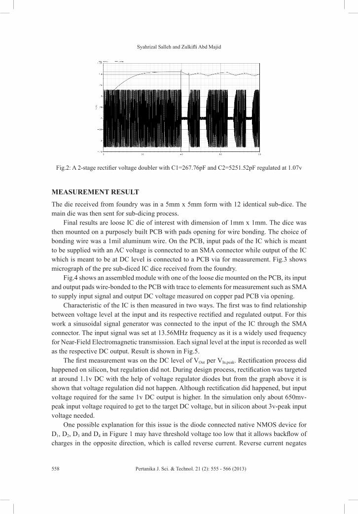
Syahrizal Salleh and Zulkifli Abd Majid
558 Pertanika J. Sci. & Technol. 21 (2): 555 - 566 (2013)
MEASUREMENT RESULT
The die received from foundry was in a 5mm x 5mm form with 12 identical sub-dice. The main die was then sent for sub-dicing process.
Final results are loose IC die of interest with dimension of 1mm x 1mm. The dice was then mounted on a purposely built PCB with pads opening for wire bonding. The choice of bonding wire was a 1mil aluminum wire. On the PCB, input pads of the IC which is meant to be supplied with an AC voltage is connected to an SMA connector while output of the IC which is meant to be at DC level is connected to a PCB via for measurement. Fig.3 shows micrograph of the pre sub-diced IC dice received from the foundry.
Fig.4 shows an assembled module with one of the loose die mounted on the PCB, its input and output pads wire-bonded to the PCB with trace to elements for measurement such as SMA to supply input signal and output DC voltage measured on copper pad PCB via opening.
Characteristic of the IC is then measured in two ways. The first was to find relationship between voltage level at the input and its respective rectified and regulated output. For this work a sinusoidal signal generator was connected to the input of the IC through the SMA connector. The input signal was set at 13.56MHz frequency as it is a widely used frequency for Near-Field Electromagnetic transmission. Each signal level at the input is recorded as well as the respective DC output. Result is shown in Fig.5.
The first measurement was on the DC level of VOut per VIn,peak. Rectification process did happened on silicon, but regulation did not. During design process, rectification was targeted at around 1.1v DC with the help of voltage regulator diodes but from the graph above it is shown that voltage regulation did not happen. Although rectification did happened, but input voltage required for the same 1v DC output is higher. In the simulation only about 650mv-peak input voltage required to get to the target DC voltage, but in silicon about 3v-peak input voltage needed.
One possible explanation for this issue is the diode connected native NMOS device for D1, D2, D3 and D4 in Figure 1 may have threshold voltage too low that it allows backflow of charges in the opposite direction, which is called reverse current. Reverse current negates
Fig.2: A 2-stage rectifier voltage doubler with C1=267.76pF and C2=5251.52pF regulated at 1.07v
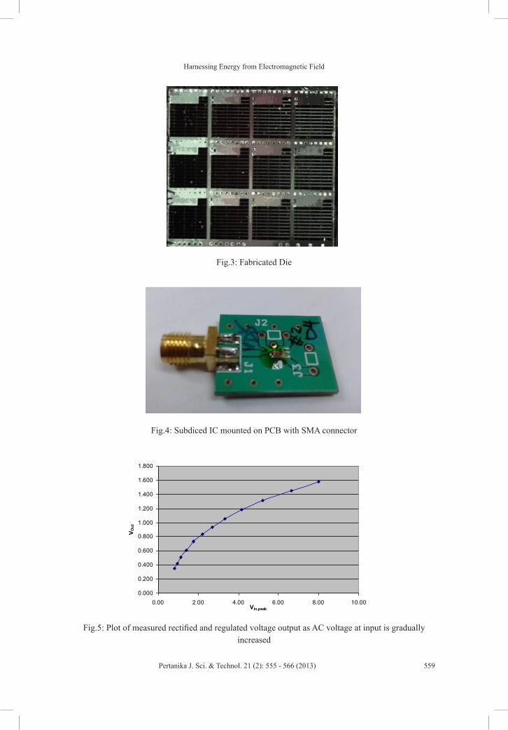
Harnessing Energy from Electromagnetic Field
559Pertanika J. Sci. & Technol. 21 (2): 555 - 566 (2013)
Fig.3: Fabricated Die
0.000
0.200
0.400
0.600
0.800
1.000
1.200
1.400
1.600
1.800
0.00 2.00 4.00 6.00 8.00 10.00Vin,peak
V Out
Fig.4: Subdiced IC mounted on PCB with SMA connector
Fig.5: Plot of measured rectified and regulated voltage output as AC voltage at input is gradually increased
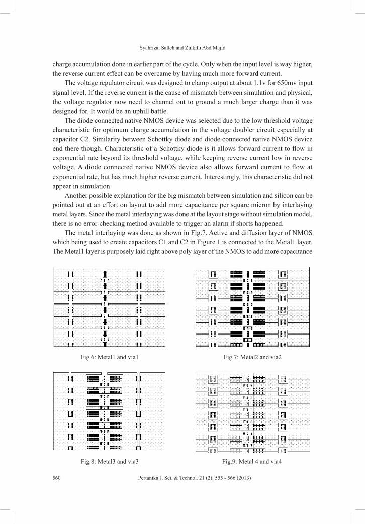
Syahrizal Salleh and Zulkifli Abd Majid
560 Pertanika J. Sci. & Technol. 21 (2): 555 - 566 (2013)
charge accumulation done in earlier part of the cycle. Only when the input level is way higher, the reverse current effect can be overcame by having much more forward current.
The voltage regulator circuit was designed to clamp output at about 1.1v for 650mv input signal level. If the reverse current is the cause of mismatch between simulation and physical, the voltage regulator now need to channel out to ground a much larger charge than it was designed for. It would be an uphill battle.
The diode connected native NMOS device was selected due to the low threshold voltage characteristic for optimum charge accumulation in the voltage doubler circuit especially at capacitor C2. Similarity between Schottky diode and diode connected native NMOS device end there though. Characteristic of a Schottky diode is it allows forward current to flow in exponential rate beyond its threshold voltage, while keeping reverse current low in reverse voltage. A diode connected native NMOS device also allows forward current to flow at exponential rate, but has much higher reverse current. Interestingly, this characteristic did not appear in simulation.
Another possible explanation for the big mismatch between simulation and silicon can be pointed out at an effort on layout to add more capacitance per square micron by interlaying metal layers. Since the metal interlaying was done at the layout stage without simulation model, there is no error-checking method available to trigger an alarm if shorts happened.
The metal interlaying was done as shown in Fig.7. Active and diffusion layer of NMOS which being used to create capacitors C1 and C2 in Figure 1 is connected to the Metal1 layer. The Metal1 layer is purposely laid right above poly layer of the NMOS to add more capacitance
Fig.6: Metal1 and via1 Fig.7: Metal2 and via2
Fig.8: Metal3 and via3 Fig.9: Metal 4 and via4
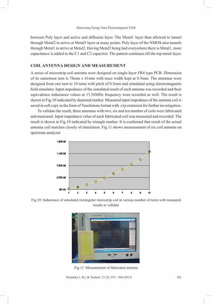
Harnessing Energy from Electromagnetic Field
561Pertanika J. Sci. & Technol. 21 (2): 555 - 566 (2013)
between Poly layer and active and diffusion layer. The Metal1 layer then allowed to tunnel through Metal2 to arrive at Metal3 layer at many points. Poly layer of the NMOS also tunnels through Metal1 to arrive at Metal2. Having Metal2 being laid everywhere there is Metal1, more capacitance is added to the C1 and C2 capacitor. The pattern continues till the top metal layer.
COIL ANTENNA DESIGN AND MEASUREMENT
A series of microstrip coil antenna were designed on single-layer FR4 type PCB. Dimension of its outermost turn is 78mm x 41mm with trace width kept at 0.5mm. The antennas were designed from one turn to 10 turns with pitch of 0.5mm and simulated using electromagnetic field simulator. Input impedance of the simulated result of each antenna was recorded and their equivalence inductance values at 13.56MHz frequency were recorded as well. The result is shown in Fig.10 indicated by diamond marker. Measured input impedance of the antenna coil is saved in soft copy in the form of Touchstone format with .s1p extension for further investigation.
To validate the result, three antennas with two, six and ten number of coils were fabricated and measured. Input impedance value of each fabricated coil was measured and recorded. The result is shown in Fig.10 indicated by triangle marker. It is confirmed that result of the actual antenna coil matches closely of simulation. Fig.11 shows measurement of six coil antenna on spectrum analyzer.
Fig.10: Inductance of simulated rectangular microstrip coil at various number of turns with measured results to validate
Fig.11: Measurement of fabricated antenna

Syahrizal Salleh and Zulkifli Abd Majid
562 Pertanika J. Sci. & Technol. 21 (2): 555 - 566 (2013)
THEORY
Equivalent circuit of the antenna coil and the fabricated IC is shown in Fig.12. The resistance RL and capacitance CL is the component of the integrated circuit input impedance while the capacitance CCoil, RCoil and LCoil are components of the antenna coil.
The integrated rectifier and regulator circuit designed and fabricated as described in Figure 1 is modeled as RL and CL in Fig.12. From measurement, the value of RL is known at 194.4Ω while value of CL is known at 131pF at 13.56MHz frequency. In contrast, based on simulation data, value of RL is at 348.07Ω while value of CL is at 58.93pF at 13.56MHz frequency.
At resonance, all reactance of components CL, CCoil and externally connected CExt is a complex conjugate of reactance value of LCoil. What’s left are real impedance RL and RCoil. The final circuit at resonance is as in Fig.13. Finding VL, input voltage to the integrated circuit is just a matter of voltage divider.
According to Constantine (1997), when an electromagnetic plane waves impinges upon a coil antenna, an open circuit voltage developed. The open circuit voltage is referred to as VOC and shown in Fig.13. The supply voltage VOC is defined in Constantine (1997) as
2 aOC ocV j V j B Nω ω π= = ∗ [2]
where πa2 is the area inside the circular coil, N is number of turns in the coil and B is the incident magnetic flux density. Since for this case, rectangular coil antenna is used instead, some deliberate modification to the equation is needed. Also, most literature describes generated
RL CL CCoil LCoilR‘CoilCExt
AC VOC
R‘Coil
R L
+
-
VL
Fig.12: Equivalence circuit using Thevenin’s
Fig.13: Equivalence circuit at resonance

Harnessing Energy from Electromagnetic Field
563Pertanika J. Sci. & Technol. 21 (2): 555 - 566 (2013)
field in electromagnetic field (H) term more than in magnetic field (B) term. Thus, the final VOC equation that will be used here is
0 OC eff nV j H Aω π= ∗Σ [3]
where n is the number of turn, An is area of the rectangle of interest and µ0 is vacuum permeability. At Heff of 3A/m (rms), VOC for each turn case is presented in Table 1.
TABLE 1 Area of antenna at each turns of coil and expected VOC
N A VOC (rms) VOC (p-p)5 1.37 x 10⁻² 4.41 v 6.24 v4 1.14 x 10⁻² 3.67 v 5.19 v3 8.90 x 10⁻³ 2.86 v 4.04 v2 6.16 x 10⁻³ 1.98 v 2.80 v1 3.20 x 10⁻³ 1.03 v 1.45 v
For better understanding on distance between the field generating antenna and receiving antenna, ISO 10373-7 standard is used for some insight. In the standard, the field generating antenna for testing is defined as a circular coil with two turns and radius of 150mm. The standard also defined that typical operating distance as 37.5mm at H of 150mA/m rms. Using Biot-Savart equation as below
2
2 32
(I N R )H(R +z)
= [3]
where R is the radius of the coil, N is number of turns and z is the distance from center of the coil perpendicular to the plane of the coil.
Rearranging the equation reveals that to get the electromagnetic field strength of 150mA/m as described in the standard require 0.55 Ampere of AC current injected into the coil. Rearranging the equation again, this time for distance z, we have a plot as in graph as in Fig.14.
IC AND ANTENNA INTEGRATION
As mentioned in the Theory section, VL, the input voltage to the integrated circuit is a divided voltage of VOC. For that reason this section is dedicated to establishing value of R’Coil at resonance. Since value of RL is known from measurement, ratio of VL to VOC can be established easily.
In the spirit of saving time and cost, further measurements were done in system simulator. Touchstone file format of each component which was stored during measurement stage can be read by system simulator such as ADS. External capacitor, CExt, was added to the input port of the receiving antenna’s Touchstone model in system simulator. The CExt is parallel to the
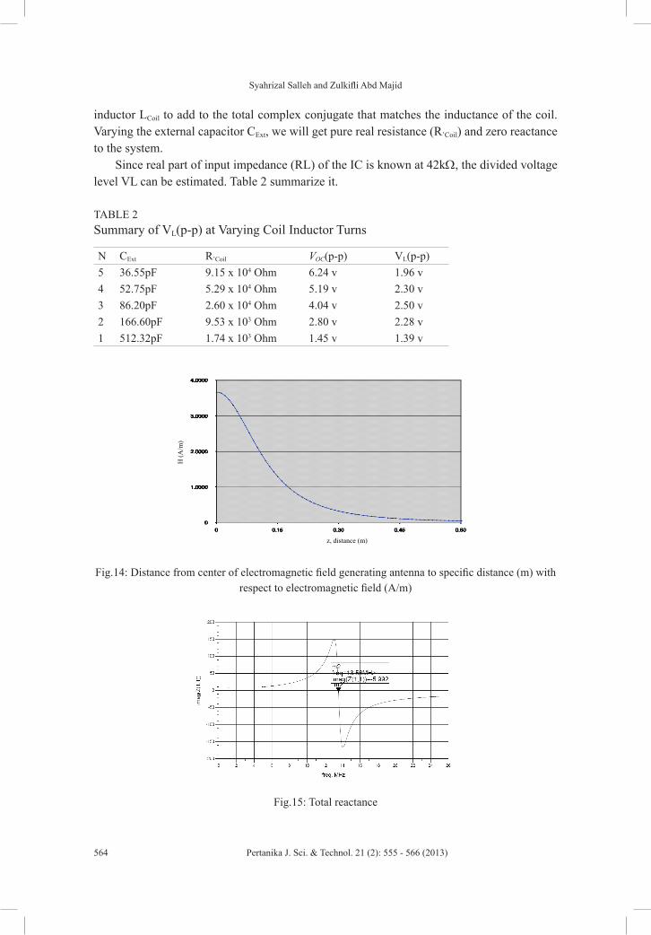
Syahrizal Salleh and Zulkifli Abd Majid
564 Pertanika J. Sci. & Technol. 21 (2): 555 - 566 (2013)
inductor LCoil to add to the total complex conjugate that matches the inductance of the coil. Varying the external capacitor CExt, we will get pure real resistance (R’Coil) and zero reactance to the system.
Since real part of input impedance (RL) of the IC is known at 42kΩ, the divided voltage level VL can be estimated. Table 2 summarize it.
TABLE 2 Summary of VL(p-p) at Varying Coil Inductor Turns
N CExt R’Coil VOC(p-p) VL(p-p)5 36.55pF 9.15 x 10⁴ Ohm 6.24 v 1.96 v4 52.75pF 5.29 x 10⁴ Ohm 5.19 v 2.30 v3 86.20pF 2.60 x 10⁴ Ohm 4.04 v 2.50 v2 166.60pF 9.53 x 10³ Ohm 2.80 v 2.28 v1 512.32pF 1.74 x 10³ Ohm 1.45 v 1.39 v
H(A
/m)
z, distance (m)
Fig.15: Total reactance
Fig.14: Distance from center of electromagnetic field generating antenna to specific distance (m) with respect to electromagnetic field (A/m)
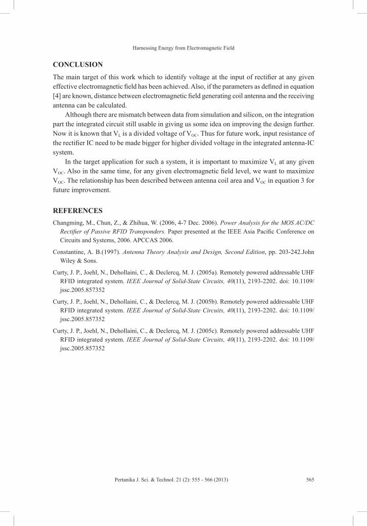
Harnessing Energy from Electromagnetic Field
565Pertanika J. Sci. & Technol. 21 (2): 555 - 566 (2013)
CONCLUSION
The main target of this work which to identify voltage at the input of rectifier at any given effective electromagnetic field has been achieved. Also, if the parameters as defined in equation [4] are known, distance between electromagnetic field generating coil antenna and the receiving antenna can be calculated.
Although there are mismatch between data from simulation and silicon, on the integration part the integrated circuit still usable in giving us some idea on improving the design further. Now it is known that VL is a divided voltage of VOC. Thus for future work, input resistance of the rectifier IC need to be made bigger for higher divided voltage in the integrated antenna-IC system.
In the target application for such a system, it is important to maximize VL at any given VOC. Also in the same time, for any given electromagnetic field level, we want to maximize VOC. The relationship has been described between antenna coil area and VOC in equation 3 for future improvement.
REFERENCESChangming, M., Chun, Z., & Zhihua, W. (2006, 4-7 Dec. 2006). Power Analysis for the MOS AC/DC
Rectifier of Passive RFID Transponders. Paper presented at the IEEE Asia Pacific Conference on Circuits and Systems, 2006. APCCAS 2006.
Constantine, A. B.(1997). Antenna Theory Analysis and Design, Second Edition, pp. 203-242.John Wiley & Sons.
Curty, J. P., Joehl, N., Dehollaini, C., & Declercq, M. J. (2005a). Remotely powered addressable UHF RFID integrated system. IEEE Journal of Solid-State Circuits, 40(11), 2193-2202. doi: 10.1109/jssc.2005.857352
Curty, J. P., Joehl, N., Dehollaini, C., & Declercq, M. J. (2005b). Remotely powered addressable UHF RFID integrated system. IEEE Journal of Solid-State Circuits, 40(11), 2193-2202. doi: 10.1109/jssc.2005.857352
Curty, J. P., Joehl, N., Dehollaini, C., & Declercq, M. J. (2005c). Remotely powered addressable UHF RFID integrated system. IEEE Journal of Solid-State Circuits, 40(11), 2193-2202. doi: 10.1109/jssc.2005.857352

Pertanika J. Sci. & Technol. 21 (2): 567 - 580 (2013)
SCIENCE & TECHNOLOGYJournal homepage: http://www.pertanika.upm.edu.my/
ISSN: 0128-7680 © 2013 Universiti Putra Malaysia Press.
INTRODUCTION
The surging price of cure oil, together with environmental issue has been encouraging many countries to seek alternative fuels. Since 2004, Indonesia becomes a net importer of crude oil. Some alternatives energy sources have been developed, such as Gas and coal,
Palm Oil Transesterification Processing to Biodiesel Using a Combine of Ultrasonic and Chemical Catalyst
Supranto, S.Chemical Engineering Department, Gadjah Mada University, Jalan Grafika 2, 55281 Yogyakarta, Indonesia
ABSTRACT
A combination of ultrasonic and chemical catalyst affects to the transesterification reaction rate of palm oil conversion to biodiesel is investigated in a 5 Liter capacity reactor equipped with the heater and temperature controller and the 42 Hz ultrasonic generator of 35 watt with process parameters of (a) reaction temperature, (b) methanol to palm oil ratio, (c) and the amount of chemical catalyst and (d) duration of the ultrasonic activation. The result shows that by combining the ultrasonic and chemical catalyst in the palm oil transesterification processing increases the chemical reaction rate, the higher the frequency of the ultrasonic activation used, the higher the biodiesel conversion.The transesterification operating process condition of 60 to 70 oC, Methanol to palm oil ratio of 5, reaction duration time of 60 minute, and catalyst activation of 30 minute, using a 42 KHz , 35 watt ultrasonic, may be applied to produce biodiesel with a conversion as high as 94% for palm oil feed stock and 91% for coconut oil feedstock
Keywords: Biodiesel, palm oil, transesterification, ultrasonic, chemical catalyst
Article history:Received: 26 December 2011Accepted: 15 March 2012
E-mail address: [email protected] (Supranto, S.)
Hydropower, Geothermal and Biofuel. Two well-known biofuels commercially produced are biodiesel and bioethanol. As a large agricultural country, Indonesia has very big potential to produce biofuel. Currently, most biodiesel is commercially produced from vegetable oils by transesterification / esterification reaction. This is the most common process technology of biodiesel that proven in the world.The detailed process of biodiesel production varies between one another depending on licensor. However, the
Supranto, S.
568 Pertanika J. Sci. & Technol. 21 (2): 567 - 580 (2013)
principle of process is similar which consisting of esterification transesterification reaction followed by glycerol separation and then ester (biodiesel) purification.
The Indonesia domestic consumption of fuel oil has been increasing steadily, while the production of fuel oil and its availability tends to decrease. The continued reliance on fossil fuel for fulfilling national energy demand has to be gradually decreased by utilizing other energy sources including agricultural products. Developing biofuel is a must for Indonesia due to several reasons including the abundance availability of feed stocks, its potential to improve air quality in big cities and its potential to reduce the poverty in rural areas. Two well-known biofuels commercially produced are biodiesel and bioethanol. In the year 2010, petroleum solar oil consumption in Indonesia is about 28 million kilo Liters and petroleum diesel oil is more than 300 kilo Liters. This means that for 10% of biodiesel mixture with 90% petroleum solar or diesel oil (B10), there will be a demand of more than 2.8 million tons of biodiesel per year in 2010. This is huge demand for biodiesel in Indonesia (Biodiesel Research Group, 2007). The technology for producing biodiesel from vegetable oil need to be developed and improved. The use of combining of the ultrasonic and chemical catalyst is introduced in this paper.
SELECTION OF BIODIESEL FEEDSTOCK
The advantage of biodiesel over fossil fuel is its sulfur free, so that its flue gas can be easily controlled and environmentally friendly. The Kyoto Protocol signed in 1997 requires, from the European Union (EU), a commitment to reduce, between 2008 and 2012, greenhouse gas emissions by 8% from their 1990 level. One of the instruments chosen by the EU Commission to achieve these results is reported in the Directive 2003/30/EU, which states that, starting from 2010, at least 5.75% of the fuel used for driving engines in a number of EU states should come from renewable sources. However, it is well-known that biodiesel must be mixed with diesel or solar oil if it is to be used for combustion engine, with the usage range from 5%(B5) to 40% (B40) of biodiesel. Although 100% of biodiesel can also be used directly to the engine but this is not common practice. Problems associated with the use of vegetable oils as fuel were oil deterioration and incomplete combustion. Polyunsaturated fatty acids were very susceptible to polymerization and gum formation caused by oxidation during storage or by complex oxidative and thermal polymerization at the higher temperature and pressure of combustion. The gum did not combust completely, resulting in carbon deposits and lubricating oil thickening. To overcome these problems the oil requires slight chemical modification mainly transesterification, pyrolysis and emulsification. Among these, the transesterification is the key and foremost important step to produce the cleaner and environmentally safe fuel from vegetable oils (Biodiesel Research Group, 2007).
Currently, most biodiesel is commercially produced from vegetable oils by transesterification / esterification. This is the most common process technology of biodiesel that proven in the world. In the reaction, the oil and alcohol are reacted to produce alkyl esters (biodiesel). Methanol is used as the alcohol for commercially producing biodiesel because it is the least expensive alcohol. Hence, methanol is important raw material for biodiesel, with its demand in Indonesia being around 280,000 ton per year.

Palm Oil Transesterification Processing to Biodiesel
569Pertanika J. Sci. & Technol. 21 (2): 567 - 580 (2013)
Process technology of a biodiesel plant depends upon the quality of the feedstock, the plant capacity and the quality requirements for finished biodiesel. It is well known, transesterification or esterification is an equilibrium reaction. To ensure the increase of triglyceride conversion, an excess of alcohol is used. The minimum equivalent ratio of alcohol to vegetable oil is three.
The biodiesel research conducted in Gadjah Mada University Yogyakarta Indonesia was started in 1980’s. The vegetable oil processed were rubber seed oil, peanut oil, castor oil, nyamplung seed oil, jatropha curcas oil, palm oil, kapuk seed oil, and candlenut oil etc. The equivalent ratio of alcohol (ethanol or methanol) to vegetable oil is in the range of 3 to 14. The higher the equivalent ratio of alcohol to vegetable oil, the higher the conversion is, but the cost of alcohol recovery is also higher. An excessive amount of alcohol also makes the recovery of glycerol difficult, so the optimum ratio of alcohol to oil has to be established, considering each individual process (Biodiesel Research Group, 2007; Supranto, 2003, 2004)). Some researchers (Supranto, 2004; Freedman et al., 1986; Encinar et al., 2005) found the molar ration of 6 : 1 of methanol to oil gave the best conversion. Moreover Freedman et al. (1984) studies the effect of molar ratio on ester conversion with vegetable oils such as soybean, sunflower, peanut and cotton seed oils behaved similarly and achieved highest conversions (93 – 98%) at 6 : 1 molar ratio. The similar results have been found for transesterification of rubber seed oil with methanol (Mustanginah, 2006).
CPO is recently verry attractive to be converted to biodiesel, although CPO based biodiesel is a bit unsuitable in European countries. Other potential raw materials for biodiesel are abundant in Indonesia, including coconut oil and Jathropa Curcas. Until 2005, increasing planting area was observed not only in Jatropha but also Oil Palm and Peanut. Increasing oil palm planting area is due to the world demand for oil palm edible oil that increases every year and there is enough suitable land across the country (Supranto, 2010).
A. Palm Oil
Crude palm oil can be processed to produce many product derivatives which are very important in supporting different types of industry. Indonesian government has targeted to enlarge oil palm area till 18 millions tons in 2010. The oil palm planting area since 2000 has been spread out in Sumatra, Kalimantan, Sulawesi and Papua. Until 2005, North Sumatra and Riau dominate the area in the country in almost 1 million ha each. Riau has the largest oil palm area in the country, though the local production in North Sumatra is higher. The productivity of oil palm in North Sumatra is the best across the country. The production can reach 3785 ton/ha/year of bunch (Biodiesel Research Group, 2007).
B. Coconut
The use of oil palm to produce edible oil has affected the development of Coconut planting area. Though the total number of Coconut planting area increased in 2001, the planting area then has continually decreased till 2005. The reduction of Coconut planting area might be due to its cultivation being not economically visible. Many estates have changed their Coconut to other profitable estate crop such as oil palm. Riau, Central and East Java, North Sulawesi are the area of coconut. Coconut can be found in the back yard and dry land field especially in the

Supranto, S.
570 Pertanika J. Sci. & Technol. 21 (2): 567 - 580 (2013)
coastal side. Now days, coconut was cultivated extensively across the country, therefore the productivity seems very low. In the centre production area, the productivity can reach only 1 ton/ha. The best productivity was reported in Central Sulawesi, the highest local production was observed in Riau. The potential production of coconut is estimated to be stagnant until 2010 (Biodiesel Research Group, 2007).
C. Jathropa
Jatropha was uncultivated crop which is easily founded in the fence of field or backyard. Jatropha can be grown in different types of land. In the marginal land such as unfertile dry land area, it can produce enough seed. In the national level, the planting area of jatropha in 2000 was only 12807 ha. Lampung, Java, Nusa Tenggara and Central Kalimantan were the place where jatropha was easily seen. East Java and Nusa Tenggara which were believed as dry area have the largest planting area. Since 2000, the planting area in Lampung, Banten, Central Java, East Java and West Nusa Tenggara has no significant increased. Different situation could be seen in West Java and East Nusa Tenggara. The planting area has significantly inclined. In 2005 the planting area has 10 times multiplied. The trend of increasing planting area in West Java and East Nusa Tenggara may be due to the concern of the government in developing energy source diversification. In West Java, several research institutions have proposed jatropha as energy source alternatives, therefore many field researches may be conducted in the area. Field action research may also been executed in East Nusa Tenggara due to the dry climate in the area (Biodiesel Research Group, 2007).
Increasing planting area has not been followed by the increase of seed production. Different effect can be observed between West Java and East Nusa Tenggara. Though the productivity in these two areas right now is considered very low, West Java can maintain its productivity. Different result has been founded in East Nusa Tenggara; increasing planting area may even reduce the productivity. This phenomenon might be caused by the condition that the cultivation technology was still missing. The potency to increase national seed production is still possible because there is a very large suitable area and government support policy.
Indonesia has very big potential to produce biodiesel doe to the fact that Indonesia is the second largest Crude Palm Oil (CPO) producer in the world and also has a very large area of Coconut plantation. About 75% of the product CPO is exported as crude material. CPO is recently the most attractive followed by the Coconut oil to be converted to biodiesel, although CPO based biodiesel is a bit unsuitable in European countries. The development of technology for producing biodiesel from Palm and Coconut Oil are need to done such as by combining the use of ultrasonic and chemical catalyst to increase its rate processes.
EXPERIMENTAL RESULT AND DISCUSSION
A. Experimental Work
The objective of experimental work of converting palm and coconut oil to biodiesel using a combine ultrasonic and chemical catalyst was to identify the suitable process condition,
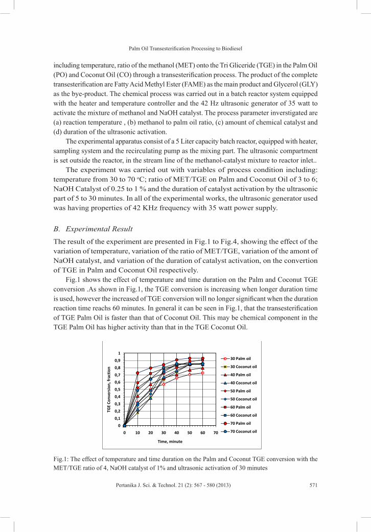
Palm Oil Transesterification Processing to Biodiesel
571Pertanika J. Sci. & Technol. 21 (2): 567 - 580 (2013)
including temperature, ratio of the methanol (MET) onto the Tri Gliceride (TGE) in the Palm Oil (PO) and Coconut Oil (CO) through a transesterification process. The product of the complete transesterification are Fatty Acid Methyl Ester (FAME) as the main product and Glycerol (GLY) as the bye-product. The chemical process was carried out in a batch reactor system equipped with the heater and temperature controller and the 42 Hz ultrasonic generator of 35 watt to activate the mixture of methanol and NaOH catalyst. The process parameter inverstigated are (a) reaction temperature , (b) methanol to palm oil ratio, (c) amount of chemical catalyst and (d) duration of the ultrasonic activation.
The experimental apparatus consist of a 5 Liter capacity batch reactor, equipped with heater, sampling system and the recirculating pump as the mixing part. The ultrasonic compartment is set outside the reactor, in the stream line of the methanol-catalyst mixture to reactor inlet..
The experiment was carried out with variables of process condition including: temperature from 30 to 70 oC; ratio of MET/TGE on Palm and Coconut Oil of 3 to 6; NaOH Catalyst of 0.25 to 1 % and the duration of catalyst activation by the ultrasonic part of 5 to 30 minutes. In all of the experimental works, the ultrasonic generator used was having properties of 42 KHz frequency with 35 watt power supply.
B. Experimental Result
The result of the experiment are presented in Fig.1 to Fig.4, showing the effect of the variation of temperature, variation of the ratio of MET/TGE, variation of the amont of NaOH catalyst, and variation of the duration of catalyst activation, on the convertion of TGE in Palm and Coconut Oil respectively.
Fig.1 shows the effect of temperature and time duration on the Palm and Coconut TGE conversion .As shown in Fig.1, the TGE conversion is increasing when longer duration time is used, however the increased of TGE conversion will no longer significant when the duration reaction time reachs 60 minutes. In general it can be seen in Fig.1, that the transesterification of TGE Palm Oil is faster than that of Coconut Oil. This may be chemical component in the TGE Palm Oil has higher activity than that in the TGE Coconut Oil.
0
0,1
0,2
0,3
0,4
0,5
0,6
0,7
0,8
0,9
1
0 10 20 30 40 50 60 70
TGE
Conv
ersi
on, f
ract
ion
Time, minute
30 Palm oil
30 Coconut oil
40 Palm oil
40 Coconut oil
50 Palm oil
50 Coconut oil
60 Palm oil
60 Coconut oil
70 Palm oil
70 Coconut oil
Fig.1: The effect of temperature and time duration on the Palm and Coconut TGE conversion with the MET/TGE ratio of 4, NaOH catalyst of 1% and ultrasonic activation of 30 minutes
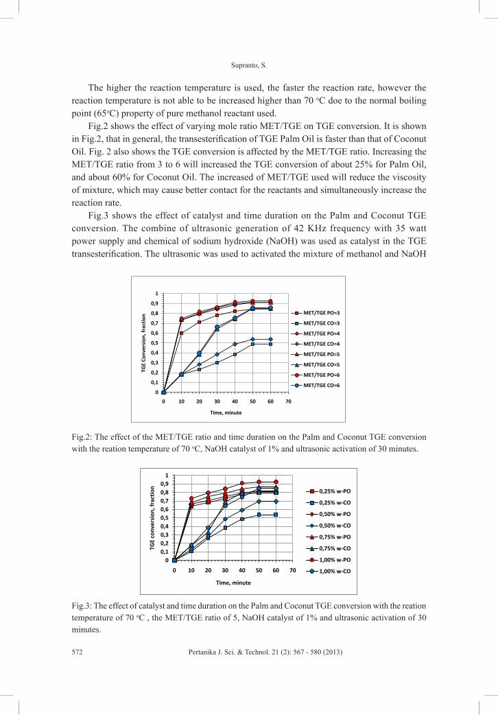
Supranto, S.
572 Pertanika J. Sci. & Technol. 21 (2): 567 - 580 (2013)
The higher the reaction temperature is used, the faster the reaction rate, however the reaction temperature is not able to be increased higher than 70 oC doe to the normal boiling point (65oC) property of pure methanol reactant used.
Fig.2 shows the effect of varying mole ratio MET/TGE on TGE conversion. It is shown in Fig.2, that in general, the transesterification of TGE Palm Oil is faster than that of Coconut Oil. Fig. 2 also shows the TGE conversion is affected by the MET/TGE ratio. Increasing the MET/TGE ratio from 3 to 6 will increased the TGE conversion of about 25% for Palm Oil, and about 60% for Coconut Oil. The increased of MET/TGE used will reduce the viscosity of mixture, which may cause better contact for the reactants and simultaneously increase the reaction rate.
Fig.3 shows the effect of catalyst and time duration on the Palm and Coconut TGE conversion. The combine of ultrasonic generation of 42 KHz frequency with 35 watt power supply and chemical of sodium hydroxide (NaOH) was used as catalyst in the TGE transesterification. The ultrasonic was used to activated the mixture of methanol and NaOH
0
0,1
0,2
0,3
0,4
0,5
0,6
0,7
0,8
0,9
1
0 10 20 30 40 50 60 70
TGE
Conv
ersi
on, f
ract
ion
Time, minute
MET/TGE PO=3
MET/TGE CO=3
MET/TGE PO=4
MET/TGE CO=4
MET/TGE PO=5
MET/TGE CO=5
MET/TGE PO=6
MET/TGE CO=6
Fig.2: The effect of the MET/TGE ratio and time duration on the Palm and Coconut TGE conversion with the reation temperature of 70 oC, NaOH catalyst of 1% and ultrasonic activation of 30 minutes.
00,10,20,30,40,50,60,70,80,9
1
0 10 20 30 40 50 60 70
TGE
conv
ersi
on, f
ract
ion
Time, minute
0,25% w-PO
0,25% w-CO
0,50% w-PO
0,50% w-CO
0,75% w-PO
0,75% w-CO
1,00% w-PO
1,00% w-CO
Fig.3: The effect of catalyst and time duration on the Palm and Coconut TGE conversion with the reation temperature of 70 oC , the MET/TGE ratio of 5, NaOH catalyst of 1% and ultrasonic activation of 30 minutes.
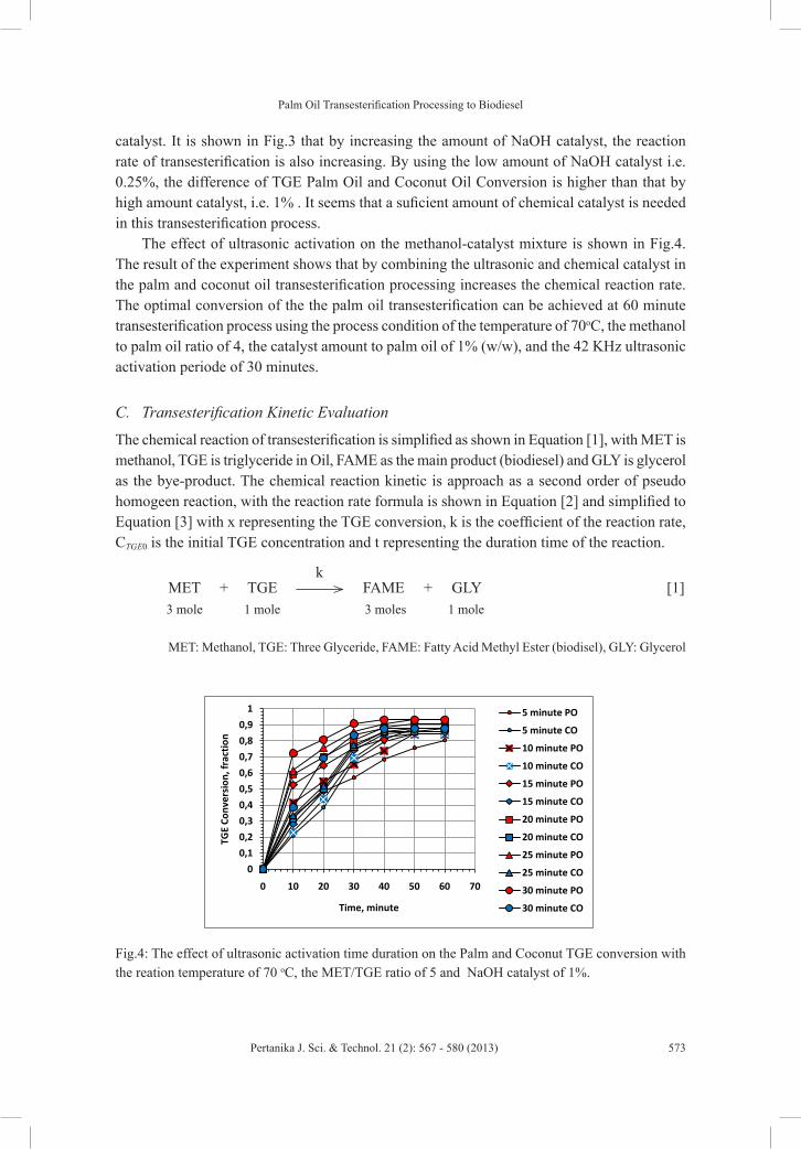
Palm Oil Transesterification Processing to Biodiesel
573Pertanika J. Sci. & Technol. 21 (2): 567 - 580 (2013)
catalyst. It is shown in Fig.3 that by increasing the amount of NaOH catalyst, the reaction rate of transesterification is also increasing. By using the low amount of NaOH catalyst i.e. 0.25%, the difference of TGE Palm Oil and Coconut Oil Conversion is higher than that by high amount catalyst, i.e. 1% . It seems that a suficient amount of chemical catalyst is needed in this transesterification process.
The effect of ultrasonic activation on the methanol-catalyst mixture is shown in Fig.4. The result of the experiment shows that by combining the ultrasonic and chemical catalyst in the palm and coconut oil transesterification processing increases the chemical reaction rate. The optimal conversion of the the palm oil transesterification can be achieved at 60 minute transesterification process using the process condition of the temperature of 70oC, the methanol to palm oil ratio of 4, the catalyst amount to palm oil of 1% (w/w), and the 42 KHz ultrasonic activation periode of 30 minutes.
C. Transesterification Kinetic Evaluation
The chemical reaction of transesterification is simplified as shown in Equation [1], with MET is methanol, TGE is triglyceride in Oil, FAME as the main product (biodiesel) and GLY is glycerol as the bye-product. The chemical reaction kinetic is approach as a second order of pseudo homogeen reaction, with the reaction rate formula is shown in Equation [2] and simplified to Equation [3] with x representing the TGE conversion, k is the coefficient of the reaction rate, CTGE0 is the initial TGE concentration and t representing the duration time of the reaction.
MET + TGE FAME + GLY [1]
MET: Methanol, TGE: Three Glyceride, FAME: Fatty Acid Methyl Ester (biodisel), GLY: Glycerol
0
0,1
0,2
0,3
0,4
0,5
0,6
0,7
0,8
0,9
1
0 10 20 30 40 50 60 70
TGE
Conv
ersi
on, f
ract
ion
Time, minute
5 minute PO
5 minute CO
10 minute PO
10 minute CO
15 minute PO
15 minute CO
20 minute PO
20 minute CO
25 minute PO
25 minute CO
30 minute PO
30 minute CO
Fig.4: The effect of ultrasonic activation time duration on the Palm and Coconut TGE conversion with the reation temperature of 70 oC, the MET/TGE ratio of 5 and NaOH catalyst of 1%.
k
3 mole 1 mole 3 moles 1 mole
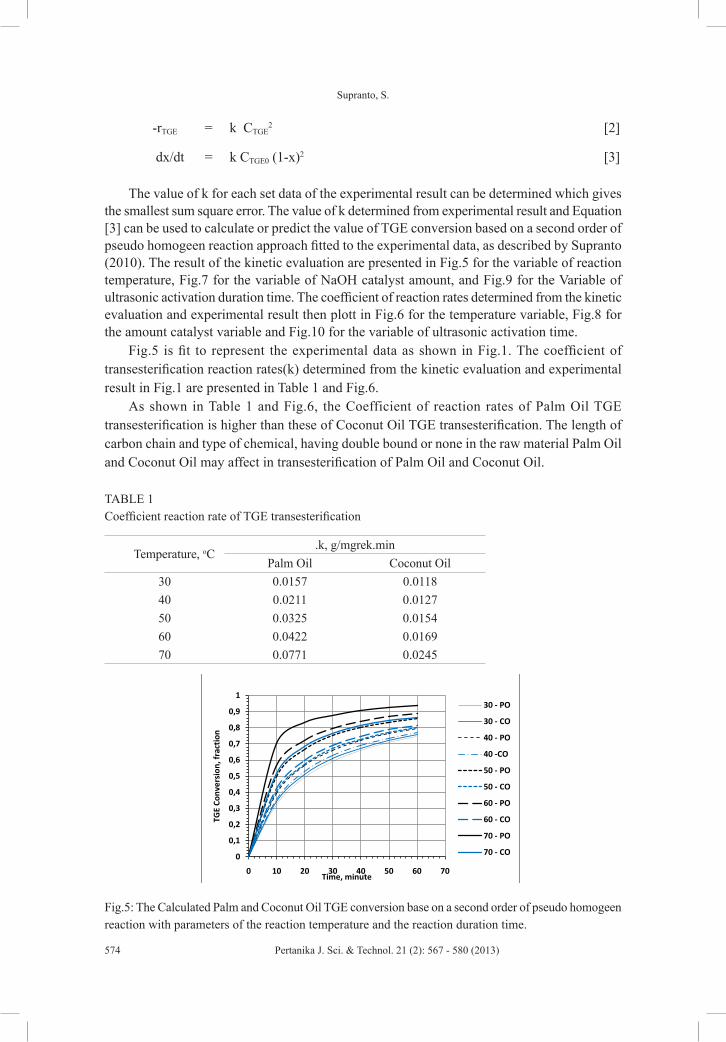
Supranto, S.
574 Pertanika J. Sci. & Technol. 21 (2): 567 - 580 (2013)
-rTGE = k CTGE2 [2]
dx/dt = k CTGE0 (1-x)2 [3]
The value of k for each set data of the experimental result can be determined which gives the smallest sum square error. The value of k determined from experimental result and Equation [3] can be used to calculate or predict the value of TGE conversion based on a second order of pseudo homogeen reaction approach fitted to the experimental data, as described by Supranto (2010). The result of the kinetic evaluation are presented in Fig.5 for the variable of reaction temperature, Fig.7 for the variable of NaOH catalyst amount, and Fig.9 for the Variable of ultrasonic activation duration time. The coefficient of reaction rates determined from the kinetic evaluation and experimental result then plott in Fig.6 for the temperature variable, Fig.8 for the amount catalyst variable and Fig.10 for the variable of ultrasonic activation time.
Fig.5 is fit to represent the experimental data as shown in Fig.1. The coefficient of transesterification reaction rates(k) determined from the kinetic evaluation and experimental result in Fig.1 are presented in Table 1 and Fig.6.
As shown in Table 1 and Fig.6, the Coefficient of reaction rates of Palm Oil TGE transesterification is higher than these of Coconut Oil TGE transesterification. The length of carbon chain and type of chemical, having double bound or none in the raw material Palm Oil and Coconut Oil may affect in transesterification of Palm Oil and Coconut Oil.
TABLE 1 Coefficient reaction rate of TGE transesterification
Temperature, oC.k, g/mgrek.min
Palm Oil Coconut Oil30 0.0157 0.011840 0.0211 0.012750 0.0325 0.015460 0.0422 0.016970 0.0771 0.0245
0
0,1
0,2
0,3
0,4
0,5
0,6
0,7
0,8
0,9
1
0 10 20 30 40 50 60 70
TGE
Conv
ersi
on, f
ract
ion
Time, minute
30 - PO
30 - CO
40 - PO
40 -CO
50 - PO
50 - CO
60 - PO
60 - CO
70 - PO
70 - CO
Fig.5: The Calculated Palm and Coconut Oil TGE conversion base on a second order of pseudo homogeen reaction with parameters of the reaction temperature and the reaction duration time.
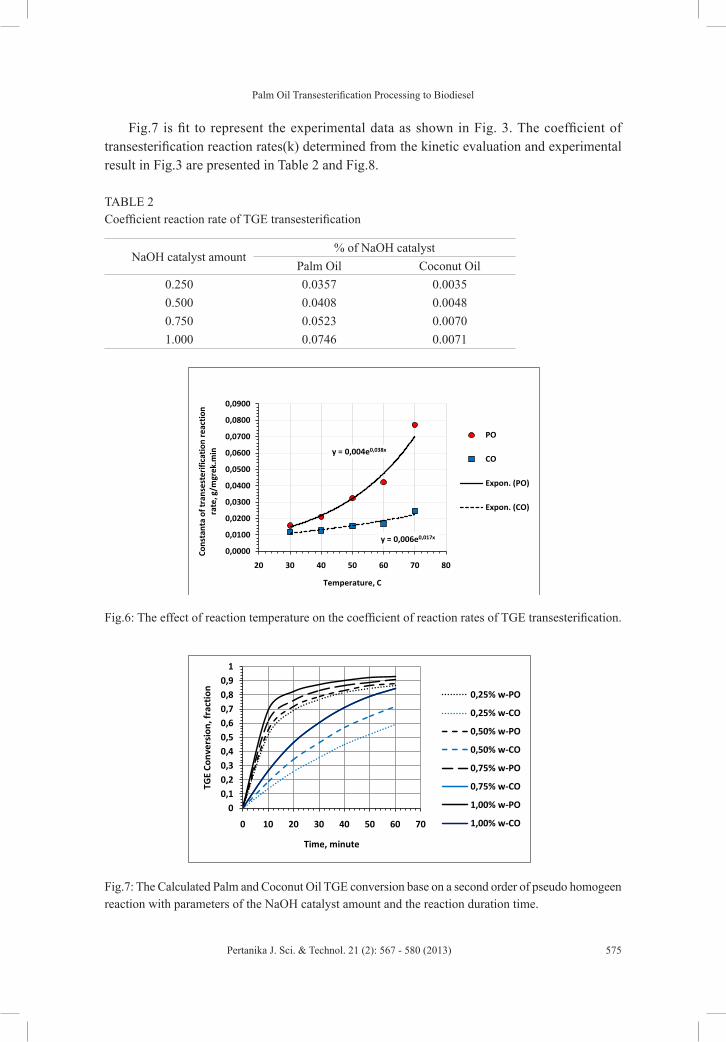
Palm Oil Transesterification Processing to Biodiesel
575Pertanika J. Sci. & Technol. 21 (2): 567 - 580 (2013)
Fig.7 is fit to represent the experimental data as shown in Fig. 3. The coefficient of transesterification reaction rates(k) determined from the kinetic evaluation and experimental result in Fig.3 are presented in Table 2 and Fig.8.
TABLE 2 Coefficient reaction rate of TGE transesterification
NaOH catalyst amount% of NaOH catalyst
Palm Oil Coconut Oil0.250 0.0357 0.00350.500 0.0408 0.00480.750 0.0523 0.00701.000 0.0746 0.0071
y = 0,004e0,038x
y = 0,006e0,017x
0,0000
0,0100
0,0200
0,0300
0,0400
0,0500
0,0600
0,0700
0,0800
0,0900
20 30 40 50 60 70 80
Cons
tant
a of
tran
sest
erifi
cati
on r
eact
ion
rate
, g/m
grek
.min
Temperature, C
PO
CO
Expon. (PO)
Expon. (CO)
00,10,20,30,40,50,60,70,80,9
1
0 10 20 30 40 50 60 70
TGE
Conv
ersi
on, f
ract
ion
Time, minute
0,25% w-PO
0,25% w-CO
0,50% w-PO
0,50% w-CO
0,75% w-PO
0,75% w-CO
1,00% w-PO
1,00% w-CO
Fig.6: The effect of reaction temperature on the coefficient of reaction rates of TGE transesterification.
Fig.7: The Calculated Palm and Coconut Oil TGE conversion base on a second order of pseudo homogeen reaction with parameters of the NaOH catalyst amount and the reaction duration time.
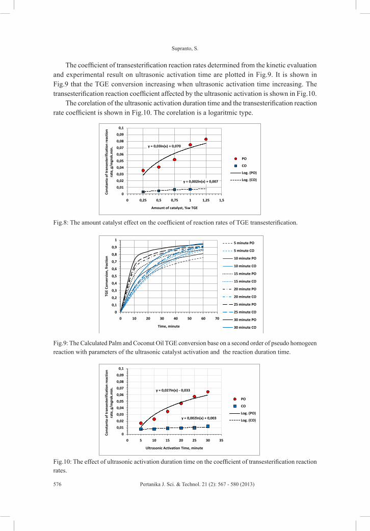
Supranto, S.
576 Pertanika J. Sci. & Technol. 21 (2): 567 - 580 (2013)
The coefficient of transesterification reaction rates determined from the kinetic evaluation and experimental result on ultrasonic activation time are plotted in Fig.9. It is shown in Fig.9 that the TGE conversion increasing when ultrasonic activation time increasing. The transesterification reaction coefficient affected by the ultrasonic activation is shown in Fig.10.
The corelation of the ultrasonic activation duration time and the transesterification reaction rate coefficient is shown in Fig.10. The corelation is a logaritmic type.
y = 0,03ln(x) + 0,070
y = 0,002ln(x) + 0,007
0
0,01
0,02
0,03
0,04
0,05
0,06
0,07
0,08
0,09
0,1
0 0,25 0,5 0,75 1 1,25 1,5
Cons
tant
a of
tran
sest
erifi
cati
on r
eact
ion
rate
, g/m
grek
.min
.
Amount of catalyst, %w TGE
PO
CO
Log. (PO)
Log. (CO)
0
0,1
0,2
0,3
0,4
0,5
0,6
0,7
0,8
0,9
1
0 10 20 30 40 50 60 70
TGE
Conv
ersi
on, f
ract
ion
Time, minute
5 minute PO
5 minute CO
10 minute PO
10 minute CO
15 minute PO
15 minute CO
20 minute PO
20 minute CO
25 minute PO
25 minute CO
30 minute PO
30 minute CO
y = 0,027ln(x) - 0,033
y = 0,002ln(x) + 0,003
0
0,01
0,02
0,03
0,04
0,05
0,06
0,07
0,08
0,09
0,1
0 5 10 15 20 25 30 35
Cons
tant
a of
tran
sest
erifi
cati
on r
eact
ion
rate
, g/m
grek
.min
.
Ultrasonic Activation Time, minute
PO
CO
Log. (PO)
Log. (CO)
Fig.8: The amount catalyst effect on the coefficient of reaction rates of TGE transesterification.
Fig.9: The Calculated Palm and Coconut Oil TGE conversion base on a second order of pseudo homogeen reaction with parameters of the ultrasonic catalyst activation and the reaction duration time.
Fig.10: The effect of ultrasonic activation duration time on the coefficient of transesterification reaction rates.
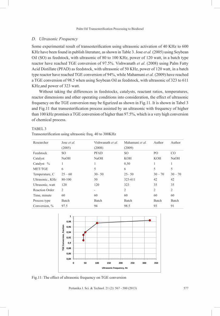
Palm Oil Transesterification Processing to Biodiesel
577Pertanika J. Sci. & Technol. 21 (2): 567 - 580 (2013)
D. Ultrasonic Frequency
Some experimental result of transesterification using ultrasonic activation of 40 KHz to 600 KHz have been found in publish literature, as shown in Table 3. Jose et al. (2005) using Soybean Oil (SO) as feedstock, with ultrasonic of 80 to 100 KHz, power of 120 watt, in a batch type reactor have reached TGE conversion of 97.5%. Vishwanath et al. (2008) using Palm Fatty Acid Distillate (PFAD) as feedstock, with ultrasonic of 50 KHz, power of 120 watt, in a batch type reactor have reached TGE conversion of 94%, while Mahamuni et al. (2009) have reached a TGE conversion of 98.5 when using Soybean Oil as feedstock, with ultrasonic of 323 to 611 KHz,and power of 323 watt.
Without taking the differences in feedstocks, catalysts, reactant ratios, temperatures, reactor dimensions and other operating conditions into consideration, the effect of ultrasonic frequency on the TGE conversion may be figurized as shown in Fig.11. It is shown in Tabel 3 and Fig.11 that transesterification process assisted by an ultrasonic with frequency of higher than 100 kHz promises a TGE conversion of higher than 97.5%, which is a very high conversion of chemical process.
TABEL 3 Transesterification using ultrasonic freq. 40 to 300KHz
Researcher Jose et al. (2005)
Vishwanath et al. (2008)
Mahamuni et al. (2009)
Author Author
Feedstock SO PFAD SO PO COCatalyst NaOH NaOH KOH KOH NaOHCatalyst % 1 1 0,50 1 1MET/TGE 6 5 6 5 5Temperature, C 25 – 60 30– 50 25– 50 30 – 70 30 – 70Ultrasonic., KHz 80-100 50 323-611 42 42Ultrasonic, watt 120 120 323 35 35Reaction Order 2 - 2 2 2Time, minute 60 60 60 60 60Process type Batch Batch Batch Batch BatchConversion, % 97.5 94 98.5 93 91
0,84
0,86
0,88
0,9
0,92
0,94
0,96
0,98
1
0 50 100 150 200 250 300 350
TGE
Conv
ersi
on, f
ract
ion
Ultrasonic frequency, Hz
Fig.11: The effect of ultrasonic frequency on TGE conversion
Supranto, S.
578 Pertanika J. Sci. & Technol. 21 (2): 567 - 580 (2013)
CONCLUSION
From the experimental result and the literature study some conclusion may be sumerized as follow:
1. The transesterification process of Palm and Coconut Oil using methanol with an ultrasonic and chemical catalyst of NaOH follows a reaction kinetic of order 2. The reaction rate coefficient of palm oil transesterification is almost 10 time higher than that of coconut oil.
2. The corelation of the temperature and the transesterification reaction coefficient is an exponential type, while the ultrasonic activation and catalyst related to the transesterification reaction coefficient is of logaritmic corelation type.
3. The transesterification operating process condition of 60 to 70 oC, MET/TGE ratio of 5, reaction duration time of 60 minute, and catalyst activation of 30 minute, using a 42 KHz, 35 watt ultrasonic, may be applied to produce biodiesel with conversion as high as 94% for palm oil feed stock and 91% for coconut oil feedstock.
4. In general the higher the frequency of the ultrasonic activation, the higher the conversion of the TGE to bodiesel. Hovewer the use of ultrasonic frequency higher than 400 KHz is not recomended doe to a very high of electric energy consumption.
ACKNOWLEDGEMENTS
Author would like to thank to the Indonesia government c.q. the Ministry of research and technology, for the financial support of this research through an Insentif Research Program 2010 “Pengembangan propelan berbasis material nabati”.
REFERENCES Biodiesel Research Group. (2007). Guide line for investment on biodiesel plant in Indonesia. Final Report
by the Department of Chemical Engineering, Gadjah Mada University, Indonesia, 2007.
Colucci, J., Borrero, E., & Alape, F. (2005). Biodiesel from an alkaline transesterification reaction of soybean oil using ultrasonic mixing. Journal of the American Oil Chemists’ Society, 82(7), 525-530.
Deshmane, V. G., Gogate, P. R., & Pandit, A. B. (2008). Ultrasound-Assisted Synthesis of Biodiesel from Palm Fatty Acid Distillate. Industrial & Engineering Chemistry Research, 48(17), 7923-7927.
Encinar, J. M., González, J. F., & Rodríguez-Reinares, A. (2005). Biodiesel from Used Frying Oil. Variables Affecting the Yields and Characteristics of the Biodiesel. Industrial & Engineering Chemistry Research, 44(15), 5491-5499.
Freedman, B., Butterfield, R. O., & Pryde, E. H. (1986). Transesterification Kinetics of Soybean, Oil, J. Am. Oil. Chem. Soc, 63, 1375-1380.
Freedman, B., Pryde, E. H., & Mounts, T. L. (1984). Variables affecting the yields of fatty esters from transesterified vegetable oils. Journal of the American Oil Chemists Society, 61(10), 1638-1643.
Mahamuni, N. N., & Adewuyi, Y. G. (2009). Optimization of the Synthesis of Biodiesel via Ultrasound-Enhanced Base-Catalyzed Transesterification of Soybean Oil Using a Multifrequency Ultrasonic Reactor. Energy & Fuels, 23(5), 2757-2766.

Palm Oil Transesterification Processing to Biodiesel
579Pertanika J. Sci. & Technol. 21 (2): 567 - 580 (2013)
Mustanginah, U. (2006). Etanolisis Katalitik pada Minyak Biji Karet (In Indonesian). Laporan Penelitian Laboratorium Proses Kimia, Universitas Gadjah Mada, Yogyakarta, 2006.
Supranto, S. (2003). The biodiesel process production from crude palm oil. In the proceeding of the 2nd Regional Conference on Energy Toward a Clean Environment, Phuket, Thailand, 12-14 February 2003.
Supranto, S. (2004). Pre-design of the flow process diagram of the biodisel production from palm oil fatty acid distillate. Paper presented at the Regional Symposium of the Chemical Engineer 2004, Bangkok, King Mongkut University, Thailand, December 1st -3rd, 2004.
Supranto, S. (2005). The biodiesel production process from vegetable oil. Asia-Pasific Journal of Chemical Engineering, Developments in Chemical Engineering and Mineral Processing, Special Issue: Special Theme Issue: Bioprocess and Environmental Biotechnology Research, 13(5-6), 687–692.
Supranto, S. (2010). Selection of the oil feedstock for Indonesia biodiesel production. In the proceeding of the 2nd AUN/SEED-Net Regional Conference on New/Renewable Energy, Faculty of Engineering, Burapha University, Thailand, January 21-22, 2010.

Pertanika J. Sci. & Technol. 21 (2): 581 - 588 (2013)
SCIENCE & TECHNOLOGYJournal homepage: http://www.pertanika.upm.edu.my/
ISSN: 0128-7680 © 2013 Universiti Putra Malaysia Press.
INTRODUCTION
Bioelectricity production using microbial fuel cells (MFCs) has drawn much attention recently as a future renewable energy production (Lovley, 2006). Electricity can
Electricity Generation from Citronella Bagasse (CB) Using Dual Chamber Microbial Fuel Cell
Nik Azmi Nik Mahmood1*, Mohd Nazlee Faisal Md Ghazali1, Kamarul’Asri Ibrahim2 and Nur Muhammad ElQarni Md Norodin1
1Department of Bioprocess Engineering, Faculty of Chemical Engineering, Universiti Teknologi Malaysia, 81310 Skudai, Johor, Malaysia2Department of Chemical Engineering, Faculty of Chemical Engineering, Universiti Teknologi Malaysia, 81310 Skudai, Johor, Malaysia
ABSTRACT
The aim of this project is to produce electricity from citronella biomass using isolated microbes from wastewater as biocatalyst in a dual chamber microbial fuel cell (MFC). MFC is one such system that not only reduced biomass, which contains mostly waste products but can also liberate electricity from them. MFC system is well-established and using lignocellulosic biomass as fuel is one step to future energy generation. Trials of MFC experiments have been conducted but using citronella bagasse (CB) as fuel source. Furthermore, pre-treatment of the biomass was done using NaOH pre-treament and effluent treatment wastewater from a palm edible oil company as a source for microorganism. The end results indicate that bioelectricity production from CB is possible though very low yield in the present MFC.
Keywords: Microbial fuel cell, citronella bagasse, bioelectricity
Article history:Received: 26 December 2011Accepted: 15 March 2012
E-mail addresses: [email protected] (Nik Azmi Nik Mahmood), [email protected] (Mohd Nazlee Faisal Md Ghazali), [email protected] (Kamarul’Asri Ibrahim), [email protected] (Nur Muhammad ElQarni Md Norodin)*Corresponding Author
be generated in MFCs using many types of substrates mainly any form of biodegradable organic matters (Pant et al., 2010). Simple carbohydrates such as glucose, sucrose, xylose and polymeric starch have been utilized as fuel for electricity generation using a dual-chambered MFCs, proved to be successful though at low yield production (Catal et al., 2008; Behera & Ghangrekar, 2009; Niessen et al., 2004). In contrast, though extracting bioelectricity from lignocellulosic biomass is not new but advances are rather slow in terms of development compare to biofuel
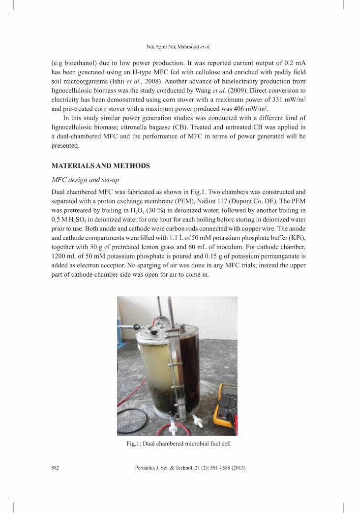
Nik Azmi Nik Mahmood et al.
582 Pertanika J. Sci. & Technol. 21 (2): 581 - 588 (2013)
(e.g bioethanol) due to low power production. It was reported current output of 0.2 mA has been generated using an H-type MFC fed with cellulose and enriched with paddy field soil microorganisms (Ishii et al., 2008). Another advance of bioelectricity production from lignocellulosic biomass was the study conducted by Wang et al. (2009). Direct conversion to electricity has been demonstrated using corn stover with a maximum power of 331 mW/m2 and pre-treated corn stover with a maximum power produced was 406 mW/m2.
In this study similar power generation studies was conducted with a different kind of lignocellulosic biomass; citronella bagasse (CB). Treated and untreated CB was applied in a dual-chambered MFC and the performance of MFC in terms of power generated will be presented.
MATERIALS AND METHODS
MFC design and set-up
Dual chambered MFC was fabricated as shown in Fig.1. Two chambers was constructed and separated with a proton exchange membrane (PEM), Nafion 117 (Dupont Co. DE). The PEM was pretreated by boiling in H2O2 (30 %) in deionized water, followed by another boiling in 0.5 M H2SO4 in deionized water for one hour for each boiling before storing in deionized water prior to use. Both anode and cathode were carbon rods connected with copper wire. The anode and cathode compartments were filled with 1.1 L of 50 mM potassium phosphate buffer (KPi), together with 50 g of pretreated lemon grass and 60 mL of inoculum. For cathode chamber, 1200 mL of 50 mM potassium phosphate is poured and 0.15 g of potassium permanganate is added as electron acceptor. No sparging of air was done in any MFC trials; instead the upper part of cathode chamber side was open for air to come in.
Fig.1: Dual chambered microbial fuel cell

Electricity Generation from Citronella Bagasse (CB) Using Dual Chamber Microbial Fuel Cell
583Pertanika J. Sci. & Technol. 21 (2): 581 - 588 (2013)
Inoculum preparation
Wastewater taken from Anfil Tower (anaerobic tank), Effluent Treatment Plant, Pan Century Edible Oil (M) Sdn Bhd, Pasir Gudang was kept in refrigerated condition before used. The wastewater was added into a dual chambered MFC anode and acetate (20 mM) was used as an energy source for enhancing bacterial growth. After period of time (3 months of enrichment), the inoculum was centrifuged at 6000 rpm, 10 minutes and 4 ˚C which supernatant was discarded and pellet was resuspended by adding 20 mL of autoclaved 50 mM potassium phosphate buffer (pH 7.0) for each of the inoculum without any other modifications such as pH adjustment or addition of nutrients or trace-metals.
CB pre-treatment
CB leaves was oven-dried prior to use. The CB was ground in using household blender, subsequently sieved to obtain particle sizes of 0.25 mm to 1.0 mm. 50 g of grinded CB was mixed with 0.75 (w/v) % of NaOH solution and autoclaved for 15 min, under 121C and 15 psi. The pre-treated CB was recovered by filtration through porcelain Buchner funnel and was washed with several times of distilled water (approximately 4 L) to neutralize the pH. The pre-treated CB was immediately added to MFC. All CB was freshly pre-treated in every MFC operations.Pre-treated CB was analyzed for compositional content (cellulose, hemicelluloses and lignin) using standard analysis (Han & Rowell, 1996).
Calculation
Voltages produced by MFCs were recorded every 2 hrs using digital multimeter with data recorder (Fluke, USA). Current density (i, A/m2) was calculated according to Ohm’s Law i = V/RA, where V (V) is the voltage measured, R (Ω) is the external resistance, and A (m2) is the projected surface area of the anode. Power density was calculated as P (mW/m2) = 1000iV, where 1000 is needed for the given units.
RESULTS AND DISCUSSION
CB pre-treatment
Lignocellulosic biomass like CB can be used as the substrate in MFC. In fact, it is the promising feedstock for cost effective energy production. Anyway, it has to be pre-treated first to remove lignin, hemicelluloses and reduce the crystallinity of cellulose so that bacteria can utilize this biomass as substrate (Kumar et al., 2009). Before pre-treatment, dry CB was analyzed and its composition determined as of 29.64 % hemicellulose, 35.05 % cellulose, 19.81 % lignin, and 17.53 % others including extractives and ash. After the pre-treatment procedure, which was combination of diluted NaOH and steam hydrolysis, only 4.1 % of the cellulose was removed and more than 80 % of lignin and hemicelluloses was removed (data not shown). The composition of xylan, mannan and arabinan, that made up the hemicellulose component were not further detected since this study only focused on the reaction of the cellulose component. The chemical composition of the citronella in this study was slightly different from citronella reported by Rolz et al. (1986). The remaining cellulose was used for MFC trials.
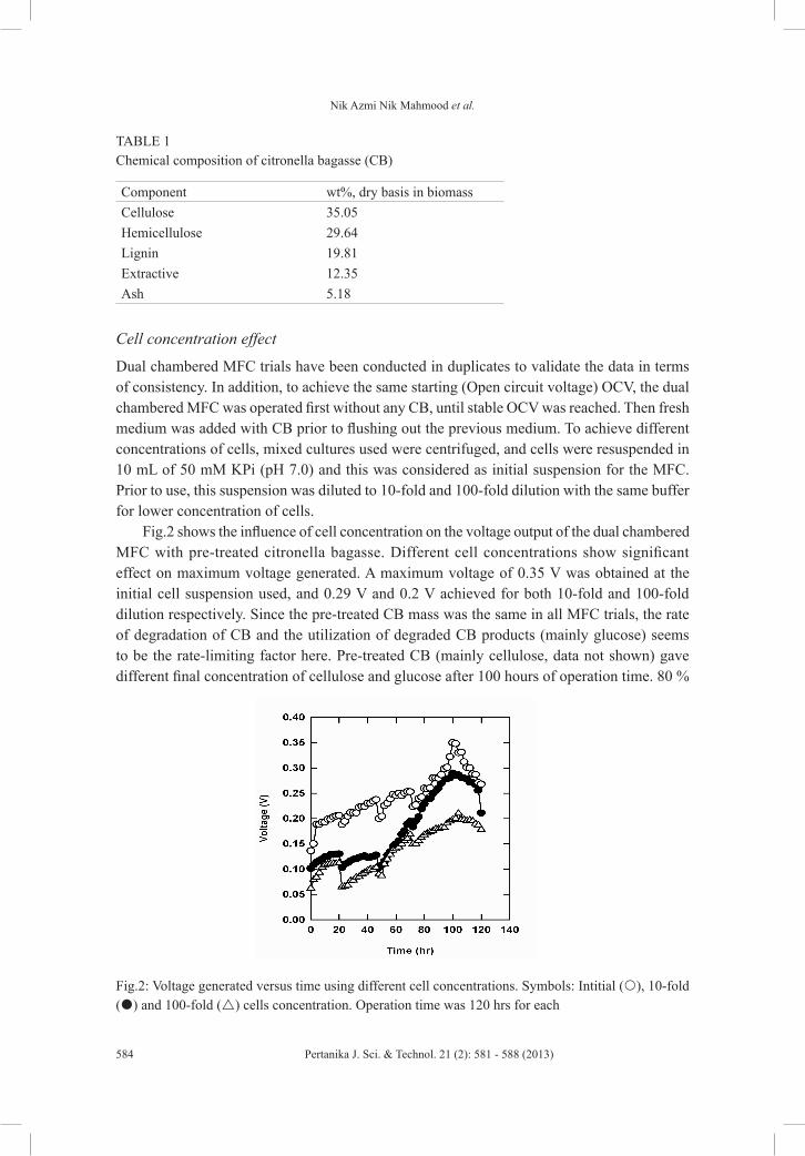
Nik Azmi Nik Mahmood et al.
584 Pertanika J. Sci. & Technol. 21 (2): 581 - 588 (2013)
TABLE 1 Chemical composition of citronella bagasse (CB)
Component wt%, dry basis in biomassCellulose 35.05Hemicellulose 29.64Lignin 19.81Extractive 12.35Ash 5.18
Cell concentration effect
Dual chambered MFC trials have been conducted in duplicates to validate the data in terms of consistency. In addition, to achieve the same starting (Open circuit voltage) OCV, the dual chambered MFC was operated first without any CB, until stable OCV was reached. Then fresh medium was added with CB prior to flushing out the previous medium. To achieve different concentrations of cells, mixed cultures used were centrifuged, and cells were resuspended in 10 mL of 50 mM KPi (pH 7.0) and this was considered as initial suspension for the MFC. Prior to use, this suspension was diluted to 10-fold and 100-fold dilution with the same buffer for lower concentration of cells.
Fig.2 shows the influence of cell concentration on the voltage output of the dual chambered MFC with pre-treated citronella bagasse. Different cell concentrations show significant effect on maximum voltage generated. A maximum voltage of 0.35 V was obtained at the initial cell suspension used, and 0.29 V and 0.2 V achieved for both 10-fold and 100-fold dilution respectively. Since the pre-treated CB mass was the same in all MFC trials, the rate of degradation of CB and the utilization of degraded CB products (mainly glucose) seems to be the rate-limiting factor here. Pre-treated CB (mainly cellulose, data not shown) gave different final concentration of cellulose and glucose after 100 hours of operation time. 80 %
Fig.2: Voltage generated versus time using different cell concentrations. Symbols: Intitial (), 10-fold () and 100-fold () cells concentration. Operation time was 120 hrs for each
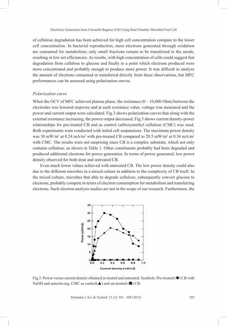
Electricity Generation from Citronella Bagasse (CB) Using Dual Chamber Microbial Fuel Cell
585Pertanika J. Sci. & Technol. 21 (2): 581 - 588 (2013)
of cellulose degradation has been achieved for high cell concentration compare to the lower cell concentration. In bacterial reproduction, most electrons generated through oxidation are consumed for metabolism; only small fractions remain to be transferred to the anode, resulting in low net efficiencies. As results, with high concentration of cells could suggest fast degradation from cellulose to glucose and finally to a point which electrons produced were more concentrated and probably enough to produce more power. It was difficult to analyze the amount of electrons consumed or transferred directly from these observations, but MFC performances can be assessed using polarization curves.
Polarization curve
When the OCV of MFC achieved plateau phase, the resistance (0 – 10,000 Ohm) between the electrodes was lowered stepwise and at each resistance value, voltage was measured and the power and current output were calculated. Fig.3 shows polarization curves that along with the external resistance increasing, the power output decreased. Fig.3 shows current density-power relationships for pre-treated CB and as control carboxymethyl cellulose (CMC) was used. Both experiments were conducted with initial cell suspensions. The maximum power density was 30 mW/m2 at 0.24 mA/m2 with pre-treated CB compared to 20.5 mW/m2 at 0.36 mA/m2 with CMC. The results were not surprising since CB is a complex substrate, which not only contains cellulose, as shown in Table 1. Other constituents probably had been degraded and produced additional electrons for power generation. In terms of power generated, low power density observed for both treat and untreated CB.
Even much lower values achieved with untreated CB. The low power density could also due to the different microbes in a mixed culture in addition to the complexity of CB itself. In the mixed culture, microbes that able to degrade cellulose, subsequently convert glucose to electrons, probably compete in terms of electron consumption for metabolism and transferring electrons. Such electron analysis studies are not in the scope of our research. Furthermore, the
Fig.3: Power versus current density obtained in treated and untreated. Symbols: Pre-treated () CB with NaOH and autoclaving, CMC as control() and un-treated () CB.
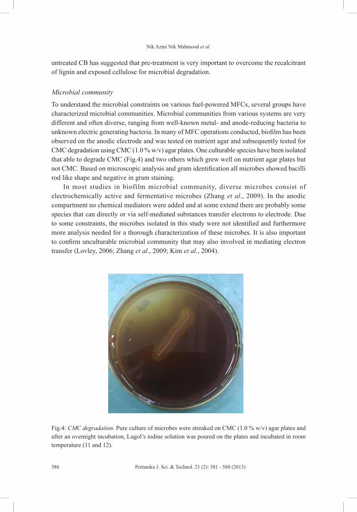
Nik Azmi Nik Mahmood et al.
586 Pertanika J. Sci. & Technol. 21 (2): 581 - 588 (2013)
untreated CB has suggested that pre-treatment is very important to overcome the recalcitrant of lignin and exposed cellulose for microbial degradation.
Microbial community
To understand the microbial constraints on various fuel-powered MFCs, several groups have characterized microbial communities. Microbial communities from various systems are very different and often diverse, ranging from well-known metal- and anode-reducing bacteria to unknown electric generating bacteria. In many of MFC operations conducted, biofilm has been observed on the anodic electrode and was tested on nutrient agar and subsequently tested for CMC degradation using CMC (1.0 % w/v) agar plates. One culturable species have been isolated that able to degrade CMC (Fig.4) and two others which grew well on nutrient agar plates but not CMC. Based on microscopic analysis and gram identification all microbes showed bacilli rod like shape and negative in gram staining.
In most studies in biofilm microbial community, diverse microbes consist of electrochemically active and fermentative microbes (Zhang et al., 2009). In the anodic compartment no chemical mediators were added and at some extend there are probably some species that can directly or via self-mediated substances transfer electrons to electrode. Due to some constraints, the microbes isolated in this study were not identified and furthermore more analysis needed for a thorough characterization of these microbes. It is also important to confirm unculturable microbial community that may also involved in mediating electron transfer (Lovley, 2006; Zhang et al., 2009; Kim et al., 2004).
Fig.4: CMC degradation. Pure culture of microbes were streaked on CMC (1.0 % w/v) agar plates and after an overnight incubation, Lugol’s iodine solution was poured on the plates and incubated in room temperature (11 and 12).
Electricity Generation from Citronella Bagasse (CB) Using Dual Chamber Microbial Fuel Cell
587Pertanika J. Sci. & Technol. 21 (2): 581 - 588 (2013)
CONCLUSION
It was demonstrated that citronella bagasse (CB) could be used as a substrate for electricity generation in dual chambered MFC. CB is a complex biomass and difficult to be utilized biologically. The power densities produced were not high enough compare to other substrates and not comparable with those achieved with glucose. In order to increase performance of MFC and production of electricity, more studies should be made in terms of efficiency of CB saccharification (more glucose produced) and optimization of degradation of CB.
ACKNOWLEDGEMENTS
We would like to express our gratitude to Lee Chun Meng and Azmi Fidzyana for their work in CB pre-treatment study. Special thanks for Ministry of Science and Technology (Electrogenesis study of microbial based fuel cell. FRGS, vote No. 78462) the support in funding the present work. We also like to thank Universiti Teknologi Malaysia for their commitment in facilitating the progress of the work.
REFERENCESAbu Bakar, N. K., Abd Aziz, S., Hassan, M. A., & F. M. Ghazali. (2010). Isolation and selection of
appropriate cellulolytic mixed microbial cultures for cellulases production from oil palm empty fruit bunch. Biotechnology, 9(1), 73 – 78.
Behera, M., & Ghangrekar, M. M. (2009). Performance of microbial fuel cell in response to change in sludge loading rate at different anodic feed pH. Bioresource Technology, 100(21), 5114-5121.
Catal, T., Li, K., Bermek, H., & Liu, H. (2008). Electricity production from twelve monosaccharides using microbial fuel cells. Journal of Power Sources, 175(1), 196-200.
Han, J. S., & Rowell, S. (1996) Chemical composition of fibers. In Rowell, R. M., Young, R. M., & Rowell, J. M. (Eds.), Chapter 5: Paper and Composites from agro-based resource (pp. 83-134). Boca Raton, FL: CRC/Lewis Publishers.
Ishii, S., Shimoyama, T., Hotta, Y., & Watanabe, K. (2008). Characterization of a filamentous biofilm community established in a cellulose-fed microbial fuel cell. BMC Microbiol, 8, 6. doi: 10.1186/1471-2180-8-6
Kim, B. H., Park, H. S., Kim, H. J., Kim, G. T., Chang, I. S., Lee, J., & Phung, N. T. (2004). Enrichment of microbial community generating electricity using a fuel-cell-type electrochemical cell. Appl Microbiol Biotechnol, 63(6), 672-681.
Kumar, P., Barrett, D. M., Delwiche, M. J., & Stroeve, P. (2009). Methods for Pretreatment of Lignocellulosic Biomass for Efficient Hydrolysis and Biofuel Production. Industrial & Engineering Chemistry Research, 48(8), 3713-3729.
Lovley, D. R. (2006). Microbial fuel cells: novel microbial physiologies and engineering approaches. Curr Opin Biotechnol, 17(3), 327-332.
Maki, M. L., Broere, M., Leung, K. T., & Qin, W. (2011). Characterization of some efficient cellulase producing bacteria isolated from paper mill sludges and organic fertilizers. Int J Biochem Mol Biol, 2(2), 146-154.

Nik Azmi Nik Mahmood et al.
588 Pertanika J. Sci. & Technol. 21 (2): 581 - 588 (2013)
Niessen, J., Schröder, U., & Scholz, F. (2004). Exploiting complex carbohydrates for microbial electricity generation – a bacterial fuel cell operating on starch. Electrochemistry Communications, 6(9), 955-958.
Pant, D., Van Bogaert, G., Diels, L., & Vanbroekhoven, K. (2010). A review of the substrates used in microbial fuel cells (MFCs) for sustainable energy production. Bioresource Technology, 101(6), 1533-1543.
Rolz, C., de Arriola, M. C., Valladares, J., & de Cabrera, S. (1986). Effects of some physical and chemical pretreatments on the composition and enzymatic hydrolysis and digestibility of lemon grass and citronella bagasse. Agricultural Wastes, 18(2), 145-161.
Wang, X., Feng, Y., Wang, H., Qu, Y., Yu, Y., Ren, N., Li, N., Wang, E., Lee, H., & Logan, B. E. (2009). Bioaugmentation for electricity generation from corn stover biomass using microbial fuel cells. Environ Sci Technol, 43(15), 6088-6093.
Zhang, Y., Min, B., Huang, L., & Angelidaki, I. (2009). Generation of electricity and analysis of microbial communities in wheat-straw biomass-powered microbial fuel cell. Appl Environ Microbiol, 75(11), 3389 – 3395.
Pertanika J. Sci. & Technol. 21 (2): 589 - 600 (2013)
SCIENCE & TECHNOLOGYJournal homepage: http://www.pertanika.upm.edu.my/
ISSN: 0128-7680 © 2013 Universiti Putra Malaysia Press.
Experimental Design Analysis of Ultra Fine Fly Ash, Lime Water, and Basalt Fibre in Mix Proportion of High Volume Fly Ash Concrete
Mochamad Solikin1,2*, Sujeeva Setunge2 and Indubhushan Patnaikuni2
1Muhammadiyah University of Surakarta Indonesia, Jl. A. Yani Tromol Pos 1 Pabelan Kartasura Surakarta, Jawa Tengah 57162, Indonesia2School of Civil, Environmental and Chemical Engineering, RMIT University, Melbourne VIC 3001, Australia
ABSTRACT
This paper reports an analysis of three factors in mix proportion of high volume fly ash concrete to produce high strength concrete. The factors analyzed are type of fly ash, kind of mixing water and the utilization of basalt fibre. The type of fly ash factor comprises of the use of raw fly ash and ultra fine fly ash, whereas the kind of water consists of the use of lime water and tap water. The addition of basalt fibre to improve the ductility of high strength concrete is studied and also high strength concrete without basalt fibre is studied. To prepare the mix proportion and to analyze the compressive strength result, experimental design, a statistical method is used. In addition, the compressive strength of concrete is tested on concrete cylinder of ∅100 mm – height 200 mm at curing ages of 28 days and 56 days. The results show that the optimum mix proportion to produce high strength concrete is the mix proportion with the combination of high volume ultra fine fly ash and the use of lime water without the use of basalt fibre. Moreover, the optimum mix proportion meets the mix design of high strength concrete and has similar strength development as normal cement concrete at the age of 28 days.
Keywords: Fatigue life, composite materials, non-destructive technique
Article history:Received: 26 December 2011Accepted: 15 March 2012
E-mail addresses: [email protected] (Mochamad Solikin), [email protected] (Sujeeva Setunge), [email protected] (Indubhushan Patnaikuni)*Corresponding Author
INTRODUCTION
Based on ACI 363R-92 (1997), the ACI committee report that high strength concrete is concrete with a compressive strength greater than 6,000 psi (41 MPa) and it is widely used in many applications, including high-rise buildings, offshore structures, bridge elements, overlays, and pavements
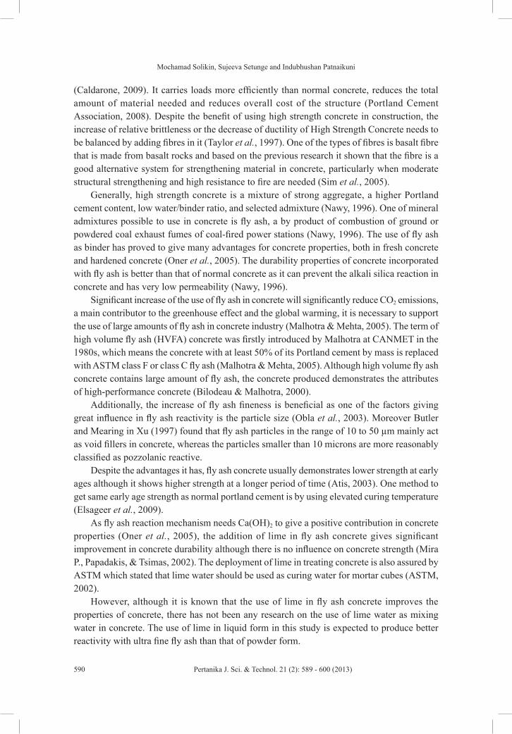
Mochamad Solikin, Sujeeva Setunge and Indubhushan Patnaikuni
590 Pertanika J. Sci. & Technol. 21 (2): 589 - 600 (2013)
(Caldarone, 2009). It carries loads more efficiently than normal concrete, reduces the total amount of material needed and reduces overall cost of the structure (Portland Cement Association, 2008). Despite the benefit of using high strength concrete in construction, the increase of relative brittleness or the decrease of ductility of High Strength Concrete needs to be balanced by adding fibres in it (Taylor et al., 1997). One of the types of fibres is basalt fibre that is made from basalt rocks and based on the previous research it shown that the fibre is a good alternative system for strengthening material in concrete, particularly when moderate structural strengthening and high resistance to fire are needed (Sim et al., 2005).
Generally, high strength concrete is a mixture of strong aggregate, a higher Portland cement content, low water/binder ratio, and selected admixture (Nawy, 1996). One of mineral admixtures possible to use in concrete is fly ash, a by product of combustion of ground or powdered coal exhaust fumes of coal-fired power stations (Nawy, 1996). The use of fly ash as binder has proved to give many advantages for concrete properties, both in fresh concrete and hardened concrete (Oner et al., 2005). The durability properties of concrete incorporated with fly ash is better than that of normal concrete as it can prevent the alkali silica reaction in concrete and has very low permeability (Nawy, 1996).
Significant increase of the use of fly ash in concrete will significantly reduce CO2 emissions, a main contributor to the greenhouse effect and the global warming, it is necessary to support the use of large amounts of fly ash in concrete industry (Malhotra & Mehta, 2005). The term of high volume fly ash (HVFA) concrete was firstly introduced by Malhotra at CANMET in the 1980s, which means the concrete with at least 50% of its Portland cement by mass is replaced with ASTM class F or class C fly ash (Malhotra & Mehta, 2005). Although high volume fly ash concrete contains large amount of fly ash, the concrete produced demonstrates the attributes of high-performance concrete (Bilodeau & Malhotra, 2000).
Additionally, the increase of fly ash fineness is beneficial as one of the factors giving great influence in fly ash reactivity is the particle size (Obla et al., 2003). Moreover Butler and Mearing in Xu (1997) found that fly ash particles in the range of 10 to 50 µm mainly act as void fillers in concrete, whereas the particles smaller than 10 microns are more reasonably classified as pozzolanic reactive.
Despite the advantages it has, fly ash concrete usually demonstrates lower strength at early ages although it shows higher strength at a longer period of time (Atis, 2003). One method to get same early age strength as normal portland cement is by using elevated curing temperature (Elsageer et al., 2009).
As fly ash reaction mechanism needs Ca(OH)2 to give a positive contribution in concrete properties (Oner et al., 2005), the addition of lime in fly ash concrete gives significant improvement in concrete durability although there is no influence on concrete strength (Mira P., Papadakis, & Tsimas, 2002). The deployment of lime in treating concrete is also assured by ASTM which stated that lime water should be used as curing water for mortar cubes (ASTM, 2002).
However, although it is known that the use of lime in fly ash concrete improves the properties of concrete, there has not been any research on the use of lime water as mixing water in concrete. The use of lime in liquid form in this study is expected to produce better reactivity with ultra fine fly ash than that of powder form.

Experimental Design Analysis of Ultra Fine Fly Ash, Lime Water, and Basalt Fibre in Mix Proportion
591Pertanika J. Sci. & Technol. 21 (2): 589 - 600 (2013)
RESEARCH SIGNIFICANCE
This research investigated the Experimental design of 3 factors in concrete mix proportion to find out the influence of those 3 factors to produce high strength concrete using high volume ultra fine fly ash. The factors analyzed are type of fly ash, kind of mixing water and the utilization of basalt fibre. Each factor comprises of 2 levels, low and high. The two levels of fly ash are the use of raw fly ash and the use of ultra fine fly ash. In addition, the two levels of mixing water are the use of tap water and the use of lime water. Moreover, the two levels of basalt fibre are the addition of basalt fibre in high strength concrete and high strength concrete without basalt fibre.
The mix proportion of concrete is based on proposed method of high performance concrete mix design (Aïtcin, 2004) for design compressive strength of 80 MPa at 28 days. The compressive strength of concrete was tested on 100 mm and 200 mm height cylinders at curing ages of 28 days and 56 days. All of the specimens were cured by immersing in a water tank with a temperature of 24oC until the day of test.
Experimental design, a statistical method, was used to prepare concrete mix proportion and to analyze the experimental results. Furthermore based on the design experimental result, a mix proportion to produce highest strength of the concrete was tested and compared with normal cement concrete.
MATERIALS
Fly ash
Fly ash for this research comes from Tarong power plant and it is classified as Low calcium fly ash or ASTM class F fly ash (Sofi et al., 2007), because the sum of SiO3 + Fe2O3 + Al2O3 is more than 70%. The chemical properties of fly ash are given in Table 1.
TABLE 1 Chemical properties of Tarong fly ash (mass %)
Tarong ASTM Class F*
SiO2 65.9The sum of SiO3 + Al2O3 + Fe2O3 min 70%Al2O3 28.89
Fe2O3 0.38TiO2 1.97MnO 0MgO 0.15CaO 0.06Na2O 0.05K2O 0.26P2O5 0.08SO3 0.03 Max, 5%LOI 1.24 Max, 6 %
*ASTM, 2003

Mochamad Solikin, Sujeeva Setunge and Indubhushan Patnaikuni
592 Pertanika J. Sci. & Technol. 21 (2): 589 - 600 (2013)
As this research investigates the influence of using raw fly ash and fine fly ash, to obtain the ultra fine fly ash the raw fly ash was ground in a Micronizer. The micronizer is a jet mill, using compressed air or gas to make high speed rotation of the particles in grinding chamber which further leads the material to have particle-on-particle impact. The micronizer can produce particle fineness ranging from 0.5 to 45 microns.
The increase of fineness of fly ash after the grinding was tested using Blaine test apparatus to find out the surface area of fly ash. The result showed that the surface area of fly ash increases from 364 m2 /kg in raw fly ash to 525 m2 /kg in ultra fine fly ash based on cement fineness. It means the fineness of fly ash increased by 40% after the grinding process using micronizer. Both pictures at Fig.1 show the difference between the raw fly ash and the ultra fine fly ash from Scanning Electron Microscopic (SEM) analysis. It proves that the particle size of ultra fine fly ash is smaller than that of the raw fly ash.
Lime water
There were two types of mixing water used in this experiment, tap water and saturated lime water. The saturated lime water was made by dissolving 3 grams of hydrated lime powder in 1 litre tap water. After being allowed to sediment for 24 hours, the top layer of the water was taken and used as mixing water while the solid hydrated lime was left on the bed. The saturated lime water has different properties compared to tap water as shown in Table 2.
The density of saturated lime water was slightly higher than that of tap water since some hydrated lime particles are dissolved in it (0.08%). Furthermore, the alkalinity of saturated lime water increased than that of the tap water. The increase of alkalinity in lime water resulted from Ca(OH)2 (hydrated lime) which will be useful when reacting with pozzolanic material like fly ash. The use of lime water in fly ash concrete is in line with what is stated by Davidovits in 1999 that geopolymer concrete might be produced by making a reaction of alkaline liquid with silicon and the aluminium from by-product material (Vijai et al., 2010). Unfortunately geopolymer concrete has a stiff consistency in fresh state. To reduce the effect, the concentration of 50% saturated lime water and 50% of tap water was used.
a) Raw fly ash b) Ultra fine fly ash
Fig.1: Scanning Electron Microscopic analysis of fly ash

Experimental Design Analysis of Ultra Fine Fly Ash, Lime Water, and Basalt Fibre in Mix Proportion
593Pertanika J. Sci. & Technol. 21 (2): 589 - 600 (2013)
TABLE 2 Properties of lime water
Water Density pHTap water 0.9909 7.3Saturated lime water 0.9917 11.4
MIX PROPORTION
The design experiment in this research was created using 3 factors, which comprise of low level and high level. The factor and each level are shown in Table 3.
To find out how each factor had influence on the compressive strength of concrete, the experimental design, a statistical method was used. The method started by finding out the combination of mix proportion which should be prepared from those factors considered. The full factorial combination of 3 factors each of which consist of 2 levels will result in 8 combinations. However, considering the affordability of resources, this study uses one-half fraction by neglecting higher order interaction between factor and levels (Montgomery, 2009). The randomization of one-half fraction of 23 designs using minitab software comes in four combination (½ x 23 = 8) treatments as shown in Table 4.
TABLE 3 The factor and the level in this experimental design
Factor Low HighType of fly ash Ultra fine fly ash (UFFA) Raw fly ashKind of water Lime water Tap waterThe used of fibre Basalt fibre No fibre
TABLE 4 The randomization of a one-half fraction of 23 designs
Combination Fly ash Fibre Mixing waterNo 1 UFFA No Fibre Tap waterNo 2 UFFA Basalt fibre Lime waterNo 3 Raw Basalt fibre Tap waterNo 4 Raw No Fibre Lime water
Based on the randomization of those factors and proposed mix design of high strength concrete, the mix proportion in this research is shown in Table 5. The mix proportion is made with specific gravity of Portland cement 3.15, fine aggregate 2.60, coarse aggregate 2.89, raw fly ash 2.01 and ultra fine fly ash 2.18. The basalt fibre used was 1% by the volume of concrete.
The total binder in the mix proportion is 450 kg/m3 with the water binder ratio of 0.3. As low w/b ratio was used, this mix proportion used HRWR sodium naphthalene formaldehyde sulphonate type with the specific gravity of 1.21. The Ultra fine fly ash need less HRWR in comparison to raw fly ash. As the HRWR is a liquid substance, the content of HRWR affected the amount of water use. The basalt fiber content was 1% of total concrete volume.

Mochamad Solikin, Sujeeva Setunge and Indubhushan Patnaikuni
594 Pertanika J. Sci. & Technol. 21 (2): 589 - 600 (2013)
Each concrete mix proportion was batched in small mixer, then it is cast in 100 diameter x 200 mm cylinder mould and was compacted using vibrating table to get better density. After the concrete specimens are cast, on the following day the mould is opened and the specimens are cured by placing them in the water tank with temperature 24°C until the day of test.
TABLE 5 Mix proportion of concrete
Mix proportion Cement Fly ash Water
AgregateHRWR
BasaltFibrefine Coarse
(kg/m3) (kg/m3) (kg/m3) (kg/m3) (kg/m3) (litre/m3) (kg/m3)UFFA without basalt fiber, tap water (No 1)
225.0 225.0 141.0 835.0 994.0 7.0 -
UFFA with basalt fiber, lime water (No 2)
225.0 225.0 141.0 809.0 994.0 7.0 26.7
Raw Fly Ash with basalt fibre,tap water (No 3)
225.0 225.0 139.0 785.0 994.0 10.2 26.7
Raw Fly Ash without basalt fibre, lime water (No 4)
225.0 225.0 139.0 811.0 994.0 10.2 -
COMPRESSIVE STRENGTH OF CONCRETE
MTS hydraulic compression test machine was used to find out the Compressive strength of concrete. Based on Australian standard the tests were conducted with loading rate of 157 kN/ minute and the compressive strength is calculated using maximum load divided by surface area of concrete cylinder (Australian Standard Comittee, 1999). The result of compression strength of concrete at 28 days and 56 days are shown in Table 6 and Fig.2.
Compression strength of concrete
40.0
60.0
80.0
100.0
No 1 No 2 No 3 No 4
(MPa
)
28 d 56 d
Fig.2: Compressive strength of concrete

Experimental Design Analysis of Ultra Fine Fly Ash, Lime Water, and Basalt Fibre in Mix Proportion
595Pertanika J. Sci. & Technol. 21 (2): 589 - 600 (2013)
The compressive strength result shows all the mix proportions did not meet the compressive strength design of 80 MPa at 28 days. However at 56 days the high volume ultra fine fly ash concrete with lime water and basalt fibre nearly has the same compressive strength as the design compressive strength. For all the mix proportion the longer the curing time the higher the strength of the high volume fly ash concrete. The increase of fly ash concrete compressive strength in correlation to the curing period is same as reported by some researchers (Oner et al., 2005), (Ramezanianpur & Malhotra, 1995) (Alvarez et al., 1988). Furthermore the use of ultra fine fly ash significantly increases the compressive strength of high volume fly ash concrete in comparison to the use of raw fly ash. The contribution of ultra fine fly ash to increase compressive strength of concrete was also reported by Chindaprasirt (Chindaprasirt et al., 2007).
TABLE 6 Compressive strength of the concrete
28 d 56 d
UFFA without basalt fiber, tap water (No 1) 70.90 74.72UFFA with basalt fiber, lime water (No 2) 73.78 78.84Raw Fly Ash with basalt fibre, tap water (No 3) 52.97 57.23Raw Fly Ash without basalt fibre, lime water (No 4) 66.69 71.97
ANALYSIS OF FACTORS
To analyze how each factor influences the compressive strength of concrete, the main effect graph and size of effect are used. It is the analysis of the difference between the average response at the low level and the average response at high level. The main effect graph and the size of effect graph for the compressive strength of concrete which were used in this experiment are shown in Fig.3 and Fig.4.
Based on the Compressive strength size of effect, the type of fly ash as part of cement replacement is the most influential factor for the compressive strength of concrete in comparison to all factors studied. The higher compressive strength of concrete with the use of ultra fine fly ash in comparison to the use of raw fly ash is also supported by some researchers (Chindaprasirt et al., 2004) (Kiattikomol et al., 2001). In addition the use of lime water as mixing water becomes the second important factor to the compressive strength of high volume fly ash concrete and the contribution increases with increase of curing age.
The least important factor to the compressive strength of concrete is the presence of basalt fibre in which the concrete without basalt fibre has higher compressive strength in comparison to the concrete with basalt fibre. Although previous researcher reported that the use of steel fibre did not reduce the compressive strength of concrete (Balendran et al., 2002), the rapid loss of basalt fibre strength and the lower volumetric stability of basalt fibre in concrete alkali environment are the reason of concrete compressive strength decrease (Sim et al., 2005).
Based on the analysis of each factor used in this experiment, to produce highest compressive strength is mix proportion with the combination of high volume ultra fine fly ash and the use of lime water without the use of basalt fibre.
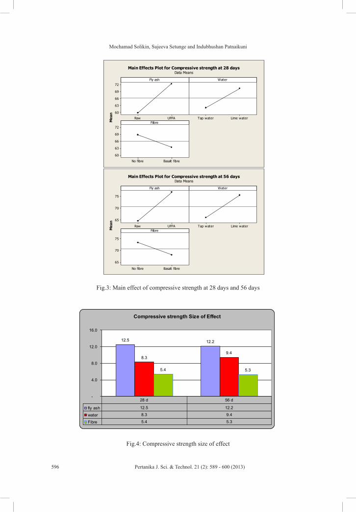
Mochamad Solikin, Sujeeva Setunge and Indubhushan Patnaikuni
596 Pertanika J. Sci. & Technol. 21 (2): 589 - 600 (2013)
UFFARaw
72
69
66
63
60
Lime waterTap water
Basalt fibreNo fibre
72
69
66
63
60
Fly ash
Mea
n
Water
Fiibre
Main Effects Plot for Compressive strength at 28 daysData Means
UFFARaw
75
70
65
Lime waterTap water
Basalt fibreNo fibre
75
70
65
Fly ash
Mea
n
Water
Fiibre
Main Effects Plot for Compressive strength at 56 daysData Means
Fig.3: Main effect of compressive strength at 28 days and 56 days
Compressive strength Size of Effect
12.5 12.2
8.39.4
5.4 5.3
-
4.0
8.0
12.0
16.0
fly ash 12.5 12.2
water 8.3 9.4
Fibre 5.4 5.3
28 d 56 d
Fig.4: Compressive strength size of effect

Experimental Design Analysis of Ultra Fine Fly Ash, Lime Water, and Basalt Fibre in Mix Proportion
597Pertanika J. Sci. & Technol. 21 (2): 589 - 600 (2013)
TABLE 7 Verification of mix proportion and normal cement concrete
Mix proportion Cement Fly ash Water
AgregateHRWR
BasaltFibrefine Coarse
(kg/m3) (kg/m3) (kg/m3) (kg/m3) (kg/m3) (litre/m3) (kg/m3)
UFFA without basalt fiber, lime water (No 10)
225.0 225.0 141.0 835.0 994.0 7.0 -
Normal cement without basalt fibre, tap water (No 5)
450.0 - 137.0 912.0 994.0 13.9 -
VERIFICATION OF MIX PROPORTION
From the experimental design result the mix proportion of high volume ultra fine fly ash concrete with lime water was prepared. The mix proportion is same as the mix proportion No 1, but the mixing water is lime water. The normal concrete as control mix proportion is also prepared. After the concrete specimens are prepared and then continued with curing stage until the test is conducted at 28 days and 56 days.
Fig.5 shows the compressive strength development of high volume ultra fine fly ash concrete with lime water and normal concrete. Both of the mix proportions satisfy the mix design of 80 MPa at 28 days. In addition the high volume ultra fine fly ash concrete with lime water has the same strength development as high strength normal concrete starting at 28 days and beyond.
In addition, the use of lime water is very useful in increasing compressive strength of high volume ultra fine fly ash concrete to be similar strength as normal cement concrete even
Compressive strength of concrete
40.0
60.0
80.0
100.0
(MPa
)
No 10 45.04 78.70 85.05
No 5 50.04 79.44 84.51
14 d 28 d 56 d
Fig.5: Compressive strength development of optimum mix proportion and normal cement concrete
Mochamad Solikin, Sujeeva Setunge and Indubhushan Patnaikuni
598 Pertanika J. Sci. & Technol. 21 (2): 589 - 600 (2013)
though the amount of ultra fine fly ash used is up to 50% as cement replacement. This result is noteworthy, as previous research using high volume fine fly ash reduced the compressive strength of concrete at the curing age of 56 days by 15% to 19.0% in comparison to the normal cement (Sengul et al., 2005) (Sengul & Tasdemir, 2009).
Moreover it proves that the use of lime water in high volume ultra fine fly ash concrete produce better reaction with silica in ultra fine fly ash in comparison to the use of hydrated lime to give same compressive strength as normal concrete. The similar research also reported about the utilization of hydrated lime in increasing compressive strength of high volume fly ash concrete, however the compressive strength did not compare to normal concrete (Barbhuiya et al., 2009).
CONCLUSION
Based on the data presented, the use of ultra fine fly ash and the use of lime water respectively become important factors to increase compressive strength of high volume fly ash concrete. Moreover the use of basalt fibre decreases the compressive strength of concrete due to the basalt fibre lower volumetric stability in alkali environment.
The use of lime water is useful to increase the compressive strength of high volume ultra fine fly ash concrete to be similar to normal cement starting at the age of concrete of 28 days and beyond. This finding is noteworthy, as high volume fine fly ash concrete from previous research has lower compressive strength in comparison to normal cement concrete. In addition the use of lime water in high volume ultra fine fly ash improved concrete compressive strength result in comparison to the use of hydrated lime in high volume fly ash concrete from precious research, as the liquid give better reaction to the silica in fly ash.
Further research should be conducted on the concentration of lime water used and the quantity of high volume ultra fine fly ash to produce optimum high strength concrete.
ACKNOWLEDGEMENTS
This research is made possible with the support of the scholarship awarded to the first author from DIKTI Indonesia. Besides, I would like to thank my supervisor for the conference fund support. Lastly, the authors wish to acknowledge the support provided by technical staff in concrete laboratory of RMIT University.
REFERENCESAïtcin, P.-C. (2004). High-Performance Concrete. New York: Taylor & Francis e-Library.
Alvarez, M., Salas, J., & Veras, J. (1998). Properties of concrete made with fly ash. The International Journal of Cement Composites and Lightweight Concrete, 10(2),109-120.
American Concrete Institute. (1997). State-of-the-Art Report on High-Strength Concrete. ACI 363R-92 (pp. 55). Detroit: American Concrete Institute.
ASTM. (2002). Standard Test Method for Compressive Strength of Hydraulic Cement Mortars (Using 2-in. or [50-mm] Cube Specimens) C109/ C109M - 02. Philadelphia, United States: Annual Book of ASTM Standards

Experimental Design Analysis of Ultra Fine Fly Ash, Lime Water, and Basalt Fibre in Mix Proportion
599Pertanika J. Sci. & Technol. 21 (2): 589 - 600 (2013)
ASTM. (2003). Standard specification for fly ash and raw calcined natural pozzolan for use as mineral admixture in portland cement concrete. C 618-03. Philadelphia, United States: Annual Book of ASTM Standard
Atis, C. D. (2003). High-Volume Fly Ash Concrete with High Strength and Low Drying Shrinkage. ASCE Journal of Materials in Civil Engineering, March-April, 153-156.
Australian Standard Comittee. (1999). Method 9: Determination of the compressive strength of concrete specimens. AS 1012.9. (pp. 1-13). Strathfield, Australia: Australian Standard Comittee.
Balendran, R. V., Zhou, F. P., Nadeem, A., & Leung, A. Y. T. (2002). Influence of steel fibres on strength and ductility of normal and lightweight high strength concrete. Building and Environment, 37, 1361-1367.
Barbhuiya, S. A., Gbagbo, J. K., Russell, M. I., & Basheer, P. A. M. (2009). Properties of fly ash concrete modified with hydrated lime and silica fume. Construction and Building Materials, 23, 3233–3239.
Bilodeau, A., & Malhotra, V. M. (2000). High-Volume Fly Ash System: Concrete Solution for Sustainable Development. ACI Materials Journal, January-February 2000, 41-50.
Caldarone, M. A. (2009). High strength concrete: A practical guide. New york, USA: Taylor & Francis.
Chindaprasirt, P., Chotithanorm, C., Cao, H. T., & Sirivivatnanon, V. (2004). Influence of fly ash fineness on strength, drying shrinkage and sulfate resistance of blended cement mortar. Cement and Concrete Research, 34 1087–1092.
Chindaprasirt, P., Chotithanorm, C., Cao, H. T., & Sirivivatnanon, V. (2007). Influence of fly ash fineness on the chloride penetration of concrete. Construction and Building Materials, 21, 356–361.
Elsageer, M. A., Millard, S. G., & Barnett, S. J. (2009). Strength development of concrete containing coal fly ash under different curing temperature conditions Paper presented at the World of Coal Ash (WOCA) Conference, Lexington, KY, USA.
Kiattikomol, K., Jaturapitakkul, C., Songpiriyakij, S., & Chutubtim, S. (2001). A study of ground coarse fly ashes with different finenesses from various sources as pozzolanic materials. Cement and Concrete Composites, 23, 335 - 343.
Malhotra, V. M., & Mehta, P. K. (2005). High Performance, High-Volume Fly Ash Concrete: materials, mixture proportioning, properties, construction practice, and case histories. (2nd ed.). Ottawa, Canada: Suplementary Cementing Materials for Sustainable Development Inc., Ottawa Canada.
Mira P., Papadakis, V. G., & Tsimas, S. (2002). Effect of lime putty addition on structural and durability properties of concrete. Cement and concrete research, 32, 683-689.
Montgomery, D. C. (2009). Design and analysis of experiments (7th edition ed.). New Jersey, USA: John Wiley & Sons.
Nawy, E. G. (1996). Fundamentals of High Strength High Performance Concrete. London, UK: Longman Group Limited.
Obla, K. H., Hill, R. L., Thomas, M. D. A., Shashiprakash, S. G., & Perebatova, O. (2003). Properties of Concrete Containing Ultra-Fine Fly Ash. ACI Material Journal, Sept.-Okt. 2003, 426-433.
Oner, A., Akyuz, S., & Yildiz, R. (2005). An experimental study on strength development of concrete containing fly ash and optimum usage of fly ash in concrete. Cement and Concrete Research, 35, 1165– 1171.

Mochamad Solikin, Sujeeva Setunge and Indubhushan Patnaikuni
600 Pertanika J. Sci. & Technol. 21 (2): 589 - 600 (2013)
Portland Cement Association. (2008). Cement and Concrete Basics: High-strength Concrete. Skokie, Illinois, USA: Portland Cement Association.
Ramezanianpur, A. A., & Malhotra, V. M. (1995). Effect of curing on compressive strength, resistance to chloride-ion penetration and porosity of concretes incorporating slag, fly ash or silica fume. Cement and Concrete Composites, 17(6 February 1995), 125-133.
Sengul, O., & Tasdemir, M. A. (2009). Compressive Strength and Rapid Chloride Permeability of Concretes with Ground Fly Ash and Slag. Journal of Materials in Civil Engineering ASCE, 21(9), 494 - 501.
Sengul, O., Tasdemir, C., & Tasdemir, M. A. (2005). Mechanical Properties and Rapid Chloride Permeability of Concretes with Ground Fly Ash. ACI Materials Journal, November-December 2005, 414-421.
Sim, J., Park, C., & Moon, D. Y. (2005). Characteristics of basalt fiber as a strengthening material for concrete structures. Composites: Part B Engineering, 36, 504-512.
Sofi, M., Deventer, J. S. J. v., Mendis, P. A., & b, G. C. L. (2007). Engineering properties of inorganic polymer concretes (IPCs). Cement and Concrete Research, 37, 251–257.
Taylor, M., Lydon, F. D., & Barr, B. I. G. (1997). Toughness measurements on steel fibre-reinforced high strength concrete. Cement and Concrete Composites, 19(4), 329-340.
Vijai, K., Kumutha, R., & Vishnuram, B. G. (2010). Effect of types of curing on strength of geopolymer concrete. International Journal of the Physical Sciences, 5(9), 1419-1423.
Xu, A. (1997). Fly ash in concrete. New Jersey: Noyes Publications.
Pertanika J. Sci. & Technol. 21 (2): 601 - 610 (2013)
SCIENCE & TECHNOLOGYJournal homepage: http://www.pertanika.upm.edu.my/
ISSN: 0128-7680 © 2013 Universiti Putra Malaysia Press.
Experimental Study on Shear Behaviour of High Strength Reinforced Recycled Concrete Beam
Oh Chai Lian*, Lee Siong Wee, Mohd Asha’ari Masrom and Goh Ching HuaInstitute of Infrastructure Engineering and Sustainable Management (IIESM), Faculty of Civil Engineering, Universiti Teknologi MARA Malaysia, 40450 Shah Alam, Selangor, Malaysia
ABSTRACT
Recently, there has been great interest on the applicability of Recycled Concrete Aggregate (RCA) as a new ecological construction material that can be sustainable in a gradually expanding construction industry. This paper reports the structural performance particularly on shear behaviour of high strength reinforced recycled concrete beams. Compressive cube strength of the tested beams ranged from 65-74 MPa at the age of 28-days. The experimental program compared conventional concrete mix with concrete mix having substitution of 25% recycled concrete aggregates of grade 25-30 MPa. In this study, three 150 mm x 200 mm x 1200 mm simply supported rectangular concrete beams in each mix were tested under a four-point bending static load with various shear span to effective depth ratios (a/d = 1.0, 1.5, 2.0). Subsequently, the shear behavior of the beams was investigated through studies of load-deflection responses, effect of a/d ratios and crack patterns. The test results reported that the substitution of 25% recycled concrete coarse aggregates barely affects the shear capacity of the high strength reinforced concrete beams with a/d of 1.5 onwards. Finally, experimental results were compared using existing design codes by ACI 318, Eurocode-2 and AS3600 which lie on the safe side
Keywords: Recycled concrete aggregate, high strength concrete, recycled beam, shear, shear span
Article history:Received: 26 December 2011Accepted: 15 March 2012
E-mail address: [email protected] (Oh Chai Lian)*Corresponding Author
Southern regions of Malaysia only, have deposited the construction and demolition (C&D) debris that comprises 28.34% of the total waste (Mohd Nasir et al., 1998). As far as environmental concern, potential uses of Recycled Concrete Aggregate (RCA) in new concreting works are constantly investigated by researchers since few decades ago. While utilization of recycling concrete could solve the growing waste disposal and conserve the
INTRODUCTION
As a result of enormous increase in demolitions of concrete building, great amount of concrete waste has been generated. The Central and
Oh Chai Lian, Lee Siong Wee, Mohd Asha’ari Masrom and Goh Ching Hua
602 Pertanika J. Sci. & Technol. 21 (2): 601 - 610 (2013)
precious limited natural sources of aggregates, it also appeared as an economical solution as the prices for natural aggregate have significantly grew in the latest decade (Ajdukiewicz & Kliszczewicz, 2007). Undoubtedly, some significant breakthroughs of RCA as replacement of natural aggregate in concrete had been successfully established by researchers in the recent past, it can be seen in the overwhelming literatures that available nowadays.
Various efforts have been put into the investigation on the mechanical properties, strength, failure mechanism and durability characteristics of the optimum concrete mix with RCA (Brito & Alves, 2010; Fonseca et al., 2011; Li, 2008; Rahal, 2007; Chakradhara et al., 2011; Xiao et al., 2005). The statement of Recycled Aggregate Concrete (RAC) possessed lightly lower strength than the conventional concrete was reported in (Casuccio et al., 2008). On the other hand, Rao concluded that the concrete with 25% RCA is able to maintain its strength under low velocity impact load (Chakradhara et al., 2011). In addition, the RAC with water cement ratio (w/c) of 0.55 demonstrated comparable compressive strength as the conventional concrete however showed no significant increase in strength with w/c below 0.40 (Rasheeduzzafar & Khan, 1984). Overall, these researchers pointed out that utilization of RCA in concrete is technically possible.
Comparatively, reports on structural behavior especially in shear capacity of the reinforced recycled concrete beams made by RCA are scarce. Researchers from the past have summarized that the shear performance of reinforced recycled concrete beams are little affected, as good as or even superior to the conventional beams made with natural aggregates (Fathifazl et al., 2010; Fathifazl et al., 2011; González-Fonteboa & Martínez-Abella, 2007; González-Fonteboa et al., 2009). Some results indicated that the shear strength diminishes as the substitution of less than 30% RCA in the concrete (Etxeberria et al., 2007; Choi et al., 2010).
Research on mechanical properties of high strength RAC has been carried out (Ajdukiewicz & Kliszczewicz, 2002), nonetheless the structural performance in shear of high strength reinforced recycled concrete beams need to be exposed and therefore are presented herein. Six (6) full-scale reinforced concrete beams produced by concrete mix with natural coarse aggregates and substitution of 25% coarse RCA are studied. Through the results, the authors hope to enhance the understanding on the shear behavior of high strength reinforced recycled beams as well as to reveal that the prediction of existing codes on the shear capacity of high strength reinforced recycled beams can be applied without any modifications.
METHODOLOGY
The experimental program comprised two series of specimens with a total number of six (6) high strength reinforced concrete beams. Specimens in series ‘CB’ were cast with conventional concrete mix whereas series ‘RB’ was produced by concrete mix with 25% coarse RCA. The coarse RCA was obtained solely from laboratory concrete cube wastes with reliable compressive strengths of approximately 25-30 MPa. The concrete cubes with age less than one year, protected against weather and aggressive conditions were crushed by jaw crusher and sieved to a maximum size 20 mm in accordance to British Standard, BS812-103: 1985 (British Standard, 1985) . The crushed recycled concrete coarse aggregates were angular and fractured in nature. The specific gravity, Los Angeles abrasion and absorption (24 hours) values

Experimental Study on Shear Behaviour of High Strength Reinforced Recycled Concrete Beam
603Pertanika J. Sci. & Technol. 21 (2): 601 - 610 (2013)
of recycled concrete coarse aggregates were tested in accordance with BS812-2: 1995 (British Standard, 1995) and presented in Table 1.
TABLE 1 Physical Properties for Recycled Coarse Aggregate
AggregateBulk specific gravity (SSD)
Apparent specific gravity
Los Angeles abrasion (%)
Absorption
RCA 2.46 2.55 35 2.45
Both concrete mixes consisted of Ordinary Portland Cement (OPC), uncrushed river sand, and either crushed natural or recycled coarse aggregates adopted optimum mix proportion of 1:1.1:2.1 and w/c of 0.41. Table 2 summarizes the concrete mix proportion produced. The established concrete mixes were aimed at producing concrete workability with slump of 10-30 mm and targeted compressive strength greater than 50 MPa at 28 days age. The concrete produced was very stiff and demonstrated a 20 mm slump for recycled concrete compared to a 25 mm slump for conventional concrete. The concrete compressive cube strength ranged from 65-74 MPa was measured from three (3) concrete cubes at 28 days lifetime with 100 mm standard mould size for each mix according to the British Standard, BS1881-116:1983 (British Standard, 1983).
TABLE 2 Mix Proportion
Mix Matrix (kg/m3) OPC Sand Natural Coarse Aggregate Coarse RCA WaterCB 570 630 1200 - 235RB 570 630 900 300 235
In both series, three (3) reinforced concrete beam specimens were designed to a size of 150 x 200 x 1200 mm based on the British Standard, BS 8110-1: 1997 (British Standard, 1997). The specimens were fabricated with two (2) 10 mm diameter high yield deformed longitudinal reinforcement bars with characteristic strength of 460 N/mm2 in both the compression and tension zone. 6 mm diameter mild steel bars with characteristic strength of 250 N/mm2 spaced at 200 mm centre to centre were used as shear links. The concrete cover was 30 mm.
Each of the simply supported specimens in both series were loaded to fail under a four-point bending static load test with different shear spans (a), namely 160 mm, 240 mm and 320 mm arriving at a shear span to effective depth ratio (a/d) of 1.0, 1.5 and 2.0 respectively. The details of the specimens are shown in Table 3 while the experimental set-up is illustrated in Fig.1. A load beam acted as a medium to transfer a load source into two static point loads to the beam specimens through steel rods. An external linear variable differential transducer (LVDT) was placed at the middle of the beam soffit to measure its central deflection. The deformation of the compression reinforcement was measured by electrical resistance strain gauges. All the data were automatically recorded by built-in data acquisition.

Oh Chai Lian, Lee Siong Wee, Mohd Asha’ari Masrom and Goh Ching Hua
604 Pertanika J. Sci. & Technol. 21 (2): 601 - 610 (2013)
TABLE 3 Specimens Details
Specimen notation CB1.0 RB1.0 CB1.5 RB1.5 CB2.0 RB2.0Shear span, a (mm) 160 160 240 240 320 320Shear span to effective depth ratio, a/d 1.0 1.0 1.5 1.5 2.0 2.0Compressive cube strength, (N/mm2) 73.25 64.77 73.25 64.77 73.25 64.77
Cross Section A-A
150
160
200
R6-200
2T10
2T10
A
A
P Load Beam
Steel Rod Specimen
Load Cell
200
100 a 500-a 100 a 500-a
1200
Fig.1: Beam specimen details (Units: mm)
RESULTS AND DISCUSSION
The effectiveness in shear of high strength recycled reinforced concrete beam specimens are examined here. The discussion will be on based the load-deflection response, effect of a/d ratio and crack patterns of the recycled specimens compared to conventional specimens. Eventually, the shear capacity of the specimens will be compared with the predicted shear capacity by existing codes, such as ACI 318, Eurocode-2 and AS3600 (ACI Committee, 2005; Eurocode, 1992; Australia Standard, 2009).
Load Deflection Response
Table 4 shows the mid-span deflection at first crack (δc) and ultimate failure (δu), shear force at the first crack (Vc) and ultimate failure (Vu). The comparison is explained in terms of maximum mid-span deflection and ultimate shear force of the recycled specimen compared to the conventional specimen for each a/d ratio, which is denoted as deflection ratio (DR) and ultimate shear ratio (VR) respectively. It also shows the ductility (δu/δc) and reserve strength (Vu/Vc) of the specimens. The results reveal that the recycled specimens perform well in deflection control and have slightly better shear capacity compared to conventional specimens at a/d ratios 1.5 onwards and are stable at approximately 0.61 (DR) and 1.01 (VR). On the contrary, their performance in deflection control and shear capacity show a significant drop at a/d ratio 1.0. It is noted that the ductility and reserve strength of the recycled specimen are generally lesser than the conventional specimen at a/d ratio 1.5 onwards with a corresponding difference of 35.51% and 44.89% respectively. Nevertheless, the recycled specimens present positive ductility and reserve strength at a/d ratio 1.0.
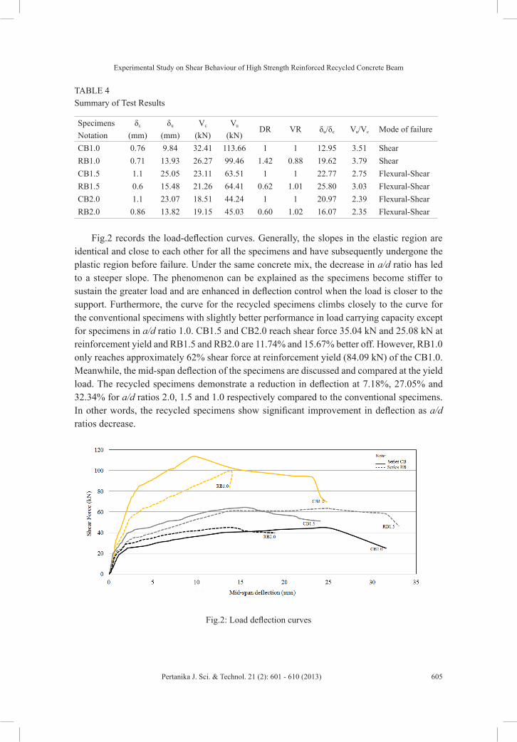
Experimental Study on Shear Behaviour of High Strength Reinforced Recycled Concrete Beam
605Pertanika J. Sci. & Technol. 21 (2): 601 - 610 (2013)
TABLE 4 Summary of Test Results
Specimens Notation
δc (mm)
δu (mm)
Vc
(kN)Vu
(kN)DR VR δu/δc Vu/Vc Mode of failure
CB1.0 0.76 9.84 32.41 113.66 1 1 12.95 3.51 ShearRB1.0 0.71 13.93 26.27 99.46 1.42 0.88 19.62 3.79 ShearCB1.5 1.1 25.05 23.11 63.51 1 1 22.77 2.75 Flexural-ShearRB1.5 0.6 15.48 21.26 64.41 0.62 1.01 25.80 3.03 Flexural-ShearCB2.0 1.1 23.07 18.51 44.24 1 1 20.97 2.39 Flexural-ShearRB2.0 0.86 13.82 19.15 45.03 0.60 1.02 16.07 2.35 Flexural-Shear
Fig.2 records the load-deflection curves. Generally, the slopes in the elastic region are identical and close to each other for all the specimens and have subsequently undergone the plastic region before failure. Under the same concrete mix, the decrease in a/d ratio has led to a steeper slope. The phenomenon can be explained as the specimens become stiffer to sustain the greater load and are enhanced in deflection control when the load is closer to the support. Furthermore, the curve for the recycled specimens climbs closely to the curve for the conventional specimens with slightly better performance in load carrying capacity except for specimens in a/d ratio 1.0. CB1.5 and CB2.0 reach shear force 35.04 kN and 25.08 kN at reinforcement yield and RB1.5 and RB2.0 are 11.74% and 15.67% better off. However, RB1.0 only reaches approximately 62% shear force at reinforcement yield (84.09 kN) of the CB1.0. Meanwhile, the mid-span deflection of the specimens are discussed and compared at the yield load. The recycled specimens demonstrate a reduction in deflection at 7.18%, 27.05% and 32.34% for a/d ratios 2.0, 1.5 and 1.0 respectively compared to the conventional specimens. In other words, the recycled specimens show significant improvement in deflection as a/d ratios decrease.
Fig.2: Load deflection curves
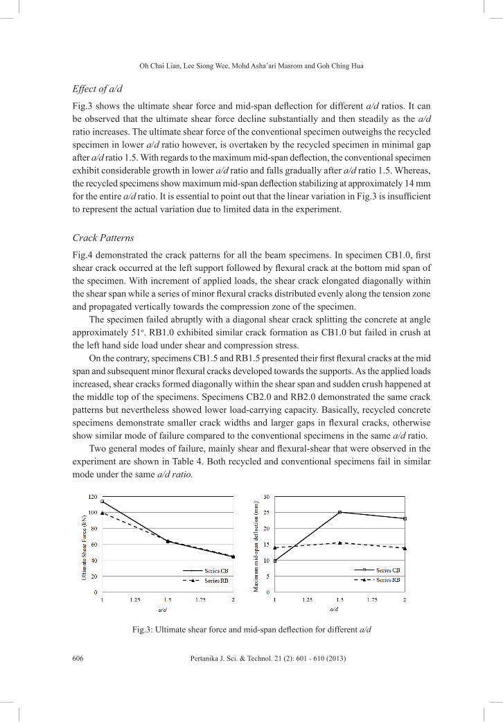
Oh Chai Lian, Lee Siong Wee, Mohd Asha’ari Masrom and Goh Ching Hua
606 Pertanika J. Sci. & Technol. 21 (2): 601 - 610 (2013)
Effect of a/d
Fig.3 shows the ultimate shear force and mid-span deflection for different a/d ratios. It can be observed that the ultimate shear force decline substantially and then steadily as the a/d ratio increases. The ultimate shear force of the conventional specimen outweighs the recycled specimen in lower a/d ratio however, is overtaken by the recycled specimen in minimal gap after a/d ratio 1.5. With regards to the maximum mid-span deflection, the conventional specimen exhibit considerable growth in lower a/d ratio and falls gradually after a/d ratio 1.5. Whereas, the recycled specimens show maximum mid-span deflection stabilizing at approximately 14 mm for the entire a/d ratio. It is essential to point out that the linear variation in Fig.3 is insufficient to represent the actual variation due to limited data in the experiment.
Crack Patterns
Fig.4 demonstrated the crack patterns for all the beam specimens. In specimen CB1.0, first shear crack occurred at the left support followed by flexural crack at the bottom mid span of the specimen. With increment of applied loads, the shear crack elongated diagonally within the shear span while a series of minor flexural cracks distributed evenly along the tension zone and propagated vertically towards the compression zone of the specimen.
The specimen failed abruptly with a diagonal shear crack splitting the concrete at angle approximately 51o. RB1.0 exhibited similar crack formation as CB1.0 but failed in crush at the left hand side load under shear and compression stress.
On the contrary, specimens CB1.5 and RB1.5 presented their first flexural cracks at the mid span and subsequent minor flexural cracks developed towards the supports. As the applied loads increased, shear cracks formed diagonally within the shear span and sudden crush happened at the middle top of the specimens. Specimens CB2.0 and RB2.0 demonstrated the same crack patterns but nevertheless showed lower load-carrying capacity. Basically, recycled concrete specimens demonstrate smaller crack widths and larger gaps in flexural cracks, otherwise show similar mode of failure compared to the conventional specimens in the same a/d ratio.
Two general modes of failure, mainly shear and flexural-shear that were observed in the experiment are shown in Table 4. Both recycled and conventional specimens fail in similar mode under the same a/d ratio.
Fig.3: Ultimate shear force and mid-span deflection for different a/d

Experimental Study on Shear Behaviour of High Strength Reinforced Recycled Concrete Beam
607Pertanika J. Sci. & Technol. 21 (2): 601 - 610 (2013)
CB1.0
RB1.5
CB1.5
RB1.0
CB2.0
RB2.0
(a) (b)
(c) (d)
(e) (f)
Fig.4: Crack patterns of beam specimens
Experimental and predictions of the concrete shear capacity (kN)
Table 5 shows the recommended expressions for determining shear capacity of beams in existing codes while Table 6 summarizes the comparison between the experimental shear and predicted shear by existing codes. Regardless the different procedures in each existing codes, the code Eurocode-2 gives the most conservative prediction on the shear capacity of the beams followed by the code AS3600 and thereafter ACI 318. It can be observed that ACI 318 and AS3600 predict well for both recycled and conventional specimens in a/d ratio 2.0 yet still remain conservative with ratios less than 1.7. Nonetheless, all the predictions in the existing codes show a divergence of up to 5.78 from the experimental shear as the a/d ratio decreases.
TABLE 5 Recommended Expressions for Determining Shear Capacity of Beams in Existing Codes
Code Recommended expressionACI-318 Clause 11.3
Eurocode-2 Clause 6.2.2
AS3600 Clause 8.2.7.1

Oh Chai Lian, Lee Siong Wee, Mohd Asha’ari Masrom and Goh Ching Hua
608 Pertanika J. Sci. & Technol. 21 (2): 601 - 610 (2013)
TABLE 6 Comparison between Experimental Shear and Predicted Shear by Existing Codes (kN)
Specimens Notation Experimental Shear ACI 318 Eurocode-2 AS3600CB1.0 113.66 31.24 (3.64) 19.68 (5.78) 27.99 (4.06)RB1.0 99.46 29.39 (3.38) 18.90 (5.26) 26.87 (3.70)CB1.5 63.51 31.24 (2.03) 19.68 (3.23) 27.99 (2.27)RB1.5 64.41 29.39 (2.19) 18.90 (3.41) 26.87 (2.40)CB2.0 44.24 31.24 (1.42) 19.68 (2.25) 27.99 (1.58)RB2.0 45.03 29.39 (1.53) 18.90 (2.38) 26.87 (1.68)
CONCLUSIONS
The paper presents the results of an investigation on the shear capacity of high strength reinforced concrete beam specimens with 25% recycled concrete coarse aggregates. Based on the experimental results, the following conclusions are drawn:
1. Concrete mix with utilization of 25% 25-30 MPa non-aggressive exposure coarse RCA achieved comparable compressive strength as the conventional concrete mix. Both were mixed with optimum proportion of 1:1.1:2.1 and w/c 0.41 yielded high strength concrete grade ranging at 65-74 MPa.
2. Recycled specimens demonstrated lower shear capacity in a/d ratio 1.0 otherwise performed quite similarly as the conventional specimens as the a/d ratio increased. Nonetheless, the recycled specimens presented good ductility and reserve strength at a/d ratio 1.0.
3. Although maximum mid-span deflection reached a peak at a/d ratio 1.5 for both recycled and conventional specimens, conventional specimens showed an upward trend as a/d ratio increased whereas all the recycled specimens stabilized at approximately 14 mm.
4. Both recycled and conventional specimens failed in shear in a/d 1.0 and flexural shear in a/d ratio 1.5 and 2.0. Smaller crack width and larger spacing in the flexural cracks were discovered in recycled concrete specimens.
5. Existing codes ACI 318, Eurocode-2 and AS3600 can be used in shear design for the recycled specimens with 25% coarse RCA, however the shear capacity for both conventional and recycled specimens is conservatively predicted especially when a/d ratio increases.
ACKNOWLEDGEMENTS
This study would not have been possible without the information and financial support provided by the following organizations. The authors would therefore like to record their appreciation to the Institute of Infrastructure Engineering and Sustainable Management (IIESM), Faculty of Civil Engineering and Research Management Institute of Universiti Teknologi MARA, Malaysia.

Experimental Study on Shear Behaviour of High Strength Reinforced Recycled Concrete Beam
609Pertanika J. Sci. & Technol. 21 (2): 601 - 610 (2013)
REFERENCESACI Committee. (2005). ACI Committee 318, Building Code Requirements for Structural Concrete and
Commentary, ACI 318-05, 2005.
Ajdukiewicz, A., & Kliszczewicz, A. (2002). Influence of recycled aggregates on mechanical properties of HS/HPC. Cement and Concrete Composites, 24(2), 269-279.
Ajdukiewicz, A., & Kliszczewicz. (2007). Comparative tests of beams and columns made of recycled aggregate concrete and natural aggregate concrete. Journal of Advanced Concrete Technology, 5, 259-273.
Australia Standard. (2009). Australia standard for concrete structures, AS 3600-2009.
British Standard. (1983). British Standard codes of practice for testing concrete: method for determination of compressive strength of concrete cubes, BS 1881-116: 1983.
British Standard. (1985). British Standard codes of practice for testing aggregates: method for determination of particle size distribution: Sieve tests, BS 812-103.1:1985.
British Standard. (1995). British Standard codes of practice for testing aggregates: methods for determination of density, BS 812-2:1995.
British Standard. (1997). British Standard codes of practice for design and construction, BS 8110: 1997.
Brito, J., & Alves, F. (2010). Concrete with recycled aggregates: the Portuguese experimental research. Materials and Structures, 43(1), 35-51.
Casuccio, M., Torrijos, M. C., Giaccio, G., & Zerbino, R. (2008). Failure mechanism of recycled aggregate concrete. Construction and Building Materials, 22(7), 1500-1506.
Chakradhara Rao, M., Bhattacharyya, S. K., & Barai, S. V. (2011). Influence of field recycled coarse aggregate on properties of concrete. Materials and Structures, 44(1), 205-220.
Chakradhara Rao, M., Bhattacharyya, S. K., & Barai, S. V. (2011). Behaviour of recycled aggregate concrete under drop weight impact load. Construction and Building Materials, 25(1), 69-80.
Choi, H. B., Yi, C. K., Cho, H. H., & Kang, K. I. (2010). Experimental study on the shear strength of recycled aggregate concrete beams. Magazine of Concrete Research, 62, 103-114. Retrieved from http://www.icevirtuallibrary.com/content/article/10.1680/macr.2008.62.2.103
Etxeberria, M., Marí, A. R., & Vázquez, E. (2007). Recycled aggregate concrete as structural material. Materials and Structures, 40(5), 529-541.
Eurocode. (1992). Eurocode 2: Design of concrete structures, BS EN 1992.
Fathifazl, G., Razaqpur, A. G., Burkan Isgor, O., Abbas, A., Fournier, B., & Foo, S. (2011). Shear capacity evaluation of steel reinforced recycled concrete (RRC) beams. Engineering Structures, 33(3), 1025-1033.
Fathifazl, G., Razaqpur, A. G., Isgor, O. B., Abbas, A., Fournier, B., & Foo, S. (2010, October). Shear strength of reinforced recycled concrete beams with stirrups. Magazine of Concrete Research, 62, 685-699
Fonseca, N., de Brito, J., & Evangelista, L. (2011). The influence of curing conditions on the mechanical performance of concrete made with recycled concrete waste. Cement and Concrete Composites, 33(6), 637-643.

Oh Chai Lian, Lee Siong Wee, Mohd Asha’ari Masrom and Goh Ching Hua
610 Pertanika J. Sci. & Technol. 21 (2): 601 - 610 (2013)
González-Fonteboa, B., & Martínez-Abella, F. (2007). Shear strength of recycled concrete beams. Construction and Building Materials, 21(4), 887-893.
González-Fonteboa, B., Martínez-Abella, F., Martínez-Lage, I., & Eiras-López, J. (2009). Structural shear behaviour of recycled concrete with silica fume. Construction and Building Materials, 23(11), 3406-3410.
Li, X. (2008). Recycling and reuse of waste concrete in China: Part I. Material behaviour of recycled aggregate concrete. Resources, Conservation and Recycling, 53(1–2), 36-44.
Mohd Nasir, H., Yusoff, M. K., Sulaiman, W. N. A., & Rakmi, A. R. (1998). Issues and problems of solid waste management in Malaysia. In the Proceeding of National Review on Environmental Quality Management In Malaysia: Towards the Nest Two Decades, pp. 179-225, 1998.
Rahal, K. (2007). Mechanical properties of concrete with recycled coarse aggregate. Building and Environment, 42(1), 407-415.
Rasheeduzzafar, & Khan, A. (1984, July). Recycled concrete-a source for new aggregate. Cement, Concrete and Aggregates CCAGDP, 6(1), 17-27.
Xiao, J., Li, J., & Zhang, C. (2005). Mechanical properties of recycled aggregate concrete under uniaxial loading. Cement and Concrete Research, 35(6), 1187-1194.
Pertanika J. Sci. & Technol. 21 (2): 611 - 624 (2013)
SCIENCE & TECHNOLOGYJournal homepage: http://www.pertanika.upm.edu.my/
ISSN: 0128-7680 © 2013 Universiti Putra Malaysia Press.
INTRODUCTION
The built environment is a major consumer of energy and consequently a significant emitter of greenhouse gases (as much as 40%). The field faces unprecedented demands to develop knowledge for reducing energy footprints, exploit renewable sources of energy and establish reliable and accurate performance measures for buildings. To
Responsive Façades: Parametric Control of Moveable Tilings
Sambit Datta*1 and Michael Hobbs2
1School of Built Environment, Curtin University of Technology, GPO Box U1987, WA 6845 Perth, Australia2Faculty of Science and Technology, Deakin University, VIC 3220 Geelong, Australia
ABSTRACT
The challenge of developing adaptive, responsive low-energy architecture requires new knowledge about the complex and dynamic interaction between envelope architecture, optimization between competing environmental performance metrics (light, heat and wind indices) and local climate variables. Advances in modeling the geometry of building envelopes and control technologies for adaptive buildings now permit the sophisticated evaluation of alternative envelope configurations for a set of performance criteria. This paper reports on a study of the parametric control of a building envelope based on moveable facade components, acting as a shading device to reduce thermal gain within the building. This is investigated using two alternative tiling strategies, a hexagonal tiling and a pentagonal tiling, considering the component design, support structure and control methods.
Keywords: Responsive envelopes, moveable façade components, parametric modelling, tiling geometry
Article history:Received: 26 December 2011Accepted: 15 March 2012
E-mail addresses: [email protected] (Sambit Datta), [email protected] (Michael Hobbs)*Corresponding Author
address these demands, a tighter coupling between the design and energy performance of buildings is necessary. Smarter and more energy efficient buildings will be significantly improved by addressing the conceptual hurdles separating the architectural design of building envelopes (the external surfaces of buildings) from the simulation of their environmental performance.
The field of building simulation research has developed tools to calculate the performance requirements (solar gain, daylight penetration, heating and cooling loads, ventilation, water use) of a building (Shaviv, 1999; Malkawi, 2004). Rapid, near real-time visual output from building
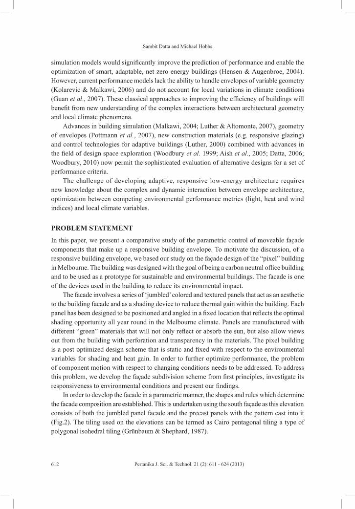
Sambit Datta and Michael Hobbs
612 Pertanika J. Sci. & Technol. 21 (2): 611 - 624 (2013)
simulation models would significantly improve the prediction of performance and enable the optimization of smart, adaptable, net zero energy buildings (Hensen & Augenbroe, 2004). However, current performance models lack the ability to handle envelopes of variable geometry (Kolarevic & Malkawi, 2006) and do not account for local variations in climate conditions (Guan et al., 2007). These classical approaches to improving the efficiency of buildings will benefit from new understanding of the complex interactions between architectural geometry and local climate phenomena.
Advances in building simulation (Malkawi, 2004; Luther & Altomonte, 2007), geometry of envelopes (Pottmann et al., 2007), new construction materials (e.g. responsive glazing) and control technologies for adaptive buildings (Luther, 2000) combined with advances in the field of design space exploration (Woodbury et al. 1999; Aish et al., 2005; Datta, 2006; Woodbury, 2010) now permit the sophisticated evaluation of alternative designs for a set of performance criteria.
The challenge of developing adaptive, responsive low-energy architecture requires new knowledge about the complex and dynamic interaction between envelope architecture, optimization between competing environmental performance metrics (light, heat and wind indices) and local climate variables.
PROBLEM STATEMENT
In this paper, we present a comparative study of the parametric control of moveable façade components that make up a responsive building envelope. To motivate the discussion, of a responsive building envelope, we based our study on the façade design of the “pixel” building in Melbourne. The building was designed with the goal of being a carbon neutral office building and to be used as a prototype for sustainable and environmental buildings. The facade is one of the devices used in the building to reduce its environmental impact.
The facade involves a series of ‘jumbled’ colored and textured panels that act as an aesthetic to the building facade and as a shading device to reduce thermal gain within the building. Each panel has been designed to be positioned and angled in a fixed location that reflects the optimal shading opportunity all year round in the Melbourne climate. Panels are manufactured with different “green” materials that will not only reflect or absorb the sun, but also allow views out from the building with perforation and transparency in the materials. The pixel building is a post-optimized design scheme that is static and fixed with respect to the environmental variables for shading and heat gain. In order to further optimize performance, the problem of component motion with respect to changing conditions needs to be addressed. To address this problem, we develop the façade subdivision scheme from first principles, investigate its responsiveness to environmental conditions and present our findings.
In order to develop the facade in a parametric manner, the shapes and rules which determine the facade composition are established. This is undertaken using the south façade as this elevation consists of both the jumbled panel facade and the precast panels with the pattern cast into it (Fig.2). The tiling used on the elevations can be termed as Cairo pentagonal tiling a type of polygonal isohedral tiling (Grünbaum & Shephard, 1987).

Responsive Façades: Parametric Control of Moveable Tilings
613Pertanika J. Sci. & Technol. 21 (2): 611 - 624 (2013)
Fig.1: The Pixel building, Studio 505. Source – www.australiandesignreview.com
Fig.2: South elevation with Cairo tiling overlayed. Image courtesy of VDM Consulting
RESPONSIVE ENVELOPE SCHEME
First, a subdivision scheme is developed for the dynamic (near real-time) performance optimisation of building envelope geometry using parametric methods. The main features of the parametric tessellation and tiling scheme are:
• Component design: a “carrier-component” (Pitts & Datta, 2009) representation of the envelope;
• Support structure: responsiveness of the carrier and components to performance constraints; and
• Control Method: Modification of the façade model using local and global control parameters.

Sambit Datta and Michael Hobbs
614 Pertanika J. Sci. & Technol. 21 (2): 611 - 624 (2013)
The responsive envelope scheme presented above is developed using two methods of tiling: a hexagonal tiling and a pentagonal tiling strategy. In each of these methods of tiling, the three aspects of component design, support structure and control method are tested.
HEXAGONAL TILING
In order to do initial testing of the model a simplified tiling was identified; that of hexagonal tiling as the Cairo tiling can be seen as a union of two flattened perpendicular hexagonal tilings. Hexagonal tiling is a regular tiling (Grünbaum & Shephard, 1987) in which three hexagons meet at each vertex. Within the facade, key vertical lines of fixing can also be identified, which then pass through the center of the simplified hexagonal tiling, as shown in Fig.3.
Component Design
The component was mapped out based on a half hexagonal tiling, in order to allow the two halves of the hexagon to rotate independently around the supporting structure. A mid-point to the long side of the shape was given as the origin handle, with a Y Direction point across the face to give the orientation. In order to develop the boundaries of the panel a variable factor was used. This factor was derived from the initial study of the facade, with all the key measurements of a panel being evenly divisible by 300mm. The key dimensions were line01 (panelFACTORx3), line02 and line03 (panel FACTORx4), and line 04 and line 05 (panelFACTORx1) as in Fig.4.
Support Structure
To begin the Facade form, an early problem that was faced was how to create a staggered pattern across a flat surface, which was required in order to achieve the hexagonal tiling. Parametric software can easily define a surface with a point grid across it, containing a given U and V series. However, due to the staged nature of the tiling this is not a desirable method. In order to overcome this issue, the form was set out in a staging process rather than a direct point grid.
The first geometry to define the façade was its width, a simple line across the base, relative to the section of façade covered with the panels. On this base line, points were spread out at 2400mm spacing, giving 8 points. This set of points, which behaves as a single element, becomes the base point for the first collection of vertical façade elements. From this set of points a series of lines is generated covering the three top floors of the façade – Fig.5 (Left). On these lines, a new point is spread evenly across the line at the same specific spacing, 2400mm, as the horizontal base points. Due to the lines being a collection, this new point is replicated on all lines in the collection – Fig.5 (Right). The final point gives the general arrangement of half the façade pattern.
The second half of the geometry was achieved by offsetting a new single point at 1200mm across (Y Direction) and 1200mm upwards (Z Direction)from the start point of the first half. This new point allows for the first half of the geometry to be copied, while maintaining identical arrangement parameters, and giving a staggered arrangement of points.
From these points, a line can be established to be able to identify the Y Direction in both collections. The reason for this was so that a direction property could be found in response to

Responsive Façades: Parametric Control of Moveable Tilings
615Pertanika J. Sci. & Technol. 21 (2): 611 - 624 (2013)
Fig.3: South elevation with Hexagonal tiling overlayed. Image courtesy of VDM Consulting.
Fig.4: The half hexagon tile component and its parametric variables.
Fig.5: Left – Initial supporting lines. Right – First collection of points.

Sambit Datta and Michael Hobbs
616 Pertanika J. Sci. & Technol. 21 (2): 611 - 624 (2013)
the general environmental orientation, the base coordinate system Y Direction, at each given origin of a panel/component.
The component of the single panel was then generated across each point in both collections, shown in Fig.6. Since the component only covers one direction from the point, the component had to be generated twice to produce both the Y and –Y Directions.
Control Method
The earlier setup of the Panel component required only two inputs; origin and orientation. To be able to change the responsive nature of these panels in the façade, the orientation input needs to be revised. In the initial development of the façade the orientation was based on the environmental orientation, the base coordinate system.
If the panels are able to respond to a point in space, this point can change the orientation of the panels as it moves across the face of the façade. The point behaves as an attractor and can be used to define environmental conditions. A new set of framework was developed within the model to define the path of the attractor, a line, and the attractor itself, a point capable of moving along the line (Fig.7). The extent of the path matched the current framework of the façade.
In order for the panels to now respond to the attractor some further geometry is required to define the direction of the point from any given panel. As the façade is made up of two panels, a direct application of the attractor as the direction point cannot be used, otherwise all panels in the set would point directly at the attractor. A circle was created at the origin of each panel, with the point of the attractor projected onto the circle edge. This formed the individual rotation of one side of each panel set, in this case the right or Y Direction side. Using a coordinate system that originates from the panel origin and defines the upward direction of the façade, Z Direction, a plane could be established to mirror the point on the circle edge (Fig.8). This means that each set of two mirrored panels responds collectively as the attractor point moves (Fig.9).
While this model is influenced by the environment with the panel orientation changing based on the environmental input, the attractor point, further exploration of the orientation of the panels was desired. With the original design of the facade being one of ‘jumbled’ panels, the uniformity that exists by the use of an attractor point is in contrast to this. If the orientation of the panels is more random, then the facade will be more varied.
Interactive Hexagonal-Tiling Design Tool
The initial hexagonal tiling patterns presented above were developed utilizing the Rhinoceros 3-D freeform modeling tool (McNeel USA, 2012), through the Grasshopper generative modeling add-on tool (Davidson, 2012). These tools permitted experimentation with the design of the foundation hexagonal tiling approach but there were limitations in this approach. Limitations included a lack of real-time interactive design support, and no easy way to evaluate the performance (thermal/lighting/wind) criteria of an envelope using this tile design.
To address the limitations of Rhino3D and Grasshopper, a prototype interactive design tool was developed using the open-source programming language Processing (http://processing.org/). The objective of this tool was to provide a 3D interface to the design of a façade using a given geometrical tiling approach, where various parameters of the design could be

Responsive Façades: Parametric Control of Moveable Tilings
617Pertanika J. Sci. & Technol. 21 (2): 611 - 624 (2013)
Fig.8:From left to right, addition of the circle, projected point, coordinate system, and mirrored point.
Fig.6: First component application. Fig.7: Attractor framework.
Fig.9: Panels responding to the attractor point

Sambit Datta and Michael Hobbs
618 Pertanika J. Sci. & Technol. 21 (2): 611 - 624 (2013)
modified and the resultant façade displayed. In the first version of this tool, hexagonal-tiling was implemented and (initially) two control parameters supported: number of tiles in the X/Y dimensions; and the ‘kink’ angle of the individual tile. Screenshots of this initial prototype are shown in Fig.10.
It is intended that this tool provide an interface to additional performance modeling tools, which would measure a given façade’s performance such as: shading, thermal and wind properties. The base tool has been designed to be flexible and additional tiling approaches to be added later – such as Pentagonal tiling, presented in the following section.
PENTAGONAL TILING
Returning to the original shape grammar, it was identified that the Cairo tile was used to define the facade pattern. In order to simplify the initial model a hexagonal tiling was used, utilizing data lists a pentagonal tiling can be achieved and provide greater control of the individual tiles.
Component Design
The geometry of the pentagons that make up the Cairo tiling can be extracted from our initial hexagonal tiling. This also provides a starting point from which to develop the underlying surfaces that support the actual tiles. The overall facade pattern can be made up of vertical collections of pentagons, with four differently orientated sets of pentagons in each collection.
Support Structure
The first step was to establish the surface geometry of a single vertical set of tiles, beginning with the bottom pentagon from the hexagonal collection. A horizontal line was created based on the width of the tile unit, 1.2m. From the start and end points of this line, two vertical lines were created with an initial length of 14.4m. This length input was drawn from a variable allowing it to be changed later, but in order to ensure that there was an even division of the surface, regardless of length, the variable was based on the number of units multiplied by the height of the tile. Between the two vertical lines a base surface could now be generated.
The base surface was then subdivided using its U and V parameters. In the case of the U, the vertical aspect, it was divided by one as this surface was only going to carry a single vertical set of tiles. The V subdivision was produced by taking the facade height input and dividing it by the tile height property, which always produces an even division because of the facade height inputs underlying rules as discussed above.
With the first supporting surface established, three more are required and can be achieved by offsetting the first. Moving in a clockwise direction the offsetting can be undertaken by adjusting the start point of the baseline from 0, 0, 0 to:
• -0.6, 0, 0.6 (left)
• 0, 0, 0 (top)
• 0.6, 0, 0.6 (right)

Responsive Façades: Parametric Control of Moveable Tilings
619Pertanika J. Sci. & Technol. 21 (2): 611 - 624 (2013)
The top tile uses the same starting point as the bottom tile, but its surface height is calculated by combining the facade height input and the tile height to allow for one extra tile to be generated. As with the hexagonal system a position count is used, but it is based on each set of four tiled pentagons, so all four of these surfaces receive the same position count input. The surfaces are then subdivided by the U and V parameters, with the U being 1 and the V being based on the facade height divided by the tile height (Fig.12). As in the hexagonal model the facade height input is based on the tile dimension so that a clean tile division always occurs.
When the component is applied to the supporting surface a pentagon is generated in each of the polygons which results in too many pentagons that overlap. Using the data lists the excess tiles can be culled, leaving the desired pattern. The cull function uses a true false pattern which allows for the desired tiles to be maintained, removing the overlap and producing the Cairo tile (Fig.13).
Fig.10: Prototype design tool implemented in Processing.
Fig.11: Panels with pentagonal tiling configuration.

Sambit Datta and Michael Hobbs
620 Pertanika J. Sci. & Technol. 21 (2): 611 - 624 (2013)
With one vertical section complete, offset sections are now required which will allow for a complete facade to be produced. A position count variable is used to achieve this, which influences all four pentagons in a set, so only the Z attribute of the baseline needs adjusting. A simple subtraction of the existing Z value by the tile height is built in, which results in the baseline being offset downwards, with the position count adjusting the sideways offset.
Control Method
With the facade tiling established, the rotation of the individual tiles can now be undertaken. The first step in this process is to set an axis for rotation. Two attributes are taken from the existing geometry of the underlying surface of each set; that of the center point of the base
Fig.12: Offsetting of the supporting surfaces and subdivision.
Fig.13: Culling of the pentagons to produce the Cairo tiling.
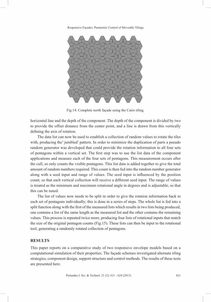
Responsive Façades: Parametric Control of Moveable Tilings
621Pertanika J. Sci. & Technol. 21 (2): 611 - 624 (2013)
horizontal line and the depth of the component. The depth of the component is divided by two to provide the offset distance from the center point, and a line is drawn from this vertically defining the axis of rotation.
The data list can now be used to establish a collection of random values to rotate the tiles with, producing the’ jumbled’ pattern. In order to minimize the duplication of parts a pseudo random generator was developed that could provide the rotation information to all four sets of pentagons within a vertical set. The first step was to use the list data of the component applications and measure each of the four sets of pentagons. This measurement occurs after the cull, so only counts the visible pentagons. This list data is added together to give the total amount of random numbers required. This count is then fed into the random number generator along with a seed input and range of values. The seed input is influenced by the position count, so that each vertical collection will receive a different seed input. The range of values is treated as the minimum and maximum rotational angle in degrees and is adjustable, so that this can be tuned.
The list of values now needs to be split in order to give the rotation information back to each set of pentagons individually; this is done in a series of steps. The whole list is fed into a split function along with the first of the measured lists which results in two lists being produced, one contains a list of the same length as the measured list and the other contains the remaining values. This process is repeated twice more, producing four lists of rotational inputs that match the size of the original pentagon counts (Fig.15). These lists can then be input to the rotational tool, generating a randomly rotated collection of pentagons.
RESULTS
This paper reports on a comparative study of two responsive envelope models based on a computational simulation of their properties. The façade schemes investigated alternate tiling strategies, component design, support structure and control methods. The results of these tests are presented here.
Fig.14: Complete north façade using the Cairo tiling.
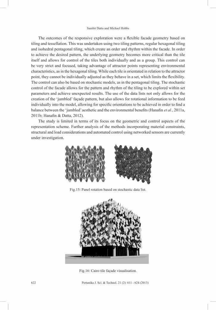
Sambit Datta and Michael Hobbs
622 Pertanika J. Sci. & Technol. 21 (2): 611 - 624 (2013)
The outcomes of the responsive exploration were a flexible facade geometry based on tiling and tessellation. This was undertaken using two tiling patterns, regular hexagonal tiling and isohedral pentagonal tiling, which create an order and rhythm within the facade. In order to achieve the desired pattern, the underlying geometry becomes more critical than the tile itself and allows for control of the tiles both individually and as a group. This control can be very strict and focused, taking advantage of attractor points representing environmental characteristics, as in the hexagonal tiling. While each tile is orientated in relation to the attractor point, they cannot be individually adjusted as they behave in a set, which limits the flexibility. The control can also be based on stochastic models, as in the pentagonal tiling. The stochastic control of the facade allows for the pattern and rhythm of the tiling to be explored within set parameters and achieve unexpected results. The use of the data lists not only allows for the creation of the ‘jumbled’ façade pattern, but also allows for rotational information to be feed individually into the model, allowing for specific orientations to be achieved in order to find a balance between the ‘jumbled’ aesthetic and the environmental benefits (Hanafin et al., 2011a, 2011b; Hanafin & Datta, 2012).
The study is limited in terms of its focus on the geometric and control aspects of the representation scheme. Further analysis of the methods incorporating material constraints, structural and load considerations and automated control using networked sensors are currently under investigation.
Fig.15: Panel rotation based on stochastic data list.
Fig.16: Cairo tile façade visualisation.
Responsive Façades: Parametric Control of Moveable Tilings
623Pertanika J. Sci. & Technol. 21 (2): 611 - 624 (2013)
ACKNOWLEDGEMENTS
This project forms part of Curtin University’s “responsive envelopes project” and was part funded by Deakin University’s CRGS scheme. Michael Sharman of Deakin University produced the early model of the facade and Fig.5 to Fig.8 are based on this CRGS work. Stuart Hanafin, was a masters student and research assistant on the CRGS project, during which he implemented and developed the rotation of the cairo tilings. The authors also acknowledge the support of VDM Consulting, for sharing the structural analysis and façade engineering expertise used in the pixel building, on which this work is based.
REFERENCESAish, R., & Woodbury, R. (2005). Multi-level Interaction in Parametric Design. In A. Butz, B. Fisher,
A. Krüger & P. Olivier (Eds.), Smart Graphics (Vol. 3638, pp. 151-162): Springer Berlin Heidelberg.
Datta, S. (2006). Modeling dialogue with mixed initiative in design space exploration. Artif. Intell. Eng. Des. Anal. Manuf., 20(2), 129-142.
Davidson, S. (2012). Grasshopper. Retrieved on March 1, 2012 from http://www.grasshopper3d.com
Grünbaum, B., & Shephard, G. C. (1987). Tilings and patterns. New York: W.H. Freeman.
Guan, L., Yang, J., & Bell, J. M. (2007). Cross-correlations between weather variables in Australia. Building and Environment, 42(3), 1054-1070.
Hanafin, S., Hobbs, M. et al. (2011a). Responsive Building Envelopes: Parametric Control of Moveable Facade components. Proceedings of the 3rd International CUTSE Conference. Miri, Sarawak Malaysia, Curtin Sarawak. pp.770-774.
Hanafin, S., & Datta, S. (2012). Envelope tesselation with stochastic rotation of 4-fold penttiles. Beyond Codes and Pixels. In the Proceedings of the 17th International Conference on Computer-Aided Architectural Design Research in Asia (CAADRIA). Chennai, India, Association for Computer-Aided Architectural Design Research in Asia (CAADRIA), Hong Kong.
Hanafin, S., Datta, S., & Rolfe, B. (2011b). Tree Facades: Generative Modelling with an Axial Branch Rewriting System. In Herr, C. M. Gu, N., Roudavski, S., & Schnabel, M. A. (Eds.). Circuit Bending, Breaking and Mending. In the Proceedings of the 16th International Conference on Computer-Aided Architectural Design Research in Asia, Apr 27-30 2011, pp. 175-184. Newcastle, NSW: Association for Computer-Aided Architectural Design Research in Asia (CAADRIA).
Hensen, J., & Augenbroe, G. (2004). Performance simulation for better building design. Energy and Buildings, 36(8), 735-736.
Kolarevic, B., & Malkawi, A. M. (2006). Performative Architecture: Beyond Instrumentality. Spon Press, 2006.
Luther, M. (2000). Responsive and dynamic building envelopes. In the Proceedings of 30th International Conf on Environmental Systems and the 7th European Symposium on Space Environmental Control Systems, Toulouse, France, 2000.
Luther, M., & Altomonte, S. (2007). Natural and environmentally responsive building envelopes. In the 37th International Conference on Environmental Systems, Society of Automotive Engineers (SAE), Chicago, 2007.

Sambit Datta and Michael Hobbs
624 Pertanika J. Sci. & Technol. 21 (2): 611 - 624 (2013)
Malkawi, A. M. (2004). Developments in environmental performance simulation. Automation in Construction, 13(4), 437-445.
McNeel USA. (2012). Rhino3D. Retrieved on March 1, 2012 from http://www.rhino3d.com/
Pitts, G., & Datta, S. (2009). Surface geometries: experiments with constrained tessellation. In Gu, N. Ostwald. J., Williams, A. (Eds). Computing, cognition and education : recent research in the architectural sciences, pp. 33-46, Australian and New Zealand Architectural Science Association, Newcastle, N.S.W.
Pottmann, H., Asperl, A., Hofer, M., & Kilian, A. (2007). Architectural Geometry. Eaton: Bentley Institute Press.
Processing.org (2012). Open-source programming language and environment. Retrieved on March 1, 2012 from http://processing.org/
Woodbury, R., Burrow, A., Datta, S., & Chang, T. (1999). Typed feature structures and design space exploration. Journal of Artificial Intelligence for Engineering Design, Analysis and Manufacturing, AIEDAM, 13(4), 287-302.
Sambit, D., & Rolfe, B. (2011). Computational Exploration of Design Spaces: Non-deterministic choice and stochastic generation. In Chakrabarti, A. (Ed). Research into Design: Supporting Sustainable Product Development, pp. 607-614. Singapore: Research Publishing.
Shaviv, E. (1999). Integrating energy consciousness in the design process. Automation in Construction, 8(4), 463-472.
Woodbury, R. (2010). Elements of parametric design. London ; New York, NY: Routledge.
Pertanika J. Sci. & Technol. 21 (2): 625 - 634 (2013)
SCIENCE & TECHNOLOGYJournal homepage: http://www.pertanika.upm.edu.my/
ISSN: 0128-7680 © 2013 Universiti Putra Malaysia Press.
INTRODUCTION
Peat represents the extreme form of soft soil. It is an organic soil which consists more than 70% of organic matters. Peat deposits are
A Numerical Study of Ground Improvement Technique Using Group of Soil-Column on Peat
Muntohar, A. S.1*, Rahman, M. E.1, Hashim, R.2 and Islam, M. S.3
1Department of Civil & Construction Engineering, Curtin University, Sarawak Campus, 98009 Miri, Sarawak, Malaysia2Department of Civil Engineering, Faculty of Engineering, Universiti Malaya, Kuala Lumpur, Malaysia3Postgraduate Student, Department of Civil Engineering, Monash University , Clayton Campus, Wellington Road, Clayton, Victoria 3800, Australia
ABSTRACT
The importance of numerical analysis in investigation of piled embankment over soft soil has been developed since 1990. Several investigators have extended the numerical analysis to model ground improvement using soil-column to support embankment or structures. This paper presents a numerical analysis of the Pulverized Fuel Ash (PFA) column-treated peat and compared with field static-loading test results. Back analysis was performed to determine the material parameters and soil stiffness surrounding soil & soil-column. Two geometrical models were used in this analysis: (a) block (Model A), and (b) column group (Model B). This situation was analyzed using commercially available finite element package PLAXIS 2D ver. 8.2. It is found that both models are reliable to simulate the field static-loading test for column-treated peat. Model B shows a higher stability to failure if compared to Model A.
Keywords: Peat, load-settlement curve, PFA column, FEM
Article history:Received: 26 December 2011Accepted: 15 March 2012
E-mail addresses: [email protected] (Muntohar, A. S.), [email protected] (Rahman, M. E.), [email protected] (Hashim, R.), [email protected] (Islam, M. S.)*Corresponding Author
found where conditions are favourable for their formation. In Malaysia, three million hectares of land is covered with peat. While in Indonesia, peat covers about 26 million hectares of the country land area. Two third of the world coverage of tropical peat are in South East Asia. Since the coverage of peat is quite extensive, utilization of marginal soil has been required in recent years. Hence, suitable geotechnical design parameters and construction techniques are needed for this type of ground condition. Peat poses serious
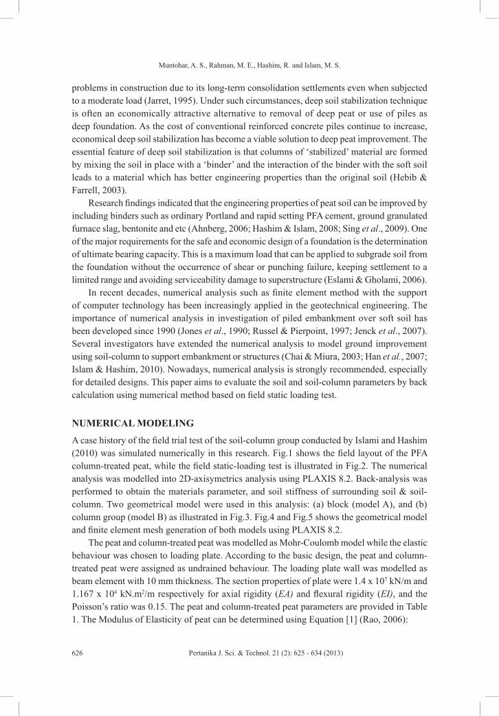
Muntohar, A. S., Rahman, M. E., Hashim, R. and Islam, M. S.
626 Pertanika J. Sci. & Technol. 21 (2): 625 - 634 (2013)
problems in construction due to its long-term consolidation settlements even when subjected to a moderate load (Jarret, 1995). Under such circumstances, deep soil stabilization technique is often an economically attractive alternative to removal of deep peat or use of piles as deep foundation. As the cost of conventional reinforced concrete piles continue to increase, economical deep soil stabilization has become a viable solution to deep peat improvement. The essential feature of deep soil stabilization is that columns of ‘stabilized’ material are formed by mixing the soil in place with a ‘binder’ and the interaction of the binder with the soft soil leads to a material which has better engineering properties than the original soil (Hebib & Farrell, 2003).
Research findings indicated that the engineering properties of peat soil can be improved by including binders such as ordinary Portland and rapid setting PFA cement, ground granulated furnace slag, bentonite and etc (Ahnberg, 2006; Hashim & Islam, 2008; Sing et al., 2009). One of the major requirements for the safe and economic design of a foundation is the determination of ultimate bearing capacity. This is a maximum load that can be applied to subgrade soil from the foundation without the occurrence of shear or punching failure, keeping settlement to a limited range and avoiding serviceability damage to superstructure (Eslami & Gholami, 2006).
In recent decades, numerical analysis such as finite element method with the support of computer technology has been increasingly applied in the geotechnical engineering. The importance of numerical analysis in investigation of piled embankment over soft soil has been developed since 1990 (Jones et al., 1990; Russel & Pierpoint, 1997; Jenck et al., 2007). Several investigators have extended the numerical analysis to model ground improvement using soil-column to support embankment or structures (Chai & Miura, 2003; Han et al., 2007; Islam & Hashim, 2010). Nowadays, numerical analysis is strongly recommended, especially for detailed designs. This paper aims to evaluate the soil and soil-column parameters by back calculation using numerical method based on field static loading test.
NUMERICAL MODELING
A case history of the field trial test of the soil-column group conducted by Islami and Hashim (2010) was simulated numerically in this research. Fig.1 shows the field layout of the PFA column-treated peat, while the field static-loading test is illustrated in Fig.2. The numerical analysis was modelled into 2D-axisymetrics analysis using PLAXIS 8.2. Back-analysis was performed to obtain the materials parameter, and soil stiffness of surrounding soil & soil-column. Two geometrical model were used in this analysis: (a) block (model A), and (b) column group (model B) as illustrated in Fig.3. Fig.4 and Fig.5 shows the geometrical model and finite element mesh generation of both models using PLAXIS 8.2.
The peat and column-treated peat was modelled as Mohr-Coulomb model while the elastic behaviour was chosen to loading plate. According to the basic design, the peat and column-treated peat were assigned as undrained behaviour. The loading plate wall was modelled as beam element with 10 mm thickness. The section properties of plate were 1.4 x 10⁷ kN/m and 1.167 x 10⁴ kN.m2/m respectively for axial rigidity (EA) and flexural rigidity (EI), and the Poisson’s ratio was 0.15. The peat and column-treated peat parameters are provided in Table 1. The Modulus of Elasticity of peat can be determined using Equation [1] (Rao, 2006):

A Numerical Study of Ground Improvement Technique Using Group of Soil-Column on Peat
627Pertanika J. Sci. & Technol. 21 (2): 625 - 634 (2013)
u uE sα= [1]
where, Eu is the undrained modulus of elasticity and su is the undrained shear strength, and α = 150 ~ 500 (for soft soil/peat), and α = 15 ~ 70 (for cement column-treated soil).
The stability of column group for each models were analysed numerically using phi-c reduction approach. This method allows the PLAXIS to calculate a global safety factor (SF). In this approach the cohesion and the tangent of friction angle are reduced in the same proportion:
tantanr r
c Msfc
φφ
= = ∑ [2]
where, c and φ are the input cohesion and friction angle, cr and φr are reduced cohesion and friction angle. The cr and φr parameters are calculated just large enough to maintain equilibrium.
Fig.1: The layout of group PFA column-treated peat after 28 days (Islam & Hashim, 2010)
Fig.2: Layout of the static loading test (Islam & Hashim, 2010)
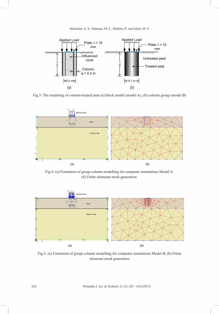
Muntohar, A. S., Rahman, M. E., Hashim, R. and Islam, M. S.
628 Pertanika J. Sci. & Technol. 21 (2): 625 - 634 (2013)
(a) (b)
1m
Applied Load
Column,= 0.2 m
0.5 m
Plate, t = 10mm
Influencedzone 1
m
0.7 m
Applied LoadPlate, t = 10
mm
Treated peat
Untreated peat
(a) (b)
Fig.3: The modeling of column-treated peat (a) block model (model A), (b) column group (model B)
(a) (b)
Fig.4: (a) Formation of group column modelling for computer simulations Model A, (b) Finite elemenet mesh generation.
(a) (b)
Fig.5: (a) Formation of group column modelling for computer simulations Model B, (b) Finite elemenet mesh generation
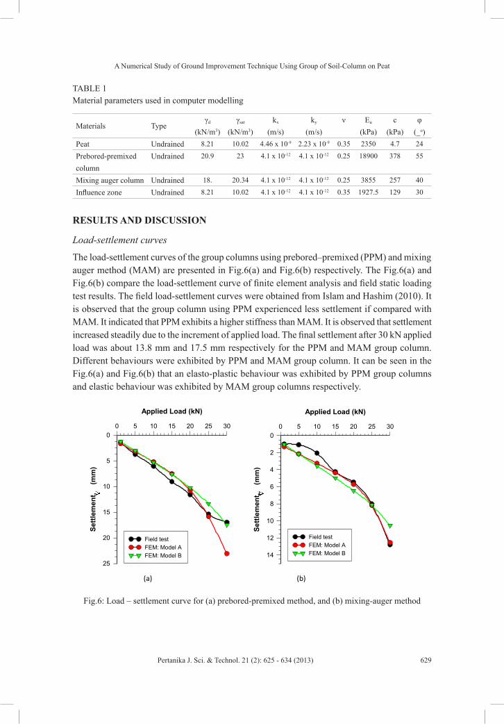
A Numerical Study of Ground Improvement Technique Using Group of Soil-Column on Peat
629Pertanika J. Sci. & Technol. 21 (2): 625 - 634 (2013)
TABLE 1 Material parameters used in computer modelling
Materials Typeγd
(kN/m3)γsat
(kN/m3)kx
(m/s)ky
(m/s)ν Eu
(kPa)c
(kPa)φ
(_o)Peat Undrained 8.21 10.02 4.46 x 10⁻⁹ 2.23 x 10⁻⁹ 0.35 2350 4.7 24
Prebored-premixed column
Undrained 20.9 23 4.1 x 10⁻¹² 4.1 x 10⁻¹² 0.25 18900 378 55
Mixing auger column Undrained 18. 20.34 4.1 x 10⁻¹² 4.1 x 10⁻¹² 0.25 3855 257 40
Influence zone Undrained 8.21 10.02 4.1 x 10⁻¹² 4.1 x 10⁻¹² 0.35 1927.5 129 30
RESULTS AND DISCUSSION
Load-settlement curves
The load-settlement curves of the group columns using prebored–premixed (PPM) and mixing auger method (MAM) are presented in Fig.6(a) and Fig.6(b) respectively. The Fig.6(a) and Fig.6(b) compare the load-settlement curve of finite element analysis and field static loading test results. The field load-settlement curves were obtained from Islam and Hashim (2010). It is observed that the group column using PPM experienced less settlement if compared with MAM. It indicated that PPM exhibits a higher stiffness than MAM. It is observed that settlement increased steadily due to the increment of applied load. The final settlement after 30 kN applied load was about 13.8 mm and 17.5 mm respectively for the PPM and MAM group column. Different behaviours were exhibited by PPM and MAM group column. It can be seen in the Fig.6(a) and Fig.6(b) that an elasto-plastic behaviour was exhibited by PPM group columns and elastic behaviour was exhibited by MAM group columns respectively.
Applied Load (kN)
0 5 10 15 20 25 30
Settl
emen
t, (m
m)
0
5
10
15
20
25
Field testFEM: Model AFEM: Model B
Applied Load (kN)
0 5 10 15 20 25 30
Settl
emen
t, (m
m)
0
2
4
6
8
10
12
14
Field testFEM: Model AFEM: Model B
(a) (b)
Fig.6: Load – settlement curve for (a) prebored-premixed method, and (b) mixing-auger method
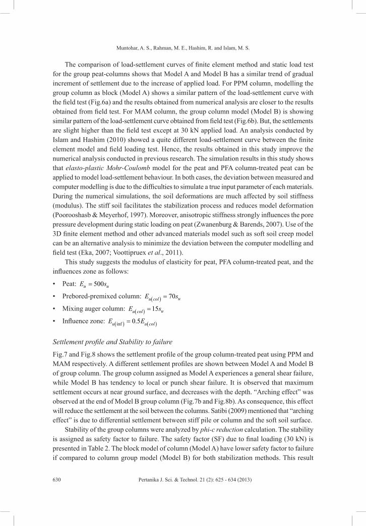
Muntohar, A. S., Rahman, M. E., Hashim, R. and Islam, M. S.
630 Pertanika J. Sci. & Technol. 21 (2): 625 - 634 (2013)
The comparison of load-settlement curves of finite element method and static load test for the group peat-columns shows that Model A and Model B has a similar trend of gradual increment of settlement due to the increase of applied load. For PPM column, modelling the group column as block (Model A) shows a similar pattern of the load-settlement curve with the field test (Fig.6a) and the results obtained from numerical analysis are closer to the results obtained from field test. For MAM column, the group column model (Model B) is showing similar pattern of the load-settlement curve obtained from field test (Fig.6b). But, the settlements are slight higher than the field test except at 30 kN applied load. An analysis conducted by Islam and Hashim (2010) showed a quite different load-settlement curve between the finite element model and field loading test. Hence, the results obtained in this study improve the numerical analysis conducted in previous research. The simulation results in this study shows that elasto-plastic Mohr-Coulomb model for the peat and PFA column-treated peat can be applied to model load-settlement behaviour. In both cases, the deviation between measured and computer modelling is due to the difficulties to simulate a true input parameter of each materials. During the numerical simulations, the soil deformations are much affected by soil stiffness (modulus). The stiff soil facilitates the stabilization process and reduces model deformation (Poorooshasb & Meyerhof, 1997). Moreover, anisotropic stiffness strongly influences the pore pressure development during static loading on peat (Zwanenburg & Barends, 2007). Use of the 3D finite element method and other advanced materials model such as soft soil creep model can be an alternative analysis to minimize the deviation between the computer modelling and field test (Eka, 2007; Voottipruex et al., 2011).
This study suggests the modulus of elasticity for peat, PFA column-treated peat, and the influences zone as follows:
• Peat: 500u uE s=
• Prebored-premixed column: ( ) 70 uu colE s=
• Mixing auger column: ( ) 15 uu colE s=
• Influence zone: ( ) ( )inf 0.5u u colE E=
Settlement profile and Stability to failure
Fig.7 and Fig.8 shows the settlement profile of the group column-treated peat using PPM and MAM respectively. A different settlement profiles are shown between Model A and Model B of group column. The group column assigned as Model A experiences a general shear failure, while Model B has tendency to local or punch shear failure. It is observed that maximum settlement occurs at near ground surface, and decreases with the depth. “Arching effect” was observed at the end of Model B group column (Fig.7b and Fig.8b). As consequence, this effect will reduce the settlement at the soil between the columns. Satibi (2009) mentioned that “arching effect” is due to differential settlement between stiff pile or column and the soft soil surface.
Stability of the group columns were analyzed by phi-c reduction calculation. The stability is assigned as safety factor to failure. The safety factor (SF) due to final loading (30 kN) is presented in Table 2. The block model of column (Model A) have lower safety factor to failure if compared to column group model (Model B) for both stabilization methods. This result
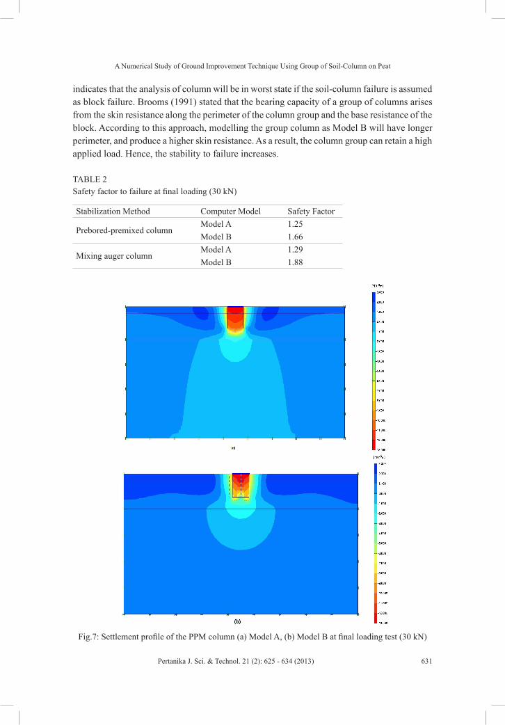
A Numerical Study of Ground Improvement Technique Using Group of Soil-Column on Peat
631Pertanika J. Sci. & Technol. 21 (2): 625 - 634 (2013)
indicates that the analysis of column will be in worst state if the soil-column failure is assumed as block failure. Brooms (1991) stated that the bearing capacity of a group of columns arises from the skin resistance along the perimeter of the column group and the base resistance of the block. According to this approach, modelling the group column as Model B will have longer perimeter, and produce a higher skin resistance. As a result, the column group can retain a high applied load. Hence, the stability to failure increases.
TABLE 2 Safety factor to failure at final loading (30 kN)
Stabilization Method Computer Model Safety Factor
Prebored-premixed columnModel A 1.25Model B 1.66
Mixing auger columnModel A 1.29Model B 1.88
Fig.7: Settlement profile of the PPM column (a) Model A, (b) Model B at final loading test (30 kN)
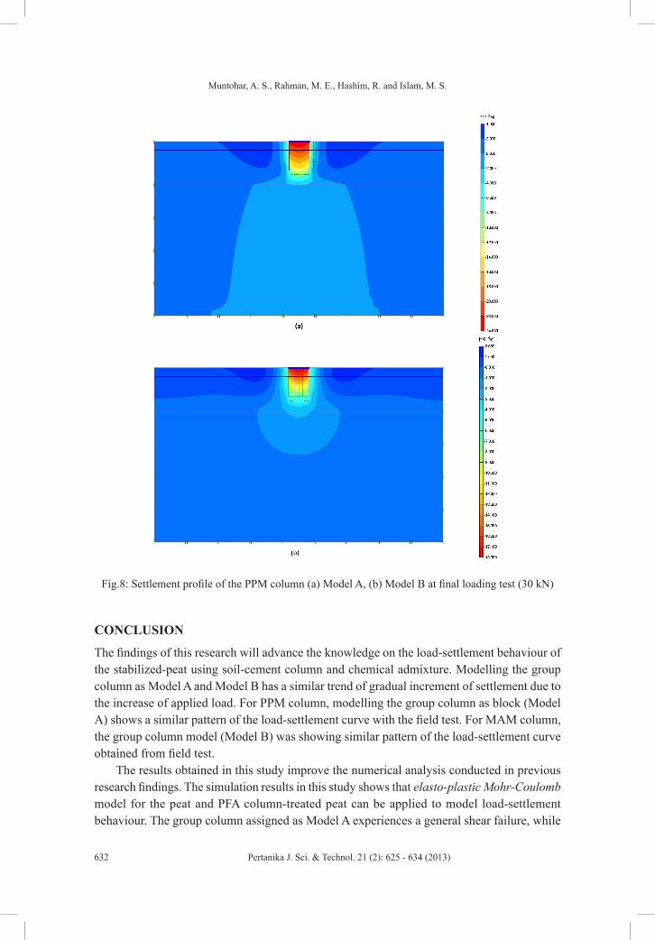
Muntohar, A. S., Rahman, M. E., Hashim, R. and Islam, M. S.
632 Pertanika J. Sci. & Technol. 21 (2): 625 - 634 (2013)
CONCLUSION
The findings of this research will advance the knowledge on the load-settlement behaviour of the stabilized-peat using soil-cement column and chemical admixture. Modelling the group column as Model A and Model B has a similar trend of gradual increment of settlement due to the increase of applied load. For PPM column, modelling the group column as block (Model A) shows a similar pattern of the load-settlement curve with the field test. For MAM column, the group column model (Model B) was showing similar pattern of the load-settlement curve obtained from field test.
The results obtained in this study improve the numerical analysis conducted in previous research findings. The simulation results in this study shows that elasto-plastic Mohr-Coulomb model for the peat and PFA column-treated peat can be applied to model load-settlement behaviour. The group column assigned as Model A experiences a general shear failure, while
Fig.8: Settlement profile of the PPM column (a) Model A, (b) Model B at final loading test (30 kN)

A Numerical Study of Ground Improvement Technique Using Group of Soil-Column on Peat
633Pertanika J. Sci. & Technol. 21 (2): 625 - 634 (2013)
Model B has tendency to local or punch shear failure. The block model of column (Model A) have lower safety factor to failure if compared to column group model (Model B) for both stabilization methods. Whole results in this study show that the models and estimated materials parameter using equation [1] are reliable to model load-settlement using finite element method.
ACKNOWLEDGEMENTS
The first Author is grateful to the R&D Department, Curtin University Sarawak for financial support to conduct this research work under CSRF scheme.
REFERENCESAhnberg, H. (2006). Strength of Stabilized Soils: A laboratory study on clays and organic soils stabilized
with different types of binder. In the 16th Report of Swedish Deep Stabilization Research Centre, Linkoping, Sweden.
Broms, B. B. (1991). Stabilization of Soil with Lime Columns. In Fang, H-Y. & van Nostrand, R. (Eds). Foundation Engineering Handbook, 2nd Edition. New York. pp. 833-855.
Chai, J. C., & Miura, N. (2003, October). Effect of soil-cement column construction to surrounding subsoil. In the Proceeding of Geotechnical Engineering in Urban Construction. Sino-Japanese Symp. Geotech. Engrg., Beijing, China, pp. 96-101, 29-30 October 2003.
Eka, P. (2007). Behaviour of Tiang Tongkat foundation over Pontianak soft organic soil using 3D–finite element analysis. (Doctoral thesis dissertation). Technischen Universität Bergakademie Freiberg, Germany, 2007.
Eslami, A., & Gholami, M. (2006). Analytical model for the ultimate bearing capacity of foundations from cone resistance. Scientia Iranica, 13, 223-233.
Han, J., Oztoprak, S., Parsons, R. L., & Huang, J. (2007). Numerical analysis of foundation columns to support widening of embankments. Computers and Geotechnics, 34(6), 435-448.
Hashim, R., & Islam, S. (2008). Properties of stabilized peat by soil-cement column method. Elec. J. Geotech. Engrg. 13(J), 1-8.
Hebib, S., & Farrell, E. R. (2003). Some experiences on the stabilization of Irish peats. Canadian Geotechnical Journal, 40(1), 107-120.
Islam, M. S., & Hashim,R. (2010). Stabilization of peat soil by soil-column technique and settlement of the group columns. Int. J Physical Sci., 5(9), 1411-1418.
Jarret, P. M. (1995). Geoguide 6, site investigation for organics soils and peat (JKR Document 20709-0341-95). Institut Kerja Raya Malaysia, 1995.
Jenck, O., Dias, D., & Kastner, R. (2007). Two-Dimensional Physical and Numerical Modeling of a Pile-Supported Earth Platform over Soft Soil. Journal of Geotechnical and Geoenvironmental Engineering, 133(3), 295-305.
Jones, C. J. F. P., Lawson, C. R., & Ayres, D. J. (1990). Geotextile reinforced piled embankment. In the Proceeding of 4th Int. Conf. on Geotex., Geomembranes and Related Products, Vol 1, The Haque, A.A. Balkema, pp. 155-160.

Muntohar, A. S., Rahman, M. E., Hashim, R. and Islam, M. S.
634 Pertanika J. Sci. & Technol. 21 (2): 625 - 634 (2013)
Poorooshasb, H. B., & Meyerhof, G. G. (1997). Analysis of behavior of stone columns and lime columns. Computers and Geotechnics, 20(1), 47-70.
Rao, K. N. (2006). Numerical modeling and analysis of pile supported embankments. (MS Thesis dissertation). University of Texas at Arlington, USA, 2006.
Russel, D., & Pierpoint, N. (1997). Assessment of design methods for piled embankment. Ground Engrg., 30(10), 39-49.
Satibi, S. (2009). Numerical analysis and design criteria of embankments on floating piles. (Doctoral thesis dissertation). Instituts für Geotechnik Universität Stuttgart, Germany, 2009.
Sing, W. L., Hashim, R., & Ali, F. H. (2009). Unconfined compressive strength of cemented peat. Aust. J Basic App. Sci., 3(4), 3850-3856.
Voottipruex, P., Suksawat, T., Bergado, D. T., & Jamsawang, P. (2011). Numerical simulations and parametric study of SDCM and DCM piles under full scale axial and lateral loads. Computers and Geotechnics, 38(3), 318-329.
Zwanenburg, C, & Barends, F. B. J. (2007). The influences of anisotropic stiffness on the consolidation of peat. Soil Found., 47(3), 507-516.

REFEREES FOR THE PERTANIKA JOURNAL OF SCIENCE AND TECHNOLOGY
VOL. 21(2) JUL. 2013
The Editorial Board of the Journal of Science and Technology wishes to thank the following for acting as referees for manuscripts published in this issue of JST.
While every effort has been made to include a complete list of referees for the period stated above, however if any name(s) have been omitted unintentionally or spelt incorrectly, please notify the Executive Editor, Pertanika Journals at [email protected].
Any inclusion or exclusion of name(s) on this page does not commit the Pertanika Editorial Office, nor the UPM Press or the University to provide any liability for whatsoever reason.
Special Acknowledgement
The JST Editorial Board gratefully acknowledges the assistance of Doreen Dillah, who served as the English language editor for this issue.
UPM- Universiti Putra MalaysiaUSM- Universiti Sains MalaysiaUM- Universiti Malaya
IIUM- International Islamic University of MalaysiaUPNM- Universiti Pertahanan Nasional Malaysia
Aaron Goh Suk Meng (Curtin University, Malaysia)
Abrar Muslim (University of Syiah Kuala, Indonesia)
Agus Saptoro (Curtin University, Malaysia)
Ahmad Zuhairi Abdullah (USM, Malaysia)
Akif Al-Fugura (Zarqa University, Jordan)
Ali Dehghantanha (UPM, Malaysia)
Amar Sahed (Curtin University, Malaysia)
Antapattu (Curtin University, Malaysia)
Asma Ismail (USM, Malaysia)
Baharuddin Saad (USM, Malaysia)
Desa Ahmad (UPM, Malaysia)
Edi Syams Zainudin (UPM, Malaysia)
G Venkatesan (Anna University of Technology, India)
Gan Seng Neon (UM, Malaysia)
Gatut Sudarjanto (University of Queensland, Australia)
Habil Biswajeet Pradhan (UPM, Malaysia)
Hailiza Kamarulhaili@Harun (USM, Malaysia)
Hamid Assilzadeh (The University of Calgary, Canada)
Heng Swee Huay (MMU, Malaysia)
Heng Swee Huay (MMU, Malaysia)
Irwandi Jaswir (IIUM, Malaysia)
Jacek Uziak (University of Botswana, Botswana)
Jayakumar Muthuramalingam (Curtin University, Malaysia)
Kaniraj Shenbaga (UNIMAS, Malaysia)
Lau Siong Hoe (MMU, Malaysia)
Law Ming Chiat (Curtin University, Malaysia)
Leblouba Moussa (Curtin University, Malaysia)
Lim Hwee San (USM, Malaysia)
Mazlan Hashim (UTM, Malaysia)
Megat Mohamad Hamdan Megat Ahmad (UPNM, Malaysia)
Mohamad Wijayanuddin Ali (UTM, Malaysia)
Mohd Amaluddin Yusoff (Curtin University, Malaysia)
Mohd Sapuan Salit (UPM, Malaysia)
Muhamad Mat Noor (UMP, Malaysia)
Muhammad Ekhlasur Rahman (Curtin University, Malaysia)
Naser Nassif Barsoum (Curtin University, Malaysia)
Nor Azah Yusof (UPM, Malaysia)
Oon Shea Ming (UM, Malaysia)
P Rajesh Prasanna (Anna University of Technology, India)
Peh Kok Khiang (USM, Malaysia)
Perumal Kumar (Curtin University, Malaysia)
Phang Sook Wai (UM, Malaysia)
Pradeep Kumar Garg (Indian Institute of Technology Roorkee, India)
Putra Sumari (USM, Malaysia)
Ravi Prakash (Jaypee University of Information Technology, India)
Safian Sharif (UTM, Malaysia)
Saied Pirasteh (UPM, Malaysia)
Samuel Suman Raj Dasary (Jackson State University, USA)
Sanusi S Ahamad (USM, Malaysia)
Shymala Doraisamy (UPM, Malaysia)
Sojinu Olatunbosun Samuel Setonji (Redeemer’s University, Nigeria)
Son Radu (UPM, Malaysia)
Sujan Debnath (Curtin University, Malaysia)
Suman Kapur (Birla Institute of Technology & Science, Pilani, India)
Suraya Mohd Tahir (UPM, Malaysia)
Ujjal Kumar Ghosh (Curtin University, Malaysia)
Visal Keshari (Defense Research & Development Organisation, India)
Yusuke Asakuma (University of Hyogo, Japan)
Zurina Zainal Abidin (UPM, Malaysia)
MMU- Multimedia University of MalaysiaUMP- Universiti Malaysia Pahang


PertanikaOur goal is to bring high quality research to the widest possible audience
Journal of Science & Technology
INSTRUCTIONS TO AUTHORS(Manuscript Preparation & Submission Guidelines)
Revised: January 2013
We aim for excellence, sustained by a responsible and professional approach to journal publishing. We value and support our authors in the research community.
Please read the guidelines and follow these instructions carefully; doing so will ensure that the publication of your manuscript is as rapid and efficient as possible. The Editorial Board reserves the right to return manuscripts that are not prepared in accordance with these guidelines.
About the JournalPertanika is an international peer-reviewed journal devoted to the publication of original papers, and it serves as a forum for practical approaches to improving quality in issues pertaining to tropical agriculture and its related fields. Pertanika began publication in 1978 as Journal of Tropical Agricultural Science. In 1992, a decision was made to streamline Pertanika into three journals to meet the need for specialised journals in areas of study aligned with the interdisciplinary strengths of the university. The revamped Journal of Science and Technology (JST) is now focusing on research in science and engineering, and its related fields. Other Pertanika series include Journal of Tropical Agricultural Science (JTAS); and Journal of Social Sciences and Humanities (JSSH).
JST is published in English and it is open to authors around the world regardless of the nationality. It is currently published two times a year i.e. in January and July.
Goal of PertanikaOur goal is to bring the highest quality research to the widest possible audience.
Quality We aim for excellence, sustained by a responsible and professional approach to journal publishing. Submissions are guaranteed to receive a decision within 12 weeks. The elapsed time from submission to publication for the articles averages 5-6 months.
Indexing of PertanikaPertanika is now over 33 years old; this accumulated knowledge has resulted in Pertanika JST being indexed in SCOPUS (Elsevier), EBSCO, Thomson (ISI) Web of Knowledge [CAB Abstracts], DOAJ, Google Scholar, ERA, ISC, Citefactor, Rubriq and MyAIS.
Future visionWe are continuously improving access to our journal archives, content, and research services. We have the drive to realise exciting new horizons that will benefit not only the academic community, but society itself.
We also have views on the future of our journals. The emergence of the online medium as the predominant vehicle for the ‘consumption’ and distribution of much academic research will be the ultimate instrument in the dissemination of the research news to our scientists and readers.
Aims and ScopePertanika Journal of Science and Technology aims to provide a forum for high quality research related to science and engineering research. Areas relevant to the scope of the journal include: bioinformatics, bioscience, biotechnology and bio-molecular sciences, chemistry, computer science, ecology, engineering, engineering design, environmental control and management, mathematics and statistics, medicine and health sciences, nanotechnology, physics, safety and emergency management, and related fields of study.
Editorial StatementPertanika is the official journal of Universiti Putra Malaysia. The abbreviation for Pertanika Journal of Science & Technology is Pertanika J. Sci. Technol.

Guidelines for AuthorsPublication policiesPertanika policy prohibits an author from submitting the same manuscript for concurrent consideration by two or more publications. It prohibits as well publication of any manuscript that has already been published either in whole or substantial part elsewhere. It also does not permit publication of manuscript that has been published in full in Proceedings. Please refer to Pertanika’s Code of Ethics for full details.
Editorial processAuthors are notified on receipt of a manuscript and upon the editorial decision regarding publication.
Manuscript review: Manuscripts deemed suitable for publication are sent to the Editorial Board members and/or other reviewers. We encourage authors to suggest the names of possible reviewers. Notification of the editorial decision is usually provided within to eight to ten weeks from the receipt of manuscript. Publication of solicited manuscripts is not guaranteed. In most cases, manuscripts are accepted conditionally, pending an author’s revision of the material.
Author approval: Authors are responsible for all statements in articles, including changes made by editors. The liaison author must be available for consultation with an editor of The Journal to answer questions during the editorial process and to approve the edited copy. Authors receive edited typescript (not galley proofs) for final approval. Changes cannot be made to the copy after the edited version has been approved.
Manuscript preparationPertanika accepts submission of mainly four types of manuscripts. Each manuscript is classified as regular or original articles, short communications, reviews, and proposals for special issues. Articles must be in English and they must be competently written and argued in clear and concise grammatical English. Acceptable English usage and syntax are expected. Do not use slang, jargon, or obscure abbreviations or phrasing. Metric measurement is preferred; equivalent English measurement may be included in parentheses. Always provide the complete form of an acronym/abbreviation the first time it is presented in the text. Contributors are strongly recommended to have the manuscript checked by a colleague with ample experience in writing English manuscripts or an English language editor.
Linguistically hopeless manuscripts will be rejected straightaway (e.g., when the language is so poor that one cannot be sure of what the authors really mean). This process, taken by authors before submission, will greatly facilitate reviewing, and thus publication if the content is acceptable.
The instructions for authors must be followed. Manuscripts not adhering to the instructions will be returned for revision without review. Authors should prepare manuscripts according to the guidelines of Pertanika.
1. Regular articleDefinition: Full-length original empirical investigations, consisting of introduction, materials and methods, results and discussion, conclusions. Original work must provide references and an explanation on research findings that contain new and significant findings.
Size: Should not exceed 5000 words or 8-10 printed pages (excluding the abstract, references, tables and/or figures). One printed page is roughly equivalent to 3 type-written pages.
2. Short communicationsDefinition: Significant new information to readers of the Journal in a short but complete form. It is suitable for the publication of technical advance, bioinformatics or insightful findings of plant and animal development and function.
Size: Should not exceed 2000 words or 4 printed pages, is intended for rapid publication. They are not intended for publishing preliminary results or to be a reduced version of Regular Papers or Rapid Papers.
3. Review articleDefinition: Critical evaluation of materials about current research that had already been published by organizing, integrating, and evaluating previously published materials. Re-analyses as meta-analysis and systemic reviews are encouraged. Review articles should aim to provide systemic overviews, evaluations and interpretations of research in a given field.
Size: Should not exceed 4000 words or 7-8 printed pages.
4. Special issuesDefinition: Usually papers from research presented at a conference, seminar, congress or a symposium.
Size: Should not exceed 5000 words or 8-10 printed pages.
5. OthersDefinition: Brief reports, case studies, comments, Letters to the Editor, and replies on previously published articles may be considered.
Size: Should not exceed 2000 words or up to 4 printed pages.

With few exceptions, original manuscripts should not exceed the recommended length of 6 printed pages (about 18 typed pages, double-spaced and in 12-point font, tables and figures included). Printing is expensive, and, for the Journal, postage doubles when an issue exceeds 80 pages. You can understand then that there is little room for flexibility.
Long articles reduce the Journal’s possibility to accept other high-quality contributions because of its 80-page restriction. We would like to publish as many good studies as possible, not only a few lengthy ones. (And, who reads overly long articles anyway?) Therefore, in our competition, short and concise manuscripts have a definite advantage.
FormatThe paper should be formatted in one column format with at least 4cm margins and 1.5 line spacing throughout. Authors are advised to use Times New Roman 12-point font. Be especially careful when you are inserting special characters, as those inserted in different fonts may be replaced by different characters when converted to PDF files. It is well known that ‘µ’ will be replaced by other characters when fonts such as ‘Symbol’ or ‘Mincho’ are used.
A maximum of eight keywords should be indicated below the abstract to describe the contents of the manuscript. Leave a blank line between each paragraph and between each entry in the list of bibliographic references. Tables should preferably be placed in the same electronic file as the text. Authors should consult a recent issue of the Journal for table layout.
Every page of the manuscript, including the title page, references, tables, etc. should be numbered. However, no reference should be made to page numbers in the text; if necessary, one may refer to sections. Underline words that should be in italics, and do not underline any other words.
We recommend that authors prepare the text as a Microsoft Word file.
1. Manuscripts in general should be organised in the following order:
o Page 1: Running title. (Not to exceed 60 characters, counting letters and spaces). This page should only contain the running title of your paper. The running title is an abbreviated title used as the running head on every page of the manuscript.
In addition, the Subject areas most relevant to the study must be indicated on this page. Select the appropriate subject areas from the Scope of the Journals provided in the Manuscript Submission Guide.
A list of number of black and white / colour figures and tables should also be indicated on this page. Figures submitted in color will be printed in colour. See “5. Figures & Photographs” for details.
o Page 2: Author(s) and Corresponding author information. This page should contain the full title of your paper with name(s) of all the authors, institutions and corresponding author’s name, institution and full address (Street address, telephone number (including extension), hand phone number, fax number and e-mail address) for editorial correspondence. The names of the authors must be abbreviated following the international naming convention. e.g. Salleh, A.B., Tan, S.G., or Sapuan, S.M.
Authors’ addresses. Multiple authors with different addresses must indicate their respective addresses separately by superscript numbers:
George Swan1 and Nayan Kanwal2 1Department of Biology, Faculty of Science, Duke University, Durham, North Carolina, USA. 2Office of the Deputy Vice Chancellor (R&I), Universiti Putra Malaysia, Serdang, Malaysia.
o Page 3: This page should repeat the full title of your paper with only the Abstract (the abstract should be less than 250 words for a Regular Paper and up to 100 words for a Short Communication). Keywords must also be provided on this page (Not more than eight keywords in alphabetical order).
o Page 4 and subsequent pages: This page should begin with the Introduction of your article and the rest of your paper should follow from page 5 onwards.
Abbreviations. Define alphabetically, other than abbreviations that can be used without definition. Words or phrases that are abbreviated in the introduction and following text should be written out in full the first time that they appear in the text, with each abbreviated form in parenthesis. Include the common name or scientific name, or both, of animal and plant materials.
Footnotes. Current addresses of authors if different from heading.
2. Text. Regular Papers should be prepared with the headings Introduction, Materials and Methods, Results and Discussion, Conclusions in this order. Short Communications should be prepared according to “8. Short Communications.” below.
3. Tables. All tables should be prepared in a form consistent with recent issues of Pertanika and should be numbered consecutively with Arabic numerals. Explanatory material should be given in the table legends and footnotes. Each

table should be prepared on a separate page. (Note that when a manuscript is accepted for publication, tables must be submitted as data - .doc, .rtf, Excel or PowerPoint file- because tables submitted as image data cannot be edited for publication.)
4. Equations and Formulae. These must be set up clearly and should be typed triple spaced. Numbers identifying equations should be in square brackets and placed on the right margin of the text.
5. Figures & Photographs. Submit an original figure or photograph. Line drawings must be clear, with high black and white contrast. Each figure or photograph should be prepared on a separate sheet and numbered consecutively with Arabic numerals. Appropriate sized numbers, letters and symbols should be used, no smaller than 2 mm in size after reduction to single column width (85 mm), 1.5-column width (120 mm) or full 2-column width (175 mm).
6. Failure to comply with these specifications will require new figures and delay in publication. For electronic figures, create your figures using applications that are capable of preparing high resolution TIFF files acceptable for publication. In general, we require 300 dpi or higher resolution for coloured and half-tone artwork and 1200 dpi or higher for line drawings. For review, you may attach low-resolution figures, which are still clear enough for reviewing, to keep the file of the manuscript under 5 MB. Illustrations may be produced at extra cost in colour at the discretion of the Publisher; the author could be charged Malaysian Ringgit 50 for each colour page.
7. References. Literature citations in the text should be made by name(s) of author(s) and year. For references with more than two authors, the name of the first author followed by ‘et al.’ should be used.
Swan and Kanwal (2007) reported that …The results have been interpreted (Kanwal et al. 2009).
o References should be listed in alphabetical order, by the authors’ last names. For the same author, or for the same set of authors, references should be arranged chronologically. If there is more than one publication in the same year for the same author(s), the letters ‘a’, ‘b’, etc., should be added to the year.
o When the authors are more than 11, list 5 authors and then et al.
o Do not use indentations in typing References. Use one line of space to separate each reference. The name of the journal should be written in full. For example:
• Jalaludin, S. (1997a). Metabolizable energy of some local feeding stuff. Tumbuh, 1, 21-24.
• Jalaludin, S. (1997b). The use of different vegetable oil in chicken ration. Malayan Agriculturist, 11, 29-31.
• Tan, S. G., Omar, M. Y., Mahani, K. W., Rahani, M., & Selvaraj, O. S. (1994). Biochemical genetic studies on wild populations of three species of green leafhoppers Nephotettix from Peninsular Malaysia. Biochemical Genetics, 32, 415 - 422.
o In case of citing an author(s) who has published more than one paper in the same year, the papers should be distinguished by addition of a small letter as shown above, e.g. Jalaludin (1997a); Jalaludin (1997b).
o Unpublished data and personal communications should not be cited as literature citations, but given in the text in parentheses. ‘In press’ articles that have been accepted for publication may be cited in References. Include in the citation the journal in which the ‘in press’ article will appear and the publication date, if a date is available.
8. Examples of other reference citations:
Monographs: Turner, H. N., & Yong, S. S. Y. (2006). Quantitative Genetics in Sheep Breeding. Ithaca: Cornell University Press.
Chapter in Book: Kanwal, N. D. S. (1992). Role of plantation crops in Papua New Guinea economy. In Angela R. McLean (Ed.), Introduction of livestock in the Enga province PNG (p. 221-250). United Kingdom: Oxford Press.
Proceedings: Kanwal, N. D. S. (2001). Assessing the visual impact of degraded land management with landscape design software. In Kanwal, N. D. S., & Lecoustre, P. (Eds.), International forum for Urban Landscape Technologies (p. 117-127). Lullier, Geneva, Switzerland: CIRAD Press.
9. Short Communications should include Introduction, Materials and Methods, Results and Discussion, Conclusions in this order. Headings should only be inserted for Materials and Methods. The abstract should be up to 100 words, as stated above. Short Communications must be 5 printed pages or less, including all references, figures and tables. References should be less than 30. A 5 page paper is usually approximately 3000 words plus four figures or tables (if each figure or table is less than 1/4 page).
*Authors should state the total number of words (including the Abstract) in the cover letter. Manuscripts that do not fulfill these criteria will be rejected as Short Communications without review.

STYLE OF THE MANUSCRIPTManuscripts should follow the style of the latest version of the Publication Manual of the American Psychological Association (APA). The journal uses American or British spelling and authors may follow the latest edition of the Oxford Advanced Learner’s Dictionary for British spellings.
SUBMISSION OF MANUSCRIPTSAll articles should be submitted electronically using the ScholarOne web-based system. ScholarOne, a Thomson Reuters product provides comprehensive workflow management systems for scholarly journals. For more information, go to our web page and click “Online Submission”.
Alternatively, you may submit the electronic files (cover letter, manuscript, and the Manuscript Submission Kit comprising Declaration and Referral forms) via email directly to the Executive Editor. If the files are too large to email, mail a CD containing the files. The Manuscript Submission Guide and Submission Kit are available from the Pertanika’s home page at http://www.pertanika.upm.edu.my/ or from the Executive Editor’s office upon request.
All articles submitted to the journal must comply with these instructions. Failure to do so will result in return of the manuscript and possible delay in publication.
Please do not submit manuscripts to the editor-in-chief or to any other office directly. All manuscripts must be submitted through the executive editor’s office to be properly acknowledged and rapidly processed at the address below:
Dr. Nayan KANWALThe Executive Editor Pertanika Journals, UPM PressOffice of the Deputy Vice Chancellor (R&I)IDEA Tower II, UPM-MTDC Technology CentreUniversiti Putra Malaysia43400 UPM, Serdang, Selangor Malaysia
E-mail: [email protected]; tel: + 603-8947 1622.or visit our website at http://www.pertanika.upm.edu.my/home.php for further information.
Authors should retain copies of submitted manuscripts and correspondence, as materials can not be returned. Authors are required to inform the Executive Editor of any change of address which occurs whilst their papers are in the process of publication.
Cover letter
All submissions must be accompanied by a cover letter detailing what you are submitting. Papers are accepted for publication in the journal on the understanding that the article is original and the content has not been published or submitted for publication elsewhere. This must be stated in the cover letter.
The cover letter must also contain an acknowledgement that all authors have contributed significantly, and that all authors are in agreement with the content of the manuscript.
The cover letter of the paper should contain (i) the title; (ii) the full names of the authors; (iii) the addresses of the institutions at which the work was carried out together with (iv) the full postal and email address, plus facsimile and telephone numbers of the author to whom correspondence about the manuscript should be sent. The present address of any author, if different from that where the work was carried out, should be supplied in a footnote.
As articles are double-blind reviewed, material that might identify authorship of the paper should be placed on a cover sheet.
Peer reviewPertanika follows a double-blind peer-review process. Peer reviewers are experts chosen by journal editors to provide written assessment of the strengths and weaknesses of written research, with the aim of improving the reporting of research and identifying the most appropriate and highest quality material for the journal.
In the peer-review process, three referees independently evaluate the scientific quality of the submitted manuscripts. Authors are encouraged to indicate in the Referral form using the Manuscript Submission Kit the names of three potential reviewers, but the editors will make the final choice. The editors are not, however, bound by these suggestions.
Manuscripts should be written so that they are intelligible to the professional reader who is not a specialist in the particular field. They should be written in a clear, concise, direct style. Where contributions are judged as acceptable for publication on the basis of content, the Editor reserves the right to modify the typescripts to eliminate ambiguity and repetition and improve communication between author and reader. If extensive alterations are required, the manuscript will be returned to the author for revision.

The Journal’s review processWhat happens to a manuscript once it is submitted to Pertanika? Typically, there are seven steps to the editorial review process:
1. The executive editor and the editorial board examine the paper to determine whether it is appropriate for the journal and should be reviewed. If not appropriate, the manuscript is rejected outright and the author is informed.
2. The executive editor sends the article-identifying information having been removed, to three reviewers. Typically, one of these is from the Journal’s editorial board. Others are specialists in the subject matter represented by the article. The executive editor asks them to complete the review in three weeks and encloses two forms: (a) referral form B and (b) reviewer’s comment form along with reviewer’s guidelines. Comments to authors are about the appropriateness and adequacy of the theoretical or conceptual framework, literature review, method, results and discussion, and conclusions. Reviewers often include suggestions for strengthening of the manuscript. Comments to the editor are in the nature of the significance of the work and its potential contribution to the literature.
3. The executive editor, in consultation with the editor-in-chief, examines the reviews and decides whether to reject the manuscript, invite the author(s) to revise and resubmit the manuscript, or seek additional reviews. Final acceptance or rejection rests with the Editorial Board, who reserves the right to refuse any material for publication. In rare instances, the manuscript is accepted with almost no revision. Almost without exception, reviewers’ comments (to the author) are forwarded to the author. If a revision is indicated, the editor provides guidelines for attending to the reviewers’ suggestions and perhaps additional advice about revising the manuscript.
4. The authors decide whether and how to address the reviewers’ comments and criticisms and the editor’s concerns. The authors submit a revised version of the paper to the executive editor along with specific information describing how they have answered’ the concerns of the reviewers and the editor.
5. The executive editor sends the revised paper out for review. Typically, at least one of the original reviewers will be asked to examine the article.
6. When the reviewers have completed their work, the executive editor in consultation with the editorial board and the editor-in-chief examine their comments and decide whether the paper is ready to be published, needs another round of revisions, or should be rejected.
7. If the decision is to accept, the paper is sent to that Press and the article should appear in print in approximately three months. The Publisher ensures that the paper adheres to the correct style (in-text citations, the reference list, and tables are typical areas of concern, clarity, and grammar). The authors are asked to respond to any queries by the Publisher. Following these corrections, page proofs are mailed to the corresponding authors for their final approval. At this point, only essential changes are accepted. Finally, the article appears in the pages of the Journal and is posted on-line.
English language editingPertanika emphasizes on the linguistic accuracy of every manuscript published. Thus all authors are required to get their manuscripts edited by professional English language editors. Author(s) must provide a certificate confirming that their manuscripts have been adequately edited. A proof from a recognised editing service should be submitted together with the cover letter at the time of submitting a manuscript to Pertanika. All costs will be borne by the author(s).
This step, taken by authors before submission, will greatly facilitate reviewing, and thus publication if the content is acceptable.
Author material archive policyAuthors who require the return of any submitted material that is rejected for publication in the journal should indicate on the cover letter. If no indication is given, that author’s material should be returned, the Editorial Office will dispose of all hardcopy and electronic material.
CopyrightAuthors publishing the Journal will be asked to sign a declaration form. In signing the form, it is assumed that authors have obtained permission to use any copyrighted or previously published material. All authors must read and agree to the conditions outlined in the form, and must sign the form or agree that the corresponding author can sign on their behalf. Articles cannot be published until a signed form has been received.
Lag time A decision on acceptance or rejection of a manuscript is reached in 3 to 4 months (average 14 weeks). The elapsed time from submission to publication for the articles averages 5-6 months.
Hardcopies of the Journals and off printsUnder the Journal’s open access initiative, authors can choose to download free material (via PDF link) from any of the journal issues from Pertanika’s website. Under “Browse Journals” you will see a link entitled “Current Issues” or “Archives”. Here you will get access to all back-issues from 1978 onwards.
The corresponding author for all articles will receive one complimentary hardcopy of the journal in which his/her articles is published. In addition, 20 off prints of the full text of their article will also be provided. Additional copies of the journals may be purchased by writing to the executive editor.

Pertanika began publication in 1978 as the
Journal of Tropical Agricultural Science (JTAS).
In 1992, a decision was made to streamline
Pertanika into 3 journals. i.e.,
1. Journal of Tropical Agricultural Science (JTAS) 2. Journal of Science and Technology (JST) 3. Journal of Social Sciences and Humanities (JSSH)
PROFILE: Pertanika publishes original academic
articles rapidly. It is fully committed to the
Open Access Initiative and provides free access
to all articles as soon as they are published.
QUALITY: Articles submitted to Pertanika
undergo rigid originality checks. Our double-
blind peer review procedures are fair and open.
AUTHOR SERVICES: We ensure that your work
reaches the widest possible audience in print
and online rapidly. Submissions are through
ScholarOne system by Thomson Reuters.
The Journal accepts articles as regular, short
communication or review papers.
The article should include the following:
An abstract of not more than 300 words; Up to 8 related keywords; Name(s), Institutional affiliation(s) and
email(s) of each author. The maximum length of your article
must not exceed: o approximately 6000 words or 27 pages,
including abstract, diagrams tables and references for full research papers,
o 2000 words for short communication papers, or
o 4000 words for review papers
References should be listed in APA style.
You may submit your articles at any time of the
year. The journal is now accepting papers for
its 2013-14 issues.
For guidance on the submission process, or for any questions regarding submissions, you may contact the Chief Executive Editor at: [email protected]
BACKGROUND
BENEFITS TO AUTHORS
………………………………………………………………………
Call for Papers 2013-14 now accepting submissions… ……………………………………………………………..………
About the Journal
An international multidisciplinary peer-reviewed leading Malaysian journal.
Publishes articles in English biannually. i.e., January and July.
The elapsed time from submission to publication for the articles averages 5 to 6 months. A decision on acceptance of a manuscript is reached in 3 to 4 months (average 14 weeks).
Indexed in SCOPUS (Elsevier), EBSCO, DOAJ, CABI, Google Scholar, MyAIS & ISC.
Scope of Journal Pertanika Journal of Science and Technology caters for
science and engineering research dealing with issues of worldwide relevance.
Refer to our website for detailed scope areas. http://www.pertanika.upm.edu.my/scope.php
Format for Paper Submission Articles should include the following:
o problem formulation o conceptual framework o methodology/ approach o research design (if applicable) o statistical analysis (if applicable) o main findings o overall contribution o conclusions & suggestion for further research o acknowledgements (if applicable)
Rapid research publication… Pertanika is the resource to support you in strengthening your research.
Journal’s profile: http://www.pertanika.upm.edu.my/
SUBMISSION GUIDELINES
SUBMISSION DEADLINE
CONTACT US View current issue Submit your manuscript to http://mc.manuscriptcentral.com/upm-jst
View journal archives
Having trouble viewing this email? Click here to view online | View in a Mobile Device


Palm Oil Transesterification Processing to Biodiesel Using a Combine of Ultrasonic and Chemical Catalyst
567
Supranto, S.
Electricity Generation from Citronella Bagasse (CB) Using Dual Chamber Microbial Fuel Cell
581
Nik Azmi Nik Mahmood, Mohd Nazlee Faisal Md Ghazali, Kamarul’Asri Ibrahim and Nur Muhammad ElQarni Md Norodin
Experimental Design Analysis of Ultra Fine Fly Ash, Lime Water, and Basalt Fibre in Mix Proportion of High Volume Fly Ash Concrete
589
Mochamad Solikin, Sujeeva Setunge and Indubhushan Patnaikuni
Experimental Study on Shear Behaviour of High Strength Reinforced Recycled Concrete Beam
601
Oh Chai Lian, Lee Siong Wee, Mohd Asha’ari Masrom and Goh Ching Hua
Responsive Façades: Parametric Control of Moveable Tilings 611Sambit Datta and Michael Hobbs
A Numerical Study of Ground Improvement Technique Using Group of Soil-Column on Peat
625
Muntohar, A. S., Rahman, M. E., Hashim, R. and Islam, M. S.

Production of Orthophoto and Volume Determination Using Low-Cost Digital Cameras
387
Khairul Nizam Tahar and Anuar Ahmad
Climate Change Resilience Assessment Using Livelihood Assets of Coastal Fishing Community in Nijhum Dwip, Bangladesh
397
Hossain, M. S., Rahman, M. F., Thompson, S., Nabi, M. R. and Kibria, M. M.
Goal Event Detection in Soccer Videos via Collaborative Multimodal Analysis 423Alfian Abdul Halin and Mandava Rajeswari
On the Diophantine Equation x2 + 4.7b = y2r 443Yow, K. S., Sapar, S. H. and Atan, K. A.
Electrical Conductivity of Anionic Surfactant-Doped Polypyrrole Nanoparticles Prepared via Emulsion Polymerization
459
Ghalib, H., Abdullah, I. and Daik, R.
Landslide Susceptibility Mapping Using Averaged Weightage Score and GIS: A Case Study at Kuala Lumpur
473
Mahmud, A. R., Awad, A. and Billa, R.
GIS Modeling for Selection of a Transfer Station Site for Residential Solid Waste Separation and Recycling
487
Billa, L. and Pradhan, B.
Comparative Study on the Effect of Density on Water Absorption of Particle Boards Produced from Nipa Palm Fibres with HDPE Wastes
499
Ekpunobi, U. E., Eboatu, A. N. and Okoye, P.-A.
Rootkit Guard (RG) - An Architecture for Rootkit Resistant File-System Implementation Based on TPM
507
Teh Jia Yew, Khairulmizam Samsudin, Nur Izura Udzir and Shaiful Jahari Hashim
Selected Articles from CUTSE International Conference 2011Guest Editor: Ashutosh Kumar SinghGuest Editorial Board: Sujan Debnath and Muhammad Ekhlasur Rahman
Theoretical Modeling of Pseudo Hydrostatic Force in Solid-Liquid Pipe Flow with Two Layers
521
Hussain H. Al-Kayiem and Iylia Elena Abdul Jamil
Improvement of Coke Strength by Phenolic Resin Coating: Experimental and Theoretical Studies of Strengthening Mechanism
533
Y. Asakuma, Y. Komatsu, S. Nishi, A. Kotani and M. Nishimura
Application of Markov Chain in the PageRank Algorithm 541Ravi Kumar, P., Alex Goh, K. L. and Ashutosh, K. S.
Harnessing Energy from Electromagnetic Field: Practical Implementation Integrating Coil Antenna and IC Load
555
Syahrizal Salleh and Zulkifli Abd Majid
VOL. 21 (2) JUL. 2013
Pertanika JSTU
PM Press, M
alaysiaVol. 21 (2) Jul. 2013
Pertanika Journal of Science & TechnologyVol. 21 (2) Jul. 2013
Contents
Pertanika Editorial OceOce of the Deputy Vice Chancellor (R&I), 1st Floor, IDEA Tower II, UPM-MTDC Technology CentreUniversiti Putra Malaysia43400 UPM SerdangSelangor Darul EhsanMalaysia
http://www.pertanika.upm.edu.my/E-mail: [email protected]: +603 8947 1622/1620
Foreword
iNayan Deep S. Kanwal
Invited PaperSystems Informatics and Analysis of Biomass Feedstock Production 273
Shastri Y. N., Hansen A. C., Rodríguez L. F. and Ting K. C.
Review ArticlesA Review of Cosmetic and Personal Care Products: Halal Perspective and Detection of Ingredient
281
Hashim, P. and Mat Hashim, D.
A Review on the Effects of Probiotics and Antibiotics towards Infections
293
Hazirah, A., Loong, Y. Y., Rushdan, A. A., Rukman, A. H. and Yazid, M. M.
Methodologies for Measuring Sustainability of Product/Process: A Review 303Pezhman Ghadimi, Noordin Mohd Yusof, Muhamad Zameri Mat Saman and Mahmood Asadi
Regular ArticlesDetection of Ethanol Vapours Using Titanium Dioxide (TiO2) Catalytic Pellet by 327
Ang Gaik Tin, Mohamad Zailani Abu Bakar and Cheah Mooi Chen
Green Compression Strength of Tin Mine Tailing Sand for Green Sand Casting Mould
335
Azhar Abdullah, Shamsuddin Sulaiman, B. T. Hang Tuah Baharudin,
Web-Based Decision Support System for Paddy Planting Management 343C. Y. N. Norasma, A. R. M. Shariff, E. Jahanshiri, M. S. M. Amin, S. Khairunniza-Bejo and A. R. Mahmud
Development of an Automation and Control Design System for Lowland Tropical Greenhouses
365
W. I. Wan Ishak, R. M. Hudzari and M. Y. Tan
Recovery of Heavy Metals from Spent Etching Waste Solution of Printed Circuit Board (PCB) Manufacturing
375
A. H. M. Ali, S. Sobri, Salmiaton. A. and Faizah M. Y.
Copyright © 2022 FDOKUMEN