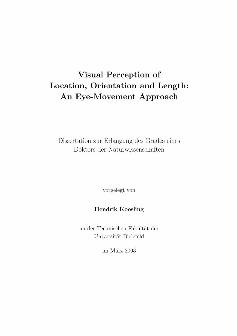
Visual Perception of Location, Orientation and Length: An Eye ...
312
Visual Perception of Location, Orientation and Length: An Eye-Movement Approach Dissertation zur Erlangung des Grades eines Doktors der Naturwissenschaften vorgelegt von Hendrik Koesling an der Technischen Fakult¨at der Universit¨ at Bielefeld imM¨arz2003
-
Upload
khangminh22 -
Category
Documents
-
view
3 -
download
0
Transcript of Visual Perception of Location, Orientation and Length: An Eye ...
Visual Perception of
Location, Orientation and Length:
An Eye-Movement Approach
Dissertation zur Erlangung des Grades eines
Doktors der Naturwissenschaften
vorgelegt von
Hendrik Koesling
an der Technischen Fakultat der
Universitat Bielefeld
im Marz 2003


i
Acknowledgement
I would like to thank (in alphabetical order) Elena Carbone, Thomas Clermont, Sinead
Conneely, Kai Essig, Rudiger and Ursel Koesling, Sven Pohl, Marc Pomplun, Helge
Ritter, Lorenz Sichelschmidt and Jurgen Stroker for their continuous support, helpful
comments, suggestions and advice during my PhD research. This research was conducted
within the Neuroinformatics Group and the Collaborative Research Center 360 “Situated
Artificial Communicators” (SFB 360, Unit B4) at the University of Bielefeld. The project
was funded by the Deutsche Forschungsgemeinschaft (DFG).
Bielefeld, 17th June 2003 Hendrik Koesling

ii
Abstract
One of the most common tasks in life is probably that of visual object recognition and
comparison. We often have to decide, for example, which of two objects is smaller, longer
or, in general, more suitable for an intended use. This task might considerably be com-
plicated when objects are quite alike, located far apart or not being visible at the same
time. The comparison process is thus not only influenced by the relevant intrinsic object
attributes, but also by object similarity and the objects’ spatial and temporal relations
to each other.
This PhD thesis documents a comprehensive investigation of the visual assessment of
typical attributes of abstract stimuli in different comparison scenarios, taking similarity
and relational aspects into account as well. The analysis of data recorded in eye-tracking
experiments provided insight into underlying perceptive and cognitive processes during
such object comparison tasks, focussing on characteristic stimulus features such as posi-
tional eccentricity, line segment length and orientation. The empirical findings then led
to the implementation of corresponding computational models that can be employed in
machine-vision systems.
In principle, the focal points of the investigations that are presented here were guided
by the cognitive structure of visual comparison tasks. This structure can be characterised
by the following processing steps: Assessment, memorisation, comparison. The validity of
two fundamental hypotheses was tested in order to explore these processes in detail.
The first hypothesis addressed the decomposition of length and orientation assessment:
Can the assessment of line segment length or orientation be accomplished by assessing
the locations of the end points of a line segment and the subsequent “fusion” of the lo-
cation data to yield line segment length or orientation? The hypothesis was investigated
in a gaze-contingent comparison scenario with sequential stimulus presentation. Results
demonstrated a high correlation between the assessment error of peripherally perceived
lengths or orientations of line segments and the mislocation of marker positions, depend-
ing on eccentricity. The empirical data generally supports the hypothesis: The assessment
of a line segment can be formalised as the localisation of line segment end points and the
computation of their distance to yield line segment length. In analogy, the computation
of the spatial relation of end points yields line segment orientation. An accordingly imple-
mented, probabilistic computational model successfully reproduced the empirical findings
and thus yielded further support for the proposed underlying perception principles.
The second hypothesis formulated the existence of two distinct visual processing strate-
gies when assessing line segment length in a free gaze, simultaneous comparison scenario:
Depending on the discrimination difficulty, either holistic or analytic visual processing
strategies are pursued. These strategies should manifest in characteristic eye-movement
patterns. Results show that the holistic strategy is apparently a peripheral process as
such: Length is mentally represented as the distance between a fixated and a peripherally
perceived end point of a line segment. In contrast, a specific pattern of foveal visual atten-
tion is characteristic for the analytic perception strategy, influenced by peripheral length
perception. Saccadic “visual measurement” constitutes the basis for the memorisation

iii
and manipulation of the corresponding mental line segment representations. If the mental
representations are not sufficiently accurate to solve the given comparison task – Which
of two line segments is the longer one? – assessment and mental mapping are re-iterated.
The findings also helped to better understand visual phenomena such as the horizontal-
vertical illusion which appears to be induced by inaccurate measurement at a oculomotor
level already. Integrating components of the “eccentricity model”, in particular stimulus
decomposition, a comprehensive computational model could be developed. It takes into
account the visual length assessment strategies and convincingly reproduces the empirical
data. This yields further support for the involvement of the proposed mechanisms in the
assessment of line segment attributes in the chosen comparison scenarios.

iv

Contents
Acknowledgement . . . . . . . . . . . . . . . . . . . . . . . . . . . . . . . . . . . i
Abstract . . . . . . . . . . . . . . . . . . . . . . . . . . . . . . . . . . . . . . . . ii
Table of Contents . . . . . . . . . . . . . . . . . . . . . . . . . . . . . . . . . . . v
1 Motivation 1
1.1 The Brain–Computer Analogy . . . . . . . . . . . . . . . . . . . . . . . . . 1
1.2 Visual Information Processing . . . . . . . . . . . . . . . . . . . . . . . . . 5
1.3 The Eye–Mind Hypothesis . . . . . . . . . . . . . . . . . . . . . . . . . . . 10
1.4 Tracking Eye Movements . . . . . . . . . . . . . . . . . . . . . . . . . . . . 12
2 Visual Comparison and Assessment of Object Proportions 19
2.1 Visual Comparison . . . . . . . . . . . . . . . . . . . . . . . . . . . . . . . 19
2.2 Assessment of Object Proportions . . . . . . . . . . . . . . . . . . . . . . . 25
2.3 New Insights through Eye Movements . . . . . . . . . . . . . . . . . . . . . 38
2.4 Hypotheses . . . . . . . . . . . . . . . . . . . . . . . . . . . . . . . . . . . 40
3 Methodological Preliminaries 43
3.1 Eye-Tracking Laboratory . . . . . . . . . . . . . . . . . . . . . . . . . . . . 43
3.2 Stimuli . . . . . . . . . . . . . . . . . . . . . . . . . . . . . . . . . . . . . . 49
3.3 Procedure . . . . . . . . . . . . . . . . . . . . . . . . . . . . . . . . . . . . 52
3.4 Independent and Dependent Variables . . . . . . . . . . . . . . . . . . . . 58
3.5 Summary . . . . . . . . . . . . . . . . . . . . . . . . . . . . . . . . . . . . 62
4 Sequential Comparison – Eccentricity Effects 65
4.1 Variables and Stimuli . . . . . . . . . . . . . . . . . . . . . . . . . . . . . . 67
5 Experiment E0: Location Assessment in Peripheral Vision 75
5.1 Method . . . . . . . . . . . . . . . . . . . . . . . . . . . . . . . . . . . . . 75
5.2 Results . . . . . . . . . . . . . . . . . . . . . . . . . . . . . . . . . . . . . . 78
5.3 Discussion and Conclusions . . . . . . . . . . . . . . . . . . . . . . . . . . 88
6 Experiment E1: Length Assessment in Peripheral Vision 93
6.1 Method . . . . . . . . . . . . . . . . . . . . . . . . . . . . . . . . . . . . . 93
6.2 Results . . . . . . . . . . . . . . . . . . . . . . . . . . . . . . . . . . . . . . 95
6.3 Discussion and Conclusions . . . . . . . . . . . . . . . . . . . . . . . . . . 100

vi CONTENTS
7 Experiment E2: Orientation Assessment in Peripheral Vision 105
7.1 Method . . . . . . . . . . . . . . . . . . . . . . . . . . . . . . . . . . . . . 105
7.2 Results . . . . . . . . . . . . . . . . . . . . . . . . . . . . . . . . . . . . . . 107
7.3 Discussion and Conclusions . . . . . . . . . . . . . . . . . . . . . . . . . . 111
8 Modelling Eccentricity Effects 115
8.1 Why Modelling? . . . . . . . . . . . . . . . . . . . . . . . . . . . . . . . . . 115
8.2 A Model for Peripheral Visual Perception of Line Segments . . . . . . . . . 116
8.3 Model Results and Discussion . . . . . . . . . . . . . . . . . . . . . . . . . 125
8.4 Summary and Conclusions . . . . . . . . . . . . . . . . . . . . . . . . . . . 135
9 Simultaneous Comparison – Similarity Effects 139
9.1 Variables and Stimuli . . . . . . . . . . . . . . . . . . . . . . . . . . . . . . 142
10 Experiment S1: Simultaneous Dynamic Length Assessment 147
10.1 Method . . . . . . . . . . . . . . . . . . . . . . . . . . . . . . . . . . . . . 148
10.2 Results . . . . . . . . . . . . . . . . . . . . . . . . . . . . . . . . . . . . . . 150
10.3 Discussion and Conclusions . . . . . . . . . . . . . . . . . . . . . . . . . . 171
11 Experiment S2: Simultaneous Binary Length Comparison 187
11.1 Determination of Discrimination Parameters . . . . . . . . . . . . . . . . . 188
11.2 Method . . . . . . . . . . . . . . . . . . . . . . . . . . . . . . . . . . . . . 190
11.3 Results . . . . . . . . . . . . . . . . . . . . . . . . . . . . . . . . . . . . . . 193
11.4 Discussion and Conclusions . . . . . . . . . . . . . . . . . . . . . . . . . . 214
12 Modelling Similarity Effects 235
12.1 A Model for Simultaneous Length Assessment/Discrimination . . . . . . . 235
12.2 Model Motivation, Concept and Structure . . . . . . . . . . . . . . . . . . 236
12.3 Model Implementation . . . . . . . . . . . . . . . . . . . . . . . . . . . . . 243
12.4 Model Results and Discussion . . . . . . . . . . . . . . . . . . . . . . . . . 256
12.5 Summary and Conclusions . . . . . . . . . . . . . . . . . . . . . . . . . . . 273
13 Conclusions and Outlook 279
13.1 Summary and Conclusions . . . . . . . . . . . . . . . . . . . . . . . . . . . 279
13.2 Outlook . . . . . . . . . . . . . . . . . . . . . . . . . . . . . . . . . . . . . 284
References 289

Chapter 1
Motivation
1.1 The Brain–Computer Analogy
The brain can certainly be considered one of nature’s most complex structures. It must
be assumed, however, that human consciousness of this complexity has only developed
with the evolution of the brain itself: At some stage, humans “decided” to find out more
about the brain. Ever since, attempts have been made to understand how the brain works.
In the present “computer era”, comparing the brain to the computer has been by far the
most important metaphor.
Two very different insights apparently motivate the characterisation of the brain as a
computer (Churchland & Grush, 1997). The first and more fundamental assumes that the
defining function of nervous systems is representational: Brain states represent states of
some other system – the outside world or the body itself – where transitions between states
can be explained as computational operations on representations. The second insight is
derived from a domain of mathematical theory that defines computability in a highly
abstract sense. The mathematical approach is based on the idea of a Turing machine
(Turing, 1950). Not an actual machine, the Turing machine is a conceptual way of saying
that a well-defined function could be executed, step by step, according to simple “if-you-
are-in-state-P-and-have-input-Q-then-do-R” rules, given enough time. Insofar as the brain
is a device whose input and output can be characterised in terms of some mathematical
function – however complicated – then in that very abstract sense, it can be mimicked by
a Turing machine. Because neurobiological data indicates that brains are indeed cause-
effect machines, brains are, in this formal sense, equivalent to a Turing machine as stated
in the Church-Turing thesis (Church, 1936; Turing, 1936; Kleene, 1967).
Significant though this result is mathematically, it reveals nothing specific about the
nature of mind-brain representation and computation. It does not even imply that the best
explanation of brain function will actually be in computational/representational terms.
For in this abstract sense, livers, stomachs and brains, even the solar system, all compute.
What is believed to make the brain unique, however, is its evolved capacity to represent
the brain’s body and its world, and by virtue of computation, to produce coherent, adaptive
motor behaviour in real time. Precisely what properties enable the brain to do this requires

2 Motivation
empirical , not just mathematical, investigation.
This challenging task brought together scientists from different research field, leading
to the launch of a novel research discipline, namely Cognitive Science. Based on the
idea that the mind is an information processing system where the mind is to the brain
as a computer’s software is to its hardware, interdisciplinary teams were established to
explore the brain’s processing principles. The major contributor disciplines have been
psychology, computer science, biology, neuroscience, medicine, physics, linguistics as well
as philosophy. However, each discipline has its own motive for this pursuit of knowledge,
for example (Pomplun, 1998):
Philosophy: Are human beings “only” biological supercomputers? What is consciousness
and under which circumstances can it arise?
Psychology: How do individuals gather, store and share information about themselves
and their environment?
Medicine: Getting more information on the brain’s functional structure will result in
more patients with brain injuries or abnormalities being cured.
Computer Science: What can we learn from the brain in order to improve our “Artifi-
cial Intelligence” systems? The better we understand the way our brain works, the
better human-computer interfaces can be constructed.
Along with the developments in cognitive science, new techniques were being pioneered
in neurophysiology that allowed scientists to begin to understand the workings of the brain
as an information processing device. Neurophysiologists, for example, developed methods
for recording the activity of individual brain cells. This technique allowed Nobel Laureates
David Hubel and Thorsten Wiesel to determine the patterns of retinal stimulation that
caused cells in visual cortex to fire (Hubel & Wiesel, 1962). Several decades of work
building on their pioneering studies have increased the understanding of the physiological
mechanisms underlying vision which serves as a model for other areas of the brain. Due to
its invasive nature, however, this method could only be tested on animals. Furthermore,
higher cognitive processing, for example related to language, could not be explored.
More recent advances in physiology evolved from various brain scanning and imag-
ing techniques, such as computer-assisted tomography (CT), magnetoencephalography
(MEG), functional magnetic resonance imaging (fMRI), electroencephalography (EEG)
and positron emission tomography (PET). These methods display images of brain activity
in a non-invasive manner:
EEG: Electroencephalography uses a number of electrodes (between 16 and 64) on a
subjects’ scalp to measure the oscillation of electric potentials caused by the activity
of neurons (da Silva, 1987). EEG provides high temporal resolution (<1ms), but
unsatisfactory spatial accuracy. Only the potentials in the brain’s outermost layers
can be measured this way, and it is not clear to what extent this data interferes
with potentials in the inner brain regions.

1.1 The Brain–Computer Analogy 3
Figure 1.1: MRI (b/w) with an fMRI overlay (coloured areas). The yellow/orange regions at the backof the brain are most strongly responding to a visual stimulus.
PET: Positron emission tomography is a tracer method which uses compounds labelled
with short-lived positron emitters to visualise and quantitate biochemical processes
(Taylor, 1990). PET yields spatial information on brain activation in high resolution
(approx. 1mm), but no accurate temporal data. Therefore, only regions of activation
can be determined; activation dynamics are not available.
fMRI: Based on measuring nuclear magnetic resonance (Horowitz, 1995), functional
magnetic resonance imaging analyses changes in the chemical composition of brain
areas or in the flow of fluids that occur over time (“conventional” MRIs do not
contain functional information, they only yield brain images). In the brain, blood
perfusion is presumably related to neural activity, so fMRI, like PET, visualises the
brain function when subjects perform specific tasks or are exposed to specific stim-
uli (Figure 1.1). However, fMRI shows better temporal and spatial resolution than
PET (Cohen & Bookheimer, 1994).
MEG: Magnetoencephalography measures the electric field (outside the head), generated
by the electric current that is constituted by activated (“firing”) neurons (George
et al., 1995). As the magnetic field is very small, extremely sensitive magnetic de-
tectors – SQUIDs, Superconducting Quantum Interference Devices – must be used.
The equipment is expensive and experiments can only take place in magnetically
shielded environments (Gallen et al., 1994). MEG yields both excellent spatial and
temporal data. However, as only two thirds of the cortical currents are tangential
to the skull and can thus be detected by the sensors, one third of the currents re-
mains invisible for MEG. Figure 1.2 shows the probe biomagnetometer (left) and
the brain’s “activation” image for a moving stimulus (right).
CT: Computer tomography uses low-ionising X- or γ-ray beams at various angles to
create cross-sectional images of specific areas, providing information on the spatial
distribution of mass density, atomic number and chemical species down to the micron

4 Motivation
Figure 1.2: Left: BTi 37 channel probe biomagnetometer (Biomagnetic Technologies, USA). Right: Mag-netic field over the brain, 0.15 seconds after display of a moving visual stimulus. The yellow/orange regionindicates where the magnetic field is strongest.
level. The sequence of images creates a 3-dimensional representation in much greater
detail than a conventional x-ray.
These non-invasive techniques have allowed human brains to be studied in ways hereto-
fore impossible. For example, scientists can now identify specific regions of brain damage
in neurological patients so that symptoms can be correlated with anatomical location.
Using these methods in conjunction with those of cognitive psychology, cognitive neu-
roscientists are beginning to map out the function of major areas of the human brain
and to understand how they interact – as necessary for the analysis of complex cognitive
phenomena.
However, the direct measurement of neural activity has its limitations and presents
several drawbacks. Apart from the aspects already mentioned, such as costs and bulk of
equipment, the interpretation of directly measured data can be very difficult. Correspon-
dences between patterns of neural activity and specific mental processes, especially with
respect to high-level functions, are difficult to establish. Furthermore, experiments using
the above-mentioned methodologies often do not provide the most naturalistic circum-
stances in which to study human cognition. With fMRI, for example, human participants
must be almost entirely motionless while their heads are engulfed in the surprisingly loud
fMRI apparatus.
Alternatively, various methods of indirect investigation of mental processes can be
applied. Indirect methods are based on the idea that the brain “communicates” with
the environment through diverse channels or “interfaces”. Hence, channels that stimulate
brain activity can be considered “input devices”, and those that generate response “out-
put devices”. In humans, these interfaces are either uni- or bidirectional, i.e., they either
serve exclusively as input or output devices or they realise both modalities. Hearing, for
example, is strictly unidirectional (input), whereas haptics can be bidirectional – tactile
sensoring (input) and object manipulation (output) with the hands. Employing such in-
direct methods, a chosen “input device” is stimulated and the corresponding reaction of
1.2 Visual Information Processing 5
a suitable “output device” is recorded. Measuring and analysing parameters of human
behaviour in specific experimental situations then allows researchers to draw conclusions
about the underlying cognitive processes.
Indeed, indirect methods are by far the most widely applied ones in psychology and
cognitive science. One of the most common experimental methods in cognitive psychology
consists of recording a person’s reaction time or error rate. However, information gained
by these standard indirect methods is rather sparse. Furthermore, with reaction times,
it can sometimes be difficult to know exactly what can be concluded from one stimulus
eliciting a response that is a mere 50 milliseconds faster than another stimulus’ response. It
therefore seems to be sensible to consider observing a more promising human “interface”:
The eyes.
It has been said that you can sometimes tell what a person is thinking “by the look in
his/her eye”, i.e. what the eye gaze is directed at. Before this eye–mind hypothesis (Just &
Carpenter, 1987) will be considered in detail in Section 1.3, we will establish how visual
information is processed in humans.
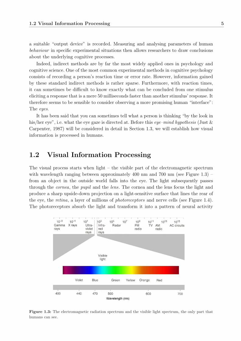
1.2 Visual Information Processing
The visual process starts when light – the visible part of the electromagnetic spectrum
with wavelength ranging between approximately 400 nm and 700 nm (see Figure 1.3) –
from an object in the outside world falls into the eye. The light subsequently passes
through the cornea, the pupil and the lens . The cornea and the lens focus the light and
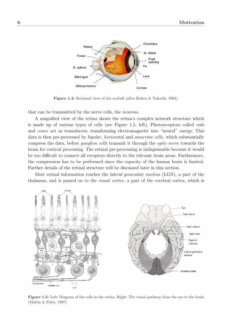
produce a sharp upside-down projection on a light-sensitive surface that lines the rear of
the eye, the retina, a layer of millions of photoreceptors and nerve cells (see Figure 1.4).
The photoreceptors absorb the light and transform it into a pattern of neural activity
Figure 1.3: The electromagnetic radiation spectrum and the visible light spectrum, the only part thathumans can see.
6 Motivation
Figure 1.4: Sectional view of the eyeball (after Rohen & Yokochi, 1994).
that can be transmitted by the nerve cells, the neurons .
A magnified view of the retina shows the retina’s complex network structure which
is made up of various types of cells (see Figure 1.5, left). Photoreceptors called rods
and cones act as transducers, transforming electromagnetic into “neural” energy. This
data is then pre-processed by bipolar , horizontal and amacrine cells , which substantially
compress the data, before ganglion cells transmit it through the optic nerve towards the
brain for cortical processing. The retinal pre-processing is indispensable because it would
be too difficult to connect all receptors directly to the relevant brain areas. Furthermore,
the compression has to be performed since the capacity of the human brain is limited.
Further details of the retinal structure will be discussed later in this section.
Most retinal information reaches the lateral geniculate nucleus (LGN), a part of the
thalamus, and is passed on to the visual cortex , a part of the cerebral cortex, which is
Figure 1.5: Left: Diagram of the cells in the retina. Right: The visual pathway from the eye to the brain(Matlin & Foley, 1997).
1.2 Visual Information Processing 7
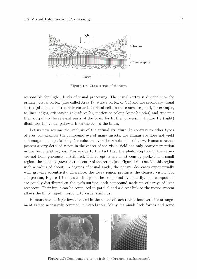
Figure 1.6: Cross section of the fovea.
responsible for higher levels of visual processing. The visual cortex is divided into the
primary visual cortex (also called Area 17, striate cortex or V1) and the secondary visual
cortex (also called extrastriate cortex). Cortical cells in these areas respond, for example,
to lines, edges, orientation (simple cells), motion or colour (complex cells) and transmit
their output to the relevant parts of the brain for further processing. Figure 1.5 (right)
illustrates the visual pathway from the eye to the brain.
Let us now resume the analysis of the retinal structure. In contrast to other types
of eyes, for example the compound eye of many insects, the human eye does not yield
a homogeneous spatial (high) resolution over the whole field of view. Humans rather
possess a very detailed vision in the center of the visual field and only coarse perception
in the peripheral regions. This is due to the fact that the photoreceptors in the retina
are not homogeneously distributed. The receptors are most densely packed in a small
region, the so-called fovea, at the center of the retina (see Figure 1.6). Outside this region
with a radius of about 1.5 degrees of visual angle, the density decreases exponentially
with growing eccentricity. Therefore, the fovea region produces the clearest vision. For
comparison, Figure 1.7 shows an image of the compound eye of a fly. The compounds
are equally distributed on the eye’s surface, each compound made up of arrays of light
receptors. Their input can be computed in parallel and a direct link to the motor system
allows the fly to rapidly respond to visual stimulus.
Humans have a single fovea located in the center of each retina; however, this arrange-
ment is not necessarily common in vertebrates. Many mammals lack foveas and some
Figure 1.7: Compound eye of the fruit fly (Drosophila melanogaster).

8 Motivation
animals, for example horses and birds, have two foveas in each eye. In horses, this is a
clever evolutionary adaptation, allowing the horse to see directly ahead while seeing the
ground at its feet at the same time. Still, with high spatial resolution in a very small
region of the visual field only, a mechanism to shift the fovea area would be desirable to
provide high resolution and a wide field of view at the same time. This is conveniently
realised through eye movements.
1.2.1 Eye movements
Figure 1.8: The ocular eye muscles (after Faller, 1995).
In humans, three antagonistic pairs of muscles (see Figure 1.8) move the eyeball ex-
tremely fast, reaching speeds of up to 600 degrees per second (Hallett, 1986) and allowing
the eyes to move from one region of the field of view to another. This enables humans to
systematically aim their eyes precisely at those regions that contain objects most relevant
for the potential action that is demanding the most consideration at that point in time.
The result is that people tend to look at several different objects in quick succession, and
certainly not at random.
Eye movements can be classified in two basic groups, according to whether the angle
between the “lines of sight” for the two eyes remains constant or changes as the eyes
move: Version (or conjugate) movements and vergence movements.
Version movements describe eye movements in which this angle remains relatively
constant and both eyes move in the same direction. Version movements usually occur
when tracking objects that move in a plane at a fixed distance from the observer. Let us
consider two important types of version movements: Saccadic and pursuit movements.
Saccadic movements
When looking at static scenes, the eyes are moved in a series of “jumps” (Huey, 1908/1968;
Findlay, 1992; Irwin, 1992; Rayner, 1992) rather than continuously. The term saccadic
movement refers to these rapid movements from one inspected location to the next.

1.2 Visual Information Processing 9
During a jump, the so-called saccade, no visual information other than a blur (Ir-
win, 1993) can be perceived. The perception of visual information can only take
place during fixations, the motionless phases between saccades. The planning of a
saccade requires about 200 ms (Abrams, 1992), the time to exert the saccade itself
ranges from 20 to 100 ms, depending on the distance the eyes move (Findlay, 1992).
Saccade planning usually involves peripheral processing in order to determine the
saccade’s landing point, in particular in abstract scenarios when only little contextual
information is provided (e.g. Abrams, 1992). Fixations usually last about 200 ms.
However, even during steady fixations small eye movements, micro-saccades, drifts and
tremors occur (e.g. Bridgeman et al., 1994). Based on the information from several
fixations, the brain constructs a clear composite view of a larger portion of the visual field.
Pursuit movements
The second type of version movements are pursuit movements. They are required to
track moving objects against a stationary background in order to keep objects in the
fovea for greatest acuity. The two most important attributes of pursuit movements are
their low velocity, typically between 30 and 100 degrees per second (Hallett, 1986), and
the fact that they are smooth, in contrast to the jerky saccades. Even though smooth
pursuit movements attempt to match a target’s speed, they have a general tendency to
“underpursue”. This results in the target’s image moving on the retina which makes it
difficult to see details on moving images (Murphy, 1978). Figure 1.9 shows typical eye-
movement behaviour in a pursuit condition when the eye follows a spot of light which
acts as a target. The target starts to move at time zero. At first, the eye does not move
(onset latency). Then, it starts a slow smooth pursuit movement but soon the observer
realises that the target is moving ahead of the gaze, so a corrective saccade (Kapoula &
Robinson, 1986) is made. After that, a smooth pursuit movement is made which follows
the spot of light. This entire process only covers an angular distance of about three degrees
and takes about one second.
Figure 1.9: The graph shows the gaze position as a function of the position of a spot of light which actsas a target the eye is following.

10 Motivation
Vergence movements
In contrast to the version movements discussed so far, vergence movements is the term
used for eye movements in which the angle between the lines of sight changes and the
eyes move toward or away from each other. More specifically, the eyes converge when
looking at nearby objects and diverge when looking at distant ones. The purpose of
vergence movements is to allow both eyes to focus on the same target in space, crucial
for maintaining acuity, the precision with which we can see fine details. Compared to
saccadic movements, vergence movements are rather slow; their velocities rarely exceed
ten degrees per second (Hallett, 1986) and they last about one second.
————
Provided with the required terminology used in eye-movement research, all preliminar-
ies should have been established for the apprehension of the eye-mind hypothesis that was
quoted earlier. In principle, it attempts to motivate why the eyes (and eye movements)
can be considered convenient indicators for mental processes.
1.3 The Eye–Mind Hypothesis
It was not until 1879 that Professor Emile Javal from the University of Paris observed
that a reader’s eyes do not sweep smoothly across print but make a series of short pauses
at different places until reaching the end of a line. They then move to the beginning of the
next in a smooth, unbroken fashion (Huey, 1908/1968). Although perhaps obvious now,
these observations set in motion eye-movement research. Before Javal, it was assumed that
the eyes glided unceasingly across text or other visual stimuli, a movement that offered
no real insight into the underlying cognitive processes. With the new acknowledgment
of non-continuous eye movements, numerous questions arose to become obvious points
of departure for exploration: Where does the eye stop? For how long? Why does it stop
there? Why does it regress at times?
According to the “eye-mind hypothesis” (Just & Carpenter, 1987), the eye commonly
fixates on the symbols currently being processed by the brain. Several experiments have
demonstrated that the eye can in fact be a window to the mind . In a typical experiment,
human subjects were shown a small array of simple drawings of common objects. When
the subjects were asked, “What makes of car can you name?”, they tended to look at
the drawing of a car while responding. Furthermore, if the subjects were asked the same
question after the display was removed, they still fixated on the same position in space
where the drawing of the car had been located. These results, for example, suggest that
eye fixations play an important organisational or place-keeping role in cognition. More
generally, the number of fixations and the distribution of fixations are thought to indicate
to which extent specific stimulus regions affect perceptual and cognitive processing.
In addition, fixation duration can be considered as a measure of the effort of informa-
tion processing. The longer a fixation lasts, the longer the visual information processing
presumably takes. Prolonged fixation can, for example, be observed when visual attention
rests on very complex regions of an image or is directed at areas that are considered
1.3 The Eye–Mind Hypothesis 11
relevant and of particular value for solving a given task. This relationship is strongly
supported by results from reading research. The fixation duration when reading written
text depends on the length of the currently fixated word and its frequency in a language
(e.g. d’Ydewalle & van Rensbergen, 1993; Rayner & Sereno, 1994; Rayner, 1997). However,
fixation duration does not seem to be affected by the previous word, thus the syntactic
and semantic analysis of a word is evidently performed during its fixation. Saccade length
is another basic eye-movement variable and an indicator for how thoroughly a certain
region of a stimulus is scanned. Long saccades imply that a scene is only coarsely viewed
whereas short saccades indicate a close inspection of stimulus details.
In summary, all types of eye movements yield data on locations and the temporal order
of the acquisition of visual information which then reveals the distribution and dynamics
of visual attention. Nevertheless, there are some restrictions concerning the link between
eye movements and visual attention which might not render eye movements a perfect
reflection of cognitive processes in some aspects. First, it is for example possible to fixate
on a certain point in space while in fact thinking about something completely different
from the scene. Obviously, eye movements do not tell much about visual attention in
this case. If subjects have to solve a particular visual task, however, they should direct
their attention towards the stimuli such that gaze position and attention are correlated.
Second, humans are able to focus attention on different points during a fixation, i.e. shifts
of attention can occur independently of eye movements. These small shifts of attention to
locations within the fovea region are referred to as “covert” shifts of attention and only
occur when time for extensive inspection is not sufficient (e.g. Cohen & Ivry, 1989, 1991;
Treisman, 1982; Treisman & Gormican, 1988; Wolfe, 1994; Wolfe et al, 1989).
Despite these slight restrictions – which can be eliminated by careful experimental
design – eye movements present a very good index of the moment-to-moment online pro-
cessing activities that accompany visual cognition tasks such as reading, scene perception
or visual search. Eye movements can give considerably greater insight into mental pro-
cesses than simple manual response tests and allow for a more direct and convenient
monitoring of these processes than image-based brain-scanning methods. As a result, eye
movements have been studied in various fields of research, for example (Pomplun, 1998):
Reading research: While reading written text, a subject’s eye movements tell us the
duration needed for processing a particular word. These data enable scientists to
draw conclusions about the structure of language information stored in our brain.
Medical research: Eye-movement measurement can help physicians to diagnose certain
diseases of the nervous system, for example schizophrenia or Parkinson’s disease,
because these diseases lead to characteristic distortions of eye-movement parameters.
Moreover, eye-movement analysis can provide information on the state of a patient’s
healing process during his/her therapy.
Traffic research: A car driver’s eye movements tell scientists which factors distract the
driver’s attention and are thus likely to cause traffic accidents. The arrangement of
instruments, for example, can be optimised with the help of these investigations.

12 Motivation
Consumer research: It is important for advertising agencies to test the visual appeal of
their commercial spots or brochures before launching a publicity campaign. Subjects’
eye movements can indicate which parts of the spot or brochure attract most of the
subjects’ attention. In particular, it can be investigated whether the name of the
advertised product is shown in a position in which it can be properly recognised.
After this discussion of the fundamentals of visual information processing, types of eye
movements and a motivation and validation of their function as indicators for cognitive
processing, the following section addresses the methodological aspects of eye-movement
research: How can we measure eye movements?
1.4 Tracking Eye Movements
Let us recall some of the obvious questions often asked in eye-movement research: Where
does the eye stop? For how long? Why does it stop there? It becomes clear that the plain
measurement of the eyes’ sensorimotor data (oculomotor data), i.e. the movement of the
eyeball, is not sufficient for most research purposes. Instead, the gaze position within
the presented visual stimulus, usually a two- or three-dimensional image, is required for
analysis. Consequently, body or head movements have to be measured (or eliminated)
and their orientations have to be considered as well for the computation of the gaze
position. Taking these requirements and research goals into account, gaze trajectories , i.e.
spatio-temporal scan paths constitute the optimal data to be obtained from eye-tracking
experiments.
Thus, various techniques to accurately track eye movements were developed alongside
the ongoing research. Since the early experiments (see Figure 1.10) conducted at the
beginning of the twentieth century, for example Dodge (1900), Buswell (1922, 1935, 1937)
or Judd and Buswell (1922), eye-tracking techniques have steadily improved. They now
allow for extremely accurate and high-resolution eye tracking. Young and Sheena (1975)
and Lee and Zeigh (1991) is recommended reading for a comprehensive survey of methods
for measuring eye orientation. The following paragraphs provide an overview of selected
eye-tracking methods.
Figure 1.10: Early record of eye movements (Buswell, 1935) during free examination of the painting“The great wave of Katsushika Hokusai” (1760–1850).
1.4 Tracking Eye Movements 13
Electrooculogram (EOG)
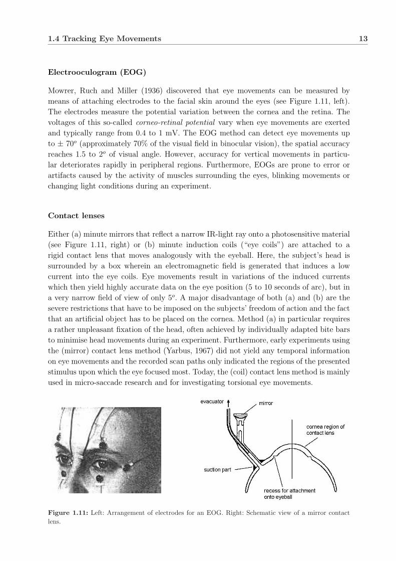
Mowrer, Ruch and Miller (1936) discovered that eye movements can be measured by
means of attaching electrodes to the facial skin around the eyes (see Figure 1.11, left).
The electrodes measure the potential variation between the cornea and the retina. The
voltages of this so-called corneo-retinal potential vary when eye movements are exerted
and typically range from 0.4 to 1 mV. The EOG method can detect eye movements up
to ± 70o (approximately 70% of the visual field in binocular vision), the spatial accuracy
reaches 1.5 to 2o of visual angle. However, accuracy for vertical movements in particu-
lar deteriorates rapidly in peripheral regions. Furthermore, EOGs are prone to error or
artifacts caused by the activity of muscles surrounding the eyes, blinking movements or
changing light conditions during an experiment.
Contact lenses
Either (a) minute mirrors that reflect a narrow IR-light ray onto a photosensitive material
(see Figure 1.11, right) or (b) minute induction coils (“eye coils”) are attached to a
rigid contact lens that moves analogously with the eyeball. Here, the subject’s head is
surrounded by a box wherein an electromagnetic field is generated that induces a low
current into the eye coils. Eye movements result in variations of the induced currents
which then yield highly accurate data on the eye position (5 to 10 seconds of arc), but in
a very narrow field of view of only 5o. A major disadvantage of both (a) and (b) are the
severe restrictions that have to be imposed on the subjects’ freedom of action and the fact
that an artificial object has to be placed on the cornea. Method (a) in particular requires
a rather unpleasant fixation of the head, often achieved by individually adapted bite bars
to minimise head movements during an experiment. Furthermore, early experiments using
the (mirror) contact lens method (Yarbus, 1967) did not yield any temporal information
on eye movements and the recorded scan paths only indicated the regions of the presented
stimulus upon which the eye focused most. Today, the (coil) contact lens method is mainly
used in micro-saccade research and for investigating torsional eye movements.
Figure 1.11: Left: Arrangement of electrodes for an EOG. Right: Schematic view of a mirror contactlens.

14 Motivation
Corneal reflection
In the late 1960’s Kenneth Mason developed the theory for the corneal-reflection method.
It describes an automated procedure for observing the eye using a camera, measuring
the locations of the pupil center and corneal reflection, and calculating the direction of
gaze (Mason, 1969). In the early 1970’s John Merchant and Richard Morrisette built a
system that implemented the concept in practice (Merchant & Morrisette, 1973). Their
“oculometer” employed a video camera to observe the subject’s eye and a computer to
process the camera’s image of the eye (see Figure 1.12, left). Their image processing algo-
rithms consisted of innovative methods to (a) recognise the pupil of the eye and calculate
its geometrical center, and (b) locate the relative position of the corneal reflection. They
introduced the use of higher order polynomial equations to correct for non-linearities in
the oculometer, and they developed root-mean-square regression methods for calibrating
the equations to individual people’s eyes.
Purkinje Images
Cornsweet (1973) developed the Purkinje image method. This method uses a camera and
an IR-light source and computes the eye’s orientation based on light reflections from both
the front and rear surfaces of the lens of the eye. Because it does not depend on the
pupil opening and closing concentrically about the eye’s optic axis, the Purkinje image
method can be more accurate than the corneal-reflection method. However, it requires a
significantly more controlled lighting environment to be able to detect the rear surface
reflection of the lens of the eye. Figure 1.12 (right) illustrates how the reflections of the
light beam create the Purkinje images.
Figure 1.12: Left: Apparatus used for tracking eye movements with the corneal reflection method.Right: Reflections from cornea and lens yield Purkinje images.
Pupillography
Applying video-based techniques and an image-processing system, either the border be-
tween the iris and the sclera (limbus tracking) or between the pupil and the iris (pupil
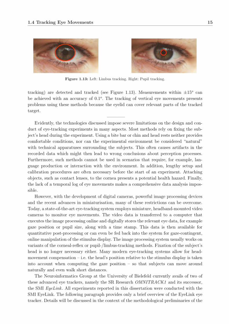
1.4 Tracking Eye Movements 15
Figure 1.13: Left: Limbus tracking. Right: Pupil tracking.
tracking) are detected and tracked (see Figure 1.13). Measurements within ±15o can
be achieved with an accuracy of 0.1o. The tracking of vertical eye movements presents
problems using these methods because the eyelid can cover relevant parts of the tracked
target.
————
Evidently, the technologies discussed impose severe limitations on the design and con-
duct of eye-tracking experiments in many aspects. Most methods rely on fixing the sub-
ject’s head during the experiment. Using a bite bar or chin and head rests neither provides
comfortable conditions, nor can the experimental environment be considered “natural”
with technical apparatuses surrounding the subjects. This often causes artifacts in the
recorded data which might then lead to wrong conclusions about perception processes.
Furthermore, such methods cannot be used in scenarios that require, for example, lan-
guage production or interaction with the environment. In addition, lengthy setup and
calibration procedures are often necessary before the start of an experiment. Attaching
objects, such as contact lenses, to the cornea presents a potential health hazard. Finally,
the lack of a temporal log of eye movements makes a comprehensive data analysis impos-
sible.
However, with the development of digital cameras, powerful image processing devices
and the recent advances in miniaturisation, many of these restrictions can be overcome.
Today, a state-of-the-art eye-tracking system employs miniature, headband-mounted video
cameras to monitor eye movements. The video data is transferred to a computer that
executes the image processing online and digitally stores the relevant eye data, for example
gaze position or pupil size, along with a time stamp. This data is then available for
quantitative post-processing or can even be fed back into the system for gaze-contingent,
online manipulation of the stimulus display. The image processing system usually works on
variants of the corneal-reflex or pupil-/limbus-tracking methods. Fixation of the subject’s
head is no longer necessary either. Many modern eye-tracking systems allow for head-
movement compensation – i.e. the head’s position relative to the stimulus display is taken
into account when computing the gaze position – so that subjects can move around
naturally and even walk short distances.
The Neuroinformatics Group at the University of Bielefeld currently avails of two of
these advanced eye trackers, namely the SR Research OMNITRACK1 and its successor,
the SMI EyeLink . All experiments reported in this dissertation were conducted with the
SMI EyeLink. The following paragraph provides only a brief overview of the EyeLink eye
tracker. Details will be discussed in the context of the methodological preliminaries of the

16 Motivation
experiments in Section 3.1. Stampe (1993) is recommended reading for obtaining further
information on the underlying technical principles of both OMNITRACK1 and EyeLink
systems.
The SMI EyeLink Eye Tracker
The main component of the SMI EyeLink eye tracker is a lightweight headband on which
three digital cameras are attached: Two eye cameras (one per eye) recording images of
the eyes as they move, and a head camera recording an infra-red (IR) image of the sub-
ject’s field of view (Figure 1.14). The two eye cameras facilitate binocular eye tracking.
Convergence movements and gaze positions in three dimensions can easily be determined
from their separate recordings. The key information contained in the head camera’s image
is the position of four IR light emitting diodes (LEDs) that have to be attached to the
corners of the stimulus display, usually a computer screen. The subject’s head position
relative to the screen can be computed from the location of the IR LEDs which appear
as bright spots in an otherwise dark head-camera image. The eye cameras are linked to
an image processing interface that derives the pupil positions from the cameras’ images.
Using a non-linear projection, the aggregated head and pupil positions are then mapped
onto the display coordinate system, yielding the desired gaze position. In order to de-
termine the projection’s parameters, a calibration procedure has to be performed prior
to an experiment. Here, a target marker sequentially moves across the screen while sub-
jects visually track it. The calibration procedure can be completed within 30 seconds and
leads to a high spatial accuracy of eye gaze measurement in the subsequent experimental
recording. In summary, the SMI EyeLink eye tracker provides both natural conditions
Figure 1.14: Headset of the SMI EyeLink eye tracker.

1.4 Tracking Eye Movements 17
for subjects (freedom of head movements) and a highly accurate measurement of binoc-
ular eye-movement data. Furthermore, as the gaze position data is available online, the
SMI EyeLink eye tracker can be used for gaze-contingent experiments.
————
Both the technical equipment and the apparent validity of eye movements as indica-
tors of perceptive and cognitive processing in the human brain – as described above –
now leave us with the challenge of selecting a promising research paradigm to explore.
This choice should mainly be guided by the consideration whether, compared to more
“conservative” methods, the measurement of eye movements and the investigation of eye-
movement parameters yields new insight into visual processing given a certain task or
not. Relevant aspects to be considered in this respect are:
• Which stimuli are presented?
• What is the subjects’ task?
• Which hypotheses are to be tested?
• Which are the relevant eye-movement parameters to be investigated?

18 Motivation
Chapter 2
Visual Comparison and Assessment
of Object Proportions
2.1 Visual Comparison
Research in the Neuroinformatics Group at the University of Bielefeld has rendered the
eye-tracking methodology particularly useful for investigating the paradigm of visual com-
parison (e.g. Koesling, 1997; Pomplun, 1998; Pomplun & Ritter, 1999).
In principle, all studies concerned with the paradigm of visual comparison use a similar
experimental scenario: Two stimulus pictures A and B are shown either simultaneously
side by side or sequentially one after the other. Subjects then have to decide, for example,
whether A and B are identical or different. If A and B are found to be different, subjects
may also have to state the type of difference. Alternatively, for more complex tasks,
subjects are asked to match A and B: They have to manipulate A so that it looks like B.
Furthermore, it can be assumed that all visual comparison tasks share a common
cognitive structure. In order to solve such a task, apparently the following processing
steps have to be accomplished:
(a) Assessment of A.
(b) Memorisation of A.
(c) Assessment of B.
(d) Comparison/matching with A.
A closer inspection reveals that each step describes quite complex perceptual and cog-
nitive processes. It is, for example, not intuitively clear how humans assess a specific
stimulus picture. Which factors determine visual scan path, how do these contribute to
the memorisation of relevant attributes of the picture? Which information is included
in the memorised “percepts”, how are these mentally represented? Is any of the memo-
rised information lost until the representation is recalled for comparison? What exactly
is compared, how is the comparison/matching process accomplished?

20 Visual Comparison and Assessment of Object Proportions
Apparently, the answers to these questions are closely related to the experimental
design. The essential aspects with respect to the experimental scenario and the specific
task will thus be discussed in the following.
First, the choice of stimuli certainly has a great impact on visual comparison tasks
and the cognitive processing steps. The investigation of different types of stimuli thus
appears to be a promising strategy for the systematic exploration of the paradigm of
visual comparison. Stimuli can, for example, be varied along three characteristic “axes”
of stimulus properties:
• Semantic content.
• Stimulus dimension.
• Stimulus distribution.
Along the axis of semantic content, investigations may focus on abstract stimuli or
on realistic scenes. Abstract stimuli do not carry much conceptual information and their
visual processing only involves factors operating on a low semantic level – such as colour,
shape or spatial arrangement. In contrast, the visual processing of realistic scenes in-
volves factors operating on a high semantic level. Humans usually have a specific concept
of how to perceive such scenes. This knowledge is likely to influence eye-movement pat-
terns. Experiments using ambiguous pictures (Pomplun, Ritter & Velichkovsky, 1996), for
example, have shown that the distribution of attention is not only influenced by the geo-
metrical properties of the stimulus, but also by the semantic interpretation of the picture
elements. Although conceptual factors are difficult to parameterise and hence difficult
to access for quantitative analysis, realistic scenes are preferable to abstract ones: They
provide a higher ecological validity.
The choice of the stimulus dimension can also be considered in terms of ecological va-
lidity. In everyday life, humans usually perceive and manipulate three-dimensional objects
in three-dimensional environments. Using lower-dimensional stimuli in experiments would
thus not exactly present ecologically plausible situations. On the other hand, the percep-
tion of realistic, three-dimensional scenes involves processes on a higher semantic level.
This would render data analysis and interpretation more complicated (see above). Abstract
three-dimensional objects could be used in an attempt to exclude semantic factors such
as knowledge or interpretation. However, in comparison with one- or two-dimensional
stimuli, the visual perception of three-dimensional still requires processing on a higher
semantic level due to the influence of object depth.
Alternatively, two-dimensional stimuli that can be interpreted as three-dimensional ob-
jects can be used instead of real three-dimensional objects. Most of these stimuli, however,
are not ideal for eye-movement investigations. In particular stimuli consisting of abstract
objects do often not yield stable three-dimensional visual representations. Experiments
using the so-called “Necker-Cube”, for example, have shown that the distributions of at-
tention significantly differ for the two possible spatial interpretations (Pomplun, Ritter &
Velichkovsky, 1996). This interpretation “flipping” does not facilitate the interpretation

2.1 Visual Comparison 21
of eye-movement pattern – unless the the investigation focusses on the “flipping” iteself.
Consequently, abstract geometrical one- or two-dimensional stimuli should be preferred in
order to minimise the influence of higher semantic processes on visual perception. “Sim-
ple” objects, for example one-dimensional line segments or basic two-dimensional figures
such as circles or squares, can reliably be defined using few dimension parameters such as
length, size and orientation.
The stimulus distribution describes the number of stimulus constituents and their
spatial arrangement. Variation along this axis of stimulus properties must be considered
in the context of the type of the visual comparison task. Using only few constituents
to form a stimulus picture, the visual assessment can be assumed to focus – or, more
appropriately: to foveate – on the constituents and their details. Such sparse, localised
distributions should thus be convenient for the assessment of individual object properties
or proportions, i.e. for the investment of local, detailed visual perception processes. In
fact, single objects rather than object distributions would constitute appropriate stimuli
for such investigation purposes.
In contrast, distributions of numerous stimulus constituents that are widely spread
across the stimulus picture can conveniently be used to study more global aspects of
visual comparison. Here, the global characteristics of a visual scan path should be in the
focus of the investigation. It can be assumed that such scan paths are also influenced
by the local properties of the stimulus constituents. These, however, are not likely to be
visually examined in details.
The strategy to systematically explore different types of stimuli and different types of
visual comparison tasks has been successfully pursued in recent studies at the University
of Bielefeld. The visual comparison tasks of comparative visual search and numerosity
estimation were explored. According to the eye-mind hypothesis, eye movements were
investigated in order to gain the desired insight into the underlying cognitive processes.
Comparative visual search tasks investigated abstract and realistic scenarios, using
low- and high-dimensional stimuli. Stimulus pictures usually contained large numbers
of constituents in both comparative visual search and numerosity estimation tasks. As
a consequence, the investigations primarily yielded information about global processing
mechanisms during the assessment and comparison of widely distributed stimuli. Only
little insight could be gained into local visual comparison processes. The following para-
graphs briefly summarise the recent investigations and present their key results.
Abstract Comparative Visual Search
In comparative visual search subjects had to detect a single mismatch (in either colour
or form) between two otherwise identical, simultaneously presented images. These im-
ages consisted of large numbers of abstract items (see Figure 2.1, left). Various studies
have shown, for example, that the task completion involves two distinct phases (Pom-
plun, 1998): First, subjects serially search the images for the mismatch. This results in
pendulum-like eye movements, comparing one or more memorised items, depending on
parameters like object density or entropy, in corresponding areas of both hemifields. Sec-

22 Visual Comparison and Assessment of Object Proportions
Figure 2.1: Left: An abstract sample stimulus as presented in comparative visual search studies. Left:A three-level model for comparative visual search (in Pomplun, 1998).
ond, when the mismatch is found, the eye gaze shifts back and forth several times between
the targets to verify the mismatch. Eye-movement parameters varied significantly between
colour and form search, when “top down” information (subjects were informed about the
relevant mismatch dimension prior to the experiment) or “bottom up” information (the
irrelevant mismatch dimension remained constant) was provided: Search scan paths and
therefore reaction times were generally shorter for colour search and in the “top down”
and “bottom up” conditions.
These and further findings were formalised in a “three-level model” (see Figure 2.1,
right). This model adequately simulate the human visual scan path for the given com-
parative search task that used distributed, abstract stimuli. Further information can be
found in Pomplun and Ritter (1999) and Pomplun et al. (2001).
Conceptual Comparative Visual Search
The abstract stimuli used in the previous experiments allowed to draw conclusions mainly
about perceptual and “low-level” cognitive processing strategies in visual comparison
tasks. The stimuli used were not suitable for investigating the influence of cognitively
more complex, conceptual information on such tasks. Moving along the “axis” of semantic
content, stimuli that now could be semantically interpreted were used in a comparative
visual search scenario. In order to investigate the transition between perceptual and “high-
level” cognitive processing levels, so-called “Mooney Faces” were chosen as stimuli. This
type of stimulus was rendered ideal for the investigation: When presented in an upright
orientation, the black and white regions can be interpreted as faces. A rotation of 180o
transforms the stimuli into images with no semantic content, they only seem to show
random arrangements of black and white regions.
The investigation yielded rather unexpected results. Basically, no significant differ-
ences were found in the eye-movement data between the upright and rotated conditions.
These findings suggest that similar visual comparison strategies are used, irrespective of
the semantic content of the stimuli. Alternatively, it can be speculated that the compar-
ison strategy differs between the two levels of semantic content, but that this does not

2.1 Visual Comparison 23
Figure 2.2: A sample stimulus as presented in comparative visual search studies, overlaid with a gazetrajectory.
show in the measured variables. It appears more likely, however, that the chosen stim-
uli were not entirely suitable to investigate the transition between the different semantic
levels. The recognition of faces in the stimuli might have been too “costly” and subjects
applied the same visual scanning strategy in both the upright “faces” and the rotated
“random” scenarios. This strategy is guided by geometrical factors rather than by con-
ceptual considerations. Figure 2.2 shows a typical gaze trajectory for an upright “faces”
stimulus.
Numerosity Estimation
With the previous study demonstrating that conceptual, semantic content is quite different
to parameterise, the row of visual comparison investigations returned to abstract stimuli.
Now another task was explored: Numerosity estimation. As for abstract comparative
visual search, stimulus pictures consisted of large numbers of items. As a consequence, the
findings of the investigations must primarily be viewed with respect to global processing
mechanisms.
The influence of structural information on the perception of numerosity in two-
dimensional object distributions was determined in several studies (see Figure 2.3). When
subjects tried to adjust the number of items in the stimulus’ right hemifield so as to match
the number on the left, this generally resulted in an underestimation. Furthermore, the
intensity of underestimation varied, for example, with the overall item number, cluster
size and different types of structural information.
Again, eye-movement recordings yielded valuable information to help explain the ob-
served behaviour: Instead of single items, clusters were fixated as a whole and attention
was mainly focused on areas with high object density in proximity to the stimulus cen-

24 Visual Comparison and Assessment of Object Proportions
Figure 2.3: A sample stimulus as presented in numerosity estimation studies (Koesling, 1997).
ter. In contrast to fixation durations which significantly rose with increasing numbers of
items, the number of fixations remained constant. It appears that the number of (central)
clusters was somehow incorporated into the numerosity estimation, leading to an under-
estimation effect that increased when more items were presented. Prolonged fixations are
obviously not suitable to compensate for the “laziness” of not executing further fixations
as would be necessary to correctly perceive the surplus information. The implementation
of a model based on neural information processing principles, so-called “receptive fields”,
scored well at simulating the underestimation effects as observed in humans. An in-depth
discussion of all aspects of these studies is documented in Koesling (1997) and Koesling
et al. (submitted).
The Next Step: Assessment of Individual Objects
The successful application of eye-tracking methods yielded novel insights into human
visual information processing regarding the above-mentioned comparison tasks. It now
appears to be quite rewarding to transfer this previous experience to a similar, but new
domain. Furthermore, problems should be addressed that appeared imminent, but were
yet unattended. The aim must be to complement the current image of processes guiding
visual comparison in order to obtain a (more) comprehensive understanding of this re-
search paradigm. In fact, the following studies can be motivated quite naturally by moving
further along the different “axes” that have determined the type of stimuli and guided
the investigations so far.
With a view to the axis of stimulus distribution it is quite clear where investigations
should move to: In contrast to analysing visual processes on a rather global – or macro –
level as has been done so far, particular attention should now be paid to the local – micro
level. The key question must now be: How do humans perceive individual objects?
Let us also consider semantic content. Stimuli with both low and high levels of concep-

2.2 Assessment of Object Proportions 25
tual information were explored so far. The findings clearly demonstrated that experimental
control is apparently compromised when stimuli with a high level of conceptual informa-
tion have to be assessed. It must in general be considered quite difficult to attribute
specific observations to conceptual influence or to other, more abstract, factors. The use
of abstract stimuli that can be reliably parameterised should thus be recommended, in
particular with regard to the interpretation of eye-movement parameters.
That leaves us with the choice of convenient stimulus dimensions and the choice of
an appropriate comparison task to explore the perception of abstract, individual objects.
Let us consider the choice of the comparison task first.
A promising paradigm in this context appears to be the visual perception and assess-
ment of proportions of objects, embedded into the overall paradigm of visual comparison.
The principal experimental scenario of the investigation within this thesis is thus fairly
exactly specified: Two abstract, individual objects will be presented either sequentially
or simultaneously. The subjects’ task will then either be to decide if the stimuli are iden-
tical – or different – or they have to state the type of difference. Alternatively, for more
complex tasks, subjects will be asked to match A and B with respect to the proportion
in question. This also means that the cognitive structure outlined earlier is preserved:
Assessment, memorisation, comparison. Accordingly, the investigations will again focus
on the accomplishment of these processing steps.
But is proportion assessment indeed suitable for eye-movement research? In order to
understand why objects are perceived in a specific manner the following questions must
be addressed: Which factors influence perception when assessing object proportions, what
effects do they cause and how can these effects be explained? Which proportions should
be investigated? Which hypotheses can be advanced regarding the details of the cognitive
structure for such comparison tasks?
These questions certainly cannot be answered instantly. The following sections try to
clarify the essential preliminaries and give an overview of previous work in this scientific
field. This allows us to more specifically determine the experimental structure and to
hypothesise particular aspects of the cognitive structure that the investigations will focus
on. The following sections will also render some stimulus dimensions more promising than
others – a relevant aspect that has not been decided on yet.
2.2 Assessment of Object Proportions
Let us first consider what exactly the term “object proportions” means and how these
proportions can possibly be assessed.
In general, the term refers to the various physical dimensions or attributes of an object
or a physical phenomenon. Such dimensions could, for example, be the weight of a solid
object, the length or orientation of a line segment or the amplitude and frequency of a
sound.
The assessment of proportions evidently requires the perception of the respective ob-
ject and includes all sensorimotor , perceptive and conceptual processes. Consequently,

26 Visual Comparison and Assessment of Object Proportions
the “percept” is not a simple representation of physical evidence, but a combination of
information from different cognitive processing levels. Stimulation from sensorimotor re-
ceptors – for example from visual, tactile or auditory channels (or a mixture of them) –
is evaluated along with prior knowledge or contextual data. Thus, the finally emerging
result is often a somewhat “distorted”, subjective internal representation – the so-called
mental model (Johnson-Laird, 1983) – of an object or a scene. If, for example, subjects
have to lift various objects and judge their weights with regard to a standard, different
object sizes can lead to changes in the perceived weights, even if their masses are identical.
This makes clear that, when assessing object proportions, the perceived proportions do
not necessarily coincide with the original ones.
In fact, research into the assessment of object proportions has a long history. Perti-
nent experiments have proven rather popular in the past – early systematic recordings
dating back to the 1830s (Wheatstone, 1838) – and at present. However, as the follow-
ing paragraphs will demonstrate, fundamental principles are still not understood. Various
different hypotheses exist to explain particular phenomena only and often rather specific
cases were/are addressed. Many studies deal(t) with the assessment of length, size and
orientation, primarily concerned with phenomena of visual illusions , namely geometrical
illusions .
Visual Illusions
Of all such illusions, the Muller-Lyer illusion is one of the most thoroughly examined:
Two line segments – “shafts” – of equal physical length are presented parallel to each
other. Attached to the line segments’ end points are arrowheads, pointing either inward
(obtuse angle) or outward (acute angle). In this classical form (Muller-Lyer, 1889), the
illusion consists of the obtuse-angle illusion of shaft overestimation and the acute-angle
illusion of shaft underestimation (see Figure 2.4 (a)).
The illusion has been studied extensively, partly because of the belief that the under-
standing of visual illusions can reveal the principles governing non-illusory visual percep-
tion (Warren, 1976; Warren & Bashford, 1977). It is well accepted that the human visual
system decomposes an image using local filters tuned for stimulus features, such as spa-
tial frequency or orientation (Campbell & Robson, 1968; Kulikowski et al., 1973; Sagi &
Hochstein, 1983). Psychophysical and physiological evidence suggests that the local fil-
ters are not completely independent (Polat & Sagi, 1993; Kapadia et al., 1995; Chen &
Levi, 1996). Rather, they receive input from filters coding for neighbouring spatial fre-
quencies and orientations, thus suggesting interactions between neighbouring channels.
This network of long-range inter-connections may serve as substrate for context depen-
dence, i.e. the fact that the perceived visual attributes of a target stimulus depend on the
context within which the target is placed. Consequently, the Muller-Lyer illusion with its
context-induced subjective distortion of shaft length is a prime example of where these
interactions are involved.
Various theories were offered to explain the classical Muller-Lyer illusion. The depth or
linear perspective theory (Gregory, 1963; Gillam, 1998) relies on direct size scaling mech-

2.2 Assessment of Object Proportions 27
anisms and hypothesises that length distortions are due to misapplication or confusion
of size constancy to the two spans. The perceptual assimilation of the length of the shaft
towards the lengths of the wings – or the contextual elements in general – serves as a
basis for the averaging theory (Day & Dickinson, 1976; Brigell et al., 1977; Pressey &
Pressey, 1992). This theory assumes that the arrowheads interfere with the perceptual
system for measuring the span of the horizontals and therefore observers confuse or av-
erage the distance between the arrowhead tips. Other approaches (Chiang, 1968; Stuart,
et al., 1984; Morgan et al., 1990; Glennerster & Rogers, 1993) hypothesise the incor-
rect encoding of the positions of the vertices of the wings – displaced vertex theory , in
which the perceptual system miscalculates the location of the arrowhead vertex, displac-
ing it toward the concave side. Finally, properties of the low frequency visual channels
(Ginsburg, 1984) and object recognition processes, such as mechanisms associated with
preperceptual adjustments (Warren & Bashford, 1977) and visual scene interpretation
(Redding & Hawley, 1993; Redding et al., 1993) are thought to be responsible for the
illusion (see Figure 2.4 (b)). It has been found that vertices presented in isolation have
consistent and predictable effects on size scaling and should therefore be unambiguously
interpreted. This is consistent with current computational theories of object recognition,
for example when modelling the interpretation of line drawings (e.g. Guzman (1968);
Waltz, 1975; Biedermann, 1987; Malik, 1987; Winston, 1992).
In fact, the Muller-Lyer illusion can be observed for various variants of the original
stimuli. The illusion persists even when the shafts are absent and the distance between the
arrowheads has to be estimated. Replacing the arrowheads with other symbols still results
in incorrectly perceived length (see Figure 2.4 (c)). Several studies were concerned with the
effect of the arrow angle on the magnitude of the illusion. Erlebacher and Sekuler (1969),
for example, found a less pronounced under-/overestimation of line length when the angle
was increased. Using different colours for shafts and arrowheads reduced the magnitude of
the illusion as well (Sadza & de Weert, 1984). Schulz (1991) demonstrated that a delay of
between 35 to 400 ms between the presentation of shafts and arrowheads still caused the
Figure 2.4: (a) Original Muller-Lyer illusion stimuli. (b) Vertex labelling as used in line-drawing inter-pretations by Waltz (1975) and Winston (1992). (c) Context variant where arrowheads are replaced byboxes. Notice that the illusion still persists.

28 Visual Comparison and Assessment of Object Proportions
illusion. Another interesting finding suggests that the magnitude of the illusion decreases
with increased presentation times of the stimuli (Brosvic et al, 1997). It was shown that the
illusion can even be induced by only imagining the arrowheads (Berbaum & Chung, 1981).
Furthermore, McKelvie (1984) established a task-effect of the psychophysical method
on the illusion magnitude. He found a less intense illusion for the so-called “method of
adjustment” compared to the “method of constant stimuli” and the “method of limits”1.
Finally, the alignment and the spatial locations, i.e. distance, of the two line segments
influence the illusion. Pressey and di Lollo (1978), for example, observed a decreasing
illusion the further the two line segments were positioned apart.
Whereas the added information in the one-dimensional Muller-Lyer figures caused
a distorted perception of length, a similar effect emerges for perceived size in the two-
dimensional Ebbinghaus illusion (also called Titchener illusion; see Figure 2.5, left). Here,
small circles lead to the overestimation of the size of the central circle they surround.
Vice versa, surrounding large circles lead to the underestimation of the size of the central
circle. In the Delbœuf figure (see Figure 2.5, right), the left outer circle appears larger
than the right inner circle.
Figure 2.5: Left: Original Ebbinghaus illusion stimuli. Right: Original Delbœuf illusion stimuli.
Compared with the Muller-Lyer illusion, not quite as many studies are concerned
with the Ebbinghaus and Delbœuf illusions. Major works examined proximity effects
of the surrounding circles in the Ebbinghaus illusion. Weintraub (1979), for example,
found a decreasing magnitude of the illusion with increasing distance between central
and surrouding circles. A study by Coren and Enns (1993) supported the assumption
that a figural similarity between central and surrounding items (not necessarily circles)
resulted in a larger magnitude of the Ebbinghaus illusion. A successive presentation of
the central items and their context, in contrast, reduced the illusion or even caused it to
completely disappear (Jaeger, 1978). Contrast variations revealed similar effects (Jaeger &
Pollack, 1977).
In order to understand the Ebbinghaus illusion, the averaging theory (see above) –
alternatively referred to as the contrast and assimilation theory – is frequently quoted.
Within the Ebbinghaus figure, the illusion is assigned to the overestimation of the size
differences (“contrast”) between the circles. However, the contrast and assimilation theory
1The method of adjustment allows subjects to continuously vary a stimulus, i.e. its relevant dimen-sion/intensity. In contrast, stimuli are controlled by the experimenter when the other methods are applied.In the method of constant stimuli , stimuli are presented in random order. Employing the method of limits,stimulus intensities are successively increased or decreased from trial to trial.

2.2 Assessment of Object Proportions 29
only facilitates the classification of various illusions, but it neither explains the underlying
perception mechanisms nor their functions. It even cannot be applied to some illusions,
for example to the Poggendorff (see Figure 2.6, left) or the horizontal-vertical illusion (see
Figure 2.6, right).
The horizontal-vertical illusion was one of the first to be experimentally studied
(Kunnapas, 1955) and is of particular relevance with regard to the research reported
in the following chapters. Individuals adjusting vertical line segments to equate to corre-
sponding horizontal line segments are prone to perceptual errors: The vertical line segment
is usually made shorter than the horizontal line segment.
Figure 2.6: Left: Original Poggendorff illusion stimuli. Right: Original horizontal-vertical illusion stimuli.
An early explanatory theory was put forward by Segall et al. (1966) and represents
a perspectivist’s view along the lines of Gregory’s (1963, 1970) constancy-scaling theory,
which presumes an apparent expansion of space in the upper part of the visual field: If
a vertical line appears longer than an objectively equal horizontal line because it is in-
terpreted as located on a plane receding or partly tilting away from the observer, then
two parallel vertical lines should appear to be diverging from each other at their upper
ends. In fact, Piaget’s (1969) studies of the horizontal-vertical illusion seem to support
this theory: If the horizontal and vertical lines are presented in the form of an inverted
“L” figure, then the overestimation of the vertical relative to the horizontal is less than
when they form a normal “L” figure. Piaget himself accounts for this effect in terms of
greater frequency of eye movements and more attention being paid to the upper part of
the visual field. Evidence that such attentional factors contribute to this bias comes from
contemporary studies (Piaget, 1961; Gainotti & Tiacci, 1971): Dimensions of items on
which gaze is mostly fixed are overvalued. In this context, the asymmetry of performance
demonstrated by left-to-right readers who deviate leftward when bisecting horizontal line
segments must be mentioned. Taking Piaget’s and Gainotti and Tiacci’s observations into
account, the leftward bias could reflect either an underestimation of the right half of the
line segment or an overestimation of the left half-line. As findings from Bartolomeo and
Chokron (2001) seem to support the first possibility, an underestimation of the overall
length of horizontal lines could be explained - and, consequently, account – at least par-
tially – for the horizontal-vertical illusion as well. These observations make clear that
other factors such as the angles of the lines, the format in which the lines are presented,
and particularly whether the lines are shown in inverted-T or L-shaped formations must

30 Visual Comparison and Assessment of Object Proportions
be taken into account as well (McKelvie, 1990).
The theory most commonly quoted to explain the horizontal-vertical illusion is the
frame theory . It is based on the assumption that differential context effects serve to mod-
ulate the relative perception of stimuli oriented horizontally and vertically and, in doing
so, serve to modulate the size of the horizontal-vertical illusion. It has long been known
that the horizontal-vertical illusion is sensitive to the “frame” of the visual field around
the target (Kunnapas, 1955, 1957, 1959). Indeed, a strong case can be made that the
tendency for verticals to appear longer than horizontals across a wide range of conditions
reflects the intrinsic shape of the visual field, which is elliptical and wider than it is high
(e.g. Prinzmetal & Gettleman, 1993). The typical explanation is now that length is per-
ceived relative to this frame. A given vertical line occupies a greater proportion of the
vertical field than a physically equivalent horizontal line occupies of the horizontal field.
Thus, the vertical line encroaches on the upper and lower borders of the visual field to a
greater extent than the horizontal line does on the left and right borders.
Another possible way to account for the dependence of the horizontal-vertical illusion
on the shape of the visual field, namely in terms of differential context effects, was only
recently put forward by Armstrong and Marks (1997). Because the visual field’s width
is greater than its height, people may tend to experience greater horizontal than vertical
extents. With binocular viewing, the visual field is ovoid, its horizontal axis being ap-
proximately 0.5 times greater than its vertical axis, about 200o versus 130o (Prinzmetal &
Gettleman, 1993). If, as a result of this asymmetry, people are exposed on average to
greater horizontal than vertical extents, the long-term discrepancy in the distribution of
horizontal and vertical perceptions might induce a differential effect on the perception of
vertical and horizontal lengths, enhancing the former relative to the latter and thereby
producing the horizontal-vertical illusion. Armstrong and Marks’ theory is based on the
findings of Caelli (1977) who had subjects compare the length of lines varying in shape
(“squiggles”, sinewaves) and who inferred from the results that the horizontal-vertical
illusion is related to interactions between “orientation detectors” in the visual system.
In Caelli’s view, the perception of length is tied directly to mechanisms that underlie
discrimination of stimulus orientation. However, Armstrong and Marks suspect that dif-
ferential effects of stimulus context operate at a level in the visual system beyond that
of orientation detectors, much as the analogous effects in the perception of loudness arise
in the auditory system beyond the level of the initiation of critical bands. In their view,
the changes in perceived horizontal and vertical lengths constitute changes in the per-
ceptual metric, i.e. compression and decompression of visual space. If so, the attenuation
produced along a given spatial axis, whether horizontal or vertical, should be evident
over the entire range of possible visual stimuli, not just over the range of stimuli used
to induce it. According to Armstrong and Marks, these changes most likely take place in
retinotopic coordinates, not in “external” space. “For, if a metric of perceived length were
tied to distal rather than proximal stimuli, it should also depend on contextual distribu-
tion along other stimuli dimensions, such as wavelength compositions. But it does not.”
(Marks, 1992 (p. 192)).
After all, however, even this quite elaborate theory does not comprehensively account

2.2 Assessment of Object Proportions 31
for the illusion. Armstrong and Marks themselves had to accept that the illusion still
persists when stimuli are presented within a frame that is equally wide and high, i.e. in the
absence of a concurrent asymmetric visual frame. Furthermore, the illusory effect decreases
with repeated trials – although it is still present after 20 trials (Kubi & Slotnick, 1993) –
and intertrial feedback leads to a magnified decrease of the illusory effect (Brosvic &
Cohen, 1988).
Even though rather rewarding – as demonstrated in the previous paragraphs – not all
research that addresses the assessment of object proportions focuses on the phenomena of
visual illusions. Several studies deal with fundamental principles of “normal” object pro-
portion perception, i.e. how unambiguous objects are perceived in unambiguous environ-
ments. The following overview again mainly centers on the assessment of the dimensions
of length, size and orientation which are relevant here.
Physical and Apparent Magnitude
One of the most consistent findings in visual perception is that with physical distance
and size held constant, perceived size varies as a function of retinal eccentricity. Investi-
gations concerning the extent and direction of the variations in the apparent size of an
object, however, led to contradictory results. Helmholtz (1910/1962), who was, along with
James (1890/1950) one of the first to systematically explore the nature of perceived size
variations, noted, for example, that “if a long strip of paper, with parallel edges about
three inches apart, is laid on top of the same table, it will be noticed, on looking at the
middle of it, that by indirect vision it appears to be narrower at the ends than in the
middle, and that it is apparently bounded by two arcs with their concavities towards each
other” (p. 302). This simple observation suggests that as an object is moved out towards
the periphery, its apparent size decreases. This, in turn, implies that in order for an ob-
ject to maintain its apparent size, its objective size must increase as the object is moved
into the periphery. The considerations – amongst others – led Helmholtz to construct the
so-called “checkerboard illusion” (see Figure 2.7). If an enlarged version of this figure is
viewed from such a distance that the two vertices on the vertical meridian just above
and below the horizontal meridian subtend an angle of approximately 10o, the curved
lines appear straight and the apparent size of the resultant “squares” on the checkerboard
appear approximately equal.
Stevens (1908), however, reported experiments in which the apparent sizes of periph-
eral objects do not agree with the observation of Helmholtz and the checkerboard illusion.
He used simultaneous comparisons of a peripheral stimulus (“disk”) with a fixed stimulus
in foveal view. He found that, for most peripheral positions, a disk whose physical size
was identical to that of the disk in the fovea appeared larger in the periphery. This is
the opposite of what would be expected on the basis of the checkerboard illusion. He also
found a considerable amount of variation in apparent size as a function of visual-field
position with, for example, the same disk appearing, for one observer, larger in the right
visual field, and smaller in the left visual field.
Optical factors may partly account for some of these results. As the checkerboard
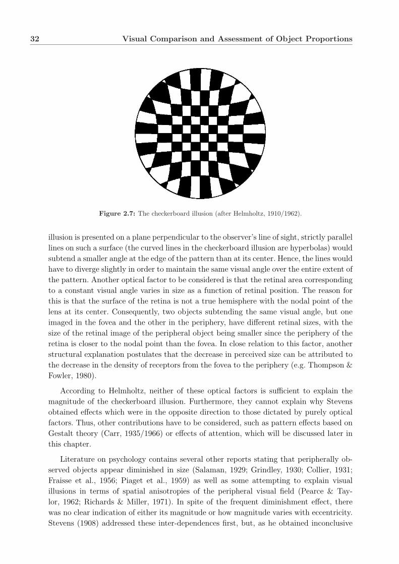
32 Visual Comparison and Assessment of Object Proportions
Figure 2.7: The checkerboard illusion (after Helmholtz, 1910/1962).
illusion is presented on a plane perpendicular to the observer’s line of sight, strictly parallel
lines on such a surface (the curved lines in the checkerboard illusion are hyperbolas) would
subtend a smaller angle at the edge of the pattern than at its center. Hence, the lines would
have to diverge slightly in order to maintain the same visual angle over the entire extent of
the pattern. Another optical factor to be considered is that the retinal area corresponding
to a constant visual angle varies in size as a function of retinal position. The reason for
this is that the surface of the retina is not a true hemisphere with the nodal point of the
lens at its center. Consequently, two objects subtending the same visual angle, but one
imaged in the fovea and the other in the periphery, have different retinal sizes, with the
size of the retinal image of the peripheral object being smaller since the periphery of the
retina is closer to the nodal point than the fovea. In close relation to this factor, another
structural explanation postulates that the decrease in perceived size can be attributed to
the decrease in the density of receptors from the fovea to the periphery (e.g. Thompson &
Fowler, 1980).
According to Helmholtz, neither of these optical factors is sufficient to explain the
magnitude of the checkerboard illusion. Furthermore, they cannot explain why Stevens
obtained effects which were in the opposite direction to those dictated by purely optical
factors. Thus, other contributions have to be considered, such as pattern effects based on
Gestalt theory (Carr, 1935/1966) or effects of attention, which will be discussed later in
this chapter.
Literature on psychology contains several other reports stating that peripherally ob-
served objects appear diminished in size (Salaman, 1929; Grindley, 1930; Collier, 1931;
Fraisse et al., 1956; Piaget et al., 1959) as well as some attempting to explain visual
illusions in terms of spatial anisotropies of the peripheral visual field (Pearce & Tay-
lor, 1962; Richards & Miller, 1971). In spite of the frequent diminishment effect, there
was no clear indication of either its magnitude or how magnitude varies with eccentricity.
Stevens (1908) addressed these inter-dependences first, but, as he obtained inconclusive

2.2 Assessment of Object Proportions 33
results (see above), could not formalise any relations. More recently, Newsome (1972) con-
ducted studies to quantitatively explore the above-mentioned relations: Subjects matched
the apparent size of a peripherally viewed object to a foveally viewed standard by adjusting
the distance of the peripheral object (see Figure 2.8). This technique was applied before
by Thouless (1931) and Joynson (1949), indicating that reliable measurements could in-
deed be obtained through peripheral viewing. However, it was argued that Newsome’s
procedure might cause artifacts due to background or contextual depth information. Fur-
thermore, his studies yielded only sparse data as only one size of standard stimulus was
employed, so that it was not possible to specify the extent of apparent size change for
objects of different sizes. Later, Schneider (1978) provided data on exactly that depen-
dence. He obtained magnitude estimates for the apparent length of line segments of various
lengths and orientations at different eccentricities along the horizontal and vertical merid-
ians. Results again showed that the apparent length of a line segment decreases as the
line segment is moved away from the midline position into the periphery. Power functions
adequately described the growth of line length so that equal-length contours could be
derived.
Figure 2.8: Apparatus used by Newsome (1972) to provide a simultaneous display of two stimulussquares with one stimulus adjustable in distance and eccentricity.
Psychophysical Scaling: Formal Relations between Physical and Apparent
Magnitude
Indeed, in order to formalise the relation between discrimination and physical magnitude
and that relation between apparent and physical magnitude, several different mathemati-
cal formulae could be thought to determine these correlations – not only regarding visual
perception and such correlations with respect to line segments. Weber (1834) is cred-
ited with this idea and the terms “Weber law” and “Weber fraction” were subsequently
coined, originally describing the correlation between apparent and physical weight. Even
though Weber did not discuss the issue, it is evident that the relation could be a linear,
logarithmic or power function – or some more complex function. From Weber’s research

34 Visual Comparison and Assessment of Object Proportions
on sensory thresholds Fechner (1860/1966) attempted to generalise the relation between
stimulus intensity and sensation magnitude. He believed that sensations could not be di-
rectly measured, so he derived estimates of sensory magnitude from the measurement of
difference thresholds. Fechner proposed a logarithmic function of the form
S = k · log(I) (2.1)
where S is sensation, k is a constant and I is physical intensity. This logarithmic function
was widely accepted for over 80 years (e.g. Adrian & Matthews, 1927) and provided
an impetus for the measurement of sensory processes. Although Fechner examined the
discrimination of lifted weights, his research contributed more to the development of
psychophysical methods than to the discovery of the sensory mechanisms involved in force
perception (Boring, 1942). With the introduction of new techniques for scaling sensory
magnitude, such as magnitude estimation, category ratings and ratio matching, several
different psychophysical functions emerged. Stevens (1956, 1957, 1958) argued for a power
law of the form
S = k · In (2.2)
(where n is the exponent of the power function) and maintained that this followed the
underlying neural firing rate.
All functions that occur, however, seem to depend very much on the measurement tech-
nique and the different biases they produce (Poulton, 1989). There are also difficulties in
how the physical stimulus is measured: Weights and lengths, for example, are measured on
a linear scale, but sound intensity is measured on a logarithmic scale (decibels). Of course,
the units of the scale have a profound influence on the resulting function (Weiss, 1981;
Myers, 1982). The relation between stimulus intensity and the rate of neural firing is also
controversial (Lipetz, 1971): Neural firing varies with the site at which it is measured
(peripheral or more central), the state of adaptation, the sense modality, and many other
factors. In some modalities, intensity is not coded by the rate of neural firing, but by the
number of neurons recruited. Other modalities are more qualitative than quantitative.
Thus, various authors have made a distinction between additive, prothetic or intensive
dimensions (such as heaviness, loudness or brightness) and substitutive, metathetic or
extensive dimensions (such as pitch and position). Stevens and Galanter (1957) claimed
that the former produce subjective magnitude scales that can be fitted by power functions
while the latter do not. It has also been claimed (e.g Stevens, 1939; Postman, 1946) that
the former are suspectible to the time-order error (in which the second stimulus usually
appears more intense than the first), while the latter are not. However, the distinction
between the two is often blurred: Length of line segments, for example, gives a linear func-
tion rather than a power function (Poulton, 1989), but it is often described as a prothetic
dimension (Pitz, 1965).
Thus, Stevens’ (1975) hope of finding a clear resolution between stimulus intensity,
the rate of neural firing and apparent intensity, seems in vain. If power functions are
valid descriptors, the exponent of the power function can be used as a simple measure to
describe the growth of the apparent magnitude in a given sensory domain. However, there
is little agreement about unique exponents for the different modalities (Ross, 1997).

2.2 Assessment of Object Proportions 35
In fact, the construction of a psychophysical function is often not even clear within one
sensory modality. A study regarding line length judgements – subjects judged the ratio
of pairs of lines of different lengths – originally conducted by Engen (1971) demonstrates
this. Whereas Engen claimed that subjective line length is a nonlinear function of physical
line length and that it follows a power function, Bogartz (1979) challenged Engen’s experi-
mental procedure and showed that Engen’s data indicates a linear function instead. This
again was questioned by Fagot (1982), finally concluding that a psychophysical function
cannot be constructed using either of the two previously proposed models.
After this excursion to the fundamentals of psychophysical scaling and the highlight-
ing of considerable problems associated with the constructability of an appropriate psy-
chophysical function for line judgements, let us resume the survey of studies dealing with
processes involved in the visual perception of proportions and offering possible alternative
explanations for the various observations.
Attention and the Assessment of Object Proportion
As mentioned before, attention is assumed to have a major effect on basic perceptual
operations as well. This is true for both peripheral and foveal viewing. In this respect,
Tsal’s (1999) paper provides a good source for current findings, in particular concerning
the effects of attention on visual localisation and length perception. In a recent study, Tsal
and Shalev (1996) investigated how briefly presented vertical line segments are perceived.
Here, the major comparison was between judgements of attended and unattended lines.
Attention to line segments was achieved by presenting them at expected locations, whereas
peripheral precuing was used to distract attention from the presentation position of the
line segment and thus yielding the inattention condition. Results show that unattended
line segments are perceived to be longer than attended ones and that attended judgements
are more accurate for short line segments, unattended judgements more accurate for long
ones. However, as Prinzmetal and Wilson (1997) suggested, the lengthening effect might
be influenced by spatial interactions between the cue and the line segment. Studies of
microgenesis (e.g. Nakatani, 1995) show that another important factor involved in length
estimation is stimulus duration. Specifically, line length is underestimated in very brief
presentations and is overestimated in longer presentations. This supports findings that
Yokose et al. (1957) and Erlebacher and Sekuler (1974) obtained in earlier studies.
In order to explain the difference in representing an attended or an unattended (ver-
tical) line, Tsal (1999) proposes the existence of different scales or metrics for estimating
the length of attended and unattended line segments. The metric for unattended stimuli
is composed of larger or rougher units, and the final output is mediated by rounding up
processes, so that the unattended judgement is systematically longer than the attended
one. Tsal thus introduces a concept of “attentional receptive fields” (ARFs) whose sizes
reflect these metric properties and concludes that ARFs are an appropriate concept at
least for distinguishing between coarse unattended and fine attended perception. Results
from Bachmann and Kahusk’s (1997) microgenesis studies regarding differential effects
of attention on fine-quantitised and coarse-quantitised images seem to be consistent with

36 Visual Comparison and Assessment of Object Proportions
the concept of ARFs.
In additional studies, Tsal subsequently tried to apply the ARF hypothesis to visual
localisation tasks, again assessing the effects of attention and inattention. His prediction
that unattended stimuli can only be coarsely localised whereas a finer localisation of at-
tended stimuli can be achieved, was supported (Tsal & Bareket, 1999; Tsal & Bareket,
2001). The results of the two localisation studies clearly showed that attention improves
the localisation of stimuli in the visual field. Furthermore, the results are in line with
previous studies that demonstrated significant effects of attention on localisation (But-
ler, 1980; Egyl & Homa, 1984; Muller & Rabbit, 1989), and are inconsistent with the
notion that localisation is a completely preattentive operation (e.g. Sagi & Julesz, 1985).
Taking into account findings from neuropsychological investigations, several other au-
thors support this view. Van der Heijden (1992, 1993, 1996), Musseler (1987), Musseler
and Neumann (1992) and Musseler and Aschersleben (1998) quote the “position-as-a-
code-for-position” assumption, which states that the topographic location of an object
in the outer world is represented geometrically by the location of a set of neurons in a
topographic map in the brain (cf. Smythies, 1994). One of the major theoretical prob-
lems the assumption introduces is, for example, that even the best topographic map in
the visual cortex, V1, is not geometrically congruent with the topography in the visual
field. Thus, purely neurological processes based on the anatomy of retinal or cortical maps
could hardly encode positional information alone. Instead, van der Heijden et al. (1999)
conducted partial-report bar-probe studies that again suggest that visual selective atten-
tion is closely connected with visual perception of position. According to those authors,
the calculation of perceived position involves two processes, a globally and a locally op-
erating one: Globally, the spatial position in the visual field is coded in terms of eye
movements, the local operation has more in common with processing identity rather than
position. Similar views can be found in Wolff (1987) and Koenderink (1990) or, earlier,
in Poincare (1902, 1905), Helmholtz (1910/1962) and Taylor (1975).
A “receptive field approach”, similar to the idea of ARFs from Tsal (1999), was ad-
vanced by Bacon and King-Smith (1977), describing line (feature) detection processes.
This idea was inspired by Hubel and Wiesel’s (1962, 1968) demonstration that cortical
neurons in the cat and monkey respond strongly only to visual stimuli (e.g. lines and edges)
of a specific orientation. Subsequent attempts followed to analyse human psychophysical
data in terms of “subunits, “channels” or “detectors” and established similar properties,
for example Campbell and Kulikowski (1966) and Blakemore and Nachmias (1971) re-
garding orientation-specific masking and adaptation effects or Andrews (1967a, 1967b)
regarding the error in orientation judgements of straight line segments. Bacon and King-
Smith now assumed in their psychophysical study that independent “subunits” – similar
to the simple cells of the visual cortex that have long narrow receptive fields and are
strongly excited by lines oriented along their long axis – contribute, by probability sum-
mation, to the detection of a line. If a line segment is shorter than the subunit length,
then extending the line length will increase the sensitivity of all the subunits affected
by the line, and a relatively large increase in visual sensitivity will occur, corresponding
to this “physiological summation” within subunits. However, for a line segment which is

2.2 Assessment of Object Proportions 37
substantially longer than the subunit length, the main effect of extending line length is
to stimulate more subunits, resulting in a relatively small increase in sensitivity owing to
probability summation. The performance of Bacon and King-Smith’s proposed quantita-
tive model to estimate the subunit length is in good agreement with Andrews’ (1967b)
analysis of orientation sensitivity. However, it by no means explains all their data. It was
shown, for example, that the ability of a subject to judge the orientation of a broken line
as compared with a continuous line is poorer than expected from considering the contri-
bution of the missing section. This could be due to inhibitory and facilitatory interactions
between subunits which were not accounted for by the model.
A “Classical” Psychophysical Measure: Reaction Time
Apart from the relevant aspects regarding line perception mentioned already, such as ec-
centricity, position, alignment, length, orientation, psychophysical method of presentation,
task effect and the influence of visual illusions, “conventional” measures such as reaction
time (RT) were analysed as well. Papers by Link and Tindall (1970, 1971) present an ex-
tension to Henmon’s (1908) finding that RT decreases as the difficulty of discriminating the
difference between two line segments decreases – results Birren and Botwinick (1955) and
Botwinick et al. (1958) obtained as well. By imposing a maximum RT limit (known to sub-
jects), Link and Tindall demonstrate that RT remains constant with respect to changes in
discrimination difficulty, but that the correct response probability increases with increas-
ing difference between two line segments. This questions the validity of the assumption
that a speed-accuracy trade-off results from a binary mixture of two RT distributions
associated with detection and guessing performance (cf. Atkinson, 1963; Luce, 1963; Oll-
man, 1966; Yellot, 1967), two modes of operation subjects obviously choose between given
such a task. Link and Tindall presume that with an RT deadline the temporal process
controlling RT imposes limitations on the amount of information fed into the decision
process, so that the temporal process dominates the decision process.
Rather than investigating discrimination tasks, Hartley (1977, 1981) considered RT an
essential variable in attempting to understand the processes involved in perceptual mag-
nitude estimation. He observed that RT increases systematically with judged magnitude
of a comparison in relation to a standard line – an observation Sekuler and Nash (1972),
Bundesen and Larsen (1975), Larsen and Bundesen (1978) and Uhlarik et al. (1980) made
for size judgements as well. Encouraged by his subjects’ reports that they laid off a mental
model along the line to be estimated, Hartley proposed an image-based mental measure-
ment model. Indeed, the model was consistent with the linear relation between the time
required to make a magnitude estimation and the value of the estimate itself. These re-
sults suggest that RT depends on the number of times the standard was mentally laid off
against the comparison.
A study by Kerst and Howard (1983), however, challenged Hartley’s image-based
mental measurement model. In an experiment where subjects made magnitude estimates
of the loudness of a tone preceded by a standard, the relationship between RT and judged
magnitude held as well. As the effect is obviously not restricted to spatial judgements

38 Visual Comparison and Assessment of Object Proportions
but occurs in the non-spatial continuum of loudness as well, a visual imagery explanation
should be revised as it might be too specific to account for an RT effect in the general case.
Kerst and Howard therefore suggest a more general, sensory model – based on Hartley’s
proposal – that lays off sensory representations, i.e. visual codes in the spatial, length
estimation case, and auditory codes in the intensive, loudness case (cf. Krantz, 1972).
————
In summary, the findings of numerous studies investigating the visual perception of
proportions – and that of line segments in particular – indicate a strong influence of
attention. Taking this into account, it is striking that only few authors considered the
measurement of eye movements a useful instrument to validate their assumptions and
explanatory approaches. As has been shown in Sections 1.1 and 1.2, eye movements yield
data on the locations and the temporal order of the acquisition of visual information,
which then reveals the distribution and dynamics of visual attention.
2.3 New Insights through Eye Movements
Ikeda et al. (1977) are among the authors who conducted studies that relate eye move-
ments to line perception. They were particularly interested in the influence of the visual
field size upon acuity in comparing lengths of two line segments. Using a gaze-contingent
stimulus presentation method, only a portion of the two horizontally arranged line seg-
ments was visible at a time. The position of the visible portion was controlled by the
subject’s eye movements so that the fixation point coincided with the center of that por-
tion. When the visual field, i.e. the visible portion, was narrowed to and below a size that
approximately equaled one of the lines’ length, the comparison acuity dropped rapidly.
The authors thus concluded that very accurate length comparisons (cf. Pollock& Chapa-
nis, 1952; Le Grand, 1967) are only possible when the whole line segment can be observed
at one time and – obviously essential – peripheral information is available. Ikeda et al. seek
support for these conclusions from findings in size perception: When comparing the size
of two squares, often no fixation points fall on edges of the squares (Buchsbaum, 1972),
which presumably would have occurred if the fovea was used exclusively.
However, Ikeda et al.’s study is controversial insofar as line length was not systemati-
cally varied and results should consequently not be generalised. Even more important, it
must be criticised that the authors do not consider the possibility that, in line compari-
son, peripheral information might be used to generate new fixation points for subsequent
foveal processing rather than contribute to length estimates directly. In that case, line
perception could in fact involve different mechanisms than size perception. Controlling
the size of the visual field may thus not be appropriate because results could not be
transferred to normal viewing conditions for generalisation purposes.
A diverse range of studies addressed the effects of multiple eye fixations on the percep-
tion of visual attributes with particular emphasis on memory for these attributes. Some
of these studies have involved the integration of information from eye fixation to eye fix-
ation (trans-saccadic integration), either in general or within a more narrowly defined

2.3 New Insights through Eye Movements 39
domain such as direction constancy across saccades. In integration paradigms, a pair of
(more or less complex) displays is presented sequentially and subjects must integrate the
two displays to perform a task. Within such a paradigm, various authors, for example
DiLollo (1977), Sun and Irwin (1987) and Irwin and Brown (1988), showed that, when
complex patterns are viewed, eye movements interfere with visual memory and/or inte-
gration: When subjects move their eyes between the presentation of the two displays,
visual memory does not persist in such a way as it does without eye movements (Irwin
et al., 1983; O’Regan & Levy-Schoen, 1983; Rayner & Pollatsek, 1983). Instead of inte-
grating two displays, Irwin et al.’s (1990) and Irwin’s (1991) follow-up studies required
a same-different judgement of the two displays (cf. Phillips, 1974). When this was done
across eye movements, performance was above chance, indicating that some memory sur-
vived. But, performance was much worse than that observed without eye movements,
which again indicates that eye movements interfere with memory. This, however, is not
always the case.
Studies of visual direction constancy, i.e. the ability to judge the position of objects
accurately despite changes in eye position, have shown that there is essentially no interfer-
ence from eye movements with memory (e.g. O’Regan, 1984; Hansen & Skavenski, 1985;
Matin, 1986). Using other paradigms, it has been shown that, for example, eye move-
ments facilitate shape-recognition tasks (Schlingensiepen et al., 1986; Hayhoe et al., 1991),
which provide at least indirect “evidence” for some memory surviving interference with
eye movements. In an attempt to provide a more systematic way to measure the degree
of interference due to eye movements, a study by Palmer and Ames (1992) quantified
the degree of interference for a variety of stimuli and also attempted to isolate memory
limitations from other performance limitations. Several experiments illustrated that size
and shape attributes were remembered from previous fixations for several procedural vari-
ations with little or no interference. According to the authors, this finding is consistent
with the “hypothesis that no very short term visual store survives eye movements. In-
stead, information must be recoded into some kind of limited-capacity memory to survive
from eye fixation to eye fixation” (p. 296).
————
The overview of research in this and the previous sections – although only a fraction
of studies in this field could be reviewed – makes clear that a large number of phe-
nomena, often very special cases, exist which were investigated regarding many aspects
of the perception of object proportions. Furthermore, it appears that there is no single
comprehensive, consistent explanation or theory to account for the various observations.
Researchers approached the questions of, for example, how line segment length or object
size are visually processed from various directions. They advanced specific theories and
models based on psychological, psychophysical as well as physiological and neurophysi-
cal explanations. It is evident that all these factors contribute to the perception process;
however, it is not clear yet to what extent, and how, they interact. Even though it is
frequently claimed that the study of visual illusions is capable of revealing the princi-
ples governing non-illusory visual perception as well, it can be questioned if the rather
particular stimuli and experimental conditions involved do not interfere with the visual

40 Visual Comparison and Assessment of Object Proportions
perception processes. Results should therefore be carefully reviewed before being used to
explain “normal” vision mechanisms as they might otherwise lead to blurred “evidence”.
Criticism could also be made with respect to the often very elaborate and sophisti-
cated psychophysical methods applied. Apart from task effects which are shown to easily
lead to complete inversions of results, the conclusions drawn from indirect measurement
methods are at least not undisputed. Results from different studies sometimes appear to
be contradictory and can be difficult to integrate. Partly due to this, many of the theories
put forward are often not capable of explaining the underlying perception mechanisms
and their functions. It appears that (some or maybe even all) the relevant parts of the
“puzzle” have been identified, but that we still have to understand how they actually
function and, later still, how to put them together.
2.4 Hypotheses
From the findings presented, it appears to be both sensible and promising to further pur-
sue an eye-movement approach to learn more about the principles underlying the visual
perception of object proportions. In particular the perception of line segments as a proto-
typical example for a basic and abstract stimulus under normal viewing conditions should
be ideal to provide insight into these fundamental perception processes. The decision to
further explore line segments has also answered the so far open question regarding the
stimulus dimension (see Section 2.1). Due to high costs of the eye-tracking device and
only recent advances in technology, the opportunities this paradigm offers have not been
sufficiently explored so far. Data from eye-tracking experiments provides very detailed
spatio-temporal information on the distribution of attention, which is directly accessible
and highly relevant in this context.
It might now be possible to advance some hypotheses about the perception processes in
the proposed scenario while following the fundamental cognitive structure for the solution
of (visual) comparison tasks.
The first (cognitive) step that has to be accomplished when comparing two line seg-
ments A and B is the assessment of the “target” line segment A. As line segments have
a certain one-dimensional “extent”, namely their length, it is possible that the entire
line segment cannot be assessed holistically with one look. Instead the gaze may have to
shift across the line segment in an attempt to analyse the line segments and its relevant
attributes.
What could be possible candidates that attract attention and thus initiate these shifts
of attention? The end points of a line segment probably yield such attractor or “land-
mark” points. This could suggest that a line segment is decomposed: Key locations are
foveally scanned, relevant information perceived at several of such locations and then
fused or integrated to yield the originally intended assessment. More specifically, it can
be hypothesised that for the analysis of characteristic attributes of lines segments, in
particular their length or orientation, the assessment accuracy of such attractor locations
plays an important role. Length assessment would thus be decomposed into the location

2.4 Hypotheses 41
assessment of the two end points and the “computation” of the distance between these
perceived locations to yield the line segment length. However, it is not clear if one end
point has to be foveally observed, i.e. fixated, while the other is only peripherally assessed.
Alternatively, the distance between the two end points could be visually measured by a
saccade when attention shifts between the two end points. Both mechanisms should yield
the length of the line segment.
Not only in case the first, “peripheral” strategy is pursued, it might be worth to inves-
tigate location, length and orientation assessment in “eccentricity experiments”. Findings
from these experiments might also contribute to the further exploration of the visual
measurement strategy: Saccade planning is known to be a process mainly guided by pe-
ripheral visual perception and could thus also benefit from knowledge about the accuracy
of peripheral location assessment. The accuracy of location assessment might thus also
influence the accuracy of measuring saccades.
The previous consideration are also relevant for the next cognitive processing step,
namely the memorisation of an attribute of a line segment. Length could thus be men-
tally represented as saccade length or as the distance between a fixated and a peripherally
perceived end point of a line segment. On appearance of the “comparison” line segment B,
the visual assessment has to be repeated, the previously memorised representation of A
recalled and mentally compared to that of B. Depending on various factors this could
be easy of difficult. If stimuli are, for example, shown sequentially one after the other,
line segment A cannot be re-assessed by shifting attention back to the respective line
segment – it is not visible any longer. This, in contrast, could happen in a simultane-
ous comparison scenario where A and B are presented side by side. Let us, for example,
assume that the subjects’ task is to state which of the two line segments is longer. If
the representation of one of the line segments or their relevant attributes is not accu-
rate enough to accomplish this task attention, i.e. gaze, can shift back to that stimulus.
This will “update” and preferably improve the mental representation. Depending on the
lengths differences between the two stimuli (“discrimination difficulty“) in such a scenario
the above-mentioned holistic or analytic processing modes might be applied, manifested
in corresponding eye-movement patterns.
The following investigations will attempt to test these hypotheses and validate the pro-
posed processing mechanisms. The analysis of eye movements in particular should provide
insight into the perceptual processes of the specific comparison task of line segment as-
sessment. If the empirical data supports the hypotheses, this can further be understood to
yield support for an adequate representation of the different steps of the cognitive struc-
ture. This would finally present the opportunity to build a model that computationally
implements the perception mechanisms in an attempt to reproduce the empirical data.
The next chapter discusses in detail the methodological preliminaries such as stimuli,
experimental design and chosen setup. The chapter starts with a comprehensive descrip-
tion of the eye-tracking laboratory at the University of Bielefeld and presents the technical
details of the SMI EyeLink eye-tracking system.

42 Visual Comparison and Assessment of Object Proportions

Chapter 3
Methodological Preliminaries
3.1 Eye-Tracking Laboratory
The comparison of various eye-tracking techniques demonstrated that not all of them
are equally suitable for reliable and accurate measurement of eye movements (see Sec-
tion 1.4). Furthermore, most techniques do not provide natural conditions for subjects
during experiments. They severely restrict the freedom of movement, require the wearing
of uncomfortable tracking devices and include lengthy setup and calibration procedures.
These artificial conditions easily produce data artifacts and can therefore yield incorrect
conclusions on visual processes. The SMI EyeLink eye-tracking system (see Figure 3.1)
that was used for all experiments reported here overcomes the above-mentioned restric-
tions.
Figure 3.1: The eye-tracking laboratory of the Neuroinformatics Group at the University of Bielefeld.

44 Methodological Preliminaries
Figure 3.2: Scheme of the SMI EyeLink system.
Basically, the EyeLink system consists of three components: The eye-tracker headset ,
a so-called Operator PC and a Subject PC . Figure 3.2 schematically shows the system
setup and cabling.
Eye-tracker Headset
The main component of the EyeLink system is the eye-tracker headset (see Figure 1.14)
as already discussed in detail in Section 1.4. In summary, the headset consists of two
IR cameras that yield images of the eyes and enable binocular eye tracking. An additional
camera which is necessary for monitoring the head position observes four IR LEDs at-
tached to the corners of the stimulus display. Data from the three cameras is transmitted
to an image processing interface that computes the gaze positions in stimulus display co-
ordinates, incorporating head movement compensation. In order to obtain reliable data,
the exact adjustment of the cameras and the execution of a calibration procedure are
necessary. The following paragraph provides an overview of the system’s specifications:
Sampling rate: 250 Hz temporal resolution for both pupil tracking and head movement
compensation.
Eye position tracking range: ±30o horizontally and ±20o vertically, depending on system
setup.
Gaze position tracking range: More than ±20o horizontally and ±17o vertically with
moderate head motion. Head tracking is used to compute eye-rotation angles and
gaze-position resolution (effective screen distance) in real-time. Head-position data
is not available as output data.

3.1 Eye-Tracking Laboratory 45
Gaze and eye position resolution: 0.005o (20 seconds of arc), noise level (standard devi-
ation): 0.01o. This allows for an unfiltered velocity level of better than 3o/sec.
Gaze position accuracy: 0.5o–1.0o average error, measured by calibration-accuracy vali-
dation. This accuracy is primarily limited by fixation accuracy of the subject during
calibration. Accuracy is reduced during large head movements (greater than ±15o)
due to calibration extrapolation.
Pupil size resolution: 0.1% (0.01 mm change in diameter reliably detectable). Pupil size
noise level of 0.003 mm rms.
Working distance: 4–7 cm camera-to-eye distance. 40–140 cm display-to-eye working
range. However, the display-to-eye working range can be extended to up to 400 cm
when using a set of IR screen-markers with higher luminance.
Headset weight: 600g, which means a reduction of 50% compared to the previously used
OMNITRACK1 headset.
Eye illumination: 2 IR LEDs per eye, wavelength: 940 nm. Irradiance at eye: Typical
0.8 mW/cm2, maximum 1.2 mW/cm2.
Online eye-movement parser: Detection and analysis of saccades, fixations and blinks in
real-time. Saccades of 0.5o or less are reliably detected.
Operator PC
The Operator PC is a PC compatible computer – Pentium I/166MHz – with MS-DOS 6.2
and MS-Windows 3.11 and the following EyeLink-specific components installed:
• High-speed eye-tracking hardware
• Ethernet card
• EyeLink eye-tracking software
• EyeLink analog and digital I/O card
• File viewing and analysis tools
This PC performs real-time eye tracking at 250 samples per second during operation so
that the true gaze positions on the subject display (sample data) are made available every
4 ms. Sample data can be transmitted to either a standard built-in or a customised online
detection analysis of eye-motion events such as saccades and fixations (event data). Sample
or event data (or both) can be stored in a data file on the Operator PC, sent through
the Ethernet link to the Subject PC or output as analog signals. All data is stored along
with a time stamp which enables easy synchronisation of eye-movement data with, for
example, stimulus presentation times or response button events. Data sent through the
Ethernet link is available to the Subject PC only about 6 ms after an event occurs. Due

46 Methodological Preliminaries
to this short transmission latency, data can be used to control the stimulus display online
(see below).
The experiments are monitored from the Operator PC. All relevant information is dis-
played on a 17” computer monitor screen and only visible to the operator, not to subjects.
The operator performs subject setup, monitors performance and can control applications
running on the Subject PC. Various EyeLink software menus allow the operator to select
options such as “Camera Adjustment” or “Calibration” and adjust corresponding param-
eters such as “Pupil size threshold” or “Calibration sequence type”. This is performed in
the pre-experimental subject setup.
During an experiment, the Operator PC monitor screen shows a simplified represen-
tation of the scene on the Subject PC and a superimposed marker indicating the current
gaze position of the subject. This enables the operator to monitor eye movements during
recording. The operator can thus decide online whether setup changes or recalibration is
necessary in order to achieve more accurate measurements.
Subject PC
The Subject PC is a PC compatible computer – AMD K7/600MHz – with MS-DOS 6.2
and MS-Windows ’98 and the following components installed:
• Ethernet card
• EyeLink communication drivers and applications
• File viewing and analysis tools
Applications running on this PC provide subject displays for experiments and calibration
targets during eye-tracker calibrations. All stimuli are presented to subjects on a 20” Sony
MultiScan 20sf II computer monitor screen. A calibration procedure has to be performed
prior to every experiment (see Section 1.4 for details).
During the experiment, a control programme determines how the experiment pro-
ceeds, for example, which stimuli are presented and when button responses are required.
Most experiments reported here use custom-made C(++) control programs run under
MS-DOS. Only recently, the so-called VDesigner was developed (Clermont, 2001; Koes-
ling, Clermont & Ritter, 2001). The VDesigner is an MS Windows-based programming
environment for psychological experiments and was used for the Experiments S1 and S2.
The VDesigner Visual Programming Environment
So far, the design and implementation of eye-tracking experiments demanded an in-depth
knowledge of technical aspects of the hard- and software employed. However, often scien-
tists with little or no programming experience are involved. To address these requirements,
the visual programming language “V” and the visual programming environment “VDe-
signer” were implemented for a user-friendly realisation of psychological experiments,
incorporating an eye-tracker system.

3.1 Eye-Tracking Laboratory 47
Visual programming techniques present a promising approach to the efficient develop-
ment of software prototypes. They enable programmers to generate computer programs
by intuitively “drawing” diagrams rather than by typing in command sequences as in
conventional textual programming languages. Existing experimental environments in gen-
eral, for example ERTS (Beringer, 1994) or PESt (Duwe & Claußen, 1995), and those for
eye-tracking experiments in particular, such as KODAVA (Pomplun, 1994) or CLAFIEE
(Becker, 1998), are based on textual programming and show the common restrictions of
this concept, in particular concerning usability and versatility.
The VDesigner’s visual programming concept allows the user to select objects from a
menu, place them on the workspace and connect them by drawing line segments so that
the established route determines the processing order (see Figure 3.3). Objects represent
specific functions, for example “eye-tracker calibration” or “show box” and carry param-
eters that can be adjusted to specific requirements via drop-down menus. Objects are
available in various classes according to their functionality, for example “eye tracker” or
“graphics display”. An on-line help provides support for users.
Object pool
Project view
Object inspector
Preview window
Message window
Figure 3.3: Screenshot of the VDesigner programming environment for eye-tracking experiments.
The VDesigner is Microsoft-Windows based, so that, for example, standard Windows
hard- and software interfaces are accessible. The VDesigner supports multimedia applica-
tions such as hypertext page or video and sound presentation, often needed in eye-tracking
experiments. Since timing is known to be critical in Windows environments, an indepen-
dent timing function was implemented which gives a highly accurate account of run-time
behaviour. Extensive research and testing has shown that the system’s temporal behaviour
is absolutely uncritical, essential in eye-tracking research.
Furthermore, the VDesigner was implemented as an open system and can be adapted
to specific demands. The object-oriented philosophy of the visual programming language
V allows to enhance the system’s functionality by programming new objects. This can

48 Methodological Preliminaries
be realised via a C++ interface. A so-called “ObjectHelpWorkshop” was implemented to
assist programmers with the generation of on-line help for new objects. Altogether, the
VDesigner can be considered an extremely versatile development environment for eye-
tracking experiments. It supplies programmers with a user-friendly graphical interface for
rapid experiment development in a wide field of eye-movement research (and beyond).
————
Both the C(++) and VDesigner control programs use the EyeLink software libraries
or DLLs (Dynamic Link Libraries) for communication with the Operator PC via the Eth-
ernet link. As already mentioned, eye and gaze positions for example can be received
from the Operator PC online and in real time via this link. This allows for a gaze contin-
gent stimulus presentation on the Subject PC screen which opens new horizons to both
experiments and applications:
• It is now possible to design experiments where stimulus visibility is restricted to
a designated area around the actual gaze position – important with regard to the
effect of peripheral vision on visual guidance, for example, in visual search tasks
(Pomplun et al., 2001) (see Figure 3.4, left).
• Possible applications now include gaze controlled computer interfaces – particularly
useful as communication or interaction devices in natural or virtual environments
for physically handicapped individuals (see Figure 3.4, right).
All in all, the EyeLink configuration provides a convenient basis for eye tracking re-
search in view of the planned experiments. Flexible programming interfaces are provided
to ensure that all desired stimuli can be presented as intended. Maybe even more im-
portant, the technical equipment with its high-resolution tracking device and gaze data
available online enables us to access and record the eye-movement and gaze-trajectory
data required for a reliable statistical analysis.
Figure 3.4: Left: Possible stimulus display in a gaze contingent visual search task. Right: Gaze controlledkeyboard for human-human or human-machine interaction.

3.2 Stimuli 49
3.2 Stimuli
Exploring the theoretical background of the perception of object proportions in Chap-
ter 2 and reviewing the capabilities of the technical eye-tracking equipment available has
partly cleared the way for the current research. The findings of Chapter 2 render an
eye-movement approach promising for learning more about the principles underlying the
visual perception of object proportions in comparison tasks. The spatio-temporal data
from eye-tracking experiments should make a valuable contribution to better understand
the attention processes which seem to play an important role here. From a technological
point of view, the EyeLink eye-tracking system provides an ideal basis for presenting a
wide range of individual stimuli and accurately monitoring and recording subjects’ eye
movements. Next, the stimuli that will be used have to be defined and the experimental
task(s) established.
The choice of stimuli and procedure are essential preliminaries that must be made
carefully, as the combination of these two determines whether or not the subsequent anal-
ysis of experimental data yields interesting information on the intended relationships. In
this context, the definition of independent and dependent variables is also very impor-
tant. So, what exactly do we want to investigate, which stimuli seem appropriate for this
investigation and by which means and following which strategy can we obtain the desired
results? The following paragraphs address these questions.
3.2.1 Choice of Stimuli
Depending on the type of stimulus to be assessed, the perception of its proportions ob-
viously takes place in one particular dimension or a combination of various sensory di-
mensions. Usually, either tactile, auditory, olfactory or visual sensors are stimulated by
the stimuli’s basic physical quantities of length, orientation, mass and time and other
quantities such as weight, density, rate, force or energy. In the present context, the visual
perception of stimuli and some of their relevant attributes will be investigated.
As concluded from Chapter 2, the visual perception of line segments emerged to be
of particular interest for exploration within a visual comparison paradigm. Line segments
represent very basic and abstract stimuli. Furthermore, if presented in isolation, it should
be possible to eliminate perceptual interference from high-level factors, such as context
and figural or Gestalt-based aspects, i.e. semantic content. Due to the simplicity of line
segments – and when presented in an uncluttered environment – these stimuli should be
ideal to provide insight into fundamental perception processes under normal viewing con-
ditions. So, what exactly should line segments look like, which dimensions seem promising
for systematic variation, and which levels of variation make sense?
3.2.2 Selection and Variation of Stimulus Dimensions
According to the NRICH Online Mathematics Thesaurus of the University of Cambridge,
UK (http://www.thesaurus.maths.org), a line in a mathematical sense is defined as “an
element of geometry that has only one dimension, its [infinite] length. It has no breadth or

50 Methodological Preliminaries
Figure 3.5: “Standard” line segment (left) and variations of relevant line segment dimensions (from leftto right): Length, orientation, colour/contrast, breadth/width, continuity.
width and is often thought of as a set of points that are so very closely set down that there
are no gaps between them. A line segment is usually part of a straight line between two
given points on it. There are many different types of line segments. They can be diagonal,
horizontal, vertical, oblique, parallel, perpendicular”. According to this definition, a line
segment is mainly determined by its length (with regard to a standard measure) and its
orientation (with regard to the horizontal, i.e. 0o tilt).
Several other visual attributes also determine the appearance of line segments. Fig-
ure 3.5 shows a “standard” line segment and illustrates a number of possible dimensions of
line segments that can be varied and may be expected to greatly influence visual process-
ing. Apart from the already mentioned length and orientation dimensions these can be,
for example: The line segment’s colour or contrast towards the presentation background,
the line segment’s breadth or width (although this is not in accordance with the definition
quoted above) and its continuity. In detail, these factors could have the following possible
impacts on visual perception processes (see also Chapter 2):
Length: The most basic dimension of a line segment, namely its length, is an obvious
candidate for variation. In fact, varying this dimension seems promising when it
is done in such a way that the presented lengths of the line segments coincide
with the extent of either foveal, parafoveal or peripheral visual processing ranges.
Depending on length, distinct processing strategies for the different ranges might be
applied, possibly manifested in distinct eye-movement patterns or gaze trajectories.
An assumption could, for example, constitute the summation of length across several
saccades for “long” line segments. This aggregation could then lead to a less accurate
assessment of overall length in comparison with a comprehensive, one-fixation, foveal
assessment of a “short” line.
N.B.: It can be argued whether absolute or relative assessment accuracy (“error”) is
the “better” measure. Either choice could invert results of the other so that “good”
relative accordance might turn into “poor” absolute accordance (and vice versa).
Particular care should consequently be taken when error measures are quoted to
judge assessment performance. This problem will be discussed again later.
Orientation: Orientation is another basic dimension that affects the perception of (the
length of) line segments. In particular, the interactions between orientation and
perceived line segment length are well known in visual illusions and under normal
viewing conditions, although explanations are not very consistent (see Section 2.2).

3.2 Stimuli 51
Assuming that attention plays an important role in length perception, variations in
shifts of attention (manifested in eye-movement patterns) for different line segment
orientations could help to explain differences in length assessment accuracy. This, in
return, might then facilitate the understanding of orientation-induced phenomena
as present in visual illusions. Line segment orientation variation from horizontal,
through oblique to vertical should consequently be investigated.
Colour/Contrast: The colour of line segments and the contrast between line segment
and background should be of some significance, in particular with regard to attention
processes involved in the perception of length. Furthermore, this should be the case
regardless of the specific procedure or psychophysical task, for example direct or
sequential comparison, discrimination or target matching. Less salient colours or a
less pronounced contrast, i.e. line segments that do not “pop out”, should result in
a need to more closely visually inspect the line segment attributes that are relevant
for the dimension to be assessed. Alternatively, if this attention is not increased, a
deterioration in assessment accuracy could emerge.
Breadth/Width: Depending on the ratio of the width of a line segment to its length,
two different consequences for the length perception processes are possible. If the
line is only slightly increased in width, this could have a similar effect to choosing a
“pop out” colour or a high contrast: Assessment of length is facilitated, peripheral
information is easier to integrate and less direct attention has to be paid to the
line segment attributes relevant for length assessment. In case the width of a line
segment is increased to such an extent that it will rather be perceived as a two-
dimensional object, other factors related to shape processing and the assessment of
size rather than length could influence the attention processes. An investigation of
these attributes appears to be rather rewarding, however, mechanisms concerned
with size perception and Gestalt principles will have to be considered here as well.
Continuity: In the extreme case of reduced continuity, a line segment would be deter-
mined by its end points alone. This, however, could imply a distance rather than
constitute a line segment length. Yet again, if we consider a continuous line segment
to denote the distance between two points – namely the line segment’s end points –
the notions of length and distance become equivalent and inter-changeable. It is
not clear how variations in continuity interact with other stimulus factors. A naıve
assumption would be that the presentation of the end points of a line segment does
not affect length (distance) assessment. It might even facilitate it because essential
information (and only that) is available. Regarding orientation assessment of such
a line segment, no facilitatory effect should (naıvely) be expected: Orientation has
to be calculated indirectly from the relative positions of the two end points to each
other, which would rather complicate orientation assessment and therefore make it
more susceptible to (greater) error.
The variety of factors, their possible interactions and their impacts on the perception
processes involved in the assessment of line segment lengths (in particular) provides great

52 Methodological Preliminaries
scope for promising visual comparison experiments. As we will see later, only a selection
of those factors can indeed be reviewed: Even when such a limitation is imposed, the
possible observations become very numerous and yield rather complex interactions that
have to be analysed. But, which tasks and which strategy determining the course of
consecutive experiments would be most sensible now? The following section shows the
available options and aims to motivate the chosen procedure(s).
3.3 Procedure
The overview of previous research concerned with visual comparisons and the assessment
of object proportions revealed a great variety of possible experimental settings and proce-
dures the authors employed to address specific questions and hypotheses (see Chapter 2).
Depending on the investigated phenomena and the intended conclusions, some of the
chosen psychophysical methods and procedures seem more suitable than others. How-
ever, criticism of and dispute over the chosen procedures and those that would have been
preferable are common and widespread.
3.3.1 General Experimental Proceeding
Again, the objective of the research presented in the thesis at hand is to find out more
about how attention processes, manifested in eye-movement patterns and gaze-trajectories
and, of course, “conventional” psychophysical data, contribute to the perception of object
proportions. Based on previous studies, the investigation of the main attributes of line
segments such as length and orientation in a visual comparison scenario was rendered
most rewarding in this respect. Following the fundamental cognitive structure for the
solution of (visual) comparison tasks – assessment–memorisation–comparison – the main
hypotheses were formulated.
In order to test these hypotheses and construct a comprehensive “image” of line seg-
ment assessment and comparison from the various cognitive processing steps, the pro-
cedural concept must be developed accordingly. The emerging general structure should
reflect the processing steps so that, in the end, it is possible to describe the mechanisms
involved in line segment perception. The empirical findings will then be formalised within
a mathematical model. The following paragraphs sketch the sequence of experimental
procedures that the investigation will follow.
Basically, three psychophysical methods are most common in experiments concerned
with the assessment of object proportions: The method of adjustment, the method of
constant stimuli and the method of limits (see Section 2.2). For the present investigation
of a visual comparison paradigm the first two methods appear best suited and will be
used as follows:
Method of adjustment: Consider an experimental setting with a stimulus presentation
analogous to the one that can be seen in Figure 3.6. Here, two line segments are
simultaneously presented side by side. If the subject’s task is to adjust one of the

3.3 Procedure 53
Figure 3.6: Which of the two line segments is longer?
line segments’ length (comparison stimulus) in order to match the length of the
corresponding segment (target stimulus), the following processing steps must be
performed for task completion:
(a) Visual exploration and memorisation of the target stimulus.
(b) Shift of attention to the comparison stimulus.
(c) Visual exploration of comparison and matching with memorised length infor-
mation of target.
(d) Adjustment of comparison according to memorised length – if necessary.
(e) Shift of attention to target.
(f) Validation of adjustment.
(g) Re-iteration of the previous steps in case validation fails or is unsatisfactory.
These items represent the various steps that determine line segment length compar-
ison. They present an “extension” to the cognitive structure and also describe the
assessment–memorisation–comparison steps in greater detail – given such a task.
However, it is already clear that such a complex setting and the possibly interacting
processes could turn out to be too difficult to understand all at once. Thus, it may
be a good approach to first choose a simpler setting in order to observe isolated
phenomena which may then be easier to explain. Using the method of constant
stimuli it should be possible to eliminate at least one factor – namely the influence
of length adjustment – to achieve this goal. Length adjustment must be considered a
dynamic process as the stimulus changes its length (its end points “move”) during
the adjustment step(s).
Method of constant stimuli: Rather than dynamically adjusting the line segment
length to match the target and comparison stimuli, the method of constant stim-
uli that we favour for this investigation requires subjects to make a simple binary
decision – for example, which of the two stimuli is the longer one. The sequence
of processing steps for task completion is similar to the previous one, but does not
include the step of adjustment of line segment length.

54 Methodological Preliminaries
When dynamic stimuli are used, it is usually difficult to attribute particular shifts
of attention uniquely to either these adaptation processes – as dynamic processes,
i.e. movement or stimulus changes, are well known to be prime attractors for visual
attention – or to an influence of specific stimulus attributes. The elimination of the
dynamic process of line segment length adjustment should facilitate the monitoring
and understanding of comparison processes and the influence of line segments at-
tributes thereupon. This static procedure should be particularly beneficial for the
interpretation of eye-movement patterns and associated attention processes.
If considered in detail, the proposed discrimination task implicitly suggests a vari-
ation of discrimination difficulty. Here, it appears to be particularly sensible to
distinguish between an “easy” and a “difficult” discrimination task condition, as
these might lead to rather interesting and very different processing strategies. As
outlined in Section 2.4, an easy discrimination task could be solved “holistically”
without much focused information acquisition whereas the difficult condition might
require an “analytic” processing mode.
But, what could be appropriate definitions for the easy and difficult conditions?
In fact, the experiment described above, which applies the method of adjustment,
should help to solve this problem. The results obtained here yield information on
how accurately subjects can match the length of two line segments. We can then
use this data to infer which differences between line segment lengths are difficult to
distinguish – obviously those that lie within this accuracy – and which are easy to
distinguish – those that lie considerably outside the accuracy. This distinction thus
determines the easy and difficult conditions for an experiment using the method of
constant stimuli.
An aspect not explicitly accounted for in the sequence of processing steps so far, but
one that was hypothesised to greatly affect the visual exploration, inter-stimulus compari-
son and attention processes, is the contribution of peripheral vision, viewed in the context
of stimulus decomposition and fusion. As formulated in the hypotheses (see Section 2.4),
it should initially be considered in isolation and, in a next step, must be integrated in
the final explanatory model. The next paragraphs address procedural considerations as-
sociated with experiments investigating peripheral vision in general and propose specific
experimental procedures for the line segment assessment and comparison paradigm.
The investigation of peripheral vision always presents a challenge to experimenters and
requires a particularly sophisticated experimental design: It must be ensured that subjects
do not foveally look at the stimulus relevant to the investigation, but that the stimulus is
visible for the subject in a specific eccentricity region instead. Maintaining such a “seeing
without looking” condition is usually not too difficult for short presentation times, for
example when tachistoscopic displays are used . Here, cues are presented and foveally
viewed by subjects prior to the stimulus in question which subsequently appears in the
designated periphery of the visual field for a very short time only. However, with prolonged
stimulus presentation times, it is found to be increasingly difficult to prevent subjects from
foveally looking at the stimulus. Even with sophisticated pre-cuing and distractor tasks, it

3.3 Procedure 55
cannot always be ensured that subjects look where they are supposed to for the duration
of the experiment. Furthermore, it is difficult to reliably state if subjects obey to the rules
of “not looking”. Finally, it is at least controversial if the distractor tasks do not influence
the performance of peripheral perception and consequently bias the experimental findings.
Rather than indirectly generating peripheral viewing conditions accompanied by the
above-mentioned uncertainties regarding validity, an alternative approach seems feasible:
The monitoring of eye movements to ensure that peripherally presented stimuli are indeed
viewed peripherally. Specifically, two options are available with such a method:
(a) Offline: Eye movements are monitored “in the background”, i.e. they are recorded
during the experiment and analysed offline after task completion to select “valid”
(see below) trials.
(b) Online: The EyeLink eye tracker makes online tracking of eye movements feasible.
As already described in Section 1.4 and, in more detail, in Section 3.1, this feature
allows for the almost instantaneous analysis of the eye-gaze data just measured
during the experiment.
In both cases, trials are rendered valid if, for the entire display time, subjects view
the stimulus peripherally only and make no fixations outside a small, pre-defined region
around a designated fixation point. The “active” monitoring of eye movements online,
however, has clear advantages over the “passive” offline method: Online eye-movement
monitoring may provide feedback as to whether a trial was valid or not during the experi-
ment. In contrast, feedback is only available after the experiment when eye movements
are monitored offline. Online feedback must certainly be preferred as it usually encour-
ages subjects to produce more valid trials. This generates more valid data per subject for
analysis. Furthermore, the procedure can be interrupted as soon as fixations are made
outside a pre-defined region. In addition, invalid trials can be repeated to obtain an equal
number of valid trials from all subjects in order to minimise bias induced by individual
subjects.
Taking these preliminary considerations into account, it is evident that the choice
of an active, online eye-movement monitoring method is most favourable for validity
tests in experiments that investigate peripheral vision. For the research projected here it
appears to be most promising to investigate the assessment of lengths and orientations of
line segments presented in different eccentricity regions . We expect eccentricity to have a
considerable influence on the processes involved in the perception and assessment of a line
segment itself as well as on the processes that guide comparison in the above-mentioned
line segment adjustment and discrimination tasks.
For the investigation of eccentricity effects, we shall use a variant of the method of
adjustment. Rather than simultaneous comparison, we will use sequential comparison so
that (roughly) the following sequence of procedural steps emerges:

56 Methodological Preliminaries
Figure 3.7: Experimental setting for the investigation of eccentricity effects on position and line segmentperception. The central dot serves as a fixation marker the subjects have to observe while trying to assesseither length or orientation of the peripherally presented line segment or the position of the peripherallypresented cross. The possible eccentricity regions I–IV are marked and shaded in the figure for clarityreasons only.
(a) Presentation of a line segment (target stimulus) at an eccentric position relative
to a central fixation marker (see Figure 3.7) – restricted, gaze contingent viewing
condition.
(b) Blanking of the display.
(c) Presentation of a line segment (comparison stimulus).
(d) Adjustment of comparison length or orientation, respectively, to match correspond-
ing dimension of previously viewed target – unrestricted free gaze condition.
With respect to the effects of eccentricity on line segment perception relevant here,
sequential comparison is, in fact, the best option for obtaining the desired data. By pre-
senting only one stimulus at a time, subjects have a single task to accomplish with every
procedural step. This is in particular important during the gaze contingent viewing of the
target where interference from concurrent stimuli or parallel tasks is not intended (see
above). Rather than trying to assess the designated dimension of a peripherally visible
target and simultaneously adjust the comparison line, subjects “only” have to accomplish
the assessment part – which alone is difficult enough. No task interference from the si-
multaneous adjustment will bias or even dominate the perception processes. On the other
hand, it can be argued that the time between the end of the presentation of the target
3.3 Procedure 57
and beginning of the presentation of the comparison has a negative effect on reproduction
accuracy (“memory effect”). However, we argue that this possible objection is more than
compensated for by the procedural advantages in the previously accounted respects.
As line segment length assessment can be thought of as a process that involves stim-
ulus decomposition and the calculation of the distance between the line segment’s two
end points (data fusion) these end points evidently play an important role. Particularly
important for accurate length assessments would thus be the accurate assessment of end
point positions. In analogy, the same is true for line segment orientation assessment when
this is viewed as a process that is guided by the calculation of the relative positions of the
two end points to each other. As a consequence, it appears sensible to conduct a further
experiment in order to explore how accurately position (or location) can be assessed.
For such an experiment, the design of the previous setting would have to be altered
only in one minor point: A position marker rather than a line segment is displayed within
a certain eccentricity region of the fixation point (see Figure 3.7). Furthermore, the ad-
justment procedure (see item (d) above in the sequence of procedural steps) now requires
the positional reproduction of the target marker.
As the performance in position estimation, i.e. the levels of accuracy achieved, might
vary with the position of the target relative to the fixation point (“meridial position”),
either horizontal or vertical, an investigation of this factor is also advisable (cf. Gre-
gory, 1970; Schneider, 1978; Prinzmetal & Gettleman, 1993; Armstrong & Marks, 1997).
The thin diagonal lines in Figure 3.7 indicate these distinct areas. As results from posi-
tion assessment might serve as the basis to understand more about the processes involved
in line segment length and orientation assessment – not only in peripheral vision – this
(position assessment) experiment should be conducted first.
Thus, in order to obtain valuable data for analysis that yield useful results regard-
ing the visual perception of line segments and the assessment of selected attributes, the
following sequence of experiments is proposed:
(1) Sequential comparison –
Eccentricity effects in position and line segment perception
• Experiment E0: The basis – Position assessment
• Experiment E1: Length assessment
• Experiment E2: Orientation assessment
(2) Simultaneous comparison –
Similarity effects in line segment perception
• Experiment S1: The basis – Dynamic adjustment in length matching
• Experiment S2: Holistic vs. analytic processing – Binary judgements in length
discrimination
So far, we have established the methodological preliminaries for the upcoming experi-
ments with respect to technological aspects, stimuli and procedural strategy. In the course

58 Methodological Preliminaries
of this, we incidentally introduced the relevant factors the investigation will focus on and
their effects on specific variables as well. The next section will now more formally define
and specify these parameters, i.e. independent and dependent variables .
3.4 Independent and Dependent Variables
Independent and dependent variables are crucial for a quantitative analysis of the data
recorded during experiments. These variables must be chosen sensibly in order to obtain
valuable conclusions regarding the quantitative relations between stimulus conditions on
one side and experimental observations on the other. In the present investigation, the
stimuli, i.e. line segments, are conveniently determined by several quantitative parame-
ters. A statistical analysis of these stimulus parameters, such as line segment length or
orientation, with regard to their effects on eye-movement and “conventional” psychophys-
ical parameters should yield the desired quantitative results. Which exactly will be the
independent variables – or factors – here and how will we define the dependent variables –
or variates –, in particular for the analysis of eye-movement parameters?
3.4.1 Independent Variables
In Section 3.2.2 we already introduced most of the independent variables as the attributes
that determine line segments. These should thus be systematically varied in the experi-
ments. In addition, the list of quantitative parameters to be varied was not yet complete.
Let us now briefly consider the definitions of Section 3.2.2 and add the still missing factors.
The following parameters that characterise the stimuli line segments are defined al-
ready as possible independent variables:
• Line segment length.
• Line segment orientation.
• Line segment colour/contrast.
• Line segment breadth/width.
• Line segment continuity.
From these factors, length and orientation are apparently the most characteristic at-
tributes of line segments (see definition for “line segment”, Section 3.2.2). As these two
variables in particular affect the extent of the stimulus, they are most important for the
investigation of line segment length assessment with respect to their influence on eye-
movement parameters. We thus propose to examine the “main” independent variables
length and orientation within experiments. This restriction is further advisable as the
combination of variations of all factors within an experiment would lead to too large a
number of experimental trials. Subjects would need too much time to complete the ex-
periment which might lead to fatigue effects and could bias the results. Furthermore, the

3.4 Independent and Dependent Variables 59
need for repetition of conditions within subjects could not be met. This then would affect
statistical validity of the quantitative analysis. Finally, we must not forget that there is
one extra independent variable for each of the two proposed series of experiments which
must be included in the analyses as well:
• Sequential comparison experiments: Eccentricity of the stimulus presentation.
• Simultaneous comparison experiments: Difficulty of discrimination.
The additional (obvious) factor eccentricity (of presentation) was introduced briefly
already for the experiments concerned with eccentricity effects in position and line segment
perception. The systematic variation of the eccentricity levels so that they coincide with
conditions of foveal, parafoveal and peripheral viewing will be explored in Experiment E0
with respect to position assessment accuracy. In fact, a distinction will be made here
between the presentation of the position marker along the horizontal or vertical meridians
relative to the fixation point. This horizontal/vertical (or meridial position) condition
represents a further independent variable.
For the experiments concerned with similarity effects in line segment perception, the
factor difficulty (of discrimination) should additionally be varied to explore different vi-
sual processing strategies (Experiment S2). The possible discrimination levels “easy” and
“difficult” will be investigated with respect to “holistic” or “analytic” processing patterns,
manifested in distinct differences in eye-movement parameters. The levels of this factor
are determined by the previously conducted Experiment S1 that assesses line segment
length matching accuracy.
3.4.2 Dependent Variables
The relevant independent variables which determine the stimuli and details of their pre-
sentation were listed in the previous paragraphs. Due to the varying experimental goals,
these factors are not all the same across experiments. In analogy, the relevant dependent
variables will differ from experiment to experiment as well. Which are the dependent
variables that yield the most interesting information on line segment assessment in each
experiment?
The first series of Experiments E0–E2 makes use of the eye tracker only as a control
device for eye movements. The eye tracker monitors whether a fixation restriction imposed
on subjects is met. As eye movements are thus suppressed, no sensible eye-movement data
are available for analysis. Instead, the following dependent variables are measured (for an
illustration of selected measures see Figure 3.8):
Reaction time (RT): RT denotes the time from the onset of the stimulus displayed in
an eccentricity region to the subject’s manual response which ends the “fixed focus”,
peripheral viewing condition. RT is measured in milliseconds (ms).
Radial deviation (DX): After subjects peripherally view the target marker and the
display is blanked, they position a comparison marker at the location where they

60 Methodological Preliminaries
Figure 3.8: Left: Positional deviations in Experiment E0. Middle: Length difference in Experiment E1.Right: Orientation difference in Experiment E2.
perceive the target. Eye movements are not restricted then. DX is the positional
deviation (mislocation) of the comparison marker in relation to the original position
of the target marker along the radial axis. The fixation point at the center of the
display marks the origin of the radial axis. Rather than measuring the deviations
within a coordinate system oriented along the horizontal and vertical display dimen-
sions, we favour measurement within a coordinate system formed by the radial axis
and the associated perpendicular (tangential , see below) axis. Thus, the new coor-
dinate system is Euclidean, rotated around its origin (subjects’ fixation point). Due
to a radial-symmetric arrangement of eccentricity regions around the fixation point,
such a coordinate system is advisable here in order to obtain valid data regarding
eccentricity effects. DX is measured in degrees (o) of visual angle (Experiment E0).
Tangential deviation (DY): This is the positional deviation of the comparison marker
in relation to the original position of the target marker perpendicular to the radial
axis. DY is measured in degrees of visual angle (Experiment E0).
Euclidean deviation (DXY): This is the Euclidean distance between the positions of
the comparison and the target markers. DXY is measured in degrees of visual angle
(Experiment E0).
Length difference (DL): DL is the difference between the length of the comparison
line segments and the original length of the target line segment. DL is measured in
degrees of visual angle (Experiment E1).
Orientation difference (DO): DO is the difference between the orientation of the com-
parison line segment and the original orientation of the target line segment. DO is
measured in degrees (o) (Experiment E2).
In the second series of experiments, eye movements are recorded and analysed – along
with the “conventional” psychophysical data – in both the stimulus matching (Experi-
ment S1) and the discrimination (Experiment S2) tasks. The following dependent variables
are measured (Figure 3.9 intuitively illustrates the relevance of (most of) the measured
dependent variables):

3.4 Independent and Dependent Variables 61
Figure 3.9: A typical gaze trajectory recorded in Experiment S2. Fixations are denoted by circles whosediameters reflect fixation duration. The straight lines represent the saccades that link successive fixations.The fixations are numbered so that their temporal occurrence becomes clear. The green circle marks thefirst, the red circle the last fixations in this trial.
Reaction time (RT): RT denotes the time subjects take to either match the comparison
line segment length to that of the target (Experiment S1) or to decide which of the
target or comparison line segment is the longer one (Experiment S2). RT is measured
in milliseconds (ms).
Length difference (DL): See definition of DL for Experiment E1. DL is an important
dependent variable in Experiment S1 as it greatly determines the computation of
line segment lengths that constitute the “easy” and “difficult” conditions in Experi-
ment S2.
Correctness of discrimination (DC): This dependent variable will be measured in
Experiment S2 to determine the percentage/ratio of correct responses regarding the
subjects’ decision as to which of the two stimuli is the longer one. DC serves as a
control to check whether the “easy” and “difficult” discrimination conditions were
adequately established in the previous Experiment S1.
Number of fixations (NF): This is the total number of fixations per trial, accounting
for fixations on both the target and comparison stimulus. In order to investigate the
influence of the dynamic adjustment task in Experiment S1, NF will be analysed
separately for the two hemifields where target and comparison are shown.
Fixation duration (FD): FD denotes the time that every single fixation lasts and is
measured in milliseconds (ms). Due to the EyeLink eye tracker’s temporal resolution
of 250 Hz, fixation duration is accurate within a range of 4 ms.
Number of saccades between hemifields (SB): SB is the number of saccades that
are made across the display from target to comparison or vice versa, i.e. the number
of inter-stimulus saccades.
Number of successive fixations within the same hemifield (FW): This is the
number of successive fixations that occur within one hemifield before the eye gaze
is directed to the other hemifield. This measurement is of particular value when

62 Methodological Preliminaries
we consider only those fixations in a hemifield that lie within the immediate region
covered by the stimulus.
Saccade length (SL): Saccade length is defined as the spatial distance between two
successive fixations within the region of either the target or the comparison. As
saccades between the two hemifields are presumed to be invariant in length, inter-
hemifield saccades are excluded from the analysis of saccade length. SL is measured
in degrees (o) of visual angle.
3.5 Summary
The motivation to study line segment assessment with particular emphasis on eye move-
ments and visual attention, as discussed in Chapter 2, and the definition of the method-
ological preliminaries in this chapter have cleared the ground for our investigations.
The review of previous research, sometimes with (Section 2.3), but often without the
integration of data from eye tracking experiments (Section 2.2), rendered it rather promis-
ing to pursue an eye-movement approach to learn more about the principles underlying
the visual perception of object proportions. We consider line segments to be ideal targets
for empirical investigation as they are both basic and highly versatile. Despite their appar-
ent simplicity their appearance can vary greatly. In addition, the line segments’ attributes
that determine their appearance can be conveniently formalised in a set of quantitative pa-
rameters which is ideal for statistical analysis. As there is strong indication that attention
processes play an important role in the perception and assessment of line segments, we
should be able to define the relation between the quantitative parameters that determine
line segments and the observations made in eye-movement experiments, i.e. quantitative
data regarding eye-movement parameters.
From the technological point of view (Sections 1.4 and 3.1), ideal conditions are pro-
vided by using the EyeLink eye tracker for recording eye movements during experiments.
The EyeLink system offers the flexibility required for a controlled presentation of computer
generated stimuli with the desired stimulus parameters. Stimulus presentation, recording
of eye movements and subjects’ manual response are synchronised and guarantee high
temporal and spatial accuracy of the experimental data. Eye-tracking experiments using
the EyeLink system provide experimental data which is easy to access and process. Fur-
thermore, the eye-tracker headset is comfortable to wear so that no negative influence
from the technical equipment on the experimental performance of subjects is to be ex-
pected. In the present investigation, the fact that eye-movement data is available online
is a great advantage for the experimental procedure of Experiments E0-E2. Rather than
controlling subjects’ gaze by procedures that might interfere with the intended processes
of peripheral vision, the eye tracker monitors the subjects’ gaze and intervenes in case a
position different from the one requested is fixated.
With the more detailed specification of experiments (Sections 3.2–3.4), i.e. the stim-
uli, the experimental procedures, the overall procedural strategy and the definition of
independent and dependent variables, a clearer image was generated of what will be in-
3.5 Summary 63
vestigated and how results will be obtained in order to test the hypotheses formulated
in Section 2.4. Two series of experiments will be conducted to investigate the assessment
of line segments. The first series closely examines the effects of eccentricity on position
and on line segment assessment. Furthermore, the effects of the factor meridial position
are investigated, assuming that assessment accuracy is better for stimuli presented along
the horizontal than along the vertical meridian. (N.B.: As we will later learn, this factor
must only be considered for position assessment.) In particular the eccentricity effects
are thought to be relevant in simultaneous line segment assessment as well: Both saccade
planning and the processing of relevant stimulus attributes are assumed to be influenced
by peripheral perception and may require stimulus decomposition. The findings of the
eccentricity Experiments E0–E2 may thus help to account for or explain the observed be-
haviour in Experiments S1 and S2. The effects of the difficulty of a discrimination task on
line segment length assessment are explored in Experiments S1 and S2. Depending on the
similarity of two line segments, we expect to obtain evidence for two distinct processing
strategies, either “holistic” or “analytic”. In particular in analytic mode line segments
could be decomposed for length assessment: End point are inspected to acquire location
data. This data is then fused to obtain the distance between the end points which thus
yields the line segment length. Decomposition and fusion might be accomplished either
peripherally or require saccadic visual measurement. These strategies should involve dif-
ferent patterns of distribution of attention and therefore result in significant statistical
differences when comparing the relevant eye-movement parameters (and psychophysical
data as well). Correspondingly, the processing strategies should also yield two distinct,
characteristic gaze trajectories.
With all preliminaries discussed, the empirical research can begin. The first experi-
ments that investigate the eccentricity effects on positional and line segment length and
orientation assessment accuracy in a sequential comparison setting will be described in
the following chapters.

64 Methodological Preliminaries

Chapter 4
Sequential Comparison –
Eccentricity Effects in Position and
Line Segment Perception
After we established the preliminaries for the present research in the previous chapter(s),
the more or less coarse “plans” laid out there have to be finalised and put into prac-
tice, i.e. we have to precisely specify the experimental methods and conduct the actual
experiments.
As an overall goal, we are primarily interested in the processes that characterise the
visual perception and the assessment of line segments and, in particular, how visual at-
tention guides comparison processes of line segment length. However, we are well aware
of the fact that we probably cannot understand all at once how humans accomplish this
rather complex perceptual and cognitive task. Instead, we think it is worthwhile to iden-
tify and explore the fundamental mechanisms behind it and find out how they interact.
An investigation of these less complex mechanisms in isolation should yield results that
contribute to our understanding of the complex task of line segment assessment. If we
then manage to integrate the results appropriately, their “sum” might lead to the de-
sired understanding of the whole process. We thereby propose a bottom-up “explorative”
strategy.
We already identified the influence of peripheral vision in Section 3.3.1 as one of
the fundamental factors in the assessment of line segments. This conclusion is based on
observations from various authors as presented in Sections 2.2 and 2.3. In summary, their
findings suggest that information from the peripheral visual field yields necessary or even
essential data for object identification and the processing of object attributes. It was also
hypothesised that complex stimuli are decomposed . Less complex attributes are assessed
separately and then combined (or fused) to yield the stimulus attribute whose assessment
was originally intended.
However, data is often perceived in a distorted manner which then leads to the mis-
judgement of the original dimensions. This is in particular true for line segments. Due to
their extension in only one dimension they are usually not very “compact” – unless they
are very short – so that peripheral visual processing is essential, for example, to determine

66 Sequential Comparison – Eccentricity Effects
line segment length.
Peripheral processing should play an even more important role in line segment compar-
ison tasks. Here, not only the length of each segment must be assessed, but the comparison
has to be accomplished. This might often be greatly facilitated by peripherally assessing
the relevant attributes of both the target and comparison line segments at the same time –
memory involvement as required in sequential comparison could thus be minimised. We
will address this simultaneous comparison in the second part of our investigations and
focus on a “forced” sequential comparison with only one stimulus visible at a time in
these earlier chapters.
Although a number of experiments were conducted with a view to eccentricity effects
on line segment assessment, data cannot simply be taken over or adopted for our inves-
tigation. Depending on the stimuli, the specific task and the goal of the investigation,
rather inconsistent results emerged and sparked dispute over the validity of possible in-
terpretations (see, for example, the controversy between Engen, 1971, Bogartz, 1979 and
Fagot, 1982). Even almost identical experiments sometimes produced contradictory or in-
verse findings. Stevens (1908) and Helmholtz’ (1910/1962) inconsistent results regarding
the apparent sizes of peripheral objects may serve as an early prototypical example.
Apart from these factors, the experimental procedure in general and the procedure to
maintain constant peripheral viewing conditions throughout the experiment in particular
were not always optimal in the past. As discussed in detail in Section 3.3.1, distractor
tasks to control the eye gaze position are at least controversial. They might induce unin-
tended side effects that could also be difficult to identify. Thanks to now-available online
eye tracking available now, these problems can be eliminated and undistracted, “pure”
peripheral viewing conditions can be reliably generated and maintained.
However, as further explained in Section 3.3.1 we will not begin with an experiment
that assesses line segment length or orientation. Instead, we use an even more simplified
scenario to serve as the basis for the investigation where the positional assessment in
specific eccentricity regions is explored.
Subjects’ comparison acuity deteriorated drastically in experiments that only displayed
line segment fragments or obliterated the terminal sections so that the whole line segment
was not visible at any one time (see Section 2.3, e.g. Buchsbaum, 1972; Ikeda et al., 1977).
These findings lend support to our assumption that end point information is vital for the
assessment of line segment attributes such as length and orientation (decomposition hy-
pothesis). Furthermore, this could lead to the conclusion that the accuracy in line segment
assessment is closely related to the accuracy in positional assessment. It might thus be
possible to directly infer line segment length or orientation accuracy from position as-
sessment accuracy: When people assess the positions of two markers in an eccentricity
region and subsequently compute the difference, i.e. distance, between the two position
assessments (including their positional “uncertainties”), this might yield a similar result
to assessing the length of a line segment in the same eccentricity region and determined
by end points that coincide with the two previously shown markers.
In order to test these assumptions – and hopefully find support for them – we will
conduct
4.1 Variables and Stimuli 67
• Experiment E0 – Position assessment
• Experiment E1 – Length assessment
• Experiment E2 – Orientation assessment
in this order. Subsequently, we will develop a model that takes into account the findings
from Experiment E0 and will ideally be able to replicate the empirical results from the
Experiments E1 and E2 in a way as hypothesised in the last paragraph (see above).
4.1 Variables and Stimuli
This section describes the algorithmic generation of the stimuli for all three Experi-
ments E0, E1 and E2 and motivates the choice of levels for the independent variables
in
• Experiment E0:
– Eccentricity
– Meridial position relative to the central fixation point
• Experiments E1 and E2:
– Eccentricity
– Length
– Orientation
Before we can determine the algorithm for the generation of stimuli, we have to decide
which would be sensible choices for the different levels of the independent variables. Let
us first consider the independent variable which will be studied in all three experiments,
namely eccentricity .
4.1.1 Levels of Independent Variables
If the same independent variable is being used in different experiments, it is advisable as
a general rule to define the same levels for that independent variable in each experiment.
If either the number of levels or their magnitude are not maintained across experiments,
this could render a comparison between experiments rather difficult and give reason for
controversy – if not make such an analysis impossible. Both the number of levels and their
magnitudes should consequently be agreed on only when it is clear that their choices are
compatible with further independent variables that determine the stimuli appearance
in all experiments concerned. Of course, this applies to the factor eccentricity in our
investigation as well. As we intend to draw conclusions from findings of one experiment
in order to help explaining the results of the others, the levels and their magnitudes of
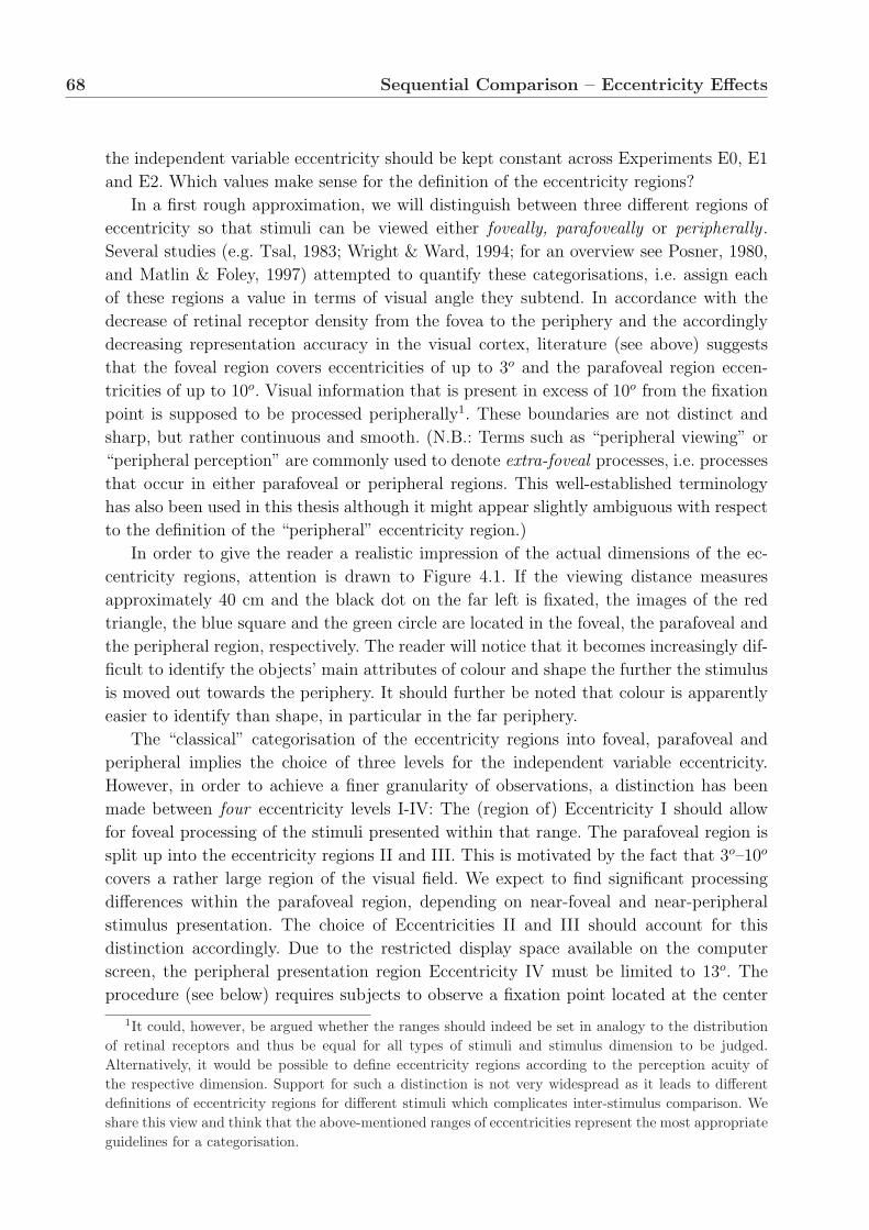
68 Sequential Comparison – Eccentricity Effects
the independent variable eccentricity should be kept constant across Experiments E0, E1
and E2. Which values make sense for the definition of the eccentricity regions?
In a first rough approximation, we will distinguish between three different regions of
eccentricity so that stimuli can be viewed either foveally, parafoveally or peripherally .
Several studies (e.g. Tsal, 1983; Wright & Ward, 1994; for an overview see Posner, 1980,
and Matlin & Foley, 1997) attempted to quantify these categorisations, i.e. assign each
of these regions a value in terms of visual angle they subtend. In accordance with the
decrease of retinal receptor density from the fovea to the periphery and the accordingly
decreasing representation accuracy in the visual cortex, literature (see above) suggests
that the foveal region covers eccentricities of up to 3o and the parafoveal region eccen-
tricities of up to 10o. Visual information that is present in excess of 10o from the fixation
point is supposed to be processed peripherally1. These boundaries are not distinct and
sharp, but rather continuous and smooth. (N.B.: Terms such as “peripheral viewing” or
“peripheral perception” are commonly used to denote extra-foveal processes, i.e. processes
that occur in either parafoveal or peripheral regions. This well-established terminology
has also been used in this thesis although it might appear slightly ambiguous with respect
to the definition of the “peripheral” eccentricity region.)
In order to give the reader a realistic impression of the actual dimensions of the ec-
centricity regions, attention is drawn to Figure 4.1. If the viewing distance measures
approximately 40 cm and the black dot on the far left is fixated, the images of the red
triangle, the blue square and the green circle are located in the foveal, the parafoveal and
the peripheral region, respectively. The reader will notice that it becomes increasingly dif-
ficult to identify the objects’ main attributes of colour and shape the further the stimulus
is moved out towards the periphery. It should further be noted that colour is apparently
easier to identify than shape, in particular in the far periphery.
The “classical” categorisation of the eccentricity regions into foveal, parafoveal and
peripheral implies the choice of three levels for the independent variable eccentricity.
However, in order to achieve a finer granularity of observations, a distinction has been
made between four eccentricity levels I-IV: The (region of) Eccentricity I should allow
for foveal processing of the stimuli presented within that range. The parafoveal region is
split up into the eccentricity regions II and III. This is motivated by the fact that 3o–10o
covers a rather large region of the visual field. We expect to find significant processing
differences within the parafoveal region, depending on near-foveal and near-peripheral
stimulus presentation. The choice of Eccentricities II and III should account for this
distinction accordingly. Due to the restricted display space available on the computer
screen, the peripheral presentation region Eccentricity IV must be limited to 13o. The
procedure (see below) requires subjects to observe a fixation point located at the center
1It could, however, be argued whether the ranges should indeed be set in analogy to the distributionof retinal receptors and thus be equal for all types of stimuli and stimulus dimension to be judged.Alternatively, it would be possible to define eccentricity regions according to the perception acuity ofthe respective dimension. Support for such a distinction is not very widespread as it leads to differentdefinitions of eccentricity regions for different stimuli which complicates inter-stimulus comparison. Weshare this view and think that the above-mentioned ranges of eccentricities represent the most appropriateguidelines for a categorisation.

4.1 Variables and Stimuli 69
Figure 4.1: Illustration of eccentricity regions: If viewed from a distance of approximately 40 cm withthe black dot fixated on the far left, the image of the red triangle is located in the foveal, the blue squarein the parafoveal and the green circle in the peripheral region.
of the display. With a viewing distance of approximately 60 cm from a computer screen
with a 20-inch screen diagonal, stimuli cannot be presented in eccentricities greater than
13o in each direction of the fixation point. The stimuli will accordingly be displayed within
four eccentricity regions which cover the following ranges (in degrees of visual angle):
• Eccentricity I: 1o–4o
• Eccentricity II: 4o–7o
• Eccentricity III: 7o–10o
• Eccentricity IV: 10o–13o
In fact, the choice of the ranges of the eccentricity levels is closely related to the choice
of levels for the independent variables line segment length and orientation in Experi-
ments E1 and E2, respectively. Let us consider the line segment length factor first.
An intuitive classification of line segment lengths would suggest line segments that are
“short”, “intermediate” and “long”. But how can we quantify this? The approach we take
is guided by factors that have to be taken into account when designing the stimuli for the
later simultaneous line segment length comparison experiments. With respect to the goals
of Experiments S1 and S2, it appears to be appropriate to choose line segments whose
lengths can either be perceived foveally or require parafoveal or peripheral processing. In
a comparison scenario with unrestricted eye gaze, shifts of visual attention are then likely
to be performed for “longer” line segments in order to foveally acquire relevant dimension
information. We expect that this is true in difficult discrimination tasks in particular.
Such a visual strategy would support an analytical processing hypothesis, in contrast to
possibly preferable holistic processing in “short” line comparisons, in particular for easy
discrimination tasks. As these considerations are also of some relevance in Experiments E1
and E2 and, furthermore, as conclusions from these experiments might contribute to the
explanation of some aspects of the observations in Experiments S1 and S2, the selection
of levels as discussed above is the most preferable.
However, we have to take into consideration that, due to the size of eccentricity regions,
the line segment lengths are limited and cannot be chosen in analogy to the ranges of the
eccentricity regions. Its eccentricity regions are radial-symmetric in shape, the maximum
line segment length is determined by the size of the innermost eccentricity region, i.e.
Eccentricity I. A line segment that yields the maximum possible length and can still

70 Sequential Comparison – Eccentricity Effects
be displayed in full within that eccentricity region must be oriented tangential to the
boundary of the radial-symmetric area around the fixation point. If we introduce a further
constraint, namely that the line segments must not be displayed within a certain margin
m of the eccentricity boundaries, the maximum line segment length lmax is computed as
lmax = 2 ·√
(r2 −m)2 − (r1 + m)2 (4.1)
where r1 denotes the radius of the fixation region boundary – which equals the inner
boundary of Eccentricity I, i.e. 1o – and r2 denotes the radius of the outer boundary of
Eccentricity I, i.e. 4o. Figure 4.2 illustrates the constraints that determine the computation
of the maximum line segment length lmax.
When we set the disallowed margin m to 0.3o, only line segments with a length of
up to 7o can be placed within the Eccentricity I without overlap of the neighbouring
eccentricities (see Figure 4.5). We thus select the following lengths for line segments as
displayed in the Experiments E1 and E2 (in degrees of visual angle):
• Short: 1o ± 0.3o
• Intermediate: 4o ± 0.3o
• Long: 7o ± 0.3o
In order to keep differences equal between the levels of the independent variable line
segment length, the short line segments were chosen to be 1o and the intermediates to be
4o. Although not exactly, these lengths still reflect the foveal, parafoveal and peripheral
regions of the visual field in good approximation. In an attempt to minimise habitual
effects that might occur when always exactly the same values have to be assessed, Gaussian
“noise” is introduced that randomly varies the line segment length by 0.3o around the
short, intermediate and long levels listed above.
Figure 4.2: Restriction of line segment length in Experiments E1 and E2 due to eccentricity boundaries.

4.1 Variables and Stimuli 71
For another independent variable, orientation, the choice of levels and their magni-
tudes are restricted by the size of the eccentricity regions insofar as not all combinations
of orientations and line segment lengths can be presented at all locations within the ec-
centricity regions. It is, for example, impossible to show a long, vertically oriented line
segment at a position directly on or in proximity to the vertical meridian, i.e. above or
below the fixation point. Such a configuration would result in the line segment’s end parti-
tions being visible in adjacent eccentricity regions rather than in the intended part of the
visual field only. As we will learn in Section 5.2, results from Experiment E0 suggest that
the meridial location of a stimulus, i.e. its position relative to the fixation point, does not
affect the acuity of position assessment. If we assume that the same is true for length or
orientation assessment, the meridial position will not have to be systematically varied as
an independent variable in Experiments E1 and E2. Meridial position does therefore not
constitute a critical factor and can be excluded from the list of constraints. This allows
us to circumnavigate the problem of incompatible stimulus combinations with respect to
orientation limitations.
For the independent variable orientation, the following levels are chosen:
• Horizontal: 0o ± 22.5o
• Oblique: 45o ± 22.5o or 135o ± 22.5o
• Vertical: 90o ± 22.5o
To be precise, the orientation regions should indeed be called “near horizontal”,
“oblique” and “near vertical”. The choice of the categories and their ranges appears
appropriate as they cover all possible orientations. Rather than only investigating line
segments that are oriented exactly horizontal, vertical or at an angle of 45o, no habitual
effects must be feared for orientation assessment due to the variation of line segment
orientations around those angles. Figure 4.3 illustrates the ranges of possible angles for
the three horizontal, oblique and vertical orientations. Each segment covers an angle of
45o (22.5o either side) around the respective guidance orientations of 0o, 45o and 90o. The
blue sample line segment shown in the figure is thus classified as belonging to the oblique
range.
In order to test whether the meridial location of stimuli, i.e. their position relative
to the fixation point, has an effect on position assessment, this additional factor is var-
ied in Experiment E0. As earlier research suggested (e.g. Kunnapas, 1955, 1957, 1959;
Prinzmetal & Gettleman, 1993; Armstrong & Marks, 1997) acuity differences depending
on whether stimuli were perceived either along the horizontal or the vertical meridian,
these two (natural) categories are chosen for the independent variable meridial position
in Experiment E0. The two diagonal light grey lines in Figure 3.7 or Figure 4.4 (top)
define the segments. No further distinction will be made between either the left and right
horizontal segments or the upper and lower vertical segments.
After the quantification of all relevant variables and the discussion in the previous
paragraphs of constraints that an appropriate stimulus design has to comply with, these
stimuli can now be generated algorithmically.
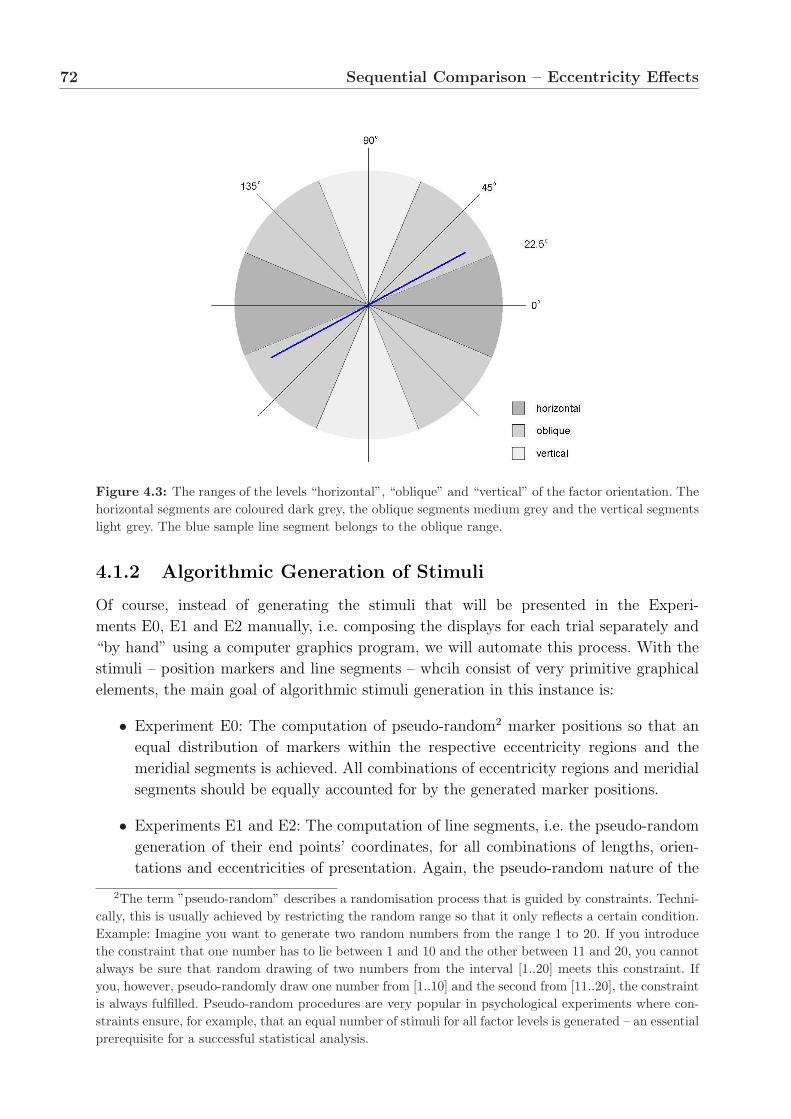
72 Sequential Comparison – Eccentricity Effects
Figure 4.3: The ranges of the levels “horizontal”, “oblique” and “vertical” of the factor orientation. Thehorizontal segments are coloured dark grey, the oblique segments medium grey and the vertical segmentslight grey. The blue sample line segment belongs to the oblique range.
4.1.2 Algorithmic Generation of Stimuli
Of course, instead of generating the stimuli that will be presented in the Experi-
ments E0, E1 and E2 manually, i.e. composing the displays for each trial separately and
“by hand” using a computer graphics program, we will automate this process. With the
stimuli – position markers and line segments – whcih consist of very primitive graphical
elements, the main goal of algorithmic stimuli generation in this instance is:
• Experiment E0: The computation of pseudo-random2 marker positions so that an
equal distribution of markers within the respective eccentricity regions and the
meridial segments is achieved. All combinations of eccentricity regions and meridial
segments should be equally accounted for by the generated marker positions.
• Experiments E1 and E2: The computation of line segments, i.e. the pseudo-random
generation of their end points’ coordinates, for all combinations of lengths, orien-
tations and eccentricities of presentation. Again, the pseudo-random nature of the
2The term ”pseudo-random” describes a randomisation process that is guided by constraints. Techni-cally, this is usually achieved by restricting the random range so that it only reflects a certain condition.Example: Imagine you want to generate two random numbers from the range 1 to 20. If you introducethe constraint that one number has to lie between 1 and 10 and the other between 11 and 20, you cannotalways be sure that random drawing of two numbers from the interval [1..20] meets this constraint. Ifyou, however, pseudo-randomly draw one number from [1..10] and the second from [11..20], the constraintis always fulfilled. Pseudo-random procedures are very popular in psychological experiments where con-straints ensure, for example, that an equal number of stimuli for all factor levels is generated – an essentialprerequisite for a successful statistical analysis.
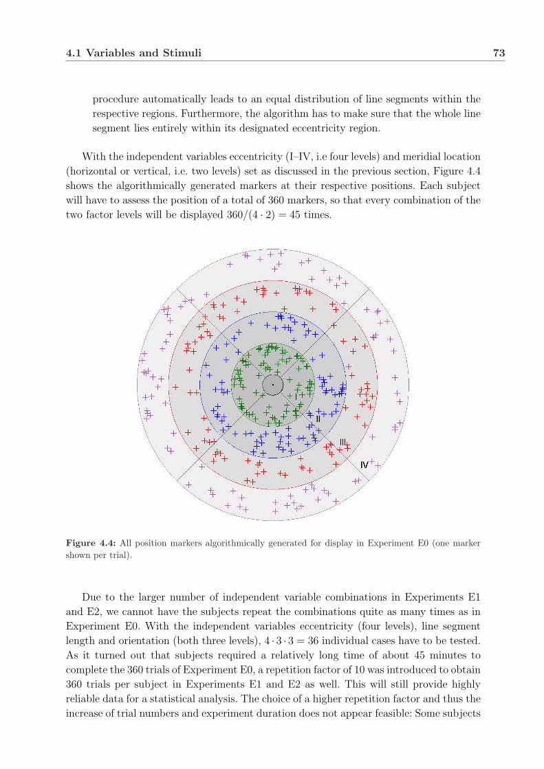
4.1 Variables and Stimuli 73
procedure automatically leads to an equal distribution of line segments within the
respective regions. Furthermore, the algorithm has to make sure that the whole line
segment lies entirely within its designated eccentricity region.
With the independent variables eccentricity (I–IV, i.e four levels) and meridial location
(horizontal or vertical, i.e. two levels) set as discussed in the previous section, Figure 4.4
shows the algorithmically generated markers at their respective positions. Each subject
will have to assess the position of a total of 360 markers, so that every combination of the
two factor levels will be displayed 360/(4 · 2) = 45 times.
Figure 4.4: All position markers algorithmically generated for display in Experiment E0 (one markershown per trial).
Due to the larger number of independent variable combinations in Experiments E1
and E2, we cannot have the subjects repeat the combinations quite as many times as in
Experiment E0. With the independent variables eccentricity (four levels), line segment
length and orientation (both three levels), 4 · 3 · 3 = 36 individual cases have to be tested.
As it turned out that subjects required a relatively long time of about 45 minutes to
complete the 360 trials of Experiment E0, a repetition factor of 10 was introduced to obtain
360 trials per subject in Experiments E1 and E2 as well. This will still provide highly
reliable data for a statistical analysis. The choice of a higher repetition factor and thus the
increase of trial numbers and experiment duration does not appear feasible: Some subjects

74 Sequential Comparison – Eccentricity Effects
Figure 4.5: All line segments algorithmically generated for display in Experiments E1 and E2 (one linesegment shown per trial)
complained of fatigue in Experiment E0, probably due to the tiring fixed-focus restriction.
Figure 4.5 shows all line segments algorithmically generated for Experiments E1 and E2.
The following chapter will describe Experiment E0, the experiment that investigates
the eccentricity effects on positional assessment accuracy in a sequential comparison set-
ting. After explaining the particularities of the method for this experiment the results will
be presented and discussed in detail.

Chapter 5
Experiment E0: Location
Assessment in Peripheral Vision
Experiment E0 is the first in a series of three experiments that aim to establish and
quantify the effects of eccentric stimulus presentation on the perception and assessment of
specific stimulus dimensions. For the investigation, we explore the paradigm of sequential
comparison, paired with the psychophysical method of adjustment. In order to control a
restriction that is imposed on the subjects and requires them to only look at a designated
region during target stimulus presentation, we monitor the subjects’ eye gaze using the
EyeLink eye tracker. This method ensures that only valid trials, i.e. those where subjects
follow the gaze restriction, are recorded and subsequently analysed.
As demonstrated in the previous sections, peripheral vision is identified as one of the
fundamental factors that influence the perception of line segments, in particular if at-
tentional processes are involved. In order to understand line segment perception, it is
regarded a promising approach to consider position assessment first. Data acquired in
Experiment E0, which requires subjects to assess the positions of markers presented in
various regions of eccentricity, is intended to yield valuable contributions to the under-
standing of the processes involved in line segment assessment (see Chapter 4) – inves-
tigated in Experiments E1 and E2, and again, later, in Experiments S1 and S2. The
following sections describe the experimental method for Experiment E0 in detail based
on the methodological preliminaries that were established in Chapters 3 and 4.
5.1 Method
5.1.1 Subjects
The subjects were fifteen experimentally naive students – eight male and seven female –
from the University of Bielefeld. Their average age was 26.8 years. All subjects had normal
or corrected-to-normal vision and no pupil anomalies. The subjects were paid for their
participation in the experiment.

76 Experiment E0: Location Assessment in Peripheral Vision
5.1.2 Stimuli
The stimulus pictures were presented on a computer screen with a spatial resolution
of 1280×1024 pixels (39.0o×29.4o of visual angle). A fixation point with 0.2o of visual
angle in diameter was displayed at the center of each picture. The stimulus position
marker was presented at a pseudo-random location (see Section 4.1.2), determined by
its eccentricity region I–IV and its meridial segment (horizontal or vertical) relative to
the fixation point. The position marker had a “+” shape, both the horizontal and the
vertical bar constituents measured 0.4o of visual angle in length. The fixation point and
the position marker were dark grey in colour with their RGB-values set to (R, G, B) =
(100, 100, 100) and were presented on a light grey background with its RGB-values set to
(R,G, B) = (180, 180, 180). The choice of a light grey background colour proved to reduce
reflections on the display monitor to a minimum which may have had a facilitatory effect
on the position assessment. Figure 5.1 shows a typical stimulus picture.
Figure 5.1: Typical stimulus picture in Experiment E0. Subjects had to assess the position of the targetmarker (“+”) while observing the central fixation point.
5.1.3 Apparatus
The experiment took place in the eye tracking laboratory of the Neuroinformatics Group at
the University of Bielefeld. The laboratory was artificially illuminated by ceiling-mounted,
indirect light sources that yielded homgeneous lighting conditions. The stimuli were pre-
sented on a 19” colour computer monitor with a cathode-ray tube (CRT) display. The
subjects were seated at an approximate distance of 50–60 cm from the display. The wall
to the back of the subjects was covered with matt, black cloth to reduce reflections on
the stimulus display. Eye movements were monitored using the SMI EyeLink eye-tracker
system during the presentation of the peripheral target stimulus.

5.1 Method 77
5.1.4 Procedure
All subjects were tested individually. Prior to the start of the experiment, they were
provided with written instructions explaining the task they had to complete. Next, the eye
tracker was set up and calibrated for each subject. To complete the calibration procedure,
subjects had to look at nine dots that successively appeared at specific locations on the
display.
Each trial of the experiment began with the presentation of the fixation point at the
center of the screen (Frame 1, see Figure 5.2). 1000 ms after fixation point onset, the
“+”-shaped target stimulus appeared in one of the eccentricity regions I-IV (Frame 2).
The instructions required the subjects to assess the target marker position as accurately
as possible without foveating it. Instead, the subjects had to focus on the central fixation
point. If this restriction was violated and the eye tracker measured a gaze position outside
the region of 1o around the fixation point, a buzzer sounded and the trial was aborted.
When subjects had successfully finished the assessment task and memorised the perceived
position of the target marker, they pressed the left button of a computer mouse. A blank
screen was displayed for 500 ms (Frame 3).
Next, the fixation point reappeared (Frame 4). After 300 ms, the comparison posi-
tion marker was superimposed on it (Frame 5). The comparison marker had the same
shape (“+”) and dimensions as the previously shown target marker. Subjects were then
Figure 5.2: The sequence of procedural steps for a trial of Experiment E0. Frame 1: Fixation point.Frame 2: Target marker assessment. Frame 3: Blank screen. Frame 4: Fixation point. Frame 5: Comparisonmarker. Frame 6: Adjustment of comparison marker.

78 Experiment E0: Location Assessment in Peripheral Vision
instructed to move the comparison marker using the computer mouse to the exact posi-
tion where they originally perceived the target marker. When subjects moved the target
away from the starting position, the fixation point remained at the center of the display
as a point of reference (Frame 6). Once subjects had moved the comparison marker to its
final position coinciding with their memorised target marker position, they pressed the
left button of the computer mouse to confirm their adjustment and to start the next trial.
The completion of this task did not require focussing on the fixation point, but allowed
the gaze to move freely across the whole screen. Figure 5.2 illustrates the sequence of
procedural steps for one trial.
The eye tracker was recalibrated after every trial in order to compensate for the head-
set becoming displaced due to head movements. Subjects had to fixate a single calibration
marker at the center of the display to accomplish this “drift correction”. The frequent
recalibrations were necessary as the measurement of eye movements in such a setting
requires extremely high accuracy. The region around the fixation point where eye move-
ments are allowed is very small – 2o of visual angle in diameter – so that even a minor
misalignment of the headset might result in eye gaze positions that are evaluated as “out
of bounds”, even though they might in fact still be within the allowed region. Thus,
frequent recalibration prevents subjects from being irritated by potentially unmotivated
abortions of trials.
Subjects viewed a total of 360 stimulus pictures during the experiment, each possible
combination of the four position eccentricities and the two meridial segments was displayed
45 times. Ten practice trials were conducted prior to the experimental trials in order to
accustom the subjects to the eye-tracker headset, the experimental task and, in particular,
the gaze-restricted viewing conditions.
5.2 Results
The eye tracker was only used in this experiment as a monitoring device to control the
gaze restrictions imposed on subjects in the assessment phase of the peripherally presented
target position marker. The eye-gaze data recorded here does not provide any valuable
contribution to the understanding of the assessment process and will consequently not be
analysed.
During the subsequent phase of adjustment of the comparison marker, the execution of
eye movements could be expected as the gaze restriction did not apply any more. Although
the visual strategy pursued in the adjustment phase was not the prime interest of this
investigation, we consider it worthwhile to at least informally introduce two respective
options. The first possible strategy could see subjects that continue fixating the center of
the display while peripherally adjusting the comparison marker – i.e they do not actually
execute eye movements. The idea here might be that the preservation of the viewing
conditions and the possibility of matching the comparison with some sort of an after-image
of the target stimulus facilitates the adjustment. However, the analysis of eye-movement
data does not support this strategy, but favours an alternative approach. This second
5.2 Results 79
strategy suggests that the subjects’ gaze guides the comparison marker movements and,
vice versa, that the current marker position provides feedback to the eyes on the progress
of the adjustment. Indeed, subjects seem to follow this second strategy.
As a consequence, we will not further analyse this eye-movement data, which obviously
experiences interference from the adjustment procedure when the comparison marker is
moved across the screen. Eye-movement data is mainly influenced by the marker move-
ment – which suggests a smooth pursuit tracking eye-movement “mode” – rather than
by the previous peripheral viewing condition. Certainly, this renders an interpretation
difficult – or impossible – with regard to the effects of eccentricity on position assessment
acuity. Instead, only the conventional psychophysical data, measured in the dependent
variables as discussed in Section 3.4.2, are entered in an analysis of variance. The influ-
ence of the factors eccentricity region and meridial position is tested on the dependent
variables reaction time RT, radial deviation DX, tangential deviation DY and Euclidean
deviation DXY of the comparison marker position from the target marker position in a
two-factorial analysis of variance. For all subsequent analyses of variance the α-level for
the significance of effects is set to p = 0.05.
5.2.1 Dependent Variables
Reaction Time RT
Figure 5.3 (left) shows a histogram of all measured reaction times RT that subjects re-
quired in order to assess the position of the target marker under restricted gaze. The rela-
tive frequencies are charted irrespective of the eccentric and meridial locations of the target
marker. RT varies from a minimum of 155 ms to a maximum of 3100 ms, with approxi-
mately 95% of the measured reaction times lying within the interval of 250 to 1350 ms.
The histogram peaks at approximately 410 ms and subjects needed 662.1 ms on average
to assess the marker position. A suitable fitting function would be asymmetrical (e.g.
the χ2 distribution or the Gamma-function (for details see Section 12.3)) with a positive
skewness of +1.98.
In order to test the influence of the factors eccentricity and meridial position of presen-
tation, RT is subjected to an analysis of variance. This detailed analysis of reaction times
reveals a significant effect of the region of eccentricity on RT (F (3; 42) = 9.88; p < 0.001):
The assessment of the target marker position took increasingly longer from Eccentric-
ity I (624.9 ms) to Eccentricities II (652.8 ms), III (662.2 ms) and IV (696.3 ms). Fur-
thermore, a post-hoc comparison of means using the Newman-Keuls test (for details see
Hochberg & Tamhane, 1987; Toothaker, 1991; Glass & Hopkins, 1996) is computed.
For this and subsequent post-hoc comparisons of means the α-level for critical ranges
is set to p = 0.05. It reveals that no significant difference in RT exists between the
two parafoveal Eccentricities II and III (Rcrit = 26.618; p = 0.321) whereas RT sig-
nificantly differs between all other eccentricity regions: (Rcrit = 32.125; p = 0.034) for
the comparison of RT between the Eccentricities I and II, (Rcrit = 33.010; p = 0.013)
for I vs. III, (Rcrit = 36.451; p < 0.001) for I vs. IV, (Rcrit = 35.432; p = 0.005) for
II vs. IV and (Rcrit = 32.578; p = 0.024) for III vs. IV. No significant main effect on

80 Experiment E0: Location Assessment in Peripheral Vision
reaction time RT (ms)
rela
tive
freq
uenc
y
0
0.02
0.04
0.06
0.08
0.10
0 500 1000 1500 2000 2500 3000
eccentricity
reac
tion
time
RT
(m
s)
600
620
640
660
680
700
720
I II III IV
horizontal meridianvertical meridian
Figure 5.3: Left: Relative frequency distribution of reaction times RT, aggregated over all eccentricityregions and all meridial marker positions. Right: Reaction time RT as a function of eccentricity whenposition markers are presented either along the horizontal or the vertical meridian.
RT can be established for the meridial position factor (F (1; 14) = 1.68; p = 0.215). In-
teraction effects of eccentricity and meridial position on RT are not significant either
(F (3; 42) = 0.53; p = 0.661). Figure 5.3 (right) shows the reaction time RT as a function
of eccentricity and the meridial position of the target marker.
Positional Deviations DX, DY and DXY
The analysis of the mislocation of the comparison marker, relative to the target marker,
i.e. the radial as well as the tangential and the Euclidean deviations of the comparison
marker position from the target marker position can be accomplished by using one of two
possible data sets: Either the absolute (positive) deviations from the target or a deviation
measure that takes into account the direction of the deviation as well. As results are quite
different for both data sets, the choice of the respective set has to be considered carefully
with regard to the intended further employment of the findings and interpretation.
The relationship between the target and the comparison marker positions in terms
of radial, tangential and Euclidean deviation was already discussed in Section 3.4.2 and
is again illustrated in Figure 5.4. If we consider the “directional” data, the radial devia-
tion DX will be assigned a positive value in case the radial coordinate of the comparison
marker position has a greater value than that of the target marker position, i.e. when the
radial position of the target marker is “overestimated”. Accordingly, DX will be negative
when the radial coordinate of the comparison marker is closer to the fixation point than
that of the target marker, i.e. when the radial position of the target marker is “underes-
timated”.
Regarding the tangential deviation, we determine DY as positive when the tangential
coordinate of the target marker position has to be shifted clockwise – rotation of the radial
axis around the fixation point – to match that of the comparison marker, and negative
when shifted counter-clockwise. Here, it obviously does not make sense to classify the
deviations as “overestimation” or “underestimation”.
The Euclidean deviation DXY is assigned a positive value if the Euclidean distance

5.2 Results 81
Figure 5.4: Radial and tangential axes and the respective deviations DX (pink) and DY (black) of thecomparison marker from the target marker. DXY (light blue) denotes the Euclidean distance betweenthe target (green) and the comparison marker (red).
between the fixation point and the comparison marker is greater than that between the
fixation point and the target marker – and negative otherwise. Figure 5.4 thus shows a
configuration where all DX, DY and DXY are positive. The “absolute” data sets ignore the
directional information and are represented by the positive deviations only, i.e. directional
and absolute data would be identical for the sample scenario in Figure 5.4.
As we will later be interested in modelling the distribution of the positional assess-
ments of the target, information from both data types is required. If the distribution is
thought of as being bivariate in nature, the analysis of directional data yields information
on the origin and the orientation of the distribution whereas the distributions “extent”
can be more reliably determined through the absolute data – this is particularly true
for symmetric distributions such as the normal distribution. The following paragraphs
detail the results for DX, DY and DXY when both absolute and directional analyses are
performed.
Absolute Radial Deviation DXp
Let us first consider the absolute radial deviation DXp. As the case with reaction time RT
before, we enter DXp into a two-factorial analysis of variance in order to test the influence
of the independent variables eccentricity and meridial position on the radial deviation.
The results show that an increase of DXp coincides with the target marker presentation in
increasingly peripheral locations. The mean absolute radial deviations (all given in degrees
of visual angle) measure 0.47o for Eccentricity I, 0.79o for Eccentricity II, 0.91o for Eccen-
tricity III and 1.06o for Eccentricity IV. The standard deviations for DXp are computed as
0.39, 0.62, 0.70 and 0.84o for the Eccentricities I–IV, respectively. The differences between
the eccentricity levels are highly significant (F (3; 42) = 1.37; p < 0.001). A post-hoc com-
parison of means using the Newman-Keuls test reveals that significant differences exist be-
tween all eccentricity levels: (Rcrit = 0.149; p < 0.001) for the comparison of DXp between
the Eccentricities I and II, (Rcrit = 0.147; p < 0.001) for I vs. III, (Rcrit = 0.147; p < 0.001)

82 Experiment E0: Location Assessment in Peripheral Vision
eccentricity
abso
lute
rad
ial d
evia
tion
DX
p (d
egre
es)
0
0.2
0.4
0.6
0.8
1.0
1.2
1.4
1.6
I II III IV
horizontal meridian
vertical meridian
Figure 5.5: Absolute radial deviation DXp of the comparison marker position from the target markerposition for all eccentricities and meridial positions.
for I vs. IV, (Rcrit = 0.101; p = 0.040) for II vs. III, (Rcrit = 0.142; p < 0.001) for II vs. IV
and (Rcrit = 0.128; p = 0.009) for III vs. IV.
Again, no main effect for the meridial position can be observed (F (1; 14) = 0.13; p =
0.070). However, there appears to be a tendency towards less absolute radial deviation
when the target markers are presented in proximity to the horizontal meridian than in
proximity to the vertical meridian. Interaction effects of eccentricity and meridial position
on DXp are not significant (F (3; 42) = 0.02; p = 0.663). Figure 5.5 shows the mean
absolute radial deviation DXp as a function of eccentricity and meridial position of the
target marker.
Absolute Tangential Deviation DYp
Analogous to DXp, the absolute tangential deviation DYp is subjected to an analysis
of variance. Similar to the previous findings, differences between the Eccentricities I–IV
are highly significant for DYp (F (3; 42) = 3.26; p < 0.001). A post-hoc comparison of
means using the Newman-Keuls test reveals that significant differences exist between all
eccentricity levels: (Rcrit = 0.071; p < 0.001) for the comparison of DYp between the
Eccentricities I and II, (Rcrit = 0.067; p < 0.001) for I vs. III, (Rcrit = 0.072; p < 0.001)
for I vs. IV, (Rcrit = 0.057; p < 0.001) for II vs. III, (Rcrit = 0.064; p < 0.001) for II vs. IV
and (Rcrit = 0.070; p < 0.001) for III vs. IV. The least tangential deviation is found for
Eccentricity I (0.31o) and then constantly increases for Eccentricities II (0.45o), III (0.60o)
and IV (0.73o). The standard deviations for DYp are computed as 0.26o, 0.36o, 0.49o and
0.59o for the Eccentricities I–IV, respectively. The meridial position does not exert a
significant effect on DYp (F (1; 14) = 0.10; p = 0.098), but the tendency towards a more
accurate assessment of absolute tangential position of the target markers in proximity
to the horizontal meridian – compared with those presented in proximity to the vertical

5.2 Results 83
eccentricity
abso
lute
tang
entia
l dev
iatio
n D
Yp
(deg
rees
)
0
0.2
0.4
0.6
0.8
1.0
1.2
1.4
1.6
I II III IV
horizontal meridian
vertical meridian
Figure 5.6: Absolute tangential deviation DYp of the comparison marker position from the target markerposition for all eccentricities and meridial positions.
meridian – prevails as for DXp. No interaction effects between eccentricity and meridial
position on DYp can be observed (F (3; 42) = 0.03; p = 0.384). Figure 5.6 illustrates the
mean values of DYp for the different peripheral regions and the meridial positions.
Qualitatively comparing the magnitudes of DXp and DYp already suggests that these
two measures are significantly different from each other: The radial deviation is larger
than the tangential deviation. When we enter the distinction between these two axes
as an additional factor into the analysis of variance, the ad-hoc hypothesis is confirmed
eccentricity
devi
atio
n (d
egre
es)
0
0.2
0.4
0.6
0.8
1.0
1.2
1.4
1.6
I II III IV
radial deviation DXp
tangential deviation DYp
Figure 5.7: The absolute radial deviations DXp and the absolute tangential deviations DYp of thecomparison marker position from the target marker position as functions of eccentricity.

84 Experiment E0: Location Assessment in Peripheral Vision
(F (1; 14) = 1.04; p < 0.001). Figure 5.7 shows the means of DXp in comparison with
those of DYp for all eccentricity regions I–IV, collapsed over the horizontal and meridial
presentation positions.
Absolute Euclidean Deviation DXYp
The Euclidean deviation DXYp is the last dependent variable that is tested in Experi-
ment E0 with respect to possible interactions with the peripheral and meridial presenta-
tion positions. DXYp, which is computed from DXp and DYp as the Euclidean distance
between the target and comparison marker positions, increases with increasing eccentric-
ity. This highly significant effect (F (3; 42) = 2.37; p < 0.001) is manifested by mean values
for DXYp of 0.60o for Eccentricity I, 0.98o for Eccentricity II, 1.18o for Eccentricity III and
1.40o for Eccentricity IV. The standard deviations for DXYp are computed as 0.40o, 0.59o,
0.70o and 0.84o for the Eccentricities I–IV, respectively. A post-hoc comparison of means
using the Newman-Keuls test reveals that significant differences again exist between all
eccentricity levels: (Rcrit = 0.153; p < 0.001) for the comparison of DXYp between the
Eccentricities I and II, (Rcrit = 0.153; p < 0.001) for I vs. III, (Rcrit = 0.158; p < 0.001)
for I vs. IV, (Rcrit = 0.114; p = 0.001) for II vs. III, (Rcrit = 0.153; p < 0.001) for II vs. IV
and (Rcrit = 0.160; p < 0.001) for III vs. IV.
In accordance with the results of the analyses of variance for DXp and DYp, a cor-
responding tendency towards an effect of the meridial position on DXYp can be noted
(F (1; 14) = 0.31; p = 0.064): The Euclidean deviation of the comparison from the target
marker appears to be slightly less when the target marker is presented in proximity to
the horizontal meridian. This tendency is qualitatively visible in Figure 5.8 where the
Euclidean deviation DXYp is shown as a function of eccentricity and the meridial posi-
tion of the target marker. There is no interaction effect between eccentricity and meridial
eccentricity
abso
lute
Euk
lidia
n de
viat
ion
DX
Yp
(deg
rees
)
0
0.2
0.4
0.6
0.8
1.0
1.2
1.4
1.6
I II III IV
horizontal meridian
vertical meridian
Figure 5.8: Absolute Euclidean deviation DXYp of the comparison marker position from the targetmarker position for all eccentricities and meridial positions.

5.2 Results 85
position on DXYp (F (3; 42) = 0.02; p = 0.537).
As already briefly mentioned, the distribution of the comparison marker positions –
which can be thought of as sketched in Figure 5.9 (left) – requires more than just knowl-
edge of the “extent” of the distribution. The origin of the distribution, i.e. its “anchor
point”, for example, constitutes essential information for describing the distribution func-
tion. The analyses of DXp, DYp and DXYp do not yield this data. Instead, an analysis
of the “directional” data sets is required to obtain the direction of the deviation of the
comparison marker relative to the target marker. These deviations will again be anal-
ysed separately for the radial (DX), tangential (DY) and Euclidean (DXY) dimensions.
In Figure 5.9 (left), the green dot highlights the target marker position that the subjects
had to assess, the black dots show all positions (for all subjects and repetitive measures
by subjects) where they placed the comparison marker. The red dot marks the averaged
comparison marker position. The ellipsis illustrates the results of a principal component
analysis (PCA) that approximates the (orientation of the) distribution of the compar-
ison marker positions. If the relative frequencies of assessment positions are also taken
into account and charted on an axis perpendicular to the x–y–coordinate (paper) plane,
a distribution shaped similarly to that shown in Figure 5.9 (right) emerges. The exact
procedure will be discussed later in Chapter 8.
Figure 5.9: Left: Approximation of a sample distribution of comparison marker positions using principalcomponent analysis (PCA). Right: Original distribution of the same comparison marker positions andtheir relative frequencies.
As the analyses of DXp, DYp and DXYp revealed, the meridial position of the target
marker does not have a significant effect on the absolute radial, tangential or Euclidean
deviations of the comparison marker position from the target marker position. We will
thus collapse the data over the factor meridial position and only test the effect of the
eccentricity region on the “directional” deviations DX, DY and DXY.
Radial Deviation DX
An analysis of variance yielded a significant eccentricity effect on the radial deviation DX
(F (3; 42) = 0.09; p = 0.048) and the means for DX are computed to -0.17o for Eccentric-
ity I, -0.34o for Eccentricity II, -0.37o for Eccentricity III and -0.43o for Eccentricity IV.

86 Experiment E0: Location Assessment in Peripheral Vision
A post-hoc comparison of means using the Newman-Keuls test reveals that significant
differences exist between almost all eccentricity levels: (Rcrit = 0.285; p = 0.012) for the
comparison of DX between the Eccentricities I and II, (Rcrit = 0.267; p = 0.021) for
I vs. III, (Rcrit = 0.255; p = 0.029) for I vs. IV, (Rcrit = 0.267; p = 0.021) for II vs. IV and
(Rcrit = 0.284; p = 0.015) for III vs. IV. Only when comparing DX between the eccen-
tricity levels II and III the Newman-Keuls test does not produce a significant difference
(Rcrit = 0.213; p = 0.065).
Thus, for all eccentricities, subjects on average placed the comparison marker closer
to the fixation point on the radial axis. The standard deviations for DX are computed as
0.59o, 0.92o, 1.08o and 1.28o for the Eccentricities I–IV, respectively. Figure 5.10 illustrates
the means of the radial deviations DX for the Eccentricities I–IV.
eccentricity
radi
al d
evia
tion
DX
(de
gree
s)
-0.5
-0.4
-0.3
-0.2
-0.1
0
0.1
0.2
0.3
I II III IV
Figure 5.10: Radial deviation DX of the comparison marker position from the target marker positionfor all eccentricities, collapsed over the horizontal and vertical meridial locations.
Tangential Deviation DY
When the data for the tangential deviation DY is entered into an analysis of variance,
a significant effect of eccentricity thereupon emerges (F (3; 42) = 0.20; p = 0.002). How-
ever, as the computation of means for the four eccentricities shows, no steady tendency for
direction for the mislocation is visible. Means are -0.02o for Eccentricity I, 0.02o for Eccen-
tricity II, -0.08o for Eccentricity III and 0.02o for Eccentricity IV. A post-hoc comparison
of means using the Newman-Keuls test reveals that significant differences exist only be-
tween the following eccentricity levels: (Rcrit = 0.079; p = 0.003) for the comparison of
DY between the Eccentricities II and III and (Rcrit = 0.080; p = 0.003) for III vs. IV. In
contrast, differences between the eccentricity levels I and II (Rcrit = 0.059; p = 0.192),
between I and III (Rcrit = 0.067; p = 0.055), I and IV (Rcrit = 0.062; p = 0.141) and II

5.2 Results 87
eccentricity
tang
entia
l dev
iatio
n D
Y (
degr
ees)
-0.5
-0.4
-0.3
-0.2
-0.1
0
0.1
0.2
0.3
I II III IV
Figure 5.11: Tangential deviation DY of the comparison marker position from the target marker positionas a function of eccentricity.
and IV (Rcrit = 0.040; p = 0.790) are not significant.
The tangential deviations are significantly smaller than the radial deviations
(F (1; 14) = 0.30; p = 0.010). The standard deviations for DY are computed as 0.41o,
0.57o, 0.78o and 0.94o for the Eccentricities I–IV, respectively. Figure 5.11 shows the
means of the tangential deviations DY for the Eccentricities I–IV.
Euclidean Deviation DXY
The analysis of variance for the Euclidean deviation DXY yields a significant effect for the
tested factor eccentricity (F (3; 42) = 0.07; p = 0.039). A post-hoc comparison of means
using the Newman-Keuls test reveals that significant differences again exist between all
eccentricity levels: (Rcrit = 0.240; p = 0.026) for the comparison of DXY between the
Eccentricities I and II, (Rcrit = 0.220; p = 0.015) for I vs. III, (Rcrit = 0.213; p = 0.010)
for I vs. IV, (Rcrit = 0.251; p = 0.045) for II vs. III, (Rcrit = 0.251; p = 0.030) for
II vs. IV and (Rcrit = 0.256; p = 0.039) for III vs. IV. The computed means are -0.15o
for Eccentricity I, -0.33o for Eccentricity II, -0.38o for Eccentricity III and -0.44o for
Eccentricity IV. The standard deviations for DXY are computed as 0.71o, 1.06o, 1.31o
and 1.57o for the Eccentricities I–IV, respectively.
As could be expected from the result of the analyses of DX and DY, the greater mag-
nitudes of the radial deviations – compared to the tangential deviations – dominate the
Euclidean deviations and yield a steadily increasing Euclidean deviation with more pe-
ripheral target marker positions. The negative values of DXY account for the fact that
subjects positioned the comparison markers closer to the fixation point than where the
target markers were located. Figure 5.12 illustrates the means of the Euclidean devia-
tions DXY for the Eccentricities I–IV.

88 Experiment E0: Location Assessment in Peripheral Vision
eccentricity
Euk
lidia
n de
viat
ion
DX
Y (
degr
ees)
-0.5
-0.4
-0.3
-0.2
-0.1
0
0.1
0.2
0.3
I II III IV
Figure 5.12: Euclidean deviation DXY of the comparison marker position from the target marker po-sition as a function of eccentricity.
5.3 Discussion and Conclusions
After the quantitative analysis of the data recorded in Experiment E0 in the previous
section, we will now discuss the results with particular respect to their implications for
the following Experiments E1 and E2 that research line segment length and orientation.
The discussion will also be guided by the intention to model the location assessment results
so that they can be used to simulate the experimental data obtained in Experiments E1
and E2.
Let us briefly recall which independent variables were tested to influence which de-
pendent variables in Section 5.2: The factors meridial position and eccentricity were sys-
tematically varied and we analysed these effects on the dependent variables reaction time
RT, radial deviation DX (and DXp), tangential deviation DY (and DYp) and Euclidean
deviation DXY (and DXYp) of the comparison marker position from the target marker
position. How can we now interpret these various interactions and what do they imply?
The two most fundamental observations the findings yield are that
1. the factor meridial position does not exert a significant effect and
2. the factor eccentricity exerts a significant effect
on the dependent variables. Whereas the second observation might be expected, the lack
of an effect of the position of the target relative to the fixation point, either along the
horizontal or the vertical meridian, comes as a surprise. But, let us have a look at the
various observations in detail.
Due to the viewing restriction imposed on the subjects, their gaze must remain more
or less stationary during the position assessment. The voluntary, controlled execution of
5.3 Discussion and Conclusions 89
saccades within the allowed range of 1o from the central fixation point is almost impossible,
particularly when the task requires “covert” attention to a peripheral location. Indeed,
the eye-movement data shows that in most cases only a single fixation was recorded, so
that for the given scenario the fixation duration coincides with the reaction time RT.
When we now take into account that, under normal viewing conditions when the gaze
is not restricted, eye fixations approximately last between 150 and 400 ms, it is quite
“natural” that the values measured here for RT are quite low. Even without the special
requirements of the task here, it is a rather difficult task for subjects to accomplish
extremely long fixations. Consequently, only very few values of RT exceed 1350 ms and
were measured on the rare occasions when subjects managed to execute more than just
one fixation within the allowed range around the fixation point – although it is known
from aftereffect experiments that subjects are able to fixate a particular point for about
30 seconds. For the present task, however, subjects obviously extend fixation durations
to only such a degree that still does not present too great a (concentration) effort and,
on the other hand, does not – at least in their own belief – compromise too much their
performance in the assessment of the target marker location.
Certainly, the further the target marker is moved out to the periphery of the fixation
point, the more difficult the assessment of the marker position becomes. Although subjects
obviously do not feel very comfortable executing long fixations, they try to compensate
for the increased difficulty of the task by an increase of RT. This may be understood
when discussed in the context of mental rotation experiments where reaction time was
found to increase for larger angles between two (target and comparison) stimuli. In the
present scenario, the task may be considered a “mental translation”. In analogy to men-
tal rotation, longer translation distances may require more time to accomplish stimulus
assessment. This could possibly explain the increase of RT in more peripheral regions in
this experiment.
An interesting finding, which the analyses of the other dependent variables – at least
partially – support, is that the difference between RT for Eccentricity II and Eccentric-
ity III is considerably smaller than the differences between the other adjacent eccentricity
regions, although the boundaries between the eccentricity regions are all spaced at equally
distant intervals. We recall the original definition of both the Eccentricities II and III as
belonging to the parafoveal region, as the range of this region (from 3o to 10o) appeared
to be too large to be accounted for by only a single level of the factor eccentricity in
these studies. Although the marker position in Eccentricity III still takes longer to be
assessed than in Eccentricity II, the respective RTs are not found to differ significantly.
This observations could be interpreted as supporting the classification of peripheral view-
ing in foveal, parafoveal and peripheral perception regions. In addition, it could give rise to
the hypothesis that the perception effort (in terms of RT) within each eccentricity region
does not vary considerably or is possibly even invariant and that differences are most pro-
nounced around the designated boundaries of these eccentricity regions. However, if we
consider a physiological approach that attributes the differences to a decrease in receptor
density in the retina, this density drops rapidly from the fovea to the periphery, but does
not show obvious plateaux that could account for three explicit eccentricity levels. Maybe

90 Experiment E0: Location Assessment in Peripheral Vision
a detailed review of the finer structures in the topology of the retinal receptors or the
respective cortical areas could produce evidence for or against such a link.
What these physiological properties and the findings regarding RT certainly do not
imply, is, of course, that sharp boundaries exist to separate the foveal from the parafoveal,
and the parafoveal from the peripheral region. On the basis of the analysis of RT alone,
a distinction between three levels (foveal, parafoveal and peripheral) and the choice of
boundaries between them as accomplished in our studies appear nevertheless sensible.
In contrast to the effect of eccentricity on reaction time, the lack of significant differ-
ences in RT for the two meridial positions (horizontal vs. vertical, relative to the fixation
point) can be considered a first indicator that no such differences exist in the other de-
pendent variables either – which is indeed the case. Alternatively, we could also have
concluded that subjects were just not aware that one of the meridial configurations would
be more difficult to assess than the other, but then find significant differences in the
positional deviations DX(p), DY(p) and/or DXY(p).
However, the analyses of the deviations suggest no influence of the meridial position
on those variables. Although we noticed this effect – or rather that such an effect does
not exist – for RT, it is again surprising to find no such effect for the positional deviations
either. Whether the marker’s position has to be assessed when it is presented in proximity
to the horizontal or to the vertical axis does not obviously result in significant differences
within either DX, DY or DXY. Specifically, targets’ positions along the vertical meridian
can be as accurately judged as those along the horizontal meridian.
We would certainly not have expected this observation initially. First, we must con-
sider that the retina is not a true hemisphere, but ellipsoidal in shape with the horizontal
axis being the longer. Furthermore, with binocular viewing, the visual field is ovoid, its
horizontal axis being approximately 0.5 times greater than its vertical axis (Prinzmetal &
Gettleman, 1993). Taking this asymmetry into account, the preferred horizontal orienta-
tion of the visual field and the further range of receptors along this axis could be well
expected to lead to a better position assessment accuracy along the horizontal than along
the vertical meridian. Instead, the tendencies towards an interaction in the analyses of
DX, DY and DXY in Experiment E0 only slightly hint at such a dependence. It must be
taken into account, however, that the assessment is probably based on the cortical rather
than the retinal representation. The retinal information may thus be corrected in subse-
quent processing steps as to compensate for the retinal distortion. This apparently yields
cortical position representations which are equally accurate for all meridial positions of
the stimulus marker.
Contrary to the missing meridial position effect, the significantly increasing assessment
error with increasing eccentricity could be expected. The rise of all absolute deviations
DXp, DYp and DXYp the further the target is being presented from the fixation point can
be attributed to the poorer spatial resolution in the peripheral visual field (e.g. Thomp-
son & Fowler, 1980). This again is an integral part of Tsal’s (1999) concept of different
metrics for attended and unattended stimuli. Even though advanced by Tsal for length
estimation (cf. Section 2.2), the idea of metrics composed of fine units for attended judge-
ment – resembling high spatial resolution in foveal viewing due to the retinal anatomy

5.3 Discussion and Conclusions 91
with high central receptor density – and of coarse units for unattended judgement – re-
sembling low(er) spatial resolution in peripheral viewing – appears appealing for visual
localisation as well. Targets that are presented foveally or in near-foveal regions, for ex-
ample in eccentricity region I, can be explicitly visually attended . This can be achieved
without the execution of eye movements, which are not permitted in this experiment,
and thus allows for fine judgements with respect to the target position. In consequence,
this leads to a fairly accurate position assessment. In contrast, targets presented in more
eccentric regions, such as in the eccentricity regions II, III and IV, cannot be directly
visually attended. The then only coarse position judgement of these unattended stimuli
produces less accurate results with a greater variance or standard deviation – as observed
in Experiment E0.
Some specific observations require clarification in this discussion with regard to the
separate analyses for the radial deviation DX(p), the tangential deviation DY(p) and the
Euclidean deviation DXY(p). Thus, the comparison between the absolute deviations DXp
and DYp reveals that the tangential position of the target marker can be far better assessed
than the radial position. In other words, it appears to be much easier for subjects to
correctly judge the direction of the marker relative to the fixation point – which can be
seen as corresponding with the tangential position – than to correctly judge the distance
between the fixation point and the marker – corresponding with the radial position. This
is shown in DX and DY – the two variables that take into account the direction of the
respective deviations – even more explicitly than in the absolute deviations DXp and DYp.
Here it can be clearly seen that, on average, there is hardly any systematic deviation of
the comparison from the target position in the tangential direction. Furthermore, this
judgement is achieved more or less independently of the eccentric position. However, the
increase in standard deviations with increased peripheral presentation indicates that the
tangential position can be judged with less precision under eccentric viewing conditions,
although no specific directional effect, i.e. clockwise or counter-clockwise from the original
tangential position, prevails.
On the other hand, the radial deviation DX exhibits a directional effect, the distance
between fixation point and target marker position is increasingly underestimated with
increasing eccentricity. The uncertainty along the radial axis, which might be termed “ec-
centricity axis” as well, seems to be greater than along the tangential axis and it appears
that with increasing eccentricity the axis “contracts” so that distances appear closer than
they actually are. This could possibly be caused by mapping the same distance on fewer
receptors in the peripheral than in the more central visual field. If this is not compensated
for by other mechanisms – which is obviously not the case – the distance perceived in the
periphery will be judged shorter. The fact that the distance judgement along the eccentric-
ity axis is characterised by constantly changing receptor densities – which decrease with
increasing eccentricity – does not facilitate the computation either. (It must be noted,
however, that the receptor density decreases much stronger than the observed underes-
timation effect and can thus probably not alone account for this effect.) The fact that
the tangential (“direction”) assessment of the target marker does not have to account for
such changes – as being computed along the axis perpendicular to the eccentricity axis –

92 Experiment E0: Location Assessment in Peripheral Vision
might motivate the better performance in tangential position judgement.
These results suggest that the assessment of position is governed by two distinct pro-
cesses. The first process is responsible for the assessment of the direction in which the
target in question is situated, a process that obviously works quite accurately and more or
less independently of the peripheral position of the target. The second process determines
the distance between fixation point and target. This process yields less accurate judge-
ments as the radial position of the target is significantly underestimated. Furthermore, this
process is eccentricity dependent. On aggregate, the combination of these two processes
yields positional judgements that are dominated by the distance component and results
in a perceived position of the target marker that is shifted towards the fixation point, but
shows very little directional divergence.
The following chapters will now address the perception of the next more complex,
higher dimensional stimulus type, namely line segments , under the same peripheral view-
ing conditions as in Experiment E0. First, the assessment of line segment lengths will be
discussed.

Chapter 6
Experiment E1: Length Assessment
in Peripheral Vision
In the second experiment (Experiment E1) in this series of three experiments that aim
to establish and quantify the effects of eccentric stimulus presentation on the perception
and assessment of specific stimulus dimensions, we investigate line segment length. The
“reference” data obtained in this experiment allows for the testing of the existence of cor-
relations between the assessment error of peripherally perceived lengths of line segments
and the mislocation of marker positions. If a correspondence can be found, this would
indicate that observations in this experiment can possibly be attributed to mechanisms
that were identified to influence location assessment. The peripheral assessment of line
segment length might thus be decomposed and could be accomplished by peripherally
assessing the locations of the end points of the line segment. The distance between the
end points then yields the line segment length.
The following sections describe the experimental method for Experiment E1, based on
the methodological preliminaries that were established in Chapters 3 and 4. Subsequently,
the results will be presented and discussed which allows us to draw conclusions about the
mechanisms that may govern peripheral length perception.
6.1 Method
6.1.1 Subjects
The subjects were twelve experimentally naive students – six male and six female – from
the University of Bielefeld. Their average age was 27.5 years. All subjects had normal
or corrected-to-normal vision and no pupil anomalies. The subjects were paid for their
participation in the experiment.
6.1.2 Stimuli
As in Experiment E0, the stimulus images were displayed on a computer screen with
a spatial resolution of 1280x1024 pixels. At the center of each picture a fixation point

94 Experiment E1: Length Assessment in Peripheral Vision
Figure 6.1: Typical stimulus picture in Experiment E1. Subjects had to assess the length of the targetline segment while observing the central fixation point.
was displayed with 0.2o of visual angle in diameter. The stimulus target line segment was
presented at a pseudo-random location so that it lay entirely within one of the eccentricity
regions I–IV (see Section 4.1.2). The target line segment had a thickness of one pixel
(0.03o), an orientation of either 0o ± 22.5o (“horizontal”), 45o ± 22.5o or 135o ± 22.5o
(“oblique”) or 90o± 22.5o (“vertical”) and a length of either 1o± 0.3o (“short”), 4o± 0.3o
(“intermediate”) or 7o±0.3o (“long”) of visual angle (see Section 4.1). The fixation point,
the target line segment and the background were set to the same dark and light grey
colours, respectively, as in Experiment E0. Figure 6.1 shows a typical stimulus picture.
6.1.3 Apparatus
The apparatus used was the same as in Experiment E0.
6.1.4 Procedure
The procedure varied from that implemented in Experiment E0 only insofar, as subjects
were asked to assess the length of the target line segment presented in one of the eccentric-
ity regions I-IV without foveally looking at it. Again, the gaze was restricted to a region
of 1o around the central fixation point (Frame 1) and this contingency was monitored by
the eye tracker. When subjects had successfully finished the assessment task and memo-
rised the perceived length of the target line segment, they pressed the left button of the
computer mouse (Frame 2). Subsequently, a blank screen was shown for 500 ms (Frame 3)
and the fixation point reappeared (Frame 4) for 300 ms.
The fixation point was then replaced by the comparison line segment (Frame 5), the
line segment center being located at the center of the screen. The comparison line segment
had the same dimensions as the previously shown target line segment with respect to

6.2 Results 95
Figure 6.2: The sequence of procedural steps for a trial of Experiment E1. Frame 1: Fixation point.Frame 2: Target line segment length assessment. Frame 3: Blank screen. Frame 4: Fixation point. Frame 5:Comparison line segment. Frame 6: Adjustment of comparison line segment length.
thickness, colour and orientation. However, the length of the comparison line segment
was set to a random value within the range of 0.03o to 20.0o. The subject was instructed
to adjust the length of the comparison line segment using the computer mouse so that
it exactly matched the memorised perceived length of the target line segment (Frame 6).
Moving the mouse to the left resulted in a decrease in the length of the comparison line
segment and moving the mouse to the right resulted in an increase in length. A press of
the left mouse button confirmed the length adjustment and started the next trial. During
this adjustment phase, subjects could move their gaze freely across the whole screen.
Figure 6.2 illustrates the sequence of procedural steps for one trial.
Subjects viewed a total of 360 stimulus pictures during the experiment, so that each
possible combination of the four position eccentricities, the three orientations and the
three lengths was displayed ten times. Ten practice trials were conducted prior to the
experimental trials.
6.2 Results
In comparison with Experiment E0, the choice of stimuli and the procedural design require
a slightly altered analysis of data. Rather than the previous two-factorial analysis of
variance, data is now subjected to a three-factorial analysis of variance in order to account
for the three independent variables of eccentricity region, target line segment length and

96 Experiment E1: Length Assessment in Peripheral Vision
orientation. The effects of these factors are tested on the dependent variables reaction
time RT and the length deviation DL of the comparison line segment from the target line
segment.
6.2.1 Dependent Variables
Reaction Time RT
The relative frequencies for RT are distributed in Experiment E1 almost identical to the
distribution of reaction times RT measured in the previous experiment. The measured
reaction times range from a minimum of 156 ms to a maximum of 3976 ms. The overall
mean RT, averaged over all values, is computed at 660.7 ms and the histogram peaks at
430 ms. As before, an asymmetrical function with a positive skewness of +1.98 would be
appropriate to fit the distribution of RT. Approximately 95% of the values lie within the
interval of 250 to 1450 ms. Figure 6.3 (left) shows the respective histogram for RT.
As in the previous experiment, the factor eccentricity exerts a significant effect on the
reaction time RT required for the assessment of line segment lengths (F (3; 33) = 4.54; p =
0.009). The mean RT increases from 640.1 ms for Eccentricity I, through 655.3 ms and
671.0 ms for the Eccentricities II and III, to 683.2 ms for Eccentricity IV. A post-hoc
comparison of means using the Newman-Keuls test reveals that significant differences exist
between the following eccentricity levels: (Rcrit = 32.198; p = 0.039) for the comparison of
RT between the Eccentricities I and III, (Rcrit = 37.514; p = 0.012) for I vs. IV, (Rcrit =
30.992; p = 0.047) for II vs. III and (Rcrit = 35.672; p = 0.035) for II vs. IV. In contrast,
only tendencies for the existence of significant differences in RT can be found between
the Eccentricities I and II (Rcrit = 25.401; p = 0.080) and between the Eccentricities III
and IV (Rcrit = 27.941; p = 0.078).
Both target line segment length and orientation factors do not show a significant
main effect on RT, the analysis of variance yields (F (2; 22) = 1.00; p = 0.383) and
(F (2; 22) = 2.50; p = 0.125), respectively. Furthermore, no significant effects can be
observed for all possible two- and three-way interactions. However, there appears to
reaction time RT (ms)
rela
tive
freq
uenc
y
0
0.02
0.04
0.06
0.08
0.10
0 500 1000 1500 2000 2500 3000 3500 4000
eccentricity
reac
tion
time
RT
(m
s)
600
620
640
660
680
700
720
I II III IV
shortintermediatelong
Figure 6.3: Left: Cumulative relative frequency distribution of reaction times RT over all eccentricityregions, line segment lengths and orientation levels. Right: Reaction time RT as a function of eccentricity,separated for short, intermediate and long line segments.

6.2 Results 97
be a tendency towards an interaction between eccentricity and line segment length
(F (6; 66) = 2.04; p = 0.072) which suggests that short and intermediate lines require
less processing time for length assessment only when presented at near-foveal locations
(Eccentricities I and II). Furthermore, a closer inspection of the data reveals that RT
remains at a high level between 667.3 and 689.3 ms for long line segments, independent
of the eccentric presentation position of the target line segments. Figure 6.3 (right) illus-
trates the means of RT as a function of the Eccentricities I–IV and the target line segment
lengths (short, intermediate, long).
Length Deviation DL
Similar to the absolute (positive) and directional value types for the radial, tangential and
Euclidean positional deviations in Experiment E0, we also distinguish between these two
types here. Whereas the absolute values give a better impression of how much the lengths
of the comparison line segments differ from those of the target line segments, the analysis of
the directional data is indispensable in determining whether target lengths were under- or
overestimated. For the following analyses, we will thus consider the length deviations DLp,
which represents the positive deviations between the lengths of the comparison and the
target line segments. DL, the directional pendant, will be negative in case the length of
the comparison line segment is shorter than that of the target, and positive otherwise.
Both DL and DLp are relative measures that correlate the deviation to the target length.
Example: A comparison line segment that is adjusted to LC = 110 pixels when the target
is LT = 100 pixels long constitutes
DL = (LC − LT )/LT = 0.1, (6.1)
i.e. a length deviation of (+)10%.
Positive Relative Length Deviation DLp
In order to test the effects of the eccentricity region, the target line segment length and
orientation on DLp, a three-way analysis of variance is conducted. Significant main effects
can be established for the factors eccentricity (F (3; 33) = 11.82; p < 0.001) and target
line segment length (F (2; 22) = 33.25; p < 0.001). A post-hoc comparison of means using
the Newman-Keuls test reveals that significant differences exist between the following
eccentricity levels: (Rcrit = 0.038; p = 0.040) for the comparison of DLp between the
Eccentricities I vs. II, (Rcrit = 0.045; p = 0.001) for I vs. III, (Rcrit = 0.049; p < 0.001) for
I vs. IV, (Rcrit = 0.041; p = 0.035) for II vs. III and (Rcrit = 0.043; p = 0.002) for II vs. IV.
In contrast, only a tendency towards the existence of a significant difference in DLp can
be found between the Eccentricities III and IV (Rcrit = 0.034; p = 0.089). The differences
between all levels of the factor target line segment length are significant (Newman-Keuls
post-hoc test) with respect to DLp: (Rcrit = 0.084; p < 0.001) for the comparison between
short and intermediate lengths, (Rcrit = 0.080; p < 0.001) for short vs. long lengths and
(Rcrit = 0.069; p = 0.042) for intermediate vs. long lengths.

98 Experiment E1: Length Assessment in Peripheral Vision
When data is averaged over lengths and orientations (for all subjects), comparison line
segment lengths deviate from the target lengths by 16.6% for Eccentricity I, 18.6% for
Eccentricity II, 21.9% for Eccentricity III and 23.8% for Eccentricity IV. A cumulation of
data over the factors eccentricity and orientation yields that subjects (incorrectly) adjust
the length of the comparison line segment with deviations of 31.8% (short), 17.2% (inter-
mediate) and 11.8% (long) on average. The factor orientation does not yield a significant
main effect on DLp (F (2; 22) = 0.22; p = 0.800).
eccentricity
posi
tive
rela
tive
leng
th d
evia
tion
DL
p
-0.2
-0.1
0
0.1
0.2
0.3
0.4
0.5
I II III IV
short
intermediate
long
Figure 6.4: Positive relative deviation DLp of the length of the comparison from the target line segmentas a function of Eccentricity I–IV and target line segment length (short, intermediate, long).
In addition, the interaction between eccentricity and target line segment length reaches
significance level (F (6; 66) = 3.87; p = 0.002). This can be attributed to the fact that DLp
constantly increases with greater eccentricities for short and intermediate line segments,
whereas it remains unaffected for long line segments. For short line segments, DLp is com-
puted to be 0.28, 0.31, 0.35, 0.36, for intermediate length 0.11, 0.14, 0.21., 0.24, and for
long line segments 0.11, 0.11, 0.11, 0.14 – each for the respective Eccentricities I–IV. This
is supported by a post-hoc comparison of means using a Newman-Keuls test. It reveals
significant differences between the four eccentricity levels for targets with short and in-
termediate lengths. In contrast, such differences cannot be found between the eccentricity
levels for long targets1. No other interactions show significant effects on DLp. Figure 6.4
shows the positive relative length deviation DLp as a function of eccentricity and target
line segment length.
1Due to the large number of results for the factor combinations of the Newman-Keuls test in the form(Rcrit = ...; p = ...), these individual values are not explicitly reported here.

6.2 Results 99
Relative Length Deviation DL
In order to investigate the directional extent of the line segment length assessment, DL
is subjected to an identical multi-factorial analysis of variance as was conducted for DLp
before.
The analysis yields a significant main effect of the factor eccentricity on DL (F (3; 33) =
19.57; p < 0.001). The target line segment length is generally overestimated, increasingly
so with increasingly eccentric presentation. The overestimation effect reaches the following
values: 4.8% when the target line segment is presented within the eccentricity region I,
9.6% in eccentricity region II, 15.7% in eccentricity region III and 17.9% in eccentricity
region IV. A post-hoc comparison of means using the Newman-Keuls test reveals that
significant differences exist between the following eccentricity levels: (Rcrit = 0.052; p =
0.014) for the comparison of DL between the Eccentricities I vs. II, (Rcrit = 0.059; p <
0.001) for I vs. III, (Rcrit = 0.058; p < 0.001) for I vs. IV, (Rcrit = 0.056; p = 0.004) for
II vs. III and (Rcrit = 0.059; p < 0.001) for II vs. IV. In contrast, no significant difference
in DL can be found between the Eccentricities III and IV (Rcrit = 0.044; p = 0.120).
Another significant main effect on DL can be found for target line segment length
(F (2; 22) = 60.37; p < 0.001). If we average over eccentricity and orientation, a mean
overestimation of 28.9% for short and of 8.9% for intermediate line lengths emerges. Long
line segments are underestimated by 1.9% on average. According to a Newman-Keuls
post-hoc test, the differences between all levels of the factor target line segment length
are significant with respect to DL: (Rcrit = 0.090; p < 0.001) for the comparison between
short and intermediate lengths, (Rcrit = 0.092; p < 0.001) for short vs. long lengths and
(Rcrit = 0.075; p = 0.006) for intermediate vs. long lengths.
Again, no significant main effect for the factor orientation can be observed (F (2; 22) =
0.66; p = 0.524). The further analysis shows that the previously (for DLp) significant
eccentricity
rela
tive
leng
th d
evia
tion
DL
-0.2
-0.1
0
0.1
0.2
0.3
0.4
0.5
I II III IV
short
intermediate
long
Figure 6.5: Relative deviation DL of the length of the comparison from the target line segment as afunction of eccentricity and target line segment length.
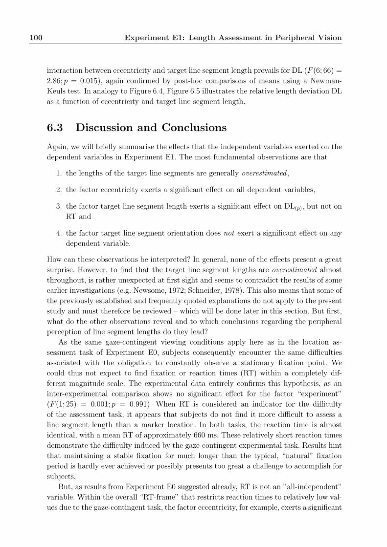
100 Experiment E1: Length Assessment in Peripheral Vision
interaction between eccentricity and target line segment length prevails for DL (F (6; 66) =
2.86; p = 0.015), again confirmed by post-hoc comparisons of means using a Newman-
Keuls test. In analogy to Figure 6.4, Figure 6.5 illustrates the relative length deviation DL
as a function of eccentricity and target line segment length.
6.3 Discussion and Conclusions
Again, we will briefly summarise the effects that the independent variables exerted on the
dependent variables in Experiment E1. The most fundamental observations are that
1. the lengths of the target line segments are generally overestimated ,
2. the factor eccentricity exerts a significant effect on all dependent variables,
3. the factor target line segment length exerts a significant effect on DL(p), but not on
RT and
4. the factor target line segment orientation does not exert a significant effect on any
dependent variable.
How can these observations be interpreted? In general, none of the effects present a great
surprise. However, to find that the target line segment lengths are overestimated almost
throughout, is rather unexpected at first sight and seems to contradict the results of some
earlier investigations (e.g. Newsome, 1972; Schneider, 1978). This also means that some of
the previously established and frequently quoted explanations do not apply to the present
study and must therefore be reviewed – which will be done later in this section. But first,
what do the other observations reveal and to which conclusions regarding the peripheral
perception of line segment lengths do they lead?
As the same gaze-contingent viewing conditions apply here as in the location as-
sessment task of Experiment E0, subjects consequently encounter the same difficulties
associated with the obligation to constantly observe a stationary fixation point. We
could thus not expect to find fixation or reaction times (RT) within a completely dif-
ferent magnitude scale. The experimental data entirely confirms this hypothesis, as an
inter-experimental comparison shows no significant effect for the factor “experiment”
(F (1; 25) = 0.001; p = 0.991). When RT is considered an indicator for the difficulty
of the assessment task, it appears that subjects do not find it more difficult to assess a
line segment length than a marker location. In both tasks, the reaction time is almost
identical, with a mean RT of approximately 660 ms. These relatively short reaction times
demonstrate the difficulty induced by the gaze-contingent experimental task. Results hint
that maintaining a stable fixation for much longer than the typical, “natural” fixation
period is hardly ever achieved or possibly presents too great a challenge to accomplish for
subjects.
But, as results from Experiment E0 suggested already, RT is not an ”all-independent”
variable. Within the overall “RT-frame” that restricts reaction times to relatively low val-
ues due to the gaze-contingent task, the factor eccentricity, for example, exerts a significant

6.3 Discussion and Conclusions 101
influence on reaction times. The assessment of the lengths of the target line segments be-
comes more and more difficult with increasing distance from the fixation point. Again,
subjects obviously try to compensate for the increased assessment difficulty by prolonged
reaction times in this Experiment E1. However, the following analyses of the assessment
“quality”, i.e. the length deviation DL(p) of the comparison line segment from the target
line segment, rather questions the success of the “RT-compensation-strategy”: DL(p) in-
creases for more peripheral line segment presentations, i.e. the length assessment quality
deteriorates. As in Experiment E0, this might again be attributed to the required “men-
tal translation”: Longer mental translation distances require more time, explaining the
increase of RT when the lengths of line segments have to be assessed in more peripheral
regions.
Before we turn to the discussion of the length deviation results, two more points
have to be made with respect to the analysis of RT. First, the values of RT now show
a pronounced difference between the eccentricity regions II and III. In contrast to the
almost identical values measured in Experiment E0 for these two eccentricity regions, the
observations here no longer suggest the existence of three designated eccentricity levels,
but rather a continuous eccentricity band without clearly identifiable boundaries.
Second, the interaction effects of eccentricity and target line segment length on RT, al-
though only tendential, encourage some speculation. We observed that RT yields relatively
high values for long line segments – compared to RT measured for short and intermediate
lengths – with only little divergence between the eccentricity levels I–IV. This can be un-
derstood when recalling that the long line segments were chosen such that their lengths
represent a “peripheral length” (due to the extent of the foveal eccentricity region I, line
segments with a peripheral length could only be 7o long here (see Section 4.1)). Subjects
obviously find the assessment of such length particularly difficult, even when the line seg-
ments are presented in proximity to the fixation point, and take more time to accomplish
this task. In summary, it could thus be that not only a far eccentric location of the stimu-
lus, but also a line segment length that cannot be perceived foveally results in prolonged
processing times. Furthermore, the relative stability of RT over the different eccentricities
for assessing long line segments, i.e. the independence of RT from the eccentricity region,
could indicate that, in this case, the (long) reaction times can mainly be attributed to the
processing difficulties induced by peripheral length rather than by eccentricity.
One of the most striking findings of all the studies presented in this thesis is that
the lengths of the target line segments are generally overestimated . Although a num-
ber of recent studies arrive at similar results (see Section 2.2, e.g. Nakatani, 1995; Tsal &
Shalev, 1996; Prinzmetal & Wilson, 1998; Tsal, 1999), the majority of earlier investigations
observed underestimation effects during size or length assessment in peripheral regions
(see Section 2.2, e.g. Pearce & Taylor, 1962; Richards & Miller, 1971; Newsome, 1972;
Schneider, 1978; Thompson & Fowler, 1980). In Experiment E1, short and intermedi-
ate line segments are overestimated in all but the foveal eccentricity region. Here, the
assessment for intermediate line segments is highly accurate and shows a deviation of
only -2%, i.e. a slight underestimation of the target line segment length. Such highly
accurate assessment levels can also be found for long line segments, independent of the

102 Experiment E1: Length Assessment in Peripheral Vision
eccentricity region. The analysis of the “directional” length deviation DL in particular
reveals that long line segments lengths are no less than 9% under- and no more than 5%
overestimated. This is significantly more accurate than is the case with the other two line
segment lengths. Furthermore, these highly accurate assessments of long line segments
can be maintained even in the more eccentric regions. A possible explanation for these
observations could be the more salient image the longer segments yield on the retina, due
to the excitation of more receptors as in the case of shorter line segments. Whereas for
those, in particular for the short length in more peripheral eccentricity regions, only a
“blotch” with possibly no directional or length information might be perceived, the ori-
entation and extent of longer line segments should still be visible, but blurred as well. For
intermediate line segment lengths, a reasonable amount of length information seems to be
available if not presented too far from the fixation point. For far peripheral locations then,
the line segment shape becomes increasingly blurred and so does the length information,
leading to greater uncertainty in the perceived size and thus less accurate assessments.
The fact that all assessments are independent of the orientation of the target line
segment could be expected. As the comparison line segments were presented in the same
orientations as the respective targets, possible interference from horizontal-vertical effects
could be eliminated. These could have been expected if the comparison marker was pre-
sented in a fixed, for example always horizontal orientation: Due to the horizontal-vertical
illusion (see Section 2.2), the lengths of vertical target line segments should then have been
overestimated. However, even with this factor being eliminated, it could have been that
orientation affected the length assessment: When, for example, a vertical line segment
has to be assessed that is located along the horizontal meridian, i.e. left or right of the
fixation point, both its end points have more or less the same distance from the fixation
point. When a horizontal line segment is now shown at the same meridial position, its end
points have different distances from the fixation point, which might then complicate the
length assessment. However, as the findings show, this is not the case. At least when, as
in Experiment E1, the line segments lie entirely within one eccentricity region, the factor
orientation does not affect the assessment of line segment lengths.
As already mentioned, the overestimation effect for most line segment lengths and the
fact that this effect is more pronounced with increasing eccentricity could not always be
observed in earlier experiments. With only few similar experimental findings, explanations
for the causes of such overestimation effects are also sparse. Furthermore, the respective
explanatory approaches put forward could only partially account for the experimental
observations. They frequently failed to yield a detailed representation of how particular
factors influence peripheral length assessment. Even the promising studies of Tsal (1999),
Tsal and Bareket (1999) and Tsal and Bareket (2001) and their subsequently introduced
concept of “attentional receptive fields” (ARFs), for example, can be considered an ap-
propriate concept only for distinguishing between coarse unattended and fine attended
perception (see Section 2.2). It is not clear in how far this concept is able to correctly ac-
count for the quantitative aspects of the assessments, i.e. to correctly represent the ratios
between the target and comparison dimensions, and how ARFs deal with complementary
stimulus attributes, such as line segment orientation. However, it appears to be reasonable

6.3 Discussion and Conclusions 103
to share their view that there exists a significant effect of attention on peripheral stim-
ulus assessment (see earlier studies by Butler (1980), Egyl and Homa (1984) and Muller
and Rabbit (1989)), and that it is not a completely preattentive operation (e.g. Sagi &
Julesz, 1985).
The possible explanation proposed here for the overestimation effects reported in Ex-
periment E1 is based mainly on two assumptions: First, we suggest that the line segment’s
end points play an important role for the length assessment. Second, we assume that, for
the peripheral length assessment, similar principles apply as in the peripheral location
assessment task in Experiment E0. In detail, the explanation of the overestimation of
line segment lengths in Experiment E1 is based on the finding of Experiment E0 that
the actual position of the target marker is perceived as being shifted towards the fixation
point (underestimation of the radial target marker position, see Sections 5.2.1 and 5.3).
In contrast, very little divergence between the tangential position of the comparison and
the target marker were noticed. Let us now transfer these observations to the current
study, assuming that the principles of location assessment apply to the peripheral per-
ception of line segment lengths as well. It then emerges that, when memorising a periph-
erally perceived line segment, subjects lay off a mental representation (or mental model
(Johnson-Laird, 1983)) of a line segment of approximately the original (target) length,
but shifted towards the fixation point. This (mental) “shift” or dislocation of the line
segment towards the observer leads to an elongation of the line segment when its mental
model is recalled in the reconstruction phase of the experiment, i.e. when the length of
the comparison line segment has to be adjusted. This might be due to the principle of
size/length constancy which states that the size/length of objects seems to increase when
they are moved towards the observer (cf. Section 2.2).
Although this approach intuitively appears plausible and well suitable for explaining
the overestimation of line segment lengths, further support should be provided that the
explanation holds and is based on sensible assumptions. The development of an according
(computational) model appears to be promising in that respect. Such a model would
enables us to test if and how the perceived length of peripherally presented line segments
can be concluded as a result of the peripheral assessment of the location of its end points –
as formulated in the (stimulus) decomposition hypothesis. This would then allow us to
perform a quantitative analysis of the model data and compare the outcome with the
empirical findings. In case of a positive correlation of these two data sets, not only support
would have been presented for the correctness of the previous assumptions. The model
would also suggest a possible explanatory approach that accounts for the major empirical
observations. Finally, a model would have been implemented that adequately simulates
the quantitative ratios of the assessment effects as well.
However, it would be desirable to develop a model that does not only account for the
eccentricity effects on the assessment of line segment lengths . Although no significant effect
of the factor orientation on the length assessment could be established in Experiment E1 –
due to the specific experimental procedure – we consider this dimension another essential
factor in the characterisation of line segments. Thus, Experiment E2 will be conducted in
order to investigate how accurately subjects can assess the orientation of line segments

104 Experiment E1: Length Assessment in Peripheral Vision
that are again presented at different eccentric locations (Chapter 7). Subsequently, we
should be able to discuss the development of a model under the premises that it ideally
incorporates both line segment length and orientation assessment (Chapter 8).

Chapter 7
Experiment E2: Orientation
Assessment in Peripheral Vision
The last experiment in this series of three experiments investigates the perception of line
segments orientation. The “reference” data obtained here allows for the testing of the ex-
istence of correlations between the assessment error of peripherally perceived orientations
of line segments and the mislocation of marker positions. In analogy to Experiment E1, if
a correspondence can be found, this would indicate that observations in this experiment
can possibly be attributed to mechanisms that were identified to influence location assess-
ment. The peripheral assessment of line segment orientation might thus be accordingly
decomposed and could be accomplished by peripherally assessing the locations of the end
points of the line segment. The relative position of the end points to each other then yields
the line segment orientation.
The following sections describe the experimental method for Experiment E2, based on
the methodological preliminaries that were established in Chapters 3 and 4. Subsequently,
the results will be presented and discussed which allows us to draw conclusions about the
mechanisms that may govern peripheral orientation perception.
7.1 Method
7.1.1 Subjects
The subjects were twelve experimentally naive students – five male and seven female –
from the University of Bielefeld. Their average age was 26.1 years. All subjects had normal
or corrected-to-normal vision and no pupil anomalies. The subjects were paid for their
participation in the experiment.
7.1.2 Stimuli
The stimuli were almost the same as in Experiment E1, differing only in the comparison
line segment used.

106 Experiment E2: Orientation Assessment in Peripheral Vision
7.1.3 Apparatus
The apparatus used was the same as in Experiments E0 and E1.
7.1.4 Procedure
The procedural steps in this experiment were almost identical to those in Experiment E1.
Only the experimental task varied, subject were asked to assess the orientation of the
target line segment presented in one of the eccentricity regions I-IV without foveally
looking at it. Again, the gaze was restricted to a region of 1o around the central fixation
point (Frame 1) and this contingency was monitored by the eye tracker. When subjects
had successfully finished the assessment task and memorised the perceived orientation of
the target line segment, they pressed the left button of the computer mouse (Frame 2).
Subsequently, a blank screen was shown for 500 ms (Frame 3) and the fixation point
reappeared at the center of the display (Frame 4) for 300 ms.
The fixation point was replaced by the comparison line segment (Frame 5) with the
line segment center located at the center of the screen. The comparison line segment had
the same dimensions as the previously shown target line segment with respect to thick-
ness, colour and length. However, this time the comparison line segment was randomly
oriented between 0.0o and 179.9o. The subject was instructed to adjust the orientation
of the comparison line segment with the computer mouse so that it exactly matched the
memorised perceived orientation of the target line segment (Frame 6). Moving the mouse
to the left resulted in a counter-clockwise rotation of the comparison line segment around
Figure 7.1: The sequence of procedural steps for a trial of Experiment E2. Frame 1: Fixation point.Frame 2: Target line segment orientation assessment. Frame 3: Blank screen. Frame 4: Fixation point.Frame 5: Comparison line segment. Frame 6: Adjustment of comparison line segment orientation.

7.2 Results 107
its center, moving the mouse to the right in a clockwise rotation. A press of the left mouse
button confirmed the orientation adjustment and started the next trial. During this ad-
justment phase, subjects could move their gaze freely across the whole screen. Figure 7.1
illustrates the sequence of procedural steps for one trial.
Subjects viewed a total of 360 stimulus pictures during the experiment, so that each
possible combination of the four position eccentricities, the three orientations and the three
lengths (see Section 6.1.2) was displayed ten times. Ten practice trials were conducted
prior to the experimental trials.
7.2 Results
As the choice of stimuli and the procedural design remains almost unchanged from Ex-
periment E1, no major changes regarding the data analyses are required either. Again,
data will be subjected to a three-factorial analysis of variance in order to account for the
three independent variables eccentricity region, target line segment length and orienta-
tion. The effects of these factors are tested on the dependent variables reaction time RT
and, here, on the orientation deviation DO of the target line segment from the comparison
line segment.
7.2.1 Dependent Variables
Reaction Time RT
First, we chart the relative frequencies of the reaction time RT in a histogram (see Fig-
ure 7.2, left). The distribution is again based on all measured values for RT, irrespective
of eccentricity, target line segment length or orientation, and takes into account the data
from all subjects. A minimum RT of 154 ms and a maximum RT of 4310 ms are measured,
the overall mean is 662 ms. The histogram reaches a peak at approximately 410 ms. Ap-
proximately 95% of the values lie within the interval of 250 to 1650 ms, the general shape
of the distribution for RT closely resembles those of Experiment E0 and Experiment E1
and can be fitted by an asymmetrical function with positive skewness of +2.10.
The analysis of variance yields a significant main effect on RT for the factor eccen-
tricity (F (3; 33) = 10.02; p < 0.001). When the target line segment is presented foveally
(Eccentricity I), subjects on average require 621.2 ms to assess its orientation, for more ec-
centric presentation positions, RT increases from 646.7 ms (Eccentricity II) and 660.7 ms
(Eccentricity III) to 722.0 ms (Eccentricity IV) for the orientation assessment. A post-
hoc comparison of means using the Newman-Keuls test reveals that significant differences
exist between the following eccentricity levels: (Rcrit = 46.011; p = 0.031) for the compar-
ison of RT between the Eccentricities I and III, (Rcrit = 48.891; p < 0.001) for I vs. IV,
(Rcrit = 47.775; p = 0.001) for II vs. IV and (Rcrit = 46.990; p = 0.002) for III vs. IV.
In contrast, only a tendency towards the existence of a significant difference in RT can
be found between the Eccentricities I and II (Rcrit = 42.009; p = 0.086). No significant
difference exists between the Eccentricities II and III (Rcrit = 38.655; p = 0.211).

108 Experiment E2: Orientation Assessment in Peripheral Vision
reaction time RT (ms)
rela
tive
freq
uenc
y
0
0.02
0.04
0.06
0.08
0.10
0 500 1000 1500 2000 2500 3000 3500 4000 4500
eccentricity
reac
tion
time
RT
(m
s)
600
620
640
660
680
700
720
I II III IV
shortintermediatelong
Figure 7.2: Left: Cumulative relative frequency distribution of reaction times RT over all eccentricityregions, line segment lengths and orientation levels. Right: Reaction time RT as a function of eccentricity,separated for short, intermediate and long line segments.
Furthermore, the factor target line segment length exerts a significant effect on RT
(F (2; 22) = 5.10; p = 0.015). On average, subjects take longer to assess the orientation of
the target line segments when they are short (682.3 ms) than when they are intermediate
(650.2 ms) or long (655.3 ms) in length. According to a Newman-Keuls post-hoc test
the differences between the following levels of the factor target line segment length are
significant with respect to RT: (Rcrit = 27.119; p = 0.013) for the comparison between
short and intermediate lengths and (Rcrit = 26.001; p = 0.044) for short vs. long lengths.
RTs for intermediate vs. long lengths do not significantly differ (Rcrit = 21.340; p = 0.101),
only a slight tendency can be noted.
A closer inspection of the data (see Figure 7.2, right) reveals that RT most drastically
increases with increasing eccentricities for short lengths whereas for intermediate and, in
particular, for long target line segments such a considerable increase of RT can only be
observed for Eccentricity IV. However, the interaction between eccentricity and target
line segment length does not exert a significant effect on RT (F (6; 66) = 1.69; p < 0.136).
The factor orientation, does not reach significance either, but demonstrates a tendency
(F (2; 22) = 2.88; p < 0.077) towards shorter RT for target line segments that are oriented
(near-)vertically (639.9 ms), compared to RT for (near-)horizontal (672.7 ms) and (near-
)oblique oriented (675.4 ms) target line segments. No interaction exerts a significant effect
on RT. Figure 7.2 (right) shows RT as a function of eccentricity and target line segment
length.
Orientation Deviation DO
Rather than making distinctions between analyses for absolute or directional and relative
values as in the previous experiments, there is no need for separate investigations regarding
the orientation deviation DO. As there appears to be no reason to assume a directional
effect (systematic clock- or counter-clockwise DO) of the rotation of the comparison line
segment relative to the target orientation, all values for DO are positive. We will enter
the absolute positive measured values of the orientation difference (in degrees) between

7.2 Results 109
the target and the comparison line segments in a three-factorial analysis of variance to
test the effects of the independent variables eccentricity, target line segment length and
orientation on DO.
The analysis of variance yields significant main effects for all factors. First, the effect
of eccentricity on the orientation deviation DO reaches significance (F (3; 33) = 11.75; p <
0.001). As for most other eccentricity effects before, the subjects’ performance deteriorates
the further away the target line segment appears from the fixation point. On average,
the subjects in Experiment E2 misjudge the orientation of the target line segment by
6.0 degrees in Eccentricity I, by 6.4 degrees in Eccentricity II, by 7.1 degrees in Eccen-
tricity III and by 7.5 degrees in Eccentricity IV. A post-hoc comparison of means using
the Newman-Keuls test reveals that significant differences exist between all eccentricity
levels: (Rcrit = 0.540; p = 0.048) for the comparison of DO between the Eccentricities I
and II, (Rcrit = 0.695; p = 0.001) for I vs. III, (Rcrit = 0.731; p < 0.001) for I vs. IV,
(Rcrit = 0.655; p = 0.028) for II vs. III, (Rcrit = 0.685; p = 0.002) for II vs. IV and
(Rcrit = 0.544; p = 0.049) for III vs. IV.
Next, the factor target line length is also found to have a highly significant effect
on DO. The respective analysis yields a significance level of (F (2; 22) = 31.67; p < 0.001),
manifested in a greater mean orientation deviation for short line segments (7.4 degrees)
than for intermediate ones (6.9 degrees), and in a yet smaller DO for long line segments
(5.8 degrees). According to a Newman-Keuls post-hoc test the differences between all
levels of the factor target line segment length are significant with respect to DO: (Rcrit =
0.448; p = 0.038) for the comparison between short and intermediate lengths, (Rcrit =
0.555; p < 0.001) for short vs. long lengths and (Rcrit = 0.547; p < 0.001) for intermediate
vs. long lengths. Figure 7.3 shows DO as a function of the eccentricity region (I–IV) and
the length of the target line segments (short, intermediate, long).
Finally, the third factor, target line orientation, also shows a significant effect on DO
eccentricity
orie
ntat
ion
devi
atio
n D
O (
degr
ees)
0
1
2
3
4
5
6
7
8
9
10
I II III IV
short
intermediate
long
Figure 7.3: Orientation deviation DO of the comparison from the target line segment as a function ofEccentricity I–IV and target line segment length.

110 Experiment E2: Orientation Assessment in Peripheral Vision
(F (2; 22) = 9.34; p = 0.001). When target line segments are oriented near-horizontally
(i.e., according to our definition of the horizontal category, 0o ± 22.5o (see Section 4.1)),
the average orientation deviation measures 5.4 degrees. DO then increases for oblique ori-
entations (45o±22.5o or 135o±22.5o) to 7.3 degrees and further to 7.7 degrees for vertical
line segments (90o ± 22.5o). According to a Newman-Keuls post-hoc test the differences
between the following levels of the factor target line segment orientation are significant
with respect to DO: (Rcrit = 1.345; p = 0.003) for the comparison between horizontal and
oblique orientations and (Rcrit = 1.387; p = 0.002) for horizontal vs. vertical orientations.
No significant difference in DO can be found for the comparison between oblique and ver-
tical orientation levels (Rcrit = 1.136; p = 0.334). Figure 7.4 shows DO for all eccentricity
regions (I–IV), separated for the three possible orientations of the target line segments
(horizontal, oblique, vertical).
eccentricity
orie
ntat
ion
devi
atio
n D
O (
degr
ees)
0
1
2
3
4
5
6
7
8
9
10
I II III IV
horizontal
oblique
vertical
Figure 7.4: Orientation deviation DO of the comparison from the target line segment as a function ofEccentricity I–IV and target line segment orientation.
The only interaction that reaches the significance level is that between target line seg-
ment length and orientation (F (4; 44) = 3.28; p = 0.019). For horizontal target line seg-
ments, irrespective of the target line segment length and aggregated over all eccentricities,
the orientation deviation DO remains approximately constant at a low level (5.4 degrees).
A post-hoc comparison of means using the Newman-Keuls test reveals that no significant
differences exist between the three length levels when the target is oriented horizontally:
(Rcrit = 0.834; p = 0.361) for short vs. intermediate lengths, (Rcrit = 0.867; p = 0.295) for
short vs. long lengths and (Rcrit = 1.023; p = 0.129) for intermediate vs. long lengths. In
contrast, when oriented either obliquely or vertically, DO almost linearly decreases from
8.4 degrees for short to 7.8 degrees for intermediate and to 6.2 degrees for long target line
segments. Accordingly, a Newman-Keuls test reveals significant differences between the
three length levels. Oblique targets: (Rcrit = 1.189; p = 0.045) for short vs. intermediate

7.3 Discussion and Conclusions 111
lengths, (Rcrit = 1.332; p < 0.001) for short vs. long lengths and (Rcrit = 1.237; p = 0.006)
for intermediate vs. long lengths. Vertical targets: (Rcrit = 1.003; p = 0.041) for short
vs. intermediate lengths, (Rcrit = 1.310; p < 0.001) for short vs. long lengths and
(Rcrit = 1.302; p = 0.001) for intermediate vs. long lengths.
All other two-way interactions and the three-way interaction between eccentricity,
target line segment length and orientation do not show significant effects on the orientation
deviation DO.
7.3 Discussion and Conclusions
As before, we will again briefly summarise the main results of the current experiment.
The most fundamental observations the analyses yield are as follows:
1. The factor eccentricity exerts a significant effect on RT and DO.
2. The factor target line segment length also exerts a significant effect on RT and DO.
3. The factor target line segment orientation exerts a significant effect on DO, but only
a tendential effect on RT.
As far as the reaction time RT is concerned, the results of this “orientation experiment”
closely resemble those of the previous Experiments E0 and E1. The similarity holds with
respect to both the quantitative statistical values, for example the mean RT, and the
more qualitative results, such as the relative frequency distribution of RT. In an inter-
experimental comparison, a two-way analysis of variance of the factors experiment and
eccentricity – the only two that could be compared between the Experiments E0, E1
and E2 – does not reveal any significant difference concerning the effect of “experiment”
on RT. The reaction times measured in Experiment E2 neither differ significantly from
those in Experiment E0 (F (1; 25) = 0.001; p = 0.988) nor from those in Experiment E1
(F (1; 22) = 0.001; p = 0.981). It appears that subjects do not find it more difficult to
assess a line segment orientation than to assess its length or a marker location. This, of
course, again assumes that RT can be considered a valid indicator for task complexity
even under the gaze contingent viewing conditions that apply in Experiment E2 as well.
The fact that the factor eccentricity exerts a significant effect on RT seems to supports
this assumption: With increasingly eccentric location of the target line segment – and thus
a certainly more complex orientation assessment task – RT increases in Experiment E2.
The orientation assessment appears to be a particularly difficult task in eccentricity re-
gion IV. In analogy to Experiments E0 and E1, this could again be attributed to the
“mental translations” which may take longer when covering longer distances – as the case
when orientations of line segments are assessed in more peripheral regions. When the data
is accumulated over line segments length and orientation, the difference in RT between the
eccentricity regions II and III is by far smaller than for the comparison between the other
eccentricity regions. This could be understood as at least a further hint of the existence of
three designated eccentricity regions , just as found for RT in Experiment E0. Within these

112 Experiment E2: Orientation Assessment in Peripheral Vision
eccentricity regions, RT shows very little variation. Significant changes occur only in the
“border regions”. It must be remembered, however, that the analyses of Experiment E1
did not support this hypothesis.
Apart from the eccentric region, RT is significantly influenced by the length of the
target line segment in this experiment. In Experiment E1, the length of the target line seg-
ments had no such effect on RT, but it subsequently emerged that the length of short(er)
line segments could be less accurately assessed. If we conclude that these lengths must thus
have been more difficult to judge, the lack of a corresponding effect on RT, i.e. longer RT
for short(er) line segments, suggests that subjects did apparently not attempt to compen-
sate for the increased complexity of assessing short line segment lengths in Experiment E1
through an increase in RT. This, however, is the case in Experiment E2. The orientation
assessment of short line segments appears to be a far more complex task than that of
intermediate or long line segments, in particular in the far peripheral regions. Subjects
try to compensate for the higher orientation assessment complexity of short line segments
through the increase in RT. In the gaze-contingent stimulus presentation condition this
is done again within the limited (time) range of still acceptable concentration effort.
The subjects’ tendency – only marginally short of significance – to produce shorter
reaction times when the target line segments are displayed in (near-) horizontal rather than
in (near-) oblique or (near-) vertical orientations hints at a preference of horizontal over
vertical information processing strategies. Indeed, the tendency towards the facilitatory
effects of processing horizontal line segments as visible in RT is supported by the significant
effect that target line orientation exerts on the orientation deviation DO. The fact that
the orientation of horizontal line segments can be more accurately assessed than those of
oblique and vertical line segments clearly favours horizontal processing. This is possibly
due to the anatomy/physiology of the eye and the retina and, probably even more so, to
the fact that most visual information processing requires a horizontally oriented strategy,
such as reading – at least in Western cultures. These requirements are supposed to have
influenced preferred visual strategies in many other tasks as well and thus, as a habituation
effect, resulted in the improved “visual performance” along this orientation. In eye-tracking
studies at the University of Bielefeld this was shown, for example, in comparative visual
search (e.g. Pomplun, 1998) and numerosity estimation tasks (Koesling, 1997; Koesling
et al (submitted)).
Although it takes subjects longer to assess the orientation of the target line segments
in more peripheral regions, the extra time does not help to improve the assessment ac-
curacy in general. In some cases, however, there appears to be such a facilitatory effect;
for example for short line segments: While RT is about equal for short and intermediate
line segments in the eccentricity regions I and II, the orientation deviation DO is signif-
icantly larger for short line segments. However, with the sharp increase of RT for short
line segments that are presented in the eccentricity regions III and IV, no such difference
in DO between short and intermediate lengths is visible in the eccentricity regions III
and IV any more. These observations might indeed suggest that for specific lengths an
increased reaction time helps to more accurately assess line segment orientation. Never-
theless, subjects do not succeed in achieving the same assessment accuracy level for short

7.3 Discussion and Conclusions 113
(and intermediate) length as for long line segments. The accuracy differences regarding
the orientation assessment between these two types of line segment length, i.e. short(er)
and long, remain about the same, independent of the eccentricity region and unaffected
by RT differences.
As before, the decreasing accuracy of the orientation assessments must probably be
attributed to a more and more “blotch”-like retinal image the further away the target
stimulus is displayed from the fixation point. Such a blurred representation is then laid
off as an equally blurred mental image or model. This obviously renders the accurate
assessment of line segment lengths difficult as the end points of line segments and thus
the line segment’s extent cannot exactly be determined (see Experiment E1, Chapter 6).
Furthermore, the orientation of a line segment can only vaguely be assessed when only a
rather diffuse image of the stimulus is perceived in the periphery. It could even be expected
that, at some stage, either in very far eccentric locations or for very short line segments,
all directional information is lost. The only information available to the visual system
then would be the existence of some object in the periphery, but none of its features such
as its orientation and length relevant here.
Let us now – at least partly – consider again the suggestions made at the end of
the previous chapter. It was proposed that the end points of a line segment play an
important role for its length assessment (Experiment E1) and that their mislocation (Ex-
periment E0) towards the observer leads to the overestimation of line length. With regard
to the assessment of the orientation of line segments, possibly similar processing principles
apply.
Indeed, it appears to be a promising approach to think of orientation assessment as
a process determined by the perceived locations of the line segments’ end points as well.
In detail, the computation of the relative spatial positions of the two end points to each
other should yield the target orientation information. This could be laid off as a mental
representation and subsequently be recalled during the adjustment of the orientation
of the comparison line segment. If we take into account the findings for the location
assessment from Experiment E0, in particular considering the eccentricity effects on the
location accuracy along the radial and tangential axes, these could also be reflected in
and probably account for some of the results of Experiment E2. For example, due to the
greater variance along the radial rather than along the tangential axis in the location
assessment task of Experiment E0, a considerable variation in the orientation assessment
must be expected – and could indeed be observed in Experiment E2. The same is true for
the increased uncertainty in the orientation assessment in more eccentric regions, which
appears plausible when we take into account the increasing location uncertainty – mainly
in the radial direction – with increasing eccentricity in Experiment E0. Thus, this approach
again seems plausible and intuitively suggests to account for the orientation deviations
observed in Experiment E2. However, if it really does, this must be validated.
Due to the close resemblance of the suggested explanatory approaches for the pe-
ripheral assessment of the length and orientation of line segments, it now appears to be
favourable to develop a common model . This should enable us to test if and how both the
perceived length and orientation of peripherally viewed line segments can be concluded as

114 Experiment E2: Orientation Assessment in Peripheral Vision
a result of the peripheral assessment of the location of its end points. As suggested in the
previous chapter, an appropriate model should not only present support for the adequacy
of the assumptions made – the decomposition hypothesis – and suggest an explanatory ap-
proach that may account for the empirical observations. Furthermore, it should adequately
simulate the quantitative ratios of the assessment effects as well. The attempts made to
design, implement and validate such a model are presented in the following chapter.

Chapter 8
Modelling Eccentricity Effects
8.1 Why Modelling?
A close inspection of the psychological literature reveals that, in general, the majority
of studies follows the same strategy to arrive at its conclusions. After the motivation of
a study, the review of related works and the choice of the experimental conditions and
setup, the actual experiment is conducted. Next, the collected empirical data is subjected
to qualitative and quantitative, mainly statistical analyses. Characteristic values such as
means or standard deviations are computed and statistical analyses are performed in order
to relate the experimental observations – the dependent variables – to the systematically
varied parameters – the independent variables (e.g. Sichelschmidt & Carbone, 2003).
All these steps are rather straightforward and present a more or less standardised
procedure. The exciting, but often troublesome part of work only starts here. The crucial
questions that scientific studies should attempt to find an appropriate answer for are:
Why did we get the results just as they are, what do the observations tell us and how
can the findings be interpreted in the experimental and, preferably, in a more general
context? One of the common problems of the discussions of experimental results is that
conclusions drawn from the empirical data are not entirely conclusive. Many conclusions
apparently rely on vague interpretations of the observations and sometimes incorporate a
considerable amount of speculation.
In an attempt to provide more support their interpretations and conclusions, some
authors propose models , formalised descriptions of their reasoning on the basis of as-
sumptions the experimental data seem to suggest. Unfortunately, most of these models
only unspecifically describe the (proposed) theory and rarely contain clear suggestions
with respect to a concrete implementation of the model. Very few authors present models
that can be parameterised so that an algorithmic implementation realises the reproduc-
tion of empirical data. However, only such a simulation enables us to compare empirical
and simulation data in order to test the correctness of the model. In return, this then al-
lows for testing the validity of the initial premises and the suggested interpretation of the
empirical data that led to the generation of the model. This closed loop of empirical data
acquisition — interpretation — modelling — verification represents a promising strategy

116 Modelling Eccentricity Effects
for making reliable statements on the processes underlying specific (human) performance.
Exactly these are the premises for the development of the present model.
8.2 A Model for Peripheral Visual Perception of Line
Segments
The aim now is to develop a specific model to simulate the processes involved in the
peripheral visual perception of the length and the orientation of line segments. The model
will be implemented as an algorithm and produce data in analogy to that generated by
subjects in the experimental studies of the Experiments E0, E1 and E2. This then allows
for the direct comparison of the empirical and simulated data sets in order to validate the
correctness of the model. In case of a positive correlation, it can be concluded that the
model might indeed account for the underlying perception principles. This means that we
have possibly identified the correct processing strategy pursued by the subjects. If there
is no positive correlation, at least an adequate strategy to solve these assessment tasks
has been successfully implemented.
The following sections will motivate the model idea, determine the modelling prelim-
inaries and explain the methods in detail. The implementation of the model is described
and finally the simulation results are presented and discussed with respect to the empirical
findings of Experiments E1 and E2.
8.2.1 Model Motivation and Concept
The underlying ideas for the modelling approach pursued here were already briefly intro-
duced in the previous chapters. We will now present these ideas in detail and lay out the
procedural structure of the model.
The proposed model approach for the peripheral assessment of line segments is based
on the decomposition hypothesis (see Section 2.4) and assumes that end point information
is essential for the assessment of line segment attributes such as length and orientation.
This modelling idea is inspired by results of earlier studies (see Section 2.3, e.g. Buchs-
baum, 1972; Ikeda et al., 1977). Subjects’ comparison acuity was found to deteriorate
drastically in experiments that only displayed line segment fragments or obliterated the
terminal sections so that the whole line segment was not visible at any one time. The
new conclusions from the findings of Experiments E0, E1 and E2 could now suggest that
not only end point information is important for line segment assessment, but that there
might exist a direct correlation between the accuracy in line segment assessment and the
accuracy in positional assessment. It should in fact be possible to directly infer line seg-
ment length or orientation accuracy from position assessment accuracy, i.e. to compute
the quantitative values of the length and orientation divergences based on those values of
the positional divergences. If this assumption proves to be correct, it could be further con-
cluded that the geometrical structure of objects may guide the perceptual and cognitive
processes that determine the assessment of geometrical object attributes – at least as far

8.2 A Model for Peripheral Visual Perception of Line Segments 117
as the assessment of line segment length and orientation is concerned.
In detail, the line segment length and orientation assessment will be modelled as the
assessment of two positional markers in an eccentricity region. Each marker position can
only be assessed – as Experiment E0 demonstrated – with a specific uncertainty in its
radial and tangential position. If, subsequently, the difference between the two position
assessments, i.e. their distance, is computed, this should yield a similar result as the
assessment of the length of a line segment (Experiment E1) in the same eccentricity
region and determined by end points that coincide with the two previously shown markers.
Of course, the same should be true if we compare the spatial relation between the two
position assessments, yielding an orientation, with the assessment of the orientation of a
line segment such as shown in Experiment E2.
Although based on obviously sensible assumptions, this model must now be tested for
its correctness and capability to reproduce the empirical data. Only then can we assume
that it supports the correctness of the assumptions, suggests an appropriate explanation
that may account for (some of) the empirical observations and adequately simulates the
quantitative ratios of the assessment effects. How can the model now be implemented to
yield the desired support?
8.2.2 Model Implementation
So far, the presentation of the model concept only gave a rather theoretical account of
its realisation. We will now discuss the computational steps it requires to implement
the modelling approach in an algorithmic form. Specifically, we suggest the following
procedure to accomplish the implementation of the proposed model:
(a) Description of the distribution of the position assessments for the target marker,
based on the empirical data and the statistical analyses of Experiment E0.
(b) Generation of a first position coordinate that takes into account (a).
(c) Analogous generation of a second position coordinate so that the spatial relations
of the underlying target marker positions reflect the lengths and orientations of the
target line segments of Experiments E1 and E2, respectively.
(d) Computation of the distance between and the spatial relation of the two coordi-
nates (the end points of a “virtual” line segment), yielding simulated length and
orientation information, respectively.
(e) Statistical analysis of the simulation data in analogy to the previous analyses of the
empirical data.
(f) Comparison of the simulation and the empirical data sets for model validation.
In accordance with the list of procedural steps, we will first address the task of finding a
suitable description for the distribution of the positional assessments for the target marker.
As the analyses of the empirical data recorded in Experiment E0 revealed, the position

118 Modelling Eccentricity Effects
of the target marker could only be reproduced with a specific uncertainty. Subjects were
unable to exactly match the comparison marker position with that of the previously shown
target marker they had peripherally perceived and memorised. This positional mismatch
was manifested in the marked positional deviations of the comparison from the target
marker positions, mainly dependent on the eccentricity region where the target marker
was displayed. Furthermore, the extent of the positional mismatch differed significantly
between the radial and the tangential direction. For a given target marker position, a
(sample) distribution of comparison marker positions such as shown in Figure 8.1 can
be observed for the data from Experiment E0. Here, the green dot denotes the target
marker position that had to be assessed, the black dots mark the positions where subjects
placed the comparison markers over repeated trials. In order to conveniently describe
the distribution of the data, it appears promising to compute a Principal Component
Analysis .
Figure 8.1: Sample distribution of comparison marker positions (black) and its mean (red) for a giventarget marker position (green). The ellipsis approximates the distribution of the comparison markerpositions using principal component analysis (PCA).
Principal Component Analysis
The Principal Component Analysis (PCA), also known as the Eigen-XY analysis or
Karhunen-Loeve expansion, is among the oldest and most widely used multivariate tech-
niques. Originally introduced by Pearson (1907) and independently by Hotelling (1933),
the basic principle of the method is to describe the variation of a set of multivariate data
in terms of a set of uncorrelated variables each of which is a particular linear combination
of the original variables. The new variables are derived in decreasing order of importance
so that, for example, the first principal component accounts for as much as possible of
the variation in the original data. Usually, only the first several such components are used
to describe the original data while the others are cut off. The new variables can thus be
used to summarise the data with little loss of information, thus providing a reduction in

8.2 A Model for Peripheral Visual Perception of Line Segments 119
the dimensionality of the original data. This might be useful in simplifying later analyses,
data interpretation and data parameterisation, for example for modelling purposes.
Let us consider the geometrical interpretation of this technique for the two-dimensional
data of Experiment E0. If we assume that the positions of the comparison marker can be
described by a bivariate normal distribution that reflects the greater radial than tangential
deviation, these positions lie within an ellipsis, the so-called correlation ellipsis. Its shape
and orientation represent the magnitude of the correlation. The PCA now implements the
transformation of the original coordinate system into that of the principal components
(axes) of the correlation ellipsis. The transformation consists of the translation of the
coordinate system’s origin to the center of gravity of the data distribution and of the
orienting of the coordinate system along the principal components of the distribution, the
Eigenvectors.
This means that, formally, this transformation is equivalent to the solution of an
Eigenvalue problem where the first principal component yields the Eigenvector with the
largest Eigenvalue λ1. The second principal component is oriented orthogonal to the first
and yields the second largest Eigenvalue λ2 with λ2 < λ1 – and so on.
Mathematically, Eigenvectors are defined as
λi · ei = M ∗ ei, (8.1)
i.e. the Eigenvectors of a Matrix are exactly those that, if multiplied by the Matrix M ,
constitute a multiple (the Eigenvalue λ) of themselves. In order to execute the transfor-
mation, the computation of the expected mean µ and the covariance matrix C~r of the
original data distribution is required. For n data points ~ri = (xi, yi)T with i = 1, ..., n
µx = 1n·
n∑i=1
xi
µy = 1n·
n∑i=1
yi
⇒ ~µ~r =
(µx
µy
)(expected mean) (8.2)
C~r =1
n·
n∑i=1
(~ri · ~r Ti − ~µ~r · ~µT
~r ) = {cij} (covariance matrix) (8.3)
In order to compute the Eigenvalues of the covariance matrix, the following Eigenvalue
equation has to be solved
det(C~r − λ · I) = |C~r − λ · 1| = 0 (8.4)
For two-dimensional data as the case in Experiment E0, this requires the solution of a
quadratic equation and yields the Eigenvalues λ1 and λ2. The corresponding Eigenvectors
V can subsequently be computed as
V = C~r − λ · I (8.5)
The correlation ellipses that adequately describe the original data distribution are
thus entirely determined by the expected means (ellipsis origin), the Eigenvectors (ellipsis
orientation) and the Eigenvalues (“length” of the ellipsis’ principal components).

120 Modelling Eccentricity Effects
Figure 8.2: Distribution of comparison marker positions and their approximations using PCA for Ec-centricities I–IV in Experiment E0.
If we now map all recorded data for the comparison marker positions with respect to a
standard target marker position each for the eccentricity regions I-IV, the PCA will yield
the four correlation ellipses shown in Figure 8.2. The black dots mark the standardised
target marker position for the different eccentricities, the intersection of the principal
components of the ellipses the center of gravity of the respective data distributions.
Finding a suitable, simplified description of the distribution of the data from Ex-
periment E0 as realised with the PCA is only the first step in the development of the
suggested computational model. In close relation to the determination of the shape and
orientation of the data distribution in two-dimensional shape, we address the modelling of
the distribution of the number of observations for particular comparison marker positions
within the correlation ellipsis next. Although partly accounted for by the PCA technique
already, the relative frequencies of the single observations have to be reflected in the
model, in particular in the algorithmic generation of the “virtual” comparison marker
positions. For the given empirical data of Experiment E0, a two-dimensional sample dis-
tribution of the comparison marker positions and their relative frequencies are shown in
a three-dimensional diagram in Figure 8.3.
In a good approximation, the distribution of the relative frequencies can be described
by a two-dimensional bivariate normal distribution. Mathematically, the density of the
bivariate normal distribution is described by the following equation
φN(x, y) =1
2 · π|Γ| 12· e− 1
2
hx−µxy−µy
iTΓ−1
hx−µxy−µy
iwith (8.6)
Γ = cov
(X
Y
)=
σ2
x σxy
σxy σ2y
where (8.7)

8.2 A Model for Peripheral Visual Perception of Line Segments 121
Figure 8.3: Sample distribution of comparison marker positions and their relative frequencies.
X = x1, ..., xn and (8.8)
Y = y1, ..., yn and (8.9)
|Γ| = σ2x · σ2
y − σ2xy = (1− ρ2) · σ2
x · σ2y with (8.10)
ρ =σxy
σx · σy
(correlation between X and Y) and (8.11)
σxy =√
E[(X − µx) · (Y − µy)] (8.12)
=
√√√√ 1
n·
n∑i=1
(xi − µx) · (yi − µy) (covariance) (8.13)
Such a distribution must now be oriented along the previously computed principal
components of the correlation ellipses that span in the x–y plane. It further takes into
account the Eigenvalues that reflect the variance in the data and determine the normal
distribution’s “width” so that the distribution finally constitutes a complete, appropriate
representation of the empirical data of Experiment E0. The analyses of the empirical data
of Experiment E0 further showed significantly different results for the positional assess-
ment accuracy, depending on the eccentric location of the target marker. Consequently,
the distributions must be individually adapted for the different eccentricity regions, using
the relevant values – such as expected means, standard deviations, covariances, Eigen-
values and Eigenvectors – as computed in the previous statistical analyses and the PCA.
Figure 8.4 visualises the accordingly parameterised empirical data for the eccentricity
regions I–IV.
In the next step of the model design, we have to consider a suitable method of how
to adequately generate virtual comparison marker positions, so that the properties of the
simulated data equal those of the empirical data sets and their just-developed parame-

122 Modelling Eccentricity Effects
I
IIIII IV
Eccentricities I - IV
Figure 8.4: Distribution of the comparison marker positions and their relative frequencies for Eccen-tricities I–IV in Experiment E0.
terised descriptions. A promising approach is the reproduction of data described by the
bivariate frequency distributions using a Monte Carlo Simulation method.
Monte Carlo Simulation
Basically, the Monte Carlo simulation method (MCS) provides approximate solutions to
a variety of mathematical problems by performing statistical sampling experiments on a
computer. The method applies to problems with no probabilistic content as well as to
those with inherent probabilistic structure.
Technically, the fundamental idea of the MCS is to simulate a random process using
random numbers. This concept requires a design of the simulation so that the random
numbers – which are assigned to the results of the random process – yield corresponding
probabilities of occurrence. If this can be achieved, the MCS presents a very reliable
method for approximating data whose analytical computation is difficult or impossible.
The following example illustrates the idea of the Monte Carlo simulation method.
Let is assume we want to determine some unknown number m. In order to apply the
MCS, we have to define a random variable X with an expected mean of E(X) = m. We
will further assume that, for example, we want to compute m as the dark grey shaded
area under the graph shown in Figure 8.5. The graph describes the density of the standard
normal distribution φ, given as
φ(z) =1√
2 · π · σ2· e− (z−µ)2
2·σ2 with µ = 0 and σ = 1 (8.14)
=1√2 · π · e
− 12·z2
(8.15)
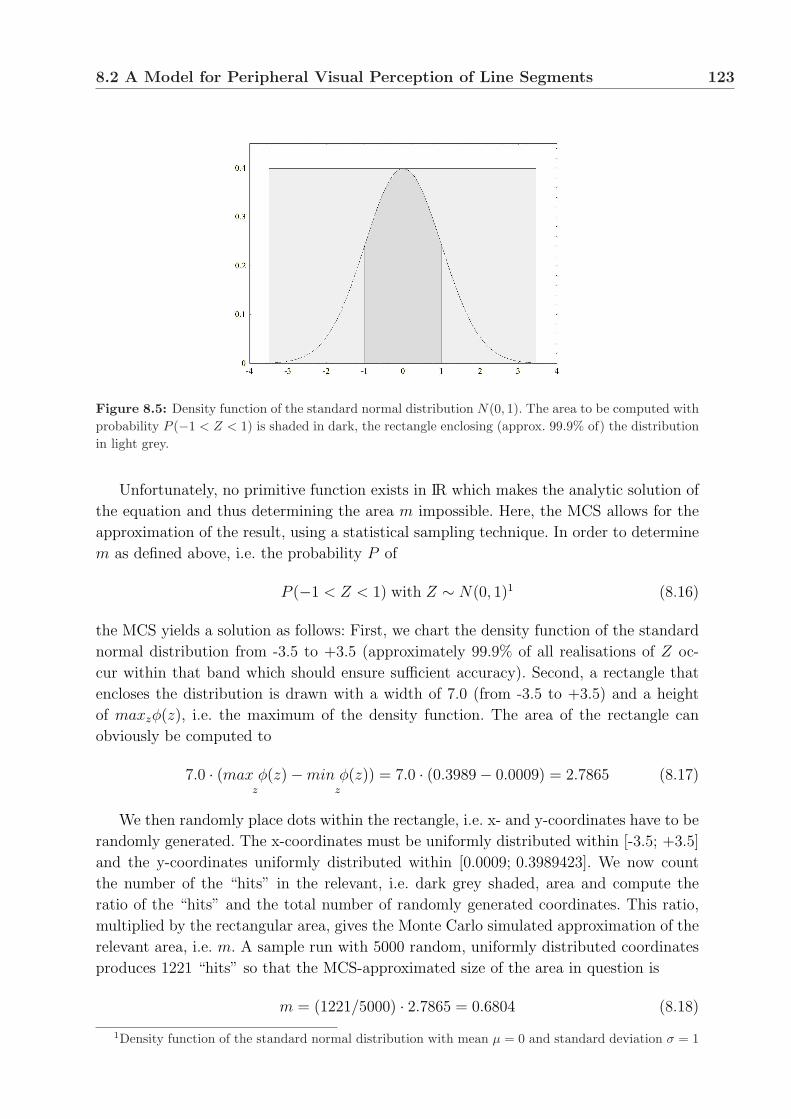
8.2 A Model for Peripheral Visual Perception of Line Segments 123
Figure 8.5: Density function of the standard normal distribution N(0, 1). The area to be computed withprobability P (−1 < Z < 1) is shaded in dark, the rectangle enclosing (approx. 99.9% of) the distributionin light grey.
Unfortunately, no primitive function exists in IR which makes the analytic solution of
the equation and thus determining the area m impossible. Here, the MCS allows for the
approximation of the result, using a statistical sampling technique. In order to determine
m as defined above, i.e. the probability P of
P (−1 < Z < 1) with Z ∼ N(0, 1)1 (8.16)
the MCS yields a solution as follows: First, we chart the density function of the standard
normal distribution from -3.5 to +3.5 (approximately 99.9% of all realisations of Z oc-
cur within that band which should ensure sufficient accuracy). Second, a rectangle that
encloses the distribution is drawn with a width of 7.0 (from -3.5 to +3.5) and a height
of maxzφ(z), i.e. the maximum of the density function. The area of the rectangle can
obviously be computed to
7.0 · (max φ(z)z
−min φ(z)z
) = 7.0 · (0.3989− 0.0009) = 2.7865 (8.17)
We then randomly place dots within the rectangle, i.e. x- and y-coordinates have to be
randomly generated. The x-coordinates must be uniformly distributed within [-3.5; +3.5]
and the y-coordinates uniformly distributed within [0.0009; 0.3989423]. We now count
the number of the “hits” in the relevant, i.e. dark grey shaded, area and compute the
ratio of the “hits” and the total number of randomly generated coordinates. This ratio,
multiplied by the rectangular area, gives the Monte Carlo simulated approximation of the
relevant area, i.e. m. A sample run with 5000 random, uniformly distributed coordinates
produces 1221 “hits” so that the MCS-approximated size of the area in question is
m = (1221/5000) · 2.7865 = 0.6804 (8.18)
1Density function of the standard normal distribution with mean µ = 0 and standard deviation σ = 1

124 Modelling Eccentricity Effects
The MCS generally yields very high quality approximations, for “large” simulations
the approximation error converges toward 0. Among all numerical methods that rely
on N-point evaluations in M-dimensional space to produce an approximate solution, the
Monte Carlo method has absolute error of estimate that decreases as N−1/2 whereas, in
the absence of exploitable special structure all other methods have errors that decrease
as N−1/M at best.
Rather than for the approximation of primitive functions as in the example above,
the Monte Carlo simulation method presents a very convenient tool with respect to the
simulation in the scope of the current investigation. We previously described the empirical
data of Experiment E0 by bivariate frequency distributions with the characteristics of a
normal distribution and determined the orientation and typical statistical values such as
expected mean and standard deviation by a principal component analysis.
The MCS now allows us to generate random coordinates x and y whose distribution
is equivalent to that of the empirical data or, more accurately, to that given by the bi-
variate normal frequency distribution that describes the empirical data. This is achieved
by generating an extra random z-coordinate for each (random) pair of x and y. The x-
and y-coordinates are considered valid coordinates only when the associated z is located
“under” the bivariate normal frequency distribution (see Figure 8.6). Consequently, this
leads to the generation of x- and y-coordinates whose frequency distribution simulates
the empirically given example. This procedure thus simulates comparison marker posi-
tions for given target marker positions in accordance with the subjects’ assessments. Due
to the significant empirical differences found for position assessment in Experiment E0 for
the factor eccentricity, the model employs different parameters for the four eccentricity
Figure 8.6: Density function of a bivariate standard normal distribution. The green marker at a ran-domly MCS-generated position (x,y,z) can be labelled “valid” because it is located “under” the distribu-tion. The red marker is obviously not.

8.3 Model Results and Discussion 125
regions I–IV. Here, the specific characteristics of the PCAs and the frequency distribu-
tions are taken into account for the MCS modelling of the simulated comparison marker
positions.
Recall that we hypothesised that the assessment of line segment length and orienta-
tion is a process strongly influenced by the assessment of the line segments’ end point
information. Thus, the goal of the simulation is to compare line segment length and ori-
entation assessments from Experiments E1 and E2, respectively, to “virtual” comparison
line segment lengths and orientations. These virtual line segments are constituted by their
simulated end points using the MCS method explained above. As the steps (b)-(d) of the
model implementation (s. page 117) suggest, an MCS has to be computed for the two end
points that determine the target line segment, yielding the simulated end points of the
comparison line segment (steps (b) and (c)). Computing the difference (step (d)) between
these points yields the length and orientation of the model comparison line segments. In
the subsequent statistical analyses the length and orientation divergences can be com-
puted (step (e)) in analogy to those conducted in Experiments E1 and E2, respectively.
The comparison of the model results to the empirical ones (step (f)) finally yields insight
into the performance and the possible adequacy of the model. The latter two steps will
now be discussed in the following Section 8.3.
8.3 Model Results and Discussion
Let us now consider how the proposed model scores. For the relevant dimensions, com-
parison line segment length and comparison line segment orientation, analyses of variance
were conducted to establish possible effects of the factors eccentricity of presentation, tar-
get line segment length and target line segment orientation on the respective assessment
accuracy. Furthermore, the corresponding mean values for the various factor levels were
computed. A subsequent direct comparison of the empirical and simulated data enables
us to validate whether the model correctly accounts for the effects and their magnitudes
established in Experiments E1 and E2.
As the model approach does not yield values for RT, only the simulated length devia-
tions MDL(p) and the orientation deviations MDO of the simulated comparison from the
target line segment will be investigated. The underlying data was computed according
to the previously described modelling procedure and constituted data sets of the same
structure as recorded in the Experiments E1 and E2. Furthermore, data was simulated for
the same combinations of the factors eccentricity, target line segment length and orienta-
tion. The number of repeated measures and (here “virtual”) subjects was identical, too,
in order to ensure equal conditions for the comparison of the simulated and the empirical
data sets.
Modelling Length Assessment
In analogy to the analyses in Experiment E1, both the absolute (positive) and the direc-
tional length deviations, MDLp and MDL, respectively, will be considered.

126 Modelling Eccentricity Effects
MDLp: A three-way analysis of variance established significant main effects for the
factors eccentricity (F (3; 33) = 72.88; p < 0.001) and target line segments length
(F (2; 22) = 122.17; p < 0.001) on MDLp. Averaging data over lengths and orientations
(for all “virtual” subjects), modelled comparison line segment lengths deviate from the
target lengths by 13.7% for Eccentricity I, 18.0% for Eccentricity II, 21.6% for Eccentric-
ity III and 26.8% for Eccentricity IV. A cumulation of data over the factors eccentricity
and orientation yields that subjects incorrectly adjust the length of the comparison line
segment by 38.4% (short), 12.9% (intermediate) and 7.3% (long) on average. The factor
orientation does not yield a significant main effect on MDLp (F (2; 22) = 1.29; p = 0.296).
In addition, the interaction between eccentricity and target line segment length reaches
significance (F (6; 66) = 31.42; p < 0.001). This can be attributed to the fact that DLp
constantly increases with greater eccentricities for short and intermediate line segments,
whereas it remains level for long line segments. For short line segments, DLp is computed
to be 0.27, 0.35, 0.41, 0.47, for intermediate length 0.08, 0.13, 0.16. 0.19 and for long line
segments 0.06, 0.07, 0.08, 0.09 – each for the respective Eccentricities I–IV. Furthermore,
the interaction between eccentricity and target line segment orientation shows a significant
effect on MDLp (F (6; 66) = 2.39; p = 0.0376). No other interactions have significant effects
on MDLp. Figure 8.7 shows the positive relative length deviation MDLp as a function of
eccentricity and target line segment length.
eccentricity
mod
elle
d po
sitiv
e re
lativ
e le
ngth
dev
iatio
n M
DL
p
-0.2
-0.1
0
0.1
0.2
0.3
0.4
0.5
I II III IV
short
intermediate
long
Figure 8.7: Modelled positive relative deviation MDLp of the length of the comparison from the targetline segment as a function of Eccentricity I–IV and target line segment length (short, intermediate, long).
MDL: An identical multi-factorial analysis of variance as for MDLp is conducted for MDL,
the dependent variable that additionally contains directional information on the length
deviation of the comparison from the target line segment length. The analysis yields a
significant main effect of the factor eccentricity on MDL (F (3; 33) = 48.56; p < 0.001).
The target line segment length is generally overestimated, increasingly so with increasingly

8.3 Model Results and Discussion 127
eccentric presentation. The overestimation effect reaches the following values: 2.7% when
the target line segment is presented within the eccentricity region I, 9.7% in eccentricity
region II, 17.0% in eccentricity region III and 19.0% in eccentricity region IV. Another
significant main effect on MDL can be found for target line segment length (F (2; 22) =
239.49; p < 0.001). If we average over eccentricity and orientation, a mean overestimation
of 28.3% for short and of 6.0% for intermediate line lengths emerges. Long line segments
are overestimated by 2.0% on average. Again, no significant main effect for the factor
orientation can be observed (F (2; 22) = 1.26; p = 0.304). The further analysis shows
that the interaction between eccentricity and target line segment length, which proved
significant for MDLp, prevails for MDL (F (6; 66) = 31.28; p < 0.001). Figure 8.8 illustrates
the relative length deviation MDL as a function of eccentricity and target line segment
length.
eccentricity
mod
elle
d re
lativ
e le
ngth
dev
iatio
n M
DL
-0.2
-0.1
0
0.1
0.2
0.3
0.4
0.5
I II III IV
short
intermediate
long
Figure 8.8: Modelled relative deviation MDL of the length of the comparison from the target linesegment as a function of eccentricity and target line segment length.
How can we now rate the performance of the implemented model for the assessment
of line segment lengths? In order to achieve reliable conclusions in this respect, the em-
pirical results of Experiment E1 and the simulated model data are subjected to further
statistical analysis. With the introduction of the between-subjects factor “experiment”,
i.e. Experiment E1 vs. simulation, the two data sets can be compared and checked for cor-
respondence. The respective analysis yields no significant effect for the factor experiment
on the relevant dependent variables (M)DLp (F (1; 22) = 0.03; p = 0.861) and (M)DL
(F (1; 22) = 2.15; p = 0.157). These promising results indicate that no significant differ-
ences exist between the simulated and the empirical data sets, i.e. that the modelling
approach chosen might indeed be suitable to adequately reproduce the data as measured
in Experiment E1.
Further support is obtained from the comparison of the results of the various analyses

128 Modelling Eccentricity Effects
Experiment E1 Model Comp./Diff.
Significant effect of ... on (M)DLp
• ECC + + ⊕• LEN + + ⊕• ORI - - ⊕• ECC × LEN + + ⊕• ECC × ORI - + ª• LEN × ORI - - ⊕• ECC × LEN × ORI - - ⊕
Mean (M)DLp in/for ...• ECC I 16.6% 13.7% 2.9%• ECC II 18.6% 18.0% 0.6%• ECC III 21.9% 21.6% 0.3%• ECC IV 23.8% 26.8% 3.0%• LEN short 31.8% 38.4% 6.6%• LEN intermediate 17.2% 12.9% 4.3%• LEN long 11.8% 7.3% 4.5%
Significant effect of ... on (M)DL• ECC + + ⊕• LEN + + ⊕• ORI - - ⊕• ECC × LEN + + ⊕• ECC × ORI - - ⊕• LEN × ORI - - ⊕• ECC × LEN × ORI - - ⊕
Mean (M)DL in/for ...• ECC I +4.8% +2.7% 2.1%• ECC II +9.6% +9.7% 0.1%• ECC III +15.7% +17.0% 1.3%• ECC IV +17.9% +19.0% 1.1%• LEN short +28.9% +28.3% 0.6%• LEN intermediate +8.9% +6.0% 2.9%• LEN long -1.9% +2.0% 3.9%
Note: ECC – eccentricity region; LEN – target length; ORI – target orientation
Table 8.1: Summary of the results of modelling line segment lengths in comparison with the empiricalfindings of Experiment E1.
of variance conducted for Experiment E1 and the model data, respectively. In Table 8.1,
all main and interaction effects tested on the empirical and the simulated data are listed
(for details, see Sections 6.2 and 8.3). In the first column, the type of effect on (M)DL(p)
is shown, the “+” or “-” in the second and third column marks whether the effect was
significant or not for the empirical and simulated data, respectively. The ª or ⊕ in the
last column indicates the (non-) conformity of the significance levels of the two data sets.
Obviously, a convincing correspondence exists between the levels of significance that the

8.3 Model Results and Discussion 129
data from Experiment E1 and the model data yielded. All but one effect (2-way interaction
of eccentricity and orientation (ECC × ORI) for (M)DLp) of the empirical data could be
reproduced in the simulation.
However, the analyses of variance do not yield reliable information concerning the
“directions” and the magnitudes of the differences in the dependent variables for the factor
levels. Even two “inverse” data sets could produce analogous significance effects. Different
magnitude scales in the two data sets would not be accounted for by the within-subjects
analysis of variance either. It is therefore essential to closely examine the absolute mean
values and their ranks for the relevant factor levels in the empirical and simulated data
and to directly compare them. Only then can reliable statements regarding the conformity
of the data – and thus the rating of the model performance – be made.
Apart from the lists of effects which reached significance (or not) in Experiment E1
and the simulation, Table 8.1 charts the absolute mean values for (M)DLp and (M)DL
(for details, see Sections 6.2 and 8.3). The differences between these values for the empir-
ical and model data are generally very small, ranging from 0.1% to a maximum of only
6.6%. On average, MDLp diverges from DLp by 3.1% and MDL from DL only by a mere
1.7%. This very accurate approximation confirms that the simulation suitably models the
absolute empirical values. This observation is further visualised in Figures 8.9 and 8.10.
Here, data from Figures 8.7 and 6.4 and Figures 8.8 and 6.5, respectively, is merged to
facilitate the comparison. The figures do not only show the close resemblance of the ab-
solute mean values, but also indicate that the model data ranks are equivalent to those of
the empirical data. These more qualitative findings are supported by statistical evidence:
The analysis of variance yields no significant interaction effects of the (between-subjects)
factor experiment and the factor eccentricity, target orientation or length on the relevant
dependent variables (M)DLP and (M)DL.
eccentricity
posi
tive
rela
tive
leng
th d
evia
tion
-0.1
0
0.1
0.2
0.3
0.4
0.5
0.6
I II III IV
Model Exp.E1
short
intermediate
long
Figure 8.9: Comparison of the empirical and simulated positive relative deviations DLp and MDLp forthe Eccentricities I–IV and the target line segment lengths (short, intermediate, long).
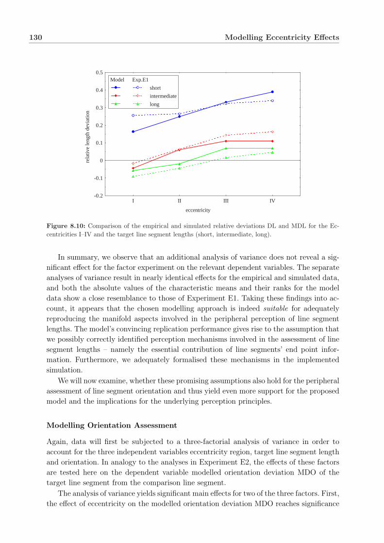
130 Modelling Eccentricity Effects
eccentricity
rela
tive
leng
th d
evia
tion
-0.2
-0.1
0
0.1
0.2
0.3
0.4
0.5
I II III IV
Model Exp.E1
short
intermediate
long
Figure 8.10: Comparison of the empirical and simulated relative deviations DL and MDL for the Ec-centricities I–IV and the target line segment lengths (short, intermediate, long).
In summary, we observe that an additional analysis of variance does not reveal a sig-
nificant effect for the factor experiment on the relevant dependent variables. The separate
analyses of variance result in nearly identical effects for the empirical and simulated data,
and both the absolute values of the characteristic means and their ranks for the model
data show a close resemblance to those of Experiment E1. Taking these findings into ac-
count, it appears that the chosen modelling approach is indeed suitable for adequately
reproducing the manifold aspects involved in the peripheral perception of line segment
lengths. The model’s convincing replication performance gives rise to the assumption that
we possibly correctly identified perception mechanisms involved in the assessment of line
segment lengths – namely the essential contribution of line segments’ end point infor-
mation. Furthermore, we adequately formalised these mechanisms in the implemented
simulation.
We will now examine, whether these promising assumptions also hold for the peripheral
assessment of line segment orientation and thus yield even more support for the proposed
model and the implications for the underlying perception principles.
Modelling Orientation Assessment
Again, data will first be subjected to a three-factorial analysis of variance in order to
account for the three independent variables eccentricity region, target line segment length
and orientation. In analogy to the analyses in Experiment E2, the effects of these factors
are tested here on the dependent variable modelled orientation deviation MDO of the
target line segment from the comparison line segment.
The analysis of variance yields significant main effects for two of the three factors. First,
the effect of eccentricity on the modelled orientation deviation MDO reaches significance

8.3 Model Results and Discussion 131
(F (3; 33) = 21.29; p < 0.001). Similar to the eccentricity effects in the empirical data, the
“virtual” subjects’ performance deteriorates the further the target line segment appears
in the periphery. On average, the simulated orientation of the comparison line segment
deviates from that of the target line segment by 5.5 degrees in Eccentricity I, by 7.4 degrees
in Eccentricity II, by 7.7 degrees in Eccentricity III and by 8.7 degrees in Eccentricity IV.
Second, the factor target line length is once again found to have a highly significant
effect on MDO. The respective analysis yields a significance level of (F (2; 22) = 118.99; p <
0.001), manifested in a greater mean orientation deviation for short line segments (9.8
degrees) than for intermediate ones (7.2 degrees), and in an again smaller MDO for long
line segments (4.7 degrees). Figure 8.11 shows MDO as a function of the eccentricity
region (I–IV) and the length of the target line segments (short, intermediate, long).
In contrast to the empirical findings, the third factor, target line orientation, does not
show a significant effect on MDO (F (2; 22) = 1.07; p = 0.360). Independent of the orienta-
tion of the target line segment, the average orientation deviation measures approximately
6.5 degrees. Figure 8.12 shows MDO for all eccentricity regions (I–IV), separated for the
three possible orientations of the target line segments (horizontal, oblique, vertical).
One of two interactions that reach the significance level is that between target line
segment length and orientation (F (4; 44) = 2.73; p = 0.041). Here, this effect must be
attributed to the fact that, for horizontal and vertical target orientations, MDO does not
significantly differ between short and intermediate target line segment length, whereas
this is the case for oblique line segments and for all other comparisons between differ-
ent line segment lengths, irrespective of their orientation. Unlike the interaction between
eccentricity and target line segment length in Experiment E2, this interaction reaches sig-
nificance in the simulation (F (6; 66) = 6.49; p < 0.001). It can be observed that MDO for
short target line segments does not significantly differ between the different eccentricities,
eccentricity
mod
elle
d or
ient
atio
n de
viat
ion
MD
O (
degr
ees)
0
1
2
3
4
5
6
7
8
9
10
11
12
I II III IV
short
intermediate
long
Figure 8.11: Modelled orientation deviation MDO of the comparison from the target line segment as afunction of eccentricity and target line segment length.

132 Modelling Eccentricity Effects
eccentricity
mod
elle
d or
ient
atio
n de
viat
ion
MD
O (
degr
ees)
0
1
2
3
4
5
6
7
8
9
10
I II III IV
horizontal
oblique
vertical
Figure 8.12: Modelled orientation deviation MDO of the comparison from the target line segment as afunction of eccentricity and target line segment orientation.
whereas MDO does for intermediate and long line segments: The modelled orientation
deviation almost linearly increases from eccentricity region I–IV and MDO shows signif-
icant differences between the separate eccentricities. All other two-way interactions and
the three-way interaction between eccentricity, target line segment length and orientation
do not show significant effects on the modelled orientation deviation MDO.
In order to evaluate the model performance with respect to the reproduction of the
empirical orientation assessment data, the same comparison procedure will be followed
as before when modelling length assessment. When comparing the empirical data from
Experiment E2 and the simulated data, the then introduced between-subjects factor “ex-
periment” yields no significant effect on (M)DO (F (1; 22) = 2.88; p = 0.124). This suggests
that no significant differences exist between the simulated and empirical data sets and,
thus, that the chosen modelling approach might indeed be adequate to account for the
data measured in Experiment E2 as well.
In analogy to the previous comparison, the upper part of Table 8.2 contains the results
of the separate multi-factorial analyses of variance as conducted in Experiment E2 and for
the simulated data. It emerges that the model could successfully reproduce the majority
of “empirical” effects. However, the significant main effect of the orientation of the target
line segment on DO in Experiment E2 is “lost” in the simulation. In contrast, the simu-
lation “gains” an interaction effect between eccentricity and target length (ECC × LEN)
on MDO, which is not significant in the empirical data. The results further indicate that
the interaction between target length and orientation (LEN × ORI) – although present
both in Experiment E2 and the simulation – becomes significant for different reasons (see
above).
The lower bottom part of Table 8.2 charts the absolute mean values for (M)DO (for
details see Sections 7.2 and 8.3). As before, the differences between these values for the

8.3 Model Results and Discussion 133
empirical and model data are generally very small, ranging from 0.3o to a maximum of
only 2.4o. On average, MDO diverges from DO by only 0.8o when data is aggregated over
eccentricity, by 1.3o (over target length) and by 1.0o (over target orientation). These highly
accurate approximations initially suggest that the simulation suitably models the absolute
empirical values. In general, this observation is true and holds for most values. Taking the
previously found differences in the statistical analyses into account, a closer inspection of
the data reveals, however, that the simulation does not as accurately model all aspects
of orientation as those of length assessment. These differences become somewhat more
obvious in Figures 8.13 and 8.14. Here, data from Figures 8.11 and 7.3 and Figures 8.12
and 7.4, respectively, is merged to facilitate the comparison.
Thus, Figure 8.13 illustrates that the model data very closely resembles the empirical
data from Experiment E2 with respect to their absolute values and their ranks for the
different eccentricities and the different levels of target line segment length. The model
data is shifted considerably upwards only for short line segments, but still maintains the
shape of the empirical curve. However, this results in a significant interaction effect of
the (between-subjects) factor experiment and the factor target length on the dependent
variable (M)DO (F (2; 44) = 18.21; p < 0.001).
Differences between empirical and model data become more pronounced in Figure 8.14,
where the orientation deviation for the eccentricity regions I–IV is separately charted for
Experiment E2 Model Comp./Diff.
Significant effect of ... on (M)DO• ECC + + ⊕• LEN + + ⊕• ORI + - ª• ECC × LEN - + ª• ECC × ORI - - ⊕• LEN × ORI + + ⊕• ECC × LEN × ORI - - ⊕
Mean (M)DO in/for ...• ECC I 6.0o 5.5o 0.5o
• ECC II 6.4o 7.4o 1.0o
• ECC III 7.1o 7.7o 0.6o
• ECC IV 7.5o 8.7o 1.2o
• LEN short 7.4o 9.8o 2.4o
• LEN intermediate 6.9o 7.2o 0.3o
• LEN long 5.8o 4.7o 1.1o
• ORI horizontal 5.4o 6.5o 1.1o
• ORI oblique 7.3o 6.6o 0.7o
• ORI vertical 7.7o 6.4o 1.3o
Note: ECC – eccentricity region; LEN – target length; ORI – target orientation
Table 8.2: Summary of the results of modelling line segment orientations in comparison with the em-pirical findings of Experiment E2.

134 Modelling Eccentricity Effects
eccentricity
orie
ntat
ion
devi
atio
n (d
egre
es)
0
1
2
3
4
5
6
7
8
9
10
11
12
I II III IV
Model Exp.E2
short
intermediate
long
Figure 8.13: Comparison of the empirical and simulated orientation deviations DO and MDO for theEccentricities I–IV and the target line segment lengths (short, intermediate, long).
the different orientations of the target line segment. Although the absolute differences
between the two data sets are, according to Table 8.2, quite small, the lack of the sta-
tistically significant effect of the target orientation on MDO is well visible between the
“empirical” and “model graphs” for horizontal target line segments: Whereas subjects in
Experiment E2 could (significantly) more accurately assess the orientation of horizontal
target line segments than that of oblique or vertical ones, the model does not account
for this dependence. All three model curves do not vary significantly and more closely
resemble those of the empirical oblique and vertical graphs. Consequently, an analysis
of variance yields a significant interaction effect between the (between-subjects) factor
experiment and the factor target orientation (F (2; 44) = 7.89; p = 0.001).
In summary, we observe that an additional analysis of variance does not reveal a
significant effect for the factor experiment on the relevant dependent variables (M)DO.
However, interaction effects between experiment and orientation and between experiment
and target length reach significance, indicating deficits of the model in accounting for all
aspects of simulating the orientation assessment of line segments. This is further supported
by the separate analyses of variance that result in identical (non-) significant effects for
the empirical and simulated data for all but the above-mentioned factors. In accordance
with these findings, both the respective absolute means and their ranks for the model
data show a close resemblance to those of Experiment E2 as far as the simulation of
the eccentricity effects and the dependence of MDO on the target line segment length
is concerned. The simulation does not convincingly reproduce the empirical data with
respect to the influence of the target orientation on (M)DO.
Altogether, the chosen model still presents quite a successful approach to reproduce
the essential aspects involved in the peripheral perception of line segment orientation. Its
main deficit, however, is the inability to adequately account for the influence of orientation

8.4 Summary and Conclusions 135
eccentricity
orie
ntat
ion
devi
atio
n (d
egre
es)
0
1
2
3
4
5
6
7
8
9
10
11
12
I II III IV
Model Exp.E2
horizontal
oblique
vertical
Figure 8.14: Comparison of the empirical and simulated orientation deviations DO and MDO for theEccentricities I–IV and the target line segment orientations (horizontal, oblique, vertical).
of the target line segment on the accuracy of the orientation assessment. The model
performance thus allows us to conclude that we possibly correctly identified some of the
essential perception mechanisms involved in the assessment of line segment orientation,
namely the essential contribution of line segments’ end point information, as was the
case for the assessment of line segment length as well. However, peripheral orientation
assessment appears to be guided by additional mechanisms. These might take other line
segment information into account, presumably segment-inherent, and thus lead to more
diversified empirical findings, in particular with respect to orientation dependences. The
implemented model approach therefore seems to be primarily adequate for simulating
peripheral lengths rather than peripheral orientation assessments. Nevertheless, it still
allows for the latter in good approximation.
8.4 Summary and Conclusions
Let us recall that the overall goal of the investigation is to identify and better under-
stand the processes that characterise the visual perception and the assessment of line
segments and their essential dimension(s). As a promising strategy to achieve this goal,
a data driven, explorative bottom-up approach is chosen. First, fundamental mechanisms
governing the specific task solution are explored in isolation. If, as a result, the various
findings can be integrated appropriately, this might ideally lead to the understanding of
the whole, possibly rather complex perception process.
Inspired by earlier research that suggested the influence of peripheral vision as one of
such fundamental factors on the assessment of line segments, the previous chapters aimed
at an in-depth understanding of eccentricity effects on the visual perception of line seg-

136 Modelling Eccentricity Effects
ments. In particular with respect to length and orientation assessment, the hypothesised
decomposition strategy was explored. Rather than only collecting psychophysical data,
the design and sequence of the studies conducted in this respect were chosen in order to
primarily meet the following criteria:
• A maximum validity of the empirical results must be ensured. This can be questioned
in several other studies where distractor tasks were used to indirectly generate (quite
unnatural) peripheral viewing conditions that still could not be reliably monitored.
In this case, the application of a sophisticated eye-tracking system creates natural,
realistic viewing conditions for subjects and yields transparent, reliable data for the
experimenter.
• The sequence of the Experiments E0–E2 was chosen as it ideally reflects the initial
decomposition hypothesis: When we assume that end point information is vital for
the assessment of line segment attributes such as length and orientation, it might
thus be possible to directly infer line segment length or orientation accuracy from po-
sition assessment accuracy. Such a decomposition of peripheral perception processes
then encourages the development of an analogous model to simulate the line seg-
ment length and/or orientation perception principles based on peripheral positional
assessment modelling. This model of eccentricity effects may later be integrated into
the more complex model of simultaneous line segment comparison.
According to these specifications, the Experiments E0, E1 and E2 were conducted
and, indeed, yield great support for the above-mentioned hypothesis.
With respect to location assessment in peripheral vision, the results from Experi-
ment E0 suggest that the assessment of position is governed by two distinct processes.
One is responsible for the assessment of the direction where the target in question is sit-
uated, a process that obviously works quite accurately and more or less independent of
the eccentric position of the target. The second process involved determines the distance
between fixation point and target. This process yields less accurate judgements as the
radial position of the target is significantly underestimated. Furthermore, this process is
eccentricity-dependent and shows deteriorating assessment accuracy for the radial target
position with increasing peripheral viewing. On aggregate, the combination of these two
processes yields positional judgements that are dominated by the distance component
and results in a perceived position of the target marker that is shifted in the direction of
the fixation point, but shows very little directional divergence. In addition, the statistical
analysis demonstrated that no significant difference exists whether the target marker is
positioned horizontally or vertically, relative to the fixation point. Taking the ellipsoidal
shape of the retina and the ovoid shape of the (binocular) visual field into account (both
with the horizontal axis being the longer), this finding is rather unexpected. Due to the
asymmetry, the preferred horizontal orientation of the visual field and the further range
of receptors along this axis could be well expected to lead to a better position assessment
accuracy along the horizontal than along the vertical meridian. However, this is obviously
not the case.

8.4 Summary and Conclusions 137
In Experiment E1, the assessment of the length of peripherally viewed line segments
demonstrates that the lengths of the target line segments are generally overestimated. This
overestimation effect significantly increases the further the target line segment is displayed
in the periphery. Whereas the factor target line segment orientation does not exert a sig-
nificant effect on the length assessment accuracy, the target length does: The longer the
target line segments are, the more accurately their length can be assessed. Based on the
observation regarding location assessment in Experiment E0 and the assumption that the
line segment’s end points play an important role for the length assessment, a possible
explanation for the (eccentricity) effects on line segment length assessment reported in
Experiment E1 can be formulated. In detail, the explanation of the overestimation of line
segment lengths in Experiment E1 is based on the finding of Experiment E0, that the
actual position of the target marker is perceived as being shifted towards the fixation
point (underestimation of the radial target marker position). In contrast, very little di-
vergence between the tangential position of the comparison and the target marker was
noticed. We now transfer these observations and assume that the principles of location
assessment apply to the peripheral perception of line segment lengths as well. It then
emerges that, when memorising a line segment peripherally perceived, subjects develop a
mental model of a line segment of approximately the original (target) length, but shifted
towards the fixation point. This (mental) “shift” or dislocation of the line segment towards
the observer leads to an elongation of the line segment when its mental model is recalled
in the reconstruction phase of the experiment, i.e. when the length of the comparison line
segment has to be adjusted. This is due to the principle of size/length constancy which
states that the size/length of objects seems to increase when they are moved towards the
observer.
The third experiment in this series, where eccentricity effects on the assessment of
line segment orientation are investigated, yields findings analogous to those of Experi-
ment E1. Again, the factor eccentricity exerts a significant effect – here on the orientation
deviation DO – and results show a markedly better orientation assessment for more foveal
than for more eccentric presentation locations of the target line segment. Furthermore,
the orientation of longer target line segments can also be assessed more accurately. In con-
trast to the findings of Experiment E1, the factor target line segment orientation exerts
an additional significant effect on DO. The discussion of these results again rendered the
previously introduced approach promising, to think of orientation assessment also as a
process determined by the perceived locations of the line segments’ end points. If we take
into account the findings for the location assessment from Experiment E0, these could
also be reflected in and probably account for some of the results of Experiment E2. For
example, due to the greater variance along the radial rather than the tangential axis in
the location assessment task of Experiment E0, a considerable variation in the orientation
assessment must be expected – and could indeed be observed in Experiment E2. Thus,
this approach again seems plausible and intuitively suggests an account for the orientation
deviations observed in Experiment E2.
With respect to the subsequent development of a simulation, the analogous results of
the Experiments E1 and E2 and possibly related principles behind peripheral length and
138 Modelling Eccentricity Effects
orientation assessment of line segments encourages the “integrated” modelling, based on
the findings from Experiment E0. The goal of the simulation is to compare line segment
length and orientation assessments from the Experiments E1 and E2, respectively, to
“virtual” comparison line segment lengths and orientations. These virtual line segments
are constituted by their simulated end points using the Monte-Carlo Simulation (MCS)
method. The MCS takes into account the specific characteristics of the frequency distri-
butions of the empirical comparison marker positions, manifested and parameterised by
means of a principal component analysis (PCA).
In summary, we observe that statistical analyses do not reveal significant differences
between empirical and simulated data, produce nearly identical (non-) significant effects
for the empirical and simulated data and both the absolute values of the characteristic
means and their ranks for the model data show a close resemblance in particular to those
of Experiment E1. With regard to Experiment E2, the model cannot be rated as quite as
convincing in all aspects. Although, on aggregate, performance can still be rated as very
good, it has some deficits with respect to a correct representation of orientation effects and
the reproduction accuracy of some absolute statistical values. Irrespective of these (minor)
disadvantages, taking the findings of both length and orientation modelling into account,
it appears that the chosen approach is indeed suitable to adequately reproduce the mani-
fold aspects involved in the peripheral perception of line segment lengths and – with some
restrictions – of line segment orientation as well. The model’s convincing replication per-
formance supports the decomposition hypothesis and gives rise to the assumption that we
correctly identified the perception mechanisms involved in the assessment of line segments,
namely the essential contribution of line segments’ end point information. Furthermore,
we successfully implemented these mechanisms in the simulation algorithms.
As already mentioned, peripheral processing should play an even more important role
in simultaneous line segment comparison tasks. Here, not only the length of each segment
must be assessed, but also the comparison has to be accomplished. This might often be
greatly facilitated by peripherally assessing the relevant attributes of both the target and
comparison line segments at the same time – memory involvement as explicitly required
in sequential comparison would thus be reduced. The chosen free gaze scenario also al-
lows us to re-assess the decomposition hypothesis, eye movements will provide essential
hints towards its validity. The analysis and interpretation of eye movement should fur-
ther facilitate the exploration of the other processing steps that determine the cognitive
structure of visual comparison tasks and allow for the testing of the other hypotheses
formulated in this respect – in particular regarding the existence of holistic and analytic
visual processing strategies, depending on discrimination difficulty.
We will now address this simultaneous comparison in the second part of the inves-
tigations. We thereby hope to integrate many aspects of the findings from the previous
chapters and to be able to adapt the already formalised modelling aspects into an ex-
tended model for the simulation of perception processes involved in simultaneous line
segment comparison.
Chapter 9
Simultaneous Comparison –
Similarity Effects in Line Segment
Perception
Let us recall the intention of the procedural concept this thesis follows: The aim is to
establish a series of logical steps, each of which represents a valuable contribution to the
overall understanding of visual processing of line segments in comparison scenarios. The
empirical findings will then be formalised within a mathematical model.
Some of this “programme” has been completed in the previous chapters: The collection
of relevant empirical data and their interpretation with regard to the contribution of pe-
ripheral perception processes and decomposition mechanisms to the overall understanding
of line segment assessment has been accomplished. Furthermore, the formal representation
of fundamental perception principles in this respect could successfully be implemented in
a simulation model.
As introduced in Chapter 3, the investigation now moves on to studying line segment
perception in a more complex scenario. The focus will be on similarity effects in line
segment perception in simultaneous comparison. Furthermore, the intention will be pur-
sued to integrate the previous findings into a comprehensive explanatory approach and to
implement a computational model that adequately describes line segment perception and
closely follows the cognitive structure of visual comparison tasks. When we consider that
the implementation for the modelling of eccentricity effects – which we also render essen-
tial for non-peripheral line segment assessment – scored higher for the assessment of line
segment length than orientation, it appears to be logical that the following experiments
will be mainly concerned with line segment length rather than orientation aspects.
A wide range of potentially interesting issues can be investigated based on an experi-
mental setting where two line segments are simultaneously presented side by side (see
Figure 3.6). Opposed to the eccentricity effects in sequential comparison, similarity ef-
fects present such an issue in simultaneous comparison, for example. As motivated in
Chapters 2 and 3, the following two experiments will be conducted:

140 Simultaneous Comparison – Similarity Effects
• Experiment S1: The basis – Dynamic adjustment in length matching
• Experiment S2: Holistic vs. analytic processing – Binary judgements in length dis-
crimination
Let us remember the basic hypotheses formulated in Section 2.4 and elaborate them
in more detail.
The proposed discrimination task in Experiment S2 (“Which of the two line segments
is the longer one?”) implicitly suggests a variation of the discrimination difficulty, i.e. the
length similarity of the two line segments shown simultaneously. The distinction between
an “easy” and a “difficult” discrimination task should be particularly promising with
respect to the applied solution strategies and should be reflected in corresponding visual
processing strategies. Solving an easy discrimination task could be accomplished “holisti-
cally” without much focused information acquisition whereas the difficult condition might
require an “analytic” processing mode. These two opposing solution strategies (cognitive
level) will most likely result in different visual processing strategies (perceptual level),
manifested in distinct differences in eye-movement parameters (sensorimotor level) and
gaze trajectories.
For high similarity comparisons (“difficult”), i.e. when the two line segments’ lengths
are approximately, but not exactly equal, a thorough visual analysis of the scene must be
expected. It is reasonable that overt shifts of attention occur not only between the two
stimuli for the actual comparison, but that relevant features within the line segments are
foveally scanned as well. Again, the end points of the line segments could be promising
candidates for fixations if we assume that “visually measuring” the distance between two
such points yields the required accurate length information. This data might then be
stored in the respective mental line segment model to be compared with the comparison
stimulus. However, even in high similarity conditions, subjects might apply efficient visual
scanning strategies. These could constitute gaze trajectories that demonstrate an explicit
fixation of only one of a line segment’s end points and the peripheral assessment of the
other. It is also possible that intermediate points “on” the line segment are fixated, such as
its mid point (“center of gravity”), and that the overall length is subsequently extrapolated
therefrom.
In case of low similarity comparisons (“easy”), i.e. when the line segments’ lengths
clearly differ, we would generally not expect such analytic visual scanning. Instead, we
hypothesise that a holistic scene perception strategy yields sufficient information to make
a correct decision as to which of the line segments is longer: A central point in between
the two stimuli is fixated and the line segments’ lengths are assessed peripherally. Rather
than fixating such a central point, it might alternatively be favourable to foveally view
one of the segments and peripherally assess the other. Finally, it might be feasible in
some cases, even for apparently easy comparisons, to fixate both stimuli once or even
to “switch” to analytic “mode”. These strategies could be pursued, for example, when
different orientations of the two line segments induce (subjective) changes in perceived
length due to optical illusion effects.

141
As also already motivated in Chapter 3, the binary judgement task in Experiment S2
does not only allow for the investigation of similarity effects in simultaneous length as-
sessment that constitute potentially different processing strategies. Moreover, this experi-
mental setting and the method of constant stimuli create ideal conditions for an eye-
movement investigation. Rather than the dynamic adjustment of line segment length to
match the target and comparison stimuli, the simple binary decision required here makes
it easier to attribute particular shifts of attention uniquely to either adaptation processes
or to an influence of specific stimulus attributes. The elimination of the dynamic process
of line segment length adjustment should facilitate the monitoring and understanding
of comparison processes and the influence of line segments attributes thereupon. This
static procedure should in particular be beneficial for the interpretation of eye-movement
patterns and associated attention and memorisation/representation processes.
However, it is absolutely essential to conduct Experiment S1 as well. Although we just
motivated that dynamic processes certainly do not facilitate the interpretation of eye-
movement data, the challenge to do so persists. Furthermore, a dynamic setting presents
the attractive opportunity not only to learn about how these dynamic processes influence
eye movements and vice versa, but also to include them into an enhanced model that
simulates both eye movements/gaze trajectories and the relevant psychophysical data.
For a start, Experiment S1 is indispensable in establishing appropriate definitions for
the easy and difficult conditions of Experiment S2. The results obtained will provide in-
formation on how accurately subjects can match the length of two line segments. We can
then use this data to infer which differences between line segment lengths are difficult to
distinguish – obviously those that lie within this accuracy – and which are easy to distin-
guish – those that lie considerably outside the accuracy. This distinction thus determines
the easy and difficult conditions to be compared in Experiment S2.
The following section describes the algorithmic generation of the stimuli for the Ex-
periments S1 and S2 and motivates the choice of levels for the independent variables
in
• Experiment S1:
– Length
– Orientation
• Experiment S2:
– Similarity level (i.e. “difficulty”)
– Length
– Orientation

142 Simultaneous Comparison – Similarity Effects
9.1 Variables and Stimuli
Let us again first consider the choice of independent variables and their respective different
levels which will be varied in Experiments S1 and S2.
9.1.1 Levels of Independent Variables
One of the aims of Experiment S1 is to provide data that will subsequently be used
to determine the experimental conditions in Experiment S2. When subjects adjust the
length of the comparison line segments to match the perceived length of the target line
segment, the adjustment will certainly incorporate some error. This error in Experiment S1
provides information regarding the magnitude of length differences between the target
and comparison line segments that should be observed to constitute easy and difficult
comparison conditions in Experiment S2. Due to these strong inter-experiment links, it
must be ensured that the independent variables and their respective levels represent logical
choices that can be maintained in both experiments in order to obtain reliable findings.
The close resemblance of the two experimental settings should not render this too difficult,
however. But, which would now be the most sensible choices for the levels of target line
segment length and orientation?
For the length of the target line segments, we suggest three different magnitudes. In
analogy to the previously chosen lengths in Experiment E1, it appears to be appropriate
to choose “short”, “intermediate” and “long” line segments whose lengths can either be
perceived foveally or require parafoveal or peripheral processing, respectively. In fact, we
initially motivated the choice of target length in Experiment E1 with the special require-
ments of Experiments S1 and S2. In a comparison scenario with unrestricted eye gaze,
shifts of visual attention within one stimulus are then likely to be performed for “longer”
line segments in order to foveally acquire relevant dimension information. We expect this
to be true in particular in the difficult discrimination tasks of Experiment S2. Such a vi-
sual strategy would then support the assumed analytic processing hypothesis. The choice
of target lengths in analogy to those studied in Experiment E1 also appears desirable –
if not essential – in order to incorporate the conclusions from the eccentricity Experi-
ments E0–E2 into the explanation of the observations in the similarity Experiments S1
and S2.
In Experiment E1 we had to realise that, due to the size of the eccentricity regions I–
IV, the line segment lengths were limited and could not exactly be chosen according
to the “standard” definitions of the eccentricity regions. Due to the restriction to “fit”
the “long” line segment into eccentricity region I without overlap of other eccentricity
regions in Experiment E1, “short”, “intermediate” and “long” length had to be chosen
as 1o ± 0.3o, 4o ± 0.3o and 7o ± 0.3o, respectively. As no such restrictions apply in the
current Experiments S1 and S2, the target line lengths here will more closely resemble
the “classical” eccentricity categorisations, established in several studies (e.g. Tsal, 1983;
Wright & Ward, 1994; Posner, 1980; Matlin & Foley, 1997): Foveal ≤ 3o, parafoveal ≤ 9o,
peripheral ≥ 10o (for details, see Sections 2.2 and 4.1). Thus, the following selection of

9.1 Variables and Stimuli 143
target line segment lengths that will be presented in the Experiments S1 and S2 seems
appropriate:
• Short: 1o ± 0.5o
• Intermediate: 6o ± 0.5o
• Long: 11o ± 0.5o
This choice accounts for equal distances between the different line segment lengths as
well as attempts to minimise habitual effects that might occur when always exactly the
same values have to be assessed. As before, “noise” is introduced that randomly varies
the line segment length, here within a 0.5o-band, around the short, intermediate and long
target length levels.
With the systematic variation of the second independent variable in the Experi-
ments S1 and S2, the orientation of the target line segment, a new aspect known to
often significantly influence visual perception is added to the scope of the present inves-
tigation, namely that of visual illusory effects . More specifically, the “horizontal-vertical
illusion” (see, e g., Kunnapas, 1955; Piaget, 1969; and, more recently, Prinzmetal & Get-
tleman, 1993; Bartolomeo & Chokron, 2001) is of central interest here. As discussed in
detail in Section 2.2, vertical or oblique line segments are generally perceived to be longer
than horizontal ones that are displayed simultaneously and have identical physical length
(see Figure 2.6).
In the present investigation, the inter-stimulus orientation and its possible illusory
effects on the assessment of line segments’ lengths must not be neglected. It should sig-
nificantly influence the length assessment accuracy in Experiment S1 and will thus affect
the determination of the easy and difficult discrimination conditions in Experiment S2.
The present studies allow for the quantification of the horizontal-vertical illusion effect
(Experiment S1) and they also present the opportunity to gain some insight into the un-
derlying visual processes, manifested in eye movements. Their analysis (Experiment S1
and, in particular, Experiment S2) could help to explain the misjudgement and might fi-
nally lead to a better understanding not only of “normal” line segment length perception,
but also of (at least this type of) visual illusions.
With the comparison line segment always being horizontally oriented, the following
levels are chosen for the factor target line segment orientation:
• Horizontal: 0o
• Oblique: 45o
• Vertical: 90o
This choice is made in accordance with that of the eccentricity Experiments E1 and E2.
However, as orientation is not assessed in the following experiments, orientation “noise”
to eliminate habituation effects does not have to be introduced here. The orientations of
the target line segments will remain fixed at exactly 0, 45 or 90 degrees.

144 Simultaneous Comparison – Similarity Effects
As for the third independent variable, the discrimination difficulty or, in other words,
the length similarity of the target and comparison line segment – only varied in Experi-
ment S2 – the choice of the exact parameters for either
• easy discrimination, i.e. low similarity, or
• difficult discrimination, i.e. high similarity,
depends on the results of Experiment S1 and will be discussed in the “Methods” section
of Experiment S2 (see Section 11.2).
After the quantification of all relevant variables and the discussion of constraints that
an appropriate stimulus design has to comply with, these stimuli can now be generated
algorithmically.
9.1.2 Algorithmic Generation of Stimuli
Again, the stimulus line segments displayed in the Experiments S1 and S2 are pseudo-
randomly generated. However, as the stimuli always appear at the same locations on the
screen with a constant distance between them, the algorithmic generation of stimuli mainly
consists of the determination of a list of all possible combinations of the independent
variables.
With the independent variables target line segment length (short, intermediate and
long) and target line segment orientation (horizontal, oblique and vertical) set as discussed
Figure 9.1: Three sample stimulus combinations in Experiment S1. Target line segments are shown onthe left, comparisons on the right. Target stimuli here are oblique/long (top), horizontal/short (middle)and vertical/intermediate (bottom). The dotted lines mark the ranges for dynamic adjustment of thecomparison line segments.

9.1 Variables and Stimuli 145
in the previous section, Figure 9.1 shows three algorithmically generated sample stimulus
combinations as shown to subjects in Experiment S1. Subjects have to dynamically ad-
just the length of the (always horizontally oriented) comparison line segment to match the
target length. Each subject will have to assess and adjust the length of a total of 90 line
segments, so that every combination of the two factors will be displayed 90/(3 · 3) = 10
times. As we argued in the Experiments E1 and E2, this repetition factor should yield
very reliable data for a statistical analysis while maintaining an acceptable experiment
duration for subjects. Although considerably fewer trials have to be completed than in
the eccentricity experiments, the average experiment duration still measured approxi-
mately 30 minutes: The more complex comparison task in combination with the dynamic
adjustment procedure resulted in prolonged reaction times.
In the following chapter Experiment S1 investigates the assessment accuracy of line
segment length in a simultaneous comparison setting. Using a dynamic method for com-
parison line segment adjustment, the findings allow us to draw conclusions about the
magnitude of the vertical-horizontal illusion and to establish the parameters for the dis-
crimination difficulty levels easy and difficult in Experiment S2. The chapter begins with
an explanation of the method for this experiment, then the results will be presented and
discussed in detail.

146 Simultaneous Comparison – Similarity Effects

Chapter 10
Experiment S1: Simultaneous
Dynamic Length Assessment
Experiment S1 is the first of two experiments that investigate the assessment and visual
perception of specific stimulus dimensions – here, primarily line segment length – in
the perceptually and cognitively more complex scenario of simultaneous comparison. It
can be assumed, however, that the previously investigated effects of eccentric stimulus
presentation on this stimulus dimension play an important role in simultaneous assessment
as well. Results obtained in the Experiments E0–E2 should thus be viewed as valuable
prerequisites for the understanding of the more complex processes in Experiments S1
and S2.
In Experiment S1, we explore the paradigm of simultaneous comparison paired with
the psychophysical method of adjustment. On the one hand, this experimental design
is required if we want to establish the easy and difficult conditions to investigate holis-
tic and analytic visual processing strategies using the method of constant stimuli in the
subsequent Experiment S2. The adjustment accuracies of the line segment lengths in Ex-
periment S1 allow us to infer which differences between line segment lengths are difficult
to distinguish – obviously those that lie within this accuracy – and which are easy to
distinguish – those that lie considerably outside the accuracy – so that the discrimina-
tion/similarity conditions can be determined accordingly in Experiment S2. On the other
hand, although we must accept that the dynamic adjustment does certainly not facilitate
the interpretation of eye-movement data, the setting of Experiment S1 presents the at-
tractive opportunity not only to learn about how these dynamic processes influence eye
movements and vice versa, but also to include them into an enhanced model that simu-
lates both eye movements/gaze trajectories and the relevant psychophysical data. Data
recorded and analysed in this experiment will thus comprise psychophysical measures
such as the reaction time RT, the adjusted length of the comparison line segment or its
difference to the given target length. Furthermore, the relevant eye-movement data, such
as number of fixations NF, fixation duration FD or saccade length SL (for details see
Section 3.4.2) will be quantitatively analysed. The gaze trajectories will be qualitatively
reviewed.

148 Experiment S1: Simultaneous Dynamic Length Assessment
10.1 Method
10.1.1 Subjects
The subjects were fifteen experimentally naive students – ten male and five female – from
the University of Bielefeld. Their average age was 27.5 years. All subjects had normal
or corrected-to-normal vision and no pupil anomalies. The subjects were paid for their
participation in the experiment.
10.1.2 Stimuli
The stimulus pictures were presented on a computer screen with a spatial resolution of
800×600 pixels (39.0o×29.4o of visual angle). The stimuli consisted of two line segments
that were placed on the screen so that their mid points were centered in the two respective
hemifields of the display. The distance between the two line segments’ mid points mea-
sured approximately 22o. The target line segment consistently appeared on the left and
showed one of the possible combinations of length and orientation as specified below. The
comparison line segment was shown on the right, always in a horizontal orientation. Its
initial length, i.e. that at the time of appearance, was randomly varied within the interval
[0.05o, 2 · target length] with initial length being shorter or longer than the target length
in 50% of the trials each. The initial comparison length could then be manipulated by
mouse movements within the interval [0.05o, 2 · target length].
The line segments had a thickness of one pixel (0.05o), an orientation of either 0o
(“horizontal”), 45o (“oblique”) or 90o (“vertical”) and a length of either 1o±0.5o (“short”),
6o ± 0.5o (“intermediate”) or 11o ± 0.5o (“long”) of visual angle (see Section 9.1). The
line segments and the background were set to the same dark and light grey colours,
respectively, as in the Experiments E0–E2. Figure 10.1 shows a typical stimulus picture.
Figure 10.1: Typical stimulus picture in Experiment S1. Subjects had to adjust the length of thehorizontal comparison line segment (right hemifield) so that it matched the perceived length of the targetline segment displayed in the left hemifield.

10.1 Method 149
10.1.3 Apparatus
The apparatus used was the same as in Experiment E0.
10.1.4 Procedure
All subjects were tested individually. Prior to the start of the experiment, they were
provided with written instructions that explained their task. Next, the eye tracker was
set up and calibrated for each subject. To complete the calibration procedure, subjects
had to look at nine dots that successively appeared at specific locations on the display.
Each trial of the experiment started with the presentation of the fixation point at the
center of the screen (Frame 1, see Figure 10.2). 700 ms after fixation point onset, the two
line segments were displayed simultaneously in the left (target) and right (comparison)
hemifields, respectively (Frame 2). The fixation point disappeared 200 ms thereafter. The
instructions required the subjects to assess the length of the target line segment and to
adjust the length of the comparison line segment accordingly as accurately as possible.
Subjects accomplished the length adjustment by horizontal mouse movements that were
synchronised with the stimulus display (Frame 3). Moving the mouse to the right resulted
in an elongation of the comparison line segment, movements to the left in a shortening.
The resolution for the adjustment was 0.1o (equivalent to two pixels). Mouse movements
resulted in a symmetric change (relative to the mid point) of the length of the comparison
line segment. The length was increased or decreased by 0.05o, i.e. in one-pixel increments or
decrements, at each end of the line segment. When subjects had finished their adjustment,
they pressed the left mouse button for confirmation and the next trial started.
As mentioned above, the comparison line segment was always shown on the right, in-
tuitively corresponding with the (right) hand that usually operates the computer mouse.
Figure 10.2: The sequence of procedural steps for a trial of Experiment S1. Frame 1: Fixation point.Frame 2: Simultaneous display of target and comparison line segments. Frame 3: Adjustment of compar-ison line segment length.

150 Experiment S1: Simultaneous Dynamic Length Assessment
Changing the presentation hemifields for the two stimuli would have resulted in initial
mouse movements in order to identify the comparison line segment. These are certainly
unrelated to the actual task and would have rendered data analysis more difficult and
influenced the subjects’ performance. Similar effects could have been expected if the com-
parison line segment had been shown in changing rather than a constant (here: Horizontal)
orientation.
No gaze restrictions applied throughout Experiment S1 and subjects could move their
gaze freely across the whole screen. Figure 10.2 illustrates the sequence of procedural steps
for one trial.
In order to compensate for the possible displacement of the headset due to head move-
ments, the eye tracker was recalibrated after every 9 trials. In contrast to the eccentricity
Experiments E0–E2 where tight gaze restrictions applied, minor misalignments of the
headset can be tolerated now and would not lead to potentially unmotivated abortion of
trials due to boundary violations.
Subjects viewed a total of 90 stimulus pictures during the experiment so that each
possible combination of the three target lengths and the three target orientations was
displayed ten times. Prior to the experimental trials, nine practice trials were conducted
to accustom the subjects to the eye-tracker headset and the experimental task. As well
as the reaction time and the assessment/adjustment accuracy, eye movements were mon-
itored and written into a file. The recorded data contained all required information for
the subsequent computation of the eye-movement parameters relevant here and for the
visualisation of gaze trajectories that occurred during the dynamic length adjustment
process.
10.2 Results
Rather than the eye movements recorded during the experimental trials, we will first
address the “conventional” psychophysical data, namely the length assessment accuracy.
It is manifested in the length deviation DL, i.e. the difference between the target line
segment length and the adjusted length of the comparison line segment. On the one hand,
this measure is of particular importance for Experiment S2, where DL and the associated
standard deviation σDL determine the (then fixed) comparison line segment lengths for
the easy and difficult discrimination conditions. On the other hand, the statistical analysis
of DL allows us to once again establish and quantify the visual illusory effects – if present –
induced by the orientation difference between the target and comparison line segments.
All experimental data is subjected to a two-factorial analysis of variance in order to
account for the two independent variables target line segment length and orientation.
The effects of these factors are tested on the dependent variables length deviation DL
(“length assessment accuracy”) and on the following eye-movement parameters (for de-
tailed definitions, see Section 3.4): Number of fixations (NF), fixation duration (FD) and
saccade length (SL) and derived measures such as number of successive fixations within
the same hemifield (FW) or the number of saccades between hemifields (SB). In analogy

10.2 Results 151
to the eccentricity Experiments E0–E2, the reaction time RT are entered into an analysis
of variance as well. The following section presents the detailed results for all dependent
variables, starting with the analysis of RT.
10.2.1 Dependent Variables
Reaction Time RT
First, we chart the relative frequencies of the reaction time RT in a histogram (see Fig-
ure 10.3, left). The distribution is based on all measured values for RT, irrespective of
target line segment length or orientation, and takes into account the data from all subjects.
We measure a minimum RT of 429 ms and a maximum RT of 27151 ms, the overall mean is
4626 ms. The histogram reaches a peak at approximately 2900 ms. Approximately 95% of
the values lie within the interval of 1800 to 8000 ms, the general shape of the distribution
can be fitted by an asymmetrical function with positive skewness of +2.60.
The analysis of variance yields a significant main effect on RT for the factor target
line segment length (F (2; 28) = 18.25; p < 0.001). When the target line segment is short
subjects require 3841.6 ms on average to assess its length and adjust the comparison
line segment accordingly. For intermediate target lengths (parafoveal), RT increases to
4581.4 ms, for long line segments (peripheral) to 5426.6 ms. A Newman-Keuls reveals
that theses differences are indeed all significantly different from each other: (Rcrit =
590.132; p = 0.008) for the comparison between short and intermediate target lengths,
(Rcrit = 660.938; p < 0.001) for short vs. long target lengths and (Rcrit = 609.419; p =
0.004) for intermediate vs. long target lengths. The factor target line segment orientation
does not exert a significant effect on RT (F (2; 28) = 0.54; p = 0.588).
A closer inspection of the data, however, yields an interaction effect between target
length and orientation (F (2; 56) = 3.11; p < 0.022). When targets are short, RT decreases
depending on their orientation: Horizontally oriented target line segments take longer
(4158.1 ms) to assess than oblique ones (3806.8 ms), which again take longer to assess
than vertical ones (3530.6 ms). The post-hoc comparison of means using a Newman-
reaction time RT (ms)
rela
tive
freq
uenc
y
0
0.02
0.04
0.06
0.08
0.10
0 5000 10000 15000 20000 25000
target length
reac
tion
time
RT
(m
s)
3000
3500
4000
4500
5000
5500
6000
short intermediate long
horizontalobliquevertical
Figure 10.3: Left: Cumulative relative frequency distribution of reaction times RT over all target linesegment length and orientation levels for all subjects. Right: Reaction time RT as a function of targetline segment length, separated for the three target orientations.

152 Experiment S1: Simultaneous Dynamic Length Assessment
Keuls test confirms the existence of significant differences between the three orientation
levels for short line segments: (Rcrit = 630.640; p = 0.044) for the comparison between
horizontal and oblique target orientations and (Rcrit = 642.835; p = 0.004) for horizontal
vs. vertical target orientations. However, the comparison between short oblique and short
vertical targets does not produce significant differences in RT, but only a tendency (Rcrit =
500.908; p = 0.104). For intermediate and, in particular, for long target line segments this
dependence cannot be found (qualitatively visible in Figure 10.3, right). RT for these
lengths remains almost constant irrespective of the factor orientation, only for long target
line segments there appears to be an inverse tendency to that found for short line segments:
RT slightly increases from horizontally through oblique to vertically oriented target line
segments. Here, Newman-Keuls tests confirm that no significant differences exist between
the three orientation levels for intermediate or long targets. Intermediate targets: (Rcrit =
461.318; p = 0.616) for the comparison between horizontal and oblique target orientations,
(Rcrit = 440.567; p = 0.632) for horizontal vs. vertical and (Rcrit = 430.450; p = 0.647) for
oblique vs. vertical. Long targets: (Rcrit = 560.716; p = 0.407) for the comparison between
horizontal and oblique target orientations, (Rcrit = 550.349; p = 0.480) for horizontal vs.
vertical and (Rcrit = 395.978; p = 0.745) for oblique vs. vertical. Figure 10.3 (right)
shows RT as a function of target line segment length and orientation.
Length Deviation DL
In contrast to the separate analyses of the length deviations for either absolute (DLp) or
“directional” (DL) cases, we only consider DL in the present experiment. This appears to
be sensible for various reasons. First, we must keep in mind that the length deviations –
and their respective standard deviations – observed in this experiment will be used to
determine the lengths of the comparison line segments in Experiment S2. As we intend
to create easy and difficult discrimination conditions, the lengths should guarantee that
target and comparison line segment lengths are indeed quite similar or rather different
in length, respectively. This certainly requires considering length deviations that take
into account the “direction” of the deviation, i.e. whether the length of the target line
segment was under- or overestimated. The second reason for preferring the analysis of DL
over that of DLp is closely related to the over- and underestimation aspect. We not only
intend to establish the discrimination conditions for the subsequent experiment, but are
also interested in the investigation of the magnitude and “direction” of the visual illusory
effect on the perceived lengths, induced by the specific alignment of the two stimulus
constituents. Furthermore, with a view to the development of a comprehensive model that
not only simulates certain aspects of the visual “behaviour”, but also correctly represents
the adjustment procedure and the illusion-induced effects, the analysis of the directional
deviation DL of the comparison line segment length from the target line segment length
is recommended.
DL will be negative in case the length of the comparison line segment is shorter than
that of the target (“target underestimation”), and positive otherwise (“target overestima-
tion”). DL is again a relative measure that correlates the deviation to the target length

10.2 Results 153
as defined in Equation 6.1 in Section 6.2. Example: A comparison line segment that is
adjusted to 90 pixels when the target is 100 pixels long constitutes a length deviation of
(90− 100)/100 = −0.1, i.e. an underestimation of the target length of (-)10%.
In order to test the effects of the target line segment length and orientation on DL, a
two-way analysis of variance is conducted first. The analysis yields significant main effects
on DL for both factors. Significance levels are computed as (F (2; 28) = 53.10; p < 0.001)
for target line segment length and as (F (2; 28) = 10.87; p < 0.001) for target line segment
orientation. In general, target line segment lengths are overestimated. This overestimation
is significantly more pronounced the shorter the target line segments are. When data is
averaged over the target orientations (for all subjects), comparison line segment lengths
deviate from the target lengths by 15.3% for short target lengths, 10.4% for intermediate
target lengths and 7.0% for long target lengths. A Newman-Keuls test again confirms that
these means are all significantly different from each other: (Rcrit = 0.025; p = 0.009) for
the comparison between short and intermediate target lengths, (Rcrit = 0.026; p < 0.001)
for short vs. long target lengths and (Rcrit = 0.023; p = 0.038) for intermediate vs. long
target lengths.
With respect to the target orientation, the analysis shows that oblique and verti-
cal target line segments are significantly more overestimated than those that are hor-
izontally oriented. The cumulation of data over the factor target line segment length
yields that subjects overestimate the lengths of the target line segments by 4.8% (hor-
izontal), 14.4% (oblique) and 13.4% (vertical) on average, i.e. the lengths of the com-
parison line segments are adjusted longer than the physical target lengths. A Newman-
Keuls test confirms that only the means for the comparisons between horizontal and
oblique targets (Rcrit = 0.026; p < 0.001) and between horizontal and vertical targets
(Rcrit = 0.026; p < 0.001) are significantly different. The comparison between oblique and
target length
rela
tive
leng
th d
evia
tion
DL
-0.05
0
0.05
0.1
0.15
0.2
0.25
short intermediate long
horizontal
oblique
vertical
Figure 10.4: Length deviation DL as a function of target line segment length, separated for the threetarget orientations.

154 Experiment S1: Simultaneous Dynamic Length Assessment
vertical targets does not not produce a significant difference (Rcrit = 0.021; p = 0.301). In
addition, the interaction between target line segment length and orientation reaches sig-
nificance (F (4; 56) = 5.06; p = 0.001). Figure 10.4 shows the relative length deviation DL
as a function of target line segment length and orientation.
As both the factors target line segment length and orientation as well as their interac-
tion exert a significant effect on the length deviation DL, it will apparently be necessary
to individually set the lengths of the comparison line segments in Experiment S2 for the
combinations of the two factors later on. Therefore, all relevant data is summarised in
Table 10.1. The upper two rows of each “block” of the table chart the adjusted lengths of
the comparison line segments LC and the associated standard deviations σLC for all factor
combinations of target line segment length and orientation in Experiment S1. The lower
two rows contain in addition the derived relative length deviations DL of the comparison
from the target line segments lengths and their respective standard deviations σDL upon
which the previous analyses in this section were based. These measures will subsequently
be used in Experiment S2 to determine the comparison line segment lengths for the binary
comparison task (see Sections 11.1 and 11.2).
After the analyses yielded significant effects of the factors target line segment length
and orientation on the “conventional” empirical data types reaction time RT and length
deviation DL, these effects will be tested on ”typical” eye-movement parameters in the
following paragraphs. The integration of all results in the subsequent discussion might
then facilitate the interpretation and understanding of the observations and underlying
perception principles.
target length LT
short (1o) intermediate (6o) long (11o)
LC = 1.082o LC = 6.260o LC = 11.219o
σLC = 0.131o σLC = 0.508o σLC = 0.632o
⇓ ⇓ ⇓DL = 0.082 DL = 0.044 DL = 0.020
hor
izon
tal(0
o)
σDL = 0.131 σDL = 0.084 σDL = 0.057
LC = 1.127o LC = 6.896o LC = 12.090o
σLC = 0.132o σLC = 0.611o σLC = 0.901o
⇓ ⇓ ⇓DL = 0.18 DL = 0.151 DL = 0.102
targ
etor
ienta
tion
oblique
(45o
)
σDL = 0.132 σDL = 0.102 σDL = 0.081
LC = 1.202o LC = 6.698o LC = 11.949o
σLC = 0.123o σLC = 0.638o σLC = 0.969o
⇓ ⇓ ⇓DL = 0.202 DL = 0.117 DL = 0.089
vert
ical
(90o
)
σDL = 0.123 σDL = 0.106 σDL = 0.087
Table 10.1: Overview of adjusted lengths of the comparison line segments LC, length deviations DL ofthe comparison from the target line segments and the respective standard deviations σLC and σDL forall combinations of target line segment lengths LT and orientations in Experiment S1.

10.2 Results 155
Analysis of Eye-Movement Data: Preliminaries
One of the most fundamental eye-movement parameters to be investigated in a statis-
tical analysis is certainly the number of fixations NF that subjects perform during an
experimental trial. Whereas the overall number of fixations in general yields valuable in-
formation on the task complexity and the influence of certain experimental conditions on
visual perception and, furthermore, cognitive processes, the analysis of spatially separate
fixations is often even more rewarding. This appears to be the case in this experiment
also, where local numbers of fixations will be considered. Here, these local NFs will be
computed for the two stimulus hemifields, i.e. for fixations that lie in proximity to the
presentation positions of the target and the comparison line segment, respectively.
Such a distinction seems to be sensible here if we consider the overall distribution
of the fixations. In order to get a better impression of this distribution, the fixation
points are superimposed onto the stimulus display as presented in Figures 10.5 and 10.6.
Figure 10.5 shows the distribution of the fixation points of all subjects when a long
target stimulus is in an oblique orientation, Figure 10.6 illustrates the distributions for all
possible combinations of target line segment lengths and orientations. Qualitatively, the
figures already confirm that indeed the majority of the fixations lies within a certain range
around the two line segments. However, “intermittent” fixations must not be discarded as
Figure 10.5: Distribution of the fixation points for a long target stimulus in an oblique orientation,aggregated over all subjects. The length of the comparison line segment equals that of the target. Thestimuli line segments are coloured blue, the blue dots mark the segments’ centers. The black boxescircumscribe the stimuli so that a minimum distance of 5o is maintained between the box edges andthe enclosed stimuli. A PCA yields the red ellipses. The black dotted box circumscribes the intermittentsection.

156 Experiment S1: Simultaneous Dynamic Length Assessment
Figure 10.6: Distribution of the fixation points for all possible combinations of target line segmentlengths and orientations, aggregated over all subjects (analogous to Figure 10.5).

10.2 Results 157
they yield information on peripheral visual processing. Thus, rather than only considering
the two stimulus display hemifields, we divide the space into two sections surrounding the
line segments and an intermittent section for which separate analyses for NF and, in the
following paragraphs, for various other eye-movement parameters will be computed.
The size of the stimulus sections is individually calculated according to the respective
stimulus dimensions so that a minimum distance of 5o – relative to the outermost points
of the stimuli – is observed. This measure is established to ensure that only fixations
are included in the analyses that can be characterised at least “near foveal” (to the
respective stimulus) whereas the intermittent section contains fixations that allow for the
peripheral perception of the target and/or comparison stimuli. Furthermore, this choice
conveniently excludes fixation artifacts from the analysis that obviously do not contribute
to the assessment task. The intermittent section’s width fills up the space between the
stimulus sections, its height is computed to the mean of the heights of the two stimulus
sections.
In order to validate this – seemingly arbitrary – choice of the size of these three sections,
a cluster analysis is computed using the k-means clustering algorithm (e.g. Hartigan &
Wong, 1979). This non-hierarchial method initially takes the number of components of
the population equal to the final required number k of clusters. In this step itself the final
required number of clusters is chosen such that the points are mutually farthest apart.
Next, it examines each component in the population and assigns it to one of the clusters
depending on the minimum distance. The centroid’s position is recalculated every time
a component is added to the cluster. These steps are re-iterated until all components
are grouped into the final required number of clusters and no data points have to be
regrouped. When this terminates, all cluster centers are at the mean of their Voronoi sets,
i.e. the set of data points which are nearest to the cluster center.
The comparison of the clustering (k-means algorithm with k = 3) and the definition
of sections as described in the previous paragraph yields very little divergence, only few
fixations are assigned to different clusters or sections, respectively. On average, this ratio
of inconsistently assigned fixations measures only 0.4%1. This then indicates that the
“sectioning” defines a useful basis for the subsequent computation of local eye-movement
parameters.
It could, however, be argued that the different sizes of the sections that contain the
relevant data bias the analyses and possibly produce misleading results and lead to in-
correct conclusions. Such effects could emerge either when comparing results for different
line segment lengths, between target and comparison stimuli sections for oblique target
line segments, or for the comparison between oblique and horizontal or vertical target
line segments. However, the Figures 10.5 and 10.6 qualitatively demonstrate that indeed
all relevant fixations lie within the marked sections, irrespective of their size. This again
confirms the sensible choice of these sections and, furthermore, discourages the argument
of a possible size interaction. It can thus be assumed that no such influence or bias must
1In Figure 10.5, the encircled dots mark the inconsistently assigned fixations. Whereas the k-meansalgorithm assigned the two fixations surrounded by the grey circles to the intermittent section and thetwo fixations surrounded by black circles to the stimuli sections, the box boundaries suggest the opposite.

158 Experiment S1: Simultaneous Dynamic Length Assessment
be feared or would require compensation in the statistical analyses. For clarity reasons
Figures 10.5 and 10.6 only visualise the boundaries of the stimulus sections (black boxes).
The red ellipses also included in the figure will be discussed later in this chapter (see
Section 10.3).
Number of Fixations NF
After the definitions and the evaluation of the boundaries for eye-movement data to be
taken into account for the subsequent analyses, we thus define three separate measures for
the numbers of fixations accordingly: NFT and NFC for fixations that occur in proximity
to the target and the comparison stimuli, respectively, and NFI for intermittent fixations
that occur between the two stimuli. To start with, a separate analysis of the overall number
of fixations NF is computed and possible effects of the independent variables target line
segment length and orientation thereupon will be established.
The analysis of variance reveals a significant main effect of the factor target line
segment length on NF (F (2; 28) = 24.29; p < 0.001). On average, subjects fixate 8.46
times on the whole stimulus display during the assessment of a short target line segment.
When the target line segment has intermediate length, the overall number of fixations NF
increases to 11.63 and further to 14.81 fixations for long targets. These means are indeed
all significantly different from each other as a Newman-Keuls test demonstrates: (Rcrit =
1.856; p = 0.002) for the comparison between short and intermediate targets, (Rcrit =
2.264; p < 0.001) for short vs. long targets and (Rcrit = 1.902; p = 0.002) for intermediate
vs. long targets.
In contrast, independent of the target orientation, NF remains almost constant at
approximately 11.65 when data is aggregated over all target lengths. Accordingly, no
significant effect on NF can be observed for the factor target line segment orientation
(F (2; 28) = 0.92; p = 0.411). The interaction between target line segment length and
orientation does not reach significance either (F (4; 56) = 2.11; p = 0.112). Figure 10.7
graphically illustrates these dependences and charts the relevant mean values for NF as
a function of target line segment length and orientation.
In analogy to the statistical analyses for NF, similar analyses are computed for the
local numbers of fixations NFT , NFC and NFI . The analysis of variance for NFT , i.e. the
number of fixations that occur in proximity to the target line segment, yields a significant
main effect for the factor target line segment length (F (2; 28) = 14.32; p < 0.001), whereas
no such significant main effect is established for the factor target line segment orientation
(F (2; 28) = 1.45; p = 0.252). In correspondence with these results, NFT notably increases
from only 3.83 fixations in the target area for short target line segments through 4.58
for intermediate to 5.65 for long targets. Approximately 4.65 fixations occur in the target
area, independent of the target orientation, reflecting the lacking significant effect of target
orientation on NFT . These means are again all significantly different from each other as a
Newman-Keuls test demonstrates: (Rcrit = 0.695; p = 0.039) for the comparison between
short and intermediate targets, (Rcrit = 0.846; p < 0.001) for short vs. long targets and
(Rcrit = 0.790; p = 0.004) for intermediate vs. long targets. As was the case for NF, the

10.2 Results 159
target length
num
ber
of f
ixat
ions
NF
0
2
4
6
8
10
12
14
16
18
short intermediate long
horizontal
oblique
vertical
Figure 10.7: Overall number of fixations NF as a function of target line segment length, separated forthe three target orientations.
interaction between target line segment length and orientation does not reach a significant
level either (F (4; 56) = 1.24; p = 0.303). Figure 10.8 (top left) visualises all means for NFT
for the three possible target orientations as a function of target length.
Similar effects of the factors target line segment length and orientation can be found
on NFC , i.e. the number of fixations that occur in proximity to the comparison line seg-
ment. Again, target length exerts a highly significant effect (F (2; 28) = 28.76; p < 0.001),
whereas target orientation does not (F (2; 28) = 1.16; p = 0.327). As visible in Figure 10.8
(top right), NFC remains almost identical at 6.4 fixations for all target orientations, but
increases for longer target line segments. More specifically, averaged over the target ori-
entations, NFC is computed to 4.07 for short, to 6.54 for intermediate and to 8.86 for
long target line segments. Yet again, these means are all significantly different from each
other (according to a Newman-Keuls test): (Rcrit = 1.500; p < 0.001) for the compari-
son between short and intermediate targets, (Rcrit = 1.576; p < 0.001) for short vs. long
targets and (Rcrit = 1.293; p = 0.001) for intermediate vs. long targets. The interac-
tion between target line segment length and orientation does not reach a significant level
(F (4; 56) = 2.28; p = 0.101).
The statistical analysis of the number of intermittent fixations NFI that occur in
the area between the two stimuli yields rather different results compared to those ob-
tained in the previous analyses of the NFs. First, it must be noted that the main effects
of the factors target line segment length (F (2; 28) = 9.72; p < 0.001) and orientation
(F (2; 28) = 12.32; p < 0.001) both reach significance. Whereas NF, NFT and NFC re-
mained almost unchanged for the different target orientations, NFI significantly increases
for oblique and vertical target orientations, compared to horizontals: 0.37 fixations for
horizontal, 0.41 fixations for oblique and 0.59 fixations for vertical target line segments.
A post-hoc comparison of means (Newman-Keuls test) shows that the following means

160 Experiment S1: Simultaneous Dynamic Length Assessment
are significantly different from each other: (Rcrit = 0.113; p < 0.001) for the comparison
between horizontal and vertical targets and (Rcrit = 0.110; p = 0.001) for oblique vs. ver-
tical targets. The comparison of means between horizontal and oblique targets does not
produce a significant effect (Rcrit = 0.092; p = 0.397).
Furthermore, complementary to the means computed for NF, NFT and NFC , NFI
now decreases from 0.57 fixations for short to 0.51 fixations for intermediate and then to
0.29 fixations for long target line segments. A post-hoc comparison of means (Newman-
Keuls test) shows that the following means are significantly different from each other:
(Rcrit = 0.163; p = 0.001) for the comparison between short and long targets and (Rcrit =
0.159; p = 0.002) for intermediate vs. long targets. The comparison of means between short
and intermediate targets does not produce a significant effect (Rcrit = 0.134; p = 0.449).
On average, intermittent fixations thus occur in between every second and third trial. In
other words, only approximately 4% of all fixations fall into the intermittent section. The
interaction between target line segment length and orientation does not reach significance
level (F (4; 56) = 1.47; p = 0.131). Figure 10.8 (bottom left) charts the mean NFI for the
possible factor combinations.
Considering the absolute values of NFT , NFC and NFI it can be suspected that signif-
target length
num
ber
of ta
rget
fix
atio
ns N
F T
0
2
4
6
8
10
short intermediate long
horizontalobliquevertical
target length
num
ber
of c
ompa
riso
n fi
xatio
ns N
F C
0
2
4
6
8
10
short intermediate long
horizontalobliquevertical
target length
num
ber
of in
term
itten
t fix
atio
ns N
F I
0
0.2
0.4
0.6
0.8
1
short intermediate long
horizontalobliquevertical
target length
num
ber
of f
ixat
ions
0
2
4
6
8
10
short intermediate long
target fixations NFT
intermittent fixations NFI
comparison fixations NFC
Figure 10.8: Local numbers of fixations in the target (NFT , top left), the comparison (NFC , top right)and the intermittent (NFI , bottom left) sections as a function of target line segment length and orienta-tion. Bottom right: Comparison of the local numbers of fixations in the target (NFT ), intermittent (NFI)and comparison (NFC) sections as a function of target line segment length. (N.B.: Different vertical scaleused for NFI)

10.2 Results 161
icant differences exist between those measures. To validate this dependence, an enhanced
analysis of variance is computed. It tests in particular for the effects of the additional factor
“section” on the number of fixations with factor levels being the target, comparison and in-
termittent fixation sections. Indeed, the analysis confirms the assumed significant effect of
the fixation section on the number of fixations (F (2; 28) = 49.02; p < 0.001). Furthermore,
a post-hoc comparison of means using the Newman-Keuls test is computed. It reveals that
significant differences not only exist between NFT and NFI (Rcrit = 0.931; p < 0.001)
and between NFC and NFI (Rcrit = 1.814; p < 0.001), but also between NFT and NFC
(Rcrit = 1.119; p = 0.004). As the separate anlyses for NFT and NFC suggested already,
considerably fewer fixations occur in the target (4.69) than in the comparison section
(6.49), almost none (0.46) in the intermittent section. These statistically significant differ-
ences are visualised in Figure 10.8 (bottom right) where NFT , NFC and NFI are displayed
in direct comparison for the three possible target lengths.
In the following section, an eye-movement parameter directly associated with the num-
ber of fixations is considered, namely the mean fixation duration FD. In conjunction
with NF, FD should yield valuable results for the discussion of the effects that the ma-
nipulation of stimuli determinants has on the comparison and matching process and the
overall distribution of visual attention.
Fixation Duration FD
Analogous to the analyses for the number of fixations, separate analyses for FD and the
local fixation durations within the target section (FDT ), the comparison section (FDC)
and the intermittent section (FDI) will be computed. Analyses of variance will establish
the effects of the factors target line segment length and orientation on the FDs. Again,
typical values of descriptive statistics such as FD means will be computed and visualised
in bar charts.
With respect to the overall fixation duration FD, irrespective of any designated areas
in the stimulus picture, the two-factorial analysis of variance reveals a significant main
effect for the factor target length (F (2; 28) = 17.26; p < 0.001). The absolute means of FD
indicate a decrease from 338.83 ms for short target line segments through 309.15 ms for
intermediate down to 284.61 ms for long targets. Again, the target line segment orienta-
tion does not significantly influence FD (F (2; 28) = 0.83; p = 0.447). The average fixation
duration only differs between 314.96 ms for vertical targets and 304.18 ms for oblique
ones. When horizontal targets are presented, the mean FD is 313.35 ms. The interac-
tion between target segment length and orientation does not reach significance either
(F (4; 56) = 0.56; p = 0.692). Figure 10.9 charts the mean values for NF as a function of
target line segment length and orientation.
In succession, analogous analyses are computed for the local fixation durations FDT ,
FDC and FDI . Fixations in proximity to the target line segment location last 219.93 ms,
249.34 ms and 240.96 ms for short, intermediate and long targets, respectively. An analysis
of variance demonstrates that the factor target line segment length has a significant effect
on FDT (F (2; 28) = 15.24; p < 0.001). However, as can be suspected from the differences

162 Experiment S1: Simultaneous Dynamic Length Assessment
target length
fixa
tion
dura
tion
FD (
ms)
0
50
100
150
200
250
300
350
400
450
500
550
short intermediate long
horizontal
oblique
vertical
Figure 10.9: Average global fixation duration FD as a function of target line segment length, separatedfor the three target orientations.
between the means for the three target lengths, this effect originates from significant
differences in FDT between short and intermediate and between short and long target line
segments only. The corresponding results of the Newman-Keuls test produced (Rcrit =
12.392; p < 0.001) and (Rcrit = 14.911; p = 0.004) for those two comparisons, but (Rcrit =
11.722; p = 0.149), i.e. no significant effect, for the comparison between intermediate and
long targets.
Testing the effects of the factor orientation on FDT produces rather similar results.
FDT is computed to 240.05 ms for horizontal, 244.93 ms for oblique and 225.27 ms for verti-
cal target line segments. Whereas the two-factorial analysis of variance shows a significant
effect of the factor orientation on FDT (F (2; 28) = 3.55; p = 0.042), the Newman-Keuls
test reveals that this effect can only be established for a comparison between horizontal
and vertical (Rcrit = 13.941; p = 0.047) and between oblique and vertical target orien-
tations (Rcrit = 16.864; p = 0.050), but not between horizontal and oblique orientations
(Rcrit = 9.263; p = 0.799). The interaction between target line segment length and orien-
tation does not reach a significant level (F (4; 56) = 1.14; p = 0.345). Figure 10.10 (top
left) visualises all means for FDT for the three possible target orientations as a function
of target length.
The statistical analysis of FDC results in a highly significant effect of the factor target
line segment length (F (2; 28) = 27.62; p < 0.001). The longer the target line segment
is, the shorter fixation times are in proximity to the comparison stimulus: 494.41 ms
for short, 373.55 ms for intermediate and only 321.95 ms for long targets are computed
as FDC means. No significant effect can be established for the factor target orientation
(F (2; 28) = 0.26; p = 0.771). Accordingly, FDC remains almost constant at 402.91 ms,
392.86 ms and 393.49 ms for horizontal, oblique and vertical orientations, respectively.
All means are charted in Figure 10.10 (top right), separated for all possible combinations

10.2 Results 163
target length
targ
et f
ixat
ion
dura
tion
FDT (
ms)
0
100
200
300
400
500
short intermediate long
horizontalobliquevertical
target length
com
pari
son
fixa
tion
dura
tion
FDC (
ms)
0
100
200
300
400
500
short intermediate long
horizontalobliquevertical
target length
inte
rmit
tent
fix
atio
n du
rati
on F
DI (
ms)
0
100
200
300
400
500
short intermediate long
horizontalobliquevertical
target length
fixa
tion
dur
atio
n (m
s)
0
100
200
300
400
500
short intermediate long
target fixations FDT
intermittent fixations FDI
comparison fixations FDC
Figure 10.10: Local fixation durations in the target (FDT , top left), the comparison (FDC , top right) andthe intermittent (FDI , bottom left) sections as functions of target line segment length and orientation.Bottom right: Comparison of the local fixation duration in the target (FDT ), intermittent (FDI) andcomparison (FDC) sections as a function of target line segment length.
of target line segment length and orientation. Again, the interaction between target line
segment length and orientation does not reach significance (F (4; 56) = 1.26; p = 0.296).
Finally, the statistical analysis of FDI produces means of 279.11 ms for short, 304.12 ms
for intermediate and 295.92 ms for long target line segments. When subjects fixate in
between the two stimuli, the fixation duration is 291.07 ms for horizontal, 309.74 ms for
oblique and 278.32 ms for vertical target line segments. As could be expected from these
rather unsystematic distributions of FDI , neither main effects of target length (F (2; 28) =
0.31; p = 0.738) or orientation (F (2; 28) = 1.42; p = 0.256), nor the interaction between
these two factors (F (4; 56) = 1.46; p = 0.227) reaches significance. Figure 10.10 (bottom
left) charts the mean NFI for the possible factor combinations.
Again, we will validate if significant differences exist between FDT , FDC and FDI .
The enhanced analysis of variance shows a significant effect for the factor “section” on
the fixation duration (F (2; 28) = 21.17; p < 0.001). On average, fixations last 239.06 ms in
the target section, 291.81 ms in the intermittent section and 396.44 ms in the comparison
section. The Newman-Keuls test reveals that significant differences indeed exist between
all measures FDT , FDC and FDI . In detail: FDT vs. FDI : (Rcrit = 51.739; p = 0.017),
FDC vs. FDI : (Rcrit = 56.130; p = 0.003), FDT vs. FDC : (Rcrit = 48.749; p < 0.001).

164 Experiment S1: Simultaneous Dynamic Length Assessment
A particularly notable observation here is that fixations thus last significantly longer in
proximity to the comparison than in proximity to the target line segment. The statistically
significant differences are visualised in Figure 10.10 (bottom right) where FDT , FDC and
FDI are displayed in direct comparison for the three possible target lengths.
Number of Saccades between Hemifields SB
As far as the more “global” measures are concerned, let us finally consider the number of
saccades between the two stimulus hemifields SB. With the number of fixations in the in-
termittent section being so low – there are many more “direct” saccades from one stimulus
region to the other – it apparently makes more sense here to consider such “inter-stimulus”
saccades (see also the following paragraph on “Number of Successive Fixations Within
the Same Hemifield FW”) in order to obtain more reliable conclusions. The analysis of
variance yields a significant main effect for the factor target line segment length on SB
(F (2; 28) = 44.85; p < 0.001). When target line segments are short, 3.73 inter-hemifield
saccades occur on average. For intermediate and long targets SB then increases to 4.92
and 5.74 saccades, respectively. The factor target line segment orientation does not exert a
significant main effect on SB (F (2; 28) = 2.69; p = 0.085), only a slight tendency towards
fewer saccades between the two stimulus hemifields emerges when targets are oriented
obliquely or vertically (compared to horizontal target line segments): 4.99, 4.73 and 4.71
saccades are executed for the horizontal, oblique and vertical target orientations, respec-
tively. No significant interaction between target line segments length and orientation can
be observed (F (4; 56) = 1.04; p = 0.396). The detailed SB means for the combinations of
target lengths and orientations are charted in Figure 10.11.
As we will discuss in detail in Section 10.3 later, these analyses of the number of
fixations, fixation duration and the number of saccades between hemifields contribute to
target length
num
ber
of s
acca
des
betw
een
hem
ifie
lds
SB
0
0.5
1
1.5
2
2.5
3
3.5
4
4.5
5
5.5
6
6.5
7
short intermediate long
horizontal
oblique
vertical
Figure 10.11: Number of saccades between stimulus hemifields SB as a function of target line segmentlength and orientation.

10.2 Results 165
the understanding of the global processes that govern visual perception. The analyses
of NF, FD and SB allow us to draw conclusions on the overall “visual effort” of foveal
information processing required to solve a specific task. They provide insight into the
general distribution of attention paid to the stimuli and how the manipulation of stimulus
determinants could lead to systematic changes in these distributions. Even local numbers
of fixations, such as NFT , NFC and NFI and local fixation durations, such as FDT , FDC
and FDI rather contribute to the understanding of the more global aspects of visual
perception – here, the comparison and matching of two line segments.
However, these clusters of “visual interest” then determine promising areas for a more
detailed local investigation – beyond “simple” local NFs and FDs. The analysis of appro-
priate, more sophisticated local eye-movement parameters might thus clarify how within-
cluster information is used to accomplish the given task. One of these advanced local
measures is considered in the following section, namely the number of successive fixations
within one hemifield FW. In conjunction with saccade length SL in particular we can hope
to learn more about the perception of a single line segment and its memorisation for the
subsequent matching with the comparison line segment in the other display hemifield –
here, with particular respect to line segment length.
Number of Successive Fixations within the same Hemifield FW
As the name suggests, separate analyses will be computed for the target and the compar-
ison stimuli hemifields rather than for the three previously defined sections. The absolute
numbers of (all) fixations in the intermittent display section between the two line seg-
ments was below 1 already. Consequently, even lower values would be computed for FWI .
This does not constitute a sensible sequence of fixations for that region which can thus
be excluded from the analysis. FW is therefore defined as the number of fixations that
occur in succession within either the target or the comparison hemifield of the display
before a shift to the other hemifield occurs. FW, averaging over both hemifields, will be
analysed in order to test general effects of target length and orientation on this measure.
Statistical analyses for FWT and FWC yield additional information with respect to pos-
sible differences between the visual analysis strategies for the target and comparison line
segments.
The analysis of variance for FW yields a significant main effect for the factor target
line segment length (F (2; 28) = 12.76; p < 0.001), but not for the factor target line
segment orientation (F (2; 28) = 2.48; p = 0.102). Independent of the target orientation,
on average 1.65 fixations occur in succession within each hemifield before the gaze moves
to the other hemifield when short target line segments are presented. For intermediate
length FW measures 1.81 fixations and for long targets 2.08 fixations. Independently
of the target orientation, approximately 1.85 fixations occur within the same hemifield.
Figure 10.12 visualises the means for the number of successive fixations within the same
hemifield FW for the three target orientations as a function of target line segment length.
The separate analyses for FWT and FWC also result in a significant main effect for the
factor target line segment length: (F (2; 28) = 5.78; p = 0.007) for FWT and (F (2; 28) =

166 Experiment S1: Simultaneous Dynamic Length Assessment
target length
num
ber
of s
ucce
ssiv
e fi
xatio
ns w
ithin
the
sam
e he
mif
ield
FW
0
0.2
0.4
0.6
0.8
1
1.2
1.4
1.6
1.8
2
2.2
2.4
2.6
2.8
short intermediate long
horizontal
oblique
vertical
Figure 10.12: Average number of successive fixations within the same hemifield FW – either in thetarget or the comparison hemifield – as a function of target line segment length, separated for the threetarget orientations.
16.51; p < 0.001) for FWC . FWT is computed to 1.60, 1.50 and 1.67 for short, intermediate
and long targets, respectively. In analogy, FWC measures 1.72, 2.13 and 2.48 for the
three target lengths. As some of the values for FWT appear quite similar, it can be
assumed that only a single contrast renders the differences between the three target length
levels significant. Thus, the computation of a post-hoc comparison of means is certainly
advisable. The Newman-Keuls test reveals that significant differences indeed exist only
between intermediate and long targets (Rcrit = 0.091; p = 0.001). Neither the comparison
between short and intermediate (Rcrit = 0.112; p = 0.091) nor that between short and
long targets (Rcrit = 0.125; p = 0.186) reaches significance.
The analysis of variance further shows a significant effect of the target orientation on
FWT (F (2; 28) = 3.42; p = 0.047). Again, the means of FWT , 1.54 for horizontal target
target length
num
ber
of s
ucce
ssiv
e ta
rget
fix
atio
ns F
WT
0
0.5
1
1.5
2
2.5
short intermediate long
horizontalobliquevertical
target length
num
ber
of s
ucce
ssiv
e co
mp.
fix
atio
ns F
WC
0
0.5
1
1.5
2
2.5
short intermediate long
horizontalobliquevertical
Figure 10.13: Number of successive fixations within the target hemifield FWT (left) and within thecomparison hemifield FWC (right) as functions of target line segment length and orientation.
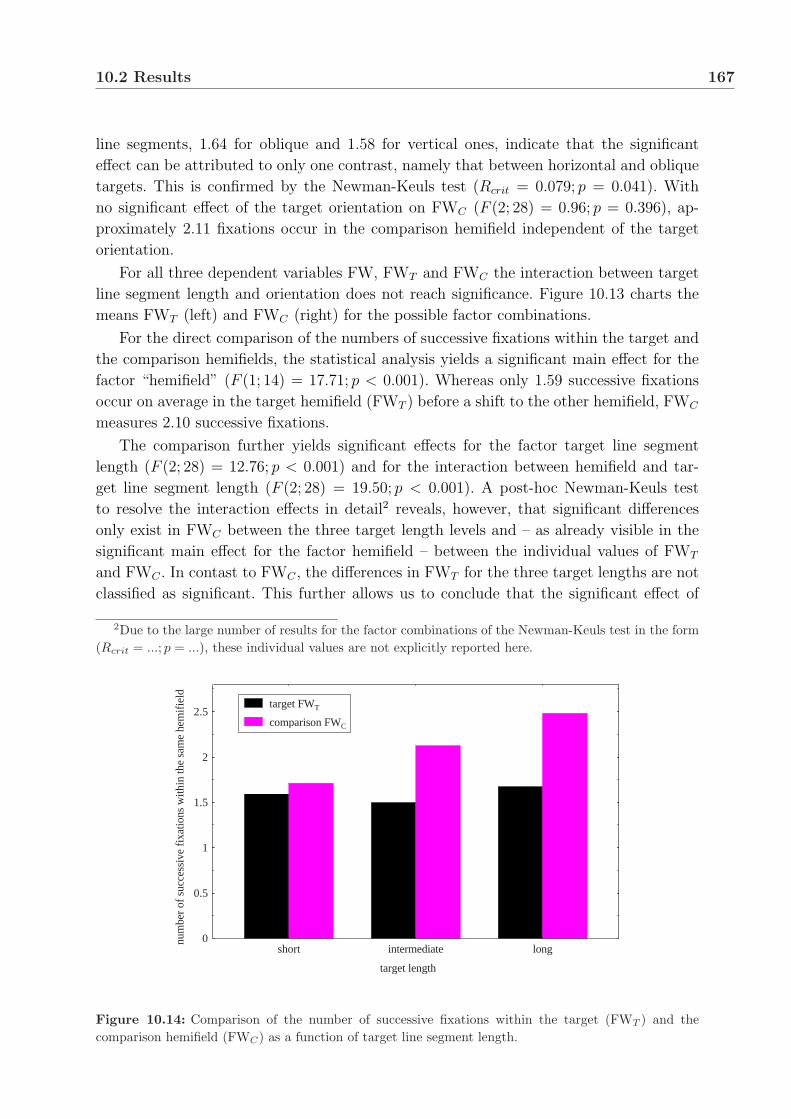
10.2 Results 167
line segments, 1.64 for oblique and 1.58 for vertical ones, indicate that the significant
effect can be attributed to only one contrast, namely that between horizontal and oblique
targets. This is confirmed by the Newman-Keuls test (Rcrit = 0.079; p = 0.041). With
no significant effect of the target orientation on FWC (F (2; 28) = 0.96; p = 0.396), ap-
proximately 2.11 fixations occur in the comparison hemifield independent of the target
orientation.
For all three dependent variables FW, FWT and FWC the interaction between target
line segment length and orientation does not reach significance. Figure 10.13 charts the
means FWT (left) and FWC (right) for the possible factor combinations.
For the direct comparison of the numbers of successive fixations within the target and
the comparison hemifields, the statistical analysis yields a significant main effect for the
factor “hemifield” (F (1; 14) = 17.71; p < 0.001). Whereas only 1.59 successive fixations
occur on average in the target hemifield (FWT ) before a shift to the other hemifield, FWC
measures 2.10 successive fixations.
The comparison further yields significant effects for the factor target line segment
length (F (2; 28) = 12.76; p < 0.001) and for the interaction between hemifield and tar-
get line segment length (F (2; 28) = 19.50; p < 0.001). A post-hoc Newman-Keuls test
to resolve the interaction effects in detail2 reveals, however, that significant differences
only exist in FWC between the three target length levels and – as already visible in the
significant main effect for the factor hemifield – between the individual values of FWT
and FWC . In contast to FWC , the differences in FWT for the three target lengths are not
classified as significant. This further allows us to conclude that the significant effect of
2Due to the large number of results for the factor combinations of the Newman-Keuls test in the form(Rcrit = ...; p = ...), these individual values are not explicitly reported here.
target length
num
ber
of s
ucce
ssiv
e fi
xatio
ns w
ithin
the
sam
e he
mif
ield
0
0.5
1
1.5
2
2.5
short intermediate long
target FWT
comparison FWC
Figure 10.14: Comparison of the number of successive fixations within the target (FWT ) and thecomparison hemifield (FWC) as a function of target line segment length.

168 Experiment S1: Simultaneous Dynamic Length Assessment
the factor target line segment length – when comparing FWT and FWC – can mainly be
attributed to differences that exist between the absolute values for FWT and FWC and
the differences FWC shows for the three target lengths. FWT varies far less with respect
to these levels (cf. results for overall FW). To qualitatively support these dependences,
Figure 10.14 illustrates the relevant means for the comparison of FWT and FWC as a
function of target line segment length.
Saccade Length SL
As already indicated, the investigation of the saccade length SL should also help to under-
stand the processes that govern the perception of a single line segment and its memorisa-
tion for the subsequent matching with the comparison line segment in the other display
hemifield. Rather than considering a “global” SL, the “local” saccade lengths SLT and
SLC are particularly promising. SLT measures the average saccade length within the tar-
get hemifield, SLC measures that within the comparison hemifield. As for FW, the saccade
length in the intermittent section will not be considered – again, the insufficient number
of fixations in that display section renders the computation of SLI void. With respect to
the more global understanding of the comparison process, the saccade length between the
two relevant stimulus regions SLb will be investigated first.
An analysis of variance tests the effects of the factors target line segment length and
orientation on the saccade length between the two hemifields SLb. It yields significant
main effects for both factors on SLb: (F (2; 28) = 3.26; p < 0.001) for target length and
(F (2; 28) = 3.47; p < 0.001) for target orientation. The comparison of means shows that
SLb decreases from 21.21o for short target line segments, through 20.82o for intermedi-
ate to 19.54o for long target line segments. A post-hoc comparison of means using the
Newman-Keuls test produces significant differences between all levels of target length:
(Rcrit = 0.354; p = 0.029) for the comparison between short and intermediate lengths,
(Rcrit = 0.446; p < 0.001) for short vs. long lengths and (Rcrit = 0.421; p < 0.001) for
intermediate vs. long lengths. When the target line segment is oriented horizontally, SLb
covers 20.08o, 20.43o for oblique and 21.06o for vertical targets. The differences between
all target orientation levels are significant: (Rcrit = 0.199; p = 0.002) for the comparison
between horizontal and oblique orientations, (Rcrit = 0.240; p < 0.001) for horizontal vs.
vertical orientations and (Rcrit = 0.239; p < 0.001) for oblique vs. vertical orientations.
In addition, the interaction between the two factors target line segment length and
orientation also reaches significance (F (4; 56) = 2.63; p < 0.001). This can be attributed
to the observation that, when short target line segments are presented, SLb remains almost
constant at approximately 21.2o independent of the target orientation. A post-hoc compar-
ison of means using the Newman-Keuls test confirms that no significant differences exist
between the three orientation levels when the target is short: (Rcrit = 0.277; p = 0.430)
for horizontal vs. oblique orientation, (Rcrit = 0.234; p = 0.820) for horizontal vs. vertical
orientation and (Rcrit = 0.259; p = 0.565) for oblique vs. vertical orientation. This not
the case for intermediate and long targets. In case of intermediate length, SLb increases
slightly from 20.5o for horizontal to 20.7o for oblique and then significantly to 21.4o for

10.2 Results 169
vertical target line segments. Such an increase in SLb over the three orientations is even
more pronounced – and significant between all levels – for long targets: From 18.5o through
19.5o to 20.6o for horizontal, oblique and vertical target orientations, respectively. Accord-
ingly, a Newman-Keuls test reveals significant differences between (almost) all orientation
levels. Intermediate targets: (Rcrit = 0.355; p < 0.001) for horizontal vs. vertical orien-
tations and (Rcrit = 0.348; p < 0.001) for oblique vs. vertical orientations. Long targets:
(Rcrit = 0.349; p < 0.001) for horizontal vs. oblique orientations, (Rcrit = 0.350; p < 0.001)
for horizontal vs. vertical orientations and (Rcrit = 0.353; p < 0.001) for oblique vs. vertical
orientations. Exception: No significant difference in SLb can be found between horizon-
tal and oblique orientations for intermediate target length (Rcrit = 0.279; p = 0.442).
Figure 10.15 charts the mean values of SLb as a function of target line segment length,
separated for the three target orientations.
target length
sacc
ade
leng
th b
etw
een
hem
ifie
lds
SLb
(deg
rees
)
16
17
18
19
20
21
22
23
short intermediate long
horizontal
oblique
vertical
Figure 10.15: Saccade length between the two stimulus hemifields SLb as a function of target linesegment length and orientation.
Let us now consider the “local” saccade lengths. The analysis of variance for SLT
reveals a significant main effect for the factor target line segment length (F (2; 28) =
1.45; p < 0.001). Averaged over the three possible target orientations, the saccade length
within the target section SLT increases from 1.56o for short target line segments through
2.31o for intermediate to 2.94o for long ones. A post-hoc comparison of means using the
Newman-Keuls test produces significant differences between all levels of target length:
(Rcrit = 0.446; p < 0.001) for the comparison between short and intermediate lengths,
(Rcrit = 0.427; p < 0.001) for short vs. long lengths and (Rcrit = 0.357; p = 0.003) for
intermediate vs. long lengths.
Another main effect can be established for the factor target line segment orientation
(F (2; 28) = 1.54; p < 0.001). Here, SLT decreases from 2.94o for horizontal to 2.02o
for oblique and further to 1.81o for vertical targets. Here, only the differences between

170 Experiment S1: Simultaneous Dynamic Length Assessment
the following target orientation levels are significant: (Rcrit = 0.410; p < 0.001) for the
comparison between horizontal and oblique orientations and (Rcrit = 0.412; p < 0.001)
for horizontal vs. vertical orientations. Means of SLT do not significantly differ for the
comparison of oblique and vertical orientations (Rcrit = 0.338; p < 0.385).
The interaction between target line segment length and orientation also exerts a sig-
nificant effect on SLT (F (4; 56) = 1.62; p < 0.001): Whereas SLT remains almost constant
at approximately 1.5o for short targets, irrespective of their orientation, it significantly
decreases from horizontal through oblique to vertical for intermediate – 2.97o, 2.04o and
1.87o, respectively – and long targets – 4.32o, 2.47o and 2.04o, respectively. Accordingly,
a post-hoc comparison of means using the Newman-Keuls test confirms that no sig-
nificant differences exist between the three orientation levels when the target is short:
(Rcrit = 0.408; p = 0.671) for horizontal vs. oblique orientation, (Rcrit = 0.315; p = 0.732)
for horizontal vs. vertical orientation and (Rcrit = 0.428; p = 0.613) for oblique vs. ver-
tical orientation. Furthermore, the Newman-Keuls test reveals significant differences be-
tween (almost) all orientation levels. Intermediate targets: (Rcrit = 0.487; p < 0.001)
for horizontal vs. oblique orientations and (Rcrit = 0.501; p < 0.001) for horizontal
vs. vertical orientations. Long targets: (Rcrit = 0.492; p < 0.001) for horizontal vs.
oblique orientations, (Rcrit = 0.499; p < 0.001) for horizontal vs. vertical orientations and
(Rcrit = 0.485; p = 0.007) for oblique vs. vertical orientations. Exception: No significant
difference in SLT can be found between oblique and vertical orientations for intermediate
target length (Rcrit = 0.305; p = 0.981). Figure 10.16 (top left) illustrates the mean values
for SLT as a function of target length and orientation.
In contrast to SLT , the analysis for the saccade length within the comparison stimulus
hemifield SLC shows a significant main effect for the factor target line segment length
only (F (2; 28) = 3.46; p < 0.001). The comparison of means yields that SLC increases
from 1.40o for short through 2.25o for intermediate to 3.89o for long target line segments.
A Newman-Keuls test produces significant differences between all levels of target length:
(Rcrit = 0.441; p = 0.001) for the comparison between short and intermediate lengths,
(Rcrit = 0.537; p < 0.001) for short vs. long lengths and (Rcrit = 0.530; p = 0.003) for
intermediate vs. long lengths.
No significant effect on SLC can be established for the factor target line segment
orientation (F (2; 28) = 0.006; p = 0.902). Irrespective of the target orientation, SLC
measures approximately 2.6o. (Remember that the comparison line segment is always
oriented horizontally.) The interaction between target length and orientation does not
reach a significant level either (F (4; 56) = 0.05; p = 0.508). Figure 10.16 (top right)
illustrates the mean values for SLC as a function of target length and orientation.
A comparison between SLT and SLC demonstrates no significant main effect for the
factor hemifield (F (2; 28) = 0.02; p = 0.519). On average, saccade length measures 2.35o
within the target hemifield and 2.49o within the comparison hemifield. However, as could
be expected from the previous separate analyses of SLT and SLC , the interactions be-
tween the factors hemifield and target line segment length (F (2; 28) = 1.36; p < 0.001)
and between the factors hemifield and target line segment orientation reach significance
(F (2; 28) = 0.54; p < 0.001). Whereas SLT and SLC do not considerably differ for short

10.3 Discussion and Conclusions 171
target length
sacc
ade
leng
th w
ithin
targ
et h
emif
ield
SL
T (
degr
ees)
0
1
2
3
4
5
6
short intermediate long
horizontalobliquevertical
target length
sacc
ade
leng
th w
ithin
com
pari
son
hem
ifie
ld S
LC (
degr
ees)
0
1
2
3
4
5
6
short intermediate long
horizontalobliquevertical
target length
sacc
ade
leng
th w
ithin
hem
ifie
ld (
degr
ees)
0
1
2
3
4
5
6
short intermediate long
target SLT
comparison SLC
target orientation
sacc
ade
leng
th w
ithin
hem
ifie
ld (
degr
ees)
0
1
2
3
4
5
6
horizontal oblique vertical
target SLT
comparison SLC
Figure 10.16: Saccade length within the target hemifield SLT (top left) and within the comparisonhemifield (top right) as functions of target line segment length and orientation. Comparison of the saccadelength within the target (SLT ) and comparison (SLC) sections as a function of target line segment length(left) and orientation (right).
and intermediate target lengths, SLC is significantly longer than SLT for long targets.
With respect to the target orientation, SLT decreases from horizontal through oblique
to vertical targets whereas SLC remains about constant, irrespective of the target orien-
tation. A post-hoc Newman-Keuls test confirms these interaction details. However, the
individual values are not explicitly reported here due to the large number of results for
the factor combinations. Figure 10.16 illustrates the relevant means for the comparison
of SLT and SLC as a function of target line segment length (bottom left) and orientation
(bottom right).
10.3 Discussion and Conclusions
Let us recall the context within which the findings of the current Experiment S1 have
to be considered and interpreted. One of the fundamental questions this study addresses
concerns the accuracy that humans can achieve in the assessment and matching of line

172 Experiment S1: Simultaneous Dynamic Length Assessment
segment lengths in a simultaneous comparison scenario. With the variation of characteris-
tic dimensions, namely length and – presumingly even more so – orientation, for this type
of stimulus the study also aims to thoroughly investigate visual illusory effects on the
assessment accuracy. The empirically acquired psychophysical data, such as the length
deviation DL, allows us to manifest and exactly quantify the illusory effects induced
by the various stimulus feature combinations. Rather than relying only on “classical”
psychophysical results, the interpretation of additional eye-movement recordings should
facilitate the understanding of the occurrence of these illusory effects and their extents.
The results provide information on both the “local” intra-line-segment perception aspects
as well as those concerning the “global” inter-line-segment comparison mechanisms of the
length perception and assessment task. The discussion should provide insight in how far,
for example, “visual measurement” of length, “lean” fixation patterns or length extrap-
olation strategies and peripheral processing influence length assessment and explain the
observations. The discussion of eye-movement parameters may also help to understand
certain misjudgements of line segment length, induced by the horizontal-vertical illusion.
The interpretation of the sensorimotor data might further allow us to infer how mental
representations of line segments and their relevant attributes are generated, memorised,
dynamically updated and recalled for comparison. On aggregate, this should constitute a
comprehensive image of the applied visual problem-solving strategy and thus make the
fundamental steps of the cognitive structure for this type of visual comparison task more
transparent. Finally, with a view to the subsequent Experiment S2, the data collected
here provides the basis for determining which differences in line segment lengths should
be easy or difficult to discriminate.
As before, we will briefly summarise the most outstanding effects that were observed
in Experiment S1:
1. The lengths of the target line segments are overestimated throughout.
2. The factor target line segment length exerts a significant effect on all dependent
variables, except for FDI .
3. The factor target line segment orientation mainly exerts significant effects on specific
dependent variables, namely on the local measures in the target hemifield such as
FDT , FWT and SLT . In addition, orientation effects on DL, NDI and SLb reach
significance.
How can these observations and the associated, specific means for the factor combinations
be interpreted, how do their relations and interactions form a comprehensive “image” of
the processes involved in simultaneous dynamic length assessment and matching? To
achieve this goal, we will now discuss and integrate the experimental results step by step
in an attempt to gradually build up and complete such an image.
Compared to the reaction times measured in the eccentricity experiments E0, E1
and E2 (approximately 660 ms), RTs are now much longer (approximately 4620 ms).
This is not very surprising and can mainly be attributed to the experimental task in Ex-
periment S1 which is quite different from the previous ones. Not only the perception and
10.3 Discussion and Conclusions 173
memorisation of a single item and its length has to be accomplished, but also the com-
parison procedure. This procedure itself is a complex one, comprising memory recall and
the actual feature comparison. The procedure also includes the dynamic length match-
ing of the comparison stimulus. Furthermore, the number of inter-hemifield saccades SB
indicates that the whole process is often re-iterated several times.
However, the higher complexity of the task might not account for the differences in
RT alone. It must probably be considered as well that the free gaze condition favours
other strategies to accomplish this task. With the gaze not being restricted, subjects
in the current experiment can now follow more convenient, conceivably more “natural”
visual strategies. The analyses of eye-movement parameters prove that such alternatives
are indeed being used. Subjects foveally explore the relevant stimulus regions, generally
yielding multi-fixation gaze trajectories – as will be discussed later. This detailed visual
analysis must consequently lead to a further increase of RT.
The significant increase of RT from short through intermediate to long target line seg-
ments can be considered a first indicator for the structure of the visual strategies pursued
during length assessment and adjustment. Even without knowledge of the supportive eye-
movement data, it can thus be speculated that the increase of RT might be a consequence
of an increase of the number of fixations that are necessary to assess longer line segments.
If this assumption holds, we can further speculate that the visual strategy applied incor-
porates some sort of “visual measurement” of line segment lengths. It appears that this
procedure requires an increasing number of fixations for longer line segments. Long line
segments in particular can probably not be assessed as a whole; even two (end point) fix-
ations might not suffice. Instead, a “step-by-step” measurement via intermittent fixations
could be feasible, leading to prolonged response times. When such a strategy is indeed
applied, the generation, memorisation, recall, comparison and matching or adaptation of
the corresponding mental representation(s) becomes an increasingly complex cognitive
task. The longer the respective line segments are, the more “constituents” have to be
integrated into the representation. Such models might be more difficult to maintain or
more prone to decay (“blur”) and thus require additional (visual) verification, possibly
manifested in an increasing number of inter-stimulus saccades – aspects then reflected in
RT as well.
In contrast to the target length, the lack of a significant effect of the target orientation
on RT does not allow for much speculation about possible visual strategies applied in
dynamic line segment length assessment. However, the lacking orientation effect itself
comes as a surprise when we take into account that the oblique and vertical targets
induce a horizontal-vertical illusion – remember that the comparison is always horizontally
oriented. These conditions could have been thought to constitute more challenging tasks
than when comparing horizontal targets with horizontal comparisons. Subjects might just
not be aware of the illusion; they obviously do not attempt to compensate for the difficult
comparison conditions by spending more time on the task completion. Irrespective of the
subjects’ apparent unawareness of the visual illusion, differences in RT between the three
orientation levels could also have been expected because switching between horizontal
“scanning mode” in one hemifield and oblique/vertical mode in the other could have

174 Experiment S1: Simultaneous Dynamic Length Assessment
been assumed to be more challenging than for horizontal–horizontal comparisons where
the scanning mode remains horizontal in both hemifields. Yet, none of these aspects is
reflected in RT.
Indeed, the significant interaction effect between target length and orientation on RT –
when targets are short RT decreases from horizontal to oblique and again to vertical tar-
gets, whereas RT remains almost constant for intermediate and long targets, irrespective
of their orientation – seems to suggest the opposite. When the target line segments are
short, subjects might actually try to accomplish the horizontal–horizontal matching task
very accurately because this configuration appears to be easiest and thus most promising
to “score” highly – although this extra accuracy does compromise RT, but not consider-
ably. On the other hand, the combinations of oblique or vertical targets and horizontal
comparisons might be assumed to be rather difficult so that achieving a high accuracy
in matching the lengths would compromise RT too much and is not considered efficient.
This, however, appears to apply only when short target line segments have to be assessed.
For intermittent and long targets, the differences in RT between the different orientation
levels fade, possibly – as discussed in the previous paragraph – as greater lengths could
require a more thorough visual analysis anyway.
The reluctance of subjects to spend more time on the assumedly more difficult
horizontal–oblique and horizontal–vertical comparisons than on the horizontal–horizontal
ones could be one reason why the accuracy of the length matching, manifested in the rela-
tive length deviation DL, is better for the latter configuration of the target and comparison
line segments. Furthermore, the increased length deviations when target and comparison
line segments are not oriented co-linearly clearly indicate the presence of the horizontal-
vertical illusion. The illusion yields its typical effects on perceived length, confirming a
significant length overestimation of the target line segment when presented in oblique or
vertical orientation. Subjects do obviously not succeed in ignoring or in compensating for
the perceived length differences induced by the illusion – which they might not even be
aware of. Thus, the incorrectly adjusted comparison lengths for obliquely and vertically
oriented targets emerge as a logical consequence.
To understand the significant improvement of the assessment accuracy – i.e. the de-
crease of DL – for intermediate and, further, for long targets, compared to the length
deviation for short ones, reference must be drawn to the discussion of RT. Viewed in
conjunction with the prolonged reaction times for longer targets, the deceiving effects of
the horizontal-vertical illusion might lessen. As the longer RTs are thought to indicate a
more thorough visual analysis and subsequent mental representation of the stimuli, illu-
sory effects could probably be easier realised and more conveniently compensated than
during short inspection times. However, even then the illusion persists.
A finding that is certainly worth of discussion is that the overestimation of target
lengths also occurs for equally oriented segments. One should have assumed that no “di-
rectional” effect, i.e. no over- or underestimation, should have occurred when both target
and comparison are oriented horizontally. Let us consider possible explanations. As the
two stimulus constituents do not differ with respect to their appearance (orientation,
colour, thickness, intensity, etc.) on the display screen, it could be assumed that the ad-

10.3 Discussion and Conclusions 175
justment procedure is responsible for the persisting overestimation. Starting point effects
can be excluded as the initial lengths of the comparison stimuli were pseudo-randomly
chosen so that they were shorter than the targets in fifty percent of the trials and longer
in the remaining trials.
The decision to always present the target in the left hemifield and the comparison in
the right hemifield probably yields a point for criticism. If this had been randomly varied,
however, the initial localisation process – “Which line segment is the adjustable one?” –
would certainly have caused more interference than the current procedure. Furthermore,
no reference in literature could be found that indicates such side effects for these or similar
experimental scenarios. This leaves the dynamic adjustment itself to cause the observed
effect. It can only be speculated here that the “movements” of the comparison line segment
when subjects dynamically adjust its length interfere with the preservation and recall
of the memorised target line segment. The symmetric adaptation of the comparison –
i.e. the line segment length changes symmetric to its center point and not at one end
only – could worsen this interference. Visual attention is drawn to both end points of
the comparison line segment which probably further complicates the matching with the
target representation. Although the underlying principles remain unclear, this interference
could distort the length representation in such a way that it is recalled longer than it was
originally perceived and memorised – and thus also lead to the overestimation of horizontal
targets. If this were true, it should hold for long lines in particular. Alternatively, and
independent of the dynamic procedure, it could also be hypothesised that the “decay” of
the representation between memorisation and recall generally leads to the expansion of the
representation over (even short) time periods. To comprehensively explore these effects
and validate the proposed hypotheses, it would be recommended to conduct a whole new
series of experiments. It must be noted, however, that even when data is corrected for the
base “offset”, all above-mentioned effects persist and conclusions thus remain valid.
Let us now turn to the discussion of the eye-movement parameters. To what extent do
they contribute to explaining the underlying processing mechanisms and perception princi-
ples which lead to the assessment–memorisation–adjustment/matching performance? How
can eye-movement parameters account for phenomena such as the observed horizontal-
vertical illusion? For most such parameters investigated here, both global and local mea-
sures are considered. This distinction is motivated by the assumption that corresponding –
global and local – fundamental mechanisms characterise the assessment strategy. Glob-
ally, shifts of attention occur between the two stimulus constituents – the target and
comparison line segments – which are then locally analysed. The associated global eye-
movement parameters are assumed to yield information mainly on the task complexity
and the general influence of the length and orientation factor levels on visual percep-
tion. The respective local measures should foster our understanding of the detailed visual
perception of the stimuli themselves and how line segments are mentally represented.
The proposed distinction appears intuitive – both with respect to the assumed global
and local strategies and with respect to the location of designated “areas of interest”.
However, intuition cannot always be trusted, but requires some sort of validation. In the
present case, the distribution of fixations (see Figure 10.6) indeed seems to lend support

176 Experiment S1: Simultaneous Dynamic Length Assessment
to the hypothesised strategy. Fixation points are cumulated in proximity to the target and
comparison line segments. They also appear more numerous in an intermittent display
section, extremely few fixations are located elsewhere. To demonstrate that this qualitative
result holds, a cluster analysis (k-means clustering) was computed. With the help of this
method it was thus possible to successfully validate the obvious “regions of interest” in a
quantitative manner. These are otherwise often arbitrarily determined.
Furthermore, the clustering procedure and a subsequently applied principal compo-
nent analysis (PCA) yield first insights into the local scanning strategies applied to assess
the individual lengths of the stimuli. Due to the few fixations in the intermittent display
section – compared to the numbers of fixations in proximity to the two line segments – the
k-means clustering algorithm was only computed for two clusters. Thus, only two ellipses
emerge as the result of the subsequent PCA (marked red in Figure 10.6). Their character-
istic features, namely shape and, specifically, location and orientation, then indicate the
following: The offset of the ellipsis’ center of gravity suggests that target line segments
are only partially assessed foveally and their lengths extrapolated, possibly taking into ac-
count peripheral visual information. The direction of the offset towards the display center
for horizontal targets and towards the upper end point for oblique and vertical ones also
speaks for an efficient visual strategy that takes into account only that part of the target
line segment that is closer to the comparison.
The shape of the ellipsis makes clear that indeed only parts of the target line segment
are considered, in particular when the targets are longer. In contrast, the axes along
the first principal component of the “comparison ellipses” are actually longer than the
corresponding comparison line segment. This can certainly be attributed to the changing
lengths of the comparison during the dynamic length adaptation. For certain adaptation
steps in the course of the adjustment procedure, the comparison length exceeded the final
length.
Finally, the orientations of both the target and the comparison ellipses resemble that
of the respective line segments. The target ellipses only reach such high co-linearity for
horizontal targets whereas the comparison ellipses very accurately do so. However, even
for oblique and vertical orientations, the target ellipses are correspondingly oriented. It
can thus be assumed that fixations indeed rather closely follow the line segments during
the local scanning, possibly even “visually measuring” the line segment lengths. However,
as the distributions of fixations do not contain temporal information that determines the
sequences of fixations, the assumption of “visual measurement” of line segment lengths –
or parts thereof – must still be validated. The discussion of the numbers of successive
fixations within the same hemifield FW should clarify this point. And indeed, as we will
see soon, this measure supports the yet vague assumption.
The rather general discussion so far provided important information concerning the va-
lidity of the chosen measures. Based on the distributions of fixations and their parametri-
sations using computational methods such as clustering and principal component analysis,
the results of the more specific eye-movement parameters can now be discussed “on safe
ground”. Furthermore, the previous discussion yielded first insights into both the globally
and locally applied visual analytic strategies already. This encourages a further discussion

10.3 Discussion and Conclusions 177
that is guided by these premises.
In analogy to the presentation of the statistical results in the previous section, the
overall number of fixations NF will be considered first. The significant increase of NF
indicates that the task complexity rises the longer the target line segments – and, logically,
the comparison ones also – become. However, as we noticed that the assessment accuracy
improved for longer line segments, it is apparent that the greater visual effort “pays
off”. Subjects thus notice the more demanding task of assessing long line segments and
successively compensate for it by a more detailed foveal visual analysis – gaze probably
directed at the relevant stimuli rather than at blank space. If we assume that the awareness
of the presence of a visual illusory effect also results in a more thorough analysis of the
scene, a considerable increase in NF for oblique and vertical target would have been
expected in an attempt to resolve the illusion. However, a dependence of NF on target
orientation cannot be found. We must thus conclude that no attempt – in terms of extra
visual/foveal effort – is made to compensate for the higher, illusion-induced complexity.
The significant overestimation of the length of the target line segment when the horizontal-
vertical illusion is present confirms that this is indeed the case.
The separate analyses of the local numbers of fixations in the target and comparison
hemifields confirm these conclusions. Neither NFT nor NFC greatly varies with the target
orientation as could have been expected following the argumentation for the overall NF.
The increase of NFT as well as NFC for longer targets shows that not only one of the
two variables is responsible for the increase of the overall NF from short through inter-
mediate to long target line segments, but that both stimulus constituents require a more
detailed visual analysis in order to achieve satisfactory length assessment and matching
accuracy. The significant differences between the absolute values of NFT and NFC can
only be attributed to the different requirements of the perceptual and cognitive tasks
that subjects have to accomplish when looking either at the target or the comparison line
segment. The visual assessment of the line segment in focus, the mental representation
and storage of its length, the recall of the representation of the other line segment and its
memorised length and the mental matching constitute the tasks in both hemifields. The
dynamic adjustment of the comparison stimulus, however, requires extra cognitive and,
as significantly higher values for NFC demonstrate – compared to those for NFT – extra
visual effort as well. The process of length adaptation first requires a dynamic update
of the comparison representation in accordance with the adaptation steps and, second,
a repeated (mental) matching with the memorised target model and its length. Of these
two additional processes, it is most likely that the first one can be characterised by further
fixations. These will most certainly occur when the adapted comparison (length) has to
be assessed again to yield the updated representation.
The very low absolute number of intermittent fixations NFI renders the interpretation
of this measure problematic, in particular with respect to the effects of the factors target
length and orientation thereupon. On the other hand, it can reliably be claimed that
the contribution of peripheral vision on global visual analytic strategies for this specific
experimental setting is negligible. If intermittent fixations are assumed to be indicators for
peripheral processing of the line segments in the target and comparison hemifields, simply

178 Experiment S1: Simultaneous Dynamic Length Assessment
too few occur to be possibly relevant for the assessment process. If these intermittent
fixations are not considered relevant “anchor” locations for peripheral processing, but
intermediate points “on the way” from target to comparison or vice versa, the significant
effects of both target length and orientation on NFI might indeed be interesting.
Two observations seem to speak in favour of the idea of intermediate fixations be-
ing “on the way” orientation points. First, the fixation duration FDI is relatively short,
probably too short to allow for explicit peripheral perception. This is also supported by
the reaction times of the eccentricity Experiments E0–E2 which were considerably longer.
Even more than FDI , the angle between a saccade to and the subsequent one from an
intermittent fixation point imply that such locations are only passed on the way: In 95%
of all cases, this angle is larger than 135o, indicating that no drastic direction changes
occur between two successive saccades. This clearly speaks in favour of a sequence of
“in-line” fixations so that the “gaze passes through” the region between the two stimulus
constituents “on the way” from one line segment to the other. (When the angle between
two successive saccades is considerably smaller then 90o, the intermittent fixation rather
marks a “turning point”. The second saccade then leads back to where the first saccade
started from.) It can now be assumed that even fewer intermittent fixations are necessary
when long line segments are shown, in particular when they are horizontally oriented.
They are then more closely located to each other than short ones and subjects do not
need intermittent fixations to guide their gaze from one stimulus constituent to the other.
That is exactly what the significant decrease of NFI from short through intermediate to
long target lengths and the significant increase of NFI from horizontal through oblique to
vertical target orientations demonstrate.
Let us also include the results of the PCA that describes the distribution of fixations
in the target section. The analysis indicated that more fixations are located in proximity
to the upper (inner) half of the target line segment if it is vertically (obliquely) oriented.
When the gaze moves over from the horizontal comparison stimulus to an oblique or
vertical target, or, more specifically, to its upper part, often an intermittent fixation might
be required to change direction from the horizontal to an upwardly directed saccade.
This process could also contribute to significantly higher numbers of fixations in the
intermittent display section for oblique or vertical targets. However, no reference could be
found in literature that reports a similar pattern of the inter-stimulus gaze trajectory.
Next, the discussion of the overall fixation duration FD and, specifically, its decrease
from short through intermediate to long target line segments should yield further in-
sight into the visual perception processes that govern the assessment of line segments
and their lengths. In conjunction with the observation that fewer fixations occur when
line segments are short(er), it can be concluded that subjects obviously consider a visual
scanning strategy that relies on fewer, but more “intense” fixations more efficient for the
length assessment of line segments whose extent is restricted to a small local region. The
prolonged fixation times might also allow for some peripheral processing of those parts of
the line segment that are not directly foveally perceived. In contrast, the data seems to
suggest a spatially more detailed visual analysis for longer line segments that, in return,
does not necessarily require such long fixation times as for short ones.

10.3 Discussion and Conclusions 179
In addition, it could also be concluded that possibly more fixations occur in close
proximity to each other when targets are longer. During these fixations, less visual infor-
mation must be processed due to an overlap of the neighbouring, foveally scanned areas.
Fixations could consequently be executed quicker. Furthermore, the only type of locally
proximal fixations that would appear to make sense in the current setting are those that
show a linear pattern. Fixations would probably be aligned along a line segment which
might yield further support for an underlying strategy of “visually measuring” the line
segments in order to obtain the relevant length information.
Alternatively, another explanatory approach should be considered. Assuming that
short and long line segments require the same amount of processing, we could still expect
more but shorter fixations for long lengths. This is because larger objects induce larger
shifts of attention, which, in turn, are more likely to cause saccades. Consequently, more
but shorter fixations should be expected.
The separation of FD into the local fixation durations shows that these conclusions
must be further diversified and do not uniformly apply to both FDT and FDC . The consid-
erable differences between these two measures, that fixations in the comparison hemifield
last much longer than those in the target hemifield, can probably again be attributed to
the influence of the dynamic adjustment procedure. A closer look at the procedure clari-
fies this. A joint analysis of the adjustment steps – also stored in the eye-tracker data file
and synchronised with the eye-movement recordings – and the fixations shows that often
only a single fixation occurs (never more than two) during each adjustment step (several
of these are required to accomplish the whole assessment and matching task). The eye
gaze thus remains stationary considerably longer than in the target hemifield where no
such procedure “delays” fixation times.
Another interesting point for discussion with respect to FDT and FDC is that orienta-
tion effects on fixation times reach significance only when a fixation is “directly” influenced
by orientation, i.e. for those fixations in the target hemifield. This significant influence on
FDT is not “carried over” to the comparison side, where line segments are always oriented
horizontally. FDC remains unaffected by targets that have oblique or vertical orientation.
We may consider this as an indicator for independent assessment processes in the two
hemifields. The visual analysis of the comparison does not take orientation effects into
account which might possibly have been relevant for the compensation of the horizontal-
vertical illusion – further support for the idea that such a compensation is not attempted
which thus renders the observed illusory effect even more explicable.
What does the analysis of the number of saccades between hemifields SB tell about the
“nature” of the simultaneous comparison process? As motivated earlier, not only the small
number of fixations in the intermittent display section, but also the obtuse angle between
saccades to and from these intermittent fixations allow us to define SB as a measure for
saccades that directly link the two relevant stimulus constituents. SB is thus one of the
essential parameters when it comes to understanding the global comparison process. SB
is the “joint” between the individual local assessment processes of the stimuli themselves
and describes the global shifts of attention. Their considerable increase for longer targets
(but not for greater differences between target and comparison angles, i.e. when targets

180 Experiment S1: Simultaneous Dynamic Length Assessment
are oriented obliquely or vertically) makes clear that significantly more matching steps are
required before subjects are satisfied with their estimate of the length of the comparison
line segment. More specifically, the additional shifts of attention between the two stimulus
constituents for longer target line segments indicate that extra local visual analysis of such
line segments is required. Long line segments demand at least one extra local assessment
operation. Again, subjects do not consider differently oriented target and comparison line
segments to be worth any extra visual analysis, ignoring – or being unaware of – the
illusion-induced higher complexity of the task.
In close relation to SB, the saccade length between the two stimulus hemifields SLb
also contributes to the comprehension of the global shifts of attention. The fact that the
distance between the target and comparison line segments decreases the longer the line
segments are is accordingly reflected by shorter inter-stimulus saccades. This is also true
for the distance changes caused by orientation variation. In correspondence, SLb increases
when the target is oriented obliquely or vertically rather than horizontally. Although the
extent of the changes in saccade lengths do not directly reflect the length differences
between the levels of the target length – or the changes in distance between the two
line segments when their orientations change – this observation can still be considered
“evidence” that the gaze is indeed guided by the stimuli. This clearly speaks in favour of
predominant foveal processing rather than a peripheral perception strategy on the global
processing level. Furthermore, SLb provides valuable hints towards which parts of the line
segments might be primarily considered for the subsequent local visual analysis of the line
segment. Specifically, it supports the discussion of the distribution of fixations and the
corresponding principal component analysis: SLb being generally shorter than the distance
between the two line segments’ center points (DTC) suggests that probably the innermost
parts of the line segment are evaluated, pointing to an efficient visual processing strategy.
However, it is also known that long saccades – such as the inter-stimulus saccades in the
present scenario – typically undershoot in all tasks. Some of the difference between SLb
and DTC might thus have to be attributed to this observation.
So far, the discussion of results concerned variables which mainly contribute to the
understanding of the more global aspects of line segment assessment, even when local
measures derived from NF and FD were considered. However, the discussion also gave
rise to various assumptions about the processes that could determine the local assessment
of the individual length of the respective line segments, the generation and the recall of
their internal representations. The following discussion of the local measures will shed
more light on these principles so that finally a comprehensive image of global and local
aspects involved in the simultaneous assessment and matching of lengths of line segments
should emerge.
The joint discussion of the number of successive fixations within the same hemifield
FW and the saccade lengths within that respective hemifield should now yield the desired
insight into the local strategies pursued during the detailed visual analyses of the line
segments. The overall FW strongly supports the previous assumption that about two
fixations occur that could be required to visually measure the length of a line segment or
at least parts thereof. As FW varies between approximately 1.7 for short targets and 2.1
10.3 Discussion and Conclusions 181
for long ones, such a strategy appears to be particularly feasible for those line segments
that cannot completely be assessed foveally, i.e. intermediate and long ones. However,
even short line segments often require more than just one fixation in order to assess their
length. The distribution of fixations implies that indeed locations on or at least in close
proximity to the respective line segments are fixated – rather than just two arbitrary
points within the target or comparison section. Similar observations are also common in
other tasks as fixations almost never land in “empty space”.
The separate analyses of FWT and FWC also demonstrate that in this dynamic ad-
justment scenario the comparison line segment in particular requires multi-fixation as-
sessment. Compared to approximately 1.6 successive fixations in the target hemifield, 2.1
are executed in the comparison one. It appears likely that after each adjustment of the
comparison line segment a new visual measurement of its length is performed. When long
targets are presented, even more than just two successive fixations occur in proximity
to the comparison (which is “long” as well). This could be interpreted as a local visual
strategy in that hemifield that is constituted by an initial fixation point which is kept
stable during the adjustment step – the prolonged fixation times FDC speak in favour
in this respect, too – and the subsequent new measuring of the current length of the
comparison line segment.
In contrast, the average FWT , which is well below two successive fixations, could indi-
cate that typically the target is only once visually measured, assumedly by a two-fixation
procedure at the beginning of each trial. Then, in the subsequent inter-hemifield compari-
son steps, the initially generated and memorised mental representation of the target might
only require a “refreshing”. Not always, but in most cases, this can probably be realised by
executing just a single fixation in proximity to the target. The target representation thus
refreshed is then used for the following mental comparison with the accordingly updated
mental representation of the comparison line segment. The effects of target length and
orientation on FWT demonstrate, however, that for obviously “difficult” comparisons, i.e.
when the line segments are either long or not co-linearly oriented, the target line segment
also requires a more thorough local visual assessment and representation “refreshing”. On
the other hand, short line segments that can be perceived foveally do allow for a simpli-
fied local assessment strategy in the comparison hemifield and, even when the target is
obliquely or vertically oriented, in the target hemifield as well.
Finally, the discussion of saccade lengths within each hemifield should resolve remain-
ing doubts about the local visual strategy that is assumedly applied. The discussion should
further yield insight into which parts or which ratio of the line segments are taken into
account for length assessment. It might also answer the question if, for example, “lean”
visual scanning strategies and extrapolation mechanisms, maybe incorporating peripheral
visual information processing, are applied. In this respect, it is promising to find that sac-
cades within the target hemifield have indeed about the same length as the target when it is
short (1o). This clearly speaks in favour of the suggested visual measurement mechanism
of line segments’ lengths. As closer investigation further reveals that these short target
measuring saccades are actually longer – 1.6o for horizontal targets, 1.55o for oblique ones
and 1.5o for vertical ones on average – than the respective physical target lengths. This

182 Experiment S1: Simultaneous Dynamic Length Assessment
would then link the horizontal-vertical illusion effects to oculomotor processes which may
account for the overestimation even of horizontal targets.
Why exactly is that so? Let us consider that the (physical) length of a short horizontal
target line segment (1o) is internally represented and memorised as the length of the
corresponding “measuring saccades” in the target hemifield, i.e. as 1.6o (see above). This
representation is being recalled during the assessment of the comparison and its adaptation
performed accordingly. The comparison length is thus adjusted longer than the physical
target length and consequently yields the overestimation effect for horizontal targets.
The same phenomenon conceivably affects the horizontal-vertical illusion as well: In
accordance with the saccades “measuring” oblique and vertical target lengths, the adap-
tation of the comparison is accomplished. For short targets, the accordingly generated
mental representations of the target length is again longer than their physical length.
Again, these representations are recalled to adjust the comparisons and thus contribute
to the observed overestimation effect.
It can be assumed that these principles do not uniquely apply to the short targets that
we have discussed so far. However, when targets have intermediate or long length, the
situation appears to be somewhat more complicated. Only fractions of the line segments
are visually measured, these fractions being significantly smaller, i.e. shorter, than the
entire length of the target line segment. Although these saccade lengths within the target
and the comparison hemifields significantly vary, their absolute values are not completely
different. We can therefore assume that the length assessment and matching process is
constituted by comparing the memorised representation of the target fraction with a
designated comparison fraction. This seems more likely than the also possible comparison
of a fraction of one line segment with the whole length of the other. Such a process would
then require the additional, explicit (mental) representation of a “multiplication” factor
to relate the ratio of the represented fraction to the overall length of the line segment.
Instead, the proposed strategy of a “fractional comparison” (for both line segments)
does not necessarily require an explicit, but rather an implicit ratio representation. That
is because it must still be ensured that an equally sized fraction of the comparison line
segment is considered for the comparison with the recalled representation of the mem-
orised fraction of the target length. This would then require determining and at least
implicitly representing the size of the fraction. As, in particular for oblique and vertical
targets, very little foveal scanning of the outermost half of the line segment is observed, it
must be assumed that the essential information for storing such fraction data is acquired
peripherally. The fraction data to be stored might thus be represented in terms of the
distance between the peripherally perceived outermost end point and one of the fixations
that contribute to the actual “measuring saccade” of the respective line segment. This
clearly indicates that the decomposition of line segments also presents a fundamental as-
sessment mechanism in simultaneous, free gaze comparison scenarios that allow for the
foveal assessment of line segment length. The decomposition might further guide saccade
planning, in particular for measuring saccades: While fixating one end point of a line
segment, the other end point is likely to be peripherally assessed and serve as a “land-
mark” location for the landing point of a measuring saccade. The actual landing point

10.3 Discussion and Conclusions 183
will usually not be the landmark (end) point. In accordance with the fractional visual
measurement strategy the saccade will rather aim at an intermittent location – at least
for longer line segments.
Furthermore, it must be assumed that although such an efficient visual strategy of
length assessment is pursued for all orientations when targets have intermediate or long
lengths, larger fractions are taken into account for the assessment of horizontal targets.
This appears to facilitate the comparison and allows for the more accurate assessment of
horizontal target lengths. The relatively small differences between saccade lengths within
either the target or the comparison hemifield confirm this. They also present more ev-
idence for the fact that the – here fractional – visual measurement is pursued in both
hemifields to achieve the length matching. In fact, the differences between SLT and SLC
can be considered valid accuracy measures and represent an equivalent measure – at least
qualitatively – to the length deviation DL.
In comparison to SLT for horizontal intermediate and long targets, very much smaller
line segments fractions are taken into account when the targets are either obliquely or ver-
tically oriented. According to the perception strategy described above, this consequently
means more peripheral information processing which must also be achieved in even further
peripheral regions. With respect to the findings of the eccentricity Experiments E0–E2,
it is thus not unexpected that this obviously renders the length assessment in the current
scenario less accurate – clearly visible in SLC . As SLC is considerably larger than SLT ,
this again confirms that possible causes for the horizontal-vertical illusion might already
be found in oculomotor processes.
10.3.1 Summary
The discussion has demonstrated that the perception principles that determine the si-
multaneous comparison of line segment length, paired with a dynamic length matching
procedure prove a lot more complicated than could initially have been expected. The
empirical findings yield that even “simple” line segment stimuli and the assessment of
their basic features such as length trigger diverse, characteristic visual analysis patterns
guided by elaborate strategies, in general also strongly influenced by “secondary” stimulus
determinants.
All data support local, foveal “visual measurement” as a fundamental principle to
assess line segment length within the present scenario. This visual measurement principle
is generally characterised by two successive fixations within the same hemifield. More
specifically, these fixations are located in close proximity to or rather “on” either the target
or the comparison stimulus. The saccade length between the two fixations closely coincides
with the overall length of the respective line segment when it is short or, when longer, often
only covers the innermost fraction of the line segment. In the latter case only, additional
information on the size of the fraction in relation to the overall length must be stored along
with the mental representation of the saccade length for the subsequent comparison. As
discussed, this could probably have been achieved by incorporating peripherally perceived
information on the outermost end point of the line segment in question and requires the
184 Experiment S1: Simultaneous Dynamic Length Assessment
decomposition of the line segment. The “lean” visual exploration strategy is probably
pursued for reasons of efficiency. Rather than exhibiting “laziness” by executing only
short and/or infrequent saccades, it can instead be assumed that the proposed strategy
is followed because it might yield “better” matching results than step-by-step foveally
measuring the whole line segment and storing a multiple-fixation/saccade representation.
This would certainly demand greater memory “effort” in order to store the data and, in
particular, to maintain and update the various representations.
Eye movements indicate that after the visual measurement of one of the two stimulus
constituents and the generation of a corresponding mental representation, attention di-
rectly shifts to the other line segment. The comparison stimulus is analogously assessed, i.e.
visually measured, and the correspondingly generated representation mentally compared
with the previously memorised one. If the two representations are not found to match in
length, the comparison is adjusted and the mental comparison is executed again with the
updated comparison representation. This procedure can be re-iterated several times until
the two representations of the target and comparison line segments are found to match
in length. Fixation data also suggests that sometimes intermittent saccades to the target
line segment occur (single fixations only), probably to “refresh” the initially memorised
target representation – in particular when numerous adjustment steps are necessary to
match the comparison length.
The discussion also yields some conclusions that must possibly be attributed to the
dynamic adjustment procedure. This renders the procedure at least critical when assign-
ing specific observations – as intended – solely to the actual line segment assessment task.
Results suggest that, for example, the extended fixation times FD and the distributions of
fixations that determine the shape of the ellipses the PCA yielded in the comparison hemi-
field are influenced by the dynamic procedure. The overestimation of horizontal targets
can possibly be attributed to the dynamic procedure as well – although the visual mea-
surement strategy was later found to more plausibly account for it. On the other hand, the
dynamic adjustment procedure proves indispensable in determining the accuracy of line
segment length perception. Not only does it yield the required data to determine easy and
difficult discrimination conditions in the final Experiment S2, but the stimulus-induced
horizontal-vertical illusion could also be quantified. More interestingly with respect to
the illusory effects, the analysis of eye-movement data even hints at new aspects to be
considered in explanatory approaches: Taking the visual measurement strategy into ac-
count, in particular saccade lengths indicate that mental representations that are longer
than the physical lengths of the line segments are stored and referred to for comparison
and matching. This may then yield the typical overestimation of oblique and vertical line
segments induced by the illusion.
In summary, the current scenario not only allows for the elucidation of typical visual
scanning strategies and the influence of feature variations thereupon in order to under-
stand the perception principles of line segment length assessment. It also produces insight
into the extent of the stimuli-induced horizontal-vertical illusion effects and provides new
approaches to assist its understanding. With data regarding the accuracy of the length
matching process now available, this should allow us to determine length perception prin-

10.3 Discussion and Conclusions 185
ciples in even greater detail in Experiment S2. Its static scenario should eliminate the
“side-” effects induced by the current dynamic adjustment procedure. It apparently dis-
tracts subjects from the “pure” length perception task and makes it often difficult to
assign specific observations solely to the dynamic adjustment process or to the actual line
segment assessment task.

186 Experiment S1: Simultaneous Dynamic Length Assessment

Chapter 11
Experiment S2: Simultaneous Binary
Length Comparison
The second experiment of this series exploring simultaneous length assessment focusses on
the effects of length similarity on visual line segment perception and processing. Depending
on the level of similarity of two simultaneously presented line segments, it can be assumed
that rather different processing strategies are pursued to decide, for example, which of the
two is the longer. Specifically, we hypothesised two distinct strategies, namely a holistic
and an analytic one.
Comparing two line segments that clearly differ in length, i.e. show a low length
similarity, obviously constitutes an easy discrimination task. Instead of talking of a low
similarity level, the notion of a high discrimination level can also be used. It appears
to be intuitively clear that solving this simple task requires mostly holistic perception
processes. As discussed in detail in Chapter 9, these are probably characterised by an
efficient, “lean” visual exploration strategy, manifested in sparse eye movements and much
peripheral processing.
When the two line segments do not significantly vary in length, i.e. show a high sim-
ilarity level (equivalent to a low discrimination level), the discrimination task is difficult
and demands a thorough visual analysis of the scene. This analytic strategy, if indeed
pursued, will be characterised by a type of visual exploration that is manifested in eye
movements very different to those for holistic processing: As already explained in more de-
tail in Chapter 9, numerous (overt) shifts of attention can be expected in order to foveally
scan the two line segments and their supposedly relevant features, helping to solve the
length discrimination task.
These two opposing solution strategies (cognitive level) should lead to different vi-
sual processing strategies (perceptive level) and manifest in distinct differences in eye-
movement parameters (sensorimotor level) and gaze trajectories. To validate these as-
sumptions, we explore the paradigm of simultaneous comparison paired with the psy-
chophysical method of constant stimuli in Experiment S2. This experimental paradigm
creates more valid conditions for an eye-movement investigation than the method of ad-
justment used in Experiment S1. The elimination of the dynamic process of line segment
length adjustment should facilitate the monitoring and understanding of comparison pro-

188 Experiment S2: Simultaneous Binary Length Comparison
cesses and the influence of line segments attributes thereupon. This static procedure
should in particular be beneficial for the interpretation of eye movement-patterns and
associated attention processes.
Results from the previous experiment make a valuable contribution to establishing
the easy and difficult conditions. The adjustment accuracies of the line segment lengths
in Experiment S1 can be used to infer which differences between line segment lengths
are difficult to distinguish – obviously those that lie within this accuracy – and which
are easy to distinguish – those that lie considerably outside the accuracy – the discrim-
ination/similarity conditions can be determined accordingly. More specifically, the key
determinants will be the mean values for the length assessments and their respective
standard deviations measured in Experiment S1. Difficult discrimination conditions will
thus be those where the difference between the target and the perceived comparison line
segment lengths does not exceed the standard deviation boundaries of the length ad-
justment. In the easy discrimination condition, this difference will be a multiple of the
standard deviation in order to yield clearly varying lengths for the target and comparison
line segments, respectively.
For statistical analysis, the relevant eye-movement data, such as number of fixa-
tions NF, fixation duration FD or saccade length SL (for details see Section 3.4.2) will be
statistically analysed, gaze trajectories will be qualitatively analysed. However, reaction
time should also be suitable for yielding reliable information regarding the two processing
strategies. Before these analyses can be computed, however, it must be ensured that the
chosen discrimination parameters yield valid conditions, i.e. that supposedly easy tasks
are indeed easy and difficult tasks are indeed difficult. Therefore, the discrimination pa-
rameters will be empirically determined and evaluated prior to the actual Experiment S2
by analysing the correctness of the subjects’ responses in a pre-experiment.
11.1 Determination of Discrimination Parameters
From Experiment S1, we obtained the perceived lengths of line segments for all possible
combinations of lengths and orientations, i.e. the lengths of the comparison line segments
LCS1 that subjects adjusted so that they matched – in their belief – those of the si-
multaneously presented target line segments LTS1, i.e. LCS1 = LTS1. As results from
Experiment S1 demonstrated, however, the adjustments did not coincide with the orig-
inal target length. Instead, they were characterised by significantly different means, i.e.
LCS1 6= LTS1, and corresponding standard deviations σLCS1. We can thus assume that
the simultaneous presentation of the previously shown target line segments with lengths
LTS2 = LTS1 and the corresponding comparison line segment with lengths of
LCS2 = LCS1 ± σLCS1(11.1)

11.1 Determination of Discrimination Parameters 189
is a rather difficult task, as the two line segments obviously appear quite similar in
length. This defines the high similarity condition1.
An obvious definition for the low similarity condition, i.e. one that renders it easy for
subjects to decide which of the two line segments is the longer, would be to define the
lengths of the comparison line segments shown in Experiment S1 as
LCS2 = LCS1 ± λ · σLCS1(11.2)
with λ a suitable factor greater than one. However, it must be ensured that λ is defined
so that the lengths of the comparison line segments are “sufficiently” different from those
of the target line segments in order to constitute “reliable” easy comparison conditions.
This can be achieved by analysing the correctness of the discrimination task for different
factors. If the percentage of correct answers lies above a certain threshold, let us say 95%,
we will assume that we established the appropriate factor and that the task is indeed an
easy one. As we did not intend to create conditions that are too easy, the minimum factor
λ to achieve 95% correctness of subjects’ responses was determined in a pre-experiment.
As the stimuli and procedure employed in this pre-experiment were almost identical to
those of the following Experiment S2, we will only briefly describe the experimental setting
at this point (for details see Section 11.2).
Subjects viewed two simultaneously presented line segments. A target line segment in
various lengths and orientations was shown in the left hemifield of the display, a compar-
ison line segment in the right hemifield, always in horizontal orientation. The length of
the comparison line segment was computed according to Equation 11.2. The equation’s
constituents LCS1 and σLCS1were determined in Experiment S1 and are functions of the
independent variables target length and orientation. Furthermore, λ was systematically
varied as an additional independent variable. The factor levels for λ were set to either 2, 3,
4, 5 or 6. With each of these 3×3×5 = 45 possible combinations of the three independent
variables shown twice, each subject had to assess 90 stimuli pictures and decide which of
the two line segments was longer.
The subsequent analysis, where only the overall correctness of the discrimination (DC,
in percent) was investigated, yielded the following results:
λ DC (%)
2 813 894 965 1006 100
According to the suggestion to choose λ so that at least 95% of the subjects’ responses
are correct, it appears to be reasonable to set λ = 4. In order to add more variation to
1With LCS1 6= LTS1 and σLCS1 6= 0, Equation 11.1 allows for the computation and display of com-parison line segments in Experiment S2 that have the same physical lengths as the simultaneously showntarget line segments with lengths LTS2 = LTS1. However, according to the findings of Experiment S1,subjects should not perceive them as equally long.

190 Experiment S2: Simultaneous Binary Length Comparison
the lengths of the comparison line segments, LCS2 will be determined as
LCS2easy = LCS1 ± λeasy · σLCS1with λeasy ∈ [4, 5] (11.3)
LCS2diff= LCS1 ± λdiff · σLCS1
with λdiff ∈ ]0, 1] (11.4)
for the easy and difficult conditions, respectively. Thus, all preliminaries for the inves-
tigation of similarity effects on the perception of simultaneously presented line segment
length are established. The following sections now discuss the respective Experiment S2.
11.2 Method
11.2.1 Subjects
The subjects were thirty-four experimentally naive students – eighteen male and sixteen
female – from the University of Bielefeld. Their average age was 26.9 years. All subjects
had normal or corrected-to-normal vision and no pupil anomalies. The subjects were paid
for their participation in the experiment.
11.2.2 Stimuli
Stimuli were presented on a computer screen with the same physical size and spatial reso-
lution as in Experiment S1. Furthermore, most other stimuli specifications with regard to
their colour, line segment thickness, length and orientation of the target line segments and
presentation location remained unchanged. Again, the target line segment was always pre-
sented at the center of the left hemifield of the display and the comparison in a horizontal
orientation at the center of the right hemifield. In Experiment S2, however, the length of
the comparison line segment could not be changed, but was set to a fixed measure. This
length was chosen in relation to that of the target line segment so that it yielded either a
difficult or an easy discrimination task (see previous section). Specifically, the comparison
line segment lengths LC for the possible combinations of target line segment lengths LT
(columns) and orientations ORI (rows) were set to a random value within the intervals as
charted in Table 11.1, separated for the easy (LCeasy, top) and difficult (LCdiff , bottom)
conditions. In accordance with the Equations 11.3 and 11.4, the upper row for each factor
combination was computed as
LCeasy/diff = LCS1 − λeasy/diff · σLCS1(11.5)
and the lower row as
LCeasy/diff = LCS1 + λeasy/diff · σLCS1(11.6)
with LCS1 and σLCS1computed in Experiment S1 and λeasy/diff determined in the pre-
vious section. Figure 11.1 shows typical stimulus pictures for the easy (top) and difficult
(bottom) discrimination conditions.

11.2 Method 191
ORI LCeasy
short intermediate long
(LT = 1o) (LT = 6o) (LT = 11o)
(LCS1 = 1.08o) (LCS1 = 6.26o) (LCS1 = 11.22o)
0o [0.43o , 0.56o[ [3.71o , 4.22o[ [8.07o , 8.70o[
]1.60o , 1.73o] ]8.30o , 8.81o] ]13.74o , 14.37o]
(LCS1 = 1.13o) (LCS1 = 6.90o) (LCS1 = 12.09o)
45o [0.48o , 0.61o[ [3.85o , 4.46o[ [7.59o , 8.49o[
]1.65o , 1.78o] ]9.34o , 9.95o] ]15.69o , 16.59o]
(LCS1 = 1.20o) (LCS1 = 6.70o) (LCS1 = 11.95o)
90o [0.60o , 0.72o[ [3.50o , 4.14o[ [7.10o , 8.07o[
]1.68o , 1.80o] ]9.26o , 9.90o] ]15.83o , 16.80o]
ORI LCdiff
short intermediate long
(LT = 1o) (LT = 6o) (LT = 11o)
(LCS1 = 1.08o) (LCS1 = 6.26o) (LCS1 = 11.22o)
0o [0.95o , 1.08o[ [5.75o , 6.26o[ [10.59o , 11.22o[
]1.08o , 1.21o] ]6.26o , 6.77o] ]11.22o , 11.85o]
(LCS1 = 1.13o) (LCS1 = 6.90o) (LCS1 = 12.09o)
45o [1.00o , 1.13o[ [6.29o , 6.90o[ [11.19o , 12.09o[
]1.13o , 1.26o] ]6.90o , 7.51o] ]12.09o , 12.99o]
(LCS1 = 1.20o) (LCS1 = 6.70o) (LCS1 = 11.95o)
90o [1.08o , 1.20o[ [6.06o , 6.70o[ [10.98o , 11.95o[
]1.20o , 1.32o] ]6.70o , 7.34o] ]11.95o , 12.92o]
Table 11.1: Lengths of the comparison line segments LC for all combinations of target line segment
lengths and orientations as shown in Experiment S2. The top table shows LC for the easy discrimination
task, the bottom table for the difficult discrimination task (σ values obtained in Experiment S1).
11.2.3 Apparatus
The apparatus used was the same as in Experiment E0.
11.2.4 Procedure
The procedure in Experiment S2 closely resembled that in Experiment S1, both with
respect to the employment of the eye-tracker device and the stimulus presentation in
general. However, the psychophysical method of constant stimuli employed here required
changing the procedure in some respect.
After the initial phase of eye-tracker setup and calibration, the actual experiment

192 Experiment S2: Simultaneous Binary Length Comparison
Figure 11.1: Typical stimulus pictures in Experiment S2. Subjects had to decide which of the two linesegments was longer. The similarity of the two line segments was either low (top) or high (bottom),inducing either holistic or analytic processing strategies, respectively.
commenced. As before, each trial started with the presentation of a fixation point at the
center of the screen (Frame 1, see Figure 11.2). 700 ms after fixation point onset, the two
line segments were displayed simultaneously in the left and right hemifields (Frame 2).
The fixation point disappeared 200 ms thereafter. The subjects were instructed to make a
simple binary decision as to which of the two line segments they perceived as being longer.
Subjects then pressed the respective mouse button to communicate their decision – left
button for longer target (left hemifield of the display) or right button for longer comparison
(right hemifield)– and to start the next trial.
The target line segment was always shown in the left hemifield, the comparison line
segment – in horizontal orientation – in the right hemifield. The orientation and length of
the target line segment and the length of the comparison line segment, i.e. the similarity
level, were varied according to the respective independent variables. No gaze restrictions
applied, subjects could move their gaze freely across the whole screen. Figure 11.2 illus-
Figure 11.2: The sequence of procedural steps for a trial of Experiment S2. Frame 1: Fixation point.Frame 2: Simultaneous display of target and comparison line segments. Frame 3: Binary decision: Whichof the two line segments is longer?

11.3 Results 193
trates the sequence of procedural steps for one trial.
Subjects viewed a total of 180 stimulus pictures during the experiment so that each
possible combination of the three target lengths, the three target orientations and the two
similarity conditions was displayed ten times. For five of these repetitions, the lengths of
the comparison line segments were shorter than the (perceived) target lengths. For the
remaining five, the lengths of the comparison line segments were longer than the (per-
ceived) target lengths. The stimulus combinations were presented in random order. Eight
practice trials were conducted prior to the experimental trials. The recorded data allowed
for the subsequent computation of the reaction time, the discrimination correctness and
relevant eye-movement parameters such as the number of fixations, fixation duration or
saccade length – and derivatives.
11.3 Results
In comparison with Experiment S1, the procedural design here results in a more complex
statistical data analysis. Rather than the previous two-factorial analysis of variance, data
is now subjected to a three-factorial analysis of variance in order to account for the three
independent variables, namely target line segment length, orientation and, in addition,
the discrimination difficulty. The effects of these factors are tested on the dependent
variables discrimination correctness DC, the reaction time RT and the same eye-movement
parameter that were investigated in Experiment S1. In order to more clearly visualise
the differences between the easy and difficult discrimination conditions in the measured
dependent variables, line plots will be used instead of the bar charts.
11.3.1 Dependent Variables
Discrimination Correctness DC
Let us first see how subjects “scored”, i.e. how successfully they accomplished their task to
correctly identify the longer of the two line segments presented. As the length differences
for the easy discrimination condition were set in a pre-experiment (see Section 11.1) in
order to yield more than 95% correctness – and thus not allow for much variation – the
statistical analysis of DC in the difficult discrimination condition should be of particular
interest here.
The analysis of variance confirms the expected effect of the factor discrimination dif-
ficulty on the discrimination correctness DC (F (1; 33) = 145.74; p < 0.001). If data is
aggregated over target line segment length and orientation, approximately 99.4% of sub-
jects’ judgements are correct for low line segment length similarity, but only 64.1% when
the length similarity is high. The subsequent analysis of the interaction between the dis-
crimination difficulty with either target line segment length (F (2; 66) = 75.01; p < 0.001)
or orientation (F (2; 66) = 33.94; p < 0.001) yields almost identical results to the respec-
tive analyses for the main effects of the factors target length (F (2; 66) = 75.00; p < 0.001)
and orientation (F (2; 66) = 33.93; p < 0.001). This can be understood when we consider

194 Experiment S2: Simultaneous Binary Length Comparison
that neither of the two latter factors significantly influences DC in the easy discrimina-
tion condition, but does considerably so in the difficult one. Irrespective of target line
segment length or orientation the discrimination correctness remains stable between 99%
and 100% in the easy discrimination condition.
In contrast, when the two line segment lengths are apparently difficult to distin-
guish, DC drops from 87.7% for short to 56.9% for intermediate and then to 48.8% for
long target lengths. Similarly, DC drops from 85.6% for horizontal to 56.5% for oblique
and then to 51.3% for vertical target line segments. As DC remains constant in the easy
discrimination condition, independent of the factors target line segment length and ori-
entation, these interactions can also be interpreted as main effects that these two factors
exert on DC in the difficult discrimination condition. A post-hoc comparison of means
using the Newman-Keuls test reveals that significant differences indeed exist between all
levels of the factor target line segment lengths: (Rcrit = 0.066; p < 0.001) for short vs.
intermediate, (Rcrit = 0.083; p < 0.001) for short vs. long, (Rcrit = 0.058; p = 0.019) for
intermediate vs. long target line segments. For the factor target line segment orientation,
however, the Newman-Keuls test reveals that significant differences in DC can only be
observed between factor levels horizontal and oblique (Rcrit = 0.086; p < 0.001) and be-
tween horizontal and vertical (Rcrit = 0.107; p < 0.001), but not between oblique and
vertical (Rcrit = 0.082; p = 0.200).
In analogy, the significance of the three-way interaction between the discrimination
difficulty, target line segment length and orientation (F (4; 132) = 4.51; p = 0.003) is
to a large extent due to the difference between the latter two factors when the length
discrimination is difficult. The analysis of this two-way interaction, i.e. between tar-
get length and orientation, confirms this assumption, yielding almost identical values
(F (4; 132) = 4.52; p < 0.001). The interaction is obviously caused by considerably more
target length
disc
rim
inat
ion
corr
ectn
ess
DC
0.2
0.3
0.4
0.5
0.6
0.7
0.8
0.9
1
1.1
short intermediate long
easy / 0o diff / 0o
easy / 45o diff / 45o
easy / 90o diff / 90o
Figure 11.3: Discrimination correctness DC as a function of discrimination difficulty and target linesegment orientation for the three possible target lengths.
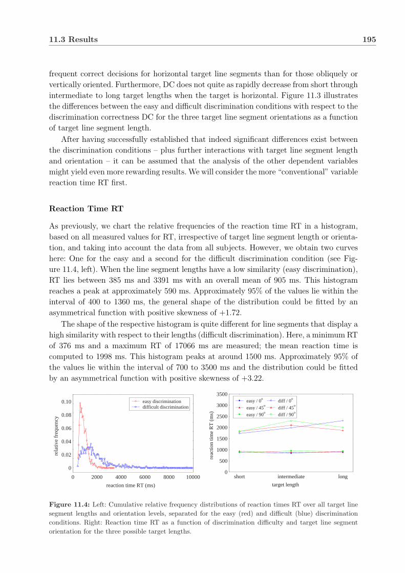
11.3 Results 195
frequent correct decisions for horizontal target line segments than for those obliquely or
vertically oriented. Furthermore, DC does not quite as rapidly decrease from short through
intermediate to long target lengths when the target is horizontal. Figure 11.3 illustrates
the differences between the easy and difficult discrimination conditions with respect to the
discrimination correctness DC for the three target line segment orientations as a function
of target line segment length.
After having successfully established that indeed significant differences exist between
the discrimination conditions – plus further interactions with target line segment length
and orientation – it can be assumed that the analysis of the other dependent variables
might yield even more rewarding results. We will consider the more “conventional” variable
reaction time RT first.
Reaction Time RT
As previously, we chart the relative frequencies of the reaction time RT in a histogram,
based on all measured values for RT, irrespective of target line segment length or orienta-
tion, and taking into account the data from all subjects. However, we obtain two curves
here: One for the easy and a second for the difficult discrimination condition (see Fig-
ure 11.4, left). When the line segment lengths have a low similarity (easy discrimination),
RT lies between 385 ms and 3391 ms with an overall mean of 905 ms. This histogram
reaches a peak at approximately 590 ms. Approximately 95% of the values lie within the
interval of 400 to 1360 ms, the general shape of the distribution could be fitted by an
asymmetrical function with positive skewness of +1.72.
The shape of the respective histogram is quite different for line segments that display a
high similarity with respect to their lengths (difficult discrimination). Here, a minimum RT
of 376 ms and a maximum RT of 17066 ms are measured; the mean reaction time is
computed to 1998 ms. This histogram peaks at around 1500 ms. Approximately 95% of
the values lie within the interval of 700 to 3500 ms and the distribution could be fitted
by an asymmetrical function with positive skewness of +3.22.
reaction time RT (ms)
rela
tive
freq
uenc
y
0
0.02
0.04
0.06
0.08
0.10
0 2000 4000 6000 8000 10000
easy discriminationdifficult discrimination
target length
reac
tion
time
RT
(m
s)
0
500
1000
1500
2000
2500
3000
3500
short intermediate long
easy / 0o diff / 0o
easy / 45o
diff / 45o
easy / 90o diff / 90o
Figure 11.4: Left: Cumulative relative frequency distributions of reaction times RT over all target linesegment lengths and orientation levels, separated for the easy (red) and difficult (blue) discriminationconditions. Right: Reaction time RT as a function of discrimination difficulty and target line segmentorientation for the three possible target lengths.

196 Experiment S2: Simultaneous Binary Length Comparison
The analysis of variance yields a significant main effect on RT for the factor discrim-
ination difficulty (F (1; 33) = 41.20; p < 0.001) (means: See above). RT also significantly
varies with target line segment length (F (2; 66) = 5.84; p = 0.007). When the target line
segment is short, subjects on average require 1354.3 ms to assess its length. For intermedi-
ate and long target lengths, RT increases to 1513.9 ms and to 1486.3 ms, respectively. The
post-hoc comparison of means using the Newman-Keuls test reveals that significant dif-
ferences only exist between short and intermediate (Rcrit = 129.7; p = 0.019) and between
short and long line segments (Rcrit = 112.2; p = 0.024), but not between intermediate and
long line segments (Rcrit = 67.5; p = 0.397). The third factor target line segment orienta-
tion does not exert a significant main effect on RT (F (2; 66) = 0.98; p = 0.387), RT only
slightly varies between 1445.6, 1422.3 and 1486.5 ms for the three target orientations 0o,
45o and 90o, respectively.
Apart from these main effects, only the interaction between target line segment length
and orientation reaches significance (F (4; 132) = 3.28; p = 0.017). This must be attributed
to the steadily increasing RT for horizontally oriented target line segments over target
lengths (1314.7, 1418.6, 1603.7 ms for short, intermediate and long target line segments) –
in contrast to the curves for the obliquely (1383.1, 1496.1, 1387.1 ms) and vertically
(1364.3, 1627.0, 1468.1 ms) oriented ones that peak for intermediate lengths.
The observed dependences are visualised in Figure 11.4 (right) where RT is displayed
as a function of discrimination difficulty and target line segment orientation for the three
possible target lengths.
Analysis of Eye-Movement Data: Preliminaries
The analyses of the relevant eye-movement parameters will be conducted here in analogy
to Experiment S1. This in particular means that measures such as the number of fixa-
tions NF or fixation duration FD will be analysed both globally – averaged over the whole
stimulus display – and locally – within specific spatial display regions that we consider
potentially relevant for the solution of the discrimination task.
Again, we divide the space into two sections surrounding the line segments and an
intermittent section for which separate analyses for NF and, in the following paragraphs,
for the other eye-movement parameters will be computed. The sizes of these sections are
set according to the previous specifications (see Section 10.2.1, paragraph “Analysis of
Eye-Movement Data: Preliminaries”) and subsequently validated using the same cluster-
analysis method (k-means algorithm). As before, the comparison of the clustering and the
definition of sections yields very little divergence. On average, this ratio of inconsistently
assigned fixations measures only 0.3%. We can thus assume that the “sectioning” presents
a plausible basis for the subsequent computation of local eye-movement parameters in
Experiment S2 as well.
Figures 11.5 and 11.6 illustrate the distributions for all possible combinations of target
line segment lengths and orientations. Figure 11.5 shows these distributions for the easy
discrimination condition, Figure 11.6 for the difficult one.

11.3 Results 197
Figure 11.5: Distribution of the fixation points for all possible combinations of target line segmentlengths and orientations, aggregated over all subjects for the easy discrimination condition.

198 Experiment S2: Simultaneous Binary Length Comparison
Figure 11.6: Distribution of the fixation points for all possible combinations of target line segmentlengths and orientations, aggregated over all subjects for the difficult discrimination condition.
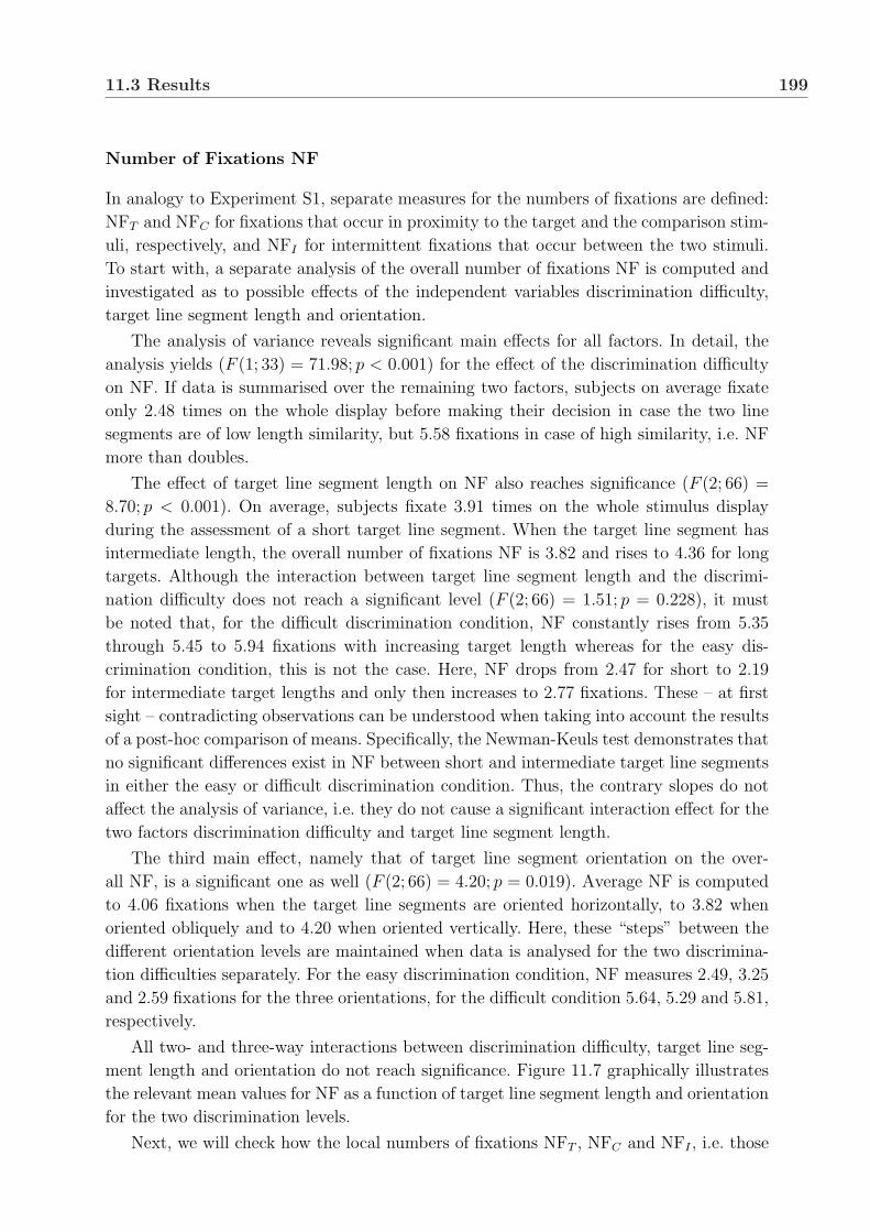
11.3 Results 199
Number of Fixations NF
In analogy to Experiment S1, separate measures for the numbers of fixations are defined:
NFT and NFC for fixations that occur in proximity to the target and the comparison stim-
uli, respectively, and NFI for intermittent fixations that occur between the two stimuli.
To start with, a separate analysis of the overall number of fixations NF is computed and
investigated as to possible effects of the independent variables discrimination difficulty,
target line segment length and orientation.
The analysis of variance reveals significant main effects for all factors. In detail, the
analysis yields (F (1; 33) = 71.98; p < 0.001) for the effect of the discrimination difficulty
on NF. If data is summarised over the remaining two factors, subjects on average fixate
only 2.48 times on the whole display before making their decision in case the two line
segments are of low length similarity, but 5.58 fixations in case of high similarity, i.e. NF
more than doubles.
The effect of target line segment length on NF also reaches significance (F (2; 66) =
8.70; p < 0.001). On average, subjects fixate 3.91 times on the whole stimulus display
during the assessment of a short target line segment. When the target line segment has
intermediate length, the overall number of fixations NF is 3.82 and rises to 4.36 for long
targets. Although the interaction between target line segment length and the discrimi-
nation difficulty does not reach a significant level (F (2; 66) = 1.51; p = 0.228), it must
be noted that, for the difficult discrimination condition, NF constantly rises from 5.35
through 5.45 to 5.94 fixations with increasing target length whereas for the easy dis-
crimination condition, this is not the case. Here, NF drops from 2.47 for short to 2.19
for intermediate target lengths and only then increases to 2.77 fixations. These – at first
sight – contradicting observations can be understood when taking into account the results
of a post-hoc comparison of means. Specifically, the Newman-Keuls test demonstrates that
no significant differences exist in NF between short and intermediate target line segments
in either the easy or difficult discrimination condition. Thus, the contrary slopes do not
affect the analysis of variance, i.e. they do not cause a significant interaction effect for the
two factors discrimination difficulty and target line segment length.
The third main effect, namely that of target line segment orientation on the over-
all NF, is a significant one as well (F (2; 66) = 4.20; p = 0.019). Average NF is computed
to 4.06 fixations when the target line segments are oriented horizontally, to 3.82 when
oriented obliquely and to 4.20 when oriented vertically. Here, these “steps” between the
different orientation levels are maintained when data is analysed for the two discrimina-
tion difficulties separately. For the easy discrimination condition, NF measures 2.49, 3.25
and 2.59 fixations for the three orientations, for the difficult condition 5.64, 5.29 and 5.81,
respectively.
All two- and three-way interactions between discrimination difficulty, target line seg-
ment length and orientation do not reach significance. Figure 11.7 graphically illustrates
the relevant mean values for NF as a function of target line segment length and orientation
for the two discrimination levels.
Next, we will check how the local numbers of fixations NFT , NFC and NFI , i.e. those

200 Experiment S2: Simultaneous Binary Length Comparison
target length
num
ber
of f
ixat
ions
NF
0
1
2
3
4
5
6
7
8
9
short intermediate long
easy / 0o diff / 0o
easy / 45o diff / 45o
easy / 90o diff / 90o
Figure 11.7: Overall number of fixations NF as a function of target line segment length, separated forthe three target orientations. The three line plots in the lower field of the graph illustrate NF for the easydiscrimination condition, those in the upper field for the difficult one.
in the target and comparison hemifields and that in the intermittent display section, are
affected by the factors discrimination difficulty, target line segment length and orientation.
The first analysis shows that NFT is significantly influenced only by the factors
discrimination difficulty (F (1; 33) = 75.58; p < 0.001) and target line segment length
(F (2; 66) = 3.66; p = 0.031). On average, subjects fixate the target section of the stimu-
lus display 1.27 times when the discrimination is easy. Like NF, NFT more than doubles
when the two line segment lengths are difficult to distinguish and measures 2.79 fix-
ations. Although the effect of target line segment length on NFT reaches significance
(see above), absolute differences between the target length levels are rather small –
1.98 fixations in the target section for short, 1.96 for intermediate and 2.14 for long
targets. Furthermore, a Newman-Keuls test confirms that significant differences exist
between short and long (Rcrit = 0.157; p = 0.028) and intermediate and long target
length levels (Rcrit = 0.127; p = 0.046), but not between short and intermediate levels
(Rcrit = 0.133; p = 0.841). Separated by discrimination difficulty, NFT measures 1.27, 1.16
and 1.39 fixations for the three target lengths short, intermediate and long in the easy dis-
crimination condition, in the difficult condition 2.70, 2.78 and 2.89, respectively. The main
effect of the factor target line segment orientation on NFT (F (2; 66) = 1.87; p = 0.163)
and all two- and three-way interactions between discrimination difficulty, target line seg-
ment length and orientation do not reach significance. Figure 11.8 (top left) graphically
illustrates the relevant mean values for NFT as a function of target line segment length
and orientation for the two discrimination levels.
Similar effects of the factors discrimination difficulty, target line segment length and
orientation can be found on NFC , i.e. the number of fixations that occur in proximity
to the comparison line segment. Discrimination difficulty (F (1; 33) = 70.78; p < 0.001)
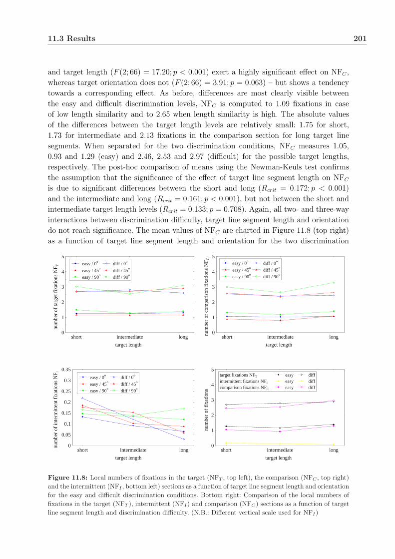
11.3 Results 201
and target length (F (2; 66) = 17.20; p < 0.001) exert a highly significant effect on NFC ,
whereas target orientation does not (F (2; 66) = 3.91; p = 0.063) – but shows a tendency
towards a corresponding effect. As before, differences are most clearly visible between
the easy and difficult discrimination levels, NFC is computed to 1.09 fixations in case
of low length similarity and to 2.65 when length similarity is high. The absolute values
of the differences between the target length levels are relatively small: 1.75 for short,
1.73 for intermediate and 2.13 fixations in the comparison section for long target line
segments. When separated for the two discrimination conditions, NFC measures 1.05,
0.93 and 1.29 (easy) and 2.46, 2.53 and 2.97 (difficult) for the possible target lengths,
respectively. The post-hoc comparison of means using the Newman-Keuls test confirms
the assumption that the significance of the effect of target line segment length on NFC
is due to significant differences between the short and long (Rcrit = 0.172; p < 0.001)
and the intermediate and long (Rcrit = 0.161; p < 0.001), but not between the short and
intermediate target length levels (Rcrit = 0.133; p = 0.708). Again, all two- and three-way
interactions between discrimination difficulty, target line segment length and orientation
do not reach significance. The mean values of NFC are charted in Figure 11.8 (top right)
as a function of target line segment length and orientation for the two discrimination
target length
num
ber
of ta
rget
fix
atio
ns N
F T
0
1
2
3
4
5
short intermediate long
easy / 0o diff / 0o
easy / 45o
diff / 45o
easy / 90o diff / 90o
target length
num
ber
of c
ompa
riso
n fi
xatio
ns N
F C
0
1
2
3
4
5
short intermediate long
easy / 0o diff / 0o
easy / 45o
diff / 45o
easy / 90o diff / 90o
target length
num
ber
of in
term
itten
t fix
atio
ns N
F I
0
0.05
0.1
0.15
0.2
0.25
0.3
0.35
short intermediate long
easy / 0o diff / 0o
easy / 45o
diff / 45o
easy / 90o diff / 90o
target length
num
ber
of f
ixat
ions
0
1
2
3
4
5
short intermediate long
target fixations NFT easy diffintermittent fixations NFI easy diffcomparison fixations NFC easy diff
Figure 11.8: Local numbers of fixations in the target (NFT , top left), the comparison (NFC , top right)and the intermittent (NFI , bottom left) sections as a function of target line segment length and orientationfor the easy and difficult discrimination conditions. Bottom right: Comparison of the local numbers offixations in the target (NFT ), intermittent (NFI) and comparison (NFC) sections as a function of targetline segment length and discrimination difficulty. (N.B.: Different vertical scale used for NFI)

202 Experiment S2: Simultaneous Binary Length Comparison
levels.
The statistical analysis of the number of intermittent fixations NFI that occur in the
area between the two stimuli yields rather different results compared to those obtained
in the previous analyses of the NFs. Specifically, now all main effects reach significance.
A detailed analysis of means reveals that again only very few fixations fall within the
intermittent section, NFI is computed to 0.19 in case of an easy discrimination and to
0.14 in case of a difficult one, yielding a significant main effect of the discrimination
difficulty on NFI (F (1; 33) = 4.45; p = 0.043). In other words, on average intermittent
fixations only occur between every seventh and ninth trial. If we further consider that,
overall, more than twice as many fixations (NFI) occur when the discrimination task is a
difficult one – compared to the easy discrimination condition – it must be noted that these
intermittent fixations account for approximately 2% of all fixations in case of a difficult
discrimination, but for approximately 4% in case of an easy one.
The comparison of means also yields that significantly fewer intermittent fixation occur
the longer the target line segment becomes (F (2; 66) = 15.32; p < 0.001): 0.17 fixations for
short targets, 0.12 for intermediate and 0.09 for long ones – with differences between all
target length levels being significantly different from each other, according to a Newman-
Keuls post-hoc test: (Rcrit = 0.034; p = 0.002) for the comparison between short and
intermediate targets, (Rcrit = 0.030; p < 0.001) for the comparison between short and
long targets and (Rcrit = 0.025; p = 0.022) for the comparison between intermediate and
long targets.
Finally, the factor target length orientation exerts a significant main effect on the de-
pendent variable NFI (F (2; 66) = 6.11; p = 0.004). On average 0.11 intermittent fixations
occur when the target is oriented horizontally, 0.13 when it is oblique and 0.15 when
vertical. The post-hoc comparison of means, however, yields that only the difference be-
tween horizontal and vertical target line segments accounts for this significant main effect
(Rcrit = 0.023; p = 0.003), whereas the other factor levels do not: (Rcrit = 0.019; p = 0.089)
for the comparison between horizontal and oblique and (Rcrit = 0.022; p = 0.081) for the
comparison between oblique and vertical. The two- and three-way interactions between
discrimination difficulty, target line segment length and orientation do not reach signifi-
cance. Figure 11.8 (bottom left) charts the mean NFI for the possible factor combinations.
In order to check if significant differences exist between NFT , NFC and NFI an en-
hanced analysis of variance is computed. As introduced in Experiment S1, it tests in
particular for the effects of the additional factor “section” on the number of fixations
with factor levels being the target, comparison and intermittent fixation sections. Indeed,
the analysis confirms the assumed significant effect of the fixation section on the number
of fixations (F (2; 66) = 185.88; p < 0.001). However, the Newman-Keuls test reveals that
significant differences only exist between NFT and NFI (Rcrit = 0.257; p < 0.001) and
between NFC and NFI (Rcrit = 0.262; p < 0.001) – which could have been expected. In
contrast to the findings of the “dynamic” Experiment S1, no significant differences exist
between NFT and NFC (Rcrit = 0.115; p = 0.156). Figure 11.8 (bottom right) visualises
these dependences. NFT , NFC and NFI are displayed in direct comparison for the three
possible target lengths and the easy and difficult discrimination conditions. As target line

11.3 Results 203
segment orientation does not exert a significant effect on NFT and NFC and in order to
improve clarity of the chart, data is aggregated over this factor.
Fixation Duration FD
Separate analyses are also computed for the overall fixation duration FD and its local
equivalents FDT , FDC and FDI , i.e. the fixation durations within the target, the compar-
ison and the intermittent stimulus display section, respectively.
Let us start examining the overall fixation duration FD. The analysis of variance yields
a significant main effect of the factor discrimination difficulty on FD (F (1; 33) = 42.77; p <
0.001). The comparison of means for the two factor levels shows that subjects on average
fixate 215.91 ms when the line segment length similarity is low, but that fixations are
prolonged by approximately 15% and last 247.63 ms when the length similarity is high. We
further observe that FD increases for long target line segments (249.42 ms), compared to
short (233.78 ms) and intermediate ones (212.1 ms). This constitutes a highly significant
effect of the factor target line segment length on FD (F (2; 66) = 15.94; p < 0.001).
No significant effect of target line segment orientation is found (F (2; 66) = 0.35; p =
0.704). FD remains almost constant at approximately 231 ms, irrespective of the target
orientation.
The only interaction effect to reach a significant level is that between the discrimination
difficulty and target length (F (2; 66) = 11.38; p < 0.001). When we consider FD separately
for the two discrimination conditions, their means show an increase in FD from short
through intermediate to long target lengths – as found when we established the significant
main effect of target length on FD (see above) – only when the discrimination is easy. In
this case the overall fixation duration rises from 192.36 ms for short through 210.22 ms for
intermediate to 245.17 ms for long target line segments. When the two line segment lengths
are difficult to discriminate, FD significantly increases only from short (231.88 ms) to
intermediate target lengths (257.34 ms), but then remains on that FD level for long lengths
(253.68 ms). This is confirmed by a post-hoc comparison of means using the Newman-
Keuls test: (Rcrit = 11.539; p < 0.001) for differences between short and intermediate
target line segment length, (Rcrit = 13.836; p = 0.003) for differences between short
and long ones and (Rcrit = 10.748; p = 0.494) for differences between intermediate and
long ones. All other two- and three-way interactions between the factors do not reach
significance. Figure 11.9 charts the mean values for NF as a function of target line segment
length and orientation for the two discrimination conditions.
In addition, separate analyses are computed for the local fixation durations FDT ,
FDC and FDI . The analysis of variance yields a significant main effect for the factor
discrimination difficulty on FDT (F (1; 33) = 58.66; p < 0.001). The average FDT is com-
puted to 209.21 ms for the easy discrimination condition and increases to 244.68 ms
for the difficult condition. Furthermore, fixations in proximity to the target line seg-
ment location last 213.11 ms, 231.30 ms and 236.42 ms for short, intermediate and long
targets, respectively. An analysis of variance demonstrates that the factor target line seg-
ment length has a significant effect on FDT (F (2; 66) = 14.90; p < 0.001). However, as

204 Experiment S2: Simultaneous Binary Length Comparison
target length
fixa
tion
dura
tion
FD (
ms)
180
200
220
240
260
280
300
320
short intermediate long
easy / 0o diff / 0o
easy / 45o diff / 45o
easy / 90o diff / 90o
Figure 11.9: Average global fixation duration FD as a function of target line segment length, separatedfor the three target orientations and the two discrimination conditions.
can be suspected from the differences between the means for the three target lengths,
this effect originates from significant differences in FDT between short and intermediate
and between short and long target line segments only. The corresponding results of the
Newman-Keuls test produced (Rcrit = 9.306; p < 0.001) and (Rcrit = 7.869; p < 0.001)
for those two comparisons, but (Rcrit = 10.055; p = 0.308), i.e. no significant effect,
for the comparison between intermediate and long targets. A closer inspection of the
FDT means reveals that considerable differences exist between FDT when separated for
the two discrimination conditions. Analogous to the findings for the overall fixation du-
ration FD, these differences are indeed significant, as the significance level of the in-
teraction between the factors discrimination difficulty and target line segment length
proves (F (2; 66) = 4.83; p = 0.011). Whereas FDT significantly increases between all tar-
get length levels when the length discrimination is easy (short: 191.98 ms; intermediate:
209.39 ms; long: 226.27 ms), FDT does not in case the discrimination is difficult (short:
234.23 ms; intermediate: 253.22 ms; long: 246.58 ms). Here, a significant increase in FDT
can only be found between short and intermediate (Rcrit = 12.809; p = 0.005) and short
and long target line segments (Rcrit = 13.581; p = 0.021), but not between intermediate
and long ones (Rcrit = 10.811; p = 0.221), according to a Newman-Keuls post-hoc test.
Neither the main effect of the factor target orientation nor any other two- or three-way
interaction of the three factors discrimination difficulty, target line segment length and
orientation reaches significance. Figure 11.10 (top left) visualises all means for FDT for
the two discrimination difficulties and the three possible target orientations as a function
of target length.
Taking into account that the comparison between the number of fixations in the tar-
get and comparison sections, NFT and NFC , respectively, did not result in statistically
significant differences, it might be assumed that similar correlations exists regarding FDT

11.3 Results 205
and FDC . Indeed, the analysis of variance for FDC and the comparison of means seem to
confirm this assumption; results and effects very closely resemble those obtained for FDT .
In detail, we can establish a significant main effect of the factors discrimination difficulty
(F (1; 33) = 62.50; p < 0.001) and target line segment length (F (2; 66) = 9.74; p < 0.001;)
on FDC . Average FDC is 231.11 ms for the easy discrimination condition and increases
to 267.09 ms for the difficult condition. Fixations in proximity to the comparison line
segment location last 225.98 ms, 254.92 ms and 266.40 ms for short, intermediate and
long targets, respectively. Analogous to the analysis of FDT , a post-hoc comparison of
means using the Newman-Keuls test demonstrated that this effect originates from signif-
icant differences in FDC between short and intermediate (Rcrit = 10.242; p < 0.001) and
between short and long target line segments (Rcrit = 22.941; p = 0.001) only. The test
produced no significant effect for the comparison between intermediate and long targets
(Rcrit = 21.704; p = 0.290).
Neither the main effect of the factor target orientation nor most two- or three-way
interactions of the three factors discrimination difficulty, target line segment length and
orientation reach significance. Only the interaction between the factors discrimination
difficulty and target line segment length yields a significant two-way interaction effect on
target length
targ
et f
ixat
ion
dura
tion
FDT (
ms)
180
200
220
240
260
280
300
320
short intermediate long
easy / 0o diff / 0o
easy / 45o
diff / 45o
easy / 90o diff / 90o
target length
com
pari
son
fixa
tion
dura
tion
FDC (
ms)
180
200
220
240
260
280
300
320
short intermediate long
easy / 0o diff / 0o
easy / 45o
diff / 45o
easy / 90o diff / 90o
target length
inte
rmitt
ent f
ixat
ion
dura
tion
FDI (
ms)
140
160
180
200
220
240
260
280
short intermediate long
easy / 0o diff / 0o
easy / 45o
diff / 45o
easy / 90o diff / 90o
target length
fixa
tion
dura
tion
180
200
220
240
260
280
300
320
short intermediate long
target fixations FDT easy diffintermittent fixations FDI easy diffcomparison fixations FDC easy diff
Figure 11.10: Local fixation durations in the target (FDT , top left), the comparison (FDC , top right) andthe intermittent (FDI , bottom left) sections as a function of target line segment length and orientation forthe easy and difficult discrimination conditions. Bottom right: Comparison of the local fixation durationin the target (FDT ), intermittent (FDI) and comparison (FDC) sections as a function of target linesegment length and discrimination difficulty.

206 Experiment S2: Simultaneous Binary Length Comparison
FDC (F (2; 66) = 14.12; p < 0.001), reflecting considerable differences between FDC for
short, intermediate and long targets when separated for the two discrimination conditions.
Whereas FDC significantly increases between all target length levels when the length
discrimination is easy (short: 200.82 ms; intermediate: 228.56 ms; long: 263.94 ms), FDC
does not when the discrimination is difficult (short: 251.15 ms; intermediate: 281.27 ms;
long: 268.85 ms). Here, a significant increase in FDC can only be found between short and
intermediate (Rcrit = 15.342; p < 0.001) and short and long target line segments (Rcrit =
19.452; p = 0.050), but not between intermediate and long ones (Rcrit = 15.729; p =
0.118), according to a Newman-Keuls post-hoc test. Figure 11.10 (top right) visualises
all means for FDC for the two discrimination difficulties and the three possible target
orientations as a function of target length.
Finally, the investigation of the duration of intermittent fixation, FDI , completes the
statistical analysis of FDs. The comparison of means yields almost identical average fix-
ation durations for both discrimination conditions, about 188.82 ms. Consequently, the
analysis of variance does not produce a significant main effect for the factor discrimi-
nation difficulty (F (1; 33) = 0.09; p = 0.767). As for FDT and FDC , the factor target
line segment length exerts a significant effect on FDI (F (2; 66) = 7.14; p = 0.002) and
yields means that increase from 176.62 ms for short through 188.63 ms for intermediate
to 201.54 ms for long targets. The analysis of variance also reveals a significant main
effect of the factor target line segment orientation on FDI (F (2; 66) = 7.52; p = 0.002).
As the means for the different orientation levels suggest – 201.99 ms for horizontal tar-
gets, 179.12 ms for oblique and 185.69 ms for vertical ones – the significance of this effect
has to be attributed to the significant differences between the factor levels horizontal and
oblique (Rcrit = 12.146; p < 0.001) and horizontal and vertical (Rcrit = 13.297; p = 0.018),
whereas the Newman-Keuls test cannot establish significance for the difference between
oblique and vertical target orientation levels (Rcrit = 11.505; p = 0.254). None of the two-
and three-way interactions between the factors reach significance. Figure 11.10 (bottom
left) charts the mean NFI for the possible factor combinations.
Although results obtained for the statistical analyses of FDT and FDC are very similar
(see above) and do not seem to suggest significant differences between the sections with
regard to the fixation duration, a final “comparative” analysis is being computed as before.
It tests in particular for the effects of the additional factor “section” on the fixation
duration with factor levels being the target, comparison and intermittent fixation sections.
Indeed, the analysis confirms the assumed significant effect of the fixation section on the
number of fixations (F (2; 66) = 26.80; p < 0.001), the mean fixation time is 226.94 ms in
the target section, 249.10 ms in the comparison and only 188.93 ms in the intermittent
one. Contrary to the earlier expectation that no significant differences exist between FDT
and FDC , the Newman-Keuls test reveals significant differences between all levels of the
factor section. It yields (Rcrit = 18.412; p = 0.020) between FDT and FDC , (Rcrit =
17.359; p < 0.001) between FDT and FDI and (Rcrit = 14.677; p < 0.001) between FDC
and FDI . Figure 11.10 (bottom right) visualises these dependences, FDT , FDC and FDI
are displayed in direct comparison for the three possible target lengths and the easy and
difficult discrimination conditions. As target line segment orientation does not exert a

11.3 Results 207
significant effect on FDT and FDC and in order to improve clarity of the chart, data is
aggregated over this factor.
Number of Saccades between Hemifields SB
As in Experiment S1 previously, we consider the number of saccades between the two stim-
ulus hemifields SB as the last more “global” measure. The analysis of variance yields a sig-
nificant main effect for the factor discrimination difficulty (F (1; 33) = 107.64; p < 0.001).
SB significantly increases from only 1.79 for the easy discrimination condition to 3.55 for
the difficult one. The effects of both target line segment length (F (1; 33) = 8.05; p = 0.001)
and orientation (F (2; 66) = 5.22; p = 0.008) on SB also reach significance, however, dif-
ferences between the individual levels of these two factors are less pronounced. When
targets are short, average SB measures 2.59, when intermediate 2.77 and when vertical
2.81. As the post-hoc comparison of means shows (Newman-Keuls test), a significant
increase can only be observed for the SB differences between short and intermediate
(Rcrit = 0.130; p = 0.007) and between short and long targets (Rcrit = 0.127; p = 0.002),
but not between intermediate and long targets (Rcrit = 0.092; p = 0.486). More specif-
ically, separated by the discrimination difficulty, SB is 1.77, 1.88 and 2.02 for short, in-
termediate and long target line segments when the discrimination is easy and 3.41, 3.66
and 3.59 when the discrimination is difficult. For horizontal, oblique and vertical tar-
gets, the average SB is computed to 2.77, 2.62 and 2.78, respectively. According to the
Newman-Keuls post-hoc test, the significant main effect has to be attributed to signif-
icant differences in SB between horizontal and oblique (Rcrit = 0.073; p < 0.001) and
between vertical and oblique targets (Rcrit = 0.130; p = 0.023), but not between hori-
zontal and vertical targets (Rcrit = 0.118; p = 0.947). No significant interactions between
discrimination difficulty, target line segment length and/or orientation can be observed.
target length
num
ber
of s
acca
des
betw
een
hem
ifie
lds
SB
0
1
2
3
4
5
short intermediate long
easy / 0o diff / 0o
easy / 45o diff / 45o
easy / 90o diff / 90o
Figure 11.11: Number of saccades between stimulus hemifields SB as a function of target line segmentlength and orientation, separated for the two discrimination difficulties.

208 Experiment S2: Simultaneous Binary Length Comparison
The detailed SB means for the combinations of discrimination difficulties, target lengths
and orientations are charted in Figure 11.11.
Number of Successive Fixations within the same Hemifield FW
As argued in Experiment S1, the analysis of the number of successive fixations within the
same hemifield will be considered in the target (FWT ) and comparison (FWC) sections,
i.e. hemifields, only. With the number of fixations NFI being considerably below one in
the intermittent stimulus display section, a sensible sequence of fixations for that region
cannot be constituted in Experiment S2 either. FWI can thus be excluded from the
analysis. In addition to FWT and FWC , an overall FW, averaging over both hemifields,
will be analysed again first.
The analysis of variance for FW yields significant main effects for all factors. The
effect for the discrimination difficulty is computed to (F (1; 33) = 124.75; p < 0.001) and
manifested in a mean FW of 1.56 for the easy discrimination condition and 2.18 for the
difficult one. FW also significantly varies with target line segment length (F (2; 66) =
11.86; p < 0.001). Mean FW measures 1.82 for short target segments, remains almost
unchanged for intermediate ones (1.79) and then rises to 2.00 fixations for long ones. As
expected, the Newman-Keuls post-hoc test confirms the significant differences between the
target length level short and long (Rcrit = 0.110; p = 0.003) and intermediate and long
(Rcrit = 0.077; p < 0.001), but not between short and intermediate (Rcrit = 0.090; p =
0.502). Separated for the two discrimination levels, FW is 1.52, 1.45 and 1.71 for short,
intermediate and long targets when the line segments have a low length similarity and
2.12, 2.14 and 2.29 when the length similarity is high.
Finally, the target line segment orientation also exerts a significant main effect on
FW (F (2; 66) = 5.36; p = 0.007). With FW being identical when the target is oriented
either horizontally or obliquely (1.84), it does not come as a surprise that the Newman-
Keuls test only classifies the differences between these two orientation levels and the
vertical level – where FW is 1.93 – as statistically significant and being responsible for the
significance of the main effect. More specifically, the test yields (Rcrit = 0.058; p = 0.976)
for the difference between the orientation factor levels horizontal and oblique, (Rcrit =
0.058; p = 0.004) for the difference between horizontal and vertical and (Rcrit = 0.075; p =
0.021) for the difference between oblique and vertical. Separated for the two discrimination
levels, FW is 1.53, 1.53 and 1.62 for horizontal, oblique and vertical targets when the line
segments have a low length similarity and 2.16, 2.15 and 2.24 when the length similarity
is high. None of the two- or three-way interactions reaches significance. Figure 11.12
visualises the means for the number of successive fixations within the same hemifield FW
for the three target orientations and the discrimination difficulty as a function of target
line segment length.
Let us next consider the number of successive fixations within the target FWT and
comparison FWC hemifields. A separate analysis of variance for FWT results in significant
main effects for all factors discrimination difficulty (F (1; 33) = 57.44; p < 0.001), target
line segment length (F (2; 66) = 57.44; p = 0.006) and orientation (F (2; 66) = 6.17; p =
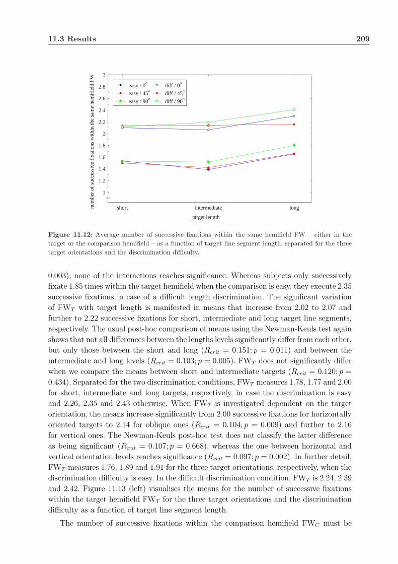
11.3 Results 209
target length
num
ber
of s
ucce
ssiv
e fi
xatio
ns w
ithin
the
sam
e he
mif
ield
FW
1
1.2
1.4
1.6
1.8
2
2.2
2.4
2.6
2.8
3
short intermediate long
easy / 0o diff / 0o
easy / 45o diff / 45o
easy / 90o diff / 90o
Figure 11.12: Average number of successive fixations within the same hemifield FW – either in thetarget or the comparison hemifield – as a function of target line segment length, separated for the threetarget orientations and the discrimination difficulty.
0.003); none of the interactions reaches significance. Whereas subjects only successively
fixate 1.85 times within the target hemifield when the comparison is easy, they execute 2.35
successive fixations in case of a difficult length discrimination. The significant variation
of FWT with target length is manifested in means that increase from 2.02 to 2.07 and
further to 2.22 successive fixations for short, intermediate and long target line segments,
respectively. The usual post-hoc comparison of means using the Newman-Keuls test again
shows that not all differences between the lengths levels significantly differ from each other,
but only those between the short and long (Rcrit = 0.151; p = 0.011) and between the
intermediate and long levels (Rcrit = 0.103; p = 0.005). FWT does not significantly differ
when we compare the means between short and intermediate targets (Rcrit = 0.120; p =
0.434). Separated for the two discrimination conditions, FWT measures 1.78, 1.77 and 2.00
for short, intermediate and long targets, respectively, in case the discrimination is easy
and 2.26, 2.35 and 2.43 otherwise. When FWT is investigated dependent on the target
orientation, the means increase significantly from 2.00 successive fixations for horizontally
oriented targets to 2.14 for oblique ones (Rcrit = 0.104; p = 0.009) and further to 2.16
for vertical ones. The Newman-Keuls post-hoc test does not classify the latter difference
as being significant (Rcrit = 0.107; p = 0.668), whereas the one between horizontal and
vertical orientation levels reaches significance (Rcrit = 0.097; p = 0.002). In further detail,
FWT measures 1.76, 1.89 and 1.91 for the three target orientations, respectively, when the
discrimination difficulty is easy. In the difficult discrimination condition, FWT is 2.24, 2.39
and 2.42. Figure 11.13 (left) visualises the means for the number of successive fixations
within the target hemifield FWT for the three target orientations and the discrimination
difficulty as a function of target line segment length.
The number of successive fixations within the comparison hemifield FWC must be

210 Experiment S2: Simultaneous Binary Length Comparison
target length
num
ber
of s
ucce
ssiv
e ta
rget
fix
atio
ns F
WT
1
1.5
2
2.5
3
short intermediate long
easy / 0o diff / 0o
easy / 45o
diff / 45o
easy / 90o diff / 90o
target length
num
ber
of s
ucce
ssiv
e co
mp.
fix
atio
ns F
WC
1
1.5
2
2.5
3
short intermediate long
easy / 0o
diff / 0o
easy / 45o diff / 45o
easy / 90o
diff / 90o
Figure 11.13: Average number of successive fixations within the target hemifield FWT (left) and withinthe comparison hemifield (right) as functions of target line segment length, separated for the three targetorientations and the discrimination difficulty.
investigated before we can check for possible differences between the number of suc-
cessive fixations within each of the two hemifields. The analysis of variance yields the
same significant main effects for all factors on FWC as it did for FWT before. Thus, the
influence of the discrimination difficulty constitutes a highly significant effect on FWC
(F (1; 33) = 163.01; p < 0.001) with the area in proximity to the comparison stimulus
being successively fixated 1.27 times before directing the eye gaze to the target hemi-
field in the easy discrimination condition. FWC increases to 2.01 when the length sim-
ilarity is high, i.e. the discrimination difficulty. The factor target line segment length
also yields a significant main effect on FWC (F (2; 66) = 13.39; p < 0.001). When the
target length is short, the mean FWC is computed to 1.62 successive fixations, when
intermediate to 1.52 and when long to 1.78 fixations. Separated for the two discrimina-
tion levels, FWC is 1.27, 1.12 and 1.41 for short, intermediate and long targets when
the line segments have a low length similarity and 1.98, 1.91 and 2.15 when the length
similarity is high. Finally, the target line segment orientation exerts a significant main
effect on FWC as well (F (2; 66) = 10.54; p < 0.001). With FWC being almost identi-
cal when the target is oriented either horizontally (1.68) or vertically (1.69), it does not
come as a surprise that the Newman-Keuls test only classifies the differences between
these two orientation levels and the oblique level – where FWC is 1.54 – as statistically
significant and being responsible for the significance of the main effect. The test yields
(Rcrit = 0.072; p < 0.001) for the difference between the orientation factor levels horizontal
and oblique, (Rcrit = 0.074; p = 0.699) for the difference between horizontal and vertical
and (Rcrit = 0.084; p = 0.001) for the difference between oblique and vertical. Separated
for the two discrimination levels, FWC is 1.30, 1.17 and 1.33 for horizontal, oblique and
vertical targets when the line segments have a low length similarity and 2.07, 1.91 and
2.06 when the length similarity is high. The two- and three-way interactions between the
factors do not reach significance level. Figure 11.13 (right) visualises the means for the
number of successive fixations within the comparison hemifield FWC for the three target
orientations and the discrimination difficulty as a function of target line segment length.
The subsequent direct comparison of the numbers of successive fixations within the

11.3 Results 211
target and the comparison hemifields yields a significant main effect for the factor “hemi-
field” (F (1; 33) = 17.62; p < 0.001). Whereas, on average, 2.10 successive fixations occur
in the target hemifield (FWT ) before a shift to the other hemifield, FWC measures only
1.64 successive fixations. As computed in the separate analyses already, the individual
means for FWT and FWC compare 1.85 to 1.27 in the case of an easy discrimination and
2.35 to 2.01 in the difficult length discrimination condition. Figure 11.14 illustrates the
relevant means for the comparison of FWT and FWC for the two discrimination difficul-
ties, for clarity reasons in two separate graphs either as a function of target line segment
length (left) or orientation (right).
target length
num
ber
of s
ucce
ssiv
e fi
xatio
ns w
ithin
the
sam
e he
mif
ield
1
1.5
2
2.5
3
short intermediate long
target FWT easy diffcomparison FWC easy diff
target orientation
num
ber
of s
ucce
ssiv
e fi
xatio
ns w
ithin
the
sam
e he
mif
ield
1
1.5
2
2.5
3
horizontal oblique vertical
target FWT easy diffcomparison FWC easy diff
Figure 11.14: Comparison of the number of successive fixations within the target (FWT ) and thecomparison hemifields (FWC) for the easy and difficult discrimination conditions as a function of targetline segment length (left) and orientation (right).
Saccade Length SL
In addition, a achieve a more global understanding of the comparison process, the saccade
length between the two relevant stimulus regions SLb will be investigated again in this
experiment. Due to the very small number of fixations within the intermittent stimulus
section, the saccade length will also be computed “locally” for those saccades that occur
entirely either within the target (SLT ) or the comparison hemifield (SLC) of the display
only.
An analysis of variance tests the effects of the factors discrimination difficulty, target
line segment length and orientation on the saccade length between the two hemifields SLb.
It yields significant main effects for all factors on SLb: (F (1; 33) = 1.79; p < 0.001)
for the discrimination difficulty, (F (2; 66) = 17.18; p < 0.001) for target length and
(F (2; 66) = 2.74; p < 0.001) for target orientation. When the two stimulus line seg-
ments have a low length similarity, the average SLb is computed to 19.08o and when
the length similarity is high to 19.79o. The comparison of means further shows that SLb
decreases from 20.96o for short target line segments, through 19.65o for intermediate to
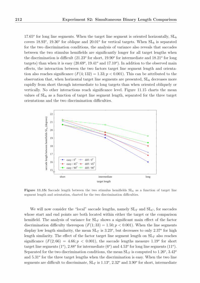
212 Experiment S2: Simultaneous Binary Length Comparison
17.65o for long line segments. When the target line segment is oriented horizontally, SLb
covers 18.93o, 19.36o for oblique and 20.01o for vertical targets. When SLb is separated
for the two discrimination conditions, the analysis of variance also reveals that saccades
between the two stimulus hemifields are significantly longer for all target lengths when
the discrimination is difficult (21.23o for short, 19.90o for intermediate and 18.21o for long
targets) than when it is easy (20.69o, 19.41o and 17.10o). In addition to the observed main
effects, the interaction between the two factors target line segment length and orienta-
tion also reaches significance (F (4; 132) = 1.33; p < 0.001). This can be attributed to the
observation that, when horizontal target line segments are presented, SLb decreases more
rapidly from short through intermediate to long targets than when oriented obliquely or
vertically. No other interactions reach significance level. Figure 11.15 charts the mean
values of SLb as a function of target line segment length, separated for the three target
orientations and the two discrimination difficulties.
target length
sacc
ade
leng
th b
etw
een
hem
ifie
lds
SLb
(deg
rees
)
15
16
17
18
19
20
21
22
short intermediate long
easy / 0o diff / 0o
easy / 45o diff / 45o
easy / 90o diff / 90o
Figure 11.15: Saccade length between the two stimulus hemifields SLb as a function of target linesegment length and orientation, charted for the two discrimination difficulties.
We will now consider the “local” saccade lengths, namely SLT and SLC , for saccades
whose start and end points are both located within either the target or the comparison
hemifield. The analysis of variance for SLT shows a significant main effect of the factor
discrimination difficulty thereupon (F (1; 33) = 1.50; p < 0.001). When the line segments
display low length similarity, the mean SLT is 3.23o, but decreases to only 2.37o for high
length similarity. The effect of the factor target line segment length on SLT also reaches
significance (F (2; 66) = 4.66; p < 0.001), the saccade lengths measure 1.19o for short
target line segments (1o), 2.88o for intermediate (6o) and 4.53o for long line segments (11o).
Separated for the two discrimination conditions, the mean SLT is computed to 1.26o, 3.42o
and 5.31o for the three target lengths when the discrimination is easy. When the two line
segments are difficult to discriminate, SLT is 1.13o, 2.32o and 3.90o for short, intermediate

11.3 Results 213
and long targets, respectively. This notably steeper increase in SLT with target lengths for
the easy than for the difficult discrimination condition is also manifested in a significant
interaction between these two factors (F (2; 66) = 0.38; p = 0.002).
The third factor, target line segment orientation, exerts a significant effect on SLT as
well (F (2; 66) = 0.69; p < 0.001), the saccade lengths measure 3.23o for horizontal target
line segments, 2.73o for oblique and 2.54o for vertical segments. Separated for the two
discrimination conditions, the mean SLT is computed to 3.64o, 3.22o and 2.85o for the
three target orientations when the discrimination is easy. When the two line segments
are difficult to discriminate, SLT is 2.83o, 2.23o and 2.06o for horizontal, oblique and
vertical targets, respectively. Whereas this interaction does not reach significance level
(F (2; 66) = 0.01; p = 0.807), the interaction between target line segment length and
orientation does (F (2; 66) = 0.21; p = 0.008). This can be attributed to SLT means that
more sharply increase over target length when oriented horizontally – 1.21o (short), 3.32o
(intermediate) and 5.16o (long) – than obliquely – 1.18o, 2.90o and 4.10o – or vertically –
1.18o, 2.41o and 3.76o. None of the remaining two-way or the three-way interactions exert
significant effects on SLT . Figure 11.16 (left) charts the means for the saccade lengths
within the target hemifield SLT for the three target orientations and the discrimination
difficulty as a function of target line segment length.
In contrast to SLT , the analysis for the saccade lengths within the comparison stim-
ulus hemifield SLC shows significant main effects for the factors discrimination difficulty
(F (1; 33) = 2.54; p < 0.001) and target line segment length only (F (2; 66) = 14.01; p <
0.001). For the easy discrimination condition, SLC on average measures 4.17o, for the
difficult one 3.21o. The comparison of means further yields that SLC increases from 1.24o
for short through 3.69o for intermediate to 6.12o for long target line segments. As for SLT ,
SLC shows a steeper increase over target length when the discrimination is easy than when
it is difficult. Means for this interaction significantly vary (F (2; 66) = 0.78; p < 0.001) and
yield 1.28o, 4.27o and 6.92o for short, intermediate and long target line segments when the
target length
sacc
ade
leng
th w
ithin
targ
et h
emif
ield
SL
T (
degr
ees)
0
1
2
3
4
5
6
7
short intermediate long
easy / 0o diff / 0o
easy / 45o
diff / 45o
easy / 90o diff / 90o
target length
sacc
ade
leng
th w
ithin
com
pari
son
hem
ifie
ld S
LC (
degr
ees)
0
1
2
3
4
5
6
7
short intermediate long
easy / 0o
diff / 0o
easy / 45o diff / 45o
easy / 90o
diff / 90o
Figure 11.16: Saccade length within the target hemifield SLT (left) and within the comparison hemi-field SLC (right) as functions of target line segment length and orientation, charted for the two discrimi-nation difficulties.

214 Experiment S2: Simultaneous Binary Length Comparison
discrimination is easy and 1.19o, 3.11o and 5.32o for the target length levels in the case of
a difficult discrimination condition. Here, no significant effect on SLC can be established
for the factor target line segment orientation (F (2; 66) = 0.13; p = 0.114). Irrespective of
the target orientation, SLC measures approximately 3.63o. The other two- and three-way
interactions do not reach significance level. Figure 11.16 (right) charts the means for the
saccade lengths within the comparison hemifield SLC for the three target orientations and
the discrimination difficulty as a function of target line segment length.
Again, we directly compare the saccade lengths within the target (SLT ) and the com-
parison hemifields (SLC). The statistical analysis yields a significant main effect for the
factor “hemifield” (F (1; 33) = 2.59; p < 0.001). Whereas the average saccade length in
the target hemifield is 2.80o, it measures 3.69o in the comparison hemifield. As computed
in the separate analyses already, the individual means for SLT and SLC compare 3.24o
to 4.17o, respectively, in the case of an easy discrimination and 2.37o to 3.22o in the case
of a difficult length discrimination condition. Figure 11.17 illustrates the relevant means
for the comparison of SLT and SLC for the two discrimination difficulties, for reasons of
clarity in two separate graphs either as a function of target line segment length (left) or
orientation (right).
target length
sacc
ade
leng
th w
ithin
hem
ifie
ld
0
1
2
3
4
5
6
7
short intermediate long
target SLT easy diffcomparison SLC easy diff
target orientation
sacc
ade
leng
th w
ithin
hem
ifie
ld
2
3
4
5
horizontal oblique vertical
target SLT easy diffcomparison SLC easy diff
Figure 11.17: Comparison of the saccade lengths within the target (SLT ) and the comparison hemifields(SLC) for the easy and difficult discrimination conditions as a function of target line segment length (left)and orientation (right).
11.4 Discussion and Conclusions
The discussion of the results of the previous Experiment S1 has demonstrated that the
perception principles that determine the simultaneous comparison of line segment length
prove a lot more complicated as could initially have been expected. The empirical findings
yield that even “simple” line segment stimuli and the assessment of their basic features
such as length trigger diverse, characteristic visual analysis patterns guided by elaborate
cognitive strategies. For the then applied “dynamic” length matching procedure the dis-
cussion revealed foveal “visual measurement” as a fundamental mechanism to accomplish

11.4 Discussion and Conclusions 215
the (line segment length) assessment “step” of the characteristic cognitive structure of
comparison tasks (see Section 2.1). For longer line segment lengths, this strategy was
adapted to a “fractional” visual measurement and the subsequent length extrapolation
in order to improve efficiency, assumedly decomposing the line segment and taking into
account peripherally perceived end point information. Accordingly, mental line segment
representations were generated, memorised and manipulated.
However, the dynamic adjustment procedure apparently influenced some observations
in Experiment S1, for example regarding the fixation durations FD which were prolonged
in the comparison hemifield (for details, see Section 10.3). This rendered the procedure at
least critical when assigning specific observations – as intended – solely to the actual line
segment assessment task. The current static method of constant stimuli should now have
helped in eliminating these undesirable “side effects”. As the lengths of the comparison
line segments were set in accordance with the perceived target lengths of Experiment S1,
possible interference of visual illusory effects can also be excluded. The experimental find-
ings of Experiment S2 should be less ambiguous and allow for further reliable conclusions
regarding the underlying principles of line segment length perception. The findings will
be discussed with particular respect to the initially hypothesised different strategies that
subjects apply depending on the discrimination difficulty: Holistic or analytic visual pro-
cessing when the length discrimination task is “easy” or “difficult”, respectively.
The following are the most outstanding effects the factors in Experiment S2, namely
the discrimination difficulty, target line segment length and orientation, exerted on the in-
dependent variables, i.e. the discrimination correctness, the reaction time and the various
eye-movement parameters:
1. As expected, the discrimination correctness DC reaches almost 100% when the dis-
crimination task is “easy”. The “difficult” discrimination condition indeed appears
to be difficult as less than two thirds of all responses are correct.
2. Both “conventional” variables such as the reaction time RT and eye-movement pa-
rameters such as the number of fixations NF, the number of fixations within the
same hemifield FW or the number of saccades between hemifields SB are signif-
icantly higher when the discrimination is difficult. These findings are compatible
with the view that a holistic visual processing strategy is pursued when the line
length similarity is low and an analytic one when it is high.
3. More generally speaking, the factor discrimination difficulty exerts a significant effect
on all dependent variables but FDI .
4. The factor target line segment length exerts a significant effect on all dependent
variables.
5. The factor target line segment orientation exerts significant effects on most depen-
dent variables: DC, NF, NFI , FDI , SB, FW, FWT , FWC , SLb and SLT . However,
fixation duration, the “local” numbers of fixations NFT and NFC , the reaction time

216 Experiment S2: Simultaneous Binary Length Comparison
RT and the saccade length within the comparison hemifield SLC are not significantly
affected.
On the one hand, the statistical analysis of the discrimination correctness DC serves as
a “control” function. Almost 100% of all subjects’ responses are correct when the length
differences between the target and the comparison line segments are set so as to establish
“easy” discrimination conditions. This confirms the findings of the pre-experiment and
demonstrates that length discrimination is indeed easy when the similarity of line seg-
ment lengths is low. The fact that DC is considerably lower when the length differences
between the target and the comparison line segments are set so as to establish “difficult”
discrimination conditions not only proves that length discrimination is indeed difficult
when the similarity of line segment lengths is high. It also shows that the two discrimi-
nation conditions are sensibly chosen to yield significant differences between them. This
indicates that such differences might exist between the two conditions with respect to the
other dependent variables as well. This is highly promising with a view to the anticipated
different visual processing strategies.
Furthermore, it is important to note that subjects’ responses in the difficult discrim-
ination task are well above chance level. The difficult condition is apparently not too
difficult. If it was, subjects would make random decisions. This would probably coincide
with sparse visual scanning because a more detailed visual analysis might not be ren-
dered helpful in such a case – yielding an unwanted “random” rather than the intended
“difficult” discrimination condition.
However, DC is not just a convenient “control” variable that successfully demon-
strates that the two discrimination conditions were sensibly established. The significant
differences in DC between the different target length and orientation levels when the
discrimination is difficult require further discussion. Initially, it appears contradictory to
the previous findings, for example, that DC is best for short line segments. The previous
experiments yielded the least accurate results when subjects had to assess length or ori-
entation of short line segments, both in sequential or simultaneous comparison scenarios.
A closer look reveals, however, that exactly this might have caused the good discrimina-
tion performance here. Let us recall that the relative length deviation DL between the
target and the comparison line segments was largest when subjects had to assess short
targets and adjust the comparison accordingly in Experiment S1. As we used these length
deviations – and associated standard deviations – to determine comparison lengths in
Experiment S2, (relative) length differences between target and comparison line segments
will consequently be largest for short targets here. As results of this experiment now
demonstrate, this obviously facilitates the binary discrimination task to such an extent
that it leads to the highest discrimination correctness DC for short line segments. It thus
appears that line segments that are short are the most difficult ones to assess and match –
i.e. the assessment accuracy is worst compared to other lengths – in the dynamic length
adjustment task of Experiment S1. Given the less demanding binary comparison task of
Experiment S2, length differences of a magnitude not detected and compensated for by
adjustment in Experiment S1 are now correctly identified. The dynamic assessment task
obviously interferes with the length perception processes insofar as it also compromises

11.4 Discussion and Conclusions 217
the assessment accuracy.
In analogy to making the binary discrimination task in Experiment S2 easier for short
length – due to larger length deviations DL in Experiment S1 – a similar development
could have been expected for the orientation levels. With DL being significantly larger
when targets and comparisons were not equally oriented, the discrimination could have
been thought to be easier and yield a higher discrimination correctness DC for oblique
and vertical target orientations. This, however, is not the case. It must be assumed that
the length differences in the difficult discrimination condition only compensate for the
horizontal-vertical illusion induced by the different orientations of the target and compar-
ison line segments. Other than obviously the case for short target length, the larger length
differences for oblique and vertical orientations do not facilitate the comparison and thus
do not affect the discrimination correctness DC. Even when the comparison length is set
so as to compensate for the illusory effects, it is obviously a lot more difficult to compare
lengths when the respective line segments are not equally oriented.
The analysis of the reaction time in Experiment S2 fits in well with the discussion of
RT in the previous experiments. Compared with Experiment S1 which had an average RT
of approximately 4620 ms, average reaction times of approximately 910 ms in the easy
and approximately 2000 ms in the difficult discrimination condition appropriately reflect
the less demanding method. Only the binary decision of which of the two line segments
is longer is required. The time-consuming process of dynamically matching the length
as in Experiment S1 does not have to be accomplished anymore. Subjects now compare
the static representation of the length of one stimulus constituent with the memorised
and recalled representation of the other. Subjects might actually save extra time not
only because of the procedure itself, but also – although closely related to it – because
no dynamic adaptation of the mental representation of the comparison stimulus after
adaptation steps is necessary.
The reaction times for the two discrimination conditions are more than just a slight
hint towards very different assessment strategies pursued by subjects, depending on the
similarity of line segment lengths. Although they provide little insight into the processes
that govern each strategy – exactly how subjects perceive the scene – it must be assumed
that the short RT in the easy condition does not allow enough time for a thorough foveal
analysis. Cognitively challenging principles as “visual measurement” and extrapolation
mechanisms will probably not be feasible; efficient peripheral processing might rather
have to be applied. In contrast, the extended RT when the lengths of the target and com-
parison line segments are similar should give enough time to apply just these proposed
visual processing mechanisms. We can thus expect to find support for either holistic or an-
alytic visual processing strategies. In addition, taking the discrimination correctness DC
into account, we also see that even analytic, quite complex visual strategies and cognitive
processing are not able to compensate for the higher task complexity. When the discrim-
ination task is “easy”, coarse, holistic visual processing still yields significantly better
results.
The significant increase of RT from short to intermediate and long target line seg-
ments was also noted in Experiment S1. In Experiment S1, we could only speculate about

218 Experiment S2: Simultaneous Binary Length Comparison
the possible causes. After the subsequent discussion of the eye-movement data in Experi-
ment S1, it becomes clear that the increase of RT in Experiment S2 might again be a
consequence of an increase of the number of fixations that are necessary to assess longer
line segments – assuming that similar visual perception strategies/principles such as visual
measurement apply in Experiment S2 as well. In analogy, the generation, memorisation,
recall, comparison and matching – however not the adaptation as in the dynamic Experi-
ment S1 – of the corresponding mental representation becomes an increasingly complex
cognitive task. For longer line segments, more “constituents” have to be integrated into
the representation. The fact that significant differences in RT only exist between short
and intermediate and short and long line segments, but not between intermediate and
long ones, indicates, however, that maybe only a distinction between short and “longer”
has to be made. A step-by-step, multi-fixation analysis of each line segment might not
be required. Two-fixation measuring could be sufficient, even for long line segments. This
appears to be likely when we further consider that – at least in Experiment S1 – only
fractions of the line segments were visually scanned.
The lack of a significant effect of the target orientation on the reaction time might
explain why the discrimination correctness DC decreases for oblique and vertical targets –
compared to targets that are horizontally oriented. We can thus conclude that comparisons
of not co-linearly oriented line segments are indeed more complicated. When we further
consider that this is so although the comparison length is being compensated for the
illusory effects, the previous assumption that “basic” orientation differences between two
stimuli alone complicate the comparison appears even more likely. Subjects do not seem to
be aware of the higher complexity, otherwise they could have been expected to compensate
for it, for example by a more thorough visual analysis. This would certainly have resulted
in increased reaction times for unequally oriented line segments. However, that is not the
case in Experiment S2.
Again, it appears that the discussion of eye-movement data will be indispensable for
understanding the underlying visual processing and perception principles that are char-
acteristic for the assessment and simultaneous comparison of the lengths of line segments.
Undisturbed by a dynamic adaptation process as in Experiment S1, the discussion here
should provide even more insight into the visual strategies of “pure” length perception.
The particular focus here lies on the differences between the hypothesised holistic and
analytic assessment strategies. As the discussion of DC and RT strongly suggests that
these might indeed exist, the discussion of the eye-movement parameters should provide
“evidence” for or against them. In particular with respect to the analytic variant, we
can expect to obtain clear information on how foveal information is integrated into a
model that yields the representation of line segment lengths and how this representation
is manipulated and matched with other (length) representations.
As in Experiment S1, the distinction between global and local eye-movement measures
appears appropriate. In particular for the difficult discrimination task we can assume a
strategy that combines distinct global and local processes which have to be accounted for
accordingly. To prove that the assumed locations of designated “areas of interest” for the
investigation of local parameters were sensibly chosen, another cluster analysis (k-means

11.4 Discussion and Conclusions 219
clustering with k = 2) was computed. The clustering and a subsequently applied princi-
pal component analysis yielded similar results to that of the corresponding procedures in
Experiment S1. Reflecting the obvious observation that fixation points are again cumu-
lated in proximity to the target and comparison line segments, two ellipses (marked red
in Figures 11.5 and 11.6 for the easy and difficult discrimination conditions, respectively)
approximate the fixation distribution.
In principle, the characteristic ellipses features shape, location and orientation lead
to the same implications as in Experiment S1: The offset of the center of gravity of the
ellipses suggests that target line segments are only partially assessed foveally and that their
lengths are extrapolated, possibly taking into account peripheral visual information. The
direction of the offset towards the display center for horizontal targets and towards the
upper end point for oblique and vertical ones also speak for an efficient visual strategy that
takes into account the part of the target line segment only that is closer to the comparison –
as far as foveal assessment is concerned. The shapes of the ellipses support that indeed
only parts of the target line segment are considered, in particular when the targets are
longer.
Not unexpectedly, the orientations of both the target and the comparison ellipses again
resemble that of the respective line segments. Furthermore, in contrast to the observations
in Experiment S1, both the comparison and the target ellipses very accurately do so when
the discrimination task is difficult. Even for oblique and vertical orientations, the target
ellipses are correspondingly oriented. It can thus be assumed that fixations indeed quite
accurately follow the line segments during the local scanning, possibly again “visually
measuring” the line segment lengths – a strong indicator for an analytic strategy that
might be applied when the lengths of the comparison and target line segments are similar
and thus difficult to discriminate. On the other hand, even when the discrimination is easy
the principal axes of the ellipses show a strong co-linearity to the respective line segments.
This indicates that even then some analytic visual processing rather than pure holistic
perception might be applied. Probably the fact alone that double as many intermittent
fixations occur when the discrimination is easy than when it is difficult will cause the
ellipses to tilt less – and thus not as closely resemble the target orientation as it does in
the difficult discrimination condition.
Figure 11.18 shows two characteristic gaze trajectories in this experiment. The upper
one was recorded during the assessment of two line segments whose lengths were easy
to discriminate, the lower one when the discrimination was difficult. These trajectories
qualitatively illustrate the differences between the two visual processing strategies. Fur-
thermore, they convincingly reflect the distributions of fixations and also offer qualitative
support for the holistic and analytic natures of the strategies.
Having established a “safe ground”, proving the validity of the chosen measures via the
computational methods of clustering and PCA in this experiment as well, the discussion of
the specific eye-movement parameters will now attempt to clarify the existing uncertainties
regarding the pursued visual strategies.
The more global measures will be addressed first. In order to test the hypothesis that
two rather different visual processing strategies are pursued to solve the simultaneous

220 Experiment S2: Simultaneous Binary Length Comparison
Figure 11.18: Typical gaze trajectories in the easy (top) and difficult (bottom) discrimination condi-tions, reflecting the holistic and analytic visual processing strategies, respectively. Numbers show thetemporal sequence of fixations; circle size signifies fixation duration.
length discrimination task, the global and local numbers of fixations NF, NFT , NFC and
NFI and of the number of saccades between hemifields SB provide the most promising
basis for discussion. Although FW and SL are certainly better suited for the subsequent
discussion of the local processes of these strategies, NF, NFT , NFC , NFI and SB should
still provide valuable, at least initial insight in this respect as well.
For a start, the overall number of fixations NF clearly indicates a more thorough
visual analysis of the scene when the discrimination is difficult. More than double as
many fixations occur than in the easy discrimination condition. Comparing the local
NFs with the overall numbers of fixations demonstrates that subjects almost exclusively
fixate in either the target or the comparison stimulus areas. Only between 2% (difficult
discrimination) and 4% (easy discrimination) of all fixations lie in the intermittent display
section. Taking the distributions of the fixation locations into account as well, it can be
very confidently stated that line segments are indeed foveally viewed during the comparison
task and that very little global peripheral visual processing takes place. This is certainly not
surprising for the difficult length discrimination task which was supposed to be analytic.
With respect to the easy discrimination, however, we could at first not be sure on which
level holistic perception would occur. The observations of the number of fixations, the
fixation location distributions and the number of inter-stimulus saccades start to clarify
this point now. It can be concluded that probably no global holistic visual processing
strategies are applied. Although twice as many intermittent fixations occur when the
discrimination is easy, the low percentage – remembering that only 4% of all fixations are
intermittent ones – rules out that subjects assess and compare the two stimuli peripherally
in such a way that they fixate a position at the display center. It appears more likely

11.4 Discussion and Conclusions 221
that a local holistic visual processing of the target and comparison line segments takes
place. In general, subjects only fixate once in proximity to each stimulus constituent,
but do rarely analyse the respective line segments by multiple successive fixations in the
easy discrimination condition – as we expect to find when the discrimination is difficult.
However, even the easy discrimination could require such analytic visual scanning in some
cases.
The closer inspection of the absolute number of saccades between the stimulus hemi-
fields shows that it is sufficient to generate a reliable representation of a line segment and
its length by only looking once at a each line segment in the easy discrimination condi-
tion. Attention is paid to one of the line segments, its internal representation is generated
and memorised. Based on the findings of the eccentricity Experiments E0–E2 it can be
assumed that the line segment is decomposed. The length representation is obtained by
fusing the peripherally perceived location data of the end points. Then, attention typi-
cally shifts to the other line segment, the previous length representation is recalled and
compared with that of the currently fixated line segment. In some cases, attention shifts
back to the other line segment, probably for validation purposes.
When the lengths of the two line segments are similar, subjects require significantly
more shifts of attention, coinciding with the repeated update of the mental representations.
Each line segment is viewed between two and three times before subjects arrive at a con-
clusion which of the two is longer. Due to the higher task complexity, such an analytic
visual processing strategy is applied. Consequently, much more foveally acquired informa-
tion has to be integrated into the representations. This makes generation, memorisation
and recall for matching a lot more complicated so that multiple shifts of attention are
necessary to obtain reliable representations. The analysis of DC demonstrated however,
that, in terms of correctness, these representations cannot really be considered accurate
or “reliable”.
Target length and orientation influence the global eye-movement measures as well. In
general, they do so in a similar manner as in Experiment S1 so that analogous conclusions
can be drawn here. The overall number of fixations significantly rises when the length of
targets increases, indicating that the assessment of longer lengths is a considerably more
complex task . To meet these higher cognitive demands that longer line segments pose for
an appropriate generation and manipulation of the corresponding representations, more
foveal information has to be integrated. This is particularly so when the discrimination is
difficult and an analytic visual scanning strategy is pursued. Such an increase can also be
found in the local numbers of fixations. Both NFT and NFC rise for longer line segments,
again particularly so when the discrimination is difficult. In contrast to the previous
Experiment S1, NFT is not significantly different from NFC any more. This supports the
assumption that the dynamic adjustment procedure in Experiment S1 was indeed at least
partially responsible for the significantly higher values of NFC , compared to those for NFT .
The method of adjustment apparently complicated the assessment of the comparison line
segment whereas now the method of constant stimuli successfully eliminates such effects.
The observations in Experiment S2 can thus be more reliably attributed to the actual
length perception processes alone.

222 Experiment S2: Simultaneous Binary Length Comparison
The interpretation of the orientation effect on the number of fixations – or the lack
thereof – is slightly more complicated than in Experiment S1. First, discovering that the
overall number of fixations NF is affected by orientation presents a surprise when we
consider that neither NFT nor NFC significantly vary between the three target orienta-
tions. This only leaves NFI , which was found to significantly increase when the target and
comparison stimuli were not co-linearly oriented, to account for the significant orientation
effect on the overall number of fixations. This, however, is not intuitively explicable as
NFI only accounts for a very small fraction of the overall number of fixations.
Discussed in isolation, the lack of a significant orientation effect on either NFT or
NFC suggests that probably similar visual processing strategies – at least on the global
level – are pursued in both display hemifields irrespective of the orientation. Although
it is not clear whether a more thorough foveal analysis would have helped to improve
the assessment accuracy in the difficult discrimination condition for longer line segments,
the subjects’ significantly poorer performance (see analysis of the discrimination correct-
ness DC) certainly renders the pursued strategy inadequate in that respect. Subjects
should at least have attempted to compensate for the obviously higher complexity of a
comparison of two line segments that are not equally oriented. A corresponding conclu-
sion was drawn from the findings in Experiment S1 already. There, the reluctance to
adapt the number of fixations was assumed to contribute to the stronger effects of the
horizontal-vertical illusion on the length adjustment error.
Although we already noted that the very low absolute number of intermittent fixa-
tions NFI renders the interpretation of this measure problematic (also see Section 10.3),
it still allowed for the conclusion that global peripheral perception processes are obvi-
ously negligible for this binary simultaneous length comparison task – not also only when
line segment lengths are similar, but also when they are largely different and thus easy
to discriminate. Furthermore, the close correspondence between the findings of Experi-
ments S1 and S2 with respect to NFI , FDI and the angle between a saccade to and the
subsequent one from an intermittent fixation point supports the previous “landmark” as-
sumption. Fixations in the intermediate display section serve as “landmark” orientation
points which are only being passed “on the way” from one line segment to the other. In Ex-
periment S2, the fixation duration in the intermittent section FDI is significantly shorter
than those in the two stimulus sections, and, probably even more important, considerably
shorter than the reaction times measured in the Experiments E0–E2. In particular the
reaction times measured in the eccentricity experiments can be assumed to yield refer-
ence FDs that enable accurate peripheral processing of line segments in order to assess
their lengths. Thus, FDI as measured in Experiment S2 is probably too short to allow for
explicit peripheral perception.
The angle between two successive saccades that pass through the intermittent display
section supports the assumption that this section is indeed only “passed”: Now, in 92% of
all cases the angle is larger than 135% – irrespective of the discrimination difficulty. Under
the “landmark” hypothesis, the significant decrease of NFI from short through interme-
diate to long target lengths and the significant increase of NFI from horizontal through
oblique to vertical target orientations can be understood: Following the argumentation of

11.4 Discussion and Conclusions 223
Experiment S1, long(er), in particular horizontal line segments are more closely located to
each other than short ones so that intermittent fixations are not required to guide the gaze
from one stimulus constituent to the other. In addition, when the gaze moves over from
the horizontal comparison stimulus to an oblique or vertical target, or, more specifically,
to its upper part (see results of the PCA, Figures 11.5 and 11.6), often an intermittent
fixation might be required to change direction from the horizontal to an upwardly directed
saccade. In analogy to the discussion of Experiment S1, this process could also contribute
to significantly higher numbers of fixations in the intermittent display section for oblique
or vertical targets. However, it must be remembered that no reference could be found in
literature that reports a similar pattern of the inter-stimulus gaze trajectory.
Apart from SB, the saccade length between the two stimulus hemifields SLb must
be considered for discussion in the context of global shifts of attention. As the factors
target line segment length and orientation produce almost identical effects on SLb and
as the statistical analysis yields rather similar means as in Experiment S1, analogous
conclusions can be drawn here (also see Section 10.3). In short, the principal findings
thus indicate that the gaze is indeed guided by the stimuli and suggest – globally – a
predominant foveal processing rather than a global peripheral perception strategy. Even
when the discrimination task is easy the two line segments are apparently at least once
foveally viewed. Furthermore, the fact that SLb is again shorter than the distance between
the two line segments’ center points suggests that the innermost parts of a line segment
are evaluated, pointing to a “lean” visual processing strategy. This is also supported by
the discussion of the distribution of fixations and the corresponding principal component
analysis.
In contrast, the discussion of the overall fixation duration FD and of the local FDT and
FDC here must lead to rather different conclusions than those drawn from the findings in
Experiment S1. Not too surprisingly, however, longer FDs in the difficult discrimination
condition could be expected. Subjects obviously render it a successful visual strategy to
execute more fixations that also last longer in an attempt to compensate for the higher
task complexity. The longer fixation durations can be considered clear indicators for more
complex perceptive and cognitive processes that are accomplished during fixations when
line segments with high length similarity are compared. Let us assume the analytic pro-
cesses here can be characterised by similar mechanisms as for the length assessment in
Experiment S1. First, the very accurately, foveally “visually measured” length of the line
segment has to be acquired and computed at each fixation point. In addition, the (size
of the) fraction of the line segment has to be obtained with equal accuracy, probably by
peripheral visual processing. This information must then be integrated into the current
representation of the line segment at each fixation point. It is thus quite understandable
that the generation and update of such a mental representation of line segment length
takes considerably longer – manifested in longer fixation durations – than in case of an
easy discrimination task. The coarse line segment representation then requires less intense,
“holistic” visual processing and can be generated more quickly – coinciding with shorter
fixation durations.
Other than during dynamic length matching, the fixation durations increase for longer

224 Experiment S2: Simultaneous Binary Length Comparison
line segments in Experiment S2. Looking back at the findings in Experiment S1 reveals,
however, that the decreasing overall fixation FD from short (339 ms) through intermediate
(309 ms) to long target lengths (285 ms) had to be entirely attributed to a corresponding
such effect in FDC (494 ms, 374 ms and 322 ms for the three target lengths, respectively).
For FDT , the effect of the factor target length on the target fixation duration reversed, FDT
was approximately 220 ms when short targets were presented and rose to about 245 ms for
intermediate and long ones. The increase of FD, FDT and also that of FDC in the current
Experiment S2 does consequently not come as a surprise any more. Not being directly
affected by the dynamic adjustment procedure in Experiment S1, FDT already suggested
this increase when “stable” objects have to be perceived – which is confirmed here for
both the target and the comparison fixation durations in Experiment S2. This yields
further evidence that the dynamic adjustment procedure itself significantly influences
visual perception as already discussed in detail in Section 10.3.
Finding a significant interaction effect between the discrimination difficulty and the
target length on all FD, FDT and FDC further complicates the discussion. This requires
two different explanatory approaches that can account for the increase of these fixation
times for longer line segments, depending on the discrimination difficulty. So, why do
fixation durations constantly increase with target length when the target and comparison
line segments have low length similarity whereas FDs significantly differ only for short
line segments (compared to intermediate and long ones) when length similarity is high?
Let us consider the latter – high similarity – case first. Here, it appears that for
short line segments only, the generation and manipulation of a corresponding mental
representation requires less cognitive processing at each fixation point. Still assuming
“visual measurement” and peripheral fraction extrapolation as the key mechanisms for the
analytic visual processing mode, only the visual measurement component is required for
the generation of a mental representation of short line segments. This is supported by the
findings regarding FW and SL in Experiment S1, only then line segments are obviously
entirely visually measured. Thus, less information has to be cognitively processed and
integrated into the line segment representation at each fixation. For both intermediate
and long line segments the additional (peripherally) perceived “fractional” information
has to be integrated, thus prolonging the fixation times.
In contrast, an (assumedly) holistic processing strategy is applied when the length
similarity is low. With this strategy, which conceivably very much depends on (local)
peripheral rather than on foveal processing, the peripheral perception of line segment
lengths certainly becomes more difficult the further away from the fixation point the
relevant information is located – as is the case for the end points of longer line segments.
To compensate for this obviously increasing complexity of the task with increasing line
segment length, subjects extend fixation duration correspondingly. This is supported by
the findings in the eccentricity Experiments E0–E2 that yielded an increase in the reaction
times – which can be considered corresponding measures to the FDs measured in the
current Experiment S2 – when stimuli were presented at even more eccentric locations.
So far, we established that obviously two distinct visual processing strategies exist and
how these strategies differ on a more global level when subjects have to solve either an easy

11.4 Discussion and Conclusions 225
or a difficult length discrimination task. What remains now is the discussion of the local
eye-movement measures in order to explore whether the hints for local holistic and analytic
processing, found in the global measures already, are indeed confirmed. Undisturbed by
adjustment procedures, we should then have created a rather comprehensive “image”
of the visual perception processes and their interaction that determine the underlying
strategies during line segment length assessment. The following paragraphs will show if
such local visual scanning strategies are actually pursued: Mainly peripheral processing
when the discrimination task is easy, and foveal “visual measurement” of specific line
segment’ fractions paired with peripheral extrapolation when the discrimination task is
difficult.
First, the overall number of successive fixations within the same hemifield FW and
its local derivatives FWT and FWC strongly support these assumptions. The large dif-
ferences between the values of these measures in either the easy or the difficult length
discrimination task clearly indicate that rather different visual strategies are pursued on
the local processing level as well. Finding that significantly more successive fixations oc-
cur within each hemifield for the difficult discrimination yields further support for one of
the principal hypotheses, namely that the visual strategy can be described as “analytic”.
In contrast, the few successive fixations that occur when the target and the comparison
lengths are easy to discriminate may intuitively justify classifying the corresponding visual
strategy as “holistic”. However, what really renders the strategies analytic and holistic
and reveals their specific “nature” are the absolute values of the FWs rather than the
relative differences between them for the two discrimination conditions.
Let us consider the processing strategy in case of an easy discrimination first. In fact,
the values of FW as measured during the easy discrimination task can hardly be considered
“successive” at all. Only about 1.5 successive fixations occur within each hemifield, i.e.,
on average, only every second shift of attention between hemifields is followed by two
successive fixations in the same hemifield. In the remaining fifty percent of the cases, only
a single fixation occurs before attention is shifted between stimuli constituents again. This
certainly does not allow for an analytic scanning of the respective line segment and the
visual measurement of its length. The discussion of the local numbers of fixations further
reveals that significantly more successive fixations occur in proximity to the target line
segment than in proximity to the comparison one. With FWC being only 1.2 on average,
it becomes clear that the comparison in particular is only fixated once before attention
shifts back to the target hemifield. This very sparse fixation “pattern” that shows a single
fixation in the comparison hemifield in 80% of all cases only allows for the peripheral
perception of the comparison length. According to the initial “definition”, this certainly
constitutes a holistic visual processing strategy.
On the other hand, the average FWT of 1.8 indicates that the target line segment is
not entirely holistically perceived although the discrimination is (supposed to be) easy.
In a considerable number of “visits” to the target stimulus, two successive fixations are
executed, possibly to visually measure its length. This is the case in particular when line
segments are longer, thus even in the easy discrimination task apparently not all relevant
length information can be reliably perceived peripherally. An average FWT of 2.0 clearly
226 Experiment S2: Simultaneous Binary Length Comparison
indicates a rather analytic process for this specific situation. Furthermore, when targets
are “long”, the visual strategy becomes more analytical in the comparison hemifield as
well. Finally, finding FWT significantly higher than FWC can be understood when we
consider the orientation effects. Is is apparently more difficult to assess targets that are
not co-linearly oriented to the respective comparison, a foveal analysis of the oblique and
vertical target is required. Although such target orientations influence FWC also, it mainly
results in an increase of FWT , yielding the overall higher numbers of successive fixations
within the target hemifield.
In summary, the discussion of the number of successive fixations within the same hemi-
field in case of an easy discrimination task yields strong support for a largely holistic visual
processing strategy. Sparse fixation patterns often only show a single fixation rather than
a more detailed visual analysis of the line segment before attention shifts to the other
display hemifield. This clearly indicates that the perception of line segment length in
easy discrimination tasks is mainly a peripheral visual process. However, given certain
obviously complex target–comparison combinations of long and not co-linearly oriented
line segments, a tendency to foveally analyse the target stimulus becomes considerably
more pronounced. In those cases, probably a quite accurate target representation obtained
through (partial) foveal length measurement is compared with a coarse comparison rep-
resentation, generated by local peripheral processing when fixating a (central) point on
that line segment. As the target line segment can be oriented obliquely and vertically –
whereas the comparison is always presented in a horizontal orientation – its visual per-
ception in general can be rendered more complex and obviously requires a higher number
of successive fixations than for the comparison. However, FWs in the easy discrimination
condition certainly do not imply a thorough analytic visual perception strategy.
This is the case when the discrimination is difficult. The number of successive fixa-
tions within each hemifield suggests a more detailed foveal visual scanning of both stim-
ulus constituents and yields a strategy which we can classify as entirely “analytic”. All
FWs strongly support the specific assumption that about two fixations occur that could be
required to visually measure the length of a line segment or parts thereof when the dis-
crimination is difficult. As FW varies between approximately 2.1 for short targets and 2.3
for long ones, this strategy appears to be feasible even for such line segments that could
completely be assessed foveally. Unlike in Experiment S1, where FW suggested that short
line segments only sometimes required more than just one fixation in order to assess their
length, here FW indicates that this is always so. Due to the task difficulty, subjects obvi-
ously find it advisable to fixate even short line segments about twice. Presuming that the
visual measurement principle holds, only the exact foveal end point processing probably
allows them to reliably determine the line segment length by computing the distance of
its end points. Although we have not discussed the implications of the saccade lengths
yet, the distribution of fixations already implies that the successive fixations are indeed
positioned so as to enable visual measurement. Taking into account that these fixations
are again located on or at least in close proximity to the respective line segment is a
further indication in favour of such a visual strategy.
Although it now appears that this specific analytic processing strategy is pursued

11.4 Discussion and Conclusions 227
irrespective of the length of the line segments, significant difference still exist. The average
FW clearly in excess of two when targets are long(er) shows that in a considerable number
of cases three successive fixations must occur. The comparison of FWT and FWC further
yields that this is even more so for fixations that are located in proximity to the target
line segment. As in the easy discrimination condition, the target is the apparently more
complex one to assess and thus demands a more detailed foveal analysis.
A number of explanations exists to motivate the third successive fixation in these
cases. It would, for example, be possible that the FWs increase during the assessment
of longer line segments because subjects sometimes have to execute a corrective saccade
after shifting attention from one display hemifield to the other. However, this could rather
have been expected when short line segments were shown. The distance between the two
line segments is then larger than in case that long line segments have to be assessed.
Accordingly, longer inter-hemifield saccades are required for short line segments. The
longer the saccades become, the more prone they generally are to inaccurate “landings”
with respect to the intended destination. This might then require a corrective saccade,
however, in the given scenario for short line segments rather than for long(er) ones.
Instead, it is more likely that the visual measurement directly causes the third succes-
sive fixation. It could either be that the third fixation “lands” back on where the first one
was located. The same distance would be measured once again, i.e. the two corresponding
saccades alternate “back and forth” over the line segment or a designated fraction of it.
This could be done in order to enforce or to improve the mental representation. Alter-
natively, a “step-by-step” multi-fixation analysis could be thought of that successively
integrates smaller line segments and their visually measured lengths into the overall line
segment representation. An analysis of the angles between successive saccades does not
yield support for only one of these two alternatives. When at least three successive fixa-
tions occur in either hemifield, in about 30% of these cases an angle below 20o suggests
“alternating” saccades. In about 60%, an angle between 160o and 200o apparently speaks
in favour of the “step-by-step” visual scanning.
Although the target orientation exerts significant effects on all FWs, the number of
successive fixations within the target hemifield FWT exhibits a more prominent such ef-
fect than FWC . As the target line segment is shown in different orientations, but not
the comparison one, it appears that only such direct influence (of orientation) mani-
fests in corresponding effects. When the target and the comparison line segments are not
co-linearly oriented, subjects obviously try to compensate for the higher comparison com-
plexity by a more thorough local visual analysis of the target stimulus. On average, every
second “visit” to the target hemifield constitutes three successive fixations rather than
just (the overall average) two. This cannot be found when the comparison line segment
is analysed which is always oriented horizontally. Subjects obviously do not transfer the
higher orientation-induced complexity of co-linearly oriented line segments to the com-
parison hemifield in such an “indirect” way that the number of successive fixations within
that hemifield FWC also increases when the target is obliquely or vertically oriented.
This certainly considerably contributes to FWT being significantly higher than FWC . In
general, we can assume that this difference is thus due to a more detailed local visual

228 Experiment S2: Simultaneous Binary Length Comparison
analysis of the target line segment. This is apparently required in order to account for the
higher complexity of the perception and following cognition processes of not co-linearly
oriented line segments in the difficult discrimination task. The generation and matching of
representations must be expected to be particularly complicated by intermediate mental
manipulation mechanisms. Here, the mental rotation of one line segment must be accom-
plished (e.g. see Johnson-Laird, 1983) to facilitate the comparison of line segments (and
their representations) that are not co-linearly oriented.
This now only leaves the discussion of the visual measurement hypothesis. The analy-
ses of the saccade lengths within the two stimulus hemifields SLT and SLC again provide
the reliable basis to validate the assumption that this indeed is the fundamental local
processing principle of line segment length assessment, in particular when the target and
comparison line segments demonstrate high length similarity. However, as the statistical
analyses of these saccade lengths could only take saccades into account that were en-
tirely located within a hemifield, at least two successive fixations within that hemifield
are required. In that case, we assumed earlier that even for the easy discrimination con-
dition subjects conduct a detailed foveal analysis of a line segment, probably visually
measuring its length. We might thus not expect to find similarly large differences in the
respective saccade lengths between the two discrimination conditions as for the previously
investigated eye-movement parameters.
In general, the saccade length data yields great support for the conclusion that visual
measurement is in fact the principal underlying mechanism of visual length perception
and assessment – at least for difficult discrimination tasks in the given simultaneous
comparison scenario. Finding that the saccade lengths within both the comparison and the
target hemifields very closely resemble the lengths of the respective line segments when
these are short indicates a very “pure” such principle for this length level. The entire
length is visually measured, not just a certain fraction of it. The respective number of
successive fixations of almost exactly two when line segments are short and difficult to
discriminate (see previous paragraphs) further confirms that this only requires a single
saccade. No successive, step-by-step multi-fixation scanning strategy is pursued. Finally,
the distribution of fixations demonstrates that indeed the respective line segments are
fixated rather than any other locations within the comparison or target hemifield.
The detailed analysis of the values of SLT and SLC for short line segments inspires
further discussion. Assuming that such (short) line segments are indeed visually measured
as described above, saccade lengths actually exceed the line segment lengths. Interestingly,
this is even more so in the target hemifield than in the comparison one. On first sight,
this appears contradictory to the results of the statistical analysis which demonstrates
that SLT is shorter than SLC . However, we must take into account that Experiment S1
revealed an overestimation of the lengths of target line segments. In order to create line
segments that are perceived as equally long, the physical length of comparisons had to
be increased in Experiment S2 accordingly. Not surprisingly, the statistical analysis now
yields absolute SLCs that are longer than the absolute SLT s. Nevertheless, the comparison
between the physical target length and SLT showed greater differences than that between
the physical comparison length – which is not equal to the perceived comparison length –

11.4 Discussion and Conclusions 229
and SLC . Apparently, the comparison line segments are more accurately visually measured
than the target ones. However, the absolute differences are rather small.
Furthermore, the correlation between the saccade lengths and the discrimination dif-
ficulty is higher when the target and comparison line segment lengths are similar. In that
case, subjects obviously try to very accurately visually measure both the target and the
comparison lengths in an attempt to facilitate the difficult discrimination task. When
subjects apply this more detailed visual analysis in an easy discrimination task – which
only happens occasionally as the previous discussion of NF and FW demonstrated – this is
apparently done less “accurately”, probably influenced by the holistic processing strategy
they generally pursue in such cases. Orientation aspects seem to play no important role
here, short target line segments are visually measured equally accurately as the respec-
tive comparisons, even when the two line segments are not co-linearly oriented. However,
the higher correlation between saccade SL and line segment length in the comparison
hemifield persists.
In contrast to the “pure” visual measurement strategy that subjects pursue when line
segments are short, the perceptive and cognitive processes that characterise the length
assessment become more complicated for longer lines segments. As in Experiment S1, SLs
suggest that only fractions of line segments are visually scanned. It appears likely that
this partial length data must be integrated into an according mental representation along
with additional information on the entire line segment length. Due to the lack of further
saccades and the fixation distributions/PCAs which only imply “visits” to one – and,
when repeated, to the same – part of a line segment, the “fraction size” can obviously
only peripherally be acquired. Although significant differences exist between SLT and SLC ,
it can be assumed that this “fractional visual measurement” strategy is pursued in both
hemifields to solve the discrimination task. Taking the FWs into account also, it becomes
clear that subjects apply this strategy mainly when the line segment lengths are similar.
In analogy to Experiment S1, the analytic visual strategy for such a difficult length
discrimination task thus appears to comprise the following processing steps: A certain
section of one of the two line segments is visually measured and the length of the “mea-
suring saccade” is internally represented and memorised. In addition, a “multiplication”
factor must be stored to represent the ratio between the viewed fraction and the overall
line segment length. As discussed in detail in Experiment S1, this factor representation
is generated implicitly, i.e. an abstract numerical representation is stored rather than an
imagery line segment representation made up of the viewed line segment fraction and
the multiplication factor. As very little foveal scanning of the outermost half of the line
segments can be observed, it is likely that the essential information for the storage of the
fraction data is acquired peripherally and might again require the decomposition of the
line segment as lined out earlier. The fraction data might thus be represented in terms of
the distance between the peripherally perceived outermost end point and one of the fixa-
tion points that contribute to the actual measuring saccade of the respective line segment.
Attention then shifts to the other line segment where the same procedure is repeated to
assess an equally sized fraction of that line segment and mentally represent its length
as well. Next, the previously stored length representation is recalled and the memorised

230 Experiment S2: Simultaneous Binary Length Comparison
representation of the line segment fraction and the multiplication factor are compared to
those of the currently viewed line segment. If this comparison does not produce a consid-
erable difference – which can easily be the case when the discrimination is difficult and
differences are accordingly small – attention shifts back and the comparison procedure is
re-iterated, employing updated representations, until the “mental matching” produces a
notable length difference between the target and comparison length representations.
Finally, the specific saccade lengths yield insight into the value of the multiplication
factor. Intuitively, it can be speculated that possibly half of the line segment is visually
measured, yielding an “easy” to represent multiplication factor of value two. In fact, the
current experimental setting seems to further encourage this, in particular when the target
is either obliquely or vertically oriented. As clearly visible, for example in Figure 11.1,
the comparison line segment, when moved over to the left, would intersect the target one
in the middle. If we imagine that the subjects’ gaze follows the horizontal orientation of
the comparison line segment when attention shifts to the target hemifield, it might easily
meet the target just there and yield a convenient first fixation point for the subsequent
visual (target) measurement.
Indeed, the saccade lengths seem to yield considerable support for just such a section-
ing, in particular when we also consider the number of successive fixations within each
hemifield. Within the target hemifield, SLT accounts for between 35 and 40% of the target
line segment length when it has intermediate or long length, respectively. When we further
take into account that for such lengths often more than just two successive fixations oc-
cur in the target hemifield (30–40% of all “visits” to that hemifield show three successive
fixations) this combination of SLT and FWT yields an average total visual measurement
length within that hemifield – before attentions shift to the comparison – that covers
about 50% of the target line segment length. However, as the discrimination correctness
drops considerably the longer line segments are, it apparently becomes increasingly more
difficult to maintain, manipulate and correctly recall the mental representations that in-
volve more complex generation steps. Often, three-step-fixations make up the visually
measured length and the accurate peripheral end point perception becomes more difficult
also because longer line segments require processing in further peripheral areas.
When the target orientation is not co-linear to that of the comparison line segment,
SLT drops significantly, but FWC does not increase accordingly for compensation. This
could be the possible reason for a worse discrimination correctness DC when targets are
obliquely or vertically oriented, compared to horizontal ones: Subjects still assume they
visually measure and represent half the target stimulus, but they actually do not. Alterna-
tively, the shorter visually measured line segment could mean more peripheral processing
which must also be achieved in further peripheral regions. According to the findings of the
eccentricity Experiments E0–E2, this might render the length assessment in the current
scenario less accurate as well. As, at the same time, SLC is not influenced by orienta-
tion this certainly leads to more false discrimination decisions. Finally considering SLC
in conjunction with FWC further confirms the representation of halves of line segments:
SLC almost exactly coincides with 50% (48% for intermediate, 47% for long length) of
the (physical) comparison lengths while FWC measures very accurately two – as already

11.4 Discussion and Conclusions 231
mentioned, both variables irrespective of target orientation. Thus only a single saccade is
executed within the comparison hemifield that approximately visually measures half its
lengths.
11.4.1 Summary
The fundamental conclusion that can be drawn from the current Experiment S2 is that
two very distinct visual processing strategies can be established, depending on the dis-
crimination difficulty. Furthermore, the discussion convincingly demonstrates that these
strategies can indeed be classified as either “holistic” or “analytic”. In accordance with
the initial ”definition” of holistic, subjects only coarsely visually scan line segments that
exhibit a low length similarity. When length similarity is high which makes the discrimi-
nation difficult, a detailed foveal analysis of the line segments is conducted to accurately
assess and represent their lengths for a subsequent mental comparison.
More specifically, the two strategies significantly differ on two levels that are character-
istic for the simultaneous comparison scenario employed here. Reflected by corresponding
eye-movement parameters, a rather different visual “behaviour” is found to describe the
inter-stimulus, global processing strategy. In analogy, characteristic differences also exist
on the local level, describing the intra-stimulus processing.
When the discrimination task is easy, the experiments yield strong support for a
holistic processing strategy. A closer look reveals that this strategy is locally holistic
rather than globally . Initially, the latter variant was hypothesised, assuming that subjects
fixate a center position on the display and try to globally peripherally perceive lengths
of the target and comparison line segments. Data shows, however, that subjects even in
the easy discrimination condition usually fixate each stimulus constituent (at least) once.
They locally peripherally assess the length of the respective line segment. A single fixation
is found to be sufficient in almost all cases to successfully accomplish the discrimination
task. As the further findings strongly indicate that the end points of the line segments
are of particular relevance for length assessment, this very sparse fixation pattern only
allows for a coarse perception of the line segment lengths and constitutes a process that
is certainly entirely peripheral.
In some cases, subjects do not exhibit this local holistic behaviour even when the
discrimination is classified “easy”. A more analytic strategy is pursued instead and two
successive fixations within the same hemifield are executed. This only occurs in the tar-
get hemifield where the orientation can change between horizontal, oblique and vertical.
When the target and the (always horizontally oriented) comparison line segment do not
have a co-linear orientation, a detailed foveal analysis of the target is obviously helpful.
This is in particular so when the assessment is further complicated because the line seg-
ments are long and cannot be that easily perceived peripherally. In this case, the analytic
visual perception process is thought to yield a more accurate target length representation,
mentally rotated to match the comparison orientation, and subsequently compared to the
comparison representation. The comparison length is perceived peripherally so that this
process must still be classified as “locally holistic”.

232 Experiment S2: Simultaneous Binary Length Comparison
In all cases, the generated representations are accurate enough to instantly correctly
discriminate the lengths. Only a single shift of attention between the two stimulus con-
stituents is sufficient before subjects make their decision. In summary, the easy length
assessment and discrimination task can reliably be classified as a “locally holistic” pro-
cess. The pursued visual strategy almost entirely relies on the peripheral processing of
the relevant line segment information. This then yields sufficiently accurate mental rep-
resentations of line segment lengths in order to ensure a reliable length comparison and
discrimination.
When the discrimination task is difficult, the sketched analytic visual processing strat-
egy is pursued throughout. The empirical data supports local, foveal “visual measurement”
as a fundamental principle to assess line segment lengths within both the target and the
comparison hemifield. This visual measurement principle is generally characterised by two
successive fixations within the same hemifield. Even more than in the previous Experi-
ment S1, these fixations are located “on” the target or the comparison stimulus. The
saccade length between the two fixations closely coincides with the overall length of the
respective line segment when it is short or, when longer, only covers a specific, rather
innermost, fraction of the line segment. In particular the generation of mental represen-
tations of obviously complex target line segments – such as those that are long and not
co-linearly oriented to the comparison – often requires step-by-step visual analysis of the
target where three successive fixations are executed. In a considerable number of these
cases, gaze also alternates between two designated locations on the line segment and
can be thought to “enforce” the length representation or to improve the representation
accuracy.
Additional information on the size of the fraction in relation to the overall length is
also stored along with the mental representation of the saccade length(s) for the sub-
sequent comparison. This is probably achieved by incorporating peripherally perceived
information on the outermost end point of the line segment in question. Data indicates
that apparently half of the overall physical length of the respective line segment is visually
measured, constituting a “multiplication” factor of two. When data perceived by multiple
successive fixations must be integrated, the addition of several saccade lengths obviously
demands greater cognitive and memory “effort” in order to store, maintain and compare
the various representations. Such representations, which are made up of data that is in-
creasingly complex to integrate, are apparently not ideal. The discrimination correctness
considerably decreases in such cases.
In analogy to the findings in Experiment S1, eye movements further indicate that after
the visual measurement of one of the two stimulus constituents and the generation of a
corresponding mental representation, attention directly shifts to the other line segment.
No or only little peripheral information is taken into account during the global phase
of the comparison process. The comparison stimulus is analogously assessed, i.e. visually
measured, and the correspondingly generated representation mentally compared with the
previously memorised one. If the two representations are not found to yield a signifi-
cant difference in perceived length, the comparison procedure is repeated and the mental
comparison is executed again with the updated representation. In contrast to the easy

11.4 Discussion and Conclusions 233
discrimination condition, these global shifts of attention and the subsequent procedure
are re-iterated several times when the discrimination is difficult in order to increase the
accuracy of the representations – until the length discrimination task can be solved.
Length assessment apparently requires the decomposition of the line segments both
in holistic and analytic mode. The assessment of the locations of the line segment end
points is of particular relevance. For local peripheral processing that is characteristic in
holistic mode, length is mentally represented and memorised as the distance between one
end point that is foveally viewed and the second end point that is peripherally perceived.
For the foveal visual measurement of length in analytic mode line segments must be
decomposed so that their end points provide landmarks for the measuring saccades.
In summary, the discussion should then have created a rather comprehensive image of
the visual perception processes and their interactions that determine the underlying strate-
gies during line segment length assessment. In particular the analysis of eye-movement
parameters proved essential in this respect. Undisturbed by dynamic adjustment proce-
dures, we could proceed to assigning specific observations solely to the actual line segment
assessment task. This finally yields support for the hypothesised holistic and analytic strate-
gies that subjects pursued and and helps understanding the underlying visual processing
and perception principles that are characteristic for the assessment and simultaneous
comparison of the lengths of line segments. Furthermore, we could gain insight into the
generation and manipulation of corresponding mental line segment representations.
The following chapter now attempts to implement a comprehensive computational
model, integrating components of the previous “eccentricity model”, that successfully
mimics the visual length assessment strategies as applied by subjects in the simultaneous
comparison tasks of the Experiments S1 and S2.

234 Experiment S2: Simultaneous Binary Length Comparison

Chapter 12
Modelling Similarity Effects
Let us recall the sequence of procedural steps while exploring eccentricity effects on the
visual perception of various stimulus dimensions such as location, length and orientation.
Following the data acquisition and the proposal of possible interpretations of the obser-
vations (Experiments E0–E2, see Chapters 5, 6 and 7), a computational model could
successfully be implemented in Chapter 8. In general, this approach achieved a good
reproduction of the empirical data. The model demonstrated a particularly convincing
performance in this respect with regard to the peripheral assessment of the length of line
segments that were presented in a sequential visual comparison scenario. Many character-
istic effects of peripheral orientation perception were also adequately accounted for by the
implementation. Being based on the decomposition hypothesis, the model thus presented
support for the proposed perception mechanisms that apparently characterise the differ-
ent steps of the cognitive structure of comparison tasks, namely assessment, memorisation
and comparison. We can now hope to obtain similar benefits from the development of an
extended model to simulate the effects of similarity on the perception of line segments
(lengths).
12.1 A Model for Simultaneous Length Assess-
ment/Discrimination
Ideally, a computational model should be able to reproduce the empirical findings as
recorded in the Experiments S1 and S2. We will thus attempt to advance a formalised
description of the procedure subjects pursue when they accomplish a simultaneous length
comparison/discrimination task. The challenge will be to parameterise this process so that
an algorithmic implementation reproduces the empirical data while taking into account
the hypothesised perception mechanisms. This then allows us to directly compare the
empirical and simulated data sets in order to validate the correctness of the model. In
case of a positive correlation, we will not only have developed a working model, but also
obtained considerable support for the correctness of the assumed underlying perceptual
mechanisms that govern human length assessment .
The following sections motivate the model idea, determine the modelling preliminar-

236 Modelling Similarity Effects
ies and explain the methods in detail. The implementation of the model is described
and finally the results of the simulation are presented and discussed with respect to the
empirical findings of the Experiments S1 and S2.
12.2 Model Motivation, Concept and Structure
The underlying ideas for the modelling approach pursued here were briefly introduced in
the previous chapters. We will now develop these ideas in detail and lay out the procedural
structure of the model.
The discussion of the findings of Experiment S1 revealed that subjects were apparently
distracted from the “pure” length perception task by the dynamic adjustment procedure.
This often made it difficult to assign specific observations solely to the dynamic adjust-
ment process or to the actual line segment assessment task. The static scenario of Experi-
ment S2 eliminated such “side-” effects previously induced by the dynamic adjustment
procedure. In an attempt to account for the subjects’ visual assessment, memorisation and
comparison strategies and reduce the influence of the dynamic adjustment procedure, the
current model approach will thus mainly focus on the findings of Experiment S2. The im-
plementation primarily aims at simulating the length assessment and discrimination task
of Experiment S2 rather than the adjustment procedure/steps of Experiment S1. How-
ever, it will also attempt to replicate the target overestimation effect of Experiment S1,
induced by the horizontal-vertical illusion. Let us consider the processing steps in detail.
Experiment S2 has clearly established two distinct visual processing strategies. De-
pending on the discrimination difficulty, subjects perform either a holistic or an analytic
visual analysis of the scene. The initial distinction between these two “modes” must cer-
tainly be accounted for by the model. After switching to one of the modes, the accordingly
assigned visual scanning strategies must be represented. These were found to significantly
differ on two levels, namely the global level, describing the visual inter-stimulus processing,
and the local one, describing the intra-stimulus processing.
Globally, for example, fewer shifts of attention are characteristic when the discrimina-
tion is easy than when it is difficult. This further varies with the other factor combinations.
In particular when the target and comparison line segments are long and not co-linearly
oriented, the number of inter-stimulus shifts can significantly increase, even when the dis-
crimination task is classified as easy. The global visual scan-pattern then resembles the
one that can normally be expected for a difficult discrimination task.
Similar dependences can be observed when considering the local visual processes. In
case of an easy discrimination task, only a rough visual scanning of line segments must
normally be represented in the model. Isolated, single fixations on the line segments in-
dicate that much information is only peripherally processed rather than foveally. Line
segments are certainly not visually measured via saccades. However, the model imple-
mentation must account for the fact that a rather detailed foveal analysis may also be
pursued in easy discrimination tasks for certain factor combinations of line segment length
and orientation. Such a detailed foveal analysis of the line segments on the local processing
12.2 Model Motivation, Concept and Structure 237
level is generally required in the analytic model mode, i.e. when the length discrimination
is difficult. Let us now consider in greater detail how these characteristic procedural steps
for simultaneous line segment length assessment/discrimination can be represented.
12.2.1 Pre-attentive Mode Selection
First, an initial distinction between the two modes – holistic vs. analytic – must be made.
Viewing this distinction as a global peripheral length assessment task appears to be a
promising idea. It is apparently accomplished pre-attentively at the beginning of each
trial when subjects fixate at the center of the display, half way between the stimulus con-
stituents. From this fixation point they peripherally assess the length of both the target
and the comparison line segments and (mentally) compare their two lengths. Although
we learned from the eccentricity Experiments E0–E2 that such peripherally acquired rep-
resentations only roughly represent the actual (physical) object dimensions, such repre-
sentations should prove accurate enough to decide whether the two line segments are of
similar length or not. Accordingly, either the analytic or the holistic processing mode for
the subsequent visual scanning is chosen. However, when the two line segments are not
co-linearly oriented, a mental rotation is required for the comparison of their peripher-
ally perceived lengths. This additional mental processing step obviously deteriorates the
representation accuracy and makes the discrimination more difficult even when the (phys-
ical) length differences are obvious. This is reflected by switching to analytic rather than
holistic mode although the discrimination might actually be easy.
It appears realistic that subjects indeed initially ”make up their minds” about which
strategy to follow rather than doing so at a later stage of the discriminiation/comparison
process: The fixation duration FD (348 ms) of the initial fixation at the display cen-
ter is significantly longer than the mean FD (231 ms) of those measured subsequently
(F (1; 33) = 21.73; p < 0.001). This at least strongly suggests that subjects may allow
sufficient time for the sketched initial peripheral length assessment of the two stimulus
constituents. In the current model, this initial peripheral length assessment will be mod-
elled as the assessment of two positional markers in their specific eccentricity region –
the two end points of the target and the comparison line segments – relative to the cen-
tral fixation point. The subsequent computation of their distances as introduced when
modelling eccentricity effects in Chapter 8 then yields the lengths of the target and the
comparison line segments. These processing steps thus propose the decomposition of line
segments and the fusion of end points to yield line segment length.
Depending on the difference of these rough, initial length assessments either the an-
alytic (small difference) or the holistic model mode (large difference) will be activated
for subsequent processing. As already indicated in the previous paragraph, subjects may
not only obtain rough length data from this initial local peripheral assessment of the line
segments, but also information regarding their orientation. According to the standard de-
viations for peripheral length and orientation assessment in Experiments E1 and E2, both
length and orientation data should be more than accurate enough to (coarsely) classify
lengths as either short, intermediate or long and orientations as either horizontal, oblique

238 Modelling Similarity Effects
or vertical. The classification within the current scenario is even more coarse-grained and
should thus be achieved more reliably: Here, the relative orientation of two line segments
must only be classified as being co-linear or not. Although the eccentricity model did not
produce quite as accurate results for the simulation of the peripheral orientation assess-
ment as it did for the length assessment, it will also be used to yield this classification of
lengths and orientations. As these factors were found to significantly influence the sub-
jects’ visual strategies, the model should certainly “know” these stimulus attributes in
order to adequately account for their impact on the subsequent model processing steps.
Once in either holistic or analytic processing mode, subjects follow the corresponding
visual strategies already sketched – in holistic mode a rough, locally peripheral visual
processing of line segments with few shifts of attention between stimulus constituents
or, in analytic mode, a detailed foveal scanning of line segments to accomplish “visual
measurement” of line segment lengths, paired with multiple inter-stimulus saccades. How
can these visual scan paths and the respective eye-movement parameters be simulated
adequately?
12.2.2 Saccade Planning
The planning and execution of successive saccades presents one of the main goals – or
challenges – for the generation of “artificial” gaze trajectories similar to those of subjects.
In order to determine the “landing” point of a saccade, i.e. the subsequent fixation point
relative to the current one, almost exclusively peripheral information on possible fixation
“candidates” is available. In particular with abstract stimuli the planning of saccades is
thought to be an almost entirely peripheral process (e.g. Abrams, 1992; Findlay, 1992).
No or only little conceptual information is provided to guide attention otherwise. In the
current scenario, which is definitely an abstract one, it can thus reliably be assumed that
(the location of) the end point of a saccade must be determined peripherally. As the lo-
cation assessment in Experiment E0 demonstrates, this again can only be achieved with
a specific location accuracy/uncertainty. In order to realise saccade planning and exe-
cution, the model approach chosen here should integrate the findings of the eccentricity
Experiments E0 and E1 and the modelling principles of eccentricity effects. The saccade’s
landing point should therefore be modelled in analogy to the model introduced in Chap-
ter 8 as a peripheral location assessment. However, another question remains which must
be answered before any saccade can be executed: How can the point be determined that
yields the “landmark” for the saccade landing?
Simple line segments obviously only provide very few “locations of interest”. The
(statistical) investigations of saccade lengths and the (qualitative) visualisations of gaze
trajectories suggest that only the end points of line segments (and probably mid points
as well) “qualify” in this respect. Data further suggests that preferably those end points
closest to the current fixation are considered likely candidates, in particular for inter-
hemifield saccades. This then mainly determines the global aspects of how to realise
the shifts of attention between the two stimulus hemifields/constituents. In principle,
the subsequent saccades within each hemifield can be modelled analogously. However,

12.2 Model Motivation, Concept and Structure 239
depending on the processing mode, the empirical fixation patterns vary significantly. The
model has to take this into account as well.
12.2.3 Holistic Mode
Local Peripheral Assessment
When the discrimination task is initially classified as being easy, often only one fixation at
the landing point of the inter-stimulus saccade occurs and no saccade is executed within
the (same) hemifield. In this case, the second end point of a line segment is peripherally
assessed from the currently fixated end point. It is not fixated for foveal assessment and no
saccadic visual measurement takes place. The distance between the peripherally assessed
location and the current fixation point then yields the length of the line segment. This
distance must be mentally mapped and memorised for the subsequent comparison with
the length of the other line segment: After (overtly) shifting attention to its hemifield,
i.e. a saccade to one of the end points – usually the innermost one – of the other line
segment, the method of local peripheral length assessment as just described is reapplied.
This generates a corresponding representation of the length of the second line segment.
In most cases of easy discrimination tasks the subsequent comparison of the memorised
length representation with the newly generated one yields sufficiently discrepant lengths –
although it must further be assumed that the accuracy of the memorised representation
decays over time. The model will then terminate and yield a response without further
shifts of attention or iteration of the local assessment processes.
Analytic Processing in Holistic Mode
However, such an extremely sparse fixation pattern cannot always be observed when solv-
ing an easy discrimination task. The modelling should thus also allow for the somewhat
more analytical, detailed foveal processing patterns, which can be observed in some cases.
Here, the described local peripheral length assessment is applied to only one of the stimu-
lus constituents, usually the comparison line segment. In contrast, the target line segment
is assessed analytically: After shifting attention from the comparison hemifield to the tar-
get one by a saccade “landing” in proximity to the innermost end point of the target line
segment, a second fixation will subsequently be executed “on” that line segment. For short
line segments, i.e. those with “foveal” length (see definitions in Sections 3.2.2 and 9.1), a
saccade to the other end point is planned and accordingly executed. This saccade plan-
ning and execution will be represented in the model as the peripheral location perception
of the outermost line segment end point, viewed from the first fixation point on the line
segment. The saccade will then be executed towards the location which is computed using
the method introduced for modelling eccentricity effects in Chapter 8. For short line seg-
ments the resulting landing point of that saccade is determined within the accuracy that
location estimation yielded for the eccentricity region I in Experiment E0 (see Chapter 5).
According to the assumption of “visual measurement” of line segment length, the length
of the saccade will be mentally represented as the length of the respective line segment.

240 Modelling Similarity Effects
More interestingly, the saccade planning for intermediate and long line segments, i.e.
those with “parafoveal” and “peripheral” lengths (see above), demonstrates an even more
complex cognitive structure – proposed in Sections 10.3 and 11.4 and now to be adequately
represented in the model. Again, the planning of the saccade within one of the hemifields
takes into account the distance between the line segment’s two end points. However,
as the empirical data revealed that often only one half of the line segment is visually
measured, the modelling procedure differs in some respect. As previously explained for
short line segments, the location of the outermost line segment end point is peripherally
assessed from the first fixation point on that line segment. The distance is computed
accordingly (see above) to judge the length of the line segment. Unlike before, this (mental)
overall length representation is apparently (mentally) intersected in the middle to yield
the representation of half the line segment. Now, the intersecting point rather than the
outermost end point of the line segment serves as the landing point of the saccade.
This additional processing step certainly compromises the assessment accuracy and
thus the accuracy of the length representation for the subsequent comparison. The com-
parison, at least for the easy discrimination task which is currently being discussed, is
mostly accomplished locally peripherally and does not involve the visual measurement of
the respective other line segment. Due to the mental representation and memorisation
of half a line segment, this local peripheral assessment must also represent half the line
segment only. Such patterns for easy discrimination tasks will mostly be found when the
target and the comparison line segments are not co-linearly oriented and/or when the
lengths of the line segments are intermediate or – even more so – long.
12.2.4 Analytic Mode
The previous paragraphs outlined how the model should account for the more detailed
foveal scanning of line segments under certain conditions when the discrimination is easy.
The analytic processing mode in difficult discrimination tasks leads to such visual be-
haviour throughout – further enhanced by some exceptions which render this procedure
even more difficult to simulate.
Foveal Visual Measurement
Normally, the saccade planning and execution will be determined by the visual measure-
ment mechanisms of both stimulus constituents. Depending on the line segment lengths,
saccades covering either their whole length (short line segments) or approximately half
their lengths (intermediate and long line segments) will be executed. The saccade lengths
are then mentally mapped and memorised to represent the line segment lengths or spe-
cific fractions thereof. These representations are then compared in an attempt to solve the
given discrimination task. In principle, the model representation for the saccade guidance
will thus be the same as already described. It is again based on modelling the peripheral
location assessment accuracy as when modelling eccentricity effects in Chapter 8.
However, in some cases the foveal scanning of line segments to yield (mental) repre-
sentations of their lengths obviously cannot be achieved by only two successive fixations

12.2 Model Motivation, Concept and Structure 241
on the same stimulus constituent before attention (overtly) shifts to the respective other
line segment. In such cases the model must also account for the extended visual scanning
strategies observed in the empirical data of the Experiments S1 and S2. Accordingly, at
least two derivatives of the visual measurement strategy must be represented in the model.
These are applied in particular when a difficult discrimination task is further complicated
by showing long line segments which are not co-linearly oriented. For such configurations,
the second end point of a line segment can only (far) peripherally be assessed from the
currently fixated one. Furthermore, a mental rotation of one line segment (representation)
might be required to accomplish the comparison.
Extended Foveal Visual Measurement
As one option to solve this complex discrimination task, subjects sometimes execute “al-
ternating” saccades between one end point and the mid-point of a line segment. They
probably attempt to amend the representation accuracy of the length by more accurately
determining the mid-point and thus improving the visual measurement of the line seg-
ment fraction (see Sections 10.3 and 11.4). The model could adequately represent this
amendment mechanism when we take into account that from the second fixation on a
line segment, namely that one in proximity to the mid-point, both end points are far
less peripherally located and can thus be assessed more accurately. The model could then
compute the distance between the currently fixated mid-point and either of the two end
points. If the difference between these two distances is considered “too large”, the visual
measurement of the respective line segment fraction must be repeated and attempts to
compensate for the intersection error noticed. The newly determined mid-point should
now more accurately coincide with the real physical mid-point of the line segment.
Alternatively, the visual measurement is made up not only of two but three successive
fixations “in-line” to represent (a specific fraction of) the line segment length. The proce-
dural steps to be modelled here would then be as follows: Again, the location of the second
end point of a line segment is peripherally assessed from the other end point. However,
rather than visually measuring half of the resulting distance with a single saccade, an in-
termittent saccade whose length measures about one forth of the entire length of the line
segment is executed first. From its landing point the already peripherally assessed location
of the one end point can probably be more accurately reassessed because it now appears
in a less peripheral region. This amended location and the length information derived
therefrom, however, will be more difficult to integrate into a corresponding mental repre-
sentation for memorisation and comparison. First, the two peripherally assessed distances
have to be integrated to yield the fixation points: The first of these distances measures
one forth of the entire line segment length. The second, even more complicatedly, should
ideally measure one third of the “new” distance between the landing point of the first
measuring saccade and the peripherally perceived end point location. This would yield
the desired landing point of the second measuring saccade which again lies in proximity
to the (physical) mid-point of the line segment. Furthermore, the two visually measured
lengths have to be integrated to yield the mental length representation. Finally, as such

242 Modelling Similarity Effects
successive in-line measuring saccades are often only executed within one hemifield, namely
the target one, the comparison with the more “conventional” two-fixation measurement
might pose another difficulty and further compromise the assessment accuracy.
The general lack of corrective saccades – only very few are executed aiming to improve
the assessment accuracy by determining accurate starting and landing points of measuring
saccades – shows that usually no further corrective information must be integrated into the
length representations. Subjects probably find that the additional integration effort does
not contribute sufficiently to the gain in assessment accuracy – or they assume that the
higher complexity of the integration step causes the overall representation to deteriorate
rather than helping to improve it.
12.2.5 Global Shifts of Attention
Finally, let us consider again the global processing level in difficult discrimination tasks.
It is usually characterised by multiple shifts of attention between the stimulus hemifields
and according repetitions of the assessment and the actual (mental) matching/comparison
processes. Saccades between the two stimulus constituents be initiated when the local as-
sessment of a line segment is complete. If only one line segment has been locally assessed
and its length being represented yet, an inter-stimulus saccade will always occur. The
respective saccade should land on the end point of the line segment in the other display
half closest to the current fixation. This position of the landing point will again be mod-
elled using the mechanisms that can be assumed to guide peripheral location assessment.
Intermittent fixations as found in some cases of the empirical data will be modelled as
well. Viewed from such an intermittent fixation point (usually close to the display center)
the landing point on the innermost end point of a line segment can be determined more
accurately – as viewed less peripherally than from within the other display hemifield. If
no intermittent fixation “on the way” occurs, one of the few corrective saccades may be
executed on “arrival” at the other stimulus constituent. However, this is only the case if
the distance between the landing point of the saccade and the actual end point of the line
segment (that the saccade aimed at) is “too large”.
Inter-stimulus saccades will occur until the discrimination, i.e. the mental comparison
of the currently perceived length and the memorised length of the other line segment,
yields a sufficiently large difference. This then allows subjects to classify one of the two
line segments as the longer one. We hereby assume that repeated visits to the same stimu-
lus constituent amend the accuracy of the already existing representation. The peripheral
visual perception of end points and length computation by visual measurement is repeated
on subsequent visits to the line segment and can be used to update the existing represen-
tation and thus improve its accuracy. The modelling approach will attempt to account for
this improvement by a reduced deviation of the peripherally perceived end point location
from the actual (physical) one – compared to the last visit. Eventually, after a certain
number of shifts of attention the increasingly more accurate length representations should
allow for a good discrimination performance. However, the algorithm must not be allowed
to re-iterate too often. On the one hand, this would not adequately reflect the empirical

12.3 Model Implementation 243
Figure 12.1: Schematic illustration of the basic concept for modelling similarity effects during the si-multaneous assessment of line segment lengths.
results for the number of saccades between hemifields SB. On the other hand, the simula-
tion would yield significantly more correct discrimination results than the empirical data
(compare the dependent variable discrimination correctness DC in Section 11.3).
Figure 12.1 illustrates the fundamental components of the model concept that is im-
plemented to accomplish the simultaneous length discrimination task.
Yet again, this modelling approach must “prove” its correctness. Only then can we
assume that it supports the correctness of the assumptions, suggests an appropriate ex-
planation that accounts for the major empirical observations and adequately simulates
the visual strategies and the corresponding eye-movement parameters. The following sec-
tion describes the (algorithmic) model implementation which aims to yield the desired
support.
12.3 Model Implementation
The presentation of the model concept only yields a rather abstract description of its
realisation. In order to implement the modelling approach in algorithmic form, the com-
putational steps must be discussed. By partially integrating the relevant mechanisms
that have been established when modelling eccentricity effects in Chapter 8, the following

244 Modelling Similarity Effects
procedure to accomplish the implementation of the proposed model will be pursued in
principle (for details see the previous Section 12.2):
(a) Initial, pre-attentive peripheral length assessment of both the target and the com-
parison line segments, viewed from a fixation point at the display center. Addi-
tional peripheral assessment of the target orientation. Implementation according to
the algorithm for simulating the lengths and orientations of peripherally perceived
line segments as introduced when modelling eccentricity effects (see Section 8.2.2,
page 117).
(b) Comparison of the two line segment lengths simulated in (a).
(c) Switch to holistic visual processing mode in case the comparison yields a “signifi-
cant” length difference. Otherwise, switch to analytic mode.
(d) Determine “landmark” point at which the following saccade aims:
· Holistic: Usually that end point of one of the line segments which is closest to the
current fixation point. The mid point of the line segment may be chosen in some
cases, in particular for fixations on oblique or vertical targets.
· Analytic: That end point of one of the line segments which is closest to the current
fixation point.
(e) Simulate the peripheral assessment of the location of the landmark point of (d)
according to the eccentricity model procedure, thus determining the (location of
the) landing point of the saccade.
(f) Execute a saccade from the current fixation point to the saccade landing point
simulated in (e).
(g) Holistic:
· Peripherally assess the location of the second end point of the line segment, again
according to the eccentricity model procedure.
· Compute the distance between the current fixation point and the modelled location
of the second end point as the locally peripherally perceived length of the line
segment. No saccade is executed to visually measure this length or a fraction thereof.
· When the current fixation point is “on“ (better: in proximity to) the mid point
of the line segment (see above), peripherally assess both end points analogously.
Add the distances between the midpoint and the two end points to obtain the line
segment length.
· When the target and comparison line segments have intermediate or long length and
are not co-linearly oriented, switch to local analytic processing to visually measure
the length, executing a “measuring saccade” (see “(h) Analytic” below).

12.3 Model Implementation 245
· Memorise length representation. The representation accuracy deteriorates over time.
· Shift attention to the other line segment and assess its length analogously: Re-iterate
steps (d)—(g).
· Compare the representations of the two line segment lengths that were simulated
by local peripheral assessment mechanisms.
· If the comparison yields a significant length difference, choose the respective longer
line segment to generate a corresponding response and terminate the trial. Other-
wise, re-iterate steps (d)–(g).
(h) Analytic:
· Peripherally assess the location of the second end point of the line segment according
to the eccentricity model procedure.
· Compute the distance between the current fixation point and the modelled location
of the second end point as the locally peripherally perceived length of the line
segment. Divide this distance by two to obtain the length of the subsequent saccade
that attempts to visually measure half the perceived length of the line segment.
· Execute the measuring saccade. Its direction aims at the peripherally assessed end
point of the line segment.
· Evaluate the distances from the new fixation point to both end points of the line
segment, using the peripheral location assessment model. If they are not about equal,
adjust the representation of the saccade length accordingly. This update improves
the representation that the visual measurement process yielded. A corrective saccade
is not usually executed – unless the currently fixated point is “too distant” from the
mid point of the line segment.
· When the line segments are short, the peripheral assessment and fraction represen-
tations are not required. Instead, the two end points of the line segment are foveally
assessed. A measuring saccade is executed from the modelled location of one end
point to that of the other. The landing point of the saccade can be modelled accord-
ingly within the accuracy of location estimations in the eccentricity region I (see
Experiment E0). The entire length of the connecting measuring saccade represents
the length of the line segment.
· Memorise the length representation. The representation accuracy deteriorates over
time.
· Shift attention to the other line segment and assess its length analogously: Re-iterate
steps (d)—(f) and (h).
· Compare the two line segment length representations that were simulated by frac-
tional visual measurement.

246 Modelling Similarity Effects
· If the comparison yields a “significant” length difference, choose the respective longer
line segment to generate a corresponding response and terminate the trial. Other-
wise, re-iterate steps (d)–(f) and (h).
These steps of the abstract “algorithm” have to be computationally implemented. Let
us now consider this implementation task in detail.
12.3.1 Peripheral Assessment and Representation
The list of procedural steps stipulates once again that quite a large number of processes
involve the peripheral assessment of locations and lengths. The assessment of such visual
information in certain eccentricity regions appears to be important not only in holistic
mode, but also for the analytic assessment of line segment length. Peripherally perceived
location information is “directly” integrated into the length computations in holistic mode
when the discrimination task is easy and length assessment is denoted a local peripheral
process. When line segments have to be foveally scanned to judge lengths in analytic
mode, peripherally acquired data is also essential to determine saccade landing points or,
more general, for saccade planning and execution.
Conveniently, the respective algorithms to formalise such peripheral location and
length assessment processes were already implemented to develop the eccentricity model
in Chapter 8. The distributions of estimates for target marker locations in different eccen-
tricity regions in Experiment E0 were parameterised, using principal component analysis
(PCA), and then simulated, using the probabilistic Monte Carlo simulation model. When
these mechanisms were applied to model the locations of end points of line segments, the
subsequent computation of the distance between the simulated end points quite accu-
rately yielded the same lengths of line segments as when subjects peripherally assessed
line segment lengths. Consequently, these algorithms will be re-used here to formalise the
peripheral assessment aspects in the current similarity model implementation.
Saccade Planning Essentials
The peripheral modelling processes and their conjunction according to the decomposi-
tion/fusion hypothesis can account for several other aspects of the proposed similarity
model. Apart from the global and local peripheral assessment of line segments, peripheral
end point assessment is essential for saccade execution. Before details of saccade planning
and execution can be discussed (see Section 12.3.2), the saccade planning essentials will
be considered.
The determination of a “landmark” point that a saccade aims at is of particular
interest here. Although the decomposition hypothesis already suggests that end points
of line segments are likely “candidates”, it must still be determined which of the end
points a saccade aims at. With regard to the global (inter-hemifield) saccade planning, a
“nearest-neighbour” approach appears reasonable. With the current fixation point
Pt = {~pfix} (12.1)

12.3 Model Implementation 247
the according landmark point for the current fixation
Lt = {~lfix} (12.2)
and the end points (of the other stimulus constituent) that serve as possible landmark
“candidates” for the subsequent saccade
Lt+1 = {~li}; i = 1, .., n (12.3)
minimising the (Euclidean) distance d according to
dmin(Pt, Lt+1) = mini‖~pfix − ~l
′i ‖ where ~l
′i ∈ Lt+1 \ Lt (12.4)
yields the innermost end point of the line segment in the other stimulus hemifield as the
preferred candidate for the subsequent fixation when inter-hemifield saccades are to be
executed. This (initial) choice of the nearest-neighbour algorithm is then subject to post-
processing by a probability function in order to introduce a certain amount of “noise”. This
allows some saccades to aim at the outermost end point of a line segment – as found in the
empirical data. Rather than always selecting the nearest neighbour, i.e. the innermost end
point, the algorithm can also choose the outermost end point of the line segment in the
other stimulus hemifield as the landmark for the saccade landing point with a rather small
probability. The probability function will be further tuned so as to yield outermost end
points more often when attention shifts from the target to the comparison hemifield than
vice versa. To account for mid-point fixations after shifts of attention between hemifields,
a certain percentage of saccades will also aim at those landmark points.
For the simulation, the observed empirical distributions of the ratios/percentages of
fixations that aim at the innermost or outermost end points of a line segment or at its
mid-point will be approximated. This can be achieved using distributions which can be
exactly described mathematically using probability functions. For the current discrete
probability distributions, a discrete multinomial (or polynomial) probability function is
required:
f(k1, k2, ..., ks|n, p1, p2, ..., ps) =
n!
k1! · k2! · ... · ks!· (p1)
k1 · (p2)k2 · ... · (ps)
ks =
n!s∏
i=1
ki!·
s∏i=1
(pi)ki where (12.5)
1, 2, ..., s are the different “events” (innermost, outermost,
mid-line landmark point), i.e. s = 3,
n is the number of (simulation) trials,
k1, k2, ..., ks are the numbers of observations for the different
events and
p1, p2, ..., ps are their probabilities.

248 Modelling Similarity Effects
It should not go unmentioned that, for s = 2, Equation 12.5 is reduced to the well-
known formula that yields the probabilities for a binomial distribution:
f(X = k|n) =
(n
k
)· pk · qn−k where (12.6)
f(X = k|n) is the probability for the random variable X to be
of value k when n independent (Bernoulli) trials
are conducted and p + q = 1.
Equation 12.5 yields the probability distribution of the different events, occurring with
a certain probability, which can be observed after a specific number of trials. Consequently,
using Equation 12.5 with the probabilities for p1, p2 and p3 as computed from the subject
data – for choosing innermost, outermost or mid-line landmark points, respectively –
produces probabilities whose multinomial probability distribution simulates the empirical
one.
12.3.2 Foveal Assessment and Representation
This approach to integrate “controlled” noise, based on observed empirical uncertainty,
into the saccade planning model may not only be used to affect the simulation of the
global strategy level. Such an approach also appears to be promising in order to enable
the model to adequately account for specific empirical observations on the local processing
level. Analogous probability functions will be used now to approximate the characteristic
distributions found in the subjects’ data regarding when or how often more successive
fixations occur in an attempt to visually measure a line segment – compared to the
common pattern in analytic mode of two successive fixations on a line segment preceding
attention shifts to the other display hemifield. However, rather than depending entirely
on such probabilistic mechanisms, most parameters that determine the implementation
of the saccade planning model are influenced by other factors.
As the most relevant factors, the model will take into account the attributes of the line
segments, i.e. their lengths and orientations relative to each other. Furthermore, primar-
ily data from the last fixation/saccade and the accuracy of the current/previous visual
measurement, i.e. the current state of the mental representation so far generated by the
model implementation, will affect saccade planning and length representation generation
and update. The principle the current model uses for saccade planning in analytic mode
is similar to the basic implementation of the peripheral visual length assessment of a
line segment in holistic mode. This model aspect will thus be implemented according to
the algorithm presented in Chapter 8 for modelling eccentricity effects. However, several
adaptations have to be made in this case. These adaptations are required, for example,
as otherwise the foveal visual measurement in analytic mode would result in the same
accuracy as the peripheral length assessment in holistic mode: It must be expected that
subjects consider foveal scanning and visual measurement as being more accurate than
peripheral length assessment as they shift to analytic mode in case the assessment task
12.3 Model Implementation 249
becomes more difficult. To account for this improvement in the assessment accuracy, the
model algorithm will perform an “evaluation” of the location of the second fixation of a
measuring saccade.
Let us recall that initially the landing point of a measuring saccade is computed as
being located at about half the distance between the first fixation on the line segment –
in proximity to one end point – and the peripherally assessed other end point (when
line segments have intermediate or long lengths). After this measuring saccade has been
executed, the location of its landing point can now be evaluated with respect to the (phys-
ical) mid point of the line segment. The evaluation will be implemented as peripherally
assessing the two end points of the line segment, viewed from the landing point of the
measuring saccade. This should be achieved more accurately with the locations to be
assessed now only being half as distant as for the initial assessment, yielding the periph-
erally perceived length of each half of the line segment. If a significant difference between
these two perceived lengths is found, the length representation based on the previously
executed measuring saccade will be adjusted accordingly. However, a corrective saccade
will not be executed, only the mental model representation will be adapted.
The evaluation and amendment mechanism is only implemented for line segments
that have intermediate or long lengths. Another evaluation mechanism attempts to also
improve the accuracy of length assessments for short line segments. It is based on the
repeated visual measurement of line segment length while no intermediate shifts of atten-
tion to the other hemifield occur. This mechanism will also be used to further improve the
assessment accuracy of longer line segments – if required. After visually measuring a line
segment once, the algorithm will compute a saccade back to the previously fixated end
point of the line segment – the equivalent to the “alternating saccades” observed in the
empirical data. Having previously stored the location of that point along with additional
information on the location deviation from the physically correct location of that end
point, the backward saccade will be able to more accurately measure the length of the
line segment or the respective fraction than the previous measuring saccade. This will be
implemented as a reduction of the standard deviations of the bivariate normal distribution
φN(x, y) =1
2 · π|Γ| 12· e− 1
2
hx−µxy−µy
iTΓ−1
hx−µxy−µy
i(12.7)
that describes the distribution of the location assessments in that specific eccentricity (see
Section 8.2.2, Equation 8.6). The current standard deviations σx and σy will be reduced
so that the deviation ~d of the previously stored location of the fixation (x, y) from the
distribution origin (µx, µy)
~d =
(x
y
)−
(µx
µy
)(12.8)
now yields σ′x and σ
′y so that
250 Modelling Similarity Effects
φN(~d) = φ′N(~d′) where (12.9)
~d′ = 2 ·(
σ′x
σ′y
)with (12.10)
σ′x
σ′y=
σx
σy
(12.11)
This yields a bivariate normal distribution that preserves the ratio of its principal
components, but has its standard deviations reduced so that approximately 95.5% of
the function values are closer to its origin than the previously fixated location was. The
subsequent computation of the Monte Carlo Simulation will thus produce fixation points
that with a very high probability are located closer to the actual landmark point (one of
the line segment’s end points or its intermediate point) than before. This improvement
can be observed with every iteration, i.e. with every repeated visit to a previously visited
location.
In contrast to improving the assessment accuracy over repeated visits or when alter-
nating saccades occur, the model should yield less accurate length estimates when a line
segment is visually measured by three successive fixations that are oriented “in line”.
On first sight, this appears contradictory to the previous paragraph where it was argued
that three successive fixations rather improve the assessment accuracy. However, we must
consider that the alternating saccade “updates” an already existing length representa-
tion, yielding additional data that amends the representation by improving the accuracy
of the location of end points. In contrast, all three “in line” fixations contribute to the
initial, step-by-step generation of a length representation; the second saccade does not
serve a validation function. It thus appears to be plausible that the deterioration of the
assessment accuracy may be caused by more complex mental processing steps and the
need to integrate more data into the computation of length. In fact, subjects most fre-
quently produce such a pattern for “complex” configurations when the line segments to
be assessed are long and not co-linearly oriented so that a mental rotation of a stimulus
may be required whose overall length can only be assessed peripherally. Using the above-
mentioned multinomial probability function that approximates the empirical distribution
of how often three successive in-line fixations occur (in relation to the usual two-fixation
visual measuring or an alternating fixation pattern) for a specific stimulus configuration
(defined by line segment lengths and orientations determined during the initial global pe-
ripheral assessment of the line segment), the model should be able to apply this fixation
pattern in an adequate number of cases.
The model can now quite naturally reflect the pattern itself along with its associated
length representation effects in according computational steps: Using the “usual” periph-
eral location assessment algorithm to determine the distance between the current fixation
point in proximity of one end point of the line segment and the other end point, this dis-
tance now has to be divided by four (see Section 12.2) to yield the location at which the

12.3 Model Implementation 251
first of the two successive saccades aims. If we consider that this “computation” might be
accomplished by mentally intersecting the peripherally assessed overall length of the line
segment twice, each of these processing steps can be assumed to aggravate the location
accuracy. Although the end point already peripherally assessed can now be re-assessed
from a less peripheral position (the new fixation point), improving the location assess-
ment accuracy and thus the distance assessment, the subsequent division is even more
complicated. To yield about half the overall length of the line segment, the newly assessed
distance has to be divided by three. This process cannot be simplified by re-iterating men-
tal intersections at half the distance as previously for divisions by four. Furthermore, the
two odd length representations must be added to yield the desired length representation.
It must further be assumed that the representation of the length of the first saccade has
already deteriorated in the meantime. In addition, the outlined procedure generates con-
current memory representations. This may result in an even more pronounced memory
decay.
The model will account for these effects by adding “noise” to each division process.
This will result in each line segment fraction, irrespective of whether it is visually mea-
sured by two or three successive fixations, not being divided by exactly two or three,
respectively. In order to account for the effects of the horizontal-vertical illusion (tar-
get length overestimation in Experiment S1), the “noise function” should not simply be
Gaussian. Instead, an asymmetrical function with a positive skewness and centered at the
respective correct dividend (two or three) should be chosen. A distribution that meets
these requirements is the χ2 (Chi-Square) distribution. It results when df independent
variables zi, i = 1, ..., df with standard normal distributions are squared and summed:
χ2df = z2
1 + z22 + ... + z2
df =
df∑i=1
z2i (12.12)
df is referred to as the degrees of freedom or “shape factor” of the χ2 distribution.
The χ2 distribution has the properties
mean µ = df,
standard deviation σ =√
2 · df,
skewness γ = 232 /
√df
= 2 ·√
2/df
and its shape can be described by the following probability density function:
φ(χ2) =1
2df2 · Γ(df
2)· e− 1
2·χ2 · (χ2)
df2−1 (12.13)
where Γ is Euler’s Gamma function with
Γ(α) =
∫ ∞
0
tα−1 · e−tdt (12.14)

252 Modelling Similarity Effects
Generating values that show such a probability distribution will, on average, produce
dividends smaller than two (or three) as the median is smaller than the mean µ. This
yields larger fraction representations of the target line segment (which is often visually
measured by three successive fixations when it is not co-linearly oriented with the compar-
ison line segment) than according representations of the comparison line segment. Thus
the comparison representation will be considered too short or, in other words, the target
length is overestimated. While for divisions by three a “noise function” with a higher posi-
tive skewness and a larger standard deviation than for divisions by two will be introduced,
the division by four will be implemented as two iterated divisions by two, thus yielding
less accurate results. Figure 12.2 illustrates several χ2 distributions and shows that their
probability distributions indeed produce the intended effects of larger variances for higher
degrees of freedom, i.e “more noise” when df = 3 (division by three) than when df = 2
(divisions by two).
χ2
φ(χ2
)
0
0.1
0.2
0.3
0.4
0.5
0 1 2 3 4 5 6 7 8 9 10 11 12 13 14 15 16 17 18 19 20
df=1df=2df=3df=6df=10
Figure 12.2: Density distributions of χ2 distributions for different degrees of freedom.
12.3.3 Memorisation
In order to model memory “loss” over time, a decay function is implemented. It takes
into account the durations of all fixations that occurred within each hemifield during the
generation of the mental representations. Consequently, the observation of more numer-
ous fixations plus the assumption that the more complex computations to integrate more
complex data into a length representation take longer, both increase the memory loss.
The representation accuracy thus decreases and makes the result of the discrimination
task more prone to error. This model implementation also adds to the illusory effects of
the horizontal-vertical illusion. With the assessment of an oblique or vertical target line
segment requiring more fixations and the subsequent data integration taking longer, the
decay of the target length representation will be more pronounced. The model interprets
decay as a slight increase in the represented length (which is in line with the observa-
12.3 Model Implementation 253
tions in Experiment E1 where lengths of peripherally perceived and memorised targets
were overestimated). This decay is represented along a logarithmic (decay) function (see
Ebbinghaus, 1885/1964)
LT (t) = LT0 · (1 + e−n(t)·FDo,l
t ) (12.15)
where
LT (t) is the representation of the assessed target length
at time t
LT0 = LT (t = 0) the representation of LT at the time of the first
(peripheral) assessment
n(t) n the number of fixations so far, and
FDo,l the mean fixation duration for the present factor
combination of line segment length and orienta-
tion,
yielding longer target lengths at comparison time than when initially perceived. This can
also be used to model the overestimation of target line segment length in the dynamic
adjustment scenario of Experiment S1.
To be able to model this time-dependent decay function, the fixation duration must
also be adequately represented in the model. This will be achieved by approximating the
distributions of fixation duration FD for the various factor combinations of target line
segment length (l) and orientation (o) by Gaussian distributions
φ(FD, l, o) =1√
2 · π · σ2l,o
· e−(FD−µl,o)2
2·σ2l,o (12.16)
taking their means µl,o and standard deviations σl,o from the empirical data. Again, using
Monte Carlo simulation to select FD for modelling while respecting the corresponding pa-
rameterised distributions, it can be assumed to simulate adequate time-dependent memory
decay functions as well as to reproduce the empirical values for the fixation times.
12.3.4 Comparison and Matching
Let us finally consider again the global modelling aspects. We must assume that multi-
ple visits to the two stimulus constituents improve the assessment accuracy. In analogy
to updating and thus amending length representations by alternating intra-stimulus sac-
cades (see previous paragraphs), a similar mechanism can be implemented to account
for the representation update during various shifts of attention between hemifields. Al-
though some representation accuracy is lost again during inter-stimulus saccades due to
memory decay, the model approach will account for repeated visits to the same stimulus
regions, i.e. its end and intermediate points, by moving the fixation closer to the physical

254 Modelling Similarity Effects
location of the landmark point a saccade is aimed at and should thus improve the length
assessment accuracy compared to the initial assessment. This will be implemented as a re-
duction of the standard deviations of the bivariate normal distribution that describes the
distribution of the location assessments at that specific eccentricity. The implementation
follows the principles as lined out for the improvement of the assessment accuracy when
alternating saccades occur. The algorithm applied then to model the adaptation of the
standard deviations during intra-hemifield processing can be taken over for re-use here.
The Equations 12.7 – 12.11 mathematically describe the required algorithmic processing
steps. These adaptations of the bivariate normal distribution will result in the subsequent
computation of the Monte Carlo Simulation to produce fixation points that move closer
to the actual landmark point, namely the line segment’s end or intermediate point with
every iteration, i.e. with every repeated visit to that hemifield.
This leaves only few questions regarding the algorithmic implementation of the model
unanswered. It must, for example, be determined which differences in the length represen-
tations will be considered as being large enough to reliably decide which of the two line
segments is longer. In accordance with the length differences that were established in Ex-
periment S1 to distinguish between easy and difficult discrimination tasks in the following
Experiment S2, a minimum distance of (4 · σLCS1) (see Section 11.1) will be used, (σLCS1
)
varying for the different factor combinations of target line segment length and orientation.
If a difference less than that is found between the target and the comparison lengths after
the first local peripheral length assessment in holistic mode, the “first” line segment will
again be assessed locally peripherally. Should this not allow for a reliable discrimination,
one of the line segments will be foveally measured in a further step. If then still no reliable
discrimination result emerges, the model completely shifts to analytic mode and proceeds
with the typical procedure for that task difficulty as sketched. The criterion for a reliable
length discrimination must be set differently in analytic mode. As the physical lengths
between target and comparison differed by (1 · σLCS1), the model terminated when the
simulated length representations yielded at least such a minimum difference.
Finally, the model must be prevented from shifting attention between hemifields too
often. If this is not being accounted for, the simulation can be expected to produce a higher
number of correct discrimination results than the empirical data. This is due to the fact
that the assessment accuracy of the model improves with each repetition. A maximum
number of SB of between three and five, randomly chosen, is thus introduced. However,
for most model trials, the comparison should terminate before reaching this “artificially”
imposed limit.
Based on Figure 12.1, Figure 12.3 now illustrates the computational model for simul-
taneous line segment length assessment and comparison in more detail. The next section
shows the results that the algorithm yielded and discusses its performance, based on the
results of a statistical analysis, in relation to the empirical data.

12.3 Model Implementation 255
Figure 12.3: Detailed illustration of the model implementation for the simultaneous assessment of linesegment lengths.

256 Modelling Similarity Effects
12.4 Model Results and Discussion
Analyses of variance were computed to establish the effects of the factors discrimination
difficulty, target line segment length and target line segment orientation on the model
discrimination correctness MDC and the same eye-movement parameters that already
constituted the dependent variables in Experiment S2. In addition, the corresponding
mean values for the various factor levels were computed. Introducing the between-subjects
factor “experiment”, i.e. Experiment S2 vs. simulation, the direct comparison of the em-
pirical and simulated data allows us to validate whether the model correctly accounts for
the effects and their magnitudes established in Experiment S2. For the sake of clarity
of the presentation, data visualisation in particular focuses on this comparison. Due to
the large number of dependent variables – compared to the investigation of eccentricity
effects – the separate charting of means for the model variables as in Section 8.3 is not
recommended.
In addition, the model implementation produced the perceived lengths of the target
and comparison line segments, so that the length deviations DL could be computed.
The comparison of this model-generated data with the respective empirical values thus
further allows us to validate if the model could also account for the visual illusory effects
found in Experiment S1 – although the model did not implement the dynamic adjustment
procedure of that experiment.
The model data was computed according to the previously described modelling pro-
cedure and constituted data sets of the same structure as recorded in Experiment S2.
Furthermore, data was simulated for the same combinations of the factors discrimination
difficulty, target line segment length and orientation. The number of repeated measures
and (here “virtual”) subjects was also identical in order to ensure equal conditions for the
comparison of the simulated and the empirical data sets.
Model Discrimination Correctness MDC
Let us first see how the model “scores” in the discrimination task, i.e. how successfully it
correctly identifies the longer of the two line segments presented – and how MDC compares
to the empirical DC.
The four-factorial analysis of variance of the factors experiment, discrimination diffi-
culty, target line segment length and orientation yields no significant main effect of the
factor experiment on the discrimination correctness (F (1; 66) = 0.21; p = 0.646), indi-
cating that the model algorithm succeeds in reproducing similar ratios of correct and
incorrect answers in the discrimination task. This high correlation between the empiri-
cal and the model data (see Figure 12.4, easy discrimination) could certainly have been
expected in case of the easy discrimination condition. Here, the model implementation
largely relies on (local) peripheral processing and is based on the successful eccentricity
modelling approach. This model has already demonstrated (see Chapter 8) that it can
quite accurately assess the length of line segments presented in the peripheral visual field.
With the length differences of the two simultaneously presented line segments being con-
siderably larger than the accuracy of the eccentricity model, the high model rate of almost
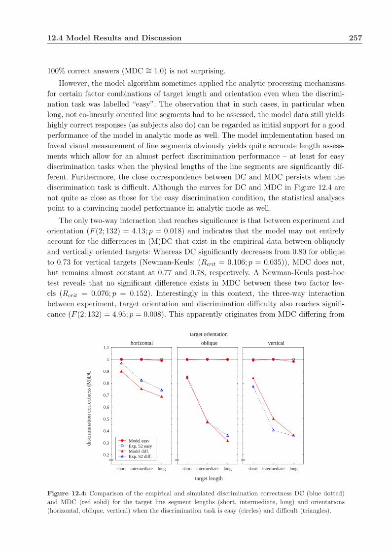
12.4 Model Results and Discussion 257
100% correct answers (MDC ∼= 1.0) is not surprising.
However, the model algorithm sometimes applied the analytic processing mechanisms
for certain factor combinations of target length and orientation even when the discrimi-
nation task was labelled “easy”. The observation that in such cases, in particular when
long, not co-linearly oriented line segments had to be assessed, the model data still yields
highly correct responses (as subjects also do) can be regarded as initial support for a good
performance of the model in analytic mode as well. The model implementation based on
foveal visual measurement of line segments obviously yields quite accurate length assess-
ments which allow for an almost perfect discrimination performance – at least for easy
discrimination tasks when the physical lengths of the line segments are significantly dif-
ferent. Furthermore, the close correspondence between DC and MDC persists when the
discrimination task is difficult. Although the curves for DC and MDC in Figure 12.4 are
not quite as close as those for the easy discrimination condition, the statistical analyses
point to a convincing model performance in analytic mode as well.
The only two-way interaction that reaches significance is that between experiment and
orientation (F (2; 132) = 4.13; p = 0.018) and indicates that the model may not entirely
account for the differences in (M)DC that exist in the empirical data between obliquely
and vertically oriented targets: Whereas DC significantly decreases from 0.80 for oblique
to 0.73 for vertical targets (Newman-Keuls: (Rcrit = 0.106; p = 0.035)), MDC does not,
but remains almost constant at 0.77 and 0.78, respectively. A Newman-Keuls post-hoc
test reveals that no significant difference exists in MDC between these two factor lev-
els (Rcrit = 0.076; p = 0.152). Interestingly in this context, the three-way interaction
between experiment, target orientation and discrimination difficulty also reaches signifi-
cance (F (2; 132) = 4.95; p = 0.008). This apparently originates from MDC differing from
disc
rim
inat
ion
corr
ectn
ess
(M)D
C
0.2
0.3
0.4
0.5
0.6
0.7
0.8
0.9
1
1.1
short intermediate long short intermediate long short intermediate long
Model easy Exp. S2 easy Model diff. Exp. S2 diff.
target orientation
horizontal oblique vertical
target length
Figure 12.4: Comparison of the empirical and simulated discrimination correctness DC (blue dotted)and MDC (red solid) for the target line segment lengths (short, intermediate, long) and orientations(horizontal, oblique, vertical) when the discrimination task is easy (circles) and difficult (triangles).

258 Modelling Similarity Effects
DC between the oblique and vertical target orientations only when the discrimination task
is difficult. It thus appears possible that the model is well able to adopt its processing
mechanisms in analytic mode to account for co-linearly and not co-linearly oriented line
segments differently – and in accordance with the empirical data.
However, the model algorithm may still have some deficits in making finer distinctions
between different tilted line segments, i.e. to distinguish between oblique and vertical, for
example. As no other differences between DC and MDC become significant and, in general,
means of MDC very closely resemble those of DC, the chosen model implementation can
still be considered promising in this respect so far. Figure 12.4 qualitatively supports this
statement and shows the means of the empirical data of Experiment S2 in comparison
with those of the similarity model as a function of target line segment length. In order
to improve the clarity of the illustration, the values are charted separately for the three
target orientations horizontal, oblique and vertical.
Model Reaction Time MRT
The model implementation does not explicitly simulate reaction time. Rather, MRT, the
modelled reaction time, can be implicitly computed from the modelled fixation duration
MFD (see later in this section). Rather than only summing up all MFDs per trial, sac-
cade durations must also be added to yield MRT. With saccade “velocity” remaining
almost constant in the empirical data, independent of saccade length, saccade duration is
calculated as
saccade duration =saccade length
saccade velocity
and added to MRT for each saccade executed. It must be noted that this equation is a
simplification which assumes that saccade velocity remains constant during a saccade. In
reality, this is not the case.
The four-factorial analysis of variance yields no significant main effect of the factor
experiment on the discrimination correctness (F (1; 66) = 10.21; p = 0.142), indicating
that the model-generated reaction times MRT in general are quite similar to those that
the subjects produced in Experiment S2. The comparison of means (see Figure 12.5) shows
that for both the easy and the difficult discrimination condition MRT is longer than RT.
Although not significant, it appears that the model algorithm generates slightly more
fixations and saccades than subjects – or that FDs are longer in the model than in the
empirical data. The differences between MRT and RT are most pronounced when long,
not co-linearly oriented line segments are presented. A deficit of the model to correctly
reproduce FDs thus appears less likely, otherwise probably all MRTs should have been
prolonged equally. Furthermore, FDs have been modelled based on the distributions of
the empirical data, taking into account the individual differences of those for the various
factor combinations. The FD-model should thus be quite accurate (see later in this section,
“Fixation duration MFD”). Instead, when the discrimination is easy, the model may “too
soon”, i.e. too often, switch from holistic into analytic mode. This generates more fixations
and saccades and thus increases the overall MRT. When the model pursues the analytic
strategy for difficult discrimination tasks already, the increased MRTs may be caused by

12.4 Model Results and Discussion 259
reac
tion
time
(M)R
T (
ms)
500
1000
1500
2000
2500
3000
short intermediate long short intermediate long short intermediate long
Model easy Exp. S2 easy Model diff. Exp. S2 diff.
horizontal oblique vertical
target length
target orientation
Figure 12.5: Comparison of the empirical and simulated reaction times RT (blue dotted) and MRT (redsolid) for the target line segment lengths (short, intermediate, long) and orientations (horizontal, oblique,vertical) when the discrimination task is easy (circles) and difficult (triangles).
too many shifts of attention between display hemifields and/or a slightly higher rate of
three successive fixations within the same hemifield for such a factor combination. The
analyses of the respective variables later in this section should clarify these considerations.
In this context, the only significant interaction effect on (M)RT involving the factor
experiment, namely that between experiment, target length and orientation (F (4; 264) =
2.98; p = 0.020), must be considered. A post-hoc comparison of means using the Newman-
Keuls test reveals that significant differences indeed exist (Rcrit = 168.03; p < 0.001)
between the model and the empirical data when the length of long vertical targets has
to be assessed. The analysis does not yield any other significant interactions between
the model and Experiment S2. Figure 12.5 shows the RT means of Experiment S2 in
comparison with MRT of the similarity model as a function of target line segment length.
In order to improve the clarity of the illustration, the values are charted separately for the
three target orientations horizontal, oblique and vertical. The two resembling curves for
each factor combination visualise the good correspondence between model and experiment
with respect to reaction time and thus are in line with the statistical results.
Model Number of Fixations MNF
After the statistical comparisons of the empirical and the model results have demonstrated
a high correlation between those two data sets with respect to the more “conventional”
variables (M)DC and (M)RT, the eye-movement parameters must now be addressed.
Most of the comparisons of the numbers of fixations do not produce a significant
difference between the empirical and the model results. Four-factorial analyses of variance
do not yield such an effect for the overall numbers of fixations (M)NF (F (1; 66) = 1.03; p =

260 Modelling Similarity Effects
0.313), the numbers of fixations in proximity to the target (M)NFT (F (1; 66) = 10.21; p =
0.142), or those in proximity to the comparison (M)NFC (F (1; 66) = 10.21; p = 0.142).
The only significant interaction affected by the comparison between Experiment S2 and
the model is that between the factors experiment, target length and orientation. The
analysis of variance yields (F (4; 264) = 3.08; p = 0.049) for (M)NF and (F (4; 264) =
1.79; p = 0.032) for (M)NFT for these three-way interactions; none was found for (M)NFC .
A closer inspection of Figure 12.6 reveals that there indeed appears to be a difference
between the empirical and the model data when targets are obliquely oriented. Both charts
for (M)NF and (M)NFT show that these numbers of fixations slightly increase from short
through intermediate to long targets in the model whereas the empirical data remains
almost constant for the different lengths (or even slightly decreases). This is in particular
visible in the difficult discrimination condition. Quantitatively, this is supported by a
post-hoc comparison of means using the Newman-Keuls test that identifies the already
(quantitatively) noted differences – and only those – as being responsible for the significant
interaction effect: The test computes (Rcrit = 0.82; p = 0.025) and (Rcrit = 0.89; p =
0.019) for the differences between the empirical and the model data in (M)NF for oblique
targets when their lengths are intermediate and long, respectively, and (Rcrit = 0.69; p =
0.047) for the differences between the empirical and the model data in (M)NFT for oblique
targets when their lengths are long.
With regard to the number of fixations in the intermittent display section, MNFI
is significantly higher than NFI and the four-factorial analysis of variance produces a
significant main effect for the factor experiment (F (1; 66) = 1.22; p = 0.015). As for
the other categories of the numbers of fixations, the model values are higher than those
measured in Experiment S2. In case of (M)NFI , the difference is now a significant one,
Figure 12.7 (bottom) illustrates the apparently large differences. However, the absolute
differences are not quite as drastic as they appear. In order to visualise the individual
differences, the vertical scale is of a different order of magnitude compared to those for
(M)NF, (M)NFT and (M)NFC . Thus, the largest (absolute) difference between empirical
and model data only measures 0.2 fixations. As the model algorithm does not explicitly
distinguish between holistic and analytic mode when executing intermittent fixations, it is
not likely to find the same differences in the model data as in the empirical data. However,
MNFI is implicitly influenced by the planning of inter-stimulus saccades. Since in holistic
mode a larger percentage of such model saccades aim at the center or outermost point
of the line segment in the other display hemifield than in analytic mode, the distance
between the current and the subsequent fixation point is longer in the first case. The
assessment of more peripheral points will consequently be less accurate and will lead,
according to the model implementation, to the execution of intermittent fixations more
often when the discrimination is easy. On the other hand, more shifts of attention between
hemifields should occur when the discrimination is difficult. This would then increase the
number of intermittent fixations in that processing mode, so that the rather equal values
for MNFI , irrespective of the discrimination difficulty, can be understood. Following the
same argumentation, it is clear that the model adequately reproduces the effects of target
length and orientation on NFI : Line segments that are not co-linearly oriented are further

12.4 Model Results and Discussion 261
num
ber
of f
ixat
ions
(M
)NF
0
1
2
3
4
5
6
7
8
short intermediate long short intermediate long short intermediate long
Model easy Exp. S2 easy Model diff. Exp. S2 diff.
target orientation
horizontal oblique vertical
target length
num
ber
of ta
rget
fix
atio
ns (
M)N
F T
0
1
2
3
4
5
6
7
8
short intermediate long short intermediate long short intermediate long
Model easy Exp. S2 easy Model diff. Exp. S2 diff.
target orientation
horizontal oblique vertical
target length
Figure 12.6: Comparison of the empirical (blue dotted) and simulated (red solid) numbers of fixationsas a function of target line segment length and orientation when the discrimination task is easy (circles)and difficult (triangles). Top: Overall numbers of fixations NF vs. MNF. Bottom: Target numbers offixations NFT vs. MNFT .
apart and might thus require intermittent fixations more often when attention shifts from
one to the other. The same is true when the length of line segments is short.
In general, Figures 12.6 and 12.7 show that the model produces slightly more fixations
than subjects do in Experiment S2, an effect consistent with the prolonged reaction times
MRT found previously. Although this effect is again not significant so that the model per-
formance can be considered adequate with respect to this (first) eye-movement parameter,
it suggests that some of the model parameters, for example those that determine the den-

262 Modelling Similarity Effects
num
ber
of c
ompa
riso
n fi
xatio
ns (
M)N
F C
0
1
2
3
4
5
6
7
8
short intermediate long short intermediate long short intermediate long
Model easy Exp. S2 easy Model diff. Exp. S2 diff.
target orientation
horizontal oblique vertical
target length
num
ber
of in
term
itten
t fix
atio
ns (
M)N
F I
0
0.1
0.2
0.3
0.4
0.5
short intermediate long short intermediate long short intermediate long
Model easy Exp. S2 easy Model diff. Exp. S2 diff.
target orientation
horizontal oblique vertical
target length
Figure 12.7: Comparison of the empirical (blue dotted) and simulated (red solid) numbers of fixationsas a function of target line segment length and orientation when the discrimination task is easy (circles)and difficult (triangles). Top: Comparison numbers of fixations NFC vs. MNFC . Bottom: Intermediatenumbers of fixations NFI vs. MNFI . (N.B.: Different vertical scale used in the bottom chart.)
sity distribution functions and their approximations or the “noise models”, might still
require some optimisation. In addition, the model reproduces the numbers of intermittent
fixations MNFI on a higher overall level than given by the empirical data. Although the
absolute difference appears negligible in relation to (M)NFT and (M)NFC , this might also
account for some of the empirical–model differences. Nevertheless, the resemblance of the
modelled numbers of fixations to the empirical ones is quite good. Furthermore, when
viewed in relation to the convincing model reproduction of the discrimination correctness
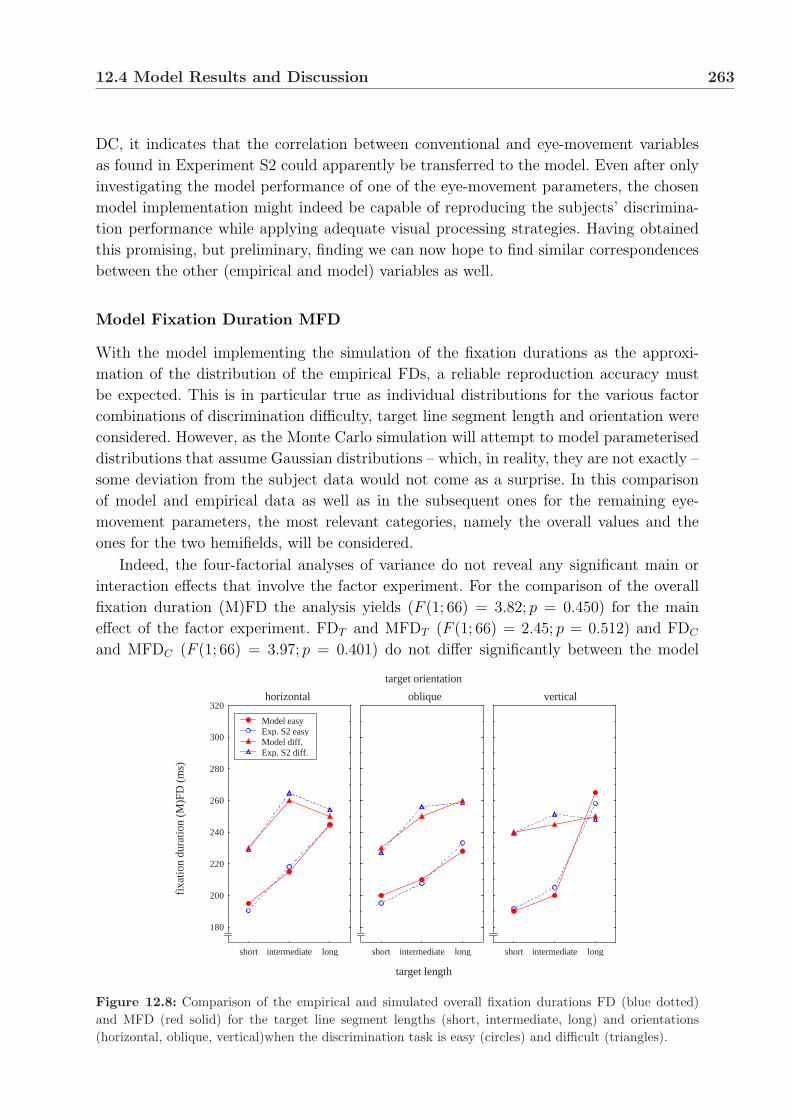
12.4 Model Results and Discussion 263
DC, it indicates that the correlation between conventional and eye-movement variables
as found in Experiment S2 could apparently be transferred to the model. Even after only
investigating the model performance of one of the eye-movement parameters, the chosen
model implementation might indeed be capable of reproducing the subjects’ discrimina-
tion performance while applying adequate visual processing strategies. Having obtained
this promising, but preliminary, finding we can now hope to find similar correspondences
between the other (empirical and model) variables as well.
Model Fixation Duration MFD
With the model implementing the simulation of the fixation durations as the approxi-
mation of the distribution of the empirical FDs, a reliable reproduction accuracy must
be expected. This is in particular true as individual distributions for the various factor
combinations of discrimination difficulty, target line segment length and orientation were
considered. However, as the Monte Carlo simulation will attempt to model parameterised
distributions that assume Gaussian distributions – which, in reality, they are not exactly –
some deviation from the subject data would not come as a surprise. In this comparison
of model and empirical data as well as in the subsequent ones for the remaining eye-
movement parameters, the most relevant categories, namely the overall values and the
ones for the two hemifields, will be considered.
Indeed, the four-factorial analyses of variance do not reveal any significant main or
interaction effects that involve the factor experiment. For the comparison of the overall
fixation duration (M)FD the analysis yields (F (1; 66) = 3.82; p = 0.450) for the main
effect of the factor experiment. FDT and MFDT (F (1; 66) = 2.45; p = 0.512) and FDC
and MFDC (F (1; 66) = 3.97; p = 0.401) do not differ significantly between the model
fixa
tion
dura
tion
(M)F
D (
ms)
180
200
220
240
260
280
300
320
short intermediate long short intermediate long short intermediate long
Model easy Exp. S2 easy Model diff. Exp. S2 diff.
target orientation
horizontal oblique vertical
target length
Figure 12.8: Comparison of the empirical and simulated overall fixation durations FD (blue dotted)and MFD (red solid) for the target line segment lengths (short, intermediate, long) and orientations(horizontal, oblique, vertical)when the discrimination task is easy (circles) and difficult (triangles).

264 Modelling Similarity Effects
and experimental data sets either. This is also illustrated in Figures 12.8 and 12.9 where
all model means for all factor combinations closely resemble those of the empirical data
from Experiment S2. Only rather small deviations are visible in some cases. Furthermore,
these deviations appear to be random rather than systematic, indicating that the assumed
Gaussian density distribution was appropriate for the probabilistic model approach chosen
to simulate the fixation durations – otherwise, i.e. in case of systematically either lower
or higher MFDs than FDs, it would have been more appropriate to employ skewed distri-
butions such as a χ2 or a Gamma function in order to adequately describe the empirical
distributions of FDs.
targ
et f
ixat
ion
dura
tion
(M)F
DT (
ms)
180
200
220
240
260
280
300
320
short intermediate long short intermediate long short intermediate long
Model easy Exp. S2 easy Model diff. Exp. S2 diff.
target orientation
horizontal oblique vertical
target length
com
pari
son
fixa
tion
dura
tion
(M)F
DC (
ms)
180
200
220
240
260
280
300
320
short intermediate long short intermediate long short intermediate long
Model easy Exp. S2 easy Model diff. Exp. S2 diff.
target orientation
horizontal oblique vertical
target length
Figure 12.9: Comparison of the empirical (blue dotted) and simulated (red solid) fixation durations asa function of target line segment length and orientation when the discrimination task is easy (circles) anddifficult (triangles). Top: Target fixation duration FDT vs. MFDT . Bottom: Comparison fixation durationFDC vs. MFDC .

12.4 Model Results and Discussion 265
Model Number of Saccades between Hemifields MSB
As Figure 12.10 shows qualitatively, the model also quite accurately reproduces the num-
bers of saccades between hemifields. The modelled shifts of attention between the stimulus
constituents significantly vary between the easy and difficult discrimination conditions in
the same way as they do in the empirical data. The main effect of the factor experiment
does not reach significance level (F (1; 66) = 0.75; p = 0.390). The characteristics of the
“global” variable MSB not only indicate that the model successfully simulates the global
processes of either holistic (few shifts of attention) or analytic (several shifts of atten-
tion) visual processing. Furthermore, it can be assumed that this is only so because the
model also shows similar “behaviour” to that of subjects on the local processing level:
The specific strategies the model applies in order to locally assess the line segments’
length, i.e. local peripheral length assessment in case of an easy discrimination task and
foveal visual measurement via saccades in case of a difficult discrimination task, appar-
ently yield length assessments that are accurate enough to solve the discrimination task
after few shifts of attention (holistic mode) or require several re-assessments, update and
validation of existing length representations.
num
ber
of s
acca
des
betw
een
hem
ifie
lds
(M)S
B
0
1
2
3
4
5
short intermediate long short intermediate long short intermediate long
Model easy Exp. S2 easy Model diff. Exp. S2 diff.
target orientation
horizontal oblique vertical
target length
Figure 12.10: Comparison of the empirical and simulated numbers of saccades between stimulus hemi-fields SB (blue dotted) and MSB (red solid) for the target line segment lengths (short, intermediate, long)and orientations (horizontal, oblique, vertical) when the discrimination task is easy (circles) and difficult(triangles).
Although a good overall correspondence is noted between model and empirical data,
a significant four-way interaction is found (F (4; 264) = 1.23; p = 0.041). The post-hoc
comparison of means using the Newman-Keuls test demonstrates that the empirical
and the model data differ in the difficult discrimination condition when long oblique
(Rcrit = 0.67; p = 0.045) or long vertical line segments (Rcrit = 0.64; p = 0.038) have to be

266 Modelling Similarity Effects
assessed. The model algorithm then requires more shifts of attention between hemifields
than subjects. This finding for long, not co-linearly oriented line segments during analytic
assessment can probably be understood when considering that this combination certainly
represents the most complex condition for the comparison and discrimination task. On
the local processing level the model will quite often have to integrate data from more than
just two successive fixations. These extra computations have been modelled to decrease
the assessment accuracy and take extra time so that more re-assessment of stimuli in par-
ticular for this combination may be required. Conceivably, this assessment modelling on
the local visual processing level in analytic mode slightly “over-deteriorates” the length
representations. However, the reproduction of the empirical data is still achieved quite
convincingly. Even for the factor combinations where significant differences are found,
these only amount to approximately 0.4 saccades.
Model Number of Successive Fixations within the same Hemifield MFW
Finally, it must be verified if the model reproduces the empirical data for the local eye-
movement parameters. When the simulated numbers of successive fixations within the
same hemifield and saccade lengths do not differ significantly from those obtained from
the subjects’ eye-movement recordings, the chosen implementation apparently succeeds
in adequately modelling the foveal visual measurement of line segment length via sac-
cades. The analysis of variance does not yield a significant main effect for the influence of
the factor experiment on the aggregated number of successive fixations within the same
hemifield (M)FW (F (1; 66) = 1.82; p = 0.451). Furthermore, no significant influence of the
factor experiment can be found on the separate numbers of successive fixations within the
target hemifield (M)FWT (F (1; 66) = 1.02; p = 0.381) or within the comparison hemifield
(M)FWC (F (1; 66) = 1.25; p = 0.254).
The comparison of means (see Figures 12.11 and 12.12) shows again that the model
produces slightly more successive fixations within the same hemifield than subjects do.
This general upward shift of model data which was already noticed in some of the other
parameters may thus to some extent be attributed to the model more often executing
three successive fixations to measure a line segment length than subjects do in analytic
mode. This is in particular so when the two line segments are not co-linearly oriented.
However, whereas subjects significantly more often execute such fixations when the target
is vertical, the model also quite often generates an extra fixation when targets are oblique.
Furthermore, it appears that MFW increases for not co-linearly oriented line segments
of medium length. The resulting measuring saccades should most likely be alternating
ones in an attempt to validate and improve the representation accuracy of the first visual
length measurement.
Such an overestimation of the numbers of successive fixations, in particular for oblique
and/or intermediate targets – compared to the empirical ones – are in fact most notica-
ble in MFWC . This can be understood when considering that the model implementation
takes into account the representation of the previously generated target length. For longer,
oblique (or vertical) targets this representation is usually less accurate than the compari-

12.4 Model Results and Discussion 267
num
ber
of s
ucce
ssiv
e fi
xatio
ns w
ithin
the
sam
e he
mif
ield
(M
)FW
1
1.2
1.4
1.6
1.8
2
2.2
2.4
2.6
2.8
3
3.2
short intermediate long short intermediate long short intermediate long
Model easy Exp. S2 easy Model diff. Exp. S2 diff.
target orientation
horizontal oblique vertical
target length
Figure 12.11: Comparison of the empirical and simulated numbers of successive fixations within thesame hemifield FW (blue dotted) and MFW (red solid) for the target line segment lengths (short, in-termediate, long) and orientations (horizontal, oblique, vertical) when the discrimination task is easy(circles) and difficult (triangles).
son representation. While subjects, after visually measuring the comparison line segment
and so far failing to solve the discrimination task yet, probably realise that mainly the
inaccurate target representation has to be improved and thus shift their attention back
to that stimulus constituent, the model does not. Instead, as currently attending to the
comparison stimulus anyway, the algorithm first updates that length representation using
an alternating saccade before shifting attention back to the target for reassessment.
The statistical analysis demonstrates that indeed a significant interaction effect exists
between the factors experiment, target length and orientation on (M)FWC (F (4; 264) =
5.67; p = 0.043). The subsequent post-hoc comparison of means further yields signifi-
cant differences between the model and the empirical data only for oblique intermediate
(Rcrit = 0.22; p = 0.031), oblique long (Rcrit = 0.27; p = 0.038) and vertical intermedi-
ate (Rcrit = 0.26; p = 0.047) targets when the discrimination is difficult. In particular
the seemingly different (M)FWC values for horizontal and oblique intermediate targets
in the easy discrimination condition (see Figure 12.12, bottom) do not contribute to this
effect. The charts suggest that the algorithm slightly more often switches over to analytic
mode in case of an easy discrimination task in general, and, more often so, for those spe-
cific factor combinations. Although the effect is not significant it can be speculated that
the implementation of the local peripheral length assessment does not yield sufficiently
accurate length representations for the more complex stimulus configurations. The then
applied analytic visual processing would lead to the increase of MFWs. The statistical
analysis does not yield any further significant interaction effects.
In general, the model reproduction can again be considered quite successful with re-
spect to (M)FW. Only some deviations from the empirical data emerge. As the above
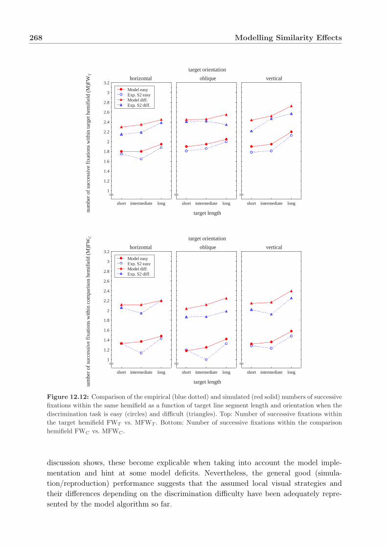
268 Modelling Similarity Effects
num
ber
of s
ucce
ssiv
e fi
xatio
ns w
ithin
targ
et h
emif
ield
(M
)FW
T
1
1.2
1.4
1.6
1.8
2
2.2
2.4
2.6
2.8
3
3.2
short intermediate long short intermediate long short intermediate long
Model easy Exp. S2 easy Model diff. Exp. S2 diff.
target orientation
horizontal oblique vertical
target length
num
ber
of s
ucce
ssiv
e fi
xatio
ns w
ithin
com
pari
son
hem
ifie
ld (
M)F
WC
1
1.2
1.4
1.6
1.8
2
2.2
2.4
2.6
2.8
3
3.2
short intermediate long short intermediate long short intermediate long
Model easy Exp. S2 easy Model diff. Exp. S2 diff.
target orientation
horizontal oblique vertical
target length
Figure 12.12: Comparison of the empirical (blue dotted) and simulated (red solid) numbers of successivefixations within the same hemifield as a function of target line segment length and orientation when thediscrimination task is easy (circles) and difficult (triangles). Top: Number of successive fixations withinthe target hemifield FWT vs. MFWT . Bottom: Number of successive fixations within the comparisonhemifield FWC vs. MFWC .
discussion shows, these become explicable when taking into account the model imple-
mentation and hint at some model deficits. Nevertheless, the general good (simula-
tion/reproduction) performance suggests that the assumed local visual strategies and
their differences depending on the discrimination difficulty have been adequately repre-
sented by the model algorithm so far.

12.4 Model Results and Discussion 269
Model Saccade Length MSL
Finally, the evaluation of the model results with regard to saccade length has to be
accomplished. Model and empirical data will be compared for the saccade lengths between
hemifields (SLb vs. MSLb) and for the saccade lengths within each hemifield (SLT vs. MSLT
and SLC vs. MSLC). Furthermore, the ratio of the modelled within-hemifield saccade
lengths
MDL = (MSLC −MSLT )/MSLT (12.17)
can be interpreted as the (relative) length deviation between the measurement of the
target and comparison line segment lengths, i.e. as describing target length over- or un-
derestimation. MDL can thus be compared to the relative length deviation DL measured
in Experiment S1. This allows us to validate if the suggested model approach also repro-
duces the effects induced by the horizontal-vertical illusion – presuming that such visual
illusory effects can at least partially be attributed to oculomotor processes.
The four-factorial analysis of variance does not yield a significant main effect of the
factor experiment on the saccade length between hemifields (M)SLb (F (1; 66) = 0.56; p =
0.625). Furthermore, none of the possible two-, three- or four-way interaction effects in-
volving the factor experiment reach significance level either. Figure 12.13 supports the high
correlation between the model and the empirical data. However, a comparison of means
and the closer inspection of Figure 12.13 reveal that now MSLb is longer when the discrim-
ination task is easy than when it is difficult. A separate analysis of variance shows that the
effect of discrimination difficulty on MSLb is a significant one (F (1; 33) = 1.56; p = 0.001).
This finding is inverse to the observations in the empirical data, when SLb was found to be
significantly shorter for easy than for difficult discriminations (F (1; 33) = 1.79; p < 0.001,
sacc
ade
leng
th b
etw
een
hem
fiel
ds (
M)S
Lb
(deg
rees
)
15
16
17
18
19
20
21
22
short intermediate long short intermediate long short intermediate long
Model easy Exp. S2 easy Model diff. Exp. S2 diff.
target orientation
horizontal oblique vertical
target length
Figure 12.13: Comparison of the empirical and simulated saccade lengths between hemifields SLb (bluedotted) and MSLb (red solid) for the target line segment lengths (short, intermediate, long) and orienta-tions (horizontal, oblique, vertical) when the discrimination task is easy (circles) and difficult (triangles).

270 Modelling Similarity Effects
see Section 11.3). This may be due to the model algorithm often generating inter-stimulus
saccades that start at the mid-point of one line segment and aim at the mid-point of the
other when in holistic mode. In contrast, usually the innermost end point of the line
segment in the other stimulus hemifield is aimed at when the model executes shifts of
attention in analytic mode. With those inter-stimulus saccades often also starting at the
innermost end point, MSLb should be shorter in analytic than in holistic model mode.
As found for most other eye-movement parameters before, the model quite accurately
sacc
ade
leng
th w
ithin
targ
et h
emfi
eld
(M)S
LT (
degr
ees)
0
1
2
3
4
5
6
7
8
short intermediate long short intermediate long short intermediate long
Model easy Exp. S2 easy Model diff. Exp. S2 diff.
target orientation
horizontal oblique vertical
target length
sacc
ade
leng
th w
ithin
com
pari
son
hem
fiel
d (M
)SL
C (
degr
ees)
0
1
2
3
4
5
6
7
8
short intermediate long short intermediate long short intermediate long
Model easy Exp. S2 easy Model diff. Exp. S2 diff.
target orientation
horizontal oblique vertical
target length
Figure 12.14: Comparison of the empirical (blue dotted) and simulated (red solid) saccade length withinthe same hemifield as a function of target line segment length and orientation when the discriminationtask is easy (circles) and difficult (triangles). Top: Saccade length within the target hemifield SLT vs.MSLT . Bottom: Saccade length within the comparison hemifield SLC vs. MSLC .

12.4 Model Results and Discussion 271
reproduces the saccade lengths within each hemifield. Neither a significant main effect of
the factor experiment on (M)SLT (F (1; 66) = 2.45; p = 0.421) or (M)SLC (F (1; 66) =
2.00; p = 0.355) nor any interactions with the factors discrimination difficulty, target line
segment length and/or orientation can be found. Although not significant, the lengths of
the model saccades in particular within the target hemifield MSLT appear to be slightly
shorter than the empirical values. This could again support the earlier observations that
the model may actually execute two “in-line“ measuring saccades more often, leading to
a decrease of the respective saccade lengths. Furthermore, the model might also generate
slightly more corrective saccades, possibly due to deficits in the model determination of
saccade landing points. Subjects might achieve this task more accurately and thus require
less corrective saccades. Compared to the measuring saccades, these are usually quite
short and can thus be thought to influence MSL even when only few are executed.
Figure 12.14 illustrates the again close correspondence between the two data sets for
(M)SLT (top) and (M)SLC (bottom). Interestingly here, the curves for holistic and ana-
lytic processing are not reversed as found for (M)SLb. This is in line with the specifications
of the model algorithm for foveal visual measurement of line segment lengths: When the
model applies measuring saccades for the foveal assessment of line segment lengths al-
though the discrimination task is easy, these will always measure half the length of a
line segment. Two successive saccades “in-line” (to measure the same fraction of the line
segment, but consequently yielding saccade lengths of only one quarter of the length of
the line segment) will not be executed as is the case for some of the saccadic measurement
when the discrimination task is difficult. Furthermore, corrective saccades are generally
not executed when in analytic mode for easy discriminations – whereas the model would
have executed them for similar situations when the discrimination is difficult. Thus, on
average, the saccade lengths within each hemifield MSLT and MSLC are shorter when
Figure 12.15: Model gaze trajectories in the easy (top) and difficult (bottom) discrimination conditions.

272 Modelling Similarity Effects
the discrimination is easy than when it is difficult – similar to the observations in the
subjects’ data SLT and SLC .
This yet again clearly indicates that the assumed (local) visual processes in both
holistic and analytic mode were adequately represented in the model. In fact, the good
reproduction of eye-movement parameters can be understood to have enabled the accu-
rate reproductions of the more “conventional” parameters. The local visual processes,
either local peripheral length assessment or foveal visual measurement via saccades, could
apparently be parameterised in the model implementation in an adequate manner. The
quantitative analysis is further supported by qualitative data. Gaze trajectories that were
generated by the model (Figure 12.15) and those that subjects produced (see Figures 3.9
and/or 11.18) closely resemble each other. Finally, the application of visual strategies im-
plemented according to empirical specification yields appropriate length representations
so that the subsequent modelling of the comparison and representation update processes
also generates proportions of discrimination correctness MDC that very closely resemble
those of subjects.
This only leaves us to verify if there also exists a correlation between the ratios of
the modelled saccade lengths within each hemifield (see Equation 12.17), yielding MDL,
and the relative length deviations DL as measured in Experiment S1. At first sight, Fig-
ure 12.16 does not seem to present very promising results in favour of such a positive
correlation: Neither are the absolute values of DL and MDL of the same magnitude nor is
MDL able to reproduce the effect of DL to decrease for longer target length. Instead MDL
drastically increases from short through intermediate to long targets (Figure 12.16, left).
However, two rather important correspondences between DL and MDL can be found:
First, MDL can be understood as producing an overestimation of the target length which
is in line with DL. Second, this overestimation increases when the two line segments are
not co-linearly oriented. Furthermore, the model even reproduces the strong increase in
DL from horizontal to oblique and the less pronounced increase from oblique to vertical
(Figure 12.16, right) – to be precise, MDL does not increase from oblique to vertical, but
remains at the same level.
With respect to the horizontal-vertical illusion, orientation effects can certainly be
target length
rela
tive
leng
th d
evia
tion
(M)D
L
0
0.1
0.2
0.3
0.4
0.5
short intermediate long
ModelExp. S1
target orientation
rela
tive
leng
th d
evia
tion
(M)D
L
0
0.1
0.2
0.3
0.4
0.5
horizontal oblique vertical
ModelExp. S1
Figure 12.16: Comparison of the empirical (blue dotted) and simulated (red solid) length deviationsDL and MDL as a function of target line segment length (left) or orientation (right).

12.5 Summary and Conclusions 273
considered as more relevant than length effects. The model, using the ratios of measuring
saccades to represent deviations in perceived lengths, quite correctly reproduces these
orientation effects and, more specifically, the overestimation of the length of oblique tar-
gets. Although the extent of the illusory effect is certainly on a different magnitude scale,
this finding appears to present some support for at least partially attributing this illusory
effect to low-level sensorimotor processes. Apparently, the oculomotor system has a se-
vere deficit executing accurate measuring saccades when the lengths of line segments that
are not co-linearly oriented are foveally assessed. Mental length representations based on
these inaccurate measurements will probably not be very accurate either. However, as
the model is not capable reproducing all effects observed in the empirical data and only
simulates the illusory effect on a different magnitude scale, oculomotor processes alone
cannot explain all aspects of the horizontal-vertical illusion.
The following section summarises the fundamental results of Chapters 9–12.
12.5 Summary and Conclusions
After the contributions of peripheral perception processes to the overall understanding of
line segment assessment had been established earlier, the investigation then moved on to
studying line segment perception in a more complex scenario. The focus here has been on
similarity effects in line segment length perception during simultaneous comparison tasks.
This scenario appeared to be particularly promising for the investigation of different vi-
sual strategies that subjects apply in order to solve discrimination tasks – holistic visual
processing for easy discriminations vs. analytic visual scene analysis for difficult discrim-
inations. The comprehension of the perceptual mechanisms and the underlying cognitive
processing steps should be greatly facilitated by the analysis of eye movements which
manifest the pursued visual strategies. The chosen scenario also appeared promising with
a view to modelling the observed empirical visual behaviour. With saccade planning (not
only) for such visual strategies being largely guided by peripheral information process-
ing, an attempt should be made to integrate the previous findings into a comprehensive
explanatory approach. Based thereupon, it should further be possible to develop a compu-
tational model that adequately describes line segment perception and comparison while
taking into account components of the eccentricity model of Chapter 8.
The first experiment in this series, Experiment S1, already yields great support for
some of the hypothesised fundamental mechanisms that are applied to assess line segment
length within the present comparison scenario. Furthermore, it becomes clear that without
the analysis of eye movements, these mechanisms and visual processing strategies would
have been difficult – if not impossible – to establish. The discussion of results for example
shows that foveal “visual measurement” of line segments appears to be the central element
of length assessment, generally characterised by two successive fixations on the respective
line segment. The saccade length between the two fixations closely coincides with the
overall length of the respective line segment when it is short or, when longer, only covers
a specific fraction of the line segment. Additional information on the size of the fraction

274 Modelling Similarity Effects
in relation to the overall length must be memorised along with the mental representation
of the saccade length for the subsequent comparison. This requires the incorporation
of peripherally perceived information on the outermost end point of the line segment in
question and suggests that line segments must be decomposed in simultaneous comparison
tasks as well.
Eye movements further indicate that after the visual measurement of one of the two
stimulus constituents, attention shifts to the other line segment. The comparison stim-
ulus is analogously assessed, i.e. visually measured, and the correspondingly generated
representation mentally compared with the previously memorised one. If the two repre-
sentations are not found to match in length, the comparison is adjusted and the mental
comparison executed again with the updated comparison representation. This procedure
can be re-iterated several times until the two representations of the target and comparison
line segments are found to match in length. Fixation data also suggests that sometimes
intermittent saccades to the target line segment occur (single fixations only), probably
to “refresh” the initially memorised target representation – in particular when numerous
adjustment steps are necessary to match the comparison length.
The investigation of eye movements in Experiment S1 also yields valuable informa-
tion on the extent of the stimuli-induced horizontal-vertical illusion and provides new
approaches to assist its understanding: Taking the visual measurement strategy into ac-
count, saccade lengths indicate that mental representations of lengths larger than the
physical lengths of target line segments are stored and referred to for comparison and
matching. This may cause the typical overestimation of oblique and vertical line segments
induced by the illusion. The finding suggests that the illusory effects may at least partially
be attributed to deficits during low level, oculomotor processing. Here, the dynamic ad-
justment procedure applied in Experiment S1 proves indispensable. The stimulus-induced
horizontal-vertical illusion could only be quantified using this procedure.
Even more importantly, the dynamic procedure yields the essential data to determine
easy and difficult discrimination conditions in the following Experiment S2. However, Ex-
periment S2 is not only required to investigate the corresponding holistic and analytic
visual strategies. Comparing results from Experiments S1 and S2 suggest that, for exam-
ple, fixation times FD and the distribution of fixations in the comparison hemifield are
influenced by the dynamic procedure of Experiment S1. It apparently distracts subjects
from the “pure” length perception task and makes it difficult to reliably attribute specific
effects solely to the dynamic adjustment process or to the actual line segment assessment
task. The static scenario in Experiment S2 should eliminate the “side-”effects induced by
the dynamic adjustment procedure in Experiment S1 and thus allow us to explore length
perception principles in even greater detail.
The fundamental conclusion that can be drawn from Experiment S2 is that indeed two
distinct visual processing strategies can be established, depending on the discrimination
difficulty. Furthermore, the discussion demonstrates that the initial hypothesis appropri-
ately classifies these strategies as “holistic” and “analytic”. In accordance with the initial
definition of holistic, subjects only coarsely visually scan line segments that exhibit a low
length similarity. When length similarity is high which makes the discrimination diffi-

12.5 Summary and Conclusions 275
cult, a detailed foveal analysis of the line segments is conducted to accurately assess and
represent their lengths for a subsequent mental comparison.
When the discrimination task is easy, the discussion of the results of Experiment S2
reveals that the holistic strategy is applied locally rather than globally. Even in the easy
discrimination condition subjects usually fixate each stimulus constituent (at least) once.
They locally peripherally assess the length of the respective line segment. A single fixation
is found to be sufficient in almost all cases to successfully accomplish the discrimination
task. As further findings strongly indicate that the line segments’ end points are of par-
ticular relevance for length assessment, this very sparse fixation pattern only allows for
the coarse perception of the line segment lengths and constitutes a process that is en-
tirely peripheral. In some cases, however, when the target and the (always horizontally
oriented) comparison line segments are not co-linearly oriented, a detailed foveal analysis
of the target is conducted. This is in particular so when the assessment is further com-
plicated because the line segments are so long that they cannot be perceived peripherally
that easily. Switching to analytic visual mode is thought to yield a more accurate target
length representation, mentally rotated to match the comparison orientation, and subse-
quently compared to the comparison representation. The comparison length is perceived
peripherally so that this process can still be classified as locally holistic. In all cases, the
generated representations are accurate enough to correctly discriminate the lengths in an
instant. Only a single shift of attention between the two stimulus constituents is sufficient
before subjects make their decision.
When the discrimination task is difficult, an analytic visual processing strategy is
pursued throughout. The discussion supports local, foveal “visual measurement” as a
fundamental principle in assessing line segment lengths within both the target and the
comparison hemifield. This visual measurement principle is generally characterised by two
successive fixations within the same hemifield. Even more than in the previous Experi-
ment S1, these fixations are now located “on” the target or the comparison stimulus. The
saccade length between the two fixations closely coincides with the overall length of the
respective line segment when it is short or, when longer, only covers a specific, usually the
innermost, fraction of the line segment. In particular the generation of mental represen-
tations of obviously complex target line segments – such as those that are long and not
co-linearly oriented to the comparison – often requires step-by-step visual analysis of the
target where three successive fixations are executed. In a considerable number of these
cases, gaze “alternates” between two designated locations on the line segment and can
be thought to augment the length representation or to improve the representation accu-
racy. Additional information on the size of the fraction in relation to the overall length
is also stored along with the mental representation of the saccade lengths for the sub-
sequent comparison. This is probably achieved by incorporating peripherally perceived
information on the outermost end point of the line segment in question. Data yields that
apparently half of the overall physical length of the respective line segment is visually
measured, constituting a “multiplication” factor of two.
When data perceived by multiple successive in-line fixations must be integrated, the
addition of several saccade lengths obviously demands greater cognitive and memory “ef-

276 Modelling Similarity Effects
fort” in order to store, maintain and compare the various representations. Such represen-
tations are apparently not ideal as it becomes increasingly difficult to integrate multiple
data. Furthermore, data itself is more complex. Rather than representing half the length
of a line segment, “odd” fractions must now be processed. The discrimination correctness
considerably decreases in such cases. In analogy to the findings in Experiment S1, eye
movements further indicate that after the visual measuring of one of the two stimulus
constituents and the generation of a corresponding mental representation, attention di-
rectly shifts to the other line segment. The comparison stimulus is analogously assessed,
i.e. visually measured, and the correspondingly generated representation mentally com-
pared with the previously memorised one. If the two representations are not found to yield
a significant difference in perceived length, the comparison procedure is repeated and the
mental comparison is executed again with the updated representation. In contrast to the
easy discrimination condition, these global shifts of attention and the subsequent proce-
dure are re-iterated several times when the discrimination is difficult in order to increase
the accuracy of the representations – until the length discrimination task can be solved.
The findings render the decomposition of line segments essential in both processing
modes. The assessment of line segment length apparently requires the assessment of end
point locations. In holistic mode length assessment is then accomplished by fusing pe-
ripherally perceived end point positions to “compute” line segment length. The end point
component(s) yield important landmark locations for saccade planning and foveal visual
measurement in analytic mode. This supports the validity of the initially formulated de-
composition hypothesis also in free gaze simultaneous comparison scenarios.
Taking the empirical findings into account, a comprehensive computational model,
integrating components of the previous eccentricity model, is implemented. The model
is a formalised description of the procedure subjects pursue when they accomplish a si-
multaneous length comparison task. This is accomplished by parameterising the proposed
perception mechanisms so that an algorithmic implementation reproduces the empirical
data. After the model pre-attentively “decides” whether to switch to either holistic or
analytic mode, based on a global peripheral assessment of the two line segments’ lengths,
the algorithm simulates saccade planning which resembles that followed by subjects in
Experiment S2. The characteristics of the scan path both on the global level, describing
the visual inter-stimulus processing, and on the local level, describing the intra-stimulus
processing, are taken into account by the model. This is accomplished depending on the
discrimination difficulty: Local peripheral length assessment is paired with sparse shifts
of attention between stimulus hemifields in holistic mode and foveal visual measurement
via saccades is paired with repeated shifts of attention in analytic mode. The eccentricity
model that is based on the decomposition hypothesis could rather conveniently be inte-
grated into the implementation of both strategies. It either yields the peripheral length
assessments as such in holistic mode or, in both holistic and analytic mode, generates
saccade landing points.
The chosen model implementation successfully represents the visual length assessment
strategies as applied by subjects in the simultaneous comparison tasks of Experiment S2.
It not only achieves a convincing reproduction of the discrimination accuracy, but further-

12.5 Summary and Conclusions 277
more does so by applying visual strategies similar to those subjects use. This is strongly
supported by a model data set of eye-movement parameters that very closely resembles
that obtained in Experiment S2. Both the statistical comparison of these two data sets and
the quantitative illustrations of means for almost all independent variables do not yield
significant differences. Model-generated gaze trajectories close resemble those of subjects.
Furthermore the model implementation, using the length ratios of measuring saccades
to represent deviations in perceived lengths as found in Experiment S1, quite correctly
reproduces the orientation effect of line segments on perceived length as characteristic for
the horizontal-vertical illusion. The length of oblique line segments is overestimated when
compared with horizontal ones. It appears that these illusory effects may at least to some
extent be attributed to deficits of the oculomotor system when visually measuring line
segment lengths.
In summary, Chapters 9–12 have created a rather comprehensive “image” of the vi-
sual perception processes and their interaction that determine the underlying strategies
during line segment length assessment. In particular the analyses of eye-movement param-
eters proved essential in this respect. They support the hypothesised holistic and analytic
strategies that subjects pursue. These could adequately be represented in a comprehensive
computational model, successfully integrating components of the eccentricity model that
was developed earlier.

278 Modelling Similarity Effects

Chapter 13
Conclusions and Outlook
This chapter again summarises the fundamental findings of the present thesis. A great
variety of aspects that influence the visual perception of location, orientation and length in
different visual comparison scenarios have been investigated and successfully formalised in
computational model simulations. Furthermore, an outlook on future research is provided.
It is clear that not all aspects could have been considered so far. Some findings also put
new questions into view. It thus appears promising, for example, to transfer the identified
processing mechanisms to other types of stimuli. This leaves room for future studies, some
of which are currently underway and already provide some preliminary results.
13.1 Summary and Conclusions
In principle, the present investigations explored the different processing steps of the cog-
nitive structure which determines visual comparison tasks: Assessment, memorisation,
comparison/matching. More specifically, the visual mechanisms that guide line segment
perception in sequential and simultaneous visual comparison scenarios were analysed. Eye
movements in particular facilitated the identification of these perception mechanisms and
thus allowed to understand how the different cognitive processing steps were accomplished.
After initially exploring assumed mechanisms that govern such tasks in isolation, the in-
dividual findings could subsequently be integrated to yield a comprehensive, formalised
description of the whole process. This description was finally implemented as a computa-
tional model. The close resemblance between empirical and simulated data supports the
conclusion that the proposed explanatory approaches are reasonable and indeed correctly
reflect the cognitive structure of such visual comparison tasks. Unfortunately however,
even then there is no final “evidence” that the assumed perception mechanisms are really
deployed in the specified manner, i.e. that they are psychologically adequate.
The influence of peripheral vision as one of the fundamental contributing factors to the
assessment of line segments in general was formulated in a decomposition hypothesis. The
sequence of the Experiments E0–E2 reflected the “decomposition” of complex processes
into simpler ones: It should be possible to infer line segment orientation or length from
location assessment, assuming that end point information is essential for the assessment
280 Conclusions and Outlook
of such line segment attributes. More specifically, the assessment of a line segment can
be formalised as the localisation of line segment end points and the computation of their
distance to yield line segment length. In analogy, the computation of the spatial relation
of end points yields line segment orientation.
The first experiment, Experiment E0, consequently investigated the accuracy of loca-
tion assessment in peripheral vision. Results suggest that the assessment of position is
governed by two distinct processes. One is responsible for the assessment of the direc-
tion where a target marker is situated, a process that obviously works quite accurately
and more or less independent of the level of eccentricity of the target. The second pro-
cess determines the distance between fixation point and target. This process yields less
accurate judgements as the radial position of the target is significantly underestimated.
Furthermore, this process is eccentricity-dependent and shows deteriorating assessment
accuracy for the radial target position with increasing peripheral viewing. On aggregate,
the combination of these two processes yields positional judgements that are dominated
by the distance component and results in a perceived position of the target marker that
is shifted towards the fixation point, but shows very little directional divergence.
In order to validate the decomposition hypothesis, the assessment of the length and
orientation of peripherally viewed line segments were investigated in Experiments E1
and E2. The “reference” data obtained in these experiments allowed for the testing of the
existence of correlations between the assessment error of peripherally perceived lengths
or orientations of line segments and the mislocation of marker positions, depending on
eccentricity.
Findings of Experiments E1 and E2 yielded support for the decomposition hypothesis.
Based on the observations regarding the “distance” and “direction” components of loca-
tion assessment, the overestimation of the length of peripherally perceived line segments
could be explained: When memorising a peripherally perceived line segment, subjects
develop a mental model of a line segment of approximately the correct physical length,
but shifted towards the fixation point. Due to the principle of size/length constancy this
mental “shift” of the line segment towards the observer leads to an elongation of the
line segment when its mental model is recalled for comparison. The deteriorating accu-
racy of the assessment of line segment orientation with increasing peripheral presentation
could also be explained with reference to the observations in Experiment E0: Due to the
greater variance along the radial rather than the tangential axis in location assessment,
a considerable variation in orientation assessment must be expected – and could indeed
be observed in Experiment E2.
The development of explanations for the observations made in Experiments E1 and E2
that are based on mechanisms which were found to describe the marker mislocation in
Experiment E0 strongly supports the decomposition hypothesis. Furthermore, the strong
links found between the assessment accuracies for location and those for line segment
length and orientation encouraged an “integrated” model based on the findings of Ex-
periment E0. An accordingly implemented computer simulation successfully reproduced
the empirical data. It yielded line segment length as the distance between the peripherally
assessed locations of the line segment end points and line segment orientation as the rela-

13.1 Summary and Conclusions 281
tive position of the peripherally assessed locations of the line segment end points. Taking
the findings of both length and orientation modelling into account, it appears that the
chosen approach is indeed suitable to adequately reproduce the manifold aspects involved
in the peripheral perception of line segment lengths and – with some restrictions – of
line segment orientation as well. The model’s convincing replication performance further
supports the decomposition hypothesis and gives rise to the assumption that we correctly
identified the perception mechanisms involved in the assessment of line segments, namely
the essential contribution of line segment end point information. Furthermore, we suc-
cessfully implemented these mechanisms in the simulation algorithms.
The eccentricity Experiments E0–E2 yielded a variety of novel insights into visual
peripheral processing – which must definitely be rendered quite interesting in its own re-
spect. Viewed within the greater context of the present thesis, the experiments even more
so provided data that could be integrated into a comprehensive model describing line seg-
ment assessment in a more complex scenario. This was realised in Experiments S1 and S2
which focussed on similarity effects in line segment length perception during simultaneous
comparison tasks. This scenario appeared to be particularly promising for the investi-
gation of different visual strategies that subjects apply in order to solve discrimination
tasks – holistic peripheral visual processing when the discrimination is easy or analytic
foveal scene analysis when the discrimination is difficult. In the chosen free gaze scenario,
the identification and comprehension of the underlying perceptual mechanisms, again
viewed with respect to the underlying cognitive structure of assessment–memorisation–
comparison, should be greatly facilitated by the analysis of eye movements which manifest
the pursued visual strategies.
Indeed, the analysis of eye movements proved essential in establishing the charac-
teristic visual processing strategies. The fundamental results showed that foveal “visual
measurement” of line segments appears to be one of the central mechanisms in length
assessment. It is generally characterised by two successive fixations on the respective line
segment, constituting a “measuring saccade”. The saccade length between the two fixa-
tions closely coincided with the overall length of the respective line segment when it was
short or, when longer, only covered a specific fraction of the line segment. Additional
information on the size of the fraction in relation to the overall length must apparently
be stored along with the mental representation of the saccade length for the subsequent
comparison, requiring the incorporation of peripherally perceived information on the end
point locations of the line segment.
Eye movements further indicated that after the visual measurement of one of the two
stimulus constituents attention shifted to the other line segment. The comparison stimulus
was analogously assessed, i.e. visually measured, and the correspondingly generated rep-
resentation mentally compared with the previously memorised one. If, given the dynamic
adjustment comparison task of Experiment S1, the two representations did not match
in length, the comparison was adjusted and the mental comparison executed again with
the updated comparison representation. Fixation data also suggested that the update can
efficiently be achieved by “refreshing” the initially memorised representation using single
fixations rather than re-iterating measuring saccades. This requires the incorporation of

282 Conclusions and Outlook
peripherally perceived information on the end points of the line segment and suggests
that line segments must be decomposed in simultaneous comparison tasks as well.
The analysis of eye movements in Experiment S1 also suggests that the horizontal-
vertical illusion effects may be attributed to deficits during low level, oculomotor process-
ing: The lengths of measuring saccades indicate that mental representations of lengths
larger than the physical lengths of target line segments are stored and referred to for
comparison and matching which then causes the typical overestimation of oblique and
vertical line segments.
The static scenario in Experiment S2 then eliminated the “side-”effects induced by
the dynamic adjustment procedure in Experiment S1. Depending on the discrimination
difficulty, i.e. the length similarity of two simultaneously presented line segments, the ini-
tially hypothesised distinct visual processing strategies could be established. It was indeed
appropriate to classify these strategies as “holistic” and “analytic”. In short, subjects only
coarsely visually scanned line segments in easy discrimination tasks whereas a detailed
foveal analysis of the line segments was conducted to accurately assess and represent their
lengths for a subsequent mental comparison in difficult discrimination tasks.
More specifically, when the discrimination task was easy, the holistic strategy applied
was locally holistic rather than globally: Subjects usually locally peripherally assessed the
line segment length of each stimulus constituent using a single fixation. This suggests an
entirely peripheral process where, according to the decomposition hypothesis, again the
end points of the line segment provide the relevant location information for the subse-
quent distance computation which then generates the length representation. When the
easy discrimination task was more complex because the presented stimuli were long and
not co-linearly oriented, subjects often switched from holistic to analytic processing mode.
However, only the target stimulus was foveally measured, the horizontally oriented com-
parison mostly locally holistic assessed. Only a single shift of attention between the two
stimulus constituents was sufficient for subjects to make a highly correct decision – Which
of the two line segments is the longer one? – in the easy discrimination condition.
An entirely analytic visual processing strategy characterised difficult discrimination
tasks: Local, foveal “visual measurement” constituted the fundamental mechanism to
assess line segment lengths within both the target and the comparison hemifields. The
saccade length between two successive fixations “along” a line segment closely coincided
with the entire length of short line segments. In contrast, measuring saccades only cov-
ered a specific, usually the innermost, half of longer line segment. In order to obtain an
appropriate mental representation of line segment length it is thus required to memorise
a “multiplication” factor of two along with the length of the measuring saccade. The rep-
resentation accuracy may be improved when “alternating” measuring saccades between
two designated locations on the line segment “enforce” the length representation.
More complex representations made up from three successive in-line fixations were also
found, often when assessing long and not co-linearly oriented stimulus configurations. The
integration of multiple saccade lengths and multiplication factors is apparently not ideal;
the discrimination correctness considerably decreased in such cases.
Mental length representations were subsequentially generated of both the target and

13.1 Summary and Conclusions 283
the comparison stimuli, “visually linked” by shifts of attention between the two line seg-
ments. If the comparison of the memorised length representation with the length of the
currently inspected line segment did not produce a significant length difference, the as-
sessment, representation and comparison steps were re-iterated in order to increase the
accuracy of the representation(s) – until the length discrimination task could be solved.
All mechanisms observed, local peripheral assessment in holistic mode and saccadic
measurement of line segments (or fractions thereof) render the decomposition of line seg-
ments essential. The assessment of line segment length apparently requires the assessment
of end point locations. In holistic mode length assessment is then accomplished by fusing
peripherally perceived end point positions to “compute” line segment length. The end
point component(s) yield important landmark locations for saccade planning and foveal
visual measurement in analytic mode. The current findings thus support the validity of the
initially formulated decomposition hypothesis also in free gaze simultaneous comparison
scenarios.
Based on the empirical findings and the proposed perception mechanisms and visual
strategies, a comprehensive computational model, integrating components of the previous
eccentricity model, was implemented. The model is a formalised description of the pro-
cedure subjects pursue when they accomplish a simultaneous length comparison task.
This was accomplished by parameterising the proposed perception mechanisms so that
an algorithmic implementation can reproduce the empirical data. First, the model pre-
attentively decides whether to switch to holistic or analytic mode, based on a global pe-
ripheral assessment of the two line segment lengths. The algorithm then simulates saccade
planning which resembles that followed by subjects in Experiment S2 and largely depends
on discrimination difficulty: Local peripheral length assessment paired with sparse shifts
of attention between stimulus hemifields in holistic mode and foveal visual measurement
via saccades paired with repeated shifts of attention in analytic mode.
The eccentricity model could rather conveniently be integrated into the implemen-
tation of both strategies and represents the decomposition and “fusion” mechanisms. It
either yields the peripheral length assessments as such in holistic mode or, in both holistic
and analytic mode, generates saccade landing points. In order to appropriately account
for memory aspects that influence the mental mapping of the length representation, the
model also incorporates a memory component. Implemented as a decay function mainly
taking gaze duration into account, it causes length representation accuracy to deteriorate
over time. This makes the discrimination task more prone to error, in particular for more
complex, multi-fixation assessments of line segments. The memory component also con-
tributes to modelling the illusory effects induced by the horizontal-vertical illusion: With
the assessment of an oblique or vertical target line segment requiring more fixations, the
subsequent data integration takes longer so that the target length representation is subject
to stronger decay than the comparison representation.
The chosen model implementation quite successfully represented the visual length
assessment strategies. It did not only achieve a convincing reproduction of the discrim-
ination accuracy as found in Experiment S2, but furthermore did so by applying simi-
lar visual strategies as subjects do. This is strongly supported by a model data set of

284 Conclusions and Outlook
eye-movement parameters that very closely resembles the one that was obtained in Ex-
periment S2. Model-generated gaze trajectories also closely resemble those of subjects.
Finally, the model implementation quite correctly reproduces the orientation effect of line
segments on perceived length as characteristic for the horizontal-vertical illusion: The
modelled length of oblique line segments is overestimated when compared to horizontal
line segments.
In summary, this thesis set out to create a comprehensive image of the visual percep-
tion processes that characterise the underlying strategies of line segment length assessment
in comparison tasks. In particular, the analysis of eye-movement parameters proved es-
sential in this respect. They yielded support for the hypothesised holistic and analytic
visual strategies that subjects pursued. The respective visual processing and perception
mechanisms could adequately be represented in a comprehensive computational model,
successfully integrating the eccentricity model that is based on the decomposition hypoth-
esis.
13.2 Outlook
Reasonable explanations could be proposed for most of the empirical findings and subse-
quently be formalised to yield a convincing model representation. However, several obser-
vations put new questions into view. These obviously require further investigation and al-
ternative explanatory approaches. Whereas length assessment under both peripheral and
foveal viewing conditions could adequately be represented in respective computational
models, these models present significant deficits with respect to orientation assessment.
This could indicate that the location of end points is possibly not one of the essential
mechanisms behind orientation assessment. Rather than the determination of the rela-
tive position of a line segment’s end points, other mechanisms may yield its orientation.
Indeed, the existence of explicit orientation-sensitive receptive fields in the visual cortex
might provide quite accurate orientation data already. Rather than information present
at the end points of a line segment, it would be more likely then that the central region of
a line segment is of particular interest. The findings of additional experiments carried out
in the Bielefeld eye-tracking group (Stroker, 2002) are in line with this hypothesis. When
only the end points of a line segment were presented (see Figure 13.1, left), the accuracy
of peripheral orientation assessment deteriorated – compared to that for the assessment
of line segments as used in Experiment E2. If end points were indeed the key components
of a line segment for orientation assessment, their presence “undistracted” by the actual
line segment should have rather improved the orientation assessment accuracy. Instead,
the opposite happened, indicating that the line segment itself is essential for orientation
processing, possibly as “input” for the receptive fields.
It can be further speculated that the visual system is actually capable of compensating
for the lack of receptive field input by applying an alternative orientation assessment
strategy, namely the end point dependent strategy proposed in the eccentricity model.
However, it obviously causes severe problems when neither of the two strategies can be

13.2 Outlook 285
pursued alone, as was the case in another experiment where Stroker (2002) used line
segment fractions (see Figure 13.1, right). Here the accuracy of peripheral orientation
assessment was again significantly worse than when only end points were shown. It appears
that two concurrent visual processing strategies collide: Whereas end points are quite
difficult to determine as the line segment now yields four (two per fraction) instead of
two of them, the receptive field might encounter further difficulties due to the lack of the
central fraction of the line segment. Thus neither of the two possible strategies in isolation
yields accurate orientation assessment and, when combined, the aggregated result might
yet again be worse.
Figure 13.1: Stimuli used in Stroker’s (2002) experiments. Left: Line segment end points. Right: Linesegment fragments.
The findings of the present investigation also inspire further research. After the in-
vestigation of mechanisms that guide the visual perception of characteristic attributes of
one-dimensional objects, various options are available. The current investigations could,
for example, be extended to higher dimensional stimuli, studying size and volume per-
ception. Here, an attempt could be made to transfer – and possibly adapt – the existing
processing mechanisms for one-dimensional stimuli to account for size and/or volume
perception. Alternatively, empirical findings might indicate that the development of new
mechanisms is required. For simple, symmetric geometrical shapes, it indeed appears re-
alistic that visual measurement of contours yields size information and should thus lead
to equivalent mechanisms as found in the assessment of line segments. This should be
true in particular for those figures with explicit junctions, i.e. corners, that may attract
visual attention – compared to “round” figures where visual “landmark” points can be
determined less reliably. Here, visual measurement of radii (for circles or ellipses) might
be feasible to obtain size assessments or to be able to discriminate different shapes.
Taking the third dimension into consideration, the situation would certainly be more
complicated again. Whereas similar principles may again apply as for the assessment of
one- and two-dimensional stimuli, it would be particularly interesting to see how “real”
three-dimensional figures are assessed. In comparison with the less-dimensional stimuli,
vergence eye movements must now be taken into account and observer–object distances
and varying perspectives must be considered as well. This then leads to a whole new field
of research, namely that of mental representations of three-dimensional objects. This poses
not only the question of how to compare their various attributes, but also how the mental
representations are initially generated – prior to the actual comparison.
Studies by Koesling, Ritter, Carbone and Sichelschmidt (unpublished) already at-

286 Conclusions and Outlook
Figure 13.2: Sample stimulus used to investigate the generation of mental representations of three-dimensional geometrical objects. Overlaid is a typical gaze trajectory subjects produced when they hadto decide whether the red line segment was convex- or concave-oriented.
tempted to investigate which aspects determine the generation of mental representations
of three-dimensional scenes, employing rather complex object configurations (see Fig-
ure 13.2). Results indicate that the generation of such mental geometrical representations
is guided by the integration of foveally perceived local object attributes (“Is this edge
convex or concave?”) and peripherally perceived global scene information (“Are the steps
receding or protruding?”). Figure 13.2 shows a sample stimulus overlaid with a typical
gaze trajectory.
These findings were initially regarded contradictory to the authors’ hypothesis for the
perception of such complex scenarios: They assumed that mental representations were
generated here in synchrony with a detailed foveal fixation pattern, visually analysing the
figure – an idea based on connectionist approaches for the interpretation of line drawings
(Guzman, 1968; Winston, 1992). Following a relaxation algorithm (Waltz, 1975), junc-
tions and edges can be labelled (see Figure 13.3) so that attributes of specific junctions
or edges, for example convex or concave, can later be retrieved. When the labelling can
be completed successfully, the consistency of the whole figure can be determined. Corre-
spondingly, this also enables the algorithm to identify “impossible figures” when labelling
cannot be accomplished consistently. However, the implementation of such an approach
to simulate corresponding gaze trajectories using a relaxation algorithm did not yield
Figure 13.3: Classification and labelling of junctions (left) and edges (right) according to Waltz’s (1975)algorithm. The algorithm usually “contracts” (i.e. relaxes from outer to inner picture elements) and labelsedges based on the preceding junction classification.

13.2 Outlook 287
close correspondence with the empirical results. On the other hand, the foveal scanning of
the relevant local information paired with global peripheral figure assessment appears, in
principle, not too different from the assessment mechanism found in the Experiments S1
and S2. This finally gives rise to the assumption that even for the assessment of charac-
teristic attributes of three-dimensional stimuli at least some of the identified perception
mechanisms apply, in particular when investigated in simplified scenarios as used in Ex-
periment S2.
Moving along the axis of semantic content, the current investigations could be ex-
tended to stimuli that allow for a conceptual interpretation. Although previous studies
using Mooney Faces (see Section 2.1) did not render an eye-movement approach very
successful, the investigation of eye movements may be more promising when more “con-
venient” stimuli are chosen and presented in a less “crowded” scenario. It was apparently
difficult to identify the faces within the Mooney stimuli. The identification was further
complicated as stimuli pictures contained several Mooney Faces. In addition, in some ex-
periments, Mooney Faces were “morphed”, i.e. the contours of adjacent faces were merged,
so that face recognition was almost impossible – and thus not accomplished. The visual
scanning strategy was obviously guided by geometrical factors rather than by conceptual
considerations. Instead, stimuli should be chosen for future studies that can be recognised
easily and interpreted unambiguously and only consist of a single stimulus constituent.
The “easy” recognition should at least allow for the categorisation of the stimulus, i.e.
“face” and should be accomplished pre-attentively so that recognition and comparison do
not interfere. Eye-movement studies might then indeed be suitable to explore the different
steps of the cognitive structure of such comparisons. It could, for example, be hypothe-
sised that decomposition strategies can again be identified. However, “components” might
be different and be chosen in accordance with conceptual rather than in accordance with
geometrical consideration. This conceptual strategy is presumably induced by the specific
task and the stimulus category: The decision which of two cars is the faster one will most
likely be determined by other components than the decision which of two faces looks
nicer. The first task might require a functional, objective visual analysis of the relevant
components of a car whereas the second rather suggests an emotion-guided, subjective
decomposition of typical features of a face.
In summary, the above-mentioned aspects should be considered in new series of studies
that are apparently closely related to the present investigations. These present investiga-
tions have successfully contributed to a better understanding of the cognitive structure of
visual comparison tasks when characteristic object attributes such as location, line seg-
ment length or orientation have to be assessed. Empirical eye-movement investigations
allowed us to propose fundamental processing mechanisms. Line segments, for example,
can be assessed either holistically or analytically depending on the discrimination diffi-
culty. Furthermore, the assessment apparently requires the decomposition of the stimulus:
Length assessment may be accomplished by the assessment of locations of line segment
end points. This location information is subsequently fused to yield the distance between
the end points and thus the line segment length. The length is mentally represented and
memorised as the distance between one end point that is foveally viewed and the second

288 Conclusions and Outlook
end point that is peripherally perceived. Alternatively, line segment length can be repre-
sented as the length of a measuring saccade along the line segment or a fraction thereof.
If the mental representations are not sufficiently accurate to solve a given comparison
task – Which of two line segments is the longer one? – assessment and mental mapping
are re-iterated.
The proposed processing mechanisms could be successfully integrated in a comprehen-
sive, formalised model which was implemented as a computer simulation. The simulation
reproduced the empirical observations in a convincing manner. This yields further sup-
port for the involvement of the proposed mechanisms in the assessment of line segment
attributes in comparison scenarios.
Object assessment in visual comparison scenarios is now open to a wide range of new
research. Inspired by the present findings, it does not only appear promising to further
explore abstract, low-dimensional stimuli. The assessment of high-dimensional geometrical
figures and objects with a high semantic content must also be considered highly rewarding.
Eye movements should again provide valuable insight into the perception processes and
the underlying cognitive structure of such complex comparisons. In conclusion, there is
no doubt that this field of research still provides a large number of aspects for exploration
in the future.

References
Abrams, R.A. (1992). Planning and programming saccadic eye movements. In K. Rayner
(Ed.), Eye movements and visual cognition: Scene perception and reading (pp. 66–
88). New York: Springer-Verlag.
Adrian, E.D & Matthews, R. (1927). The action of light on the eye: 1. The discharge
of impulses in the optic nerve and its relation to the electric changes in the retina.
Journal of Physiology , 63, 378–414.
Andrews, D.P. (1967a). Perception of contours in the central fovea. Part I: Short lines.
Vision Research, 7, 975–997.
Andrews, D.P. (1967b). Perception of contours in the central fovea. Part II: Spatial
integration. Vision Research, 7, 999–1013.
Armstrong, L. & Marks, L.E. (1997). Differential effects of stimulus context on per-
ceived length: Implications for the horizontal-vertical illusion. Perception and Psy-
chophysics , 59(8), 1200–1213.
Atkinson, R.C. (1963). A variable sensitivity theory of signal detection. Psychological
Review , 70, 91–106.
Bachmann, T. & Kahusk, N. (1997). The effects of coarseness of quantisation, exposure
duration and selective spatial attention on the perception of spatially quantised
(“blocked”) visual images. Perception, 26, 1181–1196.
Bacon, J. & King-Smith, P.E. (1977). The detection of line segments. Perception, 6(2),
125–131.
Bartolomeo, P. & Chokron, S. (2001). Unilateral neglect: The effect of competing stimuli
on estimated line length. Brain and Cognition, 5, 34–38.
Becker, M. (1998). Entwicklung und Implementierung einer Programmiersprache fur
blickpunktgesteuerte Eyetracking-Experimente. Diplomarbeit. Technische Fakultat,
Universitat Bielefeld.
Berbaum, K. & Chung, C.S. (1981). Mueller-Lyer illusion induced by imagination. Jour-
nal of Mental Imagery , 5, 125–128.

290 References
Beringer, J. (1994). ERTS: A flexible software tool for developing and running psycho-
logical reaction time experiments on IBM PCs. Behavior Research Methods, Instru-
ments & Computers, 26, 368–369.
Biedermann, I. (1987). Recognition by components: A theory of human image under-
standing. Psychological Review, 94, 115–147.
Birren, J.E. & Botwinick, J. (1955). Speed of response as a function of perceptual diffi-
culty and age. Journal of Gerontology , 10, 433–436.
Blakemore, C. & Nachmias, J. (1971). The orientation specificity of two visual after-
effects. Journal of Physiology (London), 213, 157–174.
Bogartz, R.S. (1979). Line ratio judgements yield subjective lengths proportional to
physical lengths: Reanalysis of Engen’s data. Perception and Psychophysics , 26,
247–249.
Boring, E.G. (1942). Sensation and perception in the history of experimental psychology.
New York: Appleton-Century-Crofts.
Botwinick, J., Brinley, J.F. & Robbin, J.S. (1958). The interaction effects of perceptual
difficulty and stimulus exposure time on age differences in speed and accuracy of
response. Gerontologia, 2, 1–10.
Bridgeman, B., Van der Heijden, A.H.C. & Velichkovsky, B.M. (1994). A theory of visual
stability across saccadic eye movements. Behavioral and Brain Sciences , 17, 247–
292.
Brigell, M., Uhlarik, J, & Goldhorn, P. (1977). Contextual influences on judgements of
linear extent. Journal of Experimental Psychology: Human Perception and Perfor-
mance, 3, 105–118.
Brosvic, G.M. & Cohen, B. (1988). The horizontal-vertical illusion and knowledge of
results. Perceptual and Motor Skills , 67, 463–469.
Brosvic, G.M., Walker, M.A., Perry, N. & Degnan, S. (1997). Illusion decrement as a
function. Perceptual and Motor Skills , 84, 779–783.
Buchsbaum, M. (1972). Individual differences in eye-movement patterns. Perceptual and
Motor Skills , 35, 895–901.
Bundesen, C. & Larsen, A. (1975). Visual transformation of size. Journal of Experimental
Psychology: Human Perception and Performance, 1, 214–220.
Buswell, G.T. (1922). Fundamental reading habits: A study of their development.
Chicago, IL: University of Chicago Press.
Buswell, G.T. (1935). How people look at pictures. Chicago, IL: University of Chicago
Press.

291
Buswell, G.T. (1937). How adults read. Chicago, IL: University of Chicago Press.
Butler, B. (1980). Attention and stimulus localisation. Canadian Journal of Psychology ,
34, 119–133.
Caelli, T. (1977). Is perceived length affected by interactions between orientation detec-
tors? Vision Research, 17, 837–841.
Campbell, F.W. & Kulikowski, J.J. (1966). Orientation selectivity of the human visual
system. Journal of Physiology (London), 187, 437-445.
Campbell, F.W. & Robson, J.G. (1968). Application of Fourier analysis to the visibility
of gratings. Journal of Physiology (London), 197, 551–556.
Carr, H.A. (1966). An introduction to space perception. (Originally published 1935). New
York: Hafner.
Chen, S. & Levi, D.M. (1996). Angle adjustment – is the whole the sum of its parts?
Vision Research, 36, 1721–1735.
Chiang, C. (1968). A new theory to explain geometrical illusions produced by crossing
lines. Perception and Psychophysics, 3, 174–176.
Church, A. (1936). An unsolvable problem of elementary number theory. American Jour-
nal of Mathematics, 58, 345–363.
Churchland, P.S. & Grush, R. (1997). Computation and the brain. In R.A. Wilson &
F.C. Keil (Eds.), The MIT Encyclopedia of the Cognitive Sciences. Cambrige: MIT
Press.
Clermont, T. (2001). VDesigner: Eine visuelle Programmiersprache und ihre Entwick-
lungsumgebung. Diplomarbeit. Technische Fakultat, Universitat Bielefeld.
Cohen, A. & Ivry, R. B. (1989). Illusory conjunction inside and outside the focus of at-
tention. Journal of Experimental Psychology: Human Perception and Performance,
15, 650–663.
Cohen, A. & Ivry, R. B. (1991). Density effects in conjunction search: Evidence for coarse
location mechanism of feature integration. Journal of Experimental Psychology: Hu-
man Perception and Performance, 17(4), 891–901.
Cohen, M.S., Bookheimer, S.Y. (1994). Localisation of brain function using magnetic
resonance imaging. Techniques in Neuroscience, 17(7), 268–277.
Collier, R.M. (1931). An experimental study of form perception in peripheral vision.
Journal of Comparative Psychology , 1, 281–289.
Coren, S. & Enns, J.T. (1993). Size contrast as a function of conceptual similarity be-
tween test and inducers. Perception and Psychophysics , 54, 579–588.

292 References
Cornsweet, T.N. (1973). Eye tracker. U.S. Patent 3,712,716.
Day, R.H., Dickinson, R.G. (1976). Apparent length of the arms of acute and obtuse
angles in the components of the Mueller-Lyer illusion. Australian Journal of Psy-
chology, 26, 49–59.
DiLollo, V. (1977). Temporal characteristics of iconic memory. Nature, 267, 241–243.
Dodge, R. (1900). Visual perception during eye movement. Psychological Review , VII,
454–465.
Duwe, I. & Claußen, H. (1995). PESt 1.1 – Eine psychologische Experimental-Steuerung
fur DOS-PCs. SFB-Report 95/5. SFB 360, Universitat Bielefeld.
d’Ydewalle, G. & van Rensbergen, J. (1995). Perception and cognition. Amsterdam:
Elsevier.
Ebbinghaus, H. (1964). Memory: A contribution to experimental psychology.
(H.A. Ruger & C.E. Bussenius, Trans.). New York: Dover Publications. (Original
work published 1885).
Egyl, R. & Homa, D. (1984). Sensitisation of the visual field. Journal of Experimental
Psychology: Human Perception and Performance, 10, 778–793.
Engen, T. (1971). Psychophysics II: Scaling methods. In J.W. Kling& L.A. Riggs (Eds.),
Woodworth & Schlosberg’s experimental psychology (3rd ed.). New York: Holt, Rine-
hart & Winston.
Erlebacher, A. & Sekuler, R. (1969). Explanation of the Muller-Lyer illusion: Confusion
theory examined. Journal of Experimental Psychology , 80, 462–467.
Erlebacher, A. & Sekuler, R. (1974). Perceived length depends on exposure duration:
Straight lines and M-L stimuli. Journal of Experimental Psychology , 103, No. 4,
724–728.
Fagot, R.F. (1982). Constructability and the power function for line judgements. Per-
ception and Psychophysics , 31(4), 392–394.
Faller, A. (1995). Der Korper der Menschen: Einfuhrung in Bau und Funktion. Stuttgart:
Thieme Verlag.
Fechner, G.T. (1966). Elemente der Psychophysik. Leipzig: Breitkopf und Hrtel, 1860.
Vol. 1 translated as Elements of Psychophysics by H.E. Adler, New York: Holt,
Rinehart & Winston.
Findlay, J.M. (1992). Programming of stimulus-elicited saccadic eye movements. In K.
Rayner (Ed.), Eye movements and visual cognition: Scene perception and reading
(pp. 8–30). New York: Springer-Verlag.

293
Fraisse, P., Ehrlich, S. & Vurpillot, E. (1956). Etudes de la centration perceptive par la
methode tachistocopique. Archives de Psychologie, 35, 194–214.
Gainotti, G. & Tiacci, C. (1971). The relationships between disorders of visual perception
and unilateral spatial neglect. Neuropsychologia, 9, 451–458.
Gallen, C.C., Schwartz, B., Rieke, K., et al. (1994). Intrasubject reliability and validity of
somatosensory source localisation using a large array biomagnetometer. Electroen-
cephalography in Clinical Neurophysiology, 90, 145–156.
George, J.S., Aine, C.J., Mosher, J.C., Schmidt, M.D., Ranken, D.M., Schlitt, H.A.,
Wood, C.C., Lewine, J.D., Sanders, J.A. & Belliveau, J.W. (1995). Mapping func-
tion in the human brain with magnetoencephalography, anatomical magnetic res-
onance imaging, and functional magnetic resonance imaging. Journal of Clinical
Neurophysiology, 12, 406–431.
Gillam, B. (1998). Illusions at century’s end. In J. Hochberg (Ed.), Perception and cog-
nition at century’s end (pp. 95–136). San Diego: Academic Press.
Ginsburg, A.P. (1984). Visual form perception based on biological filtering. In L.
Spillmann & B.R. Wooten (Eds.), Sensory experience, adaptation and perception:
Festschrift for Ivo Kohler (pp. 53–72). Hillsdale, NJ: Erlbaum.
Glass, G.V. & Hopkins, K.D. (1996). Statistical methods in education and psychology.
Needham Heights, MA: Allyn & Bacon.
Glennerster, A. & Rogers, B. (1993). New depth to the Muller-Lyer illusion. Perception,
22, 691–704.
Gregory, R.L. (1963). Distortions of visual space as inappropriate constancy scaling,
Nature, 199, 678–680.
Gregory, R.L. (1970). The intelligent eye. London: Weidenfeld & Nicolson.
Grindley, G.C. (1930). Psychological factors in peripheral vision. Medical Research Coun-
cil, Special Reporting Service, No. 163.
Guzman, A. (1968). Decomposition of a visual scene into three-dimensional bodies.
AFIPS Fall Joint Conferences , 33, 291-304.
Hallett, P.E. (1986). Eye movements. In K.R Boff, L. Kaufman & J.P. Thomas (Eds.),
Handbook of perception and human performance (pp 10.1–10.112). New York: Wiley.
Hansen, R.M. & Skavenski, A.A. (1985). Accuracy of spatial localisations near the time
of saccadic eye movements. Vision Research, 25, 1077–1082.
Hartigan, J.A. & Wong, M.A. (1979). A K-means clustering algorithm. Applied Statistics ,
28, 100-108.

294 References
Hartley, A.A. (1977). Mental measurement in the magnitude estimation of length. Jour-
nal of Experimental Psychology: Human Perception and Performance, 3, 622–628.
Hartley, A.A. (1981). Mental measurement of line length: The role of the standard .
Journal of Experimental Psychology: Human Perception and Performance, 7, 309–
317.
Hayhoe, M., Lachter, J. & Feldman, J. (1991). Integration of form across saccadic eye
movements. Perception, 20, 392–402.
Helmholtz, H. (1962). Treatise on Physiological Optics, Volume 3. (English translation
by J.P.C. Southall for the Optical Society of America (1925) from the 3rd German
edition of Handbuch der physiologischen Optik , Hamburg: Voss, 1910; first published
in 1867, Leipzig: Voss). New York: Dover.
Henmon, V.A.C. (1908). The time of perception as a measure of differences in sensation.
Archives of Philosophy, Psychology and Scientific Methods , 8, 5–75.
Hochberg, Y. & Tamhane, A.C. (1987). Multiple comparison procedures. New York: John
Wiley & Sons, Inc.
Horowitz, A. L. (1995). MRI physics for radiologists: A visual approach (3rd ed.). New
York: Springer-Verlag.
Hotelling, H. (1933). Analysis of a complex of statistical variables into principal compo-
nents. Journal of Education Psychology , 24, 417–441, 498–520.
Hubel, D.H. & Wiesel, T.N. (1962). Receptive fields, binocular interaction and functional
architecture in the cat’s visual cortex. Journal of Physiology (London), 160, 106–154.
Hubel, D.H. & Wiesel, T.N. (1968). Receptive fields and functional architecture of mon-
key striate cortex. Journal of Physiology (London), 195, 215–243.
Huey, E.B. (1968). The psychology and pedagogy of reading. Cambridge, MA: MIT Press.
(Originally published in 1908).
Ikeda, M., Saida, S. & Sugiyama, T. (1977). Visual field size necessary for length com-
parison. Perception and Psychophysics , 22(2), 165–170.
Irwin, D.E. (1991). Information integration across saccadic eye movements. Cognitive
Psychology , 23, 420–456.
Irwin, D.E. (1992). Visual memory within and across fixations. In K. Rayner (Ed.), Eye
movements and visual cognition: Scene perception and reading (pp. 146–165). New
York: Springer-Verlag.

295
Irwin, D.E. (1993). Perceiving an integrated visual world. In D.E Meyer & S. Kornblum
(Eds.), Attention and performance XIV: Synergies in experimental psychology, ar-
tificial intelligence, and cognitive neuroscience (pp.121–142). Cambridge, MA: MIT
Press.
Irwin, D.E., Yantis, S. & Jonides, J. (1983). Evidence against visual integration across
saccadic eye movements. Perception and Psychophysics , 34, 49–57.
Irwin, D.E. & Brown, J.S. (1988). Visual integration across saccadic eye movements.
Paper presented at the meeting of the Psychonomic Society, Chicago.
Irwin, D.E., Zacks, J.L. & Brown, J.S. (1990). Visual memory and the perception of a
stable visual environment. Perception and Psychophysics , 47, 35–46.
Jaeger, T. (1978). Ebbinghaus illusions: Size contrast or contour interaction phenomena?
Perception and Psychophysics , 24, 337–342.
Jaeger, T. & Pollack, R.H. (1977). Effect of contrast level and temporal order on the
Ebbinghaus circles illusion Perception and Psychophysics , 21, 83–87.
James, W. (1950). Principles of psychology. Volume II (Originally published 1890. Lon-
don: Macmillan). New York: Dover.
Johnson-Laird, P.N. (1983). Mental models: Towards a cognitive science of language,
inference and consciousness. Cambridge: Cambridge University Press.
Joynson, R.B. (1949). The problem of size and distance. Quarterly Journal of Psychology ,
1, 119-135.
Judd, C.H. & Buswell, G.T. (1922) Silent reading: A study of the various types. Chicago,
IL: University of Chicago Press.
Just, M.A. & Carpenter, P.A. (1987). The psychology of reading and language compre-
hension. Boston: Allyn & Bacon.
Kapadia, M.K., Ito, M., Gilbert, C.D. & Westheimer, G. (1995). Improvement in visual
sensitivity by changes in local context: Parallel stuides in human observers and in
V1 of alert monkeys. Neuron, 15, 843–856.
Kapoula, Z., Robinson, D.A. (1986). Saccadic undershoot is not inevitable: Saccades can
be accurate. Vision Research, 26, 735–743.
Kerst, S.M. & Howard, J.H. (1983). Mental processes in magnitude estimation of length
and loudness. Bulletin of the Psychonomic Society , 21(2), 141–144.
Kleene, S.C. (1967). Mathematical logic. New York: Wiley.
Koenderink, J.J. (1990). The brain a geometry engine. Psychological Research, 52, 122–
127.

296 References
Koesling, H. (1997). Einfluß von Strukturinformation auf die Mengenschatzung in zwei-
dimensionalen Objektverteilungen. Diplomarbeit. Technische Fakultat, Universitat
Bielefeld.
Koesling, H., Clermont, T. & Ritter, H. (2001). VDesigner – A Visual Programming
Environment for Eye-Tracking Experiments. Proceedings of the 11th European Con-
ference on Eye Movements, Turku, Finland.
Koesling, H., Pomplun, M., Ritter, H., Carbone, E. & Sichelschmidt, L. (manuscript
submitted to CogSci2003). One + One = Two? - The Effects of Non-Spatial Object
Clustering on Numerosity Estimation.
Kunnapas, T.M. (1955). An analysis of the “horizontal-vertical illusion”. Journal of
Experimental Psychology, 49, 134–140.
Kunnapas, T.M. (1957). Vertical-horizontal illusion and surrounding field. Acta Psycho-
logica, 13, 35–42.
Kunnapas, T.M. (1959). The horizontal-vertical illusion in artificial visual fields. Journal
of Psychology, 47, 41–48.
Krantz, D.H. (1972). A theory of magnitude estimation and cross-modality matching.
Journal of Mathematical Psychology , 9, 168–199.
Kulikowski, J.J., Abadi, R. & King-Smith, P.E. (1973). Orientation selectivity of grating
and line detectors in human vision. Vision Research, 13, 1479–1486.
Kubi, E. & Slotnick, B. (1993). The horizontal-vertical illusion: Transfer of illusion decre-
ment. Perceptual and Motor Skills , 77, 339–347.
Larsen, A. & Bundesen, C. (1978). Size scaling in visual pattern recognition. Journal of
Experimental Psychology: Human Perception and Performance, 4, 1–20.
Lee, J.R. & Zeigh, D.S. (1991). The Neurology of Eye Movements. Philadelphia: F.A.
Davies.
Le Grand, Y. (1967). Form and space perception. Bloomington: Indiana University Press.
Link, S.W. & Tindall, A.D. (1970). An investigation of speed versus accuracy: Compar-
ative line length judgements. Technical Report, No. 32, Department of Psychology,
McMaster University.
Link, S.W. & Tindall, A.D. (1971). Speed and accuracy in judgements of line length.
Perception and Psychophysics , 9, 284–288.
Lipetz, L.E. (1971). The relation of physiological and psychological aspects of sensory
intensity. In W.R. Loewenstein (Ed.) Handbook of sensory physiology, Vol.1. Prin-
ciples of receptor physiology . Berlin: Springer-Verlag, pp 191–225.

297
Luce, R.D. (1963). A threshold theory for simple detection experiments. Psychological
Review , 70, 61–79.
Malik, J. (1987). Interpreting line drawings of curved objects. International Journal of
Computer Vision, 1, 73–103.
Mason, K.A. (1969) Control apparatus sensitive to eye movement. U.S. Patent 3, 462,
604.
Matin, L. (1986). Visual localisation in eye movements. In K.R. Boff, L. Kaufman &
J.P. Thomas (Eds.), Handbook of perception and human performance, Vol. 1, New
York: Wiley, pp 20-1, 20-45.
Matlin, M.W. & Foley, H.J. (1997). Sensation and perception (4th Edition). Reading,
Mass.: Allyn & Bacon.
Marks, L.E. (1992). The slippery context effect in psychophysics: Intensive, extensice
and qualitative continua. Perception and Psychophysics , 51, 187–198.
McKelvie, S.J. (1984). Effect of psychophysical method on measurement of the Mueller-
Lyer illusion. Perceptual and Motor Skills , 58, 822.
McKelvie, S.J. (1990). Effect of the standard size on the horizontal-vertical illusion.
Perceptual and Motor Skills , 71, 120–122.
Merchant, J. & Morrisette, R. (1973). A remote oculometer permitting head movement.
Aerospace Medical Research Laboratory, Wright Patterson Air Force Base, Ohio,
AMRL-TR-73-69.
Morgan, M.J., Hole, G.J. & Glennerster, A. (1990). Biases and sensitivities in geometrical
illusions. Vision Research, 30, 1793–1810.
Mowrer, O.H., Ruch, R.C. & Miller, N.E. (1936). The corneo-retinal potential difference
as the basis of the galvanometric method of recording eye movements, American
Journal of Physiology, Vol. 114, 423.
Muller-Lyer, F.C. (1889). Optische Urteilstauschungen, Archiv fur Anatomie und Phys-
iologie: Physiologische Abteilung, 2 (Suppl.), 263–270.
Muller, H.J. & Rabbit, P.M. (1989). Spatial cuing and the relation between the accuracy
of “where” and “what” decision in visual search. Quarterly Journal of Experimental
Psychology: A. Human Experimental Psychology., 41, 747–773.
Musseler, J. (1987). Aufmerksamkeitsverlagerungen und Relativitat. Ein experimenteller
Beitrag zur Raum-Zeit-Wahrnehmung anhand eines Kontraktionsphanomens
(Tandem-Effekt). Munchen: Minerva.

298 References
Musseler, J. & Neumann, O. (1992). Apparent distance reduction with moving stimuli
(Tandem Effect): Evidence for an attentional-shifting model. Psychological Research,
54, 246–266.
Musseler, J. & Aschersleben, G. (1998). Localising the first position of a moving stimu-
lus: The Frohlich effect and an attention shifting explanation. Perception and Psy-
chophysics , 60, 683–695.
Murphy, B.J. (1978). Pattern thresholds for moving and stationary gratings during
smooth eye movement. Vision Research, 18, 521–530.
Myers, A.K. (1982). Psychophysical scaling and scales of physical stimulus measurement.
Psychological Bulletin, 92, 203–214.
Nakatani, K. (1995). Microgenesis of the length perception of paired lines. Psychological
Research/Psychologische Forschung , 58, 75–82.
Newsome, L.R. (1972). Visual angle an apparent size of objects in peripheral vision.
Perception and Psychophysics , 12(3), 300–304.
Ollman, R. (1966). Fast guesses in choice reaction time. Psychonomic Science, 6, 155–
156.
O’Regan, J.K. (1984). Retinal versus extraretinal influences in flash localisation during
saccadic eye movements in the presence of a visible background. Perception and
Psychophysics , 36, 1–14.
O’Regan, J.K. & Levy-Schoen, A. (1983). Integrating visual information from successive
fixations: Does trans-saccadic fusion exist? Vision Research, 23, 765–768.
Palmer, J. & Ames, C.T. (1992). Measuring the effect of multiple eye fixations on memory
for visual attributes. Perception and Psychophysics , 52(3), 295–306.
Pearce, D.G. & Taylor, M.N. (1962). Visual length as a function of orientation at four
retinal positions. Perceptual and Motor Skills , 14, 431–438.
Pearson, K. (1907). On further methods of determining correlation. Draper’s Company
Memoirs, Biometric Series.
Phillips, W.A. (1974). On the distinction between sensory storage and short-term visual
memory. Perception and Psychophysics , 16, 283–290.
Piaget, J. (1961). Les mecanismes perceptifs. Paris: PUF.
Piaget, J. (1969). The mechanisms of perception. London: Routledge & Kegan Paul.
Piaget, J., Rutschmann, J. & Matalon, B. (1959). Nouvelles mesures des effets de cen-
tration en presentation tachistocopique. Archives de Psychologie, 37, 140–165.

299
Pitz, G.F. (1965). Magnitude scales of line length. Psychonomic Science, 2, 213–214.
Poincare, H. (1902). La science et l’hypothese. Paris: Flamarion.
Poincare, H. (1905). La valeur de la science. Paris: Flamarion.
Polat, U. & Sagi, D. (1993). Lateral interactions between spatial channels: Suppression
and facilitation revealed by lateral masking experiments. Vision Research, 33, 993–
999.
Pollock, W.T. & Chapanis, A. (1952). The apparent length of line as a function of its
inclination. Quarterly Journal of Experimental Psychology , 4, 895–901.
Pomplun, M. (1994). Aufmerksamkeitsverteilung in ambigen Bildern und ein vielseitiges
Programmpaket fur Eyetracker-Experimente. Diplomarbeit. Technische Fakultat,
Universitat Bielefeld.
Pomplun, M. (1998). Analysis and models of eye movements in comparative visual search.
Dissertation. Gottingen: Cuvillier Verlag.
Pomplun, M., Ritter, H. & Velichkovsky (1996). Disambiguating complex visual informa-
tion: Towards communication of personal views of a scene. Perception, 25, 931–948.
Pomplun, M. & Ritter, H. (1999). A three-level model of comparative visual search. In
Proceedings of the Twenty-First Annual Meeting of the Cognitive Science Society.
Simon Fraser University, Vancouver, Canada.
Pomplun, M., Sichelschmidt, L., Wagner, K., Clermont, T., Rickheit, G. & Ritter, H.
(2001). Comparative Visual Search: A Difference that Makes a Difference. Cognitive
Science, Vol. 1, No. 25, 3–36.
Pomplun, M., Reingold, E.M. & Shen, Y. (2001, in press). Peripheral and parafoveal
cuing and masking effects on saccadic selectivity in a gaze-contingent window
paradigm. Vision Research.
Posner, M.I. (1980). Orienting of attention. Quarterly Journal of Experimental Psychol-
ogy , 32, 3–25.
Postman, L. (1946). The time-error in auditory perception. American Journal of Psy-
chology , 59, 193–219.
Poulton. E.C. (1989). Bias in quantifying judgements. Hove: Lawrence Erlbaum Asso-
ciates.
Pressey, A.W. & di Lollo, V. (1978). Effects of distance between standard and comparison
lines on the Mueller-Lyer illusion. Perception and Psychophysics , 24, 415–419.

300 References
Pressey, A.W. & Pressey, C.A. (1992). Attentive fields are related to focal and contextual
features: A study of Muller-Lyer distortions. Perception and Psychophysics, 51, 423–
436.
Prinzmetal, A. & Gettleman, L. (1993). Horizontal-vertical illusion: One eye is better
than two. Perception and Psychophysics , 53, 81–88.
Prinzmetal, A. & Wilson, A. (1997). The effect of attention on phenomenal length.
Perception and Psychophysics , 26, 193–205.
Rayner, K. (1997). Understanding eye movements in reading. Scientific Studies of Read-
ing, 1, 317–339.
Rayner, K. & Pollatsek, A. (1983). Is visual information integrated across saccades?
Perception and Psychophysics , 34, 39–48.
Rayner, K. & Sereno, S.C. (1994). Eye movements in reading. Psycholinguistic studies.
In M.A. Gernsbacher (Ed.), Handbook of psycholinguistics (pp. 57–81). San Diego:
Academic Press.
Redding, G.M. & Hawley, E. (1993). Length illusion in fractional Muller-Lyer stimuli:
An object-perception approach. Perception, 22, 819–828.
Redding, G.M., Winston, G.D. & Temple, R.O. (1993). The Muller-Lyer contrast illusion:
A computational approach Perception and Psychophysics, 54, 527–534.
Richards, W. & Miller, J.F. (1971). The corridor illusion. Perception and Psychophysics ,
9, 421–423.
Rohen, J.W. & Yokochi, C. (1994). Anatomie des Menschen: Photographischer Atlas der
systematischen und topologischen Anatomie. Stuttgart: Schattauer.
Ross, H.E. (1997). On the possible relations between discriminability and apparent mag-
nitude. British Journal of Mathematical and Statistical Psychology , 50, 187–203.
Sadza, K.J. & de Weert, C.M. (1984). Influence of color and luminance on the Mueller-
Lyer illusion. Perception and Psychophysics , 35, 214–220.
Sagi, D. & Hochstein, S. (1983). Discriminability of suprathreshold compound spatial
frequency gratings. Vision Research, 23, 1595–1606.
Sagi, D. & Julesz, B. (1985). “Where” and “what” in vision. Science, 228, 1217–1219.
Salaman, M. (1929). Some experiments on peripheral vision. Medical Research Council,
Special Reporting Service, No. 136.
Schlingensiepen, K.H., Campbell, F.W., Legge,G.E. & Walker, T.D. (1986). The impor-
tance of eye movements in the analysis of simple patterns. Vision Research, 26,
1111-1117.

301
Schneider, B. (1978). Changes in the apparent length of lines as a function of degree of
retinal eccentricity. Perception, 7, 215–223.
Schulz, T. (1991). A microgenetic study of the Mueller-Lyer illusion. Perception, 20,
501–512.
Segall, M.H., Campbell, D.T., Herskovits, M.J. (1966). The influence of culture on visual
perception. Indianapolis, IN: Bobbs-Merrill.
Sekuler, R. & Nash, D. (1972). Speed of size scaling in human vision. Psychonomic
Science, 27, 93–94.
Sichelschmidt, L & Carbone, E. (2003). Experimentelle Methoden. In G. Rickheit,
T. Herrmann & W. Deutsch (Eds.), Psycholinguistik – Ein internationales Hand-
buch (pp. 114–124). Berlin: de Gruyter.
Silva, L. da & Mars, N.J.I. (1987). Parametric methods in EEG analysis. In A.S. Gevins
& A. Remond (Eds.), Handbook of Electroencephalography and Clinical Neurophys-
iology. Elsevier, Vol. 1, 243–260.
Smythies, J.R. (1994). Requiem for the identity theory. Inquiry , 37, 311-329.
Stampe, D.M. (1993). Heuristic filtering and reliable calibration methods for video-based
pupil-tracking systems. Behavioral Research Methods, Instruments, and Computers,
25, 137–142.
Stevens, H.C. (1908). Particularities of peripheral vision. Psychological Review , 15, 69–
93.
Stevens, S.S. (1939). On the problem of scales for the measurement of psychological
magnitudes. Journal of Unified Science, 9, 94–99.
Stevens, S.S. (1956). The direct estimation of sensory magnitude-loudness. American
Journal of Psychology , 69, 1–25.
Stevens, S.S. (1957). On the psychophysical law. Psychological Review, 64, 153–181.
Stevens, S.S. (1958). Problems and methods of psychophysics. Psychological Bulletin,
55, 177–196.
Stevens, S.S. (1975). Psychophysics: Introduction to its perceptual, neural, and social
prospects. New York: Wiley.
Stevens, S.S. & Galanter, E.H. (1957). Ratio scales and category scales for a dozen
perceptual continua. Journal of Experimental Psychology , 54, 377–411.
Stroker, J. (2002). Der Einfluß von Linieninformation auf die Langenschatzung . Diplo-
marbeit, Technische Fakultat, Universitat Bielefeld.

302 References
Stuart, G.W., Day, R.H. & Dickinson, R.G. (1984). Mueller-Lyer: Illusion of size or
position? Quarterly Journal of Experimental Psychology, 36A, 663–672.
Sun, J.S. & Irwin, D.E. (1987). Retinal masking during pursuit eye movements: Implica-
tions for spatiotopic visual persistence. Journal of Experimental Psychology: Human
Perception and Performance, 13, 140–145.
Taylor, J.G. (1975). The behavioral basis of perception. New Haven: Yale University Press.
Reprint: Westport, CT: Greenwood Press.
Taylor, R. (1990). Evolutions: Brain imaging. The Journal of NIH Research, Vol. 2, 103.
Thompson, J.G. & Fowler, K.A. (1980). The effects of retinal eccentricity and orientation
on perceived length. Journal of General Psychology , 103, 227–232.
Toothaker, L.E. (1991). Multiple comparisons for researchers. Newbury Park, CA: Sage
Publications.
Thouless, R.H. (1931). Phenomenal regression to the real object. British Journal of
Psychology , 21, 338–359.
Treisman, A. (1982). Perceptual grouping and attention in visual search for features and
objects. Journal of Experimental Psychology: Human Perception and Performance,
8, 194–214.
Treisman, A., & Gormican, S. (1988). Feature analysis in early vision: Evidence from
search asymmetries. Psychological Review, 95, 14–48.
Tsal, Y. (1983). Movements of attention across the visual field. Journal of Experimental
Psychology: Human Perception and Performance, 9, 523–530.
Tsal, Y. (1999). Effects of attention on length perception, gap detection and visual lo-
calisation. In G. Aschersleben, T. Bachmann & J. Musseler (Eds.), Cognitive Con-
tributions to the Perception of Spatial and Temporal Events. Amsterdam: Elsevier,
155–166.
Tsal, Y. & Shalev, L. (1996). Inattention magnifies perceived length: The attentional
receptive field hypothesis. Journal of Experimental Psychology: Human Perception
and Performance, 22, 233–243.
Tsal, Y. & Bareket, T. (1999). Localisation judgements under conditions of attention
and attentional receptive fields. (submitted manuscript)
Tsal, Y. & Bareket, T. (2001). Effects of attention on localisation of stimuli in the visual
field. Psychonomic Bulletin and Review.
Turing, A.M. (1936). On computable numbers, with an application to the Entschei-
dungsproblem. Proceedings of the London Mathematical Society, Series 2, 42, 230–
265.

303
Turing, A.M. (1950). Computing machinery and intelligence. Mind, 59, 433–460.
Uhlarik, J., Pringle, R., Jordan, K. & Misceo, G. (1980). Size scaling in two-dimensional
pictorial arrays. Perception and Psychophysics , 27, 60–70.
Van der Heijden, A.H.C. (1992). Selective attention in vision. London: Routledge.
Van der Heijden, A.H.C. (1993). The role of position in object selection in vision. Psy-
chological Research, 56, 44–58.
Van der Heijden, A.H.C. (1996). Visual attention. In O. Neumann & A.F. Sanders (Eds.),
Handbook of perception and action: Attention (Vol. 3, pp. 5–42). London: Academic
Press.
Van der Heijden, A.H.C., Musseler, J. & Bridgeman, B. (1999). On the perception of
position. In G. Aschersleben, T. Bachmann & J. Musseler (Eds.), Cognitive Con-
tributions to the Perception of Spatial and Temporal Events. Amsterdam: Elsevier,
19–37.
Waltz, D. (1975). Understanding line drawings of scenes with shadows. In P.H. Winston
(Ed.), The psychology of computer vision (pp. 19–92). New York: McGraw-Hill.
Warren, R.M. (1976). Auditory illusions and perceptual processes. In N.J. Lass (Ed.),
Contemporary issues in experimental phonetics, New York: Academic Press, 389–
417.
Warren, R.M. & Bashford, J.A. (1977). Muller-Lyer illusions: Their origin in processes
facilitating object recognition. Perception, 6, 615–626.
Weber, E.H. (1834, 1996). De tactu. Annotationes anatomicae et physiologicae. Leipzig:
Koehler. Translated in H.E. Ross & D.J. Murray (Eds), E.H. Weber on the tactile
senses , 2nd edition. Hove: Erlbaum (UK), Taylor & Francis, 1996.
Weintraub, D.J. (1979). Ebbinghaus illusion: Context, contour and age influence the
judged size of a circle amidst circles. Journal of Experimental Psychology: Human
Perception and Performance, 5, 353–364.
Weiss, D.J. (1981). The impossible dream of Fechner and Stevens. Perception, 10, 431–
434.
Wheatstone, C. (1838). Contributions to the physiology of vision – Part the first: On some
remarkable, and hitherto unobserved, phenomena of binocular vision. Philosophical
Transactions of the Royal Society (London), Part 2, 371–394.
Winston, P.H. (1992). Artificial Intelligence, 3rd Edition. New York: Addison-Wesley.
Wolfe, J.M. (1994). Guided search 2.0: A revised model of visual search. Psychonomic
Bulletin & Review , 1, 202–238.

304 References
Wolfe, J.M., Cave, K.R. & Franzel, S.L. (1989). Guided search: An alternative to the
feature integration model for visual search. Journal of Experimental Psychology:
Human Perception and Performance, 15(3), 419–433.
Wolff, P. (1987). Perceptual learning by saccades: A cognitive approach. In H. Heuer &
A.F. Sanders. (Eds.), Perspectives on perception and action (pp. 249–274). Hillsdale,
NJ: Erlbaum.
Wright, R.D. & Ward, L.M. (1994). Shifts of visual attention: A historical and method-
ological overview. Canadian Journal of Experimental Psychology , 48(2), 151–166.
Yarbus, A., (1969). Eye movements and vision. New York: Plenum Press (first Russian
Edition 1967).
Yellot, J.I. (1967). Correction for guessing in choice reaction time. Psychonomic Science,
8, 321–322.
Yokose, Z., Uchiyama, M. & Yokoyama, A. (1957). The relationship between visual
phenomena and the stimulus time: About the growing process of the perceived
length and size. Japanese Journal of Psychology , 28, 10–17.
Young, L. & Sheena, D. (1975). Survey of eye-movement recording methods. Behavior
Research Methods and Instrumentation, Vol. 7(5), 397–429.