Visual Navigation in Natural Environments: From Range and Color Data to a Landmark-Based Model

Autonomous Robots 13, 143–168, 2002c© 2002 Kluwer Academic Publishers. Manufactured in The Netherlands.

Visual Navigation in Natural Environments: From Rangeand Color Data to a Landmark-Based Model

RAFAEL MURRIETA-CID∗

ITESM Campus Ciudad de Mexico, Calle del puente 222, Tlalpan, Mexico [email protected]

CARLOS PARRA†

Pontificia Universidad Javeriana, Cra 7 No 40-62 Bogota D.C., [email protected]

MICHEL DEVYLaboratoire d’Analyse et d’Architecture des Systemes (LAAS-CNRS), 7, Avenue du Colonel Roche,

31077 Toulouse Cedex 4, [email protected]

Abstract. This paper concerns the exploration of a natural environment by a mobile robot equipped with botha video color camera and a stereo-vision system. We focus on the interest of such a multi-sensory system to dealwith the navigation of a robot in an a priori unknown environment, including (1) the incremental construction of alandmark-based model, and the use of these landmarks for (2) the 3-D localization of the mobile robot and for (3)a sensor-based navigation mode.

For robot localization, a slow process and a fast one are simultaneously executed during the robot motions. Inthe modeling process (currently 0.1 Hz), the global landmark-based model is incrementally built and the robotsituation can be estimated from discriminant landmarks selected amongst the detected objects in the range data. Inthe tracking process (currently 4 Hz), selected landmarks are tracked in the visual data; the tracking results are usedto simplify the matching between landmarks in the modeling process.

Finally, a sensor-based visual navigation mode, based on the same landmark selection and tracking, is alsopresented; in order to navigate during a long robot motion, different landmarks (targets) can be selected as asequence of sub-goals that the robot must successively reach.

Keywords: vision, robotics, outdoor model building, target tracking, multi-sensory fusion, visual navigation

1. Introduction

This paper deals with perception functions requiredon an autonomous robot which must explore a naturalenvironment without any a priori knowledge. From a

∗This research was funded by CONACyT, Mexico.†This research was funded by the PCP program (Colombia—COLCIENCIAS and France) and by the ECOS Nord project numberC00M01.

sequence of range and video images acquired duringthe motion, the robot must incrementally build a model,correct its estimate situation or execute some visual-based motion.

This work is related to the context of a Mars rover.The robot must at first build some representationsof the environment based on sensory data beforeexploiting them in order to perform some tasks suchas picking up rock samples. A fundamental task inthis context is simultaneous localization and modeling

144 Murrieta-Cid, Parra and Devy

(SLAM). This task will be described below in moredetails. In this paper we do not take profit of anyexternal robot localization system provided by DGPS(Dumaine et al., 2001) or by the cooperation betweenaerial and terrestrial robots.

The proposed approach is suitable for environmentsin which (1) the terrain is mostly flat, but can bemade by several surfaces with different orientations(i.e. different areas with a rather horizontal ground,and slopes to connect these areas) and (2) objects(bulges or depressions) can be distinguished from theground. Several experimentations on data acquired onsuch environments have been done. Our approach hasbeen tested partially or totally in the EDEN site ofthe LAAS-CNRS (Murrieta-Cid, 1998; Murrieta-Cidet al., 1998a, 1998b; Murrieta-Cid et al., 2001), theGEROMS site of the CNES (Parra et al., 1999), oreven over data acquired in the Antarctica (Vandapelet al., 1999). These sites have the characteristics forwhich this approach is suitable. The EDEN site is aprairie, and the GEROMS site is a simulation of a Marsterrain.

For this topics, the classical lines of research in per-ception for mobile robots are based on 3-D informa-tion, obtained by a laser ranger finder or a stereoscopicsystem (Krotkov et al., 1989; Kweon and Kanade,1991; Betg-Brezetz et al., 1996). Our previous method(Betge-Brezetz et al., 1995; Betg-Brezetz et al., 1996)dedicated to the exploration of such an environment,aimed to build an object-based model, considering onlyrange data. An intensive evaluation of this method hasshown that the main difficulty comes from the match-ing of objects perceived in multiple views acquiredalong the robot paths. From numerical features ex-tracted from the model of the matched objects, therobot localization can be updated (correction of theestimated robot situation provided by internal sensors:odometry, compass, ...) and the local models extractedfrom the different views can be consistently fused ina global one. The global model was only a stochasticmap in which the robot situation, the object featuresand the associated variance-covariance matrix wererepresented in a same reference frame (typically, thefirst robot situation during the exploration task). Robotlocalization, fusion of matched objects and introduc-tion of new perceived objects are executed each time alocal model is built from a new acquired image (Smithet al., 1990). If any mistake occurs in the object match-ings, numerical errors were introduced in the globalmodel and the robot situation could be lost.

The main reason of these failures, is that a 3D geo-metric representation is not enough to get a completedescription of the environment. Other information suchas the nature of the objects detected in the scene need tobe taken into consideration. In this paper, we present animproved modeling method, based on a multi-sensorycooperation using both range and visual data in orderto make the matching step more reliable. Our maincontributions concern two main topics:

• The model building by using both 2D and 3D knowl-edges. In our approach we add to the geometric rep-resentations (intrinsic shape attributes, positions, ...),other attributes based on texture and/or color infor-mations. From all these attributes, using an a priorilearning step, a classifier can provide a semantic la-belling of the detected objects or regions.

• The dynamic aspects of the visual processes both,for the incremental environment modeling and forthe visual navigation towards landmarks selected astargets. The matching between landmarks detected indifferent perceptions is required for the global modelconstruction and is facilitated by using the result of atracking process. The semantic labelling is exploitedto select the landmarks and to check the trackingconsistency.

Our local modeling approach includes an interpre-tation procedure suitable for outdoor natural scenes.For every acquired image, it consists on several steps.Firstly, a segmentation algorithm provides a descrip-tion of the scene as a set of regions. Our segmentationmethod is able to get a synthetic scene description evenfor complex environments and can be applied to both2D and 3D information either in sequential or parallelmanner. The segmentation technique will be presentedin detail in Section 3. Then, regions obtained by thesegmentation step, are characterized by using severalattributes, and finally their nature is identified by prob-abilistic methods.

Our tracking method, has been presented inHuttenlocher et al. (1993b), Dubuisson and Jain (1997),Murrieta-Cid (1997), and Rucklidge (1997). The track-ing is done using a comparison between an image anda model. The Hausdorff distance is used to measure theresemblance of the image with the model. The associ-ation between the motion estimation in the image andthe scene interpretation has been used to select a land-mark having the required nature and shape as a targetfor the tracking.

Visual Navigation in Natural Environments 145

Finally, the global model is built from the succes-sive fusion of the local models, using the trackingresults. With respect to our previous work, the samelocalization and fusion procedures are used, but now,our global model has several levels, like in Bulata andDevy (1996): A topological level gives the relation-ships between the different ground surfaces (connectiv-ity graph). The model of each terrain area is a stochasticmap which gives information only for the objects de-tected on this area. This map gives the position of theseobjects with respect to a local frame linked to the area.

Let us describe the organization of this paper. InSection 2, some related works and an overview of oursystem are presented. In the Section 3, a general func-tion which performs the construction of a local modelfor the perceived scene, will be detailed. This functionis implemented as a slow loop (from 0.1 to 0.2 Hz ac-cording to the scene complexity and the available com-puter) from the acquisition of range and visual data tothe global model updating. The landmark selection pro-cess is presented in Section 4, this one is executed onlyat the beginning or after the detection of an inconsis-tency by the modeling process. The tracking process isdescribed in Section 5. The tracking process is imple-mented as a fast loop (from 2 to 4 Hz), which requiresonly the acquisition of an intensity image.

The global model building and robot localization aredescribed in Section 6. Finally, experimental results ofSLAM and visual navigation obtained from a partialintegration of these processes will be presented andanalyzed in the Section 7. Our navigation method hasbeen evaluated either on a lunar-like environment or onterrestrial natural areas. The experimental tested used tocarry out these experiments is the robot LAMA (Fig. 1).It is equipped with a stereo-vision system composed

Figure 1. The robot LAMA.

by two black and white cameras. Additionally to thisstereo-vision system a single color camera has beenused to model scenes far away from the robot.

2. The General Approach

2.1. Related Work

The construction of a complete model of an outdoornatural environment, suitable for the navigation re-quirements of a mobile robot, is a quite difficult task.The complexity resides on several factors such as (1)the great variety of scenes that a robot could find in out-door environments, (2) the fact that the scenes are notstructured, then difficult to represent with simple geo-metric primitives, and (3) the variation of the currentconditions in the analyzed scenes, for instance, illu-mination and sensor motion. Moreover, another strongconstraint is the need of fast algorithm execution sothat the robot can react appropriately in the real world.

Several types of partial models have been proposedto represent natural environments. Some of them arenumerical dense models (Krotkov et al., 1989; Hebertet al., 1989), other are probabilistic and based on grids(Lacroix et al., 1994). There exist also topological mod-els, for instance, Dedeoglu et al. (1999), for indoor en-vironments. In general, it is possible to divide the typesof models in three categories (Chatila and Laumond,1985):

1. geometric models: this model contains the descrip-tion of the geometry of the ground surface or someof its parts.

2. topological models: this model represents the topo-logical relationships among the areas in the envi-ronment. These areas have specific characteristicsand are called “places”.

3. semantic models: this is the most abstract repre-sentation, because it gives to every entity or objectfound in the scene, a label corresponding to a class(tree, rock, grass. . . ). The classification is based ona priori knowledge learnt off line and given to thesystem. This knowledge could consist in (1) a listof possible classes that the robot could identify inthe environment, (2) attributes learnt for some sam-ples of each class, (3) the kind of environment to beanalyzed, . . .

A very large majority of methods proposed to modela natural environment, have been focused on geometric


models. Nevertheless there are some works which builda topological model of natural environments basedon:

• Grid representations. Grids, with sometimes differ-ent hierarchical levels, are often selected for theirsimplicity (Metea and Tsai, 1987).

• Graph representations. Some geometrical character-istics of a geometrical model allow to define a graphof objects (Kweon and Kanade, 1991); these char-acteristics can be also used to split the environmentin homogeneous areas (Asada, 1988), using sensorconstraints (visibility of landmarks) or locomotionconstraints (nature of the terrain).

Some recent works propose landmark-based naviga-tion methods. In McKerrow and Ratner (2001), thelandmarks are detected using only an ultrasonic sen-sor, but the environment is very simple (typically agolf course) and detected landmarks are only poles.On the opposite side, the work presented in Rosenblumand Gothard (2000) is based on very expensive FLIRcameras; from the images, attributes are extracted, andimage regions are labelled Rock, Grass, Bush, Tree, ...a reactive navigation mode is based on these labelledimages. Our approach is close to this previous one,but (1) we use only color cameras, (2) the robot ex-ecutes either a trajectory-based or a landmark-basednavigation process and (3) visual tracking is integratedso that landmarks are dynamically tracked during therobot motions.

2.2. The Navigation Modes

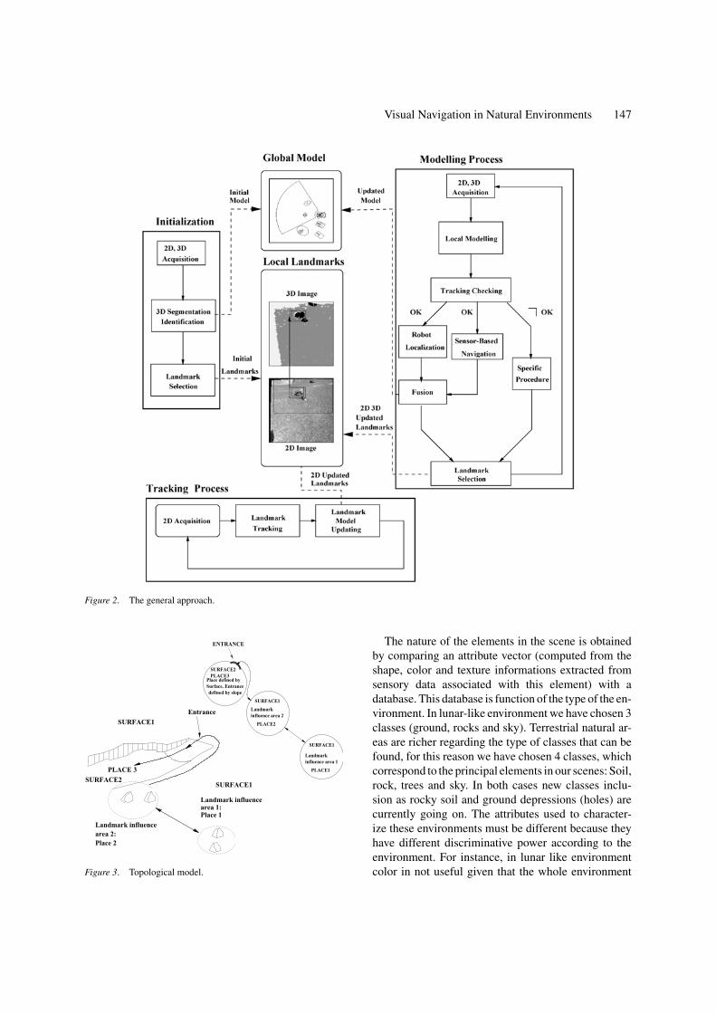
We have described on Fig. 2 the relationships betweenthe main representations built by our system, andthe different processes which provide or update theserepresentations.

We propose here two navigation modes whichcan take profit of the same landmark-basedmodel: Trajectory-based navigation or sensor-basednavigation.

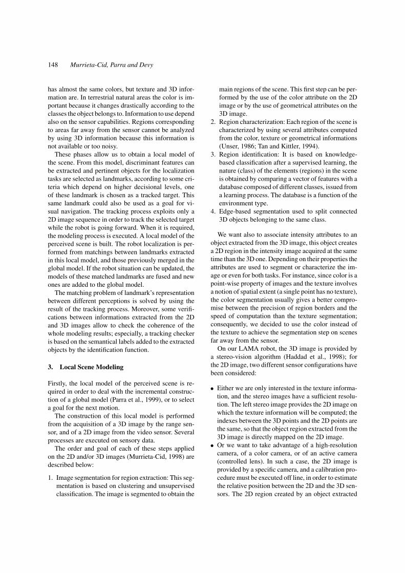
The sensor-based navigation mode needs only atopological model of the environment. It is a graph,in which a node (a place) is defined both by the in-fluence area of a set of landmarks and by a rather flatground surface. Two landmarks are in the same area ifthe robot can execute a trajectory between them havingalways landmarks of the same set in the stereo-visionfield of view (max range = 8 m). Two nodes are con-nected by an edge if their ground surfaces have signifi-

cantly different slopes, or if sensor-based motions canbe executed to reach one place from the other.

The boundary between two ground surfaces is in-cluded in the environment model as a border line (Devyand Parra, 1998). These lines can be interpreted as“doors” towards other places. These entrances towardsother places are characterized by their slope. A tiltedsurface becomes an entrance if the robot can navigatethrough it. An arc between two nodes corresponds ei-ther with a border line, or with a 2D landmark that therobot must reach in a sensor-based mode. In Fig. 3 areshown a scheme representing the kind of environmentwhere this approach is suitable and its representationwith a graph.

The trajectory-based navigation mode has an inputprovided by a geometrical planner. It is selected insidea given landmark(s) influence area. The landmarks inthis type of navigation mode must be perceived by 3Dsensors, because they are used to localize the robot (seeFigs. 23 and 25). The sensor-based navigation modecan be simpler, because it exploits the landmarks assub-goals where the robot has to go. The landmarkposition in a 2D image is used to give the robot a motiondirection (see Fig. 24).

Actually, both of the navigation modes can beswitched depending on (1) the environment condition,(2) whether there is 3D or 2D information and (3) theavailability of a path planner. In this paper we presentoverall examples when 3D information is available.3D information allows the trajectory-based navigationmode based on robot localization from the 3D landmarkpositions.

2.3. Overview of Our System

In the model proposed the main entities are: (1) groundareas defined by the surfaces (rather smooth, sloped ornot) and their nature (grass, sand, earth, . . . ). (2) objectsdefined by their shape (if 3D data is available) or anyspatial area represented by a region (if only 2D data isavailable) and their nature (rocks, tree, bushes, . . . ). (3)boundaries between these entities which can be ratherapproximative.

The landmark-based model proposed is built byusing several processes: A segmentation algorithmprovides a synthetic description of the scene. Entitiesissued from the segmentation stage (ground areas orobjects) are then characterized and afterwards identi-fied in order to obtain their nature (e.g., soil, rocks,trees . . . ).


Figure 2. The general approach.

R. Local 2 S1

SURFACE1

SURFACE3

ENTRANCE

SURFACE2PLACE3

Place defined bySurface. Entrancedefined by slope

Landmark influence area 2

PLACE2

SURFACE1

Landmark

PLACE1

SURFACE1

influence area 1

Place 1

SURFACE1

SURFACE1

Place 2

SURFACE2

PLACE 3

Entrance

Landmark influencearea 2:

Landmark influencearea 1:

Figure 3. Topological model.

The nature of the elements in the scene is obtainedby comparing an attribute vector (computed from theshape, color and texture informations extracted fromsensory data associated with this element) with adatabase. This database is function of the type of the en-vironment. In lunar-like environment we have chosen 3classes (ground, rocks and sky). Terrestrial natural ar-eas are richer regarding the type of classes that can befound, for this reason we have chosen 4 classes, whichcorrespond to the principal elements in our scenes: Soil,rock, trees and sky. In both cases new classes inclu-sion as rocky soil and ground depressions (holes) arecurrently going on. The attributes used to character-ize these environments must be different because theyhave different discriminative power according to theenvironment. For instance, in lunar like environmentcolor in not useful given that the whole environment


has almost the same colors, but texture and 3D infor-mation are. In terrestrial natural areas the color is im-portant because it changes drastically according to theclasses the object belongs to. Information to use dependalso on the sensor capabilities. Regions correspondingto areas far away from the sensor cannot be analyzedby using 3D information because this information isnot available or too noisy.

These phases allow us to obtain a local model ofthe scene. From this model, discriminant features canbe extracted and pertinent objects for the localizationtasks are selected as landmarks, according to some cri-teria which depend on higher decisional levels, oneof these landmark is chosen as a tracked target. Thissame landmark could also be used as a goal for vi-sual navigation. The tracking process exploits only a2D image sequence in order to track the selected targetwhile the robot is going forward. When it is required,the modeling process is executed. A local model of theperceived scene is built. The robot localization is per-formed from matchings between landmarks extractedin this local model, and those previously merged in theglobal model. If the robot situation can be updated, themodels of these matched landmarks are fused and newones are added to the global model.

The matching problem of landmark’s representationbetween different perceptions is solved by using theresult of the tracking process. Moreover, some verifi-cations between informations extracted from the 2Dand 3D images allow to check the coherence of thewhole modeling results; especially, a tracking checkeris based on the semantical labels added to the extractedobjects by the identification function.

3. Local Scene Modeling

Firstly, the local model of the perceived scene is re-quired in order to deal with the incremental construc-tion of a global model (Parra et al., 1999), or to selecta goal for the next motion.

The construction of this local model is performedfrom the acquisition of a 3D image by the range sen-sor, and of a 2D image from the video sensor. Severalprocesses are executed on sensory data.

The order and goal of each of these steps appliedon the 2D and/or 3D images (Murrieta-Cid, 1998) aredescribed below:

1. Image segmentation for region extraction: This seg-mentation is based on clustering and unsupervisedclassification. The image is segmented to obtain the

main regions of the scene. This first step can be per-formed by the use of the color attribute on the 2Dimage or by the use of geometrical attributes on the3D image.

2. Region characterization: Each region of the scene ischaracterized by using several attributes computedfrom the color, texture or geometrical informations(Unser, 1986; Tan and Kittler, 1994).

3. Region identification: It is based on knowledge-based classification after a supervised learning, thenature (class) of the elements (regions) in the sceneis obtained by comparing a vector of features with adatabase composed of different classes, issued froma learning process. The database is a function of theenvironment type.

4. Edge-based segmentation used to split connected3D objects belonging to the same class.

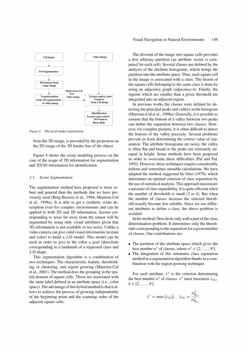
We want also to associate intensity attributes to anobject extracted from the 3D image, this object createsa 2D region in the intensity image acquired at the sametime than the 3D one. Depending on their properties theattributes are used to segment or characterize the im-age or even for both tasks. For instance, since color is apoint-wise property of images and the texture involvesa notion of spatial extent (a single point has no texture),the color segmentation usually gives a better compro-mise between the precision of region borders and thespeed of computation than the texture segmentation;consequently, we decided to use the color instead ofthe texture to achieve the segmentation step on scenesfar away from the sensor.

On our LAMA robot, the 3D image is provided bya stereo-vision algorithm (Haddad et al., 1998); forthe 2D image, two different sensor configurations havebeen considered:

• Either we are only interested in the texture informa-tion, and the stereo images have a sufficient resolu-tion. The left stereo image provides the 2D image onwhich the texture information will be computed; theindexes between the 3D points and the 2D points arethe same, so that the object region extracted from the3D image is directly mapped on the 2D image.

• Or we want to take advantage of a high-resolutioncamera, of a color camera, or of an active camera(controlled lens). In such a case, the 2D image isprovided by a specific camera, and a calibration pro-cedure must be executed off line, in order to estimatethe relative position between the 2D and the 3D sen-sors. The 2D region created by an object extracted


Transformation

Mask from 3-D over

3-D Segmentation

3D features fromrange image

from 3D segmentationfrom 2-D image

Identification

3-D Image Video Image

to video image

video image

Bayes Rule

FeaturesTexture and/or color

3D FeaturesTexture color and/or

Figure 4. The local model construction.

from the 3D image, is provided by the projection onthe 2D image of the 3D border line of the object.

Figure 4 shows the scene modeling process on thecase of the usage of 3D information for segmentationand 2D/3D information for identification.

3.1. Scene Segmentation

The segmentation method here proposed is more ro-bust and general than the methods that we have pre-viously used (Betg-Brezetz et al., 1994; Murrieta-Cidet al., 1998a). It is able to get a synthetic scene de-scription even for complex environments and can beapplied to both 2D and 3D information. Scenes cor-responding to areas far away from the sensor will besegmented by using only visual attributes given that3D information is not available or too noisy. Unlike avideo camera can give valid visual information (textureand color) to build a 2-D model. This model can beused in order to give to the robot a goal (direction)corresponding to a landmark of a requested class and2-D shape.

This segmentation algorithm is a combination oftwo techniques: The characteristic feature, threshold-ing or clustering, and region growing (Murrieta-Cidet al., 2001). The method does the grouping in the spa-tial domain of square cells. Those are associated withthe same label defined in an attribute space (i.e., colorspace). The advantage of this hybrid method is that it al-lows to achieve the process of growing independentlyof the beginning point and the scanning order of theadjacent square cells.

The division of the image into square cells providesa first arbitrary partition (an attribute vector is com-puted for each cell). Several classes are defined by theanalysis of the attribute histograms, which brings thepartition into the attribute space. Thus, each square cellin the image is associated with a class. The fusion ofthe square cells belonging to the same class is done byusing an adjacency graph (adjacency-4). Finally, theregions which are smaller than a given threshold areintegrated into an adjacent region.

In previous works the classes were defined by de-tecting the principal peaks and valleys in the histogram(Murrieta-Cid et al., 1998a). Generally, it is possible toassume that the bottom of a valley between two peakscan define the separation between two classes. How-ever, for complex pictures, it is often difficult to detectthe bottom of the valley precisely. Several problemsprevent us from determining the correct value of sep-aration: The attribute histograms are noisy, the valleyis often flat and broad or the peaks are extremely un-equal in height. Some methods have been proposedin order to overcome these difficulties (Pal and Pal,1993). However, these techniques require considerablytedious and sometimes unstable calculations. We haveadapted the method suggested by Otsu (1979), whichdetermines an optimal criterion of class separation bythe use of statistical analysis. This approach maximizesa measure of class separability. It is quite efficient whenthe number of thresholds is small (3 or 4). But whenthe number of classes increase the selected thresh-old usually become less reliable. Since we use differ-ent attributes to define a class, the above problem isavoided.

In his method, Otsu deals only with a part of the classdetermination problem. It determines only the thresh-olds corresponding to the separation for a given numberof classes. Our contributions are:

• The partition of the attribute space which gives thebest number n∗ of classes, where n∗ ∈ [2, . . . , N ].

• The integration of this automatic class separationmethod in a segmentation algorithm thanks to a com-bination with the region growing technique.

For each attribute, λ∗ is the criterion determiningthe best number n∗ of classes. λ∗ must maximize λ(k),

k ∈ [2, . . . , N ].

λ∗ = max(λ(k)

); λ(k) =

σ 2B(k)

σ 2W(k)


where λ(k) is the maximal criterion for exactly k classes.σ 2

B(k)is the inter-classes variance defined by:

σ 2B(k)

=k−1∑m=1

k∑n=m+1

[ωn · ωm(µm − µn)2]

σ 2W(k)

is the intraclass variance defined by:

σ 2W(k)

=k−1∑m=1

k∑n=m+1

[ ∑i∈m

(i − µm)2 · p(i)

+∑i∈n

(i − µn)2 · p(i)

]

µm denote the mean of the level i of the class m, ωm theclass probability and p(i) the probability of the level iof the histogram.

µm =∑i∈m

i · p(i)

ωmωm =

∑i∈m

p(i) p(i) = ni

Np

The normalized histogram is considered to be a prob-ability distribution. ni is the number of samples fora given level and Np is the total number of samples.A class m is delimited by two values (the inferiorand superior limits) corresponding to two levels in thehistogram.

The automatic class separation method was appliedto the two histograms shown in Fig. 5. In both casesthe class division was tested for two and three classes.For the first histogram, the value λ∗ corresponds to adivision into two classes, the threshold is placed in thevalley bottom between the two peaks. In the secondhistogram, the optimal λ∗ corresponds to a divisioninto three classes.

3.1.1. The 3D Segmentation. This segmentation al-gorithm can be applied to images of range, by the useof 3D attributes (height and normals). On our LAMArobot, the 3D image is provided by a stereo-vision al-gorithm (Haddad et al., 1998): Height and normals arecomputed for each point in the 3D image. The normals(θ and φ) are computed in a spherical coordinate sys-tem (Betg-Brezetz et al., 1994), and are coded in 256levels.

Once the ground regions have been extracted in theimage, it remains the obstacle regions which could re-quire a specific segmentation in order to isolate eachobstacle. We make the assumption that an obstacle is aconnected portion of matter emerging from the ground.

Figure 5. Localization of threshold.

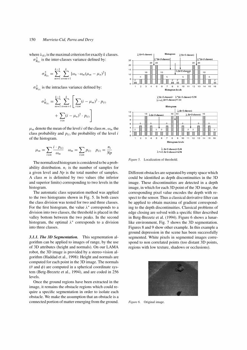
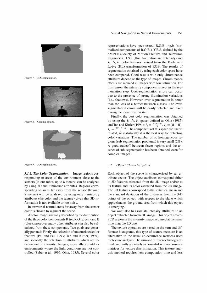
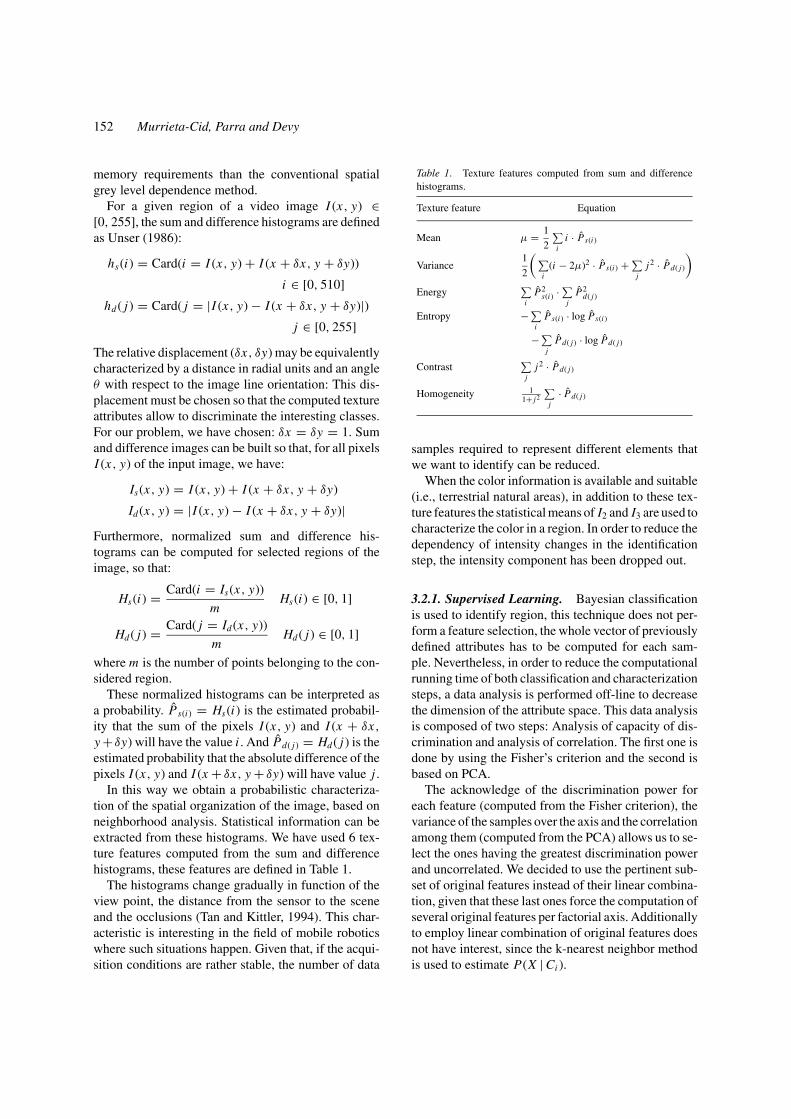
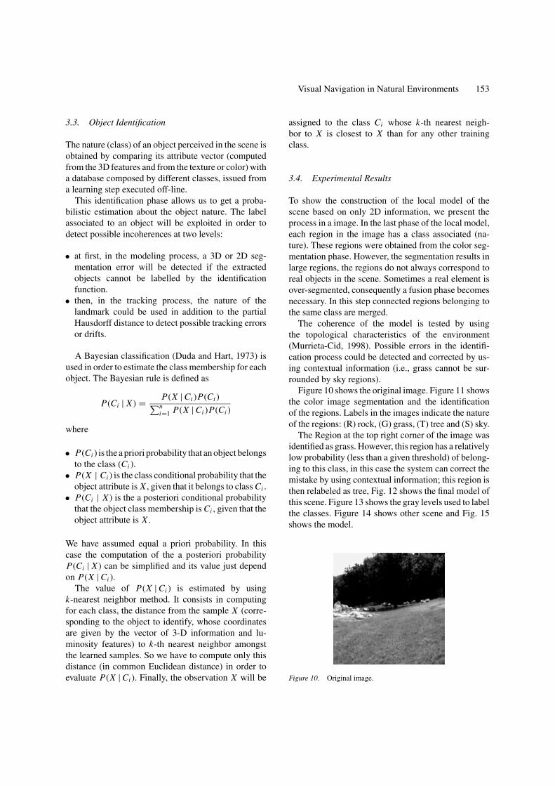
Different obstacles are separated by empty space whichcould be identified as depth discontinuities in the 3Dimage. These discontinuities are detected in a depthimage, in which for each 3D point of the 3D image, thecorresponding pixel value encodes the depth with re-spect to the sensor. Thus a classical derivative filter canbe applied to obtain maxima of gradient correspond-ing to the depth discontinuities. Classical problems ofedge closing are solved with a specific filter describedin Betg-Brezetz et al. (1994). Figure 6 shows a lunar-like environment, Fig. 7 shows the 3D segmentation.Figures 8 and 9 show other example. In this example aground depression in the scene has been successfullysegmented. White pixels in segmented images corre-spond to non correlated points (too distant 3D points,regions with low texture, shadows or occlusions).

Figure 6. Original image.


Figure 7. 3D segmentation.


Figure 9. 3D segmentation.

3.1.2. The Color Segmentation. Image regions cor-responding to areas of the environment close to thesensors (in our robot, up to 8 meters) can be analyzedby using 3D and luminance attributes. Regions corre-sponding to areas far away from the sensor (beyond8 meters) will be analyzed by using only luminosityattributes (the color and the texture) given that 3D in-formation is not available or too noisy.

In terrestrial natural areas far away from the sensorcolor is chosen to segment the scene.

A color image is usually described by the distributionof the three color components R (red), G (green) and B(blue), moreover many other attributes can also be cal-culated from these components. Two goals are gener-ally pursued: Firstly, the selection of uncorrelated colorfeatures (Pal and Pal, 1993; Tan and Kittler, 1994),and secondly the selection of attributes which are in-dependent of intensity changes, especially in outdoorenvironments where the light conditions are not con-trolled (Saber et al., 1996; Ohta, 1985). Several color

representations have been tested: R.G.B., r.g.b. (nor-malized components of R.G.B.), Y.E.S. defined by theSMPTE (Society of Motion Pictures and TelevisionEngineers), H.S.I. (Hue, Saturation and Intensity) andI1, I2, I3, color features derived from the Karhunen-Loeve (KL) transformation of RGB. The results ofsegmentation obtained by using each color space havebeen compared. Good results with only chrominanceattributes depend on the type of images. Chromimanceeffects are reduced in images with low saturation. Forthis reason, the intensity component is kept in the seg-mentation step. Over-segmentation errors can occurdue to the presence of strong illumination variations(i.e., shadows). However, over-segmentation is betterthan the loss of a border between classes. The over-segmentation errors will be easily detected and fixedduring the identification step.

Finally, the best color segmentation was obtainedby using the I1, I2, I3 space, defined as Ohta (1985)and Tan and Kittler (1994): I1 = R+G+B

3 , I2 = (R− B),I3 = 2G−R−B

2 . The components of this space are uncor-related, so statistically it is the best way for detectingcolor variations. The number of no homogeneous re-gions (sub-segmentation problems) is very small (2%).A good tradeoff between fewer regions and the ab-sence of sub-segmentation has been obtained, even forcomplex images.

3.2. Object Characterization

Each object of the scene is characterized by an at-tribute vector: The object attributes correspond eitherto 3D features extracted from the 3D image and/or toits texture and its color extracted from the 2D image.The 3D features correspond to the statistical mean andthe standard deviation of the distances from the 3-Dpoints of the object, with respect to the plane whichapproximates the ground area from which this objectis emerging.

We want also to associate intensity attributes to anobject extracted from the 3D image. This object createsa 2D region in the intensity image acquired at the sametime than the 3D one.

The texture operators are based on the sum and dif-ference histograms, this type of texture measure is analternative to the usual co-occurrence matrices usedfor texture analysis. The sum and difference histogramsused conjointly are nearly as powerful as co-occurrencematrices for texture discrimination. This texture anal-ysis method requires less computation time and less


memory requirements than the conventional spatialgrey level dependence method.

For a given region of a video image I (x, y) ∈[0, 255], the sum and difference histograms are definedas Unser (1986):

hs(i) = Card(i = I (x, y) + I (x + δx, y + δy))

i ∈ [0, 510]

hd ( j) = Card( j = |I (x, y) − I (x + δx, y + δy)|)j ∈ [0, 255]

The relative displacement (δx, δy) may be equivalentlycharacterized by a distance in radial units and an angleθ with respect to the image line orientation: This dis-placement must be chosen so that the computed textureattributes allow to discriminate the interesting classes.For our problem, we have chosen: δx = δy = 1. Sumand difference images can be built so that, for all pixelsI (x, y) of the input image, we have:

Is(x, y) = I (x, y) + I (x + δx, y + δy)

Id (x, y) = |I (x, y) − I (x + δx, y + δy)|Furthermore, normalized sum and difference his-tograms can be computed for selected regions of theimage, so that:

Hs(i) = Card(i = Is(x, y))

mHs(i) ∈ [0, 1]

Hd ( j) = Card( j = Id (x, y))

mHd ( j) ∈ [0, 1]

where m is the number of points belonging to the con-sidered region.

These normalized histograms can be interpreted asa probability. Ps(i) = Hs(i) is the estimated probabil-ity that the sum of the pixels I (x, y) and I (x + δx,

y +δy) will have the value i . And Pd( j) = Hd ( j) is theestimated probability that the absolute difference of thepixels I (x, y) and I (x + δx, y + δy) will have value j .

In this way we obtain a probabilistic characteriza-tion of the spatial organization of the image, based onneighborhood analysis. Statistical information can beextracted from these histograms. We have used 6 tex-ture features computed from the sum and differencehistograms, these features are defined in Table 1.

The histograms change gradually in function of theview point, the distance from the sensor to the sceneand the occlusions (Tan and Kittler, 1994). This char-acteristic is interesting in the field of mobile roboticswhere such situations happen. Given that, if the acqui-sition conditions are rather stable, the number of data

Table 1. Texture features computed from sum and differencehistograms.

Texture feature Equation

Mean µ = 1

2

∑i

i · Ps(i)

Variance1

2

( ∑i

(i − 2µ)2 · Ps(i) + ∑j

j2 · Pd( j)

)

Energy∑

iP2

s(i) · ∑j

P2d( j)

Entropy − ∑i

Ps(i) · log Ps(i)

− ∑j

Pd( j) · log Pd( j)

Contrast∑

jj2 · Pd( j)

Homogeneity 11+ j2

∑j

· Pd( j)

samples required to represent different elements thatwe want to identify can be reduced.

When the color information is available and suitable(i.e., terrestrial natural areas), in addition to these tex-ture features the statistical means of I2 and I3 are used tocharacterize the color in a region. In order to reduce thedependency of intensity changes in the identificationstep, the intensity component has been dropped out.

3.2.1. Supervised Learning. Bayesian classificationis used to identify region, this technique does not per-form a feature selection, the whole vector of previouslydefined attributes has to be computed for each sam-ple. Nevertheless, in order to reduce the computationalrunning time of both classification and characterizationsteps, a data analysis is performed off-line to decreasethe dimension of the attribute space. This data analysisis composed of two steps: Analysis of capacity of dis-crimination and analysis of correlation. The first one isdone by using the Fisher’s criterion and the second isbased on PCA.

The acknowledge of the discrimination power foreach feature (computed from the Fisher criterion), thevariance of the samples over the axis and the correlationamong them (computed from the PCA) allows us to se-lect the ones having the greatest discrimination powerand uncorrelated. We decided to use the pertinent sub-set of original features instead of their linear combina-tion, given that these last ones force the computation ofseveral original features per factorial axis. Additionallyto employ linear combination of original features doesnot have interest, since the k-nearest neighbor methodis used to estimate P(X | Ci ).


3.3. Object Identification

The nature (class) of an object perceived in the scene isobtained by comparing its attribute vector (computedfrom the 3D features and from the texture or color) witha database composed by different classes, issued froma learning step executed off-line.

This identification phase allows us to get a proba-bilistic estimation about the object nature. The labelassociated to an object will be exploited in order todetect possible incoherences at two levels:

• at first, in the modeling process, a 3D or 2D seg-mentation error will be detected if the extractedobjects cannot be labelled by the identificationfunction.

• then, in the tracking process, the nature of thelandmark could be used in addition to the partialHausdorff distance to detect possible tracking errorsor drifts.

A Bayesian classification (Duda and Hart, 1973) isused in order to estimate the class membership for eachobject. The Bayesian rule is defined as

P(Ci | X ) = P(X | Ci )P(Ci )∑ni=1 P(X | Ci )P(Ci )

where

• P(Ci ) is the a priori probability that an object belongsto the class (Ci ).

• P(X | Ci ) is the class conditional probability that theobject attribute is X , given that it belongs to class Ci .

• P(Ci | X ) is the a posteriori conditional probabilitythat the object class membership is Ci , given that theobject attribute is X .

We have assumed equal a priori probability. In thiscase the computation of the a posteriori probabilityP(Ci | X ) can be simplified and its value just dependon P(X | Ci ).

The value of P(X | Ci ) is estimated by usingk-nearest neighbor method. It consists in computingfor each class, the distance from the sample X (corre-sponding to the object to identify, whose coordinatesare given by the vector of 3-D information and lu-minosity features) to k-th nearest neighbor amongstthe learned samples. So we have to compute only thisdistance (in common Euclidean distance) in order toevaluate P(X | Ci ). Finally, the observation X will be

assigned to the class Ci whose k-th nearest neigh-bor to X is closest to X than for any other trainingclass.

3.4. Experimental Results

To show the construction of the local model of thescene based on only 2D information, we present theprocess in a image. In the last phase of the local model,each region in the image has a class associated (na-ture). These regions were obtained from the color seg-mentation phase. However, the segmentation results inlarge regions, the regions do not always correspond toreal objects in the scene. Sometimes a real element isover-segmented, consequently a fusion phase becomesnecessary. In this step connected regions belonging tothe same class are merged.

The coherence of the model is tested by usingthe topological characteristics of the environment(Murrieta-Cid, 1998). Possible errors in the identifi-cation process could be detected and corrected by us-ing contextual information (i.e., grass cannot be sur-rounded by sky regions).

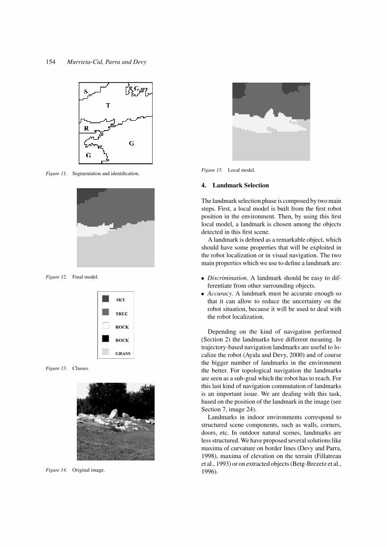
Figure 10 shows the original image. Figure 11 showsthe color image segmentation and the identificationof the regions. Labels in the images indicate the natureof the regions: (R) rock, (G) grass, (T) tree and (S) sky.

The Region at the top right corner of the image wasidentified as grass. However, this region has a relativelylow probability (less than a given threshold) of belong-ing to this class, in this case the system can correct themistake by using contextual information; this region isthen relabeled as tree, Fig. 12 shows the final model ofthis scene. Figure 13 shows the gray levels used to labelthe classes. Figure 14 shows other scene and Fig. 15shows the model.



Figure 11. Segmentation and identification.

Figure 12. Final model.

Figure 13. Classes.


Figure 15. Local model.

4. Landmark Selection

The landmark selection phase is composed by two mainsteps. First, a local model is built from the first robotposition in the environment. Then, by using this firstlocal model, a landmark is chosen among the objectsdetected in this first scene.

A landmark is defined as a remarkable object, whichshould have some properties that will be exploited inthe robot localization or in visual navigation. The twomain properties which we use to define a landmark are:

• Discrimination. A landmark should be easy to dif-ferentiate from other surrounding objects.

• Accuracy. A landmark must be accurate enough sothat it can allow to reduce the uncertainty on therobot situation, because it will be used to deal withthe robot localization.

Depending on the kind of navigation performed(Section 2) the landmarks have different meaning. Intrajectory-based navigation landmarks are useful to lo-calize the robot (Ayala and Devy, 2000) and of coursethe bigger number of landmarks in the environmentthe better. For topological navigation the landmarksare seen as a sub-goal which the robot has to reach. Forthis last kind of navigation commutation of landmarksis an important issue. We are dealing with this task,based on the position of the landmark in the image (seeSection 7, image 24).

Landmarks in indoor environments correspond tostructured scene components, such as walls, corners,doors, etc. In outdoor natural scenes, landmarks areless structured. We have proposed several solutions likemaxima of curvature on border lines (Devy and Parra,1998), maxima of elevation on the terrain (Fillatreauet al., 1993) or on extracted objects (Betg-Brezetz et al.,1996).


In previous works we have defined a landmark as abulge, typically a natural object emerging from a ratherflat ground (e.g., a rock), only the elevation peak of suchan object has been considered as a numerical attributeuseful for the localization purpose. A realistic uncer-tainty model has been proposed for these peaks, so thatthe peak uncertainty is function of the rock sharpness,of the sensor noise and of the distance from the robot.

In a segmented 3D image, a bulge is selected as can-didate landmark if:

• It is not occluded by another object. If an object isoccluded, it will be difficult to find in the followingimages and will not have a good estimate on its top.

• Its topmost point is accurate. This is function of thesensor noise, resolution and object top shape.

• It must be in “ground contact”.

These criteria are used so that only some objectsextracted from an image are selected as landmarks. Themost accurate one (or the more significant landmarkcluster in cluttered scenes) is then selected in order tosupport the reference frame of the first explored area.Moreover, a specific landmark must be defined as thenext tracked target for the tracking process. Differentcriteria, coming from higher decisional levels, could beused for this selection, for example:

• Track the sharper or the higher object: it will be easierto detect and to match between successive images.

• Track the more distant object from the robot, towardsa given direction (visual navigation).

• Track the object which maximizes a utility func-tion, taking into account several criteria (activeexploration).

• Or, in a teleprogrammed system, track the objectpointed on the 2D image by an operator.

In order to navigate during a long robot motion, asequence of different landmarks (or targets) is used assub-goal the robot must successively reach (Murrieta-Cid et al., 2001). The landmark change is automatic. Itis based on the nature of the landmark and the distancebetween the robot and the target which represents thecurrent sub-goal. When the robot attains the currenttarget (or, more precisely, when the current target isclose to the limit of the camera field of view), anotherone is dynamically selected in order to control the nextmotion (Murrieta-Cid et al., 1998b).

At this time due to integration constraints, onlyone landmark can be tracked during the robot mo-

tion. We are currently developing a multi-trackingmethod.

This landmark will be used for several functions:

• It will support the first reference frame linked to thecurrent area explored by the robot so that, the ini-tial robot situation in the environment can be easilycomputed.

• It will be the first tracked target in the 2D image se-quence acquired during the next robot motion (track-ing process fast-loop). If visual navigation is chosenin the higher level decision system as a way to de-fine the robot motions during the exploration task,this same process will be also in charge of generat-ing commands for the mobile robot and for the panand tilt platform on which the cameras are mounted.

• It will be detected again in the next 3D image ac-quired in the modeling process, so that the robotsituation could be easily updated, as this landmarksupports the reference frame of the explored area.

Moreover, the first local model allows to initializethe global model which will be upgraded by the incre-mental fusion of the local models built from the next3D acquisitions. Hereafter, the automatic procedure forthe landmark selection is presented.

The local model of the first scene (obtained from the3-D segmentation and identification phases) is used toselect automatically an appropriated landmark, froman utility estimation based on both its nature and shape(Murrieta-Cid et al., 1998a). Landmarks can be usedto both, localization and navigation tasks. Localizationbased on environment features improves the autonomyof the robot.

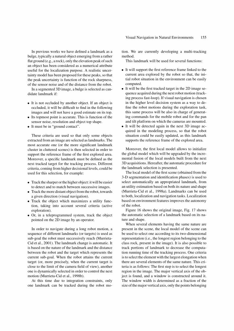
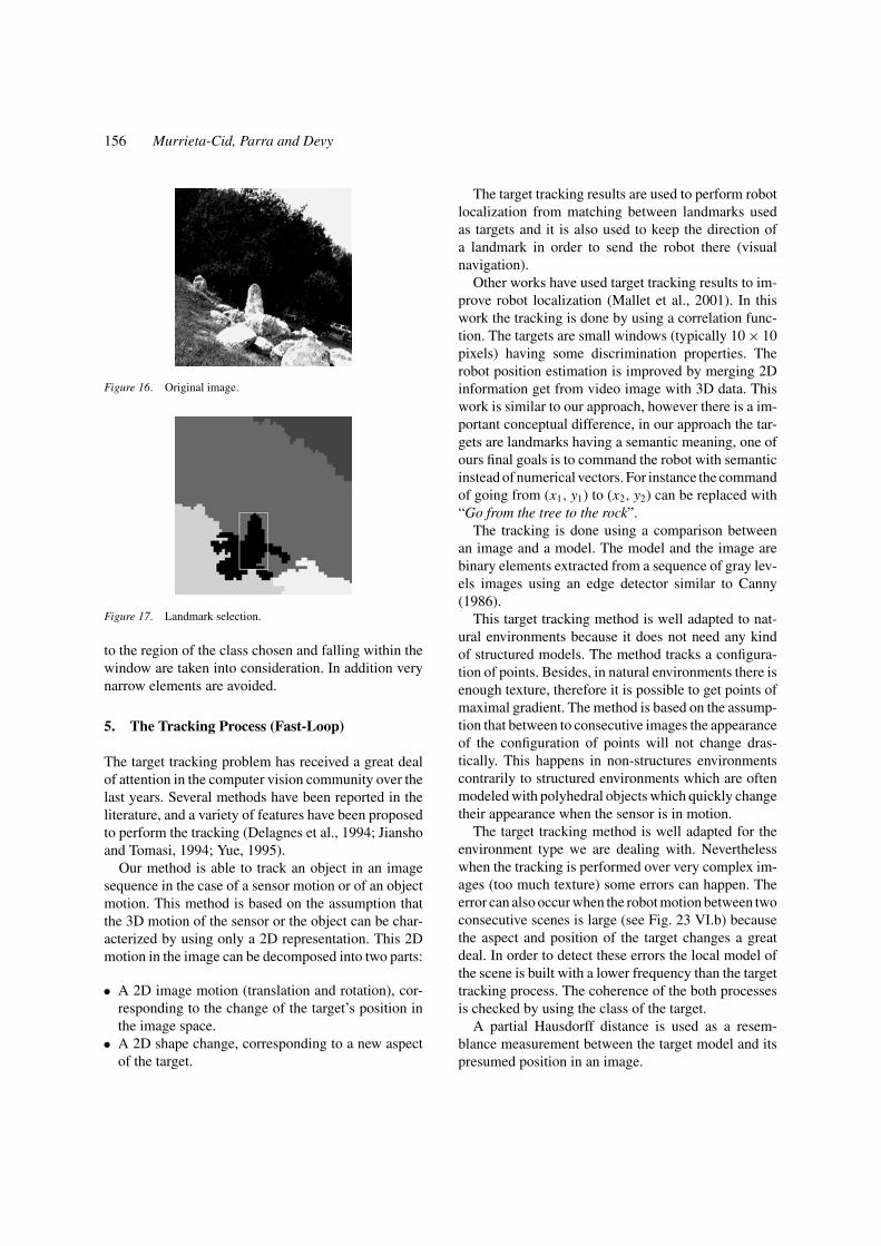
Figure 16 shows the original image, Fig. 17 showsthe automatic selection of a landmark based on its na-ture and shape.

When several elements having the same nature arepresent in the scene, the local model of the scene canbe used to select one according to its two-dimensionalrepresentation (i.e., the longest region belonging to theclass rock, present in the image). It is also possible totrack portions of landmark to decrease the computa-tion running time of the tracking process. One criteriais to select the element with the largest elongation whenthere are several elements of the same nature. This cri-teria is as follows: The first step is to select the longestregion in the image. The major vertical axis of the ob-ject is found, and a window is constructed around it.The window width is determined as a fraction of thesize of the major vertical axis, only the points belonging



Figure 17. Landmark selection.

to the region of the class chosen and falling within thewindow are taken into consideration. In addition verynarrow elements are avoided.

5. The Tracking Process (Fast-Loop)

The target tracking problem has received a great dealof attention in the computer vision community over thelast years. Several methods have been reported in theliterature, and a variety of features have been proposedto perform the tracking (Delagnes et al., 1994; Jianshoand Tomasi, 1994; Yue, 1995).

Our method is able to track an object in an imagesequence in the case of a sensor motion or of an objectmotion. This method is based on the assumption thatthe 3D motion of the sensor or the object can be char-acterized by using only a 2D representation. This 2Dmotion in the image can be decomposed into two parts:

• A 2D image motion (translation and rotation), cor-responding to the change of the target’s position inthe image space.

• A 2D shape change, corresponding to a new aspectof the target.

The target tracking results are used to perform robotlocalization from matching between landmarks usedas targets and it is also used to keep the direction ofa landmark in order to send the robot there (visualnavigation).

Other works have used target tracking results to im-prove robot localization (Mallet et al., 2001). In thiswork the tracking is done by using a correlation func-tion. The targets are small windows (typically 10 × 10pixels) having some discrimination properties. Therobot position estimation is improved by merging 2Dinformation get from video image with 3D data. Thiswork is similar to our approach, however there is a im-portant conceptual difference, in our approach the tar-gets are landmarks having a semantic meaning, one ofours final goals is to command the robot with semanticinstead of numerical vectors. For instance the commandof going from (x1, y1) to (x2, y2) can be replaced with“Go from the tree to the rock”.

The tracking is done using a comparison betweenan image and a model. The model and the image arebinary elements extracted from a sequence of gray lev-els images using an edge detector similar to Canny(1986).

This target tracking method is well adapted to nat-ural environments because it does not need any kindof structured models. The method tracks a configura-tion of points. Besides, in natural environments there isenough texture, therefore it is possible to get points ofmaximal gradient. The method is based on the assump-tion that between to consecutive images the appearanceof the configuration of points will not change dras-tically. This happens in non-structures environmentscontrarily to structured environments which are oftenmodeled with polyhedral objects which quickly changetheir appearance when the sensor is in motion.

The target tracking method is well adapted for theenvironment type we are dealing with. Neverthelesswhen the tracking is performed over very complex im-ages (too much texture) some errors can happen. Theerror can also occur when the robot motion between twoconsecutive scenes is large (see Fig. 23 VI.b) becausethe aspect and position of the target changes a greatdeal. In order to detect these errors the local model ofthe scene is built with a lower frequency than the targettracking process. The coherence of the both processesis checked by using the class of the target.

A partial Hausdorff distance is used as a resem-blance measurement between the target model and itspresumed position in an image.


Given two sets of points P and Q, the Hausdorffdistance is defined as Serra (1982):

H (P, Q) = max(h(P, Q), h(Q, P))

where

h(P, Q) = maxp∈P

minq∈Q

‖p − q‖

and ‖ · ‖ is a given distance between two points p andq. The function h(P, Q) (distance from set P to Q) isa measure of the degree in which each point in P isnear to some point in Q. The Hausdorff distance is themaximum among h(P, Q) and h(Q, P).

By computing the Hausdorff distance in this waywe obtain the most mismatched point between the twoshapes compared consequently, it is very sensitive tothe presence of any outlying points. For that reason itis often appropriate to use a more general rank ordermeasure, which replaces the maximization operationwith a rank operation. This measure (partial distance)is defined as Huttenlocher et al. (1993a):

hk = K thp∈P min

q∈Q‖p − q‖

where K thp∈P f (p) denotes the K −th ranked value of

f (p) over the set P .

5.1. Finding the Model Position

The first task to be accomplished is to define the po-sition of the model Mt in the next image It+1 ofthe sequence. The search for the model in the im-age (or image’s region) is done in some selecteddirection. We are using the unidirectional partial dis-tance from the model to the image to achieve this firststep.

The minimum value of hk1(Mt , It+1) identifies thebest “position” of Mt in It+1, under the action of somegroup of translations G. It is possible also to identifythe set of translations of Mt such that hk1(Mt , It+1) isno larger than some value τ , in this case there maybe multiple translations that have essentially the samequality (Huttenlocher et al., 1993b).

However, rather than computing the single transla-tion giving the minimum distance or the set of transla-tions, such that its correspond hk1 is no larger than τ ,it is possible to find the first translation g, such that itsassociated hk1 is no larger than τ , for a given searchdirection.

Although the first translation which hk1(Mt , It+1)associated is less than τ it is not necessarily the bestone, whether τ is small, the translation g should bequite good. This is better than computing all the setof valuable translation, whereas the computing time issignificantly smaller.

5.2. Building the New Model

Having found the position of the model Mt in the nextimage It+1 of the sequence, we now have to build thenew model Mt+1 by determining which pixels of theimage It+1 are part of this new model.

The model is updated by using the unidirectionalpartial distance from the image to the model as a crite-rion for selecting the subset of images points It+1 thatbelong to Mt+1. The new model is defined as:

Mt+1 = {q ∈ It+1 | hk2(It+1, g(Mt )) < δ}

where g(Mt ) is the model at the time t under the actionof the translation g, and δ controls the degree to whichthe method is able to track objects that change shape.

In order to allow models that may be changing insize, this size is increased whenever there is a signifi-cant number of nonzero pixels near the boundary and isdecreased in the contrary case. The model’s position isimproved according to the position where the model’sboundary was defined.

The initial model is obtained by using the local modelof the scene previously computed. With this initialmodel the tracking begins, finding progressively thenew position of the target and updating the model. Thetracking of the model is successful if:

k1 > f M | hk1(Mt , It+1) < τ

and

k2 > f I | hk2(It+1, g(Mt )) < δ,

in which f M is a fraction of the number total of pointsof the model Mt and f I is a fraction of image’s pointof It+1 superimposed on g(Mt ).

5.3. Our Contributions Over the GeneralTracking Method

Several previous works have used the Hausdorff dis-tance as a resemblance measure in order to track an


object (Huttenlocher et al., 1993b; Dubuisson and Jain,1997). This section enumerates some of the extensionsthat we have made over the general method (Murrieta-Cid, 1997).

• Firstly, we are using an automatic identificationmethod in order to select the initial model. Thismethod uses several attributes of the image such astexture and 3-D shape.

• Only a small region of the image is examined toobtain the new target position, as opposed to the en-tire image. In this manner, the computation time isdecreased significantly. The idea behind a local ex-ploration of the image is that if the execution of thecode is quick enough, the new target position willthen lie within a vicinity of the previous one. We aretrading the capability to find the target in the wholeimage in order to increase the speed of computationof the new position and shape of the model. In thisway, the robustness of the method is increased tohandle target deformations, since it is less likely thatthe shape of the model will change significantly in asmall δt . In addition, this technique allows the pro-gram to report the target’s location to any externalsystems with a higher frequency (for an applicationsee Becker et al. (1995)).

• Instead of computing the set of translations ofMt , such that hk1(Mt , It+1) is no larger than somevalue τ , we are finding the first translation whosehk1(Mt , It+1) is less than τ . This strategy signifi-cantly decreases the computational time.

Recently other work (Ayala et al., 2000) has im-proved the target tracking approach here presented, therobustness has been increased by (1) a refinement of thetarget model, (2) usage of a target search strategy thatsweeps space of possible translation following a spi-ral trajectory (having as result an error mean of targetimage localization equal to zero) and (3) an alternativestrategy to select the target by doing a motion detectionin the image, based on background model provided bya Gaussian mixture.

5.4. Experimental Results: Tracking

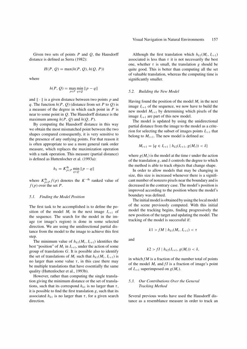
The tracking method was implemented in C on a real-time operating system (Power-PC), the computationrunning time is dependent on the region size exam-ined to obtain the new target position. For sequencesthe code is capable of processing a frame in about0.25 seconds. In this case only a small region of theimage is examined given that the new target position

will lie within a vicinity of the previous one. Processingincludes, edge detection, target localization, and modelupdating for a video image of (256 × 256 pixels).

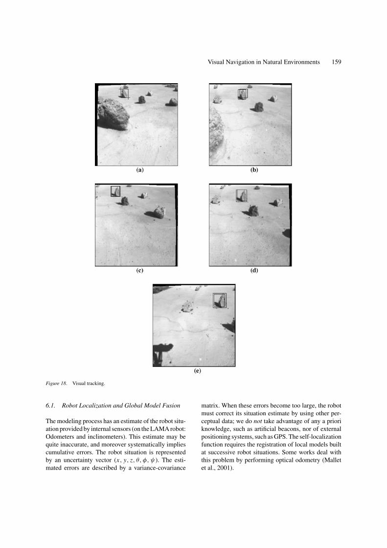
Figure 18 show the tracking process in a lunar-like environment. Figure 18(a) shows initial target se-lection, in this case the user specifies a rectangle inthe frame that contains the target. An automatic land-mark (target) selection is possible by using the lo-cal model of the scene. Figure 18(b)–(e) shows thetracking of a rock through an image sequence. Therock chosen as target is marked in the figure with aboundary box. Another boundary box is used to de-lineate the improved target position after the modelupdating. In these images the region being examinedis the whole image, the objective is to show the capac-ity of the method to identify a rock among the set ofobjects.

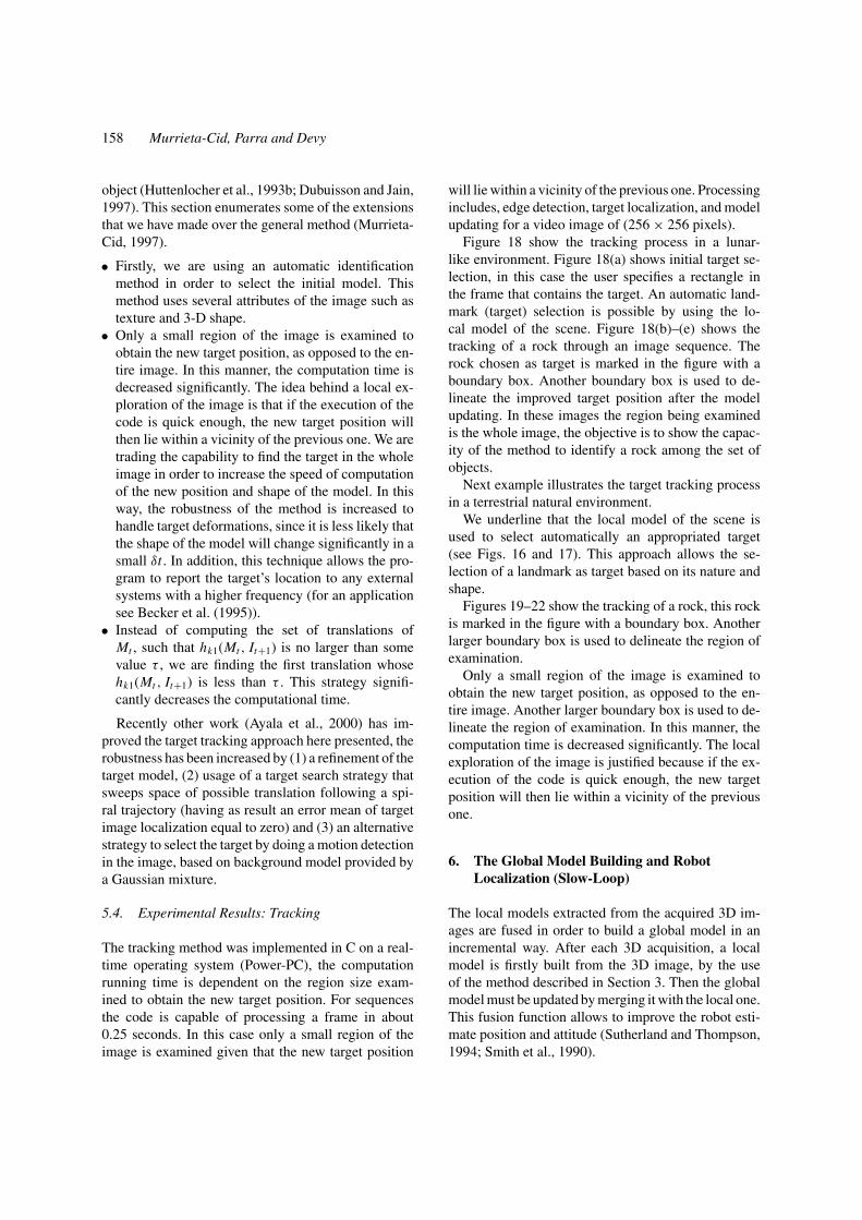
Next example illustrates the target tracking processin a terrestrial natural environment.

We underline that the local model of the scene isused to select automatically an appropriated target(see Figs. 16 and 17). This approach allows the se-lection of a landmark as target based on its nature andshape.

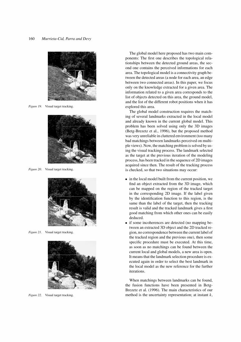
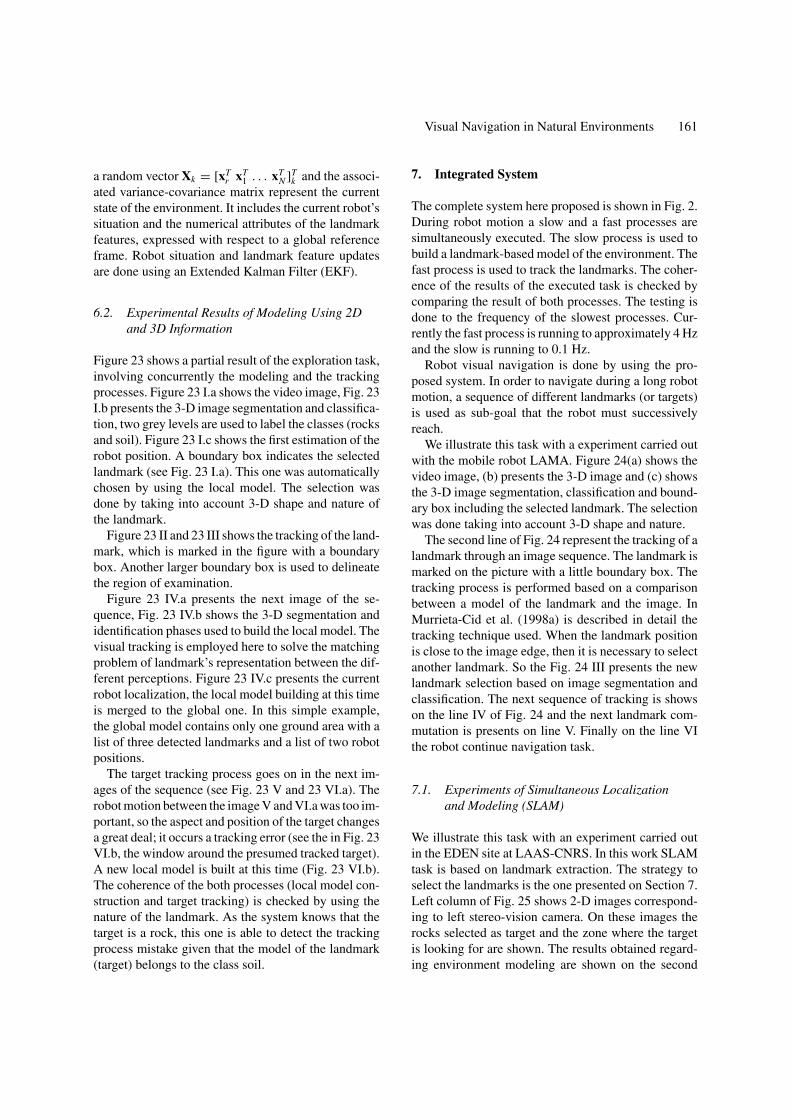
Figures 19–22 show the tracking of a rock, this rockis marked in the figure with a boundary box. Anotherlarger boundary box is used to delineate the region ofexamination.

Only a small region of the image is examined toobtain the new target position, as opposed to the en-tire image. Another larger boundary box is used to de-lineate the region of examination. In this manner, thecomputation time is decreased significantly. The localexploration of the image is justified because if the ex-ecution of the code is quick enough, the new targetposition will then lie within a vicinity of the previousone.

6. The Global Model Building and RobotLocalization (Slow-Loop)

The local models extracted from the acquired 3D im-ages are fused in order to build a global model in anincremental way. After each 3D acquisition, a localmodel is firstly built from the 3D image, by the useof the method described in Section 3. Then the globalmodel must be updated by merging it with the local one.This fusion function allows to improve the robot esti-mate position and attitude (Sutherland and Thompson,1994; Smith et al., 1990).


Figure 18. Visual tracking.

6.1. Robot Localization and Global Model Fusion

The modeling process has an estimate of the robot situ-ation provided by internal sensors (on the LAMA robot:Odometers and inclinometers). This estimate may bequite inaccurate, and moreover systematically impliescumulative errors. The robot situation is representedby an uncertainty vector (x, y, z, θ, φ, ψ). The esti-mated errors are described by a variance-covariance

matrix. When these errors become too large, the robotmust correct its situation estimate by using other per-ceptual data; we do not take advantage of any a prioriknowledge, such as artificial beacons, nor of externalpositioning systems, such as GPS. The self-localizationfunction requires the registration of local models builtat successive robot situations. Some works deal withthis problem by performing optical odometry (Malletet al., 2001).


Figure 19. Visual target tracking.




The global model here proposed has two main com-ponents: The first one describes the topological rela-tionships between the detected ground areas, the sec-ond one contains the perceived informations for eacharea. The topological model is a connectivity graph be-tween the detected areas (a node for each area, an edgebetween two connected areas). In this paper, we focusonly on the knowledge extracted for a given area. Theinformation related to a given area corresponds to thelist of objects detected on this area, the ground model,and the list of the different robot positions when it hasexplored this area.

The global model construction requires the match-ing of several landmarks extracted in the local modeland already known in the current global model. Thisproblem has been solved using only the 3D images(Betg-Brezetz et al., 1996), but the proposed methodwas very unreliable in cluttered environment (too manybad matchings between landmarks perceived on multi-ple views). Now, the matching problem is solved by us-ing the visual tracking process. The landmark selectedas the target at the previous iteration of the modelingprocess, has been tracked in the sequence of 2D imagesacquired since then. The result of the tracking processis checked, so that two situations may occur:

• in the local model built from the current position, wefind an object extracted from the 3D image, whichcan be mapped on the region of the tracked targetin the corresponding 2D image. If the label givenby the identification function to this region, is thesame than the label of the target, then the trackingresult is valid and the tracked landmark gives a firstgood matching from which other ones can be easilydeduced.

• if some incoherences are detected (no mapping be-tween an extracted 3D object and the 2D tracked re-gion, no correspondence between the current label ofthe tracked region and the previous one), then somespecific procedure must be executed. At this time,as soon as no matchings can be found between thecurrent local and global models, a new area is open.It means that the landmark selection procedure is ex-ecuted again in order to select the best landmark inthe local model as the new reference for the furtheriterations.

When matchings between landmarks can be found,the fusion functions have been presented in Betg-Brezetz et al. (1996). The main characteristics of ourmethod is the uncertainty representation; at instant k,


a random vector Xk = [xTr xT

1 . . . xTN ]T

k and the associ-ated variance-covariance matrix represent the currentstate of the environment. It includes the current robot’ssituation and the numerical attributes of the landmarkfeatures, expressed with respect to a global referenceframe. Robot situation and landmark feature updatesare done using an Extended Kalman Filter (EKF).

6.2. Experimental Results of Modeling Using 2Dand 3D Information

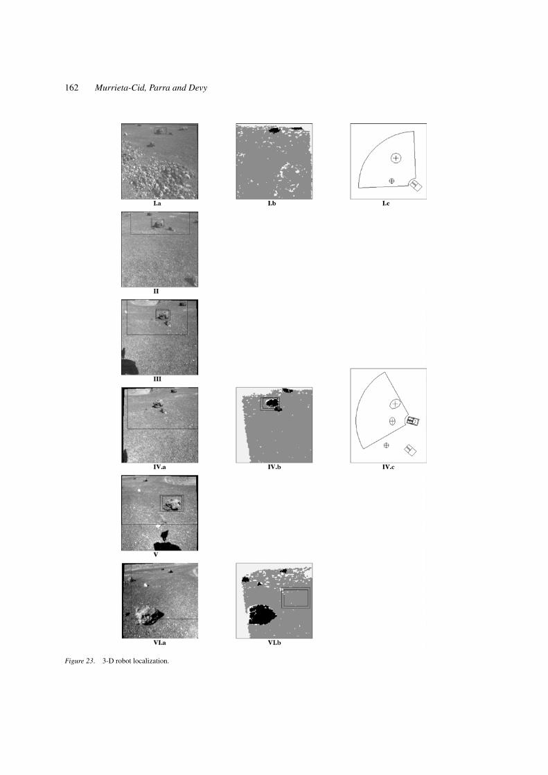
Figure 23 shows a partial result of the exploration task,involving concurrently the modeling and the trackingprocesses. Figure 23 I.a shows the video image, Fig. 23I.b presents the 3-D image segmentation and classifica-tion, two grey levels are used to label the classes (rocksand soil). Figure 23 I.c shows the first estimation of therobot position. A boundary box indicates the selectedlandmark (see Fig. 23 I.a). This one was automaticallychosen by using the local model. The selection wasdone by taking into account 3-D shape and nature ofthe landmark.

Figure 23 II and 23 III shows the tracking of the land-mark, which is marked in the figure with a boundarybox. Another larger boundary box is used to delineatethe region of examination.

Figure 23 IV.a presents the next image of the se-quence, Fig. 23 IV.b shows the 3-D segmentation andidentification phases used to build the local model. Thevisual tracking is employed here to solve the matchingproblem of landmark’s representation between the dif-ferent perceptions. Figure 23 IV.c presents the currentrobot localization, the local model building at this timeis merged to the global one. In this simple example,the global model contains only one ground area with alist of three detected landmarks and a list of two robotpositions.

The target tracking process goes on in the next im-ages of the sequence (see Fig. 23 V and 23 VI.a). Therobot motion between the image V and VI.a was too im-portant, so the aspect and position of the target changesa great deal; it occurs a tracking error (see the in Fig. 23VI.b, the window around the presumed tracked target).A new local model is built at this time (Fig. 23 VI.b).The coherence of the both processes (local model con-struction and target tracking) is checked by using thenature of the landmark. As the system knows that thetarget is a rock, this one is able to detect the trackingprocess mistake given that the model of the landmark(target) belongs to the class soil.

7. Integrated System

The complete system here proposed is shown in Fig. 2.During robot motion a slow and a fast processes aresimultaneously executed. The slow process is used tobuild a landmark-based model of the environment. Thefast process is used to track the landmarks. The coher-ence of the results of the executed task is checked bycomparing the result of both processes. The testing isdone to the frequency of the slowest processes. Cur-rently the fast process is running to approximately 4 Hzand the slow is running to 0.1 Hz.

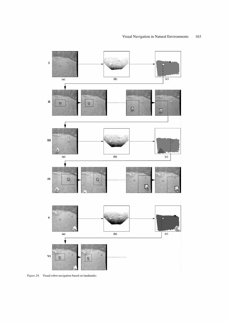
Robot visual navigation is done by using the pro-posed system. In order to navigate during a long robotmotion, a sequence of different landmarks (or targets)is used as sub-goal that the robot must successivelyreach.

We illustrate this task with a experiment carried outwith the mobile robot LAMA. Figure 24(a) shows thevideo image, (b) presents the 3-D image and (c) showsthe 3-D image segmentation, classification and bound-ary box including the selected landmark. The selectionwas done taking into account 3-D shape and nature.

The second line of Fig. 24 represent the tracking of alandmark through an image sequence. The landmark ismarked on the picture with a little boundary box. Thetracking process is performed based on a comparisonbetween a model of the landmark and the image. InMurrieta-Cid et al. (1998a) is described in detail thetracking technique used. When the landmark positionis close to the image edge, then it is necessary to selectanother landmark. So the Fig. 24 III presents the newlandmark selection based on image segmentation andclassification. The next sequence of tracking is showson the line IV of Fig. 24 and the next landmark com-mutation is presents on line V. Finally on the line VIthe robot continue navigation task.

7.1. Experiments of Simultaneous Localizationand Modeling (SLAM)

We illustrate this task with an experiment carried outin the EDEN site at LAAS-CNRS. In this work SLAMtask is based on landmark extraction. The strategy toselect the landmarks is the one presented on Section 7.Left column of Fig. 25 shows 2-D images correspond-ing to left stereo-vision camera. On these images therocks selected as target and the zone where the targetis looking for are shown. The results obtained regard-ing environment modeling are shown on the second


Figure 23. 3-D robot localization.


Figure 24. Visual robot navigation based on landmarks.


Figure 25. Simultaneous localization and modeling (SLAM) based on landmarks.


column. The maps of the environment and the local-ization of the robot are presented on the third column.On the row “I” the robot just takes one landmark asreference in order to localize itself. On the last row therobot uses 3 landmarks to perform localization task, therobot position estimation is shown by using rectangles.The most important result here is that the robot positionuncertainty does not grow thanks to the usage of land-marks. The landmarks allow to stop the incrementalgrowing of the robot position uncertainty.

8. Conclusion and Future Work

The work presented in this paper concerns the environ-ment representation and the localization of a mobilerobot which navigates in a planetary environment orterrestrial natural areas.

A local model of the environment is constructed inseveral phases:

• region extraction: firstly, the segmentation gives asynthetic representation of the environment.

• object characterization: each object of the scene ischaracterized by using 3-D features and its textureor/and its color. Having done the segmentation tex-ture color and 3-D features can be used to character-ize and to identify the objects. In this phase, visualattributes are taken into account to profit from itspower of discrimination. The texture and color at-tributes are computed from regions issued from thesegmentation, which commonly give more discrimi-nant informations than the features obtained from anarbitrary division of the image.

• object identification: the nature of the elements (ob-jects and ground) in the scene is obtained by com-paring an attribute vector with a database composedby different classes, issued from a learning process.

The local model of the first scene is employed inorder to select automatically an appropriate landmark.The matching problem of landmark’s is solved by usinga visual tracking process. The global model of the envi-ronment is updated at each perception and merged withthe current local model. The current robot’s situationand the numerical attributes of the landmark featuresare updated by using an Extended Kalman Filter (EKF).

Comparing the approach here proposed with our pre-vious work, one important improvement is the currentsegmentation algorithm. Here we are using an unsuper-vised classification method in order to automatically

generate classes in the attribute space. Thanks to thismethod our segmentation is more robust. In our system,the most difficult task to accomplish is segmentation,so if this step is robust, the whole system will be too.

Comparing our approach with other outdoor mapbuilding methods, the main contributions are: (1) Theuse of semantic labeling of objects and regions whichallows to command the robot using semantic instead ofnumeric vectors. (2) The use of tracking of landmarksto aid matching perceived the local scene model witha global world model.

Based on intensive evaluation of our previousmethod we found out that the main problem to fuselocal models into a global one is the matching of ob-jects perceived in multiple views acquired during therobot motion. The tracking method allows to keep thecorrespondence between some of the landmarks duringan image sequence simplifying the match among theremaining landmarks.

Some possible extensions to this system are goingon: firstly, we plan to study image preprocessors thatwould enhance the extraction of those image featuresthat are appropriate to the tracking method. Secondly,we plan to include new classes (e.g., rocky soil andground depressions) to improve the semantic descrip-tion of the environment.

Given that the identification step is based on super-vised learning process, its good performance dependson the utilization of a database representative enoughof the environment. However if the robot navigates justin a single type of environment (i.e., terrestrial naturalareas or planetary terrains), this limit is not a big dealbecause a specific environment can be represented bya reduced number of classes. If different types of en-vironment are considered, it can be possible to solvethe problem by a hierarchical approach: A first stepcould identify the environment type (i.e., whether theimage shows a forest, a desert or an urban zone) andthe second one the elements in the scene. The first stephas been considered in recent papers (Rubner et al.,1998). These approaches are not able to identify the el-ements in the scene but the whole image like an entity.After having obtained the scene type, our identificationmethod could be used to realize the second step. In thiscase a database organized in function of the types of en-vironment is suitable. It allows to reduce the number ofclasses, then decreasing the complexity of the problem(i.e., in lunar environment the tree class is not lookedfor, but the depression class “holes” is). Additionallyit is easier to profit from contextual information when


the environment type is known. We propose this strat-egy as enhancement of our method (Murrieta-Cid et al.,2002).

We are also working in a more complete topologicalrepresentation of the environment in order to move therobot along very large paths where the environmentcan change significantly. Finally, this approach is beingmodified to detect new specific entities such as countryroads. We also have the intention to apply this work inagricultural tasks.

Acknowledgments

The authors thank Nicolas Vandapel, Maurice Briot,Victor Ayala, Raja Chatila and Simon Lacroix for theircontributions to the development of the ideas presentedin this paper and to the implementation of some of thesoftware. This work was funded by CONACyT Mexico(PhD scholarship and project J34670-A), by COL-CIENCIAS Colombia, France Foreign Office (PhDscholarship) and ITESM Campus Ciudad de Mexico.

References

Asada, M. 1988. Building a 3D world model for a mobile robot fromsensory data. In Proc. International Conference on Robotics andAutomation (ICRA), Philadelphia, USA.

Ayala, V. and Devy, M. 2000. Active selection and tracking ofmultiple landmarks for visual navigation. In Proc. 2th Interna-tional Symposium on Robotics and Automation (ISRA), Monterrey,Mexico.

Ayala, V., Parra, C., and Devy, M. 2000. Active tracking based onHaussdorf matching. In Proc. IEEE 15th International Conferenceon Pattern Recognition (ICPR), Barcelona, Spain.

Becker, C., Gonzalez, H., Latombe, J.-L., and Tomasi, C. 1995. Anintelligent observer. In Proc. International Symposium on Exper-imental Robotics (ISER).

Betg-Brezetz, S., Chatila, R., and Devy, M. 1994. Natural sceneunderstanding for mobile robot navigation. In Proc. IEEE Inter-national Conference on Robotics and Automation (ICRA), SanDiego, USA.

Betg-Brezetz, S., Hebert, P., Chatila, R., and Devy, M. 1996. Un-certain map making in natural environments. In Proc. IEEEInternational Conference on Robotics and Automation (ICRA),Minneapolis, USA.

Betge-Brezetz, S., Chatila, R., and Devy, M. 1995. Object-basedmodelling and localization in natural environments. In Proc. IEEEInternational Conference on Robotics and Automation (ICRA),Osaka, Japan.

Bulata, H. and Devy, M. 1996. Incremental construction of alandmark-based and topological model of indoor environmentsby a mobile robot. In Proc. IEEE International Conference onRobotics and Automation (ICRA), Minneapolis, USA.

Canny, J. 1986. A computational approach to edge detection. IEEETransactions on Pattern Analysis and Machine Intelligence, 8(6).

Chatila, R. and Laumond, J.-P. 1985. Position referencing and con-sistent world modeling for mobile robots. In Proc IEEE Int. Conf.on Robotics and Automation (ICRA).

Dedeoglu, G., Mataric, M., and Sukhatme, G. 1999. Incremental,on-line topological map building with a mobile robot. In Proc.Mobile Robots XIV SPIE99, Boston, USA, pp. 129–139.

Delagnes, P., Benois, J., and Barba, D. 1994. Adjustable polygons:A novel active contour model for objects tracking on complexbackground. Journal on Communications, 45:83–85.

Devy, M. and Parra, C. 1998. 3D scene modelling and curve-based localization in natural environments. In Proc. IEEE Interna-tional Conference on Robotics and Automation (ICRA), Leuven,Belgium.

Dubuisson, M. and Jain, A. 1997. 2D matching of 3D moving ob-jects in color outdoors scenes. In Proc. IEEE Computer SocietyConference on Computer Vision and Pattern Recognition (CVPR).

Duda, R.O. and Hart, P.E. 1973. Pattern Classification and SceneAnalysis, Wiley & Sons.

Dumaine, M., Perrinot, O., Guennon, R., Hurteau, R., and DeSantis,R.M. 2001. Odometry and DGPS integrated navigatation systemfor ground vehicles. In Proc. International Conference on Fieldand Service Robotics (FSR), Helsinki, Finland.

Fillatreau, P., Devy, M., and Prajoux, R. 1993. Modelling of un-structured terrain and feature extraction using B-spline surfaces.In Proc. International Conference on Advanced Robotics (ICAR),Tokyo, Japan.

Haddad, H., Khatib, M., Lacroix, S., and Chatila, R. 1998. Reactivenavigation in outdoor environments using potential fields. In Proc.International Conference on Robotics and Automation (ICRA),Leuven, Belgium.

Hebert, M., Caillas, C., Krotkov, E., Kweon, I., and Kanade, T. 1989.Terrain mapping for a roving planetary explorer. In Proc. Interna-tional Conference on Robotics and Automation (ICRA), vol. 2.

Huttenlocher, D.P., Klanderman, A., and Rucklidge, J. 1993a. Com-paring images using the hausdorff distance. IEEE Transactions onPattern Analysis and Machine Intelligence, 15(9):850–863.

Huttenlocher, D.P., Rucklidge, W.J., and Noh, J.J. 1993b. Trackingnon-rigid objects in complex scenes. In Proc. Fourth InternationalConference on Computer Vision (ICCV).

Jiansho, S. and Tomasi, C. 1994. Good features to track. In Proc.IEEE International Conference on Computer Vision and PatternRecognition (CVPR).

Krotkov, E., Caillas, C., Hebert, M., Kweon, I., and Kanade, T. 1989.First results in terrain mapping for a roving planetary explorer. InProc. NASA Conference on Space Telerobotics.

Kweon, I.S. and Kanade, T. 1991. Extracting topological featuresfor outdoor mobile robots. In Proc. International Conference onRobotics and Automation (ICRA), Sacramento, USA.

Lacroix, S., Chatila, R., Fleury, S., Herrb, M., and Simeon, T. 1994.Autonomous navigation in outdoor environment: Adaptive ap-proach and experiment. In Proc. IEEE International Conferenceon Robotics and Automation (ICRA), San Diego, USA.

Mallet, A., Lacroix, S., and Gallo, G. 2001. Position estimation inoutdoor environments using a pixel tracking and stereovision. InProc. IEEE International Conference on Robotics and Automation(ICRA), San Francisco, USA.

McKerrow, P.J. and Ratner, D. 2001. Navigating an outdoor robotwith simple discontinuous landmarks. In Proc. Fourth EuropeanWorkshop on Advanced Mobile Robots (EUROBOT), Lund,Sweeden.


Metea, M.B. and Tsai, J. 1987. Route planning for intelligentautonomous land vehicles using hierarchical terrain representa-tion. In Proc. IEEE International Conference on Robotics andAutomation (ICRA), Raleigh, USA.

Murrieta-Cid, R. 1997. Target tracking method based on a compa-ration between an image and a model. Technical Report Num.97023, LAAS CNRS, written during a stay at Stanford University.

Murrieta-Cid, R. 1998. Contribution au developpement d’un systemede Vision pour robot mobile d’exterieur. PhD Thesis (in French),INPT, LAAS CNRS, Toulouse, France.

Murrieta-Cid, R., Briot, M., and Vandapel, N. 1998a. Landmarkidentification and tracking in natural environment. In Proc.IEEE/RSJ International Conference on Intelligent Robots andSystems (IROS), Victoria, Canada.

Murrieta-Cid, R., Parra, C., Devy, M., and Briot, M. 1998b.Contribution on vision and modelling. In Proc. InternationalSymposium on Robotics and Automation (ISRA), Saltillo, Mexico.

Murrieta-Cid, R., Parra, C., Devy, M., and Briot, M. 2001. Scenemodelling from 2D and 3D sensory data acquired from naturalenvironments. In Proc. IEEE International Conference onAdvanced Robotics (ICAR), Budapest, Hungary.

Murrieta-Cid, R., Parra, C., Devy, M., Tovar, B., and Esteves,C. 2002. Building multi-level models: From landscapes tolandmarks. In Proc. IEEE International Conference on Roboticsand Automation (ICRA), Washington, USA.

Ohta, Y. 1985. Knowledge-Based Interpretation of Outdoor NaturalColor Scenes, Morgan Kaufman: Palo Alto, CA.

Otsu, N. 1979. A threshold selection method from gray-level histro-grams. IEEE Transaction on Systems, Man and Cybernetics,9(1):62–66.

Pal, N.R. and Pal, S.K. 1993. A review on image segmentationtechniques. Pattern Recognition, 26(9):1277–1294.

Parra, C., Murrieta-Cid, R., Devy, M., and Briot, M. 1999. 3-Dmodelling and robot localization from visual and range datain natural scenes. In Proc. International Conference on VisionSystems (ICVS), Las Palmas, Spain.

Rosenblum, M. and Gothard, B. 2000. A high fidelity multi-sensorscene understanding system for autonomous navigation. In Proc.IEEE Intelligent Vehicles Symposium (IV), Detroit, USA.

Rubner, Y., Tomasi, C., and Guibas, J. 1998. A metric for distributionswith applications to image databases. In Proc. IEEE InternationalConference on Computer Vision (ICCV), Bombay, India.

Rucklidge, W. 1997. Efficiently locating objects using the haus-dorff distance. International Journal of Computer Vision,24(3):251–270.

Saber, E., Tekalp, A.M., Eschbach, R., and Knox, K. 1996.Automatic image annotation using adaptative color classification.Graphical Models and Image Processing, 58(2):115–126.

Serra, J. 1982. Image Analysis and Mathematical Morphology,Academic Press: London.

Smith, R.C., Self, M., and Cheeseman, P. 1990. Estimating uncertainspatial relationships in robotics. Autonomous Robot Vehicules.

Sutherland, K.T. and Thompson, B. 1994. Localizing in unstructuredenvironments: Dealing with the errors. IEEE Transactions onRobotics and Automation.

Tan, T.S.C. and Kittler, J. 1994. Colour texture analysis using colourhistogram. In Proc. IEE Vis. Image Signal Process.

Unser, M. 1986. Sum and difference histograms for textureclassification. IEEE Transactions on Pattern Analysis andMachine Intelligence.

Vandapel, N., Moorehead, S., Whittaker, W., Chatila, R., andMurrieta-Cid, R. 1999. Preliminary results on the use of stereocolor cameras and laser sensors in Antarctica. In Proc. 6thInternational Symposium on Experimental Robotics (ISER),Sydney, Australia.

Du, Y. and Crisman, J. 1995. A color projection for fast generictarget tracking. In Proc. International Symposium on IntelligentRobots and Systems (SIRS), Pisa, Italy.

Rafael Murrieta-Cid received the B.Sc. degree in Industrial PhysicsEngineering from ITESM campus Monterrey (Mexico) in 1990, theM.Sc. degree in Automatic Manufacturing Systems from ITESMcampus Monterrey in 1993 and DEA “Diplome d’Etudes Appro-fondies” (French Master) in Signals and Images from INP ofToulouse in 1995. In 1996, he was visitor student at the StanfordRobotics Laboratory. In November 1998 he received the Ph.D. fromINP of Toulouse France. His Ph.D research was done at the RIAgroup of the LAAS/CNRS, in Toulouse. In 1998–1999, he was Post-doctoral researcher in the Computer Science Department at StanfordUniversity. Rafael Murrieta-Cid is currently Assistant Professor inthe Electrical Engineering Department at ITESM campus MexicoCity and is working on Motion Planning, Perception and Experi-mental Mobile Robotics.

Carlos Parra got his B.Sc. degree in Electronic Engineering fromPontificia Universidad Javeriana of Bogota-Colombia in 1992 andthen a M.Sc. degree in Electrical Engineering from Universidad delos Andes of Bogota-Colombia in 1994. He got a DEA in Con-trol Science and Industrial Computer Science from Paul SabatierUniversity. In Mars 1999 he received the Ph.D. from Paul SabatierUniversity in Toulouse-France. His Ph.D. research was performedat the RIA group at the LAAS/CNRS, in Toulouse. In 1999, he dida Postdoctoral research in the LAAS/CNRS. Carlos Parra is cur-rently Associate Professor in the Electronic Department at PontificiaUniversidad Javeriana. His research interest include perception,mobile robots for natural environments, applications of computervison and experimental mobile robotics.


Michel Devy got his degree in Computer Science Engineering in1976 from IMAG, in Grenoble (France), and received is Ph.D. in

1980 in Toulouse (France). Since 1980, he has participated to theRobotics and Artificial Intelligence group of LAAS-CNRS; his re-search is devoted to the application of computer vision in Automa-tion and Robotics. He has been involved in numerous national andinternational projects, about Manufacturing Applications, MobileRobots for space exploration or for civil safety, Vision technologyfor Intelligent Vehicles, 3D modelling for body modelling. He isnow Research Director at CNRS, head for the Perception Area inthe Robotics Group of LAAS-CNRS and his main scientific top-ics concerns Perception for Mobile Robots in natural or indoorenvironments.

Visual Navigation in Natural Environments: From Range and Color Data to a Landmark-Based Model

Documents

Transcript of Visual Navigation in Natural Environments: From Range and Color Data to a Landmark-Based Model