Vision-Based Localization and Scanning of 1D UPC and EAN ...

Vladimir Kulyukin & Tanwir Zaman

International Journal of Image Processing (IJIP), Volume (8) : Issue (5) : 2014 355

Vision-Based Localization and Scanning of 1D UPC and EAN Barcodes with Relaxed Pitch, Roll, and Yaw Camera Alignment

Constraints

Vladimir Kulyukin [email protected] Department of Computer Science Utah State University Logan, UT, USA

Tanwir Zaman [email protected] Department of Computer Science Utah State University Logan, UT, USA

Abstract Two algorithms are presented for vision-based localization of 1D UPC and EAN barcodes with relaxed pitch, roll, and yaw camera alignment constraints. The first algorithm localizes barcodes in images by computing dominant orientations of gradients (DOGs) of image segments and grouping smaller segments with similar DOGs into larger connected components. Connected components that pass given morphological criteria are marked as potential barcodes. The second algorithm localizes barcodes by growing edge alignment trees (EATs) on binary images with detected edges. EATs of certain sizes mark regions as potential barcodes. The algorithms are implemented in a distributed, cloud-based system. The system’s front end is a smartphone application that runs on Android smartphones with Android 4.2 or higher. The system’s back end is deployed on a five node Linux cluster where images are processed. Both algorithms were evaluated on a corpus of 7,545 images extracted from 506 videos of bags, bottles, boxes, and cans in a supermarket. All videos were recorded with an Android 4.2 Google Galaxy Nexus smartphone. The DOG algorithm was experimentally found to outperform the EAT algorithm and was subsequently coupled to our in-place scanner for 1D UPC and EAN barcodes. The scanner receives from the DOG algorithm the rectangular planar dimensions of a connected component and the component’s dominant gradient orientation angle referred to as the skew angle. The scanner draws several scanlines at that skew angle within the component to recognize the barcode in place without any rotations. The scanner coupled to the localizer was tested on the same corpus of 7,545 images. Laboratory experiments indicate that the system can localize and scan barcodes of any orientation in the yaw plane, of up to 73.28 degrees in the pitch plane, and of up to 55.5 degrees in the roll plane. The videos have been made public for all interested research communities to replicate our findings or to use them in their own research. The front end Android application is available for free download at Google Play under the title of NutriGlass. Keywords: Skewed Barcode Localization & Scanning, Image Gradients, Mobile Computing, Eyes-free Computing, Cloud Computing.

1. INTRODUCTION

A common weakness of many 1D barcode scanners, both free and commercial, is the camera alignment requirement: the smartphone camera must be horizontally or vertically aligned with barcodes to obtain at least one complete scanline for successful barcode recognition (e.g., [1], [2]). This requirement is acceptable for sighted users but presents a serious accessibility barrier to visually impaired (VI) users or to users who may not have adequate dexterity for satisfactory camera alignment. One approach that addresses the needs of these two user groups is 1D barcode localization and scanning with relaxed pitch, roll, and yaw constraints. Figure 1 shows



the roll, pitch, and yaw planes of a smartphone. Such barcode processing is also beneficial for sighted smartphone users, because the camera alignment requirement no longer needs to be satisfied.

FIGURE 1: Pitch, roll, and yaw planes of a smartphone. In our previous research, we designed and implemented an eyes-free algorithm for vision-based localization and decoding of aligned 1D UPC barcodes by augmenting computer vision techniques with interactive haptic feedback loops to ensure that the smartphone camera is horizontally and vertically aligned with the surface on which a barcode is sought [3]. We later developed another algorithm for localizing 1D UPC barcodes skewed in the yaw plane [4]. In this article, two new algorithms are presented that relax the alignment constraints to localize and scan 1D UPC and EAN barcodes in frames captured by the smartphone’s camera misaligned with product surfaces in the pitch, roll, and yaw planes. Our article is organized as follows. Section 2 covers related work. Section 3 presents the first localization algorithm that uses dominant gradient orientations (DOGs) in image segments. Section 4 presents the second barcode localization algorithm that localizes barcodes by growing edge alignment trees (EATs) on binary images with detected edges. Section 5 presents our 1D barcode localization experiments on a corpus of 7,545 images extracted from 506 videos of bags, boxes, bottles, and cans in a supermarket. Section 6 describes our 1D barcode scanner for UPC and EAN barcodes and how it is coupled to the DOG localization algorithm. Section 7 gives technical details of our five node Linux cluster for image processing. Section 8 presents our barcode scanning experiments on the same sample of 7,545 images as well as our experiments to assess the ability of the system to scan barcodes skewed in the pitch, roll, and yaw planes. These experiments were conducted on ten products (two cans, two bottles, and six boxes) in our laboratory. Section 9 discusses our findings and outlines several directions for future work.

2. RELATED WORK

The use of smartphones to detect barcodes has been the focus of many research and development projects for a long time. Given the ubiquity and ever increasing computing power of smartphones, they have emerged as a preferred device for many researchers to implement and test new techniques to localize and scan barcodes. Open source and commercial smartphone applications, such as RedLaser (redlaser.com) and ZXing (code.google.com/p/zxing), have been developed. However, these systems are intended for sighted users and require them to center barcodes in images. To the best of our knowledge, the research effort most closely related to the research presented in this article is the research by Tekin and Coughlan at the Smith-Kettlewell Eye Research



Institute [1, 2, 5]. Tekin and Coughlan have designed a vision-based algorithm to guide VI smartphone users to center target barcodes in the camera frame via audio instructions and cues. However, the smartphone cameras must be aligned with barcode surfaces and the users must undergo training before they can use the mobile application in which the algorithm is implemented. Wachenfeld et al. [6] present another vision-based algorithm that detects barcodes on a mobile phone via image analysis and pattern recognition methods. The algorithm overcomes typical distortions, such as inhomogeneous illumination, reflections, or blurriness due to camera movement. However, a barcode is assumed to be present in the image. Nor does the algorithm appear to address the localization and scanning of barcodes misaligned with the surface in the pitch, roll, and yaw planes. Adelmann et al. [7] have developed a randomized vision-based algorithm for scanning barcodes on mobile phones. The algorithm relies on the fact that, if multiple scanlines are drawn across the barcode in various arbitrary orientations, one of them might cover the whole length of the barcode and result in successful barcode scans. This recognition scheme does not appear to handle distorted or misaligned images. Lin et al. [8] have developed an automatic barcode detection and recognition algorithm for multiple and rotation invariant barcode decoding. However, the system requires custom hardware. In particular, the proposed system is implemented and optimized on a DM6437 DSP EVM board, a custom embedded system built specifically for barcode scanning. Galo and Manduchi [9] present an algorithm for 1D barcode reading in blurred, noisy, and low resolution images. However, the algorithm detects barcodes only if they are slanted by less than 45 degrees in the yaw plane. The researchers appear to make no claims on the ability of their algorithm to handle barcodes misaligned in the pitch and roll planes. Peng et al. [10] present a smartphone application that helps blind users locate EAN barcodes and expiration dates on product packages. It is claimed that, once barcodes are localized, existing barcode decoding techniques and OCR algorithms can be utilized to obtain the required information. The system provides voice feedback to guide the user to point the camera to the barcode of the product, and then guide the user the point the camera to the expiration date for OCR. The system requires user training and does not appear to handle misaligned barcodes.

3. BARCODE LOCALIZATION ALGORITHM I 3.1 Dominant orientation of gradients The first algorithm is based on the observation that barcodes characteristically exhibit closely spaced aligned edges with the same angle, which sets them apart from text and graphics. Let I be an RGB image and let f be a linear relative luminance function computed from a pixel’s RGB components:

( ) .0722.07152.02126.0,, BGRBGRf ++= (1)

The gradient of f and the gradient’s orientation � can then be computed as follows:

.tan;,1

∂

∂

∂

∂=

∂

∂

∂

∂=∇ −

y

f

x

f

y

f

x

ff θ

(2)

Let M be an n x n mask, n > 0, convolved with I. Let the dominant orientation of gradients of M, DOG(M), be the most frequent discrete gradient orientation of all pixels covered by M. Let (c, r) be the column and row coordinates of the top left pixel of M. The regional gradient orientation



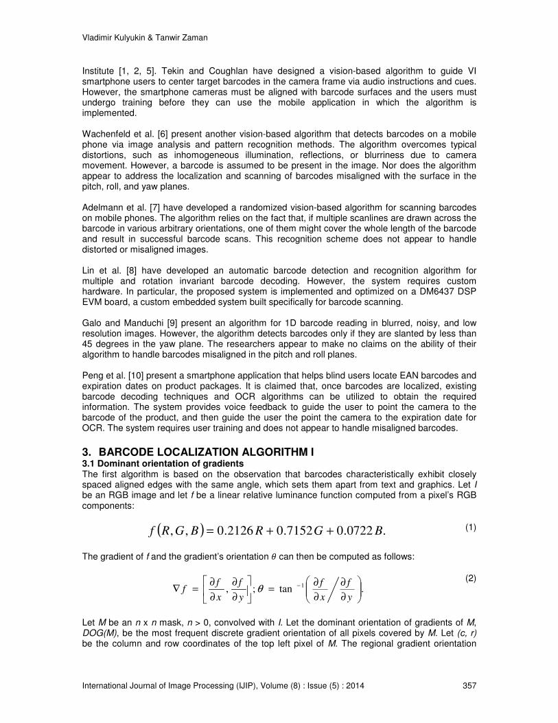
table of M, RGOT(c, r), is a map of discrete gradient orientations to their frequencies in the region of I covered by M. The global gradient orientation table (GGOT) of I is a map of the top left coordinates of image regions covered by M to their RGOTs. In our implementation, both GGOTs and RGOTs are implemented as hash tables.

FIGURE 2: Logical structure of global gradient orientation table.

Figure 2 shows the logical organization of an image’s GGOT. Each GGOT maps (c, r) 2-tuples to RGOT tables that, in turn, map discrete gradient orientations (i.e., GO1, GO2, …, GOk in Figure 2) to their frequencies (i.e., FREQ1, FREQ2, …, FREQk in Figure 2) in the corresponding image regions. Each RGOT represents the region whose top left coordinates are specified by the corresponding (c, r) 2-tuple and whose size is the size of M. Each RGOT is subsequently converted into a single real number called the most frequent gradient orientation. This number, denoted by DOG(M), is the region’s dominant orientation of gradients, also known as its DOG.

FIGURE 3: UPC-A barcode skewed in the yaw plane. Consider an example of a barcode skewed in the yaw plane in Figure 3. Figure 4 gives the DOGs for a 20 x 20 mask convolved with the image in Figure 3. Each green square is a 20 x 20 image region. The top number in each square is the region’s DOG, in degrees, whereas the bottom



number is the frequency of that particular DOG in the region, i.e., how many pixels in that region has this gradient value. If no gradient orientation clears a given frequency count threshold, both numbers are set to 0. Figure 5 displays the DOGs for the 50 x 50 mask convolved with the image in Figure 3. It should be noted that Figures 4 and 5 show a typical tendency that, as the size of the mask increases, fewer image regions are expected to clear the DOG threshold if the latter is set as a ratio of pixels with specific gradient values over the total number of the region’s pixels in the image. Figure 5 displays the DOGs for the 50 x 50 mask convolved with the image in Figure 3. It should be noted that Figures 4 and 5 show a typical tendency that, as the size of the mask increases, fewer image regions are expected to clear the DOG threshold if the latter is set as a ratio of pixels with specific gradient values over the total number of the region’s pixels in the image.

FIGURE 4: GGOT for a 20 x 20 mask.

.

FIGURE 5: GGOT for a 50 x 50 mask.



FIGURE 6: D-neighborhood found in GGOT in Figure 4.

3.2 D-Neighborhoods Let an RGOT 3-tuple ( )kkk DOGrc ,, consist of the coordinates of the top left corner, ( )kk rc , , of the

subimage covered by an n x n mask M whose dominant gradient orientation is DOGk. We define

DOG-neighborhood (D-neighborhood) is a non-empty set of RGOT 3-tuples ( )kkk DOGrc ,, such

that for any such 3-tuple ( )kkk DOGrc ,, there exists at least one other 3-tuple ( )jjj DOGrc ,, such

that ( ) ( )kkkjjj DOGrcDOGrc ,,,, ≠ and ( ) ( )( ) ,,,,,, TrueDOGrcDOGrcsim kkkjjj = where sim is a

Boolean similarity metric. Such similarity metrics define various morphological criteria for D-neighborhoods. In our implementation, the similarity metric returns true when the square regions specified by the top left coordinates (i.e., ( )kk rc , and ( )

jj rc , ) and the mask size n are horizontal,

vertical, or diagonal neighbors and the absolute difference of their DOGs does not exceed a small threshold.

FIGURE 7: D-neighborhood detected in Figure 6.



.

FIGURE 8: Multiple d-neighborhoods.

An image may have several D-neighborhoods. The D-neighborhoods are computed simultaneously with the computation of the image’s GGOT. As each RGOT 3-tuple becomes available during the computation of RGOTs, it is placed into another hash table for D-neighborhoods. The computed D-neighborhoods are filtered by the ratio of the total area of their component RGOTs to the image area. For example, Figure 6 shows RGOTs marked as blue rectangles that are grouped into a D-neighborhood by the similarity metric defined above, because they are horizontal, vertical, and diagonal neighbors and the absolute difference of their DOGs does not exceed a small threshold. This resultant D-neighborhood is shown in Figure 7. This neighborhood is computed in parallel with the computation of the GGOT in Figure 4. Detected D-neighborhoods are enclosed by minimal rectangles that contain all of their RGOT 3-tuples, as shown in Figure 7, where the number in the center of the white rectangle denotes the neighborhood’s DOG. A minimal rectangle is the smallest rectangle that encloses all RGOTs of the same connected component. All detected D-neighborhoods are barcode region candidates. There can be multiple D-neighborhoods detected in an image. For example, Figure 8 shows all detected D-neighborhoods when the threshold is set to 0.01, which is too low. Figure 7 exemplifies an interesting and recurring fact that multiple D-neighborhoods tend to intersect over a barcode. The DOG algorithm is given in Appendix A. Its asymptotic complexity is O(k

2), where k is the

number of masks that can be placed on the image. This is because, in the worst case, each RGOT constitutes its own D-neighborhood, which makes each subsequent call to the function FindNeighbourhoodForRGOT(), which finds the home D-neighborhood for each newly computed RGOT, to unsuccessfully inspect all the D-neighborhoods computed so far. A similar worst-case scenario happens when there is one D-neighborhood that absorbs all computed RGOT, which takes place when the similarity metric is too permissive. Both of these scenarios, while theoretically possible, rarely occur in practice.



FIGURE 9: EAT algorithm.

4. BARCODE LOCALIZATION ALGORITHM II The second algorithm for skewed barcode localization with relaxed pitch, roll, and yaw constraints is based on the idea that binarized image areas with potential barcodes exhibit continuous patterns (e.g., sequences of 1’s or 0’s) with dynamically detectable alignments. We call the data structure for detecting such patterns the edge alignment tree (EAT). Figure 10 shows several examples of EATs marked with different colors. In principle, each node in an EAT can have multiple children. In practice, since barcodes have straight lines or bars aligned side by side, most dynamically computed EATs tend to be linked lists, as shown in Figure 10. The EAT algorithm is given in Appendix B. Each captured frame is put through the Canny edge detection filter and binarized [11] as one of the most reliable edge detection techniques [12]. The binarized image is divided into smaller rectangular subimages. The size of subimages is specified by the variable maskSize in the function ComputeEATs() in Appendix B. Each mask is a square. The subimages are scanned row by row and column by column. For each subimage, the EATs are computed to detect the dominant skew angle of the edges.

FIGURE 10: EATs from binarized edges.



The algorithm starts from the first row of each subimage and moves to the right column by column until the end of the row is reached. If a pixel’s value is 255 (white), it is treated as a 1, marked as the root of an EAT, and stored in the list of nodes. If the current row is the subimage’s first row, the node list contains only the root nodes. In the second row (and all subsequent rows), whenever a white pixel is found, it is checked against the current node list to see if any of the nodes can become its parent. The test of parenthood is done by checking the angle between the potential parent’s pixel and the current pixel with Equation 3.

(3)

If the angle is between 45 and 135 degrees, the current pixel is added to the list of children of the found parent. Once a child node is claimed by a parent, it cannot become the child of any other parent. This parent-child matching is repeated for all nodes in the current node list. If none of the nodes satisfies the parent condition, the orphan pixel becomes a EAT root that can be matched with a child on the next row. Once all the EATs are computed, as shown in Figure 10, the dominant angle is computed for each EAT as the average of the angles between each parent and its children, all the way down to the leaves. For each subimage, the standard deviation of the angles is computed for all EATs. If the subimage’s standard deviation is low (less than 5 in our current implementation), the subimage is classified as a potential barcode region. The asymptotic complexity of the EAT algorithm, which is presented in Appendix B, is as follows. Let I be an image of side n. Let the mask’s size be m. Recall that each mask is a square. Let k denote the number of masks, where k= n

2/m

2. The time complexity of the Canny edge detector is

Θ(n) [11]. In the worst case, for each subimage, m trees are grown of the height equal to the number of rows in the subimage, which takes km

3 computations, because each grown EAT must

be linearly scanned to compute its orientation angle. Thus, the overall time complexity can be calculated as Θ(n) + O(k*m

3) = O(n

2m).

5. LINUX CLUSTER We built a Linux cluster out of five nodes for cloud-based computer vision and data storage. Each node is a PC with an Intel Core i5-650 3.2 GHz dual-core processor that supports 64-bit computing. The processors have 3MB of cache memory. The nodes are equipped with 6GB DDR3 SDRAM and have Intel integrated GMA 4500 Dynamic Video Memory Technology 5.0. All nodes have 320 GB of hard disk space. Ubuntu 12.04 LTS was installed on each node. We installed JDK 7 in each node.

We used JBoss (http://www.jboss.org) to build and configure the cluster and the Apache mod_cluster module (http://www.jboss.org/mod_cluster) to configure the cluster for load balancing. The cluster has one master node and four slaves. The master node is the domain controller that runs mod_cluster and httpd. All nodes are part of a local area network and have hi-speed Internet connectivity. The JBoss Application Server (JBoss AS) is a free open-source Java EE-based application server. In addition to providing a full implementation of a Java application server, it also implements the Java EE part of Java. The JBoss AS is maintained by jboss.org, a community that provides free support for the server. JBoss is licensed under the GNU Lesser General Public License (LGPL). The Apache mod_cluster module is an httpd-based load balancer. The module is implemented with httpd as a set of modules for httpd with mod_proxy enabled. This module uses a communication channel to send requests from httpd to a set of designated application server nodes. An additional communication channel is established between the server nodes and httpd. The nodes use the additional channel to transmit server-side load balance factors and lifecycle



events back to httpd via a custom set of HTTP methods collectively referred to as the Mod-Cluster Management Protocol (MCMP). The mod_cluster module provides dynamic configuration of httpd workers. The proxy's configuration is on the application servers. The application server sends lifecycle events to the proxies, which enables the proxies to auto-configure themselves. The mod_cluster module provides accurate load metrics, because the load balance factors are calculated by the application servers, not the proxies. All nodes in our cluster run JBoss AS 7. Jboss AS 7.1.1 is the version of the application server installed on the cluster. Apache httpd runs on the master node with the mod_cluster-1.2.0 module enabled. The Jboss AS 7.1.1 on the master and the slaves are discovered by httpd. A Java servlet for image recognition is deployed on the master node as a web archive file. The servlet’s URL is hardcoded in every front end smartphone. The servlet receives images uploaded with HTTP POST requests, recognizes barcodes, and sends an HTML response back to front end smartphones. No data caching is done on the servlet or the front end smartphones.

6. BARCODE LOCALIZATION EXPERIMENTS 6.1 Experimental Design The DOG and EAT algorithms were tested on images extracted from 506 video recordings of common grocery products. Each video recorded one specific product from various sides. The videos had a 1280 x 720 resolution and were recorded on an Android 4.2.2 Galaxy Nexus smartphone in a supermarket in Logan, Utah. All videos were recorded by a user who held a grocery product in one hand and a smartphone in the other. The videos covered four different categories of products: bags, bottles, boxes, and cans. The average video duration is fifteen seconds. There were 130 box videos, 127 bag videos, 125 box videos, and 124 can videos. Images were extracted from each video at the rate of 1 frame per second, which resulted in a total of 7,545 images, of which 1950 images were boxes, 1905 images were bags, 1875 images were bottles, and 1860 images were cans. These images were used in the experiments and the outputs of both algorithms, i.e., enclosed barcode regions (see Figures 7 and 8), were manually evaluated by the two authors independently. A frame was classified as a complete true positive if there was a D-neighborhood where at least one straight line across all bars of a localized barcode. A frame was classified as a partial true positive if there was a D-neighborhood where a straight line could be drawn across some, but not all, bars of a barcode. An image was classified as a false positive if there was a D-neighborhood that covered an image area with no barcode and no D-neighborhood detected in the same image covered a barcode either partially or completely. For example, in Figure 8, the D-neighborhood, with a DOG of 100, in the upper left corner of the image, covers an area with no barcode. However, the entire frame in Figure 8 is classified as a complete true positive, because there is another D-neighborhood, with a DOG of 47, in the center of the frame that covers a barcode completely. A frame was classified as a false negative when it contained a barcode but no D-neighborhoods covered that barcode either completely or partially and no D-neighborhood covered an area with no barcode, because in the latter case, the frame was classified as a false positive. A frame was classified as a true negative when the frame contained no barcode and could not be classified as a false positive.

6.2 DOG Localization Experiments The DOG algorithm was implemented in Java with OpenCV2.4 bindings for Android 4.2 and ran on Galaxy Nexus and Samsung Galaxy S2. In our previous research [4], the best threshold values for each mask size were determined. These values are given in Table 1. We used these values to run the experiments for each category of products. The performance analysis for the DOG algorithm is presented in the pie charts in Figures 11-14 for each category of products.



Product Type Mask Size Threshold Bag 20 x 20 0.02

Bottle 40 x 40 0.02

Box 20 x 20 0.02

Can 20 x 20 0.01

TABLE 1: Optimal mask sizes and threshold.

As can be seen in Figures 11 – 14, the DOG algorithm produces very few false positives or false negatives and performs well even on unfocussed and blurry images. The large percentages of true negatives show that the algorithm is conservative. This is done by design, because it is more important, especially for blind and visually impaired users, to avoid false positives. Moreover, at a rate of two frames per second, eventually there will be a frame where a barcode is successfully and quickly localized. The algorithm produces very few false negatives, which indicates, that, if a frame contains a barcode, it will likely be localized.

FIGURE 11: DOG performance on bags.

Figure 15 gives the DOG precision, recall, accuracy, and specificity values for different categories of products. The graph shows that the algorithm produced the best results for boxes, which can be attributed to the clear edges and smooth surfaces of boxes that result in images without major distortions. The largest percentages of false positives were on bags (8 percent) and bottles (7 percent). Many surfaces of these two product categories had shiny materials that produced multiple glares and reflections.



FIGURE 12: DOG performance on bottles.

FIGURE 13: DOG performance on boxes.



FIGURE 14: DOG performance on cans.

6.3 DOG Localization Experiments The EAT algorithm was also implemented in Java with OpenCV2.4 bindings for Android 4.2 and ran on Galaxy Nexus and Samsung Galaxy S2. The algorithm’s pseudocode is given in Appendix B. The EAT algorithm gave best results for bags with a Canny threshold of (300,400). For bottles, boxes and cans, it performed best with a threshold of (400,500). The algorithm gave the most accurate results for window size of 10 for all categories of products.

FIGURE 15: DOG precision, recall, specificity, and accuracy.



FIGURE 16: EAT performance on bags.

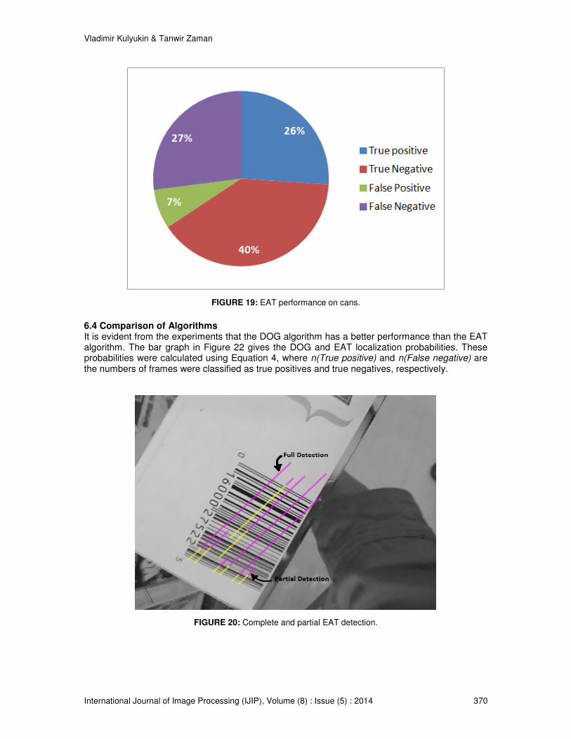
The charts in Figures 16 - 19 summarize the performance of the EAT algorithm for each product category. The experiments were performed on the same sample of 509 videos. The video frames in which detected barcode regions had single lines crossing all bars of a barcode were considered as complete true positives. Frames where such lines covered some of the bars were classified as partial true positives. Figure 20 shows examples of complete and partial true positives. Frames, where detected barcode regions did not have any barcodes were classified as false positives. True negatives were the frames with no barcodes where the algorithm did not detect anything. False negatives were the frames where the algorithm failed to detect a barcode in spite of its presence. The experiments showed that the false negative rates of the EAT algorithm were substantially higher than those of the DOG algorithm. The true positives rates of the EAT algorithm were also lower. Figure 21 shows the statistical analysis for each category of products. The best results were produced for boxes and the worst for cans. These results were similar to the results of the DOG algorithm.



FIGURE 17: EAT performance on bottles.

FIGURE 18: EAT performance on boxes.



FIGURE 19: EAT performance on cans.

6.4 Comparison of Algorithms It is evident from the experiments that the DOG algorithm has a better performance than the EAT algorithm. The bar graph in Figure 22 gives the DOG and EAT localization probabilities. These probabilities were calculated using Equation 4, where n(True positive) and n(False negative) are the numbers of frames were classified as true positives and true negatives, respectively.

FIGURE 20: Complete and partial EAT detection.



FIGURE 21: EAT precision, recall, specificity, and accuracy.

(4)

It can be seen that the DOG algorithm gives better results than the EAT algorithm for all four types of products. Our analysis of the poorer performance of the EAT algorithm indicates that it may be attributed to the algorithm’s dependency on the Canny edge detector. The edge detector found reliable edges only in the frames that were properly focused and free of distortions, which negatively affected the subsequent barcode localization. In that respect, the DOG algorithm is more robust, because it does not depend on any other edge detection. It should also be noted that the DOG algorithm is in-place, because it does not allocate any additional memory structures for image processing. Based upon this observation we decided to choose the DOG algorithm as the localization algorithm for our barcode scanning experiments covered in Section 8.

FIGURE 22: DOG and EAT localization probabilities.



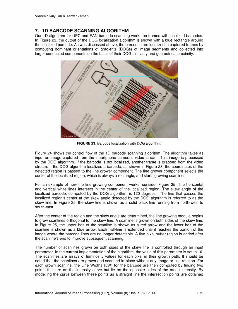
7. 1D BARCODE SCANNING ALGORITHM Our 1D algorithm for UPC and EAN barcode scanning works on frames with localized barcodes. In Figure 23, the output of the DOG localization algorithm is shown with a blue rectangle around the localized barcode. As was discussed above, the barcodes are localized in captured frames by computing dominant orientations of gradients (DOGs) of image segments and collected into larger connected components on the basis of their DOG similarity and geometrical proximity.

FIGURE 23: Barcode localization with DOG algorithm.

Figure 24 shows the control flow of the 1D barcode scanning algorithm. The algorithm takes as input an image captured from the smartphone camera’s video stream. This image is processed by the DOG algorithm. If the barcode is not localized, another frame is grabbed from the video stream. If the DOG algorithm localizes a barcode, as shown in Figure 23, the coordinates of the detected region is passed to the line grower component. The line grower component selects the center of the localized region, which is always a rectangle, and starts growing scanlines. For an example of how the line growing component works, consider Figure 25. The horizontal and vertical white lines intersect in the center of the localized region. The skew angle of the localized barcode, computed by the DOG algorithm, is 120 degrees. The line that passes the localized region’s center at the skew angle detected by the DOG algorithm is referred to as the skew line. In Figure 35, the skew line is shown as a solid black line running from north-west to south-east. After the center of the region and the skew angle are determined, the line growing module begins to grow scanlines orthogonal to the skew line. A scanline is grown on both sides of the skew line. In Figure 25, the upper half of the scanline is shown as a red arrow and the lower half of the scanline is shown as a blue arrow. Each half-line is extended until it reaches the portion of the image where the barcode lines are no longer detectable. A five pixel buffer region is added after the scanline’s end to improve subsequent scanning. The number of scanlines grown on both sides of the skew line is controlled through an input parameter. In the current implementation of the algorithm, the value of this parameter is set to 10. The scanlines are arrays of luminosity values for each pixel in their growth path. It should be noted that the scanlines are grown and scanned in place without any image or line rotation. For each grown scanline, the Line Widths (LW) for the barcode are then computed by finding two points that are on the intensity curve but lie on the opposite sides of the mean intensity. By modelling the curve between these points as a straight line the intersection points are obtained



between the intensity curve and the mean intensity. Interested readers are referred to our previous publication on 1D barcode scanning for technical details of this procedure [3, 4].

FIGURE 24: Barcode localization with DOG algorithm.

Figure 26 shows a sequence of images that gives a visual demonstration of how the algorithm works on a captured frame. The top image in Figure 26 is a frame captured from the smartphone camera’s video stream. The second image from the top in Figure 26 shows the result of the clustering stage of the DOG algorithm that clusters small subimages with similar dominant gradient orientations and close geometric proximity. The third image shows a localized barcode enclosed in a white rectangle. The bottom image in Figure 26 shows ten scanlines, one of which results in a successful barcode scan.

FIGURE 25: Growing a scanline orthogonal to skew angle.



FIGURE 26: 1D barcode scanning.

8. BARCODE SCANNING EXPERIMENTS Our 1D algorithm for UPC and EAN barcode scanning works on frames with localized barcodes. In Figure 23, the output of the DOG localization algorithm is shown with a blue rectangle around the localized barcode. As was discussed above, the barcodes are localized in captured frames by computing dominant orientations of gradients (DOGs) of image segments and collected into larger connected components on the basis of their DOG similarity and geometrical proximity. 8.1 Experiments in a Supermarket We conducted our first set of barcode scanning experiments in a local supermarket to assess the feasibility of our system. A user, who was not part of this research project, was given a Galaxy Nexus 4 smartphone with an AT&T 4G connection. Our front end application was installed on the smartphone. The user was asked to scan ten products of his choice in each of the four categories: box, can, bottle, and bag. The user was told that he can choose any products to scan so long as each product was in one of the above four categories. A research assistant accompanied the user and recorded the scan times for each product. Each scan time started



from the moment the user began scanning and ended when the response was received from the server. Figure 27 denotes the average times in seconds for each category. The cans showed the longest scanning average due to glares and reflections. Bags showed the second longest scanning average due to some crumpled barcodes. As we discovered during these experiments, another cause for the slower scan times on individual products in each product category is the availability of Internet connectivity at various locations in the supermarket. During the experiments in the supermarket, we noticed that at some areas of the supermarket the Internet connection did not exist, which caused delays in barcode scanning. For several products, a 10- or 15-step change in location within a supermarket resulted in a successful barcode scan. 8.2 Impact of Blurriness The second set of barcode scanning experiments was conducted to estimate the impact of blurriness on skewed barcode localization and scanning. These experiments were conducted on the same set of 506 videos of boxes, bags, bottles, and cans that we used for our barcode localization experiments described in Section 6. The average video duration is fifteen seconds. There are 130 box videos, 127 bag videos, 125 box videos, and 124 can videos. Images were extracted from the videos at the rate of 1 frame per second, which resulted in a total of 7,545 images, of which 1950 images were boxes, 1905 images were bags, 1875 images were bottles, and 1860 images were cans. Each frame was automatically classified as blurred or sharp by the blur detection scheme using Haar wavelet transforms [13, 14] that we implemented in Python. Each frame was also manually classified as having a barcode or not and labeled with the type of grocery product: bag, bottle, box, can. There were a total of sixteen categories. Figure 28 shows the results of the experiments. Images that contained barcodes for all four product categories had no false positives. In each product category, the sharp images had a significantly better true positive percentage than the blurred images. A comparison of the bar charts in Figure 28 reveals that the true positive percentage of the sharp images is more than double that of the blurry ones. Images without any barcode for all categories produced 100% accurate results with all true negatives, irrespective of the blurriness. In other words, the algorithm is highly specific in that it does not detect barcodes in images that do not contain them.

FIGURE 27: Average scan times.



Another observation on Figure 28 is that the algorithm showed its best performance on boxes. The algorithm’s performance on bags, bottles, and cans was worse because of some crumpled, curved, or shiny surfaces. These surfaces caused many light reflections, which hindered performance of both barcode localization and barcode scanning. The percentages of the skewed barcode localization and scanning were better on boxes due to smoother surfaces. Quite expectedly, the sharpness of images made a positive difference in that the scanning algorithm performed much better on sharp images in each product category. Specifically, on sharp images, the algorithm performed best on boxes with a detection rate of 54.41%, followed by bags at 44%, cans at 42.55%, and bottles at 32.22%.

FIGURE 28: Blurred vs. non-blurred images.

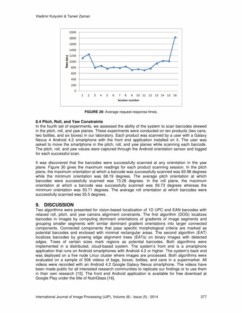
8.3 Robustness and Speed of Linux Cluster The third set of experiments was conducted to assess the robustness and speed of our five Linux cluster for image processing described in Section 5. After all classifications were completed (blurred vs. sharp; barcode vs. no barcode; type of grocery product), the classified frames were stored in the smartphone's sdcard. An Android service was implemented and installed on a Galaxy Nexus 4 smartphone. The service took one frame at a time and sent it to the node cluster via an http POST request over a local Wi-Fi network with a download speed of 72.31 Mbps and an upload speed of 29.64 Mbps. The service recorded the start time before uploading each image and the finish time once a response was received from the cluster. The difference between the finish and start times was logged as a total request-response time. The service was run with one image from each of the sixteen categories described in Section 8.2 for 3000 times, and the average request-response time for each session. Each image sent by the service was processed on the cluster as follows. The DOG localization algorithm was executed and, if a barcode was successfully localized, the barcode was scanned in place within the localized region with ten scanlines, as described in Section 7. The detection result was sent back to the smartphone and recorded on the smartphone’s sdcard. Figure 29 gives the graph of the node cluster’s request-response times. The lowest average request-response time was 712 milliseconds; the highest average was 1813 milliseconds.



FIGURE 29: Average request-response times.

8.4 Pitch, Roll, and Yaw Constraints In the fourth set of experiments, we assessed the ability of the system to scan barcodes skewed in the pitch, roll, and yaw planes. These experiments were conducted on ten products (two cans, two bottles, and six boxes) in our laboratory. Each product was scanned by a user with a Galaxy Nexus 4 Android 4.2 smartphone with the front end application installed on it. The user was asked to move the smartphone in the pitch, roll, and yaw planes while scanning each barcode. The pitch, roll, and yaw values were captured through the Android orientation sensor and logged for each successful scan. It was discovered that the barcodes were successfully scanned at any orientation in the yaw plane. Figure 30 gives the maximum readings for each product scanning session. In the pitch plane, the maximum orientation at which a barcode was successfully scanned was 83.98 degrees while the minimum orientation was 68.19 degrees. The average pitch orientation at which barcodes were successfully scanned was 73.28 degrees. In the roll plane, the maximum orientation at which a barcode was successfully scanned was 59.73 degrees whereas the minimum orientation was 50.71 degrees. The average roll orientation at which barcodes were successfully scanned was 55.5 degrees.

9. DISCUSSION Two algorithms were presented for vision-based localization of 1D UPC and EAN barcodes with relaxed roll, pitch, and yaw camera alignment constraints. The first algorithm (DOG) localizes barcodes in images by computing dominant orientations of gradients of image segments and grouping smaller segments with similar dominant gradient orientations into larger connected components. Connected components that pass specific morphological criteria are marked as potential barcodes and enclosed with minimal rectangular areas. The second algorithm (EAT) localizes barcodes by growing edge alignment trees (EATs) on binary images with detected edges. Trees of certain sizes mark regions as potential barcodes. Both algorithms were implemented in a distributed, cloud-based system. The system’s front end is a smartphone application that runs on Android smartphones with Android 4.2 or higher. The system’s back end was deployed on a five node Linux cluster where images are processed. Both algorithms were evaluated on a sample of 506 videos of bags, boxes, bottles, and cans in a supermarket. All videos were recorded with an Android 4.2 Google Galaxy Nexus smartphone. The videos have been made public for all interested research communities to replicate our findings or to use them in their own research [15]. The front end Android application is available for free download at Google Play under the title of NutriGlass [16].



The DOG algorithm was found to outperform the EAT algorithm on the image sample and was generally faster because it does not require edge detection. In other words, the algorithm is highly specific, where specificity is the percentage of true negative matches out of all possible negative matches. In all product categories, the true negative and false positive percentages were 0, which means that the algorithm is accurate not to recognize barcodes in images that do not contain them. The algorithm is designed to be conservative in that it rejects the frames on the slightest chance that it does not contain any barcode. While this increases false negatives, it keeps both true negatives and false positives close to zero. The DOG algorithm was subsequently coupled to our 1D UPC and EAN barcode scanner. The scanner receives a localized barcode region from the DOG algorithm along with the region’s skew angles and uses a maximum of ten scanlines drawn at the skew angle to scan the barcode in place without any rotation of the scanlines or the localized barcode region. After the DOG algorithm was coupled to our 1D barcode scanner, four sets of barcode scanning experiments were conducted with the system. The first set of barcode scanning experiments was conducted in a local supermarket to assess the feasibility of our system by a user with a Galaxy Nexus 4 smartphone with an AT&T 4G connection. The user was asked to scan ten products of his choice in each of the four categories: box, can, bottle, and bag. The cans showed the longest scanning average due to glares and reflections. Bags showed the second longest scanning average due to some crumpled barcodes. Another cause for the slower scan times on individual products was the availability of Internet connectivity at various locations in the supermarket. At some areas of the supermarket the Internet connection did not exist, which caused delays in barcode scanning. The second set of barcode scanning experiments was conducted to estimate the impact of blurriness on skewed barcode localization and scanning. These experiments were conducted on the same set of 506 videos of boxes, bags, bottles, and cans. Images were extracted from the videos at the rate of 1 frame per second, which resulted in 1950 box images, 1905 bag images, 1875 bottle images, and 1860 can images. Images for all four product categories had no false positives. In each product category, the sharp images had a significantly better true positive percentage than the blurred images. The true positive percentage of the sharp images was more than double that of the blurry ones. Images without any barcode for all categories produced 100% accurate results with all true negatives, irrespective of the blurriness. The sharpness of images made a positive difference in that the scanning algorithm performed much better on sharp images in each product category. The third set of experiments was conducted to assess the robustness and speed of our five Linux cluster for image processing. An Android service was implemented and installed on a Galaxy Nexus 4 smartphone. The service took one frame at a time and sent it to the node cluster via an http POST request over a local Wi-Fi network with a download speed of 72.31 Mbps and an upload speed of 29.64 Mbps. Sixteen sessions were conducted during each of which 3,000 images were sent to the cluster. The cluster did not experience any failures. The lowest average request-response time was 712 milliseconds; the highest average was 1813 milliseconds. In the fourth set of experiments, the system’s ability to scan barcodes skewed in the pitch, roll, and yaw planes. These experiments were conducted on ten products (two cans, two bottles, and six boxes) in our laboratory. The user was asked to move the smartphone in the pitch, roll, and yaw planes while scanning each barcode. The pitch, roll, and yaw values were captured through the Android orientation sensor and logged for each successful scan. The barcodes were successfully scanned at any orientation in the yaw plane. The average pitch orientation at which barcodes were successfully scanned was 73.28 degrees. The average roll orientation at which barcodes were successfully scanned was 55.5 degrees. Thus, the system can scan barcodes skewed at any orientation in the yaw plane, at 73.28 degrees in the pitch plane, and at 55.5 degrees in the roll plane.



One limitation of the current front end implementation is that it does not compute the blurriness of the captured frame before sending it to the back end node cluster where barcode localization and scanning are performed. As the experiments described in Section 8.2 indicate, the scanning results are substantially higher on sharp images than on blurred images. This limitation points to a potential improvement that we plan to implement in the future. When a frame is captured, its blurriness coefficient can be computed on the smartphone and, if it is high, the frame should not even be sent to the cluster. This improvement will reduce the load on the cluster and increase its responsiveness. Another approach to handling blurred inputs is to improve camera focus and stability, both of which are outside the scope of our research agenda, because it is, technically speaking, a hardware problem. It is likely to work better in later models of smartphones. The current implementation on the Android 4.2 platform attempts to force the camera focus at the image center through the existing API. Over time, as device cameras improve and more devices run newer versions of Android, this limitation will likely have a smaller impact on the system’s performance.

10. REFERENCES [1] E. Tekin and J. Coughlan. “An algorithm enabling blind users to find and read barcodes,” in

Proc. of Workshop on Applications of Computer Vision, pp. 1-8, Snowbird, UT, December, 2009. IEEE Computer Society.

[2] E. Tekin and J. Coughlan. “A mobile phone application enabling visually impaired users to

find and read product barcodes,” in Proc. of the 12th international conference on Computers helping people with special needs, pp. 290-295, Vienna, Austria, 2010. Klaus Miesenberger, Joachim Klaus, Wolfgang Zagler, and Arthur Karshmer (Eds.), Springer-Verlag, Berlin, Heidelberg.

[3] V. Kulyukin, A. Kutiyanawala, and T. Zaman. “Eyes-free barcode detection on smartphones

with Niblack's binarization and support vector machines,” in Proc. of the 16-th International Conference on Image Processing, Computer Vision, and Pattern Recognition, vol. 1, pp. 284-290, Las Vegas, NV, 2012. CSREA Press.

[4] V. Kulyukin and T. Zaman. “Vision-based localization of skewed upc barcodes on

smartphones,” in Proc. of the International Conference on Image Processing, Computer Vision, & Pattern Recognition, pp. 344-350, Las Vegas, NV, 2013. CSREA Press.

[5] E. Tekin, D. Vásquez, and J. Coughlan. “S-K smartphone barcode reader for the blind.”

Journal on Technology and Persons with Disabilities, to appear. [6] S. Wachenfeld, S. Terlunen, J. Xiaoyi. “Robust recognition of 1-D barcodes using camera

phones,” in Proc. of the 19th International Conference on Pattern Recognition, pp. 1-4, Tampa, FL, 2008. IEEE Computer Society.

[7] R. Adelmann, M. Langheinrich, and C. Floerkemeier. “A Toolkit for barcode recognition and

Resolving on Camera Phones - Jump Starting the Internet of Things,” in Proc. of workshop on mobile and embedded information systems (MEIS’06) at informatik, Dresden, Germany, 2006.

[8] D.T. Lin, M.C. Lin, and K. Y. Huang. “Real-time automatic recognition of omnidirectional

multiple barcodes and DSP implementation.” Appl. Mach. Vision, 22, vol. 2, pp. 409-419, 2011.



[9] O. Gallo and R. Manduchi. “Reading 1D barcodes with mobile phones using deformable templates.” IEEE Transactions on Pattern Analysis and Machine Intelligence, 33, vol. 9, pp. 1834-1843, 2011.

[10] E. Peng, P. Peursum, and L. Li. “Product barcode and expiry date detection for the visually

impaired using a smartphone,” in Proc. of international conference on digital image computing techniques and applications, pp. 3-5, Perth Western Australia, Australia, 2012. Curtin University.

[11] J. A. Canny. “A computational approach to edge detection.” IEEE Transactions on Pattern

Analysis and Machine Intelligence, 8, vol. 6, pp. 679-698, 1986. [12] R. Maini and H. Aggarwal. “Study and comparison of various image edge detection

techniques.” International Journal of Image Processing. 3, vol. 1, pp. 1-11, 2009. [13] H. Tong, M. Li, H. Zhang, and C. Zhang. “Blur detection for digital images using wavelet

transform,” in Proc. of the IEEE international conference on multimedia and expo, pp. 27-30, Taipe, 2004. IEEE Computer Society.

[14] Y. Nievergelt. Wavelets Made Easy. Birkhäuser, Boston, 1999. [15] T. Zaman and V. Kulyukin. Videos of common bags, bottles, boxes, and cans. Available

from https://www.dropbox.com/sh/q6u70wcg1luxwdh/LPtUBdwdY1. [May 9, 2014]. [16] NutriGlass: An android application for scanning skewed barcodes. Available from

https://play.google.com/store/apps/details?id=org.vkedco.mobappdev.nutriglass. [May 8, 2014].

11. APPENDIX A: DOMINANT ORIENTATION OF GRADIENTS 1. FUNCTION ComputeDOGs(Image, MaskSize) 2. ThetaThresh = 360; MagnThresh = 20.0; 3. FreqThresh = 0.02; ListOfNeighborhoods = []; 4. GGOT = new HashTable(); 5. Foreach mask of MaskSize in Image Do 6. SubImage = subimage currently covered by mask; 7. RGOT = ComputeRGOT(SubImage, ThetaThresh, MagnThresh); 8. GGOT[coordinates of masks’ top left corner] = RGOT; 9. If RGOT ≠ NULL Then 10. RGOT.row = mask.row; 11. RGOT.column = mask.column; 12. If (RGOT(freq)*1.0/(SubImage.cols * subImage.rows)>=FreqThresh) 13. Neighbourhood = FindNeighbourhoodForRGOT(RGOT, ListOfNeighborhoods); 14. If ( Neighbourhood ≠ NULL ) Then Neighbourhood.add(RGOT); 15. Else 16. NewNeighbourhood=Neighbourhood(RGOT.dtheta, ListOfNeighborhoods.size+1); 17. NewNeighbourhood.add(RGOT) 18. ListOfNeighborhoods.add(newNeighborhood); 19. EndIf 20. EndIf 21. EndIf 22. EndForeach



1. FUNCTION ComputeRGOT(Image, THETA_THRESH, MAGN_THRESH) 2. Height = Image.height; Width = Image.width; 3. RGOT = new HashTable(); 4. For row = 1 to Height Do 5. For column = 1 to Width Do 6. DX = Image(row, column+1)[0]-Image(row, column-1)[0]; 7. DY = Imaget(row -1, column)[0]- Image(row +1, column)[0]; 8. GradientMagn = sqrt(DX^2+DY^2); 9. GradTheta = arctan(DY/DY)*180/PI; 10. If (|GradTheta|≤THETA_THRESH) AND (|GradMagn|≥MAGN_THRESH)) Then 11. If (RGOT contains GradTheta) Then 12. RGOT[GradTheta] += 1; 13. Else 14. RGOT[GradTheta] = 1; 15. EndIf 16, EndIf 17. EndFor 18. EndFor 19. Return RGOT; 1. FUNCTION FindNeighbourhoodForRGOT(RGOT, ListOfNeighborhoods) 2. ThetaThresh = 5.0; 3. Foreach neighborhood in LisOfNeighborhoods Do 4. If (|neighborhood.dtheta - RGOT.theta| < ThetaThresh) Then 5. If (HasNeighborMmask(neighborhood, RGOT)) Then 6. Return neighborhood; 7. EndIf 8. EndIf 9. EndForeach 1. FUNCTION HasNeighborMask(neighborhood, RGOT) 2, Foreach RGOTMember in Neighborhood.members Do 3. If ( RGOT.row = RGOTMember.row ) Then 4. If ( | RGOT.column – RGOTMember.column | = maskSize ) Then 5. Return True; 6. EndIf 7. EndIf 8. If ( RGOT.column = RGOTMember.column ) Then 9. If ( | RGOT.row – RGOTMember.row | = maskSize ) Then 10. Return True; 11. EndIf 12. EndIf 13. If ( |RGOT.column – RGOTMember.column| = maskSize ) Then 14. If ( |RGOT.row – RGOTMember.row| = maskSize ) Then 15. Return True; 16. EndIf 17. EndIf 18. EndForeach



12. APPENDIX B: EDGE ALIGNMENT TREE 1. FUNCTION ComputeEATs(Image, MaskSize) 2. AngleList = [] 3. IsBarcodeRegion = false; 4. Foreach subimage of MaskSize in Image Do 5. AngleList = DetectSkewAngle(subimage); 6. If ( IsBarcodeRecigion(AngleList) ) Then 7. Barcode detected; 8. EndIf 9. EndForeach 1. FUNCTION DetectSkewAngle(SubImage) 2. ListOfAngles = []; 3. ListOfRoots = []; 4. CannyEdgeDetector(400, 500); 5. //Initialize all 1’s in first row as roots 6. J = 0; 7. For I=0 to SubImage Width Do 8. If ( SubImage(J, I)[0]==255 ) Do 9. Node = TreeNode( I , J ); 10. ListOfRoots = ListOfRoots U { Node }; 11. EndIf 12. EndFor 13. FormTreeDetectAngle(ListOfRoots, SubImage, J); 14. If ( ListOfRoots.size ≠ 0 ) Then 15. Foreach root in ListOfRoots Do 16. ListOfAngles = ListOfAngles U FindAnglesForTree(root); 17. EndForEach 18. EndIf 1. FUNCTION IsBarcodeRegion(ListOfAngles) 2. STD = StandardDeviation(ListOfAngles); 3. If STD < 5 Then 4. Return True; 5. Else 6. Return False; 7. EndIf 1. FUNCTION FormTreeDetectAngle(ListOfRoots, Image, rowLevel) 2. Theta = 0; 3. ParentExists = False; 4. K = rowLevel; 5. While K=rowLevel to Image.rows Do 6. For I=0 to Image.columns Do 8. If ( Image[K,I] = 255) Then 9. Node = Treenode(K,I); 10. NextRowNodeList = NextRowNodeList U { node }; 11. EndIf 12. EndFor 13. EndWhile 14. //Check if a next row node can form a child of a root node, otherwise form a new root



15. Foreach Node in NextRowNodeList Do 16. Foreach ParentNode in ListOfRoots Do 17. Theta = arctan((Node.row – ParentNode.row)/(ParentNode.column – Node.column)); 18. If ( Theta >=45 AND Theta <= 135 ) Then 19. ParentNode = ParentNode U { Node }; 20. ParentExists = True; 21. break; 22. EndIf 23. EndForeach 24. If ( ParentExist = False ) Then 25. ListOfRoots = ListOfRoots U { Node }; 26. EndIf 27. EndForeach 28. FormTreeDetectAngle(NextRowNodeList, Image, K); 1. FUNCTION FindAnglesForTtree(RootNode) 2. Theta = 0; 3. RunningAvgTheta = 0; 4. ChildList = RootNode.children; 5. While ChildList.size ≠ 0 Do 6. TempChild = new Node(); 7. Foreach Child in ChildList Do 8. If Child.children.size ≠ 0 Do 9. Theta = arctan((Child.row-RootNode.row)/(RootNode.column – Child.column)); 10. TempChild = Child; 11. EndIf 12. EndForeach 13. ChildList = TempChild.children; 14. RunningAvgTheta = (Theta+ RunningAvgTheta)/2; 15. EndWhile 16. Return RunningAvgTheta;

Vision-Based Localization and Scanning of 1D UPC and EAN ...

Documents

Transcript of Vision-Based Localization and Scanning of 1D UPC and EAN ...