Virtual green band for GOES-R

Irina Gladkovaa, Fazlul Shahriara, Michael Grossberga,George Boneva, Donald Hillgerb, and Steven Millerc

aNOAA-CREST, City College of New YorkbNOAA/NESDIS/STAR/RAMMBcCIRA, Colorado State University

ABSTRACT

The ABI on GOES-R will provide imagery in two narrow visible bands (red, blue), which is not sufficient todirectly produce color (RGB) images. In this paper we present a method to estimate green band from a simulatedABI multi-spectral image. To address this problem we propose to use statistical learning to train and updatefunctions that estimate the value for the 550 nm green channel using the values that will be present in otherbands of the ABI as input parameters. One challenge is that in order to exploit as many bands as possible,we cannot use straightforward non-parametric methods such as a look-up tables because the number of entriesin look-up tables grows exponentially with the number of input parameters. Other simple approaches such assimple linear regression on the multi-spectral input parameters will not produce satisfactory results due to theunderlying non-linearity of the data. For instance, the relationship among different spectra for cloud footprintswill be radically different from that of a desert surface. The approach we propose is to use piecewise multi-linearregression on the multi-spectral input to train the green channel predictor. Our predictor is built from thecombination of a classifier followed by a multi-linear function. The classifier assigns each pixel to a class basedon the array of values from the simulated (or proxy) ABI bands at that pixel. To each class is associated a setof coefficients for a multi-linear predictor for 550 nm green channel to be predicted. Thus, the parameters ofthe predictor consist of parameters of the classifier, as well as coefficients defining the approximating hyperplanefor each class. To determine these classifiers we will use methods based on K-means clustering, as well asmulti-variable piecewise linear approximation.

Keywords: GOES-R, ABI, green, color, regression, true color

1. INTRODUCTION

The growing wealth of remote sensing data from hundreds of space-based sensors is providing us with enormousnew opportunities to better understand the earth at a time when that understanding may be critical. Yetdesigning, building, and launching these sensors entail enormous projects typically taking many years and costingbillions of dollars. Unfortunately these missions are often delayed or canceled. Even when the sensors are deployedthey may not provide data for all of the earth, or they may not measure the precise spectral bands of interest,or they may not visit sites of interest frequently enough. Even when remote sensing projects are successful, aninstrument providing data may fail, or lack funding for continuing operation and thus be retired.

Fortunately, growing computational power and statistical learning techniques provide a means to leveragethe hundreds of satellites already observing the earth, which produce multi-, hyper- or ultra-spectral images.Statistical analysis and machine learning techniques can be used to produce virtual integrated sensors. Theseintegrated sensors can help address some of the issues that cannot be addressed with hardware sensors alone.

For example, current GOES is providing panchromatic visible imagery every 15 (or 30) minutes, while thefuture ABI on GOES-R will improve this to at least every 5 minutes (over the CONUS) and will provide 2 visiblecolor components, but will still not provide true color imagery at that sampling rate. As a result, GOES-R willnot produce color images despite the widespread demand for such images for use as decision aids by meteorologists

Further author information: (Send correspondence to I.G.)I.G.: E-mail: gladkova@cs.ccny.cuny.edu

and for visualization by the public. To address this problem we propose to use non-parametric methods such asnearest neighbor regression, kernel methods, and cluster analysis to capture these complex relationships.

In this paper we present a method to estimate 550 nm green band from a simulated ABI constructed fromsimilar MODIS bands as a proxy. The algorithm produces a function that estimates required color bands fromthe GOES-R visible and near-visible bands. The algorithm produces this function by training on data whereboth proxies for GOES-R and green band are available. This makes it possible to build a statistical predictorto determine the green values for GOES-R. Hence the currently planned GOES-R data acquisition is leveragedby this method to create a new virtual green band data acquisition product. This is important because naturalcolor images are easier for both meteorologists and the public to interpret, providing better decision aids andvisualizations for GOES-R visible imagery.

This paper grew out of an attempt to refine the methods for the synthesis of the green spectral data fromother spectral data, as developed in.2,3 To briefly review the techniques developed in,2,3 an extensive collectionof observational and modeled spectral data, including green, was analyzed, and the green value for each suchdata point was tabulated as a function of the remaining variables, which in2,3 consisted of values for 470 nmblue band (B), 640 nm red band (R), and 860 nm near infra-red (NIR) band. In the prior work, a look up tablewas created for this data, which was used, in the absence of green data, to approximately predict the likely greenvalue, based on the known values of the other variables. In the prior work, there were several variations usedto produce the look-up table. In the present paper, we propose a refinement and improvement over building alookup table on three bands to predicting green values. Our improvements involve refinements in the followingthree areas:

1. Our approximating function for green will depend on five spectral parameters as opposed to the three thatwere employed in2,3

2. We replace the piecewise constant green approximation by a piecewise linear approximation over the Voronoicells associated with our sampling points.

3. We will employ variably spaced sampling points, as opposed to the lattice-spaced sampling points usedin2,3

The first area is based on the idea that there may be different valued green pixels which have similar associatedR, G and NIR triplets, but can be disambiguated by the values in other bands. Because we use a larger inputspace a fully non-parametric lookup table becomes infeasible, but we argue that a locally parametric method,that of piecewise multi-linear function, is able to maintain enough flexibility to handle nonlinear variations inthe surface but still able to cope with the relative data sparsity due to the larger input space. The third pointmakes it possible for the predictor function to change rapidly in parts of the input space where there is morevariation, while efficiently remaining simple in parts of the input space where a multi-linear prediction workswell.

2. BACKGROUND

The issue of generating a synthetic green band has been investigated by both CIMSS and CIRA using a look-uptable (LUT) method.2,3 The starting point is a large collection of data gathered from remote sensing dataand generated from models, which we refer to as “training” data because the LUT is trained using this data,before it is used. Two algorithms presented in 2 and3 differ in how the LUT was trained, either with raw orRayleigh-corrected reflectance values. Both LUT use values for the 470 nm blue band, 640 nm red band, andthe 860 nm near infra-red band as inputs and predicts 550 nm green band value. The reflectance value in eachB,R, and NIR are quantized into one of N evenly spaced bins per band. The number stored in that entry is theaverage reflectance value of G restricted to those pixels in the training data whose B,R, and NIR values fall intothe range determined by that entry in the 3D data-tables.

Figure 1 shows how the LUT is used (once built) for the algorithm presented in.2 In this variation, N = 200.The predicted green value reflectance along with reflectances in R and B bands are then Rayleigh and solarzenith corrected then stretched using a log function to enhance contrast.

Figure 2 shows a second variation of the algorithm3 where the Rayleigh and solar zenith corrections areapplied to B, R, and NIR before being quantized to find the entry into the 3D LUT. In this case, N = 250quantization levels, and the G values averaged and stored in that entry of the LUT are also Rayleigh and solarzenith corrected. As a further refinement, the images can be first segmented by ground surface type. A separateLUT can then be built for pixels in that surface type. Since the surface type is assumed known, the selection ofLUT is done through geo-location pre-process. A typical result of applying these algorithms to generate a truecolor RGB image such as is shown in Figure 3. A comprehensive analysis on which of the LUT algorithms hasbetter performance has not been completed. There are indications that the results depend on the image. As arepresentative of all of these methods we compare only to the first algorithm outlined in Figure 1.

Figure 1. Block diagram for generating true-color/RGB images, with application of Green-LUT, followed by Rayleigh-correction, followed by log-enhancement.

Figure 2. Block diagram for generating true-color/RGB images using Rayleigh-corrected reflectances prior consulting thetable

Figure 3. True color image simulated at CIMSS .

3. APPROACH

In this section we outline an approach to improving the results obtained with a lookup table. The approach wepropose can be understood as three component ideas though which to improve the green prediction function:increasing input dimension, partitioning input space into homogeneous clusters, and determining a piecewisemulti-linear prediction function.

Dimension: Figure 4 shows the mutual information,measured in bits, of bands 1, 2, 3, 6 and 7 with greenband 4. MODIS band 5 was not considered becauseit does not have a direct mapping to the ABI. Clearlybands 1 (Red) and bands 3 (Blue) show the most sig-nificant mutual information with tha band 4 (Green).In addition band 2 (NIR) clearly does have some mu-tual information with band 4 but so do bands 6 and 7(also NIR). Though a multivariate mutual informationwould be needed to separate how informative bands 6and 7 are about band 4 independent of band 2, thisat least suggests band 6 and 7 are at least as informa-tive about band 4 as is band 2. In fact, our experimentshave convincingly shown that there is more informationavailable in five spectral channels that can improve theprediction of green than available in the three used inin.2,3 From the point of view of building a predictionfunction, we can interpret this as the extra informa-tion disambiguating the prediction of green where threechannels are unable to do so.

Figure 4. Mutual information of bands 1, 2, 3, 6 and 7 withgreen band 4 in bits.

One challenge in using more channels is that LUT become increasingly problematic with increasing thenumber of input dimensions. To see this assume we have d input dimension, in our case d = 5 vs. d = 3. If therewe use N bins for quantization in each dimension, then the total number of entries in the lookup table is Nd.Thus the size of the LUT table is exponential in the number of input parameters. So adding two more channelsassuming N = 200 increases the size of the LUT by a factor of 40, 000. This is not only a problem of increasedspace needed for memory or computational complexity. Ultimately the most significant impact is on data. Forthe entries of the LUT to be filled we need data with multiple instances for each bin. Again, in the case of anincrease by 2 dimensions with N = 200 this means 40, 000 times as much data is needed.

Partitioning: In,2,3 the regularly spaced partitioningpoints give rise to cubical cells within which the greenprediction function is approximated by a constant. Asnoted above, the number of regular cells required is ex-ponential in the number of input dimensions. However,if we create regions based on Voronoi cells (cf. Figure 5)around selected sample points in the input space wherethe relationship of the input values to green is relativelyhomogeneous, we can dramatically reduce the numberof pieces, and thus the number of parameters. Againthis both helps in the amount of data that needs bestored, and the amount of data needed to train thepredictor function. The association of a region with aninput value based on the Voronoi cell in which the in-put cell is located is a equivalent to a nearest neighborclassifier. Figure 5. Voronoi regions.

Approximating functions: While an LUT is a piecewise constant function, by moving to a piecewise linearfunction we can reduce the number of pieces without reducing accuracy. By reducing the number of pieces weeffectively reduce the number of parameters, using less memory, and requiring less data.

In summary, our predictor of the green value will consist of a classifier, which will assign an ABI pixel to a classbased on the array of values from all the other bands at that pixel. Each class then has an associated normalvector that defines a hyperplane for a multi-variable piecewise linear predictor. Thus, the parameters of thepredictor consist of parameters of the classifier, as well as a multidimensional vector, defining the approximatingfunction for each class. We will use the training data to fit a classifier and then fit a hyperplane for each class.To determine these classifiers we will use methods based on K-means clustering, as well as standard least squaresapproximation. The resulting algorithm for computing the green values form the ABI measurements can now bequickly described as follows. When new data (a collection of points in six-dimensional space) is received, thesepoints are input, respectively into the appropriate regions, and the corresponding piecewise linear function iscomputed, which yields the green value.

The general outline of the approach we propose is presented in the diagram shown in figure 6. The proposedapproach falls into three components. The first component is obtaining and building ground truth training andtesting data sets. The second is development of an effective parameterized predictor, along with an efficientmethod of estimating the predictor parameters. Finally, the third component is the development of our testingand evaluation of the predictor.

Figure 6. Block diagram of the algorithm.

The first component, data preparation, starts with selection of the MODIS bands 1, 2, 3, 6, and 7 cor-responding to the ABI 470 nm, 640 nm, 865 nm, 1.64 μm, and 2.25 μm center wavelengths, followed by twopreprocessing steps for each band. We start processing the data by attempting to fix out-of-valid range valuesin each of the considered MODIS bands. We preprocess out-of-range values using an adaptive mean value filter,which replaces isolated missing pixels with the mean value of the valid pixels in a window with an adaptive size.The adaptive window size is the minimum size such that the majority of the pixels in the window are withinvalid range. Note that the window is limited to a fixed maximum size. The file is abandoned if more than halfof the pixels in the input bands are bad.

The next step when working with the data is destriping the radiances. As observed in Rakwatin et al.,8

destriping can significantly improve regression. In theory, an image of properly calibrated radiances should nothave stripes, nevertheless some striping artifacts remain and can be removed using histogram specification as iscommonly done,6.7 We apply destriping to all bands, but if a band’s detectors are well matched so that destripingis not required then the algorithm essentially returns the unstriped values. We will maintain an independenttesting data set for evaluation.

The third component, prediction and evaluation, can be described very simply, as has been done above. Wewill therefore concern ourselves with a more detailed description of the second component, which is training.We begin with six preprocessed MODIS bands listed above, which can be thought of as a collection of pointsin six dimensional space, one of which represents green value. We regard the remaining five dimensions as thedomain space and the green dimension as standing in a functional relationship to the other five. The point ofthe training component algorithm is to formulate an accurate model of the functional relationship, which canthen be used by the predictive algorithm. The process we use to create our predictive green value is presentedin the diagram shown in Figure 7.

1 For each training granule, we randomly select Npoints in the domain space R5. We use theserandom points to initialize the K-means cluster-ing algorithm which we run on the input data todetermine a set of clusters for a single granule.

2 The union of all the cluster centers for all granulesis combined, and the aggregated list of centers isused to build Voronoi domains.

3 For each such Voronoi domain we find a leastsquares best linear approximation for the greenvalue expressed as a multi-linear function of theremaining five parameters.

The prediction function, following this method,takes a tuple with values from bands 1, 2, 3, 6, and7 as input. The first step is to use a nearest classifierto assign this pixel to a Voronoi domain by finding theclosest cluster center. Since each center has an asso-ciated multi-linear function, this function is applied tothe tuple of bands to predict band 4 (green). Again,for the ABI the corresponding bands would be used.

Figure 7. Block diagram of the training algorithm.

4. DISCUSSION

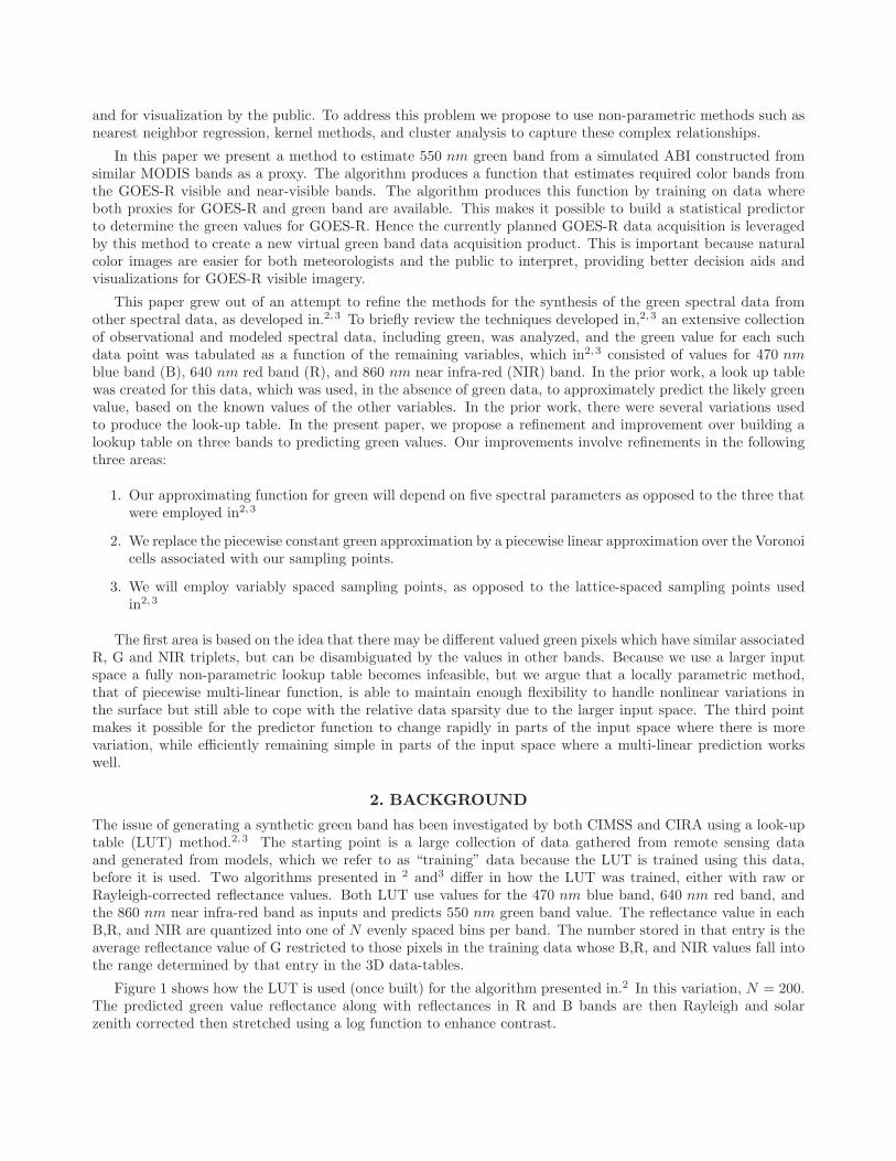
In this paper we present a preliminary algorithm implementing the approach outlined in the previous section. Toexplore how the algorithm is impacted by changing the number of Voronoi domains, we first set the per-granulenumber of clusters to N = 50 training using 40 training granules, resulting in 2, 000 clusters total. When theclusters were aggregated, very small clusters were eliminated. For illustrative purposes we picked a test granule(not part of the training granules) which illustrates smoke-over-vegetation case in the midwestern U.S., collectedby Terra MODIS on 28 June 2002 at 1640 UTC. The portions where the relative error (the absolute error dividedby original value) is over 15% are mapped in the figure 8. We can see in this figure that the largest errors occuron the boundaries. This is likely because on the boundaries, more Voronoi cells are needed in the partition inorder to handle pixels of mixed type. If we increase the per-granule number of initial clusters to N = 200 theresult improves dramatically, as seen in figure 9. Further increases in the number of clusters used in training donot seem to result in improvements in the testing, but perhaps increasing the number of training granules could.

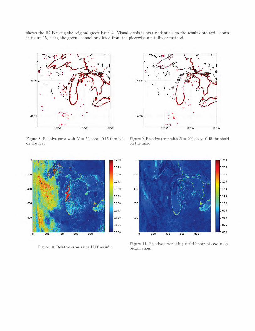
The results of partitioning into Voronoi cells, followed by the multi-linear regression appears to compare quitefavorably with results obtained by LUT.2 Figure 10 shows the relative error for the first variation of the LUTdescribed in section 2. When N = 200 is used in per-granule partitioning, the resulting relative error from thepiecewise multi-linear prediction is shown in figure 11. The error in the upper left portion and over the lake inthe middle improves dramatically. The reflectance values over the lake regions are relatively low. If we considerthe scatter plot of predicted band 4 value to actual band for value using the LUT method, as shown in figure 12,the errors over the lakes result in a wider spread in the lower left of the figure. The corresponding scatter usingthe piecewise multi-linear method has a smaller spread in the lower left, as shown in figure 13. The figure 14

shows the RGB using the original green band 4. Visually this is nearly identical to the result obtained, shownin figure 15, using the green channel predicted from the piecewise multi-linear method.

Figure 8. Relative error with N = 50 above 0.15 thresholdon the map.

Figure 9. Relative error with N = 200 above 0.15 thresholdon the map.

Figure 10. Relative error using LUT as in2 .Figure 11. Relative error using multi-linear piecewise ap-proximation.

Figure 12. Scatter plot of the LUT restored green band asin2 versus original green band.

Figure 13. Scatter plot of the piece wise approximation ver-sus original green band.

Figure 14. Natural color image using original 550 nmMODIS band.

Figure 15. Natural color using predicted green band.

5. CONCLUSION

We presented an approach to the problem of estimating a green band from GOES-R using piecewise multi-linearpredictor on five input bands to improve upon previous a LUT-based approach which uses a Red, Blue and singleNIR band. We show that there are two additional NIR bands which have comparable mutual information tothe NIR used previously to build the LUT. We outline a new approach which uses these extra bands to predicta green band. To overcome the explosion in LUT entries with increasing dimension due to more bands, we usea partition of the input space followed by a multi-linear regression. We have presented preliminary results thatshow that this approach can significantly reduce the error and produce a result that is visually indistinguishablefrom the true color RGB image with a green band. In future work we will make the partition adaptive to

further reduce the error by introducing more partitions in those regions where the error is highest. We willalso systematically compare with the multiple variations on the LUT approach. In addition, we will examinewhether by combining our method with the LUT approach which classifies by surface type, can further improvethe prediction of the green band.

REFERENCES

[1] Grossberg, M., Shahriar, F., Gladkova, I., Alabi, P., D. Hillger, D. and Miller, S., ”Estimating True ColorImagery for GOES-R,” Proc. SPIE 8048(50), (2011).

[2] Hillger, D., Grasso, L., Miller, S.D., Brummer, R., and DeMaria, R., ”Synthetic advanced baseline imagertrue-color imagery,” J. Appl. Remote Sens. 5, in press (2011).

[3] Miller, S.D., Schmidt, C., Schmit, T.J. and Hillger, D.W., ”A Case for Natural Color Imagery from Geosta-tionary Satellites and an Approximation for the GOES-R ABI,” Int. J. of Remote Sens., (in press) (2011)

[4] Schmit, T.J., Gunshor, M. M., Menzel, W. P., Li, J., Bachmeier, S., Gurka, J. J., ”Introducing the Next-generation Advanced Baseline Imager (ABI) on GOES-R,” Bull. Amer. Meteor. Soc., 8, 1079-1096 (2005)

[5] Grasso, L. D., Sengupta, M., Dostalek, J. F., Brummer, R. and DeMaria, M., ”Synthetic satellite imageryfor current and future environmental satellites,” Int. J. of Remote Sens., 29(15), 4373-4384 (2008)

[6] Gumley, L., Frey, R. and Moeller, C., ”Destriping of MODIS L1B 1KM Data for Collection 5 AtmosphereAlgorithms,” http://modis.gsfc.nasa.gov/sci team/meetings/200503/poster.php (2005)

[7] Cheng, J. S., Shao, Y., Guo, H. D., Wang, W. and Zhu, B., ”Destriping MODIS data by power filtering,”IEEE Trans. on Geoscience and Remote Sens., 49, 2119-2124 (2003).

[8] Rakwatin, P.,Takeuchi, W. and Yasuoka, Y., ”Restoration of Aqua MODIS Band 6 Using HistogramMatchingand Local Least Squares Fitting,” IEEE Trans. on Geoscience and Remote Sens., 47(2), 613-627 (2009).