VIOLATION OF RICHARDSON'S CRITERION VIA INTRODUCTION OF A MAGNETIC

FIELD

This article has been downloaded from IOPscience. Please scroll down to see the full text article.

2010 ApJ 712 1116

(http://iopscience.iop.org/0004-637X/712/2/1116)

Download details:

IP Address: 132.177.249.233

The article was downloaded on 11/03/2010 at 20:41

Please note that terms and conditions apply.

The Table of Contents and more related content is available

Home Search Collections Journals About Contact us My IOPscience

The Astrophysical Journal, 712:1116–1128, 2010 April 1 doi:10.1088/0004-637X/712/2/1116C© 2010. The American Astronomical Society. All rights reserved. Printed in the U.S.A.

VIOLATION OF RICHARDSON’S CRITERION VIA INTRODUCTION OF A MAGNETIC FIELD

Daniel Lecoanet1,5

, Ellen G. Zweibel2,5

, Richard H. D. Townsend3,5

, and Yi-Min Huang4,5,6

1 Department of Physics, University of Wisconsin, Madison, WI 53706, USA; lecoanet@wisc.edu2 Departments of Astronomy and Physics, University of Wisconsin, Madison, WI 53706, USA

3 Department of Astronomy, University of Wisconsin, Madison, WI 53706, USA4 Space Science Center, University of New Hampshire, Durham, NH 03824, USA

Received 2009 November 25; accepted 2010 February 9; published 2010 March 10

ABSTRACT

Shear flow instabilities can profoundly affect the diffusion of momentum in jets, stars, and disks. The Richardsoncriterion gives a sufficient condition for instability of a shear flow in a stratified medium. The velocity gradient V ′can only destabilize a stably stratified medium with squared Brunt–Vaisala frequency N 2 if V ′2/4 > N2. We findthis is no longer true when the medium is a magnetized plasma. We investigate the effect of stable stratification onthe magnetic field and velocity profiles unstable to magneto-shear instabilities, i.e., instabilities which require thepresence of both magnetic field and shear flow. We show that a family of profiles originally studied by Tatsuno &Dorland remains unstable even when V ′2/4 < N2, violating the Richardson criterion. However, not all magneticfields can result in a violation of the Richardson criterion. We consider a class of flows originally considered byKent, which are destabilized by a constant magnetic field, and show that they become stable when V ′2/4 < N2, aspredicted by the Richardson criterion. This suggests that magnetic free energy is required to violate the Richardsoncriterion. This work implies that the Richardson criterion cannot be used when evaluating the ideal stability of asheared, stably stratified, and magnetized plasma. We briefly discuss the implications for astrophysical systems.

Key words: hydrodynamics – instabilities – magnetohydrodynamics (MHD) – stars: magnetic field – stars: rotation

1. INTRODUCTION

Rotation plays an important role in the structure and evo-lution of stars. Although rotation directly modifies hydrostaticequilibrium only in the most rapid rotators, it drives large-scalecirculation, modifies the structure of convection and the natureof convective transport, and is a key component of magneticdynamos. These phenomena in turn modify the rotation througha complex interplay of nonlinear processes.

Shear flow instability is one of the mechanisms through whichrotation influences and is influenced by its environment. Themotion associated with the instability generates stresses, whichreact back on the flow and drive it toward a stable state. Ifthe amplitude of the unstable perturbations is sufficiently large,the motions become turbulent. Shear flow instability and shearflow turbulence can amplify magnetic fields and mix chemicalspecies, in addition to modifying the rotation profile itself.

In the case of the Sun, and possibly other low-mass main-sequence stars, the most likely venue for shear flow instabilityis the so-called tachocline, the region of strong shear justbelow the base of the convection zone (see Gough 2007,for a review). Although the mechanisms which maintain thetachocline are still uncertain, it is almost certainly a componentof the solar dynamo, and its existence has implications for theway the convection zone, which is spun down by the solarwind, is coupled to the radiative core. The tachocline may besubject to purely hydrodynamic instabilities (Rashid et al. 2008;Kitchatinov & Rudiger 2009), global magnetohydrodynamics(MHD) instabilities driven by the latitudinal structure of the field(Gilman & Fox 1997; Gilman et al. 2007) magnetorotationalinstabilities (Ogilvie 2007), and, if hydromagnetic forces arelarge enough, magnetic buoyancy instabilities (Silvers et al.

5 Center for Magnetic Self-Organization in Laboratory and AstrophysicalPlasmas.6 Center for Integrated Computation and Analysis of Reconnection andTurbulence.

2009; Vasil & Brummell 2009). All these instabilities couldmodify the tachocline’s structure.

Massive stars, which evolve quickly and tend to rotate rapidly,are potentially more profoundly affected by shear flow instabil-ity. The past two decades have witnessed significant advancesin understanding how the internal rotation of massive luminousstars shapes, and is shaped by, their evolution (see Maeder &Meynet 2000, and references therein for a comprehensive re-view). Rapidly rotating massive stars follow bluer, more lumi-nous evolutionary tracks in the Hertzsprung–Russell diagram(HRD) than non-rotating equivalents, because strong merid-ional circulation injects fresh hydrogen fuel into the convectivecore (see, e.g., Meynet & Maeder 2000). This rotational mix-ing brings CNO-cycle nucleosynthetic products from the stars’cores to their surfaces, leading to changes in photospheric abun-dance ratios (e.g., Talon et al. 1997).

The prevailing view of rotation in massive stars is basedon a canonical narrative developed by Zahn (1992). In thisscenario, turbulent diffusion of angular momentum is highlyanisotropic, with much stronger transport in the horizontaldirection than the radial one. This leads to a “shellular” rotationprofile, in which the angular velocity is constant on sphericalshells. The exchange of angular momentum between these shellsis then mediated by a combination of meridional circulation,convection (in convective zones), and radial turbulent diffusion.The turbulence itself is driven by secular shear instability(Maeder & Meynet 2000), which grows on a thermal timescale(see also Maeder 1995; Maeder & Meynet 1996; Talon & Zahn1997).

Recent studies have considered the role that magnetic fieldsmight play in modifying angular momentum transport (e.g.,Maeder & Meynet 2004). Generally, these studies of the impactof magnetic fields have focused around contributions to theradial angular momentum diffusivity arising from the fieldstiffness (Petrovic et al. 2005). However, as Spruit (1999) hasdiscussed, a field can also introduce new instabilities that play a

1116

No. 2, 2010 VIOLATION OF RICHARDSON’S CRITERION 1117

role in angular momentum transport. In this paper, we explorea hitherto-overlooked magnetic-mediated instability, wherebythe presence of a horizontal field can destabilize a stratifiedshear layer that—according to the Richardson criterion—wouldotherwise be stable.

The paper is organized as follows. First we will briefly discussshear flow instabilities in Section 2. In Section 3, we set upthe eigenvalue problem which determines the linear stabilityof an MHD shear flow in a stratified medium. We reviewprevious analytic results in Section 4, and describe our numericalmethods for solving the eigenvalue problem in Section 5.Starting in Section 6 we examine specific examples, first addingstratification to the linear velocity and parabolic magnetic fieldexample considered in a recent paper by Tatsuno & Dorland(2006, hereafter TD06). Our key result is that sufficiently strongparabolic magnetic fields can yield instability for arbitrarilystrong stratification, in violation of the Richardson criterion.We consider and extend a family of velocity profiles which Kent(1968, hereafter K68) showed can be destabilized by a constantmagnetic field in Section 7. In contrast to the parabolic magneticfield case, it seems that the introduction of a constant magneticfield cannot result in a violation of the Richardson criterion. Thissuggests that the free energy of an inhomogeneous magneticfield is essential to breaking the Richardson criterion. We discusspossible applications to rotating stars in Section 8 and concludein Section 9.

2. INTRODUCTION TO SHEAR FLOW INSTABILITIES

The best known shear flow instability is the hydrodynamicKelvin–Helmholtz instability. The Kelvin–Helmholtz instabilityhas been studied extensively. Perhaps the most famous result isthe inflexion point criterion, stating that a necessary conditionfor instability is the presence of an inflexion point in the velocityprofile (see, for example, Drazin & Reid 1981). Others havealso given necessary conditions for instability, making extraassumptions on the flow profile (Lin 1955; Howard 1961;Rosenbluth & Simon 1964).

Many have worked to extend parts of these results to MHDshear instabilities. It is well known that a sufficiently strongmagnetic field stabilizes the Kelvin–Helmholtz instability(Chandrasekhar 1961). It was shown years ago, but is perhapsless well known, that a magnetic field can destabilize an other-wise stable shear flow (K68). In particular, an inflexion point isno longer necessary for shear instability. In hydrodynamics vor-ticity is frozen into the flow, ensuring that perturbations are sta-ble when there is no inflexion point (Lin 1955), but the presenceof a magnetic field can break the vorticity frozen-in condition,relaxing the inflexion point criterion. K68 constructed a familyof flow profiles which are marginally stable in the absence ofa magnetic field and destabilized by a uniform field parallel tothe direction of flow. TD06 studied how a linear flow profile,which has no inflexion point and is marginally stable, can bedestabilized by a particular family of magnetic field profiles. Inparticular, TD06 find that a parabolic magnetic field can rendera linear velocity profile unstable.

In this paper, we add a new piece of physics to the analysis:density stratification. We employ the Boussinesq approximationand assume that the plasma is stably stratified, i.e., the squaredBrunt–Vaisala frequency, N 2, is positive. In hydrodynamics,the Richardson criterion provides a sufficient condition for thestability of a shear flow in a stratified medium (see, for example,Drazin & Reid 1981). The interchange of two fluid elementsat different heights can release kinetic energy from the flow.

A necessary condition for instability is that the gravitationalenergy required for the interchange must be less than the kineticenergy released. However, in the presence of an inhomogeneousmagnetic field, energy can also be extracted from the magneticfield, even if the field would be stable in the absence of shearflow. Our main result is that the Richardson criterion no longerholds for inhomogeneous magnetic fields.

We will only consider the effect of stable stratification onmagneto-shear instabilities. However, Tatsuno et al. (2003)studied how a shear flow can destabilize a homogeneousmagnetic field in the presence of an unstable density gradient.They found that a linear (Couette) velocity profile can bedestabilizing when the velocity shear was not too strong. Theirresult is similar to ours in the sense that the system is maximallydestabilized when the velocity gradient, magnetic field, anddensity stratification all have comparable strength.

In this paper, we consider only ideal instabilities, i.e., we setthe resistive, viscous, and thermal diffusivities to zero. Diffusiveeffects could unleash a host of additional instabilities such astearing modes (e.g., Furth et al. 1963), doubly diffusive modes(e.g., Schmitt & Rosner 1983), and secular shear instabilities(e.g., Maeder & Meynet 2000). Although such instabilities areimportant in their own right, in this paper we focus entirely ondynamical instabilities.

3. BASIC EQUATIONS

The time evolution of an ideal, incompressible plasma is givenby

ρ

(∂V∂t

+ V · ∇V)

= −∇(

p +B2

2μ0

)+

1

μ0B · ∇B − gρez,

(1)

∂B∂t

= ∇ × (V × B) , (2)

0 = ∇ · V, (3)

0 = ∇ · B, (4)

0 = ∂ρ

∂t+ V · ∇ρ, (5)

where the symbols have their usual meanings. Equation (1) isthe momentum equation, Equation (2) is the induction equation,Equation (3) enforces incompressibility, Equation (4) is thedivergenceless magnetic field condition, and Equation (5) is thecontinuity equation. We will write the unit vectors in the x, y,and z directions as ex , ey , and ez, respectively. The gravitationalstrength is parameterized by g, and gravity is assumed to point inthe −ez direction. We denote background velocity and magneticfields with capital letters, and then perturb the backgroundfields with fields denoted with lower case letters, except thatthe background density is denoted by ρ, and the perturbeddensity by ρ. We assume that the background quantities ρ,V, and B all are the functions of only z, and that our domainis the volume between z = −z0 and z = +z0 with “free-slip,”perfectly conducting boundary conditions in the z direction,and periodic boundary conditions in the x and y directions. By“free-slip,” we mean no constraint on perturbed quantities in thex and y directions at the walls, but that perturbations have noz component at the walls. These are the boundary conditionsadopted by TD06 (who termed them “no-slip” which is notcorrect—as will be shown in Section 6.3, the perturbations slip

1118 LECOANET ET AL. Vol. 712

along, but do not penetrate, the walls). Next, we assume thatV is oriented toward only one direction throughout the domain,which we define to be the x direction. Thus, we take

V = (V (z), 0, 0), (6)

in Cartesian coordinates. The background magnetic field B is

B = (Bx(z), By(z), 0) (7)

in Cartesian coordinates. The background fields are assumed tobe in equilibrium, so we have that

∇(

p +B2

2μ0

)+ gρez = 0. (8)

Equation (8) specifies an integral equation for the backgroundpressure p for arbitrary B and ρ. The induction and continuityequations for the background fields are automatically satisfiedby the geometry we have imposed.

Now assume the perturbation fields all have the form

f (x, y, z, t) = f (z) exp(ikxx + ikyy − ikxct). (9)

We will take k ≡ kxex + kyey , k = |k| and k = k/k. In manyapplications, the density gradient ρ ′ is small in comparison tothe velocity gradient V ′—where prime denotes differentiationwith respect to z—but the strength of gravity g is large.Assuming this, we recover the Boussinesq approximation, inwhich we drop terms proportional to ρ ′ alone, but keep termsproportional to gρ ′. These assumptions yield the followingeigenvalue problem for ξ , the plasma displacement in the zdirection:([

k2x (V − c)2 − k2A2

]ξ ′)′

− k2[k2x (V − c)2 − k2A2

]ξ + k2N2ξ = 0, (10)

where A ≡ k ·B/√

ρμ0 is the Alfven velocity, and N2 ≡ gρ ′/ρis the Brunt–Vaisala frequency in the Boussinesq approxima-tion. To simplify our analysis, we assume that N 2 is constantthroughout the domain, which corresponds to the exponentiallydecaying density profile. When computing the Alfven velocity,the Boussinesq approximation will allow us to consider ρ tobe a constant. The boundary conditions are that ξ = 0 at theboundaries at z = −z0 and z = +z0.

There is an asymmetry in how velocity shear, magnetic fields,and density stratification depend on the wavenumber k. Fork = kyey , kx = 0 and the velocity shear is irrelevant (note thatkxc, the growth rate, could still be finite). The purpose of thispaper is to examine the interplay between velocity and magneticfields, so we will not consider this case. Also note that the Alfvenvelocity, as it occurs in Equation (10), is a function of k. Forexample, if B is constant in the z direction, there exists a k forwhich A = 0, so the magnetic field would have no effect onsuch a perturbation. The strength of gravity in relation to shearflow contains a factor of k2/k2

x . Thus, gravity is maximallydestabilized by shear flows when ky = 0.

Consider an eigenvalue problem for the magnetic field B,velocity V, Brunt–Vaisala frequency N 2, and wavenumberk = kxex +kyey , with ky �= 0. We will show that this eigenvalueproblem is equivalent to another eigenvalue problem withky = 0, but with different B, N 2, and kx. Define B′ ≡ exk ·B/kx ,N ′2 ≡ k2N2/k2

x , and k′ ≡ kex . Then the magnetic field B′,

velocity V, Brunt–Vaisala frequency N ′2, and wavenumber k′have the same eigenvalue equation as above. Thus, finite ky isequivalent to ky = 0, if one appropriately rotates and augmentsthe magnetic field, and increases the density stratification. Withthis in mind, we will consider the ky = 0 case in the remainderof this paper, for which the eigenvalue equation reduces to([

(V − c)2 − A2]ξ ′)′ − k2

[(V − c)2 − A2

]ξ + N2ξ = 0.

(11)The eigenvalue Equation (11) possesses some symmetries.

First, the sign of A is unimportant, so changing the sign of themagnetic field does not change the problem. Another symmetryis translational: taking V → V + ΔV and c → c − ΔVcorresponds to Galilean transformations. Thus, without lossof generality, we can and do put ourselves in a frame inwhich V (0) = 0. To make the problem more tractable, weadd additional symmetries to the equation by postulating thatA is even in z and V is odd. There is a rescaling symmetry:Equation (11) remains invariant under

z → z/z0,

V → V/z0,

A → A/z0, (12)

k → kz0,

c → c/z0.

Note that N 2 and Ri are left unchanged under this transforma-tion.

There is also structure in the eigenvalues. In general, c andξ are complex: c = cr + ici , ξ = ξr + iξi . We ignore thesingular ci = 0 case. If ξc is an eigenfunction with eigenvaluec, then ξ ∗

c , the complex conjugate of ξc, is a solution toEquation (11) with eigenvalue c∗. Thus, eigenvalues come incomplex conjugate pairs, regardless of the symmetry propertiesof A and V. Assuming that A is even and V is odd, we can showthat if c is an eigenvalue, then −c is also an eigenvalue, witheigenfunction ξc(−z).

Numerically, we only find eigenvalues with cr = 0 andwith the following eigenfunction symmetry. If we normalizethe eigenfunction ξ such that ξ (0) = 1, then ξr is even and ξi

is odd. In Sections 6 and 7, we assume that cr = 0, and theeigenfunction has this symmetry. These properties are linked. Ifwe multiply Equation (11) by ξ ∗ and integrate over the domainthe result is∫ z0

−z0

[(V − c)2 − A2

] (∣∣∣∣dξ

dz

∣∣∣∣2

+ k2 |ξ |2)

− N2|ξ |2dz = 0.

(13)The imaginary part of Equation (13) is

2ici

∫ z0

−z0

(cr − V )

(∣∣∣∣dξ

dz

∣∣∣∣2

+ k2 |ξ |2)

dz = 0. (14)

If the real and imaginary parts of ξ each have definite parity,the term proportional to V in Equation (14) vanishes. Therefore,crci ≡ 0, and unstable modes have cr = 0. This result is usefulin searching for unstable modes, as described in Section 5.

We find that generally the growth rate c = ici is small incomparison to V, which is O(1). When V 2 = A2, the coefficientof the ξ ′′ term in Equation (11) goes to | − c2

i | 1. Thus, theequation becomes “almost singular” when |V | = |A|, and be-comes actually singular when c = 0. The “almost singularities”

No. 2, 2010 VIOLATION OF RICHARDSON’S CRITERION 1119

are characterized by large gradients in the eigenfunctions, as isshown in Sections 6 and 7.

We will often consider the limit k2 = 0. When k2 = 0, thegrowth rate, kc, is formally zero. However, one can view theeigenvalue c as a function of the various parameters A,V, k2,and N 2. We assume that c(k2) is analytic about k2 = 0, so ourresults for the k2 = 0 case still hold in a neighborhood of k2 = 0.Thus, when we consider k2 = 0, we are really taking the limit ask becomes small. The k2 term in Equation (11) is only importantwhen it is comparable to the scale heights of the velocity andmagnetic fields and the perturbation ξ . Numerically, we findthat kz0 < 0.1 is “small” for the examples presented in thispaper.

4. REVIEW OF ANALYTIC RESULTS

Shear flow instabilities are global instabilities. Thus, thetwo categories of analytic results—necessary conditions forinstability and sufficient conditions for instability—can beviewed as local and global conditions. Necessary conditionsfor instability give criteria which must be satisfied in at leastone spot in the domain, whereas the sufficient conditions forinstability are global criteria involving integrals over the domain.We present a short overview of the analytic results regarding thelinear stability of shear flows. We begin by discussing shearflows alone, and then add stratification, a magnetic field, andthen both. The zero magnetic field and zero density gradientcases can be viewed as limits of the more general problem.

4.1. Shear Flow Instabilities

Probably the best known result is the inflexion point criterion,which states that V ′′ must have a zero in the domain for thereto be instability. This is a local, necessary condition. There areseveral physical interpretations of the inflexion point criterion.Consider the Reynolds stress of the perturbation, τ = −ρvxvz,where the bar denotes averaging with respect to x. Assumingc �= 0, one can show that dτ/dz has a zero iff V ′′ has a zero (forinstance, in Lin 1955, or K68). Since τ = 0 at the boundaries,when c �= 0, we must have that V ′′ has a zero. Lin (1955)has proposed an alternate interpretation considering vorticity. Azero in V ′′ corresponds to an extremum in vorticity, and Lin hasshown that perturbations feel a restoring force unless they areat an extremum of vorticity.

The inflexion point theorem is useful because it rules out alarge class of velocity profiles as stable. However, it cannot beused to show that a particular shear flow is unstable. Rosenbluth& Simon (1964) were able to prove a necessary and sufficientcondition for instability by using the additional assumptionsthat V ′′ has a single zero and V is monotonic. Under theseassumptions, V is unstable in z1 � z � z2 if and only if

1

V ′(Vc − V )

∣∣∣∣z2

z1

−∫ z2

z1

V ′′

V ′3(V − Vc)dz > 0, (15)

where Vc is the velocity at the inflexion point. This result isderived for the k2 = 0 case. A priori, it seems that there couldbe velocity profiles which are unstable for k2 > 0 but stable fork2 = 0. Then an instability condition for k2 = 0 would be onlysufficient for instability. This is addressed by a theorem of Lin(1955) which shows that under the assumptions of Rosenbluth& Simon, velocity profiles which are unstable for k2 > 0 arealso unstable for k2 = 0.

4.2. Shear Flow Instabilities in a Stratified Medium

The key stability result for stratified media is the Richardsoncriterion, a necessary condition for the instability of a shear flowin a stratified medium. If

Ri ≡ N2

V ′2 >1

4(16)

everywhere, then there is stability. A physical interpretation(see, for example, Chandrasekhar 1961 or Drazin & Reid 1981)is that if exchanging fluid elements at slightly different heightsincreases the potential energy more than it decreases the kineticenergy, then the perturbation is stable.

Provided that Ri < 1/4, we have that

k2c2i � max

(1

4V ′2 − N2

). (17)

This result by Howard (1961) follows from the proof of theRichardson criterion and is also discussed in Drazin & Reid(1981).

4.3. Magneto-shear Instabilities

Magnetic fields can both stabilize and destabilize shear flows.First, we consider their stabilizing effect. Perturbations whichbend magnetic field lines induce a restoring magnetic tensionforce. A classic result is that in a constant density medium, thevortex sheet V (z) = −U for z < 0 and V (z) = +U for z > 0for some constant U, is stabilized by a magnetic field A if andonly if A2 > V 2 (Chandrasekhar 1961). This step function ve-locity profile is the limiting distribution of V (z) = U0 tanh(z/a)as a → 0. Keppens et al. (1999) have investigated the hyper-bolic tangent V case with a constant magnetic field, includingcompressibility, and found the magnetic field stabilizing. Theseresults were qualitatively similar to those by Chandrasekhar,which is expected because a constant magnetic field has nolength scale (or it has an infinite length scale), so it cannot tellthe difference between the a → 0 and a finite case.

Keppens et al. also found that the addition of a non-uniformmagnetic field could be destabilizing. When they added a smallfield A(z) = −A0 for z < 0 and A(z) = A0 for z > 0,they found that the growth rate increased, and was even largerwhen A reversed smoothly. Although their calculation, unlikeours, includes compressibility, there is one robust effect whichis always present: magnetic fields allow transfer of vorticitybetween fluid elements. The loss of the frozen-in vorticityconstraint changes the range of motions allowed in the plasma,and yielding instability.

We now review some general results on magneto-shearinstabilities in order to understand how the Richardson criterioncan be violated by the introduction of a magnetic field.

The necessary and sufficient instability condition of Rosen-bluth & Simon (1964; Equation (15)) has been generalized tothe MHD case by K68 and Chen & Morrison (1991). Both ar-guments use that when k2 = 0, there is an exact solution toEquation (11),

ξ (z) =∫ z

z1

dz′

(V − c)2 − A2, (18)

and then define

f (c) ≡∫ z2

z1

dz

(V − c)2 − A2= ξ (z2). (19)

1120 LECOANET ET AL. Vol. 712

The eigenvalues of Equation (11) are then just the zeros of f (c),and one can search for instabilities by implementing Nyquist’smethod to determine if there are any zeros of f (c) for ci > 0.Nyquist’s method is an application of the argument principle(see, for instance, Gamelin 2001), which states that the integralof the argument of f (c) on the boundary ∂D of some region Dis equal to 2π (N0 − N∞), where N0 is the number of zeros off (c) in D, and N∞ is the number of poles of f (c) in D. In ourcase, we assume N∞ = 0, so counting the number of times f (c)wraps around the origin tells us how many zeros, i.e., unstablemodes, there are. Further discussion of Nyquist’s method canbe found in Krall & Trivelpiece (1973).

Nyquist’s method can only be applied if we know whatcontour to use. The real part of c can be bounded by extendingan important hydrodynamic result by Rayleigh. It can be shown(Hughes & Tobias 2001) that cr must lie in the range of V, so thecontour in c space is bounded by Vmin < cr < Vmax. The lowerbound for ci is 0+, and the upper bound can be recovered bymodifying Howard’s semicircle theorem (Howard 1961). In thehydrodynamic case, Howard showed (see, for instance, Drazin& Reid 1981) that

[cr − 1

2 (Vmax + Vmin)]2

+ c2i �

[12 (Vmax − Vmin)

]2. (20)

Thus, we have that ci � 1/2(Vmax − Vmin). Hughes & Tobias(2001) have shown that in MHD, we have the two inequalities

(V 2 − A2)min � c2r + c2

i � (V 2 − A2)max, (21)

and[cr − 1

2 (Vmax + Vmin)]2

+ c2i �

[12 (Vmax − Vmin)

]2 − (A2

)min .

(22)

This gives an even stronger upper bound on ci, that

ci �√

(1/2(Vmax − Vmin))2 − (A2)min. (23)

These two inequalities can be used to show stability, if onecan show that there are no c which simultaneously satisfy bothinequalities.

Chen & Morrison (1991) used Nyquist’s method to provide asufficient condition for instability for flows in which V is even,and A is either odd or even. They showed that

�∫ z0

−z0

dz

(V − iε)2 − A2> 0 (24)

as ε → 0 is sufficient for instability. Note that it is not assumedthat V has an inflexion point.

K68 considered the effects of a small, constant magnetic fieldon a stable velocity profile. He showed that when V ′′ has a singlezero, and there exist points ys, yt such that the velocities at thesepoints, Vs, Vt satisfy Vs − Vt = 2A and V ′

s − V ′t = 0, then

M(A) ≡ ℘

∫ z2

z1

dz

(V − c0)2 − A2> 0, (25)

implies instability. Here, c0 is defined by c0 = (Vs +Vt )/2, and ℘denotes the principal value of the integral. For small A, c0 is thevelocity at the inflexion point, but as A increases, it can deviatesomewhat. For a marginally stable velocity profile, we haveM(0) = 0. In the remainder of this section, we will use ˙ (dot)

to denote derivative with respect to A. In the limit A → 0, wehave M(A) → 0. Thus, to evaluate the stability of V to infinitelysmall A, we need to consider M(0), which Kent shows is givenby

M(0) = 2cr (0)∫ z2

z1

dz

(V − C0)3+ 2

∫ z2

z1

dz

(V − C0)4, (26)

where

cr (0) = − C(4)0

3C0C(3)0

. (27)

This criterion is useful because one can change variables tointegrate over V, and if C0 = 0 and ω(V ) := dz/dV is even,then

M(0) =∫ V2

V1

ωdV

V 4, (28)

where Vi = V (zi). Although these conditions are sufficient forinstability, they are not necessary. Unlike in the hydrodynamiccase, there can be unstable modes for finite k2 for a velocityprofile which is stable at k2 = 0 (K68).

Another way to tackle the general problem with arbitraryvelocity and magnetic field profiles is to attempt to extend thephysical arguments behind the inflexion point criterion to theMHD problem. In the MHD problem, one must consider boththe Reynolds and Maxwell stresses, so the total stress is givenby

τtot = −ρvxvz + bxbz. (29)

A necessary condition for instability is still dτtot/dz = 0somewhere in the flow. K68 has shown that this condition canbe written as

�[|X|X

′

X

]′= 0, (30)

or

�[

2XX′′ − X′2

4X2

]= 0, (31)

where X ≡ (V − c)2 − A2. Unfortunately, these (equivalent)conditions are not as useful as the inflexion point criterionbecause they depend on both the flow profile and the growth rate.Thus, one needs to check Equations (30) or (31) for all possible c.This condition seems to be fairly weak, and is satisfied by manystable profiles.

4.4. Magneto-shear Instabilities in a Stratified Medium

The addition of a magnetic field to a shear flow in a stratifiedmedium makes the problem significantly more complex. TheRichardson criterion is no longer valid, but it can be generalized.We have carried out the same analysis used to derive theRichardson criterion, but included magnetic fields. The result isthat if

0 >1

ci

�(

2ZZ′′ − Z′2

4Z2+

V ′Z′

Z+

V ′24 − N2

Z

(V − c)

)(32)

everywhere in the domain, then the system is stable. Here,Z ≡ 1 − A2/(V − c)2. Similar to the generalization of theinflexion point criterion (Equations (30) and (31)), this conditioninvolves c. This condition also seems to be weak.

Although we normally assume that cr = 0, this condition canbe relaxed, and we can find bounds for cr. The argument by

No. 2, 2010 VIOLATION OF RICHARDSON’S CRITERION 1121

Hughes & Tobias (2001) mentioned in Section 4.3 still holdswhen stratification is introduced and shows that cr must liewithin the range of V. This bound on cr is valid with and withoutmagnetic field, and with and without stratification.

5. NUMERICAL METHODS

Because the problem is global, analytic results exist only incases with particular symmetries (i.e., k2 = 0 or N2 = 0),so we must generally solve for stability numerically. Wehave implemented three numerical methods for solving theeigenvalue problem, Equation (11). In the first, we discretize theequation onto a Chebyshev grid, and use a finite-dimensionalapproximation for the differential operator. Then Equation (11)can be rewritten as a generalized finite-dimensional eigenvalueequation:

γ

(D 0 00 1 00 0 1

) (vz

bz

ρ

)

=⎛⎝−ikxVD + ikxV

′′ ikAD − ikA′′ −N2k2

ikA −ikxV 01 0 −ikxV

⎞⎠

(vz

bz

ρ

),

(33)where D ≡ ∂2

z − k2. Matlab was used to solve this finite-dimensional eigenvalue problem. This approach was usefulwhen we did not require high resolution. This method was notable to resolve the large gradients in the eigenfunctions thatsometimes appeared when |V | = |A|.

Another strategy, for k = 0, was implementing Nyquist’smethod. We used Mathematica to calculate f (c), as defined inEquation (19) for various c. As mentioned in Section 4.4, weknow that cr lies between the minimum and maximum of V. Theadvantage of Nyquist’s method is that we need not assume that cis imaginary. We picked the rectangle with vertices at iε + Vmax,iε + Vmin, ia + Vmin, and ia + Vmax as the contour, with a oforder 1 and ε small. If one plots f (c), where c traverses thiscontour, it is easy to see if there are any unstable modes withc in this contour. We varied the size of the rectangular contourto find the exact eigenvalues. For the examples presented belowin Sections 6 and 7, eigenvalues were always purely imaginary,and the eigenfunctions had the symmetry properties describedin Section 3.

Finally, we used a finite difference relaxation code to integrateacross the domain. We assumed that c was imaginary, andintegrated Equation (11) over the domain for c between iε andia for a of order 1 and ε small, in logarithmic steps. When thereal part of f (c) changed sign between two consecutive steps,the secant method was used to find the zero in the real part off (c), which corresponds to a zero in f (c). This algorithm wasthe most efficient, but makes the assumption that the eigenvaluesare purely imaginary. As mentioned in Section 3, we have notfound any eigenvalues with non-vanishing real part using theother two methods mentioned above, so this seems to be a validassumption.

All three numerical methods give similar results in caseswhere we used more than one.

6. LINEAR V, PARABOLIC A

In this section, we add density stratification to the linearvelocity and parabolic magnetic field profiles considered byTD06. The main result is that we find instability even whenV ′2/4 < N2 everywhere, i.e., when the Richardson criterion

predicts stability. We believe this is because the magneticfield provides another free energy source for the instability.At k2 = 0, there are magnetic field profiles which are unstablefor arbitrarily large N 2, but when k2 > 0, there is only a finiterange of N 2 which are unstable for the profiles considered here.

6.1. The Field and Flow Profiles

Consider the following velocity and magnetic field profiles ina domain from z = −1 to z = +1:

V (z) = z, (34)

A(z) = (1 − α)z2 + α. (35)

These are the fields considered in Section III.A.1 of TD06(where we call their α1 parameter α). The magnetic field isa parabola with A(0) = α and A = 1 at the boundaries.

An important characteristic of these profiles is that neitherthe magnetic field nor the velocity profile are unstable bythemselves. The instability is truly a magneto-shear instability,as both magnetic field and shear flow play a part in renderingthe profiles unstable. In this respect, this example is differentfrom those considered by others in which a magnetic instabilityis stabilized by gravity (Dikpati et al. 2009), a magnetic layerdestabilizes a stratified medium (Newcomb 1961), or magneticfield and shear flow modify a buoyancy instability (Howes et al.2001).

These profiles can be viewed as local approximations to awide range of field and flow profiles. The parabolic magneticfield profile is valid locally whenever B has an extremum, whichwe take to be at z = 0. As mentioned in Section 3, takingA → −A does not change the problem, so although we areconsidering a local minimum, the exact same results hold forA(z) = −(1 − α)z2 − α, which characterizes a local maximum.We can always transform to a frame in which V (0) = 0, so thevelocity has a local expansion of the form of Equation (34).

To view these profiles as a local approximation, we also needto make an assumption about the relative strength and scaleof variation of the magnetic field and the shear flow, since werequire that |V | = |A| at the boundary. When α is close to zero,the magnetic field and velocity are changing at similar rates, sothe locality assumption is plausible. But when α is close to 1 orvery negative, the scale heights of the flow and magnetic fieldare very different, so viewing these profiles as a local expansionis not as accurate.

Depending on the sign of α, the magnetic field has either twoor zero nulls. When α < 0, A = 0 at

z = ±√

α

α − 1. (36)

When α > 0, there are no nulls in the magnetic field, and whenα = 0, there is a single null at z = 0. We find that the nullsin the magnetic field are unimportant in this problem—rather,zeros of V 2 − A2 are important. The eigenfunctions discussedbelow (see Section 6.3) show no special behavior at A = 0, buthave sharp gradients when |A| = |V |. In terms of α, |V | = |A|at

z = ± 1, (37)

z = ± α

1 − α. (38)

1122 LECOANET ET AL. Vol. 712

When α > 0.5, the solutions in Equation (38) are no longer in thedomain. This means that V � A in the entire domain, yieldingstability by Equation (24). Heuristically, when α becomes morepositive, the strength of the magnetic field in the domainincreases until the magnetic tension force becomes so strongthat all perturbations become stable.

In the opposite limit, when α becomes very negative, thesolutions in Equation (38) approach z = ±1. For arbitrarilynegative α, there is still some region for which V > A. Tatsuno& Dorland find instability for α as small as −25, and we canprove that there is instability for all α < 0.5 when k2 = 0using the sufficient condition for instability by Chen & Morrisondescribed in Section 4. The explicit computation is messy, butis included in the Appendix.

The limit in which α → −∞ is probably not physicallyrelevant. As the two “almost singular” layers approach eachother (see Equations (37) and (38)), there are large gradients atthe boundary of the domain. In this case, the instability probablyrelies crucially on our choice of boundary conditions. Moreover,when stratification is included, the high field strengths andlarge currents corresponding to |α| 1 are destabilizing inthemselves, in contrast to what we assume here. Thus, resultsin this limit should be viewed as proving a point about theRichardson criterion, but are not necessarily physically relevantby themselves. As we show in explicit calculations presentedbelow, α does not need to be very negative to recover the resultsdescribed in the infinitely negative case.

6.2. Effect of Stratification on Stability

Our main result is evidence for the following conjecture.There is instability as α → −∞, even in the presence of arbi-trarily strong density stratification, in violation of the Richard-son criterion. There does not seem to be any way to prove thisclaim analytically, as there was in the N2 = 0 case. The suf-ficient condition for stability presented by Chen & Morrison(1991) relies crucially on the analytic solution to the eigenvalueequation when k2 = 0. When N2 �= 0, we no longer have ananalytic solution to the eigenvalue equation, even when k2 = 0,so there is no extension of the proof.

Given the assumptions made above, the growth rate c is afunction of the following parameters: k 2, N 2, and α. We firstspecialize to the k2 = 0 case, and then examine the more generalk2 finite case.

6.2.1. k2 = 0

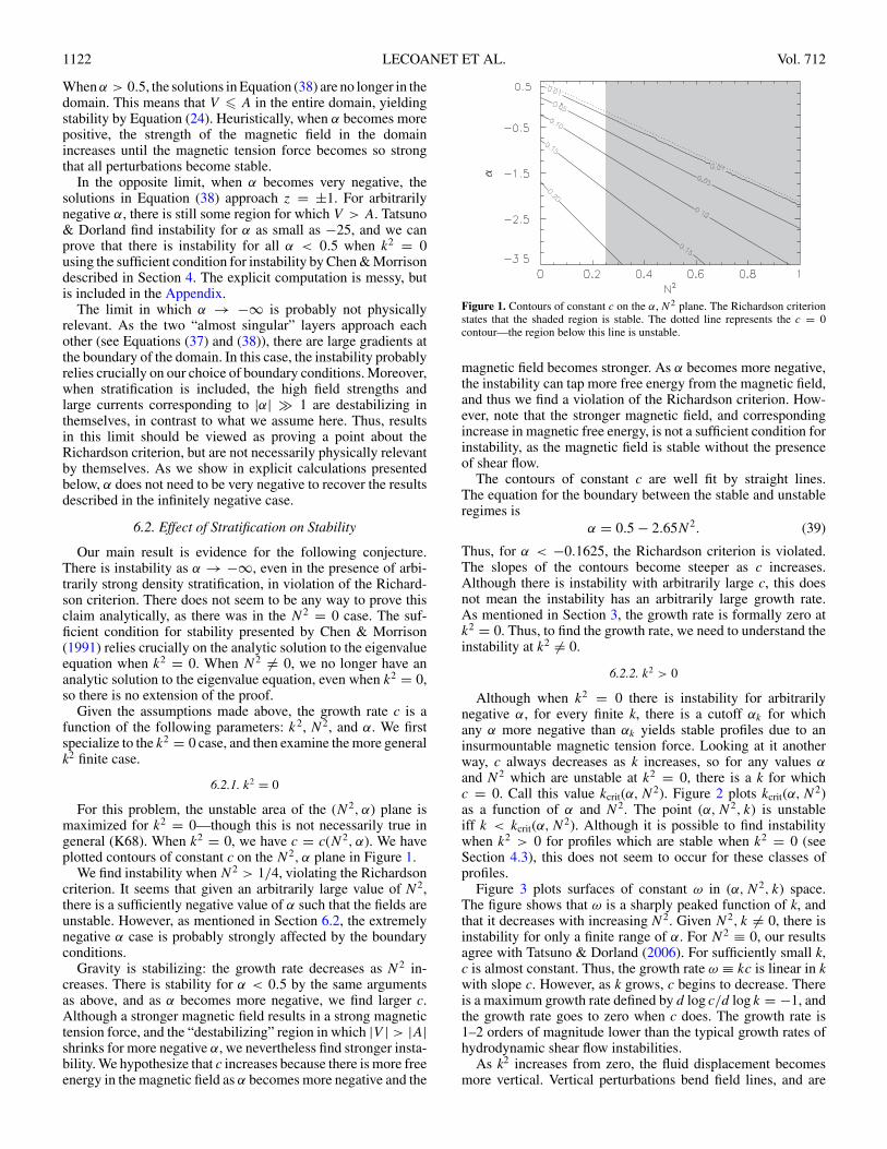
For this problem, the unstable area of the (N2, α) plane ismaximized for k2 = 0—though this is not necessarily true ingeneral (K68). When k2 = 0, we have c = c(N2, α). We haveplotted contours of constant c on the N2, α plane in Figure 1.

We find instability when N2 > 1/4, violating the Richardsoncriterion. It seems that given an arbitrarily large value of N 2,there is a sufficiently negative value of α such that the fields areunstable. However, as mentioned in Section 6.2, the extremelynegative α case is probably strongly affected by the boundaryconditions.

Gravity is stabilizing: the growth rate decreases as N 2 in-creases. There is stability for α < 0.5 by the same argumentsas above, and as α becomes more negative, we find larger c.Although a stronger magnetic field results in a strong magnetictension force, and the “destabilizing” region in which |V | > |A|shrinks for more negative α, we nevertheless find stronger insta-bility. We hypothesize that c increases because there is more freeenergy in the magnetic field as α becomes more negative and the

Figure 1. Contours of constant c on the α, N 2 plane. The Richardson criterionstates that the shaded region is stable. The dotted line represents the c = 0contour—the region below this line is unstable.

magnetic field becomes stronger. As α becomes more negative,the instability can tap more free energy from the magnetic field,and thus we find a violation of the Richardson criterion. How-ever, note that the stronger magnetic field, and correspondingincrease in magnetic free energy, is not a sufficient condition forinstability, as the magnetic field is stable without the presenceof shear flow.

The contours of constant c are well fit by straight lines.The equation for the boundary between the stable and unstableregimes is

α = 0.5 − 2.65N2. (39)

Thus, for α < −0.1625, the Richardson criterion is violated.The slopes of the contours become steeper as c increases.Although there is instability with arbitrarily large c, this doesnot mean the instability has an arbitrarily large growth rate.As mentioned in Section 3, the growth rate is formally zero atk2 = 0. Thus, to find the growth rate, we need to understand theinstability at k2 �= 0.

6.2.2. k2 > 0

Although when k2 = 0 there is instability for arbitrarilynegative α, for every finite k, there is a cutoff αk for whichany α more negative than αk yields stable profiles due to aninsurmountable magnetic tension force. Looking at it anotherway, c always decreases as k increases, so for any values αand N 2 which are unstable at k2 = 0, there is a k for whichc = 0. Call this value kcrit(α,N2). Figure 2 plots kcrit(α,N2)as a function of α and N 2. The point (α,N2, k) is unstableiff k < kcrit(α,N2). Although it is possible to find instabilitywhen k2 > 0 for profiles which are stable when k2 = 0 (seeSection 4.3), this does not seem to occur for these classes ofprofiles.

Figure 3 plots surfaces of constant ω in (α,N2, k) space.The figure shows that ω is a sharply peaked function of k, andthat it decreases with increasing N 2. Given N2, k �= 0, there isinstability for only a finite range of α. For N2 ≡ 0, our resultsagree with Tatsuno & Dorland (2006). For sufficiently small k,c is almost constant. Thus, the growth rate ω ≡ kc is linear in kwith slope c. However, as k grows, c begins to decrease. Thereis a maximum growth rate defined by d log c/d log k = −1, andthe growth rate goes to zero when c does. The growth rate is1–2 orders of magnitude lower than the typical growth rates ofhydrodynamic shear flow instabilities.

As k2 increases from zero, the fluid displacement becomesmore vertical. Vertical perturbations bend field lines, and are

No. 2, 2010 VIOLATION OF RICHARDSON’S CRITERION 1123

Figure 2. Largest k, denoted kcrit, for each α and N 2 which is unstable. Thewhite area is stable.

subject to a restoring magnetic tension force. Thus, it makessense that the most unstable modes are the horizontal modescharacterized by k2 = 0. For some applications, such as stellarinteriors (see Section 8), it is important to consider the verticaltransport (of angular momentum, etc.) by these modes. In thiscase, the k2 = 0 mode is irrelevant. One must then consider anoptimization problem in which modes with too low k2 have novertical transport effects, whereas modes with too high k2 arestable. This argument is only valid assuming that the nonlinearevolution is similar over a broad range of k2. A full nonlinearsimulation for various k2 is necessary in order to understand thetransport properties of these instabilities.

6.3. Eigenfunctions

We normalize the eigenfunctions as described in Section 3.The eigenfunctions all look like the example plotted in Figure 4.The most salient features are the sharp gradients at z = ±.47,where |V | = |A|. Note that the nulls in the magnetic field ata = ±.69 produce no special features.

7. CONSTANT A WITH VELOCITY PROFILESSUGGESTED BY KENT

In Section 4.3, we summarized Kent’s discussion (K68) ofvelocity profiles which are marginally stable in the absence ofa magnetic field and destabilized by a small, constant field. Inthis section, we generalize Kent’s construction and investigatethe stability of the resulting family of Kent flows.

The velocity profile is most conveniently specified by theinverse relation z = z(V ). Note that only invertible velocity

Figure 3. Surfaces of constant growth rate ω in (α,N2, k) space. The maximumω in this range of (α,N2, k) is given also.

profiles, i.e., dV/dz �= 0, can be specified by this inverserelation. When k2 = 0 and N2 = 0, we can use the in-stability condition by Chen & Morrison (1991) and evaluatethe integral in Equation (24) in closed form. This provides atranscendental equation for the growth rate. From solving thisequation numerically, it seems that there exist velocity pro-files which are (marginally) stable at A0 = 0, but unstable for0 < A0 < |V |max. When we increase N 2 from zero, we alwaysfind stability when N2 � (max V ′)2/4, but can find instabilityfor all N 2 up to this limit. Our interpretation of this result isthat the positive energy required to perturb a constant magneticfield triumphs over the extra freedom granted by magneticallybreaking the frozen-in vorticity constraint.

7.1. N2 = 0

First we consider various velocity profiles defined by z =z(V ) at k2 = 0. Define

ω(V ) ≡ dz

dV. (40)

We restrict ourselves to velocity profiles which are marginallystable at A = 0, as they seem to be maximally destabilizedby magnetic fields. We will first consider velocity profileswith walls at z = ±z0, with the condition that V (±z0) =±1. This will simplify the algebra when deriving analyticstability results. We will then employ the rescaling symmetry

Figure 4. Vertical displacement ξ (left panel) and horizontal displacement ξx = −iξ ′/k (right panel), where prime denotes differentiation with respect to z,eigenfunctions for α = −0.9, N2 = 0.3, and k = 0.2. The thick solid lines are the real part of the eigenfunctions, and the thick dashed lines are the imaginary part ofthe eigenfunctions. The thin vertical dotted lines are at z = ±.47 where |V | = |A| and the thin vertical dot-dashed lines are at z = ±.69, where A = 0.

1124 LECOANET ET AL. Vol. 712

described in Equation (12) to present numerical results usingthe normalization z0 = 1.

The condition for marginal stability (Kent 1968) is

∫ 1

−1

ω(V )dV

V= 0, (41)

where we have assumed that V ranges from −1 to +1 in thedomain. Assuming

z = V + a3V3 + a5V

5 + · · · , (42)

we haveω = 1 + 3a3V

2 + 5a5V4 + · · · , (43)

so the marginal stability condition on the aj’s is

∑j�3,odd

jaj

j − 2= 1. (44)

Our construction is a generalization of K68, who truncated theseries in Equation (42) at three terms. Next we assume that thereis only one inflexion point at z = 0. This condition impliesthat ω cannot have any extrema, so none of the aj are negative.Numerical work suggests that the results discussed here hold forvelocity profiles with multiple inflexion points, so by assumingonly one inflexion point, we make the problem much easier, butdo not qualitatively change the results.

Now we add a constant magnetic field. When k2 = 0, wehave that ∫ z0

−z0

dz

(V − c)2 − A20

= 0 (45)

implies instability with growth rate c. If we change variables toV, we find ∫ 1

−1

ω(V )dV

(V − c)2 − A20

= 0, (46)

where ω(V ) is defined as in Equation (40). We can rewrite theintegral in Equation (46) as

∫ 1

−1

1

2A0ω(V )dV

(1

V − c − A0− 1

V − c + A0

)= 0. (47)

The two integrals have equal real parts, so all we need tocalculate is

�∫ 1

−1

ω(V )dV

V − c − A0= 0. (48)

When specifying ω(V ) as a power series in odd powers of V, asin Equation (43), we can evaluate the integral by noticing that

1

2

∫ 1

−1

V ndV

V − c − A0= c + A0

n − 1+

(c + A0)3

n − 3+ · · · + (c + A0)n−1

+1

2(c + A0)n (log(1 − c − A0) − log(−1 − c − A0)) , (49)

and summing over each term in the power series for ω(V ).This gives a transcendental condition for stability, instead of thedifferential condition of Equation (11).

Note that the location of the walls plays a crucial role in theequation for stability, Equation (49). Moving the walls from thez0 where V (z0) = 1 could make the marginally stable velocityprofiles stable or unstable. Although we will only consider

Figure 5. Velocity profile solutions of Equation (50) for n = 5 (solid) andn = 41 (dashed).

velocity profiles which are marginally stable with no magneticfield below, our results do not change qualitatively when weadd a constant magnetic field to a velocity profile which isstable or unstable when A0 = 0. We choose marginally stablevelocity profiles because they are more clearly destabilized bymagnetic fields than unstable velocity profiles, and they are moredestabilized than stable velocity profiles.

For the remainder of this paper, we will normalize the problemby setting the walls at z = ±1. Under the assumptions that V hasonly a single inflexion point and is marginally stable at A = 0,we numerically find that the most unstable velocity profile atk2 = 0 and N2 = 0 is given by

z = V +

(1 +

n − 2

n

)n−1 (n − 2)V n

n, (50)

for n odd, when n → ∞. In this limit, the velocity profileapproaches

V (z) =

⎧⎪⎨⎪⎩

+ 12 , 1

2 < z < 1

z, − 12 < z < 1

2

− 12 , −1 < z < − 1

2 .

(51)

For every n odd and greater than 3, the velocity in Equation (50)is marginally stable. We plot the velocity profile for n = 5 andn = 41 in Figure 5. Note that max V ′ = 1, so the Richardsoncriterion states that N2 > 1/4 yields stability.

For each n, we can plot c as a function of A0 at k2 = 0. Becausewe assumed the magnetic field is parallel to the velocity, weknow there is stability when A0 > Vmax. Thus, Vmax sets a naturalscale for measuring the magnetic field strength. Figure 6 plotsc(A0/Vmax) for n = 5 and n = 41. It seems that as n → ∞, themaximum c approaches ≈ 0.125 for A0 ≈ 0.65Vmax = 0.325.

Figure 7 shows an eigenfunction for A0 = 0.65Vmax ≈ 0.31,n = 41. Note that it is very similar to the eigenfunction for theTatsuno & Dorland (2006) profiles in Section 6.3.

7.2. N2 �= 0

As mentioned in Section 7.1, the velocity profiles consideredhere have max V ′ = 1, so the Richardson criterion states thatN2 > 1/4 implies stability. As n increases, the maximallyunstable N 2 increases, but never seems to reach 1/4. Figure 8shows contours of c as a function of N 2 and A0/Vmax for k = 0and n = 41. Although there is instability for N 2 very close to1/4, we find stability at N2 = 0.25. It seems that the Richardsoncriterion is not violated when adding a constant magnetic fieldto this class of velocity profiles.

No. 2, 2010 VIOLATION OF RICHARDSON’S CRITERION 1125

Figure 6. Imaginary part of the eigenvalue c as a function of A0/Vmax for thevelocity profiles given by Equation (50) for n = 5 (solid) and n = 41 (dashed).

Figure 7. Eigenfunction for A = 0.6Vmax ≈ 0.31 and velocity given byEquation (50) for n = 41. The thick solid line is the real part of the eigenfunction,and the thick dashed line is the imaginary part of the eigenfunction. The verticaldotted lines denote the points where |V | = |A|, at z = ±0.40.

Figure 9 shows a typical eigenfunction. As with the velocityand magnetic field profiles considered in Section 6, there aresharp gradients when |V | = |A|. Unlike the eigenfunctionsconsidered above, the real part of this eigenfunction is close tozero at the origin.

The constant magnetic field case is very different from theparabolic case because there is no violation of the RichardsonCriterion. We can understand result heuristically by notingthat a constant magnetic field cannot increase the free energyof the perturbation, and thus cannot render a velocity profilewith N2 > max V ′2/4 unstable. Although there is no energyprinciple in the presence of shear flow, one can show thata sufficient condition for stability is that the energy of aperturbation is positive, i.e., F(ξ ) ·ξ > 0, where F(ξ ) is the forceoperator (Frieman & Rotenberg 1960). A constant magneticfield contributes +|Q|2 to the energy of a perturbation, whereQ = ∇ × (ξ × B). Thus, a constant magnetic field alwaysincreases the energy of a perturbation.

However, in Section 7.1, we describe an entire class ofvelocity profiles which are (marginally) stable at A0 = 0, butunstable for A0 > 0. Our interpretation of the destabilized is asfollows. An unstable perturbation must have negative energy(Frieman & Rotenberg 1960), but this is only a necessarycondition for instability. Thus, perturbations to the velocityprofiles considered in Section 7.1 have negative energy, but arestill stable. For a sufficiently small magnetic field (A0 < Vmax),the increase in energy of the perturbation from the magneticfield can be overcome by a negative contribution from the shearflow, so the total energy of the perturbation is negative and therecould be instability.

Because the Richardson criterion can be understood fromenergetic arguments (see Section 4.2), one could assume that

Figure 8. Contours of c as a function of N 2 and A0/Vmax for k = 0 and thevelocity profile given by Equation (50) with n = 41. The white area is stable.

Figure 9. Eigenfunction for A = 0.6Vmax ≈ 0.31 and velocity given byEquation (50) for n = 41, with N2 = 0.225, k = 0. The thick solid line isthe real part of the eigenfunction, and the thick dotted line is the imaginary partof the eigenfunction. The vertical dot-dashed lines are at z ≈ ±0.31, where|V | = |A|.

when N2 > V ′2/4 in the entire domain that the energy isnecessarily positive. Then the addition of a constant magneticfield only further increases the energy of the perturbation,preventing instability. This is a rather considerable assumption,so this argument is best viewed as a heuristic.

8. APPLICATION TO ASTROPHYSICAL SYSTEMS

We have studied shear flow instability in stably stratifiedmedia for flow profiles which would be stable in the absenceof a magnetic field and shown that Richardson’s criterionfor buoyancy stabilization can be violated, provided that themagnetic field is inhomogeneous. In this section, we brieflydiscuss astrophysical applications.

First, some general considerations. Our analysis holds whenthe flow and field are perpendicular to gravity. We ignoredthe effect of the magnetic field on the density stratification,thereby precluding any instabilities associated with magneticbuoyancy. Thus, our work applies primarily to situations inwhich the field is not too strong and its scale height is notmuch less than the pressure scale height. Thus, although wegave an example in Section 6 of a system that can be unstableat arbitrarily large Ri, instability at large Ri required in thatcase that the flow be sub-Alfvenic in most of the domain andthat the magnetic scale length be much less than the velocityshear length. In addition to the possible introduction of magneticbuoyancy effects, a small magnetic scale height relative to thevelocity scale height requires that the magnetic Prandtl numberPm—the ratio of viscous to magnetic diffusivity—be muchgreater than unity, opposite to the situation in dense plasmas

1126 LECOANET ET AL. Vol. 712

such as stellar interiors. Bearing these things in mind, there isprobably a practical upper limit on Ri at which magnetic fieldsare destabilizing according to the mechanism discussed here.

It is useful to cast Ri in a form which allows its magnitude tobe estimated. We introduce a buoyancy parameter fbu in termsof which N 2 can be written in terms of the local gravity andpressure scale height as

N2 = fbu

g

Hρ

, (52)

where g and Hρ are the local gravity and density scale height,respectively; in the Boussinesq approximation, fbu = 1. Spe-cializing to the case that V is a rotational velocity, we introducethe velocity scale height Hv by V

′ = V/Hv and a breakupparameter fbr by

|V ′ |2 = fbr

rg

H 2v

, (53)

where r is the distance from the rotation axis. UsingEquations (52) and (53), Ri can be written as

Ri = fbu

fbr

Hv

Hρ

Hv

r. (54)

In stably stratified systems with uniform composition, fbu isgenerally O(1), while a molecular weight gradient can renderfbu 1. Except for systems rotating near breakup, fbr 1.Typically, Hv exceeds the geometric width of a shear layerbecause V changes by only a fraction of itself. Thus, althoughthe second and third ratios on the rhs of Equation (54) arebelow unity, they are generally not enough to offset fbu/fbr , andRi 1. One exception to these considerations occurs near theboundaries of convection zones, where N 2 crosses through zero.Thus, a thin layer on the stably stratified side of the boundarycould be magnetically destabilized even if Ri > 1/4.

The expectation that Ri 1 in the stably stratified portionsof stellar interiors is borne out by examination of stellar models.First, we consider the Sun. Helioseismology has revealed a thinshear layer, known as the tachocline, below the base of the solarconvection zone, which is thought to lie at 0.713 R� (see Gough2007 for a review). If we take N 2 at 0.700 R� from Gough andV

′from Schatzman et al. (2000), we find that at the equator

Ri = 6400 and fbu ∼ 10−2. In other words, even very close tothe base of the convection zone Ri is quite large, and increaseswith depth from the value given here.

We also evaluated Ri in an evolutionary sequence of models ofmassive, rotating stars generously provided to us by G. Meynet.The initial mass is 20 M� (which decreases due to mass loss)and the initial surface rotation period is about 1.2 days. Whenthe star first reaches the main sequence, the core is convectiveand the envelope is radiative. As hydrogen is exhausted in thecore, strong nonhomologous contraction spins up the core andcreates strong shear layers, which tends to reduce Ri. At thesame time, steep negative molecular weight gradients increasefbu. We find that in the bulk of the interior, Ri is between 102 and106. In the models, the boundaries of convection zones (whichform in association with shell burning) actually show spikes inRi. This is because Ω is set to a constant in convection zones, dueto efficient turbulent mixing. Thus, although there is probablya thin layer in which Ri drops to small values, it cannot beevaluated from these models.

These estimates suggest that destabilization of stellar rotationprofiles by weak magnetic fields is likely to occur only in

thin layers outside convection zones. However, the tendencyfor such fields to destabilize a system may be important evenwhen physical processes neglected by our analysis are included.Chief among them is thermal diffusion, which can suppress thestabilizing effects of buoyancy (Zahn 1974) and leads to a largercritical Ri to guarantee stabilization. Whether this carries overour analysis is a topic for future study.

The instability could conceivably also operate on poloidalflows. However, because such flows are generally slow com-pared with rotation, their Ri tends to be even larger than Rifor rotation. And because rotational shear tends to make themagnetic field predominantly toroidal, magnetic effects on thestability of poloidal flow are probably weak.

Similar considerations hold for accretion disks. The verticalshear in a Keplerian disk of thickness H is smaller than theradial shear by a factor of H/r . If the radial inflow velocity isa function of height, its shear could be large, but the magneticfield is expected to be predominantly toroidal. Therefore, thisinstability is probably not critically important for either rotationor radial flow in disks.

9. CONCLUSION

Turbulence is a key ingredient in the transport of chemicalspecies, entropy, angular momentum, and magnetic flux inastrophysical settings. Shear flows, which are driven almostubiquitously in nature, can become turbulent through instability.

In this paper, we have considered ideal instabilities of magne-tized shear flows in stably stratified systems. In the absence ofmagnetic fields, the Richardson criterion provides a necessarycondition for instability based on comparing the kinetic energyreleased by vertical interchange of fluid elements to the potentialenergy required to displace them. The Richardson criterion isoften assumed to set the ideal stability boundary for shear flowinstabilities in stratified media such as stars and accretion disks.The main result of this paper is that the Richardson criterionis no longer valid when inhomogeneous magnetic fields are in-cluded: because such fields carry free energy, buoyancy forcesmust be stronger to stabilize the system. We have provided anexample by adding density stratification to the fields describedby Tatsuno & Dorland (2006). These fields can be viewed as alocal approximation of any shear flow in the presence of a mag-netic extremum. The system has the interesting property thatthe flow is neutrally stable in the absence of the magnetic field,but unstable in its presence. Solving the eigenvalue problem inEquation (11), we find unstable modes for arbitrarily large N 2,provided that the magnetic field is sufficiently strong. Even formagnetic fields yielding Alfven velocities comparable to flowvelocities, we find violation of the Richardson criterion. Thus,when considering the ideal stability of a plasma shear flow in astratified medium, it is not sufficient to consider the Richardsoncriterion.

We were unable to find an example in which a constantmagnetic field leads to violation of the Richardson criterion. Weextended and analyzed a class of velocity profiles considered byKent (1968), which were shown to be destabilized by a constantmagnetic field. Although we were able to destabilize the flowswhen N2 = 0, and the fastest growing modes have moderatelystrong magnetic fields, when N2 > V ′2/4, we always foundstability. We provided two heuristics for understanding thedestabilization due to magnetic fields. An inhomogeneousmagnetic field provides a free energy source which can betapped by an instability. Thus, while a homogeneous magneticfield can be destabilizing because vorticity is no longer frozen

No. 2, 2010 VIOLATION OF RICHARDSON’S CRITERION 1127

into the flow, allowing new unstable plasma motions, only aninhomogeneous field can provide the source of energy neededto violate Richardson’s criterion.

We briefly applied our results to the solar tachocline and tohigh mass, rapidly rotating stars. In the bulk of the tachocline,Ri is very large because the Sun rotates slowly. Very near theboundary of the convection zone, Ri drops because N 2 is passingthrough zero. A similar situation holds, for different reason, inhigh mass stars. Although these stars rotate rapidly, the regionsof strong shear coincide with regions of strong, stabilizing,molecular weight gradient. This keeps Ri large, except nearconvection zone boundaries. Thus, in stars, the destabilizationof stratified shear flow by magnetic fields is most likely to occurin thin regions on the stable side of convection zone boundaries.If the weakening of buoyancy by thermal diffusion destabilizesmagnetized flow in the same way as unmagnetized flow, theunstable region could be much larger, however.

Our two-dimensional slab model is not a realistic geome-try for many applications. The introduction of additional terms,such as curvature terms from toroidal geometry or the cen-trifugal force for rotation, probably changes our results quan-titatively, but not qualitatively. The Boussinesq approximationcould also be relaxed to allow more realistic density profilesand other physics. Inclusion of diffusive effects would allowus to consider non-ideal instabilities, including the secularshear instability. For many applications, the nonlinear phaseand saturation of these instabilities is also important for de-termining effects such as angular momentum transport. Theseconsiderations should be investigated further to better under-stand the nature of magneto-shear instabilities in a stratifiedmedium.

This work was supported by the University of Wisconsin—Madison Hilldale Undergraduate/Faculty Research Fellowshipto D.L. and E.G.Z., NSF Cooperative Agreement PHY-0821899which funds the Center for Magnetic Self-Organization, NSFgrants AST-0507367 and AST-0903900, NASA grant LTSANNG05GC36G, and the University of Wisconsin—MadisonGraduate School. We acknowledge useful discussions with B.Brown, F. Ebrahimi, J. Everett, & I. Shafer, and grateful toG. Meynet for supplying us with models of massive, rotatingstars.

APPENDIX

INSTABILITY OF V = z, A = (1 − α)z2 + α WHEN α < 0.5

We will prove that the velocity and magnetic field profilesconsidered in Section 6, V = z, A = (1−α)z2 +α, are unstablewhen α < 0.5. In Section 4.3, we described the followingsufficient condition for instability at k2 = 0 by Chen & Morrison(1991; Equation (24)): If

∫ 1

−1

1

(V − iε)2 − A2> 0 (A1)

as ε → 0, then there is instability. We can factor the denominatorto get

1

2

∫ +1

−1

dz

A(V − iε − A)− 1

2

∫ +1

−1

dz

A(V − iε + A). (A2)

Let us examine how these two integrals are related. Defineu = −z. Then

− 1

2

∫ +1

−1

dz

A(z)(V (z) − iε + A(z))

= 1

2

∫ −1

+1

du

A(z)(V (z) − iε + A(z))

= −1

2

∫ +1

−1

du

A(u)(−V (u) − iε + A(u))

= 1

2

∫ +1

−1

du

A(u)(V (u) + iε − A(u)), (A3)

which has the same real part as the first integral, but oppositeimaginary part. Thus, we need only check that

�∫ +1

−1

dz

A(V − iε − A)> 0 (A4)

as ε → 0 to prove instability. Integrals of this form can beevaluated in a closed form, but must first be factored. To simplifythe algebra, we reduce the degree of the polynomial in thedenominator through partial fractions.

�∫ +1

−1

dz

A(V − iε − A)

= �∫ +1

−1

dz

A(V − iε)+ �

∫ +1

−1

dz

(V − iε)(V − iε − A). (A5)

The first integral gives no contribution because multiplying byV + iε in the numerator, and denominator shows that the realpart is odd and integrates to zero. Thus, we need only evaluatethe second integral.

We can integrate the remaining part by brute force, i.e., usingMathematica. Assuming ε > 0, Mathematica gives∫

dz

(V − iε)(V − iε − A)

= − 1

4(α − ε2 + αε2)

[−4i arctan

(ε

z

)− log

(ε2 + (−1 + z)2z2 − 2α(−1 + z)2z(1 + z) + α2(−1 + z2)2)

+4(1 − 2i(1 − α)ε)√

−1 − 4α2 + 4iε − 4iα(i + ε)

× arctan

(−1 + 2(1 − α)z√

−1 − 4α2 + 4iε − 4iα(i + ε)

)

+ 2i arctan

((−1 + z)(z − αz − α)

ε

)+ 2 log

(ε2 + z2

)]. (A6)

Note that the prefactor has the opposite sign as α. The term onthe first line is imaginary, so we do not need to consider it. In thelogarithm on the second line, the third and fourth terms whichare 0 at z = ±1. On the last line, the first term is imaginary andthe second term is even, so neither contribute to the integral.Thus, if

− 1

4(α − ε2 + αε2)

[log

(ε2 + 4

ε2

)

+ � 4(1 − 2i(1 − α)ε)√−1 − 4α2 + 4iε − 4iα(i + ε)

× arctan

(−1 + 2(1 − α)√

−1 − 4α2 + 4iε − 4iα(i + ε)

)

1128 LECOANET ET AL. Vol. 712

− � 4(1 − 2i(1 − α)ε)√−1 − 4α2 + 4iε − 4iα(i + ε)

× arctan

(−1 − 2(1 − α)√

−1 − 4α2 + 4iε − 4iα(i + ε)

)]> 0 (A7)

for a particular α as ε → 0, then the profiles for that α areunstable. The ε for which the rhs of Equation (A7) equalszero is the growth rate of the instability. Thus, this relationgives a transcendental equation for the growth rate, which issignificantly easier to solve than the differential eigenvalueproblem given in Section 3.

As ε → 0, the logarithm term diverges and is positive. How-ever, when z = +1, the arctan term also diverges, approaching−i∞, meaning that the entire term gives a negative divergentcontribution. We need to see which diverges faster. The argu-ment of the z = +1 arctan term is

1 − 2α√−1 − 4α2 + 4iε − 4iα(i + ε)

= −i1 − 2α√

4α2 − 4α + 1 − 4iε(1 − α)

= −i

(1 − 4iε(1 − α)

4α2 − 4α + 1

)−1/2

≈ −i

(1 +

1

2

4iε(1 − α)

(1 − 2α)2

). (A8)

In general, arctan(z) is given by

arctan(z) = i 12 (log(1 − iz) − log(1 + iz)) . (A9)

The divergent part for us is the first term, so

arctan

(−1 − 2(1 − α)√

−1 − 4α2 + 4iε − 4iα(i + ε)

)

≈ i1

2log

(−2iε(1 − α)

(1 − 2α)2

). (A10)

If we neglect the ε terms which are not in the divergence, wefind that the coefficient of the log(ε) term is −2/(1−2α). Thus,only considering the terms in Equation (A7) which are divergentas ε → 0, and taking ε = 0 except for in the divergence, we areleft with

− 1

4α

(2 log(ε) − 2

1 − 2αlog(ε)

). (A11)

When α < 0, we have that −1/4α > 0, and the first log(ε)term dominates, so the whole quantity is positive. Thus, we have

proven that there is instability for α < 0. When 0.5 > α > 0, wehave −1/4α < 0, but the second logarithm term dominates andis negative, again yielding instability. However, when α > 0.5,both divergent terms become positive, but −1/4α < 0, so thequantity is negative as ε → 0, and the profiles are stable. Inorder to show instability at α = 0, we would need to retainmore terms in our perturbative expansion in ε.

REFERENCES

Chandrasekhar, S. 1961, Hydrodynamic and Hydromagnetic Stability (Oxford:Clarendon)

Chen, X. L., & Morrison, P. J. 1991, Phys. Fluids B, 3, 863Dikpati, M., Gilman, P. A., Cally, P. S., & Miesch, M. S. 2009, ApJ, 692,

1421Drazin, P. G., & Reid, W. H. 1981, Hydrodynamic Stability (London: Cambridge

Univ. Press)Frieman, E. A., & Rotenberg, M. 1960, Rev. Mod. Phys., 32, 898Furth, H. P., Killeen, J., & Rosenbluth, M. N. 1963, Phys. Fluids, 6, 459Gamelin, T. W. 2001, Complex Analysis (Berlin: Springer)Gilman, P. A., Dikpati, M., & Miesch, M. S. 2007, ApJS, 170, 203Gilman, P. A., & Fox, P. A. 1997, ApJ, 484, 439Gough, D. 2007, in The Solar Tachocline, ed. D. W. Hughes, R. Rosner, & N.

O. Weiss (Cambridge: Cambridge Univ. Press), 3Howard, L. N. 1961, J. Fluid Mech., 10, 509Howes, G. G., Cowley, S. C., & McWilliams, J. C. 2001, ApJ, 560, 617Hughes, D. W., & Tobias, S. M. 2001, Proc. R. Soc. Lond. A, 457,

1365Kent, A. 1968, J. Plasma Phys., 2, 543Keppens, R., Toth, G., Westermann, R. H. J., & Goedbloed, J. P. 1999, J. Plasma

Phys., 61, 1Kitchatinov, L. L., & Rudiger, G. 2009, A&A, 504, 303Krall, N. A., & Trivelpiece, A. W. 1973, Principles of Plasma Physics (New

York: McGraw-Hill)Lin, C. C. 1955, The Theory of Hydrodynamic Stability (London: Cambridge

Univ. Press)Maeder, A. 1995, A&A, 299, 84Maeder, A., & Meynet, G. 1996, A&A, 313, 140Maeder, A., & Meynet, G. 2000, ARA&A, 38, 143Maeder, A., & Meynet, G. 2004, A&A, 422, 225Meynet, G., & Maeder, A. 2000, A&A, 361, 101Newcomb, W. A. 1961, Phys. Fluids, 4, 391Ogilvie, G. I. 2007, in The Solar Tachocline, ed. D. W. Hughes, R. Rosner, &

N. O. Weiss (Cambridge: Cambridge Univ. Press), 299Petrovic, J., Langer, N., Yoon, S.-C., & Heger, A. 2005, A&A, 435, 247Rashid, F. Q., Jones, C. A., & Tobias, S. M. 2008, A&A, 488, 819Rosenbluth, M. N., & Simon, A. 1964, Phys. Fluids, 7, 557Schatzman, E., Zahn, J., & Morel, P. 2000, A&A, 364, 876Schmitt, A. H. M. M., & Rosner, A. 1983, ApJ, 265, 901Silvers, L. J., Vasil, G. M., Brummell, N. H., & Proctor, M. R. E. 2009, ApJ,

702, L14Spruit, H. C. 1999, A&A, 349, 189Talon, S., & Zahn, J.-P. 1997, A&A, 317, 749Talon, S., Zahn, J.-P., Maeder, A., & Meynet, G. 1997, A&A, 322, 209Tatsuno, T., & Dorland, W. 2006, Phys. Plasmas, 13, 092107Tatsuno, T., Yoshida, Z., & Mahajan, S. M. 2003, Phys. Plasmas, 10, 2278Vasil, G. M., & Brummell, N. H. 2009, ApJ, 690, 783Zahn, J. 1974, in Stellar instability and evolution, ed. P. Ledoux, A. Noels, &

A. W. Rodgers (Dordrecht: Reidel), 185Zahn, J.-P. 1992, A&A, 265, 115