Vijay P. Singh Shalini Yadav Ram Narayan Yadava Editors Select ...
568
Water Science and Technology Library Vijay P. Singh Shalini Yadav Ram Narayan Yadava Editors Environmental Pollution Select Proceedings of ICWEES-2016
-
Upload
khangminh22 -
Category
Documents
-
view
0 -
download
0
Transcript of Vijay P. Singh Shalini Yadav Ram Narayan Yadava Editors Select ...

Water Science and Technology Library
Vijay P. SinghShalini YadavRam Narayan Yadava Editors
Environmental PollutionSelect Proceedings of ICWEES-2016

Water Science and Technology Library
Volume 77
Editor-in-chief
Vijay P. Singh, Texas A&M University, College Station, TX, USA
Editorial Advisory Board
R. Berndtsson, Lund University, SwedenL.N. Rodrigues, Brasília, BrazilA.K. Sarma, Indian Institute of Technology, Guwahati, IndiaM.M. Sherif, UAE University, Al Ain, United Arab EmiratesB. Sivakumar, The University of New South Wales, Sydney, AustraliaQ. Zhang, Sun Yat-sen University, Guangzhou, China
The aim of the Water Science and Technology Library is to provide a forum fordissemination of the state-of-the-art of topics of current interest in the area of waterscience and technology. This is accomplished through publication of referencebooks and monographs, authored or edited. Occasionally also proceedings volumesare accepted for publication in the series.Water Science and Technology Library encompasses a wide range of topics
dealing with science as well as socio-economic aspects of water, environment, andecology. Both the water quantity and quality issues are relevant and are embracedby Water Science and Technology Library. The emphasis may be on either thescientific content, or techniques of solution, or both. There is increasing emphasisthese days on processes and Water Science and Technology Library is committed topromoting this emphasis by publishing books emphasizing scientific discussions ofphysical, chemical, and/or biological aspects of water resources. Likewise, currentor emerging solution techniques receive high priority. Interdisciplinary coverage isencouraged. Case studies contributing to our knowledge of water science andtechnology are also embraced by the series. Innovative ideas and novel techniquesare of particular interest.
Comments or suggestions for future volumes are welcomed.Vijay P. Singh, Department of Biological and Agricultural Engineering &
Zachry Department of Civil Engineering, Texas A&M University, USA Email:[email protected]
More information about this series at http://www.springer.com/series/6689
Vijay P. Singh • Shalini YadavRam Narayan YadavaEditors
Environmental PollutionSelect Proceedings of ICWEES-2016
123
EditorsVijay P. SinghDepartment of Biological and AgriculturalEngineering, and Zachry Department ofCivil Engineering
Texas A&M UniversityCollege Station, TXUSA
Shalini YadavDepartment of Civil EngineeringAISECT UniversityBhopal, Madhya PradeshIndia
Ram Narayan YadavaAISECT UniversityHazaribag, JharkhandIndia
ISSN 0921-092X ISSN 1872-4663 (electronic)Water Science and Technology LibraryISBN 978-981-10-5791-5 ISBN 978-981-10-5792-2 (eBook)https://doi.org/10.1007/978-981-10-5792-2
Library of Congress Control Number: 2017947025
© Springer Nature Singapore Pte Ltd. 2018This work is subject to copyright. All rights are reserved by the Publisher, whether the whole or partof the material is concerned, specifically the rights of translation, reprinting, reuse of illustrations,recitation, broadcasting, reproduction on microfilms or in any other physical way, and transmissionor information storage and retrieval, electronic adaptation, computer software, or by similar or dissimilarmethodology now known or hereafter developed.The use of general descriptive names, registered names, trademarks, service marks, etc. in thispublication does not imply, even in the absence of a specific statement, that such names are exempt fromthe relevant protective laws and regulations and therefore free for general use.The publisher, the authors and the editors are safe to assume that the advice and information in thisbook are believed to be true and accurate at the date of publication. Neither the publisher nor theauthors or the editors give a warranty, express or implied, with respect to the material contained herein orfor any errors or omissions that may have been made. The publisher remains neutral with regard tojurisdictional claims in published maps and institutional affiliations.
Printed on acid-free paper
This Springer imprint is published by Springer NatureThe registered company is Springer Nature Singapore Pte Ltd.The registered company address is: 152 Beach Road, #21-01/04 Gateway East, Singapore 189721, Singapore
Preface
Fundamental to sustainable economic development, functioning of healthyecosystems, reliable agricultural productivity, dependable power generation, main-tenance of desirable environmental quality, continuing industrial growth, enjoymentof quality lifestyle, and renewal of land and air resources is water. With growingpopulation, demands for water for agriculture and industry are skyrocketing. On theother hand, freshwater resources per capita are decreasing. There is therefore a needfor effective water resources management strategies. These strategies must alsoconsider the nexus between water, energy, environment, food, and society. Withthese considerations in mind, the International Conference on Water, Environment,Energy and Society (WEES-2016) was organized at AISECT University in Bhopal,MP, India, during March 15–18, 2016. The conference was fifth in the series and hadseveral objectives.
The first objective was to provide a forum to not only engineers, scientists, andresearchers, but also practitioners, planners, managers, administrators, and policy-makers from around the world for discussion of problems pertaining to water, envi-ronment, and energy that are vital for the sustenance and development of society.
Second, the Government of India has embarked upon two large projects: one oncleaning of River Ganga and the other on cleaning River Yamuna. Further, it isallocating large funds for irrigation projects with the aim to bring sufficientgood-quality water to all farmers. These are huge ambitious projects and requireconsideration of all aspects of water, environment, and energy as well as society,including economics, culture, religion, politics, administration, law, and so on.
Third, when water resources projects are developed, it is important to ensure thatthese projects achieve their intended objectives without causing deleterious envi-ronmental consequences, such as water logging, salinization, loss of wetlands,sedimentation of reservoirs, loss of biodiversity, etc.
Fourth, the combination of rising demand for water and increasing concern forenvironmental quality compels that water resources projects are planned, designed,executed and managed, keeping changing conditions in mind, especially climatechange and social and economic changes.
v

Fifth, water resources projects are investment intensive and it is thereforeimportant to take a stock of how the built projects have fared and the lessons thatcan be learnt so that future projects are even better. This requires an open and frankdiscussion among all sectors and stakeholders.
Sixth, we wanted to reinforce that water, environment, energy, and societyconstitute a continuum and water is central to this continuum. Water resourcesprojects are therefore inherently interdisciplinary and must be so dealt with.
Seventh, a conference like this offers an opportunity to renew old friendships andmake new ones, exchange ideas and experiences, develop collaborations, andenrich ourselves both socially and intellectually. We have much to learn from eachother.
Now the question may be: Why India and why Bhopal? India has had a longtradition of excellence spanning several millennia in the construction of waterresources projects. Because of her vast size, high climatic variability encompassingsix seasons, extreme landscape variability from flat plains to the highest mountainsin the world, and large river systems, India offers a rich natural laboratory for waterresources investigations.
India is a vast country, full of contrasts. She is diverse yet harmonious, mys-terious yet charming, old yet beautiful, ancient yet modern. Nowhere we can findmountains as high as the snow-capped Himalayas in the north, the confluence ofthree seas and large temples in the south, long and fine sand beaches in the east aswell as architectural gems in the west. The entire country is dotted with unsur-passable monuments, temples, mosques, palaces, and forts and fortresses that offer aglimpse of India’s past and present.
Bhopal is located in almost the center of India and is situated between NarmadaRiver and Betwa River. It is a capital of Madhya Pradesh and has a rich, severalcentury-long history. It is a fascinating amalgam of scenic beauty, old historic city,and modern urban planning. All things considered, the venue of the conferencecould not have been better.
We received an overwhelming response to our call for papers. The number ofabstracts received exceeded 450. Each abstract was reviewed and about two thirdsof them, deemed appropriate to the theme of the conference, were selected. This ledto the submission of about 300 full-length papers. The subject matter of the paperswas divided into more than 40 topics, encompassing virtually all major aspects ofwater and environment as well energy. Each topic comprised a number of con-tributed papers and in some cases state-of-the-art papers. These papers provided anatural blend to reflect a coherent body of knowledge on that topic.
The papers contained in this volume, “Environmental Pollution,” represent onepart of the conference proceedings. The other parts are embodied in six companionvolumes entitled, “Hydrologic Modelling,” “Groundwater,” “Energy andEnvironment,” “Water Quality Management,” “Climate Change Impacts,” and“Water Resources Management.” Arrangement of contributions in these sevenbooks was a natural consequence of the diversity of papers presented at the con-ference and the topics covered. These books can be treated almost independently,although significant interconnectedness exists among them.
vi Preface

This volume contains five parts. Part I containing seven papers deals with someaspects of environmental pollution. Part II discusses pollution indicators. Part IIIfocuses on generation of pollution as described in nine papers. Water qualityassessment is described in Part IV containing 11 papers. Part V contains four papersthat present water quality modelling.
The book will be of interest to researchers and practitioners in the field of waterresources, hydrology, environmental resources, agricultural engineering, watershedmanagement, earth sciences, as well as those engaged in natural resources planningand management. Graduate students and those wishing to conduct further researchin water and environment and their development and management may find thebook to be of value.
WEES-16 attracted a large number of nationally and internationally well-knownpeople who have long been at the forefront of environmental and water resourceseducation, research, teaching, planning, development, management, and practice. Itis hoped that long and productive personal associations and friendships will bedeveloped as a result of this conference.
Vijay P. SinghConference Chair
College Station, USA
Shalini YadavConference Organizing Secretary
Bhopal, India
Ram Narayan YadavaConference Co-Chair
Hazaribag/Bhopal, India
Preface vii
Acknowledgements
We express our sincere gratitude to Shri Santosh Choubey, Chancellor, andDr. V.K. Verma, Vice Chancellor, Board of Governing Body, and Board ofManagement of the AISECT University, Bhopal, India, for providing their con-tinuous guidance and full organizational support in successfully organizing thisinternational conference on Water, Environment, Energy and Society on theAISECT University campus in Bhopal, India.
We are also grateful to the Department of Biological and AgriculturalEngineering, and Zachry Department of Civil Engineering, Texas A&M University,College Station, Texas, U.S.A., and International Centre of Excellence in WaterManagement (ICE WaRM), Australia, for their institutional cooperation and sup-port in organizing the ICWEES-2016.
We wish to take this opportunity to express our sincere appreciation to all themembers of the Local Organization Committee for helping with transportation,lodging, food, and a whole host of other logistics. We must express our appreciationto the Members of Advisory Committee, Members of the National and InternationalTechnical Committees for sharing their pearls of wisdom with us during the courseof the Conference.
Numerous other people contributed to the conference in one way or another, andlack of space does not allow us to list all of them here. We are also immenselygrateful to all the invited Keynote Speakers, and Directors/Heads of Institutions forsupporting and permitting research scholars, scientists and faculty members fromtheir organizations for delivering keynote lectures and participating in the confer-ence, submitting and presenting technical papers. The success of the conference isthe direct result of their collective efforts. The session chairmen and co-chairmenadministered the sessions in a positive, constructive and professional manner. Weowe our deep gratitude to all of these individuals and their organizations.
We are thankful to Shri Amitabh Saxena, Pro-Vice Chancellor, Dr. Vijay Singh,Registrar, and Dr. Basant Singh, School of Engineering and Technology, AISECTUniversity, who provided expertise that greatly helped with the conference orga-nization. We are also thankful to all the Heads of other Schools, Faculty Members
ix

and Staff of the AISECT University for the highly appreciable assistance in dif-ferent organizing committees of the conference. We also express our sincere thanksto all the reviewers at national and international levels who reviewed and moderatedthe papers submitted to the conference. Their constructive evaluation and sugges-tions improved the manuscripts significantly.
x Acknowledgements
Sponsors and Co-sponsors
The International Conference on Water, Environment, Energy and Society wasJointly organized by the AISECT University, Bhopal (MP), India and Texas A&MUniversity, Texas, USA in association with ICE WaRM, Adelaide, Australia. It waspartially supported by the International Atomic Energy Agency (IAEA), Vienna,Austria; AISECT University, Bhopal; M.P. Council of Science and Technology(MPCOST); Environmental Planning and Coordination Organization (EPCO),Government of Madhya Pradesh; National Bank for Agriculture and RuralDevelopment (NABARD), Mumbai; Maulana Azad National Institute ofTechnology (MANIT), Bhopal; and National Thermal Power Corporation (NTPC),Noida, India. We are grateful to all these sponsors for their cooperation and pro-viding partial financial support that led to the grand success to the ICWEES-2016.
xi
Contents
Part I Environmental Pollution
Socioeconomic Environment Assessment for SustainableDevelopment . . . . . . . . . . . . . . . . . . . . . . . . . . . . . . . . . . . . . . . . . . . . . . . . 3Atul Kumar Rahul, Shaktibala, Bhartesh and Renu Powels
Research Need on Environmental Gains in Conservation-InducedRelocation . . . . . . . . . . . . . . . . . . . . . . . . . . . . . . . . . . . . . . . . . . . . . . . . . . 15Surendra Singh Rajpoot and M.S. Chauhan
Environmental Issues Due to Fire in Coal Mines: Its Impactand Suggestions for Implementing Precautionaryand Control Measures . . . . . . . . . . . . . . . . . . . . . . . . . . . . . . . . . . . . . . . . 27R.V.K. Singh, D.D. Tripathi, N.K. Mohalik, A. Khalkho,J. Pandey and R.K. Mishra
Redevelopment of Urban Slum Dwellings: Issues and Challenges . . . . . . 37Dhrupad S. Rupwate, Rajnit D. Bhanarkar, Vishakha V. Sakhareand Rahul V. Ralegaonkar
Importance of Indoor Environmental Quality in Green Buildings . . . . . 53Alisha Patnaik, Vikash Kumar and Purnachandra Saha
Meteorological Factors Influencing Dispersion of VehicularPollution in a Typical Highway Condition . . . . . . . . . . . . . . . . . . . . . . . . 65Rajni Dhyani and Niraj Sharma
Study of Air and Noise Pollution in Mega Cities of India . . . . . . . . . . . . 77Amrit Kumar, Pradeep Kumar, Rajeev Kumar Mishra and Ankita Shukla
Part II Pollution Indicators
A Critical Review on Air Quality Index . . . . . . . . . . . . . . . . . . . . . . . . . . 87Shweta Kumari and Manish Kumar Jain
xiii

Aquatic Insects as Pollution Indicator—A Study in Cachar,Assam, Northeast India . . . . . . . . . . . . . . . . . . . . . . . . . . . . . . . . . . . . . . . 103Arpita Dalal and Susmita Gupta
Monitoring of Air Pollution in Different Regions Along Road Network,Jharia Coalfield, Dhanbad, India . . . . . . . . . . . . . . . . . . . . . . . . . . . . . . . . 125Shiv Kumar Yadav, Manish Kumar Jain and Dinesh Kumar Patel
Spatial Distribution and Baseline Concentration of HeavyMetals in Swell–Shrink Soils of Madhya Pradesh, India . . . . . . . . . . . . . 135S. Rajendiran, T. Basanta Singh, J.K. Saha, M. Vassanda Coumar,M.L. Dotaniya, S. Kundu and A.K. Patra
Associative Study of Aerosol Pollution, Precipitationand Vegetation in Indian Region (2000–2013) . . . . . . . . . . . . . . . . . . . . . 147Manu Mehta, Shivali Dubey, Prabhishini and Vineet
Fuzzy Logic Based Performance Evaluation of EIA Reportsfor Hydroelectric Projects. . . . . . . . . . . . . . . . . . . . . . . . . . . . . . . . . . . . . . 153Purbashree Sarmah and Arvind K. Nema
Assessment and Prediction of Environmental Noise Generatedby Road Traffic in Nagpur City, India . . . . . . . . . . . . . . . . . . . . . . . . . . . 167Sameer S. Pathak, Satish K. Lokhande, P.A. Kokateand Ghanshyam L. Bodhe
Time-Dependent Study of Electromagnetic Field and IndoorMeteorological Parameters in Individual Working Environment . . . . . . 181A.K. Mishra, P.A. Kokate, S.K. Lokhande, A. Middey and G.L. Bodhe
Fish Biodiversity and Its Periodic Reduction: A Case Studyof River Narmada in Central India . . . . . . . . . . . . . . . . . . . . . . . . . . . . . . 193Muslim Ahmad Shah, Vipin Vyas and Shalini Yadav
Effects of Anthropogenic Activities on the Fresh Water Ecosystem—ACase Study of Kappithodu in Kerala. . . . . . . . . . . . . . . . . . . . . . . . . . . . . 207Sherly P. Anand and D. Meera
Degradation of Heptachlor by High-Carbon Iron Filings (HCIF) . . . . . . 217Yangdup Lama and Alok Sinha
Part III Generation of Pollution
Biomedical Waste Generation and Management in Public SectorHospital in Shimla City . . . . . . . . . . . . . . . . . . . . . . . . . . . . . . . . . . . . . . . 225Prachi Vasistha, Rajiv Ganguly and Ashok Kumar Gupta
Fuel Loss and Related Emissions Due to Idling of MotorizedVehicles at a Major Intersection in Delhi . . . . . . . . . . . . . . . . . . . . . . . . . 233Niraj Sharma, P.V. Pradeep Kumar, Anil Singh and Rajni Dhyani
xiv Contents
Emission Inventorisation and Modelling of Non-MethaneVolatile Organic Compounds from Petrol DistributionCentres in an Urban Area . . . . . . . . . . . . . . . . . . . . . . . . . . . . . . . . . . . . . 243Sunil Gulia, Richa Sehgal, Sumit Sharma and Mukesh Khare
Comprehensive Physicochemical Characterization of CoalCombustion Residues from a Thermal Power Station of India . . . . . . . . 253Ritesh Kumar
Influence of Semi-arid Climate on Characterizationof Domestic Wastewater . . . . . . . . . . . . . . . . . . . . . . . . . . . . . . . . . . . . . . . 281Vinod Kumar Tripathi and Pratibha Warwade
Anomalous Features of Black Carbon and Particulate MatterObserved Over Rural Station During Diwali Festival of 2015 . . . . . . . . . 293P.C.S. Devara, M.P. Alam, U.C. Dumka, S. Tiwariand A.K. Srivastava
Decolorization of Reactive Yellow 17 Dye UsingAspergillus tamarii . . . . . . . . . . . . . . . . . . . . . . . . . . . . . . . . . . . . . . . . . . . . 309Anuradha Singh, Arpita Ghosh and Manisha Ghosh Dastidar
Discovery of the Helium Rare Gas in Saugor Division,Southern Ganga Basin, Bundelkhand Region, MP, India . . . . . . . . . . . . 317Arun K. Shandilya
How Soil Texture Affects the Organic Carbon Loadin the Mangrove Ecosystem? A Case Study fromBhitarkanika, Odisha . . . . . . . . . . . . . . . . . . . . . . . . . . . . . . . . . . . . . . . . . 329Kakoli Banerjee, Gobinda Bal and Abhijit Mitra
Part IV Water Quality Assessment
Recent Developments in Defluoridation of DrinkingWater in India. . . . . . . . . . . . . . . . . . . . . . . . . . . . . . . . . . . . . . . . . . . . . . . 345Swati Dubey, Madhu Agarwal and A.B. Gupta
Water Quality Assessment and Correlation Studyof Physico-Chemical Parameters of Sukinda ChromiteMining Area, Odisha, India . . . . . . . . . . . . . . . . . . . . . . . . . . . . . . . . . . . . 357R.K. Tiwary, Binu Kumari and D.B. Singh
Water Quality Assessment of a Lentic Water BodyUsing Remote Sensing: A Case Study . . . . . . . . . . . . . . . . . . . . . . . . . . . . 371B.K. Purandara, B.S. Jamadar, T. Chandramohan, M.K. Joseand B. Venkatesh
Contents xv
Assessment of Water Quality Trends of Khadakwasla ReservoirUsing CCME-WQI . . . . . . . . . . . . . . . . . . . . . . . . . . . . . . . . . . . . . . . . . . . 381Savitri K. Hansda, K.K. Swain, S.P. Vaidya and R.S. Jagtap
Assessment of Agricultural Water Quality of ShallowGroundwater Between Budhni and Chaursakhedi, Northof River Narmada, District Sehore, Madhya Pradesh, India . . . . . . . . . . 403Sunil Kumar Sharma, Shalini Yadav, V.K. Parashar and Pramod Dubey
Active Water Quality Management in Rural Small Watersheds . . . . . . . 419Koichi Unami, Goden Mabaya, Abul Hasan Md. Badiul Alamand Masayuki Fujihara
Evaluation of the Surface Water Quality Index of JhariaCoal Mining Region and Its Management of SurfaceWater Resources . . . . . . . . . . . . . . . . . . . . . . . . . . . . . . . . . . . . . . . . . . . . . 429Prasoon Kumar Singh, Binay Prakash Panigrahy,Poornima Verma and Bijendra Kumar
Studies on the Production of Salt-Tolerant Alkaline ProteaseIsolated from Proteus mirabilis and Its Degradationof Hyper-Saline Soak Liquor . . . . . . . . . . . . . . . . . . . . . . . . . . . . . . . . . . . 439P. Maharaja, E. Nanthini, S. Swarnalatha and G. Sekaran
Relative Contribution of Phosphorus from Various Sourcesto the Upper Lake, Bhopal . . . . . . . . . . . . . . . . . . . . . . . . . . . . . . . . . . . . . 459Mounissamy Vassanda Coumar, S. Kundu, J.K. Saha, S. Rajendiran,M.L. Dotaniya, Vasudev Meena, J. Somasundaram and A.K. Patra
Assessment of Fluoride in Rainfed and Irrigated AgriculturalSoil of Tonalite–Trondjhemite Series in Central India . . . . . . . . . . . . . . . 469Bijendra Kumar and Anshumali
Biomonitoring of Paravur Lake in Kerala UsingMacro-Invertebrates . . . . . . . . . . . . . . . . . . . . . . . . . . . . . . . . . . . . . . . . . . 477J. Sreeja
Change Detection of Sodic Land in Raebareli DistrictUsing Remote Sensing and GIS Techniques . . . . . . . . . . . . . . . . . . . . . . . 487Arif Ahmad, R.K. Upadhyay, B. Lal and Dhananjay Singh
Part V Water Quality Modeling
Process Modelling of Gas–Liquid Stirred Tank with NeuralNetworks . . . . . . . . . . . . . . . . . . . . . . . . . . . . . . . . . . . . . . . . . . . . . . . . . . . 501Neha Phukon, Mrigakshee Sarmah and Bimlesh Kumar
xvi Contents

Identification and Planning of Water Quality MonitoringNetwork in Context of Integrated Water ResourceManagement (IWRM). . . . . . . . . . . . . . . . . . . . . . . . . . . . . . . . . . . . . . . . . 513Surjeet Singh, Gopal Krishan, N.C. Ghosh, R.K. Jaiswal,T. Thomas and T.R. Nayak
An Updated Review on Quantitative and QualitativeAnalysis of Water Pollution in West Flowing Tapi Riverof Gujarat, India . . . . . . . . . . . . . . . . . . . . . . . . . . . . . . . . . . . . . . . . . . . . . 525Shreya Gaur
Ensemble MCDM Approach to Determine Prioritiesof Parameters for WQI. . . . . . . . . . . . . . . . . . . . . . . . . . . . . . . . . . . . . . . . 549Ritabrata Roy, Mrinmoy Majumder and Rabindra Nath Barman
Aerosol Optical Depth Variation During a Recent Dust Eventin North India . . . . . . . . . . . . . . . . . . . . . . . . . . . . . . . . . . . . . . . . . . . . . . . 567Manu Mehta, Vaishali Sharma and Gaurav Jyoti Doley
Contents xvii
About the Editors
Prof. Vijay P. Singh is University Distinguished Professor, Regents Professor,and the inaugural holder of the Caroline and William N. Lehrer DistinguishedChair in Water Engineering in the Department of Biological and AgriculturalEngineering and Zachry Department of Civil Engineering at Texas A&MUniversity. He received his B.S., M.S., Ph.D., and D.Sc. degrees in engineering. Heis a registered professional engineer, a registered professional hydrologist, and anHonorary Diplomate of American Academy of Water Resources Engineers.
Professor Singh has extensively published the results of an extraordinary rangeof his scientific pursuits. He has published more than 900 journal articles; 25textbooks; 60 edited reference books, including the massive Encyclopedia ofSnow, Ice and Glaciers and Handbook of Applied Hydrology; 104 bookchapters; 314 conference papers; and 72 technical reports in the areas of hydrology,ground water, hydraulics, irrigation engineering, environmental engineering, andwater resources.
For his scientific contributions to the development and management of waterresources and promoting the cause of their conservation and sustainable use, he hasreceived more than 90 national and international awards and numerous honors,including the Arid Lands Hydraulic Engineering Award, Ven Te Chow Award,Richard R. Torrens Award, Norman Medal, and EWRI Lifetime AchievementAward, all given by American Society of Civil Engineers; Ray K. Linsley Awardand Founder’s Award, given by American Institute of Hydrology; Crystal DropAward, given by International Water Resources Association; and OutstandingDistinguished Scientist Award given by Sigma Xi, among others. He has receivedthree honorary doctorates. He is a Distinguished Member of ASCE, and afellow of EWRI, AWRA, IWRS, ISAE, IASWC, and IE and holds membershipin 16 additional professional associations. He is a fellow/member of 10 interna-tional science/engineering academies. He has served as President and Senior VicePresident of the American Institute of Hydrology (AIH). Currently he iseditor-in-chief of two book series and three journals and serves on editorial boardsof 20 other journals.
xix
Professor Singh has visited and delivered invited lectures in all most all partsof the world but just a sample: Switzerland, the Czech Republic, Hungary, Austria,India, Italy, France, England, China, Singapore, Brazil, and Australia.
Prof. Shalini Yadav is Professor and Head of the Department of CivilEngineering, AISECT University, Bhopal, India. Her research interests includesolid and hazardous waste management, construction management, environmentalquality and water resources. She has executed a variety of research projects/consultancy in Environmental and Water Science and Technology and has got richexperience in Planning, formulating, organizing, executing and management ofR&D programs, seminars, and conferences at national and international levels. Shehas got to her credit guiding an appreciable number of M.Tech. and Ph.D. students.She has published more than 10 journal articles and 30 technical reports. Dr. Shalinihas also visited and delivered invited lectures at different institutes/universities inIndia and abroad, such as Australia, South Korea, and Kenya.
Professor Shalini Yadav graduated with a B.Sc. in Science from the BhopalUniversity. She earned her M.Sc. in Applied Chemistry with a specialization inEnvironmental Science from Bhopal University and M.Tech. in Civil Engineeringwith a specialization in Environmental Engineering from Malaviya NationalInstitute of Technology, Jaipur, India in 2000. Then she pursued the degree of Ph.D. in Civil Engineering from Rajiv Gandhi Technical University, Bhopal, India in2011. Also, she is a recipient of national fellowships and awards. She is a reviewerfor many international journals. She has been recognized for one and half decadesof leadership in research, teaching, and service to the Environmental EngineeringProfession.
Dr. Ram Narayan Yadava holds the position of Vice Chancellor of the AISECTUniversity, Hazaribag, Jharkhand. His research interests include solid mechanics,environmental quality and water resources, hydrologic modeling, environmentalsciences and R&D planning and management. Yadava has executed a variety ofresearch/consultancy projects in the area of water resources planning andmanagement, environment, remote sensing, mathematical modeling, technologyforecasting, etc.
He has got adequate experience in establishing institutes/organizations,planning, formulating, organizing, executing and management of R&D programs,seminars, symposia, conferences at national and international level. He has got tohis credit guiding a number of M.Tech. and Ph.D. students in the area of mathe-matical sciences and Earth sciences. Dr. Yadava has visited and delivered invitedlectures at different institutes/universities in India and abroad, such as USA,Canada, United Kingdom, Thailand, Germany, South Korea, Malaysia, Singapore,South Africa, Costa Rica, and Australia.
He earned an M.Sc. in Mathematics with a specialization in Special Functionsand Relativity from Banaras Hindu University, India in 1970 and a Ph.D. inMathematics with specialization in Fracture Mechanics from Indian Institute ofTechnology, Bombay, India, in 1975. Also, he is a recipient of Raman ResearchFellowship and other awards. Dr. Yadava has been recognized for three and half
xx About the Editors

decades of leadership in research and service to the hydrologic and water resourcesprofession. Dr. Yadava’s contribution to the state of the art has been significant inmany different specialty areas, including water resources management, environ-mental sciences, irrigation science, soil and water conservation engineering,and mathematical modeling. He has published more than 90 journal articles;4 textbooks; 7 edited reference books.
About the Editors xxi

Part IEnvironmental Pollution
Socioeconomic Environment Assessmentfor Sustainable Development
Atul Kumar Rahul, Shaktibala, Bhartesh and Renu Powels
Abstract Sand mining is proposed at Alappad, Panmana, and Ayanivelikulangaraof Kollam District within an area of 180 ha because of which nearly 550 familiesare being exposed to the impact of this mining. Families suffer from variousproblems associated with the mining activity, which includes environmental, social,and economical health. In addition, they have to be rehabilitated to other acceptableareas. The Resettlement & Rehabilitation (R&R) plans are an integral part of thisEIA (Environmental Impact Assessment) study. Hence, this issue needs to becarefully studied and solved in an amicable manner. The objective of the presentstudy is to ascertain the socioeconomic and other impacts on the people and on thearea of operation and preparation of R&R plan for the project-affected families inthe 180 ha mine lease area in line with Indian Rare Earth’s (IRE’s) R&R plans. Weneed to identify reasons of various social–political driving forces causing com-plaints and obstruction of existing in proposed mining and work out mechanismsfor consultation with all stakeholders and influential forces in order to addressissues related to mining.
Keywords EIA (Environmental impact assessment) � R&R (Research &development) and IRE � Social-economical � Mining activities � Sand miningKollam district
A.K. Rahul (&)IIT BHU, Varanasi, Indiae-mail: [email protected]
ShaktibalaPoornima Group of Institutions, Jaipur, Rajasthan, Indiae-mail: [email protected]
BharteshAP Goyal Shimla University, Shimla, India
R. PowelsS.O.E Cochin University of Science and Technology, Kochi, Kerala, India
© Springer Nature Singapore Pte Ltd. 2018V.P. Singh et al. (eds.), Environmental Pollution, Water Scienceand Technology Library 77, https://doi.org/10.1007/978-981-10-5792-2_1
3

Introduction
Kerala is known for its 570-km-long coastline as one of world’s most potentialfishing grounds with unique biodiversity and as the abundant source of some of therarest minerals in the globe, especially its southern coast. It is one of the ten‘Paradises Found’ by the National Geographic Traveler, for its diverse geographyand overwhelming greenery, in which, fall some of the sandy beaches and back-waters. It is situated on the southwest coast of Kerala between 9° 28′ and 8° 45′latitude and 76° 28′ 77° 17′ north longitude. Kollam District is bounded on thenorth by Alappey and du, South by Trivandrum District and west by LakshadweepSea. South to Ernakulam is the commercial capital of the State. Kollam is connectedto Ernakulum, by both road and rail. Indiscrete disposal of industrial waste leads toseveral geoenvironmental disasters on land and it has huge socioeconomic effectson the population residing in the impacted area, especially in terms of livelihoodand health. Once this happens, it becomes a news item and comes into focus forgeoenvironmental evaluation. Mining and processing of heavy and rare-earthminerals inevitably involves distress of the land environment, the magnitude andintensity of which depends on the type of chemicals, and processes used, the effortstaken in the management of waste as well as on environmental fragility of location.
Central Government laid strict mining rules and regulations (Atomic Energy Act,1962), which prohibited individuals or private enterprises from undertaking suchmining activity. The Policy Statement also allows selective entry of the privatesector. Sandy beaches rank among the most intensively used coastal ecosystems byman (Schlacher et al. 2006). In many jurisdictions around the world, beach man-agement has almost exclusively focused on maintaining and restoring sand budgets,with very little consideration for ecological dimensions (Nordstrom 2000; Wong2003; Schlacher and Thompson 2007; Aarninkhof et al. 2010). A framework forintegrated impact assessment of chemicals was proposed by Briggs (2008) withregard to integrated environmental health impact assessment, whereas Crane (2010)reported on approaches for converting environmental risk assessment outputs intosocioeconomic impact assessment. The adoption of EIA procedure, in fact, withdue differences, encompasses developed, developing, and transitional countries(Lee and George 2000). That means sustainable development should meet the needsof present generations while preserving the natural environment in its undisturbedstate. Economic development must not compromise environmental integrity (Hilsonand Murck 2000). Improper management of the industrial waste from the titaniumdioxide (TiO2) pigment producing industry is a cause for concern. The Census ofMarine Life indicates that a number of marine biological resources have beendepleted. Due to overfishing, stocks of species such as tunas, sharks, and sea turtleshave declined sharply in the past decade, some even reduced by 90–95% (Ausubelet al. 2010; Hilson et al. 2011). People of the area live under the constant threat andfury of nature. Studies show that coastal erosion is prevalent in the coastal stripproposed for mining. As a study indicates ‘towards south of Palakkad fromThrikkunnapuzha to Thottapally, a zone of 4.3 km is under moderate erosion’
4 A.K. Rahul et al.
(Seakale et al. 1997). Kerala has a history of environmental social movements,which has won victories many a time, environmental activists had been supportingthe anti-beach sand mining movement scientifically and intellectually right from theinitial stages onward. In the present, study the seriousness of the social, environ-mental, and health hazards that might result from the indiscriminate mining activityby a profit-oriented company. A statement validity analysis is also conducted inorder to summarize the findings of the study. Shoreline changes of Kerala coastevery year (Sreekala et al. 1998).
Objectives
• To assess the extent of socioeconomic impact and preparation of R&R for theproject-affected families in line with IRE R&R in the areas of Alappad,Panmana, and Ayanivelikulangara of Kollam district.
• To ascertain the reasons and various social and political driving forces causingcomplaints and obstruction of existing and proposed mining.
• To work out mechanisms through consultation with all stakeholders andinfluential forces in order to address issues relating to mining.
• To make creative recommendations for getting the cooperation of localcommunities
Methodology
Description of the Study Area
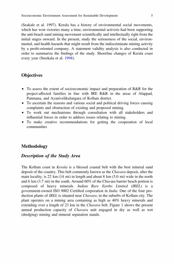
The Kollam coast in Kerala is a blessed coastal belt with the best mineral sanddeposit of the country. This belt commonly known as the Chavara deposit, after themain locality, is 22 km (14 mi) in length and about 8 km (5.0 mi) wide in the northand 6 km (3.7 mi) in the south. Around 60% of the Chavara barrier beach portion iscomposed of heavy minerals. Indian Rare Earths Limited (IREL) is agovernment-owned ISO 9002 Certified corporation in India. One of the four pro-duction plants of IREL is situated near Chavara, in the suburbs of Kollam city. Theplant operates on a mining area containing as high as 40% heavy minerals andextending over a length of 23 km in the Chavara belt. Figure 1 shows the presentannual production capacity of Chavara unit engaged in dry as well as wet(dredging) mining and mineral separation stands.
Socioeconomic Environment Assessment for Sustainable Development 5
Types of Data Collected
The following types of data were collected for the study:
• Documentary evidence mainly from records and published materials available invarious related departments.
• Interview data from the families of the project-affected areas of Alappad,Panmana, and Ayanivelikulangara of Kollam district.
• Field notes by the researcher through observation and discussion with theknowledgeable persons, local leaders, and other resource persons.
• Focus group discussions with the stakeholders.
Tools of Data Collection
Data for the empirical study were collected mainly through interview schedules andfocus group discussions. The schedule-elicited information on areas required forgetting the information given in the objectives. Wherever possible the responses inthe schedule were pre-coded to facilitate easy tabulation and analysis. Most of thequestions had distinct options for answers and only a few qualitative parameterswere elicited through open-ended questions.
Fig. 1 Chavara unit miningand mineral site
6 A.K. Rahul et al.
Data Collection Analysis
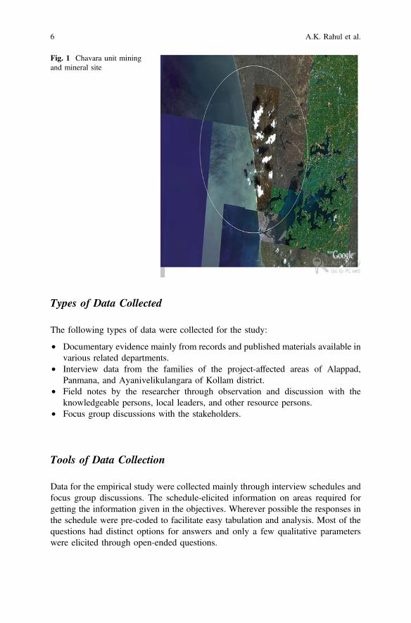
Quantitative analysis rests judgmental conclusion based purely on data. Qualitativeassumptions are about how the world works, what are suitable categories for data.Figure 2 describes what constitute good data, and the validity of scientific proce-dures to explain the descriptive and inferential statistics. For future projections, therole of qualitative assumptions is significant.
Personal Profile
The socioeconomic and demographic profiles of the respondents are given whichcovers detailed information on the various dimensions of the families in theproject-affected areas of Alappad, Panmana, and Ayanivelikulangara of Kollamdistrict. The personal information gives a benchmark data of the families in theseareas, which will be useful to understand the general characteristics of the areasunder study.
Fig. 2 Quantitive assumption of Chavara site
Socioeconomic Environment Assessment for Sustainable Development 7

Age
Maturity is an index to understand the issues of the sand mining in an intelligentway. The age-wise classification of the occupants of the mining lease area is givenin Table 1.
Sex
Male-to-female ratio in these three villages are given in Table 2. It is clear from thetable that men are more exposed to the issues of the sand mining, as they are morein touch with many people in the areas (Fig. 3).
Table 1 Age analysis
Age group (years) Frequency Percentage
15–25 14 2.6
26–35 53 9.9
36–45 127 23.8
46–55 159 29.9
56–65 110 20.6
66–75 52 9.8
Above 75 18 3.4
Total 533 100
Table 2 Sex analysis
Sex Frequency Percentage
Male 393 73.7
Female 140 26.3
Total 533 100
Fig. 3 Education analysis
8 A.K. Rahul et al.
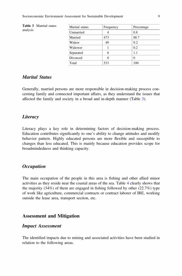
Marital Status
Generally, married persons are more responsible in decision-making process con-cerning family and connected important affairs, as they understand the issues thataffected the family and society in a broad and in-depth manner (Table 3).
Literacy
Literacy plays a key role in determining factors of decision-making process.Education contributes significantly to one’s ability to change attitudes and modifybehavior pattern. Highly educated persons are more flexible and susceptible tochanges than less educated. This is mainly because education provides scope forbroadmindedness and thinking capacity.
Occupation
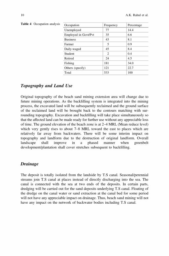
The main occupation of the people in this area is fishing and other allied minoractivities as they reside near the coastal areas of the sea. Table 4 clearly shows thatthe majority (34%) of them are engaged in fishing followed by other (22.7%) typeof work like agriculture, commercial contracts or contract laborer of IRE, workingoutside the lease area, transport section, etc.
Assessment and Mitigation
Impact Assessment
The identified impacts due to mining and associated activities have been studied inrelation to the following areas.
Table 3 Matrital statusanalysis
Marital status Frequency Percentage
Unmarried 4 0.8
Married 473 88.7
Widow 49 9.2
Widower 1 0.2
Separated 6 1.1
Divorced 0 0
Total 533 100
Socioeconomic Environment Assessment for Sustainable Development 9
Topography and Land Use
Original topography of the beach sand mining extension area will change due tofuture mining operations. As the backfilling system is integrated into the miningprocess, the excavated land will be subsequently reclaimed and the ground surfaceof the reclaimed land will be brought back to the contours matching with sur-rounding topography. Excavation and backfilling will take place simultaneously sothat the affected land can be made ready for further use without any appreciable lossof time. The ground elevation of the beach zone is at 2–4 MRL (Mean reduce level)which very gently rises to about 7–8 MRL toward the east to places which arerelatively far away from backwaters. There will be some interim impact ontopography and landform due to the destruction of original landform. Overalllandscape shall improve in a phased manner when greenbeltdevelopment/plantation shall cover stretches subsequent to backfilling.
Drainage
The deposit is totally isolated from the landside by T.S canal. Seasonal/perennialstreams join T.S canal at places instead of directly discharging into the sea. Thecanal is connected with the sea at two ends of the deposits. In certain parts,dredging will be carried out for the sand deposits underlying T.S canal. Floating ofthe dredge on the canal water or sand extraction at the canal bed for some periodwill not have any appreciable impact on drainage. Thus, beach sand mining will nothave any impact on the network of backwater bodies including T.S canal.
Table 4 Occupation analysis Occupation Frequency Percentage
Unemployed 77 14.4
Employed in Govt/Pvt 35 6.6
Business 43 8.1
Farmer 5 0.9
Daily-waged 45 8.4
Student 2 0.4
Retired 24 4.5
Fishing 181 34.0
Others (specify) 121 22.7
Total 533 100
10 A.K. Rahul et al.

Air Environment
Due to beach sand extraction, primary concentration, and backfilling, there will notbe an appreciable rise in gaseous or particulate pollution level in ambient and workzone environment. Sand extraction process (dredging) is a wet primary process andbackfilled mass is a moist in form which does not release dry dust in the miningarea. Therefore, in the proposed area, pollution will be insignificant. At stack atMSP-monitored particulate matter, SO2 and CO values, in general, are withinpermissible limits. Monitored SPM, SO2, NOx, and CO values at AAQ stations andat work zone are also well within respective permissible limits. The predictions ofground level concentration of pollution from the two stacks of 30 t/day FBD and3 t/day FBD have been carried out with the help of air quality simulation modelISCST3, released by USEPA. At the present EIA study, GLCs (Ground levelconcentration) are predicted for 24 h for SO2 and SPM. As a first step, actualmonitored site meteorological data for winter season have been considered. Themeteorological data were generated near plant site for a 1-month period on anhourly basis. Stabilities have been determined with the monitored data by usingTurner method (insulation-based classification). Up to a height of 30 m, SO2 andNOx values will remain stable. The maximum height at Cochin has been taken as areference for the present study. The locations are located with respect to 16 radialwind directions (N to NNW) and the radial distances have been fixed based onphysical stack height, as the major stack height is 30 m, the receptors in each of theradial directions were fixed at 75, 150, 300, 600, 825, 900, 975, 1050, 1200, 1350,1650, 2100, 2700, 3300, 4200, and 5000 m (Table 5).
Water Environment
Water from T.S Canal is utilized for supplying makeup water to dredge pond. Wateris utilized for primary concentration at MRP. In CUP (and BWP) the pumped outwater from T.S canal is circulated in gravity spirals. Freshwater drawn from borewells is used for washing the CUP concentrate. At present 30 m3/h of bore water isdrawn from the bore wells. After expansion, 60 m3/h of freshwater shall berequired. No trace of saline water ingress has been noted because groundwater isdrawn from a depth of 230 m only. Entire mining lease on a narrow strip of sandy
Table 5 Predicted GLC results
Description Height(m)
Flowrate(nm3/h)
Top dim(m)
SPM SO2 Temp(°c)
Location
mg/Nm3 kg/h mg/Nm3 kg/h X Y
30 t/dayFBD
30 12,400 0.5 dia. 150 1.8 363 4.5 80 0 0
3 t/dayFBD
12 1250 0.3 * 0.3 150 0.1° 363 0.45 80 92 2
Socioeconomic Environment Assessment for Sustainable Development 11
formation being surrounded by saline water on either side and freshwater has beenvery thin in the locality.
Impacts of Ecology
The existing and proposed core zones are the sea beach and inland areas close to thebeach. The inland areas are covered by coconut groves and backwaters. In addition,coconut trees are present at the edges of the beach. In order to carry out mining, thecoconut trees will have to be cut down. The herbs and shrubs growing on the beachand inland will also have to be removed. Due to mining the beach fauna (consistingof crabs, mole crabs, bivalves, and small gastropods) will perish. Similarly, thebenthic flora and fauna in mining areas in the backwaters will also perish due tomining. However, the effects of mining will be temporary. The coconut trees whichwill be cut down will be replaced by new saplings after backfilling the mined outareas. Ipomoea pes-caprae and spinifexsps, which are the main plants growing onthe sand, will be planted soon after backfilling to stabilize the sand. Seeds of otherplants are airborne and will recolonise the backfilled areas within a few months.Larval forms of the beach fauna are present in the sea water and will startrecolonising the backfilled areas within a few days after completion of mining. Theair pollutants released by diesel powered machinery will be of very small quantityand will be easily diluted and will have no impacts on the ecosystems.
Impacts on Soil and Agriculture
The core zone soil is basically sandy soil. The mining will involve extraction of thissandy soil, and dumping back the tailings in the mined out areas. Since the heavymineral extraction is a simple physical process, the sand which is dumped back willnot differ chemically from the pre-mining sand except that the heavy minerals areno longer present. The physical changes which will occur will be minor and willhave no lasting impacts. Mining will involve cutting down of coconut trees leadingto loss in coconut production. But these trees will be placed by new saplings ofimproved variety which will actually improve the agricultural yield. The emissionfrom MSP is also too less to have any impact on the soil or agriculture production inthe study area.
Land Use
Excavated land will be subsequently reclaimed by backfilling with reject tailings.Backfilling is integrated into operating system. Land areas under the four blocks are
12 A.K. Rahul et al.
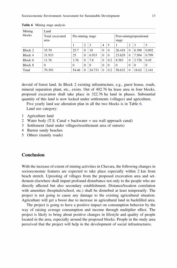
devoid of forest land. In Block 2 existing infrastructure, e.g., guest house, roads,mineral separation plant, etc., exists. Out of 402.76 ha lease area in four blocks,proposed excavation shall take place in 322.76 ha land in phases. Substantialquantity of this land is now locked under settlements (villages) and agriculture.
Five yearly land use alteration plan in all the two blocks is in Table 6.Land use category:
1 Agriculture land2 Water body (T.S. Canal + backwater + sea wall approach canal)3 Settlement (land under villages/resettlement area of outsets)4 Barren sandy beaches5 Others (mainly roads)
Conclusion
With the increase of extent of mining activities in Chavara, the following changes insocioeconomic features are expected to take place especially within 2 km frombeach stretch. Uprooting of villages from the proposed excavation area and set-tlement elsewhere shall impart profound disturbance not only to the people who aredirectly affected but also secondary establishment. Distance/location correlationwith amenities (hospitals/school, etc.) shall be disturbed at least temporarily. Theproject is not going to cause any damage to the existing agricultural situation.Agriculture will get a boost due to increase in agricultural land in backfilled area.
The project is going to have a positive impact on consumption behavior by theway of raising average consumption and income through multiplier effect. Theproject is likely to bring about positive changes in lifestyle and quality of peoplelocated in the area, especially around the proposed blocks. People in the study areaperceived that the project will help in the development of social infrastructures.
Table 6 Mining stage analysis
Miningblocks
Land
Total excavatedarea
Pre-mining stage Post-mining/operationalstage
1 2 3 4 5 1 2 3 5
Block 2 35.70 25.7 0 10 0 0 26.418 0 8.390 0.892
Block 4 31.933 25 0 6.933 0 0 23.629 0 7.504 0.799
Block 6 11.76 3.76 0 7.8 0 0.2 8.583 0 2.726 0.45
Block 8 0 0 0 0 0 0 0 0 0 0
Total 79.393 54.46 0 24.733 0 0.2 58.632 0 18.62 2.141
Socioeconomic Environment Assessment for Sustainable Development 13
References
Aarninkhof S, Dalfsen JV, Mulder J, Rijks D (2010) Sustainable development of nourishedshorelines. Innovations in project design and realization, Netherlands
Ausubel JH, Crist DT, Waggoner PE (2010) First cenus of marine life 2010: highlights of a decadeof discovery. Census of Marine Life Secretariat, Washington, DC
Briggs DJ (2008) A framework for integrated environmental health impact assessment of systemicrisks. Environ Health Perspect 23(7):61–78
Crane M (2010) Application of approaches for converting environmental risk assessment outputsinto socioeconomic impact assessment inputs when developing restrictions under REACH.Report to the Luxembourg Environment Agency. WCA-Environment, Faringdon, UnitedKingdom
Hilson G, Murck B (2000) Sustainable development in the mining industry: clarifying thecorporate perspective. Resour Policy 26(4):227–238
Hilson G, Murck B, Lin ZX (2011) The protection and management of marine biological diversityin areas beyond national jurisdiction. Pac J 19(10):94–102
Lee N, George C (2000) Environmental assessment in developing and transitional countries.Wiley, Chichester
Nordstrom KF (2000) Beaches and dunes on developed coasts. Cambridge University Press, UK,p 338
Schlacher TA, Thompson L (2007) Exposure of fauna to off-road vehicle (ORV) traffic on sandybeaches. Coast Manag 35:567–583
Schlacher TA, Schoeman DS, Lastra M, Jones A, Dugan J, Scapini F (2006) Neglected ecosystemsbear the brunt of change. Ethol Ecol Evol 18:349–351
Sreekala SP, Baba M, Muralikrishna M (1998) Shoreline changes of Kerala coast using IRS dataand aerial photographs. Indian J Mar Sci 27(1998):144–148
The Atomic Energy Act, 1962. Government of India, No. 33Wong P (2003) Where have all the beaches gone, Coastal erosion in the tropics. Singap J Trop
Geogr 24(1):111–132
14 A.K. Rahul et al.

Research Need on Environmental Gainsin Conservation-Induced Relocation
Surendra Singh Rajpoot and M.S. Chauhan
Abstract Relocations are made for developmental- and conservation-inducedscenario. Conservation-induced relocations are different from developmental-induced relocations, in the sense that site is vacated due to it is environmentallyimproved. There are a lot of studies on social impact of conservation-inducedrelocation, but very few studies have been undertaken on environmental gainsthrough it. With more emphasis on maintaining ecological balance and sustenanceof biodiversity, nowadays conservation-induced relocation is taking place, spe-cially, within the protected areas. Therefore, research to assess ecological andenvironmental gains is needed, so as to judge objectively very aim of such relo-cation. Studies related to pros and cons, need and necessities, and areas of existingstudies about relocation for biodiversity conservation with reference to protectedareas have been dealt in this paper. Based on the above studies, broader fields areassessed, in which further research and study are required, toward environmentalgains through such relocation.
Introduction
Protected areas are considered to be biodiversity hub of planet earth. Protectedareas, which today accounts for only 1.4% of the Earth’s surface, are home toalmost half of the plant species and more than one-third of all vertebrates (Heltberg2001). Ever since the publication of Hardin’s articles ‘The Tragedy of theCommons’, there has been a growing debate on common pool resources, propertyrights, and resource degradation. The concept has been used to explain
S.S. RajpootNarmada Valley Development Authority, Narmada Bhawan, Bhopal, MP, Indiae-mail: [email protected]
M.S. Chauhan (&)Department of Civil Engineering, Maulana Azad National Institute of Technology,Bhopal 462003, Indiae-mail: [email protected]
© Springer Nature Singapore Pte Ltd. 2018V.P. Singh et al. (eds.), Environmental Pollution, Water Scienceand Technology Library 77, https://doi.org/10.1007/978-981-10-5792-2_2
15

overexploitation of forests and fisheries, overgrazing, air and water pollution, abuseof public lands, population problems, extinction of species, and other problem ofresource misallocation (Stevenson 1991). Due to overexploitation of naturalresources, of the protected areas, voluntary conservation-induced relocation is usedas a management tool.
The fragile nature of biodiversity in many nature reserves, ongoing conflicts, andthe demand from people for better living standards necessitate the conservationcommunity to examine relocation as a possible conservation solution (Karanth 2002;Karanth and Karanth 2007). There are two opposite sides of conservation-inducedrelocation; first socialists and second biologists. Both have almost antagonizingviews over the subject. There is a dearth of studies about conservation-inducedrelocation, especially environmental gains of such relocation. This paper deliberatesabout the need for research and studies about environmental and ecological gains ofconservation relocations, so as to have a more qualitative assessment of the issues.
Relocation
Relocation of the people is broadly classified into two categories, i.e.,development-induced relocation (DIR) and conservation-induced relocation (CIR).Conceptually development-induced and conservation-induced displacements areindistinguishable, either from the perspective of the state (both are due to statemanagement of resources as part of plans to increase prosperity and well-being) orfrom the point of view of people evicted (for whom the precise cause of eviction isof little importance) (Brockington and Igoe 2006). Although DIR and CIR haveabove similarities, they differ in nature, as ecologically and environmentally theland vacated due to relocation undergoes change. The characteristic change in DIRis totally different from original land use, e.g., in construction of irrigation dam, theland is submerged and has adverse environmental impact, whereas in CIR thevacated site is environmentally improved.
Protected Areas
A protected area is a clearly defined geographical space, recognized, dedicated, andmanaged, through legal or other effective means, to achieve the long-term con-servation of nature with associated ecosystem services and cultural values (IUCNDefinition 2008). Protected areas—national parks, wilderness areas, communityconserved areas, nature reserves, and so on—are a mainstay of biodiversity con-servation, while also contributing to people’s livelihoods, particularly at the locallevel. Protected areas are at the core of efforts towards conserving nature and theservices it provides us—food, clean water supply, medicines, and protection fromthe impacts of natural disasters. Their role in helping mitigate and adapt to climate
16 S.S. Rajpoot and M.S. Chauhan

change is also increasingly recognized; it has been estimated that the global net-work of protected areas stores at least 15% of terrestrial carbon. Protected areas areconsidered to be biodiversity hub of planet earth. Protected areas, which todayaccounts for only 1.4% of the Earth’s surface, are home to almost half of the plantspecies and more than one-third of all vertebrates (Heltberg 2001).
India also has ten biogeographic realms and is one of 17 mega-diversity coun-tries that together support two-thirds of the world’s biological resources (Rodgersand Panwar 1988; Briggs 2003). Thirty-three percent of the country’s 49,219 plantspecies are endemic (MoEF 1999). Although India covers just 2.4% of the Earth’sarea, it harbors 7.3% of the world’s terrestrial vertebrate species and 89,451 faunalspecies (MoEF 2000). India has several charismatic mammal species, including40% of the world’s tigers, and most of the world’s Asian elephants. Overall, someestimates suggest that 20% of Indian mammal species face imminent extinction,and several have already disappeared from over 90% of their historic range(Madhusudan and Mishra 2003). India has less than 5% under-protected areas, butharbors more than 50% of its biodiversity. This calls for better protection andmanagement of these sanctum sanctorum areas for conservation of biodiversity andsustainable use of natural resources.
Classification of Protected Areas
Based on objects, purpose of constitution and level of protection, PAs are classifiedinto various categories. The International Union for the Conservation of Nature andNatural Resources (IUCN) protected area management categories are a frameworkfor organizing and understanding protected lands around the world. The categoriescame into to being following many efforts to establish a “common understanding ofprotected areas” when countries had very different ways of looking at protectedareas, used different terms, and assigned different meanings to similar or identicalterms. There are six categories (IUCN published its revision of category definitionsin 2008) into which protected lands can be sorted.
India has the following kinds of protected areas, in the sense of the worddesignated by IUCN:
National parks (IUCN Category II): India’s first national park was Hailey NationalPark, now Jim Corbett National Park, established in 1935. By 1970, India had fivenational parks; today it has over 120 national parks. All national park lands thenencompassed a total 39,919 km2 (15,413 sq mi), comprising 1.21% of India’s totalsurface area (MoEF website). Animal sanctuary (IUCN Category IV): India hasover 500 animal sanctuaries, referred to as Wildlife Sanctuaries (MoEF website).Biosphere reserve IUCN (Category V): There are 18 biosphere reserves in India.Reserved forests and protected forest (IUCN Category IV or VI, depending onprotection accorded): These are forested lands where logging, hunting, grazing, andother activities may be permitted on a sustainable basis to members of certain
Research Need on Environmental Gains in Conservation … 17
communities. In reserved forests, explicit permission is required for such activities.In protected forests, such activities are allowed unless explicitly prohibited. Thus, ingeneral reserved forests enjoy a higher degree of protection with respect to pro-tected forests (Indian Forest Act 1927).Conservation Reserve and Community Reserve (IUCN Category V and VI,respectively): These are areas adjoining existing protected areas which are ofecological value and can act as migration corridors, or buffer zone. Conservationreserves are designated government-owned land from where communities may earna subsistence, while community reserves are on mixed government/private lands.Community reserves are the only privately held land accorded protection by thegovernment of India (Indian Forest Act 1927).Village and panchayat forests (IUCN Category VI): These are forested landsadministered by a village or a panchayat on a sustainable basis, with the habitat,flora and fauna being accorded some degree of protection by the managing com-munity (Indian Forest Act 1927).
Need for Conservation of Biodiversity
Why is there a need to conserve biodiversity? The reasons are neither obvious norwidely agreed upon. Environmental philosophers identify two very different sets ofarguments, based on the utilitarian (or instrumental) versus the intrinsic (or inher-ent) value of nature. The utilitarian value of nature refers to the product or functionthat nature can provide, whereas intrinsic value inheres in the natural object orsystem itself, irrespective of whether it has any use. Arguments for conservingbiodiversity that are based on the utilitarian value are often labeled anthropocentric(human-centered), whereas the arguments predicated on intrinsic value are oftencalled bio-centric (or eco-centric) since the value exists independent of its use tohuman beings. The utilitarian value of biodiversity may be divided into four basiccategories: goods, services, information, and spiritualism (Table 1) (Mulder andCoppolillo 2004). Intrinsic value is a much more subjective matter. While mostpeople take the intrinsic value of humans for granted, the view that “Nature” (oftenpersonalized in this sense) has inherent rights and is as such subject to the samemoral, ethical, and legal protection afforded humans is more controversial.
Table 1 Categories of utilitarian values
Category Examples
Goods Food, fuel, fiber, medicine
Services Pollination, recycling, nitrogen fixation, homeostatic regulation, carbonstorage
Information Genetic engineering, applied biology, pure science
Psycho-spiritual Aesthetic beauty, religious awe, scientific knowledge, recreation, tourism
18 S.S. Rajpoot and M.S. Chauhan
Biodiversity is to be conserved for maintaining the following services:Maintenance of ecosystem includes recycling and storage of nutrients, com-
bating pollution, stabilizing climate, protecting water resources, formation andprotection of soil, and maintaining eco-balance. Provider of biological resourcesincludes provision of medicines and pharmaceuticals, food, ornamental plants,wood products, breeding stock and diversity of species, ecosystem, and genes.
Social benefits include recreation and tourism, cultural value, and education andresearch (Cardinale et al. 2012).
Need for Conservation-Induced Relocation
The importance of biodiversity conservation has been discussed as above. Most ofthe biodiversities in the present days are within the limits of protected areas. Theseprotected areas account for less than 5% of the geographical area of the India.Globally, large terrestrial mammals are among the most threatened taxa in theworld, with 25% of species facing extinction (Ceballos et al. 2005; Schipper et al.2008). Recent studies suggest that South Asia harbors the most threatened terrestrialmammals (Schipper et al. 2008). For India, in particular, conservative estimatessuggest that 20% of large mammal species may face extinction, and several specieshave already disappeared from over 90% of their original range (Madhusudan andMishra 2003). The Indian subcontinent harbors more than 500 mammal species, butalso has a ‘modern’ conservation history of regulating land uses to protect naturalareas that date back over a century (Blythe 1863; Jerdan 1874; Russell 1900; Prater1948; Stebbing 1920; Rangarajan 2001).
The tiger (Panthera tigris) or the greater one-horned rhino (Rhinoceros unicornis)occupy just one to five percent of their historical range. Races of some species suchas the Asian lion (Panthera leo persica) and the hardground barasingha (Cervusduvauceli branderi) are confined to single site, microscopic remnants of a once vastrange (Divyabhanusinh 2005; Karanth 2006). In Sariska Tiger Reserve, adversechanges in vegetation structure and plant species composition were caused bychronic biomass extraction that was likely affecting forest avifauna as well (Kumarand Shahabuddin 2005). The Biligiri Rangan Hills Temple Sanctuary in southernIndia reports reduced recruitment of some extracted NTFP species and changingtree species composition of forests due to long-term use (Murali et al. 1996;Shankar et al. 1998). Studies in Pin Valley National Park in the Indian Himalayaindicate that there may be competition for pastures between domestic goats/sheepand wild ibex, given the coincidence of diet choice (Bagchi et al. 2004).
Ever since the publication of Hardin’s articles ‘The Tragedy of the Commons’,there has been a growing debate on common pool resources, property rights, andresource degradation. The concept has been used to explain overexploitation offorests and fisheries, overgrazing, air and water pollution, abuse of public lands,population problems, extinction of species, and other problem of resource misal-location (Stevenson 1991). When property rights to natural resources are absent and
Research Need on Environmental Gains in Conservation … 19
unenforced, i.e., when there is open access, no individual bears the full cost ofresource degradation. The result is ‘free riding’ and overexploitation, what Hardintermed the ‘Tragedy of the Commons’ (Hardin 1968).
Available reports suggest that between 50 and 100% of stricter protected areas inSouth America and Asia are used or occupied by people (Kothari et al. 1989;Amend and Amend 1995; Bruner et al. 2001; Rao et al. 2002; Bedunah andSchmidt 2004). Growing human population and shrinking natural resources havedisturbed ecological balance in some areas. There are many studies which suggestit. An increasing number of scientific studies point to the habitat degradation causedby biomass extraction such as grazing, fuelwood collection, and commercialnon-timber forest produce (NTFP) extraction inside areas, set aside for biodiversityconservation (Siebert 2004; Karanth et al. 2005).
Biologists therefore emphasize the fact that some amount of inviolate zone(strictly protected area) is required to maintain the entire spectrum of biodiversity aswell as to minimize conflicts with large mammalian fauna (Terborgh et al. 2002;Ministry of Environment and Forests 2005). The fragile nature of biodiversity inmany nature reserves, ongoing conflicts, and the demand from people for betterliving standards necessitates the conservation community and examines relocationas a possible conservation solution (Karanth 2002; Karanth and Karanth 2007).
It is evident that human activities in some parts of the protected areas haveaffected habitat and ecology adversely. People living within these protected areasfor their economic well-being have also been opting to move voluntarily out of thearea. Case of people willing to be relocated appears to be a win–win situation forthe both park managers and people. The National Tiger Conservation Authority ofIndia has come up with legal provisions for voluntary relocation from TigerReserves. The provisions therein incorporate willingness of people, social, andecological studies to make the whole process transparent and people friendly.
Following are provisions made in section 38 V (5) Wildlife (Protection) Act1972:
Save as for voluntary relocation on mutually agreed terms and conditions pro-vided that such terms and conditions satisfy the requirements laid down in thissubsection; no Scheduled Tribes or other forest dwellers shall be resettled or havetheir rights adversely affected for the purpose of creating inviolate areas for tigerconservation unless:
(i) The process of recognition and determination of rights and acquisition ofland or forest rights of the Scheduled Tribes and such other forest dwellingpersons is complete;
(ii) The concerned agencies of the State Government, in exercise of their powersunder this act, establish with the consent of the Scheduled Tribes and suchother forest dwellers in the area, and in consultation with an ecological andsocial scientists familiar with the area, that the activities of the ScheduledTribes and other forest dwellers or the impact of their presence upon wildanimals are sufficient to cause irreversible damage and shall threaten theexistence of tigers and their habitat;
20 S.S. Rajpoot and M.S. Chauhan

(iii) The State Government, after obtaining the consent of the Scheduled Tribesand other forest dwellers inhabiting the area, and in consultation with anindependent ecological and social scientist familiar with the area, has cometo a conclusion that other reasonable options of co-existence are notavailable;
(iv) Resettlement or alternative package has been prepared to provide thelivelihood for the affected individuals and communities and fulfills therequirements given in the National Relief and Rehabilitation Policy;
(v) The informed consent of the Gramsabha concerned, and of the personsaffected, to the resettlement program has been obtained; and
(vi) The facilities and land allocation at the resettlement location are providedunder the said program, otherwise their existing rights shall not be interferedwith (Wild life (Protection) Act 1972, Section 38 V (5)).
Need for Study of Environmental Gains Due to CIR
CIR even being a contagious issue has philosophers both for and against it, butthere is hardly any complete and detailed study about the consequences. It has takenmany months of burrowing through libraries, reading through back issues ofjournals and trawling through bibliographic databases to produce this list. Just asthe literature is not well ordered, the activities of researchers examining reloca-tion from protected areas have also not been systematic. Only recently,Schmidt-Soltau’s work (2005a), there has been an attempt to build up a retro-spective assessment of the patterns of eviction (Brockington et al. 2006). There isan extraordinary dearth of good information about the social impacts of protectedareas. Protected areas have expanded threefold in recent years, and the strictercategory 1–4 protected areas now some 49,000 and cover 6% of the land surface ofthe planet. One should expect this to have involved some evictions. Yet when twoof us recently reviewed as much literature on protected area displacements as wecould, we found just under 250 books and papers containing information on justover 150 protected areas. A significant proportion of reports and case material(nearly half) merely stated that people had been moved. There was no furtherdiscussion of these moves, let alone good investigation of their consequences(Brockington et al. 2006).
Only a few studies, that we are aware of, systematically use consistentmethodology to assess involuntary resettlements and evictions from protected areasat the regional level (Cernea and Schmidt-Soltau 2003, 2006). We now review themain environmental, socioeconomic, and other impacts of the displacement of localcommunities from PAs in India. As far as possible, we do this for both the old andthe new sites (before and after relocation). Unfortunately, the information is rather
Research Need on Environmental Gains in Conservation … 21
incomplete, as we found a very few studies of post-relocation, and almost nonehave assessed the situation over a long-term period (Lasgorceix and Kothari 2009).In India, there is as yet no full-length study of conservation-related displacementthat can compare with those in eastern or southern Africa. In Tanzania and SouthAfrica, cases of forceful eviction of pastoral peoples from game reserves arebecoming increasingly common (Carruthers 1995; Neumann 1998).
There could be two possible reasons for the paucity of cases. Either few caseshave been reported because few have happened, or eviction has been ignored. Theappropriate answer may well vary according to country and region. We will arguebelow that in some regions there is good evidence that eviction from protected areashas been substantially overlooked. Second, in many cases the quality of theinformation is poor. A significant proportion of reports and case material (nearlyhalf) merely stated that people had been moved. There was no further discussion ofthese moves, let alone good investigation of their consequences. This sort of reportmight be found in conservation literature in which the movement of people wasmentioned in connection with the establishment of a new protected area. But it alsocharacterized a significant proportion of the literature about indigenous peoples.Much of this was protest literature, whose purpose was to alert the world to thelosses of indigenous groups. The significance of such events for livelihoods andcultures is often not explored (and for good reason, the main impacts will beobvious) nor are methods made clear (again for good reason, these are not academicpublications). Third, and most importantly, this literature is not (yet) a catalogue.These works are diffused and often hard to locate. It has taken many months ofburrowing through libraries, reading through back issues of journals and trawlingthrough bibliographic databases to produce this list. Just as the literature is not wellordered, the activities of researchers examining relocation from protected areashave also not been systematic. Only recently, Schmidt-Soltau’s work (2005a), therehas been an attempt to build up a retrospective assessment of the patterns ofeviction, and this is only for one region, and, as we shall see, from an unusuallycomplete coverage of protected areas in existence.
Countless workshops, lectures, and discussions delved into topics such aspoverty alleviation, social injustice, indigenous peoples’ rights, community man-agement of protected areas, and gender equity in conservation. All these have theirplace in a global agenda but for me they dominated and drowned out the discussionof themes more directly related to conserving nonhuman life on this planet(Terborgh 2004). Detailed quantitative assessments of the consequences of dis-placement for conservation are few, the literature on the historical erasures andreinventions of place, people and landscape is rich (Carruthers 1995; Ranger 1999).This signifies that studies related to conservation-induced relocation are few andwhatever has been taken place deals with social angle only and almost negligibleabout ecological point of view.
22 S.S. Rajpoot and M.S. Chauhan
Conclusion
Biodiversity is an important issue and needs to be conserved. Globally protectedareas are harboring bulk of biodiversity, which is in percentage terms is too large incomparison to the area of protected areas. In India too the scenario is similar to it.Therefore, efficient protection and management of these areas are of utmostimportance. As a conservation tool, voluntary relocation of human population fromsuch area has been on the agenda of biologist. This kind of conservation-inducedrelocation has two facets of it, namely social and ecological sides. Socialist andbiologist have antagonizing views over CIR. As the review of literature reveals thatthere is paucity of enough literature on both the angles. Whatever studies areavailable are not comprehensive and focused on multilateral issues.
Among the available literature, focus has been mostly towards human-centricissues and no concrete study of ecological and environmental gains at vacated sitehas been taken up. The authors could not find any study/research which deliberateson this issue. It is therefore required to have ecological and environmental studies,taking into account pre- and post-relocation scenario of the vacated site and developa model for future reference to assess environmental gains in similar cases.
References
Amend S, Amend T (1995) Balance sheet: inhabitants in national parks—an unsolvablecontradiction? The South American experience. World Conservation Union, Gland,pp 449–460
Bagchi S, Mishra C, Bhatnagar YV (2004) Conflicts between traditional pastoralism andconservation of Himalayan ibex (Capra sibirica) in the Trans-Himalayan mountains. AnimConserv 7:121–128
Bedunah DJ, Schmidt SM (2004) Pastoralism and protected area management in Mongolia’s GobiGurvansaikhan National Park. Dev Change 35:167–191
Blythe E (1863) Catalogue of the mammalia in the museum Asiatic society. Savielle andCranenburgh. Bengal Printing Committee Ltd., Calcutta
Briggs J (2003) The bio-geographic and tectonic history of India. J Biogeogr 30:381–388Brockington D, Igoe J (2006) Conserv Soc 4(3):424–470Brockington D, Igoe J, Schmidt-Soltau K (2006) Conserv Biol 20(1):250–252Bruner AG, Gullison RE, Rice RE, da Fonseca GAB (2001) Effectiveness of parks in protecting
tropical biodiversity. Science 291:125–128Cardinale B et al (2012) Bio diversity loss & its impact on huminty. Nature 486(7401):59–67Carruthers J (1995) The Kruger National Park: a social and political history. University of Natal
Press, PietermaritzburgCeballos G, Ehrlich PR, Soberon J, Salazar I, Fay JP (2005) Global mammal conservation: what
must we manage? Science 309:603–607Cernea MM, Schmidt-Soltau K (2003) The end of forcible displacements? Conservation must not
impoverish people. Policy Matters 12(3):8–34Cernea MM, Schmidt-Soltau K (2006) Poverty risks and national parks: policy issues in
conservation and resettlement. World Dev 34(10):1808–1830Divyabhanusinh (2005) The story of Asia’s last lions, Mumbai
Research Need on Environmental Gains in Conservation … 23
Hardin G (1968) The tragedy of commons. Science 162Heltberg R (2001) Determinants and impact of local institutions for community resource
management. Environ Dev Econ 6(4):183–208Indian Forest Act, 1927IUCN Definition of Protected Areas, 2008Jerdan TC (1874) A handbook of mammals of India. Reprint by Mittal Publications, IndiaKaranth KU (2002) Nagarahole: limits and opportunities in wildlife conservation. In: Terborgh J,
van Schaik C, Davenport L, Rao M (eds) Making parks work: strategies for preserving tropicalnature. Island Press, Washington, D.C.
Karanth KU (2006) A view from the Machan: how science cans save the fragile predator.Permanent Black, Delhi
Karanth KU, Karanth KK (2007) Free to move: conservation and resettlement in the WesternGhats of Karnataka, India. In: Redford KH, Fearn E (eds) Protected areas and humandisplacement: a conservation perspective. Working paper 29. Wildlife Conservation Society,New York, USA
Karanth K, Curran LM, Reuning-Scherer JD (2005) Village size and forest disturbance in Bhadrawildlife sanctuary, Western Ghats, India. Biol Conserv 128:147–157
Kothari A, Pande P, Singh S, Variava D (1989) Management of national parks and sanctuaries inIndia. A status report. Indian Institute of Public Administration, New Delhi
Kumar R, Shahabuddin G (2005) Effects of biomass extraction on vegetation structure, diversityand composition of an Indian tropical dry forest. Environ Conserv 32(3):1–12
Lasgorceix A, Kothari A (2009) Displacement and relocation of protected areas: a synthesis andanalysis of case studies. Econ Polit Wkly EPW xliv(49)
Madhusudan MD, Mishra (2003) Why big, fierce animals are threatened: conserving largemammals in densely populated landscapes. In: Saberwal V, Rangarajan M (eds) Battles overnature: science and politics of conservation. Permanent Black, New Delhi, India
Ministry of Environment and Forests (2005) Joining the dots. Report of the Tiger Task Force.Government of India
MoEF (2000) Annual report 2000–2001. Ministry of Environment and Forests, Government ofIndia. New Delhi, India
MoEF (Ministry of Environment and Forests) (1999) National policy and macro level actionstrategy on biodiversity ministry of environment and forests. Government of India, New Delhi(Website)
Mulder MB, Coppolillo P (2004) Conservation. Princeton University PressMurali KS, Shaanker RU, Shankar U, Ganeshaiah KN, Bawa KS (1996) Extraction of non-timber
forest produce in the forests of Biligiri Rangan hills, India. 2. Impact of NTFP extraction onregeneration, population structure and species composition. Econ Bot 50(2):252–269
Neumann RP (1998) Imposing wilderness. Struggles over livelihood and nature preservation inAfrica. University of California Press Berkeley, Los Angeles
Prater SH (1948) The book of Indian animals. Bombay Natural History Society, BombayRangarajan M (2001) India’s wildlife history. Permanent Black, New DelhiRanger T (1999) Vocies from the rocks. Nature, culture and history in the Matapos Hills of
Zimbabwe. James Currey, OxfordRao M, Rabinowitz A, Khaing ST (2002) Status review of the protected-area system in Myanmar,
with recommendations for conservation planning. Conserv Biol 16:360–368Rodgers WA, Panwar HS (1988) Planning a wildlife protected area network in India, vol I.
Wildlife Institute of India, Dehra DunRussell CEM (1900) Bullet and shot in Indian forest, plain and hill. Thacker and Co. Ltd.,
Bombay, IndiaSchipper et al (2008) The status of the world’s land and marine mammals: diversity, threat, and
knowledge. Science 322:225–230Shankar U, Murali KS, Shaanker RU, Ganeshaiah KN, Bawa KS (1998) Extraction of non-timber
forest products in the forests of Biligiri Rangan hills, India. 4. Impact on floristic diversity andpopulation structure in a thorn scrub forest. Econ Bot 52(3):302–315
24 S.S. Rajpoot and M.S. Chauhan

Siebert SF (2004) Demographic effects of collecting rattan cane and their implications forsustainable harvesting. Conserv Biol 18(2):424–431
Stebbing EP (1920) The diary of a sportsman naturalist in India. John Lane, the Bodely Head,London
Stevenson GG (1991) Common property economics: a general theory and land use application.Cambridge University Press
The IUCN Protected Area Management Categories, 2008Terborgh J (2004) Reflections of a scientist on the world parks congress. Conserv Biol 18:619–620Terborgh J, van Schaik C, Davenport L, Rao M (2002) Making parks work: strategies for
preserving tropical nature. Island Press, USAWild life (Protection) Act 1972, Section 38 V (5)
Research Need on Environmental Gains in Conservation … 25
Environmental Issues Due to Fire in CoalMines: Its Impact and Suggestionsfor Implementing Precautionaryand Control Measures
R.V.K. Singh, D.D. Tripathi, N.K. Mohalik, A. Khalkho, J. Pandeyand R.K. Mishra
Abstract There are several factors responsible for polluting the environment andcreating pollution; and especially in coalfields, fire in coal mines is one significantof them. Presently, about 70% of the production of coal is being carried out byopencast mining (from coal benches) over underground developed galleries inJharia and its adjoining coalfields. Most of the mines developed earlier by under-ground are presently being excavated by opencast method to meet the productiontarget. Due to intrinsic characteristics of coal with add-on of prevailing practices ofmining operation, the spontaneous heating/fire has occurred in most of the galleriesof developed coal seams. Fire in the developed galleries affects the normal pro-duction during excavation by the opencast method. It releases noxious gases, heat,smoke and dust and poses a serious health hazard. Fire in mines also causes directloss of equipment, damage to the surface structure and loss of country’s preciouscoal reserves. In addition to these, it affects the normal production. The objective ofthis paper is to describe the environmental impacts due to fire in coal mines, andissues that affect society as well as to render suggestions for taking precautionaryand control measures.
Introduction
The problem of spontaneous combustion is very common in coal mines worldwide.Coal faces are exposed to the atmosphere and react with oxygen (air) as a result ofwhich it catches fire, depending on the incubation period, the quality of the coal andother factors inherently associated with the coal. The phenomenon of the sponta-neous combustion is caused by two interrelated process, viz. the interactionbetween oxygen and coal (oxidation) and the exothermic reaction (heat sheddingprocess), leading to heat build-up in coal due to the property of its non-conductivity
R.V.K. Singh (&) � D.D. Tripathi � N.K. Mohalik � A. Khalkho � J. Pandey � R.K. MishraMine Fire Division, CSIR-Central Institute of Mining & Fuel Research, Barwa Road,Dhanbad 826015, Jharkhand, Indiae-mail: [email protected]
© Springer Nature Singapore Pte Ltd. 2018V.P. Singh et al. (eds.), Environmental Pollution, Water Scienceand Technology Library 77, https://doi.org/10.1007/978-981-10-5792-2_3
27
of heat. In Indian coal mines, spontaneous combustion (fires) commonly occurs inthe underground-developed workings during extraction by the opencast methods.Spontaneous combustion incidence can occur anywhere in coal mines (undergroundand surface) during or after mining operations. Spontaneous heating initiates in coalmines particularly in pillars, in developed galleries, faces, benches, stockpiles, anddumps. Environment is badly affected due to release of noxious gases in all theabove-mentioned cases after the occurrence of spontaneous heating (Banerjee1985). Different types of fire require a different approach for prevention and controlof spontaneous heating. In Indian mines, spontaneous combustion/fires in thedeveloped galleries worked by opencast method pose a serious problem. When theexposed developed gallery mouth is left idle for a longer time after extraction ofcoal, then the fire aggravates very rapidly and damage the surface structure such asroadways, buildings and important structures available on the surface. One suchcase that happened in Giddi colliery being operated by Central Coalfields Limitedhas been discussed in this paper.
Environmental Pollution
Fire affects the direct loss of equipment, damage to surface structure and loss ofcountry’s precious coal reserves. In addition to these, they affect normal productionand pollute the environment. Due to fire in coal mines (underground and opencast),the basic elements of environment, i.e. air, water and land, are seriously affected.Fire continues and causes atmospheric and thermal pollution. Coal that is burning inthe underground as well as surface mines around the world is adding tonnes of soot,toxic fumes and greenhouse (GHGs) into the atmosphere. Coal fires burn to pro-duce large quantities of CO2 along with several other gases such as oxides anddioxides of sulphur and nitrogen. CO2 from coal fires contributes significantly tothe greenhouse effect, a phenomenon which is a prime concern for Planet Earth. It isworth mentioning here that complete combustion of 1 gm of coal having about 70%carbon content produces about 3 gm of CO2 and thus burning of one million tonneof coal per annum can produce 3 � 109 kg of CO2. Quantitative global estimate ofthe amount of CO2 produced due to fire in coal mines is difficult to access.However, main greenhouse gas (CO2) is occurring in China producing 2−3% of theworld’s total annual production of CO2. This was more than double the CO2
produced by the Netherland from all source of CO2. A Dutch team concluded thatunderground fires in China release up to 360 Mt of carbon dioxide.
Air—Burning of coal releases noxious gases like carbon monoxide, oxides ofnitrogen and sulphur, unburnt hydrocarbons and other particulate and heat are beingcontinuously discharged to the atmosphere and polluting the environment.Water—Fire pollutes water, increasing its acidity as well as contaminates it withtarry distillation products. Due to the presence of 1–2% sulphur in coal in the form
28 R.V.K. Singh et al.

of pyrites, mine water may be acidic: it cannot be used directly and requires sometreatment by various methods.Land—Due to fire in the underground, surface structure is damaged; cracks havebeen developed and nearby vegetation is badly affected due to heat, smoke, dustand high temperature causing soil sterilisation. Surface structures like productionpits, plants, railways, jorebeds, roads and houses are affected due to fire.
The environmental problem is caused by fires mainly from the release of noxiousgases into the atmosphere. In situ coal is a mixture of mineral matter and coalmatrix; the main constituents are not only carbon and hydrogen but also thepresence of small quantities of oxygen, nitrogen, sulphur and other trace elements.When coal burns, the carbon is converted to CO or CO2, sulphur mainly to SO2 andthe nitrogen gets converted to NO2. But in cases of mine fire, what proportion ofcoal gets burnt or distilled depends upon the condition of combustion. If the fire isof shallow depth then the formation of CO and CO2 will be high due to completecombustion. On the other hand, a deep-seated fire of a thick seam may result inincomplete combustion and renders more CO. The emissions from fire areas consistof toxic gases as SO2, NOX, CO/CO2 and particulate matter of soot and condensedvapours. Fine ash particles are also emitted if a strong draught is created by the fireand the resistance of the air path in the burnt bed gets reduced. This phenomenon isseen when a burning bed of coal seam is excavated out by a shovel in the developedpillars being worked by opencast mining (Singh 2013).
The coal seam contains higher percentage of sulphur (1–2%) in the form ofpyrites, which oxidises easily in the presence of air and moisture at ordinarytemperature as shown by the following equation:
2FeS2 + 7O2 + 2H2O ! 2H2SO4 + 2FeSO4 + 316 kcal
The above reaction is highly exothermic compared to oxidation of carbon:
CþO2 ! CO2 þ 94:5 kcal:
Thus, the oxidation of pyrites accelerates the in situ temperature very fast andalso cracks up the solid coal mass—since the volume of the product is more thanthe volume of the reactant. This increases the exposed coal surface area and therebyenhances the rate of rise of temperature favouring spontaneous heating. Directhazards to humans and the environment posed by coal fires include emissions ofpollutants, such as CO, CO2, nitrogen oxides, particulate matter, sulphur dioxide,toxic organic compounds and potentially toxic trace elements, such as arsenic, Hgand selenium (Finkelman 2004).
Environmental Issues Due to Fire in Coal Mines … 29

Case Study
There are several fire problems existing in different coal mines, where fire createsenvironmental pollution, damage to the environment and loss of natural resources.Here, authors are presenting a case study of fire at Giddi colliery, Argada Area,CCL, where successful site-specific comprehensive technology has been appliedand the fire was totally combated/controlled. The project Giddi ‘A’ is accessiblefrom Ramgarh Ranchi Road and Patratu railway station which lies on the NationalHighway No. 33. The project was started in June 1958 for the operation of bothunderground mine and mechanised opencast mine. Mining activities were started inboth underground and opencast mines in Argada, Argada-A, Sirka, Bansgarha,Hatidari and Semana seam. Underground mine working was stopped in March1984, whereas coal production continued by opencast only. Fire was noticed in theyear 1997 near Giddi workshop and surface was subsided from the quarry side. Thecolliery authority tried to control the fire using overburden material. But after sometime, filled up overburden material was also heated and fire reached very near toworkshop and sub-station (11).
Location
The Karanpura coalfields in Jharkhand form the westernmost patch of the lowerGondwana of the Damoder Valley situated within latitude 23° 28′ and 23° 56′North and longitude 84° 46′ and 85° 28′ East. This coalfield is extended over anarea of 550 sq. miles (1424.50 km2). An elongated patch of the Lower Gondwanarocks covers an area of 75 sq. miles (194.25 km2). Giddi-A block comprises almosta rectangular patch 1.75 sq. miles (4.50 km2) situated in the district Hazaribagh,Jharkhand. The Damodar River which forms the western and southern blockboundaries takes ‘Z’ blend here. The southern margin is also marked by the con-fluence of Damodar River and Nakri Nallah. In the northeast, the mine is boundedby the mining lease of Religara colliery (Giddi-B block). To the north lies“Kurkutta Block”, on the west the subleases of Khas Karanpura and the AssociatedKaranpura collieries are situated. To the southwest and south Sounda B block,working mines of Bhurkunda collieries of CCL are lying.
Geology of the Seam
The coal seam occurring in Giddi-A block belongs to Barakar formation.Thirty-two coal seams have been proved varying in thickness from 0.76 to 24.28 m.Out of 32 seams, the Sirka, Argada, Argada-A and Argada-B is considered asworking seams due to their thickness and persistence. Argada seam varies from15.85 to 24.28 m. Parting between Sirka seam and Argada seam varies from 43.28
30 R.V.K. Singh et al.
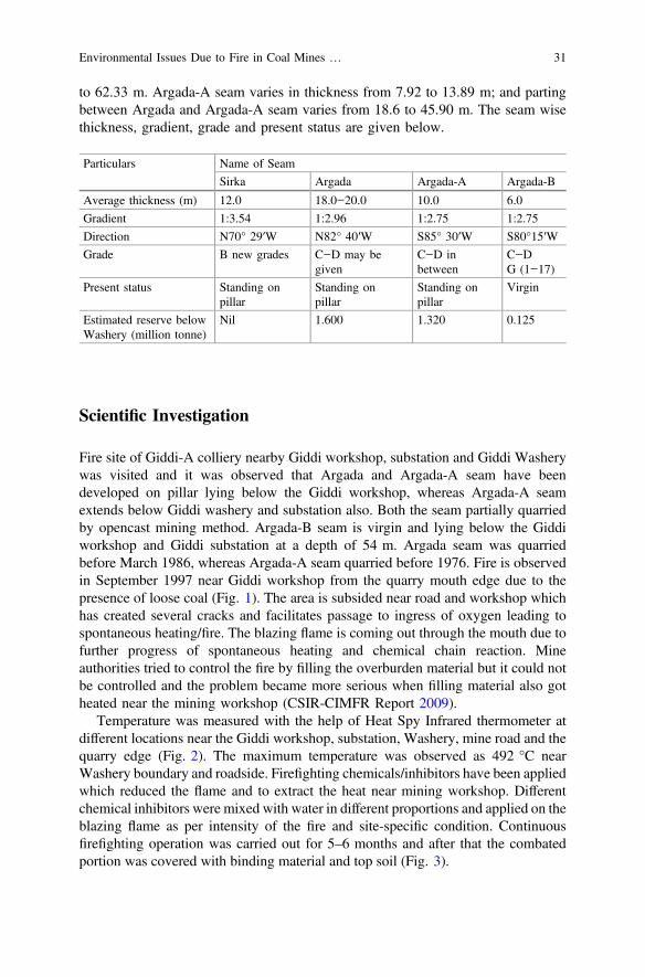
to 62.33 m. Argada-A seam varies in thickness from 7.92 to 13.89 m; and partingbetween Argada and Argada-A seam varies from 18.6 to 45.90 m. The seam wisethickness, gradient, grade and present status are given below.
Particulars Name of Seam
Sirka Argada Argada-A Argada-B
Average thickness (m) 12.0 18.0−20.0 10.0 6.0
Gradient 1:3.54 1:2.96 1:2.75 1:2.75
Direction N70° 29′W N82° 40′W S85° 30′W S80°15′W
Grade B new grades C−D may begiven
C−D inbetween
C−DG (1−17)
Present status Standing onpillar
Standing onpillar
Standing onpillar
Virgin
Estimated reserve belowWashery (million tonne)
Nil 1.600 1.320 0.125
Scientific Investigation
Fire site of Giddi-A colliery nearby Giddi workshop, substation and Giddi Washerywas visited and it was observed that Argada and Argada-A seam have beendeveloped on pillar lying below the Giddi workshop, whereas Argada-A seamextends below Giddi washery and substation also. Both the seam partially quarriedby opencast mining method. Argada-B seam is virgin and lying below the Giddiworkshop and Giddi substation at a depth of 54 m. Argada seam was quarriedbefore March 1986, whereas Argada-A seam quarried before 1976. Fire is observedin September 1997 near Giddi workshop from the quarry mouth edge due to thepresence of loose coal (Fig. 1). The area is subsided near road and workshop whichhas created several cracks and facilitates passage to ingress of oxygen leading tospontaneous heating/fire. The blazing flame is coming out through the mouth due tofurther progress of spontaneous heating and chemical chain reaction. Mineauthorities tried to control the fire by filling the overburden material but it could notbe controlled and the problem became more serious when filling material also gotheated near the mining workshop (CSIR-CIMFR Report 2009).
Temperature was measured with the help of Heat Spy Infrared thermometer atdifferent locations near the Giddi workshop, substation, Washery, mine road and thequarry edge (Fig. 2). The maximum temperature was observed as 492 °C nearWashery boundary and roadside. Firefighting chemicals/inhibitors have been appliedwhich reduced the flame and to extract the heat near mining workshop. Differentchemical inhibitors were mixed with water in different proportions and applied on theblazing flame as per intensity of the fire and site-specific condition. Continuousfirefighting operation was carried out for 5–6 months and after that the combatedportion was covered with binding material and top soil (Fig. 3).
Environmental Issues Due to Fire in Coal Mines … 31
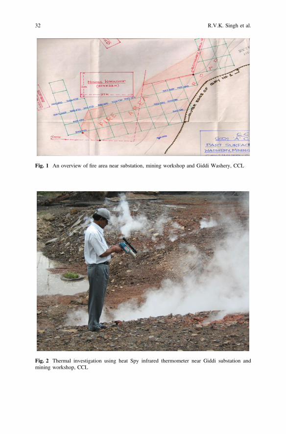
Fig. 1 An overview of fire area near substation, mining workshop and Giddi Washery, CCL
Fig. 2 Thermal investigation using heat Spy infrared thermometer near Giddi substation andmining workshop, CCL
32 R.V.K. Singh et al.

Results and Discussion
During thermal investigation, it was found that fire was present in most of theportion nearby area of roadways and substation; and fire was under blazing con-dition near Giddi workshop. Temperature was in the range of 265–307 °C atworkshop and 492 °C observed near the washery boundary towards roadside. Afterapplication of firefighting chemical inhibitors/additives temperature reduced to therange 35–46 °C. Combated fire surface was treated with different binding materialsto minimise the ingress of air which was applied on an area of 3750 m2 on surfacearea using 7250 m3 of topsoil. Detailed thermal profile was marked on surface layout before application of fire fighting chemicals to the final surface sealing operationas per requirement. Finally, temperature was found to be near about ambient aftersurface sealing. Mine authorities were trained for application of firefightingchemicals. Suggestion was also given for making two benches using top soil inquarry side for checking the penetration of air from the mouth of gallery andblanketed area should be compacted time to time. Early implementation of thecontrol and combating technology has given successful result for control of fire near
Fig. 3 Fire combated portion treated with binding material with top soil near mining workshopand Giddi power substation, CCL
Environmental Issues Due to Fire in Coal Mines … 33
Giddi workshop and substation. After controlling the fire, the valuable nationalproperties like Giddi substation and washery have been salvaged and the envi-ronment was also protected from the release of noxious and other greenhouse gases.
Suggestions
As per studies carried out during the project work and site-specific fire condition,the following preventive and control measures are suggested for control of fire andprotection of environment:
1. Thermal monitoring should be carried out using Heat Spy Infrared thermometerregularly for detection of fire, so that immediate control measures can beplanned as per site situation.
2. Fire should be combated by application of firefighting chemical additives/inhibitors for suppressing the fire and extracting the heat and it should becontinued till the temperature reduces to ambient level.
3. Dozing/compaction is very much essential in the compacted area after someinterval to minimise the air ingress.
4. Minimum two benches should be formed from bottom to top using top soil inquarry side for checking the ingress of air from the mouth of gallery to save themine roadways, washery and substation.
Conclusion
After carrying out a scientific investigation for control of fire near my workshop andsubstation, it is concluded that speedy implementation of the control and combatingtechnology has given successful results. After control of fire, the valuable nationalproperty has been saved. Environment was also protected from the release ofnoxious gases. Under these circumstances, direct application of firefighting chem-ical inhibitors will be much effective for suppression of flame, extraction of heat andcooling the hot mass. Author has taken a new R&D Project under PlanningCommission (earlier); presently, Niti Aayog Research work of this project is beingcontinued and rigorous laboratory work is going on.
Acknowledgements Authors are grateful to Dr. P.K. Singh, Director, CSIR-Central Institute ofMining & Fuel Research, Dhanbad for giving permission to present the paper. Authors are alsograteful to the management and officials of Giddi-A colliery for providing all facilities and fullcooperation for carrying out the project work. Thanks are due to the staff of Mine Fire Division ofCSIR-CIMFR for their assistance in various stages during laboratory and field work. Viewsexpressed in this paper are of authors and not necessarily of CSIR-CIMFR.
34 R.V.K. Singh et al.

References
Banerjee SC (1985) Spontaneous combustion of coal and mine fire. Oxford & IBH Publishing Co.Pvt. Ltd., New Delhi
Central Institute of Mining & Fuel Research (CIMFR) Unpublished Project Report (2009)Scientific investigation for control of fire nearby Giddi. A workshop, Giddi washery plant andadvice thereof, CCL Project No. GC/MS/156/2007-08
Finkelman RB (2004) Potential health impacts of burning coal beds and waste banks. Int J CoalGeol 59:19–24
Singh RVK (2013) Spontaneous heating and fires in coal mines. Procedia Eng 62:78–90
Environmental Issues Due to Fire in Coal Mines … 35
Redevelopment of Urban Slum Dwellings:Issues and Challenges
Dhrupad S. Rupwate, Rajnit D. Bhanarkar, Vishakha V. Sakhareand Rahul V. Ralegaonkar
Abstract Urbanization has created a large housing demand of urban poor.Although different stakeholders are involved, there is a challenge to meet theredevelopment of urban slum dwelling projects in an effective manner. The conceptis discussed with a case study of a slum in Nagpur City. Physical data was collectedfrom stakeholders (construction material choices and cost incurred) and site mon-itoring (indoor temperature and light). The study revealed the possible issues andchallenges related to project execution, i.e. resource and time management. Theoutcome of the study is to suggest a suitable strategy for improving the functionalityof the project to increase the speed and conserve the resources that ultimatelybenefit government as well as end user.
Introduction
Urbanization can be termed as by product of economic and social development.Rapid advancements in science and technology have made remarkable changes inthe settlement pattern and living habits of the people. Urban areas are viewed asplaces with potential for greater economic opportunities and improved standard ofliving in urban areas attracts rural migrants which are leading to the emergence ofslums. Slums are the products of failed policies, bad governance, corruption,inappropriate regulation, dysfunctional land markets, unresponsive financial sys-tems and a fundamental lack of political will (Sufaira 2013).
World’s population is projected to be 8.1 billion by 2030 out of which 5 billion(61%) of world’s population will live in cities and 90% of growth will be indeveloping countries (UNFPA 2000). Indian urban population will increased to
D.S. Rupwate (&) � R.D. Bhanarkar � V.V. Sakhare � R.V. Ralegaonkar (&)Department of Civil Engineering, Visvesvaraya NationalInstitute of Technology, Nagpur 440010, Indiae-mail: [email protected]
R.V. Ralegaonkare-mail: [email protected]
© Springer Nature Singapore Pte Ltd. 2018V.P. Singh et al. (eds.), Environmental Pollution, Water Scienceand Technology Library 77, https://doi.org/10.1007/978-981-10-5792-2_4
37

36% by 2025. The trends in growth of urban population can be observed fromFig. 1. And the share of urban population will be as 68.7% of urban populationlives in class I cities, 27.8% in medium cities and 9.4% in small towns (Fig. 1). Thisshows the pace of rapid urbanization in India and challenge to reach needs ofgrowing population.
Problems reinforced with urbanization can be noted as poverty, unemployment,education (illiteracy), crime, waste generation, environmental degradation, pollu-tion, health problems, safety and security, infrastructure and amenities, lack ofcommunity sense, social polarity, HOUSING (Squatters and Slums). This paperdeals with the issue of housing urban poor and redevelopment of urban slumdwellings.
Background and Need of Study
A slum is defined by the United Nations agency UN-HABITAT, “is a run-downarea of a city characterized by substandard housing and squalor and lacking intenure security”. Slums were initially viewed as nothing more than nuisance; theeconomic contribution of slum dwellers was never acknowledged. Slums weretreated as refuse of the cities and demolished often for cleaner cities. They were notconsidered for planning and marked as ‘vacant land’ in Indian city’s Master plans.Till 1970 slums were treated as illegal squatters. Needs of these Informal habitatsare not considered for planning various amenities such as housing and other sup-porting services while subsidized housing is provided for poor through schemeslike Subsidized Industrial Housing Scheme (SIHS) 1952, EWS HousingScheme and LIG Housing Scheme (LIGHS) 1954 (Bouddha Charumitra). After1970 slum improvement works have come up as slums reappeared after demolitionand demolitions are termed as in human. India’s Fifth 5-year plan focused onphysical improvement of slums. Environmental Improvement in Urban Slums(EIUS) in 1972−73 Integrated with Urban Development Programme (IUDP)improved infrastructure services of notified slums. After 1990s a new concept hasevolved. The underlying land of the slums was treated as a resource incentive FSI isgiven for constructing tenements for sale in open market. Profits generated from thesale of these tenements used for cross-subsidizing the free houses to the slum
0.00%
10.00%
20.00%
30.00%
40.00%
1901 1931 1951 1971 1981 2001 2025
% of urban population
% of urbanpopula on
Fig. 1 Growth of urbanpopulation in India. SourceUNFPA 2000
38 D.S. Rupwate et al.

dwellers. Special autonomous Slum Rehabilitation Authority was established toameliorate the problems of slums dwellers. The Government of Maharashtraappointed a committee chaired by the Chief Secretary of Maharashtra, to devise ascheme to rehabilitate slum dwellers (Fig. 2).
Housing Scenario in India
India is passing through a phase of acute housing shortage like any other devel-oping country. Housing in India varies greatly and reflects the socio-economic mixof its vast population. In the last decade, there has been tremendous growth in thecountry’s housing sector, along with demographic changes, rise in income, growthin the number of nuclear families and urbanization.
According to 11th plan estimate housing requirement in India can be noted as26.53 million units for 75.01 million households.
Requirements to Achieve the Vision by 2022
By 2022, India needs to develop about 11 crore housing units requiring investmentof more than USD 2 trillion or about USD 250–260 billion annual investment until2022. Urban housing is to account for about 85–90% of the total investments; thefocus should be on affordable urban houses, which is 70% of the total urbanhousing requirement. About 1.7–2.0 lakh hectare of land is expected to be requiredto fulfil urban housing need by 2022. About 70% of the housing needs till 2022should be concentrated in ten states. These states are Uttar Pradesh, Bihar,Maharashtra, West Bengal, Madhya Pradesh, Andhra Pradesh, Telangana,Rajasthan, Tamil Nadu and Karnataka (Urban Housing Shortage 2012–17).
The state of Maharashtra is witnessing rapid urbanization. As per NationalCensus 2011, Maharashtra has the highest urban population of more than 5 crore.By the year 2022 the housing need in Maharashtra is expected to grow to 1 crore
54.06%
18.74%
46.55% 43.88%35.42% 33.32% 32.48%
20.89% 19.39% 18.88% 17.23% 14.42%13.46% 10.02%
24.13%
% of popula on in slums
Fig. 2 Percentage of population living in slums of Indian cities
Redevelopment of Urban Slum Dwellings: Issues and Challenges 39

housing units (50 lakh each in urban and rural), with more of the housingrequirements in the urban regions. The State Government has resolved to provide19 lakh houses by the year 2022, with the main thrust for Economically WeakerSection (EWS), Lower Income Group (LIG) and Middle Income Group(MIG) housing. This time-bound objective has given a dimension of urgency torevise the earlier government housing policy. Thus a new housing policy needs tobe in place in view of the new dynamic scenario by defining the role of the State asa Facilitator, Catalyst, Builder and Regulator. As per the census of 2011, out of3.36 crore census houses 2.98 crore houses were occupied in the State. The pop-ulation of the rural houses in the total census houses was 52.2 and 47.8% in urbanareas. A survey by the National Housing Bank (NHB) reveals a national housingshortage of 18.78 million in 2012–13, with Maharashtra’s shortage estimated at1.94 million houses. Urbanization in Maharashtra has increased from 42.43 to45.23% in 2001–2010. All indicators project an ever increasing trend of urban-ization. All indicators indicate the gravity of the housing deficit in the State par-ticularly in the affordable housing segment and hence affordable housing needs abig push (Source: New Housing Policy and Action Plan 2015).
Strategies for Increasing Supply of Affordable Housing
• Government lands for affordable housing.• Public–private partnership.• Employee housing.• Affordable housing scheme.• Inclusive housing in all housing projects.• Rental housing.• Affordable housing through Town Planning Scheme (TPS)/Special Township
(STS) on private.• And by CIDCO.• Townships/Industrial Townships/IT Townships by private developers.
Strategies for Optimum Use of Existing Land Resourcesby Encouraging Redevelopment
• MHADA housing initiative.• Redevelopment of MHADA transit camp.• Redevelopment of cessed building.• Urban renewal scheme.• The Bombay Development Department crawls redevelopment.• Slum redevelopment: Slum up gradation, rehabilitation and redevelopment.• Slum declaration and acquisition of private slums.• Scheme for D-Class Municipal Corporation and A-Class Municipalities.
40 D.S. Rupwate et al.

• Housing for conservancy workers.• Land acquired for Special Economic Zone (SEZ) by private developers.• Development of land owned by Central Government/Central Government
Undertaking such as LIC/RBI/ESIC, etc.• Smart city centres in cities with population of more than 10 lakhs.
Strategies for Improving Quality of Life, Overall LivingStandards with Concern for Environment
• Conservation of water, environment and heritage structures.• Preventing unauthorized/informal housing
Strategies for Ease of Doing Business
• Use of Information Technology (IT) by ULBs.• Dematerialisation of Transferable Development Rights (TDR).• Using of land as collateral security.• Built-up area in lieu of development charges.• Reimbursement
Objectives of the Study
1. Bring to light the issues and challenges related to the redevelopment projects.2. Providing a solution for timely completion of projects through resource allo-
cation methods.3. To study the impact of new technology bricks on the cost of the project.
Methodology
Study Area
Nagpur with total 446 slums out of which 289 are notified as authorized slums. Thecity has nearly 36% of its population living in these slums. Nagpur stands as fourthlargest slum population in the country. It is facing the challenge of providinghousing to the slum population. According to City Sanitation Plan (CSP) preparedby Nagpur Municipal Corporation’s health department (sanitation) almost 8.58 lakhpeople living in 1.41 lakh structures in slums have poor basic facilities.
Redevelopment of Urban Slum Dwellings: Issues and Challenges 41
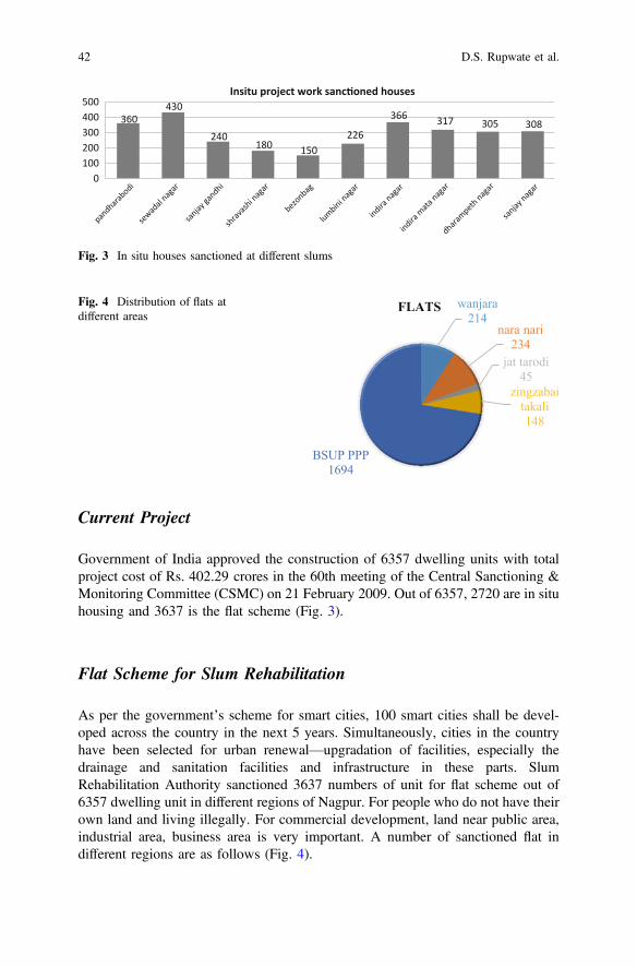
Current Project
Government of India approved the construction of 6357 dwelling units with totalproject cost of Rs. 402.29 crores in the 60th meeting of the Central Sanctioning &Monitoring Committee (CSMC) on 21 February 2009. Out of 6357, 2720 are in situhousing and 3637 is the flat scheme (Fig. 3).
Flat Scheme for Slum Rehabilitation
As per the government’s scheme for smart cities, 100 smart cities shall be devel-oped across the country in the next 5 years. Simultaneously, cities in the countryhave been selected for urban renewal—upgradation of facilities, especially thedrainage and sanitation facilities and infrastructure in these parts. SlumRehabilitation Authority sanctioned 3637 numbers of unit for flat scheme out of6357 dwelling unit in different regions of Nagpur. For people who do not have theirown land and living illegally. For commercial development, land near public area,industrial area, business area is very important. A number of sanctioned flat indifferent regions are as follows (Fig. 4).
360430
240180 150
226
366 317 305 308
0100200300400500
Insitu project work sanc oned houses
Fig. 3 In situ houses sanctioned at different slums
wanjara214
nara nari234
jat tarodi45
zingzabaitakali148
BSUP PPP1694
FLATSFig. 4 Distribution of flats atdifferent areas
42 D.S. Rupwate et al.

Detail of Money Contribution
The share of GOI, GOM, NMC and beneficiary is as given below:
Total projectcost (in lakhs)
Central share(in lakhs)
State share (in lakhs) NMC shareshare (in lakhs)
Beneficiaryshare
40229.26 18286.03 10142.80 + 3657.21(other charges)
5943.66 2199.55
In this project the cost for one in situ house = 449,724.00 Rs.
Central share for one house (50%) = 224,862 Rs.State share for one house (30%) = 134,917 Rs.Beneficiary share in one house (11%) = 49,469 Rs.Local Body share for one house (9%) = 40,475 Rs.
Total carpet area for one house (sq. feet) = 270–320 sq. feet for a different typeof house.
Cost per sq. feet = 1405–1665 Rs.
Sanctioned Cost of Single House Type A
The completion of a house was carried out in four stages. Specifications of workdone and the estimate according to schedules have been presented in Table 1. Thepercentage composition is mentioned as remarks. The progress report and detailedbar charts of work procedure are provided in the later sections.
Cost requirement in four stages is given in Table 1.One of the sites of ongoing SRA projects in Nagpur that is Pandharabodi has
been chosen for study assuming that similar conditions are prevailing in other sitesas well, as there are limitations of time and other parameters.
Pandharabodi Area
Sanctioned in situ houses details are below:
• Name of Slum: New Pandharabodi.• No of Dwelling Units: 360 Dues nos.• Carpet area of each DUS: 250–300 sq. feet.• Built-up area of each DUS: 270–350 sq. feet.• Contractor appointed: 2• Completed DUS: 150 dunes• In progress DUS: 55 no. (Fig. 5)
Redevelopment of Urban Slum Dwellings: Issues and Challenges 43
Different plans are prepared by NMC for in situ housing, according to plot sizeavailable.
Problems on Site During Construction
• Time overrun• Material quality• Scarcity of skilled labour• Problems during operation.
Time Overrun
• Out of 15 houses all are taking more than 6 month for completing work.• For construction of one house 50–60 days are sufficient.• In group construction it can be completed in 40–50 days.• First Government gives a contract of 75 dwelling units out of 166 units for the
time of 6 month on 16 November 2013.
Table 1 Cost requirements at different stages
S.No.
Components As perschedule
Remark(%)
1 STAGE I: Complete work up to plinth including plinth slab andsintex tank
140,808.77 31.31
2 STAGE II: Complete RCC frame structure up to RCC slab 77,607.01 17.26
3 STAGE III: Complete brick work of 4″ and 6″, internal–external plaster, doors, window, ventilators, kitchen otta, etc.
1,45,330.25 32.32
4 STAGE IV: Full and final bill including painting, tiles,plumbing and electrical fitting extra items complete
85,978.56 19.121
5 TOTAL (Rs.) for type A unit 449,724.59 100
Difference 449,724.59
PANDHARABODI SITE (360 HOUSES)
DISHA CONSTRUCTION 166 HOUSES
75 HOUSES IN 1ST 6 MONTH(1 JAN 14 TO 31 MAY 14)
91 HOUSES IN NEXT 6 MONTH(1JUNE 14 TO 31 DEC14)SAJID
CONSTRUCTION198 HOUSES
Fig. 5 Flow chart of project for pandharabodi area
44 D.S. Rupwate et al.

Causes of Time Overrun
• Resource Problem.• Dispute between owner and contractor.• Poor time management.• Coordination between Govt. authority and contractor.• Rework and design changes.• Delay in revised estimate.• Delay in handing over site to contractor by owner.• Bad weather condition.• Shortage of human resources.• Shortage of material on site.
Material Quality and Quantity
• Delay of construction due to lack of materials• Material quality is not tested as recommended as per IS guidelines.• Unsatisfactory methods of testing bricks and sand are followed.• Reinforcement and bar bending works are not up to mark.• Materials were not stored properly and dumped along roadside• Bricks are not watered and improper construction methods are followed (Fig. 6).
Scarcity of Skilled Labour
The following graphs will give the detailed explanation about the actual number oflabourers required to complete the work on time versus the number of labourersemployed which again led to stalling of work (Fig. 7).
Fig. 6 Aggregates are mixed with improper graded stones and last picture shows poor mixing ofconcrete. Source Authors
Redevelopment of Urban Slum Dwellings: Issues and Challenges 45

On the basis of work, potential of workers and quantity required for differentactivity requirements of human resources are calculated. Time required for par-ticular activity and calculation of skilled, semiskilled and unskilled labour areevaluated (Fig. 8).
The human resources requirements from first day to 40 days are displayed. Thefollowing chart gives inflation in demand of human resources for the designedresult. The buffer is required for healthy progress of project. For reduction of timeand human resources the group construction is very important.
Actual labour requirement for single house is 40 working days (Fig. 9).It can be observed from the charts that it is imperative to use resource
levelling/allocation techniques. This deep fluctuation damages the work order. Italso becomes difficult to plan things for future endeavours. Planning is a primeaspect when handling such projects.
0 1 2 3 4 5 6 7excava�on of trenches
foo�ng
plinth beam
column up to plinth level
slab
pain�ng
sanitary, electrical and finishing work
no of days
Fig. 7 Activities and time requirement
05
101520253035 mason labor carpenter + barbender bhis�
Fig. 8 Activities and human resources requirement
46 D.S. Rupwate et al.

Problems During Operation
• Being a government project, it has provided only a single site engineer for a vastarea due to which there was not enough inspection of site leading to dissatis-factory work.
• Daily reports were not submitted as a result of which pending work kept pilingon and caused wastage of time the next day.
• Improper storage of materials which lead to misuse and wastage brought workto a standstill on some days (rainy season).
• During the site inspection it was noticed that site engineer responsible left thejob for a month and the head mason lead the work of advising and supervising,which in turn again lead to poor quality of work.
• Lack of adequate sanitation facilities for workers.• Interference of owners and general public in day-to-day activities, the residents
interfered in the work demanding small changes in the activities which ham-pered the progress of the work (Fig. 10).
• Non-compliance to the approved drawings by SRA and challenging and dis-rupting the work of workers by the owners. Water closets provided were aes-thetically not acceptable to the people as they were part of living room as shownin Fig. 11.
0
5
10
15
20
25
0 5 10 15 20 25 30 35 40 45
labo
r req
uire
men
t
days
Fig. 9 Human resources require per day for single house
Fig. 10 Seepage of water from joint of beam and brickwork. Source Authors
Redevelopment of Urban Slum Dwellings: Issues and Challenges 47

• Improper drainage and open drains leading to stoppage of work.• Seepage of water from recently constructed houses. The joints and beams of
brickwork had water seeping through it just after a month it was constructed(image below).
• Delay in sanctioning of money and resources.
Grouping of work
Using software Primavera activity chart has been prepared for a single house asshown in Fig. 12. It can be seen that the activity has started on 5 May and ended 24June 2015, i.e. 50 days for single house. Details of construction work have beenshown in bar chart (Fig. 13).
Construction work for 8 houses was started simultaneously. Activity chart andbar chart for 8 houses have been prepared by primavera software as shown inFigs. 14 and 15; it can be seen that the work was started on 2 January 2014 andcompleted on 14 March 2014, i.e. 72 days.
It is evident that the construction of 8 houses together as group is time savingand efficient.
Work Breakdown Structure for 75 Houses
See Fig. 16.
Fig. 11 Plan showing closet
48 D.S. Rupwate et al.
Limitation
Grouping of houses for construction together was proved to be more timesaving; however, there are limitations upfront. The construction of 8 housesstudied was in a row, whereas the ongoing project has plots scattered all over
Fig. 12 Activity chart for one house
Fig. 13 Bar chart for one house
Redevelopment of Urban Slum Dwellings: Issues and Challenges 49
the slum. Government should be able to provide temporary residence for thedwellers so that grouping of houses can be done and the work would be fin-ished before time.
Fig. 14 Activity chart for 8 houses
Fig. 15 Bar chart for 8 houses
50 D.S. Rupwate et al.
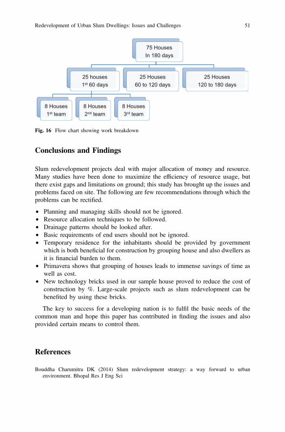
Conclusions and Findings
Slum redevelopment projects deal with major allocation of money and resource.Many studies have been done to maximize the efficiency of resource usage, butthere exist gaps and limitations on ground; this study has brought up the issues andproblems faced on site. The following are few recommendations through which theproblems can be rectified.
• Planning and managing skills should not be ignored.• Resource allocation techniques to be followed.• Drainage patterns should be looked after.• Basic requirements of end users should not be ignored.• Temporary residence for the inhabitants should be provided by government
which is both beneficial for construction by grouping house and also dwellers asit is financial burden to them.
• Primavera shows that grouping of houses leads to immense savings of time aswell as cost.
• New technology bricks used in our sample house proved to reduce the cost ofconstruction by %. Large-scale projects such as slum redevelopment can bebenefited by using these bricks.
The key to success for a developing nation is to fulfil the basic needs of thecommon man and hope this paper has contributed in finding the issues and alsoprovided certain means to control them.
References
Bouddha Charumitra DK (2014) Slum redevelopment strategy: a way forward to urbanenvironment. Bhopal Res J Eng Sci
75 HousesIn 180 days
25 houses1st 60 days
8 Houses1st team
8 Houses2nd team
8 Houses3rd team
25 Houses 60 to 120 days
25 Houses120 to 180 days
Fig. 16 Flow chart showing work breakdown
Redevelopment of Urban Slum Dwellings: Issues and Challenges 51

Sufaira C (2013) Socio economic conditions of urban slum dwellers in kannur municipality.IOSR J Humanit Soc Sci (IOSR-JHSS)
Times of India (2011) Sachin Dravekar, 27th June 2011Urban Housing Shortage (TG-12) (2012–17) Report of the technical group. Ministry of housing
and urban poverty alleviation (GoI) National buildings organisation.www.mhupa.gov.in
52 D.S. Rupwate et al.
Importance of Indoor EnvironmentalQuality in Green Buildings
Alisha Patnaik, Vikash Kumar and Purnachandra Saha
Abstract One of the primary aims of green buildings is to minimize negativeimpacts on their occupants by creating a healthy, comfortable and productiveindoor environment. The performance of indoor environment is described as indoorenvironmental quality (IEQ). The quality indoor environment can result inincreased occupant satisfaction, enhanced performance and productivity, reducedliability, marketing advantage and lower operations and maintenance costs. Theobjective of this paper is to study and discuss IEQ and its parameters and effect ongreen buildings. Building characteristics such as location, climate, design andconstruction contribute significantly to the IEQ. Thermal, visual and acousticcomfort and existing levels of volatile organic compounds (VOCs) help to measurethe IEQ of a green building.
Keywords Green buildings � Indoor environmental quality (IEQ)Building characteristics � Thermal comfort � Volatile organic compounds (VOCs)
Introduction
In recent times, global warming is a problem for every country and hence it isnecessary to deal with such problems and at the same time, develop sustainably.That is why nowadays, a lot of emphases is given to the design and construction ofgreen buildings. The construction of a green building is economical in the long runand at the same time beneficial to the environment (Pei et al. 2015).
A. Patnaik � V. Kumar � P. Saha (&)School of Civil Engineering, KIIT University, Bhubaneswar, Odisha, Indiae-mail: [email protected]
A. Patnaike-mail: [email protected]
V. Kumare-mail: [email protected]
© Springer Nature Singapore Pte Ltd. 2018V.P. Singh et al. (eds.), Environmental Pollution, Water Scienceand Technology Library 77, https://doi.org/10.1007/978-981-10-5792-2_5
53
A green building is constructed using environmentally friendly methods. Themain objective of green buildings is sustainability, energy efficiency and produc-tiveness, which reduce the effect of buildings on the environment. In the later partof 1980s, green building design began when the term “sustainability” was defined atthe UN World Commission on Environment and Development (1987). The UnitedStates (US) and Europe first started the design and certification of green buildings inthe earlier part of 1990s. In United Kingdom, BREEAM (BRE EnvironmentalAssessment Method) was developed to certify green buildings, likewise US, Francehad also developed methods for certification of green buildings. Consequently, allthe countries across the globe started making their own code and design specifi-cations for construction of green buildings. The design methodologies adoptedvaried according to the environmental conditions of that particular area (Wei et al.2015). Buildings use 30–40% of total worldwide primary energy (Holopainen et al.2015). The energy used for the construction of green buildings is approximatelyequal to 20–40% of the total emission of harmful greenhouse gases. By the con-struction of energy efficient buildings, the emission of these harmful gases can bereduced (Wells et al. 2015).
A wide variety of techniques is used for the construction of energy efficientbuildings. Some examples of these technologies are air tightness, proper insulation,heat recuperation and superior window. Some of the techniques used to preserve theenergy of a building like air tightness can cause poor ventilation resulting in inferiorquality of air inside the building (Langer et al. 2015).
According to the World Health Organization (WHO), “Health is a state ofcomplete physical, mental, and social well-being and not merely the absence ofdisease or infirmity” (WHO 1999; Bluyssen and Cox 2002). Studies have shownthat most people living in urban areas spend approximately 80% of their total timeinside a building. So poor quality and pollution of indoor air causes many problemsin the health of people and sometimes triggering many diseases (Asadi et al. 2013).
In the design of IEQ of a building, various equipment are utilized for luminance,sound system, temperature control and other purposes. Providing quality indoorenvironment, while at the same time, making the building energy efficient,environment-friendly (by reducing greenhouse gas emission) is a process whichrequires proper balance between comfort providing systems and energy econo-mizing devices (Ncube and Riffat 2012).
There is a lot of focus on sustainable use of energy and maintaining IEQ. Theparameters which characterize IEQ are thermal comfortableness and IAQ (Indoorair quality) which is affected by the concentration of carbon dioxide and otherharmful compounds (Sarbu and Pacurar 2015).
Numerous studies have been carried out from the 1970s for understandingoccupant satisfaction with the comfort conditions in indoor environments (Crociataet al. 2012). In the US, twelve buildings were studied by Fowler and Rauch (2008);they stated that the residents of the buildings were concerned about the overall IEQ
54 A. Patnaik et al.

but were relieved with the acoustics and thermal performance of these buildings atlevels below national benchmarks. Paul and Taylor (2008) evaluated the IEQperception of the inhabitants between a conventional building and a green buildinglocated in a couple of Australian universities and did not observe a superior level ofcomfort among the inhabitants of the green building. In the UK, Leaman andBordass (2007) analysed occupant surveys from 177 buildings and reported ahigher rate for green buildings in the performance of ventilation and air qualitycompared to the level determined in conventional buildings. However, it was notedthat the indoor environment of the green buildings tended to be warmer, less dryand stuffier during the summer. In South Africa, Thatcher and Milner (2012)conducted a longitudinal comparison between the occupants in green buildingsversus conventional buildings, and concluded that the Green Star-accreditedbuilding did not increase the physical fitness, mental health or perceived produc-tivity of the occupants at a significant level (Liang et al. 2014).
Indoor Environmental Quality (IEQ)
A simplified definition of IEQ is the interior conditions of the building. In additionto quality of air, accessibility of sunlight, view of natural scenery, enjoyable con-dition of acoustics, thermal comfort and resident access to control lighting, thespace and dimensions of the room are also important. The availabilities of requiredtools, equipment and people are also important; so rather than focussing on one ortwo parameters, the building supervisors can increase the gratification of thebuilding inhabitants by taking into consideration all the different aspects of IEQ.Table 1 shows some of the general problems and their causes faced by buildingoccupants with regard to IEQ.
Quality indoor environment is a fundamental principle of green buildings. Itresults to increase in satisfaction of the residents, improved functioning, mer-chandising benefits, reduction of cost of functioning and maintaining the building.
While certifying a green building, IAQ is taken into consideration in almost allcases. Figures 1 and 2 show that the weightage of IAQ in the twenty points basedon the certification of green buildings is 7.5% worldwide. Some countries like USgive additional importance on IAQ in comparison to other nations. The approxi-mate contribution of IAQ to the certifying process of green buildings in differentcountries is shown in Fig. 1. The highest share of IAQ is 10.6% in Thailand, whileUS has 9.4%.
In schemes of green building, the IAQ is preferably maintained by supervisingemission sources, proper air circulation and assessing the indoor quantity of air. Thevarious phases of the lifespan of a building are covered by these three paths.Supervising emission source consists of choosing paints and other materials used in
Importance of Indoor Environmental Quality in Green Buildings 55
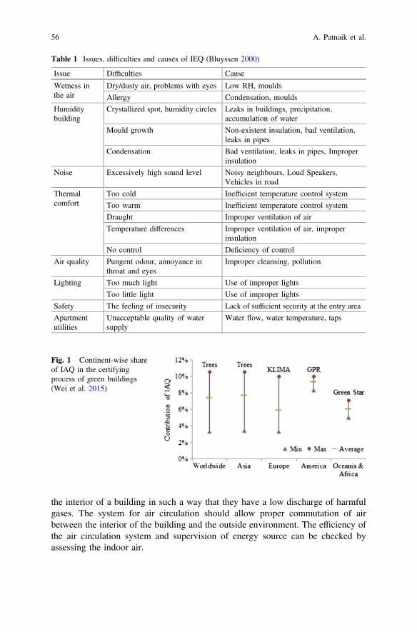
the interior of a building in such a way that they have a low discharge of harmfulgases. The system for air circulation should allow proper commutation of airbetween the interior of the building and the outside environment. The efficiency ofthe air circulation system and supervision of energy source can be checked byassessing the indoor air.
Table 1 Issues, difficulties and causes of IEQ (Bluyssen 2000)
Issue Difficulties Cause
Wetness inthe air
Dry/dusty air, problems with eyes Low RH, moulds
Allergy Condensation, moulds
Humiditybuilding
Crystallized spot, humidity circles Leaks in buildings, precipitation,accumulation of water
Mould growth Non-existent insulation, bad ventilation,leaks in pipes
Condensation Bad ventilation, leaks in pipes, Improperinsulation
Noise Excessively high sound level Noisy neighbours, Loud Speakers,Vehicles in road
Thermalcomfort
Too cold Inefficient temperature control system
Too warm Inefficient temperature control system
Draught Improper ventilation of air
Temperature differences Improper ventilation of air, improperinsulation
No control Deficiency of control
Air quality Pungent odour, annoyance inthroat and eyes
Improper cleansing, pollution
Lighting Too much light Use of improper lights
Too little light Use of improper lights
Safety The feeling of insecurity Lack of sufficient security at the entry area
Apartmentutilities
Unacceptable quality of watersupply
Water flow, water temperature, taps
Fig. 1 Continent-wise shareof IAQ in the certifyingprocess of green buildings(Wei et al. 2015)
56 A. Patnaik et al.
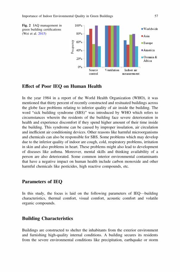
Effect of Poor IEQ on Human Health
In the year 1984 in a report of the World Health Organization (WHO), it wasmentioned that thirty percent of recently constructed and resituated buildings acrossthe globe face problems relating to inferior quality of air inside the building. Theword “sick building syndrome (SBS)” was introduced by WHO which refers tocircumstances wherein the residents of the building face severe deterioration inhealth and experience discomfort if they spend higher amount of their time insidethe building. This syndrome can be caused by improper insulation, air circulationand inefficient air conditioning devices. Other reasons like harmful microorganismsand chemicals can also be responsible for SBS. Some problems which may developdue to the inferior quality of indoor are cough, cold, respiratory problems, irritationin skin and also problems in heart. These problems might also lead to developmentof diseases like asthma. Moreover, mental skills and thinking availability of aperson are also deteriorated. Some common interior environmental contaminantsthat have a negative impact on human health include carbon monoxide and otherharmful chemicals like pesticides, high reactive compounds, etc.
Parameters of IEQ
In this study, the focus is laid on the following parameters of IEQ—buildingcharacteristics, thermal comfort, visual comfort, acoustic comfort and volatileorganic compounds.
Building Characteristics
Buildings are constructed to shelter the inhabitants from the exterior environmentand furnishing high-quality internal conditions. A building secures its residentsfrom the severe environmental conditions like precipitation, earthquake or storm
Fig. 2 IAQ management ingreen building certifications(Wei et al. 2015)
Importance of Indoor Environmental Quality in Green Buildings 57

and at the same time maintains a suitable and comfortable internal environment.According to Chatelet et al. (1998), the indoor environment of a freely floatingbuilding (a building without any air temperature control system) must not be moreuncomfortable than the external climate. This scheme is described in Fig. 3.
As per the type of clothes, residents ask for dissimilar temperatures in differentseasons. So the optimal temperature zone is higher in summer and lower in winter.The Curve for building A shows that it is well-insulated thermally, suitable devicesfor controlling solar energy and efficient air-circulating devices. During summerseason, it is protected from the heat waves but during winter season it can utilizethis solar energy to increase the indoor temperature. So luxury and comfort areprovided in the building by making minimum use of energy sources other than solarenergy. The amount of energy which is used for temperature control (i.e. cooling orheating) is saved in such buildings. The curve for building B shows that it does nothave appropriate thermal insulation and is unable to utilize solar energy effectively.So energy sources other than solar energy have to be used to control the internaltemperature of the building.
Thermal Comfort
In accordance with the ASHRAE/ANSI Standard 55-2010, thermal comfort may bedescribed as “that condition of mind which expresses satisfaction with the thermalenvironment and is assessed by subjective evaluation”. The perception of thermalcomfort may vary from person to person, any specific range of temperature cannotbe declared. One way to find out whether the inhabitants of the building are satisfiedwith the indoor thermal conditions is to go door-to-door and ask people, thusperforming a detailed survey in that building. The internal thermal conditions aregood if the majority of the residents (80%) are satisfied with the thermal conditions.
Fig. 3 Development in temperatures in a free-floating building in one year (Roulet 2001)
58 A. Patnaik et al.

The conditions which affect the thermal comfort can be categorized as personalfactors (type of clothing, physical condition) and environmental factors (moisture inair, temperature of air, velocity of wind). Both these factors play a vital part indetermining the thermal comfort of the building (Hua et al. 2014).
The situations responsible for the increase of internal temperature in a buildingare heat transfer from outside the structure and heat emitted from internal electricdevices (Nasir et al. 2011).
Another environmental factor is humidity which is defined as the quantity ofmoisture present at a particular place. The quantity of moisture is affected by thetemperature. The higher the temperature, the higher is the moisture content (Nasiret al. 2011).
For the growth of moulds wet surfaces are required. Low-temperature and humidair can contribute to the growth of moulds which deteriorate the IEQ (Nasir et al.2011). In single-paned windows there is a proper facility of air circulation and heatexchange between the internal and external environments of the building; hence,the walls which are improperly insulated have no risk of condensation on theirsurface. In case of double-paned windows with air-sealed glazing, there is mini-mum air circulation and heat exchange. So there is increased presence of indoormoisture and hence there is a risk of mould growth on walls which are improperlyinsulated.
Visual Comfort
Light and vision are related to each other; vision enables us to observe the natureand interact with others. So for the purpose of visual comfort, light is a necessity. Inlighting, proper balance of blaze and contrast is essential. Day lighting is theutilization of blaze-free sunlight for illuminating the indoor of a building and it isundeveloped in most architectural design due to lack of information of its useful-ness and depending on over-optimistic energy savings (as in simulations and blindusage) that are really met in open-plan offices. Lighting is of a paramount concernto the design of office space, as in a typical new building, it consumes up to 25% ofthe amount of energy required and this indirectly affects visual comfort which isone of the models of IEQ. The use of natural light is indeed an inevitable practiceinternationally, as it saves energy in buildings which involve bioclimatic passivesolar design. Although sustainability in the context of sustainable architecture hasbeen narrowed to ‘low energy’, energy performance boils down to energy efficiencyand IEQ. Research has shown that visual comfort relates today lighting researchsignificantly as it contributes to the well-being and performance of the users. Accessto natural daylight and fenestration with pleasant views contributes to the reductionin stress levels in an office environment, and research has also shown that mostpeople find natural lighting from day lighting better than fluorescent, incandescentlighting, help in psychological comfort and increase their productiveness; and it hasadvantages in our health and well-being. Day lighting is an element used to improve
Importance of Indoor Environmental Quality in Green Buildings 59
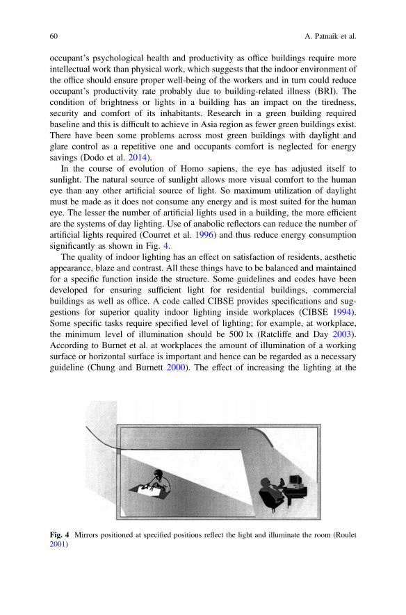
occupant’s psychological health and productivity as office buildings require moreintellectual work than physical work, which suggests that the indoor environment ofthe office should ensure proper well-being of the workers and in turn could reduceoccupant’s productivity rate probably due to building-related illness (BRI). Thecondition of brightness or lights in a building has an impact on the tiredness,security and comfort of its inhabitants. Research in a green building requiredbaseline and this is difficult to achieve in Asia region as fewer green buildings exist.There have been some problems across most green buildings with daylight andglare control as a repetitive one and occupants comfort is neglected for energysavings (Dodo et al. 2014).
In the course of evolution of Homo sapiens, the eye has adjusted itself tosunlight. The natural source of sunlight allows more visual comfort to the humaneye than any other artificial source of light. So maximum utilization of daylightmust be made as it does not consume any energy and is most suited for the humaneye. The lesser the number of artificial lights used in a building, the more efficientare the systems of day lighting. Use of anabolic reflectors can reduce the number ofartificial lights required (Courret et al. 1996) and thus reduce energy consumptionsignificantly as shown in Fig. 4.
The quality of indoor lighting has an effect on satisfaction of residents, aestheticappearance, blaze and contrast. All these things have to be balanced and maintainedfor a specific function inside the structure. Some guidelines and codes have beendeveloped for ensuring sufficient light for residential buildings, commercialbuildings as well as office. A code called CIBSE provides specifications and sug-gestions for superior quality indoor lighting inside workplaces (CIBSE 1994).Some specific tasks require specified level of lighting; for example, at workplace,the minimum level of illumination should be 500 lx (Ratcliffe and Day 2003).According to Burnet et al. at workplaces the amount of illumination of a workingsurface or horizontal surface is important and hence can be regarded as a necessaryguideline (Chung and Burnett 2000). The effect of increasing the lighting at the
Fig. 4 Mirrors positioned at specified positions reflect the light and illuminate the room (Roulet2001)
60 A. Patnaik et al.
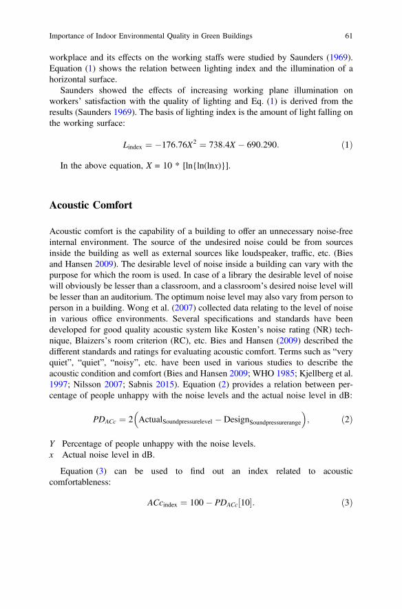
workplace and its effects on the working staffs were studied by Saunders (1969).Equation (1) shows the relation between lighting index and the illumination of ahorizontal surface.
Saunders showed the effects of increasing working plane illumination onworkers’ satisfaction with the quality of lighting and Eq. (1) is derived from theresults (Saunders 1969). The basis of lighting index is the amount of light falling onthe working surface:
Lindex ¼ �176:76X2 ¼ 738:4X � 690:290: ð1Þ
In the above equation, X = 10 * [ln{ln(lnx)}].
Acoustic Comfort
Acoustic comfort is the capability of a building to offer an unnecessary noise-freeinternal environment. The source of the undesired noise could be from sourcesinside the building as well as external sources like loudspeaker, traffic, etc. (Biesand Hansen 2009). The desirable level of noise inside a building can vary with thepurpose for which the room is used. In case of a library the desirable level of noisewill obviously be lesser than a classroom, and a classroom’s desired noise level willbe lesser than an auditorium. The optimum noise level may also vary from person toperson in a building. Wong et al. (2007) collected data relating to the level of noisein various office environments. Several specifications and standards have beendeveloped for good quality acoustic system like Kosten’s noise rating (NR) tech-nique, Blaizers’s room criterion (RC), etc. Bies and Hansen (2009) described thedifferent standards and ratings for evaluating acoustic comfort. Terms such as “veryquiet”, “quiet”, “noisy”, etc. have been used in various studies to describe theacoustic condition and comfort (Bies and Hansen 2009; WHO 1985; Kjellberg et al.1997; Nilsson 2007; Sabnis 2015). Equation (2) provides a relation between per-centage of people unhappy with the noise levels and the actual noise level in dB:
PDACc ¼ 2 ActualSoundpressurelevel � DesignSoundpressurerange� �
; ð2Þ
Y Percentage of people unhappy with the noise levels.x Actual noise level in dB.
Equation (3) can be used to find out an index related to acousticcomfortableness:
ACcindex ¼ 100� PDACc½10�: ð3Þ
Importance of Indoor Environmental Quality in Green Buildings 61

Volatile Organic Compounds (VOC)
Volatile organic compounds (VOCs) may be released from a variety of substanceswhich can be liquid or solid. Some harmful and toxic chemicals are also includedunder VOCs, and these toxic chemicals can cause deterioration of health ofoccupants. The amount of VOCs may be more inside the building as compared withthe external environment. VOCs are extensively utilized for various indoor oper-ations like painting, varnishing of furniture, perform cleansing operations, disin-fection of household items and other daily use products. During the tenure of theiruse, these products continue to emit harmful organic compounds which effect thehealth of the people inside the building (Table 2).
Table 2 Sources of VOCs and other harmful organic chemicals (Zabiegała 2006)
Sources of VOCs and other harmful organic chemicals
Interior of the building Exterior of the building
Source of origin is the building• Construction and design items• Repair and maintenance of building• Tools and machinery used inside the building• Actions of microorganisms
Chemical and oil industry
Originating from human and human activitiesinside the building• Household and consumption goods (hygieneproducts, aerosols)
• Processes connected to indoor cleaning• Cooking• Social functions• Interior flora• Human waste• Household (stoves, ovens)• Electronic machines
Small-scale business (printing,photocopying)
One time pollution sources• Break down of valves, pipelines, andpumps
• Leaks during loading/unloading• Safety valves• Cleaning of tanks
Emissions of biological origins• Green plants• Agriculture• Global ocean surface
Underground water and water bodies inthe earth’s surface
Grounds in which soil is polluted byhuman activities
Use and discarding unnecessary materials• Sewage treatment plants• Recycling of wastes
62 A. Patnaik et al.
Conclusion
The green building movement has revolutionized the way the architectural industryenvisions and designs buildings for the promotion of environmental sustainability.However, the majority of researchers till date have shared a strong focus on theeffectiveness of green buildings in energy-saving and less on keeping an IEQappropriate for indoor occupants.
IEQ is an important parameter in the majority of the certifying processes forgreen buildings all over the world. The average worldwide weightage to IEQ isabout 7.5%. VOCs and other harmful chemicals and pollutants are considered in themajority of the certifying process as they contribute to deterioration of health.Different certifications use different methods to control IEQ, almost all of them useair circulation or ventilation as a very important parameter. In 77% of the certifyingprocesses, controlling the source of release of pollutants has been included as animportant parameter. Assessing the air present in the interior of the building isconsidered in many of the certifying processes. It was observed that the method-ology used for measuring the indoor air was different in different cases. It can beconcluded that IEQ and its parameters are of paramount importance to make abuilding ‘green’. To achieve a sustainable building, designers and engineers need tofind the right balance between energy-saving imperatives and the quality indoorenvironment.
References
Asadi E, da Silva MCG, Costa JJ (2013) A systematic indoor air quality audit approach for publicbuildings. Environ Monit Assess 185:865–875
Bies DA, Hansen CH (2009) Engineering noise control, theory and practice, 4th edn. Spon PressBluyssen PM (2000) EPIQR and IEQ: indoor environment quality in European apartment
buildings. Energy Build 31(2):103–110Bluyssen PM, Cox C (2002) Indoor environment quality and upgrading of European office
buildings. Energy Build 34(2):155–162Chatelet A, Fernandez P, Lavigne P (1998) Architecture climatique, une contribution au
développement durable. Tome 2: Concepts et dispositifs, Aix-en Provence: EDISUDChung TM, Burnett J (2000) Lighting quality surveys in office premises. Indoor Built Environ
9:335–341CIBSE (1994) Code for interior lighting. The Chartered Institution of Building Services EngineersCourret G, Paule B, Scartezzini JL (1996) Anidolic zenithal openings: daylighting and shading,
Light Res Technol 28 (1)Crociata SD, Martellotta F, Simone A (2012) A measurement procedure to assess indoor
environment quality for hypermarket workers. Build Environ 47:288–299Dodo YA, Khandar MZ, Ahmad MH (2014) Correlating visual comfort with green building index
in an open plan office space el-nafaty Abbas Sa’id. Life Sci J 11(10)Fowler KM, Rauch EM (2008) Assessing green building performance: a post occupancy
evaluation of 12 GSA buildings. Department of Energy, WA, USAHolopainen R, Salmi K, Kähkönen E, Pasanen P, Reijula K (2015) Primary energy performance
and perceived indoor environment quality in Finnish low-energy and conventional houses.Build Environ
Importance of Indoor Environmental Quality in Green Buildings 63
Hua Y, Göçer O, Göçer K (2014) Spatial mapping of occupant satisfaction and indoorenvironment quality in a LEED platinum campus building. Build Environ 79:124–137
Kjellberg A, Tesarz M, Holmberg K, Landström U (1997) Evaluation of frequency-weightedsound level measurements for prediction of low-frequency noise annoyance. Environ Int23:519–527
Langer S, Bekö G, Bloom E, Widheden A, Ekberg L (2015) Indoor air quality in passive andconventional new houses in Sweden. Build Environ 93:92–100
Leaman A, Bordass B (2007) Are users more tolerant of ‘green’ buildings? Build Res Inf 35:662–673
Liang HH, Chen CP, Hwang RL, Shih WM, Lo SC, Liao HY (2014) Satisfaction of occupantstoward indoor environment quality of certified green office buildings in Taiwan. Build Environ72:232–242
Nasir ARM, Musa AR, Ani AIC, Utaberta N, Abdullah NAG, Tawil NM (2011) Identification ofindoor environmental quality (IEQ) parameter in creating conducive learning environment forarchitecture studio. Sciverse Sci Direct 20:354–362
Ncube M, Riffat S (2012) Developing an indoor environment quality tool for assessment ofmechanically ventilated office buildings in the UK—a preliminary study. Build Environ 53:26–33
Nilsson ME (2007) A-weighted sound pressure level as an indicator of short-term loudness orannoyance of road-traffic sound. J Sound Vib 302:197–207
Paul W, Taylor P (2008) A comparison of occupant comfort and satisfaction between a greenbuilding and a conventional building. Build Environ 43:1858–1870
Pei Z, Lin B, Liu Y, Zhu Y (2015) Comparative study on the indoor environment quality of greenoffice buildings in China with a long-term field measurement and investigation. Build Environ84:80–88
Ratcliffe M, Day T (2003) Improving office staff productivity while reducing carbon dioxideemissions. In: 2003 CIBSE/ASHRAE conference—building sustainability, value and profit
Roulet CA (2001) Indoor environment quality in buildings and its impact on outdoor environment.Energy Build 33(3):183–191
Sabnis GM (2015) Green buildings: contribution of concrete, 2nd edn. CRC PressSarbu L, Pacurar C (2015) Experimental and numerical research to assess indoor environment
quality and schoolwork performance in university classrooms. Build Environ 93(Part-2):141–154
Saunders JE (1969) The role of the level and diversity of horizontal illumination in an appraisal ofa simple office task. Light Res Technol 1:37–46
Thatcher A, Milner K (2012) The impact of a green building on employees’ physical andpsychological wellbeing. Work 41:3816–3823
Wei W, Ramalho O, Mandin C (2015) Indoor air quality requirements in green buildingcertifications. Build Environ 92:10–19
Wells EM, Berges M, Metcalf M, Kinsella A, Foreman K, Dearborn DG, Greenberg S (2015)Indoor air quality and occupant comfort in homes with deep versus conventional energyefficiency renovations. Build Environ 92(Part-2):331–338
WHO (1985) Indoor environment: health aspects of air quality, thermal environment, light andnoise
WHO (1999) Basic documents, 42nd edn. World Health Organization, GenevaWong LT, Mui KW, Hui PS (2007) A multivariate-logistic model for acceptance of indoor
environmental quality (IEQ) in offices, vol. 43, Department of Building Services Engineering,The Hong Kong Polytechnic University, Hong Kong, China, pp 1–6
World Commission on Environment and Development (1987) Our common future, chapter 2:towards sustainable development. Retrieved 7th Nov 2014
Zabiegała B (2006) Organic compounds in indoor environments. Pol J Environ Stud 15(3):383–393
64 A. Patnaik et al.
Meteorological Factors InfluencingDispersion of Vehicular Pollutionin a Typical Highway Condition
Rajni Dhyani and Niraj Sharma
Abstract Vehicular dispersion models, particularly highway dispersion models areused worldwide, including India, for assessment and management of air qualityalong the major roads/highways. However, dispersion of vehicular pollutants isinfluenced by various factors such as traffic, receptors and land use along withmeteorological factors. In the present study, CALINE4, a Gaussian-based vehicularpollution dispersion model has been used in Delhi, along Ring Road Corridor nearIndraprastha Park. Sensitivity analysis of CALINE4 model has been carried out foridentification and quantification of meteorological parameters, viz. wind speed,wind direction, mixing height and P–G stability class influencing the model’soutput. These input parameters in the model were systematically varied forassessing their influence on model’s output, i.e. predicted concentrations. The studyrevealed that wind speed and wind directions have significant impact on dispersionof vehicular pollutants as compared to mixing height and stability class.
Introduction
Use of these highways dispersion models has increased over the years in policysupport for large road infrastructure projects (Bennett et al. 2013). Accuracy ofvarious highways dispersion models like any other the air pollution dispersion modelresults relies on the accuracy of its input parameters. It is important to identify thoseinput variable(s) (or combination of two or more inputs) which significantly influ-ences the output of the model most. In order to establish the importance of individualparameters in the model, models are subjected to sensitivity analysis under wide
R. Dhyani (&)Environmental Science Division, Academy of Scientific and Innovative Research (AcSIR),CSIR-Central Road Research Institute, New Delhi 110025, Indiae-mail: [email protected]
N. SharmaEnvironmental Science Division, CSIR-Central Road Research Institute,New Delhi 110025, India
© Springer Nature Singapore Pte Ltd. 2018V.P. Singh et al. (eds.), Environmental Pollution, Water Scienceand Technology Library 77, https://doi.org/10.1007/978-981-10-5792-2_6
65
range of conditions. Sensitivity analysis indicates how much of the overall uncer-tainty in the model predictions is associated with the individual uncertainty in eachmodel input(s) (Nossent et al. 2011; Zhan and Zhang 2013). Sensitivity analysis ofthe model is carried out to identify key variables in modelling system and helps infocussing on collection and estimation of those influencing parameters (Trueman2007). The CALINE4 (Benson 1989) line source dispersion model is used exten-sively throughout the world including India for predicting air quality along highwaysunder prevailing traffic and meteorological conditions. CALINE4 model requiresrelatively lesser expertise and has comparatively less input data requirement thanother vehicular dispersion models (Gimson et al. 2010). In India, CALINE4vehicular pollution dispersion model is extensively use for prediction of air qualityalong the highway corridors (Sharma et al. 2013; Dhyani et al. 2013; Majumdar et al.2009; Lao 2010). However, few studies have been carried out in India regardingvalidation and performance evaluation of CALINE4 under mix traffic conditions(Majumdar et al. 2010; Dhyani et al. 2014; Konar and Chakrabarty 2012). Most ofthe vehicular pollution dispersion models like CALINE4 used in India are developedin western countries for their traffic and meteorological conditions. Further, mostmodels developed in western countries (homogeneous traffic conditions and mete-orological conditions) are unable to do fair representation real-world complexities(e.g. mixed traffic conditions) common (in the form of meteorological and trafficcondition) are still unresolved (Karim et al. 1998). Sensitivity analysis is animportant tool to examine model performance in the presence of uncertainty in themodel input variables and development of new models.
Few studies have been carried out to identify the influential parameters inCALINE4 model and for further improvement in new models. Benson (1989)comprises most of its input parameters of CALINE4 model, such as, P–G stabilityclass, mixing height, wind speed, wind direction, highway width and highwaylength; under homogeneous traffic and open terrain conditions for which model hasbeen developed. Sripraparkorn et al. (2003) used CALINE4 and reported that winddirection, traffic volume receptor heights and composite emission factors affect theoutput of the model most and atmospheric stability and mixing height affect theoutput least. Batterman et al. (2010) developed the multiplicative emission anddispersion sub-models by identifying the influential variables through sensitivityanalysis of MOBILE6.2 (USEPA 2004) and CALINE4 model, respectively. Thesub-model (a reduced-model form of CALINE4) did not include the mixing heightand stability class due to their minor contribution in CALINE4 output (i.e. predictedconcentrations). However, no such study has been carried out under mixed trafficconditions. In the present study, an effort has been made to identify the inputparameters, which influence the output of the CALINE4 model most under mixtraffic condition.
66 R. Dhyani and N. Sharma
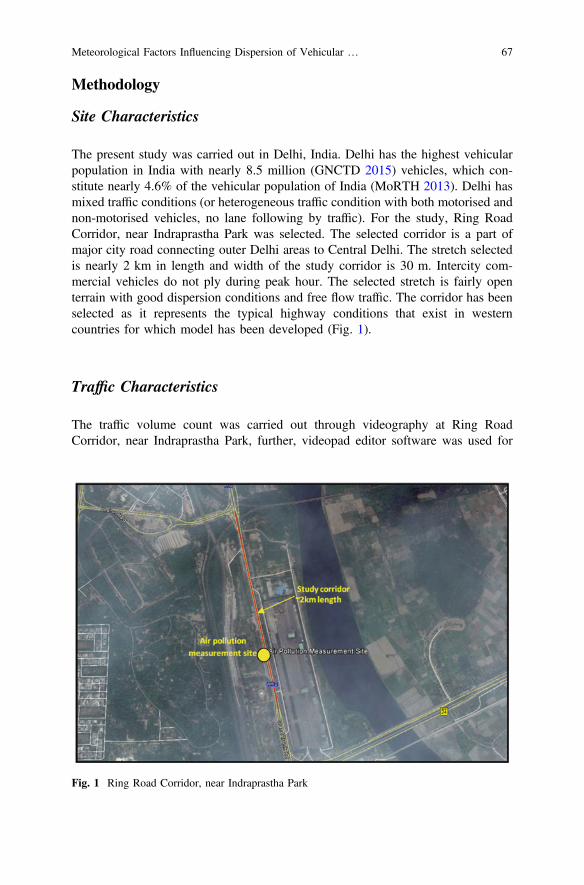
Methodology
Site Characteristics
The present study was carried out in Delhi, India. Delhi has the highest vehicularpopulation in India with nearly 8.5 million (GNCTD 2015) vehicles, which con-stitute nearly 4.6% of the vehicular population of India (MoRTH 2013). Delhi hasmixed traffic conditions (or heterogeneous traffic condition with both motorised andnon-motorised vehicles, no lane following by traffic). For the study, Ring RoadCorridor, near Indraprastha Park was selected. The selected corridor is a part ofmajor city road connecting outer Delhi areas to Central Delhi. The stretch selectedis nearly 2 km in length and width of the study corridor is 30 m. Intercity com-mercial vehicles do not ply during peak hour. The selected stretch is fairly openterrain with good dispersion conditions and free flow traffic. The corridor has beenselected as it represents the typical highway conditions that exist in westerncountries for which model has been developed (Fig. 1).
Traffic Characteristics
The traffic volume count was carried out through videography at Ring RoadCorridor, near Indraprastha Park, further, videopad editor software was used for
Fig. 1 Ring Road Corridor, near Indraprastha Park
Meteorological Factors Influencing Dispersion of Vehicular … 67
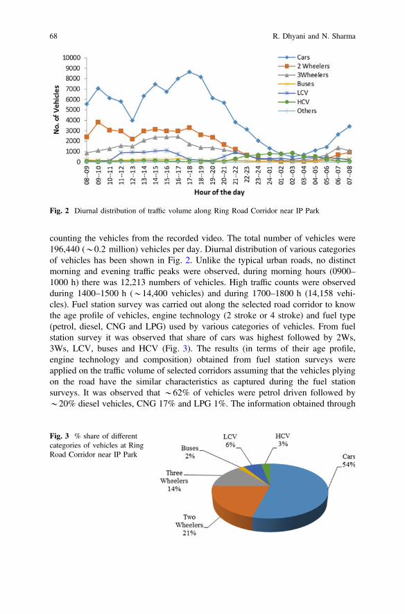
counting the vehicles from the recorded video. The total number of vehicles were196,440 (*0.2 million) vehicles per day. Diurnal distribution of various categoriesof vehicles has been shown in Fig. 2. Unlike the typical urban roads, no distinctmorning and evening traffic peaks were observed, during morning hours (0900–1000 h) there was 12,213 numbers of vehicles. High traffic counts were observedduring 1400–1500 h (*14,400 vehicles) and during 1700–1800 h (14,158 vehi-cles). Fuel station survey was carried out along the selected road corridor to knowthe age profile of vehicles, engine technology (2 stroke or 4 stroke) and fuel type(petrol, diesel, CNG and LPG) used by various categories of vehicles. From fuelstation survey it was observed that share of cars was highest followed by 2Ws,3Ws, LCV, buses and HCV (Fig. 3). The results (in terms of their age profile,engine technology and composition) obtained from fuel station surveys wereapplied on the traffic volume of selected corridors assuming that the vehicles plyingon the road have the similar characteristics as captured during the fuel stationsurveys. It was observed that *62% of vehicles were petrol driven followed by*20% diesel vehicles, CNG 17% and LPG 1%. The information obtained through
Fig. 2 Diurnal distribution of traffic volume along Ring Road Corridor near IP Park
Fig. 3 % share of differentcategories of vehicles at RingRoad Corridor near IP Park
68 R. Dhyani and N. Sharma

fuel station survey and traffic volume videography (e.g. percentage of 2W-2S and2W-4S vehicles, percentage of petrol- and diesel-driven vehicles in 4W categories)were used to estimate weighted/composite emission factors (WEFs or CEFs) as aninput in the CALINE 4 model.
The WEF (input parameter for CALINE4) is a function of vehicle emissionfactor (vehicle category, type, fuel type, age profile, vintage, etc.) and vehicleactivity (traffic volume). For estimation of WEF (gm/mile) (representative valuesfor all categories of vehicles), emission factors for Indian vehicles were used (ARAI2008).
The study was carried out in winter season in the month of February. Themicro-meteorological input parameters such as, wind speed, wind direction andrelative humidity, were measured on-site with the help of Air Pollution Mobile Vanfitted with meteorological sensors. The hourly mixing height values were obtainedfrom the Indian Meteorological Department (IMD) (Attri et al. 2008). In addition,hourly P–G stability class was estimated using wind speed, solar insolation andcloud cover (daytime and night time) (Turner 1994). The predominant wind con-dition was blowing from south-east. The ventilation coefficient is a function of windspeed and mixing height. It is a product of wind speed and mixing height andrepresents the mixing potential and ventilation capacity over a region. Duringdaytime ventilation, coefficients have higher values (unstable conditions with highmixing height) and low during night time (Table 1). Higher the ventilation coef-ficient the more will be pollutant dispersion and vice versa (Lu et al. 2012).However, it is not directly used in CALINE4 model as an input (Fig. 4).
CALINE 4 Model Description
CALINE4 model is the fourth generation simple line source Gaussian plume dis-persion model. It predicts the concentrations of CO, NO2 and PM10/PM2.5 nearroadways. It employs mixing zone concept to characterise pollutant dispersion overthe roadway (Benson 1989). CALINE4 model uses the concept of mixing zonewidth, i.e. region above roadway as zone of uniform emissions and turbulence(Benson 1989) which accounts for vehicle induced turbulence. Mixing zone widthincludes sum of roadway width, median width and 3 m on either side of theroadway. Under standard run (1-h) conditions, the model uses given meteorologicalparameters to predict CO concentrations at pre-identified receptors points. The CObeing the indicator pollutant for vehicular activities was chosen for the presentstudy.
Meteorological Factors Influencing Dispersion of Vehicular … 69
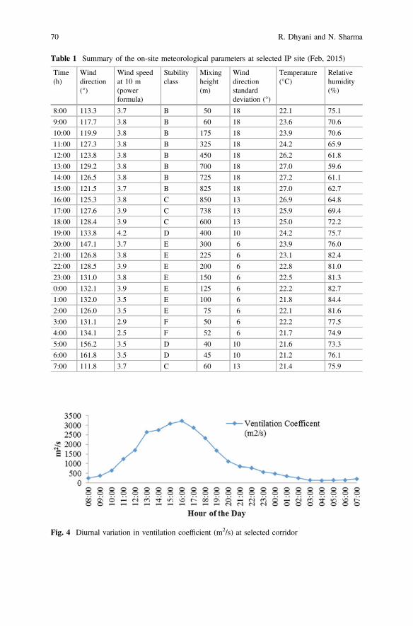
Table 1 Summary of the on-site meteorological parameters at selected IP site (Feb, 2015)
Time(h)
Winddirection(°)
Wind speedat 10 m(powerformula)
Stabilityclass
Mixingheight(m)
Winddirectionstandarddeviation (°)
Temperature(°C)
Relativehumidity(%)
8:00 113.3 3.7 B 50 18 22.1 75.1
9:00 117.7 3.8 B 60 18 23.6 70.6
10:00 119.9 3.8 B 175 18 23.9 70.6
11:00 127.3 3.8 B 325 18 24.2 65.9
12:00 123.8 3.8 B 450 18 26.2 61.8
13:00 129.2 3.8 B 700 18 27.0 59.6
14:00 126.5 3.8 B 725 18 27.2 61.1
15:00 121.5 3.7 B 825 18 27.0 62.7
16:00 125.3 3.8 C 850 13 26.9 64.8
17:00 127.6 3.9 C 738 13 25.9 69.4
18:00 128.4 3.9 C 600 13 25.0 72.2
19:00 133.8 4.2 D 400 10 24.2 75.7
20:00 147.1 3.7 E 300 6 23.9 76.0
21:00 126.8 3.8 E 225 6 23.1 82.4
22:00 128.5 3.9 E 200 6 22.8 81.0
23:00 131.0 3.8 E 150 6 22.5 81.3
0:00 132.1 3.9 E 125 6 22.2 82.7
1:00 132.0 3.5 E 100 6 21.8 84.4
2:00 126.0 3.5 E 75 6 22.1 81.6
3:00 131.1 2.9 F 50 6 22.2 77.5
4:00 134.1 2.5 F 52 6 21.7 74.9
5:00 156.2 3.5 D 40 10 21.6 73.3
6:00 161.8 3.5 D 45 10 21.2 76.1
7:00 111.8 3.7 C 60 13 21.4 75.9
Fig. 4 Diurnal variation in ventilation coefficient (m2/s) at selected corridor
70 R. Dhyani and N. Sharma

Sensitivity Analysis of CALINE4 Model
Sensitivity analysis of CALINE4 model was carried out to determine the signifi-cance and contribution of each input variable in the model’s output. According toBenson (1989), all input parameters act independently within the model andinteraction between two or more variables was presumed to be insignificant.Therefore, for sensitivity analysis, selected input variables were changed system-atically changing one input variable at a time keeping other variables constant andeffect of each input variable on predicted concentration was observed. Morningpeak hour (1000 h) data set has been selected for the sensitivity analysis of theCALINE4 model. Primarily meteorological parameters like wind speed, winddirection, P–G stability class and mixing height were considered for sensitivityanalysis (Table 2).
The sensitivity analysis results consist of CO concentration-wind angle (PHI orroadway to wind angle) graphs. Wind angle has been taken with respect to road-way, thus, 0° means parallel to the roadway and 90° means perpendicular toroadway. The CO concentration was observed/ estimated at pre-identified receptorslocations selected at a distance of 1, 5, 10, 25, 50, 100, 150 and 200 m at either sideof the mixing zone width. The sensitivity analysis was carried out for standard run(1-h) condition.
Results and Discussion
Sensitivity Analysis of CALINE4 Model
Meteorological parameters namely, wind speed, wind direction, stability class andmixing height were varied systematically from the selected input data set. COconcentration-wind angle (PHI or roadway to wind angle) graphs have been pre-sented at four distances from the mixing zone width—5, 10, 25 and 50 m to explainthe CALINE4 sensitivity for selected input parameters of the model. COconcentration-wind angle (PHI or roadway to wind angle) graphs were presented toexplain the CALINE4 sensitivity for selected input parameters of the model. Windangle was taken with respect to roadway, i.e. 0° PHI means parallel to the roadwayand PHI = 90° corresponds to perpendicular wind conditions w.r.t. roadway. Winddirection is an important parameter in air pollution dispersion, as it fixes the course
Table 2 Data set selected for sensitivity analysis
Time(h)
Winddirection(°)
Windspeed(m/s)
Stabilityclass(P–G)
Mixingheight(m)
Winddirection±SD
Pollutantbackground
Temperature(°C)
Trafficvolume(no. ofvehicles)
WEF(g/mile)
1000 119.9 3.8 B 175 18 0 23.9 10,701 3.75
Meteorological Factors Influencing Dispersion of Vehicular … 71

of pollutant dispersion. From sensitivity analysis of CALINE4 model, it wasobserved that model is most sensitive to PHI between 0° and 30°. Maximumconcentration was observed at PHI = 10°. Minimum pollutant concentration wasobserved when PHI = 80°–90° or perpendicular to roadway. During parallel PHI(0°–25°), pollutant concentrations were observed on both upwind and downwinddirection (Fig. 5a). Wind speed impacts the dilution and dispersion of pollutants. Inthe CALINE4 model Gaussian equation, wind speed is inversely proportional topredicted pollutant concentration (Benson 1989; Batterman et al. 2010; Bhaskarand Mehta 2010). Wind speed was varied from 0.5 m/s (calm) to 5 m/s in 1 m/sinterval. With every 22% increase in wind speed, i.e. 1–2 m/s, 22% decrease inpredicted concentration was observed. Maximum concentration was observedduring parallel wind direction (10° and 20° PHI) Fig. 5b.
Mixing height defines the structure of turbulence in boundary layer. Mixingheight along with wind speed determine the volume available for mixing anddispersion of pollutant (Khandokar et al. 2010; Banta and White 2003). Vehicularemissions are near ground emissions, therefore, the influence of mixing height isnot expected in dispersion of pollutant. Moreover, in the CALINE4 model thermalturbulence from exhaust of emission and mechanical turbulence generated fromvehicles are the main forces, which influence the dispersion of pollutants in mixingzone width (Benson 1989). For sensitivity analysis, mixing height was varied from25 to 2500 m (Fig. 6a). It was observed that negligible change occurred whenmixing height was varied. The data set selected for the study has B (unstableatmosphere) P–G stability class. Model uses Pasquill–Gifford stability class only,P–G stability class is a function of solar insolation intensity, wind speed, cloud
Fig. 5 Sensitivity analysis for wind angle, PHI (°) and wind speed (m/s)
72 R. Dhyani and N. Sharma

cover and time of the day. Stability class was varied from Class A (highly unstable)to Class F (highly stable). However, insignificant impact of change in stability classwas observed on predicted concentration near mixing zone width. However, slightincrease (15–30%) in concentration was observed as we move away from mixingzone width (25 and 50 m) (Fig. 6b). Thus indicating the importance of mixing zonewidth concept, where mechanical and thermal turbulence are predominant forces fordispersion. As we move away from the influence zone (mixing zone width),atmospheric features like stability class, mixing height become significant forces fordispersion and dilution process of air pollutants.
Conclusions
Sensitivity analysis of model was carried out to identify the most influencing inputparameters in the CALINE4 model. The impact of wind speed and wind directionwas more significant on dispersion of vehicular pollution. CALINE4 was found tobe most sensitive to parallel wind direction. Maximum concentration was observedat PHI = 20° (parallel wind direction). Wind speed has significant impact, it isinversely proportional on predicted concentration. Nearly, 22% increase in windspeed (0.5–1 m/s) results in 22% decrease in predicted concentration. Stability classwas observed to be influencing at a nearly 50 m away from mixing zone width. Theimpact of stability class is more prominent at receptors away from mixing zonewidth. Mixing height had insignificant influence on model prediction capability,therefore, it could be concluded that any default value could be used for the
Fig. 6 Sensitivity analysis for mixing height (m) and stability class (P–G)
Meteorological Factors Influencing Dispersion of Vehicular … 73

pollutant concentration prediction. Vehicular pollution or release of exhaust is nearto ground level, where vehicle-induced turbulence and mechanically induced tur-bulence are the most significant forces for dispersion of vehicular pollution.Therefore, effect of stability class and mixing height is not significant in that zone ornear roadway receptors. Thus, it could be concluded that among meteorologicalparameters, wind speed and wind direction have comparatively more influence onmodel prediction capabilities followed by stability class and mixing height.
Acknowledgements The authors are thankful to Director, CSIR-CRRI for kindly permitting topublish the present paper. Rajni Dhyani is thankful to CSIR for providing financial assistancethrough CSIR-Senior Research Fellowship.
References
ARAI (2008) Draft report on emission factor development for Indian vehicles’, report submitted toCPCB/MoEF as a part of Ambient air quality monitoring and emission source apportionstudies. Automotive Research Association of India, Pune, India
Attri SD, Singh S, Mukhopadhyay B, Bhatnagar AK (2008) Atlas of hourly mixing height andassimilative capacity of atmosphere in India. Met Monograph No. EnvironmentMeteorology-01/2008, Indian Meteorological Department, New Delhi, Govt. of India
Banta RM, White AB (2003) Mixing-height differences between land use types: dependence onwind speed. J Geophys Res 108(D10):4321. doi:10.1029/2002JD002748
Batterman SA, Zhang K, Kononowech R (2010) Prediction and analysis of near-roadconcentrations using a reduced-form emission/dispersion model. Environ Health 9(29):1–18
Bennett ND, Croke BFW, Guariso G, Guillaume JHA, Hamilton SH, Marsili-Libelli AJS,Newhama LTH, Norton JP, Perrin C, Pierce SA, Robson B, Seppelt R, Voinov AA, Fath BD,Andreassian V (2013) Characterising performance of environmental models. Environ ModelSoftw 40:1–20
Benson PE (1989) CALINE 4: a dispersion model for predicting air pollutant concentrations nearroadways. FHWA-CA-TL-84–15, California Department of Transportation, Sacramento, CA,USA
Bhaskar BV, Mehta VM (2010) Atmospheric particulate pollutants and their relationship withmeteorology in Ahmedabad. Aerosol Air Qual Res 10:301–315
Dhyani R, Singh A, Sharma N, Gulia S (2013) Performance evaluation of CALINE4 model in ahilly terrain-a case study of highway corridors in Himachal Pradesh (India). Int J EnvironPollut 52(3/4):244–262
Dhyani R, Gulia S, Sharma N, Singh A (2014) Air quality impact assessment of a highwaycorridor through vehicular pollution modelling. In: International conference on environmentand sustainable technologies 2014 (iCEST 2014) 3–5 Jan 2014, Manipal, Karnataka
Gimson N, Chilton R, Xie S (2010) Meteorological datasets for the Auckland region—user guide.Prepared by Golder Associates (NZ) Limited for Auckland Regional Council. AucklandRegional Council Technical Report 2010/022
GNCTD (2015) Total vehicles registered zone wise up to 31 March 2015. Transport Department.Government of National Capital Territory of Delhi
Karim MMd, Matsui H, Guensler R (1998) A mathematical model of wind flow, vehicle wake andpollutant concentration in urban road microclimate, part II: model results. Transp Res (Part D)3:171–191
Khandokar A, Mofarrah A, Husain T (2010) Comparison of upper air mixing height estimationmethods for urban air pollution modeling. In: International environmental modelling and
74 R. Dhyani and N. Sharma

software society (iEMSs) 2010 international congress on environmental modelling andsoftware modelling for environment’s sake, Fifth Biennial Meeting
Konar TS, Chakrabarty S (2012) Applicability of Caline4 model for NOx in Kolkata Roadway.Civil Environ Eng. doi:10.4172/2165-784X.S1-005
Lao Y (2010) Health risks of transportation‐related emissions: a GIS assessment. 2010‐NBG‐1062,p 10
Lu C, Deng Q-H, Liu W-W, Huang B-L, Shi L-Z (2012) Characteristics of ventilation coefficientand its impact on urban air pollution. J Cent South Univ 19(3):615–622
Majumdar BK, Dutta A, Chakrabarty S, Ray S (2009) Correction factor of CALINE4: a study ofautomobile pollution in Kolkata. Indian J Air Pollut Control 8(1):1–7
Majumdar BK, Dutta A, Chakrabarty S, Ray S (2010) Assessment of vehicular pollution inKolkata, India using CALINE4 model. Environ Monit Assess 70:33–43
MoRTH (2013) Road transport yearbook, (2011–12). Ministry of Road Transport and Highways.Government of India
Nossent J, Elsen P, Bauwens W (2011) Sobol’ sensitivity analysis of a complex environmentalmodel. Environ Model Softw 26(12):1515–1525
Sharma N, Gulia S, Dhyani R, Singh A (2013) Performance evaluation of CALINE 4 dispersionmodel for an urban highway corridor in Delhi. J Sci Ind Res 72(8):521–530
Sripraparkorn S, Jinsart W, Hooper M (2003) Application of the CALINE4 air quality model andthe TSI DustTrak for the prediction and measurement of roadside particulate matter and carbonmonoxide levels in Bangkok. In: 2nd Regional conference on energy technology towards aclean environment, 12–14 Feb 2003, Thailand
Trueman RE (2007) Incremental (marginal) analysis of basic inventory models. Decis Sci 2(3):341–355
Turner DB (1994) Workbook of atmospheric dispersion estimates an introduction to dispersionmodel, 2nd edn. CRC Press, Inc. Lewis Publishers, Florida, USA
USEPA (2004). Technical guidance on the use of MOBILE6.2 for emission inventory preparationEPA420-R-04-013. Transportation and Regional Programs Division, Office of Transportationand Air Quality. U.S. Environmental Protection Agency
Zhan Y, Zhang M (2013) Application of a combined sensitivity analysis approach on a pesticideenvironmental risk indicator. Environ Model Softw 49:129–140
Meteorological Factors Influencing Dispersion of Vehicular … 75
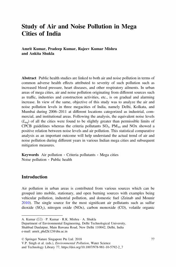
Study of Air and Noise Pollution in MegaCities of India
Amrit Kumar, Pradeep Kumar, Rajeev Kumar Mishraand Ankita Shukla
Abstract Public health studies are linked to both air and noise pollution in terms ofcommon adverse health effects attributed to severity of such pollution such asincreased blood pressure, heart diseases, and other respiratory ailments. In urbanareas of mega cities, air and noise pollution originating from different sources suchas traffic, industries and construction activities, etc., is on gradual and alarmingincrease. In view of the same, objective of this study was to analyze the air andnoise pollution levels in three megacities of India, namely Delhi, Kolkata, andMumbai during 2006–2011 at different locations categorized as industrial, com-mercial, and institutional areas. Following the analysis, the equivalent noise levels(Leq) of all the cities were found to be slightly greater than permissible limits ofCPCB guidelines whereas the criteria pollutants SO2, PM10 and NOx showed apositive relation between noise levels and air pollution. This statistical comparativeanalysis as an important outcome will help understand the actual trend of air andnoise pollution during different years in various Indian mega cities and subsequentmitigation measures.
Keywords Air pollution � Criteria pollutants � Mega citiesNoise pollution � Public health
Introduction
Air pollution in urban areas is contributed from various sources which can begrouped into mobile, stationary, and open burning sources with examples beingvehicular pollution, industrial pollution, and domestic fuel (Zeinab and Mounir2010). The single source for the most significant air pollutants such as sulfurdioxide (SO2), nitrogen oxide (NOx), carbon monoxide (CO), volatile organic
A. Kumar (&) � P. Kumar � R.K. Mishra � A. ShuklaDepartment of Environmental Engineering, Delhi Technological University,Shahbad Daulatpur, Main Bawana Road, New Delhi 110042, Delhi, Indiae-mail: [email protected]
© Springer Nature Singapore Pte Ltd. 2018V.P. Singh et al. (eds.), Environmental Pollution, Water Scienceand Technology Library 77, https://doi.org/10.1007/978-981-10-5792-2_7
77
compounds (VOCs), and particulate matter (PM) is fossil fuels (Kumar et al. 2014).Noise pollution is taken in other pollution categories due to its source and diffusioncharacteristics. There has been an increase in noise from man-made sources for last100 years, which is now doubling after every 10 years. World Health Organization(WHO) analyzed the available air quality data from 1,100 cities across the worldand the position of Delhi was reported at the top of the list of 20 most air pollutedcities (WHO 2014).
Delhi being the capital of India, has grown across all sectors such as industry,transport, and housing, and all of them have contributed to an increase in airpollution (Narain and Bell 2006; Goswami and Baruah 2008; Firdaus and Ahmad2011; Sahu et al. 2011; Guttikunda and Gurjar 2012; Guttikunda and Goel 2013).According to Center for Science and Environment (CSE), the Central PollutionControl Board (CPCB 2000, 2009) considers air to be “clean” if the levels arebelow 50% of the prescribed standards for pollutants. Commonly found air pol-lutants (also known as “criteria pollutants”) assuming the criteria pollutant to bePM10 during 2007, only 2% cities have low air pollution. At least one pollutantexceeded the annual average from ambient air quality standards in about 80% ofcities (of a total of 127 cities/towns monitored under the National Air QualityMonitoring Programme, NAMP). There are very few cities which can be referred tobe clean if the designated criteria pollutant is PM10. However, the level of SO2 hasreduced in many cities below the standards of CPCB but the NO2 levels areincreasing in many cities.
Exposure on Health
Studies in India and in other countries have consistently demonstrated higher ratesof respiratory and cardiovascular disease in populations exposed to PM, NOx, andOzone pollution (Chhabra et al. 2001; Pande et al. 2002; Gupta et al. 2007;Siddique et al. 2010; Balakrishnan et al. 2011; WHO 1999, 2014). According toWHO (2014), high concentration of small particulates such as PM10 and PM2.5
causes increased mortality and morbidity as if the concentration of same is reducedtaking other parameters as they are the mortality will also go down. Human healthstudies for long-term exposure of NO2 show the symptoms of bronchitis in asth-matic children increase while SO2 causes irritation of the eyes and may affect therespiratory system and the functions of the lungs. Exposure to road traffic noise andair pollution has both been studied and associated with problem of stroke. Fewstudies, including exposures to both gaseous pollutants show inconsistent results.Fatal stroke was reported to be because of air pollution and not because of trafficnoise. Ischemic stroke was because of traffic noise only while only air pollutioncaused risk of fatal strokes (Sørensen et al. 2014).
Due to the rapid increase in industrialization, urbanization, and transport sys-tems, noise pollution has increased to a disturbing level. The effect of noise pol-lution is hearing defects, increased blood pressure, and sleeplessness, effect on work
78 A. Kumar et al.
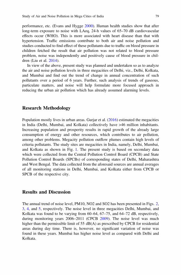
performance, etc. (Evans and Hygge 2000). Human health studies show that afterlong-term exposure to noise with LAeq, 24-h values of 65–70 dB cardiovasculareffects occur (WHO). This is more associated with heart disease than that withhypertension. Traffic emissions contribute to both air and noise pollution andstudies conducted to find effect of these pollutants due to traffic on blood pressure inchildren fetched the result that air pollution was not related to blood pressureproblem, noise was independently and positively cause of blood pressure in chil-dren (Liu et al. 2014).
In view of the above, present study was planned and undertaken so as to analyzethe air and noise pollution levels in three megacities of Delhi, viz., Delhi, Kolkata,and Mumbai and find out the trend of change in annual concentration of suchpollutants over a period of 6 years. Further, such analysis of trends of gaseous,particulate matters, and noise will help formulate more focused approach inreducing the urban air pollution which has already assumed alarming levels.
Research Methodology
Population mostly lives in urban areas. Gurjar et al. (2016) estimated the megacitiesin India (Delhi, Mumbai, and Kolkata) collectively have >46 million inhabitants.Increasing population and prosperity results in rapid growth of the already largeconsumption of energy and other resources, which contributes to air pollution,among other problems. Megacity pollution outflow plumes contain high levels ofcriteria pollutants. The study sites are megacities in India, namely, Delhi, Mumbai,and Kolkata as shown in Fig. 1. The present study is based on secondary datawhich were collected from the Central Pollution Control Board (CPCB) and StatePollution Control Boards (SPCBs) of corresponding states of Delhi, Maharashtraand West Bengal. The data collected from the aforesaid sources are annual averagesof all monitoring stations in Delhi, Mumbai, and Kolkata either from CPCB orSPCB of the respective city.
Results and Discussion
The annual trend of noise level, PM10, NO2 and SO2 has been presented in Figs. 2,3, 4, and 5, respectively. The noise level in three megacities Delhi, Mumbai, andKolkata was found to be varying from 60–64, 67–75, and 64–72 dB, respectively,during monitoring years 2006–2011 (CPCB 2009). The noise level was muchhigher than the permissible limit of 55 dB(A) as prescribed by CPCB for residentialareas during day time. There is, however, no significant variation of noise wasfound in these years. Mumbai has higher noise level as compared with Delhi andKolkata.
Study of Air and Noise Pollution in Mega Cities of India 79

During the years 2006–2011, the SO2 level in Delhi, Mumbai, and Kolkata werefound varying from 5–10, 5–12, and 8–12 µg/m3, respectively. The SO2 level wasfound within permissible limit for all megacities in India and is not considered aproblem in India anymore. Its levels in most cities are already very low and
Fig. 1 Location map of megacities in India
Fig. 2 Annual variation of ambient noise levels (2006–2011) in Indian mega cities
80 A. Kumar et al.
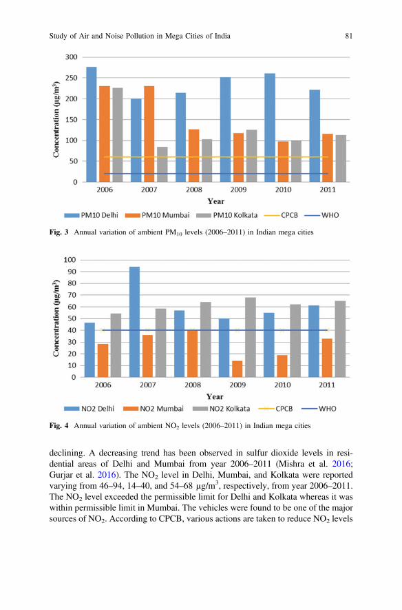
declining. A decreasing trend has been observed in sulfur dioxide levels in resi-dential areas of Delhi and Mumbai from year 2006–2011 (Mishra et al. 2016;Gurjar et al. 2016). The NO2 level in Delhi, Mumbai, and Kolkata were reportedvarying from 46–94, 14–40, and 54–68 µg/m3, respectively, from year 2006–2011.The NO2 level exceeded the permissible limit for Delhi and Kolkata whereas it waswithin permissible limit in Mumbai. The vehicles were found to be one of the majorsources of NO2. According to CPCB, various actions are taken to reduce NO2 levels
Fig. 3 Annual variation of ambient PM10 levels (2006–2011) in Indian mega cities
Fig. 4 Annual variation of ambient NO2 levels (2006–2011) in Indian mega cities
Study of Air and Noise Pollution in Mega Cities of India 81

but the numbers of vehicle are increasing drastically thereby limiting the desiredoutcome (Mishra et al. 2016).
The PM10 level in Delhi, Mumbai, and Kolkata were found to be varying from201–276, 97–230, and 85–225 µg/m3, respectively between monitoring years 2006and 2011. The particulate matter concentration is also in excess of the permissiblelimit as prescribed by CPCB and WHO which is 60 and 40 µg/m3, respectively forannual average. Most Indian cities outdo limits of particulate matter defined byCPCB. This may be because of increase in activities like refuse and biomassburning, vehicles, power plant emissions, and industrial sources (Gurjar et al.2010).
Conclusion
The study reports that the ambient air of Delhi city is more polluted as compared toMumbai and Kolkata. The annual average concentration of NO2 is found more thanprescribed limit by CPCB in Delhi and Kolkata. On the other hand, the concen-tration of SO2 in all the megacities is reported to be within the permissible limit. Allthe megacities in India showed very high concentration of particulate matter thanthe standard prescribed by CPCB and WHO, while the noise pollution level ofMumbai is higher than the noise pollution level in Delhi and Kolkata. The noisepollution level is almost similar in all respective cities from 2006 to 2011. Noisepollution is more than the permissible limit in all megacities of India. The noisepollution also has the significant role in adversely affecting the environment.
Fig. 5 Annual variation of ambient SO2 levels (2006–2011) in Indian mega cities
82 A. Kumar et al.

Therefore, it has become a matter of great concern to improve the air quality fordeveloping and maintaining a cleaner and healthier environment.
References
Balakrishnan K, Ganguli B, Ghosh S, Sambandam S, Roy S, Chatterjee A (2011) A spatiallydisaggregated time-series analysis of the short-term effects of particulate matter exposure onmortality in Chennai, India. Air Quality, Atmosphere and Health, pp 1–11
Central Pollution Control Board (2009) National ambient air quality status 2008. NationalAmbient Air Quality Monitoring Series, NAAQMS/2/2009-10
Chhabra SK, Chhabra P, Rajpal S, Gupta RK (2001) Ambient air pollution and chronic respiratorymorbidity in Delhi. Arch Environ Health 56:58–64
CPCB (2000) The noise pollution (Regulation and Control)Evans GW, Hygge S (2000) Noise and performance in children and adults. In: Prasher D
(ed) Handbook of noise and healthFirdaus G, Ahmad A (2011) Changing air quality in Delhi, India: determinants, trends, and policy
implications. Reg Environ Change 11:743–752Goswami P, Baruah J (2008) Simulation of daily variation of suspended particulate matter over
Delhi: relative roles of vehicular emission, dust, and domestic appliances. Mon Weather Rev136:3597–3607
Gupta SK, Gupta SC, Agarwal R, Sushma S, Agrawal SS, Saxena R (2007) A multicentriccase-control study on the impact of air pollution on eyes in a metropolitan city of India.Indian J Occup Environ Med 11:37–40
Gurjar BR, Jain A, Sharma A, Agarwal A, Gupta P, Nagpure AS, Lelieveld J (2010) Human healthrisks in megacities due to air pollution. Atmos Environ 44(36):4606–4613
Gurjar BR, Khaiwal R, Nagpure AS (2016) Air pollution trends over Indian megacities and theirlocal-to-global implications. Atmospheric environment, Accepted manuscript (in press)
Guttikunda SK, Gurjar B (2012) Role of meteorology in seasonality of air pollution in megacityDelhi, India. Environ Monit Assess 184:3199–3211
Guttikunda SK, Goel R (2013) Health impacts of particulate pollution in a megacity-Delhi, India.Environ Dev 6:8–20
Kumar A, Mishra RK, Singh SK (2014) GIS application in urban traffic air pollution exposurestudy: a research review. Suan Sunandha J Sci Technol 2(1):1–13
Liu EC, Carla F, Tiesler MT, Birk M, Babisch W, Sibylle CP, Koletzko B, Berg AV,Hoffmanni B, Heinrich J (2014) The associations between traffic-related air pollution and noisewith blood pressure in children: Results from the GINIplus and LISA plus studies. Int J HygEnviron Health 217(4–5):499–505
Mishra RK, Shukla A, Parida M, Pandey G (2016) Urban roadside monitoring and prediction ofCO, NO2 and SO2 dispersion from on-road vehicles in megacity Delhi. Transp Res Part D46:157–165
Narain U, Bell RG (2006) Who changed Delhi’s air? Econ Polit Wkly 41:1584–1588Pande JN, Bhatta N, Biswas D, Pandey RM, Ahluwalia G, Siddaramaiah NH (2002) Outdoor air
pollution and emergency room visits at a hospital in Delhi. Indian J Chest Dis Allied Sci 44:9Sahu SK, Beig G, Parkhi NS (2011) Emissions inventory of anthropogenic PM2.5 and PM10 in
Delhi during commonwealth games 2010. Atmos Environ 45:6180–6190Siddique S, Banerjee M, Ray M, Lahiri T (2010) Air pollution and its impact on lung function of
children in Delhi, the capital city of India. Water Air Soil Pollut 212:89–100Sørensen M, Lühdor P, Ketze M, Andersen ZJ, Tjønnel A, Overvad K, Nielsen OR (2014)
Combined effects of road traffic noise and ambient air pollution in relation to risk for stroke?Environ Res 133:49–55
Study of Air and Noise Pollution in Mega Cities of India 83

WHO (1999) Report on Guidelines for community Noise, Stockholm University & KarolinskaInstitute
WHO (2014) Burden of disease from the joint effects of household and ambient air pollution for2012. Public Health, Social and Environmental Determinants of Health Department
Zeinab S, Mounir WL (2010) Assessment of particulate matter and lead levels in the Greater Cairoarea for the period 1998–2007. J Adv Res 1:53–63
84 A. Kumar et al.

Part IIPollution Indicators
A Critical Review on Air Quality Index
Shweta Kumari and Manish Kumar Jain
Abstract Air quality index (AQI) is used worldwide to inform the public aboutlevels of air pollution (degradation or improvement) and associated to differentbiological effects. Different types of anthropogenic activity mainly transportationhave an enormous impact on the ambient air quality in several ways. The trans-portation dependence continues to grow; it is adversely affecting the quality ofhuman life. Due to pollution, the ambient air quality in major cities (Delhi, Agra,Kanpur, Lucknow, Varanasi, Faridabad, Ahmedabad, Chennai, Bangalore andHyderabad) in India is very poor. According to WHO surveys, India is one of themost polluted countries in the world. Concentrations of air pollutants affect AirQuality Index. Air Quality scenario in most of the Indian cities presents a harshpicture, the majority of national monitoring stations have recorded particulateconcentrations exceeding the WHO recommended guideline. The higher the AQIvalue, the greater the level of air pollution and greater the health concern. Thisreview paper is helpful to understand the development of Air quality Index in Indiawith the experience of the world.
Keywords Ambient air quality � Air quality index � Air pollutionTransportation � Health effect
Introduction
Unpolluted air can be considered a basic requirement of human health andwell-being. Today, air pollution is a well-known environmental problem associatedwith urban areas around the world (Beig 2010). Urban air pollution is the largest
S. Kumari � M.K. Jain (&)Department of Environmental Science & Engineering, Indian Instituteof Technology (Indian School of Mines), Dhanbad 826004, Jharkhand, Indiae-mail: [email protected]
© Springer Nature Singapore Pte Ltd. 2018V.P. Singh et al. (eds.), Environmental Pollution, Water Scienceand Technology Library 77, https://doi.org/10.1007/978-981-10-5792-2_8
87

contributor to the regional burden of disease. There are a profound relation betweenhuman health and well-being from the one side and air pollution levels from anotherside. The high concentration of air pollutants can be life threatening causingbreathing problems, headache, and dizziness; sometimes they even result in heartattacks (CPCB 2014).
Awareness of pollution levels is important not only to those who suffer fromillnesses aggravated by air pollution but also to members of the general public, who,if conscious of daily variations in air pollution levels, may choose to alter theiractivities accordingly. In order to oppose air pollution problems and to planabatement strategies, both the scientific community and the relevant authoritieshave focused on monitoring and analysing the atmospheric pollutants concentra-tion. Various monitoring programmes have been undertaken to know the quality ofair by generating the vast amount of data on the concentration of each air pollutant(e.g. SPM, CO, NOx, SO2, etc.) in different parts of the world (Pandey et al. 2014).The large data often do not convey the air quality status to the scientific community,government officials, policymakers and in particular to the general public in asimple and straightforward manner. So, in recent years air quality index (AQI) hasbecome an adequate tool to understand pollution levels of an area and is of utmostimportance for local and central governments (Ott and Thorn 1976). AQIs aresynthetic indices summarizing multiple and multiscale measurements in a uniqueindicator, being air quality monitored with respect to many stations and differentpollutants and inform the citizens about the levels of pollution in an adequate andunderstandable way and also to be used by the relevant authorities to take a series ofpredetermined measures to protect the health of the population (Air Quality Index2003).
Objective
The main objective of the present study is to review for the daily Air Quality Index,which can provide the timely information to the public to take precautionarymeasures to protect their health (Kyrkilis et al. 2007)
Air Quality Index (AQI)
Air quality index (AQI) is an integral part of the environmental quality index (EQI),which was developed and used by National Wildlife Federation of U.S. in the late1960s (Inhaber 1976). In 1971 the EQI, with a numerical index scale from 0 to 100(0 for complete environmental degradation and 100 for perfect environmentalconditions). In 1976, the USEPA established PSI which rated air quality from 0 to500. The daily PSI is determined by the highest value of one of the five main airpollutants: carbon monoxide (CO), nitrogen dioxide (NO2), ozone (O3), particulate
88 S. Kumari and M.K. Jain

matter (PM10 and PM2.5) and sulphur dioxide (SO2) (EPA 1999). Lohani (1984)applied factor analysis approach for finding the environmental index for Taiwan(Kumar and Goyal 2011).
Definition
An “air pollution index” may be defined as a scheme that transforms the (weighted)values of individual air pollution related parameters (for example, carbon monoxideconcentration or visibility) into a single number, or set of numbers. In other words,an index is an equation which combines many pollutants in some mathematicalexpression to arrive at a single number for air quality (Bishoi et al. 2009).According to EPA Air Quality Index is defined as “the AQI is an index forreporting daily air quality. It tells how clean or polluted ambient air is, and whatassociated health effects might be a concern for you. The AQI focuses on healtheffects one may experience within a few hours or days after breathing polluted air”(Air Quality Index 2003) (Table 1).
Classification of Indices
There have been several Air Quality Indices proposed in the past. These indices aredescribed in the following subsections.
Table 1 Pollutant concentration for each AQI category according to EPA
Category Good Moderate Unhealthy forsensitivegroups
Unhealthy Veryunhealthy
Hazardous Severe
Index value 0–50 51–100 101–150 151–200 201–300 301–400 401–500
Pollutant Conc.range
– – – – –
CO 8 h(ppm)
0.0–4.5 4.5–9 9–12 12–15 15–30 30–40 40–50
NO2 – – – – – 1.2–1.6 1.6–2.0
O3 dailymax (ppm)
– – – – 0.20–0.40 0.40–0.50 0.50–0.60
O3 8 h 0.00–0.06 0.06–0.08 0.08–0.10 0.10–0.12 0.12–0.37 – –
PM 10 dailymean (ppm)
0–50 50–150 150–250 250–350 350–420 420–500 500–600
SO2 0.0–0.03 0.03–0.14 0.14–0.22 0.22–0.3 0.3–0.6 0.6–0.8 0.8–1.0
A Critical Review on Air Quality Index 89
US EPA Air Quality Index
Initially, the US EPA produced an Air Quality Index known as the PollutantStandards Index (PSI) to measure pollutant concentrations for five criteria pollu-tants (particulate matter, sulphur dioxide, carbon monoxide, nitrogen dioxide andground-level ozone). The measurements were converted to a scale of 0–500. Anindex value of 100 was ascribed to the numerical level of the short-term (i.e.averaging time of 24 h or less) primary NAAQS and a level of 500 to the significantharm levels (SHLs). An index value of 50, which is half the value of the short-termstandard, was assigned to the annual standard or a concentration. Other index valueswere described as follows: 0–100, good; 101–200, unhealthy; greater than 200,very unhealthy. Use of the index was mandated in all metropolitan areas with apopulation in excess of 250,000. The EPA advocated calculation of the index valueon a daily basis for each of the four criteria pollutants and the reporting of thehighest value and identification of the pollutant responsible. Where two or morepollutants exceeded the level of 100, although the PSI value released was the onepertaining to the pollutant with the highest level, information on the other pollutantswas also released. Levels above 100 could be associated with progressive pre-ventive action by state or local officials involving issuance of health advisories forcitizens or susceptible groups to limit their activities and for industries to cut backon emissions. At a PSI level of 400, the EPA deemed that “emergency” conditionswould exist and that this would require cessation of most industrial and commercialactivity. In July 1999, EPA issued its new “air quality index” (AQI) replacing thePSI. The principal differences between the two indices are that the new AQI doesthe following:
1. Incorporates revisions to the primary health-based national ambient air qualitystandards for ground-level ozone and particulate matter, issued by the EPA in1977, incorporating separate values for particulate matter of 2.5 and 10.0 lg(PM2.5 and PM10), respectively.
2. Includes a new category in the index described as “unhealthy for sensitivegroups” (index value of 101–150) and the addition of an optional cautionarystatement, which can be used at the upper bounds of the “moderate” range of the8-h ozone standard.
3. Incorporates colour symbols to represent different ranges of AQI values(“scaled” in the manner of colour topographical maps from green to maroon)that must be used if the index is reported in a colour format.
4. Includes mandatory requirements for the authorities to supply information to thepublic on the health effects that may be encountered at the various levels,including a requirement to report a pollutant-specific sensitive group statementwhen the index is above 100.
5. Mandates that the AQI shall be routinely collected and that state and localauthorities shall be required to report it, for all metropolitan areas with morethan 350,000 people (previously the threshold was urban areas with populationsof more than 200,000).
90 S. Kumari and M.K. Jain

6. Incorporates a new matrix of index values and cautionary statements for eachpollutant.
7. Calculates the AQI using a method similar to that of the PSI—using concen-tration data obtained daily from “population-oriented State/Local AirMonitoring Stations (SLAMS)” for all pollutants except particulate matter(PM) (Ott and Thorn 1976).
The Mitre Air Quality Index (MAQI)
The Mitre air quality index (MAQI) was based on the 1970 Secondary FederalNational Ambient Air Quality Standards. The index is the root sum square(RSS) value of individual pollutant indices, each based on one of the secondary airquality standard (Ott and Thorn 1976). This index is computed as follows:
MAQI ¼ I2S þ I2C þ I2P þ I2N þ I2o� �0:5 ð1Þ
where IS is an index of pollution for sulphur dioxide, Ic is an index of pollution forcarbon monoxide, IP is an index of pollution for total suspended particulates, In isan index of pollution for nitrogen dioxide and IO is an index of pollution forphotochemical oxidants.
Sulphur Dioxide Index (IS): The sulphur dioxide index is the RSS value of indi-vidual terms corresponding to each of the secondary standards. The RSS value isused to ensure that the index value will be greater than 1 if one of the standardvalues is exceeded. The index is defined as
Is ¼ Csa=Ssað Þ2 þ K1 Cs24=Ss24ð ÞþK2 Cs3=Ss3ð Þ2h i
ð2Þ
where Csa is the annual arithmetic mean observed concentration of sulphur dioxide,Ssa is the annual secondary standard value (i.e., 0.02 ppm or 60 lg/m3) consistentwith the unit of measure of Csa, Cs24 is the maximum observed 24-h concentrationof sulphur dioxide, Ss24 is the 24-h secondary standard value (i.e., 0.1 ppm or260 lg/m3) consistent with the unit of measure of Cs24, Cs3 is the maximumobserved 3-h concentration of sulphur dioxide, Ss3 is the 3-h secondary standardvalue (i.e., 0.5 ppm or 1300 lg/m3) consistent with the unit of measure of Cs3, K1 is1 if Cs24 � Ss24 and is 0 otherwise and K2 is 1 if Cs3 � Ss3 and is 0 otherwise.
Carbon Monoxide Index (Ic): The carbon monoxide index component of theMAQI is computed in a fashion similar to the sulphur dioxide index:
Ic ¼ Cc8=Sc8ð Þ2 þK Cc1=Sc1ð Þ2h i0:5
ð3Þ
A Critical Review on Air Quality Index 91
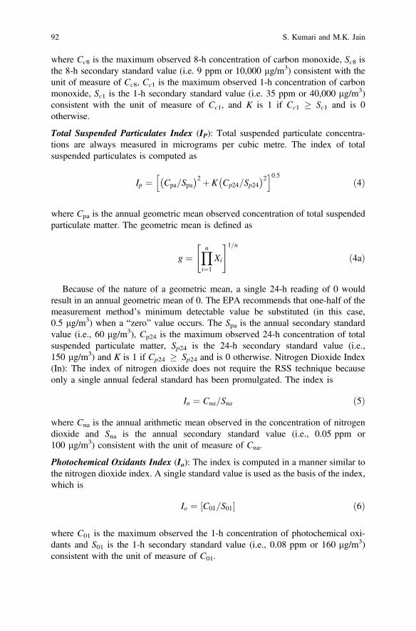
where Cc8 is the maximum observed 8-h concentration of carbon monoxide, Sc8 isthe 8-h secondary standard value (i.e. 9 ppm or 10,000 lg/m3) consistent with theunit of measure of Cc8, Cc1 is the maximum observed 1-h concentration of carbonmonoxide, Sc1 is the 1-h secondary standard value (i.e. 35 ppm or 40,000 lg/m3)consistent with the unit of measure of Cc1, and K is 1 if Cc1 � Sc1 and is 0otherwise.
Total Suspended Particulates Index (IP): Total suspended particulate concentra-tions are always measured in micrograms per cubic metre. The index of totalsuspended particulates is computed as
Ip ¼ Cpa=Spa� �2 þK Cp24=Sp24
� �2h i0:5ð4Þ
where Cpa is the annual geometric mean observed concentration of total suspendedparticulate matter. The geometric mean is defined as
g ¼Yni¼1
Xi
" #1=n
ð4aÞ
Because of the nature of a geometric mean, a single 24-h reading of 0 wouldresult in an annual geometric mean of 0. The EPA recommends that one-half of themeasurement method’s minimum detectable value be substituted (in this case,0.5 lg/m3) when a “zero” value occurs. The Spa is the annual secondary standardvalue (i.e., 60 lg/m3), Cp24 is the maximum observed 24-h concentration of totalsuspended particulate matter, Sp24 is the 24-h secondary standard value (i.e.,150 lg/m3) and K is 1 if Cp24 � Sp24 and is 0 otherwise. Nitrogen Dioxide Index(In): The index of nitrogen dioxide does not require the RSS technique becauseonly a single annual federal standard has been promulgated. The index is
In ¼ Cna=Sna ð5Þ
where Cna is the annual arithmetic mean observed in the concentration of nitrogendioxide and Sna is the annual secondary standard value (i.e., 0.05 ppm or100 lg/m3) consistent with the unit of measure of Cna.
Photochemical Oxidants Index (Io): The index is computed in a manner similar tothe nitrogen dioxide index. A single standard value is used as the basis of the index,which is
Io ¼ ½C01=S01� ð6Þ
where C01 is the maximum observed the 1-h concentration of photochemical oxi-dants and S01 is the 1-h secondary standard value (i.e., 0.08 ppm or 160 lg/m3)consistent with the unit of measure of C01.
92 S. Kumari and M.K. Jain

Application of the MAQI
An MAQI value of less than 1 indicates that all standards are being met for thosepollutants in the MAQI computations. Because nine standards for five pollutants areinvolved in computing MAQI, any MAQI value greater than 3 guarantees that atleast one standard value has been exceeded. If the MAQI values to be estimated byEq. (1) are based on only five standards for three pollutants, then, for these figures,any MAQI value greater than 2.24 guarantees that at least one standard has beenexceeded (Wang et al. 2005).
Extreme Value Index (EVI)
The extreme value index (EVI) was developed by Mitre Corporation for use inconjunction with the MAQI values. It is an accumulation of the ratio of the extremevalues for each pollutant. The EVIs for individual pollutants are combined using theRSS method. Only those pollutants are included for which secondary “maximumvalues not to be exceeded more than once per year” are defined. The EVI is givenby
EVI ¼ ½E2c þE2
s þE2p þE2
o �0:5 ð7Þ
where Ec is an extreme value index for carbon monoxide, Es is an extreme valueindex for sulphur dioxide, Ep is an extreme value index for total suspended par-ticulates and Eo is an extreme value index for photochemical oxidants.
Carbon Monoxide Extreme Value Index (Ec): The carbon monoxide extremevalue is the RSS of the accumulated extreme values divided by the secondarystandard values. The index is defined as
Ec ¼ ½ðAc8=Sc8Þ2 þðAc1=Sc1Þ2�0:5 ð8Þ
where Ac8 is the accumulation of values of those observed 8-h concentrations thatexceed the secondary standard and is expressed mathematically as
Ac8 ¼Xi
KiðCc8Þi ð8aÞ
where Ki is 1 if (Cc8) i � Sc8 and is 0 otherwise, Sc8 is the 8-h secondary standardvalue (i.e., 9 ppm or 10,000 lg/m3) consistent with the unit of measure of the (Cc8)ivalues, Ac1 is the accumulation of values of those observed 1-h concentrations thatexceed the secondary standard and is expressed mathematically as
A Critical Review on Air Quality Index 93

Ac1 ¼Xi
KiðCc1Þi ð8bÞ
where Ki is 1 if (Cc1)i � Sc1 and is 0 otherwise, and Sc1 is 1-h secondary standardvalue (i.e. 35 ppm or 40,000 µg/m3) consistent with the unit of measure of the(Cc1)i values.
Sulphur Dioxide Extreme Value Index (Es): The sulphur dioxide extreme value iscomputed in the same manner as the carbon monoxide EVI. This index alsoincludes two terms, one for each of the secondary standards, which are maximumvalues, and to be expected more than once per year. It should be noted that no termis included for the annual standard. The index is computed as
Es¼ ðAs24= Ss24Þ2 + As3= Ss3Þ2h i0:5
ð9Þ
where As24 is the accumulation of those observed 24-h concentrations that exceedthe secondary standard and is expressed mathematically as
As24 ¼Xi
KiðCs24Þi ð9aÞ
where Ki is 1 if (Cs24)i � Ss24 and is 0 otherwise, Ss24 is the 24-h secondarystandard value (i.e., 0.1 ppm or 260 mg/m3) consistent with the unit of measure ofthe (Cs24)i values, As3 is the accumulation of values of those observed 3-h con-centration that exceed the secondary standard and is expressed mathematically as
As3 ¼X
iKiðCsÞi ð9bÞ
where Ki is 1 if (Cs3)i � Ss3 and is 0 otherwise, and Ss3 is the 3-h secondarystandard value (i.e., 0.1 ppm or 260 lg/m3) consistent with the unit of measure ofthe (Cs3)I values.
Total Suspended Particulates Extreme Value Index (Ep): A secondary standardsingle maximum value not to be exceeded more than once per year is defined fortotal suspended particulates. The total suspended particulates EVI has only oneterm; no annual term is included. This index is computed as
Ep ¼ Ap24=Sp24 ð10Þ
where Ap24 is the accumulation of those observed 24-h concentrations that exceedthe secondary standard and is expressed mathematically as
Ap24 ¼Xi
KiðCp24Þi ð10bÞ
where Ki is 1 if (Cp24) � Sp24 and is 0 otherwise, and Sp24 is the 24-h secondarystandard value (i.e., 150 lg/m3).
94 S. Kumari and M.K. Jain
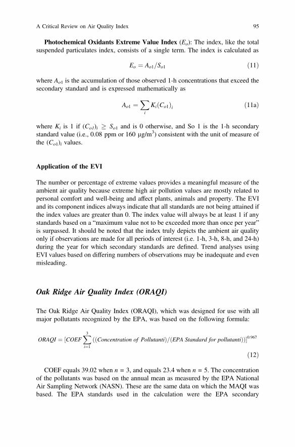
Photochemical Oxidants Extreme Value Index (Eo): The index, like the totalsuspended particulates index, consists of a single term. The index is calculated as
Eo ¼ Ao1=So1 ð11Þ
where Ao1 is the accumulation of those observed 1-h concentrations that exceed thesecondary standard and is expressed mathematically as
Ao1 ¼Xi
KiðCo1Þi ð11aÞ
where Ki is 1 if (Co1)i � So1 and is 0 otherwise, and So 1 is the 1-h secondarystandard value (i.e., 0.08 ppm or 160 lg/m3) consistent with the unit of measure ofthe (Co1)i values.
Application of the EVI
The number or percentage of extreme values provides a meaningful measure of theambient air quality because extreme high air pollution values are mostly related topersonal comfort and well-being and affect plants, animals and property. The EVIand its component indices always indicate that all standards are not being attained ifthe index values are greater than 0. The index value will always be at least 1 if anystandards based on a “maximum value not to be exceeded more than once per year”is surpassed. It should be noted that the index truly depicts the ambient air qualityonly if observations are made for all periods of interest (i.e. 1-h, 3-h, 8-h, and 24-h)during the year for which secondary standards are defined. Trend analyses usingEVI values based on differing numbers of observations may be inadequate and evenmisleading.
Oak Ridge Air Quality Index (ORAQI)
The Oak Ridge Air Quality Index (ORAQI), which was designed for use with allmajor pollutants recognized by the EPA, was based on the following formula:
ORAQI ¼ ½COEFX3i¼1
ððConcentration of PollutantiÞ=ðEPA Standard for pollutantiÞÞ�0:967
ð12Þ
COEF equals 39.02 when n = 3, and equals 23.4 when n = 5. The concentrationof the pollutants was based on the annual mean as measured by the EPA NationalAir Sampling Network (NASN). These are the same data on which the MAQI wasbased. The EPA standards used in the calculation were the EPA secondary
A Critical Review on Air Quality Index 95
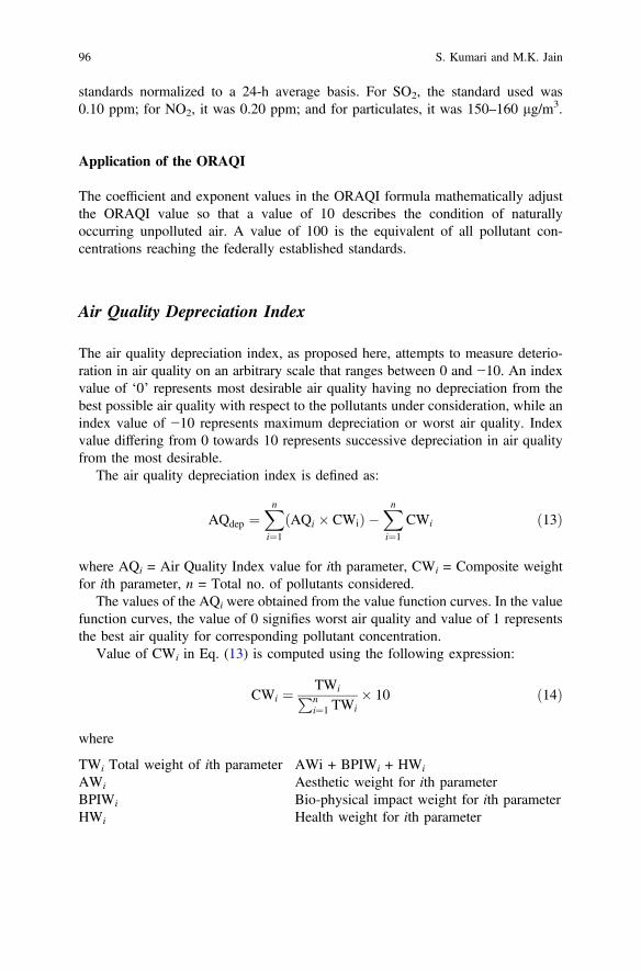
standards normalized to a 24-h average basis. For SO2, the standard used was0.10 ppm; for NO2, it was 0.20 ppm; and for particulates, it was 150–160 lg/m3.
Application of the ORAQI
The coefficient and exponent values in the ORAQI formula mathematically adjustthe ORAQI value so that a value of 10 describes the condition of naturallyoccurring unpolluted air. A value of 100 is the equivalent of all pollutant con-centrations reaching the federally established standards.
Air Quality Depreciation Index
The air quality depreciation index, as proposed here, attempts to measure deterio-ration in air quality on an arbitrary scale that ranges between 0 and −10. An indexvalue of ‘0’ represents most desirable air quality having no depreciation from thebest possible air quality with respect to the pollutants under consideration, while anindex value of −10 represents maximum depreciation or worst air quality. Indexvalue differing from 0 towards 10 represents successive depreciation in air qualityfrom the most desirable.
The air quality depreciation index is defined as:
AQdep ¼Xni¼1
AQi � CWið Þ �Xni¼1
CWi ð13Þ
where AQi = Air Quality Index value for ith parameter, CWi = Composite weightfor ith parameter, n = Total no. of pollutants considered.
The values of the AQi were obtained from the value function curves. In the valuefunction curves, the value of 0 signifies worst air quality and value of 1 representsthe best air quality for corresponding pollutant concentration.
Value of CWi in Eq. (13) is computed using the following expression:
CWi ¼ TWiPni¼1 TWi
� 10 ð14Þ
where
TWi Total weight of ith parameter AWi + BPIWi + HWi
AWi Aesthetic weight for ith parameterBPIWi Bio-physical impact weight for ith parameterHWi Health weight for ith parameter
96 S. Kumari and M.K. Jain
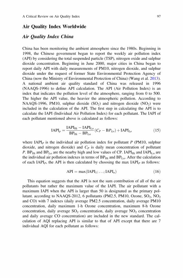
Air Quality Index Worldwide
Air Quality Index China
China has been monitoring the ambient atmosphere since the 1980s. Beginning in1998, the Chinese government began to report the weekly air pollution index(API) by considering the total suspended particle (TSP), nitrogen oxide and sulphurdioxide concentration. Beginning in June 2000, major cities in China began toreport daily API with daily measurements of PM10, nitrogen dioxide, and sulphurdioxide under the request of former State Environmental Protection Agency ofChina (now the Ministry of Environmental Protection of China) (Wang et al. 2013).A national ambient air quality standard of China was released in 1996(NAAQS-1996) to define API calculation. The API (Air Pollution Index) is anindex that indicates the pollution level of the atmosphere, ranging from 0 to 500.The higher the API value, the heavier the atmospheric pollution. According toNAAQS-1996, PM10, sulphur dioxide (SO2) and nitrogen dioxide (NO2) wereincluded in the calculation of the API. The first step in calculating the API is tocalculate the IAPI (Individual Air Pollution Index) for each pollutant. The IAPI ofeach pollutant mentioned above is calculated as follows:
IAPIp ¼ IAPIHi � IAPILoBPHi � BPLo
CP � BPLoð Þþ IAPILo ð15Þ
where IAPIP is the individual air pollution index for pollutant P (PM10, sulphurdioxide, and nitrogen dioxide) and CP is daily mean concentration of pollutantP. BPHi and BPLo are the nearby high and low values of CP. IAPIHi and IAPILo arethe individual air pollution indexes in terms of BPHi and BPLo. After the calculationof each IAPIP, the API is then calculated by choosing the max IAPIP as follows:
API ¼ max IAPI1; . . .; IAPInð Þ ð16Þ
This equation suggests that the API is not the sum contribution of all of the airpollutants but rather the maximum value of the IAPI. The air pollutant with amaximum IAPI when the API is larger than 50 is designated as the primary pol-lutant. according to NAAQS-2012, 6 pollutants (PM2.5, PM10, Ozone, SO2, NO2
and CO) with 7 indexes (daily average PM2.5 concentration, daily average PM10concentration, daily maximum 1-h Ozone concentration, maximum 8-h Ozoneconcentration, daily average SO2 concentration, daily average NO2 concentrationand daily average CO concentration) are included in the new standard. The cal-culation of AQI replacing API is similar to that of API except that there are 7individual AQI for each pollutant as follows:
A Critical Review on Air Quality Index 97
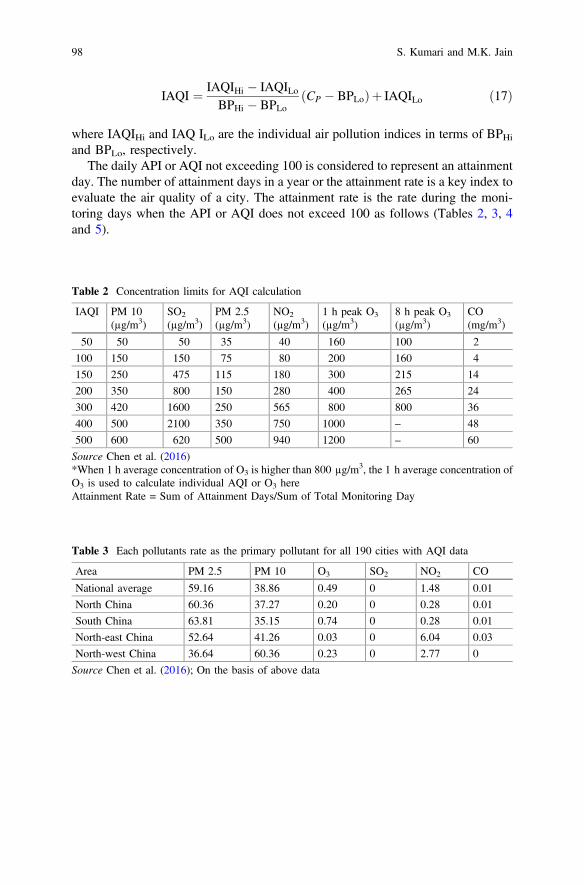
IAQI ¼ IAQIHi � IAQILoBPHi � BPLo
CP � BPLoð Þþ IAQILo ð17Þ
where IAQIHi and IAQ ILo are the individual air pollution indices in terms of BPHiand BPLo, respectively.
The daily API or AQI not exceeding 100 is considered to represent an attainmentday. The number of attainment days in a year or the attainment rate is a key index toevaluate the air quality of a city. The attainment rate is the rate during the moni-toring days when the API or AQI does not exceed 100 as follows (Tables 2, 3, 4and 5).
Table 2 Concentration limits for AQI calculation
IAQI PM 10(µg/m3)
SO2
(µg/m3)PM 2.5(µg/m3)
NO2
(µg/m3)1 h peak O3
(µg/m3)8 h peak O3
(µg/m3)CO(mg/m3)
50 50 50 35 40 160 100 2
100 150 150 75 80 200 160 4
150 250 475 115 180 300 215 14
200 350 800 150 280 400 265 24
300 420 1600 250 565 800 800 36
400 500 2100 350 750 1000 – 48
500 600 620 500 940 1200 – 60
Source Chen et al. (2016)*When 1 h average concentration of O3 is higher than 800 µg/m3, the 1 h average concentration ofO3 is used to calculate individual AQI or O3 hereAttainment Rate = Sum of Attainment Days/Sum of Total Monitoring Day
Table 3 Each pollutants rate as the primary pollutant for all 190 cities with AQI data
Area PM 2.5 PM 10 O3 SO2 NO2 CO
National average 59.16 38.86 0.49 0 1.48 0.01
North China 60.36 37.27 0.20 0 0.28 0.01
South China 63.81 35.15 0.74 0 0.28 0.01
North-east China 52.64 41.26 0.03 0 6.04 0.03
North-west China 36.64 60.36 0.23 0 2.77 0
Source Chen et al. (2016); On the basis of above data
98 S. Kumari and M.K. Jain
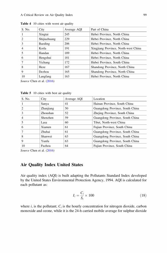
Air Quality Index United States
Air quality index (AQI) is built adapting the Pollutants Standard Index developedby the United States Environmental Protection Agency, 1994. AQI is calculated foreach pollutant as:
Ii ¼ Ci
Si� 100 ð18Þ
where i, is the pollutant; Ci is the hourly concentration for nitrogen dioxide, carbonmonoxide and ozone, while it is the 24-h carried mobile average for sulphur dioxide
Table 4 10 cities with worst air quality
S. No. City Average AQI Part of China
1 Xingtai 245 Hebei Province, North China
2 Shijiazhuang 229 Hebei Province, North China
3 Baoding 206 Hebei Province, North China
4 Korla 191 Xingjiang Province, North-west China
5 Handan 189 Hebei Province, North China
6 Hengshui 181 Hebei Province, North China
7 Yichang 172 Hubei Province, South China
8 Heze 167 Shandong Province, North China
9 Dezhou 165 Shandong Province, North China
10 Langfang 163 Hebei Province, North China
Source Chen et al. (2016)
Table 5 10 cities with best air quality
S. No. City Average AQI Location
1 Sanya 41 Hainan Province, South China
2 Zhanjiang 50 Guangdong Province, South China
3 Zhoushan 52 Zhejing Province, South China
4 Shenzhen 59 Guangdong Province, South China
5 Lasa 60 Tibet, North-west China
6 Xiamen 61 Fujian Province, South China
7 Zhuhai 61 Guangdong Province, South China
8 Shanwei 63 Guangdong Province, South China
9 Yunfu 63 Guangdong Province, South China
10 Fuzhou 64 Fujian Province, South China
Source Chen et al. (2016)
A Critical Review on Air Quality Index 99
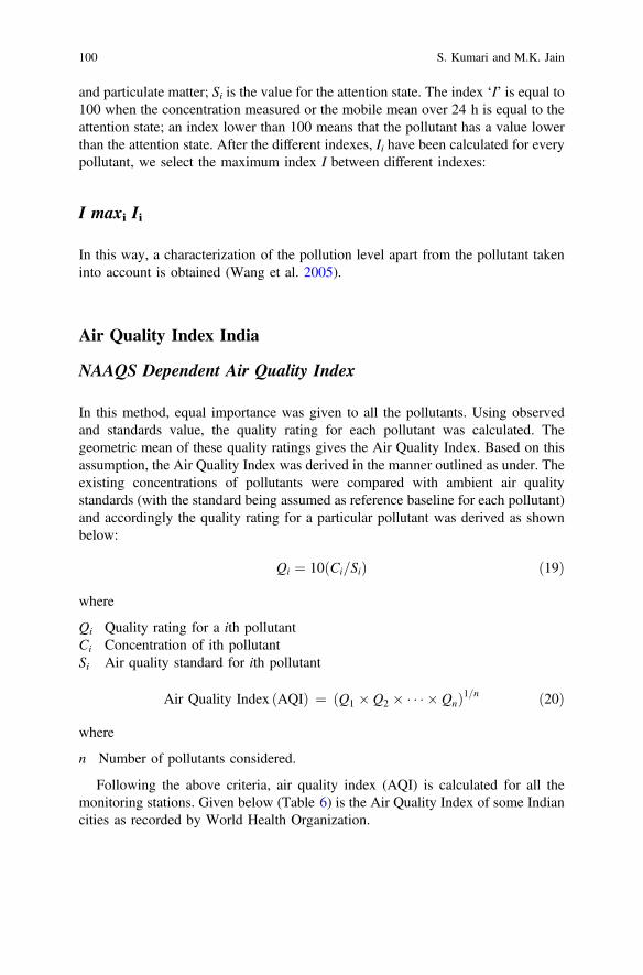
and particulate matter; Si is the value for the attention state. The index ‘I’ is equal to100 when the concentration measured or the mobile mean over 24 h is equal to theattention state; an index lower than 100 means that the pollutant has a value lowerthan the attention state. After the different indexes, Ii have been calculated for everypollutant, we select the maximum index I between different indexes:
I maxi Ii
In this way, a characterization of the pollution level apart from the pollutant takeninto account is obtained (Wang et al. 2005).
Air Quality Index India
NAAQS Dependent Air Quality Index
In this method, equal importance was given to all the pollutants. Using observedand standards value, the quality rating for each pollutant was calculated. Thegeometric mean of these quality ratings gives the Air Quality Index. Based on thisassumption, the Air Quality Index was derived in the manner outlined as under. Theexisting concentrations of pollutants were compared with ambient air qualitystandards (with the standard being assumed as reference baseline for each pollutant)and accordingly the quality rating for a particular pollutant was derived as shownbelow:
Qi ¼ 10ðCi=SiÞ ð19Þ
where
Qi Quality rating for a ith pollutantCi Concentration of ith pollutantSi Air quality standard for ith pollutant
Air Quality Index AQIð Þ ¼ Q1 � Q2 � � � � � Qnð Þ1=n ð20Þ
where
n Number of pollutants considered.
Following the above criteria, air quality index (AQI) is calculated for all themonitoring stations. Given below (Table 6) is the Air Quality Index of some Indiancities as recorded by World Health Organization.
100 S. Kumari and M.K. Jain
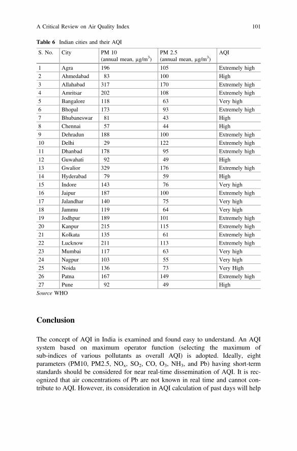
Conclusion
The concept of AQI in India is examined and found easy to understand. An AQIsystem based on maximum operator function (selecting the maximum ofsub-indices of various pollutants as overall AQI) is adopted. Ideally, eightparameters (PM10, PM2.5, NOx, SO2, CO, O3, NH3, and Pb) having short-termstandards should be considered for near real-time dissemination of AQI. It is rec-ognized that air concentrations of Pb are not known in real time and cannot con-tribute to AQI. However, its consideration in AQI calculation of past days will help
Table 6 Indian cities and their AQI
S. No. City PM 10(annual mean, µg/m3)
PM 2.5(annual mean, µg/m3)
AQI
1 Agra 196 105 Extremely high
2 Ahmedabad 83 100 High
3 Allahabad 317 170 Extremely high
4 Amritsar 202 108 Extremely high
5 Bangalore 118 63 Very high
6 Bhopal 173 93 Extremely high
7 Bhubaneswar 81 43 High
8 Chennai 57 44 High
9 Dehradun 188 100 Extremely high
10 Delhi 29 122 Extremely high
11 Dhanbad 178 95 Extremely high
12 Guwahati 92 49 High
13 Gwalior 329 176 Extremely high
14 Hyderabad 79 59 High
15 Indore 143 76 Very high
16 Jaipur 187 100 Extremely high
17 Jalandhar 140 75 Very high
18 Jammu 119 64 Very high
19 Jodhpur 189 101 Extremely high
20 Kanpur 215 115 Extremely high
21 Kolkata 135 61 Extremely high
22 Lucknow 211 113 Extremely high
23 Mumbai 117 63 Very high
24 Nagpur 103 55 Very high
25 Noida 136 73 Very High
26 Patna 167 149 Extremely high
27 Pune 92 49 High
Source WHO
A Critical Review on Air Quality Index 101
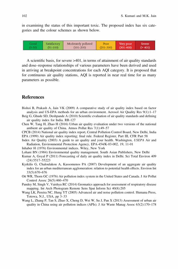
in examining the status of this important toxic. The proposed index has six cate-gories and the colour schemes as shown below.
A scientific basis, for severe >401, in terms of attainment of air quality standardsand dose–response relationships of various parameters have been derived and usedin arriving at breakpoint concentrations for each AQI category. It is proposed thatfor continuous air quality stations, AQI is reported in near real time for as manyparameters as possible.
References
Bishoi B, Prakash A, Jain VK (2009) A comparative study of air quality index based on factoranalysis and US-EPA methods for an urban environment. Aerosol Air Quality Res 9(1):1–17
Beig G, Ghude SD, Deshpande A (2010) Scientific evaluation of air quality standards and definingair quality index for India. RR-127
Chen W, Tang H, Zhao H (2016) Urban air quality evaluation under two versions of the nationalambient air quality of China. Atmos Pollut Res 7(1):49–57
CPCB (2014) National air quality index report, Central Pollution Control Board, New Delhi, IndiaEPA (1999) Air quality index reporting; final rule. Federal Register, Part III, CFR Part 58Index Air Quality (2003) A guide to air quality and your health. Washington, USEPA Air and
Radiation, Environmental Protection Agency, EPA-454/K-03-002, 19, 11-01Inhaber H (1976) Environmental indices. Wiley, New YorkLohani BN (1984) Environmental quality management. South Asian Publishers, New DelhiKumar A, Goyal P (2011) Forecasting of daily air quality index in Delhi. Sci Total Environ 409
(24):5517–55223Kyrkilis G, Chaloulakou A, Kassomenos PA (2007) Development of an aggregate air quality
index for an urban mediterranean agglomeration: relation to potential health effects. Environ Int33(5):670–676
Ott WR, Thorn GC (1976) Air pollution index system in the United States and Canada. J Air PollutControl Assoc 26(5):460–470
Pandey M, Singh V, Vaishya RC (2014) Geomatics approach for assessment of respiratory diseasemapping. Int Arch Photogram Remote Sens Spat Inform Sci 40(8):205
Wang LK, Pereira NC, Hung YT (2005) Advanced air and noise pollution control. Humana Press,Totowa, N.J., USA, pp 3–33
Wang L, Zhang P, Tan S, Zhao X, Cheng D, Wei W, Su J, Pan X (2013) Assessment of urban airquality in China using air pollution indices (APIs). J Air Waste Manag Assoc 63(2):170–178
102 S. Kumari and M.K. Jain
Aquatic Insects as Pollution Indicator—AStudy in Cachar, Assam, Northeast India
Arpita Dalal and Susmita Gupta
Abstract A seasonal study on water and aquatic insects of one oxbow lake(Satkorakandi anua) and one floodplain lake (Magura haor) of Cachar, Assam wasconducted. Environmental variables of water, diversity, and density of aquaticinsects were estimated by standard methods. In the oxbow lake, dissolved oxygenvalues were found to be lower than that of the floodplain lake. The pH of water wasfound below the acceptable limit of BIS in post-monsoon in oxbow lake, and inmost of the seasons in floodplain lake. Other variables were within the permissiblelimit. The Biological Monitoring Working Party (BMWP) and BMWPTHAI scorescomputed on the basis of tolerance level of the aquatic insects to organic pollutionrevealed poor water condition in all the sites and seasons in anua while in haorwater condition was found moderate in some seasons of the year. Different bioticindices, correlation coefficients, canonical correspondence analysis were computedand the role of aquatic insects as pollution indicator has been discussed in the paper.
Keywords Aquatic insects � Anua � Haor � Biotic score � CCA
Introduction
Freshwater ecosystems are most endangered ecosystems of the world (Dudgeon1999) and declines in biodiversity are far greater in freshwater than any otherecosystem of the world (Sala et al. 2000). Aquatic insects are important in fresh-water systems as they support the terrestrial lives through aquatic maintenance offood chains and also serve as indicators of water quality due to their varyingtolerance limits to organic and inorganic substances (Bass 1994; Mason 2002). Useof insects and/or their differential responses to stimuli in their aquatic habitat todetermine the quality of that environment is known as Biomonitoring (Arimoro andIkomi 2008; Merritt et al. 2008).
A. Dalal � S. Gupta (&)Department of Ecology and Environmental Science, Assam University, Silchar 788011, Indiae-mail: [email protected]
© Springer Nature Singapore Pte Ltd. 2018V.P. Singh et al. (eds.), Environmental Pollution, Water Scienceand Technology Library 77, https://doi.org/10.1007/978-981-10-5792-2_9
103

The district Cachar is rich in wetlands particularly in floodplain lakes and oxbowlakes formed by River Barak, the major river of south Assam. Floodplain lakes arefloodplains of river which help in drainage and flood control. Oxbow lakes are riverformed perennial U-shaped wetlands which are generally formed due to change inriver course. In spite of the presence of diverse types of wetlands in south Assam,only a few studies on aquatic insect diversity of oxbow and floodplain lakes werecarried out (Purkayastha and Gupta 2012; Gupta and Narzary 2013). Present studyfocused on the comparison of the health of two different ecosystems using aquaticinsects, popularly used in biomonitoring. The study also aimed to confirm the roleof aquatic insects as bioindicator.
Materials and Methods
Study Area
Figure 1 shows the study sites. For this study, one oxbow lake (Satkorakandi anua—591,012.65 m2) locally termed as ‘anua’ and one floodplain lake (Magura haor—187,146 m2) locally termed as ‘haor’ were selected. Both the lakes are located inCachar district ofAssam, India. This anua is ameander of theRiver Barakwhereas thehaor is the floodplain lake of the River Rukni, one of the tributaries of the River Barak(Dalal and Gupta 2015). Both anua and haor are surrounded by human habitation andagricultural fields. The selected sites were Sat1 (N 24°45.292′ E 092°52.474′) andSat2 (N 24°45.170′ E092°52.695′) fromSatkorakandi anua. The anua is located nearamosque. Sites selected fromMagura haorwereHaor1 (N 24°36.836′E092°51.887′)and Haor2 (N 24°36.910′ E 092°51.924′). These sites are mainly used for fishing.Seasonal collections (post-monsoon, winter, pre-monsoon, and monsoon) of waterand aquatic insects were done from all these sites during 2013–14.
Methods of Collection and Analyses
The samples were collected in thoroughly cleaned PVC bottles and BOD bottles(for estimating DO) to the brim, without leaving any space in order to prevent thepremature release of dissolved gases during the transit period. Environmentalvariables like air temperature (AT), water temperature (WT), rainfall (RF), trans-parency (TR), depth, pH, electrical conductivity (EC), total dissolved solid (TDS),dissolved oxygen (DO), free carbon dioxide (FCO2), total alkalinity (TA), sodium(Na), potassium (K), nitrate (NO3
−), and phosphate (PO43−) were estimated. Air
and water temperature were measured with the help of a mercury bulb thermometer(0–110 °C). RF data were collected from Meteorological Observatory, Cachar
104 A. Dalal and S. Gupta

College, Silchar, Assam. The pH and EC were measured by pH meter (Systronics µpH System 361) and conductivity meter (Systronics TDS Meter 308), respectively.TR was estimated by taking the measurement of appearance and disappearance ofSecchi’s disk (Michael 1984). DO was estimated by Winkler method while TA andFCO2 contents were analyzed by titrating with strong acid and alkali, respectively(Ramesh and Anbu 1996; APHA 2005). NO3
− was estimated by using UV spec-trophotometer and PO4
3− was estimated using light spectrophotometer (APHA2005). Sodium and potassium were estimated using flame photometer and depthwas measured following standard literature (APHA 2005).
Aquatic insects were collected from different sites by kick method whereby thevegetation is disturbed and a circular net (mesh size 60 lm) is dragged around thevegetation for a unit of time (Macan and Maudsley 1968; Brittain 1974). Three suchdrags constituted a sample. Collected insects were immediately sorted and preservedin 70% ethyl alcohol. They were identified using Motic and Magnus stereozoommicroscopes and with the help of standard keys (Kumar 1973a, b; Bal and Basu1994a, b; Westfall and Tennessen 1996; Cheng et al. 2001; Bal and Basu 2004;Epler 2006, 2010; Madden 2010). Statistical analyses of data were done usingdifferent softwares like Past, IBM SPSS STATISTICS version 21, CANOCO forwindows 4.5. Biomonitoring scores used were SIGNAL 2 (Chessman 2003),BMWP and ASPT (Mandaville 2002), BMWPTHAI, and ASPTTHAI (Mustow 2002).
Fig. 1 Map of Cachar district, Assam (India) showing the location of Magura haor andSatkorakandi anua
Aquatic Insects as Pollution Indicator … 105

Results and Discussion
Physicochemical Parameters
Tables 1 and 2 show the seasonal variations of physicochemical properties of waterfor both the lakes. In the oxbow lake, DO values in Sat1 (post-monsoon, winter andmonsoon) and Sat2 (post- and pre-monsoon) were recorded below 5 which is theacceptable limit of DO (Stiff et al. 1992). In contrast in both the sites of haor(floodplain lake) in all the seasons, DO values were above 4 except in Haor2 inmonsoon. FCO2 of all the sites in all the seasons except Haor1 in post-monsoonwere recorded beyond 6 (acceptable limit as per BIS 2012). Low photosynthesisand high respiration rate of the aquatic biota might be one of the reasons for lowDO and high FCO2 in the oxbow lake. Das and Chakrabarty (2008) also recordedDO below 4 in Hansadanga beel (oxbow lake), West Bengal. A classical negativecorrelation between FCO2 and DO (Wetzel 1984) was found in haor where RF wasfound significantly negatively correlated with DO and positively correlated withFCO2 indicating organic pollution induced by anthropogenic input by surfacerunoff (Table 3). Previous study at one oxbow lake in Cachar district also recordedpositive correlation of RF with FCO2 (Gupta and Devi 2014). TA values, NO3
− andPO4
3− concentration in water were within the permissible limit in all the sites in allthe seasons (WHO 2006; BIS 2012). This agreed with the findings of previousstudies in lentic systems of Cachar district, Assam (Purkayastha and Gupta 2012;Gupta and Narzary 2013; Barman et al. 2014; Dalal and Gupta 2014). pH of Haor1,Haor2, and Sat2 (post-monsoon, pre-monsoon, and monsoon) and Sat1(post-monsoon and monsoon) were recorded below the acceptable limit (6.5), i.e.,they were slightly acidic in nature while rest of the physicochemical variables ofwater in all the sites and in all the seasons were within the permissible limit (WHO2006; BIS 2012).
Aquatic Insects
A total of 6 orders, 22 families, 43 genera, and 53 species were recorded from thefloodplain lake, Magura haor whereas from the oxbow lake, Satkorakandi anua 5orders, 15 families, 27 genera, and 32 species were recorded. Highest number oforders was recorded from Haor1, Haor2 during post-monsoon and pre-monsoon,respectively, and Sat2 during post-monsoon and winter whereas lowest number oforders was recorded from Sat1 (monsoon). Highest number of families wasrecorded from Haor1 (pre-monsoon) and lowest from Sat1 (winter and monsoon).Haor2 (pre-monsoon) had the highest number of genera and species whereas Sat1(monsoon) had the lowest number (Fig. 2). In both the systems, 14 species were
106 A. Dalal and S. Gupta

Tab
le1
Physicochemical
prop
ertiesof
water
oftwodifferentsitesof
Maguraha
or(floo
dplain
lake)of
Cachar,Assam
during
Post-m
onsoon
–Mon
soon
(201
3–14
)(M
ean±
SD)
Seasons
Post-m
onsoon
Winter
Pre-monsoon
Monsoon
Sites
Haor1
Haor2
Haor1
Haor2
Haor1
Haor2
Haor1
Haor2
AT(°C)
25±
027
±0
24±
024
±0
28±
028
±0
34.5
±0
34.5
±0
WT(°C)
21±
021
±0
22±
022
±0
25.5
±0
26±
031
±0
28±
0
RF(m
m)
93±
84.94
93±
84.94
6.67
±11.54
6.67
±11.54
142.83
±116.7
142.83
±116.7
442.16
±17.41
442.16
±17.41
TR
(cm)
33.9
±0
14.5
±0
14.5
±0
21.65±
014.5
±0
13.1
±0
19.75±
024.5
±0
Depth
(cm)
33.9
±0
20±
017
±0
34.5
±0
27.5
±0
23.5
±0
28.5
±0
31.8
±0
DO
(mgl–1 )
8.01
±1.97
8.66
±1.88
8.22
±0.43
10.73±
1.45
6.61
±0.55
7.88
±0.85
6.33
±0.25
4.99
±0.07
FCO2(m
gl–1 )
5.99
±2
9.32
±1.15
7.06
±1.01
7.98
±0
10.98±
1.71
11.24±
3.59
10.85±
1.02
19.70±
4.40
TA
(mgl−1 )
39.27±
0.70
22.2
±2.03
27.07±
1.01
30.66±
2.31
11.93±
1.15
11±
1.71
28.8
±2.03
28.2
±2.03
NO3−
(mgl–1 )
0.18
±0.11
BDL
1.35
±1.01
0.29
±0.18
0.16
±0.16
0.23
±0.08
0.005±
0.04
0.009±
0.02
PO43−
(mgl−1 )
0.05
±0.06
0.22
±0.03
0.42
±0.25
0.15
±0.03
0.02
±0.01
0.02
±0.01
0.067±
0.03
0.186±
0.06
pH6.27
±0.07
5.68
±0.15
6.91
±0.05
6.8±
0.06
6.24
±0.10
5.98
±0.07
6.35
±0.03
6.07
±0.07
EC
(µScm
−1 )
55.55±
4.36
19.14±
3.01
44.56±
1.91
50.44±
4.56
40.2
±9.14
51.5
±11.02
38±
2.38
28.28±
3.29
TDS(ppm
)36.1
±2.85
12.49±
1.99
29.02±
1.22
32.81±
326.09±
5.94
33.46±
7.17
24.66±
1.45
18.35±
2.13
Na(m
gl−1 )
2.31
±0.86
2.97
±2.11
1.76
±0.24
4.14
±1.40
2.11
±0.23
1.80
±0.07
1.02
±0.01
1.43
±0.30
K(m
gl−1 )
3.73
±0.31
1.24
±0.23
2.56
±0.12
2.54
±0.31
3.76
±1.24
3.35
±0.004
3.05
±0.38
3.33
±0.23
Aquatic Insects as Pollution Indicator … 107
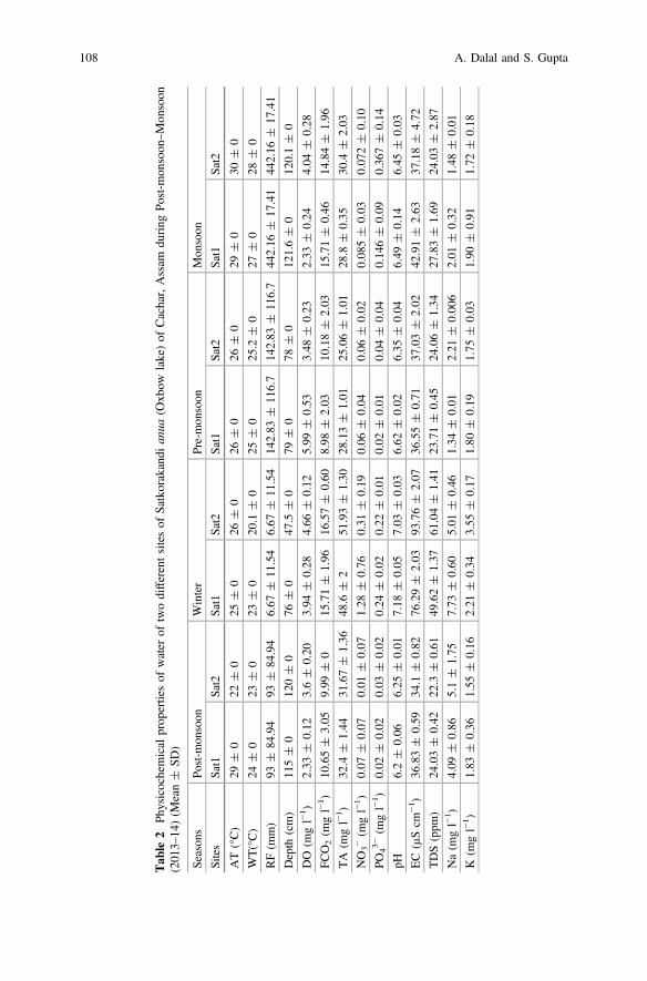
Tab
le2
Physicochemical
prop
ertiesof
water
oftwodifferentsitesof
Satkorakandi
anua
(Oxb
owlake)of
Cachar,Assam
during
Post-m
onsoon
–Mon
soon
(201
3–14
)(M
ean±
SD)
Seasons
Post-m
onsoon
Winter
Pre-monsoon
Monsoon
Sites
Sat1
Sat2
Sat1
Sat2
Sat1
Sat2
Sat1
Sat2
AT(°C)
29±
022
±0
25±
026
±0
26±
026
±0
29±
030
±0
WT(°C)
24±
023
±0
23±
020.1
±0
25±
025.2
±0
27±
028
±0
RF(m
m)
93±
84.94
93±
84.94
6.67
±11.54
6.67
±11.54
142.83
±116.7
142.83
±116.7
442.16
±17.41
442.16
±17.41
Depth
(cm)
115±
0120±
076
±0
47.5
±0
79±
078
±0
121.6±
0120.1±
0
DO
(mgl−1 )
2.33
±0.12
3.6±
0.20
3.94
±0.28
4.66
±0.12
5.99
±0.53
3.48
±0.23
2.33
±0.24
4.04
±0.28
FCO2(m
gl−1 )
10.65±
3.05
9.99
±0
15.71±
1.96
16.57±
0.60
8.98
±2.03
10.18±
2.03
15.71±
0.46
14.84±
1.96
TA
(mgl−1 )
32.4
±1.44
31.67±
1.36
48.6
±2
51.93±
1.30
28.13±
1.01
25.06±
1.01
28.8
±0.35
30.4
±2.03
NO3−
(mgl−1 )
0.07
±0.07
0.01
±0.07
1.28
±0.76
0.31
±0.19
0.06
±0.04
0.06
±0.02
0.085±
0.03
0.072±
0.10
PO43−
(mgl−1 )
0.02
±0.02
0.03
±0.02
0.24
±0.02
0.22
±0.01
0.02
±0.01
0.04
±0.04
0.146±
0.09
0.367±
0.14
pH6.2±
0.06
6.25
±0.01
7.18
±0.05
7.03
±0.03
6.62
±0.02
6.35
±0.04
6.49
±0.14
6.45
±0.03
EC
(µScm
−1 )
36.83±
0.59
34.1
±0.82
76.29±
2.03
93.76±
2.07
36.55±
0.71
37.03±
2.02
42.91±
2.63
37.18±
4.72
TDS(ppm
)24.03±
0.42
22.3
±0.61
49.62±
1.37
61.04±
1.41
23.71±
0.45
24.06±
1.34
27.83±
1.69
24.03±
2.87
Na(m
gl−1 )
4.09
±0.86
5.1±
1.75
7.73
±0.60
5.01
±0.46
1.34
±0.01
2.21
±0.006
2.01
±0.32
1.48
±0.01
K(m
gl−1 )
1.83
±0.36
1.55
±0.16
2.21
±0.34
3.55
±0.17
1.80
±0.19
1.75
±0.03
1.90
±0.91
1.72
±0.18
108 A. Dalal and S. Gupta
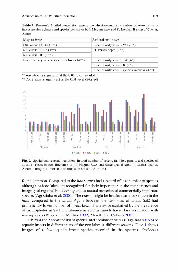
found common. Compared to the haor, anua had a record of less number of speciesalthough oxbow lakes are recognized for their importance in the maintenance andintegrity of regional biodiversity and as natural nurseries of commercially importantspecies (Agostinho et al. 2000). The reason might be less human intervention in thehaor compared to the anua. Again between the two sites of anua, Sat2 hadprominently lower number of insect taxa. This may be explained by the prevalenceof macrophytes in Sat1 and absence in Sat2 as insects have close association withmacrophytes (Wilcox and Meeker 1992; Moretti and Callisto 2005).
Tables 4 and 5 show the list of species, and dominance status (Engelmann 1978) ofaquatic insects in different sites of the two lakes in different seasons. Plate 1 showsimages of a few aquatic insect species recorded in the systems. Octhebius
Table 3 Pearson’s 2-tailed correlation among the physicochemical variables of water, aquaticinsect species richness and species density of both Magura haor and Satkorakandi anua of Cachar,Assam
Magura haor Satkorakandi anua
DO versus FCO2 (−**) Insect density versus WT (−*)
RF versus FCO2 (+**) RF versus depth (+**)
RF versus DO (−**)
Insect density versus species richness (+**) Insect density versus TA (+*)
Insect density versus K (+*)
Insect density versus species richness (+**)
*Correlation is significant at the 0.05 level (2-tailed)**Correlation is significant at the 0.01 level (2-tailed)
02468
101214161820
Post
mon
Win
ter
Pre
mon
Mon
soon
Post
mon
Win
ter
Pre
mon
Mon
soon
Post
mon
Win
ter
Pre
mon
Mon
soon
Post
mon
Win
ter
Pre
mon
Mon
soon
Orders Families Genus Species
Haor1 Haor2 Sat1 Sat2
Fig. 2 Spatial and seasonal variations in total number of orders, families, genera, and species ofaquatic insects in two different sites of Magura haor and Satkorakandi anua in Cachar district,Assam during post-monsoon to monsoon season (2013–14)
Aquatic Insects as Pollution Indicator … 109
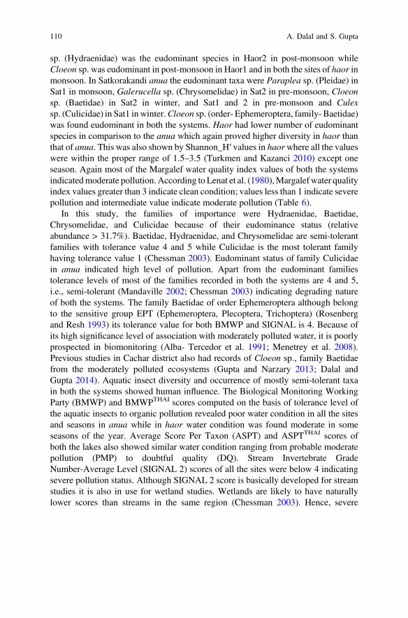
sp. (Hydraenidae) was the eudominant species in Haor2 in post-monsoon whileCloeon sp. was eudominant in post-monsoon in Haor1 and in both the sites of haor inmonsoon. In Satkorakandi anua the eudominant taxa were Paraplea sp. (Pleidae) inSat1 in monsoon, Galerucella sp. (Chrysomelidae) in Sat2 in pre-monsoon, Cloeonsp. (Baetidae) in Sat2 in winter, and Sat1 and 2 in pre-monsoon and Culexsp. (Culicidae) in Sat1 inwinter.Cloeon sp. (order- Ephemeroptera, family- Baetidae)was found eudominant in both the systems. Haor had lower number of eudominantspecies in comparison to the anua which again proved higher diversity in haor thanthat of anua. This was also shown by Shannon_H′ values in haorwhere all the valueswere within the proper range of 1.5–3.5 (Turkmen and Kazanci 2010) except oneseason. Again most of the Margalef water quality index values of both the systemsindicatedmoderate pollution. According to Lenat et al. (1980),Margalefwater qualityindex values greater than 3 indicate clean condition; values less than 1 indicate severepollution and intermediate value indicate moderate pollution (Table 6).
In this study, the families of importance were Hydraenidae, Baetidae,Chrysomelidae, and Culicidae because of their eudominance status (relativeabundance > 31.7%). Baetidae, Hydraenidae, and Chrysomelidae are semi-tolerantfamilies with tolerance value 4 and 5 while Culicidae is the most tolerant familyhaving tolerance value 1 (Chessman 2003). Eudominant status of family Culicidaein anua indicated high level of pollution. Apart from the eudominant familiestolerance levels of most of the families recorded in both the systems are 4 and 5,i.e., semi-tolerant (Mandaville 2002; Chessman 2003) indicating degrading natureof both the systems. The family Baetidae of order Ephemeroptera although belongto the sensitive group EPT (Ephemeroptera, Plecoptera, Trichoptera) (Rosenbergand Resh 1993) its tolerance value for both BMWP and SIGNAL is 4. Because ofits high significance level of association with moderately polluted water, it is poorlyprospected in biomonitoring (Alba- Tercedor et al. 1991; Menetrey et al. 2008).Previous studies in Cachar district also had records of Cloeon sp., family Baetidaefrom the moderately polluted ecosystems (Gupta and Narzary 2013; Dalal andGupta 2014). Aquatic insect diversity and occurrence of mostly semi-tolerant taxain both the systems showed human influence. The Biological Monitoring WorkingParty (BMWP) and BMWPTHAI scores computed on the basis of tolerance level ofthe aquatic insects to organic pollution revealed poor water condition in all the sitesand seasons in anua while in haor water condition was found moderate in someseasons of the year. Average Score Per Taxon (ASPT) and ASPTTHAI scores ofboth the lakes also showed similar water condition ranging from probable moderatepollution (PMP) to doubtful quality (DQ). Stream Invertebrate GradeNumber-Average Level (SIGNAL 2) scores of all the sites were below 4 indicatingsevere pollution status. Although SIGNAL 2 score is basically developed for streamstudies it is also in use for wetland studies. Wetlands are likely to have naturallylower scores than streams in the same region (Chessman 2003). Hence, severe
110 A. Dalal and S. Gupta
Tab
le4
Dom
inance
status
oftheaquatic
insectspeciesof
thetwodifferentsitesof
Maguraha
or(floo
dplain
lake)of
Cachar,Assam
during
post-m
onsoon
–
mon
soon
,20
13–14
usingEng
elmannScale(197
8)
Orders
Seasons
Post-m
onsoon
Winter
Pre-monsoon
Monsoon
Taxa
Haor1
Haor2
Haor1
Haor2
Haor1
Haor2
Haor1
Haor2
Hem
iptera
Fam
ily:Gerrida
eNeogerrisparvula
12.07
3.64
28.61
–5.62
2.13
––
Gerrissp.
–0.91
––
––
––
Gerrislepcha
6.9
0.91
–8.33
–2.13
––
Trepobates
sp.
––
7.15
––
––
–
Limnogonusfossarum
––
––
–2.13
––
Fam
ily:Noton
ectida
eAnisops
breddini
–6.36
––
1.12
4.26
––
Nychiasappho
–0.91
––
––
––
Aphelonecta
sp.
1.72
1.82
––
–21.29
––
Anisops
bouvieri
––
––
–10.64
––
Anispos
exiguus
––
––
–2.13
––
Fam
ily:Micronectidae
Micronectahalip
loides
3.45
––
––
––
10.35
Micronectasiva
3.45
––
––
––
6.9
Micronectascutellaris
––
–8.33
––
––
Micronectaludibunda
––
––
––
–6.9
Micronectasp.
––
––
5.62
––
–
Fam
ily:Veliid
aeBaptista
colla
ris
––
–4.17
––
–
Fam
ily:Pleidae
Parapleasp.
–0.91
––
1.12
––
–
Fam
ily:Nepidae
Ranatra
elongata
–0.91
––
––
–
Ranatra
gracilis
––
–4.17
––
–
Ranatra
sordidula
––
––
––
2.78
–
Laccotrephes
ruber
––
––
–2.13
––
Fam
ily:Hyd
rometrida
eHydrometra
greeni
––
––
1.12
4.26
––
Fam
ily:Belostomatidae
Diplonychus
sp.
––
––
––
2.78
–
(con
tinued)
Aquatic Insects as Pollution Indicator … 111

Tab
le4
(con
tinued)
Orders
Seasons
Post-m
onsoon
Winter
Pre-monsoon
Monsoon
Taxa
Haor1
Haor2
Haor1
Haor2
Haor1
Haor2
Haor1
Haor2
Coleoptera
Fam
ily:Noteridae
Suphisellussp.
1.72
––
–3.37
8.51
8.33
–
Fam
ily:Hyd
roph
ilida
eLa
ccobiussp.
1.72
0.91
–4.17
––
––
Cercyon
sp.
–0.91
––
––
––
Berosus
sp.
––
7.15
–1.12
2.13
––
Helocharessp.
––
7.15
8.33
––
Berosus
indicum
––
––
1.12
––
–
Hydrobius
sp.
––
––
1.12
––
–
Fam
ily:Hyd
raenidae
Octhebius
sp.
–58.19(E)
––
––
––
Fam
ily:Dytiscida
eLa
ccophilussp.
––
–8.33
1.12
2.13
––
Cybistersp.
––
––
1.12
8.51
––
Cybisterlateralim
arginalis
––
––
–2.13
––
Fam
ily:Chrysom
elidae
Donacia
sp.
––
–20.83
––
––
Galerucella
sp.
––
––
1.12
2.13
––
Fam
ily:Hyd
rochidae
Hydrochus
sp.
––
–8.33
––
––
(con
tinued)
112 A. Dalal and S. Gupta
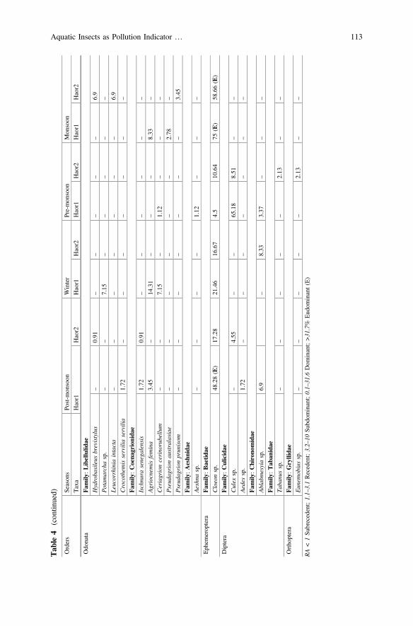
Tab
le4
(con
tinued)
Orders
Seasons
Post-m
onsoon
Winter
Pre-monsoon
Monsoon
Taxa
Haor1
Haor2
Haor1
Haor2
Haor1
Haor2
Haor1
Haor2
Odonata
Fam
ily:Libellulid
aeHydrobasileus
brevistylus
–0.91
––
––
–6.9
Potam
archasp.
––
7.15
––
––
–
Leucorrhinia
intacta
––
––
––
–6.9
Crocothem
isserviliaservilia
1.72
––
––
––
–
Fam
ily:Coena
grionida
eIschnura
senegalensis
1.72
0.91
––
––
––
Agriocnem
isfemina
3.45
–14.31
––
–8.33
–
Ceriagrioncerinorubellu
m–
–7.15
–1.12
––
–
Pseudagrion
australasiae
––
––
––
2.78
–
Pseudagrion
prunisom
––
––
––
–3.45
Fam
ily:Aeshn
idae
Aeshnasp.
––
––
1.12
––
–
Ephem
eroptera
Fam
ily:Baetida
eCloeonsp.
48.28(E)
17.28
21.46
16.67
4.5
10.64
75(E)
58.66(E)
Diptera
Fam
ily:Culicidae
Culex
sp.
–4.55
––
65.18
8.51
––
Aedes
sp.
1.72
––
––
––
–
Fam
ily:Chirono
midae
Ablabmesyiasp.
6.9
–8.33
3.37
––
–
Fam
ily:Tab
anidae
Tabanussp.
––
––
–2.13
––
Orthoptera
Fam
ily:Gryllida
eEunem
obiussp.
––
––
–2.13
––
RA<
1Su
brecedent;1.1–3.1Recedent;3.2–10
Subdom
inant;0.1–31.6
Dom
inant;>31.7%
Eudom
inant(E)
Aquatic Insects as Pollution Indicator … 113

Tab
le5
Dom
inance
status
oftheaquatic
insectspeciesof
thetwodifferentsitesof
Satkorakandi
anua
(Oxb
owlake)o
fCachar,Assam
during
post-m
onsoon
–
mon
soon
2013–14
usingEng
elmannScale(197
8)
Orders
Season
sPo
st-m
onsoon
Winter
Pre-mon
soon
Mon
soon
Taxa
Sat1
Sat2
Sat1
Sat2
Sat1
Sat2
Sat1
Sat2
Hem
iptera
Fam
ily:Gerrida
eLimno
gonu
snitid
us–
6.67
––
––
––
Fam
ily:Noton
ectida
eAnisops
niveus
–6.67
––
––
––
Anisops
breddini
––
11.11
––
––
–
Fam
ily:Mesov
eliid
aeMesovelia
vittigera
–6.67
––
––
––
Mesovelia
mulsanti
––
–2.22
––
––
Fam
ily:Micronectidae
Micronectaha
liploides
––
–8.89
7.41
22.22
11.11
5
Syna
pton
ecta
issa
––
––
7.41
––
–
Fam
ily:Pleidae
Parap
leasp.
25.81
––
–14
.81
–66
.67(E)
22.22
Fam
ily:Nepidae
Ran
atra
varipes
3.23
––
4.44
––
––
Coleoptera
Fam
ily:Noteridae
Suph
isellussp.
9.68
––
––
––
–
Fam
ily:Hyd
roph
ilida
eBerosus
sp.
–6.67
––
––
––
Laccob
iussp.
–6.67
––
––
––
Fam
ily:Chrysom
elidae
Galerucella
sp.
––
––
–33
.33(E)
––
(con
tinued)
114 A. Dalal and S. Gupta

Tab
le5
(con
tinued)
Orders
Season
sPo
st-m
onsoon
Winter
Pre-mon
soon
Mon
soon
Taxa
Sat1
Sat2
Sat1
Sat2
Sat1
Sat2
Sat1
Sat2
Odo
nata
Fam
ily:Libellulid
aeRho
dothem
isrufa
3.23
––
––
––
–
Hydroba
sileus
brevistylus
6.45
––
––
––
–
Potam
archaob
scura
3.23
–11
.11
––
––
–
Sympetrum
sp.
3.23
––
––
––
–
Sympetrum
illotum
––
11.11
2.22
––
––
Hydrocanthu
ssp.
––
–2.22
––
––
Leucorrhinia
frigida
––
11.11
––
––
5.56
Orthetrum
sabina
–13
.33
––
––
––
Neurothem
isfluctua
ns–
6.67
––
––
––
Fam
ily:Coena
grionida
eCeriagrioncerino
rubellu
m3.23
––
––
––
–
Ischnu
rasenega
lensis
3.23
––
4.44
––
––
Agriocnem
ispygm
aea
–13
.33
–2.22
––
––
Eph
emerop
tera
Fam
ily:Baetida
eCloeonsp.
–13
.33
–68
.89(E)
66.67(E)
33.33(E)
22.22
–
Diptera
Fam
ily:Culicidae
Culex
sp.
––
55.56(E)
––
––
–
Ano
pheles
sp.
––
–2.22
––
–5.56
Aedes
sp.
––
––
3.7
––
–
Fam
ily:Simuliid
aeGym
nopa
issp.
––
––
–11
.11
––
Fam
ily:Chirono
midae
Ablab
mesyiasp.
–2
–2.22
––
––
Param
erinasp.
––
––
–16
.67
RA<1Su
brecedent;1.1–
3.1Recedent;3.2–
10Su
bdom
inant;0.1–
31.6
Dom
inant;>31
.7%
Eud
ominant(E)
Aquatic Insects as Pollution Indicator … 115

pollution interpreted from SIGNAL value could be considered as moderate pollu-tion (Table 7). In both the ecosystems, insect density showed very high significantpositive correlation with species richness. Such correlation was also found inprevious studies in Cachar district in one oxbow lake and two different ponds(Gupta and Narzary 2013; Dalal and Gupta 2014) (Table 3).
Laccotrephes ruber Limnogonus nitidus Culex sp. Cybister sp.
Leucorrhinia frigid Sympetrum illotum Ranatra varipes
Ranatra gracilis Cloeon sp. Potamarcha obscura
Plate 1 Images of a few aquatic insect species
116 A. Dalal and S. Gupta

Table 6 Diversity indices of aquatic insects of two different sites of Magura haor andSatkorakandi anua of Cachar, Assam during Post-monsoon–monsoon, 2013–14
Haor1 Haor2 Sat1 Sat2
Post-monsoon Shannon_H′ 1.95 1.51 1.89 2.21
Evenness_e^H/S 0.44 0.30 0.61 0.91
Margalef 3.69 2.97 2.91 3.32
Berger–Parker 0.48 0.58 0.35 0.2
Winter Shannon_H′ 1.91 2.26 1.30 1.25
Evenness_e^H/S 0.84 0.87 0.73 0.35
Margalef 2.65 3.14 1.82 2.36
Berger–Parker 0.28 0.21 0.55 0.68
Pre-monsoon Shannon_H′ 1.53 2.61 1.061 1.31
Evenness_e^H/S 0.27 0.71 0.57 0.92
Margalef 3.56 4.67 1.21 1.36
Berger–Parker 0.65 0.21 0.66 0.33
Monsoon Shannon_H′ 0.93 1.40 0.84 1.30
Evenness_e^H/S 0.42 0.58 0.77 0.73
Margalef 1.39 1.78 0.91 1.38
Berger–Parker 0.75 0.58 0.66 0.5
Table 7 SIGNAL 2, BMWP, ASPT, BMWPTHAI and ASPTTHAI scores used at two different sitesof Magura haor and Satkorakandi anua of Cachar district, Assam during post-monsoon–monsoon,2013–14
Haor1 Haor2 Sat1 Sat2
Post-monsoon SIGNAL 2 3.38 (SP) 2.95 (SP) 2.69 (SP) 3 (SP)
BMWP 37 (P) 38 (P) 21 (P) 32 (P)
ASPT 4.62 (PMP) 5.42 (DQ) 5.25 (DQ) 4.57 (PMP)
BMWPTHAI 42 (M) 31 (P) 16 (P) 32 (P)
ASPTTHAI 4.66 (PMP) 5.16 (DQ) 5.33 (DQ) 4.57 (PMP)
Winter SIGNAL 2 3.5 (SP) 3 (SP) 2.2 (SP) 3.33 (SP)
BMWP 28 (P) 41 (M) 13 (P) 40 (P)
ASPT 5.6 (DQ) 4.55 (PMP) 6.5 (DQ) 5 (PMP)
BMWPTHAI 26 (P) 41 (M) 11 (P) 38 (P)
ASPTTHAI 5.2 (DQ) 4.55 (PMP) 5.5(DQ) 4.75 (PMP)
Pre-monsoon SIGNAL 2 2.54 (SP) 2.45 (SP) 3.22 (SP) 3.5 (SP)
BMWP 65 (M) 49 (M) 14 (P) 19 (P)
ASPT 5(DQ) 4.9 (PMP) 4.67 (PMP) 4.75 (PMP)
BMWPTHAI 63 (M) 49 (P) 14 (P) 19 (P)
ASPTTHAI 4.86 (PMP) 4.9 (PMP) 4.67 (PMP) 4.75 (PMP)(continued)
Aquatic Insects as Pollution Indicator … 117
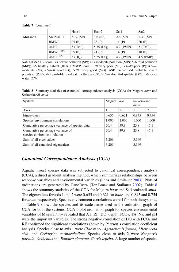
Canonical Correspondence Analysis (CCA)
Aquatic insect species data was subjected to canonical correspondence analysis(CCA), a direct gradient analysis method, which summarizes relationships betweenresponse variables and environmental variables (Leps and Smilauer 2003). Plots ofordinations are generated by CanoDraw (Ter Braak and Smilauer 2002). Table 8shows the summary statistics of the CCA for Magura haor and Satkorakandi anua.The eigenvalues for axis 1 and 2 were 0.655 and 0.621 for haor, and 0.845 and 0.754for anua, respectively. Species environment correlations were 1 for both the systems.
Table 9 shows the species and its code name used in the ordination graph ofCCA for both the systems. CCA biplot ordination graph for species environmentalvariables of Magura haor revealed that AT, RF, DO, depth, FCO2, TA, Na, and pHwere the important variables. The strong negative correlation of DO with FCO2 andRF confirmed the significant correlations shown by Pearson’s correlation coefficientanalysis. Species close to axis 1 were Cloeon sp., Agriocnemis femina, Micronectasiva, and Ceriagrion cerinorubellum. Species close to axis 2 were Neogerrisparvula, Octhebius sp., Ranatra elongate, Gerris lepcha. A large number of species
Table 8 Summary statistics of canonical correspondence analysis (CCA) for Magura haor andSatkorakandi anua
Systems Magura haor Satkorakandianua
Axes 1 2 1 2
Eigenvalues 0.655 0.621 0.845 0.754
Species environment correlations 1.000 1.000 1.000 1.000
Cumulative percentage variance of species data 20.4 39.8 23.8 45.1
Cumulative percentage variance ofspecies-environment relation
20.4 39.8 23.8 45.1
Sum of all eigenvalues 3.206 3.549
Sum of all canonical eigenvalues 3.206 3.549
Table 7 (continued)
Haor1 Haor2 Sat1 Sat2
Monsoon SIGNAL 2 3.72 (SP) 3.6 (SP) 2.6 (SP) 2.33 (SP)
BMWP 25 (P) 23 (P) 14 (P) 20 (P)
ASPT 5 (PMP) 5.75 (DQ) 4.7 (PMP) 5 (PMP)
BMWPTHAI 25 (P) 21 (P) 14 (P) 18 (P)
ASPTTHAI 5 (DQ) 5.25 (DQ) 4.7 (PMP) 4.5 (PMP)
Note SIGNAL 2 score: <4 severe pollution (SP); 4–5 moderate pollution (MP); 5–6 mild pollution(MiP); >6 healthy habitat (HH). BMWP score: −10 very poor (VP); 11–40 poor (P); 41–70moderate (M); 71–100 good (G); >100 very good (VG). ASPT score: <4 probable severepollution (PSP); 4–5 probable moderate pollution (PMP); 5–6 doubtful quality (DQ); >6 cleanwater (CW)
118 A. Dalal and S. Gupta
Table 9 List of species and its code name used in CCA biplot ordination graph of Magura haorand Satkorakandi anua
S. No. Magura haor Species codename
S. No. Satkorakandi anua Species codename
1 Neogerris parvula Neo 1 Limnogonus nitidus LimnNi
2 Gerris sp. Gerr1 2 Anisops niveus AniNi
3 Gerris lepcha Gerr2 3 Anisops breddini AniBre
4 Trepobates sp. Trepo 4 Mesovelia vittigera MesoV
5 Limnogonusfossarum
Limno 5 Mesovelia mulsanti MesMu
6 Anisops breddini AniB 6 Micronectahaliploides
MicrHal
7 Nychia sappho Nychia 7 Synaptonecta issa SynoIss
8 Aphelonecta sp. Aphelo 8 Paraplea sp. ParaS
9 Anisops bouvieri AniBo 9 Ranatra varipes RanaVar
10 Anispos exiguus AniEx 10 Suphisellus sp. SuphiS
11 Micronectahaliploides
MicrHali 11 Berosus sp. BersSp
12 Micronecta siva MicrSi 12 Laccobius sp. LaccoSP
13 Micronectascutellaris
MicrScu 13 Galerucella sp. GaleSP
14 Micronectaludibunda
MicrLudi 14 Rhodothemis rufa RhoRu
15 Micronecta sp. Micrsp 15 Hydrobasileusbrevistylus
HydBrevi
16 Baptista collaris BaptCol 16 Potamarchaobscura
PotaObs
17 Paraplea sp. Para1 17 Sympetrum sp. SympS
18 Ranatra elongata RanaElon 18 Sympetrum illotum SympIllo
19 Ranatra gracilis RanaGra 19 Hydrocanthus sp. Hydroca
20 Ranatra sordidula RanaSor 20 Leucorrhiniafrigida
LeucorFRIGI
21 Laccotrephes ruber LaccoR 21 Orthetrum sabina OrtheSa
22 Hydrometra greeni HydR 22 Neurothemisfluctuans
NeurotFlu
23 Diplonychus sp. DiploSP 23 Ceriagrioncerinorubellum
CeriaCer
24 Suphisellus sp. SupL 24 Ischnurasenegalensis
IschSene
25 Laccobius sp. LaccoSP 25 Agriocnemispygmaea
AgrioPyg
26 Cercyon sp. Cerc 26 Cloeon sp. CloeoDi
27 Berosus sp. BeR 27 Culex sp. CulexS
28 Helochares sp. Heloc 28 Anopheles sp. AnopSP
29 Berosus indicum BeroIn 29 Aedes sp. Aedes(continued)
Aquatic Insects as Pollution Indicator … 119
Table 9 (continued)
S. No. Magura haor Species codename
S. No. Satkorakandi anua Species codename
30 Hydrobius sp. HydBi 30 Gymnopais sp. Gymno
31 Octhebius sp. Octh 31 Ablabmesyia sp. Ablab
32 Laccophilus sp. LaccoS 32 Paramerina sp. ParameS
33 Cybister sp. CybS
34 Cybisterlateralimarginalis
CybLater
35 Donacia sp. Dona
36 Galerucella sp. GalL
37 Hydrochus sp. Hydroc
38 Hydrobasileusbrevistylus
HydBre
39 Potamarcha sp. Potamsp
40 Leucorrhinia intacta LeuIn
41 Crocothemis serviliaservilia
CroSer
42 Ischnurasenegalensis
IscSen
43 Agriocnemis femina AgriF
44 Ceriagrioncerinorubellum
CeriC
45 Pseudagrionaustralasiae
PseAus
46 Pseudagrionprunisom
PsePru
47 Aeshna sp. Aesh
48 Cloeon sp. Cloe10
49 Culex sp. CulSP.
50 Aedes sp. Aedes
51 Ablabmesyia sp. Ablab
52 Tabanus sp. Taba
53 Eunemobius sp. Eunem
120 A. Dalal and S. Gupta

were found clubbed in the negative side of both axis 1 and 2, not associated withany of the water variables (Fig. 3). In the case of anua, NO3
−, AT, RF, and Na werethe important variables. No species was found associated with axis 1. Species foundassociated with axis 2 were Ischnura senegalensis, Cloeon sp., Ranatra varipes,Anopheles sp., Aedes sp. and Hydrocanthus sp. (Fig. 4).
Fig. 3 Canonicalcorrespondence analysis(CCA) biplot ordination graphof species and environment ofMagura haor
Fig. 4 Canonicalcorrespondence analysis(CCA) biplot ordination graphof species and environment ofSatkorakandi anua
Aquatic Insects as Pollution Indicator … 121

Conclusion
This study found occurrence of mostly semi-tolerant species in both the systemsindicating disturbance in the systems. Values of different diversity indices andbiotic scores based on the diversity and density of aquatic insects indicated mod-erate pollution of water in both the systems. All the above facts confirmed the roleof aquatic insects as a potential pollution indicator of freshwater systems.
Acknowledgements The authors thank the head, department of Ecology and Environmentalscience, Assam University, Silchar for providing laboratory facilities. The first author thanks theDepartment of Science and Technology (DST), New Delhi for financial support through INSPIREFellowship. The authors also thank the inhabitants of both the lake areas for their help duringcollection.
References
Agostinho AA, Thomaz SM, Minte-Vera CV, Winemiller KO (2000) Biodiversity in the highParaná River floodplain; Biodiversity in Wetlands. Assessment, Function and Conservation.Vol-1 Leiden. Backhuys Publishers 1, 89–118
Alba-Tercedor JC, Zamora-Munoz A, Sanchez-Ortega Guisasola I (1991) Mayflies and stone fliesfrom the RioMonachil (Sierra, Nevada Spain) (Ephemeroptera and Plecoptera). In:Alba-Tercedor J, Sanchez Ortega A (eds) Overview and strategies of Ephemeroptera andPlecoptera. Sandhill crane press Inc, Gainesville, pp 529–538
APHA (2005) Standard methods for the examination of water and wastewater, 19th Edn.Published by American Public Health association, 1015, fifteen street NW Washington, D.C.20 R.C. 0015
Arimoro FO, Ikomi RB (2008) Ecological integrity of upper Warri river, Niger delta using aquaticinsects as bioindicators. Ecol Indic 395:1–7
Bal A, Basu RC (1994a) Insecta: Hemiptera: Belostomatidae, Nepidae, Notonectidae and Pleidae.State fauna series 5: Fauna of West Bengal. Part 5, Zoological Survey of India, Calcutta,pp 535–558
Bal, A, Basu RC (1994b) Insecta: Hemiptera: Mesovelidae, Hydrometridae, Velidae and Gerridae.State Fauna Series 3: Fauna of West Bengal, Part 5. Zoological Survey of India, Calcutta,pp 511–534
Bal A, Basu RC (2004) Insecta: Hemiptera: Corixidae, Veliidae, Mesoveliidae, Nepidae,Notonectidae and Gerridae. State fauna series 10: Fauna of Manipur (Part 2). ZoologicalSurvey of India, Kolkata, pp 625
Barman B, Gupta P, Choudhury D, Dalal A, Gupta S (2014) Biomonitoring in Lentic ecosystemsof Irongmara, district Cachar, Assam, India, with special reference to aquatic insectcommunity. Int Res J Environ Sci 3(8):26–35
Bass D (1994) Common structure and distribution patterns of aquatic macroinvertebrates in a tallgrass prairie stream ecosystem. Proc Oklahoma Acad Sci 74:3–10
BIS (2012) Indian standard drinking water—specification, Manak Bhavan, 9 Bahadur Shah ZafarMarg, New Delhi
Brittain JE (1974) Studies on the lentic Ephemeroptera and Plecoptera of Southern Norway. NorskEntomologisk Tidsskrift 2:135–151
Cheng L, Yang CM, Andersen NM (2001) Guide to the aquatic Heteroptera of Singapore andPeninsular Malaysia. I. Gerridae and Hermatobatidae. Raffles B Zool 49(1):129–148
122 A. Dalal and S. Gupta
Chessman BC (2003) New sensitivity grades for Australian river macroinvertebrates. MarFreshwater Res 54:95–103
Dalal A, Gupta S (2014) Aquatic insect diversity in two temple ponds of Silchar, Assam, N.E.India and their conservation values. Knowl Manage Aquat Ec 415:09
Dalal A, Gupta S (2015) Rapid bioassessment of Magura haor (Floodplain wetland), CacharDistrict, Assam, India using aquatic insects. CWE 10(1):296–304
Das SK, Chakrabarty D (2008) The Evaluation of ecological degradation in two tropical lakes ofIndia in respect of fin fish community structure. In: Sengupta M, Dalwani R (ed) Proceedingsof Taal 2007: The 12th World Lake Conference, pp 2023–2030
Dudgeon D (1999) Tropical Asian streams: Zoobenthos, Ecology and Conservation. Hong KongUniversity Press, Hong Kong
Engelmann HD (1978) Zur Dominanzklassifikazierung von Bodenarthropoden. Pedobilogia18:378–380
Epler JH (2006) Identification manual for the aquatic and semi-aquatic Heteroptera of Florida(Belostomatidae, Corixidae, Gelastocoridae, Gerridae, Hebridae, Hydrometridae,Mesoveliidae, Naucoridae, Nepidae, Notonectidae, Ochteridae, Pleidae, Saldidae, Veliidae).Florida Department of Environmental Protection, Tallahassee, Florida, pp 186
Epler JH (2010) The water beetles of Florida, an identification manual for the familiesChrysomelidae, Curculionidae, Dryopidae, Dytiscidae, Elmidae, Gyrinidae, Haliplidae,Helophoridae, Hydraenidae, Hydrochidae, Hydrophilidae, Noteridae, Psephenidae,Ptilodactylidae and Scirtidae. Florida Department of Environmental Protection, Tallahassee,FL. 399 + iv p
Gupta S, Devi SS (2014) Ecology of Baskandi anua, an oxbow lake of South Assam, North EastIndia. J Environ Biol 35(6):1101–1105
Gupta S, Narzary R (2013) Aquatic insect community of lake, Phulbari anua in Cachar, Assam.J Environ Biol 34:591–597
Kumar A (1973a) Descriptions of the last instar larvae of odonata from the Dehra Dun Valley(India), with notes on biology I (Suborder: Zygoptera). Orient Insects 7:23–61
Kumar A (1973b) Descriptions of the last instar larvae of Odonata from the Dehra Dun Valley(India), with notes on biology I I. (Suborder: Anisoptera). Orient Insects 7:291–331
Lenat DR, Smock LA, Penrose DL (1980) Use of benthic macroinvertebrates as indicators ofenvironmental quality. In: Douglass LW (ed) Biological monitoring for environmental effects.Lexington books, Toronto, pp 97–114
Leps J, Smilauer P (2003) Multivariate analysis of ecological data using CANOCO. CambridgeUniversity Press, pp 269
Macan TT, Maudsley R (1968) The insects of the stony substratum of windermere. Trans Soc BritEntomol 18:1–18
Madden CP (2010) Key to genera of larvae of Australian Chironomidae (Diptera). Mus VictoriaSci Report 12:1–31
Mandaville SM (2002) Benthic macroinvertebrates in freshwaters: taxa tolerance values, metrics,and protocols. Project H-1, Soil and Water Conservation Society of Metro Halifax
Mason CF (2002) Biology of freshwater pollution, 4th edn. Benjamin Cummings PublishingCompany, UK
Menetrey N, Oertli B, Sartori M, Wagner A, Lachavanne JB (2008) Eutrophication: are mayflies(Ephemeroptera) good indicators for ponds? Hydrobiologia 597:125–135
Merritt RW, Cummins KW, Berg MB (2008) An introduction to the insect of North America, 4thedn. Kendall-Hunt, Dubuque, IOWA
Michael P (1984) Ecological methods for field and laboratory investigation. Tata McGraw-Hillpublishing Company Ltd., New Delhi, p 434
Moretti MS, Callisto M (2005) Bio monitoring of benthic macroinvertebrates in the middle DoceRiver watershed. Acta Lomnol Bras 17(3):267–281
Mustow SE (2002) Biological monitoring of rivers in Thailand: use and adaptation of the BMWPscore. Hydrobiologia 479:191–229
Aquatic Insects as Pollution Indicator … 123
Purkayastha P, Gupta S (2012) Insect diversity and water quality parameters of two ponds ofChatla wetland, barak valley. Assam CWE 7(2):243–250
Ramesh R, Anbu M (1996) Chemical methods for environmental analysis: water and sediment.Macmillan Publication, India
Rosenberg DM, Resh VH (1993) Introduction to freshwater biomonitoring and benthicmacroinvertebrates. In: Rosenberg DM, Resh VH (eds) Freshwater biomonitoring and benthicmacroinvertebrates. Chapman and Hall, New York, London, pp 1–9
Sala OE, Chapin FS, Armesto JJ, Berlow R, Bloomfield J, Dirzo R, Huber-Sanwald E,Huenneke LF, Jackson RB, Kinzig A, Leemans R, Lodge D, Mooney HA, Oesterheld M,Poff NL, Sykes MT, Walker BH, Walker M Wall DH (2000) Global biodiversity scenarios forthe year 2100. Science 287:1770–1774
Stiff MJ, Cartwright NG, Crane, RI (1992) Environmental quality standards for dissolved oxygen.R & D Note 130. WRc Report no. NR 2415/1/4226. pp 58
Ter Braak CJF, Smilauer P (2002) CANOCO reference manual and CanoDraw for Windows usersguide: Software for Canonical Community Ordination (version 4.5). Microcomputer Power,Ithaca, New York. pp 500
Turkmen G, Kazanci N (2010) Applications of various biodiversity indices to benthicmacroinvertebrate assemblages in streams of a national park in Turkey. Rev Hydrobiol3:111–125
Westfall MJ Jr, Tennessen KJ (1996) Odonata. In: Merrit RW, KW Cummins KW (ed) Anintroduction to the aquatic insects of North America, 3rd edn. Kendell/Hunt PublishingCompany. Dubuque, Iowa, pp 164–211
Wetzel RG (1984) Limnology. Saunders College Publishing, New York, pp 760WHO (2006) Guidelines for drinking water quality Geneva. Report No: WHO/SDE/WSH 06.07Wilcox DA, Meeker JE (1992) Implications for faunal habitat related to altered macrophyte
structure in regulated lakes in northern Minnesota. Wetlands 12(3):192–203
124 A. Dalal and S. Gupta
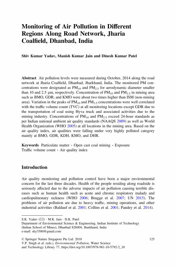
Monitoring of Air Pollution in DifferentRegions Along Road Network, JhariaCoalfield, Dhanbad, India
Shiv Kumar Yadav, Manish Kumar Jain and Dinesh Kumar Patel
Abstract Air pollution levels were measured during October, 2014 along the roadnetwork at Jharia Coalfield, Dhanbad, Jharkhand, India. The monitored PM con-centrations were designated as PM10 and PM2.5 for aerodynamic diameter smallerthan 10 and 2.5 lm, respectively. Concentration of PM10 and PM2.5 in mining areasuch as BMO, GDR, and KMO were about two times higher than ISM (non-miningarea). Variation in the peaks of PM10 and PM2.5 concentrations were well correlatedwith the traffic volume count (TVC) at all monitoring locations except GDR due tothe transportation of coal using Hyva truck and associated activities due to themining industry. Concentrations of PM10 and PM2.5 exceed 24-hour standards asper Indian national ambient air quality standards (NAAQS 2009) as well as WorldHealth Organization (WHO 2005) at all locations in the mining area. Based on theair quality index, air qualities were falling under very highly polluted categorymainly at BMO, GDR, KDH, KMO, and DHR.
Keywords Particulate matter � Open cast coal mining � ExposureTraffic volume count � Air quality index
Introduction
Air quality monitoring and pollution control have been a major environmentalconcern for the last three decades. Health of the people residing along roadside isseriously affected due to the adverse impacts of air pollution causing terrible dis-eases such as human health such as acute and chronic respiratory malady andcardiopulmonary sickness (WHO 2006; Brugge et al. 2007; UN 2015). Theproblems of air pollution are due to heavy traffic, mining operations, and otherindustrial activities (Baldauf et al. 2001; Collins et al. 2001; Pandey et al. 2014).
S.K. Yadav (&) � M.K. Jain � D.K. PatelDepartment of Environmental Science & Engineering, Indian Institute of Technology(Indian School of Mines), Dhanbad 826004, Jharkhand, Indiae-mail: [email protected]
© Springer Nature Singapore Pte Ltd. 2018V.P. Singh et al. (eds.), Environmental Pollution, Water Scienceand Technology Library 77, https://doi.org/10.1007/978-981-10-5792-2_10
125
The problems of air pollution are more critical for every living being in JhariaCoalfield (JCF). JCF is facing a huge burden of traffic congestion, overpopulationand industrial/mining problems. In particular, such issues target severely publicactivities like children moving to school, roadside vendors, and employees ofuncovered or frequently open commercial establishments in traffic dense and nar-row locations and all users of public places such as bus stands, auto stands etc. JCFhas been declared as critically polluted zone by the Central Pollution Control Board(CPCB). Increases in air pollution levels to an alarming rate along the roadside ofJharia areas have also been reported by several researchers (Ghose and Majee 2000,2001; Jain and Saxena 2002; Chaulya 2004; Dubey et al. 2012; Pandey et al. 2014).
The present study was conducted to measure air pollutants (PM10, PM2.5, SO2,NO2, and CO) concentration variations along roadside in mining and non-miningareas, JCF, Dhanbad, Jharkhand, India and their comparison of observed valueswith NAAQS 2009 and WHO 2005 standards. Apart from the observed concen-tration of pollutants, air quality index (AQI) values were also estimated for betterunderstanding and interpretation of the pollution levels.
Materials and Methods
Study Area
Jharia Coalfield (JCF) is one of the most important coalfields in eastern India,located in Dhanbad, Jharkhand, India between latitude 23° 45′ 0″ North; longitude86° 24′ 0″ East and 222 m above mean sea level (Fig. 1). JCF is the most exploitedcoalfield because of available metallurgical grade coal reserves. The mining methodhere comprises of both opencast as well as underground. A study related to JCF isof high importance due to the presence of highly populated township in the vicinityand chances of its negative impacts on society. Non-mining location was selected atthe main gate of Indian School of Mines (ISM), Dhanbad located at distance of7 km in a northeast direction (NE) from JCF for comparing the air quality of themining area. Nine monitoring locations were selected for particulate matter(PM) monitoring in the study area as per IS: 5182 Part-XIV (Fig. 1). The selectedlocations were places of maximum population, heavy traffic, commercial andindustrial/mining areas. Brief descriptions of the locations along with their GPScoordinates are presented in Table 1.
Data Collection
The present study of air pollution levels (PM10, PM2.5, SO2, NO2, and CO) wascarried out during October, 2014 at eight different locations in mining and onelocation in non-mining areas. Twenty-four-hour average sampling was done on
126 S.K. Yadav et al.
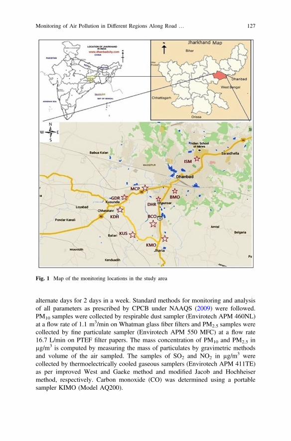
alternate days for 2 days in a week. Standard methods for monitoring and analysisof all parameters as prescribed by CPCB under NAAQS (2009) were followed.PM10 samples were collected by respirable dust sampler (Envirotech APM 460NL)at a flow rate of 1.1 m3/min on Whatman glass fiber filters and PM2.5 samples werecollected by fine particulate sampler (Envirotech APM 550 MFC) at a flow rate16.7 L/min on PTEF filter papers. The mass concentration of PM10 and PM2.5 inµg/m3 is computed by measuring the mass of particulates by gravimetric methodsand volume of the air sampled. The samples of SO2 and NO2 in µg/m3 werecollected by thermoelectrically cooled gaseous samplers (Envirotech APM 411TE)as per improved West and Gaeke method and modified Jacob and Hochheisermethod, respectively. Carbon monoxide (CO) was determined using a portablesampler KIMO (Model AQ200).
Fig. 1 Map of the monitoring locations in the study area
Monitoring of Air Pollution in Different Regions Along Road … 127

In the determination of AQI, equal importance was given to all the pollutants.The quality for each pollutant was estimated by using observed and standard value.The geometric mean of these quality ratings gives the AQI.
The existing concentrations of pollutants were compared with ambient airquality standards (with the standard being assumed as a reference baseline for eachpollutant) and accordingly the quality rating for a particular pollutant was derived inEqs. 1 and 2 as shown below:
Qi ¼ 10 Ci=Sið Þ; ð1Þ
where
Qi Quality rating for an ith pollutant,Ci Concentration of ith pollutant,Si Air quality standard for ith pollutant.
Air Quality Index AQIð Þ ¼ Q1 � Q2 � � � � � Qnð Þ1=n; ð2Þ
Table 1 Descriptions of monitoring locations along with GPS coordinates and theircharacteristics
Location ID Coordinate Major activities
N E
Bankmore BMO 23° 47′18.4″
86° 25′11.6″
Busiest road and junction, commercial,residential, high traffic flow, mining andindustrial activities within 1 km
Matkuriacheck post
MCP 23° 47′14.1″
86° 24′14.6″
Industrial, commercial and residential, mediumtraffic flow, mining activity nearby
Godhar GDR 23° 47′2.9″
86° 23′43.6″
Transportation through the roads with Hyvatruck, Open cast coal mining, Industrial, someresidential, medium traffic flow
Kenduadeeh KDH 23° 46′32.4″
86° 22′48.8″
Commercial, residential, high traffic flow,industrial/mining activity nearby
Kustaur KUS 23° 45′40.5″
86° 23′26.1″
Commercial and residential, low traffic flow,mining activity nearby
Katras more KMO 23° 44′54.5″
86° 24′36.0″
Transportation through the roads with Hyvatruck, commercial and residential, high trafficflow, industrial/mining activity nearby
Bastacola BCO 23° 45′29.1″
86° 24′42.0″
Commercial and residential, medium trafficflow, mining activity nearby
Dhansar DHR 23° 46′43.0″
86° 24′45.6″
Commercial and residential, medium trafficflow, industrial/mining activity nearby
ISM Gate(non-mining)
ISM 23° 48′32.5″
86° 26′33.6″
Commercial and residential, medium traffic flow
128 S.K. Yadav et al.

where
n Number of pollutants considered.
The categorization of AQI values has been assigned as per guidelines providedby Environment Canada (Table 2). It measures the air quality in relation to thehealth on a scale from 1 to 10. The higher the number, the greater the health riskassociated with the air quality.
The Air Quality Health Index (AQHI) is a scale designed to understand the airquality and its impact on health to make decisions related to health protection bylimiting short-term exposure to air pollution and adjusting activity levels duringhigh values (Table 3). This index is also helpful to people who are sensitive to airpollution and provides them with advice on how to protect their health during airquality levels associated with low, moderate, high and very high health risks (Ottand Thom 1976).
Table 2 Air quality ratingscale index
Index value Status of air pollution
1–3 Least polluted
4–6 Moderately polluted
7–10 Highly polluted
10+ Very highly polluted
Table 3 Air quality health index categories and health messages
Healthrisk
Air qualityhealth index
Health messages
At risk population General population
Low 1–3 Enjoy your usual outdooractivities
Ideal air quality for outdooractivities
Moderate 4–6 Consider reducing orrescheduling strenuous activitiesoutdoors if you are experiencingsymptoms
No need to modify your usualoutdoor activities unless youexperience symptoms such ascoughing and throat irritation
High 7–10 Reduce or reschedule strenuousactivities outdoors. Children andthe elderly should also take iteasy
Consider reducing orrescheduling strenuous activitiesoutdoors if you experiencesymptoms such as coughing andthroat irritation
Veryhigh
Above 10 Avoid strenuous activitiesoutdoors. Children and theelderly should also avoidoutdoor physical exertion
Reduce or reschedule strenuousactivities outdoors, especially ifyou experience symptoms suchas coughing and throat irritation
Source www.ec.gc.ca
Monitoring of Air Pollution in Different Regions Along Road … 129
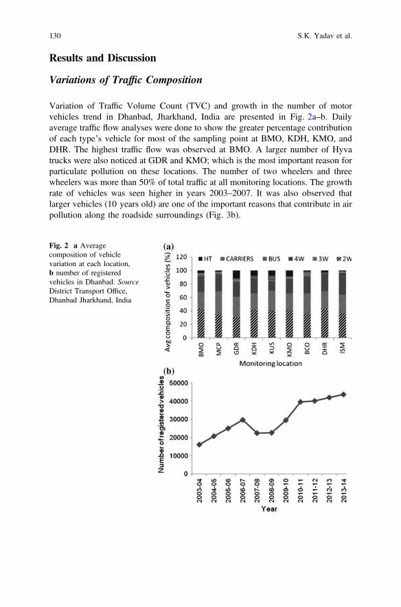
Results and Discussion
Variations of Traffic Composition
Variation of Traffic Volume Count (TVC) and growth in the number of motorvehicles trend in Dhanbad, Jharkhand, India are presented in Fig. 2a–b. Dailyaverage traffic flow analyses were done to show the greater percentage contributionof each type’s vehicle for most of the sampling point at BMO, KDH, KMO, andDHR. The highest traffic flow was observed at BMO. A larger number of Hyvatrucks were also noticed at GDR and KMO; which is the most important reason forparticulate pollution on these locations. The number of two wheelers and threewheelers was more than 50% of total traffic at all monitoring locations. The growthrate of vehicles was seen higher in years 2003–2007. It was also observed thatlarger vehicles (10 years old) are one of the important reasons that contribute in airpollution along the roadside surroundings (Fig. 3b).
Fig. 2 a Averagecomposition of vehiclevariation at each location,b number of registeredvehicles in Dhanbad. SourceDistrict Transport Office,Dhanbad Jharkhand, India
130 S.K. Yadav et al.
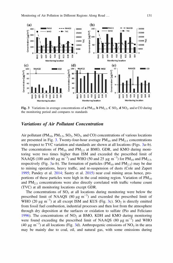
Variations of Air Pollutant Concentration
Air pollutant (PM10, PM2.5, SO2, NO2, and CO) concentrations of various locationsare presented in Fig. 3. Twenty-four-hour average PM10 and PM2.5 concentrationswith respect to TVC variation and standards are shown at all locations (Figs. 3a–b).The concentrations of PM10 and PM2.5 at BMO, GDR, and KMO during moni-toring were two times higher than ISM and exceeded the prescribed limit ofNAAQS (100 and 60 µg m−3) and WHO (50 and 25 µg m−3) for PM10 and PM2.5,respectively (Fig. 3a–b). The formation of particles (PM10 and PM2.5) may be dueto mining operations, heavy traffic, and re-suspension of dusts (Cole and Zapert1995; Pandey et al. 2014; Sastry et al. 2015) near coal mining areas hence, pro-portions of these particles were high in the coal mining region. Variation of PM10
and PM2.5 concentrations were also directly correlated with traffic volume count(TVC) at all monitoring locations except GDR.
The concentrations of SO2 at all locations during monitoring were below theprescribed limit of NAAQS (80 µg m−3) and exceeded the prescribed limit ofWHO (20 µg m−3) at all except ISM and KUS (Fig. 3c). SO2 is directly emittedfrom fossil fuel combustion, industrial processes and then lost from the atmospherethrough dry deposition at the surfaces or oxidation to sulfate (Pio and Feliciano1996). The concentrations of NO2 at BMO, KDH and KMO during monitoringwere found exceeding the prescribed limit of NAAQS (80 µg m−3) and WHO(40 µg m−3) at all locations (Fig. 3d). Anthropogenic emissions of NO2 in the areamay be mainly due to coal, oil, and natural gas, with some emissions during
Fig. 3 Variations in average concentrations of a PM10, b PM2.5, C SO2, d NO2, and e CO duringthe monitoring period and compares to standards
Monitoring of Air Pollution in Different Regions Along Road … 131

blasting, combustion processes, including vehicle exhaust. NO2 has a longer life-time in the atmosphere in the absence of sunlight (Li et al. 2008).
The hourly average CO concentrations during monitoring also exceeded theprescribed limit of NAAQS (4 mg m−3) except KUS (Fig. 3e). CO is directlyemitted from vehicle exhaust, power generators, and also from incomplete com-bustion of various other fuels (including wood, coal, charcoal, oil, paraffin, propane,natural gas, and trash).
AQI for all locations were estimated based on NAAQS (2009) as per methoddescribed earlier. AQI showed significant spatial variations during the monitoringperiod (Table 4). The AQI values were falling under very highly polluted category atBMO, GDR, KDH, KMO, and DHR locations due to their proximity to coal miningareas. Heavy traffic flow at slow speed and poor road conditions may also beattributed to these high index values. The air quality of MCP and BCO was fallingunder highly polluted category due to medium traffic flow. On the other hand, the airquality of KUS and ISM fell under moderately polluted category. At KUS vehiclemovement was less while at ISM movement of commercial vehicles were high.
Conclusion
The present study was conducted to investigate the ambient air quality of JhariaCoalfield, Dhanbad, India with respect to PM10, PM2.5, SO2, NO2, and CO at ninerepresentative locations. The spatial variations in pollutant concentrations were
Table 4 Location-wise AQI of the study area
Location Sub-index of various pollutants AQIvalue
Category
QPM10 QPM2.5 QSO2 QNO2 QCO
BMO 24.7 14.3 3.3 11.9 22.5 12.5 Very highlypolluted
MCP 11.4 9.7 2.8 7.5 12.5 7.8 Highly polluted
GDR 23.8 18.4 4.4 8.8 15.0 12.0 Very highlypolluted
KDH 19.5 15.3 2.8 10.6 17.5 10.9 Very highlypolluted
KUS 10.5 9.5 1.3 5.0 5.0 5.0 Moderatelypolluted
KMO 26.2 19.6 3.9 11.6 20.0 13.6 Very highlypolluted
BCO 13.8 12.0 3.3 9.8 12.5 9.2 Highly polluted
DHR 18.2 15.3 3.1 10.6 15.0 10.7 Very highlypolluted
ISM 9.8 5.5 2.4 7.0 12.5 6.5 Moderatelypolluted
132 S.K. Yadav et al.
quite significant, which may be caused by diversity among emissions. The con-centrations of PM10 and PM2.5 at BMO, GDR, and KMO during monitoring wereabout two times higher than ISM and exceeded the prescribed limit of NAAQS andWHO. The concentrations of SO2 at all locations during monitoring were below theprescribed limit of NAAQS and exceeded the WHO at all locations except ISM andKUS. The concentrations of NO2 at BMO, KDH, and KMO during monitoringexceeded the prescribed limit of NAAQS and WHO standards at all locations. Thehourly average CO concentrations during monitoring also exceeded the prescribedlimit of NAAQS except KUS.
Finally, through this study it can be inferred that the air quality is under veryhighly polluted category at BMO, GDR, KDH, KMO, and DHR locations based onAQI values.
References
Air Quality Health Index Categories, http://www.ec.gc.ca/cas-aqhi/default.asp?lang=En&n=79A8041B-1
Baldauf RW, Lane DD, Marote GA (2001) Ambient air quality monitoring network design forassessing human health impacts from exposures to airborne contaminants. Environ MonitAssess 66:63–76
Brugge D, Durant JL, Rioux C (2007) Near-highway pollutants in motor vehicle exhaust: a reviewof epidemiologic evidence of cardiac and pulmonary health risks. Environ Health. doi:10.1186/1476-069X-6-236-23
Chaulya SK (2004) Assessment and management of air quality for an opencast coal mining area.J Environ Manag 70:1–14
Cole CF, Zapert JG (1995) Air quality dispersion model validation at three stone quarries. NationalStone Association, Washington, D.C
Collins MJ, Williams PL, McIntosh DL (2001) Ambient air quality at the site of a formermanufactured gas plant. Environ Monit Assess 68:137–152
Dubey B, Pal AK, Singh G (2012) Trace metal composition of airborne particulate matter in thecoal mining and non-mining areas of Dhanbad Region, Jharkhand, India. Atmos Pollut Res3:238–246
Ghose MK, Majee SR (2000) Assessment of the impact on the air environment due to opencastcoal mining—an Indian case study. Atmos Environ 34:2791–2796
Ghose MK, Majee SR (2001) Air pollution caused by opencast mining and its abatement measuresin India. J Environ Manag 63(2):193–202
Jain MK, Saxena NC (2002) Air quality assessment along Dhanbad-Jharia road. Environ MonitAssess 79:239–250
Li SP, Matthews J, Sinha A (2008) Atmospheric hydroxyl radical production from electronicallyexcited NO2 and H2O. Science 319:1657–1660
NAAQS (2009) National ambient air quality standards. Central pollution control board, Gazettenotification, New Delhi
Ott WR, Thom GC (1976) A critical review of air pollution index systems in the United States andCanada. J Air Poll Control Assoc 26:460–470
Pandey B, Agrawal M, Singh S (2014) Assessment of air pollution around coal mining area:emphasizing on spatial distributions, seasonal variations and heavy metals, using cluster andprincipal component analysis. Atmos Pollut Res 5:79–86
Monitoring of Air Pollution in Different Regions Along Road … 133

Pio CA, Feliciano MS (1996) Dry deposition of ozone and sulphur dioxide over low vegetation inmoderate southern European weather conditions: measurements and modeling. Phys ChemEarth 21:373–377
Sastry VR, Ram Chandar K, Nagesha KV, Murlidhar E, Mohuiddin MS (2015) Prediction andanalysis of dust dispersion from drilling operation in opencast coal mines. Procedia EarthPlanet Sci 11:303–311
United Nations (2015) World urbanization prospects: The 2014 revision, ST/ESA/SER.A/366.Department of Economic and Social Affairs, Population Division, New York. http://esa.un.org/unpd/wup/FinalReport/WUP2014-Report.pdf
World Health Organization (2005) WHO Air quality guidelines for particulate matter, ozone,nitrogen dioxide and sulfur dioxide, global update 2005. WHO/SDE/PHE/OEH/06.02. http://www.euro.who.int/__data/assets/pdf_file/0005/78638/E90038.pdf
World Health Organization (2006) Health risks of particulate matter from long-rangetransboundary air pollution. Joint WHO/Convention task force on the health aspects of airpollution, 2006. European Centre for Environment and Health Bonn Office. http://www.euro.who.int/__data/assets/pdf_file/0006/78657/E88189.pdf
134 S.K. Yadav et al.

Spatial Distribution and BaselineConcentration of Heavy Metals in Swell–Shrink Soils of Madhya Pradesh, India
S. Rajendiran, T. Basanta Singh, J.K. Saha, M. Vassanda Coumar,M.L. Dotaniya, S. Kundu and A.K. Patra
Abstract Defining and understanding the current abundance and spatial distribu-tion of metals in soils are essential and reliable information on this aspect areneeded for proper legislation. To estimate the baseline concentrations and spatialdistribution of heavy metals (HMs) in Swell–shrink soils Sehore and Vidisha dis-tricts, 100 surface soil samples (0–20 cm) were randomly collected across the twodistricts and their physico-chemical properties and total HM contents were anal-ysed. Spatial distribution maps of HMs were prepared and influence of soilparameters on HMs was studied. Most of the soils in the region had neutral toalkaline pH (6.58–8.60), non saline (EC 0.11–1.3 dS/m), medium organic carbon(0.6%), CaCO3 0.2–11.5% and clay >40%. The baseline concentrations of HMs(mg kg−1) were Cu, 178.1; Cd, 0.7; Pb, 24.4; Cr, 116.9; Ni, 81.8; and Zn, 85.2;respectively. The concentrations of Cd, Pb and Zn in all the samples were withinthe safe range but the concentrations of Cr, Cu and Ni were a little high.
Introduction
India is bestowed with diverse soil groups due to variability in parent materials,land topography and climatic conditions in different regions (Bhattacharyya et al.2009). Each soil group as well as subgroup has distinct physical and chemicalproperties. Heavy metals are generally defined based on their atomic number, i.e.those elements having atomic number more than 20 or specific gravity (density) ofmore than >4.7 g/cm3. Among heavy metals, Ag, As, Hg, V, Cd, Co, Cr, Cu, Ni, Se
S. Rajendiran (&) � J.K. Saha � M. Vassanda Coumar � M.L. Dotaniya �S. Kundu � A.K. PatraICAR-Indian Institute of Soil Science, Nabibagh Berasia Road,Bhopal 462038, Madhya Pradesh, Indiae-mail: [email protected]
T. Basanta SinghICAR-Research Complex for North Eastern Hill Region,Umroi Road, Umiam 793103, Meghalaya, India
© Springer Nature Singapore Pte Ltd. 2018V.P. Singh et al. (eds.), Environmental Pollution, Water Scienceand Technology Library 77, https://doi.org/10.1007/978-981-10-5792-2_11
135

and Ti have high to moderately high toxicity to plants and Ag, As, Cd, Cr(VI), Hg,Sb, Se, Ti and V exhibit high toxicity to mammals (McBride 1994). Mean heavymetal concentrations in natural soil varies widely from 0.06 to 1.1 µg/g for Cd, 1.6–21.5 µg/g Co, 7–221 µg/g for Cr, 6–80 µg/g for Cu, 0.02–0.41 µg/g for Hg, 4–55 µg/g for Ni, 10–84 µg/g for Pb, 17–125 µg/g for Zn in non-contaminated soil ofthe world (McBride 1994). However, huge quantity of heavy metals are beingmined out from deeper layers of earth crust and pose threat to the environment byaffecting crop productivity and soil microbial biodiversity and also pose threat tohuman and animal health by contaminating food chain with toxic metals. Varioussoil properties determine degree of mobility/availability of heavy metals as well aseffectiveness and adoptability of some of the management options over others forpolluted soils (Saha et al. 2013). Therefore defining and understanding the currentabundance and spatial distribution of metals in soils are essential first steps in beingable to recognize and quantify natural or human-induced changes in the future. Dueto variation in natural factors like parent materials (from which soil has beendeveloped), climate, physiography, etc. wide variation in heavy metals contentsamong soils from different uncontaminated regions of different countries have beenreported. Reliable data on this aspect are also needed for proper legislation. In orderto address this issue, several other countries have established background con-centration (BG) and upper baseline concentration (UBL) of heavy metals in soils ofdifferent regions. However, such information is scanty in our country which hasdiversified types of soils and agroclimatic conditions. Realizing the importance incontrol of pollution and management of polluted soil, many investigations onbackground concentrations of soil trace metals had been performed in various areassuch as, Belgium (De Temmerman et al. 1984), China (Chen et al. 1991), Germany(Bachman et al. 1995), India (Kuhad et al. 1989), Italy (Bini et al. 1988), Poland(Andersen et al. 1994), Switzerland (Landry and Célardin 1988), The Netherlands(Denneman and Robbersen 1992), United Kingdom (Thornton 1982), United Statesof America (Holmgren et al. 1993; Bradford et al. 1996; Ma et al. 1997), Spain(Bech et al. 2005) and Western Europe (Angelone and Bini 1992). In these reportsit has been shown that the primary factors influencing trace metal concentrationsand spatial distribution in soils are parent materials and anthropogenic activities.Factors such as climate, the organic and inorganic components of soils, and redoxpotential status also affect the level of trace metals in soils. By keeping in view, thestudy is conceived and conducted with the following objectives:
1. To study the spatial distribution of heavy metals in the swell–shrink soils ofSehore and Vidisha districts of Madhya Pradesh.
2. To estimate the baseline concentrations of heavy metals in these soils.3. To study the influence of soil properties on the concentration of heavy metals.
136 S. Rajendiran et al.
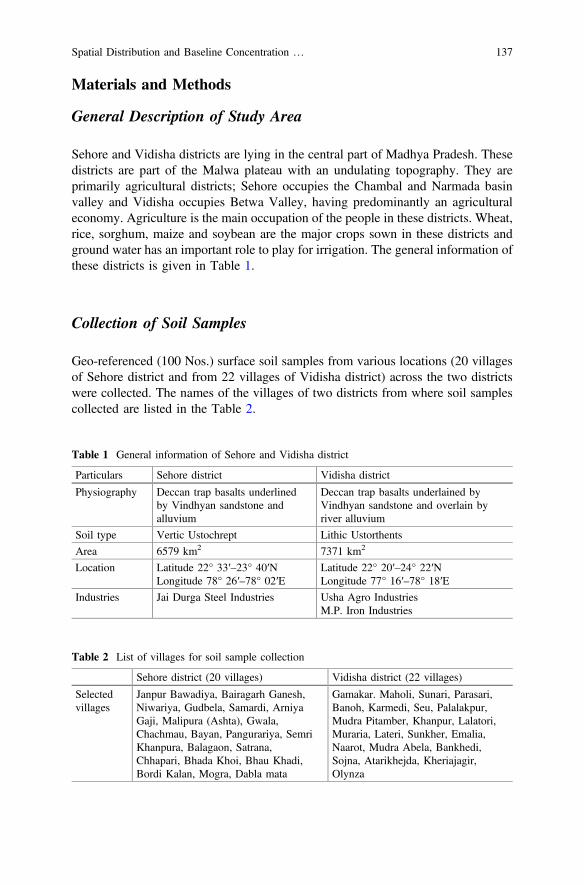
Materials and Methods
General Description of Study Area
Sehore and Vidisha districts are lying in the central part of Madhya Pradesh. Thesedistricts are part of the Malwa plateau with an undulating topography. They areprimarily agricultural districts; Sehore occupies the Chambal and Narmada basinvalley and Vidisha occupies Betwa Valley, having predominantly an agriculturaleconomy. Agriculture is the main occupation of the people in these districts. Wheat,rice, sorghum, maize and soybean are the major crops sown in these districts andground water has an important role to play for irrigation. The general information ofthese districts is given in Table 1.
Collection of Soil Samples
Geo-referenced (100 Nos.) surface soil samples from various locations (20 villagesof Sehore district and from 22 villages of Vidisha district) across the two districtswere collected. The names of the villages of two districts from where soil samplescollected are listed in the Table 2.
Table 1 General information of Sehore and Vidisha district
Particulars Sehore district Vidisha district
Physiography Deccan trap basalts underlinedby Vindhyan sandstone andalluvium
Deccan trap basalts underlained byVindhyan sandstone and overlain byriver alluvium
Soil type Vertic Ustochrept Lithic Ustorthents
Area 6579 km2 7371 km2
Location Latitude 22° 33′–23° 40′NLongitude 78° 26′–78° 02′E
Latitude 22° 20′–24° 22′NLongitude 77° 16′–78° 18′E
Industries Jai Durga Steel Industries Usha Agro IndustriesM.P. Iron Industries
Table 2 List of villages for soil sample collection
Sehore district (20 villages) Vidisha district (22 villages)
Selectedvillages
Janpur Bawadiya, Bairagarh Ganesh,Niwariya, Gudbela, Samardi, ArniyaGaji, Malipura (Ashta), Gwala,Chachmau, Bayan, Pangurariya, SemriKhanpura, Balagaon, Satrana,Chhapari, Bhada Khoi, Bhau Khadi,Bordi Kalan, Mogra, Dabla mata
Gamakar. Maholi, Sunari, Parasari,Banoh, Karmedi, Seu, Palalakpur,Mudra Pitamber, Khanpur, Lalatori,Muraria, Lateri, Sunkher, Emalia,Naarot, Mudra Abela, Bankhedi,Sojna, Atarikhejda, Kheriajagir,Olynza
Spatial Distribution and Baseline Concentration … 137
Chemical Analysis of Soils
Soil pH
Soil pH was determined from soil–water suspension in the ratio of 1:2.5 with thehelp of Systronics Microprocessor based pH metre as described by Jackson (1973).
Electrical Conductivity
Electrical conductivity (EC) of soil–water suspension (1:2.5) was estimated with thehelp of a conductivity metre as outlined by (Jackson 1973). The electrical con-ductivity was measured at room temperature (25 °C) after the soil particles havebeen settled down.
Oxidizable Organic Carbon
Organic carbon of soil was estimated by oxidizing the soil with a mixture of1N K2Cr2O7 and concentrated H2SO4 and back-titrating the excess K2Cr2O7 withstandard ferrous ammonium sulfate solution using diphenylamine indicator fol-lowing the wet digestion method of Walkley and Black (1934).
Calcium Carbonate
Percentage of CaCO3 is estimated by acid neutralization method. For this 5 g soil(0.5 mm) is treated with 25 mL of 1N HCl for one hour by covering with a watchglass. Then it is transfered into a 100 mL volumetric flask and volume is made upand filtered. From the filtrate, 20 ml aliquot is taken in a conical flask (150 mL).Little distilled water is added, heated just to boil and cooled. The aliquot is titratedagainst 0.2N NaOH by adding 0.2 ml of phenolphthalein until the pink colourpersists for 30 min.
Total Heavy Metal Concentration
For total heavy metal analysis, 1.0 g air dry soil (0.5 mm) was first pre-digestedwith 10 mL of concentrated HNO3 for overnight. The pre-digested samples weredigested in hot plate by adding 10 mL of di-acid (four parts of HClO4 and nineparts of HNO3) till the acid gets evaporated to near dryness. Process was repeatedtill the soil residue become whitish by adding di-acid mixture. One mL of HClO4
was added and the sample was evaporated until the appearance of white fumes. Theresidue was dissolved by adding 4.0 mL of 12N HCl (kept for 1 min) and 50 mL of
138 S. Rajendiran et al.

double distilled water and kept on sand bath for 4 h. Finally the volume of thedigest was made to 100 mL and filtered by using Watman No. 42 filter paper. Thefiltrate was directly fed to ICP-OES for trace metals (Cu, Zn, Cd, Cr, Pb, Ni)determination. For cross checking the accuracy of the analytical procedure, thereference standard soil samples were also analysed along with the samples. Thecorrelation between the observed values and the quoted values of reference samplecame out to be 0.95–0.99.
Determination of Baseline Concentrations of Metals
Baseline concentrations can be determined both numerical and statistical ways, viz,range and mean ± standard deviation. In many naturally occurring processes,population follows a normal distribution where 99% of the population lies withinµ ± 3 * r (µ = mean, and r = standard deviation) (Feller 1971). Thus baselineconcentration can be defined as range between µ + 3 * r and µ − 3 * r. However,many investigators found that heavy metal concentrations in naturally occurringunpolluted soils follow a log-normal distribution (Chen et al. 1999a, b; Zhang et al.2008). In that case, the geometric mean (GM) and geometric standard deviations(GSDs) are used to represent the central tendency and variation of the data. Baselineconcentrations of the seven trace metals are defined as the range betweenGM/GSD2 and GM � GSD2 and taking the concentrations between the 5th and the95th percentiles. This range included 95% of the samples (Dudka et al. 1995; Chenet al. 1999a, b; Zhang et al. 2008). This method was used to determine the baselinelimit in this experiment.
Lower baseline ¼ GM
GSD2 ð1Þ
Upper baseline ¼ GM� GSD2 ð2Þ
where GM means for geometric mean and GSD means for geometric standarddeviation.
Results and Discussion
Soil Characteristics
The important soil properties like soil reaction, electrical conductivity, oxidisableorganic carbon, calcium carbonate and soil particle size were analysed in the lab-oratory. All the properties are presented in Table 3. The soil reaction of Sehoredistrict ranged from 6.58 to 8.60 with mean value of 7.7 and for Vidisha district,
Spatial Distribution and Baseline Concentration … 139

it ranged from 7.0 to 8.4 with a mean value of 8.0. The electrical conductivity of theSehore district ranged from 0.11 to 0.62 dS/m whereas, it ranged from 0.11 to1.3 dS/m for Vidisha district with a mean value of 0.3 dS/m for both the districts.The organic carbon of Sehore district ranged from 0.21 to 1.24% with mean valueof 0.6% and for Vidisha district, it ranged from 0.17 to 1.09% with a mean value of0.6%. The percentage of CaCO3 of Sehore district ranged from 0.5 to 11.5% withmean value of 4.0% and for Vidisha district, it ranged from 0.2 to 9.15% with amean value of 2.3%. The sand, silt and clay of Sehore district ranged from 27.58 to66.96%, 12.5 to 29.2% and 15.3–59.0%, respectively with mean value of 38.7, 21.1and 40.2, respectively. The corresponding values for Vidisha district are 29.6–41.9,19.8–31.3 and 32.7–47.5, respectively with a mean value of 34.3, 24.5 and 41.2%,respectively.
The soil reactions of Sehore and Vidisha districts ranged from neutral to (6.6) toalkaline range (8.4). Out of 50 samples of Sehore district, 15 (30%) samples areunder neutral range, 14 (28%) are under mildly alkaline range, 19 (38%) are undermoderately alkaline and only 2 (4%) are under highly alkaline range. For Vidishadistrict only 3 (6%) samples are under neutral range, 5 (10%) are under mildlyalkaline range, 42 (84%) samples are under moderately alkaline range. So it is clearthat, 70% of the samples in Sehore and 94% in Vidisha are under alkaline range. Itis not strange to draw the reason for alkalinity as the parent material of thesedistricts is predominantly basalt which yields black soil on weathering. The EC ofthe Sehore (0.11–0.62 dS/m) and Vidisha (0.11–1.3 dS/m) districts were undersafer side as EC of all the samples in both the districts were below 2.0 dS/m, theyare considered to be non-saline soils. The organic carbon content in the soils ofSehore district, out of 50 samples, 14 (28%) were below 0.5% (low), 24 samples(48%) were in between 0.5 and 0.75% (medium range) and 12 samples (24%) wereabove 0.75% (high). Whereas in the Vidisha district, 18 samples (36%) were at lowcategory, 25 samples (50%) were in medium range and 7 samples (14%) were athigh range. In the Sehore district 42 samples (84%) at or below 5% and 8 samples(16%) are above 5% CaCO3. Whereas 48 samples (96%) at or below 5% and 2samples (4%) are above 5% CaCO3. The results indicated that mostly these soils are
Table 3 Important soilproperties of Sehore andVidisha districts
Soil property Sehore district (no. ofsamples = 50)
Vidisha district(no. ofsamples = 50)
Range Mean Range Mean
pH 6.58–8.60 7.7 7.00–8.40 8.00
EC 0.11–0.62 0.3 0.11–1.3 0.30
OC (%) 0.21–1.24 0.6 0.17–1.09 0.60
CaCO3 (%) 0.5–11.5 4.0 0.2–9.15 2.30
Sand (%) 27.58–66.96 38.7 29.6–41.9 34.3
Silt (%) 12.5–29.2 21.1 19.8–31.3 24.5
Clay (%) 15.3–59.0 40.2 32.7–47.5 41.2
140 S. Rajendiran et al.
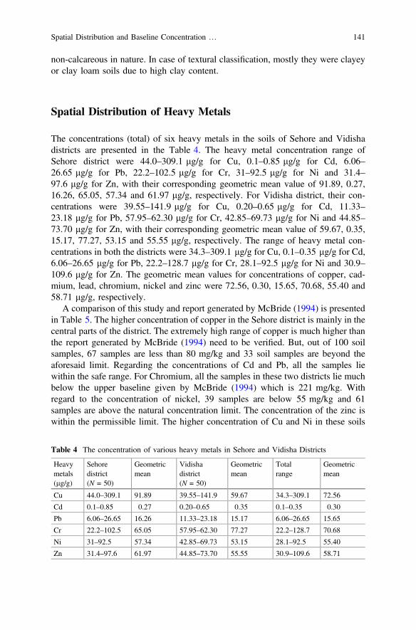
non-calcareous in nature. In case of textural classification, mostly they were clayeyor clay loam soils due to high clay content.
Spatial Distribution of Heavy Metals
The concentrations (total) of six heavy metals in the soils of Sehore and Vidishadistricts are presented in the Table 4. The heavy metal concentration range ofSehore district were 44.0–309.1 lg/g for Cu, 0.1–0.85 lg/g for Cd, 6.06–26.65 lg/g for Pb, 22.2–102.5 lg/g for Cr, 31–92.5 lg/g for Ni and 31.4–97.6 lg/g for Zn, with their corresponding geometric mean value of 91.89, 0.27,16.26, 65.05, 57.34 and 61.97 lg/g, respectively. For Vidisha district, their con-centrations were 39.55–141.9 lg/g for Cu, 0.20–0.65 lg/g for Cd, 11.33–23.18 lg/g for Pb, 57.95–62.30 lg/g for Cr, 42.85–69.73 lg/g for Ni and 44.85–73.70 lg/g for Zn, with their corresponding geometric mean value of 59.67, 0.35,15.17, 77.27, 53.15 and 55.55 lg/g, respectively. The range of heavy metal con-centrations in both the districts were 34.3–309.1 lg/g for Cu, 0.1–0.35 lg/g for Cd,6.06–26.65 lg/g for Pb, 22.2–128.7 lg/g for Cr, 28.1–92.5 lg/g for Ni and 30.9–109.6 lg/g for Zn. The geometric mean values for concentrations of copper, cad-mium, lead, chromium, nickel and zinc were 72.56, 0.30, 15.65, 70.68, 55.40 and58.71 lg/g, respectively.
A comparison of this study and report generated by McBride (1994) is presentedin Table 5. The higher concentration of copper in the Sehore district is mainly in thecentral parts of the district. The extremely high range of copper is much higher thanthe report generated by McBride (1994) need to be verified. But, out of 100 soilsamples, 67 samples are less than 80 mg/kg and 33 soil samples are beyond theaforesaid limit. Regarding the concentrations of Cd and Pb, all the samples liewithin the safe range. For Chromium, all the samples in these two districts lie muchbelow the upper baseline given by McBride (1994) which is 221 mg/kg. Withregard to the concentration of nickel, 39 samples are below 55 mg/kg and 61samples are above the natural concentration limit. The concentration of the zinc iswithin the permissible limit. The higher concentration of Cu and Ni in these soils
Table 4 The concentration of various heavy metals in Sehore and Vidisha Districts
Heavymetals(lg/g)
Sehoredistrict(N = 50)
Geometricmean
Vidishadistrict(N = 50)
Geometricmean
Totalrange
Geometricmean
Cu 44.0–309.1 91.89 39.55–141.9 59.67 34.3–309.1 72.56
Cd 0.1–0.85 0.27 0.20–0.65 0.35 0.1–0.35 0.30
Pb 6.06–26.65 16.26 11.33–23.18 15.17 6.06–26.65 15.65
Cr 22.2–102.5 65.05 57.95–62.30 77.27 22.2–128.7 70.68
Ni 31–92.5 57.34 42.85–69.73 53.15 28.1–92.5 55.40
Zn 31.4–97.6 61.97 44.85–73.70 55.55 30.9–109.6 58.71
Spatial Distribution and Baseline Concentration … 141

might be from parent material or anthropogenic activities. To confirm this, soilprofile study is necessary which is beyond the scope of this article.
Baseline Concentrations of Heavy Metals
The baseline concentrations of six heavy metals in Sehore and Vidisha districtswere estimated and presented in Table 6. The lower and upper baseline limits(range) of six heavy metals for Sehore district were 36.8 µg/g and 229.6 µg/g forCu, 0.1 µg/g and 0.8 µg/g for Cd, 9.5 µg/g and 28.0 µg/g for Pb, 35.4 µg/g and119.4 µg/g for Cr, 35.0 µg/g and 94.1 µg/g for Ni and 38.7 µg/g and 99.2 µg/g forZn. The lower and upper baseline limits (range) of six heavy metals for Vidishadistrict were 32.3 µg/g and 101.5 µg/g for Cu, 0.2 µg/g and 0.5 µg/g for Cd,11.2 µg/g and 20.3 µg/g for Pb, 57.6 µg/g and 102.3 µg/g for Cr, 42.8 µg/g and66.9 µg/g for Ni and 38.7 µg/g and 99.2 µg/g for Zn. Upper and lower baselineconcentrations of heavy metals for both the districts are 29.6 µg/g and 178.1 µg/gfor Cu, 0.1 µg/g and 0.7 µg/g for Cd, 10.0 µg/g µg/g and 24.4 µg/g for Pb,42.7 µg/g and 116.9 µg/g for Cr, 37.5 µg/g and 81.8 µg/g for Ni and 40.4 µg/g and85.2 µg/g for Zn.
The upper baseline concentration for particular metal is considered as maximumconcentration of metal in the soils of the region derived from natural phenomenon,i.e. weathering of parent material without any human-induced effect. This range isused for identification of the extent of soil pollution by HMs due to anthropogenic
Table 5 Comparison of heavy metals in the uncontaminated soils of world (McBride 1994) andthe present study
References Cu(mg/kg)
Cd(mg/kg)
Pb(mg/kg)
Cr(mg/kg)
Ni(mg/kg)
Zn(mg/kg)
McBride (1994) 6–80 0.06–1.1 10–84 7–221 4–55 17–125
This study 29.6–178.1 0.1–0.7 10–24.4 42.7–116.9 37.5–81.8 40.4–85.2
Table 6 Baseline concentration of heavy metals (mg/kg) for soils of Sehore and Vidisha
Heavy metals Sehore district Vidisha district Study area
Lower Upper Lower Upper Lower Upper
Cu 36.8 229.6 32.3 101.5 29.6 178.1
Cd 0.1 0.8 0.2 0.5 0.1 0.7
Pb 9.5 28.0 11.2 20.3 10.0 24.4
Cr 35.4 119.4 57.6 102.3 42.7 116.9
Ni 35.0 94.1 42.8 66.9 37.5 81.8
Zn 38.7 99.2 46.4 66.7 40.4 85.2
142 S. Rajendiran et al.
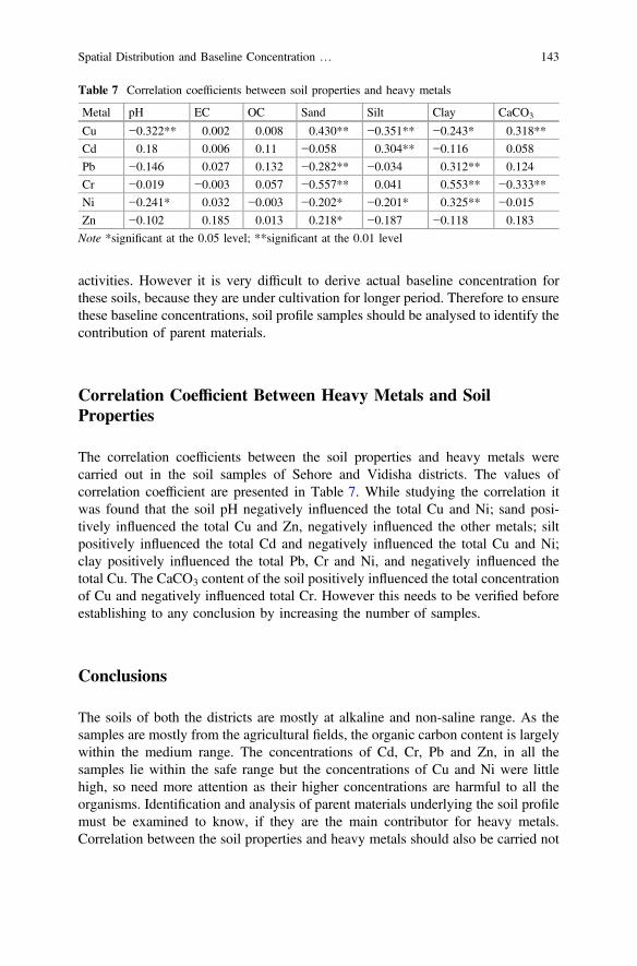
activities. However it is very difficult to derive actual baseline concentration forthese soils, because they are under cultivation for longer period. Therefore to ensurethese baseline concentrations, soil profile samples should be analysed to identify thecontribution of parent materials.
Correlation Coefficient Between Heavy Metals and SoilProperties
The correlation coefficients between the soil properties and heavy metals werecarried out in the soil samples of Sehore and Vidisha districts. The values ofcorrelation coefficient are presented in Table 7. While studying the correlation itwas found that the soil pH negatively influenced the total Cu and Ni; sand posi-tively influenced the total Cu and Zn, negatively influenced the other metals; siltpositively influenced the total Cd and negatively influenced the total Cu and Ni;clay positively influenced the total Pb, Cr and Ni, and negatively influenced thetotal Cu. The CaCO3 content of the soil positively influenced the total concentrationof Cu and negatively influenced total Cr. However this needs to be verified beforeestablishing to any conclusion by increasing the number of samples.
Conclusions
The soils of both the districts are mostly at alkaline and non-saline range. As thesamples are mostly from the agricultural fields, the organic carbon content is largelywithin the medium range. The concentrations of Cd, Cr, Pb and Zn, in all thesamples lie within the safe range but the concentrations of Cu and Ni were littlehigh, so need more attention as their higher concentrations are harmful to all theorganisms. Identification and analysis of parent materials underlying the soil profilemust be examined to know, if they are the main contributor for heavy metals.Correlation between the soil properties and heavy metals should also be carried not
Table 7 Correlation coefficients between soil properties and heavy metals
Metal pH EC OC Sand Silt Clay CaCO3
Cu −0.322** 0.002 0.008 0.430** −0.351** −0.243* 0.318**
Cd 0.18 0.006 0.11 −0.058 0.304** −0.116 0.058
Pb −0.146 0.027 0.132 −0.282** −0.034 0.312** 0.124
Cr −0.019 −0.003 0.057 −0.557** 0.041 0.553** −0.333**
Ni −0.241* 0.032 −0.003 −0.202* −0.201* 0.325** −0.015
Zn −0.102 0.185 0.013 0.218* −0.187 −0.118 0.183
Note *significant at the 0.05 level; **significant at the 0.01 level
Spatial Distribution and Baseline Concentration … 143

only for surface soils but also for the deeper layers. This kind of informationcontributes to identify the extent of soil pollution due to anthropogenic activitiesand also for more effective management of soil contaminated with heavy metals.
References
Andersen S, Odegard S, Vogt RD, Seip HM (1994) Background levels of heavy-metals in polishforest soils. Ecol Eng 3:245–253
Angelone M, Bini C (1992) Trace elements concentrations in soils and plants of western europe.In: Adriano DC (ed) Biogeochemistry of trace elements. Lewis Publishers, Boca Raton, FL,pp 10–60
Bachman G, Freier R, Konietzka R (1995) Soil Levels Based on the German Soil Protection Bill.In: van der Brink WJ, Bosman R, Arendt F (eds) Contaminated Soil, Kluwer AcademicPublishers, pp 711–719
Bech J, Tume P, Longan L, Reverter F (2005) Baseline concentrations of trace elements in surfacesoils of the torrelles and sant climent municipal districts (Catalonia, Spain). Environ MonitAssess 108(1–3):309–322. doi:10.1007/s10661-005-4331-4334
Bhattacharyya T, Sarkar D, Sehgal JL, Velaytham M, Gajbhiye KS, Nagar AP, Nimkhedkar SS(2009) Soil taxonomic database of india and states (1:250,000 scale), NBSS & LUP Pub.No. 143, 266 p
Bini C, Dall’aglio M, Ferreti O, Gragniani R (1988) Background levels of microelements in soilsof Italy. Environ Chem Health 10(2):63–69
Bradford GR, Chang AC, Page AL, Bakthar D, Frampton JA, Wrigth H (1996) Backgroundconcentrations of trace and major elements in california soils. Technical Report, KarneyFoundation Special Report of University of California, Riverside
Chen M, Ma LQ, Harris WG, Hornesby AG (1999a) Background concentrations of trace metals inflorida surface soils: taxonomic and geographic distributions of total-total and total-recoverableconcentrations of selected trace metals. Gainesville, Florida, pp 5–27
Chen M, Ma LQ, Willie GH (1999b) Baseline concentrations of 15 trace elements in Floridasurface soils. J Environ Qual 28:1173–1181
Chen J, Wei F, Zheng C, Wu Y, Adriano DC (1991) Background concentrations of elements insoils of China. Water Air and Soil Pollut 57–58:699–712
De Temmerman LO, Hoenig M, Scokart PO (1984) Determination of normal level and upper limitvalues of trace elements in soils. Zeitschrift Pflanzenernährung Bodenkunde 147:687–694
Denneman CAJ, Robbersen JG (1992) Target values for soil and groundwater—the Netherlandsintegrated soil research programme. In: European conference on integrated research for soil andsediment protection and remediation (Eurosol), commission of the European communities,Directorate General for Science, Research and Development, Maastricht
Dudka S, Ponce-Hernandez R, Hutchinson TC (1995) Current levels of total elementconcentrations in the surface laver of Sudbury’s soils. Sci Total Environ 162:161–172
Feller W (1971) An introduction to probability theory and its applications, vol 2. 3rd edn. Wiley,New York, USA
Holmgren GGS, Meyer MW, Chaney RL (1993) Cadmiun, Pb, Zn Cu and Ni in agricultural soilsof the United State of America. J Environ Qual 22:335–348
Jackson ML (1973) Soil chemical analysis. Prentice Hall of India Pvt. Ltd., NewDehliKuhad MS, Malik RS, Singh A (1989) Background levels of heavy metals in agricultural soils of
Indo-Gangetic Plains of Haryana. J Indian Soc Soil Sci 37:700–705Landry JC, Célardin F (1988) Métaux lourds dans les sols du bassin genevois: état de la question.
Arch Sci Geneve 41, 199–223
144 S. Rajendiran et al.

Ma LQ, Tan F, Harris W (1997) Concentrations and distributions of eleven metals in Florida soils.J Environ Qual 26:769–775
McBride MB (1994) Environmental chemistry of soils. Oxford University Press Inc., New York,NY
Saha JK, Rao A Subba, Mandal B (2013) Integrated management of polluted soils for enhancingproductivity and quality of crops. In: Gaur1 RK, Pradeep Sharma (eds) Approaches to plantstress and their management, Springer (India) Private Limited (in press)
Thornton I (1982) Implications of geochemical background data in relation to hazardous wastemanagement. In: Hemphill DD (ed) Trace substances in environmental health. University ofMissouri, Columbia, pp 57–67
Walkley A, Black IA (1934) An examination of Degtjareff method for determining soil organicmatter and a proposed modification of the chromic acid titration method. Soil Sci 37:29–38
Zhang HH, Li FB, Wu ZF, Li DQ, Xu DR, Yuan HX (2008) Baseline concentrations and spatialdistribution of trace metals in surface soils of Guangdong province, China. J Environ Qual 37(5):1752–1760. doi:10.2134/jeq2007.0531
Spatial Distribution and Baseline Concentration … 145
Associative Study of Aerosol Pollution,Precipitation and Vegetation in IndianRegion (2000–2013)
Manu Mehta, Shivali Dubey, Prabhishini and Vineet
Abstract The correlations between absorbing aerosol index (AAI), precipitationand Normalised Differential Vegetation Index (NDVI) have been shown in thisstudy for the Indian region annually and seasonally (winter, pre-monsoon, monsoonand post-monsoon) from 2000 to 2013. Daily Aerosol Index has been obtainedfrom OMAERov003 product provided by OMI-Aura sensor, daily precipitationused in this study is gridded IMD product, both at a spatial resolution of0.25° � 0.25°. NDVI obtained from MISR Level 3 Component Global Landproduct at a spatial resolution of 0.5° � 0.5° has been used as an indicator ofvegetation cover. Annually and seasonally, the three parameters have been found tobe highly, moderately or slightly correlated. The study has been reported at aconfidence level of more than 95% (p-value <0.05).
Keywords Aerosol index � OMI � Precipitation � NDVI � Correlation
Introduction
Aerosols are colloidal particles of sub-micron dimension suspended in condensedform in air or other gasses in solid or liquid state. In the last few decades, aerosolpollution has altered hydrologic cycle at regional and global scales. This has beenmainly due to the aerosol radiative forcing induced by absorbing or scattering solar
M. MehtaIndian Institute of Remote Sensing, ISRO, Dehradun, Indiae-mail: [email protected]
S. Dubey (&) � Prabhishini (&) � VineetDepartment of Applied Mechanics, NIT Surathkal, Surathkal, Indiae-mail: [email protected]
Prabhishinie-mail: [email protected]
Vineete-mail: [email protected]
© Springer Nature Singapore Pte Ltd. 2018V.P. Singh et al. (eds.), Environmental Pollution, Water Scienceand Technology Library 77, https://doi.org/10.1007/978-981-10-5792-2_12
147
radiation in the Earth’s atmosphere. At the same time, aerosols provide CloudCondensation Nuclei for the water evaporated from the Earth’s surface. Theaforementioned phenomena may either intensify or abate precipitation which mayin-turn affect vegetative greenness and distribution. As a result, study of influence ofaerosol–cloud interaction has gained momentum in the last decades. At the sametime, anthropogenic absorbing aerosols cause direct radiative forcing which altersEarth’s hydrological cycle and hence influences precipitation rates temporally andspatially (Wang et al. 2001). In Indian region, many studies have been performed toanalyse the impact of aerosols (mainly absorbing) on precipitation during summermonsoon. The region where there has been increase in absorbing aerosols in the airdue to anthropogenic activities is mainly Indo-Gangetic plain. In an attempt to studyaerosol–cloud interaction along this region, Tripathi et al. (2007) found maximumcorrelation coefficient between aerosol optical depth (AOD) and cloud effective radii(CER) in winter season. However, spatially high values of correlation coefficientswere found in monsoon season. Further, according to the review provided byRamachandran et al. (2013), it was found that a weak positive correlation of 0.16existed between absorbing aerosol index and precipitation and a weak negativecorrelation of −0.07 between absorbing aerosol index and Cloud Effective Radiiduring summer monsoon (2001–2010).
Also, studies have found that precipitation along with temperature, land use/landcover dynamics, soil moisture, rate of evapotranspiration, etc. have a direct influ-ence on the vegetative growth and forest cover. From normalised differentialvegetation index (NDVI), one can interpret plant health, growth and spatial dis-tribution. The study on influence of pollutants on NDVI (Sarkar and Kafatos 2004)has found that aerosols (Aerosol Index) have local impact on NDVI and is mainlyconcentrated along the major industrial belts of the country. Findings by Prasadet al. (2007) have shown that negative correlation exists between NDVI and pre-cipitation in the Indo-gangetic plain for 10 years (1990–1999), which is a highlypolluted region. A similarity was found between the spatial distribution of NDVIand the advancement of monsoon over the country, with the two parameters (NDVIand precipitation) being highly correlated during monsoon and post-monsoon(Revadekar et al. 2012) for the period between 1981 and 2010. High correlationcoefficient values between these parameters has been obtained during monsoonseason (2000–2013) using both satellite and ground measurements (Mehta andDubey 2015).
With the aim to understand association between the parameters viz., AAI, NDVIand precipitation, the study presents the seasonal (pre-monsoon, monsoon,post-monsoon and winter) and annual correlation coefficients between them. As theanalysis is seasonal, the results would primarily pertain to rain-fed agriculture andforests.
148 M. Mehta et al.

Datasets Used
Multi-angle imaging spectro-radiometer (MISR) on-board Terra satellite measuresintensity of solar radiation from the Earth’s surface and atmosphere in differentdirections and spectral bands. Component global land surface (CGLS) productprovides NDVI data at a spatial resolution of 0.5° � 0.5° (Diner et al. 2008).
Daily rainfall data, provided by National Data Center (NDC), IMD Pune, at aspatial resolution of 0.25° � 0.25° has been used for ground measurements. Thisdata has been generated by IMD by interpolating (using method proposed byShepherd 1968) the precipitation reported by around 6000 rain gauge stations intogridded format.
Level 3 global 0.25° � 0.25° gridded UV Aerosol Index from the Aura ozonemonitoring instrument (OMI) from 2005 to 2013 is used in the study. Positivevalues of UVAI (>0.2) represent absorbing aerosols, negative values (<−0.2) rep-resent small non-absorbing aerosols, (pure scattering), while near values (±0.2)represent the presence of clouds or larger non-absorbing or scattering particles(Torres et al. 2007).
Results
All correlations have been performed using analysis of variance (ANOVA) methodin MATLAB. Before performing the correlations, the datasets were brought tosimilar resolutions by performing Nearest Neighbour Interpolation using Erdas.Overall, a negative correlation exists between annually and seasonally averagedabsorbing aerosol index (AAI) and precipitation over the entire country (Fig. 1).A strong negative correlation has been found during pre-monsoon season (−0.55),on the other hand, the correlation is weak during monsoon season (−0.25). The
-0.45
-0.55
-0.25
-0.35
-0.3
-0.6 -0.5 -0.4 -0.3 -0.2 -0.1 0
Annual
Pre-monsoon
Monsoon
Post-monsoon
Winter
Fig. 1 Correlation coefficients between absorbing aerosol index (AAI) and precipitation
Associative Study of Aerosol Pollution, Precipitation … 149

findings indicate that absorbing aerosols could have suppressed precipitation overthe last decade but one cannot limit the implication here.
Again, a negative correlation exists between annually and seasonally averagedabsorbing aerosol index (AAI) and NDVI over the entire country (Fig. 2). This isindicative of the fact that NDVI could be directly influenced by precipitation(Fig. 3). Findings show highest correlation coefficient between AAI and NDVIduring monsoon season (−0.53) and least during winter season (−0.31).
Positive correlations exist between NDVI and precipitation annually as well asfor all seasons except winter (Fig. 3). During winter, factors other than precipita-tion, such as temperature, soil moisture, land use–land cover dynamics influencevegetative cover significantly (Mehta and Dubey 2015; Revadekar et al. 2012;Nischitha et al. 2014; Mehta and Dubey 2015). Strong correlation has beenobserved annually (0.51) and during monsoon season (0.48).
-0.48
-0.46
-0.53
-0.43
-0.31
-0.6 -0.5 -0.4 -0.3 -0.2 -0.1 0
Annual
Pre-monsoon
Monsoon
Post-monsoon
Winter
Fig. 2 Correlation coefficients between absorbing aerosol index (AAI) and NDVI
0.51
0.43
0.48
0.45
-0.27
-0.4 -0.2 0 0.2 0.4 0.6
Annual
Pre-monsoon
Monsoon
Post-monsoon
Winter
Fig. 3 Correlation coefficients between NDVI and precipitation
150 M. Mehta et al.

Conclusion
Absorbing aerosol index is negatively correlated with both precipitation and NDVI,signifying that absorbing aerosol pollutants have suppressed the above twoparameters in the last decade. Aerosol forcing has maximum influence on precip-itation during pre-monsoon (Correlation Coefficient = −0.55) and on NDVI duringmonsoon season (CC = −0.53). Also, positive correlations exist between NDVIand precipitation except for winter season (−0.27), confirming to otherNDVI-precipitation interaction studies mentioned in the paper. This signifies that inthe major part of a year, precipitation directly influences NDVI. Since, not allcorrelations are strong, the study could be extended further by taking into con-sideration other important climatic as well as anthropogenic factors such as tem-perature, evapotranspiration rate, humidity, land use/land cover dynamics, etc.
Acknowledgements Thanks are due to Director, IIRS for allowing to carry out the project workin the institute. Authors also thank HOD, NITK, Surathkal for his support. Special thanks are dueto NASA team for providing with the satellite data used in the study. Thanks are also due to IMD,PUNE NDC for providing the precipitation data used in the study. Special thanks to Ankit Singhand Ritu Singh, MIET for their valuable inputs used in the analysis.
References
Boucher O, Randall D et al (2013) Chapter 7: Clouds and Aerosols, Inter-government Panel onClimate Change Report
Diner DJ, Martonchik JV, Borel C, Gerstl SAW, Gordan HR, Knyazikhen Y, Myneni R, Pinty B,Verstraete MM (2008) Level 2 Surface Retrieval Algorithm Theoretical Basis. Jet PropulsionLab (JPL), CIT, D-11401, Revision E
Mehta M, Dubey S (2015) Associative study of NDVI and precipitation in Indian region usingsatellite and ground measurements. In: Proceedings of the international conference onmicrowave optical and communication engineering, Dec. 2015, IIT Bhubhneswar (IEEEexplore)
Nischitha V, Ahmed SA, Varikoden V, Revadekar JV (2014) The impact of seasonal rainfallvariability on NDVI in Tunga and Bhadra river basins, Karnataka, India. Int J Re Sen 35(23):8025–8043
Prasad AK, Sarkar S, Singh RP, Kafatos M (2007) Inter-annual variability of vegetation cover andrainfall over India. Adv Space Res 39:79–87
Ramachandran S, Kedia S (2013) Aerosol, clouds and rainfall: inter-annual and regional variationsover India. Clim Dyn 40:1591–1610
Revadekar JV, Tiwari YK, Ravikumar K (2012) Impact of climate variability on NDVI over theIndian region during 1981–2010. Int J Re Sen 33(22):7132–7150
Sarkar S, Kafatos H (2004) Inter-annual variability of vegetation over the Indian sub-continent andit’s relation to the different meteorological parameters. Rem Sens Env 90:268–280
Shepherd D (1968) A two-dimensional interpolation function for irregularly-spaced data. In:Proceedings of the 1968 23rd ACM national conference, pp 517–524
Associative Study of Aerosol Pollution, Precipitation … 151

Torres O, Tanskanen A, Veihelmann B (2007) Aerosols and surface UV products form OzoneMonitoring Instrument observations: an overview. J Geophys Res D, 112(24), Article IDD24S47
Tripathi SN, Pattnaik A, Dey S (2007) Aerosol indirect effect over Indo-Gangetic Plain. AtmosEnv 41:7037–7047
Wang J, Price KP, Rich PM (2001) Spatial patterns of NDVI in response to precipitation andtemperature in central Great Plains. Int J Re Sen 22(18):3827–3844
152 M. Mehta et al.
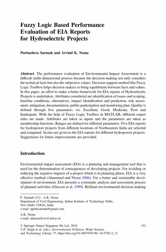
Fuzzy Logic Based PerformanceEvaluation of EIA Reportsfor Hydroelectric Projects
Purbashree Sarmah and Arvind K. Nema
Abstract The performance evaluation of Environmental Impact Assessment is adifficult multi-dimensional process because the decision-making not only considersthe technical facts but also the subjective values. Decision-support method like FuzzyLogic Toolbox helps decision makers to bring equilibrium between facts and values.In this paper, an effort to make a better framework for EIA reports of HydroelectricProjects is undertaken. Attributes considered are identification of issues and scoping,baseline conditions, alternatives, impact identification and prediction, risk assess-ment, mitigation, documentation, public participation andmonitoring plan. Quality isdefined through five parameters viz. Excellent, Good, Moderate, Poor andInadequate. With the help of Fuzzy Logic Toolbox in MATLAB, different expertrules are made. Attributes are taken as inputs and the parameters are taken asmembership functions. Ranges are defined for different parameters. Five EIA reportsfor hydropower projects from different locations of Northeastern India are selectedand compared. Scores are given to the EIA reports for different hydropower projects.Suggestions for future improvements are provided.
Introduction
Environmental impact assessment (EIA) is a planning and management tool that isused for the determination of consequences of developing projects. For avoiding orreducing the negative impacts of a project which is in planning phase, EIA is a veryeffective method (Ahammed and Nixon 2006). For a better and sustainable devel-opment of environment, EIA presents a systematic analysis and assessment processof planned activities (Glasson et al. 1999). Brilliant environmental decision-making
P. Sarmah (&) � A.K. NemaDepartment of Civil Engineering, Indian Institute of Technology Delhi,New Delhi 110016, Indiae-mail: [email protected]
A.K. Nemae-mail: [email protected]
© Springer Nature Singapore Pte Ltd. 2018V.P. Singh et al. (eds.), Environmental Pollution, Water Scienceand Technology Library 77, https://doi.org/10.1007/978-981-10-5792-2_13
153

can be made with the help of a good EIA. EIA review is the key procedure for qualitycontrol of EIA. The high quality EIA report can help in effective transformation ofEIA strategy into practice. However, a good-quality EIA report is rare in reality.There are various drawbacks remained in the EIA system even after the project isstarted. EIA expert committee members, approval authorities, project proponents,NGOs and consulting professionals, reveals various drawbacks which include;inadequate capacity of EIA approval authorities, deficiencies in screening andscoping, inadequate public participation and feeble monitoring (Panigrahi andAmirapu 2012). Different frameworks for formation of a good EIA report are madeby different scholars and institutions/agencies like European Union, World Bank,etc. In India, the first EIA comes under Environment Protection Act 1986. Althoughthe Environmental Impact Assessment Notification, 2006 and its amendments by theMinistry of Environment and Forest set certain guidelines for EIA practice in India,these guidelines are not enough for preparing a Good EIA report. The contemporaryEIA practice is facing several challenges (Rao and Ramana 2008). In Sarmah et al.(2015), nine attributes and their respective criteria are considered for EIA reports. Onthe basis of these criteria, general rules are made for EIA reports with five qualityparameters viz. Excellent, Good, Moderate, Poor and Inadequate.
In this paper, particularly EIA reports on hydroelectric projects are selected fromNortheastern part of India and expert rules are applied on them to find the quality ofthe report. Expert rules are made from expert knowledge to use and control ofdomain knowledge (Modak and Biswas 1999). These are prepared from generalrules with specialized thinking. This is creation of the coherent human thoughtprocess. Expert rules make the decision-making easier. Fuzzy logic (Zadeh 1996) isa tool which is able to compute with words. It is used for modeling qualitative humanthought processes in the study of complex methods and decisions. In Fuzzy logic,the ‘IF-THEN’ Fuzzy rules represent the qualitative sensitivity based reasoning.
Fuzzy inference is the process of creating the mapping from a given input to anoutput using Fuzzy logic. According to Fuzzy Logic Toolbox User’s Guide (2015),Fuzzy inference process comprises of five parts
• Fuzzification of the input variables.• Application of the Fuzzy operator (AND or OR) in the antecedent.• Implication from the antecedent to the consequent.• Aggregation of the consequents across the rules.• Defuzzification.
Objectives and Scope
The objectives of the paper are
• To review EIA of hydroelectric projects considering different criteria forattribute.
154 P. Sarmah and A.K. Nema
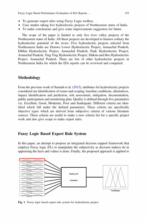
• To generate expert rules using Fuzzy Logic toolbox.• Case studies taking five hydroelectric projects of Northeastern states of India.• To make conclusions and give some improvements suggestion for future.
The scope of the paper is limited to only five river valley projects of theNortheastern states of India. All these projects are developed to harness solitary thehydroelectric potential of the rivers. Five hydroelectric projects selected fromNortheastern India are Demwe Lower Hydroelectric Project, Arunachal Pradesh,Dibbin Hydroelectric Project, Arunachal Pradesh, Pauk Hydroelectric Project,Arunachal Pradesh, Ting Ting Hydroelectric Project, Sikkim and Heo HydroelectricProject, Arunachal Pradesh. There are lots of other hydroelectric projects inNortheastern India for which the EIA reports can be reviewed and compared.
Methodology
From the previous work of Sarmah et al. (2015), attributes for hydroelectric projectsconsidered are identification of issues and scoping, baseline conditions, alternatives,impact identification and prediction, risk assessment, mitigation, documentation,public participation and monitoring plan. Quality is defined through five parametersviz. Excellent, Good, Moderate, Poor and Inadequate. Different criteria are iden-tified which fall under the defined parameters. These criteria are specificallyobjective types which are derived from subjective criteria of various literaturesources. These criteria are useful to make a new criteria list for a specific projectwork and also give scope to make expert rules.
Fuzzy Logic Based Expert Rule System
In this paper, an attempt to propose an integrated decision support framework thatemploys Fuzzy logic (FL) to manipulate the subjectivity as decision makers do inappraising the facts and values is done. Finally, the proposed approach is applied to
Fig. 1 Fuzzy logic based expert rule system for hydroelectric project
Fuzzy Logic Based Performance Evaluation of EIA Reports … 155
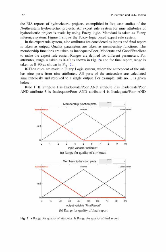
the EIA reports of hydroelectric projects, exemplified in five case studies of theNortheastern hydroelectric projects. An expert rule system for nine attributes ofhydroelectric project is made by using Fuzzy logic. Mamdani is taken as Fuzzyinference system. Figure 1 shows the Fuzzy logic based expert rule system.
In the expert rule system, nine attributes are considered as inputs and final reportis taken as output. Quality parameters are taken as membership functions. Themembership functions are taken as Inadequate/Poor, Moderate and Good/Excellentto make the expert rule easier. Ranges are defined for different parameters. Forattributes, range is taken as 0–10 as shown in Fig. 2a and for final report, range istaken as 0–90 as shown in Fig. 2b.
If-Then rules are made in Fuzzy Logic system, where the antecedent of the rulehas nine parts from nine attributes. All parts of the antecedent are calculatedsimultaneously and resolved to a single output. For example, rule no. 1 is givenbelow:
Rule 1: IF attribute 1 is Inadequate/Poor AND attribute 2 is Inadequate/PoorAND attribute 3 is Inadequate/Poor AND attribute 4 is Inadequate/Poor AND
(a) Range for quality of attributes
(b) Range for quality of final report
Fig. 2 a Range for quality of attributes. b Range for quality of final report
156 P. Sarmah and A.K. Nema

attribute 5 is Inadequate/Poor AND attribute 6 is Inadequate/Poor AND attribute 7is Inadequate/Poor AND attribute 8 is Inadequate/Poor AND attribute 9 isInadequate/Poor THEN final report is Inadequate/Poor.
Result and Discussion
Five hydroelectric projects are selected from the Northeastern Part of India. Theseprojects are
1. Demwe Lower Hydroelectric Project, Arunachal Pradesh (1750 MW).2. Dibbin Hydroelectric Project, Arunachal Pradesh (120 MW).3. Pauk Hydroelectric Project, Arunachal Pradesh (145 MW).4. Ting Ting Hydroelectric Project, Sikkim (99 MW).5. Heo Hydroelectric Project, Arunachal Pradesh (240 MW).
Quality of the EIA reports of these five hydroelectric projects is assessed. Expertrules are made by using Fuzzy Logic. Scores are given to different attributes andfinal score is obtained from Fuzzy Logic System for all the five EIA reports.
Demwe Lower Hydroelectric Project, Arunachal Pradesh
Project Description
Under this development, a concrete gravity dam is proposed to be constructed nearvillage Mompani on Lohit river in Lohit District of Arunachal Pradesh. The EIAreport has been prepared by CISMHE, University of Delhi in July, 2009.
Physical Features
The project is located at the foothill of Lohit basin. The project is located about800 m upstream of Parasuram Kund bridge on NH 52 and falls in Lohit district withreservoir extending into Anjaw district of the State of Arunachal Pradesh. Theproject area can be accessed from Dibrugarh airport, which is about 550 km fromGuwahati airport. The project site is about 215 km from Dibrugarh. A surfacepower house is proposed on the right bank of Lohit river to accommodate fivenumbers of vertical Francis turbines of 342 MW each.
Catchment area: 20,174 km2.Storage at maximum water level: 516.38 MCM.Height of dam: A concrete gravity dam of 163.12 m height above deepest foun-dation level.
Fuzzy Logic Based Performance Evaluation of EIA Reports … 157
Design discharge: 1729 cumecs.Design head: 112 m.Capacity: 1750 MW.
Performance Evaluation
Quality of nine attributes for Demwe hydroelectric project EIA report are marked asshown in Table 1. Putting these qualities in Fuzzy Logic system and giving score tonine attributes, the final score of the EIA report is evaluated. Figure 3 gives thescoring for final EIA report of Demwe hydroelectric project.
Dibbin Hydroelectric Project, Arunachal Pradesh
Project Description
The Dibbin Project is a run of river project with diurnal storage located on theBichom River in the West Kameng district of Arunachal Pradesh. The EIA reporthas been prepared by WAPCOS Centre for Environment.
Table 1 Quality of nine attributes for DEMWE hydroelectric project EIA report
Attributes 1 2 3 4 5 6 7 8 9
Quality G/E G/E I/P G/E I/P M G/E I/P M
whereG/E Good/excellentM ModerateI/P Inadequate/poor
Fig. 3 Scoring for final EIA report of DEMWE hydroelectric project
158 P. Sarmah and A.K. Nema
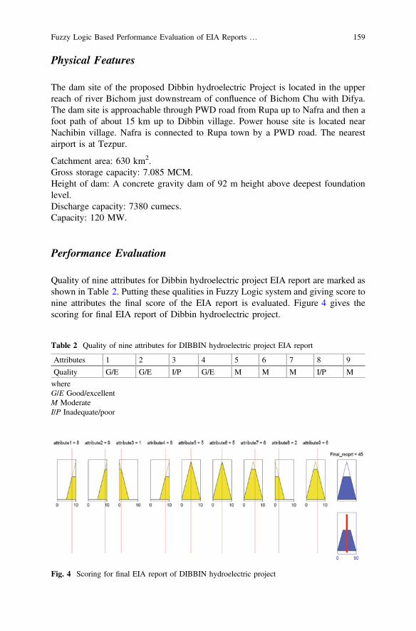
Physical Features
The dam site of the proposed Dibbin hydroelectric Project is located in the upperreach of river Bichom just downstream of confluence of Bichom Chu with Difya.The dam site is approachable through PWD road from Rupa up to Nafra and then afoot path of about 15 km up to Dibbin village. Power house site is located nearNachibin village. Nafra is connected to Rupa town by a PWD road. The nearestairport is at Tezpur.
Catchment area: 630 km2.Gross storage capacity: 7.085 MCM.Height of dam: A concrete gravity dam of 92 m height above deepest foundationlevel.Discharge capacity: 7380 cumecs.Capacity: 120 MW.
Performance Evaluation
Quality of nine attributes for Dibbin hydroelectric project EIA report are marked asshown in Table 2. Putting these qualities in Fuzzy Logic system and giving score tonine attributes the final score of the EIA report is evaluated. Figure 4 gives thescoring for final EIA report of Dibbin hydroelectric project.
Table 2 Quality of nine attributes for DIBBIN hydroelectric project EIA report
Attributes 1 2 3 4 5 6 7 8 9
Quality G/E G/E I/P G/E M M M I/P M
whereG/E Good/excellentM ModerateI/P Inadequate/poor
Fig. 4 Scoring for final EIA report of DIBBIN hydroelectric project
Fuzzy Logic Based Performance Evaluation of EIA Reports … 159
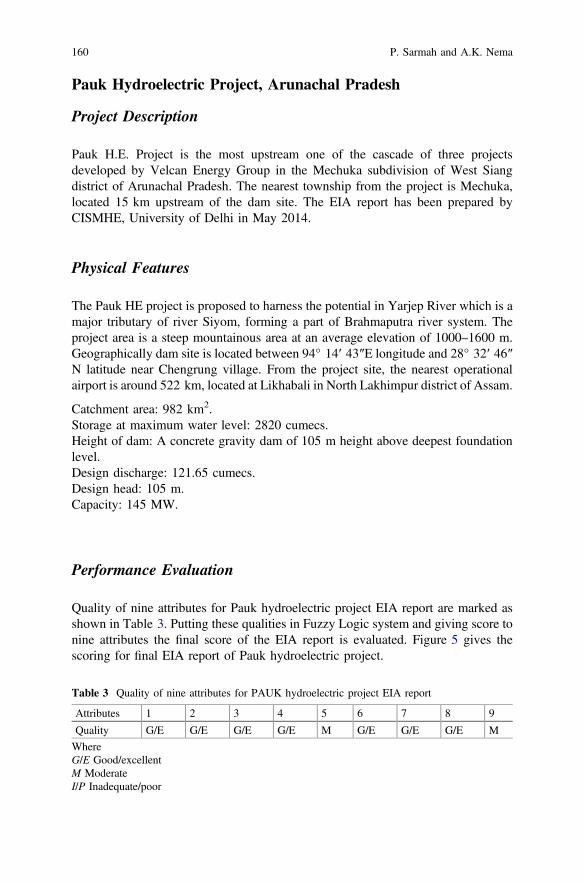
Pauk Hydroelectric Project, Arunachal Pradesh
Project Description
Pauk H.E. Project is the most upstream one of the cascade of three projectsdeveloped by Velcan Energy Group in the Mechuka subdivision of West Siangdistrict of Arunachal Pradesh. The nearest township from the project is Mechuka,located 15 km upstream of the dam site. The EIA report has been prepared byCISMHE, University of Delhi in May 2014.
Physical Features
The Pauk HE project is proposed to harness the potential in Yarjep River which is amajor tributary of river Siyom, forming a part of Brahmaputra river system. Theproject area is a steep mountainous area at an average elevation of 1000–1600 m.Geographically dam site is located between 94° 14′ 43″E longitude and 28° 32′ 46″N latitude near Chengrung village. From the project site, the nearest operationalairport is around 522 km, located at Likhabali in North Lakhimpur district of Assam.
Catchment area: 982 km2.Storage at maximum water level: 2820 cumecs.Height of dam: A concrete gravity dam of 105 m height above deepest foundationlevel.Design discharge: 121.65 cumecs.Design head: 105 m.Capacity: 145 MW.
Performance Evaluation
Quality of nine attributes for Pauk hydroelectric project EIA report are marked asshown in Table 3. Putting these qualities in Fuzzy Logic system and giving score tonine attributes the final score of the EIA report is evaluated. Figure 5 gives thescoring for final EIA report of Pauk hydroelectric project.
Table 3 Quality of nine attributes for PAUK hydroelectric project EIA report
Attributes 1 2 3 4 5 6 7 8 9
Quality G/E G/E G/E G/E M G/E G/E G/E M
WhereG/E Good/excellentM ModerateI/P Inadequate/poor
160 P. Sarmah and A.K. Nema
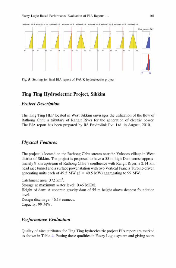
Ting Ting Hydroelectric Project, Sikkim
Project Description
The Ting Ting HEP located in West Sikkim envisages the utilization of the flow ofRathong Chhu a tributary of Rangit River for the generation of electric power.The EIA report has been prepared by RS Envirolink Pvt. Ltd. in August, 2010.
Physical Features
The project is located on the Rathong Chhu stream near the Yuksom village in Westdistrict of Sikkim. The project is proposed to have a 55 m high Dam across approx-imately 9 km upstream of Rathong Chhu’s confluence with Rangit River; a 2.14 kmhead race tunnel and a surface power station with two Vertical Francis Turbine-drivengenerating units each of 49.5 MW (2 � 49.5 MW) aggregating to 99 MW.
Catchment area: 372 km2.Storage at maximum water level: 0.46 MCM.Height of dam: A concrete gravity dam of 55 m height above deepest foundationlevel.Design discharge: 46.13 cumecs.Capacity: 99 MW.
Performance Evaluation
Quality of nine attributes for Ting Ting hydroelectric project EIA report are markedas shown in Table 4. Putting these qualities in Fuzzy Logic system and giving score
Fig. 5 Scoring for final EIA report of PAUK hydroelectric project
Fuzzy Logic Based Performance Evaluation of EIA Reports … 161
to nine attributes the final score of the EIA report is evaluated. Figure 6 gives thescoring for final EIA report of Ting Ting hydroelectric project.
Heo Hydroelectric Project, Arunachal Pradesh
Project Description
Heo H.E project is the middle project of the cascade of three projects developed byVelcan Energy in the Mechuka subdivision of the West Siang district of ArunachalPradesh. The EIA report has been prepared by CISMHE, University of Delhi inMay, 2014.
Physical Features
The Heo HE project is proposed to harness the power potential in Yarjep River (ShiShito) which is a major tributary of river Siyom, forming a part of Brahmaputrariver system. The nearest township from the project is Mechuka, located 19 kmupstream of the barrage site. The project area can be approached through amotorable road up to barrage site, and then by foot tracks from the Tato-Mechuka
Table 4 Quality of nine attributes for TING TING hydroelectric project EIA report
Attributes 1 2 3 4 5 6 7 8 9
Quality G/E G/E I/P G/E M G/E G/E M G/E
whereG/E Good/excellentM ModerateI/P Inadequate/poor
Fig. 6 Scoring for final EIA report of TING TING hydroelectric project
162 P. Sarmah and A.K. Nema
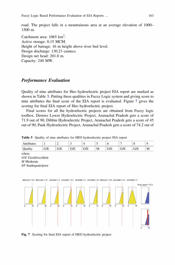
road. The project falls in a mountainous area at an average elevation of 1000–1500 m.
Catchment area: 1065 km2.Active storage: 0.15 MCM.Height of barrage: 16 m height above river bed level.Design discharge: 130.23 cumecs.Design net head: 201.8 m.Capacity: 240 MW.
Performance Evaluation
Quality of nine attributes for Heo hydroelectric project EIA report are marked asshown in Table 5. Putting these qualities in Fuzzy Logic system and giving score tonine attributes the final score of the EIA report is evaluated. Figure 7 gives thescoring for final EIA report of Heo hydroelectric project.
Final scores for all the hydroelectric projects are obtained from Fuzzy logictoolbox. Demwe Lower Hydroelectric Project, Arunachal Pradesh gets a score of71.9 out of 90, Dibbin Hydroelectric Project, Arunachal Pradesh gets a score of 45out of 90, Pauk Hydroelectric Project, Arunachal Pradesh gets a score of 74.2 out of
Table 5 Quality of nine attributes for HEO hydroelectric project EIA report
Attributes 1 2 3 4 5 6 7 8 9
Quality G/E G/E G/E G/E M G/E G/E G/E M
whereG/E Good/excellentM ModerateI/P Inadequate/poor
Fig. 7 Scoring for final EIA report of HEO hydroelectric project
Fuzzy Logic Based Performance Evaluation of EIA Reports … 163
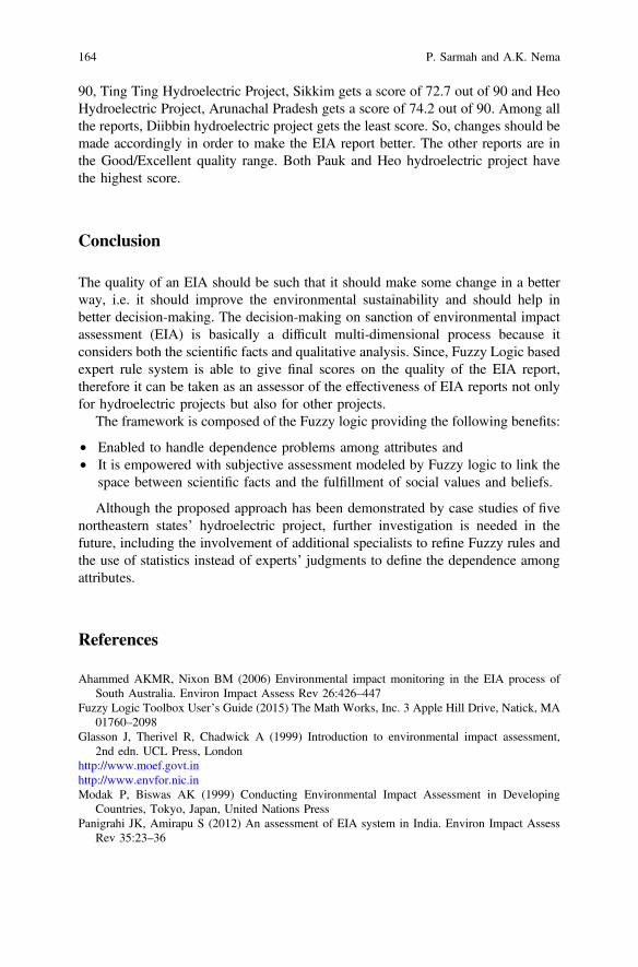
90, Ting Ting Hydroelectric Project, Sikkim gets a score of 72.7 out of 90 and HeoHydroelectric Project, Arunachal Pradesh gets a score of 74.2 out of 90. Among allthe reports, Diibbin hydroelectric project gets the least score. So, changes should bemade accordingly in order to make the EIA report better. The other reports are inthe Good/Excellent quality range. Both Pauk and Heo hydroelectric project havethe highest score.
Conclusion
The quality of an EIA should be such that it should make some change in a betterway, i.e. it should improve the environmental sustainability and should help inbetter decision-making. The decision-making on sanction of environmental impactassessment (EIA) is basically a difficult multi-dimensional process because itconsiders both the scientific facts and qualitative analysis. Since, Fuzzy Logic basedexpert rule system is able to give final scores on the quality of the EIA report,therefore it can be taken as an assessor of the effectiveness of EIA reports not onlyfor hydroelectric projects but also for other projects.
The framework is composed of the Fuzzy logic providing the following benefits:
• Enabled to handle dependence problems among attributes and• It is empowered with subjective assessment modeled by Fuzzy logic to link the
space between scientific facts and the fulfillment of social values and beliefs.
Although the proposed approach has been demonstrated by case studies of fivenortheastern states’ hydroelectric project, further investigation is needed in thefuture, including the involvement of additional specialists to refine Fuzzy rules andthe use of statistics instead of experts’ judgments to define the dependence amongattributes.
References
Ahammed AKMR, Nixon BM (2006) Environmental impact monitoring in the EIA process ofSouth Australia. Environ Impact Assess Rev 26:426–447
Fuzzy Logic Toolbox User’s Guide (2015) The Math Works, Inc. 3 Apple Hill Drive, Natick, MA01760–2098
Glasson J, Therivel R, Chadwick A (1999) Introduction to environmental impact assessment,2nd edn. UCL Press, London
http://www.moef.govt.inhttp://www.envfor.nic.inModak P, Biswas AK (1999) Conducting Environmental Impact Assessment in Developing
Countries, Tokyo, Japan, United Nations PressPanigrahi JK, Amirapu S (2012) An assessment of EIA system in India. Environ Impact Assess
Rev 35:23–36
164 P. Sarmah and A.K. Nema

Rao DB, Ramana MV (2008) Violating letter and spirit: environmental clearances forKoodankulam reactors. Econ Polit weekly
Sarmah P, Nema AK (2015) Performance Evaluation of Environmental Impact Assessment UsingQuality Index. In: Geo-Engineering and Climate Change Technologies for SustainableEnvironmental Management (GCCT-2015), Oct 9–11, 2015, Department of Civil Engineering,MNNIT Allahabad, India
Zadeh LA (1996) Fuzzy logic—computing with words. IEEE Trans Fuzzy Syst 4(2):103–111
Fuzzy Logic Based Performance Evaluation of EIA Reports … 165

Assessment and Predictionof Environmental Noise Generatedby Road Traffic in Nagpur City, India
Sameer S. Pathak, Satish K. Lokhande, P.A. Kokateand Ghanshyam L. Bodhe
Abstract The main intention of research is to quantify and predict the noise leveldue to heterogeneous traffic conditions at critical junctions and highways. A studywas carried out to assess the existing status of noise levels and its impacts on theenvironment with a possibility of further expansion of the city. Vehicular trafficnoise levels measured during peak and non-peak hours at all selected locations werehigher (71–76 dBA and 69.3–76.3 dBA) than the prescribed limits. The recognizedamount of traffic and with the help of road geometry data, prediction of noise levelis performed using modified Federal Highway Administration (FHWA) model, andthe computed noise was compared with the measured one for assuring the relevanceof this model for prediction of forthcoming noise. The outcome received from thismodel was nearer to the observed noise level, having a percentage error of ±3%,the best fit lines generated between them gives R2 of 0.457. In this study measuredand computed noise exposure levels were depicted with the help of contour maps.Octave band spectral analysis reveals that the interrupted traffic flow is above thefree flow traffic and realized that the contribution of two wheeler and cars/jeep aremainly responsible for a generation of noise level at both the lower and higherfrequencies, it also signifies that the FHWA model is convenient to be used forIndian circumstances.
Introduction
India has emanated as a rapidly developing economy, ensuing swift industrializa-tion and urbanization, the increment in vehicles can produce a life-threateningnoise. (Tripathi et al. 2006), The vehicles reported in India enhanced from around
S.S. Pathak � S.K. Lokhande (&) � P.A. Kokate � G.L. BodheAnalytical Instruments Division, CSIR-National Environmental Engineering ResearchInstitute (NEERI), Nagpur, Maharashtra, Indiae-mail: [email protected]
© Springer Nature Singapore Pte Ltd. 2018V.P. Singh et al. (eds.), Environmental Pollution, Water Scienceand Technology Library 77, https://doi.org/10.1007/978-981-10-5792-2_14
167
0.3 million in 1951 to almost 142 million in 2011 (MoRTH GoI 2013) an increaseof 7.7% annually as against a population growth of 3.8% during the same period.The annual growth was even faster at 10% during the period of 2001−2011(CSTEP). The root age of environmental noise in our daily life is mainly concernedwith the increasing urbanization and the development of transportation sectorwithin metropolitan cities (Kaklauskas et al. 2009; Shukla et al. 2009; Akgungoret al. 2008; Daunoras et al. 2008; Jovic and Doric 2010). The significant factor forinflation of noise in the urban region is vehicular traffic contributing to almost 55%of the entire noise. (Omidvari and Nouri 2009; Banerjee and Chakraborty 2006;Goswami 2009). Several previous studies on traffic noise resolve the major sourceof noise existing in the urban areas. It is a dominant source of a nuisance both in thedeveloped and developing nations. Tremendous noise can affect the health of thepeople living proximity to road junctions and busy highways. It disturbs the qualityof life in urban areas; this is due to rapid growth in vehicular traffic (Patel et al.2006; Alam et al. 2001; Calixto et al. 2003; Cowan 1994; Rylander et al. 1976).Therefore, an environmental assessment of traffic noise is more complex in Indiancities regarding the conglomeration in a traffic situation, having different vehiclecategory, congestion, road geometry and deficiency of traffic sense. (Kalaiselvi andRamachandraiah 2010; Wani and Jaiswal 2010)
Background of Nagpur City
Nagpur, the orange city, is a tertiary largest city and the second capital of the Indianstate of Maharashtra; and being virtually at the geographical centre of India. Alllarge-scale highways and railways are going through this city, it is at the colligationof two National Highways, NH-6 and NH-7 and also associated to all Metropolitanof India by air routes. This has ensued the city being a major trade and trans-portation center. Accelerated urbanization specifies the level of expansion of anyregion affecting an enormous increase in motor vehicles, which affects the envi-ronment to a significant amount. The entire length of roads in the city is 1907 kmhaving the major road is about 500 km, and other were interior roads (Indo-USAID2006). In the Nagpur district, the population is heavily focused in the city, whichprevails the urban scene, the trend of urbanization in Nagpur district is shown inFig. 1, Nagpur nearly half of the total population of the district lives in Nagpur(Bhonsle 2010).
The vehicles in Nagpur city have sprung up at a degree of 8.00% per annumduring 2009–2012 as depicted in Fig. 2. The contribution of scooter/motorcycleendured at 83.6% to 82.6 during that span. On the other hand, the share of cars andjeeps which were at 9.38% in 2009 goes to 10.08% in 2011. On an average, theshare of two wheeler taking over a dominant role in the traffic of Nagpur city(Aparajit 2012; Deo 2014).
168 S.S. Pathak et al.

Noise Prediction
In order to meliorate the assessment of traffic noise for obstructed as well as freeflow traffic, the prediction model is required to evaluate the interaction betweencharacteristics of traffic and emission levels of noise for better projection of a futuresituation based on the study of present trends (Ugbebor et al. 2015). Most of thecountries have developed their traffic noise prediction models according to theirtraffic and environmental conditions, such as Burgess model (1977) in Sydney(Australia), Griffith and Langdon Model (1968), CSTB (Centre Scientifique etTechnique du Batiment) model was formulated by the French, CoRTN (Calculationof Road Traffic Noise) model (1975) has been developed by the Transport and RoadResearch Laboratory and the Department of Transport of the United Kingdom, the
40
50
60Po
pula
tion(
%)
1951 19
46.795
61 1971
2.06 54.32
Years1981
56.75
1991
61.83
2001
64.35
Fig. 1 Percentage of urban population in Nagpur region
Veh
icle
cou
nt
10,00,000
11,00,000
12,00,000
13,00,000
14,00,000
15,00,000
16,00,000
2009-2010
12,20,657
2010-2011
13,32,720
Years2011-2012
14,52,746
2012-2013
15,68,070
Fig. 2 Vehicle count during the period of 2009−2012
Assessment and Prediction of Environmental Noise Generated … 169

RLS90 (Richtlinien für den Lärmschutz an Straben) traffic noise model in Germany,the Statens Planverk 48 model in Scandinavia, Nouvelle Methode de Prevision deBruit or simply NMPB-Routes-96 model in French, ASJ model in Japan, TheItalian Research Institute developed a TNM, the “CNR” model (ConsiglioNazionale delle Ricerche) and the GIS based road traffic noise prediction model wasdrawn up in China (2002) (Rajakumara et al. 2008).
Anti-noise legislations, major highway control ordinances and other govern-mental policies that pertain environmental noise control strategies, however, couldnot be diminished noise annoyance without a prior assessment and prediction.Hence, it’s mandatory to control noise earlier; it crosses an alarming stage. In thispaper, endeavor has been made to judge the traffic noise level in selected areas ofNagpur city and performed noise prediction using modified Federal HighwayAdministration Agency (FHWA) model and compare the estimated noise with themeasured one for assuring the relevancy of the model.
Materials and Methods
Study Area
With a probability of further elaboration of the city, a comprehensive survey wascarried out at numerous junctions and arterial roads in Nagpur city including heavytraffic jam as well as free flow traffic in the morning and evening hours.Subsequently, nine locations were selected including six junctions and threehighways namely Medical square (J1), Ram Nagar square (J2), Indora square (J3),RBI square (J4), Jagnade square (J5), HB Town square (J6); Amravati road (H1),Wardha road (H2) and Chinwada road (H3) which lies between 21° 05′ and 21° 11′N latitude and 79° 00′ to 79° 08′E longitude as illustrated in Fig. 3.
Fig. 3 Map showing study area of Nagpur city for noise monitoring
170 S.S. Pathak et al.
Evaluation of Traffic Noise
Measurement of traffic noise was accomplished at all the selected nine locationsacross the Nagpur city, in which six stations are the heavily populated junctions,while the remaining three are the highways passing towards outside of the city.Measurements of different parameters at each site and gathering of data wereexecuted for one hour at two different peak time intervals in the morning (10:00–11:00 am) and evening (6:00–7:00 pm). Traffic noise was recorded using the soundlevel metre CK: 172B Optimus Green (Cirrus, UK) as per Indian standards with fastresponse mode having “A” frequency weighted and data logging of 1s time interval,the definitive range of the equipment is of 20–140 dBA. During noise assessments,the data collection in the field was accomplished in accordance with the recom-mendations of national and international agencies. The microphone of the devicewas located at a distance of 3.5 m from the road edge and placed at the height of1.2–1.5 m from the land. In order to eradicate the consequence of interference dueto building reflections, noise exposure levels are measured 1 m away from thestructures.
Data Extraction
Noise metre was mounted on a stand and placed away from the road in order toreceive a valuable estimation of noise. Investigation of traffic volume was achievedcontinuously for one hour manually at all chosen sites and are classified into sixcategories (scooter/motorcycle, car/jeep/van, auto rickshaw, light commercialvehicles, heavy truck, and buses) based on the necessity of our study. Averagespeed for each category of vehicles was calculated by specifying two points on theroad at well-known distance, note down the entry and exit time for each category ofvehicles at beginning and end marking points, by dividing the known distance withtime difference between those points, speed in km/h for each vehicle classes wereestimated. The structure of road consisting of geometrical parameter, category,traffic lanes, road situation was also considered in the study. The distance of noiseequipment from the midpoint of road for locations Medical square, Ram Nagarsquare, Indora square, RBI square, Jagnade square, HB Town square; Amravatiroad, Wardha road and Chinwada road were around 24.5, 9, 10.5, 18, 14.5, 17,10.5, 15 and 15.5 m respectively.
Assessment and Prediction of Environmental Noise Generated … 171

Traffic Noise Modelling
The prediction of noise is achieved by applying modified FHWA model inaccordance with Indian contexts. Traffic noise can be forecasted based on singlevehicle noise, volume and speed of vehicles, observer distance from the source andother correlation coefficients. FHWA model distributes noise level through a seriesof adjustments to the reference sound level assessed via sampling stations; theequation for traffic noise prediction algorithm is shown below. (Bhattacharya et al.2001)
Leq ¼ L0 þDLi; ð1Þ
where
L0 reference noise level of a stream of vehicles;DLi adjustment applied.
The expression for well-defined FHWA model is given below.
Leqi ¼ L0 þAVS þAD þAS; ð2Þ
where
Leqi hourly equivalent noise for each category of vehicle;L0 reference energy mean emission level;Avs volume and speed correction;AD distance correction;AS ground cover correction.
The FHWA model computes noise level through a series of adjustments whichare discussed individually as shown (Nirjar et al. 2003).
Reference Energy Mean Emission Level
It is the noise level emitted by each of six classes of vehicles; the reference noiselevel was calculated using the individual noise emission equation for various cat-egories of vehicle.
Volume and Speed Correction
AVS ¼ 10 log10 D0V=Sð Þ � 25; ð3Þ
172 S.S. Pathak et al.
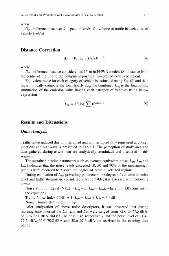
whereD0—reference distance; S—speed in km/h; V—volume of traffic in each class of
vehicle (veh/h)
Distance Correction
AD ¼ 10 log10 D0=Dð Þ1þ a; ð4Þ
whereD0—reference distance considered as 15 m in FHWA model; D—distance from
the centre of the line to the equipment position; a—ground cover coefficient.Equivalent noise for each category of vehicle is estimated using Eq. (2) and then
logarithmically compute the total hourly Leq, the combined Leq is the logarithmicsummation of the emission value having each category of vehicles using belowexpression
Leq ¼ 10 logX
10Leqi=10 ð5Þ
Results and Discussions
Data Analysis
Traffic noise induced due to interrupted and uninterrupted flow registered at chosenjunctions and highways is presented in Table 1. The perception of study area anddata gathered during assessment are analytically scrutinized and discussed in thissegment.
The sustainable noise parameters such as average equivalent noise, L10, L50 andL90 (indicates that the noise levels exceeded 10, 50 and 90% of the measurementperiod) were recorded to resolve the degree of noise at selected regions.
During estimation of Leq, prevailing parameters like degree of variation in noiselevel and traffic streams are considerably accountable; it is assessed with followingterms:
Noise Pollution Level (NPL) = Leq + a (L10 − L90), where a = 1.0 (constant inthe equation)Traffic Noise Index (TNI) = 4 (L10 − L90) + L90 − 30 dBNoise Climate (NC) = L10 − L90.After analyzation of above noise descriptors, it was observed that during
morning time interval the L10, L50 and L90 were ranged from 72.6 to 77.5 dBA;68.2 to 72.1 dBA and 63.1 to 68.8 dBA respectively and the noise level of 71.4–77.5 dBA; 65.6–70.8 dBA and 58.6–67.6 dBA are received in the evening timeperiod.
Assessment and Prediction of Environmental Noise Generated … 173

Tab
le1
Noise
levelin
dBA
atalltheselected
locatio
ns
Morning
hours
Evening
hours
Locations
Leq
L10
L50
L90
NPL
TNI
NC
Leq
L10
L50
L90
NPL
TNI
NC
J171
72.6
68.2
65.9
77.7
62.7
6.7
71.5
74.2
69.7
66.8
78.9
66.4
7.4
J272
.373
.668
.264
.881
.170
8.8
75.2
77.5
70.8
67.6
85.1
77.2
9.9
J375
.377
.172
.168
.883
.672
8.3
71.6
74.0
69.5
66.0
79.6
688
J471
.573
.068
.563
.680
.971
.29.4
71.6
73.5
69.1
64.7
80.4
69.9
8.8
J576
76.6
69.9
66.7
85.9
76.3
9.9
76.3
77.2
70.7
67.4
86.1
76.6
9.8
J673
.775
.369
.365
.183
.975
.910
.273
.274
.869
.565
.682
.472
.49.2
H1
73.7
76.8
69.9
63.1
87.4
87.9
13.7
69.3
71.4
66.4
62.3
78.4
68.7
9.1
H2
74.6
77.5
70.2
63.1
8990
.714
.472
.874
.868
.162
.385
.382
.312
.5
H3
73.1
76.3
65.9
5891
.410
1.2
18.3
71.5
74.6
65.6
58.6
87.5
92.6
16
174 S.S. Pathak et al.
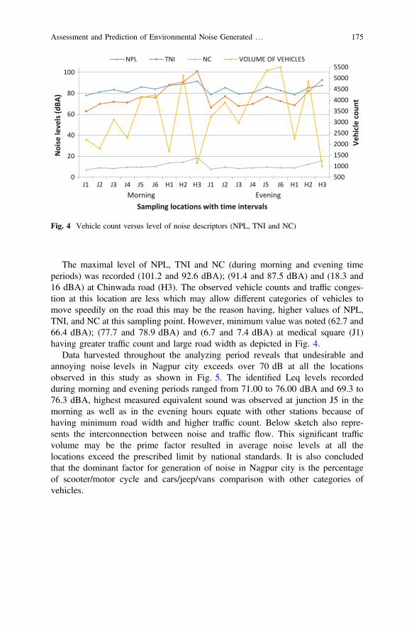
The maximal level of NPL, TNI and NC (during morning and evening timeperiods) was recorded (101.2 and 92.6 dBA); (91.4 and 87.5 dBA) and (18.3 and16 dBA) at Chinwada road (H3). The observed vehicle counts and traffic conges-tion at this location are less which may allow different categories of vehicles tomove speedily on the road this may be the reason having, higher values of NPL,TNI, and NC at this sampling point. However, minimum value was noted (62.7 and66.4 dBA); (77.7 and 78.9 dBA) and (6.7 and 7.4 dBA) at medical square (J1)having greater traffic count and large road width as depicted in Fig. 4.
Data harvested throughout the analyzing period reveals that undesirable andannoying noise levels in Nagpur city exceeds over 70 dB at all the locationsobserved in this study as shown in Fig. 5. The identified Leq levels recordedduring morning and evening periods ranged from 71.00 to 76.00 dBA and 69.3 to76.3 dBA, highest measured equivalent sound was observed at junction J5 in themorning as well as in the evening hours equate with other stations because ofhaving minimum road width and higher traffic count. Below sketch also repre-sents the interconnection between noise and traffic flow. This significant trafficvolume may be the prime factor resulted in average noise levels at all thelocations exceed the prescribed limit by national standards. It is also concludedthat the dominant factor for generation of noise in Nagpur city is the percentageof scooter/motor cycle and cars/jeep/vans comparison with other categories ofvehicles.
5001000150020002500300035004000450050005500
0
20
40
60
80
100
J1 J2 J3 J4 J5 J6 H1 H2 H3 J1 J2 J3 J4 J5 J6 H1 H2 H3
Vehi
cle
coun
t
Noi
se le
vels
(dBA
)
Sampling locations with time intervals
NPL TNI NC VOLUME OF VEHICLES
Morning Evening
Fig. 4 Vehicle count versus level of noise descriptors (NPL, TNI and NC)
Assessment and Prediction of Environmental Noise Generated … 175
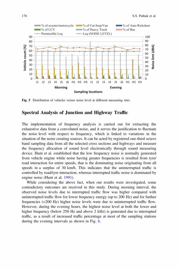
Spectral Analysis of Junction and Highway Traffic
The implementation of frequency analysis is carried out for extracting theexhaustive data from a convoluted noise, and it serves the justification to fluctuatethe noise level with respect to frequency, which is linked to variations in thesituation of the noise creating sources. It can be acted by registered one-third octaveband sampling data from all the selected cross sections and highways and measurethe frequency allocation of sound level electronically through sound measuringdevice. Hunt et al. established that the low frequency noise is normally generatedfrom vehicle engine while noise having greater frequencies is resulted from tyre/road interaction for entire speeds, that is the dominating noise originating from allspeeds in a surplus of 30 km/h. This indicates that the uninterrupted traffic iscontrolled by road/tyre interaction, whereas interrupted traffic noise is dominated byengine noise (Hunt et al. 1991).
While considering the above fact, when our results were investigated, somecontradictory outcomes are received in this study. During morning interval, theobserved noise levels due to interrupted traffic flow was higher compared withuninterrupted traffic flow for lower frequency energy (up to 200 Hz) and for furtherfrequencies (<200 Hz) higher noise levels were due to uninterrupted traffic flow.However, during the evening hours, the highest noise level at both the lower andhigher frequency (below 250 Hz and above 2 kHz) is generated due to interruptedtraffic, as a result of increased traffic percentage at most of the sampling stationsduring the evening intervals as shown in Fig. 6.
0102030405060708090100
0102030405060708090
J1 J2 J3 J4 J5 J6 H1 H2 H3 J1 J2 J3 J4 J5 J6 H1 H2 H3
Noi
se li
mt (
dBA)
Vehi
cle
coun
t (%
)
Sampling locations
% of scooter/motorcycle % of Car/Jeep/Van % of Auto Rickshaw% of LCV % of Heavy Truck % of BusPermissible Leq Leq (NOISE LEVEL)
Morning Evening
Fig. 5 Distribution of vehicles versus noise level at different measuring sites
176 S.S. Pathak et al.

Model Illustration
To find out the relevancy of the customized FHWA model, evaluation of trafficstream for various categories of vehicles and their velocity has been scrutinized andresolved that the computed noise levels were overestimated than that of observedvalues at most of the selected locations. The correlation of predicted outcomesdepicts that the evaluated noise is close to the measured values having a percentageerror of ±3% between them and the best fit line was also generated which gave anR2 value of 0.457 as shown in Fig. 7. Based on the findings, it can be observed thatthe modified FHWA model gives a strong correlation and best suitability for pre-diction of noise levels in Indian cities within an acceptable limit of accuracy.
In this research, the noise survey of Nagpur city was conducted at differentsampling stations, including cross-sections traffic as well as free flow traffic duringmorning and evening peak hours, and attempt has been made to depict the present
0102030405060708090100
01020304050607080
20Hz
31.5
Hz
50Hz
80Hz
125H
z
200H
z
315H
z
500H
z
800H
z
1.25
kHz
2kHz
3.15
kHz
5kHz
8kHz
12.5
kHz
20kH
z Noi
se le
vel (
dBA)
dur
ing
Even
ing
Noi
se le
vel (
dBA)
dur
ing
Mor
ning
Frequency (Hz)
Interrupted traffic flow (M) uninterrupted traffic flow (M)Interrupted traffic flow2 (E) uninterrupted traffic flow3 (E)
Fig. 6 Spectral analysis during measurement period
y = 0.3952x + 43.717R² = 0.4577
68
70
72
74
76
78
66 68 70 72 74 76 78 80
Mea
sure
d Le
q
Predicted Leq
Fig. 7 Correlation plot for predicted and measured noise level
Assessment and Prediction of Environmental Noise Generated … 177

noise scenario with the help of contour map for better understanding of variation ofnoise during different times of the day. The contour map demonstrated that theaverage noise level at all the sampling stations was found in the exceeded range of69.3–76.3 dBA as shown in Fig. 8.
Conclusion
This research distinctly revealed that the noise obtained from both heterogeneousand free flow traffic is higher than the recommended national standards for bothmorning and evening peak intervals and it concludes that road traffic noise directlydepends on increased noise from the vehicular engine horn during interrupted trafficflow and poor road conditions. Heavy traffic had greater velocity vehicles on theselected highways, and the transportation sector was also one of the dominantsources of noise in this city.
The statistical analysis between forecasted and measured values was performedto find out the fitness of the model. It can reveal that the modified FHWA modelgives a significantly higher correlation coefficient values and can be applied suc-cessfully for the prediction of road traffic noise under Indian traffic conditionswithin a tolerable boundary.
Evening
Morning
Fig. 8 Noise map of Nagpur city during morning and evening intervals
178 S.S. Pathak et al.
The reported noise spectrum shows the distribution of noise levels with respectto frequency, and it depicts that noise generated due to interrupted traffic flow isabove the free flow traffic. The traffic noise can also be displayed in the formcontour lines with various colour shades for different levels of noise contours andindicates the exceeded noise level at all selected locations in the Nagpur city.
Hence it is mandatory to generate the noise control policies to avoid harmfulresults of sound pollution and for restricting such unwanted noise, regulation oftraffic volume, the speed of vehicles and unwanted horns at sensitive pointsmight be helpful for reducing noise pollution, to avoid the adverse effect on thecommunity and the environment. A comprehensive program for public awareness isurgently required to control the vehicular traffic and protect the public from itsunwanted impacts.
References
Akgungor AP, Demirel A (2008) Investigating urban traffic based noise pollution in the city ofKirikkale, Turkey. Transport 23(3):273–278
Alam JB, Rauf AFMA, Ahemed MF (2001) Traffic induced noise pollution in Dhaka. J Civil EngInst Eng 01:55–63
Aparajit SM (2012) Infrastructure statistics of Maharashtra state 2009−10 and 2010−11 (firstissue), Planning Department, Government of Maharashtra, Mumbai. https://mahades.maharashtra.gov.in/files/publication/infra_stats_0910_1011.pdf
Banerjee D, Chakraborty SK (2006) Monthly variation in night time noise levels at residentialareas of Asansol city (India). J Env Sci Eng 48:39–44
Bhattacharya CC, Jain SS, Singh SP, Parida M, Mittal N (2001) Development of comprehensivehighway noise model for Indian conditions. Paper no. 481, pp 454A−478A
Bhonsle KD (2010) A study of urbanization in Nagpur district. Inst Town Planners, India J 7(3):88–95
Calixto A, Diniz FB, Zannin P (2003) Effects of traffic composition on road traffic noise in anurban setting. Cities 20(1):23−29
Cowan JP (1994) Educating the public on environmental and recreational noise exposure. In:Cooper AR (ed) Handbook of environmental acoustics, 3rd ed. Wiley, New York, pp 14−20
CSTEP, Review of urban transport in India Centre for Study of Science, Technology and Policy.Institute of Urban Transport (India). http://www.indiaenvironmentportal.org.in/files/file/Review%20of%20Urban%20Transport%20in%20India.pdf
Daunoras J, Bagdonas V, Gargasas V (2008) City transport monitoring and routes optimalmanagement system. Transport 23(2):144–149
Deo AD (2014) Infrastructure statistics of Maharashtra state 2011−12 and 2012−13 PlanningDepartment, Government of Maharashtra, Mumbai. https://mahades.maharashtra.gov.in/files/publication/infra_stats_1112_1213.pdf
Goswami S (2009) Road traffic noise: a case study of Balasore town, Orissa, India. Inter J EnvironRes 3(2):309–318
Hunt M, Samuels S (1991) Traffic noise: prediction of interrupted flow noise. Transit New ZealandResearch Report 3
Jovic J, Doric V (2010) Traffic and environmental street network modelling: Belgrade case study.Transport 25(2):155–162
Kaklauskas A, Zavadskas EK, Saparauskas J (2009) Conceptual modelling of sustainable Vilniusdevelopment. Technol Econ Develop Econ 15(1):154–177
Assessment and Prediction of Environmental Noise Generated … 179
http://www.indiaenvironmentportal.org.in/files/file/Review%20of%20Urban%20Transport%20in%20India.pdf

Kalaiselvi R, Ramachandraiah A (2010) Environmental noise mapping study for heterogeneoustraffic conditions. In: Proceedings of 20th international congress on acoustics, ICA, 23−27August 2010, Sydney, Australia, PACS:43.50. LJ, 43.50.RQ.—6
MoRTH GoI (2013) Road transport year book 2011–12 Transport Research Wing Ministry ofRoad Transport and Highways. Government of India, New Delhi. http://morth.nic.in/showfile.asp?lid=1131
Nirjar RS, Jain SS, Singh SP, Parida M, Katiyar VS, Mittal NA (2003) Study of transport relatednoise pollution in Delhi. J Inst Eng 84:6–15
Omidvari M, Nouri J (2009) Effects of noise pollution on traffic policemen. Int J Environ Res 3(4):645–52
Patel R, Tiwari TN, Patel T (2006) Noise pollution in residential areas of Jharsuguda town, Orissa(India) and its impact. J Environ Sci Eng Technol 48(3):209–212
Rajakumara HN, Gowda RM (2008) Road traffic noise prediction models: a Review. Inter JSustain Develop Planning 3(3):257–271
Rylander R, Sorensen S, Kajland A (1976) Traffic noise exposure and annoyance reactions.J Sound Vib 47(2):237–242
Shukla AK, Jain SS, Parida M, Srivastava JB (2009) Performance of FHWA model for predictingtraffic noise. A case study of metropolitan city, Lucknow (India). Transport 24(3):234–240
Tripathi BD, Pathak V, Upadhyay AR (2006) A case study of noise pollution in the city ofVaranasi. Indian J Environ Prot 26(8):737–741
Ugbebor JN, Raphael Yorkor B (2015) Measurement and evaluation of road traffic noise in threeselected junctions in Port Harcourt Metropolitant, Nigeria. J Environ Sci Comp Sci Eng Tech04(2)
USAID (2006) Final report for city development plan: Nagpur, Maharashtra, India. Indo-USAIDfinancial institutions reform and expansion project. http://pdf.usaid.gov/pdf_docs/pdacw407.pdf
Wani KA, Jaiswal YK (2010) Assessment of noise pollution in Gwalior M.P. India. AdvBiores1(1):54–60
180 S.S. Pathak et al.
Time-Dependent Study of ElectromagneticField and Indoor MeteorologicalParameters in Individual WorkingEnvironment
A.K. Mishra, P.A. Kokate, S.K. Lokhande, A. Middeyand G.L. Bodhe
Abstract Human beings in modern society are facing wide-range of electromag-netic (EMF) radiations from few hertz (Hz) to gigahertz (GHz) range. Its minorsources are power supply, personal computers, Wi-Fi routers, Zig-bee, cell phonesand base trans-receiver stations (BTS) devices. We have extensively used them inmicroenvironments like offices, restaurants, buses, close auditorium, etc. In suchindoor environments, the air quality incorporates various gaseous emissions, tem-perature, humidity, particulate matters, etc. Accordingly, the cumulative effect ofEMF and air-quality parameters can change human health and quality of life. Thispaper described exposure assessment of EMF and indoor meteorological parametersin the individual microenvironment during working and non-working hours. Theresults were obtained via broadband methodology for assessment of EMR and pointsource methodology for temperature, relative humidity and particulate matter (PM).The kriging model in surfer software approved to be more suitable to show accurategridding of EMF during working and non-working hours. No significant changeobserved in time-dependent analysis of EMF, temperature, humidity and PM count.However, telephony band was dominant during whole analysis. Hence, moreinvestigations are required to identify the quantitative relation between theseindependent parameters.
Keywords EMF � Microenvironment � Electro-smog � Indoor meteorologicalparameters
A.K. Mishra � P.A. Kokate (&) � S.K. Lokhande � G.L. BodheAnalytical Instruments Division, CSIR-National Environmental EngineeringResearch Institute (NEERI), Nagpur, Indiae-mail: [email protected]
A. MiddeyAir Pollution Control Division, CSIR-National Environmental EngineeringResearch Institute (NEERI), Nagpur, India
© Springer Nature Singapore Pte Ltd. 2018V.P. Singh et al. (eds.), Environmental Pollution, Water Scienceand Technology Library 77, https://doi.org/10.1007/978-981-10-5792-2_15
181
Introduction
In the recent years, human beings exposed to a different degree of air pollutants andelectromagnetic radiation (EMR) due to increasing population density in the urbanarea. The artificial electromagnetic fields (EMF) created a similar situation likefaradays cage in individual working environments. Air pollutants, EMF radiations,noise and improper lighting arrangement always affected the productivity of thestaff in his working place. A good air quality in any microenvironment is necessaryfor workers. Hence, several types of studies have demonstrated that the poor indoorair quality can negatively affect the human beings and his productivity (Pejtersenet al. 1999; Wargocki et al. 2002a, b; Skyberg et al. 1997). The individuals exposedto indoors can often bear little resemblance to those experienced outdoors in nature,and that many individuals exposed to inappropriate levels and types of electricfields can reduce localized concentrations of biologically essential and microbio-cidal small air ions (Jamieson et al. 2007).
Additionally, poorly designed electromagnetic environments are more prone toelectronic hypersensitivity, stress level, oxygen uptake and performance.(Kamienska-Zyla and Prync-Skotniczny 1996; Clements-Croome and Jukes 2001;Bio-Initiative Report 2007; Genuis 2008). However, the mechanism of EMF effecton human health is still a debatable issue in bio-electromagnetic community butlong-term exposure can be detrimental to human beings.
An EMF and Indoor Meteorological Parameters
There is a known fact that the EMF is invisible radiations that possess electric(E) and magnetic (H) components and flows in the direction of propagation ofcurrent. In an environment, the electric fields are produced by the local build-up ofelectric charges in the atmosphere associated with thunderstorms. The earth’smagnetic field causes a compass needle to orient in a north–south direction and isused by birds and fish for navigation.
Besides these natural sources, the electromagnetic spectrum also includes fieldsgenerated by human-made sources. In our daily life, we exposed to a different levelof EMF through electrical gadgets, Wi-Fi, mobile phones, security devices, etc. at50 Hz to 3 GHz. The long-term biological effects of the electromagnetic field aretissue damage or body heat and stress result in ‘work stoppage’ by unnecessaryheating. The considerable amount of research has been under progress to find outthe exact relationship between EMF radiation and human health. Likewise, inad-equate power, arrangement inside office also contributes accumulation of electricfield density near electrical gadgets.
182 A.K. Mishra et al.
Similarly, many solid and liquid particles are harmful to the quality of air (Ebeltet al. 2000; Dons et al. 2011; Pope et al. 2006; Puett et al. 2009; Rojas et al. 1999).They can be distributed in the air as per circulation of the airflow, temperature andhumidity. Its intensity and levels may vary based on the location of the officeenvironments. However, peoples are spending 90% of their time in closed envi-ronment of residence, office, shopping mall, theater, etc. Hence, it is important toassess the possible air quality parameter in working environments (Janssen et al.2000; Mihalis et al. 2015; Bako-Biro et al. 2004). Hence, there is a need to addressthis issue of monitoring and assessment in indoor working environment to improvethe health and productivity of workers. This article attempts to explore mostheterogeneous environmental parameter in individuals’ working environments, i.e.EMF radiation, temperature, humidity and PM. Accordingly, to map the exposuredifference during working and non-working hours were the secondary objective ofthis work.
Methodology
The International Communication for Non-Ionizing Radiation Protection (ICNIRP)guideline was followed for estimation of EMR (ICNIRP 2008). Likewise, IEEEprotocol was used for choosing the location and monitoring methodology (IEEE2010; ITU 2015). The total 11 different points from the office environment wereidentified for exposure monitoring. However, the common equipment at each placewas personal computer, scanner, air conditioner, ceiling fan, uninterrupted powersupply (UPS), cell phone and laptop. Each equipment was fixed according to itsposition and assessment point.
All the locations were selected in office environments in government office ofNagpur city. The periodic time interval data was collected during working andnon-working hours in the month of July 2015. The continuous measurements ofelectric field were taken using an SMP2 portable electromagnetic field meter. Thebroadband measurement methodology enables to assess the EMF radiation from100 kHz to 3 GHz. The 50 Hz operating equipment were neglected due to extre-mely low magnetic field at selected distance. The distance from the computers andother RF emitting equipment were 0.7−1.0 m. The temperature and relativehumidity (RH) of working as well as non-working hours was measured usingEquinox EQ-172 m. The dimensions of all the rooms were measured in feet usingGLM professional VF250. The concentration of PM was measured using a portablemini las aerosol spectrometer (Mini–LAS) model 11-R version-1.178, programmedby GRIMM Aerosol, Germany. All the equipment was calibrated and measure-ments were taken at height of 1.5 m from floor of the room.
Time-Dependent Study of Electromagnetic Field … 183

Result and Discussion
Working and Non-working Hours
To replicate this study in the future at different places, the common official workinghours were considered during monitoring, i.e. 10:00 AM to 6:00 PM and 6:00 PMto 10:00 AM. During office hours, 90% of equipment were ‘ON’ while duringnon-working hours, 10% of them were under functioning state. The electric fieldwas monitored at 11 different locations in an office environment with a samplecount of 720 at each location as per ICNIRP guidelines. However, the indoormeteorological parameter such as temperature, RH and particulate matter weremonitored thrice per day along with the EMF meter. After averaging of eachsampling location, Table 1 depicts the exposure levels of all parameters. Thehighest value observed in E-filed was 49.86 � 10−2 V/m during working hours andthe lowest was 30.09 � 10–2 V/m during non-working hours respectively.Particulate matter may occur due to regular foot movements, accumulation of dustfrom outer sources.
Table 1 Showing the average values of EMF, Temp and RH on different location during workingand non-working hours
Location Working hour(10:00 AM to 6:00 PM)
Non-working hour(6:00 PM to 10:00 AM)
EMF (V/m) TEMP(°C)
RH(%)
PM10
(µg/m3)EMF (V/m) TEMP
(°C)RH(%)
PM10
(µg/m3)
1. 49.86 � 10–2 27.85 57.32 50.3 31.86 � 10–2 29.56 77.05 30.8
2. 44.02 � 10–2 27.80 57.62 55.2 32.02 � 10–2 29.60 74.23 35.5
3. 46.49 � 10–2 27.50 56.25 49.4 30.09 � 10–2 29.60 74.21 34.5
4. 35.51 � 10–2 27.50 56.24 39.1 31.51 � 10–2 29.60 74.17 35.5
5. 42.77 � 10–2 27.42 60.32 46.5 36.77 � 10–2 29.60 74.38 40.1
6. 45.19 � 10–2 27.41 58.07 45.1 39.19 � 10–2 29.60 74.18 41.8
7. 41.78 � 10–2 26.92 55.85 35.3 36.18 � 10–2 29.60 74.12 40.2
8. 39.43 � 10–2 29.34 52.09 41.1 33.43 � 10–2 29.60 74.96 34.6
9. 35.74 � 10–2 28.01 56.13 40.5 30.74 � 10–2 29.60 74.03 31.7
10. 31.31 � 10–2 27.20 53.08 35.1 28.31 � 10–2 29.50 74.27 30.2
11. 38.70 � 10–2 26.80 59.88 43.1 33.17 � 10–2 29.50 74.04 37.8
184 A.K. Mishra et al.
Contour
Contour was plotted by selecting the length of the room as x-axis and width of theroom as y-axis whereas; value of E-field was plotted in the Z-axis. Generally,contour is used to in environmental monitoring and GIS data representation.However, the kriging model is generally used in field of environmental mapping,remote sensing, etc. First time, it has been applied to mimic the situation forelectromagnetic field using different locations. This exposure map represents anexposure level of EMF during working and non-working environment. The plottedpattern in Fig. 1a, b shows no remarkable difference between working andnon-working. Hence, the specific frequencies may be present during working andnon-working hours.
Additional Measurements
The spectrum analysis of electromagnetic field was crucial for identification of theunwanted frequency band. Hence, the spectrum from 100 kHz to 3 GHz frequencywas scanned using signal hound spectrum analyzer with broadband antenna duringworking and non-working hours. The common telephony bands of GSM900, 1800,2100 kHz were observed during working and non-working hours. Figure 2a, billustrates frequency spectrum available in indoor environments. The negligibleinterference of other frequency was observed that confirm the presence of telephonyband.
Temperature and relative humidity (RH) were also measured separately duringthe E-field and particulate matter measurements. Temperature and RH values wererecorded for 6 min, i.e. 360s similar to other parameters. Many scientific studiesreveal direct proportionality relations between RH and temperature, i.e. as tem-perature increases the relative humidity decreases and vice versa. The same kind ofpattern was found in our study also. The graph in Figs. 3a, b and 4a, b shows thatthe temperature and RH levels have not much difference. This may be occurringdue to seasonal variation and climatic conditions. The results can differ in differentseason at the same location.
Time-Dependent Study of Electromagnetic Field … 185
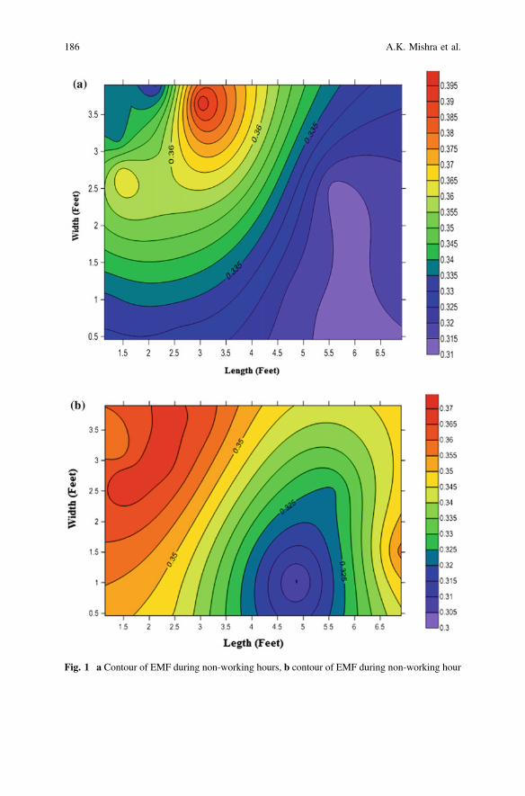
Fig. 1 a Contour of EMF during non-working hours, b contour of EMF during non-working hour
186 A.K. Mishra et al.
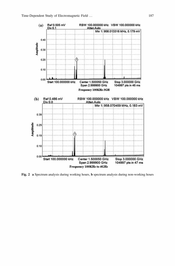
Fig. 2 a Spectrum analysis during working hours, b spectrum analysis during non-working hours
Time-Dependent Study of Electromagnetic Field … 187

Fig. 3 a Average of temperature during working hours, b Average of humidity during workinghours
188 A.K. Mishra et al.

Fig. 4 a Average of temperature during non-working hours, b Average of humidity duringnon-working hours
Time-Dependent Study of Electromagnetic Field … 189
Conclusion
The E-field and meteorological parameter’s study carried out in the original officeenvironments first time in India. An individual always spends more time in theindoor office environments and can sense mimic condition similar to faraday’s cageand exposed more via telephony equipment operating in the range of 100 kHz to3 GHz. The localized electric field effects on health are more dominant to access theexposure scenario in terms of E-field. The level of electropollution that individualsexposed can change according to the internal architecture of the room. Afteranalysis of the EMF levels the results, it is concluded that poor variations isobserved during working and non-working hours. The kriging model gives a betteroption to show EMF distribution in the working and non-working hours. Regularmonitoring of frequency selective EMF in microenvironment is very difficult due tointerference of other frequencies. However, further investigations are needed toidentify the exact correlation between electromagnetic field and indoor meteoro-logical parameters. Seasonal indoor studies of temperature, humidity and electro-magnetic field are also essential to maintain the health of workers.
References
Bako-Biro Z, Wargocki P, Weschler CJ, Fanger PO (2004) Effects of pollution from personalcomputers on perceived air quality, SBS symptoms and productivity in offices. Indoor Air14:178–187
Bio-Initiative Report (2007) A rationale for a biologically-based exposure standard forelectromagnetic radiation
Clements-Croome D, Jukes J (2001) Electromagnetic radiation and comfort in the workplace. In:Proceedings of Clima 2000, 7th REHVA World Congress, Napoli
Dons E, IntPanis L, Van Poppel M, Theunis J, Willems H, Torfs R, Wets G (2011) Impact oftime–activity patterns on personal exposure to black carbon. Atmos Environ 45(21):3594–3602
Ebelt ST, Fisher TV, Petkau AJ, Vedal S, Brauer M (2000) Exposure of chronic obstructivepulmonary disease (COPD) patients to particles: relationship between personal exposure andambient air concentrations. J Air Waste Manag Assoc 50:174–187
Genuis SJ (2008) Fielding a current idea: exploring the public health impact of electromagneticradiation. Public Health 122(2):113–124
ICNIRP (2008) Guidelines, for limiting exposure to time verying electric, magnetic andelectromagnetic fields (up to 300 GHz). Health Phys 74(4):494–522
IEEE (2010) Recommended practice for measurements and computations of electric, magnetic,and electromagnetic fields with respect to human exposure to such fields, 0 Hz to 100 kHz.IEEE—The Institute of Electrical and Electronics Engineers. IEEE Std C95.3.1
International Telecommunication Union (2015) Nomenclature of the frequency and wavelengthbands used in telecommunications. Recommendation ITU-R V.431–8
Jamiesona KS, ApSimona HM, Jamiesona SS, Bella JNB, Yost MG (2007) The effects of electricfields on charged molecules and particles in individual microenvironments. Atmos Environ41(2007):5224–5235
Janssen NAH, Hartog JJ, Hoek G, Brunekreef B, Lanki T, Timonen KL, Pekkanen J (2000)Personal exposure to fine particulate matter in elderly subjects: relation between personal,indoor, and outdoor concentrations. Air Waste 50:1133–1143
190 A.K. Mishra et al.
Kamienska-Zyla M, Prync-Skotniczny K (1996) Subjective fatigue symptoms among computersystem operators in Poland. Appl Ergonom 27:217–220
Knave BG, Wilbom RI, Voss M, Hedstrom LD, Bergqvist UOV (1985) Work with video displayterminals among office employees. I. Subjective symptoms and discomfort. Scand J WorkEnviron Health 11:457–466
Mihalis L, Norbert S, Chatoutsido SE, Glytsos T (2015) New particle formation events arisingfrom painting materials in an indoor microenvironment. Atmos Environ 102:86e95
Pejtersen J, Schwab R, Mayer E (1999) Sensory evaluation of the air in 14 office buildings: part ofan inter disciplinary SBS study in Germany. In: Proceedings of 8th international conferenceon indoor air quality and climate. London: Construction Research Communications, Ltd.,pp 390–395
Pope III CA, Dockery WD (2006) Health effects of fine particulate air pollution: lines that connect.J Air Waste Manag Assoc 56:709e742
Puett RC, Hart JE, Yanosky JD, Paciorek C, Schwartz J, Suh H, Speizer FE, Laden F (2009)Chronic fine and coarse particulate exposure, mortality, and coronary heart disease in theNurses’ health study. Environmental Health Perspectives 117:1697e1701
Rojas Bracho L, Alba N, Suh H, Koutrakis P, Oyola P (1999) Characterization of personalexposures to oxidant and particulate air pollution in Santiago. Epidemiol. 10(4):68
Skyberg K, Skulberg K, Eduard W, Vistnes AI Goffeng LO (1997) Electric fields, dust and healthproblems among VDU-users in an office environment. An intervention program. In:Proceedings of HCI international ‘97, 7th international conference on human-computerinteraction, San Francisco, Vol. 1, pp 655–657
Wargocki P, Bischof W, Brundrett G, Fanger PO, Gyntelberg F, Hanssen SO, Harrison P,Pickering A, Seppan̈en O, Sundell J, Wouters P (2002) The role of ventilation in nonindustrialindoor environments, report from a European multidisciplinary scientific consensus meeting.In: Proceedings of indoor air 2002, the 9th international conference on indoor air quality andclimate, Monterey, USA, Vol. 5, pp 33–38
Wargocki P, Sundell J, Bischof W, Brundrett G, Fanger PO, Gyntelberg F, Hanssen SO,Harrison P, Pickering A, Seppan̈en O, Wouters P (2002) Ventilation and health in nonindustrialindoor environments, report from a european multidisciplinary scientific consensus meeting.Indoor Air, 12:113–128
Time-Dependent Study of Electromagnetic Field … 191
Fish Biodiversity and Its PeriodicReduction: A Case Study of RiverNarmada in Central India
Muslim Ahmad Shah, Vipin Vyas and Shalini Yadav
Abstract Studies on fish biodiversity are important for planning remedial mea-sures for conservation of our rich aquatic biodiversity resources. The variability inlife is largely governed by the environment and genes they possess. Thus more than99% of all species amounting to over five billion species that ever lived on earth areestimated to be extinct. Information from the available sources suggest that about1.2 million have been documented and over 86% species are still not yet docu-mented. Besides natural disaster, about 99% species are presently considered asthreatened species and are at great risk from human activities, primarily thosedriving out by habitat loss, introduction of exotic species, global warming, con-struction of dams, over fishing activities, increasing demand for water, the dammingof rivers throughout the world, the dumping and accumulation of various pollutants,and finally invasive species make aquatic ecosystems one of the most threatenedpart on the planet. Thus it is not surprising that there are many fish species that areendangered in both freshwater and marine habitats.
Keywords Diversity � Species � Aquatic � Exotic � Extinction � Ecosystem
M.A. Shah (&) � V. VyasDepartment of Environmental Sciences and Limnology, Barkatullah University,Bhopal, MP 462026, MP, Indiae-mail: [email protected]
S. YadavDepartment of Civil Engineering, AISECT University, Bhopal, MP, Indiae-mail: [email protected]
© Springer Nature Singapore Pte Ltd. 2018V.P. Singh et al. (eds.), Environmental Pollution, Water Scienceand Technology Library 77, https://doi.org/10.1007/978-981-10-5792-2_16
193
Introduction
Water generally collects in a river from precipitation through a drainage basin fromsurface runoff and other sources such as ground water recharge, springs, and therelease of stored water in ice and glaciers. Rivers have always been the mostimportant fresh water resources. Biodiversity is a contraction of biological diver-sity. It reflects the number, variety, and variability of living organisms and howthese change from one location to another and over time. It includes diversitywithin species (genetic diversity) between species (species diversity) and betweenecosystems (ecosystem diversity). It is frightening but true: Our planet is now in themidst of its sixth mass extinction of plants and animals, the sixth wave of extinc-tions in the past half-billion years. We are currently experiencing the worst spate ofspecies die-offs. Although extinction is a natural phenomenon, it occurs at a natural“background” rate of about one to five species per year. Scientists estimate we arenow losing species at 1,000–10,000 times the background rate, with literally dozensgoing extinct every day. It could be a scary future indeed, with as many as 30−50%of all species possibly heading toward extinction by mid-century. Biodiversity isessential to the health of natural systems. Thus conserving biological diversity isessential for protecting life on this planet. It becomes even more important to knowabout the fact that the current anthropogenic destruction of biodiversity is dan-gerous. Hence, conservation must be analyzed both scientifically and morally.
Keeping this in mind, a comparative study on Fish Biodiversity and its periodicreduction was done during 2013–2014. Diversity is commonly used to describe thenumber, variety, and variability of living organisms.
Materials and Methods
Study Area
Narmada is the largest west flowing river of India and one of the 13 prominentrivers of India, originates from a small tank called Narmada kund located atAmarkantak town in Maikal Hill ranges from eastern part of Madhya Pradesh formsa traditional boundary between North India and South India over a length of1, 312 km before draining through the gulf of Cambey (Khambat) into the ArabianSea. The tributaries of River Narmada are of great importance in Central India asthey provide an important source of water, irrigation, and other resource-basedactivities. When river Narmada emerges from the Marble Rocks it enters into itsfirst fertile basin. This basin extends about 320 km with an average width of 35 kmin the south. The northern part of the valley is the Barna–Bareli plain, where the
194 M.A. Shah et al.
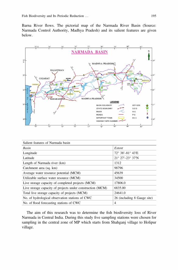
Barna River flows. The pictorial map of the Narmada River Basin (Source:Narmada Control Authority, Madhya Pradesh) and its salient features are givenbelow.
Salient features of Narmada basin
Basin Extent
Longitude 72° 38′–81° 43′E
Latitude 21° 27′–23° 37′N
Length of Narmada river (km) 1312
Catchment area (sq. km) 98796
Average water resource potential (MCM) 45639
Utilizable surface water resource (MCM) 34500
Live storage capacity of completed projects (MCM) 17806.0
Live storage capacity of projects under construction (MCM) 6835.00
Total live storage capacity of projects (MCM) 24641.0
No. of hydrological observation stations of CWC 26 (including 8 Gauge site)
No. of flood forecasting stations of CWC 4
The aim of this research was to determine the fish biodiversity loss of RiverNarmada in Central India. During this study five sampling stations were chosen forsampling in the central zone of MP which starts from Shahganj village to Holipurvillage.
Fish Biodiversity and Its Periodic Reduction … 195

Site S1: Shahganj
The stretch of the river at Shahganj station is of run condition. The depth of water isabout 370 cm and an elevation of about 290 m above sea level. Bed substratesrecorded at this site was soil, sand, and gravel type. It has a shallow region withweed infested banks and is located at 22° 14′N latitude and 77° 80′E longitude. It isa swift moving area characterized by predominantly smooth to slight turbulent flowof 49 cm. The site is inhabited with more than 100 fisher families which earn theirlively hood from this site and its adjoining areas.
Site S2: Bandrabhan (Sangam)
The Bandrabhan station is riffle habitat and is bed substrates recorded at this sitewas sand, gravel, and boulder type. This region also has weed-infested banks andhas flow of 52 cm. The water at this place is swift moving and bubbling type. Atthis site two main rivers namely Narmada and Tawa joins each other; so this site isfamous as Sangam. In this spot, a holy mela is also organized on the occasion ofKartik Purnima. This section of river is followed by some religious practices also.
Site S3: Budhni Ghat
The station Budhni is a town and a Nagar Palika in Sehore district in the state ofMadhya Pradesh, India. It is situated on Bhopal to Hoshangabad road at a distanceof 10 km from Hoshangabad in north direction on the banks of Narmada River.This site is located at 22° 76′N latitude and 77° 69′E longitude. The depth of wateris about 210 cm and an elevation of about 287 m above sea level. This region ishighly infested with aquatic vegetation near the banks of the river. This stretch is ina pool condition with a maximum range between banks is 245.5 m. Bed substratesrecorded at station was soil, sand, slit, and gravel type.
Site S4: Moukala
This station shows run habitat and is situated at 22° 73′N latitude and 77° 65′Elongitude. The depth of water is about 290 cm and an elevation of about 282 mabove sea level. There are only five fishermen families at Moukala but fishermen ofother areas come for fishing at this site. This station has a shallow region with weedinfested-bank and the river bed substrates are sand, soil, slit, and gravel type. Boththe banks of the station have agriculture lands in the vicinity and agricultural
196 M.A. Shah et al.
practice are shown at this station. Majority of the population near this site arelabors. The village near this site is will electrified and people use electric motors forirrigating the agricultural lands. Fish is the main food item for people at this site.
Site S5: Holipur
This site is 25 km far from Hoshangabad by road and it is connected with metalledroad passing 5 km through forest and is located at 22° 74′N latitude and 77° 61′Elongitude. There is a famous religious temple of Hanuman ji on the bank on thisstudy station. A very few people living neat this site are named as Mooni Maharajbecause they do not speak but express their views through writing and there is aDharamshala under construction near this study station. The depth of water at thissite is about 405 cm and is at an elevation of about 282 m above sea level. This siteis highly infested with aquatic vegetation near the banks. This stretch is in a poolcondition and the range between banks is 356 m. Bed substrates recorded at this sitewas soil, sand, slit, and gravel type. Both the banks of this station have agriculturelands in the vicinity and agricultural practice are also shown at this station. The flowof water at this site was recorded as 49 cm.
Fish Collection and Identification
In this study, fishes were collected from all sampling stations of the river stretchunder study during winter, summer, monsoon, and post-monsoon seasons. Fishingwas done at every sampling stations seasonally by using different types of netshaving mesh size of 10, 20, 30, 40, 50, 60, 70, 80, 90, and 100 mm and area size ofthe nets (gill net, cast net) was 36 sq. ft. The strategy used for fishing was same aswas used by the local fishermen of the area under study. Five stations were selectedfor fishing which ranged from Shahganj to Holipur a 30 km river stretch. The fishsampling sites, where fishing was done are Shahganj, Bandraband, Budhni ghat,Moukala and Holipur.
At least 10 fishing efforts were made at every station seasonally and the catchwas then weighed by a balancer and was noted down at every station. Further thecollected fishes catch was identified by using standard identifying keys of Jayaram(1999), Qureshi and Qureshi (1983) and Shrivastava (1998). The collected fisheswere sorted species-wise and the numbers of individuals for each species werecounted and then their percent composition was determined.
Fish Biodiversity and Its Periodic Reduction … 197
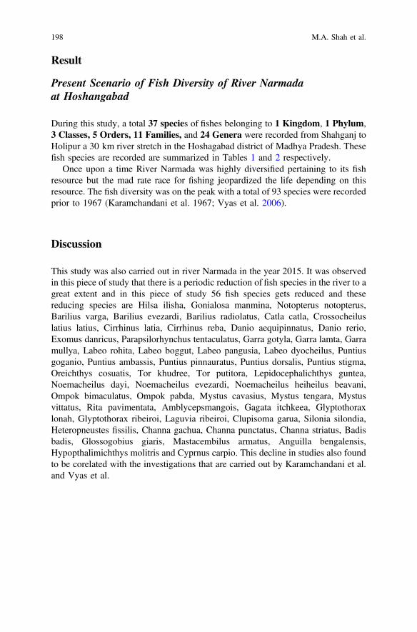
Result
Present Scenario of Fish Diversity of River Narmadaat Hoshangabad
During this study, a total 37 species of fishes belonging to 1 Kingdom, 1 Phylum,3 Classes, 5 Orders, 11 Families, and 24 Genera were recorded from Shahganj toHolipur a 30 km river stretch in the Hoshagabad district of Madhya Pradesh. Thesefish species are recorded are summarized in Tables 1 and 2 respectively.
Once upon a time River Narmada was highly diversified pertaining to its fishresource but the mad rate race for fishing jeopardized the life depending on thisresource. The fish diversity was on the peak with a total of 93 species were recordedprior to 1967 (Karamchandani et al. 1967; Vyas et al. 2006).
Discussion
This study was also carried out in river Narmada in the year 2015. It was observedin this piece of study that there is a periodic reduction of fish species in the river to agreat extent and in this piece of study 56 fish species gets reduced and thesereducing species are Hilsa ilisha, Gonialosa manmina, Notopterus notopterus,Barilius varga, Barilius evezardi, Barilius radiolatus, Catla catla, Crossocheiluslatius latius, Cirrhinus latia, Cirrhinus reba, Danio aequipinnatus, Danio rerio,Exomus danricus, Parapsilorhynchus tentaculatus, Garra gotyla, Garra lamta, Garramullya, Labeo rohita, Labeo boggut, Labeo pangusia, Labeo dyocheilus, Puntiusgoganio, Puntius ambassis, Puntius pinnauratus, Puntius dorsalis, Puntius stigma,Oreichthys cosuatis, Tor khudree, Tor putitora, Lepidocephalichthys guntea,Noemacheilus dayi, Noemacheilus evezardi, Noemacheilus heiheilus beavani,Ompok bimaculatus, Ompok pabda, Mystus cavasius, Mystus tengara, Mystusvittatus, Rita pavimentata, Amblycepsmangois, Gagata itchkeea, Glyptothoraxlonah, Glyptothorax ribeiroi, Laguvia ribeiroi, Clupisoma garua, Silonia silondia,Heteropneustes fissilis, Channa gachua, Channa punctatus, Channa striatus, Badisbadis, Glossogobius giaris, Mastacembilus armatus, Anguilla bengalensis,Hypopthalimichthys molitris and Cyprnus carpio. This decline in studies also foundto be corelated with the investigations that are carried out by Karamchandani et al.and Vyas et al.
198 M.A. Shah et al.

Tab
le1
Classificatio
nof
fish
speciesrecorded
during
thestud
y
Kingd
omPh
yllum
Class
Order
Family
Zoo
logicalnames
Animalia
Chordata
Actinopterigii
Cypriniform
esCyprinidae
Amblypha
ryng
odon
mola
Barilius
bendelisis,B.barila,La
buca
Chela
labu
ca
Cirrhinus
mrigala
Dan
iodevario
Labeoba
ta,L.
calbasu,
Lfimbriatus
Osteobram
acotio
Oxyga
ster
bacaila
,O.clupeoids,O.go
ra
Pun
tiusam
phibious,P
.crysopoma,
P.con
chonius,P.saran
a,P.sop
hore,P
.titius
Rasbo
rada
niconius
Tortor
Nem
acheilidae
Nem
acheilu
sbo
tra
Perciformis
Anabantidae
Ana
bastestud
ineus
Cha
ndana
ma
Param
bassischan
darang
a
Chann
idae
Cha
nnamarulius
Nandidae
Nan
dusna
ndus
Siluriform
isClarridae
Clarias
battrachu
s
Bagridae
Mystusao
r,M.bleekeri
Rita
rita
Siluridae
Wallago
attu
Synbrancheform
isMastacembelid
aeMastacembeluspancalus
Belon
iformis
Belon
idae
Xenentodoncancila
Osteocthy
es*P
erciform
isAnabantidae
Colisafasciata
Teleostom
i*S
iluriform
is*B
agridae
*Mystusseenghala
*Ind
icates
repeated
ones
Fish Biodiversity and Its Periodic Reduction … 199

Tab
le2
.
Recordedfish
Speciesof
river
Narmada
Fish
speciesrecorded
byKaram
chandani
etal.
(1967)
Fish
speciesmissing
asperKaram
chandani
etal.
(1967)
Fish
speciesrecorded
byVyaset
al.(2006
)Fish
speciesMissing
asperVyaset
al.
(2006)
Fish
species
recorded
inthe
presentstudy
Fish
speciesmissing
asperthePresent
Study
Hilsailisha
Hilsailisha
**
Hilsailisha
*Hilsailisha
Gonialosa
manmina
Gonialosa
manmina
**
Gonialosa
manmina
*Gonialosa
manmina
Notopterus
notopterus
Notopterusnotopterus
*Notopterus
notopterus
**
Notopterus
notopterus
Amblypharyngodon
Amblypharyngodon
*Amblypharyngodon
*Amblypharyngodan
mola
*
Barilius
bendelisis
Barilius
bendelisis
*Barilius
bendelisis
*Barilius
bendelisis
*
Barilius
varga
*Barilius
varga
*Barilius
varga
*Barilius
varga
Barilius
barila
Barilius
barila
*Barilius
barila
*Barilius
barila
*
Barilius
evezardi
Barilius
evezardi
**
Barilius
evezardi
*Barilius
evezardi
Barilius
radiolatus
Barilius
radiolatus
**
Barilius
radiolatus
*Barilius
radiolatus
Catla
catla
Catla
catla
**
Catla
catla
*Catla
catla
Crossocheilu
slatiu
slatiu
sCrossocheilu
slatiu
slatiu
s*
*Crossocheilu
slatiu
slatiu
s*
Crossocheilu
slatiu
slatiu
s
Cirrhinus
mrigala
Cirrhinus
mrigala
*Cirrhinus
mrigala
*Cirrhinus
mrigala
*
Cirrhinus
latia
*Cirrhinus
latia
*Cirrhinus
latia
*Cirrhinus
latia
Cirrhinus
reba
Cirrhinus
reba
**
Cirrhinus
reba
*Cirrhinus
reba
Danio
devario
Danio
devario
*Danio
devario
*Danio
devario
*
Danio
aequipinnatus
Danio
aequipinnatus
**
Danio
aequipinnatus
*Danio
aequipinnatus
Danio
rerio
Danio
rerio
**
Danio
rerio
*Danio
rerio
Exomus
danricus
Exomus
danricus
**
Exomus
danricus
*Exomus
danricus
Parapsilorhynchus
tentaculatus
Parapsilorhynchus
tentaculatus
**
Parapsilorhynchus
tentaculatus
*Parapsilorhynchus
tentaculatus
Garra
gotyla
Garra
gotyla
**
Garra
gotyla
*Garra
gotyla
Garra
lamta
Garra
lamta
**
Garra
lamta
*Garra
lamta (con
tinued)
200 M.A. Shah et al.

Tab
le2
(con
tinued)
Recordedfish
Speciesof
river
Narmada
Fish
speciesrecorded
byKaram
chandani
etal.
(1967)
Fish
speciesmissing
asperKaram
chandani
etal.
(1967)
Fish
speciesrecorded
byVyaset
al.(2006
)Fish
speciesMissing
asperVyaset
al.
(2006)
Fish
species
recorded
inthe
presentstudy
Fish
speciesmissing
asperthePresent
Study
Garra
mullya
Garra
mullya
**
Garra
mullya
*Garra
mullya
Labeorohita
Labeorohita
**
Labeorohita
*La
beorohita
Labeobata
Labeobata
*La
beobata
*La
beobata
*
Labeoboggut
Labeoboggut
**
Labeoboggut
*La
beoboggut
Labeocalbasu
*La
beocalbasu
Labeocalbasu
*La
beocalbasu
*
Labeopangusia
*La
beopangusia
*La
beopangusia
*La
beopangusia
Labeodyocheilu
sLa
beodyocheilu
s*
*La
beodyocheilu
s*
Labeodyocheilu
s
Labeofimbriatus
Labeofimbriatus
*La
beofimbriatus
*La
beofimbriatus
*
Labeogonius
Labeogonius
*La
beogonius
*La
beogonius
*
Chela
labuca
Chela
labuca
*Chela
labuca
*Chela
labuca
*
Oxygaster
bacaila
*Oxygaster
bacaila
Oxygaster
bacaila
*Oxygaster
bacaila
*
Oxygaster
chipeoides
Oxygaster
chipeoides
*Oxygaster
chipeoides
*Oxygaster
chipeoides
*
Puntiu
sconchonius
Puntiu
sconchonius
*Puntiu
sconchonius
*Puntiu
sconchonius
*
Puntiu
sgoganio
Puntiu
sgoganio
**
Puntiu
sgoganio
*Puntiu
sgoganio
Puntiu
ssarana
Puntiu
ssarana
*Puntiu
ssarana
*Puntiu
ssarana
*
Puntiu
sam
bassis
Puntiu
sam
bassis
**
Puntiu
sam
bassis
*Puntiu
sam
bassis
Puntiu
sam
phibius
Puntiu
sam
phibius
*Puntiu
sam
phibius
*Puntiu
sam
phibius
*
Puntiu
schrysopoma
Puntiu
schrysopoma
*Puntiu
schrysopoma
*Puntiu
schrysopoma
*
Puntiu
spinnauratus
Puntiu
spinnauratus
**
Puntiu
spinnauratus
*Puntiu
spinnauratus
Puntiu
sdorsalis
Puntiu
sdorsalis
**
Puntiu
sdorsalis
*Puntiu
sdorsalis
Puntiu
sstigma
*Puntiu
sstigma
*Puntiu
sstigma
*Puntiu
sstigma
Puntiu
stitius
Puntiu
stitius
**
Puntiu
stitius
Puntiu
stitius
*
Puntiu
ssophore
Puntiu
ssophore
*Puntiu
ssophore
*Puntiu
ssophore
*(con
tinued)
Fish Biodiversity and Its Periodic Reduction … 201
Tab
le2
(con
tinued)
Recordedfish
Speciesof
river
Narmada
Fish
speciesrecorded
byKaram
chandani
etal.
(1967)
Fish
speciesmissing
asperKaram
chandani
etal.
(1967)
Fish
speciesrecorded
byVyaset
al.(2006
)Fish
speciesMissing
asperVyaset
al.
(2006)
Fish
species
recorded
inthe
presentstudy
Fish
speciesmissing
asperthePresent
Study
Oreichthyscosuatis
Oreichthyscosuatis
**
Oreichthyscosuatis
*Oreichthyscosuatis
Rasbora
daniconius
Rasbora
daniconius
*Rasbora
daniconius
*Rasbora
daniconius
*
Tortor
Tortor
*To
rtor
*To
rtor
*
Torkhudree
Torkhudree
**
Torkhudree
*To
rkhudree
Torputitora
Torputitora
**
Torputitora
*To
rputitora
Lepidocephalichthys
guntea
Lepidocephalichthys
guntea
*Lepidocephalichthys
guntea
**
Lepidocephalichthys
guntea
Nem
acheilu
sbotia
Nem
acheilu
sbotia
*Nem
acheilu
sbotia
*Nem
acheilu
sbotia
*
Noemacheilu
sdayi
Noemacheilu
sdayi
**
Noemacheilu
sdayi
*Noemacheilu
sdayi
Noemacheilu
sevezardi
Noemacheilu
sevezardi
**
Noemacheilu
sevezardi
*Noemacheilu
sevezardi
Noemacheilu
sheiheilusbeavani
*Noemacheilu
sheiheilus
beavani
*Noemacheilu
sheiheilusbeavani
*Noemacheilu
sheiheilusbeavani
Ompokbimaculatus
Ompokbimaculatus
*Ompokbimaculatus
**
Ompokbimaculatus
Ompokpabda
*Ompokpabda
*Ompokpabda
*Ompokpabda
Mystusbleekeri
Mystusbleekeri
*Mystusbleekeri
*Mystusbleekeri
*
Mystuscavasius
Mystuscavasius
**
Mystuscavasius
*Mystuscavasius
Mystustengara
*Mystustengara
Mystustengara
**
Mystustengara
Mystusvitta
tus
Mystusvitta
tus
**
Mystusvitta
tus
*Mystusvitta
tus
Mystusaor
Mystusaor
*Mystusaor
*Mystusaor
*
Mystusseenghala
Mystusseenghala
*Mystusseenghala
*Mystusseenghala
*
Wallago
attu
Wallago
attu
*Wallago
attu
*Wallago
attu
*
Rita
rita
*Rita
rita
Rita
rita
*Rita
rita
*
Rita
pavimentata
Rita
pavimentata
**
Rita
pavimentata
*Rita
pavimentata
Amblycepsm
angois
Amblycepsm
angois
**
Amblycepsm
angois
*Amblycepsm
angois
(con
tinued)
202 M.A. Shah et al.

Tab
le2
(con
tinued)
Recordedfish
Speciesof
river
Narmada
Fish
speciesrecorded
byKaram
chandani
etal.
(1967)
Fish
speciesmissing
asperKaram
chandani
etal.
(1967)
Fish
speciesrecorded
byVyaset
al.(2006
)Fish
speciesMissing
asperVyaset
al.
(2006)
Fish
species
recorded
inthe
presentstudy
Fish
speciesmissing
asperthePresent
Study
Gagataitchkeea
Gagataitchkeea
**
Gagataitchkeea
*Gagataitchkeea
Glyptothoraxlonah
Glyptothoraxlonah
**
Glyptothoraxlonah
*Glyptothoraxlonah
Glyptothorax
ribeiroi
Glyptothoraxribeiroi
**
Glyptothoraxribeiroi
*Glyptothorax
ribeiroi
Laguviaribeiroi
Laguviaribeiroi
**
Laguviaribeiroi
*La
guviaribeiroi
Clupisomagarua
Clupisomagarua
*Clupisomagarua
**
Clupisomagarua
Siloniasilondia
*Siloniasilondia
*Siloniasilondia
*Siloniasilondia
Heteropneustes
fissilis
Heteropneustesfissilis
*Heteropneustes
fissilis
**
Heteropneustes
fissilis
Clarias
batrachus
Clarias
batrachus
*Clarias
batrachus
*Clarias
batrachus
*
Xenentodoncancila
Xenentodoncancila
*Xenentodoncancila
*Xenentodoncancila
*
Channagachua
Channagachua
*Channagachua
**
Channagachua
Channamarulius
Channamarulius
*Channamarulius
*Channamarulius
*
Channapunctatus
Channapunctatus
**
Channapunctatus
*Channapunctatus
Channastriatus
*Channastriatus
Channastriatus
**
Channastriatus
Chandanama
Chandanama
*Chandanama
*Chandanama
*
Chandaranga
Chandaranga
*Chandaranga
*Chandaranga
*
Badisbadis
Badisbadis
**
Badisbadis
*Badisbadis
Nandusnandus
Nandusnandus
*Nandusnandus
*Nandusnandus
*
Anabastestudineus
*Anabastestudineus
Anabastestudineus
*Anabastestudineus
*
Colisafasciata
*Colisafasciata
Colisafasciata
*Colisafasciata
*
Glossogobiusgiaris
Glossogobiusgiaris
*Glossogobiusgiaris
**
Glossogobiusgiaris
Mastacembilus
armatus
Mastacembilusarmatus
*Mastacembilus
armatus
**
Mastacembilus
armatus
Mastacembelus
pancalus
Mastacembeluspancalus
*Mastacembelus
pancalus
*Mastacembelus
pancalus
*
(con
tinued)
Fish Biodiversity and Its Periodic Reduction … 203

Tab
le2
(con
tinued)
Recordedfish
Speciesof
river
Narmada
Fish
speciesrecorded
byKaram
chandani
etal.
(1967)
Fish
speciesmissing
asperKaram
chandani
etal.
(1967)
Fish
speciesrecorded
byVyaset
al.(2006
)Fish
speciesMissing
asperVyaset
al.
(2006)
Fish
species
recorded
inthe
presentstudy
Fish
speciesmissing
asperthePresent
Study
Osteobram
acotio
Osteobram
acotio
*Osteobram
acotio
*Osteobram
acotio
*
Anguilla
bengalensis
Anguilla
bengalensis
**
Anguilla
bengalensis
*Anguilla
bengalensis
Oxygaster
gora
*Oxygaster
gora
Oxygaster
gora
*Oxygaster
gora
*
Hypopthalimichthys
molitris
*Hypopthalim
ichthys
molitris
*Hypopthalimichthys
molitris
*Hypopthalimichthys
molitris
Cyprnus
carpio
*Cyprnus
carpio
*Cyprnus
carpio
*Cyprnus
carpio
204 M.A. Shah et al.

Conclusion
It is concluded from this investigation that the diversity of fish species is reducing atan alarming rate. In the past less than 50 years a total of 56 species of fishes getsreduced in the river Narmada in Central India. The aquatic ecosystems are subjectedto a variety of stresses due to varied land use patterns and water resources devel-opment processes. The ecological changes following the construction of dams onthe river or its tributaries may be determined since it may restrict the fish migrationand impending their accessibility to breeding, nursery, and feeding grounds thusleads to the loss of fish diversity besides, fishing activity was found common in theriver Narmada. Thus the most widespread approaches to management involve somecontrol of fishing activities. This takes two main forms, the banning of certain typesof fishing methods as poisoning of water body and the restriction on using smallmesh size nets further commercial exploitation of river bed for extraction ofstones/pebbles should not be allowed in order to preserve the breeding grounds andfood web of the fishery. Catch control measures must be applied in the river so as toenhance species diversity and to promote fisheries sustainably.
Acknowledgements The author acknowledges the help of Ms. Nahida Bashir Pahalwan, ShahZiah, and Dr. Riaz Hasan
References
Abraham NP, Balakrishnan M (1993) Depleting natural habitats and wildlife—a case study inWynad. In: Proceedings of the fifth Kerala Science Congress, Kottayam, pp 77–80
Ajithkumar CR, Rema Devi K, Raju Thomas K, Biju CR (1999) Fish fauna, abundance anddistribution in Chalakudy river, Kerala. J Bombay Nat Hist Soc 96(2):244–254
Al-Hussaini AH (1949) On the functional morphology of the alimentary tract of some fishes inrelation to differences in their feeding habits. Quart J Mar Sci 9(2):190–240
Allen KR (1938) Some observations on the biology of the trout (Salmo truttu) in Windermere.J Anim Ecol 2:264–272
Anderson GRVA, Arunachalam M, Johnson JA, Sankaranarayanan A (1997) Fish diversity inrivers of Northern Karnataka, Westem Ghats. Int J Ecol and Environ Sci. 23:327–333
Bain MB, Finn JT, Booke HE (1988) Stream flow regulation and fish community structure. Ecol69(2):382–392
Barman RP (1991) A taxonomic revision of the Indo-Burmese species of DanioHamilton-Buchanan (Pisces: Cyprinidae). Occ Pap Rec 2001 Sum India 137:1–91
Barman RP (1998) Faunal diversity in India. Pisces, pp 418–426Basha SC (1997) Management and conservation of wildlife. In: Thampi KB, Nayar NM, Nayar CS
(eds) The natural resources of Kerala. World Wide Fund For Nature—India, Kerala state office,Thiruvananthapuram, pp 535–553
Berg K (1948) Biological studies on the river Susaa. Fol Limnol Scandinav 4:1–318Bhatnagar GK (1967) Biological investigation on the fish and fisheries of Narmada River (1958–
66). Bull Cent Inland Fish Res Inst Barrackpore 10:40 (Mimeo)Bhimachar BS (1945) Zoogeographical divisions of the Western Ghats, as evidenced by the
distribution of the hillstream fishes. Curr Sci 1:12–16
Fish Biodiversity and Its Periodic Reduction … 205

CAFF (2006) Fresh water fish diversity of central India. In: Lakra WS, Sarkar UK (eds) Workshopproceeding. Organized by NBFGR at ICAR, Bhopal, M.P., and India, pp 1–183
Desai VR (1992) Endangered, vulnerable and rare fishes of river systems in Madhya Pradesh. In:Proceedings of the National Seminar on endangered fishes of India held during 25–26 Apr1992 at N.B.F.G.R. Allahabad. Abstract No. 22
Dubey GP (1992) Endangered, vulnerable and rare fish species of west coast river system of India.In: Proceedings of the national seminar on endangered fishes of India held during 25–26 Apr1992 at N.B.F.G.R, Allahabad. Abstract No. 21
Francis Day (1994) The fishes of India. Jagmander Book Agency, New DelhiHora SL, Nair KK (1941) Fishes of Satpura Range, Hoshangabad District, Central Province. Rec
Indian Mus 43:361–373Jena JK, Gopalakrishnan A (2011) Fish genetic resources of India and their management-role and
perspective of NBFGR. In: 9th Indian Fisheries Forum Souvenir (9thIFF), pp 56–63Jena JK, Gopalakrishnan A, Lal Head KK (2011) Fishing Chimes 31(2):15–18Jhingran VG (1991) Fish and fisheries of India. Hindustan Publishing Corporation, New Delhi,
p 727Kumar R, Nalwa MK, Chakraborthy SK, Varkey DA (2008) Fishing Chimes 27(12):40–44Qureshi TA, Qureshi NA (1983) Indian fishes. Brij Brothers, Bhopal, pp 5–209Rao KS, Chatterjee SN, Singh KA (1991) Studies on preimpoudment fishery potential of Sarovar
reservoirs. J Inland Fish India 23(1):34–91Shah AM, Vyas V (2015) Assessment of macrophytic diversity in the selected reaches of river
Narmada at Hoshangabad district of M.P. Int J Sci Eng Technol Res. ISSN: 2278–7798,pp 3338–3344
Shrivastava G (1998) Fishes of U.P. and Bihar, 7th edn. Vishwavidalaya Prakashan, ChowkVaranasi India Publications. Stretch of River Tawa, Madhya Pradesh, India. J Chem Bio PhySci Sec A 3(1):706–716 (2013)
Verma D, Kanhere RR (2007) Threatened Ichthyofauna of the River Narmada in western zone.Life Sci Bull 4(1 and 2):17–20
Vyas V, Bara S, Parashar V, Damde D, Tuli RP (2006) Temporal variation in fish biodiversity ofRiver Narmada in Hoshangabad Region. Fishing Chimes 27:49–53
Vyas V, Parashar V, Bara S, Damde D (2007) Fish catch composition of River Narmada withreference to common fishing gears in Hoshangabad area. National bulletin of life sciences, 4(1and 2):1–6
Vyas V, Damde D, Parashar V (2009) Fish diversity of Narmada in submergence area of IndraSagar Reservair. J Inland Fish Soc India 41(2):18–25
Workbook on Limnology. Pratibha Publishers, Sagar India, pp 1−127
206 M.A. Shah et al.
Effects of Anthropogenic Activitieson the Fresh Water Ecosystem—A CaseStudy of Kappithodu in Kerala
Sherly P. Anand and D. Meera
Abstract A case study was conducted on the impact of anthropogenic activities onthe water quality parameters of Kappithodu, a small tributary of Pamba River, inAlappuzha district of Kerala, from October 2013 to September 2014. The river isfound to be heavily polluted with wastes and effluents from many Prawn peelingcenters, Vandanam Medical college hospitals and outlets of the septic tanks ofnearby houses. Water quality analysis and bacteriological studies were conductedbased on standard hydrological and microbiological methods. Bacteriologicalstudies revealed that water body is highly polluted with Coliform Bacteria,Klebsiella and Pseudomonas. Water quality analysis revealed the presence ofphosphates, nitrates and chloride ions in high quantities.
Keywords Physicochemical parameters � Turbidity � HardnessChloride � Kappithodu
Introduction
India ranks second in human population and first in cattle population, and has gotonly 4% of the world’s free water resources. This indicates the pressure on drinkingwater in India. 64% of the area in peninsular India is water starved, when comparedto the other parts; 80% of India’s total water usage is for irrigation. 60% of irri-gation and 80% of drinking water comes from ground water. Water pollution is oneof the major environmental issues and this causes scarcity of drinking water. Mostof the industries are located on the banks of water bodies and they dispose theirwaste directly into water bodies. Dumping of industrial and sewage waste into any
S.P. Anand (&)S. N. College for Women, Kollam 691001, Kerala, Indiae-mail: [email protected]
D. MeeraS. N. College, Kollam 691001, Kerala, Indiae-mail: [email protected]
© Springer Nature Singapore Pte Ltd. 2018V.P. Singh et al. (eds.), Environmental Pollution, Water Scienceand Technology Library 77, https://doi.org/10.1007/978-981-10-5792-2_17
207
water body results in degradation of its physical, chemical and biological qualities.Many studies have been carried out on this issue (Jayaraman et al. 2003;Damotharan et al. 2010; Prasanna and Ranjan 2010).
Solid wastes pose serious problems in many big cities and towns in Kerala.Kappithode is a canal which flows by the side of the Ambalappuzha flyover inAlappuzha district, and its pollution continues unabated, despite the promise madeby the authorities to clean it up. It was in 1983 that the problem attracted publicattention for the first time. Two students of Ambalappuzha Government LowerPrimary School situated by the side of the canal fell unconscious after inhalingpoisonous gases that emanated from the canal. It happened again in 1984, and sixstudents fell unconscious in the classroom.
In 1985, the High Court issued directives to control pollution—to dredge thecanal to increase its depth, to take steps to remove impediments for the easy flow ofwater in the canal, to ensure that liquid waste from the prawn peeling sheds wasdischarged into the canal only after purification, and to prevent the dumping of solidwaste into the canal. But the directives have not been implemented even after20 years. The present study deals with the examination of water quality as well asbacteriological parameters of Kappithodu.
Materials and Methods
The study area Kappithodu extends from 9° 23′ 36.74″N to 9° 24′ 3.09″N latitudeand 76° 21′ 3.42″E to 76° 23′ 4.14″E longitude. The three sampling stations wereselected and designated as S I, S II, and S III. Water samples were collected duringpre-monsoon, monsoon, and post-monsoon from October 2013 to September 2014.The samples were collected in clean polyethylene, white 2.0 L cans, labeledproperly, and brought to the laboratory for further analysis. All physicochemicalparameters were analyzed using standard methods (APHA 2008). A bacteriologicalstudy was also conducted to find out the extent of pollution. (Cabral 2010).
208 S.P. Anand and D. Meera
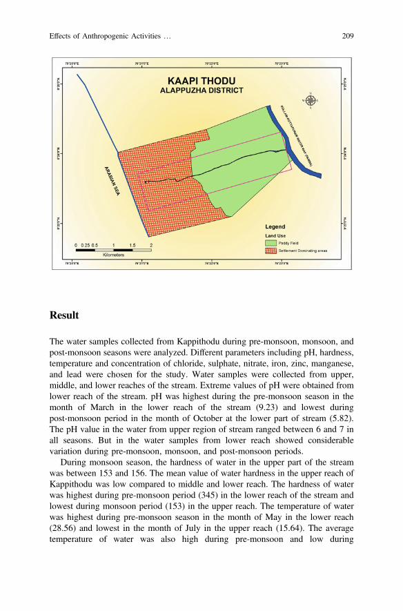
Result
The water samples collected from Kappithodu during pre-monsoon, monsoon, andpost-monsoon seasons were analyzed. Different parameters including pH, hardness,temperature and concentration of chloride, sulphate, nitrate, iron, zinc, manganese,and lead were chosen for the study. Water samples were collected from upper,middle, and lower reaches of the stream. Extreme values of pH were obtained fromlower reach of the stream. pH was highest during the pre-monsoon season in themonth of March in the lower reach of the stream (9.23) and lowest duringpost-monsoon period in the month of October at the lower part of stream (5.82).The pH value in the water from upper region of stream ranged between 6 and 7 inall seasons. But in the water samples from lower reach showed considerablevariation during pre-monsoon, monsoon, and post-monsoon periods.
During monsoon season, the hardness of water in the upper part of the streamwas between 153 and 156. The mean value of water hardness in the upper reach ofKappithodu was low compared to middle and lower reach. The hardness of waterwas highest during pre-monsoon period (345) in the lower reach of the stream andlowest during monsoon period (153) in the upper reach. The temperature of waterwas highest during pre-monsoon season in the month of May in the lower reach(28.56) and lowest in the month of July in the upper reach (15.64). The averagetemperature of water was also high during pre-monsoon and low during
Effects of Anthropogenic Activities … 209

post-monsoon period. The mean temperature of water in the lower reach was highcompared to upper and middle part of stream. The concentration of chloride wasabove 200 mg/l in the middle and lower reach of the stream but in the upper part ofstream, chloride concentration was below 190 mg/l. The average chloride con-centration was lowest during monsoon season in the upper reach of the stream(153 mg/l). The concentration of chloride was highest in the month of May in thelower part of Kappithodu. Sulphate concentration is highest in the middle part ofthe stream in the month of May (29.65 mg/l) and lowest in November in the upperreach (19.53 mg/l). The average sulphate concentration has extreme values inmonsoon season in the upper and lower reaches of Kappithodu. The mean sulphateconcentration in both pre-monsoon and monsoon seasons in the three collectionsites ranges between 20 and 30 mg/l.
Average nitrate concentration is 3.21 in pre-monsoon, 1.92 mg/l in monsoon and2.16 in post-monsoon season. Average nitrate concentration in the middle reach inpre-monsoon season is high compared to other sites and seasons (4.29 mg/l).Nitrate concentration in upper reach in monsoon season is between 1 and 1.5 mg/lonly. Concentration of iron is below 1 mg/l in all seasons and sites with averagevalues 0.67 mg/l in pre-monsoon season, 0.35 in monsoon and 0.67 mg/l inpost-monsoon season. Average iron concentration is low in pre-monsoon season inthe middle reach compared to other sites and seasons (83 mg/l). Iron concentrationis low in all the collection sites in the month of June (0.19, 0.2, 0.2 mg/l). Highestconcentration of iron was observed in the middle part and lowest in the upperpart. Average nitrate concentration is 3.21 in pre-monsoon, 1.92 mg/l in monsoonand 2.16 in post-monsoon seasons. Average nitrate concentration in the middlereach in pre-monsoon season is high compared to other sites and seasons(4.29 mg/l). Nitrate concentration in upper reach in monsoon season is between 1and 1.5 mg/l only. Average zinc concentration is 0.6, 0.3, and 0.5 mg/l inpre-monsoon, monsoon and post-monsoon seasons. Zinc concentration in upperand middle reaches is comparatively low in monsoon season. Highest zinc con-centration was observed in the month of May in the middle site (0.09 mg/l). Zincconcentration in pre-monsoon season was higher compared to the other twoseasons.
Manganese concentration is lower in lower reach and higher in upper reach in allthe three seasons. During post-monsoon season, manganese concentration in upperreach is between 0.5 and 0.6 mg/l. But during pre-monsoon season upper part of thestream has low manganese concentration (0.26–0.27 mg/l). Concentration in theupper part is above 0.1 mg/l in monsoon and post monsoon seasons. Lead con-centration is low in the upper and high in lower reach in all the three seasons.Lowest lead concentration is in the upper part of the stream in March (0.23 mg/l)and highest in June in lower reach (0.695 mg/l). The average lead concentration islow in the lower reach in monsoon season compared to other sites and seasons(0.69 mg/l).
210 S.P. Anand and D. Meera

I. pH Values
Sites Pre-monsoon Monsoon Post-monsoon
March April May June July August September October November
1 6.3 6.5 6 6.33 6.23 6.15 6.5 6.4 6.7
2 7.1 6.9 7.5 7.5 7.13 7.62 7.45 7.52 7.61
3 9.23 8.5 9 6.1 6 5.9 5.86 5.82 5.94
II. Hardness
Sites Pre-monsoon Monsoon Post-monsoon
March April May June July August September October November
1 184.66 186 185 153 154 156 165 176 182
2 298 296 310 261 275 240 285 274 270
3 321 334 345 311 293 282 318 326 329
III. Chloride
Sites Pre-monsoon Monsoon Post-monsoon
March April May June July August September October November
1 180 188 186 152 159 148 121.3 126 123
2 230 238 240 210 195 206 216 223 211
3 256 245 259 221 231 236 228 231 236
IV. Temperature
Sites Pre-monsoon Monsoon Post-monsoon
March April May June July August September October November
1 18.56 17.36 17.56 16.53 15.64 17.5 17.36 17.64 18.64
2 22.65 23.53 23.45 18.56 18.96 19.56 19.6 19.86 20.42
3 27.56 26.56 28.56 22.36 23.43 23.86 23.56 22.56 24.65
V. Sulphate
Sites Pre-monsoon Monsoon Post-monsoon
March April May June July August September October November
1 20.36 22.53 23.56 26.96 28.65 29.56 22.36 20.53 19.53
2 24.36 26.35 29.65 22.53 23.46 21.75 25.63 21.56 23.56
3 22.56 23.65 21.53 20.35 21.56 19.65 25.34 24.65 23.86
Effects of Anthropogenic Activities … 211
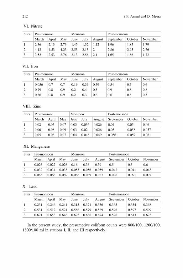
VI. Nitrate
Sites Pre-monsoon Monsoon Post-monsoon
March April May June July August September October November
1 2.36 2.13 2.73 1.45 1.32 1.12 1.96 1.85 1.79
2 4.12 4.53 4.23 2.53 2.13 2 2.86 2.95 2.76
3 3.52 2.53 2.76 2.13 2.56 2.1 1.65 1.86 1.72
VII. Iron
Sites Pre-monsoon Monsoon Post-monsoon
March April May June July August September October November
1 0.056 0.7 0.7 0.19 0.36 0.39 0.54 0.5 0.6
2 0.79 0.8 0.9 0.2 0.4 0.5 0.9 0.8 0.8
3 0.36 0.8 0.9 0.2 0.3 0.6 0.6 0.8 0.5
VIII. Zinc
Sites Pre-monsoon Monsoon Post-monsoon
March April May June July August September October November
1 0.02 0.05 0.07 0.03 0.036 0.026 0.04 0.05 0.06
2 0.06 0.08 0.09 0.03 0.02 0.026 0.05 0.058 0.057
3 0.05 0.08 0.07 0.04 0.046 0.049 0.056 0.059 0.061
XI. Manganese
Sites Pre-monsoon Monsoon Post-monsoon
March April May June July August September October November
1 0.026 0.027 0.026 0.16 0.36 0.39 0.5 0.5 0.6
2 0.032 0.034 0.038 0.053 0.056 0.059 0.042 0.041 0.048
3 0.063 0.068 0.069 0.086 0.089 0.087 0.096 0.091 0.097
X. Lead
Sites Pre-monsoon Monsoon Post-monsoon
March April May June July August September October November
1 0.231 0.246 0.241 0.315 0.321 0.356 0.365 0.354 0.368
2 0.531 0.512 0.521 0.586 0.579 0.569 0.596 0.597 0.599
3 0.621 0.653 0.646 0.695 0.686 0.694 0.596 0.613 0.623
In the present study, the presumptive coliform counts were 800/100, 1200/100,1800/100 ml in stations I, II, and III respectively.
212 S.P. Anand and D. Meera
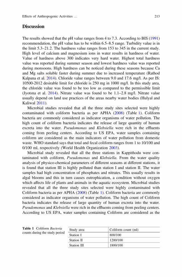
Discussion
The results showed that the pH value ranges from 4 to 7.3. According to BIS (1991)recommendation, the pH value has to be within 6.5–8.5 range. Turbidity value is inthe limit 5.3–21.2. The hardness value ranges from 153 to 345 in the current study.High level of calcium and magnesium ions in water results in hardness of water.Value of hardness above 300 indicates very hard water. Highest total hardnessvalue was reported during summer season and lowest hardness value was reportedduring monsoons. High hardness can be noticed during these seasons because Caand Mg salts soluble faster during summer due to increased temperature (RathodKalpana et al. 2014). Chloride value ranges between 9.0 and 17.6 mg/l. As per IS:10500-2012 desirable limit for chloride is 250 mg in 1000 mg/l. In this study area,the chloride value was found to be too low as compared to the permissible limit(Jyotsna et al. 2014). Nitrate value was found to be 1.1–2.8 mg/l. Nitrate valueusually depend on land use practices of the areas nearby water bodies (Hulyal andKaliwal 2011).
Microbial studies revealed that all the three study sites selected were highlycontaminated with coliform bacteria as per APHA (2008) (Table 1). Coliformbacteria are commonly considered as indicator organisms of water pollution. Thehigh count of coliform bacteria indicates the release of large quantity of humanexcreta into the water. Pseudomonas and Klebsiella were rich in the effluentscoming from peeling centers. According to US EPA, water samples containingcoliform are considered as the main indicators of water pollution from domesticwaste. WHO standard says that total and fecal coliform ranges from 1 to 10/100 and0/100 ml, respectively (World Health Organization 2003).
Microbial study revealed that all the three stations in Kappithodu were con-taminated with coliform, Pseudomonas and Klebsiella. From the water qualityanalysis of physico-chemical parameters of different seasons at different stations, itis found that station III is highly polluted than station I and station II. The watersamples had high concentration of phosphates and nitrates. This usually results inalgal blooms and this in turn causes eutrophication, a condition without oxygenwhich affects life of plants and animals in the aquatic ecosystem. Microbial studiesrevealed that all the three study sites selected were highly contaminated withColiform bacteria as per APHA (2008) (Table 1). Coliform bacteria are commonlyconsidered as indicator organisms of water pollution. The high count of Coliformbacteria indicates the release of large quantity of human excreta into the water.Pseudomonas and Klebsiella were rich in the effluents coming from peeling centers.According to US EPA, water samples containing Coliform are considered as the
Table 1 Coliform Bacteriacounts during the study period
Study area Coliform count (ml)
Station I 800/100
Station II 1200/100
Station III 1800/100
Effects of Anthropogenic Activities … 213
main indicators of water pollution. WHO standard says that total and fecal Coliformranges from 1 to 10/100 ml and 0/100 ml, respectively (WHO 2003).
The major challenge of twenty first Century century is the scarcity of safedrinking water. Microbiological analysis of drinking water should be conductedcontinuously for ensuring the quality as recommended by Cabral (2010). Theground water sources in and around the study area is seriously polluted due to thepercolation of polluted water. Health of the lower and middle class populationliving in the premises is reported to be badly affected. Children of nearby schoolsfrequently get affected by food poisoning due to the contamination of thegroundwater used for cooking in the schools.
Conclusion
Kerala is rich in streams and rivers, but these vital environmental resources aregetting polluted from multiple sources rendering useless many of the water bodiesas in the case of Kappithodu. Industrial units with inadequate waste managementprovisions, failures of the municipal administrations to address the domestic wastemanagement crisis and other increasing sources of pollution are contributing toexpanding the morbid population. The growing threat to the water bodies adverselyaffect the achievement of the Sustainable Developmental goals.
References
APHA Clescerl Leonore S, Greenberg Arnold E, Eaton Andrew D (2008) Standard methods forthe examination of water and wastewater (20th ed). American Public Health Association,Washington, DC
BIS (1991) Indian standard specification for drinking water. IS: 10500, Indian Standard InstituteCabral JPS (2010) Water microbiology. Bacterial pathogens and water. Int J Environ Res Publ
Health 7:3657–3703Damotharan P, Permal NV, Perumal P (2010) Seasonal variation of physicochemical character-
istics of Point Calimere coastal waters (South east coast of India). Middle-East J Sci Res 6(4):333–339
Hulyal SB, Kaliwal BB (2011) Seasonal variations in physico-chemical characteristics of AlmattiReservoir of Bijapur district, Karnataka State. Int J Environ Prot 1(1):58–67
Jayaraman PR, Ganga DT, Vasudevan NT (2003) Water quality studies on Karamana River,Thiruvananthapuram District, South Kerala, India. Pollut Res 22(1):89–100
Jyotsna N, Subba Rangaiah G, Narasimha Rao GM (2014) Seasonal variation of microalgae inrelation to the physico-chemical parameters of Karagam Lake, Srikakulam District, AP India.J Algal Biomass Utln 5(4):68–73
Prasanna M, Ranjan PC (2010) Physico-chemical properties of water collected from Dhamraestuary. Int J Environ Sci 1(3):334–342
214 S.P. Anand and D. Meera

Rathod Kalpana R, Chavan RP, Lokhande RS (2014) Assessment on pollution impact andcorrelation study of lake water from Thane region of Maharashtra, India. Int Res J Environ Sci3(12):44–51
WHO (2003) Guidelines for drinking water quality, 3rd edn. WHO, GenevaWorld Health Organization (2003) Emerging issues in water and infectious disease. WHO, Geneva
Effects of Anthropogenic Activities … 215
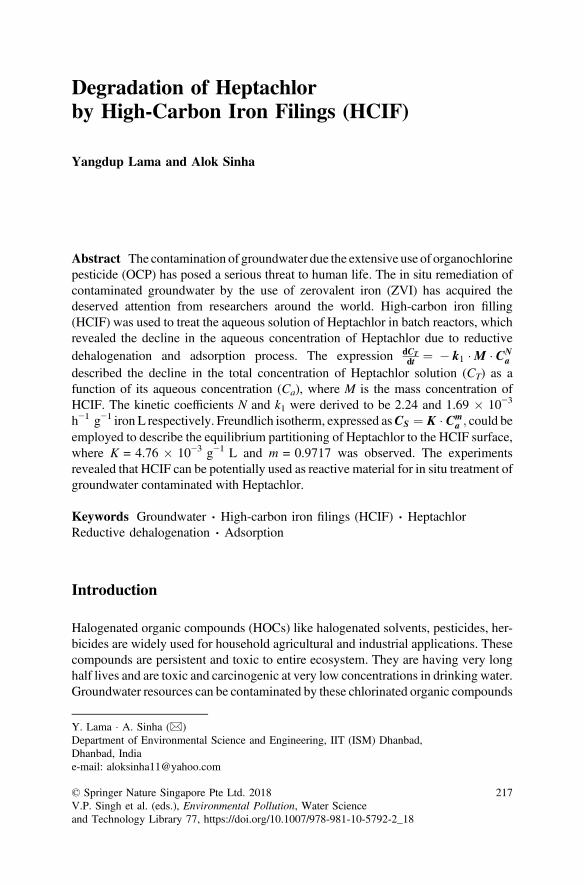
Degradation of Heptachlorby High-Carbon Iron Filings (HCIF)
Yangdup Lama and Alok Sinha
Abstract The contamination of groundwater due the extensive use of organochlorinepesticide (OCP) has posed a serious threat to human life. The in situ remediation ofcontaminated groundwater by the use of zerovalent iron (ZVI) has acquired thedeserved attention from researchers around the world. High-carbon iron filling(HCIF) was used to treat the aqueous solution of Heptachlor in batch reactors, whichrevealed the decline in the aqueous concentration of Heptachlor due to reductivedehalogenation and adsorption process. The expression dCT
dt ¼ � k1 �M � CNa
described the decline in the total concentration of Heptachlor solution (CT) as afunction of its aqueous concentration (Ca), where M is the mass concentration ofHCIF. The kinetic coefficients N and k1 were derived to be 2.24 and 1.69 � 10−3
h−1 g−1 iron L respectively. Freundlich isotherm, expressed asCS ¼ K � Cma ; could be
employed to describe the equilibrium partitioning of Heptachlor to the HCIF surface,where K = 4.76 � 10−3 g−1 L and m = 0.9717 was observed. The experimentsrevealed that HCIF can be potentially used as reactive material for in situ treatment ofgroundwater contaminated with Heptachlor.
Keywords Groundwater � High-carbon iron filings (HCIF) � HeptachlorReductive dehalogenation � Adsorption
Introduction
Halogenated organic compounds (HOCs) like halogenated solvents, pesticides, her-bicides are widely used for household agricultural and industrial applications. Thesecompounds are persistent and toxic to entire ecosystem. They are having very longhalf lives and are toxic and carcinogenic at very low concentrations in drinking water.Groundwater resources can be contaminated by these chlorinated organic compounds
Y. Lama � A. Sinha (&)Department of Environmental Science and Engineering, IIT (ISM) Dhanbad,Dhanbad, Indiae-mail: [email protected]
© Springer Nature Singapore Pte Ltd. 2018V.P. Singh et al. (eds.), Environmental Pollution, Water Scienceand Technology Library 77, https://doi.org/10.1007/978-981-10-5792-2_18
217
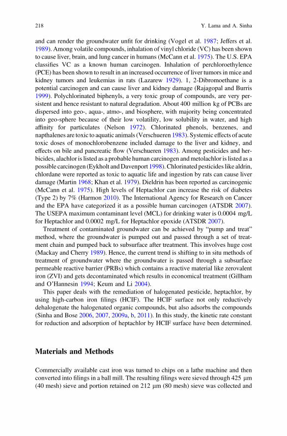
and can render the groundwater unfit for drinking (Vogel et al. 1987; Jeffers et al.1989). Among volatile compounds, inhalation of vinyl chloride (VC) has been shownto cause liver, brain, and lung cancer in humans (McCann et al. 1975). The U.S. EPAclassifies VC as a known human carcinogen. Inhalation of perchloroethylence(PCE) has been shown to result in an increased occurrence of liver tumors in mice andkidney tumors and leukemias in rats (Lazarew 1929). 1, 2-Dibromoethane is apotential carcinogen and can cause liver and kidney damage (Rajagopal and Burris1999). Polychlorinated biphenyls, a very toxic group of compounds, are very per-sistent and hence resistant to natural degradation. About 400 million kg of PCBs aredispersed into geo-, aqua-, atmo-, and biosphere, with majority being concentratedinto geo-sphere because of their low volatility, low solubility in water, and highaffinity for particulates (Nelson 1972). Chlorinated phenols, benzenes, andnapthalenes are toxic to aquatic animals (Verschueren 1983). Systemic effects of acutetoxic doses of monochlorobenzene included damage to the liver and kidney, andeffects on bile and pancreatic flow (Verschueren 1983). Among pesticides and her-bicides, alachlor is listed as a probable human carcinogen andmetolachlor is listed as apossible carcinogen (Eykholt andDavenport 1998). Chlorinated pesticides like aldrin,chlordane were reported as toxic to aquatic life and ingestion by rats can cause liverdamage (Martin 1968; Khan et al. 1979). Dieldrin has been reported as carcinogenic(McCann et al. 1975). High levels of Heptachlor can increase the risk of diabetes(Type 2) by 7% (Harmon 2010). The International Agency for Research on Cancerand the EPA have categorized it as a possible human carcinogen (ATSDR 2007).The USEPA maximum contaminant level (MCL) for drinking water is 0.0004 mg/Lfor Heptachlor and 0.0002 mg/L for Heptachlor epoxide (ATSDR 2007).
Treatment of contaminated groundwater can be achieved by “pump and treat”method, where the groundwater is pumped out and passed through a set of treat-ment chain and pumped back to subsurface after treatment. This involves huge cost(Mackay and Cherry 1989). Hence, the current trend is shifting to in situ methods oftreatment of groundwater where the groundwater is passed through a subsurfacepermeable reactive barrier (PRBs) which contains a reactive material like zerovalentiron (ZVI) and gets decontaminated which results in economical treatment (Gillhamand O’Hannesin 1994; Keum and Li 2004).
This paper deals with the remediation of halogenated pesticide, heptachlor, byusing high-carbon iron filings (HCIF). The HCIF surface not only reductivelydehalogenate the halogenated organic compounds, but also adsorbs the compounds(Sinha and Bose 2006, 2007, 2009a, b, 2011). In this study, the kinetic rate constantfor reduction and adsorption of heptachlor by HCIF surface have been determined.
Materials and Methods
Commercially available cast iron was turned to chips on a lathe machine and thenconverted into filings in a ball mill. The resulting filings were sieved through 425 lm(40 mesh) sieve and portion retained on 212 lm (80 mesh) sieve was collected and
218 Y. Lama and A. Sinha
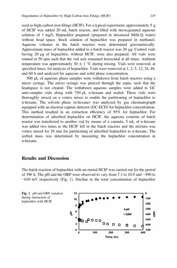
used as high-carbon iron filings (HCIF). For a typical experiment, approximately 5 gof HCIF was added 20 mL batch reactor, and filled with deoxygenated aqueoussolution of 1 mg/L Heptachlor prepared (prepared in deionized Milli-Q water)without head space. Stock solution of heptachlor was prepared in methanol.Aqueous volumes in the batch reactors were determined gravimetrically.Approximate mass of heptachlor added to a batch reactor was 20 lg. Control vialshaving 20 lg of heptachlor, without HCIF, were also prepared. All vials wererotated at 50 rpm such that the vial axis remained horizontal at all times. Ambienttemperature was approximately 30 ± 1 °C during mixing. Vials were removed, atspecified times, for analysis of heptachlor. Vials were removed at 1, 2, 5, 12, 24, 48,and 60 h and analyzed for aqueous and solid phase concentration.
500 lL of aqueous phase samples were withdrawn from batch reactors using amicro syringe. The micro syringe was pierced through the septa, such that theheadspace is not created. The withdrawn aqueous samples were added to GCauto-sampler vials along with 750 lL n-hexane and sealed. These vials werethoroughly mixed on a vortex mixer to enable the partitioning of heptachlor ton-hexane. The solvent phase (n-hexane) was analyzed by gas chromatographequipped with an electron capture detector (GC-ECD) for heptachlor concentration.This method resulted in an extraction efficiency of 95% for heptachlor. Fordetermination of adsorbed heptachlor on HCIF, the aqueous contents of batchreactor was transferred to another vial by means of a cannula. 5 mL of n-hexanewas added two times to the HCIF left in the batch reactors and the mixture wasvortex mixed for 10 min for partitioning of adsorbed heptachlor to n-hexane. Thesorbed mass was determined by measuring the heptachlor concentration inn-hexane.
Results and Discussion
The batch reaction of heptachlor with un-rusted HCIF was carried out for the periodof 396 h. The pH and the ORP were observed to vary from 7.3 to 10.9 and −490 to−630 mV respectively (Fig. 1). Decline in the total concentration of heptachlor
Fig. 1 pH and ORP variationduring interaction ofheptachlor with HCIF
Degradation of Heptachlor by High-Carbon Iron Filings (HCIF) 219
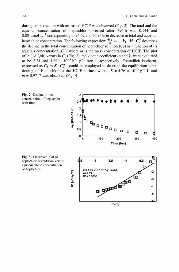
during its interaction with un-rusted HCIF was observed (Fig. 2). The total and theaqueous concentration of heptachlor observed after 396 h was 0.144 and0.08 µmol L−1 corresponding to 94.62 and 96.94% in decrease in total and aqueousheptachlor concentration. The following expression; dCT
dt ¼ � k1 �M � CNa describes
the decline in the total concentration of heptachlor solution (CT) as a function of itsaqueous concentration (Ca), where M is the mass concentration of HCIF. The plotof ln (−dCt/dt) versus ln Ca (Fig. 3), the kinetic coefficients n and k1 were evaluatedto be 2.24 and 1.69 � 10−3 h−1 g−1 iron L respectively. Freundlich isotherm,expressed as CS ¼ K � Cm
a , could be employed to describe the equilibrium parti-tioning of Heptachlor to the HCIF surface where, K = 4.76 � 10−3 g−1 L andm = 0.9717 was observed (Fig. 4).
Fig. 2 Decline in totalconcentration of heptachlorwith time
Fig. 3 Linearized plot ofheptachlor degradation versusaqueous phase concentrationof heptachlor
220 Y. Lama and A. Sinha
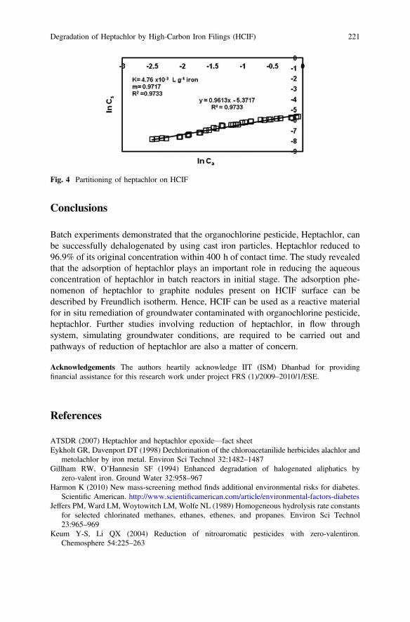
Conclusions
Batch experiments demonstrated that the organochlorine pesticide, Heptachlor, canbe successfully dehalogenated by using cast iron particles. Heptachlor reduced to96.9% of its original concentration within 400 h of contact time. The study revealedthat the adsorption of heptachlor plays an important role in reducing the aqueousconcentration of heptachlor in batch reactors in initial stage. The adsorption phe-nomenon of heptachlor to graphite nodules present on HCIF surface can bedescribed by Freundlich isotherm. Hence, HCIF can be used as a reactive materialfor in situ remediation of groundwater contaminated with organochlorine pesticide,heptachlor. Further studies involving reduction of heptachlor, in flow throughsystem, simulating groundwater conditions, are required to be carried out andpathways of reduction of heptachlor are also a matter of concern.
Acknowledgements The authors heartily acknowledge IIT (ISM) Dhanbad for providingfinancial assistance for this research work under project FRS (1)/2009–2010/1/ESE.
References
ATSDR (2007) Heptachlor and heptachlor epoxide—fact sheetEykholt GR, Davenport DT (1998) Dechlorination of the chloroacetanilide herbicides alachlor and
metolachlor by iron metal. Environ Sci Technol 32:1482–1487Gillham RW, O’Hannesin SF (1994) Enhanced degradation of halogenated aliphatics by
zero-valent iron. Ground Water 32:958–967Harmon K (2010) New mass-screening method finds additional environmental risks for diabetes.
Scientific American. http://www.scientificamerican.com/article/environmental-factors-diabetesJeffers PM, Ward LM, Woytowitch LM, Wolfe NL (1989) Homogeneous hydrolysis rate constants
for selected chlorinated methanes, ethanes, ethenes, and propanes. Environ Sci Technol23:965–969
Keum Y-S, Li QX (2004) Reduction of nitroaromatic pesticides with zero-valentiron.Chemosphere 54:225–263
Fig. 4 Partitioning of heptachlor on HCIF
Degradation of Heptachlor by High-Carbon Iron Filings (HCIF) 221

Khan MAQ, Feroz M, Sudershan P (1979) Metabolism of cyclodiene insecticides by fish.Pesticide and xenobiotic metabolism in aquatic organisms. American Chemical Society,Symposium Series 99
Lazarew NW (1929) Über die narkotische Wirkungskraft der Dämpfe der Chlorderivaten desMethans, des Äthans und des Äthylens. Naunyn-Schmiedeberg’s Arch Pharmacol 141(1):19–24
Mackay DM, Cherry JA (1989) Groundwater contamination: pump-and-treat remediation. EnvironSci Technol 23:630–636
Martin H (1968) Pesticide manual. British Corp Protection Council, Clacks Farm, Boreley,Ombersley, Doritwich, Worcester, UK
McCann J et al (1975) Detection of carcinogens as mutagens in the salmonella/microsome test:assay of 300 chemicals. Proc Nat Acad Sci USA 72(12):5135–5139
Nelson N (1972) Chairman panel on hazardous trace substances, polychlorinated biphenyls—environmental impact. Environ Res 5:249–362
Rajagopal VK, Burris DR (1999) Reduction of 1,2-dibromoethane in the presence of zero-valentiron. Environ Toxicol Chem 18:1779–1782
Sinha A, Bose P (2006) Dehalogenation of 2-chloronapthalene by cast iron. Water Air Soil Pollut172(1–4):375–390
Sinha A, Bose P (2007) Interaction Of 2-chloronaphthalene with high carbon iron filings (HCIF):adsorption, dehalogenationand mass transfer limitations. J Colloid Interface Sci 314(2):552–561
Sinha A, Bose P (2009a) Interaction of chloroethanes and chloroethenes with un-rusted and rustedhigh carbon iron filings. J Environ Eng Sci 26(1):61–70
Sinha A, Bose P (2009b) Interaction of 2,4,6-trichlorophenol with high carbon iron filings:reaction and sorption mechanisms. J Hazard Mater 164(1):301–309
Sinha A, Bose P (2011) 2-Chloronaphthalene dehalogenation by high carbon iron filings (HCIF):impact of formation of corrosion products on HCIF surface. J Environ Eng Sci 28(10):701–710
Verschueren K (1983) Handbook of environmental data on organic chemicals, 2nd edn. VanNostrand Reinhold Company Inc, New York
Vogel TM, Criddle CS, McCarty PL (1987) Transformations of halogenated aliphatic compounds.Environ Sci Technol 8:722–736
222 Y. Lama and A. Sinha

Part IIIGeneration of Pollution

Biomedical Waste Generationand Management in Public SectorHospital in Shimla City
Prachi Vasistha, Rajiv Ganguly and Ashok Kumar Gupta
Abstract Biomedical waste disposal is very important due to its infectious nature.Proper management of biomedical waste is necessary for maintaining good humanhealth and environment. Biomedical Waste (Management and Handling) rules 1998under the Environmental Protection Act, 1986 have been passed by government ofIndia which is to be followed strictly to avoid menace. The purpose of the article isto differentiate between the Biomedical Waste Management practices such ascollection, storage, transportation, and disposal along with the generation ofbiomedical waste undertaken in major public and private sector hospitals in Shimlacity. A cross-sectional study and semi-structured interview considering the variousbiomedical waste management practices and personnel handling of the biomedicalwaste undertaken in the major public and private sector hospitals in Shimla citythrough detailed analysis and questionnaire prepared will be used for the purpose ofstudy. The study will quantify the actual values and unveil the difference that lie inmanagement procedures followed by these hospitals in Shimla. The present paperpresents some initial findings of the questionnaire analysis carried out in a majorpublic hospital in Shimla.
Introduction
A hospital is a complex institution visited by people very frequently without anydistinction of age, sex, race, and religion. This is above the normal population ofhospital namely patients and staff (Rao et al. 2004). Waste production is not onlyrestricted to hospitals or research activities but waste can also be produced at homesthrough dialysis or using insulin injections and even during animal health activitiesin rural areas. This is dangerous and needs proper disposal. Although industrialwaste, municipal solid waste, agricultural waste, etc., are harmful and may pollute
P. Vasistha � R. Ganguly (&) � A.K. GuptaDepartment of Civil Engineering, Jaypee University of Information Technology,Waknaghat, District Solan, Himachal Pradesh, Indiae-mail: [email protected]
© Springer Nature Singapore Pte Ltd. 2018V.P. Singh et al. (eds.), Environmental Pollution, Water Scienceand Technology Library 77, https://doi.org/10.1007/978-981-10-5792-2_19
225
the surrounding air, water and soil, their treatment and disposal are less harmful ascompared to the effects produced from treatment and disposal of biomedical wastedue to production of toxic effluents from the burning of biomedical waste (Levendiset al. 2001; Soliman and Ahmed 2007; Jindal et al. 2013).
Hospital waste is highly toxic in comparison to the other wastes. Though, 75–90% of waste produced by health care institutes from administration unit andhousekeeping cells, is non- toxic, the remaining 10–25% of the waste is regarded as‘hazardous’ and may create variety of health risks (Shalini et al. 2012; WHO 2013).Infectious diseases such as HIV, Hepatitis (all kinds), and tetanus all are verycommon in people associated with handling of biomedical waste. In order to pre-vent such deadly infections and to protect the environment, The Ministry ofEnvironment and Forest (India) formulated and notified biomedical waste (man-agement and handling) rules in 1998 that issues guidelines to all institutes pro-ducing biomedical waste to ensure safety and soundness in management of theirwastes (Da Silva et al. 2005).
Advancement in healthcare facilities around the globe has led to seriousimprovement of biomedical waste management in developed countries. However,despite strict regulations in the Indian context, the paradox of the situation is thatthe healthcare facilities which are basis for maintenance and restoration of publichealth have caused a huge health risk due to improper management of waste bypeople in charge and have posed a huge threat to environment (Mathur et al. 2012).Globally categorized as a serious issue, biomedical waste demands appropriate andnecessary steps of management and disposal worldwide (Kumari et al. 2013). Thewaste disposal is overseen by government agencies but regulations have to beabided by private healthcare organizations too (Radha et al. 2009).
Improper management of waste may lead to change in microbial ecology andspread of antibiotic resistance. Thus, the best disposal option should aim at theminimization of toxic substances from medical institutes to the environment. In thelight of above facts and figures, the study is to be carried at the capital of the stateHimachal Pradesh i.e. Shimla. The city is located at 31° 6′ 12″ north latitude and77° 10′ 20″ east longitude and 2,206 m above the mean sea level. The populationof the city according to the 2011 census was found to be 8,13,384.
The main aim of the study to be conducted is to study, evaluate, and compare thewaste management steps, waste handling procedures, and treatment methods beingundertaken by the majority of the public and private sector hospitals in Shimla Cityto prevent the spread of infections diseases due to improper disposal of hospitalwaste.
Management of Biomedical Waste
In 1980s in United States, a huge chaos was raised by people about hospital wastehovering around and children playing around thus the management of biomedicalwaste became an issue of concern. The US Medical Waste Tracking act of 1988
226 P. Vasistha et al.
was enacted and enforced on November 1, 1988 (Dayananda 2004). A huge out-burst against various agencies by public was observed to put pressure onGovernment of India to enact appropriate laws in country against various practicesof disposal of biomedical waste. The Ministry of Environment and Forest ofGovernment of India has enacted Biomedical Waste (Management and Handling)rules which became effective from July 20, 1998. The rules have six schedules asbriefly described below.
Schedule 1 classifies the biomedical waste into ten categories (The Gazette ofIndia 1998).
Schedule 2, describes the color coding scheme and types of containers to be usedfor collection and storage of biomedical waste.
Schedules 3 and 4, recommend that containers should be appropriately labeledwith biohazard or cytotoxic symbol to avoid risk. In case the waste is to betransported offsite, appropriate measures needs to be taken to make containers leakproof to avoid any spillage.
Schedule 5 describes the treatment and disposal options for each category ofwaste.
Schedule 6, makes it compulsory for all the hospitals, clinics, nursing homes andveterinary institutes, animal house and slaughter house to install appropriate wastemanagement amenities in place.
Before the enforcement of Biomedical Waste (management and handling) rules,the municipal or government authority was solely responsible for handling all typesof waste appropriately and efficiently, but now it has become mandatory for allhealth care organizations to manage their waste according to the rules enacted bygovernment (Patil and Pokhrel 2005).
Incineration is the most general method for biomedical waste treatment and ismost apt for combustible materials. However, some material like body parts andurine bags cannot be disposed by incineration thus needing other methods for thetreatment. Incineration leads to 80% reduction in waste volume and also decon-tamination of waste being incinerated (Ferreira and Veiga 2003). It is the respon-sibility of the producer of the waste to take measures for proper and safe disposal ofwaste so that there is no undesirable effect on environment. The setting up ofincinerator in hospitals with more than 50 beds is compulsory under Section 15(1)of the Environmental (protection) Act 1996 according to which whoever fails toabide by the orders issued by the government will be punished by “imprisonmentfor term extending up to 5 years or 1,00,000 Rupees cash, or both and an additionalfine may be imposed extended up to 5000 Rupees per day if there is continueddelay or negligence after conviction for first such failure or contravention (Yadav2001).
Incineration is the most widely used technology for waste treatment but itimposes a great risk of environmental and health hazard due to wide varieties ofpollutants released from the burning of biomedical waste such as dioxins, furans,etc. Further, incineration has been concluded as the most expensive treatment forbiomedical waste management in developing countries (Diaz et al. 2005). Thereforeother methods such as plasma pyrolysis and electro-thermal deactivation
Biomedical Waste Generation and Management … 227

(ETD) may be used and encouraged as alternatives to incineration (Jang et al.2006). However, these alternatives are costly procedures and are often not imple-mented due to high operation and maintenance costs.
Methodology
The study was conducted in the major public hospital of Shimla city. From thesurvey conducted and the data acquired, the bed capacity is about 800 and dailypatient frequency in public sector hospital was about 777 patients on a daily basis.The name of the hospital has not been disclosed due to the administrative reasons.The data collected from the different units is based on the interview sessions withthe person in charge, survey of the hospital wards, field visits and the crucial siteobservations.
Observation
The field observation involved critical examination of the quantification of waste,segregation, collection, transportation, final treatment and disposal as well as theoccupational safety of the person in charge, the intensity with which the guidelineswere being followed in the hospitals and various regulations imposed by theadministrative unit for maintenance of a safe and healthy environment. It alsoconcentrated upon problems faced by the workers and the staff due to improperdisposal at disposal sites.
Questionnaire Session
The prepared questionnaire (Vasistha et al. 2015) was utilized and the questionnairewas framed with the purpose of obtaining knowledge about the present wastegeneration and strategy of management being followed in the hospital and deter-mining the various factors which restrict the proper management and disposal ofwaste being generated in various wards at the hospitals.
Management and Implementation at Public Sector Hospital
The public sector hospital has 33 departments. The Waste management in thehospital premises is done by a team of 3 main doctors with nurses and otherworkers for collection and disposal of waste. The annual statistics show that the
228 P. Vasistha et al.
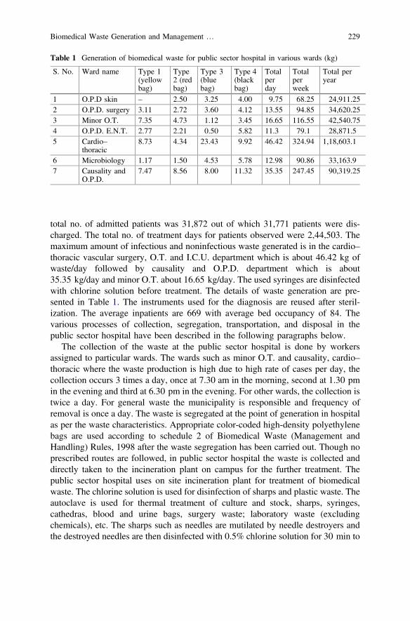
total no. of admitted patients was 31,872 out of which 31,771 patients were dis-charged. The total no. of treatment days for patients observed were 2,44,503. Themaximum amount of infectious and noninfectious waste generated is in the cardio–thoracic vascular surgery, O.T. and I.C.U. department which is about 46.42 kg ofwaste/day followed by causality and O.P.D. department which is about35.35 kg/day and minor O.T. about 16.65 kg/day. The used syringes are disinfectedwith chlorine solution before treatment. The details of waste generation are pre-sented in Table 1. The instruments used for the diagnosis are reused after steril-ization. The average inpatients are 669 with average bed occupancy of 84. Thevarious processes of collection, segregation, transportation, and disposal in thepublic sector hospital have been described in the following paragraphs below.
The collection of the waste at the public sector hospital is done by workersassigned to particular wards. The wards such as minor O.T. and causality, cardio–thoracic where the waste production is high due to high rate of cases per day, thecollection occurs 3 times a day, once at 7.30 am in the morning, second at 1.30 pmin the evening and third at 6.30 pm in the evening. For other wards, the collection istwice a day. For general waste the municipality is responsible and frequency ofremoval is once a day. The waste is segregated at the point of generation in hospitalas per the waste characteristics. Appropriate color-coded high-density polyethylenebags are used according to schedule 2 of Biomedical Waste (Management andHandling) Rules, 1998 after the waste segregation has been carried out. Though noprescribed routes are followed, in public sector hospital the waste is collected anddirectly taken to the incineration plant on campus for the further treatment. Thepublic sector hospital uses on site incineration plant for treatment of biomedicalwaste. The chlorine solution is used for disinfection of sharps and plastic waste. Theautoclave is used for thermal treatment of culture and stock, sharps, syringes,cathedras, blood and urine bags, surgery waste; laboratory waste (excludingchemicals), etc. The sharps such as needles are mutilated by needle destroyers andthe destroyed needles are then disinfected with 0.5% chlorine solution for 30 min to
Table 1 Generation of biomedical waste for public sector hospital in various wards (kg)
S. No. Ward name Type 1(yellowbag)
Type2 (redbag)
Type 3(bluebag)
Type 4(blackbag)
Totalperday
Totalperweek
Total peryear
1 O.P.D skin – 2.50 3.25 4.00 9.75 68.25 24,911.252 O.P.D. surgery 3.11 2.72 3.60 4.12 13.55 94.85 34,620.253 Minor O.T. 7.35 4.73 1.12 3.45 16.65 116.55 42,540.754 O.P.D. E.N.T. 2.77 2.21 0.50 5.82 11.3 79.1 28,871.55 Cardio–
thoracic8.73 4.34 23.43 9.92 46.42 324.94 1,18,603.1
6 Microbiology 1.17 1.50 4.53 5.78 12.98 90.86 33,163.97 Causality and
O.P.D.7.47 8.56 8.00 11.32 35.35 247.45 90,319.25
Biomedical Waste Generation and Management … 229
1 h. The final disposal of the waste though is incineration process. Table 1 illus-trates the generation of biomedical waste in the public sector hospital and Fig. 1shows the percentage composition from all the different ward categories (yearly).
Results and Discussions
It is observed that the public sector hospital segregates the waste using appropriatemethodology following guidelines prescribed in Schedules 1 and 2. The workershandling biomedical waste are aware enough to understand the oddness of thesituation; hence they follow the guidelines given to them by higher personnel.A regular report is submitted to Pollution Control Board at the year end. Alsoregular visits are paid by board members to the hospital to know the current statusof the biomedical waste management. From Table 1, it is observed that the cardio–thoracic ward generates the maximum biomedical waste and the O.P.D Skin Wardgenerates the least amount of biomedical waste. This is due to the fact that the costof treatment for skin grafting, plastic surgery, etc., are fairly high enough and notaffordable by common people as the income and standard of living of people in andaround the place is not high enough as compared to the cost of the treatment. Thus,the number of treatments and patients per day are limited in this ward so the amountof waste produced is less. Figure 1 also corroborates this fact. It was also deter-mined that incineration process is utilized for treatment of biomedical waste.
Regular visits to the hospital and analysis of questionnaire data revealed thatthe hospital disposes off their sharps and needles by landfill in secured pits.
O.P.D. Skin
O.P.D. Surgery
Minor O.T.
O.P.D. E.NT
Cardio Thorassic
Microbiology
Casuality & O.P.D
Fig. 1 Ward-wise waste percentage composition (yearly)
230 P. Vasistha et al.

After interaction with the staff and the workers of the incineration plant it was foundthat the biomedical waste management was followed at its best but at the incineratorplant site of the public sector hospital there is a need of infection control and goodenvironmental maintenance, as the building housing the incinerator needs imme-diate repairs and maintenance. Further, very few workers are involved in the actualincineration process of waste and thus there is a need to increase the number ofpersonnel to improve the biomedical waste management at the incinerator location.
Conclusion
From the above discussions, the authors conclude that the hospital is a role model inthe management of biomedical wastes in accordance with the biomedical waste(management and handling) rules as prescribed by the GOI. This is particularlysignificant in context of the limited study carried out in the area of biomedical wastemanagement in and around the state; the hospital could be set as a very goodexample of biomedical waste management. This has been successful due to supportfrom state- and national-level government, acceptance by the local people byproviding a shared-use incinerator facility for other hospitals. Also, there exists ascope for huge improvement in the region.
Acknowledgements The authors wish to express their gratitude to all doctors, nurses, staff, andworkers of the hospitals for their great guidance, support and assistance. Their information andco-operation was valuable and inevitable.
References
Dayananda CM (2004) www.expresshealthcaremgmt.com/200608/management01.shtml.Downloaded on 4 June 2016
Da Silva CE, Hoppe AE, Ravanello MM, Mello N (2005) Medical wastes management in thesouth of Brazil. Waste Manage 25:600–605
Diaz LF, Savage GM, Eggerth LL (2005) Alternatives for the treatment and disposal of healthcarewastes in developing countries. Waste Manag 25(6):626–637
Ferreira PA, Veiga MM (2003) Waste operational procedures: a case study in Brazil. WasteManage Res 21:377–382
Jang Y-C, Lee C, Yoon O-S, Kim H (2006) Medical waste Management in Korea. EnvironManage 80:107–115
Jindal AK, Gupta A, Grewal VS, Mahen A (2013) Biomedical waste disposal—a system analysis.Med J Armed Forces India 69(4):351–356
Kumari R, Srivastava K, Wakhlu A, Singh A (2013) Establishing biomedical waste managementsystem in Medical University of India—a successful practical approach. Clin Epidemiol GlobHealth 1(3):131–136
Levendis Y, Atal A, Carlson J, Quintana M (2001) PAH and soot emissions from burningcomponents of medical waste: examination/surgical gloves and cotton pads. Chemosphere42:775–783
Biomedical Waste Generation and Management … 231

Mathur P, Patan S, Shobhawat S (2012) Need of biomedical waste management system inhospitals—an emerging issue—a review. Curr World Environ 7(1):117–124
Patil VG, Pokhrel K (2005) Biomedical solid waste management in an Indian hospital: a casestudy. Waste Manag 25:592–599
Radha KV, Kalaivani K, Lavanya R (2009) A case study of biomedical waste management inhospitals. Glob J Health Sci 1:82–88
Rao SKM, Ranyal RK, Bhatia SS, Sharma VR (2004) Biomedical waste management: aninfrastructural survey of hospitals. Med J Armed Forces India 60:379–382
Shalini S, Harsh M, Mathur BP (2012) Evaluation of bio-medical waste management practices in agovernment medical college and hospital. Natl J Commun Med 3(1). pISSN: 0976 3325eISSN: 2229 6816
Soliman SM, Ahmed AI (2007) Overview of biomedical waste management in selectedgovernorates in Egypt: a pilot study. Waste Manage 27(12):1920–1923
The Gazette of India (1998) Biomedical waste (management and handling) rules, 1998.Extraordinary Part II Section 3—subsection (ii). Ministry of Environment and Forest,Government of India, India, pp 10–20 Notification dated 20th July
Vasistha P, Ganguly R, Gupta AK (2015) Questionnaire method for assessing biomedical waste inShimla City—case studies of public and private hospitals. In: 9th International Conference onInnovative Research in Civil Engineering, Architecture, and Environmental Engineering forSustainable Development (CEAESD-2015) held during December 12–13, 2015 at JawaharlalNehru University (JNU), New Delhi, India, pp 11–14
World Health Organization—WHO medical waste (2013) Available online at the following linkhttp://www.who.int/topics/medical_waste/en/
Yadav M (2001) Hospital waste—a major problem. Hospital Today 8(4):276–282
232 P. Vasistha et al.
Fuel Loss and Related Emissions Dueto Idling of Motorized Vehicles at a MajorIntersection in Delhi
Niraj Sharma, P.V. Pradeep Kumar, Anil Singh and Rajni Dhyani
Abstract Traffic intersections are considered as air quality hotspots as they mostlyexceed the prescribed air quality standards specified by various regulatory agenciesdue to high vehicular activities, idling, and related vehicular emissions. Delay attraffic intersections results in fuel loss due to idling of vehicles and related emis-sions. In the present study, Ashram Chowk, a major intersection in Delhi has beenselected. Nearly 3.4 lakh vehicles pass through Ashram intersection daily, out ofwhich nearly 20% (*60,000 nos.) of the traffic faces average time delay (or idling)for time varying from 6 to 8 min delays per hour. In the present study, amethodology has been developed for the estimation of emissions (such as CO2,CH4, CO, NOx, NO2, NMVOC, etc.) from fuel loss occurring during idling ofvehicles using IPCC emission factors. The study highlights the importance ofreducing fuel losses at intersections to achieve sustainable air quality.
Introduction
Countries around the world are concerned with the impact of transportation on theenvironment and human health. Vehicles have increased many folds in India, nearly10.5% annual vehicular growth has been observed in India from 2002 to 2012,especially in metro cities (MoRTH 2013). Delhi, the capital city of India, has seen7.7% increase in 2002–2012. It has vehicular pollution of nearly 8 million and con-stitutes around 4.6% of the total traffic in India. In Delhi, consumption of diesel andpetrol by the road sector has seen substantial growth over the past two decades. The
N. Sharma (&) � P.V. Pradeep Kumar � A. SinghEnvironmental Science Division, CSIR-Central Road Research Institute,New Delhi 110025, Indiae-mail: [email protected]
R. DhyaniAcademy of Scientific and Innovative Research (AcSIR), CSIR-Central RoadResearch Institute, New Delhi 110025, Indiae-mail: [email protected]
© Springer Nature Singapore Pte Ltd. 2018V.P. Singh et al. (eds.), Environmental Pollution, Water Scienceand Technology Library 77, https://doi.org/10.1007/978-981-10-5792-2_20
233
road transport sector consumes 35% of the total liquid commercial fuel consumptionby all sectors (Singh et al. 2008). Due to increased personalized transportation modethan public transportation system, large numbers of vehicles are on road leading tocongestion and traffic jams. The fuel consumption and fuel consumption by variouscategories of vehicles depend upon the driving cycle of the city. Driving cycle affectsthe fuel consumption of a vehicle. In urban areas idling, due to red light stop or due tocongestion or traffic jam also constitute the part of driving cycle. The direct effect ofidling of vehicle is fuel loss as well as related emissions from burning of fuel. Fuelconsumption may be small when one quantifies it for a vehicle, but when hundreds ofvehicles are idle at various intersections or due to a traffic jam in the city its magnitudeincreases and in turn emissions. The variety of settings in which vehicular idlingoccurs, can be broadly categorized into three domains: (1) idling to warm the engine;(2) idlingwhile waiting for something unrelated to traffic (e.g. waiting for a passenger;in a drive-through); and (3) idling while in traffic (e.g. at stoplights; in traffic jams)(Guttikunda 2009). Unnecessary vehicle idling is a common source of GHGs emis-sion (CO2, CH4, N2O, CO, NMVOCs, SO2, NOx) and other air pollutants. Not onlydoes it contribute to the global climate change but it also wastes a large amount of fuelthreatens our energy future (Morshed 2010).Natural Resource ofCanada (NRC2009)reported that idling longer than 10 s usesmore fuel and producesmore CO2 comparedto restarting the engine. Similarly, Burgess et al. (2009) reported that idling vehicles inthe city produce 130,000 tons of CO2 in New York City (USA). Apart from idling,these vehicles also emit 940 tons of NOx, 2,200 tons of VOCs, 24 tons of sootparticles, and 6,400 tons of CO each year. The study reported that citywide idlingwasted an average of 30,000 gallons of gasoline and 20,000 gallons of diesel on anaverage weekday, apart from fuel costs due to idling when engines run longer thannecessary. In European countries like Italy, Austria, Germany, The Netherlands,France, etc., the recommended guideline for turning off the engine range from 10 to 60s (NRC 2011). In a study conducted by Central Road Research Institute (CRRI) in2005 estimated that fuel worth of Rs. 1,000 crore is wasted every year in Delhi byvehicles idling at 600 signalized traffic signals and was around 15% of the total fuelconsumed annually in Delhi. In addition, the time loss to the commuters is alsoassociated with the delays. Further, 0.37 million kilograms of CNG, 0.13 millionliters of diesel, and 0.41 million liters of petrol wasted every day due to idling ofvehicles costing around Rs. 27.25 millions per day and Rs. 9944.5 million per year.The running engines during idling also generate emissions, which are harmful both tohuman health and ecology (Parida and Gangopadhyay 2008). In the present study, aneffort has been made to quantify the fuel consumption during idling by various cat-egories of vehicles and estimation of related emissions at amajor intersection inDelhi.
Methodology
For the present study, Ashram Chowk has been selected. It is one of the busiestintersections of Delhi city and caters to both urban and regional traffic. National
234 N. Sharma et al.

Highway-2 (NH-2) is a part of intersection joining Mathura to Delhi. The inter-section connects adjoining Faridabad and Noida city to Delhi. The intersectioncaters to the urban traffic throughout the day and intercity traffic (mostly com-mercial) during the night.
The present study pertaining to estimation of emissions due to idling of vehiclesat signalized intersection have two components: (i) carrying out fuel consumptionstudy at idling on various test vehicles of different types, categories, fuel usage(s),etc., (ii) converting the fuel losses as estimated in step (iii) into emissions byemploying appropriate emission factors (i.e. IPCC) and various other inputparameters collected from primary surveys and/or secondary sources.
Fuel Consumption Measurement
Measurement of fuel consumption at idling was carried out on petrol and dieselpowered various categories of vehicles. Depending on the type of vehicle andengine technology, a different type of fuel flow detector was used for petrol anddiesel powered vehicles [(i) MF-2200, (b) FP-214OH and (iii) FP-213S fuel flowdetector (ONO SOKKI, Japan) with measurement capability of up to 0.1 ml].Depending on fuel type and engine type, these fuel flow detectors were connectedwith a fuel flow meter to accurately measure the flow rate of fuel. For petrol anddiesel vehicles, fuel connections for the existing vehicle were removed and the fuelflow detector was connected on-line. The duration of the measurement for fuelconsumption measurement studies for different types of test vehicles was 40 minwith the first 10 min measurement was to account for engine warm up and for theengine to hot stabilize (Pradeep et al. 2014). In the present study, fuel consumptionat idling data for different categories of CNG and LPG vehicles were adopted fromearlier CRRI Study (Parida and Gangopadhyay 2008) and used for estimation offuel losses as well as corresponding emissions at the intersection.
Emission Estimation Methodology
Quantification of emissions from idling of motor vehicles at various signalizedintersections require a variety of input parameters, including (i) fuel consumed bydifferent categories of motor vehicles during idling, (ii) number of vehicles ofdifferent types and categories of vehicles [cars (4W), two wheelers (2W), threewheelers (3W), buses, light commercial vehicles (LCV), heavy commercial vehi-cles (HCV), multi-axle vehicle (MAV)] idling at selected signalized intersection,(iii) vehicles idling at intersection are further categorized by fuel type (petrol, diesel,CNG, LPG) and technology type (2 strokes, 4 strokes, etc., for 2Ws) from theinformation gathered from fuel stations surveys carried out at selected intersection(iii) traffic delays due to vehicles idling at intersection and (iv) fuel-based emission
Fuel Loss and Related Emissions Due to Idling of Motorized … 235

factor(s) for different categories of vehicles which converts fuel consumed by theseidling vehicles to corresponding air pollutants/emissions. Table 1 shows thatmethodology/surveys required collecting the above input parameters.
In the present study, fuel-based emission factors (IPCC 1996, 2006) (Table 2)were used to convert quantity of fuel consumed during idling of these vehicles tocorresponding emissions. The IPCC emission factors expressed in the terms ofkg/TJ (energy terms) uses net caloric value (NCV) of different types of fuels toestimate emissions in terms of following six pollutants, viz., CO2, CH4, CO, N2O,NOx, and NMVOC. Therefore, fuel consumption (expressed in ml/10 min) deter-mined for different fuel type, categories and vintage of vehicles during fuel con-sumption studies at idling were converted in terms of mass (i.e. gm/s) (1 mlpetrol = 0.74 g; 1 ml diesel = 0.83 g) for ease of calculation and its conversion interms of energy (MJ/gm) and then emissions (gm/MJ).
Table 1 Input data required for estimation of emissions during idling at intersection
S.No.
Input data Unit Types ofsurvey
Source
1 Idling vehicles (24-h) at signalizedintersections
Vehicles/h Manualcount
Primarysurvey
2 Categorization of vehicles based on• Fuel type (petrol, diesel, CNG, LPG)• Technology type (2 strokes, 4 strokes etc.for 2Ws)
No. ofvehicles
Fuel stationsurvey
Primarysurvey
3 Age profile/vintage of vehicles Numberor %
Fuel stationsurvey
Primarysurvey
4 Fuel consumption by different categoriesof vehicles during idling petrol and dieselvehicles
ml/10 min Fuel flowmeasurement
Primary data
5 Average hourly time delays at varioussignalized at intersections for eachcategory of vehicles
seconds Time delaysurvey
Primarysurvey
6 Net calorific value (NCV) TJ/103 t Secondarydata
IPCC (2006),Singh et al.(2008)
7 Emission factor (EF) t/TJ Secondarydata
IPCC (2006)
Table 2 Net calorific value (NCV) and IPCC emission factors
Fuel type NCV (TJ/103 t) Emission factor-(kg/TJ)
CO2 CH4 N2O CO NOx NMVOC
Petrol 44.80 69300 19.8 1.92 8000 600 1500
Diesel 43.33 74100 3.9 3.9 1000 800 200
CNG 48.00 56100 92 3 400 600 5
LPG 47.00 63100 62 0.2 400 600 5
236 N. Sharma et al.
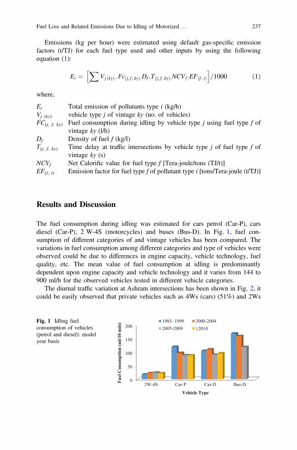
Emissions (kg per hour) were estimated using default gas-specific emissionfactors (t/TJ) for each fuel type used and other inputs by using the followingequation (1):
Ei ¼X
Vj ðkyÞ:Fc j; f ; kyð Þ:Df :T j; f ; kyð Þ:NCVf :EFðf ; iÞh i
=1000 ð1Þ
where,
Ei Total emission of pollutants type i (kg/h)Vj (ky) vehicle type j of vintage ky (no. of vehicles)FC(j, f, ky) Fuel consumption during idling by vehicle type j using fuel type f of
vintage ky (l/h)Df Density of fuel f (kg/l)T(j, f, ky) Time delay at traffic intersections by vehicle type j of fuel type f of
vintage ky (s)NCVf Net Calorific value for fuel type f [Tera-joule/tons (TJ/t)]EF(f, i) Emission factor for fuel type f of pollutant type i [tons/Tera-joule (t/TJ)]
Results and Discussion
The fuel consumption during idling was estimated for cars petrol (Car-P), carsdiesel (Car-P), 2 W-4S (motorcycles) and buses (Bus-D). In Fig. 1, fuel con-sumption of different categories of and vintage vehicles has been compared. Thevariations in fuel consumption among different categories and type of vehicles wereobserved could be due to differences in engine capacity, vehicle technology, fuelquality, etc. The mean value of fuel consumption at idling is predominantlydependent upon engine capacity and vehicle technology and it varies from 144 to900 ml/h for the observed vehicles tested in different vehicle categories.
The diurnal traffic variation at Ashram intersections has been shown in Fig. 2, itcould be easily observed that private vehicles such as 4Ws (cars) (51%) and 2Ws
0
50
100
150
200
2W-4S Car-P Car-D Bus-DFuel
Con
umpt
ion
(ml/1
0 m
in)
Vehicle Type
1985- 1999 2000-20042005-2009 ≥2010
Fig. 1 Idling fuelconsumption of vehicles(petrol and diesel): modelyear basis
Fuel Loss and Related Emissions Due to Idling of Motorized … 237

(scooter, motorcycle, etc.) (25%) are dominant vehicle categories followed by 3Ws,LCVs, buses, HCVs/MAVs (Fig. 3). Ashram intersection is a high-traffic volumeintersection (traffic volume > 2 lakh/day) it caters to *2,39,749 vehicles/day(excluding traffic pass intersection by flyovers) out of which nearly 28% of vehicles(i.e. *67000 vehicles) idle per day. The selected intersection has been classified ashigh traffic intersection according to the traffic volume.
High arrival rate of vehicles than departure rate of traffic volume at almost allintersections leads to longer queues, longer delay time and congestion are the mainreasons for the longer idling time. The average delay at the intersection ranged inbetween 400 and 550 s per hour (Fig. 4). The maximum delay was observed duringevening peak hours (1700–1800 h) and minimum during early morning hours.
Fuel loss estimated at Ashram intersection using fuel consumption per vehicle,idling traffic, time delay by using above discussed methodology. It was estimatedthat in a day, *4200 kg of fuel is lost during idling at Ashram, out of which*2,000 L is Petrol, 1,100 L Diesel, 1,900 kg CNG and 44 kg LPG is lost due toidling of vehicles (Fig. 5).
0
500
1000
1500
2000
2500
3000
3500
4000
8 9 10 11 12 13 14 15 16 17 18 19 20 21 22 23 24 1 2 3 4 5 6 7
No.
of I
dlin
g V
ehic
les
Hour of the day
Car 2W
3W LCV
Bus HCV
MAV
Fig. 2 Number of various vehicles idling at Ashram intersection
Two wheelers
25%
Cars51%
Three Wheelers
12%
LCV5%
HCV3%
Bus4%
Fig. 3 Percentagedistribution of differentcategories of vehicles atAshram intersection
238 N. Sharma et al.

Greenhouse gases (CO2, CH4, and N2O) emissions and indirect greenhouse gas(CO, NOx and NMVOC) emitted from vehicles were estimated using IPCCemission factors. It was observed that CO2 has highest contribution to emission
0
100
200
300
400
500
600
7--8
8--9
9--1
010
--11
11--
1212
--13
13--
1414
--15
15--
1616
--17
17--
1818
--19
19--
2020
--21
21--
2222
-23
23--
2424
--01
01--
0202
--03
03--
0404
--05
05--
06
Tim
e D
elay
(sec
onds
)
Hour of the day
Ashram
Fig. 4 Hourly delay of vehicles at Ashram intersection
0
500
1000
1500
2000
2500
Petrol(Litre)
Diesel(Litre)
CNG (Kg) LPG (Kg)
Fuel
loss
/day
Fuel Type
Fuel loss/day
Fig. 5 Fuel loss per day atAshram intersection
0200400600800100012001400
0102030405060708090
CO
2K
g/ d
ay
Kg/
day
Hour of the Day
NOx CO N2OCH4 NMVOC CO2
Fig. 6 Diurnal variation in GHGs emissions due to idling of vehicles at Ashram intersection
Fuel Loss and Related Emissions Due to Idling of Motorized … 239
load among all the GHGs estimated followed by CO, NOx NMVOC, and CH4
(Fig. 6). The morning peak and evening traffic peaks have resulted in correspondinghigh emissions during those hours.
Among all the pollutants it was estimated that high CO emissions has beencontributed by large share of petrol-(rich mixture due to low air: fuel ratio) drivenvehicles (*57%) in total idling vehicles. Emission NOx and N2O are mainly fromdiesel vehicles (lean air: fuel ratio) which are*20% of total vehicular fleet idling atAshram intersections. Similarly, CH4 could be contributed by CNG driven vehicleswhich are around 23% of total traffic volume.
Conclusions
Signalized traffic intersections are considered as urban hotspots due to high air pol-lution levels caused by high vehicular activities. Apart from effective red signal time, ahigh number of vehicles, traffic congestion and are the main reasons for unnecessaryidling of vehicles at signalized intersections, which results in deterioration of airquality many times exceeding the air quality standards prescribed by local regulatoryauthorities. In the present study, idling fuel consumption of various categories ofvehicles was estimated, further, Ashram intersection in Delhi was selected for esti-mation of emissions due to idling of vehicles. It was observed that nearly 6000 ofvehicles idle at Ashram intersection per day, which results in nearly 4200 kg/day offuel loss. The fuel loss accrued results in the release of emission of various GHGs,making it an apt example of an urban hotspot. Further, if we convert the fuel loss dueto idling in monetary terms it was estimated that nearly Rs. 3,00,000/days is wasted.With nearly 600 signalized intersections in Delhi the fuel loss and correspondingemissions could be detrimental economically and environmentally. The environmentaland monetary losses due to idling could be reduced by efficient public transport, whichnot only helps in reducing congestion, pollution, and is less costly and uses energyefficiently. In cities like Delhi, short trip commutation problems could be reduced byeffectively and organized use of non-motorized transport system. Comprehensivetraffic management, planning along with extensive public transportation system couldhelp to reduce the fuel loss and related emissions.
Acknowledgements The authors are thankful to Director, CSIR-CRRI for kindly permitting topublish the present paper. Rajni Dhyani is thankful to CSIR for providing financial assistancethrough CSIR Senior Research Fellowship.
References
Anil Singh S‚ Gangopadhyay PK‚ Nanda S‚ Bhattacharya C‚ Sharma C‚ Bhan C (2008) Trends ofgreenhouse gas emissions from the road transport sector in India. Sci Total Environ 390(1):124–131
240 N. Sharma et al.
Burgess E, Peffers M, Silverman I (2009) Idling gets you nowhere-The health, environmental andeconomic impacts of engine idling in New York City, Environment Defense Fund, February 2009
Guttikunda S (2009) Indicative impacts of vehicular idling on air emissions, simple interactivemodels for better air quality. SIM-air working paper series: 18–2009
IPCC (2006) Guidelines for national greenhouse gas inventories. Work book vol 2,Intergovernmental Panel on Climate Change
IPCC (1996) “Revised Guidelines for National Greenhouse Gas Inventories. vol 2, EnergyIntergovernmental Panel on Climate Change
MoRTH (2013) Road Transport Yearbook, (2011–12). Ministry of Road Transport and Highways.Government of India
Morshed MR (2010) Unnecessary idling of vehicles: an analysis of the current situation and whatcan be done to reduce it. Master of Engineering Thesis Work. Mc Master University, OntarioCanada, Sept 2010
NRC (2011) Emission impacts resulting from vehicle idling. Natural resources Canada. Retrieved15 Mar 2013 at http://oee.nrcan.gc.ca/transportation/idling/10617
NRC (2009) Idling wastes fuel and money. Natural resources Canada. Retrieved 15 Mar 2013 athttp://www.oee.nrcan.gc.ca/transportation/idling/wastes.cfm?attr=8
Parida P, Gangopadhyay S (2008) Estimation of fuel loss during idling of vehicles at signalizedintersections in Delhi. J Indian Road Congr 69(1):61–69
Pradeep PV, Sekhar CR, Singh A, Sharma N (2014) Understanding variability of fuel consumptionin vehicle. Project Stream Mag 1(1):25–26
Fuel Loss and Related Emissions Due to Idling of Motorized … 241
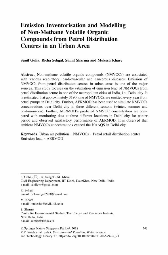
Emission Inventorisation and Modellingof Non-Methane Volatile OrganicCompounds from Petrol DistributionCentres in an Urban Area
Sunil Gulia, Richa Sehgal, Sumit Sharma and Mukesh Khare
Abstract Non-methane volatile organic compounds (NMVOCs) are associatedwith various respiratory, cardiovascular and cancerous diseases. Emission ofNMVOCs from petrol distribution centres in urban areas is one of the majorsources. This study focuses on the estimation of emission load of NMVOCs frompetrol distribution centre in one of the metropolitan cities of India, i.e., Delhi city. Itis estimated that approximately 3190 tone of NMVOCs are emitted every year frompetrol pumps in Delhi city. Further, AERMOD has been used to simulate NMVOCsconcentrations over Delhi city in three different seasons (winter, summer andpost-monsoon). Further, AERMOD’s predicted NMVOC concentration are com-pared with monitoring data at three different locations in Delhi city for winterperiod and observed satisfactory performance of AERMOD. It is observed thatambient NMVOCs concentrations exceed the NAAQS in Delhi city.
Keywords Urban air pollution � NMVOCs � Petrol retail distribution centerEmission load � AERMOD
S. Gulia (&) � R. Sehgal � M. KhareCivil Engineering Department, IIT Delhi, HauzKhas, New Delhi, Indiae-mail: [email protected]
R. Sehgale-mail: [email protected]
M. Kharee-mail: [email protected]
S. SharmaCentre for Environmental Studies, The Energy and Resources Institute,New Delhi, Indiae-mail: [email protected]
© Springer Nature Singapore Pte Ltd. 2018V.P. Singh et al. (eds.), Environmental Pollution, Water Scienceand Technology Library 77, https://doi.org/10.1007/978-981-10-5792-2_21
243
Introduction
Urban air quality is deteriorated in most of the megacities of the world. In devel-oping countries, the problems of poor air quality is serious due to increasingdemand of motorized road transportation, which is one of the dominant source ofurban air pollution (Singh et al. 2007; Ramachandra and Shwetmala 2009; CPCB2010). In addition to the emission from combustion of fuels, the fugitive emissionsof pollutant such as VOCs due to their volatile nature is one of the major problem inurban area. The non-methane organic compounds are grouped as NMVOCs as themajority of them having similar behavior in the atmosphere. In literature, it isobserved that considerable attention has been paid on management of criteria airpollutants, however, NMVOCs have steadily grown unnoticed. They are potentiallycarcinogenic and mutagenic in nature at specified concentrations levels and mayprovide significant risk to human health (Edgerton et al. 1989). In addition to thatNMVOCs act as important pre-cursors of ground level Ozone formation and sec-ondary particulates known as secondary organic aerosols (SOA). Past studiesindicate that VOCs concentration in Delhi city is exceeded the national ambient airquality standard (Srivastva et al. 2005; Singh et al. 2012; Chauhan et al. 2014). Themajor source reported in these studies are paints industries, evaporation fossil fueland vehicles exhaust emission. Evaporation of fossil fuel at fuel distribution centreis one of the major sources of NMVOCs. It may evaporates from fuel storage tanks,during loading and unloading of fuel, injection systems and refueling in vehicles.Gasoline vapors evaporates during refueling adding pollutants like benzene,toluene, ethylbenzene and xylene to the ambient air. The important factors affectingthe evaporation of gasoline are temperature fluctuations, permeation of fuel throughhoses and fitting etc. High ambient temperatures cause large evaporative losses.There is a clear need for an evaluation of these hidden sources of NMVOCs, theiremission load and control in the urban area.In the present study, an attempt hasbeen tried to evaluate the impacts of evaporative emission of NMVOCs from petrolstation in Delhi city. The study includes emission inventory development ofNMVOCs and prediction of NMVOCs concentrations over Delhi city.
Materials and Methods
The methodology of evaluation of impacts of NMVOCs emission from Petrol fillingstations on urban air quality in Delhi city is carried out in three steps: (1) Datacollection such as total number of Petrol filling stations in Delhi city, capacity ofPetrol storage at each station, number of vehicles coming for Petrol filling etc.,(2) Emission inventory development of NMVOCs and (3) Air quality modelingusing AERMOD for prediction of NMVOCs concentration over Delhi city.
244 S. Gulia et al.
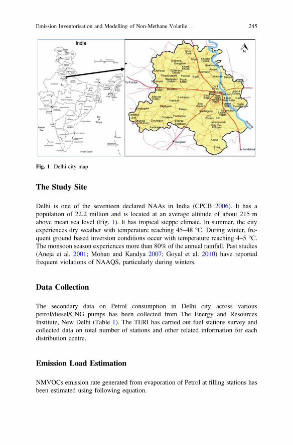
The Study Site
Delhi is one of the seventeen declared NAAs in India (CPCB 2006). It has apopulation of 22.2 million and is located at an average altitude of about 215 mabove mean sea level (Fig. 1). It has tropical steppe climate. In summer, the cityexperiences dry weather with temperature reaching 45–48 °C. During winter, fre-quent ground based inversion conditions occur with temperature reaching 4–5 °C.The monsoon season experiences more than 80% of the annual rainfall. Past studies(Aneja et al. 2001; Mohan and Kandya 2007; Goyal et al. 2010) have reportedfrequent violations of NAAQS, particularly during winters.
Data Collection
The secondary data on Petrol consumption in Delhi city across variouspetrol/diesel/CNG pumps has been collected from The Energy and ResourcesInstitute, New Delhi (Table 1). The TERI has carried out fuel stations survey andcollected data on total number of stations and other related information for eachdistribution centre.
Emission Load Estimation
NMVOCs emission rate generated from evaporation of Petrol at filling stations hasbeen estimated using following equation.
Fig. 1 Delhi city map
Emission Inventorisation and Modelling of Non-Methane Volatile … 245
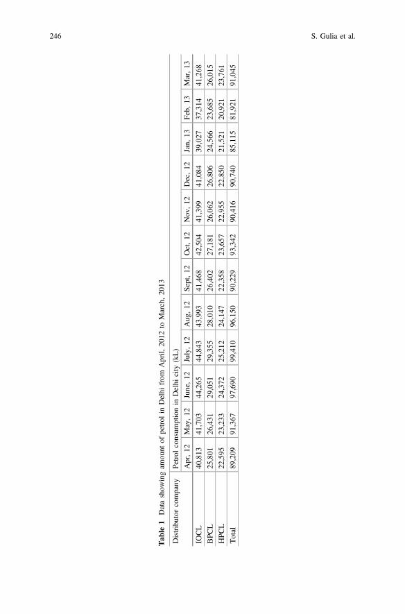
Tab
le1
Datashow
ingam
ount
ofpetrol
inDelhi
from
April,
2012
toMarch,20
13
Distributor
company
Petrol
consum
ptionin
Delhi
city
(kL)
Apr,12
May,12
June,12
July,12
Aug
,12
Sept,12
Oct,12
Nov
,12
Dec,12
Jan,
13Feb,
13Mar,13
IOCL
40,813
41,703
44,265
44,843
43,993
41,468
42,504
41,399
41,084
39,027
37,314
41,268
BPC
L25
,801
26,431
29,051
29,355
28,010
26,402
27,181
26,062
26,806
24,566
23,685
26,015
HPC
L22
,595
23,233
24,372
25,212
24,147
22,358
23,657
22,955
22,850
21,521
20,921
23,761
Total
89,209
91,367
97,690
99,410
96,150
90,229
93,342
90,416
90,740
85,115
81,921
91,045
246 S. Gulia et al.

E ¼ ef i � Vi � 10�6
where
E Emission rates of NMVOCs from evaporation of petrol at filling stations(kg yr−1)
ef Emission factor for Petrol evaporation (mgl−1)V Annual sales of petrol in Delhi city (l yr−1)
Later, emission of NMVOCs from Petrol distribution stations are distributed ingrid cell over the whole city. The equations used for calculation of grid wiseemission is as follows (Table 2).
Ek ¼ E � Nk
N
where
Ek Annual emissions of NMVOC in k grid cell, (kg yr−1)E Total emissions of NMVOC inDelhi city (kg yr−1)Nk Number of service stations in k grid cellN Total number of filling stations in Delhi city
Air Quality Dispersion Modelling
The prediction of ambient NMVOCs concentrations is carried out using AERMODmodel, an USEPA recommended air quality dispersion model for regulatory pur-poses. It is a Gaussian based dispersion model. It incorporates AERMET(Meteorological Preprocessor) replacing the P-G stability class and AERMAP, toprocess terrain features. Input data for AERMET includes hourly cloud cover
Table 2 Emission factors for petrol filling station in (mg/l)
Emission sources Emission rate (mg per litre throughout)
Underground tank filling
Submerged filling 880
Splash filling 1,380
Submerged filling and vapor balance 40
Underground tank breathing/emptying 120
Vehicle refueling
Displacement losses (uncontrolled) 1,320
Displacement losses (controlled) 132
Spillage 80
Source AP-42, USEPA (2015)
Emission Inventorisation and Modelling of Non-Methane Volatile … 247

observations, surface meteorological observations, such as, wind speed and direc-tion, temperature, dew point, humidity and sea level pressure and upper airsoundings. The AERMAP uses gridded terrain data to calculate the representativeterrain-influence height (Cimorelli et al. 2004). AERMOD are set-up using gridemission data, topographical features and meteorological conditions of Delhi cityfor a period of one week in the winter season of year 2013.
Results and Discussion
NMVOCs Emission Load
The NMVOCs emission load due to evaporation Petrol at filling stations in Delhicity is estimated 3190 tons/year. Further, the total emission load has been dis-tributed grid wise over Delhi city. Each grid cell size is 2.5 km � 2.8 km. The totalnumber of Petrol filling stations in Delhi city are 324. The maximum emission loadin grid cell with 8 number of filling stations is 78.76 tons/yr = 2.49 g/s. However,emission from single filling station is estimated to be 0.312 g/s. Figure 2 shows thegrid wise emission load of NMVOCs in Delhi city.
Fig. 2 Grid wise NMVOCs emission rate over Delhi city
248 S. Gulia et al.
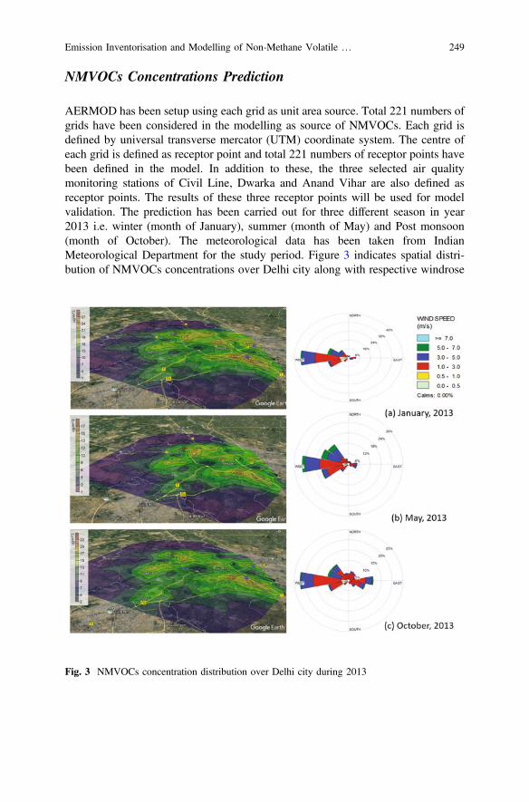
NMVOCs Concentrations Prediction
AERMOD has been setup using each grid as unit area source. Total 221 numbers ofgrids have been considered in the modelling as source of NMVOCs. Each grid isdefined by universal transverse mercator (UTM) coordinate system. The centre ofeach grid is defined as receptor point and total 221 numbers of receptor points havebeen defined in the model. In addition to these, the three selected air qualitymonitoring stations of Civil Line, Dwarka and Anand Vihar are also defined asreceptor points. The results of these three receptor points will be used for modelvalidation. The prediction has been carried out for three different season in year2013 i.e. winter (month of January), summer (month of May) and Post monsoon(month of October). The meteorological data has been taken from IndianMeteorological Department for the study period. Figure 3 indicates spatial distri-bution of NMVOCs concentrations over Delhi city along with respective windrose
Fig. 3 NMVOCs concentration distribution over Delhi city during 2013
Emission Inventorisation and Modelling of Non-Methane Volatile … 249

plot of three season. The higher NMVOCs concentration in winter season comparedto post monsoon and summer seasons clearly indicate the impacts of calm mete-orological condition in winter season. Further, it is also found the NMVOCsconcentration are found higher in Centre, East and South east of Delhi city(downwind side). It is due to high emission load in these area and due to transportof pollutants emitted in West and North West of Delhi city (upwind side).
Model Validation
The validation of AERMOD prediction has been carried out by comparing thepredicted and monitoring NMVOCs concentrations (Benzene) at three differentlocation in Delhi city (Fig. 4). The monitoring data have been collected from theDPCC operated air quality monitoring stations at Civil lines, Dwarka and AnandVihar for the month January, 2013. Figure 4 describe the scatter plot of predictedand monitoring concentrations data at all three locations. The value of r2 in range of0.41–0.57 indicate satisfactory performance of AERMOD in predicting NMVOCsconcentrations. However, AERMOD is slightly under predicted which may be dueto non-consideration of other significant sources of NMVOCs in the modellingstudy. The NMVOCs concentration are found exceeding the specified standards of5 µg/m3 (MoEF 2009).
Fig. 4 scatter plot of predicted and monitoring NMVOCs concentrations
250 S. Gulia et al.
Conclusions
The study has been carried out with aim of emission inventorisation and predictionof NMVOCs concentrations over Delhi city using AERMOD. The NMVOCsemission loads from Petrol stations in Delhi city is 3190 tons/year. Further,AERMOD predict satisfactorily the NMVOCs concentration over Delhi city. Themodelling results indicates higher NMVOCs concentration in winter season fol-lowed by post monsoon and summer seasons. The values of NMVOCs are found tobe exceeded the specified NAAQS value which needs to be control to reduce theexposure level and its harmful impacts on environment. This kind of study willassist decision makers to manage increasing air pollution level by simulating thecontrol measures such as vapor recovery systems (VRS) at the petrol distributioncentres.
References
Aneja VP, Agarwal A, Roelle PA, Philips SB, Tong Q, Watkins N (2001) Measurement andanalysis of criteria pollutants in New Delhi. India Environ Model Softw 27(1):35–42
Chauhan SK, Saini N, Yadav VB (2014) Recent trends of volatile organic compounds in ambientair & its health impacts: a review. Int J Technol Res Eng 1(8):667–678
Cimorelli AJ, Perry SG, Venktaram A, Weil JC, Paine RJ (2004) AERMOD: a dispersion modelfor industrial source applications. Part I: general model formulation and boundary layercharacterization. J Appl Meteorol 44:682–693
CPCB (Central Pollution Control Board) (2006) Air quality trends and action plan for control ofair pollution from seventeen studies. Ministry of Environment and Forest. NAAQMS/29/2006–07
CPCB (Central Pollution Control Board) (2010) Air quality monitoring, emission inventory andsource apportionment study for Indian cities. National summary report. The Central PollutionControl Board, New Delhi, India 290 p
Edgerton SA, Holdernm MW, Smith DI (1989) Inter urban comparison of ambient volatile organiccompound concentration. JAPCA 39:729–732
Goyal P, Jaiswal N, Kumar A, Dadoo JK, Dwarakanath M (2010) Air quality impact assessment ofNOx and PM due to diesel vehicles in Delhi. Transp Res Part D 15:298–303
MoEF (Ministry of Environment and Forest) (2009) National ambient air quality standards.Government of India, New Delhi. Notification number: S. O. 3067 (E), p 4
Mohan M, Kandya A (2007) An analysis of the annual and seasonal trends of air quality index ofDelhi. Environ Monit Assess 131:267–277
Ramachandra TV (2009) Emissions from India’s transport sector: statewise synthesis. AtmosEnviron 43(34):5510–5517
Singh AK, Gupta HK, Gupta K, Singh P, Gupta VB, Sharma RC (2007) A comparative study ofair pollution in Indian cities. Bull Environ Contam Toxicol 78:411–416
Singh AK, Tomer N, Jain CL (2012) Monitoring assessment and status of benzene, toluene andxylene pollution in the urban atmosphere of Delhi, India. Res J Chem Sci 2(4):45–49
Emission Inventorisation and Modelling of Non-Methane Volatile … 251

Srivastava A, Joseph AE, More A, Patil S (2005) Emissions of VOCs at urban petrol retaildistribution centres in India (Delhi and Mumbai). Environ Monit Assess 109(1–3):227–242
USEPA (2015) Transportation and marketing of petroleum liquids, emission factor, AP-42 US.Environment Protection Agency, USA. http://www3.epa.gov/ttn/chief/ap42/ch05/index.htmlAccessed in Oct 2015
252 S. Gulia et al.
Comprehensive PhysicochemicalCharacterization of Coal CombustionResidues from a Thermal Power Stationof India
Ritesh Kumar
Abstract Coal combustion residue is a by-product from combustion of pulverizedcoal in thermal power stations and is considered as a waste material. Coal com-bustion residues contain many chemical elements that may be potentially harmful tothe environment. Coal combustion residue handling and disposal is a major prob-lem from an environmental point of view. Though the utilization in India has shownincrease in percentage value, still we are to make sufficient effort to fulfill thepromise of 100% utilization. Although some of the coal combustion residues areused as construction materials and as backfill material that provides ample oppor-tunity for its bulk use, most of them are still disposed of in settling ponds, alsoknown as ash ponds or landfills. The study here presents comprehensive physico-chemical characterization of coal combustion residues from a thermal power stationof India. The present study is aimed to provide the database relevant to its findingbetter utilization potential and also see the effect of land disposal of such ash on thequality of groundwater and surface water through the laboratory study simulatingfield conditions.
Keywords Coal combustion residues � Fly ash � Bottom ash and pond ashCharacterization � Utilization
Introduction
The Indian power sector generated approximately 967.150 BU of electricity in2013–14 (Ministry of Power 2015). The growth in the power sector during the past60 years and especially in the past two decades has been phenomenal. Of the totalpower generated, more than 50% has been contributed by coal-fired power station(TEDDY 2014/15; BP 2015). This growth of the power sector during the last oneand a half decade has taken place due to increasing electricity demand and
R. Kumar (&)CSIR-Central Institute of Mining & Fuel Research, Dhanbad 826001, Jharkhand, Indiae-mail: [email protected]
© Springer Nature Singapore Pte Ltd. 2018V.P. Singh et al. (eds.), Environmental Pollution, Water Scienceand Technology Library 77, https://doi.org/10.1007/978-981-10-5792-2_22
253
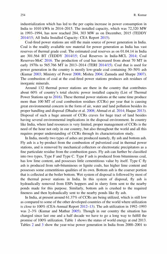
industrialization which has led to the per capita increase in power consumption inIndia to 1010 kWh in 2014–2015. The installed capacity, which was 72,320 MWin 1993–1994, has now reached 284, 303 MW as on December, 2015 (TEDDY2014/15; All India Installed Capacity: CEA Report 2015).
Coal-fired power stations are still the main source of power generation in India.Coal is the readily available raw material for power generation as India has vastreserves of thermal grade coal. The estimated coal reserves as on 01.04.14 in Indiaare 301.564 BT (TEDDY 2014/15; Coal Reserves in India-MCL 2014; CoalReserves-MoC 2016. The production of coal has increased from about 70 MT inearly 1970s to 565.766 MT in 2013–2014 (TERI 2014/15). Coal that is used forpower generation in the country is mostly low-grade coal containing 30–50% ash(Kumar 2003; Ministry of Power 2008; Mishra 2004; Zamuda and Sharpe 2007).The combustion of coal at the coal-fired power stations produces ash residues ofinorganic minerals.
Around 132 thermal power stations are there in the country that contributesabout 60% of country’s total electric power installed capacity (List of ThermalPower Stations up to 2016). These thermal power stations at the same time producemore than 100 MT of coal combustion residues (CCRs) per year that is causinggreat environmental concern in the form of air, water and land pollution besides itsproper handling and disposal (Dhadse et al. 2008; Ahmad et al. 2014; Haque 2013).Disposal of such a huge amount of CCRs craves for huge tract of land besideshaving several environmental implications in the disposal environment. In countrylike India, where land resources is very limited, proper management of CCRs is theneed of the hour not only in our country, but also throughout the world and all thisrequires proper understanding of CCRs through its characterization study.
In India, mostly two types of ashes are produced namely, fly ash and bottom ash.Fly ash is a by-product from the combustion of pulverized coal in thermal powerstations, and is removed by mechanical collectors or electrostatic precipitators as afine particulate residue from the combustion gases. Fly ash can further be classifiedinto two types, Type F and Type C. Type F ash is produced from bituminous coal,has low lime content, and possesses little cementitious value by itself. Type C flyash is produced from sub-bituminous or lignite coals, has higher lime content andpossesses some cementitious qualities of its own. Bottom ash is the coarser portionthat is collected at the boiler bottom. Wet system of disposal is followed by most ofthe thermal power stations in India. In this system of disposal, fly ash ishydraulically removed from ESPs hoppers and in slurry form sent to the nearbyponds made for this purpose. Similarly, bottom ash is crushed to the requiredfineness and then hydraulically sent to the nearby ponds like fly ash.
In India, at present around 61.37% of CCRs are being utilized, which is still lowas compared to some of the other developed countries of the world where utilizationis close to 100% (CEA-Annual Report 2012–13). The ash utilization in 1992–1993was 2–3% (Kumar and Mathur 2005). Though in our country the situation haschanged since last one and a half decade we have to go a long way to fulfill thepromise of 100% utilization. Table 1 shows the status of world energy at end 2013.Tables 2 and 3 show the year-wise power generation in India from 2000–2001 to
254 R. Kumar

2013–2014 and per capita electricity consumption in India from 2000–2001 to2013–2014, respectively. Table 4 shows the per capita consumption of electricityby leading countries of the world. Table 5 shows the India’s CCRs utilizationscenario. Similarly, Table 6 provides the data on CCRs utilized by the leadingcountries of the world.
Table 1 Status of world energy at the end 2014 (BP 2015)
2014 Change 2014 over 2013 (%)
Electricity
Generation (TWH) 23536.5 1.5
Coal
Reserves (MT) 891531 –
Production (MT) 8164.9 −0.7
Production (MT of oil equivalents) 3933.5 −0.7
Consumption (MT of oil equivalents) 3881.8 0.4
Table 2 Year-wise powergeneration in India (2003–2004 to 2013–2014) (TEDDYAnnual Report 2003/04,2004/05, 2005/06, 2009,2014/15; CEA Annual Report2011/12, 2012/13, 2014/15)
Year Generation (BUs)
2003–04 558.30
2004–05 587.40
2005–06 617.50
2006–07 662.50
2007–08 704.50
2008–09 723.80
2009–10 771.60
2010–11 811.10
2011–12 876.40
2012–13 912.06
2013–14 967.15
Table 3 Year-wise percapita electricity consumptionin India (2005–2006–2012–2013) (Garg 2012; CEAAnnual Report 2011/12,2012/13, 2014/15)
Year Consumption (kWh)
2005–06 631
2006–07 672
2007–08 717
2008–09 734
2009–10 779
2010–11 819
2011–12 884
2012–13 917
2013–14 957
2014–15 1010
Comprehensive Physicochemical Characterization of Coal … 255
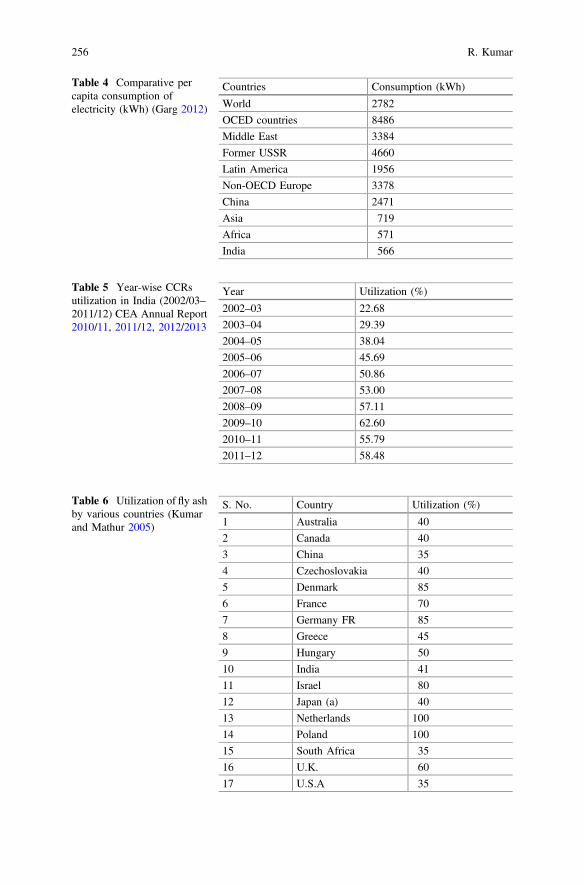
Table 4 Comparative percapita consumption ofelectricity (kWh) (Garg 2012)
Countries Consumption (kWh)
World 2782
OCED countries 8486
Middle East 3384
Former USSR 4660
Latin America 1956
Non-OECD Europe 3378
China 2471
Asia 719
Africa 571
India 566
Table 5 Year-wise CCRsutilization in India (2002/03–2011/12) CEA Annual Report2010/11, 2011/12, 2012/2013
Year Utilization (%)
2002–03 22.68
2003–04 29.39
2004–05 38.04
2005–06 45.69
2006–07 50.86
2007–08 53.00
2008–09 57.11
2009–10 62.60
2010–11 55.79
2011–12 58.48
Table 6 Utilization of fly ashby various countries (Kumarand Mathur 2005)
S. No. Country Utilization (%)
1 Australia 40
2 Canada 40
3 China 35
4 Czechoslovakia 40
5 Denmark 85
6 France 70
7 Germany FR 85
8 Greece 45
9 Hungary 50
10 India 41
11 Israel 80
12 Japan (a) 40
13 Netherlands 100
14 Poland 100
15 South Africa 35
16 U.K. 60
17 U.S.A 35
256 R. Kumar
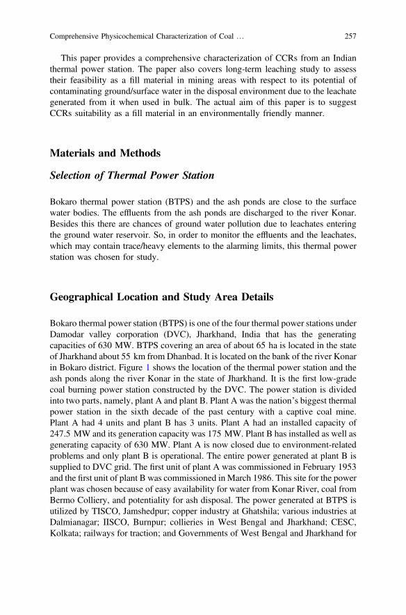
This paper provides a comprehensive characterization of CCRs from an Indianthermal power station. The paper also covers long-term leaching study to assesstheir feasibility as a fill material in mining areas with respect to its potential ofcontaminating ground/surface water in the disposal environment due to the leachategenerated from it when used in bulk. The actual aim of this paper is to suggestCCRs suitability as a fill material in an environmentally friendly manner.
Materials and Methods
Selection of Thermal Power Station
Bokaro thermal power station (BTPS) and the ash ponds are close to the surfacewater bodies. The effluents from the ash ponds are discharged to the river Konar.Besides this there are chances of ground water pollution due to leachates enteringthe ground water reservoir. So, in order to monitor the effluents and the leachates,which may contain trace/heavy elements to the alarming limits, this thermal powerstation was chosen for study.
Geographical Location and Study Area Details
Bokaro thermal power station (BTPS) is one of the four thermal power stations underDamodar valley corporation (DVC), Jharkhand, India that has the generatingcapacities of 630 MW. BTPS covering an area of about 65 ha is located in the stateof Jharkhand about 55 km from Dhanbad. It is located on the bank of the river Konarin Bokaro district. Figure 1 shows the location of the thermal power station and theash ponds along the river Konar in the state of Jharkhand. It is the first low-gradecoal burning power station constructed by the DVC. The power station is dividedinto two parts, namely, plant A and plant B. Plant A was the nation’s biggest thermalpower station in the sixth decade of the past century with a captive coal mine.Plant A had 4 units and plant B has 3 units. Plant A had an installed capacity of247.5 MW and its generation capacity was 175 MW. Plant B has installed as well asgenerating capacity of 630 MW. Plant A is now closed due to environment-relatedproblems and only plant B is operational. The entire power generated at plant B issupplied to DVC grid. The first unit of plant A was commissioned in February 1953and the first unit of plant B was commissioned in March 1986. This site for the powerplant was chosen because of easy availability for water from Konar River, coal fromBermo Colliery, and potentiality for ash disposal. The power generated at BTPS isutilized by TISCO, Jamshedpur; copper industry at Ghatshila; various industries atDalmianagar; IISCO, Burnpur; collieries in West Bengal and Jharkhand; CESC,Kolkata; railways for traction; and Governments of West Bengal and Jharkhand for
Comprehensive Physicochemical Characterization of Coal … 257
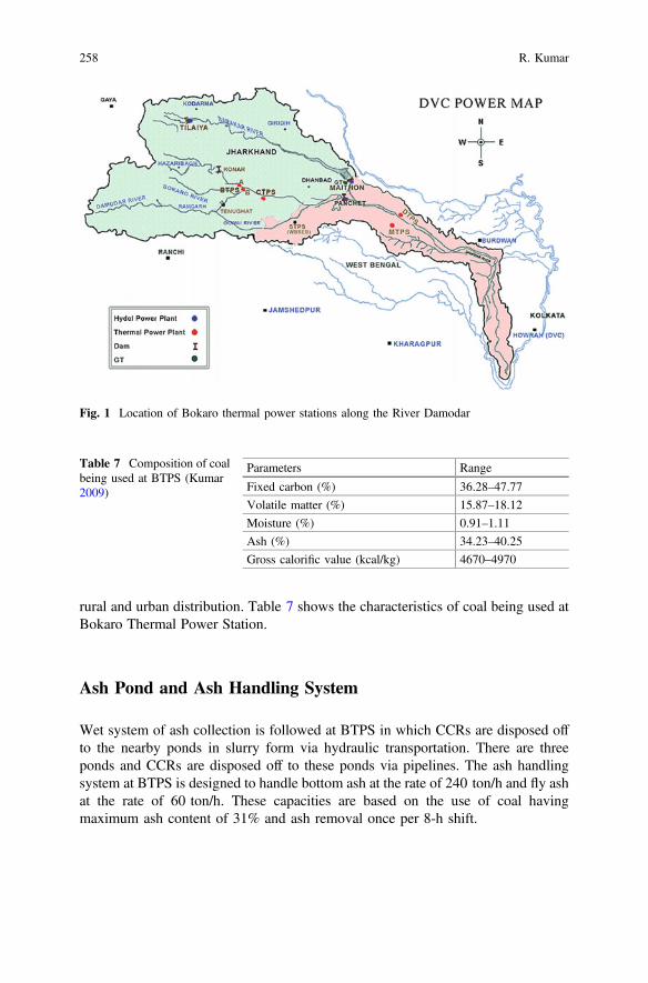
rural and urban distribution. Table 7 shows the characteristics of coal being used atBokaro Thermal Power Station.
Ash Pond and Ash Handling System
Wet system of ash collection is followed at BTPS in which CCRs are disposed offto the nearby ponds in slurry form via hydraulic transportation. There are threeponds and CCRs are disposed off to these ponds via pipelines. The ash handlingsystem at BTPS is designed to handle bottom ash at the rate of 240 ton/h and fly ashat the rate of 60 ton/h. These capacities are based on the use of coal havingmaximum ash content of 31% and ash removal once per 8-h shift.
Fig. 1 Location of Bokaro thermal power stations along the River Damodar
Table 7 Composition of coalbeing used at BTPS (Kumar2009)
Parameters Range
Fixed carbon (%) 36.28–47.77
Volatile matter (%) 15.87–18.12
Moisture (%) 0.91–1.11
Ash (%) 34.23–40.25
Gross calorific value (kcal/kg) 4670–4970
258 R. Kumar
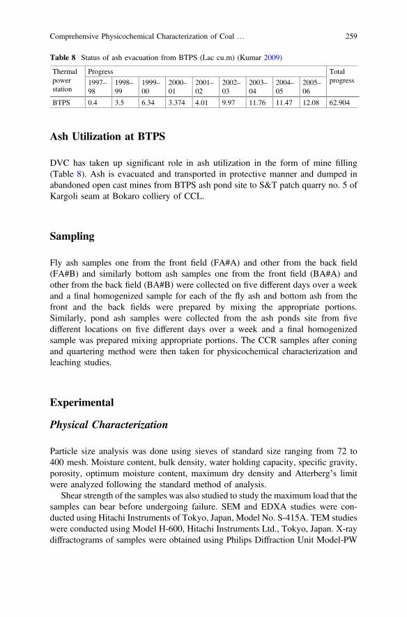
Ash Utilization at BTPS
DVC has taken up significant role in ash utilization in the form of mine filling(Table 8). Ash is evacuated and transported in protective manner and dumped inabandoned open cast mines from BTPS ash pond site to S&T patch quarry no. 5 ofKargoli seam at Bokaro colliery of CCL.
Sampling
Fly ash samples one from the front field (FA#A) and other from the back field(FA#B) and similarly bottom ash samples one from the front field (BA#A) andother from the back field (BA#B) were collected on five different days over a weekand a final homogenized sample for each of the fly ash and bottom ash from thefront and the back fields were prepared by mixing the appropriate portions.Similarly, pond ash samples were collected from the ash ponds site from fivedifferent locations on five different days over a week and a final homogenizedsample was prepared mixing appropriate portions. The CCR samples after coningand quartering method were then taken for physicochemical characterization andleaching studies.
Experimental
Physical Characterization
Particle size analysis was done using sieves of standard size ranging from 72 to400 mesh. Moisture content, bulk density, water holding capacity, specific gravity,porosity, optimum moisture content, maximum dry density and Atterberg’s limitwere analyzed following the standard method of analysis.
Shear strength of the samples was also studied to study the maximum load that thesamples can bear before undergoing failure. SEM and EDXA studies were con-ducted using Hitachi Instruments of Tokyo, Japan, Model No. S-415A. TEM studieswere conducted using Model H-600, Hitachi Instruments Ltd., Tokyo, Japan. X-raydiffractograms of samples were obtained using Philips Diffraction Unit Model-PW
Table 8 Status of ash evacuation from BTPS (Lac cu.m) (Kumar 2009)
Thermalpowerstation
Progress Totalprogress1997–
981998–99
1999–00
2000–01
2001–02
2002–03
2003–04
2004–05
2005–06
BTPS 0.4 3.5 6.34 3.374 4.01 9.97 11.76 11.47 12.08 62.904
Comprehensive Physicochemical Characterization of Coal … 259
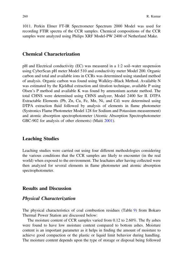
1011. Perkin Elmer FT-IR Spectrometer Spectrum 2000 Model was used forrecording FTIR spectra of the CCR samples. Chemical compositions of the CCRsamples were analyzed using Philips XRF Model-PW 2400 of Netherland Make.
Chemical Characterization
pH and Electrical conductivity (EC) was measured in a 1:2 soil–water suspensionusing CyberScan pH meter Model 510 and conductivity meter Model 200. Organiccarbon and total and available ions in CCRs was determined using standard methodof analysis. Organic carbon was found using Walkley–Black Method. Available Nwas estimated by the Kjeldhal extraction and titration technique, available P usingOlsen’s P method and available K was found by ammonium acetate method. Thetotal CHNS were determined using CHNS analyzer, Model 2400 Ser II. DTPAExtractable Elements (Pb, Zn, Cu, Fe, Mn, Ni, and Cd) were determined usingDTPA extraction fluid followed by analysis of elements in flame photometer(Systronics Flame Photometer Model 128 for Sodium and Potassium measurement)and atomic absorption spectrophotometer (Atomic Absorption SpectrophotometerGBC-902 for analysis of other elements) (Maiti 2001).
Leaching Studies
Leaching studies were carried out using four different methodologies consideringthe various conditions that the CCR samples are likely to encounter (in the realworld) when exposed to the environment. The leachates after having collected werethen analyzed for several elements in flame photometer and atomic absorptionspectrophotometer.
Results and Discussion
Physical Characterization
The physical characteristics of coal combustion residues (Table 9) from BokaroThermal Power Station are discussed below:
The moisture content of CCR samples varied from 0.12 to 2.60%. The fly asheswere found to have low moisture content compared to bottom ashes. Moisturecontent is an important parameter as it helps in finding the amount of moisture toachieve good compaction or the plastic or liquid limit behavior during handling.The moisture content depends upon the type of storage or disposal being followed
260 R. Kumar

for any particular material and the sample collection method employed. As in BTPSwet system of disposal is followed, the chances of CCR becoming airborne duringhandling is ruled out. Holding of CCR in ash pond and that too, for a long time maycreate nuisance when the pond gets dried up and the wind is blowing. On the otherhand high moisture content reduces its suitability for several economic uses. Highmoisture content is undesirable for use in manufacture of Portland cement, asbestossheet, etc.
Water holding capacity of any material is controlled by chemical and physicalnature of the material. Any material is said to be at its maximum water holdingcapacity when water fills all its pore spaces and there is no space. The water holdingcapacity of fly ashes were more (87.20 and 87.58%) compared to bottom ashes(61.82 and 55.97%) and pond ash (75.59%). Fly ashes had low moisture contentand so water holding capacity was greater compared to bottom ashes. High waterholding capacity of fly ashes was also due to greater percentage of fines present.Fine particles mean more surface area and so more water adsorptions. In case ofCCR samples water holding capacity is found to be more than those of natural soils.
Table 9 Physical characteristics of CCR samples from BTPS
Parameters Samples
FA#A FA#B BA#A BA#B PA
Moisture content (%) 0.17 1.12 0.70 2.60 0.21
Water holding capacity (%) 87.20 87.58 61.82 55.97 75.59
Permeability (�10−4 cm/s) 2.32 2.12 2.50 1.19 2.12
Specific gravity 2.47 2.53 2.11 2.40 2.60
Surface area (m2/g) 2.2 2.0 1.5 1.6 2.0
Bulk density (g/cc) 0.978 0.742 0.830 0.906 0.960
Porosity (%) 60.40 70.67 60.66 62.25 50.16
Atterberg limits
LL (%) 25 32 30 23 21
PL (%) NA NA NA NA NA
Proctor test
OMC (%) 21.57 18.76 29.32 31.78 20.68
MDD (g/cc) 1.31 1.29 1.15 1.07 1.27
Proximate analysis
Moisture (%) 0.17 1.12 0.70 2.60 0.21
Ash (%) 81.82 90.82 90.40 91.98 93.50
Volatile matter (%) 4.50 1.17 1.54 1.07 2.70
FC (by diff.) (%) 13.51 6.89 7.36 4.35 3.59
Sieve analysis
Cc 1.0907 0.8803 1.2073 1.2061 0.7836
Cu 3.3556 1.8612 2.6617 2.2437 3.500
Loss on ignition (%) 26.68 9.76 9.47 9.25 12.54
Comprehensive Physicochemical Characterization of Coal … 261
Specific gravity was found to vary from 2.11 to 2.60. In case of all the fivesamples, the specific gravity was above 2.00 and that not enough variation can beseen among the samples. Presence of unburnt carbon and cenospheres may be thereasons for the low specific gravity of the CCRs. Due to low specific gravity theflowability of the CCRs is better which makes it suitable stowing material in placeof sand for underground mines.
Table 9 indicates that permeability varied from 1.19 � 10−4 to 2.50 � 10−4
cm/sec. Permeability observed, in general, was low. This was due to higher percentof fines and high compressibility of CCRs. Such material can be used in improvingthe water retention capacity of the sandy soil, where water easily drains away owingto high porosity. Low permeability is a problem when using it as a stowingmaterial.
Surface area was found to vary from 1.5 to 2.2 m2/g. It can be seen that thesurface area of fly ashes is more compared to bottom ashes. Surface area is alsorelated to the percentage unburnt carbon in CCRs. The unburnt carbon is highlyporous and so has effect on the surface area of CCRs. Surface area is one of theimportant parameters of any particulate matter. The pre-concentration of traceelements on the particles mainly depends upon its surface area.
Bulk density of CCRs was less than 1.00 and it varied from 0.742 to 0.978 g/cc.Low bulk density is hindrance in the use of CCR as a stowing material as it takestime to settle. However, such problem can be overcome by the use of some floc-culating agent as is being experimented in CMRI. The transportation of such CCRsis also economical compared to sand when using CCRs as backfill or stowingmaterial. Such CCRs can also be used for modifying the texture of clayey soil forreducing the plasticity. This can further help in increasing the workability of suchclayey soil.
Liquid limit of the samples was found to vary from 21 to 32%. Plastic limit ofthe samples could not be found, as the materials could not be rolled to conductplastic limit test. Liquid limit of sand or sand like material is another very importantparameter in construction related works where such liquid limit make CCRs behaveas a viscous fluid and this can be at the cost of the stability of the structures.
Optimum moisture content (OMC) and maximum dry density (MDD) werefound to vary from 18.76 to 31.78% and 1.07 to 1.31 g/cc respectively. OMC andMDD are important parameters as their knowledge enables one to measure thedensity achievable for good compaction as a function of moisture. The results ofOMC were made use of in packing the materials in open column for conductingleaching experiments. The knowledge of OMC and MDD is also very important inthe sense it provide guideline when using CCRs as a structural fill material.
Pore space was found to vary from 50.16 to 70.67%. Pore space in case of flyashes was more compared to bottom ashes and pond ash. High pore space of flyashes can be the reason for their high water holding capacity.
From the proximate analysis study, it is observed that the carbon content in thesamples varied from 3.59 to 13.51%. High percentage of carbon is an indicator ofincomplete combustion in the PCC boilers. Volatile matter varied from 1.07 to4.50%. Ash content varied from 81.82 to 93.50%. The loss on ignition varied from
262 R. Kumar
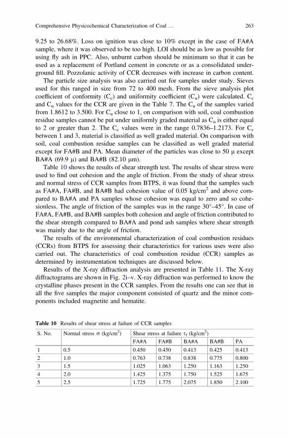
9.25 to 26.68%. Loss on ignition was close to 10% except in the case of FA#Asample, where it was observed to be too high. LOI should be as low as possible forusing fly ash in PPC. Also, unburnt carbon should be minimum so that it can beused as a replacement of Portland cement in concrete or as a consolidated under-ground fill. Pozzolanic activity of CCR decreases with increase in carbon content.
The particle size analysis was also carried out for samples under study. Sievesused for this ranged in size from 72 to 400 mesh. From the sieve analysis plotcoefficient of conformity (Cc) and uniformity coefficient (Cu) were calculated. Cc
and Cu values for the CCR are given in the Table 7. The Cu of the samples variedfrom 1.8612 to 3.500. For Cu close to 1, on comparison with soil, coal combustionresidue samples cannot be put under uniformly graded material as Cu is either equalto 2 or greater than 2. The Cc values were in the range 0.7836–1.2173. For Cc
between 1 and 3, material is classified as well graded material. On comparison withsoil, coal combustion residue samples can be classified as well graded materialexcept for FA#B and PA. Mean diameter of the particles was close to 50 l exceptBA#A (69.9 l) and BA#B (82.10 lm).
Table 10 shows the results of shear strength test. The results of shear stress wereused to find out cohesion and the angle of friction. From the study of shear stressand normal stress of CCR samples from BTPS, it was found that the samples suchas FA#A, FA#B, and BA#B had cohesion value of 0.05 kg/cm2 and above com-pared to BA#A and PA samples whose cohesion was equal to zero and so cohe-sionless. The angle of friction of the samples was in the range 30°–45°. In case ofFA#A, FA#B, and BA#B samples both cohesion and angle of friction contributed tothe shear strength compared to BA#A and pond ash samples where shear strengthwas mainly due to the angle of friction.
The results of the environmental characterization of coal combustion residues(CCRs) from BTPS for assessing their characteristics for various uses were alsocarried out. The characteristics of coal combustion residue (CCR) samples asdetermined by instrumentation techniques are discussed below.
Results of the X-ray diffraction analysis are presented in Table 11. The X-raydiffractograms are shown in Fig. 2i–v. X-ray diffraction was performed to know thecrystalline phases present in the CCR samples. From the results one can see that inall the five samples the major component consisted of quartz and the minor com-ponents included magnetite and hematite.
Table 10 Results of shear stress at failure of CCR samples
S. No. Normal stress r (kg/cm2) Shear stress at failure sf (kg/cm2)
FA#A FA#B BA#A BA#B PA
1 0.5 0.450 0.450 0.413 0.425 0.413
2 1.0 0.763 0.738 0.838 0.775 0.800
3 1.5 1.025 1.063 1.250 1.163 1.250
4 2.0 1.425 1.375 1.750 1.525 1.675
5 2.5 1.725 1.775 2.075 1.850 2.100
Comprehensive Physicochemical Characterization of Coal … 263
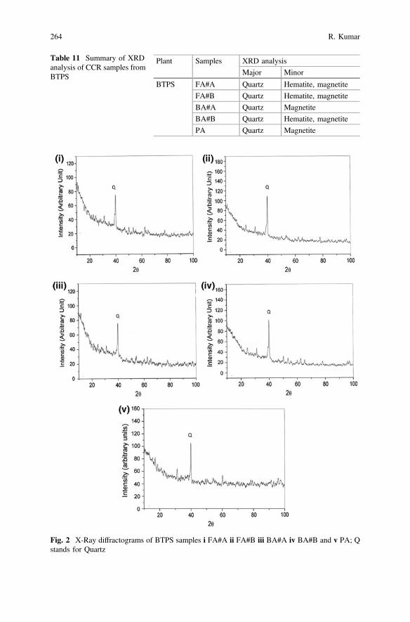
Table 11 Summary of XRDanalysis of CCR samples fromBTPS
Plant Samples XRD analysis
Major Minor
BTPS FA#A Quartz Hematite, magnetite
FA#B Quartz Hematite, magnetite
BA#A Quartz Magnetite
BA#B Quartz Hematite, magnetite
PA Quartz Magnetite
Fig. 2 X-Ray diffractograms of BTPS samples i FA#A ii FA#B iii BA#A iv BA#B and v PA; Qstands for Quartz
264 R. Kumar
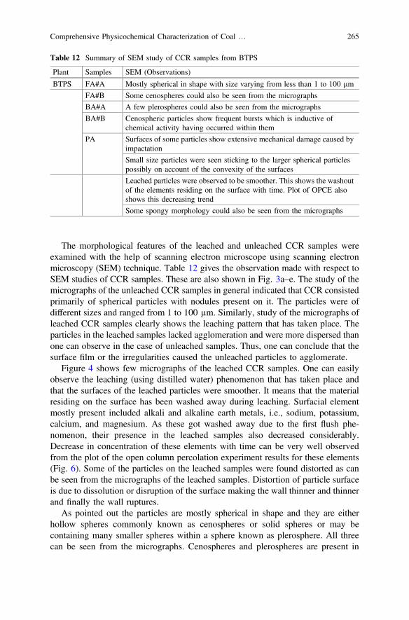
The morphological features of the leached and unleached CCR samples wereexamined with the help of scanning electron microscope using scanning electronmicroscopy (SEM) technique. Table 12 gives the observation made with respect toSEM studies of CCR samples. These are also shown in Fig. 3a–e. The study of themicrographs of the unleached CCR samples in general indicated that CCR consistedprimarily of spherical particles with nodules present on it. The particles were ofdifferent sizes and ranged from 1 to 100 µm. Similarly, study of the micrographs ofleached CCR samples clearly shows the leaching pattern that has taken place. Theparticles in the leached samples lacked agglomeration and were more dispersed thanone can observe in the case of unleached samples. Thus, one can conclude that thesurface film or the irregularities caused the unleached particles to agglomerate.
Figure 4 shows few micrographs of the leached CCR samples. One can easilyobserve the leaching (using distilled water) phenomenon that has taken place andthat the surfaces of the leached particles were smoother. It means that the materialresiding on the surface has been washed away during leaching. Surfacial elementmostly present included alkali and alkaline earth metals, i.e., sodium, potassium,calcium, and magnesium. As these got washed away due to the first flush phe-nomenon, their presence in the leached samples also decreased considerably.Decrease in concentration of these elements with time can be very well observedfrom the plot of the open column percolation experiment results for these elements(Fig. 6). Some of the particles on the leached samples were found distorted as canbe seen from the micrographs of the leached samples. Distortion of particle surfaceis due to dissolution or disruption of the surface making the wall thinner and thinnerand finally the wall ruptures.
As pointed out the particles are mostly spherical in shape and they are eitherhollow spheres commonly known as cenospheres or solid spheres or may becontaining many smaller spheres within a sphere known as plerosphere. All threecan be seen from the micrographs. Cenospheres and plerospheres are present in
Table 12 Summary of SEM study of CCR samples from BTPS
Plant Samples SEM (Observations)
BTPS FA#A Mostly spherical in shape with size varying from less than 1 to 100 lm
FA#B Some cenospheres could also be seen from the micrographs
BA#A A few plerospheres could also be seen from the micrographs
BA#B Cenospheric particles show frequent bursts which is inductive ofchemical activity having occurred within them
PA Surfaces of some particles show extensive mechanical damage caused byimpactation
Small size particles were seen sticking to the larger spherical particlespossibly on account of the convexity of the surfaces
Leached particles were observed to be smoother. This shows the washoutof the elements residing on the surface with time. Plot of OPCE alsoshows this decreasing trend
Some spongy morphology could also be seen from the micrographs
Comprehensive Physicochemical Characterization of Coal … 265
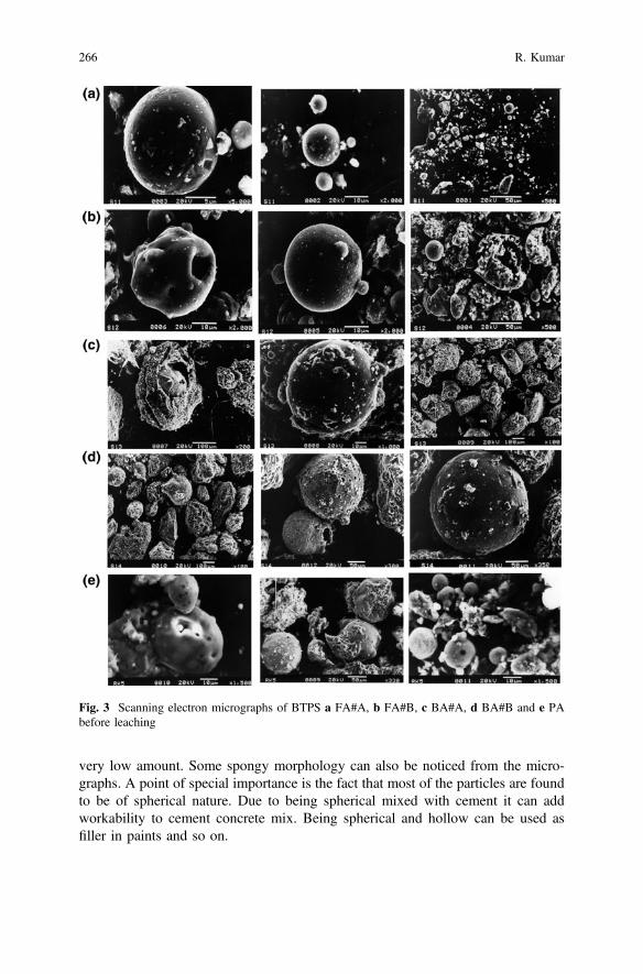
very low amount. Some spongy morphology can also be noticed from the micro-graphs. A point of special importance is the fact that most of the particles are foundto be of spherical nature. Due to being spherical mixed with cement it can addworkability to cement concrete mix. Being spherical and hollow can be used asfiller in paints and so on.
Fig. 3 Scanning electron micrographs of BTPS a FA#A, b FA#B, c BA#A, d BA#B and e PAbefore leaching
266 R. Kumar
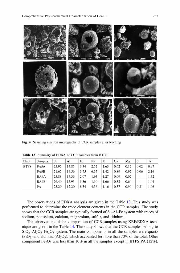
The observations of EDXA analysis are given in the Table 13. This study wasperformed to determine the trace element contents in the CCR samples. The studyshows that the CCR samples are typically formed of Si–Al–Fe system with traces ofsodium, potassium, calcium, magnesium, sulfur, and titinium.
The observations of the composition of CCR samples using XRF/EDXA tech-nique are given in the Table 14. The study shows that the CCR samples belong toSiO2–Al2O3–Fe2O3 system. The main components in all the samples were quartz(SiO2) and alumina (Al2O3), which accounted for more than 70% of the total. Othercomponent Fe2O3 was less than 10% in all the samples except in BTPS PA (12%).
Fig. 4 Scanning electron micrographs of CCR samples after leaching
Table 13 Summary of EDXA of CCR samples from BTPS
Plant Samples Si Al Fe Na K Ca Mg S Ti
BTPS FA#A 25.97 14.85 3.34 2.52 1.63 0.62 0.12 0.02 0.97
FA#B 21.67 14.56 3.75 6.35 1.42 0.89 0.92 0.06 2.16
BA#A 25.88 17.36 2.07 1.93 1.27 0.09 0.02 – 1.32
BA#B 26.40 15.93 1.36 1.10 1.66 0.32 0.64 – 1.04
PA 23.20 12.20 8.54 4.36 1.16 0.37 0.90 0.21 1.06
Comprehensive Physicochemical Characterization of Coal … 267
Minor amounts of CaO, K2O, MgO, TiO2, and SO3 were also observed in thesamples. There are fluctuations in the chemical composition of the samples mostlydue to the different mineral component in the parent coals. These fluctuations arealso related to the compositions of the parent rocks in the formation of peat and coaland also the plant species involved in the coal formation.
The observations of the qualitative analysis using XRF technique are also givenin the Table 15. From the results so obtained it can be seen that the major com-ponents in almost all the samples were iron, aluminum, silicon, titanium andpotassium. Minor components mainly included calcium, magnesium, zirconium,manganese and zinc. Common elements in the traces were barium, nickel, copper,rubidium, sulfur, phosphorus, yttrium and strontium.
The FTlR study showed that CCR samples collected from various plants showeda broad band due to the presence of O-H stretching. O-H stretching of CCRs wasbetween 3300 and 3611 cm−1. CCR samples of FCI alone showed a characteristicband due to the presence of carbonyl group. Oxides of phosphorus and oxides ofsilicon were also observed in all the samples. P-O bending was between 1079 and1084 cm−1. Table 16 gives the observations of the FTIR spectra of CCR samples.
Chemical Characterization
The coal combustion residue (CCR) samples from BTPS were analyzed for itsvarious chemical characteristics. The observation of the study is presented inTable 17. The five samples were analyzed for pH, electrical conductivity (EC),organic carbon, available nitrogen, phosphorus and potassium, cation exchange
Table 14 Summary of compositional analysis of CCR samples from BTPS
Plant Samples SiO2 Al2O3 Fe2O3 Na2O K2O CaO MgO SO3 TiO2
BTPS FA#A 55.56 28.06 4.78 3.40 1.96 0.86 0.20 0.05 1.61
FA#B 46.37 27.51 5.36 2.55 1.71 1.24 1.51 0.14 3.60
BA#A 55.37 32.79 2.95 2.60 1.53 0.13 0.03 – 2.19
BA#B 56.48 30.11 1.94 1.48 2.00 0.44 1.05 – 1.73
PA 49.63 23.05 12.21 5.87 1.40 0.52 1.50 – 1.77
Table 15 Summary of qualitative analysis of CCRs samples from BTPS
Plant Samples Major Minor Traces
BTPS FA#A Fe, Al, Si, Ti Ca, Mg, Zr Y, Sr, Rb, Zn, Cu, Ni, Mn, Cr, S, P
FA#B Fe, Al, Si, Ti, K Ca, Mg, Zr Y, Sr, Rb, Pb, Ga, Zn, Cu, Mn, Cr, S, P
BA#A Fe, Al, Si, Ti Ca, Mg, Zr, K Y, Sr, Rb, Pb, Ga, Zn, Cu, Mn, Cr, S, P
BA#B Fe, Al, Si, Ti, K Ca, Mg Zr, Sr, Rb, Ga, Zn, Cu, Ni, Mn, Cr, Ba, S, P, Y
PA Fe, Al, Si, Ti Ca, Mg, Zr, K Y, Sr, Rb, Ga, Zn, Cu, Ni, Mn, Cr, Ba, S, P
268 R. Kumar

Tab
le16
Summaryof
FTIR
analysisof
CCRsamples
from
BTPS
Vibratio
nsW.No.
(cm
−1 )
samples
O–H
(Str)
(3700–32
00)
>C=O
(173
5–17
10)
–C
=C–(A
r)(160
0–15
00)
P–O
(Str)
(1100–10
00)
Si–O–Si
(sym
.)(*
800)
Kaolin
ite(*
695)
P–O
(Bend.)
(600–50
0)Si–O–Si
(Defor)
(*46
0)
FA#A
3541
––
1085
796
–56
646
7
FA#B
3447
––
1086
795
–56
646
6
BA#A
––
–10
8479
6–
560
470
BA#B
3528
––
1085
796
–56
446
4
PA34
49–
–10
8479
4–
–45
4
Comprehensive Physicochemical Characterization of Coal … 269

capacity (CEC), calcium carbonate, ultimate analysis, and DTPA extractableelements.
The pH of the samples varied from 5.98 to 6.71. Electrical conductivity variedfrom 0.086 to 0.780 mmhos/cm. Organic carbon varied from 0.23 to 0.99%.Available nitrogen varied from 15.68 to 40.77 kg/ha. Available phosphorus andpotassium varied from 0.07 to 0.84 kg/ha and 188.16 to 448.00 kg/ha respectively.The cation exchange capacity (CEC) of the samples varied from 1.40 to39.65 meq/100 g. In all cases except pond ash CEC was below 5 meq/100 g.Calcium carbonate percentage was found to vary from 4.0 to 10.0%. Limerequirement test for the CCR was also done. As the pH of the buffer suspensionswas above the one given in the chart, no lime requirements were observed for thesample under study.
Table 17 Chemical properties of CCR samples from BTPS
Parameters Samples
FA#A FA#B BA#A BA#B PA
pH 6.08 6.12 5.98 6.43 6.71
Electrical conductivity (mmhos/cm) 0.780 0.381 0.186 0.136 0.086
Organic carbon (%) 0.72 0.23 0.48 0.50 0.99
Available nitrogen (kg/ha) 40.77 18.82 15.68 21.95 25.09
Available phosphorus (kg/ha) 0.47 0.15 0.07 0.24 0.84
Available potassium (kg/ha) 336.00 259.84 210.56 188.16 448.00
Cation exchange capacity (meq/100 g) 4.92 2.24 1.62 1.40 39.65
DTPA extractable elements (ppm)
Fe 0.048 BDL 0.084 0.032 12.496
Cu 1.556 0.822 0.866 0.790 0.488
Mn 0.688 0.128 BDL BDL 0.778
Zn 1.640 4.960 0.674 0.546 0.538
Pb 0.310 BDL 0.046 BDL 0.060
Ni 0.358 0.804 0.674 0.772 0.600
Cr BDL BDL BDL BDL BDL
Cd 0.192 0.162 BDL BDL BDL
Co 0.150 0.168 0.212 BDL 0.196
Ultimate analysis (%)
Carbon 10.97 8.93 11.34 6.59 6.30
Hydrogen – – – – 0.40
Sulfur 0.08 0.10 0.03 0.10 0.02
Nitrogen 0.47 0.13 0.43 0.09 0.29
Oxygen (by diff.) 88.48 90.84 88.20 93.22 92.99
270 R. Kumar
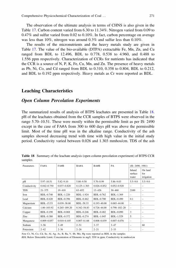
The observation of the ultimate analysis in terms of CHNS is also given in theTable 17. Carbon content varied from 6.30 to 11.34%. Nitrogen varied from 0.09 to0.47% and sulfur varied from 0.02 to 0.10%. In fact, carbon percentage on averagewas less than 10%, nitrogen was around 0.3% and sulfur less than 0.10%.
The results of the micronutrients and the heavy metals study are given inTable 17. The value of the bio-available (DTPA) extractable Fe, Mn, Zn, and Curanged from BDL to 12.496, BDL to 0.778, 0.538 to 4.960, and 0.488 to1.556 ppm respectively. Characterization of CCRs for nutrients has indicated thatthe CCR is a source of N, P, K, Fe, Cu, Mn, and Zn. The presence of heavy metalsas Pb, Ni, Co, and Cd ranged from BDL to 0.310, 0.358 to 0.804, BDL to 0.212,and BDL to 0.192 ppm respectively. Heavy metals as Cr were reported as BDL.
Leaching Characteristics
Open Column Percolation Experiments
The summarized results of analysis of BTPS leachates are presented in Table 18.pH of the leachates obtained from the CCR samples of BTPS were observed in therange 5.70–10.51. These were mostly within the permissible limit as per IS: 2490except in the case of FA#A from 300 to 600 days pH was above the permissiblelimit. Most of the time pH was in the alkaline range. Conductivity of the ashsamples showed decreasing trend with time with high value in the initial studyperiod. Conductivity varied between 0.026 and 1.303 mmhos/cm. TDS of the ash
Table 18 Summary of the leachate analysis (open column percolation experiment) of BTPS CCRsamples
Parameters FA#A FA#B BA#A BA#B PA (IS: 2490, 1981)
Inlandsurfacewater
On landforirrigation
pH 5.97–10.51 5.82–9.10 5.80–9.50 5.70–8.99 5.86–9.03 5.5–9.0 5.5–9.0
Conductivity 0.042–0.750 0.037–0.820 0.125–1.303 0.026–0.852 0.052–0.920 – –
TDS 21–375 19–410 63–652 13–426 30–460 2100 –
Iron BDL–0.740 BDL–1.220 BDL–1.924 BDL–0.762 BDL–1.369 – –
Lead BDL–0.420 BDL–0.396 BDL–0.462 BDL–0.700 BDL–0.490 0.1 –
Magnesium BDL–15.53 0.039–38.00 BDL–58.33 0.193–40.00 0.065–44.00 – –
Calcium 1.00–103.92 0.265–189.20 0.342–54.83 0.726–44.00 0.798–102–20 – –
Copper BDL–0.190 BDL–0.068 BDL–0.246 BDL–0.482 BDL–0.090 3 –
Zinc BDL–0.380 BDL–0.372 BDL–0.274 BDL–1.045 BDL–1.529 5 –
Manganese 0.009–0.057 0.010–0.105 0.007–0.148 0.008–0.039 0.007–0.076 – –
Sodium 3–56 3–49 2–51 3–37 3–47 – 60
Potassium 2–42 2–36 2–26 2–21 2–33 – –
Note Cr, Ni, Co, Cd, Se, Al, Ag, As, B, Ba, V, Sb, Mo, Hg were reported as BDL in the samplesBDL Below Detectable Limit; Concentration of Elements in mg/l; TDS in ppm; Conductivity in mmhos/cm
Comprehensive Physicochemical Characterization of Coal … 271
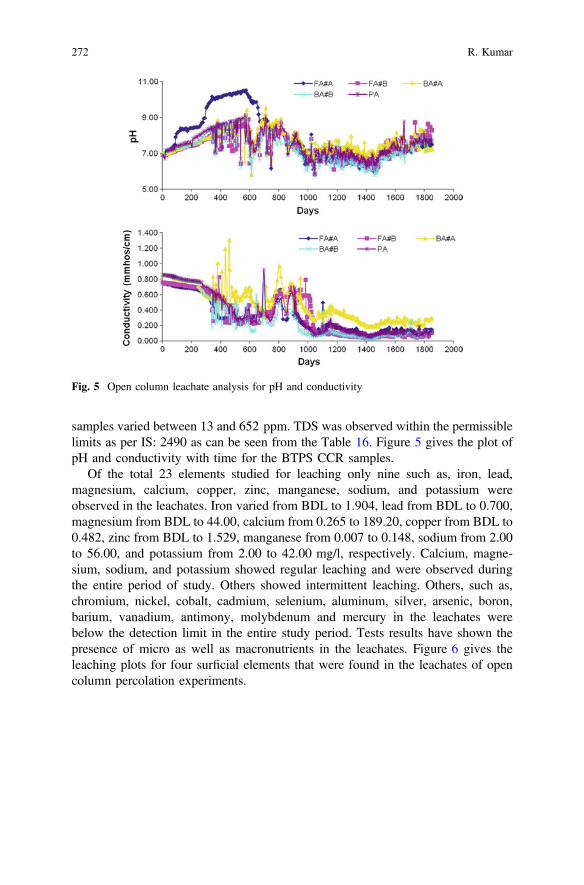
samples varied between 13 and 652 ppm. TDS was observed within the permissiblelimits as per IS: 2490 as can be seen from the Table 16. Figure 5 gives the plot ofpH and conductivity with time for the BTPS CCR samples.
Of the total 23 elements studied for leaching only nine such as, iron, lead,magnesium, calcium, copper, zinc, manganese, sodium, and potassium wereobserved in the leachates. Iron varied from BDL to 1.904, lead from BDL to 0.700,magnesium from BDL to 44.00, calcium from 0.265 to 189.20, copper from BDL to0.482, zinc from BDL to 1.529, manganese from 0.007 to 0.148, sodium from 2.00to 56.00, and potassium from 2.00 to 42.00 mg/l, respectively. Calcium, magne-sium, sodium, and potassium showed regular leaching and were observed duringthe entire period of study. Others showed intermittent leaching. Others, such as,chromium, nickel, cobalt, cadmium, selenium, aluminum, silver, arsenic, boron,barium, vanadium, antimony, molybdenum and mercury in the leachates werebelow the detection limit in the entire study period. Tests results have shown thepresence of micro as well as macronutrients in the leachates. Figure 6 gives theleaching plots for four surficial elements that were found in the leachates of opencolumn percolation experiments.
Fig. 5 Open column leachate analysis for pH and conductivity
272 R. Kumar
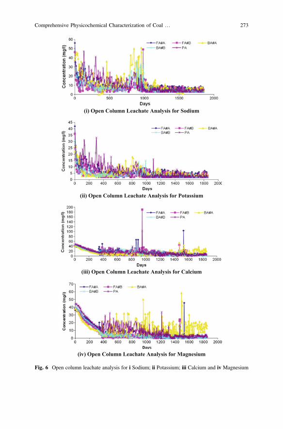
(iii) Open Column Leachate Analysis for Calcium
(iv) Open Column Leachate Analysis for Magnesium
(i) Open Column Leachate Analysis for Sodium
(ii) Open Column Leachate Analysis for Potassium
Fig. 6 Open column leachate analysis for i Sodium; ii Potassium; iii Calcium and iv Magnesium
Comprehensive Physicochemical Characterization of Coal … 273
Acid Digest Test
The summarized results of analysis of BTPS leachates are presented in Table 19. Ofthe total 23 elements studied for leaching only eleven such as, iron, lead, magne-sium, calcium, copper, zinc, manganese, sodium, potassium chromium and nickel,were observed in the leachates. Iron varied from 52.39 to 613.60, lead from BDL to0.017, magnesium from 3.127 to 29.246, calcium from 2.80 to 25.50, copper from0.068 to 0.359, zinc from 0.073 to 0.739, manganese from 0.638 to 1.329, sodiumfrom 2.10 to 28.10, potassium from 1.70 to 13.50, chromium from BDL to 2.836and nickel from 0.070 to 0.483 mg/l, respectively. Others, such as, cobalt, cad-mium, selenium, aluminum, silver, arsenic, boron, barium, vanadium, antimony,molybdenum, and mercury in the leachates was below the detection limit in theentire study period. Tests results have shown the presence of micro as well asmacronutrients in the leachates. Chromium and nickel were also observed in theleachate of acid digest test.
24-h Shake Test
The summarized results of analysis of BTPS leachates obtained from 24-h Shaketest are presented in Table 20. pH of the leachates obtained from the CCR samplesof BTPS were observed in the range 5.47–6.38. This was within the permissiblelimit as per IS: 2490. pH was in the neutral range. Conductivity varied between
Table 19 Summary of the leachate analysis (acid digest test) of BTPS CCR samples
Parameters FA#A FA#B BA#A BA#B PA (IS: 2490, 1981)
Inlandsurfacewater
On landforirrigation
Iron 52.39 82.41 79.56 152.90 613.60 – –
Lead BDL BDL 0.017 BDL BDL 0.1 –
Magnesium 3.127 3.579 8.253 9.591 29.246 – –
Calcium 2.80 4.00 8.80 6.50 25.50 – –
Copper 0.075 0.094 0.068 0.077 0.359 3 –
Zinc 0.203 0.276 0.154 0.073 0.739 5 –
Manganese 0.984 0.638 0.796 1.329 0.906 – –
Sodium 28.10 24.60 25.00 25.40 2.10 – 60
Potassium 1.7 7.6 5.2 7.0 13.5 – –
Chromium BDL 0.760 BDL 0.375 2.836 2 –
Nickel 0.108 0.118 0.173 0.070 0.483 3 –
Note Co, Cd, Se, Al, Ag, As, B, Ba, V, Sb, Mo, Hg were reported as BDL in the samplesBDL Below Detectable Limit; Concentration of Elements in mg/l; TDS in ppm; Conductivity inmmhos/cm
274 R. Kumar
0.041 and 0.198 mmhos/cm. TDS of the ash samples varied between 20 and99 ppm. TDS was observed within the permissible limits as per IS: 2490 as can beseen from the Table 18.
Of the total 23 elements studied for leaching only seven, such as, iron, mag-nesium, calcium, zinc, manganese, sodium, and potassium were observed in theleachates. Iron varied from 0.045 to 0.216, magnesium from 0.92 to 13.19, calciumfrom 0.42 to 6.34, zinc from 0.010 to 0.032, manganese from BDL to 0.031,sodium from 6.20 to 72.80, and potassium from 1.70 to 4.50 mg/l, respectively.Others, such as, lead, copper, chromium, nickel, cobalt, cadmium, selenium, alu-minum, silver, arsenic, boron, barium, vanadium, antimony, molybdenum andmercury in the leachates were observed to be below the detection limit. Tests resultlike open column percolation experiments indicates the presence of micro as well asmacronutrients in the leachates.
Toxicity Characteristic Leachate Procedure (TCLP)
The summarized results of analysis of BTPS leachates collected through TCLP testare presented in Table 21. pH of the leachates obtained from the CCR samples ofBTPS were observed in the range 4.25–5.08. Conductivity varied between 3.56 and4.54 mS/cm. TDS of the ash samples varied between 1.78 and 2.27 ppt. Both
Table 20 Summary of the leachate analysis (ASTM 24-h shake test) of BTPS CCR samples
Parameters FA#A FA#B BA#A BA#B PA (IS: 2490, 1981)
Inlandsurfacewater
On landforirrigation
pH 5.67 6.22 6.38 6.06 5.47 5.5–9.0 5.5–9.0
Conductivity 0.198 0.096 0.054 0.041 0.084 – –
TDS 99 48 27 21 42 2100 –
Iron 0.071 0.045 0.096 0.216 0.155 – –
Lead BDL BDL BDL BDL BDL 0.1 –
Magnesium 13.19 3.15 1.28 0.92 2.14 – –
Calcium 6.34 3.37 1.64 0.42 2.67 – –
Copper BDL BDL BDL BDL 0.014 3 –
Zinc 0.032 0.020 0.010 0.011 0.044 5 –
Manganese BDL 0.031 BDL BDL BDL – –
Sodium 64.30 39.80 72.80 72.70 6.20 – 60
Potassium 4.50 2.80 1.80 1.70 3.76 – –
Note Cr, Ni, Co, Cd, Se, Al, Ag, As, B, Ba, V, Sb, Mo, Hg were reported as BDL in the samplesBDL Below Detectable Limit; Concentration of Elements in mg/l; TDS in ppm; Conductivity inmmhos/cm
Comprehensive Physicochemical Characterization of Coal … 275

conductivity and TDS was observed at a higher level as can be seen from theTable 19.
Of the total 23 elements studied for leaching only ten, such as, iron, magnesium,calcium, copper, zinc, manganese, sodium, potassium, chromium and nickel wereobserved in the leachates. Iron varied from 0.022 to 0.089, magnesium from 4.850to 61.020, calcium from 304.13 to 506.00, copper from 0.021 to 0.215, zinc from0.670 to 2.140, manganese from 0.201 to 0.791, sodium from 1452 to 1857,potassium from 6.2 to 11.88, chromium from BDL to 0.803, and nickel from BDLto 1.819 mg/l, respectively. Others, such as, lead, cobalt, cadmium, selenium,aluminum, silver, arsenic, boron, barium, vanadium, antimony, molybdenum, andmercury in the leachates were below the detection limit. The study has indicatedthat the leachates had higher concentration of sodium, calcium, and magnesium inall the four samples.
Table 21 Summary of the leachate analysis (TCLP test) of BTPS CCR samples
Parameters FA#A FA#B BA#A BA#B PA (IS: 2490, 1981)
Inlandsurfacewater
On landforirrigation
pH 4.30 4.29 4.25 4.28 5.08 5.5–9.0 5.5–9.0
Conductivity 4.46 3.56 4.18 4.23 4.54 – –
TDS 2.24 1.78 2.10 2.12 2.27 2100 –
Iron 0.077 0.089 0.022 0.053 0.037 – –
Lead BDL BDL BDL BDL BDL 0.1 –
Magnesium 61.020 7.512 5.831 4.850 8.317 – –
Calcium 379.37 304.13 314.93 416.48 506.00 – –
Copper 0.030 0.215 0.078 0.021 0.047 3 –
Zinc 0.799 2.140 1.950 1.280 0.670 5 –
Manganese 0.791 0.314 0.220 0.226 0.201 – –
Sodium 1857 1452 1508 1595 1575 – 60
Potassium 11.60 8.10 7.80 6.20 11.88 – –
Chromium BDL 0.803 0.414 BDL BDL 2 –
Nickel 0.381 0.112 1.819 0.080 BDL 3 –
Note Co, Cd, Se, Al, Ag, As, B, Ba, V, Sb, Mo, Hg were reported as BDL in the samplesBDL Below Detectable Limit; Concentration of Elements in mg/l; TDS in ppt; Conductivity inmS/cm
276 R. Kumar
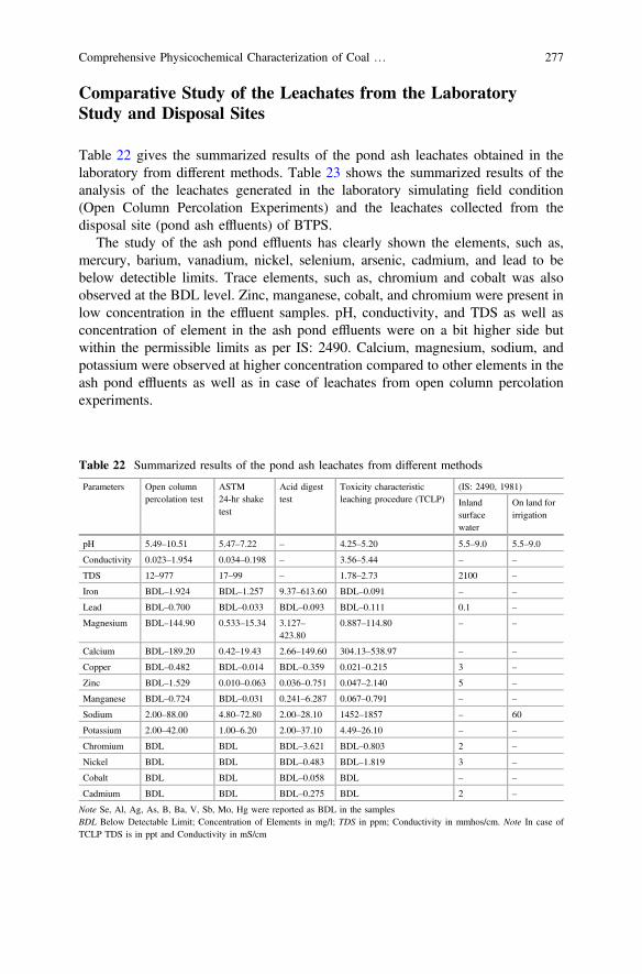
Comparative Study of the Leachates from the LaboratoryStudy and Disposal Sites
Table 22 gives the summarized results of the pond ash leachates obtained in thelaboratory from different methods. Table 23 shows the summarized results of theanalysis of the leachates generated in the laboratory simulating field condition(Open Column Percolation Experiments) and the leachates collected from thedisposal site (pond ash effluents) of BTPS.
The study of the ash pond effluents has clearly shown the elements, such as,mercury, barium, vanadium, nickel, selenium, arsenic, cadmium, and lead to bebelow detectible limits. Trace elements, such as, chromium and cobalt was alsoobserved at the BDL level. Zinc, manganese, cobalt, and chromium were present inlow concentration in the effluent samples. pH, conductivity, and TDS as well asconcentration of element in the ash pond effluents were on a bit higher side butwithin the permissible limits as per IS: 2490. Calcium, magnesium, sodium, andpotassium were observed at higher concentration compared to other elements in theash pond effluents as well as in case of leachates from open column percolationexperiments.
Table 22 Summarized results of the pond ash leachates from different methods
Parameters Open columnpercolation test
ASTM24-hr shaketest
Acid digesttest
Toxicity characteristicleaching procedure (TCLP)
(IS: 2490, 1981)
Inlandsurfacewater
On land forirrigation
pH 5.49–10.51 5.47–7.22 – 4.25–5.20 5.5–9.0 5.5–9.0
Conductivity 0.023–1.954 0.034–0.198 – 3.56–5.44 – –
TDS 12–977 17–99 – 1.78–2.73 2100 –
Iron BDL–1.924 BDL–1.257 9.37–613.60 BDL–0.091 – –
Lead BDL–0.700 BDL–0.033 BDL–0.093 BDL–0.111 0.1 –
Magnesium BDL–144.90 0.533–15.34 3.127–423.80
0.887–114.80 – –
Calcium BDL–189.20 0.42–19.43 2.66–149.60 304.13–538.97 – –
Copper BDL–0.482 BDL–0.014 BDL–0.359 0.021–0.215 3 –
Zinc BDL–1.529 0.010–0.063 0.036–0.751 0.047–2.140 5 –
Manganese BDL–0.724 BDL–0.031 0.241–6.287 0.067–0.791 – –
Sodium 2.00–88.00 4.80–72.80 2.00–28.10 1452–1857 – 60
Potassium 2.00–42.00 1.00–6.20 2.00–37.10 4.49–26.10 – –
Chromium BDL BDL BDL–3.621 BDL–0.803 2 –
Nickel BDL BDL BDL–0.483 BDL–1.819 3 –
Cobalt BDL BDL BDL–0.058 BDL – –
Cadmium BDL BDL BDL–0.275 BDL 2 –
Note Se, Al, Ag, As, B, Ba, V, Sb, Mo, Hg were reported as BDL in the samplesBDL Below Detectable Limit; Concentration of Elements in mg/l; TDS in ppm; Conductivity in mmhos/cm. Note In case ofTCLP TDS is in ppt and Conductivity in mS/cm
Comprehensive Physicochemical Characterization of Coal … 277

In general, leachates of open column percolation experiment and ash pondeffluents do not pose any environmental threat as far as leaching of traceelements/toxic metals are concerned. Results of open column percolation experi-ment and ash pond effluents are comparable as can be seen from the Tables 20 and21. Open column percolation methodology can very well be relied upon for thelong-term leaching study of CCRs compared to other methodologies discussedabove. This is the best method that simulates the actual field condition, as onewould observe in the field.
Conclusion
The study of physical properties of CCR samples has shown the suitability of thematerial like sand and thus these can be used as alternatives of sand for mine fills.The chemical characteristics of CCR samples have also established that the samplesare sources of nutrients and that if these samples are used in soil having suchdeficiencies then the problems can be solved. Further leaching studies have tried toremove the apprehensions to a greater extent regarding contamination of groundand surface water due to trace/heavy element leaching. Both short term andlong-term leaching study have been conducted simulating the field situation tounderstand the behaviour of disposed CCR samples and its effects on ground andsurface water. The study of effluents collected from the ash pond site that wasgetting into the surface stream was also carried out to compare the actual results
Table 23 Summary of the leachate analysis of pond ashes
Parameters BTPS (IS: 2490, 1981)
OPEC forpond ash
Ash pond effluents(disposal site)
Inland surfacewater
On land forirrigation
pH 5.86–9.03 6.97–8.97 5.5–9.0 5.5–9.0
Conductivity 0.052–0.920 0.549–0.897 – –
TDS 30–460 275–449 2100 –
Iron BDL–1.369 0.113–3.634 – –
Lead BDL–0.490 BDL–0.158 0.1 –
Magnesium 0.065–44.00 0.077–55.00 – –
Calcium 0.798–102–20 3.265–117.30 – –
Copper BDL–0.090 0.019–0.107 3 –
Zinc BDL–1.529 0.765–1.754 5 –
Manganese 0.007–0.076 BDL–0.083 – –
Sodium 3.00–47.00 5.00–37.00 – 60
Potassium 2.00–33.00 4.00–53.00 – –
Note Cr, Ni, Co, Cd, Se, Al, Ag, As, B, Ba, V, Sb, Mo, Hg were reported as BDL in the samplesBDL Below Detectable Limit; Concentration of Elements in mg/l; TDS in ppm; Conductivity inmmhos/cm
278 R. Kumar
with the simulated one to establish the validity of laboratory study. Effect of harshcondition such as leaching in acidic and acid buffered environment which was leastlikely to encounter in the actual field situation was also done to study the mobilityof some other elements. The concentration of trace and heavy elements was foundto be well below the permissible limits as per IS: 2490. Overall, the study hasshown no environmental hazards due to leaching and that these can be used for theirbulk utilization especially for reclamation of mined out areas in and around thevicinity of the power plant under study.
Acknowledgements The author is greatly thankful to the authorities of Bokaro Thermal PowerStation for their full co-operation throughout the period of study. The author is also thankful to theDirector, Indian School of Mines for his kind permission to work in the College. The author is alsoindebted to the Director, Central Institute of Mining and Fuel Research for his kind permission forsending this paper for publication. Lastly, the author is also grateful to IIT, Kharagpur forSEM-EDXA and XRD analysis; Indian School of Mines, Dhanbad for XRF and FTIR analysis andcolumn studies; and Indian Institute of Cultivation Science, Kolkata for CHNS analysis of CCRsamples.
References
Ahmad MdA, Shahnawaz Md, Siddiqui MdF, Khan ZH (2014) A statistical review on the currentscenario of generation and utilization of fly-ash in India. Int J Curr Eng Technol 4(4):2434–2438
All India Installed Capacity of Thermal Power Stations: CEA Report. December (2015) Retrievedfrom http://www.cea.nic.in/reports/monthly/installedcapacity/2015/installed_capacity-12.pdf.Accessed on 30 Jan 2016
BP (2015) BP statistical review of world energy—June 2015. Retrieved from http://www.bp.com/content/dam/bp/excel/energy-economics/statistical-review-2015/bp-statistical-review-of-world-energy-2015-workbook.xlsx. Accessed on 30 Jan 2016
CEA (Central Electricity Authority). Annual Report (2012–2013). Retrieved from www.cea.nic.inCEA (Central Electricity Authority). Annual Report 2010/11, 2011/12, 2012/2013. Retrieved from
www.cea.nic.inCEA (Central Electricity Authority). Annual Report 2011/12, 2012/2013, 2014/15. Retrieved from
www.cea.nic.inCoal Reserves in India as on 01.04.2014. Retrieved from http://www.mcl.gov.in/Others/
ecoalfields.php. Accessed on 30 Apr 2016Coal Reserves Retrieved from www.coal.nic.in/content/coal-reserves. Accessed on 29 Jan 2016Dhadse S, Kumari P, Bhagia LJ (2008) Fly ash characterization, Utilization and government
initiatives in India—a review. J Sci Indus Res 67:11–18Garg P (2012) Energy scenario & vision 2020 in India. J Sustain Energy Environ 3:7–17Haque MdE (2013) Indian fly ash: production and consumption scenario. Int J Waste Res 3(1):22–
25Kumar V (2003) Management of fly ash in India: a perspective. 3rd international conference—fly
ash utilisation and disposal, New Delhi, India, 19–21 Feb 2003Kumar R (2009) Environmental assessment of coal combustion residues from a few thermal power
stations. PhD Thesis, Indian School of Mines, Dhanbad, IndiaKumar V, Mathur M (2005) Fly ash in roads and embankments. National Seminar and Business
Meet in use of Fly Ash in Roads and Embankments, Allahabad, June, 3–15
Comprehensive Physicochemical Characterization of Coal … 279

List of Thermal Power Stations in India up to 2016. Retrieved from http://cbrienvis.nic.in/Thermal.Power Station in India 2016.pdf. Accessed on 24 July 2017
Maiti SK (2001) Handbook of methods in environmental studies vol 1 Water and WastewaterAnalysis
Ministry of Power (MoP), Annual Report (2008) Retrieved from powermin.nic.inMinistry of Power (MoP) (2015) Retrieved from www.powermin.nic.in/overview-0. Accessed on
26 May 2015Mishra UC (2004) Environmental impact of coal industry and thermal power plants in India.
J Environ Radioact 72(1–2):35–40TEDDY (TERI Energy Data, Directory and Yearbook) 2014/15. Annual Report 2014/15TEDDY (TERI Energy Data, Directory and Yearbook). Annual Report 2003/04, 2004/05,
2005/06, 2009, 2014/15Zamuda CD, Sharpe MA (2007) A case for enhanced use of clean coal in India: an essential step
towards energy security and environmental protection. Workshop on coal beneficiation andutilization of rejects, Ranchi, Jharkhand, India, 22–24 Aug
280 R. Kumar
Influence of Semi-arid Climateon Characterization of DomesticWastewater
Vinod Kumar Tripathi and Pratibha Warwade
Abstract Rapid urbanization causes increase in urban population. Over half of theworld’s population lives in cities. By 2050, seven out of every 10 people will becity dwellers. India is a part of this global trend. Nearly 28% of India’s populationlives in cities and this is expected to increase to 41% by the year 2020. Urbanpopulation will generate huge amount of domestic wastewater (WW). Thepromising alternative for disposal of wastewater is its utilization for irrigation aftertreatment. To utilize domestic wastewater, it is vital to generate the informationabout of different quality parameters and their variations due to seasonal weatherconditions. Physiochemical water quality parameters (EC, pH, turbidity, totalsolids, NH4–N, NO3–N, P, K, Na, Ca, Mg, CO3, HCO3 and heavy metals (Cu, Zn,Mn, Fe, Cr, Mo) of domestic wastewater were determined for the period of oneyear. The data set is used to present spatial and temporal variations of the domesticwastewater quality. Identification of wastewater quality parameters responsible fortemporal variations due to effect of semi-arid climate was done through multivariatecluster analysis. Correlation study between the identified parameters was alsoconducted. Wastewater was slightly acidic in nature with mean value of pH 6.87.Highest concentration was observed for total solids. Concentration of ammoniacalnitrogen was higher than nitrate nitrogen; similarly bicarbonate concentration washigher in comparison to carbonate concentration. In the category of heavy metalshighest concentration with mean value 0.98 mg l−1 was observed with iron andleast with molybdenum with mean value 0.01 mg l−1. Most of the water qualityparameters concentration was higher during summer season, moderate duringwinter season and least during rainy season. Correlation study between qualityparameters shows the presence of bicarbonate with calcium and magnesium.
V.K. TripathiDepartment of Farm Engineering, Institute of Agricultural Sciences, BHU,Varanasi, Indiae-mail: [email protected]
P. Warwade (&)Centre for Water Engineering and Management, Central University of Jharkhand,Ranchi, Indiae-mail: [email protected]
© Springer Nature Singapore Pte Ltd. 2018V.P. Singh et al. (eds.), Environmental Pollution, Water Scienceand Technology Library 77, https://doi.org/10.1007/978-981-10-5792-2_23
281
Presence of calcium, magnesium and bicarbonate play important role for thequantum of total solids in domestic wastewater. Wastewater quality was under safelimit throughout the year in terms of irrigation water quality indices SAR andMg/Ca ratio. But it was under safe to moderate limit in terms of residual sodiumcarbonate (RSC) index. Cluster analysis divides the months of a complete year inthree clusters. First cluster have six months (July, August, September, October,November and December), second cluster have four months (January, February,March and April) and third cluster have two months (May and June).
Introduction
Worldwide unsystematic and untreated disposal of wastewater is the biggestchallenge to environmental scientist and engineers. This problem started long backbut intensified during the last few decades, and now the situation has becomealarming in India (Girija et al. 2007). During the past three decades, the effects ofdomestic wastewater and effluents, the point source pollution, on the water qualityof canals, streams and rivers have received some attention but very little attentionhas been reported about the sewage water quality of the receiving water bodies. Theinput of large quantities of nutrients mainly nitrates and phosphates into river waterscaused eutrophication and its related effects (House and Denison 1997). Thesenutrients particularly phosphorus is often the limiting nutrient in such systems (Nealet al. 2002). Sewage effluent containing sulphate may produce hydrogen sulphidethat in the form of sulphur is poisonous; so the untreated sewage should be treatedin the sewage treatment plant (STP) before letting into the receiving water bodies.
Rapid trend of global urbanization causes wastewater generation to the tune of38254 Million Litre Per Day (MLD) from Class I cities and Class II towns of India(CPCB 2005). Wastewater is a mixture of domestic effluent consisting of black-water (excreta, urine and fecal sludge, i.e. toilet wastewater), grey water (kitchenand bathing wastewater), water from commercial establishments and institutions,hospitals, industrial effluent. Contribution of different sources, water utilized inthose sources affects the quality of wastewater. Its quality in drain is dependentupon rainfall, soil properties, agricultural activities, exploitation of water resourcesand kind of industries. The quantitative contribution of different sources also affectsthe quality of mixed wastewater. The indiscriminate release of sewage has severelydeteriorated the aquatic environment leading nutrient enrichment of the receivingwater body (Akpan 2004), affecting environment health worldwide. Indian riversand canals especially in their urban portions are grossly polluted due to release ofdomestic and industrial wastewater (CPCB 2005; Girija et al. 2007).
Worldwide wastewater is emerging as an alternative water resource for irriga-tion. The main driving forces for the growth of wastewater irrigation are globalscarcity of freshwater resources with the problem of wastewater disposal. Estimateson the extent of this practice range widely, but figures point at about 20 million ha
282 V.K. Tripathi and P. Warwade

of land irrigated in this way, most of it in Asia, Latin America and sub-SaharanAfrica (Keraita et al. 2008). In the world more than 4–6 million hectares (M ha) areirrigated with wastewater or polluted water (Jimenez and Asano 2008; UNHSP2008). A separate estimate indicates 20 million ha globally, an area that is nearlyequivalent to 7% of the total irrigated land in the world (WHO 2006). Thewastewater for irrigation poses risk to the environment and endangering the healthof the farmers and produce consumers.
Studies on water quality in Indian rivers receiving municipal sewage andeffluents have been carried out by many earlier investigators, e.g. River Ganga(Sinha et al. 1991) and Kathajodi River in Cuttack city in Orissa (Das and Acharya2003; Girija et al. 2007) also reported the water quality assessment of an urbanstream polluted with untreated effluents at Guwahati in Assam (India). The presentstudy assessed the seasonal effects of point source pollution, untreated and treatedsewage on the water quality parameters. It is imperative to characterize domesticwastewater resources on the basis of physiochemical properties with respect to timefor effective pollution control and better water resource management. This results inhuge and complex data matrix comprised of a large number of physiochemicalparameters, which are often difficult to interpret and draw meaningful conclusions(Dixon and Chiswell 1996).
In the present paper, physiochemical water quality parameters of domesticwastewater were determined. The data set is used to present spatial and temporalvariations of the domestic wastewater quality. Identification of wastewater qualityparameters responsible for temporal variations due to effect of semi-arid climatewas done through multivariate cluster analysis.
Materials and Methods
Study Area
Study was conducted at Indian Agricultural Research Institute (IARI), Pusa, NewDelhi, India, which is located within 28° 37′ 22″N and 28° 39′N latitude and77° 8′ 45″E and 77° 10′ 24″E longitude covering an area of about 475 ha at anaverage elevation of 230 m above mean sea level. On east side Arawali rangeindicates the highest point while on western side natural drain forms the lastwestern boundary of the farm. Soil of the research farm is alluvial in origin andsandy loam in texture (Typic mixed hypothermic ustocrept). Water table in the farmarea is about 5–7 m (Natrajan et al. 2004). The climate of IARI is subtropical,semi-arid with hot dry summer and cold winter and the area falls inAgro-eco-region-IV (Semi-arid with alluvium derived soil). The mean annualtemperature is 24 °C with months of May and June having 30 years normalmaximum of 40 °C, and January with the normal minimum temperature of 14 °C.The minimum temperature dips as low as 1 °C. The mean annual rainfall is710 mm of which as much as 75% is received during the monsoon season (July to
Influence of Semi-arid Climate on Characterization … 283

September). The domestic wastewater samples were collected from natural drainpassing through IARI near the western boundary. The contribution of wastewater inthis drain is urban runoff and domestic effluent from group housing and hostels.
Water Sampling and Preservation
Domestic wastewater samples were collected from the drains in each month duringthe study period (January to December, 2009). Collection of wastewater samplesfrom the drain was done across the drain at the depth of 15 cm below the surfaceand at three points then mixed. The preservation and transportation was performedaccording to the standard methods (APHA 2005).
Analysis of Wastewater Samples
Wastewater samples were analyzed for the level of pH, electrical conductivity (EC),total solids (dissolved and undissolved), turbidity, total soluble salts (TSS),ammoniacal nitrogen (NH4–N), nitrate nitrogen (NO3–N), phosphate (P), potassium(K), sodium (Na+), calcium (Ca2+), magnesium (Mg2+), carbonate (CO3
−), bicar-bonate (HCO3
−), copper (Cu), zinc (Zn), manganese (Mn), iron (Fe), chromium(Cr) and molybdenum (Mo). All the water quality parameters were expressed inmilligram per litre (mg l−1), except EC (dS m−1). To prepare all the reagents ana-lytical grade chemicals and double glass distilled deionized water were used duringanalysis. The glassware was washed with dilute nitric acid followed by distilledwater. Using few water quality parameters temporal variation in three indicesnamely sodium adsorption ratio (SAR), residual sodium carbonate (RSC) andMg/Ca ratio were estimated. SAR and RSC were estimated using Eqs. 1 and 2.
SAR ¼ Naþ
Ca2þ þMg2þ
2
� �1=2 ð1Þ
RSC mel�1� � ¼ CO2�3 þHCO�
3
� �� Ca2þ þMg2þ� � ð2Þ
Statistical Analysis
Descriptive statistical parameters were analyzed for domestic wastewater qualityparameters. To get the range of any quality parameter minimum and maximumvalues were analyzed. On the basis of total values for a particular parameter
284 V.K. Tripathi and P. Warwade
arithmetic mean was also determined. To estimate statistical dispersions from meanof any quality data standard deviation and standard error was calculated using MSExcel spread sheet.
Cluster Analysis
Clustering is a multivariate technique of grouping rows together that share similarvalues. It can use any number of variables. The variables must be numeric for whichnumerical differences makes sense. The identification of these clusters goes a longway towards characterizing the distribution of values. Hierarchical agglomerativeclustering (a combining process) was applied on entire parameters of water quality.The method starts with each point (row) as its own cluster. At each step theclustering process calculates the distance between each cluster (monthly, row) andcombines the two clusters (month) that are closest together. This combining con-tinues until all the points (month) are in one final cluster. The number of clusterscan be chosen that seems right and cuts the clustering tree at a given point. Thecombining record is portrayed as a tree, called a dendrogram, with the single pointsas leaves, the final single cluster of all points as the trunk, and the intermediatecluster combinations as branches.
Results and Discussion
Physiochemical Properties of Domestic Wastewater
Descriptive statistics (minimum, maximum, mean, standard deviation and standarderror) of WW quality for 20 parameters is presented in Table 1. Maximum electricalconductivity (EC) 1.90 dS m−1 was observed with small standard error (SE) asshown in Table 1. pH is the indicator of acidic and alkaline condition of waterstatus. pH was in the range of 6.6–7.32 with the mean of 6.87. It shows the acidicnature of WW. A pH range of 6.5–8.5 is recommended by BIS (1986) and CPCB(2005) for irrigation purpose. Maximum standard deviation of 211 mg l−1 andstandard error of 60.90 was observed for total solids. Maximum and minimumvariation was also higher with total solids. It may be due to presence of morecontaminants like heavy metals and soil particles from the drains. Turbidity of WWwas high and in the range of 33–68 NTU. The higher turbidity of WW was due topresence of surface runoff and foreign particles from anthropogenic pollution andstream bed material.
Sodium content in WW was in the range of 109–226 mg l−1. Ammoniacalnitrogen (NH4–N) in WW was observed in the range of 19.7–37.5 mg l−1 butnitrate nitrogen (NO3–N) was in the range of 3.19–8.31 mg l−1. Higher content of
Influence of Semi-arid Climate on Characterization … 285
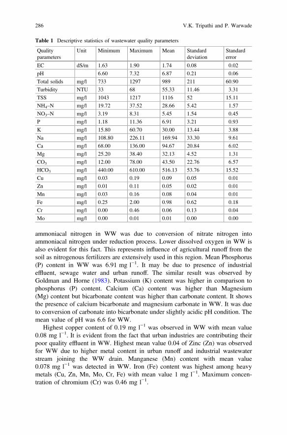
ammoniacal nitrogen in WW was due to conversion of nitrate nitrogen intoammoniacal nitrogen under reduction process. Lower dissolved oxygen in WW isalso evident for this fact. This represents influence of agricultural runoff from thesoil as nitrogenous fertilizers are extensively used in this region. Mean Phosphorus(P) content in WW was 6.91 mg l−1. It may be due to presence of industrialeffluent, sewage water and urban runoff. The similar result was observed byGoldman and Horne (1983). Potassium (K) content was higher in comparison tophosphorus (P) content. Calcium (Ca) content was higher than Magnesium(Mg) content but bicarbonate content was higher than carbonate content. It showsthe presence of calcium bicarbonate and magnesium carbonate in WW. It was dueto conversion of carbonate into bicarbonate under slightly acidic pH condition. Themean value of pH was 6.6 for WW.
Highest copper content of 0.19 mg l−1 was observed in WW with mean value0.08 mg l−1. It is evident from the fact that urban industries are contributing theirpoor quality effluent in WW. Highest mean value 0.04 of Zinc (Zn) was observedfor WW due to higher metal content in urban runoff and industrial wastewaterstream joining the WW drain. Manganese (Mn) content with mean value0.078 mg l−1 was detected in WW. Iron (Fe) content was highest among heavymetals (Cu, Zn, Mn, Mo, Cr, Fe) with mean value 1 mg l−1. Maximum concen-tration of chromium (Cr) was 0.46 mg l−1.
Table 1 Descriptive statistics of wastewater quality parameters
Qualityparameters
Unit Minimum Maximum Mean Standarddeviation
Standarderror
EC dS/m 1.63 1.90 1.74 0.08 0.02
pH 6.60 7.32 6.87 0.21 0.06
Total solids mg/l 733 1297 989 211 60.90
Turbidity NTU 33 68 55.33 11.46 3.31
TSS mg/l 1043 1217 1116 52 15.11
NH4–N mg/l 19.72 37.52 28.66 5.42 1.57
NO3–N mg/l 3.19 8.31 5.45 1.54 0.45
P mg/l 1.18 11.36 6.91 3.21 0.93
K mg/l 15.80 60.70 30.00 13.44 3.88
Na mg/l 108.80 226.11 169.94 33.30 9.61
Ca mg/l 68.00 136.00 94.67 20.84 6.02
Mg mg/l 25.20 38.40 32.13 4.52 1.31
CO3 mg/l 12.00 78.00 43.50 22.76 6.57
HCO3 mg/l 440.00 610.00 516.13 53.76 15.52
Cu mg/l 0.03 0.19 0.09 0.05 0.01
Zn mg/l 0.01 0.11 0.05 0.02 0.01
Mn mg/l 0.03 0.16 0.08 0.04 0.01
Fe mg/l 0.25 2.00 0.98 0.62 0.18
Cr mg/l 0.00 0.46 0.06 0.13 0.04
Mo mg/l 0.00 0.01 0.01 0.00 0.00
286 V.K. Tripathi and P. Warwade
Presence of heavy metals responsible for physiological effect as on kidney,digestive system, circulatory system, nervous system, etc. and various other organsand systems of the body. High level of copper may lead to chronic deceaseanaemia, ingesting copper may also implicated in coronary heart disease and highblood pressure.
Temporal Variation in Water Quality
Seasonal variation in domestic wastewater (WW) quality is presented in Fig. 1.Electrical conductivity (EC) was constant in summer season with little variation. Itmay be the reason that supply for domestic and industrial water consumption wasfrom the Yamuna river having lower EC in other than summer months. There isanother possibility for lower water supply and higher evaporation from drainagechannels causes increase in concentration of salts. pH of wastewater also followedthe same trend, i.e. higher hydrogen ion concentration during rainy season, leastduring summer season and moderate during winter season. In summer seasonmaximum exploitation of GW causes such increment. pH of WW was lower thanGW for entire year due to addition of acidic nature industrial effluent and surfacerunoff. Total solid (TS) of WW was observed higher in Nov, Dec and Jan to May. Itmay be due to higher concentration of pollutant. In summer season highest con-centration of TS, 1300 mg l−1 was observed. Turbidity (T) in WW was in the rangeof 33–68 NTU. It may be due to uneven distribution of rainfall in the catchmentarea of WW drainage channel and higher amount of rainwater added to the WW.Total soluble salt (TSS) concentration is directly related to electrical conductivity ofwater. Hence, similar seasonal variation was observed for EC and TSS.
Sodium (Na) content was higher during summer season with wastewater due tohigher concentration and excess exploitation of GW. It was added to WW afterutilization in domestic and industrial sector. Ammoniacal nitrogen was higherduring winter season (November–February) but after that the concentration wasreduced. It may be due to reduction in volatilization loss and lower demand offertilizers by microorganism because there growth rate decreases due to effect ofdrop in temperature during winter season. Maximum nitrate nitrogen content8.3 mg l−1 was observed in the month of February of winter season but ammoni-acal nitrogen was always higher in comparison to nitrate nitrogen for all the seasonsof a year. The nitrate ion is usually derived from anthropogenic sources likeuntreated domestic sewage and its effluents, agriculture watershed and storm watercontaining nitrogenous compounds (Luiza et al. 1999). Ravindra et al. (2005) alsoreported NO3 in winter and summer seasons were 5 and 9 mg/l, respectively, in theYamuna river in Haryana before entering to Delhi. During the study P and Kconcentrations were higher during the month of May and June in summer seasonwith P, 11.4 mg l−1 and K, 62.6 mg l−1. It may be due to slow rate of flow andstagnant water in WW drains.
Influence of Semi-arid Climate on Characterization … 287

Fig. 1 Temporal variation in wastewater quality
288 V.K. Tripathi and P. Warwade

Higher concentration of Calcium and Magnesium was observed during summerseason and starting of the rainy season. The main reason for higher concentration inJuly and August can be explained by the runoffs from agricultural fields andwatersheds affecting the quality of water. Carbonate and bicarbonate followed theidentical trend for seasonal variation with higher concentration during winter andsummer and lower during rainy season. It may be due to dilution of WW afteraddition of good quality freshwater in the form of rainfall. They are also highlycorrelated. Presence of metals (Cu, Zn, Mn, Fe, Mo and Cr) with maximum valuewas observed during summer, moderate during winter and minimum during rainyseason.
Temporal Variation in Water Quality Indices
Water quality indices viz. Sodium adsorption ratio (SAR), residual sodium car-bonate (RSC) and Mg/Ca ratio and its limit for safe irrigation is presented in Fig. 2.SAR was less than 10 for the entire year of study. Hence, on the basis of index SARthe WW can be used directly for irrigation (Richards 1954) without any inter-vention. The RSC is important for carbonate and bicarbonate rich irrigation waters.It indicates their tendency to precipitate Ca2+ as CaCO3. In the present study lowercarbonate content and higher bicarbonate was observed in WW. Richards (1954)has categorized RSC (mel−1) under safe (RSC < 1.25), moderate (RSC 1.25–2.5)and unsafe (RSC > 2.5) in the context of irrigation. On the basis of RSC, WW weresuitable for irrigation, except during the month of July. In July WW were unsafesince rainfall causes maximum pollution into WW drain as runoff. Another point ofview irrigation requirement will be minimum or nil during July as rainy month.Behaviour of calcium and magnesium is not same in the soil system. Magnesiumdeteriorates soil structure particularly when water has dominated sodium so muchthat it becomes highly saline. High level of Mg usually promotes higher devel-opments of exchangeable Na in the irrigated soils. Based on the ratio of Mg to Ca,waters were categorized safe if ratio is less than 1.5, moderate from 1.5 to 3.0,unsafe if more than 3.0 (Tandon 2005). Entire year Mg/Ca ratio was less than 1.5shows its suitability for irrigation.
Temporal Similarity and Period Grouping
Cluster analysis applied to detect temporal similarity grouping of twelve months onthe basis of water quality parameters for WW. The dendogram of cluster analysis isshown in Fig. 3. The clustering procedure generated three groups have similarcharacteristic features. Similarity in water quality has been shown through Cluster 1(July, August, September, October, November and December) shows similar waterquality during rainy season to mid-winter. After middle of the winter (January and
Influence of Semi-arid Climate on Characterization … 289
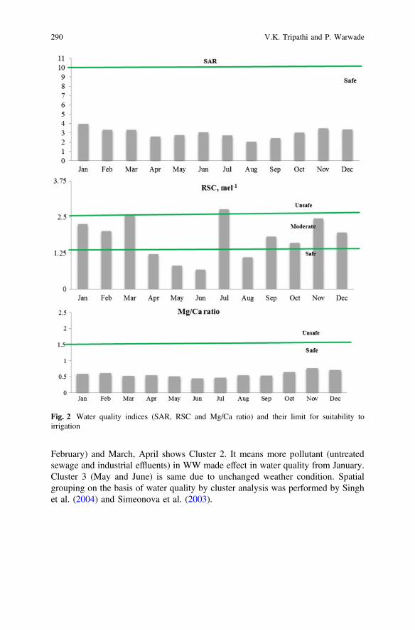
February) and March, April shows Cluster 2. It means more pollutant (untreatedsewage and industrial effluents) in WW made effect in water quality from January.Cluster 3 (May and June) is same due to unchanged weather condition. Spatialgrouping on the basis of water quality by cluster analysis was performed by Singhet al. (2004) and Simeonova et al. (2003).
Fig. 2 Water quality indices (SAR, RSC and Mg/Ca ratio) and their limit for suitability toirrigation
290 V.K. Tripathi and P. Warwade

Conclusions
Utilization of treated municipal wastewater for irrigation is a viable alternative toprotect environment, save freshwater and saving of nutrients for plant production. Itis indispensable to study the impact of semi-arid climate on domestic wastewaterwith respect to its quality parameters so that it can be used extensively for irrigationpurpose in sustainable manner. The domestic wastewater passing through perennialdrains was analyzed for different physiochemical properties (EC, pH, turbidity, totalsolids, NH4–N, NO3–N, P, K, Na, Ca, Mg, CO3, HCO3 and heavy metals (Cu, Zn,Mn, Fe, Cr, Mo). The spatio-temporal quality of wastewater shows acidic nature.Availability of major nutrients and micro elements in wastewater provides theopportunity for its use in irrigation to fulfill crop water and nutrient demand. It alsoprovides the opportunity for alternative disposal of wastewater. Most of the waterquality parameters concentration was higher during summer season, moderateduring winter season and least during rainy season. Wastewater is under safe limitthroughout the year in terms of irrigation water quality indices SAR and Mg/Caratio. Cluster analysis is useful to provide information about seasonal distribution ofwater quality data and showing the cluster of months with similar quality.Information generated from the present study will be useful for integrated waterresources planning and management.
References
Akpan A (2004) The water quality of some tropical freshwater bodies in Uyo (Nigeria) receivingmunicipal sewage effluents, slaughter house washing and agriculture land drainage. TheEnvironmentalist 24:49–55
APHA (2005) Standard methods for the examination of water and wastewater, 21st edn. AmericanPublic Health Association, Washington, DC
Fig. 3 Dendogram showingtemporal similarity for WWthrough three clusters
Influence of Semi-arid Climate on Characterization … 291
BIS (1986) Guideline for irrigation waters. Bureau of Indian Standards, IS:11624CPCB (2005) Assessment of pollution—case study, highlights, ministry of environment and
forest. Government of India, DelhiDas J, Acharya BC (2003) Hydrology and assessment of lotic water quality in Cuttack city, India.
Water Air Soil Pollut 150:163–175Dixon W, Chiswell B (1996) Review of aquatic monitoring program design. Water Res 30
(9):1935–1948Girija TR, Mahanta C, Chandramouli V (2007) Water quality assessment of an untreated effluent
imparted urban stream: the Bharalu tributary of the Brahmaputra River, India. Environ MonitAssess 130:221–236
Goldman RC, Horne JA (1983) Limnology. McGraw-Hillcompany, Book, New YorkHouse WA, Denison FH (1997) Nutrient dynamics in a lowland stream impacted by sewage
effluent: great of use, England. Sci Total Environ 205:25–49Jimenez B, Asano T (2008) Water reclamation and reuse around the world. In: Jimenez B,
Asano T (eds) Water reuse: an international survey of current practice, issues and needs. IWAPublishing, London, p 648
Keraita B, Jiménez B, Drechsel P (2008) Extent and implications of agricultural reuse of untreated,partly treated and diluted wastewater in developing countries. Perspect Agric Vet Sci Nutr NatResour 3(58):15
Luiza A, Alex V, Reynaldo L, Plinio B, De Camargo PB (1999) Effects of sewage on the chemicalcomposition of Piracicaba river, Brazil. Water Air Soil Pollut 110:67–79
Natrajan E, Yadav BR, Tomar SPS, Chandrasekharan H (2004) Bio-chemical characterization ofground water of IARI farm. J Agr Phys 4(1&2):40–43
Neal C, Jarvie HP, Williams RJ, Neal M, Wickham H, Hill L (2002) Phosphorus-calciumcarbonate saturation relationships in a lowland chalk river impacted by sewage inputs andphosphorus remediation: an assessment of phosphorus self-cleansing mechanisms in naturalwaters. Sci Total Environ 282–283:295–310
Ravindra K, Ameena M, Monika R, Kaushik A (2005) Seasonal variations in physoico-chemicalcharacteristics of River Yamuna in Haryana and its ecological best design use. J Environ Monit5:419–426
Richards LA (1954) Diagnosis and improvement of saline and alkaline soils. USDA HandbookNo. 60, pp 160
Simeonova P, Simeonov V, Andreev G (2003) Water quality study of the Struma River Basin,Bulgaria (1989–1998). Central Eur J Chem 1:136–212
Singh KP, Malik A, Mohan D, Sinha S (2004) Multivariate statistical techniques for the evaluationof spatial and temporal variations in water quality of Gomti River (India): a case study. WaterRes 38:3980–3992
Sinha AK, Pande DP, Srivastava KN, Kumar A, Tripathi A (1991) Impact of mass bathing on thewater quality at the Ganga River at Houdeshwarnath (Pratapgarth) India: a case study. Sci TotalEnviron 101(3):275–280
Tandon HLS (2005) Methods of analysis of soils, plants, waters, fertilizers and organic manures.Fertilizer Development and Consultation Organisation, New Delhi, India, pp 204 + xii
UNHSP (2008) Global atlas of excreta, wastewater sludge, and biosolids management: movingforward the sustainable and welcome uses of a global resource. In: LeBlanc R, Matthews P,Roland P (eds) UN-Habitat, Nairobi, p 632
WHO (2006) Guidelines for the safe use of wastewater, excreta and greywater. Volume 2:wastewater use in agriculture. World Health Organization, Geneva, Switzerland
292 V.K. Tripathi and P. Warwade
Anomalous Features of Black Carbonand Particulate Matter Observed OverRural Station During Diwali Festivalof 2015
P.C.S. Devara, M.P. Alam, U.C. Dumka, S. Tiwariand A.K. Srivastava
Abstract Black carbon (BC) aerosol is the second most powerful climate forcingagent, ahead of methane, and second only to carbon dioxide, formed through theincomplete combustion of fossil fuels, bio-fuel and biomass, and is emitted in bothanthropogenic and naturally occurring soot. In this communication, we presentsome interesting results of BC, particulate matter (PM), in conjunction with con-current satellite and surface meteorological products, obtained during the recentDiwali festival episode of November 2015 over a rural station characterized bysparse population and complex terrain. This comprehensive study revealed (i) aclear diurnal variation of BC, PM1, PM2.5, and PM10 mass concentration with dualmaxima (bimodal), one around early morning and the other around mid-nighthours, due to emissions from traffic with minimum concentration around afternoonhours due to well-known planetary boundary-layer dynamics, (ii) the PM showedhigher concentration (more than two-fold) during the festive period as compared tothe pre- and post-festive periods, (iii) the aerosol optical depth (AOD) showedinitially higher and subsequent dilution due to local meteorology, (iv) angstromexponent (AE) showed larger values implying enhancement in fine-mode particlesdue to festive activity and (v) The NOAA-HYSPLIT air-mass back-trajectoryanalysis and CALIPSO satellite imageries portray contribution from thetrans-boundary pollution through long-range transport mechanism. The results areexplained by considering the terrain-induced meteorological conditions and localanthropogenic activities.
P.C.S. Devara (&) � M.P. AlamAmity University Haryana (AUH), Gurgaon (Panchgaon-Manesar) 122413, Indiae-mail: [email protected]
U.C. DumkaAryabhatta Research Institute of Observational Sciences (ARIES), Nainital, Indiae-mail: [email protected]
S. Tiwari � A.K. SrivastavaIndian Institute of Tropical Meteorology (IITM), Delhi Unit, New Delhi, Indiae-mail: [email protected]
© Springer Nature Singapore Pte Ltd. 2018V.P. Singh et al. (eds.), Environmental Pollution, Water Scienceand Technology Library 77, https://doi.org/10.1007/978-981-10-5792-2_24
293
Introduction
Firework displays during festive celebrations such as Diwali (festival of lights) cancause acute air pollution as they release various gases, particulate air pollutants, andtoxic materials. Black carbon (BC) aerosol is one of the prominent constituent thatis associated with these activities. BC also may act as cloud condensation nuclei,altering the size distribution and optical properties of clouds (Twomey 1977). BCaerosol surface can act as catalytic oxidation of SO2 to sulfate and for thedestruction of ozone (Disselkamp et al. 2000). Diwali is celebrated by cleaning anddecorating homes with lights, oil lamps, and festive lights. A variety of pyrotech-nics employed in these works produce various visual, light, sound, gas, and smokeeffects. Most importantly, fireworks are set off by children and they mainly consistof rockets, Roman candles, sparkles, and wheels, etc. On this auspicious occasion,harmful gases and toxic substances are released into the environment by burstingfireworks. As a result, the RSPM (respirable suspended particulate material) levelsgo high as small particles are emitted. Moreover, to overcome shortage of elec-tricity, generators by using diesel, coal that also cause air pollution. The BC par-ticles are small enough (<1 lm), their presence in fireworks affects lungs, insomnia,heart, asthma, and bronchitis. Also, many children face accidents due to mishan-dling of fireworks and it causes burning, cutting, etc. Also, it has been observed thatmortality and morbidity rate increases in Diwali period because of RSPM(Khaparde et al. 2012). Several researchers in India and elsewhere studied theimpact of particulate matter and toxic gases released during celebrations likeDiwali, etc. on short-term environmental air-quality degradation, negative effects onhuman health, and also on long-range climate change (for example, Devara et al.2015; Betha and Balasubramanian 2013; Chatterjee et al. 2013; Thakur et al. 2010;Bach et al. 2001).
This paper mainly focuses on approaches followed for capturing mass concen-tration of various particulate matter, black carbon aerosols in particular, some of themost sensitive and representative of the influence of fireworks on environmental airquality, dispersion and transport phenomena, possible health impacts, and combatprocesses. The observed results over a typical rural station (Panchgaon) have beencorroborated with in situ satellite measurements and attributed to the local mete-orological and surrounding anthropogenic activities that are found to modulate theeffects due to the Diwali celebration.
Measurement Site Description
The study site, Panchgaon (28.31°N, 76.90°E, 285 m above mean sea level),Haryana State, is a rural location, situated around 50 km from Delhi. This site issurrounded, in the northeast direction, by two cities, namely, Gurgaon (*24 km)and Manesar (*9.5 km) which possess several small- and large-scale industries,
294 P.C.S. Devara et al.

the study site receives pollution whenever the wind blows in the northeast sector. Itsexact geographic location (indicated by donut symbol), and the Amity UniversityHaryana campus along with the monitoring site (shown with asterisk symbol) areshown in Fig. 1. It is about 5 km away from the Delhi–Jaipur National Highway(NH8) in the northeast (NE) direction, and is enveloped by Aravalli hillocks ofaverage elevation of about 200 m. Thus, the experimental site has complextopography with valley-like terrain. The site receives pollution due to traffic, par-ticularly during nighttime when the heavy vehicles ply on the NH road. Added, thecomplex wind pattern induced by the surrounding orography often affects thepollution flow at the study region. Further, the building-construction activitieswithin the campus influence the observations. It is also observed that the site isinfluenced by the Thar Desert, located in the northeast direction, and receives dustpollution through long-range transport process. Thus, although the site is primarilya rural station with sparse residential buildings, population, and vegetation fields, itposes sporadic pollution due to the abovementioned natural and anthropogenicactivities.
Material and Methodology
Regular and continuous observations of black carbon (BC) mass concentrationmeasurements using a seven-beam Aethalometer (Magee Scientific Inc. USA,Model AE-42) have been in progress in the campus of Amity University Haryana,Panchgaon (Manesar–Gurgaon) almost from the beginning of 2015 under a col-laborative program with Aryabhatta Research Institute for Observational Sciences
Fig. 1 Map showing the observation location and sampling site
Anomalous Features of Black Carbon and Particulate … 295
(ARIES), Nainital and Indian Institute of Tropical Meteorology (IITM) Delhi Unit,New Delhi. This instrument is fully automatic and uses a continuous filtration ofambient aerosols. Atmospheric air is pumped through an inlet at the desired flowrate (about 4 LPM in the present study), which impinges on a quartz micro fiberstrip. A light beam from a high intensity LED lamp is transmitted through thesample deposit on the filter strip, at 880 nm. The instrument measures BC massconcentrations in the wavelength range of 370–950 nm. The measurement of theattenuation of light beam is linearly proportional to the amount of BC deposited onfilter strip. Observations were recorded at the time base of 5 min interval. Moredetails of the instrument, measurement and data analysis procedure can be found inSumit et al. (2011 and references therein). In the present study, an absorptionefficiency value corresponding to the environment of sampling station is used todetermine the BC mass concentrations as suggested by Hansen et al. (1984, 2007)and Weingartner et al. (2003). The BC mass concentration is calculated from therate of change of attenuation (ATN). The loading effect that relates the tapeadvancement with change in ATN has been taken into account in the calculation ofBC mass concentration by following the correction algorithm suggested byVirkkula et al. (2007) and Park et al. (2010). In the absence of scattering coefficientdata, the corrected attenuation coefficient can be expressed by
bATN correctedð Þ ¼ 1þ k � ATNð Þ � bATN Aethalometerð Þ ð1Þ
where k is an empirically derived constant. The corrected aerosol BC mass con-centration is calculated as follows:
BC correctedð Þ ¼ bATN correctedð Þ=rATN¼ 1þ k � ATNð Þ � BC Aethalometerð Þ ð2Þ
The value of k varies depending on sampling location, season, aerosol compo-sition, and age of the aerosols (Hansen et al. 1984, 2007; Weingartner et al. 2003).The uncertainty involved in the concentration was estimated to be about 10%. Theconversion of attenuation absorption coefficient into BC mass concentration is doneusing appropriate absorption efficiency values which vary with wavelength.
In addition to the above-described principal equipment (MultispectralAethalometer), other two ancillary instruments that have been operated in syn-chronization with it include (i) TSI Model 3321 Aerodynamic Particle Sizer whichprovides mass concentration of aerosols at 52 size bins, from which the PM1,PM2.5, and PM10 have been derived, and (ii) Kestrel Model 4500NV Weather andEnvironmental monitor for the measurement of ambient wind, temperature, andrelative humidity. The concurrent satellite observations from Cloud-Aerosol Lidarand Infrared Pathfinder Satellite Observations (CALIPSO) and NOAA-HYSPLITair-mass back-trajectory model results have also been utilized for attributing theobserved aerosol features during the festive period. All the above datasets, archivedsimultaneously, for the period of pre-, during, and post-Diwali 2015 have beenanalyzed and the results are discussed in the sections to follow.
296 P.C.S. Devara et al.
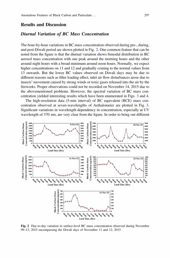
Results and Discussion
Diurnal Variation of BC Mass Concentration
The hour-by-hour variations in BC mass concentration observed during pre-, during,and post-Diwali period are shown plotted in Fig. 2. One common feature that can benoted from the figure is that the diurnal variation shows bimodal distribution in BCaerosol mass concentration with one peak around the morning hours and the otheraround night hours with a broad minimum around noon hours. Normally, we expecthigher concentrations on 11 and 12 and gradually coming to the normal values from13 onwards. But the lower BC values observed on Diwali days may be due todifferent reasons such as filter loading effect, inlet air flow disturbances arose due toinsects’ movement caused by strong winds or toxic gases released into the air by thefireworks. Proper observations could not be recorded on November 14, 2015 due tothe abovementioned problems. However, the spectral variation of BC mass con-centration yielded interesting results which have been enumerated in Figs. 3 and 4.
The high-resolution data (5-min interval) of BC equivalent (BCE) mass con-centration observed at seven-wavelengths of Aethalometer are plotted in Fig. 3.Significant variations in wavelength dependency in concentration, especially at UVwavelength of 370 nm, are very clear from the figure. In order to bring out different
Fig. 2 Day-to-day variation in surface-level BC mass concentration observed during November09–13, 2015 encompassing the Diwali days of November 11 and 12, 2015
Anomalous Features of Black Carbon and Particulate … 297

sources and their time variation of the observed BC mass, concentrations at specificwavelengths (370, 590, and 880 nm) have been displayed on each observation dayin Fig. 4.
It can be clearly seen from the figure that there is an interesting day- to-dayvariation in the signatures of BCE concentrations, particularly on core Diwali daysof November 11 and 12, 2015. As suggested in the literature (Andreae andGelelencser 2006; Moosmuller et al. 2011), the BCE concentration at 370 nmindicates the presence of aromatic organic compounds and fire/smoke aerosols[organic carbon (OC), optically known as brown carbon (BrC)], while those at590 nm (Yellow Carbon, YC), and 880 nm (Black Carbon, BC) indicate thepresence of biomass burning aerosols and fossil fuel combustion aerosols,respectively. It can be seen from Figs. 3 and 4 that BCE at 370 and 590 nm areprominent on core Diwali days (November 11 and 12, 2015) as compared toremaining days. Thus, the results of the present study are consistent and indicative
Fig. 3 High spectral resolution BCE mass concentration on November 09, 10, 11, 12, and 13,2015. The prominent variation of BCE mass on Diwali days may be noted
298 P.C.S. Devara et al.
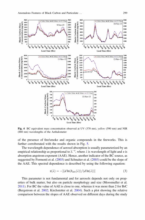
of the presence of fire/smoke and organic compounds in the fireworks. This isfurther corroborated with the results shown in Fig. 5.
The wavelength dependence of aerosol absorption is usually parameterized by anempirical relationship as proportional to k−a, where k is wavelength of light and a isabsorption angstrom exponent (AAE). Hence, another indicator of the BC source, assuggested by Formenti et al. (2003) and Schnaiter et al. (2003) could be the slope ofthe AAE. This spectral dependence is described by using the following equation:
aðkÞ ¼ �½ðd lnðbabsðkÞÞ=ðd lnðkÞÞ� ð3Þ
This parameter is not fundamental and for aerosols depends not only on prop-erties of bulk matter, but also on particle morphology and size (Moosmuller et al.2011). For BC the value of AAE is close to one, whereas it was more than 2 for BrC(Bergstrom et al. 2002; Kirchstetter et al. 2004). Such a plot showing the relativecomparison between the slopes of AAE observed on different days during the study
Fig. 4 BC equivalent mass concentration observed at UV (370 nm), yellow (590 nm) and NIR(880 nm) wavelengths of the Aethalometer
Anomalous Features of Black Carbon and Particulate … 299

period is shown in Fig. 5. Relatively higher slopes around 1.79 may be noted on 11and 12 as compared to such values observed on remaining days. This clearlyimplies the method by which the sources can be identified from multispectral BCEobservations.
Influence on Columnar AOD and ASD
The columnar aerosol optical depth (AOD), which is atmospheric extinction due toaerosol particles, measured using a Microtops-II multi-wavelength solar radiometer(Solar Light Co., USA), has been studied during the festive period. By evolvinglinear least squares fit between AOD and k (in µm) on log-log scale over thespectral range of the radiometer, the slope and intercept of the regression line yielda and b, respectively. The methodology followed for estimating AOD from solarirradiance estimations, and retrieval of Angstrom Exponent (a) and turbiditycoefficient (b) from spectral dependence of AOD has been explained in our earlierpublications (Devara et al. 1996, 2001; Sumit et al. 2011; Pawar et al. 2015). Thesize exponent, a (representative of aerosol size distribution) and b (representativeof aerosol loading) have been estimated for pre-, during, and post-Diwaliperiod. In other words, alpha is an indicator of fraction of fine-mode aerosols(radii � 1 µm) to coarse-mode aerosols (radii > 1 µm) while the b (equals AODat 1 µm), is a measure of columnar aerosol loading. If a value close to or less than1.0, then the coarse-mode aerosol particles dominate in the atmosphere, and if it isgreater than 1.5 µm, the fine-mode (radii � 1 µm) dominates in the atmosphere.Generally, a has a value between 0.5 and 2.5 while b value varies from 0.0 to 0.5(Iqbal 1983). Thus, the value of b < 0.1 indicates clean atmosphere while b > 0.1
Fig. 5 Daily variation of AAE from November 09–13, 2015. Higher values of slopes indicativeof smoke and aromatic organic compounds on core Diwali days (November 11 and 12, 2015) maybe noted
300 P.C.S. Devara et al.
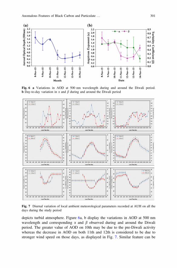
depicts turbid atmosphere. Figure 6a, b display the variations in AOD at 500 nmwavelength and corresponding a and b observed during and around the Diwaliperiod. The greater value of AOD on 10th may be due to the pre-Diwali activitywhereas the decrease in AOD on both 11th and 12th is considered to be due tostronger wind speed on those days, as displayed in Fig. 7. Similar feature can be
Fig. 6 a Variations in AOD at 500 nm wavelength during and around the Diwali period.b Day-to-day variation in a and b during and around the Diwali period
Fig. 7 Diurnal variation of local ambient meteorological parameters recorded at AUH on all thedays during the study period
Anomalous Features of Black Carbon and Particulate … 301
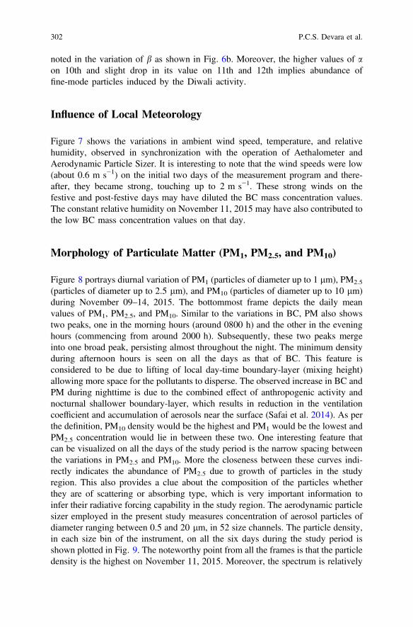
noted in the variation of b as shown in Fig. 6b. Moreover, the higher values of aon 10th and slight drop in its value on 11th and 12th implies abundance offine-mode particles induced by the Diwali activity.
Influence of Local Meteorology
Figure 7 shows the variations in ambient wind speed, temperature, and relativehumidity, observed in synchronization with the operation of Aethalometer andAerodynamic Particle Sizer. It is interesting to note that the wind speeds were low(about 0.6 m s−1) on the initial two days of the measurement program and there-after, they became strong, touching up to 2 m s−1. These strong winds on thefestive and post-festive days may have diluted the BC mass concentration values.The constant relative humidity on November 11, 2015 may have also contributed tothe low BC mass concentration values on that day.
Morphology of Particulate Matter (PM1, PM2.5, and PM10)
Figure 8 portrays diurnal variation of PM1 (particles of diameter up to 1 lm), PM2.5
(particles of diameter up to 2.5 lm), and PM10 (particles of diameter up to 10 lm)during November 09–14, 2015. The bottommost frame depicts the daily meanvalues of PM1, PM2.5, and PM10. Similar to the variations in BC, PM also showstwo peaks, one in the morning hours (around 0800 h) and the other in the eveninghours (commencing from around 2000 h). Subsequently, these two peaks mergeinto one broad peak, persisting almost throughout the night. The minimum densityduring afternoon hours is seen on all the days as that of BC. This feature isconsidered to be due to lifting of local day-time boundary-layer (mixing height)allowing more space for the pollutants to disperse. The observed increase in BC andPM during nighttime is due to the combined effect of anthropogenic activity andnocturnal shallower boundary-layer, which results in reduction in the ventilationcoefficient and accumulation of aerosols near the surface (Safai et al. 2014). As perthe definition, PM10 density would be the highest and PM1 would be the lowest andPM2.5 concentration would lie in between these two. One interesting feature thatcan be visualized on all the days of the study period is the narrow spacing betweenthe variations in PM2.5 and PM10. More the closeness between these curves indi-rectly indicates the abundance of PM2.5 due to growth of particles in the studyregion. This also provides a clue about the composition of the particles whetherthey are of scattering or absorbing type, which is very important information toinfer their radiative forcing capability in the study region. The aerodynamic particlesizer employed in the present study measures concentration of aerosol particles ofdiameter ranging between 0.5 and 20 lm, in 52 size channels. The particle density,in each size bin of the instrument, on all the six days during the study period isshown plotted in Fig. 9. The noteworthy point from all the frames is that the particledensity is the highest on November 11, 2015. Moreover, the spectrum is relatively
302 P.C.S. Devara et al.
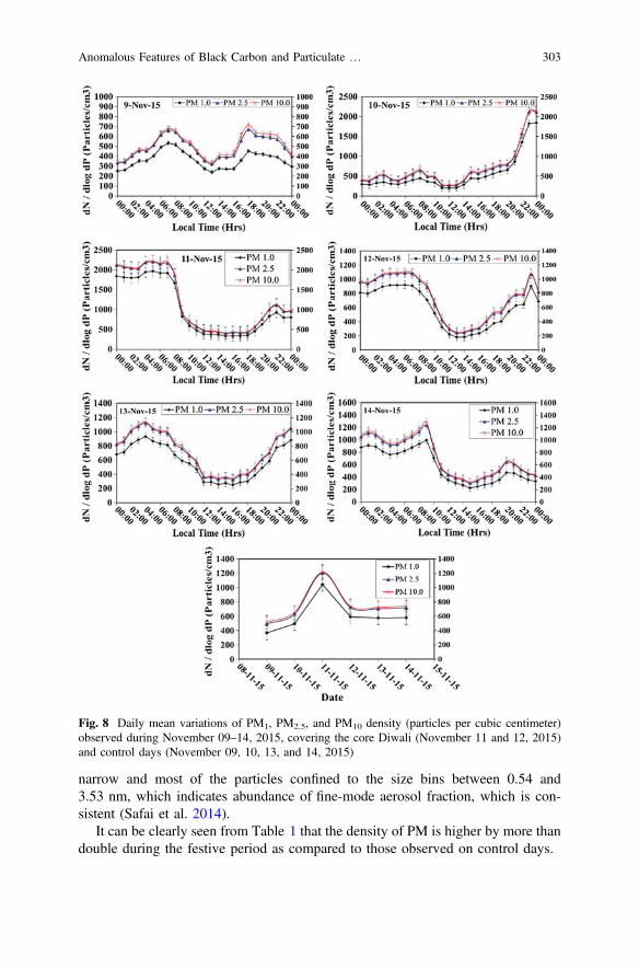
narrow and most of the particles confined to the size bins between 0.54 and3.53 nm, which indicates abundance of fine-mode aerosol fraction, which is con-sistent (Safai et al. 2014).
It can be clearly seen from Table 1 that the density of PM is higher by more thandouble during the festive period as compared to those observed on control days.
Fig. 8 Daily mean variations of PM1, PM2.5, and PM10 density (particles per cubic centimeter)observed during November 09–14, 2015, covering the core Diwali (November 11 and 12, 2015)and control days (November 09, 10, 13, and 14, 2015)
Anomalous Features of Black Carbon and Particulate … 303
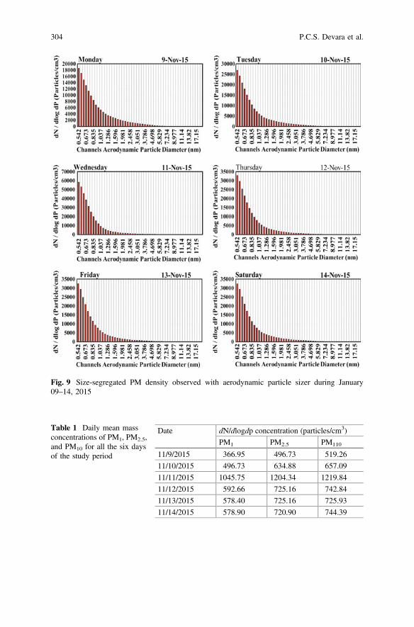
Fig. 9 Size-segregated PM density observed with aerodynamic particle sizer during January09–14, 2015
Table 1 Daily mean massconcentrations of PM1, PM2.5,and PM10 for all the six daysof the study period
Date dN/dlogdp concentration (particles/cm3)
PM1 PM2.5 PM110
11/9/2015 366.95 496.73 519.26
11/10/2015 496.73 634.88 657.09
11/11/2015 1045.75 1204.34 1219.84
11/12/2015 592.66 725.16 742.84
11/13/2015 578.40 725.16 725.93
11/14/2015 578.90 720.90 744.39
304 P.C.S. Devara et al.
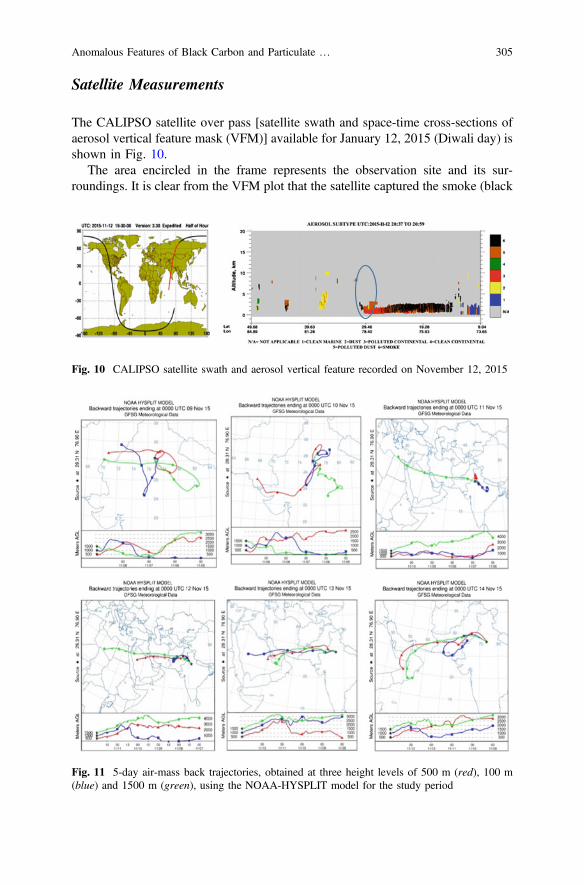
Satellite Measurements
The CALIPSO satellite over pass [satellite swath and space-time cross-sections ofaerosol vertical feature mask (VFM)] available for January 12, 2015 (Diwali day) isshown in Fig. 10.
The area encircled in the frame represents the observation site and its sur-roundings. It is clear from the VFM plot that the satellite captured the smoke (black
Fig. 10 CALIPSO satellite swath and aerosol vertical feature recorded on November 12, 2015
Fig. 11 5-day air-mass back trajectories, obtained at three height levels of 500 m (red), 100 m(blue) and 1500 m (green), using the NOAA-HYSPLIT model for the study period
Anomalous Features of Black Carbon and Particulate … 305
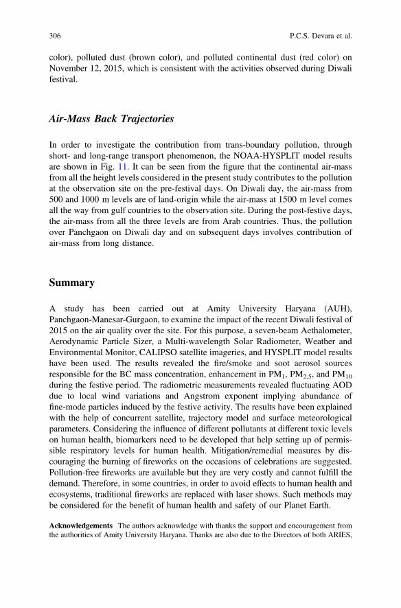
color), polluted dust (brown color), and polluted continental dust (red color) onNovember 12, 2015, which is consistent with the activities observed during Diwalifestival.
Air-Mass Back Trajectories
In order to investigate the contribution from trans-boundary pollution, throughshort- and long-range transport phenomenon, the NOAA-HYSPLIT model resultsare shown in Fig. 11. It can be seen from the figure that the continental air-massfrom all the height levels considered in the present study contributes to the pollutionat the observation site on the pre-festival days. On Diwali day, the air-mass from500 and 1000 m levels are of land-origin while the air-mass at 1500 m level comesall the way from gulf countries to the observation site. During the post-festive days,the air-mass from all the three levels are from Arab countries. Thus, the pollutionover Panchgaon on Diwali day and on subsequent days involves contribution ofair-mass from long distance.
Summary
A study has been carried out at Amity University Haryana (AUH),Panchgaon-Manesar-Gurgaon, to examine the impact of the recent Diwali festival of2015 on the air quality over the site. For this purpose, a seven-beam Aethalometer,Aerodynamic Particle Sizer, a Multi-wavelength Solar Radiometer, Weather andEnvironmental Monitor, CALIPSO satellite imageries, and HYSPLIT model resultshave been used. The results revealed the fire/smoke and soot aerosol sourcesresponsible for the BC mass concentration, enhancement in PM1, PM2.5, and PM10
during the festive period. The radiometric measurements revealed fluctuating AODdue to local wind variations and Angstrom exponent implying abundance offine-mode particles induced by the festive activity. The results have been explainedwith the help of concurrent satellite, trajectory model and surface meteorologicalparameters. Considering the influence of different pollutants at different toxic levelson human health, biomarkers need to be developed that help setting up of permis-sible respiratory levels for human health. Mitigation/remedial measures by dis-couraging the burning of fireworks on the occasions of celebrations are suggested.Pollution-free fireworks are available but they are very costly and cannot fulfill thedemand. Therefore, in some countries, in order to avoid effects to human health andecosystems, traditional fireworks are replaced with laser shows. Such methods maybe considered for the benefit of human health and safety of our Planet Earth.
Acknowledgements The authors acknowledge with thanks the support and encouragement fromthe authorities of Amity University Haryana. Thanks are also due to the Directors of both ARIES,
306 P.C.S. Devara et al.
Nainital and IITM-DU, New Delhi, for their constant cooperation. The HYSPLIT model used inthe study was provided by the NOAA Air Resources Laboratory (ARL).The CALIPSO data were acquired (http://www.calipso.larc.nasa.gov/products/lidar/browseimages/
products). The authors also appreciate the assistance from Tanojit Paul and Shubhansh Tiwari of AUHin the analysis of data. The insightful comments and valuable suggestions by the anonymous reviewersare thankfully acknowledged.
References
Andreae MO, Gelelencser A (2006) Black carbon or brown carbon? The nature of light absorbingcarbonaceous aerosols. Atmos Chem Phys 6:3131–3148
Bach W, Daniels A, Dickinson L, Hertiein F, Morrows J, Margolis S, Dinh VD (2001) Fireworkspollution and health. Int J Environ Stud 7:183–192
Bergstrom RW, Russell PB, Hignett P (2002) Wavelength dependence of the absorption of blackcarbon particles: predictions and results from Tarfox experiment and implications for theaerosol single scattering albedo. J Atmos Sci 59:567–577
Betha R, Balasubramanian R (2013) Particulate emissions from commercial handheld sparklers:evaluation of physical characteristics and emission rates. Aerosol Air Qual Res 13:301–307
Chatterjee A, Sarkar C, Adak A, Mukherjee U, Ghosh SK, Raha S (2013) Ambient air qualityduring Diwali festival over Kolkata—a mega city in India. Aerosol Air Qual Res 13:1133–1144
Devara PCS, Pandithurai G, Raj PE, Sharma S (1996) Investigations of aerosol optical depthvariations using spectroradiometer at an urban station, Pune, India. J Aerosol Sci 27:621–632
Devara PCS, Maheskumar RS, Raj PE, Dani KK, Sonbawne SM (2001) Some features of aerosoloptical depth, ozone and precipitable water content observed over land during theINDOEX-IFP99. Meteorologische Zeirschrift 10:901–908
Devara PCS, Vijayakumar K, Safai PD, Raju MP, Rao PSP (2015) Celebration-induced air qualityover a tropical urban station, Pune, India. Atmos Poll Res 6:511–520
Disselkamp RS, Carpenter MA, Cowin CM, Berkowitz CM, Chapman EG, Zaveri RA,Laulainen NS (2000) Ozone loss in soot aerosols. J Geophys Res 105:9767–9771
Formenti P, Elber W, Maenhaut W, Haywood J, Andreae MO (2003) Chemical composition ofmineral dust aerosol during the Saharan dust experiment (SHADE) airborne campaign in theCape Verde region, September 2000. J Geophys Res 108(D18):8576. doi:10.1029/2002JD002647 2005
Hansen ADA, Rosen H, Novakov T (1984) The aethalometer—an instrument for the real-timemeasurement of optical absorption by aerosol particles. Sci Total Environ 36:191–196
Hansen ADA, Turner JR, Allen GA (2007) An algorithm to compensate aethalometer data for theeffects of shadowing and scattering. In: Proceedings of 5th Asian aerosol conference, 26–29Aug, Kaohsiung, Taiwan
Iqbal M (1983) An introduction to solar radiation. Academic Press, New York, p 256Khaparde VV, Pipalatkar PP, Pustode T, Rao CV, Gajghate DG (2012) Influence of burning of
fireworks on particle size distribution of PM10 and associated barium at Nagpur. EnvironMonit Assess 184:903–911
Kirchstetter TW, Novakov T, Hobbs PV (2004) Evidence that the spectral dependence of lightabsorption by aerosols is affected by organic carbon. J Geophys Res 109:D21208. doi:10.1029/2004JD004999
Moosmuller H, Chakrabarty RK, Ehlers KM, Arnott WP (2011) Absorption angstrom coefficient,brown carbon and aerosols: basic concepts, bulk matter, and spherical particles. Atmos ChemPhys 11:1217–1225
Park SS, Hansen ADA, Sung Cho Y (2010) Measurements of real time black carbon forinvestigating spot loading effects of aethalometer data. Atmos Environ 44:1449–1455
Anomalous Features of Black Carbon and Particulate … 307
Pawar GV, Devara PCS, Aher GR (2015) Identification of aerosol types over an urban site basedon air-mass trajectory classification. Atmos Res 164–165:142–155
Safai PD, Devara PCS, Raju MP, Vijayakumar K, Rao PSP (2014) Relationship between blackcarbon and associated optical, physical and radiative properties of aerosols over twocontrasting environments. Atmos Res 149:292–299
Schnaiter M, Horvath H, Mohler O, Naumann K-H, Saathof H, Schhock OW (2003) UV-VIS-NIRspectral optical properties of soot and soot-containing aerosols. J Aerosol Sci 34:1421–1444
Sumit K, Devara PCS, Manoj MG, Safai PD (2011) Winter aerosol and trace gas characteristicsover a high-altitude station in the Western Ghats, India. Atmosfera 24:311–328
Thakur B, Chakraborty S, Debsarkar A, Chakrabarty S, Srivastava RC (2010) Air pollution fromfireworks during festival of lights (Deepawali) in Howrah, India—a case study. Atmosfera23:347–365
Twomey S (1977) Atmospheric aerosols. Elsevier, New YorkVirkkula A, Makela T, Hillamo R, Yli-Yuomi T, Hirsikko A, Hemari K, Koponen IK (2007) A
simple procedure for correcting loading effects of Aethalometer. J Air Waste Manag Assoc57:1214–1222
Weingartner E, Saathof H, Schnaiter M, Streit N, Bitnar B, Baltensperger U (2003) Absorption oflight by soot particles: determination of the absorption coefficient by means of aethalometers.J Aerosol Sci 34:1445–1463
308 P.C.S. Devara et al.
Decolorization of Reactive Yellow 17 DyeUsing Aspergillus tamarii
Anuradha Singh, Arpita Ghosh and Manisha Ghosh Dastidar
Abstract Decolorization of a reactive yellow 17 dye (Molecular formula:C20H20K2N4O12S3) using growing Aspergillus tamarii was studied in a batchbioreactor. The study was performed up to 90 h at optimized pH 5 for maximumgrowth of A. tamarii. The decolorization and biomass concentration decreased from58.8 to 6% and from 2.37 to 0.74 g/L, respectively, with increasing initial con-centration of dye from 100 to 1000 mg/L. The chemical oxygen demand(COD) after decolorization was found to be decreased from 37.2 to 16% withincreasing dye concentration from 100 to 1000 mg/L. Further, desorption study wasperformed with acidic eluants and the desorbed biomass was reused for decol-orization which was compared with that obtained using dead biomass.
Keywords Aspergillus tamarii � Reactive yellow 17 dye � Batch bioreactorColor removal � COD
Introduction
Dyes are colored substances which are used in textile, paper, plastic food, tanneries,paints, and electroplating industries. Effluents generated from these industries havehigh COD (chemical oxygen demand), BOD (biochemical oxygen demand), sus-pended solids, biodegradable organics, and pathogenic bacteria (Ranjusha et al.2010). Effluents also contain residual dyes, which are discharged to the environ-ment directly by most of the textile industries without giving adequate treatment to
A. Singh � A. Ghosh � M.G. Dastidar (&)Centre for Energy Studies, Indian Institute of Technology Delhi, Hauz-Khas, New Delhi110016, Indiae-mail: [email protected]
A. Singhe-mail: [email protected]
A. Ghoshe-mail: [email protected]
© Springer Nature Singapore Pte Ltd. 2018V.P. Singh et al. (eds.), Environmental Pollution, Water Scienceand Technology Library 77, https://doi.org/10.1007/978-981-10-5792-2_25
309
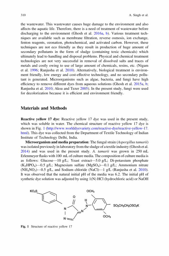
the wastewater. This wastewater causes huge damage to the environment and alsoaffects the aquatic life. Therefore, there is a need of treatment of wastewater beforedischarging to the environment (Ghosh et al. 2016a, b). Various treatment tech-niques are available such as membrane filtration, reverse osmosis, ion exchange,fenton reagents, ozonation, photochemical, and activated carbon. However, thesetechniques are not eco friendly as they result in production of huge amount ofsecondary pollutants in the form of sludge (containing toxic chemicals) whichultimately lead to handling and disposal problems. Physical and chemical treatmenttechnologies are not very successful in removal of dissolved salts and traces ofmetals and costly owing to use of large amount of chemicals, resins, etc. (Nigamet al. 1996; Ranjusha et al. 2010). Alternatively, biological treatment is environ-ment friendly, low energy and cost-effective technology, and no secondary pollu-tant is generated. Microorganisms such as algae, bacteria, and fungi have highefficiency to remove different dyes from aqueous solutions (Ghosh et al. 2015a, b;Ranjusha et al. 2010; Aksu and Tezer 2005). In the present study, fungi were usedfor decolorization because it is efficient and environment friendly.
Materials and Methods
Reactive yellow 17 dye: Reactive yellow 17 dye was used in the present study,which was soluble in water. The chemical structure of reactive yellow 17 dye isshown in Fig. 1 (http://www.worlddyevariety.com/reactive-dye/reactive-yellow-17.html). This dye was collected from the Department of Textile Technology of IndianInstitute of Technology Delhi, India.
Microorganism andmedia preparation: The fungal strain (Aspergillus tamarii)was isolated previously in laboratory from the sludge of a textile industry (Ghosh et al.2014) and was used in the present study. A. tamarii was grown in 250 mLErlenmeyer flasks with 100 mL of culture media. The composition of culture media isas follows: Glucose—10 g/L; Yeast extract—5.0 g/L; Di-potassium phosphate(K2HPO4)—0.5 g/L; Magnesium sulfate (MgSO4)—0.1 g/L; Ammonium nitrate(NH4NO3)—0.5 g/L, and Sodium chloride (NaCl)—1 g/L (Ranjusha et al. 2010).It was observed that the natural initial pH of the media was 6.2. The initial pH ofsynthetic dye solution was adjusted by using 1(N) HCl (hydrochloric acid) or NaOH
Fig. 1 Structure of reactive yellow 17
310 A. Singh et al.

(sodium hydroxide) as per the requirement (Ranjusha et al. 2010; Ghosh et al. 2014).The experiments were conducted using sterile culture media containing synthetic dyesolution inoculated with A. tamarii and incubated at 27 °C and 110 rpm to maintainconditions favorable for the growth of microorganism. The studies were carried outfor a period of 90 h. The dye solution was scanned for peak absorbance from 300 to900 nm range (Robinson et al. 2001; Namdhari et al. 2012). The maximum absor-bance (kmax) was observed at 406.8 nm by UV–visible spectrophotometer(Systronics). This absorbancewas used for calculation of percentage of decolorizationafter decolorization experiment (Olukanni et al. 2006).
%Decolorization ¼ ðC0 � C1Þ=C0f g � 100
where,
C0 initial concentration of dye (mg/L)C1 residual concentration of dye (mg/L) after decolorization study.
Decolorization at different initial concentrations of dye: Decolorization studywas conducted using solution of different initial concentrations (100–1000 mg/L)of dye at pH: 5 which is optimum for maximum growth of A. tamarii. It wasobserved earlier that maximum growth of A. tamarii was obtained at optimized pH:5 (Ghosh et al. 2014). The biomass was collected after each experiment. The dryweight of biomass was analysed through weight balance machine.
The Chemical oxygen demand (COD) is an important parameter to evaluate thetotal oxidizable substances in wastewater. The COD values of dye solutions of(100–1000 mg/L initial concentration) were estimated by using dichromate refluxprotocol (standard method) given by American Public Health Association (APHA1989; Ranjusha et al. 2010).
Desorption study and reuse of desorbed biomass: The biomass after decol-orization, was collected and dried. Study on desorption of biomass (after decol-orization) was performed using acidic eluant (such as H2SO4, HCl at differentnormalities). The pH values of acidic eluants at different normalities (0.5(N)H2SO4, 1(N) H2SO4, 0.5(N)HCl, and 1(N)HCl) were found to be 1.1, 0.85, 0.86,and 0.66, respectively. For desorption study, initially the biomass was dipped indistilled water followed by different normalities of H2SO4 and HCl for 60 min andplaced in shaker at 110 rpm. Then, the desorbed biomass was mechanically grindedwith water. All the solutions were collected, centrifuged and the absorbances weredetermined by using UV–visible spectrophotometer. The biomass after desorptionwas reused for decolorization of synthetic dye solution. Further, fresh biomass wasprepared in the absence of dye and was dried. Study on decolorization using des-orbed biomass was compared with decolorization using fresh dead biomass in batchmodes. The desorbed biomass and fresh dead biomass were added in synthetic dyesolution of 100 mg/L in conical flasks separately and placed in shaker at 110 rpmfor 60 min. The solutions were centrifuged and the %decolorization was deter-mined by using UV–visible spectrophotometer.
Decolorization of Reactive Yellow 17 Dye … 311

Scanning Electron Microscopic (SEM) Analysis: The SEM analysis of fungalbiomass was done to examine the surface of the cells before and after dye decol-orization (Ghosh et al. 2014; Ranjusha et al. 2010). The samples for SEM weremounted on the stainless steel stub by coating a thin layer of gold under vacuum inorder to improve the quality of micrographs.
Results and Discussion
Decolorization at Different Initial Concentrations of Dye
Figure 2 shows the effect of initial concentration of dye (100–1000 mg/L) withtime on decolorization at pH: 5 (optimum for the maximum growth rate ofmicroorganism). With increasing time from 0 to 90 h, it was observed that %decolorization was initially increased up to 70 h for 100 mg/L dye solution. After70 h, no improvement was observed in %decolorization. It was found that100 mg/L dye concentration shows maximum decolorization 58.8% as compared toother concentrations (such as 250, 500, 1000 mg/L) of the dye. Decolorization wasfound to be 58.8, 27, 11, and 6% at 100, 250, 500, and 1000 mg/L dye solution. Itis indicated that dye at higher concentration is toxic to the cell growth. Previously, itwas reported that Aspergillus species removed color 62.6, 69.8, and 87% separatelyfrom Reactive Black, Reactive Red, and Remazol Black B dyes solutions at100 mg/L, respectively (Ramya et al. 2007; Ranjusha et al. 2010). In present case, itis 58.8% color removal and is near to the decolorization value of Reactive black dyeas referenced above. The COD after decolorization was found to be decreased from37.2 to 16% with increasing dye concentration from 100 to 1000 mg/L.
In previous study, maximum biomass concentration was reported as 5.2 g/L inthe absence of dye (Ghosh et al. 2014). Figure 3 shows rapid decrease in thebiomass concentration from 5.2 to 2.37 g/L with increasing dye concentration from
Fig. 2 Decolorization with time at different initial concentration of dye
312 A. Singh et al.
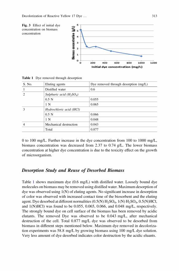
0 to 100 mg/L. Further increase in the dye concentration from 100 to 1000 mg/L,biomass concentration was decreased from 2.37 to 0.74 g/L. The lower biomassconcentration at higher dye concentration is due to the toxicity effect on the growthof microorganism.
Desorption Study and Reuse of Desorbed Biomass
Table 1 shows maximum dye (0.6 mg/L) with distilled water. Loosely bound dyemolecules on biomassmay be removed using distilled water. Maximum desorption ofdye was observed using 1(N) of eluting agents. No significant increase in desorptionof color was observed with increased contact time of the biosorbent and the elutingagent. Dye desorbed at different normalities (0.5(N) H2SO4, 1(N) H2SO4, 0.5(N)HCl,and 1(N)HCl) was found to be 0.055, 0.065, 0.066, and 0.048 mg/L, respectively.The strongly bound dye on cell surface of the biomass has been removed by acidicelutants. The removed Dye was observed to be 0.043 mg/L, after mechanicaldestruction of the cell. Total 0.877 mg/L dye was observed to be desorbed frombiomass in different steps mentioned below. Maximum dye removed in decoloriza-tion experiments was 58.8 mg/L by growing biomass using 100 mg/L dye solution.Very less amount of dye desorbed indicates color destruction by the acidic eluants.
Fig. 3 Effect of initial dyeconcentration on biomassconcentration
Table 1 Dye removed through desorption
S. No. Eluting agents Dye removed through desorption (mg/L)
1 Distilled water 0.6
2 Sulphuric acid (H2SO4)
0.5 N 0.055
1 N 0.065
3 Hydrochloric acid (HCl)
0.5 N 0.066
1 N 0.048
4 Mechanical destruction 0.043
Total 0.877
Decolorization of Reactive Yellow 17 Dye … 313
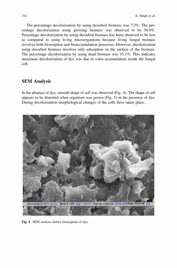
The percentage decolorization by using desorbed biomass was 7.3%. The per-centage decolorization using growing biomass was observed to be 58.8%.Percentage decolorization by using desorbed biomass has been observed to be lowas compared to using living microorganisms because living fungal biomassinvolves both biosorption and bioaccumulation processes. However, decolorizationusing desorbed biomass involves only adsorption on the surface of the biomass.The percentage decolorization by using dead biomass was 15.1%. This indicatesmaximum decolorization of dye was due to color accumulation inside the fungalcell.
SEM Analysis
In the absence of dye, smooth shape of cell was observed (Fig. 4). The shape of cellappears to be distorted when organism was grown (Fig. 5) in the presence of dye.During decolorization morphological changes of the cells have taken place.
Fig. 4 SEM analysis before biosorption of dye
314 A. Singh et al.

Conclusion
Aspergillus tamarii was isolated from the sludge of textile industry, has the abilityto grow in the presence of dye and is effective in removing Reactive yellow 17 dye.The growth of the microorganism and color removal depends on initial dye con-centration and contact time. The growing microorganism was efficient to decolorizethe dye solutions at higher concentrations. The decolorization, COD, and biomasswere decreased with increasing the concentration of dye. Also, the decolorization ofdye by A. tamarii was indicated by SEM analysis. The reuse potential of biomassafter desorption can minimize the sludge generation and make the processcost-effective.
References
Aksu Z, Tezer S (2005) Biosorption of reactive dyes on the green alga chlorella vulgaris. ProcBiochem 40:1347–1367
American Public Health Association (APHA) (1989) Standard methods for examination of waterand wastewater, 17th edn. Washington, DC
Fig. 5 SEM analysis after biosorption of dye
Decolorization of Reactive Yellow 17 Dye … 315
Banat IM, Nigam P, Singh D, Marchant R (1996) Microbial decolorization of textile dyecontaining effluents: a review. Bioresour Technol 58:217–227
Ghosh A, Dastidar MG, Sreekrishnan TR (2014) Biosorption and biodegradation of chromiumcomplex dye using Aspergillus Species. J Hazard Toxic Radioact Waste 18(4):1–9. doi:http://dx.doi.org/10.1061/(ASCE)HZ.2153-5515.0000230
Ghosh A, Das P, Sinha K (2015a) Optimization of reduction of copper using Stenotrophomonasmaltophilia PD2 biomass and artificial neural network modelling. Environ Eng Manag J14:37–44
Ghosh A, Dastidar MG, Sreekrishnan TR (2015b) Recent advances in bioremediation of heavymetals and metal complex dyes: review. J Environ Eng C4015003. doi:http://dx.doi.org/10.1061/(ASCE)EE.1943-7870.0000965
Ghosh A, Dastidar MG, Sreekrishnan TR (2016a) Bioremediation of a chromium complex dye(Navilan yellow RL) using Aspergillus flavus and Aspergillus tamarii. Chem Eng Technol.doi:10.1002/ceat.201500515
Ghosh A, Dastidar MG, Sreekrishnan TR (2016b) Response surface optimization of bioreme-diation of acid black 52 (Multi-metals complex dye) using Aspergillus tamarii. EnvironTechnol 1–12. doi:10.1080/09593330.2016.1192225
Namdhari BS, Rohilla SK, Salar RK, Gahlawat SK, Bansal P, Saran AK (2012) Decolorization ofreactive blue MR, using Aspergillus species isolated from textile wastewater. J Biol Sci 1(1):24–29
Olukanni D, Osuntoki A, Gbenle O (2006) Textile effluent biodegradation potential of textileadapted and nonadapted bacteria. Afr J Biotechnol 5:1980–1984
Ramaya M, Anusha B, Kalavathy S, Devilaksmi S (2007) Biodecolorization and biodegradation ofreactive blue by Aspergillus sp. Afr J Biotechnol 6(12):1441–1445
Ranjusha V, Pundir R, Kumar K, Dastidar M, Sreekrishnan T (2010) Biosorption of remazol blackb dye (azo dye) by the growing Aspergillus flavus. J Environ Sci Health A 45(10):1256–1263
Robinson T, McMullan G, Marchant R, Nigam P (2001) Remediation of dyes in textile effluent: acritical review on current treatment technologies with a proposed alternative. BioresourTechnol 77:247–255. J Colloid Interface Sci 275(1):131–141
http://www.worlddyevariety.com/reactive-dye/reactive-yellow-17.html
316 A. Singh et al.
Discovery of the Helium Rare Gasin Saugor Division, Southern Ganga Basin,Bundelkhand Region, MP, India
Arun K. Shandilya
Abstract The discovery of the helium rare gas in the wells in Saugor Division,southern Ganga Basin region has been done in Sagar District. The stable isotopicanalyses were carried out for the gas samples collected from the 50 tube wells inSagar and Damoh District of MP. The discovery of the rare gas helium in hydro-carbon rich zone in the tube wells in agricultural field at Garhakota, Rahatgarh,Bina, Banda and Sagar Tahsils, of District and Batiyagarh, Patharia, Jabera, tahsilsin Damoh District of MP is a unique finding in rocks of the Vindhyan Super Group,in the history of Earth Science in India. The depth of tube wells varying from 300 to750 ft. On the basis of geochemical analysis, it is remarkable to note that averagevalues of helium contents varies from 0.34 to 0.732% along with the 72–99% ofmethane and ethane, and minor amount of oxygen, nitrogen, and CO2 gases in thehydrocarbon rich zone are recorded during the geochemical and stable isotopeanalysis. It has been found in the stable isotope d C13 value, the values for themethane is −43.6 to −54.9‰ w.r.t. PDB. For the Ethane gas it is −24.9 to −26.4‰w.r.t. PDB in the gas samples collected in the saturated sodium chloride solution inthe glass bottles at various sites in Sagar and Damoh District. The occurrence ofrare helium gas in the Hydrocarbon rich zone was reported for the first time inJanuary, 2007 from the tube wells of Sagar District, which were geochemically andisotopically stable, analysed in the labs of KDMIPE Dehradun and NGRIHydrabad. The gaseous hydrocarbon analysis shows the presence of moderate tolow concentration of methane (C1) 1 to 104 ppb, Ethane (C2) −1 to 14 ppb,Propane (C3) 1 to 10 ppb, i-Butane (i C4) 1 to 9 ppb, and n Butane (n C4) 1 to8 ppb in the soil samples collected from different locations. The result of theadsorbed soil gas and stable isotopic analysis of Ethane gas in these samples haved C13 value ranging from −24.9‰ w.r.t. PDB and −26.9‰ w.r.t. PDB, and theseare indicative that the gas is of thermogenic origin, which must have been formed atvery high temperature and pressure condition in the deeper horizon of the GreatVindhyan sedimentary basin of an early Proterozoic (>600 m.y.) period.
A.K. Shandilya (&)Department of Applied Geology, Dr. Hari Singh Gour University,Sagar, MP, Indiae-mail: [email protected]
© Springer Nature Singapore Pte Ltd. 2018V.P. Singh et al. (eds.), Environmental Pollution, Water Scienceand Technology Library 77, https://doi.org/10.1007/978-981-10-5792-2_26
317
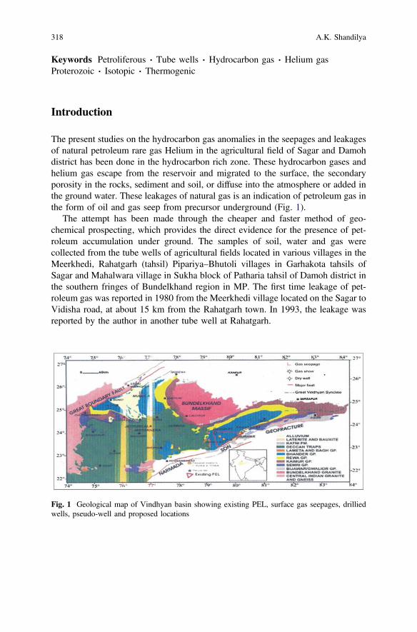
Keywords Petroliferous � Tube wells � Hydrocarbon gas � Helium gasProterozoic � Isotopic � Thermogenic
Introduction
The present studies on the hydrocarbon gas anomalies in the seepages and leakagesof natural petroleum rare gas Helium in the agricultural field of Sagar and Damohdistrict has been done in the hydrocarbon rich zone. These hydrocarbon gases andhelium gas escape from the reservoir and migrated to the surface, the secondaryporosity in the rocks, sediment and soil, or diffuse into the atmosphere or added inthe ground water. These leakages of natural gas is an indication of petroleum gas inthe form of oil and gas seep from precursor underground (Fig. 1).
The attempt has been made through the cheaper and faster method of geo-chemical prospecting, which provides the direct evidence for the presence of pet-roleum accumulation under ground. The samples of soil, water and gas werecollected from the tube wells of agricultural fields located in various villages in theMeerkhedi, Rahatgarh (tahsil) Pipariya–Bhutoli villages in Garhakota tahsils ofSagar and Mahalwara village in Sukha block of Patharia tahsil of Damoh district inthe southern fringes of Bundelkhand region in MP. The first time leakage of pet-roleum gas was reported in 1980 from the Meerkhedi village located on the Sagar toVidisha road, at about 15 km from the Rahatgarh town. In 1993, the leakage wasreported by the author in another tube well at Rahatgarh.
Fig. 1 Geological map of Vindhyan basin showing existing PEL, surface gas seepages, drilliedwells, pseudo-well and proposed locations
318 A.K. Shandilya

The carbon isotope studies of methane and other gases were done to knowwhether these petroleum gases are of biogenic or of thermogenic origin. Colemanet al. (1977) in a study on the leakage of gas from the underground storage reservoirshowed that isotopic analysis is a reliable technique for differentiating betweenmethane from thermogenic and biogenic source. A useful geochemical method tocorrelate gases with their source rocks is d C13 determination. The isotopic com-position of methane was found to be a more reliable indicator of hydrocarbonreservoir. Shandilya (2007) has reported the occurrence of the petroleum gas in theSagar District and suggested that these petroleum gases are of thermogenic inorigin. Shandilya (2008a, b, c, d) made Discovery of Natural Gas leakages fromBore wells in the rocks of the Vindhyan Super group in Sagar and Damoh Districts,
Discovery of the Helium Rare Gas in Saugor Division … 319

MP and forecasted the reserve of Natural Gas Reserves in Sagar District. Shandilya(2009a, b, c) published an article on GAS IN THE BACKYARD in theBUSINESS INDIA MAGZINE suggesting that this gas is of thermogenic origin.Shandilya (2009a, b, c) has suggested the possibility of Petroleum Gas reserve inSouthern Bundelkhand Region, MP. Shandilya and Gajbhiye (2010) made theDiscovery of Rare Helium Gas in Sagar District, MP.
Prasanna et al. (2010) conducted the detail investigation of light gaseoushydrocarbon anomalies in the surface soil around Sagar using the geochemicalexploration methods for hydrocarbon leakages. The investigation was focused onthe detection of absorbed petroleum gases by gas chromatographic method, inVindhyan basin using composition and ratio of the light hydrocarbons methane,ethane, propane and butane (Fig. 2).
Geology
The present natural gas leakages has been discovered in the dried tube wells,located on the rocks of Sandstone, shale and limestone rocks of the Rewa andBhander Group of the Vindhyan Super Group as the basement rocks. Thesepetroliferous rocks are overlain by the Lameta bed (late Cretaceous) in the westernpart of the Pipariya and Bhutoli area in Garhakota tahsil. The western part of thepresent area is overlain by the rocks of Upper Cretaceous Deccan Trap Basalticflows, which are intercalated with intertrappean limestone. The area where theleakages of petroleum gas have been discovered is located on the alluvial soil cover.The Deccan Trap Basaltic rocks are exposed in west of the Chinnoua village inGarhakota Tahsil. The dips of the sandstone and shales rocks are 10°–15° towardSE direction. The topography is more or less flat with some low-lying areas near thestream. The geological formation of Sagar area consists of 09 flows of Deccan Trap.
With several intertrappean limestone beds, whole area being underlain to the eastand south by the Lameta limestone, which forms the plains and some hills to thesouth. Western fringe of The Rahatgarh and Meerkhedi areas are covered mostly bythe Basaltic flows of Deccan Traps except few inliers of the shale and sandstonerocks of Rewa Group and Bhander Group of the Vindhyan Super Group. TheDeccan Trap basalt rocks are mostly covered by the black soil. The Deccan vol-canism during late Cretaceous must have generated the proper thermal conditionsand acted as a catalyst in triggering Mesozoic hydrocarbon generation processes inthe Vindhyan sedimentary basin in Central India (Table 1).
320 A.K. Shandilya

Fig. 2 Map of India (not to scale) showing petroliferous basins developed along the triangulararea of paleocourse of the Indian rivers (JOUR. GEOL. SOC. INDIA, VOL. 85, JUNE 2015)
Discovery of the Helium Rare Gas in Saugor Division … 321

Observation
On the request of authors, the Director Exploration, KDM IPE, ONGC Dehradunand Director, NGRI Hyderabad has sent a team of scientists for the detailedinvestigation had visited the Piparia–Bhutoli and Rahatgarh and Meerkhedi areaand collected the samples of soil, water and gas. The samples were collected fromthe following localities:
1. Bhu-1: These tube wells fall under the panchayat and P.O. chanauaa tahsilGarhakota district Sagar, MP (part of survey of India toposheet no. 55 m/L). Itis accessible by a 3 km Village road from town Garhakota around 45 km East
Table 1 The stratigraphic succession in Sagar District, MP
Age Formation
Recent subRecent/quaternaries
Alluvium soil
Black soil
Upper cretaceous Deccan trap basalt (with intertrapean limestone)
Lower cretaceous Lameta formation
Late proterozoic Bhander (containing the petroleum gas andhelium gas)
Rewa
Vindhyan super group Kaimur
Semri
Middle proterozoicBijawar super group
Phosphastic dolomite
Dolomite
Ferrugenous shale
Ferrugenous sandstone
Iron formation/BHQ
Quartzite
Conglomerate bed
Early proterozoic Bundelkhand granitecomplex
Quartz reef intrussion
Pegmatitic intrussion
Ultramafic intrusive
Granite intrussive rocks
Granite gneiss
Biotite schist
ArcheanMehroni super group
Intrussive body
Dolomitic marble
Slate
Ferrugenous formation
Quartzite
Schist
(Modified after Rang rajan 1978)
322 A.K. Shandilya

of Sagar on way to Damoh. The leakage of petroleum gas is reported from 08tube wells in the month of March 2007.
(a) These bore/tube wells varying in the depth from 260 to 400 ft. with top60 ft. is of 8″ diam with plastic casing, and rest of well is of 6″ diameterdepth 340 ft.) of Shri Bhagwan singh Yadav (lat: 23° 47′ 59.2″N, long:79° 05′ 29.6″E, Elevation 448 m).
(b) Pip-1: The tube wells (depth 400 ft.) of Sri Asharam Patel S/o Sri GhappuPatel (lat: 23° 48′ 20″N, long: 79° 50′ 20.7″E, Elevation 450 m).
2. Rah-1: This village is located 40 km west of Sagar on way to Bhopal Road. Inthe bore well of Shri Leeladhar Tiwari (Tiwari Dhawa: lat: 23° 57′ 15.7″N,long: 79° 25′ 03″E, Elevation 484 m), the tube well is situated on the deccantrap—Vindhyan contact. The leakage of petroleum gas has been reported since1993.
3. Mee-1: This tube well (lat: 23° 45′ 56″N, long: 78° 18′ 9.6″E, Elevation440 m) from where gas seepage was occurring belongs to Shri Dhan Singh. Thearea falls in the toposheet of India No. 55 I/5. This tube well is the easternextremity of village Meerkhedi, 13 km of Rahatgarh on way to Vidisha. Thistube well pouring the petroleum gas sinse 1984 having enormous bubbling in thewater. The tube well is located on the contact of daccan tram basalt and vindhyansand stone (Inlier). The quantity of petroleum gas bublings increase day by day.
4. Mah-1: The leakages of the petroleum gas has been reported since 2009 fromthis village in Patharia Tahsil of Damoh district. The 378 ft. deep tube well ispouring the water along with the natural petroleum gas and the water which iscoming out of the tube well is burning up to 2–3 ft. long flame. In the bore wellof Sri Halle singh Lodhi at Mahalwara about 11 km north of Patharia railwaystation in Damoh District. Is also containing the leakages of petroleum gas inthe 378 deep tube well, which was digged in November 2008. The tubewellwater getting fire, when light up the matchstick about 1.00 m high flameburning in water. The petroleum gas is also coming out of the tube well whenno pumping is done, the leakage of the gas can be easily seen in it.
5. Bat-1: It is located about 25 km from Damoh. In the tube wells the water givesthe smell of kerosene/diesel in the month of November–December, 2008onward. The tube wells are varying in depth from 350 to 400 ft. in theVindhyan Limestone rocks.
6. Pat-1: In this village the tube well is situated in the inliers of the Vindhyan.Rocks among the Deccan Trap cover, the tube well was digged in 2000, anddepth is about 380 ft. It is also pouring the natural petroleum gas as it wasreported in November, 2011.
7. SUK-1: In the agricultural field near the Limestone quarry of Narsingh garhCement (Heidel berg Cement Plant) there is a leakages of petroleum gas alongwith water. Reported in December, 2009.
8. Man1: A tube well situated in the Deccan trap rocks in Mandi Bamora, depth is390 ft. digged in May, 2012 also pouring the natural gas along with water. The
Discovery of the Helium Rare Gas in Saugor Division … 323
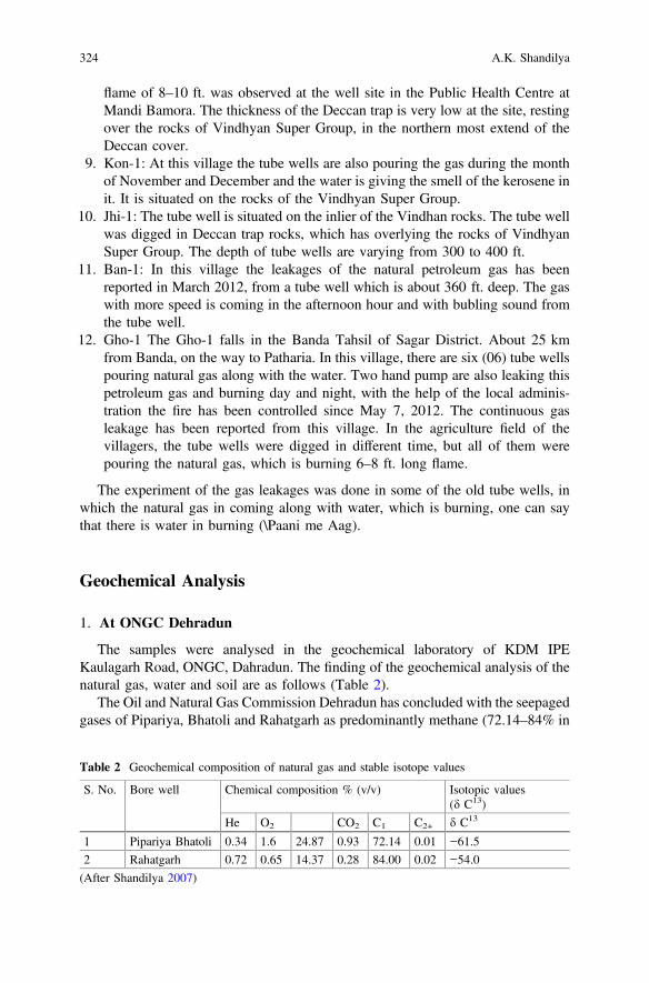
flame of 8–10 ft. was observed at the well site in the Public Health Centre atMandi Bamora. The thickness of the Deccan trap is very low at the site, restingover the rocks of Vindhyan Super Group, in the northern most extend of theDeccan cover.
9. Kon-1: At this village the tube wells are also pouring the gas during the monthof November and December and the water is giving the smell of the kerosene init. It is situated on the rocks of the Vindhyan Super Group.
10. Jhi-1: The tube well is situated on the inlier of the Vindhan rocks. The tube wellwas digged in Deccan trap rocks, which has overlying the rocks of VindhyanSuper Group. The depth of tube wells are varying from 300 to 400 ft.
11. Ban-1: In this village the leakages of the natural petroleum gas has beenreported in March 2012, from a tube well which is about 360 ft. deep. The gaswith more speed is coming in the afternoon hour and with bubling sound fromthe tube well.
12. Gho-1 The Gho-1 falls in the Banda Tahsil of Sagar District. About 25 kmfrom Banda, on the way to Patharia. In this village, there are six (06) tube wellspouring natural gas along with the water. Two hand pump are also leaking thispetroleum gas and burning day and night, with the help of the local adminis-tration the fire has been controlled since May 7, 2012. The continuous gasleakage has been reported from this village. In the agriculture field of thevillagers, the tube wells were digged in different time, but all of them werepouring the natural gas, which is burning 6–8 ft. long flame.
The experiment of the gas leakages was done in some of the old tube wells, inwhich the natural gas in coming along with water, which is burning, one can saythat there is water in burning (\Paani me Aag).
Geochemical Analysis
1. At ONGC Dehradun
The samples were analysed in the geochemical laboratory of KDM IPEKaulagarh Road, ONGC, Dahradun. The finding of the geochemical analysis of thenatural gas, water and soil are as follows (Table 2).
The Oil and Natural Gas Commission Dehradun has concluded with the seepagedgases of Pipariya, Bhatoli and Rahatgarh as predominantly methane (72.14–84% in
Table 2 Geochemical composition of natural gas and stable isotope values
S. No. Bore well Chemical composition % (v/v) Isotopic values(d C13)
He O2 CO2 C1 C2+ d C13
1 Pipariya Bhatoli 0.34 1.6 24.87 0.93 72.14 0.01 −61.5
2 Rahatgarh 0.72 0.65 14.37 0.28 84.00 0.02 −54.0
(After Shandilya 2007)
324 A.K. Shandilya
Pipariya, Bhutoli and 99% in Tiwari Dhaba, Rahatgarh Bore well, and are devoid ofhigher hydrocarbons. The hydrocarbon gases seem to have predominance of bac-terial methane. The pressure of both the seepages is extremely low. As per theowners, the quantity of gas is diminishing day-by-day. The results this time ofmethane is concerned. Genetically the seepage gases from Pipariya, Bhatoli andRahatgarh seem to be different from thermogenic gases encountered in exploratorywell Jabera-1, drilled by ONGC in Damoh District (MP).
In January 2008, in Bhutoli village further land owner bore the well up to 400 ft.deep, there is huge quantity of natural gas reported to government agencies. InFebruary, 2008 two villagers at Pipariya–Bhutoli have drilled two more tube wellsup to the depth of 300–350 ft. about 600–700 m away from the earlier wells in theshales and sandstone rocks of Lower Bhander, they could not get the ground water,but there was leakage of natural gas, which is also giving blue flame.
2. At NGRI, Hyderabad:
The samples of petroleum gas, soil and water were also collected by the sci-entists Dr. A.M. Dayal, Dr. Ravi Srivastava, and Dr. D.J. Patil of NGRI Hyderabadalong with the author on May 4–5, 2008. The detail geochemical and stable isotopicstudies of the natural petroleum gas, soil and water sample has been done in theLaboratories of NGRI (Tables 3 and 4).
The presence of the ethane gas in both the Localities, and d C13 value in the rangeof −0.249 and −26.4‰ w.r.t. PDB indicate the thermogenic source of these gases.On the basis of the geochemical and stable isotopic studies of the natural petroleumgas, soil and water suggest that the samples of the Piparia–Bhutoli–Rahatgarh–Meerkhedi of Sagar District containing 72–99% of methane, 0.34–0.742% ofHelium, along with the oxygen, carbon dioxide and Nitrogen gases. The stableisotopic d C13 value in the range varying from −43.6‰ w.r.t PDB for methane−24.66‰w.r.t PDB for ethane at Piparia–Bhutoli to−54.9‰w.r.t PDB for methaneand per mil w.r.t PDB for at Rahatgarh are indicative of the THERMOGENIC originand also that methane is associated with oil. Bernard (1978) suggested a geneticdiagram by correlating (C1/C2 + C3) ratio with d C13 1 concentration of methane to
Table 3 Stable isotopic value of hydrocarbon gas in Sagar District, MP, India
Location Name of petroleum gas Stable isotopic value d C13
Piparia–Bhutoli Methane −43.6‰ w.r.t. PDB
Ethane −24.6‰ w.r.t. PDB
Rahatgarh–Meerkhedi Methane −54.9‰ w.r.t. PDB
Ethane −26.4‰ w.r.t. PDB
(After Shandilya 2008)
Table 4 The absorbed soilhydrocarbon gasconcentration in SagarDistrict, MP
C1 C2 C3 i C4 n C4P
C3+
Minimum 1 1 1 1 1 1
Discovery of the Helium Rare Gas in Saugor Division … 325
classify natural gas types. Molecular ratio C1/C2 + C3 less than 50 are typical for thethermogenic hydrocarbon gases with d C13 values between −30 and −55% (PDB).This suggests that most of the samples fall in the thermogenic range.
The adsorbed soil gas result indicates the presence of methane, ethane, propaneand butane in Sagar District, MP. The adsorbed soil gas and carbon isotope studiessuggest that these seeped hydrocarbons are of thermogenic origin and petroliferousin nature and indicate the area is warm for hydrocarbon exploration area.
Conclusion
In my opinion the natural petroleum and helium gas are containing the higheramount of Methane (72–99%), and remarkable content 0.34–0.742% of Helium,and minor amount of oxygen, nitrogen and carbon dioxide, it suggests that it musthave been formed at higher temperature condition at deeper horizon in thePre-Cambrian Vindhyan sedimentary basin (Proterozoic in age). The reservoir mustbe lying below the ground at least 500 m or more deep level. The present leakagesof natural gas releasing through many hairline cracks/fracture and feather joints inthe sandstone, shales and limestone rocks of the Rewa and Bhander group rocks ofthe Vindhyan Super Group.
As per the geochemical and stable isotopic studies of Gas samples analysed atNGRI; it found out the methane and ethane gases. The presence of ethane gascollected from the abovementioned localities and the d C13 stable isotopic value inthe range of −24.9 to −26.9‰ w.r.t. PDB indicative of the Thermogenic sources.
Acknowledgements The authors are thankful to the Director, NGRI and Dr. A.M. Dayal Asstt.Director of NGRI Hyderabad, and the Director, KDMIPE, ONGC, Dehradun for the Geochemicaland Stable isotopic analysis of the various samples. The author is highly thankful for the criticalcomments and valuable suggestions on this manuscript by Prof. R.P. Tiwari Vice chancellor, Dr.H.S.G. University, Sagar and Prof. P.S. Saklani, Ex, Vice Chancellor, HNB Garhwal University,Srinagar Garhwal and Prof. S.P. Banarjee and Prof. K.S Pitre, Department of Chemistry, Dr. HariSingh Gour University, Sagar, MP.
References
Bernard BB (1978) Light hydrocarbon in sediments. Ph.D dissertation. Texas A&M University,USA p. 144
Coleman DD, Meents WF, Liu CL, Keogh RAS (1977) Isotopic identification of leakage gas fromunderground storage reservoir—a progress report III. Petrology 1977(111):1–10
Fuex AN (1977) The use of stable carbon isotopes in hydrocarbon exploration. J Geochem Explor7:155–188
Horvitz L (1979) Near surface evidence of hydrocarbon movement from depth problems ofpetroleum migration. Am Asso Pet Geol 10:241–269 (1979)
326 A.K. Shandilya
Lones VT, Drozd RJ (1983) Prediction of oil and gas potential by near surface geochemistry. AmAsso Petr Geol Bull 983(67):932–952
Prasanna MV, Rasheed MA, Madhavi T, Kalpana G, Patil DJ, Dayal AM (2010) Light gaseoushydrocarbon anomalies in the near surface soils of Sagar District, Vindhyan Basin, India. CurrSci 99(11):1586–1590
Raina and Tiwari et al (2007) Unpublished report of ONGC 2007Rajrajan K (1978) Geology of Sagar District and western part of Damoh district Memoirs, GSI, vol
109Shandilya AK (2007) Natural petroleum gas found in Piparia-Bhutoli-Rahatgarh in Sagar District.
Bundelkhand region MP University J Madhya Bharati 53:122–124Shandilya AK (2008a) Discovery of Natural Petroleum gas in the rocks of the Vindhyan super
group in Sagar District. Bundelkhand region MP Qtrly J GARC 16(I):24–27Shandilya Arun K (2008b) FUEL HO—leakages of gas in tube wells spew natural gas. News
Magzine Mach 2008:31–32Shandilya AK (2008c) Natural gas leakages from bore wells in the rocks of the Vidhyan super
group in Sagar and Damoh districts. MP J Himalayan Geol 29(2):174–175Shandilya AK (2008d) Natural gas reserves in Sagar District. Srujun University Newsl 9:19Shandilya AK (2009a) Gas in the backyard. Bus India Magzine 144Shandilya AK (2009b) Thermogenic petroleum gas found in tube wells of Sagar District. MP
Madhya Bharati, Diamond Jubilee Volume 314–319Shandilya AK (2009c) The possibility of petroleum gas reserve in southern Bundelkhand region.
MP University Newsl Vishwavidyalaya Samvad 2:3Shandilya AK (2011) The discovery of natural petroleum and helium gas in tube wells of Sagar–
Damoh district in Vindhyan rocks, MP. Proc Sediment Basins India Gondwana Geol SocNagpur 2011:125–130
Shandilya AK (2013) Studies on helium & natural gas anomalies in tube wells around southernGanga Basin, Bundelkhand region, MP, India. In: Janardhan Raju N, Wolgane R, Sudhakar M(eds) Book-management of water, energy & bioresources in the era of climate change. CapitalPubl. House, New delhi, pp154–160
Shandilya AK and Gajbhiye NS (2010) Discovery of rare helium gas in Sagar District, MP India.In: Proceedings of 5th international conference, South Valley University QENA, EGYPT. 2–7Jan 2010 pp 26–30
Shandilya AK, Shandilya A (2014) Helium and petroleum gas found in rocks of Vindhayn supergroup, South Ganga Basin, Bundelkhand region, MP, India. In: Proceedings of the IIIinternational conference on petroleum science and technology (ICPST2014) IIT Madras 3–5Nov 2014, p 26
Shandilya AK, Shandilya A, Shandilya A (2012) Hydrocarbon gaseous anomalies found inagriculture field around Sagar and Damoh District reactors Bundelkhand region, MP. Int JChem Life Sci 1(3):1039–1044
The News of Discovery of Petroleum gas was published in News papers: Dainik jagran, DainikBhaskar, Raj express, Nav Bharat, Nai dunia, Hindustan times, Acharan etc
The News of Discovery of Petroleum Gas was Broad Casted in TV Channels: Door Dhashan(DD) state and National both, Sahara National, India TV ETV, Times, and AajTak, KhabarBharti, ZNews, & P 7 TV channel etc
Discovery of the Helium Rare Gas in Saugor Division … 327
How Soil Texture Affects the OrganicCarbon Load in the Mangrove Ecosystem?A Case Study from Bhitarkanika, Odisha
Kakoli Banerjee, Gobinda Bal and Abhijit Mitra
Abstract We analysed the inter-relationship between soil texture and organiccarbon (OC) in 12 stations of Bhitarkanika mangrove ecosystem. Our first-orderanalysis reflects a significant positive correlation of silt and clay with OC(rsilt � organic carbon = 0.90; p < 0.01 and rclay � organic carbon = 0.84; p < 0.01).However, in case of sand, a significant negative correlation is visualized with OC(r = −0.89; p < 0.01). The results indicate that OC forms a coating over silt andclay particles on the basis of principle of cohesion, but this cohesive force is notvisible in case of sand particles. The overall analysis suggests the need of coastalvegetation conservation in the Bhitarkanika area as their decomposition productslead to the formation of organic carbon that serve as important nutrient for thegrowth and survival of the mangrove vegetation in the study area.
Keywords Bhitarkanika mangrove ecosystem � Soil textureSoil organic carbon (SOC)
Introduction
Mangrove ecosystem is a storehouse of rich floral and faunal biodiversity withendemic adaptation having great ecological and economical significance. Theproduct of biodiversity is the basic need for growing human populations. Amongthe biodiversity rich regions, the coastal marine ecosystems are one of the mostproductive, biologically diverse and significantly valuable areas. Hence, they arealso called as, “heart of ocean”. They produce high detritus and particulate organic
K. Banerjee (&) � G. BalDepartment of Biodiversity and Conservation of Natural Resources, Central Universityof Orissa, Landiguda, Koraput 764020, Odisha, Indiae-mail: [email protected]
A. MitraDepartment of Marine Science, University of Calcutta, Kolkata 700019, West Bengal, India
© Springer Nature Singapore Pte Ltd. 2018V.P. Singh et al. (eds.), Environmental Pollution, Water Scienceand Technology Library 77, https://doi.org/10.1007/978-981-10-5792-2_27
329

matter and release as nutritious food for various organisms. Some other usefulnessof mangroves are fuel, energy, health, medicine, food, fertilizer and many otherindustrial products. The important biogeochemical services of mangroves includethe entrapment of sediments and pollutants, filtering of nutrients, remineralizationof organic and inorganic matter, and export of organic matter (Alongi et al. 1992).But as a result of climate change and unplanned developmental activities, themangrove forests are suffering from its degradation.
The ongoing physical, chemical, biological and geological processes change thedead organisms, detritus and riverine organic materials, etc. into particulate matterand enrich the adjacent aquatic ecosystems. These processes also include the supplyof inorganic and organic substances from river run-off, resuspension of previouslydeposited sediments production and breakdown of biological materials, andphysico-chemical adsorption-desorption processes related to redox reactions nearwater-sediment boundary (Feeby et al. 1986). Salinity of soil depicts the geo-graphical feature and position of the ecosystem (Banerjee et al. 2012). The salinityof soil is also dependent upon the amount of fresh water discharge (Mitra et al.2011). High amount of anthropogenic sewage discharge increase the pH of soil inmangrove (Banerjee et al. 2012). The climate, geomorphology, tidal range, freshwater input, physico-chemical properties and biological factors, etc. together con-trol the nutrient status, productivity and biodiversity of mangroves. The mangrovesediments of Bhitarkanika were Pleistocene deposits comprising clay, sand, silt and‘kankar’, with reddish brown cemented pebbles and gravels due to high degree ofoxidation (Banerjee and Rao 1990). Benthic zones near continental shelf act asclosed vessels, which wells up nutrient between adjacent terrestrial land mass andocean. Mangrove largely constitutes fertile estuary with rich source of nutrientshaving detritus-based food web. The vegetation forms a direct source of food forinsects, crustaceans, invertebrate and vertebrates. Most of the productions frommangroves get transferred to other trophic levels by means of litter fall and detrituspathway.
In biological point of view, mangrove ecosystem is primarily a source of organicmatter and nutrients, which also acts as sink for organic carbon, sediments andpollutants over a long period of time (Kristensen et al. 2008). Mangrove sedimentscharacterized by high organic matter serve as organic substrates for microbialcommunities (Alongi 1998). Thus, the ecosystems play a vital role in the biogeo-chemistry of contaminants present in the tropical coastal areas (Dittmar and Lara2001) and hence they have remarkable potential to store nutrients (Dwivedi andPadmakumar 1983). The nutrient fluctuation of a mangrove ecosystem is animportant function in terms of biogeochemical cycling of elements in the coastalzone (Jennerjahn and Ittekot 2002). The sediments of mangrove play a pivotal rolein nutrient biogeochemical processes, both as a source and sink for nutrients andorganic matter. Sediments are characteristically rich in organic matter but low innutrient quality. The nutrient and organic matters dynamics in the high salinitycoastal wetlands also depends upon the river run-off, anthropogenic discharges andallochthonous (mangrove litter, phytoplankton and benthic algae) (Hedges and Keil1995; Hedges et al. 1997; Harji et al. 2010). The fate of this detritus is recycling
330 K. Banerjee et al.
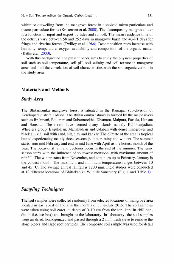
within or outwelling from the mangrove forest in dissolved micro-particulate andmacro-particulate forms (Kristensen et al. 2000). The decomposing mangrove litteris a function of input and export by tides and run-off. The mean residence time ofthe detritus vary between 58 and 252 days in mangrove basin and 40–91 days forfringe and riverine forests (Twilley et al. 1986). Decomposition rates increase withhumidity, temperature, oxygen availability and composition of the organic matter(Kathiresan 2000).
With this background, the present paper aims to study the physical properties ofsoil such as soil temperature, soil pH, soil salinity and soil texture in mangroveareas and find the correlation of soil characteristics with the soil organic carbon inthe study area.
Materials and Methods
Study Area
The Bhitarkanika mangrove forest is situated in the Rajnagar sub-division ofKendrapara district, Odisha. The Bhitarkanika estuary is formed by the major riverssuch as Brahmani, Baitarani and Subarnarekha, Dhamara, Maipura, Patsala, Hansuaand Hansina. The rivers have formed many islands namely Kalibhanjadian,Wheelers group, Bagulidian, Manakudian and Udabali with dense mangroves andblack alluvial soil with sand, silt, clay and kankar. The climate of the area is tropicalhumid experiencing mainly three seasons (summer, rainy and winter). The summerstarts from mid February and end in mid June with April as the hottest month of theyear. The occasional rain and cyclones occur in the end of the summer. The rainyseason starts with the influence of southwest monsoon, with maximum amount ofrainfall. The winter starts from November, and continues up to February. January isthe coldest month. The maximum and minimum temperature ranges between 10and 45 °C. The average annual rainfall is 1200 mm. Field studies were conductedat 12 different locations of Bhitarkanika Wildlife Sanctuary (Fig. 1 and Table 1).
Sampling Techniques
The soil samples were collected randomly from selected locations of mangrove arealocated in east coast of India in the months of June–July 2015. The soil sampleswere taken using soil corer, at depth of 0–10 cm from the top, kept in chill con-dition (i.e. ice box) and brought to the laboratory. In laboratory, the soil sampleswere air dried, homogenized and passed through a 2 mm mesh sieve to remove thestone pieces and large root particles. The composite soil sample was used for detail
How Soil Texture Affects the Organic Carbon Load … 331
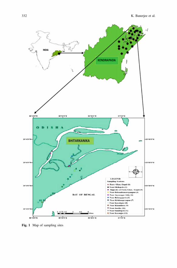
Fig. 1 Map of sampling sites
332 K. Banerjee et al.

analysis of soil salinity, pH, temperature, soil texture and organic carbon throughstandard methods.
Analysis of Soil Parameters
The soil temperature was measured by using digital thermometer (SIGMA) bydipping it in the soil directly, and five readings were taken and the average soiltemperature reading was taken as final. The soil pH was measured by using digitalpH metre (SYSTRONICS), and similar process was repeated with five readings andthe average was calculated as final. Soil salinity was determined by measuring theelectrical conductivity with the help of a conductivity metre. Soil texture wasmeasured by the Hydrometer method (Gee and Bauder 1986). Soil Organic Carbonof the samples were analysed by the standard titration method (Walkley and Black1934). The data collected were expressed as Mean ± standard deviation. In order tofind out the difference between the physico-chemical parameters of soil in man-grove areas ANOVA analysis was computed using SPSS 13.1. Correlation coeffi-cients were computed in order to find out the inter-relationship between soilphysical properties and soil organic carbon.
Table 1 Sampling site coordinates with description
S. No. Name of the stations Coordinates latitude longitude Major activity
1 Ferry Ghat, Gupti 20° 39′ 09.80″N 86° 51′ 01.07″E Transport and tourist
2 Near Okilapalo 20° 38′ 15.71″N 86° 52′ 53.15″E Transport andagriculture
3 Opposite of Gupti 20° 39′ 20.83″N 86° 51′ 05.54″E Transport and tourist
4 NearDebendranarayanpur
20° 38′ 15.92″N 86° 51′ 59.79″E Sewage discharge
5 Near Jayanagar Jetty 20° 41′ 58.51″N 86° 47′ 55.02″E Transport and tourist
6 Near Balungapeta 20° 41′ 22.57″N 86° 51′ 33.19″E Agriculture
7 Near Krishnapryapur 20° 36′ 53.95″N 86° 51′ 15.47″E Tourist and agriculture
8 Near Kanakpur 20° 36′ 02.33″N 86° 50′ 38.38″E Agriculture
9 Near Khandiora 20° 34′ 47.42″N 86° 49′ 53.73″E Agriculture
10 Near Jaudia 20° 32′ 58.04″N 86° 47′ 59.40″E Agricultureand aquaculture
11 Near Sundripal 20° 31′ 25.29″N 86° 45′ 49.29″E Agricultureand aquaculture
12 Near Karanjia 20° 31′ 27.71″N 86° 46′ 28.05″E Agricultureand aquaculture
How Soil Texture Affects the Organic Carbon Load … 333
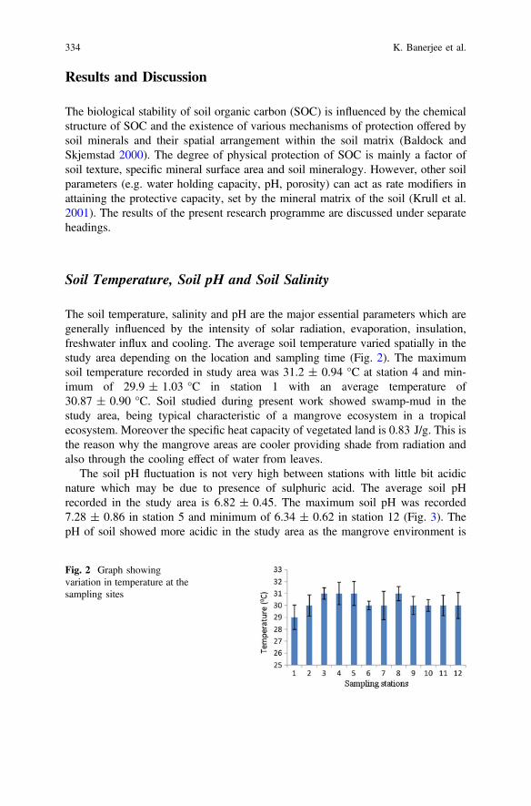
Results and Discussion
The biological stability of soil organic carbon (SOC) is influenced by the chemicalstructure of SOC and the existence of various mechanisms of protection offered bysoil minerals and their spatial arrangement within the soil matrix (Baldock andSkjemstad 2000). The degree of physical protection of SOC is mainly a factor ofsoil texture, specific mineral surface area and soil mineralogy. However, other soilparameters (e.g. water holding capacity, pH, porosity) can act as rate modifiers inattaining the protective capacity, set by the mineral matrix of the soil (Krull et al.2001). The results of the present research programme are discussed under separateheadings.
Soil Temperature, Soil pH and Soil Salinity
The soil temperature, salinity and pH are the major essential parameters which aregenerally influenced by the intensity of solar radiation, evaporation, insulation,freshwater influx and cooling. The average soil temperature varied spatially in thestudy area depending on the location and sampling time (Fig. 2). The maximumsoil temperature recorded in study area was 31.2 ± 0.94 °C at station 4 and min-imum of 29.9 ± 1.03 °C in station 1 with an average temperature of30.87 ± 0.90 °C. Soil studied during present work showed swamp-mud in thestudy area, being typical characteristic of a mangrove ecosystem in a tropicalecosystem. Moreover the specific heat capacity of vegetated land is 0.83 J/g. This isthe reason why the mangrove areas are cooler providing shade from radiation andalso through the cooling effect of water from leaves.
The soil pH fluctuation is not very high between stations with little bit acidicnature which may be due to presence of sulphuric acid. The average soil pHrecorded in the study area is 6.82 ± 0.45. The maximum soil pH was recorded7.28 ± 0.86 in station 5 and minimum of 6.34 ± 0.62 in station 12 (Fig. 3). ThepH of soil showed more acidic in the study area as the mangrove environment is
Fig. 2 Graph showingvariation in temperature at thesampling sites
334 K. Banerjee et al.
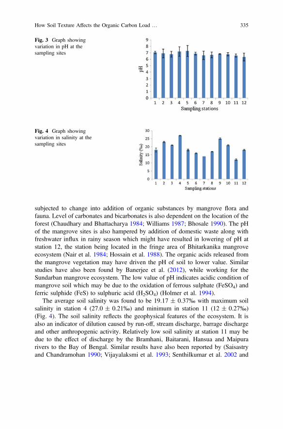
subjected to change into addition of organic substances by mangrove flora andfauna. Level of carbonates and bicarbonates is also dependent on the location of theforest (Chaudhary and Bhattacharya 1984; Williams 1987; Bhosale 1990). The pHof the mangrove sites is also hampered by addition of domestic waste along withfreshwater influx in rainy season which might have resulted in lowering of pH atstation 12, the station being located in the fringe area of Bhitarkanika mangroveecosystem (Nair et al. 1984; Hossain et al. 1988). The organic acids released fromthe mangrove vegetation may have driven the pH of soil to lower value. Similarstudies have also been found by Banerjee et al. (2012), while working for theSundarban mangrove ecosystem. The low value of pH indicates acidic condition ofmangrove soil which may be due to the oxidation of ferrous sulphate (FeSO4) andferric sulphide (FeS) to sulphuric acid (H2SO4) (Holmer et al. 1994).
The average soil salinity was found to be 19.17 ± 0.37‰ with maximum soilsalinity in station 4 (27.0 ± 0.21‰) and minimum in station 11 (12 ± 0.27‰)(Fig. 4). The soil salinity reflects the geophysical features of the ecosystem. It isalso an indicator of dilution caused by run-off, stream discharge, barrage dischargeand other anthropogenic activity. Relatively low soil salinity at station 11 may bedue to the effect of discharge by the Bramhani, Baitarani, Hansua and Maipurarivers to the Bay of Bengal. Similar results have also been reported by (Saisastryand Chandramohan 1990; Vijayalaksmi et al. 1993; Senthilkumar et al. 2002 and
Fig. 3 Graph showingvariation in pH at thesampling sites
Fig. 4 Graph showingvariation in salinity at thesampling sites
How Soil Texture Affects the Organic Carbon Load … 335

Banerjee et al. 2012) while working in the Godavari estuary, Gulf of Kachchh,Bellar estuary and Sundarban estuaries, respectively.
Soil Texture
The architecture of the soil mineral matrix refers to the arrangement of pores andsoil particles. Almost all organic carbon in soil is located within pores betweenmineral grains either as discrete particles or as molecules adsorbed onto the surfacesof mineral particles. Soil architecture can influence the biological stability oforganic materials through its effects on water and oxygen availability, entrapmentand isolation from decomposers, and through the dynamics of soil aggregation. Soiltexture is a single most important physical property of the soil and alone providesstatus of water flow potential, water holding capacity, fertility potential and suit-ability for many urban uses (Chaudhuri and Choudhury 1994; Sarkar et al. 1999). Inthe present study, the soil texture has been measured in term of sand, silt and clay atall the sampling points in the study area. The values of sand, silt and clay rangedfrom 14.0 ± 0.56% to 62.0 ± 0.65%, 13.0 ± 0.34% to 45.0 ± 0.44% and25 ± 0.13% to 49.0 ± 0.38% with an average value of 25.83 ± 0.48%,34.25 ± 0.41% and 39.9 ± 0.32%, respectively, (Figs. 5, 6 and 7). The values ofsand, silt and clay varied as per the order clay (39.9 ± 0.32%) > silt(34.25 ± 0.41%) > sand (25.83 ± 0.48%) in the mangrove area. This is mainlydue to the difference in soil susceptibility erosion (erodibility) based on texture.A soil with high percentage of sand, silt and clay particles (mangrove area) hasgreater erodibility. Under the same conditions, the high silt and clay domination intexture in the mangrove areas may be attributed to the winnowing activity ofsediment transported system through the rivers flowing in the Bhitarkanikaestuaries.
Fig. 5 Graph showingvariation in sand percentage atthe sampling sites
336 K. Banerjee et al.
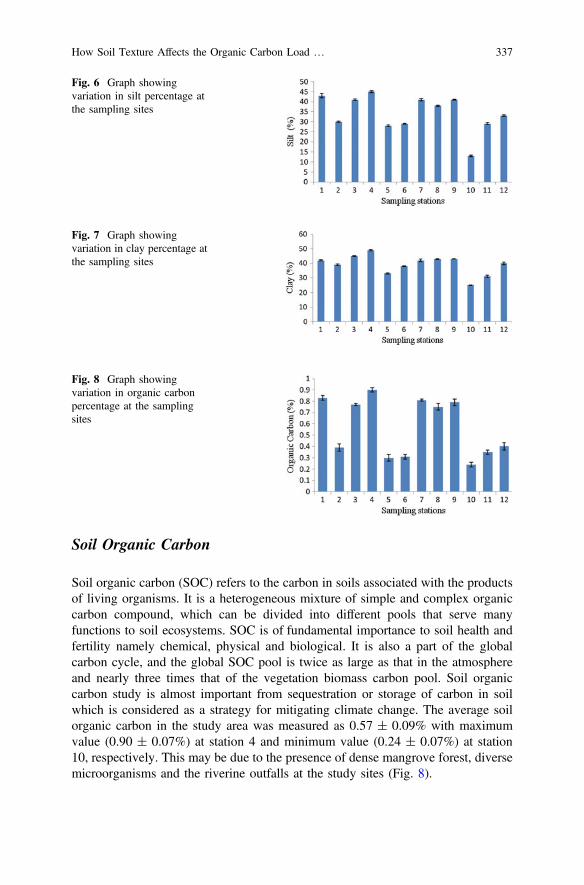
Soil Organic Carbon
Soil organic carbon (SOC) refers to the carbon in soils associated with the productsof living organisms. It is a heterogeneous mixture of simple and complex organiccarbon compound, which can be divided into different pools that serve manyfunctions to soil ecosystems. SOC is of fundamental importance to soil health andfertility namely chemical, physical and biological. It is also a part of the globalcarbon cycle, and the global SOC pool is twice as large as that in the atmosphereand nearly three times that of the vegetation biomass carbon pool. Soil organiccarbon study is almost important from sequestration or storage of carbon in soilwhich is considered as a strategy for mitigating climate change. The average soilorganic carbon in the study area was measured as 0.57 ± 0.09% with maximumvalue (0.90 ± 0.07%) at station 4 and minimum value (0.24 ± 0.07%) at station10, respectively. This may be due to the presence of dense mangrove forest, diversemicroorganisms and the riverine outfalls at the study sites (Fig. 8).
Fig. 6 Graph showingvariation in silt percentage atthe sampling sites
Fig. 7 Graph showingvariation in clay percentage atthe sampling sites
Fig. 8 Graph showingvariation in organic carbonpercentage at the samplingsites
How Soil Texture Affects the Organic Carbon Load … 337

It is generally assumed that there is a positive correlation between clay contentand preservation of SOC as documented in studies by Ladd et al. (1985), Schimelet al. (1985a, b), Spain (1990), Feller et al. (1991), Amato and Ladd (1992), andsummarized by Oades (1989). Recent studies by Schjønning et al. (1999) andThomsen et al. (1999) reported differences in the rate of degradability of soil carbonwhich was strongly correlated with water holding capacity and volumetric watercontent. In the present study, correlation coefficient computed between the soilparameters and SOC has also revealed a similar result (Table 2) at 1% level ofsignificance. To analyze the spatial variation in the soil parameters ANOVA wascomputed between the stations that also showed significant variation in soilparameters (Table 3). This proves that our results are at par with the studies done bythe earlier workers.
Conclusion
The study is extremely relevant from the point of view of mangrove growth andcoastal vegetation and its substituent carbon storage. The present study is unique initself as very few studies have been done on the comparative analysis of soil organic
Table 2 Inter-relationship between soil physico-chemical parameters and organic carbon
Temperature pH Salinity Sand Silt Clay Organiccarbon
Temperature 1
pH −0.07 1
Salinity 0.18 0.46 1
Sand −0.08 −0.09 −0.27 1
Silt 0.03 0.10 0.21 −0.99 1
Clay 0.17 0.11 0.39 −0.97 0.93 1
OrganicCarbon
−0.009 0.11 0.32 −0.90 0.91 0.84 1
Table 3 ANOVA computed to show variation among the study sites
Soil parameters Fcal Fcrit P value Average values in mangrove area
Temperature 7.46 4.30 <0.05 30.87 ± 0.90 °C
pH 109.95 4.30 <0.01 6.82 ± 0.45
Salinity 0.52 4.30 <0.1 19.17 ± 0.37‰
Sand 94.68 4.30 <0.01 25.83 ± 0.48%
Silt 124.71 4.30 <0.01 34.25 ± 0.41%
Clay 230.51 4.30 <0.01 39.9 ± 0.32%
Organic carbon 25.71 4.30 <0.01 0.57 ± 0.09%
338 K. Banerjee et al.
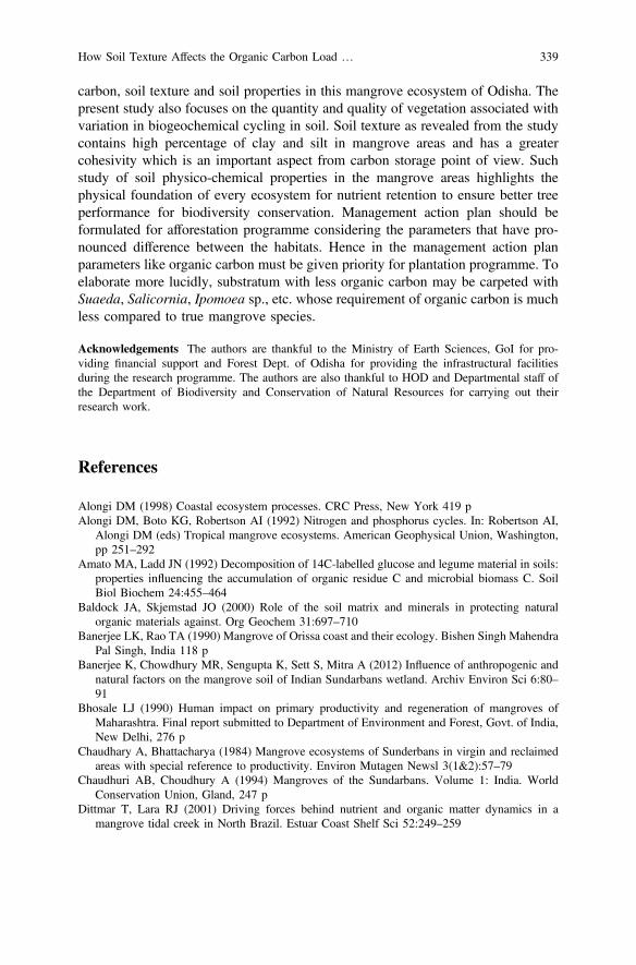
carbon, soil texture and soil properties in this mangrove ecosystem of Odisha. Thepresent study also focuses on the quantity and quality of vegetation associated withvariation in biogeochemical cycling in soil. Soil texture as revealed from the studycontains high percentage of clay and silt in mangrove areas and has a greatercohesivity which is an important aspect from carbon storage point of view. Suchstudy of soil physico-chemical properties in the mangrove areas highlights thephysical foundation of every ecosystem for nutrient retention to ensure better treeperformance for biodiversity conservation. Management action plan should beformulated for afforestation programme considering the parameters that have pro-nounced difference between the habitats. Hence in the management action planparameters like organic carbon must be given priority for plantation programme. Toelaborate more lucidly, substratum with less organic carbon may be carpeted withSuaeda, Salicornia, Ipomoea sp., etc. whose requirement of organic carbon is muchless compared to true mangrove species.
Acknowledgements The authors are thankful to the Ministry of Earth Sciences, GoI for pro-viding financial support and Forest Dept. of Odisha for providing the infrastructural facilitiesduring the research programme. The authors are also thankful to HOD and Departmental staff ofthe Department of Biodiversity and Conservation of Natural Resources for carrying out theirresearch work.
References
Alongi DM (1998) Coastal ecosystem processes. CRC Press, New York 419 pAlongi DM, Boto KG, Robertson AI (1992) Nitrogen and phosphorus cycles. In: Robertson AI,
Alongi DM (eds) Tropical mangrove ecosystems. American Geophysical Union, Washington,pp 251–292
Amato MA, Ladd JN (1992) Decomposition of 14C-labelled glucose and legume material in soils:properties influencing the accumulation of organic residue C and microbial biomass C. SoilBiol Biochem 24:455–464
Baldock JA, Skjemstad JO (2000) Role of the soil matrix and minerals in protecting naturalorganic materials against. Org Geochem 31:697–710
Banerjee LK, Rao TA (1990) Mangrove of Orissa coast and their ecology. Bishen Singh MahendraPal Singh, India 118 p
Banerjee K, Chowdhury MR, Sengupta K, Sett S, Mitra A (2012) Influence of anthropogenic andnatural factors on the mangrove soil of Indian Sundarbans wetland. Archiv Environ Sci 6:80–91
Bhosale LJ (1990) Human impact on primary productivity and regeneration of mangroves ofMaharashtra. Final report submitted to Department of Environment and Forest, Govt. of India,New Delhi, 276 p
Chaudhary A, Bhattacharya (1984) Mangrove ecosystems of Sunderbans in virgin and reclaimedareas with special reference to productivity. Environ Mutagen Newsl 3(1&2):57–79
Chaudhuri AB, Choudhury A (1994) Mangroves of the Sundarbans. Volume 1: India. WorldConservation Union, Gland, 247 p
Dittmar T, Lara RJ (2001) Driving forces behind nutrient and organic matter dynamics in amangrove tidal creek in North Brazil. Estuar Coast Shelf Sci 52:249–259
How Soil Texture Affects the Organic Carbon Load … 339
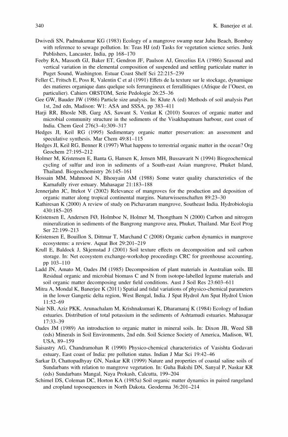
Dwivedi SN, Padmakumar KG (1983) Ecology of a mangrove swamp near Juhu Beach, Bombaywith reference to sewage pollution. In: Teas HJ (ed) Tasks for vegetation science series. JunkPublishers, Lancaster, India, pp 168–170
Feeby RA, Massoth GJ, Baker ET, Gendron JF, Paulson AJ, Grecelius EA (1986) Seasonal andvertical variation in the elemental composition of suspended and settling particulate matter inPuget Sound, Washington. Estuar Coast Shelf Sci 22:215–239
Feller C, Fritsch E, Poss R, Valentin C et al (1991) Effets de la texture sur le stockage, dynamiquedes matieres organique dans quelque sols ferrungineux et ferrallitiques (Afrique de l’Ouest, enparticulier). Cahiers ORSTOM, Serie Pedologie 26:25–36
Gee GW, Bauder JW (1986) Particle size analysis. In: Klute A (ed) Methods of soil analysis Part1st, 2nd edn, Madison: W1: ASA and SSSA, pp 383–411
Harji RR, Bhosle NB, Garg AS, Sawant S, Venkat K (2010) Sources of organic matter andmicrobial community structure in the sediments of the Visakhapatnam harbour, east coast ofIndia. Chem Geol 276(3–4):309–317
Hedges JI, Keil RG (1995) Sedimentary organic matter preservation: an assessment andspeculative synthesis. Mar Chem 49:81–115
Hedges JI, Keil RG, Benner R (1997) What happens to terrestrial organic matter in the ocean? OrgGeochem 27:195–212
Holmer M, Kristensen E, Banta G, Hansen K, Jensen MH, Bussawarit N (1994) Biogeochemicalcycling of sulfur and iron in sediments of a South-east Asian mangrove, Phuket Island,Thailand. Biogeochemistry 26:145–161
Hossain MM, Mahmood N, Bhouyain AM (1988) Some water quality characteristics of theKarnafully river estuary. Mahasagar 21:183–188
Jennerjahn JC, Ittekot V (2002) Relevance of mangroves for the production and deposition oforganic matter along tropical continental margins. Naturwissenschaften 89:23–30
Kathiresan K (2000) A review of study on Pichavaram mangrove, Southeast India. Hydrobiologia430:185–205
Kristensen E, Andersen FØ, Holmboe N, Holmer M, Thongtham N (2000) Carbon and nitrogenmineralization in sediments of the Bangrong mangrove area, Phuket, Thailand. Mar Ecol ProgSer 22:199–213
Kristensen E, Bouillon S, Dittmar T, Marchand C (2008) Organic carbon dynamics in mangroveecosystems: a review. Aquat Bot 29:201–219
Krull E, Baldock J, Skjemstad J (2001) Soil texture effects on decomposition and soil carbonstorage. In: Net ecosystem exchange-workshop proceedings CRC for greenhouse accounting,pp 103–110
Ladd JN, Amato M, Oades JM (1985) Decomposition of plant materials in Australian soils. IIIResidual organic and microbial biomass C and N from isotope-labelled legume materials andsoil organic matter decomposing under field conditions. Aust J Soil Res 23:603–611
Mitra A, Mondal K, Banerjee K (2011) Spatial and tidal variations of physico-chemical parametersin the lower Gangetic delta region, West Bengal, India. J Spat Hydrol Am Spat Hydrol Union11:52–69
Nair NB, Aziz PKK, Arunachalam M, Krishnakumari K, Dharamaraj K (1984) Ecology of Indianestuaries. Distribution of total potassium in the sediments of Ashtamudi estuaries. Mahasagar17:33–39
Oades JM (1989) An introduction to organic matter in mineral soils. In: Dixon JB, Weed SB(eds) Minerals in Soil Environments, 2nd edn. Soil Science Society of America, Madison, WI,USA, 89–159
Saisastry AG, Chandramohan R (1990) Physico-chemical characteristics of Vasishta Godavariestuary, East coast of India: pre pollution status. Indian J Mar Sci 19:42–46
Sarkar D, Chattopadhyay GN, Naskar KR (1999) Nature and properties of coastal saline soils ofSundarbans with relation to mangrove vegetation. In: Guha Bakshi DN, Sanyal P, Naskar KR(eds) Sundarbans Mangal, Naya Prokash, Calcutta, 199–204
Schimel DS, Coleman DC, Horton KA (1985a) Soil organic matter dynamics in paired rangelandand cropland toposequences in North Dakota. Geoderma 36:201–214
340 K. Banerjee et al.
Schimel DS, Stillwell MA, Woodmansee RG (1985b) Biogeochemistry of C, N, and P in a soilcatena of the short grass steppe. Ecology 66:276–282
Schjønning P, Thomsen IK, Møberg JP, de Jonge H, Kristensen K, Christensen BT (1999)Turnover of organic matter in differently textured soils: I. physical characteristics ofstructurally disturbed and intact soils. Geoderma 89:177–198
Senthilkumar S, Santhanam P, Perumal P (2002) Diversity of phytoplankton in Vellar estuary,Southeast coast of India. In: Ayyappan S, Jena JK, Mohan Joseph M (eds) The 5th Indianfisheries forum proceeding, Published by AFSIB, Mangalore and AeA, Bhubaneswar, India,245–248
Spain A (1990) Influence of environmental conditions and some soil chemical properties on thecarbon and nitrogen contents of some Australian rainforest soils. Aust J Soil Res 28:825–839
Thomsen IK, Schjønning P, Jensen B, Kristensen K, Christensen BT (1999) Turnover of organicmatter indifferently textured soils: II. Microbial activity as influenced by soil water regimes.Geoderma 89:199–218
Twilley RR, Lugo AE, Patterson-Zucca C (1986) Litter production and turnover in basinmangrove forests in southwest Florida. Ecology 67:670–683
Vijayalaksmi RN, Govindan K, Ramaiah N, Gajabhiye SN (1993) Fishery potential of the Gulf ofKachchh. J Indian Fish Assess 23:91–103
Walkley A, Black IA (1934) An examination of the Degtjareff method for determining soil organicmatter and a proposed modification of the chromic acid titration method. Soil Sci 37:29–38
Williams G (1987) Techniques and fieldwork in ecology. Bell and Hyman Ltd., London, p 156p
How Soil Texture Affects the Organic Carbon Load … 341

Part IVWater Quality Assessment
Recent Developments in Defluoridationof Drinking Water in India
Swati Dubey, Madhu Agarwal and A.B. Gupta
Abstract Presence of high fluorides in groundwater has caused systemic fluorosisto become an endemic problem in many countries of the developing world, namely,India, Sri Lanka and many African nations. It is a conclusive fact that higherconcentration of fluoride (beyond 1.5 mg/L) can cause teeth mottling and stillhigher concentrations may lead to different major health hazards including skeletaland neurological problems. The fluoride level in water in India ranges from 2 to29 ppm, whereas the permissible level in drinking water according to WHO stan-dard is 1.5 ppm and BIS 10500 permits only 1 ppm fluoride in drinking water.Various defluoridation techniques in India have been developed for maintaining theconcentration of fluoride in water up to the permissible limit like NalgondaTechnique, reverse osmosis, activated alumina adsorption, Bio-F process, etc.Nalgonda Technique involves addition of Aluminium salts, lime and bleachingpowder followed by rapid mixing, flocculation, sedimentation, filtration and dis-infection and the acceptable limit of water of 1 mg/l has been achieved.Defluoridation using activated alumina as adsorbent is not cost-effective. Hence,development of community-based defluoridation unit is needed with a techniquewhich is cost-effective, technologically simple in operation while being able to keepthe fluoride level in permissible limit. The paper critically discusses the recentdevelopments in various defluoridation processes, identifies the pertinent gaps inthem and offers plausible solutions by summarizing the ongoing research at MNITJaipur in order to obviate these gaps through appropriate technologicalinterventions.
S. Dubey (&) � M. AgarwalDepartment of Chemical Engineering, Malaviya National Institute of Technology Jaipur,Jaipur 302017, Indiae-mail: [email protected]
M. Agarwale-mail: [email protected]
A.B. GuptaDepartment of Civil Engieering, Malaviya National Institute of Technology Jaipur,Jaipur 302017, Indiae-mail: [email protected]
© Springer Nature Singapore Pte Ltd. 2018V.P. Singh et al. (eds.), Environmental Pollution, Water Scienceand Technology Library 77, https://doi.org/10.1007/978-981-10-5792-2_28
345

Keywords Fluorosis � Defluoridation techniques � Nalgonda processAdsorption � Modelling � India
Introduction
Fluorosis is the major health problem in 24 countries, including India, which lie inthe geographical fluoride belt. Fluoride, above a threshold concentration, has beendemonstrated to be toxic. Excessive consumption of fluorides for a long period invarious forms results in deleterious effects on different tissues of the body such asteeth (dental fluorosis), bone (skeletal fluorosis) and soft tissues (non-skeletalfluorosis) (Barnett et al. 1968; Shekhar et al. 2012). It is a conclusive fact thathigher concentration of fluoride (beyond 1.5 mg/L) can cause teeth mottling andstill higher concentrations may lead to different major health hazards includingskeletal and neurological problems (Sachan et al. 2014).
Dental fluorosis is characterized by staining, pitting and mottling of the dentalenamel. However, much higher concentrations (approximately 4 mg/L) andlong-time exposure can lead to crippling skeletal fluorosis and osteoporosis (Yakuband Soboyejo 2013). The highest fluoride concentration ever found in natural waterwas 2800 mg/L, recorded in Lake Nakuru in the Rift valley in Kenya (Kumar andGopal 2000).
Various fluorosis mitigation programmes have been carried out worldwidethrough technological interventions involving a host of defluoridation technologies.In India, Government of India has set up National Drinking Water Mission toprovide safe drinking water to its people and to combat fluorosis problem (Vaishand Vaish 2000), under which many subprogrammes have been initiated asdescribed below:
• Project SARITA (Durgapur, Rajasthan) (Vaish and Vaish 2000): A pilot project(Fluorosis Mitigation Programme by defluoridation using Nalgonda based drumsets and Activated Alumina filters along with community awareness activities)was launched by SARITA in four villages of Dungarpur district of Rajasthanunder the sponsorship of UNICEF.
• Sachetana Plus: Fluoride Mitigation Project (Mythri et al. 2012): BAIF Institutefor Rural Development, Karnataka (BIRD-K), a nonprofit organization based inTumkur District started a programme on fluoride mitigation through rainwaterharvesting in 1996.
• Fluorosis mitigation project at Sonbhadra, UP (Gautam and Tripathi 2009):Peoples’ Science Institute (PSI) in association with Banwasi Seva Ashram(BSA) began a programme of fluoride testing and fluorosis mitigation inSonbhadra district in September 2004. Major components included healthassessment, water quality monitoring, public awareness programmes, nutritionalinterventions, etc.
346 S. Dubey et al.
• Fluorosis Mitigation In Nuapada District, Orissa: Peoples’ Science Institute(PSI) along with Sahbhagi Vikash Abhiyan (SVA) launched a fluorosis miti-gation programme in four districts (Nuapada, Kalahandi, Bolangir, and Burger)of western Orissa in 2005.
• Fluorosis mitigation project in Dear District, MP: Water Aid (UK), VasudhaVikas Sansthan, Dhar and People’s Science Institute, Dehradun initiated afluorosis mitigation programme in November 2008 in Dhar District, MP.
• Mitigation of Fluorosis in Nalgonda District Villages (Narayana et al. 2004): SaiOral Health Foundation assisted by the Government of Andhra Pradesh, hadadopted a strategy of providing low fluoride water in affected villages(Anthampet and Batlapally) in Nalgonda district through the use of bone charbased domestic defluoridators and rainwater harvesting systems.
• Integrated Fluorosis Mitigation, Madhya Pradesh: National EnvironmentalEngineering Research Institute (NEERI) in association with UNICEF, RegionalMedical Research Center for Tribals (ICMR) and Public Health EngineeringDepartment, Govt. of Madhya Pradesh launched Integrated Fluorosis Mitigationproject in two districts (Jhabua and Dhar) based on interventions which includedwater dilution and defluoridation and nutritional supplements in both schoolsand communities.
• The state Government of Rajasthan through PHED is implementing the projectof Fluoride Mitigation called Rajasthan Integrated Fluoride Mitigation Program(RIFMP) for all districts of Rajasthan. Phase-I of this programme aims to coverall villages/habitations where sources of drinking water are having fluorideconcentration >5 ppm. All villages/habitations having drinking water source>1.5 ppm fluoride are being covered in II (3–5 ppm) and III Phases (1.5–3 ppm) of the programme. Presently, Nalgonda technique has been banned inRIFMP due to the reports of high residual aluminium in the treated water.
• National Rural Drinking Water Program (NRDWP): It was launched by Govt. ofIndia in 2009 with a goal to provide every rural person with adequate safe waterfor drinking, cooking and other domestic basic needs on a sustainable basis.
With a view to resolve the problem of water scarcity and high fluoride con-centration in drinking water, the Government of Gujarat has identified a few longterm schemes. Some of the schemes, based on the import of surface water areDharoi Reservoir Dependent Scheme, Sabarmati River Dependent Scheme andNarmada Canal Dependent Scheme (Piddennavar and Pushpanjali 2013).
Various defluoridation techniques in India have been developed for maintainingthe concentration of fluoride in water up to the permissible limit like NalgondaTechnique, reverse osmosis, adsorption using activated alumina, Bio-F process, etc.They all have their applications and limitations for the treatment of water on acommunity scale.
Recent Developments in Defluoridation of Drinking Water in India 347

Defluoridation Techniques
Defluoridation refers to methods of water treatment that reduce the concentration offluoride in the water, normally, in order to make it safe for human consumption.Methods for defluoridation can be broadly divided into two main groups: adsorp-tion and precipitation. Adsorption methods remove the fluoride by physical surfaceadsorption or ion exchange.
Nalgonda Technique
One of the most popular precipitation processes is the Nalgonda technique, which isa means of fluoride removal that depends on the flocculation, sedimentation andfiltration of fluoride with the addition of aluminium sulphate or aluminium chlorideand lime. Nalgonda Technique is preferred at all levels because of its low price andease of handling (Dahi et al. 1996). Aluminium salt may be added as aluminiumsulphate or aluminium chloride or a combination of these two, which is decidedbased on their original concentration in the water. The dose of aluminium saltincreases with increase in the fluoride and alkalinity levels of raw water.
Aluminium sulphate (Al2(SO4)3.18H2O) is added to the water to acts as aflocculent. Though aluminium sulphate is commonly used in general water treat-ment as a flocculent, the amounts used in defluoridation are much higher(150 mg/mgF or 1000 mg/L or almost 20 times the normal dose used for coagu-lation). As is typical with flocculation processes, the water must be thoroughlystirred to ensure dispersal of the flocculating agent. Because the reaction results inan excess of H+ ions, Lime (Ca(OH)2) is added to the water during the process tohelp maintain a neutral pH and hasten the settling of the sediment. The amount oflime added is typically 5% (by mass) of the aluminium sulphate added, empirically1/20th that of the dose of aluminium salt. Lime facilitates forming dense floc forrapid setting. Bleaching powder is added to the raw water at the rate of 3 mg/L fordisinfection. The chemical reactions involved in the process are shown below:
2Al2 SO4ð Þ3:18H2OþNaFþ 9Na2CO3 ! 5Al OHð Þ3:Al OHð Þ2F� �
þ 9Na2SO4 þNaHCO3 þ 8CO2 þ 45H2Oð1Þ
3Al2 SO4ð Þ3:18H2OþNaFþ 17NaHCO3 ! 5Al OHð Þ3:Al OHð Þ2F� �
þ 9Na2SO4 þ 17CO2 þ 18H2Oð2Þ
Other aluminium containing compounds are also used for defluoridation ofwater. Recently, polyaluminium chloride (PACl) has gained interest as a defluori-dating agent. Polyaluminium chlorides are synthetic polymers dissolved in water.They react to form insoluble aluminium poly-hydroxides which precipitate in bigvolumetric flocs. The flocs absorb suspended pollutants in the water which are
348 S. Dubey et al.
precipitated with the PAC and can together be easily removed. PACl can be used asa flocculant for all types of water treatment, drinking water, industrial waste water,urban waste water and in the paper industry. Against the conventional use ofaluminium sulphate (alum) it is showing distinct advantages. Highly chargedpolymer chain polymerization of aluminium ions and colloidal particles in waterwith high efficiency and power in and bridging flocculation function, can effectivelyremove the water turbidity, colour, heavy metals and trace organic compounds. TheNalgonda Defluoridation process that uses high dosages of alum varying from 145to 1600 mg/L leading to the formation of stable colloidal aluminium/microflocs,can increase turbidity because of high colloidal aluminium residuals.
The major drawback with this process is that, it can give rise to a large numberof dissolved complexes such as aluminium fluoride and aluminium hydroxylfluoride complexes in treated water due to the presence of aqua-complex aluminiumions formed during alum hydrolysis reactions and they have high charge to radiusratio. Concentrations of as aluminium fluoride and aluminium hydroxyl fluoridecomplexes depend on the nature of the aluminium hydroxide precipitates/aluminasurfaces, pH, fluoride content and temperature. Chowdhury et al. (1991) investi-gated hydrous aluminium oxide colloids produced by hydrolyzing aluminiumsulphate at 98 °C and initial SEM studies showed that the colloidal particles werespherical, with an average diameter of 0.5 ± 0.1 lm at pH of 7.8. Such particlesizes are difficult to remove through plain settling practiced in the Nalgonda pro-cess. During this process, slight variations in pH, high fluoride concentrations andhigh alum dosages can also affect the coagulation process, causing the formation ofstable colloidal aluminium/microflocs that will increase turbidity and cause highaluminium residuals (George et al. 2009). They render moderate to high quantitiesof aluminium in output water, which is objectionable. Driscoll and Letterman(1988) suggested that approximately 11% of aluminium inputs remained in thetreated water as residual aluminium. The overall residual aluminium in the treatedwater would be due to both dissolved and colloidal aluminium present in it.The WHO standards and BIS 10500 (1991) permit only 0.2 mg/L as a safe limit ofaluminium in drinking water, which is generally much lower than actual concen-tration of aluminium, treated by the above method (Selvapathy and Arjunan 1995;Berube and Brule 1994; Berkowitz et al. 2005).
A theoretical model, NALD-2, was developed by George et al. (2009) to studyfor interactions of fluoride and aluminium in the alum-based NalgondaDefluoridation Process that can predict the extent of defluoridation as well asconcentrations of dissolved and colloidal aluminium in the treated water withrespect to changes in pH, alum dosage and initial fluoride concentrations. Thismodel represents the defluoridation mechanism taking into account the chargedbehaviour of the amphoteric aluminium hydroxide colloids, available charged sitedensities and fluoride complexion reactions (Weng et al. 2002). Colloidal alu-minium concentration is a function of alum dosage and pH of the water (Sanjuanand Michard 1987). The NALD-2 model helps in predicting alum dosages forminimum residual aluminium in alum treated water, as the fluoride removal is
Recent Developments in Defluoridation of Drinking Water in India 349
dependent on the available charged sites on the aluminium hydroxide particles(NEERI 2007).
The basic assumptions in the development of the NALD-2 model simulator aredescribed as follows:
The overall residual aluminium in the treated water is due to the presence ofcolloidal and dissolved forms of aluminium (Parthasarathy et al. 1986). The dis-solved aluminium in the defluoridated water consists of aluminium fluoride com-plexes such as AlF2+, AlF2+, AlF4−, AlF2− and AlF6
3− aluminium hydroxylfluorides like AlOHF+, Al(OH)2F2
−, free Al3+; and hydroxides like AlOH2+, Al
(OH)2+, Al(OH)4
− and Al2(OH)22+, etc., and their concentrations depend on the pH,
alum and fluoride concentrations.The particulate forms of aluminium that precipitate from the hydrolysis reaction
consist of neutral forms like AlF30, AlOHF2
0, and monomeric Al(OH)30 as well as
polymeric aluminium hydroxide Aln(OH)3n0 species. Defluoridation occurs due to
fluoride complexing with protonated sites onAln(OH)3n
0 species and precipitates in its complexed form Aln(OH)3n−1F0.
The colloidal forms of aluminium in the suspension are stable charged colloidalprecipitates Aln(OH)3n−1
+ and Aln(OH)3n−1O− that do not participate in the fluoride
complexion reactions and remain in the treated water (Stumm et al. 1970).The model equation that describe for total dissolved aluminium in the treated
water including all dissolved species is described as:
AlDf g ¼ Al3þ� �þ AlF2þ
� �þ AlF2þ� �þ AlF4�
� �þ AlF2�5� �þ AlF63�f gþ AlOHFþf g
þ Al OHð Þ2F�2� �þ AlOHþ
2
� �þ Al OHð Þþ2� �þ Al OHð Þ�4
� �þ 2 Al2 OHð Þ2þ2n o
The most important application of Nalgonda Process Simulator (NALD-2) is forprediction of concentrations of various aluminium fluoride complexes (AI-F,AI-OH, AIOH-F), precipitated fluoride, residual fluoride in free and complexedforms; and dissolved, colloidal and precipitated forms of aluminium in treatedwater. It also demonstrates the effect of alum dosage, pH and initial fluoride con-centrations, etc., on these species concentrations, defluoridation process efficiencyand can determine optimal conditions for minimum residual aluminium. NALD-2model simulator can help in finding the optimum conditions and these findings areof high practical significance in not only providing a comprehensive knowledgebase of aluminium fluoride interactions in the area of defluoridation but also pavethe way for developing simulation tools for prediction of residual aluminium inalum-based defluoridation and conventional water treatment processes. This alsomay find applications in optimizing process parameters for the treatment of certainindustrial wastewaters that contain high concentrations of fluoride.
Thus, an alternative technology is required to fulfill the need for large quantity ofsafe drinking water with permissible limit of aluminium and fluoride. The ongoingresearch at MNIT, Jaipur is focused on developing methods with permissible limitof aluminium and fluoride in alum treated waters and applicable for small to largecommunities alike. For higher throughput, Nalgonda process, which is a batch
350 S. Dubey et al.

process, has been operated in a continuous mode and to keep both residual alu-minium and fluoride in drinking water under permissible limit, it is integrated withMicro filtration membranes for quicker and efficient removal of Alumino-fluorocomplexes (Al-F). Effective removal of residual Al-F complexes was expected toachieve, as the sizes of these particles are in micrometer range (�2 µm) (Georgeet al. 2005) thereby causing almost no suspensions and very low aluminium inoutput water. A 0.25 lm membrane was used by Srinivasan et al. (2000) to dif-ferentiate the colloidal aluminium from the dissolved forms. Thus, in our laboratorystudies, we have used a 0.2 lm commercial membrane as well as a membraneobtained from IIT Delhi and integrated these with Nalgonda treated water as a posttreatment. The initial results are highly encouraging with both residual fluoride aswell as residual aluminium being brought within acceptable limits after filtration(CCDU 2015).
Adsorption on Activated Alumina
Several adsorbent materials have been tested in an attempt to identify an efficientand economical defluoridating material (Sneha et al. 2012; George et al. 2010).Activated alumina (AA) has been extensively studied for years for fluoride removalfrom drinking water. Defluoridation processes based on AA have been used at bothcommunity and domestic levels. Ghorai and Pant (2004, 2005) have found thatremoval was the result of ion exchange as well as adsorption processes. The fun-damental interfa-cial properties of aluminium hydroxide are the protonation ofsurface hydroxyl groups resulting in the development of surface charge (Goldberget al. 1996; Grahame 1955). At solution pH values below 6 the surface of AA has apositive charge and thus a great capacity for fluoride adsorption. In the neutral pHrange the affinity of the surface for fluoride is much lower, limiting the practicalapplications of AA. Adsorption of fluoride onto AA depends on various factorssuch as raw water characteristics as well as AA grade, particle size, flow rate andadsorbent depth. If the bed depth is decreased, even though the other conditions aremaintained constant, concentration of the solute in treated water will rise sharplyfrom the time the effluent is first discharged from the adsorber.
The major drawback of the process is that alumina begins to leach aluminiumand its fluoride complexes below pH 6 and poses severe threats to human health, asaluminium and its fluoride complexes are thought to cause Alzheimer’s disease andother health complications (Todorovic and Milonjovic 2004; George et al. 2009).Recent attempts to increase the uptake capacity of AA with manganese/manganeseoxides (Tripathy and Raichur 2008; Teng et al. 2009; Alemu et al. 2014), mag-nesium (Maliyekkal et al. 2008) and iron hydroxide/AA mixtures (Biswas et al.2007) appear to have been successful. Adsorbent bed regeneration is an importantoperation which strongly influences the economical performance of adsorptionprocesses. Any innovative technique that can reduce the cost of the regenerationoperation can contribute to making column bed adsorption more efficient and more
Recent Developments in Defluoridation of Drinking Water in India 351
attrac-tive (Lounici et al. 2001). Several regeneration methods for an activatedalumina column saturated with fluoride ions have been reported in the literature(Barbier and Mazounie 1984; Schoeman 2009).
Defluoridation using activated alumina needs thousands of defluoridation units totreat large volume of water, for large Indian population. The activated alumina-baseddefluoridation process is considered favourable for removal of fluoride, but recentresearch has found that identification of the optimum uptake capacity for alumina isessential so that fluoride adsorption is not offset by the aluminium dissolutionmechanism on the alumina surface in presence of high fluorides (Miller et al. 1984;Kvech and Edwards 2002). Agarwal et al. (1999) reported that the treated water fromactivated alumina defluoridation process has moderately high residual aluminiumranging from 0.16 to 0.45 mg/L. Besides activated alumina-based plants, theRajasthan government has installed many defluoridation units based on Bio-F pro-cess, that involves a base of hydroxyapatite, which is impregnated with alum forcarrying out defluoridation. In a recent study, community level defluoridation plantsbased on Bio-F process were investigated for their defluoridation potential andresidual aluminium concentration in treated water was monitored at Nagaur andJodhpur districts in Rajasthan, India. A total of 38 groundwater samples were col-lected from various community level Bio-Filter® media based defluoridation plantsin fluoride rich villages of the study area. The fluoride removal efficiency of plantsoperated in Nagaur lied between 88 and 100%, while, those in Jodhpur showed 97 to100% removal. The presence of residual aluminium in treated water was found to bein trace concentrations (Yadav et al. 2015).
The activated alumina and Bio-F technique-based adsorption for fluorideremoval also have their field problems related to requirement of frequent recharg-ing. Also, the flow rate is governed by the minimum contact period required thatresults in low volumetric capacity of treatment thus limiting their application forlarger communities.
Ongoing research at MNIT Jaipur has indicated a high potential of using HAPimpregnated with alum for defluoridation (Mondal and George 2015). TheMg-HAP adsorbent developed for fluoride removal from aqueous solution has verygood potential for defluoridation with a capacity of 1.4 mg/g. Fluoride removal of92.34% was achieved with 10 g/L, and equilibrium was reached in 180 min. It wasobserved that increasing the amount of adsorbent and contact time increases thepercentage of removal initially; however, gradually, it attains equilibrium andbecomes constant. The adsorption capacity of Mg-HAP is not affected by pH of themedium. Calcium leaching in the solution was only observed at highly alkaline pH(9 and 10). Other anions such as nitrate and chloride did not affect the processsignificantly; however, the presence of bicarbonate, sulphate and phosphate ionslowered the defluoridation capacity. Adsorption pattern follows Langmuir isothermthe best and the rate of reaction followed pseudo-second-order kinetics and thesorption of fluoride ion on Mg-HAP was shown to occur through intraparticlediffusion pattern. The understanding gained from the results can be further appliedfor designing of adsorption systems for defluoridation of water for both domesticand community-based applications.
352 S. Dubey et al.
Other Processes for Defluoridation
Electrocoagulation
Electrocoagulation (EC) has been demonstrated as an effective process fordefluoridation by researchers (Hu et al. 2003; Emamjomeh and Sivakumar 2006).Production of less waste sludge by the EC process might replace the conventionalchemical coagulation (Emamjomeh et al. 2011). Recent work at MNIT Jaipur onelectrochemical process for defluoridation has indicated a good efficiency for theremoval of F and Al simultaneously using Al electrodes under 230 V DC regulatedpower supply (Sinha et al. 2012, 2015). Results obtained from the experimentsrevealed that more the detention time, more is the fluoride removal. Also chargeloading and effluent fluoride concentration does not hold a linearrelationship. Charge loading was found to be a critical parameter in defluoridationexperiments, as increase in charge loading initially decreases the fluoride concen-tration in the effluent but after a critical point the decrease in fluoride concentrationis insignificant. Electrocoagulation process also combats the major drawback ofNalgonda and Activated Alumina process as it renders lesser aluminium in theeffluent. In the work done by Sinha et al. (2015), the electrocoagulation(EC) process was used for fluoride removal. It was found that aluminium content inwater increases with an increase in the energy input. Therefore, experiments wereoptimized for a minimum energy input to achieve the target value (0.7 mg/L) offluoride in resultant water. The experimental investigations revealed that use ofbentonite clay as coagulant in clariflocculation brings down the aluminium con-centration of water below the WHO guideline.
Reverse Osmosis
In reverse osmosis, the hydraulic pressure is exerted on one side of the semi per-meable membrane which forces the water across the membrane leaving the saltsbehind. The relative size of the pollutants left behind depends on the pressure exertedon the membrane. In electrodialysis, the membranes allow the ions to pass but notthe water. The driving force is an electric current which carries the ions through themembranes (Majewska-Nowak et al. 2015). The removal of fluoride in the reverseosmosis process has been reported to vary from 45 to 90% as the pH of the water israised from 5.5 to 7. The membranes are very sensitive to pH and temperature.
The economics of the approach also deserves evaluation under specificcircumstances. The units are also subject to chemical attacks, plugging, fouling byparticulate matter, and concentrated and large quantity of wastes. The waste volumesare even larger than the ion exchange process. Sometimes, the pre-treatmentrequirements are extensive. Some of the major disadvantages of reverse osmosisprocess are it removes all the ions present in water. Since though some minerals are
Recent Developments in Defluoridation of Drinking Water in India 353
essential for proper growth, therefore, remineralization is required after treatment. Theprocess is expensive in comparison to other options. The water becomes acidic andneeds pH correction and lots of water gets wasted as brine (Kumar and Gopal 2000).
Conclusion
Fluorosis is an important public health problem in India. Drinking water is the mainsource of ingestion of fluoride. The various manifestations of chronic fluoridetoxicity are mild to severe dental fluorosis, skeletal fluorosis, crippling fluorosis andsystemic fluorosis, where visceral organs are involved. Though not life threatening,this disease causes impairment of dental aesthetics, derangement of skeletal systemwhich results in compromised quality of life. There is no cure to the disease andprevention is the only solution. The first and foremost preventive measure isdrinking fluoride-safe water. This can be accomplished by defluoridation offluoride-contaminated drinking water. Defluoridation should be taken up wherethere is no alternate source of safe drinking water.
The activation alumina and Bio-F technique-based adsorption for fluorideremoval also have their field problems related to requirement of frequent recharg-ing. Also, the flow rate is governed by the minimum contact period required thatresults in low volumetric capacity of treatment thus limiting their application forlarger communities. At MNIT, Jaipur that Nalgonda process which is batch processis made continuous and to keep both residual aluminium and fluoride in drinkingwater under permissible limit it is integrated with Micro and/or ultra filtrationmembranes for quicker and efficient removal of Alumino-fluoro complexes (Al-F).Work on electrochemical process and a low cost Bio-F process has also shown agreat promise and we are hopeful of providing acceptable field solutions fordefluoridation in near future.
References
Agarwal KC, Gupta SK, Gupta AB (1999) Development of new low cost defluoridationtechnology (KRASS). Water Sci Technol 40(2):167–173
Alemu S, Mulugeta E, Zewge F, Chandravanshi BS (2014) Water defluoridation by aluminiumoxide-manganese oxide composite material. Environ Technol 15:1893–1903
Barbier JP, Mazounie P (1984) Methods of reducing high fluoride content in drinking water.Fluoride removal methods—filtration through activated alumina: a recommended technique.Water Supply 2:3–4
Barnett P, Skonstad MW, Miller KJ (1968) Chemical characteristics of a public water supply.J AWWA 61(1):61–67
Berkowitz J, Anderson MA, Graham RC (2005) Laboratory investigation of aluminium solubilityand solid-phase properties following alum treatment of lake waters. Water Res 39:3918–3928
Berube D, Brule DG (1994) An Atlantic Canada shallow well drinking water study: First phaseresults of a national survey for major and trace elements and aluminium speciation. In: 6thNational Conference on Drinking Water, Victoria, BC, Canada, pp 307–321
354 S. Dubey et al.
Biswas K, Saha SK, Ghosh UC (2007) Adsorption of fluoride from aqueous solution by a syntheticiron(III)-aluminium(III) mixed oxide. Ind Eng Chem Res 46:5346–5356
CCDU India (2015) Report on membrane integrated modified Nalgonda defluoridation techniquefor drinking water
Chowdhury ZK, Amy GL, Bales RC (1991) Coagulation of submicron colloids in water treatmentby incorporation into aluminium hydroxide floc. Environ Sci Technol 25:1766–1773
Dahi E, Mtalo F, Njau B, Bregnhj H (1996) Defluoridation using the Nalgonda technique inTanzania, 22 WEDC Conference
Driscoll CT, Letterman RD (1988) Chemistry and fate of aluminium III in treated drinking water.J Environ Egg Div, ASCE 114:1–21
Emamjomeh MM, Sivakumar M (2006) An empirical model for defluoridation by batchmonopolar electrocoagulation/flotation (ECF) process. Hazard Mater 131(1–3):118–125
Emamjomeh MM, Sivakumar M, Varyani AS (2011) Analysis and the understanding of fluorideremoval mechanisms by an electrocoagulation/flotation process. Desalination. Doi:10.1016/j.desal.2011.02.032
Gautam A, Tripathi RC (2009) Fluoride testing and fluorosis mitigation in Sonebhadra District.Cited on 12 Dec 2014. Available from: https://ideas.repec.org/p/ess/wpaper/id1853.html
George S, Gupta AB, Agarwal M (2005) Overdosing of alum in defluoridation techniques—acause of concern. In: Proceedings of the Indian chemical industry vision-2020, XXI nationalconvention of chemical engineers organized by Institute of Engineers Udaipur Chapter,Udaipur, September 2–4, 2005, pp 295–301
George S, Pandit P, Gupta AB, Agarwal M (2009) Modeling and simulation studies for aluminium—fluoride interactions in Nalgonda defluoridation process. J Chem Prod Process Model 4(1)Article 27
George S, Pandit P, Gupta AB (2010) Residual aluminium in water defluoridated using activatedalumina adsorption—modeling and simulation studies. Water Res 44:3055–3064
Ghorai S, Pant KK (2004) Investigations on the column performance of fluoride adsorption byactivated alumina in a fixed-bed. J Chem Eng 98:165–173
Ghorai S, Pant KK (2005) Equilibrium, kinetics and break-through studies for adsorption offluoride on activated alumina. Sep Purif Technol 42:265–271
Goldberg S, Davis JA, Hem JD (1996) The surface chemistry of aluminium oxides andhydroxides. In: Sposito G (ed) The environmental chemistry of aluminium (2nd edn.) vol 27.Lewis Publishers, Boca Raton, 33 pp
Grahame DC (1955) On the specific adsorption of ions in the electrical double layer. J Phys Chem23:1166–1166
Hu CY, Lo SL, Kuan WH (2003) Effects of co-existing anions on fluoride removal inelectrocoagulation process using aluminium electrodes. Water Res 37:4513–4523
Kumar S, Gopal K (2000) A review on fluorosis and its preventive strategies. Indian J EnvironProtect 20(6):430–436
Kvech S, Edwards M (2002) Solubility controls on Aluminium in drinking water at relatively lowand high pH. Water Res 36(17):4356–4368
Lounici H, Adour L, Belhocine D, Elmidaoui A, Bariou B, Mameria N (2001) Novel technique toregenerate activated alumina bed saturated by fluoride ions. J Chem Eng 8(1):153–160
Majewska-Nowak K, Grzegorzek M, Kabsch-Korbutowicz M (2015) Removal of fluoride ions bybatch electrodialysis. Environ Prot Eng 41(1):67–81
Maliyekkal SM, Shukla S, Philip L, Indumathi MN (2008) Enhanced fluoride removal fromdrinking water by magnesia-amended activated alumina granules. J Chem Eng 140:183–192
Miller RG, Kopfler FC, Ketly KC, Stober JA, Ulmer NS (1984) The occurrence of aluminium indrinking water. J AWWA 76(1):84–91
Mondal P, George S (2015) Removal of fluoride from drinking water using novel adsorbentmagnesia-hydroxyapatite. Water Air Soil Pollut 226(8)
Mythri H, Dinesh DB (2012) Current public health perspective of fluorosis mitigation project inPavagadataluk, Karnataka. Indian J Occup Environ Med 16(3):124–126
Recent Developments in Defluoridation of Drinking Water in India 355
Narayana AS, Khandare AL, Krishnamurthi MVRS (2004) Mitigation of fluorosis in Nalgondadistrict villages. In: Dahi E, Rajchagool S (eds) Proceedings of the 4th international workshopon fluorosis prevention and defluoridation of water, 2–6 Mar 2004, Colombo, SriLanka,pp 98–106
NEERI UNICEF (2007) Report on integrated fluorosis mitigation, p 86Parthasarathy N, Buffle J, Haerdi W (1986) Combined use of calcium salts and polymeric
aluminium hydroxide for defluoridation of wastewaters. Water Res 20(4):443–448Piddennavar R, Pushpanjali K (2013) Review on defluoridation techniques of water. Int J Eng Sci
2(3):86–94Sachan S, Singh A, Prakash J, Awasthi G (2014) Fluoride: a double edged sword. World J Pharm
Res 3(7):241–254Sanjuan B, Michard G (1987) Aluminium hydroxide solubility in aqueous solutions containing
fluoride ions at 50 °C Geochimica et Cosmochimica Acta 51(7):1823–1831Schoeman JJ (2009) Performance of a water defluoridation plant in a rural area in South Africa.
Water SA 35:97–101Selvapathy P, Arjunan NK (1995) Aluminium residues in water. Third international conference on
approximate waste management technologies for developing countries, 25–26 Feb 1995,Nagpur, Technical papers, vol II
Shekar C, Cheluvaiah MB, Namile D (2012) Prevalence of dental caries and dental [8]fluorosisamong 12 and 15 years old school children in relation to fluoride concentration in drinkingwater in an endemic fluoride belt of Andhra Pradesh. Indian J Public Health 56(2):122–128
Sinha R, Khazanchi I, Mathur S (2012) Fluoride removal by a continuous flow electrocoagulationreactor from groundwater of Shivdaspura. J Eng Res Appl 2:1336–1341
Sinha R, Mathur S, Brighu U (2015) Aluminium removal from water after defluoridation with theelectrocoagulation process. Environ Technol 36:2724–2731
Sneha J, Mahesh KY, Nitin L, Sadhana R (2012) Fluoride in drinking water and defluoridation ofwater. Chem Rev 112:2454–2466
Srinivasan PT, Viraraghavan T, Subramanian KS (2000) Method development for drinking wateraluminium measurement using graphite furnace atomic absorption spectrophotometer. Am Lab32(3):76–91
Stumm W, Wiley JJ, Srinivasan PT, Viraraghavan T (1970) Characterisation and concentrationprofile of aluminium during drinking-water treatment. Water SA 28(1):99–106
Teng SX, Wang SG, Gong WX, Liu XW, Gao BY (2009) Removal of fluoride by hydrousmanganese oxide-coated alumina: performance and mechanism. J Hazard Mater 168:1004–1011
Todorovic AN, Milonjovic SK (2004) Determination of intrinsic equilibrium constants at analumina/electrolyte interface. J Serb Chem Soc 69(12):1063–1072
Tripathy SS, Raichur AM (2008) Abatement of fluoride from water using manganese dioxidecoated activated alumina. J Hazard Mater 153:1043–1051
Vaish AK, Vaish P (2000) A case study of fluorosis mitigation in Durgapur district, Rajasthan,India. In: Dahi E, Rajchagool S, Osiriphan N (eds) Proceedings of the 3rd internationalworkshop on fluorosis prevention and defluoridation of water. 20–24 Nov 2000, Chiang Mai,Thialand, pp 97–104
Weng L, Temminghoff EJM, Van Riemsdijk WH (2002) Aluminium speciation in natural waters:measurement using donnan membrane technique and modeling using NICA-Donnan. WaterResearch 36:4215–4226
Yadav M, Singh NK, Sinha R, Brighu U, Mathur S, Gupta AB (2015) Performance evaluation ofcommunity level defluoridation plants: a case study from Nagaur and Jodhpur, Rajasthan. NatEnviron Pollut Technol 14(1):83
Yakub I, Soboyejo W (2013) Adsorption of fluoride from water using sintered clay-hydroxyapatitecomposites. J Environ Eng 139:995–1003
Majewska-Nowak, K., Grzegorzek, M. & Kabsch-Korbutowicz, M., 2015. Removal of fluorideions by batch electrodialysis. Environment Protection Engineering, 41(1), pp.67–81.
356 S. Dubey et al.

Water Quality Assessmentand Correlation Studyof Physico-Chemical Parametersof Sukinda Chromite Mining Area,Odisha, India
R.K. Tiwary, Binu Kumari and D.B. Singh
Abstract The Sukinda Chromite Valley of Odisha state is endowed with thehighest reserve of chromite ore in India and produces 98% of the chromite ore ofthe country. Cr (VI) is a highly toxic form of chromium metal being used indifferent industries like leather tanning, electroplating, dye and pigment. Due toopen cast mining process in Sukinda chromite valley, huge quantity of over burdendump (OB) are being generated and during rainy season Cr (VI) leached from theOB dump and contaminate the ground water as well as surface water of the sur-rounding area. Different water samples were collected from mines, surface waterand groundwater and analyzed for their physico-chemical properties includingheavy metals and Cr (VI). The result shows that at some locations, the total Cr andCr (VI) concentration exceeded the permissible limit of 0.05 mg/L as per Indianwater quality standards, despite mine water treatment at mine sites. The concen-tration of total Cr in mine water ranged from 0.32 to 1.46 mg/L before treatmentand between 0.02 and 0.42 mg/L after treatment. Total chromium for surface watervaried from 0.04 to 0.38 mg/L and for groundwater varied from 0.001 to0.678 mg/L which exceeds the permissible limit of 0.1 mg/L for inland surfacewater. Cr (VI) content in these water samples also exceeds the permissible limit of0.05 mg/L. Pearson’s correlation analysis revealed that the Cr exhibited a signifi-cant positive correlation with pH (0.688), temperature (0.428), Total hardness(0.568) and sulphate (0.686). Cr (VI) also showed the similar results with totalchromium.
Keywords Hexavalent chromium � Correlation study � Heavy metalsContamination
R.K. Tiwary (&) � B. Kumari � D.B. SinghEnvironment Management Group, CSIR-Central Institute of Mining and Fuel Research,Dhanbad 826015, Jharkhand, Indiae-mail: [email protected]; [email protected]
© Springer Nature Singapore Pte Ltd. 2018V.P. Singh et al. (eds.), Environmental Pollution, Water Scienceand Technology Library 77, https://doi.org/10.1007/978-981-10-5792-2_29
357
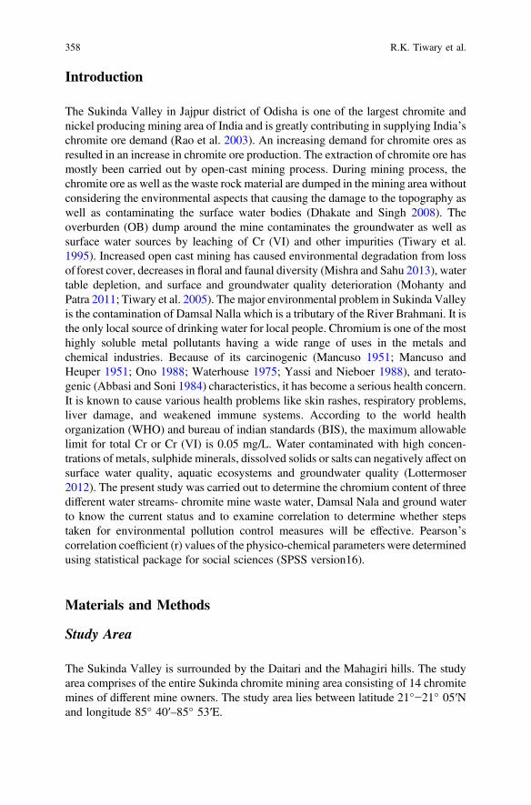
Introduction
The Sukinda Valley in Jajpur district of Odisha is one of the largest chromite andnickel producing mining area of India and is greatly contributing in supplying India’schromite ore demand (Rao et al. 2003). An increasing demand for chromite ores asresulted in an increase in chromite ore production. The extraction of chromite ore hasmostly been carried out by open-cast mining process. During mining process, thechromite ore as well as the waste rock material are dumped in the mining area withoutconsidering the environmental aspects that causing the damage to the topography aswell as contaminating the surface water bodies (Dhakate and Singh 2008). Theoverburden (OB) dump around the mine contaminates the groundwater as well assurface water sources by leaching of Cr (VI) and other impurities (Tiwary et al.1995). Increased open cast mining has caused environmental degradation from lossof forest cover, decreases in floral and faunal diversity (Mishra and Sahu 2013), watertable depletion, and surface and groundwater quality deterioration (Mohanty andPatra 2011; Tiwary et al. 2005). The major environmental problem in Sukinda Valleyis the contamination of Damsal Nalla which is a tributary of the River Brahmani. It isthe only local source of drinking water for local people. Chromium is one of the mosthighly soluble metal pollutants having a wide range of uses in the metals andchemical industries. Because of its carcinogenic (Mancuso 1951; Mancuso andHeuper 1951; Ono 1988; Waterhouse 1975; Yassi and Nieboer 1988), and terato-genic (Abbasi and Soni 1984) characteristics, it has become a serious health concern.It is known to cause various health problems like skin rashes, respiratory problems,liver damage, and weakened immune systems. According to the world healthorganization (WHO) and bureau of indian standards (BIS), the maximum allowablelimit for total Cr or Cr (VI) is 0.05 mg/L. Water contaminated with high concen-trations of metals, sulphide minerals, dissolved solids or salts can negatively affect onsurface water quality, aquatic ecosystems and groundwater quality (Lottermoser2012). The present study was carried out to determine the chromium content of threedifferent water streams- chromite mine waste water, Damsal Nala and ground waterto know the current status and to examine correlation to determine whether stepstaken for environmental pollution control measures will be effective. Pearson’scorrelation coefficient (r) values of the physico-chemical parameters were determinedusing statistical package for social sciences (SPSS version16).
Materials and Methods
Study Area
The Sukinda Valley is surrounded by the Daitari and the Mahagiri hills. The studyarea comprises of the entire Sukinda chromite mining area consisting of 14 chromitemines of different mine owners. The study area lies between latitude 21°−21° 05′Nand longitude 85° 40′–85° 53′E.
358 R.K. Tiwary et al.
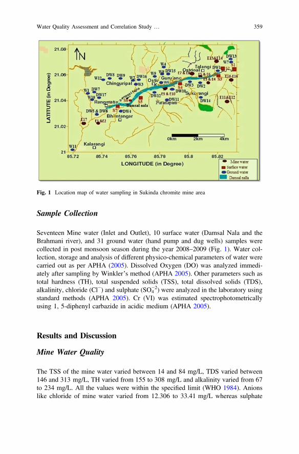
Sample Collection
Seventeen Mine water (Inlet and Outlet), 10 surface water (Damsal Nala and theBrahmani river), and 31 ground water (hand pump and dug wells) samples werecollected in post monsoon season during the year 2008–2009 (Fig. 1). Water col-lection, storage and analysis of different physico-chemical parameters of water werecarried out as per APHA (2005). Dissolved Oxygen (DO) was analyzed immedi-ately after sampling by Winkler’s method (APHA 2005). Other parameters such astotal hardness (TH), total suspended solids (TSS), total dissolved solids (TDS),alkalinity, chloride (Cl−) and sulphate (SO4
−2) were analyzed in the laboratory usingstandard methods (APHA 2005). Cr (VI) was estimated spectrophotometricallyusing 1, 5-diphenyl carbazide in acidic medium (APHA 2005).
Results and Discussion
Mine Water Quality
The TSS of the mine water varied between 14 and 84 mg/L, TDS varied between146 and 313 mg/L, TH varied from 155 to 308 mg/L and alkalinity varied from 67to 234 mg/L. All the values were within the specified limit (WHO 1984). Anionslike chloride of mine water varied from 12.306 to 33.41 mg/L whereas sulphate
Fig. 1 Location map of water sampling in Sukinda chromite mine area
Water Quality Assessment and Correlation Study … 359
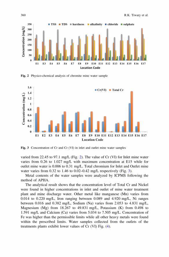
varied from 22.45 to 97.1 mg/L (Fig. 2). The value of Cr (VI) for Inlet mine watervaries from 0.26 to 1.027 mg/L with maximum concentration at E15 while foroutlet mine water is 0.006 to 0.31 mg/L. Total chromium for Inlet and Outlet minewater varies from 0.32 to 1.46 to 0.02–0.42 mg/L respectively (Fig. 3).
Metal contents of the water samples were analyzed by ICPMS following themethod of APHA.
The analytical result shows that the concentration level of Total Cr and Nickelwere found in higher concentrations in inlet and outlet of mine water treatmentplant and mine discharge water. Other metal like manganese (Mn) varies from0.014 to 0.220 mg/L, Iron ranging between 0.089 and 4.920 mg/L, Ni rangesbetween 0.016 and 0.382 mg/L, Sodium (Na) varies from 2.053 to 4.831 mg/L,Magnesium (Mg) from 18.267 to 49.831 mg/L, Potassium (K) from 0.498 to1.591 mg/L and Calcium (Ca) varies from 5.034 to 7.505 mg/L. Concentration ofFe was higher than the permissible limits while all other heavy metals were foundwithin the prescribed limits. Water samples collected from the outlets of thetreatments plants exhibit lower values of Cr (VI) Fig. (4).
0
50
100
150
200
250
300
350
E1 E3 E4 E5 E6 E7 E8 E9 E10 E11 E12 E13 E14 E15 E16 E17
Conc
entr
atio
n (m
g/L)
Location Code
TSS TDS hardness alkalinity chloride sulphate
Fig. 2 Physico-chemical analysis of chromite mine water sample
0
0.2
0.4
0.6
0.8
1
1.2
1.4
1.6
E1 E2 E3 E4 E5 E6 E7 E8 E9 E10 E11 E12 E13 E14 E15 E16 E17
Con
cent
ratio
n (m
g/L
)
Location Code
Cr(VI) Total Cr
Fig. 3 Concentration of Cr and Cr (VI) in inlet and outlet mine water samples
360 R.K. Tiwary et al.

Surface Water Quality
The physico-chemical analysis of surface water showed the TDS ranged between49 and 174 mg/l within the specified limit (WHO 1984). A similar result wasobserved in previous study (Dhakate and Singh 2008). The TSS of surface water(Damsal Nala) varied from 24 to 92 mg/L where all these values crossed thespecified limit (BIS 1991). The DO content of the Damsal Nala ranged from 6.5 to7.6 mg/L. Figure 6 shows that the Cr (VI) of the Damsal Nala vary between 0.003and 0.28 mg/l with the maximum concentration at S6, exceeding the permissiblelimits of 0.05 mg/l for drinking water limit. Heavy metal analysis shows higherconcentration of total chromium in surface water exceeding the prescribed limits.Total Cr is also found to be exceeded the prescribed limit (BIS 1981), with max-imum concentration (0.38) again at sampling location S6. This water should not beused for domestic purpose (Figs. 5 and 6).
Statistical Analysis
Correlation analysis of the Cr with physico-chemical parameters was performedusing SPSS software, version 16. The result shows that there are positive correla-tions between temperature versus pH (0.201), and temperature versus TDS (0.510)while the negative correlation between temperature with DO (−0.890). There is asignificant positive correlation between hardness and sulphate (0.661), TSS versusChloride (0.676). Non-significant positive correlation was found betweenTemperature versus TDS, hardness versus Cr (VI) (0.547) and hardness versusTotal Cr (0.568). Again pH was positively correlated with TSS (0.569), Sulphate
00.10.20.30.40.50.60.70.80.91
0
10
20
30
40
50
60
E1 E3 E4 E5 E6 E7 E8 E9 E10
Conc
entr
atio
n (m
g/L)
of C
r
Con
cent
ratio
n (m
g/L
)
Location Code
Na Mg Ca K Mn Fe Ni Cr
Fig. 4 Heavy metal concentration in mine water at different locations
Water Quality Assessment and Correlation Study … 361
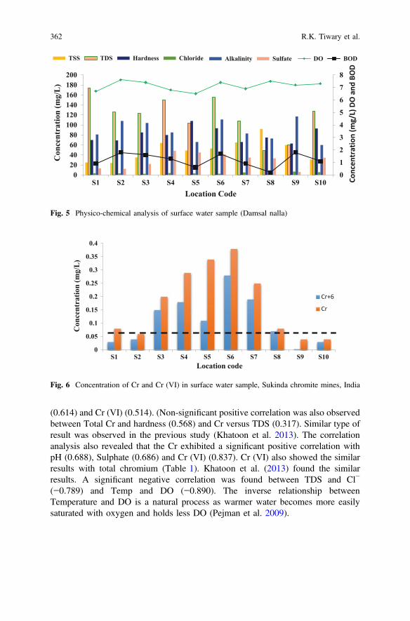
(0.614) and Cr (VI) (0.514). (Non-significant positive correlation was also observedbetween Total Cr and hardness (0.568) and Cr versus TDS (0.317). Similar type ofresult was observed in the previous study (Khatoon et al. 2013). The correlationanalysis also revealed that the Cr exhibited a significant positive correlation withpH (0.688), Sulphate (0.686) and Cr (VI) (0.837). Cr (VI) also showed the similarresults with total chromium (Table 1). Khatoon et al. (2013) found the similarresults. A significant negative correlation was found between TDS and Cl−
(−0.789) and Temp and DO (−0.890). The inverse relationship betweenTemperature and DO is a natural process as warmer water becomes more easilysaturated with oxygen and holds less DO (Pejman et al. 2009).
0
1
2
3
4
5
6
7
8
020406080
100120140160180200
S1 S2 S3 S4 S5 S6 S7 S8 S9 S10 Conc
entr
atio
n (m
g/L)
DO
and
BO
D
Con
cent
ratio
n (m
g/L
)
Location Code
TSS TDS Hardness Chloride Alkalinity Sulfate DO BOD
Fig. 5 Physico-chemical analysis of surface water sample (Damsal nalla)
0
0.05
0.1
0.15
0.2
0.25
0.3
0.35
0.4
S1 S2 S3 S4 S5 S6 S7 S8 S9 S10
Con
cent
ratio
n (m
g/L
)
Location code
Cr+6
Cr
Fig. 6 Concentration of Cr and Cr (VI) in surface water sample, Sukinda chromite mines, India
362 R.K. Tiwary et al.

Tab
le1
Correlatio
nmatrixforph
ysico-chem
ical
parameter
ofsurfacewater
samples
ofSu
kind
achromite
mine
Parameters
Tem
ppH
DO
BOD
TSS
TDS
Hardn
ess
Chloride
Alkalinity
Sulphate
Cr(V
I)Total
Cr
Tem
p1
0.20
1−0.89
0**
−0.10
7−0.19
40.51
00.35
1−0.46
1−0.28
50.32
50.44
60.42
8
pH1
−0.20
8−0.00
40.56
9−0.19
90.40
9−0.01
30.10
80.61
40.51
40.68
8*
DO
10.39
00.01
2−0.26
5−0.22
60.24
80.45
2−0.33
1−0.54
0−0.33
9
BOD
1−0.46
40.29
1−0.19
5−0.47
50.83
1**
−0.41
5−0.28
90.03
4
TSS
1−0.64
0*−0.12
90.67
6*−0.10
80.40
40.21
00.16
0
TDS
10.20
5−0.78
9**
0.00
80.15
30.07
10.31
7
Hardn
ess
1−0.38
6−0.41
80.66
1*0.54
70.56
8
Chloride
1−0.25
2−0.11
5−0.40
4−0.58
9
Alkalinity
1−0.52
2−0.27
50.06
7
Sulphate
10.69
5*0.68
6*
Cr(V
I)1
0.83
7**
Total
Cr
1
**Correlatio
nissign
ificant
atthe0.01
level(2-tailed)
*Correlatio
nissign
ificant
atthe0.05
level(2-tailed)
Water Quality Assessment and Correlation Study … 363

Ground Water Quality
The TSS of ground water samples varied between 14 and 86 mg/l, with maximumconcentration at W12 and alkalinity varied from 12 to 304 mg/L with maximumconcentration was observed at DW17 which cross the specified limit (BIS 1991).Other water quality parameters like TDS, hardness, chloride and sulphate variedfrom 38 to 345 mg/L, 14 to 214 mg/L, 1.57 to 96.98 mg/L and from nil to21.54 mg/L respectively. All the values were found within permissible limits (BIS1991) (Fig. 7). Concentration of Cr (VI) in water samples ranged fromnon-detectable to 0.10 mg/L with maximum concentration at (DW1); total Crvaried from 0.001 to 678 mg/L, with the maximum concentration at DW10.Samples collected from the dug open wells (W) have lower concentrations ofphysico-chemical parameters like TSS, TDS, hardness, alkalinity, Cl− and SO4
−2
(Fig. 7), and lower concentrations of Cr (VI), from non-detectable to 0.01 mg/L(Fig. 8). The concentration of Iron is found to be present in higher ranges in most ofthe samples. The value ranges between 0.046 and 2.930 mg/l, which is above thedesirable limit of 0.3 mg/L. Other heavy metals were found well within the pre-scribed limits for drinking water. Heavy metal concentrations in open wells werefound below the safe limits for drinking water quality (IS: 10500). Cr (VI) was alsofound below the permissible limit. Variation in Cr (VI) and Total Cr in hand pumpand dug wells of the region is shown in Fig. 8 which clearly indicate the presenceof Cr (VI) above the threshold limit values in some of the samples collected fromthe tube well of sampling site, DW1 and DW4, and same trend is observed for theTotal Cr. The concentration of Cu was within the permissible limit (<0.05 mg/l asper Indian Standards) (Fig. 9).
0
50
100
150
200
250
300
350
400
DW
1D
W2
DW
3D
W4
DW
5D
W6
DW
7D
W8
DW
9D
W10
DW
11D
W12
DW
13D
W14
DW
15D
W16
DW
17D
W18
DW
19 W1
W2
W3
W4
W5
W6
W7
W8
W9
W10
W11
W12
Con
cent
ratio
n (m
g/L
)
Location code
TSS TDS Hardness Chloride Alkalinity Sulfate
Fig. 7 Physico-chemical analysis of ground water sample
364 R.K. Tiwary et al.
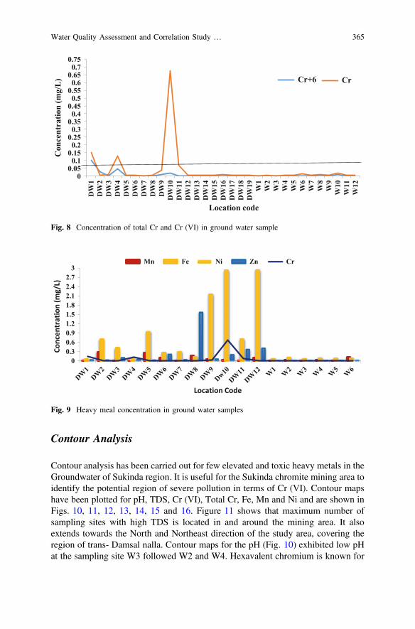
Contour Analysis
Contour analysis has been carried out for few elevated and toxic heavy metals in theGroundwater of Sukinda region. It is useful for the Sukinda chromite mining area toidentify the potential region of severe pollution in terms of Cr (VI). Contour mapshave been plotted for pH, TDS, Cr (VI), Total Cr, Fe, Mn and Ni and are shown inFigs. 10, 11, 12, 13, 14, 15 and 16. Figure 11 shows that maximum number ofsampling sites with high TDS is located in and around the mining area. It alsoextends towards the North and Northeast direction of the study area, covering theregion of trans- Damsal nalla. Contour maps for the pH (Fig. 10) exhibited low pHat the sampling site W3 followed W2 and W4. Hexavalent chromium is known for
00.05
0.10.15
0.20.25
0.30.35
0.40.45
0.50.55
0.60.65
0.70.75
DW
1D
W2
DW
3D
W4
DW
5D
W6
DW
7D
W8
DW
9D
W10
DW
11D
W12
DW
13D
W14
DW
15D
W16
DW
17D
W18
DW
19 W1
W2
W3
W4
W5
W6
W7
W8
W9
W10
W11
W12
Con
cent
ratio
n (m
g/L
)
Location code
Cr+6 Cr
Fig. 8 Concentration of total Cr and Cr (VI) in ground water sample
00.30.60.91.21.51.82.12.42.7
3
Conc
entr
atio
n (m
g/L)
Location Code
Mn Fe Ni Zn Cr
Fig. 9 Heavy meal concentration in ground water samples
Water Quality Assessment and Correlation Study … 365

85.66 85.7 85.74 85.78 85.82 85.86
Longitude (in degrees)
21
21.02
21.04
21.06
21.08
Latit
ude
(in d
egre
es)
Dw1
Dw2
Dw3
Dw4
Dw7 Dw8 Dw9
Dw10
Dw11
Dw12
W1
W2
W3W4
W5
W6
0km 2km 4km
Fig. 10 Contour map for pH
85.66 85.7 85.74 85.78 85.82 85.86
Longitude (in degrees)
21
21.02
21.04
21.06
21.08
Latit
ude
(in d
egre
es)
Dw1
Dw2
Dw3
Dw4
Dw7 Dw8 Dw9
Dw10
Dw11
Dw12
W1
W2
W3W4
W5
W6
0km 2km 4km
Fig. 11 Contour map for TDS
85.66 85.7 85.74 85.78 85.82 85.86Longitude (in degrees)
21
21.02
21.04
21.06
21.08
Latit
ude
(in d
egre
es)
Dw1
Dw2
Dw3
Dw4
Dw7 Dw8 Dw9
Dw10
Dw11
Dw12
W1
W2
W3W4
W5
W6
0km 2km 4km
Fig. 12 Contour map for Cr (VI)
366 R.K. Tiwary et al.
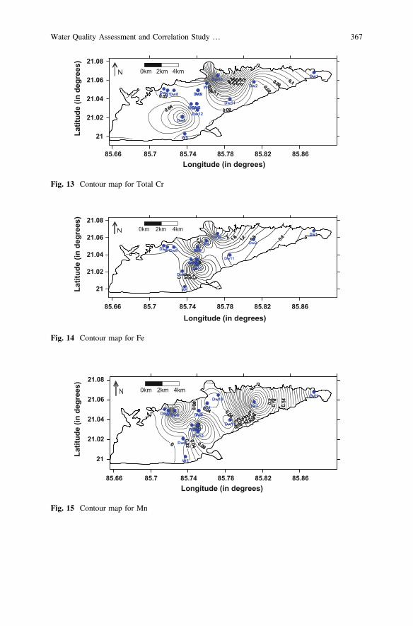
85.66 85.7 85.74 85.78 85.82 85.86Longitude (in degrees)
21
21.02
21.04
21.06
21.08
Latit
ude
(in d
egre
es)
Dw1
Dw2
Dw3
Dw4
Dw7 Dw8 Dw9
Dw10
Dw11
Dw12
W1
W2
W3W4
W5
W6
0km 2km 4km
Fig. 13 Contour map for Total Cr
85.66 85.7 85.74 85.78 85.82 85.86
Longitude (in degrees)
21
21.02
21.04
21.06
21.08
Latit
ude
(in d
egre
es)
Dw1
Dw2
Dw3
Dw4
Dw7 Dw8 Dw9
Dw10
Dw11
Dw12
W1
W2
W3W4
W5
W6
0km 2km 4km
Fig. 14 Contour map for Fe
85.66 85.7 85.74 85.78 85.82 85.86Longitude (in degrees)
21
21.02
21.04
21.06
21.08
Latit
ude
(in d
egre
es)
Dw1
Dw2
Dw3
Dw4
Dw7 Dw8 Dw9
Dw10
Dw11
Dw12
W1
W2
W3W4
W5
W6
0km 2km 4km
Fig. 15 Contour map for Mn
Water Quality Assessment and Correlation Study … 367
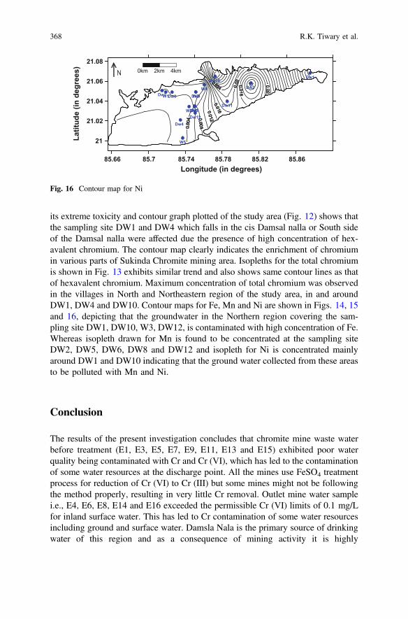
its extreme toxicity and contour graph plotted of the study area (Fig. 12) shows thatthe sampling site DW1 and DW4 which falls in the cis Damsal nalla or South sideof the Damsal nalla were affected due the presence of high concentration of hex-avalent chromium. The contour map clearly indicates the enrichment of chromiumin various parts of Sukinda Chromite mining area. Isopleths for the total chromiumis shown in Fig. 13 exhibits similar trend and also shows same contour lines as thatof hexavalent chromium. Maximum concentration of total chromium was observedin the villages in North and Northeastern region of the study area, in and aroundDW1, DW4 and DW10. Contour maps for Fe, Mn and Ni are shown in Figs. 14, 15and 16, depicting that the groundwater in the Northern region covering the sam-pling site DW1, DW10, W3, DW12, is contaminated with high concentration of Fe.Whereas isopleth drawn for Mn is found to be concentrated at the sampling siteDW2, DW5, DW6, DW8 and DW12 and isopleth for Ni is concentrated mainlyaround DW1 and DW10 indicating that the ground water collected from these areasto be polluted with Mn and Ni.
Conclusion
The results of the present investigation concludes that chromite mine waste waterbefore treatment (E1, E3, E5, E7, E9, E11, E13 and E15) exhibited poor waterquality being contaminated with Cr and Cr (VI), which has led to the contaminationof some water resources at the discharge point. All the mines use FeSO4 treatmentprocess for reduction of Cr (VI) to Cr (III) but some mines might not be followingthe method properly, resulting in very little Cr removal. Outlet mine water samplei.e., E4, E6, E8, E14 and E16 exceeded the permissible Cr (VI) limits of 0.1 mg/Lfor inland surface water. This has led to Cr contamination of some water resourcesincluding ground and surface water. Damsla Nala is the primary source of drinkingwater of this region and as a consequence of mining activity it is highly
85.66 85.7 85.74 85.78 85.82 85.86Longitude (in degrees)
21
21.02
21.04
21.06
21.08
Latit
ude
(in d
egre
es)
Dw1
Dw2
Dw3
Dw4
Dw7 Dw8 Dw9
Dw10
Dw11
Dw12
W1
W2
W3
W4
W5
W6
0km 2km 4km
Fig. 16 Contour map for Ni
368 R.K. Tiwary et al.

contaminated with Cr (VI). At sites S3-S7, Cr (VI) is elevated (0.11–0.28 mg/L),but the levels decrease with distance, and by the time the Damsal Nala travels10 km and meets the Brahmani River, hexavalent chromium is found within per-missible limits (S9 = 0.003, S10 = 0.03). Although dug wells had acceptableconcentrations of Cr (VI), two tube wells (DW1 and DW4) had concentration of Cr(VI) higher than permissible limits and the wells cannot be used for drinking water.Contour map for Cr (VI) and Cr also confirm that maximum concentration lies inthe vicinity of DW1, DW4 and DW10 which is surrounded by mining activitieswhich needs to be managed properly. All the chromite mines are situated at adistance of 2–3 km of the river. During the rainy season, Leaching from the OBdumps and surface run off from the mining area drain easily into the river andbecome the source of Cr (VI) in the river. High level of some parameters ingroundwater indicating the unsuitability of most of these water samples for potablepurposes. Similarly, Damsal nala was also unfit for drinking purpose due to highconcentration of total Chromium especially in the mining area.
Acknowledgements The authors acknowledge Council of Scientific and Industrial Research,New Delhi for financial help through networking project. We also acknowledge our colleagues ofEnvironment Management Group for rendering cooperation during field survey and laboratoryanalysis.
References
Abbasi SA, Soni R (1984) Teratogenic effects of chromium (VI) in the environment as evidencedby the impact of larvae of amphibian Rana tigrina: implications in the environmentalmanagement of chromium. Int J Environ Stud 23:131–137
APHA (American Public Health Association) (2005). Standard methods for the examination ofwater and waste water, 21st edn. APHA, American Water Works Assoc, Water EnvironmentFed, Washington, DC
BIS (Bureau of Indian Standards), 2490 part I, (1981), Tolerance limits for industrial effluentsBIS (Bureau of Indian Standards) 10500 (1991). Water quality guidelines for drinking water and
aquatic lifeDhakate R, Singh VS (2008) Heavy metal contamination in groundwater due to mining activities
in Sukinda valley, Orissa—a case study. J Geogr Reg Plann 1(4):058–067Khatoon N, Khan AH, Rehman M, Pathak V (2013) Correlation study for the assessment of water
quality and its parameters of Ganga River, Kanpur, Uttar Pradesh, India. IOSR J Appl Chem(IOSR-JAC), 5(3):80–90
Lottermoser B (2012) Mine wastes: characterization, treatment and environmental impacts.Springer, New York, p 400
Mancuso TF (1951) Occupational cancer and other health hazards in a chrome plant: a medicalappraisal. II clinical and toxicological aspects. Ind Med Surg 20:393–407
Mancuso TF, Heuper WC (1951) Occupational cancer and other health hazards in a chrome plant:a medical. appraisal: I. Lung cancers in chromate workers. Ind Med Surg 20:358–363
Mishra H, Sahu HB (2013) Environmental scenario of chromite mining at Sukinda Valley—areview. Int J Env Manag. 4(4):287–292
Mohanty M, Patra HK (2011) Attenuation of chromium toxicity in mine waste water hyacinth.J Stress Phys Biochem 7(4):336–346
Water Quality Assessment and Correlation Study … 369

Ono BL (1988) Genetic approaches in the study of chromium toxicity and resistance in yeast andbacteria. In: Nriagu JO, Niebor R (eds) Chromium in the natural and human environments.Wiley, New York, pp 351–368
Pejman AH, Bidhendi GRN, Karbassi AR, Mehrdadi N, Bidhendi ME (2009) Evaluation of spatialand seasonal variations in surface water quality using multivariate statistical techniques. Int JEnviron Sci Technol 6(3):467–476
Rao AV, Dhakate RR, Singh VS, Jain SC (2003) Geophysical and hydrogeological investigationsto delineate aquifer geometry at Kaliapani, Sukinda, Orissa. NGRI technical report no.GW-367
Tiwary RK, Gupta JP, Banerjee NN, Dhar BB (1995) Impact of coal mining activities on waterand human health in Damodar river basin. 1st world mining environment congress, New Delhi,India
Tiwary RK, Dhakate R, Rao VA, Singh VS (2005) Assessment and prediction of contaminantmigration in ground water from chromite waste dump. Environ Geol 48:420–429
Waterhouse JAH (1975) Cancer among chromium platers. Br J Cancer 32(2):262WHO (World Health Organization) (1984) Guidelines for drinking water quality. World Health
Organization. Washington, DC, pp 333–335Yassi A, Nieboer E (1988) Carcinogenicity of chromium compounds. In: Nriagu JO, Nieboer E
(eds) Chromium in the natural and human environments. Wiley, New York, pp 443–496
370 R.K. Tiwary et al.
Water Quality Assessment of a LenticWater Body Using Remote Sensing:A Case Study
B.K. Purandara, B.S. Jamadar, T. Chandramohan, M.K. Joseand B. Venkatesh
Abstract Water Quality assessment of lakes, rivers, and reservoirs is a key issuefor environmental monitoring and management. Lakes are subjected to suddenenvironmental changes caused by anthropogenic activities due to their multiple uses(agriculture, fishing, and boating, industrial and water supply). One of the mostimportant issues in lake water management is water quality. Water qualityassessments are being carried out using conventional methods which are verycommon and accurate, however, have the disadvantage of being expensive andlabor-intensive. Further, sampling method and frequency are the major constraintsto obtain representative samples. In order to overcome such hurdles in water qualitymanagement remote sensing approach has become more user-friendly and quitereliable. Remote sensing approach to water quality assessment is based on theoptical bands in the region from blue to near infrared. These data are then used toexplore the relation between the reflectance of water bodies and biophysicalparameters such as: transparency, chlorophyll concentration (phytoplankton), andthe organic and mineral suspended sediments. In the present study, an attempt hasbeen made to understand the water quality characteristics of a lake situated incoastal, Kerala, known as Vembanad lake (a Ramsar site in south India) usingLandsat-TM data. A relationship between Landsat-TM bands and suspended sed-iment concentration has been arrived at and compared with the field monitored data.It is noticed that TM bands such as TM5, TM6, and TM7 show higher correlationwith observed data than bands 1, 2, and 3.
Keywords Water quality � Remote sensing � Suspended sediments
B.K. Purandara (&) � T. Chandramohan � M.K. Jose � B. VenkateshNIH, Hard Rock Regional Center, Belagavi 590019, Karnataka, Indiae-mail: [email protected]
B.S. JamadarDepartment of Civil Engineering, Jain College of Engineering and Technology,Belagavi, Belagavi, Karnataka, India
© Springer Nature Singapore Pte Ltd. 2018V.P. Singh et al. (eds.), Environmental Pollution, Water Scienceand Technology Library 77, https://doi.org/10.1007/978-981-10-5792-2_30
371

Introduction
There is no specific definition for Lakes in India. The term “Lake” is used loosely torepresent various types of water bodies–natural, man-made and ephemeralincluding wetlands. Many lakes are categorized as wetlands, while reporting underRamsar Convention. Lakes may be manmade or natural. Most of the lakes in thetropics and coastal belts are natural. However, the environmental status and eco-logical conditions of lentic bodies (particularly lakes) are less discussed in theliterature. Though there is a distinction between freshwater lake sand brackish waterlakes. The lakes of southern peninsular India are distinct from those of theHimalayan region. In the recent years, in India the water quality of inland waterbodies like the rivers, lake sand ponds is assessed to establish their water qualitystatus and pollution level (CPCB 2008). For this, predominantly the conventionalwater quality assessment methods have been commonly used. The current tech-niques usually used in the country form on it oring and assessing the quality ofwater bodies involves in situ measurement and/or the collection of water samplesfor subsequent laboratory analysis so as to retrieve the chemical, physical andbiological characteristics of water that help in assessing its quality.
In the water quality analysis, the use of recent advanced technical tools like theremote sensing and geographical information system is however limited. Thoughthe conventional methods give accurate information about the quality of water atthe geographically specific station in the water bodies, but these results are not veryhelpful in providing a complete picture of the quality of water of the whole waterbody. Numerous researches done on the assessment of the quality of water using therecent advanced techniques like the remote sensing in integration withGeographical Information System bring to light the limitations associated withconventional methods. The major constraint of current in situ techniques of mea-suring water quality variables is quite time-consuming; and further, from thesemethods unable to provide a synoptic view of an individual water body or a set ofwater bodies across the land scape. It requires excessive traveling, sampling, andexpensive laboratory analysis, especially for a large area; thus it is very difficult toreport and predict the water quality situation in time. However, in the recent times,remote sensing (RS) techniques for water quality monitoring are accessible andreported to be very efficient. As the pollutants scatter and absorb the incoming solarradiation, the water quality is significantly correlated with the water column’soptical characteristics, such as color and transparency, which can be obtained fromRS data. Investigations suggest that optical data can provide an alternative meansfor obtaining relatively low-cost, simultaneous information on surface water qualityconditions from numerous lakes, coastal, and oceanic areas. Although the methodsto retrieve water quality from RS data might not be as precise as traditionalmethods, they are time and cost efficient over the large area and can provide theopportunity for regular observation of even very remote regions. Therefore, remotesensing techniques have been widely used in estimating the pollution situation ofsurface water (Akbar et al. 2012; Naithani 2012; Ritchie and Cooper 2001).
372 B.K. Purandara et al.

Presently, many satellites with high resolutions have been used in water qualitymonitoring studies. A number of studies have been carried out to relate waterquality parameters such as Chlorphyll-a and suspended sediments with remotesensing data. Further, these observations can be used in various numerical schemesto help characterize the trophic status of an aquatic ecosystem.
However, as stated by earlier researchers, the number of available in situ mea-surements of water quality characteristics is quite limited both spatially and tem-porally. It is reported by various researchers that chl-a and SS are optically activewater quality parameters in various water bodies and employed digital evaluationand near infrared wavelengths to assess the water quality parameters (e.g., Ritchieet al. 1990; Lathrop 1992; Choubey 1994). However, the previous studies weremostly carried out on the seriously polluted inland water body whereas the slightlypolluted water bodies, especially those drinking water sources, have not been takeninto consideration. The main reason is that they are of weak optical characteristicsand low signal noise ratio. However, these are practically the most important part ofthe water quality management. Therefore, this is the challenging part for theresearchers.
In the recent past, many researchers have used RS and ERDAS Imagine 9.1Software for water quality assessment and have shown many positive results.Improvement and advancements in sensor technologies, realtime remote monitoringwill prove to be an important tool in assessing water quality. While working on theuse of hyper spectral RS and ERDAS Imagine 9.1 Software, to assess the waterquality in coastal areas and shallow inland lakes of Iowa, USA., it is reported thatthe integration of RS and ERDAS Imagine 9.1 Software along with in situ watersampling and analysis can simplify and accelerate the procedure for water qualityassessment with an acceptable degree of accuracy (Sugumaran et al. 2005).
Study Area
The Vembanad Lake, a Ramsar site is one of the largest coastal wetland ecosystemsin south India, covering an area of 24,000 ha and contributes over 50% of the totalarea of backwaters in the state. This ecosystem has several functions and economicvalues. The lake’s total surface area is spread across three central districts of Kerala,viz., Ernakulum in the north, Kottayam in the east and Alappuzha in the south. It isthe lifeline of the area. Nearly 1.6 million people live on the banks of the lake.
This wetland and the surrounding area together form a socio-ecological systemsupporting the life of the people who live in the villages situated on its banks(Purandara 2008). Vembanad Lake is a transitional ecologically sensitive zonebetween the marine and terrestrial environments. These are highly productive zonesproviding feeding and spawning areas for a very large proportion of commercialfish and shellfish. It supports rich fishery resources such as a variety of finfish,shellfish, several species of marine fishes and shrimps. The lake system also
Water Quality Assessment of a Lentic Water Body Using Remote … 373
supports a highly productive agriculture system in Kuttanad–the “rice bowl ofKerala”—spread over 1,100 km2 which is a reclaimed portion of the lake.
A large population living in the drainage basin is directly or indirectly dependentupon this wetland ecosystem for their livelihood. Extensive field investigationscarried out in the study area, indicated that the lake is used for fishing, mining sandand lime shell deposits, harvesting live clam sand tourism-related activities.Surrounding land mass is used for rice cultivation, plantation crops, housing, touristresorts, etc. All these water-based activities depend upon the environmentalintegrity of the Vembanad Lake and its surroundings.
The environmental conditions of the lake ecosystem are undergoing a drasticchange due to both hydrological and human interference. This kind of variations inthe ecosystem may seriously affect the livelihood of surrounding people. One of themajor factors affecting the endogenic system is due to fishery activities such asunscientific fishery practices like the adoption of fishing nets with small mesh size,fishing during high tide especially near estuarine bar mouths and use of destructivemethods of catching process.
It is reported that the prime cause of environmental degradation of VembanadLake is attributed to reclamation and creation of the Wellington Island, the bundingworks in the Kuttanad area for improving agriculture, construction of theThottapally Spillway to divert floodwaters of Achankovil, Pamba, Manimala, andMeenachil directly to the sea. In addition, Thanneermukkom bund was built toprevent salinity ingress into the Kuttanad agricultural area during summer(Purandara and Dora 1987).
All the above interventions significantly altered the original flow pattern andchanged the lake ecology adversely. Figure 1 shows the Vembanad Lake withlocations of water sampling for water quality analysis.
Data Collection
The following data products were used for the present study:
1. Surface water quality of Vembanad Lake wetland system collateral data.2. Landsat-TM Satellite data.
The details of the data products used are described below.
Surface Water Quality of Vembanad Lake
Surface water samples were collected from three different zones as North zone,Central zone and South zone. Each zone having seven stations, with a total numberof 21 stations in the entire lake water body. Physic-chemical parameters from allthree zones were investigated and their results are used for the analysis of remotesensing data.
374 B.K. Purandara et al.
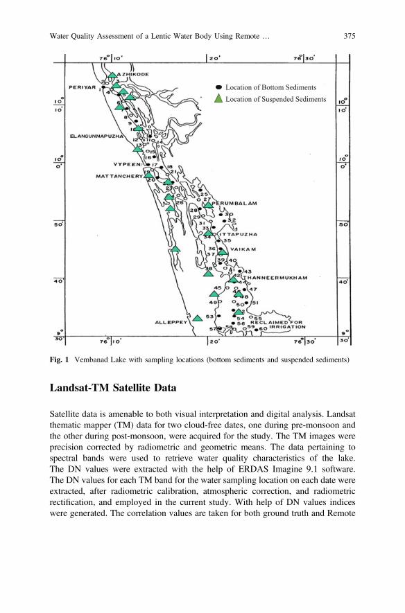
Landsat-TM Satellite Data
Satellite data is amenable to both visual interpretation and digital analysis. Landsatthematic mapper (TM) data for two cloud-free dates, one during pre-monsoon andthe other during post-monsoon, were acquired for the study. The TM images wereprecision corrected by radiometric and geometric means. The data pertaining tospectral bands were used to retrieve water quality characteristics of the lake.The DN values were extracted with the help of ERDAS Imagine 9.1 software.The DN values for each TM band for the water sampling location on each date wereextracted, after radiometric calibration, atmospheric correction, and radiometricrectification, and employed in the current study. With help of DN values indiceswere generated. The correlation values are taken for both ground truth and Remote
Location of Bottom SedimentsLocation of Suspended Sediments
Fig. 1 Vembanad Lake with sampling locations (bottom sediments and suspended sediments)
Water Quality Assessment of a Lentic Water Body Using Remote … 375

sensing data. Suspended sediment was recorded from 7-Stations only throughoutthe lake. The data pertaining to different spectral bands were used to retrieve waterquality characteristics of the Vembanad Lake (Fig. 2).
Results and Discussion
Turbidity and Suspended sediments are the two important and striking character-istics used to understand the physical status of a water body. Turbidity of water ismainly caused by suspended particles such as clay, silts, finely divided organic andinorganic matters, plankton and other microscopic organisms. Seasonal variation ofturbidity follows monsoon ! pre-monsoon ! post-monsoon. Inflow of erodedmaterials due to high rain causes the water to be highly turbid in monsoon. In orderto assess the water quality status, image processing software, viz. ERDAS 9.1 wasemployed. In remote sensing, one of the most convincing approaches of analysis isby developing derivative indices which may be used effectively to improve thepredictive characteristics of various band data (Thiam and Eastman 1999; Sudheeret al. 2006). These indices are normally derived by arithmetic manipulations of
Fig. 2 An overview of Vembanad Lake (extracted from the satellite data)
376 B.K. Purandara et al.
different combinations of TM band data. Details pertaining to various derivativeindices with band respective band combinations are shown in Table 1.
The correlation matrix of absolute variance of Derivative indices with waterquality parameters are presented in Table 2.
The correlation matrix of absolute variation was computed using statisticalsoftware SPSS. The sign of the correlation may be related to the magnitude of theDN values in individual bands and the arithmetic operation but can be ignored sincethe interest here is on the strength of the relationship between the variables. Itappears that a linear combination of four bands (with R = −0.349, −0.011, 0.272,0.069) may not result in an accurate model for SS when linearly regressed.However, other combinations of these bands (as in IND1, IND5, IND6) have goodpotential for retrieving the SS information (R = 0.703, 0.823, 0.803).
The results also show the indices IND2 and IND3 have relatively less potentialto ground truth. It is evident that the absolute variation provides a better picture ofthe strength of relationship among the variables.
The correlation matrix between the absolute variance of TM bands and the waterquality parameters is presented in Table 3. TM band combinations of TM5, TM6,
Table 1 Details of various derivative indices considered in the study
Index Band combination and form
IND1 (TM1 + TM2 + TM3)/3
IND2 TM1/TM2
IND3 TM1/TM3
IND4 TM2/TM3
IND5 (TM5 + TM7)/2
IND6 (TM4 + TM5 + TM7)/3
IND7 (TM1 − TM3)/(TM1 + TM3)
Table 2 Correlation matrix of absolute variance of derivative indices with water qualityparameters
Correlation matrix of absolute variance of derivative indices with water quality parameters
IND1 IND2 IND3 IND4 IND5 IND6 IND7 SS
IND1 1.000
IND2 −0.771 1.000
IND3 −0.138 0.343 1.000
IND4 0.355 −0.231 0.826 1.000
IND5 0.718 −0.315 −0.226 0.064 1.000
IND6 0.752 −0.389 −0.252 0.079 0.977 1.000
IND7 −0.028 0.241 0.993 0.879 −0.171 −0.191 1.000
SSa 0.703 −0.349 −0.011 0.272 0.823 0.803 0.069 1.000aSS Suspended sediments
Water Quality Assessment of a Lentic Water Body Using Remote … 377
and TM7 or a combination TM4, TM5, TM6, and TM7 is significant in retrievingSS information from remote sensing data. A significant observation is that the datafor bands TM1, TM2, and TM3 are not sensitive to SS, and hence the incorporationof DNs from these bands in modeling SS would only increase the modelcomplexity.
The regression values have been generated by comparing with the Ground truthi.e. Suspended sediments to the TM data. Each TM band is used to generatecorrelation equation and regression values with respect to suspended solids. Table 4shows regression equation for TM1, TM2, TM3, TM4, TM5, TM6, and TM7. Thevisible bands and infrared bands with correlations with ground truth show a sig-nificant relationship between Suspended Solids and their DN values in LinearRegression models. The regressions obtained are much correlated with grounddetails, in all 7-Bands the most realistic results can be obtained by using TM5 withregression value R2 = 0.835, having best fitting equation Y = 0.6874x + 11.203.
Table 3 Correlation (R) matrix of absolute variance of TM bands and water quality parameters
Correlation (R) matrix of absolute variance of TM bands and water quality parameter
TM1 TM2 TM3 TM4 TM5 TM6 TM7 SS
TM1 1.000
TM2 0.962 1.000
TM3 0.557 0.697 1.000
TM4 0.623 0.675 0.760 1.000
TM5 0.577 0.564 0.655 0.827 1.000
TM6 0.611 0.58 0.617 0.807 0.997 1.000
TM7 0.592 0.554 0.595 0.826 0.994 0.997 1.000
SS 0.574 0.547 0.415 0.658 0.821 0.835 0.831 1.000
Table 4 Comparison of observed and estimated (based on regression equations) suspendedsediments
Stations ObservedSSC(mg/l)
Average DNvalues (x)
Regressionequation (y)
Estimated SSCusing regressionequation
%error
1 155 (TM1) 145.42 0.916x−1.8459 131.35 15.25
2 79 (TM2) 112.57 0.552x+29.618 91.76 16.15
3 141 (TM3) 229.143 0.4402x+14.114 114.94 18.48
4 76 (TM4) 154.143 0.5339x+1.02 83.31 9.60
5 49 (TM5) 85.57 0.6874x+11.203 52.28 6.60
6 114 (TM6) 169.43 0.6564x−7.0497 103.99 8.70
7 139 (TM7) 199.57 0.6489x−1.8356 127.66 8.15
378 B.K. Purandara et al.

Summary
The above study highlighted the significance of remote sensing data in analyzingwater quality parameters particularly based on suspended sediments. It is noticedthat the suspended sediment concentration depends on the reflectance valuesderived from the remote sensing data. Accordingly, a remote sensing basedframework may be developed for the prediction of water quality of different sourcewaters by integrating satellite data and ground-based measurements. Regressionequations developed from the results obtained from present investigation is found tobe more reliable in the case of TM5, TM6, and TM7. From the study it is observedthat the central portion of the Vembanad Lake is more prone to pollution as it isevident from the sediment concentration. Therefore, it is suggested that it is nec-essary to regularly monitor the water quality in selected locations to help in lakewater management.
Acknowledgements Authors are highly grateful to Dr. R.D. Singh, Director, NIH, and Dr. SudhirKumar, Scientist ‘G’ and Head, Hydrological Investigation Division, NIH, Roorkee for theirconstant support and encouragement. Authors are thankful to Dr. Pramod Hanamgond. T., Head,Dept. of Geology, GSS College, Belagavi for assisting in ERDAS application.
References
Akbar TA, Hassan QK, Acharia G (2012) A remote sensing based framework for predicting waterquality of different source waters. Satellite based remote sensing approach for acquiring waterquality data. The International Archives of the Photogrammetry, Remote Sensing and SpatialInformation Sciences, vol 34, Part XXX
Choubey VK (1994) Monitoring water quality in reservoirs with IRS- 1A-LISS-I. Water ResourManage 8:121–136
CPCB (2008) Status of water quality in India. Central Pollution Control Board, New DelhiLathrop R (1992) Landsat thematic mapper monitoring of turbid inland water quality. Photogramm
Eng Remote Sens 58:465–470Naithani R (2012) Physicochemical assessment of water quality with respect to Remote sensing
and GIS techniques. Adv Pure Appl Chem (APAC) 1(1). ISSN 2167-0854Purandara BK (2008) Environmental issues of wetland ecosystem management: a case study. Ecol
Environ Conserv 14(2–3):439–448Purandara BK, Dora YL (1987) Studies on texture and Organic matter in the sediments of
Vembanad Lake and nearshore sediments. In: Proceedings of national seminar on estuarinemanagement, pp 449–452
Ritchie JC, Cooper CM (2001) Remote sensing techniques for determining water quality:applications to TMLDs”. In TMDL science issues conference, water environment federation,Alexandria, VA, pp 367–374
Ritchie JC, Charles MC, Schibe FR (1990) The relationship of MSS and TM Digital data withsuspended sediments, chlorophyll, and temperature in Moon Lake, Mississippi. Remote SensEnviron 33:137–148
Sudheer KP, Chaubey I, Garg V (2006) Lake water quality assessment from LANDSAT thematicmapper data using neural network: an approach to optimal band combination selection. J AmWater Resour Assoc 1683–1695
Water Quality Assessment of a Lentic Water Body Using Remote … 379

Sugumaran R, Clayton M, Ecker M, Stigliani B, Gimond M, Green N (2005) Hyperspectral remotesensing and geographical information systems tools to assess water quality areas and ShallowInland lake. University of Northern Iowa and NASA Kennedy Space Center. Iowa Space Grant(Cooperative) Final Technical Report, pp 1–35
Thiam S, Eastman RJ (1999) Vegetation indices. Guide GIA Image Process 2:107–122
380 B.K. Purandara et al.
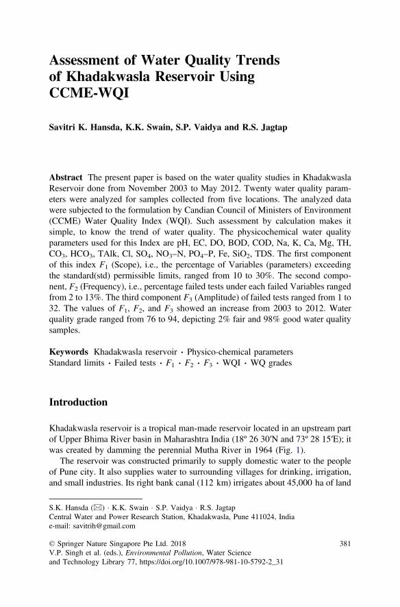
Assessment of Water Quality Trendsof Khadakwasla Reservoir UsingCCME-WQI
Savitri K. Hansda, K.K. Swain, S.P. Vaidya and R.S. Jagtap
Abstract The present paper is based on the water quality studies in KhadakwaslaReservoir done from November 2003 to May 2012. Twenty water quality param-eters were analyzed for samples collected from five locations. The analyzed datawere subjected to the formulation by Candian Council of Ministers of Environment(CCME) Water Quality Index (WQI). Such assessment by calculation makes itsimple, to know the trend of water quality. The physicochemical water qualityparameters used for this Index are pH, EC, DO, BOD, COD, Na, K, Ca, Mg, TH,CO3, HCO3, TAlk, Cl, SO4, NO3–N, PO4–P, Fe, SiO2, TDS. The first componentof this index F1 (Scope), i.e., the percentage of Variables (parameters) exceedingthe standard(std) permissible limits, ranged from 10 to 30%. The second compo-nent, F2 (Frequency), i.e., percentage failed tests under each failed Variables rangedfrom 2 to 13%. The third component F3 (Amplitude) of failed tests ranged from 1 to32. The values of F1, F2, and F3 showed an increase from 2003 to 2012. Waterquality grade ranged from 76 to 94, depicting 2% fair and 98% good water qualitysamples.
Keywords Khadakwasla reservoir � Physico-chemical parametersStandard limits � Failed tests � F1 � F2 � F3 � WQI � WQ grades
Introduction
Khadakwasla reservoir is a tropical man-made reservoir located in an upstream partof Upper Bhima River basin in Maharashtra India (18º 26 30′N and 73º 28 15′E); itwas created by damming the perennial Mutha River in 1964 (Fig. 1).
The reservoir was constructed primarily to supply domestic water to the peopleof Pune city. It also supplies water to surrounding villages for drinking, irrigation,and small industries. Its right bank canal (112 km) irrigates about 45,000 ha of land
S.K. Hansda (&) � K.K. Swain � S.P. Vaidya � R.S. JagtapCentral Water and Power Research Station, Khadakwasla, Pune 411024, Indiae-mail: [email protected]
© Springer Nature Singapore Pte Ltd. 2018V.P. Singh et al. (eds.), Environmental Pollution, Water Scienceand Technology Library 77, https://doi.org/10.1007/978-981-10-5792-2_31
381
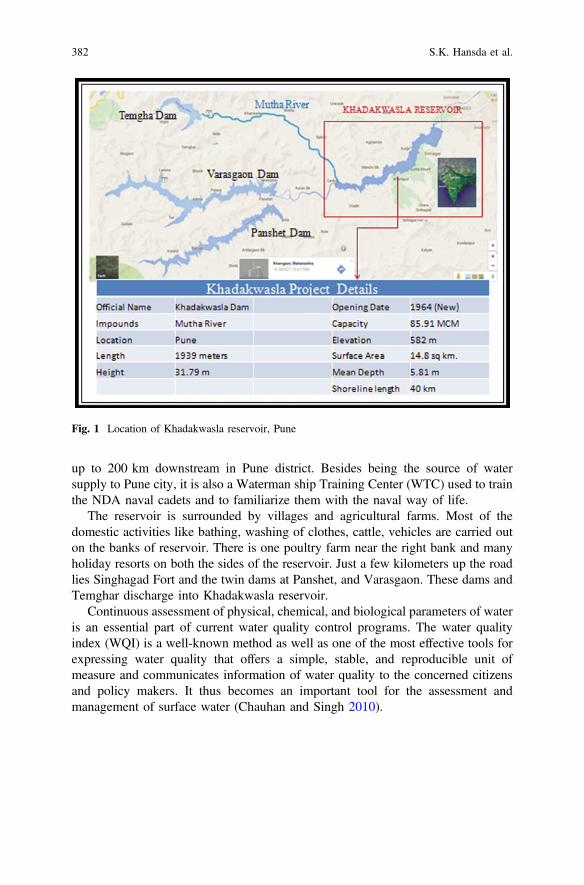
up to 200 km downstream in Pune district. Besides being the source of watersupply to Pune city, it is also a Waterman ship Training Center (WTC) used to trainthe NDA naval cadets and to familiarize them with the naval way of life.
The reservoir is surrounded by villages and agricultural farms. Most of thedomestic activities like bathing, washing of clothes, cattle, vehicles are carried outon the banks of reservoir. There is one poultry farm near the right bank and manyholiday resorts on both the sides of the reservoir. Just a few kilometers up the roadlies Singhagad Fort and the twin dams at Panshet, and Varasgaon. These dams andTemghar discharge into Khadakwasla reservoir.
Continuous assessment of physical, chemical, and biological parameters of wateris an essential part of current water quality control programs. The water qualityindex (WQI) is a well-known method as well as one of the most effective tools forexpressing water quality that offers a simple, stable, and reproducible unit ofmeasure and communicates information of water quality to the concerned citizensand policy makers. It thus becomes an important tool for the assessment andmanagement of surface water (Chauhan and Singh 2010).
Fig. 1 Location of Khadakwasla reservoir, Pune
382 S.K. Hansda et al.
Introduction to Water Quality (WQ) and Water Quality Index(WQI)
Water Quality is a measure of the condition of water able to sustain healthyecosystem and human life. It is generally referred by its physical, chemical, andbiological characteristics which are compared against a set of standards to assess itscompliance. Standards and guidelines are established to know the suitability ofwater for designated uses such as drinking, recreation, agricultural irrigation, orprotection and maintenance of aquatic life. Indian Standards specification (1983)for drinking water quality ensures that public drinking water supplies are as safe aspossible. In India, CPCB is responsible for establishing these standards.
Water Quality Index (WQI) is a single numerical expression, like a score orgrade, which reflects the composite influence of significant water quality parame-ters. The Index provides a meaningful and uniform method for assessing the overallquality of a waterbody (lentic/lotic systems), comparing quality conditions at dif-ferent points in space and time, which is also a measure of water pollution abetmentprograms. Indices are used for different intended uses of water.
History of Water Quality Index (WQI): An index number system for ratingwater quality as a tool for evaluating water quality was first started by Horton(1965). Many researchers (e.g., Brown et al. 1970; Prati et al. 1971; Dinius 1972,1987; Walski and Parker 1974; Landwehr 1979; Dunnette 1979; Bhargava 1983,1985) developed their own rating scales. The concept of indices to represent gra-dation in water quality was applied to water quality assessment and monitoring forvarious designated uses of water by Deininger and Maciunas (1971), Harkins(1974), NSF (2003), Burden et al. (2002), Buyan (2005), Cash et al. (2001). WQIwas used as a tool to know the past, present, and future state of the environment inthe Vistula and Odra river basins by Brown et al. (1972). Water Quality for BritishColumbia was reported as BCWQI (1986, 1996) and improved in 1998. ManyIndian researchers such as Chauhan and Singh (2010) used it in Evaluation OfGanga water for drinking purpose. Bagde and Verma (1985) used it inLimnological studies. Tiwari and Manzoor (1988) formulated different indices fordifferent uses of water. Application of Canadian Water Quality Index to PPWB inAlberta was used as a successful Monitoring Program (CCME 1997, 2001, 2003).
CCME-WQI
CCME-WQI has been chosen to assess water quality of Khadakwasla Reservoirbecause it has great flexibility to compare the analyzed water quality data with anyof so many prevailing standards for various water uses.
In 1997, the Water Quality Guidelines Task Group of the Canadian Council ofMinisters of the Environment (CCME) decided to review various existing tech-niques for the calculation of WQIs. Their efforts led to the development of a
Assessment of Water Quality Trends of Khadakwasla … 383
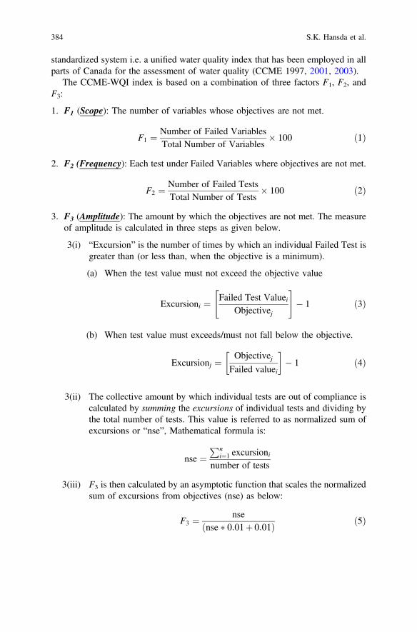
standardized system i.e. a unified water quality index that has been employed in allparts of Canada for the assessment of water quality (CCME 1997, 2001, 2003).
The CCME-WQI index is based on a combination of three factors F1, F2, andF3:
1. F1 (Scope): The number of variables whose objectives are not met.
F1 ¼ Number of Failed VariablesTotal Number of Variables
� 100 ð1Þ
2. F2 (Frequency): Each test under Failed Variables where objectives are not met.
F2 ¼ Number of Failed TestsTotal Number of Tests
� 100 ð2Þ
3. F3 (Amplitude): The amount by which the objectives are not met. The measureof amplitude is calculated in three steps as given below.
3(i) “Excursion” is the number of times by which an individual Failed Test isgreater than (or less than, when the objective is a minimum).
(a) When the test value must not exceed the objective value
Excursioni ¼ Failed Test ValueiObjectivej
" #� 1 ð3Þ
(b) When test value must exceeds/must not fall below the objective.
Excursionj ¼Objectivej
Failed valuei
� �� 1 ð4Þ
3(ii) The collective amount by which individual tests are out of compliance iscalculated by summing the excursions of individual tests and dividing bythe total number of tests. This value is referred to as normalized sum ofexcursions or “nse”, Mathematical formula is:
nse ¼Pn
i¼1 excursioninumber of tests
3(iii) F3 is then calculated by an asymptotic function that scales the normalizedsum of excursions from objectives (nse) as below:
F3 ¼ nseðnse � 0:01þ 0:01Þ ð5Þ
384 S.K. Hansda et al.
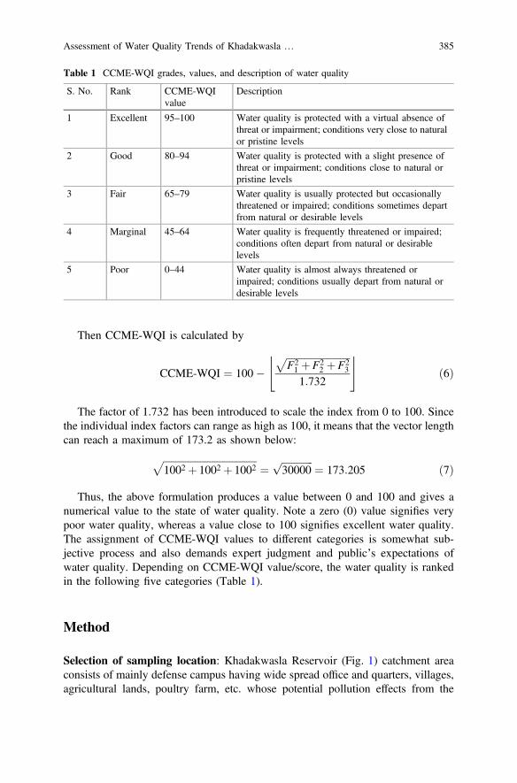
Then CCME-WQI is calculated by
CCME-WQI ¼ 100�ffiffiffiffiffiffiffiffiffiffiffiffiffiffiffiffiffiffiffiffiffiffiffiffiffiffiF21 þF2
2 þF23
p1:732
$ %ð6Þ
The factor of 1.732 has been introduced to scale the index from 0 to 100. Sincethe individual index factors can range as high as 100, it means that the vector lengthcan reach a maximum of 173.2 as shown below:
ffiffiffiffiffiffiffiffiffiffiffiffiffiffiffiffiffiffiffiffiffiffiffiffiffiffiffiffiffiffiffiffiffiffiffiffiffiffi1002 þ 1002 þ 1002
p¼
ffiffiffiffiffiffiffiffiffiffiffiffiffi30000
p¼ 173:205 ð7Þ
Thus, the above formulation produces a value between 0 and 100 and gives anumerical value to the state of water quality. Note a zero (0) value signifies verypoor water quality, whereas a value close to 100 signifies excellent water quality.The assignment of CCME-WQI values to different categories is somewhat sub-jective process and also demands expert judgment and public’s expectations ofwater quality. Depending on CCME-WQI value/score, the water quality is rankedin the following five categories (Table 1).
Method
Selection of sampling location: Khadakwasla Reservoir (Fig. 1) catchment areaconsists of mainly defense campus having wide spread office and quarters, villages,agricultural lands, poultry farm, etc. whose potential pollution effects from the
Table 1 CCME-WQI grades, values, and description of water quality
S. No. Rank CCME-WQIvalue
Description
1 Excellent 95–100 Water quality is protected with a virtual absence ofthreat or impairment; conditions very close to naturalor pristine levels
2 Good 80–94 Water quality is protected with a slight presence ofthreat or impairment; conditions close to natural orpristine levels
3 Fair 65–79 Water quality is usually protected but occasionallythreatened or impaired; conditions sometimes departfrom natural or desirable levels
4 Marginal 45–64 Water quality is frequently threatened or impaired;conditions often depart from natural or desirablelevels
5 Poor 0–44 Water quality is almost always threatened orimpaired; conditions usually depart from natural ordesirable levels
Assessment of Water Quality Trends of Khadakwasla … 385

watershed drains during rains into the common water body, the reservoir. Fivesampling locations, K1, K2, K3 on the right bank, K4 and K5 on left bank wereselected. K1, K2, and K5 represent Riverine zone and K1 and K4 Lacusterine zonekeeping in view the following points:
1. To observe the impact of Anthropogenic Activities on the left and right banks ofthe reservoir.
2. To observe the water quality at Riverine and Lacusterine zone.3. To observe the intensity of pollutants in five sampling points.
Water Sample Collection—Surface water from sampling locations were col-lected in well labeled cleaned polyethylene bottles rinsed by deionized and reser-voir water. Analysis of physicochemical parameters is done as per APHA (2005),Standard Methods for the Examination of Water and Waste Water, 21st edition,American Public Health Association, Washington, D.C., USA (Fig. 2).
Result and Discussions
The CCME-WQI was calculated location-wise as mentioned under method above.Tables 2, 3, 4, 5, and 6 are for locations from K1 to K5, respectively. They show
statistically analyzed data (field observed and lab determined) for years from 2003to 2012 for each location. Comparison of 20 physicochemical parameters (Parm)
K1, OSADE
K 2, MTALWADI
K5, KUDJE
K 3, CHAUPATI
K4, PUMP HOUSE
KHADAKWASLA DAM
Mutha River
Right Canal
Mose + Ambhi River
Fig. 2 Five sampling locations in Khadakwasla reservoir, Pune
386 S.K. Hansda et al.
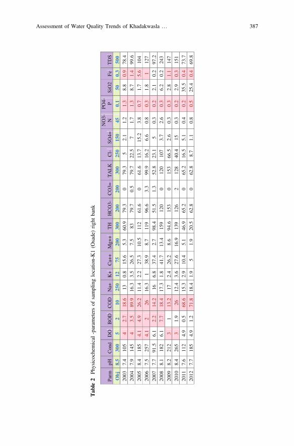
Tab
le2
Physicochemical
-param
etersof
samplinglocatio
n-K1(O
sade)righ
tbank
Par
m
pH
Con
d D
O
BO
D
CO
D
Na+
K+
Ca+
+M
g++
TH
H
CO
3-C
O3=
TA
LK
Cl-
S
O4=
NO
3-N
PO
4- P S
iO2
Fe
TD
S
Ob
j8.
530
05
210
250
1275
200
300
200
200
300
250
150
450.
150
0.3
500
2003
7.
4 10
5 4
2.7
18.6
13
0.
815
.6
5.3
60.9
79
.3
0 79
.3
5 2.
1 1.
2 1.
3 8.
8 0.
978
.4
2004
7.
9 14
5 4
3.5
89.9
16
.33.
526
.5
7.5
83
79.7
0.
5 79
.7
22.5
7
1.7
1.3
8.7
1.4
99.6
2005
8.
4 18
5 4.
1 4.
9 26
.2
11.4
2.2
27.3
10
.5
112
61.6
0
61.6
13
.7
15.2
3.
8 0.
7 1.
7 5.
610
4
2006
7.
5 25
7 4.
1 2
26
16.3
1 38
.9
8.7
119
96.6
3.
3 99
.9
16.2
6.
6 0.
8 0.
3 1.
8 1
127
2007
7.
7 91
.5
6.1
2.2
14.2
16
6.
837
.4
2.7
98.4
51
.5
1.3
52.8
23
.1
5 0.
3 0.
2 2.
1 0.
297
.2
2008
8.
1 18
2 6.
1 7.
7 18
.4
17.3
1.8
41.7
13
.4
159
120
0 12
0 10
7 3.
7 2.
6 0.
3 6.
2 0.
224
3
2009
8.
2 21
2 3
1 13
.2
17
2.4
26.2
8.
6 94
.6
153
0 15
3 66
.5
2.6
0.3
0.3
2.8
1.1
147
2010
8.
4 26
5 3
1.9
26
12.4
3.6
27.6
16
.9
139
126
2 12
8 40
.4
15
0.3
0.2
2.9
0.3
151
2011
7.
6 11
2 4.
9 0.
5 68
.6
15.3
2.9
10.4
5.
1 46
.9
65.2
0
65.2
16
.5
5.1
0.4
0.2
35.5
0.
473
.7
2012
7.
7 18
5 4.
9 1.
2 71
.8
18.4
1.9
5 1.
9 20
.5
62.8
0
62.8
8.
7 1.
1 0.
8 0.
5 25
.4
0.4
69.8
Assessment of Water Quality Trends of Khadakwasla … 387

Tab
le3
Physicochemical
-param
etersof
samplinglocatio
n-K2(G
hore/M
atalwadi)righ
tbank
Parm
pH
Con
d D
O
BO
DC
OD
N
a+
K+
Ca+
+M
g++
TH
H
CO
3-C
O3=
TA
LK
Cl-
S
O4=
NO
3-N
P
O4- P
SiO
2Fe
T
DS
Ob
j8.
530
05
210
250
1275
200
300
200
200
300
250
150
450.
150
0.3
500
2003
8.
390
4.
2 4.
2 90
.2
10.1
1.7
10.9
7.
1 54
.961
0
61
6.5
2.1
0.2
0.1
3 0.
165
.3
2004
9.
211
2 4.
2 1.
9 18
4 17
.21.
328
.9
6.3
94.4
81.8
0.
3 81
.8
30.9
7.5
1.7
0.1
6 0.
710
9 20
05
8.5
222
4.6
7.4
26.2
11
.43.
939
.8
9.8
140
74.6
0
74.6
16
.221
.3
5.8
0.5
2.9
7.5
135
2006
8.
416
9 4.
6 4.
8 39
.4
10.8
1 29
.2
8.7
91.2
84.6
2.
6 86
.5
13.3
8.8
0.7
0.3
2.9
1 91
20
07
7.9
78
5.3
0.6
14.9
14
.76.
342
.4
2 11
3 69
.1
0 69
.1
20.6
5.2
0.4
0.2
1.8
0.3
110
2008
7.
812
0 6.
5 2.
4 17
.4
16.5
3.7
38.7
8.
3 12
4 78
.9
0 78
.9
87.1
3.7
2.4
0.2
4.7
0.5
170
2009
8.
117
0 6.
5 0.
8 11
.3
20.9
2.9
55
15.7
20
2 88
.8
1.7
90.5
10
8 3.
5 0.
3 0.
3 5
0.3
249
2010
7.
717
4 8
1.4
13.7
7.
7 0.
823
.1
8.6
93.1
66.2
0
66.2
39
.811
.5
0.2
0.1
4.3
0.3
108
2011
7.
513
5 6.
3 0.
1 13
1 15
.80.
920
.3
5.3
72.3
76.7
2.
5 76
.7
26.4
8.4
0.4
0.1
34.3
0.
390
.7
2012
8.
511
8 5.
5 1.
6 59
.6
18.7
1.8
6.1
1.5
21.4
62.8
0
62.8
9.
2 1.
3 0.
5 0.
4 20
.2
0.3
70.9
388 S.K. Hansda et al.

Tab
le4
Physicochemical
-param
etersof
samplinglocatio
n-K3(Chaup
ati)righ
tbank
Par
m
pH
Con
d D
O
BO
D
CO
D
Na+
K+
Ca+
+M
g++
T
H
HC
O3-
C
O3=
T
AL
KC
l-
SO4=
NO
3-N
PO
4- P Si
O2
Fe
TD
S
Ob
j 8.
5 30
0 5
2 10
25
0 12
75
20
0 30
0 20
0 20
0 30
0 25
0 15
0 45
0.
1 50
0.
3 50
0 20
03
7.8
100
4.1
2.3
15.8
10
0.
711
9.
8 58
.773
.2
0 73
.2
7.8
2.5
0.1
0.1
2.5
0 68
.9
2004
8.
5 11
8 4.
1 1.
8 15
3 15
.21.
324
.9
5.4
70.1
67.8
0
67.8
21
.2
9.1
2.3
0.1
3 0.
7 86
.4
2005
8.
7 15
6 4.
9 6.
7 30
.8
12
0.8
39.5
6.
6 11
7 88
.2
0 88
.2
13.8
9.
4 2.
8 0.
4 1.
8 2.
9 10
3 20
06
8.6
181
4.9
2.1
17.4
11
.73.
523
.3
6.6
79.6
71.6
8.
5 72
.6
16.6
5.
9 0.
5 0.
3 1.
8 0.
8 84
.8
2007
8
74
5.3
2.6
10.3
15
3.
49.
2 1.
9 30
.446
.7
0 46
.7
18.5
4.
9 0.
4 0.
1 2
0.2
73.8
2008
8.
7 10
1 6.
3 0.
8 15
.4
15.1
1.9
20.5
7.
5 82
.162
0
62
52.3
18
0.
2 0.
2 5
0.2
126
2009
7.
9 88
6.
3 0.
9 12
.8
17.1
1.2
15.7
7.
6 70
.580
.3
0 80
.3
60.8
3.
1 0.
6 0.
3 2.
8 1.
1 12
5
2010
7.
7 16
5 6.
7 4.
1 13
.1
7.4
0.8
26.7
6.
2 92
65
.4
3 65
.4
41.6
8.
8 0.
2 0.
1 4.
6 0.
4 11
1 20
11
7.6
89
6.6
0.8
24.2
14
.31
13.6
3.
8 41
.469
.5
0 69
.5
18.4
4.
4 0.
4 0.
1 35
0.
3 70
.1
2012
7.
7 12
8 5.
8 2.
9 66
.8
21.1
2 2.
3 0.
5 7.
8 60
.3
0 60
.3
7.2
1.2
0.6
0.4
25.2
0.
3 65
.3
Assessment of Water Quality Trends of Khadakwasla … 389
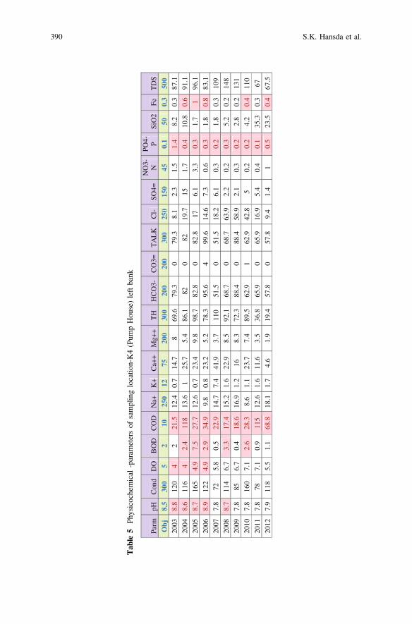
Tab
le5
Physicochemical
-param
etersof
samplinglocatio
n-K4(Pum
pHou
se)leftbank
Parm
pH
Con
d D
O
BO
DC
OD
N
a+K
+C
a++
Mg+
+T
H
HC
O3-
C
O3=
TA
LK
C
l-
SO4=
NO
3-N
PO
4- P Si
O2
Fe
TD
S
Ob
j 8.
530
0 5
2 10
25
0 12
75
20
0 30
0 20
0 20
0 30
0 25
0 15
0 45
0.
1 50
0.
350
0 20
03
8.8
120
4 2
21.5
12
.40.
7 14
.7
8 69
.679
.3
0 79
.3
8.1
2.3
1.5
1.4
8.2
0.3
87.1
2004
8.
611
6 4
2.4
118
13.6
1 25
.7
5.4
86.1
82
0 82
19
.715
1.
7 0.
4 10
.8
0.6
91.1
2005
8.
716
5 4.
9 7.
5 27
.7
12.6
0.7
23.4
9.
8 98
.782
.8
0 82
.8
17
6.1
3.3
0.3
1.7
1 96
.1
2006
8.
912
2 4.
9 2.
9 34
.9
9.8
0.8
23.2
5.
2 78
.395
.6
4 99
.6
14.6
7.3
0.6
0.3
1.8
0.8
83.1
2007
7.
872
5.
8 0.
5 22
.9
14.7
7.4
41.9
3.
7 11
0 51
.5
0 51
.5
18.2
6.1
0.3
0.2
1.8
0.3
109
2008
8.
711
4 6.
7 3.
3 17
.4
15.2
1.6
22.9
8.
5 92
.168
.7
0 68
.7
63.9
2.2
0.2
0.3
5.2
0.2
148
2009
7.
885
6.
7 0.
4 18
.6
16.9
1.2
16
8.3
72.3
88.4
0
88.4
58
.92.
1 0.
3 0.
2 2.
8 0.
213
1
2010
7.
816
0 7.
1 2.
6 28
.3
8.6
1.1
23.7
7.
4 89
.562
.9
1 62
.9
42.8
5 0.
2 0.
2 4.
2 0.
411
0
2011
7.
878
7.
1 0.
9 11
5 12
.61.
6 11
.6
3.5
36.8
65.9
0
65.9
16
.95.
4 0.
4 0.
1 35
.3
0.3
67
2012
7.
911
8 5.
5 1.
1 68
.8
18.1
1.7
4.6
1.9
19.4
57.8
0
57.8
9.
4 1.
4 1
0.5
23.5
0.
467
.5
390 S.K. Hansda et al.

Tab
le6
Physicochemical
-param
etersof
samplinglocatio
n-K
5(K
udje)leftbank
Par
mpH
C
ond
DO
B
OD
CO
D
Na+
K
+C
a++
Mg+
+T
H
HC
O3-
CO
3=T
AL
KC
l-
SO4=
NO
3-N
P
O4- P
SiO
2F
e T
DS
Ob
j 8.
530
0 5
2 10
25
0 12
75
20
0 30
0 20
0 20
0 30
0 25
0 15
0 45
0.
1 50
0.
350
0 20
03
8.3
85
4 2.
5 7.
2 9.
4 0.
68.
7 7.
1 47
.751
.9
0 51
.9
6.5
3.2
0.2
0.2
3.4
0 54
.6
2004
9.
111
2 4.
1 1.
3 12
4 14
.31
26.5
7.
1 82
.110
4 0.
8 10
4 18
.118
.5
1.4
1.8
10
0.5
105
2005
8.
915
7 4.
8 7.
8 29
.2
11.3
0.8
22.4
8.
2 89
.677
.3
0 77
.3
14
9.9
2.9
0.9
2 2.
788
.3
2006
8.
912
4 4.
8 7
25.8
11
.10.
724
.6
13.9
11
7 55
.5
1.3
55.5
15
.25.
3 0.
5 0.
3 2
0.5
80.6
20
07
7.8
72.7
5.
7 1.
1 11
.9
15.8
7.1
32.8
2.
5 89
.344
.7
4 48
.6
20.6
5.5
0.4
0.1
2.8
0.3
95.7
2008
8.
910
8 7.
3 1.
5 16
.9
16.5
1 22
.9
7.3
87.1
65.1
0
65.1
68
.45.
8 0.
7 0.
2 4.
7 0.
215
1
2009
7.
983
7.
3 1.
5 12
.2
22.7
1.3
14.4
9.
1 73
.684
.1
0 84
.1
45.6
2.1
0.4
0.3
3 0.
312
3 20
10
7.7
160
5.5
0.8
18.4
7.
6 0.
526
.5
5.9
90.5
58.9
1
58.9
40
.76.
1 0.
2 0.
2 4.
5 0.
410
9
2011
8.
178
5.
5 0.
7 65
.5
13.7
1 11
.2
3.8
32.7
65.9
0
65.9
15
.34.
8 0.
4 0.
1 28
.8
0.5
67.3
2012
7.
911
0 6.
1 1.
1 62
.6
16.2
1.2
4.4
2.2
19.9
55.3
0
55.3
8.
2 1.
3 0.
8 0.
4 22
.7
0.3
62.2
Assessment of Water Quality Trends of Khadakwasla … 391
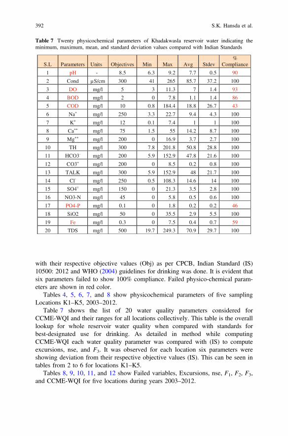
with their respective objective values (Obj) as per CPCB, Indian Standard (IS)10500: 2012 and WHO (2004) guidelines for drinking was done. It is evident thatsix parameters failed to show 100% compliance. Failed physico-chemical param-eters are shown in red color.
Tables 4, 5, 6, 7, and 8 show physicochemical parameters of five samplingLocations K1–K5, 2003–2012.
Table 7 shows the list of 20 water quality parameters considered forCCME-WQI and their ranges for all locations collectively. This table is the overalllookup for whole reservoir water quality when compared with standards forbest-designated use for drinking. As detailed in method while computingCCME-WQI each water quality parameter was compared with (IS) to computeexcursions, nse, and F3. It was observed for each location six parameters wereshowing deviation from their respective objective values (IS). This can be seen intables from 2 to 6 for locations K1–K5.
Tables 8, 9, 10, 11, and 12 show Failed variables, Excursions, nse, F1, F2, F3,and CCME-WQI for five locations during years 2003–2012.
Table 7 Twenty physicochemical parameters of Khadakwasla reservoir water indicating theminimum, maximum, mean, and standard deviation values compared with Indian Standards
S.L Parameters Units Objectives Min Max Avg Stdev %
Compliance
1 pH - 8.5 6.3 9.2 7.7 0.5 90
2 Cond µS/cm 300 41 265 85.7 37.2 100
3 DO mg/l 5 3 11.3 7 1.4 93
4 BOD mg/l 2 0 7.8 1.1 1.4 86
5 COD mg/l 10 0.8 184.4 18.8 26.7 43
6 Na+ mg/l 250 3.3 22.7 9.4 4.3 100
7 K+ mg/l 12 0.1 7.4 1 1 100
8 Ca++ mg/l 75 1.5 55 14.2 8.7 100
9 Mg++ mg/l 200 0 16.9 3.7 2.7 100
10 TH mg/l 300 7.8 201.8 50.8 28.8 100
11 HCO3- mg/l 200 5.9 152.9 47.8 21.6 100
12 CO3= mg/l 200 0 8.5 0.2 0.8 100
13 TALK mg/l 300 5.9 152.9 48 21.7 100
14 Cl- mg/l 250 0.5 108.3 14.6 14 100
15 SO4= mg/l 150 0 21.3 3.5 2.8 100
16 NO3-N mg/l 45 0 5.8 0.5 0.6 100
17 PO4-P mg/l 0.1 0 1.8 0.2 0.2 46
18 SiO2 mg/l 50 0 35.5 2.9 5.5 100
19 Fe mg/l 0.3 0 7.5 0.4 0.7 59
20 TDS mg/l 500 19.7 249.3 70.9 29.7 100
392 S.K. Hansda et al.

Tab
le8
Resultsof
samplinglocatio
nK1(O
sade)righ
tbank
Years
Total
numberof
variables
Total
numberfailed
variables
Total
number
oftests
Num
berof
failedtests
Excursion
nse
F1
F2
F3
CCME-W
QI
2003
205
408
18.45
0.46
2513
3276
2004
205
200
2867
.14
0.34
253
2579
2005
205
240
2960
.38
0.25
252
2081
2006
204
200
1512
.20
0.06
202
688
2007
203
605
1.59
0.03
155
391
2008
204
605
6.71
0.11
207
1087
2009
204
809
8.80
0.11
205
1087
2010
204
8010
6.88
0.09
205
887
2011
203
605
8.57
0.14
155
1388
2012
203
606
16.84
0.28
155
2284
Assessment of Water Quality Trends of Khadakwasla … 393

Tab
le9
Resultsof
samplinglocatio
nK2(G
ore/Matalwadi)righ
tbank
Years
Total
numberof
variables
Total
numberof
failed
variables
Total
number
oftests
Num
berof
failedtests
Excursion
nse
F1
F2
F3
CCME-W
QI
2003
203
424
10.35
0.25
157
2085
2004
205
218
2439
.93
0.18
252
1583
2005
204
262
1850
.95
0.19
202
1685
2006
204
218
2314
.64
0.07
202
688
2007
202
645
1.59
0.02
103
294
2008
204
646
4.27
0.07
206
687
2009
203
8610
5.21
0.06
153
691
2010
203
866
1.04
0.01
153
191
2011
203
649
15.61
0.24
155
2085
2012
204
644
11.89
0.19
206
1685
394 S.K. Hansda et al.
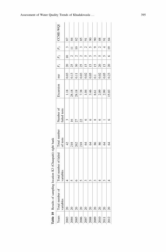
Tab
le10
Resultsof
samplinglocatio
nK3(Chaup
atti)
righ
tbank
Years
Total
numberof
variables
Total
numberof
failed
variables
Total
number
oftests
Num
berof
failedtests
Excursion
nse
F1
F2
F3
CCME-W
QI
2003
204
423
1.18
0.03
2010
387
2004
205
218
1628
.18
0.13
252
1184
2005
206
262
2728
.18
0.11
302
1082
2006
205
218
227.38
0.03
252
385
2007
203
646
1.04
0.02
155
291
2008
203
646
3.46
0.05
155
590
2009
203
868
8.61
0.1
153
990
2010
204
866
2.09
0.02
205
288
2011
203
641
2.99
0.05
155
491
2012
204
646
15.03
0.23
206
1984
Assessment of Water Quality Trends of Khadakwasla … 395
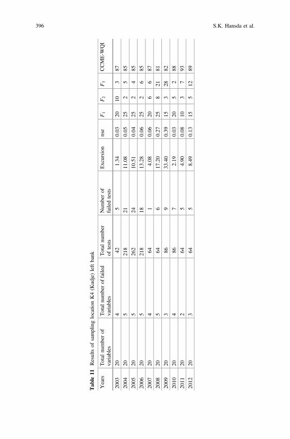
Tab
le11
Resultsof
samplinglocatio
nK4(K
udje)leftbank
Years
Total
numberof
variables
Total
numberof
failed
variables
Total
number
oftests
Num
berof
failedtests
Excursion
nse
F1
F2
F3
CCME-W
QI
2003
204
425
1.34
0.03
2010
387
2004
205
218
2111
.08
0.05
252
585
2005
205
262
2410
.51
0.04
252
485
2006
205
218
1813
.28
0.06
252
685
2007
204
641
4.08
0.06
206
687
2008
205
646
17.20
0.27
258
2181
2009
203
869
33.40
0.39
153
2882
2010
204
867
2.19
0.03
205
288
2011
202
645
4.90
0.08
103
793
2012
203
645
8.49
0.13
155
1289
396 S.K. Hansda et al.

Tab
le12
Resultsof
samplinglocatio
nK5(K
udje)leftbank
Years
Total
numberof
variables
Total
numberof
failed
variables
Total
number
oftests
Num
berof
failedtests
Excursion
nse
F1
F2
F3
CCME-W
QI
2003
203
423
1.7
0.04
157
490
2004
205
218
2350
.18
0.23
252
1982
2005
205
262
1736
.26
0.14
252
1284
2006
205
218
209.99
0.05
252
485
2007
203
644
1.28
0.02
155
291
2008
203
646
2.54
0.04
155
491
2009
203
863
4.38
0.05
153
591
2010
203
869
2.96
0.03
153
391
2011
203
646
7.85
0.12
155
1189
2012
203
644
16.55
0.26
155
2185
Assessment of Water Quality Trends of Khadakwasla … 397
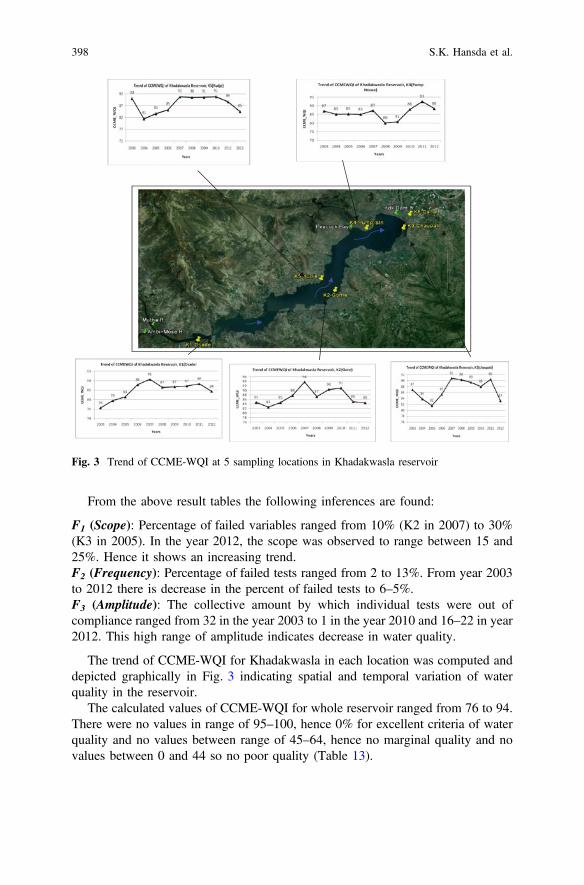
From the above result tables the following inferences are found:
F1 (Scope): Percentage of failed variables ranged from 10% (K2 in 2007) to 30%(K3 in 2005). In the year 2012, the scope was observed to range between 15 and25%. Hence it shows an increasing trend.F2 (Frequency): Percentage of failed tests ranged from 2 to 13%. From year 2003to 2012 there is decrease in the percent of failed tests to 6–5%.F3 (Amplitude): The collective amount by which individual tests were out ofcompliance ranged from 32 in the year 2003 to 1 in the year 2010 and 16–22 in year2012. This high range of amplitude indicates decrease in water quality.
The trend of CCME-WQI for Khadakwasla in each location was computed anddepicted graphically in Fig. 3 indicating spatial and temporal variation of waterquality in the reservoir.
The calculated values of CCME-WQI for whole reservoir ranged from 76 to 94.There were no values in range of 95–100, hence 0% for excellent criteria of waterquality and no values between range of 45–64, hence no marginal quality and novalues between 0 and 44 so no poor quality (Table 13).
Fig. 3 Trend of CCME-WQI at 5 sampling locations in Khadakwasla reservoir
398 S.K. Hansda et al.
Conclusion
The CCME-WQI ranged from 76 to 94, indicating grade from fair to good waterquality. “Fair” water quality was shown by 2% for location K1, and “good” waterquality by 98% for locations K2, K3, K4, and K5. Locations K1 (Osade) and K2(Matalwadi) are open banks and easy entry points for the nearby villagers forbathing and washing cloths and utensils. Agriculture activities for crops like rice,wheat, jawari, bajra, and vegetables are done near the banks in these two locations.In addition to this there is a cemetery in bank of location K2 constructed during theyear 2007–2008. Extensive anthropogenic activities like washing of clothes, cattle,utensils, vehicles, etc., and bathing are carried out daily at this location of thereservoir.
Fencing at K4 and K3 which are restriction wall/embankment/mesh link wereconstructed in early 2009. This seems to have worked for improvement in waterquality by way of containing the garbage created on the land, there itself near K3;and by limiting the access for human and cattle etc. to the left bank near dam (K4)that may cause pollution.
Lower water quality grade, i.e., 76 can be attributed to noncompliance of sixvariables, which did not comply with the objective values. Non-compliantparameters were DO, pH, BOD, Fe, PO4-P, COD.
Water Quality in this reservoir is facing pressure due to anthropogenic activitiesfrom left bank as well as from the right bank. As this reservoir is having less depth(average 5 m) and its surface area is exposed to clean winds throughout the year,which facilitates, very good natural aeration to maintain its dissolved oxygen nat-urally. As the reservoir water is continuously drawn by canal systems throughout theyear, this causes a flow circulation in the reservoir and mixing of surface water withthe deeper water at transitional and lacusterine zones. Hence in spite of anthro-pogenic activities, water wuality was found to be good. Public awareness should becreated among the villagers and visiting tourists and the resorts located near thebank. This may reduce the disposal of pollutants in the vicinity (especially at K1)and help to keep the water quality in the range of excellent (CCME-WQI = 95–100).
Table 13 The CCME-WQI distribution for five locations in Khadakwasla reservoir, Pune
Samplinglocations
CCME-WQIvalues
Qualityrating
Quality affecting activities
Range Average
K1 76–89 86 Fair–good
Due to Anthropogenic, Household,Agricultural runoff, and rooftop runoff
K2 85–94 88 Good
K3 84–91 88 Good
K4 80–94 88 Good
K5 83–94 88 Good DO, pH, BOD, Fe, PO4-P, COD getaffected
Assessment of Water Quality Trends of Khadakwasla … 399

References
APHA (2005) Standard methods for the examination of water and waste water, 21 edn. AmericanPublic Health Association, Washington, D.C., USA
Bagde US, Verma AK (1985) Limnological studies of JNU lake, New Delhi. Proc Natl Sump PureAppl Limnol 32:16–23
BCWQI (1996) Ministry of Environment, Lands, and Parks: The Water Quality Section BritishColumbia Water Quality Status Report, April, Victoria, BC
B.C. Ministry of Environment, Land and Parks (1996) British Columbia Water Quality StatusReport, 181 pp
Bhargava DS (1983) Use of water quality index for river classification and zoning of Ganga River.Environ Pollut (Series B) 6:51–67
Bhargava DS (1985) Water quality variations and control technology of Yamuna river. EnvironPollut (Series A) 37:355–376
Brown RM, McLelland NI, Deininger RA, O’Connor MF (1972) A water quality index—crashingthe psychological barrier. Indicators of Environmental Quality
Burden FR, Mc Kelvie I, Forstner U, Guenther A (2002) Environmental monitoring handbook.McGraw-Hill Handbooks, New York, pp 3.1–3.21
Buyan KC (2005) Multivariate analysis and its applications. New Central Book Agency Pvt. Ltd.Publication, pp 1–2
Cash KJ, Saffran KA, Wright CR (2001) Application of canadian water quality index to PPWBmonitoring program. Technical Report, CCME, March 2001
CCME (2001) Canadian environmental quality guidelines for the protection of aquatic life. CCMEwater quality index: technical report, 1.0
CCME (2003) Water Quality Index Workshop, November 24–25, Halifax, NS, Canada’ CanadianCouncil of Ministers of the Environment, Winnipeg, MB. Available from: http://www.ccme.ca/initiatives/water.html
Chauhan A, Singh S (2010) Evaluation of Ganga water for drinking purpose by water qualityindex at Rishikesh, Uttarakhand, India. Rep Opin 2(9):53–61
Deininger RA, Maciunas JJ (1971) A water quality index for public water supply, Report of aResearch Study, University of Michigan
Dinius SH (1972) Social accounting system for evaluating water resources. Water Resour Res 8(5):1159–1177
Dinius SH (1987) Design of an index of water quality. Water Resour Bull 23(5):833–843Dunnette DA (1979) A geographically variable water quality index used in oregon. J Water Pollut
Control Fed 51(1):53–61Harkins Ralph D (1974) An objective water quality index. J (Water Pollution Control Federation),
46(3), Part I: 588–591. Published by: Water Environment Federation Stable. URL: http://www.jstor.org/stable/25038160
Horton RK (1965) An index number system for rating water quality. J Water Pollut Control Fed 37(3):300–306
Indian Standard Specification for Drinking Water (1983) Indian Standard (IS)10500: 2012,New Delhi
Landwehr JM, Deininger RA (1976) A comparison of several water quality indexes. J Water PollutControl Fed 48(5):954
Landwehr JM (1979) A statistical view of a class of water quality indices. Water Resour Res15:460–468
NSF (2003) National Sanitation Foundation. Available from: http://Nsfconsumer.rg/environment/Wqi.asp
Prati L, Pavanello R, Pesarin F (1971) Assessment of surface water quality by a single index ofpollution. Water Res 5(7):41–75
400 S.K. Hansda et al.

Tiwari TN, Manzoor A (1988) Water quality index for Indian rivers. In: RK Trivedy (ed) Ecologyand pollution in Indian rivers. Ashish Publishing House, New Delhi, pp 271–286
Walski TM, Parker FL (1974) Consumer’s water quality index. J Environ Eng ASCE 100:593–611
WHO (2004) Guidelines for drinking water quality, vol 1, 3rd edn. Recommendations, Geneva
Assessment of Water Quality Trends of Khadakwasla … 401

Assessment of Agricultural Water Qualityof Shallow Groundwater Between Budhniand Chaursakhedi, North of RiverNarmada, District Sehore, MadhyaPradesh, India
Sunil Kumar Sharma, Shalini Yadav, V.K. Parasharand Pramod Dubey
Abstract Hydrogeochemistry of an area helps in understanding the geologicalprocesses which control the chemistry of water and plays an important role indetermining the suitability of groundwater for various purposes. In the presentstudy, an attempt has been made to understand the hydrochemistry and the agri-cultural water quality of water between Budhni and Chaursakhedi, North of riverNarmada, District Sehore, Madhya Pradesh. In all 25 representatives, shallowgroundwater samples were collected from the study area and physicochemicalparameters were analyzed. Results obtained from water chemistry were used in thedetermination of various irrigational specifications to determine the agriculturalquality of shallow groundwater. In the present study prominent specifications likesoluble sodium percentage (SSP), sodium adsorption ratio (SAR) and residualsodium carbonate (RSC), are used for determining the suitability of shallow groundwater for agricultural purposes. Result shows that the majority of shallowgroundwater of the study area belongs to Medium to High Saline and Low sodiumwater. Kelly’s ratio shows that majority of shallow groundwater belongs to suitableclass. As per Wilcox classification, the shallow groundwater belongs to Good toPermissible class. The shallow groundwater of the study area belongs to Safe classas per the classification based on RSC. As per the magnesium ratio classification, allthe shallow groundwater’s of the study area belongs to the suitable class and thereare no magnesium hazards and thus they are suitable for agricultural purposes.
S.K. Sharma (&) � S. YadavDepartment of Civil Engineering, AISECT University, Bhopal, MP, Indiae-mail: [email protected]
V.K. ParasharDepartment of Geology, Government Holkar Science College, Indore, MP, India
P. DubeySchool of Planning and Architecture, Bhopal, MP, India
© Springer Nature Singapore Pte Ltd. 2018V.P. Singh et al. (eds.), Environmental Pollution, Water Scienceand Technology Library 77, https://doi.org/10.1007/978-981-10-5792-2_32
403
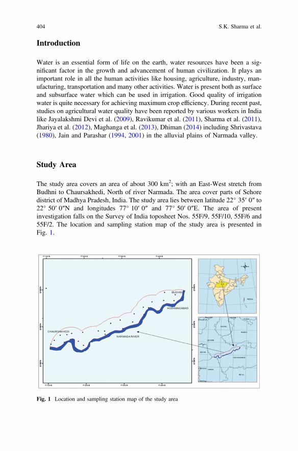
Introduction
Water is an essential form of life on the earth, water resources have been a sig-nificant factor in the growth and advancement of human civilization. It plays animportant role in all the human activities like housing, agriculture, industry, man-ufacturing, transportation and many other activities. Water is present both as surfaceand subsurface water which can be used in irrigation. Good quality of irrigationwater is quite necessary for achieving maximum crop efficiency. During recent past,studies on agricultural water quality have been reported by various workers in Indialike Jayalakshmi Devi et al. (2009), Ravikumar et al. (2011), Sharma et al. (2011),Jhariya et al. (2012), Maghanga et al. (2013), Dhiman (2014) including Shrivastava(1980), Jain and Parashar (1994, 2001) in the alluvial plains of Narmada valley.
Study Area
The study area covers an area of about 300 km2; with an East-West stretch fromBudhni to Chaursakhedi, North of river Narmada. The area cover parts of Sehoredistrict of Madhya Pradesh, India. The study area lies between latitude 22° 35′ 0″ to22° 50′ 0″N and longitudes 77° 10′ 0″ and 77° 50′ 0″E. The area of presentinvestigation falls on the Survey of India toposheet Nos. 55F/9, 55F/10, 55F/6 and55F/2. The location and sampling station map of the study area is presented inFig. 1.
Fig. 1 Location and sampling station map of the study area
404 S.K. Sharma et al.

The entire catchment area of the Narmada River is characterized by undulatingtopography with number of hill ranges, valleys and plains. The area of present studyis covered with alluvium which has been derived from weathering and masswasting of Deccan traps and present as filling the faulted trough of the Narmada riftvalley. In general the alluvial layer is thickest near the Narmada and taperingtowards the foot hill of Satpura. The alluvium is chiefly composed of reddish,brownish, yellowish and sandy clay with numerous intercalations of sand, gravelsand kankar along with pisolitic iron granules. The thickness of the alluvial depositsis variable depending upon the floor of the basin of deposition, which happens to beuneven.
The major portion of the study area is upland alluvium formed by deposition ofsediments in the inland Narmada depression. The northern portion of it is longi-tudinally occupied by the alluvium. The constituents and nature of the alluviumvary locally, depending upon the rocks present in the study area, from which theyhave been derived. The hydro-geomorphological and geological map of the studyarea is presented in Figs. 2 and 3, respectively.
Fig. 2 Hydrogeomorphological map of the study area
Assessment of Agricultural Water Quality of Shallow Groundwater … 405

Materials and Methods
Chemical analyses of water samples provide valuable information about the envi-ronment to which natural water are exposed in the hydrologic cycle. The shallowgroundwater samples were collected during pre-monsoon and post-monsoon period.The water samples were collected in one litre polyethylene bottles and analyzed byusing the procedures given by APHA (1995). The analysis of water samples wascarried out by using Hach Spectrophotometer, Flame photometer and titrationmethods. The physical properties like colour, odour, temperature and taste of watersamples were recorded at the sampling stations during field work. The pH of thewater samples was determined by pH metre. Conductivity is measured in micromohs per cm at 25 °C by conductivity metre. Total dissolved solid (TDS) wasdetermined with the help of TDS metre. The carbonate alkalinity was determined bya titrimetric method using phenolphthalein as indicator. The bicarbonate wasdetermined by titrating sample with standard acid solution using methyl orangeindicator. Total hardness as CaCO3 was determined by EDTA titrimetric methodusing Erichrome Black-T indicator. Ca content was calculated from Ca hardness bymultiplying with a factor 0.432 and the results were expressed in mg/l. Magnesiumcontent was calculated from Mg hardness by using a formula and results expressed
Fig. 3 Geological map of the study area
406 S.K. Sharma et al.

in mg/l. Chloride concentration was determined by titration method involving theformation of a reddish brown complex by adding potassium chromate which istitrated against silver nitrate solution. Nitrate is determined by phenol di sulphuricacid method as per APHA (1995) using Hach DR-4000 UV-Vis Spectrophotometer.
Results and Discussions
General Hydrochemistry
The analytical data of shallow groundwater samples collected both during thepre-monsoon and post-monsoon period are presented in Table 1 which indicatesthat there occurs considerable variation in the chemistry of shallow groundwatersamples from place to place and pre-monsoon to post-monsoon periods, respec-tively. The range of pH value of shallow ground water of the study area varies from7.2 to 8.0 in pre-monsoon and 7.0 to 7.9 in post-monsoon period. The electricalconductivity (EC) values in shallow groundwater vary from 420 to 910 µmohs/cmin pre-monsoon and 390 to 880 µmohs/cm in post-monsoon period. Calciumcontent in shallow ground water varies from 35 to 56 and 31 to 52 mg/l inpre-monsoon and post-monsoon periods, respectively. The Magnesium concentra-tion in shallow ground water varies from 10 to 29 mg/l in pre-monsoon and 08 to28 mg/l in post-monsoon period. The sodium content in shallow ground watervaries from 10 to 76 mg/l in pre-monsoon and 5 to 71 mg/l in post-monsoonperiod. The Potassium content in shallow groundwater is varies from 1.1 to8.1 mg/l in pre-monsoon and 0.6 to 7.3 mg/l in post-monsoon period. The totalhardness in terms of CaCO3 ranges from 154 to 242 mg/l in pre-monsoon and 140to 225 mg/l in post-monsoon period.
The carbonate content is found to be absent in all the samples of shallow groundwater, collected during the pre-monsoon and post-monsoon periods. Bicarbonate isthe predominant anion in the shallow ground water of the study area. Bicarbonateconcentration in the shallow ground water varies from 104 to 274 mg/l inpre-monsoon and 85 to 260 mg/l in post-monsoon period.
The chloride concentration in shallow ground water varies from 36 to 96 mg/l inpre-monsoon and 31 to 92 mg/l in post-monsoon period. The Sulphate concen-tration in the shallow ground water of the study area varies from 18 to 62 mg/l inpre-monsoon and 13 to 57 mg/l in post-monsoon period. The Nitrate in the irri-gation water serves as a nutrient to plants and crops. In the present investigation, theNitrate content in the shallow groundwater varies from 16 to 64 mg/l inpre-monsoon and 12 to 56 mg/l in post-monsoon period. The Phosphate concen-tration in shallow groundwater of the study area varies from 0.12 to 0.29 mg/l inpre-monsoon and 0.09 to 0.27 mg/l in post-monsoon period.
Assessment of Agricultural Water Quality of Shallow Groundwater … 407

Tab
le1
Pre-mon
soon
andpo
st-m
onsoon
hydrochemistryof
shallow
grou
ndwater
ofthestud
ybetweenBud
hniandChaursakh
edi
Pre-mon
soon
Well
No.
Nam
eof
the
village
pHEC
�10
6
at25
°TDS
Con
centratio
nsin
mg/I
Cations
T.H.
as CaC
Anion
s
Na+
K+
Ca+
+Mg+
+HCO3
CO3−
Cl−
NO3
SO4
PO4
12
34
56
78
910
1112
1314
1516
1Bud
hni
7.8
710
454
703.5
4219
182
180
Abs
7730
330.27
2Tatpu
ra7.8
660
422
191.3
3915
160
138
Abs
3664
220.24
3Devgaun
7.9
640
410
401.3
3825
198
189
Abs
8245
400.27
4Holipura
7.6
460
294
511.9
4017
170
122
Abs
9316
520.22
5Unchh
akheda
7.7
680
435
661.1
3624
190
195
Abs
6525
250.24
6Ninor
7.5
910
582
226.1
4217
176
116
Abs
7655
280.21
7Pathora
7.6
820
525
351.5
4023
194
190
Abs
5032
200.29
8Aaw
ali
7.5
610
390
201.7
5610
178
127
Abs
8618
290.22
9Dhank
ot7.7
730
467
183.9
4510
154
140
Abs
4549
180.29
10Mog
ra7.6
670
429
423.1
5013
180
206
Abs
4916
300.27
11Rehug
aon
7.6
690
442
368.1
3622
180
140
Abs
7536
410.23
12Nehlai
7.6
670
429
152.8
5518
212
104
Abs
8355
320.25
13Ratanpu
r7.8
730
467
103.7
4816
186
116
Abs
8756
250.27
14Sawalkh
eda
7.9
690
442
394.5
4619
192
109
Abs
9636
300.24
15Matthagaon
7.7
600
384
473.8
3825
200
172
Abs
8530
420.24
16Basaniya
7.8
780
500
293.2
3824
194
172
Abs
8835
180.26
17Chh
idgaon
7.9
560
358
463.6
4329
228
169
Abs
8125
260.28
18Manjhil
7.2
610
390
753.3
3520
170
220
Abs
7930
200.21
19Tilariya
863
040
365
3.4
5518
210
274
Abs
4535
260.23
(con
tinued)
408 S.K. Sharma et al.
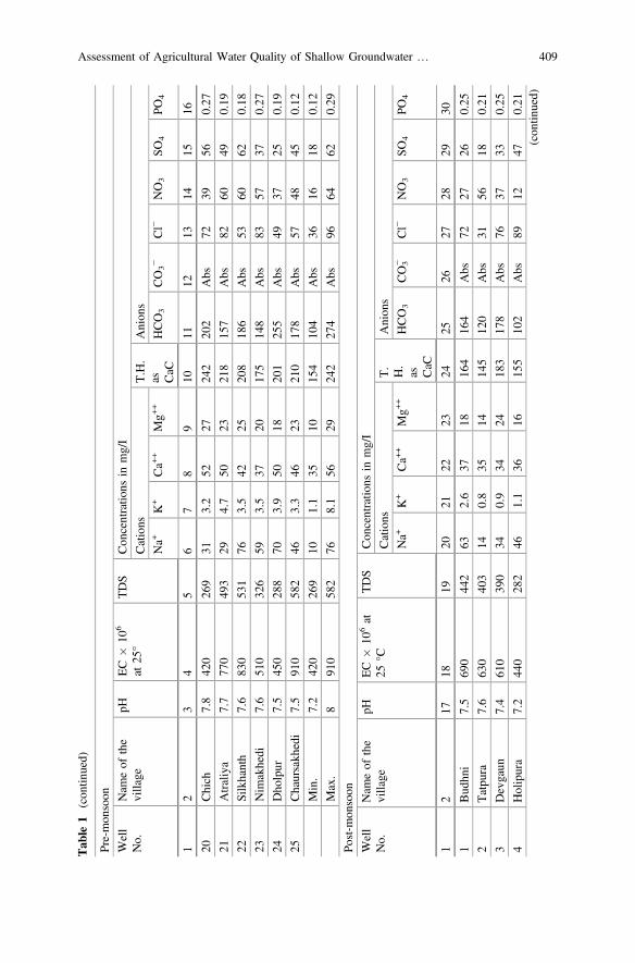
Tab
le1
(con
tinued)
Pre-mon
soon
Well
No.
Nam
eof
the
village
pHEC
�10
6
at25
°TDS
Con
centratio
nsin
mg/I
Cations
T.H.
as CaC
Anion
s
Na+
K+
Ca+
+Mg+
+HCO3
CO3−
Cl−
NO3
SO4
PO4
12
34
56
78
910
1112
1314
1516
20Chich
7.8
420
269
313.2
5227
242
202
Abs
7239
560.27
21Atraliya
7.7
770
493
294.7
5023
218
157
Abs
8260
490.19
22Silkhanth
7.6
830
531
763.5
4225
208
186
Abs
5360
620.18
23Nim
akhedi
7.6
510
326
593.5
3720
175
148
Abs
8357
370.27
24Dho
lpur
7.5
450
288
703.9
5018
201
255
Abs
4937
250.19
25Chaursakh
edi
7.5
910
582
463.3
4623
210
178
Abs
5748
450.12
Min.
7.2
420
269
101.1
3510
154
104
Abs
3616
180.12
Max.
891
058
276
8.1
5629
242
274
Abs
9664
620.29
Post-m
onsoon
Well
No.
Nam
eof
the
village
pHEC
�10
6at
25°C
TDS
Con
centratio
nsin
mg/I
Cations
T.
H.
as CaC
Anion
s
Na+
K+
Ca+
+Mg+
+HCO3
CO3−
Cl−
NO3
SO4
PO4
12
1718
1920
2122
2324
2526
2728
2930
1Bud
hni
7.5
690
442
632.6
3718
164
164
Abs
7227
260.25
2Tatpu
ra7.6
630
403
140.8
3514
145
120
Abs
3156
180.21
3Devgaun
7.4
610
390
340.9
3424
183
178
Abs
7637
330.25
4Holipura
7.2
440
282
461.1
3616
155
102
Abs
8912
470.21
(con
tinued)
Assessment of Agricultural Water Quality of Shallow Groundwater … 409

Tab
le1
(con
tinued)
Post-m
onsoon
Well
No.
Nam
eof
the
village
pHEC
�10
6at
25°C
TDS
Con
centratio
nsin
mg/I
Cations
T.
H.
as CaC
Anion
s
Na+
K+
Ca+
+Mg+
+HCO3
CO3−
Cl−
NO3
SO4
PO4
12
1718
1920
2122
2324
2526
2728
2930
5Unchh
akheda
7.5
650
416
610.6
3221
166
180
Abs
6121
200.22
6Ninor
7.4
880
563
175.1
3716
159
100
Abs
7047
250.19
7Pathora
7.3
790
506
301
3522
180
178
Abs
4427
160.27
8Aaw
ali
7.4
580
371
141.6
528
163
108
Abs
8214
260.19
9Dhank
ot7.2
700
448
133.1
419
140
125
Abs
4042
130.27
10Mog
ra7.4
630
403
352.7
4512
164
198
Abs
4313
260.26
11Rehug
aon
7.2
660
422
317.3
3119
157
126
Abs
7230
370.21
12Nehlai
7.5
640
410
102.1
5017
197
90Abs
7949
260.23
13Ratanpu
r7.7
700
448
53
4415
173
85Abs
8351
210.23
14Sawalkh
eda
7.6
650
416
343.7
4218
180
97Abs
9230
250.21
15Matthagaon
7.3
570
365
412.9
3524
186
157
Abs
8025
380.2
16Basaniya
7.4
740
474
232.5
3323
180
160
Abs
8431
130.24
17Chh
idgaon
7.6
540
346
403
3928
213
157
Abs
7620
210.27
18Manjhil
759
037
871
2.9
3119
155
203
Abs
7226
140.19
19Tilariya
7.9
600
384
602.6
5017
194
260
Abs
4131
210.21
20Chich
7.7
390
250
262.5
4726
225
190
Abs
6835
470.25
21Atraliya
7.1
740
474
233.9
4522
203
143
Abs
7953
430.17
22Silkhanth
7.3
810
518
702.7
3724
192
170
Abs
4756
570.16
(con
tinued)
410 S.K. Sharma et al.
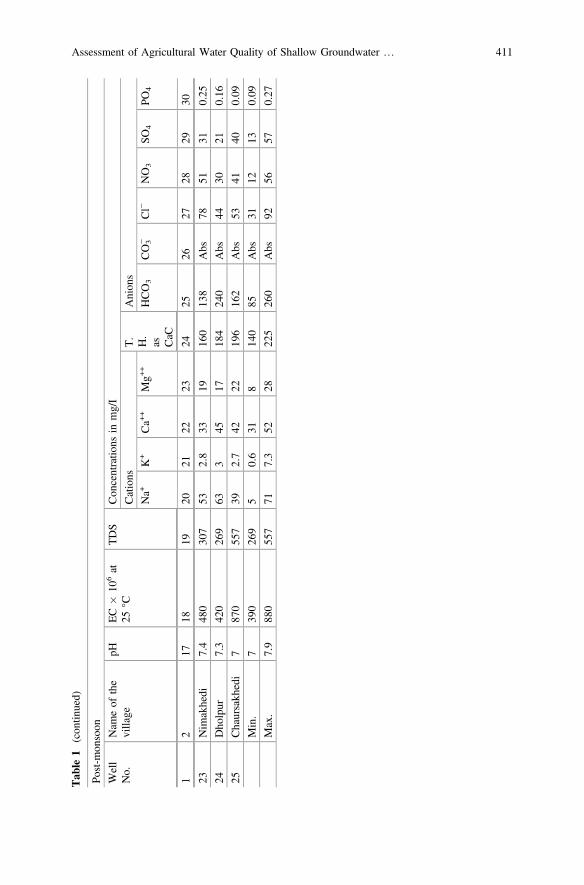
Tab
le1
(con
tinued)
Post-m
onsoon
Well
No.
Nam
eof
the
village
pHEC
�10
6at
25°C
TDS
Con
centratio
nsin
mg/I
Cations
T.
H.
as CaC
Anion
s
Na+
K+
Ca+
+Mg+
+HCO3
CO3−
Cl−
NO3
SO4
PO4
12
1718
1920
2122
2324
2526
2728
2930
23Nim
akhedi
7.4
480
307
532.8
3319
160
138
Abs
7851
310.25
24Dho
lpur
7.3
420
269
633
4517
184
240
Abs
4430
210.16
25Chaursakh
edi
787
055
739
2.7
4222
196
162
Abs
5341
400.09
Min.
739
026
95
0.6
318
140
85Abs
3112
130.09
Max.
7.9
880
557
717.3
5228
225
260
Abs
9256
570.27
Assessment of Agricultural Water Quality of Shallow Groundwater … 411
Irrigation Water Quality
The suitability of shallow groundwater has been evaluated on the basis of analyticalresults. Various specifications have been proposed from time to time by differentworkers including Asgar et al. (1936), Kelley et al. (1940); Wilcox (1948, 1955),Eaton (1950); US Soil Salinity Laboratory Staff (1954), Saligram (1961), Uppal(1964), Ramamoorthy (1964), Federal Water Pollution Control Authority (1968),Paliwal (1972), Environmental Protection Agency (1973) and Ayers and Westcot(1994). In the present study the specifications as proposed by Kelley et al. (1940);Wilcox (1948, 1955), Eaton (1950), US Soil Salinity Laboratory Staff (1954),Paliwal (1972) have been used to assess the suitability of shallow ground water foragricultural purposes.
Results and Discussion
Soluble sodium percentage (SSP), sodium adsorption ratio (SAR), residual sodiumcarbonate (RSC), Kelly’s Ratio and Magnesium hazard are the prominent specifi-cations for determining the suitability of shallow ground water for agriculturalpurposes and are presented in Table 2. The recommended classification of irrigationwater quality with respect to EC, SAR, Kelly’s Ratio, Mg. Ratio, RSC and Na% arepresented in Table 3.
Salinity hazard is evaluated on the basis of Electrical conductivity and it reflectsthe total dissolved solids (TDS) in shallow groundwater. High salt content in irri-gation water affects the soil structure, permeability and plant growth. As per theclassification proposed by Richards (1954), the water is low (if EC below250 µmohs/cm), the water is medium (if EC between 250 and 750 µmohs/cm), thewater is high (if EC content between 750 and 2250 µmohs/cm), the water is veryhigh (if EC is more than 2250 µmohs/cm) with respect to salinity in water. Whenthe shallow groundwater samples compared with this classification, Table 2 clearlyindicates that the shallow groundwater varies from 420 to 910 µmohs/cm inpre-monsoon period and 390–880 µmohs/cm in post-monsoon period, respectively,and thus they belongs to Medium to High Salinity class. Table 3, further shows that76% of shallow groundwater in pre-monsoon and 84% in post-monsoon periodbelongs to Medium salinity class.
Sodium or alkali hazard is measured on the basis of SAR. The relativity ofsodium ion in the exchange reaction with soil is expressed in terms of a ratio knownas Sodium Adsorption Ratio (SAR) which is defined as:
SAR ¼ Naffiffiffiffiffiffiffiffiffiffiffiffiffiffiffiffiffiffiffiffiffiffiffiffi
Ca + Mg/2p Where all concentrations are expressed in epm:ð Þ
412 S.K. Sharma et al.
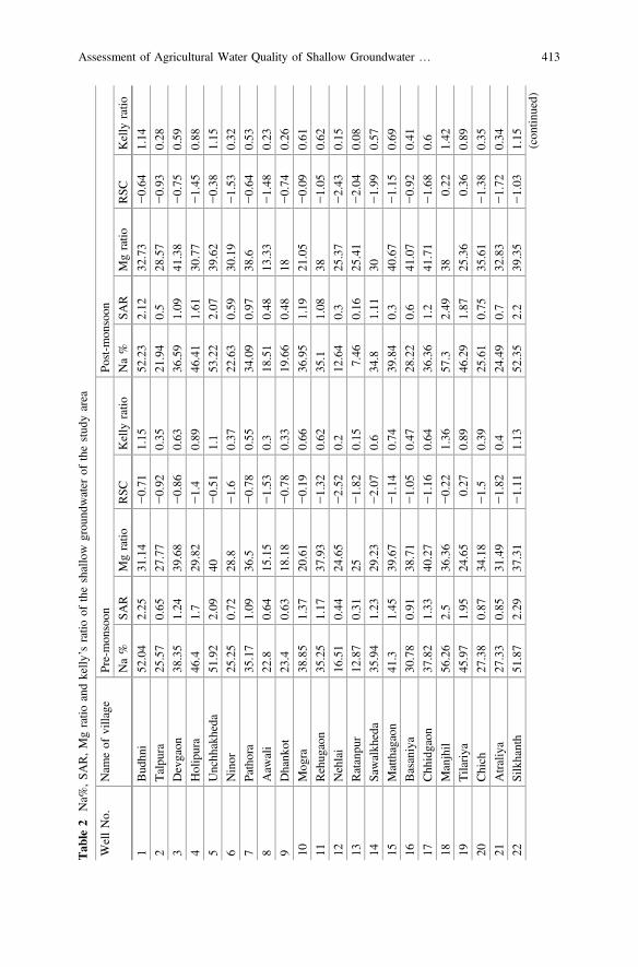
Tab
le2
Na%
,SA
R,Mgratio
andkelly
’sratio
oftheshallow
grou
ndwater
ofthestud
yarea
WellNo.
Nam
eof
village
Pre-mon
soon
Post-m
onsoon
Na%
SAR
Mgratio
RSC
Kelly
ratio
Na%
SAR
Mgratio
RSC
Kelly
ratio
1Bud
hni
52.04
2.25
31.14
−0.71
1.15
52.23
2.12
32.73
−0.64
1.14
2Talpu
ra25
.57
0.65
27.77
−0.92
0.35
21.94
0.5
28.57
−0.93
0.28
3Devgaon
38.35
1.24
39.68
−0.86
0.63
36.59
1.09
41.38
−0.75
0.59
4Holipura
46.4
1.7
29.82
−1.4
0.89
46.41
1.61
30.77
−1.45
0.88
5Unchh
akheda
51.92
2.09
40−0.51
1.1
53.22
2.07
39.62
−0.38
1.15
6Ninor
25.25
0.72
28.8
−1.6
0.37
22.63
0.59
30.19
−1.53
0.32
7Pathora
35.17
1.09
36.5
−0.78
0.55
34.09
0.97
38.6
−0.64
0.53
8Aaw
ali
22.8
0.64
15.15
−1.53
0.3
18.51
0.48
13.33
−1.48
0.23
9Dhank
ot23
.40.63
18.18
−0.78
0.33
19.66
0.48
18−0.74
0.26
10Mog
ra38
.85
1.37
20.61
−0.19
0.66
36.95
1.19
21.05
−0.09
0.61
11Rehug
aon
35.25
1.17
37.93
−1.32
0.62
35.1
1.08
38−1.05
0.62
12Nehlai
16.51
0.44
24.65
−2.52
0.2
12.64
0.3
25.37
−2.43
0.15
13Ratanpu
r12
.87
0.31
25−1.82
0.15
7.46
0.16
25.41
−2.04
0.08
14Sawalkh
eda
35.94
1.23
29.23
−2.07
0.6
34.8
1.11
30−1.99
0.57
15Matthagaon
41.3
1.45
39.67
−1.14
0.74
39.84
0.3
40.67
−1.15
0.69
16Basaniya
30.78
0.91
38.71
−1.05
0.47
28.22
0.6
41.07
−0.92
0.41
17Chh
idgaon
37.82
1.33
40.27
−1.16
0.64
36.36
1.2
41.71
−1.68
0.6
18Manjhil
56.26
2.5
36.36
−0.22
1.36
57.3
2.49
380.22
1.42
19Tilariya
45.97
1.95
24.65
0.27
0.89
46.29
1.87
25.36
0.36
0.89
20Chich
27.38
0.87
34.18
−1.5
0.39
25.61
0.75
35.61
−1.38
0.35
21Atraliya
27.33
0.85
31.49
−1.82
0.4
24.49
0.7
32.83
−1.72
0.34
22Silkhanth
51.87
2.29
37.31
−1.11
1.13
52.35
2.2
39.35
−1.03
1.15
(con
tinued)
Assessment of Agricultural Water Quality of Shallow Groundwater … 413

Tab
le2
(con
tinued)
WellNo.
Nam
eof
village
Pre-mon
soon
Post-m
onsoon
Na%
SAR
Mgratio
RSC
Kelly
ratio
Na%
SAR
Mgratio
RSC
Kelly
ratio
23Nim
akhedi
49.37
1.96
35.08
−1.06
1.63
49.16
1.82
36.53
−0.95
1.02
24Dho
lpur
49.33
2.15
26.47
0.2
1.03
49.21
2.04
27.42
0.28
1.01
25Chaursakh
edi
38.88
1.38
33.33
−1.27
0.66
36.89
1.22
34.37
−0.26
0.61
414 S.K. Sharma et al.
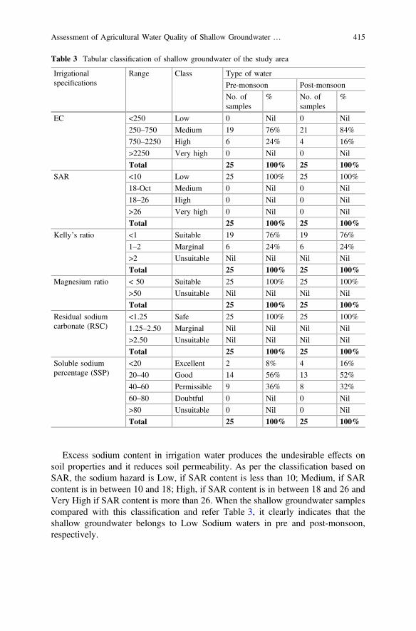
Excess sodium content in irrigation water produces the undesirable effects onsoil properties and it reduces soil permeability. As per the classification based onSAR, the sodium hazard is Low, if SAR content is less than 10; Medium, if SARcontent is in between 10 and 18; High, if SAR content is in between 18 and 26 andVery High if SAR content is more than 26. When the shallow groundwater samplescompared with this classification and refer Table 3, it clearly indicates that theshallow groundwater belongs to Low Sodium waters in pre and post-monsoon,respectively.
Table 3 Tabular classification of shallow groundwater of the study area
Irrigationalspecifications
Range Class Type of water
Pre-monsoon Post-monsoon
No. ofsamples
% No. ofsamples
%
EC <250 Low 0 Nil 0 Nil
250–750 Medium 19 76% 21 84%
750–2250 High 6 24% 4 16%
>2250 Very high 0 Nil 0 Nil
Total 25 100% 25 100%SAR <10 Low 25 100% 25 100%
18-Oct Medium 0 Nil 0 Nil
18–26 High 0 Nil 0 Nil
>26 Very high 0 Nil 0 Nil
Total 25 100% 25 100%Kelly’s ratio <1 Suitable 19 76% 19 76%
1–2 Marginal 6 24% 6 24%
>2 Unsuitable Nil Nil Nil Nil
Total 25 100% 25 100%Magnesium ratio < 50 Suitable 25 100% 25 100%
>50 Unsuitable Nil Nil Nil Nil
Total 25 100% 25 100%Residual sodiumcarbonate (RSC)
<1.25 Safe 25 100% 25 100%
1.25–2.50 Marginal Nil Nil Nil Nil
>2.50 Unsuitable Nil Nil Nil Nil
Total 25 100% 25 100%Soluble sodiumpercentage (SSP)
<20 Excellent 2 8% 4 16%
20–40 Good 14 56% 13 52%
40–60 Permissible 9 36% 8 32%
60–80 Doubtful 0 Nil 0 Nil
>80 Unsuitable 0 Nil 0 Nil
Total 25 100% 25 100%
Assessment of Agricultural Water Quality of Shallow Groundwater … 415
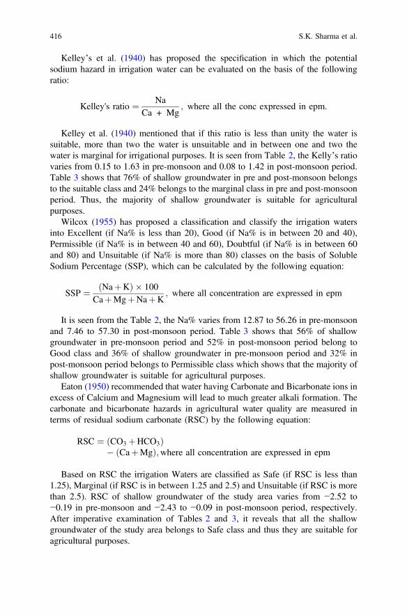
Kelley’s et al. (1940) has proposed the specification in which the potentialsodium hazard in irrigation water can be evaluated on the basis of the followingratio:
Kelley's ratio ¼ NaCa + Mg
; where all the conc expressed in epm.
Kelley et al. (1940) mentioned that if this ratio is less than unity the water issuitable, more than two the water is unsuitable and in between one and two thewater is marginal for irrigational purposes. It is seen from Table 2, the Kelly’s ratiovaries from 0.15 to 1.63 in pre-monsoon and 0.08 to 1.42 in post-monsoon period.Table 3 shows that 76% of shallow groundwater in pre and post-monsoon belongsto the suitable class and 24% belongs to the marginal class in pre and post-monsoonperiod. Thus, the majority of shallow groundwater is suitable for agriculturalpurposes.
Wilcox (1955) has proposed a classification and classify the irrigation watersinto Excellent (if Na% is less than 20), Good (if Na% is in between 20 and 40),Permissible (if Na% is in between 40 and 60), Doubtful (if Na% is in between 60and 80) and Unsuitable (if Na% is more than 80) classes on the basis of SolubleSodium Percentage (SSP), which can be calculated by the following equation:
SSP ¼ NaþKð Þ � 100CaþMgþNaþK
; where all concentration are expressed in epm
It is seen from the Table 2, the Na% varies from 12.87 to 56.26 in pre-monsoonand 7.46 to 57.30 in post-monsoon period. Table 3 shows that 56% of shallowgroundwater in pre-monsoon period and 52% in post-monsoon period belong toGood class and 36% of shallow groundwater in pre-monsoon period and 32% inpost-monsoon period belongs to Permissible class which shows that the majority ofshallow groundwater is suitable for agricultural purposes.
Eaton (1950) recommended that water having Carbonate and Bicarbonate ions inexcess of Calcium and Magnesium will lead to much greater alkali formation. Thecarbonate and bicarbonate hazards in agricultural water quality are measured interms of residual sodium carbonate (RSC) by the following equation:
RSC ¼ CO3 þHCO3ð Þ� CaþMgð Þ;where all concentration are expressed in epm
Based on RSC the irrigation Waters are classified as Safe (if RSC is less than1.25), Marginal (if RSC is in between 1.25 and 2.5) and Unsuitable (if RSC is morethan 2.5). RSC of shallow groundwater of the study area varies from −2.52 to−0.19 in pre-monsoon and −2.43 to −0.09 in post-monsoon period, respectively.After imperative examination of Tables 2 and 3, it reveals that all the shallowgroundwater of the study area belongs to Safe class and thus they are suitable foragricultural purposes.
416 S.K. Sharma et al.
Paliwal (1972) has proposed the ratio Mg � 100/Ca + Mg as an index ofmagnesium hazards to irrigation waters. As per the classification, if the Mg Ratioless than 50% the waters are suitable and if Mg ratio is more than 50% the waterbelongs to Unsuitable. The magnesium ratio of shallow groundwater of the studyarea varies from 15.15 to 40.27 in pre-monsoon and 13.33 to 41.71 inpost-monsoon period, respectively. After vital examination of Table 3, it revealsthat all the shallow groundwater of the study area belongs to the suitable class andthere is no magnesium hazard in shallow groundwater of the study area.
Conclusions
Agricultural water quality was determined on the basis of Salinity hazard, Sodiumhazard and Bicarbonate hazard. According to the classification of shallowgroundwater with respect to SAR and EC, the majority of shallow groundwater ofthe study area belongs to belongs to medium to high salinity class and Low sodiumwater. Kelly’s ratio shows that 76% of shallow groundwater in pre andpost-monsoon belongs to the suitable class. As per Wilcox classification, theshallow groundwater in pre-monsoon period and post-monsoon period belongs toGood to Permissible class. Classification based on RSC clearly indicates that all theshallow groundwater of the study area belongs to Safe class and thus they aresuitable for agricultural purposes. As per the magnesium ratio classification, all theshallow groundwater of the study area belongs to the suitable class and there are nomagnesium hazards in shallow groundwater of the study area.
From the above-mentioned discussion and interpretation of the hydrochemistryand irrigational specifications, it can be concluded that the shallow groundwater ofthe study area is quite appropriate for irrigational purposes.
References
APHA (1995) Standard methods for the examination of water and waste water, 19th edn.American Public Health Association, Washington, 1467 pp
Asgar AG, Puri AN, Taylor EM (1936) Soil deterioration in irrigated areas of Punjab, part I-III.Irrigation Research Institute Memoirs, Amritsar
Ayers RS, Westcot DW (1994) Water quality for agriculture, FAO Irrigation and Drainage, paper29, Rev. 1, Rome
Dhiman SD (2014) Groundwater quality assessment for irrigation use in Rajkot district. J IndWater Resour Soc 34(1):34–39
Eaton FM (1950) Significance of carbonate in irrigation water, soil sci, vol 69, no 2, pp 123–133Environmental Protection Agency (1973) Water quality criteria, 1972, EPA Publication, E.P.A. R.
3-73-033, p 594Federal Water Pollution Control Authority U.S.A. (1968) Report of the committee on water quality
criteria. Washington, D.C., p 234
Assessment of Agricultural Water Quality of Shallow Groundwater … 417
Jayalakshmi Devi O et al (2009) Evaluation of groundwater quality for irrigation and drinkingpurpose in selected taluks of Dakshina Kannada district in Karnataka, India. In:Ramanathan AL et al (eds) Assessment of groundwater resources and management. I. K.International Publishing House Pvt. Ltd., New Delhi, pp 301–318
Jhariya DC, Shandilya Arun K, Dewangan R (2012) Nitrate pollution in the groundwater aroundSagar Town, Madhya Pradesh, India. In: International conference on chemical, ecology andenvironmental sciences
Kelley WP, Brown SM, Liebig GF Jr (1940) Chemical effect of saline irrigation waters on soils.Soil Sci 49:95–107
Maghanga JK, Kituyi JL, Kisinyo PO, Ng’etich WK (2013) Impact of nitrogen fertilizerapplications on surface water nitrate levels within a Kenyan tea plantation. J Chem 1–4
Paliwal KV (1972) Irrigation with saline water I. A. R. I. Monograph No. 2, (New Series), NewDelhi, p 198
Parashar VK (1994) Study of quality of surface and subsurface waters and their agricultural utilityin the lower alluvial plains of narmada valley between Khalghat and Haribphal Dist. WestNimar M.P., Ph.D. Thesis Barkatullah University Bhopal
Parashar VK (2001) Excssive use of fertilizers and its impact on the quality of surface andsubsurface waters around Hoshangabad area. Project report submitted to University GrantsCommission, Central Region Bhopal
Ramamoorthy B (1964) Some aspects of the management of soil water plant climatic complex inthe arid zone. In: Proceedings of general symposium problems of Indian arid zones, CAZRI,Jodhpur, pp 276–285
Ravikumar P et al (2011) Hydrochemistry and evaluation of groundwater suitability for irrigationand drinking purposes in the Markandeya River basin, Belgaum District, Karnataka State,India. Environ Monit Assess 173(1–4):459–487. doi:10.1007/S12517-013-0940-3
Richards LA (1954) Diagnosis and improvement of saline and alkali soils. Agric Handbook 60,USDA, Washington D.C., p 160
Saligram VK (1961) Standards of suitability of underground irrigation water with special referenceto tubewells in North Gujarat. In: Paper presented at seminar on irrigation, drainage and waterlogging, Bombay
Shraddha S, Rakesh V, Savita D, Praveen J (2011) Evaluation of water quality of Narmada riverwith reference to physicochemical parameters at Hoshangabad city, M.P., India. Res J ChemSci 1(3):40–48
Shrivastava MK (1980) Study of quality and agricultural quality of groundwater in the InnerNarmada Valley between Hoshangabad and Jabalpur, Madhya Pradesh, unpublished. Ph.D.Thesis Barkatullah University, Bhopal
Uppal HL (1964) Soil and groundwater survey of Punjab, vol I, Amritsar District and vol II,Kapoorthala District Land Reclamations, Irrigation and Power Research Institute Amritsar,Punjab
U.S. Salinity Laboratory Staff (1954) Diagnosis sand improvement of saline and alkali soils, U.S.D.A. Handbook No. 60, p 160
Wilcox LV (1948) The quality of water for irrigation use, U.S.D.A. Tec. Bull., 962,Washington D.C., p. 40
Wilcox LV (1955) Classification and use of irrigation waters. U. S. Department of Agriculture,Circular, no. 969, 19 pp
418 S.K. Sharma et al.

Active Water Quality Managementin Rural Small Watersheds
Koichi Unami, Goden Mabaya, Abul Hasan Md. Badiul Alamand Masayuki Fujihara
Abstract Diverse land and water uses are found in rural areas of Monsoon regions.Based on field studies in Japan and Bangladesh, water quality management prob-lems are considered at small watershed levels. A study site in Japan is chosen in ahilly area. Upland tea plantations in the site are the major source of nitrate pollutionto the downstream water bodies because of heavy fertilizer application. Utilizingpaddy fields and irrigation tanks as buffer of the polluted water is feasible, but itrisks vulnerable aquatic ecosystems. Another study site is in the floodplains ofBangladesh. Countless ponds are used in the rural communities for domestic,animal watering and fishery purposes. Introduction of comparatively warmgroundwater into the ponds during winter seasons may accelerate the growth of fish.However, groundwater depletion is the major concern. The concept of Markovdecision processes is applied to find the optimal actions for the two different waterquality management problems.
Introduction
Rural land and water resources in Monsoon regions are used for multi-purposes dueto seasonal climatic variations. Sound distribution of water in terms of both quantityand quality in such cases is a complex issue involving hydrology, hydraulics,sociology, economics and ecology. Phong et al. (2010) focused on the integrationof aquaculture into rice farming systems in this context. In this study, scientificmethodologies are considered to promote active water quality management forrice-fish culture at rural community levels. Contrasting field studies were conductedin Japan and Bangladesh, to formulate abstract mathematical optimizationproblems.
K. Unami (&) � G. Mabaya � A.H.Md.B. Alam � M. FujiharaGraduate School of Agriculture, Kyoto University, Kitashirakawa-Oiwake-Cho,Sakyo-Ku, Kyoto 606-8502, Japane-mail: [email protected]
© Springer Nature Singapore Pte Ltd. 2018V.P. Singh et al. (eds.), Environmental Pollution, Water Scienceand Technology Library 77, https://doi.org/10.1007/978-981-10-5792-2_33
419

A study site in Japan is chosen in a hilly area, where forests, paddy fields, teaplantations and irrigation tanks are the dominant land uses. The upland tea plan-tations developed in the 1960s, are being the major source of nitrate pollution to thedownstream water bodies because of heavy application of fertilizers. Utilizing thepaddy fields and the irrigation tanks as buffer of polluted water from the teaplantations is a feasible option, but it risks vulnerable aquatic ecosystems (Mabayaet al. 2016).
Another study site in Bangladesh is in the Brahmaputra-Jamuna floodplains withdouble-cropping paddy rice system. In recent decades, the dry season paddy irri-gation for boro rice has deteriorated groundwater resources (Shahid and Hazarika2010; Rahman and Mahbub 2012), while countless artificial ponds are used in therural communities for domestic, animal watering and fishery purposes. Introductionof comparatively warm and less polluted groundwater into the artificial pondsduring winter seasons may accelerate the growth of fish, which have high economicvalues. However, groundwater depletion during the following rice irrigation sea-sons is still the major concern.
The concept of Markov decision processes can be applicable to finding theoptimal actions for sustainable rural development involving water quality man-agement. It is shown that the different practical problems in the two study sites canbe dealt with in the same mathematical framework. Dynamics of water storage, ricegrowth and fish growth are modelled to determine transition probabilities forspatio-temporally discrete processes. The Bellman equation, which is a recursiveformula, is used for computing optimal policies based on the principle of dynamicprogramming.
Field Studies
Concurrent Use of Japanese Irrigation Tanks for RiceCultivation and Aquaculture
There exist about 200,000 irrigation tanks in Japan, mostly purposing rice culti-vation during the summer seasons from April through September. However, it alsoused to be a common practice to rear edible fish species such as Cyprinus carpio(common carp) and Carassius cuvieri (white crucian carp) in irrigation tanks(Tamura 1961). Field studies from different hydro-environmental aspects have beenconducted in a small watershed, which is referred to as Site I, located in Imago ofShiga Prefecture, Japan (Hiramatsu et al. 2003; Mabaya et al. 2016). There are fourirrigation tanks in Site I, none of which is currently used for aquaculture. However,the presence of aquatic species including Oryzias latipes (Japanese rice-fish),Misgurnus anguillicaudatus (Japanese weather loach), Palaemon paucidens(freshwater prawn) and Rhinogobius sp. (freshwater gobies) has been confirmed inthe irrigation tanks, paddy fields and/or valley bottoms of inland valleys. Nitrate
420 K. Unami et al.
concentrations were measured in different water bodies distributed in Site I, usingsimplified on-site water quality pack tests (Kyoritsu Chemical Check LaboratoryCorporation, Tokyo, Japan). Nitrate has long term effects on general health, growthand breeding ability of fish (Nakasone et al. 2002). A study of Kincheloe et al.(1979) has demonstrated a positive correlation between the worst total mortalityrates and nitrate exposures. Higashi and Imago irrigation tanks are two of the fourirrigation tanks, contrasting in terms of catchment areas without and with teaplantation coverages, respectively. Another larger dam located outside of the SiteI’s watershed supplement Imago irrigation tank with less polluted water via a canal.There is an inland valley referred to as Sueda inland valley, where seepage runoff ata cliff is also observed. The catchment area of Sueda inland valley is dominantlyused for tea plantations, and there is no irrigation tank downstream. From the testresults shown in Table 1, it is inferred that tea plantations are the sources of highnitrate concentrations.
Therefore, rearing profitable fish in Imago irrigation tank is a challengingenterprise, as the water quality and the irrigation demand are the critical constraints.
Potential Use of Groundwater for Aquaculturein Bangladeshi Paddy Areas
Bangladeshi winter season (shitkal) lasts from mid-December to mid-February,corresponding to the period between rainfed (kharif) crop harvesting and starting ofirrigation season for boro rice. Rural environmental characteristics of the season arelow air temperature, less precipitation, high but declining groundwater table andless farming activities (Shankar et al. 2004). The temperature of groundwater isalmost stable throughout the year. In order to confirm these characteristics, fieldmeasurements using HOBO U20 pressure/temperature data loggers were conductedfrom September 9, 2012 through September 24, 2014 in a small watershed, which isreferred to as Site G, located in Godashimla of Jamalpur District, Dhaka Division,Bangladesh. Figure 1 shows observed data series of accumulated rainfall depthsmeasured by Decagon ECRN-50 raingauge (Rain), groundwater levels (GWL) andtemperatures (GWT), air temperatures (Air T), water depths (Pond h) and tem-peratures (Pond T) of a pond for aquaculture. The pond is connected to an irrigationcanal, whose water source is pump lifted groundwater.
Table 1 Results of nitrate concentration tests in Site I
Sub-watershed Number of samples Nitrate concentration (mg/L)
Higashi irrigation tank 11 Average = 0.04, range: 0–0.3
Imago irrigation tank 8 Average = 1.93, range: 0.2–5
Sueda inland valley seepage runoff 8 Above 10
Active Water Quality Management in Rural Small Watersheds 421
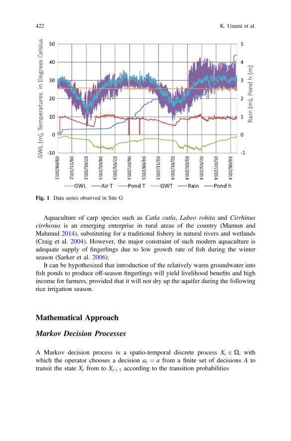
Aquaculture of carp species such as Catla catla, Labeo rohita and Cirrhinuscirrhosus is an emerging enterprise in rural areas of the country (Mamun andMahmud 2014), substituting for a traditional fishery in natural rivers and wetlands(Craig et al. 2004). However, the major constraint of such modern aquaculture isadequate supply of fingerlings due to low growth rate of fish during the winterseason (Sarker et al. 2006).
It can be hypothesized that introduction of the relatively warm groundwater intofish ponds to produce off-season fingerlings will yield livelihood benefits and highincome for farmers, provided that it will not dry up the aquifer during the followingrice irrigation season.
Mathematical Approach
Markov Decision Processes
A Markov decision process is a spatio-temporal discrete process Xt 2 X, withwhich the operator chooses a decision at ¼ a from a finite set of decisions A totransit the state Xt from to Xtþ 1 according to the transition probabilities
Fig. 1 Data series observed in Site G
422 K. Unami et al.

PijðaÞ ¼ P Xtþ 1 ¼ jjXt ¼ i; at ¼ af g: ð1Þ
If the decision a 2 A is chosen for the state i, then the cost f ði; aÞ is incurred.A policy P is a map from X to A. The expected value of the total cost incurringfrom the current time s until a prescribed terminal time T for Xs ¼ i is denoted by
VPðs; iÞ ¼ EPXt\T
t¼s
f ðXt; atÞjXs ¼ i
" #: ð2Þ
The policy P� is said to be optimal if
VP� ðs; iÞ ¼ infP
VPðs; iÞ ð3Þ
for any time s and any state i. From the principle of dynamic programming, theBellman equation
VP� ðs; iÞ ¼ mina2A
f ði; aÞþXj
PijðaÞVP� ðsþ 1; jÞ( )
ð4Þ
is deduced and is solved with the terminal condition
VP� ðT ; iÞ ¼ 0; 8i 2 X; ð5Þ
to determine the value function VP� ðs; iÞ as well as the optimal policy P� (Ben-Talet al. 2009).
Problem Formulation
The practical water quality management problems posed for Site I and Site G areformulated as a unified optimization problem for Markov decision processes. Thestate x of water storage commonly represents the storage volume of Imago irrigationtank in Site I and that of the aquifer in Site G. The capacity of the water storage isnormalized as unity. The governing equation of x is the water balance equation
dxdt
¼ Q� u ð6Þ
where Q is the uncontrollable water balance, and u is the intake discharge as thedecision variable. The states y and z are considered for the growth levels of rice and
Active Water Quality Management in Rural Small Watersheds 423
fish, respectively. The dynamics of the states y and z are assumed to be representedby the common logistic equations
dydt
¼ ry Ky � y� �
y;dzdt
¼ rz Kz � zð Þz ð7Þ
where ry and rz are the growth rates, and Ky and Kz are the carrying capacities fory and z, respectively. Maturity of rice and fish is also normalized as unity. Then, thex-y-z domain 0; 1ð Þ3 is discretized into nx � ny � nz sub-cubes. The ix-iy-iz sub-cubeis indexed as i ¼ ixnynz þ iynz þ iz to constitute the domain X of a Markov decisionprocess. Only two options are considered for decisions: to intake water at a pre-scribed rate (a ¼ 1) or not to intake water at all (a ¼ 0). Therefore, the set ofdecisions is
A ¼ 0; 1f g: ð8Þ
Table 2 shows the parameters specified for Site I and Site G. The time domain iscommonly set as 0; T½ � ¼ 0; 180½ � (days). The cost function, which is also the samefor the two sites, is prescribed as
f i; að Þ ¼ a exp � ixnx
� �� 5viy;ny�1 � 1þ cos
ptT
� �� �viz;nz�1 ð9Þ
where vi;k is the indicator function which is equal to 1 when i ¼ k and is equal to 0otherwise.
The transition probabilities are calculated so that the drifts of the states accordwith the dynamics specified in (6) and (7). However, stochastic diffusion isinevitably included due to spatio-temporal discretization. The diffusion effect isintentionally taken larger for the fish growths, since aquaculture is assumed to bemore risky enterprise than rice cultivation in both of the two sites.
Table 2 Parameters set for Site I and Site G
Parameters Site I Site G
Q 1=30 �1=30
u 0 a ¼ 0ð Þ�2=30 a ¼ 1ð Þ
�0 a ¼ 0ð Þ
�1=30 a ¼ 1ð Þ�
ry 0 a ¼ 0ð Þ3=30 a ¼ 1ð Þ
�0 for t\60,
1=30 a ¼ 0ð Þ3=30 a ¼ 1ð Þ
�for 60� t
Ky 1 1
rz 2=30 0 a ¼ 0ð Þ5=30 a ¼ 1ð Þ
�for t\60, 0 for 60� t
Kz ixnx
1
424 K. Unami et al.
Computational Results
The value functions VP� ðt; iÞ as well as the optimal policies P� for active waterquality management in Site I and Site G are obtained as the numerical solutions forthe Bellman equation with nx � ny � nz ¼ 10� 10� 10 ¼ 1;000 states. Figures 2,3 and 4 show the computational results at t ¼ 30, t ¼ 90 and t ¼ 150, respectively.The difference between Site I and Site G is significant in the early stages of activewater quality management. This is because rice cultivation has already started inSite I but only fish rearing is practiced in Site G. Figure 2 shows complexdependency of the optimal decision a on the three states ix, iy and iz in Site I.
In contrast, a is a monotone function of iz in Site G. Rice growth in Site I andfish growth in Site G are substantially in juvenile stages. Therefore, securingenough initial water storage is necessary for successful rice-fish culture. Figures 3and 4 show similar distributions of the optimal decision a in the two sites. Ricegrowth dominantly determines the optimal decision a, however, irrigation should besuspended when both of water storage and rice growth are at low levels. Thedomain of such restriction levels enlarges in the later stage of Fig. 4. The onlydifference between Site I and Site G in Figs. 3 and 4 is the optimal decision a whenwater storage is full and rice is matured. This is a consequence of the different ry,which vanishes in Site I but remains positive in Site G when a ¼ 0.
Water storage
Rice growthFish growth
Water storage
Rice growthFish growth
Fig. 2 Value functions and optimal policies at t ¼ 30 for Site I (left panel) and Site G (rightpanel). Circles of larger sizes represent the larger profit (negative cost). Filled circles representa ¼ 0, and white circles represent a ¼ 1
Active Water Quality Management in Rural Small Watersheds 425

Water storage
Rice growthFish growth
Water storage
Rice growthFish growth
Fig. 3 Value functions and optimal policies at t ¼ 90 for Site I (left panel) and Site G (rightpanel). Circles of larger sizes represent the larger profit (negative cost). Filled circles representa ¼ 0, and white circles represent a ¼ 1
Water storage
Rice growthFish growth
Water storage
Rice growthFish growth
Fig. 4 Value functions and optimal policies at t ¼ 150 for Site I (left panel) and Site G (rightpanel). Circles of larger sizes represent the larger profit (negative cost). Filled circles representa ¼ 0, and white circles represent a ¼ 1
426 K. Unami et al.
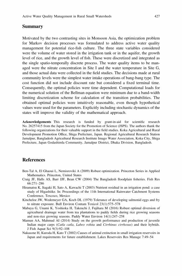
Summary
Motivated by the two contrasting sites in Monsoon Asia, the optimization problemfor Markov decision processes was formulated to address active water qualitymanagement for potential rice-fish culture. The three state variables consideredwere the volume of water stored in the irrigation tank or in the aquifer, the growthlevel of rice, and the growth level of fish. These were discretized and integrated asthe single spatio-temporally discrete process. The water quality items to be man-aged were the nitrate concentration in Site I and the water temperature in Site G,and those actual data were collected in the field studies. The decisions made at ruralcommunity levels were the simplest water intake operations of bang-bang type. Thecost function did not include discount rate but considered a fixed terminal time.Consequently, the optimal policies were time dependent. Computational loads forthe numerical solution of the Bellman equation were minimum due to a band-widthlimiting discretization scheme for calculation of the transition probabilities. Theobtained optimal policies were intuitively reasonable, even though hypotheticalvalues were used for the parameters. Explicitly including stochastic dynamics of thestates will improve the validity of the mathematical approach.
Acknowledgements This research is funded by grant-in-aid for scientific researchNo. 26257415 from the Japan Society for the Promotion of Science (JSPS). The authors thank thefollowing organizations for their valuable support in the field studies. Koka Agricultural and RuralDevelopment Promotion Office, Shiga Prefecture, Japan. Regional Agricultural Research StationJamalpur, Bangladesh Agricultural Research Institute Imago Water Association, Koka City, ShigaPrefecture, Japan Godashimla Community, Jamalpur District, Dhaka Division, Bangladesh.
References
Ben-Tal A, El Ghaoui L, Nemisroviki A (2009) Robust optimization. Princeton Series in AppliedMathematics. Princeton, United States
Craig JF, Halls AS, Barr JJF, Bean CW (2004) The Bangladesh floodplain fisheries. Fish Res66:271–286
Hiramatsu K, Itagaki H, Sato A, Kawachi T (2003) Nutrient residual in an irrigation pond: a casestudy of Higashiike. In: Proceedings of the 11th International Rainwater Catchment SystemsConference, Texcoco, Mexico
Kincheloe JW, Wedemeyer GA, Koch DL (1979) Tolerance of developing salmonid eggs and fryto nitrate exposure. Bull Environ Contam Toxicol 23(1):575–578
Mabaya G, Unami K, Yoshioka H, Takeuchi J, Fujihara M (2016) Robust optimal diversion ofagricultural drainage water from tea plantations to paddy fields during rice growing seasonsand non-rice growing seasons. Paddy Water Environ 14(1):247–258
Mamun AA, Mahmud AI (2014) Study on the growth performance and production of juvenileIndian major carps (Catla catla, Labeo rohita and Cirrhinus cirrhosus) and their hybrids.J Fish Aquat Sci 9(3):92–108
Nakasone H, Kuroda H, Kato T (2002) Causes of animal extinction in small irrigation reservoirs inJapan and requirements for future establishment. Lakes Reservoirs Res Manage 7:49–54
Active Water Quality Management in Rural Small Watersheds 427

Phong LT, van Dam AA, Udo HMJ, van Mensvoort MEF, Tri LQ, Steenstra FA, van der Zijpp AJ(2010) An agro-ecological evaluation of aquaculture integration into farming systems of theMekong Delta. Agr Ecosyst Environ 138(3–4):232–241
Rahman M, Mahbub AQM (2012) Groundwater depletion with expansion of irrigation in BarindTract: a case study of Tanore Upazila. J Water Resour Prot 4(8):567–575
Sarker MA, Chowdhury AH, Itohara Y (2006) Entrepreneurships barriers of pond fish culture inBangladesh—a case study from Mymensingh District. J Soc Sci 2(3):68–73
Shahid S, Hazarika MK (2010) Groundwater drought in Northwestern Districts of Bangladesh.Water Resour Manage 24:1989–2006
Shankar B, Halls A, Barr J (2004) Rice versus fish revisited: on the integrated management offloodplain resources in Bangladesh. Nat Resour Forum 28:91–101
Tamura T (1961) Carp cultivation in Japan. In: Borgstrom G (ed) Fish as food. Academic Press,New York, pp 103–120
428 K. Unami et al.

Evaluation of the Surface Water QualityIndex of Jharia Coal Mining Regionand Its Management of Surface WaterResources
Prasoon Kumar Singh, Binay Prakash Panigrahy, Poornima Vermaand Bijendra Kumar
Abstract In this paper, the level of surface water contamination near the mine siteis examined of Jharia coal field, Jharkhand. A modified Water quality index wasused to determine the change in surface water quality. A total of 18 surface watersamples were collected from different mining area of the study area. The domi-nation of cations and anions was in the order of Ca2+ > Mg2+ > Na+ > K forcations and HCO3 > SO4
2− > Cl− anions. Nine parameters have been consideredfor calculating the WQI such as: pH, total hardness, calcium, magnesium, bicar-bonate, chloride, nitrate, sulphate and total dissolved solids. The computed WQIshows that 17% of Good category and 22% falls in very poor category and most ofthe sample fall in poor category 61% overall percentage of the Surface Water. Suchwaters are not suitable for drinking purposes under normal condition and furtheraction for salinity control is required. The high value of WQI at this site has beenfound to be mainly due to the higher values of TDS, Ca2+, Mg2+, Na+, K+, HCo3
−
and SO42− where it was found that there is a very high correlation coefficient
between them. On careful examination of the data it was found that most of thewater quality parameters were beyond the desired limit prescribed by BIS, makingthe water unsafe for human consumption.
Keywords Surface water � Anthropogenic � Water quality index
Introduction
Water resource becomes more and more demanding in everyday life, based on thepopulation growth, the production rate of food stocks and in the evolving industry.The most important fresh water source in the world, based on stability and
P.K. Singh � B.P. Panigrahy (&) � P. Verma � B. KumarDepartment of Environmental Science and Engineering, Indian Institute of Technology,Dhanbad 826004, Jharkhand, Indiae-mail: [email protected]
© Springer Nature Singapore Pte Ltd. 2018V.P. Singh et al. (eds.), Environmental Pollution, Water Scienceand Technology Library 77, https://doi.org/10.1007/978-981-10-5792-2_34
429

importance, is the groundwater (Neag 2000). Changes in local topography anddrainage system directly affect both quality and quantity of the surface water(Vasanthavigar et al. 2010a, b). Once the surface water is contaminated, its qualitycannot be restored by stopping the pollutants from the source; therefore, it becomesvery important to regularly monitor the quality of groundwater and to device waysand means to protect it. WQI, a technique of rating water quality, is an effective toolto assess spatial and temporal changes in ground water quality and communicateinformation on the quality of water to the concerned citizens and policy makers(Mishra and Patel 2001; Tiwari and Mishra 1985). WQI is defined as a ratingreflecting the composite influence of different water quality parameters, which iscalculated from the point of view of the suitability of surface water for humanconsumption. WQI has been successfully applied to assess the quality of ground-water in the recent years due to its serves the understanding of water quality issuesby integrating complex data and generating a score that describes water qualitystatus (Horton 1965). WQI is an arithmetic tools used to transform large waterquality data into a single cumulatively derived number. It is represent a certain levelof water quality while eliminating the subjective assessment of such quality(Stambuk-Giljanovic 1999). The objective of an index is to turn multifaceted waterquality data into simple information that is comprehensible and useable by thepublic. It is one of the aggregate indices that have been accepted as a rating thatreflects the composite influence on the overall quality of numbers of precise waterquality characteristics (Tiwari and Mishra 1985). WQI reflects a composite influ-ence of contributing factors on the quality of water for any water system (Kakatiand Sarma 2007). WQI a well-known method as well as one of the most effectivetools to express water quality that offers a simple, stable, reproducible unit ofmeasure and communicate information of water quality to the policy makers andconcerned citizens. It thus, becomes an important parameter for the assessment andmanagement of ground water (Chauhan et al. 2010). WQI helps in categorizing thewater whether it is fit or unfit for drinking. The calculation of the water qualityindex originally started with (Horton 1965). Brown (1972) and his colleaguesdeveloped a water quality index by assigning proper weight age for the parametersbased on their analysis. The contaminants which alter the groundwater bothphysically and chemically can be altogether expressed in WQI. The WQI is a singlenumber that expresses water quality by aggregating the measurements of waterquality parameters (such as, pH, nitrate, sulphate, chloride, hardness, calcium,magnesium etc.). Usually, the lower score alludes to better water quality (excellent,good) and higher score to degraded quality (bad, poor). Temporal changes in thesource and nature of the recharged water, hydrologic and human factors may causeperiodic changes in Surface water quality.
430 P.K. Singh et al.

Study Area
Jharia Coal mining area is one of the most important Coal mining areas in India. Itis roughly elliptical or sickles-shaped, located in Dhanbad district of Jharkhand liesbetween latitude 23° 39′N and 23° 48′N and longitudes 86° 11′E and 86° 27′E. It isbounded in the North by Eastern Railway and in the south by Damodar River. Themain component of the natural drainage in JCF is the Damodar river, a fourth orderstream that flows approximately west to east and captures all the surface drainagefrom the JCF, the drainage pattern of the drainage system in the area is dendritic.Geology, the major feature is the great coal basin of this region with interveningareas of crystalline rocks. The ancient rock types of Dharwar and post-Dharwarsperiod from the basement rock which the lower Gondwana group of sedimentarystrata consisting of coal seams and patches of sandstone are formed. The region isimportant for its large reserves of lower Gondwana coal distributed in these fields,the main axis of the Jharia coalfield basin runs west-north–west-east–south-east andis petering gently towards west and can be seen by the dips of the Raniganj strataalong the Jamunia River.
Materials and Methods
For the assessment of surface water quality of the Jharia coalfields, systematicsamplings were carried out during post-monsoon, 2013. Eighteen surface watersamples were collected from rivers and ponds of the Jharia coalfield area (Fig. 1).The surface water samples were collected in one liter narrow mouth pre-washedpolyethylene bottles. Electrical conductivity (EC) and pH values were measured inthe field using a portable conductivity and pH meter. In the laboratory, the watersamples were filtered through 0.45 lm Millipore membrane filters to separatesuspended particles.
Results and Discussion
Major Ion Chemistry
Among major cations, calcium was the dominant ions representing on average 39%of total cations. Sodium and magnesium ions were of secondary importance,representing on average 31 and 25% of total cations, respectively. Potassium wasleast dominant cation and representing 5% of the total cations (Fig. 2). The order ofcation abundance was Ca2+ > Na+ > Mg2+ > K+. Among the major anions,
Evaluation of the Surface Water Quality Index of Jharia … 431
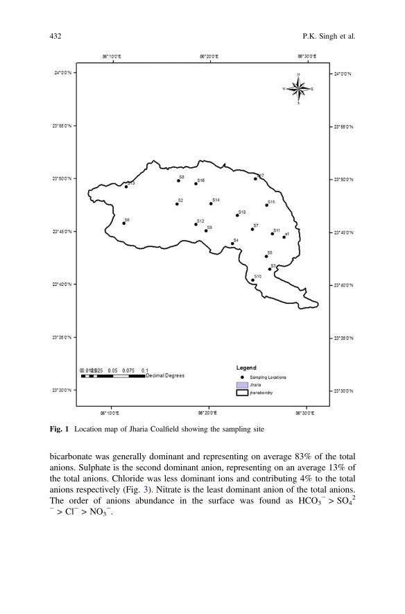
bicarbonate was generally dominant and representing on average 83% of the totalanions. Sulphate is the second dominant anion, representing on an average 13% ofthe total anions. Chloride was less dominant ions and contributing 4% to the totalanions respectively (Fig. 3). Nitrate is the least dominant anion of the total anions.The order of anions abundance in the surface was found as HCO3
− > SO42
− > Cl− > NO3−.
Fig. 1 Location map of Jharia Coalfield showing the sampling site
432 P.K. Singh et al.
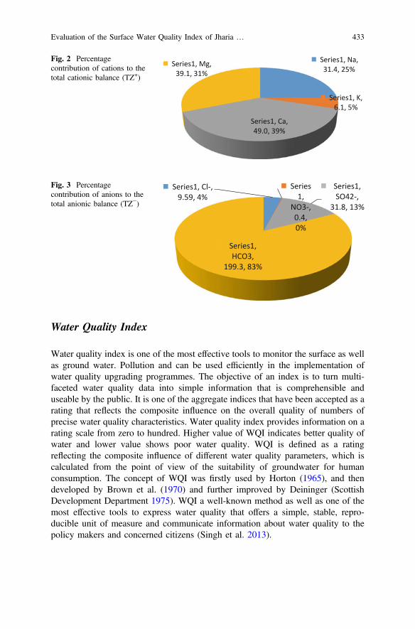
Water Quality Index
Water quality index is one of the most effective tools to monitor the surface as wellas ground water. Pollution and can be used efficiently in the implementation ofwater quality upgrading programmes. The objective of an index is to turn multi-faceted water quality data into simple information that is comprehensible anduseable by the public. It is one of the aggregate indices that have been accepted as arating that reflects the composite influence on the overall quality of numbers ofprecise water quality characteristics. Water quality index provides information on arating scale from zero to hundred. Higher value of WQI indicates better quality ofwater and lower value shows poor water quality. WQI is defined as a ratingreflecting the composite influence of different water quality parameters, which iscalculated from the point of view of the suitability of groundwater for humanconsumption. The concept of WQI was firstly used by Horton (1965), and thendeveloped by Brown et al. (1970) and further improved by Deininger (ScottishDevelopment Department 1975). WQI a well-known method as well as one of themost effective tools to express water quality that offers a simple, stable, repro-ducible unit of measure and communicate information about water quality to thepolicy makers and concerned citizens (Singh et al. 2013).
Series1, Na, 31.4, 25%
Series1, K, 6.1, 5%
Series1, Ca, 49.0, 39%
Series1, Mg, 39.1, 31%
Fig. 2 Percentagecontribution of cations to thetotal cationic balance (TZ+)
Series1, Cl-, 9.59, 4%
Series1,
NO3-, 0.4, 0%
Series1, SO42-,
31.8, 13%
Series1, HCO3,
199.3, 83%
Fig. 3 Percentagecontribution of anions to thetotal anionic balance (TZ−)
Evaluation of the Surface Water Quality Index of Jharia … 433
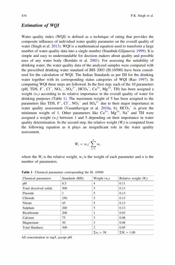
Estimation of WQI
Water quality index (WQI) is defined as a technique of rating that provides thecomposite influence of individual water quality parameter on the overall quality ofwater (Singh et al. 2013). WQI is a mathematical equation used to transform a largenumber of water quality data into a single number (Stambuk-Giljanovic 1999). It issimple and easy to understandable for decision makers about quality and possibleuses of any water body (Bordalo et al. 2001). For assessing the suitability ofdrinking water, the water quality data of the analyzed samples were compared withthe prescribed drinking water standard of BIS 2003 (IS:10500) have been consid-ered for the calculation of WQI. The Indian Standards as per ISI for the drinkingwater together with its corresponding status categories of WQI (Rao 1997). Incomputing WQI three steps are followed. In the first step, each of the 10 parameters(pH, TDS, F−, Cl−, NO3
−, SO42−, HCO3
−, Ca2+, Mg2+, TH) has been assigned aweight (wi) according to its relative importance in the overall quality of water fordrinking purposes (Table 1). The maximum weight of 5 has been assigned to theparameters like TDS, F−, Cl−, NO3
− and SO42− due to their major importance in
water quality assessment (Vasanthavigar et al. 2010a, b). HCO3− is given the
minimum weight of 1. Other parameters like Ca2+, Mg2+, Na+ and TH wereassigned a weight (wi) between 1 and 5 depending on their importance in waterquality determination. In the second step, the relative weight (Wi) is computed fromthe following equation as it plays an insignificant role in the water qualityassessment.
Wi ¼ wi=Xn
i¼1
wi
where the Wi is the relative weight, wi is the weight of each parameter and n is thenumber of parameters.
Table 1 Chemical parameters corresponding the IS: 10500
Chemical parameters Standards (BIS) Weight (wi) Relative weight (Wi)
pH 8.5 4 0.11
Total dissolved solids 500 5 0.13
Fluoride 1 5 0.13
Chloride 250 5 0.13
Nitrate 45 5 0.13
Sulphate 200 5 0.13
Bicarbonate 200 1 0.03
Calcium 75 3 0.08
Magnesium 30 3 0.08
Total Hardness 300 2 0.05
Rwi = 38 RWi = 1.00
All concentration in mg/l, accept pH.
434 P.K. Singh et al.
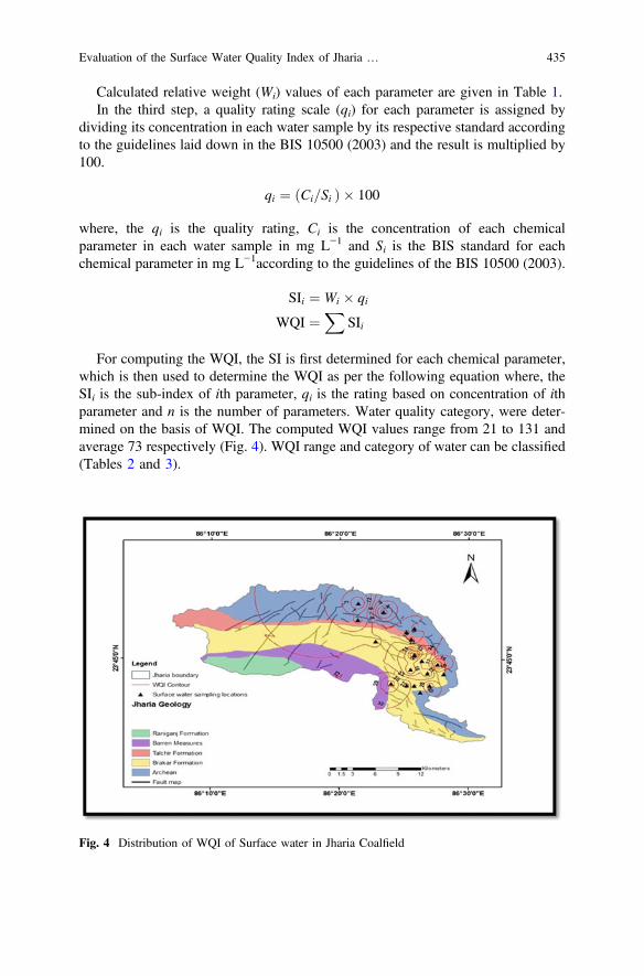
Calculated relative weight (Wi) values of each parameter are given in Table 1.In the third step, a quality rating scale (qi) for each parameter is assigned by
dividing its concentration in each water sample by its respective standard accordingto the guidelines laid down in the BIS 10500 (2003) and the result is multiplied by100.
qi ¼ Ci=Sið Þ � 100
where, the qi is the quality rating, Ci is the concentration of each chemicalparameter in each water sample in mg L−1 and Si is the BIS standard for eachchemical parameter in mg L−1according to the guidelines of the BIS 10500 (2003).
SIi ¼ Wi � qi
WQI ¼X
SIi
For computing the WQI, the SI is first determined for each chemical parameter,which is then used to determine the WQI as per the following equation where, theSIi is the sub-index of ith parameter, qi is the rating based on concentration of ithparameter and n is the number of parameters. Water quality category, were deter-mined on the basis of WQI. The computed WQI values range from 21 to 131 andaverage 73 respectively (Fig. 4). WQI range and category of water can be classified(Tables 2 and 3).
Fig. 4 Distribution of WQI of Surface water in Jharia Coalfield
Evaluation of the Surface Water Quality Index of Jharia … 435

Conclusion
This paper presents the surface water quality assessment of Jharia Coal field.Seventeen samples were taken from different sites of Jharia coal field. Whichsurface water of Jharia coalfield is slightly alkaline in nature. The chemistry ofsurface water is dominated by Ca2+ and Na+ and HCO3
− and SO2�4 . In the majority
of the samples, the analyzed parameters are well within the desirable limits andwater is potable for drinking purposes. However, concentrations of TDS, TH, Ca2+
and Mg2+ exceed the desirable limit at few sites. The surface water of this area isvery much affected by various natural sources such as rock weathering andanthropogenic sources, like Mining activity, agricultural wastes and domesticsewage disposals. The values of WQI showed higher percentage of the poor cat-egory. This shows that the water is not suitable for direct consumption and requirestreatment before its utilization.
Table 2 Classification ofWQI range and category ofwater
WQI Status
<50 Excellent water
50–100 Good water
100–200 Poor water
200–300 Very Poor water
>300 Unfit for drinking purpose
Table 3 Water quality indexfor surface water of JhariaCoalfield
Location WQI Status
Ghanoodih 79 Very poor
Goluckhdih 57.2 Poor
Titinga bad 41.3 Good
Manjhladih 69.4 Poor
Jatudih 53.5 Poor
Amdih 68.1 Poor
Modibitha 22 Good
Bagdigih Basti 83 Very poor
Dumrah 74.6 Very poor
Baghmara 58.5 Poor
Sudamdih river water 48.9 Good
Jamunia River 35.3 Good
Katri Nadi 52.9 Poor
Lilori Dham 60.9 Poor
Navagharka Barkha Talaab 61.2 poor
Moonidih 73.1 Poor
Mahuda 34.1 Good
Damodar 61.2 Poor
436 P.K. Singh et al.
References
Bordalo AA, Nilsumranchit W, Chalermwat K (2001) Water Res 35:3635–3642Brown RM, McCleiland NJ, Deininger RA, O’Connor MF (1972) A water quality index-crossing
the psychological barrier. In: Jenkis SH (ed) Proceedings of International Conference on WaterPollution Research Jerusalem, vol 6, pp 787–797
Brown RM, McClelland NI, Deininger RA, Tozer RG (1970) A water quality index-do we dare?Water Sewage Works Oct 339–343
Chauhan A, Pawar M, Lone SA (2010) Water quality status of Golden Key Lake in ClementTown, Dehradun, Uttarakhand. J Am Sci 6(11):459–464
Horton RK (1965) An Index-number system for rating water quality. J Water Pollut Control Fed37(3):300–305
Kakati SS, Sarma HP (2007) Water quality index of drinking water of Lakhimpur district. Indian JEnviron Prot 27(5):425–428
Mishra PC, Patel RK (2001) Study of the pollution load in the drinking water of Rairangpur, asmall tribal dominated town of North Orissa. Indian J Environ Ecoplanning 5(2):293–298
Neag G (2000) Soil and groundwater remediation (In Romanian). Cartea Cartii de Stiinţă,Cluj-Napoca
Scottish Development Department (1975) Towards cleaner water. Edinburgh: HMSO, report of ariver pollution survey of Scotland
Singh PK, Tiwari AK, Mahato MK (2013) Qualitative assessment of surface water of West Bokarocoalfield, Jharkhand by using water quality index method. Int J Chem Tech Res 5(5)
Stambuk-Giljanovic N (1999) Water quality evaluation by a in Dalmatia. Water Res 1999(33):3423–3440. doi:10.1016/S0043-1354(99)00063-9
Rao NS (1997) Studies on water quality index in hard rock terrain of Guntur District, AndhraPradesh, India. In: National seminar on hydrogeology of precambrian terrains and hard rocksareas, Dharwad, pp 129–134
Tiwari TN, Mishra M (1985) A preliminary assignment of water quality index of major Indianrivers. Indian J Environ Prot 5(4):276–279
Vasanthavigar M, Srinivasamoorthy K, Vijayaragavan K, Rajiv Ganthi R, Chidambaram S,Anandhan P, Manivannan R, Vasudevan S (2010a) Application of water quality index forgroundwater quality assessment: Thirumanimuttar sub-basin Tamilnadu, India. Environ MonitAssess 171(1–4):595–609
Vasanthavigar M, Srinivasamoorthy K, Vijayaragavan K, Ganthi R, Chidambaram S, Anandhan P,Manivannan R, Vasudevan S (2010b) Application of water quality index for groundwaterquality assessment: Thirumanimuttar sub-basin. Environ Monit Assess, Tamil Nadu, India.doi:10.1007/s10661-009-1302-1
Evaluation of the Surface Water Quality Index of Jharia … 437

Studies on the Production of Salt-TolerantAlkaline Protease Isolated from Proteusmirabilis and Its Degradationof Hyper-Saline Soak Liquor
P. Maharaja, E. Nanthini, S. Swarnalatha and G. Sekaran
Abstract This study mainly focuses on the degradation of soluble biomoleculespresent in high salt containing (3–7%) Soak liquor (SL) discharge from the tan-neries using the alkaline protease (AP) extracted from Proteus mirabilis (PM). Theisolation of bacterial strains from SL was done and the screening for halophilicidentification was carried out for the degradation of proteins at saline medium. Thecharacterization of bacterial strain (PM) was carried out by using 16S-rDNAsequencing analysis. The bacterial strain (PM) growth rate was optimized with theeffect of time, external carbon source, pH, temperature and metal ions. It wasobtained time 48 h, pH = 7.0, T = 30 °C, addition of glucose as the external car-bon source and the addition of Fe2+ salts as optimum for the better growth rate ofPM. The production of alkaline protease was carried out by using soak liquor as thesubstrate and the process parameters such as the effect of time, pH, and tempera-ture were optimized. The activity and the stability of alkaline protease was done.The study on the degradation of proteins was carried out and the process parameterswere optimized for the maximum conversion of proteins into amino acids. Theinstrumental analyses such as UV–visible, fluorescence, FT-IR spectroscopicstudies, and TGA analysis confirmed the degradation of proteins into amino acidunits present in the SL efficiently.
Keywords Soak liquor � Alkaline protease � Protease mirabilisProtein degradation
P. Maharaja � E. Nanthini � S. Swarnalatha � G. Sekaran (&)Environmental Technology Division, Council of Scientific & Industrial Research (CSIR),Central Leather Research Institute (CLRI), Adyar, Chennai 600020, Indiae-mail: [email protected]
P. MaharajaLeather Process Technology Lab, Central Leather Research Institute,Adyar, Chennai 600020, Tamil Nadu, Indiae-mail: [email protected]
© Springer Nature Singapore Pte Ltd. 2018V.P. Singh et al. (eds.), Environmental Pollution, Water Scienceand Technology Library 77, https://doi.org/10.1007/978-981-10-5792-2_35
439
Introduction
Tannery sector is the significant contributor to the export of Indian economy andprovides large scale employment opportunity for people of economically weakersection of the society. Further 93% of the tanneries in organized sector come underthe small scale industry category. Besides being important for economic andemployment generation consideration, the tannery sector is also important fromenvironment protection point of view, because preservation and processing ofrawhides and skins into leather cause a severe pollution problem. The main problemin handling raw hides/skins is the transport from the slaughterhouse to the tanneries.The slaughterhouses are not well organized, situated in remote areas. So transportof the raw skins/hides to the tanneries takes more time. But during transportation,the raw skin/hide degrades as a result of variation in temperature and the microbialattack due to the presence of moisture and nutrients. Therefore, the preservation ofthe raw skins/hides is necessary (Tunay et al. 1995; Senthilkumar et al. 2008;Dhaneshwar 1990).
The presence of moisture makes the hides and skins very liable to bacterialattack. Putrefying bacteria degrade the hides and skins causing damage to bothgrain and flesh side of the pelt and lead to a greater degree of degradation. To avoidthis, generally salt (30–40% on raw hide/skin weight basis) is applied on the fleshside of the hides and skins. The salt dehydrates the hides and skins to moisturecontent insufficient to support the growth of molds.
The wastewaters generated from leather industry are richer in both organic andinorganic dissolved solids (TDS) and thus limits the treatability of waste water byconventional biological wastewater treatment processes. The soak liquor generatedfrom leather industry majorly consisting of soluble proteins such as albumin andglobulin and suspended matters like dirt dung and blood in addition to inorganicsalt. Since salt (sodium chloride) is used to preserve the fresh hides/skins duringtransportation and storage. The salt has to be removed by soaking in water for 12 hfrom the hides/skins before taking into leather process. The soak liquor is char-acterized by high organic load (albumin, globulin, and natural fat and mucopolysaccharides), high suspended solids (sand, lime, hair, flesh, dung, etc.) and highsalinity. The conventional biological methods are also ineffective to degrade theorganic pollutants due to the presence of high inorganic TDS in the soak liquor(Gautam 2009).
The high inorganic TDS in soak liquor cause microbial cell rupture by plas-molysis and loss of activity of the cells, which results in the poor removal of BODor COD (Ugyur 2006). Biological treatment techniques such as sequential batchreactor (Lefebvre et al. 2005), UASB reactor, anaerobic digestion and the combinedanaerobic/aerobic treatment of soak liquor (Lefebvre et al. 2006), MembraneSequencing Bio Reactor (MSBR), hybrid upflow anaerobic sludge blanket reactorsare being widely used for the treatment of tannery waste water. The major issues ofbiological treatment of saline wastewaters are (i) a limited extent of adaptation, asconventional cultures could not be effectively used to treat saline wastewaters of
440 P. Maharaja et al.
values higher than 3–5% (w/v) salt. (ii) Salt adaptations of cultures were easily lostwhen subjected to salt-free medium. (iii) Change in ionic strength certainly dis-rupted in cell by shift in salt concentration, from 0.5 to 2% (w/v), caused significantreductions in system performance (Glass and Silverstein 1999). Even with accli-matized cultures, satisfactory performance required a constant ionic composition).Rapid changes in salt concentration cause adverse effects more than gradualchanges. This can be alleviated by an increase in hydraulic retention time (HRT) forsatisfactory performance on treatment of saline waste water. Thus, many advanceoxidation processes have been attempted to treat salt laden wastewater, but none ofthem showed an effective removal of pollution control norms.
Hence, the soak waste water in leather industry is being collected and evaporatedin solar evaporation pans/thermal evaporators in India. The presence of high con-centrations of dissolved organic matter and suspended solids (SS) retards the rate ofevaporation in solar evaporation pans (SEP). Thus, tanneries require large areas tomanage the soak liquor and moreover, the evaporated residue obtained from SEPscannot be reused because of its high organic content. The direct discharge ofresidual dried slat to open land severely contaminates the soil and water pollution.Hence, it has been advised by pollution control agencies to find an alternativesuitable technology for the management of soak liquor.
Since the dissolved sodium chloride is not easily treatable and removed from thewastewater, the discharge of untreated spent soak wastewater into land leads to thesignificant addition of salinity to the soil. The transport of salt through the groundwater affects the water bodies in the region posing a major environmental challenge.Cost-effective solutions to the TDS problem through either avoidance or end of pipetreatment are not yet forthcoming. The residue majorly consists of sodium chlorideand organic pollutants. If the organic pollutants are removed from the soak liquor,there is a scope for the reusability of the evaporated residue and thus eliminate theburden on disposal of evaporated residue. There are many reports on the treatmentof soak liquor wastewater containing high salinity discharged from leather industry(Ugyur and Kargi 2004; Santos et al. 2001). Biological, chemical and/or integratedtreatment techniques have been attempted for the treatment of soak liquor (Dincerand Kargi 2001; Moon et al. 2003; Kubo et al. 2001). However, there is no reporton the complete removal of organic pollutants from the soak liquor to meet thedischarge standards set by the pollution control board. Since the conventionalbiological and chemical treatment methods have certain limitations on the degra-dation of refractory organic pollutants due to high inorganic TDS in soak liquor.
Many researchers are attempted to treat soak liquor generated from leatherindustry by advanced oxidation processes such as Fenton reagent, Photochemicaloxidation and electrochemical oxidation. However, advanced oxidation processesdid not completely remove the organic pollutants due to refractive nature of soakliquor (De Laat et al. 2004; Umar et al. 2010). The complexity lies in the treatmentof soak liquor is due to the fragmentation of heavier organics such as proteins
Studies on the Production of Salt-Tolerant Alkaline … 441
(albumin and globulin), natural fat and muco polysaccharides (Shin et al. 1989;Adamczak and Krishna 2004; Ramani et al. 2010). Hence the present study ismainly focused on the degradation of organic biomolecule, i.e., protein by theproteolytic enzyme isolated from salt-tolerant bacterial strain Proteus mirabilis.After the initial degradation of protein into amino acids it will be subjected tocompletely mineralize the sub units by the further unit operations effectively.
Materials and Methods
Isolation of Microorganisms
The microorganisms were isolated from soak liquor acclimatized tannery soilcollected from nearby CLRI tannery. The salt tolerant proteolytic bacteria wereisolated from the above samples by the serial dilution method (APHA 1992). Thesamples were serially diluted with sterile distilled water and the bacteria wereisolated on the saline skim milk agar plates containing by the standard pour platetechnique (APHA 1992). The plates were then incubated at 37 °C for 3–96 h.Colonies forming transparent zones around the bacterial colony due to hydrolysis ofmilk casein, after 3–96 h of incubation were taken as evidence for qualitativedetermination of protease producing bacteria. Totally eight morphologically distinctbacterial colonies showing the clear zone were selected and re-streaked severaltimes on the nutrient agar to obtain pure isolates. From all the eight cultures theorganisms which show high degree of zone of clearance were taken for furthersaline-tolerant screening studies.
Screening of Bacteria for Protease Production in SalineMedium
Individual bacterial colonies were screened for protease production on skim milkagar medium. Two cultures were selected and streaked on the skim milk agar platesand incubated at 37 °C for 3–96 h at 1, 2, 3, and 4% NaCl concentrations. Theisolates having maximum clearance zone were selected for studies. The bacterialstrain (Org-8) showed maximum clearance when treated with skim milk agarcontaining 1, 2, 3, and 4% of NaCl compared to another strain. Hence, that bacterialstrain was selected for production of protease for the degradation of soak liquor.
P. mirabilis has bacillus morphology and is a Gram-negative bacterium. It ismotile, alternating between vegetative swimmers and hyper-flagellated swarmercells. It also makes a variety of fimbriae. The endotoxins of its LPS membrane elicitan inflammatory response from the host.
442 P. Maharaja et al.

Kingdom Bacteria
Phylum Proteobacteria
Class Gamma proteobacteria
Order Enterobacteriales
Family Enterobacteria
Genus Proteus
Species Proteus mirabilis
P. mirabilis produces urease is an enzyme that converts urea into ammonia bythe following Eq. (1),
NH2ð Þ2CO ! 2NH3 + CO2 ð1Þ
Infection by P. mirabilis can therefore be detected by an alkaline urine sample(pH 8 and above) with large amounts of ammonia.
Alkaline proteases have considerable industrial potential in detergents, leatherprocessing, silver recovery, medical purposes, food processing, feeds and chemicalindustries, as well as tannery waste treatment. At present, the largest part of thehydrolytic enzyme market is occupied by the alkali proteases. Extreme environ-ments are important sources for isolation of microorganisms for novel industriesand enzymes production (Vanitha et al. 2014; Karadzic et al. 2006).
Bacterial Strain Selection and Identification
Depending on the maximum relative proteolytic activity two bacterial strains wereselected and identified. Various morphological, physiological, and biochemicaltests were performed and results were interpreted according to Bergey’s Manual ofDeterminative Bacteriology (Holt et al. 1994).
Molecular Characterization
Genomic DNA was extracted by CTAB protocol. For all the strains, 16S rRNAgene was amplified by universal primers (27F, 1492R). PCR was performed in areaction volume of 50 lL consisting of 10X PCR buffer (5.0 lL), MgCl2 (1.5 mm),dNTPs mix (0.2 mm), (0.4 lm) of 27F, (0.4 lm) of 1492R primer, Taq Polymerase(1.5 U), DNA (5 lL). PCR amplification was performed with 30 cycles followingdenaturation at 94 °C for 1 min, annealing at 55 °C for 1 min and extension at 72 °C for 2 min. Purified samples were sequenced in ABI 3130 Genetic Analyzer.Sequences were then submitted to Gen Bank and accession number was assignedfor each strain.
Studies on the Production of Salt-Tolerant Alkaline … 443
Studies on Optimization of Culture Growth Conditionsin Soak Liquor
The characteristic culture growth conditions at different times were optimized formaximum population of organism, P. mirabilis, in soak liquor with 3–4% of NaClconcentration. The culture growth was checked at different time intervals such as 3,6, 24, 48, 72, and 96 h in terms of optical density. Microbes, such as bacteria, aremore tolerant of environmental conditions than other organisms. However, eachspecies has its own characteristic and particular range of values in which it growsand reproduces best. The isolated organism, P. mirabilis, was inoculated with insoak liquor with 3–4% of NaCl concentration and kept at different temperatureconditions such as 10, 20, 30, 40, and 50 °C, respectively. The isolated organism,P. mirabilis, was inoculated in soak liquor with 3–4% of NaCl concentration and1% of different carbon sources such as glucose, fructose, lactose, and maltose wereadded to the culture. The isolated organism was inoculated in soak liquor with 3–4% of NaCl concentration and 0.5% of different metal ions such as KCl, FeSO4,
MgCl2, CaCl2, and CuSO4 were added to the culture for the effect of metal ionsinvolved in the growth of the organism.
Extraction and Purification of Extracellular Enzymes
Acetone Precipitation
The production media after 48 h is centrifuged at 5000 rpm for 15 min. Thesupernatant was collected and two volumes of cold acetone added to the supernatantand it was incubated at 20 °C for 24 h. After the overnight incubation the pre-cipitated cultures are centrifuged at 5000 rpm for 15 min pellets are collected and itis mixed in 0.2 M phosphate buffer (pH 7) and stored at 4 °C.
Analytical Methods
The COD, BOD5, TOC, TDS, TSS, and TS were measured by the methods sum-marized in standard methods of analysis of wastewater (APHA 1992). The quan-tification of protein in soak liquor and degradation studies were measured as perLowry’s method using bovine serum albumin BSA (Himedia) as the standard atk650 nm using Cary 100 UV–visible spectrophotometer. Standard curves forconcentration calculations were plotted from 0, 10, 25, and 50 mg/L bovine serumalbumin (BSA) diluted from a concentrated stock of BSA. Amino acids generatedafter the degradation of protein in soak liquor were determined.
444 P. Maharaja et al.

Assay of Protease Activity
The protease activity was measured by using casein as the substrate with slightmodifications. The reaction mixture consisted of enzyme sample of volume 1 mLprepared by centrifuging the cell culture suspension at 10,000 rpm for 10 min andthe supernatant was used for assay. The reaction was carried out by the addition of2.0 mL of 50 mM phosphate buffer at pH 7.0 and incubated at 30 °C for 15 min.The reaction was terminated by the addition of trichloroacetic acid (TCA) of2.5 mL, 10% (w/v). This mixture was further incubated at 30 °C for 15 min andkept at room temperature for 30 min. 0.5 mL of the mixture was added to 5.0 mLof 0.5 M Na2CO3 and kept at room temperature for 20 min. 0.5 mL of Folin–Ciocalteu reagent: water (1:2) was added to yield a blue color and the absorbancewas measured at k 660 nm. A ‘blank’ was prepared by the same procedure usingdistilled water. One unit of protease activity is defined as the amount of enzymerequired to liberate one µg of tyrosine per min per mL at reaction conditions. Thespecific activity of enzyme was expressed as enzyme units per mg protein.
Degradation of Soak Liquor
1 kg of animal hide was soaked in 3 L of water (300% w/v) for overnight and leftfor settling for about 2 h, filtered and used for further studies. Later 1 mL ofenzyme was added and to the 50 mL soak liquor sample and the degradation abilityof the extracellular enzyme was estimated by measuring the degradation of protein,protease activity, and formation of amino acid at regular time intervals (0 min,15 min, 30 min, 45 min, and 1 h).
Instrumental Analysis
The different kinds of functional groups present in soak liquor and its degradationusing the alkaline protease were confirmed using FT-IR spectrophotometer (PerkinElmer). The samples were air-dried in sterile conditions to make as powder com-pletely free of moisture and made in the form of pellet with the thickness of 1 mmand diameter of 13 mm, using spectroscopic-grade KBr. The spectrum was ana-lyzed in the spectral range of 400–4000 cm−1. The enzymatic degradation of soakliquor was studied by UV–visible absorption spectra were collected in CARY 5EUV–VIS–NIR Spectrophotometer. The enzymatic reaction mixtures werepre-scanned using fluorescence spectrophotometer to study the excitation andemission characteristics of both soak liquor and the degraded products in the rangeof k 200–800 nm (Cary Eclipse). The thermostability of the components present in
Studies on the Production of Salt-Tolerant Alkaline … 445
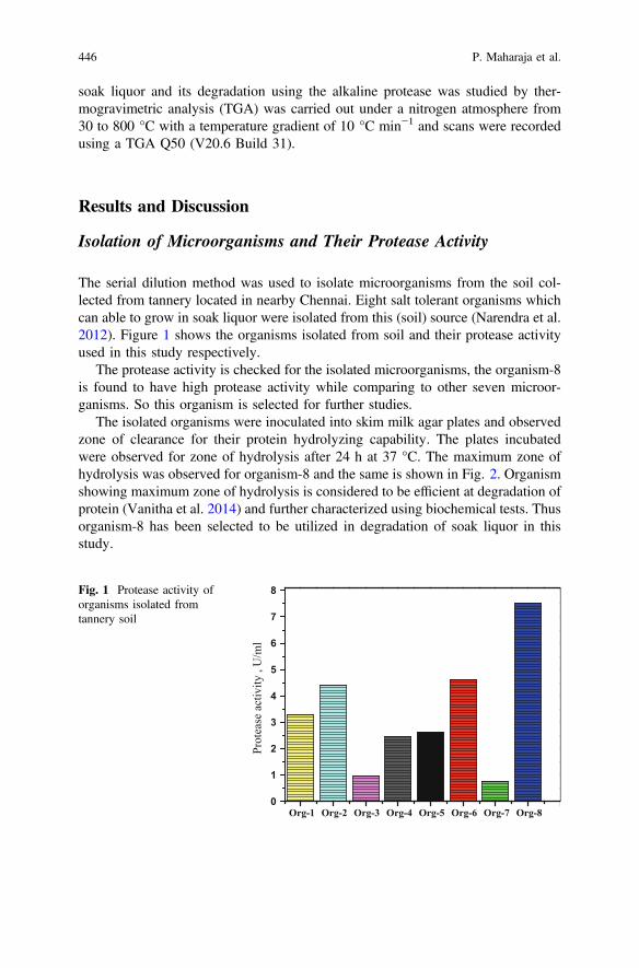
soak liquor and its degradation using the alkaline protease was studied by ther-mogravimetric analysis (TGA) was carried out under a nitrogen atmosphere from30 to 800 °C with a temperature gradient of 10 °C min−1 and scans were recordedusing a TGA Q50 (V20.6 Build 31).
Results and Discussion
Isolation of Microorganisms and Their Protease Activity
The serial dilution method was used to isolate microorganisms from the soil col-lected from tannery located in nearby Chennai. Eight salt tolerant organisms whichcan able to grow in soak liquor were isolated from this (soil) source (Narendra et al.2012). Figure 1 shows the organisms isolated from soil and their protease activityused in this study respectively.
The protease activity is checked for the isolated microorganisms, the organism-8is found to have high protease activity while comparing to other seven microor-ganisms. So this organism is selected for further studies.
The isolated organisms were inoculated into skim milk agar plates and observedzone of clearance for their protein hydrolyzing capability. The plates incubatedwere observed for zone of hydrolysis after 24 h at 37 °C. The maximum zone ofhydrolysis was observed for organism-8 and the same is shown in Fig. 2. Organismshowing maximum zone of hydrolysis is considered to be efficient at degradation ofprotein (Vanitha et al. 2014) and further characterized using biochemical tests. Thusorganism-8 has been selected to be utilized in degradation of soak liquor in thisstudy.
Org-1 Org-2 Org-3 Org-4 Org-5 Org-6 Org-7 Org-80
1
2
3
4
5
6
7
8
Prot
ease
act
ivity
, U
/ml
Fig. 1 Protease activity oforganisms isolated fromtannery soil
446 P. Maharaja et al.
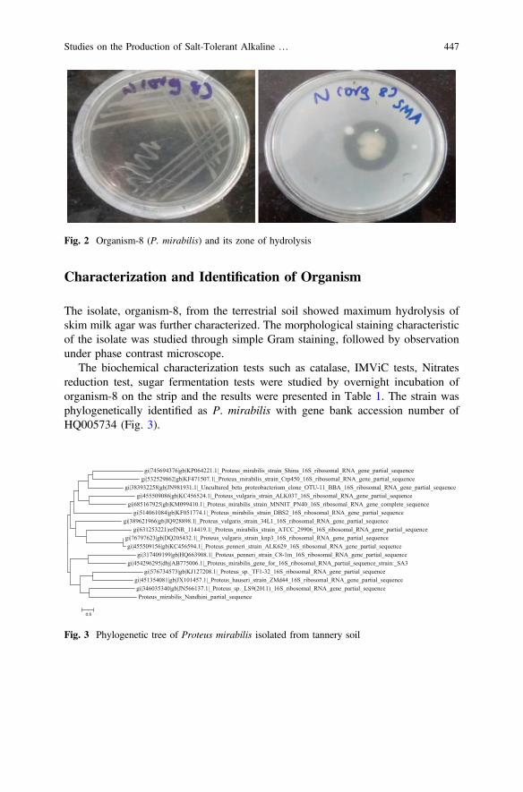
Characterization and Identification of Organism
The isolate, organism-8, from the terrestrial soil showed maximum hydrolysis ofskim milk agar was further characterized. The morphological staining characteristicof the isolate was studied through simple Gram staining, followed by observationunder phase contrast microscope.
The biochemical characterization tests such as catalase, IMViC tests, Nitratesreduction test, sugar fermentation tests were studied by overnight incubation oforganism-8 on the strip and the results were presented in Table 1. The strain wasphylogenetically identified as P. mirabilis with gene bank accession number ofHQ005734 (Fig. 3).
Fig. 2 Organism-8 (P. mirabilis) and its zone of hydrolysis
gi|745694376|gb|KP064221.1|_Proteus_mirabilis_strain_Shinu_16S_ribosomal_RNA_gene_partial_sequence gi|532529862|gb|KF471507.1|_Proteus_mirabilis_strain_Crp450_16S_ribosomal_RNA_gene_partial_sequence
gi|383932258|gb|JN981931.1|_Uncultured_beta_proteobacterium_clone_OTU-11_BBA_16S_ribosomal_RNA_gene_partial_sequence gi|455509086|gb|KC456524.1|_Proteus_vulgaris_strain_ALK037_16S_ribosomal_RNA_gene_partial_sequence
gi|685167925|gb|KM099410.1|_Proteus_mirabilis_strain_MNNIT_PN40_16S_ribosomal_RNA_gene_complete_sequence gi|514061084|gb|KF051774.1|_Proteus_mirabilis_strain_DBS2_16S_ribosomal_RNA_gene_partial_sequence
gi|389621966|gb|JQ928898.1|_Proteus_vulgaris_strain_34L1_16S_ribosomal_RNA_gene_partial_sequence gi|631253221|ref|NR_114419.1|_Proteus_mirabilis_strain_ATCC_29906_16S_ribosomal_RNA_gene_partial_sequence
gi|76797623|gb|DQ205432.1|_Proteus_vulgaris_strain_knp3_16S_ribosomal_RNA_gene_partial_sequence gi|455509156|gb|KC456594.1|_Proteus_penneri_strain_ALK629_16S_ribosomal_RNA_gene_partial_sequence
gi|317409199|gb|HQ663908.1|_Proteus_penneri_strain_C8-1m_16S_ribosomal_RNA_gene_partial_sequence gi|454296295|dbj|AB775006.1|_Proteus_mirabilis_gene_for_16S_ribosomal_RNA_partial_sequence_strain:_SA3
gi|576734573|gb|KJ127208.1|_Proteus_sp._TF1-32_16S_ribosomal_RNA_gene_partial_sequence gi|451354081|gb|JX101457.1|_Proteus_hauseri_strain_ZMd44_16S_ribosomal_RNA_gene_partial_sequence gi|346035340|gb|JN566137.1|_Proteus_sp._LS9(2011)_16S_ribosomal_RNA_gene_partial_sequence Proteus_mirabilis_Nandhini_partial_sequence
0.5
Fig. 3 Phylogenetic tree of Proteus mirabilis isolated from tannery soil
Studies on the Production of Salt-Tolerant Alkaline … 447

Studies on Optimization of Culture Growth Conditions
Optimization of Time and Temperature
The growth of microorganism by up taking soak liquor was observed as a functionof time. The growth rate of the P. mirabilis was observed to take a lag period of 3 h,followed by log growth from 3 to 24 h, from there after exponential growth till48 h. Decay phase was observed from 72 h onwards. Thus maximum growth timeof 48 h was considered to be the optimum time for growth of microorganism insoak liquor. The organism P. mirabilis used in this study showed to be sensitivewith respect to temperature during study on the temperature range of 10–50 °C. Thegraphical representation of the effect of temperature on growth of microorganism ispresented in Fig. 4a, b. The maximum growth at 30 °C and minimum growth at50 °C was observed.
Table 1 Biochemicalcharacteristics organism-8(P. mirabilis)
S. No. Test Organism 8
1 Gram reaction Gram-negative
2 Morphology Rod
3 Rhamnose +
4 Catalase +
5 Indole −
6 Urease +
7 Methyl red −
8 Voges–Proskauer’s −
9 Citrate utilization +
10 H2S +
11 ONPG −
12 Lysine utilization No reaction
13 Ornithine utilization +
14 Malonite utilization +
15 Nitrate +
16 Glucose +
17 Lactose +
18 Saccharose −
19 Phenyl alanine deamination +
20 Saccharose +
21 Raffinose −
22 Trehalose +
448 P. Maharaja et al.
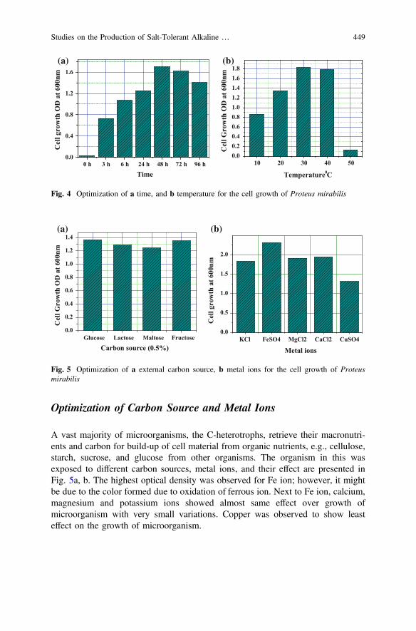
Optimization of Carbon Source and Metal Ions
A vast majority of microorganisms, the C-heterotrophs, retrieve their macronutri-ents and carbon for build-up of cell material from organic nutrients, e.g., cellulose,starch, sucrose, and glucose from other organisms. The organism in this wasexposed to different carbon sources, metal ions, and their effect are presented inFig. 5a, b. The highest optical density was observed for Fe ion; however, it mightbe due to the color formed due to oxidation of ferrous ion. Next to Fe ion, calcium,magnesium and potassium ions showed almost same effect over growth ofmicroorganism with very small variations. Copper was observed to show leasteffect on the growth of microorganism.
0 h 3 h 6 h 24 h 48 h 72 h 96 h0.0
0.4
0.8
1.2
1.6
Cel
l gro
wth
OD
at 6
00nm
Time10 20 30 40 50
0.00.20.40.60.81.01.21.41.61.8
Cel
l Gro
wth
OD
at 6
00nm
Temperature 0C
(a) (b)
Fig. 4 Optimization of a time, and b temperature for the cell growth of Proteus mirabilis
Glucose Lactose Maltose Fructose0.0
0.2
0.4
0.6
0.8
1.0
1.2
1.4
Cel
l Gro
wth
OD
at 6
00nm
Carbon source (0.5%)KCl FeSO4 MgCl2 CaCl2 CuSO4
0.0
0.5
1.0
1.5
2.0
Cel
l gro
wth
at 6
00nm
Metal ions
(a) (b)
Fig. 5 Optimization of a external carbon source, b metal ions for the cell growth of Proteusmirabilis
Studies on the Production of Salt-Tolerant Alkaline … 449

Studies on Enzyme Production and Its Stability
Enzyme Production
From the above-optimized conditions the organism selected for production at 48 hwith pH = 7 and optimized temperature 20 °C. After incubation with acetoneprecipitation was done for the organism to extract extracellular enzyme proteaseand dissolved in phosphate buffer (pH = 7) and the enzyme was purified by dialysismethod. Then, the stability of protease enzyme was studied at different pH andtemperature conditions.
Effect of pH
The protease activity was observed in different pH from 1 to 14, result is shown inFig. 6a. Many researchers found that the protease activity is highly pH dependent andthey are generally active in the range of pH 8–10 (Patel et al. 2006; Dodia et al. 2008).However, there aremany exampleswhere optimumpHwas higher; pH11, with a broadrange of activity from pH 8–11 (Purohit and Singh 2011). However, the pH optimumwas quite low pH 7.5 for the two novel halo-tolerant extracellular proteases fromBacillus subtilis strain FP-133 (Setyorini et al. 2006) and pH 8 for alkaline proteasefrom novel haloalkaliphilic Bacillus sp. (Patel et al. 2006; Rahman et al. 2005).
The activity was very low at acidic pH range of 5 and the activity was found tobe very high at pH 9. Hence, the enzyme used was observed to be alkaline protease.The activity was gradually decreasing by increasing the pH up to 14.
The activity was very low at the highest temperature of 60 ºC, and the maximumwas observed to be at a temperature of 30 ºC. It was also observed that enzyme wasvery sensitive and showed low activity towards higher temperatures beyond 30 °Cas given in Fig. 6b.
1 2 3 4 5 6 7 8 9 10 11 12 13 141
2
3
4
5
6
7
Pro
teas
e ac
tivi
ty, U
/ml
pH10 20 30 40 50 60
2
3
4
5
6
7
8
Pro
teas
e ac
tivi
ty, U
/ml
Temperature,oC
(a) (b)
Fig. 6 a Effect of pH, and b temperature on the stability of alkaline protease isolated fromProteus mirabilis
450 P. Maharaja et al.

Studies on Degradation of Soak Liquor
Characteristics of Soak Liquor
The initial characteristics of the soak liquor after the removal of suspended solidsusing SOAR (Sequential Oxic-Anoxic Bio Reactor) were determined according tostandard methods (APHA 1992) and it was listed in Table 2.
Effect of Time
The extracted alkaline protease from the organism, P. mirabilis was inoculated in50 mL of soak liquor at different time intervals from 0 to 60 min. The protein,amino acid content of the initial soak liquor was checked. After the alkaline pro-tease treatment, the proteins were degraded by cleaving the peptide bond betweenthe peptides and converted into amino acid. There was a gradual decrease in proteinconcentration from the initial concentration to at 45 min and it remains same at60 min. The degradation of protein in soak liquor as a function of time, corre-sponding amino acid formation with respect to time was presented in Fig. 7.
Effect of Temperature
The alkaline protease solution isolated from the organism P. mirabilis has beeninoculated with 50 mL of soak liquor and kept at different temperatures such as 10,20, 30, 40 and 50 °C. The protein content was high as 390 mg/L at 10 °C and at 20 °Cit was 340 mg/L and at 30 °C it was 190 mg/L, at 40 °C it was observed to be150 mg/L, at 50 °C it was found to be 280 mg/L. Thermo stable enzymes are ofspecial interest for industrial applications due to their stability under typical operationconditions; such as high temperatures and wide pH range. The thermophilic proteasescatalyze the reaction and maintain the stability at higher temperatures. In addition,
Table 2 Initialcharacteristics of soak liquorafter SOAR reactor
Parameters Values
pH 7.49
Chemical Oxygen Demand, mg/L 4025
Biochemical Oxygen Demand, mg/L 1800
NH3, mg/L 229
Total Nitrogen, mg/L 330
Protein, mg/L 557
Amino acids, mg/L 390
Lipids, mg/L 30.7
Total suspended solids (TSS), mg/L 1480
Total dissolved solids (TDS), mg/L 61,824
Studies on the Production of Salt-Tolerant Alkaline … 451
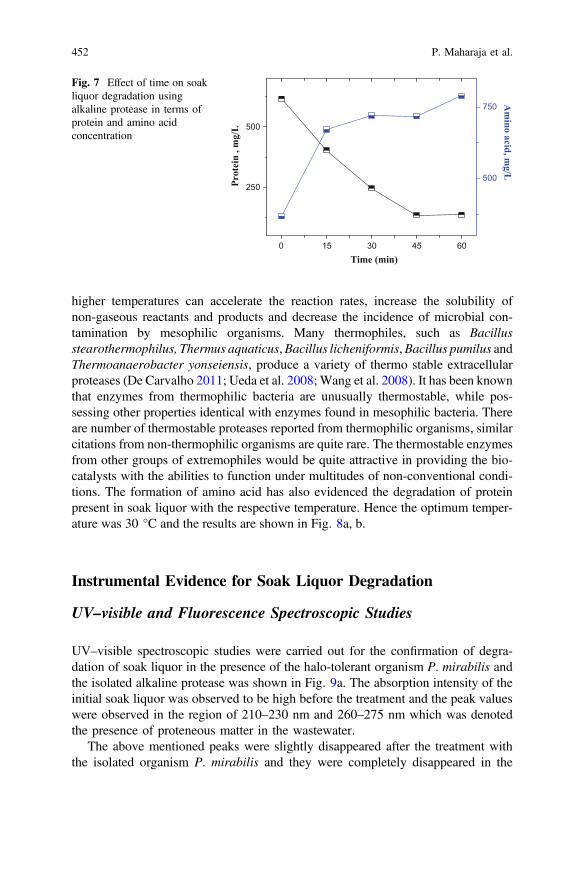
higher temperatures can accelerate the reaction rates, increase the solubility ofnon-gaseous reactants and products and decrease the incidence of microbial con-tamination by mesophilic organisms. Many thermophiles, such as Bacillusstearothermophilus, Thermus aquaticus,Bacillus licheniformis,Bacillus pumilus andThermoanaerobacter yonseiensis, produce a variety of thermo stable extracellularproteases (De Carvalho 2011; Ueda et al. 2008; Wang et al. 2008). It has been knownthat enzymes from thermophilic bacteria are unusually thermostable, while pos-sessing other properties identical with enzymes found in mesophilic bacteria. Thereare number of thermostable proteases reported from thermophilic organisms, similarcitations from non-thermophilic organisms are quite rare. The thermostable enzymesfrom other groups of extremophiles would be quite attractive in providing the bio-catalysts with the abilities to function under multitudes of non-conventional condi-tions. The formation of amino acid has also evidenced the degradation of proteinpresent in soak liquor with the respective temperature. Hence the optimum temper-ature was 30 °C and the results are shown in Fig. 8a, b.
Instrumental Evidence for Soak Liquor Degradation
UV–visible and Fluorescence Spectroscopic Studies
UV–visible spectroscopic studies were carried out for the confirmation of degra-dation of soak liquor in the presence of the halo-tolerant organism P. mirabilis andthe isolated alkaline protease was shown in Fig. 9a. The absorption intensity of theinitial soak liquor was observed to be high before the treatment and the peak valueswere observed in the region of 210–230 nm and 260–275 nm which was denotedthe presence of proteneous matter in the wastewater.
The above mentioned peaks were slightly disappeared after the treatment withthe isolated organism P. mirabilis and they were completely disappeared in the
0 15 30 45 60
250
500
Time (min)
Prot
ein
, mg/
L
500
750 Am
ino acid, mg/L
Fig. 7 Effect of time on soakliquor degradation usingalkaline protease in terms ofprotein and amino acidconcentration
452 P. Maharaja et al.

presence of alkaline protease at the optimized conditions. It was noted that theintensity difference between the absorption peaks appeared in the enzymatic and themicrobial degradation of soak liquor and it was clearly shown in Fig. 9a. Hence, theenzymatic degradation using the alkaline protease from the halo-tolerant organismP. mirabilis would be the effective process compare with the pure organism for thedegradation of soak liquor.
UV–fluorescence absorption studies were carried out for the confirmation ofdegradation of soak liquor in the presence of the halo-tolerant organism P. mirabilisand the isolated alkaline protease was shown in Fig. 9b. The spectrum shows thedifference in intensities between the soak liquor and the treated samples after theenzymatic degradation and microbial degradation at the optimized conditions.The spectrum evidenced for the presence of fluorescent inactive compounds present
10 20 30 40 50
200
400
600
800
Soak liquorTreated soak liquor using alkaline protease
Prot
ein
conc
entr
atio
n, m
g/L
Temperature, οC10 20 30 40 50
0
200
400
600
800
1000
Am
ino
acid
con
cent
ratio
n, m
g/L
Temperature, oCSoak liquorTreated soak liquor using alkaline protease
(a) (b)
Fig. 8 Effect of temperature on soak liquor degradation in terms of a protein concentration, andb amino acid concentration
200 250 300 350 400
Soak liquor (SL) SL + Alkaline protease (15 min) SL + Alkaline protease (30 min) SL + Alkaline protease (45 min) SL + Alkaline protease (60 min)
Inte
nsity
(a.u
)
Wavelength (nm)200 300 400 500 600 700 800
0
250
500
750
Inte
nsity
(a.u
.)
Wavelength (nm)
Soak liquor (SL) SL + Alkaline protease (15 min) SL + Alkaline protease (30 min) SL + Alkaline protease (45 min) SL + Alkaline protease (60 min)
(a) (b)
Fig. 9 a UV–visible and b UV–fluorescence spectrum of the soak liquor, SL+Alkaline proteaseisolated from PM
Studies on the Production of Salt-Tolerant Alkaline … 453
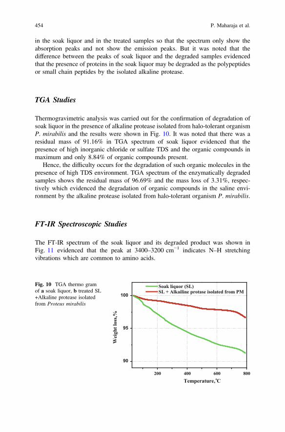
in the soak liquor and in the treated samples so that the spectrum only show theabsorption peaks and not show the emission peaks. But it was noted that thedifference between the peaks of soak liquor and the degraded samples evidencedthat the presence of proteins in the soak liquor may be degraded as the polypeptidesor small chain peptides by the isolated alkaline protease.
TGA Studies
Thermogravimetric analysis was carried out for the confirmation of degradation ofsoak liquor in the presence of alkaline protease isolated from halo-tolerant organismP. mirabilis and the results were shown in Fig. 10. It was noted that there was aresidual mass of 91.16% in TGA spectrum of soak liquor evidenced that thepresence of high inorganic chloride or sulfate TDS and the organic compounds inmaximum and only 8.84% of organic compounds present.
Hence, the difficulty occurs for the degradation of such organic molecules in thepresence of high TDS environment. TGA spectrum of the enzymatically degradedsamples shows the residual mass of 96.69% and the mass loss of 3.31%, respec-tively which evidenced the degradation of organic compounds in the saline envi-ronment by the alkaline protease isolated from halo-tolerant organism P. mirabilis.
FT-IR Spectroscopic Studies
The FT-IR spectrum of the soak liquor and its degraded product was shown inFig. 11 evidenced that the peak at 3400–3200 cm−1 indicates N–H stretchingvibrations which are common to amino acids.
200 400 600 800
90
95
100
Wei
ght l
oss,%
Temperature, oC
Soak liquor (SL)SL + Alkailine protase isolated from PM
Fig. 10 TGA thermo gramof a soak liquor, b treated SL+Alkaline protease isolatedfrom Proteus mirabilis
454 P. Maharaja et al.

The peak 2508 cm−1 shows a strong symmetrical C–H stretching of methylgroups. The peak at 1653 cm−1 indicates that the presence of amide bond (–C(=O)–NH) depicts that the secondary structure of peptides. The C–O stretching ofcarboxylic groups appears at near 1208 cm−1. The peak at near 700–600 cm−1
shows that –NH bending vibrations of the amino compounds present in soak liquor.The FT-IR spectrum of soak liquor after enzymatic degradation indicates that thepresence of 1465 cm−1 band may represents to –C=O Stretching of the carboxylategroup present in the peptide or polypeptide bond due to the cleavage of peptidebond of protein present in the soak liqour. The peak at 1220–1190 cm− 1 indicatesthat the strong stretching vibrations of –C–C (=O)–O bond of the amino acidspresent in the soak liquor present in the soak liquor after enzymatic degradation.Hence the degradation of proteins present in the soak liquor by the enzymes con-firmed through FT-IR spectrum.
Conclusion
This research study concludes that the treatment of saline wastewater is feasible,through the bacterial extracellular protease. The use of enzymes is particularlyefficient for the removal of high amounts of organic matter in effluents. Generally,biological treatment is inhibited by high salt concentrations. However, this studyhas proved feasibility of degradation using salt-adapted microorganisms capable ofwithstanding high salinities and at the same time of degrading the pollutants inwastewater.
The organism isolated was identified by 16S rDNA sequencing as P. mirabilis(HQ005734). The Optimum growth conditions in both nutrient broth and soakliquor were noted to be pH 7, time 48 h and temperature 30 °C. The alkaline
4000 3500 3000 2500 2000 1500 1000 500
Soak liquor(SL)SL + Protease isolated from PM
Tra
nsm
ittan
ce, %
Wavenumber, cm-1
Fig. 11 FT-IR spectrum ofsoak liquor and itsdegradation using alkalineprotease
Studies on the Production of Salt-Tolerant Alkaline … 455

protease was extracted from PM. The protease activity was stable at pH 7–9and temperature 30–40 °C. The degradation of protein content of soak liquor wasdone by using alkaline protease and it was confirmed through UV-visible,fluorescence, TGA and FT-IR spectroscopic studies. From this study, it was con-cluded that the biological origin of enzymes reduces their adverse impact on theenvironment thereby making enzymatic wastewater treatment an ecologically sus-tainable technique.
Acknowledgements The authors are very thankful for providing the facilities through the projectSTRAIT-CSC0201, CSIR-CLRI to carry out the research work. This research work is carried outas part of PhD registered in University of Madras.
References
Adamczak M, Krishna SH (2004) Strategies for improving enzymes for efficient biocatalysis. FoodTechnol Biotech 42(4):251–264
APHA (1992) Standard methods for the examination of water and waste-water. American WaterWorks Association and Water Pollution Control Federation, 18th edn
De Carvalho CC (2011) Enzymatic and whole cell catalysis: finding new strategies for oldprocesses. Biotechnol Adv 29(1):75–83
De Laat J, Le GT, Legube B (2004) A comparative study of the effects of chloride, sulfate andnitrate ions on the rates of decomposition of H2O2 and organic compounds by Fe (II)/H2O2 andFe (III)/H2O2. Chemosphere 55(5):715–723
Dhaneshwar RS (1990) Tannery wastewater treatment and disposal state of art. Indian J EnvironProt 10:131–141
Dinçer AR, Kargi F (2001) Salt inhibition kinetics in nitrification of synthetic saline wastewater.Enzym Microb Tech 28(7):661–665
Dodia MS, Bhimani HG, Rawal CM, Joshi RH, Singh SP (2008) Salt dependent resistance againstchemical denaturation of alkaline protease from a newly isolated haloalkaliphilic Bacillussp. Bioresour Technol 99(14):6223–6227
Glass C, Silverstein J (1999) Denitrification of high-nitrate, high-salinity wastewater. Water Res33:223–229
Holt JG, Krieg NR, Sneath PH, Staley JT, Williams ST (1994) International edition: Bergey’smanual of determinative bacteriology
Karadzic I, Masui A, Zivkovic LI, Fujiwara N (2006) Purification and characterization of analkaline lipase from Pseudomonas aeruginosa isolated from putrid mineral cutting oil ascomponent of metal working fluid. J Biosci Bioeng 102:82–89
Kubo M, Hiroe J, Murakami M, Fukami H, Tachiki T (2001) Treatment of hypersaline containingwastewater with salt-tolerant microorganisms. J Biosci Bioeng 91(2):222–224
Lefebvre O, Vasudevan N, Thanasekaran K, Moletta R, Godon JJ (2006) Microbial diversity inhypersaline wastewater: the example of tanneries. Extremophiles 10(6):505–513
Lefebvre O, Vasudevan N, Torrijos M, Thanasekaran K, Moletta R (2005) Halophilic biologicaltreatments of tannery soak liquor in a sequencing batch reactor. Water Res 39(8):1471–1480
Moon BH, Seo GT, Lee TS, Kim SS, Yoon CH (2003) Effects of salt concentration on floccharacteristics and pollutants removal efficiencies in treatment of seafood wastewater by SBR.Water Sci Technol 47(1):65–70
Narendra G, Ramalakshmi M, Roja R, Archana B, Maanasa F (2012) Isolation and character-ization of protease producing bacterial from soil and estimation of protease by spectropho-tometer. Experiment 1(1):1–7
456 P. Maharaja et al.

Patel RK, Dodia MS, Joshi RH, Singh SP (2006) Purification and characterization of alkalineprotease from a newly isolated haloalkaliphilic Bacillus sp. Process Biochem 41(9):2002–2009
Purohit MK, Singh SP (2011) Comparative analysis of enzymatic stability and amino acidsequences of thermostable alkaline proteases from two haloalkaliphilic bacteria isolated fromCoastal region of Gujarat, India. Int J Biol Macromol 49(1):103–112
Rahman RN, Geok LP, Basri M, Salleh AB (2005) Physical factors affecting the production oforganic solvent tolerant protease by Pseudomonas aeruginosa strain K. Bioresour Technol96:429–436
Ramani K, John Kennedy L, Ramakrishnan M, Sekaran G (2010) Purification, characterizationand application of acidic lipase from Pseudomonas gessardii using beef tallow as a substratefor fats and oil hydrolysis. Process Biochem 45:1683–1691
Gautam SP (2009) Recovery of better quality reusable salt from soak liquor of tanneries in solarevaporation pans. Central Pollution Control Board Ministry of Environment & Forests
Santos CA, Vieira AM, Fernandes HL, Empis JA, Novais JM (2001) Optimisation of thebiological treatment of hypersaline wastewater from Dunaliella salina carotenogenesis. J ChemTechnol Biotechnol 76:1147–1153
Senthilkumar S, Surianarayanan M, Sudharshan S, Susheela R (2008) Biological treatment oftannery wastewater by using salt-tolerant bacterial strains. Microb Cell Fact. doi:10.1186/1475-2859-7-15
Setyorini E, Takenaka S, Murakami S, Aoki K (2006) Purification and characterization of twonovel halotolerant extracellular proteases from Bacillus subtilis strain FP-133. BiosciBiotechnol Biochem 70(2):433–440
Shin S, Jung KS, Kim W, Park S (1989) Identification of the protease producing bacteria to usefish meal waste water and the producing and conditions for the enzyme. Bull Korean Fish Soc22:138–146
Tunay O, Kabdasli I, Orhon D, Ates E (1995) Characterization and pollution profile of leathertanning industry in Turkey. Water Sci Technol 32:1–9
Ueda M, Asano T, Nakazawa M, Miyatake K, Inouye K (2008) Purification and characterization ofnovel raw-starch-digesting and cold-adapted a-amylases from Eisenia foetida. Comp BiochemPhysiol B Biochem Mol Biol 150(1):125–130
Umar M, Aziz HA, Yusoff MS (2010) Trends in the use of Fenton, electro-Fenton andphoto-Fenton for the treatment of landfill leachate. Waste Manage 30(11):2113–2121
Ugyur A (2006) Specific nutrient removal rates in saline wastewater treatment using sequencingbatch reactor. Process Biochem 41(1):61–66
Ugyur A, Kargi F (2004) Salt inhibition on biological nutrient removal from saline wastewater in asequencing batch reactor. Enzym Microb Tech 34(3):313–318
Vanitha N, Rajan S, Murugesan AG (2014) Optimization and production of alkaline proteaseenzyme from Bacillus subtilis 168 isolated from food industry waste. Int J Curr Microbiol AppSci 3(6):36–44
Wang Q, Hou Y, Xu Z, Miao J, Li G (2008) Optimization of cold-active protease production bythe psychrophilic bacterium Colwellia sp. NJ341 with response surface methodology.Bioresour Technol 99(6):1926–1931
Studies on the Production of Salt-Tolerant Alkaline … 457

Relative Contribution of Phosphorusfrom Various Sources to the Upper Lake,Bhopal
Mounissamy Vassanda Coumar, S. Kundu, J.K. Saha, S. Rajendiran,M.L. Dotaniya, Vasudev Meena, J. Somasundaram and A.K. Patra
Abstract An investigation on phosphorus loading from the point and non pointsources to the Upper Lake, Bhopal and its contribution on eutrophication wasundertaken at Indian Institute of Soil Science, Bhopal. Geo-referenced watersamples from different entry points (15 locations), where water from differentsources (agriculture and municipal water) enters to the Upper Lake, were collectedand analyzed for various P fractions. The results showed that the total phosphorus(TP) content varied from 0.30 to 0.73 mg/L with a mean value of 0.47 mg/L havinglowest and highest content from Kholukhedi (agriculture source) and Bhadbada(domestic wastewater), respectively. Among the P fractions, the bioavailable Pfraction (total dissolved phosphorus-TDP) was highest in the water sample from thedomestic source, whereas, the dominant P fractions in the water samples fromagricultural source was particulate P (PP). The results shows that the total P in thesediment of post-monsoon stage samples ranges from 0.03 to 0.07% with a meanvalue of 0.04%. The mean sediment inorganic phosphorus (SIP) and the sedimentorganic phosphorus (SOP) is 68.01 and 31.98% of total phosphorus (TP), respec-tively. Among the inorganic P fractions in the sediment, Ca bound P was maximumand found to be in the range of 86.32–96.97% of total sediment inorganic P fol-lowed by Fe bound P (2.10–11.51%) and loosely sorbed P (LSP) (0.39–5.66%). Tosummarize, the source of water from the city (domestic wastewater) and at idolimmersion location contains relatively higher total phosphorus (TP) and dissolvedreactive phosphorus (DRP).
M. Vassanda Coumar (&) � S. Kundu � J.K. Saha � S. RajendiranM.L. Dotaniya � V. Meena � J. Somasundaram � A.K. PatraICAR-Indian Institute of Soil Science, Nabibagh, Berasia Road, Bhopal 462038,MP, Indiae-mail: [email protected]
© Springer Nature Singapore Pte Ltd. 2018V.P. Singh et al. (eds.), Environmental Pollution, Water Scienceand Technology Library 77, https://doi.org/10.1007/978-981-10-5792-2_36
459
Introduction
Phosphorus is one of the key elements necessary for the growth of all forms of lifeand therefore for food production. There is no substitute for phosphorus in foodproduction and it cannot be manufactured, hence its greater significance tohumanity. Phosphate rock, like oil, is a non-renewable resource and approximately50–100 years remain of current known reserves. Further, a peak in global pro-duction—peak phosphorus—is estimated to occur by 2035. After the peak, supplyis expected to decrease year by year, constrained by economic and energy costs,despite rising demand. On the other hand, remaining reserves is declining due to:(a) lower concentration of phosphorus (% P2O5) in the remaining phosphate rockreserves; and (b) increasing concentrations of heavy metals like cadmium anduranium that are highly toxic to soils, flora, fauna and humans. While good agro-nomic management requires use of P to optimize crop growth, excessive applicationof P may degrade water quality. Thus, phosphorus plays a key role in crop pro-duction as well as environmental sustainability.
The investigation from the UNEP (United Nation Environmental Protection)indicates that about 30–40% of the lakes and reservoirs have been affected more orless by water eutrophication all over the world. Eutrophication is the natural agingof lakes or streams brought on by nutrient enrichment and eventually promoteexcessive plant growth, favoring simple algae and plankton over other morecomplicated plants, and cause a severe reduction in water quality. Eutrophicationprocess can be greatly accelerated by human activities which increase nutrientloading rates to water. While nitrogen, phosphorus, carbon and in some cases,silicon contribute to eutrophication, P is the primary agent in freshwater eutroph-ication, as many algae are able to obtain N from the atmosphere (Schindler 1997).Phosphorus has fewer sources, making it easier to achieve smaller concentrations.Also, it is easier to make phosphorus insoluble in water, thus making it lessavailable to plants for their growth. In addition, phosphorus sources are more oftenfrom human activities that we may be able to control more easily than naturalsources. Thus, controlling eutrophication mainly requires reducing P inputs tosurface waters, despite the fact that P is an essential nutrient for crop and animalproduction.
Since, late 1960s, the relative contributions of P to water bodies, both from pointand diffuse sources have changed dramatically. In recent years, relatively greaterefforts have been made to control P pollution from point sources discharge. But lessattention have been directed to control diffuse sources of P, mainly due to thedifficulty in their identification and control (Sharpley and Rekolainen 1997). Thus,control of diffuse sources of P is a major hurdle for protecting fresh surface watersfrom eutrophication (Sharpley and Tunney 2000; Withers et al. 2014). A plenty ofinformation is available on point and non-point sources (NPS) of phosphorus
460 M. Vassanda Coumar et al.
loading to the lake system, across the world. However, in India, limited researchwork is done on phosphorus loading from non point sources to the lake system. TheUpper and Lower lakes of Bhopal, constructed in the eleventh and eighteenthcentury, respectively are glaring examples of urban water bodies. Till the middle ofthe last century, the water of Upper Lake did not require any treatment before supplyfor drinking purposes. However, increased anthropogenic activities around this lakeresulted in the deterioration of water quality of the lakes. While the Lower Lakebecame eutrophic, only certain pockets of Upper Lake have reached the level ofeutrophication. The Upper Lake still contributes about 40% of water supply to thecity. Hence protection of this valuable resource from pollution for sustainable use isof great importance. Keeping this in view, the present research project envisioned tostudy the NPS of phosphorus loading to the Upper Lake, Bhopal.
Materials and Methods
The Study Area
In the present study, the Upper Lake which is geographically located at 23° 12′Nlatitude and 77° 18′E longitude of Bhopal (M.P.) at an altitude of 508.65 m abovemean sea level is considered as a case study to quantify relative contribution ofphosphorus from different sources to the lake water bodies. The Upper Lake is oneof the oldest lake constructed in the eleventh century and largest impoundments anda major drinking water source for the city of Bhopal. The Upper Lake still con-tributes about 40% of water supply to the city. In view of its ecological importance,the Ministry of Environment and Forests, Government of India has recognizedUpper Lake as wetland of national importance in 1998 and later declared it asRamsar site in the year 2002.
The Upper Lake is an east-westerly elongated manmade lake with the totalsubmergence area of 36.54 km2. Total water storage capacity of the lake isapproximately 117 mm3 with maximum depths of 11.7 m. In shallow portion oflake, luxuriant growth of aquatic vegetation can be observed. Catchment of theUpper Lake displays a complete range of urban and rural activity with varyingintensities that contribute nutrients and pollution load through point and non-pointpollution sources. Majority of the catchment area is under agricultural activities(213.1 km2) followed by scrub or without scrub (87.7 km2) and built-up area(20.9 km2).
Relative Contribution of Phosphorus from Various Sources … 461
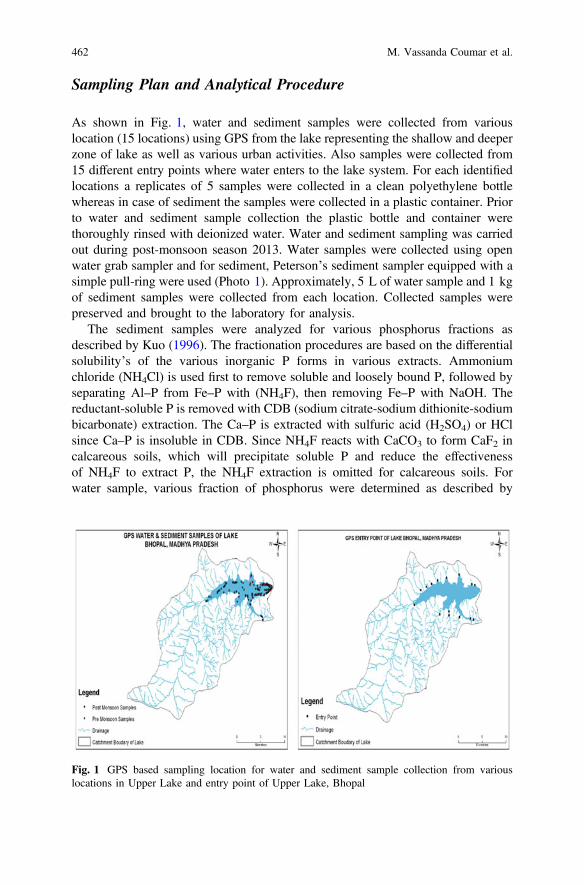
Sampling Plan and Analytical Procedure
As shown in Fig. 1, water and sediment samples were collected from variouslocation (15 locations) using GPS from the lake representing the shallow and deeperzone of lake as well as various urban activities. Also samples were collected from15 different entry points where water enters to the lake system. For each identifiedlocations a replicates of 5 samples were collected in a clean polyethylene bottlewhereas in case of sediment the samples were collected in a plastic container. Priorto water and sediment sample collection the plastic bottle and container werethoroughly rinsed with deionized water. Water and sediment sampling was carriedout during post-monsoon season 2013. Water samples were collected using openwater grab sampler and for sediment, Peterson’s sediment sampler equipped with asimple pull-ring were used (Photo 1). Approximately, 5 L of water sample and 1 kgof sediment samples were collected from each location. Collected samples werepreserved and brought to the laboratory for analysis.
The sediment samples were analyzed for various phosphorus fractions asdescribed by Kuo (1996). The fractionation procedures are based on the differentialsolubility’s of the various inorganic P forms in various extracts. Ammoniumchloride (NH4Cl) is used first to remove soluble and loosely bound P, followed byseparating Al–P from Fe–P with (NH4F), then removing Fe–P with NaOH. Thereductant-soluble P is removed with CDB (sodium citrate-sodium dithionite-sodiumbicarbonate) extraction. The Ca–P is extracted with sulfuric acid (H2SO4) or HClsince Ca–P is insoluble in CDB. Since NH4F reacts with CaCO3 to form CaF2 incalcareous soils, which will precipitate soluble P and reduce the effectivenessof NH4F to extract P, the NH4F extraction is omitted for calcareous soils. Forwater sample, various fraction of phosphorus were determined as described by
Fig. 1 GPS based sampling location for water and sediment sample collection from variouslocations in Upper Lake and entry point of Upper Lake, Bhopal
462 M. Vassanda Coumar et al.
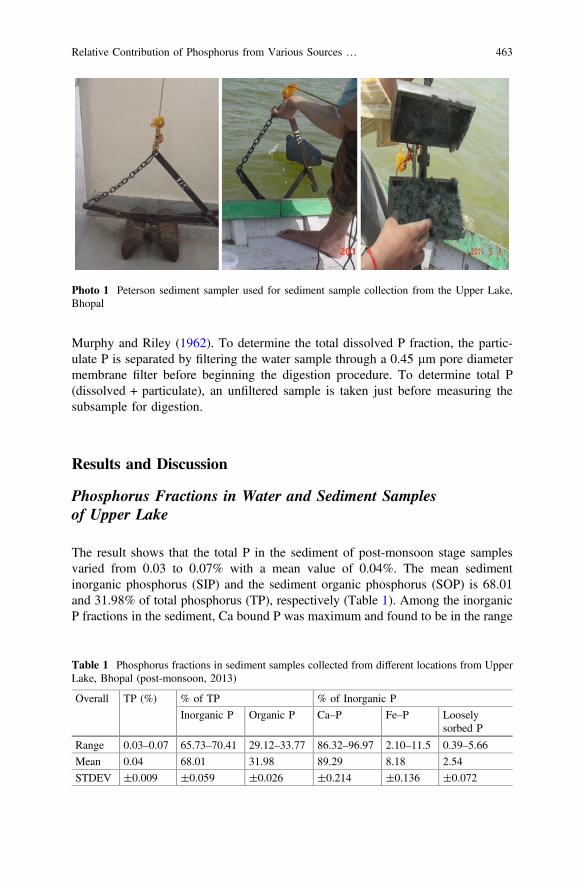
Murphy and Riley (1962). To determine the total dissolved P fraction, the partic-ulate P is separated by filtering the water sample through a 0.45 lm pore diametermembrane filter before beginning the digestion procedure. To determine total P(dissolved + particulate), an unfiltered sample is taken just before measuring thesubsample for digestion.
Results and Discussion
Phosphorus Fractions in Water and Sediment Samplesof Upper Lake
The result shows that the total P in the sediment of post-monsoon stage samplesvaried from 0.03 to 0.07% with a mean value of 0.04%. The mean sedimentinorganic phosphorus (SIP) and the sediment organic phosphorus (SOP) is 68.01and 31.98% of total phosphorus (TP), respectively (Table 1). Among the inorganicP fractions in the sediment, Ca bound P was maximum and found to be in the range
Photo 1 Peterson sediment sampler used for sediment sample collection from the Upper Lake,Bhopal
Table 1 Phosphorus fractions in sediment samples collected from different locations from UpperLake, Bhopal (post-monsoon, 2013)
Overall TP (%) % of TP % of Inorganic P
Inorganic P Organic P Ca–P Fe–P Looselysorbed P
Range 0.03–0.07 65.73–70.41 29.12–33.77 86.32–96.97 2.10–11.5 0.39–5.66
Mean 0.04 68.01 31.98 89.29 8.18 2.54
STDEV ±0.009 ±0.059 ±0.026 ±0.214 ±0.136 ±0.072
Relative Contribution of Phosphorus from Various Sources … 463
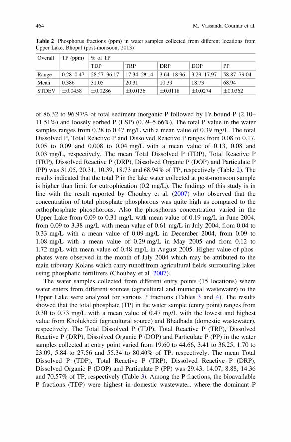
of 86.32 to 96.97% of total sediment inorganic P followed by Fe bound P (2.10–11.51%) and loosely sorbed P (LSP) (0.39–5.66%). The total P value in the watersamples ranges from 0.28 to 0.47 mg/L with a mean value of 0.39 mg/L. The totalDissolved P, Total Reactive P and Dissolved Reactive P ranges from 0.08 to 0.17,0.05 to 0.09 and 0.008 to 0.04 mg/L with a mean value of 0.13, 0.08 and0.03 mg/L, respectively. The mean Total Dissolved P (TDP), Total Reactive P(TRP), Dissolved Reactive P (DRP), Dissolved Organic P (DOP) and Particulate P(PP) was 31.05, 20.31, 10.39, 18.73 and 68.94% of TP, respectively (Table 2). Theresults indicated that the total P in the lake water collected at post-monsoon sampleis higher than limit for eutrophication (0.2 mg/L). The findings of this study is inline with the result reported by Choubey et al. (2007) who observed that theconcentration of total phosphate phosphorous was quite high as compared to theorthophosphate phosphorous. Also the phosphorus concentration varied in theUpper Lake from 0.09 to 0.31 mg/L with mean value of 0.19 mg/L in June 2004,from 0.09 to 3.38 mg/L with mean value of 0.61 mg/L in July 2004, from 0.04 to0.33 mg/L with a mean value of 0.09 mg/L in December 2004, from 0.09 to1.08 mg/L with a mean value of 0.29 mg/L in May 2005 and from 0.12 to1.72 mg/L with mean value of 0.48 mg/L in August 2005. Higher value of phos-phates were observed in the month of July 2004 which may be attributed to themain tributary Kolans which carry runoff from agricultural fields surrounding lakesusing phosphatic fertilizers (Choubey et al. 2007).
The water samples collected from different entry points (15 locations) wherewater enters from different sources (agricultural and municipal wastewater) to theUpper Lake were analyzed for various P fractions (Tables 3 and 4). The resultsshowed that the total phosphate (TP) in the water sample (entry point) ranges from0.30 to 0.73 mg/L with a mean value of 0.47 mg/L with the lowest and highestvalue from Kholukhedi (agricultural source) and Bhadbada (domestic wastewater),respectively. The Total Dissolved P (TDP), Total Reactive P (TRP), DissolvedReactive P (DRP), Dissolved Organic P (DOP) and Particulate P (PP) in the watersamples collected at entry point varied from 19.60 to 44.66, 3.41 to 36.25, 1.70 to23.09, 5.84 to 27.56 and 55.34 to 80.40% of TP, respectively. The mean TotalDissolved P (TDP), Total Reactive P (TRP), Dissolved Reactive P (DRP),Dissolved Organic P (DOP) and Particulate P (PP) was 29.43, 14.07, 8.88, 14.36and 70.57% of TP, respectively (Table 3). Among the P fractions, the bioavailableP fractions (TDP) were highest in domestic wastewater, where the dominant P
Table 2 Phosphorus fractions (ppm) in water samples collected from different locations fromUpper Lake, Bhopal (post-monsoon, 2013)
Overall TP (ppm) % of TP
TDP TRP DRP DOP PP
Range 0.28–0.47 28.57–36.17 17.34–29.14 3.64–18.36 3.29–17.97 58.87–79.04
Mean 0.386 31.05 20.31 10.39 18.73 68.94
STDEV ±0.0458 ±0.0286 ±0.0136 ±0.0118 ±0.0274 ±0.0362
464 M. Vassanda Coumar et al.

Table 3 Total Phosphorus and bioavailable P fraction (DRP) in water samples collected atdifferent entry points of Upper Lake, Bhopal
Location TP (ppm) DRP (ppm)
Koh-e-fiza (city) 0.46 0.107
Shahid Nagar (city) 0.41 0.062
Lalgati (Ag) 0.36 0.019
Bairagarh (Idol) 0.48 0.100
Baisenkhedi (Ag) 0.38 0.016
Bhauri (Ag) 0.35 0.012
Jamoniya Cherra (Ag) 0.35 0.017
Kholukhedi (Ag) 0.30 0.037
Kolans Nala (Ag) 0.36 0.066
Mugaliya Chap (Ag) 0.38 0.016
Goregoan (Ag) 0.35 0.003
Barkeranathu (Ag) 0.35 0.006
Bhadbada (Idol) 0.73 0.082
Prempura (city) 0.41 0.029
Badbhada lake sample 0.39 0.057
Min 0.30 0.003
Max 0.73 0.107
Average 0.47 0.042
Ag represents water drains to lake predominately from agriculture (Ag) field run off
Table 4 Phosphorus fractions (% of total phosphorus) in water samples collected at differententry points of Upper Lake, Bhopal
Location % of TP
DRP TRP TDP PP DOP
Koh-e-fiza (City) 23.09 36.25 44.66 55.34 27.56
Shahid Nagar (City) 15.07 28.68 40.95 59.05 19.94
Lalgati (Ag) 6.25 12.17 30.82 69.18 11.17
Bairagarh (Idol) 20.92 29.92 35.56 64.44 25.92
Baisenkhedi (Ag) 4.21 6.32 26.05 73.95 9.08
Bhauri (Ag) 3.43 5.43 25.14 74.86 8.33
Jamoniya Cherra (Ag) 4.89 7.47 25.29 74.71 9.87
Kholukhedi (Ag) 10.28 13.91 24.44 75.56 15.26
Kolans Nala (Ag) 2.54 5.07 20.85 79.15 18.57
Mugaliya Chap (Ag) 4.25 6.37 23.11 76.89 9.24
Goregoan 3.69 5.96 23.26 76.74 5.84
Barkeranathu (Ag) 1.70 3.41 19.60 80.40 6.69(continued)
Relative Contribution of Phosphorus from Various Sources … 465
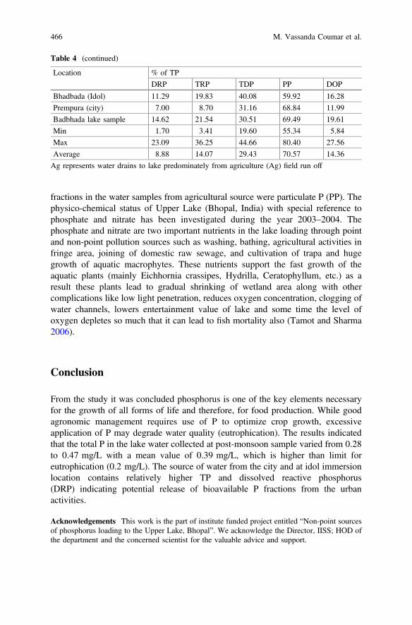
fractions in the water samples from agricultural source were particulate P (PP). Thephysico-chemical status of Upper Lake (Bhopal, India) with special reference tophosphate and nitrate has been investigated during the year 2003–2004. Thephosphate and nitrate are two important nutrients in the lake loading through pointand non-point pollution sources such as washing, bathing, agricultural activities infringe area, joining of domestic raw sewage, and cultivation of trapa and hugegrowth of aquatic macrophytes. These nutrients support the fast growth of theaquatic plants (mainly Eichhornia crassipes, Hydrilla, Ceratophyllum, etc.) as aresult these plants lead to gradual shrinking of wetland area along with othercomplications like low light penetration, reduces oxygen concentration, clogging ofwater channels, lowers entertainment value of lake and some time the level ofoxygen depletes so much that it can lead to fish mortality also (Tamot and Sharma2006).
Conclusion
From the study it was concluded phosphorus is one of the key elements necessaryfor the growth of all forms of life and therefore, for food production. While goodagronomic management requires use of P to optimize crop growth, excessiveapplication of P may degrade water quality (eutrophication). The results indicatedthat the total P in the lake water collected at post-monsoon sample varied from 0.28to 0.47 mg/L with a mean value of 0.39 mg/L, which is higher than limit foreutrophication (0.2 mg/L). The source of water from the city and at idol immersionlocation contains relatively higher TP and dissolved reactive phosphorus(DRP) indicating potential release of bioavailable P fractions from the urbanactivities.
Acknowledgements This work is the part of institute funded project entitled “Non-point sourcesof phosphorus loading to the Upper Lake, Bhopal”. We acknowledge the Director, IISS; HOD ofthe department and the concerned scientist for the valuable advice and support.
Table 4 (continued)
Location % of TP
DRP TRP TDP PP DOP
Bhadbada (Idol) 11.29 19.83 40.08 59.92 16.28
Prempura (city) 7.00 8.70 31.16 68.84 11.99
Badbhada lake sample 14.62 21.54 30.51 69.49 19.61
Min 1.70 3.41 19.60 55.34 5.84
Max 23.09 36.25 44.66 80.40 27.56
Average 8.88 14.07 29.43 70.57 14.36
Ag represents water drains to lake predominately from agriculture (Ag) field run off
466 M. Vassanda Coumar et al.

References
Choubey VK, Sharma MK, Dwivedi VK (2007) Water quality characteristics of the Upper Lake,M.P., India. In: The 12th world lake conference, pp 366–372
Kuo S (1996) Phosphorus. In: Sparks DL (ed) Methods of soil analysis. Agronomy 9. ASA-SSSA,Madison, WI
Murphy J, Riley JP (1962) A modified single solution method for the determination of phosphatein natural waters. Anal Chim Acta 27:31–36
Schindler DW (1997) Evolution of phosphorus limitation in lakes. Science 195:260–262Sharpley AN, Rekolainen S (1997) Phosphorus in agriculture and its environmental implications.
In: Tunney H, Carton OT, Brookes PC, Johnston AE (eds) Phosphorus loss from soil to water.CAB International, Arlington, pp 1–54
Sharpley AN, Tunney H (2000) Phosphorus research strategies to meet agricultural andenvironmental challenges of the 21st century. J Environ Qual 9:176–181
Tamot S, Sharma P (2006) Physico-chemical status of Upper Lake (Bhopal, India) water qualitywith special reference to phosphate and nitrate concentration and their impact on lakeecosystem. Asian J Exp Sci 20(1):151–158
Withers PJA, Sylvester-Bradley R, Jones DL, Healey JR, Talboys PJ (2014) Feed the crop not thesoil: rethinking phosphorus management in the food chain. Environ Sci Technol 48:6523–6530
Relative Contribution of Phosphorus from Various Sources … 467
Assessment of Fluoride in Rainfedand Irrigated Agricultural Soilof Tonalite–Trondjhemite Seriesin Central India
Bijendra Kumar and Anshumali
Abstract The systematic and comprehensive geochemical analysis of fluoride(F) in 20 agricultural soil samples was carried out to understand the spatial vari-ability, mechanism of retention and release, and the areas of potential risk due topoor or high concentrations of soil F around Sidhi District, Central India. Thespatial variations in physicochemical parameters revealed significant difference inthe methods of cultivation due to geomorphological constraints, availability ofsurface water and ground water, rainfall pattern, etc., in the study area. The northand small pocket in central Sidhi were rich in fertile soils due to availability ofsurface water and ground water. The southern and eastern Sidhi were rainfed areas,hence, the mono-cropping system by traditional methods showed less impact on thesoil physicochemical parameters. The soil F varied from 366.94 to 1178 mg/kg and2–4 times greater than the background soil value (320 mg/kg) of the world. Thepollution indexes were <1 revealed prevalence of elevated soil fluoride.
Keywords Soil fluoride � Fertilizers � Geogenic � Silicate mineralsSurface water � Rainfed
Introduction
The Sidhi District is situated on the northeastern boundary of the Madhya PradeshState, India which lies over a transitional area between the Indo-Gangetic plain in thenorth and the Deccan plateau in the south and the remotest district of MadhyaPradesh. Soil is one of the important and valuable resources of the nature. All livingthings are directly and indirectly dependent on soil for day-to-day needs and 95% ofthe human food is derived from the earth. Making plan for having healthy and
B. Kumar (&) � AnshumaliDepartment of Environmental Science and Engineering,Indian Institute of Technology (ISM) Dhanbad,Dhanbad 826004, Jharkhand, Indiae-mail: [email protected]
© Springer Nature Singapore Pte Ltd. 2018V.P. Singh et al. (eds.), Environmental Pollution, Water Scienceand Technology Library 77, https://doi.org/10.1007/978-981-10-5792-2_37
469
productive soil is essential to human survival. Soil is a natural body consisting oflayers (soil horizons) of mineral constituents of variable thicknesses, which differfrom the parent materials in their morphological, physical, chemical, and miner-alogical characteristics. Soil is composed of particles of broken rock that have beenaltered by chemical and mechanical processes that include weathering and erosion.The total fluoride concentration in soils are often derived from parent material,whereby its distribution in soil profiles is a function of soil-forming process, ofwhich the degree of weathering and clay content are the most prominent factors. Theaverage fluoride content of most soils worldwide has been documented as329 mg/kg (Kabata-Pendias and Pendia 1992). In general, the lowest F contents arefound in sandy soils in humid climate, whereas higher F concentrations occur inheavy clay soils and in soils from weathered mafic rocks (Fuge and Andrews 1988).Most of the fluoride in the soil is insoluble and, therefore, less available to plants.However, high soil fluoride concentrations or low pH, clay and/or organic matter canincrease fluoride levels in soil solution, increasing uptake via the plant root. Iffluoride is taken up through the root, its concentrations are often higher in the rootthan in the shoot, due to the low mobility of fluoride in the plant. Symptoms offluoride toxicity include emaciation, stiffness of joints, abnormal teeth and bones,lowered milk production, and detrimental effects on the reproductive capacity ofanimals. Soil is the medium from which plants and animals directly or indirectlyderive their nutrients and food, however, information regarding the concentrations offluoride in the around cultivated soils of the Sidhi District is limited or unavailable.
In view of this, no attention has ever been drawn to address the problem offluoride toxicity due to elevated concentration in the agricultural soils. In thisconnection, the present work aims at the determination of spatial distribution offluoride.
Study Area
The Sidhi District is situated on the northeastern boundary of the Madhya PradeshState, India which lies over a transitional area between the Indo-Gangetic plain inthe north and the Deccan plateau in the south. It is situated between 22° 47.5′ and24° 42.10′ North latitude and 81° 18.40′ and 82° 48.30′ East latitude (Fig. 1).
The physiography is characterized by low hill, extensive plateaus and rivervalleys such as Sone river valley which is a depository of the Gondwana rocks.Topographically the district can be divided into three zones, Vindhyan hills orKaimour range, Gondwana zone and Archean zone. Clay minerals like kaolinite,halloysite, diaspore, gibbsite, nacrite, dicktite, etc., were derived by the localizedweathering of arkosicmeta sediments (Mehrotra et al. 1979). The average elevationof the area is 311 m above MSL. The climate of the area is tropical monsoon typewith three distinct seasons as hot and dry summer (March–June), monsoon (July–September), and winter (November–February). The average annual rainfall variesfrom 1000 to 1200 mm, peaks in the months of July and August. The total
470 B. Kumar and Anshumali

population of the area is 1,126,515 spread with a density of 110/km2 (Census2011). The total land covered in the Sidhi District is 10,536 km2 in which the forestarea covers 40%. The portion of the land used for agricultural purpose is 47%, butonly 17% of the land used for agricultural purpose has assured supply of irrigationand the rest of the agricultural land is dependent on rainfed irrigation and producesonly one crop a year. The land is largely undulating terrain, which often has steepgradients not ideal for cultivation; the valleys along the major rivers like the Son
Fig. 1 Map of study area showing geology and sampling locations
Assessment of Fluoride in Rainfed and Irrigated Agricultural … 471
and the Gopad have fertile soils. The crops grown are rice, maize, barley, pigeonpea, and jute in Kharif season, and wheat, mustard and lentil in Rabi season.Sugarcane and cotton are grown at places under irrigated conditions. The naturalvegetation comprises tropical dry deciduous forests.
Method
Sampling: Moist Soil samples with water were collected from 20 different locationsof Sidhi District, where agricultural activities are more. These 20 sampling loca-tions are indicated in the map numbered from SSS1 to SSS20. The laboratoryanalysis is as follows: The pH and electrical conductivity (EC) were measured on a1:2.5 and 1:5 soil: water (w/v) ratio, respectively (Allison and Moodie 1965); soilorganic carbon and organic matter content was determined by the Walkley andBlack dichromate oxidation method (Nelson and Sommers 1982); the cationexchange capacity (CEC) by ammonium acetate method; The total soil fluoride wasobtained using the alkaline fusion method (Mcquaker and Gurney 1977). The totalcarbon (TC) and total nitrogen (TN) by Elemental Analyser (Thermo Flash 2000).The elements (Al, Fe, Ca, Mg, Mn, and P) were analyzed by the ICP-OES (LeemanProfile Plus) at NMDC, Donimalai, Karnataka. The particle size analysis wascarried out by Microtrac S3500 analyzer in Jawaharlal Nehru University. To assessthe pollution degree of fluoride in soils, single factor pollution index (SFPI) methodwas used (EPAC 2005): Pi = Ci/Si, where Pi is the single factor pollution index offluoride, Ci is the content of fluoride in soils at the sampling site, and Si is theevaluative standard value of fluoride. The background value (320 mg/kg) of theworld was taken as references to determine the starting value and contaminationlevels of soils (Alina and Henryk 1984). The descriptive statistical analysis wascarried out by the SPSS (version 16.00). The map of fluoride spatial distributionpattern was produced by using the Arcview (9.3) software for ordinary kriginginterpolation.
Results and Discussion
The pH of soil samples varied from 6.5 to 7.9 with scarce differences in mean soilpH between sites. Particle size analysis of soil samples showed a diversified rangeof sand, silt, and clay as 1.52–43.66%, 45.91–84.41% and 10.43–44.97%,respectively, with silt as the most dominating fraction. The soil organic carbon(SOC) and soil organic matter (SOM) at different locations were found to beranging from 0.24 to 1.93% and 0.43 to 3.32%, respectively. Across all locationsCEC showed significant spatial variation ranging from 7.65 to 20.38 Cmol/kg. Thefluoride concentrations ranged from 366.94 to 1178 mg/kg (Table 1). The soilfluoride concentrations in the Sidhi District were much higher than 320 mg/kg in
472 B. Kumar and Anshumali
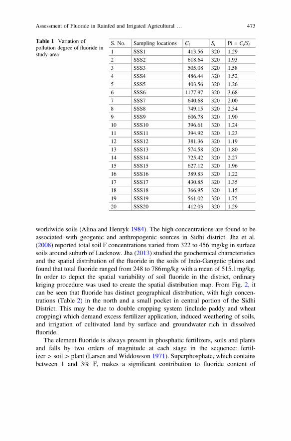
worldwide soils (Alina and Henryk 1984). The high concentrations are found to beassociated with geogenic and anthropogenic sources in Sidhi district. Jha et al.(2008) reported total soil F concentrations varied from 322 to 456 mg/kg in surfacesoils around suburb of Lucknow. Jha (2013) studied the geochemical characteristicsand the spatial distribution of the fluoride in the soils of Indo-Gangetic plains andfound that total fluoride ranged from 248 to 786mg/kg with a mean of 515.1mg/kg.In order to depict the spatial variability of soil fluoride in the district, ordinarykriging procedure was used to create the spatial distribution map. From Fig. 2, itcan be seen that fluoride has distinct geographical distribution, with high concen-trations (Table 2) in the north and a small pocket in central portion of the SidhiDistrict. This may be due to double cropping system (include paddy and wheatcropping) which demand excess fertilizer application, induced weathering of soils,and irrigation of cultivated land by surface and groundwater rich in dissolvedfluoride.
The element fluoride is always present in phosphatic fertilizers, soils and plantsand falls by two orders of magnitude at each stage in the sequence: fertil-izer > soil > plant (Larsen and Widdowson 1971). Superphosphate, which containsbetween 1 and 3% F, makes a significant contribution to fluoride content of
Table 1 Variation ofpollution degree of fluoride instudy area
S. No. Sampling locations Ci Si Pi = Ci/Si1 SSS1 413.56 320 1.29
2 SSS2 618.64 320 1.93
3 SSS3 505.08 320 1.58
4 SSS4 486.44 320 1.52
5 SSS5 403.56 320 1.26
6 SSS6 1177.97 320 3.68
7 SSS7 640.68 320 2.00
8 SSS8 749.15 320 2.34
9 SSS9 606.78 320 1.90
10 SSS10 396.61 320 1.24
11 SSS11 394.92 320 1.23
12 SSS12 381.36 320 1.19
13 SSS13 574.58 320 1.80
14 SSS14 725.42 320 2.27
15 SSS15 627.12 320 1.96
16 SSS16 389.83 320 1.22
17 SSS17 430.85 320 1.35
18 SSS18 366.95 320 1.15
19 SSS19 561.02 320 1.75
20 SSS20 412.03 320 1.29
Assessment of Fluoride in Rainfed and Irrigated Agricultural … 473
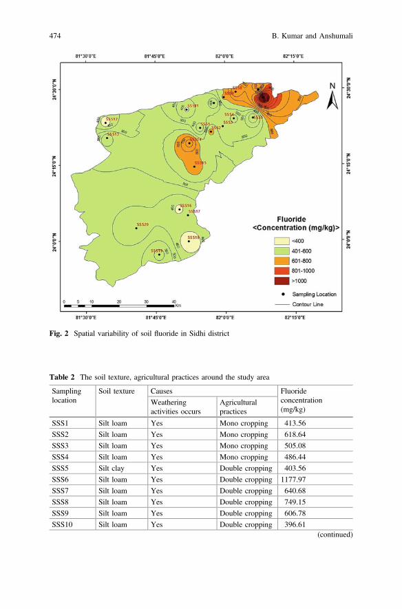
Fig. 2 Spatial variability of soil fluoride in Sidhi district
Table 2 The soil texture, agricultural practices around the study area
Samplinglocation
Soil texture Causes Fluorideconcentration(mg/kg)
Weatheringactivities occurs
Agriculturalpractices
SSS1 Silt loam Yes Mono cropping 413.56
SSS2 Silt loam Yes Mono cropping 618.64
SSS3 Silt loam Yes Mono cropping 505.08
SSS4 Silt loam Yes Mono cropping 486.44
SSS5 Silt clay Yes Double cropping 403.56
SSS6 Silt loam Yes Double cropping 1177.97
SSS7 Silt loam Yes Double cropping 640.68
SSS8 Silt loam Yes Double cropping 749.15
SSS9 Silt loam Yes Double cropping 606.78
SSS10 Silt loam Yes Double cropping 396.61(continued)
474 B. Kumar and Anshumali
agricultural soils. The major part of the district confirmed that the spatial distri-bution of soil fluoride (<400–600 mg/kg) was controlled by properties of regionalparent rocks than anthropogenic fluoride input.
Conclusions
The major cause of higher soil fluoride in northern Sidhi District and small pocketin central Sidhi, is not only by weathering of fluoride-rich minerals in the countryrocks but also by intensive agricultural activities, which is a major livelihoodoption, accelerated the cycling of soil fluoride. The overall contents of pedogenicelements reflect the highly weathered, dominance of non-silicate forms. From thedistribution of factor scores and loadings, it is observed that the predominantretention mechanism of fluoride on clays is supported by fine soil texture, organicmatter, and organic carbon. The double cropping systems augment fluoride toxicityin the northern Sidhi and a small pocket in central Sidhi. The major anthropogenicfactor responsible for fluoride enrichment is intensive fertilizer application. In anutshell, the natural sources are weathering of parent rocks and irrigation of cul-tivated land by surface water and ground water rich in dissolved fluoride.
Acknowledgements The authors thank the Ministry of Human Resource Development,Government of India and Indian School of Mines, Dhanbad for funding the research work. We arealso grateful to the Department of Environmental Science and Engineering, ISM, Dhanbad forproviding the logistic support to carry out field monitoring and laboratory analysis.
Table 2 (continued)
Samplinglocation
Soil texture Causes Fluorideconcentration(mg/kg)
Weatheringactivities occurs
Agriculturalpractices
SSS11 Silt clay loam Yes Double cropping 394.92
SSS12 Silt loam Yes Double cropping 381.36
SSS13 Silt loam Yes Double cropping 574.58
SSS14 Silt loam Yes Double cropping 725.42
SSS15 Silt loam Yes Double cropping 627.12
SSS16 Loam Yes Mono cropping 389.83
SSS17 Silt loam Yes Mono cropping 430.85
SSS18 Loam Yes Mono cropping 366.95
SSS19 Loam Yes Mono cropping 561.02
SSS20 Silt loam Yes Mono cropping 412.03
Assessment of Fluoride in Rainfed and Irrigated Agricultural … 475
References
Allison LE, Moodie CD (1965) Carbonates. P.1379-400. In: Black CA et al (eds) Methods of soilanalysis. Part 2. 2nd ed. Agron. Monogr. 9. ASA, CSSA and SSSA, Madison, WI
Alina KP, Henryk P (1984) Trace elements in soils and plants. CRC Press, FloridaCensus (2011) Census of India for Provisional population totals. Ministry of home affairs.
Government of IndiaEPAC (2005) The technical speciation for soil environment monitoring (HJ/T166-2004).
Environmental Press of China, BeijingFuge R, Andrews MJ (1988) Fluoride in the UK Environ. Environ Geochem Health 96:10Jha SK, Nayak AK, Sharma YK, Mishra VK, Sharma DK (2008) Fluoride accumulation in soil
and vegetation in the vicinity of Brick Fields. Bull Environ Contam Toxicol 80:369–373Jha SK (2013) Geochemical and spatial appraisal of fluoride in the soils of Indo-Gangetic Plains of
India using multivariate analysis. CLEAN—Soil Air Water 41(3):313–314Kabata-Pendias A, Pendia H (1992) Trace elements in soils and plants. CRC Press, BocaratonLarsen S, Widdowson AE (1971) Soilfluoride. J Soil Sci 22:211–221Mcquaker NR, Gurney M (1977) Determination of total fluoride in soil and vegetation using an
alkali fusion–selective ion electrode technique. Anal Chem 49:53–6Mehrotra RC, Varma SN, Singh BK (1979) Physico-chemical behaviour of hydrated aluminium
oxides and associated clay minerals occurring around Pipra, District Sidhi, India. J Therm Anal16:453–462
Nelson DW, Sommer LE (1982) Total carbon, organic carbon, and organic matter. In: Page AL(ed) Methods of soil analysis, 2nd ed. Chemical and microbiological properties, (methodsof-soilan2), pp 539–579
476 B. Kumar and Anshumali
Biomonitoring of Paravur Lake in KeralaUsing Macro-Invertebrates
J. Sreeja
Abstract Macro-invertebrates are the most commonly suggested bioindicators forbiomonitoring and have been extensively studied in temperate areas. On the otherhand, the methodology and theoretical background of biomonitoring have not yetbeen sufficiently adapted to tropical aquatic environments. Bioassessment/biomonitoring is a reliable and holistic method of ecosystem assessment integrat-ing water quality assessment, habitat assessment and biological assessment. Bioassessment protocol using macro-invertebrates was adapted from United StatesEnvironment Protection Agency (USEPA) and applied successfully in ParavurLake, located on the southwest coast of Kerala. This lake is one of the ecologicallydegraded lakes due to certain anthropogenic activities. Three sites were selected inorder to assess the health status of Paravur Lake. From the three sites selected, site Iwas less polluted (Reference Station), site II was slightly polluted and site III washeavily polluted. Category I macroorganisms were found in site I, category II werefound dominant in site II and category III organisms were dominant in site III.A multimetric analysis using physicochemical parameters, species diversity andcommunity analysis of macro-invertebrates were carried out to evaluate the presenthealth status of Paravur Lake ecosystem.
Introduction
Backwaters are valuable fishery resources that contribute to the inland fish pro-duction of a country. Environmental conditions play a vital role in governing thelife history, behavior distribution and abundance of organisms particularly in theaquatic environments. Knowledge of the environmental condition is highlyessential for understanding the occurrence and abundance of aquatic organisms.
J. Sreeja (&)Department of Zoology, S. N. College for Women, Kollam 691001, Kerala, Indiae-mail: [email protected]
© Springer Nature Singapore Pte Ltd. 2018V.P. Singh et al. (eds.), Environmental Pollution, Water Scienceand Technology Library 77, https://doi.org/10.1007/978-981-10-5792-2_38
477
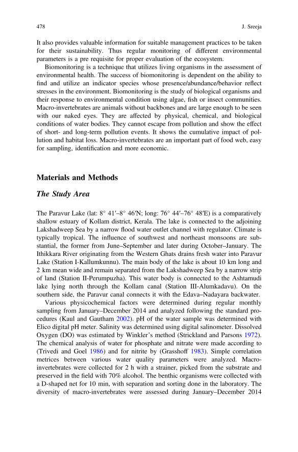
It also provides valuable information for suitable management practices to be takenfor their sustainability. Thus regular monitoring of different environmentalparameters is a pre requisite for proper evaluation of the ecosystem.
Biomonitoring is a technique that utilizes living organisms in the assessment ofenvironmental health. The success of biomonitoring is dependent on the ability tofind and utilize an indicator species whose presence/abundance/behavior reflectstresses in the environment. Biomonitoring is the study of biological organisms andtheir response to environmental condition using algae, fish or insect communities.Macro-invertebrates are animals without backbones and are large enough to be seenwith our naked eyes. They are affected by physical, chemical, and biologicalconditions of water bodies. They cannot escape from pollution and show the effectof short- and long-term pollution events. It shows the cumulative impact of pol-lution and habitat loss. Macro-invertebrates are an important part of food web, easyfor sampling, identification and more economic.
Materials and Methods
The Study Area
The Paravur Lake (lat: 8° 41′–8° 46′N; long: 76° 44′–76° 48′E) is a comparativelyshallow estuary of Kollam district, Kerala. The lake is connected to the adjoiningLakshadweep Sea by a narrow flood water outlet channel with regulator. Climate istypically tropical. The influence of southwest and northeast monsoons are sub-stantial, the former from June–September and later during October–January. TheIthikkara River originating from the Western Ghats drains fresh water into ParavurLake (Station I-Kallumkunnu). The main body of the lake is about 10 km long and2 km mean wide and remain separated from the Lakshadweep Sea by a narrow stripof land (Station II-Perumpuzha). This water body is connected to the Ashtamudilake lying north through the Kollam canal (Station III-Alumkadavu). On thesouthern side, the Paravur canal connects it with the Edava–Nadayara backwater.
Various physicochemical factors were determined during regular monthlysampling from January–December 2014 and analyzed following the standard pro-cedures (Kaul and Gautham 2002). pH of the water sample was determined withElico digital pH meter. Salinity was determined using digital salinometer. DissolvedOxygen (DO) was estimated by Winkler’s method (Strickland and Parsons 1972).The chemical analysis of water for phosphate and nitrate were made according to(Trivedi and Goel 1986) and for nitrite by (Grasshoff 1983). Simple correlationmetrices between various water quality parameters were analyzed. Macro-invertebrates were collected for 2 h with a strainer, picked from the substrate andpreserved in the field with 70% alcohol. The benthic organisms were collected witha D-shaped net for 10 min, with separation and sorting done in the laboratory. Thediversity of macro-invertebrates were assessed during January–December 2014
478 J. Sreeja

following standard techniques (Hilsenhoff 1998). Hilsenhoff Biotic Index (HBI),Family Biotic Index (FBI), Pollution Tolerance Index (PTI) were calculated.
Result
The results of various physico–chemical parameters revealed that the Station III ishighly depleted and has poor water quality (HBI = 6.5, PTI = 8, FBI = 8.5) and wasbelow the desirable limits o f US-EPA and CPCB (Central Pollution Control Board).In Station II HBI = 4.2, PTI = 5, FBI = 5.3 and thus water quality is in a desirablelevel. Station I is the reference site where HBI = 2.1, PTI = 1 and FBI = 3.8. Hencethe water quality is very good. Different types of macro-invertebrates collected fromdifferent Stations are represented in Figs. 1, 2, 3 and 4).
From the multimetric indices-IBI showed that the organisms like caddis flylarvae, may fly larvae and stone fly larvae, water penny and dytiscus larvae are verysensitive to pollution and seen only in site I. The nymph of stone flies and May fliesare the first to disappear from water which has high organic pollution. As pollutionincreases caddis fly larvae, dytiscus larvae and water pennies move into less pol-luted region. These organisms found in site I are completely absent in site II and IIIdue to organic pollution. In Station II, Mussels are the dominant organisms,followed by shrimp. Dragon and damsel fly larvae are seen in region where thewater quality is in desirable limit. Category II organisms comparatively have moretolerance than category I organisms. In Station III mosquito larvae are the dominantspecies followed by snails, chironomous larvae, tubifex and rat tailed maggots.
Fig. 1 Map showing study area of Paravur lake
Biomonitoring of Paravur Lake in Kerala Using Macro-Invertebrates 479

These category III organisms have high pollution tolerance index. Hence they areable to survive in such a highly polluted area like StationIII.
The different physico-chemical parameters of the three Stations were representedin Tables 1, 2 and 3. Atmospheric temperature varied between 25 °C (Monsoonseason, Station III) to 30 °C (Post monsoon period in Station I). Water temperaturevaried between 22 °C (Monsoon season, Station III) to 28 °C (Post monsoon periodin Station I). pH variation noted during all the seasons and ranged between 6.8 inStation I during pre-monsoon season and 12 in Station III during post monsoonperiod. Maximum salinity (6‰) noticed in Station II during monsoon season andno salinity at Station I in monsoon season. Dissolved oxygen ranged between
210
128
180
215
90
305 Caddi's fly larva
May fly larva
Stone fly larva
Water penny
Whirligis beetle
Dy scus
Fig. 2 Macro-invertebrates collected from Station I (Category I)
88
55
280 395
78 30
Damsel fly larva
Dragon fly larva
Shrimp
Mussel
Planarians
Snails
Fig. 3 Macro-invertebrates collected from Station II (Category II)
480 J. Sreeja
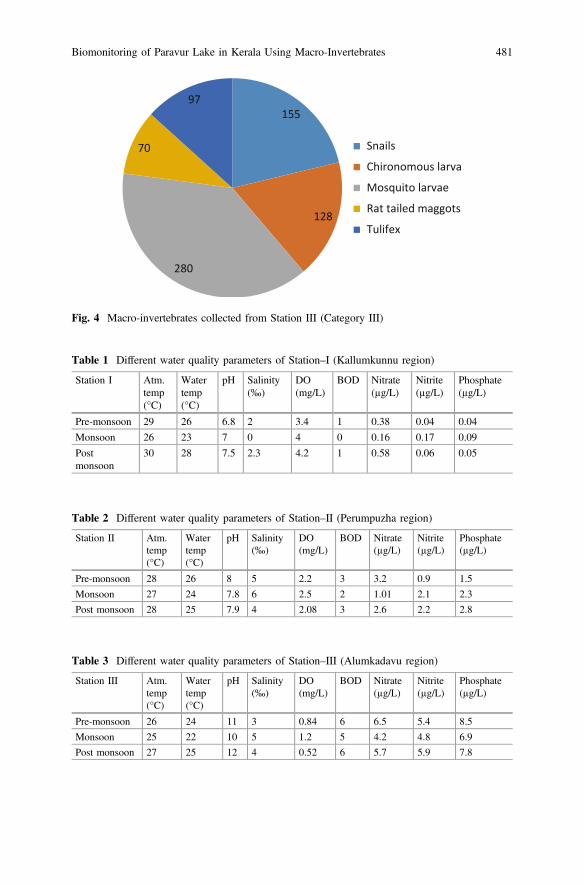
155
128
280
70
97
Snails
Chironomous larva
Mosquito larvae
Rat tailed maggots
Tulifex
Fig. 4 Macro-invertebrates collected from Station III (Category III)
Table 1 Different water quality parameters of Station–I (Kallumkunnu region)
Station I Atm.temp(°C)
Watertemp(°C)
pH Salinity(‰)
DO(mg/L)
BOD Nitrate(µg/L)
Nitrite(µg/L)
Phosphate(µg/L)
Pre-monsoon 29 26 6.8 2 3.4 1 0.38 0.04 0.04
Monsoon 26 23 7 0 4 0 0.16 0.17 0.09
Postmonsoon
30 28 7.5 2.3 4.2 1 0.58 0.06 0.05
Table 2 Different water quality parameters of Station–II (Perumpuzha region)
Station II Atm.temp(°C)
Watertemp(°C)
pH Salinity(‰)
DO(mg/L)
BOD Nitrate(µg/L)
Nitrite(µg/L)
Phosphate(µg/L)
Pre-monsoon 28 26 8 5 2.2 3 3.2 0.9 1.5
Monsoon 27 24 7.8 6 2.5 2 1.01 2.1 2.3
Post monsoon 28 25 7.9 4 2.08 3 2.6 2.2 2.8
Table 3 Different water quality parameters of Station–III (Alumkadavu region)
Station III Atm.temp(°C)
Watertemp(°C)
pH Salinity(‰)
DO(mg/L)
BOD Nitrate(µg/L)
Nitrite(µg/L)
Phosphate(µg/L)
Pre-monsoon 26 24 11 3 0.84 6 6.5 5.4 8.5
Monsoon 25 22 10 5 1.2 5 4.2 4.8 6.9
Post monsoon 27 25 12 4 0.52 6 5.7 5.9 7.8
Biomonitoring of Paravur Lake in Kerala Using Macro-Invertebrates 481
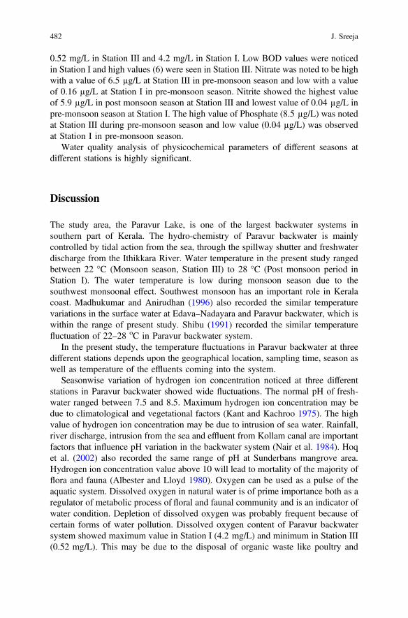
0.52 mg/L in Station III and 4.2 mg/L in Station I. Low BOD values were noticedin Station I and high values (6) were seen in Station III. Nitrate was noted to be highwith a value of 6.5 µg/L at Station III in pre-monsoon season and low with a valueof 0.16 µg/L at Station I in pre-monsoon season. Nitrite showed the highest valueof 5.9 µg/L in post monsoon season at Station III and lowest value of 0.04 µg/L inpre-monsoon season at Station I. The high value of Phosphate (8.5 µg/L) was notedat Station III during pre-monsoon season and low value (0.04 µg/L) was observedat Station I in pre-monsoon season.
Water quality analysis of physicochemical parameters of different seasons atdifferent stations is highly significant.
Discussion
The study area, the Paravur Lake, is one of the largest backwater systems insouthern part of Kerala. The hydro-chemistry of Paravur backwater is mainlycontrolled by tidal action from the sea, through the spillway shutter and freshwaterdischarge from the Ithikkara River. Water temperature in the present study rangedbetween 22 °C (Monsoon season, Station III) to 28 °C (Post monsoon period inStation I). The water temperature is low during monsoon season due to thesouthwest monsoonal effect. Southwest monsoon has an important role in Keralacoast. Madhukumar and Anirudhan (1996) also recorded the similar temperaturevariations in the surface water at Edava–Nadayara and Paravur backwater, which iswithin the range of present study. Shibu (1991) recorded the similar temperaturefluctuation of 22–28 oC in Paravur backwater system.
In the present study, the temperature fluctuations in Paravur backwater at threedifferent stations depends upon the geographical location, sampling time, season aswell as temperature of the effluents coming into the system.
Seasonwise variation of hydrogen ion concentration noticed at three differentstations in Paravur backwater showed wide fluctuations. The normal pH of fresh-water ranged between 7.5 and 8.5. Maximum hydrogen ion concentration may bedue to climatological and vegetational factors (Kant and Kachroo 1975). The highvalue of hydrogen ion concentration may be due to intrusion of sea water. Rainfall,river discharge, intrusion from the sea and effluent from Kollam canal are importantfactors that influence pH variation in the backwater system (Nair et al. 1984). Hoqet al. (2002) also recorded the same range of pH at Sunderbans mangrove area.Hydrogen ion concentration value above 10 will lead to mortality of the majority offlora and fauna (Albester and Lloyd 1980). Oxygen can be used as a pulse of theaquatic system. Dissolved oxygen in natural water is of prime importance both as aregulator of metabolic process of floral and faunal community and is an indicator ofwater condition. Depletion of dissolved oxygen was probably frequent because ofcertain forms of water pollution. Dissolved oxygen content of Paravur backwatersystem showed maximum value in Station I (4.2 mg/L) and minimum in Station III(0.52 mg/L). This may be due to the disposal of organic waste like poultry and
482 J. Sreeja
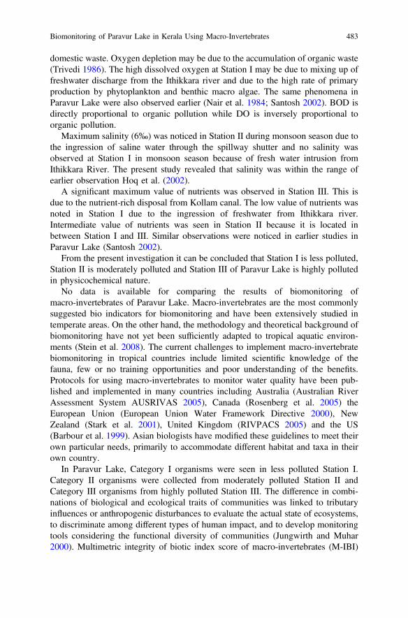
domestic waste. Oxygen depletion may be due to the accumulation of organic waste(Trivedi 1986). The high dissolved oxygen at Station I may be due to mixing up offreshwater discharge from the Ithikkara river and due to the high rate of primaryproduction by phytoplankton and benthic macro algae. The same phenomena inParavur Lake were also observed earlier (Nair et al. 1984; Santosh 2002). BOD isdirectly proportional to organic pollution while DO is inversely proportional toorganic pollution.
Maximum salinity (6‰) was noticed in Station II during monsoon season due tothe ingression of saline water through the spillway shutter and no salinity wasobserved at Station I in monsoon season because of fresh water intrusion fromIthikkara River. The present study revealed that salinity was within the range ofearlier observation Hoq et al. (2002).
A significant maximum value of nutrients was observed in Station III. This isdue to the nutrient-rich disposal from Kollam canal. The low value of nutrients wasnoted in Station I due to the ingression of freshwater from Ithikkara river.Intermediate value of nutrients was seen in Station II because it is located inbetween Station I and III. Similar observations were noticed in earlier studies inParavur Lake (Santosh 2002).
From the present investigation it can be concluded that Station I is less polluted,Station II is moderately polluted and Station III of Paravur Lake is highly pollutedin physicochemical nature.
No data is available for comparing the results of biomonitoring ofmacro-invertebrates of Paravur Lake. Macro-invertebrates are the most commonlysuggested bio indicators for biomonitoring and have been extensively studied intemperate areas. On the other hand, the methodology and theoretical background ofbiomonitoring have not yet been sufficiently adapted to tropical aquatic environ-ments (Stein et al. 2008). The current challenges to implement macro-invertebratebiomonitoring in tropical countries include limited scientific knowledge of thefauna, few or no training opportunities and poor understanding of the benefits.Protocols for using macro-invertebrates to monitor water quality have been pub-lished and implemented in many countries including Australia (Australian RiverAssessment System AUSRIVAS 2005), Canada (Rosenberg et al. 2005) theEuropean Union (European Union Water Framework Directive 2000), NewZealand (Stark et al. 2001), United Kingdom (RIVPACS 2005) and the US(Barbour et al. 1999). Asian biologists have modified these guidelines to meet theirown particular needs, primarily to accommodate different habitat and taxa in theirown country.
In Paravur Lake, Category I organisms were seen in less polluted Station I.Category II organisms were collected from moderately polluted Station II andCategory III organisms from highly polluted Station III. The difference in combi-nations of biological and ecological traits of communities was linked to tributaryinfluences or anthropogenic disturbances to evaluate the actual state of ecosystems,to discriminate among different types of human impact, and to develop monitoringtools considering the functional diversity of communities (Jungwirth and Muhar2000). Multimetric integrity of biotic index score of macro-invertebrates (M-IBI)
Biomonitoring of Paravur Lake in Kerala Using Macro-Invertebrates 483
obtained from nine benthic metrics ranged from 11 to 45 showed that VellayaniLake ranked under excellent water quality with 45 as IBI score where as poor tovery poor conditions at Veli-Akkulam lake (Abhijna and Biju Kumar 2012;Abhijna and Biju Kumar 2014). The relative taxonomic composition ofmacro-invertebrate taxa showed maximum abundance and dominance of less pol-lution tolerant group in Vellayani lake of Kerala (Abhijna et al. 2013). The result ofthe Paravur Lake is in agreement with the studies done in Vellayani lake in Kerala(Abhijna and Biju Kumar 2014). Therefore the study recommends the introductionof biomonitoring techniques and improvement of water quality by proper man-agement practices to restore water quality conditions and ensure the health status ofParavur Lake in Kerala.
Conclusion
The hydrographical study can be concluded as that Station I was less polluted,Station II was moderately polluted and Station III of Paravur Lake was highlypolluted. Biomonitoring methodology also revealed the same result. Hence thistechnique is a simple and reliable method for sustainable management of waterresources.
References
Abhijna UG, Biju Kumar A (2012) Diversity and community analysis of order: diptera ofVeliAkkulam Lake, South west Coast of Kerala. J Environ Ecol 30(2):386–392
Abhijna UG, Kumar AB (2014) Benthic macro-invertebrates community as indicators of health ofVellayani freshwater lake, Kerala. In: Pillai VNR (ed) Proceedings of the 26th Kerala sciencecongress, Pookode, Wayanad, pp 459–470, Kerala State Council for Science, Technology andEnvironment, Thiruvananthapuram, Kerala
Abhijna UG, Ratheesh R, Biju Kumar A (2013) Diversity and distribution of aquatic insects offresh water Vellayani lake, South west coast of Kerala. J Environ Biol 34:605–611
Albester JS Lloyd R (1980) Water quality criteria for fresh water fish. Batterworth and Co. Ltd.,London
Australian River Assessment System (AUSRIVAS) (2005) AUSRIVAS Bioassessment:macro-invertebrates.http://ausrivas.canberra.edu.au/Bioassessment/macro-invertebrates/
Barbour MT, Gerritsen J, Snyder BD, Stribling JB (1999) Rapid bioassessment protocols for use instreams and wadeable rivers: periphyton, benthic macro-invertebrates and fish, 2nd edn.Washington, DC, USEPA
European Union Water Framework Directive (2000) WFD, Directive 2000/60/EC. Official J EurCommun 23:1–72
Grasshoff K (1983) Determination of nitrite. In: Grasshoff K, Ehrhardt M, Kremling K(eds) Methods of sea water analysis, Verlag Chemic Gymb, Weinheim, 419 p
Hilsenhoff WL (1998) A modification of the biotic index of organic stream pollution to remedyproblems and permit its use throughout the year. Great Lakes Entomol 31:1–12
484 J. Sreeja
Hoq EM, Islam ML, Paul HK, Ahmed SU (2002) Decomposition and seasonal changes in nutrientconstitution in Mangrove litter of Sunderbans Mangrove, Bangladesh. Indian J Mar Sci 31(2):130–135
Jungwirth M, Muhar S, Schmutz (2000) Assessing the ecological integrity of running water.Kluwer Academic Publ 153–162
Kant S, Kachroo P (1975) Limnological studies in Kashmir Lakes-II. Diurnal movement ofphytoplankton. J Ind Bot Soc 54(1/2):9–12
Kaul SN, Gautham A (2002) Water and waste water analysis, Daya Publ. House, 335 pMadhukumar A, Anirudhan TS (1996) The hydrographic features and chemical characteristics of
Edava-Nadayara and Paravur backwaters. Enviromedia (Roll Res) 15(1):79–84Nair NB, Abdul Azis PK, Krishnakumar K, Dharmaraj K, Arunachalam M (1984) Ecology of
Indian estuaries: Part VI-physicochemical conditions in Kadinamkulam backwater, southwestcoast of India. Indian J Mar Sci 13(2):69–74
RIVPACS (2005). http://dorset.ceh.ac.uk/River_Ecology/River_Communities/Rivpacs_2003/rivpacs_Introduction.htm
Rosenberg DM, Davies IJ, Cobb DG, Wiens AP (2005) Protocols for measuring biodiversity:benthic macro-invertebrates in freshwaters. Department of Fisheries and Oceans, Winnipeg,Canada
Santosh S (2002) Hydro-chemistry of Paravur-Kappil backwater with special reference toplankton, Kollam dt, Kerala, India. Ph.D. thesis, Univ of Kerala. Trivandrum
Shibu S (1991) Ecology of Paravur lake. Ph.D. thesis, Univ of Kerala, TrivandrumStark JD, Boothroyd IKG, Harding JS et al. (2001) Protocols for sampling macro-invertebrates in
wadeable streams. New Zealand Ministry for the Environment, Auckland, NewzealandStein H, Springer M, Kohlmann B (2008) Comparison of two sampling methods for biomonitoring
using aquatic macro-invertebrates in the Dos Novillos river. Costa Rica J Ecol Eng 34(4):267–275
Strickland JDH, Parsons TR (1972) A practical handbook of sea water analysis. Bull Fish Res BiolCan 167, 311 p
Trivedi RK, Goel PK (1986) Chemical and biological methods for water pollution studies. EnvironPubl Karad (India), 248 p
Biomonitoring of Paravur Lake in Kerala Using Macro-Invertebrates 485
Change Detection of Sodic Landin Raebareli District Using RemoteSensing and GIS Techniques
Arif Ahmad, R.K. Upadhyay, B. Lal and Dhananjay Singh
Abstract Remote sensing and GIS play a vital role in trend analysis over sodicland and use of alternative measures to minimize the time and cost in reclamationprocesses. Sodic land is the highly contaminated of salt having pH range of 9.5–10.5 and sodium percentage greater than 15% above which is caused by naturallyand anthropogenic. In this study, Raebareli district has been taken as the study areafor mapping and monitoring the change detection with respect to sodic lands.LISS III data are used for mapping sodic land in both years 1997 and 2012. Themaximum likelihood algorithm method was used for area statistics of differentcategories of sodic land followed by integration of both the classification of satellitedata of Rabi seasons. The Sodic land covers 28823.91 ha area in 1997, which is8.80% of the total geographical area of the district. At present the total area of sodic
A. Ahmad (&)School of Geo-informatics, Remote Sensing Applications Centre, Lucknow 226021,Uttar Pradesh, Indiae-mail: [email protected]
R.K. UpadhyayAgriculture Resources Division (ARD), Remote Sensing Application Centre, Lucknow226021, Uttar Pradesh, Indiae-mail: [email protected]
B. LalSoil Resources Division (SRD), Remote Sensing Application Centre, Lucknow 226021,Uttar Pradesh, Indiae-mail: [email protected]
D. SinghRemote Sensing Application Centre, Lucknow 226021, Uttar Pradesh, Indiae-mail: [email protected]
© Springer Nature Singapore Pte Ltd. 2018V.P. Singh et al. (eds.), Environmental Pollution, Water Scienceand Technology Library 77, https://doi.org/10.1007/978-981-10-5792-2_39
487

lands have been decreased by 18483.60 ha, which covers 10340.31 ha area in2012, which is 5.64% of the total geographical area of the district. The majorchanges have been reported mainly in terms of wastelands, fallow land and sodicland areas, which have been reported to decrease over the years.
Keywords Remote sensing and GIS � Sodic land � Multi seasonal remotesensing satellite data � NDVI � Change detection
Introduction
Salt-influenced soils have a field over the world, particularly in semi-arid, arid andsub-humid regions. Salt-influenced soils happen both normally and as the aftereffect of man’s adjustment of the hydrologic forms which activate and accumulatesalts within the landscape. Nonetheless, it ought to be noted at the start that there aretwo expansive classes of salt-influenced soils. Saline soils are those with a liftedconvergence of any sort of salt, though “sodic” soils are those soils with a highextent of sodium particles in respect to different cations in the soil or water. Anextensive list of land disturbance activities, including road development, happen onsodium-influenced soils. Soils with abnormal amounts of replaceable sodium andlow levels of aggregate dissolvable salts are vulnerable to clay dispersion whichprompts to crusting, low permeability, high bulk density and low porosity. Soilsaltiness and water logging are two of the fundamental requirements introduce inirrigated agricultural lands. The capacity of space platforms to give synoptic per-spective of the region makes remote sensing an exceptional tool for quick andtimely observing of earth resources and depiction of salt-influenced soils. Thecombination of remote sensing with the geographical information system (GIS) isutilized for assortment information to delineate salt affected soil.
The most regularly utilized procedure for a salinity index is the calculation ofvarious indices and proportion pictures utilizing infrared and visible spectral bandin the electromagnetic range. Dry soil for the most part has higher reflectance andno absorption in red region have been utilized in vegetation indices. Among a fewvegetation indices, normalized difference vegetation index (NDVI), soil adjustedvegetation index (SAVI), and were utilized to describe crop growth conditionimpacted by salinity (ref.).
Three spectral indices for the identification of saltiness in Raebareli, UttarPradesh, India, using the LISS-III sensor on IRS-platform 1C and P6, are the soilbrightness index (SBI), normalized difference vegetation index (NDVI), Statisticalinvestigation of the study area and generation of Change detection map delineate
488 A. Ahmad et al.

with the help of satellite data (IRS-stage 1C and P6). Land cover/land use and sodicland changes additionally include the alteration either immediate or roundabout ofcharacteristic natural surroundings and their effect on the ecology of the area.Remote sensing technology for catching the spatial information, GeographicInformation System for undertaking coordinated investigation, presentation ofspatial and associated attribute information are observed to be a great deal moresuccessful to known the change detection of land use/land cover.
Study Area
The study area is Raebareli district, Uttar Pradesh, India. The study area is situatedbetween geo-coordinates UTM_Zone_44, 25° 49′ to 26° 36′N Latitude and between100° 41′ and 81° 34′E Longitude. The district of Raebareli has a large area cover of4,609 km2. Though compact and irregular in shape the dimensions of districtchanges every year due to the course of holy River Ganga and its action. Littlechange in the stream of river makes significant variation in the area of this territorythat is likely to every year. Loamy sand, sandy loam, clay loam and silt loam soilsare found in the district. During summers the mercury level could go as high as 45–50 °C. A little alleviation could be seen by mid June with precipitation principallyfrom South Western Winds. It rains from 900 to 1200 mm here from June toSeptember approximately every year (Fig. 1).
Material and Method
For the purpose following multi-date LISS III Satellite data of 01 February 1997and 07 February 2012 are used for image processing and salt delineation of thestudy area. During the month of February and May salt has got accumulated on thesurface due to high evaporation rates. The published soil survey reports, soil maps,atlas of India, and water quality reports (RSAC, UP) for the study area, were arecollected and utilized during interpretation and field work. Salinity is a naturalcharacteristic of soil, but salinization is caused by the human interactions. Salinity isdefined by the accumulation of Salt soluble in the soil.
Change Detection of Sodic Land in Raebareli … 489
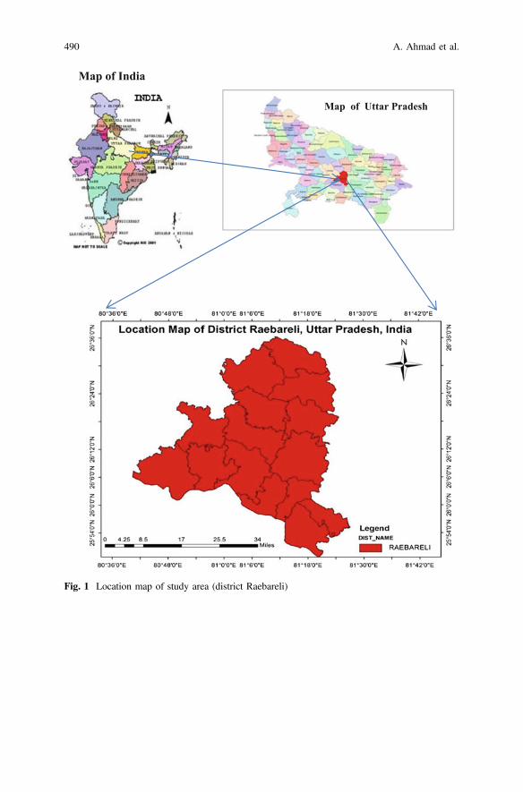
Map of India
Map of Uttar Pradesh
Fig. 1 Location map of study area (district Raebareli)
490 A. Ahmad et al.

Multi-date Data IRS-1C/P6 LISS-III Data
Rabi Season (01 Feb 1997) Rabi Season (07 Feb 2012)
Satellite data download, & import data (Bhuwan etc.)
Image to image Registration
Boundary overlay and subset district area
Mask (Inside, Outside, Non-agriculture, Soil area, Combined)
Un-Supervised classification
Using ground truth data Combined Mask (Major crops, other crops and Fallowlandetc.)
Generation of cropping pattern map of Rabi season
Change detection mapping
Composition of Change detection map of the study area
Change Detection of Sodic Land in Raebareli … 491
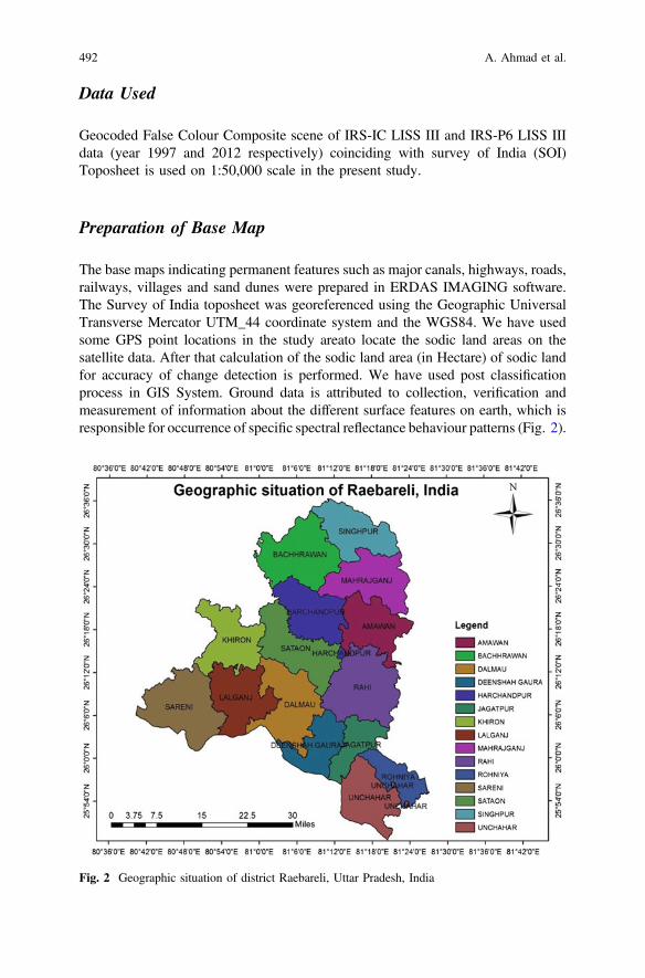
Data Used
Geocoded False Colour Composite scene of IRS-IC LISS III and IRS-P6 LISS IIIdata (year 1997 and 2012 respectively) coinciding with survey of India (SOI)Toposheet is used on 1:50,000 scale in the present study.
Preparation of Base Map
The base maps indicating permanent features such as major canals, highways, roads,railways, villages and sand dunes were prepared in ERDAS IMAGING software.The Survey of India toposheet was georeferenced using the Geographic UniversalTransverse Mercator UTM_44 coordinate system and the WGS84. We have usedsome GPS point locations in the study areato locate the sodic land areas on thesatellite data. After that calculation of the sodic land area (in Hectare) of sodic landfor accuracy of change detection is performed. We have used post classificationprocess in GIS System. Ground data is attributed to collection, verification andmeasurement of information about the different surface features on earth, which isresponsible for occurrence of specific spectral reflectance behaviour patterns (Fig. 2).
Fig. 2 Geographic situation of district Raebareli, Uttar Pradesh, India
492 A. Ahmad et al.
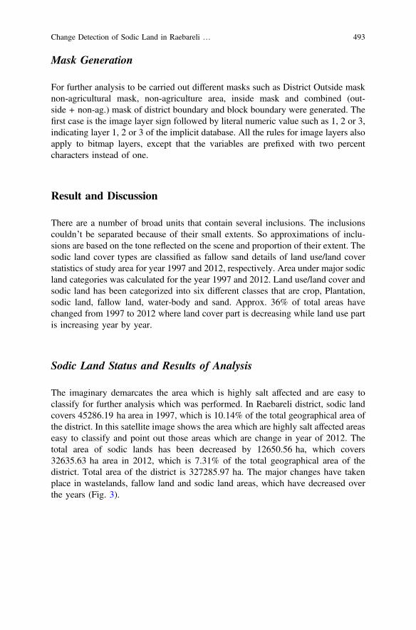
Mask Generation
For further analysis to be carried out different masks such as District Outside masknon-agricultural mask, non-agriculture area, inside mask and combined (out-side + non-ag.) mask of district boundary and block boundary were generated. Thefirst case is the image layer sign followed by literal numeric value such as 1, 2 or 3,indicating layer 1, 2 or 3 of the implicit database. All the rules for image layers alsoapply to bitmap layers, except that the variables are prefixed with two percentcharacters instead of one.
Result and Discussion
There are a number of broad units that contain several inclusions. The inclusionscouldn’t be separated because of their small extents. So approximations of inclu-sions are based on the tone reflected on the scene and proportion of their extent. Thesodic land cover types are classified as fallow sand details of land use/land coverstatistics of study area for year 1997 and 2012, respectively. Area under major sodicland categories was calculated for the year 1997 and 2012. Land use/land cover andsodic land has been categorized into six different classes that are crop, Plantation,sodic land, fallow land, water-body and sand. Approx. 36% of total areas havechanged from 1997 to 2012 where land cover part is decreasing while land use partis increasing year by year.
Sodic Land Status and Results of Analysis
The imaginary demarcates the area which is highly salt affected and are easy toclassify for further analysis which was performed. In Raebareli district, sodic landcovers 45286.19 ha area in 1997, which is 10.14% of the total geographical area ofthe district. In this satellite image shows the area which are highly salt affected areaseasy to classify and point out those areas which are change in year of 2012. Thetotal area of sodic lands has been decreased by 12650.56 ha, which covers32635.63 ha area in 2012, which is 7.31% of the total geographical area of thedistrict. Total area of the district is 327285.97 ha. The major changes have takenplace in wastelands, fallow land and sodic land areas, which have decreased overthe years (Fig. 3).
Change Detection of Sodic Land in Raebareli … 493
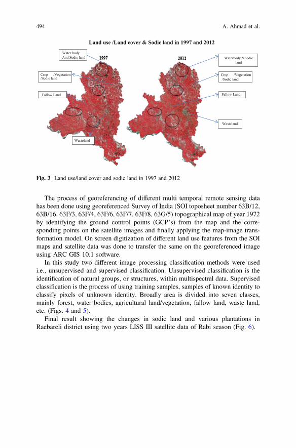
The process of georeferencing of different multi temporal remote sensing datahas been done using georeferenced Survey of India (SOI toposheet number 63B/12,63B/16, 63F/3, 63F/4, 63F/6, 63F/7, 63F/8, 63G/5) topographical map of year 1972by identifying the ground control points (GCP’s) from the map and the corre-sponding points on the satellite images and finally applying the map-image trans-formation model. On screen digitization of different land use features from the SOImaps and satellite data was done to transfer the same on the georeferenced imageusing ARC GIS 10.1 software.
In this study two different image processing classification methods were usedi.e., unsupervised and supervised classification. Unsupervised classification is theidentification of natural groups, or structures, within multispectral data. Supervisedclassification is the process of using training samples, samples of known identity toclassify pixels of unknown identity. Broadly area is divided into seven classes,mainly forest, water bodies, agricultural land/vegetation, fallow land, waste land,etc. (Figs. 4 and 5).
Final result showing the changes in sodic land and various plantations inRaebareli district using two years LISS III satellite data of Rabi season (Fig. 6).
Water body And Sodic land
Crop /Vegetation/Sodic land
Wasteland
Fallow Land
Waterbody &Sodicland
Crop /Vegetation/Sodic land
Fallow Land
Wasteland
Land use /Land cover & Sodic land in 1997 and 2012
Fig. 3 Land use/land cover and sodic land in 1997 and 2012
494 A. Ahmad et al.
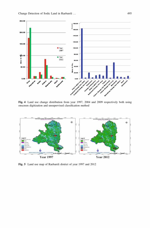
Fig. 4 Land use change distribution from year 1997, 2004 and 2009 respectively both usingonscreen digitization and unsupervised classification method
Year 1997 Year 2012
Fig. 5 Land use map of Raebareli district of year 1997 and 2012
Change Detection of Sodic Land in Raebareli … 495

Conclusion
In Raebareli district, sodic land covers 45286.19 ha area in 1997, which is 10.14%of the total geographical area of the district. At present the total area of sodic landshave been decreased by 12650.56 ha, which covers 32635.63 ha area in 2012,which is 7.31% of the total geographical area of the district. The major changeshave taken place in wastelands, fallow land and sodic land areas, which havedecreased over the years. However, the fallow lands have converted into cultivatedlands, some wastelands have also converted into cultivated lands.
From this study it was concluded that remote sensing technique and GIS is animportant tool to mapping and monitoring of sodic/wasteland. It is cost-effectiveand saves time as compared to other methods of survey/monitoring due to synopticview and repetitivity of remote sensing satellites. This study is also helpful inevaluating the different soil reclamation projects running by government and privatebodies. It is highly recommended to the government that they should include thoseareas for reclamation processes which are left due to some reasons and remain sodictill date. This study help us in many ways like identification of sodic land areas,calculate the available land resources for the purpose of policy and planning forproper land utilization in various sectors, i.e. infrastructure, development, etc. ofRaebareli district.
Fig. 6 Change detection map of sodic land from 1997 to 2012 year
496 A. Ahmad et al.

This research also help for the site suitability of the environmental issues likewaste land, sodic land, solid waste management, energy development site like solarpower plant, thermal power plant, etc. As, the district boundary of the Raebareliattached to metropolitan city as well as capital of Uttar Pradesh, i.e. Lucknow “Cityof Nawabs”, its importance increased daily due to fast growing economy.
References
Ansari AA (2008) Soil profile studies during bioremediation of sodic soils through the applicationof organic amendments (vermiwash, tillage, green manure, mulch, earthworms andvermicompost). World J Agric Sci 4(5):550–553
Bhargava GP, Kumar R (2004) Genesis, characteristics and extent of sodic soils of theIndo-Gangetic Alluvial plain. In: Conference on sustainable management of sodic lands, Feb9–14, 2004 UPCAR, Lucknow, India, pp 15–22
Cambardella CA, Elliott ET (1992) Particulate soil organic-matter changes across a grasslandcultivation sequence. Soil Sci Soc Am J 56(3):777–783
Change Detection of Sodic Land in Raebareli … 497
Dehni A, Lounis M (2012) Remote sensing techniques for salt affected soil mapping: applicationto the Oran region of Algeria. Procedia Eng 33:188–198
Herrero J, Pérez-Coveta O (2005) Soil salinity changes over 24 years in a Mediterranean irrigateddistrict. Geoderma 125(3):287–308
Liu H, Zhou Q (2004) Accuracy analysis of remote sensing change detection by rule-basedrationality evaluation with post-classification comparison. Int J Remote Sens 25(5):1037–1050
Metternicht GI, Zinck JA (2003) Remote sensing of soil salinity: potentials and constraints.Remote Sens Environ 85(1):1–20
Mouat DA, Mahin GG, Lancaster J (1993) Remote sensing techniques in the analysis of changedetection. Geocarto Int 8(2):39–50
Nelson PN, Oades JM (1998) Organic matter, sodicity and soil structureOlang LO, Fürst J (2011) Effects of land cover change on flood peak discharges and runoff
volumes: model estimates for the Nyando River Basin, Kenya. Hydrol Processes 25(1):80–89Rai PK, Gupta S, Mishra A, Onagh M (2011) Multi-seasonal IRS-1c LISS III satellite data for
change detection analysis and accuracy assessement: a case study. J GIS Trends 2(1):13–19Rengasamy P, Olsson KA (1991) Sodicity and soil structure. Soil Res 29(6):935–952Shu-wen CJJZ, Jun-mei CJT (2003) Soil salinization detection with remote sensing and dynamic
analysis in DaQing City. J Arid Land Resour Environ 4:018Sujatha G, Dwivedi RS, Sreenivas K, Venkataratnam L (2000) Mapping and monitoring of
degraded lands in part of Jaunpur district of Uttar Pradesh using temporal spacebornemultispectral data. Int J Remote Sens 21(3):519–531
Suarez DL, Rhoades JD, Lavado R, Grieve CM (1984) Effect of pH on saturated hydraulicconductivity and soil dispersion. Soil Sci Soc Am J 48(1):50–55
Vink APA (1964) Some thoughts of photo interpretation publication of the international institutefor aerial survey and earth resources, Netherlands
Washington-Allen RA, Ramsey RD, Norton BE, West NE (1998) Change detection of the effect ofsevere drought on subsistence agropastoral communities on the Bolivian Altiplano. Int JRemote Sens 19(7):1319–1333
498 A. Ahmad et al.

Part VWater Quality Modeling

Process Modelling of Gas–Liquid StirredTank with Neural Networks
Neha Phukon, Mrigakshee Sarmah and Bimlesh Kumar
Abstract Stirred tank reactors are widely used as the major processing unit inenvironmental and waste management engineering. It also finds its applicability inmany chemical, pharmaceutical and petroleum industries. Due to the dynamicnature of the chemical reactions involved and the non-linear functional relationshipbetween the input and output variables, it is difficult to correctly predict a universalempirical correlation for the process variables, i.e. mass transfer coefficient and gashold-up rate. As such, intelligent modelling using neural networks was adopted inthe present experimental work. Experiments were conducted with two types ofimpeller such as Rushton and curved blade to observe the mass transfer rate and gashold-up characteristics. The Levenberg–Marquardt optimization algorithm wasused to train the neural network so that the error between the desired output andactual output is reduced. The predictive capability of the model has been foundsatisfactorily and also independent of the impeller type.
Keywords Stirred tanks � Rushton impeller � Mass transfer rate � Gas hold-up
Introduction
A stirred tank reactor has a cylindrical or curved base along with a mixer such as astirrer or propeller to facilitate the mixing of the reactor contents. When air isbubbled through the reactor it is called sparged stirred tank or a gas-liquid stirredtank (Gracia-Ocha and Gomez 1998). Air sparging is required for effective oxygentransfer in liquid volumes greater than 3 L.
A stirred tank as a chemical reactor is one of the most important unit operationsin the chemical industry. It is used primarily in homogenous liquid phase flowreactions requiring constant agitation. A continuous stirred tank reactor is used in
N. Phukon (&) � M. Sarmah � B. KumarDepartment of Civil Engineering, Indian Institute of Technology Guwahati,Guwahati 781039, Indiae-mail: [email protected]
© Springer Nature Singapore Pte Ltd. 2018V.P. Singh et al. (eds.), Environmental Pollution, Water Scienceand Technology Library 77, https://doi.org/10.1007/978-981-10-5792-2_40
501
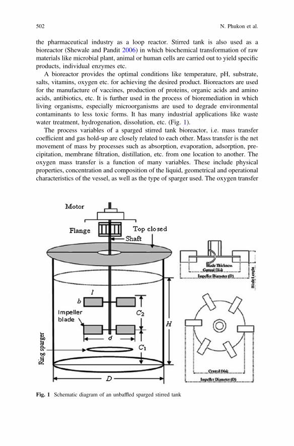
the pharmaceutical industry as a loop reactor. Stirred tank is also used as abioreactor (Shewale and Pandit 2006) in which biochemical transformation of rawmaterials like microbial plant, animal or human cells are carried out to yield specificproducts, individual enzymes etc.
A bioreactor provides the optimal conditions like temperature, pH, substrate,salts, vitamins, oxygen etc. for achieving the desired product. Bioreactors are usedfor the manufacture of vaccines, production of proteins, organic acids and aminoacids, antibiotics, etc. It is further used in the process of bioremediation in whichliving organisms, especially microorganisms are used to degrade environmentalcontaminants to less toxic forms. It has many industrial applications like wastewater treatment, hydrogenation, dissolution, etc. (Fig. 1).
The process variables of a sparged stirred tank bioreactor, i.e. mass transfercoefficient and gas hold-up are closely related to each other. Mass transfer is the netmovement of mass by processes such as absorption, evaporation, adsorption, pre-cipitation, membrane filtration, distillation, etc. from one location to another. Theoxygen mass transfer is a function of many variables. These include physicalproperties, concentration and composition of the liquid, geometrical and operationalcharacteristics of the vessel, as well as the type of sparger used. The oxygen transfer
Fig. 1 Schematic diagram of an unbaffled sparged stirred tank
502 N. Phukon et al.

area is greatly increased when bubbles are introduced into the culture fluid bysparging. Bubbles are broken up by agitation which further increases the masstransfer coefficient. Gas hold-up is another important parameter and defined as thetotal volume of large or microscopic gas bubbles in the liquid at any instant duringthe gas-liquid contact process. Sometimes when gas hold-up is prolonged there is atendency for all the gas bubbles to coalesce forming a very big bubble and givingthe appearance of a static void within the broth. When the system is sparged with aparticular gas, the broth around the impeller becomes less dense and hence requiresless power than an ungassed system. Impellers play a very important role as theyperform the task of solid suspension, mixing and dissolution of oxygen to liquidphase and maximizing the interfacial area between liquid and gaseous phases. Thedesign and speed of the impeller, the velocity of the gas used and the physicalproperties of the liquid are the factors which influence the rate of gas hold-up in animpeller agitated reactor.
It is necessary to be able to correctly predict the mass transfer coefficient and gashold-up rate in a sparged stirred tank in order to optimize its performance. Howeverthe empirical correlations predicted for these parameters take into account only theexperimental conditions. Hence, these empirical formulae are valid only in itsexperimental range, which limits its applicability outside the range and in otherengineering applications. Thus, recent advancement such as intelligent modellinghas been adopted in the present work. Intelligent modelling is a discipline whichmerges mathematical approach and computer technology. It uses technologies suchas neural network, automatic modelling and verification, computer calculating,simulation etc. It comprises of appropriate learning algorithms, which is useful inlearning complicated relationships from a set of related input–output vectors.
Artificial neural network (ANN) is designed based on the biological equivalentof the human brain. The system consists of a large number of highly interconnectedneurons which send messages to each other, working in parallel to solve a specificproblem. Conventional computers follow a specific set of instructions which isgiven by the user in order to solve a problem. This is known as the algorithmicapproach. As opposed to this, neural networks learn by example. As such, there isno need to devise an algorithm to understand the internal mechanisms of the task.A learning process configures an ANN for a specific application, such as patternrecognition and data classification. Hence the problem solving capability of neuralnetworks is enhanced as they can analyse data and detect trends that are toocomplex to be noticed by either humans or other computer techniques. ANN has thefollowing characteristics:
• Nonlinearity• Ability to learn• Input–output mapping• Ability to adapt• Fault tolerance.
Process Modelling of Gas … 503

Back-propagation (Irie and Miyanki 1988) is the most adaptable algorithm forthe feed forward layered network. Neural networks can find any nonlinear rela-tionships between input and output (Hornik et al. 1989) without having anyknowledge of the system beforehand. In the back-propagation algorithm, the neuralnetwork computes the error derivative of the weights. The weights are adjusted sothat the error between the desired output and the actual output is reduced.
One of the major drawbacks of back-propagation is that it is affected by localminima. Many modifications to back-propagation have been proposed and one ofthe significant modifications is given by Levenberg–Marquardt (Hagan and Menhaj1994). This algorithm is based on the assumption that the underlying functionwhich is modelled by the neural network is linear. Here the minimum is determinedexactly in a single step. The calculated minimum is now tested. If the error is lowerthe weights are moved to a new point. This process of iteration is repeated for eachgeneration.
Estimation of the volumetric oxygen transfer coefficient (kLa) from the gasbalance and using a neural network technique was carried out by Cruz et al. (1999).The use of gas balance and dynamic methods to obtain an estimate of the volu-metric oxygen transfer coefficient (kLa) in a conventional reactor is reported in thispaper. This experiment is done during the growth phase of the microorganismCephalosporium acremonium. The parameter measurements of the related variableswere taken as the inputs. The training of the feed forward neural network was donewith the calculated values of kLa. The gas balance method was comparatively lessuseful than the neural network technique which proves effective, predicting thevalues of kLa accurately from input data not used during the training phase.Estimation of oxygen mass transfer coefficient in stirred tank reactors using artificialneural networks was carried out by Garćia-Ochoa and Castro (2001). Volumetricmass transfer coefficient kLa was estimated in stirred tank reactors using ANN. Thefactors taken into account were the operational conditions, properties of fluids andgeometrical parameters. Stirred tank reactors of different volumes were taken andthe learning sets of input–output patterns were obtained. Neural network wascombined with an empirical equation forming a hybrid model which provides abetter representation of estimated parameter values. The predicted output by thehybrid ANN was compared with experimental data and some correlations previ-ously proposed for tanks of different sizes. Model-based control of a yeast fer-mentation bioreactor using optimally designed artificial neural networks was carriedout by Nagy (2006). In this paper the use of feedforward neural networks fordynamic modelling and temperature control of a continuous yeast fermentationbioreactor is described. The back-propagation learning algorithm was used to traindifferent ANNs. A pruning algorithm was proposed to avoid overfitting of the dataand achieve the best prediction ability with the simplest structure possible. Thecontrol performance of the structure was tested by testing the resulting ANNs.
Investigation of experiments in unbaffled gas-liquid stirred tank using Rushtonand curved blade impellers has been used to explore the process modeling of thesystem through ANN. In the present work, data obtained from experimentation wasfitted in the empirical correlations proposed by different researchers for calculation
504 N. Phukon et al.
of mass transfer coefficient and gas hold-up rate. Alternatively, neural network wasused to predict the values of the same. The overall performance of both the methodsadopted was compared.
Experimentation
Two sizes of circular unbaffled tank of diameter (D) 200 and 150 mm was testedunder laboratory conditions. Rushton and curved blade impellers were used in theexperiment. The blade height (b), the blade length (l) and the disc thickness were setas d/5, d/4 and 0.035d respectively. The central disc diameter was 0.5d. The liquiddepth (H) in the stirred tank was maintained equal to the tank diameter in allexperiments. Water was taken as the working fluid with density, qw, of 1000 kg/m3.For maximum gas hold-up, a ring sparger of diameter 0.8d is required was observedby Rewatkar et al. (1993). Smaller number of holes and holes of smaller size gives alarger gas hold-up (Rewatkar et al. 1993). For supplying air, 0.8d with holes of2 mm was used. Air was supplied to the ring sparger by a compressor fitted with avalve to control the supply. To measure the volumetric flow rate (1 and 5 L/min) arotameter was fitted before the valve. In each experiment the location of the spargerwas fixed at 0.09d from the bottom of the tank.
To measure the volumetric mass transfer rate, the standard dynamic method wasused. For this, the liquid phase was flushed with nitrogen to deoxygenate. Afterreplacement of nitrogen with air, measurement of the variation in dissolved oxygenconcentration with time takes place until saturated. It was assumed that the liquidphase was well mixed and gas absorption is liquid phase controlled, the volumetricmass transfer coefficient at T oC was determined using the empirical formulae:
kLaT ¼ ln Cs � C0ð Þ � ln Cs � Ctð Þ½ �=t ð1Þ
where, ln represents natural logarithm and the concentrations Cs, C0, and Ct aredissolved oxygen (DO) concentrations in parts per million (ppm), Cs = the satu-ration DO concentration at time tending to very large values, C0 is at t = 0 and Ct isat time t = t.
Gas hold-up was measured by visual method. A graph paper with graduationwas pasted on the outside of the vessel. The difference in level, with and withoutaeration was noted and the hold-up was found out using empirical formulae:
e ¼ H � H0ð Þ=H0 ð2Þ
H0 is the ungassed column height (m) and H is the column dispersion height dueto the presence of gas bubbles (m).
The statistical data of the experiment are tabulated in Table 1.
Process Modelling of Gas … 505
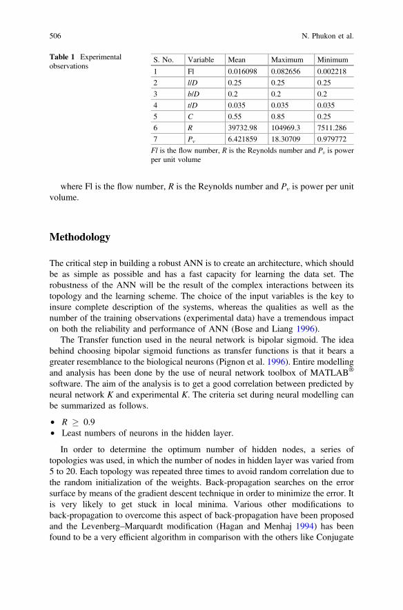
where Fl is the flow number, R is the Reynolds number and Pv is power per unitvolume.
Methodology
The critical step in building a robust ANN is to create an architecture, which shouldbe as simple as possible and has a fast capacity for learning the data set. Therobustness of the ANN will be the result of the complex interactions between itstopology and the learning scheme. The choice of the input variables is the key toinsure complete description of the systems, whereas the qualities as well as thenumber of the training observations (experimental data) have a tremendous impacton both the reliability and performance of ANN (Bose and Liang 1996).
The Transfer function used in the neural network is bipolar sigmoid. The ideabehind choosing bipolar sigmoid functions as transfer functions is that it bears agreater resemblance to the biological neurons (Pignon et al. 1996). Entire modellingand analysis has been done by the use of neural network toolbox of MATLAB®
software. The aim of the analysis is to get a good correlation between predicted byneural network K and experimental K. The criteria set during neural modelling canbe summarized as follows.
• R � 0.9• Least numbers of neurons in the hidden layer.
In order to determine the optimum number of hidden nodes, a series oftopologies was used, in which the number of nodes in hidden layer was varied from5 to 20. Each topology was repeated three times to avoid random correlation due tothe random initialization of the weights. Back-propagation searches on the errorsurface by means of the gradient descent technique in order to minimize the error. Itis very likely to get stuck in local minima. Various other modifications toback-propagation to overcome this aspect of back-propagation have been proposedand the Levenberg–Marquardt modification (Hagan and Menhaj 1994) has beenfound to be a very efficient algorithm in comparison with the others like Conjugate
Table 1 Experimentalobservations
S. No. Variable Mean Maximum Minimum
1 Fl 0.016098 0.082656 0.002218
2 l/D 0.25 0.25 0.25
3 b/D 0.2 0.2 0.2
4 t/D 0.035 0.035 0.035
5 C 0.55 0.85 0.25
6 R 39732.98 104969.3 7511.286
7 Pv 6.421859 18.30709 0.979772
Fl is the flow number, R is the Reynolds number and Pv is powerper unit volume
506 N. Phukon et al.

gradient algorithm or variable learning rate algorithm. Levenberg–Marquardt worksby making the assumption that the underlying function being modelled by theneural network is linear. Based on this calculation, the minimum can be determinedexactly in a single step. The calculated minimum is tested, and if the error there islower, the algorithm moves the weights to the new point. This process is repeatediteratively on each generation. Since the linear assumption is ill-founded, it caneasily lead Levenberg–Marquardt to test a point that is inferior (perhaps even wildlyinferior) to the current one. The clever aspect of Levenberg–Marquardt is that thedetermination of the new point is actually a compromise between a step in thedirection of steepest descent and the above-mentioned leap. Successful steps areaccepted and lead to a strengthening of the linearity assumption (which isapproximately true near to a minimum). Unsuccessful steps are rejected and lead toa more cautious downhill step. Thus, Levenberg–Marquardt continuously switchesits approach and can make very rapid progress. The Levenberg–Marquardt algo-rithm performs very well and its efficiency is found to be of several orders above theconventional back-propagation with learning rate and momentum factor.
Fig. 2 Results of ANN model for mass transfer
Process Modelling of Gas … 507

Results and Discussions
All the experimental data points collected were used to build and validate the ANNcorrelations. In the training algorithm of the back-propagation neural networks, themean squared error (MSE) was minimized for each epoch, i.e. iteration. Thenumber of epochs was set 10,000, and a termination rule was maintained as MSE of0.0001 or maximum epoch. Weights are updated though batch learning. The per-formance of the modelling has been given in the Figs. 2 and 3 for mass transfer andgas hold-up, respectively.
It can be clearly seen from Figs. 2 and 3 that the linear coefficient of correlationis very high between observed experimental data and values predicted throughneural nets. This shows the learning and generalization performance of the networkis good. Present experimental observations have been tested with the empiricalequations available in the literature as given in Table 2. Thus it can be said thataeration phenomena can be modelled through neural networks. Therefore, instead
Fig. 3 Results of ANN model for gas hold-up
508 N. Phukon et al.
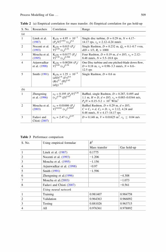
Table 2 (a) Empirical correlation for mass transfer. (b) Empirical correlation for gas hold-up
S. No. Researchers Correlation Range
(a)
1 Linek et al.(1987)
KLaT = 4.95 � 10−3
(Pg/V)0.593 (vg)
0.4Single disc turbine, D = 0.29 m, N = 4.17–14.17 rps, vg = 2.12–4.24 mm/s
2 Nocenti et al.(1993)
KLaT = 0.015 (Pg/V)0.59 (vg)
0.55Single Rushton, D = 0.232 m, Qg = 0.1–0.7 vvm,d/D = 1/3, Re > 1000
3 Moucha et al.(1995)
KLaT = 0.0177 (Pg/V)0.58 (vg)
0.588Four Rushton, D = 0.19 m, d = D/3, vg = 2.12–8.48 mm/s, N = 5.5–18.8 rps
4 Arjunwadkaret al. (1998)
KLaT = 0.00204 (Pg/V)0.68 (vg)
0.58One Disc turbine and one pitched-blade down flow,D = 0.18 m, vg = 0.98–3.3 mm/s, N = 6.6–12.5 rps
5 Smith (1991) KLaT = 1.25 � 10−4
(d/D)2.8 (Fr)0.6
(Re)0.7 (Fl)0.45
(d/g)−0.5
Single Rushton, D = 0.6 m
(b)
1 Zhengminget al. (1996)
eG = 0.195 (Pg/V)0.28
(vg)0.56 (D)0.45
Baffled, single Rushton, D = 0.287, 0.495 and1.1 m, H = D, d = D/3, vg = 0.003–0.0344 m/s,Pg/V = 0.15–5.2 � 103 W/m3
2 Moucha et al.(2003)
eG = 0.01686 (Pg/V)0.6241 (vg)
0.5669Baffled Rushton, D = 0.29 m, d = D/3,C = C1 = d, C2 = D, vg = 2.12, 4.24 and8.48 mm/s, N = 4.17–14.17 rps
3 Fadavi andChisti (2007)
eG = 2.47 (vg)0.97 D = 0.148 m, V = 0.01625 m3, vg � 0.04 m/s
Table 3 Performace comparison
S. No. Using empirical formulae R2
Mass transfer Gas hold-up
1 Linek et al. (1987) 0.1775
2 Nocenti et al. (1993) −1.206
3 Moucha et al. (1995) −1.156
4 Arjunwadkar et al. (1998) −0.97
5 Smith (1991) −1.596
6 Zhengming et al.(1996) −4.308
7 Moucha et al.(2003) −1.073
8 Fadavi and Chisti (2007) −0.561
Using neural network
1 Training 0.981407 0.984758
2 Validation 0.964363 0.966092
3 Testing 0.881026 0.963715
4 All 0.976361 0.978892
Process Modelling of Gas … 509

of proposing a compact correlation for modelling the re-aeration rates, a neural netwith weights can be supplied for the modelling.
These correlations have been tested on the basis of R2, which are tabulated inTable 3.
Thus it can be said that stirred tank process dynamics can be modelled throughneural networks. Therefore instead of proposing a compact correlation for mod-elling the system, a neural net with weights can be supplied for the modelling.
Conclusion
Values obtained from regression analysis from empirical correlations proposed inprevious studies indicate variation in regression coefficient value. It reveals thatdirect relation is not possible between theoretical and experimental values of theprocess variables. However, it has been observed that these correlations are validonly in their experimental range and cannot be used outside that range. It can beconcluded that a universal correlation is not present to predict the values of masstransfer coefficient and gas hold-up. The ANN method has been used to predict thevalues of mass transfer coefficient and gas hold-up. It has the ability to develop arelation between complex variables and consequently detect better trends. Onapplication of this method, it has been observed that the value of regressioncoefficient is nearly equal to one. It reveals that learning and generalization per-formance of ANN is better as compared with previous studies.
References
Arjunwadkar SJ, Sarvanan K, Kulkarni PR, Pandit AB (1998) Gas–liquid mass transfer in dualimpeller bioreactor. Biochem Eng J 1(2):99–106
Bose NK, Liang P (1996) Neural network fundamentals with graphs, algorithms, and applications.Tata McGraw-Hill, NewDelhi
Cruz AJG, Silva AS, Araujo MLGC, Giordano RC, Hokka CO (1999) Estimation of thevolumetric oxygen transfer coefficient (KLa) from the gas balance and using a neural networktechnique. Brazilian J Chem Eng 16
Fadavi A, Chisti Y (2007) Gas hold-up and mixing characteristics of a novel forced circulationloop reactor. Chem Eng J 131:105–111
Garcı ́a-Ochoaa F, Castro EG (2001) Estimation of oxygen mass transfer coefficient in stirred tankreactors using artificial neural networks. Enzyme Microb Technol 28(6):560–569
Garcia-Ochoa F, Gomez E (1998) Mass transfer coefficient in stirrer tank reactors for xanthansolutions. Biochem Eng J 1:1–10
Hagan MT, Menhaj MB (1994) Training feedforward networks with the Marquardt algorithm.IEEE Trans Neural Netw 6:989–993
Hornik K, Stinchcombe M, White H (1989) Multilayer feedforward networks are universalapproximaters. Neural Netw 2:359–366
Irie B, Miyanki S (1988) Capabilities of three layer perceptrons. In: IEEE second internationalconference on neural networks, San Diego, vol 1, pp 641–648
510 N. Phukon et al.

Linek V, Vacek V, Benes P (1987) A critical review and experimental verification of correct use ofdynamic method for the determination of oxygen transfer in aerated agitated vessels to water,electrolytic solutions and viscous liquids. Chem Eng J 34:11–34
Moucha T, Linek V, Sinkule J (1995) Measurement of kLa in multiple impeller vessels withsignificant axial dispersion in both phases. Trans IChemE 73, part A, 99 286–290
Moucha T, Linek V, Prokopová E (2003) Gas hold-up, mixing time and gas–liquid volumetricmass transfer coefficient of various multiple-impeller configurations: Rushton turbine, pitchedblade and techmix impeller and their combinations. Chem Eng Sci 58:1839–1846
Nagy ZK (2006) Model based control of a yeast fermentation bioreactor using optimally designedartificial neural networks. Chem Eng J 127(1):95–109
Nocentini M, Fajner D, Pasquali G, Magelli F (1993) Gas–liquid mass transfer and hold-up invessels stirred with multiple Rushton turbine: water and water-glycerol solutions. Ind EngChem Res 32:19–26
Pignon D, Parmiter PJM, Slack J, Hall TJ, van Daalen M, Shawe-Taylor J (1996) Sigmoid neuraltransfer function realised by percolation. Opt Lett 21(3):222–224
Rewatkar VB, Deshpande AJ, Pandit AB, Joshi JB (1993) Gas hold-up behavior of mechanicallyagitated gas–liquid reactors using pitched blade downflow turbines. Can J Chem Eng 71:226–237
Shewale SD, Pandit AB (2006) Studies in multiple impeller agitated gas–liquid contactors. ChemEng Sci 61:489–504
Smith JM (1991) Simple performance correlations for agitated vessels. In: Proceedings of 7thEuropean conference on mixing. Brugge, Belgium
Zhengming G, Yinchen W, Litian S, Jufu F (1996) Theoretical and experimental studies on bubblediameter and gas hold-up in aerated stirred tanks. Chinese J Chem Eng 4(4):283–289
Process Modelling of Gas … 511
Identification and Planning of WaterQuality Monitoring Network in Contextof Integrated Water ResourceManagement (IWRM)
Surjeet Singh, Gopal Krishan, N.C. Ghosh, R.K. Jaiswal, T. Thomasand T.R. Nayak
Abstract Hydrological system is a quite complex and dynamic in nature becauseof the heterogeneity of the earth crust and surrounding atmosphere. Water exists onthe earth in all three forms of liquid, solid and gas. The scarcity of its liquidfreshwater has resulted because of increasing demand in response to growingpopulation, contamination and pollution of freshwater bodies due to urbanizationand industrialization. Precise measurement of water quality, in present time, hasbecome the necessity because of increasing scarcity of this precious resource. In aglobal perspective, organizations dealing with water supply and monitoring are everconcerned about precise assessment of water quality. Researchers are focusing onthe assessment of surface and ground water quality on spatial scale rather than pointscale, which needs strengthening of monitoring networks time-to-time. The designof a hydrometric network starts ideally with a minimum number of stations, andincreases gradually until an optimum network is attained when the amount andquality of data collected and information processed is economically justifiable and itmeets the user’s needs to make specific decisions. In hydrology, monitoring of datais mostly site-specific and proper representation of this data on spatial scale requiresproper network planning. Since the drivers of water quality vary in space and time,the quality of water also varies in space and time. It is therefore imperative tomonitor the quality of water under heterogeneous space-dependent conditions forwhich a specialized water quality monitoring network is essential. The presentpaper is in the context of identifying and planning of water quality monitoringnetwork for data acquisition for Integrated Water Resources Management (IWRM).
S. Singh � G. Krishan (&) � N.C. GhoshNational Institute of Hydrology, Roorkee 247667, Uttarakhand, Indiae-mail: [email protected]
R.K. Jaiswal � T. Thomas � T.R. NayakNational Institute of Hydrology, Ganga Plains South Regional Centre, Bhopal 462042, India
© Springer Nature Singapore Pte Ltd. 2018V.P. Singh et al. (eds.), Environmental Pollution, Water Scienceand Technology Library 77, https://doi.org/10.1007/978-981-10-5792-2_41
513
Introduction
The monitoring of hydrologic system is known from the ancient times, whereas thefirst description of the rain gauge and its use is contained in the Arthashastra byChanakya (300 BC). Varahamihira’s (AD 505–587) Brihatsamhita containsdescriptions of the rain gauge, wind vane and prediction procedures for rainfall.Egyptians knew the importance of the stage measurement of rivers and records ofthe stages of the Nile dating back to 1800 BC have been located. The knowledge ofthe hydrologic cycle came to be known to Europe much later, around AD 1500(Subramanya 2010).
In recent times, the issues related to the optimal design of water quality moni-toring networks and efficiency improvements have been the subject of researchsince 1970s (Ning and Chang 2002) and the basic principles of monitoring networkdesign and site selection criteria for individual monitoring stations have beenevaluated and applied by many researchers (Skalski and Mackenzie 1982;Lettenmaier et al. 1986; Smith and McBride 1990). Later studies have focusedgreater attention on the effective design of water quality monitoring networks usingvarious types of statistical and/or programming techniques, such as integer pro-gramming, multi-objective programming, Kriging theory and optimization analysis(Hudak et al. 1995; Dixon and Chiswell 1996; Timmerman et al. 1997).
In India, various water monitoring and water supply organizations and institu-tions are more concerned to monitor the water resources more accurately and onwider geographic region, and thus strengthening their monitoring network fromtime-to-time. Such agencies and researchers are monitoring precipitation (in theform of rainfall and snow), stream flow (CPCB 2009; Sargaonkar and Deshpande2003; Samantray et al. 2009; Jindal and Sharma 2011), groundwater (Krishan et al.2013, 2014, 2015, 2016a; Lapworth et al. 2015; MacDonald et al. 2015), lakes andreservoirs, as well as water quality of various water bodies (Krishan et al. 2016b;Rao et al. 2016).
The design of a hydrometric network starts ideally with a minimum number ofstations and increases gradually until an optimum network is attained when theamount and quality of data collected and information processed is economicallyjustifiable and it meets the user’s needs to make specific decisions. Networkplanning is the backbone of any monitoring system. In hydrology, monitoring ofdata is mostly site-specific and proper representation of this data on spatial scalerequires proper network planning. The present paper is in the context of identifyingand planning of water quality monitoring network for data acquisition for IntegratedWater Resources Management (IWRM).
514 S. Singh et al.
Water Quality Monitoring Network
Water sample collection network is quite general in nature which may include anetwork for collection of wide variety of samples. The samples collected under thisnetwork may be used for various hydrological analysis, viz. water quality, isotopicanalysis, sedimentation, etc.
There are several approaches to water quality monitoring. Monitoring can bedone through a network of strategically located long-term stations, by repeatedshort-term surveys, or a combination of these two. In addition to the basic objec-tives of the water quality monitoring programme, the location of stations shouldtake into account the following factors:
• Existing water problems and conditions;• Potential growth centres (industrial and municipal);• Population trends;• Climate, geography and geology;• Accessibility:• Available manpower, funding, field and laboratory data handling facilities;• Inter-jurisdictional considerations;• Travel time to the laboratory (for deteriorating samples); and• Safety of personnel.
Water Quality Parameters
The parameters that characterize water quality may be classified in several ways,including physical properties (e.g. temperature, electrical conductivity, colour,turbidity), inorganic chemical components (e.g. dissolved oxygen, chloride, alka-linity, fluoride, phosphorous, metals), organic chemicals (e.g. phenols, chlorinatedhydrocarbons, polycyclic aromatic hydrocarbons and pesticides), and biologicalcomponents, both microbiological, such as faecal coliforms, and macrobiotic, suchas worms, plankton and fish, which can indicate the ecological health of the aquaticenvironment (WMO 1994).
A second classification is done according to the importance attached to theparameter. This will vary with the type of water body, the intended use of the waterand the objectives of the monitoring programme. Water quality variables aresometimes grouped within following two categories:
(a) Basic variables (given in Table 1).(b) Use-related variables:
• Drinking water supplies• Irrigation, and• General quality of aquatic life.
Identification and Planning of Water Quality Monitoring Network … 515
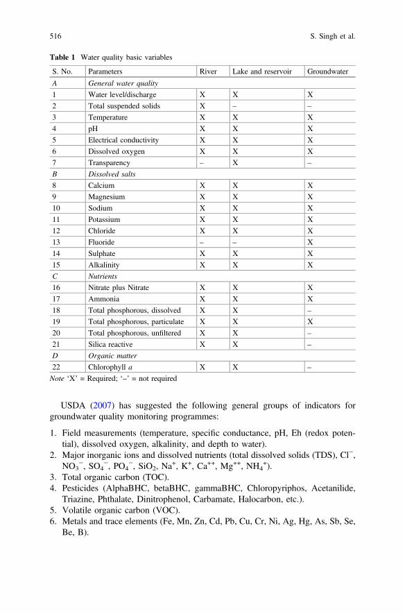
USDA (2007) has suggested the following general groups of indicators forgroundwater quality monitoring programmes:
1. Field measurements (temperature, specific conductance, pH, Eh (redox poten-tial), dissolved oxygen, alkalinity, and depth to water).
2. Major inorganic ions and dissolved nutrients (total dissolved solids (TDS), Cl−,NO3
−, SO4−, PO4
−, SiO2, Na+, K+, Ca++, Mg++, NH4
+).3. Total organic carbon (TOC).4. Pesticides (AlphaBHC, betaBHC, gammaBHC, Chloropyriphos, Acetanilide,
Triazine, Phthalate, Dinitrophenol, Carbamate, Halocarbon, etc.).5. Volatile organic carbon (VOC).6. Metals and trace elements (Fe, Mn, Zn, Cd, Pb, Cu, Cr, Ni, Ag, Hg, As, Sb, Se,
Be, B).
Table 1 Water quality basic variables
S. No. Parameters River Lake and reservoir Groundwater
A General water quality
1 Water level/discharge X X X
2 Total suspended solids X – –
3 Temperature X X X
4 pH X X X
5 Electrical conductivity X X X
6 Dissolved oxygen X X X
7 Transparency – X –
B Dissolved salts
8 Calcium X X X
9 Magnesium X X X
10 Sodium X X X
11 Potassium X X X
12 Chloride X X X
13 Fluoride – – X
14 Sulphate X X X
15 Alkalinity X X X
C Nutrients
16 Nitrate plus Nitrate X X X
17 Ammonia X X X
18 Total phosphorous, dissolved X X –
19 Total phosphorous, particulate X X X
20 Total phosphorous, unfiltered X X –
21 Silica reactive X X –
D Organic matter
22 Chlorophyll a X X –
Note ‘X’ = Required; ‘–’ = not required
516 S. Singh et al.

7. Bacteria (Coliform bacteria, E. coli, Entrococci, etc.).8. Radionuclides (Radium Radon, Uranium).9. Environmental isotopes (H, O, N, C, S).
Techniques for Water Quality Monitoring Network Design
Following factors need to be considered for planning of the water quality moni-toring network:
1. Monitoring of bedrock and superficial aquifers2. Depending on hydrological structures3. Based on water use and site condition4. Based on mixing of water5. Based on specific yield6. Based on flow capacity of river7. Based on water surface area of lake and reservoir8. Parallel to coastline9. Based on land use
10. Based on areal extent
Monitoring of Bedrock and Superficial Aquifers
The proposed network must reflect the diverse hydrogeological, soil and land-useconditions. Therefore, both bedrock and superficial aquifers should be monitored ina variety of soil conditions. The network should continue to include different typesof sources, although less emphasis should be given to wells, which are generallypoor monitoring points. The nature of water quality in these two types of aquifersgenerally differs significantly, and hence water quality monitoring is essential.
Depending on Hydrological Structures
The number of sampling points on a river depends on the hydrology and the wateruses. The greater the water quality fluctuation, the greater the frequency of mea-surement required. In humid regions, where concentrations of dissolved matter arelow, fewer observations are needed than in dry climates, where concentrations,particularly of critical ions such as sodium, may be high. At many locations, thewater quality sampling stations may be coupled to the stream gauging stations andstructures such as barrage, dams, etc. Similarly, the gauging sites of the spring flowmay also be used for the water sampling purpose.
Identification and Planning of Water Quality Monitoring Network … 517
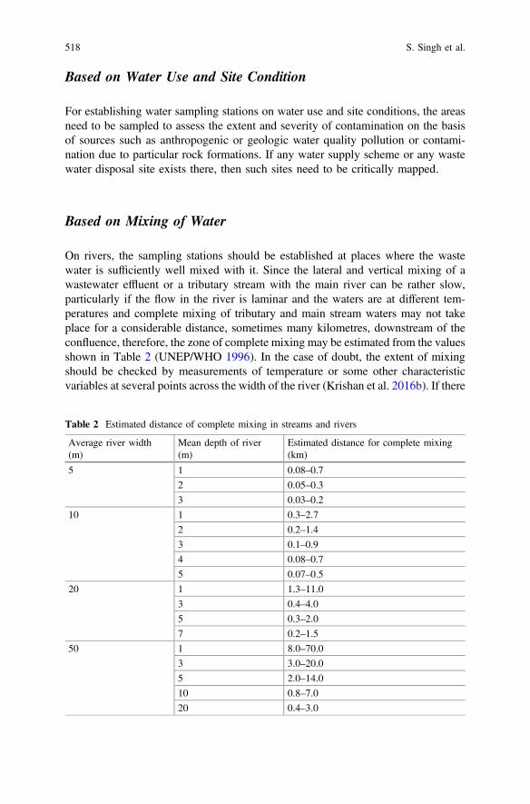
Based on Water Use and Site Condition
For establishing water sampling stations on water use and site conditions, the areasneed to be sampled to assess the extent and severity of contamination on the basisof sources such as anthropogenic or geologic water quality pollution or contami-nation due to particular rock formations. If any water supply scheme or any wastewater disposal site exists there, then such sites need to be critically mapped.
Based on Mixing of Water
On rivers, the sampling stations should be established at places where the wastewater is sufficiently well mixed with it. Since the lateral and vertical mixing of awastewater effluent or a tributary stream with the main river can be rather slow,particularly if the flow in the river is laminar and the waters are at different tem-peratures and complete mixing of tributary and main stream waters may not takeplace for a considerable distance, sometimes many kilometres, downstream of theconfluence, therefore, the zone of complete mixing may be estimated from the valuesshown in Table 2 (UNEP/WHO 1996). In the case of doubt, the extent of mixingshould be checked by measurements of temperature or some other characteristicvariables at several points across the width of the river (Krishan et al. 2016b). If there
Table 2 Estimated distance of complete mixing in streams and rivers
Average river width(m)
Mean depth of river(m)
Estimated distance for complete mixing(km)
5 1 0.08–0.7
2 0.05–0.3
3 0.03–0.2
10 1 0.3–2.7
2 0.2–1.4
3 0.1–0.9
4 0.08–0.7
5 0.07–0.5
20 1 1.3–11.0
3 0.4–4.0
5 0.3–2.0
7 0.2–1.5
50 1 8.0–70.0
3 3.0–20.0
5 2.0–14.0
10 0.8–7.0
20 0.4–3.0
518 S. Singh et al.
are rapids or waterfalls in the river, the mixing will be speeded up and representativesamples may be obtained downstream. Sampling for the determination of dissolvedoxygen, however, should take place upstream of the rapids or waterfall because theturbulence will cause the water to be saturated with oxygen. In such a case, severalsamples should be taken across the width of the river to allow for the possibility ofincomplete mixing.
A bridge is an excellent place to establish a sampling station (provided that it islocated at a sampling site on the river). It is easily accessible and clearly identifiablelocation. Furthermore, a bridge is often a hydrological gauging station and, if so,one of the bridge piers will have a depth gauge marked on it, thus allowing thecollection of stream flow information at the time of sampling. Usually, a sampletaken from a bridge at mid-stream or in mid-channel, in a well-mixed river, willadequately represent all of the water in the river.
To verify that there is complete mixing at a sampling station it is necessary totake several samples at points across the width and depth of the river and to analysethem. If the results do not vary significantly one from the other, a station can beestablished at mid-stream or some other convenient points. If the results are sig-nificantly different it will be necessary to obtain a composite sample by combiningsamples taken at several points in the cross section of the stream. Generally, themore the points that are sampled, the more representative the composite sample willbe. Sampling at 3–5 points is usually sufficient and fewer points are needed fornarrow and shallow streams. Suggestions are provided in Table 3 for the number ofpoints from where samples should be obtained in streams or rivers of different sizesand with different flow rates.
Based on Specific Need
Water quality sampling stations may also be required to be fixed based on the need.Such needs may arise due to any or some of the reasons mentioned below:
1. Occurrence of health problems in a particular area.2. Drinking water supply scheme.3. Research needs.4. Waste water disposal in a stream.5. Just before an international boundary, if the river is draining outside the country.6. Just after an international boundary, if the river is entering into the country.7. Just before or after the inter-state boundary, if the river is draining in more than
one state.8. Above the points of withdrawal for irrigation, or domestic, or industrial purpose
under a major scheme.9. Outlets of lakes and reservoirs.
Identification and Planning of Water Quality Monitoring Network … 519

Based on Flow Capacity of River
Lakes and reservoirs can be subjected to several influences that cause water qualityto vary from place to place and from time-to-time. It is, therefore, prudent toconduct preliminary investigations to ensure that sampling stations are truly rep-resentative of the water body. Where feeder streams or effluents enter lakes orreservoirs, there may be local areas where the incoming water is concentrated,because it has not yet mixed with the main water body. Isolated bays and narrowinlets of lakes are frequently poorly mixed and may contain water of a differentquality with the rest of the lake. Wind action and the shape of a lake may lead to alack of homogeneity; for example, when wind along a long, narrow lake causes aconcentration of algae at one end. Table 3 suggests the sampling regimes forcomposite samples in the flowing water.
In India, a vast river quality monitoring data has been accumulated over theyears but it has not been properly utilized for reasons of limited ability to com-municate the data to the common man. Some researchers have tried to use the riverwater quality indices with limited success (Sargaonkar and Deshpande 2003;Samantray et al. 2009; Jindal and Sharma 2011).
Based on Water Surface Area of Lake and Reservoir
A number of sampling locations vary with the size and depth of any water body. Ifthe water surface area of lake or reservoir is large enough, multiple samplinglocations are necessary. To allow for the size of a lake (UNEP/WHO 1996) hassuggested that the number of sampling stations should be the nearest whole numberto the log10 of the area of the lake in km2. Thus, a lake of 10 km2 requires onesampling station, 100 km2 requires two stations, and so on. For lakes with irregularboundaries, it is advisable to conduct preliminary investigations to determinewhether and where differences in water quality occur before deciding on thenumber of stations to establish.
The most important feature of water in lakes and reservoirs, especially in tem-perate zones, is vertical stratification, which results in differences in water quality atdifferent depths (UNEP/WHO 1996). Stratification at a sampling station can bedetected by taking a temperature reading at 1 m below the surface and another at
Table 3 Suggested sampling regimes for composite samples in flowing water (UNEP/WHO1996)
Average river discharge(m3/s)
Type ofstream/river
Number of samplingpoints
Number of samplingdepths
<5 Small stream 2 1
5–140 Stream 4 2
150–1000 River 6 3
� 1000 Large river � 6 4
520 S. Singh et al.
1 m above the bottom. If there is a significant difference (e.g. >3 °C) between thesurface and the bottom readings, there is a “thermocline” (a layer where the tem-perature changes rapidly with depth) and the lake or reservoir is stratified and it islikely that there will be important differences in some water quality variables aboveand below the thermocline. Consequently, in stratified lakes, more than one sampleis necessary to describe the water quality. For lakes or reservoirs of � 10 m depth itis essential, therefore, that the position of the thermocline is first investigated bymeans of regularly spaced temperature readings through the water column (e.g.metre intervals). Samples for water quality analysis should then be taken accordingto the position and extent (in depth) of the thermocline. As a general guide, theminimum samples should consist of
• m below the water surface,• just above the determined depth of the thermocline,• just below the determined depth of the thermocline, and• m above the bottom sediment (or closer if this can be achieved without dis-
turbing the sediment).
If the thermocline extends through several metres depth, additional samples arenecessary from within the thermocline in order to characterize fully the waterquality variations with depth. Whilst the position of the thermocline is stable, thewater quality for a given station may be monitored by fewer samples but, inpractice, the position of a thermocline can vary in the short- (hours) or long-term(days) due to internal seiches (periodic oscillations of water mass) and mixingeffects. In general, in tropical climates where the water depth at the sampling siteis <10 m, the minimum sampling should consist of a sample taken 1 m below thewater surface and another sample taken at 1 m above the bottom sediment.
Parallel to Coastline
Sea water intrusion is the most common problem in the coastal aquifers. Withoutsalinity monitoring of groundwater in the coastal aquifers, it is not impossible todecide on the sea water intrusion. It is thus imperative to have a good network ofobservation wells in the coastal aquifers particularly parallel to the coastline. Thegroundwater table is very shallow near the coast and goes down below the landsurface on moving away from the coast. For monitoring the dynamics of saline andfresh water interface, at least 03 observation wells should be placed perpendicularto the coastline at regular intervals, either fixed or depending on rock formationssusceptible to the sea water ingress, withdrawal patterns in the aquifers, etc. The 03observation wells shall be placed at 2, 4 and 6 km away from the coastline for thesalinity monitoring.
Identification and Planning of Water Quality Monitoring Network … 521
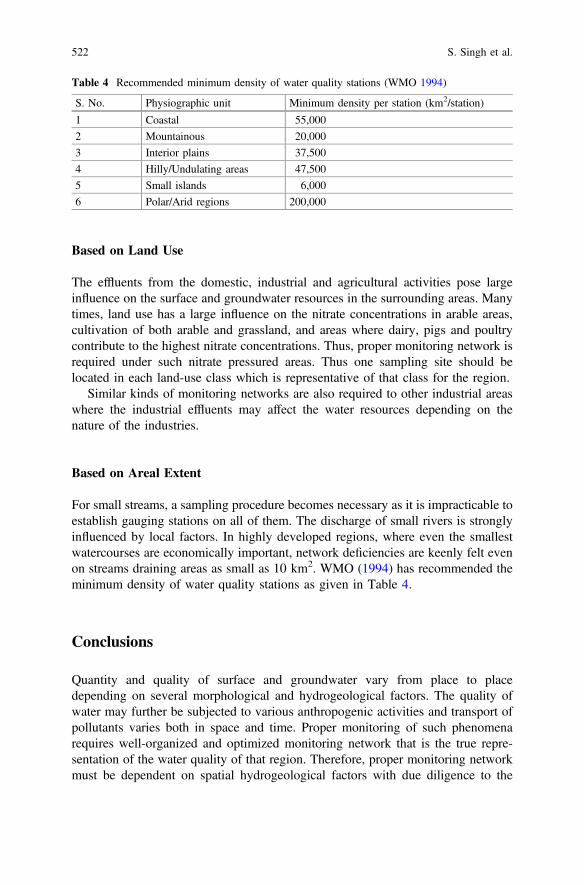
Based on Land Use
The effluents from the domestic, industrial and agricultural activities pose largeinfluence on the surface and groundwater resources in the surrounding areas. Manytimes, land use has a large influence on the nitrate concentrations in arable areas,cultivation of both arable and grassland, and areas where dairy, pigs and poultrycontribute to the highest nitrate concentrations. Thus, proper monitoring network isrequired under such nitrate pressured areas. Thus one sampling site should belocated in each land-use class which is representative of that class for the region.
Similar kinds of monitoring networks are also required to other industrial areaswhere the industrial effluents may affect the water resources depending on thenature of the industries.
Based on Areal Extent
For small streams, a sampling procedure becomes necessary as it is impracticable toestablish gauging stations on all of them. The discharge of small rivers is stronglyinfluenced by local factors. In highly developed regions, where even the smallestwatercourses are economically important, network deficiencies are keenly felt evenon streams draining areas as small as 10 km2. WMO (1994) has recommended theminimum density of water quality stations as given in Table 4.
Conclusions
Quantity and quality of surface and groundwater vary from place to placedepending on several morphological and hydrogeological factors. The quality ofwater may further be subjected to various anthropogenic activities and transport ofpollutants varies both in space and time. Proper monitoring of such phenomenarequires well-organized and optimized monitoring network that is the true repre-sentation of the water quality of that region. Therefore, proper monitoring networkmust be dependent on spatial hydrogeological factors with due diligence to the
Table 4 Recommended minimum density of water quality stations (WMO 1994)
S. No. Physiographic unit Minimum density per station (km2/station)
1 Coastal 55,000
2 Mountainous 20,000
3 Interior plains 37,500
4 Hilly/Undulating areas 47,500
5 Small islands 6,000
6 Polar/Arid regions 200,000
522 S. Singh et al.
anthropogenic sources including the intended use of the monitoring network. Thusa well-planned water quality monitoring network for Integrated Water ResourcesManagement (IWRM) can be achieved (i) if goals are clear, defined and welldeveloped; (ii) the hydrogeology and geology of the aquifer formation is wellunderstood and taken into consideration; (iii) the budgetary constraints are lookedinto; and (iv) some statistical techniques for optimization of network. Varioustechniques for planning and identification of the monitoring points and waterquality parameters to be included are presented and discussed in the paper.
Acknowledgements Authors thank Director, National Institute of Hydrology, Roorkee for all thesupport and encouragement.
References
CPCB, Central Pollution Control Board (2009) National Water Quality Monitoring Programme.http://www.cpcb.nic.in/divisionsofheadoffice/pams/NWMP.pdf
Dixon W, Chiswell B (1996) Review of aquatic monitoring program design. Water Res 30:1935–1948
Hudak PF, Loaiciga HA, Marino MA (1995) Regional-scale ground water quality monitoring viainteger programming. J Hydrol 164:153–170
Jindal R, Sharma C (2011) Studies on water quality of Satluj river around Ludhiana with referenceto physic-chemical parameters. Environ Monit Assess 174(2):417–425
Krishan G, Lohani AK, Rao MS et al (2013) Optimization of groundwater monitoring network inBist-Doab, Punjab. In: Proceedings of an international conference “India Water Week2013-Efficient Water Management: Challenges and Opportunities” (IWW-2013), 08–12 April2013 at New Delhi, India, pp 274
Krishan G, Lohani AK, Rao MS, Kumar CP (2014) Prioritization of groundwater monitoring sitesusing cross-correlation analysis. NDC-WWC J 3(1):28–31
Krishan G, Singh RP, Takshi KS (2015) Water level fluctuation as the sum of environmental andanthropogenic activities in Southeast, Punjab (India). J Environ Anal Toxicol 5:298
Krishan G, Singh S, Kumar CP, Garg PK, Gurjar S, Ghosh NC, Chaudhary A (2016a) Assessmentof groundwater quality for drinking purpose using water quality index in Muzaffarnagar andShamli districts, Uttar Pradesh, India. Hydrology. Current Research 7:1. doi:10.4172/2157-7587.1000227
Krishan G, Singh S, Sharma A, Sandhu C, Grischek T, Gurjar S, Kumar S, Singh RP, Glorian H,Bornick H (2016b) Assessment of river quality for river bank filtration along Yamuna River inAgra-Mathura districts of Uttar Pradesh. Int J Environ Sci 7(1):56–67
Lapworth DJ, MacDonald AM, Krishan G, Rao MS, Gooddy DC, Darling WG (2015)Groundwater recharge and age-depth profiles of intensively exploited groundwater resources innorthwest India. Geophys Res Lett 42(18):7554–7562. doi:10.1002/2015GL065798
Lettenmaier DP, Anderson DE, Brenner RN (1986) Consolidation of a stream quality monitoringnetwork. Water Resour Bull 22:1049–1051
MacDonald AM, Bonsor HC, Taylor R et al (2015) Groundwater resources in the Indo-Gangeticbasin—resilience to climate change and abstraction. British Geological Survey Open Report,OR/15/047, 63 pp
Ning SK, Chang NB (2002) Multi-objective, decision-based assessment of a water qualitymonitoring network in a river system. J Environ Manage 4:121–126
Identification and Planning of Water Quality Monitoring Network … 523
Rao MS, Sampath K L, Rangaraj C et al (2016) Application of isotopes in studying lake water –groundwater interactions in parts of Tumkur district of Karnataka. Curr World Environ. 11(3):751-755
Samantray P, Mishra BK, Panda CR, Rout SP (2009) Assessment of water quality index inMahanadi and Atharabanki rivers and Taldanda Canal in Paradip area, India. J Hum Ecol 26(3):153–161
Sargaonkar A, Deshpande V (2003) Development of an overall index of pollution for surfacewater based on a general classification scheme in Indian context. Environ Monit Assess 89(1):43–67
Skalski JR, Mackenzie DH (1982) A design for aquatic monitoring programs. J Environ Manage14:237–251
Smith DG, McBride GB (1990) New Zealand’s national water quality monitoring network—design and first year’s operation. Water Resour Bull 26:767–775
Subramanya K (2010) Engineering hydrology, 3rd edn. Tata McGraw Hill Publishers, New DelhiTimmerman JG, Adriaanse M, Breukel RMA, Van Oirschot MCM, Ottens JJ (1997) Guidelines
for water quality monitoring and assessment of transboundary rivers. Euro Water PollutControl 7:21–30
UNEP/WHO (1996) Water quality monitoring—a practical guide to the design and implemen-tation of freshwater quality studies and monitoring programmes, Jamie Bartram and RichardBalance, eds, Published on behalf of United Nations Environment Programme and the WorldHealth Organization, ISBN 0 419 22320 7 (Hbk) 0 419 21730 4 (Pbk)
USDA (2007) United States Department of Agriculture, Technical Guide to Managing GroundWater Resources, FS-881
World Meteorological Organization (WMO) (1994) Guide to hydrological practices. WMO-164,5th edn. WMO-No. 168, Geneva, Switzerland
524 S. Singh et al.
An Updated Review on Quantitativeand Qualitative Analysis of WaterPollution in West Flowing Tapi Riverof Gujarat, India
Shreya Gaur
Abstract A river plays an important role in development of any society or even thecountry, being the solitary source of water supply to meet our domestic, industrial,agricultural, aquatic and even the power generation needs. It is agonizing to see thatsome of the rivers used to pass through big cities, and their huge water resources areutilized for disposal of domestic and industrial wastes too, which ultimately leads tomultifarious pollution hazards towards land, water, vegetation and nearby livingsociety. Tapi is one of the three major rivers in central India which flows from eastto west with a length of 724 km, encompassing the contributing catchment to thetune of about 30,000 km2. It passes through Surat, a mega city of Gujarat, com-promising with multiple land use complexes. Historical importance as well aspeculiar characteristics of this river and its water body are reviewed and presentedto show the updated status in regards to degree and extent of contamination.Write-up presents an updated review on status of prevailing water quality, encir-cling indicators like heavy metals (Fe, Cu, Zn, Pb, As, Hg, Ni, Cd, etc.), suspendedsediments, bed loads and other pollutant with their causes and effects. Efforts aremade to critically review some of the updated status and estimates in regards tooverexploitation of water and river reaches, riverbank erosion, channel geomor-phologic constituents, sedimentation (erosion, transport and deposition) and theirvaried patterns with ever increasing human and natural interferences. Influences ofritual functions like dipping of Lord Ganesha Idol and other associated activities arealso visited, revealing that these manmade causes contributed significant deterio-rations in river water quality, in particular the physiochemical parameters (pH,Temperature, Dissolved Oxygen, free CO2, Hardness, Alkalinity, BOD, COD, etc.).The available field data and findings of previous researchers are critically viewedand analysed providing a better understanding on quantitative variability of annualrunoff, sedimentation patterns, flood inundations and flood-based threats in and
S. Gaur (&)Government Engineering College, Surat 395001, Gujarat, Indiae-mail: [email protected]
© Springer Nature Singapore Pte Ltd. 2018V.P. Singh et al. (eds.), Environmental Pollution, Water Scienceand Technology Library 77, https://doi.org/10.1007/978-981-10-5792-2_42
525

around study river. Critical limits in regards to above cited indicators (quantitative,qualitative) are offered, to provide a better understanding of river water manage-ment meeting the prevailing demands in sustainable manner.
Introduction
Rivers play an important role in the life of the people because these are mostly usedas a source of water for drinking, bathing, irrigation, recreation and other miscel-laneous purposes. Accordingly, it governs the overall development of the countryand people as well. River water happens to be the only important surface watersource which obtains its input from rains. The history of ancient civilization andindustrial growth in India very well depicts the factual scenarios, that how thisimperative volume of surface water gets uncertain both in quantity as well asquality. At one hand, it is highly influenced by drastic changes in climate andrainfall patterns, while on other hand it is severely prejudiced in its qualitativeaspects. The even changing pattern of rainfall, both with respect to location as wellas time, have made river water discharges very much uncertain. Some times at somelocations there are floods while other time there exits droughts leading to declinedvolumes of water in rivers. If we consider the changing scenarios in respect ofquality of river water, it is emerging as another burning issue for people and society.The ever-changing land use patterns, industrial and agricultural interventions havecontributed a lot to degrade the quantity as well as quality of river water. It includesmany processes as well as versions like, pesticides and fertilizers in agriculturalrunoff water, human and animal wastes in sewage, industrial pollutants/waste andmany other point source or non-point source pollutants. This altogether is releasingmany adverse impacts on human life, including deficit water availability, waterborne diseases, overall deterioration in soil and water, complex scenarios of floodsand droughts, and many such adverse effects which directly or indirectly influenceliving and nonliving settings situated in and around the rivers. The deterioratedquantity and quality of water in these rivers is having close correlation with pre-vailing state of social, economical and technological problems at micro and macroscales.
Indian River System
In India, rivers are classified mainly of two types based on their geographicallocations and origin viz. Himalayan rivers and Peninsular rivers. The Himalayanrivers are glacier fed and perennial, while peninsular rivers remained altogethermonsoon fed. A broad sketch of major Indian rivers with their basins is shown inFig. 1. Among peninsular rivers, majority of them are east coast rivers (e.g.Mahanadi, Krishna, Godavari and Cauvery) and empty their water in Bay of
526 S. Gaur

Bengal; while a few others, i.e. west coast rivers (e.g. Narmada, Tapi, Sabarmatiand Luni) are west flowing and drain out in Arabian sea. All the peninsular riversare entirely dependent on monsoonal rhythm and display from very poor water flowto heavy flood and accordingly exhibit the fluctuating ecological and biologicalconditions.
Fig. 1 Relative location of west flowing Tapi river under major river basins of India
An Updated Review on Quantitative and Qualitative Analysis … 527

Above rivers are indeed the life line of country, but during prevailing conditionsare suffering from enormous number of pollution, which is being caused by belowgiven two reasons,
• Untreated urban sewage, industrial effluents, agricultural runoff, mining wastes,religious ceremonies and navigational operations.
• Indiscriminate destruction of drainage basin because of clearing of riparian zonevegetation which, in turn, is responsible for elevated load of suspended solid andincreased magnitude and frequency of flood changing the level of interactionbetween land and water; and hence affects all inputs of energy source.
Among these rivers, three are exceptionally explicit (Mahi, Narmada, Tapi)which flows from east to west and directly drain into sea. All these passes throughGujarat state of India, which happens to be most the industrialist and developedstate in the country, encompassing an area of approximately 196,000 km2 and isenclosed within the North Latitude 20° 10′ to 24° 50′ and East Longitude 68° 40′to 74° 40′. Obviously, the course of these rivers remains via many urban settings aswell as cities. Present paper incorporates one of these rivers namely ‘Tapi’ which isthe most peculiar and passes through Surat—the Diamond city of Country, famousfor world class industries on diamonds, textiles, and chemicals. Paper presents anupdated review towards prevailing scenario of Tapi river in and around Surat city ofGujarat, by incorporating certain quantitative as well qualitative aspects. Thespectrum of findings by various researchers in regards to causes and effects ofvarious activities to create river water pollution, reported values of pollution indi-cators, logical interpretations and discussions on relevant issues are discussed. Thecontents of this write-up remains only a work review by other researchers only,with an aim to visualize the issue of river water pollution and offer certain food forthought for this specific study region. This could be vital utilities towards framingsuggestions for futuristic R&D and other development plans/strategies to cope upthe problem and evolve suitable site specific preventive measures and action plans.
Methodology
While conducting an updated review on water pollution, a specific river namelyTapi is adopted in this write-up. Review and discussion are presented by adoptingcommon hypothesis as emerged and well established, based upon findings ofseveral researchers. According to these, the physicochemical purity of water in theriver Tapi, as well as, ground water available in nearby wells on both banks of riveris greatly deteriorated due to two basic reasons, (1) release of excessive pollutedsubstances from nearby industries and (2) excessive use of organic and inorganicfertilizers and use of pesticides and insecticides in agricultural lands which travelsdown underground towards wells and river water bodies. This all together affectedthe water quality in river and total hygiene/health of population living near to rivers.
528 S. Gaur
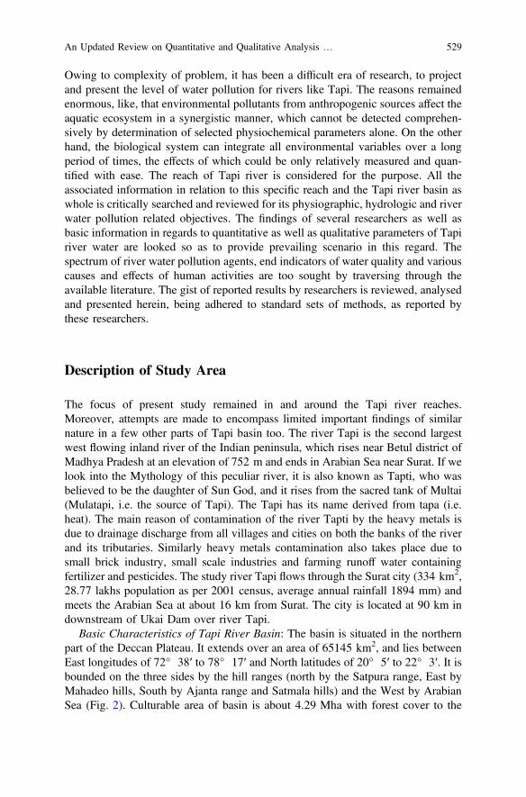
Owing to complexity of problem, it has been a difficult era of research, to projectand present the level of water pollution for rivers like Tapi. The reasons remainedenormous, like, that environmental pollutants from anthropogenic sources affect theaquatic ecosystem in a synergistic manner, which cannot be detected comprehen-sively by determination of selected physiochemical parameters alone. On the otherhand, the biological system can integrate all environmental variables over a longperiod of times, the effects of which could be only relatively measured and quan-tified with ease. The reach of Tapi river is considered for the purpose. All theassociated information in relation to this specific reach and the Tapi river basin aswhole is critically searched and reviewed for its physiographic, hydrologic and riverwater pollution related objectives. The findings of several researchers as well asbasic information in regards to quantitative as well as qualitative parameters of Tapiriver water are looked so as to provide prevailing scenario in this regard. Thespectrum of river water pollution agents, end indicators of water quality and variouscauses and effects of human activities are too sought by traversing through theavailable literature. The gist of reported results by researchers is reviewed, analysedand presented herein, being adhered to standard sets of methods, as reported bythese researchers.
Description of Study Area
The focus of present study remained in and around the Tapi river reaches.Moreover, attempts are made to encompass limited important findings of similarnature in a few other parts of Tapi basin too. The river Tapi is the second largestwest flowing inland river of the Indian peninsula, which rises near Betul district ofMadhya Pradesh at an elevation of 752 m and ends in Arabian Sea near Surat. If welook into the Mythology of this peculiar river, it is also known as Tapti, who wasbelieved to be the daughter of Sun God, and it rises from the sacred tank of Multai(Mulatapi, i.e. the source of Tapi). The Tapi has its name derived from tapa (i.e.heat). The main reason of contamination of the river Tapti by the heavy metals isdue to drainage discharge from all villages and cities on both the banks of the riverand its tributaries. Similarly heavy metals contamination also takes place due tosmall brick industry, small scale industries and farming runoff water containingfertilizer and pesticides. The study river Tapi flows through the Surat city (334 km2,28.77 lakhs population as per 2001 census, average annual rainfall 1894 mm) andmeets the Arabian Sea at about 16 km from Surat. The city is located at 90 km indownstream of Ukai Dam over river Tapi.
Basic Characteristics of Tapi River Basin: The basin is situated in the northernpart of the Deccan Plateau. It extends over an area of 65145 km2, and lies betweenEast longitudes of 72° 38′ to 78° 17′ and North latitudes of 20° 5′ to 22° 3′. It isbounded on the three sides by the hill ranges (north by the Satpura range, East byMahadeo hills, South by Ajanta range and Satmala hills) and the West by ArabianSea (Fig. 2). Culturable area of basin is about 4.29 Mha with forest cover to the
An Updated Review on Quantitative and Qualitative Analysis … 529
tune of about 25%. Physiographically, the area is a basaltic landscape with majorphysiographic units of plateau lands, hills, and valley plains. Basin has twowell-defined physical regions, viz., the hilly regions and the plains. The plains coverthe Khandesh plains which are broad and fertile areas suitable for cultivation. Thedrainage area of the Tapi basin up to Ukai dam is reported as 62,225 km2 out ofwhich 9804 km2 falls in Madhya Pradesh, 51,504 km2 in Maharashtra and 917 km2
in Gujarat.Tapi basin has vast water potential, comprising surface water potential to the
tune of 14.88 km3 and the ground water potential as of 8.27 km3. Though goodwater potential prevails, still there remains a plethora of problems in relation towater resources development of the basin. During monsoons, the Tapi River fre-quently projects floods, which occasionally cause havoc in the plains of lowerreaches. In post-monsoon period, the discharge in the river remains quite low(300 m3/s or so). In the basin, rain storms typically move from east to west, whichuse to be the general runoff flow direction too. Most floods occur during the periodof July to September with maximum number of floods in August. Heavy floodswere observed 1944, 1945, 1958, 1959, 1968, 1969, 1970, 1994 and 1998 causingconsiderable damage to the Surat city and other low lying areas on the downstream.Entire view of Tapi river basin is illustrated in Fig. 2, where dense morphologicalconstituents of river could be speculated being major factors for its flood pronenature at extreme downstream ends (Fig. 3).
Fig. 2 Entire view of Tapi river basin (Source www.wrmin.nic.in)
530 S. Gaur
Methods for Physiochemical Assessments: Most of the researchers (APHA 2005;Prasad and Gaur 1992) have analysed the physiochemical parameters of waterquality using standard methods usually in accordance to APHA (American PublicHealth Association), with below given findings,
• Physiochemical characterization of river water, sediments and nearby soilsample such as pH, conductivity, hardness, total alkalinity bicarbonates, phos-phate, chloride, calcium, magnesium, sodium, potassium, etc.
• Heavy metal concentration in water (Fe, Cu, Zn, Cd, Pb, As, Hg, Ni)• Sediment dynamics and nearby soil sampling• Detection of some organic compounds such as BHC, DDT• Data processing for statistical analysis• Effect of river water on Ground Water Quality and Soil Quality
If we look into the general/specific methods as adopted by researchers, forvarious parameters, it is evident that in most of the studies, the pH metre wasadopted for recording values of pH, conductivity metre EC, standard EDTA methodfor determining hardness parameter, volumetric methods for assessing total alka-linity, spectrophotometric method for phosphates, Mohr’s method for chloride,standard AAS methodologies (AAS, Flame photometry) for heavy metals and GasChromatographic techniques for pesticides and similar pollutants.
River Pollution Causes
Approximately 75% of urban waste in India ends up in the country’s rivers. Theunchecked urban growth across the country combined with poor governmentoversight escort the problem in getting it worse and shoddier. This situation hasarisen despite the huge investments made by subsequent governments in rivercleaning efforts/strategies. The end results are still to be visualized. The more
Fig. 3 Schematic view of Tapi river within Surat city showing biological effects
An Updated Review on Quantitative and Qualitative Analysis … 531

recently launched National Ganga Cleaning Mission by Govt of India is beinglooked by everybody with great hope, because as on now our own survival and thatof rivers is almost at stake.
Major Sources of Pollution
According to the Centre for Science and Environment, approximately 75–80% ofthe river’s pollution is the result of raw sewage, industrial runoff and the garbagethrown into the river and it totals over 3 billion litres of waste per day. This remainstrue for rivers like Tapi, where domestic waste water/industrial pollutants are boundto be dumped in intensive magnitudes, giving manifold higher ammonia concen-tration (even 0.5 mg/L or more). There are not only the formal or documentedsources of pollution of river water, but there remains enormous other sources whichare not easy to be controlled and thus demanding a strategic planning and imple-mentations by involving technocrats, society and government agencies all together.Description of all such sources/processes of pollution is avoided here, moreoversome of the relevant ones are being described below in brief to reflect the prevailingscenario in and around the study area of present study.
Pollution from Industrial Units: Industrial units located along or nearby to rivers,often discharges their wastes and effluents directly or indirectly into the river waterbodies, irrespective of time and water flowing conditions. Majority of theseindustrial wastes are toxic to life forms that consume the polluted river water.Certain industries which are extremely chronic from this point of view, whichincludes electroplating industrial units, textile industries, diamond industries,chemical and fertilizer industries, etc. There exists a dense population of suchindustries near study river reach which are releasing pollutants very intensively.The released loads of varied pollutants use to be the greatest source of contami-nation in river water, with multiple adverse influences on environment, human lifeand many other on-site/off-site impacts. This all together creates the water resourcemanagement of region as one complex issue, which needs its properrealizations/solutions.
Pollution from Agricultural Lands: It happens to be another major source tocreate and accelerates river contamination, by directly or indirectly affecting thewater quality of Tapi river, through ground and surface water runoff. It is gettingplaced from agricultural land through monsoon/non-monsoon precipitation andseepage of irrigation water, which is composed of artificial fertilizerresidues/insecticides/herbicides/pesticides/farm yard waste.
Pollution from Urban and Rural Settings: Dumping of Solid waste and Garbageis another polluting agents as well polluting action by society, whose propermanagement is inevitable in rivers particularly for the one which is considered inthis write-up. The main reason for it remains the high density of the populationliving in Surat city, dumping of untreated water and solid waste (human faecalmatter, cow dung) into river, demanding optimum managerial solutions.
532 S. Gaur
Other Sources of Pollution: Being country of intensive rituals/festivals, theannual occasions like large number of festivals, thousands of peoples take a dip inthe river and leave behind worship materials, polythene bags, clay idols, humanexcreta, account books and floral offerings in the river water, which increases thesuspended materials and other pollutants inside the river water. The superstitiousmindset of the peoples has contributed, and still contributing and escalating theTapi river pollution. Further large number of villages and small towns are locatedall along the river, majority of which do not have adequate/proper sanitationfacilities. Hence, people uses river catchment areas for defecation, which causespathogenic and organic contamination in the river. Also, peoples have the habit ofdumping un-burnt bodies of human beings and animals into the river. According tosuperstition, bodies of those who die from certain diseases (asthma, tuberculosis,leprosy, snake bite, poisoning, etc.) and those of newborn babies, unmarried per-sons and holy men are consigned to the river. Poor people also dump bodies into therivers to save the costly wood cremation.
River Sediments and Their Detrimental Effects
Soil erosion by natural process increases sediments in river water. Sediments, beingsoil and mineral particles, are washed away from the land by flood waters andcreates extensive pollution of surface water. It is well established by scientists thatthey are the prime sources of organic and inorganic matter in the streams, freshwater river, estuaries, oceans and other water supply systems. From quantitativepoint of view too, the extent of sediment yields remained an alarming situation.Subramanian (1996) gave a realistic scenario in this regards, while reporting ero-sion and sediment yielded from global and regional perspectives and with extre-mely large variability of river sediments as transported by Indian rivers, even to thetune of more than 1200 tonnes per km2 per year for rivers like Ganges. Theavailable literature clearly reveals this fact in regards to present study area too,where higher levels of organic matter in sediments are believed in comparison toeven the soils. These sediments are highly harmful and their physical presenceinside the Tapi river water bodies remained extremely dynamic. Owing to riverflows and other reasons, sediments have differential positions with respect to timeas well as space, and accordingly, their concentration remained highly variable. Onedoes not easily predict or estimate that at what point of time and at what exactlocation the sediments are being added to river water and in what quantity andquality. It depends upon several associated parameters, say for example in case ofTapi river, one of the dominating parameter was found the meandering and poorriver banks characteristics of the river. Considering physiographic attributes, theplacement of sediments gets highly influenced. The relative quantity and concen-tration of sediment in river water in different layers of flow governs the ultimateinfluences of sediments on water pollution. In case of Tapi river, many researchers(Vyas et al. 2008; Varsani 2010; Dinakaran and Krishnaiyya 2011) have found that
An Updated Review on Quantitative and Qualitative Analysis … 533
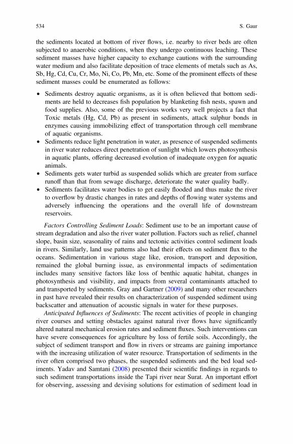
the sediments located at bottom of river flows, i.e. nearby to river beds are oftensubjected to anaerobic conditions, when they undergo continuous leaching. Thesesediment masses have higher capacity to exchange cautions with the surroundingwater medium and also facilitate deposition of trace elements of metals such as As,Sb, Hg, Cd, Cu, Cr, Mo, Ni, Co, Pb, Mn, etc. Some of the prominent effects of thesesediment masses could be enumerated as follows:
• Sediments destroy aquatic organisms, as it is often believed that bottom sedi-ments are held to decreases fish population by blanketing fish nests, spawn andfood supplies. Also, some of the previous works very well projects a fact thatToxic metals (Hg, Cd, Pb) as present in sediments, attack sulphur bonds inenzymes causing immobilizing effect of transportation through cell membraneof aquatic organisms.
• Sediments reduce light penetration in water, as presence of suspended sedimentsin river water reduces direct penetration of sunlight which lowers photosynthesisin aquatic plants, offering decreased evolution of inadequate oxygen for aquaticanimals.
• Sediments gets water turbid as suspended solids which are greater from surfacerunoff than that from sewage discharge, deteriorate the water quality badly.
• Sediments facilitates water bodies to get easily flooded and thus make the riverto overflow by drastic changes in rates and depths of flowing water systems andadversely influencing the operations and the overall life of downstreamreservoirs.
Factors Controlling Sediment Loads: Sediment use to be an important cause ofstream degradation and also the river water pollution. Factors such as relief, channelslope, basin size, seasonality of rains and tectonic activities control sediment loadsin rivers. Similarly, land use patterns also had their effects on sediment flux to theoceans. Sedimentation in various stage like, erosion, transport and deposition,remained the global burning issue, as environmental impacts of sedimentationincludes many sensitive factors like loss of benthic aquatic habitat, changes inphotosynthesis and visibility, and impacts from several contaminants attached toand transported by sediments. Gray and Gartner (2009) and many other researchersin past have revealed their results on characterization of suspended sediment usingbackscatter and attenuation of acoustic signals in water for these purposes.
Anticipated Influences of Sediments: The recent activities of people in changingriver courses and setting obstacles against natural river flows have significantlyaltered natural mechanical erosion rates and sediment fluxes. Such interventions canhave severe consequences for agriculture by loss of fertile soils. Accordingly, thesubject of sediment transport and flow in rivers or streams are gaining importancewith the increasing utilization of water resource. Transportation of sediments in theriver often comprised two phases, the suspended sediments and the bed load sed-iments. Yadav and Samtani (2008) presented their scientific findings in regards tosuch sediment transportations inside the Tapi river near Surat. An important effortfor observing, assessing and devising solutions for estimation of sediment load in
534 S. Gaur

Tapi river was reported by them, by incorporating non uniform bed material con-sidering the various variables like discharge, hydraulic mean depth, flow velocity,bed slope, etc. by collecting the field data of Tapi River for 10–15 years duration.Bed load was found to be a dominating part of sediment transport with significantinfluences of non-uniformities of river-bed materials. Sediments of varied sizeshave its own impact and greater control on many environmental and engineeringconcerns, specifically from managerial point of view, as pin pointed below inTable 1.
Idol Immersion and Other Ritual Activities
India is the country of rituals and people used to believe and deeply follow these.Most of these rituals are performed near the bank of river and water bodies. The‘Ganesh Chaturthi’ or ‘Durga Ashtami/Navratri’ use to be important festivals ofHindu and during these festival thousands of Idols having various sizes areimmersed every year in different water bodies of the cities. In Gujarat, the Idolimmersion of Lord Ganesha happens to be a grand celebration in each year, wherelarge number of Idols got immersed in rivers after 10 days worship during themonths of August or September. If we consider the area of present study, only in
Table 1 Probable influences of sediments on environmental and engineering concerns
Sedimentsize
Environmental issues Associated engineering issues
Silts andclays
Erosion, especially loss of topsoil inagricultural areas; gullying
High sediment loads to reservoirs Reservoir siltation
Chemical transport of nutrients, metalsand chlorinated organic compounds
Drinking-water supply
Accumulation of contaminants inorganisms at the bottom of the food chain(particulate feeders)
Silting of fish spawning beds anddisturbance of habitats (by erosion orsiltation) for benthic organisms
Sand River bed and bank erosion River channel deposition,navigation problems, instability ofriver cross-sections
River bed and bank erosion Sedimentation in reservoirs
Habitat disturbance
Gravel Channel instability when dredged foraggregate
Instability of river channel leads toproblems of navigation and floodcontrol
Habitat disturbance
An Updated Review on Quantitative and Qualitative Analysis … 535
Tapi river, on an average about 3000–4000 idols were being immersed during eachsuch festival in recent years. These idols are constructed by plaster of paris, clay,cloths, small iron rods, bamboo and decorated with different paints such as varnish,water colours, etc. and when immersed in the water, leads to significant alteration inthe water quality (Dhote et al. 2001; Swain et al. 2005; Vyas et al. 2008; Dhote andDixit 2011 and Bhat et al. 2012). The input of biodegradable andnon-biodegradable substances found to be responsible for greatly deteriorating thewater quality and enhancing silt load in the river. The floating materials releasedthrough idol in the river or lake after decomposition results in eutrophication too.Thakre et al. (2013) reported certain important findings on environmental impactsof Idol immersion at foremost upstream reaches of river Tapi and found it as amajor cause for river water contamination. The immersion practices resulted indegradation of water quality apart from siltation. After immersion of the idols, theriver water quality parameters like turbidity, total hardness, chemical oxygendemand (COD), biochemical oxygen demand (BOD), dissolved oxygen (DO), oiland grease depicted higher values well beyond their maximum permissible limits asprescribed by standard agencies.
Reported Results/Findings on Tapi River Pollution
Surat is the only major city in the state to have been blessed by a perennial river.But, the river is being stabbed by citizens. A Delhi-based firm engaged by the SuratMunicipal Corporation (SMC) found that there are more than 7000 illegal drainsemptying their contents into the Tapi, making it more polluted than the Sabarmatiwhen it comes to faecal bacteria content. An analysis of Tapi waters done inFebruary by SVNIT in the upstream of causeway (Sarthana, Varachha, Katargamand Rander) from where the city draws its drinking water, records a pH factor of9.06, suggesting that the water has turned highly alkaline. Its coliform bacteriacontent peaked to 1.6 lakh in litre by the time it crossed Varachha and Jehangirpuraareas instead of the required 500 per 100 ml. Coliform is the main indicator offaecal content in water. The biochemical oxygen demand (BOD) has alwaysremained above 30 mg/L. In the downstream of the causeway, the total coliformcontent peaks to as high as 1.1 crore per litre at Singanpore, where the city drains itssewage. The dissolved oxygen is reported as ‘zero’ at Ginger hotel, Sardar Bridgeand Ved hotel. The BOD levels are as high as 315 mg/L while the standards are30 mg/L. Even the chemical oxygen demand (COD) levels exceed desirable levelsat Sardar bridge, Vivekanand bridge and the Singanpore areas and hovers between520 and 800 mg/L—the standard being 250 mg/L. Excessive sand mining has alsoplayed its part in changing the contours of the river. Encroachments on both the sidewithin the civic limit area has also resulted in the carrying capacity coming downfrom 8.5 lakh cusecs to merely 3.5 lakh cusecs. “Weir-cum-causeway has actuallyblocked the passage of impurities on Tapi, when both organic and inorganicimpurities accumulate at the causeway, decomposition leads to birth of more
536 S. Gaur

microorganisms. We need to get rid of these accumulated impurities”. Siltation isthe major problem for Tapi river today, as high tides bring in a lot of impuritiesfrom the sea to the river, but does not pull it back. This raises the river-bed level ofTapi through the last 35 km of its journey which passes through the city. The scopeof this updated review remained to assess some of the dominating physiochemicalparameters on the course of water in the river Tapi, based upon available literature.Presenting reviewed results of all water quality attributes, remained out of scopehere, moreover some of the significant ones are attempted herein with their reportedvalues/causes/effects in study area.
Status of Quantitative Discharges/Floods
City of Surat is located between Mumbai and Ahmedabad on banks of river Tapi,which originates from Multai in MP and merge into Arabian Sea at Dumas. Thoughthere remained many recent estimates of river discharges for study locations, but thesame could not find place here owing to large variations even in short span of time,in particular the recent years, when climate and rainwater are showing totallyunpredictable and non-homogeneous results. If we see some of the historicalrecords for Tapi river discharges for Surat location, the total annual runoff volumewas used to be projected as 12,000 Million Cubic Metres (MCM) which wasconsidered to be an assured flow for 75% of years. Out of this, Maharastra hadallocated 6000 MCM quota for its use, while the Gujarat had created reservoir atUkai (about 100 km upstream of Surat) for storage of 8600 MCM. Floods in andaround Surat and villages remained the chronic issues for all the past years and thusthey remained as an active part of flood drainage of Tapi River. Some of thehistorical estimates (as evident from Ukai dam data using indirect sources) clearlyrevealed the facts that the Tapi river can contain about 6 lakhs cusecs of floodwithin banks in major areas of Surat city and around. Since 1882, many extremefloods/high discharges are recorded, and most of them occurred in the months ofAugust and September. Major floods (1933, 1959, 1968, 1970, 1998 and 2006)gave a situation when recorded floods even crossed 9 lakhs cusecs capacity.
One of the recent estimation (Patel and Gundaliya 2014) for calculating thedischarge carrying capacities of River Tapi was found to be of great relevance andimportance for this write-up. Massive floods of 2006, as occurred in Surat,remained the centre of focus, where greater damage to personal and properties wereseen in 2006, and authors had presented estimated discharge capacities of Tapi riverfor more than 300 cross sections across lower Tapi basin. Table 2, presents somehistorical peak discharge values as observed during few important floods in Surat.The carrying capacity of river Tapi, is being drastically deteriorated and needssuitable modifications. Agnihotri and Patel (2011) provided ways and means ofimproving carrying capacities of river Tapi, which has its own importance tocurrent scenario.
An Updated Review on Quantitative and Qualitative Analysis … 537
Status of Sediment Characteristics
For Tapi river the suspended sediment loads as well as the bed load of sediments,both were found to be equally important and sensitive. This is due to the fact thatthe river reaches are located at most downstream side near to the sea. Majority offindings have clearly established the facts that the sediment transport remains thedirect function of water movement. Chakrapani (2005) reported excellent findingson variety of factors which ultimately control the variations in sediment loads insidethe rivers. Looking the physics of sediment transport inside the river, it is quiteevident from physical observations that during floods, sediment particles getsseparated into suspended material (silt + clay + sand) and bed load (some partmoving along bed and other getting deposited on bed). Bed load as reported forTapi is usually stony material, such as gravel and cobbles, that moves by rollingalong the river bed being too heavy to be lifted into suspension by flowing water.
A baseline study was conducted by Marathe et al. (2011) to determine the basicphysical and chemical characteristics of the sediments of Tapi river, being con-centrated on whole river length at about 10 different locations along its course. Theoverall ranges of certain sediment related characteristics revealed following factualranges of variations,
• Texture of sediments—sandy to loamy (muddy) sand soils with pH 7.01–8.05• Organic carbon in Sediments—0.16–0.54%• Electric Conductivity (EC) of sediments—3.11–5.05 ds/m• Available Nitrogen (N), Potassium (K) and Phosphorous (K) in sediments—
71.8–244.3; 6.7–20.7; and 168.2–367.0 kg/ha, respectively• Exchangeable Ca and Mg in sediments—13.97–16.07 and 20.01–
20.40 me/100 mg
The Physicochemical characteristics of Tapti river sediments, particularly forSurat station were too reported, according to which the representative values of pH,Organic carbon (%), EC (ds/m), Exchangeable Ca (me/100 gm), Exchangeable Mg(me/100 gm), Available N (Kg/ha), Available P (Kg/ha), Available K (Kg/ha) were
Table 2 Comparison of different floods in Surat flood
Year Peak inflow(lakh cusec)
Max outflow(lakh cusec)
Rose level at hopebridge (m)
Outcome
1968 (no dam) – 15 12.01 Major flood
1978 <8 4.4 – No flood
1979 <8 3.3 – No flood
1994 8.9 6 10.2 Flood
1998 10.5 7 11.5 Flood
2006 10.6 9 12.01 Major flood
Source People Committee on Gujarat Flood 2006: A Report
538 S. Gaur
reported to be 7.01, 0.38, 3.99, 15.0, 20.11, 170.2, 190.0 and 367.2, respectively.Dinakaran and Krishnayya (2011) presented an interesting spectrum on organiccarbon and grain size distribution in certain ephemeral river sediments in westernIndia. Total Organic Carbon (TOC) and grain size distribution (sand, silt and clay)in the ephemeral Mahi River (western India) sediments were measured to look attheir effectiveness in understanding the late Quaternary monsoon conditions. Foursites spread across the alluvial zone and three sites from the estuarine zone weresampled. TOC concentration in the sediments of the alluvial and estuarine zonesites ranged between 0.04 and 0.39% and 0.04 and 0.23%, respectively. It wasobserved that grain size differed significantly at alluvial zone sites, while a uniformtrend was found in estuarine zone sites.
Status of River Water Quality
Earlier, works done on Tapi Water resources are said to be polluted because ofman’s action resulting in the addition of matter to the water or altering the physical,chemical or biological characteristics of water to such an extent that its utility forany reasonable purpose or its environmental value is demonstrably depreciated. Thequality of physicochemical and biological characterizations of water is an index toprovide a complete and reliable picture of the conditions prevailing for tropic statusin the water bodies. For present study following published literatures have beenreviewed viz Heavy Metal are considered as major environmental pollutants, whichis consistently increasing through effluents, sedimentation of rocks and miningactivities. High concentrations of all heavy metals are toxic to biological systemsand affect the growth and differentiation of a blue green and green algae.Researchers have studied and reported a lot to assess the pollution load of TapiRiver adopting standard methods (APHA 2005) with below given majorsteps/efforts,
• Survey and selection of sites for river water samples for certain confinedsections.
• Physiochemical characterization of river water sediments and nearby soil sam-ples for pH, conductivity, hardness, total alkalinity, bicarbonates, phosphate,chlorides, calcium, magnesium, sodium, potassium, etc.
• Heavy metal concentration in water, sediments and soil nearby soil samplessuch as Fe, Cu, Zn, Cd, Pb, As, Hg, Ni.
• Detection of some organic compounds such as BHC and DDT in river water.• Water Analysis in pre-monsoon and post-monsoon season.• Long term comparison and statistical analysis of data between river water and
sediment.• Ground water quality and soil quality in nearby land and water bodies.• Prevailing and projected awareness among the public/society living nearby.
An Updated Review on Quantitative and Qualitative Analysis … 539
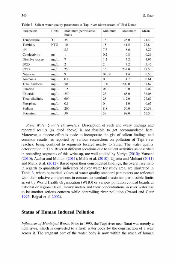
River Water Quality Parameters: Description of each and every findings andreported results (as cited above) is not feasible to get accommodated here.Moreover, a sincere effort is made to incorporate the gist of salient findings andcommon results, as reported by various researchers on pollution of Tapi riverreaches, being confined to segments located nearby to Surat. The water qualitydeterioration in Tapi River at different locations due to salient activities as describedin preceding segments of this write-up, are well studied by Variya (2010); Varsani(2010); Azahar and Multani (2011); Malik et al. (2010); Ujjania and Multani (2011)and Malik et al. (2012). Based upon their consolidated findings, the overall scenarioin regards to quantitative indicators of river water for study area, are illustrated inTable 3, where numerical values of water quality standard parameters are reflectedwith their relative comparisons in contrast to standard maximum permissible limitsas set by World Health Organization (WHO) or various pollution control boards atnational or regional level. Heavy metals and their concentrations in river water useto be another serious concern while controlling river pollution (Prasad and Gaur1992; Bajpai et al 2002).
Status of Human Induced Pollution
Influences of Municipal Waste: Prior to 1995, the Tapi river near Surat was merely atidal river, which is converted to a fresh water body by the construction of a weiracross it. The stagnant part of the water body is now within the reach of human
Table 3 Salient water quality parameters at Tapi river (downstream of Ukai Dam)
Parameters Units Maximum permissiblelimits
Minimum Maximum Mean
Temperature °C 35 18 25.0 21.4
Turbidity NTU 10 15 41.5 23.8
pH – 8.5 7.7 8.6 8.27
Conductivity ms 1 0.2 0.8 0.29
Dissolve oxygen mg/L 7 1.2 7.2 4.95
BOD mg/L 2 2 7.2 5.45
COD mg/L 250 16 232.0 79.5
Nitrate-n mg/L 9 0.019 1.4 0.53
Ammonia mg/L 0.1 0 1.7 0.61
Total hardness mg/L 500 100 202.0 137.67
Fluoride mg/L 1.5 0.01 0.0 0.02
Chloride mg/L 250 23 65.0 36.08
Total alkalinity mg/L 600 28 112.0 77.67
Phosphate mg/L 0.1 0 1.0 0.67
Sodium mg/L 200 8.8 50.0 20.59
Potassium mg/L 50 39 98.0 56.5
540 S. Gaur
habitat and accumulates waste load (organic pollutant and nutrients) turning it to beeutrophic. Due to the federal system of governance prevalent in India, both theCentral and State governments exploit rivers as a national natural resource and thewater is transported to meet people’s needs at remote places beyond the river basin.Besides this orderly use, the river is also exploited by those living on the riverbanksforming a user group usually not documented. These users draw water, dischargewastewater and sometimes over exploit the aquatic resource. The activities that fallunder this unorganized category include washing clothes, cattle farming, religiousactivities, cremation, open defecation, recreation, fishing and agriculture. SuratMunicipal Corporation carried out a survey in 2001 to identify the majorwastewater discharges into the river. The survey revealed that the population of2,811,614 individuals within the municipal limit, living in 7 villages along the riverbank, 15 km upstream of the weir, accounts for wastewater discharge of 5204 m3
per day through 28 inlet points. If we see on animal sides, in some of thereports/news papers of past, it was reported that at least 35 cattle farmers with morethan 100 cattles were occupying the Tapi river bank, which might have grown tomany fold by now. Moreover, its an established and reliable estimate that about400 kg of animal dung is wasted every day, assuming that each cattle generate 4 kgof dung per day. Anyone can visualize the pollution scenario, when such a largequantity of dung is being discharged into Tapi river. The results as reported byDubey and Ujjania (2013) indicated that most of the physicochemical parameters(pH, Turbidity, dissolved oxygen (DO), biological oxygen demand (BOD),chemical oxygen demand (COD), phosphate, ammonia and potassium) from TapiRiver were beyond the WHO and BIS limits for drinking water and even notsuitable for domestic purposes.
Influences of Idol Immersion on Water Quality: Tapi river is investigated bymany researchers, in this regard, encompassing varied locations along river course.It is difficult to incorporate all such results here, moreover certain confined results,as observed for its tail end locations (near Surat) are being reported herein. Mohiniet al. (1991) gave very comprehensive findings based upon their observed watersamples at idol immersion sites on Tapi River, revealing the fact that values of mostof the water quality parameters gets adversely affected during the immersion whichlater recovered in the post-immersion period. For example, the value of temperatureduring the pre-immersion, immersion and post-immersion period was stated as32.5, 30.2 and 30 °C, respectively. Turbidity of water during immersion period wasreported highest (126 NTU) while it was shown comparatively low during thepre-immersion (98 NTU) and post-immersion (54 NTU). Conductivity was reported12.2 ms during immersion period while it was 4.6 and 0.5 ms duringpre-immersion and post-immersion, respectively. High value of total solids1260 mg/L was observed during the immersion period that was comparatively low930 mg/L during pre-immersion and 650 mg/L during post-immersion period.Similarly total dissolved solid was shown 650 mg/L during immersion period whilepre-immersion and post-immersion period, it was found low 370 and 480 mg/L,respectively. Total suspended solids was found high 610 mg/L during immersionperiod compare to pre-immersion 569 mg/L and post-immersion period 170 mg/L,
An Updated Review on Quantitative and Qualitative Analysis … 541

respectively. The pH of river water was found alkaline 8.5 during immersion periodwhile it was 8.2 and 8.8 during pre-immersion and post-immersion period,respectively. In their study, total alkalinity was found 224.0 mg/L duringpre-immersion period compare to immersion and post-immersion period 96.0 and104.0 mg/L, respectively. Total hardness was observed as 1510.0 mg/L duringimmersion period while 340 mg/L during pre-immersion and 160 mg/L inpost-immersion period. The calcium hardness was observed as 310 mg/L duringimmersion period while 100 mg/L during pre-immersion period and 50 mg/Lduring post-immersion period, respectively. During immersion period, DO wasobserved 4.35 mg/L while it was observed comparably high during thepre-immersion 1.62 mg/L and post-immersion 3.24 mg/L. BOD was observed32.4 mg/L during the immersion period that was significantly high when comparedto pre-immersion 20.2 and 12.2 mg/L during post-immersion period. High value ofCOD 63.2 mg/L was observed in the immersion period and was comparatively low27.8 mg/L during pre-immersion and 34.5 mg/L during post-immersion period. Oiland grease was observed high 0.90 mg/L during immersion period while inpre-immersion and post-immersion period, these were reported low 0.70 and0.54 mg/L, respectively.
Ujjania and Mistry (2012) categorically assessed the environmental impact ofGanesh idol immersion activity on water quality of Tapi River with significantchanges in physicochemical properties of river water. It was found that the pH ofwater notably affects the solubility of nutrients. The pH was noted acidic or high(7.5–7.9) during the immersion period, while it was reported low during thepre-immersion (6.9–7.4) and post-immersion (7.6–7.7) periods. The range oftemperature during the pre-immersion, immersion and post-immersion period werereported as 27.0–31.0, 28.0–31.0 and 28.0–30.0 °C, respectively. Such rising intemperature was stated as a reason to speed up chemical reaction and biologicalactivity that reduce the solubility of gases in water. Similarly, DO during immersionperiod was observed very low (2.8–4.4) mg/L while it was observed comparablyhigh during the pre-immersion 4.8–6.8 mg/L. High value of carbon dioxide (12.32–14.08 mg/L), total hardness (166.0–178.0 mg/L) and total calcium (126–134 mg/L)were detected during the immersion period in comparison to other time periods.Other researchers too supported and supplemented similar inferences from theirfindings on different reaches of Tapi river.
The influences of ritual activities like Idol immersions were intensively studiedand reported by many other researchers too in different alike river segments (Maliket al. 2010; Ujjania and Multani 2011 and Malik et al. 2012). If we look into twospecific reaches of Tapi river viz. (a) Multai (Madhya Pradesh) an extreme upstreamlocation from where the river originates and (b) Surat (Gujarat) an extremedownstream location where the river almost finishes its course; the relative quan-titative status of river water pollution owing to idol immersions is reflected inTable 4, where the reported results are concisely presented. Same are selfexplanatory to reflect the adverse influences of Idol immersion activities in theriver, showing varied quality of river water during pre-immersion, immersion aswell as post-immersion periods.
542 S. Gaur
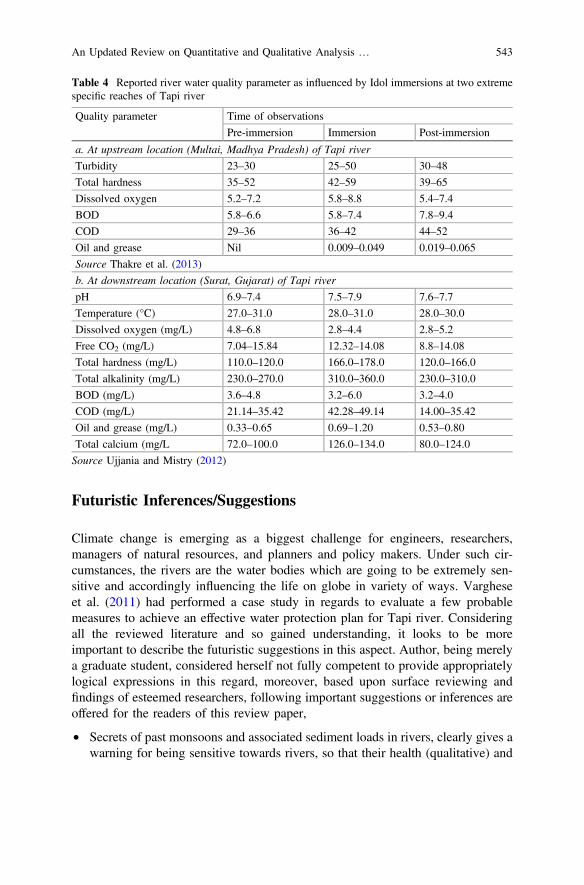
Futuristic Inferences/Suggestions
Climate change is emerging as a biggest challenge for engineers, researchers,managers of natural resources, and planners and policy makers. Under such cir-cumstances, the rivers are the water bodies which are going to be extremely sen-sitive and accordingly influencing the life on globe in variety of ways. Vargheseet al. (2011) had performed a case study in regards to evaluate a few probablemeasures to achieve an effective water protection plan for Tapi river. Consideringall the reviewed literature and so gained understanding, it looks to be moreimportant to describe the futuristic suggestions in this aspect. Author, being merelya graduate student, considered herself not fully competent to provide appropriatelylogical expressions in this regard, moreover, based upon surface reviewing andfindings of esteemed researchers, following important suggestions or inferences areoffered for the readers of this review paper,
• Secrets of past monsoons and associated sediment loads in rivers, clearly gives awarning for being sensitive towards rivers, so that their health (qualitative) and
Table 4 Reported river water quality parameter as influenced by Idol immersions at two extremespecific reaches of Tapi river
Quality parameter Time of observations
Pre-immersion Immersion Post-immersion
a. At upstream location (Multai, Madhya Pradesh) of Tapi river
Turbidity 23–30 25–50 30–48
Total hardness 35–52 42–59 39–65
Dissolved oxygen 5.2–7.2 5.8–8.8 5.4–7.4
BOD 5.8–6.6 5.8–7.4 7.8–9.4
COD 29–36 36–42 44–52
Oil and grease Nil 0.009–0.049 0.019–0.065
Source Thakre et al. (2013)
b. At downstream location (Surat, Gujarat) of Tapi river
pH 6.9–7.4 7.5–7.9 7.6–7.7
Temperature (°C) 27.0–31.0 28.0–31.0 28.0–30.0
Dissolved oxygen (mg/L) 4.8–6.8 2.8–4.4 2.8–5.2
Free CO2 (mg/L) 7.04–15.84 12.32–14.08 8.8–14.08
Total hardness (mg/L) 110.0–120.0 166.0–178.0 120.0–166.0
Total alkalinity (mg/L) 230.0–270.0 310.0–360.0 230.0–310.0
BOD (mg/L) 3.6–4.8 3.2–6.0 3.2–4.0
COD (mg/L) 21.14–35.42 42.28–49.14 14.00–35.42
Oil and grease (mg/L) 0.33–0.65 0.69–1.20 0.53–0.80
Total calcium (mg/L 72.0–100.0 126.0–134.0 80.0–124.0
Source Ujjania and Mistry (2012)
An Updated Review on Quantitative and Qualitative Analysis … 543

geometry (physical state) could be properly taken care by involving all segmentsof society.
• The river systems do respond to climatic changes but the response is notovernight, it may take hundreds of years to show a lasting change, hence moreintensive research studies are of great importance in today’s context when moreand more habitats are coming up on the river banks or along the flood pathwaysof the rivers.
• Rivers should not be taken for granted. Planning course of action on them in anyof the desired ways/means, just to fulfill the vested interest (political, com-mercial, popularity stunt, forceful obligations, long term business/benefits, etc.),needs to be avoided. Merely translation of river into cosmetic beautification inthe name of river fronts development or other catchy projects, looks beautiful inits first catch, but technologically they could release harms rather benefits forriver water bodies/river system in totality, as it invites only the real estate forconcrete structures to attain the end target of recreational/commercial activities.Do we really need river front development models? Is it a true river restoration?Such questions could be considered as a big food for thought for us, beinginclined towards ecological and climatic adjustment of river eco systems.
• The water pollution of Tapi river has gained large heights, and now it becameimperative to yield a plan, identifying viable remedial options and strategies forits effective clean up. Efforts needs to be made to resort to a bottom-up approachrather than a top-down one to help this highly polluted river, which is the majorlife-supporting artery of Surat city. We need to develop awareness amongmasses, education, and improved watershed management that can improve theoverall water quality of this holy river.
• Huge quantity of waste water discharges into river, which needs proper man-agement and treatment to remove or at least reduces the organic matter, solids,nutrients, disease-causing organ isms and other pollutants from the river waterbody.
• Looking into ever increasing shortage and uncertainties of water both in urbanand rural areas, conservation of water must be given top priority, which could bewell achieved by adopting several strategies like, promoting wastewatertreatment/technologies, drainage water management/treatment, recycling/reuseof waste water, improving sewerage system, upgrading of sewage treatmentplant, effective disposal of sewage, agricultural practices improvement withreduced applications of chemicals/fertilizes, better environmental managementof rivers considering interactions among ecology/hydrology/waterquality/climate/flooding/droughts, afforestation, canal developments, integratedwatershed management in river catchments, etc.
• Strong awareness among the people and creation of proper legislation and finesis another critical needs of time, where different organizations/groups of com-mon people, and even the youth and students must take active part controllingvisible/invisible abuses to rivers and river water bodies. This could evolve somesimple and innovating ways and means to tackle this alarming situation whereriver water pollution is touching greater heights.
544 S. Gaur
• A better and deep understanding of causes and effects of river water pollutionneeds to be made available to common people using social media, showing theanticipated on-site and off-site impacts. River water pollution not only remainsconfined to visible water bodies of the rivers, but could have multiple adverseimpacts/deteriorations towards invisible soil columns, ground water bodieswhich are sensitive sources to gets easily polluted.
• Relocation of religious activities and crematoria along rivers looks to be a need,but from practical considerations it is not at all feasible to totally avoid it.Moreover, certain alternative plans and thinking needs to be evolved at thisjuncture, to reduce the extent of problem. This objective could be attained byeducating the concerned people, by providing alternate disposal facility for thewaste, properly relocating the cause points of pollution like cattle shed, watersupply, biogas energy generation plants, outlets for marketing of dairy products,alternate water sources for washermen making cloth washing as organizedactivity by identifying a suitable locality and dedicated source of water withpumping station.
Conclusion
Rivers are the lifeline for human beings on the globe as they use to be the onlyreliable source of water for domestic, industrial, agricultural and all other activitiesof life. Owing to fast developments, the river water quality is getting deteriorated inan alarming fashion, which altogether demands for a proper understanding of itscauses and effect to evolve suitable solutions. The rivers located nearby to urbanareas are more severely influenced and need special attention.
Present study reflects an updated review of river water pollution in regards to animportant west flowing Tapi river of India, by incorporating reported findings orresults by various researchers, considering the major water quality parameterswhich includes Temperature, Turbidity, pH, Conductivity, Dissolve Oxygen, BOD,COD, Nitrate-n, Ammonia, Total Hardness, Fluoride, Chloride, Total alkalinity,Phosphate, Sodium, Potassium, Free carbon dioxide, Oil and grease, Total calcium,etc.
The values of these sensitive indicators were found to be significantly deviatingfrom the standard prescribed safe limits as established by agencies like WHO orpollution control boards at regional or national scales. The deep analysis of severalpredominant causes of river water pollution, showed an alarming situation for riverunder study, where activities under three specific categories (1) Domestic/Humaninduced (2) Industrial (3) Agricultural; have released sizeable inputs to deterioratethe river water bodies physically as well as chemically. Influences of ritual activitieslike Idol immersion are specifically screened which showed high influences onleading water quality parameters and demands for framing alternative regulationsand strategies to cope up with the issue.
An Updated Review on Quantitative and Qualitative Analysis … 545
The extent of sediment and its detrimental effects on river water quality werefound to be the leading concern, which remains the sole ingredients towards riverwater pollution. The in depth reading and analysis of more than 50 researchpapers/publications, made the author educative and a bit capable to draw certainspecific conclusions and inferences on the subject, which are mentioned in pre-ceding sub section namely “Futuristic Inferences/Suggestions”, hence not beingrepeated here.
References
Agnihotri PG, Patel JN (2011) Improving carrying capacity of river Tapi (Surat, India). By channelmodification. Int J Adv Eng Technol II(II):231–238 (ISSN: 0976-3945)
APHA (2005) Standard methods for examination of water and waste water. American PublicHealth Association, Washington, D.C.
Bajpai A, Pani S, Jain RK, Mishra SM (2002) Heavy metal contamination through idol immersionin a tropical lake. Ecol Environ Conserv Organ 8(2):157–159
Bhat NA, Wanganeo R, Ashwani Wanganeo (2012) Pollution status of bhoj wetland before & afterimmersion of idols. South Asian J Tourism Heritage 5(1):153–156
Chakrapani GJ (2005) Factors controlling variations in river sediment loads. Curr Sci 88(4):25Dinakaran J, Krishnayya NSR (2011) Variations in total organic carbon and grain size distribution
in ephemeral river sediments in western India. Int J Sedim Res 26(2011):239–246Dhote S, Varghese B, Mishra SM (2001) Impact of idol immersion on water quality of Twin lakes
of Bhopal. Indian J Environ Prot 21:998–1005Dhote S, Dixit S (2011) Hydro chemical changes in two eutrophic lakes of central India after
immersion of Durga and Ganesh idol. Res J Chem Sci 1(1):38–45Dubey M, Ujjania NC (2013) Water quality and pollution status of Tapi river, Gujarat, India. Int J
Pure Appl Zool 1(3):261–266Gajanand T, Mishra PK, Bajpai A, Pani S (2013) Environmental impact of idol immersion on
Tapti River of Multai, Distt. Betul, MP, India. Res J Chem Sci Int Sci Congr Assoc, 3(10):31–35
Gray JR, Gartner JW (2009) Technological advances in suspended-sediment surrogate monitoring.Water Resour Res 45(4)
Malik GM, Raval VH, Zadafiya SK, Patel AV (2012) Idol immersion and physico-chemicalproperties of South Gujrat rivers India. Res J Chem Sci 2(3):21–25
Malik GM, Raval VH, Zadafiya SK, Patel AV (2010) Idol immersion and physico-chemicalproperties of South Gujarat rivers. Curr World Environ J 5(1):173–176
Marathe RB, Marathe YV, Sawant CP (2011) Sediment characteristics of Tapti river, Maharashtra,India. Int J Chem Tech Res 3(3):1179–1183
Mohini G, Ekhalak A, Ranjana S (1991) Pollution load assessment of Tapi river during Ganeshfestival India. Octa J Environ Res 2(4):310–313
Multani AA (2011) Impact of ganesh idol immersion on Tapi river at Ashwanikumar Ovara. M.Sc.Dissertation, Veer Narmad South Gujarat University Surat
Patel CG, Gundaliya PJ (2014) Calculating discharge carrying capacity of river Tapi. Int J Eng ResTechnol (IJERT), 3(3) ISSN: 2278-0181
Prasad D, Gaur HS (1992) Environmental pollution: water. Venus Publishing House, New Delhipp 294–330
Rajesh V (2010) Impact of Ganesh idol immersion on Tapi river at Umara ovara. M.Sc.Dissertation, Veer Narmad South Gujarat University
546 S. Gaur

Ujjania NC, Mistry CA (2012) Environmental impact of Idol immersion on Tapi river (India). Int JGeol Earth Environ Sci 2(3):11–16 (ISSN: 2277)
Ujjania NC, Multani AA (2011) Impact of Ganesh idol immersion activities on the water quality ofTapi river, Surat (Gujarat) India. Res J Biol 1(1):11–15
Varghese KG, Shah IK, Mudliar SL, Alappat BJ (2011) Integrated source water protection plan foran urban water body—A case study of Tapi river, India. Int J Environ Sci 1(7)
Varsani A (2010) Impact of Ganesh Idol Immersion on Tapi River at Ashwanikumar Ovara. M.Sc.Dissertation, Veer Narmad South Gujarat University, Surat
Vyas A, Bajpai A, Verma N (2008) Water quality improvement after shifting of idol immersionsite: a case study of Upper Lake, Bhopal, India. Environ Monit Assess 145(1–3):437–443
Yadav SM, Samtani BK (2008) Bed load transport in Tapi river, India. Glob J Environ Res 2(2):96–101 (ISSN: 1990-925X)
Subramanian V (1996) The sediment load of Indian rivers—an update. Erosion and sedimentyield: global and regional perspectives. In: Proceedings of the exeter symposium, July 1996.IAHS Publ. No. 236, pp 183–189
Swain SK, Mohapatra S, Patel RK (2005) A measure of pollution load in temple ponds of Puri,Orissa on the basis of NSF-WQI suggestions. Poll Res 24(3):599–603
An Updated Review on Quantitative and Qualitative Analysis … 547
Ensemble MCDM Approach to DeterminePriorities of Parameters for WQI
Ritabrata Roy, Mrinmoy Majumder and Rabindra Nath Barman
Abstract Priorities of different water quality parameters are required to be deter-mined for the calculation of Water Quality Indices. The procedures of determiningpriorities (importance) to the parameters are often subjective and preferential. Thepresent study proposes an objective and non-preferential method to determine thepriorities of water quality parameters to calculate Water Quality Index. Relativeimportance of the parameters were determined on the basis of important criteria likehazard potential, utility, cost, and citation frequency using Multi-CriteriaDecision-Making methods like Analytic Hierarchy Process, Fuzzy LogicDecision-Making, and their combinations. Different Water Quality Indices (MCDMWQI) were developed from the priority values of the parameters, determined byeach of the methods applied. A case study was performed in Tripura, India tovalidate those Water Quality Indices. Sensitivity analysis, statistical analysis, andcomparison with an established Water Quality Index (NSF WQI) were performedfor each of the indices developed. The MCDM WQIs were found to be close toNSF WQI (less than 2% deviation) and also follow similar patterns. The HybridAHP-FLDM method was found to be closest to NSF WQI (0.29% deviation)among the methods used. Thus, the MCDM WQI is successful in representing theoverall water quality.
Keywords Water quality index � WQI � Objective � Non-preferentialMulti-criteria decision-making � MCDM � Ensemble � Analytic hierarchyprocess � AHP � Fuzzy � Tripura � IndiaR. Roy (&) � M. MajumderSchool of Hydro-Informatics Engineering, National Institute of Technology Agartala,Barjala, Jirania 799046, Tripura (W), Indiae-mail: [email protected]
M. Majumdere-mail: [email protected]
R.N. BarmanDepartment of Mechanical Engineering, National Institute of Technology Durgapur,Durgapur 713209, West Bengal, Indiae-mail: [email protected]
© Springer Nature Singapore Pte Ltd. 2018V.P. Singh et al. (eds.), Environmental Pollution, Water Scienceand Technology Library 77, https://doi.org/10.1007/978-981-10-5792-2_43
549

Introduction
In recent years, Multi-Criteria Decision-Making (MCDM) methods like AnalyticalHierarchy Process (AHP) (Saaty 1977, 1980) and Fuzzy Logic Decision-Making(FLDM) (Zadeh 1965) are being widely used to support decision-making in com-plex situations, where multiple factors are involved (Triantaphyllou 2000). In thepresent study, MCDM is used to determine the priorities of the Water QualityParameters (WQP) in an objective and non-preferential way. Water Quality Index(WQI) is a concise numerical representation of overall water quality of a water body,which is convenient to interpret and widely used (Tyagi et al. 2013). WQI of water isessentially a function of the water quality parameters and their concentrations.
Equation 1 WQI is a function of parameters and their concentration
WQI ¼ f P;Cð Þ ð1Þ
where
P Water quality parameterC Concentration of that parameter.
P 2 RjP[ 0 and C 2 Rj C[ 0Not all the WQP are equally important in assessing the overall quality of water.
A fewer parameters with greater importance may be enough to represent the overallquality. As different water quality parameters have different importance in assessingoverall water quality, the priorities of the parameters are required to be determinedfor calculation of WQI. In initial (Horton 1965; Brown et al. 1970; Dunnette 1979)and later works (Bhargava 1983; House and Ellis 1987) on WQI, the importance ofthe parameters were determined from subjective opinions of the experts(Avvannavar and Shrihari 2008). The number of experts surveyed was very small incomparison to the huge pool of experts throughout the globe. Moreover, only theexperts’ opinions were considered, but the criteria on which the importance of theparameters were determined, were out of the scope of those WQIs.
In later phase, the trend was to develop a method which is more general andobjective in nature (BCWQI—Rocchini and Swain 1995; CWQI—CCME 2001;WAWQI—Chauhan and Singh 2010). However, in these cases, the WQIs werecalculated by quantification of the failure of the parameters to meet the objectivevalues, rather than their individual importance. Also, the selection of parametersand objective values depends upon the consideration of the users. Therefore, theseindices are rather subjective and biased (Terrado et al. 2010) in nature. Anotherdisadvantage of these indices is they are quite time consuming to calculate as alarge number of data are required.
550 R. Roy et al.
In some recent works, use of MCDM methods like AHP (Karbassi et al. 2011),FLDM (Lermontov et al. 2009; Semiromi et al. 2011; Sahu et al. 2011; Mourhir et al.2014) and their combinations (Ocampo-Duque et al. 2006; Carbajal-Hernándezaet al. 2012) was found to be successful in the determination of importance of theparameters in objective and non-preferential manner. In the present study, multiplesignificant criteria were selected first from experts’ opinions. Expert survey isreplaced by literature survey in the selection of WQP to integrate the views of a largenumber of experts. On the basis of those selected criteria, the relative importance ofthe parameters was determined in an objective and non-preferential way using dif-ferent MCDM methods and their combinations. Novelty of the study is that hazardpotential, utility, and cost were considered together for the determination of weightsof importance of the parameters. So, the weights, determined by the proposedmethod, were able to represent the impact on the cost of mitigation, utilities, andhazards of the parameters considered. Again, MCDM methods like AHP, FLDM,and their combinations were used to determine the priorities of the parameters.
Objective
The objective of this study was to determine Priority Values (PV) of differentWQPs for WQI in an objective and non-preferential way on the basis of importantcriteria, so that the index can be more realistic and holistic.
Methodology
The PV of different WQP were determined on the basis of some important criteria,using different MCDM methods and their aggregation. The method was then val-idated through a case study where different WQIs were calculated from the samplesusing those PV. Sensitivity analysis, statistical analysis, and comparison with anestablished WQI were then performed on those WQI for that validation.
Selection of Criteria
Four important criteria, viz., hazard potential, utility, cost and citation score, wereselected on the basis of expert survey. A brief description of those criteria is givenhere:
Hazard Potential (H): Hazard potential is a relative estimation of the potentialextent of hazard caused by each of the specific water quality parameters. The mosthazardous (or least beneficial) parameter gets the lowest score.
Ensemble MCDM Approach to Determine Priorities of Parameters … 551
Utility (U): Utility is a relative estimation of how useful is each of the waterquality parameters to assess the overall quality of the water. The most usefulparameter gets the highest score.
Cost (C) of Mitigation: It is a relative estimation of how expensive the miti-gation of the negative impact imposed by each of the specific water qualityparameters. The most expensive parameter gets the lowest score.
Citation Score (F): Citation frequency is the percentage of frequency of using ofparameters in related studies. The most used parameter gets the highest score andvice versa.
Selection of Parameters
The parameters were selected from the metastatic analysis of extensive literaturesurvey. Citation scores of the parameters found in literatures were calculated bytheir frequencies of use in the related studies (Eq. 2) (Debnath et al. 2015; Ghoshet al. 2016).
Equation 2 Citation score of parameters from Literature Survey
S ¼ PC� 100 ð2Þ
where
S Citation score of a parameterP Number of times a particular parameter was found in literatureC Total number of times all the parameter was found in literature.
The WQP which have at least 5% presence in literature, were selected for thisstudy (Craparo 2007). Citation score being fractional values, the WQP which havescores greater than 4.5 were taken as selected, following the rule of approximation.
Scoring of Parameters
Selected WQP were scored on the basis of each of the selected criteria from ametastatic literature survey.
Hazard Potential (H): When the importance of the parameters was determinedon the basis of hazard potential, their benefits and negative effects were assessedfrom the literature qualitatively. The qualitative values were then converted toquantitative values using a scale of 1–5 (Table 1).
552 R. Roy et al.
The scoring of hazard potential was calculated by combining the quantitativevalues from all the literature surveyed (Eq. 3).
Equation 3 Scoring of hazard potential of the parameters
IH ¼P
Hi
Nð3Þ
where
IH Relative importance score of a hazard potential of a parameterHi Importance value (scale of 1–5) of hazard potential in ith literature for that
parameterN Number of literature surveyed.
For example, the parameter Dissolved Oxygen (DO) found to be very beneficialas per some related literature. The qualitative importance of DO was assigned in thefollowing manner for each of the papers surveyed:
Paper Hazard potential Score
1 Most beneficial 5
2 Beneficial 4
3 Most beneficial 5
4 Most beneficial 5
5 Most beneficial 5
Then the hazard potential score of DO is (5 + 4 + 5 + 5 + 5)/5 = 24/5 = 4.8.The hazard potential of all the parameters was calculated in the similar way.
Utility (U): When the importance of the parameters was determined on the basisof their utilities, their usefulness was assessed from the literature qualitatively. Thequalitative values were then converted to quantitative values using a scale of 1–5(Table 2).
Table 1 Scale of hazard potential of the parameters
Criteria Mosthazardous/leastbeneficial
Hazardous/lessbeneficial
Neitherhazardousnorbeneficial
Beneficial/lessHazardous
Leasthazardous/mostbeneficial
Scale 1 2 3 4 5
Table 2 Scale of utility of the parameters
Criteria Most useful Very useful Moderately useful Less useful Least useful
Scale 5 4 3 2 1
Ensemble MCDM Approach to Determine Priorities of Parameters … 553
The scoring of utility was calculated by combining the quantitative values fromall the literature surveyed (Eq. 4).
Equation 4 Scoring of utility of the parameters
IU ¼P
Ui
Nð4Þ
where
IH Relative importance score of a hazard potential of a parameterUi Importance value (according to the scale of 1–5) of utility in ith literature for
that parameterN Number of literature surveyed.
For example, the parameter temperature was found to be moderately useful asper some related literature. The qualitative importance of temperature was assignedin the following manner for each of the papers surveyed:
Paper Hazard potential Score
1 Moderately useful 3
2 Moderately useful 3
3 Very useful 4
4 Moderately useful 3
5 Less useful 2
Then the utility score of pH is (3 + 3 + 4 + 3 + 2)/5 = 15/5 = 3. The utility ofall the parameters was calculated in the similar way.
Cost (C): Cost of mitigation of native impacts of each of the WQP was alsodetermined in the similar way.
Citation Frequency (F): The citation frequencies of the parameters weredetermined from their citation scores (Eq. 5).
Equation 5 Citation frequency of parameters from Literature Survey
F ¼ S100
ð5Þ
where, F = Citation frequency and S = Citation score.
Determination of Weights of the Criteria
The opinions of five experts were taken to assess the relative importance of thecriteria. The scale of importance is given in Table 3.
The importance values of the criteria were calculated by multiplying the scalevalue with the number of experts, given that importance scores (Eq. 6).
554 R. Roy et al.
Equation 6 Calculation of Relative Importance of the Criteria
I ¼P
S� EN
ð6Þ
where
I Relative importance score of a parameterS A Scale value (1–5)E Number of Experts, given that value to that parameterN Number of Experts.
For the criterion utility, the evaluations of the experts were as follows:
Expert No. Evaluation Score
1 Moderately important 3
2 Important 4
3 Moderately important 3
4 Important 4
5 Moderately important 3
So, the Relative Importance Score of utility is ((3 � 3) + (4 � 2))/5 = (9 + 8)/5 = 17/5 = 3.4. The Relative Importance Score of all the criteria was calculated inthe similar way.
Determination of Weights of the Parameters
The weights of the parameters were determined using MCDM methods likeAnalytical Hierarchy Process (AHP) and Fuzzy Logic Decision-Making (FLDM)and their combinations.
Weights by AHP
For the determination of weights by AHP method, the comparison matrix of theselected criteria was prepared from their citation frequencies (Eq. 2) and the criteriascore was calculated. Then comparison matrices of all the parameters were prepared
Table 3 Scale of importance of the criteria
Importance Mostimportant
Important Moderatelyimportant
Lessimportant
Notimportant
Scale 5 4 3 2 1
Ensemble MCDM Approach to Determine Priorities of Parameters … 555
for each of the criterion, using Saaty scale (Saaty 1977). After that, the scores wereworked out my multiplying the matrix of criteria scores with that of parameterscores. The normalized values of the importance scores were taken as the weights ofthe parameters.
Weights by FLDM
Similarly, the weights of fuzzy comparison matrices of the criteria and theparameters were prepared using FLDM. The multiplication of matrices of theimportance scores of the criteria and parameters was performed to find out the finalimportance scores of the parameters. The normalized values of the importancescores from FLDM process were taken as the weights of the parameters in thesimilar manner.
Weights by Combination of AHP and FLDM
The weights of the parameters were determined in another way. The scores of thequalitative criteria (i.e., whose comparison was done qualitatively) were determinedby FLDM and that of quantitative criteria (i.e., whose comparison was donequantitatively) were determined by AHP. The similar procedure was followed tofind out the scores of the parameters. Then the fuzzy values were converted to crispvalues to form the matrices. Again, the normalized values of the matrices weretaken as the weights of the parameters.
Weights by Hybrid of AHP and FLDM
Yet another method was applied—the standard AHP procedure was followed, butthe comparison of the criteria and parameters was performed using FLDM. In thiscase also, the matrices of the importance scores of the criteria and parameters weremultiplied to obtain importance scores. The normalized values of the importancescores were taken as the weights of the parameters as usual.
Aggregated Weight
Finally, the mean values of the weights of each of the parameters, worked out bydifferent procedures, were calculated. These values were named as Aggregated
556 R. Roy et al.

Weight of the parameters. The key differences among the methods used for thedetermination of the priorities of the parameters are summarized in Table 4.
Validation of the Proposed Method
AWQI was developed from the priority values of the parameters, determined by theproposed method. For validation of the proposed method, sensitivity analysis andscenario analysis on different landscape patterns were performed. The WQI wasalso compared with NSF WQI.
Case Study
Samples were collected from 38 different water bodies of South and West ofTripura, a state located in the north eastern part of India. The WQIs of the sampleswere calculated using the different indices, developed by applying different MCDMmethods.
Developing WQI with the Determined Prioritiesof the Parameters
Different WQIs (MCDM WQI) were developed using the weights of the parameterscalculated by the MCDM method to verify its applicability. The sub-index valueswere calculated by multiplying the weights of respective parameters with their Qvalues (Eq. 7) (Brown et al. 1970).
Equation 7 Calculation of AHP WQI
WQI ¼Pn
i¼1 WiQiPni¼1 Wi
ð7Þ
Table 4 Key differences among the methods used
AHP FLDM CombinedAHP-FLDM
AHP-FLDMhybrid
Aggregated score
Procedurefollowed
AHP FLDM AHP AHP Mean values of thescores from these fourmethods were takenComparison
procedureCrisp Fuzzy Crisp for
Quantitative criteria,Fuzzy forQualitative criteria
Fuzzy
Ensemble MCDM Approach to Determine Priorities of Parameters … 557

where
Qi Q value for ith water quality parameterWi Weight associated with ith water quality parametern Number of water quality parameters.
Sensitivity Analysis
Sensitivity analysis of the parameters was performed in respect to WQI usingtornado model (Eschenbach 2006). The importance scores of the parameters werecompared with their sensitivity to verify whether the most important parameters arethe most sensitive also.
Comparison of the MCDM WQI with NSF WQI
WQIs of the same samples were calculated using the National SanitationFoundation Water Quality Index (NSF WQI) (Brown et al. 1970). The values ofMCDM WQI were then compared with that of NSF WQI. The difference betweenthe MCDM WQI and NSF WQI was assessed by Mean Absolute PercentageDeviation (MAPD) (Eq. 8) (Hyndman and Athanasopoulos 2013).
Equation 8 Calculation of MAPD of WQI from NSF WQI
MAPD ¼ 100n
Xn
i¼1
Ni �Mi
Nið8Þ
where,
Ni NSF WQI of ith sampleMi WQI of ith sample by proposed methodsn Number of samples.
Result and Discussion
Selection of Parameters
In the 182 literatures surveyed, 51 water quality parameters were found. The totalnumbers of times all those parameters used were found as 765. Now, the parameterpH was found 49 times in those literatures. Therefore, the citation score of pH is
558 R. Roy et al.

49765 � 100 ¼ 6:41. The citation scores of all the parameters were calculated in thesimilar way. The selected parameters and their citations scores are given in Table 5.
The first eight parameters (Dissolved Oxygen, pH, Temperature, BiochemicalOxygen Demand, Phosphate, Nitrate, Total Solids, and Turbidity) were selected forthe present study.
Determination of the Priorities of the Parameters
The priorities of the selected parameters were determined, using AHP, FLDM, andtheir combinations. The hierarchy of the criteria and the parameters are describedschematically in Fig. 1.
Table 5 Citation scores of various water quality parameters found in the literature
SL Parameters Citation score SL Parameters Citation score
1 DO 7.71 27 Cadmium 1.18
2 BOD 7.06 28 Selenium 1.18
3 pH 6.41 29 Zinc 1.18
4 Phosphate 5.62 30 Sodium 0.78
5 Temperature 5.36 31 Hardness 0.78
6 Nitrate 4.84 32 Iron 0.78
7 TS 4.71 33 Barium 0.78
8 Turbidity 4.58 34 Anionic Surfactant 0.78
9 Conductivity 3.86 35 Alkalinity 0.39
10 Ammonia 3.62 36 Salinity 0.39
11 Nitrite 3.13 37 Boron 0.39
12 Chloride 2.98 38 Carbonate 0.39
13 Sulfate 2.89 39 Calcium 0.39
14 TDS 2.87 40 Magnesium 0.39
15 COD 2.88 41 Manganese 0.39
16 Fecal Coliform 1.96 42 TOC 0.39
17 Arsenic 1.96 43 Cryptosporidium 0.39
18 Chromium VI 1.96 44 Aluminium 0.39
19 TKN 1.77 45 Silver 0.39
20 Total Coliform 1.67 46 Cyanide 0.39
21 Lead 1.67 47 Nickel 0.39
22 Copper 1.57 48 TA 0.39
23 Fluoride 1.28 49 SAR 0.39
24 TS 1.21 50 Oil & Grease 0.39
25 Color 1.18 51 Oxidation Ability 0.39
26 Mercury 1.18
Ensemble MCDM Approach to Determine Priorities of Parameters … 559
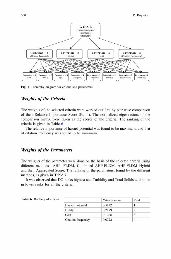
Weights of the Criteria
The weights of the selected criteria were worked out first by pair-wise comparisonof their Relative Importance Score (Eq. 4). The normalized eigenvectors of thecomparison matrix were taken as the scores of the criteria. The ranking of thecriteria is given in Table 6.
The relative importance of hazard potential was found to be maximum, and thatof citation frequency was found to be minimum.
Weights of the Parameters
The weights of the parameter were done on the basis of the selected criteria usingdifferent methods—AHP, FLDM, Combined AHP-FLDM, AHP-FLDM Hybridand their Aggregated Score. The ranking of the parameters, found by the differentmethods, is given in Table 7.
It was observed that DO ranks highest and Turbidity and Total Solids tend to bein lower ranks for all the criteria.
G O A L(Determination of
Priorities of Parameters)
Criterion – 1(Hazard Potential)
Criterion – 2(Utility)
Criterion – 3(Cost)
Criterion – 4(Citation Frequency)
Parameter – 1(DO)
Parameter – 2(BOD)
Parameter – 3(pH)
Parameter – 4(Phosphate)
Parameter – 5(Temperatur
e)
Parameter – 6(Nitrate)
Parameter – 7(Total Solids)
Parameter – 8(Turbidity)
Fig. 1 Hierarchy diagram for criteria and parameters
Table 6 Ranking of criteria Criteria score Rank
Hazard potential 0.5872 1
Utility 0.2179 2
Cost 0.1228 3
Citation frequency 0.0722 4
560 R. Roy et al.

Case Study
A case study was performed for the validation of the proposed method for deter-mining the PV of WQP.
MCDM WQI
WQIs were developed from the PV of the different MCDM methods and collec-tively called as MCDM WQI. The MCDM WQIs were calculated similarly asNSF WQI as it is an established and widely used one. Now, there are nineparameters, recommended for NSF WQI and their weights are in a scale of 1 (i.e.,the sum of the weights of all the parameters is 1). In the present study, eightparameters were selected and their weights are also in the scale of 1. As there is amismatch in the number of parameters, a correction factor (Eq. 9) was used to scaleboth the indices similarly.
Equation 9 Calculation of the Correction Factor
Correction Factor ¼P
PNSFPPMCDM
ð9Þ
where
PNSF Weights of the common parameters in NSF andPMCDM Weights of the common parameters in Proposed.
The Correction Factor was found to be 0.84 (Eq. 8) which is the sum of theweights of common parameters in NSF WQI. Therefore, 0.84 was multiplied witheach of the weights of the selected parameter for the purpose of scaling (Table 8),so that the sum of weights of all the common parameters in both of the methods is
Table 7 Ranking of the parameters with respect to the criteria
Parameters Hazard potential(qualitative)
Utility(qualitative)
Cost(quantitative)
Citation frequency(quantitative)
DO 1 1 1 1
pH 2 3 8 3
BOD 6 4 2 4
Temperature 7 2 4 5
Phosphate 5 5 6 2
Nitrate 3 6 5 7
Turbidity 4 7 7 8
Total solids 8 8 3 6
Ensemble MCDM Approach to Determine Priorities of Parameters … 561
equal. The scaled scores were taken as the weights for the WQI of the proposedmethod.
The WQI was then calculated using these weights of the parameters. Q valueswere determined as per the method of NSF WQI.
Sensitivity Analysis
The relative sensitivity of all the input parameters toward the WQI was calculatedby the single factor analysis using Tornado technique (Eschenbach 2006). Theresults show that the first three most prioritized parameters (DO, BOD, and pH) arealso the first three most sensitive parameters. Again, the least important parameter(Total Solids) was found to be least sensitive also. Thus, weights of importance, asgiven by the MCDM methods, were found to support the results from sensitivityanalysis (Table 9).
Table 8 Weights of the parameters
Parameters Corrected weights of the parameters NSF WQIweightsAHP FLDM Combined
AHP-FLDMAHP-FLDMhybrid
Aggregatedscore
Dissolvedoxygen
0.17 0.16 0.12 0.16 0.15 0.17
pH 0.10 0.10 0.09 0.10 0.10 0.11
BOD 0.12 0.11 0.14 0.12 0.12 0.11
Temperature 0.09 0.09 0.11 0.09 0.10 0.10
Totalphosphate
0.10 0.11 0.11 0.10 0.11 0.10
Nitrates 0.10 0.10 0.09 0.10 0.10 0.10
Turbidity 0.09 0.09 0.07 0.08 0.08 0.08
Total solids 0.07 0.08 0.11 0.08 0.09 0.07
Table 9 Sensitivity analysis of the parameters
Parameters Sensitivity AHPweights
FLDMweights
CombinedAHP-FLDMweights
AHP-FLDMhybrid weights
Aggregatedweights
Dissolvedoxygen
0.39 0.20 0.19 0.19 0.20 0.20
pH 0.14 0.12 0.12 0.12 0.11 0.12
BOD 0.38 0.14 0.14 0.14 0.14 0.14
Temperature 0.01 0.11 0.11 0.11 0.13 0.11
TotalPhosphate
0.03 0.12 0.13 0.13 0.12 0.12
Nitrates 0.02 0.12 0.12 0.11 0.11 0.11
Turbidity 0.03 0.10 0.10 0.10 0.11 0.10
Total solids 0.01 0.09 0.10 0.11 0.09 0.10
562 R. Roy et al.
Statistical Analysis
Water quality of most (78%) of the samples was found to be medium. The meanwater quality was also found medium with the WQI value of 64 (Table 10). A lowstandard deviation (about 7) of the WQI values of the samples shows that there arelittle variations in water quality among the samples (Table 10). The low skewnessand kurtosis values of the WQI values also support the fact by indication that thevalues are close to each other (Table 10). However, negative values of skewnesssuggest that the water quality spreads a little bit toward bad rather than good(Table 10). Only 15% of the samples have good water quality as the 85th percentileof the values is 70—the threshold value of good water quality (Table 10).
Comparison of MCDM WQI with NSF WQI
The graphical representation of the WQI, by all the methods, shows similar patterns(Fig. 2). The graphs were prepared by plotting the WQI points in an increasingorder and joining them with smooth lines.
Table 10 Analysis of the water quality of the samples
METHODS AHP FLDM CombinedAHP-FLDM
AHP-FLDMhybrid
Aggregated NSF
Mean valueof WQI
64 64 64 64 64 64
Mean interpretation Medium Medium Medium Medium Medium Medium
Standard deviation 7.16 6.86 6.92 7.03 6.98 6.94
Skewness −0.40 −0.33 −0.29 −0.39 −0.35 −0.43
Kurtosis 0.34 0.41 −0.27 0.31 0.18 0.39
85th percentile 70 70 70 70 70 70
Fig. 2 Comparison graph of the WQI values of different methods
Ensemble MCDM Approach to Determine Priorities of Parameters … 563
All the WQI were found to be very close to NSF WQI, except the APH-FLDMHybrid WQI, which exhibits more conservative values (MAPD = 3.49%) thanNSF WQI (Table 11). The reason of such behavior seems to be contributed byfuzzy method, as it is known to give conservative output values. Among the othermethods, AHP WQI was found to be the closest (MAPD = 0.42%) to NSF WQI,followed by Combined AHP-FLDM WQI (MAPD = 0.44%) and FLDM WQI(MAPD = 0.57%) (Table 11). The Aggregated WQI was also fairly close(MAPD = 0.64%) to the NSF WQI (Table 11).
Thus, it was found that among the outputs of the different methods, the HybridAHP-FLDM method is closest to the outputs of NSF method (MAPD = 0.29%).Therefore, the Hybrid AHP-FLDM method seems to be more appropriate than theother MCDM methods used in this study.
Conclusion
The present investigation attempted to determine the priority values of water qualityparameters in agricultural runoff for estimation of WQI on the basis of hazardpotential, utility, cost of mitigation, and citation frequencies of the parameters. Themethod was developed in such a manner that subjective and preferential treatmentmay get minimized. The weights of parameters were determined by the output ofAHP, FLDM, Combined AHP-FLDM and AHP-FLDM Hybrid methods, whichhelp to estimate the weights as a direct representation of the importance ofparameters in depiction of overall quality of water. The MCDM WQI was com-pared with NSF WQI for validation. The most important PV were also found to bethe most sensitive toward the respective WQI and vice versa.
All these methods of validation showed accuracy (close to NSF WQI), applica-bility (found by sensitivity analysis) and reliability (found by statistical analysis) ofthe indices. According to the results, DO and Total Solids were found to have thehighest and lowest priorities respectively, among the eight parameters considered, inassessing the overall water quality. The sensitivity analysis showed that the mostimportant parameters are the most sensitive also, toward the WQI. Among themethods used, the AHP-FLDM Hybrid WQI was found to be the closest(MAPD = 0.29%) to NSF WQI, followed by Combined AHP WQI (MAPD =0.42%), FLDM WQI (MAPD = 0.57%) and Aggregated WQI (MAPD = 0.59%).However, AHP-FLDM Combination WQI deviates more (MAPD = 1.81%) fromNSF WQI and tends to give comparatively extreme outputs.
Table 11 MAPD of the WQI by proposed methods from NSF WQI
AHPWQI
FLDMWQI
CombinedAHP-FLDM WQI
AHP-FLDMhybrid WQI
AggregatedWQI
MAPD (%) 0.42 0.57 1.81 0.29 0.59
564 R. Roy et al.

In the present study, the criteria considered were the hazard potential, cost,utility, and citation frequency of the parameters. In future studies, more differentcriteria such as effects of the parameters on aquatic (e.g., insects, fishes, algae,planktons) and terrestrial biodiversity (both plants and animals), crop type, cropyield, human health, etc., may be included while estimating their priorities. Also,other MCDM methods (e.g.. Analytic Network Process, Weighted Sum Method,Weighted Product Method, Simple Additive Weight, Grey Relational Analysis,etc.) and their combinations may be used to determine the priorities in similarstudies.
Acknowledgements The authors thankfully acknowledge the active support of Dr. Manish Pal(HoD) and Mr. Santanu Bhowmik (Research Scholar), School of Hydro-Informatics Engineering,NIT Agartala during collection of data for the present study.
References
Avvannavar SM, Shrihari S (2008) Evaluation of water quality index for drinking purposes forriver Netravathi, Mangalore, South India. Environ Monit Assess 143:279–290
Bhargava DS (1983) Use of water quality index for river classification and zoning of Ganga River.Environ Pollut (Series B) 6:51–67
Brown RM, McClelland NI, Deininger RA, Tozer RG (1970) A water quality index- do we dare?Water Sew Works, 339–343
Canadian Council of Ministers of the Environment (2001) Canadian environmental qualityguidelines for the protection of aquatic life. CCME water quality index: technical report, 1.0
Carbajal-Hernándeza JJ, Sánchez-Fernándezb LP, Carrasco-Ochoaa JA, Martínez-Trinidad JF(2012) Immediate water quality assessment in shrimp culture using fuzzy inference systems.Expert Syst Appl 39(12):10571–10582
Chauhan A, Singh S (2010) Evaluation of Ganga water for drinking purpose by water qualityindex at Rishikesh, Uttarakhand, India. Report Opinion 2(9):53–61
Craparo RM (2007) Significance level. Encyclopedia of measurement and statistics, vol 3. SAGEPublications, Thousand Oaks, CA, pp 889–891
Debnath A, Majumder M, Pal M (2015) A cognitive approach in selection of source for watertreatment plant based on climatic impact. Water Resour Manage 29(6):1907–1919
Dunnette DA (1979) A geographically variable water quality index used in Oregon. J Water PollutControl Fed 51(1):53–61
Eschenbach TG (2006) Constructing tornado diagrams with spreadsheets. Eng Econ 51(2):195–204
Ghosh S, Majumder M, Chakraborty T, Pal M (2016) Development of the location suitabilityindex for wave energy production by ANN and MCDM techniques. Renew Sustain EnergyRev 59(2016):1017–1028
Horton RK (1965) An index number system for rating water quality. J Water Pollut Control Fed 37(3):300–305
House M, Ellis JB (1987) The development of water quality indices for operational management.Water Sci Technol 19(9):145–154
Hyndman RJ, Athanasopoulos G (2013) Forecasting: principles and practice. OTexts. www.otexts.org/fpp
Karbassi AR, Hosseini MMF, Baghvand A, Nazariha M (2011) Development of water qualityindex (WQI) for Gorganrood River. Int J Environ Res 5(4):1041–1046
Ensemble MCDM Approach to Determine Priorities of Parameters … 565
Lermontov A, Yokoyamab L, Lermontovc M, Machadod MAS (2009) River quality analysisusing fuzzy water quality index: Ribeira do Iguape river watershed, Brazil. Ecol Ind 9(6):1188–1197
Mourhir A, Rachidi T, Karim M (2014) River water quality index for Morocco using a fuzzyinference system. Environ Syst Res 3(21). www.environmentalsystemsresearch.com/content/3/1/21
Ocampo-Duquea W, Ferré-Huguetb N, Domingob JL, Schuhmachera M (2006) Assessing waterquality in rivers with fuzzy inference systems: a case study. Environ Int 32(6):733–742
Rocchini R, Swain LG (1995) The British Columbia water quality index. Water Quality Branch,Environmental Protection Department, British Columbia Ministry of Environment, Land andParks
Saaty TL (1977) A scaling method for priorities in hierarchical structures. J Math Psychol 15:59–62
Saaty TL (1980) The analytic hierarchy process, planning, priority setting, resource allocation.McGraw-Hill, New York
Sahu M, Mahapatra SS, Sahu HB, Patel RK (2011) Prediction of water quality index using neurofuzzy inference system. Water Qual Exposure Health 3(3–4):175–191
Semiromi FB, Hassani AH, Torabian A, Karbassi AR, Lotfi FH (2011) Water quality indexdevelopment using fuzzy logic: a case study of the Karoon River of Iran. Afr J Biotech 10(50):10125–10133
Terrado M, Barceló D, Tauler R, Borrell E, de Campos S, Barceló D (2010) Surface-water-qualityindices for the analysis of data generated by automated sampling networks. Trends Anal Chem29(1):40–52
Triantaphyllou E (2000) Multi-criteria decision making: a comparative study. Appl Optim 44:5–21Tyagi S, Sharma B, Singh P, Dobhal R (2013) Water quality assessment in terms of water quality
index. Am J Water Resour 1(3):34–38Zadeh LA (1965) Fuzzy sets. Inf Control 8(3):338–353
566 R. Roy et al.
Aerosol Optical Depth Variation Duringa Recent Dust Event in North India
Manu Mehta, Vaishali Sharma and Gaurav Jyoti Doley
Abstract Aerosols play a vital role in influencing the climate both by cooling andwarming up the Earth’s surface and also by altering the cloud properties. Due tonatural and large amount of anthropogenic factors, Indian region observes highvariability of loadings in aerosols both in terms of space and time in the planetaryboundary layer. Dust storms in India exert momentous influences on weather, airquality, and climate of the country. Detection and monitoring of aerosol opticaldepth (AOD) at the time of dust storms is challenging, especially in case of shortlife time of events, and strong interaction with climatic parameters. This paperaddresses the study of a dust storm event which hit Indian (North) region on June13, 2015 parts of Haryana, Punjab, Delhi, UP were affected. AOD variations overthe North Indian region has been studied using MODIS level 2 data (MOD04)obtained NASA Terra platform at a spatial resolution of 10 km � 10 km.
Keywords AOD � Dust storm � MODIS
Introduction
Satellite-based remote sensing estimations permit precise way of retrieval of aerosoloptical properties on both local and global rate (Kaufman et al. 2005; Kahn et al.2010). Dust storms are one of the major sources of aerosols in Northern India;
M. MehtaPhotogrammetry and Remote Sensing Department,Indian Institute of Remote Sensing, Dehradun 248001, Uttaranchal, Indiae-mail: [email protected]
V. Sharma (&)School of Geo-Informatics, Remote Sensing Application Centre,Lucknow 226021, Uttar Pradesh, Indiae-mail: [email protected]
G.J. DoleyNational Institute of Technology Warangal, Warangal 506004, Telangana, Indiae-mail: [email protected]
© Springer Nature Singapore Pte Ltd. 2018V.P. Singh et al. (eds.), Environmental Pollution, Water Scienceand Technology Library 77, https://doi.org/10.1007/978-981-10-5792-2_44
567
especially in spring and summer seasons. Aerosol loading is increased during thepre-monsoon season (summer season, April–June) in the Indo-Gangetic plainsbecause of large influx from higher range transport of mineral dust aerosols fromthe western arid zone (Dey et al. 2004; El-Askary et al. 2004, 2006; Singh et al.2004; Prasad and Singh 2007). A firm convection in summer took after by a deeperboundary layer, and addition of dust events results in higher aerosol optical depth(AOD) during summer (Singh et al. 2004). Dust particles can directly modify thesurface radiation budget in both visible (VS) and infrared (IR) spectral regions thatleads to temperature variation of earth’s surface and therefore impacting theexchange processes between the earth’s surface and atmosphere, as well as climaticdynamics (Alpert et al. 2004) and chemical and biological environment (Singh et al.2004). Detection of dust storms is challenging because of the short-life existence,multiple scales and strong bonding with the local surface and meteorologicalconditions. Because of specific optical features of dust storms, satellite-observedradiances having the spectral signatures of dust particles are different from those ofother atmospheric components (Zhao 2012). This paper presents the aerosol opticaldepth (AOD) variation during a dust storm event that hit over northern part of India,i.e., Delhi, NCR, Haryana regions during June 13, 2015. The satellite data at aspatial resolution 10 km � 10 km is taken from Moderate resolution ImagingSpectro-radio-meter (MODIS) onboard Terra platform.
Study Area, Data, and Method
Study area includes parts of Haryana, Himachal Pradesh, Punjab, U.P., and theUnion Territories of Delhi, NCR, and Chandigarh. This region lies inIndo-Gangetic plains covering 28°N–35° N and 70°E–78°E. According to IndianMeteorological department (IMD), temperature frequently rises above 35 °C overthe significant part of the Indo-Gangetic plain during summer. During winter, thelowest temperature on the plains falls to below 5 °C at some places (Fig. 1).
The AOD data before the dust storm (June 7, 11, 12, 2015), during the duststorm (13th June 2015) and after the dust storm (June 14, 15, 16, 19, 20, 2015 andJuly 1, 2, 2015) is visualized to have clear idea of the impact of the storm.
MODIS is a near-polar satellite sensor which is on board NASA’s Terra plat-form. It has a swath of 2,330 km (cross track) by 10 km (along track at nadir)orbiting at an altitude of 705 km and measures reflected solar radiance and globalemission in 36 spectral bands (wavelength ranges from to 0.415–14.5 lm) withresolution varying between 0.25 and 1 km at nadir. The MODIS retrieval algorithmconsiders a lookup table methodology, in which arranged aerosol types, loadings,and geometry are expected to, span the range of global aerosol conditions (Remeret al. 2005, 2010; Levy et al. 2010). The algorithm matches the lookup table withthe measured spectral reflectance.
In this paper MODIS level 2 daily aerosol data (MOD04_L2) (http://laadsweb.nascom.nasa.gov), at a spatial resolution of 10 km � 10 km at nadir, collected
568 M. Mehta et al.
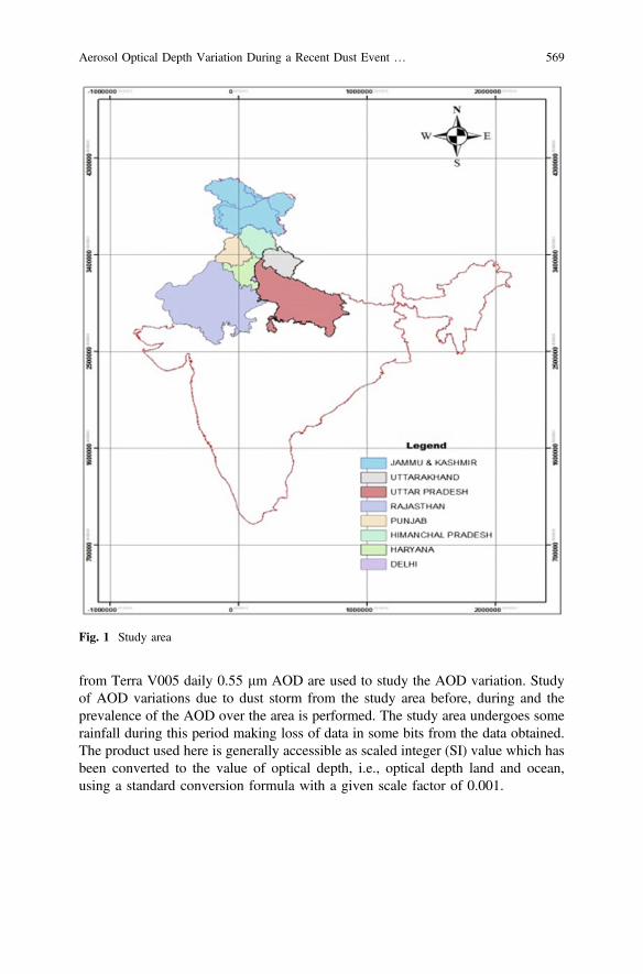
from Terra V005 daily 0.55 lm AOD are used to study the AOD variation. Studyof AOD variations due to dust storm from the study area before, during and theprevalence of the AOD over the area is performed. The study area undergoes somerainfall during this period making loss of data in some bits from the data obtained.The product used here is generally accessible as scaled integer (SI) value which hasbeen converted to the value of optical depth, i.e., optical depth land and ocean,using a standard conversion formula with a given scale factor of 0.001.
Fig. 1 Study area
Aerosol Optical Depth Variation During a Recent Dust Event … 569

Results and Conclusions
From Fig. 2, it can be seen that the area affected during dust storm covers the regionsof Northern India, mainly Rajasthan, Haryana, Delhi and Punjab and later the AODvalue increase over the Indo-Gangetic plain. Before the storm the values of the AODin the region varied from 0.4 to 0.7 i.e. from the period of June–June 7–11, 2015.The AOD values increases to 1.0 at some portion of the study area during the stormperiod i.e., June 12–14, 2015. It is interesting to note that even after 6 days, (19 June2015), the AOD values remain high in the considered study regime. This indicates
Fig. 2 AOD variations before, during and after dust storm
570 M. Mehta et al.
the longer stay times of dust particles in the atmosphere. A much later image of July1, 2015 also depicts higher AOD values in the North West India. The variationshows the accumulation of mineral dust over the study area for long time duration.
The future work in the allied area can also include a detailed trajectory analysisfor the source and sink identification of dust storm affected areas, along withquantified analysis of aerosol loading.
Acknowledgements The authors are grateful to Director of Indian Institute of Remote Sensing,Dehradun, Director and Principal of Remote Sensing Application Centre, U.P. and Director ofNational Institute of Technology, Warangal for their support in this study. Special thanks to Dr. R.K. Upadhyay, Scientist-D, In-charge––Agriculture Resource Division, RSAC, U.P. and Dr. DevaPratap, H.O.D. Civil Engineering Department, NITW. We thank the MODIS Data Support Teamfor providing with the MODIS data required for the study.
References
Alpert P, Kishcha P, Shtivelman A, Krichak SO, Joseph JH (2004) Vertical distribution of Saharandust based on 2.5-year model predictions. Atmos Res 70:109–130
Dash SK, Hunt JCR (2007) Variability of climate change in India. Curr Sci 93(6):782–788El-Askary H, Gautam R, Kafatos M (2004) Remote sensing of dust storms over the Indo-Gangetic
Basin. J Indian Soc Remote Sens 32(2):121–124El-Askary H, Gautam R, Singh RP, Kafatos M (2006) Dust storms detection over the
Indo-Gangetic basin using multi sensor data. Adv Space Res 37(4):728–733Gautam R, Hsu NC, Lau KM, Tsay SC, Kafatos M (2009) Enhanced pre‐monsoon warming over
the Himalayan‐Gangetic region from 1979 to 2007. Geophys Res Lett 36(7)Huang J, Ge J, Weng F (2007) Detection of Asia dust storms using multisensor satellite
measurements. Remote Sens Environ 110(2):186–191Levy RC, Remer LA, Kleidman RG, Mattoo S, Ichoku C, Kahn R, Eck TF (2010) Global
evaluation of the Collection 5 MODIS dark-target aerosol products over land. Atmos ChemPhys 10(21):10399–10420
Liang S, Zhong B, Fang H (2006) Improved estimation of aerosol optical depth from MODISimagery over land surfaces. Remote Sens Environ 104(4):416–425
Li Z, Zhao X, Kahn R, Mishchenko M, Remer L, Lee KH, Maring H (2009) Uncertainties insatellite remote sensing of aerosols and impact on monitoring its long-term trend: a review andperspective. Annales Geophysicae 27(7):2755–2770 Copernicus GmbH
Kahn R‚ Van Donkelaar A, Martin RV, Brauer M, Levy R, Verduzco C‚ Villeneuve PJ (2010)Global estimates of ambient fine particulate matter concentrations from satellite-based aerosoloptical depth: development and application. Environ Health Perspect 118(6):847
Kaufman YJ, Remer LA, Tanré D, Mattoo S, Chu DA., Martins JV, ... ‚ Eck TF (2005)The MODIS aerosol algorithm, products, and validation. J Atmos sci, 62(4):947–973.
Prasad AK, Singh RP (2007) Comparison of MISR-MODIS aerosol optical depth over theIndo-Gangetic basin during the winter and summer seasons (2000–2005). Remote SensEnviron 107(1):109–119.
Singh RP, Dey S, Tripathi SN, Tare V, Holben B (2004) Variability of aerosol parameters overKanpur, northern India. J Geophys Res Atmos 109(D23)
Zhao M‚ Ginoux P, Prospero JM, Gill TE, Hsu, NC (2012) Global‐scale attribution ofanthropogenic and natural dust sources and their emission rates based on MODIS Deep Blueaerosol products. Rev Geophys 50(3).
Aerosol Optical Depth Variation During a Recent Dust Event … 571