VIC-3D Educational System Testing Guide Introduction Completing a test with the VIC-3D Educational System is streamlined to make the process as straight forward as possible. This manual explains the procedure from start to finish, including:

• Prepare the specimen with a speckle pattern

• Physical setup of the system

• Using VIC-Snap EDU

• Capture calibration images

• Capture test images

• Calibration in VIC-3D EDU

• Analysis in VIC-3D EDU

• Viewing data Prepare the specimen with a speckle pattern Prepare the region of interest of your test specimen with a speckle pattern. In order to provide good tracking information, the speckle pattern should consist of the following characteristics:

• High contrast: Either dark black dots on a bright white background or bright white dots on a dark black background.

• 50% coverage: We want about equal amounts of white and black on the surface. For example, if the speckles are 5 pixels in size, they should be approximately 5 pixels apart from one another.

• Consistent speckle sizes: speckles should be ideally 3-5 pixels in size in order to optimize spatial resolution, but the most important thing is that the speckles are consistent in size and not too small (less than 3 pixels in size is too small and can cause aliased results).

• Isotropic: The speckle pattern should not exhibit a bias in any particular orientation.

• Random: It is actually hard to achieve a pattern regular enough to cause false matching, but if you are to print repeating patterns it can occur.

For the fixed field of view of this system, perfectly sized individual speckles would be 0.6mm (0.025”) in size. Larger speckles can be okay, but they should not be any smaller. An easy way to create this pattern is by applying a white spray paint base coat to the specimen surface. Avoid applying the paint too thick by using quick passes with the spray - just enough to cover the surface. When the basecoat is adequately dry, use the speckle roller supplied with your system to apply ink speckles. Several passes with the roller may be needed to achieve a dense enough pattern of speckles.

Example of speckle pattern created using ink roller. High contrast, about 50% black/white, random.

A more thorough explanation of speckle patterns and commonly used techniques is provided in Application Note AN-1701: Speckle Pattern Fundamentals, available through our online knowledgebase. Physical setup Tripod Begin by assembling the tripod. Screw the tripod head adjustment handles into the tripod head. Adjust the length of the tripod legs by releasing the levers on the legs, extending them to the desired length, and clamping the lever back down. Level the tripod head by turning the adjustment handles counter-clockwise to allow the head to rotate and then tighten them back to lock. There is a bubble level on both the tripod and tripod head to assist in leveling the system.

Inserting tripod head handles Mounting system on tripod head Next you will secure the system to the tripod. Screw the baseplate into the bottom of the system if not already installed. Open the locking mechanism on the tripod head by squeezing the small lever together and rotating it outwards. Align the baseplate with the tripod head and push it into place. The locking mechanism should snap shut when correctly secured.

Mounting the tripod plate to the bottom of the EDU system

Cables There are only two cables needed for the system. The first is the USB 3.0 type A to type B cable. Plug the type B end into the back of the system and the type A end into your computer’s USB 3.0 port. The second cable is for the power supply which also plugs into the back of the system. Plug this in to supply power to the light and system fan.

Using VIC-Snap EDU Once you have prepared the specimen with a speckle pattern, mounted the system on the tripod and mounted the system, open VIC-Snap EDU. If you are prompted to select a camera system, choose Point Grey. This is the manufacturer of the cameras used in the system. You should see two live image feeds from each camera in the system. If you need to rotate the images so that they are in their correct orientation, right click on the rotation angle below the image feed and select the appropriate orientation.

Baseplate

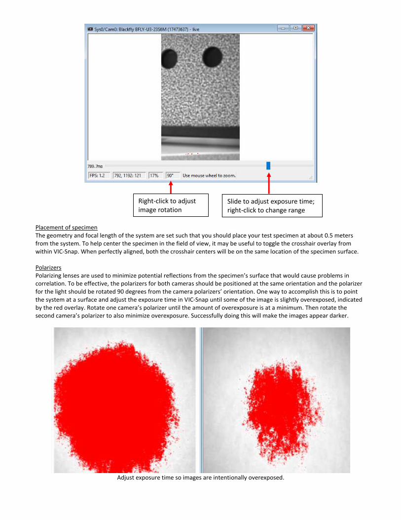
Placement of specimen The geometry and focal length of the system are set such that you should place your test specimen at about 0.5 meters from the system. To help center the specimen in the field of view, it may be useful to toggle the crosshair overlay from within VIC-Snap. When perfectly aligned, both the crosshair centers will be on the same location of the specimen surface. Polarizers Polarizing lenses are used to minimize potential reflections from the specimen’s surface that would cause problems in correlation. To be effective, the polarizers for both cameras should be positioned at the same orientation and the polarizer for the light should be rotated 90 degrees from the camera polarizers’ orientation. One way to accomplish this is to point the system at a surface and adjust the exposure time in VIC-Snap until some of the image is slightly overexposed, indicated by the red overlay. Rotate one camera’s polarizer until the amount of overexposure is at a minimum. Then rotate the second camera’s polarizer to also minimize overexposure. Successfully doing this will make the images appear darker.

Adjust exposure time so images are intentionally overexposed.

Right-click to adjust image rotation

Slide to adjust exposure time; right-click to change range

Adjusted left camera polarizer until overexposure is at a minimum (least number of red pixels).

Adjust right camera polarizer similarly; both match and have minimum red pixel overlay.

Exposure time Exposure time is the amount of time the camera sensors gather light before recording a new image. Longer exposure times make the image brighter but can also result in blur if significant motion happens during the exposure times. For many tests, blur is not a concern for the specimen, but can be an issue when acquiring images of a hand-held calibration grid. Adjust the camera’s exposure time in VIC-Snap. This is done by using the slider bar below each image viewer or by using the bracket keys. The range of the slider can be adjusted by right clicking the bar and selecting a new range. When acquiring images, the exposure time should be great enough that there is enough contrast between blacks and whites, but not too long that the image is overexposed or frame rate is limited. Overdriven pixels are indicated by the red overlay.

Exposure to long - overdriven Exposure to short - too dim Correct exposure

Capture calibration images Before beginning calibration, make sure your tripod and system are fully secured so that they do not move during or after calibration. Even small movements of the system can disrupt the calibration and result in errors and measurement bias. Changing the exposure time, however, does not disrupt calibration and can actually help make sure all images have good brightness. The goal of the calibration process is to take images of the calibration grid in a range of orientations that include tilting the grid forward, backwards, and rotating the grid. Because the calibration grid is rigid, these images can be used to perform shape measurements of the grid and determine the camera models and system parameters. Positioning grid The calibration procedure calculates variables about the camera geometry and positions; it is not specific to a plane or volume in space. Therefore, it’s not necessary to position the calibration grid in the exact same location as the intended specimen. Still, it will be most convenient to place the grid in roughly the intended plane. This will ensure that the cameras point correctly and the grid is in focus. Optimally, the specimen can be moved and replaced with the grid during the calibration. If this is not practical, it’s often possible to calibrate directly in front of the specimen; this method does require some extra depth of field because the grid will be in front of the focal plane rather than directly in it. Acquiring calibration grid images In VIC-Snap, select the directory and name for the images of this project by clicking Edit Files in the menu or toolbar. Change the image prefix to reflect that you are capturing calibration images.

With the grid in place, press the spacebar or the Capture icon in the toolbar to acquire an image pair. Capture at least 15-20 image pairs that show the calibration grid in both cameras, with a range or rotations of the grid. To accurately estimate the camera parameters, capture images with the grid rotated about all three axes. More calibration images will give a more accurate calibration and leaves more room to discard poor images (that may contain defocus, obstruction, etc). As you tilt the grid away or towards the cameras, it may be necessary to adjust the exposure time in VIC-Snap to make sure the images are sufficiently bright.

Acquire calibration images with grid rotation about 3 axes

• To acquire calibration images, capture several images of the grid in various orientations. Include significant rotations about all 3 axes.

• To accurately estimate perspective information, the grid should be tilted off-axis and/or moved closer/farther from the cameras for some images.

• To estimate aspect ratio accurately, the grid should be also rotated in-plane in some images.

• To estimate distortion accurately, grid points should cover the corners of the image field in some images. If a small grid is used, this will require specifically moving the grid to each corner and acquiring images. If the grid nearly fills the field, it will naturally fill in the corners.

• For each image pair, the grid should be visible in both images. If calibration is performed in roughly the same plane as the specimen, this will happen naturally.

• If a grid dot is partially off the edge of the image, it will be discarded. However, if it is partially blocked by, i.e., a thumb, VIC-3D may estimate the center incorrectly. This should be visible as a high error for that particular image.

• Some overdrive/saturation is acceptable, as long as black grid dots don’t appear reflective or white. Check system calibration (optional) You may want to consider performing the system calibration in VIC-3D EDU prior to running your actual test. This way you can identify any problems or avoid having a poor calibration. This isn’t strictly necessary since you can take calibration and test images in either order - if you perform your test and then realize that the calibration is poor, it is not too late to recalibrate. As long as the system has not been disturbed you may re-acquire calibration grid images. Capture test images Once calibration is complete, you may run the test. Click Edit Files again and rename the image prefix to indicate test images. There are two options available for how you capture images: Manual Capture: You may manually capture images by pressing the spacebar or the Capture icon. Timed Capture: Timed capture can be used to acquire images at the defined interval. You may also choose to have image capture terminate after a certain length of time, otherwise you will stop the capture by pressing Stop.

Calibration in VIC-3D EDU Import Images Once you have acquired calibration and test images, open VIC-3D. Import the calibration images using the Calibration images icon or from the Project menu. Navigate to the directory of your images and select them. Click Open to import the images to your project Calibrate Open the system calibration dialog using the calibration icon or from Calibration… Calibrate stereo system. With a coded grid, extraction will begin automatically. If not, select the grid you used from the Target drop down menu. Click Analyze to start extracting grid points from the target. After the calculation is complete, you will be presented with a report of calibration results and error scores. The errors will be displayed per image, as well as an overall error score.

The overall error (standard deviation of residuals for all views) should be displayed in green. If you have a good set of calibration images with good tilt and coverage of the image field, and the score is green, then the calibration is good and you can click Accept to finish. If the score is displayed in red, this indicates a potentially poor calibration. You may need to remove some images that have high individual scores or take new calibration images. VIC-EDU will automatically remove very poor images, but you can remove additional images by right-clicking in the table of scores and selecting Remove row. Below the calibration scores, the calibration results are listed. Each result is listed with a confidence interval; if the interval is very high, it may indicate a poor image sequence, even if the error score is low. If the scores are uniformly high across all images and not due to just a few outliers, there may be a problem with the setup. Check that:

• Each image does not have incorrectly extracted points or partially covered points.

• There is enough data for the calibration to converge.

• The grid images are in focus, evenly lit, and the grid points do not appear reflective.

• The exposure times are short enough to eliminate motion blur.

• The grid is rigid.

• The cameras are synchronized. Correct any potential problems and recalibrate. For each camera, the following values are displayed:

• Type: the type of camera model used in calibration.

• Center (x, y): the position on the sensor where the lens is centered. It should be roughly in the physical center of the sensor.

• Focal length (x, y): the focal length of the lens, in pixels.

• Skew: indicates out-of-square conditions for sensor grid.

• Kappa (1, 2): radial distortion coefficients of the lens.

• Magnification: the pixels/mm scale. For the rig as a whole, the following values are given:

• Angles (alpha, beta, gamma): the three angles between each camera. In general, two angles will be small and one (the stereo angle) will be larger.

• Distances (Tx, Ty, Tz): the distance between centers of camera 1 and camera 2, measured from camera 1. When the error score and confidence intervals are acceptable, click Accept to finish. The calibration data will be displayed in the Calibration tab of your project.

Analysis in VIC-3D EDU Import speckle images Import the test images into your project using the Speckle images icon or from the Project menu. Define AOI, subset, step Next you must define the area of interest (AOI) on your specimen. This is the portion of the image that contains the speckle pattern and which will be analyzed for specimen shape and displacements. To begin, double-click on the reference image file name in the Images tab to open the AOI Editor. The reference image will be displayed. You may change the reference image by right clicking a speckle image name and selecting Set reference image. Use the Create rectangle, Create polygon, or Create circle tools to select the desired AOI. Sections can be removed from the AOI using any of the Cut tools. You can define multiple AOIs in one project if necessary.

With the tool selected, clicking on the image will create a control point for the shape. Using the rectangle and circle tools, the region will be defined after the necessary endpoints are defined. With the polygon tools, double-click to finish defining the region. VIC-3D has undo and redo functionality for changes to the AOI.

Next, set the subset size for this AOI. The subset should be large enough that it contains enough pattern information that it is unique from nearby areas. A coarse speckle pattern with large speckles will require a larger subset size than a fine pattern with small speckles. In general, larger subset sizes will provide higher measurement confidence at the cost of lower spatial resolution.

Subset too small, not enough

information per subset

Good subset size

Subset unnecessarily large, results

in loss of spatial resolution Select the step size for the AOI. The step size controls how many pixels apart each data point is. Lower step sizes will result in more data points and longer analysis times. Because small step sizes result in more overlap between neighboring subsets, they will not be independent of each other and therefore do not provide much gain. A good default is to use a step size ¼ of the size of the subset. You may apply subset and step sizes to all subsets by checking “Apply to all” or individually by unchecking this option. Initial guess Prior to running the analysis, VIC-3D will attempt to automatically determine a start point and initial guess. If the calibration and speckle pattern are good, this generally works well, but in certain cases it will be necessary to provide a manual start point. Large motions between images will likely require a start point. To start this procedure, select the Create start point tool from the AOI tools.

Edges of region defined by corner points

Circle cut tool used to remove areas inside circle from analysis

Click in the AOI to place the start point. Ideally, the start point will be in a position of low motion (i.e., near a fixed grip) but anywhere on the AOI will generally work. Mouse over the start point to view the tracking progress.

When the start point finishes tracking or becomes idle, double-click on it to open the Initial Guess Editor.

In this case, the initial guess has been automatically found – the areas at the top right match, and the indicator next to each image is green. Click through the images to make sure the matches found are correct. At this point we could click Done and continue to the analysis. If the start point is not automatically found, indicated by a yellow or red dot, or is incorrectly matched, manually position the subset location and shape in the lower two images so that they match the reference images on top. Right click the subset when it is in position and confirm it is correctly matched.

Reference subsets

Deformed subsets

Create start point

You may place multiple start points in the same or multiple AOIs as needed. Analysis Options To start correlation, click the green Start Analysis button in the toolbar or select Data… Start Analysis. This will open a window which will allow you to control correlation options. The Files tab:

In the Files tab, you can select files to analyze and the directory that data files will be saved to (note: the reference image is always analyzed).

The Options tab:

In the Options tab, you can fine-tune correlation options. Subset weights: This controls the way pixels within the subset are weighted. With Uniform weights, each pixel within the subset is considered equally. Selecting Gaussian weights causes the subset matching to be center-weighted. Gaussian weights provide a better combination of spatial resolution and displacement resolution. Interpolation: To achieve sub-pixel accuracy, the correlation algorithms use gray value interpolation, representing a field of discrete gray levels as a continuous spline. Either 4-, 6-, or 8-tap splines may be selected here.

Generally, more accurate displacement information can be obtained with higher-order splines. Lower-order splines offer faster correlation at the expense of some accuracy. Criterion: There are three correlation-criteria to choose from:

• Squared differences: Affected by any lighting changes; not generally recommended.

• Normalized squared differences: Unaffected by scale in lighting (i.e., deformed subset is 50% brighter than reference.) This is the default and usually offers the best combination of flexibility and results.

• Zero-normalized squared differences: Unaffected by both offset and scale in lighting (i.e., deformed subset is 10% brighter plus 10 gray levels.) This may be necessary in special situations. However, it may also fail to converge (produce a result) in more cases than the NSSD option.

Low-pass filter images: The low-pass filter removes some high-frequency information from the input images. This can reduce aliasing effects in images where the speckle pattern is overly fine and cannot be well represented in the image. (These aliasing effects are often visible as a moiré pattern in the output data.) The multi-processor controls the number of processors/cores used for analysis. In most cases this is automatically determined for your computer.

The Thresholding tab:

The Thresholding tab allows you to set the limits beyond which data will be discarded (leaving ‘holes’ in the plot). Raising a threshold will always allow more data. If you are unsure, try using the default thresholds.

• Consistency Threshold: discards points that are inconsistent with neighbors. This is the most useful threshold for limiting false matches.

• Confidence Margin: discards matches which have a high uncertainty due to defocus, highlights, pattern degradation, etc. This option can be very useful for discarding data around cracks that grow during the test. The Stereo margin option applies only to the left-right match

• Matchability Threshold: discards matches which have poor contrast.

• Epipolar Threshold: discards matches which seem unrealistic with regards to the calibration.

The Post-Processing tab:

The Post-Processing tab allows you to control how the data is processed immediately after calculating. The Auto plane fit option will create a coordinate system based on the reference shape. The origin will be at the centroid of all measured points, with the Z-axis normal to the best-fit plane of the data field. Leaving this option cleared will leave the system in camera coordinates. To calculate strain during the correlation, rather than after, check the Strain computation box. Note: Unless you know that you need to change correlation options or thresholds, the default values often do not need to be changed.

Run the analysis Click Run to begin the analysis.

VIC-3D calculates the surface geometry (X, Y, and Z coordinates for each analyzed point) as well as the displacement for each point (U, V, and W, indicating displacement in the X, Y, and Z directions, respectively). By default, the Z value is displayed; other values can be selected by right-clicking in the plot and selecting Contour variable. The file number, data points, projection error, and analysis time are displayed at the bottom edge of the plot on the previous page. The projection error is of special interest because it will indicate potential problems with calibration or analysis. In short, projection error is the difference between where a point is expected to be based on the calibration and where it is actually found in the image. If the plot looks correct but the projection error is high (high errors will be displayed in red), check the calibration; it may be erroneous or the cameras may have been disturbed. Alternately, if the error is high and the plot shows obviously erroneous data in one region (spikes/noise), there may be a problem with the analysis in that region; check the images and AOI boundaries. If necessary, reduce the analysis area or use threshold settings to eliminate the bad data. If no points can be analyzed, an error will be shown. The most common reason for this condition would be that the software could not determine an automatic initial guess. In this case, a manual start point may be needed. When the analysis is complete, click Close.

Strain computation To calculate strain after running the correlation, select Data… Postprocessing tools… Calculate strain.

One of the computation options is the strain filter size. Since strain values are calculated in a very local manner, they are inherently noisy. To counteract this, a smoothing filter is applied. By increasing the size of the filter, strain values will be smoother and be able to resolve smaller strain values. However, this comes at the cost of reduced spatial resolution. To see more local strain values, a smaller filter is required. If you are unsure, the default value is a good starting point. Note that the filter diameter is the filter size times the step size, so increasing step size will also increase the smoothing diameter (unless filter size is accordingly reduced). You may also select the strain tensor type. By default, the Lagrange tensor is used. The other tensors available are Hencky (logarithmic), Euler-Almansi, Log. Euler-Almansi, Biot, and Engineering. Engineering strain will provide a measure that can be directly compared to strain gauges, clip extensometers, etc. At low strains, these tensors will give similar results, but they can diverge at large strains. Select Tresca strain, von Mises strain, and/or Raw gradients to compute these additional values. You can calculate strain for all files by clicking Start. Alternately, you can adjust settings and see the effect on a single file by clicking Preview. After strain calculation is complete, there will be new strain variables in the data set; right-click on the contour plot to view them. By default, you will see strain in the x- and y-axes (exx, eyy) and shear strain (exy), as well as first and second principal strain (e1, e2) and principal strain angle (gamma).

Viewing data Viewing full-field data The new data will be displayed in the Data tab shown below; double click on a file to view.

You can click and drag to rotate the data set and use the mouse wheel to zoom in and out. Right click to select different contour variables. You may also right-click and select Show 2D Plot to see a contour overlay.

To animate through the images, use the Animation toolbar.

Videos can be exported by right-clicking in the plot and selecting Export video. To save plots as images, right-click on the plot and select Save or you can right-click on any plot in VIC-3D and select Copy to copy the plot to the clipboard. Axis and contour limits By default, both axis and contour limits will auto-scale to the measured minimum and maximum values. For the shape, this means that very flat shapes will appear very noisy, as the limits will be very close together. The same applies to contours. For example, if the strain is close to constant, the strain contour plot will have a small range and noise will be exaggerated. To edit axis and contour limits, use the Plotting tools, at the left.

You may either auto-scale the axis and contour limits or clear the Auto-rescale box and manually enter limits. Data Inspection VIC-3D provides a number of facilities to reduce data from the initial point cloud. To extract data over time, open a 2D contour plot. Select from the Inspector toolbar one of the Inspect Point tools, the Inspect Rectangle, Inspect Disc tool, or the Inspect Polygon tool.

Points: The Inspect Point tool places an extraction at a single data point. Simply select the tool and click the desired location. You may remove a point by clicking on it with the Delete tool. Area average: To observe data averaged over a region, use the rectangle, circle, or polygon inspector tools. Define a rectangle by its center and one corner, a circle by its center and radius, or a polygon by clicking to place vertices and double clicking to finish. Extensometers: The extensometer tool can be used to emulate the behavior of placing an extensometer on the surface of the specimen. It measures the extensometer length and total extension. Click to place the two endpoints. Open an extraction plot to view the measurements from the extensometer. An extensometer can report ∆L/L0 (similar to engineering strain), ∆L (difference in length), L1 (deformed length), and L1 (initial length). Note that this tool gives simple end to end distances, which may not always be the same thing as strain – the tool ignores bending, etc.

Line slices: As shown above, you may also extract a slice of data with the Extract Line tool on the toolbar. Click the tool and then click two endpoints to define a line. Here, E0 is the normal strain along the vertical line shown.

Plot extractions: Plot extractions can be used to display the data from any inspector tool or global averages. Click the plot extractions icon to create a new plot window or right click the contour plot and select Extraction. By default, a line will be created for the average, and another for each placed point, disc, rectangle, or extensometer. To add, remove, or change a line, you can use the Extraction Tools at the top left. Shown above are three selected points with the values of Eyy at each point. Also shown is the line L0 between two of the points.

To modify a line's variables, you can change both the variables and the data source for the Y and X axes. Once you make a change, click the update button to the right of the axis controls to apply. To delete a selected line, click the line and then click the Delete button. To add a new plot, click the “New” item in the line list at the top. Make your selections and click Add to add the extraction to the current plot. Below, a new point, R0, is selected and the plot of Exx versus and index is shown above. Also shown above is the average of Exx along L0.

If you are using line slices, select “Line slices” from the dropdown menu at the top of the extraction tools window. This will display the data along the line for each image.

Data source

Variable selection

Update variable

Choose points, line slices, or extensometers

By default, several data files are shown, and the currently selected file is plotted as red. You can right-click and access the Settings dialog to change to plot only the selected file, or only certain files. Here, the displacement, W, is shown for points along a line L0. Navigating the plot: Use the mouse wheel to zoom in or out on the plot. Click and drag to pan; double click to fit the plot to the window. To adjust a single axis scale, mouse over that axis; the cursor will change to indicate the axis is active. Then, use the mouse wheel to zoom only that axis. To zoom to a selected box, hold the shift key and drag to indicate the zoom area. Right-clicking on the extraction plot will allow you to save/copy as an image or adjust the plot settings further. Analog Data -maybe just time data? Support You can find more details about specific features of VIC-Snap EDU and VIC-3D EDU through the help manuals included in the software. These can be accessed through Help… Help in VIC-Snap and through Help… User manual in VIC-3D. Please note that these manuals are written for the full versions of the software and will therefore contain documentation for features that may not be available in the EDU versions. You may also visit our online DIC knowledgebase containing application notes on DIC and procedures specific to the VIC software suite: http://correlatedsolutions.com/support/index.php?/Knowledgebase/List/Index/1