viability of medium-sized unmanned surface vehicles to ...
152
Calhoun: The NPS Institutional Archive DSpace Repository Theses and Dissertations 1. Thesis and Dissertation Collection, all items 2019-06 VIABILITY OF MEDIUM-SIZED UNMANNED SURFACE VEHICLES TO PROTECT SURFACE ACTION GROUPS AGAINST ANTI-SHIP CRUISE MISSILES Clark, Alex J.; Deascentis, Nathaniel E.; Hammen, Joel M.; Logan, Jonathan P.; Nelson, Layna; Pullen, Kimberly T.; Robertson, Darren B. Monterey, CA; Naval Postgraduate School http://hdl.handle.net/10945/62743 Downloaded from NPS Archive: Calhoun
-
Upload
khangminh22 -
Category
Documents
-
view
1 -
download
0
Transcript of viability of medium-sized unmanned surface vehicles to ...
Calhoun: The NPS Institutional Archive
DSpace Repository
Theses and Dissertations 1. Thesis and Dissertation Collection, all items
2019-06
VIABILITY OF MEDIUM-SIZED UNMANNED
SURFACE VEHICLES TO PROTECT SURFACE
ACTION GROUPS AGAINST ANTI-SHIP CRUISE MISSILES
Clark, Alex J.; Deascentis, Nathaniel E.; Hammen, Joel M.;
Logan, Jonathan P.; Nelson, Layna; Pullen, Kimberly T.;
Robertson, Darren B.
Monterey, CA; Naval Postgraduate School
http://hdl.handle.net/10945/62743
Downloaded from NPS Archive: Calhoun
NAVAL POSTGRADUATE
SCHOOL
MONTEREY, CALIFORNIA
SYSTEMS ENGINEERING CAPSTONE REPORT
VIABILITY OF MEDIUM-SIZED UNMANNED SURFACE VEHICLES TO PROTECT SURFACE ACTION GROUPS
AGAINST ANTI-SHIP CRUISE MISSILES
by
Alex J. Clark, Nathaniel E. Deascentis, Joel M. Hammen, Jonathan P. Logan, Layna Nelson, Kimberly T. Pullen, and
Darren B. Robertson
June 2019
Advisor: Gregory A. Miller Co-Advisor: John T. Dillard
Approved for public release. Distribution is unlimited.

THIS PAGE INTENTIONALLY LEFT BLANK
REPORT DOCUMENTATION PAGE Form Approved OMB No. 0704-0188
Public reporting burden for this collection of information is estimated to average 1 hour per response, including the time for reviewing instruction, searching existing data sources, gathering and maintaining the data needed, and completing and reviewing the collection of information. Send comments regarding this burden estimate or any other aspect of this collection of information, including suggestions for reducing this burden, to Washington headquarters Services, Directorate for Information Operations and Reports, 1215 Jefferson Davis Highway, Suite 1204, Arlington, VA 22202-4302, and to the Office of Management and Budget, Paperwork Reduction Project (0704-0188) Washington, DC 20503. 1. AGENCY USE ONLY (Leave blank) 2. REPORT DATE
June 2019 3. REPORT TYPE AND DATES COVERED Systems Engineering Capstone Report
4. TITLE AND SUBTITLE VIABILITY OF MEDIUM-SIZED UNMANNED SURFACE VEHICLES TO PROTECT SURFACE ACTION GROUPS AGAINST ANTI-SHIP CRUISE MISSILES
5. FUNDING NUMBERS
6. AUTHOR(S) Alex J. Clark, Nathaniel E. Deascentis, Joel M. Hammen, Jonathan P. Logan, Layna Nelson, Kimberly T. Pullen, and Darren B. Robertson
7. PERFORMING ORGANIZATION NAME(S) AND ADDRESS(ES) Naval Postgraduate School Monterey, CA 93943-5000
8. PERFORMING ORGANIZATION REPORT NUMBER
9. SPONSORING / MONITORING AGENCY NAME(S) AND ADDRESS(ES) N/A
10. SPONSORING / MONITORING AGENCY REPORT NUMBER
11. SUPPLEMENTARY NOTES The views expressed in this thesis are those of the author and do not reflect the official policy or position of the Department of Defense or the U.S. Government. 12a. DISTRIBUTION / AVAILABILITY STATEMENT Approved for public release. Distribution is unlimited. 12b. DISTRIBUTION CODE
A 13. ABSTRACT (maximum 200 words) This report describes equipping medium-sized unmanned surface vehicles and integrating them with surface action groups to improve defense against anti-ship cruise missile threats. Requirements for air search radar, electronic warfare, soft-kill deception countermeasure, surface-to-air missile, and close-in weapons systems are generated and allocated to physical components. Requirements for supporting subsystems, such as an integrated combat system and communications, electrical power, cooling, hydraulics, positioning, navigation, and timing systems, are also identified. The unmanned surface vehicle’s ability to extend sensor and weapons coverage for the surface action group is explored via modeling and simulation. The report presents quantitative analysis that employing unmanned surface vehicles equipped with systems to detect anti-ship cruise missile threats and soft-kill and hard-kill threat response options offers surface action groups a defensive advantage against those threats.
14. SUBJECT TERMS unmanned surface vehicle, sea hunter, anti-air, kill chain, ACTUV, USV, MUSV, SAG, EW, ASCM, AAW
15. NUMBER OF PAGES 151 16. PRICE CODE
17. SECURITY CLASSIFICATION OF REPORT Unclassified
18. SECURITY CLASSIFICATION OF THIS PAGE Unclassified
19. SECURITY CLASSIFICATION OF ABSTRACT Unclassified
20. LIMITATION OF ABSTRACT UU
NSN 7540-01-280-5500 Standard Form 298 (Rev. 2-89) Prescribed by ANSI Std. 239-18
i

THIS PAGE INTENTIONALLY LEFT BLANK
ii
Approved for public release. Distribution is unlimited.
VIABILITY OF MEDIUM-SIZED UNMANNED SURFACE VEHICLES TO PROTECT SURFACE ACTION GROUPS AGAINST ANTI-SHIP CRUISE
MISSILES
LT Alex J. Clark (USN), Nathaniel E. Deascentis, LT Joel M. Hammen (USN),
Jonathan P. Logan, Layna Nelson, Kimberly T. Pullen,
and LT Darren B. Robertson (USN)
Submitted in partial fulfillment of the requirements for the degree of
MASTER OF SCIENCE IN SYSTEMS ENGINEERING
from the
NAVAL POSTGRADUATE SCHOOL June 2019
Lead Editor: Joel M. Hammen
Reviewed by: Gregory A. Miller John T. Dillard Advisor Co-Advisor
Accepted by: Ronald E. Giachetti Chair, Department of Systems Engineering
iii

THIS PAGE INTENTIONALLY LEFT BLANK
iv

ABSTRACT
This report describes equipping medium-sized unmanned surface vehicles and
integrating them with surface action groups to improve defense against anti-ship cruise
missile threats. Requirements for air search radar, electronic warfare, soft-kill deception
countermeasure, surface-to-air missile, and close-in weapons systems are generated and
allocated to physical components. Requirements for supporting subsystems, such as an
integrated combat system and communications, electrical power, cooling, hydraulics,
positioning, navigation, and timing systems, are also identified. The unmanned surface
vehicle’s ability to extend sensor and weapons coverage for the surface action group is
explored via modeling and simulation. The report presents quantitative analysis that
employing unmanned surface vehicles equipped with systems to detect anti-ship cruise
missile threats and soft-kill and hard-kill threat response options offers surface action
groups a defensive advantage against those threats.
v

THIS PAGE INTENTIONALLY LEFT BLANK
vi

vii
TABLE OF CONTENTS
I. INTRODUCTION..................................................................................................1 A. UNMANNED SYSTEMS BACKGROUND ............................................1
1. Unmanned Vehicles in the Military..............................................1 2. Recent Unmanned Surface Vehicle Efforts .................................2 3. Surface Ship Missile Defense ........................................................4
B. PROBLEM STATEMENT .......................................................................4 C. PROJECT OBJECTIVES.........................................................................5 D. KEY ASSUMPTIONS ...............................................................................6 E. SYSTEMS ENGINEERING APPROACH .............................................6
1. Overview of Approach ...................................................................6 2. Detailed Description of Approach ................................................8
II. DESIGN REFERENCE MISSION ....................................................................11 A. DESIGN REFERENCE MISSION INTRODUCTION AND
OBJECTIVE ............................................................................................11 B. MISSION BACKGROUND ....................................................................12 C. OPERATIONAL CONTEXT AND PROJECTED
ENVIRONMENT .....................................................................................12 1. Scenario Overview .......................................................................12 2. Environmental Conditions ..........................................................14 3. Threat Details ...............................................................................15
D. MISSION AND MEASURES .................................................................17 1. Mission Success Requirements ...................................................17 2. OPSIT Definitions ........................................................................18 3. Mission Execution ........................................................................19 4. Measures .......................................................................................21
III. SYSTEM REQUIREMENTS .............................................................................23 A. SYSTEM REQUIREMENTS INTRODUCTION ................................23 B. DETECTION SUBSYSTEM REQUIREMENTS ................................24
1. Air Search Radar .........................................................................24 2. Electronic Support System ..........................................................25
C. RESPONSE SUBSYSTEM REQUIREMENTS ...................................25 1. Soft-Kill Deception Countermeasures ........................................26 2. Surface to Air Missiles .................................................................27 3. Close-in Weapons System............................................................28 4. Radio Frequency Jamming or Electronic Attack .....................29

viii
D. DERIVED SUBSYSTEM REQUIREMENTS ......................................29 1. Integrated Combat System..........................................................30 2. Electrical Power ...........................................................................30 3. Cooling ..........................................................................................31 4. Hydraulics .....................................................................................31 5. Positioning, Navigation, and Timing ..........................................32
IV. SUBSYSTEM SELECTION ...............................................................................33 A. SUBSYSTEM SELECTION INTRODUCTION ..................................33 B. DETECTION SUBSYSTEM COMPARISON AND
SELECTION ............................................................................................33 1. Air Search Radar .........................................................................33 2. Electronic Support System ..........................................................37
C. RESPONSE SUBSYSTEM COMPARISON AND SELECTION ......39 1. Soft-Kill Deception Countermeasures ........................................39 2. Surface to Air Missiles .................................................................42 3. Close-in Weapons System............................................................48 4. Radio Frequency Jamming or Electronic Attack .....................50
D. DERIVED SIZE, WEIGHT, AND POWER REQUIREMENTS .......50
V. DERIVED COMMUNICATION REQUIREMENTS .....................................53 A. OVERVIEW .............................................................................................53 B. COMMUNICATION REQUIREMENTS .............................................53 C. DATA SHARING SYSTEMS .................................................................56
VI. EVALUATION OF OPERATIONAL SCENARIOS .......................................59 A. KILL CHAIN MODEL ...........................................................................59
1. Kill Chain Model Description .....................................................59 2. Kill Chain Model Inputs ..............................................................64 3. Kill Chain Model Execution ........................................................70 4. Kill Chain Model Results and Analysis .....................................71
B. USV CUEING TIME SERIES ANALYSIS ..........................................73 1. Time Series Analysis Description ...............................................73 2. Time Series Analysis Inputs ........................................................77 3. Time Series Analysis Model Execution ......................................80 4. Time Series Analysis Results.......................................................83
C. EVALUATION OF USV GEOMETRIES.............................................93
VII. CONCLUSIONS ................................................................................................101 A. SYSTEM ENGINEERING ANALYSIS SUMMARY ........................101

ix
B. SUBSYSTEM SELECTION .................................................................102 C. MODELING AND ANALYSIS FINDINGS .......................................103
1. Markov Kill Chain Model .........................................................103 2. Time Series Analysis ..................................................................104 3. USV Formation Analysis ...........................................................104
D. AREAS FOR FUTURE STUDY ..........................................................105 1. Future Study Areas in USV Design ..........................................105 2. Future Study Areas in USV Operational Employment ..........106
APPENDIX A: DETAILED SYSTEM REQUIREMENTS ......................................109
APPENDIX B: MARKOV KILL CHAIN STATE MACHINES ..............................115
LIST OF REFERENCES ..............................................................................................119
INITIAL DISTRIBUTION LIST .................................................................................127

x
THIS PAGE INTENTIONALLY LEFT BLANK

xi
LIST OF FIGURES
Figure 1. USV System Vision. Adapted from Rucker (2018). ....................................2
Figure 2. Sea Hunter. Source: Williams (2016). .........................................................3
Figure 3. System Engineering Process for the Study ..................................................7
Figure 4. Notional Operational Picture .....................................................................13
Figure 5. Low Threat: C-704. Source: Hewson (2010). ............................................16
Figure 6. Medium Threat: YJ-83 and Export Variant. Source: Carlson (2013). .......16
Figure 7. High Threat: 3M-54. Source: Kopp (2012). ..............................................16
Figure 8. AN/SPS-49 Radar. Source: Richards (n.d.). ..............................................34
Figure 9. SAMPSON Radar (Radome Atop Mast). Source: Hpeterswald (2013). ........................................................................................................35
Figure 10. EASR Variant 1 (Left) and a Single Face of Variant 2 (Right). Adapted from Raytheon Company (2019). ................................................36
Figure 11. SEWIP Block 3 Antennas (Circled in Red). Adapted from Northrop Grumman (2019). .......................................................................................37
Figure 12. Outfit UAT (Circled in Red). Adapted from Thales 7 Seas (n.d.). ............38
Figure 13. SRBOC System. Source: BAE Systems (2019). .......................................40
Figure 14. Centurion Launcher with Cover Installed. Source: Chemring Countermeasures (2014). ...........................................................................41
Figure 15. Centurion Launcher without Cover Installed. Source: Chemring Countermeasures (2013b). .........................................................................41
Figure 16. Operators Loading a Centurion Launcher. Adapted from Wow Media Limited (2013). ...............................................................................42
Figure 17. SM-2 Launch. Source: Royal Australian Navy (2011). .............................43
Figure 18. Mk 41 VLS. Source: Ostheim (n.d.). .........................................................44
Figure 19. Aster 30 Missile. Source: MBDA Missile Systems (2016b). ....................45

xii
Figure 20. SYLVER Launching System. Source: Seaforces Naval Information (n.d.). ..........................................................................................................46
Figure 21. ESSM Launch from Mk 29 Launching System. Source: Rogoway (2017). ........................................................................................................48
Figure 22. The Phalanx CIWS. Source: Raytheon Company (2018). .........................49
Figure 23. The Goalkeeper CIWS. Source: Thales Group (n.d.). ...............................50
Figure 24. Required Internal and External USV Communications .............................55
Figure 25. State Transition Diagram ...........................................................................61
Figure 26. Scenario 1—Based on OPSIT 1A ..............................................................63
Figure 27. Scenarios 2 and 3—Based on OPSIT 1B ...................................................64
Figure 28. Scenario 4—Based on OPSIT 1B with Range Ring 1 Only ......................64
Figure 29. USV Percentage of Kills in Scenarios 1 and 2 (5000 Runs) ......................72
Figure 30. USV Percentage of Kills in Scenarios 2 and 4 (5000 Runs) ......................73
Figure 31. Topdown View of ASCM Threat against SAG—Baseline Case...............74
Figure 32. Topdown View of ASCM Threat against SAG—OPSIT 2A ....................75
Figure 33. Topdown View of ASCM Threat against SAG—OPSIT 2B ....................75
Figure 34. Topdown View of ASCM USV Detection Ranges in OPSIT 2A .............81
Figure 35. Early Warning Detection versus USV-SAG Distance ...............................84
Figure 36. Early Warning Detection versus USV Antenna Height .............................85
Figure 37. Screenshot of USV Formation Evaluation Tool ........................................94
Figure 38. Example Linear and Radial Formations ....................................................96
Figure 39. Examples of Degrees of Coverage .............................................................97
Figure 40. Total USV-SAG Distance versus Number of USVs by Formation for Baseline Parameters ...................................................................................98

xiii
LIST OF TABLES
Table 1. Threat Missile Characteristics. Adapted from Jane’s by IHS Markit (2018a, 2018c, 2018d, 2018e, 2018f, 2018h). ...........................................17
Table 2. Machine States and Transition Probabilities. Adapted from Smith (2010) and Giachetti (2015). ......................................................................66
Table 3. Machine State Times and Standard Deviations .........................................69
Table 4. Results of Markov Kill Chain Analysis Scenarios 1, 2, and 4 (5000 Runs) ..........................................................................................................71
Table 5. Example USV Cueing Time Series Analysis Model Inputs ......................80
Table 6. Early Detection Benefit Outputs for Inputs from Table 5 .........................82
Table 7. Ship Counter-fire Shot Opportunities against ASCMs by Range (km). Adapted from Smith (2010). ............................................................86
Table 8. Smith’s Missile Speeds Calculated in Kilometers per Second. Adapted from Smith (2010). ......................................................................87
Table 9. Ship Counter-fire Shot Opportunities against ASCMs by Time (Seconds). Adapted from Smith (2010). ....................................................88
Table 10. Low, Medium, and High Threat Binning Applied to Missiles from Smith’s Analysis ........................................................................................89
Table 11. Ship Counter-fire Shot Opportunities by Time against ASCMs with OPSIT 2A Benefits Considered (USV-SAG Distance = 25 NM) .............90
Table 12. Ship Counter-fire Shot Opportunities by Time against ASCMs with OPSIT 2B Benefits Considered (USV-SAG Distance = 25 NM)..............91
Table 13. Ship Counter-fire Shot Opportunities by Time against ASCMs with OPSIT 2A Benefits Considered (USV-SAG Distance = 30 NM) .............92
Table 14. Ship Counter-fire Shot Opportunities by Time against ASCMs with OPSIT 2B Benefits Considered (USV-SAG Distance = 30 NM)..............92
Table 15. Total Counter-fire Shot Opportunities Assessed against USV-SAG Range .........................................................................................................93
Table 16. Baseline Parameters for USV Formation Evaluation Tool ........................95
xiv
Table 17. Degrees of Coverage and Total USV-SAG Distance per Number of USVs ..........................................................................................................97
Table 18. State Machine for Scenario 1—Based on OPSIT 1A ..............................116
Table 19. State Machine for Scenarios 2 and 3—Based on OPSIT 1B ...................117
Table 20. State Machine for Scenario 4—Based on OPSIT 1B with Range Ring 1 Engagements Only .......................................................................118
xv
LIST OF ACRONYMS AND ABBREVIATIONS
ACTUV ASW continuous trail unmanned vessel
AESOP Afloat Electromagnetic Spectrum Operations Program
ASCM anti-ship cruise missile
ASW anti-submarine warfare
BLOS beyond line of sight
CEC Cooperative Engagement Capability
CIWS close-in weapons system
COI contact of interest
COLREGs International Regulations for Preventing Collisions at Sea
CONOPS concept of operations
COTS commercial off-the-shelf
CSG carrier strike group
DARPA Defense Advanced Research Projects Agency
DRM design reference mission
EA electronic attack
EASR Enterprise Air Surveillance Radar
ES electronic support
ESSM Evolved Sea Sparrow Missile
EW electronic warfare
F2T2EA find, fix, track, target, engage, assess
FSC future surface combatant
GOTS government off-the-shelf
HVU high value unit
ICS integrated combat system
ISR intelligence, surveillance, and reconnaissance
LOS line of sight
MCM mine countermeasures
MDUSV medium displacement unmanned surface vehicle
xvi
MIO maritime interdiction operations
MS maritime security
NM nautical miles
ONR Office of Naval Research
PEO program executive office
PEO LMW Program Executive Office for Littoral and Mine Warfare
PEO USC Program Executive Office for Unmanned and Small Combatants
PMS 406 Program Office for Unmanned Maritime Systems
SAG surface action group
SAM surface-to-air missile
SCO Strategic Capabilities Office
SEWIP Surface Electronic Warfare Improvement Program
SRBOC Super Rapid Bloom Offboard Countermeasures
SM Standard Missile
SOF special operations forces
SUW surface warfare
SWaP size, weight, and power
SYLVER SYstème de Lancement VERtical
TALONS Towed Airborne Lift of Naval Systems
TDL tactical data link
TEWA threat evaluation and weapon assignment
UAV unmanned aerial vehicle
UHF ultra-high frequency
UMS unmanned maritime systems
UNCLOS United Nations Convention on the Law of the Sea
USN United States Navy
USV unmanned surface vehicle
UUV unmanned underwater vehicle
VHF very-high frequency
VLS Vertical Launch System
xvii
EXECUTIVE SUMMARY
Adversaries continue to develop anti-ship cruise missile (ASCM) threats. Medium-
sized unmanned surface vessels (USVs) equipped with sensors to detect and systems to
respond to ASCM threats could be used as added protection for manned surface units,
including surface action groups (SAGs). This study identifies requirements for USVs
defending SAGs in such a manner, selects relevant ASCM detection and response
subsystems, and assesses the feasibility of medium-sized USVs in this ASCM defense role.
Outputs from this study could be used to inform future medium-sized USV system designs
and concepts of operation.
This study applies system engineering processes to meet the following study goals:
1. Determine functional requirements for ASCM detection and response
subsystems onboard a future USV host platform
2. Identify real world subsystems that address those requirements
3. Identify required communications between USVs and SAG units in the
ASCM defense scenario
4. Identify subsystems that meet communications requirements
5. Assess tactical utility of USVs employed in a SAG ASCM defense role
6. Assess effectiveness of potential USV formations within a SAG
Creation of a design reference mission describes the operational context, formalizes
the concept of operations, and identifies ASCM threats that could reasonably be employed
against units in a SAG. The following mission requirements define successful USV
integration in the ASCM defense role:
1. USV use shall mitigate the probability of ASCM hit on SAG ships by
defeating threats via kinetic or non-kinetic means.

xviii
2. USV use shall provide early warning and threat cueing to SAG ships,
thereby increasing available reaction time and counter-fire opportunities of
SAG ships from initial threat detection compared to a no-USV scenario.
3. ASCM detection and response subsystems on the USV host platform must
not require the USV to be larger than medium sized.
The scenarios consider defense of a SAG in an open ocean environment in
conditions of a sea state of four or less. Three modern missile threats, operating at
supersonic and subsonic speeds, are identified as high, medium, and low threats to the
SAG. The Russian 3M-54 or SS-N-27 Sizzler is the high threat, the Chinese YJ-83 or
CSS-N-8 Saccade is the medium threat, and the Chinese C-704 is the low threat. Four
operational scenarios are studied, two in which the USV detects and engages the threat and
two in which the USV makes detection and cues the SAG to engage the threat. The ASCM
launch platform is not a consideration in this study since initial detections are assumed to
occur when the missile is already in flight with no prior cueing to the SAG or USV.
USV ASCM detection subsystems are air search radar and electronic support
systems. Response subsystems are soft-kill deception countermeasures, surface-to-air
missiles, a close-in weapons system, and electronic attack systems. An integrated combat
system is required to translate and pass tactical data between the USV subsystems and units
in the SAG. Requirements for the subsystems to be integrated are defined, and potential
subsystems are evaluated against requirement criteria using publicly available data. Size,
weight, power, interoperability, and compatibility concerns, along with additional
communications requirements, are evaluated to ensure the design is feasible. The best fit
subsystems are selected for inclusion into a notional prototype system.
The best fit detection subsystems selected are:
1. Enterprise Air Search Radar Variant 2
2. Surface Electronic Warfare Improvement Program Block 3

xix
The best fit response subsystems selected are:
1. Centurion countermeasure launcher
2. Evolved Sea Sparrow Missile Block 2 launched by Mk 29 Guided Missile
Launching System
3. Phalanx Close-in Weapons System
4. Surface Electronic Warfare Improvement Program Block 3
Potential communications systems include very-high frequency and ultra-high
frequency radios, tactical data links, and Cooperative Engagement Capability. Line of sight
methods between the USV and SAG are preferred when possible.
A Markov kill chain model uses data from the previous steps of the process to assess
the tactical utility of a USV employed in the SAG ASCM defense role. This model,
developed in Microsoft Excel, uses a chain of intermediate states and associated
probabilities for each state transition to determine success rates for USV engagements
against incoming ASCM threats. Assessments of an incoming threat flying directly
overhead of the USV and a threat incoming off axis, closer to the maximum USV detection
range, are performed to determine relative success of USV engagements in the scenario.
Results from these two situations show that utilization of the USV as a weapon platform
can significantly mitigate the probability of ASCM hits on SAG units.
The utility of the USV as an early warning sensor for cueing SAG counter-fire is
explored using a time-distance analysis model created in Microsoft Excel. This model
assesses variations of a single USV placed directly on the incoming missile threat axis and
off axis such that the inbound threat is identified tangential to its maximum detection
radius. These scenarios represent the maximum and minimum benefits for early warning
detection times. Assessments for each threat missile are conducted, and the relationships
between the USV and SAG detection range rings as a function of radar antenna height and
USV-SAG spacing are explored. The early detection times for high, medium, and low
threat missiles are then translated into SAG counter-fire shot opportunities. Results of this

xx
analysis show there is clear benefit in utilization of the USV as an early warning platform
to cue SAG units to engage incoming threat missiles.
Finally, tradeoffs associated with different USV formations around the SAG are
explored using a graphical tool created in Microsoft Excel from Visual Basic for
Applications coding. The tool places all the SAG units in a single position and accounts
for relative USV-SAG spacing, detection range rings for threat missiles derived from USV
and SAG antenna heights, and inter-USV spacing. The measures of interest are degrees of
coverage in terms of the USV detection screen and total linear distance between the USVs
and SAG. The total linear distance correlates to early warning time available for SAG units
to respond. Two basic formations are evaluated: a linear screen where USVs form a line
perpendicular to a given threat access and a radial formation around the SAG, with USVs
spaced evenly. The analysis shows that as the number of USVs increases, the radial
formation provides the most degrees of coverage. The linear formation, however, presents
an advantage in the total linear distance and corresponding early warning detection times.
Tradeoffs in these measures will have to be considered when deciding on USV stationing.
This study presents quantitative analysis that employing a USV equipped with
systems to detect ASCM threats and soft-kill and hard-kill response options offers a SAG
a defensive advantage against those threats. The USV is able to defeat a significant portion
of inbound threats as well as offer early warning to SAG units, affording those units more
counter-fire opportunities when compared to a scenario without the USV.
Additional studies are recommended and could include additional analysis on USV
placement and stationing respective to SAG units, organization and design of subsystems
onboard the USV, kill chain analysis of multiple USVs, the potential for reduced subsystem
electrical loads, and the associated determination of electrical power generation
requirements onboard the USV.

xxi
ACKNOWLEDGMENTS
The authors would like to thank the following individuals and organizations,
without whom this work would not have been possible to complete.
First, we would like to especially thank our thesis advisors, Greg Miller and John
Dillard, for their sound advice and guidance, numerous constructive input, and incredible
patience as we developed our study.
We also thank Dr. Ronald Giachetti for providing guidance and pointing us in the
right direction to find related research and develop the backbone for our modeling section.
We are incredibly grateful to the following Naval Postgraduate School faculty
members who provided us with subject-matter expertise and recommendations:
RDML Rick Williams (Ret), CAPT Charles Good, Brian Wood, David Trask,
Dr. Rama Gehris, Matthew Boensel, and Dr. Joseph Klamo.
Thank you to the following individuals for advice, perspectives, and insights into
our topic selection and project execution: William Jankowski, Carmelo Fontan, and
LT John Tanalega.
For being with us from start to finish and helping with everything between, we
thank Heather Hahn.
For reviewing and editing our report, we truly appreciate Barbara Berlitz as well as
the Thesis Processing Office, and especially our thesis processor, Janice Long.
For allowing us time to complete this effort and for their support and commitment
to our education, we would like to thank our respective organizations and commands:
Helicopter Training Squadron 28, Naval Undersea Warfare Center Division Newport,
Afloat Training Group Western Pacific, Undersea Warfighting Development Center,
Space and Naval Warfare Systems Center Atlantic, and Center for Surface Combat
Systems.
Lastly, we would like to thank our families for their love, support, encouragement,
and understanding throughout this endeavor.

xxii
THIS PAGE INTENTIONALLY LEFT BLANK

1
I. INTRODUCTION
A. UNMANNED SYSTEMS BACKGROUND
1. Unmanned Vehicles in the Military
Unmanned aerial, underwater, and surface vehicles allow the military to perform
tasks that manned vehicles can accomplish with less risk to military personnel, provide
force multiplication in order to accomplish assigned missions, and reduce costs relative to
manned methods. Keane and Carr (2013) describe how current technologies—including
GPS and live video feed—enable pilots to remotely control unmanned aerial vehicles
(UAVs) like the Predator and Global Hawk from thousands of miles away to perform
advanced operations. Blidberg (2001) asserts that unmanned underwater vehicles (UUVs)
have taken a large role in the United States Navy (USN) and are now considered primary
workhorses of mine hunting and clearing operations as well as bathymetry and sediment
sampling operations. In 2007, the USN released the Unmanned Surface Vehicle (USV)
Master Plan to guide “USV development to effectively meet the Navy’s strategic planning
and Fleet objectives and the force transformation goals of the Department of Defense to
the year 2020” (Department of the Navy 2007, x). This document defined the following
seven USV mission areas in prioritized order:
1. “Mine countermeasures (MCM)
2. Anti-submarine warfare (ASW)
3. Maritime security (MS)
4. Surface warfare (SUW)
5. Special operations forces (SOF) support
6. Electronic warfare (EW)
7. Maritime interdiction operations (MIO) support” (Department of the Navy
2007, xi).
2
2. Recent Unmanned Surface Vehicle Efforts
The USN collectively designates UUVs and USVs as unmanned maritime systems
(UMS). The Navy’s UMS efforts are led by the UMS Program Office—PMS 406—within
the Program Executive Office for Unmanned and Small Combatants (PEO USC), formerly
PEO for Littoral and Mine Warfare (PEO LMW). PMS 406 is chartered to “develop,
acquire, deliver, and support operationally effective, integrated” UMS and to “direct UMS
experimentation and technology maturation efforts to meet the Fleet’s capability needs”
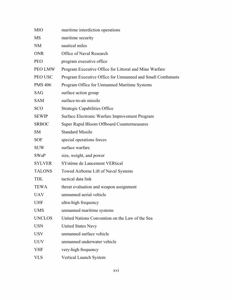
(PEO LMW 2011, 1). To that end, PMS 406 maintains the USV system vision as presented
in Figure 1. The vision shows the current Sea Hunter and Ghost Fleet USV efforts building
into the mid-term to long-term goal of the Future Surface Combatant (FSC) USV. The
stakeholder entities are shown across the bottom.
Figure 1. USV System Vision. Adapted from Rucker (2018).
In 2010, to address the 2007 USV Master Plan’s ASW mission area, the Defense
Advanced Research Projects Agency (DARPA) initiated the ASW Continuous Trail
Unmanned Vessel (ACTUV) effort, which later became Sea Hunter and the medium
displacement USV (MDUSV) when the program transitioned to the Office of Naval
Research (ONR) in 2018 (DARPA 2018). It utilizes a trimaran hull and implements an
autonomous navigation system that conforms to the International Regulations for
Preventing Collisions at Sea (COLREGs) as well as the United Nations Convention on the
Law of the Sea (UNCLOS). Additionally, autonomous ASW sensors and systems are
3
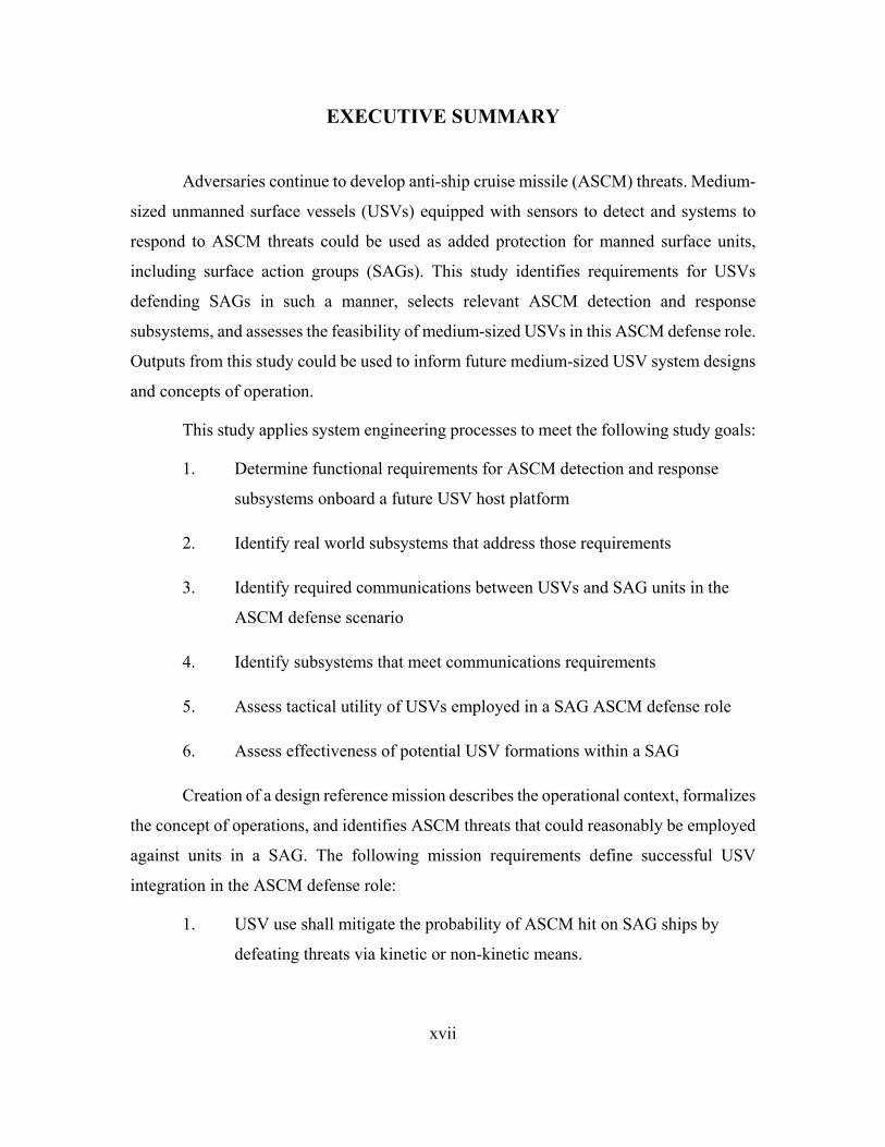
onboard. Additional systems including DARPA’s Towed Airborne Lift of Naval Systems
(TALONS) project and various MCM payloads have been tested in conjunction with
ACTUV sea trials, and they will continue to be tested on Sea Hunter (DARPA 2018). Sea
Hunter is shown in Figure 2.
Figure 2. Sea Hunter. Source: Williams (2016).
The Ghost Fleet effort was initiated by the Secretary of Defense’s Strategic
Capabilities Office (SCO) in 2017. Like other SCO efforts, Ghost Fleet is a rapid
prototyping effort meant to demonstrate new game-changing capability within five years
and serve as a risk mitigator to transition the new capability to the appropriate service
branch—in this case the USN and PMS 406 (Department of Defense 2018). The surface
component of this effort is referred to as Overlord, and it is working to “convert larger,
existing, manned ships into USVs over the next 3 years so that they can conduct existing
missions now undertaken by manned warships” (Berkoff 2018, 38).
The FSC USV effort also originated in 2017 and is led by OPNAV N96—the
Navy’s director for surface warfare (Eckstein 2018). An August 28, 2018, article from the
U.S. Naval Institute webpage describes the FSC goal to develop a mixed ship force

4
structure including a large combatant similar to a destroyer, a small combatant like the
littoral combat ship or the next generation frigate, and a large-sized and medium-sized
USV, all with “an integrated combat system that will be the common thread linking all the
platforms” (Eckstein 2018, 1).
While the Sea Hunter and Ghost Fleet efforts will be of great utility in the design
of the yet-undefined hull form and specific capabilities of the FSC USV, additional studies
are prudent. PMS 406 has specified the following mission areas as FSC USV areas of
interest: armed escort, intelligence, surveillance, and reconnaissance (ISR), EW, UUV
launch, communications relay, ASW tracking and engagement, mining and MCM, and
counter-swarm against threat boat or airborne swarms (Rucker 2018). This study seeks to
address the armed escort, ISR, EW, and communications relay areas of interest for the
future medium-sized USV.
3. Surface Ship Missile Defense
Adversaries continue to improve their anti-ship cruise missile (ASCM) designs.
These missiles range in capability from subsonic to hypersonic speeds and can be launched
from land, sea (surface and subsurface), or aerial platforms. They represent a high threat
from an aggressive force due to their speed and ability to exploit radar blind spots.
Additionally, the U.S. and near-peer forces have developed these weapons since the early
1940s, so they are ubiquitous today.
As USVs are introduced and operate with USN and partner nation naval forces,
they will be expected to play a role in increasing situational awareness for commanders.
This would involve increasing the detection range of threats—such as ASCMs—from
manned units beyond those units’ organic capabilities. USVs could also defend both
manned units and themselves from inbound ASCMs.
B. PROBLEM STATEMENT
Adversary ASCM threats continue to evolve and present new dangers to USN ships
and sailors. Methods of ASCM detection and response must evolve in parallel to pace and

5
overcome the threat. One area for exploration is the use of USVs to augment and
complement the defense of a surface action group (SAG) against ASCM threats.
C. PROJECT OBJECTIVES
The focus of this study is two-fold. First, it seeks to provide notional medium-sized
USV host platform system engineering level requirements for ASCM detection and
response subsystems. Medium-sized USVs are defined by the USN as having a length
between 12 and 50 meters (LaGrone 2019). Focusing on the higher end of the length range,
it is expected a medium-sized USV will have a maximum displacement 300 long tons, a
maximum width of approximately 7.5 meters, a draft of two meters, and a maximum height
above the waterline of approximately 15 meters. These values were determined by
comparison against the Cyclone class patrol craft measurements, whose overall length is
51.8 meters (Pike 2011b).
Detection subsystems in this study are defined as those that perform find, fix, and
track functions against ASCM threats in the find, fix, track, target, engage, and assess
(F2T2EA) kill chain. This study focuses on air search radar and electronic support (ES)
detection systems. Response systems are those that can target and engage via either kinetic
or non-kinetic means such as counter-fire, soft-kill deception countermeasures, or
electronic attack (EA).
The second focus of this study is to assess whether a notional medium-sized USV
equipped with the prescribed real-world systems could be effective in the defense of a SAG
against ASCM threats. This part of the study leverages operational analysis approaches to
determine utility of the USV in given scenarios and involves analysis of communications
paths and corresponding communications systems.
The ideas are investigated by simulating the use of USVs to increase detection
range of inbound ASCM threats relative to the protected units and employ both soft-kill
and hard-kill defensive countermeasures. Concepts studied would be applicable in high
value unit (HVU) defense as well.

6
D. KEY ASSUMPTIONS
This analysis relies on three key assumptions. The first assumption—and perhaps
the most critical—is that the USVs will be able to maintain station with the SAG, meaning
all support needs like fuel and maintenance are met by ships in company or exceeded by
the performance parameters of the USV itself and will therefore not be considered in this
analysis. Second, it is assumed any Afloat Electromagnetic Spectrum Operations Program
(AESOP) issues will be effectively de-conflicted. Effective management of the
electromagnetic spectrum is important to prevent mutual interference, which would inhibit
or restrict performance of sensors and equipment. Finally, safe recovery of the USV is
assumed to be achievable in case of loss of control. Normally, the SAG commander would
control the USVs remotely to coordinate changes in station and tactical responses to enemy
actions. The third assumption is that in the event control of the USV cannot be maintained,
communications will be reestablished quickly, or another unit will be able to tow the USV
to an intermediate maintenance facility for repair.
E. SYSTEMS ENGINEERING APPROACH
1. Overview of Approach
The systems engineering process used in this study begins with an operational
analysis. After threats and mission scenarios are identified via a design reference mission
(DRM), system requirements are generated. The system design phase then identifies
recommended ASCM detection and response subsystems and associated size, weight, and
power (SWaP) requirements. Additional communications requirements are then evaluated
based on selected subsystem and operational requirements. These are used to finalize the
proposed USV configuration and required communications pathways. Finally, this
configuration is used in simulations of the threat scenarios to evaluate the utility for using
USVs to aid in ASCM defense of the manned units. The complete systems engineering
process is depicted in Figure 3.
7
Figure 3. System Engineering Process for the Study
8
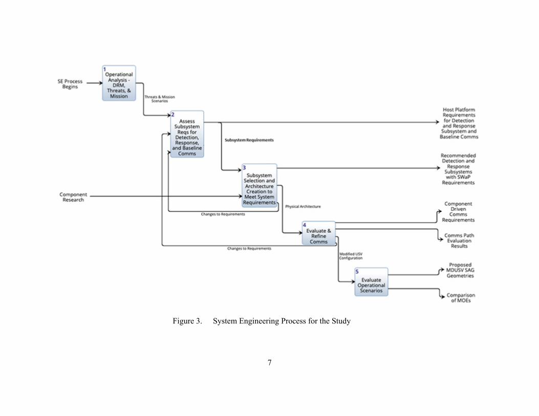
2. Detailed Description of Approach
During the operational analysis phase, a DRM is developed to produce multiple
scenarios where the USV is positioned differently relative to the rest of the SAG, projected
operating environments, mission definitions, threats, and measures. Enemy threats
identified in this phase help determine required countermeasures. Threats and mission
definitions are used for requirements generation in the following phase.
In the subsystem requirements generation phase, functional system requirements
and baseline communications requirements for the USV detection and response subsystems
are identified based on outputs from the DRM. Response systems are those that can defeat
incoming ASCM threats (via soft-kill or hard-kill means). After this process, subsystem
requirements are sent to the design phase. Once the engineering process is complete, these
requirements become an output of the study as proposed host platform requirements.
During the subsystem selection and architecting phase, current commercial off-the-
shelf (COTS) and government off-the-shelf (GOTS) detection and response subsystems
are researched and compared, to include SWaP requirements of the potential
subsystems. The subsystems most appropriate for use on a medium-sized USV are selected,
and system requirements are allocated to those components. A proposed physical
architecture for the USV system is also identified, based on the chosen subsystems. These
are collected as study deliverables for use in future USV platform design considerations.
Any additional requirements identified during this phase are used as feedback to the system
requirements phase. This includes ensuring selected systems are compatible with and do
not interfere with each other (or interference is able to be deconflicted). The outputs of this
phase are recommended detection and response subsystems with associated SWaP
requirements.
The fourth step in the process is to evaluate additional communications
requirements. Based on the selected detection and response subsystems, the team identifies
any derived communications requirements needed beyond the baseline requirements and
assesses if they are viable. If the new communications requirements are not viable, the
subsystem requirements are updated, and the team proposes how they could be
9
implemented by alternative future communications systems. The proposed USV
configuration is sent to the next phase of this process. The outputs of this phase also include
component driven communications requirements and the results of the communications
path evaluation.
The final phase of the process is to evaluate operational scenarios. An analysis of
modeled scenarios is performed to determine the utility of the USV launching and emitting
counter-fire effects in the ASCM defense mission, determine the tactical utility of the USV
as a cueing platform for SAG organic defense, and to inform discussion on various USV
geometries around the SAG.

10
THIS PAGE INTENTIONALLY LEFT BLANK
11
II. DESIGN REFERENCE MISSION
A. DESIGN REFERENCE MISSION INTRODUCTION AND OBJECTIVE
This study utilizes the DRM process, described by Skolnick and Wilkins (2000) as
characterizing the operating and threat environment in addition to defining requirements.
It also serves as a baseline to support concept development, trade study analysis, design,
and test and evaluation activities (Skolnick and Wilkins 2000). In this study, the DRM
initial outputs are baseline operational assumptions and mission context. These initial
outputs are then used to produce operational requirements and scenarios that lay the
foundation for further systems analysis and systems engineering activities.
This DRM has been conducted to support analysis of the feasibility of employing
USVs in the defense of a SAG from enemy ASCMs. To protect the SAG, the USV is
required to independently detect and counter inbound ASCM threats and cooperatively
engage with the SAG. The USV will serve as a screening vessel to mitigate the probability
of ASCM hits on SAG ships. This screening tactic is intended to provide the SAG
additional reaction time versus ASCM threats by way of cueing and also affords the USV
the chance to engage and remove the ASCM threat while it is inbound to the SAG. To
operate cooperatively with the SAG, it is assumed the USV can achieve and maintain
required speed to remain on station and will not have issues with on-station endurance.
Cooperative engagement with SAG includes the ability of the SAG ships to execute
traditional command and control of the USVs and execute counter ASCM measures based
on USV cueing in a distributed lethality context.
The DRM includes operational situations (OPSITS) that describe notional
scenarios where the USV is defending a SAG from ASCM threats to serve as a basis for
the analysis. The DRM highlights the importance of the USV’s detection and response
subsystems in our OPSITs. Each of these subsystems must be able to interact with one
another onboard the USV and pass information—including target tracks and subsystem
health and status messages—back to systems and operators in the SAG. These USV
subsystems must also be responsive to SAG command signals and remote control.

12
B. MISSION BACKGROUND
Technological advancements in ASCMs make detecting and defeating them
increasingly challenging. Advanced guidance systems enable ASCMs to hit targets with
excellent accuracy, and various stealth methods are employed to limit detectability.
ASCMs can be launched from surface ships, submarines, aircraft, and land-based
platforms. Due to the diversity of the threat, ASCM defense options for friendly surface
units must be continuously developed and improved.
Analysis of ASCM effectiveness and corresponding ASCM defense effectiveness
and methodologies is readily available. This study leverages and builds upon the kill-chain
analysis framework of Smith (2010) because his research deals specifically with surface
ship defense against ASCMs and the “formidable layered defense of a target ship to include
hard kill and soft kill measures” (Smith 2010, v).
Ship defense against ASCMs involves using EW or kinetic means to distract, jam,
and destroy the threat. Specifically, countermeasures to ASCMs include both long-range
and short-range surface-to-air missiles (SAMs), close-in weapons systems (CIWS), radio
frequency jamming, electro-optical/infrared jamming, and use of deception such as decoys,
flares, and chaff to seduce the missile away from its intended target (Smith 2010).
C. OPERATIONAL CONTEXT AND PROJECTED ENVIRONMENT
1. Scenario Overview
This scenario encompasses a blue SAG supported by forward positioned USVs.
The ships are operating in an open ocean environment with no impediments to
maneuvering. Should an ASCM be launched at friendly units, maneuvering for unit self-
defense and self-preservation will be the priority over any territorial waters or politically
sensitive area restrictions, so those are not a concern in the simulations. The ships will be
steaming under a condition III watchbill, with no prior threat indications from intelligence
sources. There are no environmental threat conditions, such as excessive winds or sea state.
The environment is assumed to be communications permissive (communications are not
degraded or denied). The SAG and USVs can communicate via line of sight (LOS) or
13
beyond line of sight (BLOS) communications systems. Friendly forces are equipped with
both soft-kill and hard-kill countermeasures.
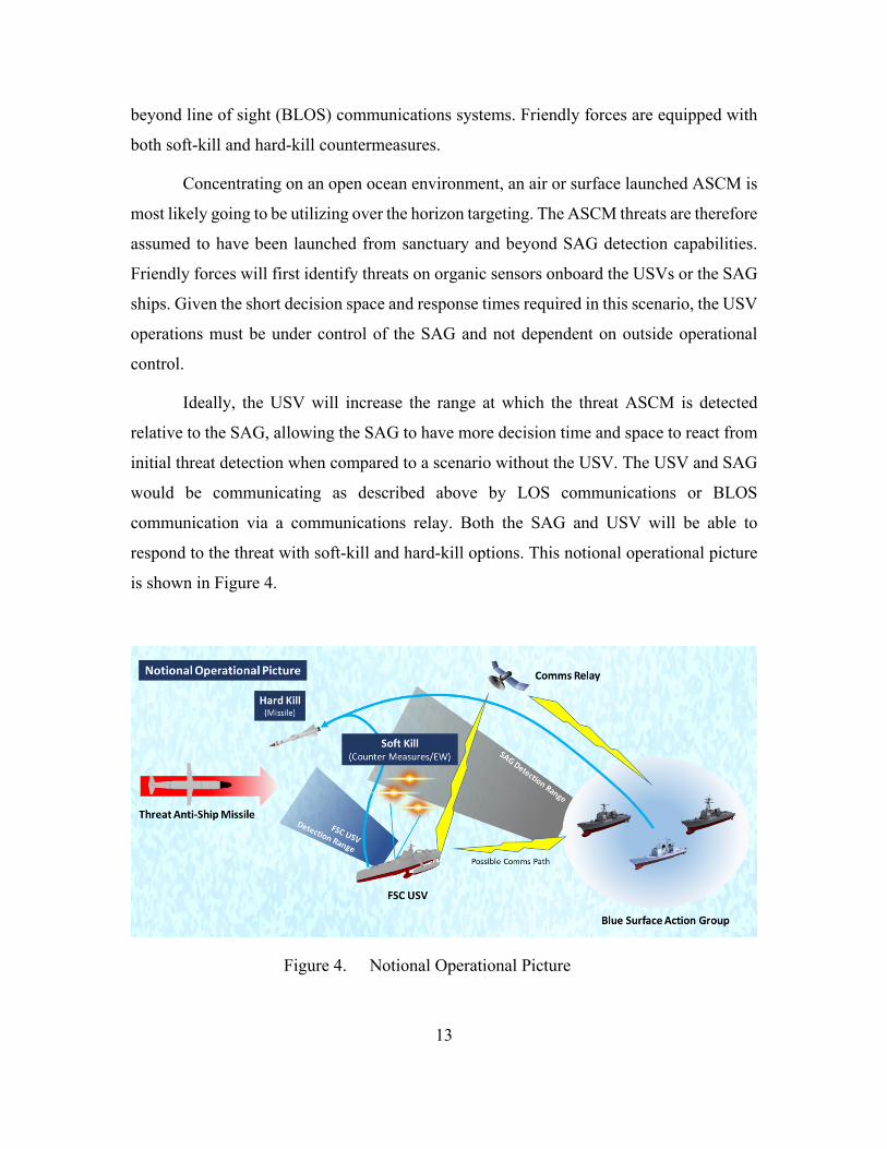
Concentrating on an open ocean environment, an air or surface launched ASCM is
most likely going to be utilizing over the horizon targeting. The ASCM threats are therefore
assumed to have been launched from sanctuary and beyond SAG detection capabilities.
Friendly forces will first identify threats on organic sensors onboard the USVs or the SAG
ships. Given the short decision space and response times required in this scenario, the USV
operations must be under control of the SAG and not dependent on outside operational
control.
Ideally, the USV will increase the range at which the threat ASCM is detected
relative to the SAG, allowing the SAG to have more decision time and space to react from
initial threat detection when compared to a scenario without the USV. The USV and SAG
would be communicating as described above by LOS communications or BLOS
communication via a communications relay. Both the SAG and USV will be able to
respond to the threat with soft-kill and hard-kill options. This notional operational picture
is shown in Figure 4.
Figure 4. Notional Operational Picture
14
The specific scenario developed for use in the simulation for the low and medium
threat ASCMs is as follows: a conflict over territorial rights in the South China Sea between
naval forces from the People’s Republic of China and a U.S. ally has resulted in open
conflict. A SAG and three medium-sized USVs have been sent from Yokosuka, Japan to
the area of conflict. The SAG consists of one Ticonderoga class cruiser and two Arleigh
Burke class destroyers. While in transit in unrestricted waters, at 0815 local time, the
American units are intercepted by Chinese strike aircraft equipped with ASCMs.
For the high threat ASCM, the scenario is as follows: a conflict over territorial
rights in the Pacific Ocean between naval forces from the Russian Federation and a U.S.
ally has resulted in open conflict. A SAG and three medium-sized USVs have been sent
from Yokosuka, Japan to the area of conflict. The SAG consists of one Ticonderoga class
cruiser and two Arleigh Burke class destroyers. While in transit in unrestricted waters, at
0815 local time, the American units are intercepted by Russian strike aircraft equipped with
ASCMs.
2. Environmental Conditions
For this study, attacks will be limited to the following environmental conditions,
which were derived based on the normal operating conditions and operational limitations
of shipboard equipment and personnel:
1. Daytime
2. Air temperature from 0–50 degrees C
3. Water temperature from 2–35 degrees C
4. No ice or snow
5. Light or no precipitation
6. Winds less than 30 knots
7. Sea state correlating to no greater than 4 on the Beaufort Wind Force
Scale (wave heights of 1–2 meters with occasional white caps)

15
8. Effects of currents and set and drift neglected (no significant effect on
ship’s performance in a tactical situation, given the described scenario and
environment)
9. No excessive haze or dust that could limit communications capabilities
10. No other communications limitations (all pathways available)
3. Threat Details
Three adversary ASCMs have been selected for this analysis and categorized into
threat levels of low, medium, and high. Threat baselines were determined by analyzing
missile speed, payload, and range. The threats were selected based on missile operational
history, capabilities, and operators (these weapons could also be launched from a different
country given weapons proliferation).
The Chinese C-704 is identified as the low threat. It is subsonic and can be launched
from ships or aircraft (Jane’s by IHS Markit 2018c, 2018d). The Chinese YJ-83 (also
known as the CSS-N-8 Saccade) is identified as the medium threat. It is subsonic and can
be launched from ships, ground units, or aircraft (Jane’s by IHS Markit 2018f, 2018h). The
Russian 3M-54 (also known as the SS-N-27 Sizzler) is identified as the high threat. It can
be launched from submarines, ships, or aircraft, depending on the variant (Jane’s by IHS
Markit 2018e). This missile is subsonic while in the cruise phase, and then deploys a
terminal supersonic missile to attack its target (Jane’s by IHS Markit 2018a). Figures 5
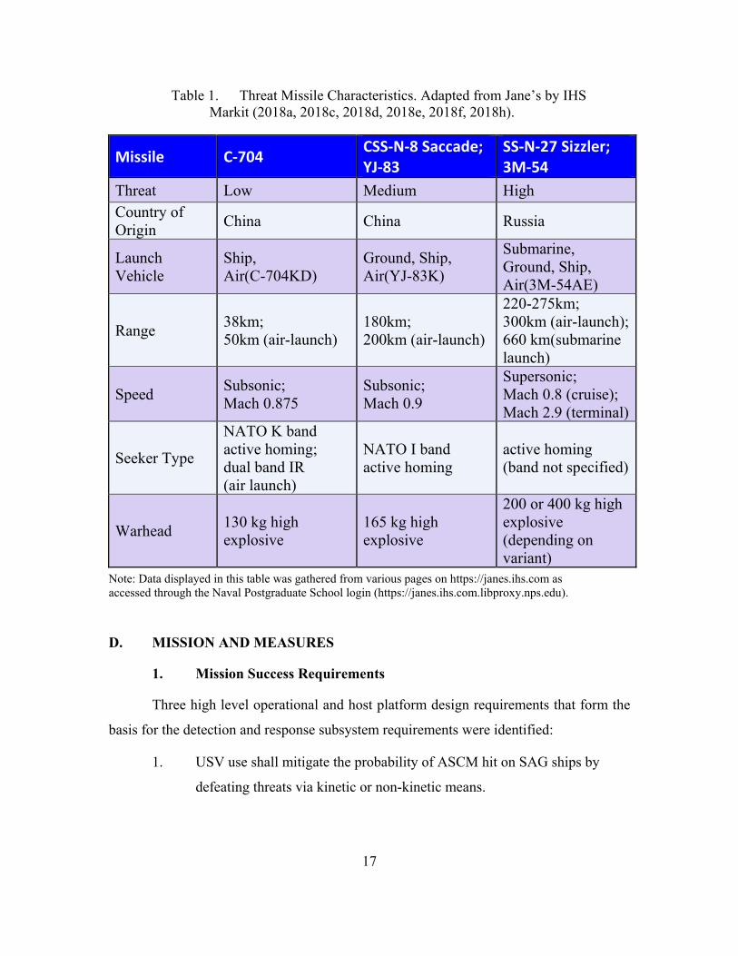
through 7 display the selected ASCMs. The threat missiles have a wide variety of
maximum ranges, from 38 to 660 kilometers, and the warheads range from 130 to 400
kilograms of high explosive (Jane’s by IHS Markit 2018a, 2018c, 2018d, 2018e, 2018f,
2018h). Table 1 displays the characteristics of the ASCMs.

16
Figure 5. Low Threat: C-704. Source: Hewson (2010).
Figure 6. Medium Threat: YJ-83 and Export Variant. Source: Carlson (2013).
Figure 7. High Threat: 3M-54. Source: Kopp (2012).
17
Table 1. Threat Missile Characteristics. Adapted from Jane’s by IHS Markit (2018a, 2018c, 2018d, 2018e, 2018f, 2018h).
Missile C-704 CSS-N-8 Saccade; YJ-83
SS-N-27 Sizzler; 3M-54
Threat Low Medium High Country of Origin China China Russia
Launch Vehicle
Ship, Air(C-704KD)
Ground, Ship, Air(YJ-83K)
Submarine, Ground, Ship, Air(3M-54AE)
Range 38km; 50km (air-launch)
180km; 200km (air-launch)
220-275km; 300km (air-launch); 660 km(submarine launch)
Speed Subsonic; Mach 0.875
Subsonic; Mach 0.9
Supersonic; Mach 0.8 (cruise); Mach 2.9 (terminal)
Seeker Type
NATO K band active homing; dual band IR (air launch)
NATO I band active homing
active homing (band not specified)
Warhead 130 kg high explosive
165 kg high explosive
200 or 400 kg high explosive (depending on variant)
Note: Data displayed in this table was gathered from various pages on https://janes.ihs.com as accessed through the Naval Postgraduate School login (https://janes.ihs.com.libproxy.nps.edu).
D. MISSION AND MEASURES
1. Mission Success Requirements
Three high level operational and host platform design requirements that form the
basis for the detection and response subsystem requirements were identified:
1. USV use shall mitigate the probability of ASCM hit on SAG ships by
defeating threats via kinetic or non-kinetic means.

18
2. USV use shall provide early warning and threat cueing to SAG ships,
thereby increasing available reaction time and counter-fire opportunities of
SAG ships from initial threat detection compared to a no-USV scenario.
3. ASCM detection and response subsystems on the USV host platform must
not require the USV to be larger than medium sized.
Based on these mission requirements, three scenarios were identified where USV
integration with SAGs would be considered successful: all three requirements met,
requirements 1 and 3 met, or requirements 2 and 3 met. Thus, the USV must remain
medium sized in all scenarios. Further, the USV must defeat inbound ASCM threats or
provide early warning and threat cueing to the SAG, or both.
2. OPSIT Definitions
The OPSITs describe notional scenarios where the USV is defending a SAG from
ASCM threats. For the low and medium threat scenarios, the Chinese strike force
consisting of eight aircraft armed with C-704s and YJ-83s approaches the SAG and
launches their missiles. For the high threat scenario, the Russian strike force consisting of
eight aircraft armed with 3M-54s approaches the SAG and launches their missiles. In all
scenarios, the SAG is on course 225o true with the USV positions varying depending on
OPSIT. Seas are calm at a sea state of two. Ambient air temperature is 22o Celsius with
50% humidity, producing a small evaporative duct height of two meters. This slightly
increases the maximum detection range of air search radars when compared to an
environment without evaporative ducting.
a. OPSIT 1 – USVs Fire on Inbound ASCMs
In OPSIT 1, the USVs are steaming in formation with the SAG, positioned between
the SAG and the inbound missiles. The USVs either detect the threat or are cued where to
search from the ships. The USVs deploy response options.
19
(1) Sub OPSIT 1A – USV Off the Threat Axis
In this sub OPSIT, the USVs are not directly between the threat and the SAG and
are positioned to detect threats near their maximum detection range.
(2) Sub OPSIT 1B – USV On the Threat Axis
In this sub OPSIT, the USVs lie directly between the threat and the SAG such that
the threat missiles pass directly overhead of the USV.
b. OPSIT 2 – Untargeted USV Detects Inbound ASCM and Cues SAG
In OPSIT 2, the SAG ships are targeted, and the USVs remain undetected or
untargeted. The USVs are positioned between the SAG and the inbound missiles and are
able to pass track data to the SAG ships to increase the available response time from initial
threat detection for the SAG ships to deploy their own response options.
(1) Sub OPSIT 2A – USV Off the Threat Axis
In this scenario, the USVs are not directly between the threat and the SAG and are
positioned to detect threats tangential to their maximum detection range. The USVs receive
the initial indications of threat missiles via their onboard air search radar or ES systems,
gain track of the ASCM(s) quickly, and pass the track data to the SAG, cueing the SAG’s
self-defense responses.
(2) Sub OPSIT 2B – USV On the Threat Axis
In this scenario, the USVs lie directly between the threat and the SAG. The USVs
receive the initial indications of threat missiles via their onboard air search radar or ES
systems, gain track of the ASCM(s) quickly, and pass the track data to the SAG, cueing
the SAG’s self-defense responses.
3. Mission Execution
a. OPSIT 1 – USVs Fire on Inbound ASCMs
1. USV or other ships in company make initial detection of inbound
ASCM through active air search radar or passive ES means (if
20
passive detection occurs first, active radar search focuses on
bearing obtained from electronic sources).
2. If initial detection is not made by USV, USV air search radars are
cued to conduct focused search or the track data is passed to USVs.
3. USV’s combat systems suite determines precise location and
assigns track numbers to ASCMs.
4. Tracks are shared and deconflicted by use of Tactical Data Links
(TDLs) and Cooperative Engagement Capability (CEC).
5. ASCM tracks are designated a high priority and updated at the
combat systems’ fastest rate.
6. USV’s combat system calculates expected track of ASCMs and
missile interceptors along with the amount of time the USV has
available to conduct a successful intercept.
7. USVs launch missile interceptors and deploy electronic
countermeasures.
8. USV radar systems and operators on manned ships in company
conduct detailed search of intercept location to make assessment.
9. If inbound ASCMs survived engagement, USVs reengage if there
is enough time to consummate the engagement or point defense
systems are cued to engage.
b. OPSIT 2 – Untargeted USV Detects Inbound ASCM and Cues SAG
1. USVs make initial detection of inbound ASCM through active air
search radar or passive ES means (if passive detection occurs first,
active radar search focuses on bearing obtained from electronic
sources).

21
2. USVs transmit track data to other ships in company.
3. Ship’s combat systems suite determines precise location and
assigns track numbers to ASCMs.
4. Tracks are shared and deconflicted by use of TDLs and CEC.
5. ASCM tracks are designated a high priority and updated at the
combat systems’ fastest rate.
6. Ships’ combat systems calculate expected track of ASCMs and
missile interceptors along with the amount of time the ship has
available to conduct a successful intercept.
7. Ships launch missile interceptors and deploy electronic
countermeasures.
8. Ships’ radar systems and operators conduct detailed search of
intercept location to make assessment.
9. If inbound ASCMs survived engagement, ships reengage if there is
enough time to consummate the engagement or point defense
systems are cued to engage.
4. Measures
The goal of employing the USV in this manner is to is to significantly reduce or
eliminate the number of threats that reach the self-defense area of SAG units. The primary
measures of interest for determining the USV’s potential to defeat ASCMs via kinetic or
non-kinetic means were therefore the number of hard kills and soft kills against ASCMs
across multiple iterations of a Markov kill chain model.
In the analysis of the USV as a cueing platform, the primary measure of interest
was the early warning detection time in seconds. This time the time from the earliest USV
detection in the scenario compared against the assessed organic SAG detection time if the
22
USV was not present. This time was also used to derive the potential number of additional
shot opportunities, another measure of interest.
In the analysis of USV-SAG geometries, the measures of interest were degrees of
coverage and linear distance. The degrees of coverage pertain to the ASCM detection
screen provided by the geometric USV spacing in a given formation. The screen was
measured in degrees radially from the SAG in the center of the USV formation. The linear
distance pertains to the summation of the distances of each USV to the SAG. This distance
relates to the potential overall early warning detection time and, correspondingly, the
number of additional shot opportunities against incoming ASCM threats.

23
III. SYSTEM REQUIREMENTS
A. SYSTEM REQUIREMENTS INTRODUCTION
In conceptual system design activities, such as in our use case of the medium-sized
USV, system needs and requirements must first be developed and understood (Blanchard
and Fabrycky 2011). From the DRM, the determined operational needs are:
1. USV use shall mitigate the probability of ASCM hit on SAG ships by
defeating threats via kinetic or non-kinetic means.
2. USV use shall provide early warning and threat cueing to SAG ships,
thereby increasing available reaction time and counter-fire opportunities of
SAG ships from initial threat detection compared to a no-USV scenario.
3. ASCM detection and response subsystems on the USV host platform must
not require the USV to be larger than medium sized.
These will form the basis of the subsystem requirements necessary to implement
ASCM defense capabilities on the medium-sized USV. The detection subsystems of
interest in this study are the air search radar and ES subsystems. The response subsystems
of interest in this study are the soft-kill deception countermeasure, SAM, CIWS, and radio
frequency jamming (also known as EA) subsystems.
For each of these subsystems, requirements were generated to address the
operational needs while being grounded by current technology or technology that could
realistically be fielded within the next two years. Concepts of employment for each
subsystem provide context to inform specific subsystem level requirements. Requirements
for additional support subsystems—such as power or cooling, for example—were derived
through discussion of these concepts of employment and further refined after system
selection. A full list of generated requirements is available in Appendix A.
24
B. DETECTION SUBSYSTEM REQUIREMENTS
The detection subsystems are the air search radar and the ES system. These two
systems interact with the USV via an integrated combat system (ICS) onboard the USV
that also drives USV responses for an ASCM attack. By providing the necessary processed
data to the SAG including target tracks, these subsystems cue the SAG ships to threats.
Additionally, they provide the ability to meld their returns into a common display with the
SAG ships, thereby increasing situational awareness.
Given the threat missiles have known velocities and may have correlative
electromagnetic signatures, the detection subsystems can implement contact
discrimination. Engagement settings and threat profiles can be established by remote SAG
operators to automatically filter out items not of interest. Filtering raw data into contacts
of interest (COIs) alleviates bandwidth consumption compared to transmission of all raw
contact data. This discrimination logic can be edited to reflect a specific operating area or
threat level. For the purpose of this paper, a COI is defined as an air contact with a velocity
of greater than 400 knots travelling towards the SAG. Friendly aircraft returning to the
SAG would be discounted based on positive identification (such as via Identification
Friend or Foe, secure communications, and check-in procedures).
1. Air Search Radar
The air search radar must detect contacts at a range that allows for sufficient time
to identify threats and deploy appropriate response measures to defeat the threat. To obtain
tactically relevant detection ranges against air threats, the air search radar must be elevated
to achieve detection over the horizon.
To prevent time lag and communication relay issues, the radar system shall process
radar data onboard. The communication subsystem will provide this processed data in the
form of target tracks to the SAG ships for threat cueing. The air search radar shall also be
able to receive changes to its operating parameters (e.g., cued search areas, power levels,
no transmission areas, and COI parameters) should an operator on one of the SAG ships
need to adapt them to a changing operational environment or to prevent interference with
other equipment, such as navigation radars.
25
Due to the high speed of ASCMs and large area to be searched, the radar system
must have both volume search and cued search capability, as well as functionality for high-
resolution tracking. This can be accomplished within one multi-function radar or the
system may consist of multiple radars to fulfill the different roles. In either case, the
radar(s) used need to be able to distinguish incoming threat missiles from other airborne
objects.
2. Electronic Support System
The ES system must be capable of detecting threat missiles in their expected emitter
operating frequency bands when they are emitting. These emitters must be detected at a
range that allows for sufficient time to identify threats and deploy appropriate response
measures to defeat the threat. The ES system must therefore also be elevated enough to
achieve adequate detection ranges. The ES system must also provide elevation angle
coverage to detect incoming threats from the surface as well as high elevation attacks.
To prevent time lag and communication relay issues, the system shall process ES
data onboard the USV. This processed data will include line of bearing information and
signal strength, and it will be provided locally to the ICS and to the SAG via the
communication subsystem. Additionally, the ES system will be capable of isolating own
ship emitters to prevent spurious detections. The ES system shall also be able to receive
changes to its operating parameters (e.g., cued search bearings, search areas, and COI
parameters) should an operator on one of the SAG ships need to adapt them to a changing
operational environment.
C. RESPONSE SUBSYSTEM REQUIREMENTS
After obtaining track on an inbound ASCM, several subsystems may be activated
to defeat the threat by either kinetic or non-kinetic means. The former seeks to destroy the
ASCM in flight while the latter seeks to disrupt or deceive the flight path of the missile by
using chaff, flares, and decoys or by attacking the missile’s terminal homing seeker on the
electromagnetic spectrum. Subsystems considered for these applications must account for
the smaller size of a medium USV relative to a standard cruiser or destroyer.
26
Regardless of method, all response subsystems are cued by the ICS after it has
received the necessary data from the detection subsystems. The timing in which responses
are activated is determined by the calculated intercept and the necessary time for personnel
and systems to react. Thus, in some instances all response subsystems may be employed
while in others only one will be used. To deconflict responses while defending the SAG,
the ICS will communicate with the rest of the SAG through TDLs and CEC. The USV can
take action either autonomously through pre-established weapons engagement settings, or
it will receive engagement commands from the SAG.
1. Soft-Kill Deception Countermeasures
One method proposed to lessen the probability of an inbound ASCM hitting a SAG
ship is the use of soft-kill deception countermeasures. These attempt to lure inbound
ASCMs away from SAG ships by deceiving them into pursuing a decoy target. This will
protect the SAG and also reduce risk of damage to the USV.
To counter the variety of ASCM threats, the USV will have the ability to launch
chaff to protect against radar guided missiles or flares to protect against infrared guided
missiles. The launcher in the chosen countermeasure system should be able to launch both
types of payloads to eliminate the need for unique launchers, thereby keeping SWaP
requirements to a minimum. The countermeasure system will need to be able to intercept
missiles coming from any direction. This can be accomplished either by installing multiple
sets of launchers with fixed firing positions to obtain 360-degree coverage or by installing
dynamic launchers that can be aimed as needed. A dynamic system should be able to use
data received from the detection subsystems to automatically aim the barrels. Launchers
chosen for this design will fire commonly available rounds (not require custom-made chaff
or flare rounds).
These countermeasure systems cannot act alone, so communication links with other
systems will be required. The ICS will analyze detection data from the radar and ES
systems to direct the countermeasure subsystem to release chaff or flares as appropriate
against the incoming ASCM. Detection subsystems will also provide information detailing
the track and speed of the ASCM. Given the threat missile velocities and relative proximity
27
to the USV that the countermeasures are deployed, it is assumed the countermeasure
system will have only one chance to neutralize the ASCM. Once a response round has
launched, an event message signifying launch will be provided by the countermeasure
system to the ICS and the SAG ships. The detection systems will continue to track the
ASCM target. After receipt of the countermeasure launch message, indications from the
detection system that the threat exists or no longer exists will serve as the battle damage
assessment. This subsystem will periodically return a status message to the ICS for further
dissemination to the SAG so operators know the health of the countermeasure launchers
and the amount of payload available for use.
2. Surface to Air Missiles
The USV will be equipped with a SAM subsystem as a long-range response
measure to engage and intercept ASCM threats. For this study, long-range is defined as
more than 3.7 kilometers (two nautical miles), the threshold range for the CIWS
subsystems. The SAM subsystem will consist of the SAM, the launcher, and corresponding
SAM control systems integrated with the ICS. The SAM subsystem will be able to be
configured to either engage threats autonomously or to require receipt of a launch order
from the SAG in order to engage threats. In both scenarios, some level of automation is
required for weapons launch. The ethics of a remote weapons launch and semi or full
automation in weapons launch is not addressed in this paper. This study will simply attempt
to address if such an employment concept is feasible and meets technical requirements.
Auto-engaging incoming threats requires a confirmed threat classification from the
ICS. The ICS will receive initial configuration of threat profiles and rules of engagement
settings and any configuration updates from operators in the SAG via the communication
subsystem.
If operational commanders determine authority to launch SAMs must be obtained
from operators in the SAG, the USV will first send a data package to the SAG detailing
target information including track and threat classification as well as calculated launch
parameters. Upon receipt, review, and approval by SAG operators, the USV would be
enabled to launch. Provided the USV is granted authorization to fire, it will either launch
28
SAMs, or it will be unable to launch because the target no longer meets launch criteria for
any reason, including that a firing solution may no longer exist due to proximity or
geometry between the ASCM and the USV or defended assets.
Following launch, the SAMs will be able to receive updated guidance information
from the USV and the SAG. The SAM subsystem will report general health and status
messages and launch event reports. The SAM subsystem will use a missile capable of in-
flight maneuvering and equipped with infrared seekers at a minimum to address the ASCM
threat.
3. Close-in Weapons System
If the ASCM passes through long-range defenses, a short-range CIWS on the USV
will be able engage the ASCMs and protect the SAG, provided the geometry between the
USV and the ASCM supports the engagement. For this study, the terms “short-range” and
“close-in” are interchangeable and defined as 3.7 kilometers (two nautical miles) or less.
Since a CIWS is inherently a short-range system, it has short timelines in which it can
prosecute targets and must leverage automation to do so.
The CIWS will need to have a maximum range of at least 3.7 kilometers (two
nautical miles) to cover the area defined as close-in. It must be able to automatically detect
and track incoming threats. The CIWS will automatically fire when a threat is identified in
range and will cease fire when it no longer detects the threat, has detected elimination of
the threat, or detects the threat is outbound or outside its engagement range, or to prevent
accidental engagement of friendly forces. The CIWS must use commonly available rounds
and must not require custom ammunition.
Even though the CIWS will be fully autonomous, it will require communication
with the ICS so operators in the SAG can configure the CIWS including rules of
engagement settings and threat profiles. Additionally, it must be able to receive handoff
information from the ICS via the long-range defenses as well. This subsystem will also
periodically send status messages to the ICS for further dissemination to the SAG operators
will know the health of the subsystem, the amount of ammunition remaining for use, and
the battle damage assessment from any engagements.
29
4. Radio Frequency Jamming or Electronic Attack
Besides attempting to cause the ASCM to detonate away from its intended target,
another soft-kill approach is to employ active radio frequency jamming. Otherwise known
as EA, this is focused on jamming the active homing seeker on the ASCM, thereby making
it unable to lock onto its intended target. Such an EA capability could be combined with
ES and soft-kill deception countermeasures into a single EW system, some capabilities
could be combined in an EW system, or the capabilities may be split up into their own
individual systems.
The range of the EA would need to be able to affect the ASCM far enough away to
ensure the ASCM fails to lock on before entering its terminal phase. Furthermore, the EA
system must operate on the frequency bands employed by the seekers on expected threat
missiles. The EA system must also be able to receive threat parameter updates from the
SAG via the ICS.
The ICS will validate the ASCM target based on information provided by the
detection subsystems and threat criteria provided by SAG operators. Upon determination
the threat is susceptible to jamming, the ICS will pass the ASCM track and emitter data to
the EA subsystem and direct execution of EA. The ASCM threat will continue to be tracked
by detection subsystems and may require additional response measures including hard-kill
responses if the ICS determines the missile threat is not sufficiently addressed by jamming
alone.
D. DERIVED SUBSYSTEM REQUIREMENTS
Additional subsystems will be necessary to support the detection and response
subsystems. All subsystems will be required to interact with the ICS, and they will also
require services from the USV such as electrical power, cooling, hydraulics, positioning,
navigation, and timing services. It was therefore necessary to articulate additional
requirements these support subsystems must perform in order to meet the detection and
response subsystem requirements.
30
1. Integrated Combat System
The ICS primary functions are to manage all USV combat system interactions and
to execute USV command and control functions with initial input and configuration
updates from SAG operators.
The ICS will act as contact manager and track integrator. Once an ES or radar COI
has been detected, the data will be compared with engagement parameters, which will be
comprised of both ES and radar threat level tripwires. These parameters and thresholds
must be editable via the SAG remotely. The ICS shall make determinations whether COIs
meet engagement parameters and command the appropriate response subsystem reaction.
It will provide relevant information including ASCM track, emitter information, and
response measure type to the launchers to maximize the effectiveness of the response
measures. It will also interface with all onboard subsystems in order to provide the
detection and response subsystems with accurate data, such as position, navigation, and
timing data or status of other systems, for instance. Response subsystems will provide the
ICS general health and status messages and launch event reports.
The ICS will serve as the primary conduit for all detection and response subsystems
to interface with the USV communications systems back to the SAG. Onboard the USV, it
will integrate with each subsystem via a common architecture like the Common Object
Request Broker Architecture. This architecture is not envisioned to be unique to our
subsystems of interest and is expected to also interface with any other subsystem not
covered under the scope of this study.
2. Electrical Power
The electrical power system must be able to generate and provide enough power at
the correct voltage, frequency, and phase to support all onboard systems. This requires the
system to generate power at 450 volts alternating current at 60 hertz in 3-phase. The power
must then be able to be directly distributed in 3-phase or in a single-phase as well as
transformed down to 120 volts. The 120 volts alternating current at 60 hertz will then be
distributed in 3-phase or in a single-phase. Frequency converters must also be able to create
120 volts alternating current power at 400 hertz in 3-phase for further distribution.

31
Since the USV will not have personnel onboard to respond to emergencies at a
moment’s notice, the system must be capable of self-monitoring for potential and
confirmed system faults. Further, the system must be able to report its status to the ICS for
further transmission to the SAG as well as respond autonomously to any electrical
problems by taking such actions as isolating circuits or equipment, shutting down
switchboards or generators, and shifting the electrical distribution configuration.
3. Cooling
For sustainable operations, subsystem cooling will be required. Seawater cooling
will be required for heat tolerant systems and chill water for heat sensitive systems.
Recalling that the envisioned operating environment for the USV is in waters from 2—35
degrees Celsius, it is noted that a seawater-based cooling system’s effectiveness will
depend on environmental conditions. Cold seawater is more advantageous, while more
tropical waters can make regular cooling more challenging.
A traditional on-board chill-water system is assumed to be a requirement for heat
sensitive subsystems such as electronics. Since the USV is unmanned, it is assumed it will
be heavily populated with electronics racks to address processing requirements of its
various subsystems and that it will already have a robust chill-water subsystem in place.
Subsystems and components like the ICS and detection and response subsystem processors
will still require additional dedicated and stable cooling.
Given the SWaP requirements for cooling units and the limited space and power
available onboard the USV, high heat generating items that can withstand changes in
temperature are ill-suited to be incorporated in the chill-water cooling system because the
chill-water system would have difficulty maintaining its cooling capability. As such, it will
be necessary to incorporate and maintain a separate seawater-based cooling system.
4. Hydraulics
USV machinery parameters must be controlled precisely. Moving hydraulic oil to
open and close hydraulic valves remotely from an automated control system can maintain
requisite fluid pressures and move heavy parts. Applications are important for propulsion,
32
electrical power generation, and steering systems, as well as for combat systems equipment
with moving parts, such as directing the launch vector for response subsystems. The
hydraulics system will need to integrate with the ICS to receive input for instantaneous
response subsystem demands and respond accordingly.
5. Positioning, Navigation, and Timing
The positioning, navigation, and timing system onboard the USV must comply with
accuracy standards set forth in the Chairman, Joint Chiefs of Staff Instruction 6130.01, the
Department of Defense Master Positioning, Navigation, and Timing Plan. This will allow
for accurate and precise determination of both the USV three-dimensional location—
referenced to World Geodetic System 1984—and the Coordinated Universal Time. These
measurements are critical to USV effectiveness as a maritime platform and the
effectiveness of its onboard weapons systems. The system must interact with the ICS to
pass positioning, navigation, and timing data to all combat systems.
Use of an inertial navigation system allows for determination of position absent
GPS input in case of GPS denial. This supports the navigation goal of the system to provide
for effective and safe navigation in accordance with COLREGs, UNCLOS, and other
international agreements, unless overridden by the ICS. Such an override would be
necessary when operational commanders determine the tactical situation warrants
navigation methods not in accordance with such agreements. Normally, operators would
pass navigation and stationing instructions to the USV via the ICS but would not override
the normal safety and international agreement conformance programming. Either way, the
system will determine and apply course and speed corrections to attain position and
maintain station.
33
IV. SUBSYSTEM SELECTION
A. SUBSYSTEM SELECTION INTRODUCTION
Following requirements generation, the physical components and corresponding
host platform SWaP requirements were identified. Potential subsystems for inclusion in
this analysis were identified and compared against the subsystem requirements and the
concepts of system employment. To maintain an unclassified study, all subsystems and
components considered for the design were current COTS or GOTS products, and all data
was collected from publicly available sources. The subsystems and components were not
restricted to any particular nation or group of nations.
Consideration was also given to combinations of subsystems to assess if emergent
behaviors are more favorable when systems operate coherently rather than individually. At
the conclusion of this analysis, a system was selected for each detection and response
subsystem of interest for inclusion in a notional medium-sized USV. For the ICS and
support systems, such as electrical power, cooling, hydraulics, positioning, navigation, and
timing services, and other services required for the proper function of the detection and
response systems, it is assumed there is an existing equivalent on the host platform. This
analysis will therefore not make specific COTS or GOTS recommendations for those
systems.
B. DETECTION SUBSYSTEM COMPARISON AND SELECTION
1. Air Search Radar
Many radars were ruled out due to their large SWaP requirements. For example,
the smallest AN/SPY-1 radar variant is the SPY-1F. This radar was designed for frigates
(larger than a medium-sized USV), consists of four 2.44-meter wide octagonal panels
mounted on the sides of the superstructure, and the entire system including below deck
portions weighs over 20 metric tons (Janes by IHS Markit 2018b; Lockheed Martin 2009).
The AN/SPS-49 fulfills the requirements for an air search radar on the USV. It has
a rotation clearance of 8.7 meters and is currently installed on U.S. aircraft carriers,

34
cruisers, and amphibious ships as well as Australian, New Zealand, Spanish, Korean, and
Canadian ships (Pike 1999). Due to the 8.7 meter clearance requirement, it was determined
this radar could be used if it was installed high or otherwise lifted, which is something that
will need to occur in order to achieve the required radar range anyways. Figure 8 shows
the SPS-49 as outfitted aboard a Korean destroyer.
Figure 8. AN/SPS-49 Radar. Source: Richards (n.d.).
A more recent option not utilized by the USN is the SAMPSON, produced by BAE
Systems and used by France and the United Kingdom. It consists of two array faces rotating
inside a radome, has a range of 400 kilometers and weighs 4.6 metric tons (Jane’s by IHS
Markit 2019b). It is also assumed to fulfill the various tracking and contact generation
requirements, since it is widely in use by the United Kingdom in conjunction with their
Sea Viper Naval Air Defense System and would probably not be if it was unable to
complete those requirements (Missile Defense Advocacy Alliance 2018). However, since
it is not used in the USN, an unknown amount of effort would need to be expended
integrating it into the ICS and the USN communication architecture since it likely will not
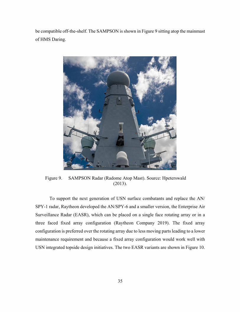
35
be compatible off-the-shelf. The SAMPSON is shown in Figure 9 sitting atop the mainmast
of HMS Daring.
Figure 9. SAMPSON Radar (Radome Atop Mast). Source: Hpeterswald (2013).
To support the next generation of USN surface combatants and replace the AN/
SPY-1 radar, Raytheon developed the AN/SPY-6 and a smaller version, the Enterprise Air
Surveillance Radar (EASR), which can be placed on a single face rotating array or in a
three faced fixed array configuration (Raytheon Company 2019). The fixed array
configuration is preferred over the rotating array due to less moving parts leading to a lower
maintenance requirement and because a fixed array configuration would work well with
USN integrated topside design initiatives. The two EASR variants are shown in Figure 10.
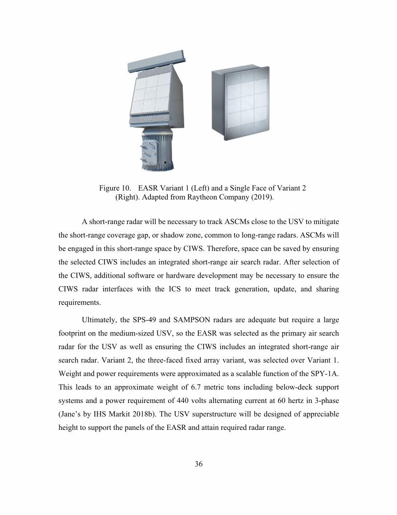
36
Figure 10. EASR Variant 1 (Left) and a Single Face of Variant 2 (Right). Adapted from Raytheon Company (2019).
A short-range radar will be necessary to track ASCMs close to the USV to mitigate
the short-range coverage gap, or shadow zone, common to long-range radars. ASCMs will
be engaged in this short-range space by CIWS. Therefore, space can be saved by ensuring
the selected CIWS includes an integrated short-range air search radar. After selection of
the CIWS, additional software or hardware development may be necessary to ensure the
CIWS radar interfaces with the ICS to meet track generation, update, and sharing
requirements.
Ultimately, the SPS-49 and SAMPSON radars are adequate but require a large
footprint on the medium-sized USV, so the EASR was selected as the primary air search
radar for the USV as well as ensuring the CIWS includes an integrated short-range air
search radar. Variant 2, the three-faced fixed array variant, was selected over Variant 1.
Weight and power requirements were approximated as a scalable function of the SPY-1A.
This leads to an approximate weight of 6.7 metric tons including below-deck support
systems and a power requirement of 440 volts alternating current at 60 hertz in 3-phase
(Jane’s by IHS Markit 2018b). The USV superstructure will be designed of appreciable
height to support the panels of the EASR and attain required radar range.
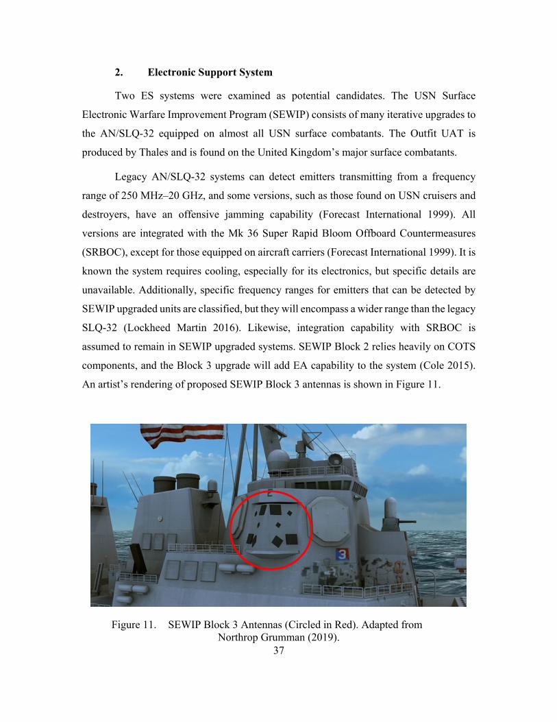
37
2. Electronic Support System
Two ES systems were examined as potential candidates. The USN Surface
Electronic Warfare Improvement Program (SEWIP) consists of many iterative upgrades to
the AN/SLQ-32 equipped on almost all USN surface combatants. The Outfit UAT is
produced by Thales and is found on the United Kingdom’s major surface combatants.
Legacy AN/SLQ-32 systems can detect emitters transmitting from a frequency
range of 250 MHz–20 GHz, and some versions, such as those found on USN cruisers and
destroyers, have an offensive jamming capability (Forecast International 1999). All
versions are integrated with the Mk 36 Super Rapid Bloom Offboard Countermeasures
(SRBOC), except for those equipped on aircraft carriers (Forecast International 1999). It is
known the system requires cooling, especially for its electronics, but specific details are
unavailable. Additionally, specific frequency ranges for emitters that can be detected by
SEWIP upgraded units are classified, but they will encompass a wider range than the legacy
SLQ-32 (Lockheed Martin 2016). Likewise, integration capability with SRBOC is
assumed to remain in SEWIP upgraded systems. SEWIP Block 2 relies heavily on COTS
components, and the Block 3 upgrade will add EA capability to the system (Cole 2015).
An artist’s rendering of proposed SEWIP Block 3 antennas is shown in Figure 11.
Figure 11. SEWIP Block 3 Antennas (Circled in Red). Adapted from Northrop Grumman (2019).
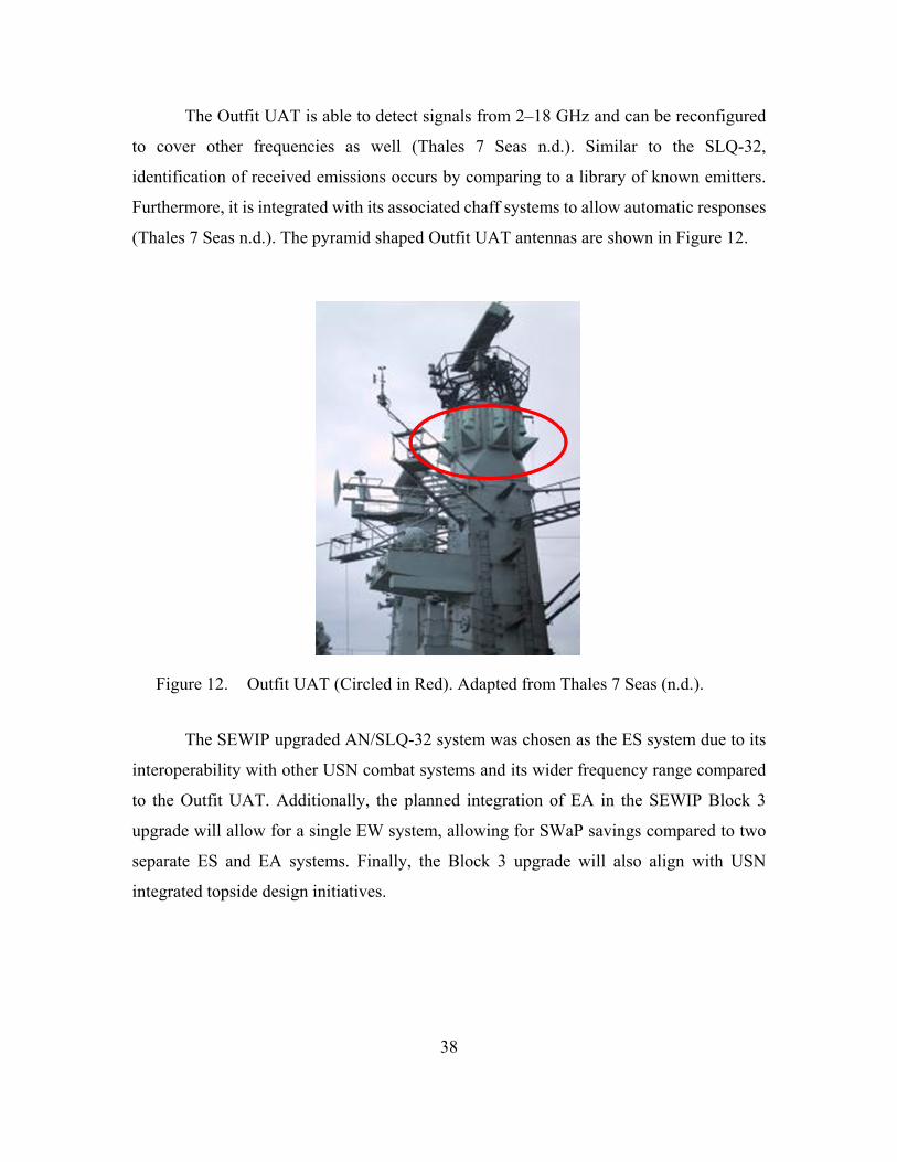
38
The Outfit UAT is able to detect signals from 2–18 GHz and can be reconfigured
to cover other frequencies as well (Thales 7 Seas n.d.). Similar to the SLQ-32,
identification of received emissions occurs by comparing to a library of known emitters.
Furthermore, it is integrated with its associated chaff systems to allow automatic responses
(Thales 7 Seas n.d.). The pyramid shaped Outfit UAT antennas are shown in Figure 12.
Figure 12. Outfit UAT (Circled in Red). Adapted from Thales 7 Seas (n.d.).
The SEWIP upgraded AN/SLQ-32 system was chosen as the ES system due to its
interoperability with other USN combat systems and its wider frequency range compared
to the Outfit UAT. Additionally, the planned integration of EA in the SEWIP Block 3
upgrade will allow for a single EW system, allowing for SWaP savings compared to two
separate ES and EA systems. Finally, the Block 3 upgrade will also align with USN
integrated topside design initiatives.
39
C. RESPONSE SUBSYSTEM COMPARISON AND SELECTION
1. Soft-Kill Deception Countermeasures
Available unclassified countermeasure information was weighed against system
requirements to compare potential subsystems. The Mk 36 SRBOC and Centurion chaff
and flare launchers were chosen for this down select process. The SRBOC is made by BAE
Systems for the USN and other countries, and the Centurion is made by Chemring
Countermeasures for the UK.
According to the manufacturers’ websites, both subsystems can launch chaff and
infrared countermeasures, meeting the requirement to be multifunctional, and both systems
can fire standard Mk 36 rounds, meeting the requirement to use standard non-custom
rounds (BAE Systems 2019; Chemring Countermeasures 2013a, 2013b). Both subsystems
are equipped with control subsystems to receive firing inputs (Chemring Countermeasures
2013b; Ward n.d.).
Where these subsystems differ is in the dynamic versus static nature of the barrels.
According to Larry Ward’s data sheet from United Defense (n.d.), a single launcher in the
SRBOC system contains six static barrels, and the system supports installing multiple
launchers in different areas to cover the required 360-degree area around the defended unit.
These barrels are aimed at fixed locations, some at 45 degrees and some at 60 degrees
(Ward n.d.). The SRBOC system is shown in action in Figure 13.
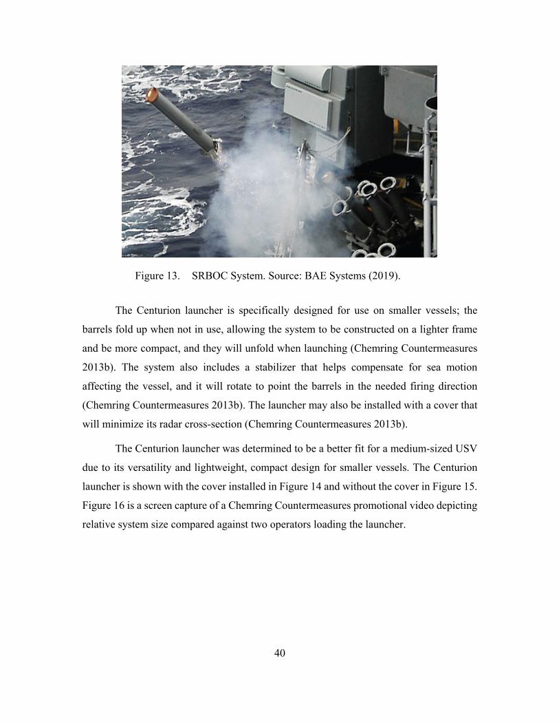
40
Figure 13. SRBOC System. Source: BAE Systems (2019).
The Centurion launcher is specifically designed for use on smaller vessels; the
barrels fold up when not in use, allowing the system to be constructed on a lighter frame
and be more compact, and they will unfold when launching (Chemring Countermeasures
2013b). The system also includes a stabilizer that helps compensate for sea motion
affecting the vessel, and it will rotate to point the barrels in the needed firing direction
(Chemring Countermeasures 2013b). The launcher may also be installed with a cover that
will minimize its radar cross-section (Chemring Countermeasures 2013b).
The Centurion launcher was determined to be a better fit for a medium-sized USV
due to its versatility and lightweight, compact design for smaller vessels. The Centurion
launcher is shown with the cover installed in Figure 14 and without the cover in Figure 15.
Figure 16 is a screen capture of a Chemring Countermeasures promotional video depicting
relative system size compared against two operators loading the launcher.
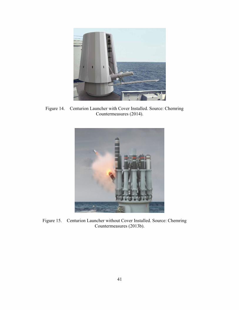
41
Figure 14. Centurion Launcher with Cover Installed. Source: Chemring Countermeasures (2014).
Figure 15. Centurion Launcher without Cover Installed. Source: Chemring Countermeasures (2013b).
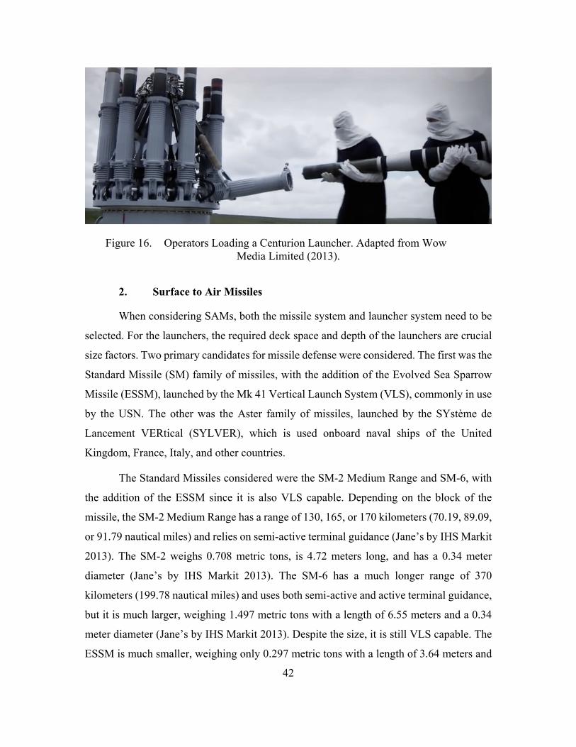
42
Figure 16. Operators Loading a Centurion Launcher. Adapted from Wow Media Limited (2013).
2. Surface to Air Missiles
When considering SAMs, both the missile system and launcher system need to be
selected. For the launchers, the required deck space and depth of the launchers are crucial
size factors. Two primary candidates for missile defense were considered. The first was the
Standard Missile (SM) family of missiles, with the addition of the Evolved Sea Sparrow
Missile (ESSM), launched by the Mk 41 Vertical Launch System (VLS), commonly in use
by the USN. The other was the Aster family of missiles, launched by the SYstème de
Lancement VERtical (SYLVER), which is used onboard naval ships of the United
Kingdom, France, Italy, and other countries.
The Standard Missiles considered were the SM-2 Medium Range and SM-6, with
the addition of the ESSM since it is also VLS capable. Depending on the block of the
missile, the SM-2 Medium Range has a range of 130, 165, or 170 kilometers (70.19, 89.09,
or 91.79 nautical miles) and relies on semi-active terminal guidance (Jane’s by IHS Markit
2013). The SM-2 weighs 0.708 metric tons, is 4.72 meters long, and has a 0.34 meter
diameter (Jane’s by IHS Markit 2013). The SM-6 has a much longer range of 370
kilometers (199.78 nautical miles) and uses both semi-active and active terminal guidance,
but it is much larger, weighing 1.497 metric tons with a length of 6.55 meters and a 0.34
meter diameter (Jane’s by IHS Markit 2013). Despite the size, it is still VLS capable. The
ESSM is much smaller, weighing only 0.297 metric tons with a length of 3.64 meters and
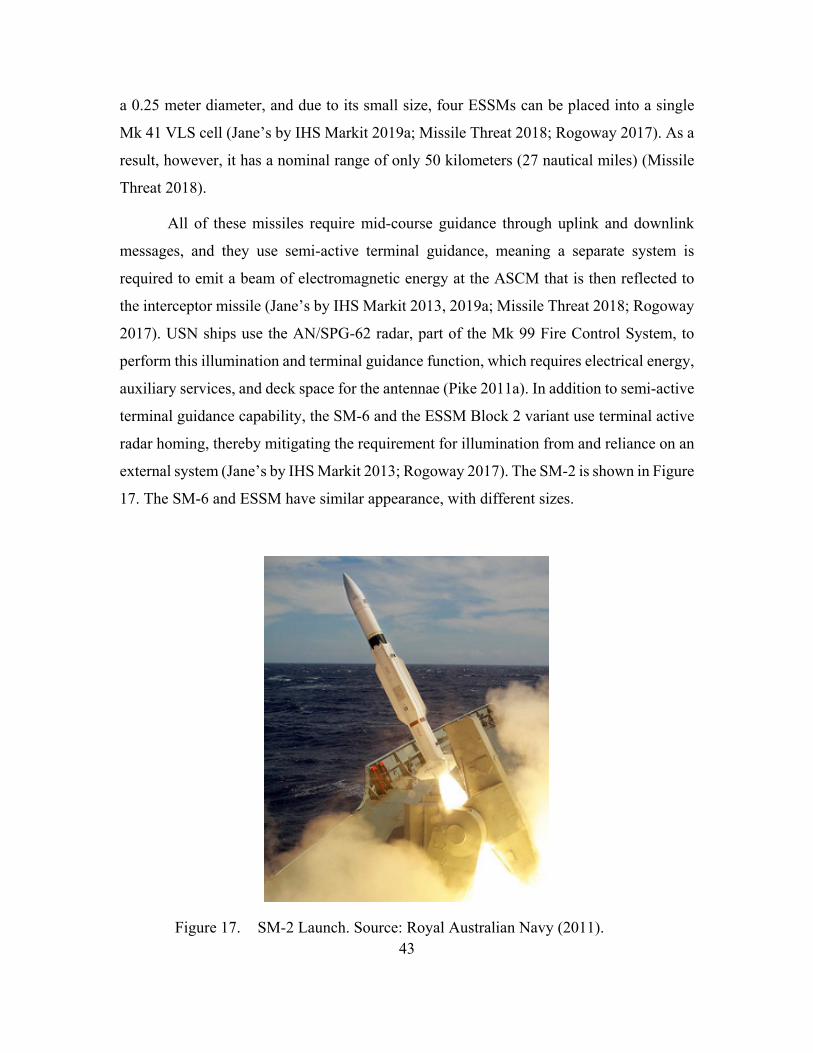
43
a 0.25 meter diameter, and due to its small size, four ESSMs can be placed into a single
Mk 41 VLS cell (Jane’s by IHS Markit 2019a; Missile Threat 2018; Rogoway 2017). As a
result, however, it has a nominal range of only 50 kilometers (27 nautical miles) (Missile
Threat 2018).
All of these missiles require mid-course guidance through uplink and downlink
messages, and they use semi-active terminal guidance, meaning a separate system is
required to emit a beam of electromagnetic energy at the ASCM that is then reflected to
the interceptor missile (Jane’s by IHS Markit 2013, 2019a; Missile Threat 2018; Rogoway
2017). USN ships use the AN/SPG-62 radar, part of the Mk 99 Fire Control System, to
perform this illumination and terminal guidance function, which requires electrical energy,
auxiliary services, and deck space for the antennae (Pike 2011a). In addition to semi-active
terminal guidance capability, the SM-6 and the ESSM Block 2 variant use terminal active
radar homing, thereby mitigating the requirement for illumination from and reliance on an
external system (Jane’s by IHS Markit 2013; Rogoway 2017). The SM-2 is shown in Figure
17. The SM-6 and ESSM have similar appearance, with different sizes.
Figure 17. SM-2 Launch. Source: Royal Australian Navy (2011).
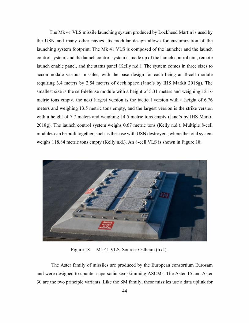
44
The Mk 41 VLS missile launching system produced by Lockheed Martin is used by
the USN and many other navies. Its modular design allows for customization of the
launching system footprint. The Mk 41 VLS is composed of the launcher and the launch
control system, and the launch control system is made up of the launch control unit, remote
launch enable panel, and the status panel (Kelly n.d.). The system comes in three sizes to
accommodate various missiles, with the base design for each being an 8-cell module
requiring 3.4 meters by 2.54 meters of deck space (Jane’s by IHS Markit 2018g). The
smallest size is the self-defense module with a height of 5.31 meters and weighing 12.16
metric tons empty, the next largest version is the tactical version with a height of 6.76
meters and weighing 13.5 metric tons empty, and the largest version is the strike version
with a height of 7.7 meters and weighing 14.5 metric tons empty (Jane’s by IHS Markit
2018g). The launch control system weighs 0.67 metric tons (Kelly n.d.). Multiple 8-cell
modules can be built together, such as the case with USN destroyers, where the total system
weighs 118.84 metric tons empty (Kelly n.d.). An 8-cell VLS is shown in Figure 18.
Figure 18. Mk 41 VLS. Source: Ostheim (n.d.).
The Aster family of missiles are produced by the European consortium Eurosam
and were designed to counter supersonic sea-skimming ASCMs. The Aster 15 and Aster
30 are the two principle variants. Like the SM family, these missiles use a data uplink for
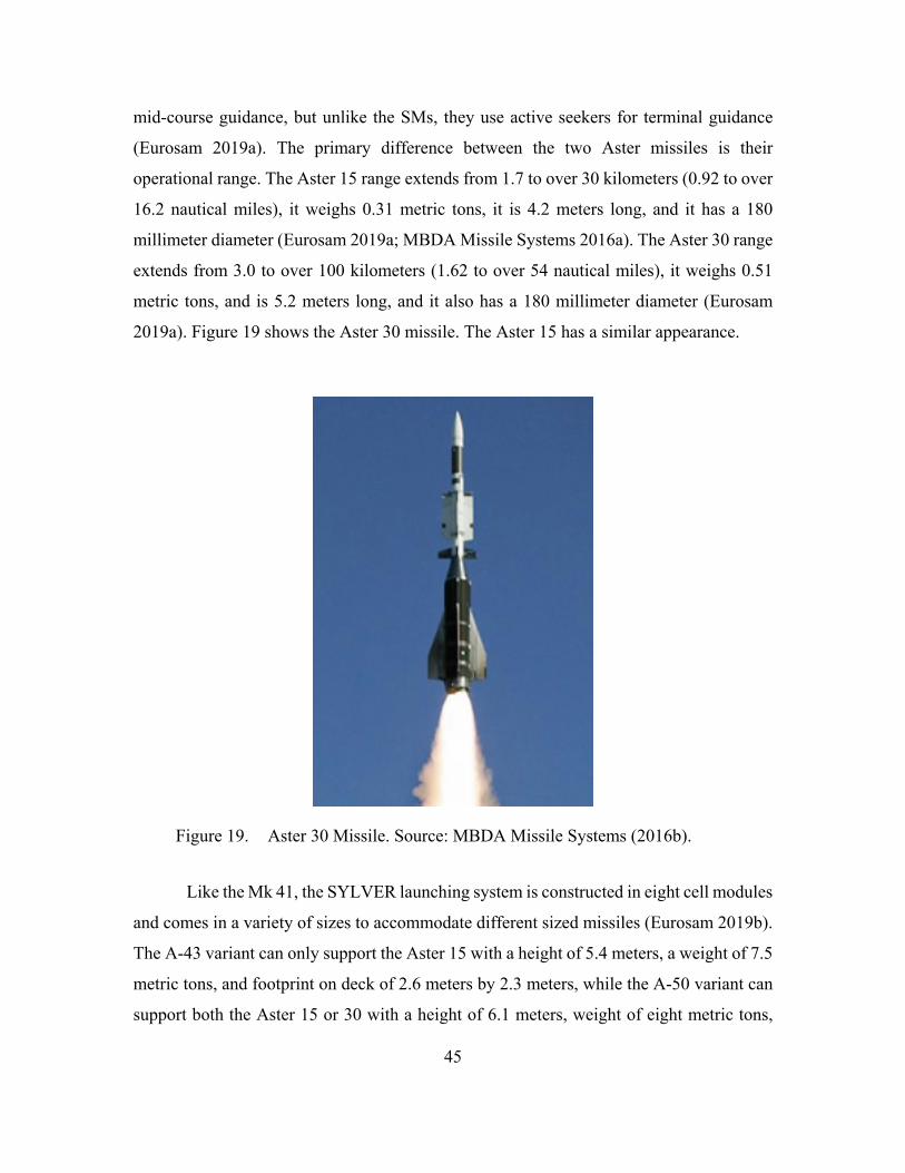
45
mid-course guidance, but unlike the SMs, they use active seekers for terminal guidance
(Eurosam 2019a). The primary difference between the two Aster missiles is their
operational range. The Aster 15 range extends from 1.7 to over 30 kilometers (0.92 to over
16.2 nautical miles), it weighs 0.31 metric tons, it is 4.2 meters long, and it has a 180
millimeter diameter (Eurosam 2019a; MBDA Missile Systems 2016a). The Aster 30 range
extends from 3.0 to over 100 kilometers (1.62 to over 54 nautical miles), it weighs 0.51
metric tons, and is 5.2 meters long, and it also has a 180 millimeter diameter (Eurosam
2019a). Figure 19 shows the Aster 30 missile. The Aster 15 has a similar appearance.
Figure 19. Aster 30 Missile. Source: MBDA Missile Systems (2016b).
Like the Mk 41, the SYLVER launching system is constructed in eight cell modules
and comes in a variety of sizes to accommodate different sized missiles (Eurosam 2019b).
The A-43 variant can only support the Aster 15 with a height of 5.4 meters, a weight of 7.5
metric tons, and footprint on deck of 2.6 meters by 2.3 meters, while the A-50 variant can
support both the Aster 15 or 30 with a height of 6.1 meters, weight of eight metric tons,

46
and footprint on deck of 2.6 meters by 2.3 meters (Eurosam 2019b). The SYLVER
launching system is shown in Figure 20.
Figure 20. SYLVER Launching System. Source: Seaforces Naval Information (n.d.).
In consideration of the best fit missile, nominal USV detection range must first be
assessed. Missiles with ranges that exceed the organic detection radius of the USV provide
no practical advantage in this study. Equation 1 is Robinson’s (2019) simplified radar
horizon equation against a target at elevation in metric units, adapted for use where the
surface unit is the detection platform against an inbound ASCM. Therefore, RH is the radar
horizon range in kilometers, hAntenna is the height of the USV (or ship) radar antenna in
meters, and hASCM is the height of the ASCM in meters.
4.124 ( )H Antenna ASCMR h h= × + (1)
Assuming the USV radar height is 12 meters and given the nominal cruise missile
altitude for each of the three missile threats from Jane’s by IHS Markit (2018a, 2018c,
2018d, 2018e, 2018f, 2018h) of approximately 20 meters, the equation results in the USV’s
maximum detection range of 32.72 kilometers (17.67 nautical miles).
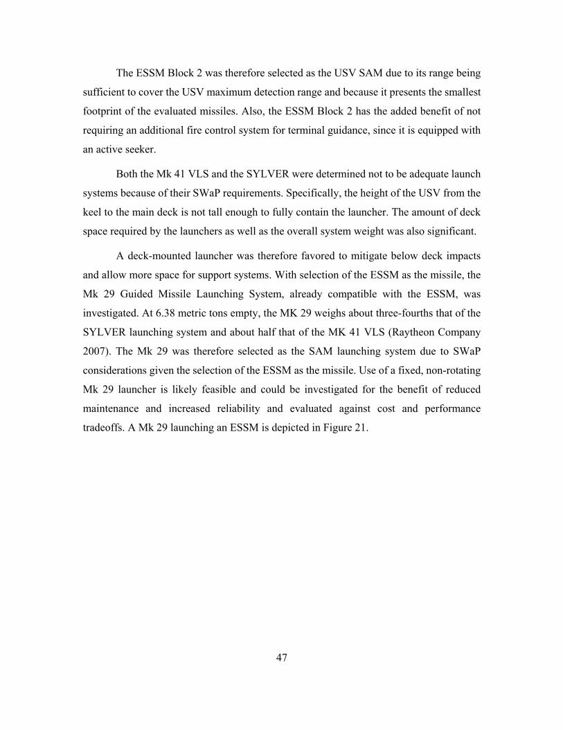
47
The ESSM Block 2 was therefore selected as the USV SAM due to its range being
sufficient to cover the USV maximum detection range and because it presents the smallest
footprint of the evaluated missiles. Also, the ESSM Block 2 has the added benefit of not
requiring an additional fire control system for terminal guidance, since it is equipped with
an active seeker.
Both the Mk 41 VLS and the SYLVER were determined not to be adequate launch
systems because of their SWaP requirements. Specifically, the height of the USV from the
keel to the main deck is not tall enough to fully contain the launcher. The amount of deck
space required by the launchers as well as the overall system weight was also significant.
A deck-mounted launcher was therefore favored to mitigate below deck impacts
and allow more space for support systems. With selection of the ESSM as the missile, the
Mk 29 Guided Missile Launching System, already compatible with the ESSM, was
investigated. At 6.38 metric tons empty, the MK 29 weighs about three-fourths that of the
SYLVER launching system and about half that of the MK 41 VLS (Raytheon Company
2007). The Mk 29 was therefore selected as the SAM launching system due to SWaP
considerations given the selection of the ESSM as the missile. Use of a fixed, non-rotating
Mk 29 launcher is likely feasible and could be investigated for the benefit of reduced
maintenance and increased reliability and evaluated against cost and performance
tradeoffs. A Mk 29 launching an ESSM is depicted in Figure 21.

48
Figure 21. ESSM Launch from Mk 29 Launching System. Source: Rogoway (2017).
3. Close-in Weapons System
Two CIWS components were chosen for this down select process due to their
autonomous capability and ability to fire commonly available rounds. The first was the
Phalanx originally created by General Dynamics and equipped on almost all USN surface
ships and used by many foreign militaries (General Dynamics 2003b). This system was
purchased by Raytheon who is the current manufacturer (Department of the Navy 2019).
The second CIWS system was the Goalkeeper made by Thales Defense in conjunction with
General Dynamics, currently in use by several foreign militaries (General Dynamics
2003a). Range information on these systems is classified.
According to General Dynamics (2003b), the Phalanx CIWS uses a Gatling gun
that fires 20 millimeter rounds at a speed up to 4,500 rounds per minute. The magazine of
this weapon holds 1,550 rounds, and the system is autonomous, using a Ku-band search
and track radar at 12 to 18 GHz (General Dynamics 2003b). This CIWS weighs 6.17 metric
tons and has an internal seawater cooling system (General Dynamics 2003b). The Phalanx
is shown in Figure 22.
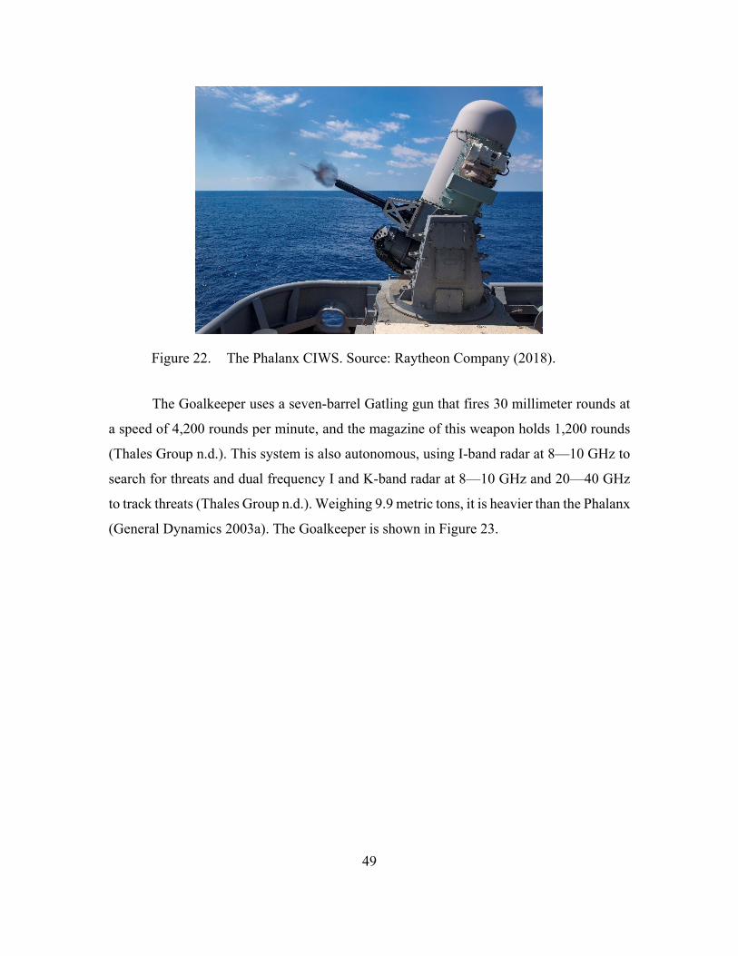
49
Figure 22. The Phalanx CIWS. Source: Raytheon Company (2018).
The Goalkeeper uses a seven-barrel Gatling gun that fires 30 millimeter rounds at
a speed of 4,200 rounds per minute, and the magazine of this weapon holds 1,200 rounds
(Thales Group n.d.). This system is also autonomous, using I-band radar at 8—10 GHz to
search for threats and dual frequency I and K-band radar at 8—10 GHz and 20—40 GHz
to track threats (Thales Group n.d.). Weighing 9.9 metric tons, it is heavier than the Phalanx
(General Dynamics 2003a). The Goalkeeper is shown in Figure 23.
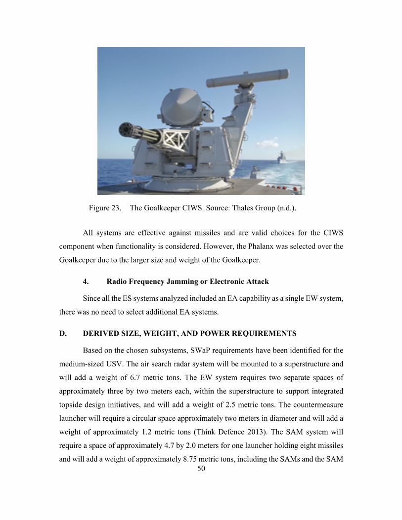
50
Figure 23. The Goalkeeper CIWS. Source: Thales Group (n.d.).
All systems are effective against missiles and are valid choices for the CIWS
component when functionality is considered. However, the Phalanx was selected over the
Goalkeeper due to the larger size and weight of the Goalkeeper.
4. Radio Frequency Jamming or Electronic Attack
Since all the ES systems analyzed included an EA capability as a single EW system,
there was no need to select additional EA systems.
D. DERIVED SIZE, WEIGHT, AND POWER REQUIREMENTS
Based on the chosen subsystems, SWaP requirements have been identified for the
medium-sized USV. The air search radar system will be mounted to a superstructure and
will add a weight of 6.7 metric tons. The EW system requires two separate spaces of
approximately three by two meters each, within the superstructure to support integrated
topside design initiatives, and will add a weight of 2.5 metric tons. The countermeasure
launcher will require a circular space approximately two meters in diameter and will add a
weight of approximately 1.2 metric tons (Think Defence 2013). The SAM system will
require a space of approximately 4.7 by 2.0 meters for one launcher holding eight missiles
and will add a weight of approximately 8.75 metric tons, including the SAMs and the SAM
51
launch control unit. The chosen CIWS will require approximately three by three meters of
deck space for one unit and will add a weight of 6.17 metric tons.
These subsystems add a total weight of approximately 25.5 metric tons. This total
subsystem weight is within the rule of thumb that “a modern warship’s mission payload
makes up 10–15% of its total displacement” (Kelley 2002, 42). For a vessel with a 300
long ton displacement, that maximum is 30 to 45 long tons. This leaves available weight
for required support systems and any additional payloads. This heuristic was developed for
manned vessels; with no requirement for crew considerations, the percentage of mission
payload displacement is expected to be even greater.
Standard ship power is three phase 450 volts at 60 hertz along with the ability to
convert it to 400 hertz or transform it to 120 volts. Many of the chosen subsystems will
draw from standard ship power, so consideration will be needed during USV integration to
ensure it can handle the power draw of the newly added subsystems. The largest power
requirement for the selected subsystems will be those of the EASR and SEWIP. Power
consumption data could not be obtained for EASR or SEWIP, but peak power consumption
is expected to be on the order of tens of megawatts. The Phalanx product specification
sheets indicate a 70 kilowatt peak power consumption, and the Mk 29 Guided Missile
Launching System specification sheets present a 55 kilowatt peak value (General
Dynamics 2003b; Raytheon Company 2007). The Centurion power consumption could not
be obtained but is expected to also be on the order of kilowatts. Future study areas for ship
power include identification of total maximum load for all subsystems.

52
THIS PAGE INTENTIONALLY LEFT BLANK
53
V. DERIVED COMMUNICATION REQUIREMENTS
On the USV, many systems need to seamlessly send and receive information to and
from other systems to properly execute the mission. This includes external communications
from the USV to the SAG and internal communications amongst the USV subsystems.
This chapter discusses requirements and considerations for the communications subsystem.
Areas outside the scope of this project involving communications are an enemy’s
ability to misdirect the USV, causing defensive gaps, and specific communication system
selection. Enemy misdirection of the USV is not within the realm of the DRM, and it would
be difficult to maintain an unclassified study if specific communication systems’
capabilities were discussed in detail. Both areas would be good candidates for future study.
A. OVERVIEW
The USV must be able to receive and execute tactical commands from the SAG via
the ICS. Additionally, the USV needs to indicate receipt of and compliance with these
directions so operational commanders can account for USV use or plan accordingly if the
USV is not in receipt of tasking or unable to comply. All directives received from an
external source must be disseminated to the respective USV subsystems via the ICS, and
those subsystems must be able to send response messages back to the ICS for compilation
and dispatch to the SAG.
The USV subsystems also all use information from each other. Therefore, either all
subsystems shall be able to communicate with each other in a mutually understandable
language, or the ICS must be able to communicate with all subsystems in their specific
language.
B. COMMUNICATION REQUIREMENTS
In addition to tactical direction, operators on the SAG will send configuration
updates to the ICS to set operating parameters of the autonomous subsystems. Such
parameters include threat profiles, rules of engagement, and COI criteria. The SAG and
USV need to send tactical data to each other to ensure they share a common operating

54
picture. Initial operating picture data will be sent to the ICS on the USV, and tracks sent
from the USV back to the SAG will then update the common operating picture. LOS
communications will be primary, with BLOS methods used if the distance between the
USV and SAG is greater than that supported by LOS communications. Methods available
for USV to SAG communications include very-high frequency (VHF) radio, ultra-high
frequency (UHF) radio, satellite communications, and direct datalink systems.
To detect and appropriately respond to threats, internal communications are
required between the subsystems located on the USV, facilitated by the ICS. These internal
communications can be sent over a local area network cable using Ethernet or other
standard network protocols. Local area network speeds are assumed to be fast enough to
carry all internal communications in a timely manner.
Detection subsystems (air search radar and ES portion of the EW system) will
receive search orders to initiate threat searches. Response subsystems will receive arm and
disarm orders as well as configuration updates from the ICS. The countermeasure and SAM
subsystems will need to know the location, type, and speed of the threat to know what
measure to launch and where. The EW system will need to know where to direct EA. This
information will be provided by the ICS via launch or EA orders developed using track
data received from the air search radar and EW subsystems. The ICS will receive status
reports from the response subsystems and forward them to the SAG for monitoring.
Figure 24 shows the communications that are required internal to the USV and between
the USV and the SAG as described above.
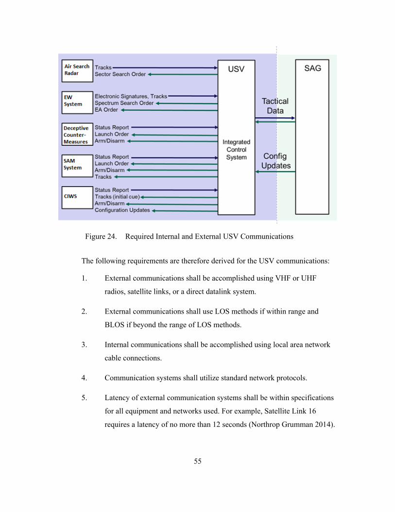
55
Figure 24. Required Internal and External USV Communications
The following requirements are therefore derived for the USV communications:
1. External communications shall be accomplished using VHF or UHF
radios, satellite links, or a direct datalink system.
2. External communications shall use LOS methods if within range and
BLOS if beyond the range of LOS methods.
3. Internal communications shall be accomplished using local area network
cable connections.
4. Communication systems shall utilize standard network protocols.
5. Latency of external communication systems shall be within specifications
for all equipment and networks used. For example, Satellite Link 16
requires a latency of no more than 12 seconds (Northrop Grumman 2014).

56
C. DATA SHARING SYSTEMS
Data must be able to be shared between the USV and the SAG on compatible
systems. This is to allow for tracks and engagement information—such as orders, reports,
and battle damage assessments—to be reported from the USV to the SAG and vice versa
with minimal delay. Common TDLs and CEC will therefore be used.
The most common TDLs found aboard USN vessels are Link 11, Link 16, and Link
22. Link 11 is the oldest data link still in use. It creates a network between users for mutual
exchange of tactical data and operates on both the HF (2—30 MHz) and UHF (225—400
MHz) portions of the radio spectrum (Northrop Grumman 2014). Two primary
disadvantages of Link 11 compared to other TDLs are that it is not jam resistant, and it
relies on a specific unit as a central node (Northrop Grumman 2014). In this construct, if
the node is lost, the network will go down (Northrop Grumman 2014).
Link 16 is a secure data link installed on nearly all operational cruisers, destroyers,
aircraft carriers, airborne early warning aircraft, and fighters. It is transmitted over UHF
for LOS applications and also has BLOS capability via satellites (Northrop Grumman
2014). According to the Tactical Data Link Guide by Northrop Grumman (2014), Link 16
data is formatted in J-Series messages, point-to-point messages or networks of users are
supported, and it uses the time division multiple access principle to allocate transmission
and receive timeframes across all units in the network. Link 16 is therefore node-less. It
also employs frequency hopping to be jam resistant (Northrop Grumman 2014).
Link 22 is the replacement for Link 11. One of the biggest improvements is that it
is much more secure and resistant to jamming than Link 11 in part by also employing
frequency hopping and formatting information it transmits in J-Series messages, allowing
it to integrate with Link 16 (Northrop Grumman 2014). According to the Tactical Data
Link Guide by Northrop Grumman (2014), up to eight networks can be integrated into a
super network consisting of up to 125 units, and it has a built-in automatic relay setting
that will pass on received data to the rest of the network without any operator actions. It
has a transmission range of 300 nautical miles (Northrop Grumman 2014).
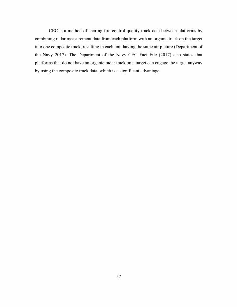
57
CEC is a method of sharing fire control quality track data between platforms by
combining radar measurement data from each platform with an organic track on the target
into one composite track, resulting in each unit having the same air picture (Department of
the Navy 2017). The Department of the Navy CEC Fact File (2017) also states that
platforms that do not have an organic radar track on a target can engage the target anyway
by using the composite track data, which is a significant advantage.

58
THIS PAGE INTENTIONALLY LEFT BLANK

59
VI. EVALUATION OF OPERATIONAL SCENARIOS
To evaluate the operational scenarios described in the DRM, two analysis methods
were applied: a Markov kill chain and a time series analysis. These analyses use Microsoft
Excel, Visual Basic for Applications, and Real Options Valuation’s Risk Simulator to
determine the effectiveness of the USV. The Markov chain model addresses the study goal
of determining utility of USV responses to ASCM threats. The time series analysis is a
separate unrelated analysis and determines if the USV provides additional reaction time
and counter-fire opportunities in the event an incoming ASCM is targeted at the SAG.
Finally, two basic USV-SAG geometric formations are explored, and their potential
benefits are compared.
A. KILL CHAIN MODEL
1. Kill Chain Model Description
The first model for this project determines the capability of the USV to defeat
incoming ASCMs, providing the SAG a defensive advantage as in OPSITs 1A and 1B. The
model uses a Markov kill chain analysis and was based on Giachetti’s (2015) “System of
Systems Capability Needs Analysis via a Stochastic Network Model.” A Markov chain
model is a stochastic model that describes event states and the probability based potential
transitions between states.
a. State Transition Diagram
This model uses the state transition diagram presented in Figure 25. The states are
either transitional or final. Transitional states are intermediate states used to determine
probabilities for and times until reaching the final states. States 1 through 5 constitute the
Find, Fix, and Track components of the traditional F2T2EA kill chain. States 6, 7, and 8
correspond to the Target component of the kill chain. State 6 is for threat evaluation and
weapons assignment (TEWA), where the determination is made to either employ USV or
SAG ship subsystems to engage the threat, and states 7 and 8 reflect targeting with the
appropriate response subsystem onboard the SAG and USV. State 7 also includes Engage
60
and Assess portions of the kill chain for the SAG and was not used in this study. This is
because the model was developed to incorporate the option for SAG responses in addition
to USV responses, but only the USV defensive measures were explored to meet the study
goals.
States 9, 11, 13, 15, and 17 comprise the USV’s Engage component of the F2T2EA
kill chain. Three different range rings centered around the USV are used for this part of the
model. These range rings are labeled as “RR” in Figure 25 as well as in following tables.
When the threat missile is only inside Range Ring 1, SAMs are used to engage the threat.
When the threat closes to be within Range Ring 2, electronic attack is employed, and range
ring 3 comprises CIWS and soft-kill deception countermeasure engagements.
States 10, 12, 14, and 16 constitute the assess component of the F2T2EA kill chain.
In states 2, 3, or 4, the target can be lost, requiring a transition back to state 1 “Search” for
the USV to reacquire the threat. In states, 10, 12, 14, or 16, the battle damage assessment
can indicate the target has not been destroyed, requiring a transition back to state 1 for the
USV to begin another kill chain sequence. States 18, 19, and 20 are the model’s three final
states: Hard Kill, Soft Kill, or No Kill. The model completes when a final state is reached.
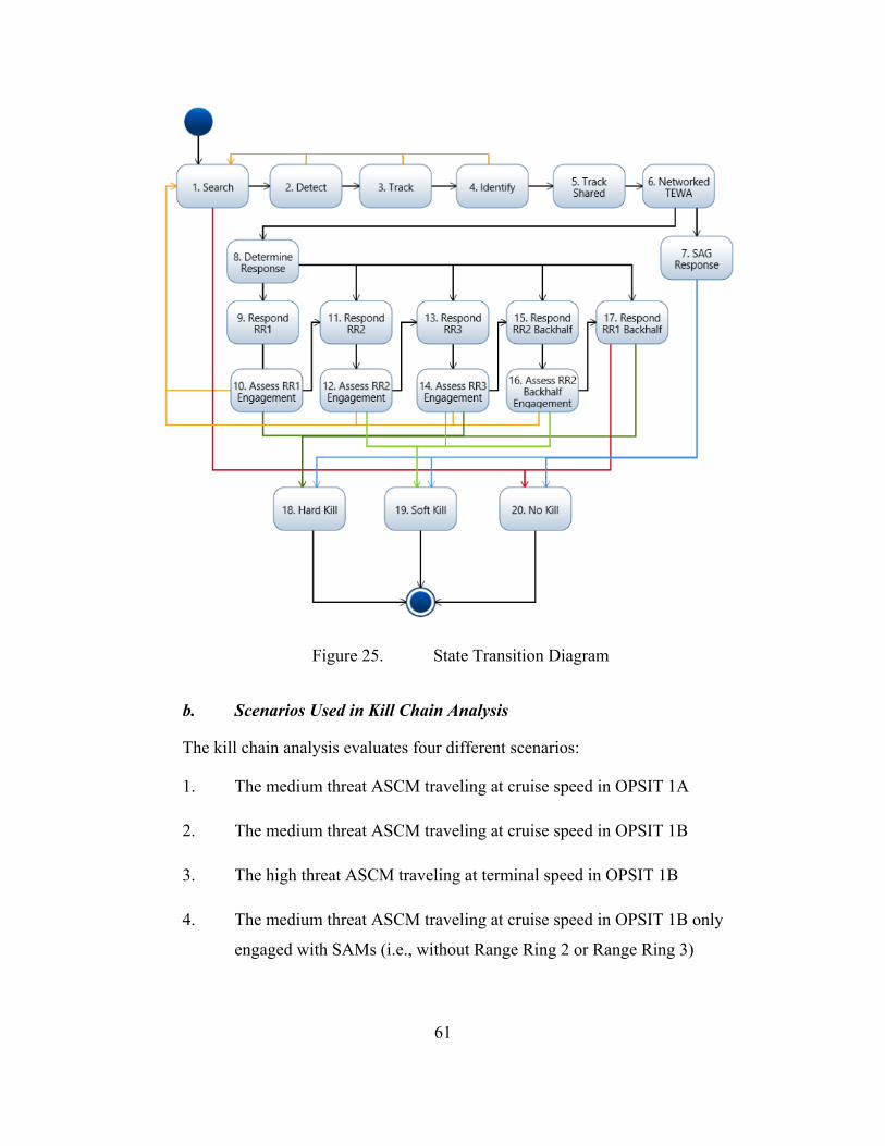
61
Figure 25. State Transition Diagram
b. Scenarios Used in Kill Chain Analysis
The kill chain analysis evaluates four different scenarios:
1. The medium threat ASCM traveling at cruise speed in OPSIT 1A
2. The medium threat ASCM traveling at cruise speed in OPSIT 1B
3. The high threat ASCM traveling at terminal speed in OPSIT 1B
4. The medium threat ASCM traveling at cruise speed in OPSIT 1B only
engaged with SAMs (i.e., without Range Ring 2 or Range Ring 3)

62
The low threat ASCM was not used for this model due to having both a lower cruise
speed and a lower terminal speed than the other two threat levels. It is assumed the USV
will perform equally or better against this lower level threat. The medium threat was chosen
for the majority of the modeling due to the threat having the highest cruise speed, and the
high threat was chosen in order to represent the worst-case scenario where the incoming
ASCM is already at terminal speed when detected. In all scenarios for this model, if an
incoming threat is detected by the USV, the SAG must provide authorization for the USV
to employ countermeasures during the Networked TEWA state.
Each range ring in the model represents specific response options the USV will
employ. The range rings are time-based, commensurate with the ASCM’s position along
its threat axis as it continues inbound. The times associated with how long it takes an
incoming threat to reach the SAG are calculated based on a time-speed-distance analysis
using the cruise speed of Mach 0.9 for the medium threat and the high threat terminal speed
of Mach 2.9, with the maximum USV detection range in each case as the starting distance.
This range was determined from Equation 1, using a USV antenna height of 12 meters and
an ASCM height of 20 meters for the medium threat and five meters for the high threat,
based on ASCM cruise and terminal heights.
Figure 26 displays Scenario 1, which is based on OPSIT 1A where the USV is
offset from the incoming threat missile. In this scenario, the USV is only able to engage
the ASCM once within Range Ring 1.
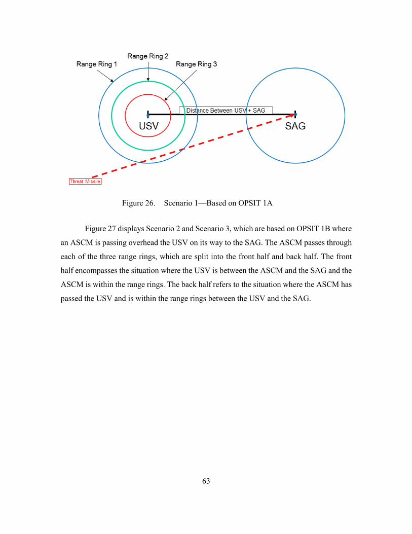
63
Figure 26. Scenario 1—Based on OPSIT 1A
Figure 27 displays Scenario 2 and Scenario 3, which are based on OPSIT 1B where
an ASCM is passing overhead the USV on its way to the SAG. The ASCM passes through
each of the three range rings, which are split into the front half and back half. The front
half encompasses the situation where the USV is between the ASCM and the SAG and the
ASCM is within the range rings. The back half refers to the situation where the ASCM has
passed the USV and is within the range rings between the USV and the SAG.
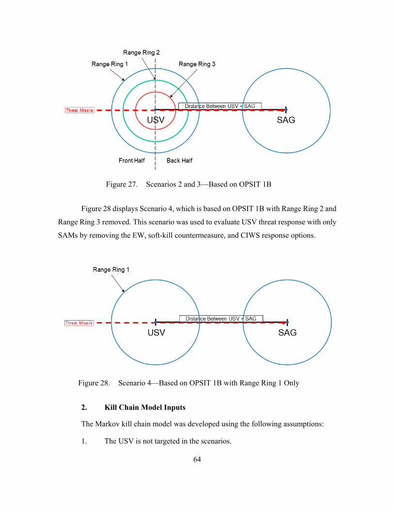
64
Figure 27. Scenarios 2 and 3—Based on OPSIT 1B
Figure 28 displays Scenario 4, which is based on OPSIT 1B with Range Ring 2 and
Range Ring 3 removed. This scenario was used to evaluate USV threat response with only
SAMs by removing the EW, soft-kill countermeasure, and CIWS response options.
Figure 28. Scenario 4—Based on OPSIT 1B with Range Ring 1 Only
2. Kill Chain Model Inputs
The Markov kill chain model was developed using the following assumptions:
1. The USV is not targeted in the scenarios.

65
2. The USV is in a defensive mode only.
3. Each response subsystem onboard the USV is assigned to a range ring,
with multiple systems able to be assigned to the same range ring.
4. The SAG and its units are counted as a single target.
5. Given the speeds of the missiles relative to the USV and SAG, the USV
and SAG shall be considered stationary for the purposes of this model.
6. ASCMs are launched from sanctuary (maximum distance), so low and
medium threats will be detected after they have reached cruise speed and
altitude, while the high threat will be detected only after reaching its
terminal speed and altitude.
7. SAM effectiveness is equivalent on both sides of the USV.
8. The USV and SAG are both in battle-ready state (equipment and systems
onboard the USV and SAG are available, energized, and not
malfunctioning, and system operators are awake and alert).
Using the state transition diagram, a state machine was developed in Microsoft
Excel to analyze the scenarios. Probabilities were assigned to each transition between states
based on previous research, unclassified data, and estimation. Table 2 uses the states and
transitions identified in Figure 25 and shows the possible transitions from each state and
the associated probabilities of transition. The far-left column displays the state that is being
transitioned out of. The following columns on the same row show the possible states that
can be transitioned to, and the probabilities for each transition are shown in bold font. This
table was used to develop the probabilities for reaching the three final states.
For example, from the Search state, there is a 99% probability of transitioning to
the Detect state and a 1% chance of transitioning to the final No Kill state (meaning the
track was never gained and therefore could not be engaged). After transitioning to the
Detect state, there is a 99% probability of transitioning to the Track state and a 1% of losing
the target and therefore returning to the Search state. These transition probabilities continue
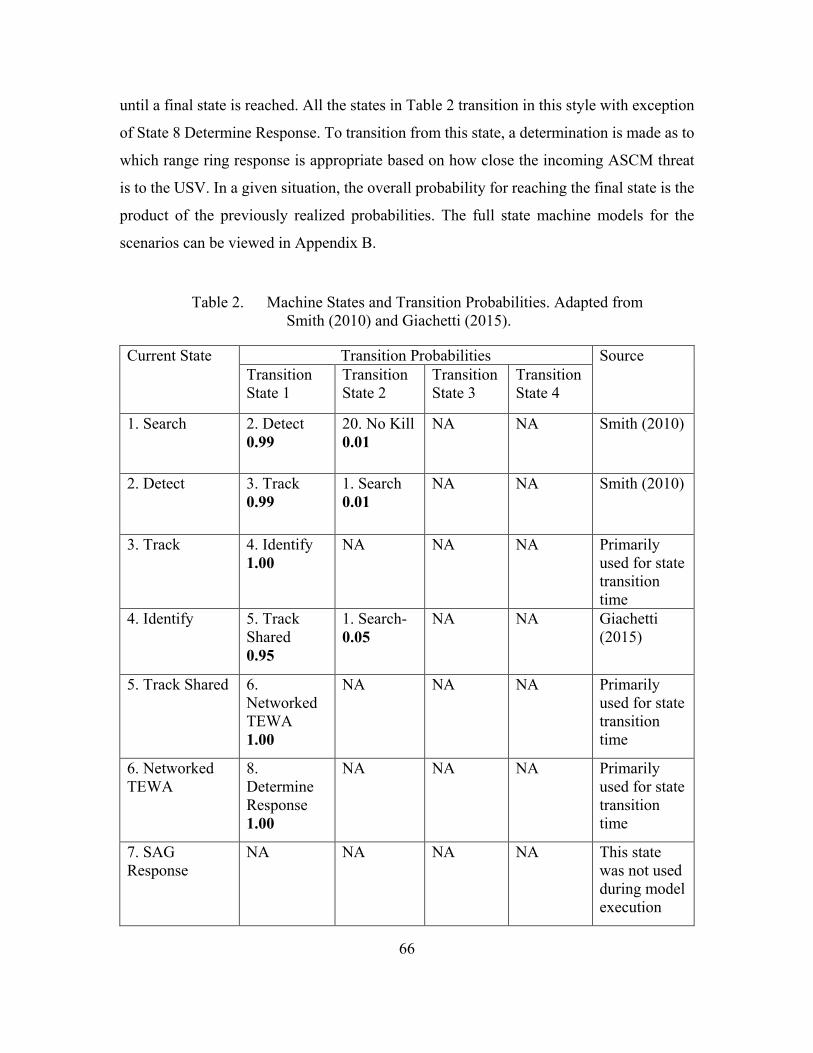
66
until a final state is reached. All the states in Table 2 transition in this style with exception
of State 8 Determine Response. To transition from this state, a determination is made as to
which range ring response is appropriate based on how close the incoming ASCM threat
is to the USV. In a given situation, the overall probability for reaching the final state is the
product of the previously realized probabilities. The full state machine models for the
scenarios can be viewed in Appendix B.
Table 2. Machine States and Transition Probabilities. Adapted from Smith (2010) and Giachetti (2015).
Current State Transition Probabilities Source Transition State 1
Transition State 2
Transition State 3
Transition State 4
1. Search 2. Detect 0.99
20. No Kill 0.01
NA NA Smith (2010)
2. Detect 3. Track 0.99
1. Search 0.01
NA NA Smith (2010)
3. Track 4. Identify 1.00
NA NA NA Primarily used for state transition time
4. Identify 5. Track Shared 0.95
1. Search-0.05
NA NA Giachetti (2015)
5. Track Shared 6. Networked TEWA 1.00
NA NA NA Primarily used for state transition time
6. Networked TEWA
8. Determine Response 1.00
NA NA NA Primarily used for state transition time
7. SAG Response
NA NA NA NA This state was not used during model execution

67
Current State Transition Probabilities Source Transition State 1
Transition State 2
Transition State 3
Transition State 4
8. Determine Response
9. Respond RR1
OR
11. Respond RR2
OR
13. Respond RR3
OR
15. RR2 Backhalf
OR
17. RR1 Backhalf 1.00
NA NA NA Assumption: based on current state time, the appropriate RR can be selected to engage at the ASCM’s expected position
9. Respond RR1
10. Assess RR1 Engagement 1.00
NA NA NA Primarily used for state transition time
10. Assess RR1 Engagement
18. Hard Kill 0.82
11. Respond RR2 0.13
1. Search 0.05
NA Giachetti (2015)
11. Respond RR2
12. Assess RR2 Engagement 1.00
NA NA NA Primarily used for state transition time
12. Assess RR2 Engagement
19. Soft Kill 0.20
13. Respond RR3 0.75
1. Search 0.05
NA Smith (2010)
13. Respond RR3
14. Assess RR3 Engagement 1.00
NA NA NA Primarily used for state transition time
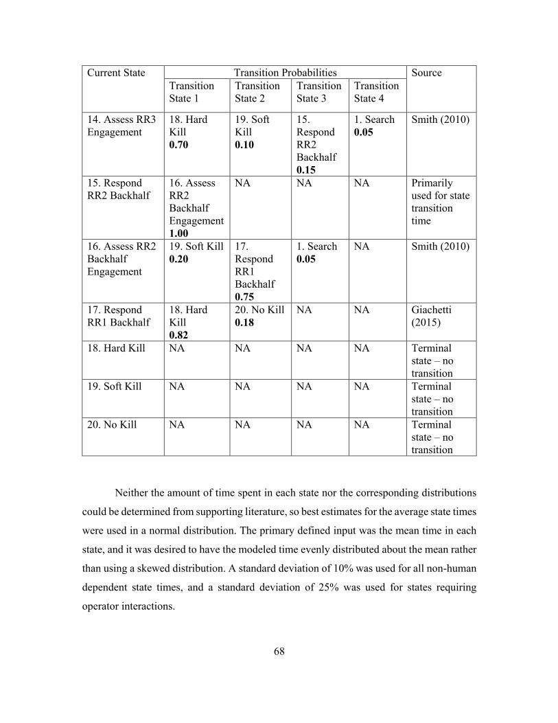
68
Current State Transition Probabilities Source Transition State 1
Transition State 2
Transition State 3
Transition State 4
14. Assess RR3 Engagement
18. Hard Kill 0.70
19. Soft Kill 0.10
15. Respond RR2 Backhalf 0.15
1. Search 0.05
Smith (2010)
15. Respond RR2 Backhalf
16. Assess RR2 Backhalf Engagement 1.00
NA NA NA Primarily used for state transition time
16. Assess RR2 Backhalf Engagement
19. Soft Kill 0.20
17. Respond RR1 Backhalf 0.75
1. Search 0.05
NA Smith (2010)
17. Respond RR1 Backhalf
18. Hard Kill 0.82
20. No Kill 0.18
NA NA Giachetti (2015)
18. Hard Kill NA NA NA NA Terminal state – no transition
19. Soft Kill NA NA NA NA Terminal state – no transition
20. No Kill NA NA NA NA Terminal state – no transition
Neither the amount of time spent in each state nor the corresponding distributions
could be determined from supporting literature, so best estimates for the average state times
were used in a normal distribution. The primary defined input was the mean time in each
state, and it was desired to have the modeled time evenly distributed about the mean rather
than using a skewed distribution. A standard deviation of 10% was used for all non-human
dependent state times, and a standard deviation of 25% was used for states requiring
operator interactions.

69
For instance, it is assumed it takes two seconds on average, with a standard
deviation about that mean of 0.2 seconds, for the USV to detect an incoming ASCM threat
because of the time for the software to establish enough consistent data on the threat to rule
out clutter. The only state requiring operator interaction was state 6 “Networked TEWA,”
during which a SAG operator gives the USV authorization to employ threat responses.
These state times and their associated standard deviations are displayed in Table 3. States
18, 19, and 20 are the possible end states for the state machine. These states represent the
final battle damage assessment from the USV’s perspective when the USV has either
physically destroyed the ASCM (hard kill), managed to force the ASCM to miss its target
(soft kill), or failed to defeat the ASCM resulting in it penetrating to the SAG self-defense
area (no kill).
Table 3. Machine State Times and Standard Deviations
State Mean Time in State (seconds)
Requires Operator Interaction?
Standard Deviation (seconds)
1. Search 1 No 0.1 2. Detect 2 No 0.2 3. Track 2 No 0.2 4. Identify 1 No 0.1 5. Track Shared 1 No 0.1 6. Networked TEWA 4 Yes 1.0 7. SAG Response 0 N/A 0.0 8. Determine Response 1 No 0.1 9. Respond RR 1 4 No 0.4 10. Assess RR 1 Engagement 1 No 0.1 11. Respond RR 2 5 No 0.5 12. Assess RR 2 Engagement 1 No 0.1 13. Respond RR 3 5 No 0.5 14. Assess RR 3 Engagement 1 No 0.1 15. Respond RR 2 Backhalf 5 No 0.5 16. Assess RR 2 Backhalf Engagement 1 No 0.1 17. Respond RR 1 Backhalf 8 No 0.8 18. Hard Kill 0 N/A 0.0 19. Soft Kill 0 N/A 0.0 20. No Kill 0 N/A 0.0
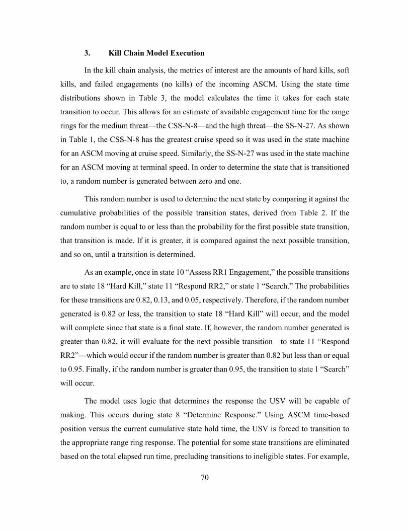
70
3. Kill Chain Model Execution
In the kill chain analysis, the metrics of interest are the amounts of hard kills, soft
kills, and failed engagements (no kills) of the incoming ASCM. Using the state time
distributions shown in Table 3, the model calculates the time it takes for each state
transition to occur. This allows for an estimate of available engagement time for the range
rings for the medium threat—the CSS-N-8—and the high threat—the SS-N-27. As shown
in Table 1, the CSS-N-8 has the greatest cruise speed so it was used in the state machine
for an ASCM moving at cruise speed. Similarly, the SS-N-27 was used in the state machine
for an ASCM moving at terminal speed. In order to determine the state that is transitioned
to, a random number is generated between zero and one.
This random number is used to determine the next state by comparing it against the
cumulative probabilities of the possible transition states, derived from Table 2. If the
random number is equal to or less than the probability for the first possible state transition,
that transition is made. If it is greater, it is compared against the next possible transition,
and so on, until a transition is determined.
As an example, once in state 10 “Assess RR1 Engagement,” the possible transitions
are to state 18 “Hard Kill,” state 11 “Respond RR2,” or state 1 “Search.” The probabilities
for these transitions are 0.82, 0.13, and 0.05, respectively. Therefore, if the random number
generated is 0.82 or less, the transition to state 18 “Hard Kill” will occur, and the model
will complete since that state is a final state. If, however, the random number generated is
greater than 0.82, it will evaluate for the next possible transition—to state 11 “Respond
RR2”—which would occur if the random number is greater than 0.82 but less than or equal
to 0.95. Finally, if the random number is greater than 0.95, the transition to state 1 “Search”
will occur.
The model uses logic that determines the response the USV will be capable of
making. This occurs during state 8 “Determine Response.” Using ASCM time-based
position versus the current cumulative state hold time, the USV is forced to transition to
the appropriate range ring response. The potential for some state transitions are eliminated
based on the total elapsed run time, precluding transitions to ineligible states. For example,
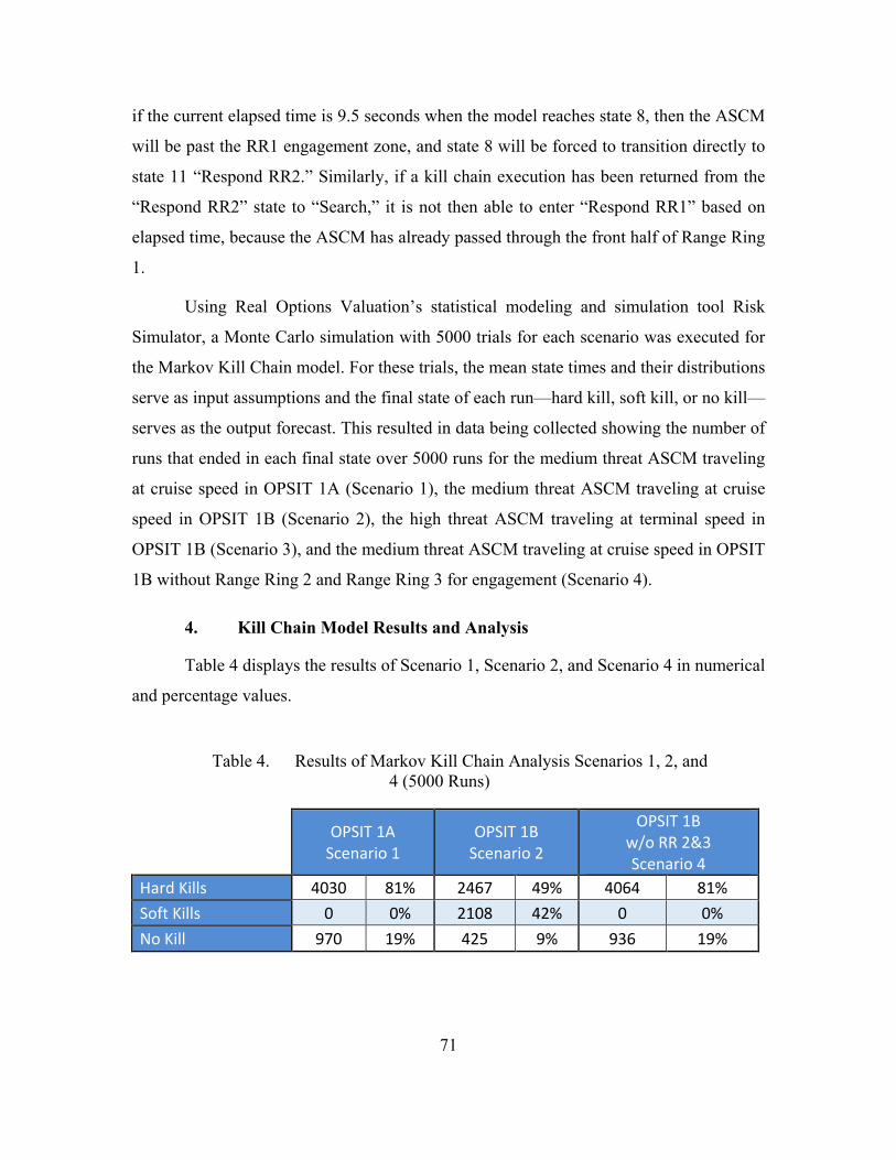
71
if the current elapsed time is 9.5 seconds when the model reaches state 8, then the ASCM
will be past the RR1 engagement zone, and state 8 will be forced to transition directly to
state 11 “Respond RR2.” Similarly, if a kill chain execution has been returned from the
“Respond RR2” state to “Search,” it is not then able to enter “Respond RR1” based on
elapsed time, because the ASCM has already passed through the front half of Range Ring
1.
Using Real Options Valuation’s statistical modeling and simulation tool Risk
Simulator, a Monte Carlo simulation with 5000 trials for each scenario was executed for
the Markov Kill Chain model. For these trials, the mean state times and their distributions
serve as input assumptions and the final state of each run—hard kill, soft kill, or no kill—
serves as the output forecast. This resulted in data being collected showing the number of
runs that ended in each final state over 5000 runs for the medium threat ASCM traveling
at cruise speed in OPSIT 1A (Scenario 1), the medium threat ASCM traveling at cruise
speed in OPSIT 1B (Scenario 2), the high threat ASCM traveling at terminal speed in
OPSIT 1B (Scenario 3), and the medium threat ASCM traveling at cruise speed in OPSIT
1B without Range Ring 2 and Range Ring 3 for engagement (Scenario 4).
4. Kill Chain Model Results and Analysis
Table 4 displays the results of Scenario 1, Scenario 2, and Scenario 4 in numerical
and percentage values.
Table 4. Results of Markov Kill Chain Analysis Scenarios 1, 2, and 4 (5000 Runs)
OPSIT 1A Scenario 1
OPSIT 1B Scenario 2
OPSIT 1B w/o RR 2&3 Scenario 4
Hard Kills 4030 81% 2467 49% 4064 81% Soft Kills 0 0% 2108 42% 0 0% No Kill 970 19% 425 9% 936 19%
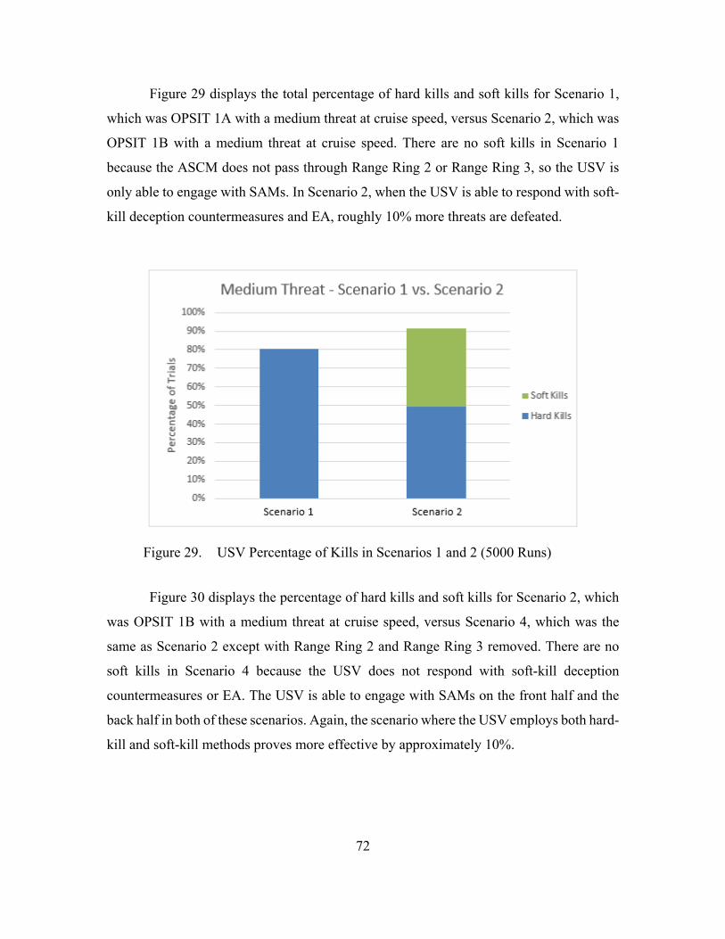
72
Figure 29 displays the total percentage of hard kills and soft kills for Scenario 1,
which was OPSIT 1A with a medium threat at cruise speed, versus Scenario 2, which was
OPSIT 1B with a medium threat at cruise speed. There are no soft kills in Scenario 1
because the ASCM does not pass through Range Ring 2 or Range Ring 3, so the USV is
only able to engage with SAMs. In Scenario 2, when the USV is able to respond with soft-
kill deception countermeasures and EA, roughly 10% more threats are defeated.
Figure 29. USV Percentage of Kills in Scenarios 1 and 2 (5000 Runs)
Figure 30 displays the percentage of hard kills and soft kills for Scenario 2, which
was OPSIT 1B with a medium threat at cruise speed, versus Scenario 4, which was the
same as Scenario 2 except with Range Ring 2 and Range Ring 3 removed. There are no
soft kills in Scenario 4 because the USV does not respond with soft-kill deception
countermeasures or EA. The USV is able to engage with SAMs on the front half and the
back half in both of these scenarios. Again, the scenario where the USV employs both hard-
kill and soft-kill methods proves more effective by approximately 10%.
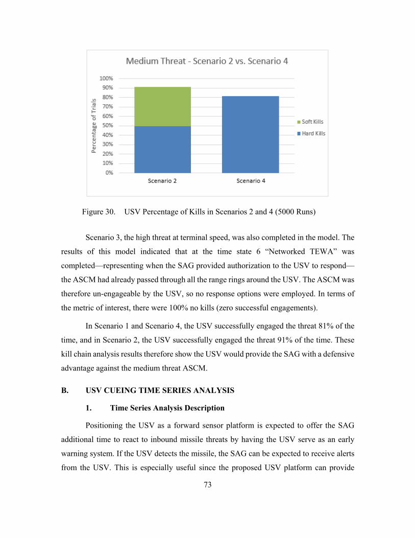
73
Figure 30. USV Percentage of Kills in Scenarios 2 and 4 (5000 Runs)
Scenario 3, the high threat at terminal speed, was also completed in the model. The
results of this model indicated that at the time state 6 “Networked TEWA” was
completed—representing when the SAG provided authorization to the USV to respond—
the ASCM had already passed through all the range rings around the USV. The ASCM was
therefore un-engageable by the USV, so no response options were employed. In terms of
the metric of interest, there were 100% no kills (zero successful engagements).
In Scenario 1 and Scenario 4, the USV successfully engaged the threat 81% of the
time, and in Scenario 2, the USV successfully engaged the threat 91% of the time. These
kill chain analysis results therefore show the USV would provide the SAG with a defensive
advantage against the medium threat ASCM.
B. USV CUEING TIME SERIES ANALYSIS
1. Time Series Analysis Description
Positioning the USV as a forward sensor platform is expected to offer the SAG
additional time to react to inbound missile threats by having the USV serve as an early
warning system. If the USV detects the missile, the SAG can be expected to receive alerts
from the USV. This is especially useful since the proposed USV platform can provide
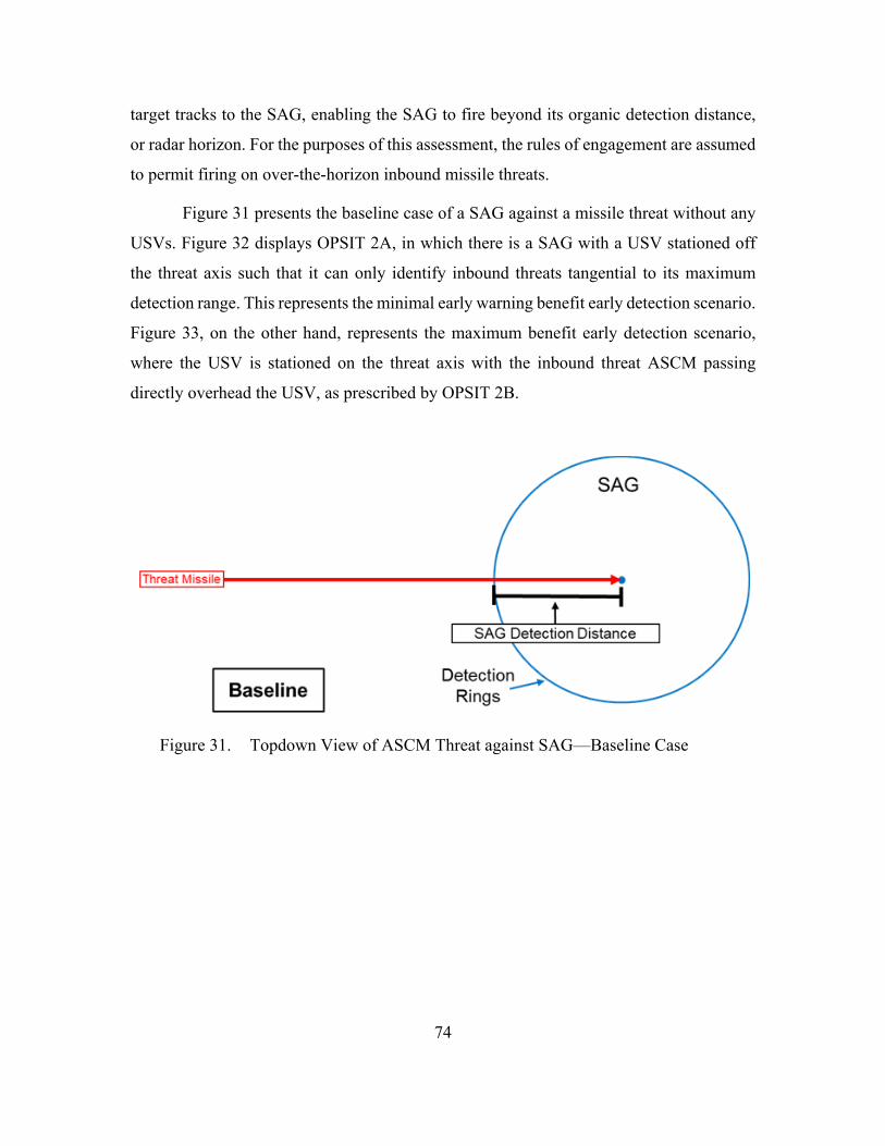
74
target tracks to the SAG, enabling the SAG to fire beyond its organic detection distance,
or radar horizon. For the purposes of this assessment, the rules of engagement are assumed
to permit firing on over-the-horizon inbound missile threats.
Figure 31 presents the baseline case of a SAG against a missile threat without any
USVs. Figure 32 displays OPSIT 2A, in which there is a SAG with a USV stationed off
the threat axis such that it can only identify inbound threats tangential to its maximum
detection range. This represents the minimal early warning benefit early detection scenario.
Figure 33, on the other hand, represents the maximum benefit early detection scenario,
where the USV is stationed on the threat axis with the inbound threat ASCM passing
directly overhead the USV, as prescribed by OPSIT 2B.
Figure 31. Topdown View of ASCM Threat against SAG—Baseline Case
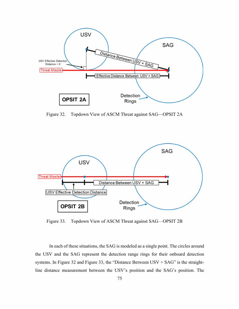
75
Figure 32. Topdown View of ASCM Threat against SAG—OPSIT 2A
Figure 33. Topdown View of ASCM Threat against SAG—OPSIT 2B
In each of these situations, the SAG is modeled as a single point. The circles around
the USV and the SAG represent the detection range rings for their onboard detection
systems. In Figure 32 and Figure 33, the “Distance Between USV + SAG” is the straight-
line distance measurement between the USV’s position and the SAG’s position. The
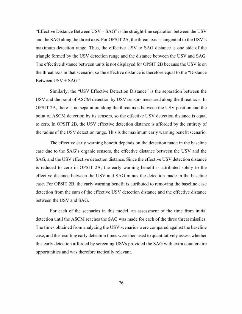
76
“Effective Distance Between USV + SAG” is the straight-line separation between the USV
and the SAG along the threat axis. For OPSIT 2A, the threat axis is tangential to the USV’s
maximum detection range. Thus, the effective USV to SAG distance is one side of the
triangle formed by the USV detection range and the distance between the USV and SAG.
The effective distance between units is not displayed for OPSIT 2B because the USV is on
the threat axis in that scenario, so the effective distance is therefore equal to the “Distance
Between USV + SAG”.
Similarly, the “USV Effective Detection Distance” is the separation between the
USV and the point of ASCM detection by USV sensors measured along the threat axis. In
OPSIT 2A, there is no separation along the threat axis between the USV position and the
point of ASCM detection by its sensors, so the effective USV detection distance is equal
to zero. In OPSIT 2B, the USV effective detection distance is afforded by the entirety of
the radius of the USV detection range. This is the maximum early warning benefit scenario.
The effective early warning benefit depends on the detection made in the baseline
case due to the SAG’s organic sensors, the effective distance between the USV and the
SAG, and the USV effective detection distance. Since the effective USV detection distance
is reduced to zero in OPSIT 2A, the early warning benefit is attributed solely to the
effective distance between the USV and SAG minus the detection made in the baseline
case. For OPSIT 2B, the early warning benefit is attributed to removing the baseline case
detection from the sum of the effective USV detection distance and the effective distance
between the USV and SAG.
For each of the scenarios in this model, an assessment of the time from initial
detection until the ASCM reaches the SAG was made for each of the three threat missiles.
The times obtained from analyzing the USV scenarios were compared against the baseline
case, and the resulting early detection times were then used to quantitatively assess whether
this early detection afforded by screening USVs provided the SAG with extra counter-fire
opportunities and was therefore tactically relevant.
77
2. Time Series Analysis Inputs
To begin the assessment, assumptions were made consistent with performance
information for the threat missiles. Missile flight profile altitudes of 20 meters for cruise
and five meters for terminal were based on data common to all three missiles (Jane’s by
IHS Markit 2018a, 2018c, 2018d, 2018e, 2018f, 2018h). Information about cruise to
terminal transition standoff distances from their targets as well as information regarding
presence of terminal pop-up maneuvers could not be identified in the unclassified research.
The cruise to terminal mode transition standoff distance assumptions were therefore made
based on educated guess, and threat ASCMs were treated as targets proceeding straight
inbound at terminal altitude (five meters) and speed with no additional pop-up or zig-zag
maneuvers. For each missile, the transition from cruise to terminal mode is treated as an
instantaneous event.
The following list summarizes these assumptions:
1. Each missile operates in a sea-skimming mode following transition to
cruise.
2. The cruise altitude of each sea-skimming missile is 20 meters (Jane’s by
IHS Markit 2018a, 2018c, 2018d, 2018e, 2018f, 2018h).
3. The terminal altitude of each sea-skimming missile is five meters (Jane’s
by IHS Markit 2018a, 2018c, 2018d, 2018e, 2018f, 2018h).
4. The low-missile threat, C-704, and the medium missile threat, CSS-N-8
Saccade, maintain their cruise speeds—Mach 0.875 and Mach 0.9,
respectively (Jane’s by IHS Markit 2018c, 2018d, 2018f, 2018h).
5. The high missile threat, SS-N-27 Sizzler, has a terminal supersonic speed
of Mach 2.9 (Jane’s by IHS Markit 2018a).
6. The low and medium threats have an assumed transition from cruise to
terminal modes 10 nautical miles (18.52 kilometers) from their target.
78
7. The high missile threat has an assumed transition from cruise to terminal
modes 20 nautical miles (37.04 kilometers) from its target.
Given the cruise and terminal altitudes of the threat missile sea-skimming profiles,
the USV and SAG detection distances could be derived from Equation 1, the simplified
radar horizon equation against a target at elevation in metric units. Utilizing the earlier
assumption that the USV radar height is 12 meters and given the threat missile profile
altitudes of 20 meters cruise altitude and five meters terminal altitude (Jane’s by IHS
Markit 2018a, 2018c, 2018d, 2018e, 2018f, 2018h), the resultant USV maximum detection
range is 33 kilometers for missiles in cruise mode and 24 kilometers for missiles in terminal
mode. Threat missile cruise and terminal profile altitudes were treated as constants in this
analysis, and USV radar height will be further explored.
Assumptions were made about the probability of the SAG and USV detecting
ASCMs at these maximum detection ranges based upon Smith’s 2010 thesis “Using Kill-
Chain Analysis to Develop Surface Ship CONOPs To Defend Against Anti-Ship Cruise
Missiles.” In his analysis, Smith evaluated characteristics of 19 missiles and determined
the probability for the targeted ship to detect the ASCM was greater than 0.995 at the radar
range horizon (2010). Further, 16 of his 19 missiles had at least a 0.999 probability of
detection (Smith 2010). Based on these findings, this time series analysis model assumes
a 100% probability of detection at the maximum detection distances for simplicity.
To implement the model, the following input variables were identified:
1. Blue Forces: Distance between USV and SAG
2. Blue Forces: USV Antenna Height
3. Blue Forces: SAG Antenna Height
The following inputs were also identified but set as constants in this analysis:
1. Red Forces: Low Missile Threat (C-704) Cruise to Terminal Distance
from Target
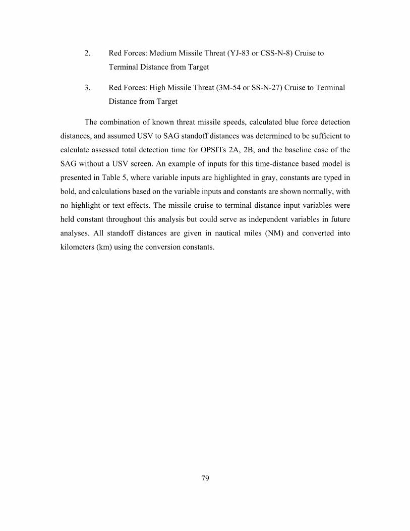
79
2. Red Forces: Medium Missile Threat (YJ-83 or CSS-N-8) Cruise to
Terminal Distance from Target
3. Red Forces: High Missile Threat (3M-54 or SS-N-27) Cruise to Terminal
Distance from Target
The combination of known threat missile speeds, calculated blue force detection
distances, and assumed USV to SAG standoff distances was determined to be sufficient to
calculate assessed total detection time for OPSITs 2A, 2B, and the baseline case of the
SAG without a USV screen. An example of inputs for this time-distance based model is
presented in Table 5, where variable inputs are highlighted in gray, constants are typed in
bold, and calculations based on the variable inputs and constants are shown normally, with
no highlight or text effects. The missile cruise to terminal distance input variables were
held constant throughout this analysis but could serve as independent variables in future
analyses. All standoff distances are given in nautical miles (NM) and converted into
kilometers (km) using the conversion constants.
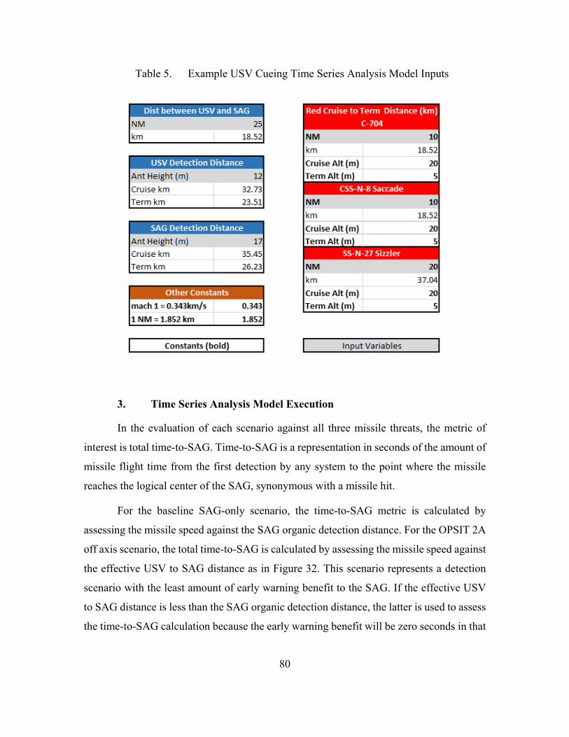
80
Table 5. Example USV Cueing Time Series Analysis Model Inputs
3. Time Series Analysis Model Execution
In the evaluation of each scenario against all three missile threats, the metric of
interest is total time-to-SAG. Time-to-SAG is a representation in seconds of the amount of
missile flight time from the first detection by any system to the point where the missile
reaches the logical center of the SAG, synonymous with a missile hit.
For the baseline SAG-only scenario, the time-to-SAG metric is calculated by
assessing the missile speed against the SAG organic detection distance. For the OPSIT 2A
off axis scenario, the total time-to-SAG is calculated by assessing the missile speed against
the effective USV to SAG distance as in Figure 32. This scenario represents a detection
scenario with the least amount of early warning benefit to the SAG. If the effective USV
to SAG distance is less than the SAG organic detection distance, the latter is used to assess
the time-to-SAG calculation because the early warning benefit will be zero seconds in that
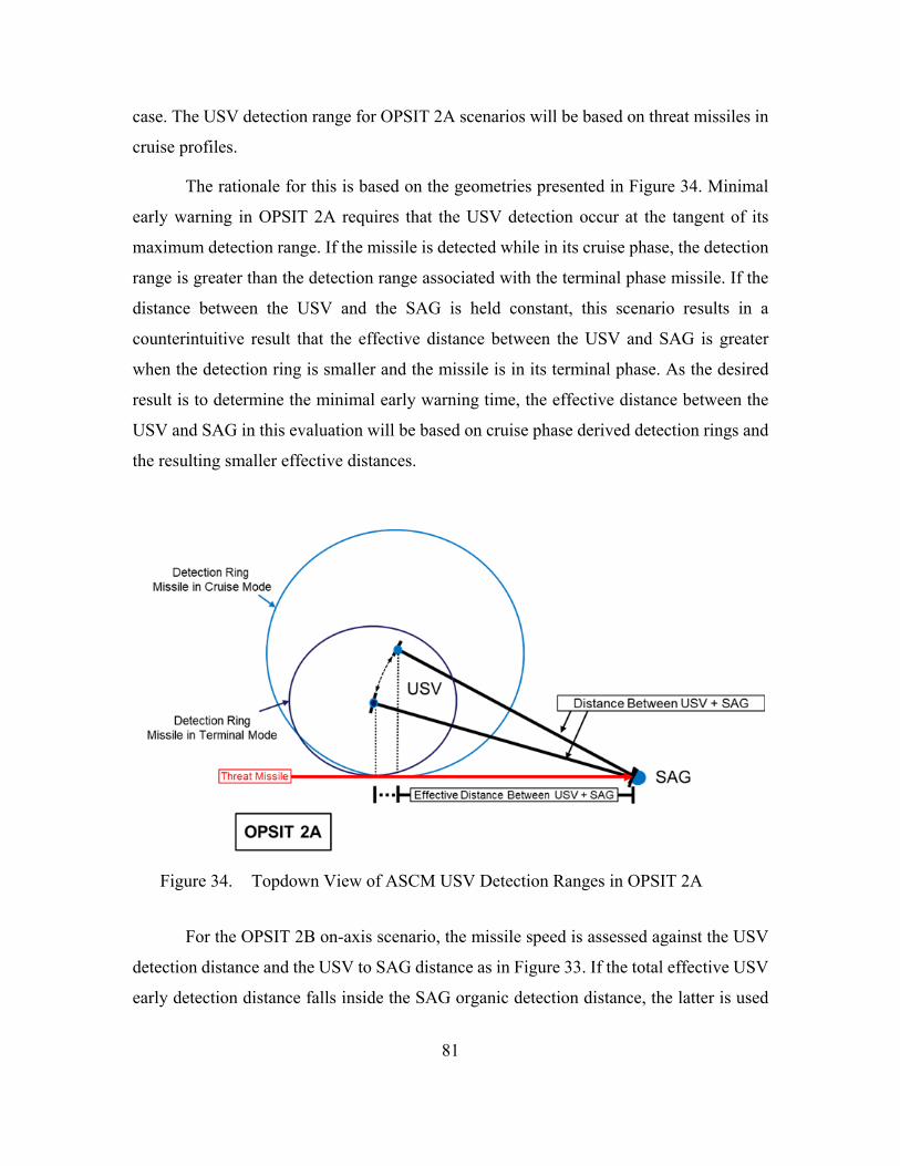
81
case. The USV detection range for OPSIT 2A scenarios will be based on threat missiles in
cruise profiles.
The rationale for this is based on the geometries presented in Figure 34. Minimal
early warning in OPSIT 2A requires that the USV detection occur at the tangent of its
maximum detection range. If the missile is detected while in its cruise phase, the detection
range is greater than the detection range associated with the terminal phase missile. If the
distance between the USV and the SAG is held constant, this scenario results in a
counterintuitive result that the effective distance between the USV and SAG is greater
when the detection ring is smaller and the missile is in its terminal phase. As the desired
result is to determine the minimal early warning time, the effective distance between the
USV and SAG in this evaluation will be based on cruise phase derived detection rings and
the resulting smaller effective distances.
Figure 34. Topdown View of ASCM USV Detection Ranges in OPSIT 2A
For the OPSIT 2B on-axis scenario, the missile speed is assessed against the USV
detection distance and the USV to SAG distance as in Figure 33. If the total effective USV
early detection distance falls inside the SAG organic detection distance, the latter is used
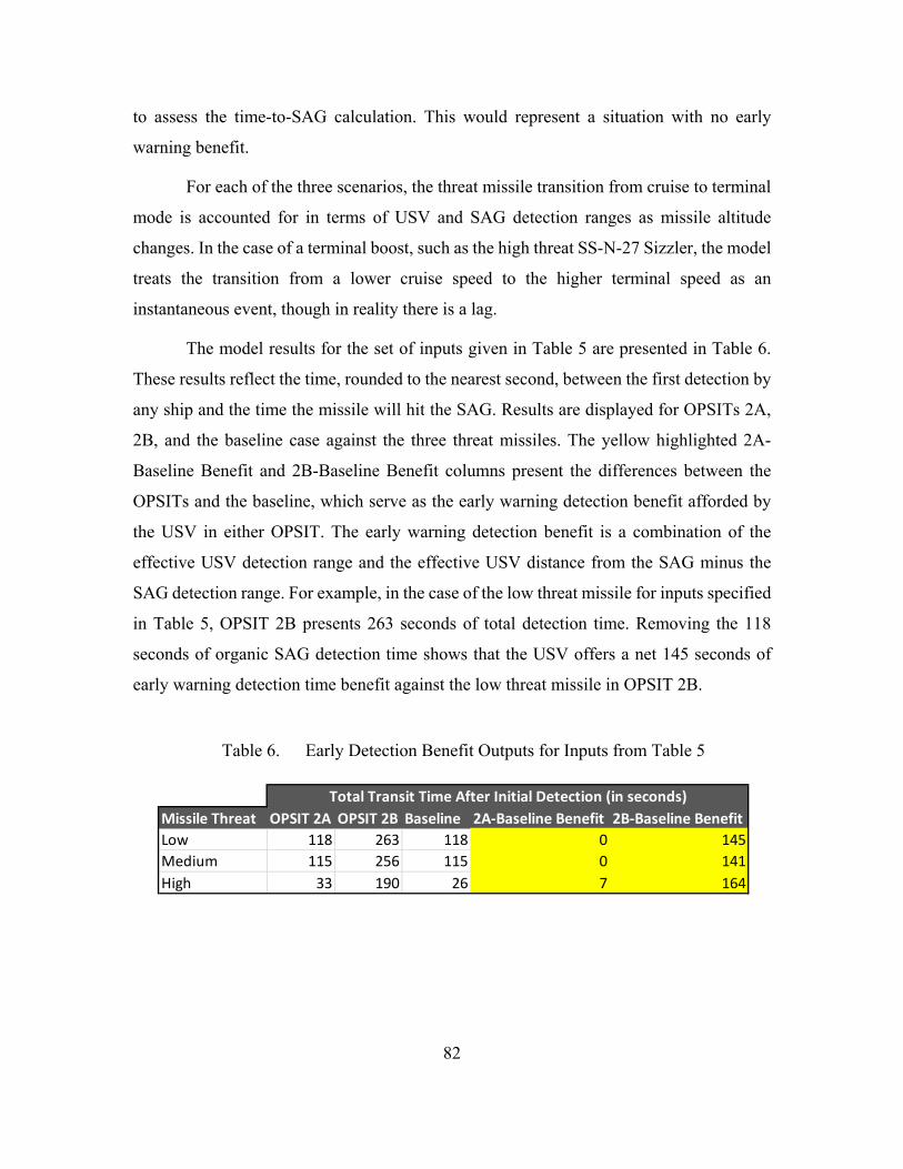
82
to assess the time-to-SAG calculation. This would represent a situation with no early
warning benefit.
For each of the three scenarios, the threat missile transition from cruise to terminal
mode is accounted for in terms of USV and SAG detection ranges as missile altitude
changes. In the case of a terminal boost, such as the high threat SS-N-27 Sizzler, the model
treats the transition from a lower cruise speed to the higher terminal speed as an
instantaneous event, though in reality there is a lag.
The model results for the set of inputs given in Table 5 are presented in Table 6.
These results reflect the time, rounded to the nearest second, between the first detection by
any ship and the time the missile will hit the SAG. Results are displayed for OPSITs 2A,
2B, and the baseline case against the three threat missiles. The yellow highlighted 2A-
Baseline Benefit and 2B-Baseline Benefit columns present the differences between the
OPSITs and the baseline, which serve as the early warning detection benefit afforded by
the USV in either OPSIT. The early warning detection benefit is a combination of the
effective USV detection range and the effective USV distance from the SAG minus the
SAG detection range. For example, in the case of the low threat missile for inputs specified
in Table 5, OPSIT 2B presents 263 seconds of total detection time. Removing the 118
seconds of organic SAG detection time shows that the USV offers a net 145 seconds of
early warning detection time benefit against the low threat missile in OPSIT 2B.
Table 6. Early Detection Benefit Outputs for Inputs from Table 5
Missile Threat OPSIT 2A OPSIT 2B Baseline 2A-Baseline Benefit 2B-Baseline BenefitLow 118 263 118 0 145Medium 115 256 115 0 141High 33 190 26 7 164
Total Transit Time After Initial Detection (in seconds)
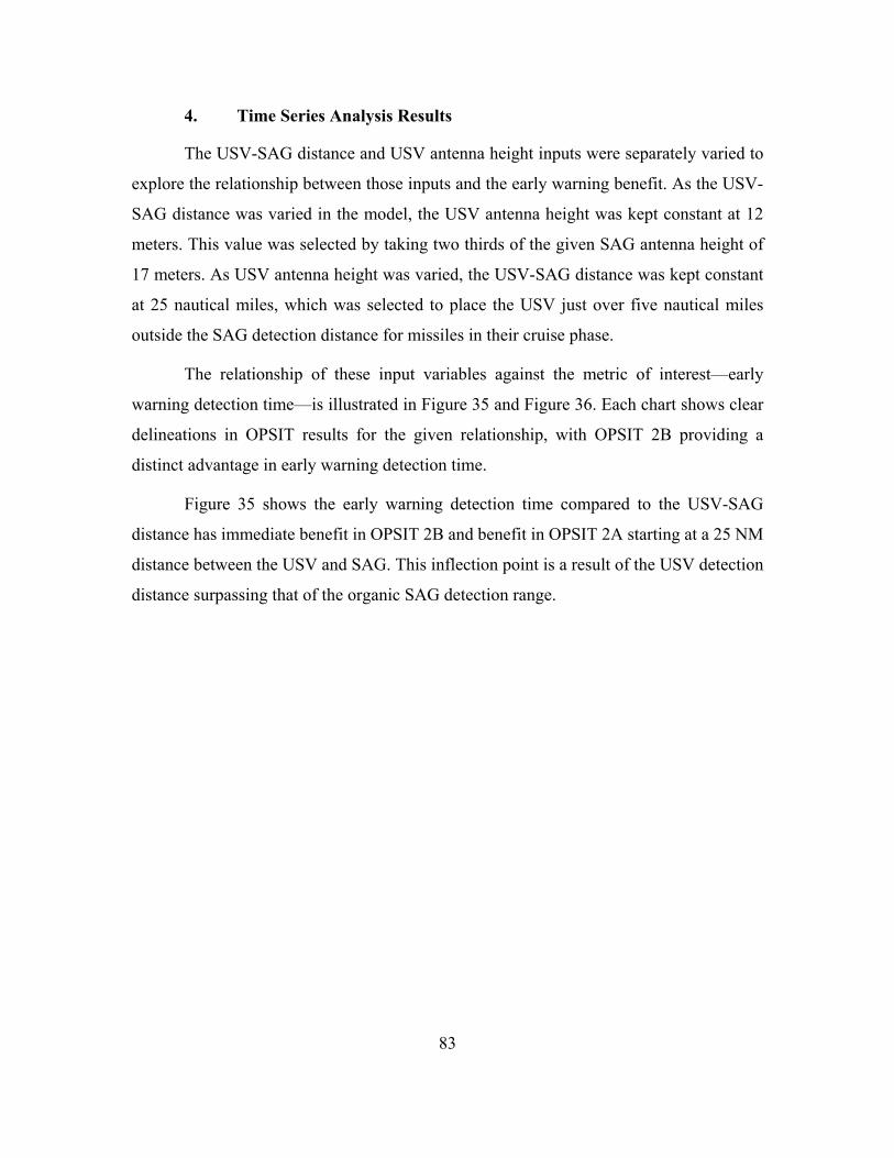
83
4. Time Series Analysis Results
The USV-SAG distance and USV antenna height inputs were separately varied to
explore the relationship between those inputs and the early warning benefit. As the USV-
SAG distance was varied in the model, the USV antenna height was kept constant at 12
meters. This value was selected by taking two thirds of the given SAG antenna height of
17 meters. As USV antenna height was varied, the USV-SAG distance was kept constant
at 25 nautical miles, which was selected to place the USV just over five nautical miles
outside the SAG detection distance for missiles in their cruise phase.
The relationship of these input variables against the metric of interest—early
warning detection time—is illustrated in Figure 35 and Figure 36. Each chart shows clear
delineations in OPSIT results for the given relationship, with OPSIT 2B providing a
distinct advantage in early warning detection time.
Figure 35 shows the early warning detection time compared to the USV-SAG
distance has immediate benefit in OPSIT 2B and benefit in OPSIT 2A starting at a 25 NM
distance between the USV and SAG. This inflection point is a result of the USV detection
distance surpassing that of the organic SAG detection range.
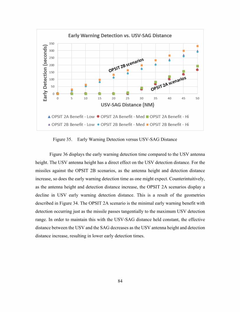
84
Figure 35. Early Warning Detection versus USV-SAG Distance
Figure 36 displays the early warning detection time compared to the USV antenna
height. The USV antenna height has a direct effect on the USV detection distance. For the
missiles against the OPSIT 2B scenarios, as the antenna height and detection distance
increase, so does the early warning detection time as one might expect. Counterintuitively,
as the antenna height and detection distance increase, the OPSIT 2A scenarios display a
decline in USV early warning detection distance. This is a result of the geometries
described in Figure 34. The OPSIT 2A scenario is the minimal early warning benefit with
detection occurring just as the missile passes tangentially to the maximum USV detection
range. In order to maintain this with the USV-SAG distance held constant, the effective
distance between the USV and the SAG decreases as the USV antenna height and detection
distance increase, resulting in lower early detection times.

85
Figure 36. Early Warning Detection versus USV Antenna Height
From the analysis described, it can be concluded that a forward-positioned USV
can provide the SAG an increased reaction time to respond to the missiles. To better
quantify the above findings and determine if this increased reaction time is tactically
relevant to the SAG, Smith’s (2010) methodology was again leveraged.
In his work, Smith describes 19 different missiles of varying capabilities and their
assessed effectiveness against a notional surface ship equipped with long-range and short-
range SAMs and a CIWS (Smith 2010). Of particular interest to this study is Smith’s
timeline analysis of counter-fire shot opportunities from the ship against the threat missiles
in his “Table 4. Line diagram range results” (Smith 2010, 28). An adapted version of this
table is presented in Table 7. In this table, columns R1 through R8 represent counter-fire
opportunities from a SAM launching unit. The data inside column R1 represents the
intercept range in kilometers for the first SAM launched against the threat missile. R2 is
the intercept range for the second, and so on. Some shot opportunities, however, will not
be viable due to the threat missile being beyond the radar horizon range. These are shaded
in gray. For example, against the CSS-N-8 Saccade, the platform has seven columns
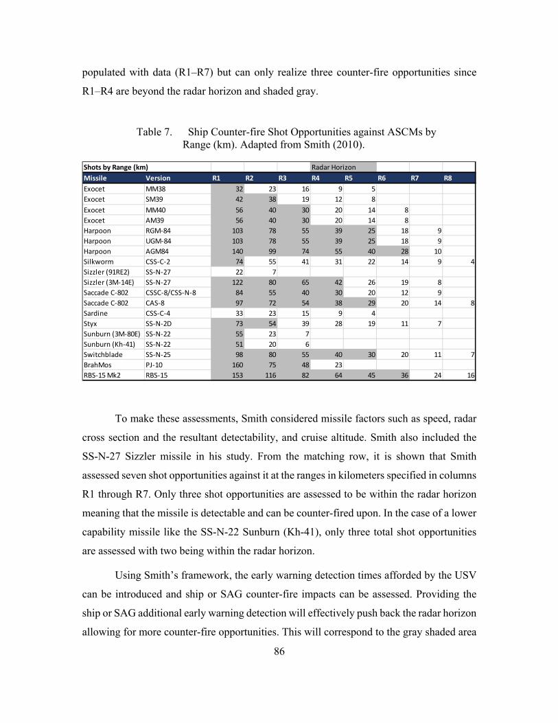
86
populated with data (R1–R7) but can only realize three counter-fire opportunities since
R1–R4 are beyond the radar horizon and shaded gray.
Table 7. Ship Counter-fire Shot Opportunities against ASCMs by Range (km). Adapted from Smith (2010).
To make these assessments, Smith considered missile factors such as speed, radar
cross section and the resultant detectability, and cruise altitude. Smith also included the
SS-N-27 Sizzler missile in his study. From the matching row, it is shown that Smith
assessed seven shot opportunities against it at the ranges in kilometers specified in columns
R1 through R7. Only three shot opportunities are assessed to be within the radar horizon
meaning that the missile is detectable and can be counter-fired upon. In the case of a lower
capability missile like the SS-N-22 Sunburn (Kh-41), only three total shot opportunities
are assessed with two being within the radar horizon.
Using Smith’s framework, the early warning detection times afforded by the USV
can be introduced and ship or SAG counter-fire impacts can be assessed. Providing the
ship or SAG additional early warning detection will effectively push back the radar horizon
allowing for more counter-fire opportunities. This will correspond to the gray shaded area
Shots by Range (km)Missile Version R1 R2 R3 R4 R5 R6 R7 R8Exocet MM38 32 23 16 9 5Exocet SM39 42 38 19 12 8Exocet MM40 56 40 30 20 14 8Exocet AM39 56 40 30 20 14 8Harpoon RGM‐84 103 78 55 39 25 18 9Harpoon UGM‐84 103 78 55 39 25 18 9Harpoon AGM84 140 99 74 55 40 28 10Silkworm CSS‐C‐2 74 55 41 31 22 14 9 4Sizzler (91RE2) SS‐N‐27 22 7Sizzler (3M‐14E) SS‐N‐27 122 80 65 42 26 19 8Saccade C‐802 CSSC‐8/CSS‐N‐8 84 55 40 30 20 12 9Saccade C‐802 CAS‐8 97 72 54 38 29 20 14 8Sardine CSS‐C‐4 33 23 15 9 4Styx SS‐N‐2D 73 54 39 28 19 11 7Sunburn (3M‐80E) SS‐N‐22 55 23 7Sunburn (Kh‐41) SS‐N‐22 51 20 6Switchblade SS‐N‐25 98 80 55 40 30 20 11 7BrahMos PJ‐10 160 75 48 23RBS‐15 Mk2 RBS‐15 153 116 82 64 45 36 24 16
Radar Horizon
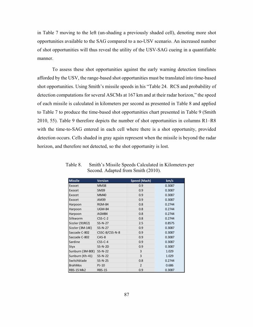
87
in Table 7 moving to the left (un-shading a previously shaded cell), denoting more shot
opportunities available to the SAG compared to a no-USV scenario. An increased number
of shot opportunities will thus reveal the utility of the USV-SAG cueing in a quantifiable
manner.
To assess these shot opportunities against the early warning detection timelines
afforded by the USV, the range-based shot opportunities must be translated into time-based
shot opportunities. Using Smith’s missile speeds in his “Table 24. RCS and probability of
detection computations for several ASCMs at 167 km and at their radar horizon,” the speed
of each missile is calculated in kilometers per second as presented in Table 8 and applied
to Table 7 to produce the time-based shot opportunities chart presented in Table 9 (Smith
2010, 55). Table 9 therefore depicts the number of shot opportunities in columns R1–R8
with the time-to-SAG entered in each cell where there is a shot opportunity, provided
detection occurs. Cells shaded in gray again represent when the missile is beyond the radar
horizon, and therefore not detected, so the shot opportunity is lost.
Table 8. Smith’s Missile Speeds Calculated in Kilometers per Second. Adapted from Smith (2010).
Missile Version Speed (Mach) km/sExocet MM38 0.9 0.3087Exocet SM39 0.9 0.3087Exocet MM40 0.9 0.3087Exocet AM39 0.9 0.3087Harpoon RGM‐84 0.8 0.2744Harpoon UGM‐84 0.8 0.2744Harpoon AGM84 0.8 0.2744Silkworm CSS‐C‐2 0.8 0.2744Sizzler (91RE2) SS‐N‐27 2.5 0.8575Sizzler (3M‐14E) SS‐N‐27 0.9 0.3087Saccade C‐802 CSSC‐8/CSS‐N‐8 0.9 0.3087Saccade C‐802 CAS‐8 0.9 0.3087Sardine CSS‐C‐4 0.9 0.3087Styx SS‐N‐2D 0.9 0.3087Sunburn (3M‐80E) SS‐N‐22 3 1.029Sunburn (Kh‐41) SS‐N‐22 3 1.029Switchblade SS‐N‐25 0.8 0.2744BrahMos PJ‐10 2 0.686RBS‐15 Mk2 RBS‐15 0.9 0.3087
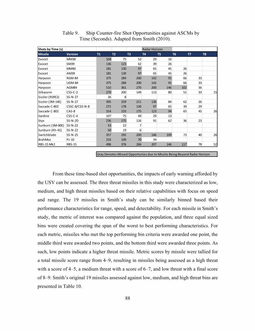
88
Table 9. Ship Counter-fire Shot Opportunities against ASCMs by Time (Seconds). Adapted from Smith (2010).
From these time-based shot opportunities, the impacts of early warning afforded by
the USV can be assessed. The three threat missiles in this study were characterized as low,
medium, and high threat missiles based on their relative capabilities with focus on speed
and range. The 19 missiles in Smith’s study can be similarly binned based their
performance characteristics for range, speed, and detectability. For each missile in Smith’s
study, the metric of interest was compared against the population, and three equal sized
bins were created covering the span of the worst to best performing characteristics. For
each metric, missiles who met the top performing bin criteria were awarded one point, the
middle third were awarded two points, and the bottom third were awarded three points. As
such, low points indicate a higher threat missile. Metric scores by missile were tallied for
a total missile score range from 4–9, resulting in missiles being assessed as a high threat
with a score of 4–5, a medium threat with a score of 6–7, and low threat with a final score
of 8–9. Smith’s original 19 missiles assessed against low, medium, and high threat bins are
presented in Table 10.
Shots by Time (s)Missile Version T1 T2 T3 T4 T5 T6 T7 T8Exocet MM38 104 75 52 29 16Exocet SM39 136 123 62 39 26Exocet MM40 181 130 97 65 45 26Exocet AM39 181 130 97 65 45 26Harpoon RGM‐84 375 284 200 142 91 66 33Harpoon UGM‐84 375 284 200 142 91 66 33Harpoon AGM84 510 361 270 200 146 102 36Silkworm CSS‐C‐2 270 200 149 113 80 51 33 15Sizzler (91RE2) SS‐N‐27 26 8Sizzler (3M‐14E) SS‐N‐27 395 259 211 136 84 62 26Saccade C‐802 CSSC‐8/CSS‐N‐8 272 178 130 97 65 39 29Saccade C‐802 CAS‐8 314 233 175 123 94 65 45 26Sardine CSS‐C‐4 107 75 49 29 13Styx SS‐N‐2D 236 175 126 91 62 36 23Sunburn (3M‐80E) SS‐N‐22 53 22 7Sunburn (Kh‐41) SS‐N‐22 50 19 6Switchblade SS‐N‐25 357 292 200 146 109 73 40 26BrahMos PJ‐10 233 109 70 34RBS‐15 Mk2 RBS‐15 496 376 266 207 146 117 78 52
Gray Denotes Missed Opportunies due to Missile Being Beyond Radar Horizon
Radar Horizon
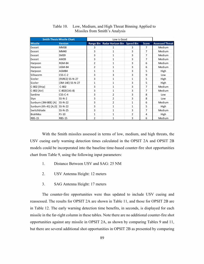
89
Table 10. Low, Medium, and High Threat Binning Applied to Missiles from Smith’s Analysis
With the Smith missiles assessed in terms of low, medium, and high threats, the
USV cueing early warning detection times calculated in the OPSIT 2A and OPSIT 2B
models could be incorporated into the baseline time-based counter-fire shot opportunities
chart from Table 9, using the following input parameters:
1. Distance Between USV and SAG: 25 NM
2. USV Antenna Height: 12 meters
3. SAG Antenna Height: 17 meters
The counter-fire opportunities were thus updated to include USV cueing and
reassessed. The results for OPSIT 2A are shown in Table 11, and those for OPSIT 2B are
in Table 12. The early warning detection time benefits, in seconds, is displayed for each
missile in the far-right column in these tables. Note there are no additional counter-fire shot
opportunities against any missile in OPSIT 2A, as shown by comparing Tables 9 and 11,
but there are several additional shot opportunities in OPSIT 2B as presented by comparing
Missile Version Range Bin Radar Horizon Bin Speed Bin Score Assessed ThreatExocet MM38 3 1 3 7 MediumExocet MM40 3 1 3 7 MediumExocet SM39 3 1 3 7 MediumExocet AM39 3 1 3 7 MediumHarpoon RGM‐84 2 1 3 6 MediumHarpoon UGM‐84 2 1 3 6 MediumHarpoon AGM84 1 1 3 5 HighSilkworm CSS‐C‐2 3 3 3 9 LowSizzler (91RE2) SS‐N‐27 3 1 1 5 HighSizzler (3M‐14E) SS‐N‐27 1 1 3 5 HighC‐802 [Ship] C‐802 3 1 3 7 MediumC‐802 [Air] C‐802(CAS‐8) 3 1 3 7 MediumSardine CSS‐C‐4 3 2 3 8 LowStyx SS‐N‐2 3 2 3 8 LowSunburn (3M‐80E) [A] SS‐N‐22 3 2 1 6 MediumSunburn (Kh‐41) [A,D] SS‐N‐22 3 1 1 5 HighSwitchblade SS‐N‐25 3 1 3 7 MediumBrahMos PJ‐10 1 1 2 4 HighRBS‐15 RBS‐15 2 1 3 6 Medium
Smith Thesis Missile Chart Low is Good

90
Tables 9 and 12. This is most easily observed by the reduced number of gray shaded boxes
indicating that fewer shot opportunities are beyond the radar horizon, and additional
counter-fire opportunities are therefore available.
Table 11. Ship Counter-fire Shot Opportunities by Time against ASCMs with OPSIT 2A Benefits Considered (USV-SAG Distance = 25
NM)
OPSIT 2A (all value are in seconds)Missile Version T1 T2 T3 T4 T5 T6 T7 T8 From Missile Info Tab 2A Benefit (s)Exocet MM38 104 75 52 29 16 Medium 0Exocet SM39 136 123 62 39 26 Medium 0Exocet MM40 181 130 97 65 45 26 Medium 0Exocet AM39 181 130 97 65 45 26 Medium 0Harpoon RGM‐84 375 284 200 142 91 66 33 Medium 0Harpoon UGM‐84 375 284 200 142 91 66 33 Medium 0Harpoon AGM84 510 361 270 200 146 102 36 High 7Silkworm CSS‐C‐2 270 200 149 113 80 51 33 15 Low 0Sizzler (91RE2) SS‐N‐27 26 8 High 7Sizzler (3M‐14E) SS‐N‐27 395 259 211 136 84 62 26 High 7Saccade C‐802 CSSC‐8/CSS‐N‐8 272 178 130 97 65 39 29 Medium 0Saccade C‐802 CAS‐8 314 233 175 123 94 65 45 26 Medium 0Sardine CSS‐C‐4 107 75 49 29 13 Low 0Styx SS‐N‐2D 236 175 126 91 62 36 23 Low 0Sunburn (3M‐80E) SS‐N‐22 53 22 7 Medium 0Sunburn (Kh‐41) SS‐N‐22 50 19 6 High 7Switchblade SS‐N‐25 357 292 200 146 109 73 40 26 Medium 0BrahMos PJ‐10 233 109 70 34 High 7RBS‐15 Mk2 RBS‐15 496 376 266 207 146 117 78 52 Medium 0
Gray Denotes Missed Opportunies due to Missile Being Beyond Radar Horizon
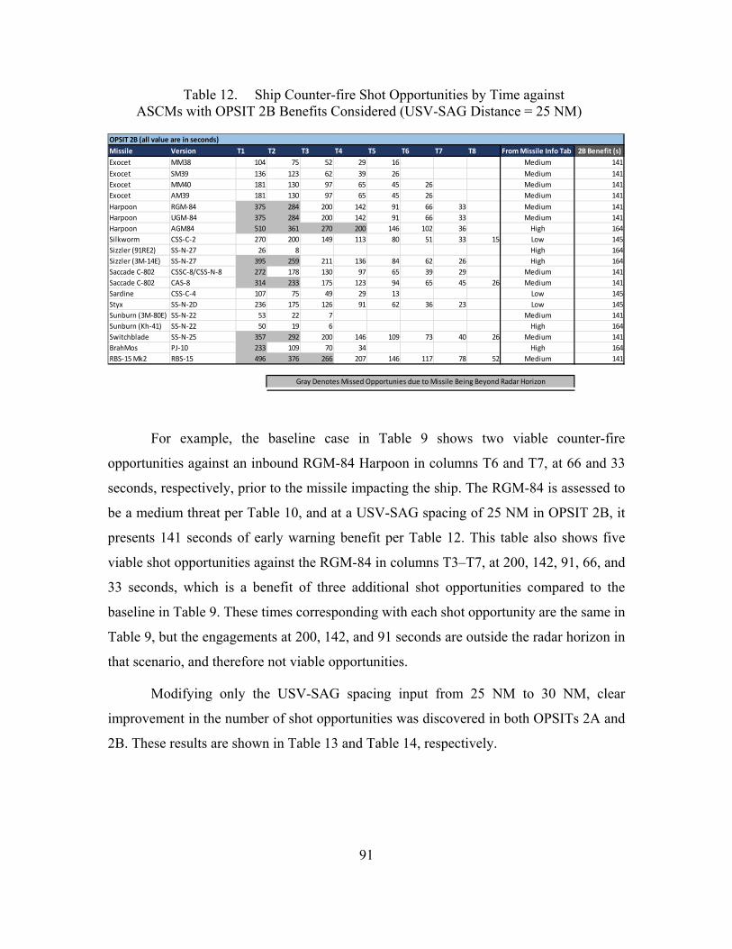
91
Table 12. Ship Counter-fire Shot Opportunities by Time against ASCMs with OPSIT 2B Benefits Considered (USV-SAG Distance = 25 NM)
For example, the baseline case in Table 9 shows two viable counter-fire
opportunities against an inbound RGM-84 Harpoon in columns T6 and T7, at 66 and 33
seconds, respectively, prior to the missile impacting the ship. The RGM-84 is assessed to
be a medium threat per Table 10, and at a USV-SAG spacing of 25 NM in OPSIT 2B, it
presents 141 seconds of early warning benefit per Table 12. This table also shows five
viable shot opportunities against the RGM-84 in columns T3–T7, at 200, 142, 91, 66, and
33 seconds, which is a benefit of three additional shot opportunities compared to the
baseline in Table 9. These times corresponding with each shot opportunity are the same in
Table 9, but the engagements at 200, 142, and 91 seconds are outside the radar horizon in
that scenario, and therefore not viable opportunities.
Modifying only the USV-SAG spacing input from 25 NM to 30 NM, clear
improvement in the number of shot opportunities was discovered in both OPSITs 2A and
2B. These results are shown in Table 13 and Table 14, respectively.
OPSIT 2B (all value are in seconds)Missile Version T1 T2 T3 T4 T5 T6 T7 T8 From Missile Info Tab 2B Benefit (s)Exocet MM38 104 75 52 29 16 Medium 141Exocet SM39 136 123 62 39 26 Medium 141Exocet MM40 181 130 97 65 45 26 Medium 141Exocet AM39 181 130 97 65 45 26 Medium 141Harpoon RGM‐84 375 284 200 142 91 66 33 Medium 141Harpoon UGM‐84 375 284 200 142 91 66 33 Medium 141Harpoon AGM84 510 361 270 200 146 102 36 High 164Silkworm CSS‐C‐2 270 200 149 113 80 51 33 15 Low 145Sizzler (91RE2) SS‐N‐27 26 8 High 164Sizzler (3M‐14E) SS‐N‐27 395 259 211 136 84 62 26 High 164Saccade C‐802 CSSC‐8/CSS‐N‐8 272 178 130 97 65 39 29 Medium 141Saccade C‐802 CAS‐8 314 233 175 123 94 65 45 26 Medium 141Sardine CSS‐C‐4 107 75 49 29 13 Low 145Styx SS‐N‐2D 236 175 126 91 62 36 23 Low 145Sunburn (3M‐80E) SS‐N‐22 53 22 7 Medium 141Sunburn (Kh‐41) SS‐N‐22 50 19 6 High 164Switchblade SS‐N‐25 357 292 200 146 109 73 40 26 Medium 141BrahMos PJ‐10 233 109 70 34 High 164RBS‐15 Mk2 RBS‐15 496 376 266 207 146 117 78 52 Medium 141
Gray Denotes Missed Opportunies due to Missile Being Beyond Radar Horizon

92
Table 13. Ship Counter-fire Shot Opportunities by Time against ASCMs with OPSIT 2A Benefits Considered (USV-SAG Distance = 30
NM)
Table 14. Ship Counter-fire Shot Opportunities by Time against ASCMs with OPSIT 2B Benefits Considered (USV-SAG Distance = 30 NM)
In Table 15, the number of total shot opportunities is displayed for each OPSIT
against USV-SAG ranges, assessed every five NM from 0–50 NM. This total is the
OPSIT 2B (all value are in seconds)Missile Version T1 T2 T3 T4 T5 T6 T7 T8 From Missile Info Tab 2B Benefit (s)Exocet MM38 104 75 52 29 16 Medium 171Exocet SM39 136 123 62 39 26 Medium 171Exocet MM40 181 130 97 65 45 26 Medium 171Exocet AM39 181 130 97 65 45 26 Medium 171Harpoon RGM‐84 375 284 200 142 91 66 33 Medium 171Harpoon UGM‐84 375 284 200 142 91 66 33 Medium 171Harpoon AGM84 510 361 270 200 146 102 36 High 198Silkworm CSS‐C‐2 270 200 149 113 80 51 33 15 Low 176Sizzler (91RE2) SS‐N‐27 26 8 High 198Sizzler (3M‐14E) SS‐N‐27 395 259 211 136 84 62 26 High 198Saccade C‐802 CSSC‐8/CSS‐N‐8 272 178 130 97 65 39 29 Medium 171Saccade C‐802 CAS‐8 314 233 175 123 94 65 45 26 Medium 171Sardine CSS‐C‐4 107 75 49 29 13 Low 176Styx SS‐N‐2D 236 175 126 91 62 36 23 Low 176Sunburn (3M‐80E) SS‐N‐22 53 22 7 Medium 171Sunburn (Kh‐41) SS‐N‐22 50 19 6 High 198Switchblade SS‐N‐25 357 292 200 146 109 73 40 26 Medium 171BrahMos PJ‐10 233 109 70 34 High 198RBS‐15 Mk2 RBS‐15 496 376 266 207 146 117 78 52 Medium 171
Gray Denotes Missed Opportunies due to Missile Being Beyond Radar Horizon
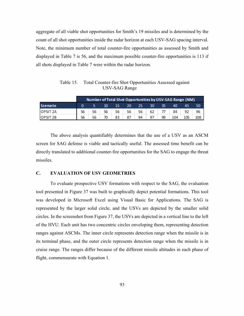
93
aggregate of all viable shot opportunities for Smith’s 19 missiles and is determined by the
count of all shot opportunities inside the radar horizon at each USV-SAG spacing interval.
Note, the minimum number of total counter-fire opportunities as assessed by Smith and
displayed in Table 7 is 56, and the maximum possible counter-fire opportunities is 113 if
all shots displayed in Table 7 were within the radar horizon.
Table 15. Total Counter-fire Shot Opportunities Assessed against USV-SAG Range
The above analysis quantifiably determines that the use of a USV as an ASCM
screen for SAG defense is viable and tactically useful. The assessed time benefit can be
directly translated to additional counter-fire opportunities for the SAG to engage the threat
missiles.
C. EVALUATION OF USV GEOMETRIES
To evaluate prospective USV formations with respect to the SAG, the evaluation
tool presented in Figure 37 was built to graphically depict potential formations. This tool
was developed in Microsoft Excel using Visual Basic for Applications. The SAG is
represented by the larger solid circle, and the USVs are depicted by the smaller solid
circles. In the screenshot from Figure 37, the USVs are depicted in a vertical line to the left
of the HVU. Each unit has two concentric circles enveloping them, representing detection
ranges against ASCMs. The inner circle represents detection range when the missile is in
its terminal phase, and the outer circle represents detection range when the missile is in
cruise range. The ranges differ because of the different missile altitudes in each phase of
flight, commensurate with Equation 1.
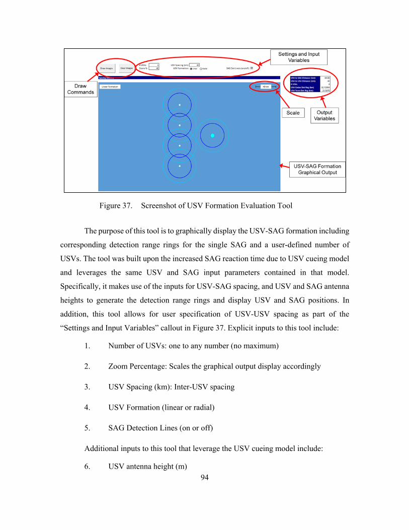
94
Figure 37. Screenshot of USV Formation Evaluation Tool
The purpose of this tool is to graphically display the USV-SAG formation including
corresponding detection range rings for the single SAG and a user-defined number of
USVs. The tool was built upon the increased SAG reaction time due to USV cueing model
and leverages the same USV and SAG input parameters contained in that model.
Specifically, it makes use of the inputs for USV-SAG spacing, and USV and SAG antenna
heights to generate the detection range rings and display USV and SAG positions. In
addition, this tool allows for user specification of USV-USV spacing as part of the
“Settings and Input Variables” callout in Figure 37. Explicit inputs to this tool include:
1. Number of USVs: one to any number (no maximum)
2. Zoom Percentage: Scales the graphical output display accordingly
3. USV Spacing (km): Inter-USV spacing
4. USV Formation (linear or radial)
5. SAG Detection Lines (on or off)
Additional inputs to this tool that leverage the USV cueing model include:
6. USV antenna height (m)
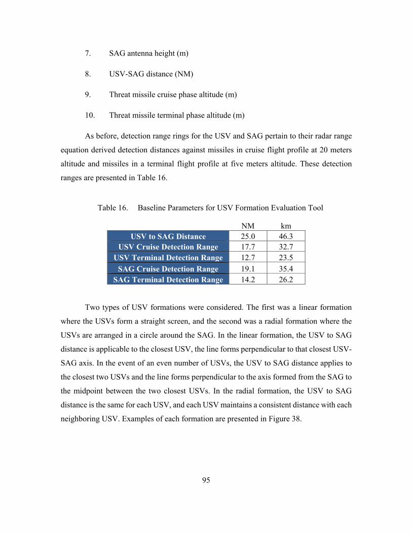
95
7. SAG antenna height (m)
8. USV-SAG distance (NM)
9. Threat missile cruise phase altitude (m)
10. Threat missile terminal phase altitude (m)
As before, detection range rings for the USV and SAG pertain to their radar range
equation derived detection distances against missiles in cruise flight profile at 20 meters
altitude and missiles in a terminal flight profile at five meters altitude. These detection
ranges are presented in Table 16.
Table 16. Baseline Parameters for USV Formation Evaluation Tool
NM km USV to SAG Distance 25.0 46.3
USV Cruise Detection Range 17.7 32.7 USV Terminal Detection Range 12.7 23.5
SAG Cruise Detection Range 19.1 35.4 SAG Terminal Detection Range 14.2 26.2
Two types of USV formations were considered. The first was a linear formation
where the USVs form a straight screen, and the second was a radial formation where the
USVs are arranged in a circle around the SAG. In the linear formation, the USV to SAG
distance is applicable to the closest USV, the line forms perpendicular to that closest USV-
SAG axis. In the event of an even number of USVs, the USV to SAG distance applies to
the closest two USVs and the line forms perpendicular to the axis formed from the SAG to
the midpoint between the two closest USVs. In the radial formation, the USV to SAG
distance is the same for each USV, and each USV maintains a consistent distance with each
neighboring USV. Examples of each formation are presented in Figure 38.
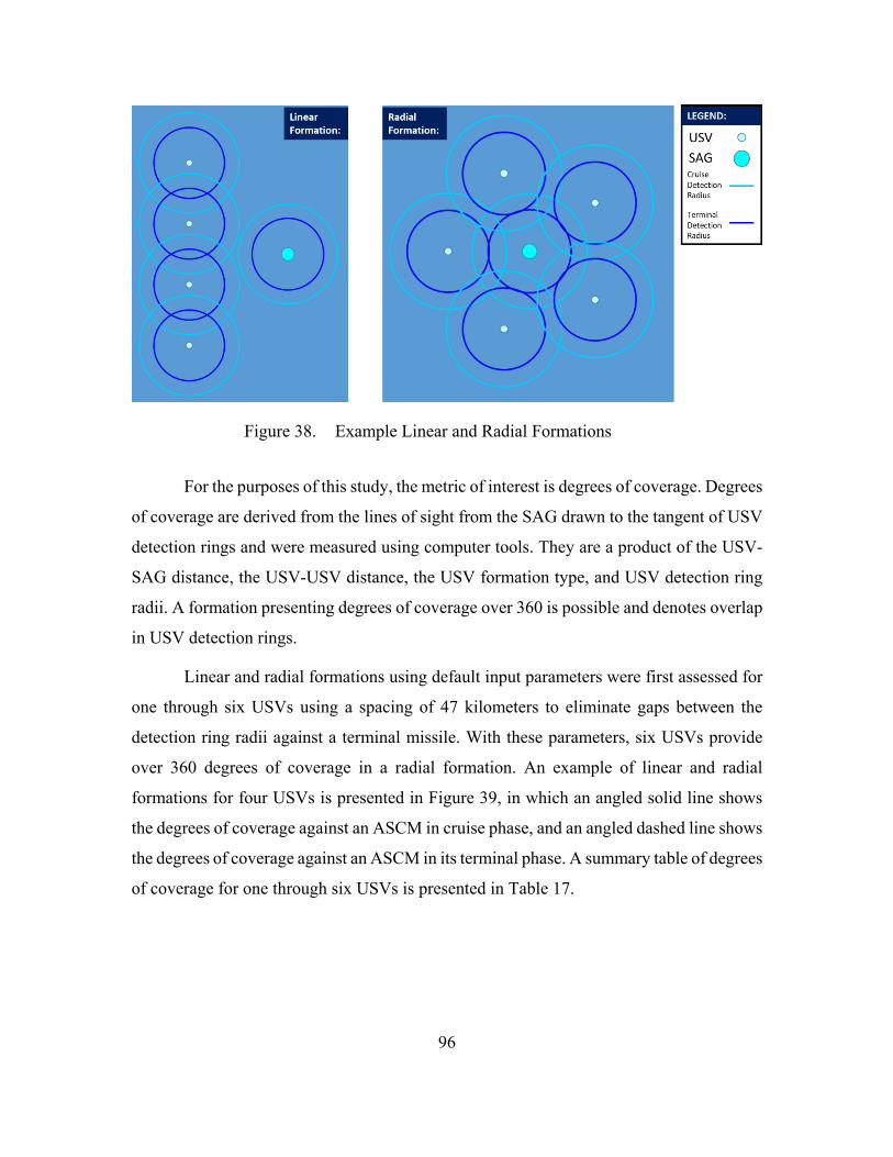
96
Figure 38. Example Linear and Radial Formations
For the purposes of this study, the metric of interest is degrees of coverage. Degrees
of coverage are derived from the lines of sight from the SAG drawn to the tangent of USV
detection rings and were measured using computer tools. They are a product of the USV-
SAG distance, the USV-USV distance, the USV formation type, and USV detection ring
radii. A formation presenting degrees of coverage over 360 is possible and denotes overlap
in USV detection rings.
Linear and radial formations using default input parameters were first assessed for
one through six USVs using a spacing of 47 kilometers to eliminate gaps between the
detection ring radii against a terminal missile. With these parameters, six USVs provide
over 360 degrees of coverage in a radial formation. An example of linear and radial
formations for four USVs is presented in Figure 39, in which an angled solid line shows
the degrees of coverage against an ASCM in cruise phase, and an angled dashed line shows
the degrees of coverage against an ASCM in its terminal phase. A summary table of degrees
of coverage for one through six USVs is presented in Table 17.
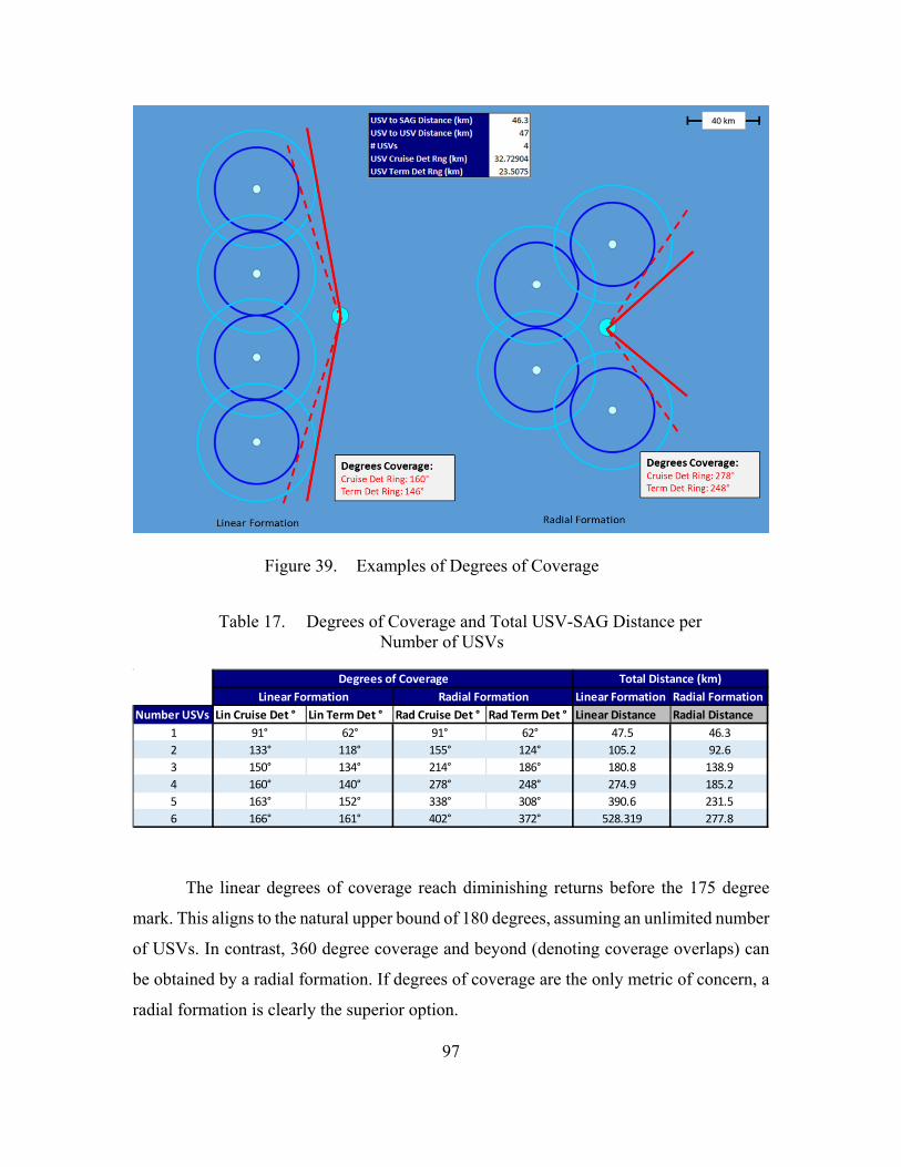
97
Figure 39. Examples of Degrees of Coverage
Table 17. Degrees of Coverage and Total USV-SAG Distance per Number of USVs
The linear degrees of coverage reach diminishing returns before the 175 degree
mark. This aligns to the natural upper bound of 180 degrees, assuming an unlimited number
of USVs. In contrast, 360 degree coverage and beyond (denoting coverage overlaps) can
be obtained by a radial formation. If degrees of coverage are the only metric of concern, a
radial formation is clearly the superior option.
Linear Formation Radial FormationNumber USVs Lin Cruise Det ° Lin Term Det ° Rad Cruise Det ° Rad Term Det ° Linear Distance Radial Distance
1 91° 62° 91° 62° 47.5 46.32 133° 118° 155° 124° 105.2 92.63 150° 134° 214° 186° 180.8 138.94 160° 140° 278° 248° 274.9 185.25 163° 152° 338° 308° 390.6 231.56 166° 161° 402° 372° 528.319 277.8
Degrees of Coverage Total Distance (km)Linear Formation Radial Formation
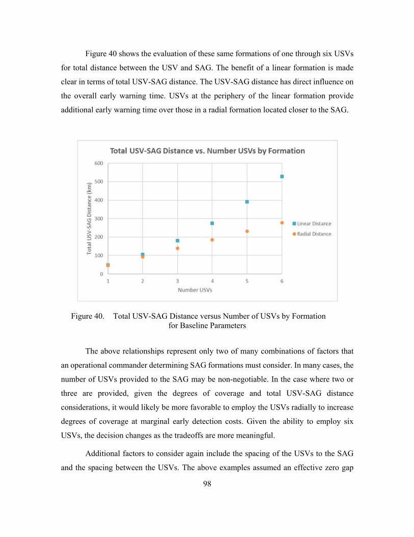
98
Figure 40 shows the evaluation of these same formations of one through six USVs
for total distance between the USV and SAG. The benefit of a linear formation is made
clear in terms of total USV-SAG distance. The USV-SAG distance has direct influence on
the overall early warning time. USVs at the periphery of the linear formation provide
additional early warning time over those in a radial formation located closer to the SAG.
Figure 40. Total USV-SAG Distance versus Number of USVs by Formation for Baseline Parameters
The above relationships represent only two of many combinations of factors that
an operational commander determining SAG formations must consider. In many cases, the
number of USVs provided to the SAG may be non-negotiable. In the case where two or
three are provided, given the degrees of coverage and total USV-SAG distance
considerations, it would likely be more favorable to employ the USVs radially to increase
degrees of coverage at marginal early detection costs. Given the ability to employ six
USVs, the decision changes as the tradeoffs are more meaningful.
Additional factors to consider again include the spacing of the USVs to the SAG
and the spacing between the USVs. The above examples assumed an effective zero gap

99
between the USV detection radii against threat missiles in terminal flight profiles.
Increasing the USV spacing could increase the overall cruise flight profile detection rings
without increasing the number of USVs involved but at increased risk to terminal phase
threat missiles sneaking through the screen in gapped detection zones. Follow on studies
could further explore the tradeoffs of USV to SAG spacing, USV spacing, and alternative
formations.

100
THIS PAGE INTENTIONALLY LEFT BLANK
101
VII. CONCLUSIONS
This study attempted to determine whether using medium-sized USVs in support
of a SAG will positively impact the SAG’s survivability against ASCM attacks. First, the
systems engineering process was followed to develop a notional medium-sized USV. High
level needs and functional requirements were determined, and component subsystems were
then selected. Following development of the USV, two operational situations where the
SAG was targeted by enemy ASCMs were investigated: a situation where the USV
responded to the threat and a situation where the USV did not directly respond but provided
early warning and threat cueing to the SAG.
Both situations were analyzed to determine if the USV mitigated the probability of
an ASCM hitting the SAG. The first situation was meant to examine this mitigation by way
of the USV defeating the threats before they reached the SAG. The second situation
examined the mitigation by way of the USV offering the SAG additional reaction time and
counter-fire opportunities to organically respond to the ASCM. Analysis of both situations
revealed there is clear tactical utility in using USVs to defend SAGs against ASCMs.
Finally, the utility of different formations between USVs and the SAG was also explored.
A. SYSTEM ENGINEERING ANALYSIS SUMMARY
Operational requirements were derived by developing a DRM to illustrate a
projected operational environment for the USV. It was determined that to mitigate the
probability of an ASCM hit on the SAG, the USV needs to either defeat the threat or
increase the SAG’s available reaction time by providing threat cueing. From these high-
level operational requirements, the need for two categories of USV subsystems was
identified. First, detection subsystems, which were an air search radar and an ES system,
would find and track any incoming ASCM. Second, response subsystems in the form of
soft-kill deception countermeasures, SAMs, CIWS, and EA were needed to defeat the
detected ASCM. Specific subsystem functional requirements were derived and formed the
basis for selection of currently available COTS and GOTS systems. The process identified
that multiple potential system selection outcomes are possible and chose the best systems
102
to meet the operational needs and remain within SWaP constraints imposed by the
maximum size of a medium USV.
B. SUBSYSTEM SELECTION
To provide the functionality required, research was conducted to determine what
capabilities are available currently or in the near-term that could be integrated onto a
medium-sized USV. Additional functional requirements were derived for the USV based
on the chosen subsystems, including communications, electrical power, cooling,
hydraulics, positioning, navigation, and timing services.
The specific detection and response subsystems selected were:
1. Air search radar – Enterprise Air Search Radar Variant 2
2. Electronic support system – Surface Electronic Warfare Improvement
Program Block 3
3. Soft-kill deception countermeasures – Centurion countermeasure launcher
4. Surface-to-air missile system – Evolved Sea Sparrow Missile Block 2 and
Mk 29 Guided Missile Launching System
5. Close-in weapons system – Phalanx
6. Radio frequency jamming (electronic attack) – Surface Electronic Warfare
Improvement Program Block 3
These subsystems were chosen because of their small footprint yet high level of
capability. Because the USVs are significantly smaller than a typical warship, the
subsystems must optimize the space available. It was also determined that communications
requirements could be met with current communication capabilities.
From analysis of physical attributes for each selected subsystem, the overall SWaP
requirements were developed. These requirements were assessed against the notional
medium-sized USV host platform characteristics including length, width, and
displacement. This assessment concluded that the overall subsystem requirements do not
103
exceed the medium-sized USV host platform limits and that medium-sized USVs can be
equipped with the combination of prescribed detection and response subsystems.
C. MODELING AND ANALYSIS FINDINGS
1. Markov Kill Chain Model
Using a Markov kill chain, the first model presents the use of a single USV as a line
of defense for the SAG. The USV utilizes SAMs, soft-kill deception countermeasures, EA,
and CIWS to respond to incoming ASCM threats. The model uses a state transition diagram
that is developed into a state machine. The state machine uses the time in each state and
the probability of transitioning between states to determine the time until and probabilities
for reaching one of the three final states: hard kill, soft kill, or no kill. Risk Simulator was
used to run 5000 trials in each scenario.
This model ran four different scenarios using a combination of OPSITs 1A and 1B
and the medium and high threats. Scenario 2—based on OPSIT 1B with all USV response
options available to use against the medium threat—proved to be the most effective in
eliminating incoming threats. Scenarios 1 and 4, however, with the USV in OPSIT 1A and
in OPSIT 1B employing only SAMs, respectively, both still proved to be highly effective
with over 81% success rate at defeating ASCMs.
In Scenario 3, the model shows that the USV is not provided authorization from the
SAG in sufficient time and is therefore unable to engage the high threat at terminal speed.
By the time the SAG issues a direction to the USV, the incoming ASCM will already have
passed through the USV’s range rings. A good candidate for further study would be to
determine if there is any difference when taking the man out of the loop in this scenario.
In Scenario 4, the USV responds to OPSIT 1B with the use of Range Ring 1 only.
When comparing the results for OPSIT 1B for use of all three range rings and the use of
only one range ring, it is evident that soft-kill deception countermeasures, EW, and CIWS
increase USV effectiveness in engaging incoming ASCM threats.
While limitations of this model include that it does not take into consideration the
limited number of SAMs available for utilization or the SAG’s ability to also engage the
104
incoming threats, the results show that the USV as a weapon platform can greatly reduce
the incoming ASCM threats, providing a defensive advantage for the SAG.
2. Time Series Analysis
The utility of the USV as an early warning cueing sensor for SAG counter-fire was
demonstrated using a time-distance analysis model created in Excel. Assessments for each
threat missile were conducted, and the relationships of USV and SAG detection rings as a
function of radar antenna height and USV-SAG spacing were explored. The early detection
times for high, medium, and low threat missiles were then translated into SAG counter-fire
shot opportunities to quantitatively demonstrate the potential early warning benefit. The
results of this analysis show that USVs providing early warning cueing of incoming threats
has clear benefit in the SAG’s ability to engage incoming threat missiles.
In the assessment of the USV as an early warning cueing sensor, additional
takeaways were realized. As antenna height on the USV increases, the detection radius of
the USV also grows corresponding in increased early warning detection time. As such, the
radar should be positioned as high as feasible within the limits of ship design. The more
significant means of increasing the early warning detection time is to position the USV
further from the SAG. Increasing the spacing between the USV and the SAG does present
a tradeoff in the effective coverage arc, explored in the final assessment.
3. USV Formation Analysis
Tradeoffs in effective arc coverage were examined in the analysis of USV
formations around the SAG using a graphical tool developed in Excel using Visual Basic
for Applications. The tool accounted for relative USV-SAG spacing, detection rings for
threat missiles derived from USV and SAG antenna heights, and inter-USV spacing. The
metrics of interest include degrees of coverage in terms of the USV detection screen, and
total linear distance between the USVs and SAG. The total linear distance corresponds to
early warning time for SAG counter-fire. Two generic formations were evaluated, a linear
screen where USVs formed a line perpendicular to a given threat access and a radial
formation with even spacing around the SAG.

105
The analysis showed that as the number of USVs increased, the radial formation
provided the best degrees of coverage. The linear formation, however, presented an
advantage in the total linear distance and corresponding early warning detection times. In
any case, an increase in USV-SAG spacing will result in increased early warning detection
times but can result in reduced degrees of coverage. USV-USV spacing impacts are
situational, but for both linear and radial formations, an increase in this spacing will
generally also produce radar coverage gaps. Tradeoffs in these measures of interest will
have to be considered when deciding on the USV formation with respect to the SAG.
D. AREAS FOR FUTURE STUDY
Two broad categories were identified for further research into USV applications to
defend SAGs against ASCMs. The first was additional research needed to complete the
total USV system design, and the second was expanded research into realistic scenarios for
USV operational employment.
1. Future Study Areas in USV Design
This study considers capabilities that exist in the present, leaving future technology
analysis for another study. It is however assumed that the fielding of technological
advancements in the maritime environment will progress such that the findings herein will
still be valid should the Navy implement a USV defensive line in the coming years.
Another area for continued research is the selection of specific subsystems
necessary to support the detection and response subsystems, such as communications,
electrical power, cooling, hydraulics, positioning, navigation, and timing services. In the
conduct of this study, it was assumed these necessary services would be provided. To
ensure a complete system design, a detailed investigation into these support subsystems
must therefore be conducted, including a selection of specific components and
identification of total support requirements for each subsystem.
As a part of vessel design, development of the interior and exterior component lay-
out of the USV will then be necessary. This includes designing the USV with weight
balance in mind. Trade-offs in vessel stability and placement of identified subsystems to

106
optimize tactical performance and minimize blockage zones must be considered. A future
research project could be to perform a stability study to determine the righting moments
and roll angles of various configurations.
A further area that will require additional research is systems integration onboard
the USV. Since all detection, response, and support subsystems interact with the ICS,
integrating all these systems with the ICS is paramount. Effective tactical performance
demands these interactions occur seamlessly. While there are currently combat systems
that integrate each of the subsystems recommended by this study, no ICS has been designed
to integrate with all of them together and operate on an unmanned vessel of this size.
Similarly, as the functional requirements show, each subsystem also depends on others to
varying degrees. Further efforts are needed to study the integration of all interfacing
systems.
Adversaries may also be able to pinpoint and exploit weaknesses in an unmanned
systems’ command and control system, giving the adversaries the ability to misdirect the
USV and cause defensive gaps for friendly units. Cybersecurity for all USV systems is a
critical design area for further research.
2. Future Study Areas in USV Operational Employment
Large numbers of USVs could be used to create an expansive common tactical
picture covering thousands of square miles. While some studies have considered the
problem of the robustness of smaller networks, a very large network compounding said
problem would be a good candidate for future study.
It is also likely the USV will be deployed to regions where adversaries can contest
the electromagnetic environment. As this study found, the benefits of this vessel are not
fully realized unless it is networked into the common tactical picture collectively produced
by friendly forces in the area. Anti-jamming capabilities should be explored to ensure the
USV can participate in the tactical picture network.
Another important method of adapting to the expected contested electromagnetic
environment are emissions control procedures. By securing equipment operating on certain
107
portions of the electromagnetic spectrum, military units can avoid being identified as a U.S.
or friendly military unit or even avoid being passively detected altogether. With respect to
the USV, further studies should be conducted to develop emissions control procedures such
that its systems can quickly be de-energized (and re-energized) by remote command.
This study examined three particular threats with a wide variation in range, speed,
and explosive yield between them. Of course, there are many types of ASCMs employed
around the world, with still more in development. Further examination of these threats is
necessary to thoroughly assess the utility of medium-sized USVs as an ASCM defense
option.
Future explorations for modeling could include situations where the USV fires
multiple SAMs, either at a single threat based on doctrine or based on necessity when there
are multiple incoming ASCMs. This research would determine at what point the USV will
become ineffective as a defensive measure against a raid of ASCM threats due to depletion
of missile inventory or oversaturation of threats. Additionally, it would be worthwhile for
a study to investigate the effects of multiple USVs engaging incoming threats. This would
further explore the benefits of having different geometries with various numbers of USVs
in the path of the incoming ASCMs.
Finally, as USVs prove to be tactically beneficial, our adversaries will notice and
respond accordingly. As the USVs will likely be targeted directly by the threat missiles,
future studies will need to be conducted to explore USV self-defense capabilities.

108
THIS PAGE INTENTIONALLY LEFT BLANK
109
APPENDIX A: DETAILED SYSTEM REQUIREMENTS
Air Search Radar • The radar system shall fit within the footprint of the medium-sized USV. • The radar system shall be capable of disregarding returns not meeting COI
classification. • The radar system shall be capable of remote configuration updates such as COI
parameters, threat profiles, cued search areas, no transmission areas, power levels, and the like.
• The radar system shall be capable of large-scale search functionality and high-resolution tracking. This may be accomplished by one or multiple air search radars.
• The radar system shall automatically designate track COIs meeting pre-assigned parameters.
• The radar system shall fix the location of COIs. • The radar system shall track the movement and path of COIs. • The radar system shall not interfere with other radars, including USV navigation
radars or response subsystem radars. • The radar system shall provide target track data to the ICS for further
transmission to the SAG.
Electronic Support • The electronic support system shall fit within the footprint of the medium-sized
USV. • The electronic support system shall be capable of detecting threat missiles in their
expected emitter operating frequency bands. • The electronic support system shall process detection data onboard the USV, to
include the threat emitter, line of bearing information, and signal strength. • The electronic support system shall automatically designate COIs meeting pre-
assigned parameters. • The electronic support system shall provide all detection data for COIs to the ICS
for further transmission to the SAG. • The electronic support system shall provide high elevation angle coverage. • The electronic support system shall isolate own ship emitters. • The electronic support system shall be capable of remote configuration including
threat profiles and cued search bearings or areas.
Soft-Kill Deception Countermeasures • The soft-kill deception countermeasure system shall fit within the footprint of the
medium-sized USV.

110
• The soft-kill deception countermeasure system shall be capable of launching either chaff or flare countermeasure payloads.
• The soft-kill deception countermeasure system shall be capable of launching countermeasure rounds in use by the USN or Allied forces.
• The soft-kill deception countermeasure system shall be capable of providing health and status messages to the ICS, including round inventory information.
• The soft-kill deception countermeasure system shall be capable of providing launch event status messages indicating status of countermeasure launches.
• The soft-kill deception countermeasure system shall be capable of receiving launch commands, ASCM track and ES signature data from the ICS.
• The soft-kill deception countermeasure system shall be capable of receiving automatic launch parameter updates from the SAG via the ICS.
Surface-to-Air Missiles • The surface-to-air missile system shall fit within the footprint of the medium-
sized USV. • The surface-to-air missile system shall be capable of launch from a launcher
employed on the USV. • The surface-to-air missile system shall be capable of receiving guidance
information from the USV and the SAG. • The surface-to-air missile system shall be capable of in-flight maneuvering and
speed required to address threat ASCM targets. • The surface-to-air missile system shall be capable of receiving in-flight target
updates. • The surface-to-air missile system shall be equipped with an infrared seeker at a
minimum to enable target engagement. • The surface-to-air missile system shall be capable of receiving launch orders from
the ICS. • The surface-to-air missile system shall integrate with the ICS to be capable of
receiving weapons posture and engagement configuration updates from the SAG. • The surface-to-air missile system shall use a single variant of SAM. • The surface-to-air missile system shall enable the USV to auto-fire SAMs on
incoming ASCM threats. • The surface-to-air missile system shall generate and provide the ICS and SAG
general health and status messages and launch event reports.
Close-in Weapons System • The close-in weapons system shall fit within the footprint of the medium-sized
USV. • The close-in weapons system shall have a detection and engagement range of at
least 3.7 kilometers (2 nautical miles).

111
• The close-in weapons system shall be capable of receiving track hand-off from the ICS.
• The close-in weapons system shall be capable of automatically detecting ASCMs. • The close-in weapons system shall automatically fire when a threat is detected, is
in range, and meets the engagement criteria. • The close-in weapons system shall automatically cease firing when it no longer
detects the threat, has detected the elimination of the threat, detects the threat is outbound or outside engagement range, or to prevent accidental engagement of blue forces.
• The close-in weapons system shall be capable of firing rounds in use by the USN or Allied forces.
• The close-in weapons system shall be compatible with a centralized cooling system to cool system electronics.
• The close-in weapons system shall generate and provide the ICS health and status messages and firing event status messages indicating engagement events.
• The close-in weapons system shall be capable of remote configuration including engagement settings and threat profiles.
Electronic Attack • The electronic attack system shall fit within the footprint of the medium-sized
USV. • The electronic attack system shall be capable of receiving engagement cueing
from the ICS. • The electronic attack system shall automatically begin emitting when a threat is
detected, is in range, and meets engagement criteria. • The electronic attack system shall automatically cease emitting when it no longer
detects the threat, has detected the elimination of the threat, detects the threat is outside engagement parameters, or to prevent mutual interference with other blue forces.
• The electronic attack system shall be compatible with a centralized cooling system to cool system electronics.
• The electronic attack system shall be able to provide health and status messages and firing event status messages indicating engagement events.
• The electronic attack system shall be capable of remote configuration including engagement settings and threat profiles.
Integrated Combat System • The integrated combat system shall be capable of passing ASCM track and ES
signature data to the deception countermeasure, SAM, CIWS, and EA systems. • The integrated combat system shall be capable of commanding deception
countermeasure launches and SAM launches and specifying payload type to
112
launch for either subsystem, to include commanding other USV subsystems to provide information or services as required.
• The integrated combat system shall be capable of commanding EA subsystem engagement against an ASCM target, to include commanding other USV subsystems to provide information or services as required.
• The integrated combat system shall be capable of receiving and disseminating (to the SAG) health and status reports from the air search radar, ES, deception countermeasure, SAM, CIWS, and EA subsystems, or any other subsystem integrated with the ICS.
• The integrated combat system shall be capable of receiving and disseminating (to the SAG) launch or emit reports from the deception countermeasure, SAM, CIWS, and EA subsystems.
• The integrated combat system shall be capable of receiving remote configuration updates from the SAG and applying them to applicable subsystems. These include rules of engagement settings and threat profiles for all USV subsystems.
• The integrated combat system shall merge contact data from the air search radar and ES systems.
• The integrated combat system shall interface with the off-hull communications subsystems.
• The integrated combat system shall leverage a common architecture like the Common Object Request Broker Architecture or similar.
• The integrated combat system shall be capable of directing the positioning, navigation, and timing system to ignore COLREGs, UNCLOS, or other international agreements as necessary and proceed as tactically directed when the operational situation warrants.
Electrical Power System • The electrical power system shall provide enough power to support all onboard
systems. • The electrical power system shall generate and distribute power at 450 volts
alternating current at 60 hertz in 3-phase and in single-phase for use by requisite 440 volt rated systems and for transformation down to 120 volts.
• The electrical power system shall use transformers to generate and distribute power at 120 volts alternating current at 60 hertz in 3-phase and in single-phase for use by requisite 115 volt rated systems.
• The electrical power system shall use frequency converters to generate power at 115 volts alternating current at 400 hertz and in 3-phase and shall distribute that power as necessary.
• The electrical power system shall comply with safety design requirements set forth in Naval Ship’s Technical Manual Chapter 300.
• The electrical power system shall be capable of self-monitoring for potential and confirmed system faults.
113
• The electrical power system shall send periodic system health and status messages to the ICS for further transmission to the SAG.
• The electrical power system shall be capable of autonomously initiating procedures to maintain USV equipment in the event of electrical problems, such as isolation, generator shutdown, and load-shed procedures.
Cooling System • The cooling system shall have separate chill water and seawater cooling
capabilities. • The cooling system shall use seawater to cool systems able to withstand high
amounts of heat. • The cooling system shall use chill water to cool systems sensitive to changes in
heat.
Hydraulics System • The hydraulics system shall use an automated control system. • The hydraulics system shall move hydraulic oil to open or close hydraulic
operated valves and move machinery parts as necessary. • The hydraulics system shall be capable of receiving and responding to direction
from the ICS to open or close valves or move machinery in order to properly employ combat systems.
• The hydraulics system shall generate and provide the ICS and SAG general health and status messages, to include hydraulic oil tank levels and reports on any detected hydraulic oil leaks.
Positioning, Navigation, and Timing System
• The positioning, navigation, and timing system shall comply with Chairman, Joint Chiefs of Staff Instruction 6130.01, the Department of Defense Master Positioning, Navigation, and Timing Plan.
• The positioning, navigation, and timing system shall operate with Department of Defense approved positioning, navigation, and timing equipment.
• The positioning, navigation, and timing system shall accurately and precisely determine USV location three-dimensionally, referenced to World Geodetic System 1984.
• The positioning, navigation, and timing system shall use an inertial navigation system capable of determining position absent GPS input in case of GPS denial.
• The positioning, navigation, and timing system shall provide for effective and safe navigation in accordance with COLREGs and other international agreements, such as UNCLOS, unless overridden by the ICS due to tactical considerations.
• The positioning, navigation, and timing system shall apply course and speed corrections to attain position and maintain station as directed by the SAG via the ICS.
114
• The positioning, navigation, and timing system shall determine and maintain Coordinated Universal Time and be capable of converting the time to any time zone specified by SAG operators via the ICS.
• The positioning, navigation, and timing system shall be resistant to jamming. • The positioning, navigation, and timing system shall interact with the ICS to pass
positioning, navigation, and timing data to all combat systems and to receive maneuvering directions and override orders to ignore COLREGs or UNCLOS if needed.
General Subsystem Requirements Environmental • The system shall be rugged in accordance with MIL-STD-810G for shock,
vibration, and saltwater environments. • The system shall be capable of operating in air temperatures from 0–50 degrees
Celsius. • The system shall be capable of operating in water temperatures from 2–35 degrees
Celsius.
115
APPENDIX B: MARKOV KILL CHAIN STATE MACHINES
Tables 18 through 20 show the state machines used in the Markov kill chain
analysis. Table 18 shows the state machine for Scenario 1, corresponding to OPSIT 1A.
Table 19 shows the state machine for Scenario 2 and Scenario 3, corresponding to OPSIT
1B. Finally, Table 20 shows the state machine for Scenario 4, corresponding to OPSIT 1B
without Range Ring 2 and Range Ring 3. The current state is represented by each row, and
the state names are shown in the column on the far left. The states to be transitioned to are
represented by the following columns and are named across the top of the tables. The values
inside each cell are the probabilities for transitioning from the state identified by the cell’s
particular row to the state identified by the cell’s particular column. Therefore, when
viewing the tables, the value in the cell where the current state under investigation and the
desired transition state intersect denotes the probability for that transition to occur. For
example, based on the value at the intersection of the Identify row and the Track Shared
column, Table 18 shows that the probability for transitioning from Identify to Track Shared
is 0.95. To further aid in understanding, it is recommended to view these tables with Figure
25, the state transition diagram.

116
Table 18. State Machine for Scenario 1—Based on OPSIT 1A
Search Detect Track IdentifyTrack
SharedNetworked
TEWASAG
ResponseDetermine Response
Respond RR1
Assess RR1 Engagement
Respond RR2Assess RR2
EngagementRespond
RR3Assess RR3
EngagementRespond RR2 BH
Assess RR2 BH Engagement
Respond RR1 BH
Hard Kill Soft Kill No Kill
P S1 S2 S3 S4 S5 S6 S7 S8 S9 S10 S11 S12 S13 S14 S15 S16 S17 S18 S19 S20Search S1 0 0.99 0 0 0 0 0 0 0 0 0 0 0 0 0 0 0 0 0 0.01Detect S2 0.01 0 0.99 0 0 0 0 0 0 0 0 0 0 0 0 0 0 0 0 0Track S3 0.01 0 0 0.99 0 0 0 0 0 0 0 0 0 0 0 0 0 0 0 0
Identify S4 0.05 0 0 0 0.95 0 0 0 0 0 0 0 0 0 0 0 0 0 0 0Track Shared S5 0 0 0 0 0 1 0 0 0 0 0 0 0 0 0 0 0 0 0 0
Networked TEWA S6 0 0 0 0 0 0 0 1 0 0 0 0 0 0 0 0 0 0 0 0SAG Response S7 0 0 0 0 0 0 0 0 0 0 0 0 0 0 0 0 0 0.6 0.25 0.15
Determine Response S8 0 0 0 0 0 0 0 0 1 0 0 0 0 0 0 0 0 0 0 0Respond RR1 S9 0 0 0 0 0 0 0 0 0 1 0 0 0 0 0 0 0 0 0 0
Assess RR1 Engagement S10 0 0 0 0 0 0 0 0 0 0 0 0 0 0 0 0 0 0.82 0 0.18Respond RR2 S11 0 0 0 0 0 0 0 0 0 0 0 0 0 0 0 0 0 0 0 0
Assess RR2 Engagement S12 0 0 0 0 0 0 0 0 0 0 0 0 0 0 0 0 0 0 0 0Respond RR3 S13 0 0 0 0 0 0 0 0 0 0 0 0 0 0 0 0 0 0 0 0
Assess RR3 Engagement S14 0 0 0 0 0 0 0 0 0 0 0 0 0 0 0 0 0 0 0 0Respond RR2 Backhalf S15 0 0 0 0 0 0 0 0 0 0 0 0 0 0 0 0 0 0 0 0
Assess RR2 Backhalf Engagement S16 0 0 0 0 0 0 0 0 0 0 0 0 0 0 0 0 0 0 0 0Respond RR1 Backhalf S17 0 0 0 0 0 0 0 0 0 0 0 0 0 0 0 0 0 0 0 0
Hard Kill S18 0 0 0 0 0 0 0 0 0 0 0 0 0 0 0 0 0 1 0 0Soft Kill S19 0 0 0 0 0 0 0 0 0 0 0 0 0 0 0 0 0 0 1 0No Kill S20 0 0 0 0 0 0 0 0 0 0 0 0 0 0 0 0 0 0 0 1

117
Table 19. State Machine for Scenarios 2 and 3—Based on OPSIT 1B
Search Detect Track IdentifyTrack
SharedNetworked
TEWASAG
ResponseDetermine Response
Respond RR1
Assess RR1 Engagement
Respond RR2Assess RR2
EngagementRespond
RR3Assess RR3
EngagementRespond RR2 BH
Assess RR2 BH Engagement
Respond RR1 BH
Hard Kill Soft Kill No Kill
P S1 S2 S3 S4 S5 S6 S7 S8 S9 S10 S11 S12 S13 S14 S15 S16 S17 S18 S19 S20Search S1 0 0.99 0 0 0 0 0 0 0 0 0 0 0 0 0 0 0 0 0 0.01Detect S2 0.01 0 0.99 0 0 0 0 0 0 0 0 0 0 0 0 0 0 0 0 0Track S3 0.01 0 0 0.99 0 0 0 0 0 0 0 0 0 0 0 0 0 0 0 0
Identify S4 0.05 0 0 0 0.95 0 0 0 0 0 0 0 0 0 0 0 0 0 0 0Track Shared S5 0 0 0 0 0 1 0 0 0 0 0 0 0 0 0 0 0 0 0 0
Networked TEWA S6 0 0 0 0 0 0 0 1 0 0 0 0 0 0 0 0 0 0 0 0SAG Response S7 0 0 0 0 0 0 0 0 0 0 0 0 0 0 0 0 0 0.6 0.25 0.15
Determine Response S8 0 0 0 0 0 0 0 0 1 0 0 0 0 0 0 0 0 0 0 0Respond RR1 S9 0 0 0 0 0 0 0 0 0 1 0 0 0 0 0 0 0 0 0 0
Assess RR1 Engagement S10 0.05 0 0 0 0 0 0 0 0 0 0.13 0 0 0 0 0 0 0.82 0 0Respond RR2 S11 0 0 0 0 0 0 0 0 0 0 0 1 0 0 0 0 0 0 0 0
Assess RR2 Engagement S12 0.05 0 0 0 0 0 0 0 0 0 0 0 0.75 0 0 0 0 0 0.2 0Respond RR3 S13 0 0 0 0 0 0 0 0 0 0 0 0 0 1 0 0 0 0 0 0
Assess RR3 Engagement S14 0.05 0 0 0 0 0 0 0 0 0 0 0 0 0 0.65 0 0 0.2 0.1 0Respond RR2 Backhalf S15 0 0 0 0 0 0 0 0 0 0 0 0 0 0 0 1 0 0 0 0
Assess RR2 Backhalf Engagement S16 0.05 0 0 0 0 0 0 0 0 0 0 0 0 0 0 0 0.75 0 0.2 0Respond RR1 Backhalf S17 0 0 0 0 0 0 0 0 0 0 0 0 0 0 0 0 0 0.82 0 0.18
Hard Kill S18 0 0 0 0 0 0 0 0 0 0 0 0 0 0 0 0 0 1 0 0Soft Kill S19 0 0 0 0 0 0 0 0 0 0 0 0 0 0 0 0 0 0 1 0No Kill S20 0 0 0 0 0 0 0 0 0 0 0 0 0 0 0 0 0 0 0 1

118
Table 20. State Machine for Scenario 4—Based on OPSIT 1B with Range Ring 1 Engagements Only
Search Detect Track IdentifyTrack
SharedNetworked
TEWASAG
ResponseDetermine Response
Respond RR1
Assess RR1 Engagement
Respond RR2Assess RR2
EngagementRespond
RR3Assess RR3
EngagementRespond RR2 BH
Assess RR2 BH Engagement
Respond RR1 BH
Hard Kill Soft Kill No Kill
P S1 S2 S3 S4 S5 S6 S7 S8 S9 S10 S11 S12 S13 S14 S15 S16 S17 S18 S19 S20Search S1 0 0.99 0 0 0 0 0 0 0 0 0 0 0 0 0 0 0 0 0 0.01Detect S2 0.01 0 0.99 0 0 0 0 0 0 0 0 0 0 0 0 0 0 0 0 0Track S3 0.01 0 0 0.99 0 0 0 0 0 0 0 0 0 0 0 0 0 0 0 0
Identify S4 0.05 0 0 0 0.95 0 0 0 0 0 0 0 0 0 0 0 0 0 0 0Track Shared S5 0 0 0 0 0 1 0 0 0 0 0 0 0 0 0 0 0 0 0 0
Networked TEWA S6 0 0 0 0 0 0 0 1 0 0 0 0 0 0 0 0 0 0 0 0SAG Response S7 0 0 0 0 0 0 0 0 0 0 0 0 0 0 0 0 0 0.6 0.25 0.15
Determine Response S8 0 0 0 0 0 0 0 0 1 0 0 0 0 0 0 0 0 0 0 0Respond RR1 S9 0 0 0 0 0 0 0 0 0 1 0 0 0 0 0 0 0 0 0 0
Assess RR1 Engagement S10 0.05 0 0 0 0 0 0 0 0 0 0 0 0 0 0 0 0.13 0.82 0 0Respond RR2 S11 0 0 0 0 0 0 0 0 0 0 0 0 0 0 0 0 0 0 0 0
Assess RR2 Engagement S12 0 0 0 0 0 0 0 0 0 0 0 0 0 0 0 0 0 0 0 0Respond RR3 S13 0 0 0 0 0 0 0 0 0 0 0 0 0 0 0 0 0 0 0 0
Assess RR3 Engagement S14 0 0 0 0 0 0 0 0 0 0 0 0 0 0 0 0 0 0 0 0Respond RR2 Backhalf S15 0 0 0 0 0 0 0 0 0 0 0 0 0 0 0 0 0 0 0 0
Assess RR2 Backhalf Engagement S16 0 0 0 0 0 0 0 0 0 0 0 0 0 0 0 0 0 0 0 0Respond RR1 Backhalf S17 0 0 0 0 0 0 0 0 0 0 0 0 0 0 0 0 0 0.82 0 0.18
Hard Kill S18 0 0 0 0 0 0 0 0 0 0 0 0 0 0 0 0 0 1 0 0Soft Kill S19 0 0 0 0 0 0 0 0 0 0 0 0 0 0 0 0 0 0 1 0No Kill S20 0 0 0 0 0 0 0 0 0 0 0 0 0 0 0 0 0 0 0 1
119
LIST OF REFERENCES
BAE Systems. 2019. “Mk 36 Super Rapid Bloom Offboard Countermeasures (SRBOC) Chaff and Decoy Launching System.” Accessed April 1, 2019. https://www.baesystems.com/en/product/mk-36-super-rapid-bloom-offboard-countermeasures-srboc-chaff-and-decoy-launching-system.
Berkoff, Howard. 2018. “Expanding the Navy’s Unmanned Systems Portfolio, An Update.” Defense Systems Informational Analysis Center Journal 5, no. 1 (Winter): 33–38. https://www.dsiac.org/sites/default/files/journals/survice_dsiac_winterjournal_singlepgs_dr8_031918.pdf.
Blanchard, Benjamin S. and Wolter J. Fabrycky. 2011. Systems Engineering and Analysis. 5th ed. Upper Saddle River, NJ: Prentice Hall.
Blattenberger, Kirt. 1996. “Electronic Warfare and Radar Systems Handbook: Radar Horizon / Line of Sight.” Accessed March 01, 2019. http://www.rfcafe.com/references/electrical/ew-radar-handbook/radar-horizon-line-of-sight.htm.
Blidberg, Richard. 2001. “The Development of Autonomous Underwater Vehicles (AUV); A Brief Summary.” Paper presented at the 2001 International Conference on Robotics and Automation, Seoul, Korea. http://ausi.org/publications/ICRA_01paper.pdf.
Carlson, Christopher. 2013. “China’s Eagle Strike-Eight Anti-ship Cruise Missiles: the YJ-83, C803, and the Family Tree Part 3.” Defense Media Network. February 8, 2013. https://www.defensemedianetwork.com/stories/chinas-eagle-strike-eight-anti-ship-cruise-missiles-the-yj-83-c803-and-the-family-tree/.
Chemring Countermeasures. 2013a. “Cart CM Chaff 130mm Mk36 Type 1.”
http://www.chemringcm.com/~/media/Files/C/Chemring-CounterMeasures-V2/documents/mk36-type1.pdf.
———. 2013b. “Naval Platform Protection System Centurion.”
http://www.chemringcm.com/~/media/Files/C/Chemring-CounterMeasures-V2/documents/centurion.pdf.
———. 2014. “Expendable Countermeasures for Sea and Air Systems.” Accessed April
1, 2019. https://www.chemring.co.uk/~/media/Files/C/Chemring-V2/PDFs/Chemring-Countermeasures.pdf.
Cole, Sally. 2015. “U.S. Navy’s Electronic Warfare Modernization Effort Centers on COTS.” Military Embedded Systems. Volume 11, No. 6, September 2015. http://pdf.cloud.opensystemsmedia.com/emag/MES_2015_SeptRG.pdf.

120
Defense Advanced Research Projects Agency. 2018. “ACTUV “Sea Hunter” Prototype Transitions to Office of Naval Research for Further Development.” January 30, 2018. https://www.darpa.mil/news-events/2018-01-30a.
Department of Defense. 2018. Fiscal Year (FY) 2019 President’s Budget—Operation and Maintenance, Defense-Wide. Washington, DC: Office of the Secretary of Defense. https://comptroller.defense.gov/Portals/45/Documents/defbudget/fy2019/budget_justification/pdfs/01_Operation_and_Maintenance/O_M_VOL_1_PART_1/OSD_OP-5.pdf.
Department of the Navy. 2007. The Navy Unmanned Surface Vehicle (USV) Master Plan. Washington, DC: Department of the Navy. https://www.navy.mil/navydata/technology/usvmppr.pdf.
———. 2017. “United States Navy Fact File: CEC – Cooperative Engagement Capability.” January 25, 2017. https://www.navy.mil/navydata/fact_display.asp?cid=2100&tid=325&ct=2.
———. 2019. “United States Navy Fact File: MK 15 – Phalanx Close-In Weapon System (CIWS).” January 15, 2019. https://www.navy.mil/navydata/fact_display.asp?cid=2100&tid=487&ct=2.
Eckstein, Megan. 2018. “Navy’s Next Large Surface Combatant Will Draw From DDG-51, DDG-1000 — But Don’t Call it a Destroyer Yet.” U.S. Naval Institute News, January 27, 2019. https://news.usni.org/2018/08/28/navys-next-large-surface-combatant-will-draw-ddg-51-ddg-1000-dont-call-destroyer.
Eurosam. 2019a. “Aster Hit-to-Kill Missile Interceptors.” Accessed February 19, 2019. https://www.eurosam.com/products/eurosams-building-block/aster/.
———. 2019b. “SYLVER Naval Vertical Launch System.” Accessed February 19, 2019. https://www.eurosam.com/products/eurosams-building-block/sylver/.
Forecast International. 1999. Electronic Warfare Forecast Report: SLQ-32(V). Newtown, CT: Forecast International. https://www.forecastinternational.com/archive/disp_old_pdf.cfm?ARC_ID=733.
General Dynamics Ordnance and Tactical Systems. 2003a. “Goalkeeper 30mm Close-In Ship Defense System.” July, 2003. https://www.gd-ots.com/wp-content/uploads/2017/11/Goalkeeper.pdf.
———. 2003b. “PHALANX Close-In Weapon System (CIWS).” July, 2003. https://www.gd-ots.com/wp-content/uploads/2017/11/Phalanx.pdf.
121
Giachetti Ronald. 2015. “System of Systems Capability Needs Analysis via a Stochastic Network Model.” Naval Engineers Journal 127, no. 4 (Winter): 67–79. https://calhoun.nps.edu/bitstream/handle/10945/49635/Giachetti_System_of_Systems_Capability_Needs.pdf?sequence=1&isAllowed=y.
Giammarco, Kristin, Spencer Hunt and Clifford Whitcomb. 2015. An Instructional Design Reference Mission for Search and Rescue Operations. Report No. NPS-SE-15-002. https://calhoun.nps.edu/bitstream/handle/10945/46782/NPS-SE-15-002.pdf.
Hewson, Robert. 2010. “China Aerospace Science and Industry Corporation’s Radar-Guided C-704R Missile.” Jane’s by IHS Markit. Accessed March 1, 2019. https://janes-ihs-com.libproxy.nps.edu/ExternalItems/Janes/images/binder/ jalw/jalw66/data/images/1296597.jpg.
Hpeterswald. 2013. “HMS Daring SAMPSON is a Multi-Function AESA Radar.”
Wikimedia Commons. October 7, 2013. https://commons.wikimedia.org/wiki/File:HMS_Daring_SAMPSON_is_a_multi-function_AESA_radar.jpg.
Jane’s by IHS Markit. 2013. “[ARCHIVED] RIM-66/-67/-156 Standard SM-1/-2, RIM-
161 Standard SM-3, and RIM-174 Standard SM-6.” July 30, 2013. https://janes-ihs-com.libproxy.nps.edu/Janes/DisplayFile/JSWS0208.
———. 2018a. “3M-54 (SS-N-27A ‘Sizzler’).” March 12, 2018. https://janes.ihs.com.libproxy.nps.edu/Janes/DisplayFile/JNWSA015.
———. 2018b. “AN/SPY-1.” September 26, 2018. https://janes-ihs-com.libproxy.nps.edu/Janes/Display/jc4im0028-jc4im.
———. 2018c. “C-704 (Nasr-1/Nasir).” April 18, 2018. https://janes.ihs.com.libproxy.nps.edu/Janes/Display/jnwsa036-jnw_.
———. 2018d. “C-704KD (Nasr).” October 3, 2018. https://janes.ihs.com.libproxy.nps.edu/Janes/DisplayFile/JALWA021.
———. 2018e. “The Club Family; Club-K/Club-M/Club-N/Club-S/Club-U; 3M-14E Series (SS-N-30B)/3M-54E Series (SS-N-27B)/91RE1 and 91RTE2.” March 5, 2018. https://janes.ihs.com.libproxy.nps.edu/Janes/DisplayFile/JNWSA030.
———. 2018f. “CSS-N-4 ‘Sardine’ (YJ-8/YJ-8A/C-801); CSS-N-8 ‘Saccade’ (YJ-82/YJ-83/C-802/C-802A/Noor/Ghader).” May 3, 2018. https://janes.ihs.com.libproxy.nps.edu/Janes/Display/jnws0132-jnw_.
———. 2018g. “GMVLS Mk 41/Mk 57.” April 18, 2018. https://janes-ihs-com.libproxy.nps.edu/Janes/Display/jnws0225-jnw_.
122
———. 2018h. “YJ-8K (C-801K), YJ-82K (C-802K), YJ-83K (C-802AK), YJ-83KH (CM-802AKG).” October 10, 2018. https://janes.ihs.com.libproxy.nps.edu/Janes/DisplayFile/JALW2892.
———. 2019a. “RIM-7 SeaSparrow and RIM-162 Evolved SeaSparrow Missile (ESSM).” March 26, 2019. https://janes-ihs-com.libproxy.nps.edu/Janes/DisplayFile/JNWS0168.
———. 2019b. “SAMPSON Multifunction Radar (MFR).” January 16, 2019. https://janes-ihs-com.libproxy.nps.edu/Janes/Display/jrew0365-jc4im.
Keane, John F., and Stephen S. Carr. 2013. “A Brief History of Early Unmanned Aircraft.” Johns Hopkins APL Technical Digest 32 (3): 558–571. https://www.jhuapl.edu/techdigest/TD/td3203/32_03-Keane.pdf.
Kelley, Stephen H. 2002. “Small Ships and Future Missions” Proceedings 128, no. 9 (September): 42–44. https://www.usni.org/magazines/proceedings/2002/september/small-ships-and-future-missions.
Kelly, Steve. n.d. “Vertical Launch System (VLS) – Mk 41 Strike-Length Module.” United Defense Armament Systems Division. Accessed March 10, 2019. https://fas.org/man/dod-101/sys/ship/weaps/mk41-strike.pdf.
Kopp, Carlo. 2012. Soviet/Russian Cruise Missiles. Report No. APA-TR-2009-0805 http://www.ausairpower.net/APA-Rus-Cruise-Missiles.html#mozTocId95513.
LaGrone, Sam. 2019. “Navy to Contract New Class of Unmanned Surface Vehicle by
Year’s End.” U.S. Naval Institute News, March 6, 2019. https://news.usni.org/2019/03/06/navy-contract-new-class-unmanned-surface-vehicle-years-end.
Lockheed Martin. 2009. “SPY-1 Family of Radars.” https://web.archive.org/web/20110915180551/http://www.lockheedmartin.com/data/assets/ms2/pdf/SPY-1_Family_brochure_6-pager.pdf.
———. 2013. “MK 41 Vertical Launching System.” https://www.lockheedmartin.com/content/dam/lockheed-martin/rms/documents/naval-launchers-and-munitions/MK41_VLS_factsheet.pdf.
———. 2016. “Surface Electronic Warfare Improvement Program (SEWIP): Protecting the Fleet.” https://lockheedmartin.com/content/dam/lockheed-martin/rms/documents/electronic-warfare/SEWIP-brochure.pdf.
MBDA Missile Systems. 2016a. “Aster Anti-Air Missile.” January, 2016. https://www.mbda-systems.com/?action=force-download-attachment&attachment_id=13346.

123
———. 2016b. “Italian Navy First Launch Aster 30 Missile Nave Bergamini.” November 24, 2016. https://www.mbda-systems.com/2016/11/24/italian-navy-first-launch-aster-30-missile-nave-bergamini/.
Missile Defense Advocacy Alliance. 2018. “SAMPSON Radar.” June 1, 2018. http://missiledefenseadvocacy.org/air-defense/air-defense-of-u-s-partners/allied-air-defense-sensor-systems/sampson-radar/.
Missile Threat. 2018. “Evolved Seasparrow Missile (ESSM).” Center for Strategic and International Studies Missile Defense Project. July 12, 2018. https://missilethreat.csis.org/defsys/evolved-seasparrow-missile-essm/.
Northrop Grumman. 2014. Understanding Voice and Data Link Networking: Northrop Grumman’s Guide to Secure Tactical Data Links, First Revision. Document No 135–02-005. https://www.northropgrumman.com/Capabilities/DataLinkProcessingAndManagement/Documents/Understanding_Voice+Data_Link_Networking.pdf.
———. 2019. “Production to Begin on Game-Changing Electronic Warfare Capability
for U.S. Navy Fleet.” Northrop Grumman Newsroom, January 24, 2019. https://news.northropgrumman.com/news/releases/northrop-grumman-authorized-to-build-sewip-block-3-low-rate-initial-production-systems-following-successful-milestone-c-decision.
Ostheim, Jakob. n.d. “Mk-41 VLS (8 Cells) Aboard a Royal Norwegian Navy Fridtjof
Nansen Class Frigate.” Seaforces Naval Information. Accessed April 07, 2019. http://www.seaforces.org/wpnsys/SURFACE/Mk-41-missile-launcher.htm.
Pike, John. 1999. “AN/SPS-49 Very Long-Range Air Surveillance Radar.” Federation of
American Scientists Military Analysis Network. June 30, 1999. https://fas.org/man/dod-101/sys/ship/weaps/an-sps-49.htm.
———. 2011a. “AN/SPG-62 Fire Control Radar.” Global Security Military Guide. July 7, 2011. https://www.globalsecurity.org/military/systems/ship/systems/an-spg-62.htm.
———. 2011b. “PC-1 Cyclone Class Patrol Coastal Boats.” Global Security Military Guide. July 7, 2011. https://www.globalsecurity.org/military/systems/ship/pc-1-specs.htm.
Program Executive Officer, Littoral & Mine Warfare. 2011. “Unmanned Maritime Systems Program Office Fact Sheet.” http://auvac.org/uploads/publication_pdf/Pms406_PROGRAM.pdf.

124
Raytheon Company. 2007. “MK 29 SEASPARROW Guided Missile Launching System with ESSM Upgrade.” January 25, 2007. http://www.alternatewars.com/BBOW/Weapons/Mk29_GMLS.pdf.
———. 2018. “Phalanx Close-In Weapon System.” Accessed December 13, 2018.
https://www.raytheon.com/capabilities/products/phalanx. ———. 2019. “Enterprise Air Surveillance Radar.” Accessed March 4, 2019.
https://www.raytheon.com/capabilities/products/easr. Richards, Ron. n.d. “The AN/SPS-49(V)5 Antenna Aboard South Korea’s Chungmugong
Yi Sun-sin (KDX-2)-Class Destroyer ROKS Gang Gam Chan.” Jane’s by IHS Markit. Accessed March 8, 2019. https://janes-ihs-com.libproxy.nps.edu/ExternalItems/Janes/images/yb/jc4im/ jc4im2019/data/images/1574126.jpg.
Robertson, Sue. 2019. Practical ESM Analysis. Norwood, MA: Artech House.
Rogoway, Tyler. 2017. “Watch the Navy Fire Its New Evolved Sea Sparrow Block II Missile for the First Time.” The Warzone Newsletter, November 2, 2017. https://www.thedrive.com/the-war-zone/15718/watch-the-navy-fire-its-new-evolved-sea-sparrow-block-ii-missile-for-the-first-time.
Royal Australian Navy. 2011. “A Standard Missile (SM 2) is Fired from the Royal Australian Navy Guided-Missile Frigate HMAS Sydney During a Live-Fire Exercise.” June 18, 2011. https://www.flickr.com/photos/usnavy/5963900217/in/photostream/.
Rucker, Jon. 2018. “Status of Unmanned Systems: Executing!” PMS 406 January 2018
Status Brief. https://www.navsea.navy.mil/Portals/103/Documents/Exhibits/SNA2018/UnmannedSystems-Rucker.pdf?ver=2018-01-11-145102-270.
Seaforces Naval Information. n.d. “DCNS Sylver A-43 VLS (2 x 8 cells) for Aster 15 SAM aboard ITS Cavour (C 550).” Accessed April 07, 2019. http://www.seaforces.org/wpnsys/SURFACE/DCNS-Sylver-vertical-launching-system.htm.
Skolnick, Fred and Phillip Wilkins. 2000. “Laying the Foundation for Successful Systems Engineering.” Johns Hopkins APL Technical Digest 21 (2): 208–216. https://pdfs.semanticscholar.org/61d9/50c78437225bb6f18c280b2bd4c5d4741b8a.pdf.
Smith, Roy M. 2010. “Using Kill-Chain Analysis to Develop Surface Ship CONOPS to Defend Against Anti-Ship Cruise Missiles.” Master’s Thesis, Naval Postgraduate School, Monterey, CA. https://calhoun.nps.edu/bitstream/handle/10945/5345/10Jun_Smith_Roy.pdf.

125
Thales 7 Seas. n.d. “UAT.” Accessed February 1, 2019. http://www.thales7seas.com/html_2014/product380.html.
Thales Group. n.d. “Goalkeeper – Close-In Weapon System.” Accessed January 27, 2019. https://www.thalesgroup.com/en/goalkeeper-close-weapon-system.
Think Defence. 2013. “The Chemring Centurion.” April 3, 2013. https://www.thinkdefence.co.uk/2013/04/the-chemring-centurion/.
Ward, Larry. n.d. “Mk 36 SRBOC Chaff and Decoy Launching System.” United Defense Armament Systems Division. Accessed January 30, 2019. https://www.globalsecurity.org/military/systems/ship/systems/mk36-srboc.pdf.
Williams, John. 2016. “U.S. Navy Photo.” Department of the Navy. April 07, 2016. https://www.navy.mil/view_image.asp?id=214556.
Wow Media Limited. 2013. “Chemring Centurion.” YouTube video, 3:20. June 14, 2013.
https://www.youtube.com/watch?v=jtTXYUaxQao.

126
THIS PAGE INTENTIONALLY LEFT BLANK
127
INITIAL DISTRIBUTION LIST
1. Defense Technical Information Center Ft. Belvoir, Virginia 2. Dudley Knox Library Naval Postgraduate School Monterey, California