Target Geolocation from a Small Unmanned Aircraft System
19
1 Target Geolocation from a Small Unmanned Aircraft System Richard Madison & Paul DeBitetto The Charles Stark Draper Laboratory 555 Technology Square Cambridge, MA 02139 617-258-4305 {RMadison, PDeBitetto}@draper.com A. Rocco Olean Natick Soldier RDEC Kansas Street Natick, MA 01760 508-233-6466 [email protected] Mac Peebles AeroVironment, Inc. 900 Enchanted Way Simi Valley, CA 93065 805-581-2198 [email protected] Abstract—Draper Laboratory and AeroVironment, Inc. of Monrovia, CA are implementing a system to demonstrate target geolocation from a Raven-B Unmanned Aircraft System (UAS) as part of the U.S. Army Natick Soldier Research, Development & Engineering Center’s Small UAS (SUAS) Advanced Concept Technology Demonstration (ACTD). The system is based on feature tracking, line-of- sight calculation, and Kalman filtering from Draper’s autonomous vision-aided navigation code base. The system reads imagery and telemetry transmitted by the UAS and includes a user interface for specifying targets. Tests on a snapshot of on-going work indicate horizontal targeting accuracy of approximately 10m, compared with 20-60m for the current Raven-B targeting software operating on the same flight video/telemetry streams. This accuracy likely will be improved through further mitigation of identified error sources. This paper presents our targeting architecture, the results of tests on simulator and flight data, an analysis of remaining error, and suggestions for reducing that error. 12 TABLE OF CONTENTS 1. INTRODUCTION...................................................... 1 2. TARGETING METHODS.......................................... 2 3. DVAN .................................................................... 5 4. TARGETING ARCHITECTURE ................................ 5 5. SIMULATION .......................................................... 8 6. FLIGHT TEST 1 .................................................... 10 7. FLIGHT TEST 2 .................................................... 13 8. ERROR SOURCES AND MITIGATION ................... 14 9. CONCLUSION ....................................................... 17 ACKNOWLEDGEMENT ............................................. 18 REFERENCES ........................................................... 19 BIOGRAPHY ............................................................. 19 1. INTRODUCTION The Small Unmanned Aircraft Systems (SUAS) military user community has indicated a desire for improved reconnaissance and surveillance capabilities for tactical SUAS, defined as rucksack portable systems whose air vehicle component (UAV) has less than 15 pounds gross 1 1-4244-1488-1/08/$25.00 ©2008 IEEE 2 IEEEAC paper #1244, Version 7, Updated November 23, 2007 vehicle weight. The SUAS Advanced Concept Technology Demonstration (ACTD) at Natick Soldier Research, Development & Engineering Center (NSRDEC) has been tasked to develop these capabilities. The ACTD is a government R&D program focused on investing in high technology readiness level (TRL 6-8) technologies, conducting a structured assessment process, and transitioning those technologies that exhibit military utility. Oversight responsibility is the purview of the Deputy Under Secretary of Defense (DUSD) for Advanced Systems & Concepts (AS&C). One area of technology development under investigation by the ACTD is the ability to detect, geolocate, and identify/ classify targets of interest. An important piece of this is targeting, which can be defined as the combination of two related processes: the generation of a coordinate in military grid reference system (MGRS); and the transmission of this coordinate through the appropriate communications systems and networks for review and action. The capability to provide accurate coordinates and error bounds for an object of interest in a UAS video stream has many applications both civilian and military. The coordinate can be used to direct fire, rescue, pinpoint landing, or other action depending on the nature of the target. Targeting methods currently employed by SUAS lack the desired accuracy and do not provide a confidence assessment through error bounding. To remedy these deficiencies, the ACTD has engaged Draper Laboratory and AeroVironment Inc. (AV) to assist in developing and evaluating the military utility of new SUAS targeting capabilities. Under this program, Draper and AV are implementing a system to demonstrate improved targeting from a Raven-B [1], a 4.2 pound tactical SUAS that is widely fielded throughout the Army, Marine Corps, and Special Operations Forces (SOF). The Draper/AV system, called AVTargeting, addresses the first component of targeting, providing MGRS coordinates with increased accuracy and error bounds. AVTargeting is based on visual feature tracking, line-of- sight calculation, and Kalman filtering developed by Draper Laboratory for autonomous, vision-aided navigation [6]. The filter is adapted for use in targeting. A new user
-
Upload
independent -
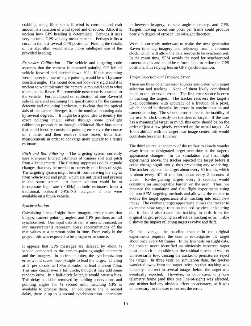
Category
Documents
-
view
1 -
download
0
Transcript of Target Geolocation from a Small Unmanned Aircraft System
1
Target Geolocation from a Small Unmanned Aircraft System
Richard Madison & Paul DeBitetto
The Charles Stark Draper Laboratory 555 Technology Square Cambridge, MA 02139
617-258-4305 {RMadison, PDeBitetto}@draper.com
A. Rocco Olean Natick Soldier RDEC
Kansas Street Natick, MA 01760
508-233-6466 [email protected]
Mac Peebles AeroVironment, Inc. 900 Enchanted Way
Simi Valley, CA 93065 805-581-2198
Abstract—Draper Laboratory and AeroVironment, Inc. of Monrovia, CA are implementing a system to demonstrate target geolocation from a Raven-B Unmanned Aircraft System (UAS) as part of the U.S. Army Natick Soldier Research, Development & Engineering Center’s Small UAS (SUAS) Advanced Concept Technology Demonstration (ACTD). The system is based on feature tracking, line-of-sight calculation, and Kalman filtering from Draper’s autonomous vision-aided navigation code base. The system reads imagery and telemetry transmitted by the UAS and includes a user interface for specifying targets. Tests on a snapshot of on-going work indicate horizontal targeting accuracy of approximately 10m, compared with 20-60m for the current Raven-B targeting software operating on the same flight video/telemetry streams. This accuracy likely will be improved through further mitigation of identified error sources. This paper presents our targeting architecture, the results of tests on simulator and flight data, an analysis of remaining error, and suggestions for reducing that error. 12
TABLE OF CONTENTS
1. INTRODUCTION......................................................1 2. TARGETING METHODS..........................................2 3. DVAN....................................................................5 4. TARGETING ARCHITECTURE ................................5 5. SIMULATION ..........................................................8 6. FLIGHT TEST 1 ....................................................10 7. FLIGHT TEST 2 ....................................................13 8. ERROR SOURCES AND MITIGATION ...................14 9. CONCLUSION .......................................................17 ACKNOWLEDGEMENT.............................................18 REFERENCES ...........................................................19 BIOGRAPHY .............................................................19
1. INTRODUCTION
The Small Unmanned Aircraft Systems (SUAS) military user community has indicated a desire for improved reconnaissance and surveillance capabilities for tactical SUAS, defined as rucksack portable systems whose air vehicle component (UAV) has less than 15 pounds gross 1 1-4244-1488-1/08/$25.00 ©2008 IEEE 2 IEEEAC paper #1244, Version 7, Updated November 23, 2007
vehicle weight. The SUAS Advanced Concept Technology Demonstration (ACTD) at Natick Soldier Research, Development & Engineering Center (NSRDEC) has been tasked to develop these capabilities. The ACTD is a government R&D program focused on investing in high technology readiness level (TRL 6-8) technologies, conducting a structured assessment process, and transitioning those technologies that exhibit military utility. Oversight responsibility is the purview of the Deputy Under Secretary of Defense (DUSD) for Advanced Systems & Concepts (AS&C).
One area of technology development under investigation by the ACTD is the ability to detect, geolocate, and identify/ classify targets of interest. An important piece of this is targeting, which can be defined as the combination of two related processes: the generation of a coordinate in military grid reference system (MGRS); and the transmission of this coordinate through the appropriate communications systems and networks for review and action. The capability to provide accurate coordinates and error bounds for an object of interest in a UAS video stream has many applications both civilian and military. The coordinate can be used to direct fire, rescue, pinpoint landing, or other action depending on the nature of the target.
Targeting methods currently employed by SUAS lack the desired accuracy and do not provide a confidence assessment through error bounding. To remedy these deficiencies, the ACTD has engaged Draper Laboratory and AeroVironment Inc. (AV) to assist in developing and evaluating the military utility of new SUAS targeting capabilities. Under this program, Draper and AV are implementing a system to demonstrate improved targeting from a Raven-B [1], a 4.2 pound tactical SUAS that is widely fielded throughout the Army, Marine Corps, and Special Operations Forces (SOF). The Draper/AV system, called AVTargeting, addresses the first component of targeting, providing MGRS coordinates with increased accuracy and error bounds.
AVTargeting is based on visual feature tracking, line-of-sight calculation, and Kalman filtering developed by Draper Laboratory for autonomous, vision-aided navigation [6]. The filter is adapted for use in targeting. A new user
2
interface allows a user to select targets and review and augment the autonomous feature tracking. AVTargeting reads the stream of imagery and telemetry output by the Raven-B Ground Control Station (GCS) and will run on a Panasonic Toughbook laptop computer attached to the GCS. Tests using Raven-B flight data show that AVTargeting can improve targeting accuracy to approximately 10m error, compared to 20-60m error for the currently fielded capability operating on the same data.
This paper presents a snapshot of AVTargeting partway through the software development. We begin with a review of targeting methods and their expected accuracy, leading to the selection of a filtering approach to targeting. Then we describe Draper’s Vision Aided Navigation capability and how components were adapted to implement a targeting filter. We discuss the architecture of the resulting targeting filter and a second targeting system that we coded for comparison. We discuss experimental assessment of targeting accuracy for these two systems using both simulation data and two sets of Raven-B flight data. Finally, we assess the sources of error for the two systems and suggest ways to mitigate these errors.
2. TARGETING METHODS
There are many ways to determine the location of an object seen in camera imagery. Four methods are already used in fielded UAVs, but three are not sufficiently accurate and the fourth requires specialized training and access to restricted databases. Several techniques that leverage multiple observations to provide accurate targeting are well developed in the literature, but not yet fielded on UAVs. A review of these various targeting techniques suggests that a line-of-sight filtering approach should provide good targeting accuracy at a modest cost in computation and user interaction.
The Paper-Map-Based Method
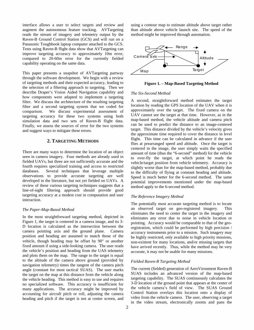
In the most straightforward targeting method, depicted in Figure 1, the target is centered in a camera image, and its 3-D location is calculated as the intersection between the camera pointing axis and the ground plane. Camera position and heading are assumed to match those of the vehicle, though heading may be offset by 90° or another fixed amount if using a side-looking camera. The user reads the vehicle’s position and heading from the UAS telemetry and plots them on the map. The range to the target is equal to the altitude of the camera above ground (provided by navigation telemetry) times the tangent of the camera pitch angle (constant for most tactical SUAS). The user marks the target on the map at this distance from the vehicle along the vehicle heading. This method is easy to use and requires no specialized software. This accuracy is insufficient for many applications. The accuracy might be improved by accounting for aircraft pitch or roll, adjusting the camera heading and pitch if the target is not at center screen, and
using a contour map to estimate altitude above target rather than altitude above vehicle launch site. The speed of the method might be improved through automation.
Figure 1. – Map-Based Targeting Method
The Six-Second Method
A second, straightforward method estimates the target location by reading the GPS location of the UAV when it is approximately over the target. The fixed camera on the UAV cannot see the target at that time. However, as in the map-based method, the vehicle altitude and camera pitch can be used to predict the distance to an image-centered target. This distance divided by the vehicle’s velocity gives the approximate time required to cover the distance in level flight. This time can be calculated in advance if the user flies at prearranged speed and altitude. Once the target is centered in the image, the user simply waits the specified amount of time (thus the “6-second” method) for the vehicle to over-fly the target, at which point he reads the vehicle/target position from vehicle telemetry. Accuracy is slightly worse than for the map-based method, probably due to the difficulty of flying at constant heading and altitude. Speed is much better for the 6-second method. The same potential improvements mentioned under the map-based method apply to the 6-second method.
The Reference Imagery Method
The potentially most accurate targeting method is to locate an observed target on geo-registered imagery. This eliminates the need to center the target in the imagery and eliminates any error due to noise in vehicle location or pointing. Accuracy would be comparable to that of the geo-registration, which could be performed by high precision / accuracy instruments prior to a mission. Such imagery may be highly restricted, only available to high priority missions, non-existent for many locations, and/or missing targets that have arrived recently. Thus, while the method may be very accurate, it may not be usable for many missions.
Fielded Raven-B Targeting Method
The current (fielded) generation of AeroVironment Raven-B SUAS includes an advanced version of the map-based targeting capability. The SUAS continuously calculates the 3-D location of the ground point that appears at the center of the vehicle camera’s field of view. The SUAS Ground Control Station overlays this location onto a display of video from the vehicle camera. The user, observing a target in the video stream, electronically zooms and pans the
Altitude
Range
Map Target
Camera axis
3
imagery to bring the target under crosshairs at image center, freezes the video stream, and reads the target location from the video overlay. The system uses the map-based method with three improvements. First, the system determines the camera heading and pitch more accurately by factoring in vehicle pitch and roll and the amount that the image crosshairs were electronically panned away from the nominal pointing direction. Second, the system improves the estimate of target altitude by representing the ground using a Digital Terrain Elevation Database (DTED). Ground altitudes are given at a grid of points and coordinates between grid points are found using bilinear interpolation. Third, the system is automated, so targeting is essentially instantaneous.
Despite the improved speed and accuracy, this system still has many potential error sources. Vehicle position and orientation are estimated and filtered to accuracy suitable for the SUAS autopilot, which can accept significantly more noise and smoothing than can visual targeting. The camera-heading estimate can be particularly bad if the vehicle’s magnetometer is not calibrated before the flight, which may happen if the SUAS is deployed in a hurry in a combat situation. This does not appear to hinder the autopilot. The estimate of the pointing direction from camera to target is impacted by camera model parameters such as optical center, field of view, and position and orientation relative to the vehicle, none of which are highly calibrated. The GCS reports vehicle position and orientation and calculates target location at 4Hz, but imagery arrives at 30Hz, so when the user freezes the video and reads target coordinates, they may represent the target that was under the cross hairs up to 8 images prior. This could be mitigated by interpolating reported vehicle position and orientation to predict values for a selected image, except that the telemetry and image streams are not synchronized, so it would not be clear where in the sequence to interpolate. In addition to the synchronization issues, it may be difficult to freeze the image exactly as the target slides under the crosshairs. Finally, accuracy of the ground intersection is limited to that of the DTED, which has noise in the altitude and location of the grid points and in bilinear interpolation between the grid points. It is not immediately clear how much error each of these factors might introduce. However, an unpublished study by AeroVironment recorded coordinates of a single target while circling the target many times and found circular error probable (CEP) on the order of 30m, averaged over altitudes and camera zoom levels. This shows improvement over map-based targeting but still reflects a reasonable amount of uncertainty.
Trivial Filtering
One simple way to improve on Raven-B targeting accuracy is to measure target coordinates over several observations and then average the measurements. The observations can be modeled as a combination of signal, bias (e.g., GPS bias), and zero-mean noise (e.g., error choosing target in an image). Averaging measurements preserves the signal and
bias while the noise averages toward zero. Averaging may also reduce the impact of some systematic biases depending on the flight trajectory. For instance, a constant yaw bias may cause a systematic targeting error of 2m in the direction of aircraft motion, but if the aircraft circles the target, this error averages toward zero. The aforementioned AeroVironment study found that, for a set of target estimates with a CEP around 25m, the average of the target estimates was within 5.6m of the actual target, a significant improvement over single-shot Raven-B targeting.
An implementation of such a system would benefit from two additional concepts. First, the average could be formulated as a filter, reporting a running average as each new observation is factored in. This would allow the user to choose at any time whether to take the current answer or wait for a higher-precision estimate later. A parallel calculation of standard deviation or CEP would aid in deciding when the precision is high enough. Second, the user should not have to manually identify the target in each frame. Rather, once the user has identified a target at image center, a tracking algorithm could keep virtual crosshairs on the target in future images, only requiring the user to intervene if the tracker loses the target.
Line-of-Sight Filtering
A potential improvement on filtering multiple observations is to calculate rays (“lines-of-sight”) from camera to target as in Raven-B targeting, but then intersect the rays with each other rather than with the ground. This eliminates the need for a DTED or other ground representation and eliminates any associated error. The intersection or closest approach of two lines-of-sight defines a 3-D target position. However, lines-of-sight typically are noisy and rarely intersect each other (or the ground) exactly at the target location. To compensate, several lines-of-sight may be used in a least squares formulation to identify the 3-D point that represents the mutual closest approach of all the lines. This may be formulated as a filter so that, as with trivial filtering, the target estimate is provided quickly and then continuously refined as more data becomes available.
A level of sophistication above the least squares filter is the Kalman Filter [2]. Using a Kalman filter provides many advantages. First, the filter is constructed to operate in terms of covariances, which explicitly encode the confidence in the targeting estimate. The user can look separately at uncertainty in altitude and horizontal coordinates and see how fast the uncertainty is changing. He can then decide whether to accept an estimate or wait for refinement. Second, the filter can be configured to estimate biases in the inputs and factor them out from future line-of-sight measurements. With biases removed, lines-of-sight converge more narrowly on the target location. The remaining noise is then more evenly balanced around zero and thus more effectively cancelled, and the target estimate is more accurate. Third, with better converging lines-of-sight, the filter correctly reports a higher precision target
4
estimate, giving the user confidence in the target estimate sooner. Fourth, biases that are consistent over time (e.g., camera mounting angle) can be estimated while viewing a “calibration” target early in a mission, and then applied to future targets, allowing those targets to be estimated quickly.
Line-of-sight filtering requires multiple observations of a target, each identifying the 2-D coordinates of the target in an image. A user may provide a small number of such observations, or a feature-tracking algorithm may follow the target through a sequence of images, reporting the coordinates for each. When using only two observations, uncertainty is minimized if the lines-of-sight are perpendicular to each other. From a UAV circling a target at constant altitude and with a camera pitch of 30° down, the two observations should be made about 110° apart in the circle. Lines-of-sight beyond the first two should be spread over an even wider arc. During this interval, the appearance of the target in the image should rotate by approximately the same angle subtended by the arc. Any feature-tracking algorithm should be able to follow the target despite this rotation or ask the user for help.
Line-of-sight filtering is the most accurate of the readily available methods described so far. Compared to trivial filtering, it eliminates noise from DTED, reduces the corrupting influence of zero-mean noise sources (such as error in selecting/tracking the target in the image), and can estimate and eliminate fixed biases (such as those caused by poor camera calibration). Similarly, the filter can eliminate noise sources such as yaw error caused by unsynchronized telemetry, which becomes a bias when the vehicle circles. However, the filter assumes that noise in the inputs consists of fixed bias plus zero mean noise, so if this is not true, for instance if poor synchronization causes a time varying noise signal, the filter estimate will be imperfect. In addition, as noise averages toward zero rather than to zero, noisier input signals take longer to average out, leaving the filter with a less accurate estimate in the mean time.
In summary, line-of-sight filtering should be very accurate, depending on the accuracy of inputs (such as vehicle position and orientation) and their noise models. Computation to incorporate any new line-of-sight should be relatively fast, though the user may wait a minute or so for the UAV to nearly circle the target as the uncertainty in the target estimate continues to drop.
Structure from Motion
The principal source of uncertainty in the line-of-sight filtering is likely to be error in the supposed orientation of the vehicle and thus the camera. As an example, at altitude 100m with a camera pitched down 30°, a wind-induced 1.5° pitch error produces 10m of targeting error, and even if this is zero-mean noise, it will damp out slowly over many frames of filtering. One way to mitigate orientation error is
to use some variant of the computer vision technique of Structure from Motion (SFM) [3][4]. This method inputs the 2-D image coordinates of multiple targets seen in images taken from multiple camera positions and solves for the 3-D locations of each target, the 3-D camera positions, and the 3-D orientation of the camera at each position. The method can be simplified and use fewer targets and/or images if some of the 3-D positions or orientations are given as inputs.
The mathematical premise of SFM has two-parts. First, when a target projects into an image, the 2-D image coordinates (u,v) of that projection are functions of the 3-D position of the target, the 3-D position of the camera, and the 3-D orientation of the camera – 2 equations in 9 unknowns. Second, observations of enough targets in enough images, at two equations per observation, produce more equations than unknowns, and the resulting system can be solved for all of the unknowns – camera positions, camera orientations, and target positions. The results are valid up to a global rotation, translation, and scale, as such transforms have no impact on the observations (u,v). The classic formulation requires 8 targets observed in 2 images, though a more brute force, nonlinear least squares solver only requires 6 targets in 2 frames, or 4 targets in 3 frames. Using more targets and/or more frames provide a least squares solution that is less influenced by noise in the reported values of (u,v).
To make the results useful for targeting, the output positions and orientations must be scaled, rotated, and shifted into world coordinates. Finding the appropriate transform requires real-world values for some combination of camera positions, camera orientations, and/or target positions. GPS provides the Raven-B with reasonable estimates of camera positions, and three or more of these are sufficient to find the transform to world coordinates, provided SFM is formulated to use at least three images. Better, these known positions can be taken as inputs instead of outputs, reducing the number of unknowns so that the SFM formulation can use observations of 3 targets in 3 images to recover the target position and camera pointing angles. This was done in [5], which found median targeting errors of 4m in Monte Carlo simulation. This result cannot be compared directly to the results preceding methods, as it was based on a Predator UAV, a different camera, and a different altitude. But it does indicate the magnitude of targeting estimation error possible with SFM.
SFM can be formulated as a least squares problem using more than three targets and/or images to reduce the impact of noise. Further, it can be implemented as a filter to operate in a real time system, providing immediate and continuously refined targeting estimates. The Draper Vision Aided Navigation (DVAN) system, described in the next section, did this successfully, though for navigation rather than targeting. The accuracy of filtered SFM should exceed that of line-of-sight filtering, as SFM does not rely on noisy
5
estimates of camera orientation that are likely the major error source for line-of-sight filtering. Rather, it uses the reported vehicle orientations only as a starting point for a nonlinear solver. Filtered SFM should be slower than line-of-sight filtering because the calculation is more complex and the user or tracker must track at least 3 targets rather than 1. Also, with the target appearance changing drastically as the UAV circles, the user probably must identify the targets or assist a tracker, and must account for 3 targets rather than 1, making SFM more user-intensive. It is less clear how non-filtered, 3-target, 3-image SFM will perform, as it eliminates error from reported vehicle orientation but is not over-constrained to reject noise from other sources. Calculation of a single target estimate would be extremely slow but might be faster than filtered methods if it required taking fewer images.
3. DVAN
Draper Laboratory’s DVAN system [6] has demonstrated a form of SFM for Vision Aided Navigation for small UAVs in GPS-denied environments. The system initializes by using the standard complement of inertial sensors (GPS, gyros) to determine the position and orientation (“pose”) of a vehicle. During this time, the system detects and tracks several targets in video from the vehicle’s camera. The system uses the line-of-sight filtering method to determine the 3-D positions of these targets. When the vehicle enters a GPS-denied environment, the system uses a Kalman Filter formulation of SFM to recover the pose of the vehicle while refining the estimated positions of the targets. While SFM in general produces its results in an arbitrary coordinate system, the well-converged target positions provide an anchor that keeps SFM from drifting with any speed. If a target is lost, it is replaced with a new target that is assigned a high covariance. The system puts little faith in the high-covariance target and continues to determine vehicle pose and refine target positions mainly from the other, better-established targets. Over time, the position of the new target is refined, its covariance decreases, and it becomes more trusted in calculating vehicle pose and refining target positions. The speed at which the system’s estimate of vehicle pose drifts from reality depends on how well younger targets converge before they become the anchors as older targets leave the field of view.
DVAN was not a targeting system, but as an implementation of SFM, it provides a number of components that are useful for targeting. The target tracker performs the same role in targeting, though DVAN’s automatic target detection may be unnecessary in line-of-sight filtering. The DVAN filter can be reused with minor modifications to filter lines-of-sight to recover the 3-D position of one target without updating camera pose. Alternately, the filter can continue to provide targeting and camera orientation via SFM, though it would need some method to propagate vehicle pose between updates. DVAN integrated an IMU for this purpose, but the Raven-B
provides infrequent IMU readings that would not be available for most image updates.
4. TARGETING ARCHITECTURE
The preceding review of targeting options and the availability of DVAN code to jump-start a targeting application lead to two credible options for a targeting architecture. The first is based on line-of-sight filtering. Under this architecture, the user selects a target in a video stream, via a user interface. A tracking algorithm follows the target into successive video frames, with the user assisting if the target is lost. The observed target coordinates are combined with a camera model and estimated camera pose to generate lines-of-sight. The lines-of-sight are combined in a Kalman Filter to find the 3-D point best approximating the intersection of the lines-of-sight. This architecture is preferred due to the simplicity of the user interface and computation. The second possible architecture is an SFM engine. The architecture differs only in the details of the Kalman Filter and the fact that at least three features must be identified and tracked, adding computation and perhaps user interface. We implemented AVTargeting based on line-of-sight filtering. We also implemented a non-filtered SFM engine in Matlab to evaluate the relative accuracy and thus determine whether a filtered SFM implementation is necessary.
Interface
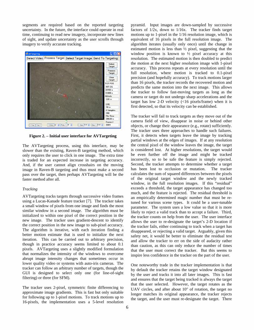
The front end of the targeting capability is a graphical user interface (GUI) being developed by AeroVironment. The initial concept is depicted in Figure 2. AVTargeting receives a stream of telemetry and video (motion imagery standards profile (MISP)-compliant MPEG2) from the Raven-B SUAS navigator and EO/IR camera. The GUI displays the first video image. The user clicks in the image to select a target. Alternately, he may scroll through the video to find an image where the target is clearly visible. This ability to stop the video and click an arbitrary location makes it easy to click exactly on the target. Once the target is selected, the AVTargeting feature tracker tracks the target through later frames until the target leaves the image, the video is exhausted, or the tracker determines that it has failed to track the target. AVTargeting converts the stream of tracked coordinates into lines-of-sight, filters them to estimate target coordinates and uncertainty, and displays these in MGRS format along the right side of the GUI.
The user may now scroll through the image sequence and verify that the tracker has correctly followed the target through the entire video. If the target is lost but reappears in later images, for instance after going behind another object, returning from outside the field of view, or disappearing due to a temporary video dropout, the user can re-designate the target location in a later frame. The tracker will continue to track the target and incorporate the new lines-of-sight into the filter. The user can choose whether additional tracking
6
segments are required based on the reported targeting uncertainty. In the future, the interface could operate in real time, continuing to read new imagery, incorporate new lines of sight, and update uncertainty as the user scrolls through imagery to verify accurate tracking.
Figure 2. – Initial user interface for AVTargeting
The AVTargeting process, using this interface, may be slower than the existing, Raven-B targeting method, which only requires the user to click in one image. The extra time is traded for an expected increase in targeting accuracy. And, if the user cannot align crosshairs on the moving image in Raven-B targeting and thus must make a second pass over the target, then perhaps AVTargeting will be the faster method after all.
Tracking
AVTargeting tracks targets through successive video frames using a Lucas-Kanade feature tracker [7]. The tracker takes a small window of pixels from one image and finds the most similar window in a second image. The algorithm must be initialized to within one pixel of the correct position in the new image. The tracker uses gradient-descent to identify the correct position in the new image to sub-pixel accuracy. The algorithm is iterative, with each iteration finding a better motion estimate that is used to initialize the next iteration. This can be carried out to arbitrary precision, though in practice accuracy seems limited to about 0.1 pixels. AVTargeting uses a slightly modified formulation that normalizes the intensity of the windows to overcome abrupt image intensity changes that sometimes occur in lower quality video or systems with auto-iris cameras. The tracker can follow an arbitrary number of targets, though the GUI is designed to select only one (for line-of-sight filtering) or three (for SFM).
The tracker uses 2-pixel, symmetric finite differencing to approximate image gradients. This is fast but only suitable for following up to 1-pixel motions. To track motions up to 16-pixels, the implementation uses a 5-level resolution
pyramid. Input images are down-sampled by successive factors of 1/2x, down to 1/16x. The tracker finds target motions up to 1-pixel in the 1/16 resolution image, which is equivalent of 16 pixels in the full resolution image. The algorithm iterates (usually only once) until the change in estimated motion is less than ½ pixel, suggesting that the window position is known to ½ pixel accuracy at this resolution. The estimated motion is then doubled to predict the motion at the next higher resolution image with 1-pixel accuracy. This process repeats at every resolution until the full resolution, where motion is tracked to 0.1-pixel precision (and hopefully accuracy). To track motions larger than 16 pixels, the tracker records the recovered motion and predicts the same motion into the next image. This allows the tracker to follow fast-moving targets as long as the camera or target do not undergo sharp accelerations and the target has low 2-D velocity (<16 pixels/frame) when it is first detected, so that its velocity can be established.
The tracker will fail to track targets as they move out of the camera field of view, disappear in noise or behind other objects, or change their appearance (e.g., rotate) sufficiently. The tracker uses three approaches to handle such failures. First, it detects when targets leave the image by tracking partial windows at the edges of images. If at any resolution the central pixel of the window leaves the image, the target is considered lost. At higher resolutions, the target would be even further off the image and might be tracked incorrectly, so to be safe the feature is simply rejected. Second, the tracker attempts to determine whether a target has been lost to occlusion or mutation. The tracker calculates the sum of squared differences between the pixels of the original target window and the newly tracked window, in the full resolution images. If this “residual” exceeds a threshold, the target appearance has changed too much, and the feature is rejected. The residual threshold is an empirically determined magic number that must be re-tuned for various scene types. It could be a user-tunable parameter. The system uses a low value so that it is more likely to reject a valid track than to accept a failure. Third, the tracker counts on help from the user. The user interface allows the user to re-designate the target’s 2-D location if the tracker fails, either continuing to track when a target has disappeared, or rejecting a valid target. Arguably, given this safety net, it would be better to eliminate the residual test and allow the tracker to err on the side of audacity rather than caution, as this can only reduce the number of times that the user must correct the tracker. But this seems to inspire less confidence in the tracker on the part of the user.
One noteworthy trade in the tracker implementation is that by default the tracker retains the target window designated by the user and tracks it into all later images. This is fast and ensures that the target being tracked is always the target that the user selected. However, the target rotates as the UAV circles, and after about 10° of rotation, the target no longer matches its original appearance, the tracker rejects the target, and the user must re-designate the target. There
7
are two common workarounds for this behavior. The first is to re-extract the target window from each new image after tracking. Image-to-image differences are small, so the tracker rarely rejects a valid target. However, the target drifts slightly with each re-designation and can drift away from the originally designated target. The user must pay more attention to identify when the target starts to drift. The second work-around uses a Shi-Tomasi tracker [8], which models affine deformations of the window. The tracker retains the original window and applies the modeled deformation so that the original window continues to match the appearance of the target in new images. This tracker is much more computationally intensive. AVTargeting can operate using the first mode, retaining the original target, or in the second mode, to evaluate whether improved rotation handling makes up for drift in the target window. The third mode has not yet been implemented.
Conversion to Lines-of-Sight
AVTargeting converts tracked 2-D coordinates to line-of-sight rays that form the input to the targeting filter. A standard geometrical camera model [9][10] is used to convert 2-D image coordinates to a unit vector giving the direction of the ray in the frame of the camera. The model accepts targets found anywhere in the image (not just at image center) and can accurately account for lens distortion. The unit vector is bundled with the camera pose (position and orientation) from the onboard navigation system and sent to the filter as a rather diffuse representation of the line-of-sight ray.
AVTargeting originally sent lines-of-sight to the filter at 4Hz, the frequency at which the UAS reports its estimated camera heading, depression, and roll as well as the Raven-B Targeting estimate. The three angles define the rotation from camera to world coordinates. The combination of targeting estimate and angles is sufficient to calculate camera position, which is assumed to match vehicle position within measurement precision. Vehicle position could be read directly from another message that arrives at 2Hz or from GPS that arrives at 1Hz but none of these messages are synchronized, adding a potential source of error. The tracker provides target coordinates (u,v) at 30Hz. Absent any clear synchronization between the image stream and the 4Hz telemetry, we read (u,v) from the image that arrives immediately before each 4Hz telemetry message.
During development testing, it became obvious that the UAV’s estimate of camera orientation was unreliable. Some error is to be expected from poor synchronization between video and telemetry and filtering for navigation purposes, but our test data featured yaw errors in excess of 45°. This was not a simple bias, which could be estimated in a filter. Rather, it was most likely due to poor magnetometer calibration. Since the magnetometer might not be calibrated prior to a mission, it is important to be able to operate in spite of the invalid yaw. As a result, the line-of-sight generation code was expanded to be able to derive
camera yaw in any of four ways. The first uses the yaw reported by vehicle. The second infers vehicle heading by subtracting consecutive, vehicle-reported positions. This assumes that: the vehicle does not crab; the navigation filtering accurately predicts vehicle position; and the vehicle flies a straight path. The third method reads vehicle heading from GPS. This occurs at only 1Hz, so lines-of-sight are generated at 1Hz, not synchronized with pitch and roll estimates. Longer time/distance between readings reduces the noise in the heading signal, and perhaps the GPS filters heading using something more intelligent than subtracting the most recent two positions (for instance, GPS velocity). This third method also assumes that the vehicle does not crab. The fourth method adjusts the reported yaw of method 1 to account for magnetometer calibration error. The adjustment is a physics-based function of reported yaw and two constants. To find these constants, the reported yaw from method 1 and the relatively-unbiased-but-noisy yaw estimate from method 2 were collected for all frames of a telemetry stream and fed with the adjustment equation into a numerical solver. As the constants are fit in retrospect, and the fitting may overcome and thus hide other error sources, this last method is useful mainly for analysis, not in operation.
Kalman Filter
AVTargeting sends lines-of-sight (in camera-coordinate-frame) and camera pose (in world coordinate frame) to an extended Kalman filter to build an estimate of a target’s 3-D position. The filter estimates only one target, though several filters can be used to estimate several independent targets. The filter maintains states for the camera pose and the target position. The filter currently contains no vehicle dynamic model and no additional source of pose information, so state propagation has no effect. State update uses large process to cause the camera pose state to simply track the camera pose input.
The filter initializes a target’s position by converting the first line-of-sight ray to world coordinates and finding the point where that ray reaches ground altitude. Ground altitude is taken from Raven-B targeting and provided as an extra filter input. In case Raven-B targeting is inaccurate, the initial target position is given a large covariance. Initialization also defines a Cartesian world coordinate system at the camera position. Filtering is performed in this static coordinate system.
Target position state update uses the current estimates of target position estimate and camera position to calculate an expected line-of-sight in world coordinates. It applies the input camera rotation to convert the input line-of-sight to world coordinates. It subtracts the two lines-of-sight to generate an error, which it applies to linearizations of partial derivatives to infer the error in camera pose and target position. Errors in camera pose are irrelevant, as those states will be fully replaced in the next cycle. Errors in target position are used to update the internal state. As the
8
filter processes more lines-of-sight, the covariance of the target position decreases, causing the estimate to converge.
The Kalman Filter architecture may seem overly complicated considering that only the target position is actually filtered. In fact, it is a repurposing of the DVAN navigation filter described earlier. The complication required to fit into the existing filter format is likely less cumbersome than the debugging required for a newly developed filter. In addition, the original functionality of the navigation filter can be returned in the future to support doing filtered SFM-based targeting, or to couple targeting into a high quality navigation filter.
At this point in the development effort, a few additional features of the filter have not been brought into play. One is the estimation of measurement biases. The actual coding of the filter contains states for biases on input measurements and equations for updating these additional states. However, these states have not yet been enabled. The other feature consists of a number of constants that specify the amount of uncertainty in the input measurements and initial target estimate as well as the amount of process noise for the target position, which controls the relative weight assigned to the existing position estimate versus each incoming line-of-sight. It probably will be necessary to tune these parameters to credible values in order to maximize the speed at which the filter converges.
Structure from Motion
We implemented an SFM algorithm in Matlab as a sanity check for results of the line-of-sight filter. The algorithm inputs the 2-D image coordinates of three targets seen in images taken at each of three or more camera locations. It also inputs the 3-D coordinates of each camera location and a rough estimate of the camera orientation at each location. AVTargeting provides all of these inputs, reporting camera locations from its 1Hz GPS input messages, very rough camera orientations from 4Hz telemetry nearest the GPS message, and image coordinates for the incoming image immediately preceding the GPS message. Very rough target positions are calculated by calculating lines-of-sight for the targets in the first image and following them to the altitude of the ground, given in the Raven-B targeting estimate from that frame.
Standard projection equations and an idealized camera [9] with no lens distortion provide two nonlinear equations for the observed coordinates of each target in each image, in terms of the known camera positions, unknown target positions, and unknown camera orientations. The equations and the rough estimates for the unknowns are sent through Matlab’s lsqnonlin function to perturb the unknowns until the error in the equations settles into a least squares solution. The solution is exact when used with three targets in three images, though it is very susceptible to noise in the inputs. When used with more than three images, the error does not
reduce to zero, but the target estimates should have less noise. If SFM turns out to be more accurate it may be re-implemented in the targeting filter to replace line-of-sight targeting.
5. SIMULATION
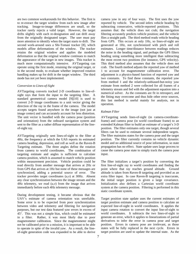
To test the accuracy of the two targeting methods, we applied them to a Raven-B telemetry-and-video stream produced using AeroVironment’s Raven-B simulator. Figure 3 shows an example video frame. The simulated Raven-B loitered in a circle about 100m above the ground, observing three targets at known locations, providing imagery at 30Hz interspersed with telemetry at 4Hz. The synchronization between the imagery and telemetry is unclear, so telemetry is assigned to the image that immediately precedes it. The simulator should not contain sensor noise, and it appears that camera orientation is not filtered in the navigation system before being packaged in telemetry, so camera angles should be accurate. It appears that GPS position and heading messages are synchronized, which may not be the case in the actual Raven.
Figure 3. – One frame from Raven-B simulation
Line-of-Sight Filtering
We investigated the relative utility of targeting running line-of-sight (LOS) filtering, Raven-B targeting, and Trivial filtering (the last two modified to accept targets anywhere on the screen) on the simulator data. We ran the algorithms three times, targeting centers of the three X-shaped objects composed of superimposed busses. We measured horizontal and vertical targeting accuracy after completing ¼, ½, ¾, and a full circle around the objects. In each case, we tested using yaw reported by the vehicle, obtained from change in vehicle position, and reported by GPS. Magnetometer-corrected yaw was not tested, as the magnetometer is assumed to be correct in simulation. Table 1 presents the recovered horizontal targeting accuracies and target altitudes, averaged over the three targets.
9
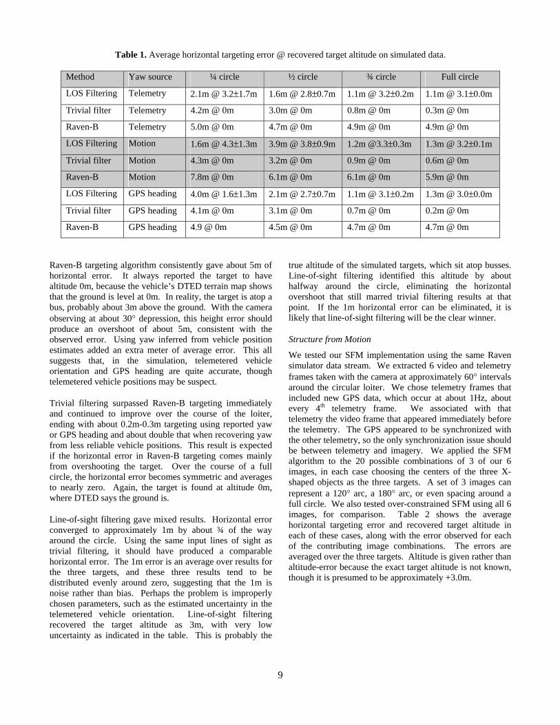
Table 1. Average horizontal targeting error @ recovered target altitude on simulated data.
Method Yaw source ¼ circle ½ circle ¾ circle Full circle
LOS Filtering Telemetry 2.1m @ 3.2±1.7m 1.6m @ 2.8±0.7m 1.1m @ 3.2±0.2m 1.1m @ 3.1±0.0m
Trivial filter Telemetry 4.2m @ 0m 3.0m @ 0m 0.8m @ 0m 0.3m @ 0m
Raven-B Telemetry 5.0m @ 0m 4.7m @ 0m 4.9m @ 0m 4.9m @ 0m
LOS Filtering Motion 1.6m @ 4.3±1.3m 3.9m @ 3.8±0.9m 1.2m @3.3±0.3m 1.3m @ 3.2±0.1m
Trivial filter Motion 4.3m @ 0m 3.2m @ 0m 0.9m @ 0m 0.6m @ 0m
Raven-B Motion 7.8m @ 0m 6.1m @ 0m 6.1m @ 0m 5.9m @ 0m
LOS Filtering GPS heading 4.0m @ 1.6±1.3m 2.1m @ 2.7±0.7m 1.1m @ 3.1±0.2m 1.3m @ 3.0±0.0m
Trivial filter GPS heading 4.1m @ 0m 3.1m @ 0m 0.7m @ 0m 0.2m @ 0m
Raven-B GPS heading 4.9 @ 0m 4.5m @ 0m 4.7m @ 0m 4.7m @ 0m
Raven-B targeting algorithm consistently gave about 5m of horizontal error. It always reported the target to have altitude 0m, because the vehicle’s DTED terrain map shows that the ground is level at 0m. In reality, the target is atop a bus, probably about 3m above the ground. With the camera observing at about 30° depression, this height error should produce an overshoot of about 5m, consistent with the observed error. Using yaw inferred from vehicle position estimates added an extra meter of average error. This all suggests that, in the simulation, telemetered vehicle orientation and GPS heading are quite accurate, though telemetered vehicle positions may be suspect.
Trivial filtering surpassed Raven-B targeting immediately and continued to improve over the course of the loiter, ending with about 0.2m-0.3m targeting using reported yaw or GPS heading and about double that when recovering yaw from less reliable vehicle positions. This result is expected if the horizontal error in Raven-B targeting comes mainly from overshooting the target. Over the course of a full circle, the horizontal error becomes symmetric and averages to nearly zero. Again, the target is found at altitude 0m, where DTED says the ground is.
Line-of-sight filtering gave mixed results. Horizontal error converged to approximately 1m by about ¾ of the way around the circle. Using the same input lines of sight as trivial filtering, it should have produced a comparable horizontal error. The 1m error is an average over results for the three targets, and these three results tend to be distributed evenly around zero, suggesting that the 1m is noise rather than bias. Perhaps the problem is improperly chosen parameters, such as the estimated uncertainty in the telemetered vehicle orientation. Line-of-sight filtering recovered the target altitude as 3m, with very low uncertainty as indicated in the table. This is probably the
true altitude of the simulated targets, which sit atop busses. Line-of-sight filtering identified this altitude by about halfway around the circle, eliminating the horizontal overshoot that still marred trivial filtering results at that point. If the 1m horizontal error can be eliminated, it is likely that line-of-sight filtering will be the clear winner.
Structure from Motion
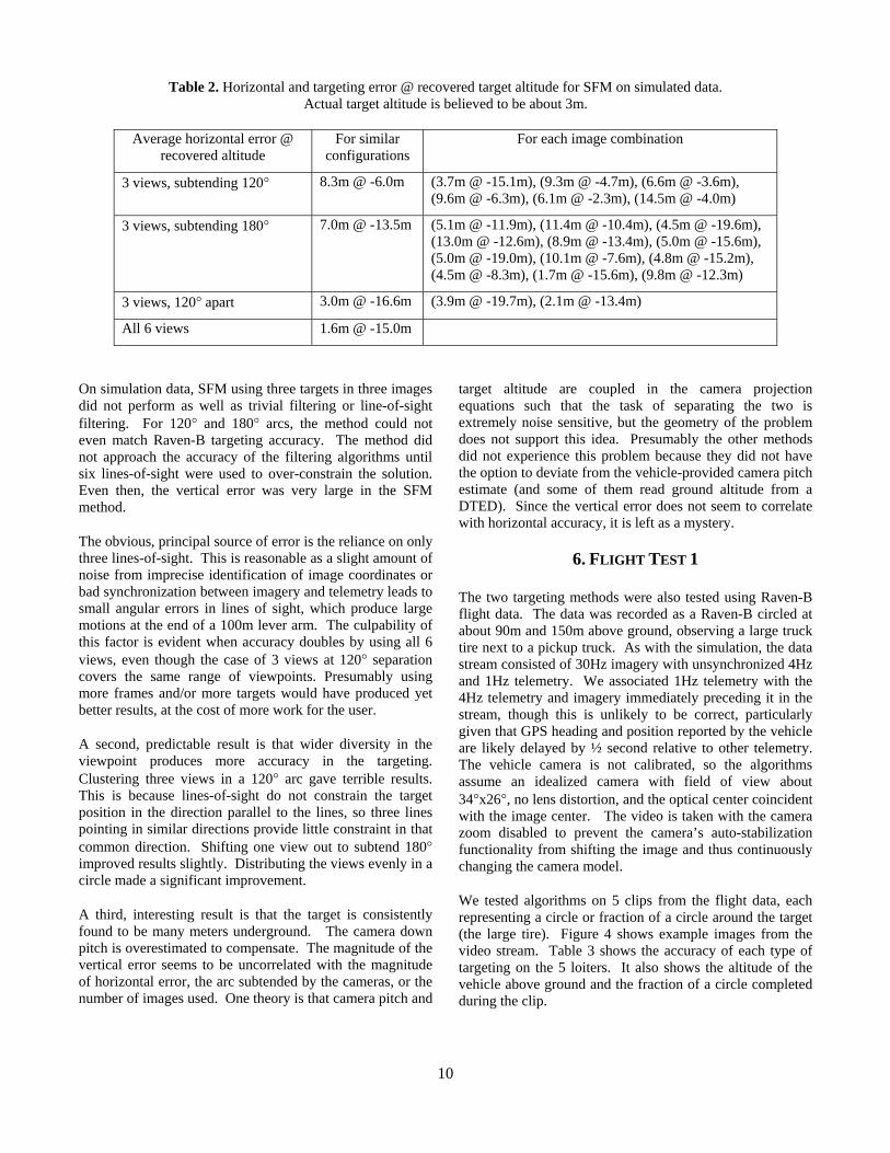
We tested our SFM implementation using the same Raven simulator data stream. We extracted 6 video and telemetry frames taken with the camera at approximately 60° intervals around the circular loiter. We chose telemetry frames that included new GPS data, which occur at about 1Hz, about every 4th telemetry frame. We associated with that telemetry the video frame that appeared immediately before the telemetry. The GPS appeared to be synchronized with the other telemetry, so the only synchronization issue should be between telemetry and imagery. We applied the SFM algorithm to the 20 possible combinations of 3 of our 6 images, in each case choosing the centers of the three X-shaped objects as the three targets. A set of 3 images can represent a 120° arc, a 180° arc, or even spacing around a full circle. We also tested over-constrained SFM using all 6 images, for comparison. Table 2 shows the average horizontal targeting error and recovered target altitude in each of these cases, along with the error observed for each of the contributing image combinations. The errors are averaged over the three targets. Altitude is given rather than altitude-error because the exact target altitude is not known, though it is presumed to be approximately +3.0m.
10
Table 2. Horizontal and targeting error @ recovered target altitude for SFM on simulated data. Actual target altitude is believed to be about 3m.
Average horizontal error @ recovered altitude
For similar configurations
For each image combination
3 views, subtending 120° 8.3m @ -6.0m (3.7m @ -15.1m), (9.3m @ -4.7m), (6.6m @ -3.6m), (9.6m @ -6.3m), (6.1m @ -2.3m), (14.5m @ -4.0m)
3 views, subtending 180° 7.0m @ -13.5m (5.1m @ -11.9m), (11.4m @ -10.4m), (4.5m @ -19.6m), (13.0m @ -12.6m), (8.9m @ -13.4m), (5.0m @ -15.6m), (5.0m @ -19.0m), (10.1m @ -7.6m), (4.8m @ -15.2m), (4.5m @ -8.3m), (1.7m @ -15.6m), (9.8m @ -12.3m)
3 views, 120° apart 3.0m @ -16.6m (3.9m @ -19.7m), (2.1m @ -13.4m)
All 6 views 1.6m @ -15.0m
On simulation data, SFM using three targets in three images did not perform as well as trivial filtering or line-of-sight filtering. For 120° and 180° arcs, the method could not even match Raven-B targeting accuracy. The method did not approach the accuracy of the filtering algorithms until six lines-of-sight were used to over-constrain the solution. Even then, the vertical error was very large in the SFM method.
The obvious, principal source of error is the reliance on only three lines-of-sight. This is reasonable as a slight amount of noise from imprecise identification of image coordinates or bad synchronization between imagery and telemetry leads to small angular errors in lines of sight, which produce large motions at the end of a 100m lever arm. The culpability of this factor is evident when accuracy doubles by using all 6 views, even though the case of 3 views at 120° separation covers the same range of viewpoints. Presumably using more frames and/or more targets would have produced yet better results, at the cost of more work for the user.
A second, predictable result is that wider diversity in the viewpoint produces more accuracy in the targeting. Clustering three views in a 120° arc gave terrible results. This is because lines-of-sight do not constrain the target position in the direction parallel to the lines, so three lines pointing in similar directions provide little constraint in that common direction. Shifting one view out to subtend 180° improved results slightly. Distributing the views evenly in a circle made a significant improvement.
A third, interesting result is that the target is consistently found to be many meters underground. The camera down pitch is overestimated to compensate. The magnitude of the vertical error seems to be uncorrelated with the magnitude of horizontal error, the arc subtended by the cameras, or the number of images used. One theory is that camera pitch and
target altitude are coupled in the camera projection equations such that the task of separating the two is extremely noise sensitive, but the geometry of the problem does not support this idea. Presumably the other methods did not experience this problem because they did not have the option to deviate from the vehicle-provided camera pitch estimate (and some of them read ground altitude from a DTED). Since the vertical error does not seem to correlate with horizontal accuracy, it is left as a mystery.
6. FLIGHT TEST 1
The two targeting methods were also tested using Raven-B flight data. The data was recorded as a Raven-B circled at about 90m and 150m above ground, observing a large truck tire next to a pickup truck. As with the simulation, the data stream consisted of 30Hz imagery with unsynchronized 4Hz and 1Hz telemetry. We associated 1Hz telemetry with the 4Hz telemetry and imagery immediately preceding it in the stream, though this is unlikely to be correct, particularly given that GPS heading and position reported by the vehicle are likely delayed by ½ second relative to other telemetry. The vehicle camera is not calibrated, so the algorithms assume an idealized camera with field of view about 34°x26°, no lens distortion, and the optical center coincident with the image center. The video is taken with the camera zoom disabled to prevent the camera’s auto-stabilization functionality from shifting the image and thus continuously changing the camera model.
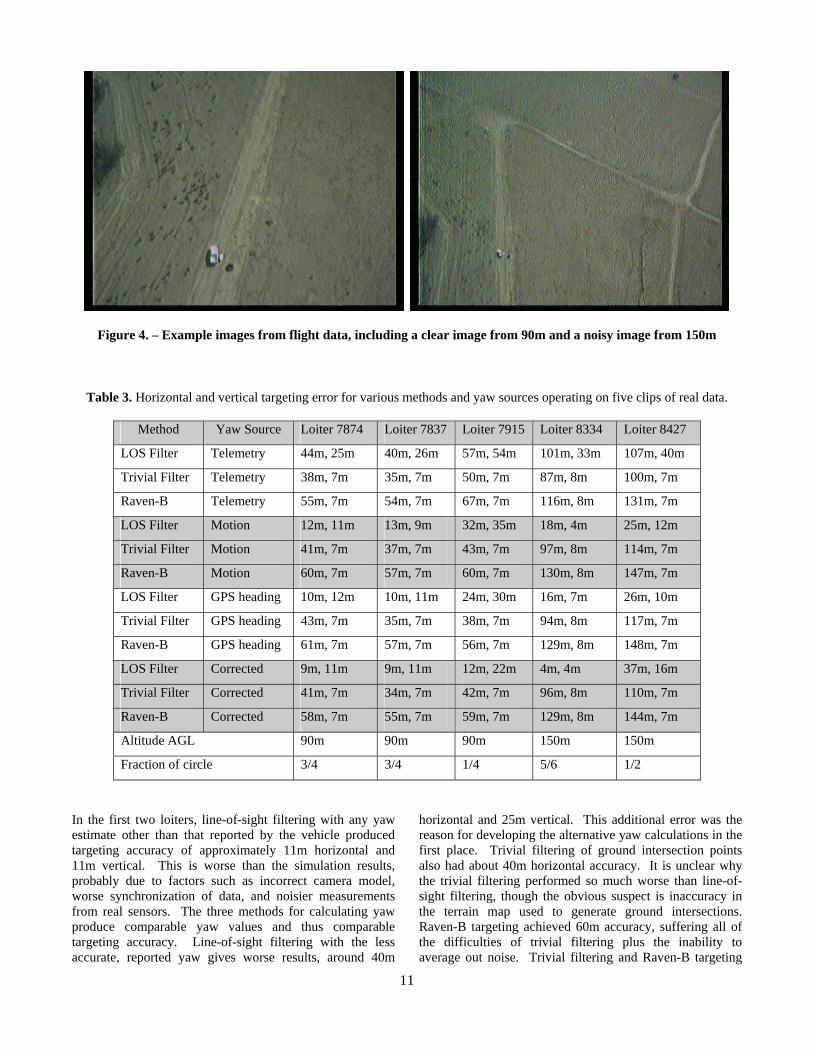
We tested algorithms on 5 clips from the flight data, each representing a circle or fraction of a circle around the target (the large tire). Figure 4 shows example images from the video stream. Table 3 shows the accuracy of each type of targeting on the 5 loiters. It also shows the altitude of the vehicle above ground and the fraction of a circle completed during the clip.
11
Figure 4. – Example images from flight data, including a clear image from 90m and a noisy image from 150m
Table 3. Horizontal and vertical targeting error for various methods and yaw sources operating on five clips of real data.
Method Yaw Source Loiter 7874 Loiter 7837 Loiter 7915 Loiter 8334 Loiter 8427
LOS Filter Telemetry 44m, 25m 40m, 26m 57m, 54m 101m, 33m 107m, 40m
Trivial Filter Telemetry 38m, 7m 35m, 7m 50m, 7m 87m, 8m 100m, 7m
Raven-B Telemetry 55m, 7m 54m, 7m 67m, 7m 116m, 8m 131m, 7m
LOS Filter Motion 12m, 11m 13m, 9m 32m, 35m 18m, 4m 25m, 12m
Trivial Filter Motion 41m, 7m 37m, 7m 43m, 7m 97m, 8m 114m, 7m
Raven-B Motion 60m, 7m 57m, 7m 60m, 7m 130m, 8m 147m, 7m
LOS Filter GPS heading 10m, 12m 10m, 11m 24m, 30m 16m, 7m 26m, 10m
Trivial Filter GPS heading 43m, 7m 35m, 7m 38m, 7m 94m, 8m 117m, 7m
Raven-B GPS heading 61m, 7m 57m, 7m 56m, 7m 129m, 8m 148m, 7m
LOS Filter Corrected 9m, 11m 9m, 11m 12m, 22m 4m, 4m 37m, 16m
Trivial Filter Corrected 41m, 7m 34m, 7m 42m, 7m 96m, 8m 110m, 7m
Raven-B Corrected 58m, 7m 55m, 7m 59m, 7m 129m, 8m 144m, 7m
Altitude AGL 90m 90m 90m 150m 150m
Fraction of circle 3/4 3/4 1/4 5/6 1/2
In the first two loiters, line-of-sight filtering with any yaw estimate other than that reported by the vehicle produced targeting accuracy of approximately 11m horizontal and 11m vertical. This is worse than the simulation results, probably due to factors such as incorrect camera model, worse synchronization of data, and noisier measurements from real sensors. The three methods for calculating yaw produce comparable yaw values and thus comparable targeting accuracy. Line-of-sight filtering with the less accurate, reported yaw gives worse results, around 40m
horizontal and 25m vertical. This additional error was the reason for developing the alternative yaw calculations in the first place. Trivial filtering of ground intersection points also had about 40m horizontal accuracy. It is unclear why the trivial filtering performed so much worse than line-of-sight filtering, though the obvious suspect is inaccuracy in the terrain map used to generate ground intersections. Raven-B targeting achieved 60m accuracy, suffering all of the difficulties of trivial filtering plus the inability to average out noise. Trivial filtering and Raven-B targeting
12
always found a 7m vertical error, perhaps a result of surveying the target at one time with one GPS receiver and flying at another time with another receiver, or perhaps a result of altimeter calibration.
The third loiter was only about ¼ of an orbit. Raven-B and trivial filtering results are comparable to those of the first two loiters for calculated yaw sources and worse when using reported yaw. This suggests that these methods may reach full accuracy within ¼ loiter when provided with reasonable yaw estimates. Or, it may suggest that the error due to a weak terrain map masks other sources. Accuracy for line-of-sight filtering diminishes for all yaw sources, compared with the other, longer loiters. This is likely due to the presence of biases that can only be averaged out as the target is seen observed over a fuller arc. Line-of-sight filtering produced horizontal accuracy noticeably better than the other two methods except when using reported yaw, where the error from incorrect yaw masked any benefit to be gained by not relying on the terrain map.
The fourth loiter was a nearly complete circle at 2/3 higher altitude. Targeting errors for line-of-sight filtering with yaw from GPS or consecutive vehicle positions increased 66% as well. This suggests that the primary error source is angular error, now scaled by a 66% longer lever arm (altitude). Horizontal errors for Raven-B targeting and trivial filtering increased by more than double compared to the first two loiters, indicating some additional error source. One clue may be that, for this loiter only, these methods found the target to be one meter lower (higher magnitude) than in all of the other loiters. Perhaps, flying in a wider circle, the vehicle began over a different area of the terrain map and started with a different estimate of its initial altitude above ground. If this is true, then perhaps errors in the terrain map contributed to increased overshoot of lines of sight being intersected with the terrain map and explain some more of the horizontal error. Line-of-sight filtering with reported yaw showed the same doubling of horizontal error, but also did a terrible job of recovering vertical target location, indicating significant pointing error, which may explain the
poor horizontal accuracy. The impressive results of line-of-sight filtering using magnetometer-corrected yaw is likely a spurious result. The insight to be gained from this loiter is that horizontal targeting error is lowest for line-of-sight filtering and (expectably) proportional to altitude.
The final loiter is a half circle at 150m. Results are worse overall compared to the fourth loiter, presumably due to more noise in the estimates of camera pointing angles – being only ½ arc rather than a full arc should have no effect on Raven-B targeting accuracy. Line-of-sight and trivial filtering should perform worse based on lines of sight from only a half-loiter. Line-of-sight filtering with yaw derived from GPS heading or vehicle positions did show this effect, but if it occurred with trivial filtering, it was completely masked by the extra noise that affected Raven-B targeting.
Structure from Motion
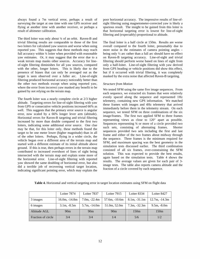
We tested SFM using the same five image sequences. From each sequence, we extracted six frames that were relatively evenly spaced along the sequence and represented 1Hz telemetry, containing new GPS information. We matched these frames with images and 4Hz telemetry that arrived immediately before them in the telemetry stream. On each sequence, we tested SFM on three combinations of the six image/frames. The first two applied SFM to three frames representing views as close to 120° apart as possible. Sequences representing ¾ or more of a circle provided two such sets, consisting of alternating frames. Shorter sequences provided two sets including the first and last frame and either of the two frames about midway through the sequence. Three frames is the minimum required for SFM, and maximum spacing was the best geometry in the simulation tests discussed earlier. The third combination consisted of all six frames, over-constraining the SFM solution. This was expected to provide the best results, again based on the simulation tests. Table 4 shows the results. The average values are given for each pair of 3-image tests. The table also reports camera altitude and the fraction of a circle covered by each sequence.
Table 4. Horizontal and vertical targeting error in target location estimates using SFM on flight data
Loiter 7874 Loiter 7837 Loiter 7915 Loiter 8334 Loiter 8427
3 images 16.0m, -14.8m 7.0m, -22.4m 57.6m, -10.6m 8.1m, -31.1m 12.7m, -14.3m
6 images 3.1m, -8.5m 5.7m, -14.0m 51.0m, 52.0m 7.3m, -32.3m 9.5m, -8.0m
Altitude AGL 90m 90m 90m 150m 150m
Fraction of circle 3/4 3/4 1/4 5/6 1/2
13
On the first two loiters, SFM recovered target positions with impressive horizontal accuracy around 10m for 3-frame SFM and 5m for over-constrained, 6-frame SFM. The combination of SFM and filtering clearly outperformed line-of-sight filtering alone. The third loiter produced terrible results, underperforming the other targeting methods. This has two obvious, potential explanations, both of which may apply. First, the GPS readings may have been particularly poorly synchronized to the imagery. Second, a ¼ circle may not provide diverse enough viewpoints to triangulate the target position. Both of these factors would account for the poor performance of all methods and the exceptionally poor performance of SFM, which relies most heavily on GPS. The problem with the third loiter was not the choice of targets, as the same targets were used for the first and third loiters.
The two high-altitude loiters kept accuracy to around 10m, using three or six images. This shows huge improvement compared to the other targeting methods. As with the other methods, angular error due to imprecision in selecting target coordinates produces a targeting error that scales with altitude and may account for the increased targeting error in the 6-image SFM at the higher altitudes. The improved performance of 3-frame SFM at the higher altitude may be because any random GPS error represents a smaller fraction of the distances between cameras and targets.
In summary, over-constrained SFM operating on real data estimates target horizontal position about twice as accurately as does line-of-sight filtering for loiters covering at least half a circle. SFM using only three images maintains this lead at high altitude and performs comparably to line-of-sight filtering at low altitude. SFM does a worse job overall of recovering target vertical position, which seems less important. SFM may require more processing than anticipated, as it can be difficult to find three targets that appear in all 3 or 6 images of the nearly-full-circle loiters that give the best results.
7. FLIGHT TEST 2
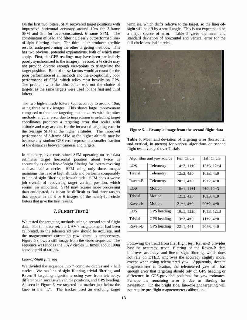
We tested the targeting methods using a second set of flight data. For this data set, the UAV’s magnetometer had been calibrated, so the telemetered yaw should be accurate, and the magnetometer correction yaw source is unnecessary. Figure 5 shows a still image from the video sequence. The sequence was shot as the UAV circles 11 times, about 100m above a grid of targets.
Line-of-Sight filtering
We divided the sequence into 7 complete circles and 7 half circles. We ran line-of-sight filtering, trivial filtering, and Raven-B targeting algorithms using yaw from telemetry, difference in successive vehicle positions, and GPS heading. As seen in Figure 5, we targeted the marker just below the knee in the “L”. The tracker used an evolving target
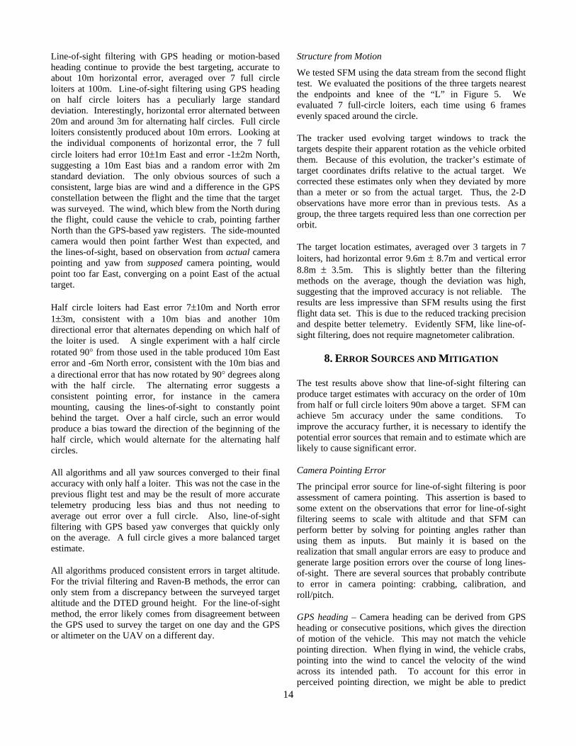
template, which drifts relative to the target, so the lines-of-sight will be off by a small angle. This is not expected to be a major source of error. Table 5 gives the mean and standard deviation of horizontal and vertical error for the full circles and half circles.
Figure 5. – Example image from the second flight data
Table 5. Mean and deviation of targeting error (horizontal and vertical, in meters) for various algorithms on second flight test, averaged over 7 trials
Algorithm and yaw source Full Circle Half Circle
LOS Telemetry 14±2, 11±0 13±3, 12±4
Trivial Telemetry 12±2, 4±0 10±3, 4±0
Raven-B Telemetry 20±1, 4±0 19±2, 4±0
LOS Motion 10±1, 11±1 9±2, 12±3
Trivial Motion 12±2, 4±0 10±3, 4±0
Raven-B Motion 21±1, 4±0 20±2, 4±0
LOS GPS heading 10±1, 12±0 10±8, 12±3
Trivial GPS heading 13±2, 4±0 11±2, 4±0
Raven-B GPS heading 22±1, 4±1 20±3, 4±0
Following the trend from first flight test, Raven-B provides baseline accuracy, trivial filtering of the Raven-B data improves accuracy, and line-of-sight filtering, which does not rely on DTED, improves the accuracy slightly more, except when using telemetered yaw. Apparently, despite magnetometer calibration, the telemetered yaw still has enough error that targeting should rely on GPS heading or difference in GPS-provided positions for yaw estimates. Perhaps the remaining error is due to filtering for navigation. On the bright side, line-of-sight targeting will not require pre-flight magnetometer calibration.
14
Line-of-sight filtering with GPS heading or motion-based heading continue to provide the best targeting, accurate to about 10m horizontal error, averaged over 7 full circle loiters at 100m. Line-of-sight filtering using GPS heading on half circle loiters has a peculiarly large standard deviation. Interestingly, horizontal error alternated between 20m and around 3m for alternating half circles. Full circle loiters consistently produced about 10m errors. Looking at the individual components of horizontal error, the 7 full circle loiters had error 10±1m East and error -1±2m North, suggesting a 10m East bias and a random error with 2m standard deviation. The only obvious sources of such a consistent, large bias are wind and a difference in the GPS constellation between the flight and the time that the target was surveyed. The wind, which blew from the North during the flight, could cause the vehicle to crab, pointing farther North than the GPS-based yaw registers. The side-mounted camera would then point farther West than expected, and the lines-of-sight, based on observation from actual camera pointing and yaw from supposed camera pointing, would point too far East, converging on a point East of the actual target.
Half circle loiters had East error 7±10m and North error 1±3m, consistent with a 10m bias and another 10m directional error that alternates depending on which half of the loiter is used. A single experiment with a half circle rotated 90° from those used in the table produced 10m East error and -6m North error, consistent with the 10m bias and a directional error that has now rotated by 90° degrees along with the half circle. The alternating error suggests a consistent pointing error, for instance in the camera mounting, causing the lines-of-sight to constantly point behind the target. Over a half circle, such an error would produce a bias toward the direction of the beginning of the half circle, which would alternate for the alternating half circles.
All algorithms and all yaw sources converged to their final accuracy with only half a loiter. This was not the case in the previous flight test and may be the result of more accurate telemetry producing less bias and thus not needing to average out error over a full circle. Also, line-of-sight filtering with GPS based yaw converges that quickly only on the average. A full circle gives a more balanced target estimate.
All algorithms produced consistent errors in target altitude. For the trivial filtering and Raven-B methods, the error can only stem from a discrepancy between the surveyed target altitude and the DTED ground height. For the line-of-sight method, the error likely comes from disagreement between the GPS used to survey the target on one day and the GPS or altimeter on the UAV on a different day.
Structure from Motion
We tested SFM using the data stream from the second flight test. We evaluated the positions of the three targets nearest the endpoints and knee of the “L” in Figure 5. We evaluated 7 full-circle loiters, each time using 6 frames evenly spaced around the circle.
The tracker used evolving target windows to track the targets despite their apparent rotation as the vehicle orbited them. Because of this evolution, the tracker’s estimate of target coordinates drifts relative to the actual target. We corrected these estimates only when they deviated by more than a meter or so from the actual target. Thus, the 2-D observations have more error than in previous tests. As a group, the three targets required less than one correction per orbit.
The target location estimates, averaged over 3 targets in 7 loiters, had horizontal error 9.6m ± 8.7m and vertical error 8.8m ± 3.5m. This is slightly better than the filtering methods on the average, though the deviation was high, suggesting that the improved accuracy is not reliable. The results are less impressive than SFM results using the first flight data set. This is due to the reduced tracking precision and despite better telemetry. Evidently SFM, like line-of-sight filtering, does not require magnetometer calibration.
8. ERROR SOURCES AND MITIGATION
The test results above show that line-of-sight filtering can produce target estimates with accuracy on the order of 10m from half or full circle loiters 90m above a target. SFM can achieve 5m accuracy under the same conditions. To improve the accuracy further, it is necessary to identify the potential error sources that remain and to estimate which are likely to cause significant error.
Camera Pointing Error
The principal error source for line-of-sight filtering is poor assessment of camera pointing. This assertion is based to some extent on the observations that error for line-of-sight filtering seems to scale with altitude and that SFM can perform better by solving for pointing angles rather than using them as inputs. But mainly it is based on the realization that small angular errors are easy to produce and generate large position errors over the course of long lines-of-sight. There are several sources that probably contribute to error in camera pointing: crabbing, calibration, and roll/pitch.
GPS heading – Camera heading can be derived from GPS heading or consecutive positions, which gives the direction of motion of the vehicle. This may not match the vehicle pointing direction. When flying in wind, the vehicle crabs, pointing into the wind to cancel the velocity of the wind across its intended path. To account for this error in perceived pointing direction, we might be able to predict
15
crabbing using filter states if wind is constant and crab amount is a function of wind speed and direction. Also, it is unclear how GPS heading is determined. Perhaps it uses very accurate GPS velocity measurements. Perhaps it fits a curve to the last several GPS positions. Finding the details of the algorithm would allow more intelligent use of the provided heading.
Extrinsics Calibration – The vehicle and targeting code assumes that the camera is mounted pointing 90° left of vehicle forward and pitched down 30°. If this mounting were imprecise, line-of-sight pointing would be off by some constant angle. The mount does not look very rigid and it is unclear to what tolerance the camera is mounted and to what tolerance the Raven-B’s removable nose cone is attached to the vehicle. Further, based on calibration of one Raven-B side camera and examining the specifications for the camera detector and mounting hardware, it is clear that the optical axis of the camera diverges from the nominal mounting axis by several degrees. It might be a good idea to identify the exact pointing angle, either through some pre-flight calibration procedure or through additional filter bias states that could identify consistent pointing error over the course of a loiter and then remove these biases from later measurements in order to converge more quickly to a target estimate.
Pitch and Roll Filtering – The targeting system currently uses low-pass filtered estimates of camera roll and pitch from 4Hz telemetry. The filtering suppresses quick attitude changes that may be needed to correctly plot lines-of-sight. The targeting system might benefit from deriving the angles from vehicle roll and pitch, which are unfiltered and present in the same stream. A better solution could be to incorporate high rate (>10Hz) attitude estimates from a traditional, onboard GPS/INS navigator if one were available on a future vehicle.
Synchronization
Calculating lines-of-sight from imagery presupposes that images, camera pointing angles, and GPS positions are all synchronized. Our input data stream is unsynchronized, so our measurements represent noisy approximations of the true values at a common point in time. From early in the project, this was expected to be a major error source.
It appears that GPS messages are delayed by about ½ second compared to the camera-pointing-angles telemetry and the imagery. In a circular loiter, the synchronization error would cause lines-of-sight to lead the target. Circling at 5° per second at 100m altitude, the lead is about 7.5m. This may cancel over a full circle, though it may add some random error. In a half-circle loiter, it would cause a bias. This delay could be removed by holding observations and pointing angles for ½ second until matching GPS is available to process them. In addition to the ½ second delay, there is up to ¼-second synchronization uncertainty
in between imagery, camera angle telemetry, and GPS. Targets moving about one pixel per frame could produce nearly ½ degree of error in line-of-sight direction.
Work is currently underway to make the next generation Raven time tag imagery and telemetry from a common clock, which will allow the data sources to be synchronized. In the mean time, SFM avoids the need for synchronized camera angles and could be reformulated to refine the GPS positions, thus relying less on GPS synchronization.
Target Selection and Tracking Error
There are three potential error sources associated with target selection and tracking. None of them likely contributed much to the observed errors. The first error source is error in tracking the targets. The tracker recovers the target’s pixel coordinates with accuracy of a fraction of a pixel, which should be dwarfed by errors in synchronization and camera pointing. The second error source is the inability of the user to click directly on the desired target. If the user has a meaningful target in mind, this error should be on the order of just a few pixels, centered on the actual target. At 100m altitude with the target near image center, this would contribute less than 1m error.
The third source is tendency of the tracker to slowly wander away from the designated target over time as the target’s appearance changes. In the simulation and first flight experiments above, the tracker rejected the target before it could change significantly, thus preventing any wandering. The tracker rejected the target about every 60 frames, which is about every 10° of rotation, about every 2 seconds of video. Re-designating targets every 2 seconds would constitute an unacceptable burden on the user. Thus, we repeated the simulation and first flight experiments using the non-SFM targeting methods and allowing the tracker to evolve the target appearance after tracking into each new image. The evolving target appearance allows the tracker to overcome slow target rotation induced by circular loitering but it should also cause the tracking to drift from the original target, producing an effective tracking error. Table 6 shows the impact of letting targets evolve and drift.
On the average, the baseline tracker in the original experiments required the user to re-designate the target about once every 60 frames. In the five tests on flight data, the tracker never identified an obviously incorrect target location; so it is possible that the residual threshold was set unnecessarily low, causing the tracker to prematurely reject the target. In three tests on simulation data, the tracker wandered away from the target twice, so that tracking was blatantly incorrect in several images before the target was eventually rejected. However, in both cases only one telemetry frame (and thus one line-of-sight) was affected, and neither had any obvious effect on accuracy, so it was unnecessary for the user to correct the error.
16
Table 6. Evolving templates drastically reduce number of user interventions
Data set Number of images Number of user interventions with normal templates
Number of user interventions with evolving templates
Impact of evolving templates on
horizontal error
Loiter 7874 927 15 1 None
Loiter 7837 842 10 1 None
Loiter 7915 315 6 1 None
Loiter 8334 2563 27 1 +1m
Loiter 8427 1351 22 1 +3m
Sim full circle ~2070 37 6 +1m
When evolving templates were used to track targets in flight data, the tracker always wandered from the target, but in the three loiters at 90m, the target only wandered a few meters over the course of the clip and did not add any detectable error. That is, over three targeting algorithms and four yaw sources, the change in final targeting accuracy was within the frame-to-frame noise. At 150m altitude, the target migrated several meters over the course of the loiters, but this still only added a few meters to the targeting error. Specifically, one loiter had error increase by approximately 1m for all three algorithms and four yaw sources, while the other loiter had error increase by about 3m for each test. The best algorithm/yaw combination gave 25m of error in this final test, so the 3m-error is a small player in the error budget. In simulation, the trackers quickly wandered away from the target, requiring the user to stop the tracker and re-designate the target 5-6 times during the full-circle loiter. For all three simulation targets and all yaw sources, horizontal error was 2-3m for line-of-sight filtering, 1-2m for trivial filtering, and 5-6m for Raven-B targeting. Adding the evolving target window has added about 1m of error to line-of-sight filtering, added 2m of error to trivial filtering, and left Raven-B filtering unchanged.
After the success of this experiment, the second flight test was conducted using only the evolved templates. This had no obvious effect on the filtering algorithms though it apparently decreased the accuracy of SFM. The SFM test required a small number of target re-designations over the course of the 7 loiters. Most of these were for the target at the end of the “L” in the images. This feature is the only feature in all of the flight tests that was not an isolated blob. The lack of rotational symmetry makes it difficult for the tracker to stay attached as the target rotates. If such features are to be used frequently, a more complex tracker [8] that explicitly handles rotation may be in order. The targets in the simulation video also were not isolated blobs and also required significant user intervention, but they involve
significant 3-D structure and probably will continue to require user intervention.
Filter Tuning
In simulation, line-of-sight filtering converged to about 1m of apparently random, horizontal error. This is not a major error source, but it may be worth tuning the parameters of the filter to anticipate the amount of noise in the measurements and thus perhaps reduce this error.
Lack of Diversity
Trivial filtering, line-of-sight filtering, and SFM all benefit from having multiple observations spread around at least half a circle and preferably close to a full circle. Otherwise, when observations are taken from nearby locations, the lines of sight all have a strong common component along which the target cannot be localized.
SFM benefits from using more than the minimum number of images. The additional images provide filtering which allows the error in individual measurements to be averaged out.
Position Error
Any GPS error that is relatively constant over the flight will simply add to targeting error. Such error is already accounted for in the experiments in this paper, as the target locations were not surveyed at the time of the flight. Perhaps the experiments should be redone using flight data where the targets were surveyed at the time of the flight, so that GPS “bias” can be accounted for separately from other errors. It is unclear whether some difference between the vehicle’s GPS and the GPS used for target surveying accounts for SFM and line-of-sight targeting consistently finding the target about 10m under ground when processing real data
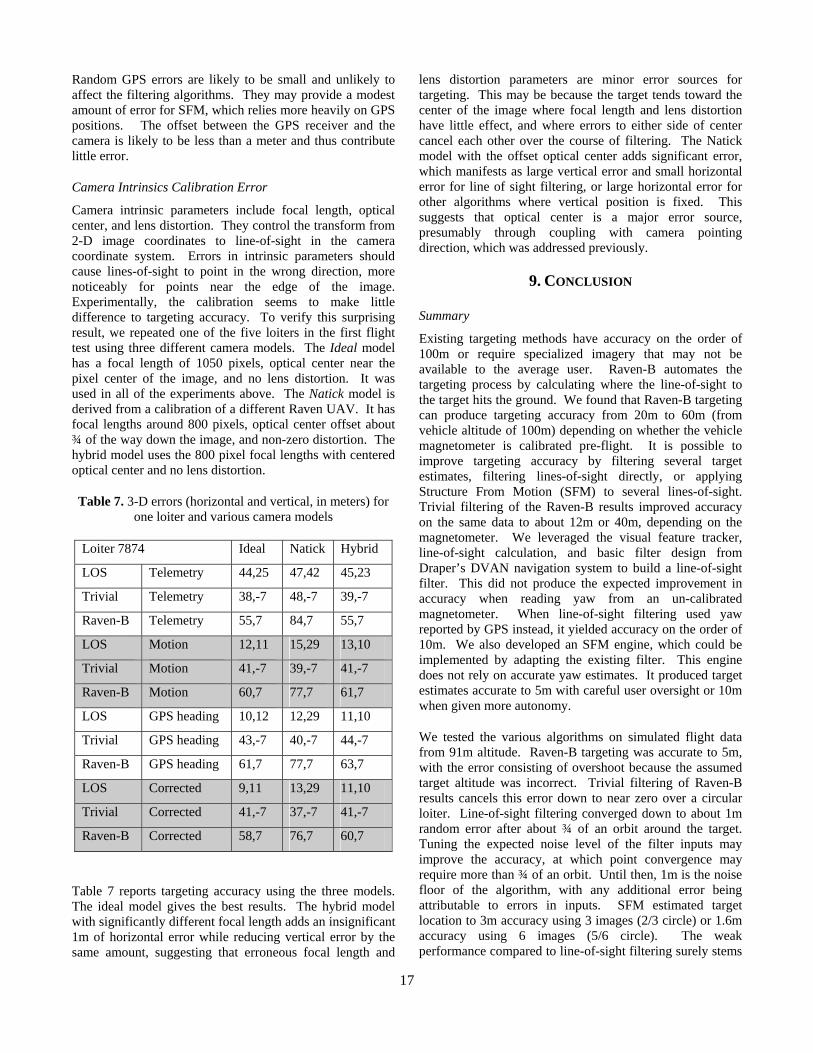
17
Random GPS errors are likely to be small and unlikely to affect the filtering algorithms. They may provide a modest amount of error for SFM, which relies more heavily on GPS positions. The offset between the GPS receiver and the camera is likely to be less than a meter and thus contribute little error.
Camera Intrinsics Calibration Error
Camera intrinsic parameters include focal length, optical center, and lens distortion. They control the transform from 2-D image coordinates to line-of-sight in the camera coordinate system. Errors in intrinsic parameters should cause lines-of-sight to point in the wrong direction, more noticeably for points near the edge of the image. Experimentally, the calibration seems to make little difference to targeting accuracy. To verify this surprising result, we repeated one of the five loiters in the first flight test using three different camera models. The Ideal model has a focal length of 1050 pixels, optical center near the pixel center of the image, and no lens distortion. It was used in all of the experiments above. The Natick model is derived from a calibration of a different Raven UAV. It has focal lengths around 800 pixels, optical center offset about ¾ of the way down the image, and non-zero distortion. The hybrid model uses the 800 pixel focal lengths with centered optical center and no lens distortion.
Table 7. 3-D errors (horizontal and vertical, in meters) for one loiter and various camera models
Loiter 7874 Ideal Natick Hybrid
LOS Telemetry 44,25 47,42 45,23
Trivial Telemetry 38,-7 48,-7 39,-7
Raven-B Telemetry 55,7 84,7 55,7
LOS Motion 12,11 15,29 13,10
Trivial Motion 41,-7 39,-7 41,-7
Raven-B Motion 60,7 77,7 61,7
LOS GPS heading 10,12 12,29 11,10
Trivial GPS heading 43,-7 40,-7 44,-7
Raven-B GPS heading 61,7 77,7 63,7
LOS Corrected 9,11 13,29 11,10
Trivial Corrected 41,-7 37,-7 41,-7
Raven-B Corrected 58,7 76,7 60,7
Table 7 reports targeting accuracy using the three models. The ideal model gives the best results. The hybrid model with significantly different focal length adds an insignificant 1m of horizontal error while reducing vertical error by the same amount, suggesting that erroneous focal length and
lens distortion parameters are minor error sources for targeting. This may be because the target tends toward the center of the image where focal length and lens distortion have little effect, and where errors to either side of center cancel each other over the course of filtering. The Natick model with the offset optical center adds significant error, which manifests as large vertical error and small horizontal error for line of sight filtering, or large horizontal error for other algorithms where vertical position is fixed. This suggests that optical center is a major error source, presumably through coupling with camera pointing direction, which was addressed previously.
9. CONCLUSION
Summary
Existing targeting methods have accuracy on the order of 100m or require specialized imagery that may not be available to the average user. Raven-B automates the targeting process by calculating where the line-of-sight to the target hits the ground. We found that Raven-B targeting can produce targeting accuracy from 20m to 60m (from vehicle altitude of 100m) depending on whether the vehicle magnetometer is calibrated pre-flight. It is possible to improve targeting accuracy by filtering several target estimates, filtering lines-of-sight directly, or applying Structure From Motion (SFM) to several lines-of-sight. Trivial filtering of the Raven-B results improved accuracy on the same data to about 12m or 40m, depending on the magnetometer. We leveraged the visual feature tracker, line-of-sight calculation, and basic filter design from Draper’s DVAN navigation system to build a line-of-sight filter. This did not produce the expected improvement in accuracy when reading yaw from an un-calibrated magnetometer. When line-of-sight filtering used yaw reported by GPS instead, it yielded accuracy on the order of 10m. We also developed an SFM engine, which could be implemented by adapting the existing filter. This engine does not rely on accurate yaw estimates. It produced target estimates accurate to 5m with careful user oversight or 10m when given more autonomy.
We tested the various algorithms on simulated flight data from 91m altitude. Raven-B targeting was accurate to 5m, with the error consisting of overshoot because the assumed target altitude was incorrect. Trivial filtering of Raven-B results cancels this error down to near zero over a circular loiter. Line-of-sight filtering converged down to about 1m random error after about ¾ of an orbit around the target. Tuning the expected noise level of the filter inputs may improve the accuracy, at which point convergence may require more than ¾ of an orbit. Until then, 1m is the noise floor of the algorithm, with any additional error being attributable to errors in inputs. SFM estimated target location to 3m accuracy using 3 images (2/3 circle) or 1.6m accuracy using 6 images (5/6 circle). The weak performance compared to line-of-sight filtering surely stems
18
from using so few images and thus having little ability to cancel out noise.
We tested the algorithms again on flight data that had terrible yaw readings because the magnetometer had not been calibrated. This is a credible operational scenario with which targeting must cope. All forms of targeting except for SFM performed terribly, with 35m accuracy for the best single data point. We adapted the algorithms to read yaw from GPS heading messages, at which point line-of-sight filtering produced target estimates accurate to 10m from 91m altitude from a nearly full circle loiter, proportionately worse at higher altitude, and significantly worse from less of a loiter. We also tested deriving yaw from difference in consecutive GPS positions, but the resulting targeting was less accurate. Raven-B targeting and trivial filtering thereof provided 60m and 40m accuracy and showed no improvement with the better yaw estimate. Their errors may be due to a poor terrain map. SFM provided the best results, with approximately 6m error when using 6 images or 10m error when using 3 images. The additional error compared to simulation comes from poor synchronization of imagery with GPS. SFM proved to be the accuracy leader, though it was difficult to apply, as it was difficult to find 3 targets that were visible in the 6 images.
We tested the algorithms again on flight data with better yaw readings. Results were qualitatively similar to those of the first flight test. Raven-B targeting gave baseline results (20m accuracy) independent of the yaw source. Trivial filtering of Raven-B outputs gave better results (12m accuracy) independent of the yaw source. Line-of-sight filtering gave relatively weak results using reported yaw and the best results so far (10m accuracy) using yaw from GPS heading or subtracting consecutive positions. The 10m error in GPS-fed line-of-sight filtering was a consistent bias over 7 tests, suggesting a bias source such as wind-induced crabbing that might be estimated and removed in the future. Half circle loiters on the same test data tended to produce slightly better targeting results for all methods, which was unexpected. Further investigation with the GPS-fed line-of-sight filtering showed that alternating half circles had errors near 0m and 20m consistently, again showing a bias, but this time depending on the direction of travel, again consistent with wind. SFM with sets of 6 images recovered the target to 10m accuracy, comparable to line-of-sight filtering, but this was in large part due to poor target tracking. A better tracker or more diligence by the user in keeping the tracker on the three targets would have cut that error in half.
Recommendations for Future Work
The project described in this paper is on-going. Remaining work will focus in part on mitigating the limitations in accuracy and usability identified by the testing described in the paper. The following are a few specific directions.
The primary direction is to investigate and reduce the error associated with camera pointing angles, which is expected to be the primary error source for line-of-sight filtering. One change is to allow the filter to estimate and remove biases. Another is to investigate the 10m targeting bias observed in the second data set and determine whether it can be eliminated by letting the filter estimate crabbing-induced bias, which is not a fixed bias but rather varies with vehicle orientation. Perhaps the filter can read wind speed and direction from the navigator. Another error-reducing goal is to tune the filter to expect the observed amounts of input noise, and to verify that the filter outputs reasonable uncertainty bounds. A third error-tuning goal is to modify the code to take into account the ½ second delay between GPS and other data.
A second direction is to implement SFM, which as of the current testing was the most accurate targeting method. It would be implemented as a filter by re-enabling components of the existing targeting filter that were disabled to prevent the filter from acting as a navigator. Filtering should reduce the (apparent) primary source of SFM error, namely the reliance on a small number of lines of sight. The principal obstacle in this task will be to automatically identify three targets that appear in most images across a full circle loiter.
A third direction is to improve the feature tracker. The current tracker can be configured to either reject targets many times during a circular loiter or drift from the target during that loiter. A stronger tracker [8] could follow the target despite rotation. The feature should be further improved to recover features that leave the image or are obscured by noise but then reappear later.
ACKNOWLEDGEMENT
We would like to thank Natick Soldier RDEC and AeroVironment, Inc. for supporting the work described in this paper. We would also like to thank the other members of the software development team, including Kyle Bailey of AeroVironment and Kai Angermueller, Scott Rasmussen, and John Scudiere of Draper Laboratory.
This document reports research undertaken at the U.S. Army Natick Soldier Research, Development and Engineering Center, Natick, MA, and has been assigned No. NATICK/TP-08/001 in a series of papers approved for publication.
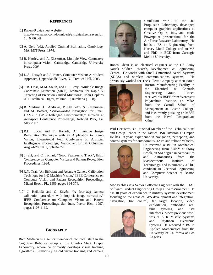
19
REFERENCES
[1] Raven-B data sheet website http://www.avinc.com/downloads/av_datasheet_raven_b_10_6_06.pdf
[2] A. Gelb (ed.), Applied Optimal Estimation, Cambridge, MA: MIT Press, 1974.
[3] R. Hartley, and A. Zisserman, Multiple View Geometery in computer vision, Cambridge: Cambridge University Press, 2003.
[4] D.A. Forsyth and J. Ponce, Computer Vision: A Modern Approach, Upper Saddle River, NJ: Prentice Hall, 2003.
[5] T.B. Criss, M.M. South, and L.J. Levy, “Multiple Image Coordinate Extraction (MICE) Technique for Rapid 5. Targeting of Precision Guided Munitions”, John Hopkins APL Technical Digest, volume 19, number 4 (1998).
[6] R. Madison, G. Andrews, P. DeBitetto, S. Rasmussen, and M. Bottkol, “Vision-Aided Navigation for Small UAVs in GPS-Challenged Environments,” Infotech at Aerospace Conference Proceedings, Rohnert Park, Ca, May 2007.
[7] B.D. Lucas and T. Kanade, An Iterative Image Registration Technique with an Application to Stereo Vision, International Joint Conference on Artificial Intelligence Proceedings, Vancouver, British Columbia, Aug 24-28, 1981, pp674-679.
[8] J. Shi, and C. Tomasi, “Good Features to Track”, IEEE Conference on Computer Vision and Pattern Recognition Proceedings, 1994.
[9] R.Y. Tsai, “An Efficient and Accurate Camera Calibration Technique for 3-D Machine Vision,” IEEE Conference on Computer Vision and Pattern Recognition Proceedings, Miami Beach, FL, 1986, pages 364-374.
[10] J. Heikkilä and O. Silvén, “A four-step camera calibration procedure with implicit image correction,” IEEE Conference on Computer Vision and Pattern Recognition Proceedings, San Juan, Puerto Rico, 1997, pages 1106-1112.
BIOGRAPHY
Rich Madison is a senior member of technical staff in the Cognitive Robotics group at the Charles Stark Draper Laboratory, where he primarily develops visual tracking algorithms. Previously he did visual tracking and camera
simulation work at the Jet Propulsion Laboratory, developed computer graphics applications at Creative Optics, Inc., and made Powerpoint presentations for the Air Force Research Laboratory. He holds a BS in Engineering from Harvey Mudd College and an MS and PhD in ECE from Carnegie Mellon University.
Rocco Olean is an electrical engineer at the US Army Natick Soldier Research, Development & Engineering Center. He works with Small Unmanned Aerial Systems (SUAS) and wireless communications systems. He previously worked for The Gillette Company at their South
Boston Manufacturing Facility in the Electrical & Controls Engineering Group. Rocco received his BSEE from Worcester Polytechnic Institute, an MBA from the Carroll School of Management at Boston College, and is currently pursuing an MSSE from the Naval Postgraduate School.
Paul DeBitetto is a Principal Member of the Technical Staff and Group Leader in the Tactical ISR Division at Draper. He has 19 years experience in navigation, perception, and control systems for autonomous UAVs and robotic vehicles.
He received a BE in Mechanical Engineering from SUNY at Stony Brook, an SM degree in Aeronautics and Astronautics from the Massachusetts Institute of Technology, and is currently a PhD candidate in Electrical Engineering and Computer Science at Boston University.
Mac Peebles is a Senior Software Engineer with the SUAS Software Product Engineering Group at AeroVironment. He has 10 years of experience in military systems development focusing on the areas of GPS development and integration, navigation, fire control, far target location, video
exploitation, embedded real time systems, and user interfaces. Mac’s previous work was at ATK Missile Systems and Raytheon Electronic Systems. He received a BS in Applied Mathematics from the University of California at Los Angeles.