Developing a Thermometallurgical Model and Furnace

Optimization for Austenitization of Al-Si Coated 22MnB5 Steel

in a Roller Hearth Furnace

by

Mohit Verma

A thesis

Presented to the University of Waterloo

In fulfillment of the

Thesis requirement for the degree of

Master of Applied Science

In

Mechanical and Mechatronics Engineering

Waterloo, Ontario, Canada, 2019

© Mohit Verma 2019

ii

Author’s Declaration

I hereby declare that I am the sole author of this thesis. This is a true copy of the thesis, including

any required final revisions, as accepted by my examiners.

I understand that my thesis may be made electronically available to the public.

iii

Abstract

Lightweighting of vehicles while preserving crash-worthiness, in order to satisfy stringent

restrictions imposed by the government on the automotive industry, has become a sought after

solution which can be realized via hot-forming die quenching (HFDQ). HFDQ is a process where

boron-manganese steel blanks, a grade of ultra-high strength steels with a thin eutectic Al-Si

coating, are heated beyond TAc3 to achieve a fully austenitic microstructure, a precursor for

martensite. Heat treatment is performed using 30 to 40 meter long roller hearth furnaces,

comprised of multiple heating zones, with two key objectives: (1) ensure complete austenitization

of blanks and (2) transformation of the Al-Si coating into a protective Al-Si-Fe intermetallic

coating. Blank heating rates are controlled by the roller speed and zone set-point temperatures,

which are currently set by trial-and-error procedures. Therefore, a thorough understanding of the

furnace parameters and the industrial objectives are essential. Patched blanks, with spatially

varying thickness, leads to inhomogenous heating, making this relationship elusive.

Previous furnace-based energy models only focused on simulating the sensible energy of

the load with no explicit information about the latent energy associated with austenitization.

Consequentially, the latent term had been incorporated into the sensible energy term thereby

defining an effective specific heat. In order to realize how blank heating rate influences

microstructural and Al-Si layer evolution, a model coupling heating and austenite kinetics is

necessary. This integrated model serves as means for optimizing the heating process.

In this work a thermometallurgical model is developed, combining a heat transfer submodel

with two austenite kinetic submodels, an empirical first-order kinetics model and a constitutive

kinetics model, via the latent heat of austenitization. The models simultaneously predict the heating

and austenitization curves, for unpatched/patched blanks heated within a roller hearth furnace.

Validation studies showed that the first-order kinetics model reliably estimated heating and

transformation kinetics compared to the constitutive model.

iv

The validated models are then used to optimize the zone set-point temperatures, roller

speed, and cycle length for a 12-zone roller hearth furnace whilst minimizing the cycle time in a

deterministic setting. A gradient-based interior point method and hybrid scheme were used to

assess the constrained multivariate minimization problem with two alternative austenitization

constraints imposed: a soak-time based and explicitly modeled requirement. In both cases, the

most savings in cycle time were achieved using the explicitly modeled phase fraction austenite

constraint, with reductions of approximately 2 to 3 times from the nominal settings.

v

Acknowledgements

I would like to begin by thanking my supervisor Professor Kyle James Daun, for entrusting me

with such an impactful project. I know that the beginning was rough and tough, in particular the

learning curve I had to exceed over a short period of time, but you never gave up on me and looked

passed my possibly unintelligible questions to help me become a significantly smarter and ethical

engineer. Your enthusiasm for constantly learning, applying concepts and of course radiation heat

transfer definitely rubbed off on me! I was able to learn the importance of being humble,

hardworking, the game changing aspect research has on practical problems, and of course how

vital our decisions are. I look forward to applying these skills, and be as exceptional as you are.

One thing I would like to say is that I was very fortunate and blessed to have you as my MASc.

supervisor! I hope that I was able to exceed your expectations.

Thank you to Professor Richard Culham, my co-supervisor, for reviewing my conference and

journal papers, as well as my thesis. Your constructive comments greatly assisted me with

preparation of this thesis.

I would also like to thank Mr. Cyrus Yao at Promatek Research Center, Mr. Parthkumar Patel and

Mr. Adam Matos, at Formet Industries, for their technical support and allowing us to perform

validation studies with their roller hearth furnace.

I would like to extend a warm gratitude to Mr. Richard Gordon for allowing me to work in his lab

space for my experiments, use of the muffle furnace, and providing the necessary PPE; Mr.

Eckhard Budziarek and Mr. Yuquan Ding for useful advice; Mr. Neil Griffett for assisting with

programing and troubleshooting DAQ issues; and last but not the least the E3 machine shop

technicians, in particular, Mr. Rob Kaptein and Mr. Jorge Cruz for their patience and assistance

with cutting and welding.

A sincere thank you to all of my fellow lab mates and colleagues for not only providing assistance

and creative problem solving techniques, but also for making the two years of my MASc. degree

ones I can never forget! To name just a few: Sina Talebi Moghaddam, Natalie Field, Stephen

vi

Robinson-Enebeli, Samuel Grauer, Timothy Sipkens, Nigel Singh, Paul Hadwin, Roger Tsang,

Rodrigo Miguel, Cory Yan, Ned Zhou, Matthew Ho, Nick Ho, Kaishsiang Lin, Massimo Di Ciano,

and Mark Whitney. A few words:

Sina – You are an amazingly talented researcher and the group’s radiation heat transfer specialist.

Your work ethics, ability to think on the spot, programming skills, and timely assistance was

amazing to experience. Thank you for all the laughter and support you provided! As the group’s

senior PhD, a lot of the wisdom will surely come from you and I know you will do a phenomenal

job!

Stephen – Man …you just started your academic career this term (F’18) but it seems like you have

been here as long as me. Thanks for the encouraging words, late night thrills (the firecracker and

bubble tea incidents), and introduction to the world of fitness “coach”. It is always fun talking with

you and seeing your enthusiasm when it comes to conversing with people (known and unknown)

as well as when you order food! Can’t thank you enough for putting up with me and listening to

my problems hours on end…I’ll miss ya bud! I know you will do a phenomenal job and remember,

“Don’t mess up!”

Tim and Sam – Thanks for being patient with me and taking the time to make sure that I understood

what you were trying to teach me. The both of you are truly brilliant researchers that will make

huge contributions and new set standards in your respective fields, as you already have. I feel that

there are not enough words to describe your amazing qualities and until this day, I cannot say how

thankful I am to have met you two.

Nigel – We did not work together, but the laughter you brought with your funny near death stories,

whenever you dropped by the lab, always lightened the mood!

Paul – First and for most, congratulations on the birth of your daughter! You are a statistical,

optimization, and Bayesian wizard. Thank you for giving me the chance to TA for your course,

enduring my numerous questions, asking me how things are going, and helping me when I looked

like I was stuck.

vii

Roger – The academic life beckoned for you once again, ha-ha. Who knew it would take a loss in

arm wrestling to make me hit the gym and seek redemption, so in that respect, thank you. Thanks

for the funny stories, sarcastic remarks, and insightful information about your experiences and life!

Rodrigo – I enjoyed hearing about your experiences in Brazil and how they compare to the life

here. You are full of persistence, a sign of a great researcher! Thank you for all of your advice

when I got stuck (concept wise and coding). In addition, thanks for always coming to lunch with

me, a true friend, when no one else wanted to go. It is impressive to see you being able to balance

academics with family life!

Cory – You played a vital role in the success of my work; perhaps without your dedication and

assistance I would not be here at this stage writing my thesis. Honestly, we had a lot of funny, very

stressful, and “what the hell…” type of moments. The questions you asked were a sign of how

passionate you are about research, and always forced me to extend my thinking beyond what I

knew in order to try to answer them. It was a pleasure to work with you and see you grow over the

course of two terms. I hope that I was able to teach you a few things just as you had taught me,

and I wish you the very best with your post graduate studies!

Ned – Thanks for being our (Stephen and my) gym buddy, putting up with our ridiculous jokes,

childish behavior in the change room, roasting us, and of course giving valuable advice. I also

wanted to say thanks for listening to me, guiding me through certain situations and remining me

to stop over analyzing things. You’ll do a phenomenal job in the future! Just remember to help

others with chemistry homework and do not leave people hanging *cough cough* ;-)

Kaihsiang – For someone who always says he is stressed, you always manage to pump out high

quality results! You are a compassionate person who truly enjoys research. I know that you miss

your home, but always remember that the group is your second family! You are going to go far in

life, proven by the fact that you are doing a phenomenal job on a research topic that is different

from your Master’s. Trust yourself and make sure to laugh, talk, and have fun in the process!

Massimo – Mass, thank you so much for all your help over the course of my degree, from

answering my questions, listening to me rant about debugging and experimental issues, sending

me useful papers, providing me access to the thermocouple welder, and showing me how to

viii

prepare samples for microscopy. You are a remarkably funny person with a great sense of humor!

Our friendship evolved quickly from acquaintance to great friends, all thanks to the hysterically

funny conversations we had (which I will keep on file in case I need to use it against you in the

future, ha-ha!!). I also wanted to thank you for clearing time in your busy schedule to meet with

me and being strict when it was necessary (definitely helped me grow as an individual and as a

professional). Congratulations once again in securing a job, can you hook a brotha up too ;-p

Mark – Thank you for helping me out on numerous occasions when access to the thermocouple

welder was required; and sharing your insightful experiences about your work and life! It was

always amazing and fun to talk to you (especially the story about relieving sore muscles) I wish

you the very best with you endeavors.

To the other friends from Waterloo, you know who you are, the lunches, dinners, and parties will

forever stay with me; I will dearly miss your companionship. Special shout out to three of my

friends for making the degree worth more than what it is: Henry Ma, Victor Qian, and Natun

Dasgupta.

At this time, I would like to thank my parents, Rajnish and Neelam Verma, for trusting my

judgement about pursuing a Master’s degree, supporting me, and ensuring my best interest.

Without your love and trust, I would not have made it where I am today! It was because of your

constant saying, “learn, learn, and learn”, that I am always hungry to improve my knowledge. I

want to thank god for helping me find this research position, with arguably one of the best

researchers in heat transfer; allowing me to learn life lessons that I could not have learned

anywhere else; for giving me the chance to make strong bonds with so many people; and for giving

me the chance to make valuable contributions to industry and the academic world.

Wow…this acknowledgement is turning into a thesis itself, so I will end now. In closure, I wanted

to say three things that I felt are crucial lessons I learned from this degree:

(1) “Theory catches up to practice.” A saying I did not understand until now.

(2) True understanding comes from making mistakes and not always staying on the safe side.

(3) The source of knowledge is experience.

ix

Dedication

I would like to dedicate this thesis to my friends,

And most importantly my family,

Rajnish, Neelam, and Gourave Verma

x

Table of Contents

Author’s Declaration ............................................................................................................................... ii

Abstract ..................................................................................................................................................... iii

Acknowledgements .................................................................................................................................. v

Dedication ................................................................................................................................................. ix

List of Figures .........................................................................................................................................xiii

List of Tables .......................................................................................................................................... xvii

Nomenclature ........................................................................................................................................ xviii

Chapter One .............................................................................................................................................. 1

Introduction to Hot Forming Die Quenching1

1.1 Hot Forming Die Quenching ...................................................................................................... 1

1.1.2 Heat Treatment .................................................................................................................. 6

1.2 Research Motivation .................................................................................................................. 14

1.3 Models for Steel Reheating Furnaces ...................................................................................... 16

1.4 Thesis Objectives ....................................................................................................................... 18

1.5 Overview of the Thesis .............................................................................................................. 19

Chapter Two ............................................................................................................................................ 20

Furnace Characterization

2.1 Roller Hearth Furnace ............................................................................................................... 20

2.1.1 Furnace Geometry ........................................................................................................... 20

2.1.2 Control Strategy ............................................................................................................... 22

2.1.3 Roller Hearth Furnace Characterization ....................................................................... 22

2.2 Laboratory Muffle Furnace ....................................................................................................... 25

2.2.1 Furnace Geometry ........................................................................................................... 25

2.2.2 Muffle Furnace Characterization .................................................................................. 26

Chapter Three ......................................................................................................................................... 28

Thermometallurgical Model

3.1 Heat Transfer Submodel ............................................................................................................ 28

3.2 Thermophysical Properties of Usibor® 1500AS .................................................................... 33

xi

3.3 Radiative Properties of Usibor® 1500AS ................................................................................ 35

3.4 Non-isothermal Transformation Kinetics Models ................................................................. 37

3.4.1 First-order (F1) Kinetics Model .................................................................................... 39

3.4.2 Phenomenological Austenitization Model ................................................................... 41

3.5 Derivation of the Thermometallurgical Model ...................................................................... 44

3.6 Numerical Implementation ....................................................................................................... 45

3.7 Model Uncertainty Quantification ........................................................................................... 45

Chapter Four ........................................................................................................................................... 47

Experimental and Model Validation

4.1 Laboratory Muffle Furnace ....................................................................................................... 47

4.1.1 Experimental Setup ......................................................................................................... 47

4.1.2 Results and Discussion ................................................................................................... 49

4.2.1 Experimental Setup ......................................................................................................... 55

4.2.2 Results and Discussion ................................................................................................... 56

4.3 Experimental and Validation Summary .................................................................................. 56

Chapter Five ............................................................................................................................................ 59

Furnace Design Optimization

5.1 Design Optimization .................................................................................................................. 59

5.2 Definition of the Design Optimization Problem .................................................................... 60

5.3 Constrained Multivariate Minimization .................................................................................. 62

5.3.1 Gradient-based Interior Point Method .......................................................................... 62

5.3.2 Metaheuristics .................................................................................................................. 68

5.3.2.1 Genetic Algorithm ................................................................................................... 69

5.3.2.2 Remarks on Metaheuristics .................................................................................... 71

5.3.3 Hybrid Method ................................................................................................................ 71

5.4 Results and Discussion .............................................................................................................. 72

5.4.1 Optimal Solution Using the Interior Point Method..................................................... 72

5.5 Summary of the Design Optimization ..................................................................................... 80

Chapter Six .............................................................................................................................................. 81

Conclusion and Future Work

6.1 Conclusion .................................................................................................................................. 81

6.2 Future Work ................................................................................................................................ 82

xii

References ................................................................................................................................................ 84

Appendix A .............................................................................................................................................. 93

Uncertainty Analysis

A.1 Heat Transfer Model ................................................................................................................. 93

A.2 First-order Kinetics Model ....................................................................................................... 95

A.3 Monte Carlo Simulation ........................................................................................................... 96

A.4 Uncertainty in Measured Values ............................................................................................. 97

A.4.1 Method ............................................................................................................................. 97

A.4.2 Temperature Measurements .......................................................................................... 98

Appendix B ............................................................................................................................................ 100

Experimental Setup

B.1 Muffle Furnace ........................................................................................................................ 100

B.2 Roller Hearth Furnace ............................................................................................................. 100

Appendix C ............................................................................................................................................ 101

Optimization Using the Phenomenological Kinetics Submodel

xiii

List of Figures

Figure 1: Structural components manufactured using UHSS blanks in hot forming die quenching,

for automotive applications [1]. ...................................................................................................... 2

Figure 2: Two variants of hot stamping process employed in industrial practice: (a) direct hot

stamping and (b) indirect hot stamping [1]. .................................................................................... 3

Figure 3: Optical microscopy of the as-received and heated microstructure of Al-Si coated

22MnB5. (a) As-received steel composed of ferrite grains and pearlite bands. Ferrite grains appear

bright and pearlite bands appear dark (due to presence of carbon). (b) Micrograph of the steel

heated to 900°C, yielding complete austenitization, which is assumed to its entirety to be

martensite upon quenching [10]...................................................................................................... 3

Figure 4: Continuous cooling curve diagram of 22MnB5 steel [4]. .............................................. 6

Figure 5: Continuous roller hearth furnace, located at Formet Industries, St. Thomas, ON. The

furnace is used for austenitizing blanks and transforming the as-received eutectic coating to an

intermetallic Al-Si-Fe layer during heating. ................................................................................... 7

Figure 6: The Fe-C phase diagram for eutectoid steels. (a) Isothermal annealing; the initial

ferrite/pearlite structure transforms to an equilibrium mixture of ferrite/austenite. (b) Non-

isothermal annealing; the initial microstructure completely transforms to austenite as the

temperature exceeds TAc3. The heating regime for each annealing method and associated

equilibrium phase has been highlighted in blue. ............................................................................. 8

Figure 7: Phase diagram of a hypoeutectoid steel illustrating the microstructural evolution during

heating. Adapted from Callister et al. [41]. .................................................................................... 9

Figure 8: (a) With increasing temperature, the phase fraction of austenite increases. (b) With

increasing soaking time, austenite increases until constrained equilibrium of carbon diffusion.

Diamonds indicate the equilibrium fraction of austenite formed. (c) Heating to 900oC with various

heating rates. With increasing heating rates, incipient austenite decreases. ................................. 12

Figure 9: Cross-section of Usibor®1500AS steel with the Al-Si coating. As observed, the as-

received coating is mainly made of an Al-Si matrix and thin layer of intermetallic phases at the

steel/coating interface [30]. ........................................................................................................... 13

Figure 10: Cross-section of the Al-Si coating heated to 930°C. At high temperatures, micro-cracks

and Kirkendall voids develop [48]. ............................................................................................... 14

xiv

Figure 11: Unprocessed patched blank. The additional steel patch locally reinforces the blank to

improve crashworthiness capabilities. Consequently, these areas of localized increase in thermal

mass are highly susceptible to incomplete austenitization. The red dashed lines represent the

patches........................................................................................................................................... 15

Figure 13: Batch layout. Batches consist of at most four blanks. Each successive batch is loaded

with a minimum gap spacing to ensure ease of loading and unloading performing using automated

robotic arms. ................................................................................................................................. 21

Figure 12: Cross-sectional view of a roller hearth furnace used in HFDQ. The furnace consists of

several independently controlled heating zones. Radiant tube burners (red circles) are located

above and below the ceramic rollers (white circles). .................................................................... 21

Figure 14: Location of the additionally installed thermocouples from Jhajj et al.’s [67] study. (a)

Full length of a radiant tube, (b) Thermocouple positioned near the circular end of the tube using

ceramic paste, (c) Installation of thermocouple on the insulating sidewall. ................................. 23

Figure 15: Temperature measurements made by Jhajj et al. [67] for zone 2 of a twelve-zone roller

hearth furnace................................................................................................................................ 24

Figure 16: ThermolyneTM lab scale muffle furnace utilized for in-house heat treatment. This

furnace was further used to validate the thermometallurgical model, discussed in chapter 4. ..... 25

Figure 17: Measured temperature variation of the laboratory scale muffle furnace during blank

heating. .......................................................................................................................................... 27

Figure 18: Control volumes used to formulate the heat transfer submodel: “A”, unpatched blank;

“B”, blank beneath the patch; and “C”, the patch. Heat conduction between “A” and “B” is

neglected based on the finite difference study by [23], but heat conduction across the air gap

separating “B” and “C” is considered. .......................................................................................... 30

Figure 19: Thermophysical properties of Usibor® 1500AS as function of temperature. The

manufacturer [68] supplied specific heat and density are plotted. Effective specific heats modeled

by Twynstra et al. [27], assumed latent heat to be uniformly distributed, and Jhajj et al. [23],

showed latent heat is non-uniformly distributed over the austenitization regime. Both model latent

heat as 85 kJ/kg [66]. .................................................................................................................... 35

Figure 20: (a) Spectral emissivity of the Al-Si coated blanks, experimentally determined by Jhajj

et al. [23], at various sample temperatures from Gleeble heated coupons. (b) Total emissivity and

absorptivity of the Al-Si coated blanks determine from the experimentally obtained

measurements [23]. ....................................................................................................................... 38

Figure 21: Sample dilatometry data for heating rate of 1°C/s. The instantaneous phase fraction of

austenite was inferred form the dilatometry data using a lever-type rule. .................................... 40

xv

Figure 22: Muffle furnace experimental set up. Red dots indicate thermocouple weld sites, while

squared dashed regions are regions used for micro-hardness and metallography. ....................... 48

Figure 23: Thermocouple measurements of the single- and double-gauge coupons heated within

the muffle furnace, upon extraction at 760°C and 820°C. The solid line represents the centrally

located thermocouple, the dashed and dotted lines represent the measuerments from the edges of

the samples. ................................................................................................................................... 50

Figure 24: Temperature distribution of muffle furnace heated coupons compared against modeled

temperatures. Solid, dashed, and dotted lines represent the three thermocouples shown in Figure

22. Blue and red lines are the most probable temperature distributions and shaded regions represent

95% credibility intervals. .............................................................................................................. 51

Figure 25: Comparison of simulated austenite phase fraction versus microhardness inferred

values. Blue and red lines corresponds to the single- and double-gauge coupons, respectively. Box

plots represent the range of the hardness-inferred f , which are contained within the 95%

confidence intervals, indicated by the shaded regions. ................................................................. 52

Figure 26: Optical micrographs of the 22MnB5 microstructure, showing (a) as-received

ferrite/pearlite microstructure; and coupons heated to (b) 760°C; (c) 820°C; and (d) 900°C, and

then quenched. The microstructure in (b) is a mix of ferrite and martensite, indicating incomplete

austenitization, while (d) shows a purely martensitic microstructure, indicating full austenitization.

Coupons (b-c) are double-gauged, and correspond to the hardness-inferred austenite fractions

shown in Figure 25........................................................................................................................ 53

Figure 27: Comparison of simulated austenite phase fraction versus microhardness nferred values

using Li et al.’s model [25]. Blue and red lines corresponds to the single- and double-gauge

coupons, respectively. Box plots represent the range of the hardness-inferred f . ...................... 54

Figure 28: Intercritical annealing experiment performed to validate proposed model with Li et

al.’s [25] constitutive model. In (a, b) the furnace temperature is set to 760°C, 5 min soak and (c,

d) the furnace temperature is set to 860°C, 1 min soak. (Box plots and dashed lines correspond to

experimental data.) ........................................................................................................................ 55

Figure 29: Industrial roller hearth trial conducted on a patched B-pillar blank. Both unpatched and

patched regions completely austenitized and is accurately predicted by the proposed model. .... 57

Figure 30: Schematic of the roller hearth furnace optimization problem. (a) zone temperatures and

blank velocity; (b) blank load and cycle length ............................................................................ 60

Figure 31: Path followed by a gradient-based method, to identify the bounded local minimum of

the Rosenbrock function. Circles represent the “best” iterates identified; arrows define the search

direction (pk); step length (k) is defined by the arrow lengths. Iterates are bounded within the

xvi

feasible regions, represented by the yellow region, defined by the problem constraints, represented

by the dashed lines. ....................................................................................................................... 63

Figure 32: Influence of the barrier term for a one-dimensional bounded problem. As 0 the

effect of the barrier function diminishes, thus allowing the solver to identify optimal iterates closer

to the boundary of the feasible region, defined here as, a ≤ x ≤ b. ............................................... 67

Figure 33: A set of individuals (or chromosomes) defines the population for the GA. The length

of each individual is equal to the number of design parameters involved in the optimization study.

....................................................................................................................................................... 70

Figure 34: Example optimization progress for the gradient-based interior point method, using the

first-order kinetics model [10], with constraint cN13a enforced. .................................................... 73

Figure 35: Optimized heating and austenitization profiles for batches with a single blank. Dashed

lines correspond to the austenite start and finish temperatures, TAc1 = 730⁰C and TAc3 = 880⁰C. Black

solid lines are zone temperatures. ................................................................................................. 74

Figure 36: Optimized heating and austenitization profiles for batches composed of four blanks.

Dashed lines correspond to the austenite start and finish temperatures, TAc1 = 730⁰C and TAc3 =

880⁰C. Black solid lines are zone temperatures. (a) Corresponds to the temperature-based austenite

constraint; (b) is the optimal for the explicitly modeled constraint. ............................................. 76

Figure 37: Optimal solutions identified by the hybrid algorithm, using a GA and gradient-based

interior point method. (a) and (b) correspond to the temperature-based austenite constraint. (c) and

(d) correspond to the explicitly modeled austenite constraint. ..................................................... 77

Figure 38: Optimized heating and austenitization profiles for batches composed of a single blank.

Dashed lines correspond to the austenite start and finish temperatures, TAc1 = 730⁰C and TAc3 =

880⁰C. Black solid lines are zone temperatures. (a) Corresponds to the temperature-based austenite

constraint; (b) is the optimal for the explicitly modeled constraint. ............................................. 79

xvii

List of Tables

Table 1: Composition (wt. %) of constituents composing 22MnB5.............................................. 5

Table 2: Critical transformation temperatures and mechanical properties of 22MnB5 [1] ........... 6

Table 3: Summary of the control volumes used to derive the thermal model for patched blanks29

Table 4: Temperature dependent thermophysical properties of Usibor® 1500AS [68] ............... 34

Table 5: Calibrated constants for Eq. (3.24) [25] ........................................................................ 43

Table 6: Calibrated constants for Li et al.’s model [25] .............................................................. 43

Table 7: Summary of the continuous heating trials performed to validate the thermometallurigcal

model............................................................................................................................................. 47

Table 8: Process constraints for furnace optimization ................................................................. 61

Table 9: Heat loss through the walls in each zone of the roller hearth furnace, in units of [kW] 61

Table 10: Burner capacity for each zone of the roller hearth furnace, in units of [kW] .............. 62

Table 11: Settings used for hybridized genetic algorithm ........................................................... 72

Table 12: Settings for the hybridized interior-point method, using MATLABTM inbuilt function

fmincon ......................................................................................................................................... 72

Table 13: Initial start point, x0, x10-x12

0 [°C], x130 [m], x14

0 [cm/s], and cycle time [s] ............... 72

Table 14: Optimal solutions and associated cycle time for the optimization problem using the first-

order model [10] and nonlinear constraints cN13 and cN13a. .......................................................... 73

Table 15: Total energy requirements, in [kW], for each zone at the optimal settings ................. 74

Table 16: Initial start point, x0, x10-x12

0 [°C], x130 [m], x14

0 [cm/s], and cycle time [s] ............... 75

Table 17: Optimal solutions and associated cycle time for the optimization problem using the first-

order model [10] and nonlinear constraints cN13 and cN13a. .......................................................... 75

Table 18: Optimal solutions and associated cycle time using the hybrid scheme. ...................... 78

xviii

Nomenclature

The symbols in the document are kept consistent, both internally and with the source literature.

Below is a list of symbols used in this thesis, categorized in the context in which they appear.

Critical Temperatures Symbol Units Description

TAe1 °C Onset of austenitization under equilibrium

TAe3 °C Completion of austenitization under equilibrium

TAc1 °C Onset of austenitization under non-isothermal heating

conditions

TAc3 °C Completion of austenitization under non-isothermal

heating conditions

Ms °C Initiation of martensite transformation

Mf °C Completion of martensite transformation

Heat Transfer Submodel Symbol Units Description

22MnB5 kg/m3 Density of 22MnB5

cp,eff J / (kgK) Effective specific heat

Vj m3 Volume of region j

dT/d °C /s Heating rate

Qrad W Radiation heat transfer rate

Qconv W Convection heat transfer rate

Qcond W Conduction heat transfer rate

T∞ K Air temperature

Nu - Nusselt number

Lc m Characteristic length

As m2 Wetted surface area

Heat Transfer Parameters Symbol Units Description

i - Biot Number

hrad W/(m2K) Linearized heat transfer coefficient

tblank m Blank thickness

G W/(m2m) Spectral irradiation

Eb W/(m2m) Spectral emissive black power

xix

P m Blank perimeter

kair W/(mK) Thermal conductivity of air

Tfilm K Film temperature

LcRa - Rayleigh number

g m/s2 Gravitational constant

K-1 Volumetric expansion coefficient

air m2/s Thermal diffusivity of air

air m2/s Kinematic viscosity of air

U W/(m2K) Overall heat transfer coefficient

Aj m2 Interfacial area

tgap m Air gap thickness

k22MnB5 W/(mK) Thermal conductivity of 22MnB5

Tb or Tblank or

T()K Blank temperature

Tsurr K Surrounding temperature

- Spectral hemispherical emissivity

- Total hemispherical emissivity

- Spectral hemispherical absorptivity

- Total spectral hemispherical absorptivity

- Spectral hemispherical reflectivity

- Total spectral hemispherical reflectivity

W/(m2K4) Stephen-Boltzmann constant

First-Order (F1) Kinetics Submodel Symbol Units Description

n - Avrami constant

w - Intermediate variable

A s-1 Pre-exponential factor

EA J/mol Activation energy

R J/(molK) Ideal gas law constant

f - Austenite phase fraction

- Mean of MVN distribution

- Covariance matrix

H0 HV Vickers micro-hardness of as-received sample

H HV Vickers micro-hardness of quenched sample

HTAc3 HV Vickers micro-hardness of sampled heated beyond TAc3

Phenomenological Kinetics Submodel Symbol Units Description

N s-1 Nucleation rate

N - Number of nuclei formed

xx

T K/s Heating rate

QN J/mol Activation energy for nucleation of critical sized nuclei

fp - Fraction of pearlite

v m3/s Volumetric growth rate

Qv J/mol Activation energy for growth '

vf - Extended volume fraction austenite

fs - Saturated volume fraction austenite

f - Rate of austenite formation in a real volume

A1, A, A - Internal and external influencing factors

B1, B, B - Material constants

C1, C2, C3 - Model fitting constants

m, n, m0, n0, N - Model constants

Thermometallurgical Model Symbol Units Description

h J/kg Latent heat of austenitization

cp J/(kgK) Sensible specific heat

df,j/d s-1 Rate of austenite formation

Newton’s Method Symbol Units Description

pk - Search direction

k - Search length

∇f(xk) - Gradient of objective function

∇2f(xk) - Hessian of objective function

Trust-region Method Symbol Units Description

- Trust-region sphere radius

Interior Point Method Symbol Units Description

(x) - Barrier function

- Weighted barrier parameter

xxi

Karush-Kuhn-Tucker (KKT) for Gradient Based Method Convergence

Symbol Units Description

∇x (x*, *) - Gradient of Lagrange function at optimal

x* - Optimal design parameters

* - Lagrange multiplier at optimum for nonlinear constraints

Optimization Model Symbol Units Description

F(x) Problem

specific Objective function

F(x*) Problem

specific Optimal objective function

c - Equality constrains

c - Inequality constraints

Lb m Batch length

Lg,min m Minimum batch gap length th - Radiant tube thermal efficiency

bm kg/s Batch (made of up to four blanks) mass flow rate

,loss iQ kW Heat loss through furnace walls

,burner iQ kW Burner capacity

1

Chapter One

Introduction to Hot Forming Die Quenching

The hot forming die quenching (HFDQ) process and its industrial relevance are explored. A

thorough description of Usibor® 1500AS, the most commonly used ultra-high strength steel

(UHSS) in HFDQ, is provided. The focus of the HFDQ process is upon the heating stage, realized

with roller hearth furnaces, with the objective of fully austenitizing UHSS blanks and transforming

the as-received Al-Si coating into an Al-Si-Fe intermetallic layer with desired properties. Issues

with current industrial practice have been identified, followed by a detailed review of past furnace

based models (heat transfer and austenitization kinetics). The chapter concludes by stating the

research objectives and an outline of the thesis structure.

1.1 Hot Forming Die Quenching

HFDQ or “hot stamping” was initially developed by Plannja, a Swedish company specializing in

saw blade fabrication (1977). Due to increased demand to satisfy fuel economy and emission

regulations, HFDQ was adopted by the automotive industry to make automotive parts (including

door beams, A- and B-pillars, front and rear bumpers, and side impact beams, cf. Figure 1.) from

ultra-high strength steels, [1], in order to obtain lighter, and thus more fuel efficient cars without

sacrificing crash-performance [2, 3]. UHSS components can realize up to 50% weight savings

compared to high strength low alloy (HSLA) steels [4], and each 10% reduction in weight results

in an approximately 2-8% improvement in vehicle fuel consumption [5]. Previously, light-

weighting was mainly done using HSLA steels and aluminum, however, due to their cost, lack of

strength, and limited formability [6, 7] boron-manganese steels have come to prominence in

automotive manufacturing.

2

The hot stamping processes can be classified as either direct or indirect, as shown in Figure

2. The direct HFDQ process is comprised of three stages: (1) heating of UHSS steel to transform

the as-received ferrite-pearlite microstructure into austenite; (2) transfer of heated steel to water-

cooled tool/die; and (3) forming and quenching of the steel to produce fully martensitic as-formed

part.

The heating stage of HFDQ, is traditionally performed using a continuous roller hearth

furnace [8]. The purpose of heating in HFDQ is two-fold; first to convert the as-received

ferrite/pearlite microstructure to austenite; and, second, to transform the Al-Si layer into an

intermetallic Al-Si-Fe layer. The heating process is non-isothermal [9] where UHSS blanks are

thermally soaked at 900°C [1], thus transforming the as-received microstructure consisting of

ferrite grains and pearlite bands [10] into austenite (a single phase solid solution of carbon stable

at high temperature [11]), as shown in Figure 3. Austenitization is the precursor to martensite and

makes the steel ductile allowing for forming of complex geometries with minimized forming

forces and reduced wear stress between the steel and forming tool [3, 12]. During heating the Al-

Si coating reacts with iron from the substrate steel to form a permanent Al-Si-Fe intermetallic layer

that prevents decarburization and provides long-term environmental corrosion protection in the

final formed automotive component [13, 14, 15].

Figure 1: Structural components manufactured using UHSS blanks in hot forming die

quenching, for automotive applications [1].

3

Figure 3: Optical microscopy of the as-received and heated microstructure of Al-Si coated

22MnB5. (a) As-received steel composed of ferrite grains and pearlite bands. Ferrite grains

appear bright and pearlite bands appear dark (due to presence of carbon). (b) Micrograph of

the steel heated to 900°C, yielding complete austenitization, which is assumed to its entirety to

be martensite upon quenching [10].

(a)

Ferrite

Pearlite

20 µm

(b)

Martensite

20 µm

Figure 2: Two variants of hot stamping process employed in industrial practice: (a) direct hot

stamping and (b) indirect hot stamping [1].

Blank Austenitization Transfer Forming and

quenchingPart

Blank Cold pre-forming Austenitization Transfer Calibration and

quenchingPart

(a)

(b)

4

Upon exiting the furnace, the blanks are immediately moved to cooling dies, via an

automated transfer system. Since the exiting blanks are very hot (~950°C), they cool rapidly

through radiative exchange and natural convection with the colder surroundings. To prevent

unwanted formation of bainite or ferrite in the final microstructure after forming/quenching,

transfer must be completed well before the blank temperature falls below TAc3 = 880°C [9, 10].

Forming and quenching are simultaneously achieved using a single-stroke water-cooled

tool/die. Prior to quenching, the heated blanks must be formed, as it is most ductile and capable of

yielding part geometries of varying complexity [1]. The quenching process converts austenite into

martensite, via a diffusionless (or “flash-freeze”) transformation [16], achieved using feasible

cooling rates [17] between 25-30°C/s [9]. The goal of this procedure is usually to achieve

homogeneous mechanical properties in the formed part through uniform cooling, although

distributed tailored properties may be desirable for certain applications [18]. Caron et al. [19]

explained that the non-uniform die surface temperatures and contact pressure affect the extent of

cooling experienced by the blank. Forming/quenching tools are designed with internal cooling

channels, to maintain uniform die surface temperatures needed to ensure adequate quenching rates

[1].

Indirect hot stamping has one additional step upstream, prior to the austenitization stage,

called cold pre-forming, in which blanks are formed into their approximate shapes. This additional

step aids in the forming/quenching process as pressing forces and tool wear are minimized. In

practice, however, direct hot stamping lines are more often employed due to the cost savings

associated with the elimination of the cold pre-forming step. This work focuses on the direct HFDQ

process.

Naderi [4] had shown that boron steel grades are the only type of alloys that form a fully

martensitic microstructure upon quenching. The hardenability of such steels is greatly influenced

by the addition of boron (eg. 10 – 50 ppm) [12], which delays austenite decomposition to bainite

and ferrite. This consequently reduces the feasible cooling rates required to achieve martensite (i.e.

shifting the “nose” of the TTT diagram to the right) [12, 17], thus making boron steels desirable

for HFDQ operations.

5

1.1.1 Usibor® 1500AS

Usibor® 1500AS is the most widespread UHSS used for HFDQ, due to its versatility, enhanced

formability, and high strength upon quenching. The base steel, 22MnB5, is a hypoeutectoid steel,

with approximately 0.23 wt%-C [10], including trace elements of boron, titanium, and manganese

which improve strength characteristics [1]. Naderi [4] explains that the segregation of boron

throughout the austenite grain boundaries delays the nucleation of ferrite during quenching,

enabling formation of martensite easily, whereas titanium slows grain growth, thus enabling finer

grain structures to form and improve toughness [4]. The average chemical composition of the steel,

as experimentally determined by Di Ciano et al. [10], is summarized in Table 1.

Table 1: Composition (wt. %) of constituents composing 22MnB5

C Mn Si Cr Al Ti Ni P Cu B Mo Fe

0.23 1.17 0.25 0.20 0.04 0.034 0.02 0.015 0.01 0.002 < 0.01 Bal.

The microstructure of the as-received steel, shown in Figure 3, consists of approximately

80%-ferrite / 20%-pearlite. Austenite nucleation initiates within the ferrite/pearlite grain structure

upon reaching the onset critical temperature, TAc1 730°C, and completes at TAc3 880°C [9, 10,

20]. The transformation process, however, is not instantaneous and requires time to achieve the

desired austenite phase fraction. Consequently, blanks quickly heated to TAc3 (e.g. through direct

contact heating [11]) require longer soaking periods in order to convert the ferrite entirely into

austenite [21]. In industrial roller hearth furnaces, the heating rate is sufficiently low (≤ 13°C/s) so

that blanks are mostly austenitized upon reaching TAc3 without requiring additional thermal

soaking, as observed by Verma et al. [22] and Jhajj et al. [23].

Figure 4 shows the continuous cooling curve (CCT) diagram for 22MnB5. The minimum

cooling rate required to transform austenite to martensite can be approximated using the CCT

diagram. The transformation from austenite to martensite begins and completes at 410°C and

280°C, respectively, with a required minimum cooling rate of 25°C/s [1, 24, 25], summarized in

6

Table 2. Literature reports that the approximate hardness of 22MnB5 steel after quenching is 480-

500 HV [18, 26].

Table 2: Critical transformation temperatures and mechanical properties of 22MnB5 [1]

TAc1

[°C]

TAc3

[°C]

Ms

[°C]

Mf

[°C]

Tcritical cool, min

[°C/s]

Yield Strength [MPa] Tensile Strength [MPa]

As-received Hot Stamped As-received Hot Stamped

730 880 410 280 25 457 1010 608 1478

1.1.2 Heat Treatment

The heating stage of HFDQ is crucial in order to obtain fully austenitic parts, the precursor for

fully martensitic components, and desired transformation of the intermetallic coating. In order to

effectively model steel heating, understanding of the heating technology, metallurgical kinetics,

and diffusional kinetics is vital.

Figure 4: Continuous cooling curve diagram of 22MnB5 steel [4].

7

Indirect-fired continuous roller hearth furnaces have been the mainstay heating technology

utilized in HFDQ to heat treat blanks [8], as shown in Figure 5. While alternative heating methods

such as batch furnaces [27], direct contact heating [28], and induction heating [1], have been

proposed, industrial implementation of these techniques is limited [28].

Roller hearth furnaces are on average 30-40 m long [1] and heated by natural-gas fired

radiant tubes, separating the blanks from the products of combustion, which are corrosive and can

cause hydrogen embrittlement. In general, the length of the furnace is a function of the mill

productivity, part geometry, heating time, and downstream buffer times [1, 29]; longer furnaces

permit a shorter cycle time. Roller hearth furnaces are constructed with several independent

heating zones, each with an individually controlled set-point temperature, ranging from 800-950°C

[23]. Ceramic rollers convey the batches, each comprised of at most four work pieces, through

different zones heated via radiation from the surroundings, convection from the enclosed atmo

sphere, and conduction from the rollers. Variations in the part geometry and thermal mass

influence the heat treatment, thus specific heating rates must be defined for each blank to achieve

complete austenitization and avoid excess coating growth [22, 23, 30]. Blank heating curves are

used as guidelines in industry to define necessary heating conditions [1].

Figure 5: Continuous roller hearth furnace, located at Formet Industries, St. Thomas, ON. The

furnace is used for austenitizing blanks and transforming the as-received eutectic coating to an

intermetallic Al-Si-Fe layer during heating.

8

There are two distinct heat treatments that may be performed in HFDQ: isothermal and

non-isothermal annealing, which are shown schematically in Figure 6. Isothermal annealing, also

known as intercritical annealing, refers to thermally-soaking blanks at a temperature between TAe1

and TAe3 [24, 25, 31, 32]. The onset temperature of the eutectoid reaction, TAe1, (i.e. ferrite/pearlite

ferrite/austenite or )), is 723°C. Under equilibrium conditions, ferrite () is fully

transformed into austenite () at the completion temperature, TAe3. This temperature is defined

relative to the completion temperature of pure iron, 910°C [25], which decreases with increasing

carbon content, causing the transition from to occur at lower temperatures [33, 34]. Soaking

blanks at an intermediate temperature between TAc1 and TAc3 results in partial austenitization, with

a final microstructure that is an equilibrium mixture of austenite and ferrite (+) [24, 25]. Non-

isothermal annealing, which is also called continuous heating, involves heating blanks above TAc3

to obtain an entirely austenitic () in the microstructure [10, 20, 24, 25]. In practice, blank heating

Figure 6: The Fe-C phase diagram for eutectoid steels. (a) Isothermal annealing; the initial

ferrite/pearlite structure transforms to an equilibrium mixture of ferrite/austenite. (b) Non-

isothermal annealing; the initial microstructure completely transforms to austenite as the

temperature exceeds TAc3. The heating regime for each annealing method and associated

equilibrium phase has been highlighted in blue.

TAe3

TAe1

%carbon

0.0 0.2 0.4 0.6 0.8

T [C

]

600

700

800

900

1000

1100(a)

TAc3

TAc1

(b)

%carbon

0.0 0.2 0.4 0.6 0.8

T [C

]

600

700

800

900

1000

1100

9

in the roller hearth furnace is a continuous heating process followed by isothermal soaking [1, 24,

25].

The phase transformation of 22MnB5 from ferrite/pearlite (+) to austenite () can be

identified using the hypoeutectoid portion of the Fe-C equilibrium phase diagram, shown in Figure

7. Austenite kinetics is a nucleation and growth process [35, 36], which was later confirmed by

Roberts and Mehl [37], as cited by Huang et al. [36]. Huang et al. [36] stated that cementite (Fe3C)

precipitates dictate nucleation sites; thus, potential nucleation sites are ferrite/pearlite interfaces

and ferrite grain boundaries with cementite particles. Under equilibrium conditions, once the steel

has reached TAe1723°C, austenite nucleation occurs both in the proeutectoid ferrite () and within

pearlite colonies (+Fe3C), composed of eutectoid ferrite () and cementite (Fe3C) arranged in a

lamellae structure. Although austenite nuclei form in both phases, pearlite transforms into austenite

more quickly due to its greater carbon content. Roosz et al. [38] and Caballero et al. [39] found

that austenite nucleation primarily occurs at the interfaces of the eutectoid ferrite/cementite within

the colony. Speich et al. [40] explained that austenite growth within the pearlite colonies is carbon

diffusion dependent, however at lower temperatures this switches to manganese diffusion. Since

Figure 7: Phase diagram of a hypoeutectoid steel illustrating the microstructural evolution

during heating. Adapted from Callister et al. [41].

AR: pearlite and ferrite ()

T

%C

TAe1

TAc1

TAc3

TAe3

superheat

+

0.2

10

heat [41]treatments are performed at temperatures greater than TAe1, austenite kinetics is primarily

controlled by carbon diffusion; the diffusivity of carbon (an interstitial atom) is orders-of-

magnitude faster compared to manganese (a substitutional atom) [42]. The phase change from

pearlite to austenite () is rapid due to short diffusion distances between adjacent cementite

lamellae [31, 43]. Once the pearlite has completely transformed, the microstructure consists of

proeutectoid ferrite ( and austenite ().

Upon further heating, Roosz et al. [38] and Speich et al. [40] had observed that the

transformation proceeded with the proeutecoid ferrite phase. Datta and Gokhale [44] and Speich

et al. [31] determined that during this stage of transformation there was no further nucleation and

the process continued only by growth of pre-existing austenite particles. Since the proeutectoid

ferrite lacks carbon, additional carbon atoms diffuse from the austenite/cementite boundary within

the pre-existing austenite and ferrite/cementite boundary from the ferrite to promote growth of the

interface [25, 38]. Concerning intercritical annealing, the phase transformation of

continues until the average carbon content of austenite equals that within the steel, thus an

equilibrium mixture of ferrite/austenite () is expected. Heating the steel beyond TAe3

completely transforms the ferrite into austenite. Under non-isothermal annealing conditions the

austenite onset and completion temperatures are shifted from their equilibrium values (TAe1 and

TAe3) to slightly higher temperatures (TAc1 and TAc3), which depend on the heating rate [45]. For

heating rates between 1-5°C/s, Di Ciano et al. [10] found TAc1 and TAc3 to lie between 723-740°C,

and 850-855°C, which is broadly consistent with values obtained from empirical correlations and

experimental studies found in literature [43, 46].

The amount of austenite formed during heating is influenced by temperature; soak time;

and heating rate. Previous studies on steels with comparable carbon content to 22MnB5 have

shown that the phase fraction of austenite increases with temperature and soaking time due to

greater carbon diffusion [24, 25, 36, 45, 46]. However, as reported by Li et al. [25] and Asadi

Asadabad et al. [46] austenitization proceeds with higher soak times until constrained equilibrium

of carbon diffusion. Austenitization studies in which steels are heated to a particular temperature

at different heating rates have shown that the fraction of austenite formed at the end of the

continuous heating stage, termed incipient austenite, decreases with higher heating rates [24, 25,

11

36, 47]. This phenomenon is due to the limited time available for carbon diffusion [24, 25]; thus

to achieve equilibrium phase fraction of austenite longer soak times are required compared to lower

heating rates. In contrast, when parts were heated to different intermediate temperatures with

higher heating rates the incipient fraction austenite was always higher. Li et al. [24, 25] explained

that higher heating rates promoted greater nuclei formation over a shorter soak period, thus

increasing overall growth rate and austenitization within the steel. Figure 8, displays the

dependence of austenitization on these parameters.

The Al-Si coating also undergoes microstructural and phase changes during blank heating.

In the as-received state, the coating consists of an Al-Si matrix and Al7Fe2Si and Al5Fe2

intermetallic phases at the steel/coating interface [14, 30, 48], as shown in Figure 9. The melting

temperature of the coating is approximately 575°C, depending on the exact Al-Si composition and

heating rate [49]. The molten coating then reacts with iron that diffuses from the substrate steel to

form a range of intermetallic compounds (e.g. Al3Fe andAl5Fe2). With further heating, the coating

becomes progressively thicker. Ideally, the coating should be no more than 40m thick to preserve

weldability [49] and an -Fe diffusion layer that is at least 20 m for durability [30]. The diffusion

layer forms at the coating/steel interface at 900°C as the aluminum and silicon diffuse into the steel

to stabilize the BCC iron lattice [30]. Previous studies [14, 30, 48, 49] performed on the Al-Si

coating have observed sensitivity to temperature, soak time, and heating rates.

Liang et al. [48] have shown that heating of the coating below 500°C (i.e. below the eutectic

temperature) resulted in no change due to significantly limited interdiffusion of Fe from the

substrate and Al atoms from the coating. However, heating beyond the eutectic temperature

resulted in rapid phase change due to exponential relationship between the diffusion coefficient

and absolute temperature (i.e. D = Doexp(-Q/RT)) [48]. Upon reaching 930°C, the coating fully

transformed into the Al-Si-Fe intermetallic layer. Liang et al. [48] characterized the ternary

intermetallic to be composed of varying fractions Al7Fe2Si, Al2Fel and Al3Fe from the surface of

the coating to the steel. Consistently observed phenomena within the coating, at higher

temperatures, are the presence of micro-cracks and Kirkendall voids, as shown in Figure 10. These

features occur due to varying thermal expansion between phases and a disparity between the

diffusion coefficient of Fe and Al atoms, respectively [48].

12

Figure 8: (a) With increasing temperature, the phase fraction of austenite increases. (b) With

increasing soaking time, austenite increases until constrained equilibrium of carbon diffusion.

Diamonds indicate the equilibrium fraction of austenite formed. (c) Heating to 900°C with various

heating rates. With increasing heating rates, incipient austenite decreases. Adopted from Li et al.

[25].

0

0.2

0.4

0.6

0.8

1

f

600 650 700 750 800 850 900 950

T [C]

(c)

1 C/s

5 C/s

25 C/s

0

0.2

0.4

0.6

0.8

1

f

600 650 700 750 800 850 900 950

T [C]

1 min

7 min

10 min

(b)

600 650 700 750 800 850 900 950 1000 10500

0.2

0.4

0.6

0.8

1

T [C]

f

750 C

820 C

(a)

1000 C

13

Shi et al. [30] and Liang et al. [48] studied the influence of dwell time on the coating. Shi

et al. [30] performed a two-stage study where Al-Si coated samples of 22MnB5 were heated to

610°C for 5 minutes, to yield the Al-Si-Fe layer, followed by immediate heating to 900°C for

various soaking periods from 0-30 minutes. They [30] observed that during the initial dwell periods

at 610°C, an Al7Fe2Si phase forms, which subsequently transforms into Al5Fe2, containing

precipitates of (Al, Si)5Fe2. Increasing soak time (2 to 30 minutes at 900°C), results in the

formation of an -Fe layer and transformation of the Al5Fe2 and (Al, Si)5Fe3 into AlFe. In addition

to the formation of these phases, an increase in the number of cracks, Kirkendall voids, and coating

porosity was reported [30, 48]. Liang et al. [48] recommended that a dwell time of three minutes

was ideal to compensate for tradeoff between production efficiency and coating properties.

Heating influences the final coating thickness, which, as mentioned by Grauer et al. [49]

should be at most 40 m thick to maintain weldability and paintability. Kolleck et al. [50, 51],

cited by Grauer et al. [49], recommend that heating rates beyond 12°C/s should not be exceeded

to avoid melting the coating. This has been shown to be a misinterpretation of the original patent

[49]. On the contrary, this specified heating rate is to prevent excessive coating growth as discussed

by Grauer et al. [49]. Grauer et al. [49] and Viet et al. [52], as provided by Liang et al. [48], proved

melting is inevitable, even with low heating rates (i.e. 0.08°C/s). Grauer et al. [49] have shown

Figure 9: Cross-section of Usibor®1500AS steel with the Al-Si coating. As observed, the as-

received coating is mainly made of an Al-Si matrix and thin layer of intermetallic phases at the

steel/coating interface [30].

14

that the melting temperature exceeds 575°C with increasing heating rate, thus reducing the final

coating thickness due to lack of interdiffusion time between the Fe and Al atoms.

1.2 Research Motivation

Cosma International, a leading Tier-1 automotive parts supplier to OEMs, use roller heath furnaces

to heat treat blanks for the production of automotive structural components. Cosma’s objective is

to optimize their process through judicious selection of the furnace parameters: zone temperatures,

blank layout (in terms of spacing between batches on the rollers), and roller speed, so as to

minimizing energy consumption and maximize productivity while ensuring batch austenitization

and adequate Al-Si-Fe coating growth. This procedure is complicated by the fact that each batch

may contain blanks of varying thickness and geometry and each blank may require certain heating

rates durations to avoid incomplete austenitization and excessive coating growth. This procedure

becomes more complex when additional steel “patches” are spot-welded at critical locations on

the blanks to locally reinforce the as-formed component strength, as shown in Figure 11. The

spatially-varying blank thickness causes inhomogeneous heating that may result in nonuniform

and substandard as-formed thus compromising final mechanical and coating properties. This issue

may be partially addressed by increasing the heating duration, but at the cost of lower productivity.

Figure 10: Cross-section of the Al-Si coating heated to 930°C. At high temperatures, micro-cracks

and Kirkendall voids develop [48].

15

Overheating the blanks can also lead to excessive Al-Si-Fe layer growth, and in extreme cases,

may cause the coating to ablate [22].

In practice, operators adjust these furnace parameters by trial-and-error with limited

guidance from basic heat transfer models. This approach is not only costly and time consuming,

but consequently results in suboptimal parameter selection [53], since trial-and-error is halted once

an adequate, but not optimal, solution is identified. The trial-and-error process is complicated by

the complex thermal and metallurgical processes that underlie blank heating and austenitization

(all modes of heat transfer, temperature-dependent thermophysical and radiative properties, along

with solid-state transport and kinetics), which makes an intuitive connection between the process

parameters and the outcomes elusive. Thus, the need for a reliable numerical model to simulate

simultaneous blank heating and austenitization is threefold:

1) Forecasting production costs, which Tier-1 suppliers could use to prepare competitive

quotes for their OEM customers.

2) Troubleshooting to identify if the furnace parameters are sufficient to achieve complete

austenitization, in case there are issues found with as-formed parts

Figure 11: Unprocessed patched blank. The additional steel patch locally reinforces the blank

to improve crashworthiness capabilities. Consequently, these areas of localized increase in

thermal mass are highly susceptible to incomplete austenitization. The red dashed lines

represent the patches.

Unpatched

Region `

Patched

Region

16

3) Improve current industrial practices, and optimize production efficiency, by providing

physical foundation for the relationship between blank heating, austenitization, and furnace

parameters.

1.3 Models for Steel Reheating Furnaces

Various thermal models have been developed to simulate heating of steel slabs, billets, or blanks

within industrial furnaces. The majority of the models [54-61] proposed in the literature are limited

in their application to strictly predicting load heating curves. Heng et al. [55] proposed a heat

transfer model of a roller hearth furnace used to austenitize steel in which the furnace interior was

discretized into finite surfaces, and used to derive a radiosity matrix equation. The transient load

was then evaluated using a two-dimensional Crack-Nicolson finite difference method, assuming

that all the energy absorbed by the load increased the sensible energy. Their model was then

incorporated into an optimization procedure to obtain optimal zone temperatures using a neural

network. Other scholars [23, 54, 55] developed transient 1D and 3D heat diffusion models to

estimate the temperature distribution and dropout temperatures of steels, which were subsequently

used to identify the zone temperatures that minimized fuel consumption. In many studies [22, 23],

however, the surfaces within each zone are modeled as isothermal at the zone set-point

temperature, and the influence of the moving load on the local radiation field is neglected. The

models reviewed in literature thus far do not relate load heating to phase transformation during

heating. Accounting for the latent heat of austenitization during heating is crucial, as recently

highlighted by Ganesh et al. [62], who modified Heng et al.’s [55] work by relating the latent heat

of austenitization and obtained different optimal results.

In the context of HFDQ, Twynstra et al. [27] adopted the approach of [63, 64, 65], in which

an effective specific heat, cp,eff, is defined by augmenting the specific heat, cp, by dividing the latent

heat of austenitization, (assumed to be 85000 J/kg [66]) with the difference between the austenite

start and completion temperatures, TAc1 and TAc3, assumed to be 730°C and 880°C [9, 10, 20]

respectively. This treatment is equivalent to assuming that austenitization occurs uniformly

between TAc1 and TAc3. Jhajj et al. [23] improved upon this treatment by defining a temperature-

dependent cp,eff based on inverse analysis of calorimetric data measured from furnace-heated

17

22MnB5 coupons. Their work showed that the latent heat of austenitization is not uniformly

distributed between TAc1 and TAc3; instead, the majority of the transformation occurs near TAc1.

Tonne et al. [61] attempted to simultaneously infer cp,eff and the total emissivity of the blank

(assumed to be grey) by regressing modeled temperatures of blanks heated within a roller hearth

furnace to experimental data, although the recovered cp,eff differed significantly from the one found

by Jhajj et al. [23] through inverse analysis.

The heat transfer models described above represent an improvement over the ones used by

industrial operators to adjust furnace process parameters, but a more accurate prediction demands

a coupled thermometallurgical model that explicitly includes phase transformation kinetics. This,

in turn, requires a theoretical understanding of how the rate of austenitization is related to

temperature. Roosz et al. [38] demonstrated how the initial microstructure influences nucleation

and growth of austenite. They further modeled nucleation and growth separately by model

regression of metallographic data [10]. In the case of isothermal processes, the austenite phase

fraction, f, grows according to the square root of the heating time [44], but this result does not

apply directly to industrial processes, which are non-isothermal. Huang et al. [36] have shown that

increased heating rates led to increased phase fraction of austenite during isothermal treatments.

Caballero et al. [20] developed a two-stage kinetics model for austenitization by considering

pearlite dissolution and ferrite to austenite transformation independently for non-isothermal

heating.

More recently, Di Ciano et al. [10] derived an empirical first-order (“F1”) model for

22MnB5 alloy, corresponding to an Avrami model with n = 1, based on dilatometry measurements

carried out at constant heating rates, from 1°C/s-20 °C/s, within a Gleeble. In this model, austenite

nucleation and grain growth, which are distinct processes in reality, were collectively represented

by a single activation energy and rate constant, which are the only model parameters. Despite its

simplicity, the model was shown to accurately predict instantaneous austenite phase fractions in

coupons heated at constant rates as well as those that follow a furnace-like temperature profile.

Li et al. [25] recently reported an alternative phenomenological kinetics model for

isothermal and non-isothermal annealing of 22MnB5. Their model relates heating rate effects on

the austenite transformation via a power law. In contrast to Di Ciano et al.’s [10] F1 model, Li et

18

al.’s model explicitly accounts for the intermediate stages involved in the transformation

procedure: nucleation, growth, and impingement. The corresponding model parameters were

found by regressing predicted austenite phase fractions to those inferred from Gleeble-based

dilatometry measurements carried out on coupons heated to temperatures between TAc1 and TAc3

and at different heating rates (1, 2, 5, and 25°C/s) and then held for a soaking period of 15 minutes.

1.4 Thesis Objectives

The aim of this research is:

(i) Develop a thermometallurgical model for furnace-based austenitization of Al-Si coated

22MnB5 steel blanks heated within a roller hearth furnace

(ii) Identify the optimal parameters of a twelve-zone roller hearth furnace to identify

optimal furnace parameters, which will minimize the cycle time.

Uncertainties in the blank temperature and austenite phase fraction arising from uncertain furnace

temperatures and austenitization model parameters are estimated using a Monte Carlo technique

and summarized through 95% confidence intervals. The models are validated comparing predicted

temperatures to thermocouple measurements and predicted austenite phase fractions to values

inferred from Vickers microhardness measurements carried out on coupons extracted at

intermediate times during heat treatment. Model validation was performed using an industrial

roller hearth furnace and a laboratory scale muffle furnace. Initial validation was performed using

the muffle furnace to verify model assumptions, ease of specific experimental validation, and

replicative ability of heating conditions. Following the lab scale testing, industrial scale testing

was performed on patched blanks.

This model then forms the basis for a multivariate optimization, with the objective of

minimizing the cycle time for a twelve-zone roller hearth furnace, by optimizing the zone

temperatures, length of cycle, and roller speed. The problem domain was initially analyzed using

the interior point method (a gradient-based method), where nonlinear constraints were

superimposed to the objective function by defining logarithmic barrier functions. The

minimization problem was then assessed by using a hybrid algorithm, which coupled a genetic

algorithm and the interior point method.

19

1.5 Overview of the Thesis

This work reports the development and application of the thermometallurgical model in five

sections.

Chapter 2 focuses on characterizing the furnaces used in the study to validate the model.

Initially, physical attributes of the furnace are discussed, including geometrical dimensions,

control strategies, and temperature set-points.

Chapter 3 presents the derivation of the thermometallurgical submodel. The chapter

outlines the assumptions and methodology used to develop the heat transfer submodel, from an

energy balance. Subsequently, two candidate kinetics submodels will be considered for

austenitization during heating. Finally, the independent models will be coupled in order to relate

blank heating to phase transformation taking place, at any instant in time.

Chapter 4 shows how the thermometallurgical model can be used to predict incomplete

austenitization for single- and double-gauge samples heated within a laboratory muffle furnace

and industrial scale patch blanks in a fourteen-zone roller hearth furnace. The chapter begins by

discussing the experimental setup for the muffle furnace followed by the roller hearth furnace.

This section concludes by comparing experimentally inferred fraction austenite and thermal

history to the model predictions.

Chapter 5 focuses on design optimization for minimizing the cycle time for a twelve-zone

roller hearth furnace. Linear and nonlinear functional constraints will be identified and described

in terms of industrial context. Two alternative austenite constraints are analyzed. The chapter

concludes by examining how the optimal parameters vary based on the choice of the austenite

constraint and choice of kinetics model.

Finally, Chapter 6 summarizes the experimental and theoretical contributions of this

research with recommendations for future work.

20

Chapter Two

Furnace Characterization

The surrounding temperature of a furnace wall constantly fluctuates about the set-point, a

consequence of the hysteresis controllers (or any controller in general). Therefore, characterization

of the furnace surroundings is necessary to incorporate appropriate boundary conditions in order

to model blank heating and austenitization.

Two types of furnaces were used in this study: an industrial roller hearth furnace and a lab

scale muffle furnace. The roller hearth furnace, manufactured by Schwartz GBMH, is located at

Formet Industries in St. Thomas, Ontario. The smaller muffle furnace, manufactured by

ThermolyneTM, is located at the University of Waterloo. The muffle furnace provided the

capability to recreate heating conditions similar to those observed in the roller hearth furnace,

while permitting ease-of-access for instrumentation and, in principle, boundary conditions that are

better characterized. The laboratory furnace served as a preliminary means to validate the

thermometallurgical model and assess its predictive capabilities. Subsequent tests were carried out

using the roller hearth furnace, in order to characterize the industrial process, and validate the

finalized thermometallurgical model. These measurements were carried out with the aid of Formet

personnel.

2.1 Roller Hearth Furnace

2.1.1 Furnace Geometry

The roller hearth furnace involved in the study was approximately 33 m in length and 2 m wide,

and consisted of 14 zones, some of which are thermally isolated from each other by baffles as

shown in Figure 12. Batches, consisting of at most four blanks, are placed onto ceramic rollers

with a minimum spacing between successive loads to facilitate ease of loading and unloading

21

performed using robotic arms, as shown in Figure 13. Ceramic rollers, uniformly spaced along

the furnace length, are used to convey blanks through the furnace, which are irradiated from the

top and bottom by natural gas-fired radiant tube heaters. Radiant tube burners are positioned above

and below of the ceramic rollers within the first 15 m, while they are only located over the top for

the remaining 15 m, and they are positioned closely together in the first half of the furnace. This

is because greater heating capacity is needed to bring the blanks to the austenitization temperature

over the first half of the furnace, while the radiant tube heaters in the latter half of the furnace are

used to maintain the temperature of the blanks, which requires less heating capacity.

Figure 13: Cross-sectional view of a roller hearth furnace used in HFDQ. The furnace consists of

several independently controlled heating zones. Radiant tube burners (red circles) are located

above and below the ceramic rollers (white circles).

Figure 12: Batch layout. Batches consist of at most four blanks. Each successive batch is loaded

with a minimum gap spacing to ensure ease of loading and unloading performing using

automated robotic arms.

22

2.1.2 Control Strategy

Patched and unpatched blanks of varying geometry and thickness are heat treated within the roller

hearth furnace. The blank thickness varies from 1 mm (unpatched) to 4 mm (patched), and the

required heating time to anneal the blanks ranges from 3 to 8 minutes. The zone temperature set-

points needed to fulfill the functional requirements of the heating phase (i.e. austenitization and

Al-Si layer transformation) are largely chosen through trial-and-error by the furnace operators.

The zone temperatures are maintained using a hysteresis controller with feedback provided from

grounded K-type thermocouples suspended in each zone of the furnace. The K-type thermocouples

measure when the set-point temperature of each zone exceed an upper and lower bound (typically

20°C), thus controlling when to turn the fuel supply on or off.

During daily operations, the surrounding set-point temperature is seldom modified between

different production cycles. Rather, different blank thicknesses are accommodated by modifying

the roller speed, with thicker blanks requiring more time in the furnace. This adjustment is

performed in a heuristic way and due to the complex and non-intuitive relationship between blank

heating, austenitization, and furnace parameters the current method is far from optimal.

2.1.3 Roller Hearth Furnace Characterization

As mentioned in §2.1.2, the temperature of each zone is regulated using a K-type

thermocouple that is installed on a sidewall, halfway between the ceramic rollers and the ceiling

of the furnace. Jhajj et al. [67] previously characterized a similar 12-zone roller hearth furnace. In

their characterization study, 15 additional K-type thermocouples were installed, five each in zones

2, 5, and 11 (i.e. near the entry, middle, and exit, respectively) in order to monitor variations within

a zone and gain detailed understanding of the furnace temperature profile. Within each zone, two

thermocouples were installed on the surface of the radiant tube; one on each end of the tube. One

thermocouple was attached to the surface of the sidewall insulation, whilst one grounded and one

ungrounded thermocouple were used to measure the ambient air temperature. Figure 14 shows the

thermocouple locations within the furnace.

23

The temperature distribution of zone 2 is shown in Figure 15. The measured temperature

profile reflects a cyclic trend, which is symbolic of the hysteresis control strategy. The temperature

profile shows that the radiant tube burner is at the highest temperature. The radiated energy from

the tubes heat the surrounding atmosphere and the walls. The local atmosphere temperature is

higher than that of the walls, due to loss of energy from the furnace walls to the external cooler

(a) (b)

(c)

Figure 14: Location of the additionally installed thermocouples from Jhajj et al.’s [67] study. (a)

Full length of a radiant tube, (b) Thermocouple positioned near the circular end of the tube

using ceramic paste, (c) Installation of thermocouple on the insulating sidewall.

Insulated sidewall

24

surroundings and furnace opening, as indicated in Figure 15. The difference between the surface

of the radiant tube and the furnace walls is approximately 10°C, and the grounded and ungrounded

thermocouple measurements were nearly identical throughout the process. The amplitude of the

fluctuations within zone 2 is between 5-7°C over a period of approximately 400 seconds. The zone

located in the middle of the furnace would experience reduced variation due to lower heat loss

compared to the zones at the beginning and end, due to greater losses through the furnace openings.

The cyclic trend becomes more frequent when heating blanks with larger thermal mass due to

greater energy absorption from the surroundings, causing frequent cycling of the radiant tube

burners. When developing a reliable model for furnace-based austenitization, it may be necessary

to incorporate the temperature fluctuations. Model development and experimental analysis,

discussed in chapters 3 and 4, make the assumption that all zones exhibit the same cyclic behavior

in the temperature distribution.

Figure 15: Temperature measurements made by Jhajj et al. [67] for zone 2 of a twelve-zone roller

hearth furnace.

895

890

885

880

875

870

865

8600 200 400 600 800 1000 1200

T [C

]

t [s]

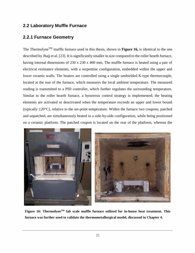
25

2.2 Laboratory Muffle Furnace

2.2.1 Furnace Geometry

The ThermolyneTM muffle furnace used in this thesis, shown in Figure 16, is identical to the one

described by Jhajj et al. [23]. It is significantly smaller in size compared to the roller hearth furnace,

having internal dimensions of 230 x 230 x 460 mm. The muffle furnace is heated using a pair of

electrical resistance elements, with a serpentine configuration, embedded within the upper and

lower ceramic walls. The heaters are controlled using a single unshielded K-type thermocouple,

located at the rear of the furnace, which measures the local ambient temperature. The measured

reading is transmitted to a PID controller, which further regulates the surrounding temperature.

Similar to the roller hearth furnace, a hysteresis control strategy is implemented; the heating

elements are activated or deactivated when the temperature exceeds an upper and lower bound

(typically 20°C), relative to the set-point temperature. Within the furnace two coupons, patched

and unpatched, are simultaneously heated in a side-by-side configuration, while being positioned

on a ceramic platform. The patched coupon is located on the rear of the platform, whereas the

Figure 16: ThermolyneTM lab scale muffle furnace utilized for in-house heat treatment. This

furnace was further used to validate the thermometallurgical model, discussed in Chapter 4.

26

unpatched coupon is near the front. In order to thoroughly model coupon heating, characterization

of the furnace surroundings may be necessary as the heating conditions near the patch may vary

compared to the unpatched coupon due to potential thermal gradient within the furnace.

2.2.2 Muffle Furnace Characterization

Since the coupon is heated primarily by radiation from the surrounding surfaces, it is important to

characterize how the temperature of these surfaces may depart from the set-point temperature

measured by the control thermocouple. The reason for the variation in the temperature is that when

the furnace door is opened and closed, to load the patched and unpatched samples, each surface is

cooled by radiative exchange with the surroundings, and some volume of the cooler air also enters

the furnace. Generally, since the door is always cooler compared to the remaining surfaces it

absorbs energy throughout the heating process.

In order to characterize the temperatures of the surrounding surfaces, four additional

thermocouples were installed within the muffle furnace: one on the inside of the door, one to

measure the ambient temperature directly near the test samples, and two along the length of the

left furnace wall. Mounting the thermocouples directly to the walls resulted in unrealistic data due

to some current leakage from the embedded electrical heaters into the thermocouple wires. To

overcome this issue, a pseudo wall was made, from Pyrotek Pyrite N-17 refractory ceramic, a

calcium silicate board, to which the thermocouples were attached using a Pyro putty, a metallic

and ceramic paste. The pseudo wall was 1 mm thick and located as close to the left furnace wall

as possible to reduce thermal and measurement lags. It was assumed that all heaters operate

symmetrically, and thus the temperature measurements should exhibit bilateral symmetry.

The temperature distribution within the furnace is shown in Figure 17. When the part is

loaded, the door and front wall experience the greatest drop in temperature compared to the back

furnace wall and ambient temperature. The door temperature is the lowest throughout the heating

duration, which may be due to lack of proper insulation and higher energy loss to the surroundings.

A noticeable temperature gradient is evident along the depth of the furnace, which may be

attributed to poor insulation along the front and rear. This information will form the basis of an

27

uncertainty measurement quantification that will be incorporated into the thermometallurgical

model.

Figure 17: Measured temperature variation of the laboratory scale muffle furnace during blank

heating.

0 50 100 150650

700

750

800

850

900

950

T [C

]

t [s]

Wall

Stand

Ambient

Door

Shielded

Ambient

Door Open Door Close

28

Chapter Three

Thermometallurgical Model

In order to relate the heating and austenitization kinetics of the 22MnB5, within the muffle furnace

and roller hearth furnace, a thermometallurgical model is necessary. Previously published furnace-

based austenitization heat transfer models for HFDQ [23, 27] implicitly accounted for

austenitization by defining an effective specific heat [63-65]. In practice, the predicted heating

curves are compared against the functional requirements of the furnace (e.g. enforcing a minimum

30 second soak time above 900°C) to ensure that the blanks have been completely (or near

completely) austenitized. Since past literature does not explicitly connect the blank heating and

the transformation kinetics, the proposed thermal models are limited in their utility and predictive

capability. It is thus necessary to derive a model that explicitly couples the two parameters.

3.1 Heat Transfer Submodel

Prior to developing a thermal model, it is essential to understand the modes of heat transfer

involved in this process. Since the furnace operates at approximately 950°C, the dominate heat

transfer mode is radiation, followed by convection, and conduction, as explained below.

Many thermal models for furnace-based austenitization evaluate the load’s 3D temperature

profile [23, 55]; this is not only computationally intensive but also difficult to implement in

industrial settings. Since the blanks are very thin relative to their planar dimensions, it is reasonable

to neglect the temperature distribution along the thickness. This assumption is justified by

evaluating the radiative Biot number, which compares the ratio of thermal resistance between

radiation to the surface (define in the linearized form) and conduction within the steel.

22 5internal

22 5external

R

1R

blank

rad blankMnB

MnB

rad

tk A h t

Bik

h A

(3.1)

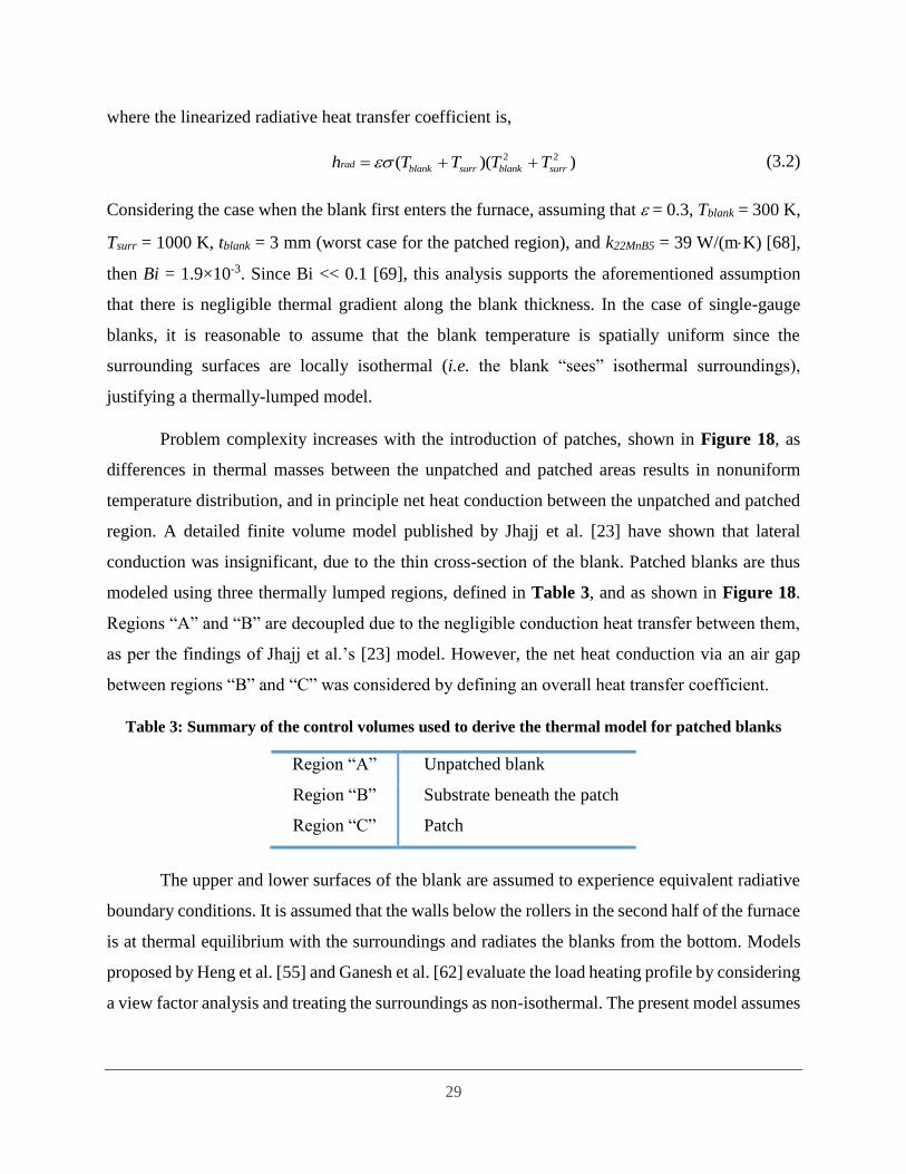
29

where the linearized radiative heat transfer coefficient is,

2 2( )( ) rad blank surr blank surrh T T T T (3.2)

Considering the case when the blank first enters the furnace, assuming that = 0.3, Tblank = 300 K,

Tsurr = 1000 K, tblank = 3 mm (worst case for the patched region), and k22MnB5 = 39 W/(mK) [68],

then Bi = 1.9×10-3. Since Bi << 0.1 [69], this analysis supports the aforementioned assumption

that there is negligible thermal gradient along the blank thickness. In the case of single-gauge

blanks, it is reasonable to assume that the blank temperature is spatially uniform since the

surrounding surfaces are locally isothermal (i.e. the blank “sees” isothermal surroundings),

justifying a thermally-lumped model.

Problem complexity increases with the introduction of patches, shown in Figure 18, as

differences in thermal masses between the unpatched and patched areas results in nonuniform

temperature distribution, and in principle net heat conduction between the unpatched and patched

region. A detailed finite volume model published by Jhajj et al. [23] have shown that lateral

conduction was insignificant, due to the thin cross-section of the blank. Patched blanks are thus

modeled using three thermally lumped regions, defined in Table 3, and as shown in Figure 18.

Regions “A” and “B” are decoupled due to the negligible conduction heat transfer between them,

as per the findings of Jhajj et al.’s [23] model. However, the net heat conduction via an air gap

between regions “B” and “C” was considered by defining an overall heat transfer coefficient.

Table 3: Summary of the control volumes used to derive the thermal model for patched blanks

Region “A” Unpatched blank

Region “B” Substrate beneath the patch

Region “C” Patch

The upper and lower surfaces of the blank are assumed to experience equivalent radiative

boundary conditions. It is assumed that the walls below the rollers in the second half of the furnace

is at thermal equilibrium with the surroundings and radiates the blanks from the bottom. Models

proposed by Heng et al. [55] and Ganesh et al. [62] evaluate the load heating profile by considering

a view factor analysis and treating the surroundings as non-isothermal. The present model assumes

30

that the furnace surroundings are locally isothermal and the local irradiation experiences negligible

influence with the presence of the blank (i.e. the small object/large isothermal enclosure

assumption [69, 70]. The assumption is further supported by the fact that the surface area of each

zone, in the roller hearth furnace, is significantly greater than that of the blank. Moreover, the

furnace atmosphere is quiescent and at thermal equilibrium with the surroundings.

With these assumptions and boundary conditions, the temperature of each region of the

blank may be determined at any instant of time by solving three coupled differential equations.

22 5 , , , , j

MnB p eff j rad j conv j cond j

dTc V Q Q Q

d

(3.3)

where subscript “j” denotes regions “A”, “B”, or “C”, and cp,eff are the temperature dependent

density [68] and effective specific heat [23] of 22MnB5, Vj is the unpatched or patched volume,

dTj/d is the rate of change in region j’s temperature, Qrad,j and Qconv,j are the radiative and

Figure 18: Control volumes used to formulate the heat transfer submodel: “A”, unpatched

blank; “B”, blank beneath the patch; and “C”, the patch. Heat conduction between “A” and “B”

is neglected based on the finite difference study by [20], but heat conduction across the air gap

separating “B” and “C” is considered.

(A)

(C)

(B)

Tsurr = T

Qrad, Qconv,t

Qrad, Qconv,b

qcond

Qrad, Qconv,b

Qrad, Qconv,t

Qrad, Qconv,t

Qrad, Qconv,b

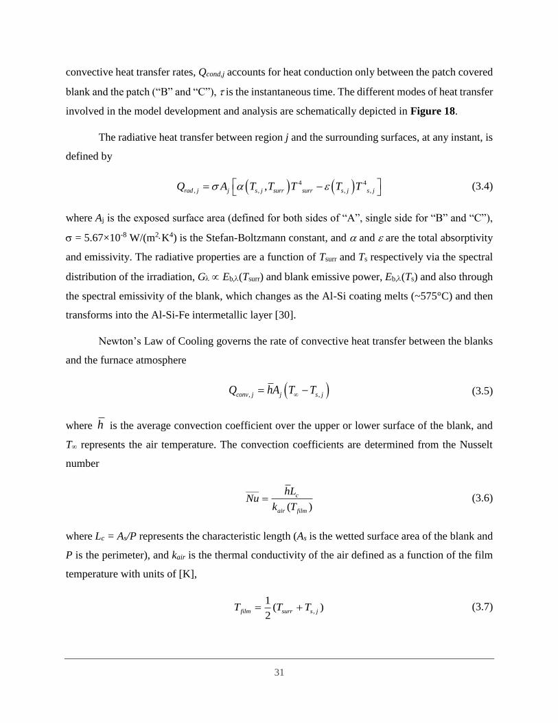
31

convective heat transfer rates, Qcond,j accounts for heat conduction only between the patch covered

blank and the patch (“B” and “C”), is the instantaneous time. The different modes of heat transfer

involved in the model development and analysis are schematically depicted in Figure 18.

The radiative heat transfer between region j and the surrounding surfaces, at any instant, is

defined by

4 4

, , , ,, rad j j s j surr surr s j s jQ A T T T T T (3.4)

where Aj is the exposed surface area (defined for both sides of “A”, single side for “B” and “C”),

= 5.67×10-8 W/(m2K4) is the Stefan-Boltzmann constant, and and are the total absorptivity

and emissivity. The radiative properties are a function of Tsurr and Ts respectively via the spectral

distribution of the irradiation, G Eb,(Tsurr) and blank emissive power, Eb,(Ts) and also through

the spectral emissivity of the blank, which changes as the Al-Si coating melts (~575°C) and then

transforms into the Al-Si-Fe intermetallic layer [30].

Newton’s Law of Cooling governs the rate of convective heat transfer between the blanks

and the furnace atmosphere

, , conv j j s jQ hA T T (3.5)

where h is the average convection coefficient over the upper or lower surface of the blank, and

T∞ represents the air temperature. The convection coefficients are determined from the Nusselt

number

____

( ) c

air film

hLNu

k T (3.6)

where Lc = As/P represents the characteristic length (As is the wetted surface area of the blank and

P is the perimeter), and kair is the thermal conductivity of the air defined as a function of the film

temperature with units of [K],

,

1( )

2 film surr s jT T T (3.7)

32

Since the blanks are conveyed through the furnace zones at a slow rate (i.e. at max 100 mm/s), so

buoyant forces dominate inertial forces and convection can be modelled as natural convection. The

Nusslet numbers over the top and bottom of the blank, respectively, are found from [69, 71]

____ 1

50.52c

upper LNu Ra (3.8)

1

4____

0.54Lc

lowerNu Ra (3.9)

where Ra, the Rayleigh number, is defined by

3

,

c

s j c

L

air air

g T T LRa

(3.10)

= 1/Tfilm is the volumetric thermal expansion coefficient of air, air and air are the thermal

diffusivity and kinematic viscosity of air, both of which are dependent on the Tfilm. The ambient air

is assumed to be in local thermal equilibrium with the respective zone.

Due to different convection heating rates on the upper and lower surfaces of the blank, heat

conduction via the air gap, separating regions “B” and “C”, can be considered, although it is

smaller in magnitude compared to the other heating modes. Conduction into region “B” from “C”

is determined by

, , , cond C B j s C s BQ UA T T (3.11)

where Aj is the interfacial area and U is a conservative, lower bound, overall heat transfer

coefficient estimated by assuming heat is exclusively conducted across the air gap (i.e. no radiative

transfer),

air

gap

kU

t (3.12)

Following the treatment of [23] an air gap thickness of approximately 0.1 mm was assumed.

Heat transfer also occurs between the rollers and the blank through some small but finite

contact area. The rollers reach a state of thermal equilibrium with the local zone temperature, in

33

the absence of blanks. However, due to periodic contact with the blanks it is expected that the

temperature will be between the blank and surroundings. As the rollers heat the blank, they also

interfere with radiation and convection on the blank underside. Due to the complexity and

uncertainties associated with the roller/blank interaction, heating from the rollers was not

considered in Eq.(3.3), with the assumption that this omission will be compensated by the

increased convection and radiation on the blank’s bottom surface.

3.2 Thermophysical Properties of Usibor® 1500AS

Characterization of the material’s thermophysical properties is crucial to reliably model the heating

stage. Temperature-dependent density, specific heat, and thermal conductivity of Usibor® 1500AS

are provided by Arcelor Mittal [68], summarized in Table 4.

The manufacturer-supplied specific heat only considers the sensible energy, that is the

energy required to simply raise the temperature of the steel per unit mass, stored by the ferrite,

pearlite, and austenite grains during heating. This ignores the latent component, the energy

absorbed by the blank for solid phase transformation. Excluding this contribution would result in

an over-prediction of the heating rate and final part temperature [23]. A severe consequence of

utilizing only the sensible energy in the optimization of the furnace parameters could be the

potential risk of incomplete blank austenitization [23].

The specific heat of a material is often characterized through differential scanning

calorimetry (DSC), as was done by Krielaart et al. [60] to determine the latent energy required to

transform a pure pearlitic structure to austenite. Jhajj et al. [23] argue that measurements from the

DSC are appropriate for HFDQ since the heating rates achieved by the device (~1°C/s) are lower

compared to what is observed in the roller hearth furnace (~3-5°C/s) during austenitization. To

overcome this hurdle an effective specific heat, cp,eff, is defined and utilized as a surrogate to

account for both the sensible and latent components. As mentioned in §1.3, Twynstra et al. [27]

assumed the effective specific heat to be uniformly distributed throughout the austenitization

regime (TAc1 and TAc3). The isothermal annealing study conducted by Garcia and Deardo [72]

contradicts this approach of defining a uniform cp,eff, as their work shows a strong correlation

between temperature and phase transformation. Jhajj et al. [23] also show that cp,eff is not uniformly

34

Table 4: Temperature dependent thermophysical properties of Usibor® 1500AS [68]

distributed; it is biased towards TAc1 suggesting majority of the austenitization takes place near the

TAc1. The experimental studies of Li et al. [24, 25] on the isothermal and non-isothermal

Temperature [°C] Conductivity [W/(mK)] Density [kg/m3] Specific Heat [J/(kgK)]

0 38.6 7880.8 433

50 38.9 7864.5 444

100 39.5 7848.0 465

150 39.9 7831.5 485

200 40.4 7814.8 505

250 41.0 7797.7 525

300 40.7 7781.0 547

350 40.9 7763.9 571

400 40.6 7746.6 598

450 40.1 7729.2 628

500 39.5 7711.7 628

550 38.5 7694.0 701

600 37.4 7676.2 748

650 35.9 7658.3 804

700 34.4 7640.2 876

725 37.4 7631.1 924

750 40.3 7622.0 971

800 39.7 7603.7 942

850 25.1 7585.2 825

880 26.0 7574.0 793

900 26.6 7566.6 771

950 27.3 7567.0 741

1000 27.9 7567.0 723

1050 28.3 7567.0 711

1100 28.6 7567.0 706

1150 29.2 7567.0 706

1200 29.7 7567.0 706

35

austenitization of 22MnB5 support the findings of [23]. Figure 19 compares the specific heat

provided by Arcelor Mittal [68] with the effective specific heats proposed by [23] and [27].

3.3 Radiative Properties of Usibor® 1500AS

The dominant mode of heating in this work comes from radiation, so characterization of the steel’s

radiative properties is of utmost importance in order to accurately model blank heating. According

to the work of Jhajj et al. [23] and Shi et al. [30] the radiative properties below the Al-Si coating

eutectic temperature (~575°C) are consistent with the manufacturer supplied values; however,

Figure 19: Thermophysical properties of Usibor® 1500AS as function of temperature. The

manufacturer [68] supplied specific heat and density are plotted. Effective specific heats

modeled by Twynstra et al. [27], assumed latent heat to be uniformly distributed, and Jhajj et

al. [23], showed latent heat is non-uniformly distributed over the austenitization regime. Both

model latent heat as 85000 J/kg [66].

0 200 400 600 800 1000 12000

cp

[J/(

kgK

)]

7500

8000

T [C]

[k

g/m

3]

[68]

cp sensible [68]

cp,eff

(Twynstra et al.) [27]

7550

7600

7650

7700

7750

7800

7850

7900

7950

250

500

750

1000

1250

1500

1750

2000

2250

2500

cp,eff

(Jhajj et al.) [23]

TAc1 TAc3

36

these properties exhibit dramatic changes beyond 575°C, due to morphological and chemical

changes in the coating, thereby influencing blank heating.

Jhajj et al. [23] carried out a detailed experimental study in order to quantify the total

emissivity and absorptivity of the blanks. They had conducted in-situ and ex-situ measurements of

the spectral emissivity (), collected using an OceanOptics NIRQuest near-infrared spectrometer

and a SOC 400 FTIR reflectometer, respectively. The OceanOptics NIRQuest is capable of directly

measuring the spectral emissivity, whereas the FTIR reflectometer measures the near-normal

spectral reflectivity (). In their method Al-Si coated samples of 22MnB5 were heated from 575-

950°C, using a Gleeble® thermomechanical simulator based on a temperature profile obtained

from instrumented blanks heated within a roller-hearth furnace. The spectrometer, mounted within

the Gleeble®, is effective from 0.9-2.5 m and the FTIR reflectometer provides characterization

over 2-25 m; thus, the combination of these two devices provided a broader wavlength over

which characterization could be performed. Ex-situ measurements were solely conducted using

the FTIR because the experimental setup would not allow the sample surface to sit flush against

the device opening and the data collection rate is significantly slower compared to the

spectrometer. Thus, ex-situ measurements involved heating the samples to the designated

temperatures and then immediately air quenching them to preserve the microstructure and

chemical composition of the coating.

Jhajj et al. [23] found that the FTIR was not suitable for inferring between 575-700°C

as the airflow, from the quenching process, distorted the surface morphology of the liquefied

coating. As a result, the radiative properties were determined using the NIR spectrometer. The

can be determined from the , via the FTIR, from the 1st law of thermodynamics

, , , , , 1 T (3.13)

The is related to by Kirchoff’s Law stating that for any surface = .

Since the sample surface is diffuse (i.e. irradiation is isotropic) the directional dependence is

neglected, thus Eq. (3.13) can be restated as

1 (3.14)

37

Spectral emissivity obtained using the NIR spectrometer and determined from the FTIR

reflectometer are shown in Figure 20a.

The total (or spectrally averaged) hemispherical emissivity, (Tb), is computed by [70]

0

4

b b b

b

b

T E T d

TT

(3.15)

where Tb is the temperature of the sample surface, Eb(Tb) is the spectral black body radiation at

the temperature the sample was heated. Since the sample is irradiated from black surroundings,

the total hemispherical absorptivity, (Tb), is determined by integrating over all wavelengths [70]

0

4

b b b

b

b

T E T d

TT

(3.16)

In both Eq. (3.15) and (3.16), Tb was assumed to be the temperature at which the blank was

quenched, although measurements made using the FTIR were performed at room temperature.

Figure 20b displays the total emissivity and absorptivity of the Al-Si coated blanks inferred from

the spectral measurements. Both and decrease upon reaching the coating melting temperature

(~575°C) due to the liquid surface of the coating. As the coating solidifies, the radiative properties

show an increase as a result of the various new phases being formed within the Al-Si coating [30].

3.4 Non-isothermal Transformation Kinetics Models

Industrial heating processes are mainly non-isothermal, followed by a period of nearly

isothermal soaking, with the objective of reaching a fully austenitic () structure. In order to ensure

sufficient austenitization, it is critical to understand the coupling between the blank temperature

history and the metallurgical transformations occurring within the blank. This thesis focuses on

two distinct non-isothermal austenite kinetic models specifically designed for heating of 22nB5.

The first model analyzed is an empirical first-order (F1) kinetics model developed by Di Ciano et

al. [10] derived from dilatometry data, which encompasses growth and nucleation within two

38

model parameters, the pre-exponential factor and activation energy. The second model is a more

physical-based model derived by Li et al. [25], which explicitly accounts for growth, nucleation,

and impingement processes.

Figure 20: (a) Spectral emissivity of the Al-Si coated blanks, experimentally determined by Jhajj

et al. [23], at various sample temperatures from Gleeble heated coupons. (b) Total emissivity and

absorptivity of the Al-Si coated blanks determined from the experimentally obtained

measurements [23].

0

0.2

0.4

0.6

0.8

0 5 10 15

[m]

=

As-received

600C

700C

800C

900C

900C with soak

0 200 400 600 800 10000

0.1

0.2

0.3

0.4

0.5

0.6

0.7

T [°C]

ε,α

Al-Si melting (~575C)

α (Tsurr = 900 °C)

ε

(b)

(a)

39

3.4.1 First-order (F1) Kinetics Model

Di Ciano et al. [10] derived an empirical austenitization model for non-isothermal heating of

22MnB5 beyond TAc3. The F1 model is mathematically similar to an Avrami-type model with n =

1. The model calculates the amount of fraction austenite formed by solving

exp

AEdwA

d RT (3.17)

where A is the pre-exponential factor [s-1], EA is the activation energy [J/mol] required for the phase

transformation to proceed, R = 8.314 J/(molK) is the ideal gas law constant, and w is the

intermediate variable that relates the temperature to the fraction austenite formed, f, expressed as

1 exp f w (3.18)

The key aspect of this model is that the nucleation, growth, and impingement mechanisms are

expressed within the activation energy (defining the energy input required to overcome the

activation barrier to enable solid-state transformation). The EA and A parameters were derived

from dilatometry measurements carried out on uncoated 22MnB5 coupons heated at constant ramp

rates ranging from 1-20°C/s using a Gleeble® thermomechanical simulator. The instantaneous

austenite phase fraction was then inferred by applying an empirical lever-type rule [36] to yield

df/d for a given heating rate, as shown in Figure 21.

Each set of dilatometry measurements was used to derive a pair of [EA, log10(A)]

parameters. The parameters derived for heating rates between 1-5°C/s, representative of furnace-

based heating, were binned and found to obey a multivariate normal (MVN) distribution,

[Ea,log10(A)]T(,), with

402 617 31.5

, 18.5 31.5 1.68

(3.19)

These distribution parameters were then used to derive a 90% confidence interval to account for

model uncertainty associated with the parameters, EA and A. Although Eqs. (3.17) and (3.18) do

40

not explicitly reflect the stages of the transformation kinetics, it reliably replicates experimental

trends. Di Ciano et al. [10] stated that although the model precludes stages associated with the

detailed kinetics, included in the work of Roosz et al. [38] and Li et al. [24, 25], it is still preferred

over a high-fidelity model due to a lower number of variables, reduced parameter uncertainty, and

minimized potential of parameter “over-tuning”. One area of weakness associated with the model,

however, is its inability to capture saturated austenite formation, in which the steel is heated to and

held at soaked temperature between TAc1 and TAc3. As noted above, this would result in an

equilibrium phase distribution containing both austenite and ferrite, but this condition cannot be

captured by the model. Since intercritical annealing of 22MnB5 is rarely done in an industrial

setting, this limitation does not unreasonably limit the applicability of this model.

The F1 model was validated by comparing the predicted austenite phase fraction with

values inferred from Vickers micro-hardness measurements using a 1 kg load, on coupons heated

and then rapidly quenched at intermediate temperatures within the Gleeble®. Di Ciano et al. [10]

inferred f, using an empirical linear interpolative formula, adopted from Huang et al. [36]

3

0

0

Ac

T

T

H Hf T

H H

(3.20)

Figure 21: Sample dilatometry data for heating rate of 1°C/s. The instantaneous phase fraction

of austenite was inferred from the dilatometry data using a lever-type rule.

Dila

tion,

∆L [m

m]

T [oC]

L1

L2

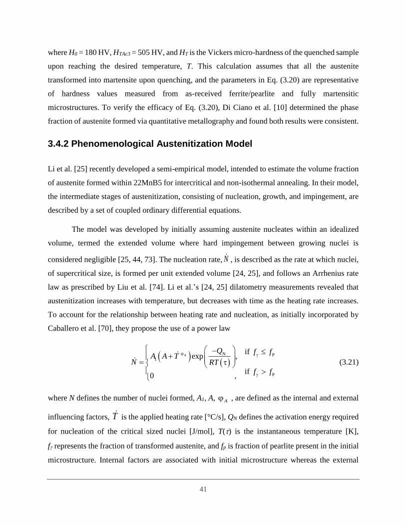
41

where H0 = 180 HV, HTAc3 = 505 HV, and HT is the Vickers micro-hardness of the quenched sample

upon reaching the desired temperature, T. This calculation assumes that all the austenite

transformed into martensite upon quenching, and the parameters in Eq. (3.20) are representative

of hardness values measured from as-received ferrite/pearlite and fully martensitic

microstructures. To verify the efficacy of Eq. (3.20), Di Ciano et al. [10] determined the phase

fraction of austenite formed via quantitative metallography and found both results were consistent.

3.4.2 Phenomenological Austenitization Model

Li et al. [25] recently developed a semi-empirical model, intended to estimate the volume fraction

of austenite formed within 22MnB5 for intercritical and non-isothermal annealing. In their model,

the intermediate stages of austenitization, consisting of nucleation, growth, and impingement, are

described by a set of coupled ordinary differential equations.

The model was developed by initially assuming austenite nucleates within an idealized

volume, termed the extended volume where hard impingement between growing nuclei is

considered negligible [25, 44, 73]. The nucleation rate, N , is described as the rate at which nuclei,

of supercritical size, is formed per unit extended volume [24, 25], and follows an Arrhenius rate

law as prescribed by Liu et al. [74]. Li et al.’s [24, 25] dilatometry measurements revealed that

austenitization increases with temperature, but decreases with time as the heating rate increases.

To account for the relationship between heating rate and nucleation, as initially incorporated by

Caballero et al. [70], they propose the use of a power law

N P

1

P

if exp ,

if 0 ,

AQ f f

A A TN RT

f f

(3.21)

where N defines the number of nuclei formed, A1, A, A , are defined as the internal and external

influencing factors, T is the applied heating rate [°C/s], QN defines the activation energy required

for nucleation of the critical sized nuclei [J/mol], T() is the instantaneous temperature [K],

frepresents the fraction oftransformed austenite, and fp is fraction of pearlite present in the initial

microstructure. Internal factors are associated with initial microstructure whereas the external

42

factors are related to the temperature and heating rate. Eq. (17) describes the two-step process of

ferrite/pearlite transformation to austenite, identified by Roosz et al. [38] and as explained in

§1.1.2. The first term expresses nucleation of austenite until complete pearlite dissolution; the

second term illustrates that no further nucleation occurs, instead, existing austenite grains simply

experience volumetric growth, within the remaining ferrite matrix. The volumetric growth rate,

assumed to be equivalent for all nuclei at the same heating conditions, is expressed similarly as

1 exp

B vQv B B T

RT (3.22)

where Qv refers to the activation energy for growth [J/mol)], which is independent of temperature

and time; B1, B, and B are material constant determined from dilatometry data [25]. The growth

rate of the extended volume austenite, expressed as a function of the nuclei formed and their

growth, is

'

f Nv (3.22)

Li et al. [25] accounted for the constrained equilibrium of carbon diffusion during intercritical

annealing by defining the saturated volume fraction of austenite, fs, as

21 3arctan 1

min

1

sAS

C TC C

f T (3.24)

In the actual transformation process, as the austenite nuclei grow their boundaries begin to overlap,

and thus the extended volume relates to the real volume via an impingement factor

'

'1

m m

s n

ff f f

f

(3.25)

P

P0

1,

1 ,

f fm

f fm (3.26)

0

Nn n f (3.27)

43

where m and n are related to the initial volume fraction of pearlite and transformation related

parameters, while mo, no, andN

are constants.

All defined model parameters were calibrated using dilatometry data, summarized in Table

5 and Table 6. Dilatometry data were obtained by performing three distinct heating trials on

rectangular samples of 22MnB5, using a Gleeble® thermomechanical simulator. The first set of

trials involved continuously heating samples to 900°C using different heating rates, ranging from

1-25°C/s; in the second trial, samples were subject to intercritical annealing with a constant heating

rate of 5°C/s. In both cases, samples were soaked for 15 minutes to achieve equilibrium phase

fraction austenite. Finally, a sample was continuously-heated to 1000°C and soaked for 2 minutes.

The inferred fraction austenite revealed that, as the heating rate increased, the incipient fraction

decreased due to lack of time available for carbon diffusion. Li et al. [25] found that the fraction

austenite increased with higher temperatures and dwell times, which is consistent with work of

Speich et al. [31] and Liang et al. [48].

Table 5: Calibrated constants for Eq. (3.24) [25]

C1 C2 C3 TAS [K]

36.0 1.2 0.475 1037

Table 6: Calibrated constants for Li et al.’s model [25]

QN [J/mol] Qv [J/mol] A1×B1 A B

1.486e5 4.05e5 2.394e6 0.8 1.0

A B mo no N

1.41 0.12 1.05 2.1 0.155

Although Li et al.’s [25] model captures the intermediate stages of austenitization, there

may be certain drawbacks limiting its applicability in industrial settings. One such limitation is

that their model consists of numerous adjustable parameters found by least squares fitting to

dilatometry data. The large number of degrees-of-freedom makes the model susceptible to over-

tuning, meaning the model fits both the physics as well as any experimental error and model error.

44

An over-tuned model is valid over the experimental conditions used to define the parameters, but

has reduced extrapolative abilities. Further doubts casted on this model is the fact that it predicts

saturated phase equilibrium obtained after thermal soaking for 15 minutes, which is significantly

longer compared to the studies by [40, 72, 76, 77] and based on industrial experience. Since the

dwell time does not accurately reflect conditions observed in industrial operations, it might be

possible that the impingement effects are overstated compared to the actual physics. Finally, the

model may lack the ability to reliably predict phase fraction austenite formed if the same steel with

slightly different chemical composition is used.

3.5 Derivation of the Thermometallurgical Model

The thermometallurigcal model is derived by extending Eq. (3.3) to include the austenitization

models, by defining the latent heat of austenitization term, h. As a result, the cp,eff term can be

replaced with the manufacturer supplied specific heat (cp). The latent heat of austenitization

couples the instantaneous fraction austenite to the temperature of the blank, thus defining the

themometallurigcal model as

,

22 5 , , , 22 5 j j

MnB p j rad j conv j cond j MnB j

dT dfc V Q Q Q V h

d d

(3.28)

where, df,j/d is the instantaneous rate of austenite formation, expressed as a volume fraction, and

cp is the temperature dependent sensible specific heat of 22MnB5 [68]. The left hand side of Eq.

(3.28) represents the sensible energy, the first term of the right hand side defines the modes of heat

transfer, and the last term corresponds to the energy required for austenitization.

The crucial variable in Eq. (3.28) is the latent heat of austenitization, h. As of now,

published literature has not reported nor characterized h for 22MnB5. Twynstra et al. [27] and

Jhajj et al. [23] assumed a value 85000 J/kg [66], corresponding to the energy necessary for

transformation of pure pearlitic iron to austenite. This however is an overestimation for 22MnB5

[78], which is 80%-ferrite/20%-pearlite in its as-received state. Di Ciano et al. [10] recently

characterized this h for 22MnB5 as 30000 J/kg, by applying a rule-of-mixtures.

45

3.6 Numerical Implementation

The thermometallurgical model was solved using two different methods: the explicit Euler scheme

and using the inbuilt MATLAB function, ODE45, which evaluates ordinary differential equations

using a fourth order Runge-Kutta scheme. Both methods were initialized with initial conditions of

Tj = 298 K and f = 0.

In the case of the explicit Euler method, a convergence study was performed which showed

that a grid independent solution (i.e. no further improvement in the solution) was obtained with a

time step of 0.15 s. However, for ODE45 a grid independent solution was obtained with a

minimum time step of 1.0 s, which may be due to the versatility of the fourth-order Runge-Kutta

method. In either case, the solutions were identical and ensured that the 1st law of thermodynamics

was conserved (i.e. Qcond = Qrad = Qconv = dT/d = df/d = 0 at steady state). In order to verify both

approaches, the numerical solutions were compared against the results published by Jhajj et al.

[23] and were in good agreement. Di Ciano et al.’s [10] F1 model was modeled using the ODE45,

however, Li et al.’s [25] model was evaluated using an explicit Euler scheme.

3.7 Model Uncertainty Quantification

Without exception, all hot stamping furnace models proposed to date, including those used in

industry, are deterministic; they accept a single set of process parameters as input, and provide a

single heating curve as output. This treatment does not capture the many uncertainties involved in

the calculation, and consequently one would not expect the predicted temperature to exactly match

the true thermal history of the blank. Moreover, the fact that production requirements are often

probabilistic (e.g. obtain a blank that is 95% austenitized with 95% probability) limits the

usefulness of a deterministic model since it is not possible to directly quantify how adjusting the

cycle time affects the trade-off between increasing the probability of sufficient austenitization and

productivity in terms of parts per minute.

It is hypothesized that uncertainties in the blank temperature and austenite phase fraction

are dominated by uncertainties in the furnace surrounding temperatures and the metallurgical

model parameters, with other uncertainty sources (e.g. the impact of the rollers, variation in the

46

properties and composition of 22MnB5) being secondary. Uncertainty in the furnace temperature

mainly arises from the hysteresis control and in the case of lab-scale furnaces, also from non-

uniform heating of the surfaces, periodic opening of the furnace door, etc. In Di Ciano et al.’s [10]

model the metallurgical model uncertainties are reflected by the MVN distribution of inferred [EA,

log10A] parameters as described above. Unfortunately, uncertainty estimates for Li et al.’s [25]

model parameters are not available.

The furnace temperature and model parameter uncertainties are propagated through the

model using a Monte Carlo procedure. The thermometallurgical model is evaluated N times: each

time the furnace surrounding temperatures and in the case of Di Ciano et al.’s model, a set of model

parameters, are sampled from corresponding probability density functions. The resulting set of

blank temperatures and austenite phase fractions are summarized by 95% highest probability

density intervals derived from histograms, as described in Appendix A. These intervals can be

interpreted to mean that they contain the “true” solution with 95% probability.

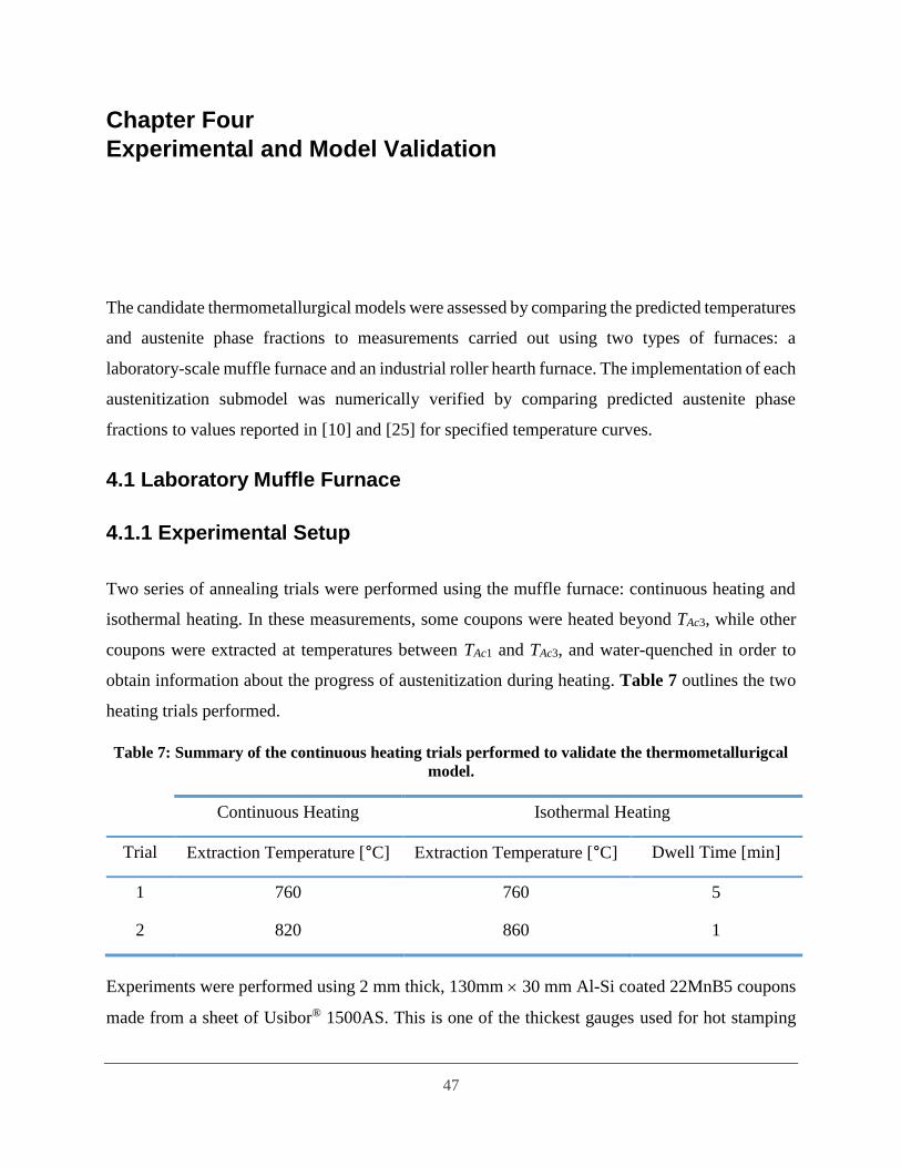
47

Chapter Four

Experimental and Model Validation

The candidate thermometallurgical models were assessed by comparing the predicted temperatures

and austenite phase fractions to measurements carried out using two types of furnaces: a

laboratory-scale muffle furnace and an industrial roller hearth furnace. The implementation of each

austenitization submodel was numerically verified by comparing predicted austenite phase

fractions to values reported in [10] and [25] for specified temperature curves.

4.1 Laboratory Muffle Furnace

4.1.1 Experimental Setup

Two series of annealing trials were performed using the muffle furnace: continuous heating and

isothermal heating. In these measurements, some coupons were heated beyond TAc3, while other

coupons were extracted at temperatures between TAc1 and TAc3, and water-quenched in order to

obtain information about the progress of austenitization during heating. Table 7 outlines the two

heating trials performed.

Table 7: Summary of the continuous heating trials performed to validate the thermometallurigcal

model.

Continuous Heating Isothermal Heating

Trial Extraction Temperature [°C] Extraction Temperature [°C] Dwell Time [min]

1 760 760 5

2 820 860 1

Experiments were performed using 2 mm thick, 130mm 30 mm Al-Si coated 22MnB5 coupons

made from a sheet of Usibor® 1500AS. This is one of the thickest gauges used for hot stamping

48

and represents a “worst case scenario”. The experiment is schematically shown in Figure 22,

whereas the equipment used is discussed in Appendix B. Measurements were carried out on

single-gauged coupons and double-gauge coupon “sandwiches”, formed by spot-welding two

single-gauge coupons at their corners, to emulate patched blanks. Each trial consisted of a single-

gauge and double-gauge coupon heated side-by-side. A platform constructed from a silica-based

ceramic (RSLE 57, Zicar Inc.) was used to consistently locate the coupons within the furnace and

minimize conduction between the platform and samples. Three K-type thermocouples were spot-

welded along the centerline of each coupon: one at the center, while the other two were located 20

mm from each end. Three trials were carried out per test to verify if the assumption that the patch

and unpatched region as being thermally-lumped, as defined in in §3.1, was valid. Each

thermocouple was insulated using a silica-based sheathing to prevent bare wires from creating

intermittent contact and reduce susceptibility to errors caused by wire heating. The lead of each

wire was individually welded to form an intrinsic junction, rather than a bead that is subsequently

welded onto the samples for greater structural integrity of the weld. An additional unshielded

thermocouple was used to monitor the ambient temperature inside the furnace, which varied by

5°C from the furnace set-point temperature of 900°C during the course of the measurements.

Figure 22: Muffle furnace experimental set up. Red dots indicate thermocouple weld sites, while

squared dashed regions are regions used for micro-hardness and metallography.

130mm

30mm

Single-gauge

Double-gaugeCeramic

holder

Vickers Microhardness

49

Prior to performing each experiment, the muffle furnace was thermally-soaked for two

hours to achieve steady state (or nearly isothermal conditions). Once the furnace reached

equilibrium the furnace door was opened to insert the coupons and then closed, a process that took

under 20 seconds. Upon reaching the desired patch temperature the coupons were extracted and

quenched in a cold water bath to ensure complete martensitic transformation. The quenched

samples were cut into 10 mm x 10 mm sections centered about each thermocouple location,

mounted, polished with 1 m diamond paste, and etched with 2% Nital solution. The 2% Nital

etchant dissolves the grain boundaries revealing different microstructures formed during the

interrupted heating cycles, which are visualized with micrographs, obtained via optical

microscopy. Microhardness measurements were then carried out on each mounted sample using a

Vickers indenter (Vickers 402 MVD, Wolpert Wilson Instruments) and a 1 kg load. Microhardness

measurements were taken in an 11 11 cruciform pattern with a spacing of 1 mm. The volume

fraction of austenite formed during heating is inferred using Eq. (3.20), following the procedure

described by Di Ciano et al. [10] and ASTM A1033-10 [79].

4.1.2 Results and Discussion

Uncertainty associated with the thermocouples measurements is within 0.9°C of the

actual measured value as discussed in Appendix A. The temperature profiles obtained for the

single- and double-gauge coupons are shown in Figure 23, for the heating trials defined in Table

7. The heating curve for both coupons extracted at different temperatures were nearly identical

(from the time they are inserted into the furnace until the time they are extracted) and thus only

thermocouple measurements for the 820°C trial are shown for clarity. The thermal history of the

heated coupons indicates that the single-gauge coupon is heated significantly faster compared to

the double-gauge sample, due to the lowered thermal inertia of the thinner sample and thus it is

also austenitized earlier than the thicker coupon. All thermocouple measurements are similar

which supports the thermally-lumped assumption made in §3.1. A slight variation is observed

between the center and edge temperatures of the single-gauge coupon, which may indicate a cold

spot within the furnace during heating, since this location was closest to the furnace door. Close

examination of the single-gauge temperature profile reveals the expected temperature drop in

heating rate at 575°C corresponding to the drop in radiative properties in Figure 20. This is

50

followed by a larger inflection near 730°C corresponding to the onset of austenitization (TAc1),

which was also observed by [10, 23].

In modelling the coupon heating, the muffle furnace surfaces were treated as isothermal,

having a probabilistic temperature that obeys a uniform distribution with an interval of 20°C

based on measured fluctuations in furnace wall temperatures at steady state described in Chapter

2. The predicted temperature curves obtained by sampling this distribution, using Di Ciano et al.’s

[10] first-order austenitization submodel are shown in Figure 24, along with the thermocouple

measurements for a single trial. The uncertainty quantification described in §3.7 was used to

construct 95% credibility intervals. Figure 24 shows that the thermocouple measurements for the

double-gauge coupon lies within the 95% credibility interval although the measured single-gauge

coupon temperatures lie below the predicted value. It is possible that the differences observed may

be a result of a model error (e.g. radiative boundary conditions) instead of an instrumentation issue

Figure 23: Thermocouple measurements of the single- and double-gauge coupons heated within

the muffle furnace, upon extraction at 760°C and 820°C. The solid line represents the centrally

located thermocouple, the dashed and dotted lines represent the measuerments from the edges

of the samples.

0 50 100 150 200 250 300

t [s]

0

200

400

600

800

1000

T [C

]

TAc3 TSingle

TDouble

TAc1

51

as the simulated and measured temperatures converge to the furnace set point. The fact that the

modeled and measured heating rates are slightly different below 575°C (the Al-Si melting

temperature), could indicate an error in the radiative properties or the assumed specific heat of

22MnB5.

The thermometallurgical model captures the variation in the temperature associated with

austenitization, although the measured temperature deviation is less pronounced for the double-

gauge coupon. The model predicts austenitization initiation at TAc1 730°C and completion upon

reaching TAc3 880°C. The modeled results and measurements indicate that most of the

austenitization occurs near TAc1, since the inflection is the greatest and gradually decreases with

time, as reported by [10, 23]. Figure 24 also shows that the latent energy is not uniformly

distributed between TAc1 and TAc3, as assumed by Twynstra et al. [27], as the inflection would have

been difficult to resolve (i.e. the inflection would be significantly smoother and less pronounced).

Figure 24: Temperature distribution of muffle furnace heated coupons compared against

modeled temperatures. Solid, dashed, and dotted lines represent the three thermocouples shown

in Figure 22. Blue and red lines are the most probable temperature distributions and shaded

regions represent 95% credibility intervals.

0 50 100 150 200 250 300

t [s]

0

200

400

600

800

1000

T [C

]

TAc3TSingle

TDouble

TAc1

52

The corresponding modeled austenite phase fractions are plotted in Figure 25, along with

box plots that summarize the inferred values from the 63 microhardness measurements. The

“whiskers” identify the upper and lower bounds of the inferred austenite phase fraction; the

horizontal line in the box represents the median value, and the upper and lower surfaces of the box

are the 75th and 25th quartiles respectively. The most probable model temperatures for both cases

are also shown, with credibility intervals excluded for clarity.

Figure 26 shows the micrographs of the as-received 22MnB5 microstructure, double-

gauged coupons extracted at 760°C and 820°C, corresponding to the box plots in Figure 25, and

a fully-austenitized single-gauge coupon. The as-received microstructure consists of ferrite grains

(bright) and pearlite bands (dark due to presence of carbon). By the time the steel reaches 760°C

all the pearlite has transformed into ferrite and austenite, the latter phase converting into martensite

during quenching. Upon reaching 820°C, most of the ferrite grains have transformed and the entire

Figure 25: Comparison of simulated austenite phase fraction versus microhardness inferred

values. Blue and red lines corresponds to the single- and double-gauge coupons, respectively. Box

plots represent the range of the hardness-inferred f, which are contained within the 95%

credibility intervals, indicated by the shaded regions.

0 50 100 150 200 250 300

t [s]

0

200

400

600

800

1000

T [C

]

0

0.2

0.4

0.6

0.8

f

1

f, Single

f, Double

820C

760C

TAc3

TAc1

53

microstructure consists almost entirely of martensite. The similarity between the microstructures

shown in Figure 26 (c) and (d) suggests that austenitization is largely completed below TAc3, which

is consistent with earlier observations [10, 23].

Figure 27 compares the temperature and austenite phase fraction predicted using Li et

al.’s [25] phenomenological model with the measured values. As mentioned previously, Li et al.

do not report uncertainties for their model parameters, so it is not possible to compute credibility

intervals. In contrast to the F1 model [10], Li et al.’s model shows a significant departure between

the measured and modeled austenite phase fractions. In particular, their model predicts a much

Figure 26: Optical micrographs of the 22MnB5 microstructure, showing (a) as-received

ferrite/pearlite microstructure; and coupons heated to (b) 760°C; (c) 820°C; and (d) 900°C, and

then quenched in a cold water bath. The microstructure in (b) is a mix of ferrite and martensite,

indicating incomplete austenitization, while (d) shows a purely martensitic microstructure,

indicating full austenitization. Coupons (b-c) are double-gauged, and correspond to the hardness-

inferred austenite fractions shown in Figure 25.

20 µm

Ferrite

Pearlite

(a)

FerriteMartensite

(b)

20 µm

(c) (d)

20 µm 20 µm

54

slower rate of austenitization for both samples and that the single-gauge coupons remains only

partially austenitized although it has exceeded TAc3, for an extended period of time. This result is

contrary to other measurements presented in the literature as well as industrial experience, which

shows that austenitization should be nearly complete once a blank reaches TAc3 at heating rates

typical of furnaces.

The discrepancy may be due to over-tuning in Li et al.’s [25] model, as described in §3.4.

Specifically, it seems likely that the impingement effects may overestimate true physical effects.

To verify this hypothesis two further muffle furnace experiments were performed with the furnace

set to 780°C and 860°C. Figure 28 shows that, for these isothermal cases, the detailed kinetics

model closely estimates the phase fraction formed, although there still is a discrepancy at higher

temperatures, which may indicate an issue with the impingement correction.

TAC3

TAC1

0 50 100 150 200 250 300

t [s]

0

200

400

600

800

1000

T [C

]

0

0.2

0.4

0.6

0.8

1

f f, Double

f, Single

820C

760C

TSingle

TDouble

Figure 27: Comparison of simulated austenite phase fraction versus microhardness inferred

values using Li et al.’s model [25]. Blue and red lines corresponds to the single- and double-gauge

coupons, respectively. Box plots represent the range of the hardness-inferred f.

55

4.2 Roller Hearth Furnace

4.2.1 Experimental Setup

Further measurements were carried out using the roller hearth furnace described in Chapter 2, in

order to validate the model in an industrial setting. The furnace used was 33 meters long, and

consists of 14 independently controlled heating zones.

Figure 28: Intercritical annealing experiment performed to validate proposed model with Li et

al.’s [25] constitutive model. In (a, b) the furnace temperature is set to 760°C, 5 min soak and (c,

d) the furnace temperature is set to 860°C, 1 min soak. (Box plots and dashed lines correspond to

experimental data.)

0 100 200 300 400 500 600 700 800

t [s]

0

200

400

600

800

1000T

[C

] TDouble

TSingle

TAc3

TAc1

(a)

0 100 200 300 400 500 600 700 800

t [s]

0

0.2

0.4

0.6

0.8

1

f

f,Single

f, Double

(b)

0 100 200 300 400 500

t [s]

0

200

400

600

800

1000

T [C

]

TAc3

TAc1

TSingle

TDouble

(c)

0 100 200 300 400 500t [s]

0

0.2

0.4

0.6

0.8

1

f f, Single

f, Double

(d)

56

The industrial heating trial involved using an instrumented Usibor® 1500AS B-Pillar with

a blank and patch thickness of 1.5 mm and 2 mm, respectively, with a roller speed of 70 mm/s. On

s ome of the blanks, two K-type thermocouples were spot-welded onto the patched blank: one on

the unpatched area far away from the patch (Region “A”) and one on the patch (Region “C”).

Similar to the muffle furnace trials, the thermocouples leads were insulated using silica-based

sheathing and individually welded to form intrinsic junctions on the blank. Other blanks were not

instrumented; as these blanks left the furnace, they were transferred to the forming/quenching die,

after which micro-hardness measurements were made to infer the fraction austenite formed

(instrumented blanks cannot be formed and quenched). All experiments were performed under the

supervision of Formet Industry personnel.

4.2.2 Results and Discussion

Since the muffle furnace trials indicated that Li et al.’s [25] model did not yield reliable results, all

subsequent analysis is done using the F1 model [10]. The predicted and measured temperature

profiles are shown in Figure 29 along with the 95% confidence intervals, calculated assuming the

temperatures are mutually-independent and obey uniform distributions over the hysteresis control

limit. The measured temperatures are close to, yet lie slightly outside of the 95% credibility

intervals. The differences observed between the simulated and measured temperatures may be

attributed to discrepancies in the applied boundary conditions, which requires further analysis.

Unlike the batch furnace measurements, it is not possible to extract the blanks at intermediate

heating times, nor is it possible to engineer controlled scenarios that will produce incomplete

austenitization, but the model accurately predicts the onset and completion of austenitization close

to the TAc1 and TAc3 temperatures. The results also show that the majority of the austenitization

occurs near TAc1, which is consistent with the muffle furnace trials.

4.3 Experimental and Validation Summary

The candidate thermometallurgical models were assessed by comparing simulated temperatures

and austenite phase fractions with thermocouple and hardness measurements made on

instrumented single- and double-gauge coupons within a laboratory muffle furnace, and patched

57

blanks heated in an industrial roller hearth furnace. Thermocouple measurements obtained from

the lab -scale furnace experiments support the assumption the unpatched and patched regions may

be treated as thermally-lumped.

The thermocouple and hardness measurements obtained from the trials are contained

within the 95% confidence interval, using the first-order submodel [10]. The first-order submodel

indicates that the majority of austenitization completes near TAc1, supported by the sharp inflection

observed in the thermocouple measurements at ~730°C, which gradually decreases and the sample

micrographs (consistent with the non-linear distribution of the latent heat reported by Di Ciano et

al. [10] and Jhajj et al. [23]). The phenomenological submodel [25], however, consistently under-

predicted the austenite phase fraction and failed to show complete austenitization for coupons

surpassing TAc3. Two reasons for the observed differences may be due to parameter over-tuning,

thereby causing experimental and model errors to be incorporated within the submodel and an

over-estimation of impingement effects.

Figure 29: Industrial roller hearth trial conducted on a patched B-pillar blank. Both unpatched

and patched regions completely austenitized and is accurately predicted by the proposed model.

0 100 200 300 400 500 600

t [s]

0

200

400

600

800

1000

T [°C

]TA

TAc3

TAc1

TC

0

0.2

0.4

0.6

0.8

1

f

f,Cf,A

58

Since the first-order submodel was generally consistent with the experimental

observations, the following analysis will focus on applying this model to optimize process

parameters of a roller hearth furnace in order to maximize production efficient while ensuring

complete batch austenitization.

59

Chapter Five

Furnace Design Optimization

The validated thermometallurgical model is now used for design optimization of the roller hearth

furnace. The optimization procedure relates blank heating and austenitization to the furnace

parameters: zone temperatures, roller speed, and the spacing between sequential batches on the

rollers (cycle length). The aim of the design optimization is to minimize the process cycle time,

while ensuring that the functional objectives and constraints are satisfied. Two optimization

techniques were used: a gradient-based interior point algorithm with a logarithmic barrier function,

and a hybrid approach that combines a metaheuristic (genetic algorithm) with the gradient-based

interior point method. The design optimization scheme is assessed by using the

thermometallurgical model with the F1 model [10], with particular focus on unpatched blanks.

5.1 Design Optimization

Optimization is the process of transforming a design problem into a multivariate minimization

problem by defining a vector of design parameters, x, that specify the design configuration and an

objective function, F(x), that quantifies the “goodness” of the design so that the objective function

is minimized by the optimal design outcome. The set of parameters that minimizes the objective

function, x* = argminx[F(x)], specifies the optimal design. Constraints can be further imposed on

x to ensure that the design complies with the functional requirements and can be implemented in

an industrial setting.

Design optimization has been widely used in furnace-based heating processes for a range

of metallurgical applications [54-60]. Specific application of optimization in HFDQ have been

more limited. Twynstra et al. [27] identified the power settings for electrical panel heaters that

provided the uniform irradiation of Usibor® 1500AS blanks in a batch furnace. Tonne et al. [61]

performed a multi-objective optimization on a roller hearth furnace to minimize the energy

consumption and process cycle time.

60

5.2 Definition of the Design Optimization Problem

A 12-zone roller hearth furnace, similar to the one defined in Chapter 2, is the prime focus for

design optimization. In this analysis, the optimization is performed to identify process parameters

solely for the austenitization of unpatched blanks.

The first step is to identify the objective function, design variables, and functional

constraints. The objective function to be minimized is the cycle time, which is defined as the

interval between batches leaving the furnace. There are fourteen design parameters to be

optimized, summarized in Figure 30, x1-x12, the cycle length, x13, comprised of the batch and gap

length, and the roller speed, x14. The cycle time is expressed as a function of the cycle length and

roller speed by

13 14 13 14, F x F x x x x (5.1)

Figure 30: Schematic of the roller hearth furnace optimization problem. (a) zone temperatures and

blank velocity; (b) blank load and cycle length

x14 = V

x1 = TZ1 x2 = TZ2x12 = TZ12. . .

(a)

(b)

x13 = Lc

Lb Lg,min

61

In order to ensure the functional requirements of the heat treatment step, including

austenitization of batches, operation within specified burner ratings, and formation of the

intermetallic layer, are fulfilled, several process constraints are introduced. The imposed functional

constraints are summarized in Table 8, and discussed in detail below.

Table 8: Process constraints for furnace optimization

Lin

ear cL1-12 Tz,i,min ≤ xi ≤ Tz,i,max, i=1,…,12 Max/min zone temperatures

cL13 x13-Lb ≥ Lg, min Min batch spacing

Nonli

nea

r

cN1-12 Eq. (5.2) Zone burner capacity

cN13 tT≥900°C ≥ 30 s Implicit austenitization

cN13a f,exit ≥ 0.95 Explicit modeled austenitization

cN14 Tt=60s ≤ 700°C Layer growth

cN15 Texit ≤ 950°C Burning of Al-Si coating

Two linear constraints have been specified to enforce a minimum gap length between sequential

loading of batches and bounds for the zone temperatures. A series of nonlinear constraints have

also been defined. The initial nonlinear constraint ensures that the heating requirements for each

zone do not exceed the manufacturer specified burner rating

,, 1 , , 1 , ,

1

bunrner ib p b i b i i i loss i

th

m c T T h f f Q Q (5.2)

where th is the thermal efficiency of the radiant tubes (approximately ~70%), bm is the mass flow

rate of the blanks through the furnace, cp is the specific heat, Tb is the blank temperature, f is the

austenite phase fraction, indices i and i+1 denote the state of the blank at the beginning and end of

each zone,,loss iQ accounts for the loss of heat through the furnace walls and door, summarized in

Table 9, and,burner iQ defines the burner capacity for each zone, specified in Table 10.

Table 9: Heat loss through the walls in each zone of the roller hearth furnace, in units of [kW]

i 1 2 3 4 5 6 7 8 9 10 11 12

,loss iQ 36 8 8 8 9 18 18 18 18 18 18 36

62

Table 10: Burner capacity for each zone of the roller hearth furnace, in units of [kW]

i 1 2 3 4 5 6 7 8 9 10 11 12

,burner iQ 320 240 180 240 180 180 120 180 180 60 60 60

Constraints to ensure complete blank austenitization and growth of the intermetallic layer

have been enforced, serving as surrogate constraints since these properties cannot be measured

directly during the heating process. The former is an industrial heuristic, which is intended to

ensure that the blanks are completely austenitized if they are soaked for 30 s beyond 900°C [1, 9,

80]. The latter constraint was assumed to be prevent melting of the Al-Si layer, if the heating rate

is maintained below 12 °C/s (or blank temperature below 700°C within the first 60 s of heating)

[50, 49]. However, Grauer et al. [49] and Veit et al. [81], cited by Liang et al. [48], have shown

that liquefaction is unavoidable under low heating conditions; rather this constraint corresponds to

preventing excessive layer growth as mentioned in the original steel patent [49]. An alternative,

explicit, austenite constraint has also been specified ensuring that each batch attains at least 95%

austenitization upon exiting. The final constraint enforces that the blank temperature remain below

950°C to prevent burning of the eutectic coating.

5.3 Constrained Multivariate Minimization

At this stage, the design problem has been recasted as a constrained multivariate minimization

problem, which can now be solved numerically. Multivariate minimization algorithms can be

categorized as either gradient-based and metaheuristic.

5.3.1 Gradient-based Interior Point Method

Commonly used gradient-based algorithms include Newton’s method, conjugate gradient (CG)

method, and trust-region algorithm [82, 83]. One common characteristic amongst these algorithms

is that they use information about the derivatives to determine iterates that improve the objective

function.

Gradient-based algorithms are generally defined by the update scheme

63

1 k k k kx x p (5.3)

where xk+1 is the new iterate, xk is the current iterate, pk is the search direction, k is a positive

scalar step size for the algorithm to take in the direction pk. The difference between the various

algorithms is with regards to how the search direction pk is computed, such that the new iterate,

xk+1 = xk + kpk, ensures f(xk+1) < f(xk) [82, 83]. This procedure continues until a termination criteria

is met or the algorithm reaches a boundary of the feasible region, as illustrated in Figure 31.

In Newton’s method, a second-order technique, pk is derived by taking a second-order

Taylor series such that f(xk + pk) is approximated by a quadratic model,

21( ) ( ) ( ) ( )

2 T T

k k k k k kf x p f x p f x p f x p (5.4)

Figure 31: Path followed by a gradient-based method, to identify the bounded local minimum of

the Rosenbrock function. Circles represent the “best” iterates identified; arrows define the search

direction (pk); step length (k) is defined by the arrow lengths. Iterates are bounded within the

feasible regions, represented by the yellow region, defined by the problem constraints,

represented by the dashed lines.

-0.5

0

0.5

1

-1 -0.5 0 0.5 1 1.5

X2

X1

64

Taking the derivative of the quadratic model with respect to pk and setting it equal to zero yields

the search direction

2

( )

( )

k

k

k

f xp

f x (5.5)

where ∇f(xk) and ∇2f(xk) are the gradient and Hessian respectively. This method requires

computation of the Hessian at each iteration, which is computationally expensive to evaluate.

Fletcher and Reeves [84] modified the linear CG method, which requires exactly n steps to reach

the minimum, for nonlinear cases. In their modification, a series of search directions that are

mutually conjugate are defined to avoid “zig-zagging” steps that may occur due to a changing

Hessian. Thus, the search direction depends on ∇f(xk) and the previous search direction, pk-1, such

that

1( ) k k k kp f x p (5.6)

where k is

1 1

( ) ( )

( ) ( )

T

k k

k T

k k

f x f x

f x f x (5.7)

Therefore, the CG method requires information about the last two iterations. Trust-region methods

approximate the objective function using the quadratic model defined in Eq. (5.3), similar to

Newton’s method. Trust-region methods define a spherical region around xk, with radius ∆k, where

the algorithm “trusts” the quadratic model within a limited neighborhood if and only if [83]

2 kp (5.8)

where p is the search direction and ∆k is the region radius at the kth iteration. At each iteration of

the algorithm, the step direction is determined by evaluating a minimization subproblem

2

2

1min ( ) ( ) ( )

2

. .

T T

k k kp

k

f x f x p p f x p

s t p

(5.9)

65

If the subproblem violates the constraint, Newton’s method cannot be applied, thus a scalar

must be determined so that

1

2

22

( ) ( )

k k kp f x f x (5.10)

If the step direction is not acceptable, the radius of the sphere is decreased to find a new minimizer,

and in general, the direction and step change with the size of the trust-region [77, 78].

Nonlinear optimization problems are challenging to solve, when inequality constraints are

present, due to the inability to identify which constraints are active (i.e. ( )c x ≥ 0 ( )c x = 0)

at the solution [82, 83]. One method to resolve this challenge involves solving a sequence of

subproblems by changing which constraints would be active at the optimum. The issue with this

approach is that there are 2 combinations, where is the number of inequality constraints; thus

the problem becomes combinatorially difficult [83]. An alternative approach for handling

inequalities, which is popular for nonlinear programming is the interior point method [85].

The interior point method, also called the barrier method is an algorithm that ensures strict

feasibility by forcing iterates to be far from the boundary of the feasible region [82, 86]. The

logarithmic and inverse functions are two types of barrier functions widely used in practice

1

x log x

m

Nj

j

c (5.11)

1

1x

( )

m

j Njc x (5.12)

where is the weight applied to the barrier function, a unitless, positive scalar quantity, whereas

cNj(x) ≥ 0 are the nonlinear constraints. As the iterate approaches the boundary of any constraint,

the barrier term approaches infinity ( ∞ as cNj 0). The interior point method is coupled with

the search direction algorithms mentioned above, such as Newton’s method and CG method. The

nonlinear constraints are redefined in terms of the weighted logarithmic barrier function and added

to the objective function such that the constrained problem can be reformulated as,

66

1

min ( , ) ( ) log ( )

. . ( ) 0, 1,...,

n

jx

j

f x c

s t c x m

x x

(5.13)

All the gradient-based algorithms mentioned above must satisfy a set of first-order

sufficient optimality conditions, called the Karush-Kuhn-Tucker (KKT) conditions, in order to

ensure a local or global minimum has been identified. The KKT conditions for an optimization

problem with only inequality constraints are [82, 87]:

*

1

( *) ( *) 0

0

* 0

(

0

*

, *

*

)*

n

j Nj

j

x x f x c x

x

x

c

(5.14)

where ∇x (x*, *) is the gradient of the Lagrange function at the optimal solution and * is the

vector of Lagrange multipliers, equal to the number of inequality constraints, at the optimal, for

the constraints. The first condition ensures that a local minimum has been identified; the second

condition ensures that the Lagrange multipliers are non-negative values; and the final condition

indicates whether each constraint is active or inactive, if constraint j is inactive *j = 0. The

Lagrange function provides ease of identifying function minima without having to work with

constraints parametrically. The Lagrange multipliers, also called the “shadow prices” or “dual

variables”, provide insight about the sensitivity of the optimal solution, x*, if the constraints are

slightly perturbed [82, 87].

The predominantly used barrier function in practice is the logarithmic function, defined in

Eq. (5.11). In the interior point method, the nonlinear constraints are redefined in terms of weighted

logarithmic barrier function, added to the objective, which penalizes the objective function if any

constraints are violated. Thus, the multivariate constrained minimization problem in §5.2 can thus

be expressed as,

67

1513

N

114

13 ,min

min ( , ) = log ( )

. . , [1,12]

j

j

lb i ub

b g

xc

x

s t x x x i

x L L

x

x x

(5.15)

where the variables are the same as described previously. The weighted parameter, , is determined

by solving a sequence of subproblems with decreasing values of until convergence. As

the barrier effect diminishes, thus allowing iterates to move closer to the constraint bounds

yielding an infinite penalty (since cNj0), as shown in Figure 32. In practice, a sequence of

subproblems are solved because defining a small makes the problem too difficult to solve, as the

barrier function will be close to infinite penalty; however, by gradually decreasing and using the

current solution as the initial seed for the next evaluation makes the computation easier [82, 87],

however, with modern computational efficiency this is not an issue. For this particular problem,

Figure 32: Influence of the barrier term for a one-dimensional bounded problem. As 0 the

effect of the barrier function diminishes, thus allowing the solver to identify optimal iterates closer

to the boundary of the feasible region, defined here as, a ≤ x ≤ b.

a b

= 1

= 0.1

= 0.01

x

68

= 10-3 and the nonlinear programming problem was solved in MATLABTM using the inbuilt

fmincon function with the interior point method [88].

5.3.2 Metaheuristics

Metaheuristics refers to going beyond the use of heuristics (i.e. trial and error) to efficiently explore

the search space, in order to find a solution that is better than what is currently available [89].

These class of solvers randomly sample the search domain in order to identify a good

approximation of the global minimum, hence making them stochastic in nature [90, 91, 92]. Two

key features of metaheuristic algorithms are diversification and intensification. The former refers

to creating a diverse solution set for efficient exploration of the search space, achieved by random

sampling of the domain, whereas the latter describes focusing the search within a local region

according to solver heuristics knowing the solution lies within a specific area [89]. It is therefore

essential to strike a balance between the two in order to efficiently determine high-quality regions

within the domain space [89]. Several algorithms belong within this class of optimization methods,

including, genetic algorithms (GA), simulated annealing (SA), and particle swarming (PS). The

mentioned algorithms vary based on the philosophy of the metaheuristic used. For instance, the

GA is based on the concepts of survival of the fittest (Darwinian evolution), simulated annealing

is based on the process of metal annealing, and particle swarming is based on trajectory of

individual birds flying in flocks [93].

Metaheuristics are classified as either trajectory-based or population-based. Trajectory-

based algorithms, such as SA, rely on analyzing the solution space using a single point at each

iteration and defining a path during the search process [89]. Population-based methods, such as

GA and PS, analyze the problem space using a large, but diverse, population at each iteration that

evolve during the search [89], and are highly popular for nonlinear problems. Metaheuristics differ

from the gradient-based methods in four ways:

(1) Given the stochastic nature of metaheuristic algorithms [89], random sampling

prevents the solver from being trapped within local minimums, thus allowing for an

effective sweep of the domain space [85], to identify the optimal solution. In the case

of gradient-based methods, once the KKT conditions are satisfied, the solver terminates

69

without further exploration. This limits the solver’s ability to identify the “best”

solution if a problem comprises of multiple minima. Gradient-based solvers yield an

identical optimal for the same initial start.

(2) Metaheuristic algorithms can handle nonlinear constraints without the added

complexity of introducing barrier functions, due to random sampling of the domain.

(3) Although the computational efficiency of metaheuristics heavily depends on the

problem and solver parameters, such as number of generations and termination

tolerances, they do not explicitly require the gradient vector or Hessian matrix, thus

requiring no storage space, unlike gradient-based methods [85].

(4) Metaheuristics are easily implemented with nonconvex and noncontinuous functions.

5.3.2.1 Genetic Algorithm

A GA is a suitable metaheuristic for this particular problem because at each iteration, the

population is constantly evolving in order to effectively explore the solution space. Genetic

algorithms belong to the class of evolutionary algorithms, which rely on biological concepts such

as crossover, mutation, elitism, and selection in order to promote diversity [90, 91, 94].

Genetic algorithms belong to the population based subclass of metaheuristic; they are

initialized by defining a population comprised of hundreds to thousands of randomly generated

individuals (or chromosomes) depending on the problem complexity. The length of a chromosome

is equivalent to the number of design parameters involved, and each element of the individual,

called a gene, can be expressed either as a binary or real-valued number, as shown in Figure 33.

With each iteration, called a generation, the population evolves; the evolution of the population

begins by selecting parents, from the previous generation, which will breed and create children

with better fitness values, for successive generations [54, 90, 91]. The selection process is related

to fitness of each individual within the population [95], where the roulette-wheel and tournament

selection [55, 86] are commonly applied techniques to select parents.

In the roulette wheel scheme, each individual within the population is assigned a

probability, Pj, based on its fitness value defined by [90, 96]

70

[ ]F

Individual is chosen

F1

i

Npop

j

j

P i (5.16)

where Fi is the fitness value of the ith individual and Npop is the population size. A series of random

numbers is generated within the interval [0, 1], and compared against the cumulative probability,

Ci, of the population [96]

1

i

i j

j

C P (5.17)

The ith individual is selected as the parent for reproducing children in the successive generation if

and only if Ci-1 < R[0, 1] ≤ Ci, where R is the randomly generated number [91]. The tournament

selection scheme however, randomly selects K individuals from the population and identifies

which of the selected has the highest fitness value [90, 94]. The individuals with the best fitness

Figure 33: A set of individuals (or chromosomes) defines the population for the GA. The length

of each individual is equal to the number of design parameters involved in the optimization study.

0 1 1 0 1

Gene

Binary Representation of An Individual

0.1 0.5 0.7 0.6 1

Real-Valued Representation of An Individual

Population

0 1 1 0 1

1 0 1 0 1

0 0 1 1 0

71

are selected as parents and this procedure is repeated until Npop for the following generation is

satisfied.

Upon selection of the parents, children with better fitness compared to their predecessors

are created by applying the biological concepts of crossover, mutation, and elitism. Crossover

refers to replacing some genes in one parent by the corresponding genes of the other [90, 91, 95].

Mutations are applied once the new generation has been created. The operator randomly selects a

few individuals and changes their respective genes [92]. Alternative to these methods is elitism,

which identifies K individuals with the highest fitness value, from the current population, and

copies the genetic information to the children in the following generation.

This process continues until one of the termination conditions has been reached: surpassing

maximum number of generation, no further improvement in the fitness value between successive

generations, or exceeding the constraint and function tolerances.

5.3.2.2 Remarks on Metaheuristics

Although metaheuristics are powerful methods and are better suited for complex nonlinear

problems compared to gradient-based methods, the solutions identified by these approaches do not

satisfy the KKT conditions, and therefore are not locally optimal. To overcome this challenge

hybrid techniques have been proposed where metaheuristics are combined with a gradient-based

solver to ensure local convergence [85]. In the hybrid approach, a metaheuristic minimization is

carried out, and this solution is then treated as the initial start for the gradient-based method to

ensure a localized minimum has been found.

5.3.3 Hybrid Method

A hybrid optimization scheme is implemented to assess the design problem. The hybrid

algorithm combines the GA with the gradient-based interior point method, which is solved in

MATLABTM using the inbuilt genetic algorithm function and fmincon interior point method. Table

11 and Table 12 summarize the settings for the GA and interior point method, respectively, which

72

yielded suitable convergence. All other parameters for each algorithm were left as the default

values.

Table 11: Settings used for hybridized genetic algorithm

Population Size Generations Selection Scheme Function Tolerance Constraint Tolerance

2000 300 Roulette Wheel 1e-9 1e-9

Table 12: Settings for the hybridized interior-point method, using MATLABTM inbuilt function

fmincon

Step Tolerance Function Tolerance Constraint Tolerance

1e-12 1e-10 1e-10

5.4 Results and Discussion

A deterministic optimization approach is employed, where uncertainties associated with the

thermometallurgical model, kinetic model parameters, and zone set-point temperatures are not

taken into consideration.

5.4.1 Optimal Solution Using the Interior Point Method

The nominal furnace settings, summarized in Table 13, served as the initial seed for the

optimization procedure. For the given roller speed and batch spacing, a corresponding cycle time

of F(x0) = 29 seconds is treated as the benchmark. Optimization proceeds from the initial point

until the default convergence criteria, which approximately satisfy the KKT conditions, are met.

The optimization progress is shown in Figure 34. The batch consists of a single component, with

a mass of 5 kg, thickness of 1.4 mm, and batch width of 0.5 m.

Table 13: Initial start point, x0, x10-x12

0 [°C], x130 [m], x14

0 [cm/s], and cycle time [s]

x10 x2

0 x30 x4

0 x50 x6

0 x70 x8

0 x90 x10

0 x110 x12

0 x130 x14

0 F(x0)

815 825 850 855 880 920 920 930 930 925 920 915 1.745 6.0 29

73

The optimal solutions are summarized in Table 14. Two scenarios for the austenitization

constraint are considered: the first one is a temperature-based criterion, cN13, which reflects current

industrial practice, and the second explicitly enforces a minimum modelled austenite phase

fraction at the furnace exit, cN13a based on the first-order austenitization model [10] presented in

Chapter 3. The optimal furnace parameters, between these two constraints, differ significantly,

although the difference in cycle time is small. The greatest savings in cycle time is realized with

cN13a, of 17 seconds faster than the nominal solution, while the improvement using cN13 is slightly

less. This reflects that the temperature-based constraint is more conservative compared to the

explicitly modelled austenite constraint. A comparison between the optimal solutions indicate that

the last seven zones of cN13, were on average 20-30°C higher than when cN13a was imposed, in

order to satisfy the temperature-based surrogate austenitization condition. In addition, the results

indicate that the zones can operate at significantly lower temperature in order to achieve desired

austenitization, which is consistent with the validation results in §4.1.2.

Table 14: Optimal solutions and associated cycle time for the optimization problem using the first-

order model [10] and nonlinear constraints cN13 and cN13a.

x1* x2

* x3* x4

* x5* x6

* x7* x8

* x9* x10

* x11* x12

* x13* x14

* F(x*)

cN13 842 843 856 860 879 905 905 908 908 907 905 903 1.765 13.2 13

cN13a 874 864 865 865 878 888 888 882 882 886 888 888 1.768 14.0 12

Figure 34: Example optimization progress for the gradient-based interior point method, using the

first-order kinetics model [10], with constraint cN13a enforced.

74

Further insight can be obtained from the optimized heating and austenitization profiles,

shown in Figure 35. A detailed comparison of Figures 32 (a) and (b) confirm that constraint cN13

is more conservative than cN13a. In both scenarios, the batch is completely austenitized prior to

TAc3, as majority of the transformation occurs near the Ac1 temperature, as reported by [10, 23].

The optimal zone temperatures are higher than the nominal case for the first five zones to

promote austenitization earlier in the heating process, thus allowing for faster part conveyance and

an overall reduction in cycle time.

The optimization procedure indicates that the 12 ⁰C/s constraint, imposed to prevent

excessive coating growth, is inactive for both austenitization conditions. However, the

temperature-based austenite constraint is active, whereas it is inactive for the explicitly modeled

austenite phase fraction. The burner capacities for both constraints are inactive, though the burner

capacity for the final zone are near active, as summarized in Table 15.

Table 15: Total energy requirements, in [kW], for each zone at the optimal settings

Zone 1 2 3 4 5 6 7 8 9 10 11 12

cN13 122 80 70 51 44 59 60 55 46 38 33 58

cN13a 131 87 74 49 43 57 56 52 45 40 35 60

Figure 35: Optimized heating and austenitization profiles for batches with a single blank. Dashed

lines correspond to the austenite start and finish temperatures, TAc1 = 730⁰C and TAc3 = 880⁰C.

Black solid lines are zone temperatures.

cN13

0 38 76 114 152 190 227t [s]

0

200

400

600

800

1000

T [⁰

C]

0 5 10 15 20 25Furnace Length [m]

300

0.2

0.4

0.6

0.8

1

f

(a)

f

Tb

cN13a

0 36 72 108 144 180 214t [s]

0

200

400

600

800

1000

T [⁰

C]

0 5 10 15 20 25Furnace Length [m]

300

0.2

0.4

0.6

0.8

1

f

(b)

75

To verify if this behavior is consistent only for the final zone, the optimization problem was re-

evaluated, using the same conditions specified above, with the omission of zone 12. The analysis

yielded similar results, where the final zone, operates near the maximum burner rating. This

suggests that the final zone is the limiting factor that ensures the selected austenite constraint is

satisfied. The optimization problem was also solved using the phenomenological model, as

explained in Appendix C.

The design problem is also solved for a batch consisting of four blanks, each with a

thickness of 1.4 mm, an equivalent mass of 20 kg and batch width of 0.5 m. The initial starting

point for this problem is specified within Table 16. In this scenario, where the batches are at full

capacity, the nominal cycle time is F(x0) = 59 seconds. The optimal solutions and corresponding

profiles are summarized in Table 17 and Figure 36, respectively.

Table 16: Initial start point, x0, x1

0-x120 [°C], x13

0 [m], x140 [cm/s], and cycle time [s]

x10 x2

0 x30 x4

0 x50 x6

0 x70 x8

0 x90 x10

0 x110 x12

0 x130 x14

0 F(x0)

815 825 850 855 880 920 920 930 930 925 920 915 3.59 5.0 59

Table 17: Optimal solutions and associated cycle time for the optimization problem using the first-

order model [10] and nonlinear constraints cN13 and cN13a.

x1* x2

* x3* x4

* x5* x6

* x7* x8

* x9* x10

* x11* x12

* x13* x14

* F(x*)

cN13 843 846 857 861 879 903 903 905 905 905 903 901 3.617 13.0 28

cN13a 907 877 905 907 883 908 891 892 851 911 871 872 3.6123 16.6 22

The first five zones for both austenite conditions are higher than the ones from the nominal

settings, whereas the remainder are significantly lower. This once again indicates that batches can

be austenitized using lower operating temperatures than currently established parameters. The

temperature-based constraint yields a savings of 31 seconds compared to the explicit constraint

corresponding to savings of 37 seconds. Similar to the single blank case all constraints were

inactive, except for cN13 and the burner capacity for zone 12. The optimized heating and

austenitization profiles shown in Figure 36 display that the batches achieve adequate

76

austenitization well before the furnace exit and that majority of the transformation takes place near

Ac1.

5.4.2 Optimal Solution Using the Hybrid Scheme

The hybrid scheme was used to evaluate the design problem, as constructed in §5.2, 15 times,

where each execution had a newly randomly generated initial population. The purpose of the

performing multiple executions is to verify that the optimal solutions were consistent amongst

different runs, which would be evident if the majority of the solutions were the same (i.e. lie within

the same optimal region region), thus yielding a near identical objective value. The hybrid scheme

focuses on batches with only a single unpatched blank.

The optimal solutions identified using the hybrid approach are shown in Figure 37. When

the temperature-based austenite constraint is applied, it is evident that the first ten zones operate

near the upper bound, ~950⁰C, allowing the batches to heat rapidly, whereas the remaining two

zones have optimal set-point temperatures that vary significantly between optimal runs. A possible

reason for this variation may be that upon reaching zone 10, the blank is either slightly above or

Figure 36: Optimized heating and austenitization profiles for batches composed of four blanks.

Dashed lines correspond to the austenite start and finish temperatures, TAc1 = 730⁰C and TAc3 =

880⁰C. Black solid lines are zone temperatures. (a) Corresponds to the temperature-based

austenite constraint; (b) is the optimal for the explicitly modeled constraint.

cN13

0 38 76 114 152 190 228

0

200

400

600

800

1000

T [⁰

C]

0 5 10 15 20 25

Furnace Length [m]

300

0.2

0.4

0.6

0.8

1

f

t [s]

f

Tb

(a)

cN13a

0 37 74 111 148 185 222

t [s]

0

200

400

600

800

1000

T [⁰

C]

0 5 10 15 20 25Furnace Length [m]

300

0.2

0.4

0.6

0.8

1

f

(b)

77

greater than 900⁰C thus the set-point temperatures for zones 11 and 12 are not as significant to the

overall process, so long as the austenite constraint is just satisfied. Thus, zones 11 and 12 act as

soaking zones (which contribute to isothermal annealing conditions in the HFDQ process). Figure

37(b) shows that the majority of the solutions yield a minimized cycle time of 9.1 seconds, which

corresponds to a savings of approximately 20 seconds from the nominal settings. Two interesting

differences between the optimums of the methods used are observed. First, the hybrid specified

optimal zone temperatures and roller speed are significantly higher than the gradient-based

scheme; second, the optimal cycle time identified by the hybrid scheme is on average 3 seconds

Figure 37: Optimal solutions identified by the hybrid algorithm, using a GA and gradient-based

interior point method. (a) and (b) correspond to the temperature-based austenite constraint. (c)

and (d) correspond to the explicitly modeled austenite constraint.

0 2 4 6 8 10 12800

850

900

950T

zon

e[⁰

C]

Zone

0 5 10 159.02

9.04

9.06

9.08

9.1

9.12

9.14

9.16

Optim

al

Cycle

Tim

e [

s]

Execution

(a) (b)

7.5

8

8.5

9

9.5

10

10.5

11

11.5

12

Op

tim

al

Cycle

Tim

e [

s]

0 5 10 15

Execution

0 2 4 6 8 10 12800

850

900

950

Tzo

ne

[⁰C

]

Zone

(c) (d)

78

faster. Both observations further reinforce how advanced heuristics allow effective exploration of

the solution space without being trapped within a local optimum. The cycle length and roller speed

were relatively consistent amongst runs with a value of 1.745 meters and 0.192 m/s, respectively.

Figure 37(c) shows the optimal results for the zone temperatures when the explicitly

modeled austenite constraint is enforced. As observed there is no clear indication of a concentrated

minimum, instead there appears to be a series of solutions that satisfy all the functional

requirements. This is further supported by the fact that at each execution of the hybrid algorithm,

the optimal cycle time is different. One possible reason for this variation may arise from the first-

order model [10] predicting that sufficient austenitization is achieved at temperatures below TAc3,

(i.e. 820°C to 950°C), while capable of satisfying the remaining constraints. This was also

observed during experimental validations, using the muffle furnace at an extraction temperature

of 820°C, as discussed in §4.1.2. Variations in the cycle length and roller speed are also evident,

ranging from 1.749 – 1.866 m and 0.15 – 0.22 m/s, respectively. Although significant savings are

realized using this constraint against the nominal settings and the soak-based constraint, for the

given number of evaluations, the best and worst cycle times are 8 seconds and 12 seconds,

respectively. Thus, only the best solution from the multiple runs will be considered.

The optimized solutions obtained using the alternative austenitization constraints are

summarized in Table 18.

Table 18: Optimal solutions and associated cycle time using the hybrid scheme.

x1* x2

* x3* x4

* x5* x6

* x7* x8

* x9* x10

* x11* x12

* x13* x14

* F(x*)

cN13 949 949 949 950 950 950 950 949 950 948 846 835 1.745 19.2 9

cN13a 949 950 944 937 939 947 942 950 943 938 845 898 1.765 22.3 8

The optimal heating and austenitization curves are shown in Figure 38. Similar to the

gradient-based method, the 12 ⁰C/s constraint and a maximum batch temperature of 950⁰C are not

exceeded. However, the austenite constraint for the soak-time based requirement is active. The

burner capacities for each of the individual zones were not exceeded, although zone 12’s rating

was close to the maximum. Compared to the gradient-based methods, it is evident that the batches

are able to exit the furnace, fully austenitized, well in advanced, due to the higher operating

79

conditions and roller speed. Similar to the interior point method, the batches austenitize well in

advance of the furnace exit; it is also observed that most of the austenitization occurs near TAc1.

Figure 38: Optimized heating and austenitization profiles for batches composed of a single blank.

Dashed lines correspond to the austenite start and finish temperatures, TAc1 = 730⁰C and TAc3 =

880⁰C. Black solid lines are zone temperatures. (a) Corresponds to the temperature-based

austenite constraint; (b) is the optimal for the explicitly modeled constraint.

0 26 52 78 104 130 156

t [s]

0

200

400

600

800

1000T

[⁰C

]

0 5 10 15 20 25

Furnace Length [m]

300

0.2

0.4

0.6

0.8

1

f

f

Tb

(a)

0

200

400

600

800

1000

T [⁰C

]

0 5 10 15 20 25

Furnace Length [m]

300

0.2

0.4

0.6

0.8

1

f

0 22 44 67 89 112 134

t [s]

(b)

80

5.5 Summary of the Design Optimization

A process optimization was carried out on a 12-zone roller hearth furnace, to minimize the cycle

time, whilst optimizing fourteen design parameters: zone temperatures, cycle length, and roller

speed, subject to a set of functional requirements. In this study, two alternative forms of

austenitization constraints were considered; a soak-time based constraint, cN13, and an explicitly

modeled constraint, cN13a. A gradient-based interior point method and a hybrid optimization

scheme, combining a GA with the interior point method, were implemented to evaluate the

problem.

The interior point method showed savings of approximately 17 seconds from the nominal

settings and indicated that batches can be adequately austenitized at lower operating temperatures.

The gradient-based technique indicated that cN13 was conservative compared to cN13a, and that all

constraints were inactive.

Next, a hybrid scheme was used to assess the problem by performing 15 executions. The

algorithm, with the soak-based constraint enforced, showed that the first ten zones operate near

the upper bound whereas the remaining two experience variability, thus behaving as soaking zones.

When the explicitly modeled austenite constraint was imposed, on the other hand, there was

considerable variability in the optimal solutions between each execution, which is a consequence

of the first-order model [10] predicting sufficient batch austenitization at temperatures below TAc3.

In both cases, the minimized cycle time achieved greater improvements compared to the gradient-

based method.

These findings indicate that the solution space may contain multiple minimums, hence the

weaker performance shown by the gradient-based method; and that the choice of the

austenitization constraint is crucial when selecting operation parameters to minimize the cycle

time, while ensuring complete austenitization.

81

Chapter Six

Conclusion and Future Work

6.1 Conclusion

The heating stage of hot stamping is used to austenitize ultra-high strength steels, and in the case

of Usibor® 1500AS, transform the Al-Si coating into a ternary Al-Si-Fe intermetallic layer with

desired properties and thickness.

In order to optimize production efficiency and improve current industrial practices, a

thermometallurgical model that couples heating and austenitization is necessary in order to provide

a physical foundation for the relationship between blank heating, austenitization, and selection of

furnace parameters. Numerous thermal models for furnace-based heating have been developed to

simulate heating of the load, yet to date none explicitly account for austenite formation.

The thermometallurgical model proposed in this study consists of a heat transfer submodel,

which simulates the transient temperature of unpatched/patched blanks, and two candidate

austenite kinetics submodels: a first-order empirical model and one that explicitly accounts for

nucleation, growth, and impingement. Confidence intervals were also constructed to account for

uncertainties with the surrounding temperatures and model parameters, using a Monte Carlo

technique.

The models were validated by comparing simulation temperature and austenite phase

fractions with thermocouple and hardness measurements made on instrumented single- and

double-gauge coupons, undergone continuous and intercritical annealing, in a laboratory muffle

furnace, and patched blanks heated in an industrial roller hearth furnace. The first-order submodel

predictions were consistent with the experimental results, whereas the phenomenological

submodel severely under estimated the austenite formation, and failed to show complete

austenitization even for coupons exceeding TAc3. The phenomenological submodel performed

82

better for the intercritical annealing tests at temperatures closer to TAc1, a consequence of model

over-tuning and over estimation of the impingement.

Next, a deterministic optimization procedure was developed using the validated

thermometallurigcal model, exclusively with the first-order kinetics submodel, to minimize the

cycle time of a 12-zone roller hearth furnace by identifying the optimal zone temperatures, cycle

length, and roller speed, subject to a set of linear and nonlinear constraints. The design problem

was evaluated using a gradient-based interior point method, which transforms nonlinear

constraints into weighted logarithmic penalty functions and a hybrid approach, combining a GA

with the interior point method. Two austenitization constraints were considered: one based on

soaking time and one on modelled austenite formation within the blanks leaving the furnace. In

general, the explicit austenite phase fraction constraint yielded significant improvements against

defined soak time, which is more conservative. The performance of the optimal solution strongly

depended on which austenitization constraint was enforced.

6.2 Future Work

The thermometalurigcal model is an effective tool to predict the heating and austenitization curves

for unpatched/patched blanks. Its effectiveness is further extended to optimizing furnace

parameters to ensure complete austenitization of batches while maximizing throughput. Although,

the model and optimization scheme yield feasible solutions, prior to industrial deployment, further

improvements are necessary.

The uncertainty estimates attached to the thermometallurgical model can be improved by

extending the Monte Carlo analysis to incorporate other model parameters, in particular the

radiative properties and specific heat of the blanks, which in practice are not perfectly known.

More advanced models should also address the Al-Si layer transformation, in particular the coating

kinetics to prevent excessive growth, which influences the thermal model through the change in

the radiative properties. The melting of coating reduces the life of ceramic rollers and causes them

to dislocate within the furnace. While coating liquefaction cannot be prevented, industry could use

such a model to determine process parameters that minimize the impact.

83

Further focus will be also dedicated to improving upon the optimization model by

considering a multi-objective scheme that minimizes the energy consumption and cycle time,

while ensuring batches are fully austenitized. Currently, the optimization scheme only focuses on

unpatched blanks; however, in industrial settings batches may consists of a combination of

unpatched/patched blanks. The optimization model could be used to identify feasible furnace

settings that not only allow sufficient batch austenitization, but also ensure adequate

transformation of the Al-Si layer. In such cases the thermal mass of the patched and unpatched

regions are the limiting factors, respectively. Most importantly, in the view of uncertainty attached

to the thermometallurgical model due to model parameters, zone temperatures, and steel

composition, further design optimization studies should be conducted in a statistical setting using

design optimization under uncertainty tools.

84

References

[1] H. Karbasian and A. E. Tekkaya, "A Review on Hot Stamping," Journal of Materials

Processing Technology, vol. 210, no. 15, pp. 2103-2118, 2010.

[2] R. A. Daziano and E. Chiew, "Electric Vehicles Rising From The Dead: Data Needs For

Forecasting Consumer Response Toward Sustainable Energy Sources In Personal

Transportation," Energy Policy, vol. 51, pp. 876-894, 2012.

[3] A. Turetta, S. Bruschi and A. Ghiotti, "Investigation Of 22MnB5 Formability In Hot

Stamping Operations," Journal of Materials Processing Technology, vol. 177, pp. 396-400,

2006.

[4] M. Naderi, "Hot Stamping of Ultra High Strength Steels," (Master's thesis, RWTH Aachen

University), 2007.

[5] R. Wohlecker, M. Johannaber and M. Espig, "Determination of Weight Elasticity of Fuel

Economy for ICE, Hybrid and Fuel Cell Vehicles," SAE Technical Paper, no. 2007-01-0343,

2007.

[6] X. Bano and J. P. Laurent, "Heat Treated Boron Steels in the Automotive Industry," in In 39

th Mechanical Working and Steel Processing Conference, 1997.

[7] T. Nonaka, K. Goto, H. Taniguchi and K. Yamazaki, "Developments of Ultra High-Strength

Cold-Rolled Steel Sheets for Automotive Use," Nippon Steel Technical Report, vol. 88, pp.

12-14, 2003.

[8] H. Lehmann, "Rollenherdöfen für die Wärmbehandlung beim Presshärten. In:Pfeifer, H.,

Nacke, B., Beneke, F. (Eds.)," Vulkan-Verlag, Essen, Germany, 2011.

[9] M. Naderi, A. Saeed-Akbari and W. Bleck, "The Effects of Non-isothermal Deformation on

Martensitic Transformation In 22MnB5 Steel," Materials Science and Engineering: A, no.

487, pp. 445-455, 2008.

[10] M. Di Ciano, N. Field, M. Wells and D. K., "Development of an Austenitization Kinetics

Model for 22MnB5 Steel," Journal of Materials Engineering and Performance, vol. 27, no.

4, pp. 1792-1802, 2018.

[11] N. Field, " Austenitization of Ultra High Strength Steel by Direct Contact Heating for Hot

Forming Die Quenching (Master's thesis, University of Waterloo)," 2017.

85

[12] M. Merklein and J. Lechler, "Investigation of The Thermo-mechanical Properties of Hot

Stamping Steels," Journal of Materials Processing Technology, vol. 177, no. 1-3, pp. 452-

455, 2006.

[13] C. Allély, L. Dosdat, O. Clauzeau, K. Ogle and P. Volovitch, "Anticorrosion Mechanisms of

Aluminized Steel for Hot Stamping," Surface and Coatings Technology, vol. 238, pp. 188-

196, 2014.

[14] M. Windmann, A. Röttger and W. Theisen, "Phase Formation at The Interface Between a

Boron Alloyed Steel Substrate and an Al-rich Coating," Surface and Coatings Technology,

no. 226, pp. 130-139, 2013.

[15] F. Borsetto, A. Ghiotti and S. Bruschi, "Investigation of The High Strength Steel Al-Si

Coating During Hot Stamping Operations," Key Engineering Materials, vol. 410, pp. 289-

296, 2009.

[16] M. Merklein and J. Lechler, "Determination of Material and Process Characteristics for Hot

Stamping Processes of Quenchenable Ultra High Strength Steels With Respect To A FE-

based Process Design," SAE International Journal of Materials and Manufacturing, vol. 1,

no. 1, pp. 411-426, 2009.

[17] L. Garcia Aranda, Y. Chastel, J. Fernández Pascual and T. Dal Negro, "Experiments and

Simulation of Hot Stamping of Quenchable Steels," Advanced Technology of Plasticity 2, pp.

1135-1140, 2002.

[18] R. George, A. Bardelcik and M. Worswick, "Hot Forming of Boron Steels Using Heated and

Cooled Tooling for Tailored Properties," Journal of Materials Processing Technology, vol.

212, no. 11, pp. 2386-2399, 2012.

[19] E. J. Caron, K. J. Daun and M. A. Wells, "Experimental Heat Transfer Coefficient

Measurements During Hot Forming Die Quenching of Boron Steel at High Temperatures,"

International Journal of Heat and Mass Transfer, vol. 71, pp. 396-404, 2014.

[20] F. G. Caballero, C. Capdevila and C. G. De Andres, "Modelling of Kinetics and Dilatometric

Behaviour of Austenite Formation in a Low-carbon Steel With a Ferrite Plus Pearlite Initial

Microstructure," Journal of Materials Science, vol. 37, no. 16, pp. 3533-3540, 2002.

[21] M. J. Holzweissig, J. Lackmann, S. Konrad, M. Schaper and T. Niendorf, "Influence of Short

Austenitization Treatments on The Mechanical Properties of Low-alloy Steels For Hot

Forming Applications," Metallurgical and Materials Transactions A, vol. 46, no. 7, pp. 3199-

3207, 2015.

86

[22] M. Verma, Y. H, J. Culham, M. Di Ciano and K. Daun, "Development and Validation of a

Thermometallurgical Model for Furnace-based Austenitization During Hot Stamping,"

(Submitted) Journal of Heat Transfer, 2018.

[23] K. Jhajj, S. Slezak and K. Daun, "Inferring the Specific Heat of an Ultra High Strength Steel

During the Heating Stage of Hot Forming Die Quenching, Through Inverse Analysis,"

Applied Thermal Engineering, vol. 83, pp. 98-107, 2015.

[24] N. Li, J. Lin, D. S. Balint and T. A. Dean, "Experimental Characterisation of the Effects of

Thermal Conditions on Austenite Formation for Hot Stamping of Boron Steel," Journal of

Materials Processing Technology, vol. 231, pp. 254-264, 2016.

[25] N. Li, J. Lin, D. S. Balint and T. A. Dean, "Modelling of Austenite Formation During Heating

in Boron Steel Hot Stamping Processes," Journal of Materials Processing Technology, vol.

237, pp. 394-401, 2016.

[26] M. J. Holzweissig, J. Lackmann, S. Konrad, M. Schaper and T. Niendorf, "Influence of Short

Austenitization Treatments on the Mechanical Properties of Low-alloy Steels For Hot

Forming Applications," Metallurgical and Materials Transactions A, vol. 46, no. 7, pp. 3199-

3207, 2015.

[27] M. Twynstra, K. Daun, E. Caron, N. Adam and D. Womack, "Modelling and Optimization

of a Batch Furnace For Hot Stamping," in ASME 2013 Heat Transfer Summer Conference,

Minneapolis, Minnesota, USA, 2013.

[28] J. N. Rasera, K. J. Daun, C. J. Shi and M. D'Souza, "Direct Contact Heating for Hot Forming

Die Quenching," Applied Thermal Engineering, vol. 98, pp. 1165-1173, 2016.

[29] J. Rasera, "Development of a Novel Technology for Rapid Austenizing Usibor 1500P,"

(Master's thesis, University of Waterloo), 2015.

[30] C. Shi, K. J. Daun and M. A. Wells, "Spectral Emissivity Characteristics of the Usibor®

1500P Steel During Austenitization In Argon And Air Atmospheres," International Journal

of Heat and Mass Transfer, vol. 91, pp. 818-828, 2015.

[31] G. R. Speich, V. A. Demarest and R. L. Miller, "Formation of Austenite During Intercritical

Annealing of Dual-phase Steels," Metallurgical and materials transactions A, vol. 12, no. 8,

pp. 1419-1428, 1981.

[32] L. O. Wolf, F. Nürnberger, D. Rodman and H. J. Maier, "The Effect of Intercritical Annealing

on the Microstructure and Mechanical Properties of Ferritic–Martensitic Two‐Phase Steels,"

Steel Research International, vol. 88, no. 2, p. 1600107, 2017.

87

[33] H. Surm, O. Kessler, M. Hunkel, F. Hoffmann and P. Mayr, "Modelling the Ferrite/Carbide→

Austenite Transformation of Hypoeutectoid and Hypereutectoid Steels," in Journal de

Physique IV, 2004.

[34] C. G. de Andrés, F. G. Caballero, C. Capdevila and L. F. Alvarez, "Application of

Dilatometric Analysis to the Study of Solid–solid Phase Transformations In Steels,"

Materials Characterization, vol. 48, no. 1, pp. 101-111, 2002.

[35] A. J. 0. and A. McWilliams, Journal of the Iron and Steel Institute, vol. 2, p. 352, 1905.

[36] J. Huang, W. J. Poole and M. Militzer, "Austenite Formation During Intercritical Annealing,"

Metallurgical and Materials Transactions A, vol. 35, no. 11, pp. 3363-3375, 2004.

[37] G. A. Roberts and R. F. Mehl, "The Mechanism and the Rate of Formation of Austenite From

Ferrite-cementite Aggregates," Transactions of the ASM, vol. 31, pp. 613-650, 1943.

[38] A. Roosz, Z. Gacsi and E. G. Fuchs, "Isothermal Formation of Austenite in Eutectoid Plain

Carbon Steel," Acta Metallurgica, vol. 31, no. 4, pp. 509-517, 1983.

[39] F. García Caballero, C. Capdevila and C. García de Andrés, "Influence of Scale Parameters

of Pearlite on the Kinetics of Anisothermal Pearlite-To-Austenite Transformation in a

Eutectoid Steel," Scripta Materialia, vol. 42, pp. 1159-1165, 2000.

[40] G. R. Speich, V. A. Demarest and R. L. Miller, "Formation of Austenite During Intercritical

Annealing of Dual-Phase Steels," Metallurgical and Materials Transactions A, vol. 12, no.

8, pp. 1419-1428, 1981.

[41] W. Callister, Fundamentals of Materials Science and Engineering, London, UK: John Wiley

& Sons, Inc..

[42] H. K. Khaira, A. K. Jena and M. C. Chaturvedi, "Effects of Heat Treatment Cycle on

Equilibrium Between Ferrite and Austenite During Intercritical Annealing," Materials

Science and Engineering: A, vol. 161, no. 2, pp. 267-271, 1993.

[43] V. I. Savran, Y. Van Leeuwen, D. N. Hanlon, C. Kwakernaak, W. G. Sloof and J. Sietsma,

"Microstructural Features of Austenite Formation in C35 and C45 Alloys," Metallurgical and

Materials Transactions A, vol. 38, no. 5, pp. 946-955, 2007.

[44] D. P. Datta and A. M. Gokhale, "Austenitization Kinetics of Pearlite and Ferrite Aggregates

in a Low Carbon Steel Containing 0.15 wt pct C," Metallurgical Transactions A, vol. 12, no.

3, pp. 443-450, 1981.

88

[45] F. L. G. Oliveira, M. S. Andrade and A. B. Cota, "Kinetics of Austenite Formation During

Continuous Heating in a Low Carbon Steel," Materials Characterization, vol. 58, no. 3, pp.

256-261, 2007.

[46] M. A. Asadabad, M. Goodarzi and S. Kheirandish, "Kinetics of Austenite Formation in Dual

Phase Steels," ISIJ international, vol. 48, no. 9, pp. 1251-1255, 2008.

[47] J. Cai, "Modelling of Phase Transformation in Hot Stamping of Boron Steel," (PhD

Dissertation Imperial College London), 2011.

[48] W. Liang, W. Tao, B. Zhu and Y. Zhang, "Influence of Heating Parameters on Properties of

the Al-Si Coating Applied to Hot Stamping," Science China Technological Sciences, vol. 60,

no. 7, pp. 1088-1102, 2017.

[49] S. J. Grauer, E. J. F. R. Caron, N. L. Chester, M. A. Wells and K. J. Daun, "Investigation of

Melting in the Al–Si Coating of a Boron Steel Sheet by Differential Scanning Calorimetry,"

Journal of Materials Processing Technology, vol. 216, pp. 89-94, 2015.

[50] R. Kolleck, R. Veit, H. Hofmann and F. J. Lenze, "Alternative Heating Concepts for Hot

Sheet Metal Forming," in 1st International Conference on Hot Sheet Metal Forming of High-

Performance SteeL, Kassel, Germany, 2008.

[51] R. Kolleck, R. Veit, M. Merklein, J. Lechler and M. Geiger, "Investigation on Induction

Heating for Hot Stamping of Boron Alloyed Steels," CIRP Annals, vol. 58, no. 1, pp. 275-

278, 2009b.

[52] R. Veit, H. Hofmann, R. Kolleck and S. Sikora, "Investigation of the Phase Formation of

AlSi‐Coatings for Hot Stamping of Boron Alloyed Steel," in In AIP Conference Proceedings,

2011.

[53] M. Verma, M. Di Ciano, J. R. Culham, C. Yau and K. J. Daun, "Minimizing the Cycle Time

of a Roller Hearth Furnace for Hot-Forming Die-Quenching," in IOP Conference Series:

Materials Science and Engineering, Waterloo, ON, 2018.

[54] N. Chakraborti, K. Deb and A. Jha, "A Genetic Algorithm Based Heat Transfer Analysis of

a Bloom Re‐heating Furnace," Steel Research, vol. 71, no. 10, pp. 396-402, 2000.

[55] V. R. Heng, H. S. Ganesh, A. R. Dulaney, A. Kurzawski, M. Baldea, O. A. Ezekoye and T.

F. Edgar, "Energy-oriented Modeling and Optimization of a Heat Treating Furnace," Journal

of Dynamic Systems, Measurement, and Control, vol. 139, no. 6, 2017.

[56] S. R. Carvalho, T. H. Ong and G. Guimaraes, "A Mathematical and Computational Model of

Furnaces for Continuous Steel Strip Processing," Journal of Materials Processing

Technology, vol. 178, no. 1-3, pp. 179-387, 2006.

89

[57] H. E. Pike Jr and S. J. Citron, "Optimization Studies of a Slab Reheating Furnace,"

Automatica, vol. 6, no. 1, pp. 41-50, 1970.

[58] H. Ramamurthy, S. Ramadhyani and R. Viskanta, "A Thermal System Model for a Radiant-

tube Continuous Reheating Furnace," Journal of Materials Engineering and Performance,

vol. 4, no. 5, pp. 519-531, 1995.

[59] A. Steinboeck, D. Wild, T. Kiefer and A. Kugi, "A Mathematical Model of a Slab Reheating

Furnace With Radiative Heat Transfer and Non-participating Gaseous Media," International

Journal of Heat and Mass Transfer, vol. 53, no. 26-26, pp. 5933-5946, 2010.

[60] S. H. Han, S. W. Baek and M. Y. Kim, "Transient Radiative Heating Characteristics of Slabs

in a Walking Beam Type Reheating Furnace," International Journal of Heat and Mass

Transfer, vol. 52, no. 3-4, pp. 1005-1011, 2009.

[61] J. Tonne, J. Clobes, M. Alsmann, A. Ademaj, M. Mischka, W. Morgenroth, H. Becker and

O. Stursberg, "Model-based Optimization of Furnace Temperature Profiles with Regard to

Economic and Ecological Aspects in Hot Stamping of 22MnB5," in 4th International

Conference: Proceedings Hot Sheet Metal Forming of High-Performance Steel, 2013.

[62] H. S. Ganesh, T. F. Edgar and M. Baldea, "Modeling, Optimization and Control of an

Austenitization Furnace for Achieving Target Product Toughness and Minimizing Energy

Use," Journal of Process Control (In Press), 2017.

[63] D. F. Watt, L. Coon, M. Bibby, J. Goldak and C. Henwood, "An Algorithm for Modelling

Microstructural Development in Weld Heat-affected Zones (Part A) Reaction Kinetics," Acta

Metallurgica, vol. 36, no. 11, pp. 3029-3035, 1988.

[64] K. Morgan, R. W. Lewis and O. C. Zienkiewicz, "An Improved Algrorithm for Heat

Conduction Problems with Phase Change," International Journal for Numerical Methods in

Engineering, vol. 12, no. 7, pp. 1191-1195, 1978.

[65] C. Bonacina, G. Comini, A. Fasano and M. Primicerio, "Numerical Solution of Phase-change

Problems," International Journal of Heat and Mass Transfer, vol. 16, no. 10, pp. 1825-1832,

1973.

[66] G. P. Krielaart, Brakman, C. M. and S. Van der Zwaag, "Analysis of Phase Transformation

in Fe-C Alloys Using Differential Scanning Calorimetry," Journal of Materials Science, vol.

31, no. 6, pp. 1501-1508, 1996.

[67] K. Jhajj, "Heat Transfer Modeling Of Roller Hearth And Muffle Furnace," (Master's thesis,

University of Waterloo), 2015.

[68] P. o. U. 1. P. Arcelor-Mittal.

90

[69] T. L. Bergman, F. P. Incropera, D. P. DeWitt and A. S. Lavine, Fundamentals of Heat and

Mass Transfer, John Wiley & Sons, Inc., 2011.

[70] J. R. Howell, R. Siegel and P. M. Menguc, Thermal Radiation Heat Transfer, CRC Press,

2016.

[71] E. Radziemska and W. Lewandowski, "Heat Transfer by Natural Convection from an

Isothermal Downward-Facing Round Plate in Unlimited Space," Applied Energy, vol. 68, pp.

347-366, 2001.

[72] C. I. Garcia and A. J. DeArdo, "Formation Of Austenite In 1.5 Pct Mn Steels," Metallurgical

Transactions A, vol. 12, no. 3, pp. 521-530, 1981.

[73] H. Chen, Y. C. Liu, D. J. Wang, Z. S. Yan, J. C. Fu and Q. Z. Shi, "A JMAK-Like Approach

for Isochronal Austenite–Ferrite Transformation Kinetics in Fe–0·055 wt-% N Alloy,"

Materials Science and Technology, vol. 26, no. 5, pp. 572-578, 2013.

[74] F. Liu, F. Sommer, C. Bos and E. J. Mittemeijer, "Analysis of Solid State Phase

Transformation Kinetics: Models and Recipes," International Materials Reviews, vol. 52, no.

4, pp. 193-212, 2007.

[75] F. García Caballero, C. Capdevila and C. García de Andrés, "Influence of Scale Parameters

of Pearlite on the Kinetics of Anisothermal Pearlite-To-Austenite Transformation in a

Eutectoid Steel," Scripta Materialia, vol. 42, pp. 1159-1165, 2000.

[76] H. Yan, M. Di Ciano, M. Verma and K. J. Daun, "Intercritical Annealing of 22MnB5 for Hot

Forming Die Quenching," in IOP Conference Series: Materials Science And Engineering,

Waterloo, ON, 2018.

[77] M. Kulakov, W. J. Poole and M. Militzer, "The Effect of the Initial Microstructure on

Recrystallization and Austenite Formation in a DP600 Steel," Metallurgical and Materials

Transactions, vol. 44, no. 8, pp. 3564-3576, 2013.

[78] M. Verma, J. R. Culham, M. Di Ciano and K. J. Daun, "Development of a Thermo-

Metallurgical Model to Predict Heating and Austenitization of 22MnB5 for Hot Forming Die

Quenching," in ASME 2017 International Mechanical Engineering Congress and Exposition,

2017.

[79] "ASTM Standard A1033-10(2015), West Conshohocken PA: ASTM International," 2015.

[80] H. Güler, "Investigation of Usibor 1500 Formability in a Hot Forming Operation," Materials

Science, vol. 19, no. 2, pp. 1392-1320, 2013.

91

[81] R. Veit, H. Hofmann, R. Kolleck and S. Sikora, "Investigation of the Phase Formation of

AlSi‐Coatings for Hot Stamping Of Boron Alloyed Steel," in AIP Conference Proceedings,

2011.

[82] S. G. Nash and A. Sofer, Linear and Nonlinear Programming, McGraw Hills, 1996.

[83] J. Nocedal and S. J. Wright, Numerical Optimization, 2nd ed., Springer, 2006.

[84] R. Fletcher and C. M. Reeves, "Function Minimization by Conjugate Gradients," The

Computer Journal, vol. 7, no. 2, pp. 149-154, 1964.

[85] V. Kelner, F. Capitanescu, O. Léonard and L. Wehenkel, "A Hybrid Optimization Technique

Coupling an Evolutionary and a Local Search Algorithm," Journal of Computational and

Applied Mathematics, vol. 215, no. 2, pp. 448-456, 2008.

[86] P. E. Gill, W. Murray and M. H. Wright, Practical Optimization, 2nd ed., Elsevier Academic

Press, 1981.

[87] D. P. Bertsekas, Nonlinear Programming, Blemont, Massachussets: Athena Scientific, 1999.

[88] R. A. Waltz, J. L. Morales, J. Nocedal and D. Orban, "An Interior Algorithm for Nonlinear

Optimization that Combines Line Search and Trust Region Steps," Mathematical

Programming, vol. 107, no. 3, pp. 391-408, 2006.

[89] C. Blum and A. Roli, "Metaheuristics in Combinatorial Optimization: Overview and

Conceptual Comparison," ACM Computing Durveys (CSUR), vol. 35, no. 3, pp. 268-308,

2003.

[90] D. S. Weile and E. Michielssen, "Genetic Algorithm Optimization Applied to

Electromagnetics: a Review," IEEE Transactions on Antennas and Propagation, vol. 45, no.

3, pp. 343-353, 1997.

[91] M. Kumar, M. Husian, N. Upreti and D. Gupta, "Genetic Algorithm: Review and

Application," International Journal of Information Technology and Knowledge

Management, vol. 2, no. 2, pp. 451-454, 2010.

[92] N. Soni and T. Kumar, "Study of Various Mutation Operators in Genetic Algorithms,"

International Journal Of Computer Science And Information Technologies, vol. 5, no. 3, pp.

4519-4521, 2014.

[93] L. Bianchi, M. Dorigo, L. M. Gambardella and W. J. Gutjahr, "A Survey on Metaheuristics

for Stochastic Combinatorial Optimization," Natural Computing, vol. 8, no. 2, pp. 239-287,

2009.

92

[94] C. A. Coello Coello and R. L. Becerra, "Evolutionary Multiobjective Optimization In

Materials Science And Engineering," Materials and Manufacturing Processes, vol. 24, no.

2, pp. 119-129, 2009.

[95] F. Glover and G. A. Kochenberge, Handbook Of Metaheuristics, New York: Kluwer

Academic Publishers, 2003.

[96] T. Pencheva, K. Atanassov and A. Shannon, "Modelling of a Roulette Wheel Selection

Operator in Genetic Algorithms Using Generalized Nets," International Journal

Bioautomation, vol. 13, no. 4, pp. 257-264, 2009.

[97] H. Coleman and W. Steele, Experimentation and Uncertainty Analysis for Engineers, New

York: John Wiley & Sons, 1989.

[98] OMEGA Engineering, The Temperature Handbook, 2004.

[99] N. Instruments, "SCXITM-1303 32-Channel Isothermal Terminal Block," National

Instruments, [Online]. Available: http://www.ni.com/pdf/manuals/321923b.pdf.

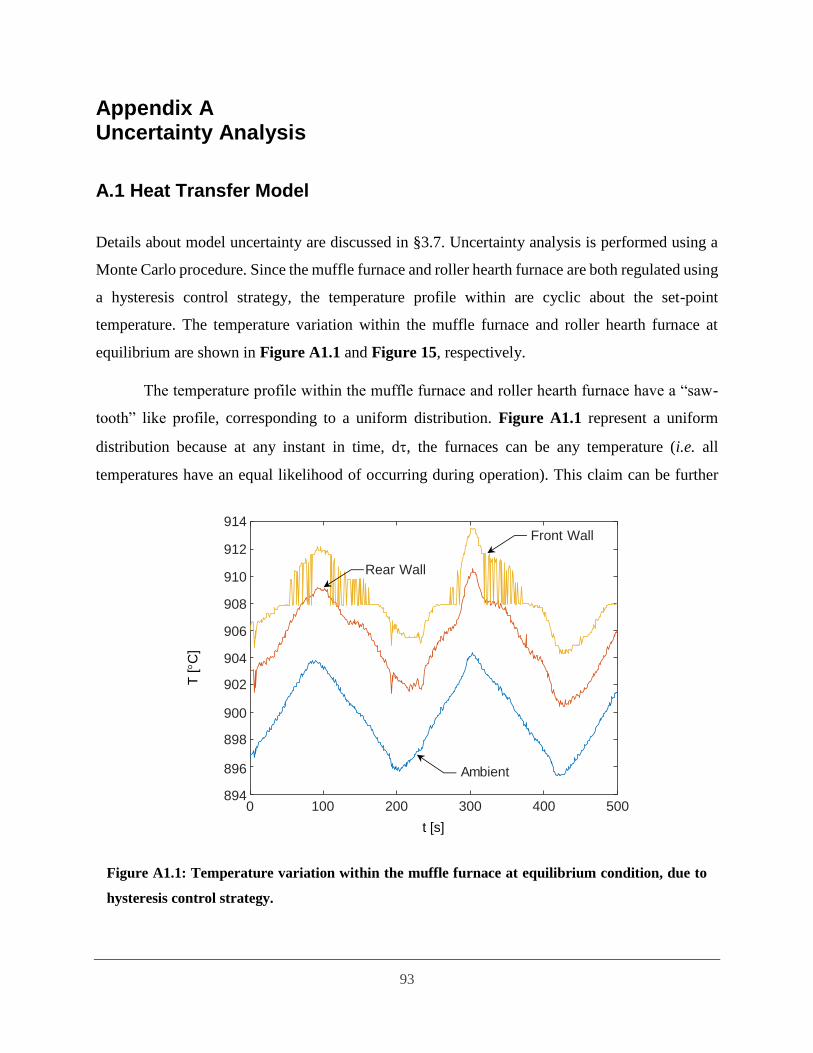
93

Appendix A

Uncertainty Analysis

A.1 Heat Transfer Model

Details about model uncertainty are discussed in §3.7. Uncertainty analysis is performed using a

Monte Carlo procedure. Since the muffle furnace and roller hearth furnace are both regulated using

a hysteresis control strategy, the temperature profile within are cyclic about the set-point

temperature. The temperature variation within the muffle furnace and roller hearth furnace at

equilibrium are shown in Figure A1.1 and Figure 15, respectively.

The temperature profile within the muffle furnace and roller hearth furnace have a “saw-

tooth” like profile, corresponding to a uniform distribution. Figure A1.1 represent a uniform

distribution because at any instant in time, d, the furnaces can be any temperature (i.e. all

temperatures have an equal likelihood of occurring during operation). This claim can be further

0 100 200 300 400 500894

896

898

900

902

904

906

908

910

912

914

T [C

]

t [s]

Front Wall

Rear Wall

Ambient

Figure A1.1: Temperature variation within the muffle furnace at equilibrium condition, due to

hysteresis control strategy.

94

supported by plotting a histogram of the probability density function (pdf) for the temperature

profiles above, as shown in Figure A1.2.

Figure A1.2: (a) Histogram showing the probability density function of the ambient temperature

within the muffle furnace. As observed, excluding the very first and last bars, majority of the

temperatures have a relatively equal probability of occurring at any instant of time. Thus, a

uniform distribution can be used to describe the nature of the temperature variation within the

furnaces involved in this study. (b) uniform distribution representing the pdf of the temperature

profile.

(a)

(b)

895 896 897 898 899 900 901 902 903 904 905

pdf(

Ta

ir)

T [C]

Tmin = 895 Tmax = 905

95

Figure A1.2 shows that there is relatively an equal probability that all ambient temperature

within the furnace can be any of the one depicted by the profile in Figure A1.1. It is noted that the

temperatures do not have the exact same probability due to noise in the measurement data;

however, by approximating the profile as being a smooth, continuous, and straight lines each

temperature point has an equal chance of occurring.

A.2 First-order Kinetics Model

As mentioned in §3.4.1, each set of dilatometry measurement was used to derive a pair of [EA,

log10(A)] parameters. The parameters representative of the heating rates in roller earth furnaces (1-

5°C/s) were binned and found to obey a multivariate normal (MVN) distribution

[Ea,log10(A)]T(,).

These distribution parameters were then used to derive a 90% confidence interval to

account for model uncertainty associated with the parameters, EA and A, shown in Figure A2.1.

340 360 380 400 420 440 460

EA x 1e3 [J/mol]

15

16

17

18

19

20

21

log

10(A

)

Figure A2.1: Austenitization model parameters derived from Gleeble dilatometry measurements

at heating rates between 1 and 5°C/s. Data used to derive 90% confidence ellipse, with mean and

covariance shown in Eq. (3.19). Red cross represents mean value of first-order model.

96

A.3 Monte Carlo Simulation

In order to define the credibility interval a Monte Carlo approach is adopted, where the surrounding

and ambient temperatures, and kinetic model parameters are drawn from their respective pdfs. The

simulation is run N times and the resulting set of blank temperatures and austenite phase fractions

are summarized via 95% highest posterior density intervals (HPDI) derived from histograms, as

shown in Figure A3.1.

Figure A3.1: (a) Monte Carlo simulation results from N number of runs; (b) Histogram for time, t,

used for deriving HPDI; (c) Identify points with equal probability, the dark red shaded region should

contain the desired credibility level. If the interval contains desired credibility interval, check other

regions. Points defining region with desired credibility level with shortest distance are selected to

define HPDI; (d) Dashed lines are the credibility interval and solid line is the most probable estimate.

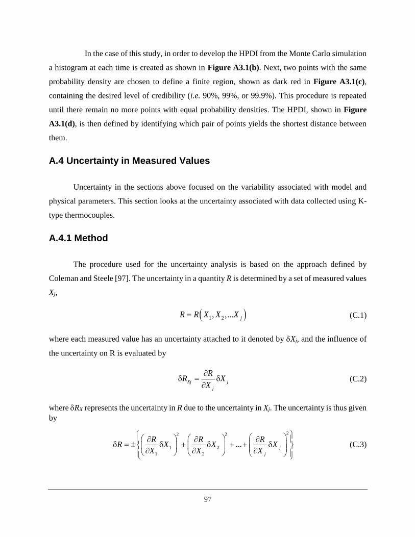
97

In the case of this study, in order to develop the HPDI from the Monte Carlo simulation

a histogram at each time is created as shown in Figure A3.1(b). Next, two points with the same

probability density are chosen to define a finite region, shown as dark red in Figure A3.1(c),

containing the desired level of credibility (i.e. 90%, 99%, or 99.9%). This procedure is repeated

until there remain no more points with equal probability densities. The HPDI, shown in Figure

A3.1(d), is then defined by identifying which pair of points yields the shortest distance between

them.

A.4 Uncertainty in Measured Values

Uncertainty in the sections above focused on the variability associated with model and

physical parameters. This section looks at the uncertainty associated with data collected using K-

type thermocouples.

A.4.1 Method

The procedure used for the uncertainty analysis is based on the approach defined by

Coleman and Steele [97]. The uncertainty in a quantity R is determined by a set of measured values

Xj,

1 2, ,... jR R X X X (C.1)

where each measured value has an uncertainty attached to it denoted by Xj, and the influence of

the uncertainty on R is evaluated by

Xj j

j

RR X

X (C.2)

where RX represents the uncertainty in R due to the uncertainty in Xj. The uncertainty is thus given

by

22 2

1 2

1 2

...

j

j

R R RR X X X

X X X (C.3)

98

If R is a function of several measured quantities and the dependence can be expressed as

1 2

1 2 ... C C Cj

jR X X X (C.4)

the overall uncertainty is calculated from the uncertainties of each of the individual measurements

12 22 2

1 2

1 2

1 2

...

j

j

j

XX XRC C C

R X X X (C.5)

The overall uncertainty in R is represented as a percentage. The following section describes the

uncertainty associated with the temperature measurements.

A.4.2 Temperature Measurements

The out-of-box error tolerance for K-type thermocouples, as per OMEGATM’s Temperature

Handbook [98], is the worst case scenario of either 2.2°C or 0.75(Measured temperature).

However, this measurement error can be improved if an ice-point cell or cold-junction is utilized.

As mentioned in Appendix B, thermocouple measurements using the muffle furnace were done

with a National Instruments SCXI-1303 isothermal block, designed with a cold-junction

temperature sensor; thus, the measurement error is 0.9°C [99]. The overall measurement error in

the temperature measurements is characterized by

[ ]

0.9

meas

T C

T T C (C.6)

Figure C5.1 shows the measurement error associated with the actual temperature measurements,

using the muffle furnace. Since the standard measurement error is very small, there is high

confidence in the thermocouple readings and in the ability of the thermocouples to detect the onset

and completion austenitization temperatures. As was observed in Chapter 4, since the simulation

results contained the experimental temperature data, the model’s predictive capabilities are

effective.

99

0 50 100 150 200 250 300 3500

200

400

600

800

1000TAC3

TAC1

t [s]

T [C

]

TSingle

TDouble

Figure C5.1: Measurement error associated with actual temperature measurements obtained from

K-type thermocouples using the National Instruments SCXI-1303 isothermal block, when performing

validation studies with muffle furnace.

100

Appendix B

Experimental Setup

B.1 Muffle Furnace

A laboratory muffle furnace is used for in-house validation studies. Details of the furnace are

discussed in Chapter 2. Data logging was performed using a National Instrument SCXI-1000

system with a SCXI-1303 terminal block with 32-channels. The equipment setup is shown in

Figure B1.1.

National Instruments LabVIEW software was used to create a program that would record

temperature measurements, developed by University of Waterloo personnel. Temperature

measurements on instrumented single- and double-gauge coupons were recorded every second.

B.2 Roller Hearth Furnace

Data logging was performed using a hand-held temperature measurement device.

Figure B1.1: Equipment setup used for the laboratory muffle furnace. National Instruments

SCXI-1000 chassis used with SCXI-1303 32-channel terminal block for thermocouple connection.

NI SCXI-1100

NI SCXI-1303

101

Appendix C

Optimization Using the Phenomenological Kinetics

Submodel

The phenomenological kinetics submodel [25], was also used to identify optimal furnace

parameters, for a batch consisting of one unpatched blank. The gradient-based interior point

method is used to evaluate the constrained multivariate minimization problem. Nominal furnace

settings, as defined in Table 13 (§5.4.1), were used as the initial start point for the algorithm. The

algorithm continued to identify new iterates until the KKT conditions were approximately

satisfied, as defined in Table 12. The optimal solutions and minimized cycle time are summarized

in Table C1, whereas the optimized heating and austenite curves are shown in Figure C1.

Table C1: Optimal solutions and associated cycle time for the optimization problem using Li et al.’s

model [25] and nonlinear constraints cN13 and cN13a.

x1* x2

* x3* x4

* x5* x6

* x7* x8

* x9* x10

* x11* x12

* x13* x14

* F(x*)

cN13 842 843 856 860 879 906 906 908 908 908 906 902 1.767 13.3 13

cN13a 816 826 851 855 880 920 920 929 929 925 920 915 1.749 6.3 28

Figure C1: Optimized heating and austenitization profiles. Dashed lines correspond to the austenite

start and finish temperatures, TAc1

= 730⁰C and TAc3

= 880⁰C. Black solid lines are zone temperatures.

102

The greatest improvement in the cycle time is achieved with the temperature-based

constraint, of 16 seconds faster than the nominal solutions. In contrast, only a savings of 1 second

is yielded with the explicit austenite constraint imposed. Figure C1, shows that although cN13 is

satisfied, the model predicts incomplete austenitization, approximately 83%, within the batch upon

exiting the furnace even though the batch exceeds TAc3, a consequence of potentially over

predicting the influence of impingement. In order to achieve adequate austenitization using the

explicit austenite constraint, cN13a, higher zone temperatures, longer residence time, and thus

longer cycle times are necessary compared to the former requirement and that predicted using the

first-order model [25].

In general, the first five zones have a higher temperature compared to the nominal settings,

to allow austenitization earlier within the heating process while avoiding excessive Al-Si layer

growth. The soak-based constraint in general shows that all the constraints can be satisfied using

lower feasible parameters, similar to the gradient-based method. The alternative constraint,

however, suggests zone temperatures identical to the nominal setting are necessary to satisfy the

austenitization criteria.

A key difference between the Li et al.’s model [25] and Di Ciano et al.’s model [10] is that

the former shows that the growth of austenite is very slow, in particular at higher temperatures.

This as mentioned in §4.2.2, may be the consequence of severe model fitting and an over

estimation of the impingement effects. The difference in the performance between the two

austenitization submodels reflect how influential the choice of austenite constraints and kinetics

submodels are when identifying feasible furnace parameters. This observation was also reported

by Ganesh et al. [56], who had extended Heng et al.’s [54] optimization model of an austenitizing

roller hearth furnace by incorporating a detailed austenite growth model.