Ph.D. Dissertation

Vehicle Ride and Handling Control UsingActive Hydraulically Interconnected Suspension

University of Technology Sydney

Electrical, Mechanical and Mechatronics School

Center for Green Energy and Vehicle Innovations

Anton TkachevPhD Candidate

Prof. Nong ZhangPrinciple Supervisor

A.Prof Steven SuCo-Supervisor

5 March 2018

Certification of Original

Authorship

I certify that the work in this thesis has not previously been submitted for a degree nor

has it been submitted as part of requirements for a degree except as fully acknowledged

within the text. I also certify that the thesis has been written by me. Any help that

I have received in my research work and the preparation of the thesis itself has been

acknowledged. In addition, I certify that all information sources and literature used

are indicated in the thesis.

Signature of Student:

Date: 5 March 2018

2

Production Note:Signature removedprior to publication.

Acknowledgements

I would like to acknowledge my principle supervisor Prof. Nong Zhang for giving me

such an excellent opportunity to work on this project and to learn. I am thankful to

Prof. Zhang for his guidance and practical advice. I would like to thank Prof. Zhang

for his friendly and fatherly attitude which he usually has towards his students. I want

to thank my co-supervisor A.Prof. Steven Su for spending a lot of time with me in the

office and the lab educating me on the control theory topics and guiding me in my work

from the control point of view. I acknowledge Dr Steven Su for his excellent teaching

skill and high professional competence that were of great help to me. I acknowledge

the Lab Engineer Christopher Chapman for his valuable pieces of advice given at the

right time on many practical matters, for assessing my CAD drawings and helping

me out in building the setup. Christopher Chapman is a good-natured person who is

always willing to help and share his experience which he attained through decades of

experimental work. I am thankful to him for being ready to discuss any question and

helping me in taking critical decisions in my project. Also, I would like to note that

his lab is kept in perfect order and tidiness at all times making work there a pleasure.

I am very thankful to Laurence Stonard and Siegfried Holler from UTSWorkshop who

were friendly, helpful and highly professional in making custom parts and assemblies.

I should say here that Laurence Stonard was always open for discussions too and gave

me some useful pieces of advice regarding the designs and the hardware. I would like

to thank Siegfried Holler for making all custom parts and assemblies and addressing

the needs of the project promptly and professionally. It was a pleasure to work with

Siegfried Holler and Laurence Stonard. I would like to thank Paul Walker for his

3

Chapter 0

support and Paul’s capstone student Sung Wook Suh who helped me a lot in the lab.

Sung Wook was doing his capstone project on the half-car testing rig under Paul’s

supervision, and we all collaborated productively. Sung Wook was always coming

to the lab when I needed help, and together with him, we have done most of the

commissioning and experimental work.

4

Dedication

I dedicate this thesis to all my dearest family: my darling wife Anastasia who loves

me and tirelessly takes care of me all the time and who came to Australia with me,

my parents Anatoly and Tatyana who brought me up in a difficult time and also love

me so much and always support me in any situation, my younger sister Elena who

is my best friend forever and who knows me like herself! I would like to specially

mention here my dear grandmother Valentina who passed away in the year 2016. She

worked as a teacher of English at a school for 40 years and she taught me not only

English but so many other good things that I feel very grateful for. And, of course,

I want to say thanks to all my good friends who share their love and support and

always make me laugh and always make me happy!

If you are reading and recognising yourself in these lines then, Hi there! :)

5

Contents

1 Introduction 19

1.1 Historical Reference . . . . . . . . . . . . . . . . . . . . . . . . . . . . 19

1.2 Hydraulically Interconnected Suspension . . . . . . . . . . . . . . . . 20

1.3 Active HIS System . . . . . . . . . . . . . . . . . . . . . . . . . . . . 20

1.4 Literature Review . . . . . . . . . . . . . . . . . . . . . . . . . . . . . 23

1.4.1 Timeline of Preceding Research . . . . . . . . . . . . . . . . . 23

1.4.2 Summary of the Publications . . . . . . . . . . . . . . . . . . 41

1.5 Research Objectives . . . . . . . . . . . . . . . . . . . . . . . . . . . . 42

1.5.1 Theoretical Component . . . . . . . . . . . . . . . . . . . . . . 42

1.5.2 Practical Component . . . . . . . . . . . . . . . . . . . . . . . 43

1.5.3 Control System Implementation . . . . . . . . . . . . . . . . . 43

1.5.4 Experimental Component . . . . . . . . . . . . . . . . . . . . 44

1.6 Methodology . . . . . . . . . . . . . . . . . . . . . . . . . . . . . . . 44

1.6.1 Lagrange Method for a Non-Conservative System . . . . . . . 45

1.6.2 Hydraulic Circuit Analysis . . . . . . . . . . . . . . . . . . . . 45

1.6.3 Forced Vibration Experiment . . . . . . . . . . . . . . . . . . 45

1.6.4 Fourier Analysis . . . . . . . . . . . . . . . . . . . . . . . . . . 45

1.6.5 State-Feedback Control . . . . . . . . . . . . . . . . . . . . . . 46

1.6.6 State Observer Design . . . . . . . . . . . . . . . . . . . . . . 46

1.7 Thesis Outline . . . . . . . . . . . . . . . . . . . . . . . . . . . . . . . 47

2 Fundamentals 48

6

Chapter 0 Contents

2.1 Non-Conservative Lagrange Equation . . . . . . . . . . . . . . . . . . 48

2.2 Huygens–Steiner Theorem . . . . . . . . . . . . . . . . . . . . . . . . 50

2.3 Ball-Screw Torque Calculations . . . . . . . . . . . . . . . . . . . . . 50

2.4 Hydraulic Impedance Method . . . . . . . . . . . . . . . . . . . . . . 51

2.4.1 Hydraulic Circuit Elements . . . . . . . . . . . . . . . . . . . 51

2.4.2 Hydraulic Resistance and Hydraulic Inertance . . . . . . . . . 53

2.4.3 Hydraulic Capacitance . . . . . . . . . . . . . . . . . . . . . . 53

2.4.4 Adiabatic Spring . . . . . . . . . . . . . . . . . . . . . . . . . 55

2.4.5 Kirchhoff’s Laws . . . . . . . . . . . . . . . . . . . . . . . . . 56

2.5 Second Order Systems . . . . . . . . . . . . . . . . . . . . . . . . . . 57

2.6 Transfer Function Representation . . . . . . . . . . . . . . . . . . . . 60

2.6.1 Discrete Transfer Function . . . . . . . . . . . . . . . . . . . . 61

2.7 State-Space Representation . . . . . . . . . . . . . . . . . . . . . . . 61

2.7.1 Hankel Singular Values of Dynamic System . . . . . . . . . . . 62

2.8 Hierarchy of Control Methods . . . . . . . . . . . . . . . . . . . . . . 64

2.9 State Feedback Control . . . . . . . . . . . . . . . . . . . . . . . . . . 65

2.9.1 Ackermann’s Formula . . . . . . . . . . . . . . . . . . . . . . . 65

2.9.2 Linear Quadratic Regulator . . . . . . . . . . . . . . . . . . . 67

2.9.3 Luenberger State Observer . . . . . . . . . . . . . . . . . . . . 68

2.9.4 Kalman State Observer . . . . . . . . . . . . . . . . . . . . . . 68

2.10 Fourier Transform . . . . . . . . . . . . . . . . . . . . . . . . . . . . . 70

2.10.1 Continuous Fourier Transform . . . . . . . . . . . . . . . . . . 70

2.10.2 Discrete Fourier Transform . . . . . . . . . . . . . . . . . . . . 71

2.11 Laplace Transform . . . . . . . . . . . . . . . . . . . . . . . . . . . . 72

2.12 Bode Plot Stability Margins . . . . . . . . . . . . . . . . . . . . . . . 74

2.12.1 Gain Margin . . . . . . . . . . . . . . . . . . . . . . . . . . . . 74

2.12.2 Phase Margin . . . . . . . . . . . . . . . . . . . . . . . . . . . 74

2.13 Akaike’s Final Prediction Error . . . . . . . . . . . . . . . . . . . . . 75

7

Contents Chapter 0

3 Modification of the Existing Setup 77

3.1 Half-Car Testing Rig . . . . . . . . . . . . . . . . . . . . . . . . . . . 77

3.1.1 Parameters Identification . . . . . . . . . . . . . . . . . . . . . 79

3.2 Hydraulic Interconnected Suspension . . . . . . . . . . . . . . . . . . 83

3.3 Modifications to the Existing Rig . . . . . . . . . . . . . . . . . . . . 83

3.3.1 Attached Roll Frame . . . . . . . . . . . . . . . . . . . . . . . 84

3.3.2 Roll Actuator . . . . . . . . . . . . . . . . . . . . . . . . . . . 86

3.3.3 Modified Half-Car Rig . . . . . . . . . . . . . . . . . . . . . . 88

3.4 Active HIS Actuator . . . . . . . . . . . . . . . . . . . . . . . . . . . 88

3.4.1 Rough Calculation . . . . . . . . . . . . . . . . . . . . . . . . 89

3.4.2 Actuator Design . . . . . . . . . . . . . . . . . . . . . . . . . . 90

3.4.3 Specifications . . . . . . . . . . . . . . . . . . . . . . . . . . . 90

4 Modelling 97

4.1 Augmented Half-Car Model . . . . . . . . . . . . . . . . . . . . . . . 97

4.2 Conventional Half-Car Model . . . . . . . . . . . . . . . . . . . . . . 102

4.3 Hydraulically Interconnected Suspension Model . . . . . . . . . . . . 103

4.3.1 Implicit and Hidden Parameters . . . . . . . . . . . . . . . . . 104

4.3.2 Sub-models . . . . . . . . . . . . . . . . . . . . . . . . . . . . 106

4.3.3 Active HIS Model Derivation . . . . . . . . . . . . . . . . . . 107

4.4 Hydraulic-to-Mechanical Boundary Condition . . . . . . . . . . . . . 109

4.5 Transfer Function Model Initialisation . . . . . . . . . . . . . . . . . 111

4.6 State-Space Model . . . . . . . . . . . . . . . . . . . . . . . . . . . . 112

4.7 System Order Analysis . . . . . . . . . . . . . . . . . . . . . . . . . . 114

4.8 Control System Design . . . . . . . . . . . . . . . . . . . . . . . . . . 115

4.8.1 Linear Quadratic Regulator . . . . . . . . . . . . . . . . . . . 116

4.8.2 State Observer Design . . . . . . . . . . . . . . . . . . . . . . 120

4.9 Scripts Call Sequence . . . . . . . . . . . . . . . . . . . . . . . . . . . 120

8

Chapter 0 Contents

5 Simulations 122

5.1 Controller Validation . . . . . . . . . . . . . . . . . . . . . . . . . . . 122

5.2 Limitations of the Experimental Setup . . . . . . . . . . . . . . . . . 122

5.3 Time Domain Simulations . . . . . . . . . . . . . . . . . . . . . . . . 124

5.4 Important Parameters Monitoring . . . . . . . . . . . . . . . . . . . . 125

5.5 Ride and Handling Ability Simulations . . . . . . . . . . . . . . . . . 126

6 Commissioning Work 131

6.1 Linear Variable Displacement Transducers HP 24V LVDT 1000 . . . 132

6.2 Hydraulic Pressure Transducers TE Connectivity AST4100 . . . . . . 133

6.3 Baldor Servomotor BSM80A-275BA . . . . . . . . . . . . . . . . . . . 134

6.4 ABB Motor Drive Microflex E150 . . . . . . . . . . . . . . . . . . . . 134

6.5 Signal Conditioning Amplifier . . . . . . . . . . . . . . . . . . . . . . 135

6.6 Dynamic Control with a Micro-Controller . . . . . . . . . . . . . . . . 138

6.6.1 Arduino Coding with Native C++ IDE . . . . . . . . . . . . . 138

6.6.2 PID Controller in Velocity Form . . . . . . . . . . . . . . . . . 139

6.6.3 The Effect of Sensor Noise . . . . . . . . . . . . . . . . . . . . 140

6.6.4 Discrete Filter Design . . . . . . . . . . . . . . . . . . . . . . 141

6.6.5 Using Timer Interrupts . . . . . . . . . . . . . . . . . . . . . . 142

6.6.6 Matlab and Simulink Arduino Support Package . . . . . . . . 143

7 Identification Experiments 144

7.1 Forced Vibration Experiment . . . . . . . . . . . . . . . . . . . . . . 145

7.1.1 Idea of Forced Vibration Experiment . . . . . . . . . . . . . . 145

7.1.2 Experiment Layout . . . . . . . . . . . . . . . . . . . . . . . . 146

7.2 Fourier Analysis Methodology . . . . . . . . . . . . . . . . . . . . . . 147

7.3 Fourier Analysis Using Matlab . . . . . . . . . . . . . . . . . . . . . . 150

7.4 Control Diagram of the Half Car Testing Rig . . . . . . . . . . . . . . 151

7.5 HIS Actuator u → u Identification Experiment . . . . . . . . . . . . . 153

7.6 Active HIS Identification Experiment . . . . . . . . . . . . . . . . . . 154

9

Contents Chapter 0

7.7 Half Car Rig u → y Identification Experiment . . . . . . . . . . . . . 155

7.8 Half Car Rig w → y Identification Experiment . . . . . . . . . . . . . 156

7.9 Half Car Rig u → y Identification Experiment . . . . . . . . . . . . . 157

8 LQG Compensator Design 158

8.1 Linear Quadratic Regulator Design . . . . . . . . . . . . . . . . . . . 158

8.2 Kalman State Observer Design . . . . . . . . . . . . . . . . . . . . . 162

9 Compensator Validation Experiments 164

9.1 Prediction Power . . . . . . . . . . . . . . . . . . . . . . . . . . . . . 164

9.2 Agreement of the Results . . . . . . . . . . . . . . . . . . . . . . . . . 165

9.3 LQG Compensator Performance . . . . . . . . . . . . . . . . . . . . . 166

10 Summary of Research Findings 173

10.1 Further Research . . . . . . . . . . . . . . . . . . . . . . . . . . . . . 174

10.2 Author’s Publications . . . . . . . . . . . . . . . . . . . . . . . . . . . 175

A Codes 176

B Tables of Measurements 191

C Mechanical Drawings 199

10

List of Figures

1.1 The dynamics of a vehicle performing a turning manoeuvre. The pro-

jections shown are: the front veiw and the top view. . . . . . . . . . . 21

1.2 The general idea of the hydraulically interconnected suspension . . . 21

1.3 The concept of passive and active hydraulically interconnected suspension 22

1.4 Active hydraulically interconnected suspension schematic diagram . . 22

2.1 Illustration to Huygens-Steiner theorem . . . . . . . . . . . . . . . . . 50

2.2 Hydraulic elements as analogous to electric circuits: a) - hydraulic

resistance, b) - hydraulic inertance, c) - hydraulic capacitance . . . . 52

2.3 Gas accumulator capacitance as a function of gas volume at P0 =

2 × 106 (Pa) initial gas pressure, V0 = 0.16 × 10−3 (m3) initial gas

volume and the specific heat ratio γ = 1.4 for N2 . . . . . . . . . . . 54

2.4 An illustration to Kirchhoff’s laws . . . . . . . . . . . . . . . . . . . . 56

2.5 Pole-zero plot . . . . . . . . . . . . . . . . . . . . . . . . . . . . . . . 59

2.6 Damping ratio . . . . . . . . . . . . . . . . . . . . . . . . . . . . . . . 60

2.7 Classification of control methods . . . . . . . . . . . . . . . . . . . . . 64

2.8 State feedback control . . . . . . . . . . . . . . . . . . . . . . . . . . 65

2.9 Concept of state feedback control . . . . . . . . . . . . . . . . . . . . 67

2.10 Luenberger state observer . . . . . . . . . . . . . . . . . . . . . . . . 69

2.11 Kalman filter as typically connected within a control diagram . . . . 69

2.12 Fourier complex amplitudes f(ω) mapped on complex plane for two

arbitrary frequencies ω1 and ω2 . . . . . . . . . . . . . . . . . . . . . 71

2.13 Typical discrete Fourier spectrum . . . . . . . . . . . . . . . . . . . . 73

11

List of Figures Chapter 0

2.14 Stagility margins . . . . . . . . . . . . . . . . . . . . . . . . . . . . . 75

3.1 Half-Car Testing Rig designed and built by Wade Smith and Chris

Chapman in 2005 . . . . . . . . . . . . . . . . . . . . . . . . . . . . . 78

3.2 Half-Car Testing Rig schematic diagram . . . . . . . . . . . . . . . . 78

3.3 Suspension spring and tire stiffness identification . . . . . . . . . . . . 80

3.4 Experimental graphs of half-car responses when subjected to a step input 81

3.5 Exponential envelopes for the bounce and the roll free vibration modes 82

3.6 Diagram explaining known active hydraulically interconnected suspen-

sion system parameters . . . . . . . . . . . . . . . . . . . . . . . . . . 84

3.7 3D CAD model of the original half-car testing rig . . . . . . . . . . . 85

3.8 Schematic diagram showing how roll moment is translated from the

actuator to the half-car body . . . . . . . . . . . . . . . . . . . . . . 85

3.9 The frame serving to pass the force moment from the roll actuator to

the half-car body . . . . . . . . . . . . . . . . . . . . . . . . . . . . . 86

3.10 Roll actuator assembly . . . . . . . . . . . . . . . . . . . . . . . . . . 87

3.11 Roll actuator mount brackets . . . . . . . . . . . . . . . . . . . . . . 92

3.12 Half-car testing rig after modification . . . . . . . . . . . . . . . . . . 93

3.13 Linkage for active HIS actuator . . . . . . . . . . . . . . . . . . . . . 94

3.14 Motor coupling . . . . . . . . . . . . . . . . . . . . . . . . . . . . . . 94

3.15 Active HIS actuator . . . . . . . . . . . . . . . . . . . . . . . . . . . . 95

3.16 Hydraulic connections flow diagram of the active HIS actuator . . . . 96

4.1 Half-car model with active HIS . . . . . . . . . . . . . . . . . . . . . 98

4.2 Active HIS . . . . . . . . . . . . . . . . . . . . . . . . . . . . . . . . . 104

4.3 Hankel singular values . . . . . . . . . . . . . . . . . . . . . . . . . . 115

4.4 Bode diagrams compared . . . . . . . . . . . . . . . . . . . . . . . . . 116

4.5 Open loop model compared with closed loop model . . . . . . . . . . 118

4.6 Simulink model for active HIS . . . . . . . . . . . . . . . . . . . . . . 121

5.1 Controlled versus uncontrolled model comparison . . . . . . . . . . . 123

12

Chapter 0 List of Figures

5.2 Controlled versus uncontrolled model Bode plot compared . . . . . . 124

5.3 Step input responses . . . . . . . . . . . . . . . . . . . . . . . . . . . 127

5.4 Non-resonant arbitrary sinewave input responses (f = 1 Hz) . . . . . 128

5.5 Responses to a sinewave input which is resonant for half-car with pas-

sive HIS (ω = 17.5 rad/s) . . . . . . . . . . . . . . . . . . . . . . . . 129

5.6 Vehicle ride and handling ability simulations . . . . . . . . . . . . . . 130

6.1 Physical connections diagram of the half-car testing rig closed loop

control, anti-roll performance validation of the active HIS actuator . . 131

6.2 LVDT calibration line . . . . . . . . . . . . . . . . . . . . . . . . . . 133

6.3 Signal conditioning amplifier . . . . . . . . . . . . . . . . . . . . . . . 136

6.4 Signal conditioning amplifier amplifier SPICE simulations . . . . . . . 137

6.5 Signal conditioning amplifier . . . . . . . . . . . . . . . . . . . . . . . 137

6.6 The effect of noise on PID controller . . . . . . . . . . . . . . . . . . 141

6.7 Typical frequency responses of most commonly used filters . . . . . . 142

6.8 Simulink function blocks to work with Arduino . . . . . . . . . . . . 143

7.1 Schematic diagram of the forced vibration experiment . . . . . . . . . 146

7.2 Sine-wave excitation response . . . . . . . . . . . . . . . . . . . . . . 147

7.3 Typical experimental data . . . . . . . . . . . . . . . . . . . . . . . . 148

7.4 Control diagram of the half-car testing rig . . . . . . . . . . . . . . . 151

7.5 HIS actuator identification . . . . . . . . . . . . . . . . . . . . . . . . 153

7.6 Active HIS identification . . . . . . . . . . . . . . . . . . . . . . . . . 154

7.7 Actuator displacement to half-car roll angle identification . . . . . . . 155

7.8 Bode diagram for roll moment disturbance to to half-car roll angle

identification . . . . . . . . . . . . . . . . . . . . . . . . . . . . . . . 156

7.9 Bode diagram for motor speed command to half-car roll angle identi-

fication . . . . . . . . . . . . . . . . . . . . . . . . . . . . . . . . . . . 157

8.1 Expected step input response of the closed loop model . . . . . . . . 161

8.2 Expected pole-zero map of the closed loop model . . . . . . . . . . . 161

13

List of Figures Chapter 0

8.3 Compensator code which executes on the micro-controller . . . . . . . 163

9.1 Experimental closed loop system identification from w to y when con-

trolled with an LQG at moderate setting . . . . . . . . . . . . . . . . 167

9.2 Experimental closed loop system identification from w to y when con-

trolled with an LQG at aggressive setting . . . . . . . . . . . . . . . . 168

9.3 Experimental Bode diagrams compared . . . . . . . . . . . . . . . . . 169

9.4 Drop test results compared with predicted step input response . . . . 170

9.5 Typical drop test pressure measurements . . . . . . . . . . . . . . . . 171

14

List of Tables

3.1 Springs identification experiment . . . . . . . . . . . . . . . . . . . . 79

3.2 Bounce exponential envelope . . . . . . . . . . . . . . . . . . . . . . . 82

3.3 Roll exponential envelope . . . . . . . . . . . . . . . . . . . . . . . . 82

3.4 Half-car rig specifications identified experimentally . . . . . . . . . . 83

3.5 Active hydraulically interconnected suspension specifications . . . . . 83

3.6 Bill of materials for active HIS actuator . . . . . . . . . . . . . . . . . 91

3.7 Active HIS actuator consolidated specifications . . . . . . . . . . . . . 91

4.1 Augmented half-car model parameters . . . . . . . . . . . . . . . . . 99

4.2 Augmented half-car model variables . . . . . . . . . . . . . . . . . . . 99

4.3 Conventional half-car model variables . . . . . . . . . . . . . . . . . . 103

4.4 Hydraulic circuit parameters . . . . . . . . . . . . . . . . . . . . . . . 105

4.5 Hydraulic circuit variables . . . . . . . . . . . . . . . . . . . . . . . . 105

4.6 Equivalent matrices explained . . . . . . . . . . . . . . . . . . . . . . 111

4.7 Transfer function model variables . . . . . . . . . . . . . . . . . . . . 113

4.8 State-space model variables . . . . . . . . . . . . . . . . . . . . . . . 114

5.1 Desired maximum ratings . . . . . . . . . . . . . . . . . . . . . . . . 123

5.2 The table of peak parameter values . . . . . . . . . . . . . . . . . . . 125

6.1 LVDT calibration data . . . . . . . . . . . . . . . . . . . . . . . . . . 133

6.2 Pressure Transducer AST4100-C00100B3D0000 Specifications . . . . 134

6.3 Baldor Servomotor BSM80A-275BA Specifications . . . . . . . . . . . 135

6.4 Bill of materials for signal conditioning amplifier . . . . . . . . . . . . 138

15

List of Tables Chapter 0

6.5 Arduino Due micro-controller board specifications . . . . . . . . . . . 139

B.1 Experimental data for HIS actuator identification . . . . . . . . . . . 192

B.2 Experimental data for active HIS identification . . . . . . . . . . . . . 193

B.3 Experimental data for actuator displacement to half-car roll angle iden-

tification . . . . . . . . . . . . . . . . . . . . . . . . . . . . . . . . . . 194

B.4 Experimental data for roll moment disturbance to half-car roll angle

identification . . . . . . . . . . . . . . . . . . . . . . . . . . . . . . . 195

B.5 Experimental data for motor speed command to half-car roll angle

identification . . . . . . . . . . . . . . . . . . . . . . . . . . . . . . . 196

B.6 Experimental data for system identification from disturbance to roll

angle when controlled with LQG at moderate setting . . . . . . . . . 197

B.7 Experimental data for system identification from disturbance to roll

angle when controlled with LQG at aggressive setting . . . . . . . . . 198

16

Abstract

In this thesis, is proposed a different actuator layout for active anti-roll hydraulically

interconnected vehicle suspension. Unlike other designs, the layout suggested, is a

closed circuit which is powered by a hydro-mechanical actuator and neither needs a

storage tank for the fluid, nor it needs a pump for charging the storage tank. The

project includes four main components: modelling, simulations, the practical part

and the experimental part. In the modelling part, the author derived an augmented

half-car model which additionally takes lateral acceleration as a disturbance. The

model of active hydraulically interconnected suspension system was also obtained.

The practical component of the author’s work focuses on the upgrade of the existing

half-car testing rig the Dynamics Laboratory at UTS. A precise CAD modelling of

the half-car testing rig was done. Then, were proposed the upgrades. The setup was

upgraded in compliance with the models designed. After the upgrades, followed the

experimental part. The experiments were conducted in three stages: the identifica-

tion experiments, the implementation of a real LQG compensator and the validation

experiments. The author adopted a methodology known as a classical approach in

control theory in which the models of a physical system are identified in the fre-

quency domain prior to the design of a control system. In the thesis, it is discussed

in detail how the experiments were conducted and the data analysed. All theoretical

derivations, mechanical drawings, and codes are thoroughly explained. The experi-

mental results indicate two significant outcomes: the identified models demonstrate

high prediction power, the LQG compensator improves frequency response charac-

teristics of the system and achieves significant roll angle reduction across the range

17

List of Tables Chapter 0

of frequencies of the interest including the resonance. Overall, the results obtained

experimentally come in excellent agreement with the simulations which confirms the

integrity of current research.

18

Chapter 1

Introduction

1.1 Historical Reference

The history of hydraulic suspensions begins from the mid-20th century. In this

section, we briefly review some historical facts significant to the development of kinetic

suspension systems. In 1955 Citroen DS introduced the first four-wheel hydropneu-

matic (nitrogen-over-oil) suspension system. In 1962 The Morris 1100’s Hydrolastic

suspension used rubber springs and water-based fluid. In 1963 The Mercedes-Benz

600 employed rubber air springs with hydraulically adjusted two-position dampers. In

1965 Rolls-Royce licensed Citroen technology for its Silver Shadow. In 1970 Citroen

GS offered a hydro-pneumatic system on a small, affordable sedan. In 1989 Chris

Heyring of Dunsborough, Western Australia founded Kinetic Suspension Technology.

In 1999 Tenneco purchased Kinetic for $52 million. In 2002 the Audi RS6 used a

cross-linked suspension with extra damper pressure supplied on demand to manage

pitch and roll. In 2004 Lexus introduced a Kinetic dynamic suspension on the GX470.

In 2006 Kinetic suspension systems were banned from use in World Rally Champi-

onship and Dakar Rally competition. In 2011 the Infiniti QX56 offered hydraulic

body motion control.

19

1.2. Hydraulically Interconnected Suspension Chapter 1

1.2 Hydraulically Interconnected Suspension

Rollover prevention is commonly considered to be one of the prominent priorities

in vehicle safety and handling control. A promising alternative to anti-roll bars is

the hydraulically interconnected suspension. Historically, passive hydraulically inter-

connected suspensions have been widely discussed and studied up until the present,

whereas a study of the active systems has been done partially and yet has some topics

to cover. Current research work focuses explicitly on active hydraulically intercon-

nected suspension systems (active HIS). Although, active HIS systems were studied

in [1], [2] and [3], in this thesis, we propose a new concept of a closed hydraulic circuit

as opposed to open circuits presented in the papers above.

The system involved consists of two separate subsystems that can be modelled in-

dependently and then combined in a robust model. One of the subsystems describes

a 4 degrees of freedom half-car model which, besides other things, is responsible for

lateral vehicle dynamics. The other subsystem is active hydraulically interconnected

suspension which is responsible for the active reduction of the roll angle. The sub-

systems are coupled via the hydraulics-to-mechanical boundary condition.

To understand the action of active HIS, consider the dynamics of a vehicle un-

dergoing a turning maneuver which is shown in figure 1.1. As seen in the figure, the

vehicle body inclines under the action of a lateral force which results from lateral dy-

namics of the vehicle. In a non-inertial reference frame associated with the vehicle’s

centre of gravity, the centrifugal force is exerted on vehicle body causing it to lean in

the roll plane.

1.3 Active HIS System

To begin, we need first to address passive HIS which was modelled and thoroughly

studied in [4], [5] and [6] by Nong Zhang, Wade A. Smith et. al. Their studies proved

HIS systems to have a promising potential for the improvement of driving safety and

rollover prevention. Figure 1.2 can illustrate the general idea of passive HIS system.

In the figure, it is seen that when the vehicle body inclines due to a turning maneuver,

20

Chapter 1 1.3. Active HIS System

Figure 1.1: The dynamics of a vehicle performing a turn-ing manoeuvre. The projections shown are: the frontveiw and the top view.

the differential pressure is built up in the HIS system creating a counter roll moment

to oppose that of the centrifugal force.

Although the original passive system is already more efficient than an anti-roll

bar, it opens an opportunity for further improvement by making the system active.

To upgrade HIS system, initially passive, one can enhance its performance with an

actuator augmented to the original passive HIS. As mentioned above, the model

derived in this thesis implements a conceptually new closed hydraulic circuit which

Figure 1.2: The general idea of the hydraulically inter-connected suspension

21

1.3. Active HIS System Chapter 1

does not require an additional storage tank for the hydraulic fluid, unlike other studies

on active HIS system, e.g., [1]. Neither this system needs a pre-charged accumulator

as a source of energy and a pump for pre-charging. The concept of the system studied

in this thesis is shown in 1.3. It can be seen that there is an additional hydraulic

actuator introduced into the hydraulic circuit. One can see that the hydraulic circuit

is closed and has neither the storage tank nor the charging pump unit.

(a) Passive HIS (b) Active HIS

Figure 1.3: The concept of passive and active hydraulically interconnected suspension

Figure 1.4: Active hydraulically interconnected suspen-sion schematic diagram

22

Chapter 1 1.4. Literature Review

1.4 Literature Review

It is important to mention that present work is mainly based on the fundamentals

of Mechanical Engineering, although it relies on many adjacent engineering fields

too, e.g., Hydraulics, Control Theory, Linear Dynamics, and so forth. An intensive

study of hydraulic interconnected suspensions had been conducted by the group of

Prof. Nong Zhang at UTS during recent ten years. In this section, we review main

publications related to the subject of current research: Hydraulically Interconnected

Suspensions, produced by Prof. Zhang’s group and other authors. In this Literature

review, we first enumerate the publications in a timely manner for the reader to get

familiar with the background of current research topic. Then, we discuss the research

gaps and a the weaknesses of these publications which is followed by a summary of

all preceding research.

1.4.1 Timeline of Preceding Research

As mentioned above, first implementations of interconnected suspension took place

in the early 2000’s. Since then, the research on this topic has advanced dramatically.

The following list of publications represents an overview of ideas and also reflects the

advancement of the research through time beginning from the year 2005 and ending

at present.

First attempts of experimental studies of hydraulically interconnected suspensions

were taken by the authors of [7] and [8]. In paper [7] the authors used hydraulically

interconnected suspension designed in Tenneco Automotive and equipped two Honda

CRV sport utility vehicles with it. They subjected the vehicles to extreme maneuvers

such as fishhook to examine the lateral behaviour of the vehicles. The key parameters

including the roll angle, vehicle speed, steering angle and the lateral acceleration were

monitored. In their experiments, the authors found a significant improvement of the

roll-over stability of the vehicles. For instance, one of the vehicles was able to increase

its NHTSA fishhook speed from 43 mph to 60 mph without ever yielding a two-wheel-

lift condition.

23

1.4. Literature Review Chapter 1

Although the paper presents an experimental study, it does not talk about the

designs of hydraulically interconnected suspensions. The parameters of the hydrauli-

cally interconnected suspension system are missing as well as the properties of the

vehicles. However, it is out of the question that the authors conducted thorough

simulations before actually building the suspensions, which is presented in the next

paper.

Paper [8] presents the computational approach to studying hydraulically intercon-

nected suspensions. A vehicle is accurately modelled with a software named ADAMS.

A simulation of vehicle lateral dynamic responses is performed under NHTSA stan-

dard tests. The simulations demonstrate the benefits of hydraulically interconnected

suspension developed by Tenneco Automotive. ADAMS software allows one to pre-

cisely simulate almost any mechanical system, however, the system under consider-

ation can be also analysed analytically which may provide additional understanding

of the designs.

In [9], two distinct principles of hydro-pneumatic suspension struts are discussed.

The two alternatives are either hydraulic or pneumatic interconnections between the

struts in wheel suspensions. The method employs a compact strut layout that in-

tegrates a gas chamber and damping valves into a unit and gives considerably more

advantage by reducing the operating pressure significantly. A cross-connection be-

tween the hydro-pneumatic struts can efficiently suppress the roll plane degree of

freedom of a vehicle. In the paper, have been studied static and dynamic heave and

roll properties of cross-connected hydraulic suspension. Such benefits as enhancing

the roll stability and at the same time keeping smooth heave experience have been

discovered. Hydraulically and pneumatically interconnected strut configurations were

analysed for heavy vehicles. Fluid compressibility was accounted for. The feedback

effect related to hydraulic interconnections was found to be significant. Roll stiffness

and damping characteristics were compared among various configurations of hydraulic

interconnections including the direct connection, cross connection and no connection.

The effects of such connections are discussed in the article and figures presented.

24

Chapter 1 1.4. Literature Review

It has been found that the cross-connection provides a noticeable roll stiffness im-

provement enhancing anti-roll stability of a vehicle. The authors conclude the most

important benefit of the interconnected suspension is the flexibility of tuning the

suspension parameters.

This paper is the only one to compare the performance between a hydraulic and

pneumatic interconnected suspension. Although the authors found both alternatives,

hydraulic and pneumatic, to enhance roll stiffness of the vehicle, we can conclude

that their preference is given to a hydraulic suspension as the one capable of handling

heavy loads sacrificing the advantage of faster action speed which can be achieved

with pneumatics.

Paper [10] studies the dynamic response of a model having uncertainties of pa-

rameters. In this study is used the half-car model which is subjected to a random

road excitation input. Such key parameters as the mass of the vehicle body, moment

of inertia of the vehicle, masses of the front and rear wheels, damping coefficients

and spring stiffness of front and rear suspensions, distances of the front and rear sus-

pension locations to the centre of gravity, and the stiffness of front and rear tires are

assumed to have random uncertainty. The roughness of the road is modelled with a

Gaussian random process with pure exponential power spectral density. Monte-Carlo

simulation is used to obtain the mean and the variance of vehicle’s natural frequencies

as well as the mean square of the vehicle’s response. The influence of the uncertainties

of vehicle parameters is then discussed in the paper and concluded to affect vehicle

performance although within appropriate tolerance frames.

This paper attempts to assess the variance of vehicle responses under the con-

dition of the uncertainty of its parameters. Theoretical foundations are given and

Monte-Carlo simulations performed. The methodology presented is important due to

the necessity to validate real models’ robustness over a range of possible parameter

deviations.

An alternative approach to finding the vehicle vibration model parameters is pro-

posed in [11]. The natural frequencies, damping ratios and the mode shapes of the

25

1.4. Literature Review Chapter 1

half-car with general hydraulically interconnected suspension system are obtained in

this paper. The proposed dynamic model of the system consists of a sprung mass,

unsprung masses, and the hydraulically interconnected suspension connected to the

wheel struts. The model is formalised in state-space representation. The state vari-

able describes lumped masses motions in the model that are also coupled to the

hydraulically interconnected suspension fluid circuit. The transient dynamics of the

model is studied in numerical simulations. In particular, free vibration responses are

obtained under specific initial conditions of the road input disturbances. The results

are compared with those obtained via the simulations of the transfer function model.

The advantages and disadvantages of state-space model as compared with the transfer

function model are then discussed. The authors conclude state-space representation

to be more practical for use. However, transfer function representation preserves the

physical meaning of the variables, unlike the state-space which may often lead to the

loss of decent physical meaning of the state variable.

In the paper, matrix equations of motion of a vehicle equipped with hydraulically

interconnected suspension were obtained. Free vibration responses were simulated.

Strangely, the authors arrived at a complex value of the state variable, which might be

incorrect. However, the paper demonstrated an alternative approach to the analysis

of hydraulically interconnected suspension which is based on analytical derivation of

the equations of motion. The advantage of this method is the possibility of compute

free vibration modes and relatively easily find the damping ratio and the natural

frequency.

In thesis [12] is examined the dynamics of hydraulically interconnected suspen-

sion which belongs to a particular class of vehicle anti-roll suspension systems. The

author of thesis claims this type of suspension to break the compromise between ride

and handling performance of a vehicle. As of 2005 hydraulically interconnected sus-

pensions had not been studied in the academic literature much. The author of the

thesis [12] believes that the involved class of suspensions features unique capabilities

among all other known passive suspensions. Specifically, unlike other passive suspen-

26

Chapter 1 1.4. Literature Review

sion systems, such as, for example, anti-roll bar, in a hydraulically interconnected

suspension system the stiffness and damping exposed depend on the excitation mode:

either bounce or articulation. The modelling approach adopted in this thesis is mul-

tidisciplinary. It involves the theory of mechanical vibrations as well as the linear

fluid dynamics theory. This thesis illustrates the basic principles and demonstrates

the application of the methodology based on a simple half-car model. The half-car

is modelled as a lumped mass multi-body system, and the hydraulic circuit is also

assumed to have some distributed parameters. Fluid circuit components are modelled

individually using the impedance method. The resulting system model forms a set

of linear frequency-dependent state-space equations that govern the dynamics of the

half-car coupled with a hydraulically interconnected suspension. The equations were

studied in different ways including free vibration analysis, ride comfort assessment

and multi-objective optimisation. The author of thesis identified some of the critical

elements influencing the performance of hydraulically interconnected suspension and

also studied how sensitive the model is towards the change of parameters identified.

The author validates his findings in two ways. First one is the simulation of an

identical half-car model with an alternative non-linear fluid model. The second way

of validation is experimental tests on the half-car testing rig which was purposely

built for the project. The author of thesis obtained experimental results in both

free and forced tests. The author concluded the results obtained to agree with the

simulated linear model at a satisfactory level of endorsement. The author claims his

methodology to be practical for modelling vehicles equipped with hydraulically inter-

connected suspensions primarily in the frequency domain. The author concludes that

his findings demonstrate hydraulically interconnected suspensions to provide a some-

what better compromise between vehicle ride and handling performance. Finally, the

author advises further investigation into the topic primarily involving modelling of a

full-scale vehicle.

In paper [13] is proposed a novel layout for so-called demand dependent active

suspension which focuses mainly on vehicle roll-over control. The authors claim that

27

1.4. Literature Review Chapter 1

as of the year 2009 using active suspensions for vehicle roll-over control had not been

widely studied although active suspensions were used for the improvement of vehicle

ride and handling. The authors proposed an active suspension design comprised of

four hydraulic actuators that are interconnected hydraulically to actively compensate

for the vehicle’s roll motion by supplying restoring roll moment at the suspension

struts. The authors conclude active suspension to outperform passive or semi-active

one regarding ride and handling improvement. The authors then validated their the-

oretical findings experimentally on a real vehicle fitted with demand dependent active

suspension. The experimental results obtained in this paper confirm the effectiveness

of demand dependent active suspension for roll-over control.

The paper explains in every detail how an experimental stand for the testing full

vehicle equipped with hydraulically interconnected suspension was created. Along

with the stand was designed and created a hydraulically interconnected suspension

with switching configuration. The authors subjected the vehicle to a random road

roughness input for two different configurations of hydraulic connections. However,

the paper can be rather considered as a report on building the experimental setup

than making a significant research contribution. Nevertheless, the paper shares the

valuable experience of design and construction of the experimental stand.

A novel approach to frequency domain analysis of a vehicle equipped with a gen-

eral hydraulically interconnected suspension system is proposed by authors of [4].

The authors believe hydraulically interconnected suspension to attribute the unique

ability compared with other passive systems to provide mode-dependent stiffness

and damping characteristics. The methodology proposed is demonstrated on a basic

lumped-mass four degree of freedom mechanical half-car model. The hydraulically

interconnected suspension force is modelled with the mechanical-to-fluid boundary

condition regarding the hydraulic suspension cylinder. The hydraulically intercon-

nected suspension force is then accounted for as external in the mechanical model.

The fluid system is modelled with hydraulic impedance method which defines, gener-

ally, differential relationships between the hydraulic flow and the pressure drop across

28

Chapter 1 1.4. Literature Review

the hydraulic lumped elements. Thus, the authors obtain a set of frequency dependent

differential equations that are further subject to free and forced vibration analysis.

In their studies, the authors considered two types of wheel-pair interconnections that

are the anti-synchronous and anti-oppositional. The paper then gives an example of

using anti-roll hydraulically interconnected suspension system. A detailed discussion

of free vibration solutions and frequency responses of the transfer functions obtained

is presented. The authors conclude that the approach proposed provides a funda-

mental basis for further research on the dynamic properties of vehicles equipped with

hydraulically interconnected suspension. The results obtained confirm hydraulically

interconnected suspension to be able to provide different mode-selective stiffness and

damping characteristics of the vehicle suspension.

This paper represents a thorough fulfilment of the analytical approach to the anal-

ysis of passive hydraulically interconnected suspension system. The authors derive

the equations of motion for the half-car model as well as the hydraulic circuit equa-

tions. The paper is the first one to reproduce the processes in such a complicated

system thoroughly. However, the model neglects viscous fluid damping as well as

fluid inertia. Another simplification is using a linear model for hydraulic accumula-

tors. The pole-zero map representation is unconventionally chosen to be a 3D surface.

Only zeros are shown in the figure, and strangely no poles. In their next paper the

authors use the model obtained to perform simulations and use them for the design

of the experimental setup.

In paper [5] the authors start their research based on the previously derived model

of a vehicle equipped with the hydraulically interconnected suspension system which

was used for frequency domain analysis. In this paper, the authors subjected the four

degrees of freedom half-car model to the ride analysis under a rough road input. The

road roughness was modelled with a two-dimensional Gaussian random process. Its

power spectral density function represented the road input profile and the frequency

responses of the half-car model were obtained for such variables as bounce, roll an-

gle, roll acceleration, suspension deflection and dynamic tyre loads. The simulation

29

1.4. Literature Review Chapter 1

results were compared in detail between a half-car fitted with hydraulically intercon-

nected suspension system and the conventional half-car model. The sensitivity of the

model to uncertainties of its parameters was also studied through simulations. The

validation of simulation results was conducted by the authors experimentally in both

free and forced vibrations tests in the half-car roll plane. The paper describes the

experimental setup in detail including mechanical and hydraulic layouts, data acqui-

sition system and the external force actuation mechanism. The authors discussed the

methodology of free and forced vibration tests regarding the validation of simulations

results. The tests were conducted at different hydraulic pressure settings across the

reasonable range of pressures. It is also discussed how the effective damper valve

pressure drop is accounted for in the mathematical models and observed experimen-

tally. The authors examined the deficiencies, and practical implications of the model

proposed and gave suggestions for future research. The authors conclude about the

performance of the roll-plane hydraulically interconnected suspension as a promising

method of enhancing vehicle roll stability and safety.

The authors of [5] report the design and construction of the half-car testing rig.

Extensive simulations performed and the outcomes used in designs of the new half-

car testing rig. The authors state that the new half-car testing rig can repeat the

behaviour of a real vehicle in bounce and roll modes. The testing rig parameters are

characterised and provided. Experimental results show good agreement between the

simulated and measured experimental response data.

The authors of paper [14] derived four degrees of freedom half-car model for study-

ing vehicles equipped with anti-roll systems. Several systems as such were involved in

this paper: the anti-roll bar, the roll plane hydraulically interconnected suspensions

as well as active suspensions. The authors first obtain a model of a vehicle followed

by parameters estimation and experimental tests conducted to compare between two

passive anti-roll systems. For purposes of modelling a torsional spring model was

adopted to represent the equivalent roll stiffness of an anti-roll bar. The authors con-

clude that the advantage of such a model is that the vehicle model and the anti-roll

30

Chapter 1 1.4. Literature Review

system model can be analysed separately. The vehicle parameters and the anti-roll

system parameters can be estimated independently as well. Moreover, the authors

claim that different anti-roll systems of the kind can be compared by merely varying

the roll stiffness of the vehicle model. The authors propose an approach to vehicle

parameters identification via free vibration tests and thus derive the transition ma-

trix by utilising the state variable method. The authors then solve the eigenvalue

problem to obtain system modes parameters such as the natural frequencies and the

decay constants, i.e. the damping ratios. The authors reconstruct the system matrix

by solving so-called inverse eigenvalue problem. Given the form of system transi-

tion equations, the inertia and stiffness parameters are estimated through solving the

inverse eigenvalue problem numerically. Damping parameters were estimated sep-

arately under an assumption of no tire damping. The agreement of the simulated

models with the experiments was confirmed by conducting vehicle roll and bounce

experimental tests. In their experiments, the authors compared the anti-roll bar with

the passive hydraulically interconnected suspension system. Both systems were con-

sequently installed on the same vehicle and then tested. Both systems showed to

enhance suspension roll stiffness. However, the anti-roll bar was also found to lock

the so-called articulation mode which appears to be a disadvantage as opposed to the

passive hydraulically interconnected suspension system.

In paper [14] the authors attempt to analyse free vibration responses of a half-

car equipped with the hydraulically interconnected suspension to a step input in

the frequency domain. However, after taking fast Fourier transform of time-domain

signals one can see that it is extremely challenging to draw conclusions out of the

frequency domain data. For this particular reason, any sensible interpretations of

frequency domain data are missing. Nevertheless, this paper makes a step towards

frequency analysis of dynamic models which is widely used in the current thesis in a

more systematic manner.

The authors of [6] contributed to the research on hydraulically interconnected

suspension systems. The authors report hydraulically interconnected suspension sys-

31

1.4. Literature Review Chapter 1

tems to be addressed more in the research community as of 2011 due to their unique

ability to provide stiffness and damping depending on the mode of operation, i.e.

bounce, roll, pitch or articulation. Unlike single wheel independent suspension sta-

tions, the hydraulically interconnected suspension allows more flexibility in tuning

the suspension performance. The authors of the paper formalised a full-car nine

degrees of freedom model and examined it under commonly used manoeuvres such

as, for example, fishhook to assess vehicle’s handling performance. The simulations

were conducted for conventional suspension model and hydraulically interconnected

suspension model to compare between the two. The fluid subsystem was modelled

with the non-linear approach. The hydraulic and mechanical systems are coupled via

a hydraulic-to-mechanical boundary condition forming a set of simultaneous differen-

tial equations that govern the dynamics of the entire system. The simulation results

demonstrate hydraulically interconnected suspension to have handling ability supe-

rior to a conventional vehicle suspension as evidently follows from the measurements

of roll angle, roll rate, roll acceleration, lateral acceleration and the vehicle’s roll-

over critical factor. The effects of hydraulically interconnected suspension on ride

performance were studied as well through the transient response simulations when

one side of the vehicle traverses a half-sine bump. The authors discussed the results

obtained and concluded the results to be consistent with the previous findings of

other researchers. The authors claimed to have posted an alternative approach to

studying the vehicles fitted with the hydraulically interconnected suspension which is

especially suited to time-domain simulations.

In the paper, is derived a model of half-car fitted with hydraulically interconnected

suspension. The equations of motion are then converted to a state-space. Vehicle

roll-over stability is assessed with the quantity named Rollover Critical Factor under

different excitation inputs including both steering input and road input. The authors

report having used a non-linear model for hydraulic accumulators. The paper contains

a thorough analysis of the results followed by a discussion of further work. As of

the year 2011, the authors reported a significant computational cost of the models

32

Chapter 1 1.4. Literature Review

obtained. However, with modern computers, the computation can be done much

faster.

The authors of [15] report the studies of hydraulically interconnected suspension

to be motivated by attempts at creating a cost-effective vehicle anti-roll system more

efficient than an anti-roll bar. The authors claim that hydraulically interconnected

suspension has been proved both theoretically and practically to have its anti-roll

ability superior to the anti-roll bars. And therefore hydraulically interconnected sus-

pension attained commercial success in racing vehicles as well as luxury sports utility

vehicles. The authors of [15] emphasise the importance of research on the vehicles

equipped with the hydraulically interconnected suspension due to the complicated

nature of vehicle as a mechanical system. As per [15], apart from anti-roll ability,

ride comfort and lateral stability, other aspects of vehicle dynamics need to be stud-

ied. In the paper is presented an experimental investigation into the dynamics of a

sports utility vehicle fitted with the hydraulically interconnected suspension system.

The vehicle is studied under a severe steady steering manoeuvre. The same vehicle

is used to independently test the performance of commonly used anti-roll bars for

comparison under the same testing conditions. The authors discuss their ideas of

how to optimise hydraulically interconnected suspension to enhance its performance

when subjected to extreme manoeuvres like the one used in the experimental tests.

The authors use real-time simulations to assist the experiments and provide a better

picture of the hydraulic system response. It is concluded that both experimentally

and theoretically hydraulically interconnected suspension performs better than an

anti-roll bar.

The paper reports building hydraulically interconnected suspension for a real ve-

hicle. The authors also conduct field tests and share the experience. Although the

paper contains both the modelling part and the experimental part, the link between

the two is somewhat missing. However the experience and experimental results con-

tribute to the research.

In [16] is proposed a novel hydraulically interconnected suspension system which

33

1.4. Literature Review Chapter 1

allows for a compromise between the pitch and bounce modes of the vehicle. The

impedance matrix of the hydraulic subsystem is derived using the transfer function

method. The hydraulic sub-model is then coupled with the mechanical system, and

the multi-body dynamic equations are obtained. The identification is made through

eigenvalue iterations performed for a frequency dependent characteristic equation of

the system which is derived from numerical optimisation. The authors compare free

vibration analysis between a three-axle truck having conventional suspension and that

fitted with the hydraulically interconnected suspension system. The results obtained

demonstrate that anti-oppositional hydraulically interconnected suspension system

can significantly reduce pitch motion of the vehicle as well as maintain ride comfort

simultaneously. For the suspension involved, the pitch stiffness increases while the

bounce mode properties become softer. The peak values of body bounce and wheel

hop reduce drastically. The damping ratio of the vehicle body bounce is also enhanced

providing passengers with better ride comfort.

The authors of [17] proposed a new implementation of the hydraulically inter-

connected suspension system for pitch and bounce mode resistance control when it

is installed on heavy three-axle trucks. A lumped mass model of a half-truck was

formalised using free body diagram method. The forces generated by the fluid sys-

tem are incorporated into the mechanical model and accounted for as external to

the mechanical system. The fluid impedance matrix of the hydraulic subsystem is

obtained through the transfer matrix method. The hydraulic subsystem consists of

the pipes, damper valves, accumulators and tee-junctions. The boundary condition

and the transfer matrix method is used to find quantitative relationships between

the mechanical and the fluid sub-models. The conventional truck model is compared

with the truck model incorporating hydraulically interconnected suspension via modal

simulations and analysis. The comparison is made for free vibration responses, the

eigenvalues, the isolation vibration capacity and the forced vibrations. The power

spectrum densities are measured. The authors of the paper conclude that the results

obtained show the effectiveness of hydraulically interconnected suspension in reduc-

34

Chapter 1 1.4. Literature Review

ing pitch mode oscillations and at the same time maintaining the ride comfort. The

pitch stiffness is reported to have increased while the bounce stiffness was slightly

softened. The peak responses of wheel hop and body bounce are said to have reduced

noticeably. The vibrations damping parameters increased.

Papers [16] and [17] are the first ones to model hydraulically interconnected sus-

pension on a multi-axle truck vehicle. The modelling equations are worked out cleanly

and represent a very complicated system. Strangely, the pole-zero map is uncom-

monly presented as a 3D figure having only the zeros and no poles. As reported by

the authors, the state variable contains complex values, which is unlikely to be cor-

rect according to theory. However, the modelling part provides valuable information

regarding the three-axle vehicle fitted with hydraulically interconnected suspension.

The Bode diagrams are obtained, analysed and interpreted. The conclusion drawn is

that the hydraulically interconnected suspension system effectively suppresses road

roughness in all the modes of a multi-axle truck vehicle. Low frequency modes are

also noticeably attenuated.

In paper [18] modelling and parameters estimation for a novel low-cost active

hydraulically interconnected suspension was performed. The findings were also con-

firmed experimentally. An estimated state-space model of the combined mechanical

system and hydraulic system was derived from designing and testing an H-infinity con-

troller for active vehicle body roll reduction. The controller was verified numerically.

The authors of the paper propose a safety-oriented low-cost active hydraulically inter-

connected suspension in an attempt make active suspensions more affordable. Unlike

other active suspensions with four individual actuators located at each wheel, the ac-

tive hydraulically interconnected suspension is controlled by a single hydraulic pres-

sure valve only, which makes it much more competitive regarding cost-effectiveness

than many other active suspension systems. The authors designed and assembled

a pressure control unit as the critical part of the hydraulic system which connects

to the existing passive hydraulic components such as hydraulic pipes and hydraulic

cylinders. The authors discuss the appropriate choice of the pressure controller pa-

35

1.4. Literature Review Chapter 1

rameters as these are of critical importance for the design of the model-based optimal

controller. The authors advise that the pressure controller needs to be simple enough

for effective control strategy implementation and the enhancement of system’s dy-

namic characteristics. The authors adopted an empirical approach to the controller

design using the estimated models obtained previously. A Bode diagram of the real

and the estimated numerical models are used as a benchmark.

Paper [18] is the first to talk about active hydraulically interconnected suspen-

sion. The paper reports building an active pressure control unit embedded into the

hydraulic circuit of a vehicle. Secondly, it is worth mentioning that the authors at-

tempted to perform real system identification using frequency analysis same as we

did in current theses. The authors managed to obtain experimental Bode plot, al-

though with a limited frequency range. The underlying model was also obtained.

The methodology of forced vibration experiment and some data interpretation was

introduced in this paper for the first time.

The authors of [19] present a detailed experimental investigation into the quan-

titative comparison of a roll-plane hydraulically interconnected suspension and an

anti-roll bar. Particularly the study focuses on the so-called articulation excitation

mode. The authors emphasise on the point that anti-roll bars usually are part of con-

ventional vehicle suspension systems that are widely used in road vehicles to enhance

the roll-stiffness, handling performance and safety of a vehicle in a rapid turning

manoeuvre. However, as opposed to hydraulically interconnected suspensions anti-

roll bars have a disadvantage of imposing undesired constraints on vertical wheel

travel when driving on an uneven surface which also affects wheel-ground holding

ability specifically in the articulation mode. Roll-plane hydraulically interconnected

suspensions can potentially replace anti-roll bars as an alternative that allows more

flexibility in changing roll damping and roll stiffness without affecting the articulation

mode. In this paper, the authors share their findings on the experimental analysis

of the roll-plane hydraulically interconnected suspension system in comparison with

anti-roll bars. The tests were conducted on a sports utility vehicle equipped with

36

Chapter 1 1.4. Literature Review

an anti-roll bar and then fitted with a hydraulically interconnected suspension sys-

tem. The articulation mode excitation tests were prioritised. The authors claim their

experimental results to demonstrate that an anti-roll bar has negative effect on the

articulation mode flexibility whereas the roll-plane hydraulically interconnected sus-

pension enhances roll stiffness and vehicle roll-over safety in general without affecting

the articulation mode.

In this paper are compared to the two alternative solutions for roll angle reduc-

tion. Namely the anti-roll bar and the hydraulically interconnected suspension. It is

common knowledge that along with positive effect on roll motion anti-roll bar inter-

locks the articulation wheel mode which is considered a disadvantage. The authors

of the paper conduct an experimental investigation into the articulation performance

of two concurrent systems and report the results. Although the experimental results

are provided, any theoretical background is missing. However, the empirical study is

profound and thorough.

Another study of the novel cost-effective active hydraulically interconnected sus-

pension is done in paper [1]. The authors chose H-infinity control strategy for active

vehicle roll motion control. The experimental test was conducted on a sports utility

vehicle equipped with an active hydraulically interconnected suspension system. Es-

timation of model parameters was done from the experimental data, and the results

were used in H-infinity controller design. The active suspension model was formalised

and combined with a half-car model via mechanical-to-hydraulic boundary conditions.

The authors also discussed the choice of appropriate weighing function for H-infinity

controller design. The experimental tests were conducted on a four-post testing rig

where a real vehicle equipped with active hydraulically interconnected suspension was

subjected to various road excitation patterns: such as single wheel bump, articulation

bump and other. The results obtained demonstrated significant roll angle reduction

delivered by the H-infinity controller. The experimental test proved H-infinity to be

an effective control strategy for active vehicle roll angle control.

In paper [1] the authors derive, implement and test an H-infinity controller on the

37

1.4. Literature Review Chapter 1

testing setup comprised by a full-car fitted with hydraulically interconnected suspen-

sion. This paper is the first attempt, although challenging, to apply advanced control

to the system under consideration. However, the controller design is based on an

assumed theoretical model, not the measured experimental one. The authors rely on

the robustness of the chosen control method and try to tune their analytical equations

to fit into the real system. This approach, in general, can succeed but requires a lot

of trials and errors due to many unknown, hidden and implicit parameters in a real

vehicle and real hydraulic circuit.

The authors of [2] claim active hydraulically interconnected suspension to be able

to compensate the limitation of conventional active suspension systems such as high

power consumption and low cost-effectiveness. In the paper, the authors propose a

layout of active hydraulically interconnected suspension with a fuzzy logic controller

implemented. Namely, the article focuses on fuzzy proportional-integral-derivative

control as well as the optimal linear quadratic regulator. A half-car model was de-

rived and combined with the model of the active hydraulically interconnected suspen-

sion system. The resultant system was simulated numerically with different control

strategies and different excitation patterns. The robustness of controllers designed

was also validated through simulations. The authors claim their results to have proved

the effectiveness of the controllers involved by assessing the amount of roll angle re-

duction. The authors conclude that fuzzy proportional-integral-derivative controller

demonstrated superior performance regarding its robustness and stability.

The authors derive two advanced controllers: fuzzy PID and LQR and perform

comparative tests. Fuzzy PID shows better performance than LQR. However, this

must be a result of improper signal filtering for LQR. According to textbooks [20]

and [21] cannot be used in its pure form. It must be used in combination with a state

observer which will perform state estimation and noise filtering. It requires a lot of

novelty and effort to design something like fuzzy PID than to design an LQR with

Kalman state observer. However, LQG controller is one of the best advanced control

methods whereas fuzzy PID is not a common one and its performance and reliability

38

Chapter 1 1.4. Literature Review

are not studied well.

In paper [3] is derived a more complicated mathematical linear model of a roll-

plane active hydraulically interconnected suspension system. The authors performed

model parameters tuning to obtain a model that was able to predict the dynamics of a

real system accurately. As of the year 2014, the authors claim to have made significant

improvements to their new model as compared with all models derived previously.

The authors verify their new model by simulations and similar experiments that

were conducted. The simulations data were compared with the experiments and

demonstrated right consistency between the numerical model and the real system.

Thus, the authors concluded their new mathematical model to be valid and accurate.

The critical hydraulic parameters were measured at the same time.

Paper [3] presents a thorough analytical derivation of half-car fitted with active

hydraulically interconnected suspension which is followed by some experimental mea-

surements. However the connection between the theory and the experiment is obscure.

The paper introduces the model equations that are thorough and reproducible. Ex-

perimental tests demonstrate the performance of a real hydraulically interconnected

suspension system.

In paper [22], the authors derive a frequency domain model of 4-degrees-of-freedom

hydraulically interconnected suspension. The authors set up frequency models of the

road surface and obtain power spectral density for such parameters as vertical accel-

eration and the roll acceleration. The effect of hydraulic parameters on suspension

response is studied with fuzzy grey correlation. The influence degree of hydraulic

parameters on the vertical motion mode and the roll mode is determined. The au-

thors conclude that the vertical mode is more affected by the hydraulic valve which is

connected to the hydraulic chamber. At the same time, the accumulators have more

impact on the roll mode.

Paper [22] presents a systematic approach to hydraulic circuit parameters opti-

misation. The authors develop a methodology allowing one to study the impact of

almost any parameter of the hydraulic circuit on the vibrational mode of the inter-

39

1.4. Literature Review Chapter 1

est. However, it should be remembered that fuzzy methods are often subjective as

they always imply a human choice of at least one variable essential to the outcome

produced by the entire method.

In PhD thesis [23] the author presents a broad review of integrated control tech-

niques of active vehicle chassis. The thesis discusses such integrated stability control

systems as

• active normal load control,

• active aerodynamics control,

• active rear steering,

• hydraulically interconnected suspension,

• active anti-roll bar,

• electronic stability control,

• torque vectoring.

General information is given on all the above topics. Some calculations and simula-

tions provided. However, the integrity of the thesis is questionable. The experimental

part is missing.

In [24] the authors conduct a theoretical study of the lateral stability of a vehicle

fitted with hydraulically interconnected suspension. The authors study the vehicle’s

yaw rate, slip angle and trajectory tracking ability. The authors conclude that roll

stability cannot enhance the lateral stability of the vehicle but the lack of lateral

stability can affect roll stability. The study investigates vehicle lateral stability using

cornering responses and compares between anti-roll bars and hydraulically intercon-

nected suspensions. The authors compare between the calculated actual path of the

vehicle and the desired path which is definitely a novelty and a good benchmarking

method. However, the study needs experimental support.

Paper [25] represents a novelty which is the invention of author researchers. In

their research, the authors came up with a fundamentally new modification of the

conventional hydraulically interconnected suspension system. Namely, the authors

proposed to add an extra hydraulic accumulator to the existing hydraulic circuit

40

Chapter 1 1.4. Literature Review

which is why the new suspension system was named ”Dual HIS”, or simply ”DHIS”.

The additional accumulator connects in parallel to the existing one on either side of

the hydraulic circuit and not only it duplicates the action of the regular one but also

shunts the action of the latter in accordance with parallel capacitor connection rule.

This introduction of another functional element brings essentially new properties

to the hydraulic circuit in particular and to the vehicle equipped with the DHIS

system in general. According to [25], the new invention needs to be thoroughly

examined before it can be reproduced commercially. Therefore, the authors derive

a model of the new system which has a high degree of accuracy as well as high

complexity. Given the model, the authors conduct an exhaustive study in order to

verify and test their ideas in simulations using various approaches and graphs. Not

only the authors use mathematical models in Matlab but they also involve another

software named CarSim to build the computational model and compare between the

two. The authors report their new DHIS system to show significant improvement

of ride performance comparing with the conventional hydraulically interconnected

suspension system which only has one hydraulic accumulator on each side and lacking

many benefits that can be attained only with DHIS.

1.4.2 Summary of the Publications

The above papers represent the recent studies conducted on the subject of hy-

draulically interconnected suspensions both passive and active. They successively

introduce such methodologies as analytical modelling, frequency domain model iden-

tification, using advanced control methods. Analytical modelling starts with sim-

plified linear models and finishes with accurate models involving non-linear effects.

Experimental methodology develops from measuring responses to road roughness to

the proposition of frequency domain system identification prior to the controller de-

sign. Advanced control methods only are used for the system which can be explained

by the complexity of the system and practical challenges when using simple control

methods such as PID, for example.

Overall the papers discussed above provide although not always self-consistent

41

1.5. Research Objectives Chapter 1

but a sufficient foundation for current research. Parts and bits of those were adopted

throughout the current project and the corresponding papers are cited where neces-

sary in the body of the thesis.

1.5 Research Objectives

The ultimate objective of the project was to build an active HIS prototype and

demonstrate the feasibility of active HIS system and its effectiveness as compared to

passive anti-roll HIS system. In this PhD dissertation, we pursued multiple directions

of research. Not only they included theory, modelling and simulations but also a sig-

nificant experimental component with 3D CAD drafting, manufacturing custom parts

and building the assemblies. The author spent a lot of time in the lab commissioning,

tuning system parameters and making everything to work together. As a result of

these efforts, the author of the thesis is delighted to say that all research components

eventually met in perfect agreement and formed a solid picture of current research

with the unification of theory, modelling, simulation and the experiment. Below, are

discussed the main research objectives the author pursued in this project.

1.5.1 Theoretical Component

Our theoretical studies were concentrated around the major aspects of active

hydraulically interconnected suspension. Mainly, our studies refer to Mechanical En-

gineering and the adjacent fields. Thus, we used Lagrange Mechanics while deriving

the equations of motion of the mechanical system. Hydraulic Circuits Theory was

used to obtain the equations for active HIS. After that, the entire half-car with active

HIS system was modelled and further studied. Linear Dynamics Theory was used

in the analysis of free vibration and forced vibration responses of the system. We

used Classical Control Theory to find the gain and phase stability margins that are

necessarily accounted for in the controller design. We also analysed the equations of

motion of the system for the subject of potential order reduction. Modern Control

Theory was used for control system design, in which we altered the poles of the orig-

inal system with Linear Quadratic Regulator and alternatively with Ackerman pole

42

Chapter 1 1.5. Research Objectives

placement technique.

1.5.2 Practical Component

Here we discuss the practical component of our research work which was primarily

focused on building the Active HIS Prototype. In order to be able to verify our

theoretical findings, we needed to design and build an experimental setup. Our design

was based on the existing Half-Car Testing Rig located in the Dynamics Lab in UTS

City Campus Building 11 Level B4. The existing rig was built by the lab engineer

Chris Chapman and the former PhD student Wade Smith, who worked under the

supervision of Prof. Nong Zhang and graduated in 2005. Originally the rig was

built for passive tests only, such as the drop test and the road disturbance test.

Therefore, we designed and built two new actuators for active HIS tests, namely

the HIS Actuator and the Force Moment Disturbance Actuator. The existing Half-

Car Rig was successfully augmented with the actuators and gained a possibility of

performing angular dynamics tests about the roll axis of the setup.

1.5.3 Control System Implementation

Not only the author was building the experimental setup, but also he worked

intensively on the implementation of the control system. And thus, control system

design and implementation constitute an individual research component. One should

remember that it is always a challenge to get a control system working in practice

rather than in simulations since the number of third factors affecting your simulated

designs is countless. If we name some of them, it will be the noise in the sensors,

electromagnetic interference, unexpected phase lags in the hardware, backlashes and

gaps in the mechanical system, model uncertainties and hidden parameters, unknown

variables, sampling errors, numerical errors, etc. Therefore, a real control system has

to have a high level of tolerance to the above factors. And this is not only a procedure

to follow step-by-step but rather an art of designing a control system, where one needs

to apply all their skill and expertise to get things work correctly and as expected by

compromising between a lot of controversial parameters and being constrained by the

43

1.6. Methodology Chapter 1

limitations of the hardware.

1.5.4 Experimental Component

The experimental component was one of the main parts of this research. The

author intended to get things done properly and to have a sound foundation under

each step and each milestone of the project. Rather than trial and error which is

often practised in research, the author believes in the heritage of European Engineer-

ing School which provides one with a comprehensive and self-consistent theoretical

background in any engineering field. Before the first experiment could be conducted

there was a great number of preparations that were done. Once all preparations were

finished, and the setup became fully operational, the author dedicated a few months

to purely experimenting. The methodology chosen implied the direct measurement of

the frequency response of the system over the range of frequencies starting from 0.1

Hz to 10 Hz with an increment of 0.1 Hz which resulted in up to 50 - 70 experimental

runs followed by data processing and analysis every time. This type of experiment

was conducted for all the subsystems of the setup multiplied by the number of differ-

ent controllers and control system settings that were tested. Also, we also conducted

the drop test as an analogy to step input response imitating the real situation of a

sudden harsh steer movement such as that defined by the NHTSA J-turn or Fishhook

maneuver.

1.6 Methodology

Throughout the current project, the author utilised his expertise in various en-

gineering fields. The methodology was borrowed from such subjects and disciplines

as Lagrange Mechanics, Mechanical Vibration, Hydraulics, Fourier Analysis, Fourier

Transform, Laplace Transform, z-Transform, Linear Dynamics, Control Systems and

others. In this section, we review the most significant methods and techniques. We

list the methods in sequential order as they were used in our work.

44

Chapter 1 1.6. Methodology

1.6.1 Lagrange Method for a Non-Conservative System

Although the half-car model can be assumed to be linear, it is yet an example of a

non-conservative system due to the damping elements represented by the suspension

dampers. Moreover, the model takes multiple force inputs such as HIS forces exerted

at the suspension struts that can be either semi-active or fully active, and the external

lateral force as the disturbance. Therefore, one needs to utilise Lagrange mechanics for

systems with non-conservative forces that also includes Rayleigh dissipation function

in charge of the dissipation of energy.

1.6.2 Hydraulic Circuit Analysis

We obtain the equations for the hydraulic system using Hydraulic Impedance

Method. The method is helpful for the analysis of linear hydraulic circuits with

lumped elements such as the HIS system is assumed to be. Although the HIS system

is not exactly linear and neither it has all its parameters lumped, the accuracy of the

method is sufficient for our purposes.

1.6.3 Forced Vibration Experiment

As known from theory, a Linear Time Invariant system responds to a sine-wave

excitation with a sine-wave of the same frequency but perhaps of different amplitude

and phase. This property of the LTI systems was exploited in the experimental part

of our research. By subjecting the system to a sine-wave excitation over the range

of frequencies of the interest we measured the system’s responses that were further

analysed.

1.6.4 Fourier Analysis

We analysed the data collected in Forced Vibration Experiment with Fourier Anal-

ysis. By taking Fast Fourier Transform of both the signals: the input disturbance and

the output of the system we could accurately measure the magnitude of the response

with the input and the phase angle between the two. These data were further graphed

on a Bode Plot and used for model identification in the frequency domain.

45

1.6. Methodology Chapter 1

1.6.5 State-Feedback Control

Since the performance of model-independent controllers such as PID is very lim-

ited, and the feedback gains are severely constrained to the stability of the system,

one can design a better controller with state-feedback techniques such as the Linear

Quadratic Regulator or the Ackerman Direct Pole Placement. In the first one, the

LQR problem is formulated, and the variation equation is solved with the penalties

given to the states that are specified by a control engineer. The solution results in a

vector of gains to be multiplied by the states of the system to alter closed-loop poles.

In the Ackerman Pole Placement, one can directly alter the position of system’s poles

with the Ackerman Formula. Both the methods require a fast state-observer.

1.6.6 State Observer Design

One needs to use a state observer to get the estimated system states. There

can exist a variety of observers, and however, in this project, we aimed at using the

most reliable and efficient ones. The simplest state observer is the Leuenberger State

Observer. It has lowest computation cost of all, but the downside of it is that it has

phase lag. Leuenberger State Observer is designed with Ackerman Formula and in

the same manner as Direct Pole Placement. One needs to position the poles of the

observer farther away from the origin on the ’s’ plane than the poles of the system.

This fact signifies that the observer will converge faster than the settling time of the

system.

Another example of another reasonable state observer is Kalman State Observer.

Kalman State Observer is the best regarding its filtering capability which is mathe-

matically proved in Control Theory as a theorem. For Kalman State Observer design

one needs to specify the two variables: the a’ priori uncertainty of the model and the

a’ posteriori uncertainty of the measurement. Kalman State Observer converges fast

having only insignificant phase lag as compared to other observers.

46

Chapter 1 1.7. Thesis Outline

1.7 Thesis Outline

To summarise, here we give an overview of current research with detailed ex-

planations of key milestones and steps undertaken for successful completion of the

project:

• formulated an objective: to build a working prototype of active HIS system,

• performed an estimated calculation of the key parameters of the system,

• modelled the system with the equations and performed simulations,

• designed and built a custom hydraulic actuator for the HIS system,

• designed and built an actuator to imitate lateral force on the system,

• conducted forced vibration experiments to identify the transfer functions,

• designed an LQG compensator for the system,

• deployed the LQG compensator on a micro-controller,

• did commissioning work to make the setup functional,

• performed experimental tests to validate the effectiveness of active HIS.

Here we also briefly review the thesis outline. In Chapter 2 are discussed the

theoretical fundamentals current research is based upon. In Chapter 3 we present our

work on upgrading the existing half-car testing rig. Two essential upgrades are the roll

actuator to simulate the external roll moment and the actuator for active hydraulically

interconnected suspension. In Chapter 4 we derive mathematical models of the setup

and design a controller for our models. In Chapter 5 we perform simulations pursuing

two primary objectives: to verify the feasibility of proposed actuator for roll angle

reduction and to obtain the estimates of the variables that are important. In Chapter

6 we discuss the commissioning work that has been done including signal conditioning,

sensor calibrations and coding. In Chapter 7 we perform identification experiments

to identify the critical system sub-models. In Chapter 8 we use the models obtained

for the design of a real LQG compensator which is to work with the physical system.

In Chapter 9 we validate the compensator experimentally and conduct a series of

identifications in the frequency domain as well as the time domain drop tests. In

Chapter 10 we conclude the overall status of the project and the research outcomes.

47

Chapter 2

Fundamentals

In this chapter, we refer to the theoretical foundations that our research is based

upon. We find it unnecessary to make these articles complete and comprehensive.

On the contrary, we only convey the essential practical information on each of the

topics. For further reading, bibliographic references are given in the text.

2.1 Non-Conservative Lagrange Equation

Since half car is a complex model with many parameters, multiple inputs and

outputs (MIMO) one should use Lagrange formalism to assure that no mistakes occur.

As the system has dampers and external force inputs the Lagrange equation will have

a non-conservative term. Consider a system with n lumped inertia elements and m

springs/dampers. Here follow the expressions for the kinetic 2.1, potential 2.2 energy

and the Rayleigh dissipation function 2.3.

T =

n∑i=1

1

2miq

2i (2.1)

In formula 2.1 for kinetic energy, mi should be understood as inertia, either a

lumped mass or moment of inertia, and qi is the generalised coordinate which can be

either linear or angular displacement of the i-th inertia element. The contributions

48

Chapter 2 2.1. Non-Conservative Lagrange Equation

are summed over N inertia elements indexed by i.

U =m∑j=1

1

2kjΔqj

2 (2.2)

In the half-car model potential energy is accumulated in springs. Therefore, in 2.2

the summation is across m springs indexed by j. Spring deflections Δqj are expressed

through the generalised coordinates qi.

D =m∑j=1

1

2bjΔqj

2 (2.3)

In 2.3, bj are the damping coefficients. The summation is across all dampers

that are assumed to be as many as the springs. To exclude some of the dampers (for

instance, tire damping), one can set b = 0 for those that are excluded from the model.

L = T − U (2.4)

d

dt

∂L∂qi

− ∂L∂qi

+∂D∂qi

= Fi (2.5)

d

dt

∂T∂qi

+∂D∂qi

+∂U∂qi

= Fi (2.6)

As per [26], Lagrange equation of a non-conservative system is given by 2.6, where

Fi is the generalised force which can be either linear force or angular force moment

applied to i-th inertia element. Thus, one obtains n equations of motion correspondent

to n inertia elements of the system. Each individual equation of motion is of the kind

of 2.7. Given n simultaneous equations we can organise them into a single equation in

a matrix form 2.8, where q = [q1 . . . qn]T , F = [f1 . . . fn]

T and M , B, K being square

matrices of size [n× n].

miqi + biqi + kiqi = fi (2.7)

49

2.2. Huygens–Steiner Theorem Chapter 2

Mq + Bq +Kq = F (2.8)

2.2 Huygens–Steiner Theorem

Huygens–Steiner theorem is also known as Parallel Axis theorem [27]. The theo-

rem states the relation between the intrinsic body moment of inertia and the moment

of inertia about an arbitrary axis which is parallel to one of the intrinsic rotation axis

of the body (see figure 2.1). If a body of mass m has an intrinsic rotation axis x

with an intrinsic moment of rotation Ixx. Then the moment of rotation I ′xx about the

parallel axis x′ is given by formula 2.9, where d is the separation distance between

the axis.

Figure 2.1: Illustration to Huygens-Steiner theorem

I ′xx = Ixx +md2 (2.9)

2.3 Ball-Screw Torque Calculations

According to [28], ball-screw torque is classified into four categories: driving

torque, back-driving torque, holding torque and drag torque. For simplicity, in this

section, we do not consider drag torque but will focus on the other three kinds of

50

Chapter 2 2.4. Hydraulic Impedance Method

ball-screw torque. As per [28], the normal driving torque is given by formula 2.10.

Formula 2.11 gives the back-driving torque. And the holding torque equals the back-

driving torque under an assumption of no drag.

Td =F p

2π ηd(2.10)

Tb =F p ηb2π

(2.11)

Here F is the ball-screw axial load in N, p is the lead pitch in mm/rev, ηd is the

normal ball-screw efficiency and ηb is the reverse ball-screw efficiency. Torques Td and

Tb are measured in N.m.

2.4 Hydraulic Impedance Method

Hydraulic impedance method was used for analysis of the HIS circuit as discussed

in [29]. As typical of an impedance method of analysis, the method is based on the

algebraization of the differential equations obtained from the Kirchhoff’s laws through

Fourier transform followed by solving the equations simultaneously in the frequency

domain.

2.4.1 Hydraulic Circuit Elements

As per [30] the elements of a hydraulic circuit for analysis can be replaced with

their idealised analogues, i.e. hydraulic resistance, hydraulic inertance and hydraulic

capacitance. The parameters of idealised elements are assumed lumped, and their

action is defined by the formulas similar to those of Electrodynamics. See equations

2.12, 2.13 and 2.14. Note that here q is the volumetric hydraulic flow in (m3/s) and

p is the pressure in (Pa).

p2 − p1 = Rq (2.12)

51

2.4. Hydraulic Impedance Method Chapter 2

Figure 2.2: Hydraulic elements as analogous toelectric circuits: a) - hydraulic resistance, b) - hy-draulic inertance, c) - hydraulic capacitance

52

Chapter 2 2.4. Hydraulic Impedance Method

p2 − p1 = Idq

dt(2.13)

q2 − q1 = Cdp

dt(2.14)

2.4.2 Hydraulic Resistance and Hydraulic Inertance

On the other hand, according to [31] R, I and C can be expressed through fun-

damental physical properties of the fluid and the parameters of the hydraulic com-

ponents that constitute the circuit. Here we give the formulas for some simple cases

that are described in the literature.

If there is a fluid of density ρ (kg/m3) and of dynamic viscosity μ (Pa.s), then for

a long pipe of inner radius r and length l hydraulic resistance is expressed by 2.15.

Hydraulic inertance, in turn, is given by 2.16.

R =8μl

πr4(2.15)

I =ρl

πr2(2.16)

2.4.3 Hydraulic Capacitance

As per the hydraulic capacitance of an accumulator such as shown in figure 2.2

c), there can be two possibilities: a mechanical spring loaded accumulator and a gas

spring accumulator. Equation 2.17 gives the definition of capacitance. In case of a

gas spring, according to [32], it follows fundamental adiabatic equation 2.18 which is

more commonly known as 2.19. However, equation 2.19 is only a consequence of 2.18

and therefore it is preferable to use 2.18 instead. Thus, out of 2.18 we can derive

an expression for gas accumulator capacitance 2.20. Here γ signifies the specific heat

ratio of the gas the accumulator is charged with.

C =dV

dP(2.17)

53

2.4. Hydraulic Impedance Method Chapter 2

Figure 2.3: Gas accumulator capacitance as a function of gas volumeat P0 = 2× 106 (Pa) initial gas pressure, V0 = 0.16× 10−3 (m3) initialgas volume and the specific heat ratio γ = 1.4 for N2

γ P dV + V dP = 0 (2.18)

P V γ = const (2.19)

C =1

γ

V

P(2.20)

One can see that in 2.20 capacitance is a non-linear function of the gas volume

and pressure. In figure 2.3 is given a log-scale graph of capacitance as a function of

gas volume.

In the case of mechanical spring we need to introduce the spring stiffness k (N/m)

and the accumulator membrane area A (m2). The capacitance of the accumulator is

derived from the mechanical spring equation 2.21, x (m) being the spring displace-

ment. The capacitance then is given by 2.22 and it is independent of the pressure

54

Chapter 2 2.4. Hydraulic Impedance Method

and the volume of accumulated fluid.

F = kx, PA = kV

A, V =

A2

kP (2.21)

C =A2

k(2.22)

2.4.4 Adiabatic Spring

With adiabatic spring it is important to distinguish between the two laws of

molecular kinetic theory: the adiabatic process law and the isothermal process law

(see [33] for details). While the adiabatic law governs the instantaneous action of

springs, the charging process is defined by the isothermal law. An accumulator is

prepared to work by initially charging it with precharge pressure P0. At this moment

the accumulator is assumed to be filled with gas only, having no liquid in it. If the

accumulator volume is V0, then the isothermal process is characterised by a constant

2.23.

P0V0 = const (2.23)

After precharging the accumulator, the hydraulic system can be charged to work-

ing pressure P which is usually higher than P0. In this case, the accumulator will

follow an isotherm and settle down in a new state PV . According to the isothermal

process, the law follows equation 2.24.

PV = P0V0 (2.24)

However, when working as a suspension spring, the accumulator is governed by

adiabatic law. Provided Q is the volumetric flow and the capacitance C is not a

constant, an accumulator can be precisely modelled with the equation 2.25.

Q =d

dt(C P ) (2.25)

55

2.4. Hydraulic Impedance Method Chapter 2

2.4.5 Kirchhoff’s Laws

Kirchoff’s laws are the two laws that apply in many engineering areas such as,

for example, electric circuits as discussed in [34]. However, Kirchoff’s laws are also

of particular use when formalising hydraulic circuit equations. There are two major

laws to be addressed commonly known as the current law and the voltage law. In

analogy to electric circuits in hydraulics one would have the laws for the volumetric

flow of the fluid and the pressure of the fluid respectively.

The volumetric flow law, see equation 2.26, postulates that the algebraic sum of

currents in a junction equals zero. This is mainly an admission of the fact that no

fluid can accumulate in a junction. The pressure law, see equation 2.27, in turn,

postulates that the algebraic sum of pressure drops across a loop in a circuit equals

zero. This is because as we monitor the pressure along a closed path in a circuit the

point where we start and end up is the same and thus, it must have the same pressure

in it. An illustration of the volumetric flow law can be seen in figure 2.4(a), and for

the fluid pressure - in figure 2.4(b).

(a) First Kirchhoff’s law (b) Second Kirchhoff’s law

Figure 2.4: An illustration to Kirchhoff’s laws

n∑i=1

qi = 0 (2.26)

56

Chapter 2 2.5. Second Order Systems

n∑i=1

Δpi = 0 (2.27)

2.5 Second Order Systems

Second order systems are most common. Therefore, the properties of second

order systems are of superior importance in such disciplines as Mechanical Vibrations,

Linear Dynamics and Control Theory. Moreover, as per the Gauss’s Fundamental

Theorem of Algebra [35], any polynomial can be rearranged as a multiplication of first-

order terms and irreducible quadratic trinomials. Note that, the latter are irreducible

only in real numbers R, although they have their roots in complex numbers C. In

this section, we review main ideas about second order systems in general as they are

essential for understanding any higher order dynamical systems.

x+ 2γx+ ω2nx = 0 (2.28)

Consider a homogeneous second order differential equation 2.28. Here, x(t) being

the variable of the process, γ - the decay constant, and ωn - the natural frequency of

the process. There are various ways of solving equation 2.28 which is commonly known

as the equation for harmonic oscillator with dissipation. We are going to find the

solution by applying Laplace transform to the equation, making use of the remarkable

property of Laplace transform 2.72. Thus we obtain 2.29, where x(s) = L{x}(s) is

the Laplace image of x(t). If x(s) is a non-zero function we can divide both parts of

2.29 by x(s) and thus obtain the characteristic equation 2.30.

s2 x(s) + 2γ s x(s) + ω2n x(s) = 0 (2.29)

λ2 + 2γ λ+ ω2n = 0

(λ− p1)(λ− p2) = 0

(2.30)

57

2.5. Second Order Systems Chapter 2

p1,2 = −γ ± i√

ω2n − γ2

p1,2 = −γ ± i ω

(2.31)

Equation 2.30 is a quadratic equation with respect to variable s and has two roots

p1,2. In the case when natural frequency is greater than the damping factor ωn > γ

the roots can be express as shown in equation 2.31. This corresponds to general

solution of the homogeneous equation 2.29 in the form shown in 2.32.

x(t) = Ae−γt sin(ωt) (2.32)

If we introduce a new variable ζ (see equation 2.33) which, according to [21], is

commonly referred to as the damping ratio, then we can rewrite the other variables:

p1,2, γ and ω, - in terms of ζ (see 2.34). Yet another variable that often can be more

convenient to work with is the specific time of the process τ - the reciprocal of γ.

ζ =γ

ωn

(2.33)

p1,2 = −ωn

(ζ ± j

√1− ζ2

),

γ = ωnζ,

ω = ωn

√1− ζ2,

τ =1

ωnζ

(2.34)

As seen in figure 2.5, the location of poles p1,2 can vary depending on the relation

between γ and ωn. The poles usually come in twins mirrored about the real axis

unless the damping ratio equals one ζ = 1. Also, in the figure, one can see that

natural frequency ωn is the magnitude of poles p1,2, whereas the actual frequency of

oscillation ω being the imaginary part of p1,2 and the decay constant γ - the real

58

Chapter 2 2.5. Second Order Systems

Figure 2.5: Pole-zero plot

part. If a pole lies in the right half-plane, then such system is called unstable, and it

diverges to infinity with time. If a pole lies in the left half-plane, then the system is

stable, and the oscillation of the system decays with time converging to a constant.

If a pole lies on imaginary axis, then such system is marginal and in theory, once

excited will never stop oscillating. One can also see that the damping ratio ζ is just

a cosine of the polar angle ϕ. The system can be classified by its damping ratio as:

a) under-damped 0 < ζ < 1/√2 , b) critically damped ζ = 1/

√2, or c) over-damped

ζ > 1/√2. An under-damped oscillator tends to oscillate more before it settles down.

An over-damped oscillator does not oscillate at all and settles down slowly due to

excessive damping. A critically damped oscillator provides an optimal compromise

between the damping and the oscillation (see figure 2.6). The general rule is that a

pair of poles (or a single pole if only real) that is farther away from the imaginary

axis to the left provides faster settling.

59

2.6. Transfer Function Representation Chapter 2

Figure 2.6: Damping ratio

2.6 Transfer Function Representation

A linear dynamics second order equation can be represented in general as shown

in 2.35. After applying Laplace transform to both sides one can obtain 2.36. If

A0, A1, A2, B0, B1, B2 are matrices and u, y - vectors, then the transfer function matrix

can be obtained as 2.37.

A2y + A1y + A0y = B0u+ B1u+ B2u (2.35)

s2A2y + sA1y + A0y = B0u+ sB1u+ s2B2u (2.36)

where u(s) = L{u(t)} and y(s) = L{y(t)}.

H(s)[n×m] = D(s)−1 ·N(s)

=(s2A2 + sA1 + A0

)−1 ·(B0 + sB1 + s2B2

) (2.37)

Here the numerator-matrix is denoted by N(s) and the denominator-matrix - by

D(s).

60

Chapter 2 2.7. State-Space Representation

2.6.1 Discrete Transfer Function

Consider a discrete transfer function H(z), see equation 2.38. A discrete transfer

function defines the relation between two variables: the input u(t) and the output

y(t), both the input and the output being discrete variables: uk and yk, where k is

the time lag index. For example, y0 would signify the output value at the current

moment of time. Similarly, for instance, u1 would mean the input value at the previous

iteration, i.e. one sampling period ago in the past, and so on. The operator z−k is

the lag operator. When z−k acts on a variable it yields the value of the variable

lagging by k sampling periods, e.g. the expression z−2u denotes the delayed value of

u, namely z−2u = u2. Thus, we can write down an equation 2.39 which states the

relation between two discrete variables. The discrete equation such as 2.39 can be

then implemented on a micro-controller in the form 2.40

H(z) =b0 + b1z

−1 + b2z−2 + · · ·

1 + a1z−1 + a2z−2 + · · · (2.38)

(1 + a1z

−1 + a2z−2 + · · ·

)y =

(b0 + b1z

−1 + b2z−2 + · · ·

)u (2.39)

y0 = − (a1y1 + a2y2 + · · · ) + b0u0 + b1u1 + b2u2 + · · · (2.40)

2.7 State-Space Representation

Given a mechanical second order equation such as 2.41 one can transform it into

a state-space equation of the form of 2.42 as shown in 2.43, 2.44, 2.45 and 2.46. In

some situation the formulas may slightly differ. The poles of the system can be found,

then, as eigenvalues of A.

My + Cy +Ky = f (2.41)

61

2.7. State-Space Representation Chapter 2

x = Ax+ Bu

y = Cx+D(2.42)

A =

⎡⎢⎣ [ 0 ]n×n [ I ]n×n

−M−1K −M−1C

⎤⎥⎦ (2.43)

B =

⎡⎢⎣ 0

M−1

⎤⎥⎦ (2.44)

C =

[I

](2.45)

D =

[0

](2.46)

2.7.1 Hankel Singular Values of Dynamic System

As per [36], Hankel singular values of a dynamic system provide a measure of

energy attributed to each of the states of the dynamic model. Hankel singular values

can be used for balanced model truncation in which high energy states are retained

and low energy states can be discarded and ignored. In this thesis we are using Hankel

singular values to make conclusions about the effective order of the dynamic model

derived for a half-car equipped with active hydraulically interconnected suspension

system.

According to [37], Singular Value Decomposition (SVD) has been widely applied

in engineering problems, such as System Identification, Model Reduction, Vibration

Control, and Sensor Placement, and so forth. Although in our research was used

a ready function from Matlab package, it is important to understand how Hankel

singular values originate so that we could further use them educated way.

If y(t) is represents impulse displacement response, N - the number of modes, r

being the index of mode, k - the matrix size, ω - the natural frequency, ζ - viscous

62

Chapter 2 2.7. State-Space Representation

damping, A - amplitude and Δt - sampling interval, then one can obtain Hankel

matrix of a dynamic system as follows.

Firstly, the impulse response of displacement can be represented as

y(t) =1

2

N∑r=1

(Are

λrt + A∗re

λ∗rt)

(2.47)

where

λr, λ∗r = ζrωr ± jωr

√1− ζ2r = ωre

±jαr

Ar = −jAr A∗r = jAr

αr = cos−1(−ζr)

(2.48)

Then, k-th sampled data can be abbreviated as

y(kΔt) = y(tk) = yk =1

2

N∑r=1

Ar

(−jeλrtk + jeλ

∗rtk

)=

N∑r=1

Are−ζrωrtk sin

(√1− ζ2rωrtk

)(2.49)

After that the sampled data can be sequentially filled to form a Hankel matrix H,

as follows

Hm×n =

⎡⎢⎢⎢⎢⎢⎢⎢⎣

y0 y1 · · · yn−1

y1 y2 · · · yn...

... · · · ...

ym−1 ym · · · ym+n−2

⎤⎥⎥⎥⎥⎥⎥⎥⎦

(2.50)

Now, without loss of generality we can let m = n = k and derive Hankel singular

values λ as the eigenvalues of Hankel matrix H

det∣∣HTH − λI

∣∣ = 0 (2.51)

63

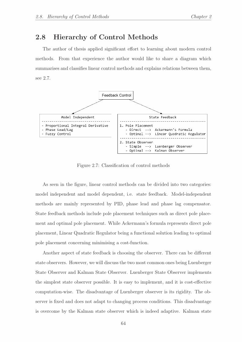
2.8. Hierarchy of Control Methods Chapter 2

2.8 Hierarchy of Control Methods

The author of thesis applied significant effort to learning about modern control

methods. From that experience the author would like to share a diagram which

summarises and classifies linear control methods and explains relations between them,

see 2.7.

Figure 2.7: Classification of control methods

As seen in the figure, linear control methods can be divided into two categories:

model independent and model dependent, i.e. state feedback. Model-independent

methods are mainly represented by PID, phase lead and phase lag compensator.

State feedback methods include pole placement techniques such as direct pole place-

ment and optimal pole placement. While Ackermann’s formula represents direct pole

placement, Linear Quadratic Regulator being a functional solution leading to optimal

pole placement concerning minimising a cost-function.

Another aspect of state feedback is choosing the observer. There can be different

state observers. However, we will discuss the two most common ones being Luenberger

State Observer and Kalman State Observer. Luenberger State Observer implements

the simplest state observer possible. It is easy to implement, and it is cost-effective

computation-wise. The disadvantage of Luenberger observer is its rigidity. The ob-

server is fixed and does not adapt to changing process conditions. This disadvantage

is overcome by the Kalman state observer which is indeed adaptive. Kalman state

64

Chapter 2 2.9. State Feedback Control

observer is somewhat harder to implement and tune, but it is much more robust

and reliable as compared to Luenberger observer. From a practical point of view,

the Kalman state observer is the most common one in the areas where human life

is entrusted to a machine. Kalman observer is used widely in the airspace, rocketry,

navigation, naval, production lines and many other industries.

In our project we proved, theoretically and experimentally, model-independent

methods to fail for our models. Therefore, the scope of our consideration will focus

on state feedback methods such as LQR, LQG and Kalman state observer.

2.9 State Feedback Control

As per [38], state feedback controllers represent a prominent category of advanced

control methods. In state feedback, the system’s state variable is multiplied by the

feedback gains vector to calculate the control effort which is required to stabilise the

plant. The diagram 2.8 shows the general idea of state feedback control. Note that

the feedback gain vector K can be found through different ways either by solving a

linear quadratic regulator problem or by direct pole placement.

Figure 2.8: State feedback control

2.9.1 Ackermann’s Formula

Ackermann’s formula [39], [40] is a control system design method developed for

solving the pole allocation problem. In control systems design, one of the primary

problems is the design of controllers that will change the properties of the plant in a

particular way by altering the location of plant’s poles to a more suitable and often

65

2.9. State Feedback Control Chapter 2

more stable region. Ackermann’s formula is an efficient pole allocation method which

allows one to move poles of the plant to an arbitrary desired location, in theory. In

practice, of course, relocation of the poles is limited by actuator capabilities.

Consider a state-space [41] of a linear time invariant model 2.52

x(t) = Ax(t) +Bu(t)

y(t) = Cx(t)

(2.52)

Then the transfer function of the system can be found as 2.53

G(s) = C(sI − A)−1B = CAdj(sI − A)

det(sI − A)B (2.53)

From 2.53 one can see that the denominator of the transfer function is given by

the characteristic polinomial of A i.e. the poles of the system are also the eigenvalues

of A.

If the system is unstable, or has a slow response or any other characteristic that

does not meet the design criteria, it could be advantageous to relocate the poles. The

realization given by the state-space, however, represents the intrinsic dynamics of the

system, and sometimes cannot be altered. One approach to this problem might be to

create a feedback loop with a gain K that will feed the state variable into the input.

If the system is controllable, then it will feature an input u(t) such that any initial

state x0 can be transferred to any other state x(t). Given that, a feedback loop can

be introduced to the system with the control input u(t) = r(t) −Kx(t), where r(t)

being the reference signal, see 2.9.

Then, the new dynamics of the system will be described by 2.54

x(t) = Ax(t) +B[r(t)−Kx(t)] = (A− BK)x(t) +Br(t)

y(t) = Cx(t)

(2.54)

In this new realisation the poles will be defined by the eigenvalues of the new ma-

66

Chapter 2 2.9. State Feedback Control

Figure 2.9: Concept of state feedback control

trix det[sI−(A−BK)]. Let D(s) be the desired characteristic polynomial. Then one

can find gain vector K with the formula 2.55, where D(A) is the desired characteristic

polynomial evaluated at matrix A.

K = [0, 0, · · · , 0, 1]C−1D(A) (2.55)

It should be also mentioned that Matlab software package contains an embed-

ded function for robust pole placement which implements the numerical algorithms

discussed in [?] and [?].

2.9.2 Linear Quadratic Regulator

According to [20] Linear quadratic regulator minimises a quadratic cost-function

J(u) for a linear time invariant system in state-space form, see equation 2.56. This

variational equation transforms into an algebraic Riccatti equation 2.57, which is to

be solved with respect to S. Then, the feedback gains vector is found as shown in

equation 2.58.

x = Ax+ Bu

J(u) =

∫ ∞

0

(xTQx+ uTRu+ 2 xTN u

)dt

(2.56)

ATS − SA− (SB +N)R−1(BTS +NT ) +Q = 0 (2.57)

67

2.9. State Feedback Control Chapter 2

K = R−1(BTS +NT ) (2.58)

For practical purposes, it is important to remember that matrices Q, R and N

are positive-definite and represent the penalties for various cross-products of system’s

states and the control effort. In practice, the penalties for the cross terms are often

not used and set equal to zero. It can be convenient in many cases to have Q as a

diagonal matrix of penalties given to each individual state. Thus the higher diagonal

element of Q signifies the penalty for a higher system state. For example, an element

q44 gives a penalty for state x4. The matrix R represents the penalty for the controller

effort which is typically kept small. Matrix N is the cross-penalty of the state and

the control effort and is set to zero in the majority of cases.

2.9.3 Luenberger State Observer

In [38], it is also explained that a state observer is nothing but a copy of the plant.

State observers are usually implemented digitally on micro-controllers. The idea of

having a copy of the plant is that we can force our digital copy to converge to plant’s

true states by placing another feedback gain L into it. As seen in figure 2.10, two

signals are collected from the real plant: the output y and the input u. Given these

two, one can duplicate the plant numerically with additional feedback gain L. The

feedback L is required to correct any deviation between the real plant output and the

predicted output of the copy such that the copy will always tend to converge to the

real plant’s state.

2.9.4 Kalman State Observer

According to [42], given a continuous plant 2.59, one can construct a state estimate

x that minimises the state estimation error covariance P = E[(x− x) · (x− x)T

].

Here, u is the known input, w is the white process noise, v is the white measurement

noise, that satisfy 2.60. Matrices Q, R, N are named process noise covariance ma-

trix, measurement noise covariance matrix, process-measurement covariance matrix,

correspondingly. Then, the optimal solution is the Kalman filter with equations 2.61,

68

Chapter 2 2.9. State Feedback Control

Figure 2.10: Luenberger state observer

Figure 2.11: Kalman filter as typically connectedwithin a control diagram

where the following conventions are taken: 2.62. Typical usage of Kalman filter is

shown on a control diagram in figure 2.11.

x = Ax+ Bu+Gw

y = Cx+Du+Hw + v

(2.59)

69

2.10. Fourier Transform Chapter 2

E [w] = E [v] = 0

E[wwT

]= Q

E[w vT

]= N

E[v vT

]= R

(2.60)

L =(P CT +N

)P = AP + P AT +Q− LRLT

˙x = Ax+ Bu+ L (y − Cx−Du)

(2.61)

Q = GQGT

R = R +H N +NT HT +H QHT

N = G(QHT +N

)(2.62)

2.10 Fourier Transform

In our experiments, we used Fourier analysis to process experimental data and

measure the frequency response of the mechanical system. As per [43], Fourier anal-

ysis is one of the most powerful techniques for temporal data processing. In this

section, we review the properties and formulas of the Fourier transform as such and

the discrete Fourier transform in particular that was useful to us in our analysis.

2.10.1 Continuous Fourier Transform

In general, Fourier transform is given by 2.63

f(ω) =1√2π

∫ +∞

−∞f(t)e−iωtdt (2.63)

The meaning of 2.63 is that we examine the function f(t) for incorporating si-

70

Chapter 2 2.10. Fourier Transform

Figure 2.12: Fourier complex amplitudes f(ω) mappedon complex plane for two arbitrary frequencies ω1 and ω2

nusoidal contributions of certain frequencies. Thus, the image f(ω) represents the

magnitude and phase angle of the corresponding harmonic fω(t). The expressions for

magnitude m(ω), phase ϕ(ω) and the harmonic fω(t) are given in 2.64. The set of

complex amplitudes f(ω) forms a Hermitian symmetric space, i.e. complex pseudo

Euclidean infinite dimension space due to the orthogonality of sinusoidal function.

Each complex amplitude can be mapped to a complex plane, see figure 2.12.

m(ω) =∣∣∣f(ω)∣∣∣ , ϕ(ω) = arg

(f(ω)

),

fω(t) = m(ω) sin (ωt+ ϕ(ω))

(2.64)

2.10.2 Discrete Fourier Transform

In many applications, using discrete Fourier transform [44] turns out to be more

practical. Suppose, we measure variable x in time with sampling rate of fN samples

per second. Thus, we have a discrete finite set of measurements {xn}, where n =

0, 1, . . . , N − 1. Then, we can apply discrete Fourier transform 2.65 to analyse

71

2.11. Laplace Transform Chapter 2

frequency properties of x(t).

Xk =N−1∑n=0

xn exp

(−i

2πk

Nn

)(2.65)

In 2.65 k ∈ [0, 1, . . . , N − 1] should be understood as the number of a harmonic

and Xk - as the corresponding complex amplitude with its magnitude and phase.

As mentioned, N is the length of the sample, and n is the number of discrete time

periods passed since the beginning of the measured sequence {xn}, that is the time

index.

fN =1

T(2.66)

fk ≤fN2

(2.67)

Let T be the sampling time in seconds. Then, the sampling rate fN , which is also

referred to as Nyquist frequency, is given by 2.66. It should be noted that according

to Nyquist sampling theorem [45], only the components having frequency smaller or

equal to half of the sampling rate can be resolved 2.67. Therefore, only the first half

of discrete spectrum {Xk}, k = 0, 1, . . . , N/2 carries useful information, whilst the

second half being nothing but a mirror image of the first one about the point k = N/2,

see figure 2.13. One can find the real frequency of k-th harmonic with formula 2.68.

The corresponding harmonic of the signal, then, is given by 2.69.

fk =k

NfN , ωk = 2πfk (2.68)

xωk(t) = |Xk| sin (ωkt+ arg(Xk)) (2.69)

2.11 Laplace Transform

Laplace transform is widely used in engineering. In this thesis, we used some

properties of the transform in our analysis and modelling. Here, we briefly review the

72

Chapter 2 2.11. Laplace Transform

Figure 2.13: Typical discrete Fourier spectrum

fundamentals of Laplace transform and some of its essential features.

Similarly to Fourier transform, Laplace transform does nothing but examines its

argument function for containing complex exponentials of all possible frequencies and

time factors, see 2.70. Note that Laplace transform converts the argument function

f(t) to its complex image f(s) and thus it maps functions and variables from time-

domain to complex s-domain, see formula 2.71, where 1/σ is the specific time of the

process, ω - is the frequency.

Another remarkable property of Laplace transform is how it acts on a function’s

derivative, see 2.72. This remarkable property allows one to transform ordinary differ-

ential equations to algebraic equations with respect to variable s, that are much easier

to analyse and solve in s-domain. Moreover, in many practical cases initial conditions

f(0), f ′(0), . . . , f (n)(0) can be assumed zero. The solution in s-domain usually takes

the form of a rational function which can be later converted back to time domain with

inverse Laplace transform 2.73 or evaluated with a numerical method, e.g. ODE45.

f(s) = L{f}(s) =∫ ∞

0

e−stf(t)dt (2.70)

s = σ + iω (2.71)

73

2.12. Bode Plot Stability Margins Chapter 2

L{f ′} = sf(s)− f(0)

L{f ′′} = s2f(s)− s f ′(0)− f(0)

L{f (n)} = snf(s)−n∑

k=1

sn−kf (k−1)(0)

(2.72)

f(t) = L−1{f}(t) = 1

2πilimT→∞

∫ γ+iT

γ−iT

estf(s)ds (2.73)

2.12 Bode Plot Stability Margins

In the experimental part of this research, we often used frequency analysis which

is associated with the interpretation of Bode plots. A Bode plot is a plot of two

graphs where one graph is the magnitude, and the other is the phase of a complex

amplitude, both plotted versus the frequency as illustrated by figure 2.14. Stability

margins are the amount of additional gain and phase delay that can be introduced

into a closed-loop system without making the system unstable.

2.12.1 Gain Margin

Suppose, we add some gain to the system. Then, it will only affect the top graph

from figure 2.14. Namely, it will make the magnitude graph shift up or down by an

amount of dB as per the gain chosen. Gain margin is the amount of additional gain

required to reach 0 dB level at a frequency where phase turns -180 degrees. In other

words, the system is stable as long as at the point of inverse phase gain remains below

0 dB.

2.12.2 Phase Margin

Similarly to the gain, if we add an arbitrary amount of phase delay to the system,

then it will only affect the phase graph from figure 2.14. Phase margin is the amount

of phase delay that can be added to the system without crossing the level of -180

degrees at a frequency where gain turns 0 dB. In other words, the system is stable as

74

Chapter 2 2.13. Akaike’s Final Prediction Error

Figure 2.14: Stagility margins

long as the phase delay at the frequency corresponding to 0 dB gain remains greater

than -180 degrees.

2.13 Akaike’s Final Prediction Error

As per [46], Akaike’s final prediction error is used as a measure of goodness of the

fitted model to the observation data. In this project, we used Akaike’s final prediction

error in our identification experiments to get an idea about the validity of the identified

models. FPE denotes Akaike’s final prediction error in the identification reports

generated in Matlab. For readers information, we define Akaike’s final prediction

error in expression 2.74.

FPE = det

[1

N

N∑1

e(t, θN)(e(t, θN)

)T](

1 + d/N

1− d/N

)(2.74)

Here N is the number of values in the estimation data set, e(t) is an n× 1 vector

75

2.13. Akaike’s Final Prediction Error Chapter 2

of prediction errors, θN represents the estimated parameters, d is the number of

estimated parameters.

76

Chapter 3

Modification of the Existing Setup

3.1 Half-Car Testing Rig

The experimental part of this project was done on a setup which is currently

located in UTS building 11 at level B4 in the Dynamics Lab. The setup is named Half-

Car Testing Rig and was built in the year 2005 by Laboratory Engineer Christopher

Chapman and a PhD student Wade Smith under the supervision of Professor Nong

Zhang. The picture of the original setup is taken from Wade Smith’s PhD thesis [12]

(see figure 3.1). The main elements of the rig are shown on diagram 3.2

As seen in the figure 3.1 and the diagram 3.2, the setup is built upon a massive

steel frame serving as a support. The half-car body itself is made of a horizontal

frame holding an additional block of mass for the inertia properties. The frame is

suspended on two suspension springs located on the left and the right. The hydrauli-

cally interconnected suspension system is embedded into the setup. The hydraulic

system provides anti-roll functionality also serving as suspension damping. There

are two minor frames on the sides that represent the unsprung masses that in a real

situation would be the wheels and the tires. The effect of tire stiffness is reproduced

by two tire springs of much higher stiffness. Additional mass blocks can be put onto

the horizontal frame on the left and on the right to increase the inertia of the system.

The bearing in the middle is restricted by the support frame to have only one vertical

degree of freedom and can move only in the vertical direction allowing roll inclination

77

3.1. Half-Car Testing Rig Chapter 3

as well. Note that suspension springs are omitted from the schematic diagram, al-

though they are present at the real setup. Overall, the system would react to external

disturbances such as, for example, lateral force and road inputs, as a real car would

react regarding vertical displacements of its elements and the body roll angle.

Figure 3.1: Half-Car Testing Rig designed and built by Wade Smithand Chris Chapman in 2005

Figure 3.2: Half-Car Testing Rig schematic diagram

78

Chapter 3 3.1. Half-Car Testing Rig

3.1.1 Parameters Identification

We started our practical work with identifying as many parameters of the half-car

testing rig as possible to the maximum possible precision. It should be mentioned

that not all parameters of the setup were well known initially. Therefore we needed

to identify the parameters of the setup experimentally. We identified stiffness of

springs by direct measurements. Inertia and damping were derived indirectly from

experimental data.

Spring Stiffness Identification

In spring stiffness identification experiment we were adding extra load blocks of

250 N each to the frame on the left and the right, and measured spring deflections

with linear voltage displacement transducers. In the table of measurements 3.1, are

shown the relative displacements of the half-car elements versus the additional load.

The data in the table was averaged over multiple repetitions. Thus, we can identify

the springs’ ratings as a linear regression of the data points obtained.

Table 3.1: Springs identification experiment

Force Δxs Δxt

N mm mm0 0.00 0.00

250 13.00 1.25500 25.75 2.75750 36.75 4.251000 48.75 6.00

In figure 3.3 are shown the graphs of suspension and tire spring stiffness. As

the setup has two springs of each type, the data was averaged over the identical

springs. We assumed here that minor parameter uncertainties were unimportant to

us at least at this stage. With regression analysis applied to the data points collected,

we identified suspension springs to have stiffness of ks = 20.0± 0.5 (kN/m) and tire

spring stiffness - kt = 172.0± 0.5 (kN/m).

79

3.1. Half-Car Testing Rig Chapter 3

Figure 3.3: Suspension spring and tire stiffness identification

Inertia and Damping Identification

To determine inertia properties and damping properties of the setup we used the

knowledge of 2nd order dynamical systems as discussed in section 2.5. To identify

inertia properties and damping we conducted two individual experiments, that is free

vibration of the car body in vertical direction and free vibration of car body in the roll

plane. We found the amplitude values of the vibration responses measured. Given

the solution of homogeneous second order differential equation (see equation 3.1) we

graphed exponential envelopes for the two modes of vibration that are the bounce and

the roll modes. In figures 3.4 are shown the free vibration responses of half-car body to

a step input excitation. In figures 3.5 are shown the exponential envelopes graphed

in logarithmic scale such that the envelope exponential curve becomes a straight

line. The corresponding data can be found in tables 3.2 and 3.3. The identified

decay parameters for the bounce mode and the roll mode are γbounce = 0.507 s-1 and

γroll = 1.823 s-1 respectively. The corresponding vibration angular frequencies are

found to be ωbounce = 8.726 rad/s and ωroll = 14.411 rad/s. Now we can also find

the natural frequency of oscillation of the setup when no damping is assumed. The

80

Chapter 3 3.1. Half-Car Testing Rig

natural frequencies turn out to be ω0 bounce = 8.741 rad/s and ω0 roll = 14.525 rad/s.

This now allows us to find the body mass and body roll inertia as ms = 475 kg and

Is = 120 kg.m2. We can find the equivalent suspension damping coefficient that is

produced by the hydraulic system as cs = 240 N/m.s-1.

It should be noted that figure 3.5(a) has three outlier data points that are taken

in a red box. The outliers can be explained by the system having some dry friction

between its parts which is known not to follow the general law of friction which is

usually assumed by default. Unlike the general law when the friction force is assumed

proportional to velocity in dry friction the force is constant and therefore it may

result in the deviation from exponential decay such as observed in figure 3.5(a). In

our analysis, of course, we disregarded the outlier data points as those would have

led us to a somewhat distorted result.

To summarise our findings, we made a table of all parameters that were identified

in this free vibration experiment (see table 3.4).

x(t) = x0e−γt sinωt (3.1)

(a) Free bounce vibration (b) Free roll vibration

Figure 3.4: Experimental graphs of half-car responses when subjected to a step input

81

3.1. Half-Car Testing Rig Chapter 3

(a) Bounce mode (b) Roll mode

Figure 3.5: Exponential envelopes for the bounce and the roll free vibration modes

Table 3.2: Bounce exponential envelope

Time Ampl.s a.u.0.00 1.000.35 0.830.71 0.691.08 0.571.45 0.491.81 0.402.18 0.332.54 0.262.90 0.183.26 0.113.62 0.06

Table 3.3: Roll exponential envelope

Time Ampl.s a.u.0.00 1.000.22 0.570.43 0.500.63 0.320.84 0.201.07 0.131.30 0.121.51 0.061.74 0.04

82

Chapter 3 3.2. Hydraulic Interconnected Suspension

Table 3.4: Half-car rig specifications identified experimentally

Parameter Notation Value UnitsHalf-car body mass ms 475 kgHalf-car body roll inertia Is 120 kg.m2

Unsprung mass mu 35 kgSuspension spring stiffness ks 20 kN/mTire stiffness kt 172 kN/mEquivalent HIS damping cs 240 N/m.s-1

Table 3.5: Active hydraulically interconnected suspension specifications

Parameter Notation Value UnitsAccumulator precharge pressure P0 250 kPaAccumulator volume V0 0.32 LOperating pressure P 14 barUpper HIS cylinder area a1 5.1× 10−4 m2

Lower HIS cylinder area a2 4.1× 10−4 m2

Actuator cylinder area a3 1.2× 10−3 m2

3.2 Hydraulic Interconnected Suspension

As for the parameters of the hydraulically interconnected suspension system, many

of them are hidden and can not be obtained by direct measurement. Even experi-

mentally, it is hard to measure such parameters as, for instance, the linear loss coeffi-

cients. When working on the half-car testing rig, we could choose such parameters as

precharge accumulator pressure and working hydraulic pressure. Other parameters

were known from our designs and technical documentation. Those are the piston

areas. In this section, we made a joint table (see table 3.5) of all known parame-

ters of the active hydraulically interconnected suspension system to the best of our

knowledge. The parameters are also explained in figure 3.6.

3.3 Modifications to the Existing Rig

We started our designs by reproducing a 3D model of the existing half-car testing

rig as shown in figure 3.7. The uncertainties in the drawing in figure 3.7 are as small

as ±20 mm. The drawings and 3D models are also attached to this thesis as they

represent a significant part of our work.

As our experiments imply testing anti-roll capability of active hydraulically inter-

83

3.3. Modifications to the Existing Rig Chapter 3

a1

a2

a3

V0P0

Pc h

V0P0

Pc h

a1

a2

Actuator

HIS

Figure 3.6: Diagram explaining known active hydraulically intercon-nected suspension system parameters

connected suspension, then we needed to add an external disturbance in the existing

setup that would simulate the effect of lateral force emerging from a rapid turning

maneuver. To simulate the external lateral force, we proposed to build a roll frame

which is to be attached to the main body from the bottom and connected with a

hydraulic actuator pushing the attached frame at the bottom against the roll centre

bearing. We refer to this actuator as roll actuator further in the text.

We demonstrate the idea of roll actuator on a schematic diagram 3.8. One can

see that as the roll actuator is pushing or pulling against the roll centre bearing, the

car body will incline in the roll plane. It should be noted that the actuator is driven

hydraulically and has a control unit allowing us to deliver an arbitrary force acting

on the roll frame.

3.3.1 Attached Roll Frame

We designed a frame (see figure 3.9(a)) which is taking the lateral load from the

roll actuator. The frame is attached to the bottom of the half-car horizontal frame

which represents the car body. The frame was then built in metal at the UTS FEIT

84

Chapter 3 3.3. Modifications to the Existing Rig

Figure 3.7: 3D CAD model of the original half-car testing rig

Figure 3.8: Schematic diagram showing how roll moment is translated from the ac-tuator to the half-car body

85

3.3. Modifications to the Existing Rig Chapter 3

workshop according to the drawings provided. The body of the frame is welded of

50 × 50 mm steel channel. In figure 3.9(b) is shown the photo of the real roll frame

as it was received from the FEIT workshop. The frame is designed to take loads as

high as 10 kN by order of magnitude.

(a) Designed (b) Manufactured

Figure 3.9: The frame serving to pass the force moment from the roll actuator to thehalf-car body

3.3.2 Roll Actuator

We, then, designed the roll actuator to push and pull the roll frame against the

roll-centre bearing. In figure 3.10(a) is shown the 3D computer-aided graphical design

and in figure 3.10(b) is shown a photo of actuator assembly with its mount brackets.

The brackets separately are shown in figure 3.11. The actuator installed in place at

the half-car rig is shown in figure 3.10(c).

86

Chapter 3 3.3. Modifications to the Existing Rig

(a) Designed

(b) Manufactured

(c) Installed

Figure 3.10: Roll actuator assembly

87

3.4. Active HIS Actuator Chapter 3

3.3.3 Modified Half-Car Rig

After all modifications the half-car rig is capable of simulating roll moment applied

to the car body as an external disturbance. The modified half-car testing rig is shown

in figure 3.12. The 3D CAD drawing 3.12(a) and the photo 3.12(b) give reader the

evidence of work that we had done.

3.4 Active HIS Actuator

To have an ability to control the half-car roll angle from the suspension side,

we designed and built an actuator for the hydraulically interconnected suspension

system. As shown in figure 3.6 a dual-acting double-rod cylinder represents the ac-

tuator. As the cylinder moves, the hydraulic fluid flows from one side to another

creating pressure difference between the two sides of the hydraulic circuit. The dif-

ferential pressure is then converted into an additional anti-roll force exerted by the

hydraulically interconnected suspension on the car body.

In reality, we approached the design of such actuator taking into account the cost

of a dual-acting double-rod custom hydraulic cylinder. Since such part is a quite

rare mechanical component, the cost of it in the market varies in the approximate

range between $3000 and $7000. Therefore, in our designs, we decided to combine two

standard cheap cylinders offered by an Australian agriculture machinery manufacturer

named Catford Engineering at an affordable price of only around $200 per piece.

The quality of the cylinders is satisfactory, and after more than two years usage the

cylinders remain in good condition.

Another expensive component of the design is the servomotor with its control

unit. These hardware pieces were borrowed from a different project of UTS which

was discontinued long time ago. Thus, the estimated cost of the assembled design is

only around $600.

88

Chapter 3 3.4. Active HIS Actuator

3.4.1 Rough Calculation

Before we begin to design the actuator for active hydraulically interconnected

suspension, it seems important to us to make a preliminary rough estimation of such

key parameters as differential pressure and actuator axial force. This calculation

will then give us an approximate idea of the loads experienced by the system and

conditions at which the actuator will work. When doing the estimation, we assume

the hydraulically interconnected system parameters to be equal to those listed in table

3.5. Additionally, we need to assume the half-car parameters equal to those in table

3.4. In this calculation we consider a half-car subjected to the lateral acceleration of

as much as al = 1g by order of magnitude.

Let us first find the lateral force exerted on the vehicle body due to a rapid

turning maneuver. From second Newton’s law we find that Fl = msal = 4.6 kN.

The lateral force will result in the roll moment of as much as M = Fl ∗ h = 2.3

kN.m which is also applied to the vehicle body. Equivalently, this roll moment will

be distributed over the car suspension which is to generate an opposing force Fs

creating an opposing roll moment of presumably same magnitude. Then we can

write M = Fs 2b or Fs = M/2b = 1.4 kN. Then force is, of course, generated by all

suspension elements, but for now, as we are only looking for orders of magnitude,

we may disregard the suspension springs and dampers and assume that all the force

comes from the hydraulically interconnected suspension. Under such an assumption

the differential pressure induced in the hydraulic system will be as high as ΔP =

Fs/a3 = 12 bar.

Thus we obtained two critical parameters to be accounted for in our designs.

Those are the suspension force Fs ≈ 1.4 kN which by value is equal to the axial force

required to move the actuator, and the differential pressure ΔP ≈ 12 bar which can

be useful to us when designing the actuator as well as in modelling and simulations.

89

3.4. Active HIS Actuator Chapter 3

3.4.2 Actuator Design

The design of this actuator includes some third-party components such as the

servomotor, the cylinders, the ball-screw actuator. Therefore, we first modelled all

these components in 3D CAD software named SolidWorks. Then we designed the

assembly and some custom parts that were somewhat complicated from the CAD

and manufacturing perspective. Custom parts were later manufactured in the FEIT

Workshop using CNC machinery. The final assembly was built in FEIT Workshop

too.

Two custom parts were designed for the actuator. One is the linkage arm between

the ball screw and the hydraulic cylinders which connect the rod of a cylinder to the

ball screw actuator as shown in figure 3.13. The other part is the coupling for the

motor which couples the motor to the ball screw shaft as shown in figure 3.14. The

final assembly is shown in figure 3.15.

The author would like to give credit and say thanks to the head of the Workshop

Laurence Stonard for valuable discussions on the designs and making things and his

willingness to help and collaborate. The author is thankful to the CNC machine

operator Siegfried Holler who manufactured all custom parts and assemblies with

high professionalism and responsibility in addressing specific needs of the project.

The author wants to say special thanks to the Dynamics Lab Engineer Christopher

Chapman who was consistently helping in so many different ways from carrying heavy

parts and to giving professional and competent pieces of advice when critical decisions

needed to be made.

3.4.3 Specifications

It may be useful to other PhD students who will probably use this setup in future

to have technical information available. Here we made two tables with the information

that is known about the active HIS actuator setup. The bill of materials for the active

HIS actuator assembly is given below in table 3.6. The specifications of the active

HIS actuator are listed in table 3.7.

90

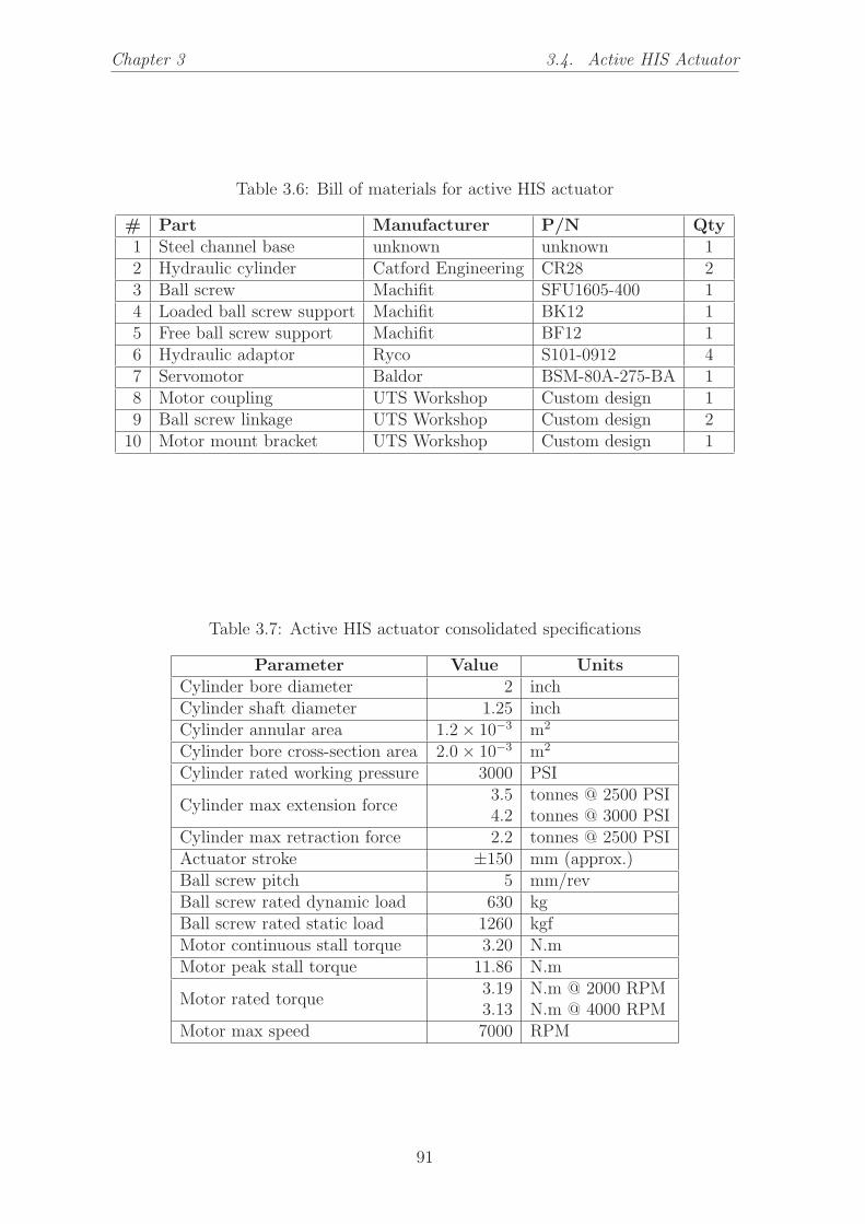
Chapter 3 3.4. Active HIS Actuator

Table 3.6: Bill of materials for active HIS actuator

# Part Manufacturer P/N Qty1 Steel channel base unknown unknown 12 Hydraulic cylinder Catford Engineering CR28 23 Ball screw Machifit SFU1605-400 14 Loaded ball screw support Machifit BK12 15 Free ball screw support Machifit BF12 16 Hydraulic adaptor Ryco S101-0912 47 Servomotor Baldor BSM-80A-275-BA 18 Motor coupling UTS Workshop Custom design 19 Ball screw linkage UTS Workshop Custom design 210 Motor mount bracket UTS Workshop Custom design 1

Table 3.7: Active HIS actuator consolidated specifications

Parameter Value UnitsCylinder bore diameter 2 inchCylinder shaft diameter 1.25 inchCylinder annular area 1.2× 10−3 m2

Cylinder bore cross-section area 2.0× 10−3 m2

Cylinder rated working pressure 3000 PSI

Cylinder max extension force3.54.2

tonnes @ 2500 PSItonnes @ 3000 PSI

Cylinder max retraction force 2.2 tonnes @ 2500 PSIActuator stroke ±150 mm (approx.)Ball screw pitch 5 mm/revBall screw rated dynamic load 630 kgBall screw rated static load 1260 kgfMotor continuous stall torque 3.20 N.mMotor peak stall torque 11.86 N.m

Motor rated torque3.193.13

N.m @ 2000 RPMN.m @ 4000 RPM

Motor max speed 7000 RPM

91

3.4. Active HIS Actuator Chapter 3

(a) Designed (b) Manufactured

(c) Designed (d) Manufactured

(e) Designed (f) Manufactured

Figure 3.11: Roll actuator mount brackets

92

Chapter 3 3.4. Active HIS Actuator

(a) Design

(b) Photo

Figure 3.12: Half-car testing rig after modification

93

3.4. Active HIS Actuator Chapter 3

(a) Designed (b) Manufactured

Figure 3.13: Linkage for active HIS actuator

(a) Designed (b) Manufactured

Figure 3.14: Motor coupling

94

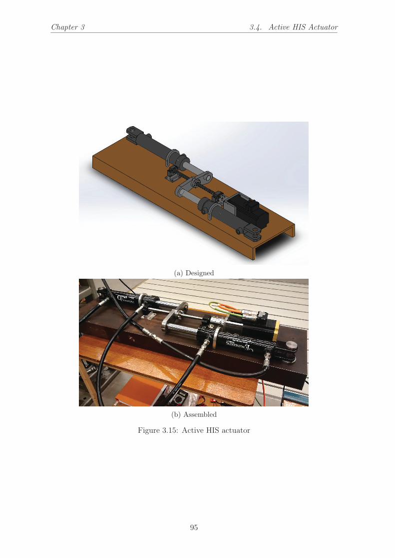
Chapter 3 3.4. Active HIS Actuator

(a) Designed

(b) Assembled

Figure 3.15: Active HIS actuator

95

3.4. Active HIS Actuator Chapter 3

Adaptor RYCO S101-09129/16" JIC Female Swivel

3/4" UNF UN O-ring Male

Hyd. cyl. CATFORD CR28

3/4" UNF UN O-ring Female Port

Hyd. hose PIRTEC 3/8" 2610 PSI9/16" JIC Female Swivel

9/16" JIC Male

Half-car rig HIS port

1/4" BSPP Female Port

Adaptor RYCO S74-04099/16" JIC Male

1/4" BSPP Encapsulated Male

Figure 3.16: Hydraulic connec-tions flow diagram of the activeHIS actuator

96

Chapter 4

Modelling

In this chapter, we obtain the half-car model with active HIS system embedded.

The half-car equations of motion are obtained by applying the Lagrange method for

systems with non-conservative forces to the mechanical model as described in 2.1.

The active HIS system model is obtained by applying the Kirchhoff’s laws discussed

in section 2.4.5 to the hydraulic circuit. The above two subsystems connect with each

other via the hydraulic-to-mechanical boundary condition.

4.1 Augmented Half-Car Model

In this section, we derive an augmented half-car model (see figure 4.1) which

has a few amendments compared to the conventional one. Along with two stan-

dard road disturbance inputs (u1, u2) the augmented model takes three other inputs:

f = (f1, f2, fr)T , where f1 and f2 are the additional suspension forces and fr is the

equivalent roll force which originates from the centrifugal force fc = msal exerted on

the car body due to a turning manoeuvre. Both models: conventional and augmented

will be used in our research.

In figure 4.1 the half-car model with embedded active HIS system is shown. The

massive block represents the car body having the mass ms (subscript ”s” stands

for ”sprung”) and inertia moment about the roll axis Is. The two smaller blocks

represent the unsprung masses of the wheels mu. The car body is suspended on the

wheels through suspension springs and dampers, ks and cs being the spring stiffness

97

4.1. Augmented Half-Car Model Chapter 4

and the damping coefficient of a damper correspondingly. Tire stiffness is modelled

by coefficient kt. Tire damping is modelled by ct. Also, we introduce wheel track

width as 2b. Table 4.1 summarises the parameters of the half-car model.

Note that according to Huygens-Steiner theorem the moment of inertia about the

roll axis of the vehicle is found as Is = Ixx + msd2, where Ixx being the intrinsic

vehicle body roll moment of inertia and d - the distance between the roll centre and

the centre of gravity of the vehicle. For the statement of the theorem, refer to section

2.2.

cs

HIS System

vaf

f

f

froll center

center of gravity

cs

ct ct

2b

ms

�s

f c al

mu mu

Is

ks

kt kt

w1

x 1

x 3

w2

x 2

x 4

ms

ks

Figure 4.1: Half-car model with active HIS

The variables of the model can be divided into three groups: state variables, inputs

and outputs. Let us briefly address each group. State variables are those that describe

the inner state of the model. The choice of state variables can be made differently.

In this model, the state variable is chosen to be a vector of four displacements that

uniquely define the position of the vehicle and all its inertia elements. The inputs of

the model are three disturbances: left road input, right road input, lateral acceleration

98

Chapter 4 4.1. Augmented Half-Car Model

and two additional suspension forces to account for the HIS system. The outputs are

two unsprung mass displacements, vehicle body bounce and vehicle body roll angle.

The model variables are summarised in table 4.2.

Table 4.1: Augmented half-car model parameters

Parameter Symbol UnitVehicle body mass ms kgVehicle body moment of inertia Is kg.m2

Suspension spring stiffness ks N/mTire stiffness kt N/mSuspension damping cs N/(m.s-1)Tire damping ct N/(m.s-1)Center of gravity height h mWheel track width 2 b m

Table 4.2: Augmented half-car model variables

Variable Symbol Unit

State variable: x = (x1, x2, x3, x4)T

Left wheel vertical displacement x1 mRight wheel vertical displacement x2 mVehicle body vertical displacement on the left x3 mVehicle body vertical displacement on the right x4 m

Input variables: f = (f1, f2, fr)T and w = (w1, w2)

T

Left road input disturbance w1 mRight road input disturbance w2 mLateral acceleration al m/s2

Additional suspension force on the left f1 NAdditional suspension force on the right f2 NEquivalent roll force due to lateral accel. fr N

Output variable: y = (x1, x2, xs, ϕs)T

Left wheel vertical displacement x1 mRight wheel vertical displacement x2 mVehicle center of gravity vertical displacement xs mVehicle body roll angle ϕs rad

Now we can write down the expressions for kinetic energy, potential energy and

the Rayleigh dissipation function as it was discussed in section 2.1. The expression

for kinetic energy 4.1, Rayleigh dissipation function 4.2 and potential energy of the

99

4.1. Augmented Half-Car Model Chapter 4

system 4.3 follow here.

T =1

2mux

21 +

1

2mux

22 +

1

2msx

2s +

1

2Isϕ

2s

T =1

2mux

21 +

1

2mux

22 +

1

8ms(x3 + x4)

2 +1

8b2Is(x3 − x4)

2

(4.1)

D =1

2cs(x3 − x1)

2 +1

2cs(x4 − x2)

2 +1

2ct(x1 − w1)

2 +1

2ct(x2 − w2)

2 (4.2)

U =1

2ks(x3 − x1)

2 +1

2ks(x4 − x2)

2 +1

2kt(x1 − w1)

2 +1

2kt(x2 − w2)

2 (4.3)

We then plug these into Lagrange equation 4.4 to obtain the equations of motion

4.5.

d

dt

∂T∂qi

+∂D∂qi

+∂U∂qi

= Fi (4.4)

mux1 + cs(x1 − x3) + ct(x1 − w1) + ks(x1 − x3) + kt(x1 − w1) = −f1

mux2 + cs(x2 − x4) + ct(x2 − w2) + ks(x2 − x4) + kt(x2 − w2) = −f2

mpx3 +mnx4 + cs(x3 − x1) + ks(x3 − x1) = f1 − fr

mpx4 +mnx3 + cs(x4 − x2) + ks(x4 − x2) = f2 + fr

(4.5)

Here the following conventions took place, see 4.6.

mp =1

4

(ms +

Isb2

)

mn =1

4

(ms −

Isb2

)

fr = fch

b= msal

h

b

(4.6)

100

Chapter 4 4.1. Augmented Half-Car Model

We can now formalise the equations of motion 4.5 into a matrix form 4.7

Mx+ Cx+Kx = Gf +Hw + Jw (4.7)

Here follow the matrices M , C, K, G, H, J . See corresponding expressions 4.8,

4.9, 4.10, 4.11, 4.12, 4.13.

M =

⎡⎢⎢⎢⎢⎢⎢⎢⎣

mu 0 0 0

0 mu 0 0

0 0 mp mn

0 0 mn mp

⎤⎥⎥⎥⎥⎥⎥⎥⎦

(4.8)

C =

⎡⎢⎢⎢⎢⎢⎢⎢⎣

cs + ct 0 −cs 0

0 cs + ct 0 −cs

−cs 0 cs 0

0 −cs 0 cs

⎤⎥⎥⎥⎥⎥⎥⎥⎦

(4.9)

K =

⎡⎢⎢⎢⎢⎢⎢⎢⎣

ks + kt 0 −ks 0

0 ks + kt 0 −ks

−ks 0 ks 0

0 −ks 0 ks

⎤⎥⎥⎥⎥⎥⎥⎥⎦

(4.10)

G =

⎡⎢⎢⎢⎢⎢⎢⎢⎣

−1 0 0

0 −1 0

1 0 −1

0 1 1

⎤⎥⎥⎥⎥⎥⎥⎥⎦

(4.11)

H =

⎡⎢⎢⎢⎢⎢⎢⎢⎣

kt 0

0 kt

0 0

0 0

⎤⎥⎥⎥⎥⎥⎥⎥⎦

(4.12)

101

4.2. Conventional Half-Car Model Chapter 4

J =

⎡⎢⎢⎢⎢⎢⎢⎢⎣

ct 0

0 ct

0 0

0 0

⎤⎥⎥⎥⎥⎥⎥⎥⎦

(4.13)

For further modelling it is convenient to have two slices of matrix G such that

G = [G1 G2] see equation 4.14.

G1 =

⎡⎢⎢⎢⎢⎢⎢⎢⎣

−1 0

0 −1

1 0

0 1

⎤⎥⎥⎥⎥⎥⎥⎥⎦

G2 =

⎡⎢⎢⎢⎢⎢⎢⎢⎣

0

0

−1

1

⎤⎥⎥⎥⎥⎥⎥⎥⎦

(4.14)

In listing A.1 is given the code initialising the parameters of a half-car model and

the matrices mentioned above.

4.2 Conventional Half-Car Model

Given the equations of motion in matrix form 4.7, we can obtain a state-space for

a conventional half-car model, see equations 4.15, 4.16, 4.17, 4.18, 4.19. In state-space

equations 4.15 the new state variable is constructed from the original one as follows:

x → (x, x)T = (x1, . . . , x8)T = x. The equations are written in assumption that

J = 0 for simplicity sake. The input variable here is u = (w1, w2, fr)T . The variables

of conventional half-car model are explicitly explained in table 4.3. In listing A.2 is

given the code initialising a conventional half-car model.

x = Ax+ Bu

y = Cx+D(4.15)

A =

⎡⎢⎣ [ 0 ]4×4 [ I ]4×4

−M−1K −M−1C

⎤⎥⎦

8×4

(4.16)

102

Chapter 4 4.3. Hydraulically Interconnected Suspension Model

B =

⎡⎢⎣ [ 0 ]4×3

M−1[H G2]

⎤⎥⎦8×3

(4.17)

C =

⎡⎢⎢⎢⎢⎢⎢⎢⎣

⎡⎢⎢⎢⎢⎢⎢⎢⎣

1 0 0 0

0 1 0 0

0 0 12

12

0 0 − 12b

12b

⎤⎥⎥⎥⎥⎥⎥⎥⎦

[ 0 ]4×4

⎤⎥⎥⎥⎥⎥⎥⎥⎦

4×8

(4.18)

D = [ 0 ]4×3 (4.19)

Table 4.3: Conventional half-car model variables

Variable Symbol Unit

State variable: x = (x1, x2, x3, x4, x1, x2, x3, x4)T

Left wheel vertical displacement x1 mRight wheel vertical displacement x2 mVehicle body vertical displacement on the left x3 mVehicle body vertical displacement on the right x4 m

Input variables: u = (w1, w2, fr)T

Left road input disturbance w1 mRight road input disturbance w2 mEquivalent roll force due to lateral accel. fr N

Output variable: y = (x1, x2, xs, ϕs)T

Left wheel vertical displacement x1 mRight wheel vertical displacement x2 mVehicle center of gravity vertical displacement xs mVehicle body roll angle ϕs rad

4.3 Hydraulically Interconnected Suspension Model

In this section, we derive the equations for active hydraulically interconnected

suspension. In figure 4.2 is shown the diagram of the hydraulic circuit. The circuit

consists of two suspension cylinders that are connected to the vehicle at the suspension

struts. The cylinders are cross-connected for anti-roll action. Thus, the circuit is

divided into two parts, each having an accumulator attached. The accumulators

103

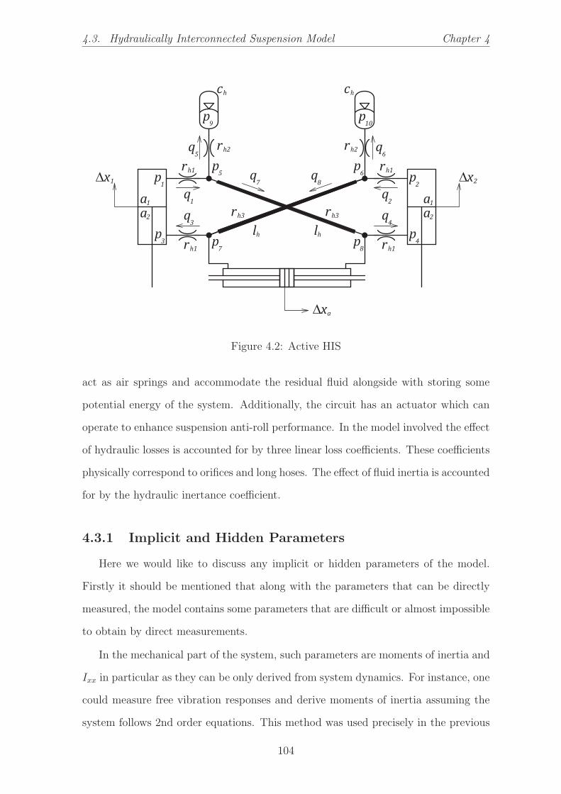
4.3. Hydraulically Interconnected Suspension Model Chapter 4

p1

p3

p2

p4

p5

p6

p7

p8

p9

q1

q3

q2

q4

q5

q6

q7

q8

rh1

ch ch

rh2

rh1

rh1 rh1

rh2

a1

a2

a1

a2rh3 rh3

lh lh

p10

x1 x2

xa

Figure 4.2: Active HIS

act as air springs and accommodate the residual fluid alongside with storing some

potential energy of the system. Additionally, the circuit has an actuator which can

operate to enhance suspension anti-roll performance. In the model involved the effect

of hydraulic losses is accounted for by three linear loss coefficients. These coefficients

physically correspond to orifices and long hoses. The effect of fluid inertia is accounted

for by the hydraulic inertance coefficient.

4.3.1 Implicit and Hidden Parameters

Here we would like to discuss any implicit or hidden parameters of the model.

Firstly it should be mentioned that along with the parameters that can be directly

measured, the model contains some parameters that are difficult or almost impossible

to obtain by direct measurements.

In the mechanical part of the system, such parameters are moments of inertia and

Ixx in particular as they can be only derived from system dynamics. For instance, one

could measure free vibration responses and derive moments of inertia assuming the

system follows 2nd order equations. This method was used precisely in the previous

104

Chapter 4 4.3. Hydraulically Interconnected Suspension Model

Table 4.4: Hydraulic circuit parameters

Parameter Symbol UnitSuspension cylinder upper area a1 m2

Suspension cylinder lower area a2 m2

Actuator cylinder annular area a3 m2

Circuit working pressure P PaAccumulator precharge pressure P0 PaAccumulator gas specific heat ratio γ –Accumulator volume V0 m3

Acc. gas volume at wrk. pressure V m3

Accumulator capacitance ch m3/PaFirst linear loss coefficient rh1 Pa/(m3.s-1)Second linear loss coefficient rh2 Pa/(m3.s-1)Third linear loss coefficient rh3 Pa/(m3.s-1)Hydraulic inertance ih Pa/(m3.s-2)

Table 4.5: Hydraulic circuit variables

Variable Symbol Unit

State variablesHydraulic pressure (p1, . . . , p10)

T PaVolumetric hydraulic flow (q1, . . . , q8)

T m3/s

Input variable Δx = (Δx1,Δx2,Δxa)T

Left suspension deflection Δx1 mRight suspension deflection Δx2 mActuator displacement Δxa m

Output variable p = (p1, p2, p3, p4)T

Pressure in upper chamber of left susp. cyl. p1 PaPressure in upper chamber of right susp. cyl. p2 PaPressure in lower chamber of left susp. cyl. p3 PaPressure in lower chamber of right susp. cyl. p4 Pa

Other variables specification (for reference)Pressure in left accumulator p9 PaPressure in right accumulator p10 Pa

105

4.3. Hydraulically Interconnected Suspension Model Chapter 4

chapter for mechanical parameters identification.

Another source of model uncertainty originates from hydraulic system linear loss

coefficients rh1, rh2, rh3. In our modelling, we only introduce three linear loss coeffi-

cients however one can always add more. It should be noted that the linear loss coef-

ficients can only be measured when physically isolated from the rest of the hydraulic

circuit. Any attempt to identify the coefficients indirectly meets a fundamental ob-

stacle that three coefficients form an under-defined system of simultaneous equations

which cannot be resolved.

4.3.2 Sub-models

Provided suspension deflections are denoted by Δx1 and Δx2 and the piston areas

- a1 and a2, then a cylinder can be modelled with the following set of equations 4.20.

q1 = a1Δx1, q2 = a1Δx2,

q3 = a2Δx1, q4 = a2Δx2

(4.20)

For simplicity hydraulic capacitor is linearized at a point (P, V ), and thus has

an approximate capacitance given in 4.21. The accumulator follows the dynamic

equations 4.22.

ch ≈ 1

γ

V

P(4.21)

p9 =1

ch

∫q5 dt, q5 = chp9

p10 =1

ch

∫q6 dt, q6 = chp10

(4.22)

An orifice can be modelled with the Poiseuille’s law 4.23, where rh is the linear

loss coefficient and Δp stands for the pressure drop across the orifice. A hose can be

modelled with a combination of the Poiseuille’s law and the hydraulic inertance law

106

Chapter 4 4.3. Hydraulically Interconnected Suspension Model

4.24, where ih is the hydraulic inertance coefficient.

Δp = rhq (4.23)

Δp = rhq + ihq (4.24)

4.3.3 Active HIS Model Derivation

The hydraulically interconnected suspension is modelled with the theory discussed

in section 2.4. As per derivation, the resulting model has only the zeros and no poles.

This fact agrees with the straightforward nature of the hydraulic equations taking

into account that the variable sought is the pressure. However, when the hydrauli-

cally interconnected suspension model is later embedded into the half-car mechanical

model, it contributes to the mechanical stiffness, damping and inertia matrices which

creates a superimposed half-car with active hydraulically interconnected suspension

model.

We use Kirchhoff’s laws to derive the equations of the model. Equations 4.25 result

from applying Kirchhoff’s current law to all junctions in the system. Then we apply

Kirchhoff’s 2nd law to the elements of the system and thus obtain a set of equations

4.26. Additionally, we have four equations for the accumulators, see equation 4.22 and

four equations for the cylinders, see equation 4.20. We solve equations 4.25, 4.26, 4.22

and 4.20 simultaneously for pressure and obtain the output vector p = (p1, p2, p3, p4)T ,

as expressed through Δx = (Δx1,Δx2,Δxa)T , which is required for the calculation

of force, see equation 4.27. The expressions for hydraulic matrices of elastance Sh,

resistance Rh and inertance Ih are given in 4.28, 4.29, 4.30 correspondingly. In listing

107

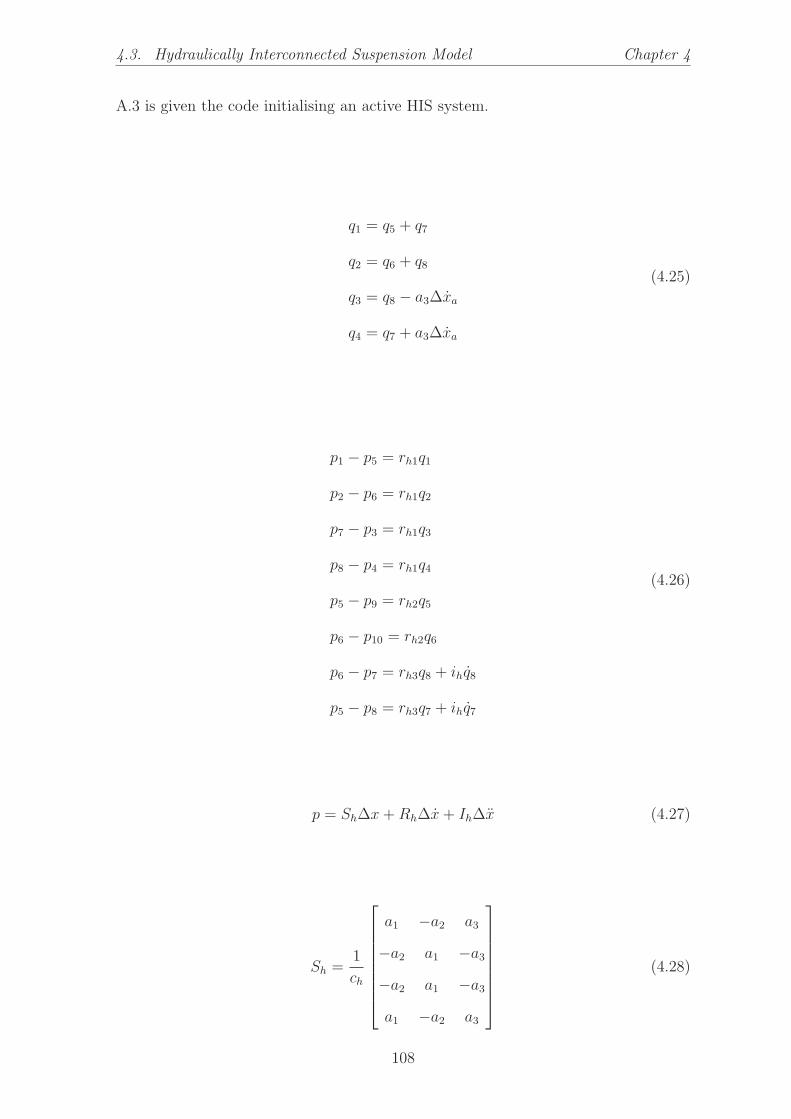
4.3. Hydraulically Interconnected Suspension Model Chapter 4

A.3 is given the code initialising an active HIS system.

q1 = q5 + q7

q2 = q6 + q8

q3 = q8 − a3Δxa

q4 = q7 + a3Δxa

(4.25)

p1 − p5 = rh1q1

p2 − p6 = rh1q2

p7 − p3 = rh1q3

p8 − p4 = rh1q4

p5 − p9 = rh2q5

p6 − p10 = rh2q6

p6 − p7 = rh3q8 + ihq8

p5 − p8 = rh3q7 + ihq7

(4.26)

p = ShΔx+RhΔx+ IhΔx (4.27)

Sh =1

ch

⎡⎢⎢⎢⎢⎢⎢⎢⎣

a1 −a2 a3

−a2 a1 −a3

−a2 a1 −a3

a1 −a2 a3

⎤⎥⎥⎥⎥⎥⎥⎥⎦

(4.28)

108

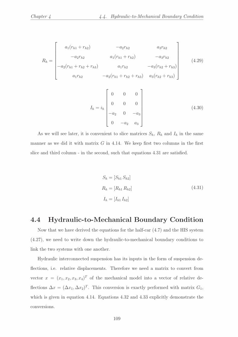
Chapter 4 4.4. Hydraulic-to-Mechanical Boundary Condition

Rh =

⎡⎢⎢⎢⎢⎢⎢⎢⎣

a1(rh1 + rh2) −a2rh2 a3rh2

−a2rh2 a1(rh1 + rh2) −a3rh2

−a2(rh1 + rh2 + rh3) a1rh2 −a3(rh2 + rh3)

a1rh2 −a2(rh1 + rh2 + rh3) a3(rh2 + rh3)

⎤⎥⎥⎥⎥⎥⎥⎥⎦

(4.29)

Ih = ih

⎡⎢⎢⎢⎢⎢⎢⎢⎣

0 0 0

0 0 0

−a2 0 −a3

0 −a2 a3

⎤⎥⎥⎥⎥⎥⎥⎥⎦

(4.30)

As we will see later, it is convenient to slice matrices Sh, Rh and Ih in the same

manner as we did it with matrix G in 4.14. We keep first two columns in the first

slice and third column - in the second, such that equations 4.31 are satisfied.

Sh = [Sh1 Sh2]

Rh = [Rh1 Rh2]

Ih = [Ih1 Ih2]

(4.31)

4.4 Hydraulic-to-Mechanical Boundary Condition

Now that we have derived the equations for the half-car (4.7) and the HIS system

(4.27), we need to write down the hydraulic-to-mechanical boundary conditions to

link the two systems with one another.

Hydraulic interconnected suspension has its inputs in the form of suspension de-

flections, i.e. relative displacements. Therefore we need a matrix to convert from

vector x = (x1, x2, x3, x4)T of the mechanical model into a vector of relative de-

flections Δx = (Δx1,Δx2)T . This conversion is exactly performed with matrix G1,

which is given in equation 4.14. Equations 4.32 and 4.33 explicitly demonstrate the

conversions.

109

4.4. Hydraulic-to-Mechanical Boundary Condition Chapter 4

The output of the HIS model is in form of pressure vector p = (p1, p2, p3, p4)T .

Pressures need to be converted into forces f = (f1, f2)T to be fed in the mechanical

model as inputs. Thus, we write down another conversion matrix Ah which is the ma-

trix containing piston area values, see equations 4.33. Now we can obtain equivalent

mechanical matrices that are super-induced by the HIS system, see equation 4.35.

Matrices G1 and Ah are given in equation 4.34. The resultant matrices from equa-

tion 4.35 are explained in table 4.6. In listing A.4 is given the code that implements

hydraulic-to-mechanical boundary conditions.

Δx = GT1 x (4.32)

f = Ah p (4.33)

GT1 =

⎡⎢⎣−1 0 1 0

0 −1 0 1

⎤⎥⎦

Ah =

⎡⎢⎣−a1 0 a2 0

0 −a1 0 a2

⎤⎥⎦

(4.34)

Mh1 = G1 Ah Ih1 GT1

Ch1 = G1 Ah Rh1 GT1

Kh1 = G1 Ah Sh1 GT1

Mh2 = G1 Ah Ih2

Ch2 = G1 Ah Rh2

Kh2 = G1 Ah Sh2

(4.35)

110

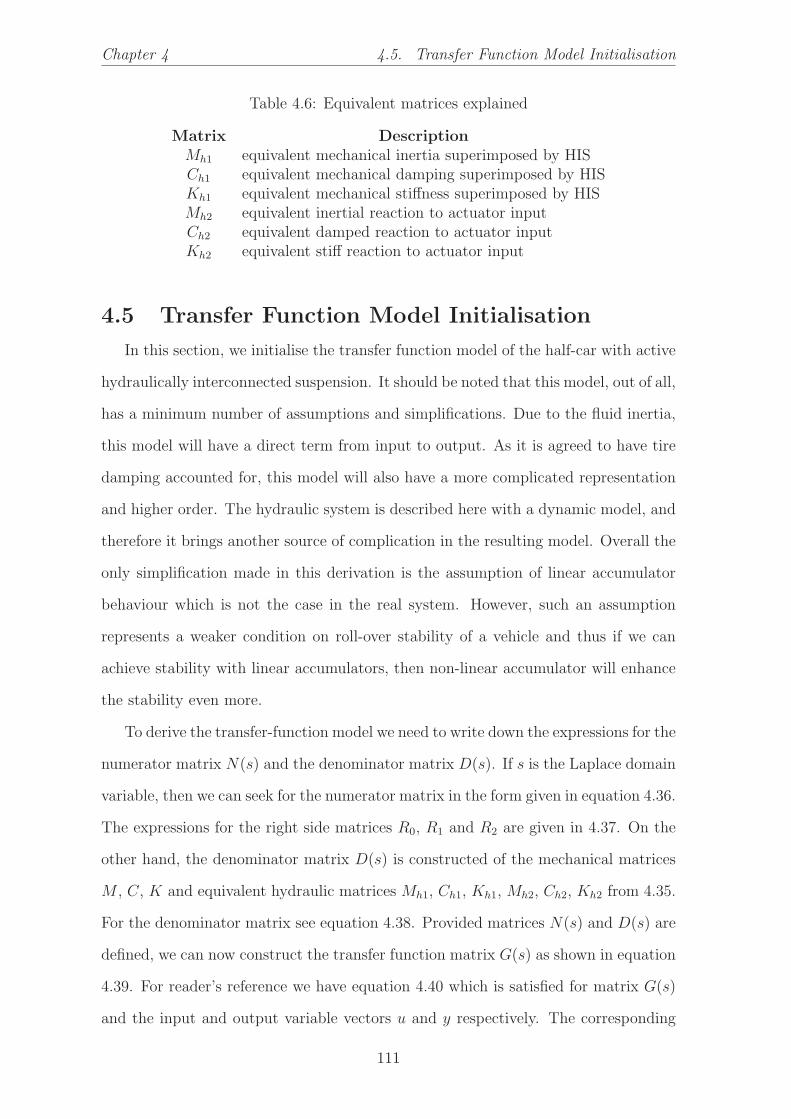
Chapter 4 4.5. Transfer Function Model Initialisation

Table 4.6: Equivalent matrices explained

Matrix DescriptionMh1 equivalent mechanical inertia superimposed by HISCh1 equivalent mechanical damping superimposed by HISKh1 equivalent mechanical stiffness superimposed by HISMh2 equivalent inertial reaction to actuator inputCh2 equivalent damped reaction to actuator inputKh2 equivalent stiff reaction to actuator input

4.5 Transfer Function Model Initialisation

In this section, we initialise the transfer function model of the half-car with active

hydraulically interconnected suspension. It should be noted that this model, out of all,

has a minimum number of assumptions and simplifications. Due to the fluid inertia,

this model will have a direct term from input to output. As it is agreed to have tire

damping accounted for, this model will also have a more complicated representation

and higher order. The hydraulic system is described here with a dynamic model, and

therefore it brings another source of complication in the resulting model. Overall the

only simplification made in this derivation is the assumption of linear accumulator

behaviour which is not the case in the real system. However, such an assumption

represents a weaker condition on roll-over stability of a vehicle and thus if we can

achieve stability with linear accumulators, then non-linear accumulator will enhance

the stability even more.

To derive the transfer-function model we need to write down the expressions for the

numerator matrix N(s) and the denominator matrix D(s). If s is the Laplace domain

variable, then we can seek for the numerator matrix in the form given in equation 4.36.

The expressions for the right side matrices R0, R1 and R2 are given in 4.37. On the

other hand, the denominator matrix D(s) is constructed of the mechanical matrices

M , C, K and equivalent hydraulic matrices Mh1, Ch1, Kh1, Mh2, Ch2, Kh2 from 4.35.

For the denominator matrix see equation 4.38. Provided matrices N(s) and D(s) are

defined, we can now construct the transfer function matrix G(s) as shown in equation

4.39. For reader’s reference we have equation 4.40 which is satisfied for matrix G(s)

and the input and output variable vectors u and y respectively. The corresponding

111

4.6. State-Space Model Chapter 4

equation of motion is given in 4.41. In table 4.7 the input and output variables of the

transfer function model are explicitly explained. In listing A.5 is given the code for

transfer function initialisation for a half-car with active hydraulically interconnected

suspension.

N(s) = R0 + sR1 + s2R2 (4.36)

R0 = [H G2 Kh2]

R1 = [J [ 0 ]4×1 Ch2]

R2 = [[ 0 ]4×3 Mh2]

(4.37)

D(s) = s2(M −Mh1) + s(C − Ch1) + (K −Kh1) (4.38)

G(s)4×4 = D−1(s)N(s) (4.39)

y(s) = G(s) u(s) (4.40)

(M −Mh1) y + (C − Ch1) y + (K −Kh1) y = R0 u+R1 u+R2 u (4.41)

4.6 State-Space Model

Now we can also derive a state-space for the model involved. In this derivation, we

assume the matrices of the right side that multiply the first and the second derivative

of the input to be equal to zero: R1 = 0 and R2 = 0. Such an assumption allows

us to keep the formalisation relatively human-friendly and straightforward as well as

to preserve the physical meaning of the system states. Although the resulting state-

112

Chapter 4 4.6. State-Space Model

Table 4.7: Transfer function model variables

Variable Symbol Unit

Input variable u = (u1, u2, u3, u4)T

Left road input u1 mRight road input u2 mEquivalent roll force u3 NHydraulic actuator displacement u4 m

Output variable y = (y1, y2, y3, y4)T

Left wheel vertical displacement y1 mRight wheel vertical displacement y2 mVehicle body vertical displacement on the left y3 mVehicle body vertical displacement on the right y4 m

space model is derived under these assumptions, it is often more practical to use this

very model rather than using a more complicated transfer function model.

We now derive the state-space for half-car with active hydraulically interconnected

suspension as it is described in section 2.7 under the assumptions mentioned above.

The matrices A, B, C, D that satisfy the state space equation 4.15 are given in

expressions 4.42, 4.43, 4.44, 4.45. The variables of the state-space model are explicitly

explained in table 4.8. The code initialising the state-space for the half-car with active

hydraulically interconnected suspension is given in listing A.6.

A =

⎡⎢⎣ [ 0 ]4×4 [ I ]4×4

−(M −Mh1)−1(K −Kh1) −(M −Mh1)

−1(C − Ch1)

⎤⎥⎦8×4

(4.42)

B =

⎡⎢⎣ [ 0 ]4×4

(M −Mh1)−1[H G2 Kh2]

⎤⎥⎦

8×4

(4.43)

C =

⎡⎢⎢⎢⎢⎢⎢⎢⎣

⎡⎢⎢⎢⎢⎢⎢⎢⎣

−1 0 1 0

0 −1 0 1

0 0 12

12

0 0 − 12b

12b

⎤⎥⎥⎥⎥⎥⎥⎥⎦

[ 0 ]4×4

⎤⎥⎥⎥⎥⎥⎥⎥⎦

4×8

(4.44)

113

4.7. System Order Analysis Chapter 4

Table 4.8: State-space model variables

Variable Symbol Unit

State variable: x = (x1, x2, x3, x4, x1, x2, x3, x4)T

Left wheel vertical displacement x1 mRight wheel vertical displacement x2 mVehicle body vertical displacement on the left x3 mVehicle body vertical displacement on the right x4 m

Input variables: u = (w1, w2, fr,Δxa)T

Left road input disturbance w1 mRight road input disturbance w2 mEquivalent roll force due to lateral accel. fr NActuator displacement Δxa m

Output variable: y = (Δx1,Δx2, xs, ϕs)T

Left suspension deflection Δx1 mRight suspension deflection Δx2 mVehicle center of gravity vertical displacement xs mVehicle body roll angle ϕs rad

D = [ 0 ]4×4 (4.45)

4.7 System Order Analysis

Finally, we obtained the model for the half-car with the active hydraulically inter-

connected suspension which in our codes is stored in a matrix object variable named

SYSSS. (system state-space). The model is generally of 8-th order and has multiple

inputs and multiple outputs. However, practically, the order of the model can be re-

duced within acceptable tolerance and accuracy bounds. Particularly for control sys-

tem design are useful the following two terms of the state-space matrix: SYSSS43(s)

and SYSSS44(s) that are originally of 8-th order. Element SYSSS43(s) stands for

the car body roll angle response to lateral force excitation. Element SYSSS44(s) is

responsible for the roll angle response to the input from the controlled actuator.

According to [36] Hankel singular values calculated for a model signify model

states’ contributions to the behaviour of the system. Thus, by checking Hankel sin-

gular values, one can examine the impact of every state on the system. This allows

114

Chapter 4 4.8. Control System Design

one to effectively truncate a model to a reasonable order and simplify further analysis

as well as the design of a control system. The respective Hankel singular values for

transfer functions SYSSS43(s) and SYSSS44(s) are shown in figure 4.3.

In figure 4.3 one can see that for both systems first two states are dominant,

whereas the third and the fourth states’ contributions are orders of magnitude smaller.

Based on this information we suppose that it is safe to truncate the models down to

second order with Matlab command reduce(SYSSS(4,4),2,’Algorithm’,’balance’).

To validate the truncation one can compare the Bode diagrams of the two systems

before and after truncation and see how well the reduced and original models match

within the range of frequencies of the interest. As discussed in the Introduction to

this thesis, the frequency range of interest for us is f = 0.1 . . . 10 Hz. In figure 4.4

the Bode diagrams are displayed. We consider the agreement of the models before

and after truncation that is seen in the figures as acceptable and satisfactory. The

truncated models will be then used in the next chapter for control system design and

simulations.

(a) SYSSS43(s) (b) SYSSS44(s)

Figure 4.3: Hankel singular values

4.8 Control System Design

For control system design we followed the tutorial from [38]. We consider a multi-

input-multi-output linear time-invariant system having two inputs and four outputs.

The system is constructed of two terms of the transfer function matrix SYSSS(s),

115

4.8. Control System Design Chapter 4

(a) SYSSS43(s) (b) SYSSS44(s)

Figure 4.4: Bode diagrams compared

namely SYSSS43(s) and SYSSS44(s). As they both belong to the same output which

is the roll angle, they share the same denominator whereas the numerator is different.

The SYSSS43(s) term is responsible for the disturbance exerted on vehicle body by

the lateral force. The SYSSS44(s) term takes account of the anti-roll actuator effort

influence on the system.

We, first, truncate the subsystem SYSSS44(s) to the order of two and store the

result in a variable SYSR(s). Then we design a linear quadratic regulator to enhance

the stability of SYSR(s). The subsystem SYSR(s) is initially stable, although near

marginal, as the poles of SYSR(s) are located relatively close to the imaginary axis

in the left half-plane. As seen in figure 4.5, the poles of the original system appear at

points −1.47± 17.5i s-1, resulting in an overshoot of 76.8%.

4.8.1 Linear Quadratic Regulator

To stabilise the plant SYSR(s) we find the state feedback gains K as a solution of

linear quadratic regulator problem. In Matlab, one can do it easily with the command

K = lqr(SYSR,Q,R,N);. It is still up to the engineer to choose the penalties. By trial

and error, we find the appropriate values of penalties that are given in equation 4.46.

116

Chapter 4 4.8. Control System Design

It is common to give higher penalty q22 = 10 to a higher state x2 as this should

normally result in the reduction of the absolute value of the error. We also assign

somewhat smaller penalty q11 = 1 to the lower state x1 as it is always a good practice

to have compensation for the error rate too. If not critical, we can keep the penalty

for the control effort R relatively small. Unless otherwise required, we are safe to

keep the cross terms all N equal to zero.

117

4.8. Control System Design Chapter 4

(a) Bode diagram

(b) Pole-zero map

Figure 4.5: Open loop model compared with closed loop model

118

Chapter 4 4.8. Control System Design

Q =

⎡⎢⎣1 0

0 10

⎤⎥⎦

R = 0.01

N =

⎡⎢⎣00

⎤⎥⎦

(4.46)

Now that we have the state-feedback gains vector K we can construct the closed

loop model. ProvidedA, B, C, D are the state-space matrices of the open loop system,

and A′, B′, C ′, D′ are the state-space matrices of the closed-loop system, we formalise

the closed loop system as shown in equation 4.47. The linear quadratic regulator

enhances the closed-loop system stability. In figure 4.5 are shown the poles of the

closed-loop system as compared with the poles of the open loop system. One can see

that the closed loop system has its poles located along the real axis and farther to the

left which results in zero overshoot, no oscillation when subjected to a step input and

a much faster settling time. For reference, is given the bode plot which is compared

between the two systems.

A′ = A− BK

B′ = B

C ′ = C

D′ = 0

(4.47)

119

4.9. Scripts Call Sequence Chapter 4

4.8.2 State Observer Design

To apply state-feedback control in practice, one also needs to design a state ob-

server. In our simulations, we are going to use Luenberger state observer as the one

which is easy to comprehend. To design the observer means to relocate the poles of a

system with state space matrices AT , CT . Relocation of poles can be done with Mat-

lab command L = place(A’,C’,[-200,-201])’; which returns observer feedback

gains vector L. One should remember that the observer must converge faster than

the observed model, that is the poles of the observer must be located farther away

to the left. As seen from the Matlab command above, our choice of observer poles is

(−200,−201) which is perhaps about ten times faster than the observed model. The

observer itself can be defined as a state-space model with matrices A′′, B′′, C ′′, D′′

that are given in equation 4.48. The script implementing the algorithms described in

this section are implemented in listing A.7.

A′′ = A− LC − BK

B′′ = L

C ′′ = [ I ]2×2

D′′ = 0

(4.48)

4.9 Scripts Call Sequence

The final piece of our modelling process is the simulation diagram. We build a

simulation diagram in Simulink environment which inherits all variables defined in

Matlab workspace. The diagram is shown in figure 4.6 and can be easily reproduced.

To produce valid models the scripts must be invoked in a particular sequence. This

120

Chapter 4 4.9. Scripts Call Sequence

call sequence is given in listing A.8.

All codes given in this section are consistent with one another, operational and

bug-free to the best of author’s knowledge. The author grants a permission to use

and modify these codes for research purposes. The author waives any responsibility

if these codes are used for commercial purposes.

Figure 4.6: Simulink model for active HIS

121

Chapter 5

Simulations

5.1 Controller Validation

Before we can start simulations, it is essential to validate the controller which we

designed in the previous chapter. There may be many ways of doing it. We prefer

to compare the controlled and uncontrolled responses of the system when subjected

to the same disturbance input as it is shown in figure 5.1. In the figure, one can see

two sub-models being tested from disturbance input to roll angle output. To judge

on the effectiveness of the controller designed we compare the Bode diagrams of the

same model when it is controlled against the situation when the model is uncontrolled

and exposes its passive behaviour, see figure 5.2. As seen in the figure, the diagram

of the controlled system efficiently does not feature any resonant frequency at all

and has consistently smaller magnitude than the uncontrolled model. At this stage,

we can conclude that we are quite satisfied with the controller and can proceed to

simulations.

5.2 Limitations of the Experimental Setup

In our simulations we pursue the following three objectives:

• to validate the simulation models,

• to demonstrate the feasibility of proposed methodology,

• to estimate the key physical parameters of the setup for design purposes.

122

Chapter 5 5.2. Limitations of the Experimental Setup

Half-car modelwith active HIS

Half-car modelwith active HIS

State observer

y

y

w

u

u

-G

LQR gain

Uncontrolled

Controlled

Disturbance: lateral forceRoll angle

Roll angle

w

Half-car with active HIS controlled by LQR

Submodel 1

Submodel 2

Disturbance

Figure 5.1: Controlled versus uncontrolled model comparison

Therefore we need to keep an eye on the maximum parameter ratings that the

experimental setup can physically handle. For convenience, we listed the most critical

parameters along with their absolute or desired maximum ratings in table 5.1.

Table 5.1: Desired maximum ratings

Variable Symbol Limit UnitActuator displacement Δxa 100 mmActuator speed Δxa 1000 mm/sBall screw axial load Fa 10 kNMechanical power Pm 1.0 kWMotor speed Ωm 4000 rpmMotor torque Tm 3.2 N.mVolumetric flow Qv 20 L/minDifferential pressure ΔP 28 bar

123

5.3. Time Domain Simulations Chapter 5

Figure 5.2: Controlled versus uncontrolled model Bode plot compared

5.3 Time Domain Simulations

Having in mind the goals, formulated above, we believe it will be sufficient to

subject the system to three different scenarios in our simulations. The first scenario

is a step input excitation. Since the Fourier spectrum of a step-function contains all

possible signal frequencies, testing the system with a step input is an efficient way

of judging about the stability and performance. Not only step input is helpful for

testing system’s stability properties, but also it will result in the system achieving

its maximum limits across many physical parameters. The most critical simulation

results for this scenario are shown in figure 5.3.

The second scenario used is a non-resonant sine-wave excitation. This scenario

will help us understand how the system is going to perform in normal non-critical

conditions. How much power is typically used, what are the typical loads, torques,

pressures and so forth. See the simulation results in figure 5.4.

The third scenario is a sine-wave excitation with a frequency that would be reso-

nant to the passive HIS system. This scenario is important because it concentrates

all excitation energy in just one single harmonic and also forces the active elements

124

Chapter 5 5.4. Important Parameters Monitoring

of the system to work against such concentrated excitation and expose maximum

performance possible. In other words, this is the worst case scenario the system must

be capable of coping with. The simulation results are shown in figure 5.5.

5.4 Important Parameters Monitoring

In all simulations, we monitor the critical parameters of the setup to account for

in our future designs. To conclude about the simulations we made a table of peak

parameter values for three different testing scenarios, see table 5.2. From the table,

one can see that in all three cases the maximum ratings were not exceeded. Therefore,

here we conclude that the system we modelled proves the feasibility of the project

and demonstrates sufficient level of anti-roll performance under different excitation

conditions. We can also conclude that the stability of the system is significantly

enhanced with the controller proposed.

Table 5.2: The table of peak parameter values

Parameter MaximumPeak value

Step Non-res. ResonantActuator displacement 100 mm 28 mm 25 mm 34 mmBall-screw axial load 10 kN 2.8 kN 2.5 kN 3.1 kNMechanical power 1 kW 0.42 kW 0.25 kW 1 kWMotor speed 4000 rpm 340 rpm 300 rpm 400 rpmMotor torque 3.2 N.m 2.2 N.m 2.1 N.m 2.5 N.mDiff. pressure 28 bar 21 bar 22 bar 26 bar

125

5.5. Ride and Handling Ability Simulations Chapter 5

5.5 Ride and Handling Ability Simulations

To understand the effect of active hydraulically interconnected suspension on ve-

hicle ride and handling ability we simulate three scenarios: vehicle response to road

roughness, vehicle response to single line shifting, vehicle response to double line

shifting.

As seen from figure 5.6, in each of the three scenarios, active hydraulically inter-

connected suspension system controlled by a linear quadratic regulator significantly

outperforms both the conventional suspension and the passive hydraulically intercon-

nected suspension.

In response to road roughness, both conventional suspension and passive hydrauli-

cally interconnected suspension systems exhibit a lot of roll oscillation whereas the

active hydraulically interconnected suspension effectively suppresses road disturbance

and keeps vehicle roll angle to a minimum.

In response to single and double line shifting, the conventional suspension and

passive hydraulically interconnected suspension oscillate and feature some transient

behaviour. At the same time, the active hydraulically interconnected suspension

eliminates all transition processes and makes the vehicle stick to the steering.

Overall we can conclude that the introduction of the active actuator into the

hydraulically interconnected suspension enhances its performance drastically both in

terms of ride comfort and also handling ability and driving safety.

126

Chapter 5 5.5. Ride and Handling Ability Simulations

(a) Lateral acceleration (b) Vehicle roll angle

(c) Mechanical power (d) Motor speed

(e) Ball-screw axial load (f) Motor torque

(g) Hydraulic pressure (h) Volumetric flow

Figure 5.3: Step input responses

127

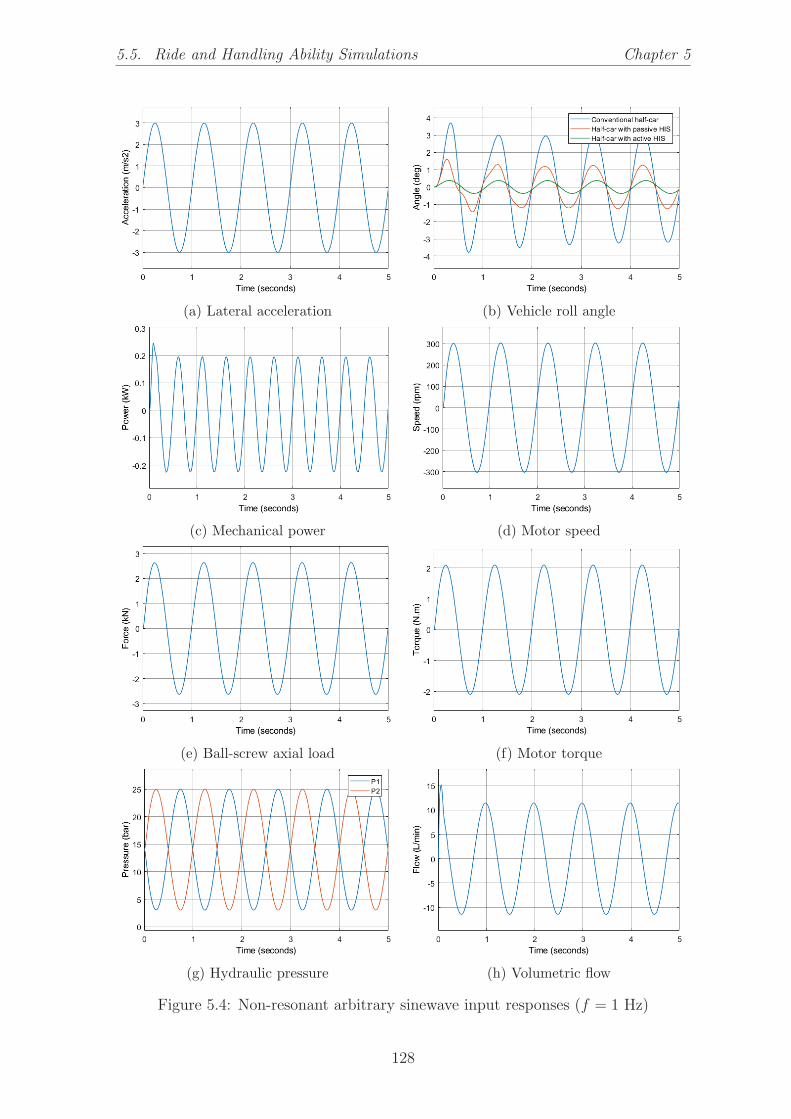
5.5. Ride and Handling Ability Simulations Chapter 5

(a) Lateral acceleration (b) Vehicle roll angle

(c) Mechanical power (d) Motor speed

(e) Ball-screw axial load (f) Motor torque

(g) Hydraulic pressure (h) Volumetric flow

Figure 5.4: Non-resonant arbitrary sinewave input responses (f = 1 Hz)

128

Chapter 5 5.5. Ride and Handling Ability Simulations

(a) Lateral acceleration (b) Vehicle roll angle

(c) Mechanical power (d) Motor speed

(e) Ball-screw axial load (f) Motor torque

(g) Hydraulic pressure (h) Volumetric flow

Figure 5.5: Responses to a sinewave input which is resonant for half-car with passiveHIS (ω = 17.5 rad/s)

129

5.5. Ride and Handling Ability Simulations Chapter 5

(a) Random process road input (b) Roll angle response to road roughness

(c) Single line shifting steering input (d) Roll angle response to single line shifting

(e) Double line shifting steering input (f) Roll ang. response to double line shifting

Figure 5.6: Vehicle ride and handling ability simulations

130

Chapter 6

Commissioning Work

After the setup was ready, there was still a lot of commissioning work to be done

before we could obtain first experimental results. In this chapter, we address the

main stages of our commissioning work. And provide somewhat more detailed tech-

nical information about the experimental setup. To better understand the physical

connections of the setup, please refer to diagram 6.1.

Drive UnitABB Microflex E150

ServomotorBaldor BSM80A-275BA

Microcontroller Board Arduino DueAlmel AT91SAM3X8E 84MHzExecutes an LQG compensator real-time

Ball-screw actuatorfor Active HIS

Mechanical SystemHalf-car Testing Rig

Personal Computer withArduino Native C++ IDE orMatlab & Simulink andArduino Support Package

SignalConditionigAmplifier

SignalConditionigAmplifier

Code deployed

Command signal

Disturbance

Roll angle

Measurement

Linear VariableDisplacement TransducerHP 24V LVDT 1000

Mechanical effort Mechanical effort

Analog signal Analog signal Analog signal

Analog signal

Figure 6.1: Physical connections diagram of the half-car testing rig closed loop control,anti-roll performance validation of the active HIS actuator

As seen in the diagram, the roll angle is measured with linear variable displace-

ments transducers. The signals then pass through a signal conditioning amplifier to

match the voltage levels between two different pieces of hardware. The signals are

fed into the ADC inputs of the microcontroller, where a linear quadratic Gaussian

131

6.1. Linear Variable Displacement Transducers HP 24V LVDT 1000 Chapter 6

compensator is digitally executed in real time. The output signals are collected from

DAC pins of the micro-controller and are proportional to the desired motor speed.

The signals are conditioned again before they are fed into the drive unit and then

passed in a native form to the motor. The motor drives the ball-screw actuator in

attempt to compensate the body roll of the half-car testing rig. The actuator itself is

another physical system which needs to be accounted for in the compensator design.

Thus, the control loop closes, and the process eventually stabilises at the roll angle

equal to zero. The appropriate compensator is primarily designed using Matlab and

Simulink or Arduino C++ IDE and the codes deployed on a micro-controller before

the setup runs.

6.1 Linear Variable Displacement Transducers HP

24V LVDT 1000

A linear variable displacement transducer is an electromechanical device used to

convert linear displacement into a voltage signal. In our project, we used Hewlett

Packard 24V LVDT 1000. This is an old model which is no longer manufactured.

The conversion principle of this particular model is electromagnetic. That is an

LVDT work as a voltage transformer with the variable core. This was also the reason

why the electromagnetic pickup noise was significantly high in our measurements.

Nevertheless, we managed to tackle the noise problem with advanced control methods

such as Kalman state observer. Below is the table of calibration 6.1 and the calibration

line graph 6.2. The corresponding calibration equation is given in 6.1 which has its

validity as high as R2 = 0.9947.

D = −6.0037V + 133.61 (6.1)

132

Chapter 6 6.2. Hydraulic Pressure Transducers TE Connectivity AST4100

Table 6.1: LVDT calibration data

Voltage DisplacementV mm

0.015 132.050.028 134.86-2.749 149.89-1.005 140.10-4.402 159.93-6.201 170.12-7.750 180.73-9.550 189.70-10.030 196.35-10.690 196.60

Figure 6.2: LVDT calibration line

6.2 Hydraulic Pressure Transducers TE Connec-

tivity AST4100

A pressure transducer is a device which converts pressure readings into a voltage

signal. In this project, we used TE Connectivity AST4100 series pressure transducers

part number C00100B3D0000. The specifications of the transducers are given in 6.2.

As per the specification, the transducer maps pressure range from 0 - 100 bar to a

voltage range from 1 - 5 V. Therefore, we can find corresponding calibration equations

133

6.3. Baldor Servomotor BSM80A-275BA Chapter 6

as shown in 6.2, where P1, V1 and P2, V2 are the pressures and transducer voltages

on the left and on the right of the HIS respectively. The V0 left = 1.036 V and

V0 right = 0.940 V are the corresponding offset voltages.

P1[bar] = 25 · (V1 − 1.036)

P2[bar] = 25 · (V2 − 0.940)

(6.2)

Table 6.2: Pressure Transducer AST4100-C00100B3D0000 Specifications

Parameter ValueProcess Connection 1/4” BSPP MalePressure Range 0 - 100 BarPressure Unit BarOutput Voltage Range 1 - 5 V

6.3 Baldor Servomotor BSM80A-275BA

In this project, we used a servomotor model Baldor BSM80A-275BA. The servo-

motor’s parameters are listed in table 6.3.

6.4 ABB Motor Drive Microflex E150

The motor was driven by the ABB Microflex E150 universal motor drive. Below,

we give some information about the drive which is important to the project. ABB

Microflex E150 has the following features:

• is a single axis drive for AC brushless servo motors,

• has a current rating of 6 A,

• can be powered with single phase 115/230V or 230V 3 phase AC voltage,

• position, velocity and current control,

• has two analog control inputs ±10 V,

• analog inputs are subject to first order embedded filter,

• works with ABB Mint Workbench software,

• connects to a PC via USB or Ethernet interface.

134

Chapter 6 6.5. Signal Conditioning Amplifier

Table 6.3: Baldor Servomotor BSM80A-275BA Specifications

Parameter Value UnitMax Speed 7000 rpmPeak Torque 12.8 N.mRated Torque 3.20 N.mRated Speed 4000 rpmAgency Approvals CE CSA TUV UR -Ambient Temperature 25 oCBearing Grease TypePolyrex EM -Duty Rating CONT -Insulation Class F -Motor Lead Quantity/Wire Size 3 @ 18 AWG -Mounting Arrangement F1 -Rated Current 4.28 ARated Power Output 1.25 kWNumber of Poles 4 -Peak Current 16.3 A

6.5 Signal Conditioning Amplifier

As mentioned above, ABB Microflex E150 drive takes two analog control signals

rated at ±10 Volts. At the same time, the LVDTs produce can produce a signal of

approximately ±6 Volts. Moreover, there is a micro-controller in between the LVDTs

and the motor drive, which encloses the control loop. As per the controller specifica-

tions, that are also given below, the microcontroller is only capable of handling signals

in the range of 0 - 5 Volts, that is the microcontroller’s ADC and DAC are both rated

at the range 0 - 5 Volts. Therefore, we needed to make a signal conditioning amplifier

to scale and shift the signals to the appropriate ranges between different pieces of

hardware.

Thus, we designed a general purpose tunable amplifier for signal conditioning.

The schematic of the amplifier and the simulation diagram are shown in figure 6.3.

The amplifier is an analog voltage-to-voltage converter with the possibility of gain

and offset adjustment.

The amplifier allows tuning the gain and the offset in a wide range which is

helpful when one needs to do analog signal manipulations such as discussed above.

The SPICE simulation diagrams are shown in figure 6.4.

135

6.5. Signal Conditioning Amplifier Chapter 6

We soldered four units of this amplifier and used them for analog signal condi-

tioning in our project. The 3D cad of a PCB is shown in figure 6.5 and the bill of

materials for making a single unit is given in table 6.4.

The amplifiers were used for signal scaling and shifting as an analog interface

between the LVDT transducers and the microcontroller and also between the micro-

controller output and the Flex II Drive unit.

TL061CP

10k

10kGND -E

+Ein

outOffset

Gain

(a) Schematic capture

(b) SPICE simulation diagram

Figure 6.3: Signal conditioning amplifier

136

Chapter 6 6.5. Signal Conditioning Amplifier

(a) Gain tuning (b) Offset tuning

Figure 6.4: Signal conditioning amplifier amplifier SPICE simulations

(a) CAD model of PCB

(b) Prototype

Figure 6.5: Signal conditioning amplifier

137

6.6. Dynamic Control with a Micro-Controller Chapter 6

Table 6.4: Bill of materials for signal conditioning amplifier

Component Manufacturer P/N QtyOperational amplifier Texas Instruments TL061CP 1Metal film resistor 10kOhm TE Connectivity LR1F10K 2Trimmer Resistor 10kOhm Bourns 3296W-1-103LF 2PCB Terminal Block Phoenix Contact 1725698 1

6.6 Dynamic Control with a Micro-Controller

We used Arduino Due micro-controller board for dynamic control. Arduino pro-

vides an outstandingly cheap alternative to such commercial products as, for example,

LabVIEW Real-Time Module (A$4,741). The cost of top Arduino board model is two

orders of magnitude less and is as low as only A$30. Despite the low price, Arduino

Due board is capable of handling real-time control loops at relatively high sampling

frequencies with the sampling time as fast as approximately 100 μs. The specifications

of the board are given in table 6.5. One should note that there are multiple ways to go

about programming Arduino. In this project, we used two different ways of doing it.

The first way is to do C++ coding in native Arduino IDE. With this one gets more

flexibility as well as more responsibility to handle lookup arrays, timer interrupts,

memory allocation, time-efficient coding and so forth. This allows one to produce

faster codes at the cost of more work and programming skill required to achieve the

same result. On the other hand, one can use Arduino Support Package for Simulink.

With that, one can create the codes that are more complicated although at the cost

of slightly longer time of execution. With Arduino Support Package for Simulink,

only the essential knowledge of hardware side is required from an engineer. Namely,

one needs to specify the sampling rate which complies with the hardware capabilities

and the solving method such as, for instance, first-order Euler’s algorithm.

6.6.1 Arduino Coding with Native C++ IDE

In this project, we started debugging our experimental setup with Arduino IDE

implementing a Proportional Integral Derivative compensator for the system in the

velocity form.

138

Chapter 6 6.6. Dynamic Control with a Micro-Controller

Table 6.5: Arduino Due micro-controller board specifications

Specification ValueMicrocontroller AT91SAM3X8EOperating Voltage 3.3VInput Voltage (recommended) 7-12VInput Voltage (limits) 6-16VDigital I/O Pins 54Digital PWM Outputs 12Analog Input Pins 12Analog Output Pins 2 (DAC)Total DC Output Current 130 mADC Current for 3.3V Pin 800 mADC Current for 5V Pin 800 mAFlash Memory 512 KBSRAM 96 KBClock Speed 84 MHzLength 101.52 mmWidth 53.3 mmWeight 36 g

6.6.2 PID Controller in Velocity Form

In this application, the actuator is a servomotor. Therefore, the actuator displace-

ment cannot be directly changed but only altered by motor speed.Thus, we need to

use the control algorithm in velocity form which will have its output signal propor-

tional to the motor speed. In ”s”-domain the velocity form for a PID controller is

given by the the expression 6.3, where Kp, Ki, Kd are proportional, integral and

derivative gains respectively.

C(s) = s

(Kp +

Ki

s+ sKd

)

C(s) = sKp +Ki + s2Kd

(6.3)

Thus, the feedback signal is differentiated once for the proportional action and

twice for the derivative action of the controller. One should note that the s operator

gain grows as fast as the angular frequency ω of the signal, and the s2 operator gain

- grows as fast as ω2. Therefore, high-frequency noise, although initially negligible,

139

6.6. Dynamic Control with a Micro-Controller Chapter 6

is amplified with extremely high gains after the differentiation and the controller

output becomes unacceptable because of the noise. This effect is often observed as

the chattering of the motor or high-frequency spikes on the control signal waveform.

6.6.3 The Effect of Sensor Noise

Suppose, a low-frequency signal is collected from a sensor. For simplicity we

assume a sine-wave (see equation 6.4) with an amplitude of a =√2 and angular

frequency of ω = 1 rad/s. Let us now add some white noise ξ(t) (see figure 6.6(b))

with a relatively small variance of σ = 1 · 10−3 to the original signal. Note that the

noise added to the signal is so small that it is not even seen by naked eye on the

graph 6.6(a). Using the definition of signal-to-noise ratio (see figure 6.5) we obtain

SNRu = 60 dB for the initial signal which is shown in figure 6.6(a).

u(t) = a sin(ωt) + ξ(t) (6.4)

SNRdB = 10 log10

(σ2signal

σ2noise

)(6.5)

Suppose the controller has a sampling rate of fN = 1 kHz meaning that the

sampling period is T = 1 · 10−3 seconds. Then, it can be shown that 1st derivative of

the signal u(t) will have signal-to-noise ratio of SNRu = −2.9 dB, see figure 6.6(c).

And 2nd derivative u(t) will have SNRu = −67.8 dB, see figure 6.6(d).

In our experiments, we measured the signal-to-noise ratio of the sensor signals

to be as small as approximately SNR = 30 dB. Thus, we can conclude that a PID

compensator is too sensitive to noise in the measurement signals and fails to provide

acceptable performance under the condition of even tiny noise in the sensors. How-

ever, we can try to design a discrete filter to make the collected signals somewhat

smoother.

140

Chapter 6 6.6. Dynamic Control with a Micro-Controller

(a) Original signal (b) Gaussian noise

(c) First differentiation (d) Second differentiation

Figure 6.6: The effect of noise on PID controller

6.6.4 Discrete Filter Design

To make the measured signals smoother we can implement one of the common

discrete filters on the controller. Typical frequency responses of most commonly used

filters are shown in figure 6.7. The figure is taken from [47]. We choose to use an

elliptic filter as it has the sharpest cut-off region of all.

A digital low-pass filter in discrete transfer function form can be easily designed

with Matlab command [b,a] = ellip(n,Rp,Rs,Wp);, where n is the order of the

filter, Rp is the passband peak to peak ripple measured in dB, Rs is stopband attenu-

ation in dB, Wp is the normalized cut-off frequency measured in fractions of Nyquist

frequency. Vector b contains discrete transfer function numerator coefficients. And

vector a contains discrete transfer function denominator coefficients.

Although with the discrete low-pass filter the measurement signal becomes much

smoother it is also subjected to a significant phase delay which imposes a severe

141

6.6. Dynamic Control with a Micro-Controller Chapter 6

Figure 6.7: Typical frequency responses of mostcommonly used filters

limitation on the stability of the system. As we found in our experiments, it is almost

impossible to tune a PID regulator to a detectable level of performance without

making the system unstable. Overall, we conclude that a PID controller, in general,

is not suitable for the application due to its high sensitivity to noise and difficulties

with tuning. The only part of PID that worked for us was the integral term alone,

which is known to be noise robust but slow.

6.6.5 Using Timer Interrupts

However, given a higher sampling rate, one could try using PID in their appli-

cations. The author would like to emphasise here one important aspect of dynamic

control, which is timer interrupts. It is often wrongly practised to use loop() func-

tion with delay() or delaymicroseconds(). The author of the thesis believes this

to be a mistake. With such an approach one can not guarantee the consistency of

sampling periods, and thus it can lead to any unexpected controller behaviour which

will also be difficult to debug.

Instead, one should use timer interrupts and interrupt service routine as demon-

strated in the listing below. In listing A.9 is given the C++ code implementing

142

Chapter 6 6.6. Dynamic Control with a Micro-Controller

discrete elliptic filter and a PID regulator in velocity form.

In our experiments we used timer interrupts setting of as fast as 1 millisecond in

order to guarantee the execution of the previous iteration to be finished by the time

the new iteration starts. The choice of this sampling time was made keeping in mind

that microcontroller clock speed is as high as 84 MHz.

6.6.6 Matlab and Simulink Arduino Support Package

Another way of programming Arduino micro-controllers is to use Arduino Support

Package for Matlab and Simulink. With Arduino for Matlab one can send commands

to the board and execute scripts. Simulink support package for Arduino offers all the

necessary function blocks (see figure 6.8) to design and execute complex control loops

in real time.

Figure 6.8: Simulink function blocks to work with Arduino

In our Simulink control diagram, we used the sampling time of 1 ms to allow

more time for the controller to solve high order differential equations. And we chose

the integration method as Euler first order integration to achieve faster performance

sacrificing some accuracy which is not so crucial in this real-time application.

Thus, we conclude here that in this section we reviewed most of the commissioning

work that we had done. However, we did not mention any work related to the project

but not containing any research component such as building and assembling hardware

parts and any other work of the kind.

143

Chapter 7

Identification Experiments

To effectively design a controller for a real physical system one needs to identify

the sub-models of interest that will be involved in the design of the compensator.

Therefore, in this chapter, we discuss a method of sub-system transfer function iden-

tification that we adopted from industry and successfully applied in our project. We

should say that in Control Engineering the feedback controllers are classified into two

major categories, namely: the model independent methods and the model dependent

methods. While model-independent techniques such as, for example, Proportional

Integral Derivative control, generally do not require the knowledge of the sub-model

and can be tuned easily by trial and error, the other category of model-dependent

methods, such as State-Feedback, necessarily require the preceding knowledge of the

sub-system transfer function or state-space. As we discussed in chapter 6, Propor-

tional Integral Derivative controller fails to deliver an appropriate level of stability

and roll angle reduction for our particular system. Therefore, we needed to think of

a more advanced controller to have more flexibility in our designs and achieve higher

stability and robustness of the control system.

The following forced vibration experiment was suggested to the author by his

co-supervisor Associate Professor Steven Su. The experiment was conducted by the

author of this thesis within approximately six months time which also included some

commissioning and troubleshooting work. The experimental data were analysed and

144

Chapter 7 7.1. Forced Vibration Experiment

processed by the author entirely independently as it will be described below in this

chapter. For the convenience of other researchers, the author will share the codes for

Fourier Analysis of the experimental data too.

7.1 Forced Vibration Experiment

Forced vibration experiment is a powerful technique used for real systems iden-

tification. It provides one with accurate equations of the system tested, that can

be formalised into a Linear Time-Invariant model, be it a state-space or a transfer

function, and allows one to design a model-dependent advanced controller such as

Linear Quadratic Gaussian controller or any other of the kind.

7.1.1 Idea of Forced Vibration Experiment

As it is commonly practised when solving linear differential equations to solve the

homogeneous equation with zero right side first, and then superimpose that solution

with a particular solution for a particular right side, the same procedure can be

implemented not only analytically but experimentally on a real system as well.

Solving homogeneous equation from the experimental perspective means free vi-

bration experiment when we excite the system with an external input, either a step or

an impulse and then observe system’s free oscillation until it entirely decays. Finding

a particular solution for an inhomogeneous equation means that we can subject the

system to an arbitrary input and measure the response. If we choose a sine-wave of

a specific amplitude and frequency to be the arbitrary input, then, as known from

the theory of second order systems, the system will respond with a sine-wave of the

same frequency but generally of different amplitude and phase. By measuring these

two quantities, the amplitude and the phase, we can identify system’s transfer func-

tion complex value at current frequency, which also places one data point on the

Bode diagram of the system. Thus, we can scan system’s responses over a range of

frequencies of the interest. Provided the number of observations at different frequen-

cies is sufficient, and the frequency range was chosen appropriately one can identify

system’s transfer function or state-space model using, for example, Matlab System

145

7.1. Forced Vibration Experiment Chapter 7

Identification tools.

One may argue here on the point that an experiment with a step input followed by

model identification in time domain only could be sufficient here. The author, then,

would argue back that time domain identification is effective only for second-order

models, whereas a system can be generally of a higher order. Moreover, if a system

being identified contains errors or noise of any nature of origin, then time domain iden-

tification becomes completely ineffective regarding the uncertainty of the identified

models. As opposed to time domain identification, frequency domain identification

yields a result of a much higher fidelity and reliability.

7.1.2 Experiment Layout

As mentioned above, when we subject a system to a sine-wave input excitation the

system will respond with a sine-wave of different amplitude and phase. To understand

this experiment better we made a quick simulation diagram 7.1 explaining the idea

of what is tested, where the excitations are fed and the signals collected.

Figure 7.1: Schematic diagram of the forced vibration experiment

As shown in the diagram 7.1, we are testing a physical subsystem by subjecting it

to a sinusoidal input excitation which can be any real physical quantity such as force,

displacement or actuator speed. The subsystem will physically respond to this with

another real physical quantity, for example, roll angle or vertical displacement or what

not. To identify the subsystem model equations, we need to collect the signals from

sensors measuring both the above quantities at the same time synchronously. This

is usually done with an oscilloscope. After measuring the signals at one particular

frequency we then switch the excitation input to a different frequency and repeat the

146

Chapter 7 7.2. Fourier Analysis Methodology

procedure as many time as needed to cover the range of frequencies of the interest.

The range of frequencies can be estimated from a rough mathematical model or found

experimentally. In our case, all the sub-models that we identified in our experiments

fall in the range from 0.1 to 10 Hz.

7.2 Fourier Analysis Methodology

Like we already said, every time we measure two graphs: the input and the output.

Here, we would like to demonstrate how different can be the simulated graphs and

the real ones in the same situation. In figure 7.2 are shown the simulated and the

experimental graphs of the same two physical quantities. One can see how on the left

figure the graphs are smooth and nice, having neither an offset or drift nor any other

distortions. The other graph on the right is obtained in the experiment, and it has

an offset. Moreover, it is slightly drifting in time towards the bottom, not to mention

the noise which is the result of the uncertainties and mechanical noise in the system

as well as sensor errors and electromagnetic pickup and other reasons.

(a) Simulation

u(t)

y(t)

umym

t�

Time

Ampl

itude

InputOutput

(b) Time domain analysis

Figure 7.2: Sine-wave excitation response

Although the experimental graphs can sometimes be distorted a lot by the factors

of influence mentioned above, we can still extract clean, useful information from

our measurements using a powerful technique of Fourier Analysis. In figure 7.3 are

shown the analysis graphs. On the one hand, we could analyse all signals in time

domain. If we denote u(t) as the input excitation signal and y(t) as the output system

147

7.2. Fourier Analysis Methodology Chapter 7

response, then this two signals, in theory, are sinusoids that are characterised by their

amplitudes um and ym and phases ϕu and ϕy. Equation 7.1 gives the expressions for

u(t) and y(t) explicitly, where ω is the excitation frequency which is common for both

input and output signals.

(a) Measured signals (b) Amplitude spectrum

Figure 7.3: Typical experimental data

u(t) = um sin (ωt+ ϕu)

y(t) = ym sin (ωt+ ϕy)

(7.1)

To place a new data point on Bode plot, we need to find two quantities that are

the magnitude and the phase. Let U(ω) and Y (ω) be the complex Fourier images

of the original signals u(t) and y(t) respectively. Both images U and Y are complex

numbers having a magnitude and a phase (see equation 7.2). As per the properties of

Fourier transform, these two quantities of a complex number: magnitude and phase

relate to those of a sine-wave as given by the equation 7.3.

U(ω) = Um(ω) eiϕu(ω)

Y (ω) = Ym(ω) eiϕy(ω)

(7.2)

148

Chapter 7 7.2. Fourier Analysis Methodology

ϕy − ϕu = ωΔt

Ym

Um

=ymum

(7.3)

Therefore, we can characterise a data point on Bode diagram with another complex

number W (ω) which is the ratio of two Fourier complex amplitudes: output over

the input, see equation 7.4. The number W (ω) signifies how a sinusoidal signal of

frequency ω is changed while passing through the system regarding its amplitude and

phase. Thus, at any given excitation frequency ω we can decompose both input and

output signals into a spectrum with fast Fourier transform. Then in the spectrum

we find the components that relate to the excitation frequency ω and take the ratio

of their complex amplitudes which makes one point on Bode diagram at frequency

ω. Of course, it is possible to automate the entire process. We should say that

the benefit of using Fourier transform and spectral analysis is not only automation

but also Fourier transform allows us to disregard all signal distortions such as noise,

offset and drift, and find the actual amplitude and phase of a sinusoidal signal. Such

algorithmic spectral analysis is also free from human error as opposed to one taking

measurements of amplitudes and phase shifts between two noisy signals with an eye

149

7.3. Fourier Analysis Using Matlab Chapter 7

and a ruler.

W (ω) = Wm(ω) eiϕw(ω)

W (ω) =Y (ω)

U(ω)

Wm(ω) =Ym(ω)

Um(ω)

ϕw(ω) = ϕy(ω)− ϕu(ω)

(7.4)

7.3 Fourier Analysis Using Matlab

Since in our experiments we obtained hundreds of measurements, we needed a

simple and powerful method to analyse the experimental data. Therefore, we devel-

oped a code script in Matlab to automatically calculate the magnitude and phase

out of a given oscilloscope waveform file. The code in listing A.10 can automatically

identify the excitation frequency and find the corresponding complex amplitudes of

the input and output signals at that particular frequency. Then it will divide the two

complex amplitudes and take the modulus and the argument of the resultant complex

number to identify the magnitude and the phase.

In our experiments we were collecting signals of the input disturbance, the out-

put response and the sometimes there was another reference signal which was the

command to the disturbance actuator. We were saving the waveforms from an oscil-

loscope to a CSV file (Comma Separated Values), which is then easily readable by

both Matlab and Microsoft Excel. In one experiment we would obtain a series of

CSV files that were then processed with the Matlab script. The script first reads a

CSV file and parses it into a data structure. Then it identifies the columns of the

data structure with variables such as time, reference, input and output. The excita-

150

Chapter 7 7.4. Control Diagram of the Half Car Testing Rig

tion frequency can be found from the input signal as the frequency featuring highest

magnitude in the spectrum of the input signal. If there is a reference signal, then the

excitation frequency is obtained from the reference in the same manner. After that,

the respective complex amplitudes of the input and the output are found and the

magnitude and phase calculated. The results are appended to the end of an output

CSV file which is then used for system identification.

7.4 Control Diagram of the Half Car Testing Rig

w

uy

Kalman State Observer

u

r

LQR Gain

Half-Car Testing Rig

Rol

l Mom

ent

Reference

Sensor Noise

Roll Angle

Feedback Controller

x

u.

HIS Actuator

K

1

y~

= A + L ( y - C )~+ B unxn+1 xn xn

s(� s + 1)

)N(0,

.

y = C xx = A x + B u + G w

Figure 7.4: Control diagram of the half-car testing rig

The control diagram of the experimental setup is shown in figure 7.4. In the

figure, it is seen that the setup includes many sub-models that represent different

physical systems as well as those executed numerically on a microcontroller, such as,

for example, Kalman state observer. The work-flow of the setup can be described as

follows. The setup is subjected to an external disturbance which is created by the

roll actuator pushing against the roll centre bearing and applying the roll moment

to the vehicle body. In response to this external input the body of the setup inclines

which is measured by the linear voltage displacement transducers on the left and

the right. The measurements are fed into the analog-digital-converter input of the

micro-controller and numerically processed by the Kalman state observer algorithm.

151

7.4. Control Diagram of the Half Car Testing Rig Chapter 7

The micro-controller then generates an output signal proportional to the desired

speed of the motor. The signal voltages are set on microcontroller’s digital-analog

converter pins. The motor follows the commands from micro-controllers and drives

the actuator of the hydraulically interconnected suspension system to oppose the roll

moment disturbance and suppress the absolute value of roll angle as well as the roll

rate.

According to the diagram 7.4, in our experiments we identified the following sub-

system models:

• the actuator, u to u - from motor speed command to actuator displacement;

• the pressure, the hydraulic pressures response to actuator displacement u;

• the half-car model, u to y - from actuator displacement to roll angle;

• the combined model, u to y - from motor speed command to roll angle;

• the disturbance, w to y - from roll moment disturbance to roll angle when

uncontrolled (open loop);

• the disturbance, w to y - from roll moment disturbance to roll angle when

controlled with an LQG compensator at the moderate setting;

• the disturbance, w to y - from roll moment disturbance to roll angle when

controlled with an LQG compensator at the aggressive setting;

Note that the last two are not discussed in this chapter but will be given in Chapter

9 - Compensator Validation Experiments. Below follow the results of the experimen-

tally identified models that will be used for the design of a real linear quadratic

Gaussian compensator in the next chapter. Each identification experiment is pre-

sented with a Bode diagram showing both the identified model and the experimental

data points and an identification report which contains the validity value in percent

as well as the values for Akaike’s final prediction error and mean squared error. The

table with the experimental data follows each identified model.

152

Chapter 7 7.5. HIS Actuator u → u Identification Experiment

7.5 HIS Actuator u → u Identification Experiment

Figure 7.5: HIS actuator identification

Listing 7.1: HIS actuator model identification report

1 From input ”Speed command to motor” to output ”HIS actuatord i sp lacement ” :

2 −5.953 −−−−−−−−−−−−−−−−−−−−−−−−−4 s ˆ2 + 10.96 s + 5.859 e−115

6 Name : t f 17 Continuous−time i d e n t i f i e d t r a n s f e r func t i on .8

9 Parameter i zat ion :10 Number o f po l e s : 2 Number o f z e r o s : 011 Number o f f r e e c o e f f i c i e n t s : 312 Use ” t fda ta ” , ” getpvec ” , ” getcov ” f o r parameters and t h e i r

u n c e r t a i n t i e s .13

14 Status :15 Estimated us ing TFEST on frequency response data ”h ” .16 Fit to e s t imat i on data : 90.79% ( s t a b i l i t y en fo r ced )17 FPE: 0 .0003111 , MSE: 0.0002849

153

7.6. Active HIS Identification Experiment Chapter 7

7.6 Active HIS Identification Experiment

Figure 7.6: Active HIS identification

Listing 7.2: Active HIS identification report

1 From input ”HIS actuator d i sp lacement ” to output ”HIS d i f f e r e n t i a lp r e s su r e ” :

2 0.0004764 s ˆ4 + 0.01676 s ˆ3 + 0.6295 s ˆ2 + 2.639 s + 40.063 −−−−−−−−−−−−−−−−−−−−−−−−−−−−−−−−−−−−−−−−−−−−−−−−−−−−−−−−−−4 s ˆ2 + 1.184 s + 169 .65

6 Name : t f 67 Continuous−time i d e n t i f i e d t r a n s f e r func t i on .8

9 Parameter i zat ion :10 Number o f po l e s : 2 Number o f z e r o s : 411 Number o f f r e e c o e f f i c i e n t s : 712 Use ” t fda ta ” , ” getpvec ” , ” getcov ” f o r parameters and t h e i r

u n c e r t a i n t i e s .13

14 Status :15 Estimated us ing TFEST on frequency response data ”h ” .16 Fit to e s t imat i on data : 84.31% ( s t a b i l i t y en fo r ced )17 FPE: 0 .03627 , MSE: 0 .02869

154

Chapter 7 7.7. Half Car Rig u → y Identification Experiment

7.7 Half Car Rig u → y Identification Experiment

Figure 7.7: Actuator displacement to half-car roll angleidentification

Listing 7.3: Actuator displacement to half-car roll angle identification report

1 From input ”Actuator d i sp lacement ” to output ”Rol l ang le ” :2 12 .55 s + 565 .83 −−−−−−−−−−−−−−−−−−−−−4 s ˆ2 + 1.336 s + 165 .85

6 Name : t f 17 Continuous−time i d e n t i f i e d t r a n s f e r func t i on .8

9 Parameter i zat ion :10 Number o f po l e s : 2 Number o f z e r o s : 111 Number o f f r e e c o e f f i c i e n t s : 412 Use ” t fda ta ” , ” getpvec ” , ” getcov ” f o r parameters and t h e i r

u n c e r t a i n t i e s .13

14 Status :15 Estimated us ing TFEST on frequency response data ”h ” .16 Fit to e s t imat i on data : 81.05% ( s t a b i l i t y en fo r ced )17 FPE: 4 .885 , MSE: 4 .293

155

7.8. Half Car Rig w → y Identification Experiment Chapter 7

7.8 Half Car Rig w → y Identification Experiment

Figure 7.8: Bode diagram for roll moment disturbance to tohalf-car roll angle identification

Listing 7.4: Actuator displacement to half-car roll angle identification report

1 From input ”Rol l moment d i s turbance ” to output ”Rol l ang le ” :2 −97.64 s + 1.063 e043 −−−−−−−−−−−−−−−−−−−−−4 s ˆ2 + 1.547 s + 176 .75

6 Name : t f 17 Continuous−time i d e n t i f i e d t r a n s f e r func t i on .8

9 Parameter i zat ion :10 Number o f po l e s : 2 Number o f z e r o s : 111 Number o f f r e e c o e f f i c i e n t s : 412 Use ” t fda ta ” , ” getpvec ” , ” getcov ” f o r parameters and t h e i r

u n c e r t a i n t i e s .13

14 Status :15 Estimated us ing TFEST on frequency response data ”h ” .16 Fit to e s t imat i on data : 92.26% ( s t a b i l i t y en fo r ced )17 FPE: 120 .6 , MSE: 112 .3

156

Chapter 7 7.9. Half Car Rig u → y Identification Experiment

7.9 Half Car Rig u → y Identification Experiment

Figure 7.9: Bode diagram for motor speed command to half-car roll angle identification

Listing 7.5: Motor speed command to half-car roll angle identification report

1 From input ”Motor speed command” to output ”Rol l ang le ” :2 100 .5 s + 63303 −−−−−−−−−−−−−−−−−−−−−−−−−−−−−−−−−−−−−−−−−−−−4 s ˆ4 + 14.58 s ˆ3 + 190 .3 s ˆ2 + 2280 s + 24.695

6 Name : t f 17 Continuous−time i d e n t i f i e d t r a n s f e r func t i on .8

9 Parameter i zat ion :10 Number o f po l e s : 4 Number o f z e r o s : 111 Number o f f r e e c o e f f i c i e n t s : 612 Use ” t fda ta ” , ” getpvec ” , ” getcov ” f o r parameters and t h e i r

u n c e r t a i n t i e s .13

14 Status :15 Estimated us ing TFEST on frequency response data ”h ” .16 Fit to e s t imat i on data : 93.06% ( s t a b i l i t y en fo r ced )17 FPE: 0 .008497 , MSE: 0 .006739

157

Chapter 8

LQG Compensator Design

Now that we have the identified model from the motor speed command signal to the

half-car roll angle, we can effectively design a controller for this very model. Unlike in

[19], [1], [2] and [3], our approach to the problem of controller design is more effective

as it eliminates all model uncertainties and hidden variables to the maximum extent

possible. It also allows one to easily design a controller which will be valid out of the

box without the necessity of blind tuning by trial and error. Moreover, this approach

is guaranteed to be in tune with the physical system the controller is designed for

and achieve maximum efficiency and best performance. We choose the controller to

be combined of two individual parts. One is the linear quadratic regulator, and the

other is the Kalman, state observer. When working together, these are equivalent

to a linear quadratic Gaussian controller which is widely used in many industries

from manufacturing to airspace and famous for its high reliability and robustness.

Dividing the design of controller into two individual problems not only facilitates the

understanding but also provides us with more flexibility in our designs.

8.1 Linear Quadratic Regulator Design

The identified transfer function of the physical model from input u to output y

(see figure 7.4), is given in equation 8.1. In our codes we convert the transfer function

into a state-space, see equation 8.2. For the state-space of the identified model, we

design a linear quadratic regulator and obtain the LQR gain which is a vector. This

158

Chapter 8 8.1. Linear Quadratic Regulator Design

vector is to be multiplied by the system’s state vector yielding the required amount

of control effort which stabilises the system in real time.

To design a linear quadratic regulator one needs to specify the penalty matrices

that are associated with the system states, the control efforts and the cross-terms

of the two. We choose the penalty for the control effort to be equal to one R = 1

and the cross-term penalty to be equal to zero N = 0. We implement two different

controller settings: the moderate and the aggressive setting. Therefore we define the

state-penalty matrix Q twice for each setting respectively. The moderate Q setting is

given in equation 8.3 and the aggressive Q setting is given in 8.4. For simplicity, we

keep all non-diagonal elements equal to zero. The diagonal values of Q matrix signify

the penalties given to different system states ordered from lowest to highest. Thus,

the diagonal element q44 specifies a penalty to the absolute deviation of the system

from the desired value, which is the desired roll angle in our case. The diagonal

element q33 has a meaning of penalty assigned for the roll angle rate. The other two

diagonal elements q22 and q11 of matrix Q are of minor importance and kept small.

Their physical meanings are the acceleration and jerk correspondingly.

As a result, we obtain two LQR gain vectors for the moderate Gm and the aggres-

sive Ga setting that is then used in the real-time evaluation of the control effort, see

equation 8.5.

The resulting closed-loop model is characterised by the predicted step input re-

sponse (figure 8.1) and pole-zero map (figure 8.2). Although, it will be seen later that

the predicted responses do not exactly match the ones that are found experimentally.

159

8.1. Linear Quadratic Regulator Design Chapter 8

H(s) =100.5 s+ 6330

s4 + 14.58 s3 + 2280 s+ 24.69(8.1)

A =

⎡⎢⎢⎢⎢⎢⎢⎢⎣

−14.46 −12.33 −9.11 −5.21 · 10−11

16 0 0 0

0 16 0 0

0 0 1 0

⎤⎥⎥⎥⎥⎥⎥⎥⎦

B = [4, 0, 0, 0]T

C = [0, 0,−0.07,−5.70]

D = 0

(8.2)

Qm =

⎡⎢⎢⎢⎢⎢⎢⎢⎣

1 0 0 0

0 1 0 0

0 0 103 0

0 0 0 105

⎤⎥⎥⎥⎥⎥⎥⎥⎦

(8.3)

Qa =

⎡⎢⎢⎢⎢⎢⎢⎢⎣

1 0 0 0

0 1 0 0

0 0 103 0

0 0 0 107

⎤⎥⎥⎥⎥⎥⎥⎥⎦

(8.4)

Gm = [11.29, 26.17, 31.95, 316.22]

Ga = [23.72, 91.81, 191.43, 3162.27]

(8.5)

160

Chapter 8 8.1. Linear Quadratic Regulator Design

Figure 8.1: Expected step input response of the closed loop model

Figure 8.2: Expected pole-zero map of the closed loop model

161

8.2. Kalman State Observer Design Chapter 8

8.2 Kalman State Observer Design

To design Kalman state observer we convert continuous time model 8.2 into a

discrete time state-space as given in 8.6 with sampling rate of 1 ms. A Kalman state

observer operates the information about uncertainties to operate. Therefore we spec-

ify three values of uncertainties: the uncertainty of state Qn = 1, the uncertainty of

measurement Rn = 105 and the state-measurement covariance uncertainty Nn = 0.

Such choice of uncertainty values is due to the significant level of noise in the measure-

ment signals which originates from the electromagnetic pickup of the motor parasite

emissions. As discussed above the typical signal to noise ratio in the measurement

signals is as small as SNR = 30 dB, which was also found experimentally.

A =

⎡⎢⎢⎢⎢⎢⎢⎢⎣

0.9855 −0.0123 −0.0090 −5.1788 · 10−14

0.0158 0.9999 −7.2607 · 10−5 −4.1531 · 10−16

0.0001 0.0159 0.9999 −2.2176 · 10−18

4.2512 · 10−8 7.9998 · 10−6 0.0009 1

⎤⎥⎥⎥⎥⎥⎥⎥⎦

B = [0.0039, 3.1845 · 10−5, 1.7004 · 10−7, 4.2543 · 10−11]T

C = [0, 0,−0.0717,−5.7055]

D = 0

(8.6)

It should be noted that Kalman state observer itself represents another dynamic

model and therefore distorts the expected simulated characteristics of the closed-loop

system such as those shown in figures 8.1 and 8.2. One can find the corresponding

codes for LQR design and Kalman state observer design in listing A.11. And the

compensator diagram which deploys and executes physically on the micro-controller

is given in figure 8.3.

162

Chapter 8 8.2. Kalman State Observer Design

Figure 8.3: Compensator code which executes on the micro-controller

163

Chapter 9

Compensator Validation

Experiments

We have already discussed the way of validating a compensator from the theoretical

point of view in Chapter 5 - Simulation. In this chapter, we propose to perform vali-

dation of the real LQG compensator with the same idea as described in section 5.1.

For reader’s convenience here we paste the same figure again, see figure ??. Figure

5.1 illustrates that in our validation experiments we are looking to measure system’s

response to external disturbance input in two situations: when the other input is

left intact and when the LQG compensator controls the other input. The difference

between these two scenarios will give us a foundation to make judgements about the

compensator performance as well as the entire active hydraulically interconnected

suspension ability for the roll angle reduction in real time. The most accurate way of

performing this experiment is the measurement of the frequency response character-

istic of the system across the range of frequencies from 0.1 Hz up to approximately

10 Hz depending on each individual system.

9.1 Prediction Power

Having made the identifications in Chapter 7, we could also efficiently predict the

responses and models that would appear when the LQG compensator controls the

system. The following identification graphs not only show the new models identified

164

Chapter 9 9.2. Agreement of the Results

but also compare them with the predicted models and responses from Chapter 8. The

reader will soon see and judge about the prediction power of the models identified

earlier in Chapter 7. The author of the thesis does not make any conclusions at

this point only for the sake of a little intrigue as the figures below are rather self-

explanatory.

9.2 Agreement of the Results

In this section, the author of the thesis would like to present here his final results

for readers judgement. As mentioned above, we tested the LQG compensator at two

different settings: moderate and aggressive. At both settings, we collected a closed-

loop response of the vehicle roll angle towards the disturbance roll moment which

was induced externally. At both settings, we have collected system responses to a

sine-wave excitation and processed the data in a way to obtain experimental data

points for Bode diagram. The experimental data was then used to identify the new

system models that we compared with the predicted ones.

One can find the Bode diagram for the moderate controller setting in figure 9.1

and the one for the aggressive controller setting in figure 9.2. In both figures, it is seen

that the experimental results have excellent agreement with the predicted diagrams

produced in Chapter 8.

Another experiment which was conducted is the drop-test when we lifted one

side of the setup with a crane and then suddenly dropped it. In our drop tests, we

recorded the readings of the roll angle and the hydraulic pressure. The experiment was

repeatedly conducted tens of times, and here we present the typical results. As seen

in figure 9.4 the agreement of predicted step input responses with the experimental

ones is near excellent. The pressure readings are also given for reader’s reference in

9.5.

High agreement of the results achieved gives us a foundation to conclude that:

• the identified models accurately characterise real physical systems,

• the identified models are valid to a high degree of confidence,

165

9.3. LQG Compensator Performance Chapter 9

• the identified models have high prediction power,

• the identified models can be effectively used for control system design,

• the identified models can be effectively used for real-time system states estima-

tion.

9.3 LQG Compensator Performance

The performance of the LQG compensator can be assessed by comparing the

experimentally identified closed loop diagrams with the open loop system’s response

to the same disturbance. In figure 9.3 is shown the magnitude diagram of the models

identified. As seen in the figure, the compensator effectively attenuates low-frequency

excitation. However, the region of our interest lies in the resonant frequency which

is approximately equal to f0 = 2.3 Hz. As known from the theory, peak magnitude

value achieved at resonance is also responsible for the peak response to a step input

in the time domain. One can see in figure 9.3 that the attenuation of the resonant

peak for moderate LQG setting is as big as approximately 4 dB or 1.6 times and

the attenuation of peak response at the aggressive setting is as big as approximately

8 dB or 2.4 times. This result is also consistent with both the predicted and the

measured step response of the system that is given in figure 9.4. A slight discrepancy

between the frequency domain and the time domain experiments is explained by the

non-linear effects such as, for example, dry friction.

As an evidence of our experimental work we also provide the tables with the

experimental data B.6 and B.7 and the identification reports in listings 9.1 and 9.2.

166

Chapter 9 9.3. LQG Compensator Performance

Figure 9.1: Experimental closed loop system identification from w to y whencontrolled with an LQG at moderate setting

167

9.3. LQG Compensator Performance Chapter 9

Figure 9.2: Experimental closed loop system identification from w to y whencontrolled with an LQG at aggressive setting

168

Chapter 9 9.3. LQG Compensator Performance

Figure 9.3: Experimental Bode diagrams compared

169

9.3. LQG Compensator Performance Chapter 9

(a) Drop-test measurements

(b) Predicted step response

Figure 9.4: Drop test results compared with predicted step input response

170

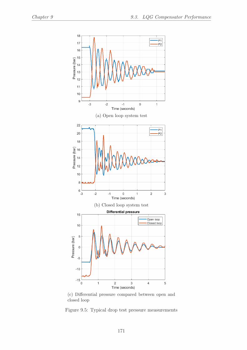
Chapter 9 9.3. LQG Compensator Performance

(a) Open loop system test

(b) Closed loop system test

(c) Differential pressure compared between open andclosed loop

Figure 9.5: Typical drop test pressure measurements

171

9.3. LQG Compensator Performance Chapter 9

Listing 9.1: Identification report for the model from disturbance to roll angle whencontrolled with LQG at moderate setting

1 mod exp =2

3 From input ”u1” to output ”y1 ” :4 −4.72 e05 s + 85555 −−−−−−−−−−−−−−−−−−−−−−−−−−−−−−−−−−−−−−−−−−−−−−−−−−−6 s ˆ4 + 55.65 s ˆ3 + 540 .9 s ˆ2 + 1.114 e04 s + 4.388 e047

8 Name : t f 19 Continuous−time i d e n t i f i e d t r a n s f e r func t i on .

10

11 Parameter i zat ion :12 Number o f po l e s : 4 Number o f z e r o s : 113 Number o f f r e e c o e f f i c i e n t s : 614 Use ” t fda ta ” , ” getpvec ” , ” getcov ” f o r parameters and t h e i r

u n c e r t a i n t i e s .15

16 Status :17 Estimated us ing TFEST on frequency response data ”h ” .18 Fit to e s t imat i on data : 81.69% ( s t a b i l i t y en fo r ced )19 FPE: 305 .7 , MSE: 272 .3

Listing 9.2: Identification report for the model from disturbance to roll angle whencontrolled with LQG at aggressive setting

1 agg exp =2

3 From input ”u1” to output ”y1 ” :4 2 .53 e06 s − 1 .899 e055 −−−−−−−−−−−−−−−−−−−−−−−−−−−−−−−−−−−−−−−−−−−−−−−−−−6 s ˆ4 + 148 .6 s ˆ3 + 9387 s ˆ2 + 4.905 e04 s + 1.586 e067

8 Name : t f 19 Continuous−time i d e n t i f i e d t r a n s f e r func t i on .

10

11 Parameter i zat ion :12 Number o f po l e s : 4 Number o f z e r o s : 113 Number o f f r e e c o e f f i c i e n t s : 614 Use ” t fda ta ” , ” getpvec ” , ” getcov ” f o r parameters and t h e i r

u n c e r t a i n t i e s .15

16 Status :17 Estimated us ing TFEST on frequency response data ”h ” .18 Fit to e s t imat i on data : 90.95% ( s t a b i l i t y en fo r ced )19 FPE: 11 .42 , MSE: 10 .02

172

Chapter 10

Summary of Research Findings

In this project, we have done the work which was not only theoretical and simula-

tion but in many ways practical as well. The significance of this research project

is supported by the fact that in this project takes place the unification of theory,

simulations, practical work and experimentation. As the reader could see throughout

the thesis, these four components together form a strong combination supporting our

statements and findings. The author of the thesis can tell that he feels quite satis-

fied with the work and the outcomes of present research. Of course, it is up to the

reviewers to judge about the author’s work. However, the author would like to say

that he considers this project complete and successful.

To conclude this research, the author can make the following statements. In this

research project

• we derived a valid augmented half-car model fitted with active hydraulically

interconnected suspension;

• we took measured the parameters of the existing half-car testing rig for upgrad-

ing it later;

• we did initial estimations required for the upgrade;

• we performed numerical simulations with the models derived to predict future

key parameters of the upgraded setup;

• our simulations also confirmed the feasibility of the methodology chosen;

173

10.1. Further Research Chapter 10

• we designed the upgraded half-car testing rig in 3D CAD software;

• we created all necessary drafts and ordered custom parts in UTS Workshop;

• we ordered where possible existing parts from the market

• we managed the manufacturing process and upgraded the half-car testing rig;

• we did all necessary commissioning work to make the upgraded setup functional;

• we conducted identification experiments to obtain the sub-models important for

the control system design;

• we designed a real LQG compensator for the system and tested it physically on

the half-car rig;

• our tests have proved active hydraulically interconnected suspension system to

have a high capacity for roll angle reduction;

• our tests also confirmed the validity of the LQG compensator designed;

• our experimental results have shown excellent agreement with the ones found

through simulations;

• overall, we can state here that our work on this project has finished successfully.

10.1 Further Research

The author suggests to continue this research using same methodology as it was

demonstrated in this thesis. Namely, precise model identification through forced vi-

bration experiment is very important. The author suggests to also pay attention to

further improvements of the half-car testing rig such as using better displacement

sensors, not LVDT’s, using a faster micro-controller. Note that LVDT sensors gener-

ate a lot of noise due to the electromagnetic interference which is picked up through

the magnetic core of LVDT.

Further research can be done in the following directions:

• implementation of other control methods: H2, H-infinity, Sliding Mode,

• assessment of controller reaction to the uncertainties in the model,

• implementation of roll-over testing scenarios used in real car crash tests,

• developing fuzzy rules to smartly switch the control method in real time.

174

Chapter 10. Summary of Research Findings 10.2. Author’s Publications

10.2 Author’s Publications

[1] Tkachev, A. A., & Zhang, N. (2017). Active Hydraulically Interconnected

Suspension. Modeling and Simulation (No. 2017-01-1561). SAE Technical Paper.

[2] Zhu, S., Xu, G., Tkachev, A., Wang, L., & Zhang, N. (2017). Comparison

of the road-holding abilities of a roll-plane hydraulically interconnected suspension

system and an anti-roll bar system. Proceedings of the Institution of Mechanical

Engineers, Part D: Journal of Automobile Engineering, 231(11), 1540-1557.

175

Appendix A

Codes

Listing A.1: Half-car parameters initialisation

1 %% Copyright Anton Tkachev 2014 − 20182 % anton . a . tkachev@gmail . com3 % I f t h i s code was o f any help to you4 % pl ea s e k ind ly g ive author a c r e d i t in your paper5

6 %% Filename ’HCM12.m’7 % This s c r i p t i n i t i a l i s e s the parameters o f a ha l f−car with va lue s8 % c l o s e to those o f a r e a l car .9

10 %% Half−car parameters11 i s = 120 ; % [ kg .m2] v e h i c l e body moment o f i n e r t i a (measured )12 ms = 475 ; % [ kg ] v e h i c l e body mass (measured )13 mu = 35 ; % [ kg ] unsprung mass ( from Wade Smith ’ s t h e s i s )14 ks = 20E3 ; % [N/m] suspens ion spr ing s t i f f n e s s (measured )15 kt = 172E3 ; % [N/m] t i r e sp r ing s t i f f n e s s (measured )16 cs = 240 ; % [N/(m/ s ) ] suspens ion damping (measured )17 ct = 1000 ; % [N/(m/ s ) ] t i r e damping ( e s t imat i on )18 b = 0 . 7 ; % [m] wheel t rack ha l f width (measured )19 h = 0 . 5 ; % [m] cente r o f g rav i ty he ight ( e s t imat i on )20

21 %% Conventions22 mp = ms/4 + i s /4/b ˆ2 ;23 mn = ms/4 − i s /4/b ˆ2 ;24

25 %% In e r t i a matrix26 Mm = [mu, 0 , 0 , 0 ;27 0 , mu, 0 , 0 ;28 0 , 0 , mp, mn;29 0 , 0 , mn, mp ] ;30

31 %% Damping matrix32 Cm = [ cs + ct , 0 , −cs , 0 ;33 0 , cs + ct , 0 , −cs ;34 −cs , 0 , cs , 0 ;35 0 , −cs , 0 , c s ] ;36

37 %% S t i f f n e s s matrix

176

Appendix A. Codes

38 Km = [ ks + kt , 0 , −ks , 0 ;39 0 , ks + kt , 0 , −ks ;40 −ks , 0 , ks , 0 ;41 0 , −ks , 0 , ks ] ;42

43 %% Forces matrix ( mu l t i p l i e d by f = [ f1 , f2 , f 3 ] ˆT)44 G = [−1 , 0 , 0 ;45 0 , −1, 0 ;46 1 , 0 , −1;47 0 , 1 , 1 ] ;48

49 %% Road input matrix ( mu l t i p l i e d by w = [w1 , w2 ] ˆT)50 H = [ kt , 0 ;51 0 , kt ;52 0 , 0 ;53 0 , 0 ] ;54

55 %% Road input de r i v . mtx . ( mu l t i p l i e d by w’ = [w1 ’ , w2 ’ ] ˆT)56 J = [ ct , 0 ;57 0 , c t ;58 0 , 0 ;59 0 , 0 ] ;60

61 %% Conventions62 G1 = G( : , 1 : 2 ) ; G2 = G( : , 3 ) ;

177

Appendix A. Codes

Listing A.2: Conventional half-car model

1 %% Copyright Anton Tkachev 2014 − 20182 % anton . a . tkachev@gmail . com3 % I f t h i s code was o f any help to you4 % pl ea s e k ind ly g ive author a c r e d i t in your paper5

6 %% Filename ’CNV12.m’7 % This s c r i p t i n i t i a l i s e s a MIMO state−space model o f8 % a convent iona l ha l f−car without HIS system . The model i s then9 % stored in a va r i ab l e named CNVSS. The system has 3 inputs

10 % and 4 outputs . The ho r i z on t a l index o f CNVSS matrix cor responds11 % to the output and the v e r t i c a l − to the input as f o l l ow s below .12

13 % +−−−−−−−+−−−−−−−+−−−−−−−+−−−−−−−+14 % | CNVSS | w1 | w2 | f 3 |15 % +−−−−−−−+−−−−−−−+−−−−−−−+−−−−−−−+16 % | x1 | sys11 | sys12 | sys13 |17 % +−−−−−−−+−−−−−−−+−−−−−−−+−−−−−−−+18 % | x2 | sys21 | sys22 | sys23 |19 % +−−−−−−−+−−−−−−−+−−−−−−−+−−−−−−−+20 % | x3 | sys31 | sys32 | sys33 |21 % +−−−−−−−+−−−−−−−+−−−−−−−+−−−−−−−+22 % | x4 | sys41 | sys42 | sys43 |23 % +−−−−−−−+−−−−−−−+−−−−−−−+−−−−−−−+24

25 %% Inputs26 % u = [w1 , w2 , f 3 ] ˆT27 % w1 − l e f t road input [m]28 % w2 − r i g h t road input [m]29 % f3 − equ iva l en t r o l l f o r c e [N] f 3 = ms∗ a l ∗h/b30

31 %% State s32 % x = [ x1 , x2 , x3 , x4 ] ˆT33 % x1 − l e f t wheel v e r t i c a l d i sp lacement [m]34 % x2 − r i g h t wheel v e r t i c a l d i sp lacement [m]35 % x3 − v eh i c l e body v e r t i c a l d i sp lacement on the l e f t [m]36 % x4 − v eh i c l e body v e r t i c a l d i sp lacement on the r i g h t [m]37

38 %% Outputs39 % y = [ y1 , y2 , y3 , y4 ] ˆT40 % y1 − l e f t wheel v e r t i c a l d i sp lacement [m]41 % y2 − r i g h t wheel v e r t i c a l d i sp lacement [m]42 % y3 − v eh i c l e body v e r t i c a l d i sp lacement [m]43 % y4 − v eh i c l e body r o l l ang le [ rad ]44

45 %% State−space convent iona l ha l f−car model46 % s ˆ2∗M∗x + s ∗C∗x + K∗x = Gf + H∗w47 % J assumed to be zero f o r s imp l i c i t y : J = 048

49 %% State space f o r convent iona l ha l f−car model50 A1 = [ z e ro s (4 ) , eye (4 ) ;51 −Mm\Km, −Mm\Cm] ;52

53 B1 = [ z e ro s (4 , 3 ) ; Mm\ [H,G2 ] ] ;54

55 C1 = [ 1 , 0 , 0 , 0 ; % l e f t wheel bounce56 0 , 1 , 0 , 0 ; % r i gh t wheel bounce

178

Appendix A. Codes

57 0 , 0 , 1/2 , 1/2 ; % v eh i c l e body bounce58 0 , 0 , −1/2/b , 1/2/b ] ; % v eh i c l e body r o l l ang le ( rad )59 C1 = [C1 , z e r o s (4 ) ] ;60

61 D1 = ze ro s (4 , 3 ) ;62

63 CNVSS = ss (A1 ,B1 ,C1 ,D1) ;64

65 %% Trans fe r func t i on fo convent i ona l model66 s = t f ( ’ s ’ ) ;67 CNVTF = ( s ˆ2∗Mm + s ∗Cm + Km) \ ( [H,G2 ] + s ∗ [ J , z e r o s (4 , 1 ) ] ) ;

179

Appendix A. Codes

Listing A.3: Hydraulically interconnected suspension parameters

1 %% Copyright Anton Tkachev 2014 − 20182 % anton . a . tkachev@gmail . com3 % I f t h i s code was o f any help to you4 % pl ea s e k ind ly g ive author a c r e d i t in your paper5

6 %% Filename ’HIS12 .m’7 % This s c r i p t i n i t i a l i s e s the parameters o f a c t i v e HIS system with8 % value s c l o s e to those o f a r e a l system9

10 %% Hydraul ic system s t a t e equat ions11 % p = s ˆ2∗ Ih∗dx + s ∗Rh∗dx + Sh∗dx12

13 %% Inputs14 % dx = [ dx1 , dx2 , dx3 ] ˆT15 % dx1 − l e f t suspens ion d e f l e c t i o n [m]16 % dx2 − r i g h t suspens ion d e f l e c t i o n [m]17 % dx3 − hydrau l i c ac tuator d i sp lacement [m]18

19 %% Outputs20 % P = [ p1 , p2 , p3 , p4 ] ˆT21 % p1 − l e f t c y l i nd e r upper chamber p r e s su r e [ Pa ]22 % p2 − r i g h t c y l i nd e r upper chamber p r e s su r e [ Pa ]23 % p3 − l e f t c y l i nd e r lower chamber p r e s su r e [ Pa ]24 % p4 − r i g h t c y l i nd e r lower chamber p r e s su r e [ Pa ]25

26 %% Hydraul ic c i r c u i t parameters27 P0 = 250E3 ; % [Pa ] − accumulator precharge p r e s su r e28 P = 14E5 ; % [Pa ] − accumulator working p r e s su r e29 V0 = 0.32E−3; % [m3] − accumulator volume30 g = 1 . 4 ; % [− ] − s p e c i f i c heat r a t i o o f N2 gas31 a1 = 5 .1E−4; % [m2] − upper susp . p i s t on area32 a2 = 4 .1E−4; % [m2] − lower susp . p i s t on area33 a3 = 1 .2E−3; % [m2] − actuator p i s t on annular area34

35 %% Unknown parameters are est imated to the order o f magnitude36 r1 = 1 .0E7 ; % [Pa/(m3/ s ) ] − 1 s t l i n e a r l o s s c o e f f i c i e n t37 r2 = 1 .0E7 ; % [Pa/(m3/ s ) ] − 2nd l i n e a r l o s s c o e f f i c i e n t38 r3 = 1 .0E7 ; % [Pa/(m3/ s ) ] − 3 rd l i n e a r l o s s c o e f f i c i e n t39 ih = 1 .0E4 ; % [Pa/(mˆ3/ s ˆ2) ] − f l u i d i n e r t i a ( omitted )40

41 %% Pre−c a l c u l a t i o n s42 V = V0∗P0/P; % [m3] − gas volume in accumulator at r e s t43 ch = V/P/g ; % [m3/Pa ] − accumulator capac i tance44

45 %% Elastance matrix46 Sh = 1/ch ∗ [ a1 , −a2 , a3 ;47 −a2 , a1 , −a3 ;48 −a2 , a1 , −a3 ;49 a1 , −a2 , a3 ] ;50

51 %% Res i s tance matrix52 Rh = [ a1 ∗( r1 + r2 ) , −a2∗ r2 , a3∗ r2 ;53 −a2∗ r2 , a1 ∗( r1 + r2 ) , −a3∗ r2 ;54 −a2 ∗( r1 + r2 + r3 ) , a1∗ r2 , −a3 ∗( r2 + r3 ) ;55 a1∗ r2 , −a2 ∗( r1 + r2 + r3 ) , a3 ∗( r2 + r3 ) ] ;56

180

Appendix A. Codes

57 %% Iner tance matrix58 Ih = ih ∗ [ 0 , 0 , 0 ;59 0 , 0 , 0 ;60 −a2 , 0 , −a3 ;61 0 , −a2 , a3 ] ;62

63 %% Conventions64 Sh1 = Sh ( : , 1 : 2 ) ; Sh2 = Sh ( : , 3 ) ;65 Rh1 = Rh( : , 1 : 2 ) ; Rh2 = Rh( : , 3 ) ;66 Ih1 = Ih ( : , 1 : 2 ) ; Ih2 = Ih ( : , 3 ) ;67

68 %% HIS model in s−domain69 s = t f ( ’ s ’ ) ;70 HIS = Sh + s ∗Rh + s ˆ2∗ Ih ;

181

Appendix A. Codes

Listing A.4: Hydraulic-to-mechanical boundary condition

1 %% Copyright Anton Tkachev 2014 − 20182 % anton . a . tkachev@gmail . com3 % I f t h i s code was o f any help to you4 % pl ea s e k ind ly g ive author a c r e d i t in your paper5

6 %% Filename ’H2M12 .m’7 % This s c r i p t implements hydrau l i c−to−mechanical8 % boundary cond i t i on and d e f i n e s equ iva l en t mechanical matr i ce s9 % to be augmented to the ha l f−car model .

10

11 %% Hydraul ic to mechanical boundary cond i t i on12 P2F = [−a1 , 0 , a2 , 0 ; % pre s su r e to f o r c e conver s i on13 0 , −a1 , 0 , a2 ] ;14

15 %% Equiva lent mechanical matr i ce s16 Mh1 = G1∗P2F∗ Ih1∗G1 ’ ; % equ iva l en t mechanical i n e r t i a17 Ch1 = G1∗P2F∗Rh1∗G1 ’ ; % equ iva l en t mechanical damping18 Kh1 = G1∗P2F∗Sh1∗G1 ’ ; % equ iva l en t mechanical s t i f f n e s s19

20 %% Equivalent r e a c t i o n s to actuator input21 Mh2 = G1∗P2F∗ Ih2 ; % equ iva l en t i n e r t i a l r e a c t i on22 Ch2 = G1∗P2F∗Rh2 ; % equ iva l en t damped r e a c t i on23 Kh2 = G1∗P2F∗Sh2 ; % equ iva l en t s t i f f r e a c t i on

182

Appendix A. Codes

Listing A.5: Transfer function model initialisation

1 %% Copyright Anton Tkachev 2014 − 20182 % anton . a . tkachev@gmail . com3 % I f t h i s code was o f any help to you4 % pl ea s e k ind ly g ive author a c r e d i t in your paper5

6 %% Filename ’MAKETF12.m’7 % This s c r i p t i n i t i a l i s e s a MIMO t r a n s f e r func t i on model o f8 % a ha l f−car with a c t i v e HIS . The model i s then s to r ed in a9 % va r i ab l e named SYSTF. The system has 4 inputs and 4 outputs .

10 % The ho r i z on t a l index o f SYSTF matrix corresponds to the output11 % and the v e r t i c a l − to the input as f o l l ow s below .12

13 % +−−−−−−−+−−−−−−+−−−−−−+−−−−−−+−−−−−−+14 % | SYSTF | u1 | u2 | u3 | u4 |15 % +−−−−−−−+−−−−−−+−−−−−−+−−−−−−+−−−−−−+16 % | y1 | t f 1 1 | t f 1 2 | t f 1 3 | t f 1 4 |17 % +−−−−−−−+−−−−−−+−−−−−−+−−−−−−+−−−−−−+18 % | y2 | t f 2 1 | t f 2 2 | t f 2 3 | t f 2 4 |19 % +−−−−−−−+−−−−−−+−−−−−−+−−−−−−+−−−−−−+20 % | y3 | t f 3 1 | t f 3 2 | t f 3 3 | t f 3 4 |21 % +−−−−−−−+−−−−−−+−−−−−−+−−−−−−+−−−−−−+22 % | y4 | t f 4 1 | t f 4 2 | t f 4 3 | t f 4 4 |23 % +−−−−−−−+−−−−−−+−−−−−−+−−−−−−+−−−−−−+24

25 %% Inputs26 % u = [ u1 , u2 , u3 , u4 ] ˆT27 % u1 − l e f t road input [m]28 % u2 − r i g h t road input [m]29 % u3 − equ iva l en t r o l l f o r c e [N]30 % u4 − hydrau l i c ac tuator d i sp lacement [m]31

32 %% Outputs33 % y = [ y1 , y2 , y3 , y4 ] ˆT34 % y1 − l e f t wheel v e r t i c a l d i sp lacement [m]35 % y2 − r i g h t wheel v e r t i c a l d i sp lacement [m]36 % y3 − v eh i c l e body v e r t i c a l d i sp lacement on the l e f t [m]37 % y4 − v eh i c l e body v e r t i c a l d i sp lacement on the r i g h t [m]38

39 %% Numerator c o e f f i c i e n t matr i ce s40 R0 = [H,G2,Kh2 ] ;41 R1 = [ J , z e r o s (4 , 1 ) ,Ch2 ] ;42 R2 = [ z e ro s (4 , 3 ) ,Mh2 ] ;43

44 %% I n i t i a l i s e s−va r i ab l e45 s = t f ( ’ s ’ ) ;46

47 %% Numerator o f the TF48 NUM = (R0 + R1∗ s + R2∗ s ˆ2) ;49

50 %% Denominator o f the TF51 DEN = (Mm − Mh1) ∗ s ˆ2 + (Cm − Ch1) ∗ s + (Km − Kh1) ;52

53 %% Trans fe r func t i on matrix (4 x4 )54 SYSTF = DEN\NUM;

183

Appendix A. Codes

Listing A.6: State-space model initialisation

1 %% Copyright Anton Tkachev 2014 − 20182 % anton . a . tkachev@gmail . com3 % I f t h i s code was o f any help to you4 % pl ea s e k ind ly g ive author a c r e d i t in your paper5

6 %% Filename ’MAKESS12.m’7 % This s c r i p t i n i t i a l i s e s a MIMO state−space model o f8 % a ha l f−car with a c t i v e HIS . The model i s then s to r ed in a9 % va r i ab l e named SYSSS . The system has 4 inputs and 4 outputs .

10 % The ho r i z on t a l index o f SYSSS matrix corresponds to the output11 % and the v e r t i c a l − to the input as f o l l ow s below .12

13 % +−−−−−−−+−−−−−−−+−−−−−−−+−−−−−−−+−−−−−−−+14 % | SYSSS | u1 | u2 | u3 | u4 |15 % +−−−−−−−+−−−−−−−+−−−−−−−+−−−−−−−+−−−−−−−+16 % | x1 | sys11 | sys12 | sys13 | sys14 |17 % +−−−−−−−+−−−−−−−+−−−−−−−+−−−−−−−+−−−−−−−+18 % | x2 | sys21 | sys22 | sys23 | sys24 |19 % +−−−−−−−+−−−−−−−+−−−−−−−+−−−−−−−+−−−−−−−+20 % | x3 | sys31 | sys32 | sys33 | sys34 |21 % +−−−−−−−+−−−−−−−+−−−−−−−+−−−−−−−+−−−−−−−+22 % | x4 | sys41 | sys42 | sys43 | sys44 |23 % +−−−−−−−+−−−−−−−+−−−−−−−+−−−−−−−+−−−−−−−+24

25 %% State−space model l im i t a t i o n s26 % State space model does not in c l ude any d e r i v a t i v e s o f the input .27 % Thus the r i gh t s i d e o f the equat ions o f motion does not conta in28 % the terms ( s ∗B1∗u) and ( s ˆ2∗B2∗u) .29 % Instead , i t only has (B0∗u) term which a l l owe s us to f o rma l i z e30 % the s t a t e space in a s imple way pr e s e rv ing31 % the phy s i c a l meanings o f system s t a t e s32

33 %% Equations o f motion34 % Mx” + Cx ’ + Kx = Bu35

36 %% Resu l t ing s ta te−space37 % x ’ = Ax + Bu38 % y = Cx + D39

40 %% Inputs41 % u = [ u1 , u2 , u3 , u4 ] ˆT42 % u1 − l e f t road input [m]43 % u2 − r i g h t road input [m]44 % u3 − l a t e r a l a c c e l e r a t i o n [m/ s2 ]45 % u4 − hydrau l i c ac tuator d i sp lacement [m]46

47 %% State s48 % x = [ x1 , x2 , x3 , x4 ] ˆT49 % x1 − l e f t wheel v e r t i c a l d i sp lacement [m]50 % x2 − r i g h t wheel v e r t i c a l d i sp lacement [m]51 % x3 − v eh i c l e body v e r t i c a l d i sp lacement on the l e f t [m]52 % x4 − v eh i c l e body v e r t i c a l d i sp lacement on the r i g h t [m]53

54 %% Outputs55 % y = [ y1 , y2 , y3 , y4 ] ˆT56 % y1 − l e f t susp . d e f l e c t i o n [m]

184

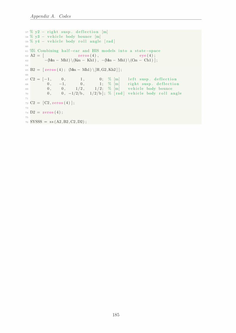
Appendix A. Codes

57 % y2 − r i g h t susp . d e f l e c t i o n [m]58 % y3 − v eh i c l e body bounce [m]59 % y4 − v eh i c l e body r o l l ang le [ rad ]60

61 %% Combining ha l f−car and HIS models i n to a s ta te−space62 A2 = [ z e ro s (4 ) , eye (4 ) ;63 −(Mm − Mh1) \(Km − Kh1) , −(Mm − Mh1) \(Cm − Ch1) ] ;64

65 B2 = [ z e ro s (4 ) ; (Mm − Mh1) \ [H,G2,Kh2 ] ] ;66

67 C2 = [−1 , 0 , 1 , 0 ; % [m] l e f t susp . d e f l e c t i o n68 0 , −1, 0 , 1 ; % [m] r i gh t susp . d e f l e c t i o n69 0 , 0 , 1/2 , 1/2 ; % [m] v e h i c l e body bounce70 0 , 0 , −1/2/b , 1/2/b ] ; % [ rad ] v e h i c l e body r o l l ang le71

72 C2 = [C2 , z e r o s (4 ) ] ;73

74 D2 = ze ro s (4 ) ;75

76 SYSSS = ss (A2 ,B2 ,C2 ,D2) ;

185

Appendix A. Codes

Listing A.7: Linear quadratic regulator design

1 %% Copyright Anton Tkachev 2014 − 20182 % anton . a . tkachev@gmail . com3 % I f t h i s code was o f any help to you4 % pl ea s e k ind ly g ive author a c r e d i t in your paper5

6 %% Filename ’SFDBCK12.m’7 % This s c r i p t de s i gn s an LQR con t r o l system f o r the submodel8 % provided . I t beg ins with model t runca t i on which i s done f o r9 % s imp l i c i t y . Then , s ta te−f eedback ga ins vec to r i s found v ia LQR

10 % method . A l t e rna t i v e l y , one can uncomment l i n e number 30 to11 % d i r e c t l y l o c a t e the po l e s o f c l o s ed loop system . The ga ins are12 % ass i gned to va r i ab l e K. Luenberger s t a t e obse rve r i s des igned13 % and s to r ed in va r i ab l e OBS.14

15 %% Reduce subsystem order to 216 SYSR = reduce (SYSSS(4 , 4 ) ,2 , ’ Algorithm ’ , ’ ba lance ’ ) ;17 % System order i s reduced to 2 us ing balanced t runcat i on method18

19 %% Conventions20 A = SYSR. a ;21 B = SYSR. b ;22 C = SYSR. c ;23

24 %% Linear Quadratic Regulator25 q11 = 1 ; % as s i gn lower pena l ty f o r e r r o r d e r i v a t i v e26 q22 = 10 ; % as s i gn h igher pena l ty f o r abso lu t e e r r o r27

28 Q = blkd iag ( q11 , q22 ) ; % s t a t e p e n a l t i e s29 R = 0 . 0 1 ; % con t r o l e f f o r t pena l ty30 N = [ 0 ; 0 ] ; % c r o s s p e n a l t i e s ( no matter )31 K = lq r (SYSR,Q,R,N) ; % LQR ga ins vec to r32

33 % K = place (A,B,[−30 ,−31]) ; % a l t e r n a t i v e pole−placement34

35 %% Closed loop system36 CLSYS = ss (A − B∗K, B, C, 0) ;37

38 %% Luenberger s t a t e obse rve r39 L = place (A’ ,C’ , [−200 ,−201]) ’ ; % obse rver feedback ga ins40 OBS = ss (A−L∗C−B∗K,L , eye (2 ) , 0 ) ; % Luenberger obse rve r

186

Appendix A. Codes

Listing A.8: Entire model initialisation call sequence

1 %% Copyright Anton Tkachev 2014 − 20182 % anton . a . tkachev@gmail . com3 % I f t h i s code was o f any help to you4 % pl ea s e k ind ly g ive author a c r e d i t in your paper5

6 %% Filename ’ INIT12 .m’7 % This s c r i p t d e f i n e s the appropr ia t e sequence o f s c r i p t s8 % one needs to c a l l in order to f u l l y i n i t i a l i z e ha l f−car model9 % with a c t i v e HIS system dr iven by an LQR c o n t r o l l e r

10

11 c l e a r ; % c l e a r workspace12 HCM12; % i n i t i a l i z e ha l f−car model parameters13 CNV12; % i n i t i a l i z e convent iona l ha l f−car model14 HIS12 ; % i n i t i a l i z e HIS model parameters15 H2M12 ; % i n i t i a l i z e hyd−to−mech boundary cond i t i on16 MAKESS12; % i n i t i a l i z e s ta te−space model17 MAKETF12; % i n i t i a l i z e t r a n s f e r func t i on model18 SFDBCK12; % des ign an LQR c o n t r o l l e r and s t a t e obse rve r19 AHIS12 ; % open Simulink diagram

187

Appendix A. Codes

Listing A.9: C++ implementation of PID controller in velocity form

1 #inc lude <TimerOne . h>2 #inc lude ”ArduinoTrueDAC . h”3

4 // E l l i p t i c Low Pass F i l t e r5 /∗ n = 2 ; % f i l t e r order6 ∗ Rp = 0 . 1 ; % passband peak to peak r i pp l e , dB7 ∗ Rs = 1000 ; % stopband attenuat ion , dB8 ∗ fn = 1000 ; % Nyquist frequency , Hz9 ∗ f c = 1 ; % cu t o f f f requency , Hz

10 ∗ Wp = f c / fn ; % normal ized c u t o f f f r equency ∗/11

12 // Sampling time13 double t = 100E−6; // 100 microseconds14 double T = 100 ; // 100 microseconds15

16 // PID c o e f f i c i e n t s17 double Kd = 0 . 1 ;18 double Kp = 1 ;19 double Ki = 10 ;20

21 // F i l t e r c o e f f i c i e n t s22 double a [ 3 ] = {1 , −1.99254216118629 , 0 .992574747774901} ;23 double b [ 3 ] = {8.05339325492860 e−06, 1.61067865098572 e−05,

8.05339325492859 e−06};24

25 // F i l t e r v a r i a b l e s26 double u [ 3 ] = {0} ; // input o f the f i l t e r27 double y [ 3 ] = {0} ; // output o f the f i l t e r28

29 void setup ( ) {30 DAC12INIT( ) ; // i n i t i a l i s e DAC31 Timer1 . i n i t i a l i z e (T) ; // i n i t i a l i s e t imer i n t e r r up t32 Timer1 . a t t a ch In t e r rup t ( timerISR ) ;33 }34

35 void loop ( ) {} // empty loop36

37 void timerISR ( ) { // t imer i n t e r r up t s e r v i c e r ou t in e38 u [ 0 ] = ( analogRead (A0) − analogRead (A1) ) ; // measurement39 y [ 0 ] = −a [ 1 ] ∗ y [ 1 ] − a [ 2 ] ∗ y [ 2 ] + b [ 0 ] ∗ u [ 0 ] + b [ 1 ] ∗ u [ 1 ] + b [ 2 ] ∗ u [ 2 ] ;

// f i l t e r i n g40

41 // Der iva t i v e 1 and 242 dy = (y [ 0 ] − y [ 1 ] ) /T;43 d2y = (y [ 0 ] − 2∗y [ 1 ] + y [ 2 ] ) /T/T;44

45 u [ 2 ] = u [ 1 ] ; u [ 1 ] = u [ 0 ] ; // s h i f t r e g i s t e r f o r the input46 y [ 2 ] = y [ 1 ] ; y [ 1 ] = y [ 0 ] ; // s h i f t r e g i s t e r f o r the output47

48 w = Ki∗y [ 0 ] + Kp∗dy + Kd∗d2y ; // PID output s i g n a l : motor speed49 DAC12(w) ; // s e t DAC value to w50 }

188

Appendix A. Codes

Listing A.10: Fourier analysis using Matlab

1 %% Copyright Anton Tkachev 2014 − 20182 % anton . a . tkachev@gmail . com3 % I f t h i s code was o f any help to you4 % pl ea s e k ind ly g ive author a c r e d i t in your paper5

6 % This code w i l l p roc e s s a waveform sto r ed in a CSV f i l e7 % and f i nd the magnitude and phase o f the s t r ong e s t8 % sp e c t r a l component9

10 %% Before running t h i s s c r i p t11 % one needs to run the l i n e12 % f i l e ID = fopen ( ’ output . csv ’ , ’w’ ) ;13 % to c r ea t a f i l e f o r the output .14

15 %% Body o f the s c r i p t16 f i l ename = ’ scope xx . csv ’ ; % prov ide waveform f i l ename here17

18 % Parse waveform data from a CSV f i l e19 waveform = importdata ( f i l ename , ’ , ’ , 2 ) ;20

21 t = waveform . data ( : , 1 ) ; % as s i gn time22 r = waveform . data ( : , 2 ) ; % as s i gn r e f e r e n c e23 u = waveform . data ( : , 4 ) ; % as s i gn input24 y = waveform . data ( : , 5 ) ; % as s i gn output25

26 R = f f t ( r ) ; % f i nd FFT of the r e f e r e n c e27 U = f f t (u) ; % f i nd FFT of the input28 Y = f f t ( y ) ; % f i nd FFT of the output29

30 N = length (R) ; % f i nd length o f R31 T = t (2) − t (1 ) ; % f i nd sampling time32

33 Rm = abs (R) ; % f i nd magnitude o f the r e f e r e n c e34 Um = abs (U) ; % f i nd magnitude o f the input35 Ym = abs (Y) ; % f i nd magnitude o f the output36

37 % Find the harmonic o f e x c i t a t i o n38 [ ˜ , k ] = max(Rm( 2 :N/2) ) ;39

40 W = Y(k+1)/U(k+1) ; % f i nd Bode complex amplitude41

42 % Bode p l o t parameters43 f r q = k/N/T; % frequency (Hz)44 mag = 20∗ l og10 ( abs (W) ) ; % magnitude (dB)45 phs = 180/ p i ∗ ang le (W) ; % phase ( deg )46

47 % Append r e s u l t s to the output f i l e48 f p r i n t f ( f i l e ID , ’%4.4 f ,%4.4 f ,%4.4 f \n ’ , f rq ,mag , phs ) ;49

50 %% After every run51 % one can change the waveform f i l ename and run the s c r i p t52 % again f o r a d i f f e r e n t waveform . Repeat as many t imes as needed .53 % The r e s u t l s w i l l be appended to the output f i l e .54 % After a l l waveforms have been proce s sed55 % one needs to run the f o l l ow i n g l i n e to c l o s e the output f i l e .56 % f c l o s e ( f i l e ID ) ;

189

Appendix A. Codes

Listing A.11: LQR and Kalman state observer design

1 %% Copyright Anton Tkachev 2014 − 20182 % anton . a . tkachev@gmail . com3 % I f t h i s code was o f any help to you4 % pl ea s e k ind ly g ive author a c r e d i t in your paper5

6 % This code de s i gn s an LQR compensator and a Kalman7 % sta t e obse rve r f o r the model s to r ed in va r i a b l e ’ sys ’ .8 % The c l o s ed loop system models are saved in v a r i a b l e s9 % c l s y s 1 and c l s y s 2

10

11 %% System state−space matr i ce s12 A = sys . a ;13 B = sys . b ;14 C = sys . c ;15 D = sys . d ;16

17 %% Kalman s t a t e obse rver des ign18 Qn = 1 ; % unce r ta in ty o f s t a t e19 Rn = 1E5 ; % unce r ta in ty o f measurement20 Nn = 0 ; % process−measurement cros s−covar iance21

22 %% LQR moderate s e t t i n g23 Q = blkd iag (1 ,1 ,1E3 , 1E5) ; % Penalty f o r s t a t e s : p o s i t i o n and v e l o c i t y24 R = 1 ; % Penalty f o r c on t r o l e f f o r t25 N = 0 ; % State−cont ro l−e f f o r t c ros s−term pena l ty26 G1 = lq r ( sys ,Q,R,N) ; % LQR gain27

28 %% LQR agg r e s s i v e s e t t i n g29 Q = blkd iag (1 ,1 ,1E3 , 1E7) ; % Penalty f o r s t a t e s : p o s i t i o n and v e l o c i t y30 R = 1 ; % Penalty f o r c on t r o l e f f o r t31 N = 0 ; % State−cont ro l−e f f o r t c ros s−term pena l ty32 G2 = lq r ( sys ,Q,R,N) ; % LQR gain33

34 %% Closed loop models35 c l s y s 1 = s s (A − B∗G1, B, C, 0) ; % moderate s e t t i n g36 c l s y s 2 = s s (A − B∗G2, B, C, 0) ; % agg r e s s i v e s e t t i n g

190

Appendix B

Tables of Measurements

191

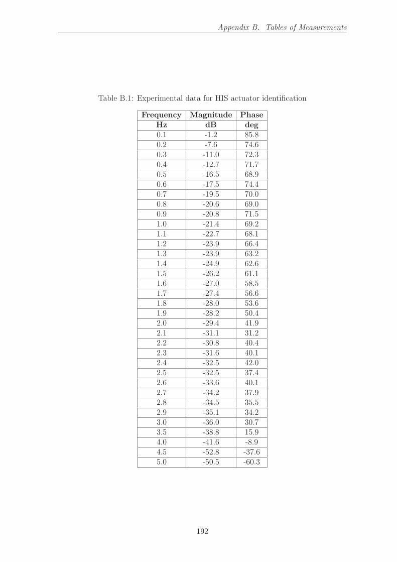
Appendix B. Tables of Measurements

Table B.1: Experimental data for HIS actuator identification

Frequency Magnitude PhaseHz dB deg0.1 -1.2 85.80.2 -7.6 74.60.3 -11.0 72.30.4 -12.7 71.70.5 -16.5 68.90.6 -17.5 74.40.7 -19.5 70.00.8 -20.6 69.00.9 -20.8 71.51.0 -21.4 69.21.1 -22.7 68.11.2 -23.9 66.41.3 -23.9 63.21.4 -24.9 62.61.5 -26.2 61.11.6 -27.0 58.51.7 -27.4 56.61.8 -28.0 53.61.9 -28.2 50.42.0 -29.4 41.92.1 -31.1 31.22.2 -30.8 40.42.3 -31.6 40.12.4 -32.5 42.02.5 -32.5 37.42.6 -33.6 40.12.7 -34.2 37.92.8 -34.5 35.52.9 -35.1 34.23.0 -36.0 30.73.5 -38.8 15.94.0 -41.6 -8.94.5 -52.8 -37.65.0 -50.5 -60.3

192

Appendix B. Tables of Measurements

Table B.2: Experimental data for active HIS identification

Frequency Magnitude PhaseHz dB deg0.1 -12.8 11.60.2 -11.5 16.80.3 -11.6 23.60.4 -13.1 21.60.5 -11.1 19.50.6 -12.2 15.80.7 -13.7 24.70.8 -13.7 36.80.9 -15.5 30.41.0 -16.3 37.31.1 -16.2 44.81.2 -16.0 52.81.3 -17.1 71.91.4 -16.1 88.21.5 -13.7 106.11.6 -10.8 122.51.7 -7.7 135.61.8 -2.4 141.81.9 2.6 138.62.0 8.8 125.92.1 11.3 82.12.2 5.9 48.62.3 2.8 40.62.4 2.1 32.92.5 1.3 30.22.6 -0.6 25.82.7 -1.6 24.32.8 -2.0 21.22.9 -1.3 13.93.0 -0.9 14.2

193

Appendix B. Tables of Measurements

Table B.3: Experimental data for actuator displacement to half-car roll angle identi-fication

Frequency Magnitude PhaseHz dB deg0.1 8.5 -1.80.2 11.0 -2.10.3 9.9 -4.40.4 12.0 -4.00.5 10.3 -3.30.6 10.0 -2.40.7 12.1 -3.00.8 13.9 -6.60.9 14.1 -7.11.0 14.8 -8.71.1 15.0 -9.41.2 14.1 -10.01.3 14.2 -10.81.4 14.7 -12.01.5 17.7 -13.81.6 19.6 -15.41.7 20.6 -16.21.8 23.0 -22.91.9 25.8 -29.32.0 30.8 -45.52.1 30.1 -99.52.2 23.8 -120.72.3 19.1 -124.02.4 19.6 -131.62.5 17.9 -131.22.6 16.1 -136.12.7 16.2 -137.62.8 14.7 -139.72.9 13.5 -140.33.0 9.2 -141.63.1 7.0 -142.9

194

Appendix B. Tables of Measurements

Table B.4: Experimental data for roll moment disturbance to half-car roll angleidentification

Frequency Magnitude PhaseHz dB deg0.1 36.8 -5.80.2 36.5 -5.90.3 36.4 -6.00.4 36.4 -6.30.5 36.5 -6.50.6 36.7 -7.30.7 37.5 -7.40.8 37.8 -6.30.9 38.1 -7.01.0 38.5 -8.01.1 38.8 -8.91.2 39.5 -10.11.3 40.3 -13.31.4 41.1 -14.81.5 42.0 -17.81.6 43.8 -17.41.7 44.8 -21.11.8 46.9 -26.11.9 49.3 -35.52.0 51.6 -49.92.1 54.0 -86.82.2 52.2 -137.22.3 48.6 -157.42.4 45.8 -162.62.5 43.5 -166.92.6 41.6 -170.62.7 40.1 -171.02.8 38.5 -173.5

Frequency Magnitude PhaseHz dB deg2.9 37.3 -173.13.0 35.9 -174.73.1 34.7 -176.93.2 33.8 -178.13.3 32.8 -178.43.4 32.0 -179.33.5 31.2 -179.43.6 30.4 -179.53.7 29.7 -179.83.8 29.0 -180.33.9 28.4 -180.64.0 27.8 -180.84.1 27.2 -181.44.2 26.6 -181.44.3 25.9 -181.24.4 25.5 -181.24.5 24.9 -181.84.6 24.3 -182.14.7 23.8 -182.44.8 23.4 -182.54.9 22.9 -182.65.0 22.4 -183.15.5 20.3 -183.76.0 18.5 -184.96.5 16.9 -186.17.0 15.2 -184.47.5 13.9 -185.58.0 12.8 -186.2

195

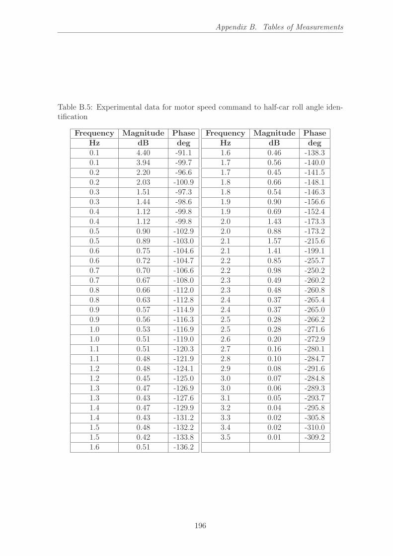
Appendix B. Tables of Measurements

Table B.5: Experimental data for motor speed command to half-car roll angle iden-tification

Frequency Magnitude PhaseHz dB deg0.1 4.40 -91.10.1 3.94 -99.70.2 2.20 -96.60.2 2.03 -100.90.3 1.51 -97.30.3 1.44 -98.60.4 1.12 -99.80.4 1.12 -99.80.5 0.90 -102.90.5 0.89 -103.00.6 0.75 -104.60.6 0.72 -104.70.7 0.70 -106.60.7 0.67 -108.00.8 0.66 -112.00.8 0.63 -112.80.9 0.57 -114.90.9 0.56 -116.31.0 0.53 -116.91.0 0.51 -119.01.1 0.51 -120.31.1 0.48 -121.91.2 0.48 -124.11.2 0.45 -125.01.3 0.47 -126.91.3 0.43 -127.61.4 0.47 -129.91.4 0.43 -131.21.5 0.48 -132.21.5 0.42 -133.81.6 0.51 -136.2

Frequency Magnitude PhaseHz dB deg1.6 0.46 -138.31.7 0.56 -140.01.7 0.45 -141.51.8 0.66 -148.11.8 0.54 -146.31.9 0.90 -156.61.9 0.69 -152.42.0 1.43 -173.32.0 0.88 -173.22.1 1.57 -215.62.1 1.41 -199.12.2 0.85 -255.72.2 0.98 -250.22.3 0.49 -260.22.3 0.48 -260.82.4 0.37 -265.42.4 0.37 -265.02.5 0.28 -266.22.5 0.28 -271.62.6 0.20 -272.92.7 0.16 -280.12.8 0.10 -284.72.9 0.08 -291.63.0 0.07 -284.83.0 0.06 -289.33.1 0.05 -293.73.2 0.04 -295.83.3 0.02 -305.83.4 0.02 -310.03.5 0.01 -309.2

196

Appendix B. Tables of Measurements

Table B.6: Experimental data for system identification from disturbance to roll anglewhen controlled with LQG at moderate setting

Frequency Magnitude PhaseHz dB deg0.1 13.7 -98.50.2 19.1 -105.60.3 21.9 -112.00.4 24.2 -118.30.5 26.4 -122.60.6 28.6 -128.30.7 30.3 -132.00.8 30.6 -135.40.9 31.9 -141.51.0 32.3 -142.51.1 33.7 -146.91.2 35.3 -153.51.3 36.7 -163.01.4 37.4 -161.91.5 39.0 -175.71.6 39.7 -189.31.7 39.8 -206.21.8 42.8 -189.01.9 43.3 -208.92.0 43.4 -213.22.1 46.3 -230.42.2 49.1 -251.52.3 48.8 -290.62.4 47.4 -306.92.5 44.7 -314.42.6 37.4 -330.5

Frequency Magnitude PhaseHz dB deg2.7 35.9 -330.42.8 35.1 -332.12.9 33.9 -335.53.0 33.2 -337.43.1 32.5 -339.53.2 31.5 -343.73.3 30.7 -346.33.4 30.2 -348.33.5 29.2 -352.13.6 28.5 -356.93.7 27.1 -361.53.8 25.9 -363.03.9 24.8 -366.44.0 23.6 -367.14.1 22.7 -368.14.2 21.8 -368.84.3 20.8 -368.64.4 20.1 -368.44.5 19.4 -369.05.0 16.3 -367.55.5 14.1 -365.66.0 12.3 -364.96.5 10.6 -364.57.0 9.0 -361.87.5 8.1 -360.88.0 6.9 -362.4

197

Appendix B. Tables of Measurements

Table B.7: Experimental data for system identification from disturbance to roll anglewhen controlled with LQG at aggressive setting

Frequency Magnitude PhaseHz dB deg0.2 6.1 87.80.3 10.7 86.40.4 12.2 85.80.5 15.4 84.20.6 17.2 83.20.7 18.9 81.90.8 20.9 80.30.9 21.1 79.81.0 23.4 77.81.1 25.1 76.01.2 25.7 75.11.3 27.7 72.41.4 29.4 69.91.5 31.6 66.01.6 32.7 63.91.7 34.3 60.01.8 36.6 53.51.9 40.6 36.52.0 42.4 22.92.1 44.0 -8.12.2 43.9 -22.12.3 41.7 -53.92.4 39.6 -66.5

Frequency Magnitude PhaseHz dB deg2.5 37.3 -76.22.6 35.0 -83.62.7 34.7 -84.72.8 32.8 -89.62.9 32.3 -90.63.0 31.8 -92.33.1 30.6 -94.73.2 30.1 -95.73.3 29.2 -97.13.4 28.5 -99.53.5 28.1 -100.53.6 27.5 -101.53.7 26.8 -103.03.8 26.5 -104.03.9 26.0 -105.44.0 24.4 -109.44.4 24.3 -109.84.5 23.8 -111.45.0 22.7 -112.35.5 21.1 -113.76.5 20.0 -114.37.0 19.0 -115.78.0 18.3 -116.9

198

Appendix C

Mechanical Drawings

199

����������� ��

��

�� ����������������

�������

��

���������� ������������

�� ����

�� ���� �����

���������

��� �����!�

���

������������ ������!����

����������������� ��

������������

��������

��������

�����������

"��

���

�!!�#�

�� #�

�����

$%&'()�*+,�$%&-.&/0

$1&/1�23.%4)(

����

����

�����

�����

�����

�����

�������

�������

�����

������

�����

�����

������������

������������������

������������

���������������������

������ ����������� ����������

������ ����������� ����������

��������������� ����������

��������������� ����������

���������������� ��!�����!��"����

!��# ������$%&'()*�

+�

,(%%)���-.��,/+0%*�*��

$'�1-�

)&)0%*

2%3&,&-1 -�1-)�,/+0%� 2+$&1'

4+)%2&+0*

+)%,&'1+)52%1+4%

%652�+1 �

62%+7�,(+28�

% '%,

.&1&,(*510%,,�-)(%2$&,%�,8%/&.&% *

&4%1,&-1,�+2%�&1�4&00&4%)%2,

,52.+/%�.&1&,(*

)-0%2+1/%,*

���0&1%+2*

���+1'50+2*

9�+

4.'

+883:

/(7:

2+$1

;<==>

?@<AB<CD�EBF=�GHBII=>

?I<CI�JKB@H=L

����

� ����������� �

��������� ������

����

�����

����

���

���� �����

������

������

����

����

��

�����������������������������������

��������

��������

���

����

���

� �

�!"�#$%��&��"�'!��(�

)��(���$**

'�+,�-��*��������.�/����

��+,�-�

012345�6767668698

:!#;<�(�

������

�<!!���$=��"�'!((�

>:;�%$�

�#�'!(

�!?#�#$%>$�%$���"�'!�>��:#%;

@��!�#�'(

>��!�#;%��A�!%�@!

>!BA���%>�

B�!�C��<��D�

!>;!�

=#%#�<(A%'!���$�<!�:#�!��D!"#=#!>(

>#@!%�#$%����!�#%�@#''#@!�!��

�A�=�"!�=#%#�<(

EFGHIJKLHMN�OPQR�SS���'#%!��(

���JKTUGJIN�VWX�YZ[W

)��

@=;

�DD?\>

"<C\>

>��:%

] _ �abcdefg

Bibliography

[1] Sangzhi Zhu, Lifu Wang, Nong Zhang, and Haiping Du. H-infinity control of

a novel low-cost roll-plane active hydraulically interconnected suspension: An

experimental investigation of roll control under ground excitation. SAE Interna-

tional Journal of Passenger Cars-Mechanical Systems, 6(2013-01-1238):882–893,

2013.

[2] Sangzhi Zhu, Haiping Du, and Nong Zhang. Development and implementation of

fuzzy, fuzzy pid and lqr controllers for an roll-plane active hydraulically intercon-

nected suspension. In Fuzzy Systems (FUZZ-IEEE), 2014 IEEE International

Conference on, pages 2017–2024. IEEE, 2014.

[3] Sangzhi Zhu, Haiping Du, Nong Zhang, and Lifu Wang. Development of a new

model for roll-plane active hydraulically interconnected suspension. SAE Inter-

national Journal of Passenger Cars-Mechanical Systems, 7(2014-01-0053):447–

457, 2014.

[4] Nong Zhang, Wade A Smith, and Jeku Jeyakumaran. Hydraulically intercon-

nected vehicle suspension: background and modelling. Vehicle System Dynamics,

48(1):17–40, 2010.

[5] Wade A Smith, Nong Zhang, and Jeku Jeyakumaran. Hydraulically intercon-

nected vehicle suspension: theoretical and experimental ride analysis. Vehicle

system dynamics, 48(1):41–64, 2010.

211

Bibliography

[6] Wade A Smith, Nong Zhang, and William Hu. Hydraulically interconnected

vehicle suspension: handling performance. Vehicle system dynamics, 49(1-2):87–

106, 2011.

[7] James R Wilde, Gary J Heydinger, Dennis A Guenther, Tom Mallin, and An-

drew M Devenish. Experimental evaluation of fishhook maneuver performance

of a kinetic suspension system. Technical report, SAE Technical Paper, 2005.

[8] James R Wilde, Gary J Heydinger, and Dennis A Guenther. Adams simulation

of ride and handling performance of the kinetic tm suspension system. SAE

Transactions, pages 1646–1659, 2006.

[9] Dongpu Cao, Subhash Rakheja, and Chun-Yi Su. Comparison of roll properties

of hydraulically and pneumatically interconnected suspensions for heavy vehicles.

Technical report, SAE Technical Paper, 2005.

[10] Wei Gao, N Zhang, and HP Du. A half-car model for dynamic analysis of vehicles

with random parameters. In 5th Australasian Congress on Applied Mechanics

(ACAM 2007), volume 1, pages 595–600. Engineers Australia, 2007.

[11] Nong Zhang, Wade Smith, Jeku Jeyakumaran, and William Hu. Determination

of modal parameters of a half-car fitted with a hydraulically interconnected sus-

pension from simulated free decay responses. In 5th Australasian Congress on

Applied Mechanics (ACAM 2007), volume 1, pages 601–607. Engineers Australia,

2007.

[12] Wade Alister Smith. An investigation into the dynamics of vehicles with hydrauli-

cally interconnected suspensions. PhD thesis, University of Technology Sydney,

Green Energy and Vehicle Innovations Centre, Electrical Mechanical and Mecha-

tronics School, 2009, http://hdl.handle.net/10453/36058.

[13] Lifu Wang, Nong Zhang, and Haiping Du. Design and experimental investigation

of demand dependent active suspension for vehicle rollover control. In Decision

and Control, 2009 held jointly with the 2009 28th Chinese Control Conference.

212

Bibliography

CDC/CCC 2009. Proceedings of the 48th IEEE Conference on, pages 5158–5163.

IEEE, 2009.

[14] Lifu Wang, Nong Zhang, Haiping Du, et al. Modelling, parameter estimation and

testing of a vehicle with anti-roll systems. In Proceedings of the 6th Australasian

Congress on Applied Mechanics, page 119. Engineers Australia, 2010.

[15] Lifu Wang, Nong Zhang, and Haiping Du. Experimental investigation of a hy-

draulically interconnected suspension in vehicle dynamics and stability control.

SAE International Journal of Passenger Cars-Mechanical Systems, 5(2012-01-

0240):759–768, 2012.

[16] Fei Ding, Nong Zhang, and Xu Han. Modeling and modal analysis of multi-

body truck system fitted with hydraulically interconnected suspension. Jixie

Gongcheng Xuebao/Journal of Mechanical Engineering, 2012.

[17] Fei Ding, Xu Han, Zhen Luo, and Nong Zhang. Modelling and characteristic

analysis of tri-axle trucks with hydraulically interconnected suspensions. Vehicle

System Dynamics, 50(12):1877–1904, 2012.

[18] Lifu Wang, Nong Zhang, Haiping Du, et al. Modelling and parameter estimation

of an active hydraulic suspension using experimental method. In Proceedings:

the 7th Australasian Congress on Applied Mechanics (ACAM 7), 9-12 December

2012, the University of Adelaide, North Terrace Campus/National Committee on

Applied Mechanics of Engineers Australia, page 727. Engineers Australia, 2012.

[19] Lifu Wang, Guangzhong Xu, Nong Zhang, and Holger Roser. Experimental

comparison of anti-roll bar with hydraulically interconnected suspension in ar-

ticulation mode. Technical report, SAE Technical Paper, 2013.

[20] William S Levine. The control handbook. CRC press, 1996.

[21] David G Alciatore. Introduction to mechatronics and measurement systems. Tata

McGraw-Hill Education, 2007.

213

Bibliography

[22] Chengyuan Ren and Kai Li. Analysis on hydraulic parameters of interconnected

suspension based on fuzzy grey correlation. International Journal of Vehicle

Noise and Vibration, 13(1):1–12, 2017.

[23] ARASH HOSSEINIAN AHANGARNEJAD. Integrated control of active vehicle

chassis control systems. 2018.

[24] Lifu Wang, Song Jian, Hengmin Qi, and Nong Zhang. Lateral stability study of

a vehicle fitted with hydraulically interconnected suspension in slalom maneuver.

In Chinese Automation Congress (CAC), 2017, pages 1702–1707. IEEE, 2017.

[25] Shengzhao Chen, Bangji Zhang, Boyuan Li, and Nong Zhang. Dynamic charac-

teristics analysis of vehicle incorporating hydraulically interconnected suspension

system with dual accumulators. Shock and Vibration, 2018, 2018.

[26] Reza N Jazar. Vehicle dynamics. Theory and Applications. Riverdale, NY:

Springer Science+ Business Media, 2008.

[27] LD Landau and EM Lifshitz. Mechanics, vol. 1. Course of theoretical physics,

3, 1976.

[28] Nook industries - ball screw torque calculations. http://www.nookindustries.

com/LinearLibraryItem/Ballscrew_Torque_Calculations, 03 2015.

(21/1/2018).

[29] Arthur Akers, Max Gassman, and Richard Smith. Hydraulic power system anal-

ysis. CRC press, 2006.

[30] A Esposito. A simplified method for analyzing hydraulic circuits by analogy.

Machine Design, 41(24):173, 1969.

[31] Brian J Kirby. Micro-and nanoscale fluid mechanics: transport in microfluidic

devices. Cambridge University Press, 2010.

[32] DV Sivukhin. A course of general physics. vol. ii, thermodynamics and molecular

physics, 1996.

214

Bibliography

[33] Mark Waldo Zemansky and Richard H Dittman. Heat and thermodynamics: an

intermediate textbook. McGraw-Hill New York, 1968.

[34] Kalil T Swain Oldham. The doctrine of description: Gustav Kirchhoff, classical

physics, and the “purpose of all science” in 19 th-century Germany. University

of California, Berkeley, 2008.

[35] Steve Smale. The fundamental theorem of algebra and complexity theory. Bul-

letin of the American Mathematical Society, 4(1):1–36, 1981.

[36] Wodek Gawronski and Jer-Nan Juang. Model reduction in limited time and

frequency intervals. International Journal of Systems Science, 21(2):349–376,

1990.

[37] An-Pan Cherng. Formulation of hankel singular values and singular vectors in

time domain. In PROCEEDINGS-SPIE THE INTERNATIONAL SOCIETY

FOR OPTICAL ENGINEERING, volume 1, pages 436–442. SPIE INTERNA-

TIONAL SOCIETY FOR OPTICAL, 1998.

[38] Control tutorials for matlab and simulink introduction statespace methods for

controller design. http://ctms.engin.umich.edu/CTMS/index.php?example=

Introduction&section=ControlStateSpace, 08 2014. (13/1/2018).

[39] Stanley M Shinners. Modern control system theory and design. John Wiley &

Sons, 1998.

[40] The University of Texas at Arlington. Control system lectures, lecture

22. http://www.uta.edu/utari/acs/ee4314/lectures/Lecture%2022.pdf,

05 2017. (24/8/2018).

[41] Control systemsstate feedback wikibooks open books for an open world.

https://en.wikibooks.org/wiki/Control_Systems/State_Feedback#

Ackerman.27s_formula, 10 2007. (24/8/2018).

215

Bibliography

[42] Kalman filter - mathworks. https://au.mathworks.com/help/control/ref/

kalmanfilter.html, 06 2016. (22/1/2018).

[43] Ronald Newbold Bracewell and Ronald N Bracewell. The Fourier transform and

its applications, volume 31999. McGraw-Hill New York, 1986.

[44] Fredric J Harris. On the use of windows for harmonic analysis with the discrete

fourier transform. Proceedings of the IEEE, 66(1):51–83, 1978.

[45] F.P. Miller, A.F. Vandome, and J. McBrewster. Nyquist-Shannon Sampling

Theorem: Aliasing, Sine Wave, Signal Processing, Nyquist Rate, Nyquist Fre-

quency, Sampling Rate, Shannon-Hartley Theorem, Whittaker-Shannon Inter-

polation Formula, Reconstruction from Zero Crossings. Alphascript Publishing,

2010.

[46] Lennart Ljung. System identification. In Signal analysis and prediction, pages

163–173. Springer, 1998.

[47] Digital filter wikipedia. https://en.wikipedia.org/wiki/Digital_filter, 01

2004. (1/1/2018).

216