Chalmers University of Technology University of Gothenburg Department of Computer Science and Engineering Göteborg, Sweden, June 2015

Vector-based map cutting In the context of cloud-based navigation systems Master of Science Thesis in Electrical Engineering ANDREAS KARLSSON KRISTOFFER WILHELMSSON

The Author grants to Chalmers University of Technology and University of Gothenburg the non-exclusive right to publish the Work electronically and in a non-commercial purpose make it accessible on the Internet. The Author warrants that he/she is the author to the Work, and warrants that the Work does not contain text, pictures or other material that violates copyright law. The Author shall, when transferring the rights of the Work to a third party (for example a publisher or a company), acknowledge the third party about this agreement. If the Author has signed a copyright agreement with a third party regarding the Work, the Author warrants hereby that he/she has obtained any necessary permission from this third party to let Chalmers University of Technology and University of Gothenburg store the Work electronically and make it accessible on the Internet. Vector-based map cutting In the context of cloud-based navigation systems Andreas Karlsson Kristoffer Wilhelmsson © Andreas Karlsson, June 2015. © Kristoffer Wilhelmsson, June 2015. Examiner: Marina Papatriantafilou Chalmers University of Technology University of Gothenburg Department of Computer Science and Engineering SE-412 96 Göteborg Sweden Telephone + 46 (0)31-772 1000 Department of Computer Science and Engineering Göteborg, Sweden June 2015

Abstract

Vector maps are used when describing real world geographical objects, such aslakes or roads, with the convenience of vectors and vector objects. Each vector,or coordinate, describes a geographical point. Two or more vectors describe aline, or polyline, and three or more cordinates can describe a polygon. A lake canthus be described by a polygon with coordinates mapping its boundary, whilea road can be described by a polyline with coordinates mappings its stretch.

When dealing with vector map objects you often bound the geographicalarea of interest by a bounding polygon. In its simplest form this is a boundingbox, but arbitrarily shaped polygons can be used as well.

This thesis report examines how vector map objects in form of polylines andpolygons can be cut out from arbitrarily formed polygons. It also describes howthe arbitrarily formed polygons in turn can be created by splitting up a corridorsurrounding a polyline, the corridor created by offsetting the polyline to eachof its sides.

It goes into details on algorithms used for polygon clipping and polylineoffsetting. The report also covers implementation of selected approaches intoa vector map based mobile navigation system, as well as benchmarking andtesting of it.

Contents1 Introduction 3

1.1 Background . . . . . . . . . . . . . . . . . . . . . . . . . . . . . . 31.2 Case study: Cloud-based navigation application Wisepilot . . . . 41.3 Analysis of old implementation . . . . . . . . . . . . . . . . . . . 4

1.3.1 Rectangular enclosure of vector maps . . . . . . . . . . . 41.3.2 Structural overview . . . . . . . . . . . . . . . . . . . . . 51.3.3 System performance . . . . . . . . . . . . . . . . . . . . . 6

1.4 Formulation of problem . . . . . . . . . . . . . . . . . . . . . . . 71.5 Aim of this thesis . . . . . . . . . . . . . . . . . . . . . . . . . . . 7

1.5.1 Project aim . . . . . . . . . . . . . . . . . . . . . . . . . . 81.6 Limitations . . . . . . . . . . . . . . . . . . . . . . . . . . . . . . 81.7 Geometric terminology conventions . . . . . . . . . . . . . . . . . 81.8 Human vs computational perception of figures . . . . . . . . . . . 91.9 Description of remaining sections . . . . . . . . . . . . . . . . . . 9

2 Related work 102.1 Offsetting algorithms . . . . . . . . . . . . . . . . . . . . . . . . . 102.2 Poly object simplification algorithms . . . . . . . . . . . . . . . . 102.3 Clockwise polygons and polygon area algorithm . . . . . . . . . . 112.4 Linear algebra . . . . . . . . . . . . . . . . . . . . . . . . . . . . . 11

2.4.1 Line intersection . . . . . . . . . . . . . . . . . . . . . . . 112.4.2 Relative positioning . . . . . . . . . . . . . . . . . . . . . 12

2.5 Locating algorithms . . . . . . . . . . . . . . . . . . . . . . . . . 132.5.1 Ray-edge intersection algorithm . . . . . . . . . . . . . . . 132.5.2 Angle-summation algorithm . . . . . . . . . . . . . . . . . 13

2.6 Polygon set-operation algorithms . . . . . . . . . . . . . . . . . . 142.6.1 Weiler-Atherton algorithm . . . . . . . . . . . . . . . . . . 152.6.2 Binary space partitioning tree algorithm . . . . . . . . . . 162.6.3 Vatti’s generic algorithm . . . . . . . . . . . . . . . . . . . 182.6.4 Experimental polygon tree algorithm . . . . . . . . . . . . 19

3 Methodology 243.1 Implementation of offset algorithms . . . . . . . . . . . . . . . . . 24

3.1.1 Equi-angular algorithm . . . . . . . . . . . . . . . . . . . 243.1.2 Encapsulation polygon algorithm . . . . . . . . . . . . . . 25

3.2 Application of polygon set-operations . . . . . . . . . . . . . . . 283.3 Implementation of locating algorithm . . . . . . . . . . . . . . . . 283.4 Computing relative position . . . . . . . . . . . . . . . . . . . . . 293.5 Implementation of polygon set-operation algorithm . . . . . . . . 29

3.5.1 Inserting intersections . . . . . . . . . . . . . . . . . . . . 303.5.2 Generating output . . . . . . . . . . . . . . . . . . . . . . 313.5.3 Filtering intersections . . . . . . . . . . . . . . . . . . . . 32

4 Results and discussion 354.1 Measured results and system performance . . . . . . . . . . . . . 35

4.1.1 Discussion . . . . . . . . . . . . . . . . . . . . . . . . . . 40

1

5 Conclusions and possible future work 415.1 Conclusion . . . . . . . . . . . . . . . . . . . . . . . . . . . . . . 415.2 Possible future work . . . . . . . . . . . . . . . . . . . . . . . . . 41

6 References 43

2

1 Introduction

1.1 BackgroundMobile navigation applications are common on today’s mobile platforms. Thereare basically two different types of navigation applications; online and offline.Online, or cloud-based, is when the route calculation and map handling is doneby an online server, as opposed to offline when routing and maps are handledlocally on the device. Cloud-based car navigation applications have many ad-vantages over offline applications, e.g. always fresh map data, no need for localstorage on the mobile device and no cumbersome download procedures. Thereare however drawbacks that need to be considered in a cloud-based approach.The obvious drawback is that the map data needs to be downloaded on demandfrom the Internet, thus the device must have network coverage. To rely as littleas possible on the network, but still enjoy the benefits of a cloud-based solu-tion, it’s important to keep the downloaded data amount as small as possible.Another reason to keep the downloads small is the cell phone data plan, whichin the end the user of the car navigation application has to pay for.

This thesis is based on a hands-on project that was carried out at AppelloSystems AB. Appello is developing and selling a mobile navigation system calledWisepilot. Wisepilot is a cloud-based car navigation application. Thus, forWisepilot, low data consumption is a selling point compared to both offline carnavigation as well as competing cloud-based solutions.

Before presenting the thesis’s problem formulation and aims, here is somegeneral terminology that will be used in the report.

Map server An online storage and service that can be queried for e.g. vectormaps and navigable routes between two points.

Client The car navigation application Wisepilot, running on a mobile device.

Map data Map data is stored on a map server that can be queried for boundingbox representations, resulting in vector map objects inside the boundingbox. On the client-side the map data is held in memory by the applica-tion. Throughout the thesis, map data will always be referred to as beingvectorized and represented by coordinates, as opposed to a rasterized maprepresentation.

Map coverage Map data for a particular geometrical area. Could be a bound-ing box represented by two coordinates but could also be of a more generalgeometrical form, e.g. the geometry of a route with a given offset fromthe route.

Map object A vector representation of a road, water area, park area or any-thing found on a map.

Route A path between two or more geographical coordinates calculated by thenavigation system. The route holds spatial information of the path, aswell as navigational instructions used to guide the user while driving.

Corridor The area surrounding a route, defined by a given offset at every pointon the route.

3

Map tile Or simply tile. A part of a an offsetted route, a set of vector mapobjcets bounded by a bounding box or polygon.

Wisepilot A cloud-based navigation system for cellular phones and smart-phones. It consists of an end user application running on a device (athin client), and a server side application feeding the client with navigableroutes and map data surrounding the routes.

1.2 Case study: Cloud-based navigation application Wisepi-lot

Wisepilot is a cloud-based navigation application for cellular phones and smart-phones. Being cloud-based, the application running on the device only showswhat it downloads from the server. Wisepilot shows maps and navigable routesthat it gets by querying an online server. To find a navigable route between twodestinations the user submits its desired destination and the application queriesthe server for a route calculated from current position to the desired destination.The server responds with the route and the nearby pieces of map informationneeded to graphically represent the current location of the user. When the userprogresses along the route the application detects this through GPS coordinatesprovided by the device, and updates the display of the map and the user’s posi-tion accordingly. This way the user will always be timely informed about comingturns, roundabouts and other landmarks needed to navigate the route. Duringthis progression, map information along the route ahead is prefetched and heldreadily available for the application to use when the user’s scope reaches itsperimeter.

Throughout this thesis references will be made to “the old implementation”,which is the implementation used for querying and cutting vector map objectsbefore the outcome of this thesis was implemented. The old implementationused a very simple algorithm deciding what vector map data should accompanythe route. The algorithm used bounding boxes as map tiles to supply the routewith map coverage along the route, which had the consequence of a an unevenmap coverage and also the same data being sent twice when the rectangulartiles where overlapping eachother. The workings, and the limitations, of the oldimplementation are more thoroughly described in section 1.3.

1.3 Analysis of old implementationIn this section we analyze the implementation that was used by Wisepilot priorto this thesis project.We describe its bounding box algorithm to show how itworks and to present its limitations. We also analyze and present its datastructure and finally the metrics used to measure system performance.

1.3.1 Rectangular enclosure of vector maps

The old implementation used an algorithm which seeks to enclose the route withrectangles. These rectangles in turn represent the bounding boxes used by thelookup requests to the map server.

As figure 1 shows this algorithm provides a very uneven map coverage aroundthe route since this coverage is not related to the geometrical properties of the

4

route itself. This leads to the application intermittently showing insufficient mapcoverage and also overlapping tiles, resulting in unnecessary data transfers.

Figure 1: A part of a route near Girona, Spain, with map rectangles outlinedin violet. Notice the sometimes very short distances from the red route to thegray field which holds no map coverage.

1.3.2 Structural overview

In the old implementaion map data is strucuted in map tiles formed as rectan-gles. These rectangles are fetched from a map server and holds infrastructuraland cartographic data stored as polygons and polylines, representing objects onthe map, e.g. buildings, water, roads, ferry lines etc. As the user travels alongthe route, new squares are passed down to the client. The map server can onlybe queried using bounding boxes, meaning that trimming of polylines and poly-gons will have to be done in the new implementation, as the new implementationwill use arbitrarily shaped bounding polygons instead of rectangles.

The route (shown as a red line in figure 2) consists of vertices, defined in aclass called ShadePoint, which holds positional data in terms of longtitude andlatitude. ShadePoints are in turn, in terms of Java terminology, an extendedversion of the IntPosition class. To emphasize a vertex where the route makesa turn there is a class called WayPoint, which extends ShadePoint. The prefix’Int’ in IntPosition implicates that longtitude and latitude are stored as integers,multiplied with 100000 to have sufficient precision. Having positions stored asintegers makes for easier handling on different types of mobile devices, whichmay have inefficient floating point handling. The shadepoints, which represents

5

the route, are accompanied by map objects which are either PolyLineObjectsor PolygonObject, which in turn also consists of IntPositions.

A map tile containing map data is represented by the VectorMap class,where functions for removing and adding map objects are found together withfunctions for writing the map to a stream or finalize objects before actuallyadding them. Figure 2 shows an example of a VectorMap object, with a routeobject drawn on top of it. The orange background in the figure is also a part ofthe vector map, spanning the vector map.

It’s sufficient to know that a vector map is a structure of polygons andpolylines and that a route is defined by shade points with coordinates, withoccasional way points where the route makes a turn, instructing the user howto navigate at that turn.

IntPosition

ShadePoint

WayPoint

Route

PolygonObjectPolyLineObject

VectorMap

Inheritance

Figure 2: a) A vector map consists of polylines (white roads) and polygons(orange background, blue and green shapes). The route (red) is not part of thevector map, but is drawn and handled as an individual object. Waypoints aremarked with a yellow dot. b) A simplified UML over how the classes are relatedto each other.

This report will not go into more detail about how each object is structured.Enhancements has been done to the existing structure to some extent, but thiswill be explained separately later on. Neither will the report explain how thealgorithm in the old implemenation works when it determines the rectanglescovering the route.

1.3.3 System performance

The two most important metrics are sufficient map coverage and small amountsof data sent to the client’s handset. Using tiles shaped as rectangles presents aproblem when combining these two. A route going from west to east, or northto south, or vice versa, is optimal for an algorithm with only rectangular tiles.However, the geographical and topological reality has a way of not allowingroads going solely in those directions. The most dreadful case for a rectangularenclosure is a diagonal route. In order to get good coverage on a diagonalroad segment one has to use either a very large rectangle, including a lot of

6

redundant data, or let smaller rectangles overlap each other. None of thesealternatives are satisfying. With focus on keeping client downloads small theold implementation used little overlap and small rectangles, letting map coveragebe somewhat scarce.

The system designed as part of this thesis can be guaranteed sufficient com-putational power by means of the powerful servers it’s running on. Even thoughmost design choices through out the project have been made with fast and effi-cient algorithms in mind, the fact that the new system will use more processorpower has not been a major concern. Measurements on CPU cycles has notbeen done and discussion on the matter is not subject of this report.

1.4 Formulation of problemIn order to deliver map coverage to clients more efficiently several problemsmust be solved along the way from the map server to the client.

• When the map server is queried for vector map objects that will surroundthe route, the query must be performed in a way that guarantees completeenclosure of the route and its corridor. The amount of data generated bysuch a query might be massive if the route is long, and the number ofqueries made to satisfy the route must be carefully considered with regardto lookup overhead and data amounts.

• The map data surrounding the route must be trimmed according to adesired offset value, preserving the integrity of the vector map objects.

• The map data surrounding the route, i.e. the corridor, must be splicedinto tiles before it’s sent to the client. This is because the client can’thandle too much vector map data at a given moment. When splicing themap data in to tiles, consideration must go into the size of these tiles inregard to the capabilities of the device and network overhead. Again, ifsuch a splice were to occur just over a map object, the object’s integritymust be preserved.

1.5 Aim of this thesisThe aim of this thesis is to describe the solution and implementation of theproblems stipulated in 1.3.1. In short we want to develop and implement aroute encapsulation corridor that doesn’t result in much more data traffic thanthe old implementation, and that also presents an even coverage around theroute. To accomplish this we need to:

• evaluate a method for calculating an offset around a route represented bya polyline

• evaluate a method for selecting map data that corresponds to the abovementioned offset geographically

• evaluate a method for splicing vector objects

• evaluate and test different map- query- and splice- sizing parameters withregard to network, system and device performance

7

Existing work related to the above problems will be investigated in order tofind algorithms and methods useful for the solutions to the problems, this isdescribed in section 2. If none is found, or deemed suboptimal, effort will beput into the creation of an algorithm that meet the demands.

1.5.1 Project aim

The project that is the base of this thesis is to provide new and improvedalgorithms for bounding vector maps, and also to implement the algorithmsfor use in Wisepilot. The main aim is to provide better map coverage, and ifpossible avoid increasing the data amount.

1.6 LimitationsThis thesis does not cover route algorithms or route calculations. The routesmentioned and used in this thesis are expected to be served by any service pro-viding a polyline describing the route with latitude and longitude coordinates.The scope of this thesis does also not cover the details of the old implemen-tation’s data structure and algorithms. Outside of the scope is also algorithmefficiency and comparisons in processing time between different algorithms, newand old. What is also not covered is comparison with other navigation systemsor map software. The thesis focuses on the methods used in handling the mapdata itself.

1.7 Geometric terminology conventionsIn the report a number of geometric expressions are used. For the reader’sconvenience they are briefly explained in this section. All geometry is two di-mensional, so that a position can be defined by two coordinates x,y or moreformally in geographical contexts: latitude and longitude. The following termi-nology will be used henceforth:

Vertex A two dimensional position. May be on its own or part of a structureof two or more vertices.

Edge A line segment spanned between two vertices.

Polyline A series of one ore more connected edges. A polyline may intersectitself.

Polygon A polyline where the first vertex has the same coordinates as thelast vertex. A polygon may not intersect itself, then known as a simplepolygon.

Merge A merge between two polygons is the result of the union of the setsrepresented by the span provided by their vertices.

Clip The intersection between two polygons.

8

1.8 Human vs computational perception of figuresAlgorithms are used to enable computers to do what we as humans might seeas trivial actions. This is especially true when dealing with geomtrical figures.Take for example the operation of clipping or intersecting two polygons. Theseare operations that are intuitive and trivial for a human simply by tracinga pen on a piece of paper. Completions of these tasks using computiationseems cumbersome in comparison because the human has instant access to allgeometrical properties of the polygons in question simply by looking at them.As the human mind creates a perception of the image, information regarding allthe vertices in the polygons becomes readily available: Which edges intersectswhich, which points lie inside which polygon and so on. Then the human usesthis information (subconciously, or not) in guiding the pencil.

A computer, however, does not use visual percepts. Instead, a data-structuralrepresentation must be created in order to evaluate the image, which is thenused to compute the result of the intended operation. These two parts arethe basis of any polygon operation algorithm: the creation of a data structurerepresenting the polygons and the subsequent traversal or manipulation of thisstrucure to create the desired result. Different algorithms have different ways ofsolving these two subproblems, leading to different complexities in the solutionsof the subproblems. If the representation of the image contains a lot of usefulinformation - it will be a lesser problem to compute the operation. On the otherhand, if the representation of the image is sparse, more computation is neededto complete the operation. This means that computational complexity can beshifted between the two operations, but how much information (in total) is vi-tal to the desired operation? Clearly, if the amount of information needed canbe minimized - the operation will require less computation and that is alwaysdesirable.

With this in mind we will in the next chapter take a closer look at whatprevious work is available in the field of polygon and polyline operations andalgorithms.

1.9 Description of remaining sectionsSection 2 will cover related work in the field of linear algebra and algorithms forpolygon and polyline computations. Section 3 will describe how the algorithmswere implemented. In section 4 we will cover the results and provide a discussionof the findings. Finally, section 5 provides conclusions and propose some futureimprovements to the implementation and algorithms.

9

2 Related work

2.1 Offsetting algorithmsOffset, or tracing, algorithms are used to traverse a polyline and trace its shape,thus creating a corridor around the polyline. There are a number of relatedarticles published in journals and in-proceedings which have been studied inorder to get a grip of the field of vector manipulation in general, and outliningand offsetting especially. Much of the work done in this field is pointed towardsthe metal industry to be used in metal cutters and pocket-machining. Thealgorithms published often have constraints, i.e. it only works on closed polylineswithout holes. One article presents a complete algorithm for outlining curvesand polylines. [9] Measurements presented in the paper shows that it outpeformsmuch of todays de facto standard CAD software products. Although this beinga fully functional set of algorithms to create outlines to polylines it is way toocomplicated to be implemented with reasonable effort. It would also requireheavy studying for someone to get acquainted with the implementation if someadjustments are to be made afterwards. [2] [7]

2.2 Poly object simplification algorithmsA normal route requst may result in a route consisting of thousands of vertices,many of them not at all necesarry to get a sufficient picture of how the routemakes its way from start to destination. In order to avoid unnecessary amountsof calculations, one of the first things that is done is a line-simplification, or line-generalization, of the route. Among the line simplification routines available inthe public domain one of the most renowned is the algorithm published by Dou-glas and Peucker in 1973 [3], and refined by others [5]. This is the algorithm usedfor line-simplification throughout this thesis. It is a recursive algorithm were avertex’s redundance is determined by its distance to a fictious line connectingthe start and the end point of a polyline. If no intermediate vertex is distancedenough from the fictious line, the line is used as an approximation. Otherwise,new fictious lines are produced using the vertex farthest away from the previousline as starting and ending point, respectively. The routine is visualized in figure3.

A B B BA A

Figure 3: Example of a line-simplifcation for a line A to B. Note the fictiousdotted line, wherefrom distances to intermediate points are calculated. Pointswith circles are placed closer than a certain distance, ϵ, from the fictious lineand not present in the generalized line to the right.

Not only are line-simplification carried out on the route itself but also onother ojbects present in the cartographic representation of the map, such asroads, parks, water areas etc. The only variable that affects the end result of

10

a line-simplification is the maximal allowed deviation, ϵ, the maximal distancebetween the fictious lines and the vertices labeled redundant. When dealing withthis algorithm it’s noteworthy that a line’s starting point cannot be the sameas its end point, causing the algorithm to not terminate. Hence, all polygonsmust be made polylines when conducting simplification on them.

2.3 Clockwise polygons and polygon area algorithmWhen dealing with polygons it is important to know if they are oriented clock-wise or counter-clockwise. It’s also important to have consequent orientationon polygons sent to the client, where they are triangulated and drawn as tri-angles. The MIDP specification for Java on embedded devices can only drawtriangles and it is important that the polygons sent for triangulation are alloriented in the same way. A method to check clockwiseness was already presentin the existing framework but proved to be inefficeint and not fully trustable.To tell the clockwiseness of a polygon one can calculate the signed area and iffound negative the polygon is clockwise, and vice versa. The signed area, A, ofa polygon with N vertices is given by formula 1.

A =1

2

N−1!

i=0

(xiyi+1 − xi+1yi) (1)

However the calculated area of a polygon is not used in the final implementationit proved helpful in the development process when comparing map coveragebetween different tiles and overlapping tiles etc. [4] [1]

2.4 Linear algebra2.4.1 Line intersection

To detect whether two edges intersect, the intersection point of two lines drawncoincident with the two edges are evaluated. As shown in figure 4 the coordinatesof the edges are used to create two vectors. Using expression 4 the respectivescalars defining the intersection point is evaluated. A scalar value including zeroup to and including one asserts that the intersection point is on the vector. Zeroputs the point on the base of the vector, and one on the point. Thus if bothscalars are in that interval the two edges intersect eachother and the coordinatesof the intersection point is evaluated using expression 5.

Forming the two lines’ equations:

PAB = A+ sAB(B −A)

PXY = X + sXY (Y −X)(2)

PAB = PXY :

Ax + sAB(Bx −Ax) = Xx + sXY (Yx −Xx)

Ay + sAB(By −Ay) = Xy + sXY (Yy −Xx)(3)

Solving for sAB and sXY yields:

11

A

B Y

X

P

s=0

s=1

s>1

s<0

Figure 4: Two lines as described by four points

sAB =(Yx −Xx)(Ay −Xy)− (Yy −Xy)(Ax −Xx)

(Yy −Xy)(Bx −Ax)− (Yx −Xx)(By −Ay)

sXY =(Bx −Ax)(Ay −Xy)− (By −Ay)(Ax −Xx)

(Yy −Xy)(Bx −Ax)− (Yx −Xx)(By −Ay)

(4)

Using sAB or sXY accordingly, P can be calculated:

Px = Ax + sAB(Bx −Ax)

Py = Ay + sAB(By −Ay)

Px = Xx + sXY (Yx −Xx)

Py = Xy + sXY (Yy −Xy)

(5)

If the denominator in expression 4 is zero, the lines are parallel. If thenumerator and denominatior both are zero, the lines are coincedent.

2.4.2 Relative positioning

Relative positioning, "left of" or "right of" and relative distance between an edgeand a point can be calculated by use of the cross product of the vector depictingthe edge and the vector depicting the point. The cross product between twothree-dimensional vectors are a third vector orthogonal to both its foundingvectors. In our case the two vectors are always in the xy-plane which meansthat the resulting cross product will be parallel to the z-axis. Evaluating thecross products z-component thus tells us the sign of the angle between b and c.

12

a = b× c

ax = bycz − bzcy

ay = bzcx − bxcz

az = bxcy − bycx

(6)

Also, the angle between b and c affects the lenght of a accordingly:

|b× c| = |b||c| sin θ (7)

2.5 Locating algorithmsClearly, it is of the highest importance to have a way of deciding whether anygiven point lies inside or outside of any given polygon. This method will becomea vital tool in the solution of many subproblems that are encountered along theway. For example, if the method is applied to all the points in a polygon P withregard to any other polygon Q one can easily deduce some basic knowledgeabout these polygons spatial relationship to eachother. The application of thisknowledge is further discussed in section 2.6.

2.5.1 Ray-edge intersection algorithm

The ray vertice algorithm is a simple assumption based on the Jordan CurveTheorem. The theorem states that every nonintersecting loop in a plane dividesthat plane in an "inside" and an "outside". The algorithm consists in countingthe number of intersections between an arbitrarilly directed ray emanating fromthe desired point and the loop, see 5. The loop in this case being the edges ofthe polygon the point is being compared to. If zero or any even number ofintersections are found, the point clearly is outside the polygon. It follows thatif one or any odd number of intersections is found, the point is on the inside ofthe polygon. [6]

Figure 5: Rays for different points and their intersections

2.5.2 Angle-summation algorithm

In the angle summation algorithm, all the angles between the rays formed bythe point and each vertice is summed. If the sum is zero the point is outsidethe polygon (7), otherwise it is inside the polygon (6). [6]

13

Figure 6: The angles formed by a point in the interior of a polygon.

Figure 7: The angles formed by a point external to a polygon.

2.6 Polygon set-operation algorithmsIt is clear that we need to perform two basic polygon operations, intersection(or clipping, denoted ∩) as shown in 9 and union (denoted ∪) as shown in 8.There’s also the case where all points in one polygon are inside the other, butthere still exists an intersection, as shown in 10.

If all the points in P are outside of Q, whilst all points in Q being insideP, and there are no intersections between any edges in P and Q it is easilyunderstood that P∪Q = P and P∩Q = Q. Thus we can easily compute thesepolygon operations in the case above. For the sake of argument it is generallyasserted that the two polygons discussed are intersecting one another, thoughwe may not know where or how many such intersections exists.

Figure 8: The union between two polygons.

14

Figure 9: The intersection between two polygons.

Figure 10: Although all the points in one polygon is inside the other, intersec-tions do exist.

2.6.1 Weiler-Atherton algorithm

The Weiler-Atherton algorithm is the algorithm that closest mimics how a hu-man would go about solving the problem at hand. For example, a person pen-tracing the union of two polygons would put her pen down on a point outsidethe other polygon and then start the trace, switching the pen between the twopolygons’ edges at each intersection, and stopping when reaching the startingpoint. If the intersection was the goal, she would simply start the trace on apoint on the inside of the other polygon and carry on like above. [15]

Representation

The polygons are commonly represented as linked lists ordered so that list-traversal corresponds to walking clockwise along the edge of the polygon. Theedges in P, constructed from two consecutive points in the list, are traversedchecking for intersections against the edges in Q.

When an intersection is found, it is inserted in both lists between the pointscreating the intersecting vertices. This continues until all vertices in P hasbeen checked against all vertices in Q, resulting in the lists now containing allintersection points as well as the original points of the polygons.

Operations

The desired operations are then carried out simply by applying the human pen-sweep to the lists. The union, for example, is attained by starting on any point

15

A D

CB

T

U V

WS2

S1AB

S1C

S2D

TS1UVWS2

Figure 11: Polygons with inserted intersection points

in any list that is outside the other polygon, traversing the list and copyingthe visited points to a new list. If during the traversal, an intersection point isfound, the traversal continues at the corresponding point in the other list. Thusmimicking the pen-tracing by switching list from which the result is read at everyintersection point until the traversal reaches its starting point. Computing theclipping is the same as above, apart from starting the traversal on a point insidethe polygon.

Considerations

The Weiler-Atherton algorithm is by far the simplest algorithm to comprehenddue to its human-like behaviour but it has its drawbacks aswell. In implementingthe Weiler-Atherton algorithm care must be taken to handle special cases thatcan arise from intersection detection. Inserting two or four intersections in thepolygons depicted in figure 12 will yield correct results, but any odd numberof intersections will generate incorrect results. This is the same problem as infigure 25. Counting the number of intersections between any two polygons isan easy way to check the integrity of the intersection detection. This since twoclosed loops in a plane intersect each other zero or an even number of times.

In order to achieve robustness, more information must be available than justthe intersection points. Which points are inside or outside the other polygon?And if all are, but intersections still exist - further investigation is needed todecide where to start the traversal.

2.6.2 Binary space partitioning tree algorithm

The binary space partitioning tree algorithm is an algoritm for dividing andsorting a space using hyperplanes. This algorithm can be used to create a tree-structure representing a polygon, which can then be manipulated with regardto another polygon to obtain the desired set-operation. [11]

Representation

Generally, the BSP-tree algorithm takes any space and recursively divides itinto two subspaces, associates a value with one space and the opposite to the

16

Figure 12: The number of detections between these polygons is dependent onhow one defines an intersection. With regard to the Weiler-Athertor algorithm,two intersections is the "correct" number.

A D

CB

T

U V

W

B

A

C

D

Figure 13: The subspaces created by the planes based in the polygon’s edges.Note that the tree containing the edges are spatially sorted accordingly.

other. E. g. left and right. Thus the tree generally describes subspaces of anyspace, and their relative spatial relationship. If these spaces boundaries were tocoincide with the edge of a polygon, clearly it can be used to obtain informa-tion about that polygon’s spatial relationship. This by asserting whether thesubject polygon lies wholly or partially within a subspace of the other polygonrepresented in the tree. [8]

The polygon is recursively divided, using its own vertices as basis for theplanes and the two parts are inserted into the left/out and right/in of the noderepresenting the plane. Thus creating a binary tree representation of the poly-gon. Inserting the faces of another polygon into the tree is done by checkingits relationship to the node-plane and moving down the tree accordingly. Ifan edge were to intersect a node’s plane it is split accordingly and the piecespassed down their corresponding side. When all faces of the subject polygon isinserted, the relative spatial relationship between the two polygons are known.This since all vertices in the subject polygon has been sorted into subspacescreated by the faces of the clip polygon.

17

Operations

The tree representation of the two polyogons can now be manipulated and tra-versed. If, for example, the union of two polygons is wanted the desired resultis actually the edge describing the edges of the polygons that are mutually ex-ternal to eachother. Which edges of the subject polygon that are external toall subspaces created by the clip polygon is already defined by the tree - sotraversing the tree and puzzling together the external edges is obviously part ofthe solution, but as can be seen in figure 13 the edges of the clip polygon alsoneeds manipulating in order to obtain the the union’s edges. In that case edgesC-D and D-A needs partitioning according to their intersection with the subjectpolygon. There are several ways of solving this. For example node-pushing asdescribed by [13] can be used to split the edge of the clip polygon. Another wayis to construct two BSP-trees, one for each polygon, and then merge them. [10]When the tree is finally manipulated to contain all faces needed for the desiredresult a polygon can be constructed using a tree-traversal algorithm.

Considerations

While harder to intuitively comprehend than the Weiler-Atherton algorithm,the Binary space partitioning tree algorithm has advantages. The subdivisionand sorting of space is a logically assertive way of approaching the problem(if, for example a point is "outside" every subspace created by the polygon -logically it must be outside the polygon itself). Also, optimization for specificoperations can be done simply by discarding faces instead of passing them downthe tree. If, when inserting the faces of the subject polygon, the union is desired- a face asserted to be on the interior of one subspace does not need checkingagainst the subspaces lower in the tree [13].

2.6.3 Vatti’s generic algorithm

Vatti’s generic algorithm processes both polygons at once in a horizontally par-titioned fashion. The polygons, in turn, are assigned types according to theiredge-profile. The algorithm searches for events and determines the output basedon the type of the edges constituting the event.

Representation

The polygons are thought of as having local maximas and minimas as describedby figure 14. The edges connectining a local minima and a local maxima areasserted to be either left or right intermediates. This depending on their re-spective orientation compared to the local minima. Both polygons are scanned,bulding a table containing local maximas and minimas.

Operations

When the polygons have been scanned, they are in effect partitioned accordingto the table containing the local minimas. The polygons are then processed ina horizontally partitioned fashion using "scanbeams". A scanbeam is definedas the area between two succesive fictional lines which are drawn horizontallythrough all the vertices in the polygons. Each scanbeam is then processed by

18

Local maxLocal max

Local minLocal min

Local max

Local max

Local min

Local min

Figure 14: Two polygons after preprocessing, partitioned according to localmaximas/minimas. Also shown are the scanbeams.

checking the faces intersected by the scanbeam for intersections with eachother.The scanbeam methodology is a simple way of asserting if two faces can intersecteachother. Two lines that does not share the same horizontally infinite spacecannot intersect eachother, but two that does may or may not. To generate thedesired output polygon(s) the scanbeams are sequentially processed accordingto a set of rules. The rules stipulate how different events found in a scanbeamshall be processed and, if appropriate, what should be written to the output.E. g. "clip’s left intermediate intersects subjects right intermediate: generatelocal maximum in output". [14] Thus the output is incrementally generated asthe scanbeams are processed.

Considerations

Vatti’s generic algorithm is the least intuitive of the three studied algorithmsdue to its sequential processing of events, whose result is simply asserted by wayof processing rules. However, it is capable of handling self-intersecting polygonsand have only one documented special case. This is in regard to horizontal linesbeing able to lie on the edge of a scanbeam.

2.6.4 Experimental polygon tree algorithm

This algorithm was developed as attempt to find out why, what kind of andhow much information is needed in order to compute the union and intersectionbetween two polygons. The goal was to create an algorithm that partitionsand sorts one polygon by intersecting it with another, thus creating a treestructure representing both polygons from which the union and intersectioncould be extracted through a simple traversal. Instead of using hyperplanes(like in the BSP-tree algorithm) only the edges of the clipping polygon acts asthe partitioning agents, and the two resulting parts of the subject polygon aresorted either to the left or the right side of that edge. The main difference beingthat whilst the BSP-tree algorithm always sorts the edge in question to the leftor right, the experimental algorithm omits clip- and subject polygon edges that

19

does not intersect from the sorting. This in an attempt to minimize the amountof information that is needed to achieve the result.

This tree-representation of the two polygons is then to be traversed usinga set of rules according to the operation that is performed. The investigationinitiates assuming only relative spatial knowledge of "left of" and "right of"is needed. Also the tree should give sufficient information for both union andintersection operations. The tree-generation algorithm checks each of the edgesin the clip polygon against the edges in the subject polygon. For each inter-section found, the subject polygon is partitioned to the left and right of theintersecting edge. It is trivial that a point lying to the right of every edge in aconvex polygon is inside it, but this is not true in the concave case as shown infigure 15. Thus it is necessary to obtain this information by other means for atleast one point in each polygon. By knowing whether the starting point for apolygon walk is either inside or outside the oter, one can keep track of whetherthe next point is inside or outside depending on the number of intersectionsdetected. For the sake of argument it is assumed that the polygon traversalsstart on a point outside the subject polygon and inside the clip polygon. Thusthe tree can be constructed with full information about direction (left of/ rightof) and locality (inside/outside other polygon). The polygons are processed inalphabetical order respectively in all examples. Eg. A-B vs T-U, A-B vs U-Vand so on.

Figure 15: A point can be to the left of an edge, but still inside the polygon.

Pseudo code for generating the tree

Cn is the current edge in the clip polygon c0-cN

if Cn is the last point in the clip polygon {return a leaf containing the subject polygon

}

for each edge S:s1-s2 in the subject polygon s0-sN {if Cn intersects S {

create intersection point Xif s1 is right of C {

append s0-s1,X to right polygon} else {

append s0-s1,X to left polygon}

}}

if C did not intersect any subject vertice {append C to current node’s verticesreturn this(Cn+1, subject polygon)

}

20

return node( this(Cn+1, left polygon), this(Cn+1, right polygon))

Note that the two polylines created by the intersection and subsequent par-titioning are appended to either the right or left polygons, this in an attemptto create as much useful output as possible in the leafs of the tree.

Some polygons and their representation

A D

CB

T

U V

WS2

S1B

A

T, S1C

S1, U, V,W, S2

D

S2,T

A

Figure 16:

A D

CB

T

U

V

WS4

S1 S2

S3

B

A

S1, U, S2 C

D

A

S3, W, S4 T, S1, S2, V, S3, S4, T

Figure 17:

A B

D C

S1

S2

S3

S4

T

U

V

X

W

Figure 21: The curve marks the edges partitioned by A-B that cannot be saidto be either left or right of A-B.

21

A D

CB

E T

W

W

U S1 S6

S2

S3

S4

S5

A

B

S1, U, W, S2 C

S3, W, S4

D

E

S6, S1S5, S6

T, S5

B

C

D

E

A

A

S2, S3, S4, T

Figure 18: A polygon generating two subtrees

Generating output

As a first attempt at generating output a simple breadth first search is used.Depending on whether the intersection or the union is sought each level is pro-cessed in different directions. From left to right for the union and from rightto left for the intersection. A leaf on the operation’s side of the tree is simplyappended to the output polygon whereas points in nodes are appended if theyare outside of the clip polygon for the union, and inside for the intersection.

This approach generates a correct output for figure 16 and figure 17, but as isvisible in figure 18, a way of handling double nodes is required. As it is desirableto keep the tree-traversal from jumping back and forth in the clip polygon thesubtree that is first in the polygon must be processed entirely before the other.An other way to view this problem is by examining the two subtrees tail-section.In the subtree rooted in point B the tailsection contains points D, E, and A asif they would not generate any leafs. This, however, is plainly visible as D-Eintersects T-U. Thus the subtree with the longer tailsection must be processedwihtout regard to the tailsections contents, whereas the subtree with the shortertailsection is processed in normal fashion.

Considerations

As can be seen in figure 16 special care is needed when handling right leafs.If a leaf is a closed polygon, the other leafs are thus not connected to it and

22

A D

CB

T

X

Y

Z

V

US1S2

S3

S4

B

A

S1, X, S2C

S3, U, V, S1, S2, Y, Z, S4

D

T, S3, S4, T

A

Figure 19:

A D

CB

U V

WT

X

S1 S2 S3 S4

B

A

C

D

A

S1, U, V, S4, S3, X, S2 T, S1, S4, W, S3, S2, T

Figure 20:

generates additional polygons, which should be closed. If a leaf contains oneendpoint it should be paired with the leaf containing the other.

Should the two subtrees be rooted in the same point the leafs must beprocessed in the order in which they are found when walking along the edgecorresponding to the node. This could be acheived by spatially sorting the leafsintersection points with regard to the point of the node. Thus enabling thepiecing-together of the output.

At this point the algorithm uses no less information or spatial processingthan the Weiler-Atherton algorithm. Unlike the BSP-tree algorithm there isno spatial sorting done per edge, but only on the edges intersecting the clippolygon. For the algorithm to be a serious contender we must do away with the"inside or outside"-preprocessing needed in order to enforce the starting-pointrules stipulated in the beginning. This, however causes the algorithm to breakdown. As can be viewed in figure 21, the edges marked by the curve cannot beasserted to be either on the left or right of the A-B edge. This could possibly besolved by terminating the tree, generating only the unambiguous leafs aroundthe A-node and then passing the ambigouos partition down a new tree rooted inB. Then we would have two trees and a new set of puzzling-together problems.The conclusion of this is that in order to achieve a robust algorithm, one mustkeep track of the entire subspace encapsulated by a polygon. Either by enclosingit with partitioning planes related to eachother, or by asserting which points inthe other polygon lies inside or outside it.

23

3 Methodology

3.1 Implementation of offset algorithmsAs stated in section 2.1 offseting algorithms are used to trace a polyline. In thecase of this project, as the algorithm traces down the route it creates a corridoraround the route that will be used to create the desired map coverage. Twoalgorithms were tested and the implementation ended up using a combinationof the two.

3.1.1 Equi-angular algorithm

Between three consecutive vertices in the route two line segments can be drawn,seperated by the angle θ. The equi-angular algorithm uses θ to place an offsetpoint on both sides of the two connected line segments, so that the offset line onone side has the same angular distance to both line segments. Offset points aresited for all line segments in the route and forms a corridor around the route.Figure 22 shows an example of a line, with a corridor formed by this algorithm.An obvious problem arises when the angle between three consecutive points issmaller than 90°, which the figure demonstrates. A solution is to add extrapoints on the outside of narrow angles, or to increase the offset. These weretested in combination with each other, but the coverage could even now beinsufficient on the inside between line segments with narrow angles.

Figure 22: Example of the equi-angular algorithm done on three points. Illus-trates the obvious problem with narrow angles.

Even though this algorithm didn’t fully meet the needs with sufficient cov-erage, it’s easy to use when dividing a longer corridor into tiles. With a tileending with a fixed angle towards the route, it’s convenient to start next tilewith that same fixed angle. Thus eliminating redundancy in coverage, and inextent minimizing redundant data down to the client.

24

3.1.2 Encapsulation polygon algorithm

Unlike the equi-angular algorithm, which uses three consecutive vertices, thismethod forms an edge of two vertices and encapsules them with a polygon, e.g.a hexagon as in 23a. A new polygon is calculated from the next line segmentand merged with the former using a polygon merging algorithm. Pilot studiesat Appello regarding a corridor shaped map coverage included this method.The main issue with this algorithm, and also what kept Appello from startinga development of it, is to create a robust merging algorithm that handles allkinds of polygons. The merging algorithm itself is described in section 3.5. Thismethod guarantees even coverage for the entire route but doesn’t provide aintuitive way to split the corridor into tiles. One could simply merge a numberof polygons created from encapsulation of the same number of edges, and let theresult of this merge be a tile. The problem is that there will be some overlappingcoverage between all adjacent tiles (23 b), not minimizing data sent to the client.

Figure 23: a) Example of an edge encapsuled by a hexagon and b) two hexagonsoverlapping each other.

As mentioned above the equi-angular algorithm for offsetting the route poly-line proved insufficient in providing decent coverage when the route made sharpturns. On a lighter note, the fashion it delimited one offsetted edge from an-other was unambiguous, making it suitable for splitting a corridor into smallerpieces.

The polygon encapsulation algorithm did in fact provide a satisfying coveragebut did not have built-in functionality to split the corridor into tiles, withoutgenerating redundant overlapping map coverage.

Taking the strength of both algorithms you end up with something purposivefor making a corridor and split in into convenient sized tiles. The coming sectionwill explain what preparations are made and how the tiles are constructed fromthe route.

Preparation of the route

First of all is the inserting of so called splice points, a boolean mark on thosevertices where a tile splitting will occur later on. The splice points are set upat a preferred distance from one another, marking what is called the preferredtile distance. The distance between vertices might be too long so that the pre-ferred tile distance marking fails. Leaving this untreated would create very largetiles, which in turn could lead to the downloading of tiles larger than a mobiledevice can handle. To avoid this behaviour intermediate vertices are insertedat the preferred tile distance. There is also another parameter in the working,

25

a precision parameter. It defines how precise the tile length should be. Theprecision parameter ranges from 0 to 1, with a value close to 1 inserting manyintermediate vertices. If a tile is to have a preferred distance of l kilometers,and the precision parameter is set to 0.9, it can use existing vertices in the routepolyline to have a distance between 0.9l and 1.1l kilometers. For the case whereno such vertices exist, intermediate vertices will be inserted at distance l.

Now when the vertices that start and end all tiles are marked, a polylinesimplification is performed on the route. Not all vertices is needed in order topresent the route properly. Fewer edges also means lighter computational loadwhen merging the polygons that will encapsule each edge, and fewer verticessent to the client. A special version of the existing line simplification has tobe done, one that preserves the newly marked splice points. It is solved byhandling the vertices between each splicepoint as separate polylines and usingthe existing polyline simplifier at each one of the semi-routes.

This concludes the preparation of the route. The following pseudo code doesa preparation of a route, without doing any special treatment for first and lastvertex in polyline:

loop through all verticesif length of current tile <= preferred tile length

if length of current tile + distance to next vertex >= preferred tile lengthmark next vertex as splice pointreset tile distance

else if tile not long enoughadd distance between vertices to this tile, check next vertex

else if distance to tile was too longadd intermediate point and mark it as splice pointreset tile distance

end loop

simplify polyline with regards taken to splice points

Creating the actual tiles

Next step, after the route is prepared with splice points, the corridor itself mustbe created. This is where the polygon encapsulation comes in. The encapsula-tion algorithm starts from the beginning of the route and creates one tile at atime, as opposed to creating the entire corridor and then splitting it into tiles.The method will be explained using hexagons as the encapsuling polygons, how-ever the algorithm works with any higher edged, even numbered, polygon. Thealgorithm is best described using a series of figures. Figure 24 describe it innine steps for a short route with one splice point, creating two tiles. Below is alist that walks through and explains the figures.

a) N=0, where N is what vertice in the route that is discussed. This figure isa short route polyline with five vertices, ordered from left to right. Thethird vertice is marked as a splice point. New vertices in every figure willbe filled with white.

b) N=1, in the first step two polylines are shaped around the first vertice. Direc-tion of polylines/polygons are always clockwise around the vertice/edge.Notice that the right hand side (in the route direction) is only one verticelong.

26

c) N=2 is not a splice point, so the encapsulation will carry on. One vertexis added to the left hand polyline, and two on the right hand polyline.Notice that vertices added to the left is added last, while vertices addedto the right is added first.

d) N=2, still on the second vertice. The hexagon around the first edge is com-pleted by creating it from the left and right polyline. Two new polylinesare being started on, again the right with only one vertice.

e) N=3, which is a splice point. Instead of doing the other side of the hexagon,one vertex on either side of the route is added. A fictious line from theroute vertice to these vertices is splitting the angle that is formed by thetwo adjacent edges in two equal parts. The hexagon around the first edgeand this pentagon is then merged to one big polygon, namely the first tile.

f) N=4, the next vertex is not a splice point, but we must use the two equi-angular vertices from the splice point to start next polygon. The polygonformed share the two equi-angular points with the first tile.

g) N=4, the start of a normal encapsulation.

h) N=5, the last vertex is handled like a normal vertex and a hexagon is createdby the two polylines.

i) N=5, finishing off by merging the last two polygons, creating the second tile.

a) b) c)

d) e) f)

g) h) i)

Figure 24: Creation of tiles from polygon encapsulation and equi-angular split-ting.

So far the method is described for a standard case but there is a special casewhen the splicepoint is located at a vertice where the route creates a narrowangle. In this special case the algorithm locates the outer part (e.g. the righthand side of the route when it makes a left hand turn) of the curve and extendsthe offset with 30%. Nothing is done about the inside of the curve becauseextending the offset may create a non-simple polygon, i.e. a polygon intersectingitself.

27

Hexagon or higher edged encapsulation

The example with hexagon encapsulation and merging gives the idea of howa route can be covered by a corridor. If the system would allow curved linesone could use half circles on each end of the two lines parallell to an edge andencapsule with a fixed offset around the edge. This is however not plausible inthe current system. What one can do is to increase the number of edges in theencapsuling polygon and use for example eight or ten edges. By doing this amore even coverage can be provided, but also creating more data that has to besent to the client. A trade-off between even coverage and amount of data hasto be done.

Simplification on tiles

After a tile has been created it may have many small edges not contributing tothe overall perfomance of good coverage. By doing a simplification on createdtiles along the route a lot of those small edges can be removed. All vertices thatare created on either side of a splicepoint must be preserved in the simplification,otherwise gaps between tiles can occur. This is done by marking those verticesas splice points, so that they are preserved if ran through the new simplificationalgorithm. Again, a trade-off has to be done. Data sent to the client is decreasingwith stronger simplification, but to strong a simplification calls for a very poorexperience.

Tiles overlapping each other

Consider a route taking a sharp turn and then continuing on a path parallelland close to the first one. If the distance also is long enough so that a new tileis beginning somewhere near the sharp turn, the two adjacent tiles will thenshare a lot of coverage. Much of the information sent to the client will onlybe a duplicate of what was already sent. To get rid of such redundant data acheck is done upon all created tiles. If the area spanned by the newly createdtile shares 50% or more of the area spanned by the previous tile, those tiles willbe merged before moving along with the rest of the route.

3.2 Application of polygon set-operationsThis section describes why and how the polygon set-operations are used in orderto create the desired map output. At this point the shape of the tile has beenasserted, what is left to do is to filter the map output. This is done by requestinga square of map-data covering the tile and subsequently computing the inter-section between the polygon formed by the tile and the polygons and polylinesin the map data. The result of the intersection-computation is packaged intoan object ready to be sent to the client.

3.3 Implementation of locating algorithmSince the ray-vertice intersection algorithm will be dependent upon the imple-mentation (and success) of the intersection-detection and also what is defined asan intersection (E. g. Does a vertice with one point on anoter vertice intersectthat vertice?), the choie is made to use the sum of angles algorithm. This in

28

order to ensure a high level of modularity in the program, meaning that onecan modify the conditions for a detected intersection when dealing with polygonoperations, thus minimizing the risk of inconsistent behavoiur originating fromthe locating algorithm.

Figure 25: Zero, one or two intersections?

The implementation of the algorithm was part of the system supplied by ourtutor.

3.4 Computing relative positionThree points are passed to a function, A, B, and X. The edge that is the basisof the comparison is described by A→B. The point’s coordinates are treated asthey were cartesian coordinates (x,y,0) and are shifted uniformly so that A isin origo and B describes a vector emanating from origo, →B, and X describesanother vector emanating from origo →X. Using expression 6 →B× →X’s z-component is evaluated. As given by 7 it will be zero if X is in line with A→B,greater than zero if X is left of, and lesser than zero if X is right of A→B. Notethat for X to be on the edge A→B, the cross-product’s z-component has toevaluate to zero and lie inside the bounding box formed by A and B’s respectivecoordinates.

A B

C

~Cz

Figure 26:

3.5 Implementation of polygon set-operation algorithmSince the number of polygons that are to be processed in each iteration arerelatively small, 0-20, and the number of edges in those polygons are relativelysmall aswell, 3-15, performance of the algorithms was deemed of little impor-tance. The algorithm should be easy to understand and modify in order tofacilitate easy modification of the system’s behaviour by any other person, andsince the investigation of the experimental polygon tree algorithm had yieldedfurther insight into the possible ambiguous intersections, and how they could be

29

detected, the Weiler-Atherton algorithm was the final choice for implementation.

X

A S1S2S3S4

Figure 27: The intersections S1-S4 will be found in the enumerated order, butif they are inserted in that order into the list that represents the polygon X itwill degenerate.

3.5.1 Inserting intersections

Firstly, the polygons’ intersection points must be found and inserted into thepolygons. This is not as simple as brute-forcing each edge in one polygon againstthe other, inserting the points when they are found. This is because of twoproperties of the problem. Firstly, the points in the polygons lie on integercoordinates, but two lines described by four integer coordinates may intersecteachother in a point that lies between integers. When inserting an intersec-tion point, one must make sure that it does not alter the original intersection-behaviour of the polygon by moving it around. In this implementation the pointsare therefore inserted but kept inactive. This allows for them to be correctlyordered in the data structure without altering the polygon itself. Secondly, onemust make sure that the points are inserted in correct order. If the intersectionpoints in figure 27 are inserted into the clipping polygon the same order as theyare found by a brute-force algorithm the resulting polygon will be out of order.Therefore it is necessary to either spatially sort the intersection points along theedge, or insert them in a smarter way. In order to solve this, a recursive wayof inserting intersection points in a polygon was developed, thus mimicking abinary search. In order to calculate the intersection point expression 5 is used,at this point the scalar interval for a valid intersection is choosed as 0 ≤ s < 1.Thus not covering the endpoints (which is the succeeding edge’s starting point)of the edges that are compared. This in order to avoid overlapping intervalswhich would create duplicate intersection detection events.

Pseudo code for inserting intersection points

Cn is the edge n -> n+1 in the clip polygonSp is the edge p -> p+1 in the subject polygon

30

lowerBound and upperBound are the scalar values defining a valid intersectionon an edge in the clipping polygon, these values are always 0 and 1 for the subject polygon.

for each Cn : Cn = [n, generate(Cn, 0, 1, subject), n+1];

generate(Cn, lowerBound, upperBound, subject){for each edge Sp in polygon

if Cn intersects Sp in point P and lowerBound =< scalarVal < upperBoundreturn(generate(c1-P,lowerBound,scalarVal,subject),

P,generate(P-c2,scalarVal,upperBound,subject));}

Thus the intersection points are inserted in both polygons in the correctorder. Note the use of scalar values in restricting the interval on Cn for whichan intersection is valid.

3.5.2 Generating output

Generating output is a fairly straightforward procedure called polygon walking.First, a suitable starting point for the polygon walk is selected. If the inter-section between two polygons is to be attained either a point inside the otherpolygon or an entering intersecion-point is used as a starting point. For theunion any point on the outside or an exiting intersection-point is selected. Thepolygon walk then commences from the starting point along the edges of thepolygon until an intersection with the other polygon is found. At this point thewalk swithces polygon and continues along the intersecting edge, continuing inthis manner until returning to its starting point. The walk is now complete andthe path taken by the walk is the result of the desired operation. Since this be-haviour is completely independent of the direction of the edges it is crucial thatthe polygons are ordered in the same way. In this thesis and its implementationthe convention of clockwise-ordered polygons are used. So what does this doin effect? The real idea here is that when walking two clockwise polygons, and"turning left" in each intersection the edge creating the outmost contour will bechosen. This since walkin along a clockwise polygon, its interior will always beto the right. Thus the innate directionality of the clockwise polygons are usedin order to turn left or right in each intersection.

Generating output for polylines is done as above, with the only differencethat no output is generated when walking in the clip polygon.

Pseudo code for output generation

P and Q are the processed polygons,containing points p0-pN and q0-qN respectively

x is the current point in polygon P

generate(P, Q, x) {if x is marked

terminateelse

mark x

if p is an intersection pointappend p to outputgenerate(Q, P, x+1) // this is a jump to the point after the intersection

//point in Q, a jump between the polygons

31

Figure 28: The two walks forming the union, note that the direction of the holeis counter-clockwise in accordance with the convention.

Figure 29: The two walks forming the two polygons that are the intersection.

elseappend p to outputgenerate(P, Q, x+1) // this is simply walking along the polygon

}

This generates both the intersection and the union depending on which pointwas selected as starting point. Also, if the polygons generates several polygons,the generation will terminate for each resulting polygon and a new starting pointmust be selected until no more starting point-candidates are unmarked.

3.5.3 Filtering intersections

Not all intersections detected are useful for for output-generation and introduc-ing them into the representational structure of the algorithm will degenarateresults in most cases. As can be seen in figure 12 only two intersections areuseful for output generation, whereas the third, if introduced, will create a de-generative result. This is due to the algorithm’s use of innate directionality ofa clockwise polygon. In the general case , where two edges intersect each othersinterior, there can be no ambiguities with regard to the way the polygon walkwill turn in the intersection. But when two polygons intersect eachother withone point lying on the edge of the other, special care is needed in order to avoida wrong turn. As implemented in this thesis these ambiguous intersections arehandled at the time of intersection detection and are either discarded or inserted.Since the directional assumptions for the general case is void, these special cases

32

must be processed with regard to spatial directionality to eachother. Meaningthat the decision whether to discard or insert an intersection point is based onmathematical evalutation of the directionality of the edges in question. Thusasserting whether the intersection is due to one polygon actually leaving orentering the other, instead of just reflecting on the edge.

Case 1: One point on the edge

In this case it is evaluated whether X and Z are on the same side of the planecreated along edge A-B. If they are, the intersection is discarded. If not, anintersection point is inserted in A-B and Y is marked as an intersection point.

X

Y

Z

A B

Z

Figure 30: Case 1

Case 2: Point overlap

This case is slightly more complex since it involves more edges, it is possibleto intersect the plane based in A-B without entering or leaving the polygon.Therefore the test must be augmented with the plane based in B-C to definethe interior of the polygon. For example the left side, or exterior is formed asfollows. If C is left of the A-B plane the left side of the polygon is what is leftof the A-B plane intersected with what is left of the B-C plane. If C is righ ofthe A-B plane, the left side of the polygon is what is left of the A-B plane inunion with what is left of the B-C plane. Thus the rule of "right-of = inside of"has been augmented to solve this special case.

33

X

Y

Z

AB

ZC

C

C

Figure 31: Case 2

Case 3: Case 1 and/or case 2 with padding parallel edges

This is in turn a special case of case 1 or case 2 which cannot be solved in theabove ways since there is no useful information to be gained from parallel edges.Instead X is marked as being ambiguous, and the polygon is marked for specialprocessing. If a polygon contiains an ambiguous intersection the one piece ofdirectional information available from the ambiguous intersection is comparedto that obtained from the first point in the polygon that useful information canbe extracted from.

X

Y 0

Z

A B

Z

Y 1 Y n-1 Y nY ...

Figure 32: Case 3

34

4 Results and discussion

4.1 Measured results and system performanceThis chapter is about the implementation and experimental evaluation and tun-ing of the methods presented in the previous chapter. The implementation wasdone in cloud-based navigation system Wisepilot, where a number of settingshas been tuned to get the best possible performance out of the implementation.One major setting that won’t be adjusted in any measurement is the offset dis-tance parameter. This is the distance between the route and the edge of themap coverage. The offset distance is hence to be considered as a fixed value.This will be set to 200 m throughout all measurements that will be presented inthis section. Using this offset gives a user experience that encompasses currentneeds in the client software. Discussions on how different offsets can be used toimprove performance will be presented in section 5.2.

To get a fair picture of the performance, three different routes will be used inthe measurements, specified in table 4.1. The first route is one within Gothen-burg, an in-city route with some freeway and many roads beinged covered, notbeing the route itself. Next route is a typical Swedish long-distance route, mainpart being freeways, starting and ending in a city. Finally, an Austrian equiva-lent to the Swedish long-distance route, chosen because Austria is a big marketfor Appello.

The metrics that have been studied to meet the aims of the thesis are:

Tile simplification factor Decides how much the polygon that makes up eachtile is simplified using the algorithm described in 2.2.

Route simplification factor Decides how much the route polyline to be en-capsulated with a corridor is to be simplified, again using the algorithmdescribed in 2.2.

Decagon or hexagon encapsulation Compares two geometric forms for en-capsulation of the line segments making up the route polyline.

Merge overlapping tiles Compares merging of adjacent tiles that overlap ge-ometrically.

Tile length When creating the corridor and splitting it up into tiles, the tilelength describes how long each tile should be.

Tile length precision Decides how exact the tile length should be.

Start Destination Route infoName Lat. Long. Name Lat. Long. Length Vertices

Järnbrott 57.65821 11.93172 Kålltorp 57.71594 12.0284 12.7 km 123

Gothenburg 57.70309 11.95902 Uppsala 59.85811 17.64463 459 km 2191

Vienna 48.20919 16.37279 Innsbruck 47.26267 11.39471 480 km 2349

Table 1: The routes that will be used in measurements.

35

Comparison between different tile simplification factors

Tile simplification is used to remove some of the angularity that arises whenmerging a lot of polygons together. Since every edge in the generalized routewill be encapsuled there will be a lot of small edges in the corridor that doesn’tadd anything to the coverage. In fact, from a user perspective, the corridor looksa lot nicer without all the small edges around the route. A smoother corridoris to prefer not only because of its appearance but also of a somewhat reducedamount of data. Table 4.1 shows how the data amount for the test routes varieswith different tile simplification factors.

Tile simpl.factor

Järnbrott to Kålltorp Gothenburg to Uppsala Vienna to Innsbruck

Bytes sent Comp. to nosimplification Bytes sent Comp. to no

simplification Bytes sent Comp. to nosimplification

0 8802 0% 88460 0% 116310 0%

10 8717 1% 87357 1% 114675 1%

20 8687 1% 87148 1% 114403 2%

30 8646 2% 86974 2% 114254 2%

40 8599 2% 86922 2% 114177 2%

Table 2: Shows how line simplification on the tile polygon affects the data amount sent to the

client. Measurements are done with route simplification = 40, tile length = 2 km, precision = 0.9,

decagon encapsulation and merging of overlapping tiles.

Using too much simplification on tiles leads to a problem with the encap-sulation. In the above measurements a decagon encapsulation have been used.With a simplification factor of 40, edges in the decagon where removed, whichof course can’t be tolerated. Reducing the simplification factor to 30 preservesthe decagon edges, but still does a little too much simplification. Figure 33 illus-trates how simplification decreases the distance from the route to the corridorborder, making it too short.

As a matter of fact, using no tile simplification at all doesn’t guraantee adistance of 200 meters, since the corridor is based on a simplified route. Onlywhen not using simplification on neither route nor tiles can one be sure to havea specified distance between the route and the corridor border. When usingtile simplification set to 20, 10 or even no simplification, the distance from theroute to the border is 173 meters. When doing distance calculations between twopoints on a curved surface, as the Earth, one cannot simpy apply Pythagora’sformula. One can however apply Haversine’s formula, explained in equation 8,where R = 6371 km is the approximated earth radius, d is the distance betweentwo latitude - longitude pairs, ∆φ = φ1 - φ2 is the radial latitude separationand ∆λ = λ1 - λ2 is the radial longitude separation. [12]

36

Figure 33: With the tile simplification set to 30 it generalizes the tiles too much,making the distance from the route to the corridor border too short.

Let haversin(θ) = sin2!θ

2

"

and let haversin

!d

R

"= haversin(∆φ) + cos(φ1) cos(φ2)haversin(∆λ)

then denote h = haversin

!d

R

"

⇒ d = R · haversin−1(h) = 2R arcsin#√

h$

(8)

Comparison between different route simplification factors

As mentioned in the previous section, route simplification has impact on thecoverage. Since the route shown in the client’s device is ungeneralized and theone that the corridor is built upon is more or less generalized, the distance fromthe route to the corridor border can vary. Aside from the coverage the routesimplification also alters the data amount, since the number of encapsulationsincreases with decreasing simplification. Table 4.1 gives the details on howdifferent simplification factors alters the data amount.

Using more than a factor of 40 results in a too rough generalization. Es-pecially where the route makes soft, big turns. When simplified with a factorof 60 the corridor is too much off-centered to get a good coverage. The extravertices in the less generalized route makes the coverage sufficiently centered onthe route.

37

Route simpl.factor

Järnbrott to Kålltorp Gothenburg to Uppsala Vienna to Innsbruck

Bytes Comp. tofactor 10 Vert’s Bytes Comp. to

factor 10 Vert’s Bytes Comp. tofactor 10 Vert’s

10 9059 0% 67 89630 0% 997 116425 0% 1052

20 8940 1% 43 88786 1% 705 115902 0% 764

40 8687 4% 27 86974 3% 514 114403 2% 545

60 8641 5% 22 86402 4% 437 113574 2% 459

Table 3: Shows how data amount, percental data amount difference and number of route vertices

varies with different route simplifications. Measurements are done with tile simplification = 20,

tile length = 2 km, precision = 0.9, decagon encapsulation and merging of overlapping tiles.

Difference between decagon and hexagon encapsulation

Using a decagon encapsulation rather than a hexagonal is an easy choice giventhe data in table 4.1. For the short in-city route the amount of data is a littlebigger, but the coverage of both hexagon encapsuled routes are not good enough.

Polygonedges

Järnbrott to Kålltorp Gothenburg to Uppsala Vienna to Innsbruck

Bytes sent Comp. to6 edges Bytes sent Comp. to

6 edges Bytes sent Comp. to6 edges

6 7987 0% 87104 0% 114407 0%

6a 7948 0% 86935 0% 114238 0%

10 8687 9% 87148 0% 114403 0%

a) Tile simplification factor = 30

Table 4: Measurements are done with route simplification = 40, tile simplification = 20, tile

length = 2 km, precision = 0.9 and merging of overlapping tiles.

Merging of overlapping tiles

The difference between using and not using merging of overlapping tiles is verysmall for long-distance routes. For a route within a city, or for a short route,the difference may be larger. To see if a tile is to be merged or not is a verysmall operation and it can be worth the effort. A comparison between the twocases are shown for the example routes in table 4.1. For the example routesthere is no difference, but given a route with many intersections it’s more likelyto make a difference.

Merge Järnbrott to Kålltorp Gothenburg to Uppsala Vienna to InnsbruckBytes Diff. to yes Bytes Diff. to yes Bytes Diff. to yes

yes 8679 0% 87148 0% 114403 0%

no 8679 0% 87148 0% 114403 0%

Table 5: Shows the lack of difference between merging and not merging adjacent overlapping

eachother. Measurements are done with route simplification = 40, tile simplification = 20, tile

length = 2 km and precision = 0.9.

38

Impact of tile length precision

Tile length precision determines how far before and after an existing vertice anew intermediate vertice can be placed. With a low precision the tiles mightend up with very different lengths, and a high precision normalizes the averagetile length. Table 4.1 tells us that for a start, for longer routes, the higher theprecision the lower the data amount. A turning point is the precision of 0.93,where after the amount of data increases. The short in-city route shows off aresult where three different, consecutive, precisions all yields the same result.They all produces the same tiles, and the precision 0.93 is in the middle of thesethree precisions.

Tile lengthprec.

Järnbrott to Kålltorp Gothenburg to Uppsala Vienna to InnsbruckBytes Tiles Bytes Tiles Byte Tiles

0.7 8783 10 91406 291 120682 307

0.8 8681 9 89061 261 117425 271

0.85 9132 8 87859 247 115470 260

0.9 8687 8 87148 234 114403 247

0.92 8588 8 86937 233 114341 245

0.93 8588 8 86879 232 113445 243

0.94 8588 8 88726 231 114537 242

0.95 8495 8 88771 230 114345 241

Table 6: A comparison of different tile length precisions. Measurements are done with route

simplification = 40, tile simplification = 20, tile length = 2 km and merging of overlapping tiles.

Comparison between different tile lenghts

The tile length is the parameter that most gravely changes the byte/tile value,not considering the offset that is constant at 200 m. As mentioned before,a mobile device can’t handle tiles that are too big. This is because of thelimited computational power, in particularly when keeping the client softwarecompatible with old devices. Table 4.1 shows how the the size of the tiles varieswith the length.

Tile length(km)

Järnbrott to Kålltorp Gothenburg to Uppsala Vienna to Innsbruck

Bytes Tiles Bytes/tile Bytes Tiles Bytes/tile Byte Tiles Bytes/tile

0.5 10890 26 419 14404 909 159 181955 958 190

1.0 9470 14 676 104548 460 228 136965 485 282

1.5 8986 10 899 92936 312 298 122131 327 373

2.0 8687 8 1086 87148 234 372 114403 247 463

2.5 8168 7 1167 83685 191 438 108885 198 550

3.0 8523 6 1421 80953 160 506 103767 167 621

Table 7: A comparison of different tile lenghts. Measurements are done with precision = 0.9,

route simplification = 40, tile simplification = 20 and merging of overlapping tiles.

39

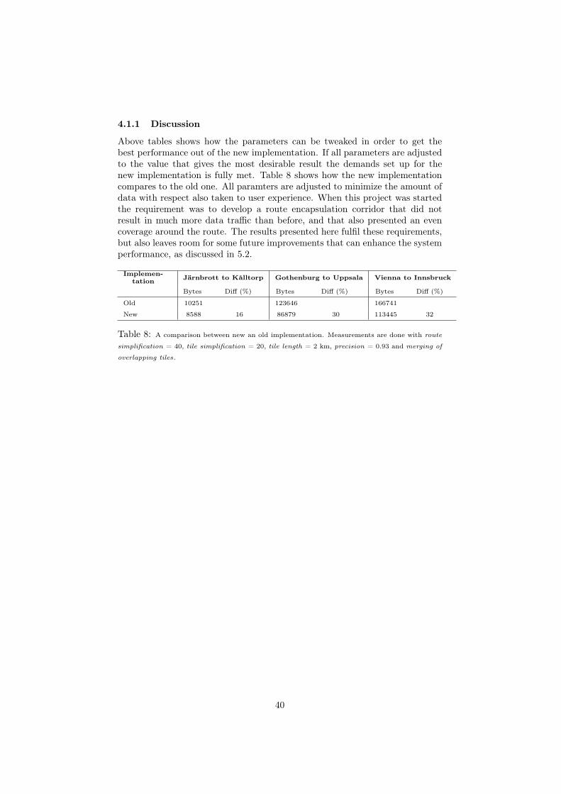
4.1.1 Discussion

Above tables shows how the parameters can be tweaked in order to get thebest performance out of the new implementation. If all parameters are adjustedto the value that gives the most desirable result the demands set up for thenew implementation is fully met. Table 8 shows how the new implementationcompares to the old one. All paramters are adjusted to minimize the amount ofdata with respect also taken to user experience. When this project was startedthe requirement was to develop a route encapsulation corridor that did notresult in much more data traffic than before, and that also presented an evencoverage around the route. The results presented here fulfil these requirements,but also leaves room for some future improvements that can enhance the systemperformance, as discussed in 5.2.

Implemen-tation Järnbrott to Kålltorp Gothenburg to Uppsala Vienna to Innsbruck

Bytes Diff (%) Bytes Diff (%) Bytes Diff (%)

Old 10251 123646 166741

New 8588 16 86879 30 113445 32

Table 8: A comparison between new an old implementation. Measurements are done with route

simplification = 40, tile simplification = 20, tile length = 2 km, precision = 0.93 and merging of

overlapping tiles.

40

5 Conclusions and possible future work

5.1 ConclusionThe thesis set out to examine if a simple bounding box based clipping algorithmcould be replaced by a more advanced algorithm based on bounding polygonsformed by the shape of the route polyline. The conclusion is that, yes, it ispossible. Not only is it possible but also provides a more even map coveragecompared to the bounding box alternative. The data amount needed to down-load the vector maps is also reduced by as much as a third.

Now, even some time after the thesis actually took place, it’s interestingto point out that the algorithms that came out of this thesis, and their imple-mentation, are busy serving vector maps to the users of cloud-based navigationapplication Wisepilot.

5.2 Possible future workPresented here are number of adjustments that can be made to the corridor andtile creating algorithms to improve the overall performance. They are presentedwith a brief description and an approximation of the effort it would take toimplement them.

Dynamic tile sizes

Since some devices running the client application is not suitable for large tiles, adifferentiation could be made when calculating the corridor and tiles for differentscreen resolutions. For example could a high-end mobile phone with high-speeddata access cope with longer tiles, thus increasing the data amount, while alower-end mobile phone could have the tiles calculated as proposed in table 8.On the other hand, if one would rather desire a wider offset, instead of the 200meters used in the measurements, a high-end phone with high screen resolutioncould increase the offset but use the same tile length.

Another use of dynamic tile sizes could be to let tiles covering a city map havebigger offset and those covering a freeway have smaller offset. When driving ona freeway it’s not likely a user is intereseted in roads passing nearby. In the city,on the other hand, a user might find it useful to see the surrounding road net,in order to get a better orientation.

An implementation of dynamic tiles for different unit types would not bea very time demanding operation. All parameters that control the tile shapeare easily changed for each corridor calculation and can thus be dependent ofscreen resolution and type of handset. To make different offsets for differentkinds of roads are bit trickier. It would mean a change of corridor offset in themiddle of a corridor calculation and also information on what kind of road thatis currently encapsuled etc.

Merge map server requests

When a request is made to the map server there is a lot of overhead data trans-fered every request. If a method for making the map server request for n suc-ceeding tiles at once, the number of map server request could be decreased and

41

the result faster calculated and transferred to the user. The response for todayssystem is not a concern, but a slight increased performance can be expected.

To implement this functionality is not to be considered especially difficult.There are some obstacles in merging and selecting from vector map data thatwould have to be conquered, but it could be done with superable effort.

42

6 References

References[1] R. Boland and J. Urrutia. Polygon area problems, 2000.

[2] Byoung Kyu Choi and Sang C. Park. A pair-wise offset algorithm for 2dpoint-sequence curve. Computer-Aided Design, 31(12):735–745, 1999.

[3] David H Douglas and Thomas K Peucker. Algorithms for the reduction ofthe number of points required to represent a digitized line or its caricature.Cartographica: The International Journal for Geographic Information andGeovisualization, 10(2):112–122, 1973.

[4] JSR 118 Expert Group. Mobile Information Device Profile for Java(TM)2 Micro Edition. Java Community Process, Sun Microsystems, 2 edition,November 2002.

[5] John Hershberger and Jack Snoeyink. Speeding up the douglas-peuckerline-simplification algorithm. In Proceedings of the 5th International Sym-posium on Spatial Data Handling, volume 1, pages 134–143, Charleston,South Carolina, 1992.

[6] Kai Hormann and Alexander Agathos. The point in polygon problem forarbitrary polygons. Computational Geometry, 20(3):131–144, 2001.

[7] G. Kalmanovich and Gregory Nisnevich. Swift and stable polygon growthand broken line offset. Computer-Aided Design, 30(11):847–852, 1998.

[8] Ravinder Krishnaswamy, Ghasem S. Alijani, and Shyh-Chang Su. On con-structing binary space partitioning trees. In CSC ’90: Proceedings of the1990 ACM annual conference on Cooperation, pages 230–235, New York,NY, USA, 1990. ACM.

[9] Xu-Zheng Liu, Jun-Hai Yong, Guo-Qin Zheng, and Jia-Guang Sun. Anoffset algorithm for polyline curves. Comput. Ind., 58(3):240–254, 2007.

[10] Bruce Naylor, John Amanatides, and William Thibault. Merging bsp treesyields polyhedral set operations. In SIGGRAPH ’90: Proceedings of the17th annual conference on Computer graphics and interactive techniques,pages 115–124, New York, NY, USA, 1990. ACM.

[11] William C. Thibault and Bruce F. Naylor. Set operations on polyhe-dra using binary space partitioning trees. SIGGRAPH Comput. Graph.,21(4):153–162, 1987.

[12] http://en.wikipedia.org/wiki/Haversine_formula. Haversine —Wikipedia, the free encyclopedia, 2015. [Online; accessed 03-May-2015].

[13] http://www.faqs.org/faqs/graphics/bsptree-faq/. Binary space par-titioning trees faq, 2015. [Online; accessed 01-May-2015].

[14] Bala R. Vatti. A generic solution to polygon clipping. Commun. ACM,35(7):56–63, 1992.

43

[15] Kevin Weiler and Peter Atherton. Hidden surface removal using polygonarea sorting. In SIGGRAPH ’77: Proceedings of the 4th annual confer-ence on Computer graphics and interactive techniques, pages 214–222, NewYork, NY, USA, 1977. ACM.

44