arX

iv:0

909.

0225

v2 [

cond

-mat

.str

-el]

14

Sep

2009

Variational determination of the second-order density matrix for the isoelectronic

series of Beryllium, Neon and Silicon

Brecht Verstichel,1, ∗ Helen van Aggelen,2 Dimitri Van Neck,1 Paul W. Ayers,3 and Patrick Bultinck2

1Center for Molecular Modeling, Ghent University, Proeftuinstraat 86, 9000 Gent, Belgium2Department of Inorganic and Physical Chemistry,

Ghent University, Krijgslaan 281 (S3), 9000 Gent, Belgium3Department of Chemistry, McMaster University, Hamilton, Ontario, L8S 4M1, Canada

The isoelectronic series of Be, Ne and Si are investigated using a variational determination of thesecond-order density matrix. A semidefinite program was developed that exploits all rotational andspin symmetries in the atomic system. We find that the method is capable of describing the strongstatic electron correlations due to the incipient degeneracy in the hydrogenic spectrum for increasingcentral charge. Apart from the ground-state energy various other properties are extracted from thevariationally determined second-order density matrix. The ionization energy is constructed using theextended Koopmans’ theorem. The natural occupations are also studied, as well as the correlatedhartree-Fock-like single particle energies. The exploitation of symmetry allows to study the basisset dependence and results are presented for correlation-consistent polarized valence double, tripleand quadruple zeta basis sets.

PACS numbers: 31.15.-p,31.15.A-,31.15.xt

Keywords: isoelectronic series, variational method, density matrix, semidefinite program

I. INTRODUCTION

The idea of a variational determination of the ground-state energy for a nonrelativistic many-body problem basedon the second-order density matrix (2DM) has a long history [1, 2, 3] and several highly appealing features. Theenergy of a system is a known linear functional of the 2DM. N -particle wave functions never need to be manipulatedsince the energy is minimized directly in terms of the 2DM. However, the minimization is constrained because thevariational search should be done exclusively with 2DMs that can be derived from an N -particle wave function (or anensemble of N -particle wave functions). Such a 2DM is called N -representable, and the complexity of the many-bodyproblem is in fact shifted to the characterization of this set of N -representable 2DMs. The complete (necessary andsufficient) set of conditions for N -representability of a 2DM is not known in a constructive form, but it is clear thatthe energy from a minimization constrained by a set of necessary N -representability conditions is a strict lower boundto the exact energy. Therefore this approach is highly complementary to the usual variational procedure based on awave-function ansatz, which produces upper bounds. In addition the method is in principle exact, in the sense thatas increasingly accurate set of N -representability conditions are imposed in the minimization, the resulting energyconverges to the exact one.

These are fascinating ideas for any true-blooded many-body theorist, as it comes close to the “ultimate reduction”of an interacting many-particle problem to solving a sequence of two-particle problems. In practice, however, imple-menting the method turns out to be very difficult and it is only in the last decade that serious attempts have beenundertaken to turn the idea into a practical calculational scheme. The massive efforts by Mazziotti et al. [4, 5, 6] andNakata et al. [7, 8] are particularly notable. The main difficulty is of a technical nature: stringent N -representabilityconditions require the positive semidefiniteness of matrix functionals of the 2DM, which turns the variational prob-lem into a so-called semidefinite program (SDP). Even applying the simplest “two-index” conditions, a direct energyminimization using Newton-Raphson methods requires a matrix operation scaling as M12 (where M is the number ofsingle-particle states) in each Newton-Raphson step. This can be circumvented in various ways, so that only matrixoperations scaling as M6 are needed. While these are nominally M6 methods, the number of iterations required toreach convergence is very high and seems to rise with system size; in practice present implementations are probablyabout 100-1000 times slower than comparable methods such as CCSD. Still, one has the feeling that there is potentialto turn it into a genuine M6 method, and it is of interest to investigate the properties of SDP applied to varioussystems.

∗Electronic address: brecht.verstichel@ugent.be

2

Up to now, most applications covered electronic structure calculations in atoms and molecules. Attention hasbeen given primarily to the resulting energy. In this paper, we focus on three issues: (i) the performance of SDP inmultireference situations (strong static correlations), (ii) the quality of the variationally obtained 2DM, and (iii) thedependence of the results on M (the size of the basis set). We do this by investigating three well-known examplesin electronic structure theory: the isoelectronic series of Be, Ne, and Si. It is well known that the correlation energyfor N electrons in the field of a positive point charge Z has a Z-dependence that strongly depends on N . Foran increasing central charge Z, the hartree-Fock spectrum tends to the hydrogenic one, which has an “accidental”degeneracy related to a special symmetry in the Coulomb Hamiltonian. For the four-electron series the incipientdegeneracy of the 2p and 2s orbitals leads to a vanishing particle-hole gap, inducing strong correlation effects with acorrelation energy proportional to Z. For the ten-electron series this does not happen because a major shell is closed,and the correlation energy becomes flat for increasing Z. The 14-electron series again shows degeneracy effects, andin addition is a spin triplet.

In Sec. II we provide theoretical and calculational backgrounds on the SDP implementation that is used. (Notethat the techniques developed in this section have been used previously to study molecular dissociation [9, 10].) Inparticular, we pay attention to the way spin and rotational symmetry are exploited, enabling the use of quite large(cc-pVQZ) basis sets. In Sec. III the SDP results for the isolectronic series of Be, Ne, and Si are discussed. A summaryis provided in Sec. IV. Atomic units are used throughout the paper.

II. THEORY

A. N-representability conditions

We will use second quantized notation where a†α (aα) creates (annihilates) an electron in a single-particle (sp) state

α. The Hamiltonian can be written as

H =∑

αγ

tαγa†αaγ +

1

4

∑

αβγδ

Vαβ;γδa†αa†

βaδaγ , (1)

where tαγ is the matrix element of the one-body part of the Hamiltonian (kinetic energy plus external potential) andVαβ;γδ is the antisymmetrized matrix element of the Coulomb interaction. The problem of finding the ground stateof a quantum mechanical many-body system can be reformulated in terms of the second-order density matrix

Γαβ;γδ = 〈ΨN |a†αa†

βaδaγ |ΨN 〉 . (2)

In principle Γ is a complex Hermitian matrix, but for a Coulomb Hamiltonian it is sufficient to consider real-symmetricmatrices,

Γαβ;γδ = Γγδ;αβ . (3)

In addition Γ obeys the fermionic relations for antisymmetry in the sp indices

Γαβ;γδ = −Γβα;γδ = −Γαβ;δγ = Γβα;δγ . (4)

The density matrix Γ can be determined variationally through the minimization of the energy functional

E(Γ) = Tr[

ΓH(2)]

=1

4

∑

αβ;γδ

Γαβ;γδH(2)αβ;γδ , (5)

where the reduced two-particle (tp) Hamiltonian is defined as

H(2)αβ;γδ =

1

N − 1(tαγδβδ − tαδδβγ − tβγδαδ + tβδδαγ) + Vαβ;γδ .

The problem with this method is that the complete set of conditions that the density matrix has to fulfill to bederivable from a physical wave function (the so-called N -representability conditions) is not known in a constructiveform [11]. Therefore one minimizes the energy functional under a limited set of N -representability conditions. Threesimple conditions, known as the P , Q and G conditions [2, 3], are known to give quite good results. The P conditionexpresses the fact that the 2DM has to be positive semidefinite. The physical interpretation of the Q condition is

3

that the two-hole matrix, Q, has to be positive semidefinite; using basis anticommutation relations Q can be writtenas a homogeneous linear mapping, from the tp matrix space onto itself:

Qαβ;γδ = 〈ΨN |aαaβa†δa

†γ |ΨN 〉

= Γαβ;γδ +1

n(δαγδβδ − δαδδβγ)Tr Γ − δβδραγ + δαδρβγ − δαγρβδ + δβγραδ . (6)

Here the particle number constraint has been used

Tr Γ =N(N − 1)

2= n ,

as well as the definition of the sp density matrix:

ραγ =1

N − 1

∑

β

Γαβ;γβ . (7)

The G condition demands that the particle-hole (ph) matrix G, is positive semidefinite; again, G can be written as ahomogeneous linear mapping, from the tp matrix space onto the ph matrix space:

Gαβ;γδ = 〈ΨN |a†αaβa†

δaγ |ΨN〉= δβδραγ − Γαδ;γβ . (8)

Recently there has been progress on improved N -representability conditions using the positive semidefiniteness ofhigher-order density matrices, e.g. the three-positivity conditions known as the T1 and T2 conditions [5, 12]. Alsosome attempts have been made to improve N -representability while remaining strictly in tp space, by consideringHamiltonian dependent positivity conditions [13], or sharp bounds on the P , Q and G operators [14]. However, inthe present paper we restrict ourselves to the standard P , Q and G conditions.

B. Inclusion of spin symmetry

1. General case

When the Hamiltonian of the system is invariant under rotations in spin space, the eigenstates can be characterizedby their total spin Σ and spin projection µ. Explicitly introducing the electron spin, a sp state is written as {|α〉 ≡|asa〉}, where a is the spatial orbital index and sa = ± 1

2 is the spin projection. Two sp states can couple to a pairwith total spin S = 0 or S = 1. The corresponding pair creation operator is

B†ab;SM =

[

a†a ⊗ a†

b

]S

M(9)

=∑

sasb

〈12sa

12sb|SM〉a†

asaa†

bsb(10)

and the density matrix Γ in spin-coupled tp space is defined as

ΣµΓSM ;S′M ′

ab;cd = 〈ΨNΣµ|B†

ab;SMBcd;S′M ′ |ΨNΣµ〉 . (11)

The B†B operator in Eq. (11) can now be further coupled to an object with good total spin. First one has to

introduce B,

Bcd;SM = (−1)S+MBcd;S −M , (12)

which is again a good spherical tensor operator. Equation (11) can now be rewritten as,

ΣµΓSM ;S′M ′

ab;cd = (−1)S′−M ′∑

ST

〈S MS′ − M ′|ST 0〉〈ΨNΣµ|

[

B†ab;S ⊗ Bcd;S′

]ST

0|ΨN

Σµ〉 . (13)

The density matrices on the right of Eq. (13) are classified by ST = 0, 1, 2 and provide an equivalent representationof the 2DM of the µth member of the spin multiplet. Note that the 2DMs of different members are trivially relatedthrough the Wigner-Eckart theorem,

〈ΨNΣµ|

[

B†ab;S ⊗ Bcd;S′

]ST

0|ΨN

Σµ〉 =(−1)Σ−µ

[ST ]〈Σ µΣ − µ|ST 0〉〈ΨN

Σ ||[

B†ab;S ⊗ Bcd;S′

]ST

||ΨNΣ 〉 , (14)

in terms of reduced matrix elements. Here [S] =√

2S + 1.

4

2. Singlet ground state

If the ground state has Σ = 0 (spin singlet), the number of matrices involved in the minimization procedure issignificantly reduced. Obviously for a singlet ground state the operator in Eq. (13) has to be scalar, i.e., only theST = 0 part is nonzero, and Eq. (13) reduces to

00ΓSM ;S′M ′

ab;cd = δSS′δMM ′ ΓSab;cd (15)

where

ΓSab;cd = 〈ΨN

00|B†ab;SMBcd;SM |ΨN

00〉 . (16)

is independent of M . This shows that, for a singlet ground state, the density matrix in a coupled tp basis is diagonalin S and M , and independent of the spin projection M . Instead of having to work with the full density matrix,all matrix manipulations can be performed on only two diagonal blocks, the S = 0 and S = 1 matrices, which arerespectively symmetric and antisymmetric in the indices related to the spatial orbitals.

We now reformulate the minization problem in the spin-coupled representation. The Q-matrix in the coupledrepresentation is similarly defined as:

QSab;cd = 〈ΨN

00|Bab;SMB†cd;SM |ΨN

00〉 . (17)

It is clear that the Q matrix has an identical block diagonal structure as Γ. After some recoupling one can write theQ-mapping, from coupled tp space onto coupled tp space, as

QSab;cd = ΓS

ab;cd +1

n(δacδbd + (−1)Sδadδbc)Tr Γ − ρacδbd − (−1)Sρbcδad − ρbdδac − (−1)Sρadδbc ,

where the sp matrix ρ

ρac = δsasc〈ΨN

00|a†asa

acsa|ΨN

00〉 (18)

=1

2

1

N − 1

∑

S

[S]2∑

l

ΓSal;cl (19)

and the trace

Tr Γ =1

2

∑

S

[S]2∑

ab

ΓSab;ab , (20)

can be expressed in terms of the coupled ΓS .The G-matrix is a bit more involved. The coupled ph creation operator reads

A†ab;SM =

[

a†a ⊗ ab

]S

M(21)

=∑

sasb

(−1)12−sb〈1

2sa12 − sb|SM〉a†

asaabsb .

The G-matrix in coupled ph space can now be written as:

GSab;cd = 〈ΨN

00|A†ab;SMAcd;SM |ΨN

00〉 . (22)

Again, one can prove that this matrix has the same block structure as the Γ and Q matrices. After some angularmomentum recoupling we get the expression for the G-map in the coupled representation:

GSab;cd = δbdρac −

∑

S′

[S′]2{

12

12 S

12

12 S′

}

ΓS′

ad;cb . (23)

5

3. Nonsinglet states

For higher-spin multiplets the same block decomposition is possible, provided a spin-averaged ensemble is considered.The density matrix for such an ensemble is defined in spin-coupled representation as

ΣΓSS′;Mab;cd =

1

2Σ + 1

∑

µ

〈ΨNΣµ|B†

ab;SMBcd;S′M |ΨNΣµ〉 . (24)

Note that the minimal energy can be reached for such an ensemble, since all members of the multiplet are degenerate.Performing the same manipulation as leading to Eq. (13) and using the Wigner-Eckart theorem as in Eq. (14) oneobtains

ΣΓSS′;Mab;cd =

∑

µ

(−1)S′−M

[Σ]2

∑

ST

〈S MS′ − M |ST 0〉 (−1)Σ−µ

[ST ]〈Σ µΣ − µ|ST 0〉〈ΨN

Σ ||[

B†ab;S ⊗ Bcd;S′

]ST

||ΨNΣ 〉 . (25)

Since (−1)Σ−µ/[Σ] = 〈ΣµΣ − µ|00〉 one can use orthogonality of the Clebsch-Gordan coefficients to work out the sumover µ in Eq. (25). The result

ΣΓSS′;Mab;cd =

δSS′

[S][Σ]〈ΨN

Σ ||[

B†ab;S ⊗ Bcd;S

]0

||ΨNΣ 〉 , (26)

implies that the ensemble 2DM is again block-diagonal in spin, and the same formulas can be used as for the singletcase.

C. Inclusion of rotational symmetry

In atomic systems, the rotational symmetry of the Hamiltonian further reduces the dimension of the blocks involvedin the density matrix. In exactly the same way as for spin, one can show that the density matrix of an ensemble,when avaraged over the third component of angular momentum, is diagonal in the two-particle angular momentumL and its z-component ML, and completely independent of the value of ML. What is more, for atomic systems thereis also the parity (π = ±1) of the two particle states. In the end one gets a density matrix that is composed out ofblocks with fixed values for LπS, enabling one to solve the variational problem in large basis sets. The sp basis forsystems with rotational and spin symmetry is written as |amasa〉, where a is shorthand for the radial basis state nala.The tp density matrix in spin and angular momentum coupled representation is defined as

Γ(LπS)ab;cd = 〈ΨN |B†

ab;LπSBcd;LπS |ΨN 〉 , (27)

where

B†ab;LπS =

[

a†a ⊗ a†

b

]LS

MLMS

=∑

mamb

∑

sasb

〈lamalbmb|LML〉〈1

2sa

1

2sb|SMS〉a†

nalamasaa†

nblbmbsb. (28)

In an analogous way as for spin coupling, the spin and angular momentum coupled Q-matrix is defined as

Q(LπS)ab;cd = 〈ΨN |Bab;LπSB†

cd;LπS |ΨN 〉 , (29)

out of which the coupled Q-map can be derived

Q(LπS)ab;cd = Γ

(LπS)ab;cd +

Tr Γ

n

(

δacδbd + (−1)L+S+lc+ldδadδbc

)

−δbdδlalcρ(la)nanc

− δacδlbldρ(lb)nbnd

, (30)

with the sp density matrix defined as

ρ(la)nanc

=1

2

1

2la + 1

1

N − 1

∑

(LπS)

[L]2 [S]2∑

nblb

Γ(LπS)nalanblb;nclanblb

. (31)

6

The G-matrix is defined as

G(LπS)ab;cd = 〈ΨN |

[

a†a ⊗ ab

](LπS)(

[

a†c ⊗ ad

](LπS))†

|ΨN〉 , (32)

where again a is a spherical tensor operator defined as

abmbsb= (−1)lb+mb+

12+sbab−mb−sb

. (33)

The spin and angular momentum coupled G-map from tp space on ph space becomes

G(LπS)ab;cd = δbdδlalcρ

(la)nanc

−∑

(LπS)′

[S′]2[L′]

2{

ld lc Llb la L′

}{

12

12 S

12

12 S′

}

Γ(LπS)′

ad;cb . (34)

D. Energy optimization with a semidefinite program

1. Interior point method

The variational problem for the 2DM can be formulated as a so-called semidefinite program [15], a constrainedoptimization program where it is demanded that certain matrices, which are functions of the variables being optimized,remain positive semidefinite. In our case, there is a convex subspace of the matrix space, which is called the feasibleregion, where Γ, Q(Γ) and G(Γ) are positive semidefinite. In Γ-space, the direction of energy decrease is given by(

−H(2))

[see Eq. (5)]. If the energy is to be minimized, the objective is to go as far as possible in this direction, withoutleaving the feasible region. The optimized density matrix is on the edge of the feasible region. Computationally, thisproblem is solved with an interior point method by optimizing the following cost function

Φ(Γ, t) = Tr ΓH(2) − t ln detP(Γ) + C , (35)

with

P(Γ) =

Γ 0 00 Q(Γ) 00 0 G(Γ)

. (36)

The constant C has no influence on the solution but is added here in order to take into account the possibility that thematrices have certain explicit zero eigenvalues connected with imposing spin constraints (see the discussion followingEq. (50); in this case C can be considered an infinite constant). Starting from a large value of t, (e.g. t = 1), the costfunction is minimized, and the resulting density matrix is used as a seed vector for the next minimization programwith a smaller value of t. This procedure continues until convergence is reached for t → 0, when the density matrixis at the edge of the feasible region.

2. Implementation

In addition to the positive semidefinite constraints, there are a number of linear constraints which the densitymatrix has to fulfill (e.g. particle number). These conditions are imposed by direct substitution. Suppose there area number of linear constraints of the form,

Tr ΓK(i) = k(i) . (37)

The way to impose these conditions is to limit the variations to the subspace orthogonal to the K(i)’s. Suppose theset of symmetric tp matrices {f i} is an orthogonal basis of this subspace,

Tr f if j = δij Tr f iK(j) = 0 . (38)

The tp density matrix can be expanded in the basis,

Γ =∑

i

Γifi + C , (39)

7

where C is a constant matrix obeying the inhomogeneous conditions

Tr CK(i) = k(i) . (40)

For the minimization of the cost function at a certain value of t, Newton’s method is used. At a given point Γ0 inmatrix space, the gradient of the cost function is

∂Φ

∂Γi

= Tr f iH(2) − t[

Tr f i{

Γ−10 + Q

(

Q(Γ0)−1

)

+ G(

G(Γ0)−1

)}]

. (41)

Using the Hermiticity of the Q and G mappings [e.g. Tr Q(Γ)A = Tr Q(A)Γ], the gradient in matrix form reads:

∇Φ =∑

i

∂Φ

∂Γi

f i = P[

H(2) − t(

Γ−10 + Q

(

Q(Γ0)−1

)

+ AG(

G(Γ0)−1

)

)]

, (42)

where P is the operator that projects onto the space spanned by the f i’s and A is the antisymmetrizer that projectsph space on tp space. The Hessian at Γ0 can be written as

Hij =∂2Φ

∂Γi∂Γj

= t{

Tr[

f iΓ−10 f jΓ−1

0

]

+ Tr[

Q(f i)Q(Γ0)−1Q(f j)Q(Γ0)

−1]

+ Tr[

G(f i)G(Γ0)−1G(f j)G(Γ0)

−1]}

.

(43)In Newton’s method the search direction ǫ is found by solving the linear system

∑

j

∂2Φ

∂Γi∂Γj

ǫj = − ∂Φ

∂Γi

. (44)

This system is solved using the linear conjugate gradient method [16]. In this method, only one matrix-vectormultiplication is needed per iteration. The special structure of the Hessian can be exploited to construct a fastmatrix-vector multiplication. The action of the Hessian on a tp matrix ǫ is

∑

j

Hijǫj = t{

Tr[

f iΓ−10 ǫΓ−1

0

]

+ Tr[

Q(f i)Q(Γ0)−1Q(ǫ)Q(Γ0)

−1]

+ Tr[

G(f i)G(Γ0)−1G(ǫ)G(Γ0)

−1]}

, (45)

which can be written in matrix form as,

Hǫ = tP[

Γ−10 ǫΓ−1

0 + Q(

Q(Γ0)−1Q(ǫ)Q(Γ0)

−1)

+ AG(

G(Γ0)−1G(ǫ)G(Γ0)

−1)

]

. (46)

It is clear that each conjugate gradient step can be calculated using only manipulations in the tp and ph matrix space.After the convergence of the conjugate gradient cycle, the direction of the Newton-Raphson step ǫ is known. A line

search in this direction is then performed in order to obtain the minimum of the cost function. Note that one alwaysstays in the feasible region since the cost function goes to +∞ at the edge.

3. Imposing the spin constraints for Σ = 0

The spin coupled form of the Σz operator can be written as:

Σz =1√2

∑

a

[

a†a ⊗ aa

]1

0. (47)

This operator lives in ph-space, and we can force the vector

{Σz}Sab =

1√2δS1δab , (48)

to be an eigenvector of G(Γ) with eigenvalue zero. In doing this we automatically impose the same constraints onG(Γ) for Σx and Σy due to the threefold degeneracy of the S = 1 block of the 2DM. It can be easily seen that in thiscase the expectation value of the total spin is zero,

〈ΨN |Σ2|ΨN〉 = 〈ΨN |Σ2x + Σ2

y + Σ2z|ΨN〉 = 0 . (49)

8

So the condition to be imposed on the density matrix becomes:

∑

S

[S]2[

1

2

1

N − 1− (−1)S

{

12

12 1

12

12 S

}]

∑

b

ΓSab;cb = 0 . (50)

For the projection of a tp density matrix on a spin singlet state, there are as many constraint matrices as there are spmatrix dimensions. Because of the zero eigenvalues in the G-matrix the projected density matrix is on the edge of thefeasible region during the whole of the minimization process, and as a result, the cost function is infinity. This can becircumvented by taking the pseudo-inverse of the G-matrix, which excludes the Σz-state from the inversion process.This will not alter the result of the program because the contribution of this state to the cost function is constant.

4. Imposing the spin constraints for Σ 6= 0

For higher-spin multiplets we use the spin-averaged ensemble (see Sec. II B 3), in which the 2DM has the same

simple structure as for the singlet case. The expectation value of the Σ2 spin operator is forced to be exact, using thelinear constraint

Tr Γ{Σ2} = Σ(Σ + 1) , (51)

where {Σ2} is the tp matrix representation of the Σ2 operator,

{Σ2}Sab;cd =

[

3

2

2 − N

N − 1+ S(S + 1)

]

(

δacδbd + (−1)Sδadδbc

)

. (52)

There is only one linear constraint for nonzero spin, in contrast to the numerous constraints for the projection onto asinglet state. It can therefore be expected that the spin constraints (i.e. the constraints on the 2DM ensuring that itis derivable from a wave function with good total spin) are less accurate than those for the singlet case. It is, in fact,known how to cure this situation [17] by considering not the spin-averaged ensemble but rather the 2DM derived fromthe highest-weight member (µ = Σ) of the multiplet. Similar to the spin singlet projection, one can then impose the

condition that, since the spin-raising ladder operator Σ+ destroys the wave function, the G(Γ) matrix must have a

zero eigenvalue (with an eigenvector in ph space corresponding to the Σ+ operator). In such a highest-weight schemes,the spin restrictions for the Σ 6= 0 case are put on the same footing as for the singlet case; in fact, the highest-weightand the spin-averaged ensemble scheme are equivalent for the singlet case. However, the highest-weight scheme forΣ 6= 0 requires one to keep track of more matrices and is computationally more demanding by about a factor of 10.We therefore used the ensemble scheme even for the nonsinglets (i.e. the Si atom), though we checked some cases withthe highest-weight method for the spin.

5. Spin and angular momentum projection

When angular momentum is taken into account, everything becomes a bit more complicated, but the principlesare the same as in the last paragraph. It can be shown that in a spin-and-angular-momentum-coupled basis thez-projections of Σ and Λ become

Σz =1√2

∑

nl

[l][

a†nl ⊗ anl

](0+1), (53)

Λz =

√

2

3

∑

nl

[l]l[

a†nl ⊗ anl

](1+0). (54)

Following the same argument as before, it can be imposed that the density matrix is derivable from an eigenstatewith zero eigenvalue of respectively the Σ and Λ operators when

∑

c

[lc]G (Γ)(0+1)ab;cc = 0 , (55)

∑

c

[lc]lcG (Γ)(1+0)ab;cc = 0 . (56)

9

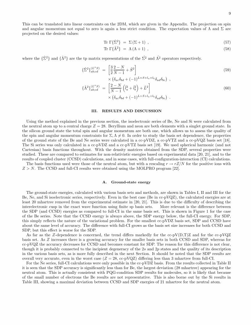
This can be translated into linear constraints on the 2DM, which are given in the Appendix. The projection on spinand angular momentum not equal to zero is again a less strict condition. The expectation values of Λ and Σ areprojected on the desired values:

Tr Γ{Σ2} = Σ (Σ + 1) , (57)

Tr Γ{Λ2} = Λ (Λ + 1) , (58)

where the {Σ2} and {Λ2} are the tp matrix representations of the Σ2 and Λ2 operators respectively.

{Σ2}(LπS)ab;cd =

[

3

2

2 − N

N − 1+ S2

]

(59)

×(

δacδbd + (−1)L+S+la+lbδadδbc

)

,

{Λ2}(LπS)ab;cd =

[

2 − N

N − 1

(

l2a + l2b

)

+ L2

]

(60)

×(

δacδbd + (−1)L+S+la+lbδadδbc

)

.

III. RESULTS AND DISCUSSION

Using the method explained in the previous section, the isoelectronic series of Be, Ne and Si were calculated fromthe neutral atom up to a central charge Z = 28. Beryllium and neon are both elements with a singlet ground state. Inthe silicon ground state the total spin and angular momentum are both one, which allows us to assess the quality ofthe spin and angular momentum constraints for Σ, Λ 6= 0. In order to study the basis set dependence, the propertiesof the ground state of the Be and Ne series were calculated in a cc-pVDZ, a cc-pVTZ and a cc-pVQZ basis set [18].The Si series was only calculated in a cc-pVDZ and a cc-pVTZ basis set [19]. We used spherical harmonic (and notCartesian) basis functions throughout. With the density matrices obtained from the SDP, several properties werestudied. These are compared to estimates for non-relativistic energies based on experimental data [20, 21], and to theresults of coupled cluster (CCSD) calculations, and in some cases, with full-configuration-interaction (CI) calculations.

The basis functions used were those of the neutral atom, but with a rescaling r → rZ/N for the positive ions withZ > N . The CCSD and full-CI results were obtained using the MOLPRO program [22].

A. Ground-state energy

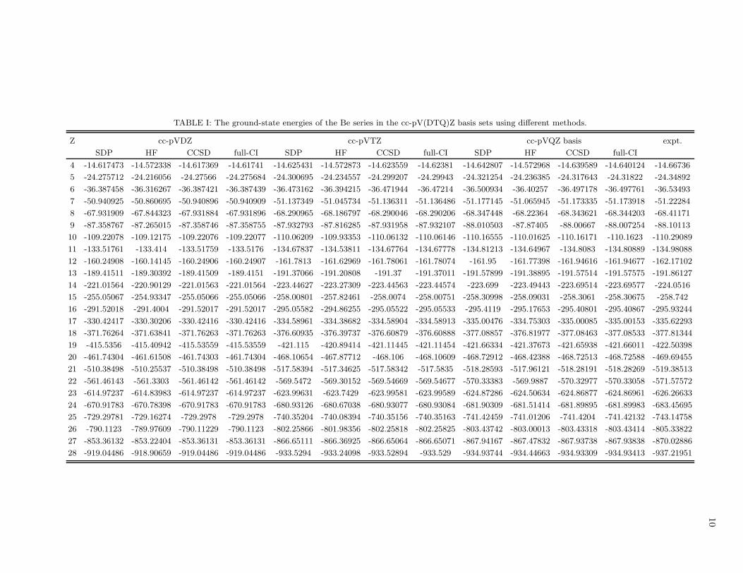
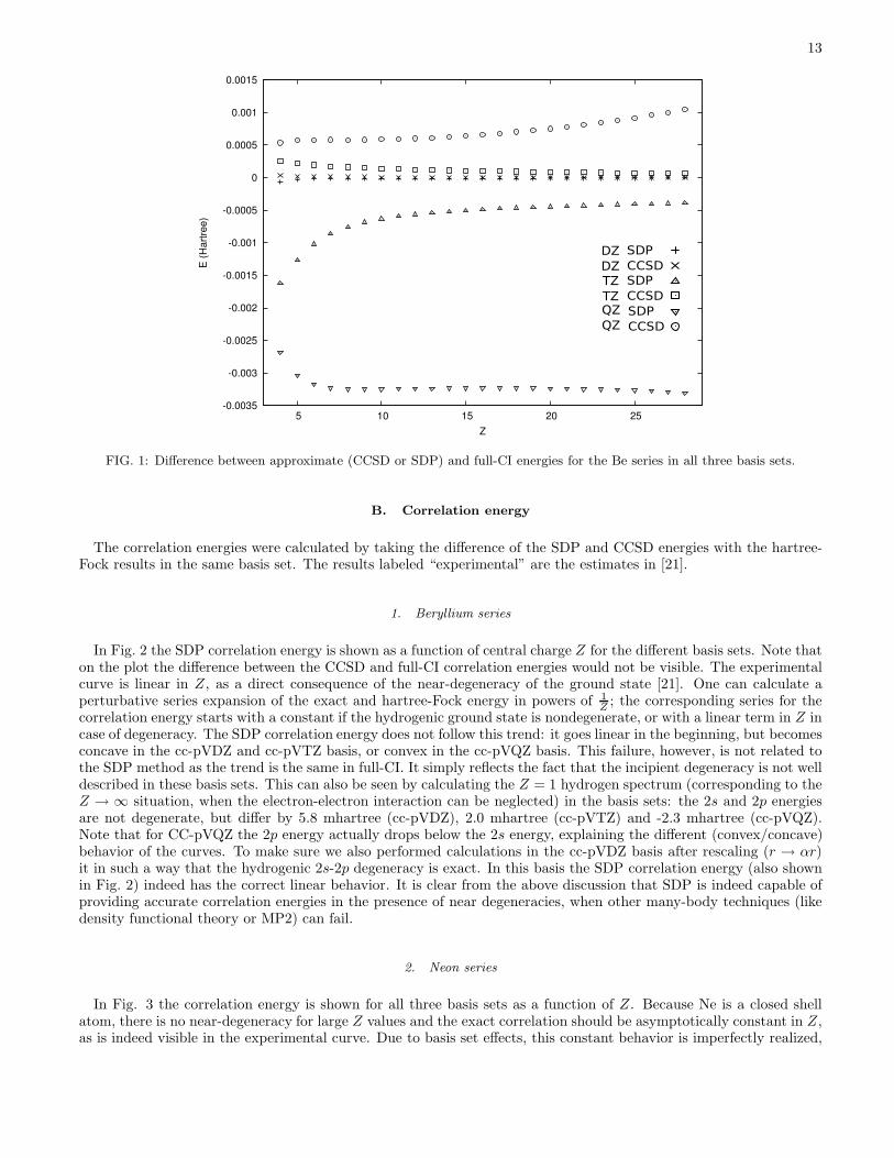
The ground-state energies, calculated with various basis sets and methods, are shown in Tables I, II and III for theBe, Ne, and Si isoelectronic series, respectively. Even in the best case (Be in cc-pVQZ), the calculated energies are atleast 20 mhartree removed from the experimental estimate in [20, 21]. This is due to the difficulty of describing theinterelectronic cusp in the exact wave function using finite sp basis sets. More relevant is the difference betweenthe SDP (and CCSD) energies as compared to full-CI in the same basis set. This is shown in Figure 1 for the caseof the Be series. Note that the CCSD energy is always above, the SDP energy below, the full-CI energy. For SDP,this simply reflects the nature of the variational problem. For the smallest cc-pVDZ basis set, SDP and CCSD haveabout the same level of accuracy. The difference with full-CI grows as the basis set size increases for both CCSD andSDP, but this effect is worse for the SDP.

As far as the Z-dependence is concerned, the trend differs markedly for the cc-pV(D,T)Z and for the cc-pVQZbasis set. As Z increases there is a growing accuracy for the smaller basis sets in both CCSD and SDP, whereas forcc-pVQZ the accuracy decreases for CCSD and becomes constant for SDP. The reason for this difference is not clear,though it is probably connected to the incipient degeneracy of the 2s and 2p states and the quality of its descriptionin the various basis sets, as is more fully described in the next Section. It should be noted that the SDP results areoverall very accurate, even in the worst case (Z = 28, cc-pVQZ) differing less than 3 mhartree from full-CI.

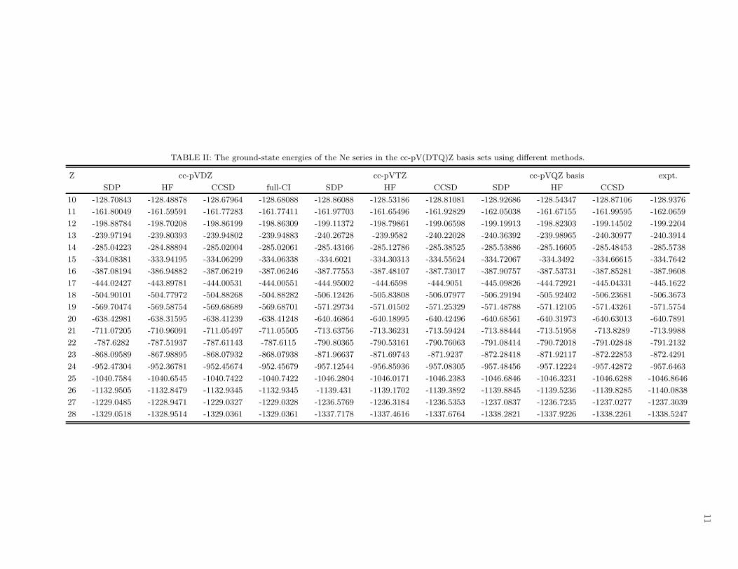
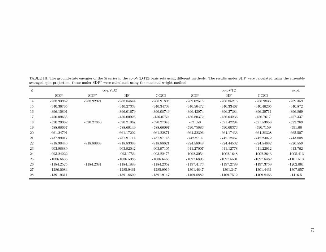
For the Ne series, full-CI calculations were only possible in the cc-pVDZ basis. From the results collected in Table IIit is seen that the SDP accuracy is significantly less than for Be, the largest deviation (28 mhartree) appearing for theneutral atom. This is actually consistent with PQG-condition SDP results for molecules, so it is likely that becauseof the small number of electrons the Be results are not representative. This is also borne out by the Si results inTable III, showing a maximal deviation between CCSD and SDP energies of 21 mhartree for the neutral atom.

10

TABLE I: The ground-state energies of the Be series in the cc-pV(DTQ)Z basis sets using different methods.

Z cc-pVDZ cc-pVTZ cc-pVQZ basis expt.

SDP HF CCSD full-CI SDP HF CCSD full-CI SDP HF CCSD full-CI

4 -14.617473 -14.572338 -14.617369 -14.61741 -14.625431 -14.572873 -14.623559 -14.62381 -14.642807 -14.572968 -14.639589 -14.640124 -14.66736

5 -24.275712 -24.216056 -24.27566 -24.275684 -24.300695 -24.234557 -24.299207 -24.29943 -24.321254 -24.236385 -24.317643 -24.31822 -24.34892

6 -36.387458 -36.316267 -36.387421 -36.387439 -36.473162 -36.394215 -36.471944 -36.47214 -36.500934 -36.40257 -36.497178 -36.497761 -36.53493

7 -50.940925 -50.860695 -50.940896 -50.940909 -51.137349 -51.045734 -51.136311 -51.136486 -51.177145 -51.065945 -51.173335 -51.173918 -51.22284

8 -67.931909 -67.844323 -67.931884 -67.931896 -68.290965 -68.186797 -68.290046 -68.290206 -68.347448 -68.22364 -68.343621 -68.344203 -68.41171

9 -87.358767 -87.265015 -87.358746 -87.358755 -87.932793 -87.816285 -87.931958 -87.932107 -88.010503 -87.87405 -88.00667 -88.007254 -88.10113

10 -109.22078 -109.12175 -109.22076 -109.22077 -110.06209 -109.93353 -110.06132 -110.06146 -110.16555 -110.01625 -110.16171 -110.1623 -110.29089

11 -133.51761 -133.414 -133.51759 -133.5176 -134.67837 -134.53811 -134.67764 -134.67778 -134.81213 -134.64967 -134.8083 -134.80889 -134.98088

12 -160.24908 -160.14145 -160.24906 -160.24907 -161.7813 -161.62969 -161.78061 -161.78074 -161.95 -161.77398 -161.94616 -161.94677 -162.17102

13 -189.41511 -189.30392 -189.41509 -189.4151 -191.37066 -191.20808 -191.37 -191.37011 -191.57899 -191.38895 -191.57514 -191.57575 -191.86127

14 -221.01564 -220.90129 -221.01563 -221.01564 -223.44627 -223.27309 -223.44563 -223.44574 -223.699 -223.49443 -223.69514 -223.69577 -224.0516

15 -255.05067 -254.93347 -255.05066 -255.05066 -258.00801 -257.82461 -258.0074 -258.00751 -258.30998 -258.09031 -258.3061 -258.30675 -258.742

16 -291.52018 -291.4004 -291.52017 -291.52017 -295.05582 -294.86255 -295.05522 -295.05533 -295.4119 -295.17653 -295.40801 -295.40867 -295.93244

17 -330.42417 -330.30206 -330.42416 -330.42416 -334.58961 -334.38682 -334.58904 -334.58913 -335.00476 -334.75303 -335.00085 -335.00153 -335.62293

18 -371.76264 -371.63841 -371.76263 -371.76263 -376.60935 -376.39737 -376.60879 -376.60888 -377.08857 -376.81977 -377.08463 -377.08533 -377.81344

19 -415.5356 -415.40942 -415.53559 -415.53559 -421.115 -420.89414 -421.11445 -421.11454 -421.66334 -421.37673 -421.65938 -421.66011 -422.50398

20 -461.74304 -461.61508 -461.74303 -461.74304 -468.10654 -467.87712 -468.106 -468.10609 -468.72912 -468.42388 -468.72513 -468.72588 -469.69455

21 -510.38498 -510.25537 -510.38498 -510.38498 -517.58394 -517.34625 -517.58342 -517.5835 -518.28593 -517.96121 -518.28191 -518.28269 -519.38513

22 -561.46143 -561.3303 -561.46142 -561.46142 -569.5472 -569.30152 -569.54669 -569.54677 -570.33383 -569.9887 -570.32977 -570.33058 -571.57572

23 -614.97237 -614.83983 -614.97237 -614.97237 -623.99631 -623.7429 -623.99581 -623.99589 -624.87286 -624.50634 -624.86877 -624.86961 -626.26633

24 -670.91783 -670.78398 -670.91783 -670.91783 -680.93126 -680.67038 -680.93077 -680.93084 -681.90309 -681.51414 -681.89895 -681.89983 -683.45695

25 -729.29781 -729.16274 -729.2978 -729.2978 -740.35204 -740.08394 -740.35156 -740.35163 -741.42459 -741.01206 -741.4204 -741.42132 -743.14758

26 -790.1123 -789.97609 -790.11229 -790.1123 -802.25866 -801.98356 -802.25818 -802.25825 -803.43742 -803.00013 -803.43318 -803.43414 -805.33822

27 -853.36132 -853.22404 -853.36131 -853.36131 -866.65111 -866.36925 -866.65064 -866.65071 -867.94167 -867.47832 -867.93738 -867.93838 -870.02886

28 -919.04486 -918.90659 -919.04486 -919.04486 -933.5294 -933.24098 -933.52894 -933.529 -934.93744 -934.44663 -934.93309 -934.93413 -937.21951

11

TABLE II: The ground-state energies of the Ne series in the cc-pV(DTQ)Z basis sets using different methods.

Z cc-pVDZ cc-pVTZ cc-pVQZ basis expt.

SDP HF CCSD full-CI SDP HF CCSD SDP HF CCSD

10 -128.70843 -128.48878 -128.67964 -128.68088 -128.86088 -128.53186 -128.81081 -128.92686 -128.54347 -128.87106 -128.9376

11 -161.80049 -161.59591 -161.77283 -161.77411 -161.97703 -161.65496 -161.92829 -162.05038 -161.67155 -161.99595 -162.0659

12 -198.88784 -198.70208 -198.86199 -198.86309 -199.11372 -198.79861 -199.06598 -199.19913 -198.82303 -199.14502 -199.2204

13 -239.97194 -239.80393 -239.94802 -239.94883 -240.26728 -239.9582 -240.22028 -240.36392 -239.98965 -240.30977 -240.3914

14 -285.04223 -284.88894 -285.02004 -285.02061 -285.43166 -285.12786 -285.38525 -285.53886 -285.16605 -285.48453 -285.5738

15 -334.08381 -333.94195 -334.06299 -334.06338 -334.6021 -334.30313 -334.55624 -334.72067 -334.3492 -334.66615 -334.7642

16 -387.08194 -386.94882 -387.06219 -387.06246 -387.77553 -387.48107 -387.73017 -387.90757 -387.53731 -387.85281 -387.9608

17 -444.02427 -443.89781 -444.00531 -444.00551 -444.95002 -444.6598 -444.9051 -445.09826 -444.72921 -445.04331 -445.1622

18 -504.90101 -504.77972 -504.88268 -504.88282 -506.12426 -505.83808 -506.07977 -506.29194 -505.92402 -506.23681 -506.3673

19 -569.70474 -569.58754 -569.68689 -569.68701 -571.29734 -571.01502 -571.25329 -571.48788 -571.12105 -571.43261 -571.5754

20 -638.42981 -638.31595 -638.41239 -638.41248 -640.46864 -640.18995 -640.42496 -640.68561 -640.31973 -640.63013 -640.7891

21 -711.07205 -710.96091 -711.05497 -711.05505 -713.63756 -713.36231 -713.59424 -713.88444 -713.51958 -713.8289 -713.9988

22 -787.6282 -787.51937 -787.61143 -787.6115 -790.80365 -790.53161 -790.76063 -791.08414 -790.72018 -791.02848 -791.2132

23 -868.09589 -867.98895 -868.07932 -868.07938 -871.96637 -871.69743 -871.9237 -872.28418 -871.92117 -872.22853 -872.4291

24 -952.47304 -952.36781 -952.45674 -952.45679 -957.12544 -956.85936 -957.08305 -957.48456 -957.12224 -957.42872 -957.6463

25 -1040.7584 -1040.6545 -1040.7422 -1040.7422 -1046.2804 -1046.0171 -1046.2383 -1046.6846 -1046.3231 -1046.6288 -1046.8646

26 -1132.9505 -1132.8479 -1132.9345 -1132.9345 -1139.431 -1139.1702 -1139.3892 -1139.8845 -1139.5236 -1139.8285 -1140.0838

27 -1229.0485 -1228.9471 -1229.0327 -1229.0328 -1236.5769 -1236.3184 -1236.5353 -1237.0837 -1236.7235 -1237.0277 -1237.3039

28 -1329.0518 -1328.9514 -1329.0361 -1329.0361 -1337.7178 -1337.4616 -1337.6764 -1338.2821 -1337.9226 -1338.2261 -1338.5247

12

TABLE III: The ground-state energies of the Si series in the cc-pV(DT)Z basis sets using different methods. The results under SDP were calculated using the ensembleavaraged spin projection, those under SDP∗ were calculated using the maximal weight method.

Z cc-pVDZ cc-pVTZ expt.

SDP SDP∗ HF CCSD SDP HF CCSD

14 -288.93962 -288.92921 -288.84644 -288.91895 -289.02515 -288.85215 -288.9835 -289.359

15 -340.36765 -340.27338 -340.34709 -340.50472 -340.33467 -340.46205 -340.872

16 -396.10801 -396.01679 -396.08749 -396.43974 -396.27384 -396.39711 -396.869

17 -456.09635 -456.00926 -456.0759 -456.80372 -456.64236 -456.7617 -457.337

18 -520.29362 -520.27860 -520.21067 -520.27348 -521.58 -521.42294 -521.53858 -522.269

19 -588.68067 -588.60149 -588.66097 -590.75683 -590.60373 -590.7159 -591.66

20 -661.24791 -661.17202 -661.22871 -664.32396 -664.17433 -664.28328 -665.507

21 -737.99017 -737.91714 -737.97148 -742.2714 -742.12467 -742.23072 -743.808

22 -818.90446 -818.88808 -818.83388 -818.88621 -824.58949 -824.44532 -824.54882 -826.559

23 -903.98889 -903.92042 -903.97105 -911.27007 -911.12778 -911.22912 -913.762

24 -993.24222 -993.1756 -993.22475 -1002.3054 -1002.1648 -1002.2643 -1005.413

25 -1086.6636 -1086.5986 -1086.6465 -1097.6895 -1097.5501 -1097.6482 -1101.513

26 -1184.2525 -1184.2381 -1184.1889 -1184.2357 -1197.4173 -1197.2789 -1197.3759 -1202.061

27 -1286.0084 -1285.9461 -1285.9919 -1301.4847 -1301.347 -1301.4431 -1307.057

28 -1391.9311 -1391.8699 -1391.9147 -1409.8882 -1409.7512 -1409.8466 -1416.5

13

FIG. 1: Difference between approximate (CCSD or SDP) and full-CI energies for the Be series in all three basis sets.

B. Correlation energy

The correlation energies were calculated by taking the difference of the SDP and CCSD energies with the hartree-Fock results in the same basis set. The results labeled “experimental” are the estimates in [21].

1. Beryllium series

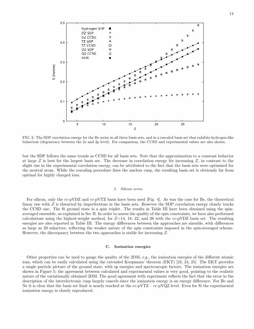
In Fig. 2 the SDP correlation energy is shown as a function of central charge Z for the different basis sets. Note thaton the plot the difference between the CCSD and full-CI correlation energies would not be visible. The experimentalcurve is linear in Z, as a direct consequence of the near-degeneracy of the ground state [21]. One can calculate aperturbative series expansion of the exact and hartree-Fock energy in powers of 1

Z; the corresponding series for the

correlation energy starts with a constant if the hydrogenic ground state is nondegenerate, or with a linear term in Z incase of degeneracy. The SDP correlation energy does not follow this trend: it goes linear in the beginning, but becomesconcave in the cc-pVDZ and cc-pVTZ basis, or convex in the cc-pVQZ basis. This failure, however, is not related tothe SDP method as the trend is the same in full-CI. It simply reflects the fact that the incipient degeneracy is not welldescribed in these basis sets. This can also be seen by calculating the Z = 1 hydrogen spectrum (corresponding to theZ → ∞ situation, when the electron-electron interaction can be neglected) in the basis sets: the 2s and 2p energiesare not degenerate, but differ by 5.8 mhartree (cc-pVDZ), 2.0 mhartree (cc-pVTZ) and -2.3 mhartree (cc-pVQZ).Note that for CC-pVQZ the 2p energy actually drops below the 2s energy, explaining the different (convex/concave)behavior of the curves. To make sure we also performed calculations in the cc-pVDZ basis after rescaling (r → αr)it in such a way that the hydrogenic 2s-2p degeneracy is exact. In this basis the SDP correlation energy (also shownin Fig. 2) indeed has the correct linear behavior. It is clear from the above discussion that SDP is indeed capable ofproviding accurate correlation energies in the presence of near degeneracies, when other many-body techniques (likedensity functional theory or MP2) can fail.

2. Neon series

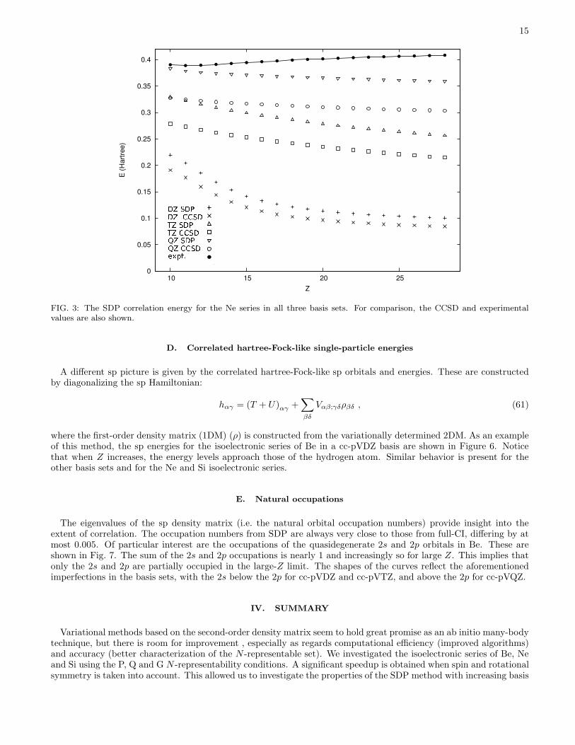
In Fig. 3 the correlation energy is shown for all three basis sets as a function of Z. Because Ne is a closed shellatom, there is no near-degeneracy for large Z values and the exact correlation should be asymptotically constant in Z,as is indeed visible in the experimental curve. Due to basis set effects, this constant behavior is imperfectly realized,

14

FIG. 2: The SDP correlation energy for the Be series in all three basis sets, and in a rescaled basis set that exhibits hydrogen-likebehaviour (degeneracy between the 2s and 2p level). For comparison, the CCSD and experimental values are also shown.

but the SDP follows the same trends as CCSD for all basis sets. Note that the approximation to a constant behaviorat large Z is best for the largest basis set. The decrease in correlation energy for increasing Z, in contrast to theslight rise in the experimental correlation energy, can be attributed to the fact that the basis sets were optimized forthe neutral atom. While the rescaling procedure fixes the nuclear cusp, the resulting basis set is obviously far fromoptimal for highly charged ions.

3. Silicon series

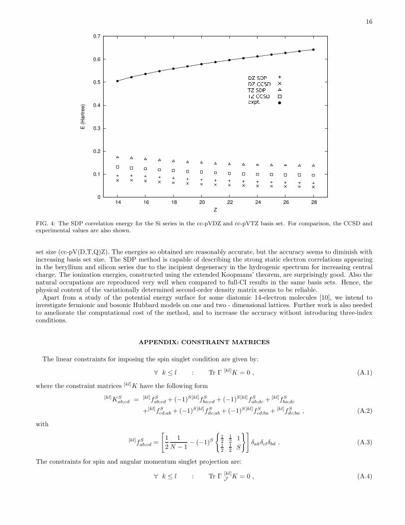
For silicon, only the cc-pVDZ and cc-pVTZ basis have been used [Fig. 4]. As was the case for Be, the theoreticallinear rise with Z is thwarted by imperfections in the basis sets. However the SDP correlation energy closely tracksthe CCSD one. The Si ground state is a spin triplet. The results in Table III have been obtained using the spin-averaged ensemble, as explained in Sec II. In order to assess the quality of the spin constraints, we have also performedcalculations using the highest-weight method, for Z=14, 18, 22, and 26 with the cc-pVDZ basis set. The resultingenergies are also reported in Table III. The energy differences between the approaches are sizeable, with differencesas large as 20 mhartree, reflecting the weaker nature of the spin constraints imposed in the spin-averaged scheme.However, the discrepancy between the two approaches is stable for increasing Z.

C. Ionization energies

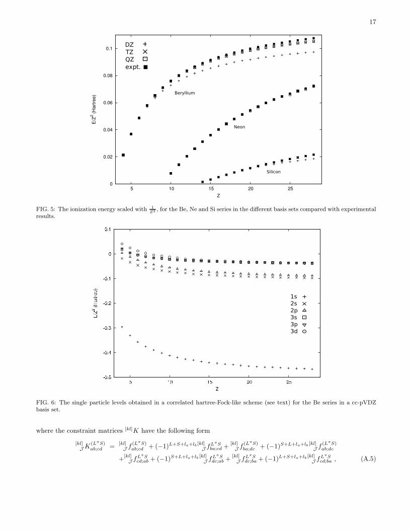
Other properties can be used to gauge the quality of the 2DM, e.g., the ionization energies of the different atomicions, which can be easily calculated using the extended Koopmans’ theorem (EKT) [23, 24, 25]. The EKT providesa single particle picture of the ground state, with sp energies and spectroscopic factors. The ionization energies areshown in Figure 5; the agreement between calculated and experimental values is very good, pointing to the realisticnature of the variationally obtained 2DM. The good agreement with experiment reflects the fact that the error in thedescription of the interelectronic cusp largely cancels since the ionization energy is an energy difference. For Be andNe it is clear that the basis set limit is nearly reached at the cc-pVTZ – cc-pVQZ level. Even for Si the experimentalionization energy is closely reproduced.

15

FIG. 3: The SDP correlation energy for the Ne series in all three basis sets. For comparison, the CCSD and experimentalvalues are also shown.

D. Correlated hartree-Fock-like single-particle energies

A different sp picture is given by the correlated hartree-Fock-like sp orbitals and energies. These are constructedby diagonalizing the sp Hamiltonian:

hαγ = (T + U)αγ +∑

βδ

Vαβ;γδρβδ , (61)

where the first-order density matrix (1DM) (ρ) is constructed from the variationally determined 2DM. As an exampleof this method, the sp energies for the isoelectronic series of Be in a cc-pVDZ basis are shown in Figure 6. Noticethat when Z increases, the energy levels approach those of the hydrogen atom. Similar behavior is present for theother basis sets and for the Ne and Si isoelectronic series.

E. Natural occupations

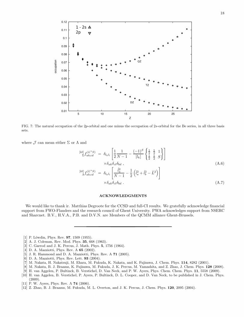
The eigenvalues of the sp density matrix (i.e. the natural orbital occupation numbers) provide insight into theextent of correlation. The occupation numbers from SDP are always very close to those from full-CI, differing by atmost 0.005. Of particular interest are the occupations of the quasidegenerate 2s and 2p orbitals in Be. These areshown in Fig. 7. The sum of the 2s and 2p occupations is nearly 1 and increasingly so for large Z. This implies thatonly the 2s and 2p are partially occupied in the large-Z limit. The shapes of the curves reflect the aforementionedimperfections in the basis sets, with the 2s below the 2p for cc-pVDZ and cc-pVTZ, and above the 2p for cc-pVQZ.

IV. SUMMARY

Variational methods based on the second-order density matrix seem to hold great promise as an ab initio many-bodytechnique, but there is room for improvement , especially as regards computational efficiency (improved algorithms)and accuracy (better characterization of the N -representable set). We investigated the isoelectronic series of Be, Neand Si using the P, Q and G N -representability conditions. A significant speedup is obtained when spin and rotationalsymmetry is taken into account. This allowed us to investigate the properties of the SDP method with increasing basis

16

FIG. 4: The SDP correlation energy for the Si series in the cc-pVDZ and cc-pVTZ basis set. For comparison, the CCSD andexperimental values are also shown.

set size (cc-pV(D,T,Q)Z). The energies so obtained are reasonably accurate, but the accuracy seems to diminish withincreasing basis set size. The SDP method is capable of describing the strong static electron correlations appearingin the beryllium and silicon series due to the incipient degeneracy in the hydrogenic spectrum for increasing centralcharge. The ionization energies, constructed using the extended Koopmans’ theorem, are surprisingly good. Also thenatural occupations are reproduced very well when compared to full-CI results in the same basis sets. Hence, thephysical content of the variationally determined second-order density matrix seems to be reliable.

Apart from a study of the potential energy surface for some diatomic 14-electron molecules [10], we intend toinvestigate fermionic and bosonic Hubbard models on one and two - dimensional lattices. Further work is also neededto ameliorate the computational cost of the method, and to increase the accuracy without introducing three-indexconditions.

APPENDIX: CONSTRAINT MATRICES

The linear constraints for imposing the spin singlet condition are given by:

∀ k ≤ l : Tr Γ [kl]K = 0 , (A.1)

where the constraint matrices [kl]K have the following form

[kl]KSab;cd = [kl]fS

ab;cd + (−1)S [kl]fSba;cd + (−1)S [kl]fS

ab;dc + [kl]fSba;dc

+[kl]fScd;ab + (−1)S [kl]fS

dc;ab + (−1)S [kl]fScd;ba + [kl]fS

dc;ba , (A.2)

with

[kl]fSab;cd =

[

1

2

1

N − 1− (−1)S

{

12

12 1

12

12 S

}]

δakδclδbd . (A.3)

The constraints for spin and angular momentum singlet projection are:

∀ k ≤ l : Tr Γ[kl]J K = 0 , (A.4)

17

FIG. 5: The ionization energy scaled with 1

Z2 , for the Be, Ne and Si series in the different basis sets compared with experimentalresults.

FIG. 6: The single particle levels obtained in a correlated hartree-Fock-like scheme (see text) for the Be series in a cc-pVDZbasis set.

where the constraint matrices [kl]K have the following form

[kl]J K

(LπS)ab;cd =

[kl]J f

(LπS)ab;cd + (−1)L+S+la+lb [kl]

J fLπSba;cd +

[kl]J f

(LπS)ba;dc + (−1)S+L+la+lb [kl]

J f(LπS)ab;dc

+[kl]J fLπS

cd;ab + (−1)S+L+la+lb [kl]J fLπS

dc;ab +[kl]J fLπS

dc;ba + (−1)L+S+la+lb [kl]J fLπS

cd;ba , (A.5)

18

FIG. 7: The natural occupation of the 2p-orbital and one minus the occupation of 2s-orbital for the Be series, in all three basissets.

where J can mean either Σ or Λ and

[kl]Σf

(LπS)ab;cd = δlkll

[

1

2

1

N − 1− (−1)S

[lk]

{

12

12 1

12

12 S

}]

×δakδclδbd , (A.6)

[kl]Λf

(LπS)ab;cd = δlkll

[

l2aN − 1

− 1

2

(

l2a + l2b − L2)

]

×δakδclδbd . (A.7)

ACKNOWLEDGMENTS

We would like to thank ir. Matthias Degroote for the CCSD and full-CI results. We gratefully acknowledge financialsupport from FWO-Flanders and the research council of Ghent University. PWA acknowledges support from NSERCand Sharcnet. B.V., H.V.A., P.B. and D.V.N. are Members of the QCMM alliance Ghent-Brussels.

[1] P. Lowdin, Phys. Rev. 97, 1509 (1955).[2] A. J. Coleman, Rev. Mod. Phys. 35, 668 (1963).[3] C. Garrod and J. K. Percus, J. Math. Phys. 5, 1756 (1964).[4] D. A. Mazziotti, Phys. Rev. A 65 (2002).[5] J. R. Hammond and D. A. Mazziotti, Phys. Rev. A 71 (2005).[6] D. A. Mazziotti, Phys. Rev. Lett. 93 (2004).[7] M. Nakata, H. Nakatsuji, M. Ehara, M. Fukuda, K. Nakata, and K. Fujisawa, J. Chem. Phys. 114, 8282 (2001).[8] M. Nakata, B. J. Braams, K. Fujisawa, M. Fukuda, J. K. Percus, M. Yamashita, and Z. Zhao, J. Chem. Phys. 128 (2008).[9] H. van Aggelen, P. Bultinck, B. Verstichel, D. Van Neck, and P. W. Ayers, Phys. Chem. Chem. Phys. 11, 5558 (2009).

[10] H. van Aggelen, B. Verstichel, P. Ayers, P. Bultinck, D. L. Cooper, and D. Van Neck, to be published in J. Chem. Phys.(2009).

[11] P. W. Ayers, Phys. Rev. A 74 (2006).[12] Z. Zhao, B. J. Braams, M. Fukuda, M. L. Overton, and J. K. Percus, J. Chem. Phys. 120, 2095 (2004).

19

[13] G. Gidofalvi and D. A. Mazziotti, Chem. Phys. Lett. 398, 434 (2004).[14] D. Van Neck and P. W. Ayers, Phys. Rev. A 75 (2007).[15] S. Boyd and L. Vandenberghe, Convex Optimization (Cambridge University Press, 2006).[16] G. H. Golub and C. F. Van Loan, Matrix Computations (The Johns Hopkins University Press, Baltimore, 1989).[17] G. Gidofalvi and D. A. Mazziotti, Phys. Rev. A 72 (2005).[18] T. H. Dunning, Jr., J. Chem. Phys. 90, 1007 (1989).[19] D. E. Woon and T. H. Dunning, Jr., J. Chem. Phys. 98, 1358 (1993).[20] E. R. Davidson, S. A. Hagstrom, S. J. Chakravorty, V. Meiser Umar, and C. Froese Fischer, Phys. Rev. A 44, 7071 (1991).[21] S. J. Chakravorty, S. R. Gwaltney, E. R. Davidson, F. A. Parpia, and C. Froese Fischer, Phys. Rev. A 47, 3649 (1993).[22] H.-J. Werner, P. J. Knowles, R. Lindh, F. R. Manby, M. Schtz, P. Celani, T. Korona, G. Rauhut, R. D. Amos, A. Bern-

hardsson, et al., MOLPRO, version 2006.1, a package of ab initio programs (2006).[23] O. Day, D. Smith, and R. Morrison, J. Chem. Phys. 62, 115 (1975).[24] D. Smith and O. Day, J. Chem. Phys. 62, 113 (1975).[25] M. Morrell, R. Parr, and M. Levy, J. Chem. Phys. 62, 549 (1975).