Variational assimilation of SSH variability from TOPEX/POSEIDON and ERS1 into an eddy-permitting...

Variational assimilation of SSH variability from

TOPEX/POSEIDON and ERS1 into an eddy-permitting model

of the North Atlantic

Armin Kohl1 and Jurgen WillebrandInstitut fur Meereskunde Kiel, Kiel, Germany

Received 16 May 2001; revised 17 September 2002; accepted 30 September 2002; published 20 March 2003.

[1] A first step for improving the climatological state of high-resolution generalcirculation models by means of data assimilation is presented. A method developed for theassimilation of statistical characteristics into chaotic ocean models is applied to assimilateSSH variability from TOPEX/POSEIDON and ERS1 in association with temperature andsalinity from the World Ocean Atlas 1997 in order to estimate the underlying meancirculation. The method requires a parameterization of SSH variability which derives fromthe approach of Green and Stone. By estimating initial conditions for temperature andsalinity, a mean state is achieved which, although not fully consistent with the altimetricand climatological data, is markedly improved on time scales of one year in comparison tothe control run. The assimilation of SSH variability data introduces complementaryinformation about the main frontal structures consistent with climatological observations.The state is however not an equilibrium state and returns back to the first guess quasi-equilibrium state for longer integration periods. INDEX TERMS: 4255 Oceanography: General:

Numerical modeling; 4263 Oceanography: General: Ocean prediction; 4532 Oceanography: Physical: General

circulation; 4520 Oceanography: Physical: Eddies and mesoscale processes; 4528 Oceanography: Physical:

Fronts and jets; KEYWORDS: data assimilation, statistical moments, North Atlantic Ocean, primitive-equation

model, eddy permitting

Citation: Kohl, A., and J. Willebrand, Variational assimilation of SSH variability from TOPEX/POSEIDON and ERS1 into an eddy-

permitting model of the North Atlantic, J. Geophys. Res., 108(C3), 3092, doi:10.1029/2001JC000982, 2003.

1. Introduction

[2] Altimetric data have become an important source ofinformation about the ocean circulation. In particular, thespatial and temporal coverage of the global ocean issuperior to most other data sources. Although the measure-ments are restricted to the ocean surface, strong verticalcoherence within the upper ocean allows one to inferinformation about the subsurface region. An optimalmethod for the extraction of information is given by theassimilation of data into a general circulation model. Twodifferent approaches are available and widely used, namelythe Kalman filter and the adjoint method. Both originatefrom the same principle, and both are limited by theimperfect knowledge of the error covariances. Most appli-cations for the assimilation of SSH anomalies are based onsimplifications of the extended Kalman filter and employvarious extrapolation schemes to account for spatial coher-ence of the error covariance matrix [Oschlies and Wille-

brand, 1996; Cooper and Haines, 1996; Evensen and vanLeeuwen, 1996; Gavart and De Mey, 1997]. An applicationof the method of Oschlies and Willebrand [1996] demon-strates that the variability is improved while the mean stateis effectively kept invariant [DYNAMO Group, 1997]. Themethod needs the mean SSH which is calculated from areference run. Since the Gulf Stream path is distinctlydifferent in the model than the observed path, solelyimproving the variability results in an unphysical interplayof the mean and the transient parts of the flow. Additionalindependent information about the mean state is thereforenecessary, and was included by Killworth et al. [2001] inthis scheme with considerable success.[3] It is not clear to what extent multiple stable equilibria

of the Gulf Stream system or model deficiencies account fordifferences to the observed data [Dijkstra and Molemaker,1999]. By minimizing a cost function the adjoint methodsearches for the trajectory of a given dynamical system thatfits the observations optimally so that the consistency of thesolution with the dynamical equations is guaranteed. Thisenables the construction of states that more closely representthe observations which, however, may not be equilibriumstates.[4] The application of the adjoint method with high-

resolution ocean models is not straightforward since thesemodels obey chaotic dynamics with limited predictability.

JOURNAL OF GEOPHYSICAL RESEARCH, VOL. 108, NO. C3, 3092, doi:10.1029/2001JC000982, 2003

1Now at Scripps Institution of Oceanography, La Jolla, California,USA.

Copyright 2003 by the American Geophysical Union.0148-0227/03/2001JC000982

37 - 1

The stability of their tangent linear models (this includesadjoint models) is characterized by positive Lyapunovexponents which also characterize the limit of predictabilityof the model [Kazantsev et al., 1998; Kazantsev, 1999].Exponential growth of the adjoint model can be related toan increasing number of secondary minima of the costfunction [Kohl and Willebrand, 2002, hereafter KW] whichprevents the convergence of the adjoint method. Applica-tions for the assimilation of altimeter data in high-resolutionmodels have therefore been restricted to very short timespans of a few months [Schroter et al., 1993; Morrow andDe Mey, 1995], which are too short to allow signals topropagate into the deep ocean. The method of KW allowsthe extension of the assimilation period by defining theadjoint method on the basis of statistical quantities. In thispaper the method is applied to assimilate sea surface height(SSH) variability into an eddy permitting model of theNorth Atlantic ocean.[5] Patterns and amplitudes of annual SSH variability are

intimately related to the underlying quasi-stationary meancirculation as described by Stammer [1997]. The close linkbetween the mean and the variable part therefore can inprinciple be utilized in reverse order for the estimation ofthe mean state from the variable part of the circulation bymeans of data assimilation. That link also serves as astarting point for recent eddy parameterizations [Treguieret al., 1997]. In the following application of the KWapproach, a parameterization based on Green [1970] andStone [1972] is included in the derivation of the adjointmodel for statistical quantities. The main emphasis of thisstudy is to show the feasibility of assimilating altimetricSSH variability to improve modeled climatological meanstates by parameter estimation and for state estimations withhigh resolution models.[6] After a brief review of the methodology, the forward

and the adjoint models are presented in section 3. Theparameterization for the SSH variability is presented insection 4. The results of a 1 year assimilation are discussedwith some emphasis on the effect of the parameterization insection 5 followed by a concluding discussion.

2. Method

[7] The adjoint method used in this study was designed toallow for the assimilation of statistical moments of data intochaotic ocean models. It is an extension of the originalformulation of Le Dimet and Talagrand [1986]. The basis ofthe method is the assumption that the dynamics of oceanmodels are decomposable into different time scale regimesassociated with different ranges of predictability. Averagedquantities are assumed to be more predictable. The adjointmodel derives from a separate model that describes themean state and that features long-term predictability. Only ashort outline of the technique is given in the following. Ahigh-resolution model with short-term predictability isemployed to calculate optimal estimates of single realiza-tions of statistical moments. A coarse resolution twinversion of the eddy-resolving model is used to approximatean independent model for the statistical moments used in thevariational method as a strong constraint. This model isintroduced to describe a predictable part of the evolution. Adetailed derivation is described by KW.

[8] The basic concept is to employ a high-resolutionmodel with short-term predictability to calculate the evolu-tion of the state vector x according to

dx

dt¼ f x;a; tð Þ; ð1Þ

depending on the parameter vector a. Estimates of singlerealizations of statistical moments that enter the costfunction are calculated from the solution of this model. Aseparate model for the mean state is employed for theconstruction of the adjoint. Coarse resolution twin version

dX

dt¼ F X ;að Þ ð2Þ

of the eddy-resolving model is used to approximate thismodel for the mean state. The adjoint derives from anexpansion at moments �x calculated from the high-resolutionmodel. The scheme then reads:minimize

J að Þ ¼ 1

2a� abð ÞTB�1 a� abð Þ þ 1

2Hx� yð ÞTO�1 Hx� yð Þ

ð3Þ

respecting the forward model

dx

dt¼ f x;a; tð Þ ð4Þ

and the adjoint to the coarse resolution version

� dldt

¼ @X Fy �x; �að Þlþ HTO�1 Hx� yð Þ; ð5Þ

where �x is a time mean and spatial average to the coarsegrid, O is the error covariance of statistical moments y ofobservations, B is the error covariance of the backgroundinformation ab of the parameter a and H is the observationoperator. The adjoint uses only temporally and spatiallyaveraged information originating from the high resolutionforward model. The estimated gradient and parameterimprovements calculated by the descent step are thereforetime independent and on the coarse resolution grid.

3. Numerical Models

[9] The primitive-equation ocean circulation model isbased on the 1/3� CME model configuration developedby Bryan and Holland [1989]. It makes use of the revisedcode described by Pacanowski et al. [1993]. The domainof high-resolution forward model and the coarse resolutiontwin covers the Atlantic Ocean basin from 15�S to 65�N.Both models have 30 levels and share the same verticalgrid spacing which increases smoothly from 35 m at thesurface to 250 m below 1000 m. Buffer zones of 5 pointswidth are applied on the closed boundaries where salinityand temperature are restored to data taken from Levitus[1982]. The northern boundary condition is supplementedin the Denmark Strait by actual section data [Doscher etal., 1994].

37 - 2 KOHL AND WILLEBRAND: VARIATIONAL ASSIMILATION OF SSH VARIABILITY

3.1. Forward Model

[10] The model configuration is essentially identical tothat described by Oschlies and Willebrand [1996]. A reviewof experiments and results of the CME configuration is givenby Boning [1996]. The model is forced with the monthlymean wind stresses of Hellerman and Rosenstein [1983] andthe heat flux is formulated according to the linear approx-imation of Han [1984]. Surface fluxes of fresh water arespecified by relaxation to the monthly mean salinity valuesof Levitus [1982]. The horizontal grid spacing is 1/3� inmeridional and 2/5� in zonal direction. Horizontal mixing isparameterized by biharmonic friction. Constant coefficientsfor viscosity and diffusivity are chosen as 2.5 � 1019 cm4/s.In the vertical, Laplacian mixing is used with constantcoefficients of 0.3 cm2/s for diffusion and 10 cm2/s forviscosity. Convection is parameterized by increasing thevertical mixing coefficients to 104 cm2/s at places in thewater column where static instability is detected.

3.2. Adjoint Model

[11] The high-resolution and the coarse resolution twinmodel are based on basically the same source code. Thehorizontal grid spacing is 1� in meridional and 1.2� in zonaldirection. Unlike in the forward model, horizontal mixing isparameterized by harmonic friction with coefficients chosenas 5 � 108 cm2/s to prevent the tangent linear model fromdeveloping unstable modes. The adjoint model was con-structed with aid of the automatic code compiler TAMC[Giering and Kaminski, 1998]. In order to prevent a compu-tational mode in the adjoint which results from the Eulercoupling steps in the forward model [Sirkes and Tziperman,1997], the forward code is modified to perform only leapfrogsteps. Divergence of the two decoupled modes is notobserved, and the adjoint variables asymptotically approacha stationary solution. As described in KW, prognosticvariables as well as air-sea thermohaline and momentumfluxes of the forward model were averaged to the coarse grid,and only their temporal mean values enter the adjoint. Thetopography was derived from the high-resolution represen-tation with the same spatial averaging procedure completedby an additional removal of holes and the restoration ofislands. The seasonal cycle is removed in the adjoint, whichis the adjoint to a model for the mean circulation. Includinga seasonal cycle into the adjoint formalism would requirethe formation of ensemble mean values in order to eliminatethe transient eddy component from the seasonal signal. Thestandard formulation of mixing in case of static instabilitiesmakes the mixing coefficients effectively time dependent.By analogy to the treatment of the forcing, convection isparameterized in the adjoint by temporally and spatiallyaveraging the mixing coefficients of the forward model.[12] For the descent algorithm the variable storage min-

imization algorithm M1QN3 by Gilbert and Lemarechal[1989] was chosen as a good compromise in terms ofstorage requirements between conjugated gradient andquasi-Newton methods. Gradients calculated by the coarseresolution model are interpolated by bicubic spline to thegrid of the 1/3� model before descent steps were performed.[13] Integration periods of several years are desirable in

order to define statistical moments, however, test runs showthat the assimilation period is limited to a range of about 1year. An exponential increase of the Lagrangian multipliers

starts after about a year of backward integration. Exponen-tial increasing Lagrangian multipliers indicate a limit ofpredictability and are related to positive eigenvalues of theadjoint operator. In the method of KW, weaker gradientsand lower extreme values of the velocity fields, in combi-nation with higher values for mixing coefficients of theadjoint, prevent in general the development of unstablemodes for integration periods of several years. In the presentmodel, spatial gradients and extreme values of the velocityfields are, even after averaging, still large enough to allowfor the development of instabilities. In agreement with thisassumption, no instabilities were found for periods ofseveral years if averaged prognostic variables originate froma coarse resolution forward model run.

4. Parameterization for SSH Variability

[14] Our statistical approach of the adjoint methodrequires a closed set of equations for all statistical momentsincluded in the cost function, which in our case includes thesecond-order moment SSH variability. Approximating thestatistical model by a low-resolution model twin as in KWrequires an additional physical relation for the inclusion ofhigher-order moments. A simple parameterization approachas described in KW is followed to mimic a model for theprediction of rms SSH variability. The idea is to search for arelation that expresses second-order moments in terms ofmean values. This parameterization forms together withcoarse resolution model the set of equations for the meanstate and the SSH variability.[15] For the inclusion of rms SSH variability, sSSH, as a

second-order moment, the eddy variability is parameterizedin terms of the density structure derived from the meantemperature and salinity distribution. The generation ofeddies is closely related to the stability properties of themean current. Eddy energies calculated from tracked drift-ing buoys [Richardson, 1983; Krauss and Kase, 1984] andaltimeter data [Stammer, 1997] indicate the major frontalzones as the primary location for the occurrence of varia-bility. Outside the tropical regime, spectral characteristics ofaltimetric data from TP analyzed by Stammer [1997]suggest baroclinic instability as the dominant source ofvariability in accordance with the spectral relations of geo-strophic turbulence. Treguier et al. [1997] shows that thedepth-integrated rms eddy velocity can be related to theRichardson number Ri in the main regions of variability.The approach used in this study was originally derived onbasis of the theory of baroclinic instability by Green [1970]and Stone [1972] who described the eddy velocity in termsof horizontal and vertical density gradients of the meanflow. Employing the thermal wind balance for the calcu-lation of the vertical velocity shear, the relation reads

sSSH ¼ g

�z

Z1250m110m

1ffiffiffiffiffiRi

p dz ¼ g

H

Z1250m110m

ffiffiffiffiffiffiffiffiffiffiffiffiffiffiffiffiffiffiffiffiffiffiffig r2y þ r2x� �f 2o rorz

vuutdz; ð6Þ

where �z is the depth interval, fo is the Coriolis parameterof a central latitude, r is the density, ro is a referencedensity, and the length g is the coefficient of proportionality.[16] The impact of employing this relation for the assim-

ilation of rms SSH variability in regions where the model

KOHL AND WILLEBRAND: VARIATIONAL ASSIMILATION OF SSH VARIABILITY 37 - 3

considerably underestimates variability is to steepen thefrontal structure. In this way the available potential energyas source for eddies generated by baroclinic instability isenhanced.[17] The parameter of proportionality g was calculated

from regressions employing data or the corresponding fieldsfrom the solution of the forward model. It spans a range ofvalues between 122 cm for the model solution and values of434–667 cm for the climatologies and TP/ERS1 SSHvariability. The correlation coefficients are of the order of0.7. The small value for the model solution may partly bedue to the fact that a large portion of the SSH variability ofthe model is over shallow regions where the parameter-ization is not defined. The value for the implementation intothe adjoint is chosen as g = 200 cm between 10�N and 50�Nand g = 0 elsewhere to exclude tropical and high-latituderegions. Tropical regions are excluded since the parameter-ization is based on the thermal wind relation. Low correla-tion coefficients in high latitudes suggest that the relation isnot suitable in this region.

[18] In order to explain the effect of the parameterization,gradients of cost function parts of experiments described insection 5.2 are calculated. The two cost function parts

JSSH ¼ 1

N

Xn

sSSHn� sobsSSHn

� �2�2d;sSSH

ð7Þ

and

JWAO97 ¼1

N

Xn

Tn � Tobsn

2�2d;T

þSn � Sobsn

2�2d;S

!ð8Þ

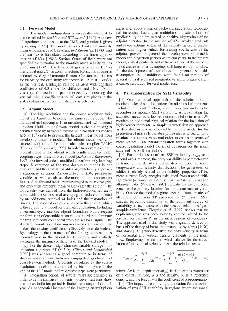
measure the difference of the modeled rms SSH variabilitysSSH to the data and the difference of modeled annual meantemperature and salinity to the values of the WOA97 data,respectively. The grid point index is n, and N is the numberof grid points of the model. Horizontal and vertical crosssections through cost function gradients with respect to thetemperature initial condition To are shown in Figure 1.

Figure 1. Cost function gradients with respect to the temperature initial condition. The part JWAO97 (a–b) measures the difference of annual mean temperature and salinity values to the WOA97 data (in 1/�C),and JsSSH

(c–d) measures the difference of the rms SSH variability. The horizontal level in Figures 1a and1c is at 230 m depth and vertical sections in Figures 1b and 1d is along 60�W.


Although there are marked differences between the patterns,both indicate the same characteristic errors of the modelwhich has a northward displaced Gulf Stream with too lowvariability and almost no Azores Current with the associatedvariability. The general features of @JSSH/@To confirm thesupposition made above; locations of underestimated SSHvariability are distinguished by spatial gradients in theproposed temperature change. Spatial structures of thegradients of either part are consistent in suggesting warmerwater south and colder water north of the Gulf Streamposition. The vertical structure of both gradients share somesimilar features. The scheme therefore provides a methodfor the vertical extrapolation of SSH data. The preciseposition of the Gulf Stream is difficult to constitute from@JWOA97/@To while the gradient of JSSH contains spatialgradient information that clearly marks the position. In thesame way, the signature of the Azores front clearly derivesfrom the associated variability whereas the climatology istoo smooth to allow for any horizontal structure of thegradient in this region.

5. Assimilation Experiments

[19] The parameterization (6) is based only on horizontaland vertical gradients of the mean density. There is noconstraint on absolute density values and the distributionamong temperature and salinity is provided by assimilatingrms SSH variability. It follows that an application of thescheme for the estimation of initial conditions for temper-ature and salinity will result in a large subspace of equivalentsolutions. In other words, the solution will be substantiallyunderdetermined. In the subsequent sections two ways arepresented to handle this problem. One is the inclusion of apriori information for the temperature and salinity initialconditions and a second is to add climatological data oftemperature and salinity. Different strategies concerning theset of the included cost function terms are pursued. The costfunction is defined as a sum of quadratic parts

J ¼ JdT þ JdS þ JdsSSH þ JdSST þ JfT þ J

fS þ J iT þ J iS

¼ 1

N

Xn

Tn � Tobs

n

2�2d;T

þXn

Sn � Sobsn

2�2d;S

þXn

sSSHn� sSSHobs

n

� �2�2d;sSSH

þXn

SSTn � SSTobsn

2�2d;SST

þXn

hf ln � hf lon 2

�2f ;TþXn

sf ln � sf lon 2

�2f ;S

þXn

Tn t ¼ 0ð Þ � Ton

2�2i;T

þXn

Sn t ¼ 0ð Þ � Son 2

�2i;S

!;

where N is total number of grid points of the model. Theorder of the J-terms correspond to the order of the sumsbelow. The term for annual or climatological means ofobservational data are labeled with d and i, f denotes the apriori information term for initial conditions and the surfaceheat (hfl), and salt flux (sfl), respectively. The notationcorresponds to the naming of the weights �b,a introduced in

Appendix A. The configuration of all performed experi-ments is listed in Table 1. The iterations are started with thesame parameter set as the control run which is the year aftera 20-year ‘‘spin-up’’ from the state of rest.

5.1. Including A Priori Information

[20] The need for an additional source of temperature andsalinity information in connection with the parameterizationwas stressed in section 4. In the experiment SST_SSH_O, apriori information of the temperature and salinity initialconditions ensures that the density information is notarbitrarily distributed among temperature and salinity cor-rections. The cost function consists of six terms whichinclude the a priori information of the fluxes and the initialcondition JT

f, JSf, JT

i, and JSi, respectively. The data terms

are J dsSSHand J dSST . The estimated parameters are the initial

conditions for temperature and salinity and the correspond-ing surface fluxes. Only a brief description of the results ispresented to give insight into the reasons for the config-uration chosen in the following section. Figure 2 depicts theannual mean SSH from the control run and the finaliteration together with data from Singh and Kelly [1997]who estimated mean SSH from a combination of hydro-graphic and altimeter data. The mean front of the control runis displaced at around 60�W to the north and is shifted ataround 42�W to the east and it is noticeably weaker than theobservations suggest. While the final iteration resemblesmore the control run than the data of Singh and Kelly[1997], the solution is nevertheless improved. This supportsthe assumption made in the introduction that it may bepossible to retrieve some information on the mean state byassimilating variability.[21] A similar experiment (SST_SSH) employing the

same data sets without including the a priori informationwas performed. The parameter set encompasses heat fluxand temperature initial conditions only. The mean SSHpattern shown in Figure 3 is in better agreement with thedata of Singh and Kelly [1997] shown in Figure 2c. TheGulf Stream position is remarkable similar to the one thatcan be inferred from the gradient shown in Figure 1. Aparticular feature of this experiment is an almost correctGulf Stream separation east of Cape Hatteras which wasfound to remain stable for more than 2 years as the modelwas integrated for 2 additional years. This suggests that thea priori information of the initial condition is very efficientin keeping the solution close to the reference run.

5.2. Including WOA97 Data

[22] In the experiment CLIM_SSH the WOA97 data weredirectly included into the cost function to constrain the

Table 1. Configuration of the Performed Experimentsa

Experiment JTd JS

d JsSSH

d JSSTd JT

f JSf JT

i JSi

SST_SSH_O * * * * * *SST_SSH * * * *CLIM_SSH * * *CLIM * *

aJsSSH

d , JSSTd JT

d, and JSd are the cost function contributions of SSH

variance, sea surface temperature, and of WOA97 temperature and salinitydata, respectively. JT

i, JSi, JT

f, and JSf are the terms for a priori information of

temperature and salinity initial conditions and of the corresponding fluxes,respectively.


mean state and dismiss the a priori information instead. Weomit the estimation of surface fluxes for this experimentbecause of their sensitivity to systematic model errors. Inaddition to the rms SSH variability data, temperature andsalinity data from the WOA97 are assimilated. The config-uration of the cost function consists of the data terms JsSSH

,JTd , and JS

d . The total value of the cost function is reducedwithin 10 iterations from the control value 0.43–0.21 at thefinal iteration. A second minimization starting from adifferent first guess was performed to investigate the sensi-tivity with respect to the starting point. The total costfunction was then reduced from 0.90 to an identical valueof 0.21 at the tenth iteration. Compared with the firstminimization, an almost identical state was found withdifferences only due to different eddy realizations. Thesecond optimization was continued for a further 14 itera-tions and reached a cost function value of 0.18. All resultspresented in the following were taken from the 24thiteration.[23] In order to evaluate the information retrieved from

the SSH variability data, an experiment (CLIM) with theidentical configuration without including SSH data wasperformed. The cost function is then reduced after 21iterations to 0.14. This value is almost identical to the oneof the corresponding cost function parts of the above

Figure 2. (opposite) Mean sea surface height in cm: (a)Control run and (b) the 11th iteration of the optimizationSST_SSH_O described in section 5.1. Additional a prioriinformation for the parameters is included in the definitionof the cost function. Optimization parameters are initialconditions for temperature and salinity and surface heat andfreshwater fluxes. (c) A mean sea surface height calculatedfrom climatological data by Singh and Kelly [1997].

Figure 3. Mean sea surface height in centimeters resultingfrom the optimization SST_SSH described in section 5.1.No a priori information for the parameter is included.Parameters are surface heat-flux and initial conditions fortemperature.


described experiment that includes additionally the rmsSSH variability term which accounts for 0.067 of the0.21. Identical hydrographic cost function parts indicatethat changes introduced by the SSH information are inde-pendent of, or consistent with the adjustments related to thehydrographic data.[24] The effect of assimilation in the experiment

CLIM_SSH is assessed by profiles of posterior rms errors

depicted in Figure 4. Except for the near surface region, theprofiles are generally in the order of twice the ensembleerror variance corresponding to a 95% level. It is not clearwhether an rms error in the order of the a priori estimatescould actually by reached, particularly since the eddyvariability is markedly enhanced (see the following) andsignatures of the eddies are still present in the annual meanvalues. The failure in the surface region results frominconsistent surface fluxes, which were not optimized.The inclusion of rms SSH variability data does not affectnoticeably the error profiles in the assimilation run (com-pare the profiles in Figures 4e and 4f ). This supports theassumption that information introduced by the assimilationof rms SSH variability is consistent with the WOA97 data.A slow return to the state of the control is documented by anincrease of the rms error for the second year (the profile inFigure 4d).[25] Figures 5a and 6a show the temperature and salinity

differences between the control run and the assimilated datain 580 m depth. The largest temperature and salinity

Figure 4. Posterior error profiles calculated from the rmsdifference with temperature and salinity fields of theWAO97 climatology. (d) Control, (c) assimilation runCLIM_SSH, (b) twice the ensemble rms variance, (a) andthe rms difference between the SAC and the WOA97climatologies from Figure 13.

Figure 5. Temperature difference in �C in 580 m: (a)Control run-WOA97 data and (b) experiment CLIM_SSH� WOA97 data (ci = 1�C).


anomalies are in the Sargasso Sea and originate from thenorthward displaced Gulf Stream. The positive temperatureand salinity anomalies in the Irminger Sea reflect a NorthAtlantic Current (NAC) that is located too far west andleads into the Irminger Sea. Smaller deviations are visible inthe Caribbean Sea and near the equator. The main source forthe error in the assimilation experiment CLIM_SSH, dis-played in Figures 5b and 6b, is caused by spurious eddieswhich are still present in the mean fields. The largestdifferences remain in the regions of high eddy kineticenergy, particularly in the region of Gulf Stream and theNAC. Significant differences also occur east of GrandBanks and in the Caribbean Sea. Below 1000 m (notshown), differences remain after optimization due to theeddy-like spots present within WOA97 data. The resultingmean state still has substantial deficiencies as will be shownin the following. Since the remaining error is to some extentcaused by the irreducible part emerging from the eddyeffects, a further reduction is difficult to achieve.

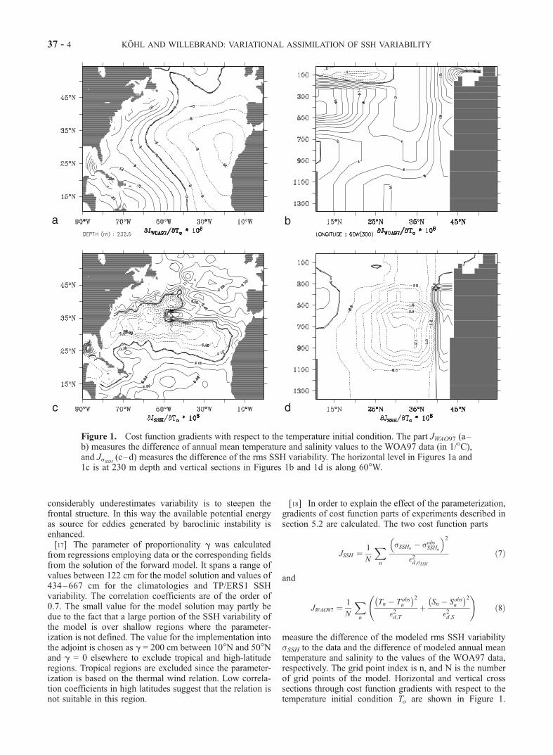
[26] The rms SSH variability error is reduced from 7.2cm to 4.8 cm. Figure 7 shows the rms SSH variability fromthe control and the assimilation CLIM_SSH together with theobservational data. The maximum of the variability of thecontrol is displaced northward and overall too low with amaximum around 47�N. By assimilation of rms SSHvariability and WOA97 data (Figure 7c), the erroneousmaximum vanished and the mean position and amplitudeof maximal variability is fairly well matched, It doesextends further to the north around 55�W, and the northwardextension at 42�W is not captured. The turnoff of the AzoresCurrent is visible by increased variability. The scales ofeddies are clearly too large in comparison with the obser-vations which may be explained by too low a resolution.The level of SSH variability in the Gulf Stream region isalso enhanced to a realistic magnitude by assimilating onlythe WOA97 data, but its position and the maximum around47�N is not changed.[27] The mean SSH of the experiment CLIM_SSH is

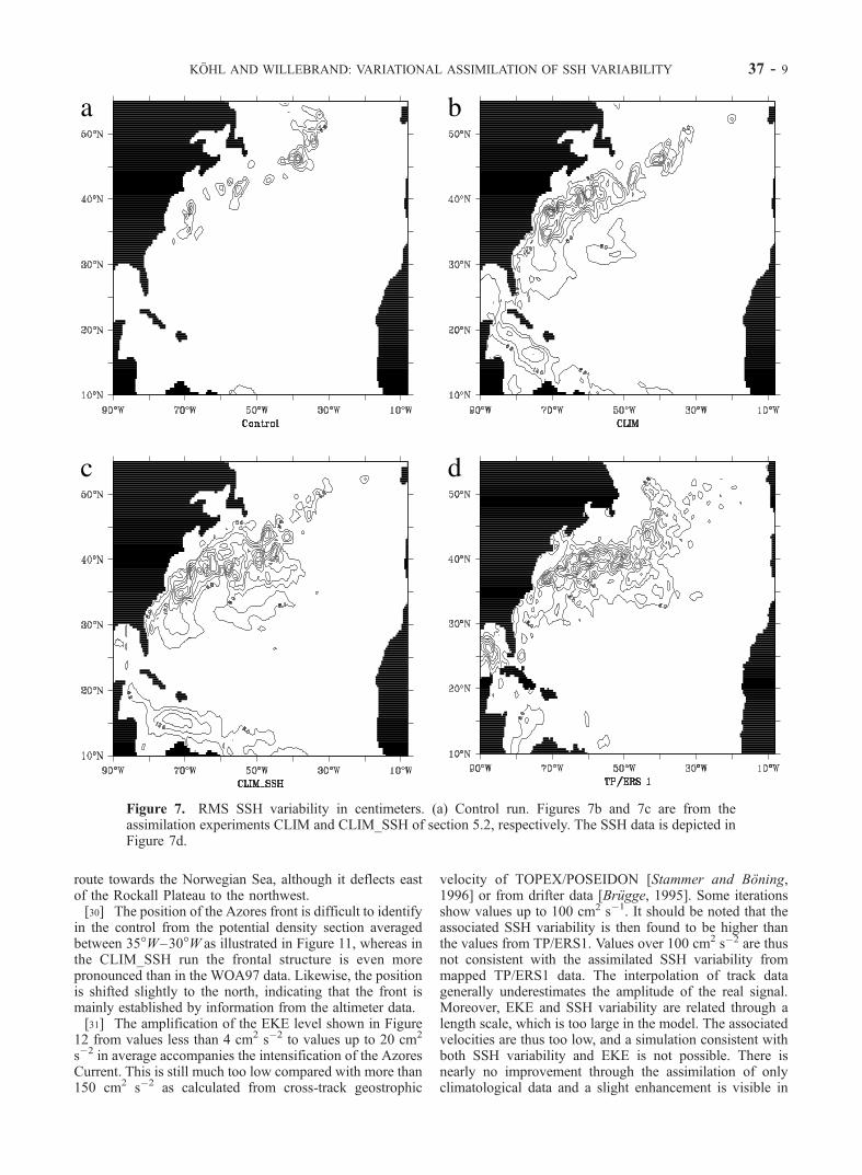
illustrated in Figure 8b. It supports the findings from Figure7. The position and amplitude around 60�W matches thedata of Singh and Kelly [1997] (see also Figure 2) with aslightly weaker front. However, the front at 42�W is notpresent in Figure 8b, although it may be seen in theestimated initial conditions, indicating a dynamical deficitof the model. The amplitude of the stationary anticycloneeast of Cape Hatteras is reduced together with the disap-pearance of the front resembling a wrong turnoff position ofthe Azores Current. The mean SSH in Figure 8a resultsfrom experiment CLIM and represents a somewhat inter-mediate state between the control state in Figure 2a and datain Figure 8b. The Gulf Stream front is stronger, but theposition is nearly unchanged in comparison to Figure 2a.The pattern in the Azores region resembles the one ofFigure 8b, but the strength of the front is very weak.[28] In order to investigate whether the solution

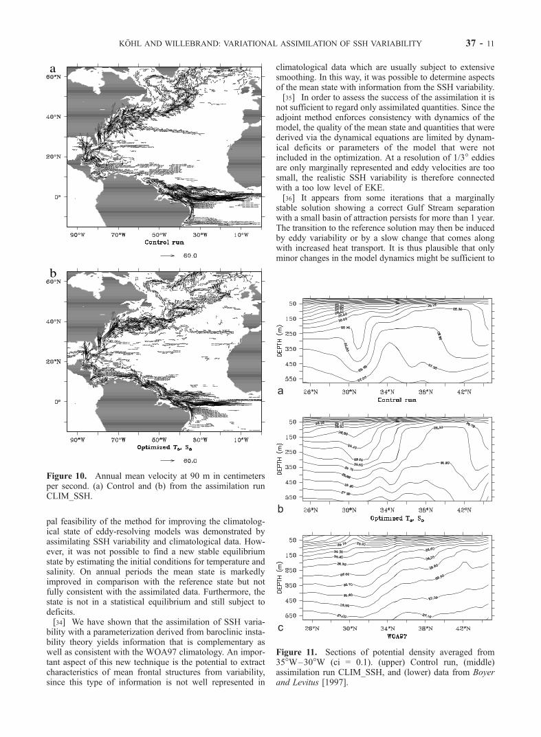
CLIM_SSH is a new equilibrium state, the integration iscontinued further. Within the following 2 years of integra-tion the state returns toward the pattern of the control run.The mean front starts continuously to split into a northwarddisplaced and a southern front visible in Figure 2a. Thereturn is documented in Figure 9, which shows a meridionaltemperature section in the Gulf Stream region. Cold waterinserted north of the Gulf Stream is rapidly removed,whereas the mean frontal position only slowly returns tothe position of the control run. As a consequence of thisrapid removal, temperature corrections of the initial con-dition are overestimated. For the same region as displayedin the figure, temperatures in January are about 1.5�C toolow at 44�N in comparison with the monthly mean value ofthe WOA97 data.[29] As visible from the near surface velocities of experi-

ment CLIMSSH in Figure 10a, the Azores Current of thecontrol run is only represented as a markedly southwardshifted band branching east of Cape Hatteras from the GulfStream. Assimilation shifts the band to the observed posi-tion at 34�N [Gould, 1985], and the current originates fromthe separation of the Gulf Stream into the North AtlanticCurrent (NAC) and the Azores Current (Figure 10b), assuggested by Sy [1988]. The erroneous flow of the NACtowards the Irminger Sea visible in Figure 10a is correctedand the transport follows after assimilation the realistic

Figure 6. Salinity difference in 580 m: (a) Control run-WOA97 data and (b) experiment CLIM_SSH � WOA97data (ci = 0.2 PSU).


route towards the Norwegian Sea, although it deflects eastof the Rockall Plateau to the northwest.[30] The position of the Azores front is difficult to identify

in the control from the potential density section averagedbetween 35�W–30�W as illustrated in Figure 11, whereas inthe CLIM_SSH run the frontal structure is even morepronounced than in the WOA97 data. Likewise, the positionis shifted slightly to the north, indicating that the front ismainly established by information from the altimeter data.[31] The amplification of the EKE level shown in Figure

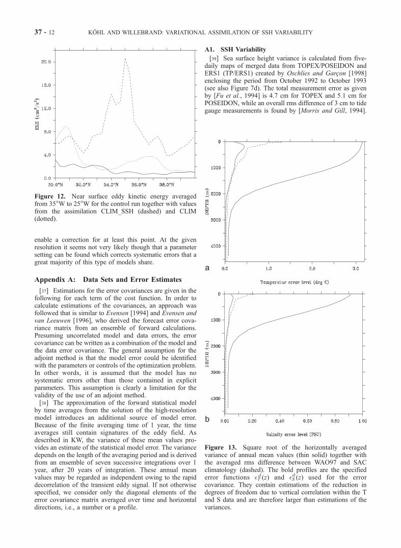
12 from values less than 4 cm2 s�2 to values up to 20 cm2

s�2 in average accompanies the intensification of the AzoresCurrent. This is still much too low compared with more than150 cm2 s�2 as calculated from cross-track geostrophic

velocity of TOPEX/POSEIDON [Stammer and Boning,1996] or from drifter data [Brugge, 1995]. Some iterationsshow values up to 100 cm2 s�1. It should be noted that theassociated SSH variability is then found to be higher thanthe values from TP/ERS1. Values over 100 cm2 s�2 are thusnot consistent with the assimilated SSH variability frommapped TP/ERS1 data. The interpolation of track datagenerally underestimates the amplitude of the real signal.Moreover, EKE and SSH variability are related through alength scale, which is too large in the model. The associatedvelocities are thus too low, and a simulation consistent withboth SSH variability and EKE is not possible. There isnearly no improvement through the assimilation of onlyclimatological data and a slight enhancement is visible in

Figure 7. RMS SSH variability in centimeters. (a) Control run. Figures 7b and 7c are from theassimilation experiments CLIM and CLIM_SSH of section 5.2, respectively. The SSH data is depicted inFigure 7d.


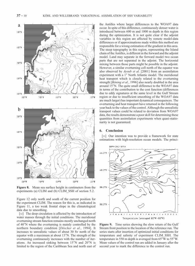
Figure 12 only north and south of the current position forthe experiment CLIM. The reason for this is, as indicated inFigure 11, a too weak frontal slope in the climatologicaldata due to smoothing.[32] The deep circulation is affected by the introduction of

water masses through the initial conditions. The meridionaloverturning stream function remains mostly unchanged northof 40�N where the overturning is mainly controlled by thenorthern boundary condition [Doscher et al., 1994]. Itincreases to unrealistic values of about 30 Sv north of theequator with a maximum at about 13�N. The strength of theoverturning continuously increases with the number of iter-ations. An increased sinking between 15�N and 20�N islimited to the region of the Caribbean Sea and north east of

the Antilles where larger differences to the WOA97 dataoccur. In spite of this difference, continuously denser water isintroduced between 600 m and 1000 m depth in this regionduring the optimization. It is not quite clear if the adjointvariables in this region are affected by remote model-datadifferences or if approximations made within this method areresponsible for a wrong estimation of the gradient in this area.The steep topography in this region, representing the Islandchain of theAntilles, is different in the forward and the adjointmodel. Land may separate in the forward model two oceanparts that are not separated in the adjoint. The horizontalmixing between those parts might be possible in the adjoint.However, a similar overturning cell north of the equator wasalso observed by Ayoub et al. [2001] from an assimilationexperiment with a 1� North Atlantic model. The meridionalheat transport which is closely related to the overturningstrength [Boning et al., 1996] also nearly doubled in the areaaround 15�N. The quite small difference to the WOA97 datain terms of the contribution to the cost function (differencesdue to eddy signatures at the same level in the Gulf Streamregion or due to insufficient smoothing of the WOA97 dataare much larger) has important dynamical consequences. Theoverturning and heat transport have returned in the followingyear back to the values of the control. Although the unrealistictransport values could be related to deviation from WOA97data, the results demonstrate a poor skill for determining thesequantities from assimilation experiments when quasi-statio-narity is not guaranteed.

6. Conclusion

[33] Our intention was to provide a framework for stateestimations with high-resolution ocean models. The princi-

Figure 8. Mean sea surface height in centimeters from theexperiments (a) CLIM and (b) CLIM_SSH of section 5.2.

Figure 9. Time series showing the slow return of the GulfStream front position to the location of the reference run. Theseries starts after insertion of optimized initial conditions fortemperature and salinity of experiment CLIM_SSH. Thetemperature in 550 m depth is averaged from 65�W to 55�W.Mean values of the control run are added in January after thesecond year to mark the difference to the control run.


pal feasibility of the method for improving the climatolog-ical state of eddy-resolving models was demonstrated byassimilating SSH variability and climatological data. How-ever, it was not possible to find a new stable equilibriumstate by estimating the initial conditions for temperature andsalinity. On annual periods the mean state is markedlyimproved in comparison with the reference state but notfully consistent with the assimilated data. Furthermore, thestate is not in a statistical equilibrium and still subject todeficits.[34] We have shown that the assimilation of SSH varia-

bility with a parameterization derived from baroclinic insta-bility theory yields information that is complementary aswell as consistent with the WOA97 climatology. An impor-tant aspect of this new technique is the potential to extractcharacteristics of mean frontal structures from variability,since this type of information is not well represented in

climatological data which are usually subject to extensivesmoothing. In this way, it was possible to determine aspectsof the mean state with information from the SSH variability.[35] In order to assess the success of the assimilation it is

not sufficient to regard only assimilated quantities. Since theadjoint method enforces consistency with dynamics of themodel, the quality of the mean state and quantities that werederived via the dynamical equations are limited by dynam-ical deficits or parameters of the model that were notincluded in the optimization. At a resolution of 1/3� eddiesare only marginally represented and eddy velocities are toosmall, the realistic SSH variability is therefore connectedwith a too low level of EKE.[36] It appears from some iterations that a marginally

stable solution showing a correct Gulf Stream separationwith a small basin of attraction persists for more than 1 year.The transition to the reference solution may then be inducedby eddy variability or by a slow change that comes alongwith increased heat transport. It is thus plausible that onlyminor changes in the model dynamics might be sufficient to

Figure 10. Annual mean velocity at 90 m in centimetersper second. (a) Control and (b) from the assimilation runCLIM_SSH.

Figure 11. Sections of potential density averaged from35�W–30�W (ci = 0.1). (upper) Control run, (middle)assimilation run CLIM_SSH, and (lower) data from Boyerand Levitus [1997].


enable a correction for at least this point. At the givenresolution it seems not very likely though that a parametersetting can be found which corrects systematic errors that agreat majority of this type of models share.

Appendix A: Data Sets and Error Estimates

[37] Estimations for the error covariances are given in thefollowing for each term of the cost function. In order tocalculate estimations of the covariances, an approach wasfollowed that is similar to Evensen [1994] and Evensen andvan Leeuwen [1996], who derived the forecast error cova-riance matrix from an ensemble of forward calculations.Presuming uncorrelated model and data errors, the errorcovariance can be written as a combination of the model andthe data error covariance. The general assumption for theadjoint method is that the model error could be identifiedwith the parameters or controls of the optimization problem.In other words, it is assumed that the model has nosystematic errors other than those contained in explicitparameters. This assumption is clearly a limitation for thevalidity of the use of an adjoint method.[38] The approximation of the forward statistical model

by time averages from the solution of the high-resolutionmodel introduces an additional source of model error.Because of the finite averaging time of 1 year, the timeaverages still contain signatures of the eddy field. Asdescribed in KW, the variance of these mean values pro-vides an estimate of the statistical model error. The variancedepends on the length of the averaging period and is derivedfrom an ensemble of seven successive integrations over 1year, after 20 years of integration. These annual meanvalues may be regarded as independent owing to the rapiddecorrelation of the transient eddy signal. If not otherwisespecified, we consider only the diagonal elements of theerror covariance matrix averaged over time and horizontaldirections, i.e., a number or a profile.

A1. SSH Variability

[39] Sea surface height variance is calculated from five-daily maps of merged data from TOPEX/POSEIDON andERS1 (TP/ERS1) created by Oschlies and Garcon [1998]enclosing the period from October 1992 to October 1993(see also Figure 7d). The total measurement error as givenby [Fu et al., 1994] is 4.7 cm for TOPEX and 5.1 cm forPOSEIDON, while an overall rms difference of 3 cm to tidegauge measurements is found by [Morris and Gill, 1994].

Figure 12. Near surface eddy kinetic energy averagedfrom 35�W to 25�W for the control run together with valuesfrom the assimilation CLIM_SSH (dashed) and CLIM(dotted).

Figure 13. Square root of the horizontally averagedvariance of annual mean values (thin solid) together withthe averaged rms difference between WAO97 and SACclimatology (dashed). The bold profiles are the specifiederror functions �T

d (z) and �Sd (z) used for the error

covariance. They contain estimations of the reduction indegrees of freedom due to vertical correlation within the Tand S data and are therefore larger than estimations of thevariances.


We have used a constant value of �d,sSSH= 4 cm throughout

the experiments.

A2. SST

[40] The sea surface temperature (SST) is taken from the9 km resolution daily nighttime maps of the AVHRROceans Pathfinder Program [Smith et al., 1996]. The meanSST is calculated from maps covering the same period asthe SSH data after building monthly mean values to reducethe bias due to cloud cover. The rms difference between thegridded Pathfinder SST data and SST from a buoy database[Podesta et al., 1995] is 0.97�C for the nighttime matchups[Smith et al., 1996]. The error value for temperatureobservations is chosen as �d,SST = 1�C.

A3. Climatological Data of Temperature and Salinity

[41] The depth-dependent rms difference of temperatureand salinity values between climatologies of Boyer andLevitus [1997], hereafter WOA97 and Gouretski and Jancke[1998], hereafter SAC is depicted in Figure 13 together withvalues calculated from the variance of an ensemble of sevenannual mean values from the model. Both approachesprovide similar estimates for the error profiles except inthe surface region where variability is underestimated by themodel due to the restoring to monthly mean values.[42] Vertical correlations in the temperature and salinity

fields, which effectively reduce the number of independentdegrees of freedom, have to be taken into consideration inparticular when surface data is included in the cost function.Typical vertical correlation radii calculated from the abovedescribed ensemble are 350 m above and 500 m below 1000m depth. Profiles that approximate the rms temperature andsalinity error profiles, respectively, are multiplied by a factorthat counts the number of layers within the correlation radius.

A4. Initial Conditions

[43] The first guess for the initial condition is the stateafter 20 years of ‘‘spin-up.’’ The error weight was approxi-mated by the deviation of the annual mean values of thereference experiment in comparison with temperature andsalinity data from the WOA97 with the additional modifi-cation to account for vertical correlations. The approxima-tions for the error profiles of the a priori information thenreads, �i,T(z) = 14�C exp(�z/800 m) and �i,S(z) = 4 PSUexp(�z/800 m), respectively.

A5. Surface Flux

[44] Weighting coefficients for the a priori parametervalues of heat and freshwater fluxes estimated as restoringtemperature and salinity were chosen as �f,T = 4�C and �f,S =0.5 PSU. For the CME model the values correspondapproximately to heat and fresh water flux values of about32 Wm�2 and 1 m yr�1, respectively.

[45] Acknowledgments. The work was supported by the Bundesmi-nisterium fur Forschung und Technologie as part of the German WOCE.

ReferencesAyoub, N., D. Stammer, and C. Wunsch, Estimating the North Atlanticcirculation with nesting and open boundary conditions using an adjointmodel, ECCO Rep. 10, Scripps. Inst. of Oceanogr., La Jolla, Calif., 2001.

Boning, C. W., Large-scale transport processes in high-resolution circula-tion models, in The Warmwatersphere of the North Atlantic Ocean, pp.91–128, Gebruder Borntrager, Berlin, 1996.

Boning, C. W., F. O. Bryan, W. R. Holland, and R. Doscher, Deep-waterformation and meridional overturning in a high-resolution model of theNorth Atlantic, J. Phys. Oceanogr., 26, 1142–1164, 1996.

Boyer, T. P., and S. Levitus, Objective analyses of temperature and salinityfor the world ocean on a 1/4 degree grid, NOAA Atlas NESDIS 11, U.S.Gov. Print. Off., Washington, D. C., 1997.

Brugge, B., Near surface mean circulation and eddy kinetic energy in thecentral North Atlantic from drifter data, J. Geophys. Res., 100, 20,543–20,554, 1995.

Bryan, F. O., and W. R. Holland, A high-resolution simulation of wind- andthermohaline-driven circulation in the North Atlantic Ocean, in Parame-trizations of Small Scale Processes, Proceedings of the Aha Hulikoa Hawaiian Winter Workshop, pp. 99–115, edited by P. Muller andD. Henderson, Univ. of Hawaii, Honolulu, 1989.

Cooper, M., and K. Haines, Altimetric assimilation with water propertyconservation, J. Geophys. Res., 101, 1059–1077, 1996.

Dijkstra, H. A., and M. J. Molemaker, Imperfections of the North Atlanticwind-driven ocean circulation: Continental geometry and windstressshape, J. Mar. Sci., 57, 1–28, 1999.

Doscher, R. C., C. W. Boning, and P. Herrman, Response of circulationand heat transport in the North Atlantic to changes in forcing in north-ern latitudes: A model study, J. Phys. Oceanogr., 24, 2306–2320,1994.

DYNAMO Group, DYNAMO Dynamics of North Atlantic Models: Simula-tion and assimilation with high resolution models, Rep. 294, Univ. Kiel,Kiel, Germany, 1997.

Evensen, G., Sequential data assimilation with a nonlinear quasigeostrophicmodel using Monte Carlo methods to forecast error statistics, J. Geophys.Res., 99, 10,143–10,162, 1994.

Evensen, G., and P. J. van Leeuwen, Assimilation of Geosat altimeter datafor the Agulhas Current using the ensemble Kalman filter with a quasi-geostrophic model, Mon. Weather Rev., 124, 85–96, 1996.

Fu, L.-L., E. J. Christensen, C. A. Yamarone, M. Lefebvre, Y. Menard,M. Dorrer, and P. Escudier, TOPEX/POSEIDON mission overview,J. Geophys. Res., 99, 24,369–24,381, 1994.

Gavart, M., and P. De Mey, Isopycnal EOFs in the Azores Current region:A statistical tool for dynamical analysis and data assimilation, J. Phys.Oceanogr., 27, 2146–2157, 1997.

Giering, R., and T. Kaminski, Recipes for adjoint code construction, Trans.Math. Software, 24, 437–474, 1998.

Gilbert, J. C., and C. Lemarechal, Some numerical experiments with vari-able-storage Quasi-Newton algorithms, Math. Program., 45, 407–435,1989.

Gould, W. J., Physical oceanography of the Azores front, Progr. Oceanogr.,14, 167–190, 1985.

Gouretski, V., and K. Jancke, A new world ocean climatology: Objectiveanalysis on neutral surfaces, WHP-SAC Tech. Rep. 3, WOCE Rep., 256/17, 1998.

Green, J. S. A., Transfer properties of the large-scale eddies and the generalcirculation of the atmosphere, Q. J. R. Meteorol. Soc., 96, 157–417,1970.

Han, Y.-J., A numerical world ocean general circulation model, II, A bar-oclinic experiment, Dyn. Atmos. Oceanogr., 8, 141–172, 1984.

Hellerman, S., and M. Rosenstein, Normal monthly windstress over theworld ocean with error estimates, J. Phys. Oceanogr., 13, 1093–1104,1983.

Kazantsev, E., Local Lyapunov exponents of the quasi-geostrophic oceandynamics, Appl. Math. Comput., 104, 217–257, 1999.

Kazantsev, E., J. Sommeria, and J. Verron, Subgrid-scale parameterizationby statistical mechanics in a barotropic ocean model, J. Phys. Oceanogr.,28, 1017–1042, 1998.

Killworth, P. D., C. Dietrich, C. L. Provost, A. Oschlies, and J. Willebrand,Assimilation of altimetric data and mean sea surface height into an eddy-permitting model of the North Atlanic, Progr. Oceanogr., 48, 313–335,2001.

Kohl, A., and J. Willebrand, An adjoint method for the assimilation ofstatistical characteristics into eddy-resolving ocean models, Tellus, Ser.A, 54, 406–425, 2002.

Krauss, W., and R. H. Kase, Mean circulation and eddy kinetic energy inthe eastern North Atlantic, J. Geophys. Res., 89, 3407–3415, 1984.

Le Dimet, F.-X., and O. Talagrand, Variational algorithms for analysis andassimilation of meteorological observations: Theoretical aspects, Tellus,Ser. A, 38A, 97–110, 1986.

Levitus, S., Climatological atlas of the world ocean, Tech. Pap., 173 pp.,Natl. Ocean. Atmos. Admin., Silver Spring, Md., 1982.

Morris, C., and S. Gill, Evaluation of the TOPEX/POSEIDON altimetersystem over great lakes, J. Geophys. Res., 99, 24,527–24,539, 1994.

Morrow, R., and P. De Mey, Adjoint assimilation of atlimetric, surfacedrifter, and hydrographic data in a quasigeostrophic model of the AzoresCurrent, J. Geophys. Res., 100, 25,007–25,025, 1995.


Oschlies, A., and V. Garcon, Eddy induced enhancement of primary produc-tion in a model of the North Atlantic Ocean, Nature, 394, 266–269, 1998.

Oschlies, A., and J. Willebrand, Assimilation of Geosat altimeter data intoan eddy-resolving primitive equation model of the North Atlantic Ocean,J. Geophys. Res., 101, 14,175–14,190, 1996.

Pacanowski, R., K. Dixson, and A. Rosati, The GFDL modular oceanmodel users guide, Tech. Rep., Geophy. Fluid Dyn. Lab., Ocean Group,Princeton Univ., Princeton, N. J., 1993.

Podesta, G. P., S. Shenoi, J. W. Brown, and R. H. Evans, AVHRR PathfinderOceans Matchup Database 1985–1993 (Version 18), 33 pp., RosenstielSch. of Mar. and Atmos. Sci., Univ. of Miami, Coral Gables, Fla., 1995.

Richardson, P. L., Eddy kinetic energy in the North Atlantic from surfacedrifters, J. Phys. Oceanogr., 88, 4355–4367, 1983.

Schroter, J., U. Seiler, and M. Wenzel, Variational assimilation of Geosatdata into an eddy resolving model of the Gulf Stream extension area,J. Phys. Oceanogr., 23, 925–953, 1993.

Singh, S., and K. A. Kelly, Monthly maps of sea surface hight in the NorthAtlantic and zonal indices for the Gulf Stream using TOPEX/Poseidonaltimeter data, Rep. WHOI-97-06, 50 pp., Woods Hole Oceanogr. Inst.,Woods Hole, Mass., 1997.

Sirkes, Z., and E. Tziperman, Finite difference of adjoint or adjoint of finitedifference?, Mon. Weather Rev., 125, 3373–3378, 1997.

Smith, E., J. Vazquez, A. Tran, and R. Sumagaysay, Satellite-derived seasurface temperature data available form the NOAA/NASA Pathfinder

program, Eos. Trans. AGU Electron. Suppl., 1996. (Available as http://www.agu.org/eos_elec/95274e.html)

Stammer, D., Global characteristics of ocean variability estimated fromregional TOPEX/POSEIDON altimeter measurements, J. Phys. Ocea-nogr., 27, 1743–1768, 1997.

Stammer, D., and C. W. Boning, Generation and distribution of mesoscaleeddies, in The Warmwatersphere of the North Atlantic Ocean, pp. 159–194, Gebruder Borntrager, Berlin, 1996.

Stone, P. H., A simplified radiative-dynamical model for the static stabilityof rotating atmospheres, J. Atmos. Sci., 29, 405–418, 1972.

Sy, A., Investigation of large scale circulation patterns in the central NorthAtlantic: the North Atlantic Current, the Azores Current, and the Medi-terranean Water plume in the area of the Mid-Atlantic Ridge, Deep-SeaRes., 35, 383–413, 1988.

Treguier, A. M., I. Held, and V. Larichev, Parametrization of quasigeos-trophic eddies in primitive equation ocean models, J. Phys. Oceanogr.,27, 567–580, 1997.

��A. Kohl, Scripps Institution of Oceanography, 8605 La Jolla Shores Dr.,

La Jolla, CA 92093-0230, USA. ([email protected])J. Willebrand, Institut fur Meereskunde, Dusternbrooker Weg 20, 24105

Kiel, Germany. ( [email protected])


Variational assimilation of SSH variability from TOPEX/POSEIDON and ERS1 into an eddy-permitting...

Documents

Transcript of Variational assimilation of SSH variability from TOPEX/POSEIDON and ERS1 into an eddy-permitting...