Technological University Dublin Technological University Dublin

ARROW@TU Dublin ARROW@TU Dublin

Conference Papers Dublin Energy Lab

2010-05-01

Validation of a Simulation Model for a Combined Otto and Stirling Validation of a Simulation Model for a Combined Otto and Stirling

Cycle Power Plant Cycle Power Plant

Jim McGovern Technological University Dublin, jim.mcgovern@tudublin.ie

Barry Cullen Technological University Dublin, barry.cullen@tudublin.ie

Michel Feidt University “Henri Poincare” of Nancy, michel.feidt@ensem.inpl-nancy.fr

See next page for additional authors

Follow this and additional works at: https://arrow.tudublin.ie/dubencon2

Part of the Energy Systems Commons

Recommended Citation Recommended Citation McGovern, J., Cullen, B., Feidt, M., Petrescu, S. (2010). Validation of a simulation model for a combined Otto and Stirling Cycle power plant. ES2010: ASME 4th International Conference on Energy Sustainability. Phoenix, Arizona, USA. May 17-22.

This Conference Paper is brought to you for free and open access by the Dublin Energy Lab at ARROW@TU Dublin. It has been accepted for inclusion in Conference Papers by an authorized administrator of ARROW@TU Dublin. For more information, please contact arrow.admin@tudublin.ie, aisling.coyne@tudublin.ie.

This work is licensed under a Creative Commons Attribution-Noncommercial-Share Alike 4.0 License

Authors Authors Jim McGovern, Barry Cullen, Michel Feidt, and Stoian Petrescu

This conference paper is available at ARROW@TU Dublin: https://arrow.tudublin.ie/dubencon2/7

Proceedings of ASME 2010 4th International Conference on Energy Sustainability ES2010

May 17-22, 2010 Phoenix, Arizona, USA

1 Copyright © 2010 by ASME

ES2010-90220

VALIDATION OF A SIMULATION MODEL FOR A COMBINED OTTO AND STIRLING CYCLE POWER PLANT

Jim McGovern Department of Mechanical Engineering

Dublin Institute of Technology Dublin 1, Ireland

Barry Cullen Department of Mechanical Engineering

Dublin Institute of Technology Dublin 1, Ireland

Michel Feidt L.E.M.T.A., U.R.A.C.N.R.S.7563

University “Henri Poincare” of Nancy 1 Avenue de la Forêt de Haye, 54504

Vandoeuvre-les-Nancy, France

Stoian Petrescu Department of Engineering Thermodynamics

University Politehnica of Bucharest Splaiul Independentei, 313

060042 Bucharest, Romania ABSTRACT

A project has been underway at the Dublin Institute of Technology (DIT) to investigate the feasibility of a combined Otto and Stirling cycle power plant in which a Stirling cycle engine would serve as a bottoming cycle for a stationary Otto cycle engine. This type of combined cycle plant is considered to have good potential for industrial use. This paper describes work by DIT and collaborators to validate a computer simulation model of the combined cycle plant. In investigating the feasibility of the type of combined cycle that is proposed there are a range of practical realities to be faced and addressed. Reliable performance data for the component engines are required over a wide range of operating conditions, but there are practical difficulties in accessing such data. A simulation model is required that is sufficiently detailed to represent all important performance aspects and that is capable of being validated. Thermodynamicists currently employ a diverse range of modeling, analysis and optimization techniques for the component engines and the combined cycle. These techniques include traditional component and process simulation, exergy analysis, entropy generation minimization, exergoeconomics, finite time thermodynamics and finite dimensional optimization thermodynamics methodology (FDOT). In the context outlined, the purpose of the present paper is to come up with a practical validation of a practical computer simulation model of the proposed combined Otto and Stirling Cycle Power Plant.

INTRODUCTION Some ongoing work in the Department of Mechanical

Engineering at the DIT has focused on the theoretical development of a novel combined cycle power generation system using a Stirling cycle engine as a bottoming cycle on a stationary Otto cycle engine. Such power plant would find use in small to medium scale power generation scenarios. Previous work has offered detail on the technological status of Otto engine systems [1], a methodology for study of the combined cycle energy system with regard to an automotive scenario [2] and some preliminary modeling results for the combined cycle system [3]. The aim of the current work is to provide details of a validation procedure for the theoretical model.

The model proposed is developed under the frameworks of what are traditionally called Finite Time Thermodynamics (FTT) and Finite Speed Thermodynamics (FST). The concept of Finite Time Thermodynamics can be said to offer a theoretical development of Classical Thermodynamics through the imposition of a finite time constraint on heat transfer to and from the system. Inception of the method is generally attributed to the independent works of Novikov and Chambadal [4–6], although a paper by Curzon and Ahlborn [7] is often credited as the original work. The technique has seen considerable development in the intervening years, particularly in relation to thermodynamic cycles. However, although the Finite Time Thermodynamics name is often used, it is apparent that the concept has broadened from the original

2 Copyright © 2010 by ASME

study of the time parameter to include other constraints typical of such applications. In a recent work, Feidt [6] has proposed use of the term Finite Dimensional Optimization Thermodynamics (FDOT) as an umbrella term to include optimization procedures that might usually be ascribed to the literature of Finite Time Thermodynamics—for example finite speed, finite area, finite volume, finite conductance and finite cost—even though their essential contribution might not specifically target analysis or optimization in terms of time. The method offers the advantage of providing good qualitative and quantitative agreement with known operating characteristics of real engines using comparatively uncomplicated models. In the present work, we draw upon models for the Otto engine and the Stirling engine that have previously been described as Finite Time Thermodynamics and Finite Speed Thermodynamics. They are presented here under the umbrella term Finite Dimensional Optimization Thermodynamics.

THE OTTO CYCLE MODEL Brief Review of Established Methods

The Otto cycle is well represented in the literature of Finite Dimensional Optimization Thermodynamics. Angulo-Brown et al [8] provide an irreversible model that encompasses global friction losses within the cycle. The work is expanded in a subsequent work to include an irreversibility parameter within the cycle [9]. Calvo Hernandez et al [10] further develop this model to account for non-instantaneous adiabatic strokes. Ge et al perform thermodynamic simulation of an Otto cycle with the inclusion of heat transfer in the system and variable specific heats of the working fluid [11]. Chen et al present information on the optimization of the Otto cycle with regard to maximum efficiency and maximum power [12]. Curto-Risso et al [13–15] develop a finite time model that includes engine speed-related irreversibility parameters. The model is validated against numerical simulations and is demonstrated to offer good correlation.

Outline of the Theoretical Model

The Otto cycle model proposed in the current study is based in the Finite Time model developed recently by Curto-Rizzo et al [13–16]. This model is perceived to have an advantage over other models in its inclusion of a greater number of system variables, particularly relating to system geometry. The model adheres to a typical form of the irreversible thermodynamics analysis method, which involves the specification of the reversible thermodynamic work of the cycle and its subsequent degradation through irreversibility mechanisms. A modification to the model is possible and is presented in this work to cater for the case of stationary engine operation.

For the Otto cycle, the reversible power of the cycle is: 𝑃REV = 𝑀𝑡th 𝐶 ,23(𝑇3 − 𝑇2) − 𝐶 ,41(𝑇4 − 𝑇1)

(1)

In comparison, the irreversible cycle power is calculated as: 𝑃irrev = |𝑊I|𝑡th − 𝑊Q𝑡th − 𝑃 (2) where |𝑊I| is the work output of the thermodynamic cycle after accounting for irreversibilities within the cycle, 𝑊Q is the work loss due to heat transfer from the cycle to the cylinder walls, 𝑃 is the cycle power lost through global frictional effects and 𝑡th

is the thermodynamic cycle period. It is important in the present analysis to differentiate between the thermodynamic cycle period and the mechanical cycle period. The full thermodynamic cycle requires two full revolutions of the crank shaft and therefore is equal to twice the mechanical cycle period. Also, the work terms all relate to one individual cylinder, and must therefore be multiplied by the number of cylinders to determine the total power output of the engine. This offers the benefit of allowing a scalable analysis of the engine. Calculation of the terms is as follows: |𝑊I| = 𝑀 𝐶𝑣,23(𝑇3 − 𝑇2) − 𝐼R𝐶𝑣,41(𝑇4 − 𝑇1) (3)

Curto-Risso et al and previous sources [17] utilized the

internal energy values of reactants and products of the chemical reaction during combustion of the fuel for calculating the combustion temperature 𝑇3. In this paper we use the simpler heat equation method with calculation of cycle temperatures from the isentropic compression and expansion relationships:

𝑇2 = 𝑇1𝑟 (4) 𝑇3 = 𝑄IN𝑀𝐶𝑣,23 + 𝑇2

(5) The temperature at the end of the power stroke, 𝑇 , is important for analysis of the exhaust process. The method for this is elaborated later.

To calculate the specific heat terms we assume air as the working fluid, thereby allowing us to use the polynomial offered by Abu-Nada et al [18] for temperature dependant specific heats of the working fluid:

𝐶 = 2.506 × 10 𝑇 + 1.454 × 10 𝑇 .−4.246 × 10 𝑇 + 3.162 × 10 𝑇 . + 1.3303−1.512 × 10 𝑇 . + 3.063 × 10 𝑇−2.212 × 10 𝑇 (6)

Also 𝐶 = 𝐶 − 𝑅g (7)

3 Copyright © 2010 by ASME

where 𝑅g is the gas constant of the working fluid, approximated as air in this case. The averaged specific heat terms for the heat addition and rejection processes are determined as: 𝐶𝑣,23 = 12 [𝐶𝑣(𝑇2) + 𝐶𝑣(𝑇3)] (8)

𝐶𝑣,41 = 12 [𝐶𝑣(𝑇4) + 𝐶𝑣(𝑇1)] (9)

However, as 𝐶𝑣,23 is required to calculate 𝑇3, 𝐶𝑣(𝑇2)is used as an approximation in Eq. (3) and Eq. (5).

The heat-loss work is determined from the relationship: 𝑊Q = 𝜋𝜀ℎ𝐵𝑡th𝑇316 𝐵 + 𝑉0𝐴p (1 + 𝑟 ) 1 + 𝑟 − 2 𝑇w𝑇3

(10)

The heat loss from the system through the cylinder walls is assumed to occur exclusively in the power stroke, and is determined from the expression [13]:

𝑄L = 𝑊Q𝜀 = 𝜋ℎ𝐵 𝐵2 + 𝑥34 𝑇34 − 𝑇w 𝑡34 (11)

where 𝑥34 is a mean piston position term given by: 𝑥34 = 0.5(𝑆) + 𝑥0 (12)

and 𝜀 is a phenomenological constant to quantify the lost work. 𝑇34 is the average temperature of the gas in the power stroke, 𝑇w is the time averaged temperature of the cylinder wall and 𝑡34 is the duration of the power stroke. The temperature at the end of the power stroke, and therefore immediately before the exhaust stroke, 𝑇4, requires knowledge of the heat transfer from the cylinder on the power stroke. If we assume the mean temperature 𝑇 to be: 𝑇 = 𝑇3 + 𝑇42 (13) then by substituting Eq. (10) and Eq. (13) into Eq. (11), we can eliminate 𝜀 and, by rearranging the expression, determine 𝑇4 as:

𝑇4 = 𝑇3𝑡th8 𝐵 + 𝑉0𝐴p (1 + 𝑟 ) 1 + 𝑟 − 2 𝑇w𝑇3𝐵2 + �̅�34 𝑡34 + 2𝑇w − 𝑇3 (14)

The friction loss power term is calculated as per the usual

method in Finite Time Thermodynamics [8]:

𝑃 = 𝜇�̅� (15) where the friction coefficient is calculated as: 𝜇 = 2𝑊f𝑡th𝜋 𝑆 (16) Mozurkewich and Berry [19] indicate that 𝑊f =0.15𝑊REV = 0.15𝑃REV𝑡th. The mean piston velocity �̅� is calculated as: �̅� = 2𝑆𝑓 (17) The power output of the engine is therefore calculated from Eq. 2. The efficiency of the engine is therefore: 𝜂otto = 𝑃irrev|𝑄23| (18) where the heat added per cylinder is: |𝑄23| = 𝑀𝑡th 𝐶𝑣,23(𝑇3 − 𝑇2)

(19)

In the current analysis though, the heat addition to the cycle is usually an imposed parameter made available from manufacturer specifications through a fuel consumption parameter, expressed as kW or otherwise. This may be considered typical for stationary engines such as those used for Combined Heat and Power generation. Unit efficiency is paramount, translating directly to cost savings for the operator. Therefore either the efficiency of the unit or the fuel consumption, or both, are made available for engineers considering the systems.

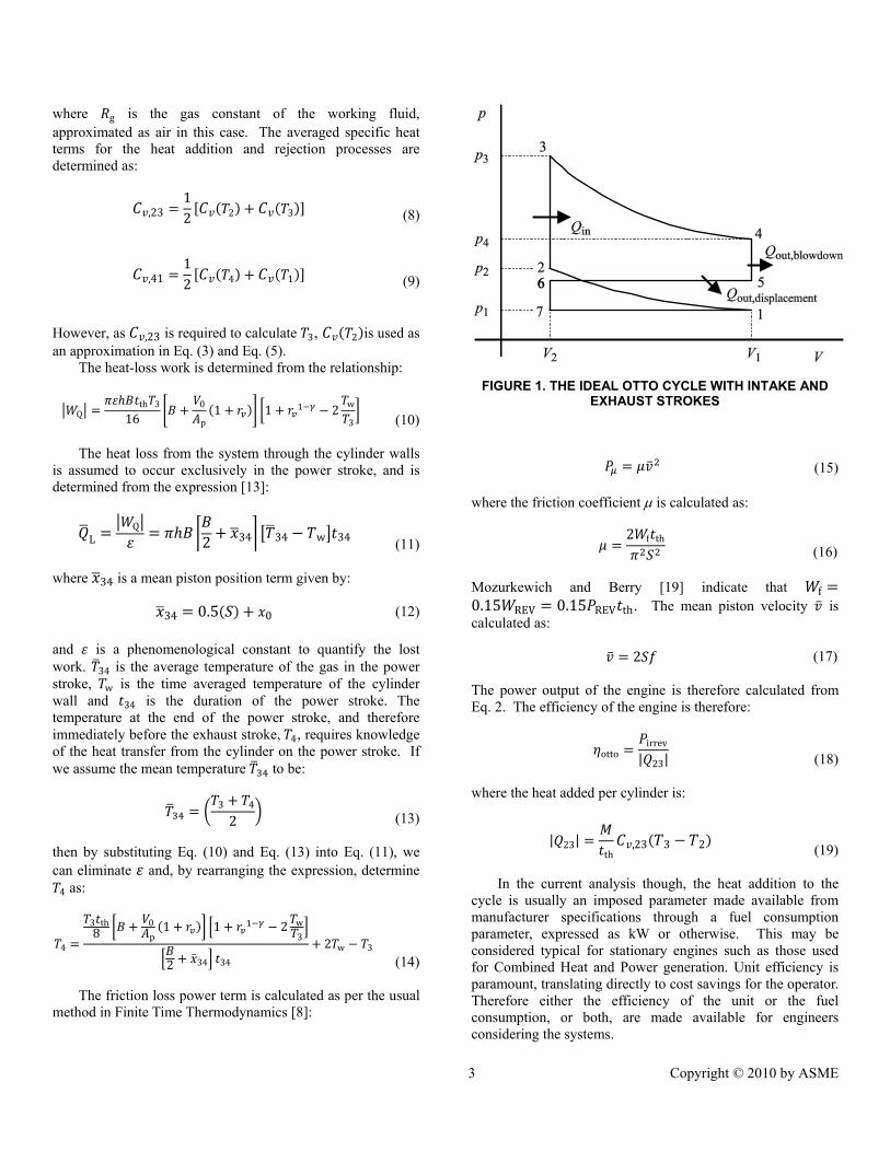
FIGURE 1. THE IDEAL OTTO CYCLE WITH INTAKE AND

EXHAUST STROKES

4 Copyright © 2010 by ASME

Detail of Model—Analytical Study of Exhaust Heat The sensible thermal energy available in the exhaust

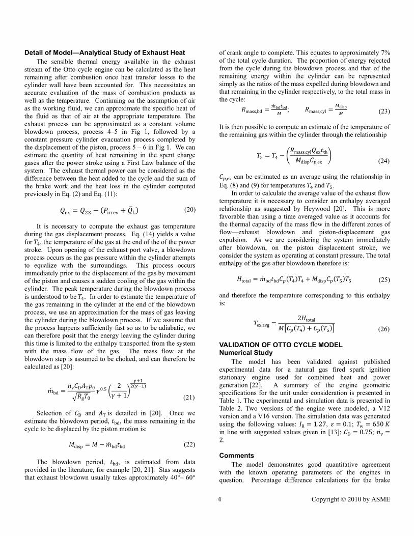
stream of the Otto cycle engine can be calculated as the heat remaining after combustion once heat transfer losses to the cylinder wall have been accounted for. This necessitates an accurate evaluation of the mass of combustion products as well as the temperature. Continuing on the assumption of air as the working fluid, we can approximate the specific heat of the fluid as that of air at the appropriate temperature. The exhaust process can be approximated as a constant volume blowdown process, process 4–5 in Fig 1, followed by a constant pressure cylinder evacuation process completed by the displacement of the piston, process 5 – 6 in Fig 1. We can estimate the quantity of heat remaining in the spent charge gases after the power stroke using a First Law balance of the system. The exhaust thermal power can be considered as the difference between the heat added to the cycle and the sum of the brake work and the heat loss in the cylinder computed previously in Eq. (2) and Eq. (11):

𝑄ex = 𝑄 − (𝑃irrev + 𝑄L) (20)

It is necessary to compute the exhaust gas temperature during the gas displacement process. Eq. (14) yields a value for 𝑇4, the temperature of the gas at the end of the of the power stroke. Upon opening of the exhaust port valve, a blowdown process occurs as the gas pressure within the cylinder attempts to equalize with the surroundings. This process occurs immediately prior to the displacement of the gas by movement of the piston and causes a sudden cooling of the gas within the cylinder. The peak temperature during the blowdown process is understood to be 𝑇4. In order to estimate the temperature of the gas remaining in the cylinder at the end of the blowdown process, we use an approximation for the mass of gas leaving the cylinder during the blowdown process. If we assume that the process happens sufficiently fast so as to be adiabatic, we can therefore posit that the energy leaving the cylinder during this time is limited to the enthalpy transported from the system with the mass flow of the gas. The mass flow at the blowdown step is assumed to be choked, and can therefore be calculated as [20]: �̇�bd = 𝑛v𝐶D𝐴T𝑝0𝑅g𝑇0 𝛾 . 2𝛾 + 1 ( )

(21)

Selection of 𝐶D and 𝐴T is detailed in [20]. Once we

estimate the blowdown period, 𝑡bd, the mass remaining in the cycle to be displaced by the piston motion is:

𝑀disp = 𝑀 − �̇�bd𝑡bd (22)

The blowdown period, 𝑡bd, is estimated from data

provided in the literature, for example [20, 21]. Stas suggests that exhaust blowdown usually takes approximately 40°– 60°

of crank angle to complete. This equates to approximately 7% of the total cycle duration. The proportion of energy rejected from the cycle during the blowdown process and that of the remaining energy within the cylinder can be represented simply as the ratios of the mass expelled during blowdown and that remaining in the cylinder respectively, to the total mass in the cycle: 𝑅mass,bd = ̇ bd bd; 𝑅mass,cyl = disp (23)

It is then possible to compute an estimate of the temperature of the remaining gas within the cylinder through the relationship 𝑇5 = 𝑇4 − 𝑅mass,cyl𝑄ex𝑡th𝑀disp𝐶 ,ex

(24) 𝐶 ,ex can be estimated as an average using the relationship in Eq. (8) and (9) for temperatures 𝑇4 and 𝑇5.

In order to calculate the average value of the exhaust flow temperature it is necessary to consider an enthalpy averaged relationship as suggested by Heywood [20]. This is more favorable than using a time averaged value as it accounts for the thermal capacity of the mass flow in the different zones of flow—exhaust blowdown and piston-displacement gas expulsion. As we are considering the system immediately after blowdown, on the piston displacement stroke, we consider the system as operating at constant pressure. The total enthalpy of the gas after blowdown therefore is: 𝐻total = �̇�bd𝑡bd𝐶 (𝑇 )𝑇 + 𝑀disp𝐶 (𝑇 )𝑇 (25) and therefore the temperature corresponding to this enthalpy is: 𝑇ex,avg = 2𝐻total𝑀 𝐶 (𝑇 ) + 𝐶 (𝑇 )

(26)

VALIDATION OF OTTO CYCLE MODEL Numerical Study

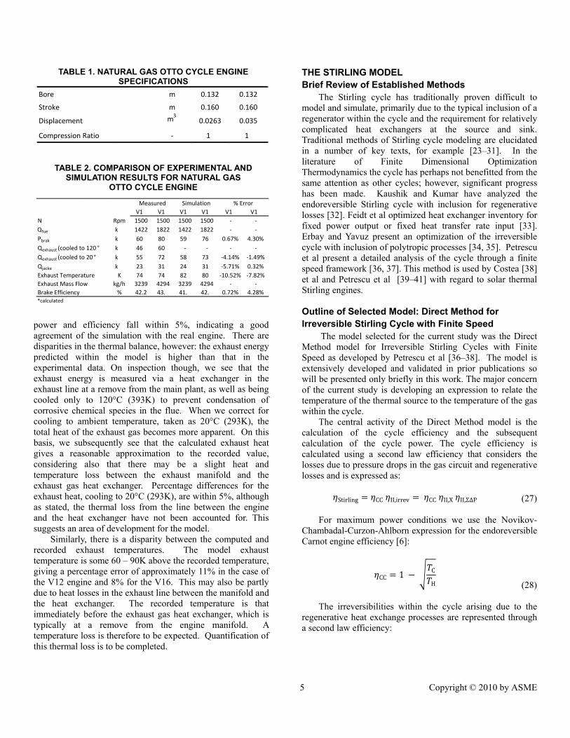
The model has been validated against published experimental data for a natural gas fired spark ignition stationary engine used for combined heat and power generation [22]. A summary of the engine geometric specifications for the unit under consideration is presented in Table 1. The experimental and simulation data is presented in Table 2. Two versions of the engine were modeled, a V12 version and a V16 version. The simulation data was generated using the following values: 𝐼R = 1.27, 𝜀 = 0.1;

𝑇w = 650 𝐾

in line with suggested values given in [13]; 𝐶D = 0.75; 𝑛v =2.

Comments The model demonstrates good quantitative agreement

with the known operating parameters of the engines in question. Percentage difference calculations for the brake

5 Copyright © 2010 by ASME

power and efficiency fall within 5%, indicating a good agreement of the simulation with the real engine. There are disparities in the thermal balance, however: the exhaust energy predicted within the model is higher than that in the experimental data. On inspection though, we see that the exhaust energy is measured via a heat exchanger in the exhaust line at a remove from the main plant, as well as being cooled only to 120°C (393K) to prevent condensation of corrosive chemical species in the flue. When we correct for cooling to ambient temperature, taken as 20°C (293K), the total heat of the exhaust gas becomes more apparent. On this basis, we subsequently see that the calculated exhaust heat gives a reasonable approximation to the recorded value, considering also that there may be a slight heat and temperature loss between the exhaust manifold and the exhaust gas heat exchanger. Percentage differences for the exhaust heat, cooling to 20°C (293K), are within 5%, although as stated, the thermal loss from the line between the engine and the heat exchanger have not been accounted for. This suggests an area of development for the model.

Similarly, there is a disparity between the computed and recorded exhaust temperatures. The model exhaust temperature is some 60 – 90K above the recorded temperature, giving a percentage error of approximately 11% in the case of the V12 engine and 8% for the V16. This may also be partly due to heat losses in the exhaust line between the manifold and the heat exchanger. The recorded temperature is that immediately before the exhaust gas heat exchanger, which is typically at a remove from the engine manifold. A temperature loss is therefore to be expected. Quantification of this thermal loss is to be completed.

THE STIRLING MODEL Brief Review of Established Methods

The Stirling cycle has traditionally proven difficult to model and simulate, primarily due to the typical inclusion of a regenerator within the cycle and the requirement for relatively complicated heat exchangers at the source and sink. Traditional methods of Stirling cycle modeling are elucidated in a number of key texts, for example [23–31]. In the literature of Finite Dimensional Optimization Thermodynamics the cycle has perhaps not benefitted from the same attention as other cycles; however, significant progress has been made. Kaushik and Kumar have analyzed the endoreversible Stirling cycle with inclusion for regenerative losses [32]. Feidt et al optimized heat exchanger inventory for fixed power output or fixed heat transfer rate input [33]. Erbay and Yavuz present an optimization of the irreversible cycle with inclusion of polytropic processes [34, 35]. Petrescu et al present a detailed analysis of the cycle through a finite speed framework [36, 37]. This method is used by Costea [38] et al and Petrescu et al [39–41] with regard to solar thermal Stirling engines. Outline of Selected Model: Direct Method for Irreversible Stirling Cycle with Finite Speed

The model selected for the current study was the Direct Method model for Irreversible Stirling Cycles with Finite Speed as developed by Petrescu et al [36–38]. The model is extensively developed and validated in prior publications so will be presented only briefly in this work. The major concern of the current study is developing an expression to relate the temperature of the thermal source to the temperature of the gas within the cycle.

The central activity of the Direct Method model is the calculation of the cycle efficiency and the subsequent calculation of the cycle power. The cycle efficiency is calculated using a second law efficiency that considers the losses due to pressure drops in the gas circuit and regenerative losses and is expressed as: 𝜂Stirling = 𝜂CC 𝜂II,irrev = 𝜂CC 𝜂II,X 𝜂II,Σ∆P (27)

For maximum power conditions we use the Novikov-Chambadal-Curzon-Ahlborn expression for the endoreversible Carnot engine efficiency [6]:

𝜂CC = 1 − 𝑇C𝑇H (28)

The irreversibilities within the cycle arising due to the

regenerative heat exchange processes are represented through a second law efficiency:

TABLE 1. NATURAL GAS OTTO CYCLE ENGINE SPECIFICATIONS

TABLE 2. COMPARISON OF EXPERIMENTAL AND SIMULATION RESULTS FOR NATURAL GAS

OTTO CYCLE ENGINE

V1 V1 V1 V1 V1 V1N Rpm 1500 1500 1500 1500 - -Q fue k 1422 1822 1422 1822 - -P brak k 60 80 59 76 0.67% 4.30%Q exhaust (cooled to 120 ° k 46 60 - - - -Q exhaust (cooled to 20 ° k 55 72 58 73 -4.14% -1.49%Q jacke k 23 31 24 31 -5.71% 0.32%Exhaust Temperature K 74 74 82 80 -10.52% -7.82%Exhaust Mass Flow kg/h 3239 4294 3239 4294 - -Brake Efficiency % 42.2 43. 41. 42. 0.72% 4.28%*calculated

% ErrorSimulation Measured

Bore m 0.132 0.132

Stroke m 0.160 0.160

Displacement m30.0263 0.035

Compression Ratio - 1 1

6 Copyright © 2010 by ASME

𝜂II,X = 1 + 𝑋 1 − 𝑇C 𝑇H⁄(𝛾 − 1)ln𝑅 S (29)

Also, the irreversibilities due to pressure losses involved in the gas processes are represented by: 𝜂II,Σ∆ = 1 − meanSL √ ln S meanSL ( . . mean)1[ ln S] (30)

where 𝑝1 is the minimum cycle pressure, and 𝜂 = 𝜂CC𝜂II,X (31)

The power output of the Stirling cycle can be calculated simply as the product of the efficiency of the unit and the heat admitted to the cycle [38]:

𝑃SE = 𝜂Stirling�̇�H (32) where �̇�H is the heat transferred to the engine from the thermal source. Calculation of the temperature ratio requires the knowledge of the gas temperatures within the cycle at their extremes within the hot side and cold side heat exchangers. An expression can be derived for this in terms of the heat available from the source, �̇�source, the heat received by the sink, �̇�sink, the averaged temperatures of the source and sink, 𝑇H and 𝑇C respectively and the respective effectivenesses of

the heat exchangers, 𝜀H and 𝜀C. The averaged temperatures of the gas within the engine are: 𝑇H,g = 𝑇H − ̇ HH min,H (33) 𝑇C,g = 𝑇C + ̇ CC min,C (34) where �̇�H = 𝜀H�̇�source

and �̇�C = �̇�sink 𝜀C⁄ . 𝐶min is the minimum heat capacitance rate of the two fluids interacting in the heat exchanger as is used in established heat transfer methodology [42]. These expressions allow us to include the two heat exchanger effectiveness values as parameters for study within the model. In the case of the combined cycle system under investigation in the current work, the thermal source for the Stirling is the exhaust gas of the Otto engine. For this situation, 𝑇H = 𝑇ex,avg; 𝑇C will equate to the average temperature of the cooling circuit; �̇�source will equate to the total �̇�ex from the Otto engine and �̇�sink will be the heat recovered from the Stirling engine in the jacket water circuit of the combined system. VALIDATION OF STIRLING MODEL

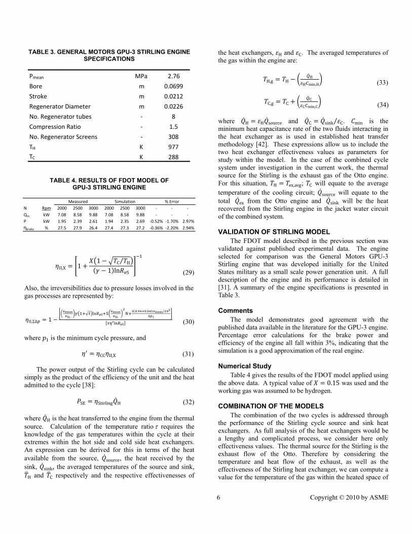
The FDOT model described in the previous section was validated against published experimental data. The engine selected for comparison was the General Motors GPU-3 Stirling engine that was developed initially for the United States military as a small scale power generation unit. A full description of the engine and its performance is detailed in [31]. A summary of the engine specifications is presented in Table 3.

Comments

The model demonstrates good agreement with the published data available in the literature for the GPU-3 engine. Percentage error calculations for the brake power and efficiency of the engine all fall within 3%, indicating that the simulation is a good approximation of the real engine.

Numerical Study

Table 4 gives the results of the FDOT model applied using the above data. A typical value of 𝑋 = 0.15 was used and the working gas was assumed to be hydrogen.

COMBINATION OF THE MODELS

The combination of the two cycles is addressed through the performance of the Stirling cycle source and sink heat exchangers. As full analysis of the heat exchangers would be a lengthy and complicated process, we consider here only effectiveness values. The thermal source for the Stirling is the exhaust flow of the Otto. Therefore by considering the temperature and heat flow of the exhaust, as well as the effectiveness of the Stirling heat exchanger, we can compute a value for the temperature of the gas within the heated space of

TABLE 3. GENERAL MOTORS GPU-3 STIRLING ENGINE SPECIFICATIONS

TABLE 4. RESULTS OF FDOT MODEL OF GPU-3 STIRLING ENGINE

N Rpm 2000 2500 3000 2000 2500 3000 - - -Q in kW 7.08 8.58 9.88 7.08 8.58 9.88 - - -P kW 1.95 2.39 2.61 1.94 2.35 2.69 -0.52% -1.70% 2.97%ηbrake % 27.5 27.9 26.4 27.4 27.3 27.2 -0.36% -2.20% 2.94%

Measured Simulation % Error

P mean MPa 2.76

Bore m 0.0699

Stroke m 0.0212

Regenerator Diameter m 0.0226

No. Regenerator tubes - 8

Compression Ratio - 1.5

No. Regenerator Screens - 308

T H K 977T C K 288

7 Copyright © 2010 by ASME

the engine and the rate of heat transfer to the cycle. For this case, Eq. (33) becomes:

𝑇H,g = 𝑇ex,avg − ̇exmin,H (35)

Where �̇�ex = �̇�source. Similarly, we can compute the

temperature in the cooled space by consideration of the respective heat exchanger effectiveness values, the sink temperature and the heat transfer rate to the cooling circuit. For this case, Eq. (34) becomes:

𝑇C,g = 𝑇C − ̇ coolantC min,C (36)

Where �̇�coolant = �̇�sink = 𝑄L𝑡th. The total power output of

the combined cycle plant is therefore the sum of the power outputs from each engine. Similarly the global efficiency of the combined plant is the ratio of total power output to the total heat addition, in this case the fuel consumption of the Otto cycle engine. CONCLUSIONS

Thermodynamic models for both the Otto and Stirling cycle engines have been presented and validated against published experimental data for existing engines. The models are both based on the principles of Finite Dimensional Optimization Thermodynamics (FDOT)—the Otto cycle model is a development of a previously available model considering the engine from a Finite Time Thermodynamic (FTT) perspective; the Stirling model is also a development of previously published work, this time considering the cycle in a Finite Speed Thermodynamic (FST) framework. Both methodologies have their own characteristics and advantages, and there is no perceived mutual exclusivity, so that it is possible to collect them under the broad FDOT title. Both models demonstrated good quantitative agreement with the performance data of the real engines concerning brake mechanical power output and brake thermal efficiency.

Analysis in terms of the FDOT methods presented here offers the advantage of presenting a comparatively uncomplicated methodology for modeling and simulation of the engines, whilst maintaining a sufficient number of parameters to facilitate realistic description. The Stirling cycle engine in particular has experienced only sporadic development in its history. It has traditionally proven difficult to model and simulate. Therefore, for some time it has relied on dedicated and enthusiastic specialists to progress the agenda for its development in competition with the more established internal combustion engines. As a consequence, full system specifications and performance data for commercially available high performance Stirling engines are difficult to ascertain. Therefore, effective and efficient simulation tools are a necessity for the technology to progress at a pace comparable to that of its rival technologies. The

FDOT modeling scenario appears to offer these benefits. With regard to the Otto cycle engine, modeling of the

engine is already well established and offers considerable simulation capability. Use of the FDOT modeling however offers the advantage of analyzing the cycle with a basis in the classical thermodynamics environment, thereby allowing perhaps a more intuitive development from the classical air standard cycle model. The considerable predictive capability of such a relatively uncomplicated modeling scheme may offer both pedagogical and practical advantage.

NOMENCLATURE 𝐴p - Area of piston face m2 𝐴T - Valve orifice area m2 𝐵 - Bore m 𝐶 - Heat capacity rate W/K 𝐶D - Discharge coefficient - 𝐶 - Specific Heat Capacity at constant

pressure J/kgK 𝐶 - Specific Heat Capacity at constant

volume J/kgK 𝑓 - Frequency Hz 𝐻 - Enthalpy J/kg ℎ - Convective heat transfer coefficient W/m2K 𝐼R - Irreversibility Factor - 𝑀 - Mass kg �̇� - Mass flowrate kg/s 𝑁 - No. regenerator screens - 𝑛v - No. of valves - 𝑃 - Power W 𝑝 - Pressure Pa 𝑅g - Specific gas constant, Otto cycle

working fluid J/kgK 𝑅mass - Mass ratio -

𝑅 S - Stirling cycle compression ratio - 𝑟 - Otto cycle compression ratio - 𝑆 - Otto cycle piston stoke m 𝑇 - Temperature K 𝑡th - Thermodynamic cycle period s 𝑡 - Period of Otto cycle power stroke s 𝑉 - Otto cycle clearance volume m3 𝑣 - velocity m/s 𝑊 - Work J 𝑋 - Regenerator loss coefficient - 𝑥 - Piston displacement m Greek Letters 𝛾 - Ratio of specific heat capacities of

Otto cycle working fluid - 𝜀 - Phenomenological constant, Otto cycle - 𝜂 - Efficiency % 𝜂CC - Carnot Efficiency % 𝜂II - Second law efficiency % 𝜇 - Friction coefficient kg/s

8 Copyright © 2010 by ASME

𝜏 - Temperature ratio, 𝑇H,g 𝑇C,g⁄ - Subscripts avg - Average bd - Blowdown C - Stirling cold side cyl - Cylinder disp - Displaced ex - Exhaust f - Friction work H - Stirling hot side 𝐼 - Irreversible irrev - Irreversible power

L - Loss mean - Mean velocity 𝑄 - Heat loss REV - Reversible SE - Stirling engine SL - Speed of sound sink - Stirling heat sink source - Stirling heat source w - Wall X - Regenerative losses 0 - Clearance, stagnation 𝜇 - Friction loss power

REFERENCES

[1] Cullen, B. and J. McGovern, The Quest for More Efficient Industrial Engines: A Review of Current Industrial Engine Development and Applications. ASME Journal of Energy Resources Technology, 2009. 131(2).

[2] Cullen, B. and J. McGovern, Energy system feasibility study of an Otto Cycle / Stirling Cycle hybrid automotive engine. Energy, 2010. 35(2): p. 1017-1023.

[3] Cullen, B., McGovern, J., Petrescu, S., Feidt, M., Preliminary Modelling Results for an Otto Cycle / Stirling Cycle Hybrid-Engine-Based Power Generation System, in ECOS 2009: 22st International Conference on Efficiency, Cost, Optimization, Simulation and Environmental Impact of Energy Systems. 2009: Foz do Iguacu, Brazil. p. 2091-2100.

[4] Denton, J.C., Thermal cycles in classical thermodynamics and nonequilibrium thermodynamics in contrast with finite time thermodynamics. Energy Conversion and Management, 2002. 43(13): p. 1583-1617.

[5] Novikov, I.I., The efficiency of atomic power stations (a review). Journal of Nuclear Energy (1954), 1958. 7(1-2): p. 125-128.

[6] Feidt, M., Optimal Thermodynamics - New Upperbounds. Entropy, 2009(11): p. 529-547.

[7] Curzon, F.L. and B. Ahlborn, Efficiency of a Carnot engine at maximum power output. American Journal of Physics, 1975. 43(1): p. 22-24.

[8] Angulo-Brown, F., J. Fernandez-Betanzos, and C. Diaz-Pico, Compression ratio of an optimized air standard Otto-cycle model. European Journal of Physics, 1994. 15: p. 38 - 42.

[9] Angulo-Brown, F. and et al., A non-endoreversible Otto cycle model: improving power output and efficiency. Journal of Physics D: Applied Physics, 1996. 29(1): p. 80.

[10] Hernandez, A.C. and et al., On an irreversible air standard Otto-cycle model. European Journal of Physics, 1995. 16(2): p. 73.

[11] Ge, Y., et al., Thermodynamic simulation of performance of an Otto cycle with heat transfer and variable specific heats of working fluid. International Journal of Thermal Sciences, 2005. 44(5): p. 506-511.

[12] Chen, J., Y. Zhao, and J. He, Optimization criteria for the important parameters of an irreversible Otto heat-engine. Applied Energy, 2006. 83(3): p. 228-238.

[13] Curto-Risso, P.L., A. Medina, and A.C. Hernandez, Theoretical and simulated models for an irreversible Otto cycle. Journal of Applied Physics, 2008. 104(9): p. 094911.

[14] Curto-Risso, P.L., A. Medina, and A.C. Hernandez, Optimizing the operation of a spark ignition engine: Simulation and theoretical tools. Journal of Applied Physics, 2009. 105.

[15] Curto-Risso, P.L., A. Medina, and A.C. Hernandez, Thermodynamic Optimization of a Spark Ignition Engine, in 22nd International Conference on Efficiency, Cost, Optimization, Simulation and Environmental Impact of Energy Systems. 2009: Foz do Iguacu, Brazil. p. 1979-1988.

[16] Curto-Risso, P.L. and et al., Optimizing the operation of a spark ignition engine: Simulation and theoretical tools. Journal of Applied Physics, 2009. 105(9): p. 094904.

[17] Angulo-Brown, F., T.D. Navarrete-Gonzalez, and J.A. Rocha-Martinez, An Irreversible Otto Cycle Model Including Chemical Reactions, in Recent Advances in Finite Time Thermodynamics, C. Wu, L. Chen, and J. Chen, Editors. 1999, Nova Science Publishers Inc.

[18] Abu-Nada, E., et al., Thermodynamic modeling of spark-ignition engine: Effect of temperature dependent specific heats. International Communications in Heat and Mass Transfer, 2006. 33(10): p. 1264-1272.

[19] Mozurkewich, M. and R.S. Berry, Optimal paths for thermodynamic systems: The ideal Otto cycle. Journal of Applied Physics, 1982. 53(1): p. 34-42.

[20] Heywood, J.B., Internal Combustion Engine Fundamentals. 1988: McGraw Hill Book Company

[21] Stas, M.J., Effect of Exhaust Blowdown Period on Pumping Losses in a Turbocharged Direct Injection

9 Copyright © 2010 by ASME

Diesel Engine, in SAE International Congress and Exposition. 1999, SAE: Detroit, Michigan.

[22] Motoren-Werke Mannheim GmbH (MWM), Gas Genset Specifications. 2007.

[23] Walker, G., Stirling Engines. 1980, Oxford: Clarendon Press.

[24] Walker, G., Fauvel, O.R., Reader, G, Bingham E.R , The Stirling Alternative. 1994: Gordon and Breach Science Publishers.

[25] Reader, G.T. and C. Hooper, Stirling Engines. 1983, London: E. & F.N. Spon.

[26] Urieli, I. and D.M. Berchowitz, Stirling Cycle Engine Analysis. 1984, Bristol: Hilger.

[27] Hargreaves, C.M., The Philips Stirling Engine. 1991, Amsterdam: Elsevier Science Publishers B.V.

[28] Finkelstein, T. and A.J. Organ, Air Engines. 2001: Professional Engineering Publishing Ltd.

[29] Organ, A.J., Thermodynamics and Gas Dynamics of the Stirling Cycle Machine. 1992: Cambridge University Press.

[30] Organ, A.J., The Regenerator and the Stirling Engine. 1997: London, Mechanical Engineering Publications.

[31] Martini, W.R., Stirling Engine Design Manual. 2nd Edition 1983: DOE/NASA.

[32] Kaushik, S.C. and S. Kumar, Finite time thermodynamic analysis of endoreversible Stirling heat engine with regenerative losses. Energy, 2000. 25(10): p. 989-1003.

[33] Feidt, M., Lesaos,K., Costea, M., Petrescu, S., Optimal allocation of HEX inventory associated with fixed power output or fixed heat transfer rate input. International Journal of Applied Thermodynamics, 2002. 5(1): p. 25-36.

[34] Erbay, L.B. and H. Yavuz, Analysis of the stirling heat engine at maximum power conditions. Energy, 1997. 22(7): p. 645-650.

[35] Erbay, L.B. and H. Yavuz, Optimization of the Irreversible Stirling Heat Engine. International Journal of Energy Research, 1999. 23: p. 863-873.

[36] Petrescu, S., Costea, M., Harman, C., Florea, T., Application of the Direct Method to irreversible Stirling cycles with finite speed. International Journal of Energy Research, 2002. 26(7): p. 589-609.

[37] Petrescu, S., et al., The First Law of Thermodynamics for Closed Systems, Considering the Irreversibilities Generated by the Friction Piston - Cylinder, the Throttling of the Working Medium and the Finite Speed of the Mechanical Interaction, in ECOS '92. 1992, ASME: Zaragoza, Spain.

[38] Costea, M., S. Petrescu, and C. Harman, The effect of irreversibilities on solar Stirling engine cycle performance. Energy Conversion and Management, 1999. 40(15-16): p. 1723-1731.

[39] Petrescu, S., Petre, C., Costea, M., Malancioiu, O., Boriaru, N., Dobrovicescu, A., Feidt, M., Harman, C., A Methodology of Computation, Design and Optimization

of Solar Stirling Power Plant using Hydrogen/Oxygen Fuel Cells. Energy, 2010. 35(2): p. 729-739.

[40] Petrescu, S., Harman, C, Costea, M., Popescu, G., Petre, C., Florea, T., Analysis and Optimisation of Solar/Dish Stirling Engines, in Proceedings of the 31st American Solar Energy Society Annual Conference, Solar 2002, "Sunrise on the Reliable Energy Economy", R. Campbell-Howe, Editor. 2002: Reno, Nevada, USA.

[41] Petrescu, S., Harman, C., Costea, M., Petre, C., Florea, T., Feidt, M., A Scheme of Computation, Analysis, Design and Optimization of Solar Stirling Engines", in 16th International Conference on Efficiency, Cost, Optimization, Simulation and Environmental Impact of Energy Systems ECOS'03, B.E. N. Houbak, B. Qvale, M. Moran, Editor. 2003: Denmark. p. 1255-1262.

[42] Incropera, F.P. and DeWitt, David P., Fundamentals of Heat and Mass Transfer. Fifth ed. 2002: John Wiley & Sons.