Valence and magnetic ordering in intermediate valence compounds: TmSe versus SmB6
22
arXiv:cond-mat/0511106v1 [cond-mat.str-el] 4 Nov 2005 Valence and magnetic ordering in intermediate valence compounds : TmSe versus SmB 6 J. Derr, G. Knebel, G. Lapertot, B. Salce, M-A. M´ easson and J. Flouquet D´ epartement de Recherche Fondamentale sur la Mati` ere Condens´ ee, CEA Grenoble, 17 rue des Martyrs, 38054 Grenoble Cedex 9, France E-mail: [email protected] Abstract. The intermediate valent systems TmSe and SmB 6 have been investigated up to 16 and 18 GPa by ac microcalorimetry with a pressure (p) tuning realized in situ at low temperature. For TmSe, the transition from an antiferromagnetic insulator for p< 3 GPa to an antiferromagnetic metal at higher pressure has been confirmed. A drastic change in the p variation of the N´ eel temperature (T N ) is observed at 3 GPa. In the metallic phase (p> 3 GPa) , T N is found to increase linearly with p. A similar linear p increase of T N is observed for the quasitrivalent compound TmS which is at ambiant pressure equivalent to TmSe at p ∼ 7 GPa. In the case of SmB 6 long range magnetism has been detected above p ∼ 8 GPa, i.e. at a pressure slightly higher than the pressure of the insulator to metal transition. However a homogeneous magnetic phase occurs only above 10 GPa. The magnetic and electronic properties are related to the renormalization of the 4f wavefunction either to the divalent or the trivalent configurations. As observed in SmS, long range magnetism in SmB 6 occurs already far below the pressure where a trivalent Sm 3+ state will be reached. It seems possible, to describe roughly the physical properties of the intermediate valence equilibrium by assuming formulas for the Kondo lattice temperature depending on the valence configuration. Comparison is also made with the appearance of long range magnetism in cerium and ytterbium heavy fermion compounds.
Transcript of Valence and magnetic ordering in intermediate valence compounds: TmSe versus SmB6
arX
iv:c
ond-
mat
/051
1106
v1 [
cond
-mat
.str
-el]
4 N
ov 2
005
Valence and magnetic ordering in intermediate
valence compounds : TmSe versus SmB6
J. Derr, G. Knebel, G. Lapertot, B. Salce, M-A. Measson and
J. Flouquet
Departement de Recherche Fondamentale sur la Matiere Condensee, CEA Grenoble,
17 rue des Martyrs, 38054 Grenoble Cedex 9, France
E-mail: [email protected]
Abstract. The intermediate valent systems TmSe and SmB6 have been investigated
up to 16 and 18 GPa by ac microcalorimetry with a pressure (p) tuning realized in situ
at low temperature. For TmSe, the transition from an antiferromagnetic insulator for
p < 3 GPa to an antiferromagnetic metal at higher pressure has been confirmed. A
drastic change in the p variation of the Neel temperature (TN ) is observed at 3 GPa.
In the metallic phase (p > 3 GPa) , TN is found to increase linearly with p. A similar
linear p increase of TN is observed for the quasitrivalent compound TmS which is at
ambiant pressure equivalent to TmSe at p ∼ 7 GPa. In the case of SmB6 long range
magnetism has been detected above p ∼ 8 GPa, i.e. at a pressure slightly higher than
the pressure of the insulator to metal transition. However a homogeneous magnetic
phase occurs only above 10 GPa. The magnetic and electronic properties are related
to the renormalization of the 4f wavefunction either to the divalent or the trivalent
configurations. As observed in SmS, long range magnetism in SmB6 occurs already
far below the pressure where a trivalent Sm3+ state will be reached. It seems possible,
to describe roughly the physical properties of the intermediate valence equilibrium
by assuming formulas for the Kondo lattice temperature depending on the valence
configuration. Comparison is also made with the appearance of long range magnetism
in cerium and ytterbium heavy fermion compounds.

Valence and magnetism in IVC 2
1. Introduction
Recently, a major interest was the study of the high pressure phase diagrams of
heavy fermion compounds (HFC)[1]. However, in these systems, the departure from
the trivalent configuration is weak ; the occupation number nf of the 4f 1 is nearly one.
Unusual magnetic properties found notably on ytterbium HFC such as YbRh2Si2 push
to revisit other situations with magnetic and valence fluctuations occuring between two
4f configurations. The cases of intermediate valence compounds (IVC) as SmS, SmB6
and TmSe, are particularely interesting[2].
To caracterize the intermediate valent state, a key parameter is the occupation number
nf of the trivalent configuration linked to the valence v by v = 2+ nf when the valence
fluctuation occurs between the divalent and the trivalent state (case of Sm, Tm and Yb)
or v = 4− nf when it happens between the trivalent and tetravalent state (case of Ce).
The important difference between Sm, Tm or Yb compounds is that nf can vary from
0 to 1 while in Ce intermetallic compounds : nf > 0.8 and at least long range magnetic
ordering (M) occurs only for nf > 0.9[3]. TmSe[4, 5, 6, 7] as well as SmS[2] and SmB6[8]
in their low pressure intermediate valent gold phase have a valence near 2.6-2.7. Their
trivalent limit will be reached smoothly only at very high pressure above 10 GPa for
TmSe and 20 GPa for SmS and SmB6[9, 10, 11] . As will be discussed, the striking
point is that for these three systems, the change from insulating to metallic conduction
at low temperature occurs when nf∼ 0.8.
The valence mixing between the divalent (2+) and trivalent (3+) configurations of the
rare earth (RE) ions is associated to the release of an itinerant 5d electron according
to the relation RE2+ ⇐⇒ RE3+ + e−5d. Experimentally, the effect of pressure is to
broaden the bands and move this equilibrium to the right (increasing nf ). Of course,
band structure calculations are necessary to describe the real situation, but the chemical
equilibrium is worthwhile to consider. In the divalent black (B) phase, the ground
state is a classical insulator. Through a first order transition at V = VB−G, a valence
transition occurs to an intermediate valence (IV) gold (G) phase which is still insulating.
However, under pressure the insulating gap will close for a fixed volume V∆. At V = V∆,
metallic conduction appears for nf∼ 0.8 at a volume quite larger than the volume V3+
calculated for a pure trivalent configuration. Figure 1 represents the location of the
different compounds at ambiant pressure.
In Sm compounds, the intermediate valent state occurs between a non magnetic 4f 6
configuration of Sm2+, with a zero angular momentum J and the Kramer’s configuration
(J=52) of Sm3+ (4f 5). It looks worthwhile to predict that, as in cerium HFC, magnetic
ordering will occur when the occupancy nf of the trivalent configuration approaches one.
In this case, following the Doniach model (see [1]), the Kondo coupling should be small
enough, so that the Kondo energy becomes smaller than the RKKY energy. However,

Valence and magnetism in IVC 3
��
����
����������
������
����
���������
���������
����������������������
����
����
����
����
2+ I. V.
v3
3+
Insulator Metal
TmSTmSe6SmB
TmTe
SmS
2 pp∆ p3+
1V1
V3+
1V∆
1VB−G
0 pB−G
Figure 1. Valence state, as a function of the density, i.e. the inverse of the molar
volume V . For V < VB−G, the system jumps from 2+ black (B) phase to IV gold (G)
phase. up to VB−G > V > V∆ the system is still insulating (The dashed lines represent
the insulating caracter). Magnetism looks also governed by the 2+ configuration. For
V < V∆, the system is metallic, and magnetism looks governed by the 3+ configuration.
The trivalent limit will appear for V3+ < V∆. Long range magnetism in SmS and SmB6
appear for 1
V∼ 1
V∆+ ǫ < 1
V3+. Of course it occurs always for TmSe whatever is the
valence
recently it was shown by use of a microscopic hyperfine technique as nuclear forward
scattering and a macroscopic probe as ac microcalorimetry that magnetic ordering
occurs already for a rather large departure from nf= 1[12, 13, 14]. Up to nf≤ 0.8, the
4f wavefunction seems to be renormalized to the 2+ configuration while above nf∼ 0.8,
it seems linked to the 3+ configuration. Furthermore, this is related to the conduction
properties : insulating below nf∼ 0.8 and metallic above.
In Tm chalcogenides, the ground state of the divalent configuration (nf = 0, case
of TmTe) is insulating, and becomes metallic for the trivalent form. In the IVC (case
of TmSe) with low nf (nf ≤ 0.8), the many body effects of the correlation lead to
the survival of an insulator. In the specific case of Tm, the novelty is that mixing
occurs between two configurations with non zero angular momentum. The divalent
one (Tm2+ 4f 13) is a Kramer’s configuration with J = 72
which leads to a doublet
or a quartet crystal field ground state, while the trivalent one (Tm3+ 4f 12) is a non
Kramer’s ion with J = 6 which may lead to a singlet crystal field ground state. The
pressure induced collapse of the insulating state is associated with a change in the
magnetic structure at p∆ ∼ 3 GPa[15]. Below p∆, i.e. for nf≤ 0.8, the ground
state is insulating, like in the low pressure intermediate valence phase of SmS and
SmB6, and antiferromagnetic of type I with properties basically given by a dressing

Valence and magnetism in IVC 4
towards a divalent renormalization (insulating conduction, doublet degeneracy of the
local magnetic level). Above p∆, the ground state is metallic (like TmS, or SmS
and SmB6 at high pressure), again antiferromagnetic, but of type II, with properties
renormalized to the trivalent configuration. A surprising report was that near p∼ 6 GPa,
TmSe may become insulating again[16, 17].
In this paper, we present a detailed study of the high pressure phase diagrams of TmSe,
TmS and SmB6 . Since for the two first cases, specific heat is already well known for p =
0, and also interplay occurs between pressure and ligand effects, those compounds allow
to verify the faisability and difficulties of high pressure microcalorimetry experiments.
As TmSe is already magnetically ordered at ambiant pressure, up to 3 GPa, one may
expect a signal in the ac calorimetry equivalent to ambiant pressure. Above 3 GPa,
the signal may change as the signal may be normalized to the 3+ configuration like in
TmS. Special attention is given on the pressure range around 6 GPa. The evolution of
TN(p) of TmSe above 3 GPa will be compared to the nearly trivalent TmS. In SmB6 ,
we found evidence for a magnetically ordered ground state for p > 8 GPa. However, a
homogeneous ground state appears only above 10 GPa.
The paper is organized as follows. First we will discuss details of the ac calorimetry
technique. Then, the experimental results on TmSe, TmS ans SmB6 will be presented
and an experimental conclusion will be given. In the last part, the influence of the
valence on the appearance of magnetic order will be discussed in detail and a comparison
to the well known high pressure phase diagrams of Ce and Yb Kondo lattice will be
given.
2. Experimental
The TmSe and TmS single crystals were prepared by F. Holtzberg in IBM research
center, New York, and samples of the same batch have been intensively studied
previously in CNRS Grenoble[18]. SmB6 single crystals were grown in CEA Grenoble,
out of an aluminium flux. The samples studied were cleaved to be approximately
200*100*50µm3 in size. The high pressure experiment were performed in a diamond
anvil pressure cell (see figure 2). Argon is used as a pressure transmitter. The pressure
is measured at low temperature by the shift of the ruby fluorescence line. In the ac
calorimetry, a laser is used as heater. The beam is modulated using a mechanical
chopper which works in the frequency range 50 Hz< f <5000 Hz. The temperature
oscillations of the sample are measured with a Au/AuFe(0.07%) thermocouple which is
spot welded on the sample. In the case of TmSe, it was glued with very diluted General
Electric varnish. It is important that the thermocouple is welded in one point to avoid
contributions of the thermoelectric power of the sample itself. A lock-in amplifier is
used to measure the voltage of the thermocouple.
The measurements were performed in a 4He bath cryostat.

Valence and magnetism in IVC 5
Figure 2. Zoom on the high pressure cell. A thermocouple made of Au and AuFe is
welded on the sample. Argon is used as pressure medium. The pressure is measured
due to the fluorescence shift of ruby. The diamater of the hole is about 350 µm.
sκ κ(1-a).P0
a.P0Bath
lethermocoup
C
Figure 3. Schematic view of the thermal system in the pressure cell. The laser gives
the power aP0 and (1 − a)P0 respectively to the thermocouple and the sample
This experimental situation can be described by a first order model neglecting all
internal time constants between sample, heater and thermometer[21] : Tac = P0
κ+iωC,
where Tac is the amplitude of the temperature oscillation, P0 the average power
transmited, κ the thermal conductivity to the bath and C the specific heat. Even
if the leak κ is unknown, the phase measured by the lock-in is supposed to give the
possibility to extract the value of the specific heat. C = P0.SV.ω
sin(φ − φ0), where V is
the voltage of the thermocouple, S its relative thermopower and (φ − φ0) the phase of
the signal. If we want to minimize the importance of the phase correction, the choice
of the frequency is crucial, as it balances the importance of the specific heat compared
to the leak in the signal measured. From this point of view (without considering noise
problems due to a decrease of the signal at high frequency), the frequency should be
the highest possible. However, the experiment will show that this model is no longer
valid at higher frequencies. If the frequency is too high, the sample decouples from the
thermocouple and, the thermocouple can be directly excited by the laser and measure
only its own temperature at high frequency[22]. The next step is to include a thermal
conductivity κS between the sample and the thermocouple and to consider that a small
proportion a of the power is directly received on the thermocouple. In this situation
(see figure 3), Tac can be reestimated:[27] Tac =P0.(1−
κeff
κS)
κeff
1+iωa CκS
1+iω Cκeff
with κeff = κκS
κ+κS
representing the total parallel thermal conductivity of leak. Three different limits can

Valence and magnetism in IVC 6
1
2
3
(a)1
Tac
κ
P0(1−κeffκS
)κs
aP0(1−κeffκS
)
iωC
23
1
0
(b)| 1Tac|
−π2
κeff
Cκs
C
−arg( 1Tac
)
ω
Figure 4. Part (a) shows graphically the inverse of Tac in the complex representation.
Leak phenomena is on the real axis whereas capacitive effects are on the imaginary
axis. The three limit cases are : (1), capacitive effect is negligible and the power P0
is transmited to the bath with the leak κ ; (2), capacitive effect becomes dominant
and the component ωC is added ; (3) The sample is decoupled from the thermocouple.
the power received is only the fraction aP0 and the main leak is still κS , towards
the sample. In part (b), the schematic shape of the phase and the module of 1
Tacis
deducted from the evolution drawn in part (a). The vertical dashed lines show the cut
off frequenciesκeff
Cand κS
Cwhich indicate the change of regime corresponding to (1),
(2) and (3).
be distinguished :
• At low frequency, if ωC ≪ κeff then Tac =P0.(1−
κeff
κS)
κeff. The value of the basic model
is recovered : the phase of the signal is nearly zero and the inverse of the module
is small.
• For the intermediate regime κeff ≪ ωC ≪ κS we recover also the basic model
Tac =P0.(1−
κeff
κS)
κeff +iωC. In good conditions, if frequency becomes high enough compared
to the leak, the phase reaches nearly -Π2.
• Finally, at high frequency, for κS ≪ ωC, Tac = (1−κeff
κS)aP0
κS.The phase reaches zero
and the module decreases again. Physically, the thermocouple is decoupled from
the sample.
To view more clearly the frequency dependence of the system, let us consider the
complex number 1Tac
. The phase measured by the lock in is directly the opposite of the
phase of this complex number, and the signal 1V
is directly linked to the module of this
complex number. Part (a) of the figure 4 explains the different regimes depending on
the frequency. From that picture, we can roughly draw the shape of the phase and of
the inverse of the module (see part (b) of the figure 4)

Valence and magnetism in IVC 7
Moreover, if we consider the variable change ω ↔ ωC, the shape of the dependance
in ω of the argument and module of 1Tac
(figure 4b) can be expanded to the dependance
in ωC. Then, considering a jump in the specific heat C at the magnetic transition, the
phase will be changed differently at high and low frequency. Around ω =κeff
Cthe signal
in the phase will be a negative peak, but around ω = κS
C, the signal of the phase can be
a positive peak. This will be confirmed later by the experimental results.
Thus, the best frequency for the measurement is between this two cut-off
frequencies. Typically, the best frequency was about 90 Hz for TmSe, 800 Hz for TmS
and 4500 Hz for SmB6. Assuming that the specific heat of TmSe is higher than that
of TmS which is higher than that of SmB6 (at least at low pressure as indicated in
figure 5), this support the model since in the conditions of measure Cω stays roughly
constant.
Nevertheless, even if the behaviour of the phase is understood, the incertitude on the
reference phase φ0 and the complex influence of pressure keep the situation delicate.
Therefore, in the following, we will usually estimate the specific heat via the simplest
expression : C = P0.SV.ω
.
The main point of the apparatus is the possibility to change the pressure at low
temperature and also to use a excellent hydrostatic medium (Ar or He). To improve the
faisability of the difficult microcalorimetric measurement under hydrostatic pressure,
the choice has been made to minimize the number of electrical leads and thus, to use a
laser as heater. The advantage of the technique is to give the pressure variation of the
Neel temperature with a great accuracy i.e. a large set of pressure. If it is an excellent
method to determine the phase diagram, the difficulty is to extract the specific heat in
absolute units.
3. Results
Preliminary results
Before discussing the specific heat under pressure, we present the specific heat at
ambiant pressure for the different systems in figure 5. The behaviour of C for the two
Tm compounds is quite different. For TmSe, the specific heat has a sharp anomaly
at TN [23]. TmS is metallic and the crystal field ground state may be a singlet. Here,
large fluctuations are already oberved above TN [24]. In the other case, as SmB6 is non
magnetic we have reported here the results for CeB6[25] in order to have an idea of the
amplitude of the signal under pressure. The comparison is worthwhile as both (4f 1)
Ce3+ and (4f 5) Sm3+ are Kramer’s ions with the same angular momentum J = 52
with
a lifting of the degeneracy by the crystal field in a Γ7 doublet and a Γ8 quartet. The
successive transitions observed for CeB6 are now well understood by a cascade from
paramagnetism to quadrupolar ordering at TN1∼ 2.9 K and to dipolar ordering at

Valence and magnetism in IVC 8
8
6
4
2
0
C/T
(J.
mol
-1.K
-2)
1086420
T (K)
TmSe TmS SmB6 CeB6
Figure 5. Specific heat divided by temperature measured at ambiant pressure for
TmSe[23], TmS[24], SmB6(measured on our sample) and CeB6[25]
3
2
1
Mod
ule
10864T(K)
TmSe, f=90Hz 1.5 GPa 5 GPa 11.2 GPa
15
10
5
0
-5
Pha
se (
degr
ee)
108642T (K)
TmSe, f=90 Hz 1.5 GPa 5 GPa 11.2 GPa
Figure 6. Raw data measured for TmSe, for several pressures (1.5, 5 and 11.2 GPa.).
Module data are normalized at high temperature ; therefore, the three curves looks
continuous after the anomaly.
TN2∼ 2.2 K, the crystal field ground state being a Γ8 quartet[26].
TmSe
The temperature dependence of the specific heat of TmSe has been measured in a wide
pressure range (1 to 14 GPa). Raw data are plotted in figure 6 for different pressures.
The modulus and also the phase show a clear anomaly at the magnetic transition. The
measurement has been realised at low frequency, so that the magnetic anomaly is seen
in the phase as a negative peak. A second very sharp positive peak is also observed,
inside the first negative peak, especially at low pressure. A simulation[27] shows that
the huge value of the specific heat jump in TmSe can induce this second positive peak
changing from the regime of low ωC to the one of high ωC. Nevertheless, the strongly
negative peak of the phase shows that we are in the low frequency regime where phase

Valence and magnetism in IVC 9
2
1 C
/T (
Arb
. uni
ts)
10864 T (K)
5 7.6 11.2
13.1
1.5
TmSe, f=90 Hz
Figure 7. Evolution of the specific heat anomaly of TmSe under pressure. Data are
normalized at high temperature and plotted for 1.5, 5, 7.6, 11.2 and 13.1 GPa.
C/T
(ar
bitr
ary
tran
slat
ed)
121086 T(K)
10.5 GPa
11.1 GPa
11.2 GPa 11.5 GPa
12 GPa 14 GPa
TmSe
Figure 8. Observation of the spliting of the specific heat anomaly of TmSe at high
pressure.
correction is supposed to be used. Moreover, as the signal is huge on the modulus, the
phase correction is not significant (This is explained because close to −Π2
the sinus is
not really sensitive). Thus we present here the simplest estimation of the specific heat
C = P0.SV.ω
. Some of the calculated curves are plotted in figure 7.
A first observation is that the magnetic anomaly is very well defined, so that, the
Neel temperatures can be easily extracted. To define TN we choose the maximum of
the anomaly. Furthermore, we found an unexpected broadening of the anomaly as the
pressure increases. This appears below 10 GPa, when hydrostaticity is still very good
(less than 0.1 GPa of variation in the cell)[28]. This broadenning cannot be explained
by pressure inhommogeneities as dTN
dpis small. Figure 8 shows C
Tfor pressures above
10 GPa. The data indicate a splitting of the magnetic anomaly, which can be followed
under pressure.
The resulting phase diagram is then represented in figure 9

Valence and magnetism in IVC 10
10
8
6
4
2
0
T (
K)
1050 p (GPa)
TmSe
Insulator
AF I
Metallic
AF II
Figure 9. (p, T) Phase diagram of TmSe. The squares represent the maximum of
each specific heat anomaly, and the circles indicate the second maximum observed at
high pressures. The dashed line show the phase transition coresponding to the slope
change.
The phase diagram can be distinguished in three parts. At low pressures, the evolution
of TN is quite flat and a maximum can be seen around 1.3 GPa. Then, a break in the
slope around 3 GPa corresponds to the pressure of transition from the insulating AF1
phase to the metallic AF2 phase. The second magnetic structure is caracterized by a
linear increase of the Neel temperature with pressure.
At low pressure, our data are completely consistent with previous resistivity
measurements[15, 16, 17]. The important observation is the continuous increase of TN
with pressure at high pressure. Contrary to recent resistivity measurements who showed
a discontinuity in the Neel temperature around 6 GPa[29], no anomaly in TN(p) is seen
in our data. Actually, our observation is consistent with a release of the 5d electrons
near 3 GPa. Recent neutrons measurements[29] confirm this idea as no change in the
magnetic structure is found at 6 GPa. Finally, an interesting splitting of the magnetic
anomaly is observed at high pressure, above 10 GPa. The evolution of the signal shape
was detailled in figure 8. The origin of this splitting and the new phase is not clear.
This observation pushs us to study TmS, which can be seen as high pressure analog
of TmSe. In TmS, evidence has been reported for two different magnetic phases [30]
around 5 GPa.
TmS
The specific heat of TmS was measured up to 19 GPa. Raw data are plotted for several
pressures in figure 10. The behaviour of the phase is detailled for the low pressures. The
previous explanation is confirmed : we can observe two different regimes for the phase,
depending if the measurement is performed at low or high frequency. This is really
reproducible and stable with pressure change. That confirms that the feature occuring
on the phase is very useful to detect the magnetic transition. Unfortunately, in the low

Valence and magnetism in IVC 11
6
4
2
0
Mod
ule
20161284 T (K)
TmS, f=800 Hz
1.8 GPa 11.3 GPa 18.7 GPa
55
50
45
40
35 Pha
se (
Arb
itrar
y sh
ifted
)
141210864 T (K)
Low frequency
High frequency
2.7 GPa
2.2 GPa
1.8 GPa TmS
(200 Hz)
(800 Hz)
Figure 10. Raw data measured for TmS. The module has been drawn for 1.8, 11.3
and 18.7 GPa. The signal has been followed until very high pressure, but at the end, it
desapears as shows the curve at 18.7 GPa. Then, the behaviour of the phase has been
detailled : the measurement at low frequency (200 Hz) and high frequency (800 Hz)
have been compared and followed with pressure from 1.8 GPa to 2.7 GPa. For the
picture the phase have been arbitrary shifted.
18
16
14
12
10
8
C/T
(A
rb. U
nits
)
16141210864 T (K)
11.3
18.7
4.8
1.8
TmS, f=800 Hz
Figure 11. Evolution of the magnetic anomaly of TmS under pressure ; specific
heat divided by temperature has been normalized at high temperature and plotted for
different pressures : 1.8, 4.8, 11.3 and 18.7 GPa
frequency regime, the feature on the modulus is very small and don’t allow us to extract
a good shape of the specific heat. On the other hand, figure 10 shows that the module
measured at high frequency is more clear. Even if the first order model is valid only
at low frequency, figure 4b shows that the evolution of the module is still monotonous
even after the first cut off. Thus, in order to avoid a correction with an arbitrary phase
φ0, we prefer to show the estimation at zero order of the specific heat at 800 Hz. Some
selected pressures are shown on figure 11.

Valence and magnetism in IVC 12
12
10
8
6
4
2
0 T
(K)
201612840 p (GPa)
TmS TN (CAC)
TN (ρ)
T1 (ρ)
T2 (ρ) Neutrons
Figure 12. Phase diagram of the compound TmS ; The maximum of the magnetic
anomaly measured under pressure has been plotted (full circles) in the same time
as previous neutron scattering[29](crosses) and resistivity measurements[30] (empty
symbols).
12
10
8
6
4
2
0
TN
(K)
14121086420 p (GPa)
TmSe TmS
Figure 13. Combination of the phase diagram of both TmSe and TmS. For the
abscisse axis, we have choosen a typical volume linked to the pressure in the TmSe
compound. That means that pressure for TmS has been renormalized .
Increasing the pressure, the maximum is shifted to higher temperature, from 6 to
12 K. Until 15 GPa the signal is only slighty broadened, and still very clear, but at
higher pressure, the signal decreases. The phase diagram of TmS is shown in figure 12.
Anomalies found in previous resistivity measurements[30] and neutron scattering[29]
have also been plotted. T1 and T2 are kinks observed in the resistivity curve. T1 looks
linked to TN and T2 indicates a new phase which has also been evidenced by neutron
scattering. Our study indicates a linear p increase of the Neel temperature. This
observation differs from published results obtained by resistivity or neutron scattering
experiments. The sensitivity of TmS to defects is well known. At ambiant pressure,
the value of TN is sample dependent and varies between 5.2 K and 7.05 K[31, 24]. Our
sample comes from the same batch than the crystal measured in reference[24] where
excellent agreements was found between different methods in the TN determination.

Valence and magnetism in IVC 13
2.0
1.5
1.0
0.5
Mod
ule
242016128T(K)
SmB6
4.7 GPa 10.2 GPa 12.5 GPa
4500 Hz-40
-20
0
20
40
Pha
se (
degr
ees)
242016128T (K)
SmB6 4.7 GPa 10.2 GPa 12.5 GPa
4500 Hz
Figure 14. Raw data measured for SmB6 for several pressures (4.7, 10.2 and
12.5 GPa.). Module data are normalized at high temperature
The second anomaly below TN observed by neutron scattering in the p range above
5 GPa is due to a ”lock-in” transition from an incommensurate to a commensurate
structure. Therefore, if entropy is just slighty changed, it might be not detected by our
specific heat measurement. Of course, an open question is again here the reproductibility
of this second anomaly with the defects’ content
In order to compare these results to TmSe, we have scaled the pressure applied on
TmS, into an equivalent pressure applied on TmSe, to obtain the same volume. The
pressure range has been shifted of 7 GPa, corresponding to the value where TmSe is
more or less trivalent, and then normalized by the ratio of the compressibility of the two
compounds (1.5 10−6 bar−1 for TmS and 3.5 10−6 bar−1 for TmSe from reference[32, 33]).
The resulting phase diagram is plotted in figure 13.
TN of TmS scales very well to TmSe. Of course, the points of TmSe don’t
follow completely the same alignement at too high pressure: the TmSe measurements
themselfs have to be renormalized at very high pressure as the compressibility of TmSe
decreases[32, 33].
SmB6
Finally, similar experiments have been performed for SmB6. Long range magnetic
ordering has been found above 8 GPa[14]. The features observed on the raw data are
already clear. They have been plotted in figure 14 and the magnetic anomaly shows
clearly up in the modulus. The feature in the modulus is so huge, and we never reach
the ”high frequency regime” with inversion of the phase, even for the highest frequency
allowed by the set up. Thermal contact between the sample and the thermocouple
was very good. Therefore, the specific heat has been extracted only from the modulus
measured at very high frequency, and a selection of the results have been plotted in
figure 15. With increasing pressure, the anomaly gets more and more pronounced.
Contrary to the case of TmSe, the peak gets sharper, even above 10 GPa.

Valence and magnetism in IVC 14
25
20
15
10
5 C
/T (
Arb
. Uni
ts)
242016128 T (K)
4.7
7.8
8.7
10.2
10.6 12.5 SmB6
4500 Hz
Figure 15. Growth of the magnetic anomaly of SmB6 under pressure ; specific
heat divided by temperature has been normalized at high temperature and plotted
for different pressures : 4.7, 7.8, 8.7, 10.2, 10.6 and 12.5 GPa
10
5
0
T (
K)
1612840p (GPa)
1 42 53 6
TN #1 TN #2
∆TN #2 NFS
100
50
0
Magnetic fraction (%
)
Figure 16. Phase diagram of SmB6. The Neel temperature (dark square) and
the broadening ∆TN have been ploted in Kelvin (the broadening is the width ot
the anomaly peak at half of the height). We have also plotted TN for another cell
measured previously (light square). These results are compared to the magnetic
fraction measured by NFS [14]. The vanishing of the gap is also represented by
arrows coresponding to different studies : 1-Sample given by K. Flachbart measured
in the laboratory, 2-ref.[34], 3-ref.[35], 4-ref.[36], 5-Sample grown by G. Lapertot and
measured in the laboratory and 6-ref.[37]. The dashed box shows the wide pressure
range corresponding to the collapse of the hybridisation gap observed in different
samples
The phase diagram of SmB6 is shown in figure 16. We choosed as criterium for TN
the maximum of the anomaly in CT. In order to look more carefully at the change of the
shape of the signal, we have also investigated the broadening of the anomaly which is
plotted in figure 16 too.
The evolution of the broadening, shows that the anomaly peak is first very broad and
then sharper. Moreover, a change of regime appears around 10 GPa. This change is
significant as we can observe a clear change in the slope of the broadening i.e. roughly

Valence and magnetism in IVC 15
at the pressure where 100% of magnetic sites has been detected by NFS[14].
Experimental conclusion
It has been shown that the experimental set up of the cell is critical to obtain correct
shapes of the specific heat. Especially the link between the thermocouple and the sample
must be very good. The main incertitude concerns the knwoledge of the reference phase
φ0. With that information, it could be possible to correct the variation due to the
leak but non monotonous behaviour of the phase before 4 K (certainly due to a T
dependence of κ(T )) has discouraged us to associate φ0 with the phase measured at low
temperature. So that, the extraction of an absolute value of the specific heat remains
difficult and as the phase correction is generally small, we have prefered to show here
estimation derived only from the module. Nevertheless, the method is very useful to
detect the pressure induced phase transitions (here, long range magnetism), and the in
situ pressure generation gives a fine pressure tuning. Thus this technique is well adapted
to draw phase diagrams.
The main experimental problem is to understand the broadening and the loss of
the magnetic anomaly under pressure. One could imagine that the thermal contact
between the sample and the thermocouple is one of the issue. But, as the systems were
well welded, we don’t believe in a loss of the contact. Another consideration is the
behaviour of the thermal leak, as it can become huge at high pressure. The first guilty
phenomenum is the argon conductivity, if we extrapole some conductivity measurements
done at higher temperature[38], the conductivity increases with more than a factor 10
between 1 and 10 GPa. At 1 GPa, the two terms ωC and κ can already be estimated of
the same order (10−3 W K−1), so that a factor 10 will be a huge effect for the relative
signal measured at 10 GPa. Of course this doesn’t explain the relative sudden character
of the effect as κ increases roughly linearly. If we consider the big compressibility of
the argon[39] we can expect a reduction of the volume of the pressure chamber of the
order of 30% .In this case, if you consider the geometry of the chamber (see figure 2), a
possible contact could occur between the sample and the gasket at high pressure ; this
could imply a big thermal contact, and a sudden increase of the thermal leak. In the
case of TmSe, the anomaly is lost quickly (before 10 GPa) but for other compounds,
the set up allows us to follow correctly the magnetic anomaly until around 15 GPa.
For SmB6 , the situation is completely different as the broadening occurs at low
pressure. There are two possible explanations for the broadening of the magnetic
anomaly. First, if we assume a very sharp transition (as it seems to be, since TN ,
nearly jumps from zero to its maximum value), the broadening could be the effect of the
pressure inhomogeneity, as even a small pressure gradient would imply a large average
of the Neel temperatures. Nevertheless, to explain the experiment, one has to assume
a quite big inhomogeneity of the order of 1 GPa. Typical deviation is about only
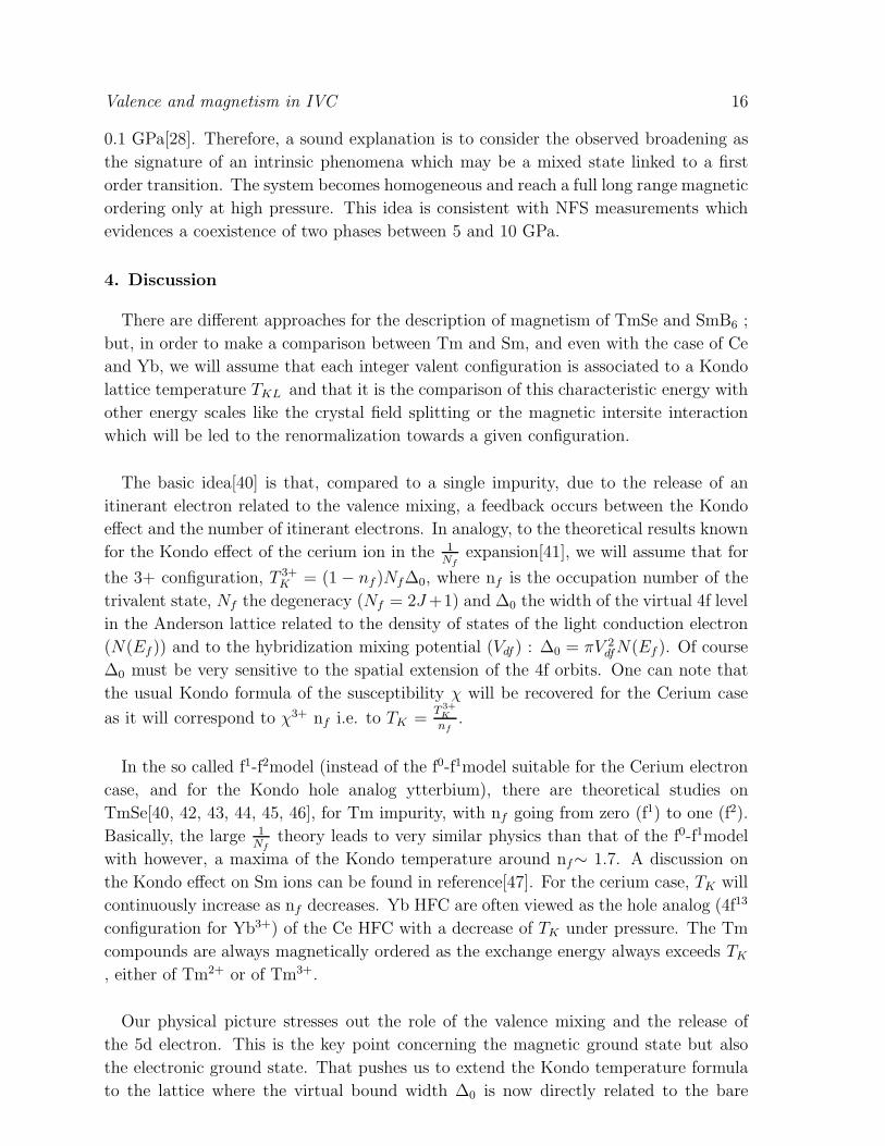
Valence and magnetism in IVC 16
0.1 GPa[28]. Therefore, a sound explanation is to consider the observed broadening as
the signature of an intrinsic phenomena which may be a mixed state linked to a first
order transition. The system becomes homogeneous and reach a full long range magnetic
ordering only at high pressure. This idea is consistent with NFS measurements which
evidences a coexistence of two phases between 5 and 10 GPa.
4. Discussion
There are different approaches for the description of magnetism of TmSe and SmB6 ;
but, in order to make a comparison between Tm and Sm, and even with the case of Ce
and Yb, we will assume that each integer valent configuration is associated to a Kondo
lattice temperature TKL and that it is the comparison of this characteristic energy with
other energy scales like the crystal field splitting or the magnetic intersite interaction
which will be led to the renormalization towards a given configuration.
The basic idea[40] is that, compared to a single impurity, due to the release of an
itinerant electron related to the valence mixing, a feedback occurs between the Kondo
effect and the number of itinerant electrons. In analogy, to the theoretical results known
for the Kondo effect of the cerium ion in the 1Nf
expansion[41], we will assume that for
the 3+ configuration, T 3+K = (1 − nf )Nf∆0, where nf is the occupation number of the
trivalent state, Nf the degeneracy (Nf = 2J +1) and ∆0 the width of the virtual 4f level
in the Anderson lattice related to the density of states of the light conduction electron
(N(Ef )) and to the hybridization mixing potential (Vdf ) : ∆0 = πV 2dfN(Ef ). Of course
∆0 must be very sensitive to the spatial extension of the 4f orbits. One can note that
the usual Kondo formula of the susceptibility χ will be recovered for the Cerium case
as it will correspond to χ3+ nf i.e. to TK =T 3+
K
nf.
In the so called f1-f2model (instead of the f0-f1model suitable for the Cerium electron
case, and for the Kondo hole analog ytterbium), there are theoretical studies on
TmSe[40, 42, 43, 44, 45, 46], for Tm impurity, with nf going from zero (f1) to one (f2).
Basically, the large 1Nf
theory leads to very similar physics than that of the f0-f1model
with however, a maxima of the Kondo temperature around nf∼ 1.7. A discussion on
the Kondo effect on Sm ions can be found in reference[47]. For the cerium case, TK will
continuously increase as nf decreases. Yb HFC are often viewed as the hole analog (4f13
configuration for Yb3+) of the Ce HFC with a decrease of TK under pressure. The Tm
compounds are always magnetically ordered as the exchange energy always exceeds TK
, either of Tm2+ or of Tm3+.
Our physical picture stresses out the role of the valence mixing and the release of
the 5d electron. This is the key point concerning the magnetic ground state but also
the electronic ground state. That pushes us to extend the Kondo temperature formula
to the lattice where the virtual bound width ∆0 is now directly related to the bare

Valence and magnetism in IVC 17
500
0A
rbitr
ary
ener
gy
1.00.80.60.40.20.0 nf
2+ magnetism
3+ magnetism
TmSe TKL2+
TKL3+
∆CF
Figure 17. Comparison of the Kondo lattice temperature and the crystal field spliting
in arbitrary units, in the case of TmSe, for both the 2+ and the 3+ configuration. With
the criteria choosen, long range magnetism is allowed if TKL is smaller than ∆CF .
bandwidth D of the 5d light conduction electrons : ∆0 = αD, with D depending on nf
and α typically of the order of 10−2 in order to recover a narrow virtual bound state for
the impurity. The change of the numbers of carrier will give here D(nf) = D0n2
3
f .
If we apply this rule to TmSe, the Kondo temperature TKL of the trivalent and
divalent configuration in a lattice will be :
• T 3+KL= αD0(1−nf )nf
2
3 N3+f
• T 2+KL= αD0nf
5
3 N2+f
where the degeneracy N3+f and N2+
f are respectevely 13 and 8. Figure 17 represents the
Kondo temperature for the two configurations. A typical value of the overall crystal field
splitting ∆CF has been added to the plot. Of course, a crucial point has been to choose
the ratio between ∆CF and D0 to compare ∆CF with TKL. In order to have a coherent
behaviour, we put αD0
∆CF∼ 4 which correspond to a very small effective bandwidth.
Anyway, if we assume that ∆CF ∼ 100 K[23], αD0 can be nearly the order of magnitude
of 400 K. The different energies has been traced versus nf , varying in the same way as
the pressure. If there is an extra effect as a electron gap, a simple way would be to add
an extra pressure dependence on D (D = 0 for p < p∆).
Extrapolating from the numerous studies performed on Ce HFC, the occurence of long
range magnetism requires at least the recovery of usual rare earth properties, notably
the full reaction to the crystal field splitting i. e. kBTKL < ∆CF . Of course a main
consideration is the relative strength of the intersite exchange interaction and TKL as
discussed for the usual Doniach model. Long range magnetism will occur only if the
energy scale of the coupling is stronger than the Kondo energy. Nevertheless, in our
simple view, we compare only ∆CF and TKL. Therefore, we only indicate when long
range magnetism will be possible. For each configuration, long range magnetism will be

Valence and magnetism in IVC 18
100
0A
rbitr
ary
ener
gy
1.00.80.60.40.20.0 nf
3+ magnetismSmB6
TKL3+
∆CF
Figure 18. Comparison of the Kondo lattice temperature and the crystal field spliting
in arbitrary units, for the 3+ configuration. In the case of SmB6 as only the trivalent
state is magnetic, long range magnetism will be allowed if T3+KL
become smaller than
∆CF .
possible while TKL is smaller than ∆CF ; that means we assume the coupling is already
strong enough. Of course, the position of the intersections are very sensitive to the
ratio ∆CF
αD0. Nevertheless, this basic model explains qualitatively the general shape of the
phase diagram. At low pressure, nf is small, and long range magnetism is due to Tm2+
; then at higher pressure, when nf increases, this long range magnetism disapears and
long range magnetism due to Tm3+ appears. The change of regime observed at 3 GPa
is well reproduced. At this critical pressure, a critical value of nf is reached, where the
renormalization of the wavefunction changes from the 2+ to the 3+ ground state since
the Kondo effect becomes crucial for the Tm2+ ions and is not strong enough for Tm3+.
For Sm Kondo lattice, the previous formula of T 3+KL is plotted in figure 18. Now,
αD0
∆CF∼ 2 is choosen. The interpretation is the same : a magnetic ground state is possible
when its trivalent Kondo lattice temperature (in charge of the long range magnetism
here, since Sm2+ is non magnetic) is low enough compared to a crystal field energy. At
low value of nf the long range magnetism will disappear as the exchange energy will
drop.
The important point is that T 3+KL reaches a broad maxima near nf= 0.4. This is a
critical difference with the Cerium case which correspond to the release of the 4f electron
from the 4f shell : Ce3+ ⇐⇒ Ce4+ + 5d. If no extra electron is considered, one may
find that T 3+KL goes, in Ce case, as T 3+
KL= (1−nf)5
3 αD0Nf (with Nf = 2J + 1 = 6). By
contrast to the previous case, T 3+KL never reaches a maximum in the Ce case. Actually,
this naive scheme gives the correct result that in Ce HFC, TK decreases continuously
with increasing nf .
In those considerations, there is the underlining assumption that the valence
fluctuation can be slow enough to follow the motion of the spin dynamics of the trivalent
configuration even for nf ∼ 0.8 as observed in SmS, SmB6 by NFS or in YbRh2Si2[52].

Valence and magnetism in IVC 19
This suggest that the 4f-5d correlation is a favorable factor to slow down the valence
fluctuation. This consideration lead to propose that SmB6, like SmS, can be regarded in
the low pressure gold phase (p < p∆) as an excitonic dielectric semiconductor with the
electron promoted from f shells spread over the p orbitals of neighboring boron sites but
with the same symmetry as the f electron in the central Sm site[53, 54]. An alternative
idea is that the electron (5d) created by the mixing of the 4f state and the hole produced
in the conduction band screen the 4f hole and form a bound state in a low carrier density
medium[55]. Up to now, there is no consideration on the pressure dependence of the 5d
screening and thus on the disappearance of the reported many body effects. In term of
a Kondo approach, one may think that one way to describe the extra many body effect
is to consider the possibility of the Kondo effect of the 5d electron itself. A many body
treatment will be required, so far its TK (5d) is lower than its crystal field splitting ∆CF
(5d). Of course, TK (5d) will be far greater than TK (4f) but also ∆CF (5d) > ∆CF (4f).
A change will occur under pressure since in all reported cases (Sm3+, Yb3+, Tm3+) their
TK(4f) decrease under p while TK(5d) increase with pressure. When TK(5d)> ∆CF (5d)
there will be no more reason to consider the extra many body effects of the 5d electron
which could be considered then as dissolved in the Fermi sea.
In the case of TmSe, entering in the trivalent state, there are two reasons that the
physics will be dominated by the formation of a magnetic moment on an initial singlet
ground state : the Kondo effect and a probable singlet crystal field level. As pointed
out, the two mechanisms leads to rather similar increase of the sublattice magnetization
under pressure on increasing the intersite exchange coupling. Thus the difference in the
crystal field ground state limits the comparison of TmSe with SmB6 and SmS. However,
let’s emphasize the similarity : up to nf∼ 0.8, the physics appear renormalized to
the divalent configuration, not only governing the magnetic properties, but also the
electronic properties (formation of many body insulating state) ; above nf∼ 0.8 the
physics is now governed by the trivalent configuration (metallic conduction and nature
of the magnetic order parameter).
Microscopic evidence to the 2+ configuration in SmS, SmB6 but even TmSe was given
by inelastic neutron squattering experiments and measurement of the magnetic form
factor[56, 57]. The demonstration of a dressing towards the 3+ configuration for SmS
and SmB6 was done by NFS as both the quadrupolar and dipolar magnetic hyperfine
structure are caracteristic of a 3+ state even for nf ∼ 0.8. Macroscopically, suggestions
of the 2+ renormalization of TmSe at p = 0 comes from the specific heat, and of the
3+ renormalization of TmSe above 3 GPa from its continuity with the quasitrivalent
compound TmS.
Concerning SmS and SmB6 we have to be careful on the coincidence in the appearance
of long range magnetism and closing of the hybridization gap. For SmS, the coincidence
has been found. An extrapolation made from inelastic measurement on Sm0.83Y0.17S

Valence and magnetism in IVC 20
suggests strongly that Sm-Sm exchange interactions play a major role even in the low
pressure gold phase[57]. No similar influence is observed for SmB6 certainly due to
the isolation of the Sm ion with the B cage. The gap is closed as function of pressure
before long range magnetic ordering appears. Typically, the gap is closed between 4
and 6 GPa[34, 36, 35, 37], but long range magnetism do not appear before 8 GPa and
a homogeneous magnetic phase picture without phase separation may occur only above
10 GPa.
Finally, the difference between SmB6 and SmS is not so surprising, as their
band structures are completely different due to symmetries which are different.
Local spin density approximation (LSDA+U approach) were published for Sm
monochalcogenides[58] and SmB6[59]. For SmS, NaCl type crystal structure with the
space group Fm3m, the occupation number nf is found equal to 0.55 (valence v = 2.55)
in the low pressure gold phase, a non zero magnetic moment is always obtained. For
SmB6 , CaB6 type crystal structure with the space group Pn3m, the calculations produce
always an integer valence ground state either divalent or trivalent. A small hybridization
energy gap is recovered in SmB6 for samarium in the divalent state. It was emphasized
that the magnetism of golden SmS as well as the formation of the IV state in SmB6
requires to go beyond this mean field approximation.
5. Conclusion
Ac calorimetry with in situ p variation at low temperature is a powerful technique to
define without ambiguity the magnetic phase diagram under pressure. We hope that
our experimental report may help to experimental progresses.
The common point in the three investigated systems TmSe, SmB6, and SmS[13, 12] is
the link between the electric conduction and the renormalization to divalent or trivalent
configurations at low temperature. Looking more deeply on SmS and SmB6, a main
difference appear between the clear onset of antiferromagnetism at p∆ in SmS and the
large pressure window in SmB6 (6 < p < 10 GPa) where an inhomogeneous behaviour
is observed. A homogeneous magnetic phase occurs in SmB6 only above 10 GPa. It is
amazing to observe that if p∆ = 2 GPa is remarkably reproducible in SmS[13], a large
dispersion appears for SmB6 (around 3 GPa). The next step is to understand the role
of the disorder in SmB6 and the impact on the collapse of the gap and the appearance
of long range magnetism.
Finally by comparison to results on Ce intermetallic heavy fermion compounds, in
these Sm and Tm systems, a long range magnetism characteristic of the trivalent
configuration occurs far below the pressure where the trivalent state will be reached.
This phenomena is quite similar to that observed in YbRh2Si2. Physically, the
interesting fact is that both slow spin and valence fluctuations must interfer.

Valence and magnetism in IVC 21
Aknowledgment
We would like to thank Christophe Marcenat for his precious clarification in the
explanation of the phase behaviour of ac microcalorimetry measurements.[1] J. Flouquet, cond-mat/0501602 (2005)
[2] P. Wachter, Handbook of physics and chemistry of rare earths, Edited by K.A. Gschneider et al.
North holland Amsterdam (1994).
[3] D. Malterre Adv. Phys. 45 299 (1996)
[4] H. Launois, M. Rawiso, E. Holland-Moritz, R. Pott, and D. Wohlleben, Phys. Rev. Lett. 44 1271
(1980).
[5] P. Haen, F. Lapierre, J. M. Mignot, J. P. Kappler, G. Krill and M. F. Ravet, J. Magn. Magn.
Mater. 47-48, 490 (1985).
[6] G. K. Wertheim, W. Eib, E. Kaldis and M. Campagna, Phys. Rev. B 22, 6240 (1980).
[7] W. D. Brewer, G. Kalkowski, G. Kaindl and F. Holtzberg, Phys. Rev. B 32, 3676 (1985).
[8] E. Beaurepaire, J. P. Kappler and G. Krill, Phys. Rev. B 41, 6768 (1990).
[9] J. Rohler et al., in Valence Instabilities, edited by P. Wachter and H. Boppart (North-Holland,
Amsterdam, 1982), p. 215.
[10] C. Dallera, E. Annese, J-P Rueff, M. Grioni, G. Vanko, L. Braicovich, A. Barla, J-P. Sanchez,
R. Gusmeroli, A. Palenzona, L. Degiorgi and G. Lapertot, J. Phys.: Condens. Matter 17 S849
(2005).
[11] N. Ogita, S. Nagai, M. Udagawa, F. Iga, M. Sera, T. Oguchi, J. Akimitsu and S. Kunii, Physica
B 359-361 941 (2005).
[12] A. Barla, J. P. Sanchez, Y. Haga, G. Lapertot, B. P. Doyle, O. Leupold, R. Ruffer, M. M. Abd-
Elmeguid, R. Lengsdorf and J. Flouquet, Phys. Rev. Lett. 92 066401 (2004).
[13] Y. Haga, J. Derr, A. Barla, B. Salce, G. Lapertot, I. Sheikin, K. Matsubayashi, N. K. Sato and J.
Flouquet, Phys. Rev. B 70, 220406 (2004)
[14] A. Barla, J. Derr, J. P. Sanchez, B. Salce, G. Lapertot, B. P. Doyle, R. Ruffer, R. Lengsdorf, M.
M. Abd-Elmeguid and J. Flouquet, Phys. Rev. Lett. 94, 166401 (2005).
[15] M. Ribault, J. Flouquet, P. Haen, F. Lapierre, J. M. Mignot and F. Holtzberg, Phys. Rev. Lett.
45 1295 (1980).
[16] M. Ohashi, N. Takeshita, H. Mitamura, T. Matsumura, T. Suzuki, T. Goto, H. Ishimoto and N.
Mori, Physica B 259-261, 326-328 (1999).
[17] M. Ohashi, N. Takeshita, H. Mitamura, T. Matsumura, T. Suzuki, T. Mori, T. Goto, H. Ishimoto
and N. Mori, J. Magn. Magn. Mater. 226-230, 158-160 (2001).
[18] F. Holtzberg, J. Flouquet, P. Haen, F. Lapierre, Y. Lassailly and C. Vettier, J. of Appl. Phys. 57
(1985) 3152-3153.
[19] B. Salce, J. Thomasson, A. Demuer, J. J. Blanchard, J. M. Martinod, L. Devoile and A. Guillaume,
Rev. sci. Instrum. 71, 2461 (2000).
[20] A. Demuer, C. Marcenat, J. Thomasson, R. Calemczuk, B. Salce, P. Lejay, D. Braithwaite and J.
Flouquet, J. of low Temp Phys, 120 245-57 (2000)
[21] Paul F. Sullivan and G. Seidel, Phys. Rev. 173, 679-685 (1968).
[22] C. Marcenat and M. A. Measson, private communication.
[23] A. Berton, J. Chaussy, B. Cornut, J. Flouquet, J. Odin, J. Peyrard and F. Holtzberg, Phys. Rev.
B, 23 3504 (1981).
[24] A. Berton, J. Chaussy, J. Flouquet, J. Odin, J. Peyrard and F. Holtzberg, Phys. Rev. B, 31 4313
(1985).
[25] T. Fujita, M. Suzuki, T. Komatsubara, S. Kunii, T. Kasuya and T. Ohtsuka, Solid-State-
Communications. Aug. 1980; 35(7): 569-72
[26] R. Shiina, O. Sakai, H. Shiba and P. Thalmeier, J. Phys. Soc. Jpn. 67 941 (1998).
[27] M. A. Measson, These de doctorat, Universite Joseph Fourrier, Grenoble (2005).
[28] J. Thomasson et al. Private communication.

Valence and magnetism in IVC 22
[29] J. M. Mignot, I. N. Goncharenko,P. Link,T. Maysumura and T. Suzuki, Hyperfine interactions
128 (2000) 207-224.
[30] M. Ohashi, N. Takeshita, H. Mitamura, T. Matsumura, Y. Uwatoko, T. Suzuki, T. Goto, H.
Ishimoto and N. Mori, Physica B 281-282, 264-266 (2000).
[31] G. Chouteau, F. Holtzberg, O. Pena, T. Penney and R. Tournier, J. Physique, colloq 40 (1979)
C5-361.
[32] Y. Lassailly, C. Vettier ,F. Holtzberg, J. Flouquet, C. M. E. Zeyen and F. Lapierre, Phys. Rev. B
28, 2880-2882 (1983)
[33] B. Batlogg, H. R. Ott, E. Kaldis, W. Thoni, and P. Wachter, Phys. Rev. B 19, 247-259 (1979).
[34] S. Gabani, E. Bauer, S. Berger, K. Flashbart, Y. Paderno, C. Paul, V. Pavlik and N. Shitsevalova,
Phys. Rev. B, 67 172406 (2003).
[35] V.V. Moshchalkov, I. V. Berman, N.B. Brandt, S. N. Pashkevich, E.V. Bogdanov, E. S. Konovalova
and M. V. Semenov, J. Magn. Magn. Mater. 47-48, 289-291 (1985).
[36] J. C. Cooley, M. C. Aronson, Z. Fisk and P. C. Canfield, Phys. Rev. Lett. 74 9 (1995).
[37] J. Beille, M. B. Maple, J. Wittig, Z. Fisk and L. E. Delong, Phys. Rev. B, 28 12 (1983).
[38] K. V. Tretiakov and S. Scandolo, Journal of Chemical Physics. (2004) 121(22) 11177-82
[39] H. Shimizu, H. Tashiro, T. Kume, S. Sasaki, Phys. Rev. Lett. 86 20, 4568-71 (2001)
[40] J. Flouquet, A. Barla, R. Boursier, J. Derr and G. Knebel, J. Phys. Soc. Jpn. 74 178-185 (2005).
[41] A. C. Hewson, The kondo problem to heavy fermions (Cambridge University Press, Cambridge,
1993).
[42] D.M. Newns and N. Read, Adv in Physcics, 36(6) 799-849 (1987)
[43] N. Read, K. Dharamvir, J. W. Rasul and D. M. Newns, J. Phys. C 19 (1986) 1597.
[44] A. C. Nunes, J. W. Rasul and G. A. Gehring, J. Phys. C 19 (1986) 1017.
[45] Y. Yafet, C. M. Varma and B. Jones, Phys. Rev. B, 32 360 (1985).
[46] T. Saso, J. Magn. Magn. Mater. 76-77, 176-178 (1988).
[47] O. Sakai, Y. Shimizu and T. Kasuya, Prog. Theor. Physics, 108 73 (1992).
[48] J. T. Waber and D. T. Cromer, J. Chem. Phys. 42 (1965) 4116.
[49] H. Harima, private communication.
[50] J. Plessel, M. M. Abd-Elmeguid, J. P. Sanchez, G. Knebel, C. Geibel, O. Trovarelli and F. Steglich,
Phys. Rev. B, 67 180403 (2003).
[51] G. Knebel, V. Glaskov, A. Pourret, P. G. Nicklowitz, G. Lapertot, B. Salce and J. Flouquet,
Physica B 359-361 (2005) 20-22.
[52] J. Sichelschmidt, V. A. Ivanshin, J. Ferstl, C. Geibel, and F. Steglich, Phys. Rev. Lett. 91 156401
(2003).
[53] K. A. Kikoin and A. S. Mishchenko, J. Phys. cond. matt. 7 307 (1995).
[54] S. Curnoe and K. A. Kikoin, Phys. Rev. B, 61 15714 (2000).
[55] T. Kasuya, Europhysics letter 26 277 (1994).
[56] J. M. Mignot and P. A. Alekseev, Physica B 215, 99 (1995).
[57] P. A. Alekseev, J.-M. Mignot, A. Ochiai, E. V. Nefeodova, I. P. Sadikov, E. S. Clementyev, V. N.
Lazukov, M. Braden, and K. S. Nemkovski, Phys. Rev. B, 65 153201 (2002).
[58] V. N. Antonov, B. N. Harmon and A. N. Yaresko Phys. Rev. B, 66 165208 (2002).
[59] V. N. Antonov, B. N. Harmon and A. N. Yaresko Phys. Rev. B, 66 165209 (2002).