Using State Administrative Data to Measure Program Performance

by

Peter R. Mueser University of Missouri-Columbia

Kenneth R. Troske

University of Missouri-Columbia & IZA, Bonn

Alexey Gorislavsky University of Missouri-Columbia

January 2004

We would like to thank seminar participants at European University Institute, Institute for Advanced Studies in Vienna, Oxford University, Tinbergen Institute, University College-Dublin, University of Illinois, University of Oklahoma, University of Zurich, and at the CERP/IZA sponsored conference, “Improving Labour Market Performance: The Need for Evaluation,” Bonn, Germany for comments. We are also especially grateful to Jeff Smith for extensive and helpful comments on an earlier draft of this paper.

Abstract

This paper uses administrative data from Missouri to examine the sensitivity of job training program earnings impact estimates based on alternative nonexperimental methods. In addition to simple regression adjustment, we consider Mahalanobis distance matching and a variety of methods using propensity score matching. In each case, we consider both cross-sectional estimates and difference-in-difference estimates based on comparison of pre- and post-program earnings. Specification tests suggest that the difference-in-difference estimator may provide a better measure of program impact. We find that propensity score matching is generally most effective, but the detailed implementation of the method is not of critical importance. Our analyses demonstrate that existing data available at the state level can be used to obtain useful estimates of program impact.

2

I. Introduction

There has been growing interest on the part of governments in evaluating the efficacy of

various programs designed to aid individuals and businesses. For example, state legislatures in

California, Illinois, Massachusetts, Oregon, and Texas have all mandated that some type of

evaluation of new state welfare programs be undertaken. In addition, the federal government has

required that federally funded training and employment programs administered at the state and

local level meet standards based on participant employment outcomes.

However, the best way for states to conduct evaluations remains an unanswered question.

Early efforts to evaluate the effect of government-sponsored training program such as the

Manpower Development Training Act (MDTA) or the Comprehensive Employment Training

Act (CETA) focused on choosing the appropriate specification of the model in the presence of

nonrandom selection on unobservables by participants in the program (Ashenfelter, 1978; Bassi,

1984; Ashenfelter and Card, 1985; Barnow, 1987; Card and Sullivan, 1988). This research

culminated in the papers by LaLonde (1986) and Fraker and Maynard (1987), which concluded

that nonexperimental evaluations had the potential for severe specification error and that the only

way to choose the correct specification for the model is through the use of experimental control

groups. This led both researchers and policy makers to argue that the only appropriate way to

evaluate government sponsored training and education programs is through the use of

randomized social experiments.

However, recent critiques of social experiments (Heckman and Smith, 1995; Heckman,

LaLonde and Smith, 1999) argue that even randomized experiments have important

shortcomings that limit their usefulness in policy making. They point out that social experiments

3

are seldom implemented appropriately, raising serious questions about whether control groups

are truly random samples. In addition, if one wants to evaluate the long-term impact of a

program, randomized social experiments can be costly to implement since they require

evaluators to collect data from both program participants and nonparticipants over an extended

period of time. Finally, even when properly implemented, estimates of impact based on social

experiments may not be directly relevant for policy makers in deciding whether to create new

programs or to expand existing ones (see also Manski, 1996).

Based in part on these concerns, recent research has begun examining alternative,

nonexperimental methods for evaluating government programs (Rosenbaum and Rubin, 1983;

Heckman and Hotz, 1989; Friedlander and Robins, 1995; Heckman, Ichimura, and Todd, 1997,

1998; Heckman, Ichimura, Smith, and Todd, 1998; Dehejia and Wahba, 1999, 2002; Smith and

Todd, forthcoming). The results from these papers suggest that there is no magic methodology

that will always produce unbiased and useful estimates of program impacts. Instead program

evaluation requires researchers to first adopt a methodology that is suitable for the question they

want to address, second, to perform appropriate specification tests, and finally, to use data that is

appropriate for estimating the parameters of interest. The results from these papers also suggest

that, conditional on having the appropriate set of observable characteristics for both participants

and nonparticipants and the use of appropriate statistical methods, it may be possible to evaluate

government-sponsored training programs using existing data sources. If this is the case, there

are tremendous opportunities for evaluating programs because most states already possess rich

data sets on participants in various state programs that are used to administer these programs, as

well as data on earnings for almost all workers in the state. Thus, it may be possible to evaluate

4

government training programs without resorting to expensive experimental evaluations, while

simultaneously producing estimates of program impacts that are useful for policy makers.

The goal of this paper is to use administrative data from one state, Missouri, to examine

the sensitivity of estimates of program impacts across alternative evaluation methods and

alternative outcome variables. We also examine the sensitivity of our results to the quality of the

data available for analysis. We assess the estimates from different methods by comparing them

to each other, and also by comparing them to estimates of program impacts based on

experimental methods that have been reported in the literature. In addition, we conduct a

number of specification checks of our evaluation methods. The methods we consider are: simple

difference, regression analysis, matching based on the Mahalanobis distance, and matching

based on propensity score. For propensity score matching we also consider a number of

alternative ways to match participants with nonparticipants such as pairwise matching, pairwise

matching with various calipers, matching with and without replacement, matching using

propensity score categories, and kernel density matching. Finally, for each method we present

both cross-sectional and difference-in-difference estimates.

The program we examine is Missouri’s implementation of job training programs under

the federal Job Training Partnership Act (JTPA). Our data on participants come from

information collected by the state of Missouri to administer this program. Our control group

consists of individuals registered with the state's Division of Employment Security (ES) for job

exchange services. Our data on earnings and employment history come from the Unemployment

Insurance (UI) program in the state. These data have a number of features that make them ideal

for use in evaluating government programs. First, they contain very detailed location

5

information allowing us to compare individuals in the same local labor market. Second, they

allow us to identify individuals in our comparison group who are currently participating or who

have recently participated in the JTPA program. Thus, we can avoid the problem of

contamination bias, which occurs when individuals in the comparison group are either current or

recent participants in the program being evaluated.1 Finally, the data on wages and employment

history are being generated by the same process for both participants and nonparticipants.

Results in Heckman, Ichimura, Smith, and Todd (1998) indicate that these factors are critical in

constructing an appropriate nonrandom comparison group. In addition, the data we have from

Missouri are similar to administrative data collected by other states in implementing various

workforce development and UI programs, so it should be possible to use the results from our

study when conducting evaluations of other states’ programs.

Our specification tests suggest that, when we use the difference-in-difference estimator,

we are constructing comparison groups that are very similar to our participant group in terms of

earnings growth, meaning we are comparing individuals who are comparable on relevant

dimensions. In addition, we find that our estimates are insensitive to the method used for

constructing comparison groups, which is exactly what one would expect conditional on having

the appropriate set of observable characteristics for both participants and nonparticipants.

Finally, we find that our estimates of the impact of the JTPA program on earnings are similar to

previous estimates of the effect of JTPA based on data from randomized experiments (Orr, et al.,

1996). While certainly not definitive, these results do suggest that it is possible to evaluate

1 We do not know whether individuals in our comparison sample are participating in other government- sponsored training programs or private training programs. Therefore, there could be other sources of contamination bias.

6

government programs such as JTPA using administrative data that are currently being collected

by most state governments.

The remainder of the paper is as follows. In the next section we discuss the various

methods we use to construct our nonexperimental comparison groups, and section III contains a

discussion of our data. Section IV presents our main results. In Section V we examine the

sensitivity of our results to the quality of the data used in the analysis. Section VI concludes.

II. Methods for Creating Nonexperimental Comparison Groups

Our goal is to estimate the effect of participating in the JTPA program on program

participants. Let Y1 be earnings for an individual following participation in the program and Y0

be earnings for that individual in the absence of participation. It is impossible to observe both

measures for a single individual. If we define D=1 for those who participate, and D=0 for those

who do not participate, the outcome we observe for an individual is

0 1(1 )Y D Y DY= − +

Experimental evaluations employ random assignment to the program, assuring that the

treatment is independent of Y0 and Y1 and the factors influencing them. Program effect may be

estimated as the simple difference in outcomes for those assigned to treatment and those

assigned to the control group. Where D is not independent of factors influencing Y, participants

may differ from nonparticipants in many ways, including the effect of the program, so the simple

difference in outcomes between participants and nonparticipants does not identify program

impact.

7

If we assume that, conditional on measured characteristics, X, participation is

independent of the outcome that would occur in the absence of participation,

Y0 ╨ D | X (1)

the effect of the program on participants conditional on X can be written as

1 0 1 0( - | 1, ) ( | 1, ) ( | 1, ) - ( | 0, )E Y Y D X E Y D X E Y D X E Y D X= = ∆ = = = = (2)

where Y1 - Y0 = ∆Y is understood to be the program effect for a given individual and the

expectation is across all individuals with given characteristics. Matching and regression

adjustment methods are all based on some version of (1). They differ in the methods used to

obtain estimates of E(Y1|D=1, X) and E(Y0|D=0, X).2

Although it is convenient to explicate estimation techniques in terms of a single

population from which a subgroup receives the treatment, in practice treatment and comparison

groups are often separately selected. The combined sample is therefore “choice based,” and

conditional probabilities calculated from the combined sample do not reflect the actual

probabilities that individuals with given characteristics face the treatment in the original

universe. However, the methods used here require only that condition (1) apply in the choice-

based sample. Furthermore, if (1) applies in the population from which the treatment and

comparison groups are drawn, (1) will also apply (in the probability limit) in the choice-based

sample where probability of inclusion differs for treated and untreated individuals, as long as

selection criteria for the two groups do not depend on unmeasured factors.3

2 Where concern focuses on program impact for nonparticipants or other subgroups, a slightly stronger assumption than (1) is required. Normally, it is assumed that both Y0 and Y1 are independent of participation, conditional on X.

3As Smith and Todd (forthcoming) note, because choice-based sampling imposes a nonlinear transformation on the probability of treatment, estimates using the methods outlined

8

Simple Regression Adjustment

The most common approach (e.g., Barnow, Cain and Goldberger, 1980) to estimating

program impact is to assume that the earnings function is the same for participants and the

comparison group. Program impact δ is estimated, along with a vector of parameters of the

linear earnings function, β, by fitting the equation

Y X D eβ δ= + +

where e is an error term independent of X and D. Although this approach can be pursued using

more flexible functional forms, estimates of program impact rely on a parametric structure in

order to compare participants and nonparticipants.

The critical question for regression adjustment is whether the functional form properly

predicts what post-program wages would be for participants if they had not participated. Even

under the maintained assumption that there are no unmeasured factors that distinguish

participants from the comparison group, if most of the comparison sample has characteristics

that are quite distinct from those of the participants, regression adjustment may be predicting

outcomes for participants by extrapolation. If the functional relationships differ by values of X,

the regression function may be poorly estimated. There are no assurances regarding the

direction of the bias for such regression adjustment.

below are not necessarily invariant under alternative choice-based sampling schemes. However, theory does not suggest that estimates based on one sampling scheme dominate another, and in the limit estimates converge.

9

Matching Methods4

Methods that focus more explicitly on matching by X are designed to ensure that

estimates are based on outcome differences between comparable individuals. Where the set of

relevant X variables is small and each has a very limited number of discrete values, it may be

possible to estimate the terms on the right hand side of (2) for each distinct combination of

characteristics. In most cases, there are too many observed values of X to make such an

approach feasible.

A natural alternative is to compare cases that are “close” in terms of X. Several

matching approaches are possible. In the analysis here, we will first consider nearest neighbor

pair matching, in which each participant is matched with one individual in the comparison group,

and where no comparison case is used for more than one match. We also consider variations on

this basic matching technique. We then turn to methods based on grouping cases with similar

measured characteristics.

Mahalanobis Distance Matching

We first undertake pair matching according to Mahalanobis distance. If we specify XN as

the vector of observed values for a participant and XO for a comparison individual, the distance

between them is calculated as,

1( , ) ( ) ( )TM X X X X V X X−′ ′′ ′ ′′ ′ ′′= − −

where V is the covariance matrix for X. Mahalanobis distance has the advantage that matching

will reduce differences between groups by an equal percentage for each variable in X, assuming

4See Rosenbaum (2002) for a general discussion of matching methods.

10

that V is the same for the two groups.5 This ensures that the difference between the two groups

in any linear function will be reduced (Rosenbaum and Rubin, 1985). Friedlander and Robins

(1995) illustrate the use of Mahalanobis distance in program evaluation.

The simplest and most common pair matching approach begins by ordering participants

and the comparison group members randomly. The first participant is matched to the

comparison group member that minimizes M(XN,XO). The matched comparison group member is

then eliminated from the set, and the second participant is matched to the remaining comparison

group member that minimizes M(XN,XO). The process continues through all participants until the

participant or comparison group is exhausted.

One problem with the simple matching procedure is that the resulting matches are not

invariant to the order in which the data are sorted prior to matching. Therefore, we also

considered a modified matching procedure in which we not only compare the distance between

the participant and all comparison group members but also compare the distance for all members

of the comparison group that were previously matched to participants. Here, a prior match is

broken and a new matched formed if M(XN,XO) from the new match is smaller than that of the

previous match. The participant in the broken match is then rematched, in accord with the same

procedure. The advantage of the second procedure is that the results will be invariant to the

ordering of the data.

5 In practice one must estimate V using either the sample of participants or nonparticipants or using a weighted average of the covariance matrices from the two groups. We follow most of the previous literature in estimating V as a weighted average of the covariance matrices from participants and nonparticipants with the weights being the proportion of each group in the data. Calculating V in this manner minimizes sampling error.

11

Of course, if the comparison group contains sufficient numbers of cases with very similar

values on all X, the matching procedure will produce directly comparable groups. In most cases,

however, there remain substantial differences between matched pairs. We try to account for this

in two ways. First, we examine the impact of additional regression adjustment on estimates of

program impact. Second, we drop the one percent of the matches with the largest distance.

Propensity Score Matching

In the combined sample of participants and comparison group members, let P(X) be the

probability that an individual with characteristics X is a participant. Rosenbaum and Rubin

(1983) show that

Y0 ╨ D | X Y Y0 ╨ D | P(X).

This means that if we consider participant and comparison group members with the same P(X),

the distribution of X across these groups will be the same. Based on this “propensity score,” the

matching problem is reduced to a single dimension. Rather than attempting to match on all

values of X, we can compare cases on the basis of propensity scores alone. In particular,

( | ) ( ( | )),PE Y P E E Y X∆ = ∆

where EP indicates the expectation across values of X for which P(X)=P in the combined sample.

This implies that

( | 1) ( | ( )),XE Y D E Y P X∆ = = ∆

where EX is the expectation across all values of X for participants.6 We estimate P(X) using a

logit specification with a highly flexible functional form allowing for nonlinear effects and

6 See Angrist and Hahn (1999) for a discussion of whether propensity score matching is efficient relative to matching on all the Xs.

12

interactions. We first undertake one-to-one matching based on the propensity score using the

methods described in the previous subsection. We also use a refinement of simple matching

where we remove matches for which the difference in propensity scores between matched pairs

exceeds some threshold or caliper. This is referred to as “caliper matching.” In the analysis we

use calipers ranging from 0.05 to 0.2.

We also consider two alternative matching or weighting functions. The first is what we

call matching by propensity score category or strata. Let the kth category or strata be defined to

include all cases with values of X such that P(X)0[P1k, P2

k]. Let Nk′ be the number of participants

within the kth strata, Nk″ the number of individuals in the comparison group within the kth strata,

and N the total number of participants in our sample. Our estimate of the treatment effect within

strata k is given by:

1 2 1 0' "1 1

1 1( ) ( ( ) [ , ])k kN N

K Kk i j

i jk k

E Y E Y P X P P Y YN N

′ ′′

= =

∆ = ∆ ∈ = −∑ ∑ (3)

Our estimated average treatment effect across all strata is then given by:

( ) * ( ).kk

k

NE Y E YN′

∆ = ∆∑ (4)

In choosing P1k and P2

k we follow the algorithm outlined in Dehejia and Wahba (2002). In

particular, we choose P1k and P2

k such that remaining differences in X between participants and

nonparticipants within the strata are likely due to chance.7

7Although we have chosen to present (3) in such a way as to highlight the symmetrical contribution of treatment and comparison cases in the estimation, the average treatment effect specified in (4) is numerically identical to that where the mean for all comparison cases within the specified stratum is taken as the comparison outcome for each treatment case in that stratum. It therefore corresponds to the approach used by Dehejia and Wahba (2002).

13

Our second approach is the kernel matching procedure described in Heckman, Ichimura

and Todd (1997), and Heckman, Ichimura, Smith and Todd (1998). The kernel matching

estimator is given by:

,0 ,1,0

1,1

,0 ,1

1

( ) ( )

1( )( ) ( )

Ci

Ci

iNj ii

jj w

k iT iNi T j i

j w

P X P XY K

bE Y Y

N P X P XK

b

=

∈

=

⎡ ⎤⎛ ⎞−⎢ ⎥⎜ ⎟⎜ ⎟⎢ ⎥⎝ ⎠∆ = −⎢ ⎥⎛ ⎞−⎢ ⎥⎜ ⎟⎜ ⎟⎢ ⎥⎝ ⎠⎣ ⎦

∑∑

∑

where T is the set of cases receiving the treatment and NT is the number of treated cases; Yi,1 and

Xi,1 are dependent and independent variables for the ith treatment case; Yij,0 and Xi

j,0 are

dependent and independent variables for the jth comparison case that is within the neighborhood

of treatment case i, i.e., for which |P(X ij,0)-P(Xi,1)| < bw/2 ; Ni

C is the number of comparison

cases within the neighborhood of i; K(C) is a kernel function; and bw is a bandwidth parameter.

In general, a kernel is simply some density function, such as the normal. In practice, the choice

of K(C) and bw is somewhat arbitrary. In our analysis we experiment with alternative choices of

both and, as we indicate below, our results appear insensitive to our choice.

Additional Issues in Implementing Matching

There are a number of additional choices about how one actually forms a matched

sample, such as the choice of whether to match with or without replacement, the choice of the

number of nearest neighbors, the use of a caliper when matching, and the size of the strata or

bandwidth, that warrant further discussion. The choice among these various options often

involves a trade-off between bias and efficiency. For example, matching with replacement will,

in general, produce closer matches than matching without replacement and therefore will result

in estimates with less bias. However, matching with replacement can also increase sampling

14

error because an individual in the comparison group can be matched to more than one individual

in the treatment group. Similar tradeoffs exist in deciding how many comparison cases to match

with a given treatment case. Using a single comparison case minimizes bias, while using

multiple comparison cases can improve precision. Similarly, a caliper has the effect of omitting

comparison cases that are poorly matched, reducing bias at the possible cost of precision.8

Which methods are appropriate depends on the overlap in the matching variables for the

treatment and the comparison samples; the appropriate matching methodology also is a function

of the quality of the data. To assess the effects these choices have on our estimates, we present

results based on a variety of matching methods. In particular, we present results based on

matching with and without replacement, matching to one, five and ten nearest neighbors, and

matching using several different calipers. We also try a number of alternative bandwidths when

conducting kernel matching. In addition, as we mentioned previously, we present estimates

based on standard matching without replacement, where the match is dependent on the order of

the data, as well as estimates based on modified matching, where the matches are independent of

the order of the data.

For each of the alternative methods for estimating the effect of the program, we construct

two different estimators, a cross-sectional estimator and a difference-in-difference estimator.

The cross-sectional estimator is based on the difference in post-program earnings between the

treatment and comparison samples. The difference-in-difference estimator is based on the

difference for the comparison and treatment samples in the difference between pre- and post-

program earnings. The advantage of the difference-in-difference estimator is that it allows one

8See Dehejia and Wahba (2002).

15

to control for any unobserved fixed individual factors that may affect program participation and

earnings. Therefore, the difference-in-difference estimator is more likely to meet the assumption

underlying matching that the determinants of program participation are independent of the

outcome measure once observable characteristics are accounted for. The disadvantage of the

difference-in-difference estimator, particularly in this setting, is that if there are any transitory

shocks to pre-program earnings that affect program participation, this could bias the difference-

in-difference estimator. Problems of estimating program effect in the presence of the now

famous “Ashenfelter dip,” where earnings for participants fall shortly before participation,

illustrates the potential bias. Since the Ashenfelter dip is a transitory decline in earnings, later

earnings are expected to increase even in the absence of intervention. If pre-program earnings

are measured during the Ashenfelter dip, the difference-in-difference estimator will produce an

upward biased estimate of the program’s impact. Therefore, when measuring pre-program

earnings we will try to do so prior to the onset of the Ashenfelter dip.

Matching Variables

The assumption that outcomes are independent of the treatment once we control for

measured characteristics depends critically on the particular measured characteristics available.

Any characteristic that is associated both with program participation and the outcome measure

for nonparticipants, after conditioning on measured characteristics, can induce bias. It has long

been recognized that controls for the standard demographic characteristics such as age, education

and race are critical. Labor market experience of the individual is also clearly relevant. Where

program eligibility is limited, factors influencing eligibility have usually been included as well.

LaLonde (1986) includes controls for age, education, race, employment status, prior earnings,

16

and residency in a large metropolitan area, as well as prior year AFDC receipt and marital status,

measures associated with eligibility in the program.

Several recent analyses (Friedlander and Robins, 1995; Heckman and Smith, 1999) have

stressed the importance of choosing a comparison group in the same labor market. Since it is

almost impossible to choose comparison groups in the same labor market as participants when

drawing comparison groups from national samples, approaches that use these data are unlikely to

produce good estimates, even if they are well matched on other individual characteristics. There

is also a growing recognition that the details of the labor market experiences of individuals in the

period immediately prior to program participation are critical. In particular, movements into and

out of the labor force and between employment and unemployment in the 18 months prior to

program participation are strongly associated with both program participation and expected labor

market outcomes (Heckman, Ichimura and Todd, 1997; Heckman, Ichimura, Smith and Todd,

1998; Heckman, LaLonde and Smith, 1999).

Finally, Heckman, Ichimura and Todd (1997) have argued that differences in data

sources, resulting from different data collection methods, are an important source of bias in

attempts to estimate program impact using comparison groups.

III. The Data This project uses administrative data deriving from three sources. We draw our sample

of program participants from records of Missouri's JTPA program. We draw our comparison

group sample from job exchange service records maintained by Missouri's Division of

Employment Security (ES). The final data source is wage record data from the Unemployment

17

Insurance programs in Missouri and Kansas. Using these data we obtain both pre- and post-

enrollment earnings and information on labor force status prior to enrollment for both

participants and nonparticipants.

The JTPA data comprise all individuals who apply to and then enroll in the JTPA

program. The data include basic demographic and income information collected at the time of

application that is used to assess eligibility, as well as information about any subsequent services

received. Our initial sample consists of all applicants in program years 1994 (July 1994 through

June 1995) and 1995 (July 1995 through June 1996) who are at least 22 years old and less than

65 and who subsequently enroll in the Title IIa program. We focus on participants 22 years old

and older because younger individuals are eligible for the youth program, which is governed by a

different set of rules. Participants in Title IIa are eligible to participate in the JTPA program

because they are judged to be economically disadvantaged.9 We focus on these participants

because they are a fairly homogeneous group and because they have been the focus of previous

evaluations of JTPA using experimental data (e.g., Orr, et al., 1996). Finally, we eliminate

records with invalid values for our demographic variables (race, sex, veteran status, education,

and labor force status).10 Our final sample consists of 2802 males and 6393 females.

Our Employment Security (ES) data include all individuals who applied to the ES

employment exchange service in program years 1994 and 1995. With some exceptions,

individuals who receive Unemployment Insurance payments in Missouri were required to

9 JTPA also serves Title III participants, who are eligible for the program because they were displaced from their previous jobs.

10 We eliminate around 10 percent of the original sample because of invalid or missing demographic variables.

18

register with ES during this period, although it is not clear how strictly this requirement was

enforced. In general, ES employment services were not very intensive. Assistance could take a

variety of forms such as providing access to a list of job openings in an area, helping individuals

prepare resumes, referring individuals to jobs, or referring individuals to other agencies for more

extensive services. All residents of Missouri were eligible to receive the basic ES services such

as access to the list of job openings or assistance in preparing a resume. During the time of our

sample almost every individual who wanted to obtain services from ES applied at one of the

Employment Security offices located around the state.11 The ES data contain basic demographic

and income information obtained on the initial application, as well as information about

subsequent services received.

When selecting our ES sample we chose individuals who were at least 22 and less than

65 years old and were deemed economically disadvantaged. Since the ES program used the

same criteria to determine whether someone was economically disadvantages as the JTPA

program, all of our ES participants should be eligible to participate in the JTPA program. In

addition to these criteria we also chose ES participants who were not enrolled in JTPA in the

program year. We further eliminated records with missing or invalid demographic variables.12

Our final sample consists of 45,339 males and 52,895 females.

The pre-enrollment and post-enrollment earnings for both our JTPA and ES samples

come from the Unemployment Insurance (UI) data. These data consist of quarterly files

11 Subsequently many of these services became available on-line so individuals no longer needed to go into an ES office and register before obtaining services.

12 Approximately 10 percent of the original ES sample was eliminated due to missing or invalid demographic variables.

19

containing earnings for all individuals in Missouri and Kansas employed in jobs covered by the

UI system.13 Both the JTPA and ES data are matched to the UI data using Social Security

Number (SSN). If we are unable to match an SSN to earnings data in a quarter, we considered

the individual not employed in that quarter and set earnings equal to zero.

Using these earnings data, we determined total quarterly earnings from all employers for

individuals in the eight quarters prior to participation, in the quarter they begin participation, and

in the subsequent eight quarters. For our cross-sectional estimator we use post-program earnings

measured as the sum of earnings in the fifth through the eighth quarters after the initial quarter of

participation. For our difference-in-difference estimator, we measure the difference between the

sum of earnings in the fifth through the eighth quarters after the initial participation quarter and

the fifth through the eighth quarters prior to the initial quarter of participation. As Ashenfelter

and Card (1985) note, taking differences for periods symmetric around the enrollment quarter

assures that the difference-in-difference estimator is valid in the case where there is

autocorrelation in the transitory component of earnings. In order to capture the dynamics of

earnings immediately prior to participation, we also control for earnings in the first through the

fourth quarters prior to the initial quarter of participation.

Previous research (Heckman and Smith, 1999) found that the dynamics of an individual’s

prior labor market status is an important determinant of both program participation and

subsequent earnings. We capture these dynamics using a series of four dummy variables. From

both the JTPA and ES data we know whether an individual is employed at the time of

13 Inclusion of Kansas wage record data is valuable since a substantial number of Missouri residents in Kansas City and surrounding areas work in Kansas. The number of Missouri residents commuting across state lines is not significant elsewhere in the state.

20

enrollment. From the UI data we know whether an individual is employed in each of the eight

quarters prior to enrollment. For an individual employed at the time of enrollment, we coded the

transition as not employed/employed if earnings were zero in any of the eight quarters prior to

enrollment and coded it as employed/employed if earnings in every quarter were positive. An

individual not employed at the time of enrollment was coded employed/not employed if earnings

were positive in any of the prior eight quarters and not employed/not employed otherwise.

Previous research has also found local labor market conditions to be an important

determinant of program participation (Heckman, Ichimura, Smith and Todd, 1998). We capture

this effect by including a dummy variable for the Service Delivery Area (SDA) where an

individual lives.14

Our measure of labor market experience is defined as:

Experience = Age - Years of Education - 6.

We also include dummy variables indicating whether someone was employed in each of the four

quarters prior to participation, to capture labor market experience immediately prior to

participation. Someone is considered employed in a quarter if earnings are greater than zero.

Table 1 presents summary statistics for our JTPA and ES samples separately for males

and females. For most of the demographic variables the two samples are similar.15 However,

14 Under JTPA, there were 15 SDAs in Missouri, each overseen by a Private Industry Council, with representatives from both the local private and public sectors. In general, SDAs are structured to identify labor market areas, corresponding to metropolitan areas and to relatively homogeneous collections of contiguous counties elsewhere. Under the Workforce Investment Act, which replaced JTPA, 13 of the 15 regions remain as administrative units, whereas two of the SDAs were combined.

15 We have modified both the occupation and education variables to ensure that they are comparable across the two files. The details of the modifications we made are provided in the Data Appendix.

21

looking at the labor market transition variables we see that JTPA participants are much more

likely to be not employed over the entire eight quarters prior to beginning participation. Looking

at earnings we see that mean post-enrollment earnings are similar for the two samples but that

mean pre-enrollment earnings are lower for JTPA participants, particularly for female

participants. The numbers in Table 1 demonstrate that there are differences in the JTPA and ES

samples, particularly in earnings and employment dynamics prior to participation. This suggests

that we need to account for these differences when estimating the impact of program

participation on JTPA participants.

One of the conclusions reached by Heckman, LaLonde, and Smith in their chapter on

program evaluation in the Handbook of Labor Economics (Heckman, LaLonde, and Smith,

1999) is that "better data help a lot" (pg. 1868) when evaluating government-sponsored training

programs. The most important criteria they mention are that outcome variables should be

measured in the same way for both participants and non-participants, that members of the

treatment and comparison groups should be drawn from the same local labor market, and that the

data should allow one to control for the dynamics of an individual's labor force status prior to

enrollment. Since our data meet all of these criteria, we feel they are ideal for examining the

impact of government-sponsored training programs.16 An additional advantage that we should

mention is that Missouri is not unique. Almost every state in the union collects similar

administrative data. Therefore, the type of analysis we perform could be conducted for other

16 Our data are somewhat limited in this latter criterion in that we are only able to identify the transition between working and not working as opposed to identifying the transition between employed, unemployed, and out of the labor force.

22

states as well. We next turn to examining the effects of alternative methods for constructing

comparison groups on the estimated impact of treatment.

IV. Estimates of Program Effects Using Alternative Methods to Form Comparison

Groups Specification Analysis

Before presenting our estimates of the effect of the JTPA program on participants, we

want to compare our various treatment and control samples and present the results from

specification tests in order to assess whether our matching methods produce valid comparison

samples. In this analysis we will focus on two variables, the sum of individual earnings in the

eighth through the fifth quarters prior to beginning participation–what we call pre-program

earnings–and the difference in earnings between the fifth and eighth quarters prior to beginning

participation–what we call the growth in pre-program earnings. Our matching and adjustment

procedures are based on individual demographic characteristics, and employment and earnings in

the year prior to program enrollment, but our measure of pre-program earnings is not explicitly

controlled in any of these approaches. Analysis of these earnings can therefore provide a

specification test for our models. In particular, testing for differences between pre-program

earnings for our treatment and comparison samples represents a formal test of our cross-sectional

estimator (Heckman and Hotz, 1989). Testing for differences in the growth in pre-program

earnings, although not a formal specification test, does provide some evidence on whether we

have formed appropriate comparison samples for our difference-in-difference estimator.

Figure 1 plots quarterly earnings for our entire sample of JTPA and ES participants for

the eight quarters prior to enrollment, the quarter of enrollment, and the eight quarters after

23

enrollment. Earnings are plotted separately for men and women. Similar to Table 1, Figure 1

shows that JTPA and ES participants have very different earnings dynamics both prior to and

after beginning participation. Prior to participation, the ES sample has much higher earnings

levels and earnings growth than the JTPA sample. In addition, the Ashenfelter dip is present in

both samples, although at somewhat different times. For the JTPA sample, quarterly earnings

begin to decline four quarters prior to participation, whereas for ES participants earnings begin

to decline one quarter prior to participation. The fact that earnings begin to decline four quarters

prior to participation for JTPA participants is primarily why we measure pre-program earnings in

the eighth through the fifth quarters when constructing the difference-in-difference estimator.

Figure 2 presents the same information as Figure 1 for our treatment and comparison

samples created by matching on the Mahalanobis distance. For each participant in the JTPA

sample, we choose a case from the comparison file for which the Mahalanobis distance is at its

minimum, yielding a paired file. This pair matching method ensures that if there is at least one

individual in the comparison sample that is similar on all values to each participant, the resulting

matched comparison group will display the same variable distribution.17 In calculating the

Mahalanobis distance, the characteristics in XN and XO include education, race, prior experience,

occupation (nine categories), our measures of employment status dynamics prior to enrollment

(three dummy variables), dummy variables for whether an individual lived in either the St. Louis

or Kansas City SDA, earnings for the four quarters prior to enrollment, and dummy variables

indicating whether an individual was employed in each of the four quarters prior to enrollment.

The figure shows that while matching has produced a comparison sample with mean

17 The matching method used here is that described by Rosenbaum and Rubin (1985). We describe it in detail above.

24

earnings prior to participation that are closer to the mean earnings of the treatment sample, they

are still not identical. However, it does appear that the treatment and comparison samples

experience similar growth in earnings prior to participation. Also, the timing of the Ashenfelter

dip corresponds more closely for these two groups, although earnings begin falling one or two

quarters earlier for JTPA participants and the decline in earnings is smaller for ES participants.

The fact that earnings in the four quarters prior to participation are higher for ES participants is

surprising since these earnings are included in the X vector used for matching. This suggests that

Mahalanobis distance matching may fail to select a comparison group that corresponds closely

even on the variables that are used in the matching process. We will see below that propensity

score matching is generally more effective.

One of the advantages of propensity-score matching is that the propensity score provides

a simple measure to compare the overlap between the treatment and comparison samples.

Properly estimating the effect of a program requires one to compare comparable individuals,

which will occur only when the two samples have common support. In addition, the amount of

overlap between the treatment and control sample determines the appropriate method to use

when matching the treatment and comparison sample and will affect the quality of the resulting

match. Figure 3 presents the distribution of propensity scores for both the JTPA and ES

participants, separately for males and females. To estimate the propensity score we use a logit

function to predict participation in the sample combining the JTPA and ES samples. In addition

to the variables used when matching based on Mahalanobis distance, we tested nearly 300

25

interactions between these variables, using a stepwise procedure to enter all interactions that

were statistically significant at the 5 percent level.18

While Figure 3 shows that a larger percentage of ES participants have a propensity score

between 0.0 and 0.1, the overlap between ES and JTPA participants spans the entire range from

0.0-1.0. This suggests that, conditional on the assumptions of propensity score matching, it will

be possible to form samples of comparable individuals. The large overlap between the ES and

JTPA samples also suggests that it will be possible to produce close matches using matching

without replacement. This is why we have chosen to focus on matching without replacement in

our subsequent analysis.

Figure 4 provides evidence on the comparability of our samples matched using the

propensity score. This figure plots quarterly earnings both prior to and after the initial quarter of

participation for our treatment and comparison samples.19 We see that matching using

propensity score produces samples of JTPA and ES participants with similar pre-program

earnings dynamics. Comparing Figures 2 and 4 shows that, relative to matching using

Mahalanobis distance, matching using propensity score produces samples that match more

closely on earnings in the four quarters immediately prior to participation. Since these variables

are used in both matching procedures, this suggests that propensity score matching is more

effective in practice. However, it is still the case that there are differences in pre-program

earnings (earnings in the fifth through eighth quarters prior to participation), particularly for

males.

18 The results from these logit estimations are available from the authors upon request.

19 These samples are formed using standard matching without a caliper. Further details on alternative matching procedures are provided below.

26

Figure 5 plots earnings for a sample of JTPA and ES participants matched using the

propensity score and applying a caliper of 0.1. In caliper matching we form optimal matches but

then break any matches that are larger than the caliper value. Figure 5 shows that caliper

matching produces samples that are very closely matched on earnings in the four quarters prior

to the treatment, although there is still a difference in the level of pre-program earnings (the fifth

through eighth quarters prior to participation) between the treatment and comparison samples.

Of course, pre-program earnings are not used in the matching procedure, so this difference is not

due to a technical shortcoming in the matching method.

Table 2 presents results from a more formal analysis of the difference in pre-program

earnings levels and the difference in the growth in pre-program earnings between our treatment

and comparison samples. The rows labeled “No regression adjustment” present the mean and

standard error of the difference in either pre-program earnings level or the growth in preprogram

earnings between our treatment and comparison samples. The rows labeled “Regression

adjustment” present the coefficients and standard errors from a linear regression model where we

include a dummy variable which equals one if an individual participated in JTPA. Controls in

the model include the standard demographic variables (race, sex, experience, experience

squared, and veteran status), years of education, along with a dummy variable identifying high

school graduates and an additional term capturing years of schooling beyond high school,

earnings in each of the four quarters prior to participation, dummy variables indicating whether

the person worked in each of the four quarters prior to participation, our employment transition

variables, nine occupation dummy variables, 15 dummy variables for each of the SDAs, and

27

eight dummy variables indicating which calendar quarter an individual entered either the JTPA

or ES program.20

The results in Table 2 summarize what we have seen in Figures 1-2 and 4-5. Without

controls, JTPA participants have appreciably lower earnings in the prior year (fifth through

eighth quarters prior to enrollment), but using regression adjustment or any of the matching

procedures causes the difference to reverse. The differences in pre-program earnings for

treatment and comparison samples are statistically significant (in the range of $800 for males and

$400 for females) for all methods used. This suggests that there are differences between

treatment and control groups that are not captured through matching or the controls in our

regressions. As a result, the cross-sectional model based on post-program earnings may be

misspecified, and so, in essence, it may not be comparing comparable individuals.

However, the results in Table 2 also show that there are much smaller differences--

differences that are in some cases not statistically significant--between our treatment and

comparison samples in the growth of pre-program earnings. While not a formal specification

test, these results do suggest that the unobserved difference between individuals in the treatment

and comparison samples may be largely fixed over time and will be captured in our difference-

in-difference specification. This, in addition to the fact that we measure pre-program earnings

before the onset of the Ashenfelter dip, makes us optimistic that our difference-in-difference

estimator may produce unbiased estimates of the effect of the program on participants.

20 These are the control variables we use throughout the paper when we are estimating any linear regression.

28

Estimates of Program Effects without Matching

We start by considering the mean differences in earnings between our sample of JTPA

and ES participants. The mean difference in post-enrollment earnings between these two

samples, as well as the mean difference in the difference between pre- and post-enrollment

earnings of the two samples are presented in line 1 of Table 3. Earnings differences between

JTPA and ES are small and not statistically significant for either men or women. In contrast,

males in the JTPA sample have almost a $1100 greater increase in earnings relative to ES

participants, while females in JTPA experience a $1500 greater increase in earnings. Given the

results presented in Table 2, as well as the differences across groups in the mean values for other

characteristics seen in Table 1, these earnings differences are very likely influenced by

differences in pre-program characteristics.

Line 2 of Table 3 presents adjusted estimates of program effects based on the simple

linear regression model. The structure of these regressions and the control variables included are

described in the previous section. The coefficient estimates for the control variables are reported

in Table A1 in the appendix. These coefficients generally correspond to expectations.

There are substantial differences between our cross-sectional and difference-in-difference

estimates of program impact. For men the cross-sectional estimate is nearly $1500, while the

difference-in-difference estimate is only about $630. For females, the cross-sectional estimate is

just under $1100, while the difference-in-difference estimate is about $700. The results in Table

2 suggest that, even after regression adjustment, the cross-sectional estimate is based on a

misspecified model. The differences in the two estimates could well be the result of unobserved

differences between the two groups.

29

As noted above, the critical question is whether regression adjustment is properly

estimating what earnings would be in the absence of participation. Our large comparison sample

has important advantages, but it also entails risks of misspecification. The estimated functional

relationships will be largely determined by the comparison sample, and if values of control

variables differ dramatically for participants, their potential earnings may be incorrectly

estimated.

Mahalanobis Distance Matching

One natural approach is to choose a selection of cases from the comparison group that

have similar values to those of participants. One measure of similarity is the Mahalanobis

distance metric. Line 3 of Table 3 shows our estimates of the program effects using the

comparison sample formed by matching using the Mahalanobis distance. Comparing the cross-

sectional estimates with the difference-in-difference estimates we again see that the difference-

in-difference estimates are much smaller.

Line 4 of Table 3 presents our estimates of the effect of the program on participants using

the matched samples and our basic linear regression model. To the extent that matching

eliminates differences in the Xs between the two samples, the estimates in lines 3 and 4 should

be the same. While the estimates are similar for females, the regression produces a different

estimate for males, suggesting that matching based on the Mahalanobis distance is not producing

a sample with the same distribution of Xs as the treatment sample. This is consistent with Figure

2, where we saw differences in the level and growth of earnings immediately prior to

participation.

30

Line 5 in Table 3 presents our estimates based on our comparison sample matched using

the Mahalanobis distance and our modified matching method. As we discussed above, when

using the standard matching algorithm, the resulting matched sample depends on the order of the

original data, whereas this is not the case with our modified matching algorithm. Line 6 presents

results based on a comparison sample created by using the standard matching algorithm but then

dropping one percent of the sample with the largest Mahalanobis distance. Comparing the

estimates in lines 3, 5 and 6 shows that all of these techniques produce similar estimates.

Propensity Score Matching

Matching cases on the basis of propensity score promises substantial simplification as

compared with any general distance metric. The theory assures us that the distribution of

independent variables will be the same across cases with a given propensity score, even when

values differ for a particular matched pair.

As we indicate above, our estimate of P(X) is based on a logit model. For each case the

predicted value from our estimated logit function provides an estimate of P(X). Table 4 presents

our estimates of the program effects using a variety of methods for creating comparison samples

based on P(X). Since standard formulas for estimating standard errors do not reflect the fact that

our samples are matched using P(X), which is measured with error, all estimates of the standard

errors are estimated using bootstrapping.21 Lines 1 and 2 of Table 4 present estimates based on

comparison samples created using standard pair matching without replacement and without a

caliper. Line 1 presents estimates without regression adjustment, while line 2 presents our

estimates that correct for any difference between treatment and matched samples based on our

21 We estimate standard errors using a bootstrap procedure (100 replications) whenever our estimates are based on propensity score matching.

31

linear regression model. Comparing the estimates in line 1 based on post-program earnings with

the difference-in-difference estimates again shows that these estimates are significantly different.

Since our previous analysis suggests that the cross-sectional estimates are based on a

misspecified model, we focus on the difference-in-difference estimates.

Comparing the regression adjustment estimates to the estimates in line 1 shows that

regression adjustment has very little impact on the estimates. This is what one would expect if

the matching was successful. These results show that the propensity score matching method is

more successful than the Mahalanobis distance matching in creating an appropriate comparison

sample.

Caliper matching differs from standard matching in that only matches within a specified

distance are permitted, so not all treatment participants may be matched. Lines 3-6 show how

our estimates differ when the caliper is set to 0.05, 0.1, and 0.2, respectively. The numbers in

brackets show the number of cases in the treatment sample that are matched. In the full JTPA

sample (after deletions of cases with missing data) there are 2802 males and 6395 females.

Looking at the size of the sample when we impose the 0.05 sample, which is the most stringent

caliper, shows that the sample size does not drop by very much. Even without imposing a

caliper we are matching individuals with similar values of P(X). Comparing our estimates in

lines 3-6 with our estimates in line 1 shows that imposing a caliper has very little effect on our

estimates of the program effect.

Comparing Pair Matching Algorithms

The matching algorithm used in the above analysis is the standard pair matching

procedure. As we discussed in the previous section, we also consider a modified matching

32

procedure that produces matched samples that are insensitive to sample ordering and should

increase the quality of the final matches. In searching the comparison sample to find a match,

this alternative procedure not only compares unmatched cases but also previously matched cases,

breaking previous matches if the new match distance is smaller.

Table 4 lines 7 and 8 present results using this alternative matching technique. The

average difference in propensity scores between matched pairs was often appreciably smaller

when this alternative was used. Nonetheless, it is clear that the effect of this alternative

matching algorithm is small relative to estimated standard errors. This reflects the fact that

although this method often selects a different comparison case to be matched with a particular

treatment case, there is little impact on the overall comparison sample.

Matching with Replacement

Matching without replacement works well when there is sufficient overlap in the

distribution of P(X) between the treatment and comparison sample to ensure close matches. In

cases where there is not sufficient overlap researchers often use matching with replacement,

where an individual in the comparison sample can be matched to more than one person in the

treatment sample. In order to examine the sensitivity of our estimates to this alternative

matching strategy we have constructed matched samples using matching with replacement. We

have also matched each person in the treatment sample to one, five, and ten nearest neighbors in

the comparison sample. Our estimates based on these samples are presented in lines 9-11 in

Table 4. Comparing these estimates with the estimates reported in line 1 again shows that this

alternative matching method produces estimates that are quite similar to our original estimates.

Equally important, standard errors are not substantially different across methods.

33

Matching by Propensity Score Category

All of the pair matching approaches described above have the important disadvantage

that they require that we discard comparison group members who are not matched. In one-to-

one matching, only one case from the larger sample can be used for each case in the smaller

sample, resulting in an immediate loss of information. Where the distribution of participants and

the comparison groups differ dramatically, either the matches will be poor, or, if a caliper is

applied, additional cases will be lost.

Group matching relaxes the requirement that the two groups be matched on a one-to-one

(or one-to-N) basis. In those regions of the data where there are some participants and some

comparison group members, group matching allows us to use all the data. The only cases that

must be discarded are those for which there are no similar cases in the other group. The

approach we use is closely modeled on that recommended by Dehejia and Wahba (2002) and is

described in section II.

In order to ensure that the propensity ranges were sufficiently small, we calculated the

mean differences on our primary independent variables between participant and comparison

groups within a propensity category. We first considered uniform propensity categories of size

0.1. However, given the large number of cases with propensity values less than 0.1, we found

that differences in our basic variables within this the lowest group were often statistically

significant. We ultimately created much smaller category widths at the lower end of the

propensity distribution, corresponding approximately to deciles in the distribution of the

combined sample.

34

The estimated program effects based on this approach are listed in Line 12 of Table 4.

The estimates are quite similar to our initial estimates although the standard errors are smaller.

Kernel Density Matching

The estimates based on propensity score categories use estimates of E(∆Y*P) that are

simple sample averages that combine cases with similar values of P. Following an approach

outlined in Heckman, Ichimura and Todd (1997, 1998) and Heckman, Ichimura, Smith and Todd

(1998), we employ a kernel density estimator to calculate the density of the propensity score and

the means for post-program earnings by propensity score for participants and the comparison

group.22 In forming our estimates we experimented with a variety of kernels and we considered

bandwidths from 0.01 to 0.11. We found that the choice of kernel and bandwidth made little

difference in our estimates. Therefore, we report estimates based on a Epanechnikov23 kernel

using a bandwidth of 0.06. The results are reported in Line 13 in Table 4. These estimates are

again similar to the other estimates reported in Table 4.

Summary of Estimated Program Effects

Table 5 presents selected estimates from Tables 3 and 4. We see that, in each case, the

estimate based on Mahalanobis distance is the smallest one reported in Table 5, and usually the

difference between this estimate and others is appreciable. Recall that results presented in

22 Heckman, Ichimura and Todd (1997) and Heckman, Ichimura, Smith and Todd (1998) recommend using local linear regression matching, which is similar to kernel matching but, given the distribution of their data, has preferable properties. We tried local linear regression matching but, given the size of our samples, it was extremely time consuming to implement. In addition, the results we obtained with this approach were similar to the results obtained using kernel density matching, so we choose to focus on the results from the kernel density matching.

23For a discussion of the properties of the Epanechnikov kernel and a comparison with alternatives, see Silverman (1986).

35

Figure 2 suggested that Mahalanobis distance matching was not successful in producing samples

that were comparable on the measures used for matching. Looking at the other methods that

control for independent variables, we see that the range of estimates is moderate. Estimates

differ by a maximum of about 30 percent, and in no case is the difference as great as two

standard errors. Overall, the results in Table 5 show that, with the exception of Mahalanobis

distance matching, which we have found does not effectively control independent variables,

estimates of program effect on participants are relatively insensitive to the methods used to form

comparison groups and weight the data.

As we have noted previously, our specification tests in Table 2 show that cross-sectional

estimates are likely to be biased, as they depend on comparison between individuals whose pre-

program earnings differ. However there is evidence in Table 2 suggesting that once individual

fixed effects are removed, earnings patterns are similar, so that difference-in-difference estimates

may be valid. Among the difference-in-difference estimates (omitting lines 1 and 3), we see

that, for men, our estimates range from a low of $628 to a high of $856. For women the

estimates range from $693 to $892.

Comparison with Previous Estimates of Treatment Effects Based on Randomized Control

Groups

Table 6 compares our estimated program effects for enrollees with those reported in Orr

et al. (1996, p. 107, Exhibit 4.6), which are based on an experimental evaluation of the JTPA

program.24 The Orr et al. estimates are for individuals who entered JTPA from November 1987

24 The estimates reported by Orr et al. (1996) include an adjustment for the fact that some of those assigned to treatment never enrolled. Since our data pertain to enrollees, this is the appropriate estimate for comparison.

36

through September 1989 at 16 sites nationwide. We have adjusted their estimates for inflation so

that they are comparable to ours. Since our estimates are for months 13-24 after assignment, we

present the Orr et al. estimates for months 7-18 and months 19-30 after assignment. Comparing

our estimates for men with the Orr et al. estimates shows that our estimates lie between theirs.

For women our estimates are below those reported by Orr et al. but the difference is not

generally statistically significant. Our estimates based on nonexperimental data appear similar to

the estimates produced using experimental data for the earlier cohort of JTPA recipients.

V. Robustness of Results to Limitations in Data Quality

The results reported in the previous section–especially those based on a difference-in-

difference specification–suggest that program effect estimates are robust to alternative methods

of matching and weighting the data. In this section we examine the sensitivity of our results to

the quality of the data used to perform the analysis. We will focus on two key aspects of data

quality, the observable characteristics for participants, and the size of the treatment and

comparison samples.

Sensitivity of Results to Observable Characteristics

We begin by examining the robustness of our results to changes in the characteristics

available for individuals. We will examine this by dropping variables from our analysis that

previous researchers have found to be important when estimating program effects (see Heckman,

LaLonde and Smith, 1999). The variables we will drop are our variables measuring employment

transitions prior to entering the program, the SDA dummy variables, which capture an

individual’s local labor market, and the variables measuring employment status and earnings in

37

the four quarters prior to participation. We will focus on estimates produced from treatment and

comparison samples that are matched using propensity score matching with a 0.1 caliper.25 For

this analysis, when we drop a set of variables, we reestimate the propensity score without those

variables in the logit regression. Next we match the treatment and comparison sample using the

new P(X). We then compute the estimates using the new matched sample. We also drop the

variables from any subsequent regression adjustment.

The results from this analysis are presented in Table 7. The first five lines of the table

present estimates with no regression adjustment while lines 6-10 present results based on our

linear regression model. The estimates in lines 1 and 6 are identical to the estimates found in

lines 4 and 5 in Table 4 and are repeated here for ease in comparison.

The largest change is observed in the estimate based on the cross-sectional model for

males. When the four quarters of prior earnings are no longer controlled, the estimate declines

by nearly two-fifths (compare lines (1) and (4)). Although dropping these variables also causes a

decline in the estimate for females, the decline is less than half as large. Other changes are much

smaller. Of interest is that dropping SDA has only a modest effect on estimates, but since our

sample is limited to a single state, it may well be that labor market could be of substantial

importance in the kinds of national samples used in many studies of program impact (cf.,

Friedlander, et al. 1997) .

The difference-in-difference estimates are not generally as sensitive to dropping any of

these variables, but there are some shifts. One surprising result is that, for men, dropping the

employment transition variables alone has a fairly large effect on the estimate, but dropping all

25 We use the standard pair matching algorithm without replacement.

38

three sets of variables produces estimates that are not substantially different from estimates

produced controlling all of the variables. The pattern is different for women, since dropping all

three classes of variables has the largest impact, increasing estimated effects by about 25 percent.

Overall, estimated impacts–especially the difference-in-difference estimates–appear

remarkably robust to dropping these variables. In addition, the regression adjustment has very

little impact on our estimates.

Sensitivity to Changes in Sample Size

It is natural to ask to what degree our conclusions may be generalized to analyses where

treatment or comparison sample sizes are substantially smaller than ours. Our first concern is the

degree to which expected values of estimates based on smaller data sets correspond with ours.

The theory assures us that as sample size increases, estimates approach true values, but expected

values of estimates from small samples need not correspond with the true values. Our second

concern is with the extent to which sampling error increases as sample size declines.

In order to examine the sensitivity of our estimates to the size of the sample we vary our

sample in three ways. First, we set the size of the comparison sample equal to the size of the

treatment sample. Second we reduce the size of the treatment sample by 90 percent, holding

constant the size of the comparison sample. Finally we reduced the size of both the treatment

and control sample by 90 percent. To form the smaller samples, we draw a sample of a given

size with replacement from the original treatment and comparison samples. We then performed

the analysis with this new sample. We repeated the process 100 times. For each repetition, we

calculated program effects for regression adjustment, propensity score pairwise matching with a

39

0.1 caliper, and estimation based on propensity score category.26 In each case, we present cross-

sectional estimates and difference-in-difference estimates. Table 8 reports the mean and

standard deviation of these 100 estimates of the program effect.

Comparing the mean estimates reported in lines 2-4 with the estimate based on the full

sample reported in line 1 shows that changing the sample size does not usually have an effect on

the expected estimate value, since most differences could easily be due to sampling error.27

However, there are some exceptions. Four of the six mean values for the difference-in-

difference estimator are substantially higher when the comparison sample is reduced to equal the

treatment sample (line 2), and it is clear that this difference could not be due to chance. This

suggests that having a sufficiently large comparison sample may be of importance. Interestingly,

the difference appears smaller in lines 3 and 4, as the treatment sample is reduced. Of course,

while there is clearly a difference in the expected value of the estimate as the size of the

comparison sample declines, it is modest relative to the standard deviation of the estimate, which

is the appropriate measure of the standard error of the estimate in the reduced sample.

Comparing the standard deviation of our estimates in rows 2-4 with the standard error of

our estimates reported in row 1 shows that reducing the sample size results in a substantially less

precise estimate of the program effect. Focusing on the difference-in-difference estimates

shows that the standard deviation of our estimates is sometimes as much as three times the

standard error of the original estimate. The greatest increase occurs when we reduce the

26 Because we are using a caliper for pairwise propensity score matching, not all records in the treatment sample are matched. The number of matched records varies for the repetitions and depends on the actual sample drawn.

27 With 100 replications, the standard error of the expected value of the estimate reported in the table can be estimated as one-tenth of the standard deviation.

40

treatment sample size (in rows 3 and 4); estimated values would not generally be statistically

significant, especially for men, in these cases.

In short, reducing the sample size has relatively little impact on the expected estimates

but does result in a substantial fall in the precision of the estimates, making it more difficult to

find significant effects. Nonetheless, we find some evidence that a large comparison sample

may serve to stabilize expected estimates, quite independent of effects on precision.

VI. Conclusion

Our results suggest that a variety of matching methods produce estimates of program

effects that are quite similar if they are based on the same control variables. The most important

exception is that we find Mahalanobis distance matching is less successful than the other

methods in producing a comparison sample that is comparable. Regression adjustment, based on

a simple linear model, seems to perform surprisingly well.

Specification tests suggest that cross-sectional program impact estimates are likely to

suffer bias. In contrast, difference-in-difference estimators appear less likely to exhibit bias.

Remarkably, difference-in-difference estimators are not only quite robust to the particular

matching method that is used, but they also remain relatively stable in the face of changes in the

available control variables.

We have focused here on program impact on a single year's earnings, but the same

approach could be extended to consider earnings over a longer period. Judgments of program

efficacy depend critically on how long earnings benefits remains. As an example, assume that

the earnings increment is $750 beginning in the in the second year after program participation, as

41

our estimates suggest, and that program cost is $2500 per person.28 If the earnings increment

remains constant throughout a 30-year working life, the internal rate of return is 30 percent, but

if the benefits depreciate by 30 percent each year, the internal rate of return is only 6 percent.

Our work shows that estimating program impacts is feasible based on administrative data

that is collected and maintained in most states. Our findings suggest that researchers use a

difference-in-difference estimator. Controlling for variables can be accomplished in a variety of

ways, although we believe that those based on propensity score matching are most likely to

provide robust estimates. Among the propensity score methods, we have a preference for

matching by propensity group, but other methods will produce similar estimates.

28Our own calculations for the JTPA program in Missouri suggest this value. Orr et al. estimate costs well under $2000.

42

Data Appendix

Occupational Codes There are two major differences in the occupational variables in the JTPA and ES files. The first is that the JTPA file contains many more records that have missing occupation codes than the ES file. Both programs ask applicants to report occupational information for their current or their most recent job. However, for applicants who have not been recently employed, this information was not considered relevant and is frequently left blank. As can be seen in Table 1, JTPA applicants are much more likely to have been unemployed for all eight quarters prior to beginning participating in JTPA, and this partly accounts for why JTPA participants are more likely to have missing occupation data. In order to use occupational information for matching individuals, we felt it was important to ensure that the probability of having a missing occupation code was similar for comparable ES and JTPA participants. To accomplish this we first estimate the probability that a record in the JTPA file has a missing occupation code using a logit model. In this model we control for whether or not individuals were employed in the quarter of enrollment, whether they were employed in each of the four quarters prior to enrollment, their earnings in each of the four quarters prior to enrollment (with earnings set to zero for individuals who were not employed in the quarter), along with a complete set of interactions between these variables. We estimate this model separately for men and women. We use the results from these regressions to compute the estimated probability that someone in either the JTPA or ES file has a missing occupation code. For men we set the occupation variable equal to missing when the estimated probability is greater than 0.5. We do the same for women when the estimated probability is greater than 0.55. For those whose occupation code was already missing we left it as missing. The second difference in the occupation variable is that in the JTPA data occupation is coded using the Occupational Employment Statistics (OES) codes, while in the ES data occupation is coded using the Dictionary of Occupational Title (DOT) codes. To create similar codes in both files we first used a crosswalk obtained from the Bureau of Labor Statistics to convert the DOT codes into OES codes. We then used the OES codes to create nine occupation groups: Managers/Supervisors (OES codes 13-19, 41, 51, 61, 71, 81); Professionals (OES codes 21-39); Sales (43-49); Clerical (53-59); Precision Production, Craft and Construction (85, 87, 89, 95); Machine Operators, Inspectors, Transportation (83, 91-93, 97); Agricultural Workers/Laborers (73-79, 98); and missing. Education In both programs, applicants are asked about the highest grade they completed. Up through a high school diploma this information is coded as the number of years of schooling, so someone whose education stopped with a high school diploma will have the value 12. For individuals who complete more than 12 years of schooling but do not obtain a degree, the highest grade completed is again coded as the number of years of schooling. However, for individuals who complete a post-high school degree, different codes are entered into this field indicating what degree they completed. This is also true for individuals who obtained a high school equivalency certificate (GED) prior to entering the program. We convert this information into years of schooling as follows: GED=12 years; associate of arts degree=14 years; BA/BS degree=16 years; masters degree=17 years; Ph.D.= 20 years.

43

References

Angrist, Josh and Jinyong Hahn. “When to Control for Covariates? Panel-Asymptotic Results for Estimates of Treatment Effects,” NBER Technical Working Paper No. 241, May 1999.

Ashenfelter, Orley. "Estimating the Effect of Training Programs on Earnings." Review of

Economics and Statistics, 60 (February 1978): 47-57. Ashenfelter, Orley and David Card. "Using the Longitudinal Structure of Earnings to Estimate

the Effect of Training Programs." Review of Economics and Statistics, 67 (November 1985): 648-660.

Barnow, Burt. “The Impact of CETA Programs on Earnings: A Review of the Literature,”

Journal of Human Resources, 22 (1987): 157-193. Barnow, Burt, Glenn Cain, and Arthur Goldberger. “Issues in the Analysis of Selectivity Bias,”

in Evaluation Studies, Vol. 5, eds. E. Stromsdorfer and G. Farkas. Beverly Hills, CA: Sage Publications, 1980.

Bassi, L. “Estimating the Effect of Training Program with Non-random Selection,” Review of

Economics and Statistics, 66 (February 1984): 36-43. Card, David and Daniel Sullivan. “Measuring the effects of CETA participation on Movements

In and Out of Employment,” Econometrica 56 (1988): 497-530. Dehejia, Rajeev H. and Wahba, Sadek. "Causal Effects in Non-Experimental Studies: Re-

Evaluating the Evaluation of Training Programs." Journal of the American Statistical Association, 94 (December 1999): 1053-1062.

Dehejia, Rajeev H. and Wahba, Sadek.. “Propensity Score-Matching Methods for

Nonexperimental Causal Studies,” The Review of Economics and Statistics, 84, (February 2002): 151-161.

Friedlander, Daniel, David H. Greenberg and Philip K. Robins. “Evaluating Government

Training Programs for the Disadvantaged.” Journal of Economic Literature 35 (1997): 1809-1855.

Friedlander, Daniel and Robins, Philip K. "Evaluating Program Evaluations: New Evidence on

Commonly Used Nonexperimental Methods." American Economic Review 85 (September 1995): 923-937.

Fraker, T. and R. Maynard. “The Adequacy of Comparison Group Designs for Evaluation of

Employment-Related Programs,” Journal of Human Resources, 22 (1987): 194-227.

44

Heckman, James J, and Joseph Hotz. “Choosing Among Alterative Methods for Estimating the Impact of Social Programs: The Case of Manpower Training,” Journal of the American Statistical Association 84 (1989): 862-874.

Heckman, James J, Robert LaLonde, and Jeffery A. Smith. “The Economics and Econometrics

of Active Labor Market Programs.” in Handbook of Labor Economics, Vol. 3, eds. Orley Ashenfelter and David Card. Amsterdam: North Holland, 1999.

Heckman, James J. and Jeffery A. Smith. "Assessing the Case for Social Experiments." Journal

of Economic Perspectives, 9 (Spring 1995), pp. 85-110. Heckman, James J. and Jeffery A. Smith. “The Pre-programme Earnings Dip and the

Determinants of Participation in a Social Programme: Implication for Simple Programme Evaluation Strategies.” The Economic Journal, 109 (July 1999): 313-348.

Heckman, J., H. Ichimura, J. Smith, and P. Todd. "Characterizing Selection Bias Using

Experimental Data." Econometrica, 66 (September 1998): 1017-1098. Heckman, J., H. Ichimura, and P. Todd. "Matching as an Econometric Evaluation Estimator:

Evidence from Evaluating a Job Training Programme." Review of Economics Studies, 64 (October 1997): 605-654.

Heckman, J., H. Ichimura, and P. Todd. "Matching as an Econometric Evaluation Estimator."

Review of Economics Studies, 65 (April 1998): 261-294. LaLonde, Robert J. "Evaluating the Econometric Evaluations of Training Programs with

Experimental Data." American Economic Review, 76 (September 1986): 604-20. Manski, Charles F. “Learning About Treatment Effects from Experiments with Random

Assignment of Treatments.” Journal of Human Resources, 31 (Fall, 1996): 709-33. Orr, Larry L., Howard Bloom, Stephen Bell, Fred Doolittle, Winston Lin and George Cave. Does

Training for the Disadvantaged Work? Evidence from the National JTPA Study. Washington D.C.: The Urban Institute Press, 1996.

Rosenbaum, P. and D. Rubin. "The Central Role of the Propensity Score in Observational

Studies for Causal Effects." Biometrika 70 (1983): 41-55. Rosenbaum, P. and D. Rubin. “Constructing a Control Group Using Multivariate Matched

Sampling Methods that Incorporate the Propensity Score.” The American Statistician, Vol. 39 (February 1985): 33-38.

Rosenbaum, P. Observational Studies. New York: Springer-Verlag, 2002.

45

Silverman, B. W. Density Estimation for Statistics and Data Analysis. New York: Chapman and Hall, 1986.

Smith, Jeffrey and Petra Todd. “Does Matching Overcome LaLonde’s Critique of

Nonexperimental Estimators?” Journal of Econometrics (forthcoming).

944.65(207.71)

Figure 1: Quarterly Earnings of JTPA and ES Participants

Note: Quarters are measured relative to the quarter of entry into the program. Quarter of entry is designated as quarter 0.

Males

0

500

1000

1500

2000

2500

-8 -7 -6 -5 -4 -3 -2 -1 0 1 2 3 4 5 6 7 8

Quarters

Qua

rter

ly E

arni

ngs

JTPAES

Females

0

500

1000

1500

2000

2500

-8 -7 -6 -5 -4 -3 -2 -1 0 1 2 3 4 5 6 7 8

Quarters

Qua

rter

ly E

arni

ngs

JTPAES

944.65(207.71)

Figure 2: Quarterly Earnings of Matched JTPA and ES Participants--Matched Using Mahalanobis Distance

Note: Quarters are measured relative to the quarter of entry into the program. Quarter of entry is designated as quarter 0.

Males

0

500

1000

1500

2000

2500

-8 -7 -6 -5 -4 -3 -2 -1 0 1 2 3 4 5 6 7 8

Quarters

Qua

rter

ly E

arni

ngs

JTPAES

Females

0

500

1000

1500

2000

2500

-8 -7 -6 -5 -4 -3 -2 -1 0 1 2 3 4 5 6 7 8

Quarters

Qua

rter

ly E

arni

ngs

JTPAES

944.65(207.71)

Figure 3: Propensity Score Distribution For JTPA and ES Samples

Males

0

20

40

60

80

100

0.0-0.1

0.1-0.2

0.2-0.3

0.3-0.4

0.4-0.5

0.5-0.6

0.6-0.7

0.7-0.8

0.8-0.9

0.9-1.0

Propensity Score

Perc

ent

JTPA ES

Females

0

20

40

60

80

100

0.0-0.1

0.1-0.2

0.2-0.3

0.3-0.4

0.4-0.5

0.5-0.6

0.6-0.7

0.7-0.8

0.8-0.9

0.9-1.0

Propensity Score

Perc

ent

JTPA ES

944.65(207.71)

Note: Quarters are measured relative to the quarter of entry into the program. Quarter of entry is designated as quarter 0.

Figure 4: Quarterly Earnings of Matched JTPA and ES Participants--Matched Using Propensity Score

Males

0

500

1000

1500

2000

2500

-8 -7 -6 -5 -4 -3 -2 -1 0 1 2 3 4 5 6 7 8

Quarters

Qua

rter

ly E

arni

ngs

JTPAES

Females

0

500

1000

1500

2000

2500

-8 -7 -6 -5 -4 -3 -2 -1 0 1 2 3 4 5 6 7 8

Quarters

Qua

rter

ly E

arni

ngs

JTPAES

944.65(207.71)

Note: Quarters are measured relative to the quarter of entry into the program. Quarter of entry is designated as quarter 0.

Figure 5: Quarterly Earnings of Matched JTPA and ES Participants--Matched Using Propensity Score with a 0.1 Caliper

Males

0

500

1000

1500

2000

2500

-8 -7 -6 -5 -4 -3 -2 -1 0 1 2 3 4 5 6 7 8

Quarters

Qua

rter

ly E

arni

ngs

JTPAES

Females

0

500

1000

1500

2000

2500

-8 -7 -6 -5 -4 -3 -2 -1 0 1 2 3 4 5 6 7 8

Quarters

Qua

rter

ly E

arni

ngs

JTPAES

JTPA ES JTPA ESAverage years of education 11.84 11.77 12.02 11.91Average years of experience 17.98 16.43 15.47 15.38Percent white non-Hispanic 63.0 68.0 66.9 63.7Percent veteran 29.1 15.5 2.3 1.4Labor market transitions (percent)

Not empl./empl 8.4 6.7 8.0 7.0Empl./empl. 7.1 9.6 9.4 10.3Empl./not empl. 23.7 36.7 15.6 34.5Not empl./not empl. 60.8 47.0 67.0 48.2

Occupation (percent)Missing 54.6 35.6 65.7 40.0Managers/supervisors 1.7 3.7 1.5 3.9Professionals 1.7 3.1 2.6 4.9Sales 2.8 2.5 4.7 6.7Clerical 3.1 3.4 6.4 14.4Service 8.9 7.9 11.9 12.9Precision production, craft, construction 4.1 12.1 0.4 0.6Machine operators, inspectors/transportation 9.6 19.1 4.5 11.8Agricultural workers/laborers 13.3 12.1 2.2 4.8

Percent in Kansas City SDA 17.6 13.0 13.2 14.2Percent in St. Louis SDA 15.3 14.7 9.0 14.7Mean post-enrollment earnings (quarters 5 to 8) 7595 7708 6543 6392Mean earnings in quarter of assignment 817 1541 573 1213Mean earnings one quarter prior to enrollment 875 2111 679 1591Mean earnings two quarters prior to enrollment 1067 2095 787 1570Mean earnings three quarters prior to enrollment 1331 2005 860 1507Mean earnings four quarters prior to enrollment 1398 1920 867 1442Mean pre-enrollment earnings (quarters -8 to -5) 5405 6616 3633 5004Growth in pre-enrollment earnings 90 297 14 205Difference between pre- and post enrollment earnings 2190 1092 2911 1388Mean estimated probability of participation 0.17 0.05 0.23 0.09Number 2802 45339 6395 52895

Table 1: Summary StatisticsMales Females

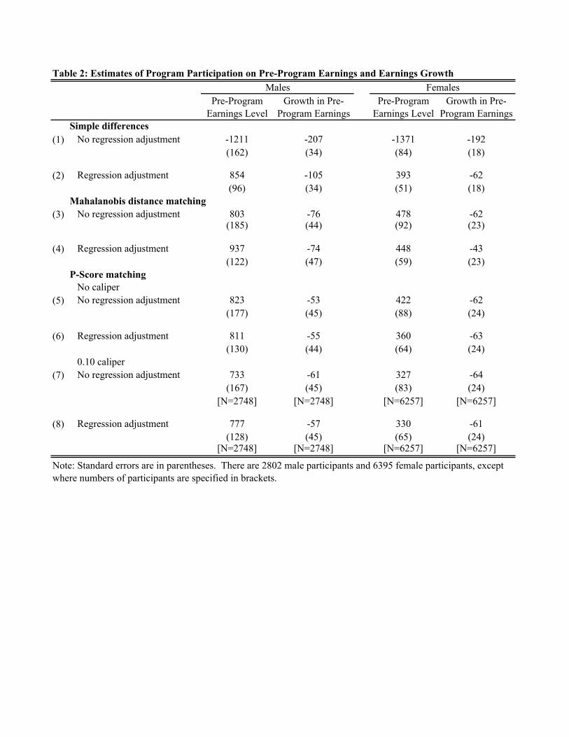
Pre-Program Earnings Level

Growth in Pre-Program Earnings

Pre-Program Earnings Level

Growth in Pre-Program Earnings

Simple differences(1) No regression adjustment -1211 -207 -1371 -192

(162) (34) (84) (18)

(2) Regression adjustment 854 -105 393 -62(96) (34) (51) (18)

Mahalanobis distance matching(3) No regression adjustment 803 -76 478 -62

(185) (44) (92) (23)

(4) Regression adjustment 937 -74 448 -43(122) (47) (59) (23)

P-Score matchingNo caliper

(5) No regression adjustment 823 -53 422 -62(177) (45) (88) (24)

(6) Regression adjustment 811 -55 360 -63(130) (44) (64) (24)

0.10 caliper(7) No regression adjustment 733 -61 327 -64

(167) (45) (83) (24)[N=2748] [N=2748] [N=6257] [N=6257]

(8) Regression adjustment 777 -57 330 -61(128) (45) (65) (24)

[N=2748] [N=2748] [N=6257] [N=6257]

Note: Standard errors are in parentheses. There are 2802 male participants and 6395 female participants, except where numbers of participants are specified in brackets.

Table 2: Estimates of Program Participation on Pre-Program Earnings and Earnings GrowthMales Females

Post-Program Earnings

Difference-in-Difference

Post-Program Earnings

Difference-in-Difference

(1) Simple differences -113 1098 151 1522(173) (190) (93) (104)

(2) Regression adjustment 1481 628 1087 693(157) (177) (86) (98)

Standard pair matching(3) 1267 465 1067 589

(194) (216) (108) (122)

(4) 656 719 1054 606(197) (220) (110) (121)

(5) Modified pair matching 1285 482 1132 620(194) (216) (108) (122)

(6) 1227 513 1066 630(191) (212) (108) (119)

[N=2770] [N=2770] [N=6331] [N=6331]

Table 3: Estimates of Program Effect Based on Simple Differences, Regression Analysis and Mahalanobis Distance Matching

Note: Standard errors are in parentheses. There are 2802 male participants and 6395 female participants, except where numbers of participants are specified in brackets.

Males Females

Mahalanobis distance matching

Standard pair matching-triming tail

No regression adjustment

Regression adjustment

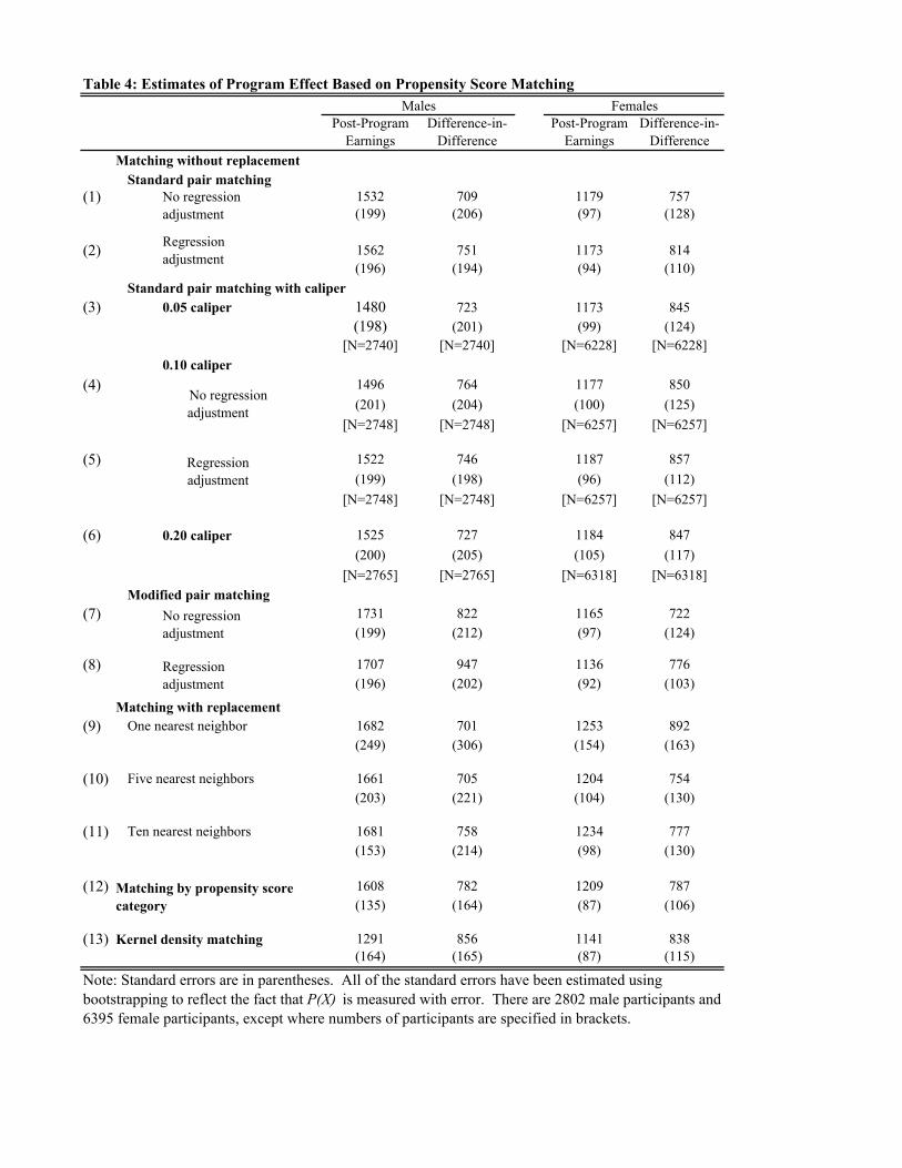
Post-Program Earnings

Difference-in-Difference

Post-Program Earnings

Difference-in-Difference

Matching without replacementStandard pair matching

(1) 1532 709 1179 757(199) (206) (97) (128)

(2) 1562 751 1173 814(196) (194) (94) (110)

(3) 0.05 caliper 1480 723 1173 845(198) (201) (99) (124)

[N=2740] [N=2740] [N=6228] [N=6228]0.10 caliper

(4) 1496 764 1177 850(201) (204) (100) (125)

[N=2748] [N=2748] [N=6257] [N=6257]

(5) 1522 746 1187 857(199) (198) (96) (112)

[N=2748] [N=2748] [N=6257] [N=6257]

(6) 0.20 caliper 1525 727 1184 847(200) (205) (105) (117)

[N=2765] [N=2765] [N=6318] [N=6318]Modified pair matching

(7) 1731 822 1165 722(199) (212) (97) (124)

(8) 1707 947 1136 776(196) (202) (92) (103)

Matching with replacement(9) One nearest neighbor 1682 701 1253 892

(249) (306) (154) (163)

(10) Five nearest neighbors 1661 705 1204 754(203) (221) (104) (130)

(11) Ten nearest neighbors 1681 758 1234 777(153) (214) (98) (130)

(12) 1608 782 1209 787(135) (164) (87) (106)

(13) Kernel density matching 1291 856 1141 838(164) (165) (87) (115)

Table 4: Estimates of Program Effect Based on Propensity Score Matching

Standard pair matching with caliper

No regression adjustment

Regression adjustment

No regression adjustment

Regression adjustment

Regression adjustment

Matching by propensity score category

Note: Standard errors are in parentheses. All of the standard errors have been estimated using bootstrapping to reflect the fact that P(X) is measured with error. There are 2802 male participants and 6395 female participants, except where numbers of participants are specified in brackets.

Males Females

No regression adjustment

Post

-Pro

gram

Ea

rnin

gsD

iffer

ence

-in-

Diff

eren

cePo

st-P

rogr

am

Earn

ings

Diff

eren

ce-in

-D

iffer

ence

(1)

Sim

ple

diff

eren

ce-1

1310

98

151

1522

(173

)(1

90)

(93)

(104

)

(2)

Reg

ress

ion

adju

stm

ent

1481

628

1087

693

(157

)(1

77)

(86)

(98)

(3)

Mah

alan

obis

dis

tanc

e m

atch

ing

1267

465

1067

589

(194

)(2

16)

(108

)(1

22)

P-sc

ore

mat

chin

g w

ithou

t rep

lace

men

t(4

)N

o ca

liper

1532

709

1179

757

(199

)(2

06)

(97)

(128

)

(5)

0.10

cal

iper

1496

764

1177

850

(201

)(2

04)

(100

)(1

25)

[N=2

748]

[N=2

748]

[N=6

257]

[N=6

257]

P-sc

ore

mat

chin

g w

ith re

plac

emen

t(6

)O

ne n

eare

st n

eigh

bor

1682

701

1253

892

(249

)(3

06)

(154

)(1

63)

(7)

M

atch

ing

by P

-sco

re c

ateg

ory

1608

782

1209

787

(135

)(1

64)

(87)

(106

)

(8)

K

erne

l den

sity

mat

chin

g12

9185

6

1141

838

(164

)(1

65)

(87)

(115

)

Tab

le 5

: Sum

mar

y of

Est

imat

es o

f Pro

gram

Eff

ect

Not

e: S

tand

ard

erro

rs a

re in

par

enth

eses

. Th

ere

are

2802

mal

e pa

rtici

pant

s and

639

5 fe

mal

e pa

rtici

pant

s, ex

cept

whe

re n

umbe

rs o

f pa

rtici

pant

s are

spec

ified

in b

rack

ets.

Mal

esFe

mal

es

Mon

ths 7

-18

Mon

ths 1

9-30

Prop

ensi

ty S

core

, N

o C

alip

erPr

open

sity

Sco

re,

0.10

Cal

iper

Prop

ensi

ty S

core

Cat

egor

ies

Ker

nel D

ensi

ty

Mat

chin

gM

en66

610

01

709

764

780

856

(478

)(5

11)

(206

)(2

04)

(190

)(1

65)

Wom

en10

1599

0

757

850

787

838

(288

)(3

19)

(128

)(1

25)

(111

)(1

15)

Cur

rent

Ana

lysi

s

Tab

le 6

: Com

pari

son

of E

stim

ated

Pro

gram

Eff

ects

Usi

ng D

iffer

ence

-in-D

iffer

ence

Est

imat

or w

ith E

ffec

ts B

ased

on

Ran

dom

ized

Con

trol

Gro

ups

Orr

, et a

l. (1

996)

Not

e: S

tand

ard

erro

rs in

par

enth

eses

. Th

e O

rr e

t. al

. (19

96) e

stim

ates

are

take

n fr

om E

xhib

it 4.

6, p

age

107.

The

y ha

ve

been

adj

uste

d fo

r inf

latio

n so

that

they

are

com

para

ble

to th

e es

timat

es fr

om th

e cu

rren

t ana

lysi

s.

Post

-Pro

gram

Ea

rnin

gsD

iffer

ence

-in-

Diff

eren

cePo

st-P

rogr

am

Earn

ings

Diff

eren

ce-in

-D

iffer

ence

No

regr

essi

on a

djus

tmen

t(1

)In

clud

ing

all v

aria

bles

1496

764

1177

850

(201

)(2

04)

(100

)(1

25)

(2)

1498

462

1421

981

(203

)(2

56)

(99)

(117

)

(3)

Dro

ppin

g SD

A15

5289

911

5779

0(2

10)

(230

)(1

20)

(124

)

(4)

957

643

1025

803

(235

)(2

79)

(129

)(1

36)

(5)

Dro

ppin

g al

l 392

483

898

010

77(2

17)

(244

)(1

34)

(139

)R

e gre

ssio

n ad

just

men

t(6

)In

clud

ing

all v

aria

bles

1522

746

1187

857

(199

)(1

98)

(96)

(112

)

(7)

1409

627

1410

998

(202

)(2

46)

(102

)(1

15)

(8)

Dro

ppin

g SD

A16

1484

311

9877

9(2

06)

(228

)(1

18)

(121

)

(9)

752

910

944

899

(222

)(2

62)

(122

)(1

32)

(10)

Dro

ppin

g al

l 399

482

9

1021

1089

(211

)(2

40)

(128

)(1

33)

Not

e: S

tand

ard

erro

rs a

re in

par

enth

eses

.

Tab

le 7

: Est

imat

es o

f Pro

gram

Eff

ect D

ropp

ing

Cer

tain

Var

iabl

es--

Prop

ensi

ty S

core

Mat

chin

g w

ith 0

.1 C

alip

erM

ales

Fem

ales

Dro

ppin

g em

ploy

men

t tra

nsiti

ons

Dro

ppin

g ea

rnin

gs 4

qu

arte

rs p

rior

Dro

ppin

g em

ploy

men

t tra

nsiti

ons

Dro

ppin

g ea

rnin

gs 4

qu

arte

rs p

rior

Post

-Pr

ogra

m

Earn

ings

Diff

-in-

Diff

Post

-Pr

ogra

m

Earn

ings

Diff

-in-

Diff

Post

-Pr

ogra

m

Earn

ings

Diff

-in-

Diff

Post

-Pr

ogra

m

Earn

ings

Diff

-in-

Diff

Post

-Pr

ogra

m

Earn

ings

Diff

-in-

Diff

Post

-Pr

ogra

m

Earn

ings

Diff

-in-

Diff

(1)

1481

628

1496

764

1608

782

1087

693

1177

850

1209

787

(157

)(1

77)

(201

)(2

04)

(135

)(1

64)

(86)

(98)

(100

)(1

25)

(87)

(106

)

(2)

1508

848

1635

966

1635

849

1096

684

1290

918

1284

877

(224

)(2

46)

(280

)(3

27)

(273

)(3

17)

(147

)(2

03)

(139

)(1

49)

(147

)(1

61)

(3)

1493

646

1662

850

1518

905

1126

751

1274

791

1116

845

(448

)(5

14)

(633

)(7

28)

(488

)(5

56)

(263

)(2

88)

(424

)(4

44)

(277

)(2

78)

(4)

1428

618

1516

756

1524

758

11

1969

212

2486

211

9477

8(4

48)

(533

)(6

25)

(679

)(5

17)

(625

)(2

68)

(324

)(3

33)

(358

)(3

25)

(374

)N

ote:

Mea

n es

timat

es b

ased

on

100

repe

titio

ns.

Stan

dard

dev

iatio

ns o

f est

imat

es in

par

enth

eses

.

Tab

le 8

: Sen

sitiv

ity o

f Est

imat

es to

Cha

nges

in th

e Si

ze o

f the

Sam

ples

Prop

ensi

ty S

core

, 0.1

C

alip

erPr

open

sity

Sco

re

Cat

egor

ies

Mal

esFe

mal

es

Reg

ress

ion

Adj

ustm

ent

Prop

ensi

ty S

core

, 0.1

C

alip

erPr

open

sity

Sco

re

Cat

egor

ies

Reg

ress

ion

Adj

ustm

ent

Com

paris

on

sam

ple

=tre

atm

ent s

ampl

e

Red

uce

treat

men

t sa

mpl

e by

90%

Red

uce

both

sa

mpl

es b

y 90

%

Full

sam

ple

Table A1: Regression Predicting Post-Program Earnings

Post-Program Earnings

Difference in Earnings

Post-Program Earnings

Difference in Earnings

Participation in JTPA1481.37(156.84)

627.76(176.84)

1086.99(86.11)

693.71(98.16)

Years of education33.51

(48.83)-40.76(55.06)

-14.19(40.16)

-120.34(45.79)

High school graduation935.09

(136.75)797.95

(154.20)1038.20(106.40)

721.74(121.30)

Years of higher education325.97(62.68)

399.34(70.68)

735.94(48.88)

787.25(55.73)

Experience-50.03(14.50)

-122.75(16.36)

49.24(10.26)

-0.59(11.70)

Experience2 -0.90(0.34)

0.04(0.39)

-2.13(0.25)

-1.87(0.28)

Not employed/employed2294.88(161.66)

2263.94(182.28)

1641.44(111.96)

1617.58(127.63)

Employed/employed3483.03(177.50)

4312.43(200.14)

2350.91(126.56)

2975.95(144.28)

Employed/ not employed-67.30

(144.55)1255.52(162.99)

-288.00(107.95)

525.62(123.06)

White946.47(97.98)

504.32(110.48)

-61.74(71.23)

-295.22(81.20)

Veteran580.98

(101.22)1105.02(114.13)

316.86(211.40)

1297.11(240.99)

Earnings 1 quarter qrior0.73

(0.03)0.48

(0.03)0.56

(0.03)0.38

(0.03)

Earnings 2 quarters prior0.32

(0.04)0.05

(0.04)-0.12(0.03)

-0.60(0.03)

Earnings 3 quarter prior0.27

(0.04)-0.29(0.04)

0.37(0.03)

-0.04(0.04)

Earnings 4 quarters prior0.36

(0.03)-1.70(0.03)

0.57(0.03)

-1.22(0.03)

Employed 1 quarter prior-482.82(147.51)

-660.51(166.32)

56.86(103.69)

77.79(118.20)

Employed 2 quarters prior-352.56(137.63)

-144.29(155.19)

421.98(94322)

576.58(107.40)

Employed 3 quarter prior-310.55(132.63)

245.08(152.93)

-219.78(95.62)

96.53(109.00)

Employed 4 quarters prior160.79

(133.00)-531.79(149.96)

-319.49(93.93)

-1460.64(107.08)

7 Quarter of enrollment dummies Yes Yes Yes Yes8 occupation dummies Yes Yes Yes Yes13 service delivery area dummies Yes Yes Yes YesAdjusted R2 0.23 0.18 0.19 0.17N 48141 48141 59290 59290

Males Females

Note: Standard errors are in parentheses.