Using RZWQM to search improved practices for irrigated maize in Fergana, Uzbekistan

Using RZWQM to search improved practices for

irrigated maize in Fergana, Uzbekistan

G. Stulina a, M.R. Cameira b,*, L.S. Pereira b

a Central Asia Research Institute for Irrigation and Drainage (SANIIRI), Karasu-4,

Tashkent 700187, Uzbekistanb Research Center for Agricultural Engineering, Institute of Agronomy, Technical University

of Lisbon, Tapada da Ajuda, 1349-017 Lisbon, Portugal

Accepted 1 September 2004

Available online 31 March 2005

Abstract

Located in the Aral Sea Basin, Uzbekistan suffers from environmental problems related to soil

salinization and water scarcity. The arid climate requires that cultivated crops be intensively irrigated.

Under conditions of limited resources, crop production must be maintained at expense of minimum

inputs but aiming at achieving maximum returns. The search of the best combination between the

available resources and crop yield can be eased by the use of system modelling. In this work, the Root

Zone Water Quality Model (RZWQM) was used. The research was conducted in an experimental

field located in the Fergana Valley, Usbekistan. The soil is a Sierozem cropped with maize (Zea maıs)

and irrigated with saline water. The soil hydraulic and crop growth components of the model were

calibrated against field data. Initial values for the soil hydraulic properties were determined by a

combination of the in situ method of the soil monolith and two alternative laboratory methods. After

calibration, the model was run as a management tool to predict the impact of different irrigation and

fertilization practices upon crop yield. Soil moisture, soil water potential, water table depth and plant

development were monitored during the 2001 growing season and used for model evaluation. Results

from the comparison of field and simulated data show a good calibration of the soil hydraulic and

plant growth model components. Soil water was simulated for five soil layers with an average

deviation from the measured values of 3.6%.

Crop yield was estimated by the model with an error of 13%. The results from the simulation of

various agricultural management scenarios can be used for further agro economical analysis and

www.elsevier.com/locate/agwat

Agricultural Water Management 77 (2005) 263–281

* Corresponding author. Tel.: +351 21 3653399; fax: +351 21 3653341.

E-mail address: [email protected] (M.R. Cameira).

0378-3774/$ – see front matter # 2005 Elsevier B.V. All rights reserved.

doi:10.1016/j.agwat.2004.09.040

assessment in view of economic profitability. Nevertheless, other model components like the

chemical modules must be calibrated against detailed field experiments.

# 2005 Elsevier B.V. All rights reserved.

Keywords: Soil hydraulic properties; Maize; Model calibration; Irrigation management; Fertilization manage-

ment; Crop growth simulation

1. Introduction

Located in the Aral Sea basin, the Republic of Uzbekistan suffers from an

environmental desertification crisis that destabilizes sustainable development. The

prevailing arid climate requires that cultivated crops be intensively irrigated. Farm

practices require specific field and modelling approaches as dealt in this paper and by Horst

et al. (2004) relative to surface irrigation improvements. In this area, up to 90% of the total

water uses are related to irrigated agriculture. Increasing irrigation water productivity is

essential to cope with the scarcity of irrigation water. Views on water, salts, and land

management relative to the Aral Sea Basin are presented by several authors, e.g.,

Dukhovny and Sokolov (1998) and Dukhovny et al. (2002).

Among others, modelling is an effective tool to develop new management approaches.

The Root Zone Water Quality Model (RZWQM) (Ahuja et al., 1999) is an integrated

physical, biological, and chemical process model simulating plant growth and movement

of water, nutrients, and pesticides over and through the root zone at a representative area of

an agricultural cropping system. The model has been successfully used in several parts of

the world (Ma et al., 2001; Cameira et al., 2000a). Cameira et al. (2000b) describe the use

of the model in combination with field studies to characterize soil hydraulic properties of

irrigated maize in a Mediterranean alluvial soil.

The model incorporates additional features needed for simulating management impacts,

such as chemical transport via macropores, tile drainage, advanced soil chemistry, and

nutrient transformations, improved water and salt dynamics, a comprehensive plant growth

model, and important water and chemical management scenarios. It can be used to simulate

the influence of different agricultural management scenarios, including irrigation and

fertilization management upon crop yields.

The RZWQM model allows simulation of a wide spectrum of management practices

and scenarios (Cameira et al., 2000a,b). These management alternatives include evaluation

of: conservation tillage and residue cover versus conventional tillage; methods and timing

of fertilizer and pesticide applications; manures and alternative chemical formulations;

irrigation and drainage technology, and the methods and timing of water applications; and

different crop rotations. Tillage and residue management affect soil’s physical and

hydraulic properties, micro-topography and surface roughness, energy and water balance,

and chemical transfer from soil to surface runoff-tillage induced changes to soil hydraulic

properties are slowly changed back to their original conditions as rainfall reconsolidates

the tilled layers (Cameira et al., 2003a).

The model’s generic crop growth component plays a major role in effecting the state of

the simulation system. Shading from the plant canopy reduces soil evaporation, while

G. Stulina et al. / Agricultural Water Management 77 (2005) 263–281264

transpiration links root water and nutrient extraction from soil layers to atmospheric

demand. Seasonal sloughing of leaf material and dead roots, coupled with harvest residue,

provide a source of carbon and nitrogen for the soil nutrient transformations. Estimates of

crop production and yield allow for a relative economic evaluation of the simulation

results.

The reliability of RZWQM depends on how well each individual process is represented

in the model and on the accuracy of the measured parameters needed to run the model. The

model components have undergone extensive verification, evaluation and refinement in

collaboration with several users in the USA and abroad. These components are water

movement (Ahuja et al., 1993), pesticide transport (Ahuja et al., 1993, 1996),

evapotranspiration (Farahani and Ahuja, 1996), subsurface tile drainage (Johnsen et al.,

1995), organic matter/nitrogen cycling (Ma et al., 1998), and plant growth (Nokes et al.,

1996).

This paper has two main objectives. The first is to present the essential aspects of

RZWQM parameterisation based upon field data when applied to a different soil

environment. The second is to analyse several alternative agronomic, irrigation and

fertilizing practices with the scope of improving agricultural production under the

perspective of environmental friendliness adapted to the conditions prevailing in Fergana

Valley, Uzbekistan.

2. Materials and methods

2.1. Location and general characterization of the experimental site

The research was conducted in an experimental field cropped with maize and irrigated

with saline water, located in the Fergana Valley, Uzbekistan. Data refer to the 2001 growing

season. The field is located in the area of the former Niyazov state farm-2, in the

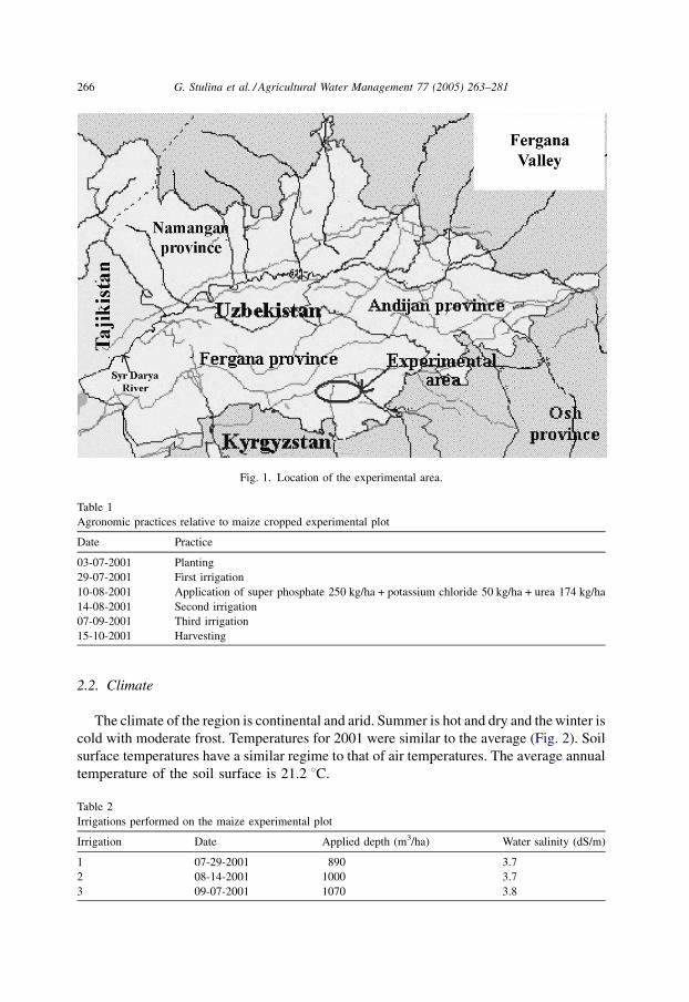
Ahunbabayev rayon of Fergana province, SyrDarya river basin (Fig. 1). The soil is a Calcic

Sierozem according to the FAO and Russian classifications. Soil hydraulic properties were

determined using an in situ monolith experiment together with laboratory methods. Soil

moisture, soil water potential, water table depth, and plant development were monitored

during the season for model evaluation.

Agronomic practices in the experimental plot followed recommendations of the local

expert agronomist (Table 1). The plot was furrow irrigated with saline water as shown in

Table 2. Irrigation scheduling was based on the soil and crop water status. Irrigation is

described in Horst et al. (2004).

The plot lies within the flat smooth proluvial plain that constitutes the peripheral

part of the alluvial cone of the Margilansay, Shahimardansay, and Isfaramsay rivers.

This plain is slightly inclined to the modern valley of the SyrDarya river. Elevation

ranges from 429 to 434.7 m. A dense network of irrigation canals supplied by the

Big Fergana Canal delivers irrigation water to the intensive agriculture that developed

in the plain. Open and close drains and drainage collectors having a depth of 5–7 m

or more constitute the drainage system. Slopes northward are low, from 0.002 to

0.005.

G. Stulina et al. / Agricultural Water Management 77 (2005) 263–281 265

2.2. Climate

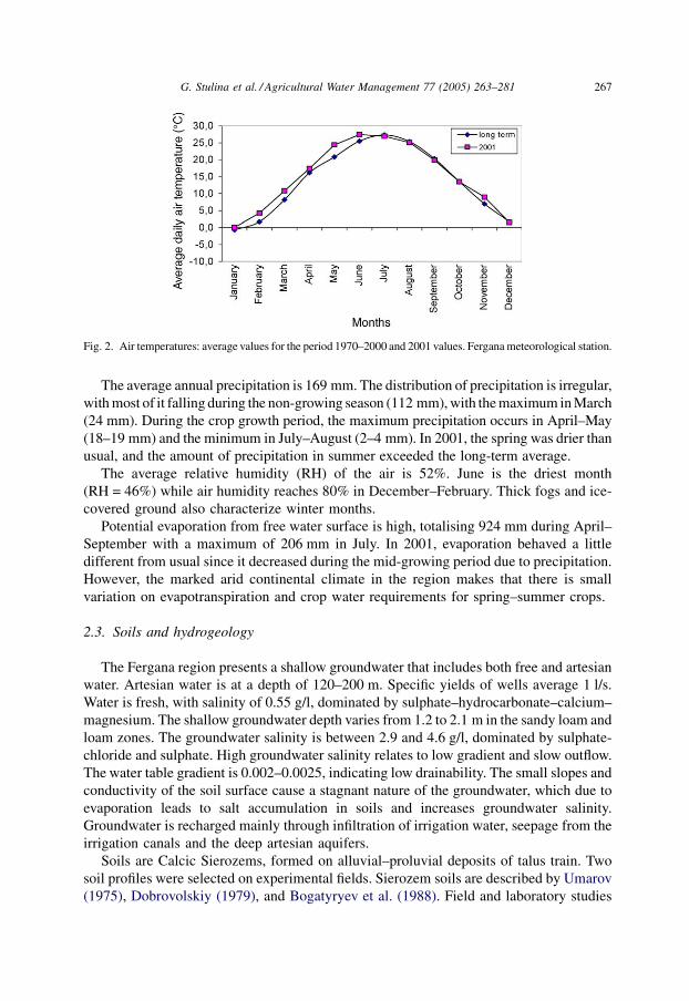
The climate of the region is continental and arid. Summer is hot and dry and the winter is

cold with moderate frost. Temperatures for 2001 were similar to the average (Fig. 2). Soil

surface temperatures have a similar regime to that of air temperatures. The average annual

temperature of the soil surface is 21.2 8C.


Fig. 1. Location of the experimental area.

Table 1

Agronomic practices relative to maize cropped experimental plot

Date Practice

03-07-2001 Planting

29-07-2001 First irrigation

10-08-2001 Application of super phosphate 250 kg/ha + potassium chloride 50 kg/ha + urea 174 kg/ha

14-08-2001 Second irrigation

07-09-2001 Third irrigation

15-10-2001 Harvesting

Table 2

Irrigations performed on the maize experimental plot

Irrigation Date Applied depth (m3/ha) Water salinity (dS/m)

1 07-29-2001 890 3.7

2 08-14-2001 1000 3.7

3 09-07-2001 1070 3.8

The average annual precipitation is 169 mm. The distribution of precipitation is irregular,

with most of it falling during the non-growing season (112 mm), with the maximum in March

(24 mm). During the crop growth period, the maximum precipitation occurs in April–May

(18–19 mm) and the minimum in July–August (2–4 mm). In 2001, the spring was drier than

usual, and the amount of precipitation in summer exceeded the long-term average.

The average relative humidity (RH) of the air is 52%. June is the driest month

(RH = 46%) while air humidity reaches 80% in December–February. Thick fogs and ice-

covered ground also characterize winter months.

Potential evaporation from free water surface is high, totalising 924 mm during April–

September with a maximum of 206 mm in July. In 2001, evaporation behaved a little

different from usual since it decreased during the mid-growing period due to precipitation.

However, the marked arid continental climate in the region makes that there is small

variation on evapotranspiration and crop water requirements for spring–summer crops.

2.3. Soils and hydrogeology

The Fergana region presents a shallow groundwater that includes both free and artesian

water. Artesian water is at a depth of 120–200 m. Specific yields of wells average 1 l/s.

Water is fresh, with salinity of 0.55 g/l, dominated by sulphate–hydrocarbonate–calcium–

magnesium. The shallow groundwater depth varies from 1.2 to 2.1 m in the sandy loam and

loam zones. The groundwater salinity is between 2.9 and 4.6 g/l, dominated by sulphate-

chloride and sulphate. High groundwater salinity relates to low gradient and slow outflow.

The water table gradient is 0.002–0.0025, indicating low drainability. The small slopes and

conductivity of the soil surface cause a stagnant nature of the groundwater, which due to

evaporation leads to salt accumulation in soils and increases groundwater salinity.

Groundwater is recharged mainly through infiltration of irrigation water, seepage from the

irrigation canals and the deep artesian aquifers.

Soils are Calcic Sierozems, formed on alluvial–proluvial deposits of talus train. Two

soil profiles were selected on experimental fields. Sierozem soils are described by Umarov

(1975), Dobrovolskiy (1979), and Bogatyryev et al. (1988). Field and laboratory studies


Fig. 2. Air temperatures: average values for the period 1970–2000 and 2001 values. Fergana meteorological station.

were carried out to study soil parameters (supplemental information in Stulina, 2003).

Fig. 3 shows the soil particles distribution and the bulk density for all soil layers between

the soil surface and 200 cm deep. Porosity averages 42.6–42.8% in the 0–200 cm layer,

44.5–44.8% in the upper root zone, but it differs substantially in horizons with high gypsum

content (41.6% in the 45–173 cm layer). Since the soil contains an important amount of

gypsum, the soil samples were dried at the temperature of 65 8C to determine the water

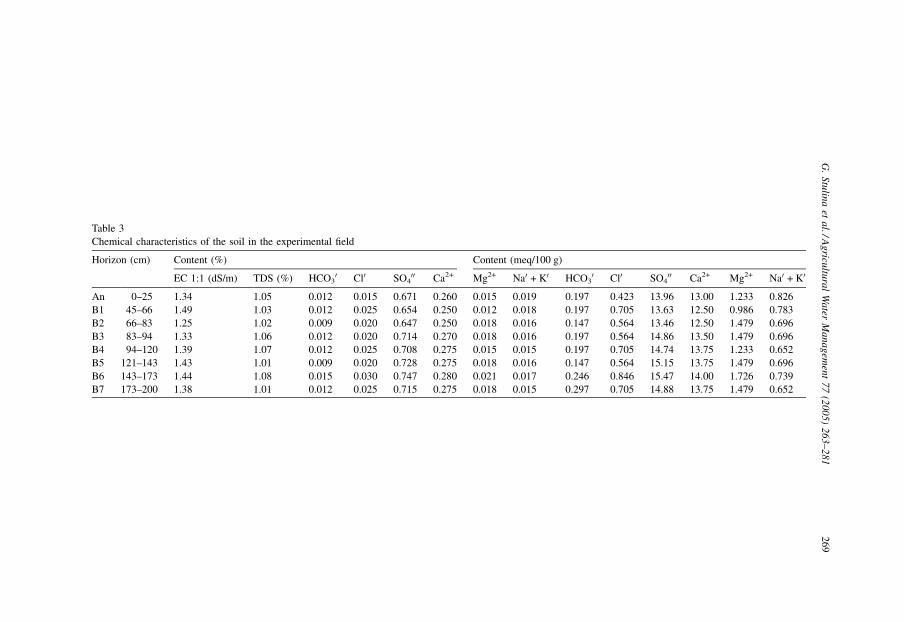
contents. Table 3 presents some chemical parameters of the soil, measured on the 1:5 water

extract. The total of salts is distributed evenly along the profile, not exceeding 1.10%. As

for the ions composition, calcium and sulphates prevail and constitute 11–15 meq/100 g of

soil. Others are Mg2+ (0.986–1.726 meq/100 g), Na+ (0.609–0.826 meq/100 g), Cl�

(0.423–0.846 meq/100 g), and CO3H� (less than 0.2 meq/100 g). Hypothetically, under

such ion composition, salts of Ca(HCO3)2, CaSO4 (soluble gypsum), MgSO4, Na2SO4, and

NaCl are present in soils. Major amount of salts are represented by the non-toxic compound

of CaSO4, which practically constitutes more than 80% of solid residue. However, the

presence of this salt in the soil solution creates osmotic effects and reduces the water

extraction by plant roots. Yield losses can be higher than 25%.

Agrochemical soil properties were studied in the top 50 cm layer. Regarding organic

matter content (OM), the soils in the plough-layer were estimated as ‘‘rich’’, with 1.6–

1.9%. This values decrease to 1.2–0.7% along the profile. N–NH4 concentrations show

values of 22–32 mg kg�1 (ppm) in the upper soil horizon, which increase up to 42–

51 mg kg�1 in underlying layers. Phosphorus in PO2 form changes with depth from low

concentration (14–16 mg kg�1) to very low (7–12 mg kg�1). Potassium (K2O) varies

within 100–154 mg kg�1, meaning low availability.

2.4. Characterization of the soil hydraulic properties

The unsaturated hydraulic conductivity, K(h), and the water retention curve, u(h), were

determined in situ in a soil monolith (2 m � 2 m � 2 m) located in the experimental plot,

according to the methodology described by Cameira et al. (2003b). The internal drainage

flux method (Green et al., 1986) was used to determine K(h). The monolith was isolated


Fig. 3. Soil particle distribution and bulk density. Fegana, field #5.

G.

Stu

lina

eta

l./Ag

ricultu

ral

Wa

terM

an

ag

emen

t7

7(2

00

5)

26

3–

28

12

69

Table 3

Chemical characteristics of the soil in the experimental field

Horizon (cm) Content (%) Content (meq/100 g)

EC 1:1 (dS/m) TDS (%) HCO30 Cl0 SO4

00 Ca2+ Mg2+ Na0 + K0 HCO30 Cl0 SO4

00 Ca2+ Mg2+ Na0 + K0

An 0–25 1.34 1.05 0.012 0.015 0.671 0.260 0.015 0.019 0.197 0.423 13.96 13.00 1.233 0.826

B1 45–66 1.49 1.03 0.012 0.025 0.654 0.250 0.012 0.018 0.197 0.705 13.63 12.50 0.986 0.783

B2 66–83 1.25 1.02 0.009 0.020 0.647 0.250 0.018 0.016 0.147 0.564 13.46 12.50 1.479 0.696

B3 83–94 1.33 1.06 0.012 0.020 0.714 0.270 0.018 0.016 0.197 0.564 14.86 13.50 1.479 0.696

B4 94–120 1.39 1.07 0.012 0.025 0.708 0.275 0.015 0.015 0.197 0.705 14.74 13.75 1.233 0.652

B5 121–143 1.43 1.01 0.009 0.020 0.728 0.275 0.018 0.016 0.147 0.564 15.15 13.75 1.479 0.696

B6 143–173 1.44 1.08 0.015 0.030 0.747 0.280 0.021 0.017 0.246 0.846 15.47 14.00 1.726 0.739

B7 173–200 1.38 1.01 0.012 0.025 0.715 0.275 0.018 0.015 0.297 0.705 14.88 13.75 1.479 0.652

laterally by a plastic film. It was equipped with a neutron probe access tube to measure

volumetric soil moisture (u) at the depths of 12.5, 27.5, 42.5, 67.5, 112.5, and 137.5 cm, and

two sets of tensiometers to measure hydraulic heads (H) at the same depths. Initially, the

monolith was saturated with water. The first measurement of u and H was performed after

infiltration. The monolith surface was then covered with a plastic film and a layer of straw to

prevent evaporation and temperature fluctuations, and the internal drainage experiment was

started. During the first day, measurements were taken every 2 h, then once a day for a week,

and then every 4 days, and finally once a week for 1 month. After this period, the surface was

uncovered allowing evaporation to occur. During this part of the experiment, measurements

were taken once a day for a week and then once a week for 1 month.

Hydraulic conductivity was determined based upon the soil water data and the matric

suction data by using the Darcy’s generalized equation:

’wðz; tÞ ¼ �KðuÞ @H

@z; (1)

where ’wðz; tÞ is the soil hydraulic flux, K(u) the hydraulic conductivity function of soil at a

volumetric water content u at the depth z, and H is the hydraulic head measured in the

tensiometers.

Applying the continuity equation to the one-dimensional flow and integrating it between

the depths zi and zi+1, we obtain:Z ziþ1

zi

@u

@t@z ¼ �½’wðziþ1; tÞ � ’ðzi; tÞ (2)

where w(zi, t) and w(zi+1, t) are the hydraulic fluxes at the depths zi and zi+1. Knowing the

soil water contents function u(z, t), the first side of the equation can be determined, and

knowing one of the fluxes the right side of the equation can also be determined. Then, once

the hydraulic head function H(z, t) is known, the hydraulic gradient can be calculated for

each time and depth. The hydraulic conductivity is obtained by applying the Darcy’s

equation. The calculation procedure is described in Fig. 4.

The matric suction curve determined in situ was complemented by laboratory values

obtained from two different methods: the pressure membrane method (pF > 2, where

pF = log(h) in cm (Klute, 1986) and the desorption method (Vadunina and Korchagina, 1973)

used in the University of Moscow (at pF 6.466, 5.955, 5.742, 5.512, 5.318, and 4.445). For

these methods, undisturbed soil samples (100 cm3) were collected in the experimental plot.

The Brooks and Corey (1964) functions modified as described by Ahuja et al. (1999)

were fitted to both u(h) and K(h) data. The Brooks and Corey modified functions consist of

the following:

The soil water content, u (cm3 cm�3), versus the soil water pressure head, h (cm),

relation is expressed by:

uðhÞ ¼ us � Ajhj; 0 � jhj � jhbj (3a)

uðhÞ ¼ ur þ Bjhj�l; jhj � jhbj (3b)

where us is the saturated water content, ur the residual water content, hb, A, B and l are

the parameters derived from best fitting of experimental data.


The hydraulic conductivity, K (cm h�1), versus the soil water pressure head, h (cm),

relation is given by:

KðhÞ ¼ Ksjhj�N1 ; 0 � jhj � jh2j (4a)

KðhÞ ¼ Cjhj�N2 ; jhj � jhbj (4b)

where Ks is the field saturated hydraulic conductivity and h2, N1, N2, and C are the

parameters derived from fitting the experimental data.

2.5. Field monitoring

Field monitoring consisted in collecting soil water and crop data to calibrate the

hydraulic properties and the crop growth modules of RZWQM.

Experimental plots with the dimensions 5 m � 6 m were established on the Field 5,

with a total area of 25 ha. The field was cultivated with maize for silage during the

year 2001. The experimental plots were equipped with two sets of tensiometers and

access tubes for neutron probe measurements, and a piezometer for monitoring the

water table to a depth of 2.5 m. Measurements of the soil water potential and soil

moisture were performed every day at the depths of 37.5, 52.5, 87.5, 107.5, and

132.5 cm. The soil water content at the depth of 12.5 cm was measured by the

gravimetric method.

Two rows of plants were selected for the crop observations. The phenological stages

were determined by observation of the crop development. At the beginning of each stage,

six plants were collected in each row, to measure plant height and above ground biomass

and rooting depth using the methodology described by Dospekhov (1985). Yield was

measured at harvest.


Fig. 4. Calculation procedure for the hydraulic conductivity with data from the monolith experiment.

2.6. Modelling

Models like RZWQM require a detailed set of parameters. Some of these parameters

cannot be easily measured or determined. Also, natural conditions of the soil–plant–

atmosphere system are difficult to define for some parameters requiring a calibration

for the site and crop. The user is confronted with the task of determining which

parameters to calibrate and how to do it. An iterative calibration approach is needed to

account for the interactions between soil water, available nitrogen and crop production.

This approach will reduce the error propagation between model components. In

this work, two model components were calibrated: the hydraulic properties and the

crop development. The evapotranspiration and the nutrient components were not

studied.

The starting moisture profile and the depth of the water table gave the initial conditions

for solving the water-flux Richards equation. At the soil surface, precipitation and potential

crop evapotranspiration were given as top boundary flux conditions. A unit soil water

potential gradient was used as the bottom boundary condition.

2.6.1. Calibration

First, the hydraulic soil properties obtained from field and laboratory experiments were

calibrated without the presence of root extraction using infiltration and redistribution

profiles. The RZWQM was then run in inverse mode to calibrate the hydraulic parameters

as described by Cameira et al. (2000b).

The crop development component of RZWQM was after calibrated for maize. In this

component, two types of parameters were calibrated. They were the duration of each

growth stage and the crop-specific parameters (Table 4). The latter reflect the effect of the

environment over the crop development for each production system. The first four values

shown in Table 4 are used to adjust the duration of each crop stage. Increasing the

parameter (6) relative to N uptake results in a decrease in biomass while increasing the

parameter (7) results in a decrease in total plant production. Parameters (6) and (7) can be

adjusted to change the slope of the biomass growth curves. When the parameter (8) is

increased yield also increases while above ground biomass is kept constant. Similar


Table 4

Phenological and site-specific maize crop parameters before and after calibration of the crop development

component

Parameter Default values Maize crop

(1) Minimum time for the beginning of the germinating phase (days) 5 5

(2) Minimum time for the beginning of emergence (days) 15 15

(3) Minimum time for the beginning of the four leaf stage (days) 20 25

(4) Minimum time for the beginning of the reproductive stage (days) 30 30

(5) Maximum N uptake rate (g/(plant day)) 5 1.0

(6) Relation N uptake/biomass (0–1/day) 0.12 0.05

(7) Specific leaf density (g/LAI) 11.5 13.5

(8) Photosynthetic efficiency in the flowering phase (0–1) 0.45 0.85

(9) Photosynthetic efficiency in the seed formation phase (0–1) 0.6 0.80

changes in parameter (9) produce the same impacts but later in the growing season.

Parameters (8) and (9) can be changed to adjust the harvest index. For this particular

component, the model developers suggest that the simulations must be within 15% of the

measured control variables, which are above ground biomass, yield and leaf area index

(Hanson, 1999).

The calibration process was initiated using the default value of 5 for parameter (1). After

the simulation the estimated biomass was compared with the measured. If the error was

higher than 15% the parameter (6) was adjusted. Then the parameter (7) was adjusted in

order to reduce the error to approximately 10%. When necessary, the harvest index was

adjusted by changing parameters (8) and (9). The process was repeated as necessary

resulting the calibrated parameters given in Table 4.

2.6.2. Using the model as a management tool

After the referred calibration of these crop growth and yield components, the model was

used as a tool to evaluate the impact of different irrigation and fertilization practices upon

crop yield. With this purpose, different simulation scenarios were created as described in

Section 3.3. The irrigation scheduling simulation model ISAREG (Teixeira and Pereira,

1992) was used to build the water management scenarios. This model was validated using

data collected in the same Fergana farm and is used to support improved irrigation

management in the area (Fortes et al., 2004).

3. Results and discussion

3.1. Soil water retention and hydraulic conductivity functions

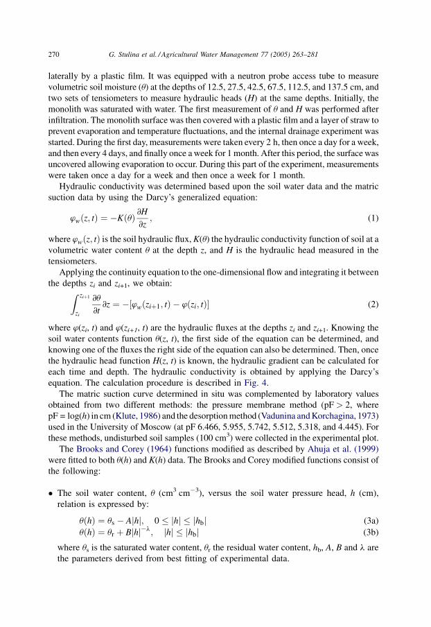
Fig. 5 shows an example of data collected during the monolith experiment.

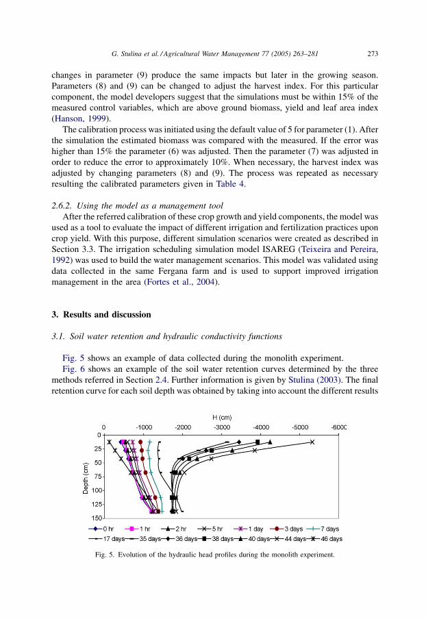
Fig. 6 shows an example of the soil water retention curves determined by the three

methods referred in Section 2.4. Further information is given by Stulina (2003). The final

retention curve for each soil depth was obtained by taking into account the different results


Fig. 5. Evolution of the hydraulic head profiles during the monolith experiment.

of those applied methods and running RZWQM in inverse mode (Cameira et al., 2000b).

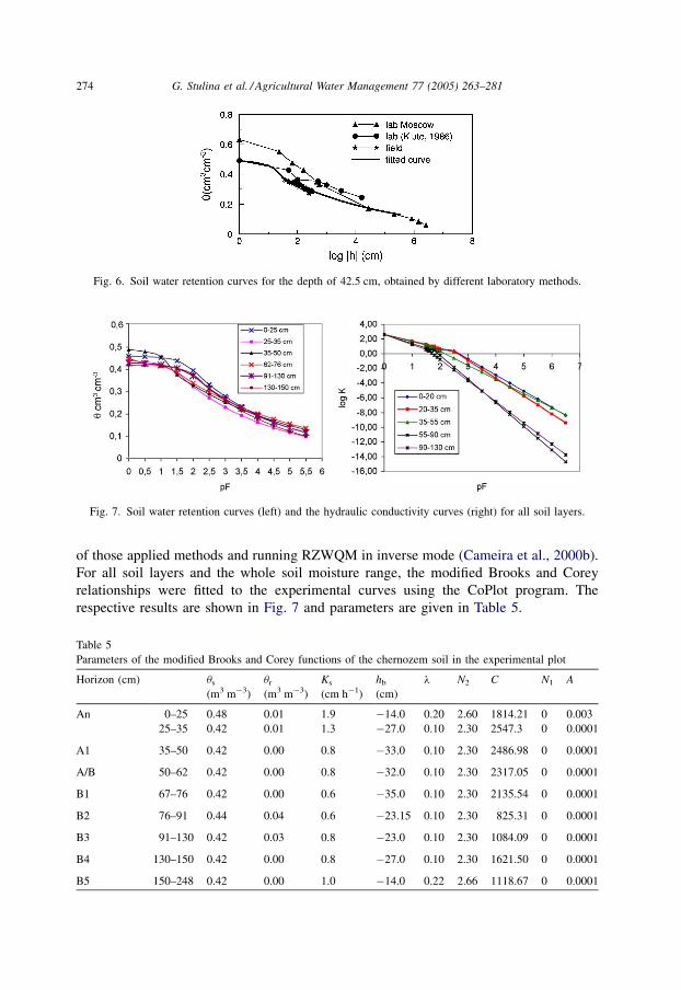
For all soil layers and the whole soil moisture range, the modified Brooks and Corey

relationships were fitted to the experimental curves using the CoPlot program. The

respective results are shown in Fig. 7 and parameters are given in Table 5.


Fig. 6. Soil water retention curves for the depth of 42.5 cm, obtained by different laboratory methods.

Fig. 7. Soil water retention curves (left) and the hydraulic conductivity curves (right) for all soil layers.

Table 5

Parameters of the modified Brooks and Corey functions of the chernozem soil in the experimental plot

Horizon (cm) us

(m3 m�3)

ur

(m3 m�3)

Ks

(cm h�1)

hb

(cm)

l N2 C N1 A

An 0–25 0.48 0.01 1.9 �14.0 0.20 2.60 1814.21 0 0.003

25–35 0.42 0.01 1.3 �27.0 0.10 2.30 2547.3 0 0.0001

A1 35–50 0.42 0.00 0.8 �33.0 0.10 2.30 2486.98 0 0.0001

A/B 50–62 0.42 0.00 0.8 �32.0 0.10 2.30 2317.05 0 0.0001

B1 67–76 0.42 0.00 0.6 �35.0 0.10 2.30 2135.54 0 0.0001

B2 76–91 0.44 0.04 0.6 �23.15 0.10 2.30 825.31 0 0.0001

B3 91–130 0.42 0.03 0.8 �23.0 0.10 2.30 1084.09 0 0.0001

B4 130–150 0.42 0.00 0.8 �27.0 0.10 2.30 1621.50 0 0.0001

B5 150–248 0.42 0.00 1.0 �14.0 0.22 2.66 1118.67 0 0.0001

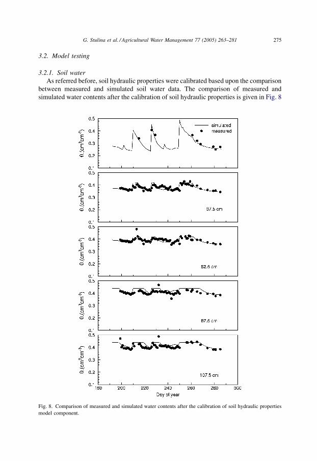
3.2. Model testing

3.2.1. Soil water

As referred before, soil hydraulic properties were calibrated based upon the comparison

between measured and simulated soil water data. The comparison of measured and

simulated water contents after the calibration of soil hydraulic properties is given in Fig. 8


Fig. 8. Comparison of measured and simulated water contents after the calibration of soil hydraulic properties

model component.

for all soil layers. Results show a good agreement between simulated and observed data

both for the upper layers where changes are more drastic between irrigations, and the

deeper layers where the variation of the soil water content was lesser. The deviation

between simulated and measured values averages 3.6%, the maximum being 18%. These

good fitting results indicate that model parameterisation of the soil hydraulic properties

have been successfully achieved. This is reinforced by the good agreement between the

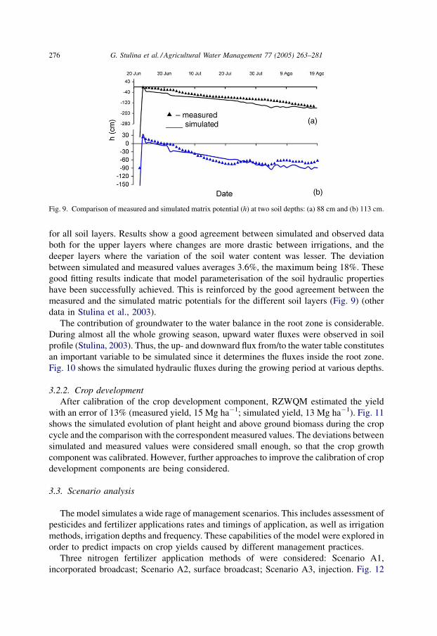
measured and the simulated matric potentials for the different soil layers (Fig. 9) (other

data in Stulina et al., 2003).

The contribution of groundwater to the water balance in the root zone is considerable.

During almost all the whole growing season, upward water fluxes were observed in soil

profile (Stulina, 2003). Thus, the up- and downward flux from/to the water table constitutes

an important variable to be simulated since it determines the fluxes inside the root zone.

Fig. 10 shows the simulated hydraulic fluxes during the growing period at various depths.

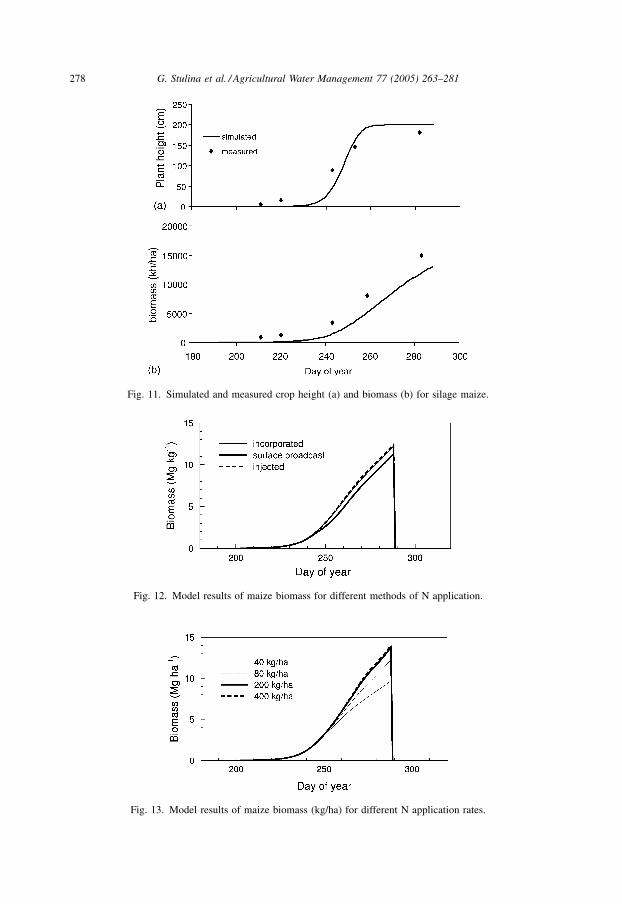
3.2.2. Crop development

After calibration of the crop development component, RZWQM estimated the yield

with an error of 13% (measured yield, 15 Mg ha�1; simulated yield, 13 Mg ha�1). Fig. 11

shows the simulated evolution of plant height and above ground biomass during the crop

cycle and the comparison with the correspondent measured values. The deviations between

simulated and measured values were considered small enough, so that the crop growth

component was calibrated. However, further approaches to improve the calibration of crop

development components are being considered.

3.3. Scenario analysis

The model simulates a wide rage of management scenarios. This includes assessment of

pesticides and fertilizer applications rates and timings of application, as well as irrigation

methods, irrigation depths and frequency. These capabilities of the model were explored in

order to predict impacts on crop yields caused by different management practices.

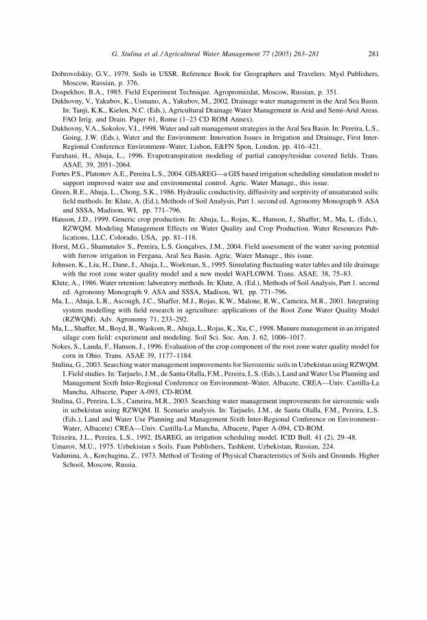
Three nitrogen fertilizer application methods of were considered: Scenario A1,

incorporated broadcast; Scenario A2, surface broadcast; Scenario A3, injection. Fig. 12


Fig. 9. Comparison of measured and simulated matrix potential (h) at two soil depths: (a) 88 cm and (b) 113 cm.

shows the simulated crop yields for each scenario. The most effective method of fertilizer

application was the injection, originating a yield increase of 5% relative to surface

broadcasted, which is the most common at present. Differences among methods are small;

thus, focusing crop management improvements in fertilizing application methods is not a

priority.

Four scenarios were considered for the amount of nitrogen fertilizer: Scenario B1,

40 kg ha�1; Scenario B2, 80 kg ha�1; Scenario B3, 200 kg ha�1; Scenario B4,

400 kg ha�1. The prediction of maize yields for the different scenarios is shown in

Fig. 13. Increasing N application up to 200 kg ha�1 leads to a steady increase in yields. For

higher rates the crop yield response is much smaller, with a lower fertilizing productivity,

thus indicating that increasing the N fertilising above that value may not be of interest.

Three irrigation scenarios were simulated in order to determine the impact of different

irrigation amounts upon crop production. Scenario C1 corresponds to the actual irrigation

performed in the field. Scenario C2 corresponds to an improved irrigation schedule aiming


Fig. 10. Simulated hydraulic fluxes at different depths.


Fig. 13. Model results of maize biomass (kg/ha) for different N application rates.

Fig. 12. Model results of maize biomass for different methods of N application.

Fig. 11. Simulated and measured crop height (a) and biomass (b) for silage maize.

at maximizing ET and yield simulated with the model ISAREG (Teixeira and Pereira,

1992), which was validated with field data obtained in the same plot. Scenario C3 is a water

saving scenario, also simulated with ISAREG, where the irrigation amount was decreased

by 16%. Results in Fig. 14a show that an improved schedule may lead to significant

increase in yields, up to 13.3 Mg ha�1, i.e., near 10% relative to the common practice, and

those in Fig. 14b show that the water saving practice results in the decrease of maize yield

by 2.45 Mg ha�1, i.e., 20% less than the control irrigation schedule. Further simulation

analysis will be performed to build up best management practices for irrigated agriculture

in the area. With this purpose, the calibration of RZWQM chemical and nutrient modules is

being performed.

4. Conclusions

The results presented in this work show that the methodology used to parameterize the

hydraulic properties and the crop development modules of RZWQM for the Fergana Valley

is adequate, thus encouraging further developments for using the model in this area.

However, several difficulties have been found due to the gypsum presence in the soil. The

shallow water table helps to create a saline environment and this is a. Overall the data

collected allowed a good description of the soil hydraulic properties of the Sierozem soils.


Fig. 14. (a) Simulated total maize biomass (kg/ha) comparing an improved irrigation schedule with the actual one.

(b) Simulated biomass (kg/ha) for the water saving irrigation scenario and the ISAREG scenario.

In relation with soil water, the deviation between simulated and measured values

averages 3.6%, the maximum being 18%. These good fitting results indicate that model

parameterisation of the soil hydraulic properties were successfully achieved. After

calibration of the crop development component, RZWQM estimated the yield with an error

of 13% (measured yield, 15 Mg ha�1; simulated yield, 13 Mg ha�1).

This work describes the first attempt to use the model RZWQM for Uzbek and Central

Asia conditions. Results confirm the ability of RZWQM to predict the impacts of different

agricultural practices, including irrigation and fertilization, upon the crop yields. When

complemented with an agro-economic analysis methodology, it constitutes a useful tool for

decision-making in the Uzbek irrigated agriculture in a medium to long run, including to

select the practices that may lead to higher land and water productivity. However, further

and detailed field studies need to be performed in order to more adequately calibrate the

model for the Fergana Valley specific conditions, particularly related to salinity, agronomic

and economic features of the model, with particular focus on the chemical modules in order

to consider the current salinity problems.

Acknowledgements

This research was funded through the research contract ICA2-CT-2000-10039 with the

European Union. The support of the NATO Science Fellowships Program is acknowledged.

Thanks are due to numerous colleagues in SANIIRI and the University of Moscow that

helped in field and laboratory experiments.

References

Ahuja, L.R., Rojas, K.W., Hanson, J.D., Shaffer, M.J., Ma, L. (Eds.), 1999. Root Zone Water Quality Model,

Modelling Management Effects on Water Quality & Crop Production. Water Resources Publications, LLC,

Colorado, USA, p. 360.

Ahuja, L., DeCoursey, D., Barnes, B., Rojas, K., 1993. Characteristics of macropores studied with the ARS root

zone water quality model. Trans. ASAE 36, 369–380.

Ahuja, L., Ma, L., Rojas, K., Boesten, J., Farahani, H., 1996. A field test of the RZWQM simulation model for

predicting pesticide and bromide behavior. J. Pestic. Sci. 48, 101–108.

Bogatyryev, L.G., Vasilyevskaya, V.D., Vladychenskiy, A.S., 1988. Soil types, their geography and use. In: Kovda,

V.A., Rozanova, B.G. (Eds.), Course of Soil Science 2 (2), Vyscshaya Shkola, Moscow, 368 pp. (in Russian).

Brooks R.H., Corey A.T., 1964. Hydraulic properties of porous media. Hydrology Paper 3, Colorado State

University, Fort Collins, CO, USA, pp. 1–15.

Cameira, M.R., Fernando, R.M., Pereira, L.S., 2000a. Assessment of NO3–N losses under different management

practices using the RZWQM. In: Mermound, A., Musy, A., Pereira, L.S., Ragab, R. (Eds.), Control of

Adverese Impacts of Fertilizers and Agrochemicals. South Africa Com. ICID, Cape Town, pp. 89–100.

Cameira, M.R., Ahuja, L., Fernando, R.M., Pereira, L.S., 2000b. Evaluating field measured soil hydraulic

properties in water transport simulations using the RZWQM. J. Hydrol. 236, 78–90.

Cameira, M.R., Fernando, R.M., Pereira, L.S., 2003a. Soil macropore dynamics affected by tillage and irrigation.

J. Soil Tillage Res. 70-2, 131–140.

Cameira, M.R., Fernando, R.M., Pereira, L.S., 2003b. Monitoring water and NO3–N in irrigated maize fields in the

Sorraia watershed. Portugal. Agric. Water Manage. 60, 199–216.


Dobrovolskiy, G.V., 1979. Soils in USSR. Reference Book for Geographers and Travelers. Mysl Publishers,

Moscow, Russian, p. 376.

Dospekhov, B.A., 1985. Field Experiment Technique. Agropromizdat, Moscow, Russian, p. 351.

Dukhovny, V., Yakubov, K., Usmano, A., Yakubov, M., 2002. Drainage water management in the Aral Sea Basin.

In: Tanji, K.K., Kielen, N.C. (Eds.), Agricultural Drainage Water Management in Arid and Semi-Arid Areas.

FAO Irrig. and Drain. Paper 61, Rome (1–23 CD ROM Annex).

Dukhovny, V.A., Sokolov, V.I., 1998. Water and salt management strategies in the Aral Sea Basin. In: Pereira, L.S.,

Going, J.W. (Eds.), Water and the Environment: Innovation Issues in Irrigation and Drainage, First Inter-

Regional Conference Environment–Water, Lisbon, E&FN Spon, London, pp. 416–421.

Farahani, H., Ahuja, L., 1996. Evapotranspiration modeling of partial canopy/residue covered fields. Trans.

ASAE. 39, 2051–2064.

Fortes P.S., Platonov A.E., Pereira L.S., 2004. GISAREG—a GIS based irrigation scheduling simulation model to

support improved water use and environmental control. Agric. Water Manage., this issue.

Green, R.E., Ahuja, L., Chong, S.K., 1986. Hydraulic conductivity, diffusivity and sorptivity of unsaturated soils:

field methods. In: Klute, A. (Ed.), Methods of Soil Analysis, Part 1. second ed. Agronomy Monograph 9. ASA

and SSSA, Madison, WI, pp. 771–796.

Hanson, J.D., 1999. Generic crop production. In: Ahuja, L., Rojas, K., Hanson, J., Shaffer, M., Ma, L. (Eds.),

RZWQM. Modeling Management Effects on Water Quality and Crop Production. Water Resources Pub-

lications, LLC, Colorado, USA, pp. 81–118.

Horst, M.G., Shamutalov S., Pereira, L.S. Goncalves, J.M., 2004. Field assessment of the water saving potential

with furrow irrigation in Fergana, Aral Sea Basin. Agric. Water Manage., this issue.

Johnsen, K., Liu, H., Dane, J., Ahuja, L., Workman, S., 1995. Simulating fluctuating water tables and tile drainage

with the root zone water quality model and a new model WAFLOWM. Trans. ASAE. 38, 75–83.

Klute, A., 1986. Water retention: laboratory methods. In: Klute, A. (Ed.), Methods of Soil Analysis, Part 1. second

ed. Agronomy Monograph 9. ASA and SSSA, Madison, WI, pp. 771–796.

Ma, L., Ahuja, L.R., Ascough, J.C., Shaffer, M.J., Rojas, K.W., Malone, R.W., Cameira, M.R., 2001. Integrating

system modelling with field research in agriculture: applications of the Root Zone Water Quality Model

(RZWQM). Adv. Agronomy 71, 233–292.

Ma, L., Shaffer, M., Boyd, B., Waskom, R., Ahuja, L., Rojas, K., Xu, C., 1998. Manure management in an irrigated

silage corn field: experiment and modeling. Soil Sci. Soc. Am. J. 62, 1006–1017.

Nokes, S., Landa, F., Hanson, J., 1996. Evaluation of the crop component of the root zone water quality model for

corn in Ohio. Trans. ASAE 39, 1177–1184.

Stulina, G., 2003. Searching water management improvements for Sierozemic soils in Uzbekistan using RZWQM.

I. Field studies. In: Tarjuelo, J.M., de Santa Olalla, F.M., Pereira, L.S. (Eds.), Land and Water Use Planning and

Management Sixth Inter-Regional Conference on Environment–Water, Albacete, CREA—Univ. Castilla-La

Mancha, Albacete, Paper A-093, CD-ROM.

Stulina, G., Pereira, L.S., Cameira, M.R., 2003. Searching water management improvements for sierozemic soils

in uzbekistan using RZWQM. II. Scenario analysis. In: Tarjuelo, J.M., de Santa Olalla, F.M., Pereira, L.S.

(Eds.), Land and Water Use Planning and Management Sixth Inter-Regional Conference on Environment–

Water, Albacete) CREA—Univ. Castilla-La Mancha, Albacete, Paper A-094, CD-ROM.

Teixeira, J.L., Pereira, L.S., 1992. ISAREG, an irrigation scheduling model. ICID Bull. 41 (2), 29–48.

Umarov, M.U., 1975. Uzbekistan s Soils. Faan Publishers, Tashkent, Uzbekistan, Russian, 224.

Vadunina, A., Korchagina, Z., 1973. Method of Testing of Physical Characteristics of Soils and Grounds. Higher

School, Moscow, Russia.


Using RZWQM to search improved practices for irrigated maize in Fergana, Uzbekistan

Documents

Transcript of Using RZWQM to search improved practices for irrigated maize in Fergana, Uzbekistan