Using Computational Intelligence to IdentifyPerformance Bottlenecks In a Computer System

Faraz Ahmed, Farrukh Shahzad and Muddassar Farooq

Next Generation Intelligent Network Research Center (nexGIN RC)National University of Computer & Emerging Sciences (FAST-NUCES)

Islamabad, Pakistan{faraz.ahmed,farrukh.shahzad,muddassar.farooq}@nexginrc.org

Abstract. System administrators have to analyze a number of systemparameters to identify performance bottlenecks in a system. The majorcontribution of this paper is a utility – EvoPerf – which has the abilityto autonomously monitor different system-wide parameters, requiring nouser intervention, to accurately identify performance based anomalies (orbottlenecks). EvoPerf uses Windows Perfmon utility to collect a numberof performance counters from the kernel of Windows OS. Subsequently,we show that artificial intelligence based techniques – using performancecounters – can be used successfully to design an accurate and efficientperformance monitoring utility. We evaluate feasibility of six classifiers– UCS, GAssist-ADI, GAssist-Int, NN-MLP, NN-RBF and J48 – andconclude that all classifiers provide more than 99% classification accuracywith less than 1% false positives. However, the processing overhead of J48and neural networks based classifiers is significantly smaller comparedwith evolutionary classifiers.

1 Introduction

The pervasive penetration of Internet and associated next generation intelligentnetworks has resulted in great demand for e-commerce, gaming and e-healthapplications that must provide ubiquitous and instant access to its potentialcustomers in a reliable and efficient manner. Currently, in most of the cases,system administrators themselves analyze and correlate a number of parameters– CPU usage, memory usage, network utilization etc. – to identify bottlenecksin a computer system [8]. A performance bottleneck can seriously compromiseor undermine the functionality of a given business: unavailability of service dueto a denial of service attack or crashing of a server process on account of lowmemory.

System administrators need diagnostic tools that can automatically identifybottlenecks on different server machines; as a result, they can efficiently invokecountermeasure strategies to gradually remove the bottleneck in the system.Therefore, in this paper, we propose a tool that can automatically monitor thesystem-wide performance of a computer and raise an alarm if the system is ex-

Fig. 1. Architecture of EvoPerf

periencing a bottleneck. 1 Our monitoring system consists of three sub-modules:(1) object monitor, (2) feature selector, and (3) classifier. An object monitoruses Windows Perfmon utility to collect a number of performance counters fromthe kernel of Windows OS. The task of feature selector is to use feature selec-tion techniques to reduce the dimensionality of input space. Finally, the reducedfeatures’ set is given as an input to a number of classifiers that raise the finalalarm.

2 Related Work

Monitoring the performance of a system in an automatic fashion is an active areaof research. In [8], SysProf is presented that can monitor performance param-eters of network applications at different granularity of time period. MoreoverSysProf, also requires active user feedback to tune its different parameters andidentify network related bottlenecks. Other tools like Paradyn [11] exist but theyare only capable of analyzing the performance of application level programs. Incomparison, our system is capable of identifying bottlenecks in a relatively largenumber of memory and network performance counters.

In [4] S. Duan et. al have presented a comparative study in which machinelearning techniques (clustering, classification and regression trees and Bayesiannetworks) are empirically compared for identification of different system states,states comparison and short-listing the attributes for system failures. The au-thors propose some important challenges in the identification of system failurewhen performing classification: use of high dimensional dataset without compro-mising accuracy is one of the main issues. Our proposed scheme is composed ofa step-wise identification methodology which efficiently eradicates all the threeproblems. We resolve high dimensionality of our dataset by monitoring and clas-sifying performance parameters of the system independently.

1 It is important to note that we collect the logs of selected performance parame-ters because maintaining logs of each process significantly increases the processingoverhead of the logging process.

3 EvoPerf: Architecture and Functionality

We present the architecture of our EvoPerf utility in Figure 1 that consists ofthree sub-modules: (1) object monitor, (2) feature extractor, and (3) classifier.We now describe the functionality of each module.

3.1 Object Monitor

As mentioned before, this module captures logs of different objects of the operat-ing system. Each object, provides one or more counters that represent a particu-lar performance indicator of a given computer system. The values of the countersare updated after periodic intervals. One can select any object monitor andlog its associated counters with the help of Perfmon utility. In EvoPerf, we usetwo types of objects: (1) Memory and paging, and (2) Network.

Memory and Paging The memory and paging objects depict the behavior ofphysical and virtual memory of a computer system. We know that physical mem-ory is fast random access memory (RAM) on a computer; while virtual memoryconsists of RAM and secondary storage on the hard disk. A number of countersin the paging object monitor the information transfer – in the unit of fixed sizememory chunks (pages) – between RAM and virtual memory. Thrashing is aspecial scenario in which a processor spends all its time in moving pages frommain memory to virtual memory and vice versa. In this scenario, the response ofa system might become significantly degraded that might eventually result in adenial of service [2]. We used 33 counters associated with the memory and pagingobjects. Some of these counter are described in Table 1. Just to substantiate thethesis that counters of memory objects can be used, we show a time series plotof three counters: CacheFaults/sec, DemandZeroFaults/sec and PagesInput/sec,in Figure 2(a) and it is obvious that the value of these counters are perturbedduring the bottleneck period in between instance number 2810 and 2850.

2800 2820 2840 2860 2880 29000

2000

4000

6000

8000

Instance Number

Mem

ory

CacheFaults/secDemandZeroFaults/secPagesInput/sec

(a) Memory

2800 2810 2820 2830 2840 28500

1

2

3

4

5x 104

Instance Number

Net

wor

k

Bytes.Total/secBytes.Received/secBytes.Sent/sec

(b) Network

Fig. 2. Performance bottleneck plot

Table 1. Memory Counters

Pool.Nonpaged.Allocs: is the number of calls to allocate space in the nonpaged pool.Pool.Paged.Allocs: is the number of calls to allocate space in the paged pool.Pages.Input/sec: is the rate at which pages are read from disk to resolve hard page faults.Pages/sec: is the rate at which pages are read from or written to disk to resolve

hard page faults.Committed.Bytes: is the amount of committed virtual memory, in bytes.Committed.Bytes.In.Use: is the ratio of Committed Bytes to the Commit Limit.Cache.Faults/sec: is the rate at which faults occur when a page sought in the file system cache

is not found.Page.Reads/sec: is the rate at which the disk was read to resolve hard page faults.System Cache Resident Bytes: gives the size of pageable operating system code present in the cache of file system.System Code Resident Bytes: the size of operating system code in memory available to be written to physical disk.System Driver Resident Bytes: gives the size of the pageable physical memory being used by device drivers.Pool Paged Resident Bytes: is the sampled size of paged pool in bytes. Paged pool describes the area of physical

memory under use of operating system for writing available objects to the disk.pagefile.sys The amount of the Page File instance in use in percentSystem.Driver.Total.Bytes bytes of the pageable virtual memory currently being used by device drivers.Free.System.Page.Table.Entries is the number of page table entries not currently in used by the system.Cache.Bytes.Peak gives the maximum number of bytes used by the file system cache since

the last system restart.Pool.Nonpaged.Bytes is the size, in bytes, of the nonpaged pool.Cache.Bytes is the sum of the System Cache Resident Bytes, System Driver Resident Bytes

System Code Resident Bytes and Pool Paged Resident Bytes counters.Available.MBytes is the physical memory available to processes running on the computer, in MegabytesAvailable.Bytes is the physical memory, in bytes, available to processes running on the computer.Available.KBytes is the physical memory available to processes running on the computer, in Kilobytes

Network Network activity is a key element in identifying bottlenecks in com-puters that are connected on the network. A computer system typically consistsof multiple wired and wireless interfaces. The counters of network interface ob-ject mostly consist of volumetric traffic statistics and connection errors. Themajority of network activity consists of TCP or UDP traffic (in case of TCP/IPnetwork); therefore, we log counters of TCP and UDP objects together withthe network interface objects[2]. TCP activity mostly results because of internetbrowsing. We use 48 counters which are associated with the network interface,TCP and UDP objects. The description of selected used Network counters isin Table 2. Figure 2(b) shows the plots of three important network counters– BytesTotal/sec, BytesReceived/sec and BytesSent/sec. We can easily see thevalues of these counters change significantly from instance number 2820 to 2840an interval in which the bottleneck was created. We can see that bottleneck ac-tivity occur at the same instances in both memory and network objects. This isbecause heavy network activity has a direct effect on the memory of the system,so a bottleneck at the network interface causes a bottleneck on the memory.

3.2 Feature Extractor

One can appreciate the fact that our initial list of features’ set consists of 33memory and 48 network counters. It means that we need to keep track of 81counters in our system which will not only increase the logging overhead butalso increase the dimensionality space of our feature set. Therefore, it becomesrelevant to use well know feature selection techniques to reduce the number ofcounters in our features’ set.

We utilize two well known schemes for feature selection: (1) information gain[19], and (2) chi-square method [20]. We provide our raw features’ set – obtainedfrom the object module – to these feature ranking schemes. Both schemes rank

Table 2. Network Counters

TCP Segments Sent/sec: gives the rate at which TCP segments are sent.TCP Segments Received/sec: gives the rate at which TCP segments are received, this includes segments

received in error.Packets Received/sec: gives the rate at which packets are received on the network interface.Packets Received Unicast/sec: gives the rate of (subnet) unicast packet delivery to a higher-layer protocol.Bytes Total/sec: gives the rate of sending/receiving bytes over the network adapter.Bytes Received/sec: is the rate at which bytes are received over each network adapter.Packets/sec: is the rate at which packets are sent and received on the network interface.TCP Segments/sec: is the rate at which TCP segments are sent or received using the TCP protocol.OutputQueueLength is the length of the output packet queue (in packets).TCPConnectionsEstablished gives the number of TCP connections whose current states are either

ESTABLISHED or CLOSE-WAIT.TCPConnections.Active is the number of TCP connection transition from the CLOSED state to the

SYN-SENT state.TCPConnections.Reset is the number of direct TCP connection transition to the CLOSED state.TCPConnections.Passive is the number of direct TCP connection transition to the SYN-RCVD state

from the LISTEN state.Packets.Outbound.Errors is the number of outbound packets that were not transmitted because of errors.UDPDatagrams.Received.Errors is the number of received UDP datagrams that were not delivered due to reasons

excluding failure of application at the destination port.TCPConnection.Failures is the number of times TCP connections have made a direct transition to

the CLOSED state from the SYN-SENT state or the SYN-RCVD state, plus thenumber of times TCP connections have made a direct transition to the LISTENstate from the SYN-RCVD state.

Bytes.Sent/sec is the rate at which bytes are sent over each each network adapter.Packets.Sent.Unicast/sec is the rate at which packets are requested to be transmitted to subnet-unicast

addresses by higher-level protocols.Packets.Sent/sec is the rate at which packets are sent on the network interface.

features separately on the basis of a feature’s ability or role in enhancing theclassification accuracy. After applying both schemes, the number of features –indicated in Table 3 – reduces from 81 to 40 (15 for memory and 25 for network).We have selected only those top ranked features which are common in bothschemes. We now provide a brief description of each scheme to make the paperself contained.

Table 3. Feature Selection

Objects Memory NetworkThreshold IG 0.089 0.067Feature IG 15 25

Threshold CS 5374.5 4823.9Feature CS 15 25

Information Gain Information gain is an entropy based information theoreticmeasure. A feature with higher information gain will have higher classificationpower and vice versa. For a given attribute X and a class attribute Y , theuncertainty is given by their respective entropies H(X) and H(Y ). Then theinformation gain of X with respect to Y is given by I(Y ;X), where

I(Y ;X) = H(Y ) − H(Y |X)

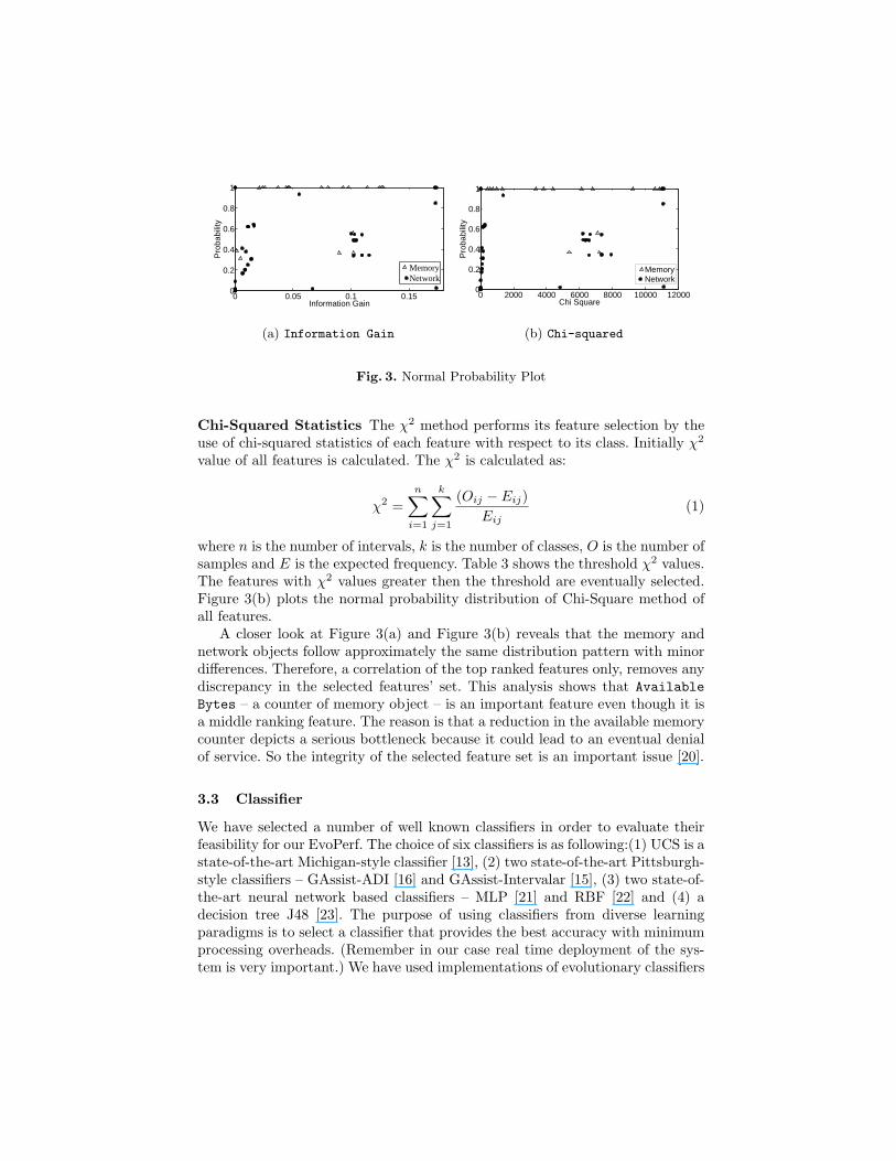
Table 3 shows the threshold values of information gain for memory and net-work objects. Figure 3(a) shows the normal probability distribution plot of in-formation gain of all features [19].

0 0.05 0.1 0.150

0.2

0.4

0.6

0.8

1

Information Gain

Pro

babi

lity

MemoryNetwork

(a) Information Gain

0 2000 4000 6000 8000 10000 120000

0.2

0.4

0.6

0.8

1

Chi Square

Pro

babi

lity

MemoryNetwork

(b) Chi-squared

Fig. 3. Normal Probability Plot

Chi-Squared Statistics The χ2 method performs its feature selection by theuse of chi-squared statistics of each feature with respect to its class. Initially χ2

value of all features is calculated. The χ2 is calculated as:

χ2 =n∑

i=1

k∑j=1

(Oij − Eij)Eij

(1)

where n is the number of intervals, k is the number of classes, O is the number ofsamples and E is the expected frequency. Table 3 shows the threshold χ2 values.The features with χ2 values greater then the threshold are eventually selected.Figure 3(b) plots the normal probability distribution of Chi-Square method ofall features.

A closer look at Figure 3(a) and Figure 3(b) reveals that the memory andnetwork objects follow approximately the same distribution pattern with minordifferences. Therefore, a correlation of the top ranked features only, removes anydiscrepancy in the selected features’ set. This analysis shows that AvailableBytes – a counter of memory object – is an important feature even though it isa middle ranking feature. The reason is that a reduction in the available memorycounter depicts a serious bottleneck because it could lead to an eventual denialof service. So the integrity of the selected feature set is an important issue [20].

3.3 Classifier

We have selected a number of well known classifiers in order to evaluate theirfeasibility for our EvoPerf. The choice of six classifiers is as following:(1) UCS is astate-of-the-art Michigan-style classifier [13], (2) two state-of-the-art Pittsburgh-style classifiers – GAssist-ADI [16] and GAssist-Intervalar [15], (3) two state-of-the-art neural network based classifiers – MLP [21] and RBF [22] and (4) adecision tree J48 [23]. The purpose of using classifiers from diverse learningparadigms is to select a classifier that provides the best accuracy with minimumprocessing overheads. (Remember in our case real time deployment of the sys-tem is very important.) We have used implementations of evolutionary classifiers

Table 4. Results of Experiments on Raw Features’ Set

Features UCS Gassist-Int Gassist-ADI RBF MLP J48 Average

Memory 33

Acc 0.994 0.999 0.999 0.999 0.999 0.995

0.998TP 140 194 195 195 195 195TN 10805 10811 10812 10812 10812 10812FP 56 2 1 1 1 1FN 7 1 0 0 0 0

Network 48

Acc 0.999 1 1 1 0.997 1

0.999TP 272 288 288 288 160 288TN 10813 10813 10813 10813 10796 10813FP 16 0 0 0 17 0FN 0 0 0 0 16 0

– UCS [13], GAssist-Int [15], GAssist-ADI [16]– provided in toolkit KEEL [12];while for neural networks – RBF and MLP – we have used WEKA [5]. We used im-plementation of J48 in WEKA. We empirically determined the best configurationsfor different parameters of classifiers.2

4 Experiments

We have collected the performance logs on a computer system in our networkslab. The hardware specifications of the system are: Intel(R) Core2Duo 1.8 GHzCPU, 2GB of RAM and 160GB of physical drive. We utilized Windows Perfmonutility for monitoring performance counters. We have collected two sets of perfor-mance counter logs: normal and artificially created bottleneck. We have selecteda sampling rate of 12 samples per minute. We have monitored user activity onthe system for more than 15 hours over a period of 3 days to get a better ideaabout the normal usage behavior. Later, we have created a number of perfor-mance bottlenecks by maximizing network and memory usage of the systemfor a period of 15 minutes. The results of our experiments show that used sixclassifiers – UCS, GAssist-ADI, GAssist-Int, NN-MLP, NN-RBF and J48 – pro-vide approximately the same accuracy. However, Neural Networks (NN) basedclassifiers have significantly smaller processing overhead, but when compared tomachine learning algorithms, J48 outperforms the rest of the classifiers. Thismakes machine learning algorithms suitable for real world deployment.

We now report the results of our experiments. We follow a 10-fold crossvalidation strategy in all experiments. The dataset of each object is divided into10 folds, 9 folds are used for training and the rest is used for testing. The processis reported for all folds and we report average value of all folds.

The results are tabulated in Table 4. It is obvious from the results of our eval-uation that all classifiers provide approximately the same accuracy. Therefore,we now need to focus on our next objective: to reduce the processing overheadof the classifiers. Towards this end, we evaluate the impact of feature selectionmodule.

2 Parameters values of RBF: clustering seed = 1, minStdDev = 0.1, numClusters =2, ridge = 1.0E-8

Table 5. Results of Experiments with Selected Features’ Set

Features UCS GAssist-Int GAssist-ADI MLP RBF J48 Average

Memory 15

Acc 0.998 0.999 0.999 0.999 0.999 0.995

0.998TP 183 192 195 195 195 195TN 10811 10812 10811 10812 10811 10812FP 1 0 1 1 1 1FN 13 4 1 0 1 0

Network 25

Acc 0.993 1 1 0.997 1 1

0.998TP 207 288 288 288 288 288TN 10813 10813 10813 10813 10813 10813FP 0 0 0 0 0 0FN 81 0 0 0 0 0

Table 6. Testing and Training times (seconds) of classifiers using all features

Parameter Memory NetworkTraining Time Testing Time Training Time Testing Time

UCS 608.1766 31.0547 523.4749 42.2907GAssist-ADI 2307.7 114.34 2187.12 81.6GAssist-Int 2254.98 107 2096.54 78NN-MLP 977.47 0.16 860.35 0.13NN-RBF 6.33 0.04 6.35 0.08

J48 1.52 0.07 1.47 0.1

5 Results and Discussions

In this section, we discuss the results obtained once we apply features’ selectiontechniques (see Table 5). Once we compare the results reported in Table 4 withthose of Table 5, it is clear that the accuracy of the classifiers remain (almost)unaffected even with a reduced features’ set. Now we analyze the impact offeatures’ reduction on training and testing times of different classifiers.

5.1 Timing Analysis

We run two sets of experiments: (1) measure training and testing times onceclassifiers are using raw features’ set, and (2) repeat the same experiments asin (1) but with reduced features’ set. The obtained results for the first case aretabulated in Table 6. It is obvious from the table that J48 has the smallesttraining times while other classifiers take significantly large amount of time –GAssist-ADI is the worst – making them infeasible for real time deployment ona computer system. Similarly J48 takes almost the same time for testing, as theneural networks based classifiers.

Table 7. Testing and Training times (seconds) of classifiers using selected features

Parameter Memory NetworkTraining Time Testing Time Training Time Testing Time

UCS 261.9124 15.2766 236.2954 14.7342GAssist-ADI 1199.85 62.4 1018 27.4GAssist-Int 1050.6 53.5 996.52 24NN-MLP 137.95 0.02 113.21 0.02NN-RBF 4.51 0.03 2.2 0.03

J48 0.57 0.04 0.66 0.04

Table 7, shows the training and testing times of different classifiers oncewe have reduced our features’ set. The results prove our thesis: the trainingand testing time of all classifiers are reduced more than 50% due to features’selection. Again, J48 is having the smallest training and testing time withoutcompromising on the detection accuracy.

6 Conclusions

The major contribution of the paper is an online real time autonomous perfor-mance monitoring system that has the capability to detect bottlenecks withoutuser intervention. In a large network of interconnected systems, the proposedsystem can significantly reduce the workload of system administrator by reliev-ing him of man-in-the-loop analysis; as a result, he can focus his attention oncountermeasure strategies. Our research shows that using performance countersof memory and network objects, classifiers can identify bottlenecks with highaccuracy. Our future work involves using other objects and analyzing the ro-bustness of the system to evasion strategies.

7 Acknowledgments

The research presented in this paper is supported by the grant # ICTRDF/TR&D/2007/13 for the project titled ISKMCD, by the National ICT R&D Fund, Min-istry of Information Technology, Government of Pakistan. The information, data,comments, and views detailed herein may not necessarily reflect the endorse-ments of views of the National ICT R&D fund.

References

1. Perfmon, Microsoft Technet, Microsoft Corporation, http://technet.

microsoft.com/en-us/library/bb490957.aspx.2. A. Silberschatz, P.B. Galvin, G. Gagne, ”Operating System Concepts”, John Wi-

ley & Sons, 7th Edition, Inc, 2004.3. Z. Ji and D. Dasgupta, ”Revisiting Negative Selection Algorithms”, Evolutionary

Computation Journal, Vol. 15, No. 2, pp. 223-251, MIT Press, 2007.4. Duan, S. and Babu, S., ”Empirical Comparison of Techniques for Automated

Failure Diagnosis”, USENIX, 2009.5. I.H. Witten, E. Frank, ”Data mining: Practical machine learning tools and tech-

niques”, Morgan Kaufmann, 2nd edition, USA, 2005.6. A.K. Jain, M.N. Murty, P.J. Flynn, ”Data clustering: a review”, ACM Computer

Survey, Vol. 31, No. 3, pp. 264-323, ACM Press, 1999.7. D. Pelleg, A.W. Moore, ”X-means: Extending k-means with efficient estimation of

the number of clusters”, International Conference on Machine Learning (ICML),pp. 727-734, Morgan Kaufmann, USA, 2000.

8. Sandip Agarwala and Karsten Schwan. SysProf: Online Distributed Behavior Di-agnosis through Fine-grain System Monitoring. Proceedings of the 26th IEEEInternational Conference on Distributed Computing Systems, Page 8, 2006.

9. S. Agarwala, C. Poellabauer, J. Kong, K. Schwan, and M. Wolf. ”Resource-AwareStream Management with the Customizable dproc Distributed Monitoring Mech-anisms” In Proc. of the 12th IEEE International Symposium on High PerformanceDistributed Computing (HPDC-12), Seattle, WA, Jun 2003

10. M. Massie, B. Chun, and D. Culler. The Ganglia Distributed Monitoring System:Design, Implementation, and Experience. 2003.

11. Barton P. Miller, Mark D. Callaghan, Jonathan M. Cargille, Jekrey K.Hollingsworth, R. Bruce Irvin, Karen L. Karavanic, Krishna Kunchithapadam,and Tia Newhall. The Paradyn parallel performance measurement tool. IEEEComputer, 28(11):37-46, 1995. G. Williams, K.

12. J. Alcala-Fdez, S. Garcia, F. J. Berlanga, A. Fernandez, L. Sanchez, M. J. delJesus, F. Herrera, KEEL: A data mining software tool integrating genetic fuzzysystems, Genetic and Evolving Systems (GEFS), 3rd International Workshop,Vol. 4 , Issue 7, pp. 83-88, 2008.

13. E.B. Mansilla, J.M.G. Guiu, ”Accuracy-Based Learning Classifier Systems: Mod-els, Analysis and Applications to Classification Tasks Ester”, Evolutionary Com-putation, 11(3), pp. 209-238, MIT Press, 2006.

14. R. Rivest, ”Learning Decision Trees”, Machine Learning, Vol. 2, pp. 229-246,1987.

15. J. Bacardit, J.M. Garrell, ”Bloat control and generalization pressure using theminimum description length principle for a Pittsburgh approach Learning Clas-sifier System”, International Workshop on Learning Classifier Systems (IWLCS),Volume 4399 of Lecture Notes in Artificial Intelligence, pp. 59-79, Springer, UK,2007.

16. J. Bacardit, J.M. Garrell, ”Evolving Multiple Discretizations with Adaptive In-tervals for a Pittsburgh Rule-Based Learning Classifier System”, Genetic andEvolutionary Computation Conference (GECCO), Volume 2724 of Lecture Notesin Computer Science, pp. 1818-1831, Springer, USA, 2003.

17. Z. Zheng, Z. Lan, B-H. Park, and A. Geist, ”System Log Pre-processing to Im-prove Failure Prediction”, Proc. of DSN’09, 2009.

18. F. Salfner and S. Tschirpke, ”Error Log Processing for Accurate Failure Predic-tion,” Proc. of WASL’08, in conjunction with OSDI, 2008.

19. Liu,H., Li,J. and Wong,L. (2002) A comparative study on feature selection andclassification methods using gene expression profiles and proteomic patterns.Genome Inform., 13, 51-60.

20. Liu, H. and Setiono, R., Chi2: Feature selection and discretization of numericattributes, Proc. IEEE 7th International Conference on Tools with Artificial In-telligence, 338-391, 1995.

21. F. Moller. A scaled conjugate gradient algorithm for fast supervised learning.Neural Networks, 525-533, (1990) .

22. D.S. Broomhead, D. Lowe. Multivariable Functional Interpolation and AdaptativeNetworks, Complex Systems, 321-355, (1988).

23. J.R. Quinlan, C4. 5: programs for machine learning, Morgan Kaufmann, 1993.